Training, Wages, and Sample Selection: Estimating Sharp Bounds on Treatment Effects *

David S. Lee

Princeton University and NBER

August 2008

Abstract This paper empirically assesses the wage effects of the Job Corps program, one of the largest federally-funded job training programs in the United States. Even with the aid of a randomized experiment, the impact of a training program on wages is difficult to study because of sample selection, a pervasive problem in applied micro-econometric research. Wage rates are only observed for those who are employed, and employment status itself may be affected by the training program. This paper develops an intuitive trimming procedure for bounding average treatment effects in the presence of sample selection. In contrast to existing methods, the procedure requires neither exclusion restrictions nor a bounded support for the outcome of interest. Identification results, estimators, and their asymptotic distribution, are presented. The bounds suggest that the program raised wages, consistent with the notion that the Job Corps raises earnings by increasing human capital, rather than solely through encouraging work. The estimator is generally applicable to typical treatment evaluation problems in which there is non-random sample selection/attrition.

* Earlier drafts of this paper were circulated as “Trimming for Bounds on Treatment Effects with Missing Outcomes,” Center for Labor Economics Working Paper #51, March 2002, and NBER Technical Working Paper #277, June 2002, as well as a revision with the above title, as NBER Working Paper #11721, October 2005. Department of Economics and Woodrow Wilson School of Public and International Affairs, Industrial Relations Section, Firestone Library, Princeton University, Princeton, NJ 08544-2098, davidlee@princeton.edu. Emily Buchsbaum, Vivian Hwa, Xiaotong Niu, and Zhuan Pei provided excellent research assistance. I thank David Card, Guido Imbens, Justin McCrary, Marcelo Moreira, Enrico Moretti, Jim Powell, Jesse Rothstein, Mark Watson, and Edward Vytlacil for helpful discussions and David Autor, Josh Angrist, John DiNardo, Jonah Gelbach, Alan Krueger, Doug Miller, Aviv Nevo, Jack Porter, Diane Whitmore, and participants of the UC Berkeley Econometrics and Labor Lunches, for useful comments and suggestions.

1 Introduction

For decades, many countries around the world have administered government-sponsored employment and

training programs, designed to help improve the labor market outcomes of the unemployed or economically

disadvantaged.1 To do so, these programs offer a number of different services, ranging from basic classroom

education and vocational training, to various forms of job search assistance. The key question of interest

to policymakers is whether or not these programs are actually effective, sufficiently so to justify the cost to

the public. The evaluation of these programs has been the focus of a large substantive and methodological

literature in economics. Indeed, Heckman et al. (1999) observe that “[f]ew U.S. government programs have

received such intensive scrutiny, and been subject to so many different types of evaluation methodologies,

as governmentally-supplied job training.”

Econometric evaluations of these programs typically focuson their reduced-from impacts on total earn-

ings, a first-order issue for cost-benefit analysis. Unfortunately, exclusively studying the effect on total

earnings leaves open the question of whether any earnings gains are achieved through raising individuals’

wage rates(price effects) or hours of work (quantity effects). That is, a training program may lead to a

meaningful increase in human capital, thus raising participants’ wages. Alternatively, the program may

have a pure labor supply effect: through career counseling and encouragement of individuals to enter the

labor force, a training program may simply be raising incomes by increasing the likelihood of employment,

without any increase in wage rates.

But assessing the impact of training programs on wage rates is not straightforward, due to the well-

known problem of sample selection, which is pervasive in applied micro-econometric research. That is,

wages are only observed for individuals who are employed. Thus, even if there is random assignment of the

“treatment” of a training program, there may not only be an effect on wages, but also on the probability that

a person’s wage will even be observed. Even a randomized experiment cannot guarantee that treatment and

control individuals will be comparableconditional on being employed. Indeed, standard labor supply theory

predicts that wages will be correlated with the likelihood of employment, resulting in sample selection

bias (Heckman, 1974). This missing data problem is especially relevant for analyzing public job training

programs, which typically target individuals who have low employment probabilities.

This paper empirically assesses thewageeffects of the Job Corps program, one of the largest federally-

1See Heckman et al. (1999) for figures on expenditures on active labor market programs in OECD countries. See also Martin(2000).

1

funded job training programs in the United States.2 The Job Corps is a comprehensive program for eco-

nomically disadvantaged youth aged 16 to 24, and is quite intensive: the typical participant will live at a

local Job Corps center, receiving room, board, and health services while enrolled, for an average of about

eight months. During the stay, the individual can expect to receive about 1100 hours of vocational and aca-

demic instruction, equivalent to about one year in high school. The Job Corps is also expensive, with the

average cost at about $14,000 per participant.3 This paper uses data from the National Job Corps Study, a

randomized evaluation funded by the U.S. Department of Labor.

Standard parametric or semi-parametric methods for correcting for sample selection require exclusion

restrictions that have little justification in this case. Asshown below, the data include numerous baseline

variables, but all of those that are found to be related to employment probabilities (i.e., sample selection)

could also potentially have a direct impact on wage rates.

Thus, this paper develops an alternative method, a general procedure for bounding the treatment effects.

The method amounts to first identifying the excess number of individuals who are induced to be selected

(employed) because of the treatment, and then “trimming” the upper and lower tails of the outcome (e.g.,

wage) distribution by this number, yielding a worst-case scenario bound. The assumptions for identifying

the bounds are already assumed in conventional models for sample selection: 1) the regressor of interest is

independent of the errors in the outcome and selection equations, and 2) the selection equation can be written

as a standard latent variable binary response model. In the case of an experiment, random assignment ensures

that the first assumption holds. It is proven that the trimming procedure yields the tightest bounds for the

average treatment effect that are consistent with the observed data. No exclusion restrictions are required,

nor is a bounded support for the outcome variable.

An estimator for the bounds is introduced and shown to be√

n-consistent and asymptotically normal

with an intuitive expression for its asymptotic variance. It not only depends on the variance of the trimmed

outcome variable, but also on the trimming threshold, whichis an estimated quantile. There is also an added

term that accounts for the estimation ofwhich quantile (e.g., the 10th, 11th, 12th, etc. percentile) of the

distribution to use as the trimming threshold.

2In the 2004 fiscal year, the U.S. Department of Labor’s Employment and Training Administration spent $1.54 billion for theoperation of the Job Corps. By comparison, it spent about $893 million on "Adult Employment and Training Activities" (jobsearch assistance for anyone and job training available to anyone if such training is needed for obtaining or retaining employ-ment) and about $1.44 billion on "Dislocated Workers Employment and Training Activities" (employment and training services forunemployment and underemployed workers) (U.S. Departmentof Labor, 2005a).

3A summary of services provided and costs can be found in Burghardt et al. (2001).

2

For the analysis of Job Corps, the trimming procedure is instrumental to measuring the wage effects,

producing bounds that are somewhat narrow. For example, at week 90 after random assignment, the es-

timated interval for the treatment effect is 4.2 to 4.3 percent, even when wages are missing for about 54

percent of individuals. By the end of the 4-year follow-up period, the interval is still somewhat informa-

tive, statistically rejecting effects more negative than -3.7 percent and more positive than 11.2 percent. By

comparison, the assumption-free, “worst-case scenario” bounds proposed by Horowitz and Manski (2000a)

produce a lower bound of -75 percent effect and an upper boundof 80 percent.

Adjusting for the reduction in potential work experience likely caused by the program, the evidence

presented here points to a positive causal effect of the program on wage rates. This is consistent with the

view that the Job Corps program represents a human capital investment, rather than a means to improve

earnings through raising work effort alone.

The proposed trimming procedure is neither specific to this application nor to randomized experiments.

It will generally be applicable to treatment evaluation problems when outcomes are missing, a problem that

often arises in applied research. Reasons for missing outcomes range from survey non-response (e.g., stu-

dents not taking tests), to sample attrition (e.g., inability to follow individuals over time), to other structural

reasons (e.g., mortality). Generally, this estimator is well-suited for cases where the researcher is uncom-

fortable imposing exclusion restrictions in the standard two-equation sample selection model, and when the

support of the outcome variable is too wide to yield informative bounds on treatment effects.

This paper is organized as follows. It begins, in Section 2, with a description of the Job Corps program,

the randomized experiment, and the nature of the sample selection problem. After this initial analysis, the

proposed bounding procedure is described in Sections 3 and 4. Section 3 presents the identification results,

while Section 4 introduces a consistent and asymptoticallynormal estimator of the bounds, and discusses

inference. Section 5 reports the results from the empiricalanalysis of the Job Corps. Section 6 concludes.

2 The National Job Corps Study and Sample Selection

This section describes both the Job Corps program and the data used for the analysis, replicates the main

earnings results of the recently-completed randomized evaluation, and illustrates the nature of the sample

selection problem. It is argued below that standard sample selection correction procedures are not appropri-

ate for this context. Also, in order to provide an initial benchmark, the approach of Horowitz and Manski

3

(2000a) is used to provide bounds on the Job Corps’ effect on wages. They are to be compared to the

“trimming” bounds presented in Section 5, which implementsthe estimator developed in Sections 3 and 4.

2.1 The Job Corps Program and the Randomized Experiment

The U.S. Department of Labor describes the Job Corps programtoday as “a no-cost education and vocational

training program ... that helps young people ages 16 through24 get a better job, make more money and take

control of their lives” (U.S. Department of Labor, 2005b). To be eligible, an individual must be a legal

resident of the United States, be between the ages of 16 and 24, and come from a low-income household

(Schochet et al., 2001). The administration of the Job Corpsis considered to be somewhat uniform across

the 110 local Job Corps centers in the United States.

Perhaps the most distinctive feature of the program is that most participants live at the local Job Corps

center while enrolled. This residential component of the program includes formal social skills training,

meals, and a dormitory-style life. During the stay, with thehelp of counselors, the participants develop

individualized, self-paced programs which will consist ofa combination of remedial high school education,

including consumer and driver education, as well as vocational training in a number of areas, including

clerical work, carpentry, automotive repair, building andapartment maintenance, and health related work.

On average, enrollees can expect to receive about 440 hours of academic instruction and about 700 hours of

vocational training, over an average of 30 weeks. Centers also provide health services, as well as job search

assistance upon the students’ exit from the Job Corps.

In the mid-1990s, three decades after the creation of Job Corps, the U.S. Department of Labor funded

a randomized evaluation of the program, which was carried about by Mathematica Policy Resarch, Inc.

Persons who applied for the program for the first time betweenNovember 1994 and December 1995, and

were found to be eligible (80,883 persons), were randomizedinto a “program” group and a “control” group.

The control group of 5977 individuals was essentially embargoed from the program for three years, while

the remaining applicants could enroll in the Job Corps as usual. Since those who were still eligible after

randomization were not compelled to participate, the differences in outcomes between program and control

group members represent the reduced-form effect of eligibility, or the “intent-to-treat” effect. This treatment

effect is the focus of the empirical analysis presented below. Throughout the paper, when I use the phrase

“effect of the program”, I am referring to this reduced-formtreatment effect.

Of the program group, 9409 applicants were randomly selected to be followed for data collection.

4

The research sample of 15386 individuals was interviewed atrandom assignment, and at three subsequent

points in time: 12, 30, and 48 months after random assignment. Due to programmatic reasons, some sub-

populations were randomized into the program group with differing, but known, probabilities. Thus, ana-

lyzing the data requires the use of the design-weights (the variable DSGN_WGT as described in Schochet

et al. (2003)).

This paper uses the public-release data of the National Job Corps Study. Table I provides descriptive

statistics for the data used in the analysis below. For baseline as well as post-assignment variables, it reports

the treatment and control group means, standard deviations, proportion of the observations with non-missing

values for the specified variable, as well as the difference in the means and associated standard error. The

table shows that the proportion non-missing and the means for the demographic variables (the first 12 rows),

education and background variables (the next 4 rows), income at baseline (the next 9 rows), and employment

information (the next 6 rows) are quite similar. For only oneof the variables – usual weekly hours on the

most recent job at the baseline – is the difference (0.91 hours) statistically significant. A logit of the treat-

ment indicator on all baseline characteristics in Table I was estimated; the chi-square test of all coefficients

equalling zero yielded a p-value of 0.577.4 The overall comparability between the treatment and control

groups is consistent with successful randomization of the treatment.

It is important to note that the analysis in this paper abstracts from missing values due to interview

non-response and sample attrition over time. Thus, only individuals who had non-missing values for weekly

earnings and weekly hoursfor every weekafter the random assignment are used; the estimation sampleis

thus somewhat smaller (9145 vs. 15386). It will become clearbelow that the trimming procedure could

be applied exclusively to the attrition/non-response problem, which is a mechanism for sample selection

that is quite distinct from the selection into employment status. More intensive data collection can solve

the attrition/non-response problem, but not the problem ofsample selection on wages caused by employ-

ment. For this reason, the analysis below focuses exclusively on the latter problem, and analyzes the data

conditional on individuals having continuously valid earnings and hours data.5

The bottom of Table I shows that the only set of variables thatshow important (and statistically sig-

nificant) differences between treatment and control are thepost-assignment labor market outcomes. The

4Missing values for each of the baseline variables were imputed with the mean of the variable. The analysis below uses thisimputed data.

5Although the analysis here abstracts from the non-responseproblem, there is some evidence that it is a second-order issue, asmentioned in Remark 2 of Sub-section 3.1.

5

treatment group has lower weekly hours and earnings at week 52, but higher hours and earnings at the 3-

year and 4-year marks. At week 208, the earnings gain is about27 dollars, with the control mean of about

200 dollars. This is consistent with Mathematica’s final report, which showed that the program had about a

12 percent positive effect on earnings by the fourth year after enrollment, and suggested that lifetime gains

in earnings could very well exceed the program’s costs (Burghardt et al., 2001). The effect on weekly hours

at that time is a statistically significant 1.95 hours.

Figure I illustrates the treatment effects on earnings for each week subsequent to random assignment.

It shows an initial negative impact on earnings for the first 80 weeks, after which point a positive treat-

ment effect appears and grows. The estimates in the bottom ofTable I and plotted in Figure I are similar

qualitatively and quantitatively to the impact estimates reported in Schochet et al. (2001).6

2.2 The Effect on Wages and the Sample Selection Problem

It seems useful to assess the impact of the program onwage rates, as distinct from total earnings, which is

a product of both the price of labor (the wage) and labor supply (whether the person works, and if so, how

many hours). Distinguishing between price and quantity effects is important for better understanding the

mechanism through which the Job Corps leads to more favorable labor market outcomes.

On the one hand, one of the goals of the Job Corps is to encourage work and self-sufficiency; thus,

participants’ total earnings might rise simply because theprogram succeeds in raising the likelihood that

they will be employed, while at the same time leaving the market wage for their labor unaffected. On the

other hand, the main component of the Job Corps is significantacademic and vocational training, which

could be expected to raise wages. There is a great deal of empirical evidence to suggest a positive causal

effect of education on wages (see Card (1999)).

Unfortunately, even though the National Job Corps study wasa randomized experiment, one cannot use

simple treatment-control differences to estimate the effect of the program on wage rates. This is because the

effective “prices” of labor for these individuals are only observed to the econometrician when the individuals

are employed. This gives rise to the classic sample selection problem (e.g., see Heckman (1979)).

Figure II suggests that sample selection may well be a problem for the analysis of wage effects of the

6In Schochet et al. (2001), the reported estimates used a lessstringent sample criterion. Instead of requiring non-missing valuesfor 208 consecutive weeks, individuals only needed to complete the 48-month interview (11313 individuals). Therefore, for thatsample, some weeks’ data will be missing. Despite the difference in the samples, the levels, impact estimates, and time profilereported in Schochet et al. (2001) are also quite similar to those found in Figures II, and III (below).

6

Job Corps. It reports employment rates (the proportion of the sample that has positive work hours in the

week) for both treated and control individuals, for each week following random assignment. The results

show that the program had a negative impact on employment propensities in the first half of the follow-up,

and a positive effect in the latter half. This shows that the Job Corps itself affected whether individuals

would have a non-missing wage rate.

Put another way, Figure II illustrates that even though proper random assignment will imply that the

treatment and control groups are comparable at the baseline, they may well be systematically different

conditional on being employedin a given period subsequent to the random assignment. As a result, the

treatment-control difference in mean log-hourly wages, asplotted in Figure III (with pointwise 95 percent

confidence intervals), may not represent the true causal effect of the program.7

There are two other reasons why sample selection can potentially be important in this case. As shown in

Figure II, a large fraction of individuals are not employed:employment rates start at about 20 percent and

grow to at most 60 percent at the four-year mark. Second, non-employed and employed individuals appear

to be systematically different on a number of important observable dimensions. Table II reports log-odds

coefficients from a logit of employment in week 208 on the treatment dummy and the baseline characteristics

listed in Table I. As might be expected, gender, race, education, criminal history, and employment status at

the baseline are all very strong predictors of employment inweek 208.

The problem of non-random sample selection is well understood in the training literature; it may be one

of the reasons why most evaluations of job training programsfocus on total earnings, including zeros for

those without a job, rather than on wages conditional on employment. Of the 24 studies referenced in a

survey of experimental and non-experimental studies of U.S. employment and training programs (Heckman

et al., 1999), most examine annual, quarterly, or monthly earnings without discussing the sample selection

problem of examining wage rates.8 As for the Job Corps, when reporting results on hourly wages for

the working, Schochet et al. (2001) is careful to note that because of the selection into employment, the

treatment-control differences cannot be interpreted as impact estimates.

7Hourly wage is computed by dividing weekly earnings by weekly hours worked, for the treatment and control groups. Notethe pattern of “kinks” that occur at the 12- and 30-month marks, which is also apparent in Figure I. This could be caused by theretrospective nature of the interviews that occur at 12-, 30-, and 48-months post-random-assignment. This pattern would be foundif there were systematic over-estimation of earnings on employment that was further away from the interview date. The lines would“connect” if respondents were reminded of their answer fromthe previous interview. Note that these potential errors donot seemto be too different between the treatment and control groups, as there are no obvious kinks in the difference (solid squares).

8The exceptions include Kiefer (1979), Hollister et al. (1984), Barnow (1987). The sources from Tables 22 and 24 in Heckmanet al. (1999) were surveyed.

7

2.3 Existing Approaches

Currently, there are two general approaches to addressing the sample selection problem. The first is to

explicitly model the process determining selection. The conventional setup, following Heckman (1979),

models the wage determining process as

Y∗ = Dβ +Xπ1+U (1)

Z∗ = Dγ +Xπ2+V

Y = 1[Z∗ ≥ 0] ·Y∗

whereY∗ is the offered market wage as of a particular point in time (e.g., week 208 after randomization),D

is the indicator variable of receiving the treatment of being given access to the Job Corps program, andX

is a vector of baseline characteristics.Z∗ is a latent variable representing the propensity to be employed. γ

represents the causal effect of the treatment on employmentpropensities, whileβ is the (constant) treatment

effect of interest.9 BothY∗ andZ∗ are unobserved, but the wage conditional on employmentY is observed,

where 1[·] is the indicator variable.(U,V) are assumed to be jointly independent of the regressors(D,X).10

Within a standard labor supply framework, it is easy to imagine the possibility that job training could raise

the market wage for individuals, leading to a positiveβ , and at the same time raise the probability of

participating in the labor force (γ > 0) since a higher wage will more likely exceed the reservation wage for

participating.11

As in Heckman (1979), sample selection bias can be seen as specification error in the conditional expec-

tation

E [Y|D,X,Z∗ ≥ 0] = Dβ +Xπ1+E [U |D,X,V ≥−Dγ −Xπ2]

.

One modeling approach is to assume that data are missing at random, perhaps conditional on a set of

covariates (Rubin, 1976). This amounts to assuming thatU andV are independent of one another, or that

9In this specification, the treatment effect is constant.10This assumption, which is stronger than necessary, is invoked now for expositional purposes. It will be shown below thatwhat

is required is instead independence of(U,V) andD, conditional onX.11Of course, it should be noted that since the goal here is to estimate a reduced-form treatment effect, we do not adopt a

particular labor supply model, or prohibit ways in which thetreatment could affect participation. For example,γ could be positiveif the program’s job search assistance component was important.

8

employment status is unrelated to the determination of wages. This assumption is strictly inconsistent with

standard models of labor supply that account for the participation decision (e.g., see Heckman (1974)).

A more common modeling assumption is that some of the exogenous variables determine sample se-

lection, but do not have their own direct impact on the outcome of interest; that is, some of the elements

of π1 are zero while corresponding elements ofπ2 are nonzero. Such exclusion restrictions are utilized in

parametric and semi-parametric models of the censored selection process (e.g., Heckman (1979), Heckman

(1990), Ahn and Powell (1993), Andrews and Schafgans (1998), Das et al. (2003)).

The practical limitation to relying on exclusion restrictions for the sample selection problem is that there

may not exist credible “instruments” that can be excluded from the outcome equation. This seems to be

true for an analysis of the Job Corps experiment. There are many variables available to the researcher from

the Job Corps evaluation, and many of the key variables are listed in Tables I and II. But for each of the

variables in Table II that have significant associations with employment, there is a well-developed literature

suggesting that those variables may also influence wage offers. For example, race, gender, education, and

criminal histories all could potentially impact wages. Household income and past employment experiences

are also likely to be correlated with unobserved determinants of wages.

Researchers’ reluctance to rely upon specific exclusion restrictions motivates a second, general approach

to addressing the sample selection problem: the construction of “worst-case scenario” bounds of the treat-

ment effect. When the support of the outcome is bounded, the idea is to impute the missing data with either

the largest or smallest possible values to compute the largest and smallest possible treatment effects con-

sistent with the data that is observed. Horowitz and Manski (2000a) use this notion to provide a general

framework for constructing bounds for treatment effect parameters when outcome and covariate data are

non-randomly missing in an experimental setting.12 This strategy is discussed in detail in Horowitz and

Manski (2000a), which shows that the approach can be useful whenY is a binary outcome.

This imputation procedure cannot be used when the support isunbounded. Even when the support is

bounded, if it is very wide, so too will be the width of the treatment effect bounds. In the context of the

Job Corps program, the bounds are somewhat uninformative. Table III computes the Horowitz and Manski

(2000a) bounds for the treatment effect of the Job Corps program on log-wages in week 208. Specifically,

12An early example of sensitivity analysis that imputed missing values is found in the work of Smith and Welch (1986). Others(Balke and Pearl, 1997; Heckman and Vytlacil, 1999, 2000b,a) have constructed such bounds to address a very different problem– that of imperfect compliance of the treatment, even when “intention” to treat is effectively randomized (Bloom, 1984;Robins,1989; Imbens and Angrist, 1994; Angrist et al., 1996).

9

it calculates the upper bound of the treatment effect as

Pr[Z∗ ≥ 0|D = 1]E [Y|D = 1]+Pr[Z∗ < 0|D = 1]YUB

−(Pr[Z∗ ≥ 0|D = 0]E [Y|D = 0]+Pr[Z∗ < 0|D = 0]YLB)

where all population quantities can be estimated, andYUB andYLB are the upper and lower bounds of the

support of log-wages. As reported in the Table,YUB andYLB are taken to be 2.77 and 0.90 ($15.96 and

$2.46 an hour), respectively.13

Table III shows that the lower bound for the treatment effecton week 208 log-wages is -0.75 and the

upper bound is 0.80. Thus, the interval is almost as consistent with extremely large negative effects as

it is with extremely large positive effects. The reason for this wide interval is that more than 40 percent

of the individuals are not employed in week 208. In this context, imputing the missing values with the

maximal and minimal values ofY is so extreme as to yield an interval that includes effect sizes that are

arguably implausible. Nevertheless, the Horowitz and Manski (2000a) bounds provide a useful benchmark,

and highlight that some restrictions on the sample selection process are needed to produce tighter bounds

(Horowitz and Manski, 2000b).

The procedure proposed below is a kind of “hybrid” of the two general approaches to the sample selec-

tion problem. It yields bounds on the treatment effect, evenwhen the outcome is unbounded. It does so by

imposing some structure on the sample selection process, but without requiring exclusion restrictions.

3 Identification of Bounds on Treatment Effects

This section first uses a simple case in order to illustrate the intuition behind the main identification result,

and then generalizes it for a very unrestrictive sample selection model.

Consider the case where there is only the treatment indicator, with no other covariates. That is,X is a

constant, so thatπ1 andπ2 will be intercept terms. It will become clear that the resultbelow is also valid

13The wage variable was transformed before being analyzed, inorder to minimize the effect of outliers, and also so that theHorowitz and Manski (2000a) bounds would not have to rely on these outliers. Specifically, the entire observed wage distributionwas split into 20 categories, according to the 5th, 10th, 15th, ... 95th percentile wages, and the individual was assigned the meanwage within each of the 20 groups. Thus, the upper “bound” of the support, for example, is really the mean log-wage for thoseearning more than the 95th percentile. The same data are usedfor the trimming procedure described below. Strictly speaking,the Horowitz and Manski (2000a) bounds would use the theoretical bounds of the support of the population log-wage distribution.Since these population maximums and minimums are not observed, one could instead utilize the log of the minimum and maximumlog-wage observed in the sample. It is clear that doing so would produce wider bounds than that given by the implementation here.

10

conditional on any value ofX. Describing the identification result in this simple case makes clear that the

proposed procedure does not rely on exclusion restrictions.14 In addition, this section and the next assumes

thatU (and henceY) has a continuous distribution. Doing so will simplify the exposition; it can be shown

that the proposed procedure can be applied to discrete outcome variables as well (see Lee (2002)). Without

loss of generality, assume thatγ > 0, so that the treatment causes an increase in the likelihoodof the outcome

being observed.

From Equation (1), the observed population means for the control and treatment groups can be written

as

E [Y|D = 0,Z∗ ≥ 0] = π1 +E [U |D = 0,V ≥−π2] (2)

and

E [Y|D = 1,Z∗ ≥ 0] = π1 + β +E [U |D = 1,V ≥−π2− γ ] , (3)

respectively. This shows that whenU andV are correlated, the difference in the means will generally be

different fromβ .

Identification ofβ would be possible if we could estimate

E [Y|D = 1,V ≥−π2] = π1 + β +E [U |D = 1,V ≥−π2] (4)

because (2) could be subtracted to yield the effectβ (sinceD is independent of(U,V) by assumption). But

the mean in (4) is not observed.

But this mean can be bounded. This is because all observations onY needed to compute this mean are a

subset of the selected population (V ≥−π2− γ). For example, we know that

E [Y|D = 1,Z∗ ≥ 0] = (1− p)E [Y|D = 1,V ≥−π2]+ pE[Y|D = 1,−π2− γ ≤V < −π2]

wherep = Pr[−π2−γ≤V<−π2]Pr[−π2−γ≤V] . The observed treatment mean is a weighted average of (4) andthe mean for

a sub-population of “marginal” individuals (−π2− γ ≤ V < −π2) that are induced to be selected into the

sample because of the treatment.

14Note that while existing procedures for point identificaiton require an instrument that satisfies an exclusion restriction, the exis-tence of such an instrument is not sufficient for identification. For example, a single binary instrument will not allow identificationwithout imposing further assumptions.

11

E [Y|D = 1,V ≥−π2] is therefore bounded above byE [Y|D = 1,Z∗ ≥ 0,Y ≥ yp], whereyp is the pth

quantile of the treatment group’s observedY distribution. This is true because among the selected population

with V ≥−π2− γ , D = 1, no sub-population with proportion(1− p) can have a mean that is larger than the

average of the largest(1− p) values ofY.

Put another way, we cannot identify which observations are inframarginal(V ≥−π2) and which are

marginal(−π2− γ ≤V < −π2). But the “worst-case” scenario is that the smallestp values ofY belong to

the marginal group and the largest 1− p values belong to the inframarginal group. Thus, by trimmingthe

lower tail of theY distribution by the proportionp, we obtain an upper bound for the inframarginal group’s

mean in (4). Consequently,E[Y| D = 1, Z∗ ≥ 0, Y ≥ yp]−E [Y|D = 0,Z∗ ≥ 0] is an upper bound forβ .

Note that the trimming proportionp is equal to

Pr[Z∗ ≥ 0|D = 1]−Pr[Z∗ ≥ 0|D = 0]

Pr[Z∗ ≥ 0|D = 1]

where each of these probabilities is identified by the data.

To summarize, a standard latent-variable sample selectionmodel implies that the observed outcome

distribution for the treatment group is a mixture of two distributions: 1) the distribution for those who

would have been selected irrespective of the treatment (theinframarginal group), and 2) the distribution for

those induced into being selected because of the treatment (the marginal group). It is possible to quantify

the proportion of the treatment group that belongs to this second group, using a simple comparison of the

selection probabilities of the treatment and control groups. Although it is impossible to identify specifically

whichtreated individuals belong to the second group, “worst-case” scenarios can be constructed by assuming

that they are either at the very top or the very bottom of the distribution. Thus, trimming the data by the

known proportion of excess individuals should yield boundson the mean for the inframarginal group.

3.1 Identification under a Generalized Sample Selection Model

This identification result applies to a much wider class of sample selection models. It depends neither on a

constant treatment effect, nor on homoskedasticity, whichare both implicitly assumed in Equation (1).

12

To see this, consider a general sample selection model that allows for heterogeneity in treatment effects:

(Y∗1 ,Y∗

0 ,S1,S0,D) is i.i.d. across individuals (5)

S= S1D+S0(1−D)

Y = S· {Y∗1 D+Y∗

0 (1−D)}

(Y,S,D) is observed

whereD, S, S0, andS1 are all binary indicator variables.D denotes treatment status;S1 andS0 are “potential”

sample selection indicators for the treated and control states. For example, when an individual hasS1 = 1

andS0 = 0, this means that there will be a non-missing data on the outcome(S= 1) if treatment is given,

and there will be missing data on the outcome(S= 0) if treatment is denied. The second line highlights

the fact that for each individual, we only observeS1 or S0. Y∗1 andY∗

0 are latent potential outcomes for the

treated and control states, and the third line points out that we observe only one of the latent outcomesY∗1

or Y∗0 , and only if the individual is selected into the sampleS= 1. It is assumed throughout the paper that

E [S|D = 1] ,E [S|D = 0] > 0.

Assumption 1 (Independence):(Y∗1 ,Y∗

0 ,S1,S0) is independent ofD.

This assumption corresponds to the independence of(U,V) and(D,X) in the previous section. In the context

of experiments, random assignment will ensure this assumption will hold.

Assumption 2a (Monotonicity): S1 ≥ S0 with probability 1.

This assumption implies that treatment assignment can onlyaffect sample selection in “one direction”. Some

individuals will never be observed, regardless of treatment assignment (S0 = S1 = 0), others will always be

observed (S0 = 1,S1 = 1), and others will be selected into the samplebecauseof the treatment (S0 = 0,

S1 = 1). This assumption is commonly invoked in studies of imperfect compliance of treatment (Imbens

13

and Angrist, 1994; Angrist et al., 1996); the difference is that in those studies, monotonicity is for how an

instrument affectstreatment status. Here, the monotonicity is for how treatment affectssample selection.

In the context of the Job Corps program, the monotonicity assumption essentially limits the degree of

heterogeneity in the effect of the program on labor force participation. It does not allow, for example, the job

search assistance services provided by Job Corps to induce some to become employed while simultaneously

causing others to drop out of the labor force. A negative impact could occur, for example, if the job search

counseling induced some to pursue further education (and hence drop out of the labor force). Similar

to the case of LATE, with only information on the outcome, treatment status, and selection status, the

monotonicity assumption is fundamentally untestable. It should be noted that monotonicity has been shown

to be equivalent to assuming a latent-variable threshold-crossing model (Vytlacil, 2002), which is the basis

for virtually all sample selection models in econometrics.

Proposition 1a: Let Y∗0 andY∗

1 be continuous random variables. If Assumptions 1 and

2a hold, then∆LB0 and∆UB

0 are sharp lower and upper bounds for the average treatment effect

E [Y∗1 −Y∗

0 |S0 = 1,S1 = 1], where

∆LB0 ≡ E [Y|D = 1,S= 1,Y ≤ y1−p0]−E [Y|D = 0,S= 1]

∆UB0 ≡ E [Y|D = 1,S= 1,Y ≥ yp0]−E [Y|D = 0,S= 1]

yq ≡ G−1(q) , with G the cdf ofY , conditional onD = 1,S= 1

p0 ≡Pr[S= 1|D = 1]−Pr[S= 1|D = 0]

Pr[S= 1|D = 1]

The bounds are sharp in the sense that∆LB0 (∆UB

0 ) is the largest (smallest) lower (upper) bound

that is consistent with the observed data. Furthermore, theinterval[∆LB

0 ,∆UB0

]is contained in

any other valid bounds that impose the same assumptions. (IfS0 ≥ S1 with probability 1, then

the control group’s, rather than the treatment group’s outcome distribution must be trimmed.)

Obviously, this result is equally valid if one were to assumemonotonicity in the opposite direction (S0 ≥ S1

with probability 1).

Remark 1. The sharpness of the bound∆UB0 means that it is the “best” upper bound that is consistent

with the data. A specific example of where this proposition can be applied is in Krueger and Whitmore

14

(2001), who study the impact of the Tennessee STAR class-size experiment. In that study, students are

randomly assigned to a regular or small class and the outcomeof interest is the SAT (or ACT) scores, but

not all students take the exam. On p. 25, Krueger and Whitmore(2001) utilize Assumptions 1 and 2a

to derive a different upper bound, given byB ≡ E[Y| D = 1,S= 1] · Pr[S=1|D=1]Pr[S=1|D=0] − E[Y| D = 0,S= 1].

Proposition 1a implies that this boundB, like any otherproposed bound utilizing these assumptions, cannot

be smaller than∆UB0 .15

Remark 2. An important practical implication of Assumptions 1 and 2ais that asp0 vanishes, so does

the sample selection bias.16 The intuition is that ifp0 = 0, then under the monotonicity assumption, both

treatment and control groups are comprised of individuals whose sample selection was unaffected by the

assignment to treatment, and therefore the two groups are comparable. These individuals can be thought

of as the “always-takers” sub-population (Angrist et al., 1996), except that “taking” is not the taking of the

treatment, but rather selection into the sample. It followsthat when analyzing randomized experiments, if

the sample selection rates in the treatment and control groups are similar, and if the monotonicity condition

is believed to hold, then a comparison of the treatment and control means is a valid estimate of an aver-

age treatment effect.17 As an example, the proportion of control group individuals,at week 90, that have

continuously non-missing earnings and hours data is 0.822,and the proportion is 0.003 smaller (standard

error of 0.006) for the treatment group. Thus, if the above assumptions are invoked to examine the non-

response/attrition problem (as opposed to the focus of thisstudy, missing wages due to nonemployment),

then the data suggest little bias due to non-response/attrition.

Remark 3. Assumptions 1 and 2a are minimally sufficient for computing the bounds. First, the inde-

pendence assumption is also important, since it is what justifies the contrast between the trimmed treatment

group and the control group.

Second, monotonicity ensures that the sample-selected control group consists only of those individuals

15Thus, in the context of Krueger and Whitmore (2001), Proposition 1a implies that computing the boundB is unnecessaryafter already computing a very different estimateT, their “linear truncation” estimate. They justifyT under a different set ofassumptions: 1) that “the additional small-class studentsinduced to take the ACT exam are from the left tail of the distribution” and2) “if attending a small class did not change the ranking of students in small classes.” Their estimateT is mechanically equivalent tothe bound∆UB

0 . Therefore, Proposition 1a implies that their estimateT is actually the sharp upper bound given the mild assumptionsthat were used to justify their boundB.

16A vanishingp corresponds to individuals with the same value of the sampleselection correction term, and it is well known thatthere is no selection bias, conditional on the correction term. See, for example, Heckman and Robb (1986), Heckman (1990), Ahnand Powell (1993), and Angrist (1997).

17Note thatp0 here is proportional to thedifferencein the fraction that are sample selected between the treatment and controlgroups. Thus, the notion of a vanishingp should not be confused with “identification at infinity” in (Heckman, 1990), in which thebias term vanishes as the fraction that is selected into the sample tends to 1.

15

with S0 = 1,S1 = 1. Without monotonicity, the control group could consist solely of observations with

S0 = 1,S1 = 0, and the treatment group solely of observations withS0 = 0,S1 = 1. Since the two sub-

populations do not “overlap”, the difference in the means could not be interpreted as a causal effect.

An interesting exception to this arises in the special case that E [S|D = 0] + E [S|D = 1] > 1, in which

case informative bounds can be constructed without invoking monotonicity, as demonstrated in Zhang and

Rubin (2003). There, the insight is that the proportion of those who areS0 = 1,S1 = 0 can be no larger than

the proportion in the treatment group who have missing values, 1−E [S|D = 1]. It follows that within the

control group, the fraction ofS0 = 1,S1 = 1 individuals cannot be less thanE [S|D = 0] −(1−E [S|D = 1]),

which is positive, as assumed. It thus follows that, for example, the upper bound for the mean ofY∗0 for

S0 = 1,S1 = 1 is the mean after trimming the bottom1−E[S|D=1]E[S|D=0] fraction of the observed control group

distribution. A symmetric argument can be made for boundingthe mean ofY∗1 for S0 = 1,S1 = 1. This

idea is formalized in Zhang and Rubin (2003), and also discussed in Zhang et al. (2008). It should be

noted, however, that the procedure of Zhang and Rubin (2003)will not produce informative bounds for a

general sample selection model, as the assumptionE [S|D = 0] + E [S|D = 1] > 1 is crucial.18 Specifically,

if E [S|D = 0]+E [S|D = 1] ≤ 1 then the “worst-case” scenario would involve trimmingall of the observed

treatment and control observations, resulting in noninformative (or “vacuous”) bounds.19

Remark 4. When p0 = 0 in a randomized experimental setting, there is a limited test of whether

monotonicity holds (and therefore whether the simple difference in means in the outcome suffers from

sample selection bias). Ifp0 = 0 and monotonicity holds, then the selected subsets of both the treatment and

control groups will consist solely of individuals with(S0 = 1,S1 = 1). Under randomization, the treatment-

control difference in the outcome should represent a causaleffect. In addition, the distribution of theXs

should be the same in the treatement and control groups,conditional on being selected. This can be tested

empirically.

In order for this test to have power, the two sub-populations(S0 = 0,S1 = 1), (S0 = 1,S1 = 0) need to

have different distributions of baseline characteristicsX. Recall that without monotonicity, the selected

treated group will be comprised of two sub-populations,(S0 = 1,S1 = 1) and (S0 = 0,S1 = 1), while the

18For example, the procedure will not work if 49 percent of the treatment group is missing and 52 percent of the control groupismissing.

19AlthoughE [S|D = 0]+E [S|D = 1] > 1 is not formally stated as an assumption in Zhang and Rubin (2003) or in Zhang et al.(2008), it is clear that it is a necessary one to produce informative bounds. Using the notation of Zhang and Rubin (2003),PCGandPTG are equivalent toE [S|D = 0] andE [S|D = 1], respectively. IfPCG+ PTG < 1, this means thatπDG is bounded above byPCG (the line below their Equation (12)), which means that theirEquations (11) and (12) yield(−∞,∞) as bounds (if the dependentvariable has unbounded support).

16

selected control group will be comprised of the groups(S0 = 1,S1 = 1) and (S0 = 1,S1 = 0). So if the

distribution of theX is the same for(S0 = 0,S1 = 1) and(S0 = 1,S1 = 0), then the selected treatment and

control groups will will have the same distribution ofX, whether or not monotonicity holds.

Finally, the trimming procedure described above places sharp bounds on the average treatment effect for

a particular sub-population – those individuals who will beselected irrespective of the treatment assignment

(S0 = 1,S1 = 1). It should be noted, however, that this sub-population isthe only one for which it is possible

to learn about treatment effects, given Assumptions 1 and 2a(at least, in this missing data problem). For the

marginal (S0 = 0,S1 = 1) observations, the outcomes are missing in the control regime. For the remaining

(S0 = 0,S1 = 0) observations, outcomes are missing in both the treatmentand control regimes. It would still

be possible to appeal to the bounds of Horowitz and Manski (2000a) to construct bounds on this remaining

population of the “never observed”, but this interval (whose width would be 2 times the width of the outcome

variable’s support) would not require any data. Whether or not the sub-population of the “always observed”

is of interest will depend on the context. In the case of the Job Corps program, for example, it is useful to

assess the impact of the program on wage rates for those whoseemployment status was not affected by the

program.

3.2 Narrowing Bounds Using Covariates

A straightforward extension to the above analysis is to produce bounds of the treatment effect, stratified by

observed “baseline” characteristicsX (those determined prior to the assignment of treatment). Examples of

such covariates in the case of Job Corps might include genderor race. It is clear that the above analysis can

all be conditioned on covariatesX. It is possible to estimate bounds for the average treatmenteffect for each

value ofX.

Alternatively, one can use these covariates to reduce the width of the bounds for the same estimand that

has been discussed so far (the average treatment effect for those who would always be observed). To gain

intuition for this, suppose half of the workers in the treatment group earns the wagewH , while the other half

earns the lower wage ofwL. The trimming procedure described in the previous sectionssuggests removing

only low wage individuals, by a proportionp0 to obtain an upper bound of the mean for the “inframarginally”

selected. The trimmed mean will necessarily be larger.

Suppose now there is a baseline covariateX that perfectly predicts whether an individual will earnwH

or wL. Then, due to the random assignment of treatment, Assumptions 1 and 2a also hold conditional on

17

X. Therefore, the results in the previous section can be applied separately for the two types of workers. If,

for both groups, the same proportion of observations is trimmed, the overall mean will not be altered by this

trimming procedure.

More formally, consider the following alternative to Assumption 1,

Assumption 3 (Independence):Let X be a vector of covariates, and let(Y∗1 ,Y∗

0 ,S1,S0,X)

be independent ofD.

As an example, this would hold in the case of the Job Corps experiment, due to random

assignment.

Proposition 1b: Let Y∗0 andY∗

1 be continuous random variables. If Assumptions 3 and

2a hold, then∆LB0 and∆UB

0 are sharp lower and upper bounds for the average treatment effect

E [Y∗1 −Y∗

0 |S0 = 1,S1 = 1], where

∆LB0 ≡

∫∆LB

x dH (x)

∆UB0 ≡

∫∆UB

x dH (x) , whereH is the cdf ofX conditional onD = 0,S= 1

∆LBx ≡ E [Y|D = 1,S= 1,Y ≤ y1−px,X = x]−E [Y|D = 0,S= 1,X = x]

∆UBx ≡ E [Y|D = 1,S= 1,Y ≥ ypx,X = x]−E [Y|D = 0,S= 1,X = x]

yq ≡ G−1x (q) , with Gx the cdf ofY , conditional onD = 1,S= 1,X = x

px ≡Pr[S= 1|D = 1,X = x]−Pr[S= 1|D = 0,X = x]

Pr[S= 1|D = 1,X = x]

The bounds are sharp in the sense that∆LB0 (∆UB

0 ) is the largest (smallest) lower (upper) bound

that is consistent with the observed data. Furthermore,∆LB0 ≥ ∆LB

0 and∆UB0 ≤ ∆UB

0 .

The first part of the proposition follows from applying Proposition 1a conditionally onX = x. The second

claim, that the width of the bounds must be narrower after utilizing the covariates, is seen by noting that

any treatment effect that is consistent with an observed population distribution of(Y,S,D,X), must also

18

be consistent with the data after throwing away informationon X, and observing only the distribution of

(Y,S,D). This necessity is strictly inconsistent with∆UB0 > ∆UB

0 .

4 Estimation and Inference

This section proposes and discusses an estimator for the bounds. The estimator can be shown to be√

n

consistent and asymptotically normal. The asymptotic variance is comprised of three components, reflecting

1) the variance of the trimmed distribution, 2) the varianceof the estimated trimming threshold, and 3) the

variance in the estimate of how much of the distribution to trim. To minimize redundancies, the discussion

below continues to consider the case thatS1 ≥ S0 with probability 1 (from Assumption 2a); the results are

also analogously valid for the reverse case ofS0 ≥ S1.

4.1 Estimation

The estimates of the bounds are sample analogs to the parameters defined in Proposition 1a. First, the

trimming proportionp is estimated by taking the treatment-control difference inthe proportion with non-

missing outcomes, and dividing by the proportion that is selected in the treatment group. Next, thepth (or

the (1− p)th) quantile of the treatment group’s outcome distributionis calculated. Finally, these quantiles

are used to trim the data for the treatment group’s outcomes and compute the bounds∆LB and∆UB.

Formally, we have

Definition of Estimator.

∆LB ≡ ∑Y ·S·D ·1[Y ≤ y1−p

]

∑S·D ·1[Y ≤ y1−p

] − ∑Y ·S· (1−D)

∑S· (1−D)(6)

∆UB ≡ ∑Y ·S·D ·1[Y ≥ yp

]

∑S·D ·1[Y ≥ yp

] − ∑Y ·S· (1−D)

∑S· (1−D)

yq ≡ min

{y :

∑S·D ·1[Y ≤ y]

∑S·D ≥ q

}

p≡(

∑S·D∑D

− ∑S· (1−D)

∑(1−D)

)/(∑S·D

∑D

)

where the summation is over the entire sample of sizen.

19

4.2 Consistency, Asymptotic Normality, Variance Estimation, and Inference

The estimators∆LB and∆UB are consistent for∆LB0 and∆UB

0 under fairly standard conditions:

Proposition 2 (Consistency): Let Y have bounded support (i.e.∃ finite L,U such that

Pr[Y ≤ L] and Pr[Y ≥U ] equal zero), and supposeE [S|D = 0] > 0 andp0 ≥ 0, then∆LB p→ ∆LB0

and∆UB p→ ∆UB0 .

As shown in the Appendix, the proof involves showing that theestimator is a solution to a GMM prob-

lem, showing that the moment function vector is, with probability 1, continuous at each possible value of

∆LB0 ,∆UB

0 , and applying Theorem 2.6 of Newey and McFadden (1994).20

The estimators∆LB and∆UB are also asymptotically normal, with an intuitive expression for the variance.

Proposition 3 (Asymptotic Normality): Define µLB ≡ E[Y| D = 1,S= 1, Y ≤ y1−p0]

andµUB ≡ E[Y| D = 1,S= 1, Y ≥ yp0]. In addition to the conditions in Proposition 2, assume

E [S|D = 0] < E [S|D = 1] < 1. Then√

n(

∆LB−∆LB0

)d→N

(0,VLB +VC

)and

√n(

∆UB−∆UB0

)

d→ N(0,VUB +VC

), where

VLB =Var[Y|D = 1,S= 1,Y ≤ y1−p0]

E [SD] (1− p0)+

(y1−p0 −µLB

)2p0

E [SD] (1− p0)

+

(y1−p0 −µLB

1− p0

)2

·V p

VUB =Var[Y|D = 1,S= 1,Y ≥ yp0]

E [SD] (1− p0)+

(yp0 −µUB

)2p0

E [SD] (1− p0)

+

(yp0 −µUB

1− p0

)2

·V p

V p = (1− p0)2

(1− α0

1−p0

)

E [D](

α01−p0

) +(1−α0)

(1−E [D])α0

(7)

20Recall that boundedness of the support ofY is unnecessary for identification. Furthermore, consistency can be proven withoutboundedness (see Lee (2005)).

20

andVC = Var[Y|D = 0,S= 1]/E [S(1−D)].21

Consider the three terms inVLB. The first term would be the variance of the estimate if the trimming

thresholdy1−p0 were known. The term 1E[SD](1−p0)

exists becausen is the size of the entire sample (both

treatment and control, and all observations including those with missing outcomes). The second term reflects

the fact that the threshold is a quantile that needs to be estimated. Taken together, the first two terms are

exactly equivalent to the expression given in Stigler (1973), which derives the asymptotic distribution of

a one-sided “p0-trimmed” mean, whenp0 is known. Butp0 is not known, and must be estimated, which

is reflected in the third term. The third term itself includesthe asymptotic variance of ˆp multiplied by the

square of the gradient of the population trimmed mean with respect top0. Note that1−α0α0

and

(1− α0

1−p0

)

(α0

1−p0

)

are the odds of an observation being missing conditional on being in the control group and the treatment

group, respectively. The Appendix contains the proposition’s proof, which involves applying Theorem 7.2

of Newey and McFadden (1994), an asymptotic normality result for GMM estimators when the moment

function is not smooth.

Estimation of the variances is easily carried out by replacing all of the above quantities (e.g.,E [SD] ,

yp0) with either of their sample analogs (e.g.,1n ∑SD, yp). After assuming a finite second moment forY,

consistency follows because the resulting estimator is a continuous function of consistent estimators for each

part.

There are two simple ways to compute confidence intervals. First, one can compute the interval[∆LB

−1.96σLB√n , ∆UB + 1.96· σUB√

n ], σLB ≡√

V(

∆LB)

, σUB ≡√

V(

∆UB)

. This interval will asymptotically

contain the region[∆LB

0 ,∆UB0

]with at least 0.95 probability.22 Imbens and Manski (2004) point out that

this same interval will contain theparameter E[Y∗1 −Y∗

1 |S0 = 1,S1 = 1] with an even greater probability,

suggesting the confidence interval for the parameter will benarrower for the same coverage rate. The results

of Imbens and Manski (2004) imply that a (smaller) interval of [∆LB −Cn· σLB√n , ∆UB + Cn

σUB√n ], whereCn

21Note that the usual asymptotic variance of the estimated mean for the control group is divided byE [S(1−D)], becausen hereis the total number of observations (selected and non-selected, treated and control).

22To see this, note that Pr[∆LB− 1.96σLB < ∆LB0 , ∆UB+ 1.96σUB > ∆UB

0 ] is equivalent to Pr[ ∆LB−∆LB0

σLB < 1.96, ∆UB−∆UB0

σUB >

−1.96] = 1−Pr[ ∆LB−∆LB0

σLB > 1.96]−Pr[ ∆UB−∆UB0

σUB < −1.96]+Pr[ ∆LB−∆LB0

σLB > 1.96, ∆UB−∆UB0

σUB < −1.96], which is equal to 1−0.025−

0.025+ Pr[ ∆LB−∆LB0

σLB > 1.96, ∆UB−∆UB0

σUB < −1.96], when ∆LB−∆LB0

σLB ,∆UB−∆UB

0σUB is standard bivariate normal.

21

satisfies

Φ

(Cn +

√n

∆UB− ∆LB

max(σLB, σUB

))−Φ

(−Cn

)= 0.95,

can be computed, and will contain the parameterE [Y∗1 −Y∗

1 |S0 = 1,S1 = 1] with a probability of at least

0.95.

The interval of Imbens and Manski (2004) is more appropriatehere since the object of interest is the

treatment effect, and not theregion of all rationalizable treatment effects. Nevertheless, for completeness,

both intervals are reported in the presentation of the results.

4.3 Inference with Unknown sgn(p0)

The discussion to this point has presumed thatp0 > 0 and therefore the procedure described so far is ap-

propriate when the researcher has reason to impose the assumption that the treatment status has a (strictly)

positive impact on the outcome being observed. But a researcher may want to remain agnostic about the

sign of p0. Specifically, we have so far assumed thatS1 ≥ S0 with probability one. But the researcher – still

concerned about sample selection – may instead want to adoptthe following assumption.

Assumption 2b (Monotonicity): EitherS1 ≥ S0 with probability 1 orS0 ≥ S1 with proba-

bility 1.

This means that monotonicity is maintained but thedirection in which treatment affects selection is un-

known.

The above identification, estimation, and inference procedure readily generalizes to this case. First, from

an identification standpoint, it is clear that the sharp lower bound is given by

∆LB0 ≡ 1[p0 ≥ 0]{E [Y|D = 1,S= 1,Y ≤ y1−p0]−E [Y|D = 0,S= 1]}

+1[p0 < 0]{

E [Y|D = 1,S= 1]−E[Y|D = 0,S= 1|Y ≥ yp∗0

]}

whereyp∗0 is thep∗0th quantile of the control group’s observed distribution ofY. In other words, whenp0 > 0,

the upper tail of the treatment group’sY distribution is trimmed, as described above; but whenp0 < 0, the

22

lower tail of thecontrol group is trimmed for exactly same reasoning as described in the previous section.

There is an analogous expression for∆UB0 .

Replacing the above population quantities with their sample analogues, an estimator for the bounds in

this less restrictive model becomes

∆LB = 1[ p≥ 0] · ∆LB +1[p < 0] · ∆LB∗

∆UB = 1[ p≥ 0] · ∆UB +1[p < 0] · ∆UB∗

where∆LB∗ and∆UB∗ are the analogous bounds when the control groups are trimmed.23 As long asp0 6= 0,

∆LB is consistent because it is a function of consistent estimators p, ∆LB, ∆LB∗ , and the function is continuous

at the true parameter values of those estimators.

It follows from the delta method that, the above estimator isalso asymptotically normal with

√n(

∆LB−∆LB0

)d→ N

(0,1[p0 ≥ 0]

{VLB +VC

}+1[p0 < 0]

{VT +VUB

C

})

√n(

∆UB−∆UB0

)d→ N

(0,1[p0 ≥ 0]

{VUB +VC

}+1[p0 < 0]

{VT +VLB

C

})

where the variance for the untrimmed treatment meanVT is analogous toVC defined previously, andVUBC

andVLBC use the analogous expressions in Proposition 3, but for the control group.

To summarize, suppose the researcher is unsure about the sign of p0, but knows thatp0 is nonzero. As

an overall procedure, it is asymptotically valid to estimate p, and if positive, trim the treatment group and

conduct inference as discussed in subsections 4.1 and 4.2. And if negative, trim the control group instead,

and conduct inference using the same formulas (i.e. letD∗ = 1−D and replaceD everywhere withD∗). The

intuition behind this is that as sample size increase, and the sampling variability ofp shrinks, the probability

that the “wrong” group (treatment or control) is trimmed, leading to the wrong asymptotic variance being

used, vanishes.

It is useful to consider the asymptotic behavior of this estimator whenp0 = 0. In the Appendix, the

estimator is shown to remain consistent, even without bounded support. Intuitively, the amount of trimming

vanishes with sample size, and so the trimmed mean convergesto the (unbiased) untrimmed mean. On

23i.e., more formally, ∆LB∗ ≡ ∑Y·S·D∑S·D −

∑Y·S·(1−D)·1[Y≥y∗

p∗

]

∑S·(1−D)·1[Y≥y∗

p∗

] and ∆UB∗ ≡ ∑Y·S·D∑S·D −

∑Y·S·(1−D)·1[Y≤y∗

1−p∗

]

∑S·(1−D)·1[Y≤y∗

1−p∗

] , with y∗q ≡

min{

y : ∑S·(1−D)·1[Y≤y]∑S·(1−D) ≥ q

}and p∗ ≡

(∑S·(1−D)∑(1−D) − ∑S·D

∑D

)/(∑S·(1−D)∑(1−D)

).

23

the other hand, it is clear that conventional first-order asymptotics will not apply. Close inspection of the

above expressions reveals that keeping all other parameters constant, the asymptotic variance of either of the

bounds is in general discontinuous atp0 = 0. Specifically, whenp0 approaches zero from the right the third

component of the variance of the trimmed treatment mean willin general converge to a quantity that differs

from the third component that must appear for the variance ofthe trimmed control mean whenp0 becomes

negative.

This leads to two practical implications. First, when the researcher knowsp0 to be exactly zero, the

above asymptotic expressions do not apply. Second, in the case whenp0 6= 0 , even though coverage rates

for confidence intervals are asymptotically correct, a large discontinuity in the asymptotic variance suggests

coverage rates may be inaccurate when sample sizes are smalland p0 is “close” to zero, which would imply

that the “wrong” group is being trimmed with nontrivial probability in repeated samples.24

It is useful to note, however, that for any finite sample size,asp0 approaches zero, the confidence interval

constructed from theuntrimmedestimator will have coverage forthe parameter of interestthat approaches

the correct rate, since the bias (the difference between theuntrimmed population mean and the population

trimmed mean) is continuous inp0, and equal to zero atp0 = 0. Therefore, the untrimmed estimator for

the treatment effect may have better coverage rates in a finite sample, even though its coverage will be

zero asymptotically. Thus, at a minimum, it seems worthwhile for the researcher to additionally report the

untrimmed estimator and standard errors. A simple, conservative approach to combining the trimmed and

untrimmed intervals is to compute their union. In repeated finite samples, atp0 arbitrarily close to zero, this

guarantees at least nominal coverage.25

The issue of the estimator’s finite sample behavior whenp0 is close to zero has some similarities to

that regarding inference in instrumental variables when the first-stage coefficient is close to zero. Just as

instrumental variables presumes the existence of a first-stage, here we presume that there is a non-trivial

selection problem (p0 nonzero). In both cases, first-order asymptotic approximations may be inadequate

in finite samples when the nuisance parameter (here,p0) is close to zero. The problem for IV is indeed

24As can be seen from the asymptotic expressions above, the discontinuity in the asymptotic variance disappears when thetreatment and control groups have similar scale, in the sense thaty−µT for the treatment group is equal toµC −y for the controlgroup, whereµT andµC are the untrimmed treatment and control means, andy andy are the population maximum and minimumfor the treatment and control groups, respectively.

25It should also be recalled that the untrimmed estimator liesbetween the point estimators of the two bounds with probability1, and therefore it may well be with many applications and sample sizes the untrimmed confidence interval may be containedin the trimmed confidence interval with high probability, meaning that inferences based on the trimming bounds would be tooconservative.

24

nontrivial, and has motivated a number of theoretical papers focusing on inference with weak instruments.26

5 Empirical Results

This section uses the trimming estimator to compute bounds on the treatment effect of the Job Corps on wage

rates. The procedure is first employed for wages at week 208, 4-years after the date of random assignment.

The width of the bounds are reasonably narrow and are suggestive of positive wage effects of the program.

The bounds for the effect at week 208 do contain zero, but the bounds at week 90 do not. Overall, the

evidence presented below points towards a positive treatment effect, but not significantly more than a 10

percent effect.

5.1 Main Results at Week 208

Table IV reports the estimates of the bounds of the treatmenteffect on wages at week 208. The construction

of the bounds and their standard errors are illustrated in the table. Rows (iii) and (vi) report the means of log-

wages for the treated and control groups. Rows (ii) and (v) report that about 61 percent of the treated group

has non-missing wages while about 57 percent of the control group have non-missing wages. This implies

a trimming proportion of about 6.8 percent of the treated group sample. Thepth quantile is about 1.64, and

therefore the upper bound for the treated group is the mean after trimming the tail of the distribution below

1.64.27 After trimming, the resulting mean is about 2.09, and so the upper bound of the treatment effect∆UB

is 0.093 (row (xi)). A symmetric procedure yields∆LB of -0.019 (row (xii)).

The width of these bounds is about 0.11. Note that this is 1/14th the width of the bounds yielded by

existing “imputation” procedures as reported in Table III (calculate 1.55 from rows (xi) and (xii)). The much

larger interval in Table III is clearly driven by the relatively wide support of the outcome variable.28 The

difference between the two sets of bounds make an important difference in gauging the magnitude of the

26See, for example, Staiger and Stock (1997) and Andrews et al.(2007) and the references therein. Although there are somesimilarities, the trimming problem presented here is quitedistinct from the IV case. For one, the bounds are still identified and theproposed estimator is still consistent (with bounded support) even whenp0 = 0.

27The procedure can be easily adapted to the case of a dependentvariable with discrete support, which can generate “ties” in thedata. After sorting the data by the dependent variable, unique ranks can be imposed (i.e. so that individuals with the exact samewage level all have different ranks). The correct proportion of data can be trimmed based on those ranks, before calculating thetrimmed mean, which is based on the remaining data. This procedure was used here, with the slight modification that the designweights were used, so the observations were dropped until the accumulated sum of the weights equaled the trimming proportiontimes the total sum of the weights in the treatment group.

28For a detailed theoretical discussion of how the imputationbounds (e.g. Table III) compare to the trimming bounds (e.g.TableIV) when the outcome is binary, see Lee (2002).

25

effects of the program. From Table III, the negative region covered by the bounds is almost as large as the

positive region contained by the bounds. In this sense, the bounds from Table III are almost as consistent

with large negative effects as they are with large positive effects.

The width of the trimming bounds in Table IV is also narrow enough to rule out plausible effect sizes. For

example, suppose the training component of the Job Corps program was ineffective at raising the marketable

skills of the participants. We would then expect Job Corps tohave a negative impact on wages, insofar as

the time spent in the program caused a delay in accumulating labor market experience.

Suppose annual wage growth is about 8 percent a year, and the program group spent more time in

education and training programs than the control group by anamount equivalent to 0.72 of a school year.29

If a full school year in training causes a year delay in earnings growth, this would imply Job Corps impact

of about -0.058. The lower bound in Table IV is -0.019. Thus, the scenario described above is ruled out

by the trimming bounds computed in Table IV. By contrast, an impact of -0.058 is easily contained by the

support-dependent interval [-0.746,0.802] of Table III.

An impact of -0.058 is also outside the interval after accounting for sampling errors of the estimated

bounds. The right side of Table IV illustrates the construction of these standard errors. For the estimate of

the upper bound for the treatment group, Component 1 is the standard error associated with the first term

in Equation (7).30 Component 2 reflects sampling error in estimating the trimming threshold.31 Component

3 reflects sampling error in estimating the trimming proportion.32 In this case, the largest source of the

variance in the upper bound comes from the estimation of the trimming proportion. The total of 0.010 is the

square root of the sum of the squared components.

Doing a similar calculation for the lower bound, and then using the standard error on the mean for the

control group, yields standard errors for∆UB and∆LB of 0.0130 and 0.0179, as shown in the bottom of Table

IV. These standard errors can then be used to compute two types of 95 percent confidence intervals. The first

29From Figure II, there appears to be about 40 percent nominal wage growth over 4 years. Inflation over that length of time inthe late 1990s was about 9 percent (CPI-U for 1995: 152.4; for1999; 166.6). Schochet et al. (2001) find that the Job Corps impacton time spent in any education and training programs amounted to about one school year per participant. The estimated impact pereligible applicant was 28 percent lower.

30Specifically, it is the square root of the sample analog of1nTRIM Var[Y|D = 1, S= 1, Y ≥ yp0], wherenTRIM is the number of

observations after trimming.

31It is the square root of the sample analog of1nUNTRIM(yp0−µUB)

2p0

(1−p0), wherenUNTRIM is the number of non-missing observations

before trimming.

32It is the square root of the sample analog of(yp0 −µUB

)2(

1nT

1− α01−p0

α01−p0

+ 1nC

1−α0α0

), wherenT andnC are the number of treatment

and control observations (missing and non-missing) in the sample.

26

covers the entire set of possible treatment effects with at least 0.95 probability, while the second interval,

using the result from Imbens and Manski (2004), covers the true treatment effect at least 95 percent of the

time. A plausible negative impact of -0.058 is outside both of these intervals.

As argued previously, the Job Corps data do not seem to include a plausible instrument for selection.

Nevertheless, it is useful to compare the bounding inference to conventional parametric and non-parametric

sample selection estimators that do rely on exclusion restrictions. The bottom of Table IV presents both

a Heckman two-step estimator, as well as the non-parametricestimator of Das et al. (2003). Both use the

“Months Employed in Previous Year” variable to predict sample selection.33

5.2 Using Covariates to Narrow Bounds

The construction of bounds that use the baseline covariates, as presented in Proposition 1b, is illustrated

using a variable that splits the sample into 5 mutually exclusive groups, based on their observed baseline

characteristics. Any baseline covariate will do, as will any function of all the baseline covariates. In the

analysis here, a single baseline covariate – which is meant to be a proxy for the predicted wage potential

for each individual – is constructed from a linear combination of all observed baseline characteristics. This

single covariate is then discretized, so that effectively five groups are formed according to whether the

predicted wage is within intervals defined by $6.75, $7, $7.50, and $8.50.34

Then, a trimming analysis is conducted for each of the five groups separately. Note that for each of the 5

groups, there is a different trimming proportion. The lowerand upper bounds of the treatment group means,

by each of the 5 groups, are given in the left and right columnsof Table V, respectively. The lower bounds

range from 1.80 to 2.12, while the upper bounds range from 1.96 to 2.20. The standard errors are computed

for each group separately in the same manner as in Table IV.

To compute the bounds for the overall averageE [Y∗1 |S0 = 1,S1 = 1], the group-specific bounds must

be averaged, weighted by the proportions Pr[Group J|S0 = 1,S1 = 1]. This is provided in the row labelled

“Total”.35 This leads to an interval of [-0.0118, 0.0889]. This interval is about 11 percent narrower than that

33Specifically, for the Heckman two-step estimator, selection status was the dependent variable in a first-step probit includingthe treatment status and Months Employed. The predicted inverse Mill’s ratio was used as an additional regressor in a regressionof wages at week 208 on treatment status. For the estimator ofDas et al. (2003), the probability of selection was predicted from aregression of selection status on treatment Months Employed, their interaction and the square of Months Employed. The second-stage regressed wages at week 208 on treatment status and thepredicted probability. As in Das et al. (2003), the orders ofthepolynomials and interactions for both first and second stages were determined by cross-validation.

34Specifically, the coefficients from the linear combination of the Xs are the coefficients from a regression of Week 208 wageson all baseline characteristics in Table I. The coefficientswere then applied toall individuals to impute a predicted wage.

35There are slight differences in the number of observations in each group after trimming, for the upper and lower bounds. This

27

reported in Table IV. The estimated asymptotic variance forthese overall averages is the sum of 1) a weighted

average of the group-specific variances and 2) the (weighted-) mean squared deviation of the group-specific

estimates from the overall mean. This second term takes intoaccount the sampling variability of the weights,

as described in Chamberlain (1994).36 These sampling errors lead to a 95 percent Imbens-Manski interval

of [-0.037,0.112].

By statistically ruling out any effect more negative than -0.037, this suggests that after 4 years, the Job

Corps enabled program group members to offset at least 35 percent (and perhaps more) of the potential

0.058 loss in wages due to lost labor market experience that could have been caused by the program.

5.3 Effects by Time Horizon and Testable Implications

An analysis of the bounds at different time horizons provides further evidence that the Job Corps program

had a positive impact on wage rates. The analysis of Table IV was performed for impacts on wage rates at

weeks 45, 90, 135, and 180, and these results are reported in Table VI.

As would be expected, the width of the intervals are directlyrelated to the treatment-control difference

in the proportion missing. When the proportion is the largest, as at week 45, the range is [-0.074,0.127]. At

week 180, when the proportion is 0.0724, the interval is [-0.033,0.087].

At week 90, the estimated trimming proportion is close to zero, and the resulting bounds are given

by the interval [0.042,0.043]. Maintaining the assumptionthat the truep0 6= 0, we note that the standard

errors are larger for these bounds, even though they are quite similar to the untrimmed treatment-control

difference. This is partly due to the sampling error in the trimming proportion. Using these standard errors,

and the Imbens and Manski (2004) confidence interval for the treatment effectparameteris computed to

be [-0.004,0.092]. As noted above, if the true trimming proportion p0 is arbitrarily close to zero, then

the untrimmed confidence interval will have almost accuratecoverage in a finite sample. This untrimmed

treatment effect confidence interval is [0.020,.065]. Thus, both procedures can rule out effects more negative

than -0.004 at conventional levels of significance.

If we were to alternatively assume thatp0 = 0 at week 90, then one can provide limited evidence on the

is due to the use of the design weights.36The weighted mean of the 5 group-specific means, can be seen asa minimum distance estimator where the weights are the

estimated proportions in each group. Chamberlain (1994) gives the asymptotic variance for this estimator even when themomentvector is mis-specified, as would be the case if the group-specific means are different. The asymptotic variance is the sumof twocomponents: 1) the (weighted) average of the asymptotic variance for each group (Λ1 in Chamberlain (1994), 2) the (weighted)average squared deviation of each group’s estimate from the“Total” mean (Λ2 in Chamberlain (1994)).

28

plausibility of the monotonicity condition (Assumption 2b). If at week 90,E [S|D = 1]−E [S|D = 0] is truly

zero, then the average causal effect on sample selectionE [S1−S0] is zero. If monotonicity holds, then this

can only be true ifS1 = S0 with probability 1.37

If the only observed data are the triple(Y,S,D), then it is impossible to test this monotonicity assumption.

On the other hand, if there exist baseline characteristicsX, as in the case of the Job Corps Experiment, then

it is possible to test whetherS0 = S1 with probability 1. That is, it is possible to test whether for each value

of X, Pr[S= 1|D = 1,X = x] = Pr[S1 = 1|X = x] is equal to Pr[S= 1|D = 0,X = x] = Pr[S0 = 1|X = x],

which should be the case for allx if S0 = S1 with probability 1. Intuitively, if it was found that for some

values ofX, the treatment caused wages to be observed, while for other values ofX, the treatment was found

to cause wages to be missing, then Assumption 2a must not hold.

By Bayes’ Rule and independence (Assumption 1), Pr[S= 1|D = 1,X = x] = Pr[S= 1|D = 0,X = x]

for all x implies that the distribution ofX conditional onS= 1,D = 1 should be the same as the distribution

conditional onS= 1,D = 0. This is because the density ofX, conditional onD, does not depend on the

value ofD, and the probability ofS= 1 conditional onD also does not depend onD, by assumption.

A simple way to check this empirically is to examine the meansof the variables in Table I, butcondi-

tional on having non-missing wages. This is done for week 90, and is reported in Appendix Table I. The

differences between the treatment and control means for each variable are small and consistently statisti-

cally insignificant. A joint test of significance is given by alogistic regression of the treatment indicator

on the baseline characteristicsX, using a sample of all those with non-missing wages at week 90.38 The

resulting test of all coefficients equaling zero yields a p-value of 0.851. Thus, the data are consistent with

the monotonicity condition holding at week 90.

6 Conclusion: Implications and Applications

This paper focuses on an important issue in evaluating the impact of a job training program on wage rates –

the sample selection problem. It is a serious issue even whenthe treatment of a training program is believed

to be independent of all other factors, as was the case in the randomized experimental evaluation of the

U.S. Job Corps. Existing sample selection correction methods are infeasible due to the absence of plausible

37If S1 = S0 with less than probability 1, then there would be a nonzero probability of S1 < S0, and it would be equal to theprobability ofS0 > S1 (in order forE [S1−S0] = 0). This would contradict monotonicity.

38This is a valid test since in this context, Pr[S= 1| D = 1,X = x] = Pr[S= 1| D = 0,X = x] for all x, is equivalent to the testPr[D = 1| S= 1,X = x]/ Pr[D = 0| S= 1,X = x] = Pr[D = 0]/Pr[D = 1].

29

exclusion restrictions, and in this case, one cannot rely upon the boundedness of the outcome variable’s

support to yield informative bounds on the treatment effectof interest.

In order to estimate the impact of the Job Corps on wages, thispaper develops a new method for bound-

ing treatment effects in the presence of sample selection inthe outcome. An appealing feature of the method

is that the assumptions for identification, independence and monotonicity, are typically already assumed in

standard models of the sample selection process, such as in Equation (1). In the case of randomized exper-

iments, the independence assumption is satisfied, and as illustrated in the previous section, the existence of

baseline characteristics suggest a limited test of monotonicity. More importantly, the bounding approach

does not require any exclusion restrictions for the outcomeequation. Nor do the trimming-bounds rely on

the bounds of the support of the outcome variable.

The analysis using the proposed “trimming” bounds points totwo substantive conclusions about the Job

Corps. First, the evidence casts doubt on the notion that theprogram only raised earnings through raising

labor force participation. Effects more negative than -0.037 can be statistically ruled out. If there were

literally no wage effect, one might expect to see a more negative impact (perhaps around a -0.058 effect)

due to lost labor market experience, since these young applicants are on the steep part of their wage profile.

Another reason to interpret the evidence as pointing to positive wage effects is that the lower bound is

based on an extreme, and unintuitive assumption – that wage outcomes are perfectlynegativelycorrelated

with the propensity to be employed. From a purely theoretical standpoint, a simple labor supply model

suggests that, all other things equal, those on the margin ofbeing employed will have lowest wages, not

the highest wages (i.e. the “reservation wage” will be the smallest wage that draws the individual into the

labor force).39 In addition, the empirical evidence in Table II suggests that there is positive selection into

employment: those who are predicted to have higher wages aremore likely to be employed (i.e.U andV

are positively correlated). If this is true, it seems relatively more plausible to trim the lower rather than the

upper tail of the distribution to get an estimate of the treatment effect.

Second, the intervals provided here are comparable to ratesof return found in the returns to education

literature. At week 208, the point estimates an interval of [-0.0118,0.0889]. Program participants may be

lagging behind their control counterparts by as much as 8 months in labor market experience due to enroll-

ment in the program. As argued above, this could translate toas much as a 5.8 percent wage disadvantage

39A recent example of the use of more restrictive assumptions that rule out extreme or arguably unintuitive (negative) correlationsin the labor supply context is found in the analysis of Blundell et al. (2007).

30

even 4 years after random assignment, because many of the individuals in this sample are still on the steep

part of their age-earnings profiles. Projecting to ages whenthe wage profile flattens leads to an interval of

[.047,0.145]. A similar adjustment for week 90 wages yieldsan interval tightly centered around 0.10. As

found in a survey of studies that exploit institutional features of school systems Card (1999), point estimates

of the return to a single year of schooling range from 0.060 to0.153.40 Thus, the magnitudes found in this

analysis of the Job Corps are roughly consistent with viewing the program as a human capital investment of

one year of schooling.

It should be emphasized that the trimming-bounds introduced here are specific neither to selection into

employment nor to randomized experiments. For example, outcomes can be missing due to survey non-

response (e.g., students not taking tests), sample attrition (e.g., inability to follow individuals over time),

or other structural reasons (e.g., mortality). As long as the researcher believes that the sample selection

process can be written as a model like Equation (1) or (5), thesame trimming method can be applied. Also,

the basis for matching estimators for evaluations is the weaker assumption that(Y∗1 ,Y∗

0 ) is independent of

D, conditional onX, rather than Assumption 3. It is immediately clear that the trimming bounds proposed

here can be applied even when(Y∗1 ,Y∗

0 ,S0,S1) is independent ofD, but only conditional onX, as long as

Assumption 2b holds conditional onX. In this situation, the procedure described in sub-section5.2 can be

applied.41

40See Table 4 in Card (1999).41But it should be noted that since the baseline characteristicsX would no longer be independent of the treatment, one could no

longer use Remark 4 to test the monotonicity assumption.

31

Mathematical Appendix

Lemma. Let Y be a continuous random variable and a mixture of two random variables,

with cdfsM∗ (y) andN∗ (y), and a known mixing proportionp∗ ∈ [0,1), so that we haveF∗ (y) =

p∗M∗ (y) + (1− p∗)N∗ (y). ConsiderG∗ (y) = max[0, F∗(y)−p∗

1−p∗

], which is the cdf ofY after

truncating thep∗ lower tail ofY. Then∫ ∞−∞ ydG∗ (y)≥ ∫ ∞

−∞ ydN∗ (y).∫ ∞−∞ ydG∗ (y) is a sharp (in

the sense of Horowitz and Manski (1995)) upper bound for∫ ∞−∞ ydN∗ (y).

Proof of Lemma. See Horowitz and Manski (1995), Corollary 4.1.

Proof of Proposition 1a. It suffices to show thatµUB ≡ E [Y|D = 1,S= 1,Y ≥ yp0] is a sharp upper

bound forE [Y∗1 |S0 = 1,S1 = 1]. A similar argument for the sharp lower bound would follow. Assumptions

1 and 2a imply thatp0 = Pr[S=1|D=1]−Pr[S=1|D=0]Pr[S=1|D=1] = Pr[S0=0,S1=1|D=1]

Pr[S=1|D=1] . Let F (y) be the cdf ofY conditional on

D = 1,S= 1. Assumption 2a implies thatF (y) = p0M (y)+ (1− p0)N(y), whereM (y) denotes the cdf of

Y∗1 , conditional onD = 1, S0 = 0, S1 = 1, andN (y) denotes the cdf ofY∗

1 , conditional onD = 1, S0 = 1,

S1 = 1. By Assumption 1,N(y) is also the cdf ofY∗1 , conditional onS0 = 1,S1 = 1. By the Lemma,µUB ≡

11−p0

∫ ∞yp0

ydF(y) ≥ ∫ ∞−∞ ydN(y) = E [Y∗

1 |S0 = 1,S1 = 1].

To show thatµUB equals the maximum possible value forE [Y∗1 |S0 = 1,S1 = 1] that is consistent with

the distribution of the observed data on(Y,S,D), it must be shown that 1) conditional onp0, µUB is a sharp

upper bound, and 2)p0 is uniquely determined by the data. 1) follows from the Lemma. 2) is true because

the data yield a unique probability function Pr[S= s,D = d], s,d = 0,1, which uniquely determinesp0.

To show that[∆LB

0 ,∆UB0

]is contained in any other valid bounds that impose the same assumptions, it

suffices to show that any∆ strictly within the interval[∆LB

0 ,∆UB0

]cannot be ruled out by the observed data,

note that∆UB0 ≥E [Y|D = 1,S= 1]−E [Y|D = 0,S= 1] ≥E [Y|D = 1,S= 1,Y < yp0]−E [Y|D = 0,S= 1].

Therefore, for any∆ betweenE [Y|D = 1,S= 1]−E [Y|D = 0,S= 1] and∆UB0 there existsλ ∈ [0,1] such

that∆ = λ∆UB0 +(1−λ ){E [Y|D = 1,S= 1,Y < yp0]−E [Y|D = 0,S= 1]}. With this λ , we can construct

1) a density ofY∗1 conditional onS0 = 1,S1 = 1 asλg(y) + (1−λ )h(y) and 2) a density ofY∗

1 condi-

tional onS0 = 0,S1 = 1 being(

1−p0p0

− 1−p0p0

λ)

g(y) +(

1− 1−p0p0

(1−λ ))

h(y), whereg(y) is the density

of Y conditional onY ≥ yp0 , andh(y) is the density ofY conditional onY < yp0. The mixture of these

two latent densities, by construction, replicates the observed density ofY conditional onD = 1,S = 1;

32

furthermore, by construction the mean of the constructed density of Y∗1 conditional onS0 = 1,S1 = 1 mi-

nus the control mean yields the proposed∆. A symmetric argument can be made about any∆ in between

E [Y|D = 1,S= 1]−E [Y|D = 0,S= 1] and∆LB0 . Therefore, each∆ within the interval

[∆LB

0 ,∆UB0

]cannot be

ruled out by the observed data. Q.E.D.

Proof of Proposition 2. It is sufficient to prove consistency for the trimmed mean forthe treatment

group, and only for the lower bound, since a symmetric argument will follow for the upper bound. Denote

µ0 ≡ E [Y|D = 1,S= 1,Y ≤ y1−p0] as the true lower bound of interest. Consistency follows from applying

Theorem 2.6 of Newey and McFadden (1994), which applies to GMM estimators. Define the moment

function

g(z,θ) ≡

(Y−µ)SD·1[Y ≤ y1−p]

(1[Y > y1−p]− p)SD(

S−α 11−p

)D

(S−α)(1−D)

whereθ ′ = (µ ,y1−p, p,α)′, θ ′0 = (µ0,y1−p0, p0,α0)

′, α0 ≡ Pr[S= 1|D = 0], andz′ = (Y,S,D)′. The estima-

tor of µ0, the lower bound ofE [Y∗1 |S1 = 1,S1 = 1], as provided in Equation (6) is a solution to minθ (∑g(z,θ))′ ·

(∑g(z,θ)). From Theorem 2.6, (i) holds because as long asE [S|D = 0] > 0 , this just-identified system

yields only one solution, (ii) holds if we take the parameterspace to be the bounds of the support for the

trimmed mean and quantiles, and[0,1] to be the parameter space for the two probabilitiesα and p , (iii)

continuity holds, and bounded support implies (iv). Q.E.D.

Proof of Proposition 3. As in the proof above, it is sufficient to focus only on the asymptotic properties

of the estimator ofµ0. This estimator will be independent of that for the (untrimmed) control group mean.

The proof follows by showing that the conditions of Theorem 7.2 of Newey and McFadden (1994) are

satisfied.

Defineg0(θ) ≡ E [g(z,θ)], andgn (θ) ≡ n−1 ∑g(z,θ). (i) of Theorem 7.2 holds. (iii) holds because by

assumption, each of the parameters is in the interior of the parameter space defined in proposition 2. (iv)

holds by the central limit theorem. LetG be the derivative ofg0 (θ) atθ = θ0. An explicit expression forG,

a square matrix, is given below and will be shown to be nonsingular; hence (ii) holds as well.

The stochastic equicontinuity condition in (v) can be shownto hold using Theorem 1 of Andrews

(1994). Assumption C of this theorem holds, and Assumption Aholds with envelopeM = |Y−Dµ0| +

|D|supµ ||µ0 − µ || for the first element, and 1 for the remaining elements ofg(z,θ). Boundedness of the

33

support impliesE |Y|2+δ < ∞ for someδ > 0, which implies thatE∣∣M∣∣2+δ

< ∞ for someδ > 0, and there-

fore Assumption B holds as well.

From Theorem 7.2 of Newey and McFadden (1994), the asymptotic variance isVLB = G−1Σ(G′)−1

whereΣ is the asymptotic variance ofgn (θ0). After letting γ ′ ≡ (µ ,y1−p)′ andδ ≡ (p,α)′, it can be shown

that G can be written as the partitioned matrix

Gγ Gδ

0 Mδ

andΣ can be partitioned as

Σ1 0

0 Σ2

.

The upper left 2× 2 block of VLB can then be shown to be equal toG−1γ Σ1

(G−1

γ)′

+ G−1γ Gδ M−1

δ Σ2·(M−1

δ)′

G′δ(G−1

γ)′

. The first term contains the variance of the trimmed mean if the trimming proportion

p0 is known. The second term captures the variance due to the estimation of the trimming proportion.

Consider the first term. After computingg0 (θ), Gγ can be shown to equal

E [SD]

−(1− p0) (y1−p0 −µ0) f (y1−p0)

0 − f (y1−p0)

,

where f (·) is the density ofY conditional onD = 1,S= 1. Σ1 is equal to

∫ y1−p0−∞ (y−µ0)

2 f (y)dy·E [SD] 0

0 p0 (1− p0)E [SD]

.

It follows that the upper left element ofG−1γ Σ1

(G−1

γ)′

is

1E [SD] (1− p0)

{Var[Y|D = 1,S= 1,Y ≤ y1−p0]+ (y1−p0 −µ0)

2 p0

}

, as stated in Equation (7).

Consider the second term. Direct calculation ofGδ , Mδ , andΣ2 yields

Gδ = E [SD]

0 0

−1 0

, Mδ =

−E [D]α01

(1−p0)2 −E [D] 1

1−p0

0 −(1−E [D])

Σ2 =

α01−p0

(1− α0

1−p0

)E [D] 0

0 α0 (1−α0)(1−E [D])

.

34

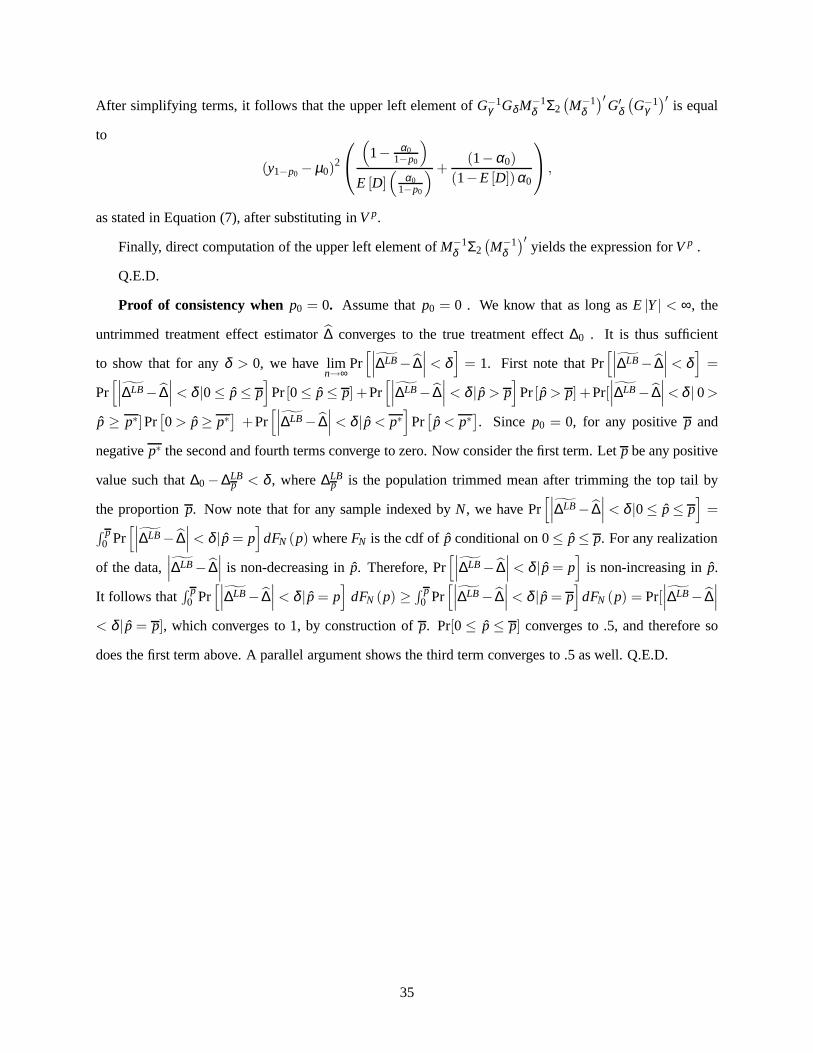
After simplifying terms, it follows that the upper left element ofG−1γ Gδ M−1

δ Σ2(M−1

δ)′

G′δ(G−1

γ)′

is equal

to

(y1−p0 −µ0)2

(1− α0

1−p0

)

E [D](

α01−p0

) +(1−α0)

(1−E [D])α0

,

as stated in Equation (7), after substituting inV p.

Finally, direct computation of the upper left element ofM−1δ Σ2

(M−1

δ)′

yields the expression forV p .

Q.E.D.

Proof of consistency whenp0 = 0. Assume thatp0 = 0 . We know that as long asE |Y| < ∞, the

untrimmed treatment effect estimator∆ converges to the true treatment effect∆0 . It is thus sufficient

to show that for anyδ > 0, we have limn→∞

Pr[∣∣∣∆LB− ∆

∣∣∣< δ]

= 1. First note that Pr[∣∣∣∆LB− ∆

∣∣∣< δ]

=

Pr[∣∣∣∆LB− ∆

∣∣∣< δ |0≤ p≤ p]

Pr[0≤ p≤ p] +Pr[∣∣∣∆LB− ∆

∣∣∣< δ |p > p]

Pr[p > p] +Pr[∣∣∣∆LB− ∆

∣∣∣< δ | 0>

p ≥ p∗]Pr[0 > p≥ p∗

]+Pr

[∣∣∣∆LB− ∆∣∣∣< δ |p < p∗

]Pr[p < p∗

]. Since p0 = 0, for any positivep and

negativep∗ the second and fourth terms converge to zero. Now consider the first term. Letp be any positive

value such that∆0 −∆LBp < δ , where∆LB

p is the population trimmed mean after trimming the top tail by

the proportionp. Now note that for any sample indexed byN, we have Pr[∣∣∣∆LB− ∆

∣∣∣< δ |0≤ p≤ p]

=

∫ p0 Pr

[∣∣∣∆LB− ∆∣∣∣< δ |p = p

]dFN (p) whereFN is the cdf ofp conditional on 0≤ p≤ p. For any realization

of the data,∣∣∣∆LB− ∆

∣∣∣ is non-decreasing in ˆp. Therefore, Pr[∣∣∣∆LB− ∆

∣∣∣< δ |p = p]

is non-increasing in ˆp.

It follows that∫ p

0 Pr[∣∣∣∆LB− ∆

∣∣∣< δ |p = p]

dFN (p) ≥ ∫ p0 Pr

[∣∣∣∆LB− ∆∣∣∣< δ |p = p

]dFN (p) = Pr[

∣∣∣∆LB− ∆∣∣∣

< δ |p = p], which converges to 1, by construction ofp. Pr[0 ≤ p ≤ p] converges to .5, and therefore so

does the first term above. A parallel argument shows the thirdterm converges to .5 as well. Q.E.D.

35

References

Ahn, Hyungtaik and James Powell, “Semiparametric Estimation of Censored Selection Modelswith aNonparametric Selection Mechanism,”Journal of Econometrics, 1993,58, 3–29.

Andrews, D. and M. Schafgans, “Semiparametric Estimation of the Intercept of a Sample SelectionModel,” Review of Economic Studies, 1998,65, 497–517.

Andrews, Donald W. K., “Empirical Process Methods in Econometrics,” in Robert F.Engle and Daniel L.McFadden, eds.,Handbook of Eonometrics, Vol. 4, Amsterdam: North Holland, 1994, pp. 2248–2296.

, Marcelo J. Moreira, and James H. Stock, “Performance of conditional Wald tests in IV regressionwith weak instruments,”Journal of Econometrics, 2007,139, 116–132.

Angrist, Joshua, “Conditional Independence in Sample Selection Models,”Economics Letters, 1997,54,103–112.

, Guido Imbens, and D. Rubin, “Identification of Causal Effects Using Instrumental Variables,”Journalof the American Statistical Association, 1996,91, 444–455.

Balke, A. and J. Pearl, “Bounds on Treatment Effects from Studies With Imperfect Compliance,”Journalof the American Statistical Association, 1997,92, 1171–1177.

Barnow, B., “The impact of CETA on the post-program earnings of participants,”Journal of Human Re-sources, 1987,22, 157–193.

Bloom, H., “Accounting for No-Shows in Experimental Evaluation Designs,” Evaluation Review, 1984,8,225–246.

Blundell, Richard, Amanda Gosling, Hidehiko Ichimura, and Costas Meghir, “Changes in the Distribu-tion of Male and Female Wages Accounting for Employment Composition Using Bounds,”Econometrica,March 2007,75 (2), 323–363.

Burghardt, John, Peter Z. Schochet, Sheena McConnell, Terry Johnson, R. Mark Gritz, Steven Glaz-erman, John Homrighausen, and Russell Jackson, “Does Job Corps Work? Summary of the NationalJob Corps Study,” Report, Mathematica Policy Research, Inc., Washington, DC 2001.

Card, David, “The Causal Effect of Education on Earnings,” in Orley Ashenfelter and David Card, eds.,Handbook of Labor Economics, Vol. 3A, Amsterdam: North Holland, 1999, pp. 1801–1863.

Chamberlain, Gary, “Quantile Regression, Censoring, and the Structure of Wages,” in C. A. Sims, ed.,Advances in Econometrics, Sixth World Congress, Vol. 1, Cambridge: Cambridge University Press, 1994.

Das, Mitali, Whitney K. Newey, and Francis Vella, “Nonparametric Estimation of Sample SelectionModels,”Review of Economic Studies, January 2003,70, 33–58.

Heckman, James and R. Robb, “Alternative methods for solving the problem of selectionbias in evaluatingthe impact of treatments on outcomes,” in H. Wainer, ed.,Drawing inferences from self-selected samples,New York, NY: Springer, 1986.

Heckman, James J., “Shadow Prices, Market Wages, and Labor Supply,”Econometrica, 1974,42, 679–694.

, “Sample Selection Bias as a Specification Error,”Econometrica, 1979,47 (1), 153–161.

36

, “Varieties of Selection Bias,”American Economic Review, May 1990,80, 313–318.

and Edward Vytlacil , “Local Instrumental Variables and Semiparametric Estimation and Latent Vari-able Models for Identifying and Bounding Treatment Effects,” Proceedings of the National Academy ofSciences, 1999,96, 4730–4734.

and , “Instrumental Variables, Selection Models, and Tight Bounds on the Average Treatment Effect,”Technical Working Paper 259, National Bureau of Economic Research 2000.

and , “Local Instrumental Variables,” Technical Working Paper252, National Bureau of EconomicResearch 2000.

, Robert J. LaLonde, and James A. Smith, “The Economics and Econometrics of Active Labor MarketPrograms,” in Orley Ashenfelter and David Card, eds.,Handbook of Labor Economics, Vol. 3A, Amster-dam: North Holland, 1999, pp. 1865–2097.

Hollister, R., P. Kemper, and R. Maynard, The National Supported Work Demonstration, Madison, WI:University of Wisconsin Press, 1984.

Horowitz, Joel L. and Charles F. Manski, “Identification and Robustness with Contaminated and Cor-rupted Data,”Econometrica, 1995,63, 281–302.

and , “Nonparametric Analysis of Randomized Experiments with Missing Covariate and OutcomeData,”Journal of the American Statistical Association, March 2000,95 (449), 77–84.

and , “Rejoinder: Nonparametric Analysis of Randomized Experiments with Missing Covariate andOutcome Data,”Journal of the American Statistical Association, March 2000,95 (449), 87.

Imbens, Guido and Joshua Angrist, “Identification and Estimation of Local Average TreatmentEffects,”Econometrica, 1994,62, 467–476.

Imbens, Guido W. and Charles F. Manski, “Confidence Intervals for Partially Identified Parameters,”Econometrica, 2004,72, 1845–1857.

Kiefer, N., The economic benefits of four employment and training programs, New York, NY: GarlandPublishing, 1979.

Krueger, Alan B. and Diane M. Whitmore, “The Effect of Attending a Small Class in the Early Grades onCollege-Test Taking and Middle School Test Results: Eviddence from Project STAR,”Economic Journal,2001,111, 1–28.

Lee, David S., “Trimming for Bounds on Treatment Effects with Missing Outcomes,” Center for LaborEconomics Working Paper 38, University of California, Berkeley March 2002.

, “Training, Wages, and Sample Selection: Estimating SharpBounds on Treatment Effects,” NBER Work-ing Paper 11721, National Bureau of Economic Research, Cambridge, MA October 2005.

Martin, John P. , “What works among Active Labour Market Policies: Evidencefrom OECD Countries’Experiences,”OECD Economic Studies, 2000,30 (1), 79–113.

Newey, Whitney K. and Daniel McFadden, “Large Sample Estimation and Hypothesis Testing,” inRobert F. Engle and Daniel L. McFadden, eds.,Handbook of Eonometrics, Vol. 4, Amsterdam: NorthHolland, 1994, pp. 2113–2245.

37

Robins, J., “The Analysis of Randomized and Non-Randomized AIDS Treatment Trials Using a New Ap-proach to Causal Inference in Longitudinal Studies,” in L. Sechrest, H. Freeman, and A. Mulley, eds.,Health Service Research Methodology: A Focus on AIDS, Washington, DC: U.S. Public Health Service,1989.

Rubin, D., “Inference and Missing Data,”Biometrika, 1976,63, 581–592.

Schochet, Peter Z., Jeanne Bellotti Ruo-Jiao Cao, Steven Glazerman, April Grady, Mark Gritz,Sheena McConnell, Terry Johnson, and John Burghardt, “National Job Corps Study: Data Documen-tation and Public Use Files, Volume I,” Documentation, Mathematica Policy Research, Inc., Washington,DC 2003.

, John Burghardt, and Steven Glazerman, “National Job Corps Study: The Impacts of Job Corps onParticipants’ Employment and Related Outcomes,” Report, Mathematica Policy Research, Inc., Washing-ton, DC 2001.

Smith, James P. and Finis R. Welch, Closing the Gap: Forty Years of Economic Progress for Blacks, SantaMonica, CA: Rand Corporation, 1986.

Staiger, Douglas and James H. Stock, “Instrumental Variables regression with Weak Instruments,” Econo-metrica, 1997,65, 557–586.

Stigler, Stephen M., “The Asymptotic Distribution of the Trimmed Mean,”Annals of Statistics, 1973,1,472–477.

U.S. Department of Labor, “Summary of Budget Authority: Fiscal Years 2004-2005,” Table, Employmentand Training Administration 2 2005.

, “What is Job Corps?,” Web Page, Employment and Training Administration 2005. <http://jobcorps.doleta.gov/about.cfm>.

Vytlacil, Edward , “Independence, Monotonicity, and Latent Index Models: AnEquivalence Result,”Econometrica, 2002,70 (1), 331–341.

Zhang, Junni L. and Donald B. Rubin, “Estimation of Causal Effects via Principal Stratification whenSome Outcomes are Truncated by "Death",”Journal of Educational and Behavioral Statistics, 2003,28,353–368.

, , and Fabrizia Mealli, “Evaluting the Effects of Job Training Programs on Wages through PrincipalStratification,” in “Modelling and Evaluating Treatment Effects in Econometrics,” Vol. 21, Eslevier Ltd.,2008, pp. 119–147.

38

Figure I: Impact of Job Corps on Weekly Earnings

Figure II: Impact of Job Corps on Employment Rates

0

50

100

150

200

250

0 52 104 156 208

Week Since Random Assignment

Control

Treatment

Wee

kly

Earn

ings

(Dol

lars

)

0

0.1

0.2

0.3

0.4

0.5

0.6

0.7

0 52 104 156 208

Week Since Random Assignment

ControlTreatmentEm

ploy

men

t Rat

e

Figure III: Differences in Log(Hourly Wage), Conditional on Employment

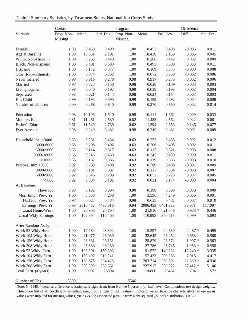
Table I: Summary Statistics, by Treatment Status, National Job Corps Study

Control Program DifferenceVariable Prop. Non- Mean Std. Dev. Prop. Non- Mean Std. Dev. Diff. Std. Err.

Missing Missing

Female 1.00 0.458 0.498 1.00 0.452 0.498 -0.006 0.011Age at Baseline 1.00 18.351 2.101 1.00 18.436 2.159 0.085 0.045White, Non-Hispanic 1.00 0.263 0.440 1.00 0.266 0.442 0.002 0.009Black, Non-Hispanic 1.00 0.491 0.500 1.00 0.493 0.500 0.003 0.011Hispanic 1.00 0.172 0.377 1.00 0.169 0.375 -0.003 0.008Other Race/Ethnicity 1.00 0.074 0.262 1.00 0.072 0.258 -0.002 0.006Never married 0.98 0.916 0.278 0.98 0.917 0.275 0.002 0.006Married 0.98 0.023 0.150 0.98 0.020 0.139 -0.003 0.003Living together 0.98 0.040 0.197 0.98 0.039 0.193 -0.002 0.004Separated 0.98 0.021 0.144 0.98 0.024 0.154 0.003 0.003Has Child 0.99 0.193 0.395 0.99 0.189 0.392 -0.004 0.008Number of children 0.99 0.268 0.640 0.99 0.270 0.650 0.002 0.014

Education 0.98 10.105 1.540 0.98 10.114 1.562 0.009 0.033Mother's Educ. 0.81 11.461 2.589 0.82 11.483 2.562 0.022 0.061Father's Educ. 0.61 11.540 2.789 0.62 11.394 2.853 -0.146 0.077Ever Arrested 0.98 0.249 0.432 0.98 0.249 0.432 -0.001 0.009

Household Inc: <3000 0.65 0.251 0.434 0.63 0.253 0.435 0.002 0.0123000-6000 0.65 0.208 0.406 0.63 0.206 0.405 -0.002 0.0116000-9000 0.65 0.114 0.317 0.63 0.117 0.321 0.003 0.008

9000-18000 0.65 0.245 0.430 0.63 0.245 0.430 0.000 0.011>18000 0.65 0.182 0.386 0.63 0.179 0.383 -0.003 0.010

Personal Inc: <3000 0.92 0.789 0.408 0.92 0.789 0.408 -0.001 0.0093000-6000 0.92 0.131 0.337 0.92 0.127 0.334 -0.003 0.0076000-9000 0.92 0.046 0.209 0.92 0.053 0.223 0.007 0.005

>9000 0.92 0.034 0.181 0.92 0.031 0.174 -0.003 0.004At Baseline:

Have Job 0.98 0.192 0.394 0.98 0.198 0.398 0.006 0.009Mos. Empl. Prev. Yr. 1.00 3.530 4.238 1.00 3.596 4.249 0.066 0.091

Had Job, Prev. Yr. 0.98 0.627 0.484 0.98 0.635 0.482 0.007 0.010Earnings, Prev. Yr. 0.93 2810.482 4435.616 0.94 2906.453 6401.328 95.971 117.097Usual Hours/Week 1.00 20.908 20.704 1.00 21.816 21.046 0.908 * 0.446

Usual Wkly Earnings 1.00 102.894 116.465 1.00 110.993 350.613 8.099 5.093

After Random Assignment:Week 52 Wkly Hours 1.00 17.784 23.392 1.00 15.297 22.680 -2.487 * 0.495Week 104 Wkly Hours 1.00 21.977 26.080 1.00 22.645 26.252 0.668 0.560Week 156 Wkly Hours 1.00 23.881 26.151 1.00 25.879 26.574 1.997 * 0.563Week 208 Wkly Hours 1.00 25.833 26.250 1.00 27.786 25.745 1.953 * 0.558Week 52 Wkly. Earn. 1.00 103.801 159.893 1.00 91.552 149.282 -12.249 * 3.335Week 104 Wkly Earn. 1.00 150.407 210.241 1.00 157.423 200.266 7.015 4.417Week 156 Wkly Earn. 1.00 180.875 224.426 1.00 203.714 239.802 22.839 * 4.936Week 208 Wkly Earn. 1.00 200.500 230.661 1.00 227.912 250.222 27.412 * 5.106Total Earn. (4 years) 1.00 30007 26894 1.00 30800 26437 794 572

Number of Obs 3599 5546Note: N=9145. * denotes difference is statistically significant from 0 at the 5 percent (or less) level. Computations use design weights.Chi-square test of all coefficients equalling zero, from a logit of the treatment indicator on all baseline characteristics (where meanvalues were imputed for missing values) yields 24.95; associated p-value from a chi-squared (27 dof) distribution is 0.577.

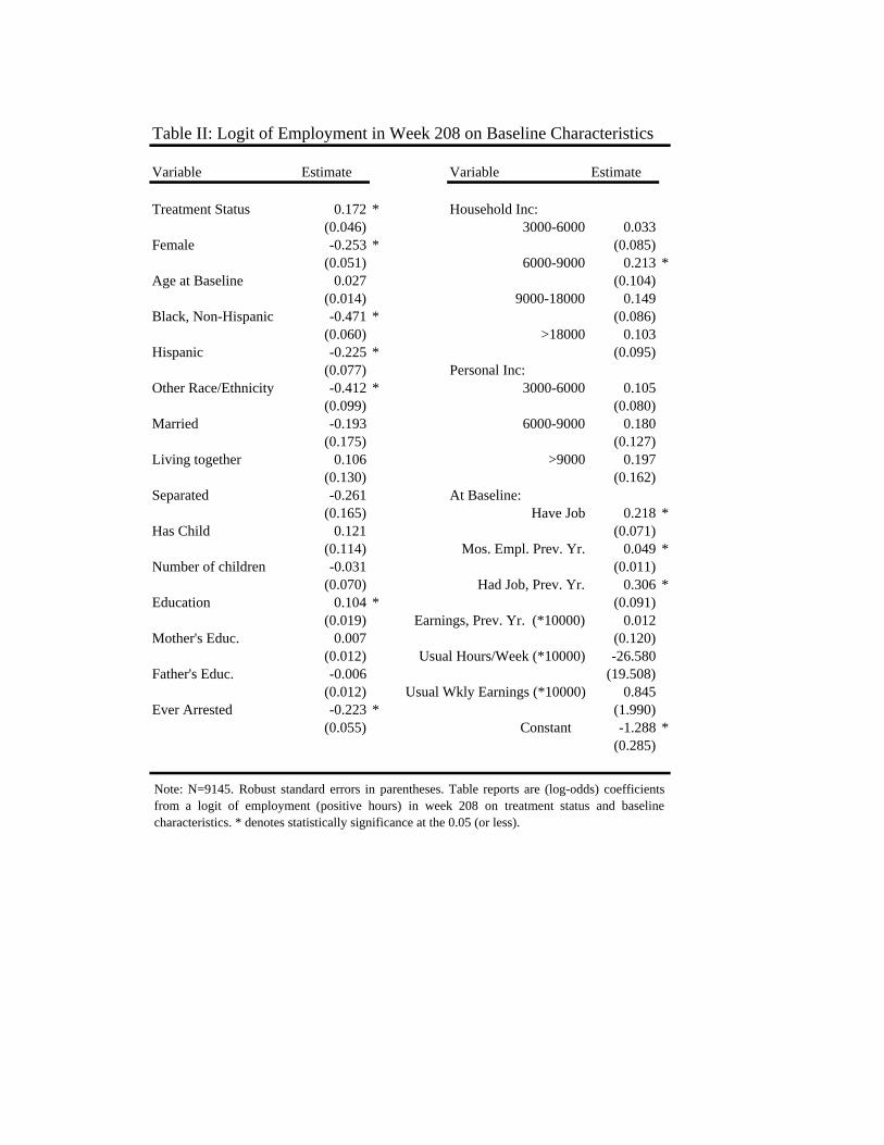
Table II: Logit of Employment in Week 208 on Baseline Characteristics

Variable Estimate Variable Estimate

Treatment Status 0.172 * Household Inc:(0.046) 3000-6000 0.033

Female -0.253 * (0.085)(0.051) 6000-9000 0.213 *

Age at Baseline 0.027 (0.104)(0.014) 9000-18000 0.149

Black, Non-Hispanic -0.471 * (0.086)(0.060) >18000 0.103

Hispanic -0.225 * (0.095)(0.077) Personal Inc:

Other Race/Ethnicity -0.412 * 3000-6000 0.105(0.099) (0.080)

Married -0.193 6000-9000 0.180(0.175) (0.127)

Living together 0.106 >9000 0.197(0.130) (0.162)

Separated -0.261 At Baseline:(0.165) Have Job 0.218 *

Has Child 0.121 (0.071)(0.114) Mos. Empl. Prev. Yr. 0.049 *

Number of children -0.031 (0.011)(0.070) Had Job, Prev. Yr. 0.306 *

Education 0.104 * (0.091)(0.019) Earnings, Prev. Yr. (*10000) 0.012

Mother's Educ. 0.007 (0.120)(0.012) Usual Hours/Week (*10000) -26.580

Father's Educ. -0.006 (19.508)(0.012) Usual Wkly Earnings (*10000) 0.845

Ever Arrested -0.223 * (1.990)(0.055) Constant -1.288 *

(0.285)

Note: N=9145. Robust standard errors in parentheses. Table reports are (log-odds) coefficientsfrom a logit of employment (positive hours) in week 208 on treatment status and baselinecharacteristics. * denotes statistically significance at the 0.05 (or less).

Table III: Bounds on Treatment Effects for Week 208 ln(wage) Utilizing Bounds of Support (Horowitz and Manski)

(i) Control Group Observations 3599(ii) Employment Rate 0.566(iii) Mean log(wage) 1.997(iv) Upper Bound 2.332(v) Lower Bound 1.520

(vi) Treatment Group Observations 5546(vii) Employment Rate 0.607(viii) Mean log(wage) 2.031(ix) Upper Bound 2.321(x) Lower Bound 1.586

(xi) Difference Upper Bound: (ix) - (v) 0.802(xii) Lower Bound: (x) - (iv) -0.746

Note: .90 and 2.77 are the lower and upper bounds of the support of ln(hourly wage)in Week 208 after random assignment. (iv) = (ii)*(iii) + [1-(ii)]*2.77. (v) = (ii)*(iii) +[1-(ii)]*(.90). Rows (ix) and (x) are defined analogously.

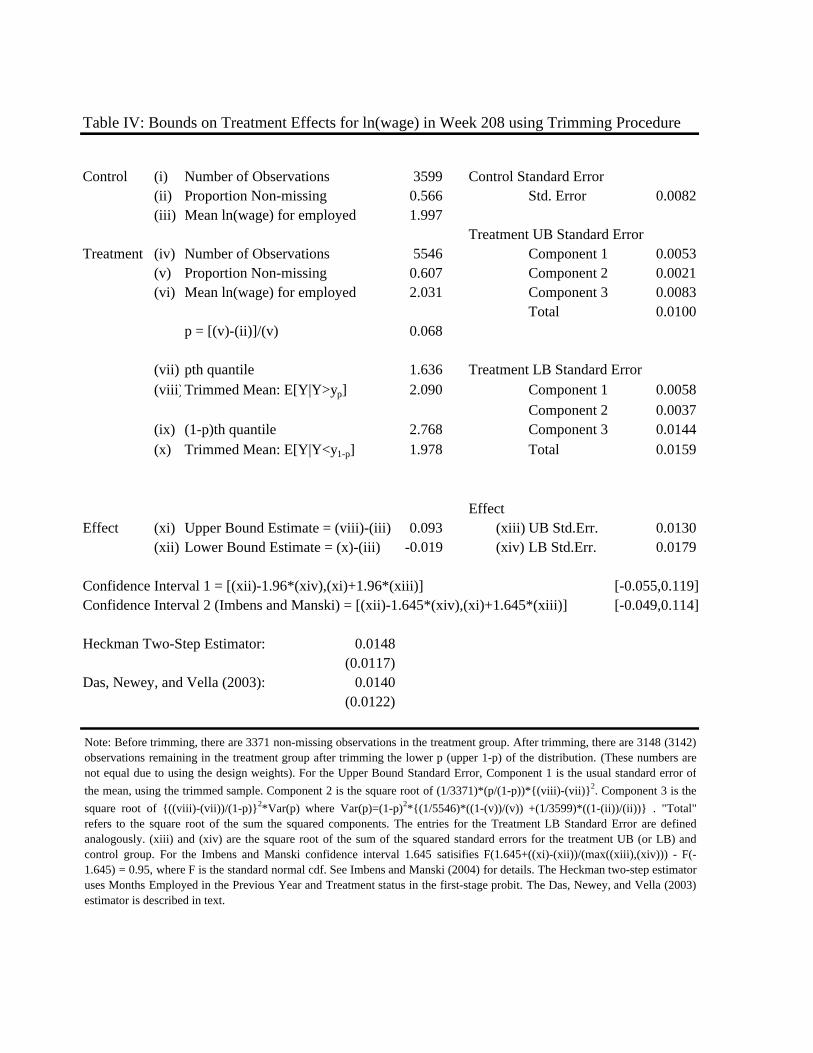
Table IV: Bounds on Treatment Effects for ln(wage) in Week 208 using Trimming Procedure

Control (i) Number of Observations 3599 Control Standard Error(ii) Proportion Non-missing 0.566 Std. Error 0.0082(iii) Mean ln(wage) for employed 1.997

Treatment UB Standard ErrorTreatment (iv) Number of Observations 5546 Component 1 0.0053

(v) Proportion Non-missing 0.607 Component 2 0.0021(vi) Mean ln(wage) for employed 2.031 Component 3 0.0083

Total 0.0100p = [(v)-(ii)]/(v) 0.068

(vii) pth quantile 1.636 Treatment LB Standard Error(viii)Trimmed Mean: E[Y|Y>yp] 2.090 Component 1 0.0058

Component 2 0.0037(ix) (1-p)th quantile 2.768 Component 3 0.0144(x) Trimmed Mean: E[Y|Y<y1-p] 1.978 Total 0.0159

EffectEffect (xi) Upper Bound Estimate = (viii)-(iii) 0.093 (xiii) UB Std.Err. 0.0130

(xii) Lower Bound Estimate = (x)-(iii) -0.019 (xiv) LB Std.Err. 0.0179

Confidence Interval 1 = [(xii)-1.96*(xiv),(xi)+1.96*(xiii)] [-0.055,0.119]Confidence Interval 2 (Imbens and Manski) = [(xii)-1.645*(xiv),(xi)+1.645*(xiii)] [-0.049,0.114]

Heckman Two-Step Estimator: 0.0148(0.0117)

Das, Newey, and Vella (2003): 0.0140(0.0122)

Note: Before trimming, there are 3371 non-missing observations in the treatment group. After trimming, there are 3148 (3142)observations remaining in the treatment group after trimming the lower p (upper 1-p) of the distribution. (These numbers arenot equal due to using the design weights). For the Upper Bound Standard Error, Component 1 is the usual standard error ofthe mean, using the trimmed sample. Component 2 is the square root of (1/3371)*(p/(1-p))*{(viii)-(vii)}2. Component 3 is thesquare root of {((viii)-(vii))/(1-p)}2*Var(p) where Var(p)=(1-p)2*{(1/5546)*((1-(v))/(v)) +(1/3599)*((1-(ii))/(ii))} . "Total"refers to the square root of the sum the squared components. The entries for the Treatment LB Standard Error are definedanalogously. (xiii) and (xiv) are the square root of the sum of the squared standard errors for the treatment UB (or LB) andcontrol group. For the Imbens and Manski confidence interval 1.645 satisifies F(1.645+((xi)-(xii))/(max((xiii),(xiv))) - F(-1.645) = 0.95, where F is the standard normal cdf. See Imbens and Manski (2004) for details. The Heckman two-step estimatoruses Months Employed in the Previous Year and Treatment status in the first-stage probit. The Das, Newey, and Vella (2003)estimator is described in text.

Table V: Bounds on Treatment Effects for ln(wage) in Week 208Trimming Procedure using Baseline Covariates

Lower Bound for Treatment Mean Upper Bound for Treatment Mean

Group Estimate Std. Error Obs Estimate Std. Error Obs Weight1 1.795 0.030 343 1.979 0.025 348 0.1072 1.938 0.052 248 1.963 0.065 250 0.1313 1.934 0.020 931 2.051 0.017 935 0.2914 2.025 0.028 745 2.127 0.020 748 0.2385 2.121 0.025 712 2.204 0.022 715 0.234

Total 1.985 0.013 2979 2.086 0.012 2996 1.000

Effect Lower Bound for Effect Upper Bound for Effect

-0.0118 0.0151 0.0889 0.0142

Note: Trimming procedure from Table III applied separately to each Group (defined in text). "Total"estimates are means of the 5 groups using the "Weight" as weights. Asymptotic variance for "Total" iscomputed according to Chamberlain (1993): it is the (weighted, using "Weight") average of the asymptoticvariance for each group (each group's sampling variance times the number of observations for the group)plus the (weighted by "Weight") average squared deviation of each group's estimate from the "Total" mean.Control mean, (iii) in Table IV, is then subtracted to obtain bounds on the treatment effect.

Table VI: Treatment Effect Estimates and Bounds, by Week

Fraction Non-missing EffectTrimming Untrimmed Lower Upper

Control Treatment Proportion Bound Bound

Week 45 0.4223 0.3424 0.1892 0.022 -0.074 0.127(0.0219) (0.011) (0.014) (0.015)

Week 90 0.4600 0.4601 0.0003 0.043 0.042 0.043(0.0232) (0.011) (0.024) (0.025)

Week 135 0.5173 0.5451 0.0509 0.028 -0.016 0.076(0.0192) (0.011) (0.021) (0.014)

Week 180 0.5403 0.5825 0.0724 0.026 -0.033 0.087(0.0177) (0.011) (0.019) (0.013)

Note: (N=9145 for each row). Standard errors in parentheses. Standard errors for Trimming Proportiongiven by formula in note to Table IV. Bounds computed according to Table IV. See text for details.

Appendix Table I: Summary Statistics, by Treatment Status, National Job Corps StudyConditional on Positive Earnings in Week 90

Control Program DifferenceVariable Prop. Non- Mean Prop. Non- Mean Diff. Std. Err.

Missing Missing

Female 1.00 0.429 1.00 0.419 -0.009 0.016Age at Baseline 1.00 18.691 1.00 18.729 0.038 0.068White, Non-Hispanic 1.00 0.310 1.00 0.328 0.018 0.015Black, Non-Hispanic 1.00 0.447 1.00 0.443 -0.004 0.016Hispanic 1.00 0.171 1.00 0.167 -0.004 0.012Other Race/Ethnicity 1.00 0.072 1.00 0.063 -0.009 0.008Never married 0.99 0.909 0.99 0.909 0.000 0.009Married 0.99 0.030 0.99 0.023 -0.007 0.005Living together 0.99 0.039 0.99 0.045 0.006 0.006Separated 0.99 0.022 0.99 0.022 0.001 0.005Has Child 0.99 0.188 1.00 0.178 -0.009 0.012Number of children 0.99 0.247 0.99 0.241 -0.007 0.019

Education 0.99 10.381 0.98 10.371 -0.010 0.050Mother's Educ. 0.83 11.506 0.84 11.579 0.072 0.090Father's Educ. 0.66 11.644 0.67 11.458 -0.186 0.111Ever Arrested 0.99 0.238 0.99 0.232 -0.006 0.013

Household Inc: <3000 0.68 0.188 0.66 0.202 0.014 0.0153000-6000 0.68 0.188 0.66 0.182 -0.006 0.0156000-9000 0.68 0.116 0.66 0.119 0.003 0.012

9000-18000 0.68 0.289 0.66 0.270 -0.019 0.017>18000 0.68 0.219 0.66 0.227 0.008 0.016

Personal Inc: <3000 0.95 0.726 0.93 0.732 0.005 0.0143000-6000 0.95 0.164 0.93 0.154 -0.010 0.0126000-9000 0.95 0.065 0.93 0.068 0.003 0.008

>9000 0.95 0.045 0.93 0.047 0.002 0.007At Baseline:

Have Job 0.98 0.251 0.98 0.254 0.002 0.014Mos. Empl. Prev. Yr. 1.00 4.572 1.00 4.558 -0.013 0.143

Had Job, Prev. Yr. 0.99 0.725 0.99 0.727 0.002 0.014Earnings, Prev. Yr. 0.94 3783.940 0.94 3699.524 -84.416 159.333Usual Hours/Week 1.00 24.600 1.00 25.165 0.565 0.642

Usual Wkly Earnings 1.00 125.147 1.00 126.297 1.150 3.838

After Random Assignment:Week 90 ln(wage) 1.00 1.827 1.00 1.870 0.043 * 0.011

Number of Obs 1660 2564Note: N=4224. * denotes difference is statistically significant from 0 at the 5 percent level. Computations usedesign weights. Chi-square test of all coefficients equalling zero, from a logit of the treatment indicator on allbaseline characteristics (where mean values were imputed for missing values) yields 19.50; associated p-value froma chi-squared (27 dof) distribution is 0.851.