IZA DP No. 1252

Reservation Wages, Search Duration,and Accepted Wages in Europe

John T. AddisonMário CentenoPedro Portugal

DI

SC

US

SI

ON

PA

PE

R S

ER

IE

S

Forschungsinstitutzur Zukunft der ArbeitInstitute for the Studyof Labor

August 2004

Reservation Wages, Search Duration,

and Accepted Wages in Europe

John T. Addison University of South Carolina

and IZA Bonn

Mário Centeno Banco de Portugal

and Universidade Técnica de Lisboa

Pedro Portugal Banco de Portugal

and Universidade Nova de Lisboa

Discussion Paper No. 1252 August 2004

IZA

P.O. Box 7240 53072 Bonn

Germany

Phone: +49-228-3894-0 Fax: +49-228-3894-180

Email: iza@iza.org

Any opinions expressed here are those of the author(s) and not those of the institute. Research disseminated by IZA may include views on policy, but the institute itself takes no institutional policy positions. The Institute for the Study of Labor (IZA) in Bonn is a local and virtual international research center and a place of communication between science, politics and business. IZA is an independent nonprofit company supported by Deutsche Post World Net. The center is associated with the University of Bonn and offers a stimulating research environment through its research networks, research support, and visitors and doctoral programs. IZA engages in (i) original and internationally competitive research in all fields of labor economics, (ii) development of policy concepts, and (iii) dissemination of research results and concepts to the interested public. IZA Discussion Papers often represent preliminary work and are circulated to encourage discussion. Citation of such a paper should account for its provisional character. A revised version may be available directly from the author.

IZA Discussion Paper No. 1252 August 2004

ABSTRACT

Reservation Wages, Search Duration, and Accepted Wages in Europe

This paper uses data from the European Community Household Panel, 1994-99, to investigate the arrival rate of job offers, the determinants of reservation wages, transitions out of unemployment, and accepted wages. In this exploratory treatment, we report that the arrival rate of job offers declines precipitously with jobless duration and age; that reservation wages do decline with the jobless spell (and aggregate unemployment); that transitions out of unemployment exhibit strong negative duration dependence for reasons that have more to do with the arrival rate of job offers than with reservation wages; and that the decline in reemployment wages with joblessness closely shadows the corresponding fall in reservation wages. JEL Classification: J64, J65 Keywords: reservation wages, job offer arrival rates, unemployment duration,

reemployment wages Corresponding author: John T. Addison Department of Economics Moore School of Business University of South Carolina 1705 College Street Columbia, SC 29208 USA Email: ecceaddi@moore.sc.edu

3

I. Introduction

High and downwardly rigid reservation wages, most likely occasioned by generous

unemployment benefits, are often held to be responsible for Europe’s high and persistent

unemployment since the early 1970s. But this proposition has to be qualified in at least two

important respects. First of all, direct evidence on the course of reservation wages is scant.1

Second of all, some European countries, most notably Eire, the Netherlands, the United

Kingdom, and Denmark have made quite impressive gains in recent years and can no longer

be included in the set of chronically-high unemployment rate countries.

Given the informational deficiencies of most datasets – in particular, the lack of

information on reservation wages and the arrival rate of job offers – the critical job search

relationship between reservation wages, the arrival rate of job offers and unemployment

duration cannot be obtained directly. Rather, it has to be inferred either from reduced-form

approaches or from severely stylized structural models.

In this paper, we explore the institutional diversity of labor markets in thirteen

European countries with a view to understanding the variation in their unemployment

experience over the sample period 1994-99. For this purpose, we rely on the longitudinal

data from European Household Panel. This dataset is unique in providing uniform

information on reservation wages, the arrival rate of job offers, elapsed unemployment

duration, transitions from unemployment to employment, and reemployment wages.

Our approach is in large part exploratory, seeking only at this stage to uncover some

stylized facts on the behavior of reservation wages and related variables. Although

descriptive, there are five important issues that we can address in this type of framework:

(i) we will illuminate the notion that in Europe the arrival rate of job offers is very low and

that acceptance rates are very high (higher than 90 percent), meaning that reservation wages

necessarily play a muted (or no) role;

(ii) we can investigate the main source of negative (unemployment) duration dependence,

found in all countries of the sample. Given that the probability of locating an acceptable job

depends on the arrival rate of job offers, the wage offer distribution, and the reservation

4

wage, we will seek to determine which component dominates in producing declining

unemployment-to-employment hazard functions. This evaluation provides the basis for a

better understanding of the mechanisms producing employer stigmatization, human capital

depreciation over the course of joblessness, the loss of informational networks that sustain

job contacts, discouragement, and even a simple sorting of the more employable into

employment;

(iii) we will look in detail into the question of whether reservation wages are constant or

instead declining through time. The constant reservation wage hypothesis provides a useful,

parsimonious way of recouping the structural parameters of the job search model. However,

in the few instances where this hypothesis is tested it has been soundly rejected (see, for

example, Kiefer and Neumann, 1979). In our case, the simple correlations between (log)

unemployment duration and reservation wages evince a negative association in all thirteen

countries (statistically insignificant in four of them), suggesting that factors such as depletion

of household income, finite lives, changes in the wage offer distribution, and/or a declining

arrival rate of job offers may play a role;

(iv) having characterized the determinants of the reservation wages, we consider the impact

of reservation wages on duration under a non-stationary regime. In this exercise, we shall

exploit the information on transitions into employment while taking into account length-bias

sampling; and,

(v) we will also take advantage of the available information about the wages earned by

reemployed workers to further investigate the indication of declining reservation wages,

which phenomenon, if sustained, should have a counterpart in a negative association

between wages and the duration of unemployment. Here, the issues of self selection into

employment and the endogeneity of jobless duration have also to be addressed.

The plan of the paper is as follows. Section II describes the unique dataset. Section

III analyzes the determinants of the arrival rates of job offers, section IV the reservation

wage, section V unemployment transitions, and section VI reemployment wages. A brief

summary concludes.

1 Studies by Lancaster (1983, 1985) and Jones (1988, 1989) for the United Kingdom, Gorter and Gorter (1993) for the Netherlands, and Prasad (2002) for Germany are notable exceptions of single-country studies that use survey information on reservation wages.

5

II. Data description

We use information from six waves of the European Community Household Panel (ECHP),

1994-99. The actual data cover the interval January 1993 through December 1998. The

ECHP survey interviews individuals once a year, and asks them a range of questions relating

to their labor market experience during the preceding calendar year. We use data from 13 out

of the 15 EU countries, namely, Germany, Denmark, the Netherlands, Belgium, France, the

United Kingdom, Ireland, Italy, Greece, Spain, Portugal, Austria, and Finland. The excluded

countries are Luxembourg and Sweden where is not possible to follow individuals through

time. With the exception of three countries, the data cover the entire period. The exceptions

are Germany, where we include data from just the 1994-96 waves (because of missing data

on hourly reservation wages in subsequent years), together with Austria and Finland which

were only added to the panel in 1995 and 1996, respectively.

In the ECHP every individual actively looking for a job is asked two questions

pertaining first to desired hours of work and second to the minimum income required to

work these hours. The actual survey questions that are used to measure the reservation wage

are: “Assuming you could find suitable work, how many hours per week would you prefer to work in this

new job?” and “What is the minimum net monthly income would you accept to work [number of hours in

previous question] hours a week in this new job?” The crucial reservation wage construct in this

paper is, then, an hourly net reservation wage, measured as the ratio of the net monthly

income to the optimal number of hours. This measure and all other monetary variables in

the different countries were transformed in a single currency unit using the Purchasing

Power Parities (PPP) published by Eurostat.

The other key variable in our study is the duration of the unemployment spell. We

use as a measure of search duration the length of each spell of joblessness. The ECHP

sampling procedure considers only jobless spells for individuals with previous work

experience, for whom we are able to identify the month and year of job loss. Given that we

know the month and year of the interview (the exception to this rule being Germany), we

compute elapsed unemployment duration as the period between the point of job loss up

until the interview month. (For Germany, we assume that all the interviews were carried out

in October.)

6

It is no less important for the purposes of this empirical inquiry to have a measure of

job offer rates. To this end, we exploit the question in the survey asking each unemployed

individual whether or not he/she received a job offer in the previous month. The actual

question is: “Have you received any job offer during the past 4 weeks?” To this reported number of

offers, for some specifications, we shall add those individuals who were employed at the

survey date but unemployed one month earlier and who therefore obtained a job during the

month preceding the interview.

As was noted earlier, the assessment made by workers of the wage distribution (of

available jobs) plays a very important role in search theory as it against this distribution that

workers set their reservation wages. Accordingly, reservation wages should be a function of

the same set of variables as determine not only accepted wages but also, and more generally,

wages available in the economy. In order to compute the expected wage of each unemployed

worker we estimate a conventional earnings function for each country, so as form an

expected wage for the unemployed individuals.2

Before presenting summary statistics of the main variables used in this study, we

need to address the quality of our data and their adequacy for an analysis of reservation

wages. First, although past studies suffer from a potential problem of low responses rates

to the reservation wage question, this is not a consideration here. With the exception of

the Netherlands, the response rate is quite large, ranging from 92 percent in Finland to

almost 100 percent in Greece (see Appendix Table 1). Second, job search theory requires

that reservation wages exceed unemployment benefits and this requirement is also

generally met in the dataset. In only 10 percent of the cases (215 out of 2,063

observations) do reservation wages fall below reported monthly unemployment benefit

levels.3 Third, another search-theoretic condition is that accepted wages exceed

reservation wages. Here, it is somewhat disturbing that our data show a relatively larger

fraction of workers accepting jobs paying below the stated reservation wages. That said,

2 Log wages were regressed on categorical variables for education and age, gender, marital status, dependent children, and a set of year dummies. 3 We only have data on monthly unemployment benefits for eight countries - Denmark, the Netherlands, France, Ireland, Italy, Greece, Portugal, and Austria - so that in practice we used annual rather than monthly benefit data. However, the use of monthly data for these eight countries resulted in very similar findings to those reported here for annual data.

7

this observation makes no allowance for self-selection into reemployment or for any

erosion of the reservation wages that might have occurred.

There is some asymmetry in the distribution of workers across countries, as can be

seen from the material given in Appendix Table 2. In particular, there is some over-

representation of individuals from southern European countries (Italy, Spain, and Portugal),

with France and Germany contributing a smaller number of workers. This reflects the

incidence of unemployment experiences among countries in the sample (e.g. the high

unemployment rate of Spain) and the shorter sample period of others (e.g. Germany).

(Table 1 near here)

Summary statistics for the main variables used in this study are presented in Table 1

for the sample of unemployed workers. The pattern is familiar for Europe but note that

while reported unemployment duration is long, what is actually being measured here is

joblessness rather than unemployment. To this extent, unemployment per se is overstated.

Also observe the relatively low level of schooling in the sample (just only 13 percent have a

college degree, 16 percent for women) and the relatively low mean age (over 50 percent of

the workers are aged less than 35 years).

III. The arrival rate of job offers

We model the determinants of the arrival rate of job offers using an extreme value

probability model as follows

( )[ ]ββπ 'expexp1)'( xx −−= , (1)

where )'( βπ x gives the probability of receiving a job offer, x denotes the vector of

explanatory variables, and β identifies the corresponding regression coefficients. The choice

of an extreme-minimal-value distribution was guided by its ability to mix naturally with the

grouped version of the proportional hazards model (Prentice and Gloeckler, 1978).4

4 The complementary log-log model is nonsymmetric. It is close to the logistic function for low values of π but with a considerably less heavy right tail (Fahrmeir and Tutz, 1994). As with other binary choice models, the interpretation of the regression coefficient is not straightforward. In this case it will be helpful to compute the implied marginal effects for the covariate xj , given by

8

Our main focus here will be upon the impact of unemployment duration and

unemployment insurance recipiency on the likelihood of a worker getting a job offer in any

four-week period. A further important consideration is the influence of age on the offer rate.

Table 2 provides the regression coefficient estimates for the probability that an unemployed

worker will receive a job offer. In the first two columns, the sample comprises only those

individuals unemployed at the time of the survey that report having received an offer in the

previous four weeks. In the last two columns, we add in those workers who got a new job in

the last four weeks and who were previously unemployed on the assumption they also

received the offer in the self-same period.5

(Table 2 near here)

Perhaps the most interesting result from the table is the negative impact of elapsed

unemployment duration on the job offer’s arrival probability. It can be seen that the arrival

rate of job offers declines very strongly with jobless duration. The marginal effect of

unemployment duration on the adjusted arrival rate of job offers – evaluated at the mean

sample values of the variables included in the regression and shown in second and fourth

columns of the table – is quite large. This holds in particular for our preferred adjusted

arrival rate of job offers (-0.131).

Other notable results from Table 2 are the effects of personal characteristics (age,

gender, education) on one hand and unemployment benefits and the rate of unemployment

on the other. Male and younger workers clearly have a much higher probability of receiving a

job offer. Age has a particularly strong negative impact on the probability of receiving a job

offer. This effect would generally add to the impact of unemployment duration, noted

earlier, since older workers typically experience longer unemployment spells. Also, workers

with more education are more likely to receive job offers. Note, however, that the results for

the household size variable intended to proxy a network effect (larger households being

associated with more extensive networks) are perverse albeit weak.

The amount of unemployment benefits received does not have any clear impact on

the probability of receiving a job offer. When we restrict the sample to unemployed workers

)'()'exp())'exp(exp()'exp()'( βπββββββπ

xxxxx

xjj

j

=−=∂

∂.

5 Germany is excluded from the regression in column three because we do not observe the month of the interview and cannot therefore compute each worker’s job tenure with the required precision.

9

(in the first column), the coefficient is positive but statistically insignificant, but if we adjust

the rate of job offers by including those workers who are already working at the time of the

survey (in the third column) the impact is negative, and receipt of benefits is clearly

associated with a lower arrival rate of job offers. The same conflicting results are obtained

for the unemployment rate. That is to say, the results in the first column point to pro-

cyclicality in the arrival rate of job offers: a higher unemployment rate decreases the

probability of receiving an offer. By contrast, in the third column the coefficient estimate is

not statistically significant and is positively signed. Arguably, adding into the ‘sample’ those

individuals who not only received a job offer but also accepted it renders that sample less

sensitive to the cycle.

IV. Determinants of the reservation wage

We now turn to an examination of the determinants of the reservation wage.

Describing the behavior of the reservation wage is of fundamental importance in

understanding its role in the worker’s unemployment experience. Special attention will be

accorded the issue of the stationarity of the reservation wage over time, and its relationship

with expected wages and aggregate economic conditions as indexed by the overall

unemployment rate.

The reservation wage equation may be expressed as

ελβ ++= txwR log'log , (2)

where x is a vector of explanatory variables, t denotes elapsed unemployment duration, and

ε is an error term.

(Table 3 near here)

Table 3 presents the estimation results for the hourly reservation wage equation. In

order to control for non-stationarity in the offered wage distribution, we include the

estimated wage computed for each unemployed individual obtained from hourly wage

regressions run for each country. As before, the excluded category for age is the group aged

above 55 years. Unemployment benefit is measured by the annual benefit amount received

during the year prior to the survey.

The first column of the table does not include elapsed unemployment duration as an

explanatory variable. In this specification, we see that reservation wages are larger for older

10

workers, while males have reservation wages that are roughly 5 percent higher than for

females. All other variables also have the expected sign. Thus, for example, those with

dependent children have higher reservation wages (more than 2 percent higher than their

counterparts without such dependents), as do workers who own their homes (although the 1

percent elevation in the reservation wage seems too small to have much traction in

subsequently raising unemployment). But most interesting of all are the results for the

unemployment benefits and the unemployment rate. In particular, we obtain a very small

elasticity of reservation wages with respect to annual unemployment benefits. In both this

specification and those in the next two columns of the table, this elasticity is always smaller

than 1 percent. Also observe the strongly pro-cyclical impact of macroeconomic conditions

on reservation wages. This result is also robust to specification. The finding that more

adverse labor market conditions are associated with a lower reservation wage is an important

and novel result of this inquiry and it provides another indication of the non-stationarity of

its distribution, especially given that we are also controlling for country and year effects.

The country dummies capture differences at the country level in reservation wages.

The low relative values reported for the United Kingdom are quite striking. Unemployed

British workers have the lowest reservation wages of all. The Portuguese unemployed come

next, while their Iberian neighbors evince the highest reservation wages.

The specification in the second column of Table 3 includes elapsed unemployment

duration as a regressor. The variable has the expected negative sign and is statistically

different from zero, with a small elasticity of -1.4 percent. However, one might expect this

estimate to be biased due to the simultaneity between duration and the reservation wage. In

an attempt to cope with this particular problem, we instrumented unemployment duration

(the instruments used to identify the reservation wage equation are the number of dependent

children, family size, and dummies for marital status, an outstanding mortgage and schooling

level). 6 The results are presented in the final column of the table and duly show a much

larger effect, with the estimated unemployment duration elasticity rising to -10 percent.

In each case the findings given in Table 3 are pooled cross-section samples. In

results not reported (but available on request) we also estimated an individual fixed-effects

6 The full set of variables for the log unemployment duration equation are: the expected wage, the number of dependent children, the unemployment rate, household size, and the log unemployment benefit, and dummies

11

model that included either multiple spells of unemployment or multiple observations of the

same spell of unemployment. The results pointed in the same direction, but are generally less

strong, with much smaller estimated elasticities.

V. Transitions out of unemployment

In this section, we investigate the duration of unemployment with a view to understanding

how reservation wages influence the transitions process. Unemployment duration

dependence will also be addressed.

We consider empirical results for transitions from unemployment into employment.

The estimation strategy is to specify the grouped version of the proportional hazards model

(after Prentice and Gloeckler, 1978) and condition the hazard function on elapsed duration.

We shall define the discrete hazard function as

[ ]{ }β')(expexp1)|( xsgxth +−−= , (3)

where s is elapsed duration, and g(s) is a fourth-degree polynomial function which reflects the

specification of the baseline hazard function 4

43

32

210)( sssssg ααααα ++++= 00 ≥α .

The estimation results are based on a hazard model, where the hazard rate gives the

probability of exiting unemployment over the course of the next twelve months (being the

periodicity of the survey), conditional on staying unemployed until a given observed elapsed

duration. In other words, one can think of the transition rate as an annual measure.

(Figure 1 near here)

It is worth mentioning at the outset that the baseline hazard function exhibits strong

negative duration dependence over the first 36 months of unemployment. Figure 1 gives the

baseline hazard function for an individual possessing sample average characteristics for the

non-dichotomous covariates, and with reference values for the binary variables (i. e. being

female, single, having basic schooling, aged between 26 and 35 years and without a

mortgage), and residing in Spain (the country with the largest number of unemployed).

for home ownership, outstanding mortgage, gender, marital status, age group, schooling, year and country of residence.

12

Negative duration dependence can arise from a number of competing causes. Within

the framework of the job search model it can be produced by declining job offer arrival

rates, increasing reservation wages, or from an adversely shifting wage offer distribution (or,

indeed, any combination of these factors). Given our previous findings on reservation wages,

it seems reasonable to anticipate that this component will not play a material role.

The seeming importance of the time pattern of the arrival rate of job offers (see

Table 2) elevates explanations for negative duration dependence based on a pure sorting of

the more employable of the unemployed. Here stigmatization by employers is based on the

signal provided by elapsed unemployment duration and, to a lesser extent, by the

depreciation of human capital stocks over the course of the spell of unemployment (which

can also be reflected in a leftward shifting wage offer distribution).

(Table 4 near here)

At the theoretical level, the relationship between reservation wages and

unemployment duration/transition probabilities is unambiguous: higher reservation wages

should lead to reduced transition rates and longer unemployment spells, ceteris paribus. This is

indeed the indication from the first two columns of Table 4. But the estimated reservation

wage elasticity is fairly small, especially once we do not allow the reservation wage to pick up

the influence of diverse labor market institutions across countries (column 2 versus 1).

Thus, a 10 percent increase in the reservation wage is estimated to depress the hazard rate by

1.4 percent in the first case, and by only 0.6 percent in the second case.

The other regression coefficient estimates shown in Table 4 are fairly conventional.

Accordingly, males have a better prospect of finding a job than females, being married

improves the odds of moving into employment, and being older that 55 severely limits the

chances of getting a job. But for its part education does not seem to be accelerate the

transition into employment nor does household size appear to influence the probability of

finding an acceptable job. Increases in the aggregate unemployment rate – once we control

for country effects – do diminish hazard rates.

13

It is interesting to note that Germany exhibits the lowest (conditional) transition

rates and Spain the highest.7 This indication is not at odds with the international evidence on

comparative unemployment rates. Nevertheless, recall that this result is conditional on

unemployment rates and, further, that the unemployment rate is determined by both the

flow into unemployment (not studied here) and the duration of unemployment.

In a non-stationary environment with declining reservation wages, the estimation of

the hazard regression model is no longer clear-cut. If reservation wages decrease over the

spell of unemployment, as hinted at above, there are clear endogeneity issues stemming from

the simultaneous determination of reservation wages and unemployment duration (and

transition rates). In an attempt to address this problem, the reservation wage variable was

instrumented, using the amount of unemployment benefits, the number of children, and the

number of dependent children as identifying instruments. The results of this exercise are

presented in the last two columns of Table 4. As before, if one allows the reservation wage

variable to pick up differences across countries, a large and statistically significant reservation

wage elasticity is reported: a 10 percent increase in the reservation wage implies a decline of

3.8 percent in the escape rate. Once one includes country effects, however, the estimated

impact of the reservation wage turns positive, although on this occasion the coefficient

estimate is not statistically significant.8

VI. Accepted wages

Estimation of the accepted wage regression function raises two main econometric problems.

The first problem is the endogeneity created by the potentially simultaneous determination

of the accepted wage and the duration of unemployment. The second problem derives from

the fact that we only observe the wages of the unemployed who are able to find a job, raising

a sample selection problem.

The econometric model, in the population, is specified as follows:

7 The seemingly favorable result for Spain is explained in large part by the high turnover rates of individuals employed under fixed-term contracts. Such contracts account for 35 percent of the stock of dependent employment (Bover et al., 2000). 8 It appears that the exclusion of country effects helps to identify the impact of reservation wages, but the basis for including country effects in the reservation wage equation and excluding them in the transition equation is open to discussion.

14

log log

log

( )

w z t u

t z u

emp z u

a a a a a

d d

e e

= + += += + >

γ αγ

γ1 0

(4)

where log wa denotes the logarithm of the accepted hourly wage, log t stands for the

logarithm of the elapsed unemployment duration, and emp is a binary variable indicating

employment status. The first function is the structural equation, the second is the linear

projection for the endogenous variable, and the third is the selection equation. Whereas

elapsed duration is always observed, accepted wages are only observed if emp is equal to 1.

Assuming that u Ne ~ ( , )0 1 and orthogonality between the error terms and the

variables included in z, the estimation procedure is:

(i) estimate the probit using all observations;

(ii) obtain $γ e and the inverse Mills ratios, $ ( )

( )λ φ γ

γiei e

i e

z

z=

Φ, where φ (. ) denotes the standard

normal density function, and Φ (.) its cumulative function;

(iii) estimate by 2SLS log log $w z tia ia a a i a ie ia= + + +γ α η λ ε , using (zi ie, $λ ) as instruments.

The hypotheses of endogeneity and of self-selection can then be tested on the basis

of the α a and ηa , using the conventional 2SLS t-ratio.

(Table 5 near here)

Regression results for the determinants of post-unemployment wages are provided in

Table 5. We specify a (log) jobless-duration-augmented Mincerian wage regression, along

the lines of Addison and Portugal (1989). This relationship between post-unemployment

(strictly displacement) wages and unemployment duration has been used as an indirect test

of the declining reservation wage hypothesis.9 The impact of unemployment duration on

wages can of course also be interpreted as an indicator (proxy) of poor productivity, or as a

measure of the depreciation of human capital during joblessness, or (to some degree) the

wage effect of stigmatisation.

The coefficient estimate for unemployment duration provided in the first column of

the Table 5 indicates that the jobless spell exerts a statistically significant depressing effect on

accepted wages. The sign and size of the coefficient are in line with the effects estimated for

15

the reservation wage, thereby vindicating the declining reservation wage hypothesis. That

said, the influence of unemployment duration on accepted wages is not large: a 10 percent

increase in unemployment duration leads to a wage decrease of 0.38 percent. The education

coefficients estimates are significant, although muted, and the two demographic variables

(being male and married) register their familiar positive effects. Surprisingly, the age-earnings

profile is remarkably flat. As for the estimated country effects, it can be seen that Denmark,

the Netherlands, and Ireland have the highest accepted wages, whereas those in Portugal and

Greece are the lowest.

A problem with the specification in the first column of the table is that it is based

solely on those workers who were able to find a job, ignoring some two-thirds of the initial

sample that remained unemployed. In the context of the job search approach it is palpably

unconvincing to argue that the sub-sample of reemployed workers is a random sample of the

population of unemployed individuals. Self-selection is clearly an issue here. As a first-pass

check, a standard Heckman self-selection model was estimated. The second column of the

table presents the sample-selection corrected estimates of the accepted wage equation. There

are three issues. First, the correction for sample selection does not materially alter the effect

of unemployment duration on wages. Second, the age-earnings profile becomes much

steeper than before. And third, there is every indication that self-selection is negative; that is,

reemployed workers (presumably because their reservation wage are low) receive wages

lower than (the expected wage of) those who continue searching, presumably because their

reservation wages are lower.

Because accepted wages and unemployment duration may be simultaneously

determined, a self-selection model with endogenous explanatory variables was also

estimated, employing the procedure described above. The results for the accepted wage

equation are presented in the third column of the table. The bottom line is that, despite our

now treating unemployment duration as an endogenous variable in the accepted wage

equation, unemployment duration elasticity is visibly higher than before.

9 The basic idea is that if reservation wages decline with duration of unemployment, so too should expected wages.

16

VII. Conclusions

The major findings of this paper have been as follows. First, with respect to the arrival rate

of job offers, we show that it declines sharply with the duration of unemployment and with

age. Second, with respect to the reservation wage, we report that there is convincing

evidence that reservation wages are not stationary. However, the fall in reservation wages

through the spell of unemployment is not very pronounced. But reservation wages appear to

be very responsive to changes in the unemployment rates. Third, concerning the duration of

unemployment, we argue that the hazard function exhibits strong negative duration

dependence, most likely due to the behavior of the arrival rate of job offers through time.

The impact of reservation wages on the probability of finding a suitable job is, however,

muted at best. Our results contain a clear suggestion that the relationship between accepted

wages and duration of unemployment shadows the relationship between reservation wages

and unemployment duration, as would be expected from job search theory.

17

References Addison John T. and Pedro Portugal (1989) “Job Displacement, Relative Wage Changes and the Duration of Unemployment,” Journal of Labor Economics, Vol. 7, pp. 281-302. Addison John T. and Pedro Portugal (2003) “Unemployment Duration: Competing and Defective Risks,” Journal of Human Resources, Vol. 38, pp. 156-191. Fahrmeir, Ludwig and Gerhard Tutz (1994) Multivariate Statistical Modelling Bases on Generalized Linear Models, Springer Verlag, Heidelberg. Flinn, Christopher J. (1986) “The Econometric Analysis of CPS-Type Unemployment Data,” Journal of Human Resources, Vol. 21, pp. 456-489. Gorter, Dirk and Cees Gorter (1993) “The Relation Between Unemployment Benefits, the Reservation Wage and Search Duration,” Oxford Bulletin of Economics and Statistics, Vol. 55, pp. 199-214. Jones, Stephen R. G. (1988) “The Relationship between Unemployment Spells and Reservation Wages as a Test of Search Theory,” Quarterly Journal of Economics, Vol. 103, pp. 741-65. Jones, Stephen R. G. (1989) “Reservation Wages and the Cost of Unemployment,” Economica, Vol. 56, pp. 225-46. Kiefer, Nicholas and George R. Neumann (1979) “An Empirical Job-Search Model, with a test of the Constant Reservation-Wage Hypothesis,” Journal of Political Economy, Vol. 87, pp. 89-107. Lancaster, Tony (1985) “Simultaneous Equations Models in Applied Search Theory,” Journal of Econometrics, Vol. 28, pp. 113-26. Lancaster, Tony (1990) The Econometric Analysis of Transition Data, Cambridge University Press. Lancaster, Tony and Andrew Chesher (1983) “An Econometric Analysis of Reservation Wages,” Econometrica, Vol. 51, pp. 1661-76. Prasad, Eswar E. (2003) “What Determines the Reservation Wages of Unemployed Workers? New Evidence from German Micro Data,” IZA DP No. 694. Prentice, R. L. and L. A. Gloeckler (1978) “Regression Analysis with Grouped Survival Data

with Application to Breast Cancer Data,” Biometrics, Vol. 34, pp. 154-164.

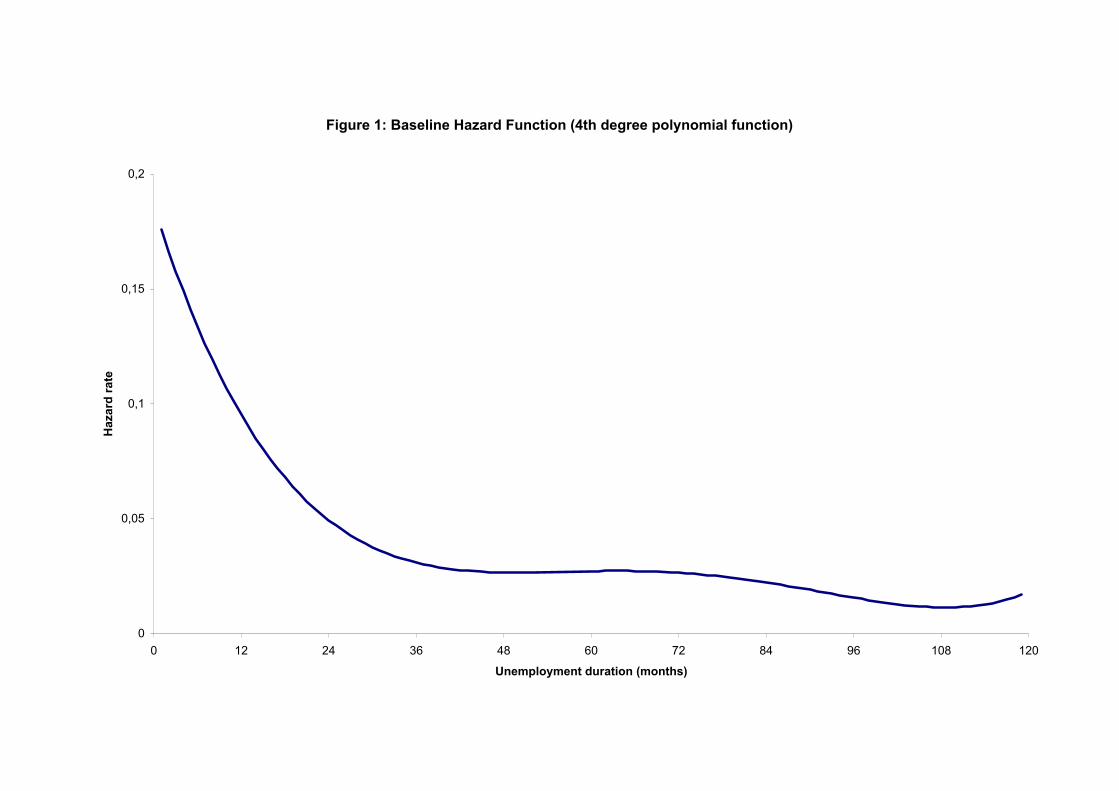
Figure 1: Baseline Hazard Function (4th degree polynomial function)

0

0,05

0,1

0,15

0,2

0 12 24 36 48 60 72 84 96 108 120

Unemployment duration (months)

Haz

ard

rate

Table 1: Sample Means and Standard Deviations

Variable All Male Female

Log hourly reservation wage 3,007 3,047 2,962(0,422) (0,432) (0,407)

Unemployment duration (months) 21,285 20,960 21,644(23,542) (23,296) (23,807)

Unemployment benefits (in logs) 7,989 8,082 7,886(0,967) (0,952) (0,972)

Unemployment rate 12,072 12,474 11,627(4,462) (4,443) (4,441)

Individual income 8,530 8,601 8,448(1,148) (1,159) (1,131)

Male 0,525(0,499)

High school graduate 0,319 0,288 0,352(0,466) (0,453) (0,478)

College graduate 0,129 0,101 0,161(0,366) (0,301) (0,367)

Age 18-25 0,244 0,237 0,252(0,429) (0,425) (0,434)

Age 26-35 0,313 0,288 0,341(0,464) (0,453) (0,474)

Age 36-45 0,216 0,208 0,225(0,411) (0,406) (0,417)

Age 46-55 0,160 0,176 0,142(0,366) (0,381) (0,349)

Household size 3,595 3,696 3,484(1.602) (1.694) (1.484)

Number of children 0,745 0,719 0,775(1,042) (1,092) (0,983)

Dependent children 0,438 0,403 0,477(0,496) (0,491) (0,500)

Married 0,473 0,449 0,498(0,499) (0,497) (0,500)

Home ownership 0,619 0,617 0,620(0.486) (0.486) (0.485)

Unemploymento to employment transition rate 0,362 0,383 0,339(0,481) (0,486) (0,473)

Log household income 9,610 9,551 9,675(0,750) (0,790) (0,697)

Unemployment benefits recipiency 0,425 0,427 0,423(0,494) (0,495) (0,494)

Job offer rate 0,091 0,088 0,095(0,288) (0,284) (0,293)

Table 2: The Determinants of the Arrival Rate of Job Offers (Extreme Value Regression Estimation)

VariablesCoefficient Marginal effect Coefficient Marginal effect

Unemployment duration -0,217 -0,023 -0,356 -0,131(0.023) (0.012)

Unemployment benefits 0,004 0,000 -0,047 -0,019(0.007) (0.004)

Unemployment rate -0,065 -0,007 0,002 0,001(0.032) (0.014)

Individual income 0,043 0,005 0,050 0,021(0.009) (0.005)

Male 0,103 0,011 0,241 0,099(0.050) (0.025)

High school graduate 0,199 0,021 0,086 0,035(0.056) (0.028)

College graduate 0,442 0,047 0,294 0,121(0.070) (0.036)

Age 18-25 1,705 0,180 1,285 0,530(0.169) (0.080)

Age 26-35 1,508 0,159 1,098 0,453(0.164) (0.078)

Age 36-45 1,369 0,145 0,909 0,375(0.166) (0.078)

Age 46-55 1,030 0,109 0,611 0,252(0.169) (0.082)

Household size -0,044 -0,005 -0,023 -0,009(0.022) (0.011)

Number of children 0,010 0,001 -0,012 -0,005(0.047) (0.022)

Dependent children 0,041 0,004 0,048 0,020(0.085) (0.042)

Married -0,018 -0,002 0,128 0,053(0.059) (0.031)

Germany -2,786 -0,294(0.313)

Denmark -3,066 -0,324 -1,148 -0,474(0.304) (0.140)

The Netherlands -3,480 -0,368 -1,463 -0,604(0.284) (0.132)

Belgium -2,991 -0,316 -1,584 -0,654(0.352) (0.169)

France -3,187 -0,337 -1,135 -0,468(0.396) (0.182)

United Kingdom -3,267 -0,345 -1,713 -0,707(0.357) (0.167)

Ireland -3,251 -0,343 -1,436 -0,593(0.450) (0.203)

Italy -3,242 -0,342 -1,795 -0,741(0.389) (0.182)

Greece -3,851 -0,407 -2,619 -1,081(0.344) (0.165)

Spain -2,532 -0,267 -1,740 -0,718(0.591) (0.270)

Portugal -4,153 -0,439 -1,861 -0,768(0.307) (0.140)

Austria -2,875 -0,304 -1,380 -0,570(0.258) (0.129)

Finland -2,767 -0,292 -1,643 -0,678(0.485) (0.224)

Log-likelihhod -5936,3 -14156,1

Number of observations 24242 28723

Asymptotic standard deviations in parentheses.

Notes: The marginal effect is computed as

The regression also includes four year dummies.

Dependent variable

Adjusted arrival rte of job offers Arrival rate of job offers

)))exp(exp( βββ XX +−

Table 3: The Determinants of the Reservation Wage (OLS and IV Estimation)

OLS OLS IVVariables

Unemployment duration -0,014 -0,100 (0.002) (0.032)

Expected wage 0,405 0,402 0,374(0.015) (0.015) (0.018)

Unemployment rate -0,053 -0,053 -0,051(0.003) (0.003) (0.003)

Unemployment benefits 0,000 0,001 0,006(0.001) (0.001) (0.002)

Male 0,053 0,052 0,038(0.006) (0.006) (0.007)

Age 18-25 -0,084 -0,095 -0,185(0.012) (0.013) (0.035)

Age 26-35 -0,085 -0,091 -0,147(0.011) (0.011) (0.023)

Age 36-45 -0,073 -0,077 -0,119(0.012) (0.012) (0.019)

Age 46-55 -0,064 -0,066 -0,093(0.012) (0.012) (0.015)

Home ownership 0,028 0,026 0,016(0.006) (0.006) (0.007)

Dependent children 0,022 0,022 0,029(0.006) (0.006) (0.006)

Germany 2,287 2,333 2,684(0.056) (0.057) (0.139)

Denmark 2,392 2,432 2,724(0.057) (0.057) (0.120)

The Netherlands 2,228 2,278 2,649(0.058) (0.058) (0.146)

Belgium 2,475 2,521 2,869(0.060) (0.060) (0.139)

France 2,388 2,433 2,762(0.062) (0.062) (0.134)

United Kingdom 1,791 1,836 2,177(0.059) (0.059) (0.137)

Ireland 2,543 2,584 2,893(0.066) (0.067) (0.130)

Italy 2,466 2,511 2,851(0.060) (0.060) (0.137)

Greece 2,232 2,274 2,582(0.052) (0.053) (0.123)

Spain 2,685 2,722 3,023(0.075) (0.075) (0.131)

Portugal 1,881 1,923 2,228(0.045) (0.046) (0.120)

Austria 1,932 1,974 2,291(0.053) (0.053) (0.126)

Finland 2,473 2,507 2,795(0.066) (0.066) (0.122)

Log-likelihood -6686,2 -6668,7 -6681,3

Number of observations 18482 18482 18482

Asymptotic standard errors in parentheses. Note: The regression also includes four year dummies.

Specification

Table 4: Transitions from Unemployment to Employment (Polynomial Hazard Function)

(1) (2) (3) (4)Variables

Reservation wage -0,138 -0,056 (0.030) (0.034)

Predicted reservation wage -0,376 0,145 (0.060) (0.371)

Unemployment rate 0,019 -0,031 0,018 -0,020(0.003) (0.016) (0.003) (0.025)

Male 0,157 0,183 0,182 0,159(0.025) (0.025) (0.026) (0.049)

High school graduate -0,097 -0,039 -0,067 -0,055(0.028) (0.029) (0.023) (0.41)

College graduate 0,007 0,034 0,058 -0,006(0.38) (0.039) (0.039) (0.080)

Age 18-25 0,548 0,556 0,504 0,594(0.070) (0.071) (0.071) (0.098)

Age 26-35 0,695 0,697 0,680 0,714(0.067) (0.067) (0.067) (0.074)

Age 36-45 0,715 0,717 0,716 0,721(0.067) (0.067) (0.067) (0.068)

Age 46-55 0,602 0,619 0,607 0,618(0.069) (0.069) (0.069) (0.070)

Household size 0,003 -0,004 0,003 -0,004(0.008) (0.008) (0.008) (0.008)

Married 0,113 0,098 0,118 0,088(0.028) (0.029) (0.028) (0.034)

Mortage 0,033 0,074 0,041 0,071(0.029) (0.030) (0.029) (0.030)

Constant -2,340 -1,168(0.138) (0.208)

Germany -2,902 -3,605 (0.204) (1.306)

Denmark -2,335 -3,062 (0.195) (1.355)

The Netherlands -2,493 -3,199 (0.196) (1.313)

Belgium -2,401 -3,148 (0.217) (1.393)

France -2,304 -3,031 (0.230) (1.359)

United Kingdom -2,828 -3,435 (0.206) (1.135)

Ireland -2,336 -3,098 (0.257) (1.427)

Italy -2,178 -2,918 (0.227) (1.381)

Greece -2,221 -2,881 (0.200) (1.230)

Spain -1,738 -2,509 (0.317) (1.459)

Portugal -2,012 -2,591 (0.172) (1.076)

Austria -2,261 -2,887 (0.173) (1.163)

Finland -1,901 -2,621 (0.265) (1.357)

Log-likelihood -10968 -10832,4 -10958,9 -10833,6

Number of observations 18482 18482 18482 18482

Asymptotic standard errors in parentheses.

Note: The regression also includes four year dummies.

Specification

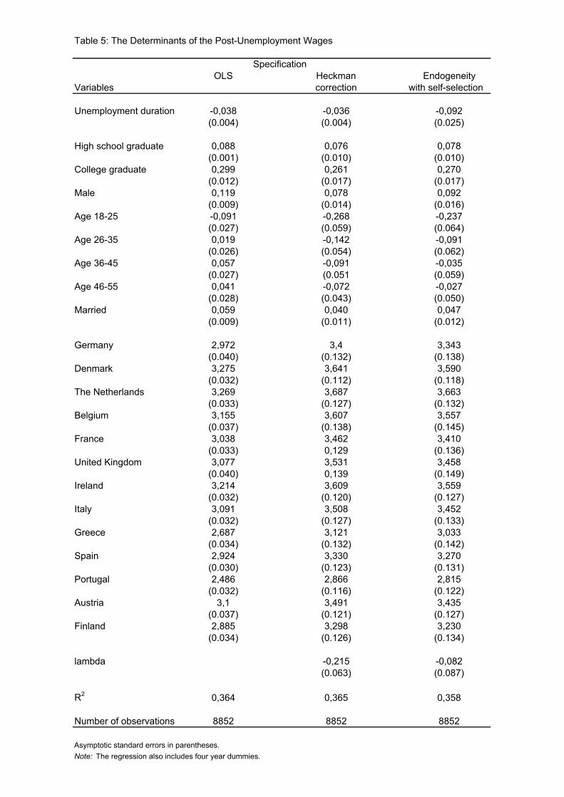
Table 5: The Determinants of the Post-Unemployment Wages

OLS Heckman EndogeneityVariables correction with self-selection

Unemployment duration -0,038 -0,036 -0,092(0.004) (0.004) (0.025)

High school graduate 0,088 0,076 0,078(0.001) (0.010) (0.010)

College graduate 0,299 0,261 0,270(0.012) (0.017) (0.017)

Male 0,119 0,078 0,092(0.009) (0.014) (0.016)

Age 18-25 -0,091 -0,268 -0,237(0.027) (0.059) (0.064)

Age 26-35 0,019 -0,142 -0,091(0.026) (0.054) (0.062)

Age 36-45 0,057 -0,091 -0,035(0.027) (0.051 (0.059)

Age 46-55 0,041 -0,072 -0,027(0.028) (0.043) (0.050)

Married 0,059 0,040 0,047(0.009) (0.011) (0.012)

Germany 2,972 3,4 3,343(0.040) (0.132) (0.138)

Denmark 3,275 3,641 3,590(0.032) (0.112) (0.118)

The Netherlands 3,269 3,687 3,663(0.033) (0.127) (0.132)

Belgium 3,155 3,607 3,557(0.037) (0.138) (0.145)

France 3,038 3,462 3,410(0.033) 0,129 (0.136)

United Kingdom 3,077 3,531 3,458(0.040) 0,139 (0.149)

Ireland 3,214 3,609 3,559(0.032) (0.120) (0.127)

Italy 3,091 3,508 3,452(0.032) (0.127) (0.133)

Greece 2,687 3,121 3,033(0.034) (0.132) (0.142)

Spain 2,924 3,330 3,270(0.030) (0.123) (0.131)

Portugal 2,486 2,866 2,815(0.032) (0.116) (0.122)

Austria 3,1 3,491 3,435(0.037) (0.121) (0.127)

Finland 2,885 3,298 3,230(0.034) (0.126) (0.134)

lambda -0,215 -0,082(0.063) (0.087)

R2 0,364 0,365 0,358

Number of observations 8852 8852 8852

Asymptotic standard errors in parentheses. Note: The regression also includes four year dummies.

Specification

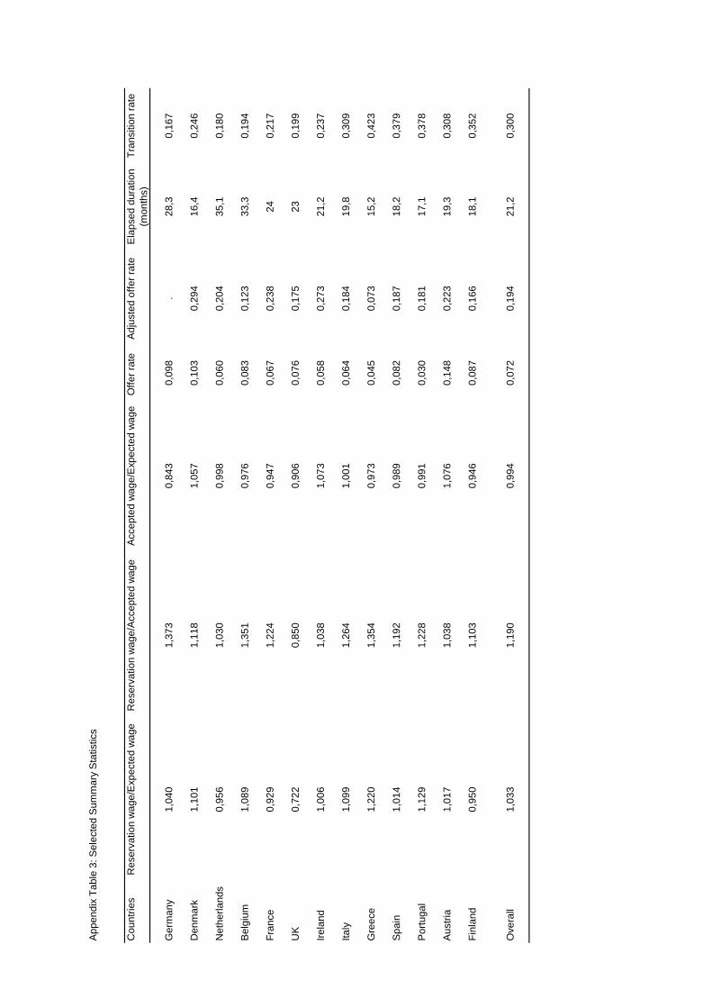
Appendix Table 1: Reservation Wage Response Rates

Country Looking for a job Reporting Reservation Wage RatioGermany 930 903 0,971Denmark 1249 1211 0,970The Netherlands 1437 832 0,579Belgium 1247 1167 0,936France 4105 4026 0,981United Kingdom 1051 978 0,931Ireland 1894 1833 0,968Italy 7004 6954 0,993Greece 3573 3556 0,995Spain 7424 7315 0,985Portugal 2183 2128 0,975Austria 560 552 0,986Finland 1885 1728 0,917Total 34542 33183 0,961

Appendix Table 2: Distribution of Individuals by Country of Residence

Country Number of observations ShareGermany 8746 0,068Denmark 4994 0,039The Netherlands 9577 0,074Belgium 6145 0,048France 13051 0,101United Kingdom 6940 0,054Ireland 7487 0,058Italy 17736 0,137Greece 11602 0,090Spain 15640 0,121Portugal 11702 0,091Austria 7271 0,056Finland 8173 0,063Total 129064 1,000

App

endi

x T

able

3: S

elec

ted

Sum

mar

y S

tatis

tics

Cou

ntrie

sR

eser

vatio

n w

age/

Exp

ecte

d w

age

Res

erva

tion

wag

e/A

ccep

ted

wag

eA

ccep

ted

wag

e/E

xpec

ted

wag

eO

ffer

rate

A

djus

ted

offe

r ra

teE

laps

ed d

urat

ion

Tra

nsiti

on r

ate

(mon

ths)

Ger

man

y1,

040

1,37

30,

843

0,09

8.

28,3

0,16

7

Den

mar

k1,

101

1,11

81,

057

0,10

30,

294

16,4

0,24

6

Net

herla

nds

0,95

61,

030

0,99

80,

060

0,20

435

,10,

180

Bel

gium

1,08

91,

351

0,97

60,

083

0,12

333

,30,

194

Fra

nce

0,92

91,

224

0,94

70,

067

0,23

824

0,21

7

UK

0,72

20,

850

0,90

60,

076

0,17

523

0,19

9

Irel

and

1,00

61,

038

1,07

30,

058

0,27

321

,20,

237

Italy

1,09

91,

264

1,00

10,

064

0,18

419

,80,

309

Gre

ece

1,22

01,

354

0,97

30,

045

0,07

315

,20,

423

Spa

in1,

014

1,19

20,

989

0,08

20,

187

18,2

0,37

9

Por

tuga

l1,

129

1,22

80,

991

0,03

00,

181

17,1

0,37

8

Aus

tria

1,01

71,

038

1,07

60,

148

0,22

319

,30,

308

Fin

land

0,95

01,

103

0,94

60,

087

0,16

618

,10,

352

Ove

rall

1,03

31,

190

0,99

40,

072

0,19

421

,20,

300