Training of Reduced-Rank Linear Transformations for

Multi-layer Polynomial Acoustic Features for Speech

Recognition

Muhammad Ali Tahir1, Heyun Huang2, Albert Zeyer1, Ralf Schluter1,Hermann Ney1,3

1 Human Language Technology and Pattern Recognition, Computer Science Department,RWTH Aachen University, Germany

2Centre for Language and Speech Technology, Radboud University Nijmegen, theNetherlands

3Spoken Language Processing Group, LIMSI CNRS, Paris, France{tahir,zeyer,schlueter,ney}@cs.rwth-aachen.de, h.huang@let.ru.nl

Abstract

The use of higher-order polynomial acoustic features can improve the per-formance of automatic speech recognition (ASR). However, dimensionality ofpolynomial representation can be prohibitively large, making acoustic modeltraining using polynomial features infeasible for large vocabulary ASR sys-tems. This paper presents a multi-layer polynomial training framework foracoustic modeling, which recursively expands the acoustic features into theirsecond-order polynomial feature space. After each expansion the dimension-ality of resultant features is reduced by a linear transformation. Experimentalresults obtained for two large-vocabulary continuous speech recognition tasksshow that the proposed method outperforms conventional mixture models.More recently the acoustic modelling community has shifted its focus to deepneural networks. We also train multi-layer polynomial features in a similarway: allowing backpropagation and using mean-normalized stochastic gra-dient descent algorithm. This has led to encouraging results. Specifically,appending a sigmoid-based feed-forward deep neural network with a finalpolynomial layer has resulted in significant word error rate improvement.

Keywords:polynomial features, log-linear model, linear transformation, deep neuralnetwork

Preprint submitted to Speech Communication December 26, 2018

1. Introduction

Automatic Speech recognition (ASR) has come a long way since the earlydays of small numerical digit and isolated word recognition tasks with smallvocabulary size. Recent systems can recognize spontaneous speech with noisyconditions and speaker variability with low error rates [Hinton & Deng+ 12,Zeyer & Doetsch+ 17, Sak & Senior+ 15]. Acoustic modeling is an integralpart of such a system, which provides the matching of spoken audio to lan-guage phonemes. The classical paradigm for acoustic modeling has beenGaussian mixture models, with Hidden Markov Models [Baker 75] to modelthe time-scale non-linearity of input speech vectors. Input to a speech recog-nition system is a stream of acoustic feature vectors, e.g. Mel-frequency cep-stral coefficients (MFCC) [Mermelstein 76]. To take acoustic context intoaccount, a fixed window of consecutive feature vectors are concatenated intoa larger vector. Such a vector naturally contains a lot of redundant informa-tion, due to similar vectors being appended together. A linear transforma-tion such as linear discriminant analysis (LDA) [Hab-Umbach & Ney 92] isapplied to this vector, for dimension reduction. LDA makes a maximum like-lihood (ML) assumption, similar to what is used for an ML-trained GMMacoustic model [Rabiner 89]. Discriminative training methods attempt tomaximize the probability of the correct phonetic classes with respect tocompeting classes. Experimentally, discriminative training has consistentlyoutperformed ML training for speech recognition tasks [Bahl & Brown+ 86,Valtchev & Odell+ 97]. This reasoning is a motivating factor to considertraining linear feature transformations using the discriminative training ap-proach. There have been several works where a linear transformation hasbeen discriminatively trained [Macherey 98, Omer & Hasegawa-Johnson 03,Povey & Kingsbury+ 05].

The motivation for using polynomial features for speech recognition stemsfrom support vector machines (SVM) where a polynomial kernel may be usedto project feature vectors to a higher space [Burges 98]. Classes which are notlinearly separable may become separable in that higher dimensional space,by fitting a hyperplane between them. High-dimensional polynomial featuresare a promising application for training of linear transformations. Polynomialfeatures are computationally expensive because the number of dimensionsgrows exponentially with polynomial order. Dimension reduction after eachsquaring of features is a way to use polynomial features while keeping themcomputationally tractable. This work investigates discriminatively trained

2

dimension reducing transforms for polynomial features.

There is a recent surge in interest related to deep learning and deep neu-ral network architectures; as they have consistently outperformed traditionalmaximum likelihood or discriminative training [Schmidhuber 11, Hinton 07].This is true for speech recognition [Hinton & Deng+ 12] as well as otherpattern recognition application areas. The first improvements came fromfeed-forward deep neural networks [Hinton & Deng+ 12]. Currently, neuralnetwork based acoustic model training is a very dynamic area of research,with new architectures and approaches being presented constantly. Someof these approaches are recurrent neural networks, specifically long short-term memory (LSTM) architectures [Hochreiter & Schmidhuber 97]. Differ-ent variations have been proposed in literature such as peephole connec-tions [Gers & Schmidhuber 01], highway networks [Srivastava & Greff+ 15]and sum-product networks [Gens & Domingos 12]. Based on this motiva-tion, we have also explored the use of polynomial features in a deep multi-hidden-layer fashion. Our polynomial features’ network topology is relatedto highway networks and peephole connections; as seen in Equation (5) eachlayer gets a combination of linear and non-linearly transformed versions oflast layer’s output. Furthermore, the polynomial function is same as theone used in sum-product networks. Therefore our work can be consideredas one of the early endeavours in these directions [Tahir & Schluter+ 11b,Tahir & Huang+ 13].

The rest of the paper is organized as follows: Section 2 gives an overviewof log-linear acoustic models and use of polynomial features with log-linearmodels. Results and comparison are presented with GMM based discrimina-tively trained system. Section 3 provides a brief introduction of deep neuralnetworks and the proposed multi-layer deep polynomial networks. Resultsare presented which show that a combination of polynomial and sigmoidbased DNN’s can bring word error rate (WER) improvement. Finally, inSection 4 some conclusions are discussed, along with possible future workdirections.

2. Training of Polynomial Features with Log-linear Acoustic Model

2.1. Log-linear Acoustic Model

Log-linear models [Hifny & Renals+ 05, Macherey & Ney 03] are an al-ternative to the Gaussian distributions, for representing emission probabili-

3

ties of HMM states. Under assumption of a pooled covariance matrix, pos-terior probabilities of Gaussian single density HMMs are equivalent to corre-sponding log-linear models’ posterior probabilities [Heigold & Schluter+ 07].For speech input features x and classes s (HMM-states), the posterior prob-abilities of a log-linear acoustic model are given as

pθ(s|x) =exp(λ>s x+ αs)∑s′ exp(λ>s′x+ αs′)

(1)

in which θ = {θs} = {λs, αs} are parameters of log-linear model. The equiv-alence of Gaussian and log-linear posterior probabilities can also be extendedto Gaussian mixture models. Due to hidden variables, this mixture model’soptimization is not a convex problem, but in principle local convergence canbe guaranteed [Heigold & Ney+ 13]. The log-linear acoustic model can bediscriminatively split into a log-linear mixture model [Tahir & Schluter+ 11].

Log-linear model parameters are estimated by optimizing the frame-levelmaximum mutual information (frame-MMI) objective function

F (frame)(θ) = −τθ||θ||2 +R∑r=1

Tr∑t=1

wst log pθ(st|xt) (2)

for a fixed alignment sT1 . τθ is a regularization parameter. ws are stateweights which could be tuned to give less weight to accumulations of e.g. noiseand silence states. αs = αs + log p(s), p(s) is the prior probability of state sand R is the total number of training segments.

2.2. Log-linear Training of Linear Feature Transformation

In Section 2.1, the log-linear acoustic model was defined. Let the inputto this acoustic model be Ax where x are the input features as before and Ais a transformation matrix.

pθ,A(s|x) =exp(λ>s Ax+ αs)∑s′ exp(λ>s′Ax+ αs′)

(3)

If the state-specific parameters λs are held constant, then the objectivefunction of Equation (2) becomes convex with respect to optimization of thelinear transform. Therefore, the dimension reducing linear feature transformcan be reliably estimated by frame-level discriminative training of a log-linear

4

Figure 1: Illustration of iterative polynomial features

acoustic model. It has been shown [Tahir & Heigold+ 09] that if the featuretransformation matrix is trained via log-linear discriminative training, it re-sults in slightly better WER than using LDA-based transform. Furthermore,it has also been shown that speaker specific transformation matrices can betrained in the same way [Loof & Schluter+ 07], and result in improvementover CMLLR-based transformation matrices.

In this work, log-linear training of linear transformations for high dimen-sional polynomial features is investigated. This technique can well be appliedto other approaches to generate high dimensional features.

2.3. Dimension-reduced Higher-order Polynomial Features

The input features (or LDA-transformed features) can be cross-multipliedwith themselves and then vectorized to create second-order polynomial fea-tures. Thus an n-dimensional feature vector becomes n×n feature vector af-ter this squaring. However, almost half of the elements in this squared vectorare duplicate values, and after removing these duplicate elements the numberof elements is (n(n+1))/2. As we have seen in Section 2.1, a Gaussian acous-tic model with a pooled covariance matrix can be simplified by cancelling thesquared feature terms. The same is true for an equivalent log-linear model.

5

However, by using squared features we can implicitly represent the sametype of information as a class-specific covariance based Gaussian/log-linearmodel. This squaring of features represents a non-linear transformation ofinput features into a much higher dimensional space, where the classes areexpected to be more easily separable.

In previous work, second order polynomial features have resulted in WERimprovements over the original MFCC features [Wiesler & Nußbaum+ 09].These features create a large feature vector and hence greatly increase thenumber of acoustic model parameters; but their WER is as good as a fullmixture system with even larger number of parameters. Therefore thesesquared features are more parameter efficient than the corresponding mixturedensity system.

Polynomial features are feasible for second order e.g. for 45 dimensionalinput features the size of squared features is 1035. After appending the orig-inal 45 dimensional vector its size becomes 1080. However, for higher orderslike fourth or eighth order, their practicality is limited by the fact that goingto higher orders increases the number of dimensions exponentially. There-fore, for second order features of 1080 dimensions, fourth order polynomialfeatures would have 585K dimensions. This is about 50 times as much pa-rameters as the full mixture acoustic model. To reduce the number of pa-rameters to a computationally tractable size, dimension-reducing log-lineartransformations can be applied to polynomial features after each squaring,thus allowing us to go to fourth-order, eighth-order polynomials and so on.At each layer k with input vector x(k−1) ∈ Rrk−1 and output vector xk ∈ Rrk ,a transformation A(k) ∈ Rrk×dk is trained:

dk = rk−1 +rk−1(rk−1 + 1)

2(4)

x(k) = A(k)

[vech(x(k−1)x(k−1)>)

x(k−1)

](5)

where A(k) is the dimension-reducing matrix to be trained in the currentlayer. For a symmetric matrix, the vech(·) operator denotes half vectoriza-tion. It is a vector of length n(n + 1)/2 obtained by vectorizing only thelower triangular part of x(k−1)x(k−1)>. Vectorizing is defined as a columnvector obtained by stacking the columns of a matrix on top of one another.

6

As seen in Equation (5), at each layer k the input features are also con-catenated with squared features to retain the information of original features[Tahir & Huang+ 13]. The posterior probabilities are:

pθ(s|x(k)) =exp

(λ(k)>s x(k) + αs

)∑

s′ exp(λ(k)>s′ x(k) + αs′

) (6)

A pictorial representation of multilayer polynomial features can be seenin Figure 1. It is noteworthy that this is like a highway neural network[Srivastava & Greff+ 15]; albeit with polynomial non-linearity instead of sig-moid. The upper part of RHS in Equation (5) can be seen as the transformgate T and lower part as carry gate C of highway networks. Like peep-hole connections of LSTM, this uses a linear activation function but in afeed-forward setting.

Training ProcedureTraining for polynomial features is done in a layer-by-layer fashion. Firstthe original LDA transformed input features are appended with its squaredfeatures and a linear dimension reduction is trained log-linearly. Using theoutput of this linear transformation as input features for the next layer,the same process is repeated and another dimension reduction is trained.This process is repeated until the desired number of layers is achieved, orderivatives become so small that no improvement in objective function isobserved. For optimization of the frame-MMI objective function, the RPROPalgorithm [Riedmiller & Braun 93] is used.

Log-linear training of transformation depends crucially on reasonable ini-tial values of the projection matrix and log-linear weights A(k0) and λ

(k0)s

respectively. k0 denotes initial values of parameters for layer k. One reasonwhy good initial values are crucial is the fact that the large scale of ASR train-ing data makes it likely that the algorithm will suffer from a slow convergenceto a (local) maximum. Assuming rk = rk−1, the parameters A(k) ∈ Rrk×dk ,

λ(k)s ∈ Rrk and α

(k)s ∈ R are initialized by setting A(k0) =

[0rk×(dk−rk) Irk×rk

],

λ(k0)s = λ

(k−1)s and α

(k0)s = α

(k−1)s respectively. This initialization guarantees

that the MMI objective function value of at the beginning of new layer’straining is exactly identical to that at the end of previous layer’s training:

7

λ>(k0)s

[0rk×(dk−rk) Irk×rk

] [vech(x(k−1)x(k−1)>)

x(k−1)

]= λ(k−1)>s x(k−1) (7)

Since the iterations continuously absorb more discriminative informationfrom higher-order polynomials, the low-dimensional reduced vector mightnot be able to capture such additional information and need to be enlarged.Below the initialization formulas are shown for the case where rk = 2rk−1

A′(k0)

=

[0rk×(dk−rk) Irk×rk0rk×(dk−rk) 0rk×rk

](8)

Accordingly, λ(k0)s is also augmented by its copy, which results in

λ′s(k0)

=

[λ(k0)s

λ(k0)s

](9)

It can be seen that λ′s(k0)>A′(k0) = λ

(k0)>s A(k0). Therefore, the additional

rows can be expected to learn additional information when higher-order poly-nomials are considered.

2.4. Experiments and Results

Experiments have been performed on two large vocabulary ASR tasks.The first corpus, European Parliament Plenary Sessions (EPPS) En-glish consists of mostly planned (non-spontaneous) speeches of EuropeanParliament under clean conditions. It is part of the TC-STAR project[Loof & Gollan+ 07]. One source of variability is the presence of a numberof non-native speakers. The input audio is sampled at 16 KHz and initialinput features are 16 MFCC features with VTLN warping plus an energyand a voiced feature. These features are concatenated together in a windowof 9 frames (−4 to +4) then transformed by LDA to a 45 dimensional vector.The lexicon consists of 60K words and the language model is a 4-gram true-case model trained on 400M running words. A triphone-based classificationand regression tree is computed which clusters allophones into 4501 classesincluding silence. The baseline acoustic model is a Gaussian mixture densitymodel with 256 densities per CART state with a WER of 16.4%. Apart fromsilence, the phoneme set also includes some non-voice phonemes like hesita-tion, noise, breath. The acoustic training data is 90 hours of audio (with

8

about 40% silence ratio). Development and evaluation corpora are about 3hours each.

The second speech recognition task for these experiments is QUAEROEnglish 50 hours corpus. The British English task consists of newsbroadcasts, debates, interviews etc. [Sundermeyer & Nußbaum-Thom+ 11].Speaking style ranges from planned for broadcast news to conversational forinterviews. Audio is sampled at 16 KHz but some recordings contain tele-phone calls which are band-limited to 4 KHz. There are also some instancesof multiple simultaneous speakers and background music/noise. For the ex-periments in this paper, a 50 hour subset of the total QUAERO training datais used. The input features for the baseline setup are 16 MFCC features withVTLN warping. 9 of such consecutive frames are concatenated together andLDA-transformed to 45 dimensions. The lexicon contains 325K words andthe language model is trained on 2G running words. There are 4501 CARTstates. For the MLP experiments in Section 3.3 the input features are slightlydifferent from the baseline setup. Instead of 9 MFCC frames, 17 consecutiveMFCC frames are concatenated together and there is no LDA transforma-tion after that. This feature arrangement was found to be better in terms ofWER. The development and evaluation corpora (eval10 and eval11 respec-tively) are 3 hours each.

Table 1: QUAERO English 50h; WER for mixture densities, polynomial features, and acombination of both

feature dim. densities final no. of WER (%)

polynomial reduction per feature params.

order state dimension × 1000 dev eval

1st no 1 45 214 35.4 43.0128 26508 23.9 30.9

2nd no 1 1080 4872 24.2 31.82nd yes 1 90 467 28.5 35.94th 135 721 27.2 34.48th 180 967 27.0 34.14th yes 32 135 19688 23.1 30.2

Figure 2 shows some results for dimension-reduced higher-order polyno-mial features on EPPS English task. The input features are 16 × 9 MFCCfeatures which have been LDA transformed to 45 dimensions. The results

9

16

18

20

22

24

26

28

30

105

106

107

108

WER(%)

No. of parameters

ML (mixtures)MMI (mixtures)

MMI (polynomial with dim. reductionMMI 2nd-order polynomial (full)

Figure 2: EPPS dev2007: WER(%) vs. No. of parameters for higher-order polynomialfeatures in comparison with mixture densities

10

30

32

34

36

38

40

42

44

105

106

107

108

WER(%)

No. of parameters

mixture densities2nd-order polynomial (full)

polynomial with dim. reductionpolynomial + mixtures

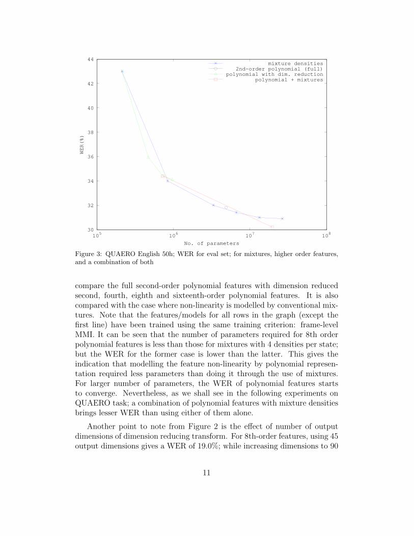
Figure 3: QUAERO English 50h; WER for eval set; for mixtures, higher order features,and a combination of both

compare the full second-order polynomial features with dimension reducedsecond, fourth, eighth and sixteenth-order polynomial features. It is alsocompared with the case where non-linearity is modelled by conventional mix-tures. Note that the features/models for all rows in the graph (except thefirst line) have been trained using the same training criterion: frame-levelMMI. It can be seen that the number of parameters required for 8th orderpolynomial features is less than those for mixtures with 4 densities per state;but the WER for the former case is lower than the latter. This gives theindication that modelling the feature non-linearity by polynomial represen-tation required less parameters than doing it through the use of mixtures.For larger number of parameters, the WER of polynomial features startsto converge. Nevertheless, as we shall see in the following experiments onQUAERO task; a combination of polynomial features with mixture densitiesbrings lesser WER than using either of them alone.

Another point to note from Figure 2 is the effect of number of outputdimensions of dimension reducing transform. For 8th-order features, using 45output dimensions gives a WER of 19.0%; while increasing dimensions to 90

11

decreases the WER to 18.2%. This shows that as the order of the polynomialfeatures gets larger, it is beneficial to use projective transformation matriceswith larger number of rows.

Similar experiments have been performed for the acoustically more diffi-cult QUAERO English 50 hours task. These results have been summarized inTable 1 and Figure 3. One additional aspect here is the result in the last row,which combines polynomial features with mixture-based acoustic model. Forthe original mixture density model with MFCC features (4th row), the bestWER is 30.9% with 128 densities per CART state. Going to higher numberof densities per state causes the model to overtrain, because the trainingcorpus is relatively small (50 hours). If mixture densities are trained on topof 4th order polynomial features as in the last row, WER drops to 30.2%with just 32 densities per state, because of better available input features.This result shows that the results obtained by dimension-reduced polynomialfeatures with log-linear mixtures are significantly better than either full-rankpolynomial features, reduced-rank polynomial features or log-linear mixturesalone.

3. Training of Polynomial Features within a Deep Neural Network

3.1. Deep Neural Networks

Deep neural networks (DNNs) have become an important tool for creat-ing probabilistic features for speech recognition. A neural network for speechrecognition consists of a multilayer-perceptron (MLP), having non-linear ac-tivation functions in the hidden and output layers. Some earlier works ex-ploring the use of MLPs for speech recognition are [Peeling & Moore+ 86,Bourlard & Wellekens 87, Waibel & Hanazawa+ 89]. These were complexsystems aiming to model the whole speech recognition process by neural net-works, but were not able to outperform the GMM-HMM based approaches.More recently, there are two ways of applying neural networks for acousticmodelling: hybrid and tandem MLPs.

� A hybrid MLP system [Bourlard & Morgan 93, Seide & Gang+ 11,Hinton & Deng+ 12] directly uses posterior probabilities of MLP net-work as acoustic model probabilities. The probabilities correspond toclustered allophone (CART) states.

� A tandem MLP system [Hermansky & Ellis+ 00] has a bottlenecklayer as the last output layer of the network and then a regular GMM

12

based maximum likelihood acoustic model is trained on top of it. Thismakes it easier to use GMM based concepts for optimization such aslinear discriminant analysis (LDA) and speaker adaptation.

A neural network is a set of neurons linked together by weighted connec-tions. A neuron’s input activation zj is a weighted combination of outputs ofnodes in the previous layer xi, plus a bias constant αj. The output activationyj of the node j is a non-linear transformation applied to the node input.

zj =∑i

λi,j · xi + αj ; yj = σ(zj) (10)

where {λi,j} are parameters of neural network. The sigmoid activationfunction is used (among others) for hidden layers of ANNs

yj =1

1 + e−zj(11)

For the last output layer of the network, a normalized softmax activationfunction is used because the outputs are to be interpreted as probabilities

yj =ezj∑i ezi

(12)

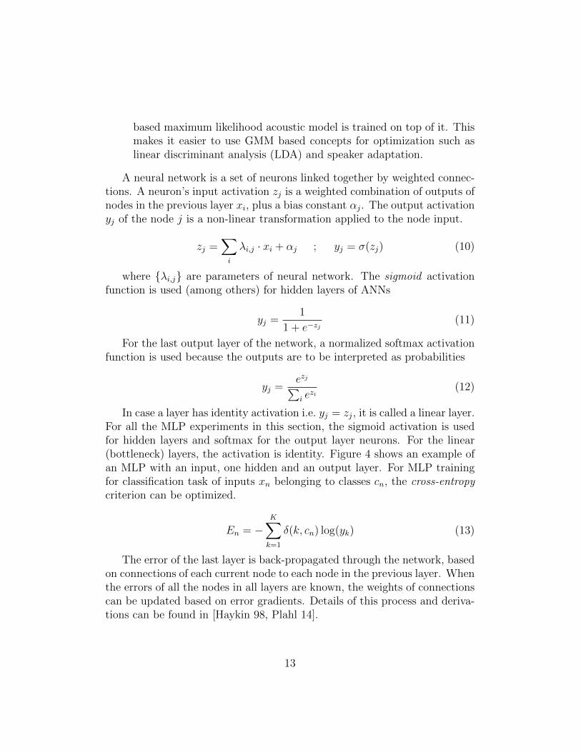
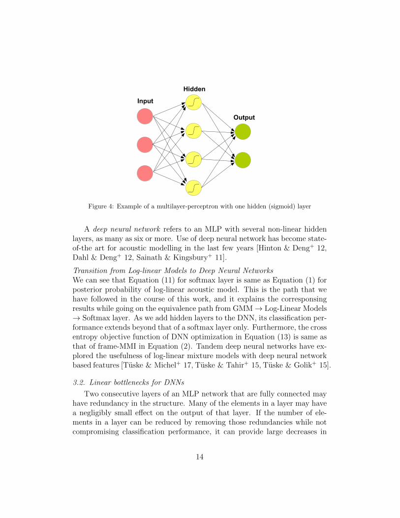
In case a layer has identity activation i.e. yj = zj, it is called a linear layer.For all the MLP experiments in this section, the sigmoid activation is usedfor hidden layers and softmax for the output layer neurons. For the linear(bottleneck) layers, the activation is identity. Figure 4 shows an example ofan MLP with an input, one hidden and an output layer. For MLP trainingfor classification task of inputs xn belonging to classes cn, the cross-entropycriterion can be optimized.

En = −K∑k=1

δ(k, cn) log(yk) (13)

The error of the last layer is back-propagated through the network, basedon connections of each current node to each node in the previous layer. Whenthe errors of all the nodes in all layers are known, the weights of connectionscan be updated based on error gradients. Details of this process and deriva-tions can be found in [Haykin 98, Plahl 14].

13

Input

Hidden

Output

Figure 4: Example of a multilayer-perceptron with one hidden (sigmoid) layer

A deep neural network refers to an MLP with several non-linear hiddenlayers, as many as six or more. Use of deep neural network has become state-of-the art for acoustic modelling in the last few years [Hinton & Deng+ 12,Dahl & Deng+ 12, Sainath & Kingsbury+ 11].

Transition from Log-linear Models to Deep Neural NetworksWe can see that Equation (11) for softmax layer is same as Equation (1) forposterior probability of log-linear acoustic model. This is the path that wehave followed in the course of this work, and it explains the corresponsingresults while going on the equivalence path from GMM→ Log-Linear Models→ Softmax layer. As we add hidden layers to the DNN, its classification per-formance extends beyond that of a softmax layer only. Furthermore, the crossentropy objective function of DNN optimization in Equation (13) is same asthat of frame-MMI in Equation (2). Tandem deep neural networks have ex-plored the usefulness of log-linear mixture models with deep neural networkbased features [Tuske & Michel+ 17, Tuske & Tahir+ 15, Tuske & Golik+ 15].

3.2. Linear bottlenecks for DNNs

Two consecutive layers of an MLP network that are fully connected mayhave redundancy in the structure. Many of the elements in a layer may havea negligibly small effect on the output of that layer. If the number of ele-ments in a layer can be reduced by removing those redundancies while notcompromising classification performance, it can provide large decreases in

14

time and memory requirements of MLP training. Several methods have beenproposed to achieve this compression. [Yu & Seide+ 12] have reduced thenumber of elements in the layers by removing the close to zero elements andconverting the matrices to an index-based representation. [Xue & Li+ 13]have factored the weight matrix into a product of two smaller matrices, pro-viding parameter compression. They have reported encouraging results bydoing a singular value decomposition (SVD) based factorization between thehidden layers. The error rate degrades at first but after doing a full net-work training with back-propagation, the classification performance of theMLP network is restored. [Wiesler & Richard+ 14] have proposed a trainingmechanism whereby a hidden layer and its low-rank factorization can be si-multaneously trained from scratch. Apart from model parameter reduction,they report an added benefit of regularization from this factorization. Thuslinear bottlenecks can reduce over-training of MLP network parameters.

3.3. Deep Polynomial Network

In this section the implementation of multilayer polynomial features as adeep network is explored. To keep in sync with our DNN baseline, there aresome differences to the log-linear training method of Section 2.3, as listedbelow.

� The previous section’s polynomial layers were trained in forward direc-tion only. Here we shall allow backpropagation of error.

� Previous training was performed by iterating over the full corpus ineach iteration (full batch). Here a stochastic algorithm is used (mini-batch).

� For input features, previously 9 MFCC vectors were windowed togetherand then transformed by linear discriminant analysis (LDA). Here, 17MFCC vectors are windowed together without any LDA.

The speech corpus is the QUAERO English 50h corpus (Section 2.4). Forthe input MFCC features the feature vector length is 29, and 17 consecutiveframes are appended along with first and second derivatives. The MLPnetwork has 493 input features. The number of nodes in the output softmaxlayer is 4501 (no. of CART states). The training objective function is cross-entropy (which is equal to frame-MMI of Section 2.1). The algorithm used fortraining is mean-normalized stochastic gradient descent. There are six hidden

15

layers and the hidden layers have a sigmoid activation function. Detaileddescription of this system can be found in [Wiesler & Richard+ 14].

Training ProcedureOur deep polynomial network takes the same windowed MFCC features asmentioned in last paragraph. A linear dimension reduction reduces these493 dimensional features to 128. These 128 dimensional features are thenexpanded to second-order polynomial and concatenated with itself, givingan 8384 dimensional vector. This large vector is again reduced to 128 dimen-sions. This expansion and reduction is repeated two more times, so that athree hidden layer deep polynomial network is created. This represents 8th-order polynomial features. Going beyond 8th-order features was tried butthe derivatives become so small that there is no tangible effect of an extralayer on objective function and WER.

Before training, the neural network is discriminatively pre-trained layer-by-layer. First, one hidden layer network is trained for a few epochs. Thenkeeping the first layer’s parameters constant, a second hidden layer is trainedusing the first hidden layer’s outputs as features, as so on. After pre-training,the full networked in trained with backpropagation. This is also describedin [Wiesler & Richard+ 14].

Table 2 shows the results of these polynomial features in comparison tothe sigmoid-based DNN baseline. The 3-layer polynomial network achievesa WER of 20.7%(dev). If the last softmax layer is split into a log-linearmixture model, then the WER is reduced to 19.9%. This is a large improve-ment of 4.0% absolute on the result for GMM trained by the same objectivefunction. This result is close to WER of sigmoid-based DNN, although stillworse. This nevertheless shows that polynomial expansion of features is acandidate to be considered for modelling non-linearity of features, just like asigmoid activation function. It was also noticed that WER for different layerswith and without backpropagation did not differ by more than 0.2% absolute.This shows that after layer-by-layer training of polynomial network to con-vergence, backpropagation is not as crucial as it is for e.g. sigmoid activationfunction.

3.4. Combination of polynomial with sigmoid-based DNN

Table 3 shows some results of combining a state-of-the-art deep neuralnetwork with polynomial features. The baseline DNN system is the same asin [Wiesler & Richard+ 14]. It has 6 sigmoid layers with a linear bottleneck of

16

Table 2: Training corpus: QUAERO 50h. Comparison of a deep polynomial networkwith a state-of-the-art DNN (sigmoid)

network mixtures no. of no. of WER (%)

type layers params. dev eval

frame-MMI GMM yes - 26M 23.9 30.9sigmoid no 6 7.9M 18.6 24.9polynomial no 1 1.7M 24.3 31.8

2 2.8M 21.2 27.43 3.9M 20.7 27.04 5.0M 20.6 27.0

polynomial yes 3 22M 19.9 26.3

Table 3: Training corpus: QUAERO English 50h. Appending a state-of-the-art DNN(sigmoid with cross-entropy) with a last polynomial layer

model polynomial additional MPE training WER (%)

type features last layer only dev eval

DNN no no 18.6 24.9DNN yes 18.3 24.3DNN yes no 18.2 24.4DNN yes 18.0 24.1

256 nodes after each sigmoid layer. The network is trained with cross-entropycriterion, which is the same as frame-MMI for log-linear training. The featureinput for the polynomial layer is the output of the last linear bottleneck. Itcan be seen that a combination of DNN features and a polynomial layer (3rdrow in table) improves the WER by 0.5% absolute (eval). If the last layer istrained by MPE criterion (4th row in table), then with polynomial featuresit achieves further WER reduction of 0.2%. Some internal experiments onthis corpus at our institute show that adding a 7th or 8th sigmoid layer tothe baseline DNN does not bring any WER improvement. Thus the WERimprovement by adding the polynomial layer can be genuinely attributed toits difference to the sigmoid layers.

For an explanation of WER improvement due to polynomial features,we can consider polynomial features’ equivalence to class-specific covarianceGaussian acoustic model. It can be shown that a log-linear model with asingle polynomial layer as in Equation (5) is equivalent to a class-specific

17

covariance based Gaussian model; due to squaring of input features. This isin contrary to a regular log-linear model or softmax, which is equivalent to apooled covariance based Gaussian model. Therefore, if a polynomial hiddenlayer is used before the last softmax, it allows an extra degree of freedom dueto its equivalence with class-specific covariance model. This in turn allowsthe DNN to achieve better classification performance and hence lower WER.

4. Conclusion and Outlook

In this paper, we presented a multi-layer linear transformation trainingframework, which can harness crucial information from higher-order (≥ 3)polynomial feature space. The framework allows us to train log-linear mod-els in the otherwise prohibitively high-dimensional feature space spannedby higher-order polynomials. By repeating second-order polynomial expan-sion n times, 2n-order polynomial features can be obtained. Following eachsquaring of polynomial features, the subsequent linear projection limits thedimensionality of features. Experiments on EPPS and QUAERO corpora re-vealed that polynomial features allow us to significantly reduce the number ofparameters. Due to recent popularity and good performance of deep neuralnetworks for speech recognition, deep polynomial features were trained byusing similar optimization algorithms and backpropagation. This work pro-poses a multi-layer polynomial network with highway/peephole connections.Experiments with DNN on QUAERO corpus showed that a combination ofsigmoid and polynomial layers leads to WER improvement over the DNNbaseline.

Future work in this direction could be further exploration of combinationsof polynomial features with sigmoid or rectified linear unit (ReLU) activationfunctions. For example a DNN with alternating polynomial and sigmoidbased layers. Furthermore, polynomial non-linearity can also be used incontext of recurrent neural networks especially LSTM architecture.

5. Acknowledgements

The research of H. Huang was funded by the European Community’sSeventh Framework Programme [FP7/2007-2013] under grant agreement no.213850 SCALE. The research leading to these results has received fund-ing from the European Union Seventh Framework Programme EU-Bridge

18

(FP7/2007-2013) under grant agreement No. 287658. H. Ney was partiallysupported by a senior chair award from DIGITEO, a French research clusterin Ile-de-France.

19

References

[Bahl & Brown+ 86] L.R. Bahl, P.F. Brown, P.V. Souza, R.L. Mercer: Max-imum mutual information estimation of hidden Markov model parametersfor speech recognition, In IEEE International Conference on Acoustics,Speech and Signal Processing (ICASSP), pp. 49-52, Tokyo, Japan. 1986.

[Baker 75] J.K. Baker: Stochastic modeling for automatic speech under-standing, In D. R. Reddy, editor, Speech Recognition, pp. 512-542. Aca-demic Press, New York, NY, USA 1975.

[Bourlard & Morgan 93] H.A. Bourlard, N. Morgan: Connectionist speechrecognition: a hybrid approach., Kluwer Academic Publishers, Norwell,MA, USA. 1993.

[Bourlard & Wellekens 87] H. Bourlard, C.J. Wellekens: Multi-layer per-ceptron and automatic speech recognition, In International Conferenceon Neural Networks (ICNN), Vol. 4, pp. 407-416, San Diego, CA, USA.1987.

[Burges 98] C. Burges: A tutorial on support vector machines for patternrecognition, Data Mining and Knowledge Discovery 2, pp. 121-167. 1998.

[Dahl & Deng+ 12] G.E. Dahl, D. Yu, L. Deng, A. Acero: Context-dependent pre-trained deep neural networks for large-vocabulary speechrecognition, IEEE Trans. Audio Speech Lang. Process., Vol. 20, No. 1,pp. 30-42. 2012.

[Gens & Domingos 12] R. Gens, P. Domingos: Discriminative Learningof Sum-Product Networks, Advances in Neural Information ProcessingSystems, 25. 2012.

[Gers & Schmidhuber 01] F.A. Gers, J. Schmidhuber: LSTM recurrentneworks learn simple context-free and context-sensitive languages, IEEETransactions on Neural Networks, 12 (6) pp. 1333-1340. 2001.

[Haykin 98] S. Haykin: Neural Networks: A Comprehensive Foundation, 2ndedition, Prentice Hall. 1998.

[Hab-Umbach & Ney 92] R. Hab-Umbach, H. Ney: Linear discriminantanalysis for improved large vocabulary continuous speech recognition, In

20

IEEE International Conference on Acoustics, Speech and Signal Process-ing (ICASSP), Vol. 1, pp. 13-16. March 1992.

[Heigold 10] G. Heigold: A log-linear discriminative modeling framework forspeech recognition, Ph.D. thesis, Computer Science Department, RWTHAachen University, Aachen, Germany. Jun. 2010.

[Heigold & Ney+ 13] G. Heigold, H. Ney, R. Schluter: Investigations on anEM-Style Optimization Algorithm for Discriminative Training of HMMs,IEEE Transactions on Audio, Speech, and Language Processing, 21 (12)pp. 2616-2626. Dec. 2013.

[Heigold & Schluter+ 07] G. Heigold, R. Schluter, H. Ney: On the equiv-alence of Gaussian HMM and Gaussian HMM-like hidden conditionalrandom fields, In Interspeech, pp. 1721-1724, Antwerp, Belgium. Aug.2007.

[Hermansky & Ellis+ 00] H. Hermansky, D.P.W. Ellis, S. Sharma: Tan-dem connectionist feature extraction for conventional HMM systems, InIEEE International Conference on Acoustics, Speech and Signal Process-ing (ICASSP), Vol. 3, pp. 1635-1638. 2000.

[Hifny & Renals+ 05] Y. Hifny, S. Renals, N.D. Lawrence: A hybrid Max-Ent/HMM based ASR system, In Interspeech, pp. 3017-3020, Lisbon,Portugal. Sep. 2005.

[Hinton 07] G. Hinton: Learning multiple layers of representation, Trendsin cognitive sciences, 11 (10) pp. 428-434. 2007.

[Hinton & Deng+ 12] G. Hinton, L. Deng, D. Yu, G. Dahl, A. Mohamed, N.Jaitly, A. Senior, V. Vanhoucke, P. Nguyen, T. Sainath, B. Kingsbury:Deep neural networks for acoustic modeling in speech recognition — Theshared views of four research groups, IEEE Signal Processing Magazine,Vol. 29, No. 6, pp. 82-97. 2012.

[Hochreiter & Schmidhuber 97] S. Hochreiter, J. Schmidhuber: LongShort-Term Memory, Neural computation, 9(8) pp. 1735-1780. 1997.

[Loof & Gollan+ 07] J. Loof, C. Gollan, S. Hahn, G. Heigold, B. Hoffmeister,C. Plahl, D. Rybach, R. Schluter, H. Ney: The RWTH 2007 TC-STAR

21

evaluation system for European English and Spanish, In Interspeech, pp.2145-2148, Antwerp, Belgium. 2007.

[Loof & Schluter+ 07] J. Loof, R. Schluter, H. Ney: Efficient estimation ofspeaker-specific projecting feature transforms, In Interspeech, pp. 1557-1560, Antwerp, Belgium. Aug. 2007.

[Macherey 98] W. Macherey: Implementation and comparison of discrim-inative training methods for automatic speech recognition, M.Sc. thesis,Computer Science Department, RWTH Aachen University, Aachen, Ger-many. Nov. 1998.

[Macherey & Ney 03] W. Macherey, H. Ney: A comparative study on max-imum entropy and discriminative training for acoustic modeling in auto-matic speech recognition, In European Conference on Speech Communi-cation and Technology (Eurospeech), pp. 493-496, Geneva, Switzerland.Sep. 2003.

[Mermelstein 76] P. Mermelstein: Distance measures for speech recogni-tion, psychological and instrumental, Pattern Recognition and ArtificialIntelligence, pp. 374-388. 1976.

[Omer & Hasegawa-Johnson 03] M.K. Omar, M. Hasegawa-Johnson: Max-imum conditional mutual information projection for speech recognition,In International Conference on Spoken Language Processing (ICSLP),pp. 505-508, Geneva, Switzerland. Sep. 2003.

[Peeling & Moore+ 86] S.M. Peeling, R.K. Moore, M.J. Tomlinson: Themulti-layer perceptron as a tool for speech pattern processing research,In Institute of Acoustics, Autumn Conference on Speech and Hearing,Vol. 8, pp. 307-314, Windermere, UK. 1986.

[Plahl 14] C. Plahl: Neural network based feature extraction for speech andimage recognition, Ph.D. thesis, Computer Science Department, RWTHAachen University, Aachen, Germany, Jan. 2014.

[Povey & Kingsbury+ 05] D. Povey, B. Kingsbury, L. Mangu, G. Saon, H.Soltau, G. Zweig: fMPE: Discriminatively trained features for speechrecognition, In IEEE International Conference on Acoustics, Speech andSignal Processing (ICASSP), pp. 961-964, Philadelphia, PA, USA. 2005.

22

[Rabiner 89] L.R. Rabiner: A Tutorial of hidden Markov models and se-lected applications in speech recognition, In Proceedings of the IEEE,Vol. 77, No. 2, pp. 257-286. Feb. 1989.

[Riedmiller & Braun 93] M. Riedmiller, H. Braun: A direct adaptivemethod for faster backpropagation learning: The RPROP algorithm, InIEEE International Conference on Neural Networks, pp. 586-591, SanFrancisco, CA, USA. 1993.

[Srivastava & Greff+ 15] R.K. Srivastava, K. Greff, and J. Schmidhuber:Training Very Deep Networks, In : Advances in neural information pro-cessing systems, pp. 2377-2385. 2015.

[Sainath & Kingsbury+ 11] T.N. Sainath, B. Kingsbury, B. Ramabhadran,P. Fousek, P. Novak, A. Mohamed: Making deep belief networks effectivefor large vocabulary continuous speech recognition, In IEEE AutomaticSpeech Recognition and Understanding Workshop (ASRU), pp. 30-35,Waikoloa, HI, USA. Dec. 2011.

[Sak & Senior+ 15] H. Sak, A. Senior, K. Rao, F. Beaufays, J. Schalkwyk:Google voice search: faster and more accurate, Sep. 2015.

[Seide & Gang+ 11] F. Seide, L. Gang, Y. Dong: Conversational speechtranscription using context-dependent deep neural network, In Inter-speech, pp. 437-440, Florence, Italy. 2011.

[Schmidhuber 11] J. Schmidhuber: Deep learning in neural networks: Anoverview, Neural Networks, vol. 61, pp. 85-117. 2015.

[Sundermeyer & Nußbaum-Thom+ 11] M. Sundermeyer, M. Nußbaum-Thom, S. Wiesler, C. Plahl, A. El-Desoky Mousa, S. Hahn, D. Nolden,R. Schluter, H. Ney: The RWTH 2010 Quaero ASR evaluation sys-tem for English, French, and German, In IEEE International Conferenceon Acoustics, Speech and Signal Processing (ICASSP), pp. 2212-2215,Prague, Czech Republic. 2011.

[Tahir & Heigold+ 09] M.A. Tahir, G. Heigold, C. Plahl, R. Schluter, H.Ney: Log-Linear framework for linear feature transformations in speechrecognition, In IEEE Automatic Speech Recognition and UnderstandingWorkshop (ASRU), pp. 76-81, Merano, Italy. Dec. 2009.

23

[Tahir & Huang+ 13] M.A. Tahir, H. Huang, R. Schluter, H. Ney, L. tenBosch, B. Cranen, L. Boves: Training log-Linear acoustic models inhigher-order polynomial feature space for speech recognition, In Inter-speech, pp. 3352-3355, Lyon, France. Aug. 2013.

[Tahir & Schluter+ 11] M.A. Tahir, R. Schluter, H. Ney: Discriminativesplitting of Gaussian/log-Linear mixture HMMs for speech recognition,In IEEE Automatic Speech Recognition and Understanding Workshop(ASRU), pp. 7-11, Waikoloa, HI, USA. Dec. 2011.

[Tahir & Schluter+ 11b] M.A. Tahir, R. Schluter, H. Ney: Log-linear Opti-mization of Second-order Polynomial Features with Subsequent Dimen-sion Reduction for Speech Recognition, In Interspeech, pp. 1705-1708,Florence, Italy. Aug. 2011.

[Tuske & Michel+ 17] Z. Tuske, W. Michel, R. Schluter, H. Ney: Paral-lel neural network features for improved tandem acoustic modeling, InInterspeech, pp. 1651-1655, Stockholm, Sweden. Aug. 2017.

[Tuske & Tahir+ 15] Z. Tuske, M.A. Tahir, R. Schluter, H. Ney: Inte-grating Gaussian mixtures into deep neural networks: softmax layer withhidden variables, In IEEE International Conference on Acoustics, Speechand Signal Processing (ICASSP), pp. 4285-4289, Brisbane, Australia.Apr. 2015.

[Tuske & Golik+ 15] Z. Tuske, P. Golik, R. Schluter, H. Ney: Speakeradaptive joint training of Gaussian mixture models and bottleneck fea-tures, In IEEE Automatic Speech Recognition and Understanding Work-shop (ASRU), pp. 596-603, Scottsdale, AZ, USA. Dec. 2015.

[Waibel & Hanazawa+ 89] A. Waibel, T. Hanazawa, G. Hinton, K. Shikano,K.J. Lang: Phoneme recognition using time-delay neural networks,IEEE Transactions on Acoustics, Speech, and Signal Processing, Vol. 37,No. 3, pp. 328-339. 1989.

[Valtchev & Odell+ 97] V. Valtchev, J.J. Odell, P.C. Woodland, S.J. Young:MMIE training of large vocabulary recognition systems, Speech Commu-nication, Vol. 22 Issue 4, pp. 303-314. Sep. 1997.

[Wiesler & Nußbaum+ 09] S. Wiesler, M. Nußbaum, G. Heigold, R. Schluter,H. Ney: Investigations on features for log-Linear acoustic models in

24

continuous speech recognition, In IEEE Automatic Speech Recognitionand Understanding Workshop (ASRU), pp. 52-57, Merano, Italy. Dec.2009.

[Wiesler & Richard+ 14] S. Wiesler, A. Richard, R. Schluter, H. Ney:Mean-normalized stochastic gradient for large-scale deep learning, InIEEE International Conference on Acoustics, Speech and Signal Process-ing (ICASSP), pp. 180-184, Florence, Italy. May 2014.

[Xue & Li+ 13] J. Xue, J. Li, Y. Gong: Restructuring of deep neural net-work acoustic models with singular value decomposition, In Interspeech,pp. 2365-2369, Lyon, France. 2013.

[Yu & Seide+ 12] D. Yu, F. Seide, G. Li, L. Deng: Exploiting sparse-ness in deep neural networks for large vocabulary speech recognition, InIEEE International Conference on Acoustics, Speech and Signal Process-ing (ICASSP), pp. 4409-4412, Kyoto, Japan. Mar. 2012.

[Zeyer & Doetsch+ 17] A. Zeyer, P. Doetsch, P. Voigtlaender, R. Schlter,and H. Ney: A Comprehensive Study of Deep Bidirectional LSTMRNNs for Acoustic Modeling in Speech Recognition, In IEEE Interna-tional Conference on Acoustics, Speech and Signal Processing (ICASSP),pp. 2462-2466, New Orleans, LA, USA. Mar. 2017.

25