traffic signal coordination and queue management in ... 2 final... · traffic signal coordination...

USDOT Region V Regional University Transportation Center

Traffic Signal Coordination and Queue Management in

Oversaturated Intersection

University of Illinois at Urbana Champaign



Report Submission Date:

USDOT Region V Regional University Transportation Center

NEXTRANS Project No. 047IY02



By

Ali Hajbabaie

PhD Candidate


[email protected]

And

Juan C. Medina

PhD Candidate


[email protected]

And

Rahim F. Benekohal (PI)

Professor


[email protected]

Report Submission Date: March 18, 2011

USDOT Region V Regional University Transportation Center Final Report


DISCLAIMER

Funding for this research was provided by the NEXTRANS Center, Purdue University

under Grant No. DTRT07-G-005 of the U.S. Department of Transportation, Research and

Innovative Technology Administration (RITA), University Transportation Centers Program. The

contents of this report reflect the views of the authors, who are responsible for the facts and the

accuracy of the information presented herein. This document is disseminated under the

sponsorship of the Department of Transportation, University Transportation Centers Program, in

the interest of information exchange. The U.S. Government assumes no liability for the contents

or use thereof.

USDOT Region V Regional University Transportation Center Final Report

TECHNICAL SUMMARY

NEXTRANS Project No 047IY02 Technical Summary - Page 1

NEXTRANS Project 047IY02 Final Report, March 2011

Traffic Signal Coordination and Queue Management in Oversaturated

Intersections

Introduction

Traffic signal timing optimization when done properly, could significantly improve network

performance by reducing delay, increasing network throughput, reducing number of stops, or

increasing average speed in the network. The optimization can become complex due to large

solution space caused by many combinations of different parameters that affect traffic

operation. In this study three different methods are used to find near-optimal signal timing

parameters in transportation networks. The methods are: Genetic Algorithms (GA), Evolution

Strategies (ES), and Approximate Dynamic Programming (ADP). Each method is introduced, the

signal timings associated with them are explained and some important measures of

performance of the networks are determined and compared. One small network with 9

intersections and one medium network with 20 intersections were used for evaluating the

optimizations methods. Three general cases (Cases 1, 2, 3) are discussed in this report. For the

small symmetric network, three levels of traffic loading are used (no overload, 10% overload

and 20% overload). For the medium network (modified Springfield IL downtown network), two

levels of entry volumes are used (750 and 1000 vehicle per hour per lane).

Findings

On the small network of nine oversaturated intersections GA and ES methods were use to find

optimal solutions for three network loading conditions (no overloading, 10%, and 20%

overloading). Also two variations of ADP (no eligibility traces and eligibility traces) and three

NEXTRANS Project No 019PY01Technical Summary - Page 2

modified ADP algorithms were tested for the small network. The results indicated that GA and

ES with no overloading and two variations of ADP and their modifications found signal timings

that resulted in similar network performances. From these four cases, the average delay was

between 215 to 226 seconds per vehicle. The ADP Modification 3 resulted in the lowest average

delay and ADP with eligibility traces resulted in the highest. System throughput was also similar

and ranged from 2095 vehicle (ES with 20% overloading) to 2320 vehicles (ADP with no

eligibility traces). When the network was overloaded by 10% or 20%, average delay per vehicles

significantly increased while system throughput was still at the same level or slightly lower.

In comparison, the signal timings for the small network found by GA and ES were similar and

resulted in cycle lengths that fluctuated between 78 and 98 seconds (with identical averages of

85 seconds). However, the ADP method (with and without eligibility traces), found cycle

lengths of 85 to 107 seconds when left turns phases were displayed, and cycle lengths of 50 to

63 seconds when left turn phases did not exist.

For the modified Springfield network, when the volumes at the entry links were 750 vehicles

per hour per lane GA and ADP found average delays of 70.3 sec and 75.8 sec, respectively, and

were shorter that average delay of 78.7 s for ES and 85.6 s for the modified ADP. Network

throughputs for GA (4987 vehicles), ES (5005 vehicles), and ADP (4981 vehicles) were similar

and slightly higher than that for modified ADP (4746 vehicles). Higher throughput and lower

delay for GA and ES was expected since they were optimizing the offsets in addition to signal

timing parameters, and as a result several intersections end up having signal coordination. ADP

on the other hand was responding to the current network condition assuming the intersections

were not interconnected. The signal coordination resulted in less number of stops in the

network and increased average speed. Thus, average number of stops for GA (2.0 stops) and ES

(2.4 stops) were fewer than that for ADP (3.0) and its modification (3.3). In addition, GA (14.0

mph), ES (12.9 mph), and ADP (13.1 mph) resulted in a higher average speed in the network

than modified ADP (12.1 mph).

When the entry volumes were set to 1000 in the modified Springfield network, GA and ES could

coordinate some of the signals of the network. As a result, average delay inside the network for


GA (144 s) and ES (137 s) was shorter than that for ADP (159 s) and modified ADP (171 s).

However, GA and ES metered vehicles at the entry links more than ADP and its modification

and did not let too many vehicles enter the network. This resulted in a larger total average

delay (inside and outside) of the network for GA (227 s) and ES (222 s) compared to ADP (187 s)

and modified ADP (203 s). Since GA and ES let fewer number of vehicles enter the network, the

throughput for ADP (4718 vehicles) was more than that for GA (4302 vehicles) and ES (4388

vehicles). On the other hand, since the links and intersections inside the network were not as

congested, the average number of stops was lower for GA (4.2 stops) and ES (4.1 stops)

compared to ADP (5.1 stops) and modified ADP (5.1 stops). Similarly, and average speed was

higher for GA (8.2 mph) and ES (8.6 mph) than ADP (7.5 mph) and modified ADP (7.0 mph)

modified ADP.

Queue management is more important than delay minimization in oversaturated network. For

queue management purposes, we simultaneously considered the efficiency of green utilization

and queue occupancy in assessing the effectiveness of the signal timing optimization methods

used in this study. The queue management analysis showed that to get the best network

performance in the oversaturated condition, the green utilization efficiency for protected

movements (through or left-turns) should be close to saturation headway.

In addition, it was found that letting too many vehicles enter into an oversaturated network is

not be the best strategy for all traffic conditions. Vehicles could enter the network up to a

certain traffic demand, but beyond this point the network will not be able to process them and

blockage or gridlocks may happen. This may in turn result in a decrease in the number of trips,

and an increase in average travel delay both inside the network and at the borders. Whenever

traffic demand is beyond this optimal level, the traffic demand should be metered to prevent a

network overload and decrease in the network throughput.

Recommendations

Future work to improve the methods described in the report, particularly for real-world

applications, is needed. Several topics can be further studied for advancing the state-of-the-


practice in traffic signal control, including: 1) reduction in the required running time for GA and

ES, 2) improvements in the algorithm for ADP regarding the state representation and the

learning functions, 3) the long term performance of the algorithms, and 4) extended capabilities

such as communication between intersection and augmented set of constraints to account for

known issues in real-world scenarios.


Contacts

For more information:

Professor Rahim F. Benekohal


205 N Mathews Ave

Urbana, IL, 61801

Phone number: 217-244-6288

Fax number: 217-333-1924

Email Address: [email protected]

NEXTRANS Center

Purdue University - Discovery Park

2700 Kent B-100

West Lafayette, IN 47906

[email protected]

(765) 496-9729

(765) 807-3123 Fax

www.purdue.edu/dp/nextrans

vi

NEXTRANS Project No. 047IY02



By

Ali Hajbabaie

PhD Candidate


[email protected]

And

Juan C. Medina

PhD Candidate


[email protected]

And

Rahim F. Benekohal (PI)

Professor


[email protected]

Report Submission Date: March 18, 2011

vii

Contents

CHAPTER 1. INTRODUCTION ............................................................................................. 1

CHAPTER 2. BACKGROUND ............................................................................................... 3

CHAPTER 3. METHODOLOGY............................................................................................. 9

3.1 Genetic Algorithms (GA) ............................................................................................... 9

3.1.1 Selection ....................................................................................................................... 10

3.1.2 Crossover ...................................................................................................................... 11

3.1.3 Mutation ........................................................................................................................ 11

3.2 Evolution Strategy (ES) ................................................................................................ 11

3.2.1 Recombination .............................................................................................................. 13

3.2.2 Mutation ........................................................................................................................ 13

3.2.3 Selection ....................................................................................................................... 14

3.3 Approximate Dynamic Programming (ADP) ............................................................... 14

3.3.1 ADP “post-decision” state variable .............................................................................. 16

3.3.2 State representation ....................................................................................................... 18

3.3.3 Cost function ................................................................................................................. 19

3.3.4 Eligibility traces – Making the most of every state change .......................................... 20

3.4 Implementation ............................................................................................................ 21

3.4.1 Genetic Algorithms ....................................................................................................... 21

3.4.2 Evolution Strategies ...................................................................................................... 24

3.4.3 Approximate Dynamic Programming ........................................................................... 25

viii

3.4.4 Calibration of VISSIM to CORSIM ............................................................................. 26

CHAPTER 4. CASE STUDY ................................................................................................. 28

CHAPTER 5. SIGNAL TIMING METHODOLOGIES USED ............................................. 33

5.1 Case 1 - Network of 9 intersections in oversaturated conditions ................................. 33

5.1.1 Genetic algorithms (GA) .............................................................................................. 33

5.1.2 Evolution Strategies (ES) ............................................................................................. 35

5.1.3 Approximate Dynamic Programming (ADP) ............................................................... 37

5.1.4 Modified ADP – Approximating ADP signal timings to fixed cycles and splits ......... 40

5.2 Case 2 - Modified Springfield network in close-to-saturation conditions .................... 43


5.2.2 Evolution strategies (ES) .............................................................................................. 45

5.2.3 Approximate dynamic programming (ADP) ................................................................ 47


5.3 Case 3 - Modified Springfield network in oversaturated conditions ............................ 49


5.3.2 Evolution strategies (ES) .............................................................................................. 51

5.3.3 Approximate dynamic programming (ADP) ................................................................ 53


CHAPTER 6. PERFORMANCE OF THE DIFFERENT STRATEGIES .............................. 56


6.1.1 Average delay and network saturation ......................................................................... 56

6.1.2 Network throughput ...................................................................................................... 58

6.1.3 Average speeds ............................................................................................................. 59

ix

6.1.4 Average number of stops and stopped delay ................................................................ 60

6.1.5 Efficient use of green .................................................................................................... 62

6.1.6 Queue overflows ........................................................................................................... 64

6.1.7 Extreme delay values .................................................................................................... 65



6.4 Computational effort ..................................................................................................... 79

6.5 Knowledge requirements .............................................................................................. 80

6.6 Potential for field implementation ................................................................................ 81

CHAPTER 7. QUEUE MANAGEMENT ANALYSIS ......................................................... 82




CHAPTER 8. CONCLUSIONS .............................................................................................. 92

Reference ................................................................................................................................. 95

1

CHAPTER 1. INTRODUCTION

Transportation demand has continued to increase over the past years. Traffic

congestion in major US metropolitan areas costs $87 billion dollars annually (Schrank &

Lomax, 2009). This cost plus other negative effects of traffic congestion, calls for practical

methods to better manage transportation networks. An effective method to reduce

congestion is transportation supply management, which can be implemented in the form of

optimal or near-optimal signal timing parameters in a network (i.e. cycle length, phase plane,

green splits, and offsets).

It is well known that solving the problem of finding optimal signal timings for a

network, particularly in oversaturated conditions, is very challenging. This is the case

because the signal timing at one intersection influences the state of other intersections, and

also because no closed-form expressions are available for network delay and throughput

based on signal timing parameters.

Consider for example a network of 20 intersections with protected left turn phases,

two-way streets, fixed signal timing (i.e. cycle length, green splits, and offsets do not change

in the study period), and a study period of 15 minutes. This simple case will result in a

decision space as large as 1.86×10153, when combining all possible signal timings. More

specifically, at each intersection with a four-phase signal plan, there are 8 different values for

left turns for each direction (assuming a minimum of 7 seconds and a maximum of 15

seconds), 60 different values for through movement at each direction (assuming a minimum

of 20 seconds and a maximum of 80 seconds), and 200 different values for offsets (assuming

2

a minimum of 0 seconds and maximum of 200 seconds). The combination of these solutions

yields (8×60×8×60×200)20, or 1.86×10153.

Therefore, traditional optimization methods either do not find the optimal solution

(since the objective function does not have a closed-form formulation), or they need an

extraordinary amount of time to find an optimal solution.

On the other hand, meta-heuristic approaches such as Genetic Algorithms (GA), and

Evolution Strategies (ES), and intelligent learning approaches such as Approximate Dynamic

Programming (ADP) could be coupled with a microscopic traffic simulation tool to

effectively determine optimal or near-optimal signal timing parameters in a transportation

network.

Thus, in this study, these approaches (GA, ES, and ADP) are used to solve the

abovementioned problem; they are individually described, analyzed, and also compared to

each other.

This report is divided into 7 chapters. Chapter 2 contains a critical review of relevant

literature. In Chapter 3 the methodology of the study is presented. Chapter 4 describes the

case study networks used in this study. Chapter 5 explains signal timing parameters found by

each search technique. In Chapter 6 the effects of different strategies on the network

performance are described and Chapter 6 presents the concluding remarks and future work.

3

CHAPTER 2. BACKGROUND

Traffic signal timing, when done properly, improves intersection traffic operation and

safety. The majority of traffic signal optimization methods use the concept of delay

minimization either alone or in combination with other factors. Delay minimization works

well in undersaturated conditions where queue spillbacks do not block the adjacent lanes or

nearby intersections. A few popular software programs (Synchro, PASSER, TRANSYT7F,

MAXBAND, etc) provide signal coordination plans using the delay minimization concept.

The demand-responsive signal coordination methods such as Split, Cycle, Offset,

Optimization Technique (SCOOT) and Sydney Coordinated Adaptive Traffic System

(SCATS) are also based on delay minimization concept. Furthermore, the adaptive methods

such as Optimization Policy for Adaptive Control (OPAC) and Real-time Hierarchical

Optimized Distributed Effective System (RHODES) are also based on delay minimization.

All these techniques work in undersaturated conditions where demand is less than the

capacity and usually the queue dissipates before the green signal ends.

However, in oversaturated conditions, the queues would not completely dissipate

after the green signal. In this case if they are not managed properly, they may grow and

eventually block an upstream signal, resulting in a gridlock. To prevent this, queues in an

oversaturated network should be carefully monitored, and the optimization technique should

take queues into account either in the objective function, or in the constraints.

In the rest of this section the previous studies on signal timing optimization in

oversaturated condition will be reviewed.

4

Early studies on signal control in oversaturated conditions were done by Gazis

(1964), and Gazis and Potts (1965). Gazis proposed a method to control two closely-located

oversaturated intersections and minimized delay (Gazis D. C., 1964) (Gazis & Potts, 1965).

Michalopoulos and Stephanopoulos (1977) used control theory to propose a strategy

to minimize delay on a single, and on two oversaturated intersections with one-way streets.

Their study considered queue constraints, travel time between the two intersections, and

turning movements. (Michalopoulos & Stephanopoulos, 1977).

Lo and chow (2004) applied their Dynamic Intersection Signal Control Optimization

(DISCO) method to a one-way arterial. DISCO uses the cell transmission model proposed by

Daganzo (1992) and simple genetic algorithms to find near-optimal signal timing. They

found that the most flexible strategy plan, variable-green-no-cycle, did not necessarily result

in the best answer under the limitations of solution heuristics, especially when no good initial

solutions were provided. However, with good initial signal timing, this plan outperformed

other plans. (Lo & Chow, 2004) (Daganzo, 1992).

Yuan et al. (2006) determined optimal signal timing in a network of three

intersections for an oversaturation period of ten minutes. They used cell transmission model,

and Genetic Algorithms (GA) to find the optimal signal timing. Their algorithm used a fixed-

cycle strategy and determined signal timing parameters. They found that the best signal

timing with fixed-cycle strategy has a cycle length that is less than the maximum cycle

length. This findings contrasted with other previous studies (Yuan, Yang, & Shen, 2006).

Abu-lebdeh and Benekohal (1999) developed a dynamic traffic signal control

procedure for oversaturated arterials. Their method produced real-time signal timings that

dynamically managed queue formation and dissipation. For a one-way arterial, their method

provided dynamic time-dependent traffic control. Offsets and green times were dynamically

changed as a function of demand and queue lengths. They found similar results for a two-

way arterial however, as expected, for the secondary direction their algorithm could not

provide all the capabilities associated with the primary direction (Abu-Lebdeh & Benekohal,

1997) (Abu-Lebdeh & Benekohal, 2000).

5

Park et al. (2000) used genetic algorithms to optimize signal timing of oversaturated

intersections and tested their method on an arterial of four intersections. They used three

objective functions that were: delay minimization, modified delay minimization with penalty

function, and throughput maximization. They found that the GA-based algorithm with delay

minimization produced a superior signal timing compared to other GA strategies and

TRANSYT-7F (Park, Messer, & Urbanik II, 2000).

Lieberman et al. (2010) proposed a signal control optimization policy that was

designed only for oversaturated condition. Their method maximized throughput while

managing queues in the system. They tested their model on a one-way oversaturated arterial

of two intersections and stated that their model provided an overall higher utilization of

intersection capacity, consistently better service for cross streets and 22% lower delay per

vehicle compared to TRANSYT-7F (Lieberman, Chang, Bertoli, & Wuping, 2010).

Zhang et al. (2010) proposed and offline method to determine signal timing for a pre-

timed two-way arterial of five oversaturated intersections. Their method determined fixed

signal timing for their study period. They used cell transmission models and GA and

determined cycle length, green splits, phase sequence, and offsets to minimize the expected

delay incurred by “high-consequence” demand scenarios. They found their method working

better against high-consequence demand scenarios without losing optimality in the average

sense (Zhang, Yin, & Lou, 2010).

Li and Chang (2010) proposed a model for signal optimization in an arterial with

enhanced cell transmission formulation that worked in both undersaturated and oversaturated

condition. They introduced a new diverging cell for formulating interactions of queue

spillback between through traffic and left turn. They stated that their model yielded effective

signal plans for undersaturated and oversaturated intersections (Li & Chang, 2010) .

Xin et al. (2010) developed a new adaptive signal control decision support system.

Their system could operate in two modes one with operator in the loop and one without the

operator or autonomous. Based on simulation results they found that their method decreased

the travel time by 8%. Based on the preliminary results, queue distribution was more

balanced when their model was used (Xin, Chang, Bertoli, & Talas, 2010).

6

Longley (1968) proposed a method that was only applicable to oversaturated and

saturated conditions. His method managed the queues so that a minimum number of

secondary intersections were blocked. His algorithm worked by changing the green split

between a maximum and a minimum so that the queue unbalanced was reduced to zero.

Simulation studies found Longley’s algorithm effective in saturated or oversaturated

condition however, if any of the intersections became undersaturated, the algorithm would

not be applicable anymore (Longley, 1968).

Singh and Tamura (1974) used optimal control theory to control traffic in

oversaturated condition. Their method did not take the interference of downstream queues

with upstream discharge into account. They assumed that the offsets were known. This

assumption could be a limitation of their study since in oversaturated condition when queues

were formed the interference with the upstream signal was not avoidable (Singh & Tamura,

1974).

D’ans and Gazis (1976) extended the work of Gazis (1964) for any number of signals

and not only for one cycle. They used fixed time signals and minimized the lost time by

vehicles in queues over the entire study period. They found that solving oversaturation

problems required optimum allocation of routes to drivers, and optimum signal switching at

each intersection, simultaneously (D'Ans & Gazis, 1976).

Girianna and Benekohal (2002) proposed dynamic signal coordination models for

oversaturated transportation networks. They formulated the model as a dynamic optimization

problem with the objective of maximizing the total number of vehicles released by the

network and penalizing it by queue accumulation along the arterials and used genetic

algorithms to find the near optimal signal timing. They found that their model successfully

managed queues along the coordinated arterials and also created opportunity for traffic

progression in specified directions (Girianna & Benekohal, 2002).

Chang and Sun (2003) proposed their method to dynamically control an oversaturated

traffic signal network by using a bang-bang like model for oversaturated intersections, and

TRANSYT-7F for undersaturated intersections. They tested their model in a network of 12

oversaturated intersections that were surrounded by 13 undersaturated intersections and they

7

allowed turning movements and compared it to TRANSYT-7F. They found that their method

provided better results than TRANSYT-7F (Chang & Sun, 2004).

Sun and Benekohal (2006) developed a bi-level programming formulation and a

heuristic solution for traffic control in an oversaturated network with dynamic demand and

stochastic route choice. They used genetic algorithms and a cell transmission based

incremental logit assignment to solve the problem and tested their method on two

transportation networks. Using dynamic signal timing, reduced the average link travel time

by 5-8% and up to 14% compared to a static signal timing (Sun, Benekohal, & Waller, 2006).

Putha et al. (2010) used ant colony optimization to solve signal coordination problem

for an oversaturated network. Their formulation and case study network was very similar to

Girianna and Benekohal’s (2002) formulations and case study. They compared the

performance of these two methods by comparing the average value of fitness function over

30 runs. They found that for most of the cases ant colony provided higher fitness compared

to simple genetic algorithm except for the case with 400 population size/ants and 50

generations/trials (Putha, Quadrifoglio, & Zechman, 2010).

Regarding the use of dynamic programming (DP), only a few attempts at solving the

problem of optimal signal timings in a traffic network are found in the literature. This is not

surprising because even though DP is a tool to solve complex problems by breaking them

down into simpler ones, it suffers from what is known as the curses of dimensionality. This is

the result of generating a sequence of optimal decisions by moving backward in time to find

exact global solutions. However, solving Belman’s optimality equation in a recursive way

can be computationally intractable, since it required the computation of nested loops over the

whole state space, the action space, and the expectation of a random variable. In addition, DP

requires knowing the precise transition function and the dynamics of the system over time,

which can also be a major restriction for some applications.

Thus, with these considerations, finding limited literature for medium or large-sized

problems exclusively using DP is not surprising. The work of Robertson and Bretherton

(1974) and Gartner (1983) is cited as an example, where they found a 56% decrease in delays

using DP compared to the best fixed-time plans.

8

On the other hand, Approximate Dynamic Programming (ADP) has increased

potential for large-scale problems. ADP uses an approximate value function that is updated

as the system moves forward in time, giving the advantage of an algorithm that increasingly

improves an estimate of the value of a state. ADP can also effectively deal with stochastic

conditions by using post-decision variables, as it will be explained in more detail in the

subsequent sections.

Despite the fact that ADP has been used extensively as an optimization technique for

a variety of fields, the literature shows only a few studies in signal timing optimization using

this approach. Nonetheless, the wide application of ADP in other areas has shown that it can

be a practical tool for real-world optimization problems, such as signal control in urban

traffic networks.

A recent study on traffic control in a single intersection by Cai et al. (2009) used ADP

with two different learning techniques: temporal-difference reinforcement learning, and

perturbation learning. They reduced the delay from 13.95 vehicle-second per second

(obtained with TRANSYT) to 8.64 vehicle-second per second. Also, a study by Teodorvic

(2006) combined dynamic programming with neural networks for a real-time traffic adaptive

signal control, claiming that the outcome of their algorithm was nearly equal to the best

solution.

9

CHAPTER 3. METHODOLOGY

In this section, the principles used by Genetic Algorithms (GA), Evolution Strategies

(ES), and Approximate Dynamic Programming (ADP) are described, as well as the details on

how they are implemented to find optimal signal timing parameters in a traffic network.

3.1 Genetic Algorithms (GA)

GAs are search techniques to find exact or approximate solutions to an optimization

or a search problem. GAs are global search meta-heuristics that are less likely to be trapped

in a local optimum. GAs are a specific class of evolutionary algorithms and use techniques

inspired by evolutionary biology such as inheritance, selection, crossover, and mutation.

GAs are implemented in a computer simulation environment where a population of

candidate solutions are created and evolved towards better solutions over different

generations. Unlike other well-known optimization techniques that start the search with one

feasible solution, GAs start the search with several points in the feasible area. The initial

population can be created randomly or by using some heuristics. Each population member is

called an individual, or a chromosome, and has a fitness value that represents the value of the

objective function for that individual. For example, if the objective function is to maximize

�� = ��, the fitness of the individual � = 3 will be 3� = 9. Based on the fitness values,

GAs stochastically select some individuals from the population, in such a way that higher

fitness results in higher probability of being selected. The selected individuals form a mating

pool where they are crossed over and mutated, and then they form some new individuals for

the population in the next generation. GAs continue to select new individuals as parents until

10

enough individuals for the next generation are created. As soon as a new individual is created

the fitness value of that individual is evaluated. The whole process of selection, crossover,

and mutation is continued until the termination criteria are met. Usually a maximum number

of generations, or a threshold for the relative difference between the maximum fitness value

and average fitness value of a population are chosen as the termination criterion.

Simple GA uses binary coding to represent decision variables. This means that a

decision variable in the form of � = ��, ��, ��, … , ��, �� is represented as the following

chromosome:

0 1 . . . 1 1 1 . . . 0 . . . . . . . . . . . . . . . . . . . . . . . .

� �� . . . . . . ��

Figure 3.1. Binary representation of decision variables in GAs.

Simple GA has three operators: Selection, Crossover, and Mutation. In simple GA

the initial population is created randomly or by using some heuristics. Then selection

operator chooses two parents. These parents are crossed over, leading to two new individuals,

which are mutated to form two individuals for the next generation. The three operators of

simple GA are explained next:

3.1.1 Selection

Selection is one of the simple GA (and other variations of GAs) operators that leads

the search to more desired parts of the feasible area. It simply selects the individuals with

higher values; however, the process of selection is stochastic rather than deterministic. This

process is not purely random but, is biased towards selection of individuals with higher

fitness values. There are three main variations of selection:

11

3.1.1.1 Proportionate Selection

3.1.1.2 Truncation Selection

3.1.1.3 Tournament Selection

In this study a tournament selection with replacement with a pressure of 6.7% is used.

3.1.2 Crossover

Crossover (also called recombination) is one of GA’s operators that results in

reproducing new generation. In GAs, crossing over two parents leads to two new individuals

that could potentially be fitter than their parents. To generate two new individuals by

crossover, two parents are randomly selected from the mating pool and then crossed over.

Several variations of cross over exist four of which are listed bellow:

3.1.2.1 Single-Point Crossover

3.1.2.2 Two-Point Crossover

3.1.2.3 Multi-Point Crossover

3.1.2.4 Uniform Crossover

In this study we have used a uniform cross over that selects each chromosome of the

offspring probabilistically from one of the parents.

3.1.3 Mutation

Mutation is used in GAs to introduce more diversity to the search. In addition, if the

parents are similar, crossing them over does not produce a new individual. In this case

mutation is needed to generate a new offspring. In bitwise mutation, each bit of the

chromosome is flipped according to the probability of the mutation. This means that, each bit

of a chromosome is flipped with probability of �� that is probability of mutation. Different

methods of mutation exist. But in this research the regular mutation is used.

3.2 Evolution Strategy (ES)

ES, genetic algorithms, and evolutionary programming are the main three paradigms

of Evolutionary Computation. In general, these three methods are based on iterative birth

12

and death, variation, and selection. The first ES had only two rules: 1) slightly change all

variables at a time at random, 2) if this set of variables leads to better results keep them

otherwise, keep the original ones. As it is apparent from the rules, this ES worked with only

two individuals per iteration: one old individual or parent, and one new individual or

offspring. This ES was later called 1+1-ES meaning that out of a single parent, one offspring

is generated and among these two individuals, the best one is chosen. The 1+1-ES with

binomially distributed mutations on a two dimensional parabolic ridge was studied by

Schwefel (Schwefel, 1965). The study showed that 1+1-ES could get stuck in a local

optimum. In this case, larger mutations were needed to escape from this local optimum. To

solve this problem, instead of using discrete variables, using continuous variable with

Gaussian distributions was suggested. Rechenberg presented approximate analyses of the

1+1-ES with Gaussian mutation on two different functions (hyper sphere, and rectangular

corridor models). He found that the convergence was inversely proportional to the number of

variables; linear convergence might be obtained if the mutation step size was set to the

proper order of magnitude; and the optimal mutation strength was in the order of one fifth for

both models. In addition, instead of using a single parent, he used µ, crossed them over, and

generated one offspring. He concluded that this method could speed up the evolution if the

speed was measured per generation; and the population might learn by itself how to adjust

the mutation step size. This method of ES was called µ+1-ES since among µ+1 individuals

the best µ individuals were selected or in other words, the worst individual is extinct. Later,

µ+1-ES was expanded to µ+λ-ES. In this method instead of creating a single offspring out of

the µ parents, λ descendants are created. Then among these µ+λ individuals the µ fittest

individuals are chosen to form the next population. Another variation of ES with µ>1 parents

and λ>1 descendants exists. In this method, after creating the new λ descendants, all parents

are discarded. Out of the λ descendants, the fittest µ are chosen to form the next population.

Thus, λ has to be strictly larger than λ. This method is called µ,λ-ES. In general, µ+λ-ES and

µ,λ-ES generate better results than 1+1-ES and µ+1-ES do. Although intuitively it is

believed that µ+λ-ES generates better results that µ,λ-ES does, for small µ and λ-to-µ ratio,

µ,λ-ES generates better results. When µ and λ-to-µ ratio increase, both algorithms perform

similarly.

13

All variations of ES with µ>1 parents and λ>1 descendants have three different

operators that are recombination, mutation, and selection. ES could be self adaptive. This

means that as the populations evolve, the strategy parameters evolve as well. This is done by

coupling of endogenous strategy parameters with the objective parameters. In other words,

the decision vector contains object parameters as well as endogenous strategy parameters.

This is shown in the equation below.

�� = ��, ��, … , ��, ��, ��, … , ��

Where : yij: the ith component of decision variable j, and

Sij: the ith component of endogenous strategy parameter j.

ES operators are briefly explained below:

3.2.1 Recombination

In recombination, � ≥ 1 individuals among parents are selected and then recombined.

When � = 1, the new offspring is simply equal to its parent meaning that no recombination

is done. There are two main methods of recombination: discrete, and intermediate. In this

study both methods have been used.

3.2.2 Mutation

Mutation is the main source of genetic variation in ES. The design of mutation

operator is problem dependent. It is suggested that each mutation operator has to have

reachability, unbiasedness, and scalability (Beyer, 2001).

Reachability means that from each parental state, any other state should be reachable

in a finite number of mutations. Mutation operator should be completely unbiased toward

individuals with higher fitness values. Instead, selection operator is biased towards fitter

individuals. Scalability means that mutation step size should be tunable in order to adapt to

the properties of the fitness landscape.

In general, the new individual, ��, is generated by mutating the recombinant, �, as

shown below:

�� = � + �

14

To determine z, three different equations may be used:

� = � × � �0,1�, … , ��0,1� �

This method of mutation is called single component mutation that results in

concentric spheres around the parental state y. This operator is easy to use since it has only

one endogenous strategy parameter however, in some situations it is beneficial to have a

vector of endogenous strategy parameters. For those cases, z is determined using the equation

below:

� = �� × �0,1�, … , �� × ��0,1� �

This equation results in ellipsoidal surfaces around the parental state y.

In the most general case, when the ellipsoid needs to be arbitrary rotated in the search

space, the following should be used to determine z.

� = #�� × �0,1�, … , �� × ��0,1� �′

Where M is an orthogonal rotation matrix. This matrix introduces correlations

between the components of z.

3.2.3 Selection

The selection operator ��;& takes the �'( best individuals out of a population of size

q. There are two variations of selection based on using “plus” or “comma” strategies. In case

of using “plus” strategy, after generating λ descendants out of µ parents, the best µ are

selected among µ+λ individuals. In case of “comma” strategy, after generating the λ

descendants, the best µ are selected among the λ descendants.

3.3 Approximate Dynamic Programming (ADP)

ADP was also selected as a method to solve the problem of finding the optimal signal

timings in an urban traffic networks with oversaturated conditions over a fixed time period.

The ADP algorithm moves forward in time to improve the value of being in each state, which

then are used as a decision-making tool. This idea contrasts with that from exact dynamic

programming, where the precise value of a state is computed by starting from the last time

15

period and sequentially backing up in time, building the optimum set of actions toward the

starting point. Similar to the standard dynamic programming, the objective of the problem

with ADP should be finding (for the whole study period) the argmax of the right hand side of

the optimality equation below:

Where Vt is the value of state St at time t, Ct is a cost function, xt is the action at time

t, SM is the transition function that finds St+1, γ is a discount factor, and E is the expectation.

For our specific traffic control problem, the cost function could be defined based on

one or multiple measures of performance. For example, the cost could reflect the delay

experienced by motorists at the intersection, the number of vehicles waiting for red, or

ultimately any combination of traffic-related factors able to provide a useful measure of the

goodness of a state.

ADP uses an approximate value function )( tt SV that is constantly being updated.

This makes the algorithm extremely useful as the estimates are available at any point in time

(thus, suitable for real-time control), and allows the use of bootstrapping for closing the gap

between approximate estimates and the true value of a state.

Since the optimization expression does not require a model of the dynamics of the

system over time, the system moves step by step following a transition function that can be

provided by a simulation environment (or incoming real-world data). This transition can be

in general expressed by the expression below:

From above, the state changes from St to St+1 in a transition that starts at time t and

ends at t+1, and Wt+1 represents the exogenous (or random) information that influences the

transition from state St to St+1, after executing action xt.

( )( )tx

tt

M

1tttttt ))x,S(S(VE)x,S(Cmax)S(V ++= γ

),,( 11 ++ = ttt

M

t WxSSS

16

This particular element of the system clearly makes the transition function stochastic

and captures the variation from one simulation run to the other. Therefore, the states should

be visited multiple times not only to improve the estimate of the state value (Vt(St)), but also

to explore the multiple possible transitioning states St+1 upon visiting state St.

3.3.1 ADP “post-decision” state variable

As it is widely known in the literature, there are a series of variants to the basic ADP

algorithm. For our specific problem, it was decided to adopt an ADP algorithm the uses the

“post-decision” state variable, more precisely the formulation described by Powell (2007).

This algorithm provides a series of computational advantages over more traditional ADP

algorithms, as it is explained below.

The “post-decision” state variable uses the concept of the state of the system

immediately after an action is taken. This can be described, in general, with the expression

that represents the transition function of our problem:

Note that this transition can also be expressed as a sequence of two steps:

The state of the system as soon as the action is taken, but no exogenous information

from time t to t+1 has been received (in other words, vehicles have not reacted to the signal):

The end of the transition, before the next action is decided, and after the exogenous

information was received (this is, after the vehicles have reacted to the signal):

In a similar way, we can describe the value of a state right after a decision is made,

and also after receiving the exogenous information:

The action has been decided and executed, at time t-1, the exogenous information (wt)

is received and the future state St (the state at time t) becomes known:

),,( 11 ++ = ttt

M

t WxSSS

)x,S(SS tt

x,Mx

t =

)W,S(SS 1t

x

t

W,M

1t ++ =

17

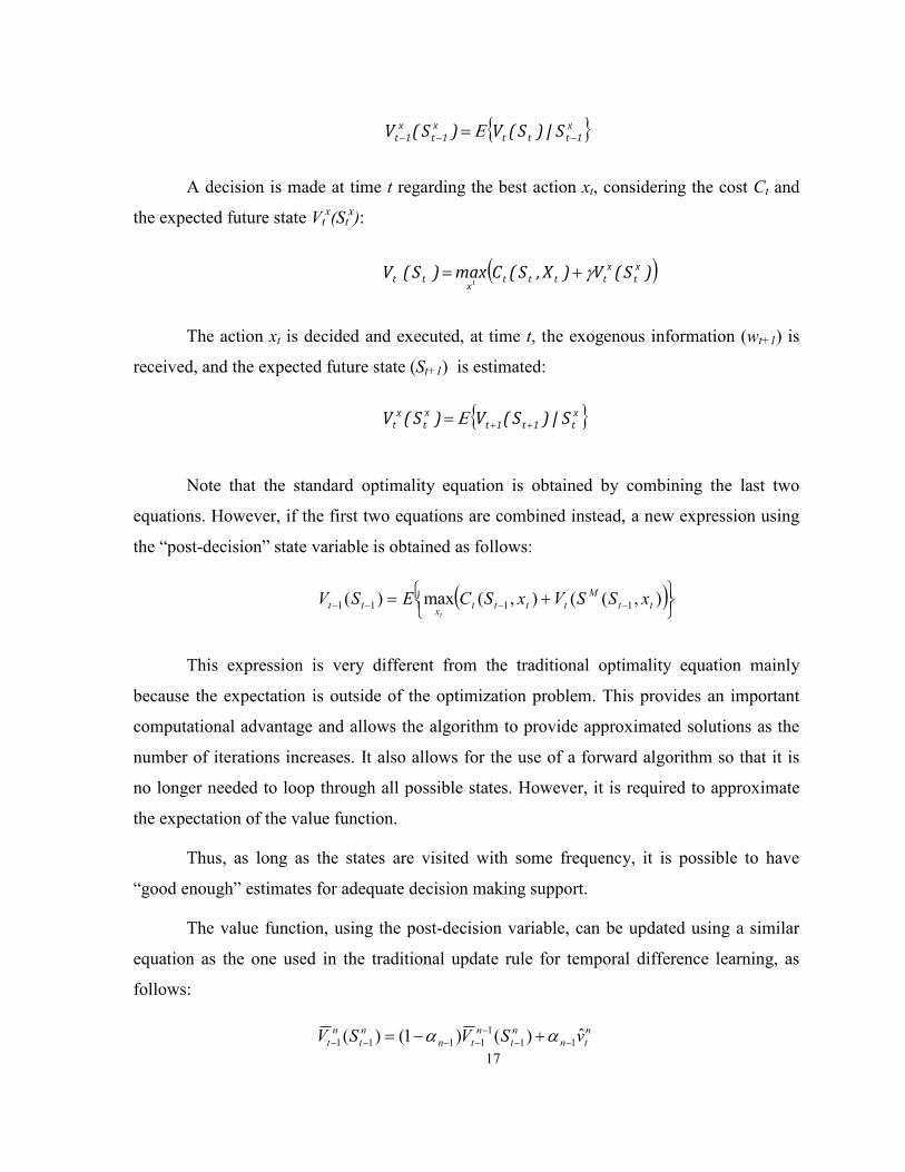
A decision is made at time t regarding the best action xt, considering the cost Ct and

the expected future state Vtx(St

x):

The action xt is decided and executed, at time t, the exogenous information (wt+1) is

received, and the expected future state (St+1) is estimated:

Note that the standard optimality equation is obtained by combining the last two

equations. However, if the first two equations are combined instead, a new expression using

the “post-decision” state variable is obtained as follows:

This expression is very different from the traditional optimality equation mainly

because the expectation is outside of the optimization problem. This provides an important

computational advantage and allows the algorithm to provide approximated solutions as the

number of iterations increases. It also allows for the use of a forward algorithm so that it is

no longer needed to loop through all possible states. However, it is required to approximate

the expectation of the value function.

Thus, as long as the states are visited with some frequency, it is possible to have

“good enough” estimates for adequate decision making support.

The value function, using the post-decision variable, can be updated using a similar

equation as the one used in the traditional update rule for temporal difference learning, as

follows:

n

tn

n

t

n

tn

n

t

n

t vSVSV ˆ)()1()( 11

1

1111 −−−

−−−− +−= αα

{ }x

1ttt

x

1t

x

1t S|)S(V)S(V −−− = Ε

( ))S(V)X,S(Cmax)S(V x

t

x

ttttx

tt tγ+=

{ }x

t1t1t

x

t

x

t S|)S(V)S(V ++= Ε

( )

+= −−−− ),((),(max)( 1111 tt

M

ttttx

tt xSSVxSCESVt

18

Where )S(V n

1t

n

1t −− is the approximated value of the state n

1tS − at iteration n, and α is

the step size or learning rate. The step size determines the weighted value of the current

direction pointed out by n

tv̂ in relation to the approximation of the state value at the current

iteration.

For convergence to be achieved, the learning rate should decrease over time. These

rules require: 1) the step sizes to be non-negative, 2) that the infinite sum of step sizes must

be infinite, and 3) that the sum of the square of the step sizes must be finite. These are typical

rules for convergence of stochastic gradient algorithms.

It is noted that since it is necessary to have a value of )( n

t

n

t SVfor each state

n

tS, the

problems do not reduce their dimensionality when using ADP, but rather reduce the number

of computations needed to find an approximate solution.

3.3.2 State representation

There are several ways to represent the state of traffic at a signalized intersection.

They vary from the number of vehicles in each approach, to the number of vehicles in queue,

to the current delay experienced by those drivers. Each of them may have advantages over

the others, and it is not easy to clearly identify the most appropriate for all types of

evaluations.

However, from past studies, a very common practice is to use the number of vehicles

in queue. This was the approach ultimately adopted for this study, thus the state was defined

as a multidimensional space with four components (one for each of four queues waiting for

the green light): 1) east-west through movement, 2) north-south through movement, 3) east-

west left-turn movement, and 4) north-south left-turn movement.

In addition, the state representation included an extra component that described the

current state of the signal (indicating the phase that was currently receiving the green

indication). This component was important in order to distinguish the pre-decision state

variable from the post-decision state variable, as the state will change as soon as the signal

19

changes (even if drivers have not reacted to it). At times when the signal was transitioning

from one phase to the next, either displaying the yellow indication or in the all-red stage, the

state would show the next phase receiving the green indication.

Thus, in total, the state was represented by a five-dimensional space: four components

describing the number of vehicles in queue for the four movements, and a component

showing the current phase with the right of way.

3.3.3 Cost function

The cost function in our problem was defined, for a given intersection, as a

combination of the number of vehicles being served by the green light (with positive sign)

and the number of vehicles waiting to be served in the remaining approaches (with negative

sign). This general formulation is one of many ways to manage the queues at an intersection,

and it is based on the idea of serving the longest queues first.

In addition, penalties were defined for situations in which the size of the queues

reached a length close to the capacity of the links. These penalties were designed to prevent

queue overflows and de-facto reds, both of which are critical in oversaturated conditions. A

second set of penalties was also assigned every time the right of way was switched from one

phase to a different one. This accounted for the lost time derived from changing phases, and

also prevented the phases to be terminated before they reached a minimum green time that

was operationally adequate (say, at least 6 seconds). The general form of the expression to

estimate the cost of an action is shown below:

Cost(Phase) = Queue receiving green – Σ (Queue receiving red) + (Ι(Phase) *

Penalty)

Where I(Phase) is an indicator function that is equal to 1 if the phase is different from

the current phase and 0 otherwise, and Penalty is calculated based on an expression of the

following form:

{ }Signal,Q,Q,Q,QS Left,SNLeft,WEThrough,SNThrough,WEt −−−−=

20

Where βi are positive coefficients, Qi is the queue of approach i ∈ {1,2,3,4} such that

i does not have the right of way, and ϕi is the proportion of the demand in approach i with

respect to the total volume arriving at the intersection. Thus, the penalty for changing a phase

decreased as the duration of the current phase increased, and it was proportional to the

fraction of the demand waiting to be served.

3.3.4 Eligibility traces – Making the most of every state change

Eligibility traces are one of the several well known mechanisms of reinforcement

learning. The basic idea is to accelerate learning by having deeper updates, as opposed to

only updating the value of the state visited in the last time step. Eligibility traces can also be

thought as a combination of concepts to bridge Monte Carlo methods (which always perform

a full backup) and the standard temporal difference expression - TD(0) (which backs up only

one step in time). The algorithms using eligibility traces are typically represented by the

letter λ to indicate the extent of the backups, or TD(λ).

The implementation of eligibility traces is relatively easy and is based on a series of

weights that keep track of how much time ago a state was visited. They are updated every

time the system is updated in such way that the most recent states will have greater weights,

and will be affected in greater proportion by new states (compared to those states visited in

older time steps). Thus, a new look-up table should be maintained in order to save the current

weight of each state (e(s)).

There are multiple algorithms already established (for reinforcement learning),

including a Sarsa(λ), standard Q(λ), Watkins’ Q(λ) (1992), and Peng’s Q(λ) (1996). In this

study, a modification of the approach used in Peng’s Q(λ) algorithm was adopted for the

ADP. The ADP algorithm can be summarized in the steps shown in Figure 3.6.

( )332211

3

21 QQQ

ionPhaseDurat

ionPhaseDuratPenalty φφφ

ββ

β −−−

−

+=

21

Figure 3.6. Algorithm for Implementing Eligibility Traces

Note that a modification in the update of the trace (e(s)) was introduced, so that states

that were visited frequently did not have traces greater than 1, potentially distorting the

learning process. This modification is known as eligibility trace with replacement, and

consists in “replacing” the trace of the visited state with a value of 1 instead of the typical

addition of 1 to its current value.

3.4 Implementation

3.4.1 Genetic Algorithms

The signal timing optimization problem is formulated as follows:

#�� ) ) ) *+,'-./

,0�1+0

2'0 − ) ) ) 4+,

' . 6+,'-./

,0�1+0

2'0

s.t.

2 ≤ 8'+ ≤ 6 : = 0, … , ;; < = 1,2, … ,

>�<*+,' ≤ >+,

' ≤ >��+,' : = 0, … , ;; < = 1,2, … , ; ? = 1,2, … , 8

0 ≤ @��+,' ≤ A+

' : = 0, … , ;; < = 1,2, … , ; ? = 1,2, … , 8

22

Where:

T: number of study periods,

N: total number of intersections,

8'+: number of phases at intersection i, at time period t,

*+,' : total number of vehicles processed by intersection i, at time period t, in phase ?,

6+,' : queue length at intersection i, at time period t, waiting to be served by phase ?, and

4+,' :penalty weight for queue length at intersection i, at time period t, waiting to be served by phase ?.

We deliberately did not include more constraints that are previously established by

Grianna and Benekohal (2005) due to the following two reasons:

1. First we wanted to make sure that the algorithm is capable of finding the near optimal

answers on its own without introducing those heuristics and,

2. We wanted to make GA, ES, and ADP is comparable as possible to each other.

In particular, the main idea was to bring the definition of these three methods closer

to each other and explore their potential in one of their basic forms. For example, it is noted

that the formulation for the fitness function in GA and ES used similar measures as the cost

function in ADP, and can be briefly summarized as a value that depends on the number of

vehicles processed, or throughput (a positive value), minus the vehicles remaining in queue

in the approaches not receiving green (a negative value). Thus, despite the fact that measures

of performance such as delay or speed could have been added to the formulations, a simple

form was preferred to evaluate the potential of the three methods based on the same

parameters.

Three different overloading patterns were used to determine the effects of them on the

network performance. These loading patterns are:

1- No overloading

2- 10% overloading

3- 20% overloading

23

For no overloading case, 4+,' is assumed to be one regardless of the queue length.

This means that the objective function is simply penalized by the queue length. For 10%

overloading, 4+,' changes when the queue length in a link changes. However, it is equal to

one until the queue fills 10% of the link. Then it is increased as the queue length is increased.

Since the length of a left turn link is different than that of a through link, we used different

functions for 4+,' for 10% overloading:

For left lane: 4+,' =0.013 × 6+,

' �− 0.0514 × 6+,

' + 1.0249

For Through: 4+,' = 0.0032 × 6+,

' �− 0.0222 × 6+,

' + 1.0217

For 20% overloading the same concept was used. The penalty was constantly equal to

1 until 20% of the link was filled by queued vehicle. Then, 4+,' was increased according to

the following equations:

For left lane: 4+,' = 0.000323 × 6+,

' �+ 1

For Through: 4+,' = 0.000033 × 6+,

' �.MN+ 1

A population of candidate solutions is generated to search the feasible area. This

population may be generated randomly, or with using some heuristics. Each member of the

population, chromosome or individual, is a set of decisions variables that forms a vector.

This vector contains signal timing parameters for each intersection, for all defined time

intervals. Signal timing parameters for each intersection, in each time interval are phase plan,

green time for each phase, and offset. Assuming “n” components for this vector, it can be

represented as follows:

� = ��, ��, ��, … , �O�, �O� =

�∅, >,

, >,� , … , >,∅

, @��, ∅�

, >�, , >�,�

, … , >�,∅ , @��

, … … … , ∅1� , >1�,

, >1�,� , …

, >1�,∅ , @��1�

, ∅1 , >1,

, >1,� , … , >1,∅

, @��1;

∅�, >,

� , >,�� , … , >,∅

� , @��, ∅�

�, >�,� , >�,�

� , … , >�,∅� , @��

�, … … … , ∅1�� , >1�,

� , >1�,�� , …

, >1�,∅� , @��1�

� , ∅1� , >1,

� , >1,�� , … , >1,∅

� , @��1�;

24

…

∅2 , >,

2 , >,�2 , … , >,∅

2 , @��2 , ∅�

2 , >�,2 , >�,�

2 , … , >�,∅2 , @��

2 , … … … , ∅1�2 , >1�,

2 , >1�,�2 , …

, >1�,∅2 , @��1�

2 , ∅12 , >1,

2 , >1,�2 , … , >1,∅

2 , @��12�

The decision variable contains the information of all time intervals sequentially. In

each time interval, the signal timing parameters of all intersections are present.

The first population is randomly generated and for each individual. Then CORSIM, a

widely used microscopic traffic simulation environment, is called to evaluate the fitness

value of the first population. Using selection, recombination and crossover, new individuals

are generated. This process is continued until enough individuals for the first generation are

created. After the new population is generated, the old one is discarded and the process is

continued until the termination criteria are met.

3.4.2 Evolution Strategies

The problem formulation used in ES is identical to GA as well as the penalties used

for queue lengths. To solve the problem with ES, the first population is randomly generated.

Each individual contains the signal timing parameters of all intersections in all time periods

as well as the endogenous strategy parameters. If we assume that there are “n” decision

variables, there will be O�O��

� endogenous strategy parameters since we use the most general

mutation cases to solve the problem . The decision variable is similar to that in GA but has

one extra component as shown below:

Q�� = ��, ��, ��, … , �O�, �O, R��

Where R�� = S�, … , �O, ��, . . , ��O, … , �O�,O, �OOT

After generating the initial population, using recombination and mutation, λ

descendants are generated. Then CORSIM is called to evaluate the fitness value of these

individuals. In case of “comma” selection strategy the best µ individuals out of these λ

parents are chosen. In cases of “plus” strategy, the best µ individuals out of the µ+λ

individuals are chosen. This process is continued until the termination criteria are met.

25

3.4.3 Approximate Dynamic Programming

The microscopic simulation environment provided by VISSIM was used for the

implementation of the ADP algorithm. VISSIM provides the option of creating external

traffic controllers through its COM interface. This feature was used to read the ADP

algorithm, which was coded in C++ and then translated to a dynamic linked library, ready to

be used by the simulation in running time.

The state of the system was updated every simulation second, but the controllers

perceived it every 2 seconds. This level of detail was able to produce green times with a

resolution of 2 seconds. Thus, the system was able to take a decision every two seconds and

choose between continuing the current phase and finding a more appropriate phase given the

current volume demand, the queue, and phase duration.

For the given network, each intersection was controlled independently by a different

external controller (through the COM interface). Therefore, every intersection had its own

separate set of state values and learnt the best actions independently. Note that since the

system updates were very frequent and in order to maintain the similarity between the

parameters between ADP and GA/ES, the exchange of information between intersections

was not implemented. As it was defined, the system was able to react within the next 2

seconds of any changes in the queue length. Additional efforts to provide communication

capabilities between intersections are expected to provide improvements in performance,

mainly for shorter links and lower volume conditions, where coordination may significantly

reduce the number of stops and prevent cycle failures.

An additional aspect of the ADP implementation dealt with the state space. Since

each of the links could store a large number of vehicles, this could increase the state space to

a number difficult to manage. As a result, the actual number of vehicles in queue was scaled

down to be represented by a smaller range of queue levels. For the through links (2000 ft

long each), vehicles in queue were represented by a number between 0 and 19, and for the

left-turn links (1000 ft long each) the scale ranged from 0 to 9. The scaling down was

performed by dividing the actual number of vehicles waiting for a given phase by a factor of

6, reducing the resolution of the state representation. Note that two opposing queues will use

26

the same phase and thus their values will be added to determine the demand for that phase

(e.g. eastbound through and westbound through).

As mentioned above, the number of available phases for the controller to choose from

was 4, including exclusive left turns and through movements. Therefore, after the queue

adjustments (scaling down), the state space for a single intersection was in the order of 202 *

102 * 4 = 1.6x105, allowing for the use of standard look-up tables for storing the values of

each state (V(s)). For future studies and in cases with state spaces that demand more memory,

it may be necessary the implementation of function approximation methods instead of look-

up tables. A typical approach for such approximations is the use of artificial neural networks.

For the queue estimation, all links in the network were divided into segments of 120

ft, and the vehicles in each segment were considered “queued” based on the following

criteria: 1) the speed of the last vehicle entering the segment was below 7mph, and 2) the

segment contained more than half of its vehicle capacity. In addition, the queue was required

to be continuous, thus once the queue was detected in a given segment of the link, it ended at

the first segment where the queue conditions were not met.

The information on the status of the queue was obtained through vehicle detectors

placed over the network and allowed the collection of data in real time through the use of the

COM interface from VISSIM. However, it is noted that other forms of collecting real-time

data through Application Program Interfaces (APIs) are also available, and may also allow

the use of other measurements aside from those collected via vehicle detectors.

The implementation of the ADP algorithm did not impose any restrictions on the

maximum green times or the phase sequence when finding the optimal actions. The system

was allowed to decide exclusively based on the functions and parameters described above,

and the ADP was not directed in any way using hard-coded information specific to the tested

traffic conditions.

3.4.4 Calibration of VISSIM to CORSIM

As mentioned before our GA and ES are coupled with CORSIM to find near-optimal

signal timing parameters. However, ADP is integrated with VISSIM as this package had the

flexibility to use external signal controllers that could modify signal timings in real time.

27

Therefore, to reduce the effects of using different simulation environments, VISSIM was

calibrated to CORSIM by taking the following steps:

1- The desired speeds for the two software packages were set to the same value (30

mph)

2- In VISSIM, two different vehicles types were created to match those that are used

by default in CORSIM.

3- The additive part of the desired safety distance in the car following model in

VISSIM was changed from 2 to 3.9 to match the saturation flow rate and the

number of vehicles processed during different green times (5, 15, 25, 35 seconds)

in both environments.

4- The standstill distance between the vehicles in VISSIM was changed from 6.9 to

3.9 to match the number of vehicles that could be stored in a link of a given length

in both environments.

The resulting conditions allowed the use of the CORSIM solutions (for GA and ES)

in the environment provided by VISSIM, and ultimately the comparison of these two

methods with ADP.

28

CHAPTER 4. CASE STUDY

Two networks were used to evaluate the performance of the three selected methods to

find near optimal signal timings. The first network was a small hypothetical network while

the second was a realistic network created by making some modifications to a portion of the

downtown network of the city of Springfield, IL.

The small hypothetical case-study network is symmetric in volume and geometry and

composed of nine intersections (a three by three square) that are 2000 ft apart from each

other. All streets are assumed to have two lanes (one per direction) and there are exclusive

left-turn pockets, 1000 ft in length, at the intersections. We assumed a short study period of

15 minutes in which the traffic demand was fixed with the rate of 1000 vehicle per hour per

lane at each entry point. This traffic demand was chosen to be high enough to ensure

oversaturation in the network. This case study network is shown in Figure 4.1.

29

Figure 4.1. Symmetric case study network.

At each intersection the following phase sequence was used for GA and ES. For GA

and ES all four phases may used if traffic conditions demand them, otherwise 2 or 3 of the

phases may be used. However, ADP did not follow such phase sequence and made the

decision to have the left turn phases when the demand justified them.

30

Figure 4.2. Phase Sequence.

In addition to the hypothetical network, a realistic network was used. The main idea

in this case was to test the algorithms under a more diverse set of conditions, closer to real

world operations. A portion of the downtown network in Springfield, Illinois was used for

this purpose. The network in the case study had 20 intersections and a combination of one-

way and two-way streets with different number of lanes. It comprised the area between 5th

and 11th street from west to east, and between Jefferson and Capitol streets from north to

south.

A few modifications were made to the real network in Springfield given the

additional vehicular demand used in the test case compared to the actual demand in the field:

1) most of the left-turn lanes in the network were shared, but this was changed by adding

exclusive left-turn pockets, 120ft in length; and 2) in cases where there was a lane drop or a

lane addition in one of the arterials, the model maintained the same number of lanes along

the corridor. The test network is called modified Springfield network, and it is shown in

Figure 4.3.

This network did not have protected left turn phases, and as a result, we limited our

algorithms to only two phases to control the signals (east-west bound, and north-south

bound).

Actual traffic volumes in this part of the network in Springfield are lower than the

capacity of links, but the objective of the test case was to examine the network performance

in close-to-saturated and oversaturated conditions. Thus, traffic volumes at entry points were

increased to match the desired conditions.

We tested two different traffic volumes in the network: 750 vehicles per hour per lane

and 1000 vehicles per hour per lane. When traffic volume was 750, we assumed that at all

intersections 10% of the drivers made a right turn (when possible), 10% of drivers made a

g1 g2 g3 g4

31

left turn (when possible), and the rest went through the intersections. When the volume was

1000 vehicle per hour per lane, we assumed that 10% of drivers turned right (when possible),

20% of the drivers turned left (when possible) and the rest went through. It is noted that the

turning percentages were estimated as the percentage of incoming volume from a single lane.

In other words, the base number to estimate this percentage was the total incoming volume

divided by the total number of incoming lanes.

32

Fig

ure

4.3

. M

odif

ied S

pri

ngfi

eld c

ase

stud

y n

etw

ork

.

33

CHAPTER 5. SIGNAL TIMING METHODOLOGIES USED

Three different methodologies were used to find optimal signal timings for the two

networks: 1) Genetic Algorithms (GA), 2) Evolution Strategies (ES), and 3) Approximate

Dynamic Programming (ADP). The first two derive from similar principles and aim at a

directed random search of the solution space, whereas the latter aims at learning the best

actions over time and it is more suitable for real-time decision-making.

This section presents the signal timings obtained using each of the three

methodologies for the following three cases:

1) Case 1 - Network of 9 intersections in oversaturated conditions

2) Case 2 – Modified Springfield network operating in close-to-saturation conditions

3) Case 3 – Modified Springfield network operating in oversaturated conditions

For each case 31 replications of VISSIM were made in each methodology. The study

period (duration) for each run is 15 minutes.

5.1 Case 1 - Network of 9 intersections in oversaturated conditions

5.1.1 Genetic algorithms (GA)

The signal timings obtained from GA for three different levels of network loading

are shown in Table 5.1. Note that GA finds signal timings for each intersection in the

network, and these timings do not change during the study period.

34

Table 5.1. Signal Timings from GA for Case 1

Although the average cycle length for the 10% and 20% overloading conditions is

similar, a comparison of the cycle lengths for individual intersections (between 10% and 20%

overloading) reveals that there were large variations in cycle lengths, indicating that the

signal timing changed for each intersection depending on the demand.

A summary of the cycle lengths for the three loading conditions is shown in Figure

5.1, where they are ordered in a 3x3 matrix that follows the same intersection arrangement as

the small diagram in Table 5.1. For example the upper left cell of the matrix shows the cycle

length (in seconds) for intersection 1, the first cell of the second row shows the cycle length

Left-turn Right-through Left-turn Right-through

1 6 24 6 28 78 0

2 6 26 6 26 78 74

3 6 32 6 32 90 0

4 6 24 6 30 80 4

5 6 26 6 28 80 68

6 6 28 6 32 86 16

7 6 30 6 34 90 66

8 6 28 6 32 86 0

9 6 36 6 36 98 20

Average 6.0 28.2 6.0 30.9 85.1

1 6 52 6 54 132 28

2 6 46 6 48 120 16

3 6 46 6 48 120 64

4 6 32 6 38 96 56

5 6 42 6 44 112 4

6 8 40 6 48 116 46

7 6 44 6 48 118 96

8 6 40 6 36 102 94

9 6 52 6 52 130 34

Average 6.2 43.8 6.0 46.2 116.2

1 6 52 6 54 132 116

2 6 46 6 42 114 54

3 6 52 6 50 128 122

4 6 46 6 52 124 36

5 8 52 10 52 136 94

6 6 34 6 36 96 88

7 6 48 6 48 122 118

8 6 46 6 42 114 56

9 6 40 6 38 104 0

Average 6.2 46.2 6.4 46.0 118.9

Network

LoadingIntersection

Green Phase Duration

E-W direction (s)


N-S direction (s)Time Difference

(s)**

No Overloading

10%

Overloading

20%

Overloading

Cycle Length (s)*

* Cycle length calculated assuming yellow time=3 seconds, all-red=1 second. Transition from left-turn to through movement did not require all-red

** Time difference indicates the beginning of the first phase of the E-W direction of a signal according to the simulation clock

35

for intersection 2, and so on. This Figure offers a quick view at the cycle lengths of the whole

network.

a) No overloading b) 10% overloading c) 20% overloading

Figure 5.1. Cycle Lengths (in seconds) from GA for Case 1

Looking at the animation of the network, it was observed that there was only limited

signal coordination and this was expected since the distance between the intersections was

2000 ft (long enough to cause platoon dispersion) and there was residual queue at the end of

most of the green phases (given the oversaturated conditions). Long links, however, did

accommodate long queues without spilling back to the upstream intersection. Thus, the GA

optimization resulted in long cycles that reduced the total lost time in the whole study period,

without a significant increase in the probability of overflow or gridlock.

5.1.2 Evolution Strategies (ES)

Similar to GA, results from the ES method were obtained for three different network

loading conditions: 1) no overloading, 2) 10% network overloading, and 3) 20% network

overloading. They are shown in detail in Table 5.2.

Signal timings obtained with the ES method were very similar to their correspondent

strategy with GA in terms of both cycle lengths and green splits. Also, the distribution of

green times for E-W and N-S movements was balanced.

Green splits and consequently cycle lengths for the overloading conditions were very

similar to each other, but different than the no-overloading condition. Green times were

78 80 90

78 80 86

90 86 98

132 96 118

120 112 102

120 116 130

132 124 122

114 136 114

128 96 104

36

longer and ranged between 36 and 54 seconds, but most of the left-turn movements had only

6 seconds.

Table 5.2. Signal Timings from ES for Case 1

A general view at the cycle lengths from the ES is shown in Figure 5.2. These

matrices follow the same structure described above for Figure 5.1. The cycle lengths of the

nine intersections are similar to those from GA.

Left-turn Right-through Left-turn Right-through

1 6 28 6 26 80 2

2 6 26 6 26 78 80

3 6 32 6 32 90 0

4 6 26 6 28 80 8

5 6 28 6 28 82 68

6 6 30 6 30 86 18

7 6 30 6 32 88 70

8 6 30 6 30 86 2

9 6 34 6 32 92 18

Average 6.0 29.3 6.0 29.3 84.7

1 6 52 6 52 130 26

2 6 46 6 46 118 14

3 6 46 6 48 120 60

4 6 36 6 38 100 54

5 6 44 6 44 114 0

6 8 44 6 46 118 40

7 6 46 6 46 118 92

8 6 40 6 36 102 86

9 6 52 6 50 128 28

Average 6.2 45.1 6.0 45.1 116.4

1 6 52 6 54 132 112

2 6 46 6 44 116 50

3 6 52 6 50 128 116

4 6 48 6 50 124 32

5 8 52 6 52 132 98

6 6 40 6 38 104 92

7 6 48 6 48 122 120

8 6 44 6 44 114 60

9 6 38 6 40 104 0

Average 6.2 46.7 6.0 46.7 119.6

No Overloading

10%

Overloading

20%

Overloading

* Cycle length calculated assuming yellow time=3 seconds, all-red=1 second. Transition from left-turn to through movement did not require

** Time difference indicates the beginning of the first phase of the E-W direction of a signal according to the simulation clock

Time Difference

(s)**

Network

LoadingIntersection


E-W direction (s)


N-S direction (s) Cycle Length (s)*

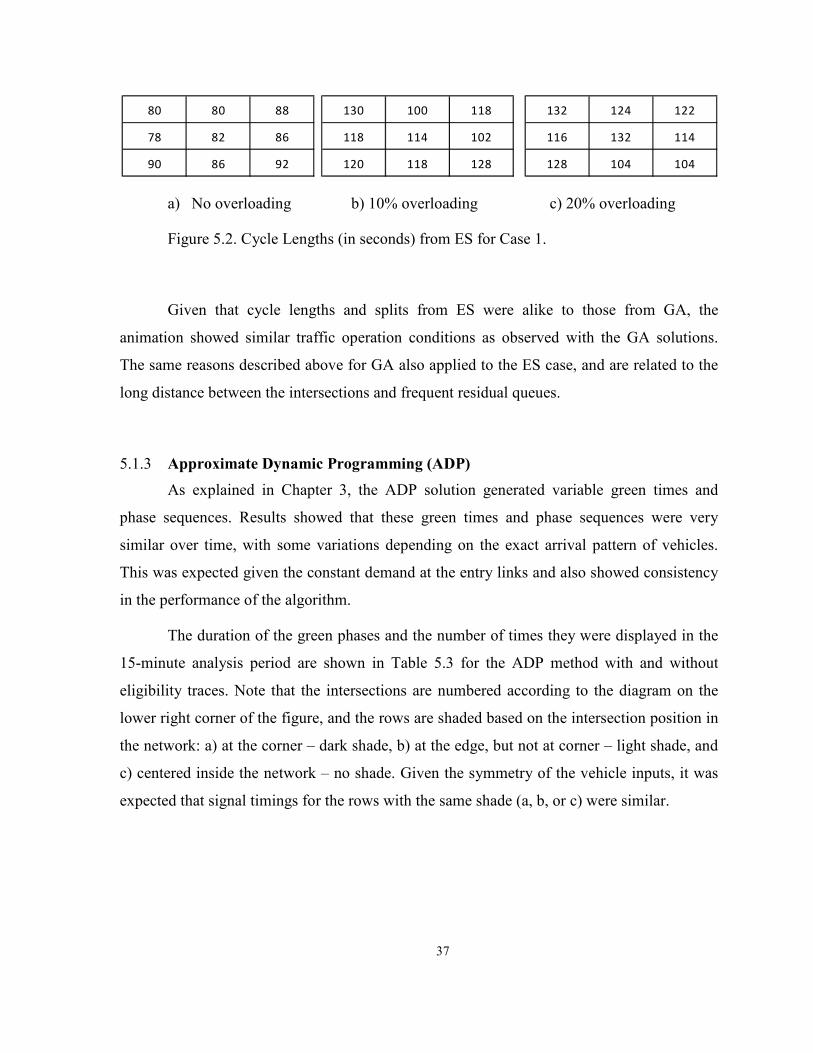
37

a) No overloading b) 10% overloading c) 20% overloading

Figure 5.2. Cycle Lengths (in seconds) from ES for Case 1.

Given that cycle lengths and splits from ES were alike to those from GA, the

animation showed similar traffic operation conditions as observed with the GA solutions.

The same reasons described above for GA also applied to the ES case, and are related to the

long distance between the intersections and frequent residual queues.

5.1.3 Approximate Dynamic Programming (ADP)

As explained in Chapter 3, the ADP solution generated variable green times and

phase sequences. Results showed that these green times and phase sequences were very

similar over time, with some variations depending on the exact arrival pattern of vehicles.

This was expected given the constant demand at the entry links and also showed consistency

in the performance of the algorithm.

The duration of the green phases and the number of times they were displayed in the

15-minute analysis period are shown in Table 5.3 for the ADP method with and without

eligibility traces. Note that the intersections are numbered according to the diagram on the

lower right corner of the figure, and the rows are shaded based on the intersection position in

the network: a) at the corner – dark shade, b) at the edge, but not at corner – light shade, and

c) centered inside the network – no shade. Given the symmetry of the vehicle inputs, it was

expected that signal timings for the rows with the same shade (a, b, or c) were similar.

80 80 88

78 82 86

90 86 92

130 100 118

118 114 102

120 118 128

132 124 122

116 132 114

128 104 104

38

Table 5.3. Signal Timings from ADP with and without Eligibility Traces for Case 1

A series of observations from Table 5.3 are described next. First, the duration and

frequencies of phases at intersections in the same group (with the same shade) were very

consistent. For example, for the no-eligibility case, the average duration of the right-through

phases (for both E-W and N-S directions) at intersections on the corners of the network

Average Max Min Average Max Min

Left-turn 4 18 16 2 4 18 16 2

Right-through 12 27 30 8 11 28 30 8

Left-turn 4 18 26 2 4 18 26 2

Right-through 12 27 38 8 12 28 38 8

Left-turn 5 17 18 6 5 17 18 6

Right-through 13 25 28 11 13 25 28 11

Left-turn 5 16 22 6 5 16 22 6

Right-through 13 23 32 8 13 23 32 8

Left-turn 4 17 18 6 4 18 18 6

Right-through 12 27 30 7 12 27 30 7

Left-turn 4 19 26 6 4 19 26 6

Right-through 12 27 32 12 12 26 32 12

Left-turn 4 16 14 2 5 16 14 2

Right-through 13 24 32 6 13 24 32 6

Left-turn 5 17 18 4 5 17 18 4

Right-through 13 24 48 3 12 25 48 3

Left-turn 5 15 14 4 5 15 14 4

Right-through 14 21 34 6 14 21 34 6

Left-turn 5 15 14 2 5 15 14 2

Right-through 15 20 26 6 14 22 26 6

Left-turn 5 16 20 6 5 16 20 6

Right-through 13 23 28 11 12 24 28 11

Left-turn 5 16 10 4 5 16 10 4

Right-through 13 24 36 7 13 25 36 7

Left-turn 4 20 14 6 4 20 14 6

Right-through 12 27 32 10 11 28 32 10

Left-turn 4 19 14 6 4 20 14 6

Right-through 11 27 32 14 11 28 32 14

Left-turn 5 15 10 4 5 16 10 4

Right-through 13 24 32 6 13 25 32 6

Left-turn 5 15 20 4 4 16 20 4

Right-through 13 23 34 6 13 24 34 6

Left-turn 4 17 14 6 4 19 14 6

Right-through 12 26 30 8 12 27 30 8

Left-turn 5 18 12 6 4 19 12 6

Right-through 12 26 32 17 12 27 32 17

= Intersection at edge - CORNER (2 entry links)

= Intersection at edge - NOT corner (1 entry l ink)

= Intersection on center of network (no entry links)

1

E-W

N-S

2

E-W

N-S

Green Phase Duration (s)Phase Green Phase Duration (s)

No EligibilityFrequency

(in 15

minutes)

EligibilityFrequency

(in 15

minutes)

DirectionIntersection

N-S

3

E-W

N-S

4

E-W

N-S

5

E-W

N-S

6

E-W

9

E-W

N-S

7

E-W

N-S

8

E-W

N-S

39

ranged between 26 s and 27 s, and each of them were displayed between 11 and 12 times in

the 15-minute analysis period. Similar observations are true for the eligibility case, and also

for the left-turn movements.

Second, the proportional amount of time allocated to the left turn phases was very

close to the actual ratio of demands. For example, the ratio of the total green time for left-

turn movements (calculated as frequency * average phase duration) to the total green time for

a given direction (e.g. E-W or N-S) ranged between 0.19 and 0.21, when the actual demand

ratio was 0.2. This was true for all intersections in both the eligibility and the no-eligibility

cases.

Third, the duration of phases with higher number of entry links (which had higher

demands) was longer than those with lower number of entry links. This was also expected as

the lost time is reduced with longer green times, resulting in a better queue management at

the entry links. Also, shorter phases at intersection with lower demand are expected to result

in lower delays and better queue management.

Fourth, the frequencies of right-through phases were about three times higher than the

frequency of the left-turn phases. This indicates that in practice, the strategy suggests

skipping the left turns every two cycles. Considering that the time allocated to the

movements is adequate, this solution has the potential to reduce lost time and manage

adequately the queue lengths.

Fifth, there is still plenty of opportunities for improvements in the solution since at

some cycles the green times were too short (in the order of 2 to 4 seconds), which is

unacceptable in practice. An easy fix to this problem can be applied by constraining the green

times to a minimum value, but for the purposes of exploring the decision-making of the

algorithms, there were no constraints in the process.

In summary, results from ADP suggest that green times for the left-turn movements

are about 2/3 of the green times for through movements, but the frequencies of the left turn

phases that are about 1/3 of the frequencies the through movement phases. This resulted in a

correct allocation of green times, but requires the controller to skip the left-turn phase in

some cycles.

40

5.1.4 Modified ADP – Approximating ADP signal timings to fixed cycles and splits

Cycle lengths or green times were not fixed when ADP is used (with or without

eligibility traces). The ADP results were used to find approximate values that resemble fixed

time signal operations. The signal timings resulted from this approximation is called

Modified ADP. This allowed for direct comparisons of the results based on the Modified

ADP with GA and ES results. It also provided solutions that could be implemented in the

field with standard traffic controllers. The fixed green times and cycle lengths based on the

solutions provided by ADP (without eligibility traces) were estimated using three different

approaches, as described next:

1) Modification 1: Left turn phases were displayed in all cycles. Green times for

through movements were based on averages from ADP. Green times for left-turn

phases were estimated from those found in ADP assuming that they will be displayed

in all cycles. This resulted in green times as low as 5 seconds in some cases. When

the estimated left turn greens were below 7 seconds, all green times were multiplied

by a factor that increased the minimum left-turn green time to 7 seconds.

2) Modification 2: Similar to Modification 1, but instead of multiplying all green times

by a factor, they were added the amount needed to increase the minimum left-turn

green time to 7 seconds.

3) Modification 3: This approximation did not assume that the left-turn phases will be

displayed in every cycle. It considered the frequency of displaying the left turn

phases. Green times for through movements were based on averages from ADP.

The exact splits and cycle times for the three ADP modifications are shown in Figure

5.3. There are several key observations to note about the signal timings found in all ADP

approximations:

1) The cycle lengths within each of the three ADP modifications are very consistent

with each other.

2) They follow the same symmetry of the traffic inputs, so that signal timings of the

intersections at the corners are similar (intersections number 1, 3, 7, and 9),

intersections with only one entry link are also similar (intersections number 2, 4,

41

6, and 8), and the timings of the intersection centered in the network (intersection

#5) have shorter cycles and splits.

3) The splits for the two competing directions of traffic (E-W and N-S) are balanced.

This is according to actual traffic demands.

4) The ratio of splits for the left-turn and the through movements are according to

the actual demand ratios (80/20 for through/left traffic).

On the other hand, the three solutions differed significantly in terms of the total cycle

length and duration of the splits, as shown in Figure 5.3, and are analyzed in the next section.

42

Explanatory key for splits and cycle lengths in part b)

Green splits and cycle lengths for ADP modifications

Figure 5.3. Signal Timings from ADP Modifications for Case 1

43

In a similar way that it was described for the GA and ES solutions, the cycle length of

the intersections from the three ADP modifications are summarized in Figure 5.4 below.

Note that the cycle lengths for the ADP modification 3 refer to the cycles that displayed the

two left-turn phases, not the cycles without the phases.

a) ADP Modification 1 b) ADP Modification 2 c) ADP Modification 3

Figure 5.4. Cycle Lengths (in seconds) for Modified ADP Solutions in Case 1.

It is also observed that the cycle lengths follow a similar trend to that observed for the

original ADP results, with longer cycles for the intersections at the corners of the network

(with 2 entry links), followed by the rest of the intersections along the borders of the network

(1 entry link each), and the shortest cycle for the intersection located at the center.

5.2 Case 2 - Modified Springfield network in close-to-saturation conditions

The modified Springfield network, with more realistic and diverse settings, was also

used to determine the performance of the three methods. Case 2 represents volume levels

near saturation at some of the entry nodes (volumes is 750 vphpl). Recall that a two-phase

signal was used for all nodes and left turns were permitted from the left-turn pockets during

the solid green phase. The signal timings for such conditions are described next.


GA found signal timings with almost identical cycle lengths and even signal time

distribution for E-W and N-S direction, as shown in Table 5.4. All cycle length were 72

seconds long except at five nodes (where they either were 2 or 4 seconds greater), and green

times were predominantly 32 seconds long, also with a few exceptions (34 or 36 seconds

long).

101 92 104

92 82 91

100 91 99

90 84 93

84 81 82

90 83 90

94 85 96

86 77 84

93 85 93

44


Analysis of the values in the Starting Time of the First Cycle indicated that there was

signal coordination between some of the intersections, allowing for good signal progression

in some of the corridors. Figure 5.5 shows the corridors in which good progression was

found. This figure was created based on both the time differences and the animations from

the simulation packages. The segments in which coordination was observed are noted with

arrows, indicating at one end (diamond shape) the starting point of the vehicle movement

from a stop position, and at the other end (arrow shape) the point where the vehicle cleared

the last intersection without the need to stop. The coordinated movements are shown separate

for E-W and N-S directions.

E-W Direction N-S Direction

1 32 32 72 24

2 32 32 72 40

3 32 32 72 64

4 32 32 72 0

5 32 32 72 6

6 32 32 72 64

7 32 32 72 64

8 32 32 72 64

9 32 32 72 64

10 32 32 72 4

11 32 32 72 64

12 32 32 72 68

13 34 32 74 16

14 32 36 76 66

15 32 32 72 18

16 32 34 74 70

17 32 36 76 66

18 32 34 74 26

19 32 32 72 70

20 32 32 72 66

Average 32.1 32.6 72.7

Intersection Cycle Length (s)* Time Difference

(s) **

Green Phase Duration (s)

GA

* Cycle length calculated assuming yellow time=3 seconds, all-red=1 second. Transition from left-turn to

through movement did not require all-red

** Time difference indicates the beginning of the first phase of the E-W direction of a signal according to the

simulation clock

Strategy

45

N-S direction E-W direction

Figure 5.5. Coordination from GA results for Case 2

From Figure 5.5 a few observations are made. The signal timings allowed

coordination to some degree in both directions of travel, but did not provide coordination for

the entire length of the arterials, except for the corridor shown by arrow 1A. In general, the

streets with three lanes (both E-W and N-S) had good progression, with about one stop

expected for those within the most favorable bandwidths. Some of the smaller streets also

had coordination to some degree, as observed in arrows 5A through 10A and 5B through

10B.

5.2.2 Evolution strategies (ES)

Timings from ES were almost identical to those from GA in terms of cycle lengths

and duration of green times. Average values at the bottom of tables 5.4 and 5.5 are almost

identical, showing that there was also similar distribution of the right of way in the two

methods. However, there was more variation in the green times in the ES solution compared

to GA, as most of them were not 32 seconds but ranged between 30 and 34 seconds.

1A

3A

4A

5A 6A

7A 8A 9A 10A

1B 2B

3B 4B

5B 6B

8B

9B7B

10B

46


The offsets in ES were also similar to those from GA, with differences in the order of

at most 8 seconds (for intersections 7 and 14) and 18 seconds for intersection 15. This

resulted in slightly different coordination patterns, as shown in Figure 5.6. Note that fewer

movements are coordinated in comparison with GA, which ultimately resulted in slightly

higher delays and number of stops, as it is described in detail in later sections.


1 30 34 72 28

2 32 32 72 40

3 30 34 72 68

4 34 30 72 6

5 32 32 72 8

6 34 30 72 70

7 30 32 70 0

8 32 32 72 70

9 32 32 72 70

10 34 30 72 8

11 34 30 72 68

12 32 32 72 68

13 34 32 74 18

14 30 34 72 2

15 30 32 70 0

16 32 32 72 2

17 32 34 74 70

18 32 34 74 32

19 30 32 70 0

20 34 32 74 70

Average 32.0 32.1 72.1

Strategy Intersection Cycle Length (s)* Green Phase Duration (s)




simulation clock

Time Difference

(s) **

ES

47

N-S direction E-W direction

Figure 5.6. Coordination from ES results in Case 2

5.2.3 Approximate dynamic programming (ADP)

A summary of the signal timings observed with the ADP strategy are shown in Table

5.6. Similar to the results for Case 1, the range of the average green times of the 20

intersections is not very wide (from 16 seconds to 24 seconds), but their maximum and

minimum values varied significantly.

The distribution of the green times favored links that carried the entry volume, by

providing up to 4 seconds of green time in comparison to the opposing direction of travel.

Note that in cases where the opposing traffic was greater than the entry volume, priority was

given by ADP to the opposing traffic, as it was the case at intersections 18 and 19.

In comparison to GA and ES, the average green times for ADP are significantly

lower, which in turn, resulted in cycle lengths that were about 20 seconds.

1A

2A

3A

5A

6A4A

8A

9A

10A

1B 2B

3B

4B

6B

7B5B

8B

7A

48

Table 5.6. Summary Signal Timings from ADP for Case 2

Average Max Min

E-W 16 22 9 21

N-S 19 23 9 21

E-W 18 24 11 21

N-S 16 22 10 21

E-W 19 23 13 20

N-S 17 22 12 20

E-W 19 23 11 20

N-S 18 24 12 20

E-W 18 23 9 21

N-S 18 22 9 20

E-W 17 22 10 21

N-S 18 22 9 21

E-W 19 22 11 20

N-S 18 23 12 20

E-W 18 22 13 20

N-S 19 23 13 20

E-W 17 23 10 21

N-S 19 24 11 21

E-W 18 23 10 21

N-S 18 23 9 21

E-W 19 23 12 20

N-S 18 23 12 20

E-W 19 23 11 20

N-S 18 23 12 20

E-W 19 25 12 18

N-S 22 36 15 18

E-W 18 24 10 19

N-S 22 51 9 19

E-W 18 22 12 21

N-S 19 23 13 20

E-W 18 22 12 20

N-S 19 23 13 20

E-W 17 24 11 21

N-S 17 23 11 21

E-W 17 23 10 21

N-S 18 25 11 21

E-W 18 25 10 18

N-S 24 42 17 18

E-W 17 23 11 21

N-S 18 23 12 21

18

19

5

6

7

8

9

10

11

12

13

14

20


ADPPhase

Frequency

(in 15 minutes)

DirectionIntersection

1

2

3

4

15

16

17

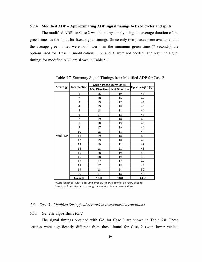
49


The modified ADP for Case 2 was found by simply using the average duration of the

green times as the input for fixed signal timings. Since only two phases were available, and

the average green times were not lower than the minimum green time (7 seconds), the

options used for Case 1 (modifications 1, 2, and 3) were not needed. The resulting signal

timings for modified ADP are shown in Table 5.7.

Table 5.7. Summary Signal Timings from Modified ADP for Case 2

5.3 Case 3 - Modified Springfield network in oversaturated conditions


The signal timings obtained with GA for Case 3 are shown in Table 5.8. These

settings were significantly different from those found for Case 2 (with lower vehicle


1 16 19 43

2 18 16 42

3 19 17 44

4 19 18 45

5 18 18 44

6 17 18 43

7 19 18 45

8 18 19 45

9 17 19 44

10 18 18 44

11 19 18 45

12 19 18 45

13 19 22 49

14 18 22 48

15 18 19 45

16 18 19 45

17 17 17 42

18 17 18 43

19 18 24 50

20 17 18 43

Average 18.0 18.8 44.7

StrategyGreen Phase Duration (s)

* Cycle length calculated assuming yellow time=3 seconds, all-red=1 second.

Transition from left-turn to through movement did not require all-red

Cycle Length (s)*

Mod ADP

Intersection

50

demands). In Case 3, the entering volumes were metered more often with shorter green

times, preventing the oversaturation of the links inside the network.


In addition, cycle lengths were significantly different from each other (unlike in Case

2). Signal coordination was found only at a few locations, as it is observed in Figure 5.7.


1 24 28 60 4

2 24 40 72 4

3 24 40 72 16

4 24 38 70 66

5 24 26 58 16

6 26 24 58 6

7 26 26 60 4

8 50 24 82 0

9 48 24 80 8

10 26 32 66 0

11 26 36 70 8

12 24 38 70 18

13 40 24 72 8

14 36 32 76 32

15 40 32 80 68

16 48 24 80 16

17 24 24 56 0

18 24 24 56 0

19 24 46 78 64

20 24 48 80 0

Average 30.3 31.5 69.8




simulation clock

Cycle Length (s)* Time Difference

(s) **Strategy Intersection


GA

51

Figure 5.7. Coordination from GA results in Case 3

5.3.2 Evolution strategies (ES)

Signal timings from ES are described in Table 5.9. The cycle lengths were shorter for

Case 3 compared to Case 2, following the same trends found in the GA solution. On the

average, there was an even distribution of green times for E-W and N-S directions, but the

green times varied significantly between the two opposing direction of the same intersection,

favoring some movements over the others. Most notably, one-way corridors with three lanes

were favored over the others, which resulted in green times for such movements that almost

doubled the opposing direction. This was the case for the two upper corridors in the E-W

direction, and the west-most corridor in the N-S direction.

1

43 5

2

6

7

52


On the other hand, given that cycle lengths were in most cases not similar to each

other, signal timings did not result in a significant number of movements being coordinated.

This is shown in Figure 5.8, where the coordinated links are indicated by arrows.


1 22 22 52 20

2 22 42 72 0

3 22 42 72 0

4 22 34 64 0

5 22 26 56 20

6 26 22 56 4

7 26 26 60 4

8 48 22 78 0

9 38 22 68 18

10 22 30 60 2

11 22 28 58 2

12 28 28 64 26

13 40 22 70 6

14 38 30 76 30

15 40 22 70 10

16 48 28 84 0

17 22 22 52 8

18 22 22 52 4

19 22 38 68 0

20 22 46 76 0

Average 28.7 28.7 65.4

Cycle Length (s)* Time Difference

(s) **




simulation clock

ES

Green Phase Duration (s)Strategy Intersection

53

Figure 5.8. Coordination from ES results in Case 3

5.3.3 Approximate dynamic programming (ADP)

A summary of the signal timings for ADP for Case 3 are shown in Table 5.10.

Average green times were longer than those for Case 2, and in the order of 17 s to 28 s. The

maximum and minimum green times had significant variation, with values as low as 6 s and

as high as 54 s.

Priorities for green times were not as clear as in Case 2, and some of the arterials

carrying greater volume (in particular the three-lane arterials running N-S on the west side of

the network) did have in some cases the same or even lower green times than their opposing

volumes. This may be the result of greater vehicles metering, which could result in lower

probability of blockages due to queue spillbacks. However, some priorities were given to

other arterials, mainly to the N-S four-lane two-way arterials on the right side of the network

(intersection numbers 13 to 16, and also the stretch from intersection 18 to 20).

32 4

1

54

Table 5.10. Summary Signal Timings from ADP for Case 3

Average Max Min

E-W 19 26 10 20

N-S 19 37 8 20

E-W 19 26 9 19

N-S 20 36 9 19

E-W 23 35 18 17

N-S 20 32 12 18

E-W 21 31 12 19

N-S 18 24 10 19

E-W 18 27 8 20

N-S 19 28 8 20

E-W 19 26 10 21

N-S 17 25 6 21

E-W 19 25 8 19

N-S 21 39 9 19

E-W 22 29 16 18

N-S 22 37 13 18

E-W 22 31 17 17

N-S 23 40 13 17

E-W 18 25 8 20

N-S 19 29 8 20

E-W 21 31 13 18

N-S 20 33 10 19

E-W 19 27 9 20

N-S 18 28 9 20

E-W 21 26 14 16

N-S 27 46 17 16

E-W 20 26 13 16

N-S 28 53 15 16

E-W 20 30 10 18

N-S 23 40 13 18

E-W 21 29 14 17

N-S 25 41 19 17

E-W 22 34 17 17

N-S 22 30 19 17

E-W 18 24 9 19

N-S 22 38 12 19

E-W 21 31 12 16

N-S 28 54 16 16

E-W 21 28 14 16

N-S 26 42 20 16

19

20

13

14

15

16

17

18

12

1

2

3

4

5

6

7

8

9

10

11

Intersection Direction

ADP

Phase Frequency

(in 15 minutes)


55


Similar to Case 2, the modified ADP for Case 3 was found by simply using the

average duration of the green times as the input for fixed signal timings. Thus for the signal

timings for modified ADP, the reader could observed the average values in Table 5.11.

Table 5.7. Summary Signal Timings from Modified ADP in Case 3


1 19 19 46

2 19 20 47

3 23 20 51

4 21 18 47

5 18 19 45

6 19 17 44

7 19 21 48

8 22 22 52

9 22 23 53

10 18 19 45

11 21 20 49

12 19 18 45

13 21 27 56

14 20 28 56

15 20 23 51

16 21 25 54

17 22 22 52

18 18 22 48

19 21 28 57

20 21 26 55

Average 20.2 21.9 50.1


Mod ADP

Strategy Intersection Cycle Length (s)*

* Cycle length calculated assuming yellow time=3 seconds, all-red=1 second. Transition

from left-turn to through movement did not require all-red

56

CHAPTER 6. PERFORMANCE OF THE DIFFERENT STRATEGIES

The performance of the networks under various signal timings were compared using a

series of measures of performances (MOP) that included traffic-related issues, computational

effort, and ease of use. Some of the MOP were focused on the queue lengths and potential

queue overflows (causing de-facto red) since the networks were oversaturated.

This chapter is divided into three sections. In the first section the findings of the small

oversaturated network are presented. In the next section the results for the modified

Springfield network in close-to-saturation condition is presented, followed by a scenario

when it is operating in oversaturated condition.

It should be noted that to determine any of the MOP the signal timing parameters

found by each method (GA, ES, or ADP) were used as an input to VISSIM with a total study

period of 15 minutes. To take the internal variability of VISSIM into account, 31 simulation

runs were made and the MOPs presented below reflect the results of those 31 runs.


6.1.1 Average delay and network saturation

The first MOP that was analyzed was the average delay of all vehicles. A summary of

the range of the average delay from the 31 replications for each of the methods is shown in

Figure 6.1. It also shows the number of vehicles in the network at the end of the simulation

period (as a measure of network congestion).

This analysis included the delay for vehicles that could not enter the network due to

long queues in the entry links. This factor was important in comparing solutions from

different methods since the inner links with less congestion show lower delay but at the cost

57

of not allowing vehicles to enter the network. This consideration also works in favor of

fairness to all strategies and adds a more realismto the calculations, accounting for metering

effects at the edges of the network. Thus, the standard estimation of delay performed by

VISSIM (the difference between the ideal travel time -no traffic, no control- and the actual

travel time experienced by the drivers) was modified to include the delay of vehicles waiting

to enter the network.

Figure 6.1. Average Delay and Network Congestion for Case 1

Figure 6.1 shows similar delays for the ADP (and its modifications) as well as the GA

and ES with no network overloading - with average delays per vehicle around 220 seconds.

The performance of the GA and ES algorithms with overloading options was not as

favorable, with average delays close to 255 seconds.

The contribution of delay from vehicles outside the network was very low and

represented less than 4% of the total delay, as it is shown in Table 6.1. In general, all

strategies managed to keep the back of the entry queues in such way that only a few vehicles

were delayed outside of the network. The values from Table 6.1 were found by tracking the

40

90

140

190

240

290

1200

1400

1600

1800

2000

2200

AD

P (

No

Elig

ibil

ity

)

AD

P (E

lig

ibil

ity

)

AD

P M

od

1

AD

P M

od

2

AD

P M

od

3

No

ove

rlo

ad

ing

Ov

erl

oa

din

g 1

0%

Ov

erl

oa

din

g 2

0%

No

ove

rlo

ad

ing

Ov

erl

oa

din

g 1

0%

Ov

erl

oa

din

g 2

0%

ADP GA ES

Ave

rag

e d

ela

y p

er

ve

hic

le (

s) -

fro

m o

ne

sim

ula

tio

n r

un

Nu

mb

er

of

ve

hic

les

Average Delay Inside the Network

Max

Min

Ave

58

queues and the blockage at the entry links, and assuming a constant (expected) arrival rate of

one vehicle every 3.6 seconds based on entry volumes (1000 vehicle per hour per lane).

Figure 6.1 also shows that the total delay increased with the number of vehicles in the

network at the end of the simulation period, as the bars in the figure follow the same trends

as the delay ranges. Thus, as the saturation level of the network increased, the total average

delay per vehicle also increased.

These considerations suggest that there should be an optimal level of network

saturation in order to achieve low average delays, high throughputs, and good queue

management.

Table 6.1. Delay of Vehicles Outside the Network for Case 1

6.1.2 Network throughput

The network throughput was defined as the total number of trips completed, or in

other words, the total number of vehicles that had left the network at the end of the analysis

period. A summary of the throughput for all strategies is shown in Figure 6.2.

In general, signal timings that result in a greater number of vehicles completing their

trips are more desirable. GA, ES, ADP without eligibility traces and its modifications, as well

ADP with eligibility traces, resulted in similar network throughput that ranged from 2220 to

2320 vehicles. It is noted that the expected demand for the 15-minute analysis period was

3000 vehicles, indicating a hard-to-reach upper bound for the number of processed vehicles.

ADP

(No Eligib.)

ADP

(Eligibil ity)

ADP

Mod1

ADP

Mod2

ADP

Mod3

No

overloading

Overloading

10%

Overloading

20%

No

overloading

Overloading

10%

Overloading

20%

Min 174.44 219.24 225.4 281.96 231.84 199.92 101.08 119 194.88 127.96 116.76

Average 268.0413 292.3 321.9 357.0 304.6 274.6 199.5 200.0 293.1 218.9 227.8

Max 335.44 375.76 390.6 412.16 366.24 357 274.12 283.64 370.16 292.04 298.76

Min 8194.48 13509.44 12737 15591 10100 9971.92 4509.12 5650.4 9628.64 6688.08 5486.32

Average 17359.2 21458.9 21030.9 ####### 18464.3 18489.7 10918.2 10816.4 17195.8 12350.0 12616.1

Max 26326.72 35735.28 30878 34855 26565 37978.64 16252.88 19422.48 25424 17922.24 19791.52

2.6% 3.2% 3.2% 3.5% 2.9% 2.8% 1.4% 1.4% 2.6% 1.6% 1.6%

Cummulative delay (s)

of those vehicles

delayed prior to enter

Average Ratio Delay vehicles

outside/Total delay

ADP GA

Vehicles delayed

outside of the network

(at entry points)

ES

59

Figure 6.2. Network Throughput (Trips Completed) for Case 1

A closer look at the number of vehicles inside the network revealed that the network

increased its saturation levels over time, since the number of vehicles processed was lower

than the actual demand. This was expected since the arriving volume at the intersections with

two competing entry links (the four intersections at the corners) was about 2000 vph, which

exceeds the actual capacity of signalized intersections with single lane approaches.

6.1.3 Average speeds

Trends from average speed data were very similar to those from the vehicle

throughput, as it can be seen from Figure 6.3. Higher speeds were obtained with the ADP

approaches and the GA and ES without network overloading, and they were in the order of

10.3 mph to 10.7 mph. Recall that the desired speed of the drivers in the network was 30

mph. Based on the findings, it is easy to observe that in general lower delays and greater

throughput resulted in higher average speeds.

1900

2000

2100

2200

2300

2400

2500

AD

P (

No

Eli

gib

ilit

y)

AD

P (

Eli

gib

ilit

y)

AD

P M

od

1

AD

P M

od

2

AD

P M

od

3

No

ov

erl

oa

din

g

Ov

erl

oa

din

g 1

0%

Ov

erl

oa

din

g 2

0%

No

ov

erl

oa

din

g

Ov

erl

oa

din

g 1

0%

Ov

erl

oa

din

g 2

0%

ADP GA ES

Ne

two

rk le

ve

l tri

ps

com

ple

ted

Max

Min

Ave

60

Figure 6.3. Average Vehicle Speeds for Case 1

6.1.4 Average number of stops and stopped delay

The average number of stops and the average stopped delay per vehicle, are shown in

Figure 6.4. Note that there was an inverse relation between the number of stops and the

stopped delay, as expected. This was the case since lower number of stops were obtained

when green times were longer, but this also resulted in vehicles having to wait longer for the

next cycle to begin - and for an opportunity to speed up again. In fact, the GA and ES

solutions with network overloading did result in lower number of stops, but higher delays

and lower throughputs than other solutions.

8

9

10

11

12

AD

P (

No

Eli

gib

ilit

y)

AD

P (

Eli

gib

ilit

y)

AD

P M

od

1

AD

P M

od

2

AD

P M

od

3

No

ov

erl

oa

din

g

Ov

erl

oa

din

g 1

0%

Ov

erl

oa

din

g 2

0%

No

ov

erl

oa

din

g

Ov

erl

oa

din

g 1

0%

Ov

erl

oa

din

g 2

0%

ADP GA ES

Av

era

ge

Sp

ee

d (

mp

h)

Max

Min

Ave

61

Figure 6.4. Number of Stops and Average Stopped Delay for Case 1

It was also observed that the average stopped delay was directly proportional to the

total average delay, thus the ratio of stopped to total delay increased as the stopped delay

increased. This is a sign of added congestion in the system (vehicles stopped completely for

longer time periods), and it was found mainly in the overloading scenarios from the GA and

ES. Details are shown in Figure 6.5, below.

0

0.5

1

1.5

2

2.5

3

3.5

4

60

80

100

120

140

160

180

200

220

240

260

AD

P (N

o E

lig

ibil

ity

)

AD

P (

Eli

gib

ilit

y)

AD

P M

od

1

AD

P M

od

2

AD

P M

od

3

No

ov

erl

oa

din

g

Ov

erl

oad

ing

10

%

Ov

erl

oad

ing

20

%

No

ov

erl

oa

din

g

Ov

erl

oad

ing

10

%

Ov

erl

oad

ing

20

%

ADP GA ES

Nu

mb

er

of

Sto

ps

pe

r v

eh

icle

Av

era

ge

Sto

pp

ed

De

lay

pe

r v

eh

icle

(s)

Stopped Delay Ave

62

Figure 6.5. Ratio of Stopped Delay to Total Delay for Case 1

Overall, it was found that a better strategy was not to minimize the number of stops,

but to minimize the total stopped delay and manage the length of the queues.

6.1.5 Efficient use of green

Another sign of good signal timing could be defined in terms of the amount of green

time that is not used to process the greatest number of vehicles, in other words, when

vehicles do not cross the stop bar at saturation flow. This is likely to be the case when (in

oversaturated conditions) the entire queue before the end of the green has been completely

discharged.

Therefore, the length of the queue was monitored for entry and non-entry links and

for through and left-turn movements, recording the amount of time that the queue was

completely dissipated. Results are shown in Figures 6.6 and 6.7.

63

Figure 6.6. Percentage of Time that Queues were Zero at Entry Links for Case 1

Figure 6.7. Percentage of Time that Queues were Zero at Non-Entry Links for Case 1

In Figures 6.6 and 6.7, lower percentages of queue lengths equal to zero was

considered desirable. Note that the ADP strategies (eligibility and no-eligibility) were in

0.0

5.0

10.0

15.0

Le

ft-t

urn

po

ck

et

Th

rou

gh

lin

k

Le

ft-t

urn

po

ck

et

Th

rou

gh

lin

k

Le

ft-t

urn

po

ck

et

Th

rou

gh

lin

k

Le

ft-t

urn

po

ck

et

Th

rou

gh

lin

k

Le

ft-t

urn

po

ck

et

Th

rou

gh

lin

k

Le

ft-t

urn

po

ck

et

Th

rou

gh

lin

k

Le

ft-t

urn

po

ck

et

Th

rou

gh

lin

k

Le

ft-t

urn

po

ck

et

Th

rou

gh

lin

k

Le

ft-t

urn

po

ck

et

Th

rou

gh

lin

k

Le

ft-t

urn

po

ck

et

Th

rou

gh

lin

k

Le

ft-t

urn

po

ck

et

Th

rou

gh

lin

k

No Eligibility Eligibility Mod 1 Mod 2 Mod 3 No

Overloading

Overloading

10%

Overloading

20%

No

Overloading

Overloading

10%

Overloading

20%

ADP GA ES

An

aly

sis

pe

rio

d (

% t

ime

)

Queue at entry links = 0

0.0

5.0

10.0

15.0

20.0

25.0

30.0

Le

ft-t

urn

po

cke

t

Th

rou

gh

lin

k

Le

ft-t

urn

po

cke

t

Th

rou

gh

lin

k

Le

ft-t

urn

po

cke

t

Th

rou

gh

lin

k

Le

ft-t

urn

po

cke

t

Th

rou

gh

lin

k

Le

ft-t

urn

po

cke

t

Th

rou

gh

lin

k

Le

ft-t

urn

po

cke

t

Th

rou

gh

lin

k

Le

ft-t

urn

po

cke

t

Th

rou

gh

lin

k

Le

ft-t

urn

po

cke

t

Th

rou

gh

lin

k

Le

ft-t

urn

po

cke

t

Th

rou

gh

lin

k

Le

ft-t

urn

po

cke

t

Th

rou

gh

lin

k

Le

ft-t

urn

po

cke

t

Th

rou

gh

lin

k


Overloading

Overloading

10%

Overloading

20%

No

Overloading

Overloading

10%

Overloading

20%

ADP GA ES

An

aly

sis

pe

rio

d (

% t

ime

)

Queue at NON-entry links = 0

64

general more efficient at preventing serving approaches with queue equals zero. This is

expected since the algorithms adjusted the signal timing settings in real time and not based

on average performance, which was the case for the other strategies.

6.1.6 Queue overflows

Carefully managing the queues is extremely important in an oversaturated network to

ensure a more efficient operation. Particular attention should be given to the back of queues

so that queue overflows do not occur. Queue overflow blocks the upstream intersection and

prevents vehicles from discharging, creating a “de-facto red” situation. Queue overflows can

create a gridlock in the network. A gridlock significantly deteriorates the performance of

networks and results in longer delays and lower throughput. The occurrence of queue

overflows was monitored for all signal timing solutions, by determining if the back of queue

at entry and non-entry links reached the upstream intersections (or the end of the link).

Results are shown in Figures 6.8 and 6.9.

Figure 6.8. Potential Queue Overflows at Non-Entry Links for Case 1

0.0

5.0

10.0

Le

ft-t

urn

po

ck

et

Th

rou

gh

lin

k

Le

ft-t

urn

po

ck

et

Th

rou

gh

lin

k

Le

ft-t

urn

po

ck

et

Th

rou

gh

lin

k

Le

ft-t

urn

po

ck

et

Th

rou

gh

lin

k

Le

ft-t

urn

po

ck

et

Th

rou

gh

lin

k

Le

ft-t

urn

po

ck

et

Th

rou

gh

lin

k

Le

ft-t

urn

po

ck

et

Th

rou

gh

lin

k

Le

ft-t

urn

po

ck

et

Th

rou

gh

lin

k

Le

ft-t

urn

po

ck

et

Th

rou

gh

lin

k

Le

ft-t

urn

po

ck

et

Th

rou

gh

lin

k

Le

ft-t

urn

po

ck

et

Th

rou

gh

lin

k


Overloading

Overloading

10%

Overloading

20%

No

Overloading

Overloading

10%

Overloading

20%

ADP GA ES

An

aly

sis

pe

rio

d (

% t

ime

)

Queue length at NON-entry links >80% link capacity

65

Figure 6.9. Potential Queue Overflows at Entry Links for Case 1

Figure 6.8 shows that signal timings from all three methodologies effectively

managed the queues inside the network and prevented queue overflows. However, it was

noticed that left-turn queues (and in minor proportion, the through queues) sometimes

reached the beginning of the entry to pocket at entry links (Figure 6.9). This may prevent

through vehicles from filling up the through link near the stop bar, increasing delays and

reducing the effective link capacity. This was the case mostly for the GA and ES solutions

with overloading (both 10% and 20% overloading), where an average left turn pocket at the

entry links reached more than 80% its capacity for about 15% of the total simulation time.

This was expected since network overloading favored a higher number of vehicles in the

links.

6.1.7 Extreme delay values

In addition to general measures of performance, the extreme values of the delay were

also monitored. This analysis reveals the least-favored movements and the amount of delay

for vehicles in such routes, as well as potential limitations on the applicability of certain

0.0

5.0

10.0

15.0

20.0

25.0

30.0

35.0

Le

ft-t

urn

po

ck

et

Th

rou

gh

lin

k

Le

ft-t

urn

po

ck

et

Th

rou

gh

lin

k

Le

ft-t

urn

po

ck

et

Th

rou

gh

lin

k

Le

ft-t

urn

po

ck

et

Th

rou

gh

lin

k

Le

ft-t

urn

po

ck

et

Th

rou

gh

lin

k

Le

ft-t

urn

po

ck

et

Th

rou

gh

lin

k

Le

ft-t

urn

po

ck

et

Th

rou

gh

lin

k

Le

ft-t

urn

po

ck

et

Th

rou

gh

lin

k

Le

ft-t

urn

po

ck

et

Th

rou

gh

lin

k

Le

ft-t

urn

po

ck

et

Th

rou

gh

lin

k

Le

ft-t

urn

po

ck

et

Th

rou

gh

lin

k


Overloading

Overloading

10%

Overloading

20%

No

Overloading

Overloading

10%

Overloading

20%

ADP GA ES

An

aly

sis

pe

rio

d (

% t

ime

)Queue length at entry links >80% link capacity

66

strategies. Table 2 shows the average, maximum, and minimum number of vehicles with

delays (per link) greater than 300 seconds, as well as the maximum delay in a single link, for

all strategies.

Table 6.2. Maximum Delays per Link and Vehicles with Delays Greater than 300 Seconds

for Case 1

StatisticMax Delay in

one link (s)

# of Vehicles

with delay

>300s in one

link

Min. 422 94

Ave. 513 152

Max. 664 204

Min. 451 117

Ave. 524 171

Max. 607 245

Min. 393 22

Ave. 491 79

Max. 612 166

Min. 391 31

Ave. 499 79

Max. 670 137

Min. 372 40

Ave. 498 109

Max. 658 167

Min. 527 135

Ave. 671 231

Max. 832 319

Min. 786 463

Ave. 901 520

Max. 1094 591

Min. 769 464

Ave. 890 519

Max. 1017 591

Min. 531 136

Ave. 652 219

Max. 780 281

Min. 762 474

Ave. 898 519

Max. 1070 606

Min. 764 471

Ave. 890 538

Max. 1045 592

ES

No

overloading

10%

overloading

20%

overloading

20%

overloading

GA

No Eligibil ity

Strategy

ADP

No

overloading

10%

overloading

Mod 1

Mod 2

Mod 3

El igibi lity

67

From Table 6.2, the best worst-case delays are obtained with the ADP modifications

2 and 3, where it was very rare that a vehicle had delays of more than 300 seconds on a

single link. At the other end of the results, the overloading options with GA and ES had the

highest maximum delays and number of vehicles with delays greater than 300 seconds,

showing very unfavorable conditions for some of the drivers in the network.

It is also important noting that for all strategies, all vehicles that experienced delays

greater than 300 seconds were left turners. Thus, all strategies clearly favored through

movements as opposed to left turns. This was expected since ratio of the through vehicles to

left-turners was 80/20, but in oversaturated conditions it also resulted in delays that seemed

(in some cases) very high for real-world applications.


In a similar way that the results were presented for Case 1 (the small network of nine

oversaturated intersections) MOEs are also presented in this section for Case 2 in the

modified Springfield network. In this case it is assumed that entry volume is 750 vehicles per

hour per lane at the entry links. For Case 2, ADP with no eligibility traces, a modified ADP,

GA with no overloading, and ES with no overloading were used.

Average delay per vehicle, 10th and 90th percentiles delay, min, max, and the number

of vehicles in the network at the end of analysis period are shown in Figure 6.10.

68

Figure 6.10. Average Delay and Network Congestion for Case 2

Average delays per vehicle were 70s to 85s, being the results from GA the lowest and

the results from modified ADP the highest. As presented in the Figure, for GA the range of

average delay is extremely wide. However, the 10th and 90th percentiles are very close to each

other. In fact, the 90th percentile delay was less than average delay. This was due to three

seeds that resulted in extremely long delays that were two times larger than the average

delay.

The greatest delay values for GA and modified ADP were the result of intersection

blockages due to queue spillbacks, mainly caused by the stochastic nature of the vehicle

arrivals. Lower fluctuations were in fact expected for ADP since it could react in real time to

these stochasticities, as opposed to fixed timings.

The importance of vehicles delayed outside the network due to queues at the entering

links was minimal with respect to the total delay. The higher average value was for GA, with

a ratio of outside delay to total delay of 1.7%, and the lowest was for ADP with an average of

0.2%.

0

20

40

60

80

100

120

140

160

180

800

900

1000

1100

1200

1300

1400

1500

1600

1700

ADP MOD ADP GA ES

Av

era

ge

de

lay

pe

r v

eh

icle

(s)

-fr

om

on

e s

imu

lati

on

ru

n

Nu

mb

er

of

ve

hic

les

10th percentile average delay

90th percentile average delay

Max

Min

Ave

Delay values include

delay inside and


69

In relation to the number of vehicles in the network at the end of the analysis period

(see the bars in Figure 6.10), the modified ADP allowed about 20% more vehicles than the

other methods (with an average of 1100 vehicles), increasing the network load. This may

result in higher probability of queue spillbacks as the signal timings are fixed, but it may also

reduce delays outside of the network.

The network throughput in the 15-minute evaluation period is shown in Figure 6.11.

Note how the averages for all four methods were very similar, but higher fluctuations were

found for modified ADP and GA. This is due to the same stochastic effects that affected the

average delays, mentioned above. Similar to average delay, three of the seeds created

extremely unfavorable network conditions for GA. Similar to delay, the 10th percentile

throughput was greater than the average throughput.


3500

4000

4500

5000

5500

6000

ADP MOD ADP GA ES

Ne

two

rk le

ve

l tri

ps

com

ple

ted

10th percentile

90th percentile

Max

Min

Ave

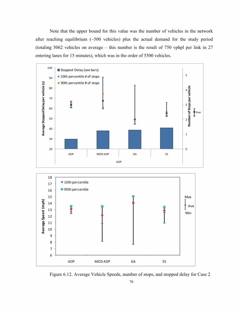
70

Note that the upper bound for this value was the number of vehicles in the network

after reaching equilibrium (~500 vehicles) plus the actual demand for the study period

(totaling 5062 vehicles on average – this number is the result of 750 vphpl per link in 27

entering lanes for 15 minutes), which was in the order of 5500 vehicles.

Figure 6.12. Average Vehicle Speeds, number of stops, and stopped delay for Case 2

0

1

2

3

4

5

20

30

40

50

60

70

80

90

100

ADP MOD ADP GA ES

ADP

Nu

mb

er

of

Sto

ps

pe

r v

eh

icle

Av

era

ge

Sto

pp

ed

De

lay

pe

r v

eh

icle

(s)

Stopped Delay (see bars)

10th percentile # of stops

90th percentile # of stops

Ave

6

7

8

9

10

11

12

13

14

15

16

17

18

ADP MOD ADP GA ES

Av

era

ge

Sp

ee

d (

mp

h)

10th percentile

90th percentile

Max

Min

Ave

71

The performance of the four methods in terms of the average number of stops and the

average speeds is shown in Figure 6.12. The signal timings from GA and ES showed

improved performance over ADP and modified ADP for both MOPs, mainly due to the

effects of signal coordination. As presented in Chapter 5, GA and ES coordinated many of

the movements in the modified Springfield network when the volumes at the entry links were

750 vehicles per hour per lane. Therefore, higher speeds and less number of stops were

observed, with the exception of a three cases in which blockages prevented vehicles from

crossing an intersection.

The animation from the simulation packages confirmed the coordination found by

GA and ES. Similar cycle lengths, longer green times and adequate offsets between adjacent

intersections also provided such indications. Some corridors were more benefited than others.

For example the corridors with three lanes per direction (say, the two upper corridors in the

E-W direction in the modified Springfield network) were an example of this situation. Thus,

the GA algorithm favored directions that had entry links with greater number of lanes, as this

would increase the throughput and reduce the overall number of vehicles queued.

Coordination was not explicitly a goal in the ADP formulation, as communication

between intersections was not allowed, but given the variations in cycle lengths from one

intersection to the other, coordination emerged at some points of the study period and also

favored the performance of the signals to some (but lesser) degree.

Similar to the small network, the queue lengths were also monitored for this case, but

since the entering volumes were lower than the capacity of the network, the results showed

favorable performances for the average simulation run. More specifically, the percentage of

time that the average links reached more than 80% of their capacity (both the links carrying

entering volumes and those inside the network) was lower than 5% for all strategies.

On the other hand, the links were also monitored for queues equal to zero. This could

be an indicator of proper distribution of green times between competing volumes and also of

effective use of green. Results showed that on the average the left-turn pockets did not have

queue for more than 70% of the time, and this measure was in the order of 20% for the

72

through links at the entering points and close to 40% for the other links. All strategies

showed similar performance in this regard.

Overall, results show that the four methods had acceptable performance in this case,

with volumes near saturation at some of the intersections at the edge of network. However,

GA and ES had better average performances mostly due to the explicit management of

coordination, which takes place by incorporating the offsets into the optimization process.

This was observed in the lower number of stops, greater average speeds, and lower delays.


In the modified Springfield network, when the traffic at entry points was 1000

vehicles per hour per lane, GA and ES resulted in lower average delays per vehicle inside the

network than ADP and modified ADP as presented in Figure 6.13.a. However, these two

methods metered vehicles at the entry points and did not let them into the network. In fact,

that was the reason of a lower average delay inside the network. Taking into account the

effect of vehicles delayed before they entered the network, resulted in the delays in Figure

6.13.b. As shown in the figure, ADP and modified ADP resulted in lower total average delay

and consequently greater number of vehicles in the network.

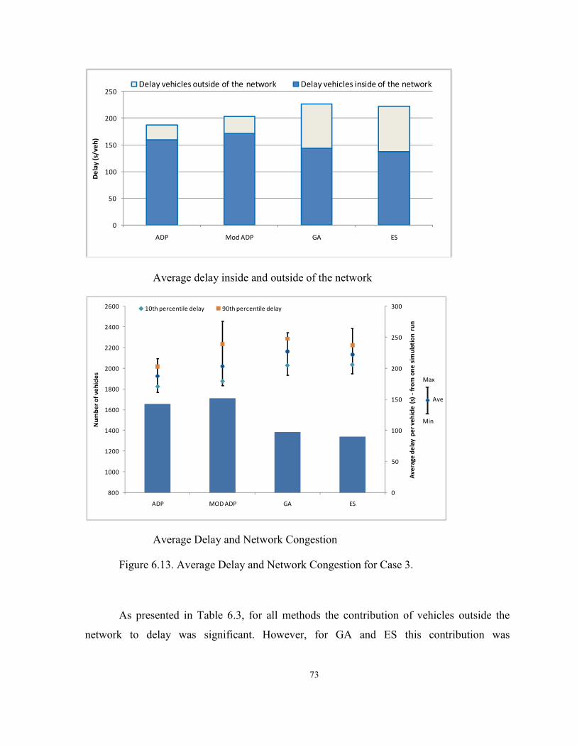
73

Average delay inside and outside of the network

Average Delay and Network Congestion

Figure 6.13. Average Delay and Network Congestion for Case 3.

As presented in Table 6.3, for all methods the contribution of vehicles outside the

network to delay was significant. However, for GA and ES this contribution was

0

50

100

150

200

250

ADP Mod ADP GA ES

De

lay

(s/

ve

h)

Delay vehicles outside of the network Delay vehicles inside of the network

0

50

100

150

200

250

300

800

1000

1200

1400

1600

1800

2000

2200

2400

2600

ADP MOD ADP GA ES

Av

era

ge

de

lay

pe

r v

eh

icle

(s)

-fr

om

on

e s

imu

lati

on

ru

n

Nu

mb

er

of

ve

hic

les

10th percentile delay 90th percentile delay

Max

Min

Ave

74

significantly more than that for ADP and modified ADP, showing the effect of metering

traffic at the entry points.

Table 6.3. Delay of Vehicles Outside the Network for Case 3

Similar to delay, since GA and ES metered the vehicles at the entry points, the

number of vehicles that were processed by them was lower than that of ADP. System

throughput for modified ADP was similar to that for GA and ES and lower than ADP. In

Figure 6.14 the network throughput for different algorithms is shown.


ADP MOD ADP GA ES

Min 1164.8 1231.72 1317.68 1366.4

Average 1242.459 1307.1 1428.8 1427.3

Max 1335.88 1384.32 1505.84 1531.04

Min 128231 131158.72 425265.1 451000.48

Average 188500.1 213725.0 558197.6 572357.5

Max 263515.8 422326.24 676083 675469.76

14.9% 15.6% 36.4% 38.2%

Cummulative delay (s)

of vehicles delayed


Average Ratio Delay vehicles

outside/Total delay

Vehicles delayed


(at entry points)

3000

3500

4000

4500

5000

5500

6000

ADP MOD ADP GA ES

Ne

two

rk le

ve

l tri

ps

com

ple

ted

Max

Min

Ave

75

Since GA and ES did not let too many vehicles enter the network, they could

maintain better level of service inside the network as the average speed for GA and ES

methods was higher than those for ADP and modified ADP cases. In addition, the number of

stops inside the network for GA and ES methods was lower than those for ADP and modified

ADP algorithms. In fact, GA and ES could coordinate some of the signals in the

oversaturated condition as discussed in Chapter 5. Average speeds, number of stops, and

stopped delay are shown in Figure 6.15.

Figure 6.15. Average

Properly managing the queues is extremely important in oversaturated condition. The

reason is that in this condition, if not managed properly, queues start

eventually block the upstream intersections. If this blockage continues it can even

4

5

6

7

8

9

10

11

12

ADP

Av

era

ge

Sp

ee

d (

mp

h)

20

40

60

80

100

120

140

160

180

ADP

Av

era

ge

Sto

pp

ed

De

lay

pe

r v

eh

icle

(s)

Stopped Delay

76

. Average Vehicle Speeds, number of stops, and stopped delay


reason is that in this condition, if not managed properly, queues start growing

eventually block the upstream intersections. If this blockage continues it can even

MOD ADP GA ES

MOD ADP GA ES

ADP

, number of stops, and stopped delay for Case 3


growing and will

eventually block the upstream intersections. If this blockage continues it can eventually cause

Max

Min

Ave

0

1

2

3

4

5

6

7

8

Nu

mb

er

of

Sto

ps

pe

r v

eh

icle

Ave

77

a gridlock which leads to significant increase in delays and loss in system throughput. Figure

6.16 shows maximum queue length at entry links of the network.

Figure 6.16. Potential Queue Overflows at Entry Links for Case 3

As expected, ADP and modified ADP resulted in fewer blockages at the entry links

compared to GA and ES. This was due to the fact that GA and ES tended to meter the traffic

at entry points resulting in longer queue in those links. On the other hand, GA and ES

resulted in less instances of long queues inside the network compared to ADP and modified

ADP. This is shown in Figure 6.17.

0.0

10.0

20.0

30.0

40.0

50.0

60.0

Left-turn

pocket

Through link Left-turn

pocket


pocket


pocket

Through link

ADP MOD ADP GA ES

An

aly

sis

pe

rio

d (

% t

ime

)

Queue length at entry links >80% link capacity

78

Figure 6.17. Potential Queue Overflows at NON-Entry Links for Case 3

In addition to the general measures of performance, the extreme values of the delay

were also monitored. This analysis reveals the least-favored movements and the amount of

delay for vehicles in such routes, as well as potential limitations on the applicability of

certain strategies. Table 6.4 shows the average, maximum, and minimum number of vehicles

with delays (per link) greater than 300 seconds, as well as the maximum delay in a single

link, for all strategies.

0.0

5.0

10.0

15.0

20.0

25.0

30.0

35.0

40.0

45.0

50.0

55.0

60.0

Left-turn

pocket


pocket


pocket


pocket

Through link

ADP MOD ADP GA ES

An

aly

sis

pe

rio

d (

% t

ime

)

Queue length at NON-entry links >80% link capacity

79

Table 6.4. Maximum Delays per Link and Vehicles with Delays Greater than 300

Seconds for Case 3

6.4 Computational effort

The amount of time required to obtain the solutions presented in this section was also

considered. Recall that the GA and ES methods are based on a search of the solution space

and select one (solution) for the entire study period, whereas ADP learns over time based on

the states that are visited and makes a decision every 2 seconds.

This gives ADP a clear advantage over the GA and ES because the algorithm has a

solution soon after the learning process starts (it is an any-time algorithm), and the action-

selection convergence was achieved in short time periods. In fact, the simulations were

initiated with no previous learning and the ADP tables accumulated the value of each state as

the 31 replications were executed in VISSIM. The approximated amount of time needed for

the ADP to find the solutions shown in this study was in the order of 4 hours of CPU time

using a PC with dual-core processors (2.4 GHz) and 4GB of memory. This was the time

needed for VISSIM to complete the 31 simulation runs, thus ADP did not require any prior

training to find the solutions.

Strategy StatisticMax Delay in

one link (s)

# of Vehicles

with delay

>300s in one

link

Min. 288 0

Ave. 421 26

Max. 616 117

Min. 328 1

Ave. 480 60

Max. 764 390

Min. 379 10

Ave. 530 57

Max. 754 142

Min. 371 17

Ave. 498 41

Max. 728 93

MOD ADP

ADP

GA

ES

80

GA and ES each make 60,000 simulation runs to find near optimal solution. Each

simulation run in CORSIM needs around 5 seconds of CPU time. As a result, to find near

optimal answer, GA and ES required around 300,000 seconds or around 3.5 days. GA and ES

runs were performed on a PC with quad-core processors (2.67 GHz) and 3 GB of memory. It

is noted that for the same network, each VISSIM simulation run takes 4 minutes and this was

the main reason of not choosing VISSIM to interface with GA and ES.

6.5 Knowledge requirements

The knowledge and time needed to utilize the methodologies of this study, in terms

of learning the techniques (ADP, GA, and ES), coding, and calibration are discussed in this

section.

It is difficult to quantify the amount of time required to learn these techniques,

considering that the background knowledge for ADP is very different from that used in GA

or ES. However, it is possible to say that prior experience with Markov decision processes

and machine learning will help fully understanding ADP, whereas knowledge in search and

optimization heuristics may help understanding GA and ES. Also, once the user understands

GA, it is fairly straightforward to implement an ES algorithm, and vice versa.

In terms of available literature and past experiences using each of these techniques,

genetic algorithms are a good base point to start the implementation of ADP, whereas

numerous past experiences with GA might be very useful for the development of the

algorithm for a particular network.

In terms of inputs, ADP requires a frequent estimation of the state of the system –

which in this case was the queue length of each approach and the phase duration. For the

computer modeling, this requirement could be satisfied by the addition of vehicle detectors at

multiple points in each link, or alternatively by reading the queue status from the simulation

in real time (through an API). Of these two methods, the former was adopted in this study.

On the other hand, the GA and ES techniques evaluate the signal timings at the end of each

simulation, and thus they do not require inputs from detectors.

81

Calibration may be needed for the three methods. For ADP, decreasing learning rates

(α) are needed as well as a discount factor (γ) and a factor (λ) if eligibility traces are used.

Lastly, the user needs to define a cost function that describes what actions are desired (such

as the one used in this study). In general, standard values used in the literature are good

starting points, but a sensitivity analysis may reveal improvements depending on the specific

problem. Calibration of GA and ES is fairly easy. The reason is that both algorithms have an

area in which the parameters yield an adequate search in the solution space (or “sweet spot”),

and the ranges of these values are easy to find.

6.6 Potential for field implementation

There is true potential for these techniques in real-world applications. For ADP, the

advantages of being suitable for real-time decision-making make it appropriate for traffic

fluctuations and adaptive control. Also, with the advance of detection technologies and in-

vehicle equipment, knowing the state of the system at all times is possible. In fact, there are

adaptive systems currently in operation that monitor the back of queue via video detection

and determine the state of the system to make decisions. Additional algorithm development

and testing under variable demands and in different network configurations are required for

further analysis.

As mentioned before, run time for GA and ES is significantly longer for real-time

application. As a result, if GA or ES are coupled with a microscopic traffic simulation, they

will not be able to determine the signal timing parameters in a reasonable time. Other

strategies such as the use of mesoscopic simulators or even models at the macroscopic level

could be explored to reduce the running time for field implementations.

82

CHAPTER 7. QUEUE MANAGEMENT ANALYSIS

Queue management was evaluated based on a series of MOPs that accounted for the

efficient utilization of green time and the probability of queue overflows at the upstream

intersection. This later MOP is similar to the analysis presented before on queues greater than

80%, but it shows the amount of time that queues actually exceeded the link capacity by

having a length greater than the link itself.

On the other hand, the efficient utilization of green times was measured in terms of

average vehicle headway during the green phase (in seconds) and analyzed based on the fact

that processing vehicles at saturation headway (set at 1.9 seconds) is expected to result in an

efficient operation. Moreover, processing vehicles at saturation headway does not only

indicate that there is no “unused green”, but also shows that the downstream links have

capacity to receive the departing vehicles. When the downstream link does not have capacity

to receive the vehicles coming from the upstream link, the departure headways would be

less than the saturation headway; thus the departure rate is less than the saturation flow.

A third MOP that was explored in queue management is related to the actual

congestion level of the network on the entry and non-entry links, and also on the through and

left-turn movements. This factor was called “queue occupancy” and was calculated as the

ratio of the summation of all queues to the total length of the links, or ) &//

) U// (where 6+is the

queue length at link i, and V+ is the length of link i). Lastly, a fourth MOP shows the global

congestion using network-level queue occupancy, which takes into account all links in the

network together. This measure shows the degree of storage capacity utilization with respect

to vehicles that are experiencing significant delay (in queue).

83


For the small network of 9 intersections, the green utilization efficiency in terms of

average headway during the green phase is shown in Table 7.1. The highlighted cells show

the most favorable methods within each of the three optimization methods, which are also

those with the lowest vehicle headway.

Table 7.1. Green Utilization Efficiency for Case 1

In general, entry links had shorter vehicle headways than non-entry links, showing

that the demand on these approaches was higher and the allocated green time processed a

greater number of vehicles per unit of time. Comparing through movements to left turns, the

ADP shows shorter headways for through vehicles than for left, and the opposite was true for

ES and GA. It is noted that some of the average vehicle headways are shorter than the

saturation headway (sat to 1.9 seconds) and this was the result of vehicles using more time of

the yellow transition (to complete the movement) compared to the lost time at the beginning

of the green phase. Thus, in practice for some movements the effective green was somewhat

longer than the actual time allocated to the green phase.

Overall, the three highlighted methods (ADP, GA, and ES) obtained vehicle

headways at the network level that were very close to the saturation headway, indicating an

effective utilization of the green time.

Through Le ft Through Left Through Left

ADP 1.91 2.00 1.85 1.88 1.93 2.05

ADP ELIG 1.95 2.04 1.89 1.92 1.98 2.09

ADP MOD1 1.98 1.96 1.91 1.90 2.01 1.98

ADP MOD2 1.93 2.18 1.87 2.10 1.96 2.21

ADP MOD3 1.93 2.00 1.86 1.96 1.96 2.01

ES 1.97 1.80 1.89 1.73 2.01 1.82

ES10 2.19 1.75 2.03 1.75 2.26 1.75

ES20 2.21 1.76 2.02 1.75 2.28 1.77

GA 1.95 1.80 1.88 1.73 1.98 1.83

GA10 2.18 1.75 2.02 1.73 2.23 1.75

GA20 2.16 1.75 2.01 1.73 2.21 1.76

All Ne twork Entry Links Non-entry Links

Average Vehicle Headway during Green Phase (s)

Method

ADP

ES

GA

84

A second MOP for the queue management analysis was the amount of time (in

seconds) that the queues exceeded the length of the links and created blockages in the

upstream intersections (or the entry points at the network edge). A summary of this MOP is

shown in Table 7.2.

Table 7.2. Time Queue Exceeded Length of the Links for Case 1

It is observed that the only points in the network in which the queue was longer than

the links was at the entry links and more specifically at the left-turn lanes. However, this

situation was detected in only a small portion of the 900-second runs and in all cases it

represented less than 10% of the analysis period.

The queue occupancy at the link level is shown in Table 7.3. Recall that these values

were found by dividing the queue length by the length of the link where the queue starts.

T hrough Left-turn T hrough Left-turn

ADP 0 0 0 0

ADP ELIG 0 0 0 0

MOD 1 0 0 0 0

MOD 2 0 0 0 0

MOD 3 0 0 0 0

ES 0 2 0 0

ES10 0 66 0 0

ES20 0 65 0 0

GA 0 3 0 0

GA10 0 78 0 0

GA20 0 68 0 0

Entry LinksMethod Non-entry Links

Ave rage T ime tha t Queue Exceeded Length of Links (s)

85

Table 7.3. Queue Occupancy for Case 1

The methods that had the “best” green utilization efficiency within each group are

highlighted. The queue occupation for entry and non-entry links was very different, as

expected, with queues in the entry links that are at least double of those in the inner links.

Note that on average the different methods did not load the links by more than 15% of their

capacity for the through or left movements in the non-entry links. Here it is evident that the

main difference between the overloading (ES10, ES20, GA10, and GA20) and the non-

overloading strategies for ES and GA was the length of the queues in the left turn lanes,

which ultimately resulted in the former group having lower performance for the entire

network.

A summary of the network-level queue occupancy is shown in Table 7.4. There is a

clear tendency for the algorithms not to allow the network to have queues longer than 20% of

its storage capacity. For the strategies designed to overload the network, the global utilization

factor increased on average 0.25-0.26.

Through Left Through Left

ADP 0.47 0.18 0.12 0.14

ADP ELIG 0.49 0.18 0.12 0.14

ADP MOD1 0.55 0.15 0.13 0.08

ADP MOD2 0.49 0.15 0.12 0.07

ADP MOD3 0.48 0.18 0.11 0.10

ES 0.50 0.27 0.10 0.12

ES10 0.50 0.53 0.08 0.25

ES20 0.50 0.53 0.10 0.26

GA 0.48 0.29 0.11 0.12

GA10 0.47 0.54 0.09 0.25

GA20 0.47 0.53 0.10 0.25

ES

GA

Queue Occupancy

Method Entry Links Non-entry Links

ADP

86

Table 7.4. Network-level Queue Occupancy for Case 1


A similar set of MOPs to those described for the small network were also investigated

for Cases 2 and 3 (modified Springfield network). First, the efficiency of green utilization for

Case 2 is described in terms of the average vehicle headway during the green phase (Table

7.5).


Vehicle headways for the four methods were above the saturation headway, but this

was expected since the entering volumes were lower than the saturation level. In particular,

headways for left turns are very high as the demand is much lower (10% of the total demand)

in comparison to the through traffic and the movement is permitted, thus they share the same

green times. Also, the undersaturated operation allowed more left turns to be processed using

gaps in the opposing traffic. The presence of very short left-turn queues is later confirmed in

this section by looking at the occupancy of the left turn pockets, which was very low.

Average Max Min

ADP 0.20 0.22 0.18

ADP ELIG 0.21 0.23 0.19

MOD 1 0.20 0.22 0.19

MOD 2 0.19 0.20 0.17

MOD 3 0.19 0.20 0.18

ES 0.20 0.22 0.19

ES10 0.25 0.27 0.23

ES20 0.26 0.28 0.24

GA 0.21 0.22 0.19

GA10 0.25 0.27 0.22

GA20 0.25 0.27 0.23

Network-leve l Queue Occupancy

Method

Through Left Through Left Through Left

ADP 2.12 21.26 2.10 21.84 2.13 21.16

MOD ADP 2.21 21.91 2.15 22.18 2.23 21.86

GA 2.27 20.27 2.21 16.92 2.28 20.88

ES 2.26 22.16 2.18 23.31 2.29 21.95

Method

Average Vehicle Headway during Green Phase (s)

All Network Entry Links Non-entry Links

87

In this particular case, queue management is not expected to be as critical in terms of

green efficiency, as with the back of the queues, which are analyzed next, in Table 7.6.


From Table 7.6 it is noted that at some points of the analysis period both the through

movements and the left-turns could have created blockages. These temporary blockages were

more prolonged at non-entry links, and more specifically at intersections 5 and 6, where

three-lane one-way streets intersected. Additional analysis at the link level showed that

another critical location was the westbound traffic at intersection 1 and the southbound traffic

at intersection 2 (both of them three-lane, one-way streets).

Queue occupancy was also obtained for Case 2, as shown in Table 7.7. The queue

length with respect to the length of the links was significantly lower than in Case 1 (given the

undersaturated conditions) even though the links were significantly shorter. Results from

Table 7.7 are in accordance with Table 7.6, showing that low average queue resulted in low

probability of blockages.


Thenetwork-level queue occupancy for the four methods is shown in Table 7.8.

Results indicate that on average from 14% to 17% of the network length was composed of

queued vehicles, with maximum values form a single run below 30%.

Through Left-turn Through Left-turn

ADP 0.2 0.3 4.5 0.9

MOD ADP 4.4 1.0 61.4 1.5

GA 7.2 6.8 32.6 8.0

ES 4.5 5.5 30.7 9.9

Method Entry Links Non-entry Links

Average T ime tha t Queue Exceeded Length of Links (s)


ADP 0.18 0.04 0.20 0.04

MOD ADP 0.23 0.05 0.21 0.04

GA 0.25 0.06 0.14 0.07

ES 0.23 0.05 0.21 0.04

Method

Queue Occupancy

Entry Links Non-entry Links

88



This case was expected to provide distinctive details on the operating strategies using

the four different methods. The oversaturated conditions and short spacing between

intersections, in addition to a variety of lane configurations, provide a very challenging

scenario for the algorithms.

The first queue management MOP is the efficient utilization of green time, expressed

as the average vehicle headway, as shown in Table 7.9. It shows that some efficiency was

lost in this case compared to the undersaturated case. This may seem counterintuitive at first

because higher demand should produce less unused green, but it was mainly the result of the

following four situations: 1) blockages due to queue overflow in the crossing street, which

prevented vehicles from reaching the downstream intersection; 2) extending green to process

long queues and prevent blockages, at the cost of platoon dispersion and lower efficiency; 3)

disparity of volume demands on two-way roadways, generating unused green in the direction

with lower traffic; and 4) the priority given to streets with greater number of lanes, as they

could process more vehicles, but also at the cost of platoon dispersion and greater headways.


Average Max Min

ADP 0.15 0.17 0.14

MOD ADP 0.17 0.27 0.14

GA 0.14 0.26 0.11

ES 0.17 0.21 0.15

MethodNe twork-leve l Queue Occupancy

Through Left Through Left Through Left

ADP 2.33 10.44 2.24 10.04 2.35 10.51

MOD ADP 2.51 10.91 2.39 10.28 2.55 11.02

GA 2.72 12.92 2.28 11.32 2.85 13.21

ES 2.59 12.56 2.19 10.93 2.71 12.85

Method

Ave rage Vehicle Headway during Green Phase (s)

All Network Entry Links Non-entry Links

89

The amount of time that the links had queues longer than the storage capacity is

shown in Table 7.10. As expected, on average both the entry and non-entry links experienced

some blockages, which most of the time did not result in gridlocks. Note that longer

blockages were found at the entry links with GA and ES, but the opposite was true for the

non-entry links where blockages were longer in ADP and modified ADP. This is also

evidence of a key difference in the results from these methods, as GA and ES did perform a

more intensive metering at some intersections, and ADP allowed more vehicles inside of the

network.


The queue occupancy of the links was grouped by entry and non-entry links, as well

as by the type of movement, as it is shown in Table 7.11. A similar picture to that described

in the previous MOPs is also found from Table 7.11. The through entry links with ADP and

MOD ADP were slightly less congested than those in GA and ES, with average queues as

long as 70% of the link capacity. On the other hand, non-entry through links with ADP and

MOD ADP reached about 40% capacity inside the network, compared to close to 30% with

GA and ES.


Left-turning links were highly congested with queues close to 70% of the link storage

capacity even inside the network. In fact, a more detail analysis of the queues at the link level

Through Left-turn Through Left-turn

ADP 73.8 572.5 233.5 465.0

MOD ADP 89.5 603.8 305.4 483.3

GA 113.8 615.8 215.0 542.1

ES 107.8 580.5 150.8 523.2

Method

Average T ime tha t Queue Exceeded Length of Links (s)



ADP 0.67 0.71 0.41 0.66

MOD ADP 0.70 0.74 0.40 0.66

GA 0.73 0.80 0.31 0.72

ES 0.72 0.73 0.27 0.68

Method

Queue Occupancy


90

showed that the majority of the top 10% most congested links for all four strategies were left-

turns, and in particular those in intersections 15, 16, 19, and 20. Recall that at this location all

four approaches had left-turning lanes and that all of them operated on a “permitted” basis.

Lastly, the network-level queue occupancy is shown in Table 7.12. Even though the

network is oversaturated, the length of queues in all the links together was on average lower

than 50% of the storage capacity of the network. These results are very different from those

in undersaturated conditions, where the global storage utilization factor was lower than 20%,

and may be a first indication of an upper bound for this factor in this particular network.


For queue management purposes, all four measures mentioned in this Chapter

provide important information for understanding the operation of a set of signal timings.

Green utilization efficiency and queue occupancy should be used simultaneously, not as

separate factors. If the green time is not efficiently used it is highly likely for the queues in

the links to start growing and eventually blocking an upstream intersection, and if this

happens in combination with high level of link occupancies the network is likely to reduce

the number of vehicles that can be processed.

One expects that number of trips in Case 3 to be higher than that in Case 2 since

traffic demand in Case 3 was higher; However, results revealed that the number of trips

completed in Case 2 was higher than that for Case 3, and this can be observed in the green

utilization efficiency and queue occupancy. By increasing traffic demand from 750 vehicle

per hour per lane to 1000 vehicle per hour per lane, queues started to grow in the network

and occasionally blocked upstream intersections. This resulted in a less efficient use of green

time as reflected by a greater green utilization factor (headways greater than the saturation

headway – set at 1.9 seconds). In addition, greater demand increased the queue occupancy of

Average Max Min

ADP 0.46 0.51 0.40

MOD ADP 0.47 0.53 0.42

GA 0.40 0.47 0.35

ES 0.38 0.44 0.33

MethodNetwork-leve l Queue Occupancy

91

the network. This suggests that allowing more vehicles in the network may not be the best

action for all traffic conditions. In fact, all vehicles could enter the network up to a certain

traffic demand; however, if more vehicles are allowed in the network beyond that point, the

network may not be able to process them. This may result in a decrease in number of trips

completed, and in an increase in average travel delay both inside the network and at the

borders.

92

CHAPTER 8. CONCLUSIONS

Three methods were used to find the optimal signal timings for two transportation

networks: Genetic Algorithms (GA), Evolution Strategies (ES), and Approximate Dynamic

Programming (ADP). While GA and ES are meta-heuristics for searching the solution space,

ADP tries to learn the best actions after knowing the state of the system. ADP has potential

for real-time implementation, whereas GA and ES are more suitable for development and

evaluation of various strategies that can be selected in real-time traffic control.

The formulations from the three methods were described, including variations that

explored different approximations to the problem solution. Two case study networks were

used. The first one was a small hypothetical network of 9 oversaturated intersections. On this

network, GA, ES methods were use to find optimal solutions for three network loading

conditions (no overloading, 10%, and 20% overloading). Also two variations of ADP (no

eligibility traces and eligibility traces) and three modified ADP algorithms were tested for the

small network. Results indicated that GA and ES with no overloading and two variations of

ADP and their modifications found signal timings that resulted in similar network

performances. For these four cases, the average delay was between 215 and 226 seconds per

vehicle. The ADP Modification 3 resulted in the lowest average delay and ADP with

eligibility traces resulted in the highest. System throughput was also similar and ranged from

2095 vehicles (ES with 20% overloading) to 2320 vehicles (ADP with no eligibility traces).

When the network was overloaded by 10% or 20%, the average delay per vehicle was

significantly increased while system throughput was at the same level or slightly lower.

93

In comparison, the signal timings (for the small network) found by the best strategies

were in some cases significantly different from each other. The strategies proposed by GA

and ES were similar and resulted in cycle lengths that fluctuated between 78 and 98 seconds,

with identical averages of 85 seconds. On the other hand, the ADP strategies (with and

without eligibility traces), suggested cycle lengths of 85 to 107 seconds when left turns

phases were displayed and cycle lengths of 50 to 63 seconds without left turn phases.

For the modified Springfield network, when the volume at the entry links was 750

vehicles per hour per lane GA (70.3 s) and ADP (75.8 s) found signal timings that resulted in

shorter average delay than ES (78.7 s) and modified ADP (85.62 s). Network throughput for

GA (4987 vehicles), ES (5005 vehicles), and ADP (4981 vehicles) was similar and slightly

higher than that for modified ADP (4746 vehicles). Higher throughput and lower delay for

GA and ES was expected since they were optimizing the offsets in addition to signal timing

parameters and as a result coordinated several intersections of the network. ADP on the other

hand was responding to the current network assuming the intersections were not

interconnected. The signal coordination resulted in less number of stops in the network and

increased average speed. Thus, average number of stops for GA (2.0 stops) and ES (2.4

stops) were fewer than that for ADP (3.0) and its modification (3.3). In addition, GA (14.0

mph), ES (12.9 mph), and ADP (13.1) resulted in a higher average speed in the network than

modified ADP (12.1 mph).

When the entry volumes were set to 1000 in the modified Springfield network, GA

and ES could coordinate some of the signals of the network. As a result, average delay inside

the network for GA (144 s) and ES (137 s) was shorter than that for ADP (159 s) and

modified ADP (171 s). However, GA and ES metered vehicles at the entry links more than

ADP and its modification and did not let too many vehicles enter the network. This resulted

in a larger average delay inside and outside of the network for GA (227 s) and ES (222 s)

compared to ADP (187 s) and modified ADP (203 s). Since GA and ES let fewer number of

vehicles in the network they could process less vehicles and network throughput for ADP

(4718 vehicles) was more than that for GA (4302 vehicles) and ES (4388 vehicles). On the

other hand, since inside the network was not that congested, the average number of stops was

lower for GA (4.2 stops) and ES (4.1 stops) compared to ADP (5.1 stops) and modified ADP

94

(5.1 stops), and average speed was higher (8.2 mph and 8.6 mph for GA and ES, 7.5 mph and

7.0 for ADP and modified ADP, respectively)

For queue management purposes, all four measures mentioned in Chapter 7 provide

important information for understanding the operation of a set of signal timings. However, it

is recommended to use the green utilization efficiency and queue occupancy simultaneously,

not as separate factors. If the green time is not efficiently used it is highly likely for the

queues in the oversaturated links to start growing and eventually blocking an upstream

intersection, and if this happens in combination with high level of link occupancies the

network is likely to reduce the number of vehicles that can be processed.

The queue management analysis showed that to get the best network performance in

the oversaturated condition, the green utilization efficiency for protected movements

(through or left-turns) should be close to saturation headway (1.9 seconds in this study).

In addition, it was found that letting all the vehicles enter the network may not be the

best action for all traffic conditions. Vehicles could enter the network up to a certain traffic

demand, but beyond this point, the network may not be able to process them and it could

result in blockages or gridlocks. This may in turn result in a decrease in the number of trips,

and an increase in average travel delay both inside the network and at the borders. Therefore,

whenever traffic demand is beyond this optimal level, the additional traffic demand should be

metered to prevent a decrease in the network throughput.

Future work to improve the methods described in the report, particularly for real-

world applications, is needed. Several topics can be further studied for advancing the state-

of-the-practice in traffic signal control, including: 1) reduction in the required running time

for GA and ES, 2) improvements in the algorithm for ADP regarding the state representation

and the learning functions, 3) the long term performance of the algorithms, and 4) extended

capabilities such as communication between intersection and augmented set of constraints to

account for known issues in real-world scenarios.

95

Reference

Beyer, H.-G. (2001). The Theory of Evolution Strategies. Heidelberg: Springer.

Cai, C., Kwong Wong, C., and Heydecker, B.G. (2009) Adaptive Traffic Signal Control

Using Approximate Dynamic Programming, Transportation Research Part C: Emerging

Technologies, vol. 17, pp. 456-474.

Chang, T.-H., & Sun, G.-Y. (2004). Modeling and Optimization of an Oversaturated

Signalized Network. Transportation Research Part B , 38, 687-707.

Daganzo, C. (1992). The Cell Transmission Model. Part I: A Simple Dynamic

Representation Of Highway Traffic. Berkeley, CA: Research Reports, California Partners for

Advanced Transit and Highways (PATH), Institute of Transportation Studies, UC Berkeley.

D'Ans, G. C., & Gazis, D. C. (1976). Optimal Control of Oversaturated Store-and-Forward

Transportation Networks. Transportation Science , 10 (1), 1-19.

Gartner, N.H. (1983) OPAC: a demand-responsive strategy for traffic signal control.

Transportation Research Record 906, 75–81.

Gazis, D. C. (1964). Optimum Control of a System of Oversaturated Intersections. Operation

Research , 12 (No. 6), 815-831.

Gazis, D. C., & Potts, R. B. (1965). The Oversaturated Intersection. Second International

Symposium on the Theory of Road Traffic Flow (pp. 221-237). Paris: Organization for

Economic Cooperation and Development.

Girianna, M., & Benekohal, R. f. (2002). Dynamic Signal Coordination for Networks with

Oversaturated Intersections. Transportation Research REcord (1811), 122-130.

Goldberg, D. E. (1989). Genetic Algorithms in Search, Optimization, and Machine Learning.

Boston, MA, USA: Addison-Wesley Longman Publishing Co., Inc.

96

Li, Z., & Chang, G.-l. (2010). Modeling Arterial Signal Optimization with Enhanced Cell

Transmission Formulation. Transportation Research Board. Washington DC: Transportation

Research Board.

Lieberman, E., Chang, j., Bertoli, B., & Wuping, X. (2010). New Signal Control

Optimization Policy for Oversaturated Arterial Systems. Transportation Research Board.

Washington DC: Transportation Research Board.

Lo, H. L., & Chow, H. F. (2004). Control Strategies for Oversaturated Traffic. Journal of

Transportation Engineering ASCE , 130 (4), 466-478.

Longley, D. (1968). A Control Strategy for a Congested Computer Controlled Traffic

Network. Transportation Research , 2, 391-408.

Michalopoulos, P. G., & Stephanopoulos, G. (1977). Oversaturated Signal System with

Queue Length Constraints-I. Transportation Research , 11, 413-421.

Park, B., Messer, C. J., & Urbanik II, T. (2000). Enhanced Genetic Algorithm for Signal-

Timing Optimization of Oversaturated Intersections. Transportation Research Record (1727),

32-41.

Peng, J., Williams R. J. (1996) Incremental Multistep Q-learning. Machine Learning, 22,

283-290.

Putha, R., Quadrifoglio, L., & Zechman, E. (2010). Using Ant Colony Optimization for

Solving Traffic Signal Coordination in Oversaturated Networks. Transportation Research

Board. Washington DC: Transportation Research Board.

Robertson, D.I., Bertherton, R.D. (1974) Optimum control of an intersection for any known

sequence of vehicular arrivals. In: Proceedings of the second IFACIFIP-IFORS Symposium

on Traffic Control and Transportation system, Monte Carlo.

Schrank, D., & Lomax, T. (2009). Urban Mobility Report. University Center for Mobility.

Texas Transportation Institute.

Schwefel, H.-P. (1965). Kybernetische Evolution als Strategie der exprimentellen Forschung

in der Strömungstechnik. Berlin: Technical University of Berlin.

97

Singh, S. P. and Sutton, R. S. (1996). Reinforcement learning with replacing eligibility

traces. Machine Learning, 22:123-158

Singh, M. G., & Tamura, H. (1974). Modelling and Hierarchical Optimization for

Oversaturated Urban Road Networks. International Journal for Control , 20 (6), 913-934.

Teodorvic D., V. Varadarajan, J. Popovic, M. R. Chinnaswamy, S. Ramaraj,. Dynamic

Dynamin programming—neural network real-time traffic adaptive signal control algorithm.

Annals of Operation Research, pp-123-131, 2006.

Watkins, C. J. C. H. and Dayan, P. (1992) Q-learning. Machine Learning 8: 279-292

Xie, Y., Zhang, Y., & Li, L. (2010). Neuro-Fuzzy Reinforcement Learning for Adaptive

Intersection Traffic Signal Control. Transportation Research Board. Washington DC:

Transportation Research Board.

Xin, W., Chang, J., Bertoli, B., & Talas, M. (2010). Integrated Adaptive Traffic Signal

Control with Real-time Decision Support. Transportation Research Board. Washington DC:

Transportation Research Board.

Yuan, C., Yang, X., & Shen, F. (2006). Fixed Cycle Strategy in Oversaturated Network

Traffic Control. the 6th World Congress on Intelligent Control and Automation, (pp. 8674-

8678).

Zhang, L., Yin, Y., & Lou, Y. (2010). Robust Signal Timing for Arterials under Day-to-Day

Demand Variations. Transportation Research Board. Washington DC: Transportation

Research Board.

traffic signal coordination and queue management in ... 2 final... · traffic signal coordination...

Documents