QEDQueen’s Economics Department Working Paper No. 1267

Trading Dynamics with Adverse Selection and Search:Market Freeze, Intervention and Recovery

Jonathan ChiuBank of Canada

Thorsten KoepplQueen’s University

Department of EconomicsQueen’s University

94 University AvenueKingston, Ontario, Canada

K7L 3N6

4-2011

Trading Dynamics with Adverse Selection and Search:

Market Freeze, Intervention and Recovery∗

Jonathan Chiu

Bank of Canada

Thorsten V. Koeppl

Queen’s University

First version: September, 2009

This version: April, 2011

Abstract

We study the trading dynamics in an asset market where the quality of assets is private

information of the owner and finding a counterparty takes time. When trading of a

financial asset ceases in equilibrium as a response to an adverse shock to asset qual-

ity, a large player can resurrect the market by purchasing bad assets which involves

financial losses. The equilibrium response to such a policy is intricate as it creates an

announcement effect: a mere announcement of intervening at a later point in time can

cause markets to function again. This effect leads to a gradual recovery in trading

volume, with asset prices converging non-monotonically to their normal values. The

optimal policy is to intervene immediately at a minimal scale when markets are deemed

important and losses are small. As losses increase and the importance of the market

declines, the optimal intervention is delayed and it can be desirable to rely more on

the announcement effect by increasing the size of the intervention. Search frictions are

important for all these results. They compound adverse selection, making a market

more fragile with respect to a classic lemons problem. They dampen the announce-

ment effect and cause the optimal policy to be more aggressive, leading to an earlier

intervention at a larger scale.

Keywords: Trading Dynamics, Adverse Selection, Search, Intervention in Asset Markets,

Announcement Effect

JEL Classification: G1, E6

∗We thank Dan Bernhardt, Michael Gallmeyer, Huberto Ennis, Nicolae Garleanu, Ricardo Lagos, MiguelMolico, Cyril Monnet, Ed Nosal, Guillaume Rocheteau, Nicolas Trachter, Pierre-Olivier Weill, StephenWilliamson and Randall Wright for their comments, as well as the audiences at many conferences andinstitutions where we presented this paper. Previous versions of this paper were circulated under differenttitles. Thorsten Koeppl acknowledges support from the Bank of Canada’s Governor’s Award and SSHRCGrant 410-2010-0610. The views expressed in this paper are not necessarily the views of the Bank of Canada.

1

1 Introduction

During the financial crisis of 2007 to 2009, there was a stunning difference in how asset

markets were affected according to their infrastructure. Markets with centralized trading

functioned rather well. To the contrary, in over-the-counter markets – where trading takes

place on a decentralized and ad-hoc basis and where assets are less standardized and arguably

more opaque – trading came to a halt. Most prominently, collateralized debt obligations,

asset backed securities and commercial paper were traded only sporadically or not at all

(see Gorton and Metrick, 2010). This prompted massive government intervention in the

from of short-term liquidity provision and long-term asset purchases which led to a (partial)

resurrection of trading in these markets over time.

Markets for structured debt financing experienced a sudden, unexpected deterioration of

the average quality of assets1 and some observers have pointed to adverse selection as the

source for these markets not functioning properly. However, the question arises whether the

peculiar features of over-the-counter trading – private information about the quality of assets

and search for a counterparty – made those markets more prone to a market freeze.2 If so,

are these features important to understand the role and design of a government intervention

in these markets? In this paper, we find that search frictions in asset markets compound

adverse selection, making the market more fragile to unexpected shocks to the quality of

assets. These trading frictions also determine the response of the market to a government

intervention and thus influence the optimal design of a policy aimed at resurrecting trading

in those markets.

To derive these insights, it is natural to combine two existing strands of literature on market

microstructure which have emphasized private information and trading frictions separately.

Starting with Kyle (1985) and Glosten and Milgrom (1989), models of traders that are

privately informed about the asset quality have been used widely to shed light on pricing

and transaction costs in financial markets. More recently, a new approach to study price

and trading dynamics has spawned from the work by Duffie, Garleanu and Pedersen (2005)

that uses random search to model over-the-counter trading, but does not take into account

that assets might be opaque.3

1Moody’s Investor Service (2010) reports large spikes in impairment probabilities for structured debtproducts across all ratings and products for 2007 to 2009).

2When assets are opaque, private information can arise when owners of assets have an advantage or ahigher incentive to acquire information about the quality of assets relative to potential buyers (see Dang,Gorton and Holmstrom, 2009).

3Another related literature uses random matching models with private information to study monetary

2

Our paper shows that shocks to asset quality lead to a market freeze due to a lemons problem

a la Akerlof (1970) when traders have to search for a counterparty. Trading, however, can

be restored, if the government reduces the adverse selection problem (Mankiw, 1986). We

capture this idea by introducing a large player that acts as a one-time, non-competitive

market-maker buying a sufficient amount of lemons permanently in response to the market

breakdown. This distinguishes our paper from the work on for-profit dealers in over-the-

counter markets. In this literature, market-makers alleviate temporary, market-wide liquidity

shocks by holding inventories (see for example Weill, 2007; Lagos and Rocheteau, 2009; Lagos,

Rocheteau and Weill, 2011), whereas in our work, liquidity in the market is endogenous

and collapses in response to adverse selection. The intervention has then to remove assets

permanently to reduce the lemons problem which always causes losses and thus requires

deep pockets – hence, the interpretation of the large player as the government. Similarly, in

the market-making literature government intervention in the form of asset purchases can be

rationalized whenever the expectation of negative profits prevents private market-making in

response to a liquidity shock.

Since our set-up is dynamic, we can study the equilibrium dynamics from a market freeze

to a recovery created by a public intervention.4 The intervention is characterized by the

amount of lemons bought, the price paid and its timing. The time dimension is the most

interesting one as it causes an announcement effect : merely announcing to intervene at a

later point in time can cause the market to recover prior to the actual intervention. The

optimal intervention trades off the costs of the intervention with the gains from a market

recovery. If the market is important, it is best to ensure that it continuously functions with

an immediate intervention. As the importance of the market declines, it becomes optimal to

delay and to increases the size of the intervention. The announcement effect then causes a

gradual recovery in trading volume before the intervention, with market prices reacting non-

monotonically, first decreasing before the intervention and then recovering to their long-term

value.

In our stylized set-up, traders randomly meet to trade an asset. There are two types of assets,

good assets that pay a dividend and lemons which for simplicity never pay any dividend.

exchange (for example Williamson and Wright, 1994; Lester, Postlewaite and Wright, 2008; Li and Rocheteau,2011, among others).

4In independent work, Tirole (2011) uses a static framework that analyzes a similar government policy.Hence, it can neither address the optimal timing of the intervention nor the interaction of this decision withthe quantity and price of the intervention. Recently, Guerreri and Shimer (2011) have extended this idea todynamic asset markets where trading is competitive. They do not, however, analyze the design of the policyin detail.

3

What makes trading difficult is adverse selection: only the current owner of the asset can

observe its quality, while the potential buyer only learns the quality after he has bought the

asset. To create an incentive to trade assets, we assume that traders are hit randomly with

a valuation shock. Upon buying a good asset, the buyer starts out with a high valuation,

but over time he will switch to a low valuation and want to resell the asset. In equilibrium,

while lemons are always up for sale, good assets will only be sold if their owners suffer a low

valuation shock. Allowing buyers to make a take-it-or-leave-it offer results in the optimal

offer being a pooling contract.5

The dynamics of trading are non-trivial and driven by search frictions. To understand them,

we can look at the evolution of buyers’ trade surplus over time which depends on two distinct

effects, one that is backward-looking and another one that is forward-looking. First, a buyer’s

expected trade surplus depends on an endogenous stochastic process that governs how many

good assets are for sale – or the average quality of assets – in the market. It is driven by the

inflow of sellers that have received a low valuation shock. But it also depends on the speed

at which transactions take place in the market which is governed by how often traders meet

and the willingness of buyers to make an offer. We call this effect quality effect, since past

trading behavior is summarized in the current quality of assets for sale. Second, a buyer’s

expected trade surplus also depends on how easy it is to resell the asset in the future. This

matters for two reasons. Having a good asset, there is value in selling it again when the

owner receives a valuation shock. But more importantly, if a buyer obtains a lemon in a

trade, he would like to sell it as quickly as possible, since it does not yield a dividend. We

call this effect strategic complementarity.6

These two effects determine how search frictions influence the fragility of the asset market

and its trading dynamics in response to an intervention. First, due to the strategic comple-

mentarity, equilibria with and without trade can co-exist. When search frictions are high,

buyers are reluctant to take on a position since they expect that it will be difficult to find

a counterparty to undo it in future. As a result, it becomes harder to sustain trading in

5This distinguishes us from Guerreri, Shimer and Wright (2010) that use competitive search to obtain aseparating equilibrium in asset markets with adverse selection. Chang (2011) builds on this work to showthat liquidity in the form of endogenous market tightness is disturbed downwards in equilibrium when thereis a lemons problem for trading assets. Other papers with dynamic adverse selection also arrive at a poolingequilibrium, but by requiring that transactions have to take place at a single price (see for example Eisfeldt,2004; Kurlat, 2010).

6Garleanu (2009) points out that this complementarity can be important for understanding trade sizeand portfolio choice in asset markets. For simplicity, we abstract from such considerations which couldstrengthen this effect.

4

equilibrium for a given quality of assets. Also, smaller shocks to quality can lead to a market

freeze. Conditional on having a market freeze, search frictions also determine the impact

of an intervention on trading through the announcement effect. A market with high search

frictions recovers later because the quality effect kicks in slower and the difficulty of finding a

counterparty reduces the absolute magnitude of the strategic complementarity.7 This implies

that the design of the optimal policy has to take into account the fact that market recovery

is slower when search frictions are large. To resurrect such a market, the large player has to

intervene more aggressively by purchasing assets at an earlier time and a higher price.

There are many papers emerging that either dwell on the role of asymmetric information or

on a strategic complementarity (and, hence, multiple equilibria) to generate a market freeze

in the context of financial markets. Our paper is unique as it combines both elements and

analyzes the trading dynamics in response to a policy that chooses the optimal timing and

scale of an intervention designed to resurrect the market.8 However, we do not investigate

how information is revealed through trading in the market place. Lester and Camargo (2010)

is an interesting contribution, since it studies, when there is asymmetric information, how

quickly a market can sort out assets with different qualities and clears in the absence of

an intervention. In our paper, the lemons problem does not diminish over time, making an

intervention necessary for a recovery. In the tradition of sequential bargaining as a foundation

of trading frictions in asset markets, Zhu (2010) generates endogenously adverse selection

in a sequential search model when sellers visit multiple buyers and infer the quality of the

assets from the frequency of their meetings. Finally, Duffie, Malamud and Manso (2009)

investigate the incentives to search for information which could be applied to a situation of

trading assets when there is asymmetric information.

The paper proceeds as follows. Section 2 introduces our model. In Section 3, we analyze

how an unanticipated, permanent negative shock to the asset quality can lead to a market

freeze. Section 4 studies how an intervention can resurrect the market and characterizes the

price and trading dynamics. Section 5 analyzes the optimal design of intervention. Section

6 calibrates the model and performs various numerical analyses. We conclude with a brief

discussion.

7In a relative sense, an intervention is more effective with high search frictions, as it brings the marketcloser to its normal time activity after an initially delayed response.

8Bolton, Santos and Scheinkman (2011) is an exception in that the timing of the intervention matters.An early intervention can prevent a market freeze, but it can also preclude the supply of private liquidity inthe secondary market for assets.

5

2 The Environment

We employ a basic model of asset pricing under search frictions and introduce adverse se-

lection. Time is continuous. There is a measure of 1 + S traders that trade S assets. These

assets are of two types. A fraction π of the assets yields a dividend δ (good assets), whereas

the rest does not yield a dividend (lemons). The return on these assets is private information

for the owner of the asset; i.e., only the trader who owns the asset can observe its return,

but not other traders.

Traders are risk-neutral and discount time at a rate r. We assume that each investor can

either hold one unit of an asset or no asset.9 A trader who owns a good asset is subject to

a random preference shock that can reduce his valuation from δ to δ − x > 0. Conditional

on holding a good asset, the preference shock arrives according to a Poisson process with

rate κ ∈ IR+. Once a trader experiences this shock, his valuation of the asset will remain

low until the asset is sold. This captures the idea that some traders who own an asset might

have a need for selling it – or in other words, have a need for liquidity. The higher κ, the

more likely an investor will face such needs. Traders therefore go through a different trading

status depending on their asset holdings and their valuation of the asset. There are four

different stages that occur sequentially: (i) buyers (b) do not own an asset; (ii) owners (o)

have a good asset and a high valuation; (iii) traders (`) who own a lemon; and (iv) sellers (s)

who have a good assets, but have experienced a transition to low valuation. We denote the

measure of traders of different types at time t as µb(t), µo(t), µ`(t) and µs(t) respectively.

There is no centralized market mechanism to trade assets. Instead, traders with an asset

and buyers are matched according to a technology given by a matching function M(t) =

λµb(t)[µo(t)+µs(t)+µ`(t)], where M(t) is the total number of matches, and λ is a parameter

capturing the matching rate.10 We assume throughout that in pairwise meetings the buyer

makes a take-it-or-leave it offer to the seller to buy one unit of the asset at price p(t)11 and

that traders cannot dispose of an asset to become a buyer again.12

9This is a restriction on total asset holdings. While assets are indivisible, traders can still use lotteriesand employ mixed strategies to trade assets.

10The interpretation is that traders are matched according to a Poisson process with a fixed arrival rate.As a result, matches with traders seeking the opposite side of a trade occur at a rate λ which is proportionalto the measure of traders in that group.

11This is a simplifying assumption merely to avoid the issue of formulating a bargaining procedure in thepresence of imperfect information.

12By restricting the number of assets relative to measure of traders in the economy, we can easily dispensewith this assumption (see Appendix B).

6

OwnersSellers

Buyers

valuation shock

search

&tra

de

κµo

λµ`µb

λµ

sµ

bλµ

sµ b

sear

ch&

trad

e

(with goodassets)

lemons(with bad

assets)search & trade

λµ`µb

Figure 1: Flow Diagram

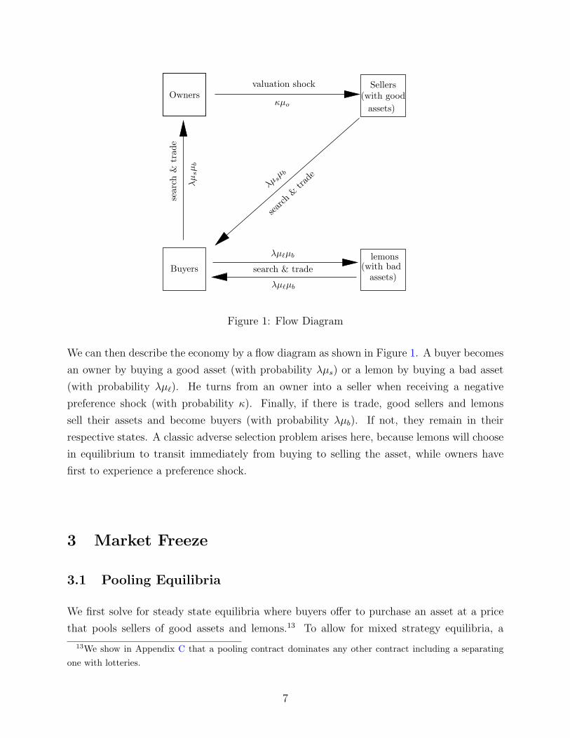
We can then describe the economy by a flow diagram as shown in Figure 1. A buyer becomes

an owner by buying a good asset (with probability λµs) or a lemon by buying a bad asset

(with probability λµ`). He turns from an owner into a seller when receiving a negative

preference shock (with probability κ). Finally, if there is trade, good sellers and lemons

sell their assets and become buyers (with probability λµb). If not, they remain in their

respective states. A classic adverse selection problem arises here, because lemons will choose

in equilibrium to transit immediately from buying to selling the asset, while owners have

first to experience a preference shock.

3 Market Freeze

3.1 Pooling Equilibria

We first solve for steady state equilibria where buyers offer to purchase an asset at a price

that pools sellers of good assets and lemons.13 To allow for mixed strategy equilibria, a

13We show in Appendix C that a pooling contract dominates any other contract including a separatingone with lotteries.

7

buyer makes a take-it-or-leave-it offer with probability γ(t) if in a meeting with another

trader at time t. When making his offer, a buyer needs to take into account whether their

price induces sellers with good assets to accept the offer. Denoting the first random time a

seller gets an offer from a buyer by τ , we obtain for the seller’s value function

vs(t) = Et

[∫ τ

t

e−r(s−t)(δ − x)ds+ e−r(τ−t) max{p(τ) + vb(t), vs(τ)}]

. (1)

The first expression on the right-hand side is the flow value from owning the security. The

second term gives the discounted value of meeting a buyer at random time τ > t and receiving

an offer. In such a meeting, the seller either accepts the offer or rejects it. If he rejects, he

stays a seller (vs(τ)). When accepting the offer, the seller will receive the price p(t) and

become a buyer with value vb(t). Differentiating this expression with respect to time t and

rearranging yields the following differential equation

rvs(t) = (δ − x) + γ(t)λµb(t) max{p(t) + vb(t)− vs(t), 0}+ vs(t). (2)

We can derive similar value functions for the other types of traders denoted by vo(t) for

owners, v`(t) for lemons and vb(t) for buyers. Notice that there is no gains from trading

between owners and buyers, as they have the same valuation of a good asset. We thus have

rvo(t) = δ + κ(vs(t)− vo(t)) + vo(t) (3)

rv`(t) = γ(t)λµb(t) max{p(t) + vb(t)− v`(t), 0}+ v`(t) (4)

rvb(t) = γ(t)λ(µs(t) + µ`(t)) max{maxp(t)

π(p)vo + (1− π(p))v`(t)− p(t)− vb(t), 0}+ vb(t).(5)

An owner enjoys the full value of the dividend flow until he receives a liquidity shock and

turns into a seller which occurs with probability κ. Sellers of lemons – which we will simply

call lemons from now on – are always on the market as they hold asset which do not yield a

dividend. Upon selling the asset at price p, they become buyers again. The value function

of a buyer takes into account that he can choose not to buy the asset in a meeting. If he

makes an offer, the buyer will choose a price that maximizes his expected pay-off given the

composition of traders that are willing to sell. This is reflected in the probability of obtaining

a good asset which is a function of the price he offers (π(p)).

Upon acquiring a lemon, a buyer will immediately try to sell it again since it offers no

dividend flow. To the contrary, when acquiring a good asset, he has the highest valuation

of the asset and will sell it only after receiving a preference shock that lowers his valuation

which occurs with frequency κ. This implies that the measure of different types of traders

8

evolves according to the following flow equations

µb(t) = −γ(t) (µs(t) + µ`(t)) + γ(t) (µs(t) + µ`(t)) = 0 (6)

µo(t) = −κµo(t) + γ(t)λµs(t) (7)

µs(t) = κµo(t)− γ(t)λµs(t) (8)

µ`(t) = −γ(t)λµ`(t) + γ(t)λµ`(t) = 0. (9)

Due to the trading structure, the number of buyers stays constant and is normalized to

µb(t) = 1. Similarly, all lemons are constantly for sale and, hence, µ`(t) = (1− π)S.

For a buyer to induce a seller to accept his take-it-or-leave-it offer, he needs to offer a

price that compensates the seller for switching to become a buyer, or p(t) ≥ vs(t) − vb(t).Since lemons do not derive any flow utility from their asset, we have that vs(t) ≥ v`(t)

and, consequently, they will accept the buyer’s offer whenever sellers do. For the buyer, the

probability of buying a good asset is thus given by

π(t) =

µs(t)

µs(t)+µ`(t)if p(t) ≥ vs(t)− vb(t)

0 if p(t) < vs(t)− vb(t).(10)

This formulates the basic adverse selection problem. While lemons are always for sale, good

assets go on sale only if their current owner experiences a preference shock. As a consequence,

there are fewer good assets for sale than in the population. Also, if the buyer offers a price

that is too low, good sellers will reject the offer and he will acquire a lemon for sure. Any

offer by the buyer will thus be given by p(t) = vs(t) − vb(t). For the further analysis, it is

convenient to define the buyer’s expected surplus from buying the asset

Γ(t) = π(p)vo + (1− π(p))v`(t)− vs(t), (11)

where we have take into account that any offer will set p(t) = vs(t)− vb(t). This yields the

following definition of equilibrium.

Definition 1. An equilibrium is given by measurable functions γ(t) and π(t) such that

1. for all t, the strategy γ(t) is optimal taking as given γ(τ) for all τ > t; i.e.,

γ(t) =

0 if Γ(t) < 0

∈ [0, 1] if Γ(t) = 0

1 if Γ(t) > 0.

(12)

2. The function π(t) is generated by γ(t) and the law of motion for µs(t).

9

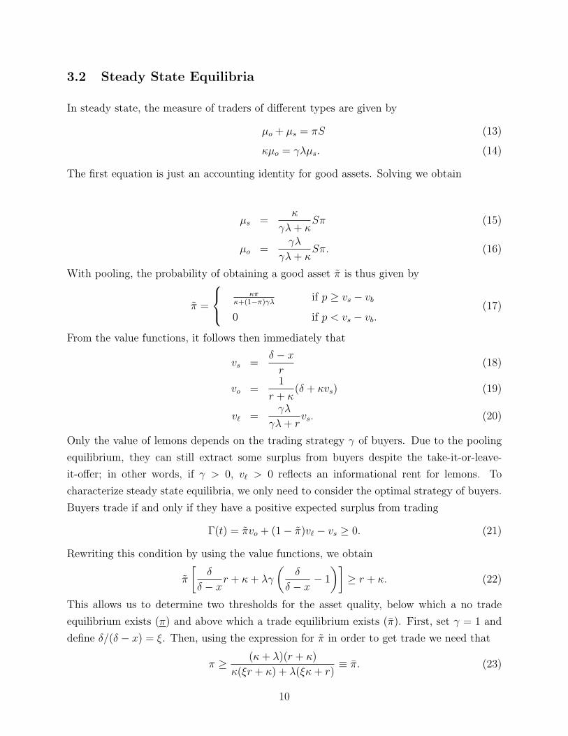
3.2 Steady State Equilibria

In steady state, the measure of traders of different types are given by

µo + µs = πS (13)

κµo = γλµs. (14)

The first equation is just an accounting identity for good assets. Solving we obtain

µs =κ

γλ+ κSπ (15)

µo =γλ

γλ+ κSπ. (16)

With pooling, the probability of obtaining a good asset π is thus given by

π =

κπκ+(1−π)γλ

if p ≥ vs − vb0 if p < vs − vb.

(17)

From the value functions, it follows then immediately that

vs =δ − xr

(18)

vo =1

r + κ(δ + κvs) (19)

v` =γλ

γλ+ rvs. (20)

Only the value of lemons depends on the trading strategy γ of buyers. Due to the pooling

equilibrium, they can still extract some surplus from buyers despite the take-it-or-leave-

it-offer; in other words, if γ > 0, v` > 0 reflects an informational rent for lemons. To

characterize steady state equilibria, we only need to consider the optimal strategy of buyers.

Buyers trade if and only if they have a positive expected surplus from trading

Γ(t) = πvo + (1− π)v` − vs ≥ 0. (21)

Rewriting this condition by using the value functions, we obtain

π

[δ

δ − xr + κ+ λγ

(δ

δ − x− 1

)]≥ r + κ. (22)

This allows us to determine two thresholds for the asset quality, below which a no trade

equilibrium exists (π) and above which a trade equilibrium exists (π). First, set γ = 1 and

define δ/(δ − x) = ξ. Then, using the expression for π in order to get trade we need that

π ≥ (κ+ λ)(r + κ)

κ(ξr + κ) + λ(ξκ+ r)≡ π. (23)

10

Similarly, we get no trade (γ = 0) if

π ≤ r + κ

ξr + κ≡ π. (24)

Comparing the two thresholds, we obtain that π ≥ π if and only if κ ≥ r. Finally, for any

given π in between these thresholds, the indifference condition requires

π =(κ+ γλ)(r + κ)

κ(ξr + κ) + γλ(ξκ+ r)(25)

Differentiating we get (up to a constant)

∂π

∂γ= (ξ − 1)(r + κ)λκ(r − κ), (26)

which depends on r relative to κ. In particular, π increases with γ if and only if r > κ. This

gives the following result.

Proposition 2. For any given π ∈ (0, 1), a steady state equilibrium exists.

If π ≥ π, we have that γ = 1 is a steady state equilibrium in pure strategies, i.e. all buyers

trade.

If π ≤ π, we have that γ = 0 is a steady state equilibrium in pure strategies, i.e. buyers do

not trade.

If κ < r, the steady state equilibrium is unique, with the equilibrium for π ∈ (π, π) being in

mixed strategies.

If κ > r, for π ∈ (π, π), there are three steady state equilibria including a mixed strategy one.

Figure 2 depicts steady state equilibria. When the average quality of the assets π is too low,

there cannot be any trading in equilibrium – a situation which we call market freeze. This

is associated with welfare losses as good assets cannot be allocated between traders that

have different valuations for the asset. Similarly, for high average quality π, trade (γ = 1) is

the unique equilibrium. For intermediate values of π, there can be multiple equilibria with

partial trade (γ ∈ (0, 1)).

3.3 The Role of Search Frictions

Search frictions as captured by the parameter λ of the matching function play a key role in

determining how severe the adverse selection problem becomes for any given average quality

11

0 1

1

π

γ

π π

equilibria

︸ ︷︷ ︸no trade

︸ ︷︷ ︸multiple

︸ ︷︷ ︸trade

0 1

1

π

γ

ππ

︸ ︷︷ ︸no trade

︸ ︷︷ ︸mixing

︸ ︷︷ ︸trade

(i) κ > r (ii) r > κ

Figure 2: Steady State Equilibria

π. This can be best understood by slightly rewriting the expected surplus of buyers to obtain

Γ

(1− π)vs=

π

1− π

(vo − vsvs

)+

(v` − vsvs

)(27)

=

(π

1− π

)(κ

κ+ λγ

)(1− ππ

)− r

r + λγ. (28)

The first term captures a quality effect and describes how the average quality of assets for

sale affects the trade surplus. If the trading volume as proxied by λγ is large, there are

relatively few good assets for sale at any point in time. This lowers the expected quality of

the asset purchased by a buyer and, hence, his expected surplus.

The second term is independent of the average quality and captures a (dynamic) strategic

complementarity. When a buyer decides to purchase an asset, it matters how easy it is to

turn around a lemon in the future. If future buyers are less willing to trade, the asset market

becomes less liquid giving the current buyer a lower incentive to trade. Conversely, if future

buyers are more willing to purchase assets, it becomes easier for a buyer to turn around a

lemon in the market increasing v`. These two effects work in opposite directions and can

cause trading even to decline when the quality of the asset increases as shown in Figure 2.

In general, as search frictions become larger – i.e., λ decreases – the difference between a

trade (γ = 1) and a no-trade equilibrium (γ = 0) vanishes as shown in Figure 3. Equation

28 implies that, in order to get trade in every meeting in equilibrium, we need(π

1− π

)(1− ππ

)≥ rκ+ rλ

rκ+ κλ. (29)

For λ→ 0, the strategic complementarity and thus the multiplicity of equilibrium disappears.

The quality effect however increases. Since there are few trades, the selling pressure is large

12

0λ

π

π

Trade

0λ

π(i) κ > r (ii) r > κ

Trade / Mixing / No trade

No Trade

Trade

Mixing

No Trade

ππ

π

Figure 3: Role of Search Frictions

in the market: there are many good assets for sale at any point in time. However, when

purchasing a lemon it is hard to sell it again. In this sense, π measures the maximum quality

effect.

When trading becomes frictionless (λ → ∞), we have that the strategic complementarity

becomes large, but at the same time, the quality effect completely disappears. This is due

to the fact that the number of good assets for sale relative to bad assets converges to 0. In

the limit, we have (π

1− π

)(1− ππ

)≥ r

κ. (30)

which defines an asymptote for π, which is the minimum value of π satisfying this inequality.

When κ > r, the complementarity dominates and it becomes easier to support trading in

equilibrium – at the expense of multiple equilibria. It is in this sense that search frictions

compound the adverse selection problem. As a consequence, markets with frictional trading

are more fragile when the quality of assets π declines as we show next.

3.4 Unanticipated Quality Shocks

We now consider a market freeze induced by an unexpected, permanent shock to the asset

quality. Suppose we are in a steady state equilibrium with trade, but that a certain fraction

of good assets turns into lemons independent of the holder of the asset being an owner or

a seller. We assume that the average quality of the asset drops unexpectedly at t = 0 to a

level π(0) < min{π, π} ≡ πmin. There cannot be continuous trade, since the surplus function

Γ is strictly negative at t = 0. Furthermore, if there is no trade, the quality of assets for

13

sale increases over time, but can never cross the threshold π where making an offer is a

strictly dominant strategy for a buyer, i.e. π(t)→ π(0) < π. Hence, there is an equilibrium

where the economy converges to the no trade steady state with no trade along the transition.

Finally, if the quality drops sufficiently, this no trade equilibrium is unique.

Proposition 3. Suppose the economy is in a steady state with trade, but there is a shock to

quality π(0) < πmin. Then there cannot be an equilibrium with continuous trade, but there

exists an equilibrium with no trade for any t that converges to the steady state with no trade.

This equilibrium is unique, if π(0) <(

rr+(1−π)λ

)π.

Proof. See Appendix A.

This implies that for a large enough shock to the asset quality the market will instantaneously

move from an equilibrium with trading to one without – our definition of a market freeze.

Note that even a small shock to π can permanently freeze the market when κ > r as shown in

Figure 2. We turn next to the question whether an intervention in the form of permanently

buying assets can resurrect trading and how trading will respond to such an intervention.

4 Trading and Price Dynamics with Intervention

4.1 Intervention

We study now an intervention by a large (strategic) player – called market-maker-of-last-

resort (MMLR) – in response to an unanticipated quality shock that causes the market to

freeze.14 We assume throughout that π(0) < min{π, π} ≡ πmin, so that there is a unique

steady state equilibrium of no trade and that without an intervention the economy converges

to this equilibrium with no trade along the transition. The MMLR purchases bad assets

which increases the average quality of the assets that are for sale after the intervention.

This action will also influence trading behavior before the intervention takes place. As

buyers anticipate the market to recover in response to the asset purchase, they can have an

incentive to start buying assets before the intervention – a situation we call announcement

effect.

14In Appendix D, we discuss how a MMLR can use a different policy – a guaranteed price floor – torespond to a self-fulfilling freeze by eliminating equilibria with less trade when multiple equilibria co-exist.

14

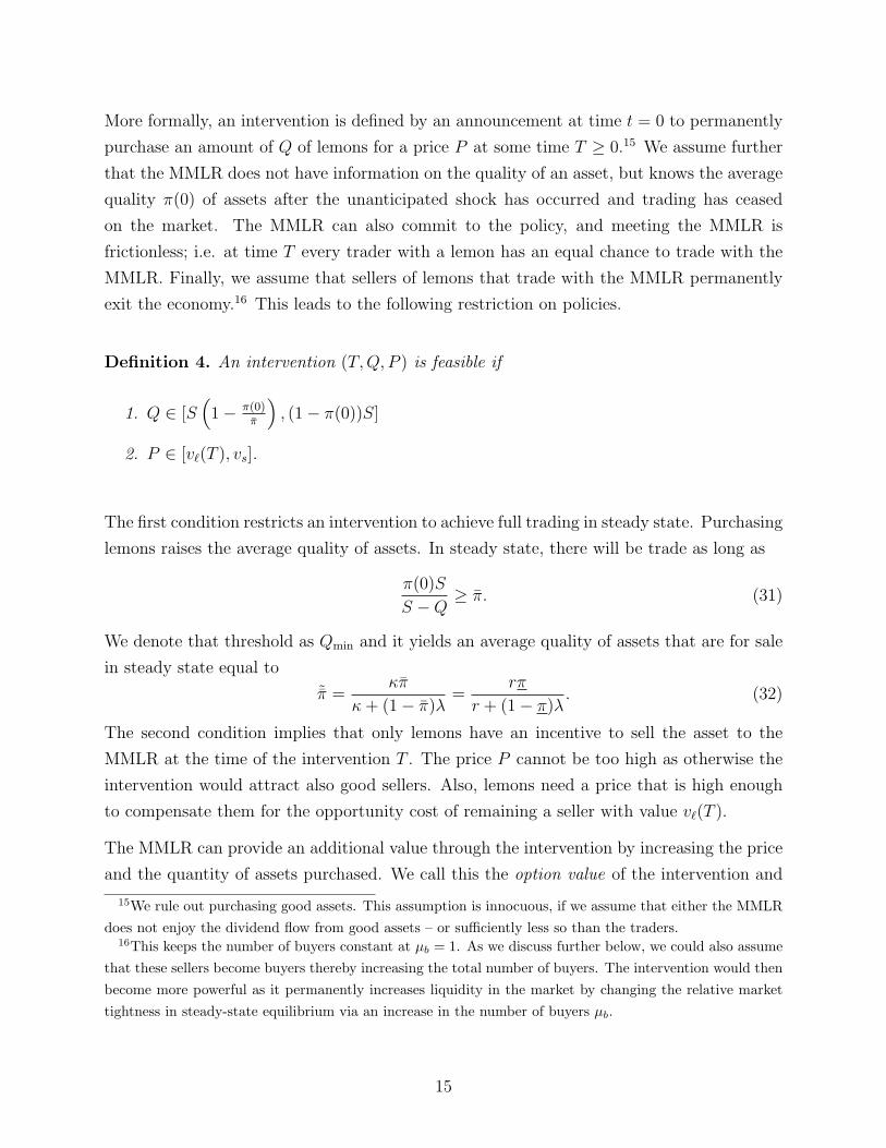
More formally, an intervention is defined by an announcement at time t = 0 to permanently

purchase an amount of Q of lemons for a price P at some time T ≥ 0.15 We assume further

that the MMLR does not have information on the quality of an asset, but knows the average

quality π(0) of assets after the unanticipated shock has occurred and trading has ceased

on the market. The MMLR can also commit to the policy, and meeting the MMLR is

frictionless; i.e. at time T every trader with a lemon has an equal chance to trade with the

MMLR. Finally, we assume that sellers of lemons that trade with the MMLR permanently

exit the economy.16 This leads to the following restriction on policies.

Definition 4. An intervention (T,Q, P ) is feasible if

1. Q ∈ [S(

1− π(0)π

), (1− π(0))S]

2. P ∈ [v`(T ), vs].

The first condition restricts an intervention to achieve full trading in steady state. Purchasing

lemons raises the average quality of assets. In steady state, there will be trade as long as

π(0)S

S −Q≥ π. (31)

We denote that threshold as Qmin and it yields an average quality of assets that are for sale

in steady state equal to

˜π =κπ

κ+ (1− π)λ=

rπ

r + (1− π)λ. (32)

The second condition implies that only lemons have an incentive to sell the asset to the

MMLR at the time of the intervention T . The price P cannot be too high as otherwise the

intervention would attract also good sellers. Also, lemons need a price that is high enough

to compensate them for the opportunity cost of remaining a seller with value v`(T ).

The MMLR can provide an additional value through the intervention by increasing the price

and the quantity of assets purchased. We call this the option value of the intervention and

15We rule out purchasing good assets. This assumption is innocuous, if we assume that either the MMLRdoes not enjoy the dividend flow from good assets – or sufficiently less so than the traders.

16This keeps the number of buyers constant at µb = 1. As we discuss further below, we could also assumethat these sellers become buyers thereby increasing the total number of buyers. The intervention would thenbecome more powerful as it permanently increases liquidity in the market by changing the relative markettightness in steady-state equilibrium via an increase in the number of buyers µb.

15

denote it by VI . To assess this option value, we look at the value of acquiring a lemon just

an instant before the intervention

v`(T−) =

Q

S(1− π(0))P (T ) +

(1− Q

S(1− π(0))

)v`(T )

=Q

S(1− π(0))(P (T )− v`(T )) + v`(T ) (33)

= VI + v`(T ).

The first term of this expression is the expected transfer of a trade with the MMLR at T

provided by the option value. If it is positive, the value function of a lemon has a downward

jump at T . The second term captures the case that, conditional on not being able to sell

to the MMLR, the lemon remains in the market. With an intervention at T , a fraction

Q/[S(1 − π(0))] of lemons have an option to sell their bad assets to the MMLR at a price

P (T ). At price P (T ) = v`(T ), they are just indifferent between selling to the MMLR or

remaining in the market. If the price is strictly higher, they strictly prefer to sell to the

MMLR as they receive an additional transfer. The option value VI is thus the difference in

expected value they obtain from the intervention relative to a minimum one. We have

0 ≤ VI ≤ vs − v`(T ). (34)

Interestingly, given the minimum price, changing the size of the intervention P (T ) = v`(T )

does not increase the option value of the intervention. The reason is that the chance to

transact with the MMLR or afterwards in the market are perfect substitutes from the per-

spective of an individual lemon. Only when the MMLR increases the price above v`(T ) do

lemons obtain an additional transfer through the intervention.

The surplus function Γ(t) has thus a jump at T for two reason. The intervention increases

discretely the average quality π, but the value of a lemon v`(T ) also jumps down at that

time, since a positive option value disappears for future lemon holders. More generally, the

surplus function depends only on the dynamics of π(t) and v`(t) over time, since buyers

extract all the rents from sellers with good assets, causing both vs and vo to be constant.

The value function of a lemon for any t < T is given by

v`(t) = Et[e−r(τm−t)vs1{τm<T} + e−r(T−t)(v`(T ) + VI)1{τm≥T}

], (35)

where τm is the random time for the next trade opportunity where buyers are willing to buy

an asset. Solving this expression for a given trading strategy γ(t), we obtain

v`(t) = λvs

∫ T

t

γ(s)eR s

t −(r+λγ(ν))dνds+ v`(T−)e

R Tt −(r+λγ(s))ds

= λvs

∫ T

t

γ(s)eR s

t −(r+λγ(ν))dνds+

(λ

λ+ rvs + VI

)e

R Tt −(r+λγ(s))ds. (36)

16

This shows that the option value VI of an intervention positively influences market trading

before the intervention through its effects on v`(t). However, the option value is discounted

by the rate of time preference r and by the chance of selling a lemon prior to the intervention

on the market as expressed by the additional discount factor λγ(t).

We first characterize now the trading dynamics after the intervention. Our strategy is to work

backwards. This is possible, since any feasible intervention is consistent with equilibrium with

full trading after the intervention, independent of trading behavior before the intervention.

All that matters here is that the minimum scale of the intervention Qmin increases the

average quality of assets sufficiently. We then characterize the equilibrium structure before

the intervention which depends on the announcement effect and give some bounds for this

effect. Finally, we derive implications for transaction prices in equilibrium when there is an

intervention.

4.2 Trading Dynamics

4.2.1 Recovery After the Intervention

A minimum intervention, Qmin, raises the average quality of assets just enough above the

critical level so that there exists a steady state equilibrium with trade. But any feasible

intervention also raises the average quality of the assets above this critical level along the

time path after the intervention at T . Importantly, this result is independent of trading

behavior before the intervention. We denote the average quality of assets for sale right after

the intervention at T by π(T ) and its long-run steady state level by πSS(Q).

Lemma 5. Consider any intervention Q ∈ [Qmin, (1− π(0))S] at time T . Then π(t) ≥ ˜π =rπ

r+(1−π)λfor all [T,∞). If there is full trade with γ(t) = 1 for all t ∈ [T,∞), the average

quality of assets for sale π(t) decreases monotonically to πSS(Q) ≥ ˜π on [T,∞).

Proof. See Appendix A.

The intuition is as follows. First, the floor for the average quality of asset that are for sale

is given by π(0). This corresponds to a situation where there is continuous trading and

the measure of sellers with good assets remains constant. When there is no trading at any

point in time, the average quality increases because more and more owners become sellers

over time due to preference shocks – or in other words, selling pressure builds up over time.

17

Hence, it must be the case that µs(t) ≥ µs(0) for all t < T . Second, the MMLR removes

only lemons from the market which causes a discrete jump in the average quality at time

T that is sufficient to raise the floor for the average asset quality to at least ˜π which is the

steady state level of the average quality of assets that are for sale when there is trading.

With trading, any built-up selling pressure will dissipate over time and the average quality

of assets for sale needs to converge to this floor in the long-run.

Based on this result, it follows that continuous trade after the intervention is indeed an

equilibrium. One needs to simply verify that buyers have an incentive to buy for any t ∈[T,∞) given that there is trade at any later stage which causes the value of a lemon to be

constant at its steady state value. This is indeed the case as the quality of assets a buyer

purchases is sufficiently high and will decline over time. Hence, there is no reason to postpone

a purchase. As a result, the economy will converge monotonically to the new steady state

with trade.

Proposition 6. Continuous trade after the intervention is an equilibrium.

Proof. When trading, the buyer’s take-it-or-leave-it-offer is given by p(t) = vs−vb(t). Hence,

he will trade (γ(t) = 1) only if

Γ(t) = π(t)vo + (1− π(t))v`(t)− vs ≥ 0.

Suppose that γ(t′) = 1 for all t′ > t. Then, v`(t) = λλ+r

vs which is time independent. Thus,

rewriting the inequality above we obtain that γ(t) = 1 if and only if

π(t) ≥ vs − v`vo − vs

=rπ

r + (1− π)λ= ˜π.

The result then follows from the previous lemma.

4.2.2 Recovery Before the Intervention

The intervention at time T can induce an announcement effect so that trading in the market

starts before the actual intervention. This can be understood best by looking at how the

intervention influences the two components associated with the surplus function from trading,

Γ(t). The quality effect is backward looking. When there is no trading, selling pressure builds

up in the market (i.e. µs(t) increases) which in turn increases the quality of assets that are

for sale π(t). This increases the willingness of buyers to purchase an asset today. Second,

there is a strategic complementarity which is forward looking. The possibility of selling a

18

lemon in the future influences the willingness to purchase an asset today. Hence, anticipating

the intervention which resurrects trading after T , buyers will start making offers as soon as

the quality for assets improves sufficiently. In equilibrium, the trading volume has of course

to be consistent with the decrease in the quality of assets when selling pressure diminishes

which yields the following trading dynamics.

Proposition 7. All equilibria before T can be characterized by two breaking points τ1(T ) ≥ 0

and τ2(T ) ∈ [τ1, T ) such that

(i) there is no trade (γ(t) = 0) in the interval [0, τ1),

(ii) there is partial trade (γ(t) ∈ (0, 1)) in the interval [τ1, τ2),

(iii) there is trade (γ(t) = 1) in the interval [τ2, T ).

Proof. See Appendix A.

There are two breaking points. The first one, τ1(T ), determines when some trading – partial

trade – takes place in the market again. With partial trade, buyers do not receive an expected

surplus as Γ(t) = 0. While welfare improves as some good assets get reallocated, lemons

extract all the rents from buyers. At a later point in time, at τ2(T ), the market fully recovers,

a situation we refer to simply as trade. Whenever τ1(T ) < T , there is an announcement

effect from committing at time 0 to an intervention at a later date. The intervention itself

of course influences these breaking points. Delaying the intervention reduces the strategic

complementarity from a market recovery, but at the same time allows selling pressure to

build up which increases the average quality of assets for buyers. Increasing the size of the

intervention adds value to holding a lemon making it more attractive for buyers to make an

offer.

4.2.3 Announcement Effect

We give now some bounds on the announcement effect, since we cannot derive analytically

how changes in the intervention influence this effect. First, unless the option value is positive,

there can only be partial trade prior to the intervention. This implies that there is a fixed

costs associated with creating an announcement effect. Furthermore, if the initial quality

drop is sufficiently large, there will be no announcement effect at all, since the quality effect

is not strong enough to overcome the initial drop in quality. Second, for a large enough

19

option value, it is always possible to delay the intervention while still maintaining trade

continuously in the market. The reason is that the MMLR can compensate a buyer fully for

acquiring a lemon with the maximum option value (VI = rr+λ

vs). This is sufficient to make

the buyer’s surplus positive provided the intervention is not delayed for too long.

Proposition 8. Suppose VI = 0. There cannot be trade with γ(t) = 1 for any interval before

T (i.e. τ2(T ) = T ). Furthermore, if π(0) ≤ π(

rr+λ(1−π)

), the unique equilibrium before the

intervention is no trade for any T (i.e. τ1(T ) = T ).

Furthermore, there exists an equilibrium with continuous trade, if and only if

π(0)vo + (1− π(0))

(λ

λ+ rvs + VIe

−(r+λ)T

)− vs ≥ 0. (37)

Proof. See Appendix A.

We discuss next how search frictions change the critical time T of the intervention so that an

announcement effect starts to arise. When there is no announcement effect – i.e., no trade

in [0, T ) – the surplus function satisfies with VI = 0

Γ(T ) =

(π(0)

1− π(0)

)(1− ππ

)vs

(1− λ

λ+ κe−κT

)− r

r + λvs < 0. (38)

The quality effect depends negatively on λ, when there is no trade. When search frictions

become less important, the average quality of assets for sale is lower to begin with. At the

same time, the complementarity is stronger, as it is easier to turn around a lemon. Totally

differentiating this expression we obtain

dT

dλ=

1

λ(κ+ λ)

[1−

(κ+ λ

r + λ

)21

AeκT

](39)

where

A =

(π(0)

1− π(0)

)(1− ππ

)< 1, (40)

since π(0) < π. When κ > r, this expression is always negative. The intuition is that the

strategic complementarity is more important than the quality effect. As λ increases, the

intervention becomes more powerful and the critical time T for an announcement effect to

occur drops. For r > κ, the quality effect dominates and how search frictions influence the

announcement effects depends on the size of the shock π(0).

20

4.3 Price Dynamics

Due to the take-it-or-leave-it offer, market prices in equilibrium with trading are given by

p(t) = vs − vb(t) (41)

and, hence, are inversely related to the value function of the buyer vb(t), which is a continuous

function. Their dynamics depend on the trading behavior over time. Once trading starts

again, there is a positive jump from zero to a price that is below the steady state price.

Interestingly, prices then behave non-monotonically: they first decline with partial trade,

before recovering to their steady-state level.

Proposition 9. Given an intervention at T , prices p(t)

(i) are zero when there is no trade and continuous on [τ1,∞),

(ii) decline at rate r with partial trade in the interval [τ1, τ2],

(iii) decline at a rate lower than r or increase with full trade in the interval (τ2, T ],

(iv) and increase monotonically to the steady state price after the intervention with a pos-

itive, discrete jump in their growth rate at T .

Proof. See Appendix A.

With trade after the intervention, the quality of the assets π(t) drops over time, implying

less surplus. Hence, sellers will require a higher price, as becoming a buyer is less attractive.

Before the intervention at T , there is an additional second effect. The intervention discretely

increases the expected surplus from trading which is discounted by traders at the rate of time

preference. When there is trading before the intervention, these two effects work against each

other giving rise to the the non-monotonicity in prices. With partial trade, the expected

surplus remains at zero, so that the buyer has to simply compensate the seller less as one

approaches the intervention.

We can quite easily compare the price range of an intervention with the market price. The

MMLR can pay a higher price for assets than the transaction price in the market at the

time of the intervention. That occurs, when he chooses to pay the full price for the asset

and the surplus for buyers is strictly positive at the time of the intervention, i.e. P (T ) =

21

vs > p(T ) = vs − vb(T ). This of course is an artefact of our assumption that lemons have to

leave the market permanently upon selling to the MMLR. At the minimum price Pmin, the

MMLR pays a lower price when search friction increase, as lemons have a lower expected

value when sold in the market.

5 Optimal Intervention

5.1 The Cost of Intervention

In order to study the optimal intervention, we need to adopt a social welfare function for

the MMLR that takes into account the costs of the intervention against the benefits of the

market allocating assets among traders with different valuations. Our welfare function is

akin to one that is commonly used in the public finance literature on regulation and given

by ∫ ∞t=0

((µo(t) + µs(t))δ − µs(t)x

)e−rtdt− θ

∫ ∞t=0

P (T )Q(T )e−rtdt. (42)

The first term describes the surplus from allocating good assets to traders with high valuation

and captures the benefits from intervening to resurrect the market. The second term ex-

presses the costs of financing the intervention. The costs are a direct transfer to traders in the

market and due to linear utility are zero sum. Hence, we introduce a parameter θ ∈ (0,∞)

which expresses the social costs of intervening as being proportional to the costs.17

Recall that the option value is given by

VI =Q

S(1− π(0))(P − v`) . (43)

We can thus represent the minimum costs associated with an intervention at time T and

option value VI by

C(VI) =

VIS(1− π(0)) +Qminv` if 0 ≤ VI ≤ Qmin

S(1−π(0))r

r+λvs ≡ VI

r+λrVIS(1− π(0)) if Qmin

S(1−π(0))r

r+λvs ≡ VI ≤ VI ≤ r

r+λvs.

(44)

The cost function is time-invariant, piece-wise linear in VI and strictly convex around a kink

that occurs at the policy that sets P = vs and Q = Qmin. The reason is that in order to

17One can interpret these costs as the distortions from having to tax the economy to provide this transferto traders. Note that this set-up implies immediately that there is no role for the MMLR of buying lemonswhen the market is functioning. There is a (social) cost of financing the intervention, but no benefit as theintervention does not affect the allocation of good assets in steady state.

22

achieve any given VI , increasing the quantity Q involves a deadweight cost. The MMLR

just provides a transfer of utility to current lemons otherwise provided for by future buyers.

However, after the MMLR pays a price equal to the good asset, he needs to increase the

quantity to achieve a higher option value VI .18 The net present value of costs is simply given

by C(VI)e−rT if the intervention takes place at T . For the purpose of characterizing optimal

policies, we can thus represent any feasible intervention simply by (T, VI).

5.2 Optimal Timing – Continuously Functioning Markets

When analyzing the decision for the MMLR to delay, we look at the special case how to best

ensure that markets function continuously, i.e. how to ensure that there is trade at all t in

response to an unanticipated shock π(0). There are two options available: the MMLR could

either intervene immediately and raise the quality of assets for sale sufficiently; or he could

delay the intervention for some time, but increase the option value VI . In either case, the

economy jumps immediately to a new steady state at t = 0, with the number of good assets

for sale being constant over time at µs(t) = κκ+λ

Sπ(0) and the amount of lemons decreasing

at the time of the intervention.

The optimal policy for the MMLR is simply to minimize the net present value of costs.

In order to delay, the net present value of the option value has to be sufficiently high to

render the surplus function positive and, hence, the option value has to jump up discretely

according to

V minI =

π(0)

1− π(0)(vs − vo) +

r

r + λvs > 0. (45)

Hence, delaying involves a fixed cost. Moreover, for a policy to ensure continuous trading,

it needs to increase VI sufficiently when delaying the intervention. Totally differentiating

condition (37), we obtaindT

dVI=

1

(r + λ)VI> 0. (46)

Traders discount the option value VI by more than the rate of time preference. They take into

account that trading opportunities arrive in the market with flow λ. When selling the lemon

to a buyer, they give up the additional transfer offered by the MMLR. Hence, the effective

discount rate of an intervention is r + λ > r. The fixed cost combined with the increased

discount rate for the option value leads to increasing costs when delaying the intervention.

18This is somewhat an artefact of the MMLR not being able to sell back any additional amount of lemonsQ−Qmin to the market immediately after the intervention at a price equal to v` − ε (see Appendix E).

23

Proposition 10. To ensure continuous markets (γ(t) = 1 for all t), it is optimal to intervene

immediately, or T ∗ = 0 and V ∗I = 0.

Proof. The problem for the MMLR is to minimize the costs of any intervention that ensures

continuous trade for all t. Taking into account the fixed cost given by P = vs, the cost

function is given by

C(VI)e−rT (VI) =

(λ+ r

r

)VIS(1− π(0))e−rT (VI).

Differentiating with respect to VI , we obtain

A

[1 + VI

∂T

∂VI(−r)

]for the derivative where A = S(1−π(0))

(r+λr

)e−rT (VI). To ensure continuous trade, we need

to require that∂T

∂VI=

1

(r + λ)VI.

This implies that∂C(VI)e

−rT (VI)

∂VI= A

[1− r

r + λ

]> 0

Hence, it is never optimal to increase VI and, hence, never optimal to delay the intervention

in order to achieve continuously functioning markets.

It is instructive to stress that the minimum jump in the option value is given by

V minI = VI =

Qmin

S(1− π(0))

(r

r + λvs

), (47)

the point at which the kink occurs in the cost function which is associated with the highest

price of the intervention P = vs. The intuition is as follows. Suppose the intervention takes

place at T = 0 where the MMLR buys Qmin at P = v`. Then, the MMLR transacts with

already existing lemons and he needs to pay a price that just makes them indifferent to stay

a lemon and wait for a trade later in the market. Consider now T = ε small, but positive.

Then, the MMLR needs to convince a buyer to purchase a lemon in the market just before

the intervention at T−, even though the quality of the asset he purchases is still π(0). He can

do so, by offering an additional option value that compensates the buyer for taking on the

increased risk of purchasing a lemon. The compensation required is exactly purchasing Qmin

lemons at the price the buyer paid for in the market. But this price is p = vs− vb(t) = vs for

a minimum intervention. Hence, P = vs. Of course, as ε > 0, discounting requires a larger

24

intervention than Qmin to compensate buyers that purchased an asset at T = 0. Letting

ε → 0, however, we obtain exactly the fixed cost being at the kink of the cost function.

Hence, the MMLR can only delay if he pays the fair market price P = vs for the good asset.

Once the MMLR pays the fair price for lemons, any increases in the quantity Q are very

costly making a delay of the intervention not optimal.19

5.3 Optimal Size of the Intervention – A Bang-Bang Result

The reasoning of the previous section can be used to evaluate optimal policies in terms of VI

more generally. To do so, we look at how certain marginal policy changes in a neighborhood

of some initial policy (T, VI) change the net present value of costs. The idea for the marginal

policy change is to keep the net present value of the option value constant – like in expression

(46) –, but for an arbitrary, fixed trading probability γ(T−) just before the intervention at

T . It turns out that the cost-minimizing policy among these policies sets VI = VI .

Lemma 11. Let γ ∈ (0, 1] and change the policy (T, VI) according to dT/dVI = 1r+λγ

1VI

for all (T, VI) with T > 0 and VI > 0. For such changes, the net present value of costs is

minimized at VI .

Proof. See Appendix A.

We establish now that it is never optimal to increase the quantity of assets to be purchased.

In other words, Q∗ = Qmin. This result can be understood as follows. Suppose it were

optimal for the MMLR to buy more lemons. Then, it must be the case that VI > VI . He

could alternatively reduce the amount purchased and intervene earlier. Consider then a

marginal policy change as in Lemma 11. This change will reduce the net present value of

costs. But it will also leave the incentives to trade before the new, earlier intervention date

unchanged. This implies that the MMLR increases welfare by lowering VI towards V – or

equivalently, by setting Q∗ = Qmin.

19When there is a lag between observing the market freeze and being able to intervene, this result impliesthat the MMLR can still achieve continuous trade by announcing an intervention immediately. This would,however, require a larger than the minimal intervention at price P = vs. Interestingly, the larger the searchfriction becomes – i.e. the smaller λ –, the more the MMLR could delay, since the market discounts thetransfer provided by VI less.

25

By similar reasoning, we obtain a slightly weaker result for the optimal price P ∗. Consider

a situation where there is full trade before the intervention, i.e. γ(T−) = 1. Then, by

Proposition 8, we know that the MMLR needs to provide a strictly positive option value VI .

This time, he could delay the intervention and increase VI according to a marginal policy

change that leaves γ(t) = 1 unchanged for all t > T . As this lowers the net present value of

costs, welfare again increases. However, due to the fixed cost of incurring a positive option

value, it could be still better to intervene earlier, but at the minimum price P . This leads to

the “bang-bang” result that an optimal intervention either offers the highest or the lowest

price, while always purchasing the minimum amount of assets.

Proposition 12. Any optimal policy with intervention (T ∗ < ∞) features Q∗ = Qmin.

Furthermore, if τ2(T ∗) < T ∗, the optimal policy either features P = v` or P = vs.

Proof. See Appendix A.

The relative weight between costs and benefits of an intervention, θ, determines the opti-

mal timing decision. If the social costs are small, but positive, it is optimal to intervene

immediately. Conversely, if they become large, it is best not to intervene and let the market

be frozen. A formal statement and proof of this result are relegated to Appendix F. Given

these results, one would expect that for intermediate values of θ, it is optimal to have a

delayed intervention. When the intervention is delayed, equilibria exhibit generically partial

trading before the intervention. Hence, welfare cannot be computed analytically anymore,

as our linear differential equations have time-dependent coefficients. We will thus resort to

numerically solve for the optimal policy – especially the optimal timing of the intervention

– in a calibrated version of our economy.

6 Numerical Analysis

6.1 Parameter Values

We calibrate our economy to capture the market for longer-term structured finance prod-

ucts such as asset-backed securities (ABS) or collateralized debt obligations (CDO). We

then interpret private information concerning the quality π of the assets as reflecting the

opaqueness associated with the tranches of these assets. In our benchmark, assets are of

26

very high quality with an average of π = 0.99 being good assets. This is consistent with

Aaa rated corporate debt which historically has a default rate of 1.09% and 2.38% for 10

and 20 year maturities respectively and a recovery rate of about 50% (see Moody’s Investor

Service, 2000). Similar impairment probabilities were associated with Aaa rated tranches of

structured debt products before 2007 (see Moody’s Investor Service, 2010). In accordance

with Duffie, Garleanu and Pedersen (2007) we set the annual interest rate r to 5% and the

fraction of investors holding an asset to S/(1 + S) = 0.8.

We then select two key parameters in our analysis, the degree of search frictions λ and the

arrival rate of a liquidity shock κ, to match annual turnover rates for debt products. A search

intensity of λ = 100 for the benchmark implies that a seller expects to contact a buyer and

to sell the asset if there is trade once every 250/100 = 2.5 trading days. We set κ to 1 so

that an asset holder remains an owner for an average of one year. With the proportion of

lemons being 1% we obtain a turnover rate of

λ(µs + µ`)

S= λ

(κπ

λ+ κ+ 1− π

)= 1.98, (48)

so that assets change hands about twice in a year on average. This is not inconsistent, but

at the upper end of the turnover rate reported by the literature.20 Later on, we conduct a

robustness check with respect to the parameter κ, which reflects the need of turning around

an asset in the secondary market. We view shorter and medium-term funding markets (e.g.

commercial paper) as markets where traders face more frequent liquidity needs (higher κ).

Table 1: Benchmark Parameter Values

λ κ S δ x r π

100 1 4 1 0.035 0.05 0.99

Table 1 gives the values of the exogenous parameters and Table 2 describes the resulting

steady-state equilibrium. Note that with our parameters, trades in good assets vs. lemons

are approximately 4 to 1. As in Duffie, Garleanu and Pedersen (2007), we have normalized

δ = 1. The valuation shock is chosen to match the spread of highly rated structure finance

products over the risk-free rate r. The yield is 1/17.4578 = 5.728% or 73 pbs above the

risk-free rate.21 As shown in Table 2, due to search frictions, a small fraction of good

20Bao, Pan and Wang (2008) give turnover rates between one and two years for corporate bonds, whileGoldstein, Hotchkiss and Sirri (2007) report a slightly lower annual rate in the range of 0.8-1.2 (see alsoEdwards, Harris and Piwowar, 2007). Data for structured products are not readily available.

21This is the total spread in Krishnamurthy and Vissing-Jorgenson (2010) for corporate debt of the highestquality. Gorton and Metrick (2010) report a range of 50 to 100 bps on highly rated ABS before 2007.

27

assets – µs/(Sπ) = 0.98% of the total – is misallocated to investors with a liquidity shock.

Also, since κ > r, the strategic complementarity dominates the quality effect, implying that

π < π. However, the steady state equilibrium falls in the range of multiple equilibria so that

it matters whether a trader can resell the asset when receiving a liquidity shock.

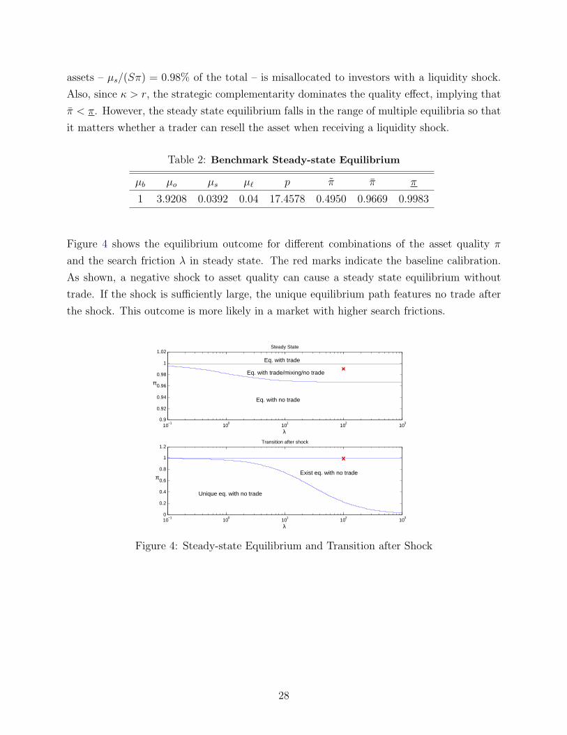
Table 2: Benchmark Steady-state Equilibrium

µb µo µs µ` p π π π

1 3.9208 0.0392 0.04 17.4578 0.4950 0.9669 0.9983

Figure 4 shows the equilibrium outcome for different combinations of the asset quality π

and the search friction λ in steady state. The red marks indicate the baseline calibration.

As shown, a negative shock to asset quality can cause a steady state equilibrium without

trade. If the shock is sufficiently large, the unique equilibrium path features no trade after

the shock. This outcome is more likely in a market with higher search frictions.

10−1

100

101

102

103

0.9

0.92

0.94

0.96

0.98

1

1.02

π

λ

Steady State

10−1

100

101

102

103

0

0.2

0.4

0.6

0.8

1

1.2Transition after shock

λ

π

Eq. with trade

Eq. with trade/mixing/no trade

Eq. with no trade

Exist eq. with no trade

Unique eq. with no trade

Figure 4: Steady-state Equilibrium and Transition after Shock

28

6.2 Trading and Price Dynamics

We now consider a negative quality shock at t = 0 such that 10% of the assets turn from good

to lemons, i.e., π(0) = 0.89 < π.22 In order to resurrect the market, the MMLR needs to

purchase at least an amount Qmin = 0.3182 which is about 8% of the total asset supply and

72% of lemons. We first compute the equilibrium trading response γ(t) and the associated

market price p(t) for three different values of λ, when there is a minimum intervention at

time T = 0.25 (see Figure 5).

0 0.1 0.2 0.3 0.4 0.519.286

19.288

19.29

19.292

19.294

19.296

19.298

19.3

t

p(t)

0 0.1 0.2 0.3 0.4 0.5

0

0.2

0.4

0.6

0.8

1

γ(t)

t

λ=25λ=50λ=100

Figure 5: Equilibrium Prices and Trading Dynamics (T = 0.25, VI = 0) – Impact of Search

Friction

The price jumps up when the market starts to recover at τ1, and drops slightly over time at

the rate of r as trading activity increases. After the intervention time T , full trade is restored

with the price increasing monotonically towards the steady-state level. With smaller search

frictions (higher λ), the market recovers earlier. But with partial trading the fraction of

buyers making offers, γ(t), is also decreasing in λ. The reason is that with less search

frictions there cannot be too much trading, as otherwise the quality of assets for sale would

drop too fast in order to maintain a mixing equilibrium. Furthermore, a higher λ tends to

increase the asset price and speed up its convergence.

22Such a shock falls within the range experienced in the financial crisis of 2007-09 where impairment rateson structured finance products with Aaa and Aa ratings jumped to a range of 5-20% depending on theproduct (see Moody’s Investor Service, 2010).

29

0 0.1 0.2 0.3 0.4 0.519.296

19.297

19.298

19.299

19.3

t

p(t)

0 0.1 0.2 0.3 0.4 0.5

0

0.2

0.4

0.6

0.8

1

γ(t)

t

VI=0

VI=0.001

VI=0.002

Figure 6: Equilibrium Prices and Trading Dynamics (T = 0.25) – Impact of Option Value

VI

For the benchmark case where λ = 100, Figure 6 examines the effects of increasing the price

of the intervention P while holding Q fixed at Qmin. Such an increase in VI strengthens the

strategic complementarity. Hence, it induces the market to recover earlier. It also raises

trading activity before the intervention which in turn increases the market price. This is due

to a faster drop in the average quality of assets that are for sale when there is more trading

in the market.

6.3 Announcement Effect

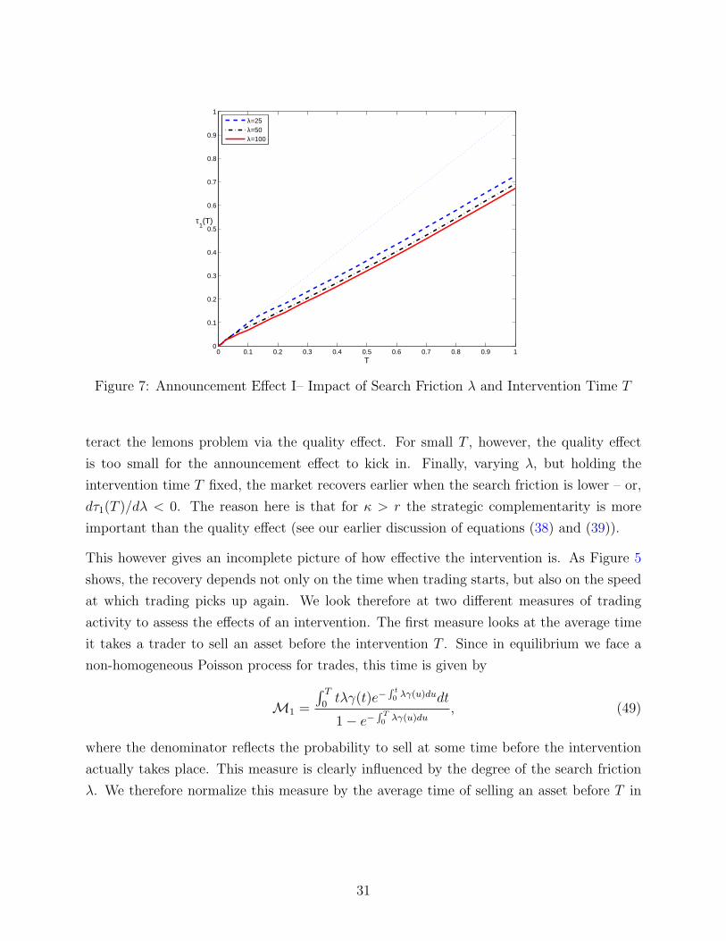
We turn next to the announcement effect. In particular, we are interested in how the time of

intervention influences the timing and intensity of market recovery. As a first pass, Figure 7

looks at the time when the market starts to respond to a minimum intervention – Qmin and

Pmin – as a function of the time of intervention T . More precisely, we plot the breaking time

τ1(T ) again for the three different levels of the search friction λ, with the solid line indicating

our baseline case. We only plot τ1(T ) here, since there is no full recovery (τ2(T ) = T ) in all

three cases.

Postponing the intervention delays the market recovery (τ ′1(T ) > 0), but increases the an-

nouncement effect in the sense that the market recovers earlier relative to T (τ ′1(T ) ≤ 1).

The interpretation is that it takes time for selling pressure to build up sufficiently to coun-

30

0 0.1 0.2 0.3 0.4 0.5 0.6 0.7 0.8 0.9 10

0.1

0.2

0.3

0.4

0.5

0.6

0.7

0.8

0.9

1

T

τ1(T)

λ=25λ=50λ=100

Figure 7: Announcement Effect I– Impact of Search Friction λ and Intervention Time T

teract the lemons problem via the quality effect. For small T , however, the quality effect

is too small for the announcement effect to kick in. Finally, varying λ, but holding the

intervention time T fixed, the market recovers earlier when the search friction is lower – or,

dτ1(T )/dλ < 0. The reason here is that for κ > r the strategic complementarity is more

important than the quality effect (see our earlier discussion of equations (38) and (39)).

This however gives an incomplete picture of how effective the intervention is. As Figure 5

shows, the recovery depends not only on the time when trading starts, but also on the speed

at which trading picks up again. We look therefore at two different measures of trading

activity to assess the effects of an intervention. The first measure looks at the average time

it takes a trader to sell an asset before the intervention T . Since in equilibrium we face a

non-homogeneous Poisson process for trades, this time is given by

M1 =

∫ T0tλγ(t)e−

R t0 λγ(u)dudt

1− e−R T0 λγ(u)du

, (49)

where the denominator reflects the probability to sell at some time before the intervention

actually takes place. This measure is clearly influenced by the degree of the search friction

λ. We therefore normalize this measure by the average time of selling an asset before T in

31

the steady state equilibrium with full trade.23

0 0.2 0.4 0.6 0.8 10

10

20

30

40

50

60

70

80

90

T

Ave

rage

Wai

ting

Tim

e be

fore

T (

Nor

mal

ized

)

λ=25λ=50λ=100

Figure 8: Announcement Effect II – Average Time of Selling an Asset before T (Normalized)

Figure 8 shows the average time it takes to sell an asset as a multiple of the one in normal

times. As the intervention is postponed, the delay in selling time rises as the announcement

effect increases less than proportional with the time of intervention. Most interestingly, when

there are more trading frictions (λ decreases), the average selling time for investors is closer

to normal times.

Since selling pressure builds up during a market freeze, our second measures looks at the total

trading volume before T to assess how the intervention influences overall market activity.

This measures is given by

M2 =

∫ T0λγ(t)[µs(t) + µ`(t)]dt∫ T

0λ[µSSs + µSS` ]dt

=

∫ T0γ(t)[µs(t) + µ`(t)]dt∫ T

0[µSSs + µSS` ]dt

(50)

where we have already normalized our measure by the steady state trading volume in normal

times. Note that with continuous trade, we would again have M2 = 1. Figure 9 gives the

23Another alternative would be to look at the probability of selling the asset before T

1− e−R T0 λγ(t)dt

1− e−Tλ.

which is normalized by the corresponding probability in the normal time. However, this measure would missthe timing dimension.

32

trading volume associated with an intervention at time T as a percentage of normal times

and shows that postponing the intervention time has a non-monotonic effect.

0 0.2 0.4 0.6 0.8 10

0.05

0.1

0.15

0.2

0.25

T

Tot

al T

radi

ng V

olum

e be

fore

T (

Nor

mal

ized

)

λ=25λ=50λ=100

Figure 9: Announcement Effect III – Trading Volume before T (Normalized)

For a given λ, the trading volume relative to normal times stays zero for small T . The

reason is that it takes time for quality to build up in order to create some announcement

effect. Once this effect kicks in, the trading volume is increasing in T because delaying the

intervention allows selling pressure to build up. The selling pressure, however, begins to

dissipate once trading starts again. As the intervention is delayed further, market recovery

is delayed and trading volume relative to normal times converges to 0. In markets with

lower search frictions, trading volume recovers and peaks faster but at a lower overall level.

The reason is that, when search frictions are small, quality improves quickly without trade,

leading to a faster recovery. However, low search frictions imply that the quality would drop

rapidly when there is trade, leading to a more subdued recovery of trading volume when the

intervention is delayed.

Overall, search frictions determine the impact of an intervention on market activity. A

market with high search frictions recovers later because the quality effect kicks in slower,

and the difficulty of finding a counterparty reduces the absolute magnitude of the strategic

complementarity. On the other hand, an intervention is more effective in a relative sense by

bringing the market closer to its trading volume in normal times, albeit requiring a longer

time to take effect.

33

6.4 Optimal Policy

We now turn to computing the optimal policy for the scenario where the quality drops by

10% leading to a market freeze. The optimal intervention depends on the (social) costs of

the intervention which is captured by the parameter θ. Figure 10 shows the optimal timing

and pricing of the intervention as a function of θ for our benchmark economy.

0 0.05 0.1 0.15 0.2 0.25 0.3 0.35 0.4 0.45 0.50

0.2

0.4

0.6

0.8

θ

Opt

imal

T

π(0)=0.89

Optimal TPartial recoveryFull recovery

0 0.05 0.1 0.15 0.2 0.25 0.3 0.35 0.4 0.45 0.519.285

19.29

19.295

19.3

θ

Opt

imal

P

Figure 10: Optimal Intervention for the Benchmark Economy

When θ is small, an immediate intervention is optimal which implies that there is no reason

to increase the option value VI . As the value of θ increases, it is optimal to delay the

intervention (T > 0) more and more and provide a positive option value (VI > 0) in order to

maximize the announcement effect. Table 3 verifies our bang-bang result: the price is always

set to Pmax when there is sufficient delay, while the quantity of purchases remains constant

at the minimum Qmin.

To put these numbers into perspective, in our baseline calibration, when the deadweight loss

of taxation is roughly 5%, the optimal policy is to commit to asset purchases about 3 weeks

later. The market will respond by starting to recover gradually about 9 trading days after

the market freezes in response to the quality shock. Finally, we address how the optimal

intervention will take into account the severity of the trading frictions in the market. Table

4 reports the results for a market where trading in normal times takes 10 days (λ = 25).

The qualitative pattern of the optimal intervention is the same. The MMLR, however, needs

to purchase a higher minimum amount of assets. Nonetheless, the optimal intervention is

34

Table 3: Optimal Intervention (λ = 100)

θ T P Q τ1

0.0100 0 19.2904 0.3182 0

0.0200 0 19.2904 0.3182 0

0.0300 0.0112 19.2904 0.3182 0.0112

0.0400 0.0472 19.2987 0.3182 0.0295

0.0500 0.0593 19.2987 0.3182 0.0365

0.1000 0.1217 19.2987 0.3182 0.0729

0.1500 0.1858 19.2987 0.3182 0.1111

0.2000 0.2474 19.2987 0.3182 0.1486

0.3000 0.3828 19.2987 0.3182 0.2335

0.4000 0.5253 19.2987 0.3182 0.3266

0.5000 0.6767 19.2987 0.3182 0.4295

now more aggressive by choosing a smaller T . The reason is twofold. First, the maximal

intervention price drops because the reservation value of a lemon is lower when λ declines.

Hence, the overall cost impact from the larger asset purchase is dampened. Second, and more

importantly, the announcement effect is decreasing in the trading friction for our parameter

values. Hence, the MMLR has less incentives to delay and to rely on this effect in order

to save costs. Quantitatively, once it becomes optimal to delay and increase the price for

lemons, the difference in policy becomes very small in response to the trading friction. Hence,

we draw the cautious conclusion from this analysis that ensuring market continuity is more

warranted for markets that are (i) more important relative to the social costs of intervention

and (ii) more riddled by trading frictions.

6.5 Robustness

6.5.1 High Liquidity Needs

In our benchmark, owners return to the market with an average frequency of once a year.

We now consider a different situation where liquidity shocks hit owners of assets more often.

Keeping λ = 100 and π = 0.99 and setting κ = 10 implies that an owner expects to return

to the market every 25 trading days resulting in an annual turnover rate of roughly 10 (see

35

Table 4: Optimal Intervention Policy (λ = 25)

θ T P Q τ1

0.0100 0 19.2615 0.3215 0

0.0200 0 19.2615 0.3215 0

0.0300 0 19.2615 0.3215 0

0.0400 0 19.2615 0.3215 0

0.0500 0 19.2615 0.3215 0

0.1000 0.0360 19.2615 0.3215 0.0360

0.1500 0.1738 19.2944 0.3215 0.1140

0.2000 0.2434 19.2944 0.3215 0.1571

0.3000 0.3820 19.2944 0.3215 0.2456

0.4000 0.5269 19.2944 0.3215 0.3420

0.5000 0.6799 19.2944 0.3215 0.4479

equation (48)).

As shown in Table 5, a rise in κ requires a larger fraction of assets to be of good quality for

trade to be a steady state equilibrium. Even though the average quality of asset π for sale

improves, a buyer expects a high valuation for the dividend of the asset for a much shorter

duration. Buyers are thus less willing to trade, which leads to a higher cut-off points for

trade. Hence, a market freeze becomes more likely even though the quality in the market

improves.

Table 5: Steady-state masses and asset price

κ µb µo µs µ` p π π π

10 1 3.6000 0.3600 0.04 17.5642 0.9000 0.9682 0.9998

1 1 3.9458 0.0158 0.0384 18.4 0.2913 0.9285 0.9904

Figure 11 illustrates how the market response to an intervention changes with κ. Given our

parameter values, in a market with high κ, an intervention generates a smaller announcement

effect, with later recovery and lower trading activities. Since κ lowers the value of being a

buyer, the trading price has to be higher to induce sellers to become buyers again.24 For

24A higher κ also reduces Qmin slightly, but this change has a negligible effect.

36

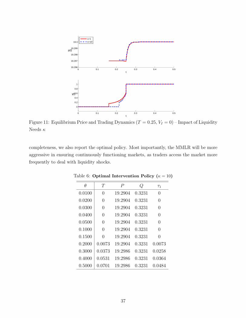
0 0.1 0.2 0.3 0.4 0.519.296

19.297

19.298

19.299

19.3

t

p(t)

0 0.1 0.2 0.3 0.4 0.5

0

0.2

0.4

0.6

0.8

1

γ(t)

t

κ=1κ=10

Figure 11: Equilibrium Price and Trading Dynamics (T = 0.25, VI = 0) – Impact of Liquidity

Needs κ

completeness, we also report the optimal policy. Most importantly, the MMLR will be more

aggressive in ensuring continuously functioning markets, as traders access the market more

frequently to deal with liquidity shocks.

Table 6: Optimal Intervention Policy (κ = 10)

θ T P Q τ1

0.0100 0 19.2904 0.3231 0

0.0200 0 19.2904 0.3231 0

0.0300 0 19.2904 0.3231 0

0.0400 0 19.2904 0.3231 0

0.0500 0 19.2904 0.3231 0

0.1000 0 19.2904 0.3231 0

0.1500 0 19.2904 0.3231 0

0.2000 0.0073 19.2904 0.3231 0.0073

0.3000 0.0373 19.2986 0.3231 0.0258

0.4000 0.0531 19.2986 0.3231 0.0364

0.5000 0.0701 19.2986 0.3231 0.0484

37

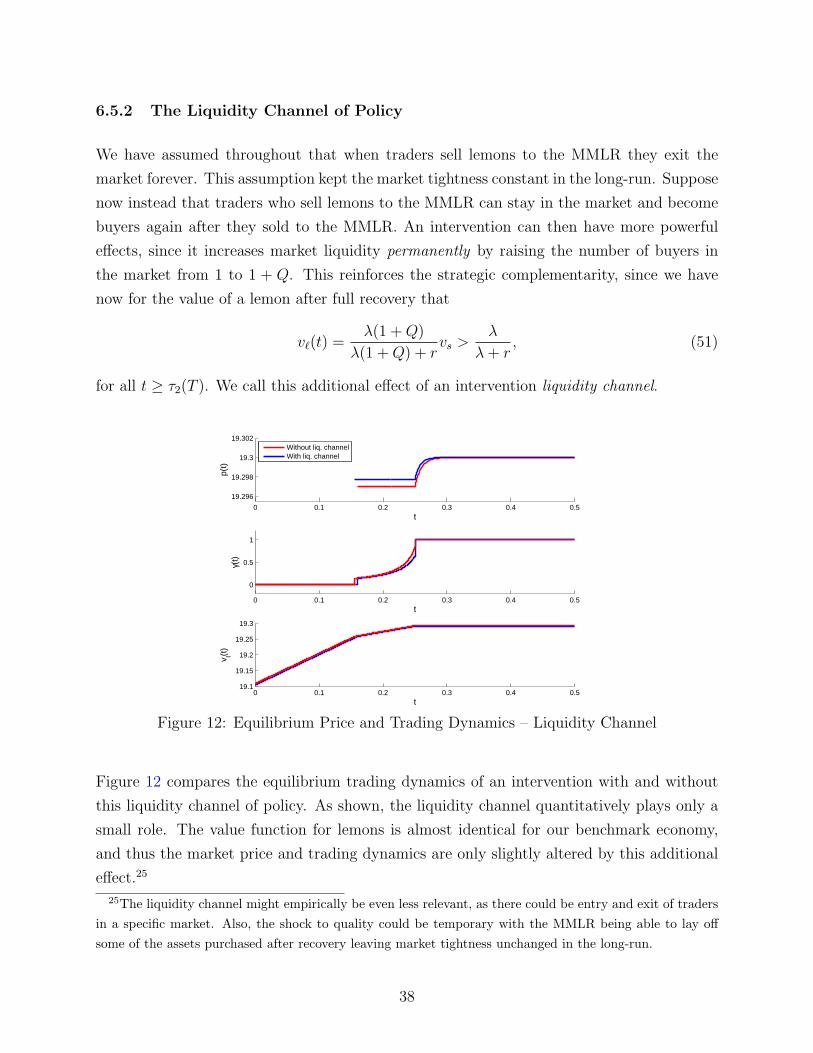
6.5.2 The Liquidity Channel of Policy

We have assumed throughout that when traders sell lemons to the MMLR they exit the

market forever. This assumption kept the market tightness constant in the long-run. Suppose

now instead that traders who sell lemons to the MMLR can stay in the market and become

buyers again after they sold to the MMLR. An intervention can then have more powerful

effects, since it increases market liquidity permanently by raising the number of buyers in

the market from 1 to 1 + Q. This reinforces the strategic complementarity, since we have

now for the value of a lemon after full recovery that

v`(t) =λ(1 +Q)

λ(1 +Q) + rvs >

λ

λ+ r, (51)

for all t ≥ τ2(T ). We call this additional effect of an intervention liquidity channel.

0 0.1 0.2 0.3 0.4 0.5

19.296

19.298

19.3

19.302

t

p(t)

0 0.1 0.2 0.3 0.4 0.5

0

0.5

1

γ(t)

t

0 0.1 0.2 0.3 0.4 0.519.1

19.15

19.2

19.25

19.3

v l(t)

t

Without liq. channelWith liq. channel

Figure 12: Equilibrium Price and Trading Dynamics – Liquidity Channel

Figure 12 compares the equilibrium trading dynamics of an intervention with and without

this liquidity channel of policy. As shown, the liquidity channel quantitatively plays only a

small role. The value function for lemons is almost identical for our benchmark economy,

and thus the market price and trading dynamics are only slightly altered by this additional

effect.25

25The liquidity channel might empirically be even less relevant, as there could be entry and exit of tradersin a specific market. Also, the shock to quality could be temporary with the MMLR being able to lay offsome of the assets purchased after recovery leaving market tightness unchanged in the long-run.

38

7 Discussion

We have shown in this paper that search frictions are important for understanding why some

markets are more prone to be fragile when there is adverse selection. It is not surprising

that a simple policy of purchasing lemons in the market by a government or central bank

can alleviate the adverse selection problem. However, we have also shown that there is

an announcement effect: simply announcing the intervention can induce investors to start

trading again. This effect gives then rise to an interesting trade-off between between the size

and the timing of the intervention which in turn depends on the degree of search frictions.

Our paper provides then some guidance for policy makers when to intervene and in what

form. In particular, we can rationalize intervention to ensure market continuity when a

particular asset market is deemed sufficiently important. Nonetheless, our analysis has

abstracted from some interesting aspects.

A stark assumption in our analysis makes the shock to the quality of the asset permanent.

With a random recovery time for π(0) to jump back to the original level our results might

change. If the initial shock is small and recovery relatively likely, the market might just

function continuously on its own. Also, there might be an incentive now to delay the inter-

vention – even if the MMLR would like to ensure continuous markets. Delaying saves costs

in expected terms, even if this requires an increase in the size of the intervention VI . Also,

once the asset quality recovers, the MMLR has the option to sell back some of the assets it

has acquired. This might induce it to intervene earlier as now the expected costs of transfers

have decreased.

A related issue is that the type of shock might also matter for optimal policy. Suppose

instead that the average quality of assets stays constant, but the market tightness temporarily

increases as some potential buyers leave the market, i.e. µb drops. This will lower the

strategic complementarity and therefore can also lead to a market breakdown. A large

player can again intervene, but there is no an important difference. He will buy lemons at a

depressed price, being able to seller them later at a higher price when the market recovers.

The policy then looks like market-making-of-last-resort rather than buying-of-last-resort.

Since there is a potential for profit now, private market-makers could have an incentive to

stabilize the market provided they have access to liquidity.

Another interesting detail of the announcement effect is that there is a time-consistency

problem. Suppose for the moment that investors believe the announcement that the inter-

vention will take place at some time T > 0 and start trading. The MMLR has then an

39

incentive at T to surprise the market by postponing the intervention for a small interval.

Even if the market would freeze for a short period, this could mean saving costs by delaying

the intervention. Investors will then view such announcements as not credible. To solve

this time-consistency problem, the MMLR might have to spread out purchases over time,

thereby reducing the gains from delaying the intervention.

We have also not looked at another, related problem. The quality shock is exogenous in

our model. Suppose, however, that investors can create new assets. Anticipating that a

MMLR will resurrect the market, investors will have an incentive to create lemons. In other

words, a moral hazard problem arises from intervening in the event of a market freeze. This

shifts the emphasis from intervention to improving the infrastructure in certain markets such

as over-the-counter markets. Our paper has unveiled two avenues for reducing the inherent

fragility in these markets: improving the transparency of assets traded and increasing market

liquidity. We leave a detailed analysis of the last two issues for future work.

40

Appendix A Proofs

A.1 Proof of Proposition 3

In steady state, the surplus function is positive, if and only if the steady state measure of

sellers satisfies µs ≥ κκ+λγ

Sπmin. Hence, if at time 0, the quality drops to π(0) < πmin,

Γ(0) < 0 and there cannot be continuous trade.

If there is no trade for any t, the law of motion for good assets that are for sale is given by

µs(t) = −µo(t) = κµo(t).

Since the fraction of good assets drops to Sπ(0) at time t = 0, the initial condition is given

by µs(0) = κκ+λγ

Sπ(0). This implies that the fraction of good assets on the market for sale

at time t, π(t), is increasing monotonically to π(0).

Since v`(t) = 0 for all t, we are left to verify that

π(t)vo − vs ≤ 0.

for all t. We have that π(t) < π(0) for all t and π(t)→ π(0) as t→∞. Hence, there exists

an equilibrium with no trade as long as

π(0)vo − vs ≤ 0

or, equivalently, π(0) ≤ π.

To show uniqueness, consider the buyer’s surplus if there is trade (γ(t) = 1) for all t. Since

supt π(t) ≤ π(0), it suffices to show that

π(0)vo + (1− π(0))v` − vs ≤ 0,

where v` = λλ+r

vs. Hence, if

π(0) ≤ vs − v`v0 − v`

= ˜π =κπ

κ+ (1− π)λ=

rπ

r + (1− π)λ

it is a strictly dominant strategy not to buy an asset at any time t, which completes the

proof.

A.2 Proof of Lemma 5

Let T be the time of intervention by the MMLR and assume that the MMLR removes

Q ≥ Qmin assets. We show first that π(t) declines for any interval in [T,∞) where γ(t) = 1.

41

For this case, the law of motion is given by

µ` = 0 (A.1)

µs(t) = κµo(t)− λµs(t) (A.2)

µo(t) = −κµo(t) + λµs(t). (A.3)

Therefore, the measure of sellers is given by

µs(t) = Sπ(0)κ

κ+ γλ

(1− e−(κ+γλ)(t−τ)

)+ µs(τ)e−(κ+γλ)(t−τ)

Again, for an interval with trade [τ, τ ′] with τ ≥ T we have

π(t) =Sπ(0) κ

κ+γλ

(1− e−(κ+γλ)(t−τ)

)+ µs(τ)e−(κ+γλ)(t−τ)

Sπ(0) κκ+γλ

(1− e−(κ+γλ)(t−τ)) + µs(τ)e−(κ+γλ)(t−τ) + (1− π(0))S −Q

which gives up to a constant

∂π(t)

∂t= −(κ+ γλ)e−(κ+γλ(t−τ) [(1− π(0))S −Q]

(µs(τ)− Sπ(0)

κ

κ+ γλ

). (A.4)

If there has been continuous trade from t = 0 until τ , i.e. γ(t) = 1 for all t ∈ [0, τ ], we have

that µs(τ) = µs(0) = Sπ(0) κκ+λ

. Hence, π(t) is constant as long as γ(t) = 1.

If there has not been full trade at some time before τ , i.e. γ(t) < 1 for some [t1, t2] ⊂ [0, τ ],

it must be the case that µs(τ) > µs(0) = Sπ(0) κκ+λ

which completes the proof of the first

statement.

For the second result, notice that the average quality of assets for sale with a minimum

intervention Qmin = S(1− π(0)π

) and at the lower bound for µs is given by

κκ+λ

Sπ(0)κ

κ+λSπ(0) + S(1− π(0))−Q

=κπ

κ+ (1− λ)π= ˜π. (A.5)

We denote this level by πSS(Qmin). Any intervention Q > Qmin will lead to π(T+) >

πSS(Qmin) and by the previous lemma, we have that π(T+) declines monotonically. Since

µs(t) → µs(0), we obtain immediately that π(t) → πSS(Q) ≥ πSS(Qmin) = κπκ+(1−π)λ

for

t→∞.

A.3 Proof of Proposition 7

First, we show that once the surplus function Γ(t) becomes positive it has to stay positive.

42

Lemma A.1. If Γ(t0) ≥ 0 for some t0 < T , then Γ(t1) ≥ 0 for all t1 ∈ (t0, T ).

Proof. Suppose not. Then, there exists a t1 ∈ (t0, T ) such that Γ(t1) < 0. As Γ is continuous,

this implies that there must be an interval (τ0, τ1) ⊂ (t0, t1) where there is no trade, i.e.

γ(t) = 0. But then, over this interval, the average quality π(t) increases and we have that

v`(t) = v`(T−)e−r(T−t)r > 0. Hence, Γ(t) must be strictly increasing over this interval

starting out at Γ(τ0) = 0. A contradiction.

This implies that after there was some trade in the economy (γ(t) > 0), we cannot have no

trade (γ(t) = 0) anymore and the surplus function Γ(t) has to stay non-negative. We next

show that with full trade (γ(t) = 1) in some interval, the surplus function has to be strictly

convex.

Lemma A.2. If γ(t) = 1 for some interval [t0, t1] with t1 < T , then Γ(t) is strictly convex

over this interval.

Proof. We have

Γ(t) = π(t)(vo − v`(t)) + (v`(t)− vs) (A.6)

Γ(t) = ˙π(t)(vo − v`(t)) + (1− π(t))v`(t) (A.7)

Γ(t) = ¨π(t)(vo − v`(t))− 2 ˙π(t)v`(t) + (1− π(t))v`(t). (A.8)

We will show that Γ(t) is strictly convex if it is positive and strictly increasing. Assuming

γ(t) = 1 for the asset quality and omitting time indexes, we have

˙π = (1− π)µs

µs + µ`(A.9)

¨π = − ˙πµs

µs + µ`+ (1− π)

(µs + µ`)µs − (µs)2

(µs + µ`)2 . (A.10)

Since γ(t) = 1, ˙π(t) < 0. Also, we either have continuous trade or we need to have a region

with less than full trade (γ(t) < 1) before. Assume w.l.o.g. that Γ(t) crosses zero from below

at time t0. Hence, at t0, we need that the right-hand derivative Γ(t+0 ) > 0. This can only be

the case if v`(t+0 ) > 0. Also, we have that

v`(t) =λ

λ+ rvs(1− e−(r+λ)(t1−t)

)+ v`(t1)e−(r+λ)(t1−t). (A.11)

43

Hence, v`(t) > 0 for t ∈ [t0, t1] if and only if v`(t+0 ) > 0. This implies that v`(t) is a strictly

increasing and strictly convex function over this interval. Hence, the last two terms are

positive in the expression for Γ(t). Note that vo − v`(t) > 0. If ¨π(t) is positive we are done.

Suppose to the contrary that ¨π(t) < 0. As long as Γ(t) > 0 over the interval, it must be the

case that

0 < vo − v`(t) < −1− π(t)

˙π(t)v`(t). (A.12)

Using this in the expression for Γ(t), it suffices to show that

− ¨π(t)1− π(t)

˙π(t)v`(t)− 2 ˙π(t)v`(t) + (1− π(t))v`(t) > 0 (A.13)

or that

−¨π(t)˙π(t)− 2

˙π(t)

1− π(t)+v`(t)

v`(t)> 0. (A.14)

Note that v`(t) = (r + λ)v`(t). Hence, rewriting and using the fact that µs = −(κ + λ)µs,

we obtain

−[− µsµs + µ`

+−(µs + µ`)(κ+ λ)− µs

µs + µ`

]− 2

µsµs + µ`

+ (λ+ r) > 0 (A.15)

(κ+ λ) + (r + λ) > 0 (A.16)

which completes the proof.

The proposition follows now directly as a corollary from this lemma. Without trade, it must

be the case that the surplus function Γ(t) is increasing over time, as both ˙π > 0 and v` > 0.

Once the surplus function becomes strictly positive, it cannot decrease anymore, as it is

strictly convex. Hence, Γ > 0 whenever γ(t) = 1 is an equilibrium.

A.4 Proof of Proposition 8

Suppose that 0 ≤ τ2(T ) < T . Then, π(t) declines over [τ2, T ], while v`(t) = v`(T ). Hence,

the surplus from trade Γ(t) declines as well over this interval. Also, it must be the case that

γ(t) < 1 for t ∈ [0, τ2) given the initial shock π(0) < πmin. Hence, Γ(t) ≤ 0 for [0, τ2). Since

Γ(t) must be continuous over [0, T ), this implies that Γ(t) < 0 for (τ2, T ]. A contradiction.

44

For the second part, note that the surplus for buyers is given by

Γ(t) = π(t)vo + (1− π(t))v`(t))− vs< π(0)vo + (1− π(0))v`(T )− vs≤ πminvo − (1− πmin)v` − vs= 0.

Hence, the surplus from trading is strictly negative for any t0 < T prior to the intervention,

even if there is trade with γ(t) = 1 for all T > t > t0. Hence, it is a strictly dominant

strategy not to trade.

For the last statement, note first that if there is trade from t = 0 onward, the quality of

assets for sale remains unchanged at π(0) until the intervention takes place at T . Suppose

first that condition (37) is satisfied. We then have that

Γ(t) > Γ(0) ≥ 0 (A.17)

for all t ∈ (0, T ], as v`(t) = λλ+r

vs +VIe−(r+λ)T is strictly increasing when there is trading for

all t. If the condition does not hold, it is optimal to not trade for t sufficiently close to 0,

even if there is trade forever afterwards.

A.5 Proof of Proposition 9

Since there is no trade in the interval [0, τ1), we set p(t) = 0. For [τ1, τ2), there is partial

trade. The expected surplus Γ(t) is constant at zero in this interval which implies for the

value function of the buyer that

vb(t) = vb(τ2)e−r(τ2−t). (A.18)

Since prices are given by p(t) = vs − vb(t), they decrease at a rate r.

For the interval [τ2, T ), we have that the differential equation of buyers is given by

vb(t)− rvb(t) = −λ(µs(t) + µ`(T

−))

Γ(t). (A.19)

Rewriting, we have

Γ(t) =1

λ (µs(t) + µ`(T−))(rvb(t)− vb(t)) > 0. (A.20)

Hence,

r >vb(t)

vb(t)(A.21)

45

which means that the price can decline at most at rate r which is less than with partial

trade.

Finally, we turn to the the interval [T,∞). After the intervention we have for the differential

equation of buyers

vb(t)− rvb(t) = −λ(µs(t)(vo − vs)− µ`(T )

r

r + λvs

). (A.22)

Note that the right-hand side of this expression is strictly negative and continuously increas-

ing as µs(t) < 0. Differentiating the differential equation for vb(t), we obtain

∂vb(t)

∂t= rvb(t)− λµs(t)(vo − vs). (A.23)

If vb(t) > 0, vb(t) is strictly convex and continuity of vb(t) in (T,∞) would imply that it

diverges. This is a contradiction since vb(t) is bounded from above.

Hence, vb(t) is strictly decreasing implying that prices are increasing or p(t) > 0. Finally,

denoting the steady state level of the buyers value function by vb(Q), we have

limt→∞

vb(t) =λ

r

{Sπ(0)

κ

κ+ λ+ (S(1− π(0))−Q)

r

r + λv`

}≡ vb(Q), (A.24)

which implies that limt→∞ p(t) = p = vs − vb(Q).

For the last statement in the proposition, note that vb(t) is continuous, but has a discrete

jump in its derivative as Γ(T ) jumps discretely at the time of intervention. The left- and

right-hand derivative both exist at T and are given by

vb(T−) = rvb(T )− λµs(T )(vo − vs)− λµ`(T−)

(− r

r + λvs + VI

)(A.25)

vb(T ) = rvb(T )− λµs(T )(vo − vs)− λµ`(T )

(− r

r + λvs

). (A.26)

We thus obtain for their difference

vb(T )− vb(T−) = λ

[µ`(T

−)

(VI −

r

r + λvs

)+ µ`(T )

r

r + λvs

]= λ

[S(1− π(0))

(VI −

r

r + λvs

)+(S(1− π(0))−Q

) r

r + λvs

](A.27)

= λ

[S(1− π(0))VI −Q

r

r + λvs

].

Using the definition of VI ,

vb(T )− vb(T−) = λ

[Q (P − v`(T ))−Q r

r + λvs

]= λQ (P − vs) (A.28)

≤ 0,

46

where the last inequality follows from P ≤ vs. Hence, at T , the derivative jumps down

discretely and thus, the derivative of the price function increases discretely.

A.6 Proof of Lemma 11

Consider the cost isoquants for any policy (T, VI). These isoquants are given by

∂C(VI)e−rT (VI)

∂VI= e−rT (VI)

[dC

dVI− rC(VI)

dT

dVI

]= 0.

Let VI > V minI . Then, we have

1

r

dC/dVIC(VI)

=1

r

1

VI>

1

r + λγ

1

VI=dT

dVI.

for all VI . Hence, the net present value of costs is increasing in the marginal policy change

(T, VI).

Now, let VI < V minI . We have

1

r

dC/dVIC(VI)

− dT

dVI< 0

if and only if

VIS(1− π(0)) <r

r + λγ(VIS(1− π(0)) +Qminv`)

or

1 <r

r + λγ

(1 +

Qminv`VIS(1− π(0))

)=

1

r + λγ

(r + λ

Qminr

r+λvs

VIS(1− π(0))

).

Since VIS(1− π(0)) ≤ Qminr

r+λvs, we have that the right-hand side of the last expression is

bounded below by (r + λ)/(r + λγ) > 1 when γ ≤ 1. Hence, the net present value of costs

is decreasing in the marginal policy change (T, VI).

A.7 Proof of Proposition 12

For establishing that Q∗ = Qmin we distinguish two cases, full (τ2(T ) < T ) and partial

recovery (τ1(T ) < τ2(T ) = T ) before the intervention given any policy (T, VI).

Consider first any policy (T, VI) for which VI > V minI and τ2(T ) < T . We construct a cheaper

policy (T ′, V ′I ) that leaves the incentives to trade unchanged at any t. Define the new time

of intervention by T ′ = T − ∆ ∈ (τ2(T ), T ) and define the new size of the intervention

corresponding to a marginal policy change by

V ′I = VIe−(r+λ)(T−T ′). (A.29)

47

Since Γ(t) > 0 for all [T ′,∞), this leaves v`(T′−) unaffected. This implies that the old

equilibrium strategy γ(t) is still an equilibrium for [0, T ), as both v`(t) and π(t) remain

unchanged leading to the same surplus function Γ(t) as before for all t ∈ [0, T ′]. For small

enough ∆ > 0, we have V ′I ≥ V minI . Hence, by Lemma 11 the net present value of costs has

decreased which implies that the original policy (T, VI) cannot be optimal.

For a policy (T, VI) such that VI > V minI and τ1(T ) < τ2(T ) = T , we have that at t ∈

(τ1(T ), T ),

v`(t) = v`(T )eR T

t −(r+λγ(s))ds −∫ T

t

eR s

t −(r+λγ(s))ds(−γ(s))λds

= v`(T )e−(r+λγ)(T−t) +λγ

λγ + rvs(1− e−(r+λγ)(T−t))

=

(λ

λ+ rvs + VI

)e−(r+λγ)(T−t) +

λγ

λγ + rvs(1− e−(r+λγ)(T−t)) ,

for some γ ∈ (0, 1). This allows us to define a new policy with T ′ = T −∆ ∈ (τ1(T ), T ) and

the size of intervention given by

V ′I = VIe−(r+λγ)(T−T ′) +

(1− e−(r+λγ)(T−T ′)

)( λγ

λγ + r− λ

λ+ r

)vs

< VIe−(r+λγ)(T−T ′).

For ∆ sufficiently small, V ′I > 0 and this new policy saves more costs than a marginal policy

change with an average γ ∈ (0, 1). As in the argument above, since v`(T′−) stays constant

for the new policy (T ′, V ′I ), the old equilibrium strategies for [0, T ′) and γ(t) = 1 for [T ′,∞)

form an equilibrium. Since the marginal policy change decreases costs and the allocation in

the market has improved, the policy (T, VI) cannot be optimal. This completes the proof of

the first part of the proposition.

For optimal prices, consider a policy (T, VI) with τ2(T ) < T . By Proposition 8, we must

have that VI ∈ (0, V minI ). Define a new policy by T ′ = T + ∆ and V ′I = VIe

−(r+λ)(T−T ′). This

defines a marginal policy change that leaves v`(T ) unchanged. Furthermore, for ∆ sufficiently

small we have that Γ(t) > 0 for all t ∈ [T, T ′), since at the original policy Γ(T−) > 0. Hence,

the old equilibrium strategy γ is still an equilibrium, but the new policy is cheaper. Hence,

(T, VI) cannot be optimal.

48

Appendix B Free Disposal of Lemons

We derive here a sufficient condition on the number of securities S that rules out incentives

for traders to dispose of assets in steady state in order to become buyers again. Notice first

that the value of sellers is larger than the value of lemons independent of the trading strategy

γ by buyers,

vs ≥ v`. (B.1)

Hence, it is sufficient to show that v` ≥ vb which also implies that p > 0 for any γ > 0. For

γ > 0, we have

v`(γ)− vb(γ)

vs=

λγ

λγ + r− 1

rλγ (µs + µ`)

[π

(1

π− 1

)+ (1− π)

r

λγ + r

]=

λγ

λγ + r− 1

r

[µsλγ

(1

π− 1

)+ µ`λγ

r

λγ + r

](B.2)

=

(λγ

λγ + r

)((1− µ`)− µs

(λγ + r

r

)((ξ − 1)r

r + κ

)).

Hence, the sign of this expression depends on(1− (1− π)S

)− Sπ

(κ(λγ + r)

(κ+ λγ)r

)((ξ − 1)r

r + κ

). (B.3)

This expression is increasing in γ whenever κ > r and decreasing otherwise.

Assume first that r > κ. Then, with γ = 0, the expression above is positive as long as

(1 + S) ≥ Sπ

(1 +

(ξ − 1)r

r + κ

)(B.4)

or

(1 + S) ≥ Sπ

π. (B.5)

Similarly, for κ > r, set γ = 1 and the expression is positive as long as

(1 + S) ≥ Sπ

π. (B.6)

This implies that a sufficient condition for traders not to dispose of any assets is given by

max{π, π}1−max{π, π}

≥ S (B.7)

whenever π ≥ min{π, π}.

When π < min{π, π}, free disposal does not matter, as there is no trade in steady state and

it cannot be an optimal strategy for any trader with a lemon to dispose of his asset with

positive probability so that there is trade again, since he would then have a strictly higher

utility from retaining the lemon.

49

Appendix C Pooling vs. Separating Contracts

We show here that offering a pooling contract is a dominant strategy for buyers. We as-

sume that there is positive trade surplus for good assets, but non-positive trade surplus for

lemons.26 Denote the net value of a good asset to a seller as vgs and to a buyer as vgb > vgs .

Denote the net value of a lemon to a seller as v`s and to a buyer as v`b ≤ v`s. Also, we assume

that vgs > v`s.27

Consider any contract (p, q), where p is the price paid by the buyer and q is the probability

that the seller transfers the asset. We want to show that buyers always prefer a pooling

contract or in other words do not have an incentive to separate sellers by using contracts

with lotteries (i.e. q < 1).

Case (1): Pooling contract with (p, q) to trade with both types

Sellers with good asset will sell at price p if and only if

p+ (1− q)vgs ≥ vgs . (C.1)

Hence, given q, the buyer will offer the price p = qvgs . The best contract for the buyer offers

maxq∈[0,1]

πqvgb + (1− π)qv`b − p = q(πvgb + (1− π)v`b − vgs

). (C.2)

Since the return is linear in q, we have that no lottery will be used and the solution is either

(p, q) = (0, 0) or (p, q) = (vgs , 1).

Case (2): Separating contract (pg, qg) and (p`, q`)

To separate and trade with the two types, the two contracts have to satisfy incentive con-

straints and make all sellers willing to sell. These constraints are given by

pg − qgvgs ≥ 0 (C.3)

pg − qgvgs ≥ p` − q`vgs (C.4)

p` − q`v`s ≥ 0 (C.5)

p` − q`v`s ≥ pg − qgv`s. (C.6)

Since there is no trade surplus from trading lemons, any equilibrium with trade must have

some trade of the good asset or qg > 0. This implies that (C.5) is never binding or that

26We could dispense of this assumption. There could then be a separating equilibrium where only lemonsare traded, but not the good asset. We would interpret such a situation still as a market freeze.

27These net values are defined by vgs = vs − vb, vgb = vo − vb, v`s = v` − vb and v`b = v` − vb.

50

lemons will always be sold (see vgs > v`s). Also, both (C.3) and (C.6) must be binding,

otherwise it is profitable for the buyer to lower both pg and p` by some ε > 0 or p` by some

ε > 0. Then, (C.4) and (C.6) imply

(qg − q`)v`s = pg − p` ≥ (qg − q`)vgs . (C.7)

Therefore, (C.4) is satisfied if and only if q` ≥ qg. We also obtain for the prices

pg = qgvgs (C.8)

p` = (q` − qg)v`s + qgvgs (C.9)

implying that p` ≤ pg.

The buyer then solves

maxq`,qg

π[qgvgb − pg] + (1− π)[q`v`b − p`]

= maxq`,qg

π[qgvgb − qgvgs ] + (1− π)[q`v`b − (q` − qg)v`s − qgvgs ] (C.10)

= maxq`,qg

qg(π[vgb − v

gs ] + (1− π)(v`s − vgs)

)+ q`(1− π)[v`b − v`s]

subject to q` ≥ qg. If v`b < v`s, it is thus optimal to set q` = qg implying that pg = p`. We

then have a pooling contract. To the contrary, if v`b = v`s, the problem becomes

maxqg

qg(πvgb + (1− π)v`b − vgs

)(C.11)

which gives exactly the same payoff as with a pooling contract. In particular, if πvgb + (1−π)v`b − vgs > 0, then qg = q` = 1 and pg = p` = vgs . If πvgb + (1 − π)v`b − vgs < 0, then there

exist only trades with lemons which generates zero trade surplus.

Case (3): Trade by good or bad sellers only at (pg, qg) or (p`, q`), respectively

To exclude lemons, we need p` − q`v`s < 0, which by (C.6) implies that pg − qgv`s < 0

contradicting (C.3). By assumption, trade of bad assets only cannot generate any positive

trade surplus for the buyers.

51

Appendix D Avoiding a Self-fulfilling Freeze through

Guarantees

Trading on the market can also cease because of a coordination failure (see Figure 2). In such

a case, there is either partial trading or no trading in steady state. We show here for steady

state equilibria that guaranteeing a floor on the value of the asset can resurrect trading. The

reason is that such a policy makes purchasing an asset when in a meeting a strictly dominant

strategy for buyers for any steady state equilibrium. More interestingly, such a guarantee

would be costless in equilibrium. Having bought a lemon, a buyer is always worse off taking

the guarantee than waiting to trade his lemon to another trader in the functioning market.

To show this, let κ > r and π ∈ (π, π). Then there exists a no trade and a partial trade

steady state equilibrium. Define the guarantee offered by the MMLR by the price

PG = v` − ε− vb(γ). (D.1)

In steady state, the surplus from trading for a buyer is given by

π(γ)vo + (1− π(γ)) max{PG + vb(γ), v`(γ)} − p− vb(γ). (D.2)

where v`(γ) = λγλγ+r

vs <λλ+r

vs. The max operator expresses the fact that a buyer with a

lemon has the option to receive a utility transfer equal to v` − ε or can wait for a trade in

the market anticipating to receive an offer with probability γ when he meets a buyer.

Suppose first that γ ∈ [0, 1). Recall that the market price is given by p = vs − vb(γ) if

γ ∈ (0, 1]. Then, since π decreases with γ, we have that

π(γ)vo+(1− π(γ)) max{PG + vb(γ), v`(γ)} − p− vb(γ)

> π(γ = 1)vo + (1− π(γ = 1))(v` − ε

)− vs > 0

(D.3)

for ε > 0 sufficiently small, since π > π. Since the trading surplus is strictly positive

independent of the future buyers’ trading strategy, it is a strictly dominant strategy to set

γ = 1. Hence, there cannot be a steady state equilibrium with γ < 1. For γ = 0, we have

vb(γ) = v`(γ) = 0. The result follows then directly, since offering p = vs yields again

πvo+(1−π) max{PG+vb(γ), v`(γ)}−vs > π(γ = 1)vo+(1−π(γ = 1))(v`−ε

)−vs > 0. (D.4)

with π > π and ε sufficiently small.

Finally, with γ = 1, buyers that obtain a lemon will not take advantage of the guarantee as

they can obtain a higher value by waiting to trade in the market for any positive ε. Hence,

52

γ = 1 is the only steady state equilibrium and the guarantee is never used in equilibrium.

Notice, however, that the floor that the guarantee provides depends explicitly on how much

trading there is on the market as reflected by vb(γ). In the unique steady state equilibrium

with trade, the guarantee gets smaller as the surplus from trading increases.

53

Appendix E Avoiding Deadweight Costs when Inter-

vening

The MMLR incurs a deadweight cost when increasing the quantity of lemons bought. For

any additional quantity ∆Q = Q − Qmin of lemons bought at price P , only the portion

(P − Pmin)∆Q provides an additional transfer to lemons, since the market functions again

after the intervention and a lemon has an expected market value of Pmin. The MMLR could,

however, avoid the deadweight cost by selling the additional quantity ∆Q back to buyers

immediately after the intervention has taken place at a price just below Pmin. The market

will still function continuously after the sale, since the average quality of the asset in the

market remains above the threshold to sustain trading in equilibrium. Also, buyers would

be willing to purchase lemons at this price, as they make non-negative profits from this

transaction in expected terms. The reason is that later on they can sell the lemon again on

the market. Thus, the deadweight cost is simply shifted from the MMLR to future buyers.

When selling additional lemons lemons back to the market at price v`, the cost of the

intervention is then approximately given by28

QP − (Q−Qmin)

(λ

λ+ r

)vs = QminPmin +Q

(P −

(λ

λ+ r

)vs

). (E.1)

The costs are thus given by a constant for the minimum intervention plus the net cost for

providing an option value VI > 0. In a sense, the MMLR can now recover the fix cost per

additional lemon purchased, while before this was a deadweight cost providing no additional

transfer to traders. Of course, the MMLR is only able to sell lemons in the market, if it

cannot be observed who bought these asset from the MMLR in the first place.

Finally, the cost of providing an option value VI ≥ VI have now decreased making it more

attractive to rely on the announcement effect and thus delaying the intervention. Indeed,

the cost function is now smooth at VI when assuming immediate exit from any additional

purchases of lemons. Also, it does not matter for the costs anymore whether the MMLR

increases Q or P . They are now perfect substitutes in terms of the costs of providing any

particular option value VI .

28The sale would occur at T + ε at price Pmin − ε. To ease the exposition, we neglect the infinitesimallysmall terms.

54

Appendix F Social Costs of Intervention and Optimal

Policy

When the social costs of intervening are positive, but sufficiently low, it is optimal to achieve

continuously functioning markets. This implies immediately that the MMLR should inter-

vene immediately in those circumstances. Conversely, when these costs get large, it is never

optimal for the MMLR to intervene. This can be stated more formally as follows.

Proposition F.1. Suppose π(0) < min{π, π}. There exists a cut-off point θ > 0 such that

it is optimal to intervene immediately for all θ ∈ (0, θ]. Conversely, if θ → ∞, it is never

optimal to intervene (T ∗ →∞).

We establish the first result by a series of lemmata. We denote by V (T = 0) and c(T = 0)

the benefits and costs associated with continuous trade. Note that we have shown that the

optimal policy conditional on continuous trade is given by T = 0 and a minimum intervention

PminQmin. We show next that never intervening cannot be optimal for small enough (social)

costs of intervention.

Lemma F.2. For θ sufficiently close to 1/2, T =∞ cannot be optimal.

Proof. Suppose to the contrary that T =∞ is optimal. We then have that

V (T =∞) > V (T = 0)− θc(T = 0). (F.1)

Since V (T =∞) < V (T = 0), for θ sufficiently close to 0 this inequality is violated.

We strengthen this result in two ways. First, we show that the optimal policy given θ –

denoted by Ψ(θ) – converges to continuous trade as the (social) costs of intervention vanish.

Then, we show that the optimal policy has the time of intervention as well as the option

value go to zero. The value associated with the optimal policy is denoted by V (Ψ(θ)) and

the cost by c(Ψ(θ)).

Lemma F.3. The optimal policy implies V (Ψ(θ)) → V (T = 0) for θ → 0. Furthermore,

the optimal policy Ψ(θ) satisfies T (Ψ(θ))→ 0 and VI(Ψ(θ))→ 0 for θ → 0.

55

Proof. Since Ψ(θ) is the optimal policy, we have that

V (T = 0)− θc(T = 0) < V (Ψ(θ))− θc(Ψ(θ)), (F.2)

where it must be the case that c(Ψ(θ)) < c(T = 0). Hence,

0 < V (T = 0)− V (Ψ(θ)) < θ [c(T = 0)− c(Ψ(θ))] , (F.3)

and the first result follows.

For the second result, suppose to the contrary that lim inf T (θ) = T > 0 for θ → 0. Then, it

must be the case that V (Ψ(θn))→ V (T = 0). This implies that τ2(T )→ 0. As T (θn) > T ,

it must be the case that

lim inf c(Ψ(θn)) > c(T = 0) + c(V minI ) > c(T = 0). (F.4)

But this implies that for θ sufficiently close to 0, c(T = 0) is cheaper. Hence, Ψ(θ) cannot

be the optimal policy, a contradiction.

The result for VI follows from an analogous argument.

We complete the proof of the first part of the proposition, by showing first that the optimal

policy has no announcement effect for θ close enough to 0. We can then show that subject

to having no announcement effect, it is indeed optimal to intervene immediately when θ > 0,

but small.

Lemma F.4. For any sequence θn → 1/2, there exists some N such that τ1 = T (Ψ(θn)) for

all n > N .

Proof. Suppose that π(0) < min{π, π} and let T > 0. For a minimum intervention, i.e.

VI = 0, we have that

Γ(0) = π(0)(vo − vs) + (1− π(0))(v`(0)− vs) < 0. (F.5)

The value of a lemon for all t < T can be at most v`(t) <λλ+r

vs + VI . For VI < V minI , we

also have that

Γ(t) = π(t)(vo − vs) + (1− π(t))(v`(t)− vs) < 0, (F.6)

for all t in some interval [0, T ) where T > 0.

56

Given π(0), we can then choose N large enough such that T and VI are sufficiently close to

0 and satisfy

Γ(T−) < π(T−)(vo − vs) + (1− π(T−))

(r

λ+ rvs + VI

)< 0. (F.7)

Then, Γ(t) < 0 for all [0, T ). Hence, there is no trade before the intervention for any

candidate policy that is better than T = 0 and where θ is sufficiently close to 1/2.

Lemma F.5. Consider any policy such that there is no trading before the intervention (τ1 =

T ). There exists an interval [0, θ] with θ > 0 such that it is optimal to intervene immediately.

Proof. Without trading before the intervention, it is never optimal to increase the price or

the quantity of the intervention. For this case, it is also possible to calculate explicitly the

welfare of traders subject to an intervention taking place at time T , which is given by

w0 = Sπ(0)

{(δ − xr

)+ x

λ

λ+ κ

[(1

r + κ

)+ e−rT

(1

r− 1

r + λ+ κ

)−e−(r+κ)T

(1

r + κ− 1

r + λ+ κ

)]}.

(F.8)

Total welfare is then given by

W (θ) = w0 − θe−rTPminQmin. (F.9)

Taking a derivative with respect to T for the above expression, we obtain

∂W (θ)

∂T= −e−rT r (A− θC) + (r + κ)Be−(r+κ)T , (F.10)

where

A =

(1

r− 1

r + λ+ κ

)xSπ(0)

λ

λ+ κ(F.11)

B =

(1

r + κ− 1

r + λ+ κ

)xSπ(0)

λ

λ+ κ(F.12)

C = PminQmin. (F.13)

The sign of ∂W (θ)∂T

is equal to the sign of

−[r (A− θC)− (r + κ)Be−κT

]. (F.14)

The last term is largest for the lowest feasible T . Since rA > (r + κ)B, there exists θ such

that the expression above is exactly 0 at this T . Hence, for any 0 ≤ θ < θ, ∂W (θ)∂T

< 0 for all

feasible T which completes the proof.

57

Finally, we prove the second part of the proposition which is restated here as a separate

lemma for the convenience of the reader.

Lemma F.6. If θ →∞, it is never optimal to intervene (T ∗ →∞).

Proof. Suppose by way of contradiction that lim supθ→∞ T = T <∞. This implies that

c(Ψ) ≥ PminQmine−rT > 0. (F.15)

We have that the benefits of any policy are bounded by V (T = 0). Hence, for any optimal

policy we have that

V (T = 0)− V (T =∞) ≥ V (Ψ(θ))− V (T =∞) ≥ θc(Ψ(θ)) ≥ θPminQmine−rT . (F.16)

Letting θ →∞ violates this inequality.

58

References

Akerlof, G. (1970). “The Market for ‘Lemons’: Quality Uncertainty and the Market

Mechanism”, Quarterly Journal of Economics, 84, pp. 488-500. 3

Bao, J., Pan, J. and Wang, J. (2008). “Liquidity of Corporate Bonds”, mimeo, Sloan

School of Management, MIT. 27

Bolton, P., Santos, T. and Scheinkman, J. (2011). “Outside and Inside Liquidity”,

Quarterly Journal of Economics, 126, pp. 259-321. 5

Chang, B. (2011). “Adverse Selection and Liquidity Distortion in Decentralized Markets”,

mimeo, Northwestern University. 4

Dang, T.V., Gorton, G. and B. Holmstrom (2009). “Ignorance and the Optimality

of Debt for the Provision of Liquidity”, mimeo, Yale University. 2

Duffie, D., Garleanu, N. and Pedersen, L. (2005). “Over-the-Counter Markets”,

Econometrica, 73, pp. 1815-1847. 2

Duffie, D., Garleanu, N. and Pedersen, L. (2007). “Valuation in Over-the-Counter

Markets”, Review of Financial Studies, 20, pp. 1865-1900. 27

Duffie, D., Malamud, S. and Manso, G. (2009), “Information Percolation with Equi-

librium Search Dynamics”, Econometrica, 77, pp. 1513-1574. 5

Edwards, A., Harris, L. and Piwowar, M. (2007). “Corporate Bond Market Trans-

action Costs and Transparency”, Journal of Finance, 62, pp. 1421-1451. 27

Eisfeldt, A. (2004). “Endogenous Liquidity in Asset Markets”, Journal of Finance, 59,

pp. 1-30. 4

Garleanu, N. (2009). “Pricing and Portfolio Choice in Illiquid Markets”, Journal of Eco-

nomic Theory, 144, pp. 532-564. 4

Glosten, L. and Milgrom, P. (1985). “Bid, Ask and Transaction Prices in a Specialist

Market with Heterogeneously Informed Traders”, Journal of Financial Economics, 14, pp.

71-100. 2

Goldstein, M., Hotchkiss, E. and Sirri, E. (2007). “Transparency and Liquidity: A

Controlled Experiment on Corporate Bonds”, Review of Financial Studies, 20, pp.235-73.

27

59

Gorton, G. and Metrick, A. (2010). “Securitized Banking and the Run on Repo”,

Journal of Financial Economics, forthcoming. 2, 27

Guerreri, V. and Shimer, R. (2011). “Competitive Equilibrium in Asset Markets with

Adverse Selection”, mimeo, University of Chicago. 3

Guerreri, V., Shimer, R. and Wright, R. (2010). “Adverse Selection in Competitive

Search Equilibrium”, Econometrica, 78, pp. 1823-1862. 4

Krishnamurthy, A. and Vissing-Jorgenson, A. (2010). “The Aggregate Demand for

Treasury Debt”, mimeo, Kellogg School of Management, Northwestern University. 27

Kurlat, P. (2010). “Lemons, Market Shutdowns and Learning”, mimeo, Stanford Univer-

sity. 4

Kyle, S. (1985). “Continuous Auctions and Insider Trading”, Econometrica, 53, pp. 1315-

1335. 2

Lagos, R. and Rocheteau, G. (2009). “Liquidity in Asset Markets with Search Fric-

tions”, Econometrica, 77, pp. 403-426. 3

Lagos, R., Rocheteau, G. and Weill, P. (2011). “Crises and Liquidity in Over-the-

counter Markets”, Journal of Economic Theory, forthcoming. 3

Lester, B. and Camargo, B. (2010). “Trading Dynamics in Decentralized Markets with

Adverse Selection”, mimeo, University of Western Ontario. 5

Lester, B., Postlewaite, A. and Wright, R. (2008). “Information and Liquidity”,

mimeo. 3

Li, Y. and Rocheteau, R. (2011). “On the Threat of Counterfeiting”, Macroeconomic

Dynamics, 15, pp. 10-41. 3

Mankiw, G. (1986). “The Allocation of Credit and Financial Collapse”, Quarterly Journal

of Economics, 101, pp. 455-470. 3

Moody’s Investor Service (2000). “Historical Default Rates of Corporate Bond Issuers”,

http://www.moodyskmv.com/research/whitepaper/52453.pdf. 27

Moody’s Investor Service (2010). “Default & Loss Rates of Structured Finance Secu-

rities: 1993-2009, http://fcic.law.stanford.edu/documents/view/1372. 2, 27, 29

60

Tirole, J. (2011). “Overcoming Adverse Selection: How Public Intervention Can Restore

Market Functioning”, American Economic Review, forthcoming. 3

Weill, P. (2007). “Leaning against the Wind”, Review of Economic Studies, 74, pp. 1329-

1354. 3

Williamson, S. and Wright, R. (1994). “Barter and Monetary Exchange under Private

Information”, American Economic Review, 84, pp. 104-23. 3

Zhu, H. (2010). “Finding a Good Price in Opaque Over-the-counter Markets”, mimeo,

Stanford GSB. 5

61