! 1

TRADE STATUS, TRADE POLICY AND PRODUCTVITY: THE BRAZILIAN CASE X. Cirera1, D. Lederman2, J.A. Mañez3, M.E. Rochina3 and J. A. Sanchis3

1 IDS, University of Sussex

2 Economics Research World Bank Group

3 University of Valencia and ERICES

4-september-2012

Abstract. The literature on firm level productivity recognizes the important role played by firm trade

status and trade policy on the evolution of firm productivity. There are many recent studies that have highlighted the importance of considering trading status (either exporting or importing) as well as the effects of trade policy in the analysis of total factor productivity. The aim of this paper is to integrate both firms’ trade status and trade policy in the analysis of productivity in Brazil. We use a two-step strategy: first, we estimate TFP following De Loecker (2010) approach and Wooldridge (2009) estimation procedure; and, second, we use this estimated TFP as the dependent variable in a model with trade policy and firm trade status as covariates, in order to disentangle the effects of those variables on TFP. From our results we can conclude that trade liberalisation (lower input and/or output tariffs) increases productivity. We also find that decreasing input tariffs has a larger effect increasing productivity for high import intensity firms and that decreasing output tariffs increases productivity for exporters more than for non-exporters. Finally, even after controlling for the effects of tariffs, there is still evidence of both learning-by-exporting and learning-by-importing effects on productivity. Key words: trade status, trade policy, Total Factor Productivity, GMM

! 2

1. Introduction.

The literature on firm productivity recognizes the important role played by firm trade status and

trade policy on the evolution of firm productivity. We find recent studies such as De Loecker

(2007, 2010), Van Biesebroeck (2005) or Kasahara and Rodrigue (2008) that have highlighted

the importance of considering trading status in the analysis of total factor productivity (TFP,

hereafter). However, whereas De Loecker (2007, 2010), De Loecker and Warzyniski (2011) or

Van Biesebroeck (2005) only consider the role of exporting, the study by Kasahara and Rodrigue

(2008) only analyses the role of importing. In relation to the effects of trade policy on firm TFP, in

recent years, Fernandes (2007) or Amiti and Konings (2007) have carried sound studies on the

impact of trade policy (proxied by tariffs) on productivity for two developing countries, such as

Colombia and Indonesia, respectively. Both studies find that the impact of tariffs reductions on

productivity is large. And the extent trade policy is expected to affect firm’s level productivity

critically depends on the size of trade policy changes.

The aim of this paper is to integrate both firms’ trade status and trade policy in the

analysis of productivity in Brazil. Further, we aim to consider jointly the role of exporting and

importing to check if there is learning-by-exporting and learning-by-importing.

Our empirical strategy consists of two steps. In the first step, we estimate TFP following

De Loecker (2010) approach and Wooldridge (2009) estimation procedure. In the second step,

we use this estimated TFP as dependent variable of a model with trade policy and trade status as

covariates in order to disentangle the effects of those variables on TFP.

The TFP estimation procedure used in this study presents various novelties with respect

to the typical control-function based estimation methods (Olley and Pakes, 1996; Levinshon and

Petrin, 2003) used to analyse the effects of trade policy. First, we allow for different demands of

intermediate materials according to firm trade status (non-traders, only exporters, only importers

! 3

and two-way traders). Second, we move from an exogenous law of motion of productivity to an

endogenous law of motion in which we allow past trading experience to affect productivity

(following De Loecker, 2007, 2010).

In the second step of our estimation strategy, similarly to Amiti and Konings (2007), we

regress our TFP estimate against trade policy measures (input and output tariffs, trade status

variables and their interactions). Our aim is to analyse the impact of input and output tariffs on

firm productivity and whether it depends on the firm’s trading status.

In order to analyse the relationship between firm productivity and both trade status and

trade policy, we use a Brazilian dataset that links firm’s characteristics, production and export

data for Brazilian firms for the period 2000 to 2008. It is important to note that while Brazil had

undergone an intense period of trade liberalization during the 1980s and 1990s, this process has

slowed down during the 2000s, where trade policy has been quite stable. In general, tariffs were

reduced very slowly until 2007, and increased in 2008.

To anticipate our results, we find that both higher output tariffs (tariffs on imports of final

goods) and higher input tariffs (tariffs on imports of intermediate inputs) decrease productivity.

Higher output tariffs decrease productivity by lowering import competition, as firms are less forced

to improve efficiency. Higher input tariffs decrease productivity by decreasing, for instance,

access to a wider range of foreign inputs, to higher quality inputs, or to foreign technology

incorporated in imported inputs (Bustos, 2011). We also find that trade liberalization, by

decreasing input tariffs, has a larger effect increasing productivity for high import intensity firms;

and, that trade liberalization, by decreasing output tariffs, increases productivity for exporters

more than for non-exporters. Finally, even after controlling for the effects of tariffs, there is still

evidence of both learning-by-exporting and learning-by-importing effects on productivity.

! 4

The rest of the paper is organized as follows. Section 2 summarises the related literature.

Section 3 explains the main features of the two-step method pursued and the production function

estimation method. Section 4 describes the data. In section 5 we discuss the results and some

robustness checks carried out. Finally, section 6 concludes.

2. Related literature.

Most of the relevant literature that analyses the relationship between productivity and trade status

and trade policy focuses separately either on the impact of trade status on productivity or the

effects of trade policy on productivity. We start reviewing first the most relevant papers that either

analyse the effects of trade status on productivity or the effects of trade policy on productivity, and

then we review those studies that jointly study the effects of both trade policy and trade status on

productivity.

2.1. Trade status and productivity.

Whereas there is a large amount of papers that have analysed whether exporting improves firm

productivity (learning-by-exporting hypothesis, LBE hereafter), the evidence on the analysis of the

impact of importing on productivity (learning-by-importing hypothesis, LBI) is much more scarce.

According to the LBE mechanism firms improve their productivity after entering a foreign

market (Clerides et al., 1998). These potential productivity gains for firms, from participating into

export markets arise from (among others): growth in sales that allows firms to profit from

economies of scale, knowledge flows from international customers that provide information about

innovations reducing costs and improving quality, or from increased competition in export markets

that force firms to behave more efficiently. In spite of the amount of studies analysing this

hypothesis, evidence on LBE is far from conclusive, whereas there are papers that do not find

! 5

any evidence on LBE, those that find it differ both on the intensity and the duration of the LBE

effect.1 However, as De Loecker (2010) has recently shown, most previous tests on the existence

of the LBE mechanism could be flawed. The usual empirical strategy is to look at whether a

productivity estimate, typically obtained as the residual of a production function estimation,

increases after firms enter in the export market. But for such an estimate to make sense, past

export experience should be allowed to impact future productivity. Yet some previous studies

(implicitly) assume that the productivity term in the production function specification is just an

idiosyncratic shock (Wagner, 2002; Hansson and Lundin, 2004; Greenaway and Kneller, 2004,

2007b, 2008; Girma et al., 2004; Máñez et al., 2010), while others assume that this term is

governed by an exogenous Markov process (Arnold and Hussinger, 2005; Serti and Tomassi,

2008). It is this sort of assumptions, often critical to obtain consistent estimates (Ackerberg et al.,

2006), what make these tests of the existence of LBE to lack internal consistency. To the best of

our knowledge, only recent papers by De Loecker (2007, 2010), De Loecker and Warzyniski

(2011) and Manjón et al. (2013) allow past export experience to impact future productivity.

Similarly, the papers testing for LBI hypothesize that the diffusion and adoption of new

technologies by importing intermediates can be an important source of productivity

improvements, especially in developing countries.2 Among them, Kasahara and Rodrigue (2008)

test for LBI allowing past import experience to affect productivity for Chilean manufacturing

plants.

!!!!!!!!!!!!!!!!!!!!!!!!!!!!!!!!!!!!!!!!!!!!!!!!!!!!!!!!1 Silva et al. (2010) provide a detailed survey of the learning by exporting literature. Further, Martins and Yang (2009) provide a meta-analysis of 33 empirical studies. Singh (2010) concludes that studies supporting self-selection overwhelm studies supporting learning-by-exporting. 2 Previous empirical studies using aggregate country or industry-level data found that importing intermediate goods that embody R&D from an industrial country can boost a country’s productivity, see for example Coe and Helpman, 1995, and Coe et al., 1997.

! 6

2.2. Trade policy and productivity.

Most of the traditional studies analysing the effect of trade liberalization on productivity have

focused on output tariffs, and most of them found that a reduction in output tariffs increases

productivity due to the increase in import competition. Thus, Treffler (2004) for the US and

Canada, using highly disaggregated tariff data, found that labour productivity gains amounted up

to 14% for those industries with the largest tariff cuts. In the same line, Pavnick (2002) for Chile

encounters that trade liberalization induced up to 10% higher gains for import competing

industries than for industries non exposed to foreign imports.3

However, these studies do not account for the possible role of input tariffs. Furthermore,

the theoretical underpinnings of these papers are the traditional theoretical models based on

economies of scale by Krugman (1979) and Helpman and Krugman (1985). In these models,

exposure to foreign competition increases the elasticity of demand faced by domestic producers,

reducing market power and forcing firms to move down along their average cost curve. But gains

from trade liberalization could also accrue from reallocation effects in favour of the more efficient

firms that would gain market share with the consequent increase in average productivity (Roberts

and Tybout, 1991). Additionally, according to Amiti and Konings other potential gains could arise

from externalities from: technical innovation, managerial efforts or domestic spillovers and

learning-by-exporting.

Among the few theoretical papers analysing the relationship between the reduction of

tariff inputs and productivity, one can find models that support a positive impact of tariff inputs on

productivity and models that suggest a negative relationship. According to Corden (1971) lower

input tariffs results in lower effective protection what softens import competition and could lead to

lower productivity. However, models by Ethier (1982), Markusen (1989) and Grossman and

!!!!!!!!!!!!!!!!!!!!!!!!!!!!!!!!!!!!!!!!!!!!!!!!!!!!!!!!3!Other relevant works on output tariffs and productivity with a lower level of disaggregation are Tybout, Melo and Corbo (1991), Levinsohn (1993), Harrison (1994), Tybout ad Westwrook (1995), Gaston and Treffler (1997), Krishna and Mitra (1998), Head and Ries (1999) or Topalova (2004).

! 7

Helpman (1991) show that tariff reductions on inputs could result in higher productivity through al

least three channels: i) availability of a larger variety of imported inputs; ii) access to higher

quality inputs; and, iii) learning effects from the foreign technology embodied in the imported

inputs. In the same vein, lower input tariffs reduce the price of international outsourcing of

material inputs, and Amiti and Konings (2007) results suggest that international outsourcing is

associated with higher TFP.

Two papers closely related to ours that analyse the effects of trade policy on firms’

productivity accounting both for output and input tariffs are Fernandes (2007) and Schor (2004),

For Fernandes (2007), the general argument linking the reduction of tariffs to productivity is that

trade liberalization results in wider exposure to foreign competition what forces domestic firms to

behave more efficiently. Fernandes (2007) widens the production function to include trade policy

as and additional input (which therefore implies allowing trade policy to shift the mean of the

production function). Further, the demand for intermediate inputs in her production function also

depends on trade policy, and so it remains in the inversion rule for productivity. However, she

maintains the assumption of an exogenous Markov process for the law of motion of productivity.

The results from her study strongly support the presence of competitive pressure-induced TFP

gains due to trade liberalization for Colombian plants. However, it is important to note that

Fernandes (2003) uses alternatively 3-digit industry output tariffs or the effective rate of

protection, and thus she is unable to separately identify the effect of output and input tariffs.

Schor (2004) estimates the effects of nominal output and input tariffs on productivity

using Brazilian firm data for the period 1986-1998 (which corresponds to the period previous to

the one we use in this study), and she finds that both types of tariffs have a negative effect on

productivity. She uses a two-step methodology: in the first step, she obtains an estimate for TFP

using a standard Levinshon and Petrin (2003, LP hereafter) methodology that does not include

! 8

trade policy measures neither as additional inputs in the production function, nor in the demand

for intermediate materials, nor in the Markov process; and, in a second step, the estimated TFP is

regressed on tariffs. Schor (2004) finds that the estimated coefficient for output tariffs in the

productivity equation turns out to be negative. Further, when a measure of tariffs on inputs is

added in the productivity equation, the coefficient associated with this measure is also negative,

and the inclusion of this new variable reduces the size of the estimated coefficient of nominal

(output) tariffs. Thus, her results seem to indicate that, along with the increased competition, the

new access to inputs that embody better foreign technology also contributes to productivity gains

after trade liberalization.

2.3. Trade policy, trade status and productivity.

Finally, among the papers that analyse jointly the effects of trade policy and trade status on

productivity are worth mentioning Muendler (2004) and Amiti and Konings (2007). Muendler

(2004) uses also data from Brazil but for the period 1986-1998 (as Schor, 2004). The empirical

strategy used consists of two steps: in the first step, he introduces as additional inputs in the

production function the foreign shares of capital and intermediate inputs to measure the impact of

differences in quality between national and foreign inputs; in the second step, the growth of TFP

estimated in the first step is regressed on import penetration4 (as a proxy to control for non-tariff

barriers), output tariffs and the share of capital and intermediate inputs. His empirical results

suggest that the use of foreign inputs plays a negligible role to explain productivity changes,

whereas foreign competition (measured by larger import penetration and lower output tariffs)

pressures firms to raise productivity.

!!!!!!!!!!!!!!!!!!!!!!!!!!!!!!!!!!!!!!!!!!!!!!!!!!!!!!!!4 Import penetration seemed to be very important in Brazil during the period analysed by Schor (2004).

! 9

Also Amiti and Konings (2007) use a two-step procedure to analyse the effect of trade

policy on Indonesian firms productivity for the period 1991-2001. In the first step, following the

approach proposed by Kasahara and Rodrigue (2005), Van Biesebroeck (2005) or De Loecker

(2007), they modify the Olley and Pakes (1996, OP hereafter) two-stage estimation setup to

account for different firms trade status in the demand of investment. This implies that the

investment demand function becomes a function of four variables, the standard capital and

productivity variables plus the export and import decisions. However, they do not incorporate firm

past trading experience into the law of motion of productivity (they do not modify the assumption

of an exogenous Markov process for the law of motion of productivity), and therefore they do not

allow past trading experience to affect current productivity. In the second step, they regress the

estimated TFP on trade policy variables (output and input tariffs) and make some robustness

checks about the possibility of input tariffs affecting more to input importers. However, they do not

check whether output tariffs affect more intensely to exporting than non-exporting firms. The

results by Amiti and Konings (2007) show that the effect of reducing input tariffs significantly

increases productivity, and that this effect is much higher than reducing output tariffs.

!

3. Methodology.

3.1. Some features of our two-step method.

As in Amiti and Konings (2007) and Muendler (2004), our empirical strategy consists of two steps.

In the first step, we estimate TFP using a procedure that introduces some novelties with respect

to the papers reviewed above. In the second step, we use this estimated TFP as dependent

variable in a regression model with trade policy and trade status as covariates.

In this two-step analysis it is crucial to decide whether to include the trade status and

trade policy variables in the TFP estimation and/or as covariates in the equation explaining the

! 10

estimated TFP. Different authors opt for different solutions. Therefore, we devote the following

paragraphs to carry out a detailed reasoning of our choices.

First, following De Loecker (2007) to capture differences in market structure among firms

with different trading status (related to the mode of competition, demand conditions, and exit

barriers), we allow for different demands of materials according to firm trading status (non-

traders, only importers, only exporters and two-way traders). Thus, we do not include firm trade

status as other inputs in the production function but only in the demand for intermediate inputs.5

According to De Loecker (2007, 2010), there are at least three reasons that advice to do so: i)

including a vector of trading status dummies as inputs (only exporters, only importers, two-way

traders dummies) implies to assume, for example, that the impact of importing in productivity is

deterministic, i.e. the productivity of all importers will increase by the estimate of the import

dummy (the same applies to only exporters or two-way traders dummies); ii) including trading

status variables in the demand for intermediate inputs allows trading status to have a different

impact for firms with different characteristics (capital, intermediate materials, etc.); and, iii) the

Cobb-Douglas production function implies that if we include trading status variables as additional

inputs, a firm can substitute any input with being an exporter/importer with a unit elasticity of

substitution.6

!!!!!!!!!!!!!!!!!!!!!!!!!!!!!!!!!!!!!!!!!!!!!!!!!!!!!!!!5 According to Van Biesebroeck (2005) and Kasahara and Rodrigue (2005) the export and import dummies should be treated also as state variables, in particular, as non-deterministic state variables. However, De Loecker (2007, 2010) and De Loecker and Warzyinski (2011), argue that these variables affect the characteristics of the markets where firms operate. Notwithstanding, from an empirical point of view both alternatives conduct to the same end: these type of variables should be included in the investment/inputs demand function. In fact, De Loecker and Warzyinski (2011) explain that regardless of considering export status as a state variable of the underlying dynamic problem of the firm or not, it has to be controlled for in the input demand function if exporters face different demand conditions. However, they recognize that it is reasonable to think that export status is a state variable, given the empirical evidence about export entry decisions facing significant sunk costs (Roberts and Tyboy, 1997, and Mañez et al., 2008). For us, the same types of arguments also work for the import status. 6 However, Van Biesebroeck (2005) introduces the export status as an additional input into the production function. This treatment can be methodologically justified by modelling log productivity, in a previously linearized production function, as with two components: one observable depending on the export status with its corresponding coefficient and another unobserved component of productivity. Under this methodological approach if the estimated coefficient on the variable export status in the production function is greater than zero it can be interpreted like a shifter out of the production frontier.

! 11

Second, we move from an exogenous law of motion of productivity to an endogenous law

of motion in which we allow past trading experience to affect productivity (following De Loecker,

2007, 2010, for export status or Kasahara and Rodrigue, 2008, for import status).7 An exogenous

Markov process is only appropriate when productivity shocks are exogenous to the firm but not if

future productivity is determined endogenously by firm choices, such as firm export and import

decisions. Therefore, those methods that do not use an endogenous Markov process suffer from

an internal inconsistency as do not accommodate endogenous productivity processes like LBE

and LBI. The same arguments are put forward in De Loecker and Warzynski (2011).

Finally, in the same vein than Amiti and Konings (2007), we do not include trade policy

variables (tariffs) either as additional inputs in the production function or in the demand for

intermediate materials, or in the law of motion of productivity. The reasons explaining this

decision are that: i) including them as additional inputs would imply the same problems explained

above for trade status variables; ii) the demand of intermediate inputs should include only firm’s

state variables (as capital) and other factors related to demand conditions, market conditions or

affecting firms’ input choices (as far as they have firm variation); and, iii) trade policy variables are

not firm level decisions that endogenously determine the evolution of productivity and, therefore,

they should not be included in the law of motion of productivity.

With respect to the technique used to estimate the TFP, we follow Wooldridge (2009) that

argues that both Olley and Pakes (1996) and Levinshon and Petrin (2003) two step estimation

!!!!!!!!!!!!!!!!!!!!!!!!!!!!!!!!!!!!!!!!!!!!!!!!!!!!!!!!7 Kasahara and Rodrigue (2008), analogously to Van Biesebroeck (2005) for exports, introduce a dummy variable for importers in the production function. They introduce this variable not because they consider it as an additional input, but because they consider that productivity depends both on a productivity shock (unobserved) and on the range of intermediate inputs available to firms. They expect that having access to a larger range of intermediate inputs will probably increase productivity. Thus they make the assumption that importing firms have access to more variety of intermediate inputs than domestic firms (assuming that domestic firms have only access to domestic intermediate inputs). But they also include the import dummy in the intermediate inputs demand function and in the law of motion for productivity, the latter because it is also considered a firm level decision. They interpret the coefficient associated to the import dummy in the production function as a static/immediate effect on productivity and, differently, the coefficient linked to the import dummy in the law of motion for productivity as measuring something dynamic (such as learning-by-importing).

! 12

procedures can be reconsidered as consisting of two equations that can be jointly estimated by

GMM in a one step estimation procedure. This joint estimation strategy has the advantages of

increasing efficiency with respect to two-step procedures, of making unnecessary bootstrapping

for the calculus of the standard errors, and solving the labour coefficient identification problem

posed by Ackelberg et al. (2006). Therefore, our estimation technique represents a step further

with respect to both De Loecker (2010) and Amiti and Konings (2007).

In the second step of our estimation strategy, similarly to Amiti and Konings (2007), we

regress our TFP estimate against trade policy measures (input and output tariffs), trade status

and their interactions. Our aim is to analyse the impact of inputs and output tariffs on firm

productivity and to analyse whether they depend on the firm’s trading status.

3.2. Productivity estimation.

We assume that firms produce a homogeneous good using a Cobb-Douglas technology:

y it = β0+β l l it +βk kit +βmmit + µt +ω it +ηit (1)

where yit is the natural log of production of firm i at time t, lit is the natural log of labour, kit is the

natural log of capital, mit is the natural log of intermediate materials, and µt are time effects. As for

the unobservables, ωit is the productivity (not observed by the econometrician but observable or

predictable by firms) and ηit is a standard i.i.d. error term that is neither observed nor predictable

by the firm.

It is also assumed that capital evolves following a certain law of motion that is not directly

related to current productivity shocks (i.e. it is a state variable), whereas labour and intermediate

! 13

materials are inputs that can be adjusted whenever the firm faces a productivity shock (i.e. they

are variable factors).8

Under these assumptions, OP show how to obtain consistent estimates of the production

function coefficients using a semiparametric procedure; see also LP for a closely related

estimation strategy. However, here we follow Wooldridge (2009), who argues that both OP and

LP estimation methods can be reconsidered as consisting of two equations which can be jointly

estimated by GMM: the first equation tackles the problem of endogeneity of the non-dynamic

inputs (that is, the variable factors); and, the second equation deals with the issue of the law of

motion of productivity. Next we consider each in detail.

Let us start considering first the problem of endogeneity of the non-dynamic inputs.

Correlation between labour and intermediate inputs with productivity complicates the estimation

of equation (1), because it makes the OLS estimator biased and the fixed-effects and

instrumental variables methods generally unreliable (Ackerberg et al., 2006). Both OP and LP

methods use a control function approach to solve this problem, by using investment in capital and

materials, respectively, to proxy for “unobserved” firm productivity.

In particular, the OP method assumes that the demand for investment in capital,

i it = i kit ,ω it( ) , is a function of firms’ capital and productivity. To circumvent the problem of firms

with zero investment in capital, the LP method uses the demand for materials, mit = m kit ,ω it( ) ,

!!!!!!!!!!!!!!!!!!!!!!!!!!!!!!!!!!!!!!!!!!!!!!!!!!!!!!!!8 The law of motion for capital follows a deterministic dynamic process according to which

kit = (1−δ )kit−1+ Iit−1 .

Where Iit-1 is investment in capital for firm i in period t-1. Thus, it is assumed that the capital the firm uses in period t was actually decided in period t-1 (it takes a full production period for the capital to be ordered, received and installed by the firm before it becomes operative). Labour and materials (unlike capital) are chosen in period t, the period they actually get used (and, therefore, they can be a function of ). These timing assumptions make them non-dynamic

inputs, in the sense that (and again unlike capital) current choices for them have no impact on future choices.

ωit

! 14

instead, as a proxy variable to recover “unobserved” firm productivity. Since we follow this last

approach, we concentrate on the demand of materials hereafter.9

Therefore, when estimating productivity using these general versions of OP and LP in a

sample where some firms do not participate in foreign markets and others participate either

exporting, importing or both, it is assumed that the demand of intermediate materials for the

different types of firms according to trade status is identical. However, as explained in the

previous section, heterogeneity in trade status may influence the demand function of intermediate

inputs. Therefore, analogously to De Loecker (2007, 2010) when analysing the effects of

exporting on firms’ productivity, and Kasahara and Rodrigue (2008) when analysing the effects of

importing on firms’ productivity, we consider different demands of intermediate materials for non-

traders, only exporters, only input importers and both exporters and input importers (two way

traders). In this sense, we extend De Loecker (2010) by introducing firms’ choices related to

imports of intermediate inputs (as in Kasahara and Rodrigue, 2008 and Amiti and Konings, 2007).

Thus, we write the demand of materials as:

mit = mTS kit ,ω it( ) (2)

where we include the subscript TS (trade status) to denote different demands of intermediate

inputs for only exporters, only input importers or both, and non-traders. Also, since the demand of

intermediate materials is assumed to be monotonic in productivity, it can be inverted to generate

the following inverse demand function for materials:

!!!!!!!!!!!!!!!!!!!!!!!!!!!!!!!!!!!!!!!!!!!!!!!!!!!!!!!!9 Both the investment of capital demand function and the demand for intermediate materials are assumed to be strictly increasing in ωit (in the case of the investment of capital this is assumed in the region in which iit>0). That is, conditional on kit, a firm with higher ωit optimally invests more (or demands more materials).

! 15

ω it = hTS kit ,mit( ) (3)

where hTS is an unknown function of kit and mit. Then, substituting the above expression (3) into

the production function (1) we get:

y it = β0+β l l it +βk kit +βmmit + µt + hTS kit ,mit( )+ηit (4)

Finally, by considering four different demand functions for intermediate materials (for non-

traders, only exporters, only input importers, two-way traders), our first estimation equation

results in:

y it = β0+β l l it + µt +1(NT )HNT kit ,mit( )

+1(E)HE kit ,mit ,Eit( )+1(I)HI kit ,mit ,Iit( )+1(EI)HEI kit ,mit ,EIit( )+ηit

(5)

where 1(NT), 1(E), 1(I) and 1(EI) are indicator functions that take value one for non-traders (NT) ,

only exporters (E), only input importers (I) and two way traders (EI), respectively. Further, the

unknown functions H in (5) are proxied by second degree polynomials in their respective

arguments.

With the specification in equation 5, the difference in the inverse demand function of firms

with different trading status arises not only from differences in the coefficients of kit and mit but

also by the fact that each inverse demand function includes a dummy variable capturing the

corresponding trading status. This is not equivalent to introduce the set of trade status dummies

as additional inputs in the production function, as each one of these dummies is interacted with all

! 16

the terms , it itk m of its corresponding polynomial. De Loecker (2007, 2010) underlines that

introducing an export dummy as an input in the production function will cause at least two

problems. First, an identification problem, as we will need another estimation step to identify the

parameter associated to that variable. Second, introducing an export dummy in the Cobb-

Douglas production function implies that a firm can substitute any input with being an exporter at

constant unit elasticity.

Notice, however, that we cannot identify βk and βm from (5). This is achieved by the

inclusion of a second estimation equation in the GMM-system that deals with the law of motion of

productivity.

The standard OP/LP approaches consider that productivity evolves according to an

exogenous Markov process:

ω it = E ω it ω it−1

⎡⎣ ⎤⎦+ξ it = f ω it−1( )+ξ it (6)

where f is an unknown function that relates productivity in t with productivity in t-1 and ξit is an

innovation term uncorrelated by definition with kit. However, this assumption neglects the

possibility of previous trading experience to affect productivity. Consequently, here we consider a

more general (endogenous Markov) process in which previous trading experience can influence

the dynamics of productivity:

ω it = E ω it ω it−1

,Eit−1,Iit−1

,EIit−1⎡⎣ ⎤⎦+ξ it = f ω it−1

,Eit−1,Iit−1

,EIit−1( )+ξ it (7)

! 17

where Eit-1, Iit-1 and EIit-1 indicate whether the firm, in period t-1, choses to only export, to only

import inputs, or both to export and import inputs, respectively. Obviously, the reference category

is to be a non-trader.

Let us now rewrite the production function (1) using (7) as:

y it = β0+β l l it +βk kit +βmmit + µt + f ω it−1

,Eit−1,Iit−1

,EIit−1( )+ξ it +ηit (8)

Further, since ω it = hTS kit ,mit( ) , we can rewrite

f ω it−1,Eit−1

,Iit−1,EIit−1( ) as:

f ω it−1,Eit−1

,Iit−1,EIit−1( ) = f hTS kit−1

,mit−1( ),Eit−1,Iit−1

,EIit−1⎡⎣ ⎤⎦ = FTS kit−1

,mit−1( )=1(NT )FNT kit−1

,mit−1( )+1(E)FE kit−1,mit−1

,Eit−1( )+1(I)FI kit−1,mit−1

,Iit−1( )+1(EI)FEI kit−1

,mit−1,EIit−1( )

(9)

with F being unknown functions to be proxied by second degree polynomials in their respective

arguments.

Lastly, substituting (9) into (8), our second estimation equation is given by:

y it = β0+β l l it +βk kit +βmmit + µt +

1(NT )FNT kit−1,mit−1( )+1(E)FE kit−1

,mit−1,Eit−1( )+1(I)FI kit−1

,mit−1,Iit−1( )+

1(EI)FEI kit−1,mit−1

,EIit−1( )+uit

(10)

where uit=ξit+ηit is a composed error term.

Wooldridge (2009) proposes to estimate jointly equations (5) and (10) by GMM using the

appropriate instruments and moment conditions for each equation. This joint estimation strategy

has several advantages: i) it increases efficiency relatively to the two step traditional procedures;

ii) it makes unnecessary to do bootstrapping for the calculus of standard errors; and, iii) it solves

! 18

the problem, pointed out by Ackerberg et al. (2006), of identification of the labour coefficient in the

separate estimation of equation (5). This procedure allows us to obtain, per each one of the 22

industries considered, both the coefficient estimates of the production function and firms’

productivity estimates.

4. Data and descriptive analysis.

In order to analyse firm productivity and trade exposure we use a dataset that links firm

characteristics, production and export data for Brazilian firms for the period 2000 to 2008. For

production and firm characteristics, we use the PIA empresa (Pesquisa Industrial Anual). PIA is a

survey for manufacturing and mining sectors conducted annually by the IBGE (Instituto Brasileiro

de Geografia e Estatistica), which focus on firms characteristics. Firms with 30 or more

employees are included in the sample, while smaller firms of up to 29 workers are included

randomly in the sample. In total PIA covers more than 40,000 firms.

For exports we use a dataset created by SECEX (Secretaria Comercio Exterior). SECEX

provides the universe of registered trade flows at the firm level, by HS-8 product and market

destination for the period 2000-2008. The dataset uses aggregates export FOB values per year,

product and destination. We complement the dataset with tariffs included in the TRAINS

database (TRAINS is a database maintained by the UNCTAD with data on tariff, imports, para-

tariffs and non-tariff measures at national level).

Table A.1 in the Appendix shows the main variables used in the analysis. We proxy

capital with assets and also include electricity and energy as intermediate inputs. We use sector

deflators provided by the IBGE to deflate the variables in the production function, with the

exception of labour. In order to calculate tariffs for inputs we first calculate the average tariff for

each of the Brazilian Input-Output sectors and, then, for each sector we use the input-output

! 19

coefficients to weight the sector tariff for those sectors that provide inputs. These input tariffs are

then mapped from Input-Output sectors to CNAE 4 digits sectors using correspondence tables

supplied by the IBGE. For the period 2000 to 2004 we use the 2000 I-O table and for the 2005 to

2008 period we use the 2005 I-O table. Both tables are available from the IBGE national

accounts. Changes in yearly tariffs and the change in I-O tables create variation on tariffs in

inputs.

Regarding tariffs on outputs, each firm is associated to a 4 digits CNAE sector based on

its main sector of production. We first convert HS-8 trade codes with tariffs to the Prodlist code

equivalent (product extension of CNAE classification) using IBGE conversion table. Then we

average the tariff for Prodlist products for each CNAE 4 digits sector.10 Finally, since we do not

have information regarding value added, we calculate the effective rate of protection (ERP) as the

difference between tariffs on outputs and inputs. 11

It is important to note that while Brazil has undergone an intense period of trade

liberalization during the 1980s and 1990s, this process slowed down during the 2000s, where

protection levels remained quite stable. Final good tariffs fell from an average of 17% to an

average of 15.34%, and input tariffs slightly increased from an average of 8.38% to 9.25% (see

Figure 1). However, these figures hide two periods: average tariffs were reduced very slowly until

2007, and increased in 2008. Up to 2007, both input and output average tariffs decreased, but the

decrease in average output tariffs was much higher (3.36%) than the one of input tariffs (0.625%).

The 2008 tariffs upturn reversed the decreasing trend in average input tariffs; as a result they are

1.42% higher in 2008 than in 2000. It also smoothed the decrease in average output tariffs, thus

!!!!!!!!!!!!!!!!!!!!!!!!!!!!!!!!!!!!!!!!!!!!!!!!!!!!!!!!10 We have also calculated an alternative tariff for outputs based on the products produced by each firm. The problem with this alternative measure is the fact that this information is only available using the survey PIA produto, and prior to 2005 only large firms entered the sample. Therefore, there are many missing values for smaller firms, which are mainly firms not engaging in trade and competing with imports. 11 For the estimations we use log transformations of tariff variables, i.e. by taking the log of (1 + tariff) in order to keep zero values for both tariffs and ERPs.

! 20

in 2008 they are 1.66% lower than in 2000. It is also noteworthy to stand out that average output

tariffs all along the period are higher than average input tariffs. Further, this is true for every

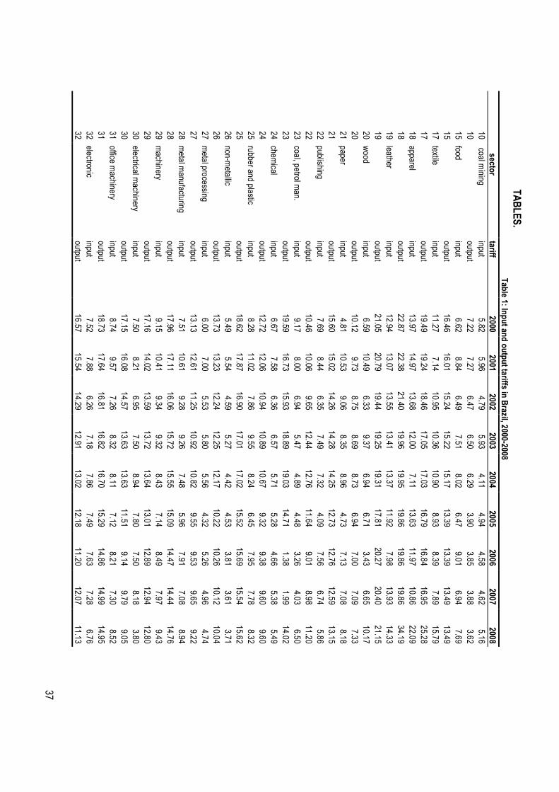
industry of the sample (Table 1)

We observe more variation in average input and output tariffs between industries than

over time (see Table 1). Thus, the lowest average input tariff over the period of analysis (4.55%)

corresponds to industry 26 (Non-metallic Mineral Product Manufacturing) and the highest one

(13.37%) to industry 18 (Apparel Manufacturing). As for the output tariffs, the lowest one (5.34%)

corresponds to industry 10-14 (Extractive industries) and the highest one (22.55%) again to

industry 18. In general, final goods tariffs show for all industries a decreasing trend from 2000 to

2007. Between 2007 and 2008, we observe an upturn of output tariffs for 10 out of the 22 sectors

(from 17 to 23 and 25, 28 and 36).

Evidence on the evolution of input tariffs is more mixed, 14 out of the 22 industries show

a decreasing trend from 2000 to 2007, and as a consequence of the generalised increase in

tariffs from 2007 to 2008, we observe an increase in tariffs for 16 industries.

Table 2 reports the main features of our data set. As can be observed, two-way traders

(both exporters and importers) are larger in terms of output, labour, capital and materials and pay

higher wages as compared to one-way traders (either exporters or importers) and to non-traders.

One-way traders are, in general, more similar in all variables. If we compare these firms with no

traders we find that are larger in terms of output, labour, capital and materials and pay higher

wages.

As regards to trade variables, we find that export intensity is larger for only exporters (as

compared to two-way traders) and that import intensity is larger for only importers (also as

compared to two-way traders).

! 21

5. Results: the effects of trade policy and firm trade status on firm productivity.

In this section we first present the main results from our analysis and then we discuss some

robustness checks we have carried out.

5.1. Main results.

In the first step of our analysis, using the methodology explained above, we estimate the

production function (1) separately for each of the 22 industries, in order to obtain estimates of the

log of TFP.12 Using these estimates, we calculate the (log) of TFP for firm i at time t and industry

s, denoted , as

tfpits = y it −β0

−β l l it −βk kit −βmmit − µt (11)

It is important to note that including a vector of time dummies ( ) in the TFP estimation

makes the estimated TFP time effects free. Controlling for time effects in this setup is crucial as

we are interested in disentangling the effects of trade policy from other possible changes in

macroeconomic policy or macroeconomic instability, or even from any other uncontrolled events,

that occurred in Brazil during our sample period.

In the second step, we use our TFP estimates as the dependent variable of a series of

reduced form equations that include as covariates either trade policy variables or both trade

policy variables and trade status variables. There are two reasons that advise to include trade

status also in the second step estimation: on the one hand, we expect the dynamic evolution of

productivity to be affected by LBI and LBE; and, on the other hand, we believe that the effects of

!!!!!!!!!!!!!!!!!!!!!!!!!!!!!!!!!!!!!!!!!!!!!!!!!!!!!!!!12 The coefficients estimated at industry level are reported in Table 3.

tfpits

µt

! 22

input and output tariffs on the evolution of firms productivity may depend on whether the firm

imports inputs and/or exports, respectively.

In this second step regression analysis we pool TFP estimates for all industries and use

panel data fixed effects estimation to simultaneously control for individual firm and industry fixed

effects.13,14 Using firm level fixed effects allows us to control for the existence of a self-selection

mechanism, that would arise if only the (a priori) more efficient firms were the ones getting

involved in international markets either as buyers, sellers or both buyers and sellers. This self-

selection process is based on the existence of higher sunk entry costs in international markets

that can only be overcome by the more productive firms (see for example Bernard and Jensen,

1999, and Melitz, 2003). The results for these firm fixed effects estimations are reported in Table

4.15

We start our analysis of the effects of trade policy and trade status by using the simplest

possible specification (see equation 12 below), where the only covariate that we include to

explain productivity is output tariffs (TO). This specification (specification 1) has been widely used

in the literature on trade liberalization and productivity.

tfpit =α +α i +γ 1TO +uit (12)

where α is a constant term and αi is and individual fixed effect.

!!!!!!!!!!!!!!!!!!!!!!!!!!!!!!!!!!!!!!!!!!!!!!!!!!!!!!!!13 We report robust standard errors by clustering at the firm level. Clustering at the industry level gives similar results. 14 Controlling for industry fixed effects, among other things, allows to account for time-invariant characteristics coming from trade policy that could make the country policy related to tariffs endogenous with respect to productivity (due to possible policy pressure from particular industries). 15 We have estimated the same set of reduced form equations linking TFP to trade policy and trade status, using a random effects approach (these results are reported in Table A.2 in the Appendix). The fact that the random effects estimates for the export and import status variables are higher than the fixed effects ones suggests that the random effects estimates suffer from an endogeneity bias problem associated to the existence of self-selection by the more productive firms, that could introduce and upwards bias in the estimation of both LBI and LBE. Further, this bias problem is larger for the import dummy than for the export dummy.

! 23

In this specification we expect to be negative. Trade liberalization policies, implying a

reduction of output tariff on imports (of final goods), may increase competitive pressure from

competing imported products and so force firms to use inputs more efficiently, and, consequently,

this would increase productivity. As the dependent variable is the log of TFP, the effect of a unit

increase in the output tariffs on TFP is computed from the estimated coefficient as

100 exp γ

1( )−1( ) . This measure shows the percentage change on the TFP when the tariff on

output increases by one unit. The estimate of γ1 (see Table 4) shows that, as expected, a

decrease in output tariff increases productivity. More specifically, a unit decrease in output tariff

increases TFP by 0.84%.

In our second specification (specification 2), we add as additional covariates both a

dummy that takes value one if the firm exports and zero otherwise (DE), and an interaction that

results from multiplying DE by the output tariff ( TO ⋅DE ). The aim of the first of these variables is to

capture whether there is a direct effect of exporting on productivity. The role of the second one is

to test whether the effect of output tariffs on productivity is different for exporters and non-

exporters.

tfpit =α +α i +γ 1TO +γ 2

TO ⋅DE +γ 3DE +uit (13)

Our results for specification 2 (see second column of Table 4) suggest that a unit

decrease in output tariffs increases productivity by 0.72% for non-exporters and by 0.94% for

exporters (we get that both γ1 and γ2 are negative). These results mean that trade liberalization

(in the form of reducing tariffs on imports of equivalent competing products) will have a larger

effect in the productivity of exporters than that of non-exporters. This can be the result of two

γ 1

γ 1

! 24

effects that work in opposite direction: on the one hand, the positive effect of a reduction in output

tariffs on productivity operates tightening competition and forcing both exporting and non-

exporting firms to behave more efficiently; on the other hand, if trade liberalization reduces

market shares of domestic firms, its impact could be larger in the market shares of the less

productive non-exporting firms (Cirera et al., 2012 show that the self-selection mechanism fully

works for Brazilian manufacturing firms) and this could lessen their incentives to increase

productivity. Additionally, the transformed estimate 100 exp γ

3( )−1( ) shows that the direct effect of

exporting (average difference in TFP between exporters and non-exporters) is of 9.33%. Once we

control by firm level fixed effects, this can be interpreted as evidence of LBE.

Traditional studies on the effects of exports have only considered the effect of firm’s

export status on productivity. The natural evolution of this literature has been to incorporate also

the role of imported inputs. Including an import variable in our analysis could allow disentangling

the effect of exporting on productivity from the effect of importing. Importing inputs may produce

efficiency improvements through the availability both of a wider range of inputs and of inputs of

superior quality for importing firms. Further, closely related to the decision of importing we aim to

analyse the role of import tariffs on productivity. We expect an increase in input tariffs to have a

negative impact on productivity as the increase in the price of the inputs could reduce the range

and quality available for domestic producers.

Thus, to start the analysis of imported inputs, in specification 3 we widen our baseline

specification 1 to include as covariates both output (TO) and input tariffs (TI):

tfpit =α +α i +γ 1TO +γ 2

TI +uit (14)

! 25

The negative sign of the estimate of γ2 in specification 3 confirms that, as expected, a

decrease in inputs tariffs has a positive effect on productivity. More specifically, a unit reduction in

input tariff increases TFP by about 0.50%. As for the effects of output tariffs on productivity, its

correspondent estimate maintains its negative sign. However, once we introduce in the analysis

input tariffs the effect of a unit reduction in output tariffs is lower: whereas in the specification

without input tariffs a unit reduction in the output tariffs increases TFP by 0.84%; when we

consider simultaneously both input and output tariffs this increase is 0.73%.

Finally, in specification 4 we widen specification 2 to take into account both the direct

effect of importing inputs on productivity and whether or not the effect of input tariffs differs

depending on whether the firm import inputs. Thus, we expect a lower impact of changes of input

tariffs for firms that do not import inputs. Therefore, in addition to the covariates already included

in specification 2, we include a dummy that takes value one if the firm imports and zero otherwise

(DI), input tariffs and an interaction that results from multiplying DI by the input tariffs variable.

Therefore, this specification allows us to analyse whether the effects of trading policy (proxied by

inputs and output tariffs) depend on the trade status of the firm,

tfpit =α +α i +γ 1TO +γ 2

TO ⋅DE +γ 3DE +γ 4

TI +γ 5TI ⋅DI +γ 6

DI +uit (15)

As for the new covariates included in specification 4 (with respect to specification 2), our

estimates for TI and TIDI suggest that a unit decrease in input tariffs increases productivity by

0.45% both for importers and non-importers. Additionally, the direct effect of importing measured

by the average difference in productivity between importers and non-importers (given by

100 exp γ

6( )−1( ) ) is 8.87%; i.e. importing inputs increases firm productivity by 8.87%, and so

provides evidence in favour of LBI. As for the exporting and output tariff related covariates (DE, TO

! 26

and TO ⋅DE ), the estimates of a unit decrease in output tariffs are lower in specification 4 than in

specification 2, both for exporters and non-exporters. When we account for input tariffs and

whether the firm imports inputs (specification 4), a unit decrease in output tariff increases TFP by

0.60% for non-exporters and by 0.82% for exporters. However, these figures are higher when we

do not account for them (specification 2), as they are 0.72% and 0.94%. The direct effect of

exporting (that can be interpreted as a measure of LBE) also gets reduced in specification 4 in

comparison to specification 2 (8.97% and 9.33%, respectively).

The larger size of the estimates obtained for output tariffs and export status in

specification 2 could be due to an omitted variable bias, produced by omitting other relevant

factors affecting TFP such as inputs tariffs and import status. The fact that when we introduce

these variables in specification 4 their coefficients are sizeable and significant confirms the

suspects of an omitted variable bias in specification 2.

5.2. Some further robustness specifications.

In this section we present some robustness tests for the previous specifications in which we have

analysed the relationship between trade policy, trade status and productivity. The first of these

robustness specifications (specification 5) is based on specification 4 and simply substitutes the

export and import dummies by export and import intensity variables, respectively.

tfpit =α +α i +γ 1TO +γ 2

TO ⋅EI +γ3EI +γ

4TI +γ 5

TI ⋅II +γ 6⋅II +uit (16)

where EE and II stand for export intensity and import intensity, respectively. The most relevant

differences between the estimates of specifications 4 and 5 are as follows: first, the impact of

! 27

output tariffs on productivity is independent of the export intensity of the firm16 (whereas in

specification 4, where we only distinguished between exporters and non-exporters, the effect was

higher for exporting firms); and, second, the negative and significant estimate of the variable

suggests that the higher the import intensity of a firm the higher the impact of changes in input

tariffs. We also find that non-importers are also positively affected by a reduction in input tariffs.

This result suggests that reducing input tariffs affect the overall quality of domestic inputs though

greater competition for inputs in the domestic market.

In our second robustness specification (specification 6), we proxy trade policy by the

effective rate of protection (ERP, hereafter) instead of proxying it using input and output tariffs.

The aim of this second robustness specification is to test which are the drivers of the relationship

between trade policy and productivity in those papers that only include the ERP as a measure of

trade policy and do not distinguish between input and output tariffs.

The traditional literature linking trade liberalization and productivity has used the ERP as

the unique measure of trade policy. In this literature, a decrease in input tariffs increases the ERP

and would result in a decrease in productivity via a reduction in the intensity of competition

among national firms. However, the most recent literature on trade liberalization and productivity

suggests using both input and output tariffs to measure trade policy. Within this approach the

opposite argument arises relating input tariffs and productivity. According to this argument, a

decrease in input tariffs eases productivity increases by domestic firms as it allows them to profit

from: the learning effect derived from the use of the incorporated technology in imported inputs,

and from the wider range and quality of the inputs available to domestic firms.

In specification 6, we include as covariates not only the ERP but also the exporter and

importer dummies, and the crossed products between these and the ERP:

!!!!!!!!!!!!!!!!!!!!!!!!!!!!!!!!!!!!!!!!!!!!!!!!!!!!!!!!16 The estimate of TO•EI is not significant at any reasonable significance level.

TI ⋅II

! 28

tfpit =α +α i +γ 1ERP +γ

2ERP ⋅DE +γ 3

DE +γ 4ERP ⋅DI +γ 5

DI +uit (17)

The results obtained in the estimation of specification 6 (equation 17) can be summarized as

follows. In comparison with specification 4 (that includes both input and output tariffs instead of

ERP) the direct effect of exporting is lower (7.09% vs. 8.97%) and the direct effect of importing is

higher (10.12% vs. 8.87%). Second, a unit increase in the ERP decreases productivity by 33.10%

for firms that neither export nor import, by 47.53% for exporters and by 56.00% for importers.

Therefore, an increase in the ERP, which softens competition in the domestic market, results in a

reduction of firms’ productivity, independently of its trading status. However, from the estimates

associated to the ERP we cannot disentangle whether the effects come from an increase in

output tariffs, from a decrease in input tariffs or from changes in the share of intermediate inputs

in the value of the final good.

Our third robustness exercise (specification 7) checks the effects of the large currency

appreciation that Brazil experienced during the period of analysis, as these can affect productivity

without implying changes in efficiency. To interpret the results in this specification we have to take

into account that an increase in the real effective exchange rate (ER, hereafter) means a

depreciation of the national currency. In specification 7 (see expression 18), we extend

specification 4 to include as covariates the cross products of the ER with the export and import

dummies. The aim of including these cross products is to check whether the ER evolution has

different effects on the productivity of importers and exporters:

tfpit =α +α i +γ 1TO +γ 2

TO ⋅DE +γ 3DE +γ 4

TI +γ 5TI ⋅DI +γ 6

DI +

γ7ER ⋅DE +γ 8

ER ⋅DI +uit

(18)

! 29

Changes in the estimates corresponding to the output and/or input tariffs would suggest

that some of the productivity improvement attributed to a reduction in output and/or input tariffs in

specification 4 could be due to exchange rate changes. Further, the coefficients of the importer

and exporter status dummies could also be affected.

As expected (see column 7 of Table 4) the inclusion of the ER and its interactions with

the export and input dummies reduces the size (in absolute terms) of the estimates

corresponding to the output and input tariffs. Thus, whereas in the specification without ER

(specification 4) a unit reduction of output tariffs increases the productivity of non-exporters and

exporters by 0.60% and 0.82%, respectively, in the specification with the ER variables

(specification 7), the increase in productivity gets reduced to 0.45% both for exporters and non-

exporters. However, there is almost no difference between the effects on productivity of a unit

reduction of input tariffs both for importers and non-importers (0.46% in specification 7 vs. 0.45 in

specification 4).

Notice that the extra increase in productivity enjoyed by exporters (in comparison with

non-exporters) in specification 4 when the output tariffs decrease vanishes with the inclusion, in

specification 7, of the variable interacting ER with the export dummy. This finding suggests that

the evolution of the ER has special incidence in the evolution of the productivity of exporters since

firms need to become more productive due to the competitiveness loss in international markets

due to exchange rate appreciation. Therefore, omitting this variable can lead to overestimating

the effect of export status in specification 4.

However, both the direct effects of exporting and importing in productivity are higher in

the specification including the ER variables than in the specification that does not include them,

confirming the existence of both LBE and LBI processes. Thus, the export premium is 10.20% in

! 30

specification 7 in comparison to 8.97% in specification 4. In the same vein, the import premium is

12.52% and 8.87% in specifications 7 and 4, respectively. Finally, the two interaction variables of

the ER with the importer and exporter dummies are negative and significant (a unit decrease in

ER increases productivity by 6.47% and 5.48 for importers and exporters, respectivey). This

could be signalling that a real appreciation increases firm productivity. In addition, to increasing

competitive pressureon exporters, a real appreciation lowers imported input prices what

increases competition in the inputs markets and so has a positive effect on productivity.

6. Conclusions.

The results from all specifications led us to conclude the following. First, higher output tariffs

(tariffs on imports of final goods) decrease productivity by lowering import competition as firms

are less forced to improve efficiency.

Second, higher input tariffs (tariffs on imports of intermediate inputs) decrease

productivity by reducing access to a wider range of foreign inputs, to higher quality inputs, or to

foreign technology incorporated in imported inputs. Therefore, we do not find for input tariffs the

link with productivity predicted by the literature linking a trade policy measure such as the ERP

with productivity, but just the opposite. According to this literature a decrease in input tariffs

increases the ERP and decreases productivity, through the reduction in industry competition.

Third, we do not generally find that trade liberalization (in the form of reducing input

tariffs) has a larger effect increasing productivity for importing firms, except in that specification in

which we interact tariffs with import intensity.

Fourth, for the effects of output tariffs on productivity, for exporters and non-exporters we

find only statistically significant different results coming from the export status, but not from the

export intensity.

! 31

Fifth, our results indicate that the effects of tariffs in the economy do spread among all

firms in the economy, and do not only affect exporting or importing firms.

Sixth, we still find evidence of both learning-by-exporting and learning-by-importing

effects on productivity. This evidence comes by the fact that we get significant effects from the

firm importing and exporting status even after controlling for the effects of tariffs.

Seven, according to a trade policy measure such as the ERP we also confirm that an

increase of it, interpreted as a decrease in competition, produces a reduction on productivity.

However, we prefer specifications including separately output and input tariffs to be able to isolate

the effect of competition on productivity from the effect of better access to inputs on productivity.

Finally, from the more complete specification, specification 7, where results over

productivity for other variables are cleaned from the effect of the evolution of exchange rates over

the analysed period, we obtain that the effects of increasing output tariffs on decreasing

productivity are quite similar to the ones coming from increasing input tariffs, but that learning-by-

importing (as captured by the import status dummy) is larger than learning-by-exporting (as

captured by the export status dummy). Further, we also obtain that real appreciations of the

currency produce an increase in productivity, being importers more affected than exporters.

! 32

REFERENCES.

Ackerberg, D. A., K. Caves and G. Frazer (2006), Structural identification of production

functions, Working Paper, Department of Economics, UCLA.

Amiti, M. and J. Konings (2007), Trade Liberalization, Intermediate Inputs, and

Productivity: Evidence from Indonesia, American Economic Review, 97, 5, 1611-1638.

Arnold, J. and K. Hussinger (2005), Export Behavior and Firm Productivity in German

Manufacturing: A Firm-level Analysis, Review of World Economics ⁄ Weltwirtschaftliches Archiv,

141, 2, 219–43.

Bernard, A. B. and J. B. Jensen (1999), Exceptional Exporter Performance: Cause,

Effect, or Both? Journal of International Economics, 47(1), 1–25.

Bustos, P. (2011), Trade liberalizations, exports, and the technology upgrading:

evidence on the impact of MERCOSUR on Argentinian firms, American Economic Review, 101,

304-340.

Cirera, X., D. Lederman, J.A. Mañez, M.E. Rochina and J.A. Sanchis (2012), Self-

selection and learning-by-exporting: the Brazilian case. University of Valencia, mimeo.

Corden, Max W (1971). The Theory of Protection. Oxford: Oxford University Press.

Clerides, S. K., S. Lach and J.R. Tybout (1998), Is Learning by Exporting Important?

Micro-Dynamic Evidence from Colombia, Mexico, and Morocco, Quarterly journal of Economics,

113(2), 903–947.

Coe, D.T. and E. Helpman (1995), International R&D spillovers. European Economic

Review, 39, 859–887.

Coe, D.T., E. Helpman and A. Hoffmaister (1997), North–South R&D spillovers.

Economic Journal, 107, 134–149.

De Loecker, J. (2007), Do Exports Generate Higher Productivity? Evidence from

Slovenia. Journal of International Economics, 73, 1, 69–98.

De Loecker, J. (2010), A Note on Detecting Learning by Exporting, NBER Working

Papers 16548, National Bureau of Economic Research, Inc.

De Loecker, J. and F. Warzyniski (2011), Markups and firm-level status, NBER Working

Papers 15198, National Bureau of Economic Research, Inc.

Ethier, W. (1982), National and International Returns to Scale in the Modern Theory of

International Trade.” American Economic Review, 72(3), 389–405.

! 33

Fernandes, A.M. (2007), Trade policy, trade volumes and plant-level productivity in

Colombian manufacturing industries, Journal of International Economics 71, 52–71

Girma, S., D. Greenaway and R. Kneller (2004), Does Exporting Increase Productivity?

A Microeconometric Analysis of Matched Firms. Review of International Economics, 12, 5, 855–

66.

Gaston, N. and D. Trefler (1997), “The Labour Market Consequences of the Canada-

U.S. Free Trade Agreement.” Canadian Journal of Economics, 30(1) 18–41.

Greenaway, D. and R. Kneller (2004), Exporting and Productivity in the UK. Oxford

Review of Economic Policy, 20, 3, 358–71.

Greenaway, D. and R. Kneller (2007b), Industry Differences in the Effect of Export

Market Entry: Learning by Exporting? Review of World Economics ⁄ Weltwirtschaftliches Archiv,

143, 3, 416–32.

Greenaway, D. and R. Kneller (2008), Exporting, Productivity and Agglomeration.

European Economic Review, 52, 5, 919–39.

Grossman, G. M. and E. Helpman (1991). Innovation and Growth in the Global

Economy. Cambridge, MA: MIT Press.

Hansson, P. and N. Lundin (2004), Exports as Indicator on or a Promoter of Successful

Swedish Manufacturing Firms in the 1990s. Review of World Economics ⁄ Weltwirtschaftliches

Archiv, 140, 3, 415–45.

Harrison, A. E. (1994), Productivity, Imperfect Competition and Trade Reform: Theory

and Evidence. Journal of International Economics, 36(1-2), 53–73.

Head, C. K. and J. Ries. 1999. Rationalization Effects of Tariff Reductions. Journal of

International Economics, 47(2), 295–320.

Helpman, Elhanan, and Paul R. Krugman (1985), Market Structure and Foreign Trade:

Increas-ing Returns, Imperfect Competition, and the International Economy. Cambridge, MA: MIT

Press.

Kasahara, H. and J. Rodrigue (2005). Does the Use of Imported Intermediates Increase

Productivity? Plant-Level Evidence," University of Western Ontario, Economic Policy Research

! 34

Institute Working Papers 20057, University of Western Ontario, Economic Policy Research

Institute.

Kasahara, H. and J. Rodrigue (2008), Does the use of imported intermediates increase

productivity? Plant-level evidence, Journal of Development Economics 87, 106–118.

Krishna, P. and D. Mitra (1998), “Trade Liberalization, Market Discipline and

Productivity Growth: New Evidence from India.” Journal of Development Economics, 56(2), 447–

62.

Krugman, P. R. (1979), Increasing Returns, Monopolistic Competition, and International

Trade. Journal of International Economics, 9(4), 469–79.

Levinsohn, J. (1993), “Testing the Imports- as-Market-Discipline Hypothesis.” Journal of

International Economics, 35(1–2): 1–22.

Levinsohn, J. and A. Petrin (2003), Estimating production functions using inputs to

control for unobservables. Review of Economic Studies 70, 317–342.

Manjón, M., J.A. Máñez, M.E. Rochina-Barrachina and J.A. Sanchis-Llopis (2013),

Reconsidering learning by exporting. Review of World Economics, forthcoming.

Mánez-Castillejo, J.A., M.E. Rochina-Barrachina and J.A. Sanchis-Llopis (2010), Does

firm size affect self-selction and learning-by-exporting? The World Economy, 33 (3), 315-346.

Markusen, J. R. (1989), Trade in Producer Services and in Other Specialized Interme-

diate Inputs, American Economic Review, 79(1), 85–95.

Melitz, M. (2003), The impact of trade on intra-industry reallocations and aggregate

industry productivity. Econometrica 71 (4), 1695–1725.

Muendler, M. (2004), Trade, technology, and productivity: a study of Brazilian

manufacturers, 1986-1998. UCSD, mimeo.

Olley, G. S. and A. Pakes (1996), The dynamics of productivity in the

telecommunications equipment industry. Econometrica, 64(6), 1263–1297.

Pavcnik, N. (2002), Trade Liberalization, Exit, and Productivity Improvements: Evidence

from Chilean Plants, Review of Economic Studies, 69(1). 245–76.

Roberts, M. and J. Tybout (1991), Size Rationalization and Trade Exposure in Devel-

oping Countries. In Empirical Studies of Commercial Policy, ed. Robert Baldwin, 169– 93.

! 35

Chicago: University of Chicago Press.

Schor, A. (2004), Heterogeneous Produc- tivity Response to Tariff Reduction: Evidence

from Brazilian Manufacturing Firms. Journal of Development Economics, 75(2), 373–96.

Serti, F., and C. Tomasi (2008), Self-Selection and Post-Entry Effects of Exports:

Evidence from Italian Manufacturing Firms. Review of World Economics/Weltwirtschaftliches

Archiv, 144 (4), 660–694.

Silva, A., A.P. Africano and Ó. Afonso (2010), Learning-by- exporting: What we know

and what we would like to know. Universidade de Porto FEP Working Papers N. 364, March.

Singh, T. (2010), Does International Trade Cause Economic Growth? A Survey. The

World Economy, 33, 1517-1564.

Topalova, P. ( 2004). Trade Liberalization and Firm Productivity: The Case of India.

IMF.Working Paper 04/28.

Trefler, Daniel (2004). The Long and Short of the Canada-U.S. Free Trade Agreement,

American Economic Review, 94(4), 870–95.

Tybout, J., de Melo, J. and Corbo, V. (1991), The Effects of Trade Reformson Scale

and Technical Efficiency: New Evi-dence from Chile.” Journal of International Economics, 31(3–

4): 231–50.

Tybout, J. and M. D. Westbrook (1995), “Trade Liberalization and the Dimensions of

Efficiency Change in Mexican Manufacturing Industries.” Journal of International Economics,

39(1–2). 53–78.

Van Biesebroeck, J. (2005), Exporting Raises Productivity in Sub-Saharan

Manufacturing Plants. Journal of International Economics, 67, 2, 373–91.

Wagner, J. (2002), The Causal Effects of Export on Firm Size and Labour Productivity:

First Evidence from a Matching Approach, Economics Letters, 77(2), 287–92.

Wooldridge, J.M. (2009), On estimating firm-level production functions using proxy

variables to control for unobservables, Economics Letters, 104, 112–114.

! 36

FIGURES

Figure 1: Evolution of average inputs and output tariffs

!Note: Weighted average input and output tariffs

810

1214

1618

perc

enta

ge

2000 2002 2004 2006 2008year

Input tariffs Output tariffs

!37

TABLES.

Table 1: Input and output tariffs in Brazil, 2000-2008 sector

tariff 2000

2001 2002

2003 2004

2005 2006

2007 2008

10 coal m

ining input

5.82 5.96

4.79 5.93

4.11 4.94

4.58 4.62

5.16 10

output

7.22 7.27

6.47 6.50

6.29 3.90

3.85 3.88

3.62 15

food input

6.62 8.84

6.49 7.51

8.02 6.47

9.01 6.94

7.69 15

output

16.46 16.01

15.24 15.22

15.17 13.39

13.39 13.49

13.49 17

textile input

11.27 7.14

10.95 10.36

10.90 8.93

8.39 7.89

15.79 17

output

19.49 19.24

18.46 17.05

17.03 16.79

16.84 16.95

25.28 18

apparel input

13.97 14.97

13.68 12.00

7.11 13.63

11.97 10.86

22.09 18

output

22.87 22.38

21.40 19.96

19.95 19.86

19.86 19.86

34.19 19

leather input

12.94 13.07

13.55 13.41

13.37 11.92

7.98 13.93

14.33 19

output

21.05 20.79

19.44 19.25

19.31 17.81

20.27 20.40

21.15 20

wood

input 6.59

10.49 6.33

9.37 6.94

6.71 3.43

6.65 10.17

20

output 10.12

9.73 8.75

8.69 8.73

6.94 7.00

7.09 7.33

21 paper

input 4.81

10.53 9.06

8.35 8.96

4.73 7.13

7.08 8.18

21

output 15.60

15.02 14.26

14.28 14.25

12.73 12.76

12.59 13.15

22 publishing

input 7.69

8.44 6.35

7.49 7.32

4.09 7.56

6.74 5.86

22

output 10.46

10.06 9.65

12.44 12.76

11.64 9.01

8.98 11.20

23 coal, petrol m

an. input

9.17 8.00

6.94 5.47

4.89 4.48

3.26 4.03

6.50 23

output

19.59 16.73

15.93 18.89

19.03 14.71

1.38 1.99

14.02 24

chemical

input 6.67

7.58 6.36

6.57 5.71

5.28 4.66

5.38 5.49

24

output 12.72

12.06 10.94

10.89 10.67

9.32 9.38

9.60 9.60

25 rubber and plastic

input 8.28

11.02 7.86

9.55 8.24

6.45 7.95

7.78 8.32

25

output 18.62

17.87 16.90

17.01 17.02

15.52 15.69

15.54 15.62

26 non-m

etallic input

5.49 5.54

4.59 5.27

4.42 4.53

3.81 3.61

3.71 26

output

13.73 13.23

12.24 12.25

12.17 10.22

10.26 10.12

10.04 27

metal processing

input 6.00

7.00 5.53

5.80 5.56

4.32 5.26

4.96 4.74

27

output 13.13

12.61 11.25

10.92 10.82

9.55 9.53

9.65 9.22

28 m

etal manufacturing

input 7.51

10.61 9.28

9.26 7.48

5.96 7.91

7.08 8.94

28

output 17.96

17.11 16.06

15.72 15.55

15.09 14.47

14.44 14.76

29 m

achinery input

9.15 10.41

9.34 9.32

8.43 7.14

8.49 7.97

9.43 29

output

17.16 14.02

13.59 13.72

13.64 13.01

12.89 12.94

12.80 30

electrical machinery

input 7.50

8.21 6.95

7.50 8.94

7.80 7.50

8.18 3.80

30

output 17.15

16.08 14.57

13.63 13.63

11.51 9.14

9.79 9.05

31 office m

achinery input

8.74 9.57

7.26 8.32

8.11 7.12

8.21 7.30

8.52 31

output

18.73 17.64

16.81 16.82

16.70 15.29

14.86 14.99

14.95 32

electronic input

7.52 7.88

6.26 7.18

7.86 7.49

7.63 7.28

6.76 32

output

16.57 15.54

14.29 12.91

13.02 12.18

11.20 12.07

11.13

!38

Table 1: Input and output tariffs in Brazil, 2000-2008

Table 1: Input and output tariffs in Brazil, 2000-2008

sector tariff

2000 2001

2002 2003

2004 2005

2006 2007

2008 33

medical equipm

ent input

9.71 9.60

8.68 8.98

8.69 6.90

8.78 7.55

7.60 33

output

14.80 13.24

13.47 12.92

12.94 12.17

11.50 11.32

9.71 34

motor vehicles

input 9.71

10.66 8.46

11.09 7.94

9.17 10.07

13.11 10.64

34

output 19.30

18.53 19.19

19.00 19.06

17.92 17.87

18.39 18.39

35 other transport

input 7.73

7.02 8.09

7.21 6.77

9.14 8.81

7.97 8.84

35

output 18.02

15.41 15.28

15.36 15.46

14.63 14.63

14.36 14.15

36 furniture and m

isc. input

7.86 12.35

8.73 10.58

8.19 8.53

7.11 8.00

7.99 36

output

20.55 19.98

19.04 19.01

18.94 17.30

17.46 17.14

17.40

Table 2. Descriptive statistics

Exporters & im

porters Only

exporters Only

importers

No traders

Production function variables

O

utput 1.35E+08

2.20E+07 2.31E+07

3.53E+06

(1.46E+09)

(1.21E+08) (7.86E+07)

(1.52E+07)

Labour 535.56

223.38 166.85

73.61

(1672.26)

(689.63) (383.04)

(123.31)

Capital

1.64E+08 2.79E+07

3.98E+07 4.05E+06

(2.86E+09)

(2.55E+08) (1.69E+09)

(3.05E+07)

Materials

9.78E+07 1.65E+07

1.71E+07 2.58E+06

(8.94E+08)

(8.28E+07) (6.26E+07)

(1.25E+07)

Wages

9.88E+06 1.89E+06

2.10E+06 4.82E+05

(8.04E+07)

(6.63E+06) (6.53E+06)

(1.47E+06)

Trade variables

Export intensity (%

) 17.08

19.85 -

-

(24.65)

(29.96) -

-

Import intensity (%

) 23.83

- 28.36

-

(25.49)

- (28.07)

-

Sample size

35560 41209

11670 179963

Notes: Standard errors in parenthesis.

!39

Table 3. Coefficients of the production function.

Industry Classification (CNAE 2 digits) Labour

Capital M

aterials 10

Coal M

ining 0.178

0.100 0.496

15 Food and Beverage M

anufacturing 0.126

0.046 0.551

17 Textile Product M

anufacturing 0.157

0.047 0.100

18 Apparel M

anufacturing 0.374

0.036 0.374

19 Leather processing, Leather products, Luggage and Footw

ear Manufacturing

0.301 0.065

0.321 20

Wood Products M

anufacturing 0.182

0.067 0.523

21 Pulp, Paper and Paper Products M

anufacturing 0.106

0.046 0.466

22 Publishing, Printing and R

eproduction of Recordings

0.190 0.101

0.332 23

Coal Products M

anufacturing, Petroleum R

efining, N

uclear Com

bustibles Processing and Alcohol Production 0.059

0.048 0.785

24 C

hemical Products M

anufacturing 0.145

0.056 0.528

25 R

ubber and Plastics Product Manufacturing

0.162 0.046

0.522 26

Non-m

etallic Mineral Product M

anufacturing 0.159

0.051 0.583

27 M

etals Production and Basic Processing 0.148

0.050 0.459

28 M

etal Product Manufacturing (excluding m

achinery and equipment)

0.256 0.059

0.503 29

Machinery and Equipm

ent Manufacturing

0.271 0.072

0.161 30

Office M

achinery and Data Processing Equipm

ent Manufacturing

0.134 0.006

0.804 31

Electrical Machinery, Equipm

ent and Supplies Manufacturing

0.216 0.048

0.588 32

Electronic Com

ponent and Com

munication Apparatus and Equipm

ent Manufacturing

0.215 0.058

0.407 33

Medical and Therapeutic Equipm

ent, Optical and Precision Instrum

ents, Equipm

ent for Industrial Automation and W

atch and Clock M

anufacturing 0.247

0.072 0.478

34 M

otor Vehicle Assembly and M

otor Vehicle, Engine, Trailer and Body Manufacturing

0.212 0.039

0.496 35

Other Transportation Equipm

ent Manufacturing

0.290 0.109

0.187 36

Furniture and Miscellaneous M

anufacturing 0.214

0.062 0.251

- N

ot distinguishing among industries

0.192 0.068

0.334

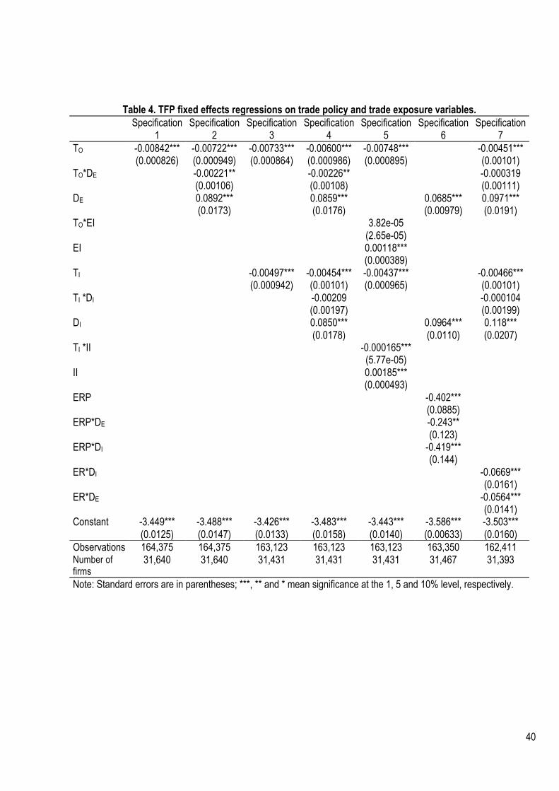
! 40

Table 4. TFP fixed effects regressions on trade policy and trade exposure variables.

Specification 1

Specification 2

Specification 3

Specification 4

Specification 5

Specification 6

Specification 7

TO -0.00842*** -0.00722*** -0.00733*** -0.00600*** -0.00748*** -0.00451*** (0.000826) (0.000949) (0.000864) (0.000986) (0.000895) (0.00101) TO*DE -0.00221** -0.00226** -0.000319 (0.00106) (0.00108) (0.00111) DE 0.0892*** 0.0859*** 0.0685*** 0.0971*** (0.0173) (0.0176) (0.00979) (0.0191) TO*EI 3.82e-05 (2.65e-05) EI 0.00118*** (0.000389) TI -0.00497*** -0.00454*** -0.00437*** -0.00466*** (0.000942) (0.00101) (0.000965) (0.00101) TI *DI -0.00209 -0.000104 (0.00197) (0.00199) DI 0.0850*** 0.0964*** 0.118*** (0.0178) (0.0110) (0.0207) TI *II -0.000165*** (5.77e-05) II 0.00185*** (0.000493) ERP -0.402*** (0.0885) ERP*DE -0.243** (0.123) ERP*DI -0.419*** (0.144) ER*DI -0.0669*** (0.0161) ER*DE -0.0564*** (0.0141) Constant -3.449*** -3.488*** -3.426*** -3.483*** -3.443*** -3.586*** -3.503*** (0.0125) (0.0147) (0.0133) (0.0158) (0.0140) (0.00633) (0.0160) Observations 164,375 164,375 163,123 163,123 163,123 163,350 162,411 Number of firms

31,640 31,640 31,431 31,431 31,431 31,467 31,393

Note: Standard errors are in parentheses; ***, ** and * mean significance at the 1, 5 and 10% level, respectively.

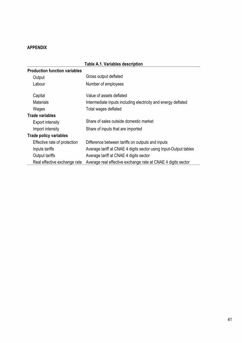
! 41

APPENDIX

Table A.1. Variables description Production function variables

Output Gross output deflated 2.20E+07 2.31E+07

3.53E+06

Labour Number of employees

Capital Value of assets deflated

Materials Intermediate inputs including electricity and energy deflated

Wages Total wages deflated Trade variables

Export intensity Share of sales outside domestic market - -

Import intensity Share of inputs that are imported

Trade policy variables Effective rate of protection Difference between tariffs on outputs and inputs

Inputs tariffs Average tariff at CNAE 4 digits sector using Input-Output tables Output tariffs Average tariff at CNAE 4 digits sector Real effective exchange rate Average real effective exchange rate at CNAE 4 digits sector

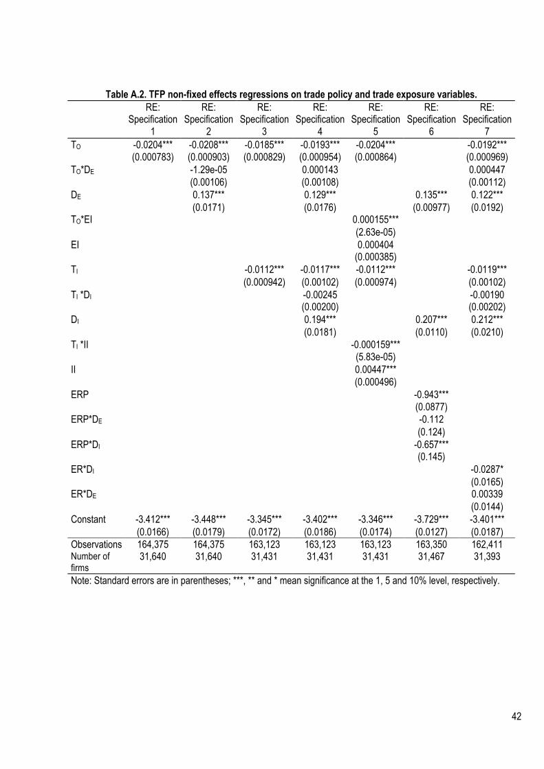
! 42

Table A.2. TFP non-fixed effects regressions on trade policy and trade exposure variables. RE:

Specification 1

RE: Specification

2

RE: Specification

3

RE: Specification

4

RE: Specification

5

RE: Specification

6

RE: Specification

7 TO -0.0204*** -0.0208*** -0.0185*** -0.0193*** -0.0204*** -0.0192*** (0.000783) (0.000903) (0.000829) (0.000954) (0.000864) (0.000969) TO*DE -1.29e-05 0.000143 0.000447 (0.00106) (0.00108) (0.00112) DE 0.137*** 0.129*** 0.135*** 0.122*** (0.0171) (0.0176) (0.00977) (0.0192) TO*EI 0.000155*** (2.63e-05) EI 0.000404 (0.000385) TI -0.0112*** -0.0117*** -0.0112*** -0.0119*** (0.000942) (0.00102) (0.000974) (0.00102) TI *DI -0.00245 -0.00190 (0.00200) (0.00202) DI 0.194*** 0.207*** 0.212*** (0.0181) (0.0110) (0.0210) TI *II -0.000159*** (5.83e-05) II 0.00447*** (0.000496) ERP -0.943*** (0.0877) ERP*DE -0.112 (0.124) ERP*DI -0.657*** (0.145) ER*DI -0.0287* (0.0165) ER*DE 0.00339 (0.0144) Constant -3.412*** -3.448*** -3.345*** -3.402*** -3.346*** -3.729*** -3.401*** (0.0166) (0.0179) (0.0172) (0.0186) (0.0174) (0.0127) (0.0187) Observations 164,375 164,375 163,123 163,123 163,123 163,350 162,411 Number of firms

31,640 31,640 31,431 31,431 31,431 31,467 31,393

Note: Standard errors are in parentheses; ***, ** and * mean significance at the 1, 5 and 10% level, respectively.