Trade Preferences: Are they of any help? ∗

David Laborde † Cristina Mitaritonna ‡ Leonardo Pupettoa§

April 15, 2010

Abstract

This article provides a very detailed analysis

JEL Classification: F13, F17Keywords: Preferential Trade Agreements (PTAs), CGEmodel,

Simulations

∗The authors acknowledge financial support by the German Marshall Fund of theUnited States. The authors are solely responsible for the content of this paper.†IFPRI, Washington D.C. (d.laborde@cgiar.org).‡CEPII (cristina.mitaritonna@cepii.fr)§Ecole Polytechnique (leonardo.puppetto@polytechnique.edu)

1

1 Introduction

Trade preferences are a key aspect of actual trade policies and trade pat-terns. If the literature has in general emphasized their limited importance(?Brenton, 2003) and their pervert effects (Ozden & Reinhardt, 2005), otherscholars provide a more favourable picture (Candau & Jean, 2005; Bureauet al., 2007).

The real value of existing preferences and the opportunity to enlargepreferential schemes is still a core issue for trade policy makers.

First, in a multilateral framework, the erosion of preferences relatedthe completion of the Doha round has raised many concerns for African,Caribbean and Pacific countries that benefit from EU historical preferencesschemes. The opposition between the G-90 and the Latin American on theissue of tropical products, such as banana, extended liberalization is a per-fect illustration of the rift existing between developing countries on this issueand the difficulty to find a compromise. On one side, countries that alreadybenefit from preferences in key markets want to delay and limit multilateralliberalization. On the other side, the non-preferred exporters suffer from un-fair discrimination and want a quick and deep multilateral market opening.At the same time, the opportunity to generalize the EBA initiative to allOECD members and to some emerging countries has been discussed and is akey achievement of the Honk Kong Ministerial (WTO 2005). However, twoquestions have been raised: how to be sure that these new preferences willprovide real benefits for LDCs and to which extent preference erosion mayappear between LDCs (Laborde, 2008). The last issue is another source ofpotential conflict between African countries that benefit from the AGOA ini-tiative in the textile and apparel sector and large and competitive exportersuch as Bangladesh. Second, regarding unilateral policies, both the EU andthe US have started to rethink their unilateral preferential schemes. In 2005the EU has simplified its GSP schemes and is currently adapting its rulesof origin system for helping developing countries to grasp the benefits of thepreferences and succeeding their integration to the international division ofthe production process. In the US, based on the existing GSP scheme andthe AGOA experience, discussions have started on The New Partnership forTrade and Development Act (McDermott, 2007) targeting LDC countries.Third, in order to avoid to loss benefits from existing discriminatory prefer-ential market access, developing countries are forced to enter in bilateral ne-gotiations with the EU and the US to replace WTO non-compatible program(Andean Trade Partneship Act, Cotonou-Lome preferences) by Free TradeAgreements (FTA), accepting at the same time to open their markets and totake additional commitments. More than never, it is important to measureeffectively the value of existing preferences. Is it worthy to fight for them? tosave them? and in the future to create new preferential access? Should de-veloping countries focus on them? If actual schemes are weakly used, what

2

is the cost of the administration constraints and rules of origin related tothem? Is the future of preferences only an EU problem or a transatlanticchallenge that concerns both the EU and the US? The present study aimsto answer these policy concerns by proposing innovating research solution.Indeed, global CGE assessment has followed a bi-polar approach. Before theintegration of the MAcMapHS6 (Bouet, Decreux, Jean and Laborde, 2008)in the GTAP database (McDougall and Dimaranan, 2005), only MFN tar-iffs were considered with the few exceptions of regional agreements such asthe EU, NAFTA and the ANZCERTA. Therefore, the role of preferencesfor developing countries was totally discarded and erosion of preferences anon problem by definition. Thanks to the information of the MAcMapHS6database on preferences, the assessment of the multilateral liberalization hasbeen improved, capturing the complexity of diverging interests among de-veloping countries (Bouët et al., 2005). However, the MAcMapHS6 datasetassume that preferences are fully used: exporters always benefit from thelowest tariff for which they are eligible. A wide econometric literature hasemphasized the fact that in reality the rate of utilization of preferences is inmany cases low (?Bre, 2003; ?)(Brenton and Mancin, 2003; Matoo, Roy andSubramanian, 2003). At the same time, exhaustive investigation conductedby other authors (Gallezot, 2003; Candau and Jean, 2005) have proven thatconsidering the whole set of overlapping preferential scheme, the overall rateof utilization of preferences is pretty high and problems concentrated in alimited number of cases (sectors or/and countries). Our work is aimed tobridge the gap between both extreme approaches. By using a CGE and us-ing disaggregated data and modeling at the HS6 level we assess the valueof both EU and US non-reciprocal schemes by considering alternatively aperfect use of preferences and an incomplete one, based on current utiliza-tion rate. Our approach combines the advantages of the CGE frameworkin terms of theoretical robustness and capacity to provide global assessmentand the importance to capture the absolute and relative value of preferentialmargins at the detailed level. Under alternative assumption of preferencesuse, we simulate three scenarios: the end of unilateral preferences by the EU(1), the end of unilateral preferences by the US (2) and the elimination ofthese schemes by both regions. In each case, countries that do not have FreeTrade Agreements with these regions will face MFN rates in the simulations.The values of existing preferences are then measured in terms of exportsand welfare for developing countries. The different assumption regardingthe rate of utilization of preferences allow us to both provide important con-clusions regarding other assessment of trade liberalization in the literatureand to provide a valuation of the efficiency and mercantilist marginal costassociated with the rule of origin.

«< COMMENTS ON RESULTS TO BE INCLUDED»>The paper is organized as follow: Section II provides a debate over the

rationality and the economic effects of preferences Section III provides a de-

3

tailed description of unilateral EU and USA schemes, as well as quantitativeindicators. A specific attention is devoted to LDCs. Section IV presents themodel and the scenario design. Results are displayed in Section V and asensitivity analysis is conducted in section VI. Section VII concludes.

4

2 The General System of Preferences: rationalityand criticisms

The Generalized System of Preferences (GSP) was one of the few ideas whichmanaged to take concrete shape as a result of the so called "internationalstrategy for development" conceived in the early sixties (12 October1970)by UNCTAD. It was created in a context where the majority of developingcountries were increasingly aware of the massive inequalities between themand developed countries; therefore the GSP was founded to be the instru-ment to help bridging the gap between them. By granting a more favorabletreatment only to developing countries, the GSP was contrary to the basicGATT principle of the most favorite nation, Article I:1 GATT, which re-quires extending any more favorable treatment granted to a Member to allother WTO Members. Since it was incompatible with the GATT ArticleI, it needed a waiver to be operational. The waiver granted in 1971, al-lowed developed countries to accord more favorable tariff treatment to theproducts of developing countries for a period of ten years. In 1979, duringthe negotiation of the Tokyo Round developing countries obtained a perma-nent deviation from the MFN with the adoption of the so called EnablingClause, whose formal name is "Decision on Differential and More FavorableTreatment, Reciprocity and Fuller Participation of Developing Countries".Since then the "Decision" has been incorporated into the GATT 1994, theAgreement establishing the WTO.

However if from one side the Enabling Clause introduced a permanentwaiver to the Article I, on the other side it did not introduce any legallybinding obligation on developed countries whose decision about the intro-duction of preferential schemes were left completely to their decision. Theresult, after more than three decades is a set of different national schemes,generally frugal and paltry, whose economic effect are still questionable (seeHoekman & Ozden (2005) for a survey of the literature). Although no con-sensus emerges upon the likely effects of different preference schemes, at leasta number of their features limit their reach. The insufficient product cover-age, especially for products in which developing countries enjoy comparativeadvantages and the lack of security of access to those schemes are two im-portant aspects that limit the value of these preferences (Inama, 2002).

Many factors introduce substantial uncertainties, and hence lower theincentive to invest in eligible sectors. GSP schemes are unilateral and thensubject to withdrawal. There are many reasons for which countries may losetheir preferential treatment.

All GSP schemes, in particular the USA preferential scheme, 1 conditiontheir preferences to some degree. Some conditions are discretionary factorsin determining beneficiary countries, whereas others trigger mandatory with-

1. See Ozden & Reinhardt (2005).

5

drawal or denial of GSP benefits. 2 For example, in 1992 the US suspendedGSP benefits for products originated from India, due to perceived inade-quacy of protection to intellectual property rights. India has been restoredto US GSP program in 2004.

Another common characteristic among GSP schemes is the so-called"graduation" system, authorized by the Enabling Clause, which allows fora beneficiary country to be excluded, totally or for certain products, fromthe preferential treatment when it has achieved a certain degree of economicdevelopment. 3 The logic behind is to avoid that more advanced develop-ing countries, taking advantage of the preference system, may endanger thedevelopment of less developed countries making them lay behind. Howeverthe purposes of graduation do not appear to have been fully reached, in factthere is evidence of a high concentration of imports from a few GSP bene-ficiaries. The majority of developing countries benefiting from the schemesare mainly those which have large and diversified economies, including sub-stantial manufacturing sectors. 4 Moreover, the EU and USA GSP programsalso contain safeguard clauses that authorize preferences to be suspendedfor certain products or states, if those imports cause real or potential injuryto domestic producers. Scholars contend that the threat of removal of re-duction of GSP benefits eviscerates the very purpose of the GSP: providingincentives for developing countries to invest in industrial capacity. 5

An additional factor that severely constrains the effectiveness of prefer-ences are the rules of origins (RoO)and the high administrative costs relatedto them (Estevadeordal, 2000; Estevadeordal & Suominen, 2004; Brenton,

2. Here we refer to "negative conditionality" which Is primarily employed by the US.However it exists also the concept of "positive" conditionality, which provides additionalreduction in GSP tariffs to countries that are already GSP beneficiary and that fulfillprescribed criteria. This is for example the case for the EU GSP+ scheme.

3. By 2002, thirty-six countries had been graduated from the US GSP, among whichChina. In the case of the EU GSP scheme only two countries -Myanmar and Belarus-remain temporarily withdrawn from GSP preferences on the basis of Council Regulations(EC) No 552/97 and No 1933/2006 respectively.

4. See for example WTO, The Generalised System of Preferences: A Preliminary Anal-ysis of the GSP Schemes in the Quad, doc. WT/COMTD/W/93, 2001, Table 5: GSPTop 20 beneficiaries, pp. 21-24. It is shown that while China is the leading beneficiaryin the schemes of the other Quad beneficiaries, it is on the contrary excluded from theUS scheme. East Asian countries and India dominate the exports versus the US, whileAngola and Democratic Republic of Congo are the only LDCs among the top 20 suppliersof the US.

5. See Garcia (2004), "GSP programsĚĚare subject to period renewal, and within eachprogram the beneficiaries must continually re-qualify for the preferences. This createsproblems for business and investment planners on both sides of the preferences."; andOzden & Reinhardt (2005), they note that the "political process leading to GSP decisions "prevents developing countries from building their export sectors from fear that preferenceswill be removed. Inversely, whenever states- successfully exporting certain goods- aredropped entirely from preferential programs, they may be left with overcapacity and aproduction structure that does not necessarily reflect their comparative advantage.

6

2003; Brenton & Manchin, 2003). Sometimes their strictness determines ex-porters to forego the tariff preferences as it is more convenient than meetingthe stringent obligations of the relevant regimes. Some economists (Francoiset al., 2006; Manchin, 2006), have been assessed the relevance of the size ofthe preference margin in the determination of the choice from beneficiarycountries (or to be accurate, exporting firms located in beneficiaries coun-tries) of the opportunity of availing themselves of preferences. It has beenestimated that in order to give incentive to traders to ask for preferences,the preference rate accorded must be 4-4.5 6 percentage points lower thanthe duties faced by non beneficiary countries (the MFN rate). This wouldbe the minimum preference margin that allows the benefits deriving frompreferences to exceed the costs of obtaining them.

It is in the manufacturing sector, mainly the textile sectors, that theauthors find RoO harder to overcome (Francois et al., 2006; ?) For instance,under the EU GSP scheme, including EBA,Candau & Jean (2005) find thatthe utilization rate for the textile and apparel sector is very low, particularlyfor South-Asian LDCs. In the agricultural sectors, instead, more and moremarket access is restricted for developing countries exports by non tariffbarriers such as sanitary and phytosanitary requirements (Disdier et al.,2008).

Talking about RoO, it is important to say that it is not only a mat-ter of underutilization, a cost associated to preferences still exist even whenpreferences are fully used. In many cases the requirements of rules of ori-gin have remained unchanged since the 70s when trade preferences havebeen first introduced with the GSP. Those rules require a vertical model ofmulti-processing manufacturing stages to be conducted in the same country.However in the modern world economy, flexibility in the sourcing of inputsis a key element in international competitiveness. Strict RoO act to con-strain the ability of firms to integrate into global and regional productionnetworks and in effect to dampen the location of any value added activities.With regard to this subject, liberalization of restrictive rules of origin canproduce significant results, as changes to AGOA GSP program demonstrate(Collier & Venables, 2007). Without neglecting those unsatisfactory aspects,as some studies have rightly pointed out, if the assessment of the utilizationof preferential programs is made on a single program, it may conduct toincorrect results (Candau & Jean, 2005). In fact a beneficiary country may

6. The result of 4 percent preferential margin as a minimum threshold, below whichis not worth using the preferences available has been obtained by the authors in a studywhich is limited to the preferential relations of non-LDCs ACP countries and the EU underthe Cotonou agreement. Although this figure is was found looking at a specific group ofdeveloping countries, the authors sustain that it provides an approximation of trade costsimplied by preferential schemes for other countries as well, as the requirements are similar.A similar analysis, confirming this main conclusion, has been conducted in other studies,see Manchin (2006).

7

have access to several preference schemes, and thus may chose to take advan-tage of those programs offering the best preference margins. Cumulativelythe preferential programs granted by different developed countries may pro-vide extensive preferential access, even when take up for one or the otherprogram is modest (Bureau et al., 2007). 7 The disappointing effects of pref-erences schemes can be understood more as an argument for their reformthan as an argument for their elimination. Recent scholarship suggests anumber of ways that preference programs can be refined to provide greaterbenefits to developing countries. 8 Current debates highlight the need toreform special and differential treatment among GSP recipients, as they donot benefit equally from the same preference schemes. This is due, partiallyto different trade specialization, but mainly to domestic capacity constraintsfaced by many developing countries. Industrialized countries already deepentheir trade preferences to LDCs’ exports, in terms of product coverage andpreferential margin, which is fully compatible with the WTO rules. For in-stance the Everything but Arms (EBA) Initiative of the EU, lunched in 2001,has entailed all products (except Sugar, Banana and Rice until 2009, andweapons) originated in LDCs to enter duty free and quota free in the EU.

If the Enabling Clause allows explicitly differential treatment betweenLDCs and other Developing Countries, discrimination across the latter cate-gory is legal only to some extent. After several WTO disputes, the AppellateBody, in the EU-India case concerning the EU conditions for granting tariffpreferences to developing countries, has clarified the issue on the 7th of April2004:

"162. In sum, we read paragraph 3(c) as authorizing preference-granting countries to "respond positively" to "needs" that are notnecessarily common or shared by all developing countries. Re-sponding to the "needs of developing countries" may thus entailtreating different developing-country beneficiaries differently. "WT/DS246/AB/R

More precisely Developed Countries can define differential GSP schemesacross developing countries, if and only if developing countries with the sameneed benefit from the same schemes, and if the tariff preferences are aimedto address the "development, financial (or) trade needs" of those countries.

Following this decision the EU had to modify his GSP system, as theprevious GSP Drugs and GSP Labour Rights did not meet these criteria.

7. Authors focus on agriculture and food products under the United States and the EUpreferential agreements. The authors find that even though utilization of certain programis limited for certain products and certain countries, if all the preferential schemes aretaken as a whole, the rate of utilization across eligible imports reaches 89% in the EU and88% in the USA. For LDCs in particular the utilization rates usually are quite high butthe trade flows concerned are relatively small.

8. see for instance Collier & Venables (2007) and Kleen & Page (2004).

8

In 2005 the European Union has reformed and simplified its GSP schemesto adopt three regimes: GSP, GSP+ 9 and EBA (see3). At the same time,this judgment has definitively outlawed the discriminatory asymmetric pref-erences of the EU with the 79 African, Caribbean and Pacific (ACP) coun-tries: the Cotonou-Lomé preferences. 10 In order to preserve the existingpreferences, the two parties have recently initiated the Economic Partner-ship Agreements negotiations (Fontagné et al., 2008), based on reciprocalpreferences in accordance with the Article XXIV of the GATT. The USAmoved in the same direction with the Caribbean(Basin Economic RecoveryAct) and South American (Andean Trade Preference Act) countries, follow-ing the expiry of their waivers:December 31, 2006 and September 30, 2008,respectively. Likewise they would find a similar solution with African coun-tries (African Growth Opportunity Act) after 2015.(Grimmett, 2008).

If for the future it is important to better differentiate among developingcountries, it seems clear that finding a way to define objective criteria todiscriminate between them is a very politically sensitive matter.

3 The Current EU and USA Preferential Schemes

Nowadays South-North trade is governed by a number of preferential ar-rangements, either because of General System of Preferences schemes (GSP),or the proliferation of Regional Trade Agreements (RTAs) 11 - both CustomUnions and Free Trade Areas - between North-South countries. Principaldonors remain the European Union and United States, even if the initiativesof preferential agreements providing better tariffs than the MFN have beenmimicked by many other countries. 12

Consequently the study focuses only on the GSP programmes of the Eu-ropean Union and the United States, as implememnted in 2004. We conciveto be unilateral preferences other schemes than GSP, while we neglect thenumerous RTAs negotiatied with several developed and developing coun-tries. 13

In particular we considered:

9. Yet the legality of the EU’s GSP+ arrangement is still questionable(Bartels, 2007).10. A similar process takes place with the Euromed agreements.11. The Article XXIV of the GATT covers the (RTAs) and defines their legality. The

main differences with unilateral preferences are twofold: they are binding treaties nego-tiated by both parties, and they involve reciprocal concessions ("substantially all trade"must be liberalized), in many cases not limited to tariffs. Thus for developing countriesRTAs means accrued, legal (WTO comlpatible) and binding preferences. These advan-tages are associated with increasing costs in terms of reciprocal market access concessionsand additional commitments in areas such as services, foreign investments and intellectualproperty rights..12. For instance, there are currently 13 national GSP schemes notified to the UNCTAD

secretariat, see http://www.unctad.org .13. An exhaustive list of RTAs is presented in table 9, in the appendix 8.2.

9

• for the US: the GSP (including the special provision for LDCs), theAGOA, the ATPA and the CBERA.

• for the EU: the standard GSP as well as two special GSP arrangem-ments: the GSP Drug and Labour rights (merged in the GSPplusin 2006- ) and the Everything But Arms (EBA)initiative, and theCotonou-Lome preferences.

3.1 Comparison between the EU and USA GSP schemes

Before showing some quantitative indicators, we present the schemes referredabove more in details, focusing on their differences and similarities.

Regarding tariffs, the US preferences are simplest than the EU ones sincethey eliminate all tariff protection. However in terms of Elegible CountriesEC’s and product coverage the Eurpean schemes seem to be more generous.

The US GSP standard program provides duty-free treatment for 4,650articles, at an eight-digit tariff number level, (out of 10,000 tariff lines),from 131 designeted beneficiary countries and territories. Certain articlesare prohibited by law from receiving GSP treatment. 14 Furthermore, theTrade Act, which enacts the US GSP, includes "competitive need limitations"(CNLs) that effectively serve as quotas, imposing ceilings for each productand country. Besides the USA favors 43 out of the 49 LDCs 15, offering themduty-free access (GSP plus)for an additional 1700 articles, as well as theexemption from the competitive need limitations.

For the EU, the standard GSP scheme grants preferential treatment foraround 7200 products (out of 11,000 tariff lines) form 178 beneficiaries coun-tries. Two categories of products have been distinguished. Products classifedas sensitive, around 3900, benefit from a 3.5 percentage points reduction onthe MFN ad valorem rates, 16 and a 30% reduction on specific MFN duties. 17

For the remaining 3300 non sensitive products, the EU allows duty free mar-ket access. Two special arrangements broaden the general EU GSP: theEverything but Arms (EBA) scheme and the GSP-plus scheme. The EBAscheme, adopted for the first time in 2001, is a special initiative accordingduty free and quota free markett access to all goods (except arms) originat-ing from LDCs countries, as defined by the United Naions. 18 A transition

14. The list is available at http://www.ustr.gov . It includes most textile, watches, foot-ware, handbags, luggage, flat goods, work gloves and other leather apparel. In addition,any other articles deemed to be "sensitive" cannot be integrated in the list. Stell, glassand electronics items are explicitly cited.15. LDCs are defined by the United Nations16. The reduction for the textile is 20%.17. Whenever there are mixed ad valorem and specific rates, only the ad valorem part

is reduced.18. For a country no longer classified by the UN as a least developed country is estab-

lished a transitional period, to alleviate any adverse effects.

10

period for the full liberalization of sugar , banana and rice was also agreed.Till 2009 decreasing tariffs apply to the the three products. 19

The second arrangment, the GSP-plus, extends the General EU GSP tomore tariff lines. Ad valorem tarffs are equal to zero for the products covered,as well as specific duties unless combined with an ad valorem duty, in whichcase only the ad valorem duty is suspended. 20 These special preferencesapply to countries already elegible for the GSP which have ratified specificintenational conventions 21 and which have been classified as "vulnerable". 22

The beneficiary countries are mostly located in Central and South America,except Georgia, Republic of Molfdavia and Mongolia. 23 The GSP-plus rep-resents an example of positive condiitionality, on whose basis beneficiarycountries are awarded more favourable preferential treatment if they complywith certain "political" conditions. This system of positive conditionalityhas only lately attracted attention on the contrary of the negative condi-tionality which has been introduced a longer time ago in the GSP scheme,according to which trade preferences are denied or withdrawn if a countryfail respecting some conditions, many of which are discretionary factors. Forinstance in the US GSP, which in this respect received the most ardent criti-cism 24, conditions fall essentially in three categories: political, human rightsand other factors related to US economic interests. 25

Each preference-granting nation has criteria for graduation, which meansthe removal of GSP elegibility because a country is suffiicently developed orcompetitive so that it no longer requires GSP benefits, either as a whole orwith respect to one or more products. Considering the US, GSP mandatesthe "graduation" of countries that have reached a certain level of devel-opment , being defined as "high income country" by the World Bank. 26

Moreover a country will lose its elegibility with respect to a product, theyear following that in which "common need limitations" are exceeded. In

19. Duties on bananas would be reduced by 20% annually starting on 1 Janaury 2002and eliminated at the atest on 1 Janaury 2006; duties on rice would be reduced by 20%on 1 September 2006, by 50% on 1 September 2007, by 80% on 1 September 2008 andeliminated at the latest by 1 September 2009; finally duties on sugar would be reducedby 20% on 1 July 2006, by 50% on 1 July 2007, by 80% on 1 July 2008 and eliminated atthe latest by 1 July 2009.20. See Article 8 of the regulation.21. These conventions concern human rigths, labor rigths, commitments in favour of sus-

tainable development and governance principles. The Article 9 of EU regulation providesfor the full list of the conventions to be signed.22. Par 3 of Article 9 gives a definition of a vulnerable country.23. Bolivia, Sri Lanka, Colombia, Costa Rica, Ecuador, El Salvador, Georgia,

Guatemala, Honduras, Mongolia, Nicaragua, Panama, Peru, Republic of Moldavia andVenezuela.24. See for instance Ozden & Reinhardt (2005).25. See US Generalized system of preferences, Guidebook 2008, available at

http://www.ustr.gov.26. That means č11,116 per capita GNP in 2006. HonK Kong, Korea, Malaysia are only

a few example of countries been graduated because of their income level.

11

the case of the EU, a new regulation has been adopted on 27 June 2005,which largely simplify the previous graduation system. The graduation ofa product for a beneficiary country still applies after meeting some param-eters for three consecutive years. 27 However the new scheme replaces theold criteria -share of preferential impors, development index and export spe-cialization index- with a single straightforward criterion: the share of theCommunity market, expressed as a share of preferential imports. Productsfrom beneficiary countries, non LDCs, which in a given sector account formore than 15% of the EU imports from GSP and GSP-plus countries, ceaseto benefit from preferential access. In the case of textiles the "graduationthreshold" is set at 12,5%, as it is for clothing. 28

Another common feature of the EU and the US GSP programs is theexistence of safeguard measures, to ensure that any significant increases inimports of a certain products do not adversely affect the receving country’sdomestic market.

Finally, both the EU and the USA used to provide extra preferences to de-veloping countries, including the use of Tariff Rate Quotas, through regionalagreements: the Cotonou preferences for the EU and the Basin EconomicRecovery Act (CBERA), the Andean Trade Preference Act (ATPA) and theAfrican Growth Opportunity Act (AGOA) for the USA. As said in section 2they are all transitory preferences, as they likely fail the non discriminationrequirements to be WTO compatible. Nowadays AGOA is the only regionalscheme fully operational, untill September 30, 2015.

All preferential systems are also associated to a set of rules of origin.Aimed initially to avoid trade deflection, they have been often invoked as anexplanation for the underutilization of preferences, promoting at the contrarythe exports of inputs from preference granting countries.

3.2 Preferences and Market Access

3.2.1 Average protection faced by preferential schemes

When they export, producers and firms face an applied tariff, which can beequal or not to the MFN one. MFN tariff in a given country for a givenproduct is normally the same for all the partners. When the applied tariff islower, it is because the exporter benefits from a preferential tariff, which canbe reciprocal - when the two countries belong to a FTA - or not. Unilateralpreferences we study are non reciprocal tariff so each scheme we presentedbefore provides applied tariffs lower than the MFN ones only for some specificproducts. But preferences will be useful for the beneficiary only if it covers

27. The three-year period is required in order to increase the predictability and fairnessof graduation "by eliminating the effect of large and exceptional variations in the importstatisitcs". See Article 3 of the Regulation No 980 of 27 june 2005.28. Under the new regime, for instance, China is graduated for 80% of its exports,

although it remains in the GSP.

12

products where he couldn’t export initially due to high tariff or where hewas already exporting.

We assess the average protection rate faced by countries measuring theaverage ad valorem equivalent (AVE) rate that we defined as:

AV Er,s =

∑h th,r,sw

RGh,r,s∑

hwRGh,r,s

(1)

with wRG the weightcorresponding to the reference group weight, and his the HS6 product, r the exporter, s the importer, and t the ad valoremequivalent of the preferential applied tariff. The reference group method-ology permits us to reduce the endogeneity bias encountered when tryingto measure tariff protection, without neglecting the exportation structureof countries we consider (Bouët et al., 2004). We use the Macmap-HS6-v2database, which provides MFN and applied ad valorem and specific dutiesfor every triplet (h, r, s). Finally, the way to compute the ad valorem equiv-alent of the specific component is non trivial and we disscuss in Appendix Athis issue.

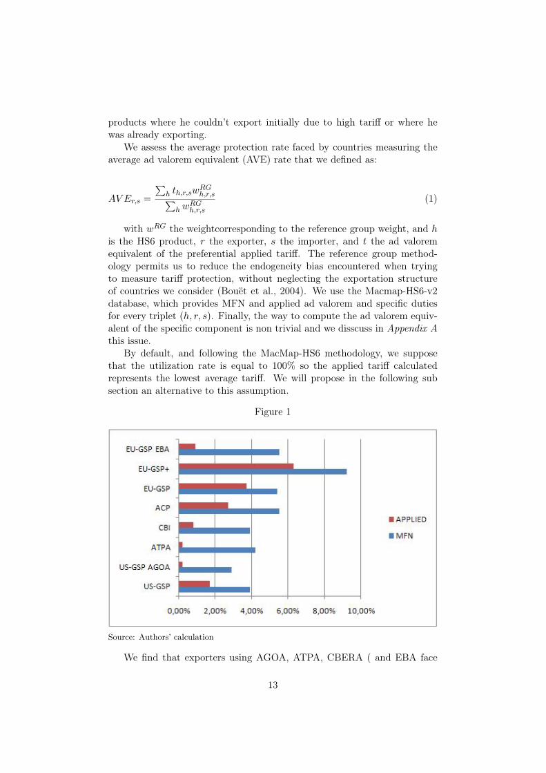
By default, and following the MacMap-HS6 methodology, we supposethat the utilization rate is equal to 100% so the applied tariff calculatedrepresents the lowest average tariff. We will propose in the following subsection an alternative to this assumption.

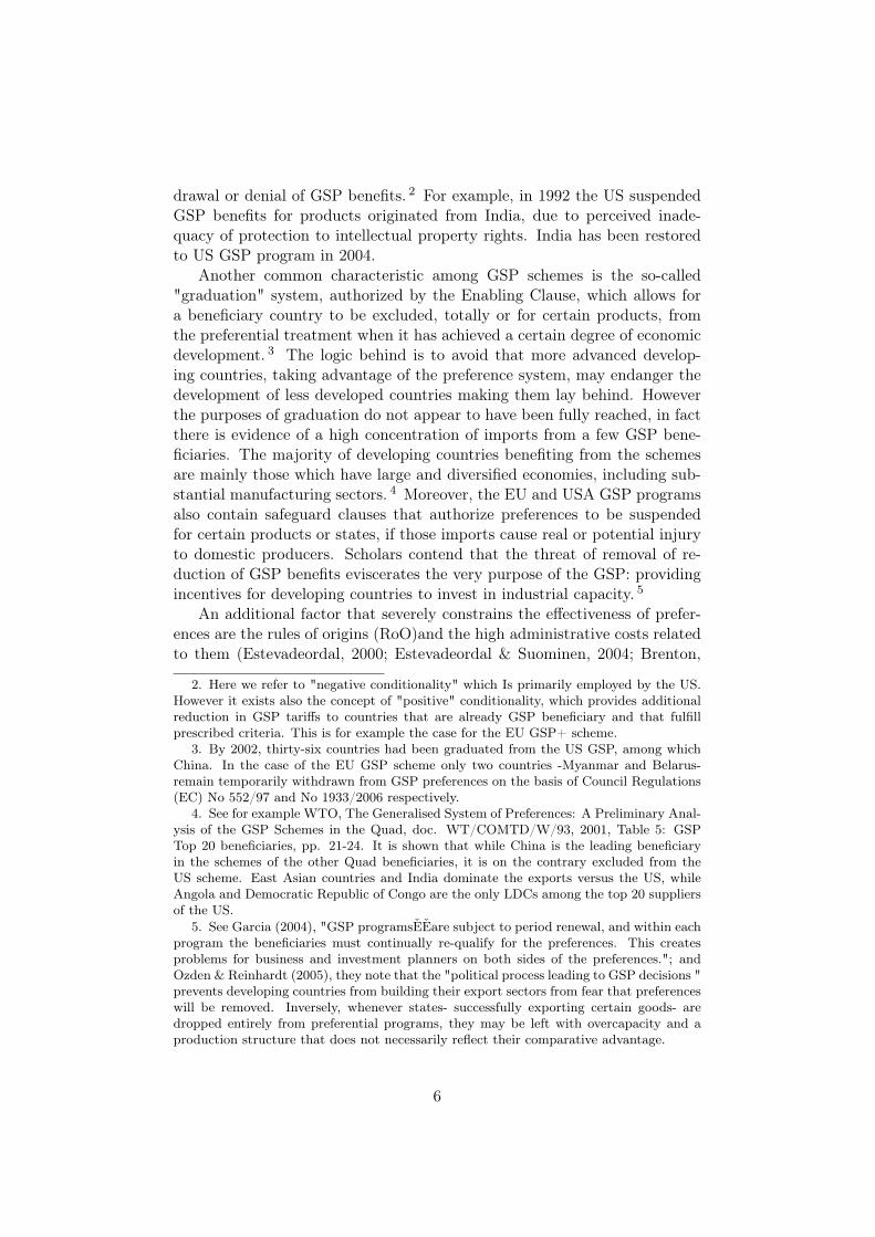
Figure 1

Source: Authors’ calculation

We find that exporters using AGOA, ATPA, CBERA ( and EBA face

13

very low tariff, less than 1% in average. But, as some authors have pointedit out, trade under preferential agreement entering the United States or theEU is very low in value. In 2002, imports under non reciprocal preferencesaccounted for about 18% (12164 M$) of total imports of EU in agrofoodsector, whereas it was only 6% (3541 M$) for the US (Bureau et al., 2007).The same year, 85% of eligible products under AGOA entered duty free(dutiable otherwise) in the US, but accounted for only 137 M$ - 0.23% fromtotal US agro-food imports- (Bureau et al., 2007; ?).

3.2.2 Beyond the average apparent rate of protection

The average AVE equivalent computed previously could be misleading incross-country comparison. Indeed, the product mix matters and two coun-tries facing the same preferential scheme will face different average rate ofprotection due to product specialisation. Precisely in 1, two countries withdifferent export structure but belonging to the same preferential scheme willface the same th,r,s but different wRG

h,r,s. Therefore, it is crucial to disentanglethe apparent preferential margins (APMr,s = AV E.,s − AV Er,s) resultingfrom the composition effects to the preferential margins computed at thetariff line level by comparison between the MFN rate 29 and the preferentialrate:

PMr,s =∑

h (MFNh,r,s − th,r,s)wh,r,s∑hwh,r,s

(2)

=∑

hMFNh,r,swh,r,s −∑

h th,r,swh,r,s∑hwh,r,s

The preferential margin informs us about the tariff reduction which hasbeen provided to a country, but it doesn’t give information about the consid-ered preference relative to the other prefered exporters. Due to the multipli-cation of preferential schemes, this aspect is not trivial. Having a preferentialaccess for a product where the MFN rate is 0 has no value but having a pref-erential access for a product where all other exporters have a preferentialaccess do not imply positive discrimination neither. Moreover, in this lattercase the issue of preference erosion will be less important. We introduceEPMh,r,s, the effective preferential margin computed as the difference be-tween the average duty faced by other exporting countries and the duty facedby the country r, when exporting to s:

EPMh,r,s =

∑m 6=r th,m,swh,m,s∑

m 6=r wh,m,s− th,r,s (3)

29. The procedure to compute the ad valorem equivalent of the MFN rate in this com-putation is detailed in Appendix A.

14

We now calculate the relative margin as

RMr,s =∑

h δth,r,swh,r,s∑hwh,r,s

This gives us a good indicator to know about the effective preferencesgiven to countries.

Finally, even if the previous indicators have interesting descriptive prop-erties, they are not a powerful measure of the effect of the preferences. Inaddition, we propose a Mercantilist Preferential Indicator, based on the ap-proach of the Mercantilist Trade Restrictevness Index of Anderson and Neary(1995). Based on the standard representation of international trade throughthe Armington assumption (1969), we can compute an homogeneous aver-age preferential margin, expressed as percentage of the MFN rate, that willdeliver the same market access than actual heterogeneous preferences. Com-pared to previous ones, this measure is theroretically founded and capturethe role of relative preferences and initial market access shares.

TO BE INCLUDED

15

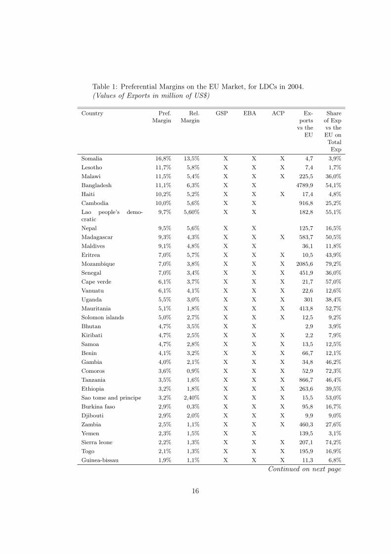
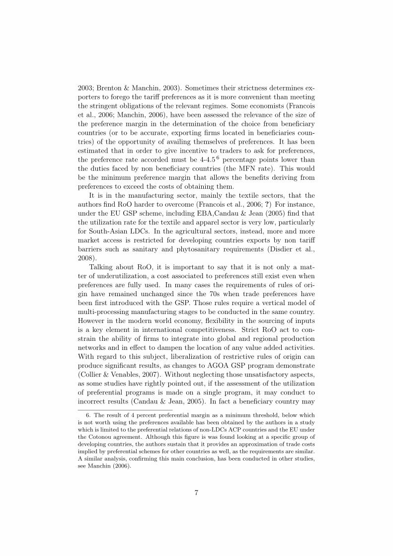
Table 1: Preferential Margins on the EU Market, for LDCs in 2004.(Values of Exports in million of US$)

Country Pref.Margin

Rel.Margin

GSP EBA ACP Ex-portsvs the

EU

Shareof Expvs theEU onTotalExp

Somalia 16,8% 13,5% X X X 4,7 3,9%Lesotho 11,7% 5,8% X X X 7,4 1,7%Malawi 11,5% 5,4% X X X 225,5 36,0%Bangladesh 11,1% 6,3% X X 4789,9 54,1%Haiti 10,2% 5,2% X X X 17,4 4,8%Cambodia 10,0% 5,6% X X 916,8 25,2%Lao people’s demo-cratic

9,7% 5,60% X X 182,8 55,1%

Nepal 9,5% 5,6% X X 125,7 16,5%Madagascar 9,3% 4,3% X X X 583,7 50,5%Maldives 9,1% 4,8% X X 36,1 11,8%Eritrea 7,0% 5,7% X X X 10,5 43,9%Mozambique 7,0% 3,8% X X X 2085,6 79,2%Senegal 7,0% 3,4% X X X 451,9 36,0%Cape verde 6,1% 3,7% X X X 21,7 57,0%Vanuatu 6,1% 4,1% X X X 22,6 12,6%Uganda 5,5% 3,0% X X X 301 38,4%Mauritania 5,1% 1,8% X X X 413,8 52,7%Solomon islands 5,0% 2,7% X X X 12,5 9,2%Bhutan 4,7% 3,5% X X 2,9 3,9%Kiribati 4,7% 2,5% X X X 2,2 7,9%Samoa 4,7% 2,8% X X X 13,5 12,5%Benin 4,1% 3,2% X X X 66,7 12,1%Gambia 4,0% 2,1% X X X 34,8 46,2%Comoros 3,6% 0,9% X X X 52,9 72,3%Tanzania 3,5% 1,6% X X X 866,7 46,4%Ethiopia 3,2% 1,8% X X X 263,6 39,5%Sao tome and principe 3,2% 2,40% X X X 15,5 53,0%Burkina faso 2,9% 0,3% X X X 95,8 16,7%Djibouti 2,9% 2,0% X X X 9,9 9,0%Zambia 2,5% 1,1% X X X 460,3 27,6%Yemen 2,3% 1,5% X X 139,5 3,1%Sierra leone 2,2% 1,3% X X X 207,1 74,2%Togo 2,1% 1,3% X X X 195,9 16,9%Guinea-bissau 1,9% 1,1% X X X 11,3 6,8%

Continued on next page

16

Country Pref.Margin

Rel.Margin

GSP EBA ACP Ex-portsvs the

EU

Shareof Expvs theEU onTotalExp

Sudan 1,8% 1,0% X X X 292,7 5,0%Niger 1,4% 1,1% X X X 220 41,0%Afghanistan 1,0% 0,7% X X 39,6 18,0%Liberia 1,0% 0,6% X X X 1045,5 74,5%Guinea 0,9% 0,5% X X X 489,3 43,4%Burundi 0,7% 0,5% X X X 26,8 26,8%Chad 0,6% 0,3% X X X 245,8 32,2%Central african repub-lic

0,5% 0,40% X X X 147,5 75,5%

Rwanda 0,5% 0,4% X X X 36,9 13,5%Congo (democraticrep,)

0,4% 0,20% X X X 920,6 70,9%

Equatorial guinea 0,4% 0,1% X X X 831,1 33,3%Mali 0,4% 0,3% X X X 260,9 24,5%Angola 0,2% 0,1% X X X 1442,7 17,1%Myanmar 0,1% -3,8% X X 478,8 21,9%

Source: Authors’ calculations using MAcMap-HS6-v2.

17

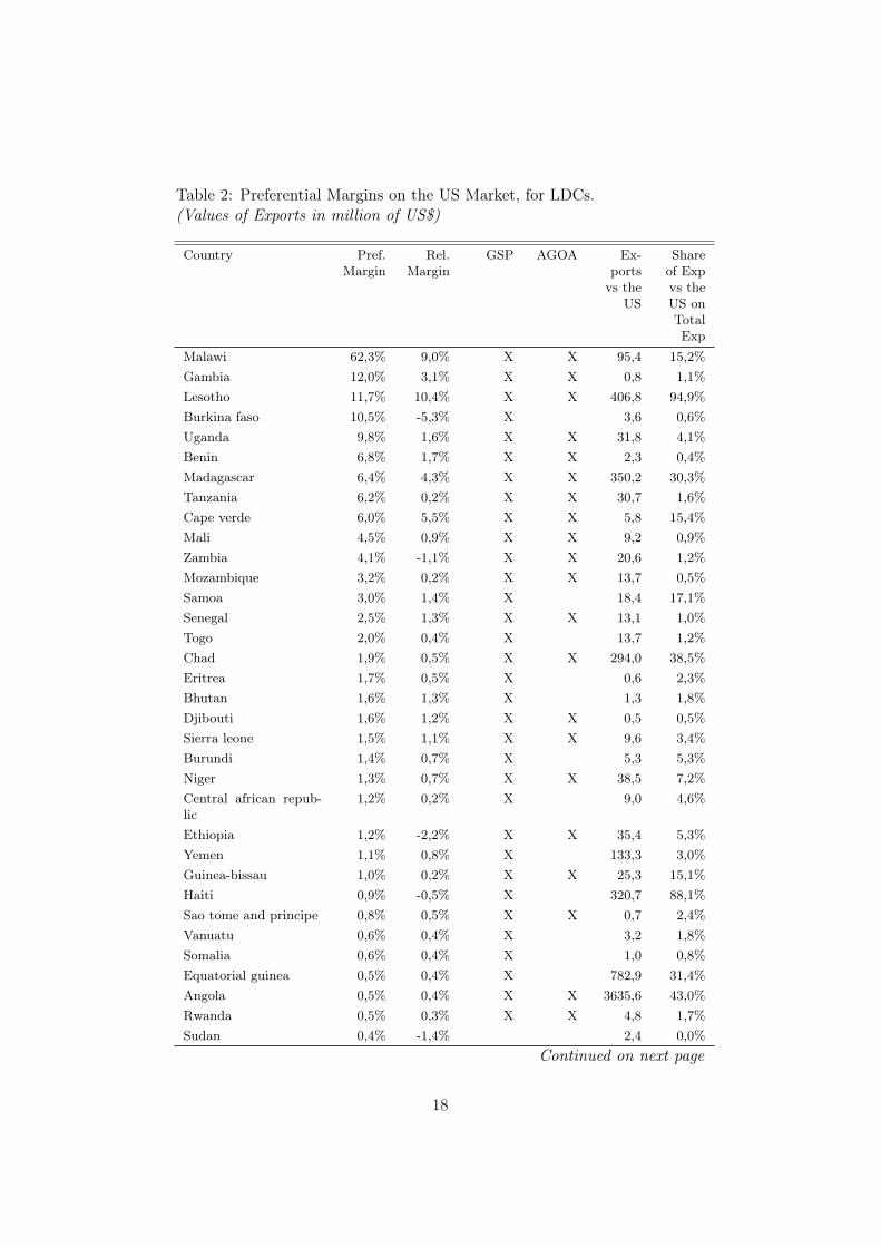
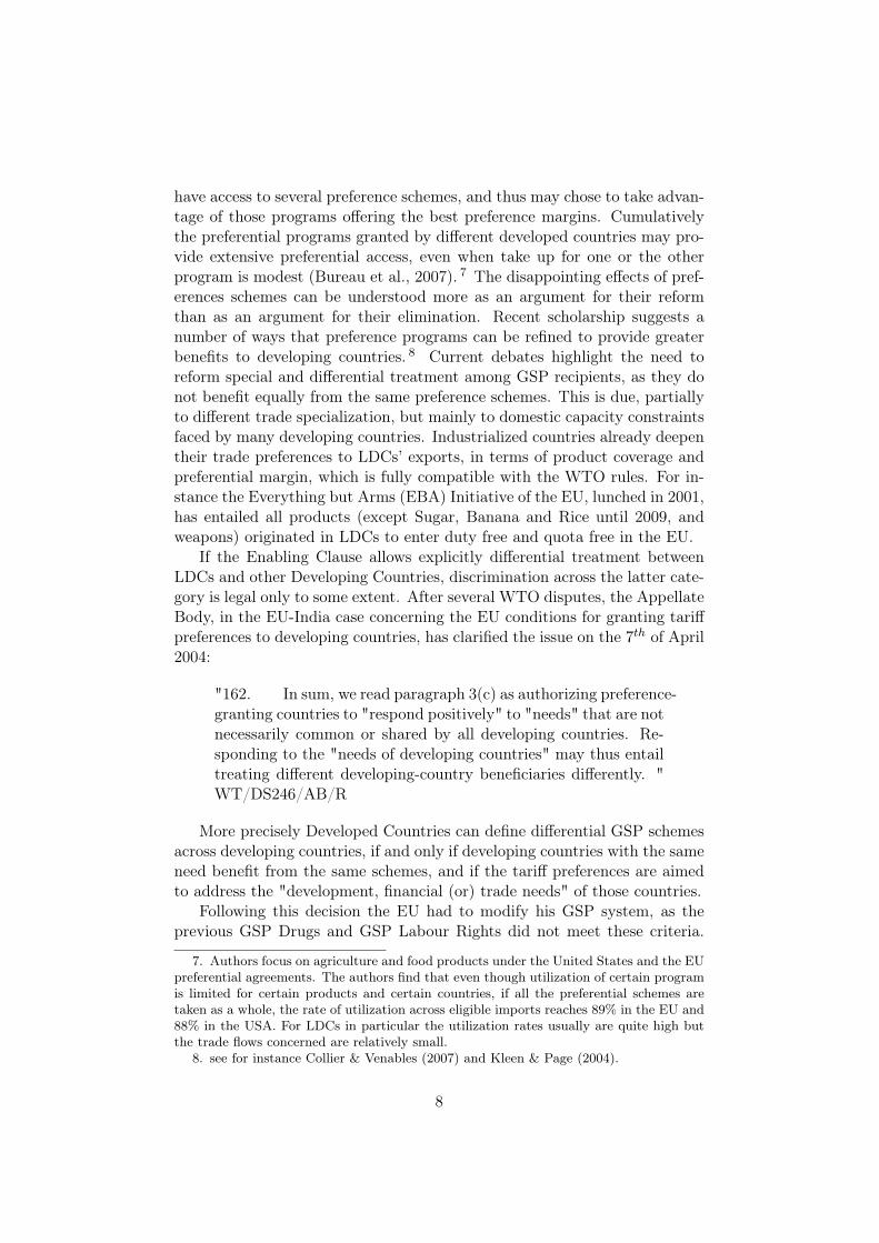
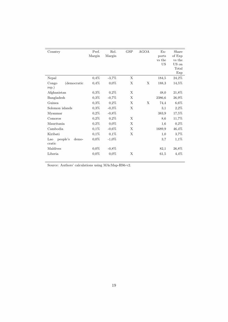
Table 2: Preferential Margins on the US Market, for LDCs.(Values of Exports in million of US$)

Country Pref.Margin

Rel.Margin

GSP AGOA Ex-portsvs the

US

Shareof Expvs theUS onTotalExp

Malawi 62,3% 9,0% X X 95,4 15,2%Gambia 12,0% 3,1% X X 0,8 1,1%Lesotho 11,7% 10,4% X X 406,8 94,9%Burkina faso 10,5% -5,3% X 3,6 0,6%Uganda 9,8% 1,6% X X 31,8 4,1%Benin 6,8% 1,7% X X 2,3 0,4%Madagascar 6,4% 4,3% X X 350,2 30,3%Tanzania 6,2% 0,2% X X 30,7 1,6%Cape verde 6,0% 5,5% X X 5,8 15,4%Mali 4,5% 0,9% X X 9,2 0,9%Zambia 4,1% -1,1% X X 20,6 1,2%Mozambique 3,2% 0,2% X X 13,7 0,5%Samoa 3,0% 1,4% X 18,4 17,1%Senegal 2,5% 1,3% X X 13,1 1,0%Togo 2,0% 0,4% X 13,7 1,2%Chad 1,9% 0,5% X X 294,0 38,5%Eritrea 1,7% 0,5% X 0,6 2,3%Bhutan 1,6% 1,3% X 1,3 1,8%Djibouti 1,6% 1,2% X X 0,5 0,5%Sierra leone 1,5% 1,1% X X 9,6 3,4%Burundi 1,4% 0,7% X 5,3 5,3%Niger 1,3% 0,7% X X 38,5 7,2%Central african repub-lic

1,2% 0,2% X 9,0 4,6%

Ethiopia 1,2% -2,2% X X 35,4 5,3%Yemen 1,1% 0,8% X 133,3 3,0%Guinea-bissau 1,0% 0,2% X X 25,3 15,1%Haiti 0,9% -0,5% X 320,7 88,1%Sao tome and principe 0,8% 0,5% X X 0,7 2,4%Vanuatu 0,6% 0,4% X 3,2 1,8%Somalia 0,6% 0,4% X 1,0 0,8%Equatorial guinea 0,5% 0,4% X 782,9 31,4%Angola 0,5% 0,4% X X 3635,6 43,0%Rwanda 0,5% 0,3% X X 4,8 1,7%Sudan 0,4% -1,4% 2,4 0,0%

Continued on next page

18

Country Pref.Margin

Rel.Margin

GSP AGOA Ex-portsvs the

US

Shareof Expvs theUS onTotalExp

Nepal 0,4% -3,7% X 184,5 24,2%Congo (democraticrep.)

0,4% 0,0% X X 188,3 14,5%

Afghanistan 0,3% 0,2% X 48,0 21,8%Bangladesh 0,3% -0,7% X 2386,6 26,9%Guinea 0,3% 0,2% X X 74,4 6,6%Solomon islands 0,3% -0,3% X 3,1 2,2%Myanmar 0,2% -0,8% 383,9 17,5%Comoros 0,2% 0,2% X 8,6 11,7%Mauritania 0,2% 0,0% X 1,6 0,2%Cambodia 0,1% -0,6% X 1689,9 46,4%Kiribati 0,1% 0,1% X 1,0 3,7%Lao people’s demo-cratic

0,0% -1,0% 3,7 1,1%

Maldives 0,0% -0,8% 82,1 26,8%Liberia 0,0% 0,0% X 61,5 4,4%

Source: Authors’ calculations using MAcMap-HS6-v2.

19

We report in table 2 and 3 the calculations of the preferential and rel-ative margins for LDC, when exporting to the EU or US respectively, withcorresponding trade flows. Although most of the LDC benefit from posi-tive relative preferences, some countries are disadvantaged through the USscheme. Lao’s, Myanmar, the Maldives, East Timor 30 and Sudan are ex-cluded from the US GSP or AGOA for non-economic reasons. Only 0.5%from the Mozambique exports are going to the US, and nearly 50% is com-posed of sugar which is highly taxed. Bangladesh exports for 2200 M$ intextiles or wearing apparel into the US, but doesn’t qualify for AGOA whichcould permit him to export duty-free within the wearing apparel scheme.Nepal, Cambodia and Haiti face the same problem, which lead to a neg-ative relative preference. Myanmar is the only country having a negativepreference through the European Union, the GSP and EBA schemes beingsuspended for political reasons.

For instance, Malawi exported for 170 M$ in other crops (such as tobacco)in the EU and 54 M$ in the US and benefits from a preferential margin to theEU equal to 12.5% and 62% to the EU, which put it among the beneficiarieswhich benefit the most their preferences. On the opposite Nepal has oneof the lowest relative margin when exporting to the US because it exportstextile and apparel that are not covered by the US GSP scheme and. Onthe opposite, theBut it finds duty free market for these products in the EUwith EBA, which explains his 2nd position in our EU ranking.

Relative margin is superior to the preferential margin when the expor-tation structure is in a good coherence with the granted preferences and/orwhen the considered country has a comparative advantage in a covered sec-tor.

To go further in our anlysis of Nepal, we would need to know the utiliza-tion rate of EBA which would tell us how much it enjoys the tariff reductionprovided by the EU 31. This case demonstrates that our results should betaken with care, and completed with the utilization rates of the differentschemes and different products to distinguish between profitable preferencesfrom those which are not.

3.2.3 The use of preferences

Focusing on specific preferential schemes, the litterature has strongly em-phasized the low rate of utilisation of preferences. Cadot et al (2002) et

30. East Timor did not benefit from LDC treatment in 2004 for both the EU and the US.East Timor has joined the United Nation in 2002 but has been recognised by UNCTADonly in 2004. Changes in national trade policies have taken place afterwards.31. If we look at the value of exports to the US and to the EU in 2004 for wearing

apparel and textile, we find that Nepal has exported for 171 M$ in US, and 92 M$ in EU: it is not possible for us to know if Nepal would like to export more in EU because ofbetter tariffs but facing lesser demand, or if the rules of origin made impossible to tradeunder EBA with EU, EU and US being then equal in tariff

20

Anson et al (2004) assess that the cost of compliance to the rules of origin inthe NAFTA agreements for the Mexican textile and automobile companiesis close to the preferential margins and therefore, the value of the agreementis very low. Brenton and Manchin (2003) focusing on the FTAs betweenthe EU15 and CEECs reach similar conclusions and find a very poor utilisa-tion of preferences. Similar results are found for non-reciprocal preferences.Brenton (2003) shows that the EU’s EBA preferences are weakly uses andMattoo et al. (2003) draw the same conclusions for the US AGOA. Basedon these conclusions, the preferences appears to have nearly no value andit will explain why beneficial countries have not managed to seize the gainsrelated to the apparent market access concessions.

However, Gallezot (2003), Gallezot and Aussilloux (2006) and Candauand Jean (2005) underline the fact that looking at only one preferentialscheme is misleading. In particular in the case of EU preferences, overlappingschemes authorize countries to be eligible to different programs and even ifthe use of preferences is relatively limited for one specific scheme the overallpicture is quite different: except for textile and clothing, the utilization ofpreferences is above 70% for developing countries export to the EU (Candauand Jean, 2005).

TO BE INCLUDED GRAPHS: DISTRIBUTION ON THE USE OFPREFERENCES FOR US and EU + comments

21

4 The modelling framework

Based on previous remarks, we asses the value of exisiting unilateral pref-erences of the EU and the US using a CGE assessing alternatively full andimperfect utilization of preferences. Since preferential margins display a largeheterogeneity accross products, we decide to implement recent developmentin CGE modelling to simulate trade shocks at the tariff line level.

4.1 Characteristics of the model

The model we use is the multi-region, multi-sector general equilibrium model,nicknamed MIRAGE, developed by the CEPII to assess the impact of tradepolicy analysis (see Decreux & Valin, 2007). MIRAGE has a sequentialdynamic recursive set-up and imperfect competition modelling. However,being interested in detailed trade flow modelling, which is very demandingin computational power, we work only in comparative static and perfectcompetition. With respect to macroeconomic closure, the current balance isassumed to be exogenous and equal to its initial value in real terms, whilereal exchange rates are endogenous.

Each sector is modelled as a representative firm whose production func-tion requires in fixed shares, value-added and intermediate consumptions.The value-added is a bundle of imperfectly substitutable primary factors(capital, skilled and unskilled labour, land and natural resources), whichare in fixed supply. The structure of value added is intended to take intoaccount the well-documented skill-capital relative complementarity. Thesetwo-factors are thus bundled separately, with a lower elasticity of substi-tution, while a higher substitutability is assumed between this bundle andother factors.

Capital stock is assumed to be perfectly mobile across sectors, whichrepresents the long run adjusting possibilities of capital market. Skilledand unskilled labour are perfectly mobile across sectors, except for unskilledlabour, which is imperfectly mobile between agricultural and other sectors.Land is assumed to be imperfectly mobile between agricultural sectors. Fi-nally, natural resources are sector specific.

A representative consumer saves, in each region, a fixed part of his in-come. The rest is spent between sectors according to a LES-CES function.He distinguishes products according to their geographical sources (Arming-ton hypothesis). The model uses GTAP Armington elasticities estimated inHertel et al. (2007).

4.2 Modelling trade at a detailed level

We decided to rely on the same modelling presented by Gouel et al. (2008).That is a genral equilibriul model at a detailed level, covering all the 5,113

22

HS6 products, not only agricoltural ones. The demand side is a simple nestedCES structure as proposed by Gohin & Laborde (2006). The consumerarbitrates between domestic consumption and imports at the GTAP level.He then chooses its level of imports of each product at the HS6 level. Finally,he selects the country source of his imports.

Detailed trade flows modelling is presented in table 3. Subscript i de-notes the aggregated sector level; h the disaggregated sector; and r and s,respectively, the source and destination regions. Once the representativeconsumer has chosen its level of consumption of the aggregate product Ca

i,s,he decides the amount of domestic good and imports,Ma

i,s. Equation ??represents this Armington assumption; imports of an aggregated productdepend on its price, PM

i,s , the price of domestic product, PDi,s and the chosen

level of consumption.The consumer then determines the imports of detailed products, Md

h,s,as a CES function of prices of detailed products from the same compositesector and the demand for imports of the composite sector (see equation??). Consequently, we can define the composite import price as a CES priceaggregate of detailed import prices (equation ??).

Equation ?? expresses the allocation of disaggregated imports betweenthe various sources. This is arbitraged through a CES function, which de-pends on the detailed bilateral prices, PMBil

h,r,s , and the detailed import.The detailed bilateral import price is defined by equation ?? as the sum

of the CIF price times the power of the equivalent ad valorem tariff ( advalorem duty plus the specific tariff converted in ad valorem).

Equation 4 is the market clearing condition for the composite good thatensures the aggregate output is sufficient to cover both domestic demand(aggregate) and exports of the disaggregated goods. We have implicitly madethe hypothesis of infinite elasticity of transformation between sub-sectors.

Table 3: Detailed trade flows modelling

Mai,s = CES

(PD

i,s, PMi,s , C

ai,s

)(4)

Mdh,s = CES

(PMd

h,s ,Mai,s

)(5)

PMd

i,s = PCES(PMd

h,s

)(6)

MBilh,r,s = CES

(PMBil

h,r,s ,Mdh,s

)(7)

PMBil

h,r,s = PCIFh,r,s

(1 + τAV E

h,r,s

)(8)

Y ai,r = Da

i,r +∑h∈i,s

MBilh,r,s (9)

For computational reasons we cannot use the modelling of TRQs pro-

23

posed by Gouel et al. (2008). Here a quota rent, whenever is generated, iscalculated exogenously at a detail level. We assume that the sum of thequota rents are accrued to the importing country.

As emphasized by Gohin & Laborde (2006), the CES nesting is veryweak to implement disaggregated modelling. This functional form presenttwo main limits, in particular when initial level of protection are high:

1. At a detailed level, the zero trade flows are numerous. The CES willmaintain this pattern and exclude any trade flows creation.

2. At the opposite, the presence of tariff peaks and significant initial tradeflows drive an explosive behaviour when liberalization is implementeddue to an increasing import demand elasticities.

However, both limits do not affect our analysis since we do not imple-ment a tariff liberalization starting from high or prohibitive tariffs but thecontrary. We start from a situation where trade matrix is filled and wherewe implement tariff increase. Still, some limits of the CES remains and theproblem of initial zero is replaced by the impossibility to reach final zero. Wemay slightly underestimate the cost of loosing preferences but as illustratedby Gohin & Laborde (2006), the problem of the CES in this situation (risingtrade costs) is much limited.

4.3 The data

For the data, we made use of a large set of sources. The main source remainsthe GTAP database (version 7 prerelease 4). It provides social accountingmatrixes necessary to calibrate the MIRAGE model for the year 2004. Bi-lateral trade at the HS6 level is based on BACI database (Gaulier et al.,2008). 32 GTAP trade data are, however, reconciled by Mark Gehlhar usingmethods different from those used with BACI, which implies that the datacannot perfectly match. Consequently, we rescale BACI’s trade flows to fitwith GTAP’s ones. For this particular study, we represent trade flows at theHS6 level for all imports from the EU and the USA, that is 5113 tariff lines.

The detailed trade flows modelling relies on two parameters. For thesubstitutability between products at the HS6 level, we take 1.2, an elasticitysuperior to the one used at the GTAP level, because we expect products tobe slightly more substitutable at this level inside a GTAP sector. 33. This isa very rough assumption but econometrics litterature do not provide robustestimates on this issue for a large set of sectors. GTAP dataset includesestimates of elasticities of substitution between sources of importation at

32. BACI is CEPII’s database for international trade flows at the product-level. It pro-vides reconciled values, quantities and unit values based on United Nations COMTRADE33. Grant et al. (2007) use an unitary elasticity to model the demand across HS6 lines

of dairy products.

24

the sector level. We think the more detailed the sector, the bigger the sub-stitution between sources. Consequently, we augment GTAP estimates forelasticities of substitution between sources by 20% and use them at the HS6level.

Trade protection policy are taken from the Market Access Maps (MAcMap-HS6) dataset version 2 . It contains, among other things, bilateral appliedprotection, including preferential provisons (e.g. GSP, FTAs) for 166 coun-tries with more than 208 partners for the year 2004. Specific and compoundtariffs and TRQ data (in and out of quota tariffs, quota levels, quota primesand imports under TRQs) are also provided at the HS6 level. Consider-ing TRQs, multilateral and preferential, are concerted in bilateral TRQs byHS6 product. Multilateral TRQs opened to all WTO members are allocatedamong them according to their bilateral trade.

For the European and the US protection, we keep protection at the HS6level. For all the (Boumellassa, Laborde and Mitaritonna, 2009) other im-porters we applied AVE tariffs aggregated at the GTAP level, using the ref-erence group weighting scheme developed for MAcMap (Bouët et al., 2004).Moreover quota rents, whenever existing, are summed up at the GTAP level.

For the other forms of trade distortive policies contained in the model, ex-port subsidies and domestic support, they come from the GTAP database 34

However GTAP 7 pre-release 4 still requires some adjustments concerningexport subsidies. For the EU27 we rely on updated information on Europeanexport subsidies from EAGGF (European Commission, 2005). The socialaccounting matrix balancing is done by increasing the bilateral exports atmarket prices, which we compensate by diminishing domestic demand inorder to keep production constant.

Without further detailed informations about export subsidies and trans-port demand per unit, we assume they are identical to those of the aggregatedsectors. We take the GTAP value for both parameters. Hence, CIF price isdefined at the GTAP level and not at the HS6 level.

4.4 Countries and sectors aggregation

As said, for the study the Mirage model is calibrated on the GTAP database(version 7 prerelease 4) which provides input-output data for 106 regions and57 sectors. For this study we have defined a specific aggregation betweenregions (20) and sectors (22), to keep the modelŠs size at a computationallyreasonable level.

4.4.1 Countries

For the regional aggregation we try to put togheter countries that facesilmilar tariffs when exporting versus the EU or the USA. A particular em-

34. GTAP domestic support data are based on OECD PSE 2005.

25

phasis is given to developing countries, 17 out of 20 are in fact developingor LDCs countries. Unfortunately the 50 LDCs countries, as defined by theUN, 35 are not yet disaggregated in the GTAP database; they are often in-cluded in larger sub regions many or which are made-up of both LDCs or De-veloping Countries. Consequently we decided to follow the World Bank clas-sifications and we divided the 20 regions in three sub-groups: High-Inocmecountries, Middle-Income countries and Low-income countries. 36 Obviously,whenever possible we keep a part LDCs countries within the Low-Income cat-egory. Finally as for H-I countries, they have been put all together, exceptHong Kong which is in the China group, and the EU-27 and the USA.

The aggregation code and the mapping between GTAP regions and ourgroups is provided in table 4.

4.4.2 Sectors

To choose the sectoral aggregation, we take into consideration sectors wherenon reciprocal preferences are relevant, notably in agriculture and in a smallnumber of industries. 37

The retained sectoral aggregation is presented in table 5.It leads us to a relatively few categories of products both for the US and

the EU.

35. See the UN classifcation on the web site http://www.un.org/speciall-rep/ohrlls/ldc/list.htm.36. The World Bank income group limits are $905 or less 2006 GNI per capita for

low-income, $906–$11,115 for middle-income,and $11,116 or more for high-income.37. For the latter they are essentially textiles and clothes.

26

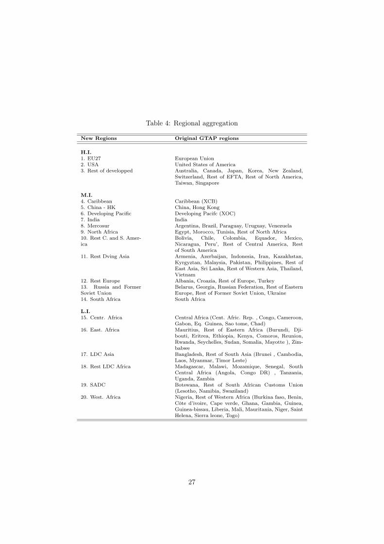
Table 4: Regional aggregation

New Regions Original GTAP regions

H.I.1. EU27 European Union2. USA United States of America3. Rest of developped Australia, Canada, Japan, Korea, New Zealand,

Switzerland, Rest of EFTA, Rest of North America,Taiwan, Singapore

M.I.4. Caribbean Caribbean (XCB)5. China - HK China, Hong Kong6. Developing Pacific Developing Pacifc (XOC)7. India India8. Mercosur Argentina, Brazil, Paraguay, Uruguay, Venezuela9. North Africa Egypt, Morocco, Tunisia, Rest of North Africa10. Rest C. and S. Amer-ica

Bolivia, Chile, Colombia, Equador, Mexico,Nicaragua, Peru’, Rest of Central America, Restof South America

11. Rest Dving Asia Armenia, Azerbaijan, Indonesia, Iran, Kazakhstan,Kyrgyztan, Malaysia, Pakistan, Philippines, Rest ofEast Asia, Sri Lanka, Rest of Western Asia, Thailand,Vietnam

12. Rest Europe Albania, Croazia, Rest of Europe, Turkey13. Russia and FormerSoviet Union

Belarus, Georgia, Russian Federation, Rest of EasternEurope, Rest of Former Soviet Union, Ukraine

14. South Africa South Africa

L.I.15. Centr. Africa Central Africa (Cent. Afric. Rep. , Congo, Cameroon,

Gabon, Eq. Guinea, Sao tome, Chad)16. East. Africa Mauritius, Rest of Eastern Africa (Burundi, Dji-

bouti, Eritrea, Ethiopia, Kenya, Comoros, Reunion,Rwanda, Seychelles, Sudan, Somalia, Mayotte ), Zim-babwe

17. LDC Asia Bangladesh, Rest of South Asia (Brunei , Cambodia,Laos, Myanmar, Timor Leste)

18. Rest LDC Africa Madagascar, Malawi, Mozamique, Senegal, SouthCentral Africa (Angola, Congo DR) , Tanzania,Uganda, Zambia

19. SADC Botswana, Rest of South African Customs Union(Lesotho, Namibia, Swaziland)

20. West. Africa Nigeria, Rest of Western Africa (Burkina faso, Benin,Côte d’ivoire, Cape verde, Ghana, Gambia, Guinea,Guinea-bissau, Liberia, Mali, Mauritania, Niger, SaintHelena, Sierra leone, Togo)

27

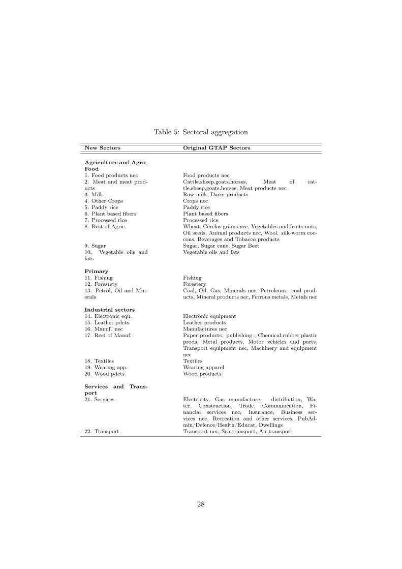
Table 5: Sectoral aggregation

New Sectors Original GTAP Sectors

Agriculture and Agro-Food1. Food products nec Food products nec2. Meat and meat prod-ucts

Cattle.sheep.goats.horses, Meat of cat-tle.sheep.goats.horses, Meat products nec

3. Milk Raw milk, Dairy products4. Other Crops Crops nec5. Paddy rice Paddy rice6. Plant based fibers Plant based fibers7. Processed rice Processed rice8. Rest of Agric. Wheat, Cerelas grains nec, Vegetables and fruits nuts,

Oil seeds, Animal products nec, Wool. silk-worm coc-cons, Beverages and Tobacco products

9. Sugar Sugar, Sugar cane, Sugar Beet10. Vegetable oils andfats

Vegetable oils and fats

Primary11. Fishing Fishing12. Forestery Forestery13. Petrol, Oil and Min-erals

Coal, Oil, Gas, Minerals nec, Petroleum. coal prod-ucts, Mineral products nec, Ferrous metals, Metals nec

Industrial sectors14. Electronic equ. Electronic equipment15. Leather pdcts. Leather products16. Manuf. nec Manufactures nec17. Rest of Manuf. Paper products. publishing , Chemical.rubber.plastic

prods, Metal products, Motor vehicles and parts,Transport equipment nec, Machinery and equipmentnec

18. Textiles Textiles19. Wearing app. Wearing apparel20. Wood pdcts. Wood products

Services and Trans-port21. Services Electricity, Gas manufacture. distribution, Wa-

ter, Construction, Trade, Communication, Fi-nancial services nec, Insurance, Business ser-vices nec, Recreation and other services, PubAd-min/Defence/Health/Educat, Dwellings

22. Transport Transport nec, Sea transport, Air transport

28

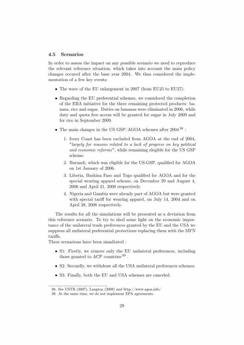
4.5 Scenarios

In order to assess the impact on any possible scenario we need to reproducethe relevant reference situation, which takes into account the main policychanges occured after the base year 2004. We thus considered the imple-mentation of a few key events:

• The wave of the EU enlargement in 2007 (from EU25 to EU27).

• Regarding the EU preferential schemes, we considered the completionof the EBA initiative for the three remaining protected products: ba-nans, rice and sugar. Duties on bananas were eliminated in 2006, whileduty and quota free access will be granted for sugar in July 2009 andfor rice in September 2009.

• The main changes in the US GSP/AGOA schemes after 2004 38 :

1. Ivory Coast has been excluded from AGOA at the end of 2004,"largely for reasons related to a lack of progress on key politicaland economic reforms", while remaining elegible for the US GSPscheme.

2. Burundi, which was eligible for the US-GSP, qualified for AGOAon 1st January of 2006.

3. Liberia, Burkina Faso and Togo qualified for AGOA and for thespecial wearing apparel scheme, on December 29 and August 4,2006 and April 21, 2008 respectively.

4. Nigeria and Gambia were already part of AGOA but were grantedwith special tariff for wearing apparel, on July 14, 2004 and onApril 28, 2008 respectively.

The results for all the simulations will be presented as a deviation fromthis reference scenario. To try to shed some light on the economic impor-tance of the unilateral trade preferences granted by the EU and the USA wesuppress all unilateral preferential protections replacing them with the MFNtariffs.Three scenarious have been simultated :

• S1: Firstly, we remove only the EU unilateral preferences, includingthose granted to ACP countries 39 .

• S2: Secondly, we withdraw all the USA unilateral preferences schemes.

• S3: Finally, both the EU and USA schemes are canceled.

38. See USTR (2007), Langton (2008) and http://www.agoa.info/39. At the same time, we do not implement EPA agreements.

29

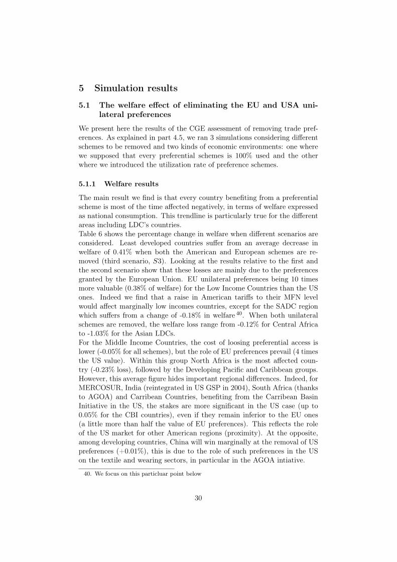
5 Simulation results

5.1 The welfare effect of eliminating the EU and USA uni-lateral preferences

We present here the results of the CGE assessment of removing trade pref-erences. As explained in part 4.5, we ran 3 simulations considering differentschemes to be removed and two kinds of economic environments: one wherewe supposed that every preferential schemes is 100% used and the otherwhere we introduced the utilization rate of preference schemes.

5.1.1 Welfare results

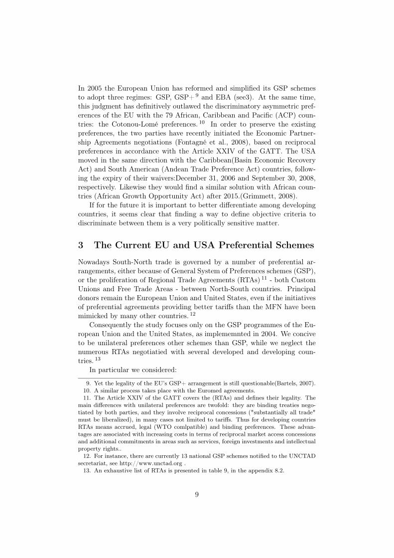
The main result we find is that every country benefiting from a preferentialscheme is most of the time affected negatively, in terms of welfare expressedas national consumption. This trendline is particularly true for the differentareas including LDC’s countries.Table 6 shows the percentage change in welfare when different scenarios areconsidered. Least developed countries suffer from an average decrease inwelfare of 0.41% when both the American and European schemes are re-moved (third scenario, S3). Looking at the results relative to the first andthe second scenario show that these losses are mainly due to the preferencesgranted by the European Union. EU unilateral preferences being 10 timesmore valuable (0.38% of welfare) for the Low Income Countries than the USones. Indeed we find that a raise in American tariffs to their MFN levelwould affect marginally low incomes countries, except for the SADC regionwhich suffers from a change of -0.18% in welfare 40. When both unilateralschemes are removed, the welfare loss range from -0.12% for Central Africato -1.03% for the Asian LDCs.For the Middle Income Countries, the cost of loosing preferential access islower (-0.05% for all schemes), but the role of EU preferences prevail (4 timesthe US value). Within this group North Africa is the most affected coun-try (-0.23% loss), followed by the Developing Pacific and Caribbean groups.However, this average figure hides important regional differences. Indeed, forMERCOSUR, India (reintegrated in US GSP in 2004), South Africa (thanksto AGOA) and Carribean Countries, benefiting from the Carribean BasinInitiative in the US, the stakes are more significant in the US case (up to0.05% for the CBI countries), even if they remain inferior to the EU ones(a little more than half the value of EU preferences). This reflects the roleof the US market for other American regions (proximity). At the opposite,among developing countries, China will win marginally at the removal of USpreferences (+0.01%), this is due to the role of such preferences in the USon the textile and wearing sectors, in particular in the AGOA intiative.

40. We focus on this particluar point below

30

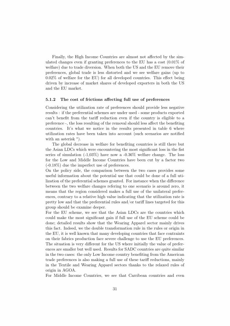
Finally, the High Income Countries are almost not affected by the sim-ulated changes even if granting preferences to the EU has a cost (0.01% ofwelfare) due to trade diversion. When both the US and the EU remove theirpreferences, global trade is less distorted and we see welfare gains (up to0.02% of welfare for the EU) for all developed countries. This effect beingdriven by increase of market shares of developed exporters in both the USand the EU market.

5.1.2 The cost of frictions affecting full use of preferences

Considering the utilization rate of preferences should provide less negativeresults : if the preferential schemes are under used - some products exportedcan’t benefit from the tariff reduction even if the country is eligible to apreference -, the loss resulting of the removal should less affect the benefitingcountries. It’s what we notice in the results presented in table 6 whereutilization rates have been taken into account (such scenarios are notifiedwith an asterisk ∗).

The global decrease in welfare for benefiting countries is still there butthe Asian LDCs which were encountering the most significant loss in the fistseries of simulation (-1,03%) have now a -0.36% welfare change. The lossfor the Low and Middle Income Countries have been cut by a factor two(-0.18%) due the imperfect use of preferences.On the policy side, the comparison between the two cases provides someuseful information about the potential use that could be done of a full uti-lization of the preferential schemes granted. For instance when the differencebetween the two welfare changes refering to one scenario is around zero, itmeans that the region considered makes a full use of the unilateral prefer-ences, contrary to a relative high value indicating that the utilization rate ispretty low and that the preferential rules and/or tariff lines targeted for thisgroup should be examine deeper.For the EU scheme, we see that the Asian LDCs are the countries whichcould make the most significant gain if full use of the EU scheme could bedone; detailed results show that the Wearing Apparel sector mainly drivesthis fact. Indeed, we the double transformation rule in the rules or origin inthe EU, it is well known that many developing countries that face contraintson their fabrics production face severe challenge to use the EU preferences.The situation is very different for the US where initially the value of prefer-ences are smaller but well used. Results for SADC countries are quite similarin the two cases: the only Low Income country benefiting from the Americantrade preferences is also making a full use of these tariff reductions, mainlyin the Textile and Wearing Apparel sectors thanks to the relaxed rules oforigin in AGOA.For Middle Income Countries, we see that Carribean countries and even

31

more MERCOSUR are the main affected by under utilization of preferenceson the US market when India is not. These two regions, with Pacific devel-oping countries, are also the more affected in relative terms by the utilizationrate in the EU. but on this market, all Middle Income strongly affected.On the methodological side, we demonstrate that assuming full use of prefer-ences can strongly overestimate their values and therefore, the potential roleof preference erosion, in particular on the EU market. However, compared toexisting litterature, using a HS6 modeling strategy still lead to large value.

5.2 Changes in international trade for benefiting countries

32

Tab

le6:

Welfare

Cha

nges

(Equ

ivalentvariationin

percentage

chan

ge)

Cou

ntries

S1

S1∗

S2

S2∗

S3

S3∗

1.H

igh

In-

com

e0,

010,

000,

000,

000,

010,

00

EU27

0,01

0,01

0,00

0,00

0,02

0,01

USA

0,00

0,00

0,00

0,00

0,01

0,00

Restof

develope

d0,01

0,00

0,00

0,00

0,01

0,00

2.M

iddle

In-

com

e-0

,04

-0,0

2-0

,01

-0,0

1-0

,05

-0,0

2

Caribbe

an-0,08

-0,03

-0,05

-0,03

-0,13

-0,06

China

-HK

0,00

0,00

0,01

0,01

0,01

0,01

Develop

ing

Pa-

cific

-0,12

-0,05

-0,01

-0,01

-0,13

-0,06

India

-0,03

-0,02

-0,02

-0,02

-0,05

-0,04

Mercosur

-0,05

-0,02

-0,03

-0,01

-0,08

-0,03

North

Africa

-0,23

-0,12

-0,00

-0,00

-0,23

-0,13

Restof

C.an

dS.

America

-0,01

-0,00

-0,00

-0,00

-0,01

-0,00

Rest

ofDving

Asia

-0,07

-0,03

-0,01

-0,01

-0,09

-0,04

Restof

Europ

e-0,02

-0,00

0,00

0,00

-0,02

0,00

Russiaan

dF.S

o-viet

Union

-0,07

-0,02

-0,01

-0,00

-0,08

-0,03

SouthAfrica

-0,00

-0,00

-0,04

-0,03

-0,04

-0,03

3.Low

Inco

me

-0,3

8-0

,15

-0,0

3-0

,02

-0,4

1-0

,18

Centr.Africa

-0,08

-0,03

-0,04

-0,03

-0,12

-0,06

East.

Africa

-0,25

-0,16

-0,03

-0,02

-0,27

-0,18

LDC

Asia

-1,04

-0,37

0,00

0,00

-1,03

-0,36

RestLD

CAfrica

-0,25

-0,11

-0,03

-0,02

-0,28

-0,14

SADC

-0,20

-0,10

-0,18

-0,17

-0,38

-0,27

West.

Africa

-0,19

-0,06

-0,03

-0,03

-0,22

-0,09

Source:Autho

rs’M

IRAGE

mod

elsimulationresults.

Note:

S1:Rem

oval

ofEU

unila

teralp

references,S

2:Rem

oval

ofUSun

ilateralp

references,S

3:Rem

oval

ofbo

thpreferen

ces.

An*indicatesscen

ario

withob

served

useof

preferen

ces.

33

6 Sensitivity analysis

In this section, we test the sensitivity of our results to some key parame-ters. The scenario that we use as a reference is the complete elimination ofunilateral preferences from both the EU and the USA, that is S3.

1. Substitution elasticity in imports between sub-sector products, σi: fromits original value, 1.2, we test by cutting by half and doubling its values,namely an elasticity of either 0.6 or 2.4.

2. Between exporters substitution elasticity, σr: the original values are20% above GTAP import-import elasticity of substitution. Becausewe expect the substitution to rise with the disaggregation, we do nottest a too low value for it. The two alternatives are −25% and +100%.

6.1 Sensitivity of detailed trade flows

6.2 Sensitivity of welfare evaluation

34

7 Conclusion

35

References

(2003). The role of skill endowments in the structure of u.s. outward foreigndirect investment. The Review of Economics and Statistics, 85(3), 726–734. available at http://ideas.repec.org/a/tpr/restat/v85y2003i3p726-734.html.

Bartels (2007). The WTO legality of the EU’s GSP Arrangement. Journalof International Economic Law, 10 (4), 869–886.

Bouët, A., Bureau, J.-C., Decreux, Y., & Jean, S. (2005). Multilateral Agri-cultural Trade Liberalisation: The Contrasting Fortunes of DevelopingCountries in the Doha Round. The World Economy, 28(9), 1329–1354.

Bouët, A., Decreux, Y., Fontagné, L., Jean, S., & Laborde, D. (2004). AConsistent, Ad-Valorem Equivalent Measure of Applied Protection Acrossthe World: The MAcMap-HS6 Database. Working Papers 2004-22, CEPIIresearch center.

Brenton & Manchin (2003). Making EU Trade Agreements Work: The Roleof Rules of Origin. The World Economy, 26, 755–769.

Brenton, P. (2003). Integrating the Least Developed Countries into the WorldTrade System: The Current Impact of EU Preferences under EverythingBut Arms. Policy Research Working Paper 3018, World Bank.

Bureau, J.-C., Chakir, R., & Gallezot, J. (2007). The Utilisation of TradePreferences for Developing Countries in the Agri-food Sector. Journal ofAgricultural Economics, 58(2), 175–198.

Candau, F. & Jean, S. (2005). What Are EU Trade Preferences Worth forSub-Saharan Africa and Other Developing Countries? Working paper05/09, TradeAg.

Collier, P. & Venables, A. J. (2007). Rethinking Trade Preferences: HowAfrica can Diversify its Exports. The World Economy, 30(8), 1326–1345.

Decreux, Y. & Valin, H. (2007). MIRAGE, Updated Version of the Modelfor Trade Policy Analysis Focus on Agriculture and Dynamics. WorkingPapers 2007-15, CEPII research center.

Disdier, Fontagné., & Mimouni (2008). The impact of regulations on agri-cultural trade : evidence from the SPS and TBT agreements. AmericanJournal of Agricultural Economics, 90(2), 336–350.

Estevadeordal (2000). Negotiating Preferential Market Access: The Case ofthe North American Free Trade Agreement. Journal of World Trade, 34,141–66.

36

Estevadeordal & Suominen (2004). Rules of Origin: A World Map and TradeEffects. mimeo, IDB, Washington, D.C.

European Commission (2005). Annexes to 34rd Financial Report - EAGGFGuarantee Section - 2004.

Fontagné, Laborde, & Mitaritonna (2008). An impact Study of the EU-ACP Economic Partnership Agreements in the Six ACP regions. WorkingPaper 4, Cepii.

Francois, J. F., Hoekman, B., & Manchin, M. (2006). Preference Erosion andMultilateral Trade Liberalization. The World Bank Economic Review, 20,Issue 2, 197–216.

Garcia (2004). Beyond Special and Differential Treatment. Boston CollegeInternational and Comparative Law Review of Agricultural Economics, 27,291–317.

Gaulier, G., Zignago, S., Sondjo, D., Sissoko, A. A., & Paillacar, R. (2008).BACI: A World Database of International Trade Analysis at the Product-level 1995-2004 Version. Working paper, CEPII research center. Forth-coming.

Gohin, A. & Laborde, D. (2006). Simulating trade policy reforms at thedetailed level: some practical solutions. In Ninth Annual Conference onGlobal Economic Analysis Addis Ababa, Ethiopia: Purdue University.

Gouel, C., Guillin, A., & Ramos, M. P. (2008). The Effects of Agricul-tural Policies on Developing Countries at a Detail Level. Working paper,TradeAg.

Grant, J. H., Hertel, T., & Rutherford, T. (2007). Extending general equi-librium to the tariff line: U.S. dairy in the Doha Development Agenda. In10th Annual Conference on Global Economic Analysis Purdue University,USA.

Grimmett (2008). Trade Preferences for Developing Countries and the WTO.Crs report for congress, American Law Division.

Hertel, T., Hummels, D., Ivanic, M., & Keeney, R. (2007). How confident canwe be of CGE-based assessments of Free Trade Agreements? EconomicModelling, 24(4), 611–635.

Hoekman & Ozden (2005). Trade Preferences and Differential treatment inDeveloping countries: A selective survey. Policy ResearchWorking Paper3566, World Bank.

Inama, S. (2002). Market Access for LDCs Issues to Be Addressed. Journalof World Trade, 36(1), 85–116.

37

Kleen & Page (2004). Special and Differential Treatment of Developing Coun-tries in the WTO organizazion. Technical report, Report for the Ministryof Foreign Afairs, Sveden.

Laborde, D. (2008). Looking for a meaningful Duty Free Quota Free Mar-ket Access initiative in the Doha Development Agenda. ICTSD discusionpaper 4, ICTSD.

Langton, D. (2008). US Trade and Investment Relationship with Sub-SaharanAfrica: The African Growth and Opportunity Act and Beyond. Technicalreport.

Manchin, M. (2006). Preferences utilisation and tariff reduction in EU im-ports from ACP countries. The World Economy, 29(9), 1243–1266.

OECD (2005). Agricultural Policies in OECD Countries : Monitoring andEvaluation. OECD Publishing.

Ozden, Ç. & Reinhardt, E. (2005). The Perversity of Preferences: GSP andDeveloping Country Policies, 1976-2000. Journal of Development Eco-nomics, 78, 1–21.

USTR (2007). 2007 Comprehensive Report on the US Trade and Invest-ment Policy towards Sub-Saharan Africa and Africa and Implementationof the African Growth and Opportunity Act. Technical report, Office ofthe United States Trade Representative.

38

8 appendix

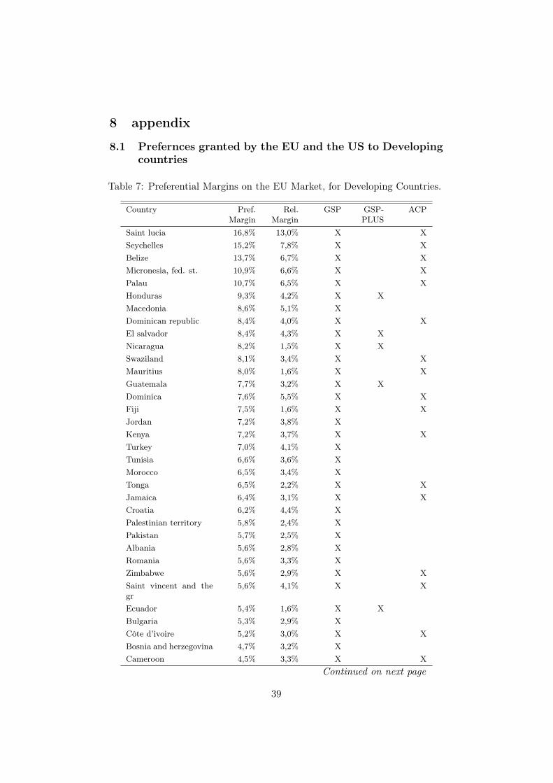
8.1 Prefernces granted by the EU and the US to Developingcountries

Table 7: Preferential Margins on the EU Market, for Developing Countries.

Country Pref.Margin

Rel.Margin

GSP GSP-PLUS

ACP

Saint lucia 16,8% 13,0% X XSeychelles 15,2% 7,8% X XBelize 13,7% 6,7% X XMicronesia, fed. st. 10,9% 6,6% X XPalau 10,7% 6,5% X XHonduras 9,3% 4,2% X XMacedonia 8,6% 5,1% XDominican republic 8,4% 4,0% X XEl salvador 8,4% 4,3% X XNicaragua 8,2% 1,5% X XSwaziland 8,1% 3,4% X XMauritius 8,0% 1,6% X XGuatemala 7,7% 3,2% X XDominica 7,6% 5,5% X XFiji 7,5% 1,6% X XJordan 7,2% 3,8% XKenya 7,2% 3,7% X XTurkey 7,0% 4,1% XTunisia 6,6% 3,6% XMorocco 6,5% 3,4% XTonga 6,5% 2,2% X XJamaica 6,4% 3,1% X XCroatia 6,2% 4,4% XPalestinian territory 5,8% 2,4% XPakistan 5,7% 2,5% XAlbania 5,6% 2,8% XRomania 5,6% 3,3% XZimbabwe 5,6% 2,9% X XSaint vincent and thegr

5,6% 4,1% X X

Ecuador 5,4% 1,6% X XBulgaria 5,3% 2,9% XCôte d’ivoire 5,2% 3,0% X XBosnia and herzegovina 4,7% 3,2% XCameroon 4,5% 3,3% X X

Continued on next page

39

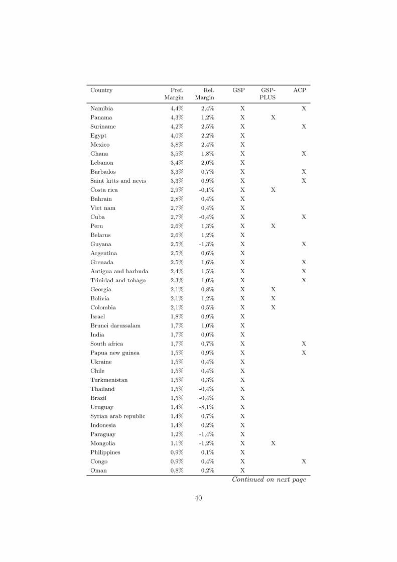
Country Pref.Margin

Rel.Margin

GSP GSP-PLUS

ACP

Namibia 4,4% 2,4% X XPanama 4,3% 1,2% X XSuriname 4,2% 2,5% X XEgypt 4,0% 2,2% XMexico 3,8% 2,4% XGhana 3,5% 1,8% X XLebanon 3,4% 2,0% XBarbados 3,3% 0,7% X XSaint kitts and nevis 3,3% 0,9% X XCosta rica 2,9% -0,1% X XBahrain 2,8% 0,4% XViet nam 2,7% 0,4% XCuba 2,7% -0,4% X XPeru 2,6% 1,3% X XBelarus 2,6% 1,2% XGuyana 2,5% -1,3% X XArgentina 2,5% 0,6% XGrenada 2,5% 1,6% X XAntigua and barbuda 2,4% 1,5% X XTrinidad and tobago 2,3% 1,0% X XGeorgia 2,1% 0,8% X XBolivia 2,1% 1,2% X XColombia 2,1% 0,5% X XIsrael 1,8% 0,9% XBrunei darussalam 1,7% 1,0% XIndia 1,7% 0,0% XSouth africa 1,7% 0,7% X XPapua new guinea 1,5% 0,9% X XUkraine 1,5% 0,4% XChile 1,5% 0,4% XTurkmenistan 1,5% 0,3% XThailand 1,5% -0,4% XBrazil 1,5% -0,4% XUruguay 1,4% -8,1% XSyrian arab republic 1,4% 0,7% XIndonesia 1,4% 0,2% XParaguay 1,2% -1,4% XMongolia 1,1% -1,2% X XPhilippines 0,9% 0,1% XCongo 0,9% 0,4% X XOman 0,8% 0,2% X

Continued on next page

40

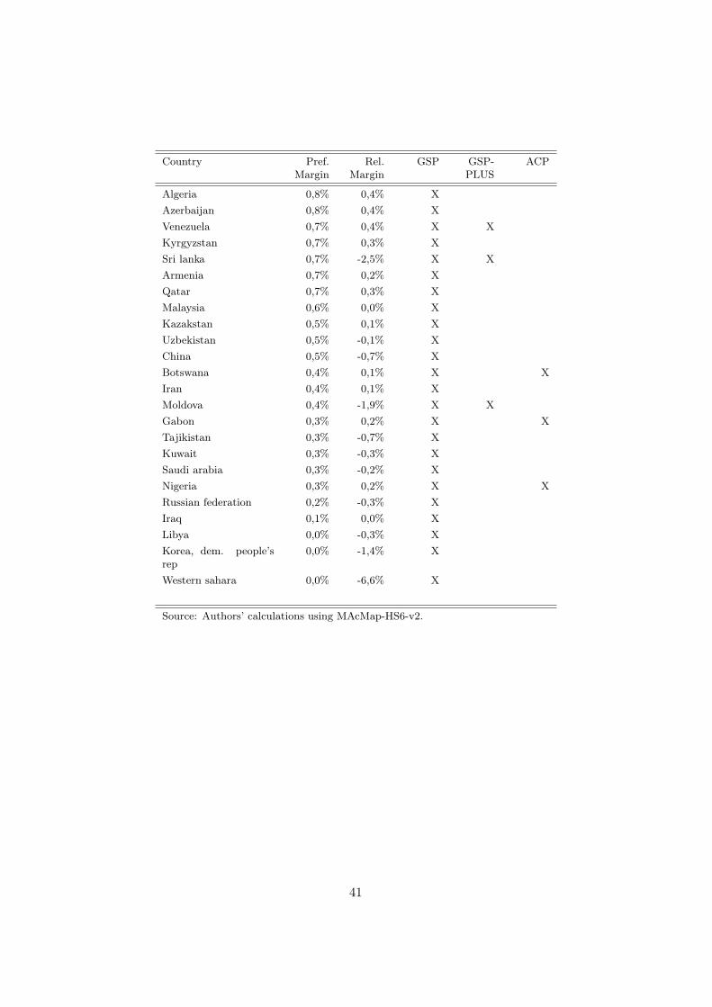
Country Pref.Margin

Rel.Margin

GSP GSP-PLUS

ACP

Algeria 0,8% 0,4% XAzerbaijan 0,8% 0,4% XVenezuela 0,7% 0,4% X XKyrgyzstan 0,7% 0,3% XSri lanka 0,7% -2,5% X XArmenia 0,7% 0,2% XQatar 0,7% 0,3% XMalaysia 0,6% 0,0% XKazakstan 0,5% 0,1% XUzbekistan 0,5% -0,1% XChina 0,5% -0,7% XBotswana 0,4% 0,1% X XIran 0,4% 0,1% XMoldova 0,4% -1,9% X XGabon 0,3% 0,2% X XTajikistan 0,3% -0,7% XKuwait 0,3% -0,3% XSaudi arabia 0,3% -0,2% XNigeria 0,3% 0,2% X XRussian federation 0,2% -0,3% XIraq 0,1% 0,0% XLibya 0,0% -0,3% XKorea, dem. people’srep

0,0% -1,4% X

Western sahara 0,0% -6,6% X

Source: Authors’ calculations using MAcMap-HS6-v2.

41

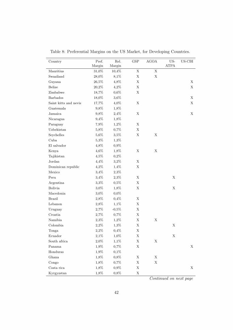
Table 8: Preferential Margins on the US Market, for Developing Countries.

Country Pref.Margin

Rel.Margin

GSP AGOA US-ATPA

US-CBI

Mauritius 31,0% 10,4% X XSwaziland 28,0% 8,1% X XGuyana 26,5% 4,8% X XBelize 20,2% 4,2% X XZimbabwe 18,7% 0,6% XBarbados 18,0% 3,6% XSaint kitts and nevis 17,7% 4,0% X XGuatemala 9,8% 1,8%Jamaica 9,8% 2,4% X XNicaragua 9,4% 1,8%Paraguay 7,9% 1,2% XUzbekistan 5,8% 0,7% XSeychelles 5,6% 3,5% X XCuba 5,3% 1,3%El salvador 4,8% 0,9%Kenya 4,6% 1,8% X XTajikistan 4,5% 0,2%Jordan 4,4% 3,2% XDominican republic 4,2% 1,4% XMexico 3,4% 2,3%Peru 3,4% 2,3% X XArgentina 3,3% 0,5% XBolivia 3,0% 1,8% X XMacedonia 3,0% 0,0%Brazil 2,8% 0,4% XLebanon 2,8% 1,1% XUruguay 2,7% -0,5% XCroatia 2,7% 0,7% XNamibia 2,3% 1,2% X XColombia 2,2% 1,3% X XTonga 2,2% 0,4% XEcuador 2,1% 1,0% X XSouth africa 2,0% 1,1% X XPanama 1,9% 0,7% X XHonduras 1,9% 0,1%Ghana 1,8% 0,8% X XCongo 1,8% 0,7% X XCosta rica 1,8% 0,9% X XKyrgyzstan 1,8% 0,8% X

Continued on next page

42

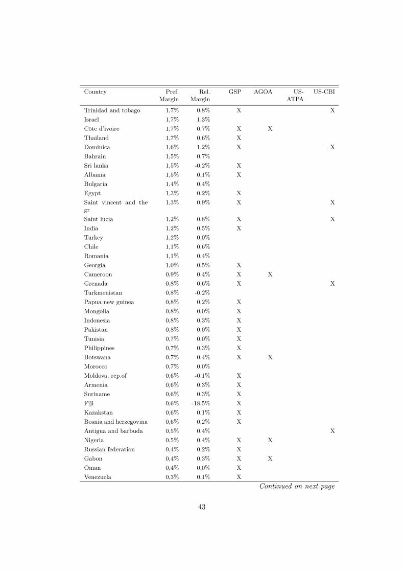
Country Pref.Margin

Rel.Margin

GSP AGOA US-ATPA

US-CBI

Trinidad and tobago 1,7% 0,8% X XIsrael 1,7% 1,3%Côte d’ivoire 1,7% 0,7% X XThailand 1,7% 0,6% XDominica 1,6% 1,2% X XBahrain 1,5% 0,7%Sri lanka 1,5% -0,2% XAlbania 1,5% 0,1% XBulgaria 1,4% 0,4%Egypt 1,3% 0,2% XSaint vincent and thegr

1,3% 0,9% X X

Saint lucia 1,2% 0,8% X XIndia 1,2% 0,5% XTurkey 1,2% 0,0%Chile 1,1% 0,6%Romania 1,1% 0,4%Georgia 1,0% 0,5% XCameroon 0,9% 0,4% X XGrenada 0,8% 0,6% X XTurkmenistan 0,8% -0,2%Papua new guinea 0,8% 0,2% XMongolia 0,8% 0,0% XIndonesia 0,8% 0,3% XPakistan 0,8% 0,0% XTunisia 0,7% 0,0% XPhilippines 0,7% 0,3% XBotswana 0,7% 0,4% X XMorocco 0,7% 0,0%Moldova, rep.of 0,6% -0,1% XArmenia 0,6% 0,3% XSuriname 0,6% 0,3% XFiji 0,6% -18,5% XKazakstan 0,6% 0,1% XBosnia and herzegovina 0,6% 0,2% XAntigua and barbuda 0,5% 0,4% XNigeria 0,5% 0,4% X XRussian federation 0,4% 0,2% XGabon 0,4% 0,3% X XOman 0,4% 0,0% XVenezuela 0,3% 0,1% X

Continued on next page

43

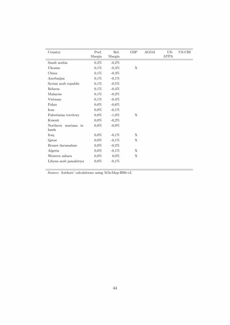
Country Pref.Margin

Rel.Margin

GSP AGOA US-ATPA

US-CBI

Saudi arabia 0,2% -0,2%Ukraine 0,1% -0,3% XChina 0,1% -0,3%Azerbaijan 0,1% -0,1%Syrian arab republic 0,1% -0,5%Belarus 0,1% -0,4%Malaysia 0,1% -0,2%Vietnam 0,1% -0,4%Palau 0,0% -0,6%Iran 0,0% -0,1%Palestinian territory 0,0% -1,0% XKuwait 0,0% -0,2%Northern mariana is-lands

0,0% -0,9%

Iraq 0,0% -0,1% XQatar 0,0% -0,1% XBrunei darussalam 0,0% -0,2%Algeria 0,0% -0,1% XWestern sahara 0,0% 0,0% XLibyan arab jamahiriya 0,0% -0,1%

Source: Authors’ calculations using MAcMap-HS6-v2.

44

8.2 The EU and USA RTAs

Table 9: List of Regional Agreements for the EU and the US in 2008

European Union USACustom Unions Andorra (1991), Turkey (1995),

San Marino (1991)

Free Trade Ar-eas

Switzerland (1973), FYMOR(2004), Croatia (2005), Albania(2006),Montenegro (2008),Bosniaand Herzegovina (2008), Alge-ria (2005), Egypt (2004), Israel(2000), Jordan (2002), Lebanon(2003), Morocco (2000), Pales-tinian Authority (1997), Syria(1977), Tunisia (1998), Chile(2003), Mexico (2000), SouthAfrica (2000), Iceland (1972),Liecthenstein (1972), Norway(1973), Burundi, Kenya, Rwanda,Tanzania, Uganda (2008), Co-moros, Madagascar, Mauritius,Seychelles, Zimbabwe (2008),Papua New Guinea, Fiji (2008),Botswana, Lesotho, Namibia,Mozambique, Swaziland (2008),Cote d’Ivoire, Ghana (2008)

Israel, Canada, Mexico, Jordan,Chile, Singapore, Australia, Mo-rocco, Bahrain, Peru, Oman

Under negotia-tions or underdiscussion

ASEAN, Canada, China, Gulf Co-operation Council, India, Iraq,South Korea, Mercosur, Moldova,Serbia, Ukraine

Colombia, Panama, South Korea,Malaysia, Thailand, United ArabEmirates, South African CustomUnions

Note Year of Entry into Force in brackets.Source DG Trade, EC.

45