trade diversification: drivers and impacts …ed_emp/documents/genericdocu… · no way be taken to...
TRANSCRIPT

TRADE DIVERSIFICATION:DRIVERS AND IMPACTS
By Olivier Cadot, Céline Carrère and Vanessa Strauss-Kahn
7.1 INTRODUCTION
Policy interest in export diversification is not new but, for over two decades, it wasmired in an ideologically loaded debate about the role of the State. Old-time industrialpolicy having died of its own excesses, the debate over what, if anything, the gov-ernment should do to promote export growth was contained within the fringe of theeconomics profession. Mainstream economists were happy to believe that whatevermarket failures were out there, government failures were worse, and that anyway mostgovernments in developing countries lacked the means to do anything. But by anironic twist of history, years of (Washington-consensus inspired) fiscal and monetarydiscipline have put a number of developing-country governments back in a positionto do something for export promotion, having recovered room to manoeuvre interms of both external balance and budget position. So the question is back.
With limited guidance from theory, the economics profession’s answer to thereturn of the industrial-policy debate has been to go back to descriptive statistics (asopposed to the investigation of causal chains). The result is a wealth of new stylizedfacts. For instance, surprising patterns of export entrepreneurship have emerged fromthe use of increasingly disaggregated data.
One area where theory has proved useful is in the exploration of the linkagesbetween productivity and trade. So-called “new-new” trade models (featuring firmheterogeneity) have highlighted complex relationships between trade diversificationand productivity, with causation running one way at the firm level and the otherway around (or both ways) at the aggregate level.
Even at the aggregate level, new issues have appeared. First, Imbs and Wacziarg(2003) uncovered a curious pattern of diversification and re-concentration in pro-duction, prompting researchers to explore whether the same was true of trade. Second,a wave of recent empirical work has questioned traditional views on the “natural-re-
253
TRADE DIVERSIFICATION:DRIVERS AND IMPACTS
By Olivier Cadot, Céline Carrère and Vanessa Strauss-Kahn
AcknowledgementsThis paper has been published as a chapter in the ILO-EU co-publication “Tradeand Employment: From Myths to Facts” (M. Jansen, R. Peters and J. M. SalazarXirinachs (Eds.)) that has been produced with the assistance of the European Union.The contents of this chapter are the sole responsibility of the authors and can inno way be taken to reflect the views of the European Union or the InternationalLabour Organization.
7

source curse”, challenging the notion that diversification out of primary resourceswas a prerequisite for growth.
Thus, our current understanding of the trade diversification/ productivity/growth nexus draws on several theoretical and empirical works, all well developedand growing rapidly. It is easy to get lost in the issues, and the present paper’s objectiveis to sort them out and take stock of elements of answers to the basic questions.
Among those questions, the first are simply factual ones — “how is export di-versification measured?” and “what are the basic stylized facts about trade exportdiversification, across time and countries?”, which we explore in sections 7.2 and 7.3,respectively. The third question is about diversification’s drivers, among which in-dustrial policy, and is tackled in section 7.7. In section 7.5, we turn to the relationshipbetween trade diversification, growth and employment. Section 7.6 focuses on theimport side; we review the evidence on the impact of import diversification on pro-ductivity and extend the discussion to labour-market issues. Section 7.7 concludes.
7.2 MEASURING DIVERSIFICATION
7.2.1 Concentration/diversification indicesWhile the focus of this chapter is on diversification, quantitative indices measureconcentration rather than diversification. These indices are mainly used in the in-come-distribution literature where they illustrate income dispersion across individuals.We will review these measures, taking the example of export diversification (whichhas anyway been the focus of most papers) but keeping in mind that they applyequally well to imports. All concentration indices basically measure inequality betweenexport shares; these shares, in turn, can be defined at any level of aggregation. Ofcourse, the finer the disaggregation, the better the measure.
The most frequently used concentration indices are the ones used in the in-come-distribution literature: Herfindahl, Gini and Theil. These indices are formalizedin technical appendix 7.A.1.1. All three indices can be easily programmed but arealso available as packages in Stata. Authors have used one or several of these measures.Across the board, results are not dependent on the index chosen.
The Theil (1972) index has decomposability properties that make it especiallyuseful. It can indeed be calculated for groups of individuals (export lines) and de-composed additively into within-groups and between-groups components (that is,the within- and between-groups components add up to the overall index).1 It is thuspossible to distinguish an increased concentration (diversification) that occurs mainlywithin groups from one that occurred mainly across groups. We will see in the nextsection a useful application of this property in our context.
Trade and Employment: From Myths to Facts
254
1 Technical appendix 7.A.1.2 presents the Theil index decomposition.

Chapter 7: Trade diversification: Drivers and impacts
255
2 An active line corresponds to a non-zero export line of the HS6 nomenclature (about 5,000 lines)for a given year.3 This mapping between the Theil decomposition and the margins was first proposed by Cadot,Carrère and Strauss-Kahn (2011).
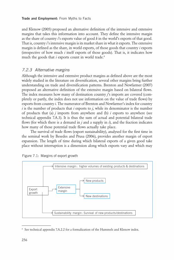
7.2.2 Trade-expansion marginsRecent research on trade diversification distinguishes evolution at the intensive andextensive margins. In summary, by focusing on the intensive margins one relates tochanges in diversification among a set of goods that are commonly traded over theperiod. In contrast, by looking at the extensive margin one takes account of the effectof newly traded (or disappearing) goods on diversification. More specifically, exportconcentration measured at the intensive margin reflects inequality between the sharesof active export lines.2 Conversely, diversification at the intensive margin during aperiod t0 to t1 means convergence in export shares among goods that were exportedat t0. Concentration at the extensive margin is a subtler concept. At the simplest, itcan be taken to mean a small number of active export lines. Then, diversification atthe extensive margin means a rising number of active export lines. This is a widelyused notion of the extensive margin (in differential form), and the decompositionof Theil’s index can be usefully mapped into the intensive and extensive marginsthus defined.
Suppose that, for a given country and year, we partition the 5,000 or so linesmaking up the HS6 nomenclature into two groups: group “one” is made of activeexport lines for this country and year, and group “zero” is made of inactive exportlines (i.e. export lines for which there are no exports). This partition can be used toconstruct within-groups and between-groups components of the overall Theil index.As shown in the technical appendix 7.A.2, by distinguishing the Theil sub-index forthe group of inactive lines from the Theil sub-index for the group of active lines,changes in concentration/diversification within and between groups can be set apart.More importantly, it can be shown that, given this partition, changes in the within-groups Theil index measure changes at the intensive margin, whereas changes in thebetween-groups Theil index measure changes at the extensive margin. In sum, Theil’sdecomposition makes it possible to decompose changes in overall concentration intoextensive-margin and intensive-margin changes.3 This is a particularly important fea-ture, as changes at the intensive margin or extensive margin reflect very differentevolution of a country’s productive activities and policies aiming at enhancing di-versification in either margin entail distinct recommendations.
The extensive margin defined this way (by simply counting the number ofactive export lines) leaves out, however, important information. To see why, observethat a country can raise its number of active export lines in many different ways. Forinstance, it could add “embroidery in the piece, in strips or in motifs” (HS 5810);or it could add “compression-ignition internal combustion piston engines” (HS 8408, i.e. diesel engines). Clearly, these two items are not of the same significanceeconomically, although a mere count of active lines would treat them alike. Hummels
Trade and Employment: From Myths to Facts
256
Intensive margin : higher volumes of existing products & destinations
Export growth
Extensive margin
New products
New destinations
Sustainability margin : Survival of new products/destinations
Figure 7.1: Margins of export growth
4 See technical appendix 7.A.2.2 for a formalization of the Hummels and Klenow index.
and Klenow (2005) proposed an alternative definition of the intensive and extensivemargins that takes this information into account. They define the intensive marginas the share of country i’s exports value of good k in the world’s exports of that good.That is, country i’s intensive margin is its market share in what it exports. The extensivemargin is defined as the share, in world exports, of those goods that country i exports(irrespective of how much i itself exports of those goods). That is, it indicates howmuch the goods that i exports count in world trade.4
7.2.3 Alternative margins Although the intensive and extensive product margins as defined above are the mostwidely studied in the literature on diversification, several other margins bring furtherunderstanding on trade and diversification patterns. Brenton and Newfarmer (2007)proposed an alternative definition of the extensive margin based on bilateral flows.The index measures how many of destination country j’s imports are covered (com-pletely or partly, the index does not use information on the value of trade flows) byexports from country i. The numerator of Brenton and Newfarmer’s index for countryi is the number of products that i exports to j, while its denominator is the numberof products that (a) j imports from anywhere and (b) i exports to anywhere (seetechnical appendix 7.A.3). It is thus the sum of actual and potential bilateral tradeflows (for which there is a demand in j and a supply in i), and the fraction indicateshow many of those potential trade flows actually take place.
The survival of trade flows (export sustainability), analysed for the first time inthe seminal work by Besedes and Prusa (2006), provides another margin of exportexpansion. The length of time during which bilateral exports of a given good takeplace without interruption is a dimension along which exports vary and which may
Chapter 7: Trade diversification: Drivers and impacts
257
also be a margin for export promotion. Figure 7.1 summarizes our decomposition ofexport growth.
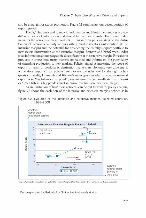
Theil’s,5 Hummels and Klenow’s, and Brenton and Newfarmer’s indices providedifferent pieces of information and should be used accordingly. The former indexmeasures the concentration in products. It thus informs policy-makers on the distri-bution of economic activity across existing products/sectors (intervention at theintensive margin) and the potential for broadening the country’s export portfolio tonew sectors (intervention at the extensive margin). Brenton and Newfarmer’s indexgives information about geographic diversification at the extensive margin. For existingproducts, it shows how many markets are reached and informs on the potentialityof extending production to new markets. Policies aimed at increasing the scope ofexports in terms of products or destination markets are obviously very different. Itis therefore important for policy-makers to use the right tool for the right policyquestion. Finally, Hummels and Klenow’s index gives an idea of whether nationalexporters are “big fish in a small pond” (large intensive margin, small extensive margin)or “small fish in a big pond” (small intensive margin, large extensive margin).
As an illustration of how these concepts can be put to work for policy analysis,figure 7.2 shows the evolution of the intensive and extensive margins defined as in
5 The interpretation for Herfindhal or Gini indices is obviously similar.
Pakistan
India
Vietnam
Indonesia
Pakistan
India
Vietnam
Indonesia
.2.1
.4.6
.81
1.2
nig raM evi sne tnI
85 90 95 100Extensive Margin
1998 2008
Intensive and Extensive Margin in Products, 1998-08
Country’smarket sharein its export portfolio
Weight ofnational exportportfolio inworld trade
Big fish in asmall pond
Small fishin a bigpond
Figure 7.2: Evolution of the intensive and extensive margins, selected countries, 1998–2008
Source: Comtrade. The authors are grateful to Swarnim Wagle, of the World Bank’s Trade Division, for sharing this graph.

Trade and Employment: From Myths to Facts
258
Hummels and Klenow for selected countries over the decade preceding the global fi-nancial crisis. It can be seen, for instance, that Pakistan’s extensive margin has beenrising, suggesting active export entrepreneurship. By contrast, its intensive margin hasslightly shrunk, suggesting that existing Pakistani exporters are finding it difficult tomaintain competitiveness. This type of broad-brush observation is useful to get a firstshot at potential constraints on growth — for example, the problem may be decliningcompetitiveness in the textile and clothing sector due to the elimination of Multi-Fibre Arrangement (MFA) quotas. By contrast, India has grown almost only at theintensive margin, which is to be expected given that it is already fully diversified (asthe products that belong to its export portfolio account for close to 100 per cent ofworld trade). Overall, countries can be expected to walk a crescent-shaped trail, firsteastward as they broaden their portfolio, then full north as they consolidate positions.
7.3 WHAT DO WE LEARN FROM THESE MEASURES?
7.3.1 Trends in diversificationThe seminal work by Imbs and Wacziarg (2003) uncovered an unexpected non-mo-notonic relationship between production diversification and gross domestic product(GDP) per capita. Past a certain level of income ($9,000 in 1985 purchasing powerparity (PPP) dollars), countries re-concentrate their production structure, whethermeasured by employment or value added. Using different data, Koren and Tenreyro(2007) confirmed the existence of a U-shaped relationship between the concentrationof production and the level of development.
Following their work, several papers have looked at whether a similar non-mo-notone pattern holds for trade. Looking at trade made it possible to reformulate thequestion at a much higher degree of disaggregation, since trade data is available forthe 5,000 or so lines of the six-digit harmonized system (henceforth HS6). In termsof concentration levels, exports are typically much more concentrated than produc-tion. This concentration, which was observed initially by Hausmann and Rodrik(2006), is documented in detail for manufacturing exports in Easterly, Reshef andSchwenkenberg (2009). A striking (but not unique) example of this concentration isthe case of Egypt, which, “[out] of 2,985 possible manufacturing products in [the]dataset and 217 possible destinations, […] gets 23 per cent of its total manufacturingexports from exporting one product — “ceramic bathroom kitchen sanitary items notporcelain” — to one destination, Italy, capturing 94 per cent of the Italian importmarket for that product” (page 3). These “big hits”, as they call them, account for asubstantial part of the cross-country variation in export volumes. But they also doc-ument that the distribution of values at the export × destination level (their unit ofanalysis) closely follows a power law; that is, the probability of a big hit decreasesexponentially with its size.
Klinger and Lederman (2006), as well as Cadot, Carrère and Strauss-Kahn (2011),analyse the evolution of trade diversification. The former study uses a panel of 73countries between 1992 and 2003, while the latter focuses on a larger one, with 156

Chapter 7: Trade diversification: Drivers and impacts
259
6 The reason has to do with the level of disaggregation rather than with any conceptual differencebetween trade, production and employment shares. Whereas Imbs and Wacziarg calculated their in-dices at a relatively high degree of aggregation (ILO, one digit; UNIDO, three digits; and OECD,two digits), Cadot, Carrère and Strauss-Kahn (2011) use very disaggregated trade nomenclature. Atthat level, there is a large number of product lines with small trade values, while a relatively limitednumber of them account for the bulk of all countries’ trade (especially so of course for developingcountries, but even for industrial ones). The reason for this pattern is that the harmonized systemused by Comtrade is derived from nomenclatures originally designed for tariff-collection purposesrather than to generate meaningful economic statistics. Thus, it has a large number of economicallyirrelevant categories, e.g. in the textile-clothing sector, while economically important categories inmachinery, vehicles, computer equipment, etc. are grouped together in “mammoth” lines.
countries representing all regions and all levels of development between 1988 and2006. In both cases, concentration measures obtained with trade data turned out tobe much higher than those obtained with production and employment data.6 Butthe U-shaped pattern showed up again, albeit with a turning point at much higherincome levels ($22,500 in constant 2000 PPP dollars for Klinger and Lederman, and$25,000 in constant 2005 PPP dollars for Cadot, Carrère and Strauss-Kahn). Notethat, as the turning point occurs quite late, the level of export concentration of therichest countries in the sample is much lower than that of the poorest.
7.3.2 Which margin matters?The literature so far shows that growth at the intensive margin is the main componentof export growth. The early work by Evenett and Venables (2002) used three-digittrade data for 23 exporters over the period 1970–97 and found that about 60 percent of total export growth is at the intensive margin, i.e. comes from larger exportsof products traded since 1970 to long-standing trading partners. Of the rest, most ofwhich was the destination-wise extensive margin, as the product-wise extensive marginaccounted for a small fraction (about 10 per cent) of export growth. Brenton andNewfarmer (2007), using Standard International Trade Classification (SITC) data atthe five-digit level over 99 countries and 20 years, also found that intensive-margingrowth accounts for the biggest part of trade growth (80.4 per cent), and that growthat the extensive margin was essentially destination-wise (18 per cent). Amurgo-Pachecoand Pierola (2008) found that extensive-margin growth accounts for only 14 per centof export at the HS6 level for a panel of 24 countries over the period 1990–2005.
The observation that the product-wise extensive margin accounts for little ofthe growth of exports may seem puzzling, as Cadot et al. (2011) found precisely thatmargin to be very active, especially at low levels of income. Thus, export entrepre-neurship is not lacking. Why then does it not generate export growth? There are twoanswers, one technical and one of substance. The technical answer is that when anew export appears in statistics, it typically appears at a small scale and can only con-tribute marginally to growth. But the following year, it is already in the intensivemargin. Thus, by construction, the extensive margin can only be small. But there isa deeper reason. In work already cited, Besedes and Prusa (2006) showed that thechurning rate is very high in all countries’ exports, and especially so for developing

ones. That is, many new export products are tried, but many also fail. Raising thecontribution of the extensive margin to export growth requires also improving the“sustainability” margin.
Although not predominant quantitatively as a driver of export growth, the ex-tensive margin can react strongly to changes in trade costs, an issue discussed laterin this chapter. For instance, Kehoe and Ruhl (2009) found that the set of least-tradedgoods, which accounted for only 10 per cent of trade before trade liberalization, maygrow to account for 30 per cent of trade or more after liberalization. Activity at theextensive margin also varies greatly along the economic development process. Klingerand Lederman (2006) and Cadot, Carrère and Strauss-Kahn (2011) show that thenumber of new exports falls rapidly as countries develop, after peaking at the lower-middle income level. The poorest countries, which have the greatest scope fornew-product introduction because of their very undiversified trade structures, unsur-prisingly have the strongest extensive-margin activity.7
Figure 7.3 depicts the contribution of the between-groups and within-groupscomponents to Theil’s overall index, using the formulae derived in the previous section.
Trade and Employment: From Myths to Facts
260
23
45
6
0 10000 20000 30000 40000GDP per capita, PPP (constant 2005 international $)
Total Theil
Between
Within
Figure 7.3: Contributions of within- and between-groups to overall concentration, all countries
Source: Cadot, Carrère and Strauss-Kahn (2011).
7 The average number of active export lines is generally low at a sample average of 2,062 per countryper year (using Cadot, Carrère and Strauss-Kahn’s sample), i.e. a little less than half the total, witha minimum of eight for Kiribati in 1993 and a maximum of 4,988 for Germany in 1994 and theUnited States in 1995.

It can be seen that the within component dominates the index while the betweencomponent accounts for most of the evolution. Put differently, most of the concen-tration in levels occurs at the intensive margin (in goods that are long-standing exports)while changes in concentration are at the extensive margin (for example the decreasedconcentration for lower-income countries results mainly from a rise in the numberof exported goods).
Whereas the extensive margin in figure 7.3 is measured only by the number ofexports, using their alternative definition (see Appendix 7.A.2) Hummels and Klenow(2005) performed a cross-sectional analysis of exports for 126 countries decomposingexports into extensive and intensive margins. Interestingly, they found that 62 percent of the higher trade of larger economies is driven by the extensive margin, whileonly 38 per cent is driven by the intensive margin. Thus, once the extensive marginis corrected for the importance of the new exports introduced (Hummels-Klenow’sversion), it dominates the intensive margin in explaining exports growth.
7.4 DRIVERS OF DIVERSIFICATION
7.4.1 Quantitative insightsWhat does the theoretical trade literature have to say on the potential determinantsof export diversification? In traditional Ricardian models, productivity affects tradepatterns. In the specification proposed by Melitz (2003) – “new-new trade theory” –firms are heterogeneous in productivity levels, and only a subset of them — the mostproductive — become exporters. Thus, exporting status and productivity are correlatedat the firm level, although this comes essentially from a selection effect.
Several papers have studied the impact of productivity/income on diversificationby putting export diversification on the left-hand side of the equation and incomeon the right-hand side. As we already saw, Klinger and Lederman (2006) as well asCadot, Carrère and Strauss-Kahn (2011) found a U-shaped relationship betweenexport concentration and GDP per capita by regressing the former on the latter,hence providing evidence of a non-linear effect of income on export diversification.
We now consider some of its non-income determinants. In a symmetric (rep-resentative-firm) monopolistic-competition model, the volume of trade, the numberof exporting firms and the number of varieties marketed are all proportional. In aheterogeneous-firms model, the relationship is more complex, but the ratio of exportto domestic varieties is also directly related to the ratio of export to domestic sales.Thus, it is no surprise that gravity determinants of trade volumes also affect thediversity of traded goods. For instance, Amurgo-Pacheco and Pierola (2008) find thatthe distance and size of destination markets is related to the diversity of bilateral trade.
Parteka and Tamberi (2008) apply a two-step estimation strategy to uncoversome of the systematic (permanent) cross-country differences in export diversification.To do so, they break down country effects into a wide range of country-specific char-acteristics, such as size, geographical conditions, endowments, human capital andinstitutional setting. Using a panel data set for 60 countries and 20 years (1985–2004),
Chapter 7: Trade diversification: Drivers and impacts
261
they show that distance from major markets and country size are the most relevantand robust determinants of export diversity, once GDP per capita is controlled for.These results are consistent with those of Dutt, Mihov and van Zandt (2009), whoshow that distance to trading centres and market access (proxied by a host of bilateraland multilateral trading arrangements) are key determinants of diversification.
We take account of the main variables used in the above cited empirical studiesand propose a quantitative assessment of the main determinants of export diversifi-cation. We then go a step further and extend the discussion by assessing whetherdeterminants mainly affect the extensive or intensive margins of diversification.8
As theoretical background stays silent on the potential form of the relationshipbetween export diversification and its determinants, we start by showing non-para-metric “smoother” regressions.9 Such regressions do not impose any functional formand are therefore well suited to a first exploration of data with no ad-hoc pre-definedrelationships between variables. In addition to per capita GDP (specified with a quadratic term to capture the hump-shaped relationship described in section 7.2.2), we introduce the following variablesin our analysis:10
● Size of the economy, proxied by population. We expect larger countries to bemore diversified due to larger internal markets and higher degree of product dif-ferentiation.
● Market access, proxied by the country membership in preferential trade agree-ments. Preferential market access should help both export volumes and exportof new products.
● Transport costs, proxied by both a remoteness index (as in Rose, 2004) and thequality of infrastructures (captured by the density of railway, paved road and tele-phone lines). The more remote a country, the lower its exports both in volumeand number of products; in contrast, better infrastructures should boost exportdiversification.
● Human capital, proxied by the number of years of schooling (from Barro andLee, 2010) and the percentage of GDP invested in research and development(R&D). We expect both variables to have a positive impact on export diversifi-cation, in particular through the extensive margin, i.e. through the developmentand export of new products.
● The quality of institution may also have a positive impact on diversification. Thisis proxied by two variables, the International Country Risk Guide (ICRG) Indi-cator of Quality of Government (QoG) and the Revised Combined Polity Score,both provided by the QoG institute.
Trade and Employment: From Myths to Facts
262
8 As a measure of diversification, we use Theil indices computed at the HS6 level by Cadot, Carrèreand Strauss-Kahn (2011) for 1988-2006.9 Non-parametric “smoother” regression (also called “lowess” regression) consists of re-estimating re-gression for overlapping samples centred on each observation.10 A detailed description of these variables is available in technical appendix 7.A.4.

Chapter 7: Trade diversification: Drivers and impacts
263
● Finally, we expect foreign direct investment (FDI) to also impact export structure.We thus introduce FDI in the analysis.
Figure 7.4 presents the scatter plots of export diversification measured by the2006 Theil index versus the variables listed above. Scatter plots show correlations be-tween the variables, whereas curves correspond to “smoother” non-parametricregression. In all scatter plots, a “full diamond” represents a developing country (i.e.low- and middle-income countries) and a “hollow circle” represents a developedcountry (i.e. high-income OECD and non-OECD countries). The sample includes129 to 150 countries depending on data availability.
Figure 7.4: Average Theil indices in 2006 on each of the ten explanatory variables in 2005
24
68
Exp
ort
Thei
l ind
ex
0 2 4 6 8Infrastructure Index
24
68
Exp
ort
Thei
l ind
ex
7.5 8 8.5 9 9.5Remoteness

Trade and Employment: From Myths to Facts
264
24
68
Exp
ort
Thei
l ind
ex
0 .2 .4 .6Reciprocal Preferential Market Access
24
68
Exp
ort
Thei
l ind
ex
–10 0 10 20 30FDI net inflows (% GDP)
24
68
Exp
ort
Thei
l ind
ex
0 1 2 3 4R&D spending (% GDP)
Figure 7.4: Average Theil indices in 2006 on each of the ten explanatory variables in 2005 (Continued)

Chapter 7: Trade diversification: Drivers and impacts
265
24
68
Exp
ort
Thei
l ind
ex
0 .2 .4 .6 .8 1ICRG Indicator of Quality of Governmeent
24
68
Exp
ort
Thei
l ind
ex
–10 –5 0 5 10Revised Combined Polity Score
24
68
Exp
ort
Thei
l ind
ex
2.0000 4.0000 6.0000 8.0000 10.0000 12.0000Years of Schooling
Figure 7.4: Average Theil indices in 2006 on each of the ten explanatory variables in 2005 (Continued)

Trade and Employment: From Myths to Facts
266
Figure 7.4: Average Theil indices in 2006 on each of the ten explanatory variables in 2005 (Continued)
24
68
Exp
ort
Thei
l ind
ex
0 5.00e+07 1.00e+08 1.50e+08 2.00e+08Population
24
68
Exp
ort
Thei
l ind
ex
0 10000 20000 30000 40000per capita GDP (constant US$2,000)
These figures reveal links between export diversification and each of these vari-ables, which, importantly, have the expected signs. A similar test run using the numberof exported products instead of the Theil index provides very similar figures, suggestingthat our variables influence essentially the extensive margin.11 In order to get furtherinsights on the impact of the set of variables described above on the extensive andintensive margins, we turn to a regression analysis. We regress the overall Theil index,the within-groups Theil, the between-groups Theil and the number of exported prod-ucts on the ten variables using a panel database, including 87 countries over the
11 These figures are available from the authors upon request.

1990–2004 period.12 Country and year fixed-effects control for unobservable charac-teristics in all regressions. The regression analysis, reported in table 7.1, confirms ourresults from the scatter plots.
Table 7.1 shows a negative significant coefficient on GDP per capita and apositive significant one on GDP per capita squared. We thus retrieve the main resultof Cadot, Carrère and Strauss-Kahn (2011) which reveals a quadratic relationship be-tween the Theil index and GDP per capita, mainly driven by the extensive margin(the between component of the Theil index). Once controlled for GDP per capita,infrastructure still appears as an important driver of diversification: a 10 per cent in-crease in the infrastructure index decreases the Theil’s index by about 0.7 per cent.13
Better infrastructure increases diversification on both margins. Remoteness also hasthe expected sign: the more remote the country, the lower its export diversification(i.e. the higher its Theil index), essentially in terms of the extensive margin andnumber of products. Our analysis thus confirms the result that high distance to im-porters increases the export fixed cost and, consequently, drastically reduces exportdiversification. Preferential market access is clearly an important factor of diversifi-cation at both margins and this result is consistent with other studies (for example,
Chapter 7: Trade diversification: Drivers and impacts
267
12 As seen in section 7.2.2, the within-groups Theil index corresponds to the intensive margin, whereasthe between-groups Theil index corresponds to the extensive margin.13 Note that the log-log specification allows an interpretation of the results in terms of elasticity,which is easily understandable.
Table 7.1: Diversification drivers in a panel data set, 1990–2004, 87 countries
Coef. Std. Err. Coef. Std. Err. Coef. Std. Err. Coef. Std. Err.
ln (per capita GDP) -0.505 0.09 *** -0.193 0.13 * -1.054 0.32 *** 1.055 0.38 ***ln (per capita GDP)squared
0.040 0.01 *** 0.009 0.01 0.054 0.02 ** -0.106 0.02 ***
ln (Infrastructure) -0.072 0.03 *** -0.122 0.04 *** -0.303 0.08 *** 0.119 0.07 *ln (Remoteness) 1.092 0.46 ** -0.439 0.50 3.753 2.14 * -3.533 1.51 **Trade liberalization -0.009 0.01 0.017 0.02 0.031 0.05 0.108 0.06 *Pref. Market Access -0.179 0.04 *** -0.244 0.05 *** -1.031 0.21 *** 0.316 0.11 ***FDI (% GDP) 0.001 0.00 ** 0.001 0.00 * 0.002 0.00 0.000 0.00ln (Years of Schooling) -0.114 0.06 * 0.017 0.07 -0.625 0.26 ** 0.619 0.21 ***ICRG -0.047 0.04 * 0.086 0.04 ** -0.584 0.14 *** 0.416 0.12 ***Polity Score -0.002 0.00 * 0.002 0.00 -0.003 0.00 0.019 0.00 ***ln (population) -0.187 0.07 *** 0.041 0.08 -0.642 0.27 ** 1.582 0.27 ***
Country fixed effectsYear fixed effectsObservationsAjusted R-squared
ln (Theil) ln (Theil_between) ln (Nber)
yes yes yes yesyes yes yes yes1195 1257 1257 12570.97 0.92 0.98 0.95
Notes: Robust standard errors in italics, with * meaning that the correspondent coefficient is significantly different from zero at 10 per cent; ** significant at 5 per cent; *** significant at 1 per cent.

Trade and Employment: From Myths to Facts
268
14 The variable on R&D spending is not included in the regression analysis as it covers only a smallnumber of countries and years, and consequently reduces the sample drastically. The “years of school-ing” variable, available every five years in the Barro and Lee database, is considered as constantwithin the five-year period.
Amurgo-Pacheco, 2006; Gamberoni, 2007; Feenstra and Kee, 2007; or Dutt, Mihovand van Zandt, 2009). In contrast, net inflows of FDI (as a percentage of GDP) seemto concentrate exports value on some products and thereby increases concentrationat the intensive margin. This result could be expected as multinational corporationsspecialize in specific products, which they produce in high volumes. We also find asignificant impact of education on export diversification. A 10 per cent increase inthe years of schooling reduces the Theil index by 1.1 per cent and increases the num-bers of exported products by 6.2 per cent. Similarly, the quality of institution appearsclearly significant, with a positive impact on diversification. As expected, the largerthe population, the more diversified the economy.14
Note that the above results should be understood with caution. Regressions intable 7.1 are informative of the factors that have a significant impact on diversificationand of the sign of this impact once controlled for others factors. It is difficult howeverto rank these factors and clearly isolate a single impact due to potential multicolinearityissues existing between these variables.
As shown in table 7.1, we also account for a potential factor of diversificationlargely ignored in empirical literature: the unilateral trade liberalization. We use thedummy variable as defined by Wacziarg and Welch (2008) (see section 7.2.2 for furtherindications on this variable). This factor appears non-significant except in column(4): import liberalization increases the diversification through a larger number of ex-ported lines. Further investigations reveal that the non-significance of the tradeliberalization variable in columns (1)-(3) is mainly due to the “year of schooling”variables. If we drop the latter from the regression, the trade liberalization dummybecomes negative and significant at the 1 per cent level in the three first columns.Strikingly, if we introduce an interactive variable between unilateral trade liberalizationand years of schooling, the trade liberalization dummies and the interactive variablesare significant, whereas schooling is not. That is: years of schooling matter for exportdiversification only in a liberalized regime. Similar conclusions hold for some otherdrivers of export diversification of Table 7.1 such as infrastructure. Thus, unilateraltrade liberalization appears to be an important underlying driver of export diversifi-cation. We now explore this feature in more detail.
7.4.2 Trade liberalization as a driver of diversification Although preferential trade liberalization has received considerable attention in theempirical literature as a driver of product diversification (for example, Amurgo-Pacheco, 2006; Gamberoni, 2007; Feenstra and Kee, 2007; or Dutt, Mihov and vanZandt, 2009), unilateral trade reforms have not. Yet we will see in section 7.5 thatthe link between import diversification and total factor productivity (TFP) is strongly

Chapter 7: Trade diversification: Drivers and impacts
269
established at the firm level. Thus, import liberalization can be taken as a positiveshock on TFP, which should, according to the Melitz (2003) argument, raise thenumber of industries with an upper tail of firms capable of exporting — and thus raiseoverall export diversification.15 Indeed, arguments running roughly along this line canbe found in, for example, Bernard, Jensen and Schott (2006) or in Broda, Greenfieldand Weinstein (2006). This section presents a brief statistical analysis of this relation-ship.
To do so, we combine the Theil index of export concentration computed atthe HS6 level by Cadot, Carrère and Strauss-Kahn (2011) for the period 1988–2006with the trade liberalization date of Wacziarg and Welch (2008). The sample used in-cludes 100 countries, 62 middle-income and 38 low-income countries over the period1988–2006, with respectively 68 per cent and 49 per cent of country-year observationsoccurring in liberalized regimes (see technical appendix table 4.A.1). We exclude fromthe sample 34 high-income countries, as 95 per cent of the observations of this groupoccurs in liberalized regimes throughout the period (Estonia and Iceland are the onlycountries considered as non-liberalized and they do not change regime over theperiod – see technical appendix table 7.A.1).
Wacziarg and Welch (2008) propose an update covering the late 1990s of Sachsand Warner (1995)’s trade liberalization dates. Such data were first collected from acomprehensive survey of broad country-specific case studies. More precisely, Sachsand Warner determined trade liberalization dates based on primary-source data onannual tariffs, non-tariff barriers and black market premium. A variety of secondarysources was also used, particularly to identify when export marketing boards wereabolished and multi-party governance systems replaced Communist Party rule.16
As shown in figure 7.5, the conditional mean of Theil’s concentration index is4.8 in a liberalized regime versus 5.9 in a non-liberalized one, while the number ofexported products is clearly higher when the trade regime is liberalized (1,893 productsversus 1,178 in a non-liberalized trade regime). The difference in Theil indices meansis higher for middle-income than for low-income countries, although it is still statis-tically significant for low-income countries. This suggests a stronger dynamic betweentrade liberalization and diversification of exports in developing countries with betterinfrastructure and higher skill levels.
15 This mechanism is further described in section 7.5.1.16 Rodriguez and Rodrik (2000) criticized the Sachs-Warner (1995) openness variable, showing thatits explanatory power on growth was driven by only two of its five components: the black marketpremium on foreign exchange (a measure of overvalued exchange rates rather than trade openness)and the presence of export marketing boards. By contrast, tariffs and non-tariff barriers correlatedpoorly with growth. As export marketing boards essentially characterized sub-Saharan Africa andovervalued exchange rate Latin America, the Sachs-Warner measure was indistinguishable fromAfrican and Latin American “dummy variables”. Wacziarg and Welch (2008) improved the method-ology by better identifying export marketing boards and trade liberalization dates. Using theirimproved openness definition and panel data over a long period, they confirmed that opennesscorrelates with faster growth, delivering on average 2 percentage points of additional growth (largelydriven by additional investment).

Trade and Employment: From Myths to Facts
270
Figure 7.5: Differential of means in liberalized versus non-liberalized regimes (100 middle- and low-income countries, 1988–2006)
3
3.5
4
4.5
5
5.5
6
6.5
All Middle Income
Low Income
Mean if No trade liberalization Mean if trade liberalization
0
500
1000
2000
1500
2500
All Middle Income
Low Income
Mean if No trade liberalization Mean if trade liberalization
7.5.a. Theil’s concentration index 7.5.b. Number of exported products
Note: For each group, the difference in means is tested to besignificantly higher in non-liberalized than in liberalizedregimes (at 1 per cent level for All and middle-income countries, and 5 per cent for low-income countries).
Note: For each group, the difference in means is tested to besignificantly lower in non-liberalized than in liberalizedregimes (at 1 per cent level).
We then run fixed-effects regressions of the Theil index on a binary liberalizationindicator defined by the dates of liberalization (equal to 1 when liberalized) to assessthe within-country effect of trade liberalization on the diversification of exports. Weuse a difference-in-difference specification similar to the one used by Wacziarg andWelch (2008):
Theilit = λi +δt +φLIBit +eit (1)
where Theilit is the Theil index of country i exports in year t; LIBit a dummyequal to 1 if t is greater than the year of liberalization (defined by Wacziarg andWelch); and 0 otherwise. We introduce both country and year fixed-effects ( λi andδt , respectively). The sample is not restricted to countries that underwent reforms.
The regression for the period 1988–2006 shows a highly significant within-country difference in export diversification between a liberalized and a non-liberalizedregime (φ reported in table 7.2, column 1), with a coefficient twice higher for middle-than for low-income countries, confirming the pattern observed in figure 7.5. Wealso regress equation (1) using the Theil index’s decomposition (within-groups versusbetween-groups, see section 7.2). Results are reported in table 7.2, columns 3-6.Controlling for country and year effects, the results suggest that middle-income coun-tries that undertook trade liberalization reforms have a significantly more diversifiedstructure of exports along the intensive margin. By contrast, low-income countriesdiversify mostly along the extensive margin. Thus, trade liberalization helps middle-

income countries to consolidate their positions in goods they are already exportingwhile it helps low-income countries to develop new exports. As the poorest countriesare often the most concentrated (see figure 7.3 and section 7.5.2), it is indeed likelythat trade liberalization do not increase exports in sectors (often natural resources)in which they already specialize.
Chapter 7: Trade diversification: Drivers and impacts
271
Table 7.2: Fixed-effects regressions of diversification index on liberalization status
Note: * means a significant coefficient (at 10 per cent level) standard errors in parentheses, heteroscedasticity consistent and adjusted forcountry clustering.
(1) (2) (3) (4) (5) (6)
Liberalization (LIB) –0.190* –0.075 –0.100*(2.0) (0.8) (2.8)
LIB - Middle-Income –0.241* –0.271* 0.067(2.0) (2.0) (0.5)
LIB - Low-Income –0.138* 0.053 –0.209*(1.6) (0.5) (2.0)
Number of Obs.Number of countries PeriodCountry fixed effectsYear fixed effectsR² within 0.39 0.39 0.28 0.29 0.75 0.75
1794100
1988-2006YesYes
1394100
1990-2004Yes
Theil Theil-within Theil-between
Yes
1394100
1990-2004YesYes
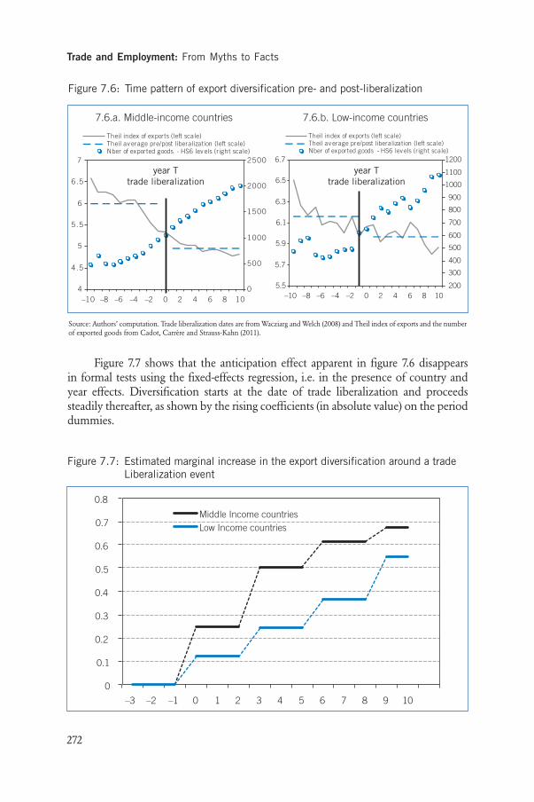
Figure 7.6 shows the time path of export diversification for an average countrybefore and after liberalization for middle- and low-income countries, respectively.The plain curve shows the Theil index (left-hand scale) and the dotted one showsthe number of exported products at the HS6 level (right-hand scale) over a windowof ten years before and after liberalization. The sample is made of countries that un-derwent permanent (non-reversed) liberalizations. For middle-income countries, astrong diversification trend (shrinking Theil index) is apparent over the entire post-liberalization windows, and particularly strong in the five years following liberalization.The figure also suggests an anticipation effect in the three years preceding liberalization.Patterns are less clear in the low-income countries figure.
In order to further examine the timing of export diversification, we followWacziarg and Welch (2008) and replace the LIB variable with five dummies, eachcapturing a two-year period immediately before and after the trade-liberalization dateT. Coefficients on these dummies capture the average difference in the Theil index(and number of exported lines) between the period in question and a baseline periodrunning from sample start to T–3.17 Estimated coefficients (in absolute value) are re-ported in figure 7.7.
17 We also run the regression on a larger sample starting at T-5, but coefficients on [T-5] to [T-3]were not significant and did not affect coefficients on other periods.
Trade and Employment: From Myths to Facts
272
Figure 7.7 shows that the anticipation effect apparent in figure 7.6 disappearsin formal tests using the fixed-effects regression, i.e. in the presence of country andyear effects. Diversification starts at the date of trade liberalization and proceedssteadily thereafter, as shown by the rising coefficients (in absolute value) on the perioddummies.
Figure 7.6: Time pattern of export diversification pre- and post-liberalization
Source: Authors’ computation. Trade liberalization dates are from Wacziarg and Welch (2008) and Theil index of exports and the numberof exported goods from Cadot, Carrère and Strauss-Kahn (2011).
7.6.b. Low-income countries7.6.a. Middle-income countries
4
4.5
5
5.5
6
6.5
7
–10 –8 –6 –4 –2 0 2 4 6 8 100
500
1000
1500
2000
2500
Theil index of exports (left scale)Theil av erage pre/post liberalization (left scale)Nber of exported goods - HS6 lev els (r ight scale)
5.5
5.7
5.9
6.1
6.3
6.5
6.7
–10 –8 –6 –4 –2 0 2 4 6 8 10200
300
400
500
600
700
800
900
1000
1100
1200
Theil index of exports (left scale)Theil av erage pre/post liberalization (left scale)Nber of exported goods - HS6 lev els (r ight scale)
year Ttrade liberalization
year Ttrade liberalization
Figure 7.7: Estimated marginal increase in the export diversification around a trade Liberalization event
0
0.1
0.2
0.3
0.4
0.5
0.6
0.7
0.8
–3 –2 –1 0 1 2 3 4 5 6 7 8 9 10
Middle Income countries Low Income countries

7.4.3 Diversification, spillovers and industrial policyThe graphs in figure 7.4 highlight a clear statistical association between governmentsupply-side policies, notably the provision of education and infrastructure, and exportdiversification.
Government provision of infrastructure and education reflects the presence ofmarket failures. As for education, the willingness of employers to provide it is limited,even for vocational training.18 Reasons include the public-good character of education,the difficulty to retain trained workers, and the footloose nature of many employersin developing countries, which does not encourage social responsibility.
As for road infrastructure, building costs are largely beyond what private-sectorusers are willing to invest given their public-good nature. Only mining companiesare sometimes willing to invest in road infrastructure directly serving their needs, orlarge plantations in local networks of rural roads. Where governments are unable orunwilling to invest in road infrastructure, transportation costs choke commercial ac-tivities, both domestic and international, as Gollin and Rogerson (2010) documentin the case of Uganda.19 As a consequence, only a tiny proportion of crops make itto urban markets and even fewer to international markets, resulting in very concen-trated export structures.
Even where roads exist, sometimes transportation services are too expensive forthe private sector to provide, in particular in low-density areas. A recent paper byRaballand et al. (2011) reports the results of a randomized experiment in rural Malawiaimed at understanding why rural transportation services are not provided even whenrural roads exist. By randomly varying bus fares, they show that bus use is stronglyprice-sensitive but, most strikingly, that there is no price with positive demand atwhich costs are covered.20 In the absence of a rural bus service, it is virtually impossibleto transport goods (handicrafts, spices and other low-volume items) to the market,reducing the scope of marketable products and income-earning opportunities (in par-ticular for women). Citing other studies that point in the same direction, Raballandet al. (2011) conclude that building roads – a favourite donor activity – does not
Chapter 7: Trade diversification: Drivers and impacts
273
18 As an illustration, the World Bank’s Private Sector Competitiveness and Economic DiversificationProject in Lesotho has aimed at building workforce skills through the establishment of two worker-training centres in Maseru and Maputsoe. The initiative had both public- and private-sector partic-ipation, the management councils in both centres being led by the private sector. But obtaininggovernment funding for the centres has proved a challenge, since only three employers (fromLesotho, South Africa and Malaysia) have expressed interest in participating in their financing.19 Gollin and Rogerson (2010) observe that the density of paved roads in Uganda today (16,300 kmfor a land area of 200,000 km2) is comparable to what the Romans left behind when they evacuatedBritain in AD 350 (between 12,000 and 15,000 km of paved roads for a land area of 242,000 km2).As a result, the prices of agricultural products when they reach markets are often more than doublethe farmgate prices.20 Raballand et al. (2011) refrain from estimating a price elasticity of demand, but instead regressthe probability that an individual took the bus over the investigation period (July-December 2009)for a fare, which was randomly assigned using a voucher system. When the bus service was free, 47per cent of the surveyed individuals took the bus at least once. The proportion declined smoothlyto reach zero at 500 kwacha (US$3.57) per ride. Similar results were obtained using the number ofrides as the dependent variable.

Trade and Employment: From Myths to Facts
274
21 On this, see Harrison and Rodríguez-Clare (2010), who provide an excellent overview of the literature on industrial policy.
appear to be enough, by itself, to get farmers to the market. In order to promote di-versification at the country and household levels, governments may need to intervenedirectly in the provision of transportation services, a notion that goes against a phi-losophy of government retrenchment that has dominated development thinking overthe last 30 years.
Other sources of market failure can hamper export diversification. Conceptually,the argument is shown in figure 7.8, where the production-possibility frontier (PPF)between two goods is shown with a convex part, reflecting economies of scale in theproduction of “good 2” in a certain range (at low levels of production).21 This is aclassic infant-industry argument. At the relative prices shown by the dotted lines, theeconomy can find itself stuck at corner equilibrium E1 where it produces only “good1” because the curvature of the PPF makes it locally unprofitable to move resourcesto good 2, even though the economy would be better off at the diversified equilibriumE2. In such circumstances, sectorally-targeted industrial policy can have a sociallybeneficial role to play.
The argument is crucially dependent on the presence of some sort of increasingreturns at the industry or cross-industry level. Do these externalities exist outside ofdevelopment-economics textbooks? Rosenthal and Strange (2004) present a substantialbody of evidence in favour of spatial agglomeration externalities. More recently,Alfaro and Chen (2009) show evidence that the location of establishments by multi-national companies follows not only “first-nature” determinants (proximity to markets
Figure 7.8: Externalities in a two-good economy
Good 1
Good 2
E2PPF
World relative-priceline
Zone of increasingreturns / agglomeration in the
production of good 2 Targeted by IP
E1

Chapter 7: Trade diversification: Drivers and impacts
275
and low production costs) but also “second-nature” ones – pure agglomeration forces.22
Among those, Alfaro and Chen examine the role of labour-market pooling (a largerpool reduces unemployment risk for workers and, therefore, wage premia), capital-equipment linkages (larger pools of capital-intensive industries attract support services),input-output (IO) linkages, and knowledge spillovers between industries measuredby cross-citations in patents. They find very strong evidence of capital-equipmentlinkages and knowledge spillovers in the location of subsidiaries. IO linkages are sig-nificant, although weaker. By contrast, evidence of labour-market pooling is weak.
Inter-industry spillovers are also identified empirically by Shakurova (2010),who estimates how the probability of exporting a good depends on previous experiencein exporting either similar goods (“horizontal” spillovers) or upstream ones (“vertical”spillovers). Cross-country regressions at the industry level show that the size of thosespillovers varies across industries but is, in most cases, statistically significant. Figure7.9 shows those spillovers in the form of marginal effects for each industry.
22 Alfaro and Chen (2009) combine geocode software with Dunn and Bradstreet’s worldbase dataset, which contains detailed location information on over 41 million establishments, to calculatedistances between establishments belonging to different industries (as Alfaro and Chen focus on be-tween-industry agglomeration). Distances are used to estimate actual and counterfactual densities,the difference between the two being the agglomeration index.
Figure 7.9: Vertical and horizontal export spillovers
Vert
ical
spi
llov
er m
argi
nal
effe
ct
Live animals
Vegetable
Oils
Food
Minerals
Chemicals
Plastics
Leather
Wood
Paper
Textiles
Footware
Glass
JewerlyMetals
Machinery
Transport
Optics
Arms0.1
.2.3
.1 .2 .3
Horizontal spillover marginal effect
Source: Adapted from Shakurova (2010).
Note: Marginal effects from a probit regression of export status in product i on export status in product j at t-1 on a cross-section of coun-tries. Those shown were significant at 5 per cent or more.

Trade and Employment: From Myths to Facts
276
Other externalities include information spillovers leading to underinvestmentin export entrepreneurship at the extensive margin (Hausmann and Rodrik, 2003).That is, export expansion at the extensive margin reflects a “self-discovery” processwhereby export entrepreneurs test the viability of new products on foreign markets.Once they succeed, imitators follow, creating a public-good problem. Spillovers atthe extensive margin among exporters of the same country are documented usingfirm-level data from four African countries by Cadot et al. (2011), who find that theprobability of survival of an exporter of good k to country d past the first year riseswith the number of exporters of k to d from the same country. Strikingly, the numberof exporters of k to d from other countries is insignificant, suggesting that the externalityis essentially within-country. Interacting this network effect with various measures ofdependence on finance suggests that the information spillover may go through do-mestic credit markets (using competitor performance as a substitute for directinformation on export risk) rather than through the direct firm-to-firm imitationeffect postulated by Hausmann and Rodrik, although the implications are similar.
If the case for externalities across exporters and industries seems fairly well-es-tablished both conceptually and empirically, what governments can do to leveragethose externalities is less clear. Harrison and Rodriguez-Clare (2010) give a long listof studies whose gist is that industries supported by government protection in oneform or another do not enjoy faster productivity growth. However, all these studiesare vulnerable to the endogeneity critique of Rodrik (2007). Namely, if governmentssupport industries to compensate for market failures, slower productivity growth insupported industries may reflect the underlying constraints rather than the effect of(endogenous) industrial policies.
A few case studies identify industries successfully supported by industrial policy.For instance, Hansen, Jensen and Madsen (2003) show how Denmark’s subsidies towind power (a guaranteed-price scheme for wind power combined with an obligationto buy for power companies that was also adopted in other EU countries, and afavourable tax treatment of investments in wind-turbine manufacturing) have helpedcreate an industry that, by the early 2000s, supplied half the world’s demand forwind turbines. As export sales were not subsidized (although they could possibly becross-subsidized by Denmark’s four large manufacturers), their growth was suggestiveof success. Hansen, Jensen and Madsen indeed show evidence of strong learningeconomies. They also argue that overall benefits from the industry’s developmenthad, by the early 2000s, outweighed the total cost of the subsidies, although the cal-culation is complex.
Export promotion has a more uneven record. After reviewing the mixed evidenceso far, Lederman, Olarreaga and Payton (2006, 2009) find, on the basis of cross-country evidence, extremely high rates of return on public money invested inexport-promotion agencies (EPAs). Some conditions, however, must be fulfilled, in-cluding private-sector involvement in agency management. They also find stronglydiminishing returns; that is, a little money does a lot of good, but a lot of moneydoes not. A recent impact evaluation of Tunisia’s export-promotion agency byGourdon et al. (2011) sheds some light on whether export promotion promotes
Chapter 7: Trade diversification: Drivers and impacts
277
growth at the intensive or extensive margin. Compared to a control group of firmsthat did not benefit from export promotion, beneficiary firms expanded at the ex-tensive margin in terms of products and markets. However, overall, their export salesgrew faster than those of control-group firms only during the year of the treatment.After one year, they were back to a parallel trajectory. Thus, export promotion seemsto foster diversification, but might in the end lead firms to spread themselves toothinly.23
By and large, it is fair to say that, given the strong empirical evidence in supportof the existence of externalities, the case for industrial policy is less easily brushedaside than it was one or two decades ago. But, as Harrison and Rodriguez-Clare(2010) put it, “the key question is whether [industrial policy] has worked in practice”.In this regard, they cite countless studies showing that infant-industry promotionthrough trade-restricting measures does not pass the classic tests of industrial policy’sworthiness.24 As for trade-promoting measures, such as tax breaks for multinationalinvestors, they are costly to public budgets and raise fairness issues. For instance, thelist of concessions offered by Costa Rica to Intel in the late 1990s strikes one astransfers from taxpayers in a poor country to shareholders in a rich one – a propositionof dubious ethical appeal even if it passes the Mill and Bastable tests. Moreover,competition between potential host countries for attracting multinational subsidiariesmakes tax breaks a negative-sum game between developing countries, even if thosetax breaks are trade-enhancing and pass the Mill and Bastable tests at the nationallevel.
7.5 EXPORT DIVERSIFICATION, GROWTH AND EMPLOYMENT
We now look at export diversification as a potential determinant of growth – diver-sification measures become explanatory rather than a dependent variable. We firstbriefly discuss the causality between export diversification and productivity. We thenreview the existing evidence on the relationship between initial diversification andsubsequent growth, starting with the widely discussed “natural resource curse”. Wethen focus on the link between export diversification and employment.
7.5.1 Diversification and productivity: An issue of causalityAs seen earlier, Ricardian theory posits that causation runs from productivity to tradepatterns and not the other way around. In Melitz (2003) models, causation may runboth ways depending on whether we look at the firm or aggregate level. Firms are
23 Volpe and Carballo (2008) also found benefits to be stronger at the extensive margin in a rigorousimpact evaluation of export promotion in Peru.24 An industrial policy passes the “Mill test” if the beneficiary industry becomes profitable withoutsupport after some period of time. It passes the “Bastable test” if the societal benefits of industrialsupport outweigh its costs (fiscal and other).

heterogeneous in productivity levels, and only the most productive export. At thefirm level, causation thus runs only one way, from productivity to export status, likein Ricardian models, as productivity draw is distributed across firms as an i.i.d. randomvariable and is not affected by the decision to export, be it through learning or anyother mechanism.
At the aggregate level, however, causation can run either way in a Melitz model,depending on the nature of the shock. To see this, suppose first that the initial shockis a decrease in trade costs. Melitz’s model and recent variants of it (for example,Chaney, 2008; Feenstra and Kee, 2008) show that more firms will export, which willraise export diversification since in a monopolistic-competition model each firm sellsa different variety. But low-productivity firms will exit the market altogether, pushingup aggregate industry productivity — albeit, again, by a selection effect. In this case,trade drives aggregate productivity.
Suppose now that the shock is an exogenous — for example, technology-driven— increase in firm productivity across the board, i.e. affecting equally all firms andall sectors. For a given trade cost, only those firms with high productivity draw canbear the cost of exporting. Ceteris paribus, the productivity shock will raise the numberof firms with high enough productivity, and thus the number of active export lines.In this case, productivity will drive trade.
The pre-Melitz empirical literature on the productivity-export linkage at thefirm level was predicated on the idea that firms learn by exporting (see, for example,Haddad, 1993; Aw and Hwang, 1995; Tybout and Westbrook, 1995). However,Clerides, Lach and Tybout (1998) argued theoretically that the productivity differentialbetween exporting and non-exporting firms was a selection effect, not a learning one,and found support for this interpretation using plant-level data in Colombia, Mexicoand Morocco. Subsequent studies (Bernard and Jensen, 1999; Eaton, Kortum andKramarz, 2004, 2007; Helpman, Melitz and Yeaple, 2004; Demidova, Kee and Krishna,2006) confirmed the importance of selection effects at the firm level. The most recentliterature extends the source of heterogeneity to characteristics other than just pro-ductivity; for instance, several recent papers consider the ability to deliver quality(Johnson, 2008; Verhoogen, 2008; or Kugler and Verhoogen, 2008). Hallak andSivadasan (2009) combine the two in a model with multidimensional heterogeneitywhere firms differ both in their productivity and in their ability to deliver quality.They find, in conformity with their model, that the empirical firm-level determinantsof export performance are more complex than just the level of productivity.
At the aggregate level, most of the literature so far (for example, Klinger andLederman, 2006; or Cadot, Carrère and Strauss-Kahn, 2011) has regressed export di-versification (i.e. left-hand side of the equation) on income (i.e. the right-hand side)and found a U-shaped relationship between export concentration and GDP per capita.This can be interpreted as supporting the income-drives-export-diversification con-jecture, as the hypothetical reverse mapping, from diversification to income, would,in a certain range, assign two levels of income (a low one and a high one) to thesame level of diversification. While multiple equilibria are common in economics,the rationale for this particular one would be difficult to understand. Feenstra and
Trade and Employment: From Myths to Facts
278

Chapter 7: Trade diversification: Drivers and impacts
279
Kee (2008) were the first to test empirically the importance of the reverse mechanism— from export diversification to productivity. They do so by estimating simultaneouslya GDP function derived from a heterogeneous-firm model and a TFP equation wherethe number of export varieties (i.e. of exporting firms) is correlated with aggregateproductivity through the usual selection effect. On a sample of 48 countries, theyfind that the doubling of product varieties observed over 1980–2000 explains a 3.3per cent cumulated increase in country-level TFP. Put differently, changes in exportvariety explain 1 per cent of the variation in TFP across time and countries. The ex-planatory power of product variety is particularly weak in the between-countrydimension (0.3 per cent). Thus, product variety does not seem to explain much ofthe permanent TFP differences across countries, but an increase in export diversifi-cation — for example, due to a decrease in tariffs — seems to trigger non-negligibleselection effects. To recall, this selection effect means that the least efficient firms exitthe domestic market when trade expands, raising the average productivity of remainingfirms. Still, even in the within-country dimension, two-thirds of the variation in pro-ductivity is explained by factors other than trade expansion.
While the determinants of diversification have been studied in the previoussection, we now turn to the other side of the causality and investigate the effect ofexport diversification on growth, starting with the well-known “natural resource curse”.
7.5.2 The “natural-resource curse”The “natural resource curse” hypothesis found support with Sachs and Warner (1997)empirical findings that a large share of natural-resource exports in GDP is statisticallyassociated, ceteris paribus, with slow growth. Since then the discussion on the existenceof such a curse has been fierce. Building on Sachs and Warner (1997), Auty (2000,2001) also found a negative correlation between growth and natural-resource exportsconcentration. Prebisch (1950) provides a set of possible explanations for this phe-nomenon: deteriorating terms of trade, excess volatility, and low productivity growth.A host of other growth-inhibiting syndromes associated with natural-resourceeconomies are discussed in Gylfason (2008). As we will see, each potential channelhas been a subject of controversy; moreover, the very conjecture holds only whenlooking at natural-resource dependence, which is endogenous to a host of influences.Endowments of natural resources, by contrast, do not seem to correlate negativelywith growth. In this section, we thus review the main arguments for and against theconjecture that concentrating on a few natural resources leads to lower growth.
The notion that the relative price of primary products has a downward trendis known as the Prebisch-Singer Hypothesis. Verification of the Prebisch-Singer hy-pothesis was long hampered by a (surprising) lack of consistent price data for primarycommodities, but Grilli and Yang (1988) constructed a reliable price index for 24 in-ternationally traded commodities between 1900 and 1986. The index has later beenupdated by the IMF to 1998. The relative price of commodities, calculated as theratio of this index to manufacturing unit-value index, indeed showed a downwardlog-linear trend of -0.6 per cent per year, confirming the Prebisch-Singer hypothesis.

Trade and Employment: From Myths to Facts
280
However, Cuddington, Ludema and Jayasuriya (2007) showed that the relative priceof commodities has a unit root, so that the Prebisch-Singer hypothesis would be sup-ported by a negative drift coefficient in a regression in first differences, not in levels(possibly allowing for a structural break in 1921). But when the regression equationis first-differenced, there is no downward drift anymore. Thus, in their words, “[d]espite50 years of empirical testing of the Prebisch-Singer hypothesis, a long-run downwardtrend in real commodity prices remains elusive” (page 134).
The second argument in support of the natural resource curse has to do withthe second moment of the price distribution. Easterly and Kraay (2000) regressed in-come volatility on terms-of-trade volatility and dummy variables marking exportersof primary products. The dummy variables were significant contributors to incomevolatility over and above the volatility of the terms of trade. Jansen (2004) confirmsthose results with variables defined in a slightly different way. Combining these resultswith those of Ramey and Ramey (1995), who showed that income volatility is sta-tistically associated with low growth, suggests that the dominance of primary-productexports is a factor of growth-inhibiting volatility. Similarly, Collier and Gunning(1999), Dehn (2000) and Collier and Dehn (2001) found significant effects of com-modity price shocks on growth.
However, these results must be nuanced. Using vector autoregressive (VAR)models, Deaton and Miller (1996) and Raddatz (2007) showed that although externalshocks have significant effects on the growth of low-income countries, together theycan explain only a small part of the overall variance of their real per-capita GDP. Forinstance, in Raddatz (2007), changes in commodity prices account for a little morethan 4 per cent of it, shocks in foreign aid about 3 per cent, and climatic and hu-manitarian disasters about 1.5 per cent each, leaving an enormous 89 per cent to beexplained. Raddatz’s interpretation is that the bulk of the instability is home-grown,through internal conflicts and economic mismanagement. Although this conclusionmay be a bit quick (it is nothing more than a conjecture on a residual), together withthose of Deaton and Miller, Raddatz’s results suggest that the effect of commodity-price volatility on growth suffers from a missing link: although it is a statisticallysignificant causal factor for GDP volatility and slow growth, it has not been shownyet to be quantitatively important.
A third line of arguments runs as follows. Suppose that goods can be arrangedalong a spectrum of something that we may loosely think of as technological sophis-tication, quality or productivity. Hausmann, Hwang and Rodrik (2005) proxy thisnotion by an index they call PRODY. For each good, this index is the weightedaverage of the income of countries that export that good where the weight correspondsto a Balassa’s index of revealed comparative advantage for each good-country pair.The central idea is that a good mainly exported by highly developed countries hashigher technology or quality content. They show that countries with a higher averageinitial PRODY (across their export portfolio) have subsequently stronger growth, sug-gesting, as they put it in the paper’s title, that “what you export matters”. As primaryproducts typically figure in the laggards of the PRODY scale, diversifying out ofthem may accelerate subsequent growth. In addition, according to the so-called

“Dutch disease” hypothesis (see references in Sachs and Warner, 1997; or Arezki andvan der Ploeg, 2007) an expanding primary-product sector may well cannibalize othertradable sectors through cost inflation and exchange-rate appreciation. Thus, naturalresources might by themselves prevent the needed diversification out of them. Dutch-disease effects can, in turn, be aggravated by unsustainable policies such as excessiveborrowing (Manzano and Rigobon, 2001, in fact argue that excessive borrowing ismore of a cause for slow growth than natural resources — more on this below).
However, Hausmann, Hwang and Rodrik’s empirical exercise must be interpretedwith caution before jumping to the conclusion that public policy should aim at struc-tural adjustment away from natural resources. Using a panel of 50 countries between1967 and 1992, Martin and Mitra (2006) found evidence of strong productivity (TFP)growth in agriculture — in fact, higher in many instances than that of manufacturing.For low-income countries, for instance, average TFP growth per year was 1.44 percent to 1.80 per cent per year (depending on the production function’s functionalform) against 0.22 per cent to 0.93 per cent per year in manufacturing. Results weresimilar for other country groupings. Thus, a high share of agricultural products inGDP and exports is not necessarily by itself (i.e. through a composition effect) a dragon growth.
Other conjectures for why heavy dependence on primary products can inhibitgrowth emphasize bad governance and conflict. Tornell and Lane (1999), amongmany others, argued that deficient protection of property rights would lead, througha common-pool problem, to over-depletion of natural resources. Many others, ref-erenced in Arezki and van der Ploeg (2007) and Gylfason (2008) put forward variouspolitical-economy mechanisms through which natural resources would interact withinstitutional deficiencies to hamper growth. In a series of papers, Collier and Hoeffler(2004; 2005) argued that natural resources can also provide a motive for armed re-bellions and found, indeed, a statistical association between the importance of naturalresources and the probability of internal conflicts.
However, recent research has questioned not just the relevance of the channelsthrough which natural-resource dependence is supposed to inhibit growth, but thevery existence of a resource curse. The first blow came from Manzano and Rigobon(2001) who showed that, once excess borrowing during booms is accounted for, thenegative correlation between natural-resource dependence and growth disappears.However, this could simply mean that natural-resource dependence breeds bad poli-cies, which is not inconsistent with the natural-resource curse hypothesis.
More recently, Brunnschweiler and Bulte (2007) argued that measuring natural-resource dependence by either the share of primary products in total exports or thatof primary-product exports in GDP makes it endogenous to bad policies and insti-tutional breakdowns, and thus unsuitable as a regressor in a growth equation. To seewhy, assume that mining is an “activity of last resort”; that is, when institutions breakdown, manufacturing collapses but well-protected mining enclaves remain relativelysheltered. Then, institutional breakdowns will mechanically result in a higher ratioof natural resources in exports (or natural-resource exports in GDP), while being alsoassociated with lower subsequent growth. The correlation between natural-resource
Chapter 7: Trade diversification: Drivers and impacts
281

dependence and lower subsequent growth will then be spurious and certainly notreflect causation. In order to avoid endogeneity bias, growth should be regressed on(exogenous) natural-resource abundance. The stock of subsoil resources, on whichthe World Bank collected data for two years (1994 and 2000), provides just one suchmeasure. But then instrumental-variable techniques yield no evidence of a resourcecurse; on the contrary, natural-resource abundance seems to bear a positive correlationwith growth. Similarly, Brunnschweiler and Bulte (2009) find no evidence of a cor-relation between natural-resource abundance and the probability of civil war.25 Thus,it is fair to say that at this stage the evidence in favour of a resource curse is far fromclear-cut.
7.5.3 A “concentration curse”?Notwithstanding the role of natural resources, it is possible that export concentrationper se has a negative effect on subsequent growth. Lederman and Maloney (2007)found a robust negative association between the initial level of a Herfindahl indexof export concentration and subsequent growth. Dutt, Mihov and van Zandt (2009)also found that export diversification correlates with subsequent GDP growth, espe-cially if the initial pattern of export specialization is close to that of the United States.
The idea that all countries should strive to imitate the US export pattern as arecipe for growth sounds slightly far-fetched and would probably not be well receivedas policy advice in developing countries. But there are additional difficulties with thenotion of a “curse of concentration”. First, if there is one, we still do not know why,as many of the arguments that could support it were questioned in the debate onthe natural-resource curse (for example, the transmission of terms-of-trade volatilityto income volatility). Second, we already saw in our discussion of Easterly, Reshefand Schwenkenberg (2009) in section7.3 that export concentration is a fact of life.More than that: as they argued, concentration may well be the result of success, whenexport growth is achieved by what they call a “big hit”. Costa Rica is an example.Thanks to a generally favourable investment climate (in addition to the specific taxbreaks it extended), it was able to attract Intel in the late 1990s and became one ofthe world’s major exporters of micro-processors. But, as a result, microprocessors nowdwarf all the rest – including bananas – in Costa Rica’s exports, and concentrationhas gone up, not down.
7.5.4 Export processing zones (EPZs), export diversification and employment
Notwithstanding the caveats above, export diversification is widely seen by govern-ments not just as insurance against the risks associated with excessive concentration,
Trade and Employment: From Myths to Facts
282
25 However, Arezki and van der Ploeg (2007) still found evidence of a resource curse for relativelyclosed economies when instrumenting for trade à la Frankel and Romer (1999) and for institutionsà la Acemoglu, Johnson and Robinson (2001). The debate is thus not quite closed.

but also as a way of fostering manufacturing employment growth. One of the mainpolicy tools used for this objective is the creation of export processing zones (EPZs).26
EPZs have spread rapidly over the last two decades. The ILO’s EPZ databasecounted 176 of them in 47 countries in 1986; by 2006, there were 3,500 in 130 coun-tries. Overall, they account for 68 million jobs worldwide, a sizeable figure which,however, represents only a very small share of global employment.
Table 7.3 shows that the share of national workforces employed in EPZs isabove 1 per cent only in the Asia and the Pacific region (which accounts for 61million of the 68 million worldwide in EPZ employment), in the Americas, and inthe Middle East and North Africa (MENA) region.
Outliers include Mauritius, whose EPZ accounts for 24 per cent of its workforce,the United Arab Emirates (UAE) (25 per cent) and Tunisia (8 per cent). In additionto generating relatively modest increases in employment, EPZs have sometimes beencriticized for relying on anti-union regulations and lax labour standards to attract in-vestors (see, for example, ILO, 2003; or ICFTU, 2003). For instance, collectivebargaining and freedom of association are restricted in EPZs in the DominicanRepublic (a highly successful one in terms of employment), as well as Bangladesh,Egypt, Nigeria, Pakistan, Panama and Sri Lanka. Strikes are banned in the EPZs ofBangladesh, Namibia, Nigeria, Panama, Turkey and Zimbabwe (World Bank, 2008).Other EPZs, however, show a less labour-hostile set up; for instance, those of thePhilippines, Singapore, and Trinidad and Tobago have labour representatives on theirboards. In terms of wages, fragmentary evidence suggests that they tend to be higherinside EPZs than outside (Kusago and Tzannatos, 1998).
Chapter 7: Trade diversification: Drivers and impacts
283
26 Export processing zones (EPZs) are also known under various other names, such as “free zones”,“special economic zones”, etc. For simplicity, this chapter uses “EPZ” throughout to designate allsuch zones, irrespective of their precise legal form.
Table 7.3: Direct employment in EPZs, 2007
Direct employment % of nat.(millions) employment
Global 68.441 0.21
Asia & Pacific 61.089 2.30
Americas 3.084 1.15
Western Europe 0.179 0.00
CEECs & Central Asia 1.590 0.00
MENA 1.458 1.59
Sub-Saharan Africa 1.040 0.20
Source: World Bank (2008), table 15.
Trade and Employment: From Myths to Facts
284
Beyond their record on employment creation and labour relations, Farole (2010)notes that EPZs have a highly uneven record as tools of industrial policy. Few ofthem have led to substantial skill development, the most notable exception beingMalaysia’s Penang Skills Development Centre. In Africa, in particular, EPZs do notseem to have played the role of catalyst for foreign investment that authorities hopedfor them. In essence, EPZs were viewed by governments — and sometimes donors— as ways of cutting through “impossible reforms”. When reforms aimed at the elim-ination of red tape, high tariff or non-tariff barriers on intermediate products, orpredatory taxes seemed impossible, it was hoped that fencing exporters in a sort ofgood-governance enclave could offer an attractive alternative. But, as Farole notes,EPZs have tended to flourish in countries that were otherwise improving governanceand moving forward with reforms. In countries plagued by bad governance and po-litical instability — in particular, in sub-Saharan Africa — EPZs failed to shelter investorsand consequently never really took off.
Farole’s cross-country regression of EPZ export performance on EPZ character-istics showed little correlation with labour costs (suggesting that “social dumping”was a poor way of luring investors) and even with the size of fiscal incentives; instead,performance seemed to correlate with the EPZs’ infrastructure and logistics quality.
The main lesson from Farole’s study (whether from the econometrics or fromthe narrative based on case studies) is that EPZs are no substitute for domestic reforms.Far from being sheltered enclaves, they reflect the general quality of the host country’sbusiness environment. Thus, countries whose export portfolios are dominated by afew primary products can hardly count on EPZs alone to generate export diversifi-cation. Ironically, the failure of Africa’s EPZs to generate sizeable employment inthe garment sector prompts Farole to recommend targeting natural-resource basedsectors for EPZ development in Africa, thus eliminating the possibility of export di-versification.
7.6 IMPORT DIVERSIFICATION, EMPLOYMENT AND INDUSTRIALPOLICIES
Trade diversification concerns imports at least as much as exports. With trade liber-alization, countries increase their imports at the intensive margin (i.e., an increase inthe size of already existing imports) but they also import new goods/varieties. Thisleads to a higher import diversification, which has important implications for aggregatewelfare, productivity, employment and inequality. The next sections focus on theseareas.
7.6.1 Gains from diversity and “import competition”Following Krugman’s (1979) seminal paper, several theoretical papers include a “love-for-variety” element capturing the gains from trade resulting from the imports of newvarieties (i.e. an increase in import diversification). Empirical work assessing thesegains remains scarce, however. Broda and Weinstein (2006) do just this, showing that,

Chapter 7: Trade diversification: Drivers and impacts
285
over the 1972–2001 period, the number of varieties (products × origin countries) im-ported by the United States has more than trebled. Half of the increase is caused byan increase in the number of products, the other half resulting from an increase inorigin countries. The authors find that although consumers have a low elasticity ofsubstitution across similar goods produced in different countries, the welfare gainsdue to increased product diversity is small. They show that consumers are willing tospend only 2.6 per cent of their income to have access to these extra varieties; putdifferently, US welfare is 2.6 per cent higher than otherwise due to the import ofnew varieties. Using Indian data over the 1989–2003 period, Goldberg et al. (2010)also find that lowering input tariffs increases welfare through a rise in the numberof imported varieties. Thanks to the new varieties, the price index is on average 4.7per cent lower per year than it would be otherwise.
A rise in diversification of imports may also lead to productivity gains through“import competition”. As a country imports new products from abroad, local pro-ducers of close substitute have to improve in order to stay competitive. Productivityincreases through this competitive effect but also though rationalization as less pro-ductive firms are forced to exit. For example, using Chilean data for 1979–86, Pavcnik(2002) shows that following trade liberalization productivity of plants in the importcompeting sector increased by 3 to 10 per cent more than in other sectors of theeconomy. Pavcnik finds evidence of both an increase in productivity within plantsand a reallocation of resources from the less to the most efficient producers. Otherstudies on developing countries include Levinsohn (1993) for Turkey; Harrison (1994)for the Ivory Coast; Tybout and Westbrook (1995) for Mexico; Krishna and Mitra(1998) for India; and Fernandes (2007) for Colombia. All these papers find a positiveeffect of increased import competition on domestic productivity. Trefler (2004) showsthat Canadian plants’ labour productivity increased by 14 per cent following theCanada-US free trade agreement. It also provides industry level evidence for thoseindustries that experience the biggest decline in tariffs. Productivity increases by 15per cent (half of this coming from rationalization) while employment decreases by12 per cent (5 per cent for manufacturing as a whole). Trefler’s paper is one of thefew to consider both the impact on productivity and on employment of lower tariffsthrough more diversified imports. The paper points out the issue of adjustment costs,which encompasses unemployment and displaced workers in the short run.27 It isworth mentioning that Trefler finds a rise in aggregate welfare.
Another strand of literature focuses on productivity gains from increasing va-rieties of imported inputs. In such cases, most gain is measured in terms of productivitygrowth realized through lower input prices, access to higher quality of inputs andaccess to new technologies embodied in the imported varieties. Early models fromEthier (1982), Markusen (1989) or Grossman and Helpman (1991) provide such ev-idence. Increased import of input may also impact the labour market as varietiesproduced abroad may substitute for local labour and/or may require specific labour
27 See the discussion in chapter 6 of this volume.
Trade and Employment: From Myths to Facts
286
skills in order to be processed. The next sections provide empirical findings on thesefeatures, studying in turn the effect of increased import diversification on productivity,employment and inequalities.
7.6.2 Impacts of imported inputs on productivity and employmentAs evidenced in Hummels, Ishii and Yi (2001), Yi (2003) or Strauss-Kahn (2004) theshare of imported inputs in production has increased drastically over the past 30years (e.g. Hummels Ishii and Yi find an increase of 40 per cent between 1970 and1995). Amador and Cabral (2009) show that this phenomenon is not specific to de-veloped countries but also concerns developing countries such as Malaysia, Singaporeor China. This recent pattern of trade reflects the increased ability of firms to “slicethe value chain” and locate different stages of production in different countries thanksto reduced transportation and communication costs. Micro-level studies, such as theone listed below, also provide evidence of such an increase in the use of importedintermediate goods and therefore of an increased diversification in imported inputs.For example, Goldberg et al. (2008) find that imported inputs increased by 227 percent from 1987 to 2000 in India while imported final goods rose by 90 per cent overthe period. How does this increased diversification impact the domestic economy?Does it entail technological transfer and productivity growth? What is its impact onemployment and exports? These are the questions we now address.
Halpern, Koren and Szeidl (2009) suggest two mechanisms by which interme-diate goods affect productivity: access to higher quality and better complementarityof inputs. The complementarity channel encompasses elements of gains from varietyand of learning spillovers between foreign and domestic goods. Variety gains comefrom imperfect substitution across goods, as in the love-of-variety setting of Krugman(1979) and Ethier (1982) and as evidenced by Broda and Weinstein (2006). Keller(2004) states that technological spillovers occur as producers of final goods learn from the technology embodied in the intermediate goods through careful study ofthe imported product (the blueprint).
Empirical studies analysing the effect of an increase in imported inputs on pro-ductivity started in the early 1990s and are still ongoing with new econometrictechniques and firm-level data. The early works of Coe and Helpman (1995) andCoe, Helpman and Hoffmaister (1997) find that foreign knowledge embodied in im-ported inputs from countries with larger R&D stocks has a positive effect on aggregatetotal factor productivity. Keller (2002) shows that trade in differentiated intermediategoods is a significant channel of technology diffusion. He finds that about 20 percent of the productivity of a domestic industry can be attributed to foreign R&D,accessed through imports of intermediate goods. Using plant-level data for Indonesiafor 1991 to 2001, Amiti and Konings (2007) disentangle the impact of a fall in tariffon output from a fall in tariff on input. They find that a decrease in input tariffs of10 percentage points increases productivity by 12 per cent in importing firms, whereasnon-importing firms benefit by only 3 per cent, suggesting productivity gains throughtechnology effects embodied in the imported inputs rather than through import price

effects.28 Kasahara, and Rodrigue (2008) use Chilean manufacturing plant data from1979 to 1996 and find a positive and immediate impact of increased use of importedinputs on importers’ productivity. They also provide some evidence of learning byimporting (i.e. past imports positively impacting current productivity). Muendler(2004), however, does not find a substantial impact of increased use of importedinputs on productivity for Brazil in the early 1990s. Loof and Anderson (2008) usea database of Swedish manufacturing firms over an eight-year period (1997-2004) andfind that the distribution of imports across different origin countries matters (i.e. pro-ductivity is increasing in the G7-fraction of total import). Bas and Strauss-Kahn (2011)distinguish varieties imported from developed and developing countries and find asimilar result. By and large, empirical studies thus evidence that diversification of im-ported inputs increases the productivity of domestic firms.
Although productivity gains may occur through different channels: increasedquality and/or complementarity, very few papers to date analyse the relative contri-bution of these mechanisms. Halpern, Koren and Szeidl (2009) stands as an exception.The authors use a panel of Hungarian firms from 1992 to 2003 to examine the qualityand variety channel (imported inputs are assumed to be imperfect substitutes for do-mestic inputs), through which imports can affect firm productivity.29 They find thatimports lead to significant productivity gains, of which two-thirds are attributed tothe complementarity argument and the remainder to the quality argument. Obviously,these two mechanisms have different implications on the economy. When quality isimportant, an increase in imported inputs entails large import substitution, hurtingdomestic intermediate goods producers and thereby employment. By contrast, whencomplementarities matter, an increase in imported inputs affects the demand for do-mestic goods much less, because they must be combined with foreign goods tomaximize output. Thus, employment is barely impacted.
Diversification in imports of intermediate goods may also affect the numberof goods produced domestically (diversification in production) and exported (diver-sification in exports). Kasahara and Lapham (2006) extend the Melitz model toincorporate imported intermediate goods. In their model, productivity gains fromimporting intermediates (through the increasing returns to variety in production)may allow some importers to start exporting. Importantly, because imports and exportsare complementary, import protection acts as export destruction. Goldberg et al.(2010) show that imports of new varieties of inputs lead to a substantial increase inthe number of domestic varieties produced. The paper provides evidence that thegrowth in product scope results from the access to new varieties of imported inputsrather than the decrease in the import price index for intermediate products. Finally,Bas and Strauss-Kahn (2011) provide robust evidence of the role of an increase in
Chapter 7: Trade diversification: Drivers and impacts
287
28 Interestingly, the effect of a decrease in input tariffs is much larger (more than twice as large) thanthe one found with a decrease in output tariffs.29 Their model includes a term related to the number of intermediate imported goods in the pro-duction function, which reflects the complementarity channel.

Trade and Employment: From Myths to Facts
288
imported intermediate inputs on the number of varieties exported. The effect occursthrough an increase in firms’ TFP.
Empirical works to date thus confirm that an increase in imported input diver-sification raises productivity. The increase in productivity results from bettercomplementarity of imported inputs with domestic varieties and learning effects offoreign technology. The increased diversification in imported inputs also entails anincrease in the number of domestic varieties produced and exported. It therefore im-pacts greatly the economic activity. Concerning the effect of increased diversificationon employment, the evidence is scarce. As far as we know, no study analyses theimpact of imported input diversification on the labour market. Productivity in moststudies is measured as total factor productivity and is therefore X-neutral (no impacton employment through variation of the input mix).
More generally, one may wonder how productivity gains affect employment.Unfortunately, and as is common in the literature, there is no clear-cut answer tothis question. The seminal work by Gali (1999) finds that productivity gains resultingfrom positive technology shocks reduced hours worked for the United States andseveral other G7 countries, except for Japan. While these findings were reinforcedby consecutive studies (for example, Gali, 2004; Basu, Fernald and Kimball, 2006;or Francis and Ramey, 2005), other studies have challenged these views, primarily onmethodological grounds, finding positive correlations of hours worked with tech-nology shocks. These studies include Christiano, Eichenbaum and Vigfusson (2003),Uhlig (2004) and Chang and Hong (2006). In a nutshell, and apart from the differentspecifications used in the papers, the impact on employment seems to depend onwhether labour productivity or TFP is considered, and on the time lag (i.e. short-runand long-run effects differ). It also varies widely across industries (see Chang andHong, 2006). In the long run the positive effect of productivity gains on employmentseems predominant (for example, this result is also found in the pro-contractionary paper of Basu, Fernald and Kimball, 2006). Concerning the measureof productivity, a negative correlation between increased labour productivity andhours worked is common to most studies. As explained in Chang and Hong (2006),labour productivity reflects change in input mix as well as improved efficiency. Thus,changes in input prices affecting the material-labour ratio increase labour productivity,whereas TFP is unchanged. How can we use this information in our context? As seenabove, the increased diversification of imports affects productivity mostly throughthe channels of better complementarity and learning spillovers. The channel of de-creased intermediate input prices leading to increased labour productivity, andconsequently decreased employment, is far less important.
7.6.3 Productivity gains and absorptive capacities The effect of an increase in imported input diversity on productivity is likely todepend on the level of the absorptive capacities of the importing country. Humancapital and spending in R&D stand out as the main absorptive capacities in term ofadoption and integration of foreign technologies into domestic production process
(see Keller, 2004; or Eaton and Kortum, 1996, for early work on the topic). Using adatabase of 22 manufacturing industries in 17 countries for the 1973–2002 period,Acharya and Keller (2007) find that imports are a major channel of international tech-nology transfer. They show that some countries benefit more from foreign technologythan others and assert that this suggests an important difference in absorptive capacity.Similarly, Serti and Tomasi (2008) find that importers sourcing from developed coun-tries are more capital-intensive and skill-intensive than firms buying only fromdeveloping countries. This may reflect the importance of absorptive capacities, ormay be a consequence of “learning by importing”.
One important paper on the topic is Augier, Cadot and Dovis (2009). Thepaper not only evaluates the impact of increased imports on firms’ productivity, butit also explores the importance of firms’ absorptive capacity in terms of their abilityto capture technologies embodied in foreign imports. Importantly, the paper considersimported inputs but also imports in capital equipment, which represents anotherchannel through which technology may spill. Augier, Cadot and Dovis (2009) use apanel of Spanish firms from 1991 to 2002, which includes information on the pro-portion of skilled labour per firm. As mentioned above, such variables may proxyfor absorptive capacities. Firms with a share of skilled labour that is 10 per cent abovethe average experience a productivity gain of 9 percentage points in the first twoyears after they start importing and of 7 percentage points in the following year. Asthese results are much higher than those found with lower-skilled labour-intensivefirms, firms’ heterogeneity in absorptive capacity seems to affect greatly the contri-bution of imported input and equipment in increasing productivity.
Further research exploring the role of absorptive capacity in capturing technologyembodied in new imported varieties is needed (looking, for example, at the role ofR&D spending, the quality of infrastructures or institutions). The evidence so far,however, points out the importance of country/industry absorptive capacities in cap-turing the positive impact of imported input diversification on productivity.
7.6.4 Offshoring and wagesRising intermediate imports may impact income inequality between skilled and un-skilled workers if it reflects a substitution of domestic labour by foreign labour forcost purposes. A first wave of studies considering this issue focused on manufacturingfirms. It included: Feenstra and Hanson (1996, 1999) for the United States; Eggerand Egger (2003) for Austria; Hijzen, Görg and Hine (2005) for the United Kingdom;or Strauss-Kahn (2004) for France. These papers investigate the impact of rising in-termediate imports on the relative demand for skilled versus unskilled workers, andthe skill premium. All evidenced that international sourcing had a large and significantimpact on relative wages and/or employment, the growth in imported inputs ac-counting for 11 per cent to 30 per cent of the observed increase in the skill premium.
More recent literature has looked at service offshoring, a new feature of inter-national trade. Amiti and Wei (2006) show that imported service inputs from UnitedStates manufacturing firms have grown at an annual rate of 6 per cent over the period
Chapter 7: Trade diversification: Drivers and impacts
289

Trade and Employment: From Myths to Facts
290
1992–2000, but they find little impact on employment. This might be because: (i)their measure of employment is too broad, as sourcing in services may affect the less-skilled workers among the skilled; and (ii) in countries with relatively flexible labourmarkets, such as the United States or United Kingdom, the bulk of the adjustmentis on wages rather than employment. Indeed, using household-level panel data com-bined with industry-level data on imported services inputs over 1992–2004, Geisheckerand Gorg (2008) found a positive impact of service outsourcing on the skill premium.
How does the increase in imported inputs by developed countries affect in-equalities in the developing world? Traditional Heckscher-Ohlin trade theory and itscorollary (the Stolper-Samuelson theorem) posits that developed countries importgoods that are relatively intensive in factors they do not have abundantly (i.e. importsare relatively unskilled-labour intensive). This should benefit unskilled workers in theexporting developing country relative to skilled workers. Thus, inequalities in devel-oping countries should decrease. However, most of the empirical evidence goes theother way (see, for example, Arbache, Dickerson and Green, 2004, for Brazil; Attanasio,Goldberg and Pavcnik, 2004, for Colombia; Berman and Machin, 2000, for 14 low-and middle-income countries; Gorg and Strobl, 2002, for Ghana; Hanson andHarrison, 1999, for Mexico; or Robbins and Gindling, 1999, for Costa Rica). Severalchannels have been proposed to explain the increased wage gap in developing coun-tries. Feenstra and Hanson (1996; 1997), as well as Zhu and Trefler (2005), explainthat products characterized as unskilled-labour intensive by developed countries mayappear skilled-labour intensive from a developing country’s perspective, hence in-creasing the relative demand for skilled labour. Similarly, Xu (2003) shows that, byexpanding a developing country’s export set, trade can raise wage inequality. Otherstudies (for example, Yeaple, 2005; or Verhoogen, 2008) argue that exporting to de-veloped countries entails quality upgrading and adoption of new technologies thatcould explain the increased demand in skilled labour and increased wage inequalityin developing countries. Thus, by and large, the increased diversification in importedinputs by developed countries entails an increase in inequality between skilled andunskilled workers in the developing world. One comment and a policy recommen-dation still have to be made. First, the increased inequality in developing countriescan also be widely attributed to skill-biased technological change (for example, personalcomputers, automated assembly lines, and so on) that touches developed as well asdeveloping countries (although mainly through international transfer of technologyfor the latter) and allows important productivity gains. In terms of policy, investmentin education seems primordial in order to supply sufficient skilled labour and therebyreduce the wage gap between skilled and unskilled workers.
7.7 CONCLUSIONS
To sum up: poor countries have, on average, undiversified exports. As they grow,they diversify, then re-concentrate at higher income levels. The extensive margin (newproducts) dominates the action in terms of diversification, but the intensive margin
(higher volumes) dominates the action in terms of export growth. Thus, if governmentsare ultimately interested in export (and employment) growth, the intensive marginappears to be a better bet. The reason for this is that there is enormous churning, sothat many of today’s new products are tomorrow’s failed products.
The direction of causation between income and diversification is unclear, perhapsbecause of the observation just outlined — namely, that diversification is driven bythe extensive margin, whereas growth is driven by the intensive margin. Even seeminglywell-established “stylized facts” linking concentration to growth, such as the natural-resource curse (a negative correlation between the importance of natural resourcesin a country’s wealth and its subsequent growth), do not appear very robust. Thus,diversification and growth are not equivalent objectives.
In spite of the many open questions, a few remarks emerge from the literatureas it stands today. First, we find that trade liberalization, which might have been ex-pected to lead to concentration on a country’s comparative-advantage sectors,statistically correlates with export diversification at both the intensive and extensivemargins.
As for targeted industrial policy, as Easterly, Resheff and Schwenkenberg (2009)show, the probability of a big hit decreases exponentially with its size, making “pickingwinners” a lottery. What industrial planner would have dreamt of advising the EgyptianGovernment to target the Italian market for “ceramic bathroom kitchen sanitaryitems, not porcelain”? We know very little about the channels by which producersof that product became informed of the market opportunities.
Who is best positioned, of the market or government, to identify potential “bighits”? One traditional argument in favour of industrial policy is that the governmentis better placed than the market to overcome market failures (for example, in thesearch for information). But the market compensates for this by its ability to generatean endless stream of gamblers, each trying his or her luck in a particular niche. Besedesand Prusa’s work (see, for example, Besedes and Prusa (forthcoming) and referencestherein) shows the importance of this trial-and-error process by the very low survivalrate of “export spells” (by which they mean periods of uninterrupted exports in oneproduct between two countries).
Recent work on African exports using firm-level data (Cadot et al. 2011) providesempirical support to the idea that there are agglomeration externalities in export. Thissuggests that export promotion by the government may be useful to overcome col-lective-action problems. Indeed, Volpe and Carballo (2008; 2010) find that exportpromotion has a statistically traceable effect on the export performance of targetedfirms. Thus, the new firm-level evidence seems rather supportive of the idea that gov-ernment intervention can help — although with three caveats. First, the evidencesuggests that export promotion works better at the intensive margin than at the ex-tensive one. That is, the rate of growth of the exports of “assisted” firms is higherthan that of non-assisted firms (although by a small margin), but the rate at whichnew products are introduced is unaffected. This does not square well with the con-jecture that government intervention can mitigate market failures in “exportentrepreneurship”. Second, the intervention studied by Volpe and Carballo is more
Chapter 7: Trade diversification: Drivers and impacts
291

Trade and Employment: From Myths to Facts
292
like a “little push” than a big one and the idea that, in export promotion, small isbeautiful is also supported by the cross-country evidence in Lederman, Olarreagaand Payton (2010).
Third, the export-diversification literature has focused largely on what is pro-duced rather than on how it is produced. Yet Acemoglu and Zilibotti (2000) developeda model highlighting differences in production methods, themselves driven by dif-ferences in the availability of skilled labour. Their work highlights that technologiesdeveloped in the North are typically tailored to the needs of a skilled workforce andtherefore inappropriate for skill-scarce countries. If countries do not have the capa-bilities to master the tacit knowledge needed to produce sophisticated goods, noindustrial policy will make them successful exporters. The most sensible policies arethen supply-side ones, in particular in education (think, for instance, of India’s gradualbuild-up of a world-class network of technology institutes).
As a last remark, although one aim of the export-diversification literature is, ul-timately, to generate useful policy advice for developing countries, it sweeps underthe carpet an important historical regularity. Practically all latecomers in the industrialrevolution, in particular the big ones — France in the early nineteenth century, Japanduring the Meiji era, Germany at the turn of the twentieth century, China today, toname but a few — have been aggressive imitators of the technology of more advancedeconomic powers. All those countries expanded their basket of exports by plunderingtechnology, sometimes (often) with government assistance and with little regard forintellectual property. This process was badly received in advanced countries, but itwas a major driver of the diffusion of the Industrial Revolution. We do not knowmuch about the policies that were put in place in the catching-up countries, and theliterature has been largely silent on this. No wonder: intellectual-property enforcementis now widely taken as one of the basic good-governance prerequisites for development,and encroachments on the intellectual property of advanced countries are now foughtmore vigorously than ever before. But for countries that were yesterday’s imitators,this might well be a modern version of Friedrich List’s famous expression, “kickingaway the ladder”.

REFERENCES
Acemoglu, D.; Zilibotti, F. 2000. “Technology differences”, mimeo.
Acharya, R.; Keller, W. 2007. “Technology transfer through imports”, NBER Working Paper No.13086.
Alfaro, L.; Chen, M. 2009. “The global agglomeration of multinational firms”, NBER WorkingPaper No. 15576.
Amador, J.; Cabral, S. 2009. “Vertical specialization across the world: A relative measure”, inNorth American Journal of Economics and Finance, Vol. 20, No. 3, pp. 267-280, Dec.
Amiti, M.; Konings, J. 2007. “Trade liberalization, intermediate inputs and productivity:Evidence from Indonesia”, in American Economic Review, Vol. 97, No. 5, pp. 1611-1638.
Amiti, M.; Wei, S.J. 2006. “Service offshoring, productivity and employment: Evidence fromthe US”, CEPR Discussion Papers No. 5475.
Amurgo-Pacheco, A. 2006. “Preferential trade liberalization and the range of exported products:The case of the Euro-Mediterranean FTA”, HEI Working Paper No. 18/2006.
Amurgo-Pacheco, A.; Pierola, M.D. 2008. “Patterns of export diversification in developingcountries: Intensive and extensive margins”, World Bank Policy Research Working PaperNo. 4473.
Arbache, J.; Dickerson, A.; Green, F. 2004. “Trade liberalization and wages in developing coun-tries”, in The Economic Journal, Vol. 114, pp. 93-96.
Arezki, R.; van der Ploeg, F. 2007. “Can the natural resource curse be turned into a blessing?The role of trade policies and institutions”, IMF Working Paper No. 07/55.
Attanasio, O.; Goldberg, P.K.; Pavcnik, N. 2004. “Trade reforms and wage inequality inColombia”, in Journal of Development Economics, Vol. 74, pp. 331-366.
Augier, P.; Cadot, O.; Dovis, M. 2009. “Imports and TFP at the firm level: The role ofabsorptive capacity”, CEPR Working Paper No. 7218.
Auty, R. 2000. “How natural resources affect economic development”, in Development PolicyReview, Vol. 18, No. 4, pp. 347-364.
Auty, R. 2001. “The political economy of resource-driven growth”, in European Economic Review,Vol. 45, No. 4-6, pp. 839-846.
Aw, B.Y.; Hwang, A.R. 1995. “Productivity and the export market: A firm-level analysis”, inJournal of Development Economics, No. 47, pp. 313-332.
Barro, R.; Lee, J.W. 2010. “A new data set of educational attainment in the world, 1950–2010”,NBER Working Paper No. 15902.
Bas, M; Strauss-Kahn, V. 2011. “Does importing more inputs raise exports? Firm-level evidencefrom France”, CEPII Working Paper, No. 2011-15, June.
Basu, S.; Fernald, J.; Kimball, M. 2006. “Are technology improvements contractionary?”, inAmerican Economic Review, Vol. 96, No. 5, pp. 1418-1448, Dec.
Berman, E.; Machin, S. 2000. “Skill-biased technological transfer around the world”, in OxfordReview of Economic Policy, Vol. 16, No. 3, pp. 12-22.
Bernard, A.B.; Jensen, J.B. 1999. “Exceptional exporter performance: cause, effect, or both?”,in Journal of International Economics, Vol. 47, No. 1, pp. 1-25.
Bernard, A.B.; Jensen, J.B.; Schott, P.K. 2006. “Survival of the best fit: Exposure to low-wagecountries and the (uneven) growth of U.S. manufacturing plants”, in Journal of InternationalEconomics, Vol. 68, No. 1, pp. 219-237.
Chapter 7: Trade diversification: Drivers and impacts
293
Bernard, A.B.; Redding, S.J.; Schott, P.K. 2007. “Comparative advantage and heterogeneousfirms”, in Review of Economic Studies, Vol. 74, No. 1, pp. 31-66, Jan.
Besedes, T.; Prusa, T.J. 2006. “Ins, outs, and the duration of trade”, in Canadian Journal ofEconomics, Vol. 39, No. 1, pp. 266-295, Feb.
Besedes, T.; Prusa, T.J. Forthcoming. “The role of extensive and intensive margins and exportgrowth”, in Journal of Development Economics.
Brenton, P.; Newfarmer, R. 2007. “Watching more than the Discovery channel: Export cyclesand diversification in development”, World Bank Policy Research Working Paper No. 4302 (WorldBank).
Broda, C.; Greenfield, J.; Weinstein, D.E. 2006. “From groundnuts to globalization: A structuralestimate of trade and growth”, NBER Working Paper No. 12512.
Broda, C.; Weinstein, D.E. 2006. “Globalization and the gains from variety”, in QuarterlyJournal of Economics, Vol. 121, No. 2, pp. 541-585, May.
Brunnschweiler, C.N.; Bulte, E.H. 2007. “The resource curse revisited and revised: A tale ofparadoxes and red herrings”, in Journal of Environmental Economics and Management, Vol. 55,No. 3, pp. 248-264, May.
Brunnschweiler, C.N.; Bulte, E.H. 2009. “Natural resources and violent conflict: Resourceabundance, dependence and the onset of civil wars”, in Oxford Economic Papers, Vol. 61, No.4, pp. 651-674, Oct.
Cadot, O.; Carrère, C.; Strauss-Kahn, V. 2011 “Export diversification: What’s behind thehump?”, in The Review of Economics and Statistics, Vol. 93, No. 2, pp. 590-605, May.
Cadot, O.; Carrère, C.; Kukenova, M.; Strauss-Kahn, V. 2010. “OECD imports: Diversificationand quality search”, World Bank Policy Research Working Paper No. 5285.
Cadot, O.; Iacovone, L.; Pierola, M.D.; Rauch, F. 2011. “Success and failure of African ex-porters”, mimeo (World Bank).
Canning, D.; 1998. “A database of world stocks of infrastructure: 1950-1995”, in World BankEconomic Review, Vol. 12, pp. 529-548.
Carrère, C.; de Melo, J.; Wilson, J. 2011. “The distance effect and the regionalization of thetrade of low-income countries”, Etudes et Documents No 2009-8 (Université d’Auvergne).
Chaney, T. 2008. “Distorted Gravity: The intensive and extensive margins of internationaltrade”, in American Economic Review, Vol. 98, No. 4, pp. 1707-1721.
Chang, Y.; Hong, J.H. 2006. “Do technological improvements in the manufacturing sectorraise or lower employment?”, in American Economic Review, Vol. 96, No. 1, pp. 352-368.
Cimoli, M.; Dosi, G.; Stiglitz, J.E. 2009. Industrial policy and development: The politicaleconomy of capabilities accumulation (Oxford University Press).
Clerides, S.K.; Lach, S.; Tybout, J.R. 1998. “Is learning by exporting important? Micro-dynamicevidence from Colombia, Mexico, And Morocco”, in The Quarterly Journal of Economics, Vol.113, No. 3, pp. 903-947.
Coe, D.; Helpman, E. 1995. “International R&D spillovers”, in European Economic Review, Vol.39, No. 5, pp. 859-887.
Coe, D.; Helpman, E.; Hoffmaister, W. 1997. “North-south R&D spillovers”, in EconomicJournal, Vol. 107, pp. 134-149, Jan.
Collier, P.; Gunning, J. 1999. “Trade shocks in developing countries”, in P. Collier et al. (eds):Africa, Vol. 1.
Trade and Employment: From Myths to Facts
294

Collier, P.; Dehn, J. 2001. “Aid, shocks, and growth”, World Bank Policy Research Working PaperNo. 2688.
Collier, P.; Hoeffler, A. 2004. “Greed and grievance in civil war”, in Oxford Economic Papers,Vol. 56, No. 4, pp. 563-595.
Collier, P.; Hoeffler, A. 2005. “Resource rents, governance, and conflict”, in Journal of ConflictResolution, Vol. 49, No. 4, pp. 625-633.
Christiano, L.J.; Eichenbaum, M.; Vigfusson R. 2003. “What happens after a technologyshock?”, NBER Working Paper No. 9819.
Cuddington, J.T.; Ludema R.; Jayasuriya, S.A. 2007. “Prebisch-Singer redux”, in Natural resources:Neither curse nor destiny, pp. 103-140 (Stanford University Press and World Bank).
Daron, A.; Johnson, S.; Robinson, J.A. 2001. “The colonial origins of comparative development:An empirical investigation”, in American Economic Review, Vol. 91, No. 5, pp. 1369-1401, Dec.
Deaton, A.; Miller, R. 1996. “International commodity prices, macroeconomic performanceand politics in Sub-Saharan Africa”, in Journal of African Economies, Vol. 5, No. 3, pp. 99-191.
Dehn, J. 2000. “The effects on growth of commodity price uncertainty and shocks”, WorldBank Policy Research Working Paper No. 2455.
Demidova, S.; Kee, H.L.; Krishna, K. 2006. “Do trade policy differences induce sorting? Theoryand evidence from Bangladeshi apparel exporters”, NBER Working Paper No. 12725.
Dutt, P.; Mihov, I.; Van Zandt, T. 2009. “Trade diversification and economic development”,mimeo (INSEAD).
Easterly, W.; Kraay, A. 2000. “Small states, small problems? Income, growth, and volatility insmall states”, in World Development, Vol. 28, No. 11, pp. 2013-2027.
Easterly, W.; Resheff, A.; Schwenkenberg, J.M. 2009. “The power of exports”, World Bank PolicyResearch Working Paper No. 5081.
Eaton, J.; Kortum, S. 1996. “Trade in ideas patenting and productivity in the OECD”, inJournal of International Economics, Vol. 40, No. 3-4, pp. 251-278.
Eaton, J.; Kortum, S.; Kramarz, F. 2004. “Dissecting trade: Firms, industries, and export des-tinations”, in American Economic Review, Vol. 94, pp. 150-154, May.
Eaton, J.; Kortum, S.; Kramarz, F. 2007. “An anatomy of international trade: Evidence fromFrench firms”, NBER Working Paper No. 14610.
Egger, H., Egger, P. 2003. “Outsourcing and skill-specific employment in a small country:Austria after the fall of the iron curtain”, in Oxford Economic Papers, Vol. 55, No. 4, pp. 625-643.
Ethier, W. 1982. “National and international returns to scale in the modern theory of inter-national trade”, in American Economic Review, Vol. 72, No. 3, pp. 389-405.
Evenett, S.J.; Venables, A.J. 2002. “Export growth in developing countries: Market entry andbilateral trade flows”, mimeo (University of Bern).
Farole, T. 2010. Special economic zones in Africa: Comparing performance and learning fromglobal experience (World Bank).
Feenstra, R.C.; Hanson, G.H. 1996. “Globalization, outsourcing, and wage inequality”, inAmerican Economic Review, Vol. 86, No. 2, pp. 240-245.
Feenstra, R.C.; Hanson, G.H. 1997. “Foreign direct investment and relative wages: Evidencefrom Mexico’s Maquiladoras”, in Journal of International Economics, Vol. 42, No. 3-4, pp. 371-394.
Chapter 7: Trade diversification: Drivers and impacts
295

Feenstra, R.C.; Hanson, G.H. 1999. “The impact of outsourcing and high-technology capitalon wages: Estimates for the United States, 1979-1990”, in The Quarterly Journal of Economics,Vol. 114, No. 3, pp. 907-941.
Feenstra, R.C.; Kee, H.L. 2007. “Trade liberalisation and export variety: A comparison ofMexico and China”, in World Economy, Vol. 30, No. 1, pp. 5-21.
Feenstra, R.C.; Kee, H.L. 2008. “Export variety and country productivity: Estimating the mo-nopolistic competition model with endogenous productivity”, in Journal of InternationalEconomics, Vol. 74, No. 2, pp. 500-518.
Fernandes, A. 2007. “Trade policy, trade volumes and plant-level productivity in Columbianmanufacturing industries”, in Journal of International Economics, Vol. 71, No. 1, pp. 52-71, March.
Francis, N.; Ramey, V. 2005. “Is the technology-driven real business cycle hypothesis dead?Shocks and aggregate fluctuations revised”, in Journal of Monetary Economics, Vol. 52, No. 8,pp. 1379-1399, Nov.
Frankel, J.A.; Romer D.H. 1999. “Does Trade Cause Growth?”, in American Economic Review,Vol. 89, No. 3, pp. 379-399, June.
Gali, J. 1999. “Technology, employment and the business cycle: Do technology shocks explainaggregate fluctuations?”, in The American Economic Review, Vol. 89, No. 1, pp. 249-271.
Gali, J. 2004. “On the role of technology shocks as a source of business cycles: Some new ev-idence”, in Journal of the European Economic Association, Vol. 2, No. 2-3, pp. 372-380.
Gamberoni, E. 2007. “Do unilateral trade preferences help export diversification? An inves-tigation of the impact of European unilateral trade preferences on the extensive and intensivemargin of trade”, IHEID Working Paper No. 17/2007.
Geishecker, I.; Gorg, H. 2008. “Services offshoring and wages: Evidence from micro data”,Working Paper No. 1434 (Kiel Institute for the World Economy).
Goldberg, P.K.; Khandelwal, A.; Pavcnik, N.; Topalova, P. 2010. “Imported intermediate inputsand domestic product growth: Evidence from India”, in Quarterly Journal of Economics, Vol. 125,No. 4, pp. 1727–1767.
Gollin, D.; Rogerson, R. 2010. “Agriculture, roads, and economic development in Uganda”,NBER Working Paper No. 15863.
Gorg, H.; Strobl, E.A. 2002. “Relative wages, openness and skilled-biased technological change”,IZA Discussion Papers No. 596 (Institute for the Study of Labor).
Gourdon, J. et al. 2011. “Pushing firms to spread themselves too thin? An evaluation ofTunisia’s export promotion program”, mimeo (World Bank).
Grilli, E.R.; Yang, M.C. 1988. “Primary commodity prices, manufactured goods prices, andthe terms of trade of developing countries: What the long run shows”, in World Bank EconomicReview, Vol. 2, No. 1, pp. 1-47.
Grossman, G.M.; Helpman, E. 1991. Innovation and growth in the global economy (Cambridge,MIT Press).
Gylfason, T. 2004. “Natural resources and economic growth: From dependence to diversifi-cation”, CEPR Discussion Paper No. 4804.
Gylfason, T. 2008. “Development and growth in mineral-rich countries”, CEPR DiscussionPaper No. 7031.
Haddad, M. 1993. “How trade liberalization affected productivity in Morocco”, World BankPolicy Research Working Paper No. 1096.
Trade and Employment: From Myths to Facts
296

Hallak, J.C.; Sivadasan, J. 2009. “Firms’ exporting behavior under quality constraints”, NBERWorking Paper No. 14928.
Halpern, L.; Koren, M.; Szeidl A. 2009. “Imported inputs and productivity”, CeFiG WorkingPaper (Central European University).
Hansen, J.; Jensen, D.; Madsen, E. 2003. “The establishment of the Danish windmill industry– Was it worthwhile?”, in Review of World Economics, Vol. 139, No. 2, pp. 324-347, June.
Hanson, G.; Harisson, A.V.E. 1999. “Trade and wage inequality in Mexico”, in Industrial andLabour Relations Review, Vol. 52, No. 2, pp. 271-288.
Harrison, A.E. 1994. “Productivity, imperfect competition and trade reform: Theory and evi-dence”, in Journal of International Economics, Vol. 36, No. 1-2, pp. 53-73.
Harrison, A.E.; Rodríguez-Clare, A. 2010. “Trade, foreign investment, and industrial policy fordeveloping countries”, in D. Rodrik; M. Rosenzweig (eds): Handbook of development Economics,Vol. 5, pp. 4039-4214.
Hausmann, R.; Rodrik, D. 2003. “Economic development as self-discovery”, in Journal ofDevelopment Economics, Vol. 72, No. 2, pp. 603-633.
Hausmann, R.; Hwang, J.; Rodrik D. 2005. “What you export matters”, NBER Working PaperNo. 11905.
Hausmann, R.; Rodrik, D. 2006. “Doomed to choose: Industrial policy as a predicament”,mimeo.
Helpman, E.; Melitz, M.J.; Yeaple, S.R. 2004. “Export versus FDI with heterogeneous firms”,in American Economic Review, Vol. 94, No. 1, pp. 300-16, Mar.
Hijzen, A.; Gorg, H.; Hine, R.C. 2005. “International outsourcing and the skill structure oflabour demand in the United Kingdom”, in The Economic Journal, Vol. 115, No. 506, pp. 860-878.
Hummels, D.; Ishii, J.; Yi, K.M. 2001. “The nature and growth of vertical specialization inworld trade”, in Journal of International Economics, Vol. 54(1), No. 1, pp. 75-96.
Hummels, D.; Klenow, P.J. 2005. “The variety and quality of a nation’s exports”, in AmericanEconomic Review, Vol. 95, No. 3, pp. 704-723, June.
Imbs, J.; Wacziarg, R. 2003. “Stages of diversification”, in American Economic Review, Vol. 93,No. 1, pp. 63-86.
International Confederation of Free Trade Unions (ICFTU). 2003. Export processing zones –Symbols of exploitation and a development dead-end.
ILO. 2003. ILO database on export processing zones (Geneva).
Jansen, M. 2004. “Income volatility in small and developing countries: Export concentrationmatters”, WTO Discussion Paper No. 3.
Johnson, R.C. 2008. “Trade and prices with heterogeneous firms”, mimeo (UC Berkeley).
Kasahara, H.; Lapham, B. 2006. “Import protection as export destruction”, Working Papers No.1064 (Department of Economics, Queen’s University).
Kasahara, H.; Rodrigue, J. 2008. “Does the use of imported intermediates increase productivity?Plant-level evidence”, in Journal of Development Economics, Vol. 87, No. 1, pp. 106-118.
Kehoe, T.J.; Ruhl, K.J. 2009. “How important is the new goods margin in international trade”,Research Department Staff Report No. 324 (Federal Reserve Bank of Minneapolis).
Keller, W. 2002. “Geographic localization of international technology diffusion”, in The AmericanEconomic Review, Vol. 92, No. 1, pp. 120-142, Mar.
Chapter 7: Trade diversification: Drivers and impacts
297

Keller, W. 2004. “International technology diffusion”, in Journal of Economic Literature, Vol. 42,No. 3, pp. 752-782.
Klinger, B.; Lederman, D. 2006. “Diversification, innovation, and imitation inside the globaltechnology frontier”, World Bank Policy Research Working Paper No. 3872.
Koren, M.; Tenreyro, S. 2007. “Volatility and development”, in Quarterly Journal of Economics,Vol. 122, No. 1, pp. 243-287, Feb.
Krishna, P.; Mitra, D. 1998. “Trade liberalization, market discipline and productivity growth:New evidence from India”, in Journal of Development Economics, Vol. 56, No. 2, pp. 447-462,Aug.
Krugman, P.R. 1979. “Increasing returns, monopolistic competition, and international trade”,in Journal of International Economics, Vol. 9, No. 4, pp. 469-479, Nov.
Krugman, P.R. 1980. “Scale economies, product differentiation, and the pattern of trade”, inThe American Economic Review, Vol. 70, No. 5, pp. 950-959, Dec.
Kugler, M.; Verhoogen, E.A. 2008. “Product quality at the plant level: Plant size, exports,output prices and input prices in Columbia”, Columbia University Discussion PapersNo. 0708-12.
Kusago, T.; Tzannatos, Z. 1998. “Export processing zones: A review in need of update”, WorldBank Social Protection Discussion Papers No. 9802.
Lederman, D.; Olarreaga, M.; Payton, L. 2006. “Export promotion agencies: What works andwhat doesn’t”, World Bank Policy Research Working Paper No. 4044.
Lederman, D.; Olarreaga, M.; Payton, L. 2009. “Export-promotion agencies revisited”, WorldBank Policy Research Working Paper No. 5125.
Lederman, D.; Maloney, W.F. 2007. “Trade structure and growth”, in D. Lederman; W.F.Maloney (eds): Natural resources: Neither curse nor destiny (World Bank).
Levinsohn, J. 1993. “Testing the imports-as-market-discipline hypothesis”, in Journal ofInternational Economics, Vol. 35, No. 1-2, pp. 1-22.
Loof, H.; Anderson, M. 2008. “Imports, productivity and the origin markets – The role ofknowledge-intensive economies”, CESIS Electronic Working Paper No. 146 (Royal Institute ofTechnology).
Manzano, O.; Rigobon, R. 2001. “Resource curse or debt overhang?”, NBER Working PaperNo. 8390.
Markusen, J.R. 1989. “Trade in producer services and in other specialized intermediate inputs”,in The American Economic Review, Vol. 79, No. 1, pp. 85-95, Mar.
Marshall, M.G.; Jaggers, K. 2002. Polity IV project: Political regime characteristics and transi-tions, 1800-2002: Dataset users’ manual (University of Maryland).
Martin, W.; Mitra, D. 2006. “Productivity growth and convergence in agriculture and manu-facturing”, mimeo (World Bank).
Melitz, M.J. 2003. “The impact of trade on intra-industry reallocations and aggregate industryproductivity”, in Econometrica, Vol. 71, No. 6, pp. 1695-1725, Nov.
Muendler, M. 2004. “Trade, technology, and productivity: A study of Brazilian manufactures,1986-1998”, Economics Working Paper No. 28149 (University of California at San Diego).
Parteka, A.; Tamberi, M. 2008. “Determinants of export diversification: An empirical investi-gation”, Working Paper No. 327 (Universita Politecnica delle Marche).
Pavcnik, N. 2002. “Trade liberalization, exit, and productivity improvement: Evidence fromChilean plants”, in Review of Economic Studies, Vol. 69, No. 1, pp. 245-276, Jan.
Trade and Employment: From Myths to Facts
298

Prebisch, R. 1950. “The economic development of Latin America and its principal problems”,reprinted in Economic Bulletin for Latin America, Vol. 7, 1962, pp. 11-22.
Raballand, G.; Thornton, R.; Yang, D.; Goldberg, J.; Keleher, N. 2011. “Are rural road invest-ments alone sufficient to generate transport flows? Lessons from a randomized experiment inrural Malawi and policy implications”, Policy Research Working Paper No. 5535 (World Bank).
Raddatz, C. 2007. “Are external shocks responsible for the instability of output in low incomecountries?”, in Journal of Development Economics, Vol. 84, No. 1, pp. 155-187, Sep.
Ramey, G.; Ramey, V.A. 1995. “Cross-country evidence on the link between volatility andgrowth”, in American Economic Review, Vol. 85, pp. 1138-1151, Dec.
Robbins, D.; Gindling, T.H. 1999. “Trade liberalization and the relative wages for more-skilledworkers in Costa Rica”, in Review of Development Economics, Vol. 3, No. 2, pp. 140-154.
Rodriguez, F.; Rodrik, D. 2000. “Trade policy and economic growth: A skeptic’s guide to thecross-national evidence”, in B. Bernanke; K.S. Rogoff (eds): NBER Macroeconomics Annual2000, Vol. 15 (MIT Press).
Rodrik, D. 2007. “Industrial development: some stylized facts and policy directions”, in D.O’Connor; M. Kjollerstrom (eds): Industrial development for the 21st century: Sustainable developmentperspectives (UNDESA).
Rose, A.K. 2004. “Do WTO members have more liberal trade policy?”, in Journal of InternationalEconomics, Vol. 63, No. 2, pp. 209-235, July.
Rosenthal, S.S.; Strange, W.C. 2004. “Evidence on the nature and sources of agglomerationeconomies” in J.V. Henderson; J.F. Thisse (eds): Handbook of regional and urban economics, Vol.4, pp. 2119-2171.
Sachs, J.D.; Warner, A. 1995. “Economic reform and the process of global integration”, inBrookings Papers on Economic Activity, Vol. 1, pp. 1-118.
Sachs, J.D.; Warner, A. 1997. “Natural resource abundance and economic growth”, NBERWorking Paper No. 5398.
Serti, F.; Tomasi, C. 2008. “Firm heterogeneity: Do destinations of exports and origins ofimports matter?”, LEM Papers Series No. 2008/14.
Shakurova, Y. 2010. “Horizontal and vertical export diversification: Propagation effects in theexport decisions”, mimeo (University of Lausanne).
Strauss-Kahn, V. 2004. “The role of globalization in the within-industry shift away fromunskilled workers in France”, in R. Baldwin; A. Winters (eds): Challenges to globalization: Analyzingthe economics (University of Chicago Press).
Teorell, J.; Charron, N.; Samanni, M.; Holmberg, S.; Rothstein, B. 2009. The quality of governmentdataset (version 17June09) (The Quality of Government Institute, University of Gothenburg).
Tornell, A.; Lane, P. 1999. “Are windfalls a curse? A non-representative agent model of thecurrent account and fiscal policy”, NBER Working Paper No. 4839.
Theil, H. 1972. Statistical decomposition analysis (North Holland Publishing Company).
Trefler, D. 2004. “The long and short of the Canada-U.S. free trade agreement”, in AmericanEconomic Review, Vol. 94, No. 4, pp. 870-895, Sep.
Tybout, J.R.; Westbrook, M.D. 1995. “Trade liberalization and the dimensions of efficiencychange in Mexican manufacturing industries”, in Journal of International Economics, Vol. 39, No.1-2, pp. 53-78.
Chapter 7: Trade diversification: Drivers and impacts
299

Uhlig, H. 2004. “Do technology shocks lead to a fall in total hours worked?”, in Journal of theEuropean Economic Association, Vol. 2, No. 2/3, pp. 361-371, Apr.-May.
Verhoogen, E.A. 2008. “Trade, quality upgrading, and wage inequality in the Mexican manu-facturing sector”, in The Quarterly Journal of Economics, Vol. 123, No. 2, pp. 489-530.
Volpe Martincus, C.; Carballo, J. 2008. “Is export promotion effective in developing countries?Firm-level evidence on the intensive and the extensive margins of exports”, in The Journal ofInternational Economics, Vol. 76, No. 1, pp. 89-106, Sep.
Volpe Martincus, C.; Carballo, J. 2010. “Beyond the average effects: The distributional impactsof export promotion programs in developing countries”, in Journal of Development Economics,Vol. 92, No. 2, pp. 201-214.
Wacziarg, R.; Welch, K.H. 2008. “Trade liberalization and growth: New evidence”, in WorldBank Economic Review, Vol. 22, No. 2, pp. 187-231, June.
World Bank. 2008. “Special economic zones: Performance, lessons learned, and implicationsfor zone development”, FIAS Report No. 45869.
World Bank. 2009a. “Déterminer la priorité des investissements dans l’infrastructure: Une ap-proche spatiale”, mimeo.
Xu, B. 2003. “Trade liberalization, wage inequality, and endogenously determined nontradedgoods”, in Journal of International Economics, Vol. 60, No. 2, pp. 417-431, Aug.
Yeaple, S.R. 2005. “A simple model of firm heterogeneity, international trade, and wages”, inJournal of International Economics, Vol. 65, No. 1, pp. 1-20, Jan.
Yi, K.M. 2003. “Can vertical specialization explain the growth of world trade?”, in Journal ofPolitical Economy, Vol. 111, No. 1, pp. 52-102, Feb.
Zhu, S.C.; Trefler, D. 2005. “Trade and inequality in developing countries: A general equilibriumanalysis”, in Journal of International Economics, Vol. 65, No. 1, pp. 21-24, Jan.
Trade and Employment: From Myths to Facts
300

TECHNICAL APPENDIX 7.A
7.A.1 Overall indices
7.A.1.1 Herfindhal, Gini and TheilFor a given country and year (but omitting country and time subscripts), theHerfindahl index of export concentration, normalized to a range between zero andone, is given by the following formula:
where is the share of export line k (with amount exported χκ) in total exports and n is the number of export lines.
As for the Gini index, several equivalent definitions have been used in the lit-erature, among which one of the simplest can be calculated by first ordering exportitems (at the appropriate level of aggregation) by increasing size (or share) and cal-culating cumulative export shares.
. The Gini coefficient is then
.
Finally, Theil’s entropy index (Theil, 1972) is given by
.
7.A.1.2 Theil decompositionLet n be the notional number of export products (the 5,016 lines of the HS6
nomenclature), nj the number of export lines in group j, μ the average dollar exportvalue, μj group j ’s average dollar export value, and χκ the dollar value of exportline k. The between-groups component is
(2)
Chapter 7: Trade diversification: Drivers and impacts
301
sk = xk / xkk=1
n
∑

and the within-groups component is
(3)
where T j stands for Theil’s sub-index for group j = 0,1. It is easily verifiedthat T W +T B
= T .
7.A.2 The intensive and extensive margins7.A.2.1 Theil decompositionLet the n lines of the HS6 nomenclature be partitioned into two groups i = 0,1where group “one” is made of active export lines for this country and year, andgroup “zero” is made of inactive export lines. The Theil index is then decomposedas in section 7.A.1.2. Note, however, that the between-groups sub-index is not defined,since μ
0 = 0 and expression (1) contains a logarithm. Thus, we have to take a
limit. By L’Hôpital’s rule,
(4)
so, based on our partition
(5)
As and, by construction,
it follows that
(6)
and, as n is fixed,
Trade and Employment: From Myths to Facts
302
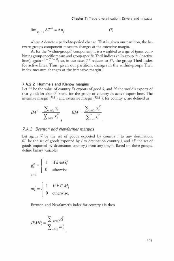
Chapter 7: Trade diversification: Drivers and impacts
303
(7)
where Δ denote a period-to-period change. That is, given our partition, the be-tween-groups component measures changes at the extensive margin.
As for the “within-groups” component, it is a weighted average of terms com-bining group-specific means and group-specific Theil indices T j. In group G0 (inactivelines), again μ
0 = T 0 = 0; so, in our case, T W reduces to T 1, the group Theil index
for active lines. Thus, given our partition, changes in the within-groups Theilindex measure changes at the intensive margin.
7.A.2.2 Hummels and Klenow marginsLet be the value of country i’s exports of good k, and the world’s exports ofthat good; let also stand for the group of country i’s active export lines. Theintensive margin (IM
i
) and extensive margin (EM i), for country i, are defined as
7.A.3 Brenton and Newfarmer margins
Let again be the set of goods exported by country i to any destination, be the set of goods exported by i to destination country j, and the set of
goods imported by destination country j from any origin. Based on these groups,define binary variables
and
Brenton and Newfarmer’s index for country i is then
mkj =
1 if k ∈M1j
0 otherwise.
⎧⎨⎪
⎩⎪
iχκ Wχ
κ
iG1
iG1
ijG1
jM1

Trade and Employment: From Myths to Facts
304
7.A.4 Description of the drivers of diversification
Market access:Countries belonging to free trade areas and customs unions obtain privileged accessto each other’s markets that do not have to be granted to non-members. To capturethis aspect of market access we compute, for each country i, a weighted sum of allthe preferential trade agreements (PTAs) it participates in. The weights correspondto partner’s market size (as measured by GDP).
where i is the exporter country, k the importer one, t the year and w the world.This variable is computed by the authors following Dutt, Mihov and van Zandt(2009). PTAs come from Jeffrey Bergstrand’s database, available at:http://www.nd.edu/~jbergstr/. For each country pair and year, we define PTA=1 ifthe exporter benefits from a reciprocal preferential access to the importer’s market.30
Remoteness:The remoteness index, also called “multilateral resistance” term , is defined as:
where i is the exporter country, k the importer one, t the year and w the world.This variable was computed by Carrère, de Melo and Wilson (2011) on the basisof Rose (2004).
Infrastructure index:This variable was computed by Carrère, de Melo and Wilson (2011), using datafrom the telecommunication sector (number of main telephone lines per 1000workers), the transportation sector (the length of the road and railway network —inkm per km2 of land area) and an index of quality in the service of transport (theshare of paved roads in total roads). These raw data come from Canning (1998) andthe World Development Indicators (WDI) database (see Carrère, de Melo and Wilson,2011, appendix A2 for more details).
Politics variables:We use two variables reflecting the political regime and quality of government. Bothvariables come from the QoG database built up by Teorell et al. (2009). This database
30 This database records the economic integration of bilateral country pairings for 195 countries an-nually from 1960 through 2005. Depending on the level of economic integration, a country pairingwas assigned a code varying from 0 to 6. We convert this code into a 0/1 dummy.

Chapter 7: Trade diversification: Drivers and impacts
305
regroups several political variables issued by international institutions and researchers’studies.
The Revised Combined Polity Score assesses the degree of democracy of acountry (see Marshall and Jaggers, 2002). It ranges from +10 (strongly democratic)to -10 (strongly autocratic).
The ICRG indicator of Quality of Government is part of the InternationalCountry Risk Guide provided by the PRS Group.31 The ICRG indicator of Qualityof Government is a mean value of the ICRG variables “Corruption”, “Law andOrder” and “Bureaucracy Quality”.32 It scales from 0 to 1 with higher values indicatinga higher quality of government.
Other variables:Population, R&D spending and FDI come from the WDI database provided by theWorld Bank.
31 Available at: http://www.prsgroup.com/ICRG.aspx.32 These component variables can be purchased at: http://www.countrydata.com.
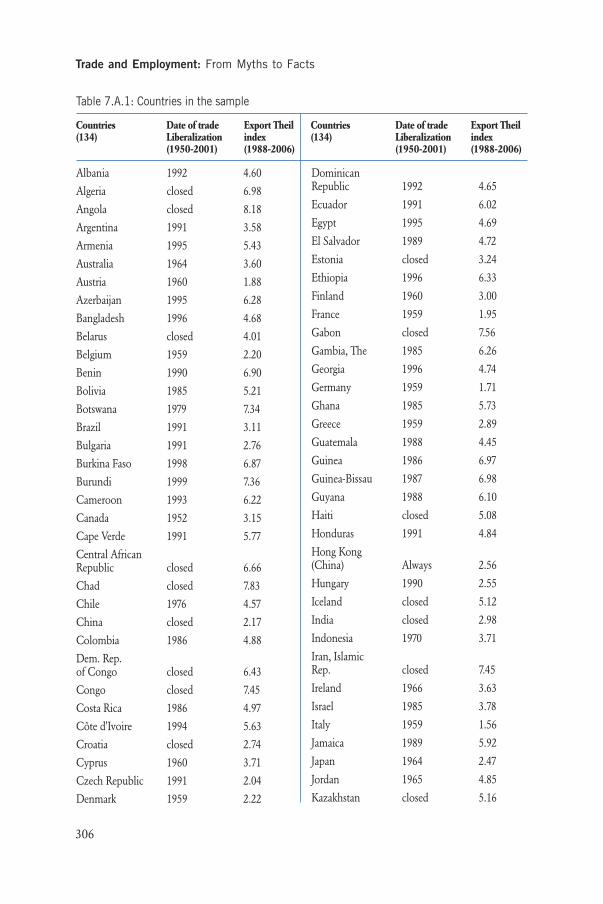
Albania 1992 4.60
Algeria closed 6.98
Angola closed 8.18
Argentina 1991 3.58
Armenia 1995 5.43
Australia 1964 3.60
Austria 1960 1.88
Azerbaijan 1995 6.28
Bangladesh 1996 4.68
Belarus closed 4.01
Belgium 1959 2.20
Benin 1990 6.90
Bolivia 1985 5.21
Botswana 1979 7.34
Brazil 1991 3.11
Bulgaria 1991 2.76
Burkina Faso 1998 6.87
Burundi 1999 7.36
Cameroon 1993 6.22
Canada 1952 3.15
Cape Verde 1991 5.77
Central AfricanRepublic closed 6.66
Chad closed 7.83
Chile 1976 4.57
China closed 2.17
Colombia 1986 4.88
Dem. Rep. of Congo closed 6.43
Congo closed 7.45
Costa Rica 1986 4.97
Côte d'Ivoire 1994 5.63
Croatia closed 2.74
Cyprus 1960 3.71
Czech Republic 1991 2.04
Denmark 1959 2.22
Dominican Republic 1992 4.65
Ecuador 1991 6.02
Egypt 1995 4.69
El Salvador 1989 4.72
Estonia closed 3.24
Ethiopia 1996 6.33
Finland 1960 3.00
France 1959 1.95
Gabon closed 7.56
Gambia, The 1985 6.26
Georgia 1996 4.74
Germany 1959 1.71
Ghana 1985 5.73
Greece 1959 2.89
Guatemala 1988 4.45
Guinea 1986 6.97
Guinea-Bissau 1987 6.98
Guyana 1988 6.10
Haiti closed 5.08
Honduras 1991 4.84
Hong Kong (China) Always 2.56
Hungary 1990 2.55
Iceland closed 5.12
India closed 2.98
Indonesia 1970 3.71
Iran, Islamic Rep. closed 7.45
Ireland 1966 3.63
Israel 1985 3.78
Italy 1959 1.56
Jamaica 1989 5.92
Japan 1964 2.47
Jordan 1965 4.85
Kazakhstan closed 5.16
Table 7.A.1: Countries in the sample
Countries Date of trade Export Theil Countries Date of trade Export Theil(134) Liberalization index (134) Liberalization index
(1950-2001) (1988-2006) (1950-2001) (1988-2006)
Trade and Employment: From Myths to Facts
306
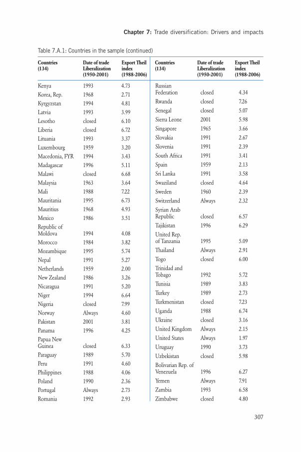
Kenya 1993 4.73
Korea, Rep. 1968 2.71
Kyrgyzstan 1994 4.81
Latvia 1993 3.99
Lesotho closed 6.10
Liberia closed 6.72
Lituania 1993 3.37
Luxembourg 1959 3.20
Macedonia, FYR 1994 3.43
Madagascar 1996 5.11
Malawi closed 6.68
Malaysia 1963 3.64
Mali 1988 7.22
Mauritania 1995 6.73
Mauritius 1968 4.93
Mexico 1986 3.51
Republic of Moldova 1994 4.08
Morocco 1984 3.82
Mozambique 1995 5.74
Nepal 1991 5.27
Netherlands 1959 2.00
New Zealand 1986 3.26
Nicaragua 1991 5.20
Niger 1994 6.64
Nigeria closed 7.99
Norway Always 4.60
Pakistan 2001 3.81
Panama 1996 4.25
Papua NewGuinea closed 6.33
Paraguay 1989 5.70
Peru 1991 4.60
Philippines 1988 4.06
Poland 1990 2.36
Portugal Always 2.73
Romania 1992 2.93
Russian Federation closed 4.34
Rwanda closed 7.26
Senegal closed 5.07
Sierra Leone 2001 5.98
Singapore 1965 3.66
Slovakia 1991 2.67
Slovenia 1991 2.39
South Africa 1991 3.41
Spain 1959 2.13
Sri Lanka 1991 3.58
Swaziland closed 4.64
Sweden 1960 2.39
Switzerland Always 2.32
Syrian Arab Republic closed 6.57
Tajikistan 1996 6.29
United Rep.of Tanzania 1995 5.09
Thailand Always 2.91
Togo closed 6.00
Trinidad andTobago 1992 5.72
Tunisia 1989 3.83
Turkey 1989 2.73
Turkmenistan closed 7.23
Uganda 1988 6.74
Ukraine closed 3.16
United Kingdom Always 2.15
United States Always 1.97
Uruguay 1990 3.73
Uzbekistan closed 5.98
Bolivarian Rep. ofVenezuela 1996 6.27
Yemen Always 7.91
Zambia 1993 6.58
Zimbabwe closed 4.80
Table 7.A.1: Countries in the sample (continued)
Countries Date of trade Export Theil Countries Date of trade Export Theil(134) Liberalization index (134) Liberalization index
(1950-2001) (1988-2006) (1950-2001) (1988-2006)
Chapter 7: Trade diversification: Drivers and impacts
307