Diversification Strategies and Adaptation Deficit: Evidence from Niger

Solomon Asfaw, Alessandro Palma and Leslie Lipper

Invited paper presented at the 5th International Conference of the African Association

of Agricultural Economists, September 23-26, 2016, Addis Ababa, Ethiopia

Copyright 2016 by [authors]. All rights reserved. Readers may make verbatim copies of

this document for non-commercial purposes by any means, provided that this copyright

notice appears on all such copies.

1

Diversification Strategies and Adaptation Deficit:

Evidence from Niger

Solomon Asfaw*, Alessandro Palma** and Leslie Lipper*

*Corresponding author. Food and Agriculture Organization (FAO) of the United Nations, Agricultural

Development Economics Division, Viale delle Terme di Caracalla, 00153 Rome (Italy). E-mail:

solomon.asfaw@fao.org

**Università Commerciale Luigi Bocconi, Centre for Research on Energy and Environmental

Economics and Policy (IEFE). Via Roentgen 1, 20136 Milano, Italy.

Abstract

This paper provides fresh empirical evidence on the adaptation process to face climate changes

through the analysis of original cross-sectional data collected at household-level in Niger

merged with detailed geo-referenced climatic information. In particular, we identify the main

drivers and barriers of crop and labour diversification, which constitute two livelihood strategies

in mitigating the adaptation deficit by employing a Seemingly-Unrelated Regression (SUR)

model, which accounts for potential interdependence among different diversification practices.

Secondly, the effectiveness of diversification practices is assessed by means of three

complementary welfare measures, namely income changes, food security and the poverty gap

using quantile regression and instrumental variable strategy. We find that, aside from climate

shocks, the diversification level varies in response to the educational level of household

members and spatial location as well as the adoption of ICTs. The impacts of diversification

appear differentiated. While labour diversification is always positively associated with all the

three welfare measures, positive coefficients of crop diversification are significant only when

associated to food security. Robust causal inference confirms that anomalies in rainfall patterns

and droughts in particular, induce adaptation responses, which result in welfare gains limited by

a richer calorie intake, while the effects on income and severity of poverty appear detrimental.

JEL Classification: Q01, Q12, Q16, Q18

Keywords: diversification, adaptation, welfare, climate change, Niger

2

1 Introduction

There is overwhelming consensus on the fact that global climate change is altering the

variability of rainfall, temperature and other climatic parameters and that such modifications

will likely lead to an increase in the incidence of environmental disasters (e.g., IPCC, 2012;

Olson et al., 2014; Parry et al., 2004). Adaptation processes to face extreme climate events

often emerge as effective strategies to be undertaken by the most exposed communities

(Adger et al., 2003). Among the different contributions that have analysed the impact of

climate change on adaptation strategies in sub-Saharan Africa (SSA) countries, Niger - one of

the most vulnerable countries - has surprisingly received very little attention. Niger

constitutes an interesting case for analysis, since it represents a critical area for climate

variation and, at the same time, a highly vulnerable country in terms of potential capabilities

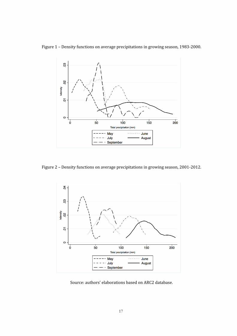
to face climatic events and economic shocks (IPCC, 2014). Figure 1 and 2 plot density

functions of average rainfall level registered in each month of the growing season and

provide a clear picture of long-run changes occurring between 1983-2000 and 2001-2012

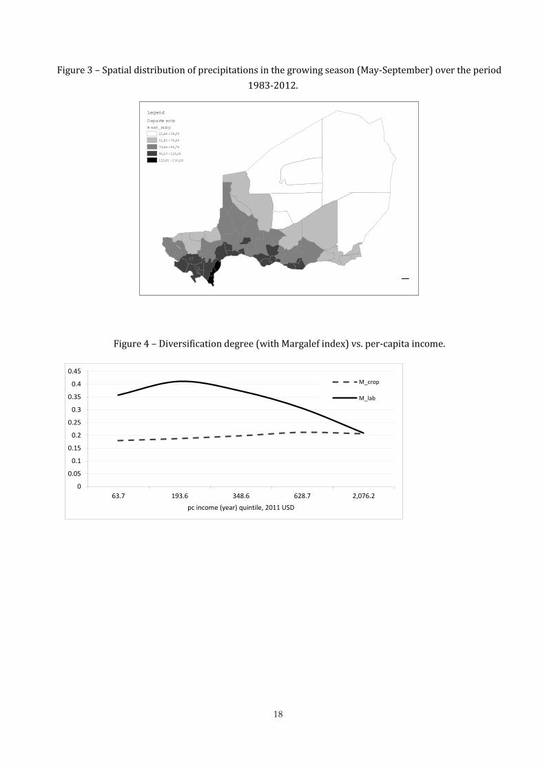
periods. At the spatial level (Figure 3), the distribution of rainfalls over Niger in the growing

season (May-September) appears to be strongly heterogeneous. Most precipitations

concentrate in southern areas, while the northern territories accumulate on average less than

40 mm of monthly rain.

Different factors can potentially make Nigerien communities particularly reluctant to

implement effective adaptation measures, including low migration levels, high presence of

nomadism phenomena, extensive rain-fed subsistence agriculture, very low education rates

and a lack of policy supports. Such elements constitute tangible and intangible barriers to

adopt adaptation practices, generating adaptation lock-in which may lead to 'wait and see' or

reactive approaches, low cognitive learning, misperception, and insufficient awareness of

climate risks with inefficient individual response to face extreme events (Le Dang et al.,

2014; Baird et al., 2014). In some cases, such barriers can also lead to competing behaviours

of indigenous traditions versus modern and more effective adaptation strategies (Baird and

Gray, 2014).

In light of this, our contribution to the existing literature is threefold. Firstly, our analysis

uses a comprehensive large national representative household level survey with rich socio-

economic information, merged with detailed geo-referenced climatic information. The

combination of these data allows us to assess the role of weather in determining farmers'

diversification decisions, and consequently, the impact on welfare. We explicitly consider the

possibility of farmers' choosing a mix of diversification options using a seemingly unrelated

regression (SUR) model, which accounts for potential interdependence among different

diversification practices. The impact of these latter is estimated through different welfare

indicators and conditioned to different levels of the welfare distribution by means of quantile

regression. Secondly, we also estimate the causal impact of crop diversification on different

measures of welfare using instrumental variables techniques (IV).

2 Data and empirical strategy

In order to determine the drivers of diversification practices as well as to test whether, and

to what extent, those practices are effective responses to guarantee sufficient livelihood

conditions in the presence of climate shocks, we exploit original cross-sectional data

3

(ECVM/A, 2011) deriving from different sources. The survey was implemented by the Niger

National Institute of Statistics with technical and financial assistance from the World Bank.

The ECVM/A envisages two visits, the first one during the planting season, and the second

one during the harvest season. A total of 25,116 individuals grouped in 3,968 households,

with information from either the first or second visit or both visits, characterized the final

dataset. The ECVM/A has been designed to have national coverage, including both urban and

rural areas all the regions of the country, with a fine spatial breakdown (270 enumerator areas

divided by urban areas, rural areas, and within the rural areas, agricultural zones, agro-

pastoral zones and pastoral zones). We combine this valuable socio-economic dataset with

detailed information on precipitation collected at enumerator area level, every ten days

(decadal), from 1983 to 2012. Weather data derive from the Africa Rainfall Climatology

Version 2 (ARC2) database and cover the 1983-2012 period. Given the specific focus of this

paper on the diversification practices as a possible livelihood strategy for the most vulnerable

communities, the final dataset only includes 2396 rural Nigerien households, observed in

2011 and distributed across 139 enumerator areas1 and eight administrative regions. In

testing the drivers of diversification and their effect on household welfare, we apply a

sequential empirical procedure. The first step aims at determining the most important

diversification drivers (Section 2.1), with a stronger emphasis on climate factors. Once such

drivers are identified, in the second step we estimate the impact of diversification on a set of

three welfare measure (Section 2.2). In addition, we also address potential endogeneity

deriving from the reverse causality of crop diversification and welfare conditions by

estimating instrumental variable techniques (Section 2.3).

2.1 Determinants of diversification

Our econometric modelling of the determinants of diversification takes into account a series

of issues. First, given that the diversification strategies result in a variety of practices

affecting different income sources, we first distinguish between diversification in crop

species and labour diversification. However, despite excluding income diversification and

focusing the analysis on rural households, the two diversifications considered can still be

linked in some cases2. Thus, when investigating the drivers of diversification, it is important

to take into account both specific and common factors which can affect at the same time and

in different directions the two types of diversification, depending on the degree of their

complementarity or substitutability.

In terms of econometric modelling, separate estimations would not capture this correlation

and would not exploit the information deriving from the entire set of common regressors. In

order to address the previous issues, for the analysis of diversification determinants we

employ a Seemingly-Unrelated Regression model (SUR) (Zellner, 1963). In particular, the

iterative two-stage generalized least square estimator allows the SUR model to provide

efficient estimations by combining information on different equations and accounts for

1 More than 40% per cent of the sample lies in desert regions.

2 Livestock activities are included in labour diversification. We intentionally do not consider income

diversification in our analysis since this implies the availability of relevant capital stocks in heterogeneous

activities, a situation unlikely to be found in rural households.

4

potential correlation in the error terms. According to the theoretical framework previously

discussed and considering the data limitations, we specify a two-equation SUR model, in

which the dependent variables measuring the degree of diversification are regressed over a

set of common predictors, while the error terms are assumed being correlated. More formally,

for each 𝑖=1,..,𝑁 household, the two-equation model in compact notation is given by:

𝑫𝑖,𝑗 = 𝜷0 +𝚿𝑖,𝑗𝛽𝑖 + 𝜺𝑖,𝑗

where 𝑁=2396 and 𝑗=1,2 indexes, respectively, the equation for crop and labor

diversification. The errors 𝜺 are assumed to be correlated within individuals and uncorrelated

across individuals, with the overall variance-covariance matrix given by Ω = 𝐸(휀휀′) =

∑⊗ 𝐼𝑁. The vector of dependent variable 𝑫 measures the degree of diversification, whose

metrics deserves some explanation. A common method for assessing the degree of

diversification is the calculation of a vector of income shares related to different income

sources (Lay et al., 2008 and Davis et al., 2010 among others). Such a method puts directly

into the relationship diversification activities and income changes but, on the other hand, a

relevant part of information related to different aspects of diversification is neglected.

Accordingly, our first diversification measure is constituted by the Shannon-Weaver index as

suggested by Duelli and Obrist (2003). In addition, robust directions on the impacts of

diversification determinants are also derived by testing in our model the Margalef index

(measuring the simple richness) and the Berger-Parker index (measuring the relative

abundance). For agricultural diversification, the indices consider the number of cultivated

crop species adjusted by land size at plot level, and for labour diversification, we calculated

the number of different work activities by distinguishing from 11 different jobs, divided by

skilled and unskilled workers3 aged between 14 and 65 and resulting in 22 labour

differentiations.

The set of independent variables, common to the two equations and represented by the

vector 𝚿 include Climate shocks variable. Our data allows us to map long-run weather

anomalies in order to identify climate shocks in the single period of interest, i.e. 2011, with

finer spatial and temporal breakdown than in previous studies (Ersado, 2003; Nhemachena

and Hassan, 2007; Dimova and Sen, 2010). In order to identify long-run climate anomalies

on the basis of the available data, we rely on the Standard Precipitation Index (SPI). The SPI

is a widely used indicator, which allows detection of significant variations in precipitations

with respect to the long-run mean. To this aim, raw precipitation data are fitted to a gamma or

Pearson Type III distribution, which is then transformed to a normal distribution (see

Guttman, 1999 for further details). The use of the SPI presents some advantages with respect

to other methods. First, in order to identify climate anomalies such as drought or excessive

rainfalls, only time-series data on precipitation are required. Moreover, the SPI is an index

based on the probability of recording a given amount of precipitation. Since the probabilities

are standardized, a value of zero indicates the median precipitation amount, thus the index is

negative for drought, and positive for wet conditions. As the dry or wet conditions become

more severe, the index becomes more negative or positive, ranging within a commonly-used

scale from -2.5 and +2.5 (WMO, 2012). The characteristic of being standardized thus

3 We assume that household members can choose between investing in skilled or unskilled activities.

5

provides a straightforward interpretation and allows for a fully indexed comparison over time

and space. In addition, the SPI can be computed for several time scales, ranging from one to

24 months, capturing various scales of both short-term and long-term anomalies. In order to

compute our climate shock variables, we first calculate the SPI at 12 months for the reference

year 2011. Once the long-run climate anomalies are detected by using the interpretation table

provided in WMO (2012), we identify drought and rainfall shocks with dummy variables

corresponding to SPI values ranging from less than -2 to more than +2, respectively. Thus, a

SPI value of -2.0 or less signals a drought shock while values of +2.0 or more indicates

extremely wet conditions4.

We also include in the model proxies of spatial position, access to markets and

infrastructures. In order to account for the access to main infrastructures, our dataset is

augmented with information on the road density within a radius of 15 km and with the

average distance to main infrastructures calculated as the simple mean of the distance from

the household and the nearest postal office, bank and hospital as a proxy of market and credit

access; We also include proxies of technology, knowledge and education level such as

average household educational level considering all the family members and, as a proxy of

knowledge absorption capacity, we include the level of technology endowment by calculating

the count of ICT assets as the total number of mobile phones, TVs, radios, cameras, video

cameras and computers owned by each households. We also included household endowments

such as livestock ownership, non-technological agricultural and technological assets, the

presence of market and crop shocks d and the adoption of modern varieties (MVs) among

others.

2.2 Effects of diversification

Our multidimensional picture of households' welfare conditions relies on a set of three

indicators, which capture different aspects and issues to be taken into account when the

analysis of wellbeing is under scrutiny. Namely, our dependent variables consider the total

household income expressed in US dollars as a basic measure of welfare. In addition, the

Dietary Energy Supply (DES) expressed in per-capita calories per day, as well as the Severity

of Poverty (SP) calculated as the squared of the poverty gap index5, also provides

information on food security and inequality among the poor, respectively.

Preliminary statistics signal that the degree of diversification changes according to the

welfare status and endowment level. In the case of income (Figure 4), labour diversification

measured by the Margalef index follows a reverse U-shaped curve, suggesting that the

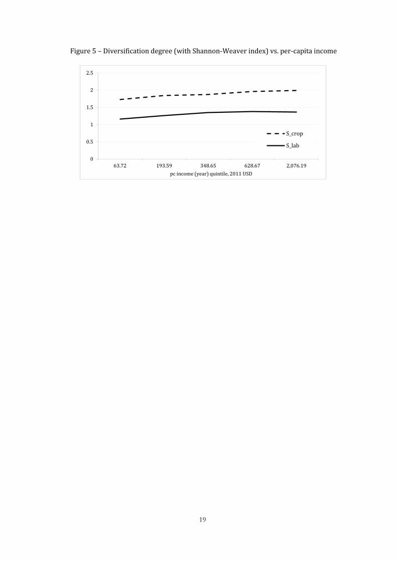
diversification level is higher in middle-income rural households. On the contrary, when the

same diversification is measured through the Shannon-Weaver index (Figure 5), which

accounts for the evenness, a monotonic trend appears. At empirical level, this evidence not

only suggests measuring the impact of diversification conditioned to different welfare ranges,

but also justifies the choice of using different diversification measures. In order to capture

4 In order to capture the specific impact of long-run weather anomalies on the rural households, the SPI is

calculated by including only the months falling in the growing season (i.e. from May to September).

5 Poverty line at 1.25 2005 PPP US Dollars (World Bank, 2015).

6

heterogeneity due to the differentiated impacts on the households' welfare, we employ a

quantile regression model (Koenker and Hallock, 2001; Koenker, 2005).

The uncorrelated effect of each type of diversification is captured by employing fitted

values of dependent variables deriving from the SUR model estimation as welfare predictors

in the quantile model, although in adopting such a procedure we do not support any causality

claim. In estimating the quantile model, the diversification impact is conditioned to three

sections of the distribution (i.e., 𝑞 = {0.25, 0.5, 0.75}) of the dependent variable, namely

income, DES and SP. It is worth mentioning that the potential bias deriving from the

sequential empirical procedure here proposed is minimized by using bootstrapping

replications for estimating the quantile model with corrected standard errors. For the 𝑖-th

household, the welfare equation of the quantile model is given by:

𝑊𝑖 = 𝛽0,𝑖 + 𝛽1𝐷𝑖1 + 𝛽2𝐷𝑖2 + 𝛽3𝜆𝑖 + 𝛽4𝛿𝑖 + 𝛽5𝜏𝑖 + 𝜖𝑖

in which 𝑊 represents the welfare level and 𝐷1, 𝐷2, are the fitted values measuring crop and

labor diversification, respectively. In addition, a series of specific variables and controls

directly related to the welfare status are also included, and namely: the sum of total non-

technological assets 𝜆 owned by each household, the age of household head 𝛿, and the

number of family members 𝛿 to control for household size. 휀 represents the idiosyncratic

error component. The model estimation is repeated with three different welfare measures

(income, DES and SP), thus providing a comprehensive picture of the households living

conditions. We also employ an instrumental variable approach to control for potential

endogeneity problem associated with diversification decision.

[Figure 4 & 5 - about here]

3 Results

3.1 Determinants of diversification

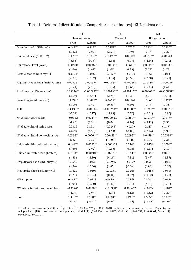
The outcomes obtained by the SUR model are presented in Table 1, in which columns 1, 2

and 3 report the estimates for Shannon-Weaver, Margalef and Berger-Parker diversification

indexes, which represent, respectively, our dependent variables.

As a general and most important result (column 1), we obtain that both crop and labour

diversification are significantly affected by weather shocks, these being expressed as dummy

variables signalling extreme deviations of the SPI values. This evidence allows us to

hypothesize a causal response of households in consequence of extreme climate fluctuations,

the latter inducing diversification behaviour as an adaptive strategy. In the case of crop

diversification, such a hypothesis will be further scrutinized and confirmed in Section 3.3 by

means of the instrumental variables technique.

[Table 1 - about here]

Further interesting results derive from the analysis of other diversification determinants. In

particular, households that are more educated enrich their portfolio of practices and are more

prone to adopt diversification strategies. As in the previous variables, the positive effect of

education is robust to other diversification measures (column 2 and 3). With respect to the

access to infrastructures, our variable of interest (the distance to main facilities) is always

associated to negative and significant coefficients for crop diversification, thus households

living far from main urban areas seem to be more prone to adopt crop diversification

7

behaviour. Higher distances should imply difficulty in accessing the main markets as well as

lower chances for socially interacting with more organized communities in search of business

opportunities. However, while higher distances act as barriers for crop diversification

performances, in the case of labour diversification they have not univocal direction. In fact,

higher values of labour diversification should be related to efficient labour markets

characterized by higher information levels and the latter, in turn, should benefit from lower

distances to urban agglomerations where most business takes place. Nevertheless, our

estimates signal that potential benefits deriving from social interactions are not fully

captured. This may reveal the existence of individual barriers which may lead to social lock-

in that negatively impact the household capacity to access the labour market and enrich the

portfolio of job activities.

A further spatial impact significant in all three model specifications is given by the

geographical location of households, which confirms the hypothesis that those households

living in desert regions and that likely constitute the most vulnerable communities are more

prone to adopt diversification practices. The impact is larger for crop diversification,

suggesting that the enrichment of crop species variety constitutes a more effective livelihood

response in households living in areas subject to drought shocks.

According to our model, higher TLU values are negatively associated with crop

diversification and seem to favour labour diversification, although this relation is significant

only when diversification is measured by the Margalef index (column 2). Interesting aspects

also emerge from the assessment of technology assets. Namely, households with higher

endowments of ICT devices (such as mobile phones, smartphones, computers, radio and

other devices that favour the communication among individuals) are more likely to

experience a higher level of labour diversification, and this relation is consistent across the

three diversification measures. On the other hand, the correlation between ICT endowment

and crop diversification is negative and significantly differs from zero only when measured

through the Berger-Parker index (column 3). Moreover, ICTs enhance the communication

process and facilitate social interaction, thus allowing households to capture pieces of

knowledge such as job offers and other opportunities, which are functional to higher levels of

labour diversification. On the other hand, the hypothesis that ICTs would play an effective

role in informing people on local weather forecasts, thus enhancing the awareness on the

risks due to extreme weather events, cannot be confirmed in our analysis of diversification

determinants.

We find a positive and significant correlation between the amount of irrigated cultivated

land and the level of labour diversification, while the relation is so far significant in the case

of crop diversification (column 2 and 3). This result is coherent with the geography of Niger,

since the extent of lands that benefit from irrigation systems is very little6. On the other hand,

the effects on crop diversification conditioned to the amount of rainfed land are characterized

by significantly positive relationships, which is also consistent across the three diversification

measures (column 2 and 3). However, the relation is not univocal for labour diversification,

whose positive and significant sign associated with the Shannon-Weaver index (column 1)

6 The share of irrigated cultivated land over the total cultivated land is 6.8%.

8

turns out to be negative and weaker when diversification is measured by the Margalef index

(column 2). This signals that in presence of rainfed land, households prefer to adopt crop

diversification instead of labour diversification. In line with the empirical agronomic

literature, farmers utilize rainfed land for subsistence purposes and there are local landraces

that are demonstrated to be more resistant to water and climatic stressors. Traditionally,

landraces are cultivated in a rich mixed cropping system so as the rainfed land is per se an

asset linked with the strategy of crop diversification. On the contrary, on irrigated land,

modern agricultural technologies may be applied in order to cultivate major and cash crops,

which require higher level of water, and in an optimal intensification approach, a mono-

cropping farming that may result in a diversity reduction (Bellon, 2004; Lipper and Cooper,

2008). Such a hypothesis is first tested by including a dummy variable indicating the

presence of modern varieties (MV). In addition, we interact the MV-dummy with the amount

of irrigated cultivated land. The variable of adoption of modern varieties (MV) seems to be

negatively correlated to both crop and labour diversification practices, and this result also

holds when diversification is measured both with Margalef and Berger-Parker index. From

the negative and significant coefficient of the interacted variable, we can infer that when land

is allocated to cultivate modern varieties, the intensification process takes place at the

expense of the variety of crop species, although this result shows less significance in the

estimations using the Margalef and Berger-Parker indices (column 2 and 3).

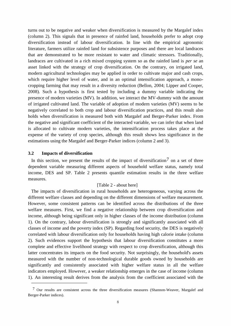
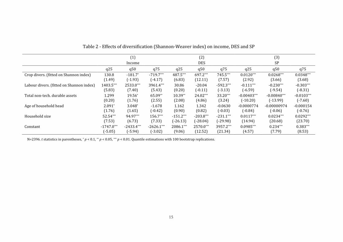
3.2 Impacts of diversification

In this section, we present the results of the impact of diversification7 on a set of three

dependent variable measuring different aspects of household welfare status, namely total

income, DES and SP. Table 2 presents quantile estimation results in the three welfare

measures.

[Table 2 - about here]

The impacts of diversification in rural households are heterogeneous, varying across the

different welfare classes and depending on the different dimensions of welfare measurement.

However, some consistent patterns can be identified across the distributions of the three

welfare measures. First, we find a negative relationship between crop diversification and

income, although being significant only in higher classes of the income distribution (column

1). On the contrary, labour diversification is strongly and significantly associated with all

classes of income and the poverty index (SP). Regarding food security, the DES is negatively

correlated with labour diversification only for households having high calorie intake (column

2). Such evidences support the hypothesis that labour diversification constitutes a more

complete and effective livelihood strategy with respect to crop diversification, although this

latter concentrates its impacts on the food security. Not surprisingly, the household's assets

measured with the number of non-technological durable goods owned by households are

significantly and consistently associated with higher welfare status in all the welfare

indicators employed. However, a weaker relationship emerges in the case of income (column

1). An interesting result derives from the analysis from the coefficient associated with the

7 Our results are consistent across the three diversification measures (Shannon-Weaver, Margalef and

Berger-Parker indices).

9

average e age of household head, which is not significantly associated only with mid- and

low-income classes (column 1). The inconsistency existing in the impact of age on income

and food supply may reveal, ceteris paribus, a decoupling effect between income

accumulation and the capacity to transform this later into proportional food security, although

such evidence cannot be confirmed here since it would require panel data analysis.

Since our first welfare measure is given by total family income, the inclusion of the

household size as a control is necessary. In the case of income (column 1), larger households

are significantly associated with higher incomes and such an effect is consistent across all the

income classes. On the contrary, when considering the amount of food consumed as well as

the severity of poverty index, the relationship assumes the opposite sign (column 2 and 3).

Building on these results, we may infer that a higher number of family members may imply

more people at work and a higher income when considering the household as a whole. At the

same time, this may also entail more need for food, which is often self-produced within the

family unit, in particular in rural and marginalized households. The resulting balance may

envisage net income gains but also lower food per capita where households have difficulty in

accessing other food sources.

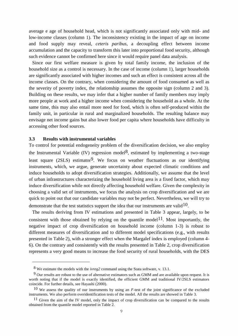
3.3 Results with instrumental variables

To control for potential endogeneity problem of the diversification decision, we also employ

the Instrumental Variable (IV) regression model8, estimated by implementing a two-stage

least square (2SLS) estimator9. We focus on weather fluctuations as our identifying

instruments, which, we argue, generate uncertainty about expected climatic conditions and

induce households to adopt diversification strategies. Additionally, we assume that the level

of urban infrastructures characterizing the household living area is a fixed factor, which may

induce diversification while not directly affecting household welfare. Given the complexity in

choosing a valid set of instruments, we focus the analysis on crop diversification and we are

quick to point out that our candidate variables may not be perfect. Nevertheless, we will try to

demonstrate that the test statistics support the idea that our instruments are valid10.

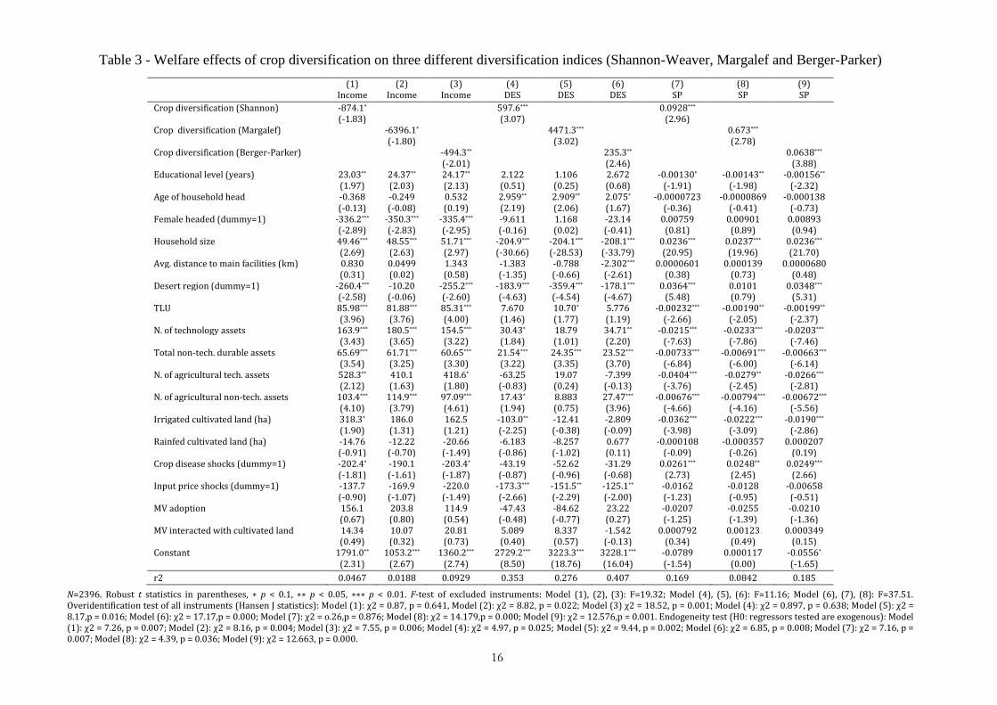
The results deriving from IV estimations and presented in Table 3 appear, largely, to be

consistent with those obtained by relying on the quantile model11. Most importantly, the

negative impact of crop diversification on household income (column 1-3) is robust to

different measures of diversification and to different model specifications (e.g., with results

presented in Table 2), with a stronger effect when the Margalef index is employed (column 4-

6). On the contrary and consistently with the results presented in Table 2, crop diversification

represents a very good means to increase the food security of rural households, with the DES

8 We estimate the models with the ivreg2 command using the Stata software, v. 13.1.

9 Our results are robust to the use of alternative estimators such as GMM and are available upon request. It is

worth noting that if the model is exactly identified, the efficient GMM and traditional IV/2SLS estimators

coincide. For further details, see Hayashi (2000). 10 We assess the quality of our instruments by using an 𝐹-test of the joint significance of the excluded

instruments. We also perform overidentification tests of the model. All the results are showed in Table 3.

11 Given the aim of the IV model, only the impact of crop diversification can be compared to the results

obtained from the quantile model reported in Table 2.

10

being positively and strongly significantly associated with crop diversification in all the three

indices (column 4-6). In addition, crop diversification also assumes an effective role in

reducing the poverty gap, although this effect is less significant than that on income and DES

(column 7-9). By combining the previous results with those obtained through IVs, we find

robust evidence of the negative role of crop diversification in terms of income gains and

limited capacity to mitigate the severity of poverty. If adapted to our context, such evidence

is in line with previous studies, which relate production performances to the degree of crop

diversification (Di Falco et al., 2010; Di Falco and Chavas, 2009). In our case, rural

households represent the most marginalized communities, which rely on crop diversification

as a mere adaptation strategy. In support of this hypothesis, it is worth considering that Niger

is characterized by imperfect markets and weak policy support, which make difficult access

to complementary agricultural inputs and food purchasing. Thus, diversifying households

cannot capture complementary welfare benefits such as income gains, deriving from richer

crop diversity; they rely on diversification mainly as an adaptive response able to guarantee

sufficient food supply.

Regarding the variables related to specific households' characteristics, we observe that

higher educational level correspond to slightly higher incomes (column 1-3) and lower values

of severity of poverty (column 7-9). We also find confirmation on the negative performances

of female-headed households both in terms of income changes (column 1-3), while no

significant impact is found with respect to food security and severity of poverty (columns 4-6

and 7-9). The size of family is significantly and positively associated to higher incomes

(column 1-3), but also implies more need for food and more income allocated to the latter

(column 4-6 and 7-9). Hence, the size of family produces differentiated impact across the

three welfare dimensions here analysed, a result consistent with the previous results reported

in Table 2. With respect to the spatial factors, we observe that the average distance to main

facilities shows no significant effects on welfare status. Living in desert regions represents a

significant welfare reduction factor, since such a negative impact holds across the three

welfare dimensions on all diversification measures. Interesting results can also be observed

when the household assets are analysed. One relevant and interesting effect is due to the role

of ICT devices, which allow households to capture a higher level of technical knowledge,

more accurate weather forecasts and other pieces of knowledge that are key for implementing

effective crop diversification strategies. ICTs produce strongly significant and positive

impacts not only in terms of income (column 1-3) but also in the amount of food calories

(columns 4-7) as well as in reducing the poverty gap (columns 7-9). Moreover, such effects

are robust to the three diversification measures. Regarding the importance of agricultural

assets, a significant role is assumed by the non-technology ones which, together to the

amount of irrigated cultivated land, are functional to producing higher incomes (columns 1-3)

and also to mitigating the severity of poverty (columns 7-9). On the other hand, households

that own rain-fed lands are not significantly affected by any welfare variations.

[Table 3 - about here]

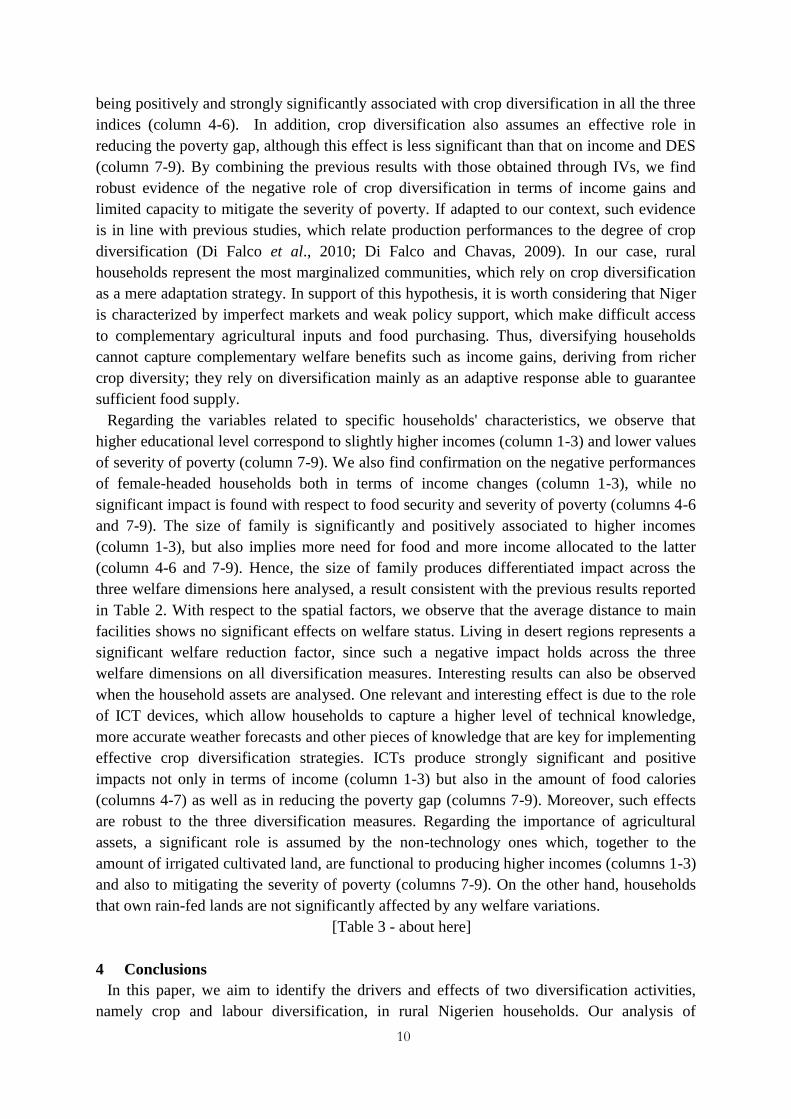
4 Conclusions

In this paper, we aim to identify the drivers and effects of two diversification activities,

namely crop and labour diversification, in rural Nigerien households. Our analysis of

11

diversification determinants confirms the hypothesis that anomalies in rainfall patterns result

in adaptation responses measured through the adoption of diversification practices. The

inducement effect of climate factors is consistent for both crop and labour diversification and

across the three indices of diversification employed, namely Shannon-Weaver, Margalef and

Berger-Parker.

Besides, the main `push' factors given by the drought shocks, the level of crop

diversification is positively associated to other significant catalysts such as the educational

level of household members, the spatial location, and different sets of household

endowments. On the other hand, main limitations to crop diversification derive from the

amount of livestock owned, from the presence of female-headed households and from

excessive rainfalls. The combined effect of adopting MVs with cultivated irrigated land

signals the potential presence of agricultural intensification processes which is detrimental to

richer degrees of crop diversification.

Regarding the labour diversification, the infrastructural level and the distance from main

facilities imply opposite diversification behaviour. While crop diversification benefits from

longer distances and from a denser road pattern, labour diversification seems to be negatively

affected by these factors. On the other hand, labour diversification positively responds to

higher levels of household ability to capture pieces of knowledge and information from ICT

devices. In addition, in line with the results obtained for crop diversification, living in desert

areas induces households to allocate labour in a richer way. Additional beneficial effects for

labour diversification are signalled by the interaction of the MV variable with the one

indicating the amount of irrigated cultivated land as well as by the amount of both

technological and non-technological agricultural assets owned by households.

The second part of our analysis focuses on the impacts of diversification, which are

scrutinized on a set of three welfare indicators. Largely the quantile model confirms our

descriptive evidence of differentiated effects across different classes of the different welfare

indicators. More in detail, labour diversification is significantly and positively associated

with income and negatively with the severity of poverty, particularly in the higher welfare

classes. However, a weakly significant correlation is also found in the case of higher classes

of DES. On the contrary, a richer calorie intake is always and strongly significantly

associated with crop diversification, while the latter is negatively correlated with income and

more severe poverty. As in the previous estimations, the instrumental variable approach also

shows that impacts of diversification significantly affect the level of welfare with

differentiated impacts. Namely, crop diversification is confirmed to reduce the income level

and to increase the severity of poverty, but its role is key for sustaining households with

larger caloric intake. This supports the hypothesis that most marginalized farmers are more

responsive to crop-diversification as a risk-minimization strategy and that such a strategy is

actually effective in increasing their food security.

References

Adger W.N., Dessai S., Goulden M., Hulme M., Lorenzoni I., Nelson D.R., Naess L.O., Wolf

J., Wreford A. (2009). Are there social limits to adaptation to climate change? Climate

Change Vol. 93, pp. 335-354.

12

Asfaw S., McCarthy N., Cavatassi R., Paolantonio A., Amare M, Lipper L. (2015)

Diversification, Climate Risk and Vulnerability to Poverty: Evidence from Rural Malawi.

FAO-ESA Working Paper.

Asmah, E. E. (2011). Rural livelihood diversification and agricultural household welfare in

Ghana. Journal of Development and Agricultural Economics 3(7): 325-334.

Babatunde, R. O., Qaim, M. (2009) Patterns of Income Diversification in Rural Nigeria:

Determinants and Impacts. Quarterly Journal of International Agriculture 48: 305-320.

Baird T. D., Gray C. L. (2014). Livelihood Diversification and Shifting Social Networks of

Exchange: A Social Network Transition? World Development, Vol. 60, pp. 14–30.

Barrett, C. B., Reardon, T. (2000) Asset, Activity, and Income Diversifications Among

African Agriculturalist: Some Practical Issues. Project report to USAID BASIS CRSP.

Biasutti, M., Held, I.M., Sobel, A.H., Giannini, A. (2008). SST forcings and Sahel rainfall

variability in simulations of the twentieth and twenty-first centuries. J. Clim., Vol. 21,

pp.3471–3486.

Brooks, N., Adger, N., Kelly, M. (2005). The determinants of vulnerability and adaptive

capacity at the national level and the implications for adaptation. Global Environ. Change

15, 151–163.

Davis, B., Winters, P., Carletto, G., Covarrubias, K., Quinones, E. J., Zezza, A., DiGiuseppe,

S. (2010). A cross-country comparison of rural income generating activities. World

Development, Vol. 38(1), pp. 48-63.

Di Falco, S., Chavas, J. P. (2009). On crop biodiversity, risk exposure, and food security in

the highlands of Ethiopia. American Journal of Agricultural Economics 91(3): 599-611.

ECVM/A (2011). 2011 National Survey on Household Living Conditions and Agriculture.

Basic information document. Republic of Niger, National Institute of Statistics.

Guttman N. B. (1999). Accepting the Standardized Precipitation Index: a calculation

algorithm. JAWRA Journal of the American Water Resources Association, vol. 35 (2), pp.

311–322.

Hayashi F. (2000). Econometrics. Princeton University Press.

Hulme, M., 2001. Climate perspectives in Sahelian desiccation. Global Environ. Change 11,

19–29.

Kahn M. (2005). The death toll from natural disasters: the role of income, geography and

institutions. Review of Economics and Statistics, 87, pp. 271-284.

Koenker (2005). Quantile Regression. Cambridge University Press: New York.

Koenker R., Hallock K. F. (2001). Quantile Regression. Journal of Economic Perspectives,

Vol. 15(4), pp- 143-156.

Kurukulasuriya P., Mendelsohn R. (2008). Crop switching as a strategy for adapting to

climate change. AfJARE Vol 2 No 1, pp. 105-126.

Mendelsohn R. O., Dinar A. (2009). Climate Change and Agriculture: An Economic Analysis

of Global Impacts, Adaptation and Distributional Effects. Edward Elgar Publishing.

Narloch, U., Drucker, A. G., Pascual, U. (2011). Payments for agrobiodiversity conservation

services for sustained on-farm utilization of plant and animal genetic resources. Ecological

Economics, 70(11), pp. 1837-1845.

13

Nhemachena C., Hassan R. (2007). Micro-level analysis of farmers’ adaptation to climate

change in Southern Africa. IFPRI Discussion Paper No. 00714. International Food Policy

Research Institute, Washington, DC.

Novella N. S., Thiaw W. M. (2013). African Rainfall Climatology Version 2 for Famine

Early Warning Systems. Journal of Applied Meteorology and Climatology, vol. 52, pp.

588-606.

Shiferaw B., Menale K., Moti J., Chilot Y. (2013). Adoption of improved wheat varieties and

impacts on household food security in Ethiopia. Food Policy.

Toya H., Skidmore M. (2007). Economic development and the impacts of natural disasters.

Economic Letters, 94 (1), pp. 20-25.

World Bank (2013). Turn Up the Heat. Climate Extremes, Regional Impacts, and the Case for

Resilience World Bank, Washington, DC

Zellner A. (1963). Estimators for seemingly unrelated regression equations: some exact finite

sample results. Journal of the American Statistical Association, Vol. 58, pp. 977-992.

14

Table 1 - Drivers of diversification (Comparison across indices) - SUR estimations.

N= 2396, t statistics in parentheses * p < 0.1, ** p < 0.05, *** p < 0.01. SUR model, correlation matrix. Breusch-Pagan test of

independence (H0: correlation across equations): Model (1): χ2=0.156, Pr=0.6927, Model (2): χ2=7.532, Pr=0.0061, Model (3):

χ2=4.661, Pr=0.0308.

(1)

Shannon-Weaver

(2)

Margalef

(3)

Berger-Parker

Crop Labour Crop Labour Crop Labour

Drought shocks (SPI≤ −2) 0.265*** 0.125** 0.0355** 0.0720* 0.313*** 0.0930**

(3.42) (2.09) (2.51) (1.69) (2.73) (2.27)

Rainfall shocks (SPI≥ +2) -0.127*** 0.00857 -0.0175*** 0.00123 -0.223*** -0.00704

(-3.83) (0.33) (-2.88) (0.07) (-4.54) (-0.40)

Educational level (years) 0.00480* 0.00368* 0.000808* 0.00616*** 0.0105*** 0.00238*

(1.84) (1.82) (1.69) (4.29) (2.72) (1.72)

Female headed (dummy=1) -0.0794** -0.0253 -0.0127* -0.0123 -0.122** -0.0145

(-2.12) (-0.87) (-1.84) (-0.59) (-2.20) (-0.73)

Avg. distance to main facilities (km) -0.00326*** 0.000874** -0.000565*** -0.000480* -0.00416*** 0.000168

(-6.21) (2.15) (-5.86) (-1.66) (-5.34) (0.60)

Road density (15km radius) 0.00144*** -0.000972*** 0.000196*** -0.00115*** 0.00361*** -0.000808***

(3.69) (-3.21) (2.74) (-5.33) (6.22) (-3.90)

Desert region (dummy=1) 0.0539** 0.0477** 0.0463*** 0.00561 0.106*** 0.0324**

(2.10) (2.40) (9.83) (0.40) (2.79) (2.38)

TLU -0.0139*** -0.00102 -0.00253*** 0.00385** -0.0247*** -0.000297

(-5.01) (-0.47) (-4.99) (2.52) (-6.01) (-0.20)

N° of technology assets -0.0132 0.0244*** 0.0000752 0.0260*** -0.0536*** 0.0144**

(-1.25) (2.98) (0.04) (4.46) (-3.41) (2.57)

N° of agricultural tech. assets 0.0319 0.191*** -0.0143* -0.0279 -0.147** 0.147***

(0.69) (5.33) (-1.68) (-1.09) (-2.14) (5.97)

N° of agricultural non-tech. assets 0.0326*** 0.00764*** 0.00623*** 0.0295*** 0.0459*** 0.00383**

(10.63) (3.22) (11.08) (17.45) (10.09) (2.35)

Irrigated cultivated land (hectars) 0.149*** 0.0592*** -0.000457 0.0142 -0.0454 0.0293**

(5.69) (2.92) (-0.10) (0.98) (-1.17) (2.11)

Rainfed cultivated land (hectars) 0.0183*** -0.00701** 0.00285*** 0.0151*** 0.0195*** -0.00276

(4.83) (-2.39) (4.10) (7.21) (3.47) (-1.37)

Crop disease shocks (dummy=1) 0.0542 -0.0230 0.00936 -0.0179 0.0938* -0.0110

(1.56) (-0.86) (1.47) (-0.94) (1.82) (-0.60)

Input price shocks (dummy=1) 0.0629 -0.0208 0.00361 0.0265 -0.0455 -0.0315

(1.27) (-0.54) (0.40) (0.97) (-0.62) (-1.20)

MV adoption 0.265*** -0.0333 0.0439*** 0.0358 0.378*** -0.0186

(4.94) (-0.80) (4.47) (1.21) (4.75) (-0.66)

MV interacted with cultivated land -0.0174** 0.0200*** -0.00308* 0.000612 -0.0172 0.0104**

(-1.98) (2.93) (-1.91) (0.13) (-1.32) (2.22)

_cons 1.398*** 1.180*** 0.0748*** 0.199*** 1.595*** 1.140***

(30.35) (33.10) (8.86) (7.85) (23.34) (46.67)

15

Table 2 - Effects of diversification (Shannon-Weaver index) on income, DES and SP

(1) (2) (3)

Income DES SP

q25 q50 q75 q25 q50 q75 q25 q50 q75

Crop divers. (fitted on Shannon index) 130.8 -181.7* -719.7*** 487.5*** 697.2*** 745.5*** 0.0120*** 0.0268*** 0.0348*** (1.49) (-1.93) (-4.17) (6.83) (12.11) (7.57) (2.92) (3.66) (3.68)

Labour divers. (fitted on Shannon index) 1403.5*** 2533.0*** 3961.4*** 30.86 -20.04 -592.3*** -0.111*** -0.230*** -0.303*** (5.83) (7.40) (5.43) (0.20) (-0.11) (-3.13) (-6.59) (-9.54) (-8.31)

Total non-tech. durable assets 1.299 19.56* 65.09** 10.39** 24.02*** 33.20*** -0.00403*** -0.00840*** -0.0103*** (0.20) (1.76) (2.55) (2.08) (4.86) (3.24) (-10.20) (-13.99) (-7.60)

Age of household head 2.091* 3.048* -1.678 1.162 1.342 -0.0630 -0.0000774 -0.00000974 -0.000154 (1.76) (1.65) (-0.42) (0.90) (0.82) (-0.03) (-0.84) (-0.06) (-0.76)

Household size 52.54*** 94.97*** 156.7*** -151.2*** -203.8*** -231.1*** 0.0117*** 0.0234*** 0.0292*** (7.53) (6.73) (7.33) (-26.13) (-28.04) (-29.98) (14.94) (20.68) (23.70)

Constant -1747.0*** -2433.4*** -2626.1*** 2086.1*** 2570.0*** 3957.2*** 0.0985*** 0.234*** 0.383*** (-5.05) (-5.94) (-3.02) (9.06) (12.52) (21.34) (4.57) (7.79) (8.53)

N=2396. t statistics in parentheses, * p < 0.1, ** p < 0.05, *** p < 0.01. Quantile estimations with 100 bootstrap replications.

16

Table 3 - Welfare effects of crop diversification on three different diversification indices (Shannon-Weaver, Margalef and Berger-Parker)

(1) (2) (3) (4) (5) (6) (7) (8) (9) Income Income Income DES DES DES SP SP SP

Crop diversification (Shannon) -874.1* 597.6*** 0.0928*** (-1.83) (3.07) (2.96) Crop diversification (Margalef) -6396.1* 4471.3*** 0.673*** (-1.80) (3.02) (2.78) Crop diversification (Berger-Parker) -494.3** 235.3** 0.0638*** (-2.01) (2.46) (3.88) Educational level (years) 23.03** 24.37** 24.17** 2.122 1.106 2.672 -0.00130* -0.00143** -0.00156** (1.97) (2.03) (2.13) (0.51) (0.25) (0.68) (-1.91) (-1.98) (-2.32) Age of household head -0.368 -0.249 0.532 2.959** 2.909** 2.075* -0.0000723 -0.0000869 -0.000138 (-0.13) (-0.08) (0.19) (2.19) (2.06) (1.67) (-0.36) (-0.41) (-0.73) Female headed (dummy=1) -336.2*** -350.3*** -335.4*** -9.611 1.168 -23.14 0.00759 0.00901 0.00893 (-2.89) (-2.83) (-2.95) (-0.16) (0.02) (-0.41) (0.81) (0.89) (0.94) Household size 49.46*** 48.55*** 51.71*** -204.9*** -204.1*** -208.1*** 0.0236*** 0.0237*** 0.0236*** (2.69) (2.63) (2.97) (-30.66) (-28.53) (-33.79) (20.95) (19.96) (21.70) Avg. distance to main facilities (km) 0.830 0.0499 1.343 -1.383 -0.788 -2.302*** 0.0000601 0.000139 0.0000680 (0.31) (0.02) (0.58) (-1.35) (-0.66) (-2.61) (0.38) (0.73) (0.48) Desert region (dummy=1) -260.4*** -10.20 -255.2*** -183.9*** -359.4*** -178.1*** 0.0364*** 0.0101 0.0348*** (-2.58) (-0.06) (-2.60) (-4.63) (-4.54) (-4.67) (5.48) (0.79) (5.31) TLU 85.98*** 81.88*** 85.31*** 7.670 10.70* 5.776 -0.00232*** -0.00190** -0.00199** (3.96) (3.76) (4.00) (1.46) (1.77) (1.19) (-2.66) (-2.05) (-2.37) N. of technology assets 163.9*** 180.5*** 154.5*** 30.43* 18.79 34.71** -0.0215*** -0.0233*** -0.0203*** (3.43) (3.65) (3.22) (1.84) (1.01) (2.20) (-7.63) (-7.86) (-7.46) Total non-tech. durable assets 65.69*** 61.71*** 60.65*** 21.54*** 24.35*** 23.52*** -0.00733*** -0.00691*** -0.00663*** (3.54) (3.25) (3.30) (3.22) (3.35) (3.70) (-6.84) (-6.00) (-6.14) N. of agricultural tech. assets 528.3** 410.1 418.6* -63.25 19.07 -7.399 -0.0404*** -0.0279** -0.0266*** (2.12) (1.63) (1.80) (-0.83) (0.24) (-0.13) (-3.76) (-2.45) (-2.81) N. of agricultural non-tech. assets 103.4*** 114.9*** 97.09*** 17.43* 8.883 27.47*** -0.00676*** -0.00794*** -0.00672*** (4.10) (3.79) (4.61) (1.94) (0.75) (3.96) (-4.66) (-4.16) (-5.56) Irrigated cultivated land (ha) 318.3* 186.0 162.5 -103.0** -12.41 -2.809 -0.0362*** -0.0222*** -0.0190*** (1.90) (1.31) (1.21) (-2.25) (-0.38) (-0.09) (-3.98) (-3.09) (-2.86) Rainfed cultivated land (ha) -14.76 -12.22 -20.66 -6.183 -8.257 0.677 -0.000108 -0.000357 0.000207 (-0.91) (-0.70) (-1.49) (-0.86) (-1.02) (0.11) (-0.09) (-0.26) (0.19) Crop disease shocks (dummy=1) -202.4* -190.1 -203.4* -43.19 -52.62 -31.29 0.0261*** 0.0248** 0.0249*** (-1.81) (-1.61) (-1.87) (-0.87) (-0.96) (-0.68) (2.73) (2.45) (2.66) Input price shocks (dummy=1) -137.7 -169.9 -220.0 -173.3*** -151.5** -125.1** -0.0162 -0.0128 -0.00658 (-0.90) (-1.07) (-1.49) (-2.66) (-2.29) (-2.00) (-1.23) (-0.95) (-0.51) MV adoption 156.1 203.8 114.9 -47.43 -84.62 23.22 -0.0207 -0.0255 -0.0210 (0.67) (0.80) (0.54) (-0.48) (-0.77) (0.27) (-1.25) (-1.39) (-1.36) MV interacted with cultivated land 14.34 10.07 20.81 5.089 8.337 -1.542 0.000792 0.00123 0.000349 (0.49) (0.32) (0.73) (0.40) (0.57) (-0.13) (0.34) (0.49) (0.15) Constant 1791.0** 1053.2*** 1360.2*** 2729.2*** 3223.3*** 3228.1*** -0.0789 0.000117 -0.0556* (2.31) (2.67) (2.74) (8.50) (18.76) (16.04) (-1.54) (0.00) (-1.65)

r2 0.0467 0.0188 0.0929 0.353 0.276 0.407 0.169 0.0842 0.185

N=2396. Robust t statistics in parentheses, ∗ p < 0.1, ∗∗ p < 0.05, ∗∗∗ p < 0.01. F-test of excluded instruments: Model (1), (2), (3): F=19.32; Model (4), (5), (6): F=11.16; Model (6), (7), (8): F=37.51. Overidentification test of all instruments (Hansen J statistics): Model (1): χ2 = 0.87, p = 0.641, Model (2): χ2 = 8.82, p = 0.022; Model (3) χ2 = 18.52, p = 0.001; Model (4): χ2 = 0.897, p = 0.638; Model (5): χ2 = 8.17,p = 0.016; Model (6): χ2 = 17.17,p = 0.000; Model (7): χ2 = o.26,p = 0.876; Model (8): χ2 = 14.179,p = 0.000; Model (9): χ2 = 12.576,p = 0.001. Endogeneity test (H0: regressors tested are exogenous): Model (1): χ2 = 7.26, p = 0.007; Model (2): χ2 = 8.16, p = 0.004; Model (3): χ2 = 7.55, p = 0.006; Model (4): χ2 = 4.97, p = 0.025; Model (5): χ2 = 9.44, p = 0.002; Model (6): χ2 = 6.85, p = 0.008; Model (7): χ2 = 7.16, p = 0.007; Model (8): χ2 = 4.39, p = 0.036; Model (9): χ2 = 12.663, p = 0.000.

17

Figure 1 – Density functions on average precipitations in growing season, 1983-2000.

Figure 2 – Density functions on average precipitations in growing season, 2001-2012.

Source: authors’ elaborations based on ARC2 database.

18

Figure 3 – Spatial distribution of precipitations in the growing season (May-September) over the period

1983-2012.

Figure 4 – Diversification degree (with Margalef index) vs. per-capita income.

–

Legend

Departm ents

m ean_rainy

22,44 - 38,39

52,83 - 76,90

79,94 - 95,79

96,53 - 116,46

122,81 - 150,18

0

0.05

0.1

0.15

0.2

0.25

0.3

0.35

0.4

0.45

63.7 193.6 348.6 628.7 2,076.2

pc income (year) quintile, 2011 USD

M_crop

M_lab

19

Figure 5 – Diversification degree (with Shannon-Weaver index) vs. per-capita income

0

0.5

1

1.5

2

2.5

63.72 193.59 348.65 628.67 2,076.19

pc income (year) quintile, 2011 USD

S_crop

S_lab