Towards Linear-time Incremental Structure from Motion

Changchang WuUniversity of Washington

Abstract

The time complexity of incremental structure from mo-tion (SfM) is often known as O(n4) with respect to thenumber of cameras. As bundle adjustment (BA) being sig-nificantly improved recently by preconditioned conjugategradient (PCG), it is worth revisiting how fast incremen-tal SfM is. We introduce a novel BA strategy that providesgood balance between speed and accuracy. Through al-gorithm analysis and extensive experiments, we show thatincremental SfM requires only O(n) time on many ma-jor steps including BA. Our method maintains high ac-curacy by regularly re-triangulating the feature matchesthat initially fail to triangulate. We test our algorithmon large photo collections and long video sequences withvarious settings, and show that our method offers state ofthe art performance for large-scale reconstructions. Thepresented algorithm is available as part of VisualSFM athttp://homes.cs.washington.edu/˜ccwu/vsfm/.

1. IntroductionStructure from motion (SfM) has been successfully used

for the reconstruction of increasingly large uncontrolledphoto collections [8, 2, 5, 4, 7]. Although a large photocollection can be reduced to a subset of iconic images [8, 5]or skeletal images [15, 2] for reconstruction, the commonlyknown O(n4) cost of the incremental SfM is still high forlarge scene components. Recently an O(n3) method wasdemonstrated by using a combination of discrete and con-tinuous optimization [4]. Nevertheless, it remains crucialfor SfM to achieve low complexity and high scalability.

This paper demonstrates our efforts for further improvingthe efficiency of SfM by the following contributions:

• We introduce a preemptive feature matching that can re-duce the pairs of image matching by up to 95% while stillrecovering sufficient good matches for reconstruction.

• We analyze the time complexity of the conjugate gra-dient bundle adjustment methods. Through theoreticalanalysis and experimental validation, we show that thebundle adjustment requires O(n) time in practice.

• We show that many sub-steps of incremental SfM,

including BA and point filtering, require only O(n) timein practice when using a novel BA strategy.

• Without sacrificing the time-complexity, we introducea re-triangulation step to deal with the problem ofaccumulated drifts without explicit loop closing.

The rest of the paper is organized as follows: Section 2gives the background and related work. We first introducea preemptive feature matching in Section 3. We analyze thetime complexity of bundle adjustment in Section 4 and pro-pose our new SfM algorithms in Section 5. The experimentsand conclusions are given in Section 6 and Section 7.

2. Related WorkIn a typical incremental SfM system (e.g. [14]), two-

view reconstructions are first estimated upon successfulfeature matching between two images, 3D models are thenreconstructed by initializing from good two-view recon-structions, repeatedly adding matched images, triangulatingfeature matches, and bundle-adjusting the structure andmotion. The time complexity of such an incremental SfMalgorithms is commonly known to be O(n4) for n images,and this high computation cost impedes the application ofsuch a simple incremental SfM on large photo collections.

Large-scale data often contains lots of redundant infor-mation, which allows many computations of 3D recon-struction to be approximated in favor of speed, for example:

Image Matching Instead of matching all the image toeach other, Agarwal et al. [2] first identify a small numberof candidates for each images by using the vocabularytree recognition [11], and then match the features by usingapproximate nearest neighbor. It is shown that the two-folded approximation of image matching still preservesenough feature matches for SfM. Frahm et al. [5] exploitthe approximate GPS tags and match images only to thenearby ones. In this paper, we present a preemptive featurematching to further improve the matching speed.

Bundle Adjustment Since BA already exploits linearapproximations of the non-linear optimization problem, it isoften unnecessary to solve the exact descent steps. Recentalgorithms have achieved significant speedup by using Pre-conditioned Conjugate Gradient (PCG) to approximately

1

solve the linear systems [2, 3, 1, 16]. Similarly, there isno need to run full BA for every new image or alwayswait until BA/PCG converges to very small residuals. Inthis paper, we show that linear time is required by bundleadjustments for large-scale uncontrolled photo collections.

Scene Graph Large photo collections often contain morethan enough images for high-quality reconstructions. Theefficiency can be improved by reducing the number ofimages for the high-cost SfM. [8, 5] use the iconic imagesas the main skeleton of scene graphs, while [15, 2] extractskeletal graphs from the dense scene graphs. In practice,other types of improvements to large-scale SfM should beused jointly with scene graph simplifications. However,to push the limits of incremental SfM, we consider thereconstruction of a single connected component withoutsimplifying the scene graphs.

In contrast to incremental SfM, other work tries to avoidthe greedy manner. Gherard et al. [6] proposed a hierarchi-cal SfM through balanced branching and merging, whichlowers the time complexity by requiring fewer BAs of largemodels. Sinha et al. [13] recover the relative camera rota-tions from vanishing points, and converts SfM to efficient3D model merging. Recently, Crandall et al. [4] exploitGPS-based initialization and model SfM as a global MRFoptimization. This work is a re-investigation of incrementalSfM, and still shares some of its limitations, such as initial-izations affecting completeness, but does not rely on addi-tional calibrations, GPS tags or vanishing point detection.

Notations We use n, p and q to respectively denotethe number of cameras, points and observations during areconstruction. Given that each image has a limited numberof features, we have p = O(n) and q = O(n). Since thispaper considers a single connected scene graph, n is alsoused as the number of input images with abuse of notation.

3. Preemptive Feature Matching

Image matching is one of the most time-consuming stepsof SfM. The full pairwise matching takes O(n2) time forn input images, however it is fine for large datasets tocompute a subset of matching (e.g. by using vocabularytree [2]), and the overall computation can be reduced toO(n). In addition, image matching can be easily paral-lelized onto multiple machines [2] or multiple GPUs [5] formore speedup. Nevertheless, feature matching is still oneof the bottlenecks because typical images contain severalthousands of features, which is the aspect we try to handle.

Due to the diversity of viewpoints in large photo collec-tions, the majority of image pairs do not match (75%−98%for the large datasets we experimented). A large portionof matching time can be saved if we can identify thegood pairs robustly and efficiently. By exploiting the

scales of invariant features [10], we propose the followingpreemptive feature matching for this purpose:1. Sort the features of each image into decreasing scale

order. This is a one-time O(n) preprocessing.2. Generate the list of pairs that need to be matched, either

using all the pairs or a select a subset ( [2, 5]).3. For each image pair (parallelly), do the following:

(a) Match the first h features of the two images.(b) If the number of matches from the subset is smaller

than th, return and skip the next step.(c) Do regular matching and geometry estimation.

where h is the parameter for the subset size, and th is thethreshold for the expected number of matches. The featurematching of subset and full-set uses the same nearestneighbor algorithm with distance ratio test [10] and requirethe matched features to be mutually nearest.

Let k1 and k2 be the number of features of two images,and k = max(k1, k2). Letmp(h) andmi(h) be the numberof putative and inlier matches when using up to h top-scalefeatures. We define the yield of feature matching as

Yp(h) =mp(h)

hand Yi(h) =

mi(h)

h. (1)

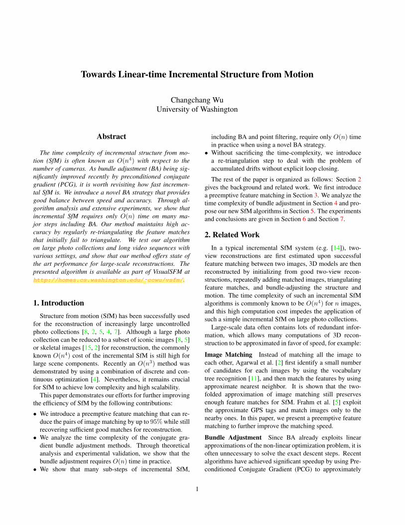
We are interested in how the yields of the feature subset cor-relate with the final yield Yi(k). As shown in Figure 1(a),the distributions of Yp(h) and Yi(h) are closely relatedto Yi(k) even for very small h such as 100. Figure 1(b)shows that the chances of have a match within the top-scalefeatures are on par with other features. This means thatthe top-scale subset has roughly h/k chance to preserve amatch, which is much higher than the h2/(k1k2) chanceof random sampling h features. Additionally, the matchingtime for the majority is reduced to a factor of h2/(k1k2)along with better caching. In this paper, we choose h = 100with consideration of both efficiency and robustness.

The top-scale features match well for several reasons: 1)A small number of top-scale feature can cover a relativelylarge scale range due to the decreasing number of featureson higher Gaussian levels. 2) Feature matching is wellstructured such that the large-scale features in one imageoften match with the large-scale features in another. Thescale variation between two matched features is jointlydetermined by the camera motion and the scene structure,so the scale variations of multiple feature matches are notindependent to each other. Figure 1(c) shows our statisticsof the feature scale variations. The feature scale variationsof an image pair usually have a small variance due to smallviewpoint changes or well-structured scene depths. For thesame reasons, we use up to 8192 features for the regularfeature matching, which are sufficient for most scenarios.While large photo collections contain redundant views andfeatures, our preemptive feature matching allows puttingmost efforts in the ones that are more likely to be matched.

2

0.40.30.20.10The final inlier yield Yi(k)

0.50

Yie

lds

whe

n us

ing

subs

ets

0.2

0.1

0.4

0.3 Median of Yi(50)

Median of Yi(400)

Median of Yp(100)

Median of Yi(200)

Median of Yi(100)

0.5

(a) Yield when using subset of features

10K

20K

0 100 200 600 1000 5000

30K

40K

50K

60K

Histogram divided into three parts [0-200][200-1000][1000-]

(b) Histogram of max index of a feature match

-1 0 1 2 30

-3 -2

0.2

0.4

0.6

0.8

1

Difference of log2 scales

Deviations from meansMean of each image pair

(c) The distribution of feature scale variations

Figure 1. (a) shows the relationship between the final yield and the yield from a subset of top-scale features. For each set of image pairsthat have roughly the same final yield, we compute the median of their subset yield for different h. (b) gives the histogram of the maxof two indices of a feature match, where the index is the position in the scale-decreasing order. We can see that the chances of matchingwithin top-scale features are similar to other features. (c) shows two distributions of the scale variations computed from 130M featurematches. The mean scale variations between two images are given by the red curve, while the deviations of scale variation from means aregiven by the blue one. The variances of scale changes are often small due to small viewpoint changes or structured scene depths.

4. How Fast Is Bundle Adjustment?Bundle adjustment (BA) is the joint non-linear opti-

mization of structure and motion parameters, for whichLevenberg-Marquardt (LM) is method of choice. Recently,the performance of large-scale bundle adjustment hasbeen significantly improved by Preconditioned ConjugateGradient (PCG) [1, 3, 16], hence it is worth re-examiningthe time complexity of BA and SfM.

Let x be a vector of parameters and f(x) be the vectorof reprojection errors for a 3D reconstruction. The opti-mization we wish to solve is the non-linear least squaresproblem: x∗ = arg minx ‖f(x)‖2. Let J be the Jacobian off(x) and Λ a non-negative diagonal vector for regulariza-tion, then LM repeatedly solves the following linear system

(JTJ + Λ) δ = −JT f,

and updates x ← x + δ if ‖f(x + δ)‖ < ‖f(x)‖. Thematrix HΛ = JTJ + Λ is known as the augmented Hessianmatrix. Gaussian elimination is typically used to firstobtain a reduced linear system of the camera parameters,which is called Schur Complement.

The Hessian matrix require O(q) =O(n) space andtime to compute, while Schur complement requires O(n2)space and time to compute. It takes cubic time O(n3) orO(p3) to solve the linear system by Cholesky factorization.Because the number of cameras is much smaller thanthe number of points, the Schur complement method canreduce the factorization time by a large constant factor.One impressive example of this algorithm is Lourakis andArgyros’ SBA [9] used by Photo Tourism [14].

For conjugate gradient methods, the dominant compu-tation is the matrix-vector multiplications in multiple CGiteration, of which the time complexity is determined by thesize of the involved matrices. By using only theO(n) spaceHessian matrices and avoiding the Schur complement, the

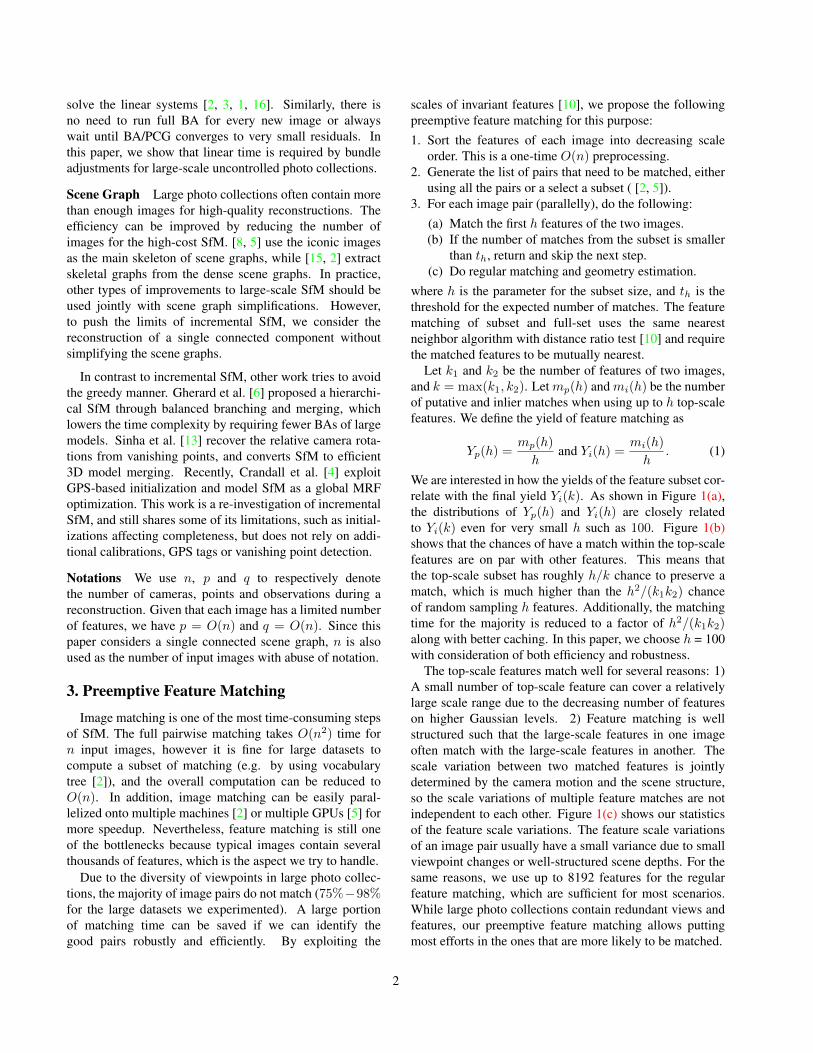
CG iteration has achieved O(n) time complexity [1, 3].Recently, the multicore bundle adjustment [16] takesone step further by using implicit multiplication of theHessian matrices and Schur Complements, which requiresto construct only the O(n) space Jacobian matrices. Inthis work, we use the GPU-version of multicore bundleadjustment. Figure 2(a) shows the timing of CG iterationsfrom our bundle adjustment problems, which exhibits linearrelationship between the time Tcg of a CG iteration and n.

In each LM step, PCG requires O(√κ) iterations to ac-

curately solve a linear system [12], where κ is the conditionnumber of the linear system. Small condition numbers canbe obtained by using good pre-conditioners, for example,quick convergence rate has been demonstrated with block-jacobi preconditioner [1, 16]. In our experiments, PCGuses an average of 20 iterations solve a linear system.

Surprisingly, the time complexity of bundle adjustmenthas already reached O(n), provided that there are O(1)CG iterations in a BA. Although the actual number of theCG/LM iterations depends on the difficulty of the inputproblems, the O(1) assumption for CG/LM iterations iswell supported by the statistics we collect from a largenumber of BAs of varying problem sizes. Figure 2(b) givesthe distribution of LM iterations used by a BA, where theaverage is 37 and 93% BAs converge within less than 100LM iterations. Figure 2(c) shows the distribution of the totalCG iterations (used by all LM steps of a BA), which are alsonormally small. In practice, we choose to use at most 100LM iterations per BA and at most 100 CG iterations per LM,which guarantees good convergence for most problems.

5. Incremental Structure from Motion

This section presents the design of our SfM that practi-cally has a linear run time. The fact that bundle adjustmentcan be done in O(n) time opens an opportunity of push-

3

6000 8000 10000 12000

Colosseum

0 2000 4000

St. Peter’s BasilicaLoopArts QuadCentral Rome

0

0.01

0.02

0.03

0.04

0.05

0.06

0.07

n - Number of cameras14000

Tcg

(se

cond

)

0.08

(a) Time spent on a single CG iteration.

40 60 80

1%

2%

3%

0 20

4%

5%

Mean = 37Median = 2993% smaller than 100

(b) Number of LM iterations used by a BA

4000 6000 8000

5%

10%

15%

0 2000

20%

Mean = 881Median = 46890% smaller than 2000Histogram bin size = 100

(c) Number of CG iterations used by a BA

Figure 2. Bundle adjustment statistics. (a) shows that Tcg is roughly linear to n regardless of the scene graph structure. (b) and (c) showthe distributions of the number of LM and CG iterations used by a BA. It can be seen that BA typically converges within a small numberof LM and CG iterations. Note that we consider BA converges if the mean squared errors drop to below 0.25 or cannot be decreased.

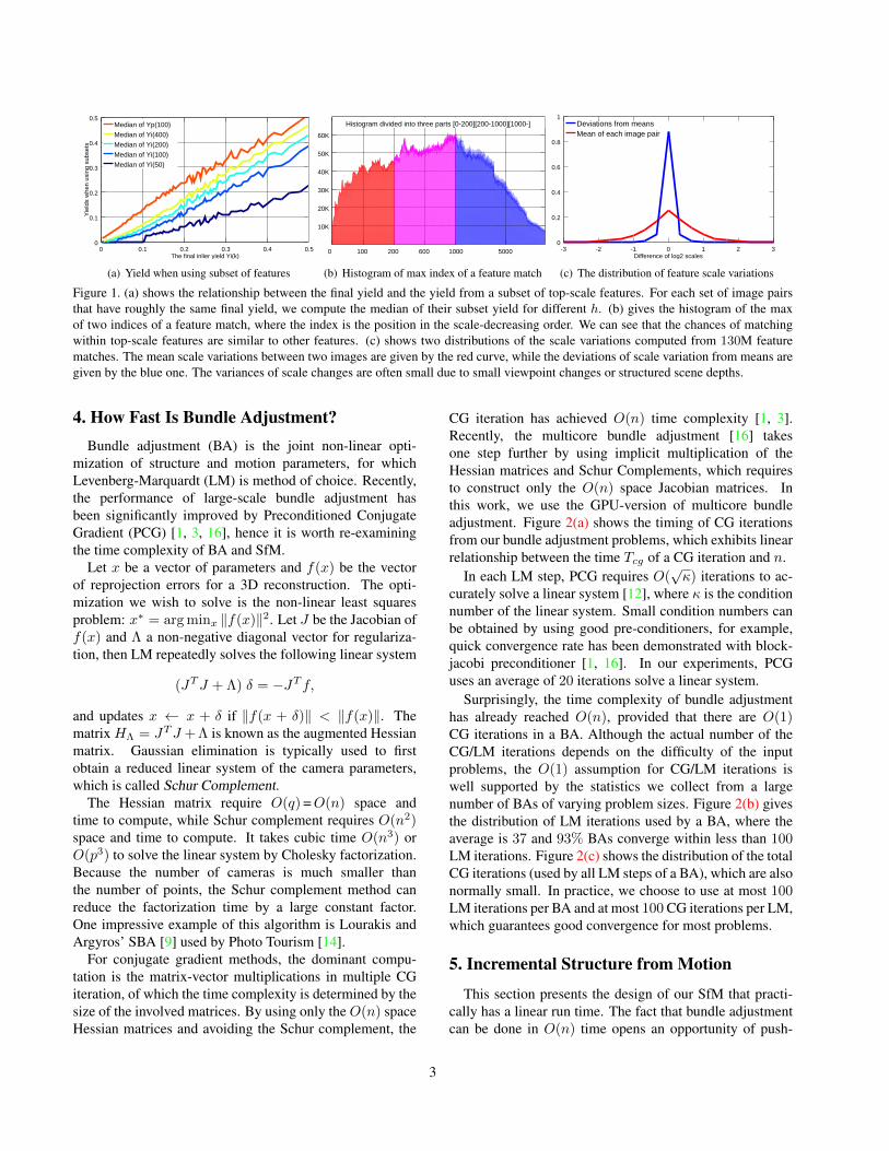
ing incremental reconstruction time closer to O(n). Asillustrated in Figure 3, our algorithm adds a single imageat each iteration, and then runs either a full BA or a partialBA. After BA and filtering, we take another choice betweencontinuing to the next iteration and a re-triangulation step.

Add Camera

Full BA

Partial BA

Filtering Re-triangulation

& Full BA

Figure 3. A single iteration of the proposed incremental SfM,which is repeated until no images can be added to reconstruction.

5.1. How Fast Is Incremental SfM?

The cameras and 3D points normally get stabilizedquickly during reconstruction, thus it is unnecessary tooptimize all camera and point parameters at every iteration.A typical strategy is to perform full BAs after addinga constant number of cameras (e.g. α), for which theaccumulated time of all the full BAs is

bn/αc∑i

TBA(i ∗ α) = O( bn/αc∑

i

(i ∗ α))

= O(n2

α

), (2)

when using PCG. This is already a significant reductionfrom the O(n4) time of Cholesky factorization based BA.As the models grow larger and more stable, it is affordableto skip more costly BAs, so we would like to study howmuch further we can go without losing the accuracy.

In this paper, we find that the accumulated time of BAscan be reduced even more to O(n) by using a geomet-ric sequence for full BAs. We propose to perform fulloptimizations only when the size of a model increasesrelatively by a certain ratio r (e.g. 5%), and the resultingtime spent on full BAs approximately becomes

∞∑i

TBA

( n

(1 + r)i

)= O

( ∞∑i

n

(1 + r)i

)= O

(nr

). (3)

Although the latter added cameras are optimized by fewerfull BAs, there are normally no accuracy problems becausethe full BAs always improve more for the parts that havelarger errors. As the model gets larger, more cameras areadded before running a full BA. In order to reduce the ac-cumulated errors, we keep running local optimizations byusing partial BAs on a constant number of recently addedcameras (we use 20) and their associated 3D points. Suchpartial optimizations involve O(1) cameras and points pa-rameters, so each partial BA takesO(1) time. Therefore, thetime spent on full BAs and partial BAs adds toO(n), whichis experimentally validated by the time curves in Figure 6.

Following the BA step, we do filtering of the points thathave large reprojection errors or small triangulation angles.The time complexity of a full point filtering step is O(n).Fortunately, we only need to process the 3D points thathave been changed, so the point filtering after a partial BAcan be done O(1) time. Although each point filtering aftera full BA takes O(n) time, they add to only O(n) due tothe geometric sequence. Therefore, the accumulated timeon all point filtering is also O(n).

Another expensive step is to organize the resection candi-dates and to add new cameras to 3D models. We keep trackof the potential 2D-3D correspondences during SfM byusing the feature matches of newly added images. If eachimage is matched to O(1) images, which is a reasonable as-sumption for large-scale photo collections, it requires O(1)time to update the correspondence information at each iter-ation. AnotherO(1) time is needed to add the camera to themodel. The accumulated time of these steps is again O(n).

We have shown that major steps of incremental SfMcontribute to an O(n) time complexity. However, the aboveanalysis ignored several things: 1) finding the portion ofdata for partial BA and partial filtering. 2) finding the subsetof images that match with a single image in the resectionstage. 3) comparison of cameras during the resection stage.These steps require O(n) scan time at each step and add toO(n2) time in theory. It is possible to keep track of thesesubsets for further reduction of time complexity. However,

4

since the O(n) part dominates the reconstruction in ourexperiments (up to 15K, see Table 2 for details), we havenot tried to further optimize these O(n2) steps.

5.2. Re-triangulation (RT)

Incremental SfM is known to have drifting problemsdue to the accumulated errors of relative camera poses.The constraint between two camera poses is provided bytheir triangulated feature matches. Because the initiallyestimated poses and even the poses after a partial BA maynot be accurate enough, some correct feature matches mayfail to triangulate for some triangulation threshold andfiltering threshold. The accumulated loss of correct featurematches is one of the main reasons of the drifting.

To deal with this problem, we propose to re-triangulate(RT) the failed feature matches regularly (with delay) dur-ing incremental SfM. A good indication of possible bad rel-ative pose between two cameras is a low ratio between theircommon points and their feature matches, which we callunder-reconstructed. In order to wait until the poses to getmore stabilized, we re-triangulate the under-reconstructedpairs under a geometric sequence (e.g. r′ = 25% when thesize of a model increases by 25%). To obtain more points,we also increase the threshold for reprojection errors duringRT. After re-triangulating the feature matches, we run fullBA and point filtering to improve the reconstruction. EachRT step requires O(n) time and accumulates to the sameO(n) time thanks to the geometric sequence.

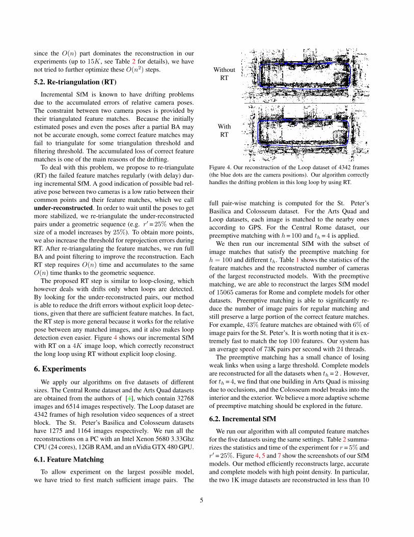
The proposed RT step is similar to loop-closing, whichhowever deals with drifts only when loops are detected.By looking for the under-reconstructed pairs, our methodis able to reduce the drift errors without explicit loop detec-tions, given that there are sufficient feature matches. In fact,the RT step is more general because it works for the relativepose between any matched images, and it also makes loopdetection even easier. Figure 4 shows our incremental SfMwith RT on a 4K image loop, which correctly reconstructthe long loop using RT without explicit loop closing.

6. ExperimentsWe apply our algorithms on five datasets of different

sizes. The Central Rome dataset and the Arts Quad datasetsare obtained from the authors of [4], which contain 32768images and 6514 images respectively. The Loop dataset are4342 frames of high resolution video sequences of a streetblock. The St. Peter’s Basilica and Colosseum datasetshave 1275 and 1164 images respectively. We run all thereconstructions on a PC with an Intel Xenon 5680 3.33GhzCPU (24 cores), 12GB RAM, and an nVidia GTX 480 GPU.

6.1. Feature Matching

To allow experiment on the largest possible model,we have tried to first match sufficient image pairs. The

WithoutRT

WithRT

Figure 4. Our reconstruction of the Loop dataset of 4342 frames(the blue dots are the camera positions). Our algorithm correctlyhandles the drifting problem in this long loop by using RT.

full pair-wise matching is computed for the St. Peter’sBasilica and Colosseum dataset. For the Arts Quad andLoop datasets, each image is matched to the nearby onesaccording to GPS. For the Central Rome dataset, ourpreemptive matching with h= 100 and th = 4 is applied.

We then run our incremental SfM with the subset ofimage matches that satisfy the preemptive matching forh = 100 and different th. Table 1 shows the statistics of thefeature matches and the reconstructed number of camerasof the largest reconstructed models. With the preemptivematching, we are able to reconstruct the larges SfM modelof 15065 cameras for Rome and complete models for otherdatasets. Preemptive matching is able to significantly re-duce the number of image pairs for regular matching andstill preserve a large portion of the correct feature matches.For example, 43% feature matches are obtained with 6% ofimage pairs for the St. Peter’s. It is worth noting that it is ex-tremely fast to match the top 100 features. Our system hasan average speed of 73K pairs per second with 24 threads.

The preemptive matching has a small chance of losingweak links when using a large threshold. Complete modelsare reconstructed for all the datasets when th = 2 . However,for th = 4, we find that one building in Arts Quad is missingdue to occlusions, and the Colosseum model breaks into theinterior and the exterior. We believe a more adaptive schemeof preemptive matching should be explored in the future.

6.2. Incremental SfM

We run our algorithm with all computed feature matchesfor the five datasets using the same settings. Table 2 summa-rizes the statistics and time of the experiment for r = 5% andr′ = 25%. Figure 4, 5 and 7 show the screenshots of our SfMmodels. Our method efficiently reconstructs large, accurateand complete models with high point density. In particular,the two 1K image datasets are reconstructed in less than 10

5

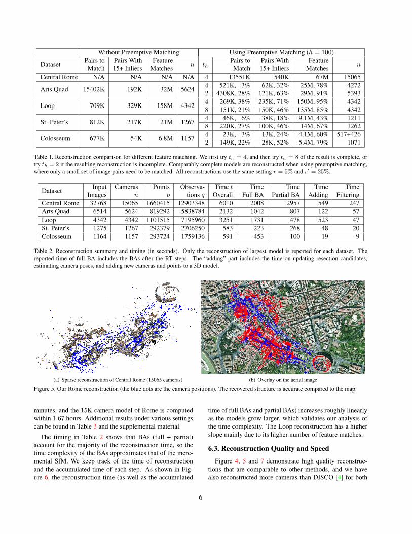
Without Preemptive Matching Using Preemptive Matching (h = 100)

Dataset Pairs to Pairs With Featuren th

Pairs to Pairs With FeaturenMatch 15+ Inliers Matches Match 15+ Inliers Matches

Central Rome N/A N/A N/A N/A 4 13551K 540K 67M 15065

Arts Quad 15402K 192K 32M 5624 4 521K, 3% 62K, 32% 25M, 78% 42722 4308K, 28% 121K, 63% 29M, 91% 5393

Loop 709K 329K 158M 4342 4 269K, 38% 235K, 71% 150M, 95% 43428 151K, 21% 150K, 46% 135M, 85% 4342

St. Peter’s 812K 217K 21M 1267 4 46K, 6% 38K, 18% 9.1M, 43% 12118 220K, 27% 100K, 46% 14M, 67% 1262

Colosseum 677K 54K 6.8M 1157 4 23K, 3% 13K, 24% 4.1M, 60% 517+4262 149K, 22% 28K, 52% 5.4M, 79% 1071

Table 1. Reconstruction comparison for different feature matching. We first try th = 4, and then try th = 8 of the result is complete, ortry th = 2 if the resulting reconstruction is incomplete. Comparably complete models are reconstructed when using preemptive matching,where only a small set of image pairs need to be matched. All reconstructions use the same setting r = 5% and r′ = 25%.

Dataset Input Cameras Points Observa- Time t Time Time Time TimeImages n p tions q Overall Full BA Partial BA Adding Filtering

Central Rome 32768 15065 1660415 12903348 6010 2008 2957 549 247Arts Quad 6514 5624 819292 5838784 2132 1042 807 122 57Loop 4342 4342 1101515 7195960 3251 1731 478 523 47St. Peter’s 1275 1267 292379 2706250 583 223 268 48 20Colosseum 1164 1157 293724 1759136 591 453 100 19 9

Table 2. Reconstruction summary and timing (in seconds). Only the reconstruction of largest model is reported for each dataset. Thereported time of full BA includes the BAs after the RT steps. The “adding” part includes the time on updating resection candidates,estimating camera poses, and adding new cameras and points to a 3D model.

(a) Sparse reconstruction of Central Rome (15065 cameras) (b) Overlay on the aerial image

Figure 5. Our Rome reconstruction (the blue dots are the camera positions). The recovered structure is accurate compared to the map.

minutes, and the 15K camera model of Rome is computedwithin 1.67 hours. Additional results under various settingscan be found in Table 3 and the supplemental material.

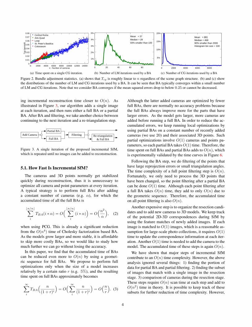
The timing in Table 2 shows that BAs (full + partial)account for the majority of the reconstruction time, so thetime complexity of the BAs approximates that of the incre-mental SfM. We keep track of the time of reconstructionand the accumulated time of each step. As shown in Fig-ure 6, the reconstruction time (as well as the accumulated

time of full BAs and partial BAs) increases roughly linearlyas the models grow larger, which validates our analysis ofthe time complexity. The Loop reconstruction has a higherslope mainly due to its higher number of feature matches.

6.3. Reconstruction Quality and Speed

Figure 4, 5 and 7 demonstrate high quality reconstruc-tions that are comparable to other methods, and we havealso reconstructed more cameras than DISCO [4] for both

6

2000

1000

n - Number of cameras

0

6000

5000

4000

3000

1400012000100008000

Central RomeArts QuadLoopSt. Peter’s BasilicaColosseum

6000400020000

Tim

e (s

econ

d)

(a) Reconstruction time.

500

n - Number of cameras

014000

2500

2000

1500

1000

12000100008000

Central RomeArts QuadLoopSt. Peter’s BasilicaColosseum

6000400020000

Tim

e (s

econ

d)

3000

(b) Accumulated time of full BA.

500

n - Number of cameras

014000

2500

2000

1500

1000

12000100008000

Central RomeArts QuadLoopSt. Peter’s BasilicaColosseum

6000400020000

Tim

e (s

econ

d)

3000

(c) Accumulated time of partial BA.

Figure 6. The reconstruction time in seconds as the 3D models grow larger. Here we report the timing right after each full BA. Thereconstruction time and the accumulated time of full BAs and partial BAs increase roughly linearly with respect to the number of cameras.Note the higher slope of the Loop reconstruction is due to the higher number of feature matches between nearby video frames.

(a) Arts Quad (5624 cameras) (b) St. Peter’s Basilica (1267 cameras) (c) Colosseum (1157 cameras)

Figure 7. Our reconstruction of Arts Quad, St. Peter’s Basilica and Colosseum.

Central Rome and Arts Quad. In particular, Figure 5 showsthe correct overlay of our 15065 camera model of CentralRome on an aerial image. The Loop reconstruction showsthat the RT steps correctly deal with the drifting problemwithout explicit loop closing. The reconstruction is firstpushed away from local minima by RT and then improvedby the subsequent BAs. The robustness and accuracy ofour method is due to the strategy of mixed BA and RT.

We evaluate the accuracy of the reconstructed camerasby comparing their positions to the ground truth locations.For the Arts Quad dataset, our reconstruction (r = 5% andr′ = 25%) contains 261 out of the 348 images whose groundtruth GPS location is provided by [4]. We used RANSACto estimate a 3D similarity transformation between the 261camera locations and their Euclidean coordinates. With thebest found transformation, our 3D model has a mean errorof 2.5 meter and a median error of 0.89 meter, which issmaller than the 1.16 meter error reported by [4].

We evaluate the reconstruction speed by two measures:• t/n The time needed to reconstruct a camera.• t/q The time needed to reconstruct an observation.Table 3 shows the comparison between our reconstructionunder various settings and the DISCO and bundler recon-struction of [4]. While producing comparably large models,our algorithm normally requires less than half a secondto reconstruct a camera in terms of overall speed. By

t/n, our method is 8-19X faster than DISCO and 55-163Xfaster than bundler. Similarly by t/q, our method is 5-11Xfaster than DISCO and 56-186X faster than bundler. It isworth pointing out that our system uses only a single PC(12GB RAM) while DISCO uses a 200 core cluster.

6.4. Discussions

Although our experiments show approximately linearrunning times, the reconstruction takes O(n2) in theoryand will exhibit such a trend the problem gets even larger.In addition, it is possible that the proposed strategy will failfor extremely larger reconstruction problems due to largeraccumulated errors. Thanks to the stability of SfM, mixedBAs and RT, our algorithm works without quality problemseven for 15K cameras.

This paper focuses on the incremental SfM stage, whilethe bottleneck of 3D reconstruction sometimes is the imagematching. In order to test our incremental SfM algorithmon the largest possible models, we have matched up toO(n2) image pairs for several datasets, which is higherthan the vocabulary strategy that can choose O(n) pairsto match [2]. However, this does not limit our methodfrom working with fewer image matches. From a differentangle, we have contributed the preemptive matching thatcan significantly reduce the matching cost.

7

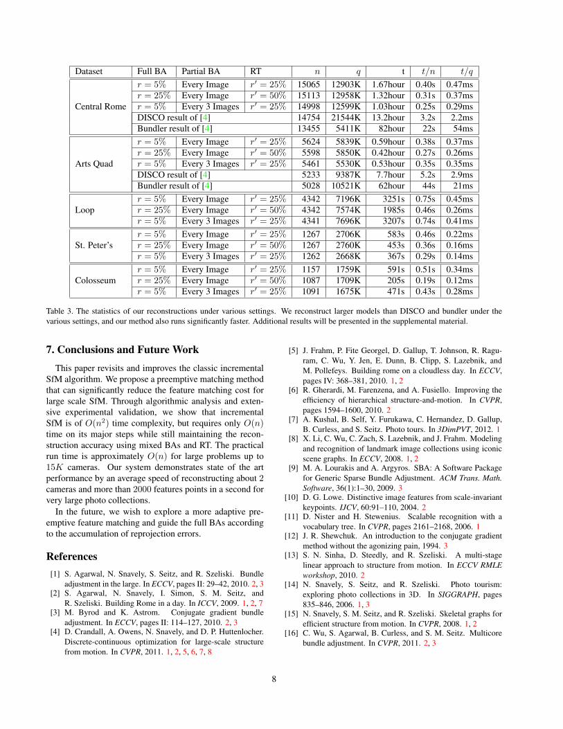
Dataset Full BA Partial BA RT n q t t/n t/q

r = 5% Every Image r′ = 25% 15065 12903K 1.67hour 0.40s 0.47msr = 25% Every Image r′ = 50% 15113 12958K 1.32hour 0.31s 0.37ms

Central Rome r = 5% Every 3 Images r′ = 25% 14998 12599K 1.03hour 0.25s 0.29msDISCO result of [4] 14754 21544K 13.2hour 3.2s 2.2msBundler result of [4] 13455 5411K 82hour 22s 54msr = 5% Every Image r′ = 25% 5624 5839K 0.59hour 0.38s 0.37msr = 25% Every Image r′ = 50% 5598 5850K 0.42hour 0.27s 0.26ms

Arts Quad r = 5% Every 3 Images r′ = 25% 5461 5530K 0.53hour 0.35s 0.35msDISCO result of [4] 5233 9387K 7.7hour 5.2s 2.9msBundler result of [4] 5028 10521K 62hour 44s 21msr = 5% Every Image r′ = 25% 4342 7196K 3251s 0.75s 0.45ms

Loop r = 25% Every Image r′ = 50% 4342 7574K 1985s 0.46s 0.26msr = 5% Every 3 Images r′ = 25% 4341 7696K 3207s 0.74s 0.41msr = 5% Every Image r′ = 25% 1267 2706K 583s 0.46s 0.22ms

St. Peter’s r = 25% Every Image r′ = 50% 1267 2760K 453s 0.36s 0.16msr = 5% Every 3 Images r′ = 25% 1262 2668K 367s 0.29s 0.14msr = 5% Every Image r′ = 25% 1157 1759K 591s 0.51s 0.34ms

Colosseum r = 25% Every Image r′ = 50% 1087 1709K 205s 0.19s 0.12msr = 5% Every 3 Images r′ = 25% 1091 1675K 471s 0.43s 0.28ms

Table 3. The statistics of our reconstructions under various settings. We reconstruct larger models than DISCO and bundler under thevarious settings, and our method also runs significantly faster. Additional results will be presented in the supplemental material.

7. Conclusions and Future WorkThis paper revisits and improves the classic incremental

SfM algorithm. We propose a preemptive matching methodthat can significantly reduce the feature matching cost forlarge scale SfM. Through algorithmic analysis and exten-sive experimental validation, we show that incrementalSfM is of O(n2) time complexity, but requires only O(n)time on its major steps while still maintaining the recon-struction accuracy using mixed BAs and RT. The practicalrun time is approximately O(n) for large problems up to15K cameras. Our system demonstrates state of the artperformance by an average speed of reconstructing about 2cameras and more than 2000 features points in a second forvery large photo collections.

In the future, we wish to explore a more adaptive pre-emptive feature matching and guide the full BAs accordingto the accumulation of reprojection errors.

References[1] S. Agarwal, N. Snavely, S. Seitz, and R. Szeliski. Bundle

adjustment in the large. In ECCV, pages II: 29–42, 2010. 2, 3[2] S. Agarwal, N. Snavely, I. Simon, S. M. Seitz, and

R. Szeliski. Building Rome in a day. In ICCV, 2009. 1, 2, 7[3] M. Byrod and K. Astrom. Conjugate gradient bundle

adjustment. In ECCV, pages II: 114–127, 2010. 2, 3[4] D. Crandall, A. Owens, N. Snavely, and D. P. Huttenlocher.

Discrete-continuous optimization for large-scale structurefrom motion. In CVPR, 2011. 1, 2, 5, 6, 7, 8

[5] J. Frahm, P. Fite Georgel, D. Gallup, T. Johnson, R. Ragu-ram, C. Wu, Y. Jen, E. Dunn, B. Clipp, S. Lazebnik, andM. Pollefeys. Building rome on a cloudless day. In ECCV,pages IV: 368–381, 2010. 1, 2

[6] R. Gherardi, M. Farenzena, and A. Fusiello. Improving theefficiency of hierarchical structure-and-motion. In CVPR,pages 1594–1600, 2010. 2

[7] A. Kushal, B. Self, Y. Furukawa, C. Hernandez, D. Gallup,B. Curless, and S. Seitz. Photo tours. In 3DimPVT, 2012. 1

[8] X. Li, C. Wu, C. Zach, S. Lazebnik, and J. Frahm. Modelingand recognition of landmark image collections using iconicscene graphs. In ECCV, 2008. 1, 2

[9] M. A. Lourakis and A. Argyros. SBA: A Software Packagefor Generic Sparse Bundle Adjustment. ACM Trans. Math.Software, 36(1):1–30, 2009. 3

[10] D. G. Lowe. Distinctive image features from scale-invariantkeypoints. IJCV, 60:91–110, 2004. 2

[11] D. Nister and H. Stewenius. Scalable recognition with avocabulary tree. In CVPR, pages 2161–2168, 2006. 1

[12] J. R. Shewchuk. An introduction to the conjugate gradientmethod without the agonizing pain, 1994. 3

[13] S. N. Sinha, D. Steedly, and R. Szeliski. A multi-stagelinear approach to structure from motion. In ECCV RMLEworkshop, 2010. 2

[14] N. Snavely, S. Seitz, and R. Szeliski. Photo tourism:exploring photo collections in 3D. In SIGGRAPH, pages835–846, 2006. 1, 3

[15] N. Snavely, S. M. Seitz, and R. Szeliski. Skeletal graphs forefficient structure from motion. In CVPR, 2008. 1, 2

[16] C. Wu, S. Agarwal, B. Curless, and S. M. Seitz. Multicorebundle adjustment. In CVPR, 2011. 2, 3

8