HAL Id: hal-01187745https://hal.archives-ouvertes.fr/hal-01187745

Submitted on 27 Aug 2015

HAL is a multi-disciplinary open accessarchive for the deposit and dissemination of sci-entific research documents, whether they are pub-lished or not. The documents may come fromteaching and research institutions in France orabroad, or from public or private research centers.

L’archive ouverte pluridisciplinaire HAL, estdestinée au dépôt et à la diffusion de documentsscientifiques de niveau recherche, publiés ou non,émanant des établissements d’enseignement et derecherche français ou étrangers, des laboratoirespublics ou privés.

Towards Applying Logico-numerical Control toDynamically Partially Reconfigurable Architectures

Nicolas Berthier, Xin An, Hervé Marchand

To cite this version:Nicolas Berthier, Xin An, Hervé Marchand. Towards Applying Logico-numerical Control to Dynami-cally Partially Reconfigurable Architectures. 5th IFAC International Workshop On Dependable Con-trol of Discrete Systems - DCDS’15, May 2015, Cancun, Mexico. 48 (7), pp.132-138. <hal-01187745>

Towards Applying Logico-numericalControl to Dynamically Partially

Reconfigurable Architectures

Nicolas Berthier ∗ Xin An ∗∗ Herve Marchand ∗

∗ INRIA Rennes - Bretagne Atlantique, Rennes, France∗∗Hefei University of Technology, Hefei, China

Abstract: We investigate the opportunities given by recent developments in the context ofDiscrete Controller Synthesis algorithms for infinite, logico-numerical systems. To this end,we focus on models employed in previous work for the management of dynamically partiallyreconfigurable hardware architectures. We extend these models with logico-numerical features toillustrate new modeling possibilities, and carry out some benchmarks to evaluate the feasibilityof the approach on such models.

Keywords: Discrete Controller Synthesis, Infinite Systems, Control of Computing, SynchronousLanguages, Hardware Architectures, Dynamically Partially Reconfigurable FPGA

1. INTRODUCTION

Recent proposals by Berthier and Marchand (2014) in thedomain of symbolic Discrete Controller Synthesis (DCS)techniques have led to the development of a tool capableof handling logico-numerical systems and properties, i.e.,involving state variables defined on infinite domains. Thehandling of such infinite systems opens the way to newopportunities for modeling and control, that still need tobe investigated.

We extend real-life models proposed by An et al. (2013a,b)for the management of Dynamically Partially Reconfig-urable (DPR) hardware architectures to: (i) assess thefeasibility of the proposal on bigger systems, (ii) performsome performance evaluations of the new tool ReaX onrealistic models, including for control objectives newly im-plemented in this tool; and (iii) introduce logico-numericalfeatures in the model to assess that the approach can stillbe applied using models involving quantitative aspects.

DPR Hardware Architectures DPR hardware architec-tures, typically Field Programmable Gate Arrays (FPGAs)(Lysaght et al., 2006), have been identified as a promisingsolution for the design of energy-efficient embedded systems(Hinkelmann et al., 2009). However, such solutions havenot been extensively exploited in practice for two mainreasons: i) the design effort is extremely high and stronglydepends on the available chip and tool versions, and ii)the simulation process, which is already complex for non-reconfigurable systems, is prohibitively large for reconfig-urable architectures. Therefore, new adequate methodsto deal with their correct dynamical reconfiguration arerequired to fully exploit their potential.

Dynamical reconfiguration management requires choosingnew configurations depending on the history of events occur-ring in the system and predictive knowledge about possibleoutcomes of reconfigurations. Such decision-making compo-nent is difficult to design because of the combinatorics of

possible choices, the transversal constraints between them,and even more, the history aspects. The work we presentadvocates the application of DCS techniques to fulfill thiscontrol problem.

Related Works The reconfiguration management in DPRtechnologies is usually addressed by using manual encodingand analysis techniques that are tedious and error-proneaccording to Gohringer et al. (2008). Other existingapproaches dedicated to self-management of adaptiveor reconfigurable systems use heuristics and machinelearning techniques (Sironi et al., 2010; Paulsson et al.,2006; Jovanovic et al., 2008) for instance. Maggio et al.(2012) discuss some approaches applying standard controltechniques such as Proportional Integral and Derivative(PID) controller or Petri nets-based control. The samekind of control has also been used for processor andbandwidth allocation in servers (Lu et al., 2002). Eustacheand Diguet (2008) applied close-loop control to selecthardware/software configurations on an FPGA with aconfiguration control based on a data-flow model anddiffusion mechanisms. We note that such a solution relieson heuristics and empirical laws that prevent instabilityand select the suitable configurations.

Compared to the above reconfiguration control techniques,major advantages of the discrete control approach consid-ered by An et al. (2013a,b) are the enabled formal correct-ness and guarantees on run-time performance, as well asthe possibility to synthesize the controller automatically.

Outline We first present in Section 2 the modeling for-malism we use for expressing the reconfiguration problem,as well as the tools involved in our work. Sections 3 detailthe problem of reconfiguration control for FPGA-basedDPR systems. We expose the modeling and formulation asa DCS problem, as well as an illustrative logico-numericalextension of the model in Section 4, and we report on ourperformance evaluation experiments in Section 5.

Preprints of DCDS 2015, May, 27-29, Cancun Mexico

132

2. MODELING FORMALISM AND TOOLS

2.1 Arithmetic Symbolic Transition Systems

The model of Arithmetic Symbolic Transition Systems(ASTSs) is a transition system with (internal or input)variables whose domain can be infinite, and composedof a finite set of symbolic transitions. Each transitionis guarded on the system variables, and has an updatefunction indicating the variable changes when a transitionis fired. This model allows the representation of infinitesystems whenever the variables take their values in aninfinite domain, while it has a finite structure and offers acompact way to specify systems handling data.

Let V = 〈v1, . . . , vn〉 be a tuple of variables and Dv the(infinite) domain of v. We note DV =

∏i∈[1,n]Dvi

the

(infinite) domain of V . vi(V ) gives the value of variable viin vector V .

Definition 1. (Arithmetic Symbolic Transition System).An ASTS is a tuple S = 〈X, I, T,A,Θ0〉 where:

• X = 〈x1, . . . , xn〉 is a vector of state variables rangingover DX =

∏j∈[1,n]Dxj and encoding the memory

necessary for describing the system behavior;• I = 〈i1, . . . , im〉 is a vector of variables that ranges

over DI =∏

j∈[1,m]Dij , called input variables;

• T is of the form (x′i := T xi)xi∈X , such that, for eachxi ∈ X, the right-hand side T xi of the assignmentx′i := T xi is an expression on X ∪ I. T is called thetransition function of S, and encodes the evolution ofthe state variable xi. It characterizes the dynamic ofthe system between the current state and the next statewhen receiving an input vector.• A is a predicate with variables in X ∪ I encoding an

assertion on the possible values of the inputs dependingon the current state;• Θ0 is a predicate with variables in X encoding the set

of initial states.

For technical reasons, we shall assume that A is expressedin a theory that is closed under quantifier elimination asfor example the Presburger arithmetic.

ASTSs can conveniently be represented as parallel compo-sitions of Mealy automata with numerical variables andexplicit locations or in its symbolic form.

Let us consider the following example ASTS where X =〈ξ, x, o〉, I = 〈a, i〉 with DX = {F,G} ×Z×B, DI = B×Z

T =

ξ′ := G if (ξ = F ∧ a ∧ x ≥ 0),

F if (ξ = G ∧ i > 42), ξ otherwisex′ := 2x+ 1 if (ξ = F ∧ a ∧ x ≥ 0),

i if (ξ = G ∧ i ≤ 42), x otherwiseo′ := (ξ = F ∧ a ∧ x ≥ 0) ∨ (ξ = G ∧ i > 42)

A(〈ξ, x, o, a, i〉) = (ξ = G ∧ 3x+ 2i ≤ 41 ∧ a)Θ0(〈ξ, x, o〉) = (ξ = F ∧ x = 0)

The corresponding Mealy automaton with explicit locations(leaving A aside) can be represented as in Figure 1.

Remark 1. Observe that the variable o is actually anoutput of the system, although it belongs to the vector ofstate variables. Indeed, we do not distinguish between thosetwo kinds of variables to keep the ASTS models simple. We

F G

a ∧ x > 0/o, x := 2x+ 1

¬a ∨ x < 0 i > 42/o

i 6 42/x := ix := 0

Fig. 1. Example ASTS as a Mealy automaton.

can characterize output variables as the ones that neverappear in the right hand side of the assignments in T .

Remark 2. We qualify as logico-numerical an ASTS whosestate (and non-output) and input variables are Booleanvariables (B) or numerical variables (typically, R or Z),

i.e., such that X = Bk ∪ Rk′ ∪ Zk′′with k + k′ + k′′ = n

(and similarly for the input variables). ASTSs with onlyBoolean non-output state variables are called finite.

To each ASTS, one can make correspond an InfiniteTransition System (ITS) defined as follows:

Given an ASTS S = 〈X, I, T,A,Θ0〉, we make correspondan ITS [S] = 〈X , I, TS ,AS ,X0〉 where:

• X = DX is the state space of [S];• I = DI is the input space of [S];• TS ⊆ X × I → X is such thatTS(x, ν) = (x′j)j∈[1,n] ⇔ ∀j ∈ [1, n], x′j := T xj (x, ν);

• AS ⊆ X × I is such thatAS = {(x, ν) ∈ X × I|A(x, ν) = true};

• X0 ⊆ X is the set of initial states, and is such thatX0 = {x ∈ X |Θ0(x) = true}.

The behavior of such a system is as follows. [S] startsin a state x0 ∈ X0. Assuming that [S] is in a statex ∈ X , then upon the reception of an input ν ∈ I suchthat (x, ν) ∈ AS , [S] evolves in the state x′ = TS(x, ν).We denote XTrace([S]) the set of states that can bereached in [S]. Given an ASTS S and a predicate Φ overX, we say that S satisfies Φ (noted S |= Φ) wheneverXTrace([S]) ⊆ {x ∈ X |Φ(x) = true}.

Control of an ASTS Assume given a system S and apredicate Φ on S. Our aim is to restrict the behaviorof S by means of control in order to fulfill Φ. Wedistinguish between the uncontrollable input variables Uwhich are defined by the environment, and the controllableinput variables C which are defined/restricted by thecontroller of the system. For technical reason, we assumethat the controllable variables are Boolean. Note thatthe partitioning of the input variables in S induces a“partitioning” of the input space in [S], so we have I = DU×DC . A controller is then given by a predicate AΦ overX ∪ U ∪ C that constrains the set of admissible (Boolean)controllable inputs so that the traces of the controlledsystem always satisfy Φ.

Definition 2. (Discrete Controller Synthesis Problem).Given an ASTS S = 〈X,U ∪C, T,A,Θ0〉 and a predicate Φover X, solving the discrete controller synthesis problemis to compute a predicate AΦ such that

S′ = 〈X,U ∪ C, T,AΦ,Θ0〉 |= Φ

and ∀v ∈ X ∪ U ∪ C,AΦ(v)⇒ A(v).

The general control problem that we want to solve isundecidable. In (Berthier and Marchand, 2014), we thenused abstract interpretation techniques to ensure, at theprice of some over-approximations, that the computation

Preprints of DCDS 2015, May, 27-29, Cancun Mexico

133

of the controller terminates (see e.g., (Cousot and Cousot,1977)). This over-approximation ensures that the forbiddenstates are not reachable in the controlled system. Thus,the synthesized controller remains correct, yet may not bemaximally permissive w.r.t the invariant. For the details onhow the controller is computed, one can refer to (Berthierand Marchand, 2014).

2.2 ReaX & BZR

ReaX Berthier and Marchand (2014) introduced the toolReaX implementing the above symbolic algorithms for thesynthesis of controllers ensuring safety properties of infinitestate systems modeled by ASTSs. Compared with what isreported in this previous work, in addition to the invarianceof a predicate, one can also request the controlled system tobe deadlock-free. Adapting techniques from Marchand andSamaan (2000), ReaX also implements classical algorithmsof invariance and reachability enforcement for finite sys-tems, as well as one-step optimization of numerical variablesfor general ASTSs.

BZR An et al. (2013a,b) used the reactive data-flowlanguage BZR (Delaval et al., 2010) to describe theirsolution. BZR programs are built as parallel compositionsof data-flow nodes, each having input and output flows. Thebody of the node describes how input flows are transformedinto output flows, in the form of a set of equationsand/or automata. They are evaluated, all together ateach step of a reactive system (hence the compositionis called synchronous), by taking all inputs, computing thetransitions and equations, and producing the outputs. Aninvariant and controllable variables can be specified, andthe BZR compiler involves DCS to automatically produce acontroller guarantying that the resulting controlled systemsatisfies the invariance property by constraining the valuesof the controllable variables. To do so, BZR involves acompilation phase using either Sigali (Marchand et al.,2000) or ReaX (Berthier and Marchand, 2014) DCS tools.

Remark 3. As Sigali supports the handling of cost functionsfor optimization purposes (functions from the finite statespace and input space of the systems to integers) (Marchandet al., 2000), the Sigali BZR backend is able to make useof this device to translate programs involving nodes withInteger output flows (Delaval et al., 2013). It is howeverunable to translate programs with Integer state variables,like the one of Figure 1.

3. FPGA CONTROL PROBLEM

We consider applications made of tasks executing accordingto dependency constraints on an FPGA platform. The lattermay provide various computation resources having differentcharacteristics or specializations for the tasks to execute,and each task may be implemented in several ways usingdissimilar sets of resources.

An et al. (2013a,b) provided a solution for the problem ofchoosing a scheduling satisfying both the execution depen-dencies between the tasks and the utilization constraints onthe resources of the FPGA platform. This proposal consistsin the model-based generation of a run-time managerwhose role is to start tasks and detect their termination,and allocate appropriate computation resources for them

a)

A0

A1 A2

A3 A4b)

B

A

C

D

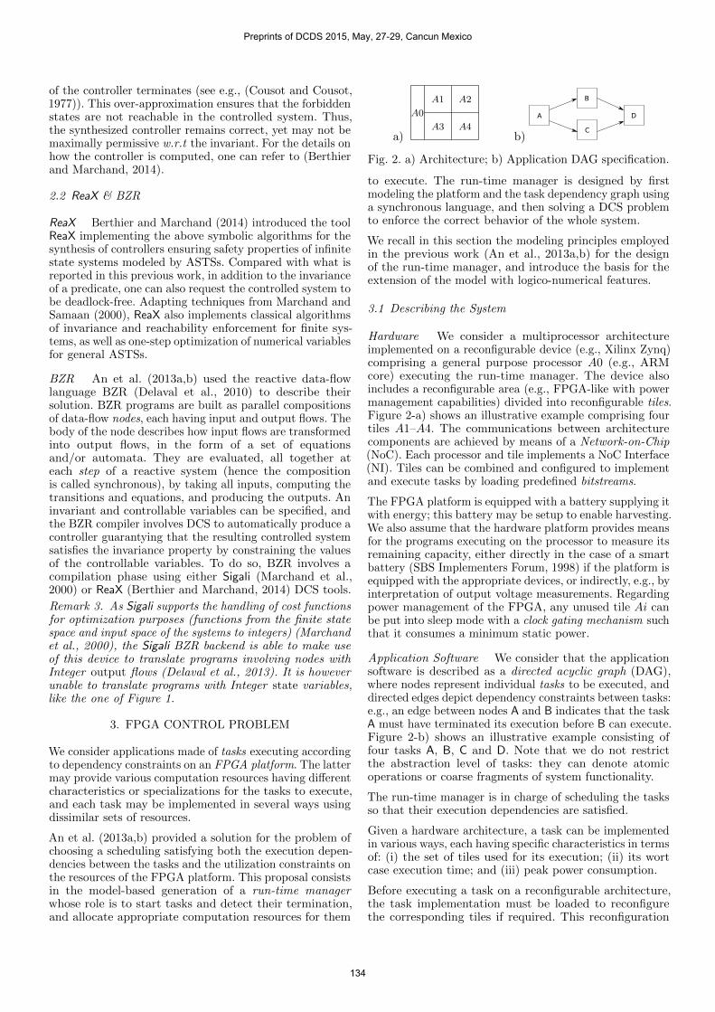
Fig. 2. a) Architecture; b) Application DAG specification.

to execute. The run-time manager is designed by firstmodeling the platform and the task dependency graph usinga synchronous language, and then solving a DCS problemto enforce the correct behavior of the whole system.

We recall in this section the modeling principles employedin the previous work (An et al., 2013a,b) for the designof the run-time manager, and introduce the basis for theextension of the model with logico-numerical features.

3.1 Describing the System

Hardware We consider a multiprocessor architectureimplemented on a reconfigurable device (e.g., Xilinx Zynq)comprising a general purpose processor A0 (e.g., ARMcore) executing the run-time manager. The device alsoincludes a reconfigurable area (e.g., FPGA-like with powermanagement capabilities) divided into reconfigurable tiles.Figure 2-a) shows an illustrative example comprising fourtiles A1–A4. The communications between architecturecomponents are achieved by means of a Network-on-Chip(NoC). Each processor and tile implements a NoC Interface(NI). Tiles can be combined and configured to implementand execute tasks by loading predefined bitstreams.

The FPGA platform is equipped with a battery supplying itwith energy; this battery may be setup to enable harvesting.We also assume that the hardware platform provides meansfor the programs executing on the processor to measure itsremaining capacity, either directly in the case of a smartbattery (SBS Implementers Forum, 1998) if the platform isequipped with the appropriate devices, or indirectly, e.g., byinterpretation of output voltage measurements. Regardingpower management of the FPGA, any unused tile Ai canbe put into sleep mode with a clock gating mechanism suchthat it consumes a minimum static power.

Application Software We consider that the applicationsoftware is described as a directed acyclic graph (DAG),where nodes represent individual tasks to be executed, anddirected edges depict dependency constraints between tasks:e.g., an edge between nodes A and B indicates that the taskA must have terminated its execution before B can execute.Figure 2-b) shows an illustrative example consisting offour tasks A, B, C and D. Note that we do not restrictthe abstraction level of tasks: they can denote atomicoperations or coarse fragments of system functionality.

The run-time manager is in charge of scheduling the tasksso that their execution dependencies are satisfied.

Given a hardware architecture, a task can be implementedin various ways, each having specific characteristics in termsof: (i) the set of tiles used for its execution; (ii) its wortcase execution time; and (iii) peak power consumption.

Before executing a task on a reconfigurable architecture,the task implementation must be loaded to reconfigurethe corresponding tiles if required. This reconfiguration

Preprints of DCDS 2015, May, 27-29, Cancun Mexico

134

task A

or

task B

task C

task B

task C

1) 2) 3)

Fig. 3. Configurations and reconfigurations.

operation inevitably involves some overheads regarding,e.g., time and energy. For simplicity, we assume that theworst case execution time of each task implementationencompasses the time required to reconfigure the tiles ituses (as in the worst case, a task implementation mustalways be loaded before being executed).

Reconfiguration Figure 3 exemplifies three system con-figurations. In 1), task A is running on tiles A3 and A4(see Figure 2-a)) while tiles A1 and A2 are in sleep mode.Configurations 2) and 3) show two scenarios where tasksB and C run in parallel. Assume tasks B and C have twoimplementations so that the system can go to either 2)or 3) once task A finishes its execution (according to thegraph of Figure 2-b)). If the current state of the batterylevel is low, the system would choose 2) as 3) requiresthe complete circuit surface and therefore consumes morepower. On the contrary, when the battery level is high, 3)would be chosen if the user expects a better performance.

3.2 System-level Objectives

The run-time manager can decide to delay the executionof a task and determines which implementation of itto trigger. These choices are made according to systemobjectives that define the system functional and non-functional requirements. The objectives considered in thiswork, are either logical control or optimization objectives.Generally speaking, logical objectives express propertiesabout discrete states of the system (e.g., mutual exclusions),whereas optimal ones concern weights and costs.

The logical control objectives we consider are: (i) exclusiveuses of tiles A1–A4 by the executing tasks; (ii) switchtiles into active or sleep mode depending on whether atask executes on them or not to save energy; (iii) avoidpower consumption peaks of the hardware platform w.r.tthe electrical charge of the battery; and (iv) once started,the application can always finish. Optimization objectivesnotably encompass the minimization of the power peaks ofthe platform to augment the lifespan of the battery.

4. MODELING RECONFIGURATION CONTROL AS ADCS PROBLEM

We focus on the management of computations on thetiles and dedicate the processor area A0 exclusively tothe execution of the resulting run-time manager. So, webuild a global system model as an ASTS representing thebehavior of the reconfigurable computing system; systemobjectives are then specified using predicates expressed onvariables of the model.

We recall, and reformulate in terms of ASTSs, the modelsproposed by An et al. (2013a,b). At the same time, weintroduce a new, logico-numerical model for the battery,to demonstrate the added expressiveness allowed by theASTSs handled by ReaX.

a)

ActiSlei

acti = true

acti = falsec_ai

not c_ai

c_ai

acti

RMi

b)

H M L

down

upup

downdown

st=h st=m st=l

stup

BM

Fig. 4. Models RMi for a tile Ai, and BM for a battery.

4.1 System Model

Modeling the Tiles Figure 4-a) depicts the model describ-ing the behavior of a tile Ai: it features two states (Sle andAct) as a tile may or may not be active at a given instant.The model switches from a state to another dependingon the value of its Boolean controllable variable c ai. Theoutput acti represents its current mode.

Discrete Battery Model Figure 4-b) represents a discretemodel for a battery proposed by An et al. (2013a,b).It is characterized with three states/levels: H (high), M(medium) and L (low). This model is assumed to take itsinputs from a dedicated software executing on processor A0,that interprets capacity measurements and drives the stateof this model by emitting up and down events dependingon the current electrical charge of the battery. The outputst ∈ {H,M, L} reflects the internal state of the model.

Logico-numerical Battery Model We now present a newmodel for a smooth representation of the state of the batteryin the system model. This model aims at illustrating theexpressiveness of logico-numerical ASTSs handled by ReaX.

This new model receives as input a rough measure cm ofthe actual electrical charge (e.g., in Coulombs) providedby a dedicated sensor, and an estimation ce of the capacityspent since the last reaction of the model. The state ofthe battery in this model consists in a numerical variablec providing an estimation of the remaining capacity ofthe battery. The domain of c can be the domain of reals(arbitrary-precision rationals actually).

At each reaction of the model, the value of c is estimated byusing some sort of exponentially weighted moving average:it is computed by using cm when the input measurementfrom the sensor is determined as valid by bounding itsabsolute difference with the estimated capacity c; the modeltries to estimate this value by other means otherwise. Themodel is further parameterized with a constant smoothingfactor α ∈ [0, 1] that specifies the impact of the variationsof cm on the state variable c. The constant β serves as abound to determine the validity of the measured input.

Although the value of c could be used directly in thedefinition of logical control predicates (and possibly op-timization objectives), e.g., to decide whether a givenpower consumption peak is admissible by the battery,for illustrative purposes we use it directly to computea value for the finite output st based on additional constantthreshold electrical charges λ and µ. In this way, this newbattery model is interchangeable with the discrete one, andsystem control and optimization objectives can be reusedwhatever the chosen battery model.

The assignment of state variable c and output st ∈{H,M, L} can be expressed as

Preprints of DCDS 2015, May, 27-29, Cancun Mexico

135

Ireq/rA

AeA/rB,rC

B,C D TeD/end

eA,eB,eC,eD

rA,rB,rC,rD

C

eB and eC/rD

eB

eC

eC/rD

B eB/rD

req

Sdl

end

Fig. 5. Application DAG execution behaviors.

WA

IA

XA1 XA

2

rA, c1rA, c2

rA, not c

c2

eAeA

c1

({A1},200,180)

({A3,A4}, 100,250)

({},0,0)

({},0,0)

TMA

rA eA

c1,c2esA

esA=XA1 esA=W esA=XA

2

esA=I

rsA,wtA,ppA

Fig. 6. Model TMA of task A. c′ := (c− ce)(1− α) + cmα if |c− cm| < β(c− ce) otherwise

st′ := L if c′ 6 λ,M if λ < c′ 6 µ,H otherwise

and c can be initialized using a predefined constant valueor with the first input measure cm, assuming it is valid(in the latter case, the model would become slightly morecomplex). c is indeed a state variable of the model, as itappears in its own assignment expression.

Note that ce may be an input of the whole system model,or even be computed by using another numerical variablekeeping track of estimated power consumption peaks, plusa measure of the time elapsed since the last reaction.

Encoding the Task Graph The software application is de-scribed by its task graph, i.e., as a DAG specifying the tasksto be executed, as well as their execution dependencies.This DAG is encoded as a scheduler automaton representingall possible execution scenarios. It does so by keeping trackof application execution states and emitting appropriatestart requests in reaction to tasks’ finish notifications.

Figure 5 shows the scheduler automaton of the applicationDAG in Figure 2-b). When in idle state I and upon receiptof application request event req, it requests the start-up oftask A by emitting event rA. Upon receipt of eA notifyingthe termination of A’s execution, events rB and rC areemitted together to request start-up of tasks B and C (thatwill then potentially execute in parallel). Task D is notrequested until the execution of both B and C is finished,respectively denoted by events eB and eC. The schedulerthen reaches the final state T and emits event end, implyingthe end of the application’s execution, upon receipt of eD.

Remark 4. Note that several scheduler automata like theone of Figure 5 can be composed in a hierarchical way todescribe complex task graphs. Using a sub-scheduler X, thiscomposition operation only requires to bind a task startrequest (say, rX) with X’s req input, and conversely itstermination notification (end) to the corresponding tasktermination request (eX).

Task Model One can distinguish several stages during atasks’ lifetime (see Section 3.1): not scheduled for execution;scheduled but not executing; and having the tiles configuredwith one of its implementation and executing.

We consequently model tasks with automata, such as theone of Figure 6 for A: it features idle and waiting statesIA and WA, plus as many execution states as availableimplementations of A (X1

A and X2A). Controllable variables

c1 and c2 are integrated in the model to encode the choicesgiven to the run-time manager; e.g., from the idle state,it can then choose to delay the execution of a task, or toselect and start the execution of one of its implementation.The output esA reflects the execution state of the task.

Three observations of interest are considered for each task.For a task t, we capture them by associating a tuple(rst,wtt, ppt) to the states of task models, where: rst ∈ 2RA

(RA being the set of architecture resources — i.e., thetiles in our case), wtt ∈ N and ppt ∈ N are the WCETand the peak power consumption for the task’s state. Theobservations associated with executing states are the valuesassociated with their corresponding implementations. Foridle and wait states, rst = ∅,wtt = 0, ppt = 0.

Remark 5. Task observation variables defined in this sec-tion are outputs of the model, and hence belong to the vectorof state variables X in the corresponding ASTS model (seeRemark 1): the fact that the domain of some of them isinfinite does not make the ASTS’s state space infinite.

Global System Model The whole system model representsall the possible system execution behaviors in the absence ofcontrol (i.e., if a run-time manager is not yet integrated). Inour example case of four tiles and set Tasks = {A,B,C,D}of tasks, it comprises the parallel composition of the sub-models for tiles RM1–RM4, battery BM and tasks TMA–TMD, plus a scheduler Sdl encoding the task graph:

S = RM1|| . . . ||RM4||BM||TMA|| . . . ||TMD||Sdl.

In terms of ASTSs, and assuming variable names donot clash between the various sub-models of the system,this parallel composition essentially boils down to con-catenate together, for each sub-model m: the vectors ofstate variables Xm’s, controllable (resp. non-controllable)inputs Cm’s and Um’s, and assignments Tm’s. The globalassumption A made about the environment is the con-junction of all assumptions of the sub-models Am’s. Asfor the initial state, the predicate Θ0 is defined so thatX0 = {〈Sle1, . . . ,Sle4,H, IA, . . . , ID, I〉}.

Global Observations The observations output locally byeach sub-model (e.g., task models) need to be combined intoa set of global values in order to account for the resourceconsumption of the whole system. These values constitutethe global observations of the model based on which logicalcontrol and optimization objectives can be expressed.

In our case, the global observations available for a particularoperating state of the system is the tuple of variables(rs,wt, pp) whose values are computed based on the indi-vidual tasks’ observations at the current reaction (denotedrs′t, wt

′t and pp′t). Global observation variables are added

to the vector of state variables as any other outputs, andare computed by adding corresponding assignments in Tas follows:

rs′ :=⋃

t∈Tasksrs′t

wt′ := mint∈Tasks

{wt′t | wt′t 6= 0} if defined, 0 otherwise

pp′ :=∑

t∈Taskspp′t

Preprints of DCDS 2015, May, 27-29, Cancun Mexico

136

Note that in the assignments above, primed versions oftasks’ observations are actually substituted in the ASTSmodel by the expression they are respectively assigned to.

Remark 6. By construction, global observation values areoutputs of the system and can be computed as functionsdefined on its state only.

4.2 System Objectives

Based on the model described above, we can formalizethe objectives of Section 3.2 in terms of the states andobservations defined on the states.

The logical control objectives to be enforced on the systemby the run-time manager can be expressed by using twopredicates Φ: DX → B and χ : DX → B, respectivelyencoding invariance and reachability requirements, andexpressed on state variables. Φ can be expressed as aconjunction, each of its conjuncts encoding one aspectof the logical control needs:

• exclusive use of tiles: Φx(X) = ∀(s, t) ∈ Tasks2, s 6=t, rss(X) ∩ rst(X) = ∅;• shut-down and start-up of tiles depending on whether

they are used or not by an executing tasks’ imple-mentation: Φa(X) = (∀a ∈ rs(X), acta = true) ∧(∀a ∈ Drs \ rs(X), acta = false);• given a mapping ppthr : {L,M,H} → N from discrete

battery levels to threshold peak power values, con-straining the total power peak depending on the levelof the battery: Φp(X) = pp(X) 6 ppthr(st(X)).

In turn, the reachability predicate χ specifies that a statemust be reachable where the value of the output end ofSdl is true (meaning that the application has finished itsexecution): χ(X) = (end(X) = true).

One-step optimal objectives aim at minimizing or maximiz-ing numerical state variables in a single step. Optimizationobjective of Section 3.2 belongs to this type, by requestingto select successor states minimizing power peaks pp.

4.3 Solving the DCS Problem and Using the Result

All the ASTS models above except the logico-numericalbattery model are finite ASTSs as their non-output statespace is finite (i.e., numerical state variables are outputs,and can thus be represented a cost functions associatingnumerical values to discrete states — see Remarks 1, 5and 6). Thus, one can write these models in BZR, useeither the Sigali or the ReaX backend of the compiler, solvethe resulting DCS problem, and then automatically obtaina controller satisfying the system objectives. Associatedwith the model, this controller can be used by the run-timemanager to dynamically reconfigure the system.

5. EVALUATION & EXPERIMENTAL RESULTS

We report in this section our experiments to evaluatethe efficiency of ReaX to solve DCS problems on modelsas described above. All executions were performed on a3.2GHz Intel® Xeon® multi-core 1 processor with about6GB of main memory. We first show comparisons of Sigaliw.r.t ReaX in the case of finite models, and then presentperformance results of ReaX on logico-numerical ASTSs.1 Note however that both Sigali and ReaX are single-threaded.

50ms

¼s

1s

5s

15s

60s

5m

¼h

1h

2 3 4 5 6 7 8 9 10 11

Synth

esis

Tim

e

Number of Tasks

SigaliReaX

Fig. 7. Synthesis times for generated benchmarks.

¼s

1s

5s

15s

60s

5m

¼h

1h

2 3 4 5 6 7 8 9 10 11

Synth

esis

Tim

e

Number of Tasks

ReaX - reachabilityReaX - one-step optim.

Fig. 8. Synthesis times of ReaX for invariance and eitherreachability enforcement or one-step optimization.

Logical Control: Efficiency of ReaX w.r.t Sigali A per-formance evaluation of Sigali for solving reconfigurationcontrol problems similar to the ones considered in this paperhas already been presented by An et al. (2013a). In orderto compare the benefits of using ReaX w.r.t Sigali for thesame kind of problems, we conducted extensive experimentsbased on multiple instances of the reconfiguration controlproblem. Each one of these models is built based on arandomly generated hierarchical task graph constructedrecursively by exploiting the idea mentioned in Remark 4.Every system model comprises a discrete battery model,plus four tile models. The task models involved representeither one or two execution modes, each associated to oneor two tiles chosen randomly, as well as with random peakpower consumption and WCET.

In order to get an idea of the variability of the performanceresults of each tool w.r.t the complexity of the models (thenumber of Boolean state variables, increasing linearly w.r.tthe number of tasks in the model), we randomly generated10 samples (from 2 to 11 tasks) of 5 task graphs each.

Figure 7 shows the measured synthesis times w.r.t thenumber of tasks in the generated task graph: one generatedtask graph results in two dots in the plot, representingone execution time for each tool. Although Sigali performsbetter for small problems (less than 5 tasks), ReaX scalesmuch better when this number grows, and still takes 30seconds to up to 15 minutes for complex applications of 11tasks for which Sigali would execute for days.

We executed ReaX on the same samples to evaluate itsperformances for invariance and either reachability or one-step optimization objectives; we plot resulting synthesistimes in Figure 8. Comparison with performance results

Preprints of DCDS 2015, May, 27-29, Cancun Mexico

137

5s

15s

60s

5m

¼h

½h

2 3 4 5 6 7 8 9 10 11

Synth

esis

Tim

e

Number of Tasks

ReaX

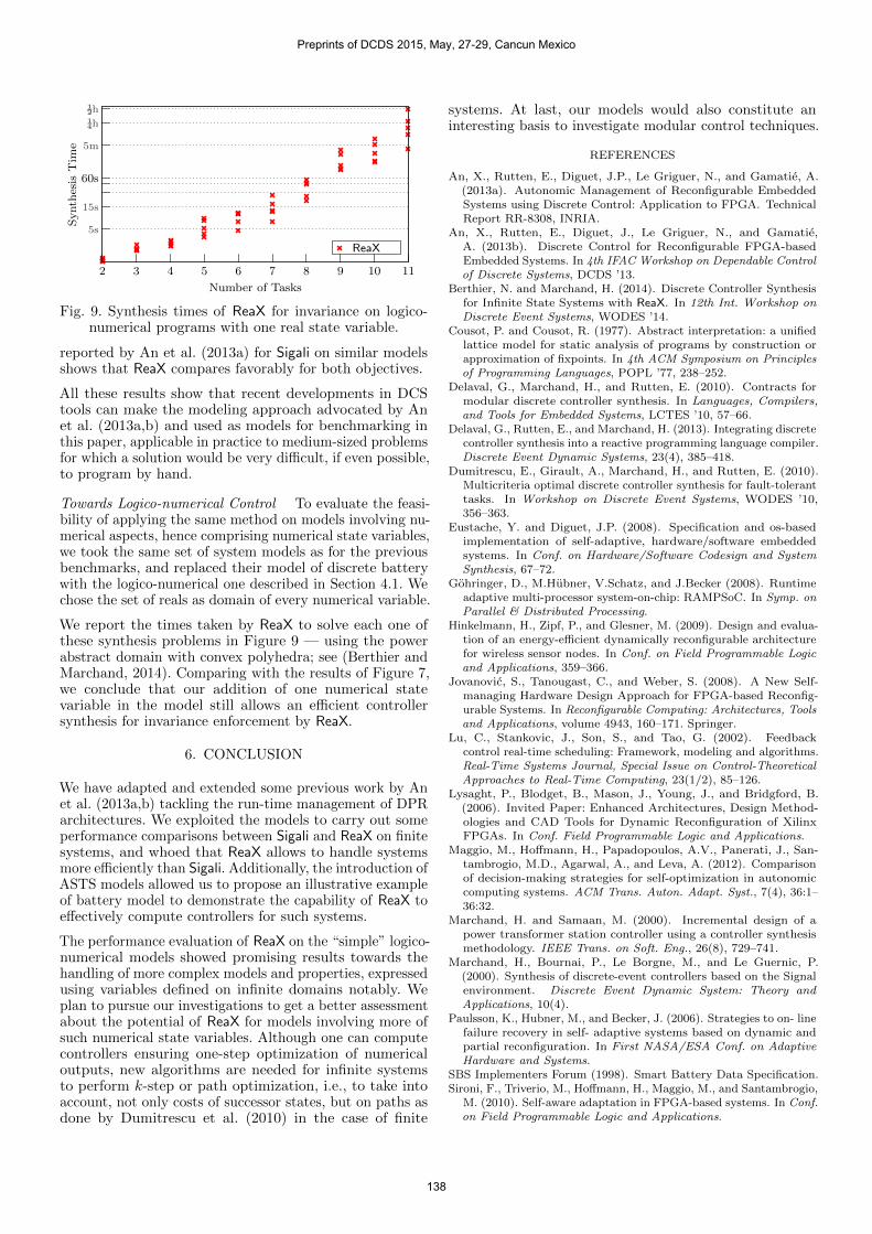
Fig. 9. Synthesis times of ReaX for invariance on logico-numerical programs with one real state variable.

reported by An et al. (2013a) for Sigali on similar modelsshows that ReaX compares favorably for both objectives.

All these results show that recent developments in DCStools can make the modeling approach advocated by Anet al. (2013a,b) and used as models for benchmarking inthis paper, applicable in practice to medium-sized problemsfor which a solution would be very difficult, if even possible,to program by hand.

Towards Logico-numerical Control To evaluate the feasi-bility of applying the same method on models involving nu-merical aspects, hence comprising numerical state variables,we took the same set of system models as for the previousbenchmarks, and replaced their model of discrete batterywith the logico-numerical one described in Section 4.1. Wechose the set of reals as domain of every numerical variable.

We report the times taken by ReaX to solve each one ofthese synthesis problems in Figure 9 — using the powerabstract domain with convex polyhedra; see (Berthier andMarchand, 2014). Comparing with the results of Figure 7,we conclude that our addition of one numerical statevariable in the model still allows an efficient controllersynthesis for invariance enforcement by ReaX.

6. CONCLUSION

We have adapted and extended some previous work by Anet al. (2013a,b) tackling the run-time management of DPRarchitectures. We exploited the models to carry out someperformance comparisons between Sigali and ReaX on finitesystems, and whoed that ReaX allows to handle systemsmore efficiently than Sigali. Additionally, the introduction ofASTS models allowed us to propose an illustrative exampleof battery model to demonstrate the capability of ReaX toeffectively compute controllers for such systems.

The performance evaluation of ReaX on the “simple” logico-numerical models showed promising results towards thehandling of more complex models and properties, expressedusing variables defined on infinite domains notably. Weplan to pursue our investigations to get a better assessmentabout the potential of ReaX for models involving more ofsuch numerical state variables. Although one can computecontrollers ensuring one-step optimization of numericaloutputs, new algorithms are needed for infinite systemsto perform k-step or path optimization, i.e., to take intoaccount, not only costs of successor states, but on paths asdone by Dumitrescu et al. (2010) in the case of finite

systems. At last, our models would also constitute aninteresting basis to investigate modular control techniques.

REFERENCES

An, X., Rutten, E., Diguet, J.P., Le Griguer, N., and Gamatie, A.(2013a). Autonomic Management of Reconfigurable EmbeddedSystems using Discrete Control: Application to FPGA. TechnicalReport RR-8308, INRIA.

An, X., Rutten, E., Diguet, J., Le Griguer, N., and Gamatie,A. (2013b). Discrete Control for Reconfigurable FPGA-basedEmbedded Systems. In 4th IFAC Workshop on Dependable Controlof Discrete Systems, DCDS ’13.

Berthier, N. and Marchand, H. (2014). Discrete Controller Synthesisfor Infinite State Systems with ReaX. In 12th Int. Workshop onDiscrete Event Systems, WODES ’14.

Cousot, P. and Cousot, R. (1977). Abstract interpretation: a unifiedlattice model for static analysis of programs by construction orapproximation of fixpoints. In 4th ACM Symposium on Principlesof Programming Languages, POPL ’77, 238–252.

Delaval, G., Marchand, H., and Rutten, E. (2010). Contracts formodular discrete controller synthesis. In Languages, Compilers,and Tools for Embedded Systems, LCTES ’10, 57–66.

Delaval, G., Rutten, E., and Marchand, H. (2013). Integrating discretecontroller synthesis into a reactive programming language compiler.Discrete Event Dynamic Systems, 23(4), 385–418.

Dumitrescu, E., Girault, A., Marchand, H., and Rutten, E. (2010).Multicriteria optimal discrete controller synthesis for fault-toleranttasks. In Workshop on Discrete Event Systems, WODES ’10,356–363.

Eustache, Y. and Diguet, J.P. (2008). Specification and os-basedimplementation of self-adaptive, hardware/software embeddedsystems. In Conf. on Hardware/Software Codesign and SystemSynthesis, 67–72.

Gohringer, D., M.Hubner, V.Schatz, and J.Becker (2008). Runtimeadaptive multi-processor system-on-chip: RAMPSoC. In Symp. onParallel & Distributed Processing.

Hinkelmann, H., Zipf, P., and Glesner, M. (2009). Design and evalua-tion of an energy-efficient dynamically reconfigurable architecturefor wireless sensor nodes. In Conf. on Field Programmable Logicand Applications, 359–366.

Jovanovic, S., Tanougast, C., and Weber, S. (2008). A New Self-managing Hardware Design Approach for FPGA-based Reconfig-urable Systems. In Reconfigurable Computing: Architectures, Toolsand Applications, volume 4943, 160–171. Springer.

Lu, C., Stankovic, J., Son, S., and Tao, G. (2002). Feedbackcontrol real-time scheduling: Framework, modeling and algorithms.Real-Time Systems Journal, Special Issue on Control-TheoreticalApproaches to Real-Time Computing, 23(1/2), 85–126.

Lysaght, P., Blodget, B., Mason, J., Young, J., and Bridgford, B.(2006). Invited Paper: Enhanced Architectures, Design Method-ologies and CAD Tools for Dynamic Reconfiguration of XilinxFPGAs. In Conf. Field Programmable Logic and Applications.

Maggio, M., Hoffmann, H., Papadopoulos, A.V., Panerati, J., San-tambrogio, M.D., Agarwal, A., and Leva, A. (2012). Comparisonof decision-making strategies for self-optimization in autonomiccomputing systems. ACM Trans. Auton. Adapt. Syst., 7(4), 36:1–36:32.

Marchand, H. and Samaan, M. (2000). Incremental design of apower transformer station controller using a controller synthesismethodology. IEEE Trans. on Soft. Eng., 26(8), 729–741.

Marchand, H., Bournai, P., Le Borgne, M., and Le Guernic, P.(2000). Synthesis of discrete-event controllers based on the Signalenvironment. Discrete Event Dynamic System: Theory andApplications, 10(4).

Paulsson, K., Hubner, M., and Becker, J. (2006). Strategies to on- linefailure recovery in self- adaptive systems based on dynamic andpartial reconfiguration. In First NASA/ESA Conf. on AdaptiveHardware and Systems.

SBS Implementers Forum (1998). Smart Battery Data Specification.Sironi, F., Triverio, M., Hoffmann, H., Maggio, M., and Santambrogio,

M. (2010). Self-aware adaptation in FPGA-based systems. In Conf.on Field Programmable Logic and Applications.

Preprints of DCDS 2015, May, 27-29, Cancun Mexico

138