1

Towards Acoustic Monitoring of Marine Mammals

at a Tidal Turbine Site: Grand Passage, NS, Canada Chloe E. Malinka*#1, Alex E. Hay*2, Richard A. Cheel*3

*Dept. of Oceanography, Dalhousie University, Halifax, Nova Scotia, Canada 1chloe.e.malinka@gmail.com, 2alex.hay@dal.ca, 3richard.cheel@dal.ca

#Now at: Sea Mammal Research Unit, Scottish Oceans Institute, University of St Andrews, St Andrews, U.K.

Abstract – There is a growing interest in extracting energy from

tidal flows using in-stream kinetic energy conversion devices, and

among the many questions are the possible effects on marine

mammals. Underwater sound is used as a tool for detecting

marine mammal presence via their vocalisations, but such

Passive Acoustic Monitoring (PAM) requires an understanding

of site-specific acoustic detection ranges, and the naturally

occurring ambient noise in high-flow environments imposes

constraints on detectability. A pilot experiment was carried out

at a proposed small-scale (<2 MW) tidal energy site (Grand

Passage, Nova Scotia, Canada) to partially assess the feasibility

of a local PAM system. One goal was to determine the effective

detection range as a function of tidal phase using sounds from a

drifting underwater sound projector and moored hydrophones.

A co-located acoustic Doppler flowmeter registered the near-bed

water velocity. The maximum observed detection range was 700

m, with a false alarm rate of 50%. A second goal was to try

different arrangements for passively reducing the effects of flow

noise on the hydrophone signal. Ambient noise levels were

computed for 4 different frequency bands: 0-2 kHz; 2-20 kHz;

20-50 kHz, and 50-200 kHz. On 0.5 to 1 h time scales, the bottom

pod data in the 0-2 kHz band exhibited the highest variability,

associated mainly with ferry and other boat traffic, and the 50-

200 kHz band the least. At tidal frequencies, the clearest

dependence of noise level on flow speed was in the bare

hydrophone data, with the strongest dependence in the highest

band, from about 48 dB re 1 µPa at slack water to about 67 dB re

1 µPa at peak tidal flow. At frequencies above 2 kHz, the data

from a drifting hydrophone exhibited a pronounced dependence

on position along the channel axis, comparable in magnitude to

the tidal variation registered by the moored hydrophone.

Keywords – Underwater acoustics ∙ Passive Acoustic

Monitoring ∙ tidal energy ∙ environmental impact ∙ marine

mammal monitoring ∙ ambient noise ∙ pseudosound

I. INTRODUCTION

In Nova Scotia and worldwide, high tidal flow

environments are the focus of a growing effort to explore the

feasibility of energy extraction using in-stream kinetic

conversion devices (turbines). The Bay of Fundy experiences

one of the highest tidal ranges in the world, and Fundy Tidal

Inc. has proposed several small-scale (<2 MW) in-stream tidal

energy projects along the Digby Neck of Nova Scotia, eastern

Canada: in Grand Passage, Petit Passage and Digby Gut, with

turbine deployments planned for 2015/16.

A. Monitoring Effects on Marine Mammals

Though marine renewables are generally viewed as

environmentally benign, the impacts on the surrounding

environment need to be comprehensively examined [1].

Among the many questions is the effect these turbines will

have on marine mammals. With its temperate and nutrient-

rich waters, the outer Bay of Fundy is an important feeding

ground for many marine mammal species [2]. A diversity of

baleen whales (mysticetes), toothed whales (odontocetes), and

seals (pinnipeds) seasonally inhabit this area. These include:

North Atlantic right whales, humpback whales, minke whales,

fin whales, harbour porpoises, Atlantic white-sided dolphins,

long-finned pilot whales, and harbour and grey seals, and

other less commonly observed species [3, 4].

The marine renewable energy industry is still in its early

stages, and because of this, not all of its impacts are

understood, let alone assessed [5, 6]. Potential concerns for

marine mammals include collision, behavioural modifications,

habitat loss due to physical presence of the turbines, habitat

loss due to anthropogenic noise disturbance, as well as

indirect impacts due to alterations in prey populations [7, 8].

The unknown environmental effects of in-stream devices

and the diversity of marine mammals in the outer Bay of

Fundy suggest the tidal project’s environmental impact

assessment should include Passive Acoustic Monitoring

(PAM) of noises, including: marine mammal sounds, natural

environmental noise, and turbine-generated noise. Using

underwater sound as a tool for detecting marine mammal

presence via their vocalisations seems an obvious choice.

Additionally, it is essential that baseline acoustic conditions

be determined prior to turbine installation in order to evaluate

potential disturbance impacts associated with marine energy

devices [9].

B. Challenges to Acoustic Monitoring in a High Flow

Environment

PAM for marine mammals at tidal energy sites requires an

understanding of the site-specific acoustics affecting acoustic

detection ranges. Acoustic detection thresholds for marine

mammal vocalisations will vary with background noise levels,

which are a function of tidal flow speed: the faster the tidal

flow, the louder the ambient noise level, the smaller the

acoustic detection range [3, 9].

Flow-induced self-noise (pseudosound) is also an issue.

This non-propagating sound is created by turbulent pressure

fluctuations in the hydrophone boundary layer and by strong

currents flowing past the hydrophone [10]. A stationary

hydrophone in a high-flow environment will sense these non-

acoustic pressure variations, just as it senses propagating

2

sound pressures [10, 11]. Pseudosound is apparent only to the

receiver, and can account for high noise levels at lower

frequencies (<1 kHz) [12]. If sufficiently intense,

pseudosound can mask sounds of interest [10]. The effective

acoustic detection range of a vocalising marine mammal at a

tidal energy site could be increased if this pseudosound is

reduced. This idea has previously been explored [13, 15],

whereby hydrophones screened tightly with polyurethane

foam have been shown to act as an acoustic shield to

minimize flow noise by reducing the effects of drag at modest

flow speeds of ~0.5 m/s.

C. Study Objectives

This study investigates the acoustics of Grand Passage in

relation to a future PAM system for marine mammals. The

objectives of this study are:

1) To determine how noisy Grand Passage is prior to

turbine installation, and to determine how sound pressure

levels change with tidal flow;

2) To partially assess the feasibility of a PAM system for

marine mammals in Grand Passage, by estimating acoustic

detection ranges of projected sounds in part of the frequency

range occupied by marine mammal vocalisations; and

3) To test if pseudosound on the hydrophone can be

reduced with open-cell foam shielding.

II. METHODS

A. Study Site and Experimental Methodology

Grand Passage is located on the eastern side of the Bay of

Fundy. It is oriented north-south between Brier Island and

Long Island, along the Digby Neck of Nova Scotia, Canada,

connecting St. Mary’s Bay to the Bay of Fundy. Grand

Passage is subject to semi-diurnal tides, has a 6 m tidal range,

and has surface tidal flows in excess of 4.3 m/s, with a flood

tide running from south to north [15, 16]. The passage is 0.75

km wide at its widest point, and is 4.25 km long, measured

from the northern tip of Brier Island to the southern tip of

Long Island (Fig. 1). The bottom type is very heterogeneous,

ranging from bedrock outcrops to mobile sediments consisting

of a mixture of gravel, fine sand and shell hash [17]. A diesel

engine ferry typically makes at least two crossings per hour

during the day, and runs on demand at night.

Fieldwork was conducted from July 5-9 2012, and focused

on the northern end of Grand Passage (Fig. 1).

Instrumentation was deployed and recovered with a fishing

vessel, the Expectations XL (Westport, NS). A rigid-hull

inflatable boat (RHIB) was used for all other aspects of the

experiment. All field tests were conducted during a spring tide

to obtain conservative estimates of acoustic detection ranges.

1) Instrumentation: An Ocean Sonics hydrophone

(icListen High Frequency) continuously collected ambient

noise time series data in both FFT (Fast Fourier Transform)

and WAV file format (Table 1). The response of the icListen

is flat (+/- 3 dBV) over 0.01-200 kHz. The manufacturer-

supplied calibration for the hydrophone was used to convert

voltage to sound pressure level.

Fig. 1 Mean current speed during flood tide in Grand Passage. Current speed

data are a synthesis of ADCP measurements, multi-beam WASSP® bathymetry, and a 2-dimensional numerical simulation for tidal currents. The

mean moored hydrophone location is represented by a black square.

(Courtesy of J. McMillan).

TABLE I

HYDROPHONE SETTINGS USED.

Parameter FFT WAV

Bandwidth (kHz) 204.8 102.4

Sample rate (kSamples/s) 512 256

Spectrum update rate 0.25 -

Processing mode Mean -

Spectrum length (points) 1024 -

Spectra per averaging interval 125 -

Resolution (Hz) 500 -

The autonomous hydrophone was moored on a fiberglass

platform ballasted by three 50 lb lead weights (Fig. 2). This

bottom pod set-up varied in order to investigate pseudosound

reduction techniques. All cables on the platform were secured

with zip ties to eliminate flapping noise.

3

Fig. 2 Sample photos of bottom pods, showing: A) the vertical hydrophone set-up, B) the “umbrella” set-up, and C) the “sock” set-up.

An Ocean Sonics underwater projector (icTalk MF Smart

Projector) was used to broadcast sounds from the RHIB while

drifting (engine off). Omnidirectional sounds transmitted in

consecutive 5 second chirps at known times, at the maximum

sound pressure level of the instrument, and spanning the

instrument’s full bandwidth (2-20 kHz at 101 dB re 1 µPa @ 1

m). This frequency range overlaps with the vocal ranges of

some marine mammal species, and a chirp was used to test

detections. The duration of each frequency (kHz) in the chirp

was ~0.3 ms. Chirps were created in Audacity

(<http://audacity.sourceforge.net/>). The projector was

suspended from the RHIB at ~2 m below the water surface.

The RHIB position during the sound projection drifts was

recorded using on-board GPS. Drifts started ~800 m upstream

of the moored hydrophone, and continued until about the same

distance downstream, and were carried out during flood, high

slack, and ebb tides. The number of drifts completed in a day

(maximum of 16) was limited by the battery life of the

autonomous hydrophone (~8 h).

A Nortek Vector acoustic Doppler velocimeter (ADV)

mounted on the bottom pod (Fig. 2) continuously sampled the

flow velocity. The ADV sample rate and velocity range had to

be adjusted after the first deployment due to data quality

issues associated with the low scatterer concentrations in the

water, despite being close to the seabed. On 5 July 2012, the

ADV was positioned on its side, and on 6-8 July 2012 the

ADV was positioned vertically, resulting in two different

sample heights (0.19 m and 0.35 m) above the seabed.

On 5-7 July 2012 a second hydrophone was suspended

below the RHIB at ~1.5 m below the water surface,

simultaneous with sound projection drifts. Since this

hydrophone was drifting with the current, pseudosound

contamination was anticipated to be reduced compared to the

moored hydrophone. Sound projection drifts were repeated

over four days to accommodate variations in bottom pod

configuration.

2) Bottom pod deployments: The hydrophone frame was

deployed during the first low slack water of the day. The

frame was deployed at nominally the same location in the

northwest of Grand Passage for each of the four tests (at

~44.2776°N, 66.3412°W). A shallow location (12.8 m to 16.5

m at low water) was chosen to allow for pod recovery by

SCUBA divers, if necessary. Sound projections occurred

through flood and ebb tides, and at the second daily slack

water (~12 h later), the frame was retrieved. A Sub Sea Sonics

acoustic interrogator (model ARI-60) transmitted commands

to trigger the release of the float recovery system.

Four frame set-ups designed to test pseudosound reduction

techniques were used. On 5 July 2012, the hydrophone was

bare and horizontal. On 6 July 2012, the hydrophone was

horizontal and wrapped in open-cell, 10 pores per inch (ppi)

polyurethane foam (2 cm thick overall) to make up a “sock”

set-up (Fig. 2c). On 7 July 2012, the hydrophone was vertical

underneath a foam shell (Fig. 2b). A dome-shaped metal

frame, or “umbrella”, was covered with two layers of foam (2

cm thick overall) and reinforced with galvanized wire

screening. A metal cage surrounded the hydrophone sensor to

prevent direct contact with the foam for both the “sock” and

“umbrella” set-ups. On 8 July 2012, the sensor was bare and

vertically oriented (Fig. 2a). Prior to deployment each day,

detergent was applied to the hydrophone sensor to reduce

surface tension, and in set-ups where foam was used, the foam

was saturated with soapy water prior to deployment.

3) Ambient Noise Drifter Trajectories: A drifting

hydrophone set-up was employed to reduce the flow noise by

recording in conditions with no anticipated pseudosound. The

drifter consisted of a hydrophone attached to a surface buoy

by a bungee cord, suspended at ~4 m below the water surface

(Fig. 3). The hydrophone was configured as before (Table 1).

“Umbrella”

“Sock”

Float recovery system

Acoustic releases

Hydrophones

ADV pressure case and ADV

Lead foot

B C

A

4

Two chimney sweep brushes acted as dampers to decouple the

hydrophone from the movement of the surface float. An

attached global positioning system (Garmin GPS) tracked

position at a sample rate of 1 Hz. The drifter (Fig. 3) was

repeatedly released on 9 July 2012 in ~25 m water depth

along the northwest side of Grand Passage. To account for

variations in background noise level with tidal state, two drifts

occurred during flood tide (sea state 2), and two drifts during

high slack water (sea state 3). Boat traffic presence and sea

state were recorded from visual observation over this time

period.

Fig. 3 Ambient noise drifter.

4) Ancillary Measurements: Wind speed and direction

were measured hourly at the Coast Guard station at the north

end of the passage. Wind speed was also estimated during the

drifts using the Beaufort wind scale. Boat traffic presence in

the vicinity of the moored hydrophone was recorded from

visual observations during sound projection and free-drift

experiments.

The water column in Grand Passage was repeatedly

profiled at various locations in the passage over four days

using an RBR CTD (Conductivity Temperature Depth sensor,

model XR-620CTDmF).

B. Data Analysis

All data analysis was done using custom scripts in Matlab

(The Mathworks Inc.).

1) GPS Data: The start and end times from the RHIB

tracks for each drift were used to identify and join consecutive

hydrophone FFT files corresponding to each drift. Ambient

noise drifter speed was determined from the GPS tracks and

then time-aligned with acoustic data from the drifter by

interpolating the GPS time base onto the hydrophone time

base.

2) ADV Data: Velocity data were averaged over 5 minute

intervals, and current speed was determined. It was discovered

that the particular ADV used had a firmware error, since

corrected by the manufacturer, which resulted in unusable

compass readings, and therefore the orientation of the frame

on the seafloor could not be reliably determined from

instrument heading. The sign of the x,y,z velocities, together

with outputs from both Acoustic Doppler Current Profiler

(ADCPs) measurements from Grand Passage and a 2D

numerical tidal current model in the passage [16], were used

to determine the frame’s orientation relative to the flow. At

the hydrophone frame location, the angles of flood and ebb

tide are 11.5 and 193 clockwise from true North,

respectively [16].

3) Acoustic Data: Four frequency bands were selected for

ambient noise level analysis: low (0-2 kHz), mid-low (2-20

kHz), mid-high (20-50 kHz), and high (50-200 kHz). These

bands were selected based on a combination of biological and

practical reasons. For example, pseudonoise and ferry noise is

mainly <2 kHz, the chirp was from 2-20 kHz, and sediment-

generated noise extends to higher frequencies. Additionally,

marine mammals are often grouped by the frequencies of their

vocalisations. For example, large mysticetes whales vocalise

at low frequencies (several tens of Hz to several kHz), and the

whistles and echolocation clicks of odontocetes range from a

few hundreds of Hz to over one hundred kHz. Data in each of

the four frequency bands were averaged over 10 s intervals

(5,000 spectra per interval). Spectra were computed using a

Hanning window with 50% overlap. Spectra computed from

WAV files and those of the corresponding FFT files,

computed by the instrument itself, agreed with one another.

Time series of noise levels (dB re 1 Pa) were analysed for

each frequency band, for all four bottom pod deployments and

the ambient noise drifts. Analyses of noise level as a function

of current speed for the bottom pod, and of noise level as a

function of drifter speed for the drifter, were completed. Fig. 4

shows icTalk-projected sounds in the hydrophone record, and

illustrates the variability in low-frequency background noise

levels.

Fig. 4 A) Data segment corresponding to one RHIB drift, showing the

distance from the bottom pod of the drifting RHIB projecting sounds; B) A spectrogram from the icListen on the bottom pod; and C) Zoom showing

signal from icTalk (2-20 kHz).

A

B

C

Time (decimal h)

5

An analysis of sound detection versus range from the

hydrophone was completed. A chirp correlator algorithm was

constructed to detect the projected sounds in the data records

registered by the hydrophone on the bottom pod, as illustrated

in Fig. 5. The correlator operates in the time-frequency

domain of the spectrogram. The algorithm is based on the

lagged cross-correlation between a synthetic chirp

spectrogram and the observed spectrogram. The synthetic

chirp, C(f,t), is a linear frequency sweep of unit amplitude

between 2 and 20 kHz. The output of the correlator, Corr(τ), is

the sum over frequency of the convolution in time of the

product of the synthetic chirp and the observed spectrum,

S(f,t): i.e.

Corr(τ) = ∑∑S(f i ,t j) C(f i ,t j+ τ)

where the double summation is over the indices i and j. The

normalized correlations were sometimes contaminated by the

low frequency sound evident in Fig. 5a, usually due to boat

traffic and resulted in low frequency variability in the

background correlation level. An example of the output of the

chirp correlator is shown in Fig. 5b. The difference in

correlation (∆Corr) effectively removed this low frequency

variability for all hydrophone records (Fig. 5c), and ∆Corr

was used in further analysis.

Fig. 5 Peak detection for a sample drift. A) Spectrogram from bottom pod hydrophone, where loud spikes show boat noise; B) Normalized correlation of

projected sound to received sound; and C) Difference in correlation of

projected sound to received sound.

A peak detection algorithm identified maxima and

minima in ∆Corr values in each 5 s interval corresponding to

the duration of the projected chirp (Fig. 6). To identify false

alarms, the highest peak in ∆Corr value was used as a central

reference. Using the 5 s chirp repetition interval, detections

were considered to be a false alarm if they did not occur at

multiples of 5 + 0.3 s from this reference point (Fig. 6). Data

points of ∆Corr were positioned 0.25 s apart, so a + 0.3 s

deviation allowed for a wavering of one data point. Only true

detections were used in further analysis.

Fig. 6 Difference in correlation of projected sound to sound received by

hydrophone for a sample drift. Shaded regions show the area zoomed in

below. Black points show the maximum correlation per 5 s interval. Black

points with blue circles show detections that lie in the 5 + 0.3 s chirp repetition interval, and represent true detections. Black points without blue

circles show false alarms. The boat positions at the times of true detections were

extracted to obtain the distances between the RHIB the bottom

pod. An analysis of sound detection versus both range (m) and

tidal speed (m/s) was completed to determine how acoustic

detection ranges varied with tidal phase. Additionally,

analyses of false alarm rate versus distance, and range at 50%

false alarm rate versus current speed, were completed for each

bottom pod set-up.

III. RESULTS

A. Water profile

At slack water and in both flood and ebb tides, CTD

measurements revealed Grand Passage to have a very well-

mixed water column with no obvious stratifications. Here, the

implication is that we can assume that sound speed was

relatively constant.

B. Bottom-mounted hydrophones

1) Ambient Noise Levels: The tidal variation of the

recorded ambient noise level was apparent across all bottom

pod deployments. The result from the bare and vertical

hydrophone deployment is shown in Figure 7. Noise levels

were ~25 dB louder at peak flood compared to slack water in

all four specified frequency bands.

A

B

C

Time (decimal h)

Time (decimal h)

Time (decimal h)

6

Fig. 7 Ambient noise levels detected by a hydrophone on the bottom pod (here, the bare vertical hydrophone data is shown). Shaded regions indicate

field-identified noise events (e.g. boat passing over hydrophone or ferry

crossing). Frequency bands are colour-coded, where red is 0-2 kHz, blue is 2-20 kHz, green is 20-50 kHz, and cyan is 50-200 kHz. The deployment (at

~12:00 UTC) was at low slack, and flood tide followed from 12-18 h, with

peak flood at ~15:00 and high slack at ~18:00.

Mean noise levels for peak flood and peak slack water, for

each deployment configuration, are presented in Table 2. The

bare horizontal hydrophone, “umbrella” hydrophone, and bare

vertical hydrophone records exhibited comparable noise levels

across all frequency bands. Obvious high noise events (e.g.

ferry crossings) were excluded from the values in Table 2. For

these three configurations, the variation in average noise level

for each of the four predefined frequency bands, across each

deployment duration was small: 5 dB in the low frequency

band, 6 dB in the mid-low frequency band, 3 dB in the mid-

high frequency band, and 3 dB in the high frequency band.

Acoustic measurements from the “sock” hydrophone

exhibited the lowest noise levels in each frequency band, of

all of the bottom pod set-ups (Table 2). Compared to the mean

values of noise levels of all three other bottom pod set-ups, the

“sock” recorded ambient noise levels at 21, 25, 12, and 9 dB

lower in the low, mid-low, mid-high, and high frequency

bands, respectively, at peak flood, and recorded noise levels at

4, 5, 9, and 5 lower in the low, mid-low, mid-high, and high

frequency bands, respectively, at peak slack.

TABLE II

NOISE LEVELS AT PEAK FLOOD AND SLACK WATER, FOR ALL FOUR

HYDROPHONE CONFIGURATIONS ON THE BOTTOM POD.

Bottom pod

set-up

Tidal

state Mean noise level (dB re 1 Pa) in

each frequency band (kHz)

0-2 2-20 20-50 50-200

Bare vertical Flood 78 70 73 67

Slack 54 44 49 48

Bare

horizontal

Flood 73 72 70 64

Slack 52 43 40 36

Umbrella Flood 72 67 71 63

Slack 58 50 41 37

Sock Flood 53 45 59 56

Slack 51 41 34 35

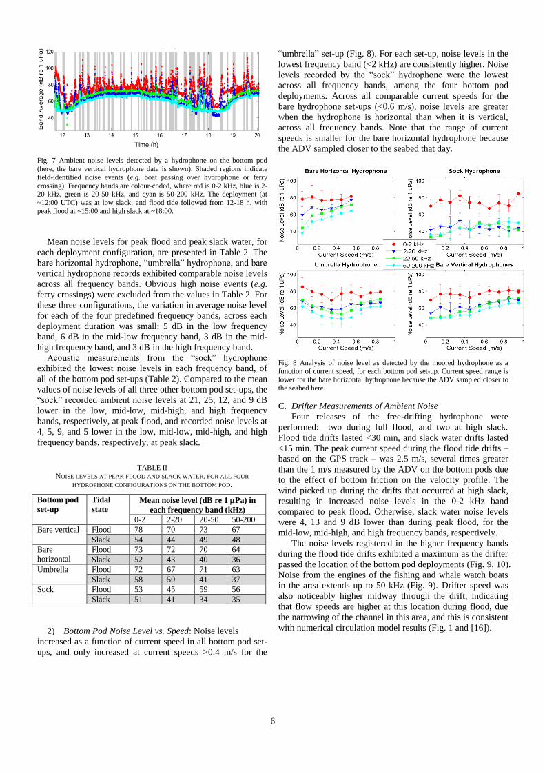
2) Bottom Pod Noise Level vs. Speed: Noise levels

increased as a function of current speed in all bottom pod set-

ups, and only increased at current speeds >0.4 m/s for the

“umbrella” set-up (Fig. 8). For each set-up, noise levels in the

lowest frequency band (<2 kHz) are consistently higher. Noise

levels recorded by the “sock” hydrophone were the lowest

across all frequency bands, among the four bottom pod

deployments. Across all comparable current speeds for the

bare hydrophone set-ups (<0.6 m/s), noise levels are greater

when the hydrophone is horizontal than when it is vertical,

across all frequency bands. Note that the range of current

speeds is smaller for the bare horizontal hydrophone because

the ADV sampled closer to the seabed that day.

Fig. 8 Analysis of noise level as detected by the moored hydrophone as a

function of current speed, for each bottom pod set-up. Current speed range is lower for the bare horizontal hydrophone because the ADV sampled closer to

the seabed here.

C. Drifter Measurements of Ambient Noise

Four releases of the free-drifting hydrophone were

performed: two during full flood, and two at high slack.

Flood tide drifts lasted <30 min, and slack water drifts lasted

<15 min. The peak current speed during the flood tide drifts –

based on the GPS track – was 2.5 m/s, several times greater

than the 1 m/s measured by the ADV on the bottom pods due

to the effect of bottom friction on the velocity profile. The

wind picked up during the drifts that occurred at high slack,

resulting in increased noise levels in the 0-2 kHz band

compared to peak flood. Otherwise, slack water noise levels

were 4, 13 and 9 dB lower than during peak flood, for the

mid-low, mid-high, and high frequency bands, respectively.

The noise levels registered in the higher frequency bands

during the flood tide drifts exhibited a maximum as the drifter

passed the location of the bottom pod deployments (Fig. 9, 10).

Noise from the engines of the fishing and whale watch boats

in the area extends up to 50 kHz (Fig. 9). Drifter speed was

also noticeably higher midway through the drift, indicating

that flow speeds are higher at this location during flood, due

the narrowing of the channel in this area, and this is consistent

with numerical circulation model results (Fig. 1 and [16]).

Time (h)

7

Fig. 9 Ambient noise measurements as detected by the drifting hydrophone

during peak flood tide, as a function of distance from the bottom pod location.

Negative distances are south of the bottom pod. Shaded regions indicate boat

noise events. The total drift duration is 26 minutes.

Fig. 10 Track locations of increased noise level collected by the ambient noise

drifter. Noisy points were identified as when noise levels in the high

frequency band (50-200 kHz) exceeded 50 dB re 1 μPa.

D. Acoustic Detection Ranges

Maximum ∆Corr values are greatest for the bare vertical

hydrophone (Fig. 11), followed by the “sock” hydrophone.

The “sock” exhibited a greatly reduced noise level in the

frequency band of 2-20 kHz which aligned with sound

projections. Maximum values of ∆Corr for the “sock” are not

larger than other bottom pod set-ups. Maximum values of

∆Corr decreased as a function of distance from the

hydrophone, for all bottom pod set-ups, except for the

“umbrella”. The highest ∆Corr values for the “umbrella” set-

up were not as high as for the other bottom pod set-ups. It is

difficult to confidently say that the “umbrella” effectively

detected sound projections at a distance, since its maximum

values of ∆Corr were not high at close range.

Maximum ∆Corr values were only higher when the tidal

current is weaker for the bare vertical and “sock” hydrophones.

For the “umbrella”, this observation holds true except for

when tidal current speed is low (<0.65 m/s). Maximum ∆Corr

values varied less as a function of current speed for the bare

horizontal hydrophone. Maximum values of ∆Corr did not

exceed 0.1 at a distance of ~150 m for the bare horizontal

hydrophone, ~75 m for the “sock”, ~200 m for the “umbrella”,

and ~250 m for the bare vertical hydrophone. Acoustic

detection ranges, as measured by maximum ∆Corr values,

were greatest for the bare vertical hydrophone.

Maximum detection range, defined as the range at which

the false alarm rate was 50%, are shown for each

configuration (Fig. 12). Acoustic detection ranges were

greatest for the bare vertical hydrophone, extending up to

~700 m from the bottom pod location. False alarm rates

increased as a function of distance from the hydrophone for all

bottom pod set-ups. Similarly, maximum detection range

tended to decrease with increasing flow speed for all four set-

ups.

Fig. 11 Acoustic detection ranges and false alarm rate for the bare horizontal hydrophone, showing the difference in peak correlation of the projected and

received sounds, as a function of distance from the hydrophone. Current

speeds are colour-coded to show acoustic detection range as a function of tidal phase.

8

Fig. 12 Maximum chirp detection range – the ranges at which the false alarm rate was 50%. Note the increase in maximum detection with decreasing

current speed for the bare vertical hydrophone.

IV. DISCUSSION

A. Ambient Noise Levels

Sound pressure levels were greater during flood tide than at

slack water, as measured by both the hydrophone on the

bottom pod and on the drifter. The noise below 2 kHz is

thought to originate from boat traffic (specifically propeller

cavitation and engine noise), and to a lesser extent from the

surface noise of waves breaking on the shoreline [18]. The

high noise levels in the low frequency band (0-2 kHz) during

the ambient noise drifts were due to windy conditions.

The ambient noise drifter (Fig. 9) should be less subject to

pseudosound than the stationary bottom pod since efforts were

taken to decouple the hydrophone from the flow. It was

therefore expected that ambient noise level as a function of

flow speed would be greater for bottom pod deployments than

for the drifter. The drifter might not have been completely

decoupled from the surface movement of the buoy, in which

case the drifter would have been subject to pseudosound. A

varying depth of the drifting hydrophone could lead to

pressure fluctuations and contaminate data [19], especially at

low frequencies (<1 kHz) [11]. Alternatively, the lower

ambient noise levels registered by the hydrophones on the

bottom pod could be due to the lower current speeds near the

seabed and their associated low-pressure fluctuations caused

by water moving around the hydrophone [14].

Since pseudosound is expected to be much lower at high

frequencies, the peak noise levels at high frequencies – i.e.

above 20 kHz – registered by both the drifting and stationary

hydrophones are likely real. Bedload transport from tidal

currents could explain the increased ambient noise levels that

were observed in all frequency bands during peak flood (Figs.

7, 9), especially across the higher frequency bands. It has

previously been shown that acoustic energy arises from inter-

particle collisions of coarse sediment, and that greater sound

pressure levels exist in higher frequencies for smaller particles

[20]. Additionally, observed high intensity sounds (120-140

dB re 1 µPa) concurrent with the tidal signal have been

attributed to the fast flow speeds that mobilize gravel and shell

hash on the seabed [11, 12]. Shortly after these experiments

(in Sept 2012), sediment samples were taken near the bottom

pod site. This region revealed gravel to sand, with shell hash

and a fine sediment top layer [17]. High-frequency (1 kHz to

200 kHz) sediment-generated noise can trigger detections of

marine mammal echolocation clicks on automated detectors,

and this has implications for passive acoustic monitoring [12,

21].

The results presented here indicate that there is

considerable spatial variability in the ambient noise levels in

Grand Passage. Background noise levels have been found to

be higher in areas experiencing greater tidal current speeds

than in more sheltered areas [9]. For any future PAM system

at this site, this variability should be taken into account when

choosing hydrophone locations (i.e. choose areas with weaker

tidal currents). Tidal current models and ADCP measurements

revealed areas of increased flow speeds (Fig. 1), and these are

likely indicative of noisier areas, as was the case for the

bottom pod location in the northwest of Grand Passage.

B. Pseudosound Reduction

The only noise reduction technique that appeared to greatly

reduce background noise levels was the “sock” (Fig. 8).

However, noise level reductions were least pronounced in the

low frequency band in which pseudosound was anticipated

(Table 2). The reduction of noise was prominent in the mid-

low frequency band, but this overlapped with frequency of

sound projections. This reduction of noise level is comparable

to what was observed previously [13], as their 3 cm thick open

cell foam flow shield reduced noise by up to 24 dB below 50

Hz.

While this field experiment started during the peak spring

tide, the tide was weaker each succeeding day. This must be

considered when comparing ambient noise levels of different

bottom pod set-ups. Direct comparisons between pseudosound

reduction techniques can be made when considering flow

noise versus current speed (Fig. 8).

C. Acoustic Detection Ranges

Acoustic detection ranges were greatest for the bare vertical

hydrophones. While a horizontal orientation positions the

hydrophone closer to the seabed where current speeds are

lower, a vertical hydrophone was deemed to be more

appropriate for PAM since its sound measurements are less

directional.

While ambient noise levels were lower across all frequency

bands for the “sock” hydrophone (Table 2), its acoustic

detection range is less than for the bare vertical hydrophone.

The acoustic detection range of the “sock” was expected to be

greatest because of the significant reduction of noise level in

the frequency band in which the icTalk was projecting sounds

(2-20 kHz). It is therefore surprising that the highest

maximum values of ∆Corr at close range are not seen in the

“sock” hydrophone set-up. Instead, it is likely that the “sock”

9

attenuated the projected chirps from the icTalk in addition to

reducing pseudosound. This is evidenced by the reduction of

noise levels in all frequency bands for the “sock”, including

the high frequency bands not associated with pseudosound

(Table 2). Therefore, this pseudosound reduction technique is

not recommended.

A previous experiment found that a flow shield

significantly suppressed much of the noise increase from

pseudosound at low frequencies (<750 Hz), when compared

with an unshielded hydrophone, at flow speeds up to 1 m/s

[11]. Their hydrophones, with and without flow shields,

recorded equivalent levels of sound >750 Hz, and suggested

that their flow shield effectively reduced pseudosound without

attenuating propagating sound [11]. It appears that the same

cannot be said for this experiment, where the “sock” is the

flow shield.

The false alarm rate of detected chirps increased with

increasing distance from the hydrophone, due to sound

attenuation over distance (Fig. 8). While it makes sense for the

maximum values of ∆Corr to decrease with distance from the

hydrophone frame, it is less obvious why the observed values

spike upwards at great distances (Fig. 8). The range at which

false alarm rate was 50% was greatest for the bare vertical

hydrophone, at ~700 m (Fig. 12).

The projected frequency range (2-20 kHz) was limited by

the icTalk, and was not fully representative of the range of

local marine mammal vocalisations. Since marine mammals

produce a variety of sound in different frequency ranges, the

icTalk would have ideally projected sounds as low as 20 Hz to

mimic fin whale calls, and up to 130 kHz to imitate harbour

porpoise clicks [3].

Sound transmission in shallow waters is highly variable due

to the influence of acoustic properties of the seabed, surface,

and the channel geometry/bathymetry [18]. The present

research could be extended to include propagation models,

and compare predicted to observed acoustic detection ranges.

V. CONCLUSION

The aim of this study was to obtain baseline ambient noise

levels and sound detection ranges as a partial basis for

determining the feasibility of a PAM system for marine

mammals in Grand Passage, NS, prior to in-stream tidal

energy development. The measurements reported here, made

in July 2012, included both ambient noise measurements and a

sound projection experiment to determine acoustic detection

range, both as a function of tidal current speed. For the

analysis of the projection experiment data, chirp correlator

and peak detector functions were constructed in Matlab.

Pseudosound reduction techniques were field tested, and a

freely drifting hydrophone characterised ambient noise levels.

Sound pressure levels at peak flood were ~25 dB greater

than during slack water. Efforts to reduce pseudosound were

not very successful. The “sock” set-up resulted in the greatest

noise suppression, but also the worst detection ranges,

whereby it reduced sound pressure levels in frequency ranges

extending beyond those affected by pseudosound (<1 kHz),

suggesting that the projected chirps were attenuated by open-

cell foam. Acoustic detection ranges were greatest when the

hydrophone was bare and vertical, and extend up to ~700 m

from the bottom pod location in the northwest of Grand

Passage. Ambient noise levels were modulated by both water

speed and location within the channel. Peak noise levels at

high frequencies – 10 kHz and higher – during high flow are

attributed to collisions among the mobile sediments on the

seabed, predominantly shell hash in Grand Passage.

The present work contributes to the future acoustic

monitoring of marine mammal presence in the vicinity of the

proposed tidal turbine. This information will help inform

future monitoring of marine mammal sounds near in-stream

tidal turbine sites, laying a basis for site-specific marine

mammal event detections. Acoustic propagation modelling of

Grand Passage would also be useful. Future investigations

should include longer acoustic recording deployments,

measurements in different seasons, projections over a wider

frequency range, and an investigation into how acoustic

detection ranges change as a function of projected frequency;

these would increase the understanding of shallow water

acoustics in Grand Passage.

ACKNOWLEDGMENT

This study was funded by a Natural Sciences and

Engineering Research Council (NSERC) ENGAGE grant to

the Ocean Acoustics Lab at Dalhousie University and Ocean

Sonics (Great Village, NS), and by a Nova Scotia Strategic

Co-operative Education Incentive grant for undergraduate

Science Co-op students. This work was also carried out in

collaboration with Greg Trowse of Fundy Tidal Inc. Thanks

are extended to Justine McMillan, Matthew Hatcher, and Nina

Stark, as well as the captain and crew of the Expectations XL,

for their assistance in the field, and to Mark Wood, Jay Abel,

Walter Judge and Doug Schillinger for technical support.

REFERENCES

[1] R. Inger, M. J. Attrill, S. Bearhop, A. C. Broderick, W. J. Grecian. D. J. Hodgson, and B. J. Godley. “Marine renewable energy: potential

benefits to biodiversity? An urgent call for research,” Journal of

Applied Ecology, vol. 46, pp. 1145-1153, Dec. 2009. [2] L. D. Murison, and D. E. Gaskin. “The distribution of right whales and

zooplankton in the Bay of Fundy, Canada,” Canadian Journal of

Zoology, vol. 67, pp. 1411-1420, Jun. 1989. [3] C. E. Malinka, “Acoustic detection ranges and baseline ambient noise

measurements for a marine mammal monitoring system at a proposed

in-stream tidal turbine site: Grand Passage, Nova Scotia,” B. Sc. Thesis, Dalhousie University, Halifax, Canada, May 2013.

[4] C. E. Malinka, M. W. Brown, G. T. Trowse, B. Winney, and V.

Zetterlind. "Observations of marine mammals in Petit Passage and Grand Passage, Nova Scotia and adjacent waters in the eastern Bay of

Fundy to assess species composition, distribution, number and

seasonality," Tech. Rep. for the Nova Scotia Offshore Energy Research Association (OERA), 44 p., Jan 2015.

[5] S. Dolman and M. Simmonds. “Towards best environmental practice

for cetacean conservation in developing Scotland’s marine renewable energy,” Marine Policy, vol. 34, issue 5, pp. 1021-1027, Sept. 2010.

[6] H. A. Viehman, “Fish in a tidally dynamic region in Maine: Hydro

acoustic assessments in relation to tidal power development,” M. Sc. Thesis, University of Maine, U.S.A., May 2012.

[7] B. Wilson, R. S. Batty, F. Daunt, and C. Carter. “Collision risks

between marine renewable energy devices and mammals, fish and diving birds,” Scottish Association for Marine Science, Oban, Scotland,

Tech. Rep. PA371QA, 2009.

10

[8] D. J. Tollit, J. D. Wood, J. Broome, and A. M. Redden. “Detection of marine mammals and effects monitoring at the NSPI (OpenHydro)

turbine site in the Minas Passage during 2010,” Fundy Ocean Research

Centre for Energy, Nova Scotia, Canada, Tech. Rep., 2011.

[9] M. Willis, M. Broudic, C. Haywood, I. Masters, and S. Thomas.

“Measuring underwater background noise in high tidal flow

environments,” Renewable Energy, vol. 49, pp. 55-58, Jan. 2013. [10] C. Bassett, J. Thomson, and B. Polagye. “Characteristics of underwater

ambient noise at a proposed tidal energy site in Puget Sound,” in

OCEANS 2010 IEEE, 2010, p. 1-8. [11] B. Polagye, J. Thomson, C. Bassett, J. Graber, R. Cavagnaro, J. Talbert,

A. Reay-Ellers, D. Tollit, J. Wood, A. Copping, et al. “Study of the

acoustic effects of hydrokinetic tidal turbines in Admiralty Inlet, Puget Sound,” U. S. Department of Energy, Tech. Rep., 2012.

[12] C. Bassett, J. Thomson, and B. Polagye. "Sediment‐generated noise and bed stress in a tidal channel." Journal of Geophysical Research:

Oceans, vol. 118(4), pp. 2249-2265, Apr 2013. [13] S. Lee, S.-R. Kim, Y. K. Lee, J. R. Yoon, and P.-H. Lee. “Experiment

on effect of screening hydrophone for reduction of flow-induced

ambient noise in ocean,” Japanese Journal of Applied Physics, vol. 50, Jul. 2011.

[14] B. Martin, C. Whitt, C. McPherson, A. Gerber, and M. Scotney.

“Measurement of long-term ambient noise and tidal turbine levels in the Bay of Fundy,” in Proc. AAS’12, 2012, p.1-7.

[15] G. Trowse, and R. Karsten. “Bay of Fundy tidal energy development –

opportunities and challenges,” in Proc. of International Conference on Ocean Energy (ICOE), p. 1-11, Bilbao, Spain, Oct 2010.

[16] J. M. McMillan, A. E. Hay, R. H. Karsten, G. Trowse, D. Schillinger, and M. O’Flaherty-Sproul., “Comprehensive Tidal Energy Resource

Assessment in the lower Bay of Fundy, Canada,” in Proc. of European

Wave and Tidal Energy Conference (EWTEC), p. 1-10, Aalborg,

Denmark, 2013.

[17] N. Stark, A. E. Hay, and G. Trowse. “Cost-effective geotechnical and

sedimentological early site assessment for ocean renewable energies,” in Proc. Of European Wave and Tidal Energy Conference (EWTEC), p.

1-8, Aalborg, Denmark, 2013.

[18] W. J. Richardson, C. R. Greene, S. I. Malme and D. H. Thomson. Marine Mammals and Noise. USA: Academic Press, 1995.

[19] P. Stein. (2011) Radiated noise measurements in a high current

environment using a drifting noise measurement buoy (part B). In DOE Marine Hydrokinetics Webinar 3: Monitoring technologies and

strategies. U.S. Department of Energy. Available:

http://mhk.pnnl.gov/publications/doe-mhk-webinar-3-monitoring-technologies-and-strategies.

[20] P. D. Thorne. “Laboratory and marine measurements on the acoustic

detection of sediment transport,” Journal of the Acoustical Society of America, vol. 80, pp. 899-910, 1986.

[21] C. E. Malinka, J. D. J. Macaulay, J. Gordon, and S. Northridge.

“Evaluation of a drifting porpoise localizing array buoy: a novel configuration for tracking porpoises in tidal rapids using passive

acoustics,” Internship report under the Marine Renewable Energy

Knowledge Exchange Programme, March 2015, p. 1-24.

The author has requested enhancement of the downloaded file. All in-text references underlined in blue are linked to publications on ResearchGate.The author has requested enhancement of the downloaded file. All in-text references underlined in blue are linked to publications on ResearchGate.