toward mapping land-use patterns from volunteered ... · volunteered geographic information jamal...
TRANSCRIPT
This article was downloaded by: [Universitaetsbibliothek Heidelberg]On: 20 June 2013, At: 00:08Publisher: Taylor & FrancisInforma Ltd Registered in England and Wales Registered Number: 1072954 Registeredoffice: Mortimer House, 37-41 Mortimer Street, London W1T 3JH, UK
International Journal of GeographicalInformation SciencePublication details, including instructions for authors andsubscription information:http://www.tandfonline.com/loi/tgis20
Toward mapping land-use patterns fromvolunteered geographic informationJamal Jokar Arsanjani a , Marco Helbich a , Mohamed Bakillah a ,Julian Hagenauer a & Alexander Zipf aa Institute of Geography, GIScience Group, Heidelberg University ,Heidelberg , GermanyPublished online: 19 Jun 2013.
To cite this article: Jamal Jokar Arsanjani , Marco Helbich , Mohamed Bakillah , JulianHagenauer & Alexander Zipf (2013): Toward mapping land-use patterns from volunteeredgeographic information, International Journal of Geographical Information Science,DOI:10.1080/13658816.2013.800871
To link to this article: http://dx.doi.org/10.1080/13658816.2013.800871
PLEASE SCROLL DOWN FOR ARTICLE
Full terms and conditions of use: http://www.tandfonline.com/page/terms-and-conditions
This article may be used for research, teaching, and private study purposes. Anysubstantial or systematic reproduction, redistribution, reselling, loan, sub-licensing,systematic supply, or distribution in any form to anyone is expressly forbidden.
The publisher does not give any warranty express or implied or make any representationthat the contents will be complete or accurate or up to date. The accuracy of anyinstructions, formulae, and drug doses should be independently verified with primarysources. The publisher shall not be liable for any loss, actions, claims, proceedings,demand, or costs or damages whatsoever or howsoever caused arising directly orindirectly in connection with or arising out of the use of this material.
International Journal of Geographical Information Science, 2013http://dx.doi.org/10.1080/13658816.2013.800871
Toward mapping land-use patterns from volunteered geographicinformation
Jamal Jokar Arsanjani*, Marco Helbich, Mohamed Bakillah, Julian Hagenauer andAlexander Zipf
Institute of Geography, GIScience Group, Heidelberg University, Heidelberg, Germany
(Received 15 November 2012; final version received 21 April 2013)
A large number of applications have been launched to gather geo-located informationfrom the public. This article introduces an approach toward generating land-use patternsfrom volunteered geographic information (VGI) without applying remote-sensing tech-niques and/or engaging official data. Hence, collaboratively collected OpenStreetMap(OSM) data sets are employed to map land-use patterns in Vienna, Austria. Initiallythe spatial pattern of the landscape was delineated and thereafter the most relevant landtype was assigned to each land parcel through a hierarchical GIS-based decision treeapproach. To evaluate the proposed approach, the results are compared with the GlobalMonitoring for Environment and Security Urban Atlas (GMESUA) data. The resultsare compared in two ways: first, the texture of the resulting land-use patterns is ana-lyzed using texture-variability analysis. Second, the attributes assigned to each landsegment are evaluated. The achieved land-use map shows kappa indices of 91, 79, and76% agreement for location in comparison with the GMESUA data set at three levelsof classification. Furthermore, the attributes of the two data sets match at 81, 67, and65%. The results demonstrate that this approach opens a promising avenue to integratefreely available VGI to map land-use patterns for environmental planning purposes.
Keywords: OpenStreetMap; land use; Global Monitoring for Environment andSecurity Urban Atlas; hierarchical GIS-based decision tree approach; Vienna
1. Introduction
1.1. Land mapping
Land use (LU) and land cover (LC) maps are key terrestrial features (Ellis 2007), which arethe input of a variety of applications, namely, environmental studies (Evans et al. 2006),spatial planning (Brown and Duh 2004), and urban management (Masoomi et al. 2013).In fact, LU and LC are distinct in essence and represent dissimilar features; however,they are not distinguished in some investigations (Ellis 2007, Wästfelt and Arnberg 2013).As Ellis (2007) and de Sherbinin (2002) state, Land cover refers to the physical and bio-logical cover over the surface, while LU illustrates human activities such as agriculture,forestry and building construction that alter land surface.
Mostly, remote-sensing techniques on satellite images and field measurements havebeen applied in mapping LU/LC patterns (e.g., Kandrika and Roy 2008; Pacifici et al.2009, Saadat et al. 2011, Qi et al. 2012). Some efforts at producing LC at global,
*Corresponding author. Email: [email protected]
© 2013 Taylor & Francis
Dow
nloa
ded
by [
Uni
vers
itaet
sbib
lioth
ek H
eide
lber
g] a
t 00:
08 2
0 Ju
ne 2
013
2 J. Jokar Arsanjani et al.
regional, and local scales have been made: examples of global scale and coarse resolu-tion approaches include GLC-2000 (Fritz et al. 2003), MODIS (Friedl et al. 2002), andGlobCover (Bicheron et al. 2008, Bontemps et al. 2011), among others. At a Europeanscale, the CORINE 2000 (Buettner et al. 2002) and Global Monitoring for Environmentand Security Urban Atlas (GMESUA; European Union 2011) provide LC and LU maps atcontinental and municipal levels, respectively. High-resolution aerial and satellite images(e.g., spot images) have been used to achieve high-accuracy maps (e.g., Kong et al. 2012).The accuracy of LU and LC maps is of great importance due to several reasons: first,how much land is covered by which land type. Second, in order to manage the naturalresources, the more accurate LU data can be attained, the better and more reliable theworld’s resources can be managed (Ellis 2007, Robinson and Brown 2009). Third, LU-dependent models have been developed via inputting the current LU/LC maps under thepremise of having the most accurate LU/LC maps, while in comparative cases an approachis verified and validated only because it represents a slightly higher (e.g., by 2%) kappaindex (Pontius and Petrova 2010, Jokar Arsanjani et al. 2013). This uncertainty is propa-gated through modeling and conversions, which can change the findings and conclusions(Pontius et al. 2004). Fourth, proper environmental monitoring and ecological studies,among others, require the most accurate LU maps (Folberth et al. 2012), so recommendedstrategies and environmental decisions will have less bias caused by incorrect inputs.
In practice, LU maps are prepared by coupling LC maps with the actual usage of landparcels (Cihlar and Jansen 2001, Jokar Arsanjani et al. 2011). Therefore, achieving a moreaccurate LU data set requires in situ measurements obtained from local residents, landmanagers, and evidence sources (GLP 2005). Hence, local residents can be considered asa great source of information about their surrounding objects, which can be exploited fordetermining the most proper LU types. However, gathering information from people istime- and cost-consuming (Fritz et al. 2003). Thus, the people’s knowledge of the environ-ment ought to be collected through an easier, more reasonable approach. In this research,it is assumed that voluntary shared information in collaborative mapping projects could bea potential data source for collecting individuals’ knowledge for determining LU classes.
1.2. Collaborative mapping projects as a potential data source
Due to the development of Web 2.0 technologies, a number of data repositories and webmapping services (WMSs; e.g., Esri’s Basemaps, Google Earth, and Bing Maps) are acces-sible via application programming interfaces (APIs) to enable people to map geographicalobjects by overlaying high-resolution image libraries. These libraries are released andcan be integrated into any online application. In general, collaborative mapping projects(CMPs; Rouse et al. 2007) provide high-resolution base maps as WMSs to collect lesslocation-shifted objects (Ramm et al. 2011). Recently, a number of CMPs, namely, Geo-wiki (Fritz et al. 2012, Comber et al. 2013), Eye on Earth (European Union 2011), eBird(Marris 2010), and Wikiloc (Castelein et al. 2010), have put this capability in the handsof individuals who would like to share their knowledge of geographical objects voluntar-ily with the public (Turner 2006). This way of generating, sharing, and editing geodata isknown as volunteered geographic information (VGI; Goodchild 2007).
For instance, the Geo-wiki project recently launched by the International Institute forApplied Systems Analysis (IIASA; Fritz et al. 2012) uses the Google Earth API to helpindividuals to detect and correct drawbacks of croplands using three global LC maps (GLC-2000, MODIS, and GlobCover) by volunteers. However, as projects like Geo-wiki are long-term projects and certainly last several years, it is questionable if and when the contributed
Dow
nloa
ded
by [
Uni
vers
itaet
sbib
lioth
ek H
eide
lber
g] a
t 00:
08 2
0 Ju
ne 2
013
International Journal of Geographical Information Science 3
data will reach a sufficient quality standard. Furthermore, attracting the public’s attentionto such a project, which needs relevant expertise in distinguishing land types, seems to bedifficult and few contributions are expected. So, a faster and more effective approach isurgently needed. A possible solution is to discover whether other active CMPs are able toprovide relevant information for this purpose.
Among CMPs providing VGI, OpenStreetMap (OSM) has been a pioneer project dueto attracting the most public attention and contribution, as indicated by Ramm et al. (2011),who reported nearly 839,700 users in August 2012. An interesting point about OSM is thehigh flexibility in importing data, as well as the availability and free access to the latestcontributions on a daily basis (Flanagin and Metzger 2008, Koukoletsos et al. 2012). As anadvantage of VGI, in general, and OSM, in particular, some data have never been col-lected before and are missing objects in the proprietary databases (Corcoran and Mooney2012, Neis and Zipf 2012). For instance, the OSM’s total route length already exceedsthat of TomTom at 27% in eastern Germany (Neis et al. 2011). Based on Chilton’s (2009)investigation studying the capital cities of the world by coverage, OSM is well ahead ofGoogle and TeleAtlas in Europe, and in Africa as well as in Asia where it is slightly ahead.Moreover, a spatial statistical comparison by Helbich et al. (2012a) between official surveydata, TomTom, and OSM confirms the high positional accuracy of OSM, particularly inurban areas. Based on these empirical results, VGI is a potential and valuable source forgenerating LU maps.
To the best of our knowledge, no studies on deriving LU patterns from VGI havebeen reported. Nevertheless, the first attempts at delineation of some specific land cate-gories have been published. For instance, Hagenauer and Helbich (2012) used a geneticalgorithm and artificial neural networks to extract urban patterns from OSM data setswithin Europe, but this study is limited to urban patterns. In contrast to their investi-gation, all existing projected LU types in GMESUA are intended to be projected in thisstudy.
This research aims to investigate and develop a novel approach to delineate LU fea-tures from VGI, particularly the OSM project. The primary objective of this research isto use individuals’ contributions to OSM in order to generate LU maps without using anyinput from remote-sensing and commercial data. Hence, this research seeks to find out (a)whether VGI is a potential data source for LU mapping and (b) how well LU patterns canbe mapped using VGI data compared to using GMESUA data.
This article is structured as follows: an overview of the utilized data sets and the chosenstudy site is given in the next section. Section 3 presents the applied methods. Section 4presents the achieved results, as well as a discussion on the attained outcomes. Section 5addresses the implications and conclusions of this research.
2. Materials
2.1. OpenStreetMap data set
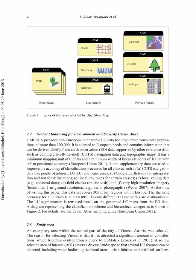
As shown in Figure 1, the OSM project organizes contributions according to several lay-ers. In general, the amount of contributions relating to roads, points of interest (POIs)and buildings is more than the other types of features. In addition to data completeness,the contributed features suffer from a lack of logical consistency and thematic accuracy(Hagenauer and Helbich 2012). Furthermore, contributions have dissimilar geometricalaccuracy and frequently overlap each other (i.e., some areas are given several attributes).Therefore, using this layer for any applications generally causes substantial limitations.
Dow
nloa
ded
by [
Uni
vers
itaet
sbib
lioth
ek H
eide
lber
g] a
t 00:
08 2
0 Ju
ne 2
013
4 J. Jokar Arsanjani et al.
OSM
OSM
OSM
OSM
Roads
Waterways
Railways
POIs
Point features Line features Polygon features
OSM
OSM
OSM
Land use
Natural
Buildings
Figure 1. Types of features collected by OpenStreetMap.
2.2. Global Monitoring for Environment and Security Urban Atlas
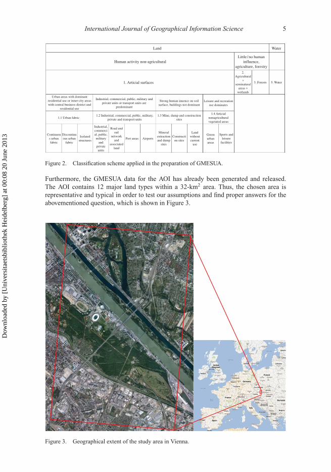
GMESUA provides pan-European comparable LU data for large urban zones with popula-tions of more than 100,000. It is adapted to European needs and contains information thatcan be derived chiefly from earth observation (EO) data supported by other reference data,such as commercial-off-the-shelf (COTS) navigation data and topographic maps. It has aminimum mapping unit of 0.25 ha and a minimum width of linear elements of 100 m with±5 m positional accuracy (European Union 2011). Some supplementary data are used toimprove the accuracy of classification processes for all classes such as (a) COTS navigationdata like points of interest, LU, LC, and water areas; (b) Google Earth (only for interpreta-tion and not for delineation); (c) local city maps for certain classes; (d) local zoning data(e.g., cadastral data); (e) field checks (on-site visit); and (f) very high-resolution imagery(better than 1 m ground resolution, e.g., aerial photographs) (Weber 2007). At the timeof writing this paper, this data set covers 305 urban regions within Europe. The thematicaccuracy for all classes is at least 80%. Twenty different LU categories are distinguished.The LU segmentation is retrieved based on the generated LC maps from the EO data.A diagram representing the classification scheme and hierarchical categories is shown inFigure 2. For details, see the Urban Atlas mapping guide (European Union 2011).
2.3. Study area
An exemplary area within the central part of the city of Vienna, Austria, was selected.The reason for selecting Vienna is that it has attracted a significant amount of contribu-tions, which becomes evident from a query to OSMatrix (Roick et al. 2011). Also, theselected area of interest (AOI) covers a diverse landscape so that several LU features can bedetected, including water bodies, agricultural areas, urban fabrics, and artificial surfaces.
Dow
nloa
ded
by [
Uni
vers
itaet
sbib
lioth
ek H
eide
lber
g] a
t 00:
08 2
0 Ju
ne 2
013
International Journal of Geographical Information Science 5
Land
Human activity non-agricultural
1. Articial surfaces
Urban areas with dominantresidential use or inner-city areaswith central business district and
residential use
1.1 Urban fabric
Continuous urbanfabric
Discontinuous urban
fabric
Isolatedstructures
Industrial,commercial, public,military
andprivateunits
Road andrail
networkand
associatedland
Port areas Airports
Mineralextractionand dump
sites
Construction sites
Landwithoutcurrent
use
Greenurbanareas
Sports andleisure
facilities
1.2 Industrial, commercial, public, military,private and transport units
1.3 Mine, dump and constructionsites
1.4 Articialnonagriculturalvegetated areas
Industrial, commercial, public, military andprivate units or transport units are
predominant
Strong human inuence on soilsurface, buildings not dominant
Leisure and recreationuse dominates
Little /no humaninfluence,
agriculture, forestry
2.Agricultural
+seminatural
areas +wetlands
3. Forests 5. Water
Water
Figure 2. Classification scheme applied in the preparation of GMESUA.
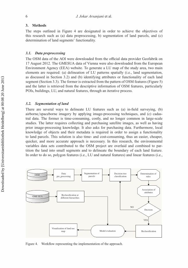
Furthermore, the GMESUA data for the AOI has already been generated and released.The AOI contains 12 major land types within a 32-km2 area. Thus, the chosen area isrepresentative and typical in order to test our assumptions and find proper answers for theabovementioned question, which is shown in Figure 3.
Figure 3. Geographical extent of the study area in Vienna.
Dow
nloa
ded
by [
Uni
vers
itaet
sbib
lioth
ek H
eide
lber
g] a
t 00:
08 2
0 Ju
ne 2
013
6 J. Jokar Arsanjani et al.
3. Methods
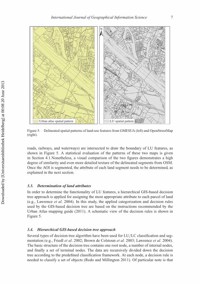
The steps outlined in Figure 4 are designated in order to achieve the objectives ofthis research such as (a) data preprocessing, b) segmentation of land parcels, and (c)determination of land segments’ functionality.
3.1. Data preprocessing
The OSM data of the AOI were downloaded from the official data provider Geofabrik on17 August 2012. The GMESUA data of Vienna were also downloaded from the EuropeanEnvironment Agency (EEA) website. To generate a LU map of the study area, two mainelements are required: (a) delineation of LU patterns spatially (i.e., land segmentation,as discussed in Section 3.2) and (b) identifying attributes or functionality of each landsegment (Section 3.3). The former is extracted from the pattern of OSM features (Figure 5)and the latter is retrieved from the descriptive information of OSM features, particularlyPOIs, buildings, LU, and natural features, through an iterative process.
3.2. Segmentation of land
There are several ways to delineate LU features such as (a) in-field surveying, (b)airborne/spaceborne imagery by applying image-processing techniques, and (c) cadas-tral data. The former is time-consuming, costly, and no longer common in large-scalestudies. The latter requires collecting and purchasing satellite images, as well as havingprior image-processing knowledge. It also asks for purchasing data. Furthermore, localknowledge of objects and their metadata is required in order to assign a functionalityto land parcels. This solution is also time- and cost-consuming, thus an easier, cheaper,quicker, and more accurate approach is necessary. In this research, the environmentalvariables data sets contributed to the OSM project are overlaid and combined to par-tition the land into small segments and to delineate the boundary of each land feature.In order to do so, polygon features (i.e., LU and natural features) and linear features (i.e.,
Datapre_processing
Reclassification atdifferent hierarchies
Visualization of land usemap Model evaluation Reclassification
YES
NODecision
Association ofattributes
Determination ofrules
OSM
GME SUA
Segmentation ofparcels
Decision treeclassification
Figure 4. Workflow representing the implementation of the approach.
Dow
nloa
ded
by [
Uni
vers
itaet
sbib
lioth
ek H
eide
lber
g] a
t 00:
08 2
0 Ju
ne 2
013
International Journal of Geographical Information Science 7
Urban atlas spatial pattern LU spatial pattern
N
Figure 5. Delineated spatial patterns of land-use features from GMESUA (left) and OpenStreetMap(right).
roads, railways, and waterways) are intersected to draw the boundary of LU features, asshown in Figure 5. A statistical evaluation of the patterns of these two maps is givenin Section 4.1.Nonetheless, a visual comparison of the two figures demonstrates a highdegree of similarity and even more detailed texture of the delineated segments from OSM.Once the AOI is segmented, the attribute of each land segment needs to be determined, asexplained in the next section.
3.3. Determination of land attributes
In order to determine the functionality of LU features, a hierarchical GIS-based decisiontree approach is applied for assigning the most appropriate attribute to each parcel of land(e.g., Lawrence et al. 2004). In this study, the applied categorization and decision rulesused by the GIS-based decision tree are based on the instructions recommended by theUrban Atlas mapping guide (2011). A schematic view of the decision rules is shown inFigure 5.
3.4. Hierarchical GIS-based decision tree approach
Several types of decision tree algorithm have been used for LU/LC classification and seg-mentation (e.g., Friedl et al. 2002; Brown de Colstoun et al. 2003; Lawrence et al. 2004).The basic structure of the decision tree contains one root node, a number of internal nodes,and finally a set of terminal nodes. The data are recursively divided down the decisiontree according to the predefined classification framework. At each node, a decision rule isneeded to classify a set of objects (Redo and Millington 2011). Of particular note is that
Dow
nloa
ded
by [
Uni
vers
itaet
sbib
lioth
ek H
eide
lber
g] a
t 00:
08 2
0 Ju
ne 2
013
8 J. Jokar Arsanjani et al.
the present study does not utilize a statistical decision tree as proposed, for instance, byBreiman et al. (1984). As different OSM data sets are shared by people, multidimensionaland multivariate logical rules (e.g., nearby objects and logical existence of a feature withinan area) concerning the location and attribute of objects are needed to associate them tothe most relevant LU types.
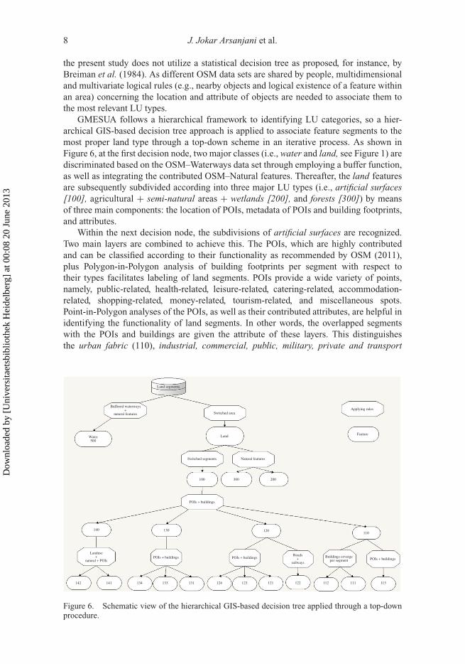
GMESUA follows a hierarchical framework to identifying LU categories, so a hier-archical GIS-based decision tree approach is applied to associate feature segments to themost proper land type through a top-down scheme in an iterative process. As shown inFigure 6, at the first decision node, two major classes (i.e., water and land, see Figure 1) arediscriminated based on the OSM–Waterways data set through employing a buffer function,as well as integrating the contributed OSM–Natural features. Thereafter, the land featuresare subsequently subdivided according into three major LU types (i.e., artificial surfaces[100], agricultural + semi-natural areas + wetlands [200], and forests [300]) by meansof three main components: the location of POIs, metadata of POIs and building footprints,and attributes.
Within the next decision node, the subdivisions of artificial surfaces are recognized.Two main layers are combined to achieve this. The POIs, which are highly contributedand can be classified according to their functionality as recommended by OSM (2011),plus Polygon-in-Polygon analysis of building footprints per segment with respect totheir types facilitates labeling of land segments. POIs provide a wide variety of points,namely, public-related, health-related, leisure-related, catering-related, accommodation-related, shopping-related, money-related, tourism-related, and miscellaneous spots.Point-in-Polygon analyses of the POIs, as well as their contributed attributes, are helpful inidentifying the functionality of land segments. In other words, the overlapped segmentswith the POIs and buildings are given the attribute of these layers. This distinguishesthe urban fabric (110), industrial, commercial, public, military, private and transport
Land segments
Buffered waterways+
natural features
Landuse+
natural + POIs
Roads+
railwaysPOIs + buildings POIs + buildings POIs + buildings
Water500
Switched area
Land
Switched segments Natural features
Applying rules
Feature
100 300
POIs + buildings
140
142 141 134 133 131 124 123 121 122 112 111 113
130
Buildings covergeper segment
120110
200
Figure 6. Schematic view of the hierarchical GIS-based decision tree applied through a top-downprocedure.
Dow
nloa
ded
by [
Uni
vers
itaet
sbib
lioth
ek H
eide
lber
g] a
t 00:
08 2
0 Ju
ne 2
013
International Journal of Geographical Information Science 9
units (120), mine, dump and construction sites (130), and artificial nonvegetated areas(140) classes.
For the last node of the decision tree, different rules are applied to distinguish the restof the subclasses according to the type of land. For instance, to identify the continuous(111) and discontinuous urban fabrics (112), the area covered by buildings is calculatedto distinguish between the two types. If the building coverage per segment exceeds 80%,it is labeled as continuous urban fabric while buildings with lower coverage values arelabeled as discontinuous urban fabric. As another example, buffer analysis of transportnetworks based on road types classifies the road and rail network and associated land(122) category. Furthermore, geographical proximity, association, dissolve, and elimina-tion functions are applied to dissolve the sliver gaps and nearby segments to the mostrelevant classes. For instance, small polygons were dissolved to the nearby polygon con-sidering the longest common border of the two objects. This decision tree is employedagain in an iterative process to consider unidentified segments. Consequently, the final out-put map is post-processed and displayed in Figure 7. Nevertheless, a number of segmentsare not labeled as any land type since no contributions were imported. They are labeled asNo class objects.
3.5. Suitability analysis
The evaluation of the proposed GIS-based decision tree approach is crucial and done bymeans of a comparison against a reference data set with a high level of accuracy. For thispurpose, the GMESUA data set is the most optimal LU data available for comparisonin terms of scale. Two main steps are followed to achieve this comparison: (a) texture-variability analysis (Eastman 2009) of the generated LU map and (b) producing a confusionmatrix (Pontius and Petrova 2010) between the two data sets to realize the accuracy of thegenerated LU map per category. For the texture-variability analysis, two indices are com-puted, namely, relative richness of variability and fractal dimension analysis. The relativerichness index depicts the diversity of LU classes by measuring the number of classes inthe defined neighborhood, while the fractal analysis calculates the fractal dimension of themap features in a 3 × 3 neighborhood. The confusion matrix shows the number of correctand incorrect classifications made by the approach compared with the actual classificationsin the reference data through computing kappa index of agreement (Pontius et al. 2004),which statistically explains how well two thematic data sets match. The kappa value variesbetween 0 and 100%, where 0% indicates that the level of agreement is equal to the agree-ment due to chance and 100% indicates perfect agreement. When comparing an alternativereference map with a reference map, Kappano specifies the overall agreement. Klocation rep-resents the extent to which the two maps match in terms of the location of each land class(Pontius and Cheuk 2006).
4. Results and discussion
This section presents the achieved results and their evaluation. Figure 7 represents theachieved LU maps at three different levels of classification.
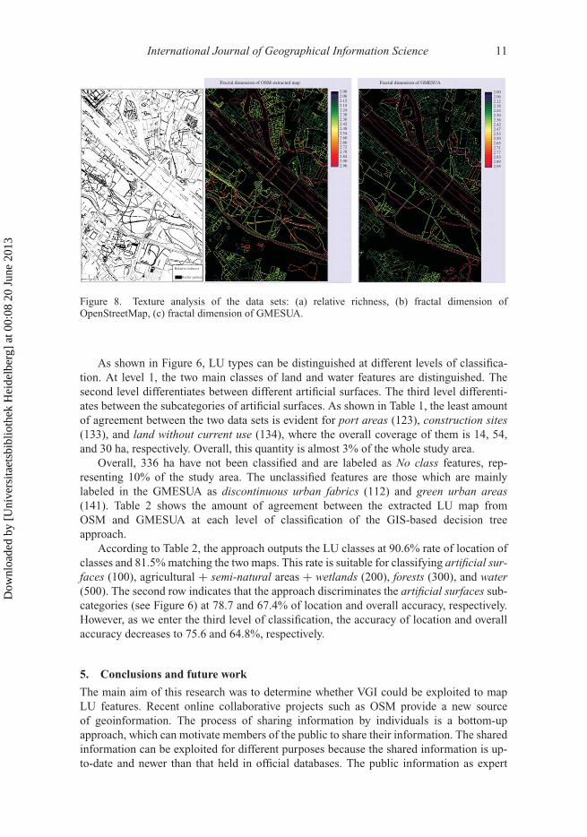
4.1. Texture analysis
As mentioned earlier, the LU patterns are delineated by intersecting the OSM features(Figure 5). A statistical comparison is carried out by texture analysis. Figure 8a
Dow
nloa
ded
by [
Uni
vers
itaet
sbib
lioth
ek H
eide
lber
g] a
t 00:
08 2
0 Ju
ne 2
013
10 J. Jokar Arsanjani et al.
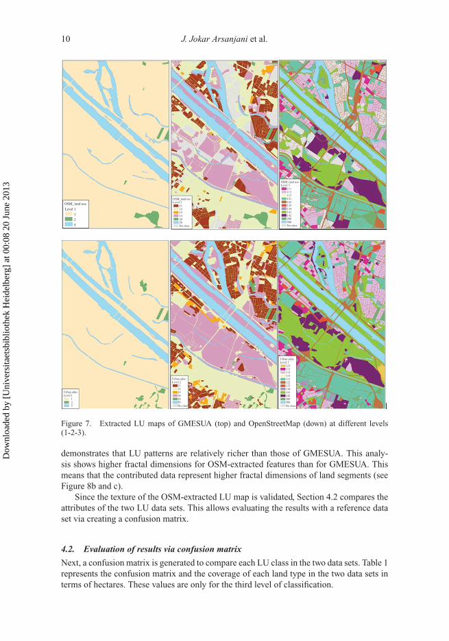
Figure 7. Extracted LU maps of GMESUA (top) and OpenStreetMap (down) at different levels(1-2-3).
demonstrates that LU patterns are relatively richer than those of GMESUA. This analy-sis shows higher fractal dimensions for OSM-extracted features than for GMESUA. Thismeans that the contributed data represent higher fractal dimensions of land segments (seeFigure 8b and c).
Since the texture of the OSM-extracted LU map is validated, Section 4.2 compares theattributes of the two LU data sets. This allows evaluating the results with a reference dataset via creating a confusion matrix.
4.2. Evaluation of results via confusion matrix
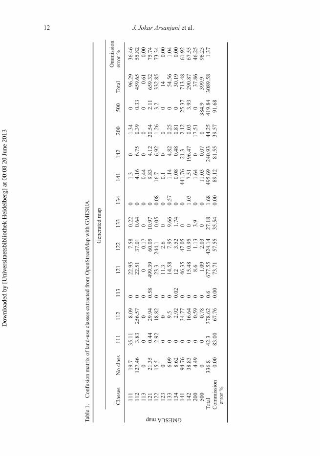
Next, a confusion matrix is generated to compare each LU class in the two data sets. Table 1represents the confusion matrix and the coverage of each land type in the two data sets interms of hectares. These values are only for the third level of classification.
Dow
nloa
ded
by [
Uni
vers
itaet
sbib
lioth
ek H
eide
lber
g] a
t 00:
08 2
0 Ju
ne 2
013
International Journal of Geographical Information Science 11
2.062.122.182.242.302.362.422.482.542.602.662.722.782.842.902.96
2.002.062.122.182.242.302.362.422.472.532.592.652.712.772.832.892.95
2.00
Fractal dimension of GMESUAFractal dimension of OSM-extracted map
Richer pattern
Relative richness
Figure 8. Texture analysis of the data sets: (a) relative richness, (b) fractal dimension ofOpenStreetMap, (c) fractal dimension of GMESUA.
As shown in Figure 6, LU types can be distinguished at different levels of classifica-tion. At level 1, the two main classes of land and water features are distinguished. Thesecond level differentiates between different artificial surfaces. The third level differenti-ates between the subcategories of artificial surfaces. As shown in Table 1, the least amountof agreement between the two data sets is evident for port areas (123), construction sites(133), and land without current use (134), where the overall coverage of them is 14, 54,and 30 ha, respectively. Overall, this quantity is almost 3% of the whole study area.
Overall, 336 ha have not been classified and are labeled as No class features, rep-resenting 10% of the study area. The unclassified features are those which are mainlylabeled in the GMESUA as discontinuous urban fabrics (112) and green urban areas(141). Table 2 shows the amount of agreement between the extracted LU map fromOSM and GMESUA at each level of classification of the GIS-based decision treeapproach.
According to Table 2, the approach outputs the LU classes at 90.6% rate of location ofclasses and 81.5% matching the two maps. This rate is suitable for classifying artificial sur-faces (100), agricultural + semi-natural areas + wetlands (200), forests (300), and water(500). The second row indicates that the approach discriminates the artificial surfaces sub-categories (see Figure 6) at 78.7 and 67.4% of location and overall accuracy, respectively.However, as we enter the third level of classification, the accuracy of location and overallaccuracy decreases to 75.6 and 64.8%, respectively.
5. Conclusions and future work
The main aim of this research was to determine whether VGI could be exploited to mapLU features. Recent online collaborative projects such as OSM provide a new sourceof geoinformation. The process of sharing information by individuals is a bottom-upapproach, which can motivate members of the public to share their information. The sharedinformation can be exploited for different purposes because the shared information is up-to-date and newer than that held in official databases. The public information as expert
Dow
nloa
ded
by [
Uni
vers
itaet
sbib
lioth
ek H
eide
lber
g] a
t 00:
08 2
0 Ju
ne 2
013
12 J. Jokar Arsanjani et al.
Tabl
e1.
Con
fusi
onm
atri
xof
land
-use
clas
ses
extr
acte
dfr
omO
penS
tree
tMap
wit
hG
ME
SU
A.
GMESUAmap
Gen
erat
edm
ap
Cla
sses
No
clas
s11
111
211
312
112
213
313
414
114
220
050
0To
tal
Om
mis
sion
erro
r%
111
19.7
35.1
18.
090
22.9
57.
580.
220
1.3
01.
340
96.2
936
.46
112
127.
463.
8325
6.57
022
.51
37.0
10.
640
4.16
6.75
0.39
0.33
459.
6555
.82
113
00
00
00.
170
00.
440
00
0.61
0.00
121
21.3
50.
4429
.94
0.58
499.
3960
.05
10.9
70
9.83
4.12
20.5
42.
1165
9.32
75.7
412
215
.52.
9218
.82
023
.324
4.1
0.05
0.08
16.7
6.92
1.26
3.2
332.
8573
.34
123
00
00
11.3
2.6
00
0.1
00
014
0.00
133
6.09
09.
50
14.5
87.
959.
660.
571.
144.
820.
250
54.5
61.
0413
48.
620
2.92
0.02
123.
521.
740
0.08
0.48
0.81
030
.19
0.00
141
94.7
60
34.7
70
46.3
547
.05
00
441.
7621
.32.
1225
.37
713.
4861
.92
142
38.8
30
16.6
40
15.4
810
.95
01.
037.
5119
6.47
0.03
3.93
290.
8767
.55
200
4.49
00.
590
8.6
1.13
3.9
01.
640
17.5
10
37.8
646
.25
500
00
0.78
01.
092.
030
011
.03
0.07
038
4.9
399.
996
.25
Tota
l33
6.8
42.3
378.
620.
667
7.55
424.
1427
.18
1.68
495.
6924
0.93
44.2
541
9.84
3089
.58
1.37
Com
mis
sion
erro
r%
0.00
83.0
067
.76
0.00
73.7
157
.55
35.5
40.
0089
.12
81.5
539
.57
91.6
8
Dow
nloa
ded
by [
Uni
vers
itaet
sbib
lioth
ek H
eide
lber
g] a
t 00:
08 2
0 Ju
ne 2
013
International Journal of Geographical Information Science 13
Table 2. The computed kappa indices for each level of classification.
Level KappaLocation (%) KappaNo (%)
1 90.64 81.472 78.69 67.383 75.58 64.79
knowledge can be imported for gathering a detailed database of our surrounding lands,for example what they are being used for. In this study, a simple methodical approach istested and proposed for extracting LU features from individuals’ contributions to the OSMproject. Here, only individuals’ knowledge of their surrounding area is incorporated intoa hierarchical GIS-based decision tree approach to generate LU patterns without usingcomplex and costly techniques such as remote sensing, surveying, or other data collectionmethods.
The proposed approach was carried out to produce LU maps by first delineating theland segments and then assigning the land segments’ attributes through the collected infor-mation into the OSM. Based on the achieved results, the research question is now answeredand VGI can be a potential data source for mapping LU patterns. The evaluation processof comparing the generated LU map with the GMESUA data at three levels verifies thatthis approach can be applied to achieve LU maps at acceptable accuracies. It must be men-tioned that as more contributions are gradually collected the accuracy of the LU mapscould increase with time.
Four main advantages of this approach must be highlighted: firstly, it imported no inputsfrom remote-sensing or any administrative data and used only OSM data. Secondly, asthe OSM database is freely available to the public, the approach does not cost financiallynor require any time spent exploring land through fieldwork. Thirdly, a number of fea-tures were labeled incorrectly in the GMESUA, which can be determined by incorporatingthe OSM data. Finally, the proposed approach is able to ease the process of updating LUmaps according to the latest information shared by people, while the GMESUA cannotbe updated frequently by authorities due to high financial costs and time requirements.Nevertheless, the approach has some limitations as well, such as (a) it is based on informa-tion shared by individuals and the accuracy of the shared data influences the outcomes; (b)some land segments remained unlabeled so that VGI could not help to determine their LUtype; and (c) the VGI domain has not been very well developed and therefore is a growingfield. However, gradually it will receive more attention from the public and new techniqueswill be developed and adopted for VGI. Of course, the more people get involved, the moreaccurate data can be shared with the public. For future work, integrating other sources ofVGI and CMPs such as Wikimapia and Flickr photos could be a practical task.
ReferencesBicheron, P., et al., 2008. GLOBCOVER: products description and validation report.Bontemps, S., et al., 2011. GLOBCOVER 2009: products description and validation report.Breiman, L., et al., 1984. Classification and regression trees. Boca Raton: CRS Press.Brown, D.G. and Duh, J.-D., 2004. Spatial simulation for translating from land use to land cover.
International Journal of Geographical Information Science, 18 (1), 35–60.Brown de Colstoun, E. C., et al., 2003. National Park vegetation mapping using multitemporal
Landsat 7 data and a decision tree classifier. Remote Sensing of Environment, 85 (3), 316–327.Buettner, G., Feranec, J., and Jaffrain, G., 2002. Corine land cover update 2000. EEA. Technical
Report, vol. 89, 17 December 2002. Copenhagen.
Dow
nloa
ded
by [
Uni
vers
itaet
sbib
lioth
ek H
eide
lber
g] a
t 00:
08 2
0 Ju
ne 2
013
14 J. Jokar Arsanjani et al.
Castelein, W., et al., 2010. A characterization of Volunteered Geographic Information. 13th AGILEInternational Conference on Geographic Information Science 2010, 10–14 May, Guimarães,Portugal.
Chilton, S., 2009. Crowdsourcing is radically changing the geodata landscape: case study ofOpenStreetMap. In 24th International cartographic conference – ICC 2009. Santiago, Chile15–21 November 2009.
Cihlar, J. and Jansen, L.J.M., 2001. From land cover to land use: a methodology for efficient land usemapping over large areas. The Professional Geographer, 53 (2), 275–289.
Comber, A., et al., 2013. Using control data to determine the reliability of volunteered geo-graphic information about land cover. International Journal of Applied Earth Observation andGeoinformation, 23, 37–48.
Corcoran, P. and Mooney, P., 2013. Characterising the metric and topological evolution ofOpenStreetMap network representations. European Physical Journal, Special Topics, 215 (1),109–122.
de Sherbinin, A., 2002. A CIESIN Thematic Guide to Land Land-Use and Land Land-Cover Change(LUCC). Center for International Earth Science Information Network (CIESIN) ColumbiaUniversity Palisades, NY, USA. Available from: http://sedac.ciesin.columbia.edu/binaries/web/sedac/thematic-guides/ciesin_lucc_tg.pdf [Accessed 16 May 2013].
Eastman, J.R., 2009. IDRISI Taiga. Worcester, MA: Clark University.Ellis, E., 2007. Land-use and land-cover change. In: R. Pontius and C.J. Cleveland, eds.
Encyclopedia of earth. Available from: http://www.eoearth.org/article/Land-use_and_land-cover_change [Accessed 16 May 2013].
European Union, 2011. Mapping guide for a European Urban atlas. Available from: http://www.eea.europa.eu/data-and-maps/data/urban-atlas [Accessed 16 May 2013].
Evans, T.P., Sun, W., and Kelley, H., 2006. Spatially explicit experiments for the explorationof land-use decision-making dynamics. International Journal of Geographical InformationScience, 20 (9), 1013–1037.
Flanagin, A. and Metzger, M., 2008. The credibility of volunteered geographic information.GeoJournal, 72, 137–148.
Folberth, C., et al., 2012. Impact of input data resolution and extent of harvested areas on cropyield estimates in large-scale agricultural modeling for maize in the USA. Ecological Modelling,235–236, 8–18.
Friedl, M.A., et al., 2002. Global land cover mapping from MODIS: algorithms and early results.Remote Sensing of Environment, 83, 287–302.
Fritz, S., et al., 2003. Harmonisation, mosaicing and production of the global landcover2000 database (beta version). Luxembourg: Office for Official Publications of the EuropeanCommunities. ISBN 92-894-6332-5.
Fritz, S., et al., 2012. Geo-Wiki: an online platform for improving global land cover. EnvironmentalModelling & Software, 31, 110–123.
GLP, 2005. Global land project: science plan and implementation strategy. Stockholm, Sweden.UNT Digital Library. Available from: http://digital.library.unt.edu/ark:/67531/metadc12009/[Accessed 11 July 2012].
Goodchild, M.F., 2007. Citizens as sensors: the world of volunteered geography. GeoJournal, 69,211–221.
Hagenauer, J. and Helbich, M., 2012. Mining urban land use patterns from volunteered geographicinformation by means of genetic algorithms and artificial neural networks. International Journalof Geographic Information Science, 26 (6), 963–982.
Jokar Arsanjani, J., et al., 2013. Integration of logistic regression, Markov chain and cellular automatamodels to simulate urban expansion. International Journal of Applied Earth Observations andGeoinformation, 21, 265–275.
Jokar Arsanjani, J., Kainz, W., and Mousivand, A.J., 2011. Tracking dynamic land-use change usingspatially explicit Markov Chain based on cellular automata: the case of Tehran. InternationalJournal of Image and Data Fusion, 2 (4), 329–345.
Kandrika, S. and Roy, P.S., 2008. Land use land cover classification of Orissa using multi-temporalIRS-P6 awifs data: a decision tree approach. International Journal of Applied Earth Observationand Geoinformation, 10 (2), 186–193.
Kong, F., et al., 2012. Simulating urban growth processes incorporating a potential model with spatialmetrics. Ecological Indicators, 20, 82–91.
Dow
nloa
ded
by [
Uni
vers
itaet
sbib
lioth
ek H
eide
lber
g] a
t 00:
08 2
0 Ju
ne 2
013
International Journal of Geographical Information Science 15
Koukoletsos, T., Haklay, M., and Ellul, C., 2012. Assessing data completeness of VGI through anautomated matching procedure for linear data. Transactions in GIS, 16 (4), 477–498.
Lawrence, R., Bunn, A., Powell, S., & Zambon, M., 2004. Classification of remotely sensed imageryusing stochastic gradient boosting as a refinement of classification tree analysis. Remote sensingof environment, 90 (3), 331–336.
Marris, E., 2010. Birds flock online. Nature, 10 August 2010. Available online at http://www.nature.com/news/2010/100810/full/news.2010.395.html [Accessed 16 May 2013].
Masoomi, Z., Mesgari, M.S., and Hamrah, M., 2013. Allocation of urban land uses by Multi-Objective Particle Swarm Optimization algorithm. International Journal of GeographicalInformation Science, 27 (3), 542–566.
Neis, P., Zielstra, D., and Zipf, A., 2011. The street network evolution of crowdsourced maps:OpenStreetMap in Germany 2007–2011. Future Internet, 4 (1), 1–21.
Neis, P. and Zipf, A., 2012. Analyzing the contributor activity of a volunteered geographic informa-tion project – the case of OpenStreetMap. ISPRS International Journal of Geo-Information, 1(2), 146–165.
Pacifici, F., Chini, M., and Emery, W.J., 2009. A neural network approach using multi-scale textu-ral metrics from very high-resolution panchromatic imagery for urban land-use classification.Remote Sensing of Environment, 113 (6), 1276–1292.
Pontius, R.G. Jr., and Cheuk, M.L., 2006. A generalized cross-tabulation matrix to compare soft-classified maps at multiple resolutions. International Journal of Geographical InformationScience, 20 (1), 1–30.
Pontius, R.G. Jr., Huffaker, D., and Denman, K., 2004. Useful techniques of validation for spatiallyexplicit land-change models. Ecological Modelling, 179 (4), 445–461.
Pontius, R.G. Jr., and Petrova, S.H., 2010. Assessing a predictive model of land change usinguncertain data. Environmental Modelling & Software, 25 (3), 299–309.
Qi, Z., et al., 2012. A novel algorithm for land use and land cover classification using RADARSAT-2 polarimetric SAR data. Remote Sensing of Environment, 118, 21–39.
Ramm, F., Topf, J., and Chilton, S., 2011. OpenStreetMap: using and enhancing the free map of theworld. 3rd ed.. Cambridge: UIT Cambridge.
Redo, D.J. and Millington, A.C., 2011. A hybrid approach to mapping land-use modification andland-cover transition from MODIS time-series data: a case study from the Bolivian seasonaltropics. Remote Sensing of Environment, 115 (2), 353–372.
Robinson, D.T. and Brown, D.G., 2009. Evaluating the effects of land-use development policieson ex-urban forest cover: an integrated agent-based GIS approach. International Journal ofGeographical Information Science, 23 (9), 1211–1232.
Roick, O., Hagenauer, J., and Zipf, A., 2011. OSMatrix – grid-based analysis and visualization ofOpenStreetMap. In proceedings of the State of the Map EU 2011, 15–17 July. Vienna, Austria.
Rouse, L.J., Bergeron, S.J., and Harris, T.M., 2007. Participating in the geospatial web: collaborativemapping, social networks and participatory GIS. In: A. Scharl and K. Tochtermann, eds. Thegeospatial web. London: Springer, 153–158.
Saadat, H., et al., 2011. Land use and land cover classification over a large area in Iran based on singledate analysis of satellite imagery. ISPRS Journal of Photogrammetry and Remote Sensing, 66 (5),608–619.
Turner, A.J., 2006. Introduction to neography. Sebastopol, CA: O’Reilly Media.Wästfelt, A. and Arnberg, W., 2013. Local spatial context measurements used to explore the rela-
tionship between land cover and land use functions. International Journal of Applied EarthObservation and Geoinformation, 23, 234–244.
Weber, J.-L., 2007. Implementation of land and ecosystem accounts at the European EnvironmentAgency. Ecological Economics, 61 (4), 695–707.
Dow
nloa
ded
by [
Uni
vers
itaet
sbib
lioth
ek H
eide
lber
g] a
t 00:
08 2
0 Ju
ne 2
013