tournament arena simulation for a …ryates/thesis/desai-thesis.pdf · tournament arena simulation...
TRANSCRIPT
TOURNAMENT ARENA SIMULATION FOR AWIRELESS ‘ECOSYSTEM’ IN UNLICENSED BANDS
BY KINJAL DESAI
A thesis submitted to the
Graduate School—New Brunswick
Rutgers, The State University of New Jersey
in partial fulfillment of the requirements
for the degree of
Master of Science
Graduate Program in Electrical and Computer Engineering
Written under the direction of
Professor Roy D. Yates
and approved by
New Brunswick, New Jersey
January, 2005
ABSTRACT OF THE THESIS
Tournament Arena Simulation for a Wireless ‘Ecosystem’
in Unlicensed Bands
by Kinjal Desai
Thesis Director: Professor Roy D. Yates
The FCC has been allocating sections of the radio spectrum as unlicensed bands over the
period of last decade with the motivation of promoting diversity and novelty of wireless
systems, services and technologies. The most recent in this series is the Unlicensed
National Information Infrastructure (U-NII), a 300 MHz of radio spectrum at 5 GHz,
providing promising avenues for modern multimedia applications in 3G systems and
beyond.
No license is required to operate in the unlicensed band, though there could be some
minimal rules that the systems need to conform to. Due to the significant cost in-
volved in bandwidth acquisition through licensing, the unlicensed bands provide an
attractive alternative to service providers in terms of time and cost of development and
deployment. This latitude, however comes at the price of enhanced mutual interference
ii
because now there are multiple wireless systems, autonomous and non-cooperating,
competing for common media resources. WINLAB proposes the novel concept of sim-
ulating ‘tournaments’ between these competing systems as a way of looking at this
problem from the simulation and modeling angle.
This thesis describes the Tournament Arena Simulator (TAS), a simulation envi-
ronment, developed for staging these tournaments between different autonomous wire-
less systems. The TAS involves modules for radio channel, mobility, geography and the
mobile station transceiver to accurately portray all aspects of the real unlicensed band
scenario. The transceiver module has the added capability of reconfigurability and dy-
namic class loading. This endows the TAS with the facility to dynamically reconfigure
or rewrite the transceiver module in order to implement different autonomous systems
and then make them compete with each other simultaneously. The fundamental system
level assumption is that the environment supports only synchronous DS-CDMA systems
in a mobile ad-hoc network scenario with point-to-point connections. The implemen-
tation is done in the Java binding of the Scalable Simulation Framework (SSF), a new
public domain discrete event simulator. The thesis also goes on to demonstrate the util-
ity and the operability of the TAS through performance evaluation of several standard
systems and staging of sample tournaments between specific systems of interest.
iii

Acknowledgements
I wish to express my deepest gratitude to my advisor Professor Roy D. Yates for his
consistent guidance, patience, and enthusiasm over last 5 years. Though the work
was spread over an extended period of time, with substantial periods of inactivity at
times, his advice was always insightful, and precise, and came with the right amount
of encouragement and urgency. I was always enthused to do my very best, and am
thankful to him for that.
I would also like to thank Dr. Christopher Rose for providing timely guidance whenever
sought, and Dr. Narayan Mandayam, for, among other things, teaching some of the
best communications engineering courses that I ever took, which contributed greatly
towards the thesis. I am also thankful to them for agreeing to serve on my thesis defense
committee.
I am grateful to WINLAB and all the wonderful people that I was fortunate to work
with, for making this such a worthwhile experience. Special thanks to Ivan Seskar and
his team for time and again providing crucial technical support during the time I worked
remotely on this, and to Melissa Gelfman for similar support on the administrative side
of things. I will be ever indebted to my fellow students and researchers at WINLAB
for their contribution to the thesis as well as my entire WINLAB experience. I would
like to make special mention of Vikram Kaul and Ivana Maric for being ever-reliable
iv

friends and excellent guides on this journey. The passionate group meetings, seminars
and thesis defenses, the stimulating discussions in the wee hours of the morning, the
interesting logistics of figuring out one’s mail and kitchen clean-up turns, the Christmas
parties - these will remain as some of my most cherished memories and I am thankful
to all the people who made these possible.
Finally, I wish to thank my parents, Pratibha and Janak Desai, my sister Mrunmayi
Desai, and my faithful group of friends in New Jersey, as well as in San Diego, for their
unflinching love and support, for making sure I go the entire distance in this endeavor.
v

Dedication
To my mother, and my father.
vi
Table of Contents
Abstract . . . . . . . . . . . . . . . . . . . . . . . . . . . . . . . . . . . . . . . . ii
Acknowledgements . . . . . . . . . . . . . . . . . . . . . . . . . . . . . . . . . iv
Dedication . . . . . . . . . . . . . . . . . . . . . . . . . . . . . . . . . . . . . . . vi
List of Tables . . . . . . . . . . . . . . . . . . . . . . . . . . . . . . . . . . . . . xi
List of Figures . . . . . . . . . . . . . . . . . . . . . . . . . . . . . . . . . . . . xii
1. Introduction . . . . . . . . . . . . . . . . . . . . . . . . . . . . . . . . . . . 1
1.1. Context . . . . . . . . . . . . . . . . . . . . . . . . . . . . . . . . . . . . 2
1.2. Objective . . . . . . . . . . . . . . . . . . . . . . . . . . . . . . . . . . . 4
1.3. Organization . . . . . . . . . . . . . . . . . . . . . . . . . . . . . . . . . 5
2. Unlicensed bands . . . . . . . . . . . . . . . . . . . . . . . . . . . . . . . . 6
2.1. Definitions . . . . . . . . . . . . . . . . . . . . . . . . . . . . . . . . . . . 6
2.2. Examples of unlicensed bands . . . . . . . . . . . . . . . . . . . . . . . . 7
2.2.1. ISM band . . . . . . . . . . . . . . . . . . . . . . . . . . . . . . . 7
2.2.2. U-PCS band . . . . . . . . . . . . . . . . . . . . . . . . . . . . . 8
vii
2.2.3. U-NII band . . . . . . . . . . . . . . . . . . . . . . . . . . . . . . 9
2.3. Comparison . . . . . . . . . . . . . . . . . . . . . . . . . . . . . . . . . . 10
3. System Model . . . . . . . . . . . . . . . . . . . . . . . . . . . . . . . . . . 12
3.1. Overview . . . . . . . . . . . . . . . . . . . . . . . . . . . . . . . . . . . 12
3.2. Radio propagation . . . . . . . . . . . . . . . . . . . . . . . . . . . . . 13
3.3. Geography and Mobility . . . . . . . . . . . . . . . . . . . . . . . . . . . 14
3.4. Transceiver mechanism . . . . . . . . . . . . . . . . . . . . . . . . . . . . 15
4. SSF Domain Fundamentals . . . . . . . . . . . . . . . . . . . . . . . . . . 18
4.1. Background . . . . . . . . . . . . . . . . . . . . . . . . . . . . . . . . . . 18
4.2. Overview . . . . . . . . . . . . . . . . . . . . . . . . . . . . . . . . . . . 19
4.2.1. Separation of modeling and simulation . . . . . . . . . . . . . . . 20
4.2.2. Object-oriented design . . . . . . . . . . . . . . . . . . . . . . . . 20
4.2.3. Event-driven executive . . . . . . . . . . . . . . . . . . . . . . . . 21
4.2.4. Parallelization Capability . . . . . . . . . . . . . . . . . . . . . . 25
4.2.5. Dynamic Modeling . . . . . . . . . . . . . . . . . . . . . . . . . . 26
4.3. SSF Model Abstractions . . . . . . . . . . . . . . . . . . . . . . . . . . 26
4.3.1. Entity . . . . . . . . . . . . . . . . . . . . . . . . . . . . . . . . 27
4.3.2. process . . . . . . . . . . . . . . . . . . . . . . . . . . . . . . . . 28
viii
4.3.3. Event . . . . . . . . . . . . . . . . . . . . . . . . . . . . . . . . . 30
4.3.4. inChannel and outChannel . . . . . . . . . . . . . . . . . . . . . . 31
5. Design and Implementation . . . . . . . . . . . . . . . . . . . . . . . . . . 33
5.1. Design Overview . . . . . . . . . . . . . . . . . . . . . . . . . . . . . . . 33
5.2. Simulation Entity . . . . . . . . . . . . . . . . . . . . . . . . . . . . . 35
5.3. MobileTerminal Entity . . . . . . . . . . . . . . . . . . . . . . . . . . . 36
5.4. RadioChannel Entity . . . . . . . . . . . . . . . . . . . . . . . . . . . . 41
5.5. Mobility Entity . . . . . . . . . . . . . . . . . . . . . . . . . . . . . . . 45
6. Transceiver Reconfigurability . . . . . . . . . . . . . . . . . . . . . . . . 52
6.1. Transceiver module requirements . . . . . . . . . . . . . . . . . . . . . . 52
6.2. Transceiver module implementation . . . . . . . . . . . . . . . . . . . . 54
6.3. Transceiver Feedback Mechanism . . . . . . . . . . . . . . . . . . . . . . 56
6.4. Environment Reconfigurability . . . . . . . . . . . . . . . . . . . . . . . 57
6.5. Reconfiguration parameters . . . . . . . . . . . . . . . . . . . . . . . . . 59
7. Sample Transceivers and Tournaments . . . . . . . . . . . . . . . . . . . 62
7.1. Transceivers . . . . . . . . . . . . . . . . . . . . . . . . . . . . . . . . . . 62
7.1.1. Transceiver Implementation . . . . . . . . . . . . . . . . . . . . . 63
7.2. Tournaments . . . . . . . . . . . . . . . . . . . . . . . . . . . . . . . . . 69
ix
7.2.1. Tournament 1: Single Transceiver System in the Arena . . . . . 69
7.2.2. Tournament 2: Two Equal-sized Transceiver Systems in the Arena 74
7.2.3. Tournament 3: Two Unequal-sized Transceiver Systems in the
Arena . . . . . . . . . . . . . . . . . . . . . . . . . . . . . . . . . 79
7.2.4. Conclusion . . . . . . . . . . . . . . . . . . . . . . . . . . . . . . 82
8. Conclusion and Future Work . . . . . . . . . . . . . . . . . . . . . . . . . 83
Appendix A. Java-SSF Example Program . . . . . . . . . . . . . . . . . . 85
Appendix B. Transceiver Reconfiguration Primer . . . . . . . . . . . . . . 93
References . . . . . . . . . . . . . . . . . . . . . . . . . . . . . . . . . . . . . . . 103
x
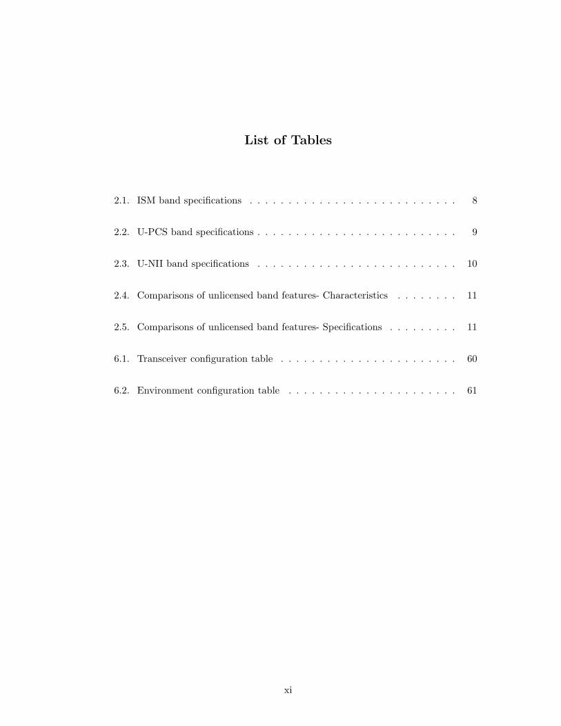
List of Tables
2.1. ISM band specifications . . . . . . . . . . . . . . . . . . . . . . . . . . . 8
2.2. U-PCS band specifications . . . . . . . . . . . . . . . . . . . . . . . . . . 9
2.3. U-NII band specifications . . . . . . . . . . . . . . . . . . . . . . . . . . 10
2.4. Comparisons of unlicensed band features- Characteristics . . . . . . . . 11
2.5. Comparisons of unlicensed band features- Specifications . . . . . . . . . 11
6.1. Transceiver configuration table . . . . . . . . . . . . . . . . . . . . . . . 60
6.2. Environment configuration table . . . . . . . . . . . . . . . . . . . . . . 61
xi
List of Figures
4.1. Hierarchy of abstraction in SSF . . . . . . . . . . . . . . . . . . . . . 22
4.2. Discrete event simulator . . . . . . . . . . . . . . . . . . . . . . . . . . . 24
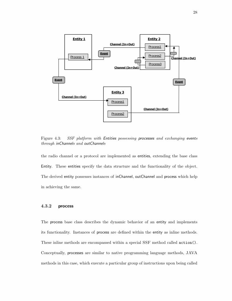
4.3. SSF platform with Entities possessing processes and exchanging events
through inChannels and outChannels . . . . . . . . . . . . . . . . . . . . 28
5.1. System Entity map . . . . . . . . . . . . . . . . . . . . . . . . . . . . . . 36
5.2. Transceiver scheme in MobileTerminal . . . . . . . . . . . . . . . . . . 37
5.3. Radio channel calculations . . . . . . . . . . . . . . . . . . . . . . . . . 43
5.4. ChannelMatrix data structure . . . . . . . . . . . . . . . . . . . . . . . 44
5.5. Random Waypoint Mobility Trail of a MS . . . . . . . . . . . . . . . 46
5.6. Mobility Update Process for a MS . . . . . . . . . . . . . . . . . . 48
5.7. Illustration of Wrap-Around . . . . . . . . . . . . . . . . . . . . . . . 49
5.8. ConnectionRegistry data structure . . . . . . . . . . . . . . . . . . . . 50
6.1. Hierarchy of class inheritance . . . . . . . . . . . . . . . . . . . . . . 55
7.1. BER vs SIR: Matched Filter Receiver . . . . . . . . . . . . . . . . . . 65
7.2. BER vs SIR: Decorrelator . . . . . . . . . . . . . . . . . . . . . . . . 66
xii
7.3. BADD Filter Structure . . . . . . . . . . . . . . . . . . . . . . . . . . . 67
7.4. BER vs SIR: BADD . . . . . . . . . . . . . . . . . . . . . . . . . . . . 68
7.5. System BER Performance: Matched Filter, SNR = 7dB . . . . . . . . 71
7.6. System BER Performance: BADD, SNR = 7dB . . . . . . . . . . . . 72
7.7. System BER Performance: Tourn. 1, Matched Filter vs. BADD . . . 73
7.8. System BER Performance: Tourn. 1, Matched Filter vs. BADD . . . 74
7.9. System BER Performance: Matched Filter Vs. BADD, SNR = 7dB . 77
7.10. System BER Performance: Matched Filter Vs. BADD, SNR = 7dB . 78
7.11. System BER Performance (Per Run): Matched Filter, SNR = 7dB . . 79
7.12. System BER Performance (Per Run): BADD, SNR = 7dB . . . . . . 80
7.13. System BER Performance: Matched Filter Vs. BADD, SNR = 7dB . 81
7.14. System BER Performance: Matched Filter Vs. BADD, SNR = 7dB . 82
xiii
1
Chapter 1
Introduction
The Federal Communications Commission (FCC) is responsible for managing the elec-
tromagnetic frequency spectrum in the US. Wireless service providers who intend to
operate and transmit signals in a particular frequency band participate in auctions to
acquire radio spectrum, paying the specified license fee to the FCC. Thereafter that
specific band of radio spectrum is exclusively owned by that service provider for its sole
operative purposes. This is the premise of the licensed bands.
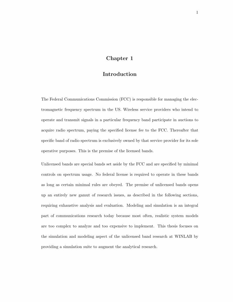
Unlicensed bands are special bands set aside by the FCC and are specified by minimal
controls on spectrum usage. No federal license is required to operate in these bands
as long as certain minimal rules are obeyed. The premise of unlicensed bands opens
up an entirely new gamut of research issues, as described in the following sections,
requiring exhaustive analysis and evaluation. Modeling and simulation is an integral
part of communications research today because most often, realistic system models
are too complex to analyze and too expensive to implement. This thesis focuses on
the simulation and modeling aspect of the unlicensed band research at WINLAB by
providing a simulation suite to augment the analytical research.
2
1.1 Context
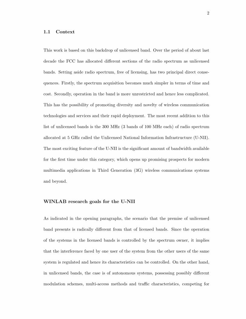
This work is based on this backdrop of unlicensed band. Over the period of about last
decade the FCC has allocated different sections of the radio spectrum as unlicensed
bands. Setting aside radio spectrum, free of licensing, has two principal direct conse-
quences. Firstly, the spectrum acquisition becomes much simpler in terms of time and
cost. Secondly, operation in the band is more unrestricted and hence less complicated.
This has the possibility of promoting diversity and novelty of wireless communication
technologies and services and their rapid deployment. The most recent addition to this
list of unlicensed bands is the 300 MHz (3 bands of 100 MHz each) of radio spectrum
allocated at 5 GHz called the Unlicensed National Information Infrastructure (U-NII).
The most exciting feature of the U-NII is the significant amount of bandwidth available
for the first time under this category, which opens up promising prospects for modern
multimedia applications in Third Generation (3G) wireless communications systems
and beyond.
WINLAB research goals for the U-NII
As indicated in the opening paragraphs, the scenario that the premise of unlicensed
band presents is radically different from that of licensed bands. Since the operation
of the systems in the licensed bands is controlled by the spectrum owner, it implies
that the interference faced by one user of the system from the other users of the same
system is regulated and hence its characteristics can be controlled. On the other hand,
in unlicensed bands, the case is of autonomous systems, possessing possibly different
modulation schemes, multi-access methods and traffic characteristics, competing for
3
common radio resources, most probably in a non-cooperative manner. This implies
that though the purpose of making radio spectrum free of license and specifying it
with minimal rules is to encourage multitude of new and varied wireless systems, if not
implemented prudently, it is actually possible that a particular system could preclude
the existence of any other system.
This thesis proposes a framework of a wireless ecosystem where different service providers
and their wireless systems compete for customers and media resources [5]. Each of the
wireless systems operating in this ecosystem would be evaluated on the basis of two
metrics, namely it’s robustness and it’s fairness. These metrics define, firstly, the ca-
pability of the system to survive in the extreme interference environment and at the
same time let other systems co-exist too. The result of these evaluations would give in-
dications about the type of systems and technologies which can cohabit the unlicensed
bands in a mutually cooperative fashion. The ultimate goal of the exercise is to make
recommendations for robust modulation schemes, media access mechanisms and adap-
tation strategies that would foster peaceful coexistence of service providers, while not
overtly restricting and limiting the diversity of possible applications.
The research approach is three-pronged, comprising simulation, modeling and theory.
The emphasis is on distillation of useful analytic models from detailed simulations of
wireless systems. The proposed methodology to achieve this is to simulate tournaments
between the varied autonomous systems wherein they compete for the common radio
resources. The comparative performance of the individual systems in such scenario
would give indications about the types of systems likely to further the goal of a wireless
ecosystem and would help crystallize the principles of peaceful co-existence. A wireless
4
simulation environment is required to serve as the arena for holding these tournaments.
1.2 Objective
This thesis addresses design and development of the simulation environment which
would serve as that arena to stage the tournaments between the autonomous systems op-
erating in the unlicensed band. This is the Tournament Arena Simulator (TAS).
It has been written in the Scalable Simulation Framework (SSF) developed by the S3
consortium [4]. SSF is a relatively new public-domain standard for discrete-event sim-
ulation of large, complex systems. SSF models are compact, flexible, portable, and
transparently parallelizable. The SSF Application Programming Interface (API) has
both C++ and JAVA bindings, with high-performance serial and scalable parallel
implementations available. The thesis uses the JAVA binding of the API.
The specific objectives of the thesis are as stated below:
• Design and implement the tournament arena simulation environment JAVA SSF,
which includes the radio channel and mobility modeled on a mobile ad-hoc net-
work scenario.
• Implement reconfigurable and dynamically loadable class for transceiver models,
which could be coded and configured independently and integrated with the envi-
ronment dynamically to provide the functionality of creating different participants
for the tournaments.
• Demonstrate the operation and utility of the simulator by staging sample tour-
naments.
5
1.3 Organization
Chapter 2 discusses the premise of unlicensed bands in general and U-NII in partic-
ular. Chapter 3 describes the system model, along with the assumptions involved in
detail. Chapters 4 and 5 deal with the specific details of implementation. The former
overviews the SSF fundamentals while the later goes into the details of the design of
the system model using SSF. Chapter 6 examines the details of dynamic modeling and
loading of the transceiver module to implement different wireless systems. Chapter 7
describes performance evaluation of some standard systems, sample tournaments be-
tween the transceivers of selected systems and the results thereof. Chapter 8 presents
the conclusions and identifies some future trails which could be explored building on
this work.
6
Chapter 2
Unlicensed bands
This chapter performs a detailed study of the unlicensed bands, in general and some of
specific examples of the same, in particular.
2.1 Definitions
No license is required to transmit in the unlicensed bands. Further, these bands are
characterized by minimal rules pertaining to spectrum usage in terms of radio emission
or media access. The motivation behind their allocation is to promote rapid develop-
ment and deployment of new and diverse wireless systems and technologies. This is
fostered by the elimination of the expensive and time consuming process of spectrum
acquisition. It also encourages smaller service providers to enter the playing field, in-
creasing the novelty and diversity of ideas and implementation. This latitude, however,
comes at the expense of susceptibility to excessive mutual interference. The interferers
in this scenario are now not only other transmitting stations of the same system but also
those of other systems operating in the same frequency bandwidth. The interference,
hence, is unregulated and therefore more difficult to analyze or characterize.
7
2.2 Examples of unlicensed bands
Following up on the principle stated above, FCC has specified different sections of the
radio spectrum as unlicensed bands for specific purposes. The following subsections list
three prominent examples of the same.
2.2.1 ISM band
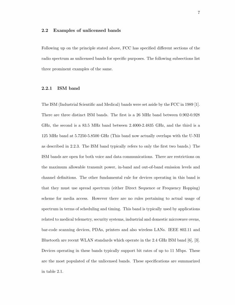
The ISM (Industrial Scientific and Medical) bands were set aside by the FCC in 1989 [1].
There are three distinct ISM bands. The first is a 26 MHz band between 0.902-0.928
GHz, the second is a 83.5 MHz band between 2.4000-2.4835 GHz, and the third is a
125 MHz band at 5.7250-5.8500 GHz (This band now actually overlaps with the U-NII
as described in 2.2.3. The ISM band typically refers to only the first two bands.) The
ISM bands are open for both voice and data communications. There are restrictions on
the maximum allowable transmit power, in-band and out-of-band emission levels and
channel definitions. The other fundamental rule for devices operating in this band is
that they must use spread spectrum (either Direct Sequence or Frequency Hopping)
scheme for media access. However there are no rules pertaining to actual usage of
spectrum in terms of scheduling and timing. This band is typically used by applications
related to medical telemetry, security systems, industrial and domestic microwave ovens,
bar-code scanning devices, PDAs, printers and also wireless LANs. IEEE 802.11 and
Bluetooth are recent WLAN standards which operate in the 2.4 GHz ISM band [6], [3].
Devices operating in these bands typically support bit rates of up to 11 Mbps. These
are the most populated of the unlicensed bands. These specifications are summarized
in table 2.1.
8
Freq. Band Max. Transmit Power Max. EIRP Bandwidth(GHz) (mW) (mW) (MHz)
0.902-0.928 1000 4000 262.4000-2.4835 1000 4000 83.55.725-5.850 1000 4K or 200K (*) 100
* 4K (mW) for point-to-point communications.200K (mW) for point-to-multi-point communications
Table 2.1: ISM band specifications
2.2.2 U-PCS band
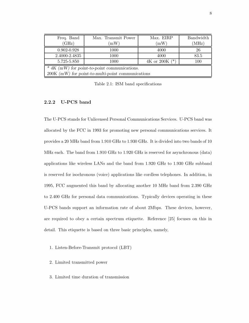
The U-PCS stands for Unlicensed Personal Communications Services. U-PCS band was
allocated by the FCC in 1993 for promoting new personal communications services. It
provides a 20 MHz band from 1.910 GHz to 1.930 GHz. It is divided into two bands of 10
MHz each. The band from 1.910 GHz to 1.920 GHz is reserved for asynchronous (data)
applications like wireless LANs and the band from 1.920 GHz to 1.930 GHz subband
is reserved for isochronous (voice) applications like cordless telephones. In addition, in
1995, FCC augmented this band by allocating another 10 MHz band from 2.390 GHz
to 2.400 GHz for personal data communications. Typically devices operating in these
U-PCS bands support an information rate of about 2Mbps. These devices, however,
are required to obey a certain spectrum etiquette. Reference [25] focuses on this in
detail. This etiquette is based on three basic principles, namely,
1. Listen-Before-Transmit protocol (LBT)
2. Limited transmitted power
3. Limited time duration of transmission
9
Freq. Max. Max. Max. Band- TrafficBand Transmit Antenna PSD Width Type(GHz) Power (mW) Gain (dBi) (mW/Hz) (MHz)
1.910-1.920 100√
B (*) 3 1 10 Asyn-chronous
1.920-1.930 100√
B 3 1 10 Iso-chronous
* B is the emission bandwidth in MHz of the transmission where thepower level is 26 dB below the level of peak transmission.
Table 2.2: U-PCS band specifications
The etiquette is designed to impart some predictability to the mutual interference be-
tween different systems. This band is mainly used by devices such as wireless LANs,
cordless phones and PDAs. Table 2.2 summarizes these specifications.
2.2.3 U-NII band
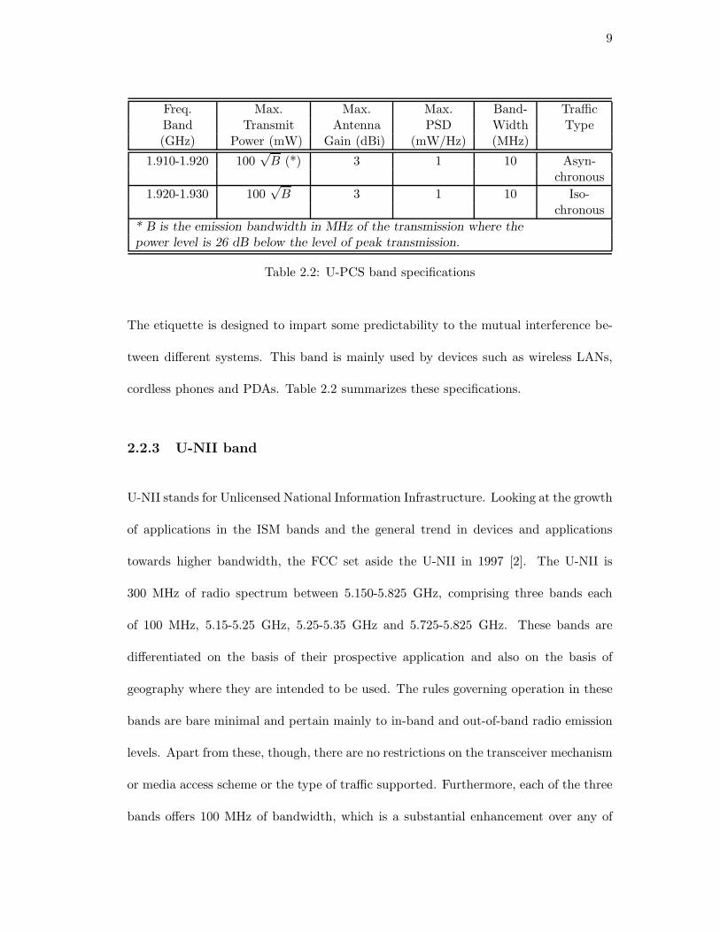
U-NII stands for Unlicensed National Information Infrastructure. Looking at the growth
of applications in the ISM bands and the general trend in devices and applications
towards higher bandwidth, the FCC set aside the U-NII in 1997 [2]. The U-NII is
300 MHz of radio spectrum between 5.150-5.825 GHz, comprising three bands each
of 100 MHz, 5.15-5.25 GHz, 5.25-5.35 GHz and 5.725-5.825 GHz. These bands are
differentiated on the basis of their prospective application and also on the basis of
geography where they are intended to be used. The rules governing operation in these
bands are bare minimal and pertain mainly to in-band and out-of-band radio emission
levels. Apart from these, though, there are no restrictions on the transceiver mechanism
or media access scheme or the type of traffic supported. Furthermore, each of the three
bands offers 100 MHz of bandwidth, which is a substantial enhancement over any of
10
Freq. Max. Max. Max. Max. LocationBand Transmit Antenna EIRP PSD Restriction(GHz) Power (mW) Gain (dBi) (mW) (mW/Hz)
5.15-5.25 50 6 200 2.5 Indoors5.25-5.35 250 6 1000 12.5 None
5.725-5.825 1000 6 4000 or 200K 50 None* 4K (mW) for point-to-point communications.200K (mW) for point-to-multi-point communications
Table 2.3: U-NII band specifications
the other unlicensed bands. These two factors make the U-NII band a very promising
avenue for deployment of high data rate 3G applications. Each of the bands can possibly
support data rates in the region of 20 Mbps. The allocation has not been made with any
particular application in mind, but rather to promote diversity and novelty of wireless
services in its true sense without any restriction. The specifications are outlined in
table 2.3.
2.3 Comparison
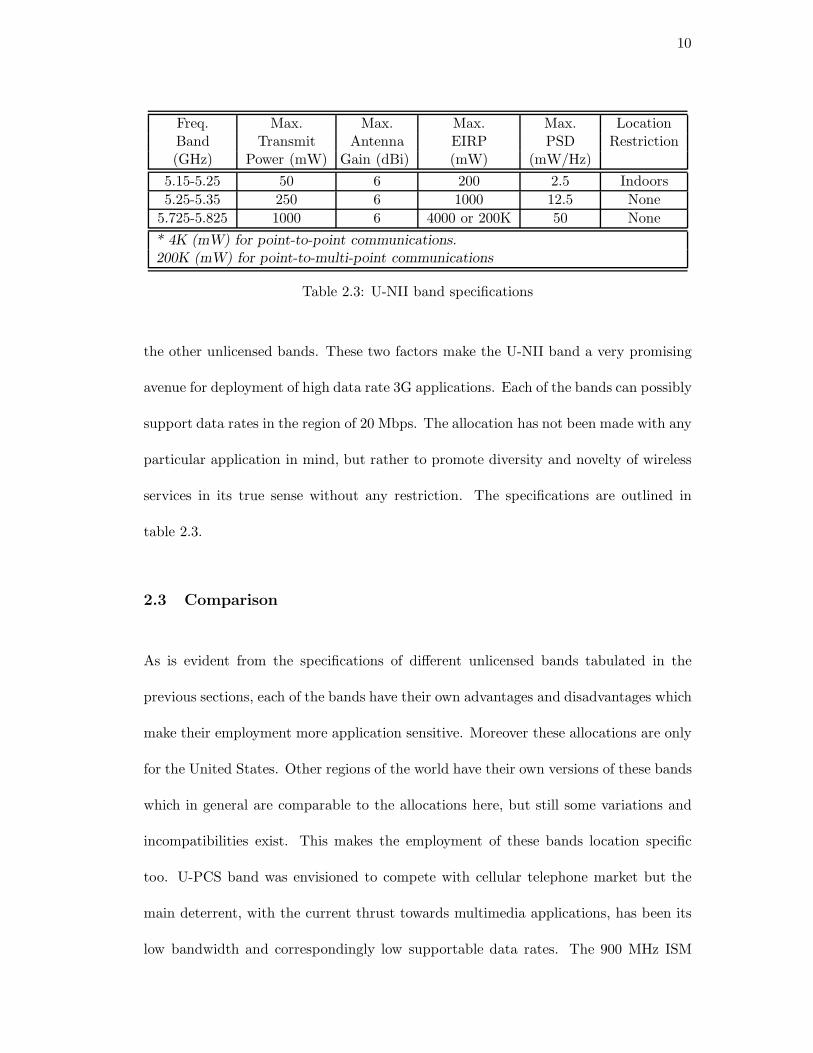
As is evident from the specifications of different unlicensed bands tabulated in the
previous sections, each of the bands have their own advantages and disadvantages which
make their employment more application sensitive. Moreover these allocations are only
for the United States. Other regions of the world have their own versions of these bands
which in general are comparable to the allocations here, but still some variations and
incompatibilities exist. This makes the employment of these bands location specific
too. U-PCS band was envisioned to compete with cellular telephone market but the
main deterrent, with the current thrust towards multimedia applications, has been its
low bandwidth and correspondingly low supportable data rates. The 900 MHz ISM
11
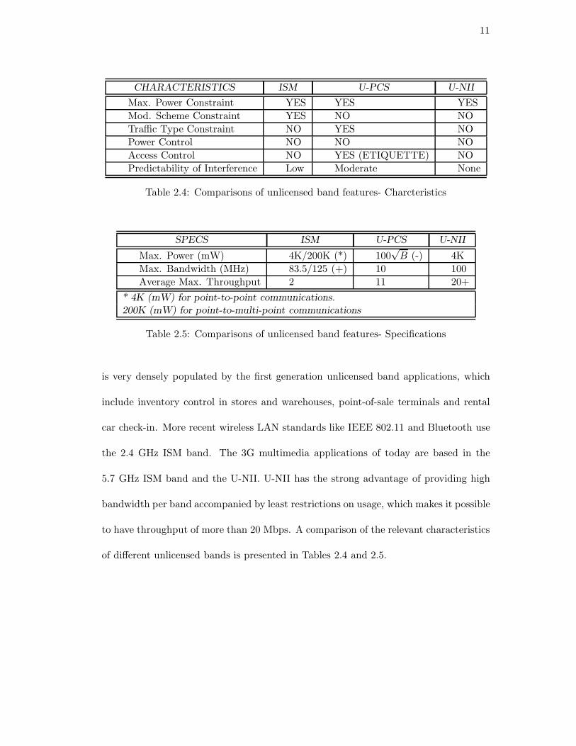
CHARACTERISTICS ISM U-PCS U-NII
Max. Power Constraint YES YES YESMod. Scheme Constraint YES NO NOTraffic Type Constraint NO YES NOPower Control NO NO NOAccess Control NO YES (ETIQUETTE) NOPredictability of Interference Low Moderate None
Table 2.4: Comparisons of unlicensed band features- Charcteristics
SPECS ISM U-PCS U-NII
Max. Power (mW) 4K/200K (*) 100√
B (-) 4KMax. Bandwidth (MHz) 83.5/125 (+) 10 100Average Max. Throughput 2 11 20+
* 4K (mW) for point-to-point communications.200K (mW) for point-to-multi-point communications
Table 2.5: Comparisons of unlicensed band features- Specifications
is very densely populated by the first generation unlicensed band applications, which
include inventory control in stores and warehouses, point-of-sale terminals and rental
car check-in. More recent wireless LAN standards like IEEE 802.11 and Bluetooth use
the 2.4 GHz ISM band. The 3G multimedia applications of today are based in the
5.7 GHz ISM band and the U-NII. U-NII has the strong advantage of providing high
bandwidth per band accompanied by least restrictions on usage, which makes it possible
to have throughput of more than 20 Mbps. A comparison of the relevant characteristics
of different unlicensed bands is presented in Tables 2.4 and 2.5.
12
Chapter 3
System Model
The following sections describe the system model adopted for the Tournament Arena
Simulator. This is the first simulation project in WINLAB implementing the concept
of tournaments and based on the unlicensed bands. Therefore the selected model and
the associated assumptions are aimed at implementing the most elementary version
which could capture the essence of the concept.
3.1 Overview
The physical or geographical setting is that of an mobile ad hoc network. It implies a
collection of mobile hosts dynamically forming a temporary network without the aid of
any standardized administration or standard support services [16]. These mobile hosts
or mobile stations are the only physical communication entities in the environment.
There are no base stations, switching centers or hubs for centralized control. Commu-
nication links can exist from the one mobile station (MS) to another. Theoretically,
any two MS can communicate with each other. The model can be further specified in
terms of its three main characteristics, namely,
• Radio propagation
13
• Mobility
• Transceiver scheme
3.2 Radio propagation
The physical layer air interface in this model is characterized only by long scale gain.
This includes purely distance losses. The effects of short scale and long scale fading are
not considered. The long scale gain is treated constant in time. For a transmitter i and
a receiver j, the long scale gain, Gi,j , would be a function of the distance, di,j between
them and can be represented as,
Gi,j = GD(di,j) (3.1)
The distance loss is due to the attenuation suffered by a signal as it travels through the
air from the transmitter to the receiver. This is proportional to the inverse power of
distance between the transmitter and the receiver i.e. GD(di,j) ∼ d−α, where α is the
propagation constant. The value of α ranges from 1 to 4 and depends on the air interface
and the geography. For a free space propagation environment, α = 2. However, for
propagation close to the earth’s surface, which is generally the case in wireless network
models, the terrain features become more significant and α = 4 is more typical [24].
Accordingly, this simulation employs the fourth power of distance loss rule.
The noise in the system is additive, white and Gaussian with a constant double sided
power spectral density N0 at a noise variance σ2 = N0/2. This noise variance is a
property of the receiver.
14
3.3 Geography and Mobility
Geography characterizes the terrain over which the MSs move and the mobility defines
the fashion in which the MSs move. The geography of this model is a rectangular
area on which a MS can take up any position. The mobility model used is a modified
version of random waypoint model, which is widely used for mobile ad hoc network
modeling [14].
Random waypoint model
Various versions of this mobility model are employed depending on the application. For
the model used in this simulation, each MS is randomly initialized at some position on
the geography. It stays stationary in that position for an exponentially distributed time
t with mean 1/µ′. Thereafter it generates three mobility co-ordinates [θ, ν, τ ], where
θ is angular direction of motion uniformly distributed between [0,2π]; ν is the speed of
motion uniformly distributed between [νmin, νmax]; and τ is the time duration of motion
with speed ν and in the direction θ. The random variable τ is exponentially distributed
with some mean 1/µ. The MS moves as specified by these co-ordinates. On reaching
the new position, it again pauses for an exponentially distributed time t. These two
steps occur repeatedly.
The special case of this model, as used in this simulation, is that the MS does not
pause at any stage. It generates an initial mobility co-ordinate set [θ1, ν1, τ1] and
starts moving to the position specified by those co-ordinates, moving with speed ν1, in
the direction θ1, for time τ1 . On reaching that position, it generates a new co-ordinate
set [θ2, ν2, τ2] and begins to move according to this new specification without a pause.
15
The geography also has wrap-around. This ensures uniform loading of the entire geo-
graphical grid so that each point on the grid is identical in terms of the radio resource
distribution. Further details are described in chapter 5.
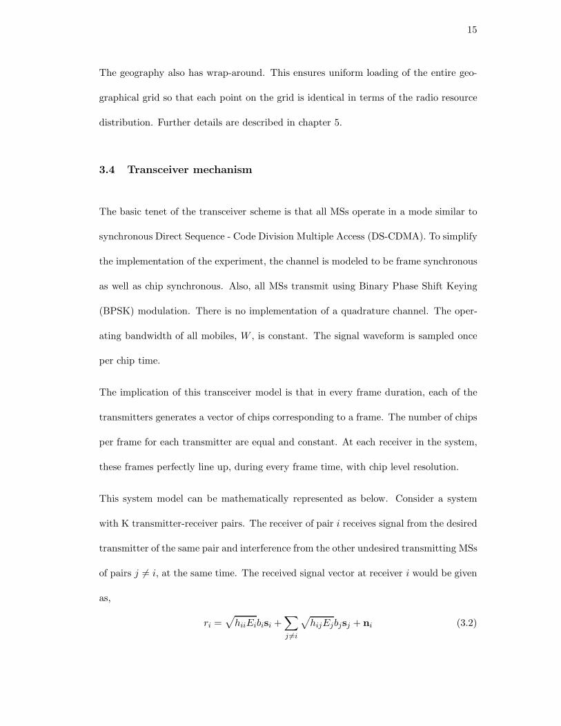
3.4 Transceiver mechanism
The basic tenet of the transceiver scheme is that all MSs operate in a mode similar to
synchronous Direct Sequence - Code Division Multiple Access (DS-CDMA). To simplify
the implementation of the experiment, the channel is modeled to be frame synchronous
as well as chip synchronous. Also, all MSs transmit using Binary Phase Shift Keying
(BPSK) modulation. There is no implementation of a quadrature channel. The oper-
ating bandwidth of all mobiles, W , is constant. The signal waveform is sampled once
per chip time.
The implication of this transceiver model is that in every frame duration, each of the
transmitters generates a vector of chips corresponding to a frame. The number of chips
per frame for each transmitter are equal and constant. At each receiver in the system,
these frames perfectly line up, during every frame time, with chip level resolution.
This system model can be mathematically represented as below. Consider a system
with K transmitter-receiver pairs. The receiver of pair i receives signal from the desired
transmitter of the same pair and interference from the other undesired transmitting MSs
of pairs j �= i, at the same time. The received signal vector at receiver i would be given
as,
ri =√
hiiEibisi +∑j �=i
√hijEjbjsj + ni (3.2)
16
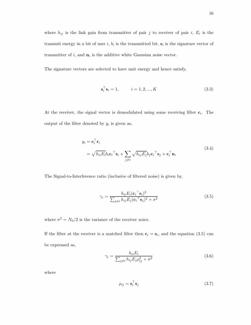
where hij is the link gain from transmitter of pair j to receiver of pair i, Ei is the
transmit energy in a bit of user i, bi is the transmitted bit, si is the signature vector of
transmitter of i, and ni is the additive white Gaussian noise vector.
The signature vectors are selected to have unit energy and hence satisfy,
s�i si = 1, i = 1, 2, ...,K (3.3)
At the receiver, the signal vector is demodulated using some receiving filter ci. The
output of the filter denoted by yi is given as,
yi = c�i ri
=√
hiiEibici�si +
∑j �=i
√hijEjbjci
�sj + c�i ni
(3.4)
The Signal-to-Interference ratio (inclusive of filtered noise) is given by,
γi =hiiEi(ci
�si)2∑j �=i hijEj(ci
�sj)2 + σ2(3.5)
where σ2 = N0/2 is the variance of the receiver noice.
If the filter at the receiver is a matched filter then ci = si, and the equation (3.5) can
be expressed as,
γi =hiiEi∑
j �=i hijEjρ2ij + σ2
(3.6)
where
ρij = s�i sj (3.7)

17
is the cross correlation between the signature sequences of user i and user j. The
mathematical modeling of the system is based on these equations.
18
Chapter 4
SSF Domain Fundamentals
This chapter describes the Scalable Simulation Framework (SSF) which provides the
platform for design and implementation of the TAS. The background and motivation
for SSF development is first given along with a brief discussion on its salient features
and advantages. The software implementation is then discussed.
4.1 Background
SSF is a public-domain standard for simulation of large and complex systems in C++
[10] and JAVA [8]. SSF has been developed by the S3 consortium, a collaboration of re-
searchers in networking, parallel simulations and software engineering. The goal of the
S3 consortium is to achieve radical improvements in speed, scalability and manageabil-
ity involved in modeling and simulations of very large multi-protocol communication
networks. Scalability and parallel performance of S3 software have been extensively
tested on large scale models of Internet, ATM and mobile wireless and satellite net-
works [15].
The Scalable Simulation Framework Application Programming Interface (SSF API)
is the single, core and unified interface which provides conformability and portability
of code and models across different SSF -compliant simulation environments. This
19
maximizes the potential for direct reuse of model code, while minimizing dependencies
on a particular simulator kernel implementation. In addition to its concrete modeling
applications, the API also functions as an abstract target for compilation of models
specified in higher level modeling languages or graphical modeling environments. The
framework’s primary design goal is to support high performance simulation. SSF makes
it possible to build models that are efficient and predictable in their use of space, able to
transparently utilize parallel processor resources, and scalable to very large collections
of simulated entities.
The reference development implementation on SSF is written in JAVA while its high
performance version is written in C++. The TAS uses the JAVA binding.
4.2 Overview
Before going onto the syntax and semantics of the SSF API, this section first focuses
upon the prominent features of the API. There are four main fundamentals on which
the API is based, which provide a significant motivation for using it as a platform for
the TAS . They are,
1. Separation of modeling and simulation
2. Object-oriented simulation framework
3. Event-driven simulation executive
4. Parallelization capability
20
4.2.1 Separation of modeling and simulation
Implementation of detailed simulations of large and complex systems involves a sub-
stantial effort in writing the ‘simulator’ itself along with all its functionality, in order
for it to process the operations while maintaining the causality. Causality, here, in
the context of simulations, refers to execution of operations in an ongoing simulation,
in an order, which is in accordance with the logical (real) time associated with those
operations so that the real-time dynamics of the actual physical system being simulated
are maintained. Ensuring this causality in a simulation is an elaborate and intricate
task [9, 21]. It, therefore, comes at the expense of the extent of detail achievable in
actual system modeling within a constraint of time. SSF provides a way to separate
domain specific modeling from the internals of the simulator so that the user can now
spend more effort on modeling actual system details. Another added advantage is that
with SSF no simulation-specific framework language like TeD [22, 23] is required as
the API is written in standard high level programming language like JAVA and C++.
4.2.2 Object-oriented design
The SSF is implemented using an object oriented programming (OOP) software design.
This provides the framework with all the advantages of OOP including encapsulation,
inheritance, polymorphism, run-time binding and parameterized typing [8, 10]. The
idea of OOP approach has great intuitive appeal in systems modeling because it is very
easy to conceptualize real world applications as being composed of objects. The SSF
API implemented as an object-oriented framework can be described as a layered design
linked hierarchically. The concepts at each layer are ‘encapsulated’ so that a user at a
21
particular layer need not be concerned about the concepts at the lower layers.
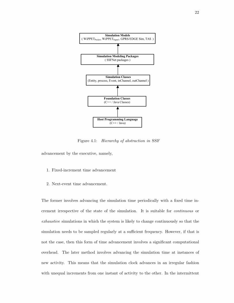
Each layer specifies the levels of abstraction, with the lowest being the most abstract
and more concrete elements added in higher levels so that at the highest level, the
final product maybe a specific simulation model. The lowest level construct is the
general OOP language, either C++ or JAVA in which SSF is implemented. The
OOP language is used to construct certain Foundation Classes which implement objects
of varied pattern and functionality. These foundation classes are used to construct
more specific Simulation Classes. These simulation classes provide for more specific
simulation-related objects and operations. The SSF API occurs at this level. The
simulation classes are further specified into Domain modeling packages which make the
framework more pertinent to the model being implemented such as either a protocol
or some network element etc. SSFNet includes such packages. The topmost level is
the Simulation Model which implements the actual real world system. The end user
of SSF can operate in the top two levels of the hierarchy. These hierarchical levels
of the framework are illustrated in figure 4.1. A generic form of this type of design is
discussed in [17]
4.2.3 Event-driven executive
The key component of a simulator is the simulation executive. The executive is respon-
sible for controlling the time advance of the central simulation clock. This clock keeps
track of the logical time relationship between the various simulation entities to ensure
causality, as defined earlier in subsection 4.2.2 . There are two main methods of time
22
Host Programming Language(C++ / Java)
Foundation Classes (C++ / Java Classes)
Simulation Classes (Entity, process, Event, inChannel, outChannel )
Simulation Modeling Packages ( SSFNet packages )
Simulation Models( WiPPETPacket, WiPPETSignal , GPRS/EDGE Sim, TAS )
Figure 4.1: Hierarchy of abstraction in SSF
advancement by the executive, namely,
1. Fixed-increment time advancement
2. Next-event time advancement.
The former involves advancing the simulation time periodically with a fixed time in-
crement irrespective of the state of the simulation. It is suitable for continuous or
exhaustive simulations in which the system is likely to change continuously so that the
simulation needs to be sampled regularly at a sufficient frequency. However, if that is
not the case, then this form of time advancement involves a significant computational
overhead. The later method involves advancing the simulation time at instances of
new activity. This means that the simulation clock advances in an irregular fashion
with unequal increments from one instant of activity to the other. In the intermittent
23
instants of inactivity the simulation clock remains idle or in other words the simulation
is not sampled. Here activity or event implies an occurance leading to the change in
the state variables, of the simulation.
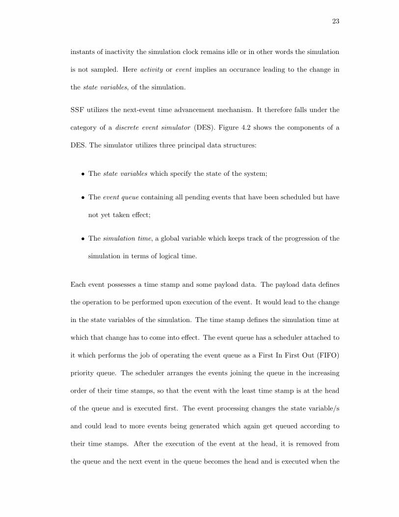
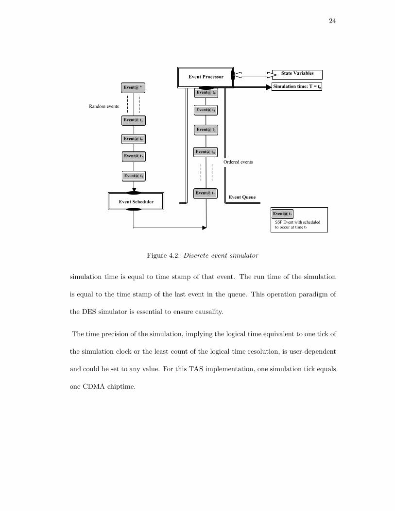
SSF utilizes the next-event time advancement mechanism. It therefore falls under the
category of a discrete event simulator (DES). Figure 4.2 shows the components of a
DES. The simulator utilizes three principal data structures:
• The state variables which specify the state of the system;
• The event queue containing all pending events that have been scheduled but have
not yet taken effect;
• The simulation time, a global variable which keeps track of the progression of the
simulation in terms of logical time.
Each event possesses a time stamp and some payload data. The payload data defines
the operation to be performed upon execution of the event. It would lead to the change
in the state variables of the simulation. The time stamp defines the simulation time at
which that change has to come into effect. The event queue has a scheduler attached to
it which performs the job of operating the event queue as a First In First Out (FIFO)
priority queue. The scheduler arranges the events joining the queue in the increasing
order of their time stamps, so that the event with the least time stamp is at the head
of the queue and is executed first. The event processing changes the state variable/s
and could lead to more events being generated which again get queued according to
their time stamps. After the execution of the event at the head, it is removed from
the queue and the next event in the queue becomes the head and is executed when the
24
Event Processor
Event Scheduler
Event@ t0
Event@ tN
Event@ t3
Event@ t1
Event@ t0
Event@ t1
Event@ t3
Event@ tN
Simulation time: T = to
Event Queue
State Variables
Random events
Event@ *
Event@ t*
Ordered events
SSF Event with scheduled to occur at time t*
Event@ t*
Figure 4.2: Discrete event simulator
simulation time is equal to time stamp of that event. The run time of the simulation
is equal to the time stamp of the last event in the queue. This operation paradigm of
the DES simulator is essential to ensure causality.
The time precision of the simulation, implying the logical time equivalent to one tick of
the simulation clock or the least count of the logical time resolution, is user-dependent
and could be set to any value. For this TAS implementation, one simulation tick equals
one CDMA chiptime.
25
4.2.4 Parallelization Capability
One of the main bottlenecks of a large and complex simulation is the speed. As ex-
plained in the previous sub-section, the DES operates on the basis of an event queue.
The events in a queue are identified by a single timeline or thread and are executed
sequentially by the processor based on the time-stamp associated with the event. How-
ever, not all events actually share a sequential relationship with each other, so that
some events could be executed totally independent of the other as long as the overall
causality is maintained. This implies that if the programming platform of the frame-
work supports multi-threading, meaning creating multiple event queues out of events
with independent timelines, then these queues could be processed concurrently on mul-
tiple processors to gain substantial advantage in speed. Theoretically if the simulation
work is distributed between two processors, then the simulation time should be half
of the time when it was carried out on a single processor. SSF supports this type
of parallelization. JAVA is inherently a multi-threaded language while for the C++
binding, additional foundation classes have been written in the framework to support
parallelization.
Parallelization with the C++ bindings is profusely experimented with in [18]. The TAS
in the current version consists of a single thread. The radio channel which is modeled
in this simulation is quite basic and simple. The simulation is not so computation-
intensive. The simulation in the single threaded version is sufficiently fast. However,
for future versions with more complex radio channel models, the JAVA SSF platform
does provide the option of parallelization.
26
4.2.5 Dynamic Modeling
SSF supports modeling of the simulation dynamically at the time of execution. This
is essential for run-time self organization of very large heterogeneous models, run-time
aggregation of sub-models and other similar novel techniques. This provides dynamic
reconfigurability to the simulation.
The TAS utilizes this feature in providing the facility to the user to code and con-
figure one’s own transceiver models and let the environment load and aggregate them
dynamically. This is explained in detail in chapter 6.
4.3 SSF Model Abstractions
This section specifies and explains the relevant syntax and semantics of SSF [7]. As
discussed, SSF is written as an object-oriented simulation, with JAVA and C++ serv-
ing as the host language. The following explanation uses common OOP terminologies.
The reader may refer to [19] for more details. The SSF syntax comprises of five base
class interfaces,
1. Entity
2. process
3. Event
4. inChannel
5. outChannel
27
These five classes form a self-contained design pattern for constructing operation-
oriented, event-oriented and hybrid simulations. They are sufficient to model any
system which could be described as a collection of different communicating objects
each implementing some distinct functionality.
An entity is a formulation of a physically or conceptually tangible object found in the real
system. It possesses processes which implement the dynamic behavior of objects that are
being modeled. From the point of shared computer memory, entities are non-contiguous
and independent blocks. The only means of interaction between different entities is
through inChannels and outChannels. These are conduits for exchanging information
between the entities. The information unit which traverses across the channels is called
event. While implementing a specific system, these base classes can then be extended
to have their derived classes implement more specific objects. Figure 4.3 illustrates this
basic frame work. There are three entities in the TAS environment. Each possesses
one or more processes which implement its functionality. Instances of inChannels and
outChannels create communication links between two different entities. The in and out
channels are not differentiated in the figure. Events are exchanged between the processes.
It is important to note that the inChannels and outChannels exist between the processes
owned by the same entity or different entities.
4.3.1 Entity
The Entity base class serves as the blue print for implementation of system objects.
Tangible physical objects like a MS or a switching center or conceptual objects like
28
Channel (In+Out)
Channel (In+Out)
Process1
Process2
Process3
Event
Process1
Process2
Entity 3
Process 1
Entity 1 Entity 2 Channel (In+Out)
Channel (In+Out)
Channel (In+Out)
EventEvent
Figure 4.3: SSF platform with Entities possessing processes and exchanging eventsthrough inChannels and outChannels
the radio channel or a protocol are implemented as entities, extending the base class
Entity. These entities specify the data structure and the functionality of the object.
The derived entity possesses instances of inChannel, outChannel and process which help
in achieving the same.
4.3.2 process
The process base class describes the dynamic behavior of an entity and implements
its functionality. Instances of process are defined within the entity as inline methods.
These inline methods are encompassed within a special SSF method called action().
Conceptually, processes are similar to native programming language methods, JAVA
methods in this case, which execute a particular group of instructions upon being called
29
by the execution thread of the main program. However the difference lies in the way
they are called. The instances of processes are initialized and activated only once at the
beginning of the simulation. Thereafter they remain ‘live’ throughout the simulation.
They may alternate between an active and a dormant state but they never become
‘dead’. Hence explicit and regular calls are not required for executing them. This is
achieved by the action() method of each process which serves as an implicit callback
method.
The processes are dynamic threads of computation owned by their host entity . The
instances of inChannel and outChannel also owned by the the host entity, actually serve
as input stream to and output stream from the process. Derived events travel on these
channels and affect the state of the process. The activation (active state) or deactivation
(dormant state) of processes is controlled by certain characteristics categorizing them.
Accordingly processes are of two types,
• Time-driven process
• Event-driven process
There is another special SSF method, wait(), used in the process in varied versions.
All versions of the wait() method suspend the process into a dormant state. The re-
activation is then regulated by the version of wait(), which is used as the terminating
statement of the process code. A time-driven process calls a waitFor() version, which
forces the process to go into a dormant state for a particular period of simulation time
which is specified as an argument to the method call. An event-driven process, on the
other hand uses a waitOn() version. It also suspends the process into dormancy, but
now the re-activation is dependent on the arrival of an event on the inChannels of the
30
process. The process keeps on listening onto the inChannel and until an event is received
on it, it stays in an inactive state. There are other versions of wait() that perform
slightly modified actions. However the above two are the most frequently used ones.
The types of actions performed in the process during execution can be categorized as
• Computation
• Synchronization
Computation actions are coded in the host language, JAVA in this case, and they
take-up zero elapsed simulation time. They are related to the actual operations and
functioning of the process. Synchronization actions are necessary to reflect the sim-
ulation time advancement with the progression of the simulation. They are effected
through the various versions of wait() method. They take-up non zero simulation
time.
4.3.3 Event
The Event base class provides the framework for the structure of the information unit
that is exchanged between the entities through the inChannels and the outChannels.
Depending on the application or the nature of the end-to-end process and entity between
which the information exchange is taking place, the unit may have to be modified in its
structure and data typing. This is achieved by specifying derived classes extending the
Event base class. All derived classes of Event must provide their own copy constructors.
The management of event storage is the responsibility of the framework, which may
release the storage of an event anytime after its last recipient process has suspended,
31
unless the modeler explicitly instructs otherwise. The events are written onto to its
outChannel by a process at one end and received at the inChannel of the recipient process
at the other end. A specific SSF method, write(), and its versions are used for this.
This traversal of events could be intra-entity or inter-entity. The receipt of the events
is non-destructive. Each designated process is allowed to receive, exactly once, each of
the events scheduled for delivery on all of its coaligned inChannels in the current instant
of the simulation time. However if no process receives an event at its time of delivery
(possible due to mismatch in inChannel and outChannel mapping), the event is lost. The
framework does not buffer it for retrospective delivery.
4.3.4 inChannel and outChannel
The inChannel and the outChannel are the base classes which provide the implemen-
tation for input and output conduits between entities. These base classes are directly
instantiated without any extensions or derived classes unlike the previously described
base classes. The instances of the inChannel and the outChannel belong to a process and
are owned by the host entity. Depending on the relationship between the different enti-
ties in the simulation, the inChannels and the outChannels are linked by a combinational
mapping. An inChannel of a process would be mapped to one or more outChannels of
another process in the same or a different entity. Vice versa for the outChannel. In
effect, the SSF supports unicast (one-to-one) as well as multicast (one-to many) in
both inChannels and outChannels in addition to bus-style mappings (many-to-many).
The channels also have a certain channel delays associated with them specified by the
modeler. A minimal channel delay can be associated with an outChannel if specified
by the modeler at the time of constructing them. A minimal mapping delay can be
32
associated with a channel mapping between an inChannel and an outChannel, again if
specified by the modeler. Finally, each outChannel can also have a per-write delay or
transmission delay associated with it. For JAVA SSF there is an inherent per-write de-
lay of one simulation tick associated with each outChannel. This could be compensated
by passing a negative delay argument to the write() method or it could be projected
using a non-negative delay argument by the modeler.
This completes the description of the SSF relevant to comprehending the essence of
the design as described in the following chapter. Detailed specification of the API is
given in [7].
33
Chapter 5
Design and Implementation
This chapter describes the design of the Tournament Arena Simulator (TAS)
and its implementation in the JAVA SSF domain. The focus is on functionality of the
system design and the SSF modules and structures involved in implementing the same.
5.1 Design Overview
As discussed in section 4.3, the physical and conceptual objects in a communication
system are modeled as an entity in the SSF domain. For a mobile ad-hoc network
model supporting point-to-point connections, the only physical communication objects
are the mobile stations (MS) occuring as transmitter-receiver pairs. Additionally, for
implementing the radio propagation aspects, a radio channel module and a mobility
module are required. These are the other conceptual objects in the simulation. These
modules get modeled as extensions or in object-oriented progamming terminology, as
a derived class of the SSF base class Entity. These derived classes are also referred to
as ‘entities’ in the following discussion for generality.
The TAS entities are itemized below.
1. Master : Simulation Entity
34
2. Radio channel : RadioChannel Entity
3. Mobility module : Mobility Entity
4. Mobile station : MobileTerminal Entity
The interactions of the different SSF simulation classes were described in chapter 4.
They are reiterated here in brief for ease of understanding. Each of the entities pos-
sess instances of the SSF base class process. They are referred to as processes, too, in
further discussion for generality. Encapsulated within the processes are JAVA meth-
ods which implement the functionality of their host entity. The entities communicate
with each other through instances of SSF base classes inChannel and outChannel. The
inter-networking between the entities is achieved by combinational mapping of these
inChannels and outChannels.
These SSF channels could be broadly differentiated into two types depending on their
logical function in the simulation.
• data channel
• info channel
Data channels act as conduits for transmitting actual communication system data be-
tween the transmitting and the receiving MSs. They can be further specified as real
data channels, which either enter or exit the RadioChannel so that the data these
conduits carry is affected by channel effects and fake data channels, which bypass the
RadioChannel and hence the data carried by these conduits has no channel effects incor-
porated. Data channels have direct analogy to actual air interface in a communication
35
system. However in the simulation the forward channel, from the transmitter MS to
the receiver MS, is implemented as real while the reverse channel, from the receiver MS
to the transmitter MS, is implemented as fake. The second type of SSF channels are
the Info Channels which carry information pertaining sustenance of simulation, like the
state of different simulation variables or triggers for initiating and terminating different
operations in the simulation.
The information is exchanged over these channels by encompassing it within instances
of extensions of SSF base class Event. Different extensions or derived classes of Event
are employed depending on the type of information to be carried, such as real data
(class DataEvent) or feedback information about link resource (class ResourceEvent)
or information about the different entity variables (class InfoEvent) or simply trig-
gers for initiating any of the processes (class TriggerEvent). Figure 5.1 provides an
approximate system map of the entities involved in the simulation.
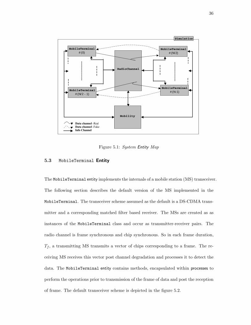
5.2 Simulation Entity
The Simulation entity does not have any physical relation to the communication sys-
tem being implemented. It simply provides the environment in which all other entities
exist and interact with each other. It creates the instances of each entity and performs
the mapping of their inChannels and outChannels. It also contains the main() method
to initiate the simulation.
36
MobileTerminal#(N/2 - 1)
RadioChannel
Mobility
Simulation
MobileTerminal#(0)
MobileTerminal#(N/2)
MobileTerminal#(N-1)
Data channel -Real Data channel -Fake Info Channel
Figure 5.1: System Entity Map
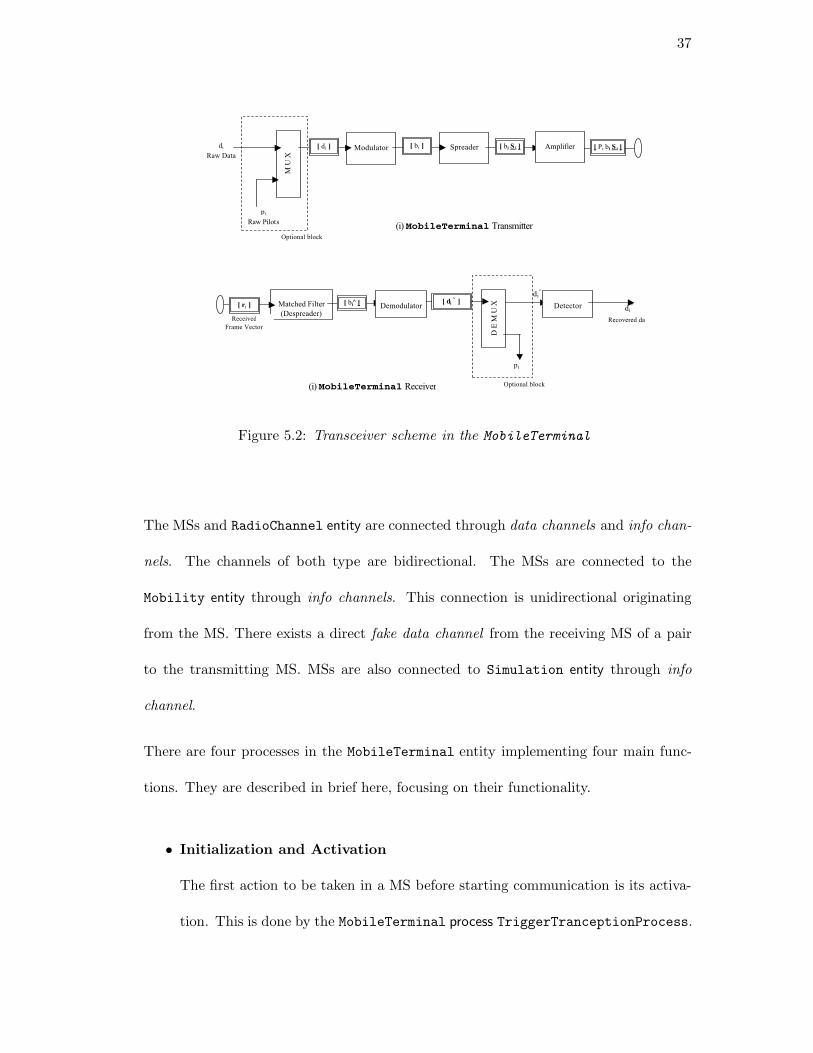
5.3 MobileTerminal Entity
The MobileTerminal entity implements the internals of a mobile station (MS) transceiver.
The following section describes the default version of the MS implemented in the
MobileTerminal. The transceiver scheme assumed as the default is a DS-CDMA trans-
mitter and a corresponding matched filter based receiver. The MSs are created as as
instances of the MobileTerminal class and occur as transmitter-receiver pairs. The
radio channel is frame synchronous and chip synchronous. So in each frame duration,
Tf , a transmitting MS transmits a vector of chips corresponding to a frame. The re-
ceiving MS receives this vector post channel degradation and processes it to detect the
data. The MobileTerminal entity contains methods, encapsulated within processes to
perform the operations prior to transmission of the frame of data and post the reception
of frame. The default transceiver scheme is depicted in the figure 5.2.
37
di^
di^
Recovered dat
Matched Filter (Despreader)
[ bi∧ ]
pi
[ ri ]
Demodulator [ di
^ ]
Detector
Received Frame Vector
D E
M U
X
Optional block (i) MobileTerminal Receiver
di
Raw Data
Spreader
M U
X
Modulator [ di ] [ bi S i ]
Amplifier [ bi ] [ Pi bi S i ]
pi
Raw Pilots (i) MobileTerminal Transmitter Optional block
Figure 5.2: Transceiver scheme in the MobileTerminal
The MSs and RadioChannel entity are connected through data channels and info chan-
nels. The channels of both type are bidirectional. The MSs are connected to the
Mobility entity through info channels. This connection is unidirectional originating
from the MS. There exists a direct fake data channel from the receiving MS of a pair
to the transmitting MS. MSs are also connected to Simulation entity through info
channel.
There are four processes in the MobileTerminal entity implementing four main func-
tions. They are described in brief here, focusing on their functionality.
• Initialization and Activation
The first action to be taken in a MS before starting communication is its activa-
tion. This is done by the MobileTerminal process TriggerTranceptionProcess.
38
The activation of the MS is accompanied by initialization of its system param-
eters like transmit power, data rate etc. There is a local data structure which
maintains these values.
• Data Transmission
The process TransmissionProcess performs this function of data transmission.
This is done one frame at a time. Since the system is synchronous upto the
precision of a chip, an integer number of chips would be transmitted in the frame
time, Tf . Let this number be Nc. These Nc chips form a frame. The frame length
of all the MS in the simulation is constant and equal.
The MS first generates raw data bits corresponding to a frame. These data bits
are then modulated and placed in the frame. If, suppose, the processing gain
used by the transmitting MS i is Ni, then the number of bits in the frame would
be Nb = Nc/Ni. This corresponds to the framed bits. The MS also generates
a pseuda-random (PN) long code sequence corresponding to the entire frame,
meaning a vector of Nc chips. The chips of this PN long code are generated in a
random fashion, by default. The raw data is spread by this long code. Each chip
is then multiplied by the amplitude of the transmit power. This frame is then
transmitted.
This set of operations is performed regularly at time interval Tf by this process.
The process has a self triggering mechanism to achieve this. Specific JAVA meth-
ods are written to achieve each of these functions. The calling of these methods
is controlled by flags. These flags enable the user to specify the exact dynamics
of the simulation, such as whether the long code sequences are fixed or generated
39
randomly; or whether pilot bits are present or absent in a frame and so on.
• Data Reception
The process ReceptionProcess performs the functions associated with receiving
the data at the receiver MS. At the interval of frame time Tf , a vector of Nc chips
is received at the input data channel of this process. It is the transmitted frame
post channel effects in the RadioChannel. The channel effects include distance
loss and interference from other transmitting MSs. Additive white Gaussian noise
is added to this received frame at the receiver. The receiving MS locally generates
the same long code as its transmitting counterpart using a common seed to feed
the long code generator. This long code is used by the receiver MS to despread the
received frame. The frame is then demodulated and the data bits are detected.
Based on the detected frame, two resource statistics, namely the bit error rate
(BER) and the signal to interference ratio (SIR) are calculated. BER calculation
is straight forward, as the receiver MS also has the capability to generate, locally,
the same raw data bits as the transmitter MS every frame using a mechanism
similar to localized long code generation. The SIR calculation is more complicated
and is explained below.
SIR Calculation
The MS in the default implementation in MobileTerminal does not use any form
of SIR estimation using pilots or any other blind estimation schemes. The exact
value of the SIR is calculated using actual channel gain values supplied directly
from the RadioChannel over the real data channel itself, coupled with the channel
data vector.
40
The SIR for a matched filter based receiver, at receiving MS, i, is given by the
equation 3.6.
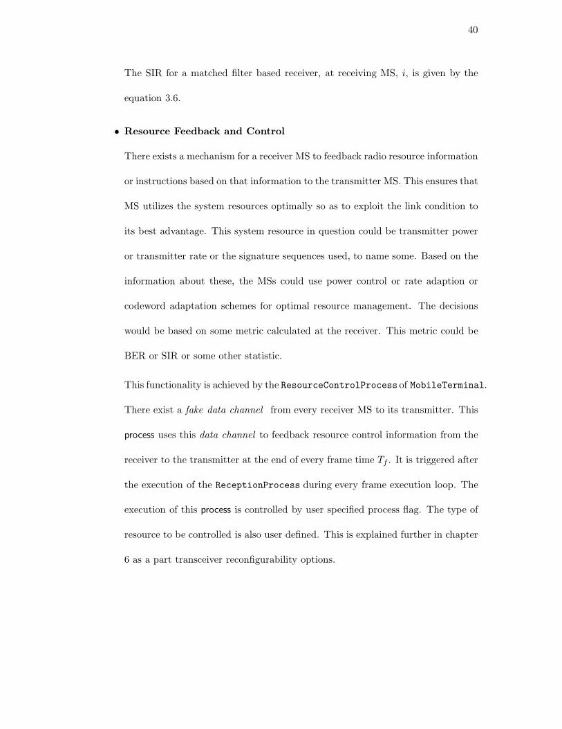
• Resource Feedback and Control
There exists a mechanism for a receiver MS to feedback radio resource information
or instructions based on that information to the transmitter MS. This ensures that
MS utilizes the system resources optimally so as to exploit the link condition to
its best advantage. This system resource in question could be transmitter power
or transmitter rate or the signature sequences used, to name some. Based on the
information about these, the MSs could use power control or rate adaption or
codeword adaptation schemes for optimal resource management. The decisions
would be based on some metric calculated at the receiver. This metric could be
BER or SIR or some other statistic.
This functionality is achieved by the ResourceControlProcess of MobileTerminal.
There exist a fake data channel from every receiver MS to its transmitter. This
process uses this data channel to feedback resource control information from the
receiver to the transmitter at the end of every frame time Tf . It is triggered after
the execution of the ReceptionProcess during every frame execution loop. The
execution of this process is controlled by user specified process flag. The type of
resource to be controlled is also user defined. This is explained further in chapter
6 as a part transceiver reconfigurability options.
41
5.4 RadioChannel Entity
The RadioChannel entity models the air channel. The air channel involves waveform
level interactions. These are modeled by a sampled time system with sampling interval
∆. In general, Tc, the duration of one CDMA chip, is a multiple of ∆; however, to reduce
the computational requirements, the simulation employs one sample per chip. Also, the
air channel is assumed to be synchronous and the channel effects include only distance
losses and additive white Gaussian noise. Short scale and long scale fading channels are
not considered. Also only the in-phase channel exists. There is no quadrature channel.
Real data channels connect the each of the transmitter MSs to the RadioChannel and
the RadioChannel to each of the receiver MSs. The RadioChannel is also closely
coupled with the Mobility through an info channel to incorporate MS motion effects
in channel calculations. The operations modeling the air channel are implemented in
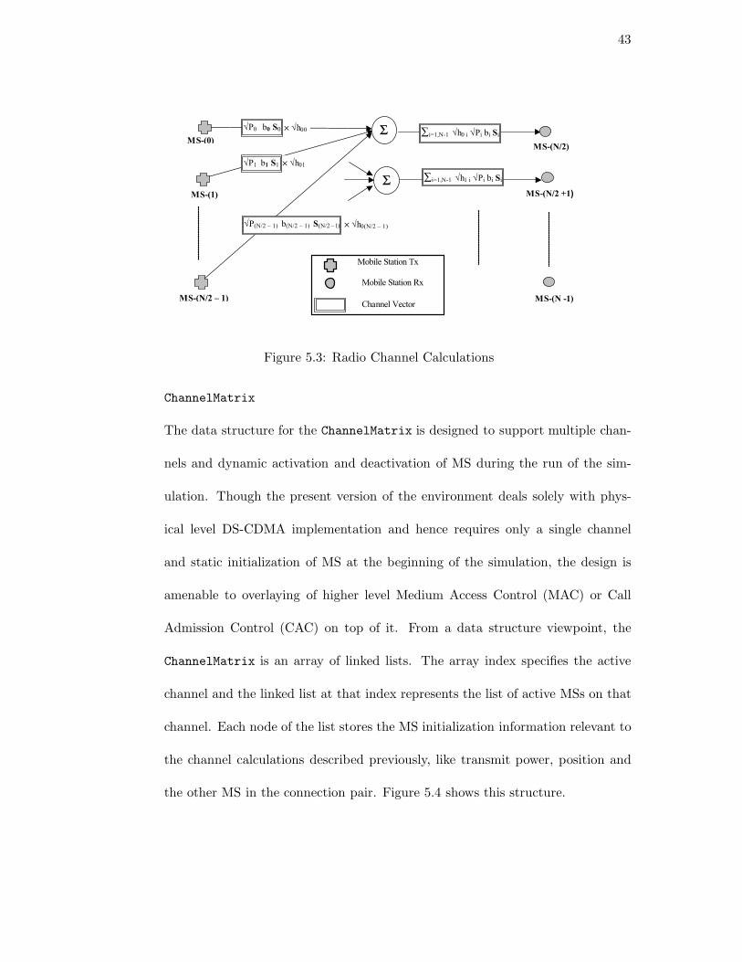
the RadioChannel. This is depicted in figure 5.3. During every frame duration, the
RadioChannel receives the transmitted frame vectors from all the transmitter MS in
the simulation. Each frame is a vector of real numbers. The frame corresponding to
transmitter i can be written as,
qi = Pibisi (5.1)
Assume that there are M transmitter and M receiver MS in the system. Then the link
42
gains to each receiver from the M transmitter form a M × M link gain matrix,
H =
⎛⎜⎜⎜⎜⎜⎜⎜⎜⎜⎜⎝
h00 h01 · · · h0(M−1)
h10 h11 · · · h1(M−1)
......
. . ....
hM0 hM1 · · · h(M−1)(M−1)
⎞⎟⎟⎟⎟⎟⎟⎟⎟⎟⎟⎠
where hij represents the link gain from the transmitter j to the receiver i. The channel
vector received at the receiver MS i after incorporating the channel effects is given as,
ri =M−1∑j=0
hijqj =M−1∑j=0
hijPjbjsj (5.2)
The RadioChannel calculates this channel vector corresponding to each of the M re-
ceiver MSs and sends it to each of them respectively.
These functions are achieved in the RadioChannel through three processes. Their func-
tional aspects are described below.
• Initialization
The ActiveMobileRegistrationProcess performs the task of initializing this en-
tity. MSs use info channels to convey their initial state to the RadioChannel. The
RadioChannel records this information into a local data base. The initialization
procedure is considered complete when this initialization information correspond-
ing to all the active mobiles in the simulation is recorded. The local data base
associated with RadioChannel is called the ChannelMatrix.
43
Σ
× √h01
× √h00
√P1 b1 S1
× √h0(N/2 – 1) √P(N/2 – 1) b(N/2 – 1) S(N/2 – 1)
MS-(0)
MS-(1)
MS-(N/2 – 1)
√P0 b0 S0 ∑i=1,N-1 √h0 i √Pi bi Si
Mobile Station Tx Mobile Station Rx Channel Vector
MS-(N/2)
MS-(N/2 +1)
MS-(N -1)
Σ ∑i=1,N-1 √h1 i √Pi bi Si
Figure 5.3: Radio Channel Calculations
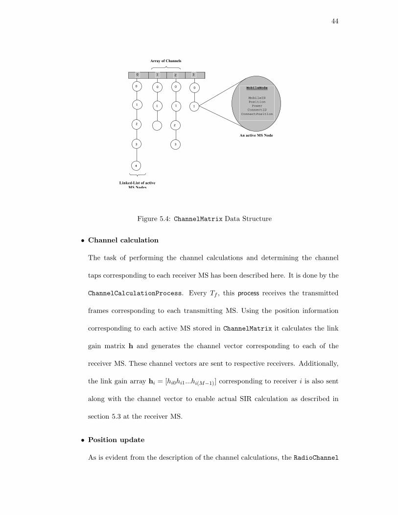
ChannelMatrix
The data structure for the ChannelMatrix is designed to support multiple chan-
nels and dynamic activation and deactivation of MS during the run of the sim-
ulation. Though the present version of the environment deals solely with phys-
ical level DS-CDMA implementation and hence requires only a single channel
and static initialization of MS at the beginning of the simulation, the design is
amenable to overlaying of higher level Medium Access Control (MAC) or Call
Admission Control (CAC) on top of it. From a data structure viewpoint, the
ChannelMatrix is an array of linked lists. The array index specifies the active
channel and the linked list at that index represents the list of active MSs on that
channel. Each node of the list stores the MS initialization information relevant to
the channel calculations described previously, like transmit power, position and
the other MS in the connection pair. Figure 5.4 shows this structure.
44
1 2 3
MobileNode
MobileID Position Power
ConnectID ConnectPosition
Array of Channels
Linked-List of active MS Nodes
An active MS Node
0
0 0 0 0
1 1 1 1
2 2
3 3
4
Figure 5.4: ChannelMatrix Data Structure
• Channel calculation
The task of performing the channel calculations and determining the channel
taps corresponding to each receiver MS has been described here. It is done by the
ChannelCalculationProcess. Every Tf , this process receives the transmitted
frames corresponding to each transmitting MS. Using the position information
corresponding to each active MS stored in ChannelMatrix it calculates the link
gain matrix h and generates the channel vector corresponding to each of the
receiver MS. These channel vectors are sent to respective receivers. Additionally,
the link gain array hi = [hi0hi1...hi(M−1)] corresponding to receiver i is also sent
along with the channel vector to enable actual SIR calculation as described in
section 5.3 at the receiver MS.
• Position update
As is evident from the description of the channel calculations, the RadioChannel
45
needs to constantly update the ChannelMatrix with the latest position of the MS
so that it can perform precise link gain calculations. Therefore it needs to commu-
nicate with the Mobility entity and retrieve the position updates with the motion
of each and every active MS. This is done by process PositionUpdateProcess,
which constantly listens on the info channel from the Mobility for new positions
of the MS. Upon receiving the information it updates the relevant fields in the
ChannelMatrix.
5.5 Mobility Entity
The Mobility is a derivative of Entity. It performs the function of providing mobility
to the MSs in the simulation. Based on the mobility model adopted, the Mobility
generates the new position values for each of the active MS at the end of the time
interval defined by the speed of the mobile and the distance resolution of the mobility
module. There exist info channels going from the Mobility to the RadioChannel that
convey these updates to the RadioChannel . There are further info channels from the
MS to the Mobility to provide initialization information of the MS to the Mobility.
Modified random waypoint model
As mentioned in section 3.3 the mobility model used is a modified Random Waypoint
model over rectangular geographical area. There is no concept of a grid because the
position which the MS can occupy are continuous valued. These two initial assumptions
make the new position calculations in the Mobility fairly complicated.
When the simulation is initiated, the MSs are randomly initialized on the geography at
different positions. These positions are specified in terms of rectangular co-ordinates
46
Figure 5.5: Random Waypoint Mobility Trail of a MS
- x and y. These positions are also registered in the Mobility in a local data base.
Each MS is identified by its mobility coordinates set defined as [θ, ν, τ ], where θ is
the direction of motion uniformly distributed between [0,2π]; ν is the speed of motion
uniformly distributed between [νmin, νmax]; τ is the time duration of motion with the
previous two values for speed and direction. The random variable τ is exponentially
distributed with some mean 1/µ. The actual computation is in fact significantly more
complicated. Consider the example below. Corresponding to the initial position,
identified as EPOCH 0 in figure 5.6, a MS generates an initial mobility coordinate
set [θ0, ν0, τ0] and starts moving to the position specified by that. On reaching that
position, identified as EPOCH 1 in this case, it generates a new co-ordinate set [θ1, ν1,
τ1] and begins to move according to this new mobility specification to this new position.
However the number of position updates that actually comprise this motion of the MS
from position identified by EPOCH 0 to that identified by EPOCH 1 depends on the
distance resolution of the mobility. Suppose the distance resolution is d and the distance
47
between the two positions is, say X, where,
X = ν0τ0 (5.3)
The position updates, hence, need to be sent at distance step of d. This translates to
a time step between position updates, τ ′ given by,
τ ′ = dν0 (5.4)
The number of such updates required to describe the traversal of the MS from position
identified as EPOCH 0 th that identified as EPOCH 1, m, would be given as,
m = �X/d� (5.5)
This is illustrated in figure 5.6.
Wrap-around geography
The other feature of the Mobility is wrap-around geography. Wrap-around model
ensures uniform loading of the geography without any bias to boundary points. This
ensures that that interference seen by any given MS is totally independent of its absolute
position on the geography, and only dependent on its position relative to other MS. From
the implementation point of view, this entails further detail in calculations.
Say the geography is specified by the co-ordinates [0,0] to [Xmax, Ymax]. Referrng to
figure 5.7, the transmitter MS is on the boundary point [x, Ymax] at position update
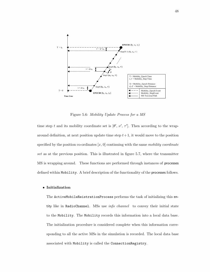
48
Step3 (θ0, υ0, t )
Step4 (θ0, υ0, t )
t = d υ0
t’ = d’ υ0
t = d υ0t = d υ0
d
EPOCH0 (θ0, υ0, τ0 )
EPOCH1 (θ1, υ1, τ1 )
T = 0
T = τ0
Time Line
t = d υ0
T = Mobility_Epoch Time t, t’ = Mobility_Step Time X = Mobility_Epoch Distance d, d’ = Mobility_Step Distance
Mobility_Epoch Event Mobility_StepEvent MS Traversal Path
Step0 (θ0, υ0, t )
Step(N-1) (θ0, υ0, t’ )
Figure 5.6: Mobility Update Process for a MS
time step t and its mobility coordinate set is [θ′, ν ′, τ ′]. Then according to the wrap-
around definition, at next position update time step t+1, it would move to the position
specified by the position co-ordinates [x, 0] continuing with the same mobility coordinate
set as at the previous position. This is illustrated in figure 5.7, where the transmitter
MS is wrapping around. These functions are performed through instances of processes
defined within Mobility. A brief description of the functionality of the processes follows.
• Initialization
The ActiveMobileReistrationProcess performs the task of initializing this en-
tity like in RadioChannel. MSs use info channel to convey their initial state
to the Mobility. The Mobility records this information into a local data base.
The initialization procedure is considered complete when this information corre-
sponding to all the active MSs in the simulation is recorded. The local data base
associated with Mobility is called the ConnectionRegistry.
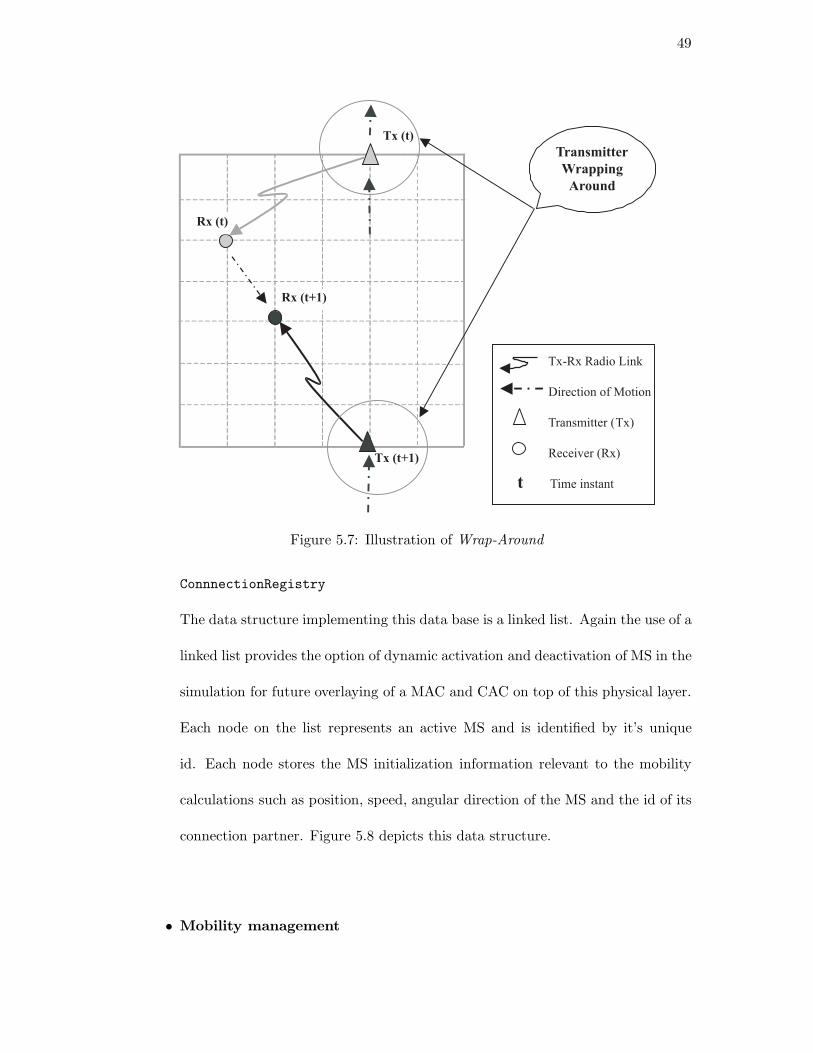
49
Figure 5.7: Illustration of Wrap-Around
ConnnectionRegistry
The data structure implementing this data base is a linked list. Again the use of a
linked list provides the option of dynamic activation and deactivation of MS in the
simulation for future overlaying of a MAC and CAC on top of this physical layer.
Each node on the list represents an active MS and is identified by it’s unique
id. Each node stores the MS initialization information relevant to the mobility
calculations such as position, speed, angular direction of the MS and the id of its
connection partner. Figure 5.8 depicts this data structure.
• Mobility management
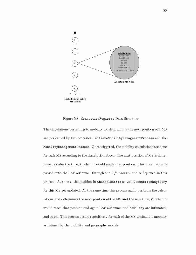
50
MobileNode MobileID Position Power Speed AngDir
ConnectID ConnectPosition
An active MS Node
0
Linked List of activeMS Nodes
1
2
3
4
Figure 5.8: ConnectionRegistry Data Structure
The calculations pertaining to mobility for determining the next position of a MS
are performed by two processes InitiateMobilityManagementProcess and the
MobilityManagementProcess. Once triggered, the mobility calculations are done
for each MS according to the description above. The next position of MS is deter-
mined as also the time, t, when it would reach that position. This information is
passed onto the RadioChannel through the info channel and self queued in this
process. At time t, the position in ChannelMatrix as well ConnectionRegistry
for this MS get updated. At the same time this process again performs the calcu-
lations and determines the next position of the MS and the new time, t′, when it
would reach that position and again RadioChannel and Mobility are intimated;
and so on. This process occurs repetitively for each of the MS to simulate mobility
as defined by the mobility and geography models.
51
This concludes the design and implementation of the system model as specified in
chapter 3 according to the SSF platform as detailed in chapter 4.
52
Chapter 6
Transceiver Reconfigurability
The TAS is a ‘tournament arena’ for comparison of different wireless systems in a par-
ticular radio environment, rather than being a ‘conventional testbed’ geared towards
the performance evaluation of a specific wireless system. This implies that the simu-
lation environment should be able to support the simultaneous existence of different
wireless systems, which use their own unique transceiver mechanisms. The transceiver
module which implements a MS needs to have the critical capability of ‘seamless dy-
namic reconfiguration’ essential to implementing a tournament arena simulation. This
chapter focuses on explaining the same.
6.1 Transceiver module requirements
The ‘seamless dynamic reconfiguration’ capability of the SSF transceiver module could
be crystallized as three individual characteristics. They are itemized below.
• Code remodeling
The most important feature of the transceiver class is the ability to support re-
modeling of the code. This is essential to allow the implementation of distinct
wireless systems having different transceiver schemes and even different media
53
access mechanisms. For the above function to be achieved most efficiently, re-
modeling needs to include the ability to modify, rewrite as well as reuse the code.
At the same time all of this needs to be relatively uncomplicated so that modelers
unfamiliar with the intricacies of the platform can still model their own versions
of the transceiver.
• Module encapsulation
The module implementing the MS and its transceiver scheme needs to be self-
contained, independent and isolated from the other modules. All interactions of
this module with the other modules should be generic. This is extremely essential
to ensure that the modifications in this module don’t warrant consequent changes
in the other modules. Seamless integration of the newer versions of this module
in to the simulation environment is critical.
• Dynamic class loading
This feature is closely related to the previous two items. The TAS is envisaged
to allow modelers to submit their distinct transceiver modules to participate in
a tournament. These modules could be written by different modelers in different
formats. The lesser the number of rules they need to conform to, the greater the
flexibility in modeling. The simulation environment, hence, needs to be able to
dynamically scan and locate these modules and load them dynamically at run-
time such that they continue to exhibit their individual features while seamlessly
integrating with the environment.
These three characteristics define the ‘seamless dynamic reconfiguration’ capability of
the transceiver module.
54
6.2 Transceiver module implementation
This section goes into the implementation details of the transceiver module necessary
to explain how the above design requirements are satisfied.
As discussed in chapter 4, all the different modules in the TAS exist in form of JAVA
SSF classes. The class MobileTerminal implements the transceiver module and per-
forms the functions of a MS. The transceiver implemented in MobileTerminal is the
scheme assumed as the default for the MSs in the TAS. The default transmitter is a DS-
CDMA transmitter and the default receiver is a matched filter. The MobileTerminal
contains the methods realizing these functionalities. It also contains the basic data
structures needed for a MS. The MobileTerminal is derived from JAVA SSF base
class Entity. It further acts as the base class for all other transceiver models. The
classes implementing specific transceiver models and hence individual wireless systems
are derived classes extending MobileTerminal. The hierarchy of this class inheritance
is shown in figure 6.1. Inheritance implies that these derived transceiver classes retain
all characteristics of the default transceiver class MobileTerminal, while possessing
newer individual traits which make them distinct from the other. A modeler wanting
to implement a new transceiver model, thus, simply writes a new JAVA SSF class
extending the MobileTerminal and possessing methods implementing the capabilities
of the new model. For example, the MobileTerminal uses the JAVA random number
generator for generating the random signature sequences. Now suppose the new model
uses Gold sequences [11,12] instead. The modeler in this case would write a new JAVA
SSF class in which the only modification is in the method generating signature se-
quences. Since this class is derived from the base class MobileTerminal all of its other
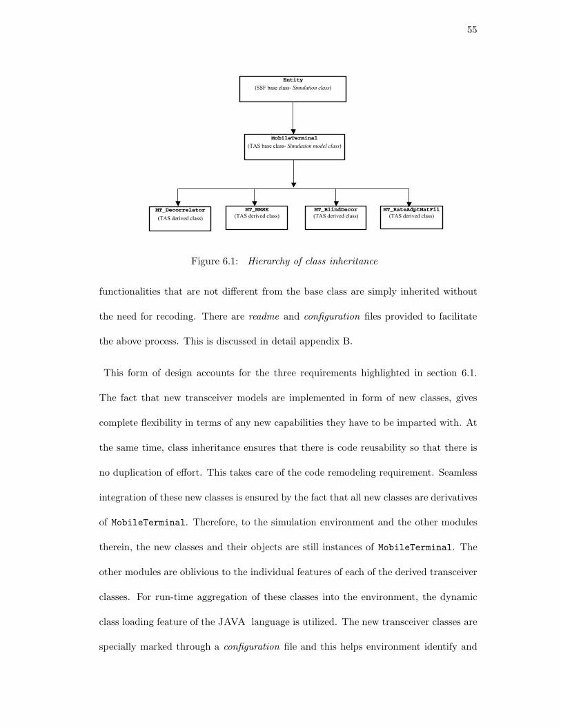
55
Entity
(SSF base class- Simulation class)
MobileTerminal
(TAS base class- Simulation model class)
MT_Decorrelator
(TAS derived class)
MT_BlindDecor (TAS derived class)
MT_RateAdptMatFil(TAS derived class)
MT_MMSE(TAS derived class)
Figure 6.1: Hierarchy of class inheritance
functionalities that are not different from the base class are simply inherited without
the need for recoding. There are readme and configuration files provided to facilitate
the above process. This is discussed in detail appendix B.
This form of design accounts for the three requirements highlighted in section 6.1.
The fact that new transceiver models are implemented in form of new classes, gives
complete flexibility in terms of any new capabilities they have to be imparted with. At
the same time, class inheritance ensures that there is code reusability so that there is
no duplication of effort. This takes care of the code remodeling requirement. Seamless
integration of these new classes is ensured by the fact that all new classes are derivatives
of MobileTerminal. Therefore, to the simulation environment and the other modules
therein, the new classes and their objects are still instances of MobileTerminal. The
other modules are oblivious to the individual features of each of the derived transceiver
classes. For run-time aggregation of these classes into the environment, the dynamic
class loading feature of the JAVA language is utilized. The new transceiver classes are
specially marked through a configuration file and this helps environment identify and
56
load these classes dynamically.
6.3 Transceiver Feedback Mechanism
The other significant aspect of the transceiver module, necessary for understanding
its operation is the reverse channel feedback mechanism. The simulation environment
provides a reverse channel connection from every receiver MS to its transmitter MS.
The purpose is to allow the MS pair to alter their transceiver and media access method
according to the link condition. The operation of reverse channel feedback mecha-
nism is closely linked with transceiver reconfigurability. It is achieved through the
ResourceControlProcess of the MobileTerminal entity.
The reverse channel is implemented as a fake data channel . This means that it is a
direct SSF channel- conduit - from the receiver MS to the transmitter MS and does
not include any actual radio channel effects. The payload of this reverse channel is
left unspecified in the MobileTerminal. It is simply declared as a void array of real
numbers and is encapsulated within the derivative of JAVA SSF class Event. The
resource control option is controlled by a switch. The MobileTerminal in its default
mode has the resource control option switched off. So no payload event is sent across
the reverse channel. A modeler wanting to use this reverse feedback channel needs
to switch the option on. Further he needs to define the payload that is going to be
fed back from the receiver to the transmitter and also define the processing or action
that is to be taken at the transmitter consequent to receiving the feedback. This is
achieved through two methods which are declared in the MobileTerminal but defined
in the new transceiver class by the modeler. This design gives the modeler the flexibility
57
to define his own unique resource control mechanism. This includes flexibility in the
resource being controlled, the metric used for exercising the control at the receiver and
the follow-up action undertaken at the transmitter. For example, the resource being
controlled could be the transmitter power or the transmitter rate, the metric used could
be either SIR or BER, the action taken could be increase or decrease the transmit power
or rate or simply switch off the transmission, and so on.
This completes the discussion of the transceiver module from its reconfiguration ca-
pability viewpoint, which is critical to the simulation environment functioning as a
tournament arena. The exact syntactical details for implementing this are given in
appendix B.
6.4 Environment Reconfigurability
It has been stressed so far that the key to operation of the ‘tournament arena’ is the
reconfiguration capability of the transceiver module. In addition to this, though, the
environment itself has some reconfiguration capability of its own. This facilitates setting
up specific system scenarios within the broad purview of the original system model as
defined in chapter 3. The simulation environment has two other modules apart from the
transceiver module, namely, the radio channel module, RadioChannel and the mobility
module, Mobility. Reconfiguration in each is discussed below.
• Radio Channel module reconfiguration
The default radio channel model is defined in chapter 3, as a flat channel compris-
ing of only distance losses and additive white Gaussian noise. All the processes
of the RadioChannel are controlled by boolean flags- switches. So there exists
58
the flexibility to modify the radio channel to suit a more specific model. For
example, there does exist a method in RadioChannel generateShadowFade(),
which generates the shadow fade values according to the Gudmundsson model [13].
However, since model parameters such as the standard deviation of the log nor-
mal process and the correlation distance are geography dependent, this option is
switched off as a default. Similarly the noise addition is operated by a switch,
and the noise variance value is also configurable. The RadioChannel is actually
designed to support multiple radio channels. This is also configurable.
• Mobility module reconfiguration
The mobility module, which also specifies the geography, is defined as mobile ad-
hoc environment with random waypoint mobility. The most important flexibility
that is available is that instead of purely ad-hoc mobility scenario, one could
actually move to a cellular-like scenario supporting multiple cells and both uplink
and downlink communication. Here ‘cellular-like’ implies that though though the
system still consists of only MSs, it is given a cellular nature by fixing all the
transmitting MSs (downlink) or all the receiving MSs (uplink) at one location on
the geography. Though this type of ‘cellular-like’ model cannot support higher
layer functions like call admission and handoff, it is sufficient to capture the
essence of radio propagation characteristics of an actual cellular system from
the physical layer viewpoint. This capability is vital for validation of results
against standard results which all happen to be mainly for cellular systems. It also
provides the possibility of tournaments between cellular and non-cellular systems.
This entire mechanism is again controlled by a single configuration flag. Apart
from this, other mobility related parameters like speed of MS, size, dimension and
59
distance resolution of the geography or even whether mobility exists or not are
configurable.
6.5 Reconfiguration parameters
The previous sections described the reconfiguration capabilities of the different modules
of the simulation environment. This section tabulates the specific parameters which are
open to modifications in each module. The configuration parameters of the transceiver
are listed in the table 6.1, and the simulation environment configuration parameters are
listed in the table 6.2, which also includes those of the radio channel and the mobility
modules. The exact configuration files which are used to achieve this are explained in
appendix B.
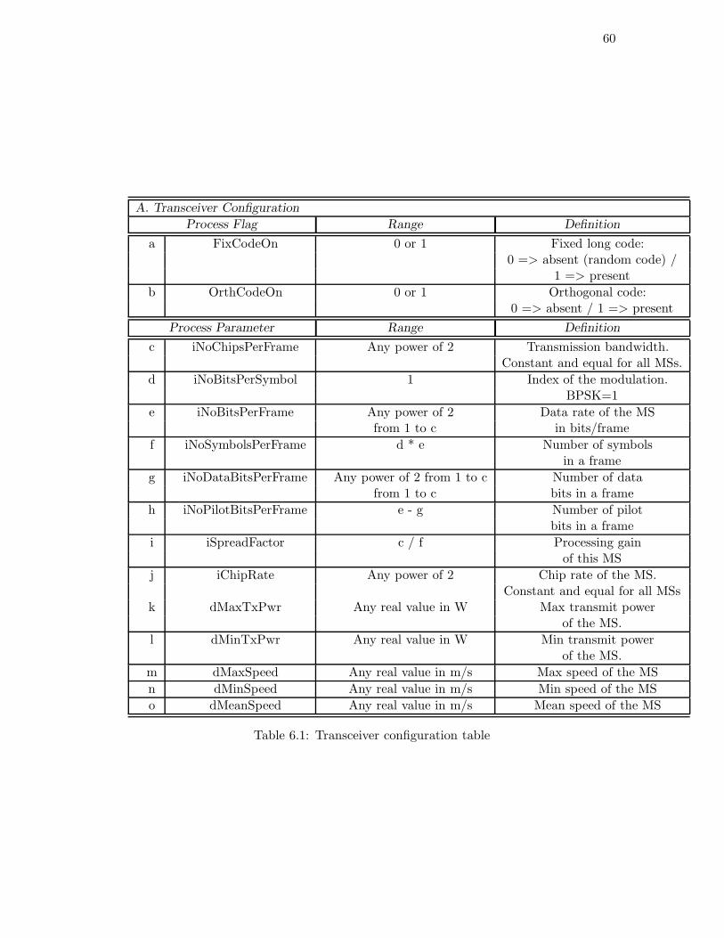
60
A. Transceiver Configuration
Process Flag Range Definition
a FixCodeOn 0 or 1 Fixed long code:0 => absent (random code) /
1 => presentb OrthCodeOn 0 or 1 Orthogonal code:
0 => absent / 1 => presentProcess Parameter Range Definition
c iNoChipsPerFrame Any power of 2 Transmission bandwidth.Constant and equal for all MSs.
d iNoBitsPerSymbol 1 Index of the modulation.BPSK=1
e iNoBitsPerFrame Any power of 2 Data rate of the MSfrom 1 to c in bits/frame
f iNoSymbolsPerFrame d * e Number of symbolsin a frame
g iNoDataBitsPerFrame Any power of 2 from 1 to c Number of datafrom 1 to c bits in a frame
h iNoPilotBitsPerFrame e - g Number of pilotbits in a frame
i iSpreadFactor c / f Processing gainof this MS
j iChipRate Any power of 2 Chip rate of the MS.Constant and equal for all MSs
k dMaxTxPwr Any real value in W Max transmit powerof the MS.
l dMinTxPwr Any real value in W Min transmit powerof the MS.
m dMaxSpeed Any real value in m/s Max speed of the MSn dMinSpeed Any real value in m/s Min speed of the MSo dMeanSpeed Any real value in m/s Mean speed of the MS
Table 6.1: Transceiver configuration table
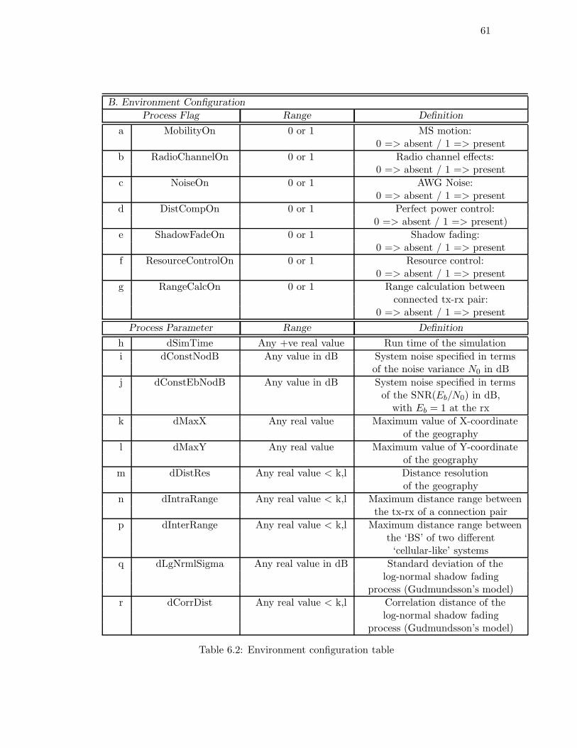
61
B. Environment Configuration
Process Flag Range Definition
a MobilityOn 0 or 1 MS motion:0 => absent / 1 => present
b RadioChannelOn 0 or 1 Radio channel effects:0 => absent / 1 => present
c NoiseOn 0 or 1 AWG Noise:0 => absent / 1 => present
d DistCompOn 0 or 1 Perfect power control:0 => absent / 1 => present)
e ShadowFadeOn 0 or 1 Shadow fading:0 => absent / 1 => present
f ResourceControlOn 0 or 1 Resource control:0 => absent / 1 => present
g RangeCalcOn 0 or 1 Range calculation betweenconnected tx-rx pair:
0 => absent / 1 => presentProcess Parameter Range Definition
h dSimTime Any +ve real value Run time of the simulationi dConstNodB Any value in dB System noise specified in terms
of the noise variance N0 in dBj dConstEbNodB Any value in dB System noise specified in terms
of the SNR(Eb/N0) in dB,with Eb = 1 at the rx
k dMaxX Any real value Maximum value of X-coordinateof the geography
l dMaxY Any real value Maximum value of Y-coordinateof the geography
m dDistRes Any real value < k,l Distance resolutionof the geography
n dIntraRange Any real value < k,l Maximum distance range betweenthe tx-rx of a connection pair
p dInterRange Any real value < k,l Maximum distance range betweenthe ‘BS’ of two different‘cellular-like’ systems
q dLgNrmlSigma Any real value in dB Standard deviation of thelog-normal shadow fading
process (Gudmundsson’s model)r dCorrDist Any real value < k,l Correlation distance of the
log-normal shadow fadingprocess (Gudmundsson’s model)
Table 6.2: Environment configuration table
62
Chapter 7
Sample Transceivers and Tournaments
Different tournaments have been staged in the TAS as a part of the thesis to demon-
strate the capabilies of the simulation platform as also to highlight the possible avenues
where this could be used for future research.
7.1 Transceivers
The most salient feature of the TAS is the ability to simulate, simultaneously, different
autonomous wireless systems with diverse, and independent tranceiver schemes. There
are some basic guidelines, though, specified based on the system model as described in
section 3.4. The most relevant point is that all mobile stations (MSs) operate in a mode
similar to DS-CDMA within a radio channel that is frame synchronous as well as chip
synchronous. Within this premise, the diversity in the tranceivers can be exercised in
a two-pronged fashion:
• Transceiver Structure
The simplest means of implementing transceiver diversity is by employing different
tranceiver structures like the matched filter, the Rake receiver, the decorrelator,
some other the multiuser detector etc in the mobile stations (MS).
63
• Resource Control Scheme
The second part of implementing tranceiver diversity is control and adaptation
of the radio resources. There are three main parameters that could be classified
as radio resource, (a) the transmit power of the mobiles, (b) rate or the number
of bits transmitted per frame and (c) the signature sequences used for spreading
the signal.
Using these as the building blocks several different transceiver schemes can be imple-
mented. Schemes largely different than these can also be tried as long as these follow
the basic guidelines of DS-CDMA in a frame synchronous and chip synchronous radio
channel. The details of this type of reconfiguration have already been explained in
chapter 6.
7.1.1 Transceiver Implementation
For the tournaments staged here as a part of this thesis and the experiments done
within, three different transceiver structures have been selected. These are (a) the
Matched Filter, (b) the Decorrelating Detector and (c) the Blind Adaptive Decorrela-
tor. Additionally, rate adaptation while keeping the transmit power and the signature
sequences fixed is employed. This subsection describes these transceiver schemes in
greater detail. It also provides results that compare these transceivers against the
theory to demonstrate the correctness of the implementation.
(a) Matched Filter
The first transceiver structure implemented is the conventional matched filter receiver as
described by equation 3.6. The probability of bit error for a single connection matched
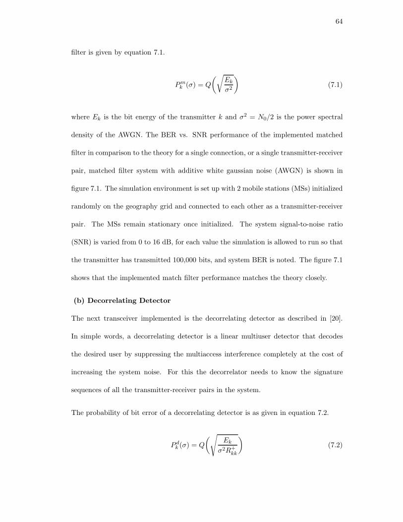
64
filter is given by equation 7.1.
Pmk (σ) = Q
(√Ek
σ2
)(7.1)
where Ek is the bit energy of the transmitter k and σ2 = N0/2 is the power spectral
density of the AWGN. The BER vs. SNR performance of the implemented matched
filter in comparison to the theory for a single connection, or a single transmitter-receiver
pair, matched filter system with additive white gaussian noise (AWGN) is shown in
figure 7.1. The simulation environment is set up with 2 mobile stations (MSs) initialized
randomly on the geography grid and connected to each other as a transmitter-receiver
pair. The MSs remain stationary once initialized. The system signal-to-noise ratio
(SNR) is varied from 0 to 16 dB, for each value the simulation is allowed to run so that
the transmitter has transmitted 100,000 bits, and system BER is noted. The figure 7.1
shows that the implemented match filter performance matches the theory closely.
(b) Decorrelating Detector
The next transceiver implemented is the decorrelating detector as described in [20].
In simple words, a decorrelating detector is a linear multiuser detector that decodes
the desired user by suppressing the multiaccess interference completely at the cost of
increasing the system noise. For this the decorrelator needs to know the signature
sequences of all the transmitter-receiver pairs in the system.
The probability of bit error of a decorrelating detector is as given in equation 7.2.
P dk (σ) = Q
(√Ek
σ2R+kk
)(7.2)
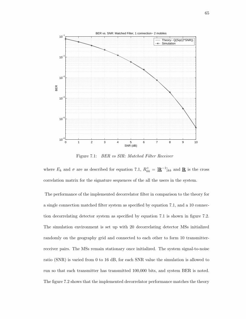
65
0 1 2 3 4 5 6 7 8 9 1010
−6
10−5
10−4
10−3
10−2
10−1
BER vs. SNR: Matched Filter, 1 connection− 2 mobiles
SNR (dB)
BE
R
Theory− Q(Sqr(2*SNR))Simulation
Figure 7.1: BER vs SIR: Matched Filter Receiver
where Ek and σ are as described for equation 7.1, R+kk = [R−1]kk and R is the cross
correlation matrix for the signature sequences of the all the users in the system.
The performance of the implemented decorrelator filter in comparison to the theory for
a single connection matched filter system as specified by equation 7.1, and a 10 connec-
tion decorrelating detector system as specified by equation 7.1 is shown in figure 7.2.
The simulation environment is set up with 20 decorrelating detector MSs initialized
randomly on the geography grid and connected to each other to form 10 transmitter-
receiver pairs. The MSs remain stationary once initialized. The system signal-to-noise
ratio (SNR) is varied from 0 to 16 dB, for each SNR value the simulation is allowed to
run so that each transmitter has transmitted 100,000 bits, and system BER is noted.
The figure 7.2 shows that the implemented decorrelator performance matches the theory
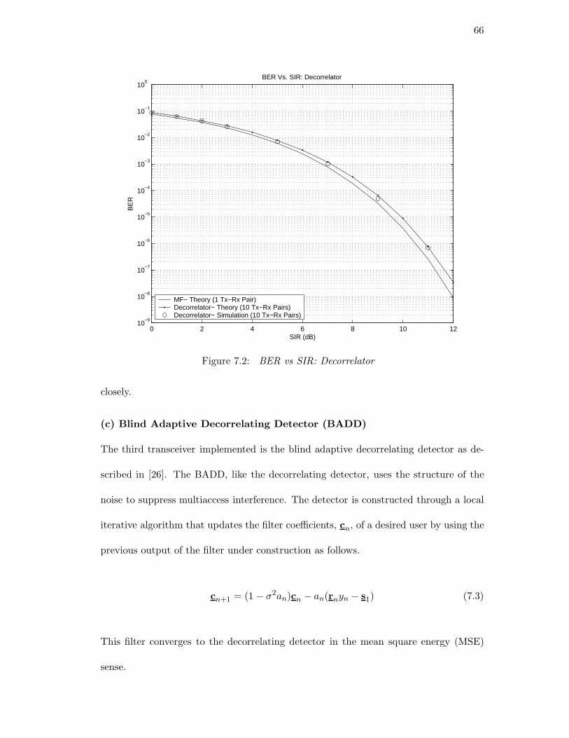
66
0 2 4 6 8 10 1210
−9
10−8
10−7
10−6
10−5
10−4
10−3
10−2
10−1
100
BER Vs. SIR: Decorrelator
SIR (dB)
BE
R
MF− Theory (1 Tx−Rx Pair)Decorrelator− Theory (10 Tx−Rx Pairs)Decorrelator− Simulation (10 Tx−Rx Pairs)
Figure 7.2: BER vs SIR: Decorrelator
closely.
(c) Blind Adaptive Decorrelating Detector (BADD)
The third transceiver implemented is the blind adaptive decorrelating detector as de-
scribed in [26]. The BADD, like the decorrelating detector, uses the structure of the
noise to suppress multiaccess interference. The detector is constructed through a local
iterative algorithm that updates the filter coefficients, cn, of a desired user by using the
previous output of the filter under construction as follows.
cn+1 = (1 − σ2an)cn − an(rnyn − s1) (7.3)
This filter converges to the decorrelating detector in the mean square energy (MSE)
sense.
67
r(n) c(n)
y(n)
Figure 7.3: BADD Filter Structure
For iteration n, cn is a vector of filter taps, rn is the received vector at the filter input,
yn is the output of the receiver filter, σ2 is the variance of the AWGN, si is the signature
sequence of the desired user i, and an is the iteration step size in iteration n. This is
shown diagramatically in Figure 7.3. The iteration step size could be fixed or time-
dependent. The time-dependent step size has been selected here as it is optimal from
the point of view of convergence time as well as the MSE, as detailed in [26, page 10].
The time-dependent step size an is specified in 7.4.
an =1
n0 + n(7.4)
where n0 = 5 is a constant and n is the iteration number.
It should be noted here that rn and yn are readily available at the input and the output
of the receiver filter. The only other system parameter that needs to be known in
advance at the receiver filter are the variance of the AWGN and the signature sequence
of the desired user. It is fairly reasonable to assume that a receiver filter will be
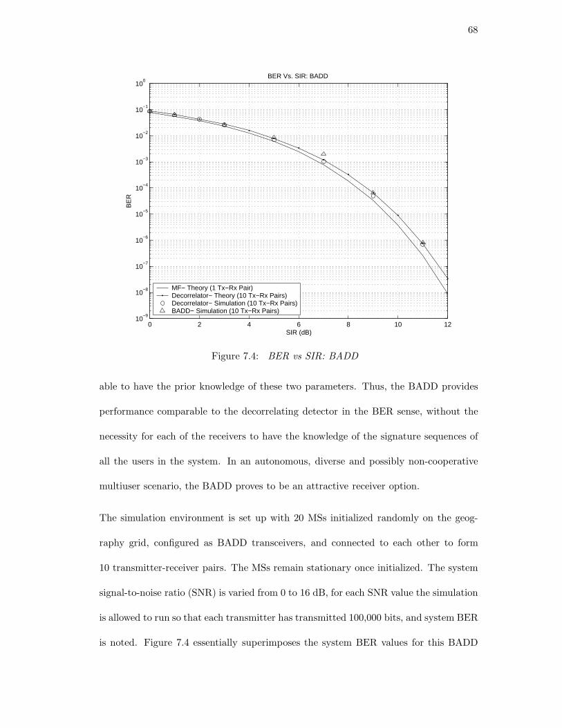
68
0 2 4 6 8 10 1210
−9
10−8
10−7
10−6
10−5
10−4
10−3
10−2
10−1
100
BER Vs. SIR: BADD
SIR (dB)
BE
R
MF− Theory (1 Tx−Rx Pair)Decorrelator− Theory (10 Tx−Rx Pairs)Decorrelator− Simulation (10 Tx−Rx Pairs)BADD− Simulation (10 Tx−Rx Pairs)
Figure 7.4: BER vs SIR: BADD
able to have the prior knowledge of these two parameters. Thus, the BADD provides
performance comparable to the decorrelating detector in the BER sense, without the
necessity for each of the receivers to have the knowledge of the signature sequences of
all the users in the system. In an autonomous, diverse and possibly non-cooperative
multiuser scenario, the BADD proves to be an attractive receiver option.
The simulation environment is set up with 20 MSs initialized randomly on the geog-
raphy grid, configured as BADD transceivers, and connected to each other to form
10 transmitter-receiver pairs. The MSs remain stationary once initialized. The system
signal-to-noise ratio (SNR) is varied from 0 to 16 dB, for each SNR value the simulation
is allowed to run so that each transmitter has transmitted 100,000 bits, and system BER
is noted. Figure 7.4 essentially superimposes the system BER values for this BADD
69
system over the figure 7.2. It can be seen that the BADD transceiver implemented here
to be almost as good as decorrelating detector in BER-performance sense.
7.2 Tournaments
Several different experiments and tournaments have been conducted with the transceivers
and the transceiver schemes defined above. It has been shown in [26, pages 7-10] that
if the simulation is allowed to run for a sufficient number of iterations, the BADD con-
verges to a decorrelating detector. This is also seen from figure 7.4 in a BER sense.
Therefore, in all the tournaments below, the participants are the matched filter and
the BADD. The tournaments are staged in a flat square geographical grid, 10,000m x
10,000m in area.
7.2.1 Tournament 1: Single Transceiver System in the Arena
This tournament has two participant transceivers, a matched filter transceiver and a
BADD transceiver. At a time, all the mobile stations (MS) in the system have the same
transceiver structure.
Round A comprises all the MSs with matched filter transceivers. The MSs (transmitter-
receiver pairs) are randomly initialized on the grid such that distance between the
transmitter and the receiver of a pair is not more than a pre-determined range. This is
done using a simple iterative loop in the code wherein after intializing the transmitter
MS of the transmitter-receiver pair, the receiver MS is initialized iteratively and its
distance from the transmitter calculated each time till the distance is lesser than the
pre-determined range. This pre-determined distance is called the Tx-Rx range from
70
here on. Once initialized, the MSs don’t move from their positions. This is to ensure
that the results are not affected by the geographical distance losses. The radio channel
is chip synchronous and frame synchronous. The transmitter transmits 1 bit per frame.
The spreading gain is 128, and the signature sequences are randomly generated and
then kept fixed with every frame. The distance loss of the transmitted signal at the
receiver is compensated by setting the transmit power so that received signal strength
at the receiver is equal for all receivers. Since the MSs don’t move once initialized,
the transmit power once set also remains fixed. The bit rate is also kept fixed at 1 bit
per frame. The two parameters that are variable in these experiments are the number
of MSs in the system and the Tx-Rx range. Several sets of experiments are run. For
each set, the Tx-Rx range is fixed, and then the number of MSs in the system are
varied with different iterations. For every iteration or run of the simulation, each MS
transmits 100,000 bits. The Signal-to-Noise ratio, with one transmitter-receiver pair
and no multiuser interference, is set to 7 dB.
The resuts are averaged over 10 runs of this experiment, i.e. for 10 different mobile
position initializations.
Round B comprises of exact same experiment as above, except that now all the MSs
have BADD transceivers as described by the equation 7.3.
The performance of these two systems are quantified in terms of the system goodput,
the system throughput and the system bit error rate (BER). The system throughput
is defined as the total number of bits transmitted in the system, the system goodput is
defined as the total number of error-free bits transmitted in the system and the system
BER is defined as the ratio of the total number of bits in error and the total number
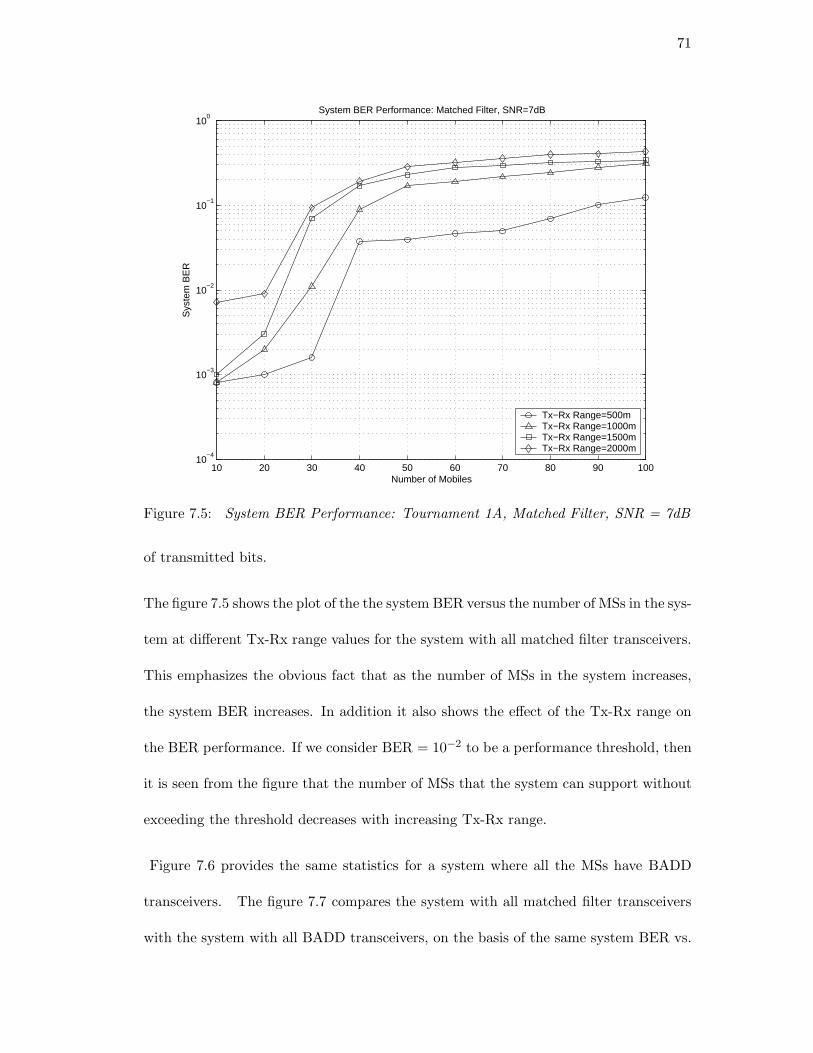
71
10 20 30 40 50 60 70 80 90 10010
−4
10−3
10−2
10−1
100
System BER Performance: Matched Filter, SNR=7dB
Number of Mobiles
Sys
tem
BE
R
Tx−Rx Range=500mTx−Rx Range=1000mTx−Rx Range=1500mTx−Rx Range=2000m
Figure 7.5: System BER Performance: Tournament 1A, Matched Filter, SNR = 7dB
of transmitted bits.
The figure 7.5 shows the plot of the the system BER versus the number of MSs in the sys-
tem at different Tx-Rx range values for the system with all matched filter transceivers.
This emphasizes the obvious fact that as the number of MSs in the system increases,
the system BER increases. In addition it also shows the effect of the Tx-Rx range on
the BER performance. If we consider BER = 10−2 to be a performance threshold, then
it is seen from the figure that the number of MSs that the system can support without
exceeding the threshold decreases with increasing Tx-Rx range.
Figure 7.6 provides the same statistics for a system where all the MSs have BADD
transceivers. The figure 7.7 compares the system with all matched filter transceivers
with the system with all BADD transceivers, on the basis of the same system BER vs.
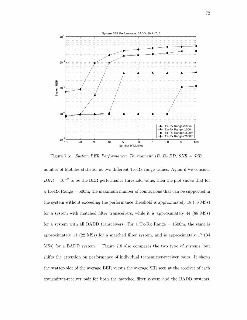
72
10 20 30 40 50 60 70 80 90 10010
−4
10−3
10−2
10−1
100
System BER Performance: BADD, SNR=7dB
Number of Mobiles
Sys
tem
BE
R
Tx−Rx Range=500mTx−Rx Range=1000mTx−Rx Range=1500mTx−Rx Range=2000m
Figure 7.6: System BER Performance: Tournament 1B, BADD, SNR = 7dB
number of Mobiles statistic, at two different Tx-Rx range values. Again if we consider
BER = 10−2 to be the BER performance threshold value, then the plot shows that for
a Tx-Rx Range = 500m, the maximum number of connections that can be supported in
the system without exceeding the performance threshold is approximately 18 (36 MSs)
for a system with matched filter transceivers, while it is approximately 44 (88 MSs)
for a system with all BADD transceivers. For a Tx-Rx Range = 1500m, the same is
approximately 11 (22 MSs) for a matched filter system, and is approximately 17 (34
MSs) for a BADD system. Figure 7.8 also compares the two type of systems, but
shifts the attention on performance of individual transmitter-receiver pairs. It shows
the scatter-plot of the average BER versus the average SIR seen at the receiver of each
transmitter-receiver pair for both the matched filter system and the BADD systems.
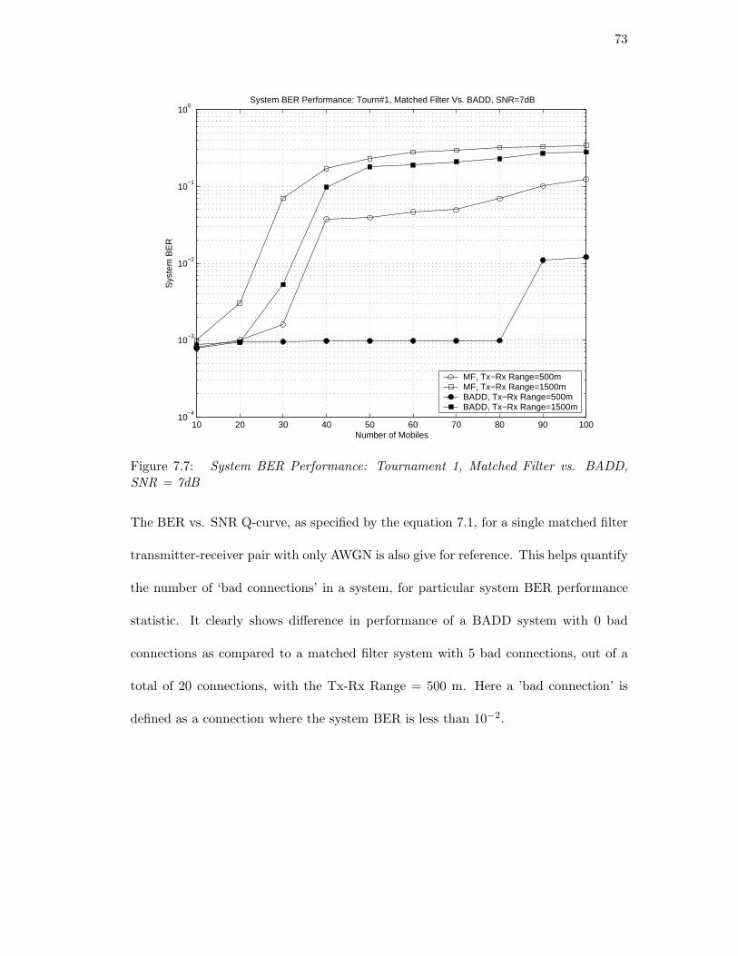
73
10 20 30 40 50 60 70 80 90 10010
−4
10−3
10−2
10−1
100
System BER Performance: Tourn#1, Matched Filter Vs. BADD, SNR=7dB
Number of Mobiles
Sys
tem
BE
R
MF, Tx−Rx Range=500mMF, Tx−Rx Range=1500mBADD, Tx−Rx Range=500mBADD, Tx−Rx Range=1500m
Figure 7.7: System BER Performance: Tournament 1, Matched Filter vs. BADD,SNR = 7dB
The BER vs. SNR Q-curve, as specified by the equation 7.1, for a single matched filter
transmitter-receiver pair with only AWGN is also give for reference. This helps quantify
the number of ‘bad connections’ in a system, for particular system BER performance
statistic. It clearly shows difference in performance of a BADD system with 0 bad
connections as compared to a matched filter system with 5 bad connections, out of a
total of 20 connections, with the Tx-Rx Range = 500 m. Here a ’bad connection’ is
defined as a connection where the system BER is less than 10−2.
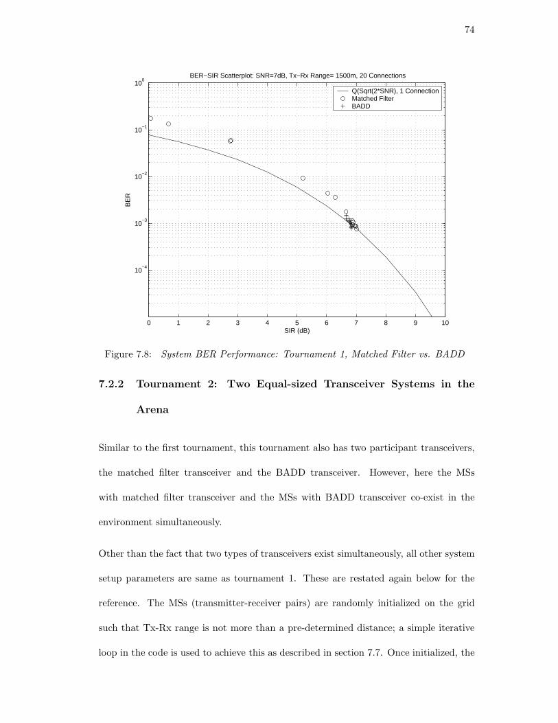
74
0 1 2 3 4 5 6 7 8 9 10
10−4
10−3
10−2
10−1
100
BER−SIR Scatterplot: SNR=7dB, Tx−Rx Range= 1500m, 20 Connections
SIR (dB)
BE
R
Q(Sqrt(2*SNR), 1 ConnectionMatched FilterBADD
Figure 7.8: System BER Performance: Tournament 1, Matched Filter vs. BADD
7.2.2 Tournament 2: Two Equal-sized Transceiver Systems in the
Arena
Similar to the first tournament, this tournament also has two participant transceivers,
the matched filter transceiver and the BADD transceiver. However, here the MSs
with matched filter transceiver and the MSs with BADD transceiver co-exist in the
environment simultaneously.
Other than the fact that two types of transceivers exist simultaneously, all other system
setup parameters are same as tournament 1. These are restated again below for the
reference. The MSs (transmitter-receiver pairs) are randomly initialized on the grid
such that Tx-Rx range is not more than a pre-determined distance; a simple iterative
loop in the code is used to achieve this as described in section 7.7. Once initialized, the
75
MSs don’t move from their positions. This is to ensure that the results are not affected
by the geographical distance losses. The radio channel is chip synchronous, and frame
synchronous. The transmitter transmits 1 bit per frame. The spreading gain is 128,
the signature sequences are randomly generated and then kept fixed with every frame.
The distance loss of the transmitted signal at the receiver is compensated by setting
the transmit power so that received signal strength at the receiver is equal for all the
receivers. Since the MSs don’t move once initialized, the transmit power is set once
and then remains fixed. The bit rate is also kept fixed at 1 bit per frame. The two
parameters that are variable in these experiments are the number of MSs in the system
and the Tx-Rx range. Several set of experiments are run. For each set, the Tx-Rx
range is fixed, and then the number of MSs in the system are varied with different
iterations. For every iteration or run of the simulation, each MS transmits 100,000
bits. The Signal-to-Noise ratio, with one transmitter-receiver pair in the system and
no multiuser interference, is set to 7 dB.
The fact that matched filter and BADD transceivers co-exist in the system leads to
some interesting changes in the signal vs. interference dynamics. For the matched
filter receiver, only the transmitter of the Tx-Rx pair is the desired user, and it has
prior knowledge of the signature sequence of the transmitter. All other transmitters,
including the BADD transmitters, are interferers. For the BADD, for a given set of
signature sequences, the performance is independent of the transceiver structure of the
other MSs in the system.
There are three statistics that we will consider while comparing the performance of
these wireless systems.
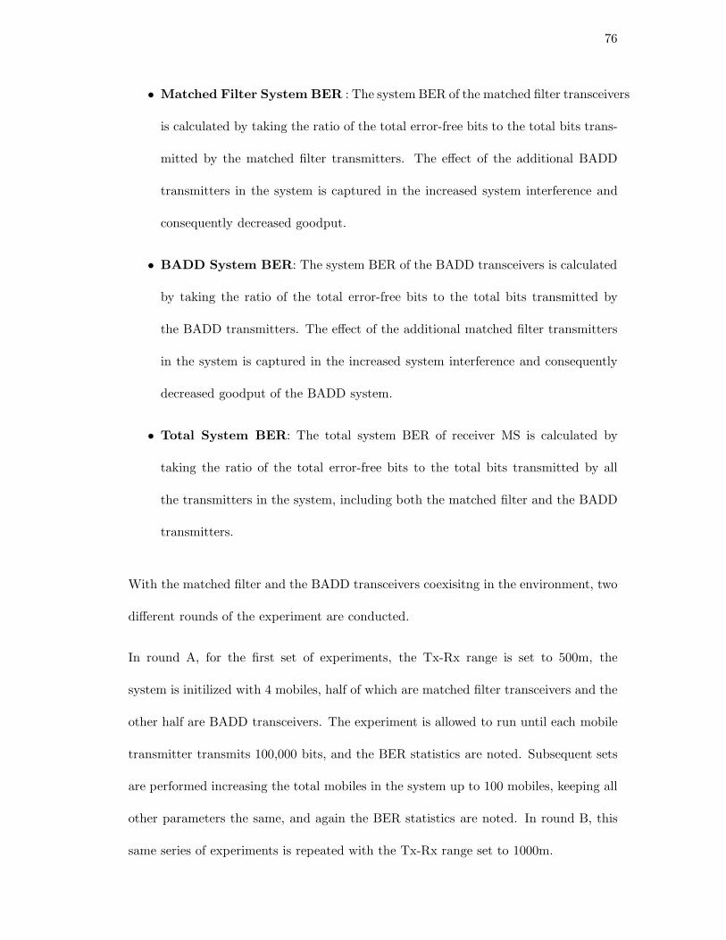
76
• Matched Filter System BER : The system BER of the matched filter transceivers
is calculated by taking the ratio of the total error-free bits to the total bits trans-
mitted by the matched filter transmitters. The effect of the additional BADD
transmitters in the system is captured in the increased system interference and
consequently decreased goodput.
• BADD System BER: The system BER of the BADD transceivers is calculated
by taking the ratio of the total error-free bits to the total bits transmitted by
the BADD transmitters. The effect of the additional matched filter transmitters
in the system is captured in the increased system interference and consequently
decreased goodput of the BADD system.
• Total System BER: The total system BER of receiver MS is calculated by
taking the ratio of the total error-free bits to the total bits transmitted by all
the transmitters in the system, including both the matched filter and the BADD
transmitters.
With the matched filter and the BADD transceivers coexisitng in the environment, two
different rounds of the experiment are conducted.
In round A, for the first set of experiments, the Tx-Rx range is set to 500m, the
system is initilized with 4 mobiles, half of which are matched filter transceivers and the
other half are BADD transceivers. The experiment is allowed to run until each mobile
transmitter transmits 100,000 bits, and the BER statistics are noted. Subsequent sets
are performed increasing the total mobiles in the system up to 100 mobiles, keeping all
other parameters the same, and again the BER statistics are noted. In round B, this
same series of experiments is repeated with the Tx-Rx range set to 1000m.
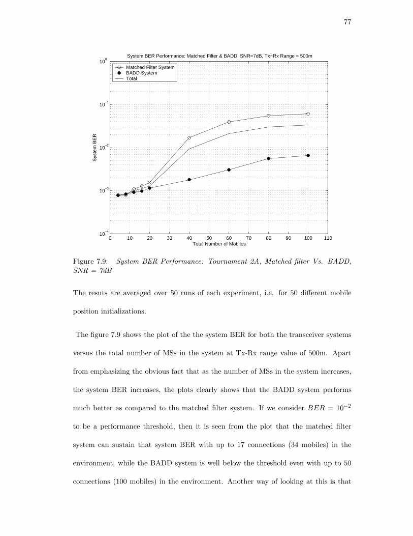
77
0 10 20 30 40 50 60 70 80 90 100 11010
−4
10−3
10−2
10−1
100
System BER Performance: Matched Filter & BADD, SNR=7dB, Tx−Rx Range = 500m
Total Number of Mobiles
Sys
tem
BE
R
Matched Filter SystemBADD SystemTotal
Figure 7.9: System BER Performance: Tournament 2A, Matched filter Vs. BADD,SNR = 7dB
The resuts are averaged over 50 runs of each experiment, i.e. for 50 different mobile
position initializations.
The figure 7.9 shows the plot of the the system BER for both the transceiver systems
versus the total number of MSs in the system at Tx-Rx range value of 500m. Apart
from emphasizing the obvious fact that as the number of MSs in the system increases,
the system BER increases, the plots clearly shows that the BADD system performs
much better as compared to the matched filter system. If we consider BER = 10−2
to be a performance threshold, then it is seen from the plot that the matched filter
system can sustain that system BER with up to 17 connections (34 mobiles) in the
environment, while the BADD system is well below the threshold even with up to 50
connections (100 mobiles) in the environment. Another way of looking at this is that
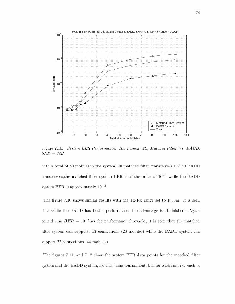
78
0 10 20 30 40 50 60 70 80 90 100 11010
−4
10−3
10−2
10−1
100
System BER Performance: Matched Filter & BADD, SNR=7dB, Tx−Rx Range = 1000m
Total Number of Mobiles
Sys
tem
BE
R
Matched Filter SystemBADD SystemTotal
Figure 7.10: System BER Performance: Tournament 2B, Matched Filter Vs. BADD,SNR = 7dB
with a total of 80 mobiles in the system, 40 matched filter transceivers and 40 BADD
transceivers,the matched filter system BER is of the order of 10−2 while the BADD
system BER is approximately 10−3.
The figure 7.10 shows similar results with the Tx-Rx range set to 1000m. It is seen
that while the BADD has better performance, the advantage is diminished. Again
considering BER = 10−2 as the performance threshold, it is seen that the matched
filter system can supports 13 connections (26 mobiles) while the BADD system can
support 22 connections (44 mobiles).
The figures 7.11, and 7.12 show the system BER data points for the matched filter
system and the BADD system, for this same tournament, but for each run, i.e. each of
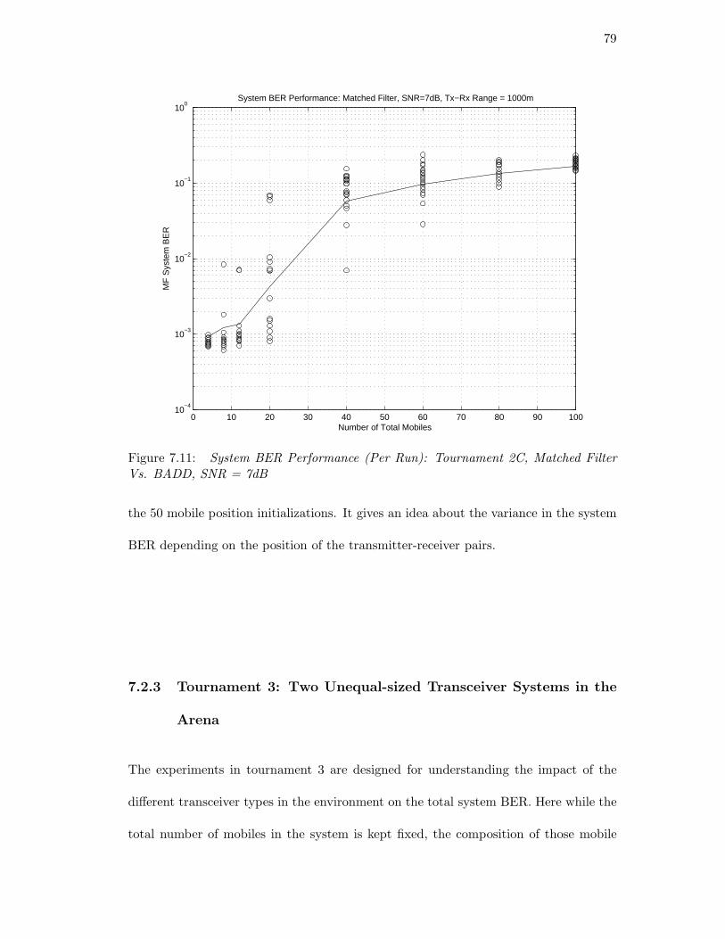
79
0 10 20 30 40 50 60 70 80 90 10010
−4
10−3
10−2
10−1
100
System BER Performance: Matched Filter, SNR=7dB, Tx−Rx Range = 1000m
Number of Total Mobiles
MF
Sys
tem
BE
R
Figure 7.11: System BER Performance (Per Run): Tournament 2C, Matched FilterVs. BADD, SNR = 7dB
the 50 mobile position initializations. It gives an idea about the variance in the system
BER depending on the position of the transmitter-receiver pairs.
7.2.3 Tournament 3: Two Unequal-sized Transceiver Systems in the
Arena
The experiments in tournament 3 are designed for understanding the impact of the
different transceiver types in the environment on the total system BER. Here while the
total number of mobiles in the system is kept fixed, the composition of those mobile
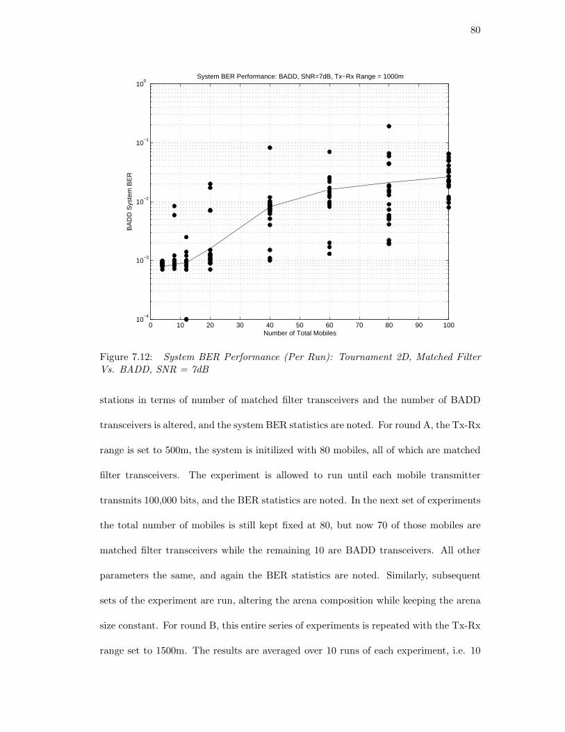
80
0 10 20 30 40 50 60 70 80 90 10010
−4
10−3
10−2
10−1
100
System BER Performance: BADD, SNR=7dB, Tx−Rx Range = 1000m
Number of Total Mobiles
BA
DD
Sys
tem
BE
R
Figure 7.12: System BER Performance (Per Run): Tournament 2D, Matched FilterVs. BADD, SNR = 7dB
stations in terms of number of matched filter transceivers and the number of BADD
transceivers is altered, and the system BER statistics are noted. For round A, the Tx-Rx
range is set to 500m, the system is initilized with 80 mobiles, all of which are matched
filter transceivers. The experiment is allowed to run until each mobile transmitter
transmits 100,000 bits, and the BER statistics are noted. In the next set of experiments
the total number of mobiles is still kept fixed at 80, but now 70 of those mobiles are
matched filter transceivers while the remaining 10 are BADD transceivers. All other
parameters the same, and again the BER statistics are noted. Similarly, subsequent
sets of the experiment are run, altering the arena composition while keeping the arena
size constant. For round B, this entire series of experiments is repeated with the Tx-Rx
range set to 1500m. The results are averaged over 10 runs of each experiment, i.e. 10
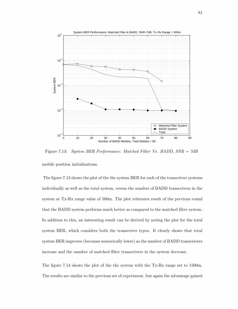
81
0 10 20 30 40 50 60 70 80 9010
−4
10−3
10−2
10−1
100
System BER Performance: Matched Filter & BADD, SNR=7dB, Tx−Rx Range = 500m
Number of BADD Mobiles, Total Mobiles = 80
Sys
tem
BE
R
Matched Filter SystemBADD SystemTotal
Figure 7.13: System BER Performance: Matched Filter Vs. BADD, SNR = 7dB
mobile position initializations.
The figure 7.13 shows the plot of the the system BER for each of the transceiver systems
individually as well as the total system, versus the number of BADD transceivers in the
system at Tx-Rx range value of 500m. The plot reiterates result of the previous round
that the BADD system performs much better as compared to the matched filter system.
In addition to this, an interesting result can be derived by noting the plot for the total
system BER, which considers both the transceiver types. It clearly shows that total
system BER improves (becomes numerically lower) as the number of BADD transceivers
increase and the number of matched filter transceivers in the system decrease.
The figure 7.14 shows the plot of the the system with the Tx-Rx range set to 1500m.
The results are similar to the previous set of experiment, but again the advantage gained
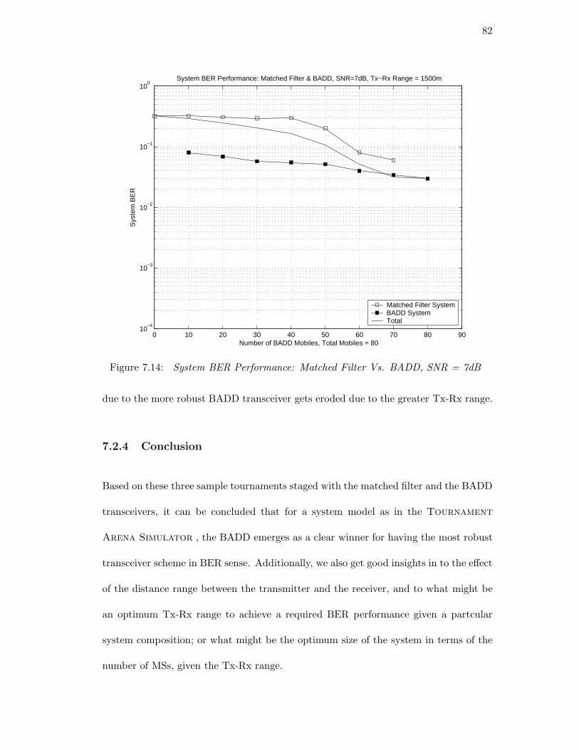
82
0 10 20 30 40 50 60 70 80 9010
−4
10−3
10−2
10−1
100
System BER Performance: Matched Filter & BADD, SNR=7dB, Tx−Rx Range = 1500m
Number of BADD Mobiles, Total Mobiles = 80
Sys
tem
BE
R
Matched Filter SystemBADD SystemTotal
Figure 7.14: System BER Performance: Matched Filter Vs. BADD, SNR = 7dB
due to the more robust BADD transceiver gets eroded due to the greater Tx-Rx range.
7.2.4 Conclusion
Based on these three sample tournaments staged with the matched filter and the BADD
transceivers, it can be concluded that for a system model as in the Tournament
Arena Simulator , the BADD emerges as a clear winner for having the most robust
transceiver scheme in BER sense. Additionally, we also get good insights in to the effect
of the distance range between the transmitter and the receiver, and to what might be
an optimum Tx-Rx range to achieve a required BER performance given a partcular
system composition; or what might be the optimum size of the system in terms of the
number of MSs, given the Tx-Rx range.
83
Chapter 8
Conclusion and Future Work
The thesis has described the Tournament Arena Simulator, a software simulation
platform for performance evaluation of wireless systems in the unlicensed bands, based
the Java binding of SSF. The concept of unlicensed band communication has been
explained. The system model, which is a simplified derivation of an unlicensed band
communication environment, is described conceptually, mathematically, and also from
the implementation point of view. The thesis has also explained how the simulation
platform can be configured to stage tournements between different wireless communi-
cations, and how meaningful statistics can be collected. The integrity of the Tour-
nament Arena Simulator has been validated by comparing the BER performance
statistics of some standard transceivers against theory. Some sample tournaments were
staged to demonstrate the functioning of the platform, and its utility in evaluating
the perfomance of different communications systems participating in the tournaments.
Some simple inferences with regards to a robust transceiver scheme were derived based
on the outcome of the sample tournamnents.
Tournament Arena Simulator has been shown to be a robust and versatile sim-
ulation platform for evaluating system performace in unlicensed band where multiple
84
autonomous wireless communications systems are existing simultaneously. It can pro-
vide performance statistics at the level of an individual mobile station, or a specific
transceiver system or for the entire wireless environment. It is possible to evaluate
one system at a time or to simultaneously evaluate several different systems. There is
adequate fexibility inherent in the platform at system parameter level as well as individ-
ual transceiver mechanism level to allow researchers implement very specific unlicensed
band communications scenarios with very specific transceiver schemes to experiment
with. The Tournament Arena Simulator is integrated with DATUM, WINLAB’s
Java SSF based viewer program, to enable viewing and run-time plotting of the graphs
for different system and mobile statistics. As shown by these results and conclusions,
the Tournament Arena Simulator can be used for exhaustive experimentation in
the area of unlicensed band communications, and as evidenced by the sample tour-
naments and its results, it could serve as a useful tool for defining the etiquette for
’peaceful co-existence’ of wireless systems.
Some avenues of future work include implementing fading in the radio channel, sup-
port of multiple-access schemes other than CDMA, defining higher level performance
statistics, and staging tournaments involving rate adaptation strategies.
85
Appendix A
Java-SSF Example Program
The objective of this appendix is to provide a basic understanding of the Java SSF
program. This is aimed at getting a better understanding of the functioning of the
TAS so as to actually help the user in setting up and running different experiments.
The main characteristic of a C++ SSF program are described in detail in [18]. The
basic fundamentals of the Java binding of the SSF are similar. This section restates
these and focuses on the functionalities that are specific to the Java binding.
We will describe the main characteristics of a SSF program by running through an
example program. Source code has been provided and the functionality of statements
has been detailed.
Consider a very basic communications system consisting of several MSs, wirelessly
connected connection as Transmitter-Receiver pairs, in a radio system environment.
There are 2 types of JAVA SSF entities:
• MobileStation : This entity represents the mobile stations and sends out mes-
sages on its outChannel, and receives messages on its inChannel
• RadioSystem : This entity encompasses all the MobileStation entities and does
the channel mapping
86
We now describe the system in more detail.
There are multiple MobileStations in the RadioSystem. Half of the MobileStations
are transmitters and the other half are receivers. Each transmitter is connected to ex-
actly one receiver. For this the transmitter MobileStations possess outChannels that
are mapped to the inChannels of the respective receiver MobileStations. The transmit-
ter and the receiver are represented by classes that extend the entity MobileStation,
which in turn is an extension of JAVA SSF base class entity.
The information is exchanged between the transmitter and the receiver MobileStations
over the outChannels and the inChannels˙
The entity MobileStation is described below. It specifies the basic parameters that
specify a mobile station such as the mobileID, the isTx flag identifying whether this is
a transmitter or not, and Info, the information it stores. MobileStation also has an
inChannel and an outChannel. The constructor initializes the MobileStation setting the
mobieId, defaulting it to a receiver, and resetting the Inf values to zero. The inChannel
and the outChannel are also initialized. It should be noted here that the outChannel is
initialized with a minimum delay of 1. This is a JAVA SSF requirement, and it implies
that every time an event is sent over the outChannel a delay of 1 simulation time unit
is added.
This is shown in the code block below.
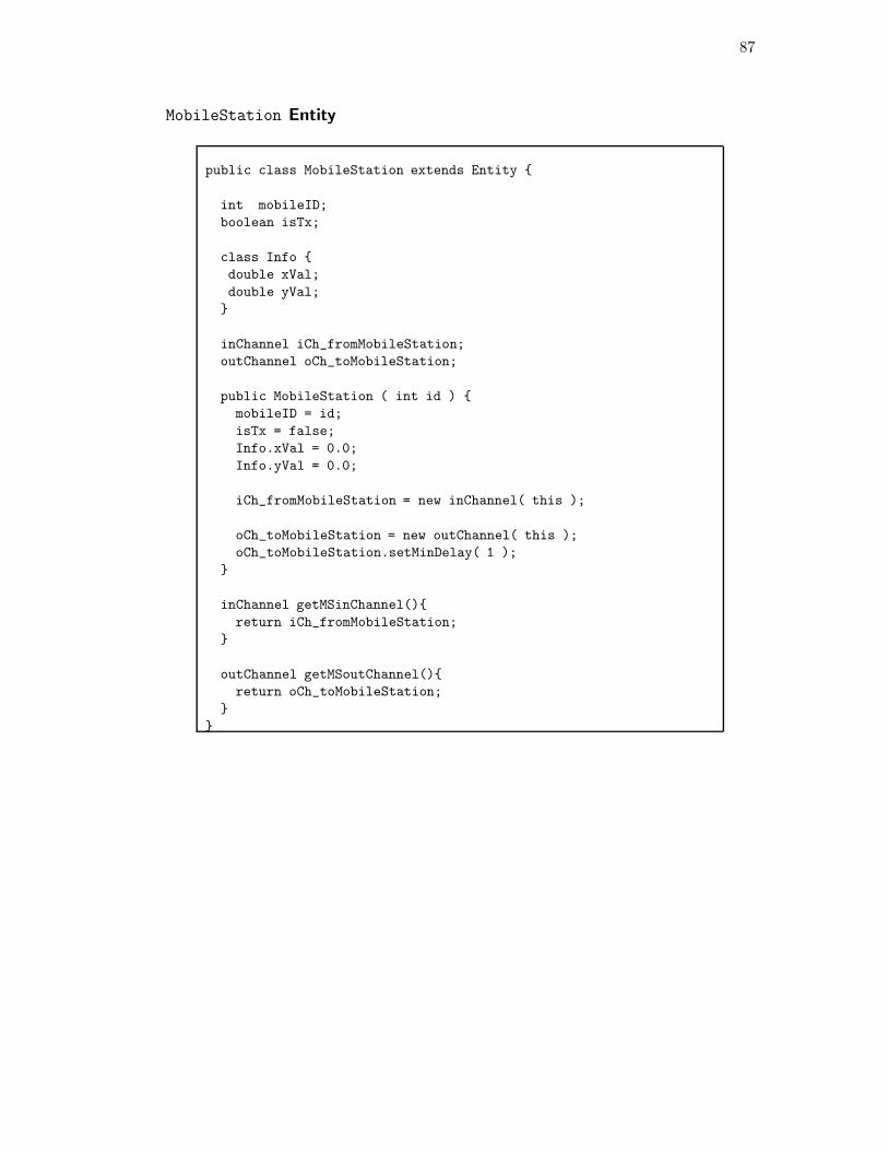
87
MobileStation Entity
public class MobileStation extends Entity {
int mobileID;boolean isTx;
class Info {double xVal;double yVal;
}
inChannel iCh_fromMobileStation;outChannel oCh_toMobileStation;
public MobileStation ( int id ) {mobileID = id;isTx = false;Info.xVal = 0.0;Info.yVal = 0.0;
iCh_fromMobileStation = new inChannel( this );
oCh_toMobileStation = new outChannel( this );oCh_toMobileStation.setMinDelay( 1 );
}
inChannel getMSinChannel(){return iCh_fromMobileStation;
}
outChannel getMSoutChannel(){return oCh_toMobileStation;
}}
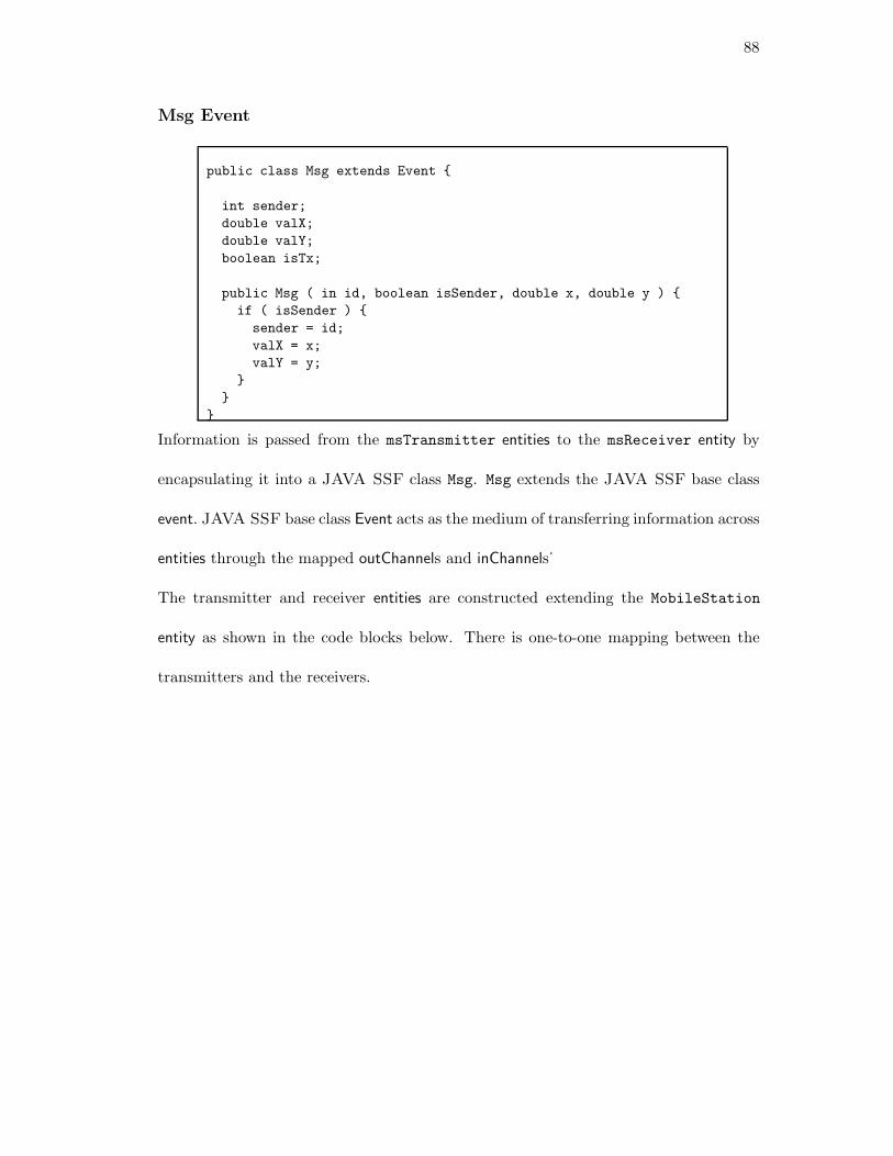
88
Msg Event
public class Msg extends Event {
int sender;double valX;double valY;boolean isTx;
public Msg ( in id, boolean isSender, double x, double y ) {if ( isSender ) {
sender = id;valX = x;valY = y;
}}
}
Information is passed from the msTransmitter entities to the msReceiver entity by
encapsulating it into a JAVA SSF class Msg. Msg extends the JAVA SSF base class
event. JAVA SSF base class Event acts as the medium of transferring information across
entities through the mapped outChannels and inChannels˙
The transmitter and receiver entities are constructed extending the MobileStation
entity as shown in the code blocks below. There is one-to-one mapping between the
transmitters and the receivers.
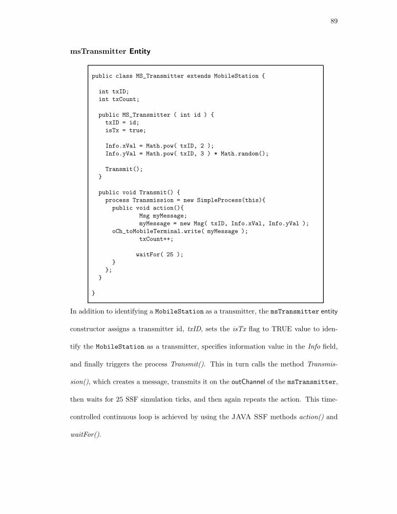
89
msTransmitter Entity
public class MS_Transmitter extends MobileStation {
int txID;int txCount;
public MS_Transmitter ( int id ) {txID = id;isTx = true;
Info.xVal = Math.pow( txID, 2 );Info.yVal = Math.pow( txID, 3 ) * Math.random();
Transmit();}
public void Transmit() {process Transmission = new SimpleProcess(this){
public void action(){Msg myMessage;myMessage = new Msg( txID, Info.xVal, Info.yVal );
oCh_toMobileTerminal.write( myMessage );txCount++;
waitFor( 25 );}
};}
}
In addition to identifying a MobileStation as a transmitter, the msTransmitter entity
constructor assigns a transmitter id, txID, sets the isTx flag to TRUE value to iden-
tify the MobileStation as a transmitter, specifies information value in the Info field,
and finally triggers the process Transmit(). This in turn calls the method Transmis-
sion(), which creates a message, transmits it on the outChannel of the msTransmitter,
then waits for 25 SSF simulation ticks, and then again repeats the action. This time-
controlled continuous loop is achieved by using the JAVA SSF methods action() and
waitFor().
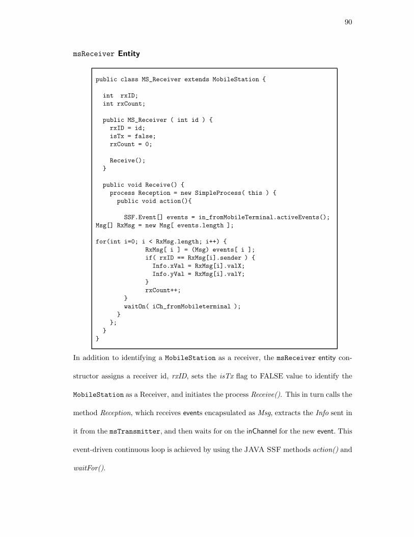
90
msReceiver Entity
public class MS_Receiver extends MobileStation {
int rxID;int rxCount;
public MS_Receiver ( int id ) {rxID = id;isTx = false;rxCount = 0;
Receive();}
public void Receive() {process Reception = new SimpleProcess( this ) {
public void action(){
SSF.Event[] events = in_fromMobileTerminal.activeEvents();Msg[] RxMsg = new Msg[ events.length ];
for(int i=0; i < RxMsg.length; i++) {RxMsg[ i ] = (Msg) events[ i ];if( rxID == RxMsg[i].sender ) {Info.xVal = RxMsg[i].valX;Info.yVal = RxMsg[i].valY;
}rxCount++;
}waitOn( iCh_fromMobileterminal );
}};
}}
In addition to identifying a MobileStation as a receiver, the msReceiver entity con-
structor assigns a receiver id, rxID, sets the isTx flag to FALSE value to identify the
MobileStation as a Receiver, and initiates the process Receive(). This in turn calls the
method Reception, which receives events encapsulated as Msg, extracts the Info sent in
it from the msTransmitter, and then waits for on the inChannel for the new event. This
event-driven continuous loop is achieved by using the JAVA SSF methods action() and
waitFor().
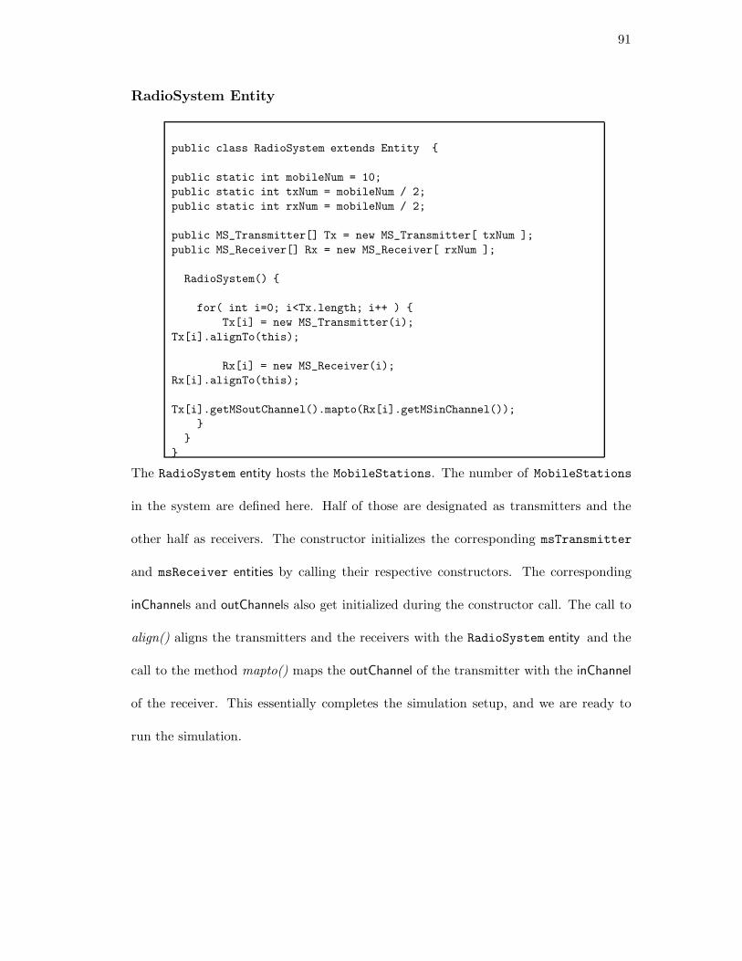
91
RadioSystem Entity
public class RadioSystem extends Entity {
public static int mobileNum = 10;public static int txNum = mobileNum / 2;public static int rxNum = mobileNum / 2;
public MS_Transmitter[] Tx = new MS_Transmitter[ txNum ];public MS_Receiver[] Rx = new MS_Receiver[ rxNum ];
RadioSystem() {
for( int i=0; i<Tx.length; i++ ) {Tx[i] = new MS_Transmitter(i);
Tx[i].alignTo(this);
Rx[i] = new MS_Receiver(i);Rx[i].alignTo(this);
Tx[i].getMSoutChannel().mapto(Rx[i].getMSinChannel());}
}}
The RadioSystem entity hosts the MobileStations. The number of MobileStations
in the system are defined here. Half of those are designated as transmitters and the
other half as receivers. The constructor initializes the corresponding msTransmitter
and msReceiver entities by calling their respective constructors. The corresponding
inChannels and outChannels also get initialized during the constructor call. The call to
align() aligns the transmitters and the receivers with the RadioSystem entity and the
call to the method mapto() maps the outChannel of the transmitter with the inChannel
of the receiver. This essentially completes the simulation setup, and we are ready to
run the simulation.
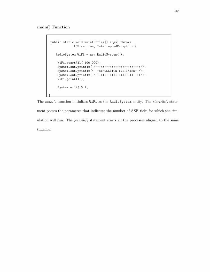
92
main() Function
public static void main(String[] args) throwsIOException, InterruptedException {
RadioSystem WiFi = new RadioSystem( );
WiFi.startAll( 100,000);System.out.println( "+++++++++++++++++++++++++");System.out.println(" -SIMULATION INITIATED- ");System.out.println( "+++++++++++++++++++++++++");WiFi.joinAll();
System.exit( 0 );
}
The main() function initializes WiFi as the RadioSystem entity. The startAll() state-
ment passes the parameter that indicates the number of SSF ticks for which the sim-
ulation will run. The joinAll() statement starts all the processes aligned to the same
timeline.
93
Appendix B
Transceiver Reconfiguration Primer
The objective of this appendix is to provide a step-by-step tutorial for achieving the
reconfiguration of the transceivers defined in the wireless environment. This appendix
should be treated as a complement to chapter 6 that talks about transceiver reconfig-
urability. The Tournament Arena Simulator provides the platform for simulating
tournaments between different autonomous wireless communication systems. It also
provides the flexibility to the users to define their own transceivers and hold tourna-
ments amongst those. The code has been set up so that the above can be achieved with
minimal knowledge of the existing code, and with only a basic working knowledge of
JAVA and SSF.
The following are the files that may need to be modified for re-defining the transceiver:
• ./code/mtMyTransceiver.java:
This is a new file, where the new transceiver is to be implemented.
• ./code/SimSetup.java :
This is the simulation setup parameter file, where both system-level and mobilestation-
level parameters are configured.
• ./code/Com.java :
94
If the tournament output needs to be written in to a file, the file defnitions are
done here.
• ./config/SysConfig.config:
This is the configuration file where the different autonomous wireless communi-
cation systems in the arena, and the number of mobilestations in each system are
specified.
The actual process of introducing new transceivers in to the tournament arena can be
explained through the following steps.
1. mtMyTransceiver Entity Definition
As explained in 6.2, MobileTerminal is the base class implementing a generic MS.
It contains all the necessary Java methods and JAVA SSF processes that provide
the basic functionality to the MS to work as a matched filter transceiver in a chip-
synchronous CDMA environment. Additional transceiver characterization can be
done by extending this JAVA SSF entity, and re-defining some of the methods and
processes. For example, in order to implement a BADD transceiver the derived
JAVA SSF class mtBADD is defined; and the process ReceptionProcess of the
MobileTerminal is over-written to include actions for filter-tap updates, and
decoding using the filter under construction.
Here we call the derived MobileTerminal class mtMyTransceiver. The sections
of the code, which are available for modification and re-definition are clearly de-
marcated, as shown below. It should be noted that Java file containing the newly
defined transceiver should have the same name as the derived MobileTerminal.
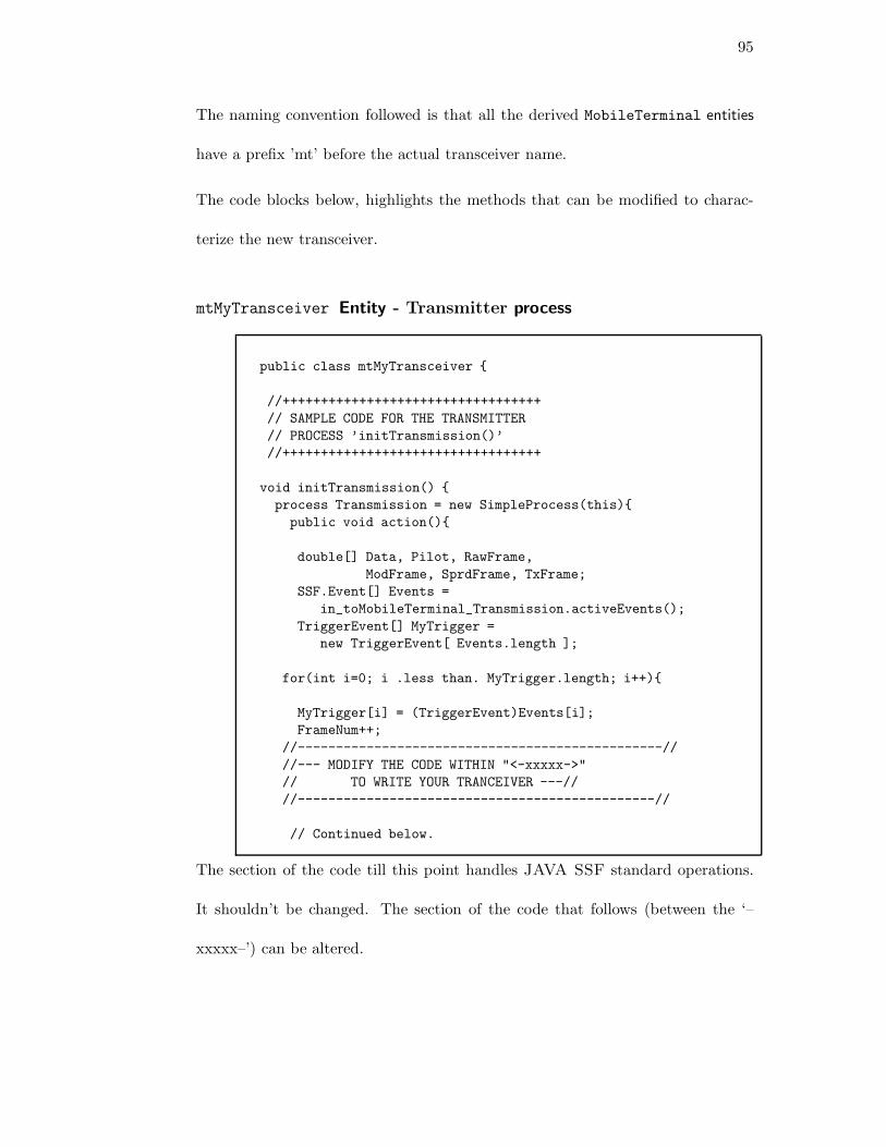
95
The naming convention followed is that all the derived MobileTerminal entities
have a prefix ’mt’ before the actual transceiver name.
The code blocks below, highlights the methods that can be modified to charac-
terize the new transceiver.
mtMyTransceiver Entity - Transmitter process
public class mtMyTransceiver {
//++++++++++++++++++++++++++++++++++// SAMPLE CODE FOR THE TRANSMITTER// PROCESS ’initTransmission()’//++++++++++++++++++++++++++++++++++
void initTransmission() {process Transmission = new SimpleProcess(this){public void action(){
double[] Data, Pilot, RawFrame,ModFrame, SprdFrame, TxFrame;
SSF.Event[] Events =in_toMobileTerminal_Transmission.activeEvents();
TriggerEvent[] MyTrigger =new TriggerEvent[ Events.length ];
for(int i=0; i .less than. MyTrigger.length; i++){
MyTrigger[i] = (TriggerEvent)Events[i];FrameNum++;
//------------------------------------------------////--- MODIFY THE CODE WITHIN "<-xxxxx->"// TO WRITE YOUR TRANCEIVER ---////-----------------------------------------------//
// Continued below.
The section of the code till this point handles JAVA SSF standard operations.
It shouldn’t be changed. The section of the code that follows (between the ‘–
xxxxx–’) can be altered.
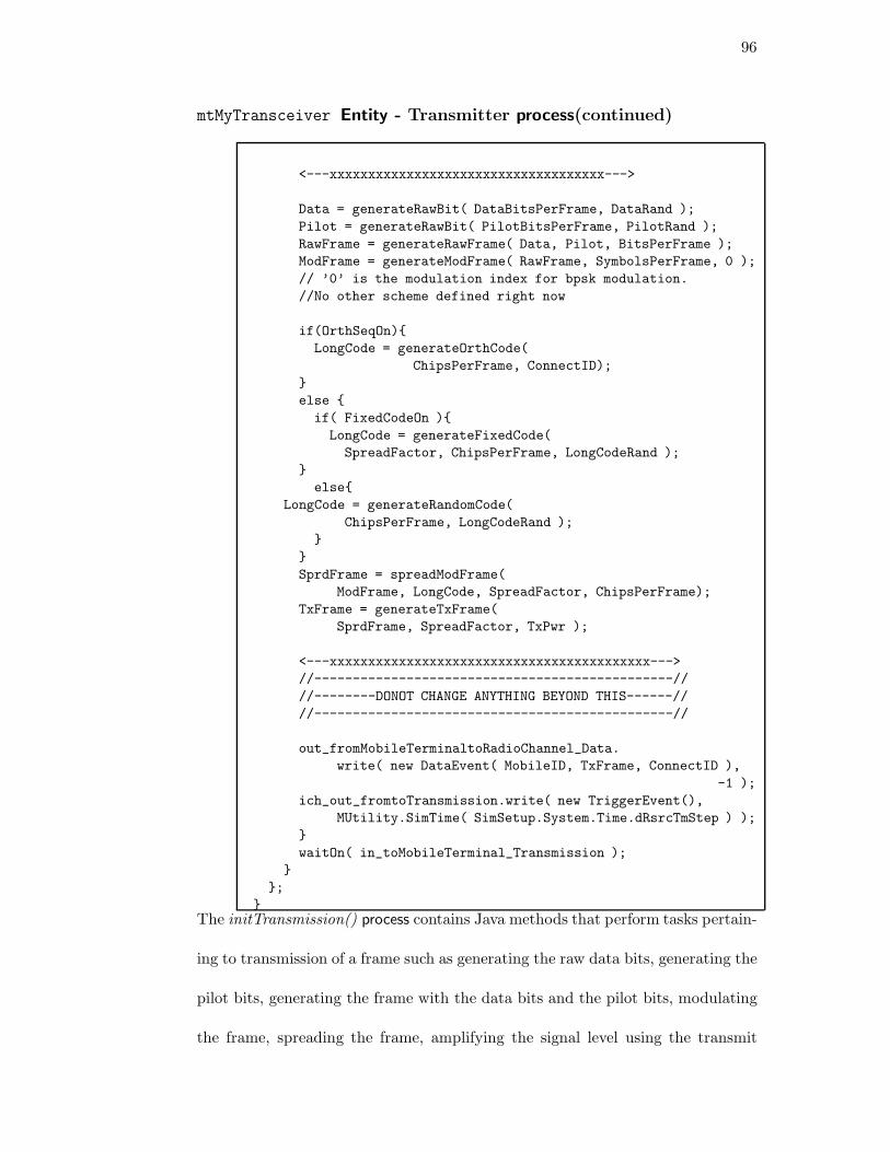
96
mtMyTransceiver Entity - Transmitter process(continued)
<---xxxxxxxxxxxxxxxxxxxxxxxxxxxxxxxxxxxx--->
Data = generateRawBit( DataBitsPerFrame, DataRand );Pilot = generateRawBit( PilotBitsPerFrame, PilotRand );RawFrame = generateRawFrame( Data, Pilot, BitsPerFrame );ModFrame = generateModFrame( RawFrame, SymbolsPerFrame, 0 );// ’0’ is the modulation index for bpsk modulation.//No other scheme defined right now
if(OrthSeqOn){LongCode = generateOrthCode(
ChipsPerFrame, ConnectID);}else {
if( FixedCodeOn ){LongCode = generateFixedCode(SpreadFactor, ChipsPerFrame, LongCodeRand );
}else{
LongCode = generateRandomCode(ChipsPerFrame, LongCodeRand );
}}SprdFrame = spreadModFrame(
ModFrame, LongCode, SpreadFactor, ChipsPerFrame);TxFrame = generateTxFrame(
SprdFrame, SpreadFactor, TxPwr );
<---xxxxxxxxxxxxxxxxxxxxxxxxxxxxxxxxxxxxxxxxxx--->//-----------------------------------------------////--------DONOT CHANGE ANYTHING BEYOND THIS------////-----------------------------------------------//
out_fromMobileTerminaltoRadioChannel_Data.write( new DataEvent( MobileID, TxFrame, ConnectID ),
-1 );ich_out_fromtoTransmission.write( new TriggerEvent(),
MUtility.SimTime( SimSetup.System.Time.dRsrcTmStep ) );}waitOn( in_toMobileTerminal_Transmission );
}};
}The initTransmission() process contains Java methods that perform tasks pertain-
ing to transmission of a frame such as generating the raw data bits, generating the
pilot bits, generating the frame with the data bits and the pilot bits, modulating
the frame, spreading the frame, amplifying the signal level using the transmit
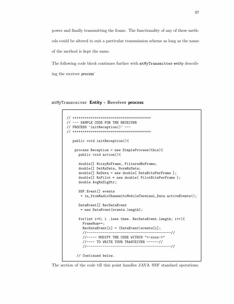
97
power and finally transmitting the frame. The functionality of any of these meth-
ods could be altered to suit a particular transmission scheme as long as the name
of the method is kept the same.
The following code block continues further with mtMyTransmitter entity describ-
ing the receiver process˙
mtMyTransceiver Entity - Receiver process
// +++++++++++++++++++++++++++++++++++++++// --- SAMPLE CODE FOR THE RECEIVER// PROCESS ’initReception()’ ---// +++++++++++++++++++++++++++++++++++++++
public void initReception(){
process Reception = new SimpleProcess(this){public void action(){
double[] NoisyRxFrame, FilteredRxFrame;double[] DetRxData, NormRxData;double[] RxData = new double[ DataBitsPerFrame ];double[] RxPilot = new double[ PilotBitsPerFrame ];double AvgRxSigStr;
SSF.Event[] events= in_fromRadioChanneltoMobileTerminal_Data.activeEvents();
DataEvent[] RecDataEvent= new DataEvent[events.length];
for(int i=0; i .less then. RecDataEvent.length; i++){FrameNum++;RecDataEvent[i] = (DataEvent)events[i];//------------------------------------------////----- MODIFY THE CODE WITHIN "<-xxxx->"//---- TO WRITE YOUR TRANCEIVER ------////------------------------------------------//
// Continued below.
The section of the code till this point handles JAVA SSF standard operations.

98
It shouldn’t be changed. The section of the code that follows (between the ‘–
xxxxx–’) can be altered.
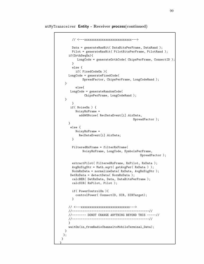
99
mtMyTransceiver Entity - Receiver process(continued)
// <---xxxxxxxxxxxxxxxxxxxxxxxxxxx--->
Data = generateRawBit( DataBitsPerFrame, DataRand );Pilot = generateRawBit( PilotBitsPerFrame, PilotRand );
if(OrthSeqOn){LongCode = generateOrthCode( ChipsPerFrame, ConnectID );
}else {if( FixedCodeOn ){
LongCode = generateFixedCode(SpreadFactor, ChipsPerFrame, LongCodeRand );
}else{
LongCode = generateRandomCode(ChipsPerFrame, LongCodeRand );
}}
if( NoiseOn ) {NoisyRxFrame =addWGNoise( RecDataEvent[i].AirData,
SpreadFactor );}else {
NoisyRxFrame =RecDataEvent[i].AirData;
}
FilteredRxFrame = filterRxFrame(NoisyRxFrame, LongCode, SymbolsPerFrame,
SpreadFactor );
extractPilot( FilteredRxFrame, RxPilot, RxData );AvgRxSigStr = Math.sqrt( getAvgPwr( RxData ) );NormRxData = normalizeData( RxData, AvgRxSigStr );
DetRxData = detectData( NormRxData );calcBER( DetRxData, Data, DataBitsPerFrame );calcSIR( RxPilot, Pilot );
if( PowerControlOn ){controlPower( ConnectID, SIR, SIRTarget);
}
// <---xxxxxxxxxxxxxxxxxxxxxxxxxxxx--->//--------------------------------------------////-------- DONOT CHANGE ANYTHING BEYOND THIS -----////--------------------------------------------//}waitOn(in_fromRadioChanneltoMobileTerminal_Data);
}};
}}
100
The initReception() process contains the Java methods for performing tasks re-
lated to the receiving and decoding of a signal by a matched filter receiver. These
include filtering the received frame, extracting the pilot bits, decoding and de-
tecting the desired bit and calculating the SIR and the BER statistics. The
functionality of any of these methods can be altered as long as the name is kept
the same.
2. Simulation Setup Configuration
Once the mtMyTransceiver is defined, the next step is to set the simulations pa-
rameters in the Java file SimSetup.java. Some of the key parameters that are likely
to be modified are the number of autonomous systems in the arena, the number
of MS per the autonomous system, the maximum allowable distance between the
transmitter and its receiver, and the simulation run-time. A comprehensive list
of the simulation setup parameters is defined in 6.5.
3. Output File Definition
If the simulation output statistics like SIR, BER etc need to be written in to a
file for further analysis, the Java file Com.java needs to be modified. This file
is already setup with methods that write the different parameters. The naming
of the output file can be customized by specifying the addIn parameter value
depending on the type of tournament.
4. Configuration File Definition
The overall composition of the tournament arena needs to be summarized in the
file SysConfig.config. This includes the names of the files that contain the updated
transceivers, the number of MSs of each transceiver type, and the type of the
101
system whether ad-hoc mobile or cellular. For example, if for a tournament the
derived MobileTerminal entities are mtMyTransceiver1 with 20 mobile stations
(10 Tx-Rx pairs), and mtMyTransceiver2 with 30 mobile stations (15 Tx-Rx
pairs), the specification of the system configuration file will be as shown in the
code block below. Additionally, the SimSetup.java file should be updated so that
the parameter System.Environ.iNoAutoSystem has value 2, and the parameter
System.Environ.iNoMobile has the value 50.
A sample configuration file is given as a part of the code block.
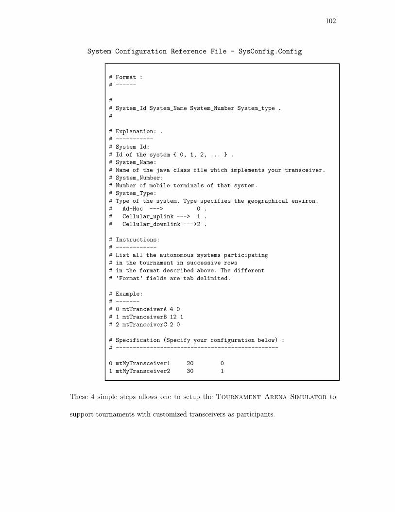
102
System Configuration Reference File - SysConfig.Config
# Format :# ------
## System_Id System_Name System_Number System_type .#
# Explanation: .# -----------# System_Id:# Id of the system { 0, 1, 2, ... } .# System_Name:# Name of the java class file which implements your transceiver.# System_Number:# Number of mobile terminals of that system.# System_Type:# Type of the system. Type specifies the geographical environ.# Ad-Hoc ---> 0 .# Cellular_uplink ---> 1 .# Cellular_downlink --->2 .
# Instructions:# ------------# List all the autonomous systems participating# in the tournament in successive rows# in the format described above. The different# ’Format’ fields are tab delimited.
# Example:# -------# 0 mtTranceiverA 4 0# 1 mtTranceiverB 12 1# 2 mtTranceiverC 2 0
# Specification (Specify your configuration below) :# ------------------------------------------------
0 mtMyTransceiver1 20 01 mtMyTransceiver2 30 1
These 4 simple steps allows one to setup the Tournament Arena Simulator to
support tournaments with customized transceivers as participants.
103
References
[1] FCC Report and Order 96-36: Amendments of Parts 2 and 15 of the Commission’sRules Regarding the Spred Spectrum Transmitters.
[2] FCC Report and Order 97-5: Amendment of the Commission’s Rules to ProvideUnlicensed NII Devices in the 5 GHz Frequency Range.
[3] Specification of the Bluetooth System.
[4] SSFNET website : http://www.ssfnet.org.
[5] U-nii: Winlab research goals and benefits. Internal Document.
[6] Wireless LAN Medium Access Control(MAC) and Physical Layer(PHY) Specifi-cations.
[7] Scalable Simulation Framework API Reference Manual, 1999. Version 1.0.
[8] Ken Arnold and James Gosling. The Java Programming Language. Addison-Wesley, 1997.
[9] Kevin Gang Chen. Integrated Dynamic Radio Resource Management of WirelessCommunication Systems. Masters thesis, Rutgers, The State University of NewJersey, New Brunswick, NJ, May 1996.
[10] M. Ellis and B. Stroustrup. The annotated C++ reference manual. Addison-Wesley, 1990.
[11] R. Gold. Optimal Binary Sequence for Spread Spectrum Multiplexing. IEEETransactions on Information Theory, Vol. IT-13), pages 619–627, October 1967.
[12] R. Gold. Maximal Recursive Sequences with 3-Valued Recursive Cross CorrelationFunctions. IEEE Transactions on Information Theory, Vol. IT-14), pages 154–156,January 1968.
[13] M. Gudmundson. Correlation model for shadow fading in mobile radio systems.Electron. Lett., 27(23):2145–2146, 1991.
[14] D. B. Johnson Y. Hu J. Broch, D. A. Matz and J. Jetcheva. A performancecomparison of multi-hop wireless ad hoc network routing protocols. Oct 1998.
[15] Jason Liu David M. Nicol Andrew T. Ogeilski James Cowie, Hongbo Liu. To-wards Realistic Million Node Internet Simulation. Proceedings of InternationalConference on Parallel and Distributed Processing Techniques and Applications,4:2129–2135, 1999.
104
[16] David B. Johnson. Routing in ad hoc networks of mobile hosts. Dec 1994.
[17] Jeffery A. Joines and Stephen D. Roberts. Design of Object Oriented Simulationsin C++. Proc. of the 1995 Winter Simulation Conference.
[18] Vikram Kaul. Multi-cell wcdma signal processing simulation testbed. Mastersthesis, Rutgers, The State University of New Jersey, New Brunswick, NJ, Oct2000.
[19] Robert Lafore. Object-Oriented programming in Turbo C++. Waite Group, 1999.
[20] R. Lupas and S. Verdu. Linear Multiuser Detectors for Synchronous Code-DivisionMultiple-Access Channels. IEEE Transactions on Information Theory, 35:123–136, Jan 1989.
[21] Jignesh Panchal. Wippet : Wireless propagation and protocol evaluation testbed.Masters thesis, Rutgers, The State University of New Jersey, New Brunswick, NJ,Sep 1998.
[22] K. Perumalla and R. Fujimoto. A C++ instance of TeD. TR GIT-CC-96-33,College of Computing, Georgia Institute of Technology, 1996.
[23] K. Perumalla, A. Ogielski, and R. Fujimoto. MetaTeD: A meta language formodeling telecommunication networks. TR GIT-CC-96-32, College of Computing,Georgia Institute of Technology, 1996.
[24] T. S. Rappaport. Wireless Communications. Prentice Hall, first edition, 1996.pages 69–192.
[25] David G. Steer. Co-existence and access etiquette in the united states unlicensedpcs band. IEEE Personal Communications, Fourth Quarter:36–43, 1994.
[26] S. Ulukus and R. Yates. A Blind Adaptive Decorrelating Detector for CDMASystems. IEEE Journal Selected Areas in Communications, 16:1530–1541, Aug1998.