To Segregate or to Integrate:Education Politics and Democracy∗

David de la Croix† Matthias Doepke‡

July 2008

Abstract

How is the quality of public education affected by the presence of pri-vate schools for the rich? Theory and evidence suggest that the link dependscrucially on the political system. We develop a theory that integrates privateeducation and fertility decisions with voting on public schooling expendi-tures. We find that the presence of a large private education sector benefitspublic schools in a broad-based democracy where politicians are responsiveto low-income families, but crowds out public-education spending in a so-ciety that is politically dominated by the rich. The main predictions of thetheory are consistent with state-level and micro data from the United Statesas well as cross-country evidence from the PISA study.

JEL Classification Numbers: D72, I21, H42, O10.

∗We thank Sandy Black, Georges Casamatta, Jean Hindriks, Omer Moav, Fabien Moizeau, Vin-cent Vandenberghe, the editor, three anonymous referees, and seminar participants at Louvain-la-Neuve, Rotterdam, the Stockholm School of Economics, Toulouse, UCLA, Royal Holloway, TelAviv, and the SED Annual Meeting in Florence for comments that helped to make substantialimprovements to the paper. Simeon Alder and David Lagakos provided excellent research assis-tance. David de la Croix acknowledges financial support from the Belgian French-speaking com-munity (grant ARC 99/04-235) and the Belgian Federal Government (grant PAI P5/21). MatthiasDoepke acknowledges support from the National Science Foundation (grant SES-0217051) andthe Alfred P. Sloan Foundation.

†Department of Economics and CORE, Universite catholique de Louvain, Place Montesquieu3, B-1348 Louvain-la-Neuve, Belgium (e-mail: david.delacroix@uclouvain.be).

‡Department of Economics, Northwestern University, 2001 Sheridan Blvd, Evanston, IL 60608(e-mail: doepke@northwestern.edu.)

1 Introduction

Public schooling is one of the most pervasive social policies around the world to-day. Following the lead of industrializing European nations in the nineteenthcentury, nearly all countries have introduced compulsory schooling laws andpublic funding of education. However, despite the almost universal involvementof governments, private and public funding of education continue to coexist. Theshare of private education funding varies greatly across countries, from only 1.9percent of total spending in Norway, to 44.5 percent in Chile (1998, see Section 6).Institutional arrangements concerning the funding of private schools also differacross countries. Private schools can be supported partly by the government asin France or New Zealand, can be entirely publicly funded as in Belgium, or mayrely exclusively on private funding as in the United States (Toma 1996).

Recently, the OECD Programme for International Student Assessment (PISA),which assesses the knowledge and skills of 15-year-old students in a cross-sectionof countries, has sparked an intense debate on the relative merits of differenteducation systems. A central question in this debate is why education systemsdiffer so much across countries in the first place. Are there particular countrycharacteristics that explain the choice of an integrated education system over aregime that segregates public from private schools? Equally important are theimplications for school quality: How is the funding level of public educationaffected by the presence of private schools for the rich?

The aim of this study is to provide a positive theory of education systems that canbe used to address these questions. We develop an analytically tractable frame-work that integrates political determination of the quality of public schools withprivate education and fertility decisions. Parents may choose between sendingtheir children to tax-financed public schools and, alternatively, opting out of thepublic system and providing private education to their children. They also deter-mine their number of children as a function of their income and of the expectedquality of schools. A key feature of our political economy setup is that it allowsfor bias in the political system: the weight of a certain group of voters in po-litical decision making may be larger or smaller that the group’s relative size inthe population. In particular, we contrast outcomes under an even distribution of

1

political power, as in a representative democracy, with outcomes when a politicalbias gives a disproportionate share of power to the rich.

Consider first the case of a true democracy, in which the rich and poor haveequal weight in the political process. Parents send their children to a privateschool only if they would like to endow their children with an education of amuch higher quality than that provided by the public system. This implies thatincome inequality is the main determinant of the extent of segregation in theschooling system. In a society with little inequality, the preferred education levelvaries little in the population, so that most or all parents use public schooling.For increasing levels of inequality, an increasing share of richer people choosesprivate education for their children.1

From a policy perspective, perhaps the most important question is how the ex-tent of private schooling affects the quality of public schooling. In our political-economy model, when more and more rich parents send their children to privateschool, these parents no longer stand to gain from high-quality public education.These parents therefore vote for lower taxes and less spending on public schools.It does not necessarily follow, however, that the quality of public schools will de-cline as the share of private education increases. When rich parents opt out of thepublic system, the remaining funding of the public system can be concentratedon fewer students. Thus, even when there is a decline in total funding, spend-ing per student (which is one measure of the quality of education) may well goup.2 We show that as long as the poor carry equal weight in the political system,the relationship between the share of private schooling and the quality of publicschooling is indeed positive.

An additional benefit from private education arises because fertility decisions areendogenous. Consistent with empirical evidence, the theory predicts that poorerparents who use public schools have more children than parents opting for costlyprivate schools. By raising their fertility rate relative to what they would choose ifthey were paying for their children’s education, the public-school parents impose

1This echoes the result of Besley and Coate (1991). Assuming that quality is a normal good,households who opt out of the public sector are those with higher incomes.

2This result provides a contrast to a literature in which a greater degree of inequality motivatesmore redistribution through higher taxes (see Alesina and Rodrik 1994, Persson and Tabellini1994, and in particular Gradstein and Justman 1997 in an application to education).

2

a fiscal externality on all taxpayers. This externality is absent if parents send theirchildren to private schools and therefore fully take into account the educationcost of the marginal child.

The findings described so far apply to countries with equal political representa-tion for all. But what about countries farther away from the democratic ideal?Consider a non-democratic country in which only the political views of an en-trenched, rich elite matter. If inequality is not too severe, one possibility is thatmost families, including the elite, use public schools. In this case, the politicalelite has a direct interest in the quality of public schools, and the outcomes interms of education spending and the quality of schooling are similar to those ofan otherwise identical democracy. However, a second possibility is that most orall of the political elite use private schools. Public education spending and thequality of public schools then tend to be low, because the political elite has novested interest in public schooling. Thus, unlike in democracies, a high share ofprivate schooling will generally lead to a low quality of public schools.

The main predictions of our theory are consistent with a set of stylized facts onpublic and private schooling in the U.S. as well as in a cross section of coun-tries. For the U.S., we document that states with higher inequality have a largershare of private schooling and lower overall spending on public schooling, but ahigher quality of public schooling. At the micro level, fertility is decreasing andthe probability of using private schools is increasing in income. Moreover, theslope of the income-fertility relationship is flatter in states with a higher qualityof public schooling. We obtain similar findings in cross-country data. Using mi-cro data from the OECD PISA program, we confirm that in a large set of countrieshigh-income households are more likely to use private education, while thesehouseholds’ fertility rates are lower. Comparing across countries, high inequal-ity is associated with a larger share of private schooling.

Concerning the role of political power, we turn to the relationship between democ-racy and education funding. If we interpret democracies as countries with aneven distribution of political power, while non-democracies are biased to the rich,our model implies that there is more scope for variation in education systems innon-democracies than in democracies. Indeed, using a cross section of 158 coun-tries, we find that the variance of public spending across countries is smaller for

3

democracies than for non-democracies.

Our paper relates to different branches of the literature. A number of authorshave addressed the choice of public versus private schooling within a majorityvoting framework (see Stiglitz 1974, Glomm and Ravikumar 1998, Epple andRomano 1996b, and Bearse, Glomm, and Patterson 2005). A recurring themein this literature is the argument that if there are private alternatives to publicschools, voters’ preferences may not be single-peaked, so that a majority votingequilibrium may fail to exist. In contrast, we rely on probabilistic voting as thepolitical mechanism, which yields a fully tractable theory of education regimesin which voting equilibria are guaranteed to exist. Moreover, our probabilisticvoting setup is not restricted to democracies, since we can analyze what happensif the political system is biased to the rich. The second main departure from theexisting literature is that we endogenize fertility decisions, which leads to novelimplications for uniqueness and efficiency properties of equilibria.

Our model makes predictions for the link between inequality in a country andthe resulting education system and quality of education. A similar objective isfollowed by Fernandez and Rogerson (1995), who consider a model where edu-cation is discrete and partially subsidized by the government, and voters decideon the extent of the subsidy. Fernandez and Rogerson emphasize that in unequalsocieties, the poor may forgo education entirely. Since all voters are taxed, inthis case public education constitutes a transfer of resources from the poor andthe rich to the middle class, echoing the findings of Epple and Romano (1996a).While these arguments are highly relevant for the case of post-secondary edu-cation, at the primary and secondary levels participation rates are high even forpoor children in most countries. Thus, at these levels the choices that we modelhere (private versus public education and the quality of public education) maybe the more important margins.

Another branch of the literature takes the schooling regime (public or private)as given, and analyzes the economic implications of each regime. Glomm andRavikumar (1992) contrast the effects of public and private schooling systemson growth and inequality. In a country with little inequality, a fiscal externalitycreated by public schooling leads to lower growth under public schooling thanunder private schooling. In unequal societies, however, public schooling can

4

dominate, since more resources are directed to poor individuals with a high re-turn on education. Similar conclusions are derived by de la Croix and Doepke(2004) in a framework which emphasizes the interdependence of fertility and ed-ucation decisions of parents. The model of Glomm and Ravikumar (1992) hasbeen extended by Benabou (1996) to allow for local interactions between agents,such as neighborhood effects and knowledge spillovers. Our work advances rel-ative to these papers by endogenizing the choice of the schooling regime as afunction of the income distribution and the political system.

Finally, Benabou (2000), among others, has pointed out that in the data, moreunequal countries tend to redistribute less. Our model provides a rationale forthis empirical finding. Benabou (2000) also develops a model that is consistentwith this observation, albeit through a different mechanism. In his setup, it is as-sumed that political participation increases with income. When inequality rises,the decisive voter is richer and decides for less redistribution. The opting-outdecision in our model provides an alternative to Benabou’s mechanism. A cru-cial difference between the two theories is that in our model, as long as politicalpower is evenly distributed an increase in inequality actually improves the wel-fare of a poor agent of a given income, even though total tax revenue declines.This is possible because the quality of public schooling improves: the numberof students who use public schools declines faster with inequality than overalltax revenue, implying that the funding level per student increases. Thus, eventhough an increase in inequality reduces the total amount of redistribution, thetransfers to public-school parents become more targeted, leaving the poor betteroff.

In the next section, we introduce our model and analyze the political equilibrium.Section 3 describes how in a democratic country the choice of a schooling regimeand the quality of schooling depend on the income distribution. Section 4 gen-eralizes the voting process to allow for unequal political power. We show thatmultiple equilibria can arise in societies dominated by the rich. In Section 5 weanalyze alternative timing assumptions. In Section 6 we confront the testable im-plications of the model with empirical evidence. Section 7 concludes. All proofsare contained in the mathematical appendix.

5

2 The Model Economy

2.1 Preferences and technology

The model economy is populated by a continuum of households of measure one.Households are differentiated by their human capital endowment x, where x isthe wage that a household can obtain in the labor market. People care aboutconsumption c, their number of children n, and their children’s education h. Theutility function is given by:3

ln(c) + γ [ln(n) + η ln(h)] . (1)

Notice that parents care both about child quantity n and quality h. The parameterγ ∈ R+ is the overall weight attached to children. The parameter η ∈ (0, 1) is therelative weight of quality.4 As we will see below, the tradeoff between quantityand quality is affected by the human capital endowment of the parent and by theschooling regime.

To attain human capital, children have to be educated by teachers. The wage ofteachers equals the average wage in the population, which is normalized to one.5

Parents can choose between two different modes of education. First, there is apublic schooling system, which provides a uniform education s to every student.Education in the public system is financed through an income tax v; apart fromthe tax, there are no direct costs to the parents. The schooling quality s and the taxrate v are determined through voting, to be described in more detail later. Parentsalso have the possibility of opting out of the public system. In this case, parentscan freely choose the education quality e, but they have to pay the teacher out of

3The logarithmic utility function is chosen for simplicity; any utility function representinghomothetic preferences over the bundle (c, n, h) would lead to the same results. Also, while wefocus on a static framework here, the working-paper version of this paper extends the analysis toa dynamic setting where today’s children are tomorrow’s adults.

4The parameter η cannot exceed 1 because the parents’ optimization problem would not havea solution. More specifically, utility would approach infinity as parents choose arbitrarily highlevels of education and arbitrarily low levels of fertility. A similar condition can be found in Moav(2005).

5The important assumption here is that the cost of education is fixed, i.e., all parents face thesame education cost regardless of their own wage. The level of the teacher’s wage is set to theaverage wage for convenience.

6

their own income. Since education e is measured in units of time of the averageteacher, the total cost of educating n children privately is given by ne. We assumethat education spending is tax deductible. While tax deductibility of educationexpenditures varies across countries, deductibility simplifies the analysis becauseit implies that taxation does not distort the choice between quantity and qualityof children.6 Apart from the education expenditure, raising one child also takesfraction φ ∈ (0, 1) of an adult’s time. The budget constraint for an adult withwage x is given by:

c = (1 − v) [x(1 − φn) − ne] . (2)

Education is thus either private, e, or public, s. Effective education can be ex-pressed as the maximum of the two: h = max{e, s}. Of course, parents whoprefer public education will choose e = 0.

Substituting the budget constraint (2) into the utility function (1) allows rewritingthe utility of a given household as:

u[x, v, n, e, s] = ln(1 − v) + ln(x(1 − φn) − ne) + γ ln n + γη ln max{e, s}.

The consumption good is produced by competitive firms using labor as the onlyinput. We assume that the aggregate production function is linear in effectivelabor units. The production setup does not play an important role in our analysis;the advantage of the linear production function is that the wage is fixed.

2.2 Timing of events and private choices

The level of public funding for education s is chosen by a vote among the adultpopulation. The voters’ preferences depend on their optimal fertility and edu-cation choices (n and e), which are made before voting takes place. In makingthese choices, agents have perfect foresight regarding the outcome of the vot-ing process. This timing is motivated by the observation that public educationspending can be adjusted frequently, while fertility cannot. Similarly, the choice

6The same result would arise if parents educated their own children (or at least had the optionto do so), because then the parents’ teaching efforts would reduce their taxable income.

7

between public versus private education entails substantial switching costs, es-pecially when educational segregation is linked to residential segregation.7

At given expected policy variables v and s, the utility function u is concave inn. Within each group, some agents may choose public schooling, in which casetheir fertility rate is denoted ns, while others opt for private education; fertilityfor those in private schools is denoted as ne. All parents planning to send theirchildren to the public school choose the same fertility level:

ns = arg maxn

u[x, v, n, 0, s] =γ

φ(1 + γ). (3)

Fertility is constant because the income and substitution effects exactly offseteach other. On the one hand, richer parents would like to have more children,but on the other hand their opportunity cost of raising children is also higher.

The households planning to provide private schooling chose:

n = arg maxn

u[x, v, n, e, s] =xγ

(1 + γ)(e + φx),

e[x] = arg maxe

u[x, v, n, e, s] =ηφx

1 − η. (4)

Private spending on education depends positively on the wage x. Since the basiccost of children is a time cost, having children is expensive for skilled parents. Incontrast, the cost of educating children is a resource cost, which is more afford-able for skilled, high-income parents. Hence, they have a comparative advantagein terms of raising educated children (as in Moav (2005)).

Notice that e is independent of the outcome of the voting process, implying thatthe timing of choosing e does not affect the results (in contrast, we will see inSection 5 that the timing of choosing between public and private schooling doesmatter). Replacing the optimal value for e[x] in the fertility equation we find:

ne =γ(1 − η)φ(1 + γ)

. (5)

Thus, conditional on choosing private schooling, fertility is independent of x as

7In Section 5 we will explore the implications of alternative timing assumptions.

8

well. From equations (3) and (5) we see that parents choosing private educationhave a lower fertility rate.

Lemma 1 (Constant parental spending on children)For given s, v and x, parental spending on children (and therefore taxable income) doesnot depend on the choice of private versus public schooling, and is equal to γ

1+γ x.

Lemma 1 implies that the tax base does not depend on the fraction of people par-ticipating in public schooling. This property will be important for establishinguniqueness of equilibrium. The lemma relies on three assumptions: homotheticpreferences, tax deductible education spending, and endogenous fertility. Withendogenous fertility, parents choosing private schools have fewer children, keep-ing their total budget allocation to children in line with those choosing publicschools.8 This is a typical feature of endogenous fertility models.

A first result is that parents with high human capital are more demanding interms of expected public education quality. In other words, child quality is anormal good:

Lemma 2 (Opting out decision)There exists an income threshold:

x =1 − η

δφηE[s] with: δ = (1 − η)

1η (6)

such that households strictly prefer private education if and only if x > x.

Here E[s] is expected quality of public schooling. An implication of the abovelemma is that if some people with income x choose public schooling, all peoplewith income x′ < x will strictly prefer public schooling. Similarly, if at least somepeople with income x opt out of the public system and choose private education,all households with income x′ > x make the same choice.

We assume a uniform distribution of human capital over the interval [1 − σ, 1 +σ]. Accordingly, the associated density function is given by g(x) = 0 for x < 1−σ

8With fixed fertility, the resources allocated to children would be xφn with public educationand xφn/(1 − η) with private education. However, even with fixed fertility a constant tax basecould be achieved through an endogenous labor supply setup.

9

and if x > 1 + σ, and g(x) = 1/(2σ) for 1 − σ ≤ x ≤ 1 + σ.9 We denote thefraction of children participating in the public education system as:

Ψ =

⎧⎪⎪⎪⎪⎨⎪⎪⎪⎪⎩

0 if x < 1 − σ,x − (1 − σ)

2σif 1 − σ ≤ x ≤ 1 + σ,

1 if x > 1 + σ.

(7)

2.3 The political mechanism

The public education system operates under a balanced-budget rule:

∫ x

0ns s g[x] dx =

∫ x

0v (x(1 − φns)) g[x] dx +

∫ ∞

xv (x(1 − φne) − e[x]ne) g[x] dx, (8)

with total spending on public education on the left-hand side and total revenueson the right-hand side. After replacing fertility and education by their optimalvalues, this constraint reduces to:

v = Ψγ

φs. (9)

Since the level of schooling and taxes are linked through the budget constraint,the policy choice is one-dimensional.

The level of public expenditures, and hence taxes, is chosen through probabilisticvoting. Assume that there are two political parties, p and q. Each one proposes apolicy sp and sq. The utility gain (or loss) of a voter with income x if party q winsthe election instead of p is u[x, vq, n, e, sq] − u[x, vp, n, e, sp]. Instead of assumingthat an adult votes for party q with probability one every time this differenceis positive (as in the median voter model), probabilistic voting theory supposes

9The uniform distribution of human capital is chosen for simplicity; other distributions wouldlead to similar results. In particular, in the probabilistic voting model described below (unlike thestandard majority voting model) there is no special significance to the relative positions of medianand mean income.

10

that this vote is uncertain. More precisely, the probability that a person votes forparty q is given by

F (u[x, vq, n, e, sq] − u[x, vp, n, e, sp]) ,

where F is an increasing and differentiable cumulative distribution function. Thisfunction captures the idea that voters care about an “ideology” variable in addi-tion to the specific policy measure at hand, i.e., the quality of public schooling.The presence of a concern for ideology, which is independent of the policy mea-sure, makes the political choice less predictable (see Persson and Tabellini 2000for different formalizations of this approach). The probability that a given voterwill vote for party q increases gradually as the party’s platform becomes moreattractive. Under standard majority voting, in contrast, the probability of gettingthe vote jumps discretely from zero to one once party q offers a more attractiveplatform than party p.

Since the vote share of each party varies continuously with the proposed policyplatform, probabilistic voting leads to smooth aggregation of all voters’ prefer-ences, instead of depending solely on the preferences of the median voter. Partyq maximizes its expected vote share, which is given by

∫ ∞0 g[x]F(·)dx. Party p

acts symmetrically, and, in equilibrium, we have s = sq = sp. The maximiza-tion program of each party implements the maximum of the following weightedsocial welfare function:10

∫ ∞

0g[x] (F)′(0) u[x, v, n, e, s]dx.

The weight (F)′(0) captures the responsiveness of voters to the change in util-ity. If there are groups in the population that differ in their responsiveness (their“ideological bias”), the distribution of political power becomes uneven. In partic-ular, a group that has little ideological bias cares relatively more about economicpolicy. Such groups are therefore targeted by politicians and enjoy high politicalpower. In addition, political power may also depend on other features of the po-litical system, such as voting rights. We will capture the political power of each

10This result was first derived by Coughlin and Nitzan (1981). The same framework can alsobe derived within the setup of lobbying models, see Bernheim and Whinston (1986).

11

person by a single parameter θ[x]. This includes the extreme cases of representa-tive democracy with equal responsiveness, and dictatorship of the rich (θ[x] = 0for x below a certain threshold). Accordingly, the objective function maximizedby the probabilistic voting mechanism is given by:

Ω[s] ≡∫ x

0u[x, v, ns, 0, s]θ[x]g[x]dx +

∫ ∞

xu[x, v, ne, e[x], 0]θ[x]g[x]dx. (10)

The maximization is subject to the government budget constraint (8).

We start by assuming that all individuals have the same political power, i.e.θ[x] = 1, implying that the weight of a given group in the objective functionis given simply by its size. The role of this assumption will be investigated fur-ther in Section 4. It can be checked that Ω[s] is strictly concave. Replacing x by2σΨ + 1− σ in the objective, taking the first-order condition for a maximum, andsolving for s yields:

s =ηφ

1 + γηΨ≡ s[Ψ]. (11)

From this expression we can see that s is decreasing in the participation rate Ψ:when more children participate in public schools, spending per child is reduced.Looking at the corresponding tax rate,

v =ηγΨ

1 + γηΨ, (12)

we observe that a rise in participation is followed by a less than proportional risein taxation. Since, by Lemma 1, the taxable income is unaffected by increasedparticipation, this translates into lower spending per child. To see the intuitionfor this result, consider the consequences of increasing Ψ for a given s. In thewelfare function maximized by the political system, the increase in Ψ leads toa proportional increase in the marginal benefit of increasing schooling s, sincemore children benefit from public education. The marginal cost of taxation, incontrast, increases more than proportionally, since the higher required taxes re-duce consumption and increase marginal utilities. To equate marginal costs andbenefits, an increase in Ψ is therefore met by a reduction in s.

12

0.01 0.02 0.03 0.04E s

0.01

0.02

0.03

0.04

s

0.01 0.02 0.03 0.04E s

0.01

0.02

0.03

0.04

sFigure 1: The fixed point with σ = 0.5 (left) and σ = 0.8 (right)

2.4 The equilibrium

So far, we have taken the participation rate Ψ as given, and solved for the cor-responding voting outcome concerning the quality of public schools. In equi-librium, the choice of whether or not to participate in public schooling has tobe optimal. In the definition of equilibrium we will use an earlier result: theincentive to use private schooling is increasing in income (Lemma 2). As a con-sequence, any equilibrium is characterized by an income threshold x such thatpeople choose public education below x and private education above x. Thisleads to the following definition of an equilibrium:

Definition 1 (Equilibrium)An equilibrium consists of an income threshold x satisfying (6), a fertility rule n = ns

for x ≤ x and n = ne for x > x, a private education decision e = 0 for x ≤ x ande = e[x] for x > x, and aggregate variables (Ψ, s, v) given by equations (7), (11) and(12), such that the perfect foresight condition holds:

E[s] = s. (13)

Proposition 1 (Existence and Uniqueness of Equilibrium)An equilibrium exists and is unique.

13

To see the intuition for the result, notice that participation in public schooling isa continuously increasing function of expected school quality through equations(6) and (7). Actual school quality, in turn, is a continuous and decreasing functionof participation. Combining these results, we can construct a continuous anddecreasing mapping from expected to actual school quality. This mapping has aunique fixed point, which characterizes the equilibrium.

The uniqueness result relies on endogenous fertility. If one assumes, to the con-trary, that fertility is exogenous and constant, Lemma 1 no longer holds, and thetax basis increases with participation Ψ. If the tax-basis effect is sufficiently pro-nounced, the actual schooling level will no longer decrease in participation, andthe equilibrium mapping may fail to have a unique fixed point.

Figure 1 shows two numerical examples of the fixed point mapping. The chosenparameters are: γ = 0.4, η = 0.55, φ = 0.075. The implied fertility levels arene = 1, ns = 2.22. In the left panel, σ = 0.5, and we have s = 0.034 and Ψ = 1 . Inthe right panel, σ = 0.8, and we have s = 0.037 and Ψ = 0.96.

3 Comparing the Education Regimes

Depending on the coverage of the public education system, we have three casesto consider.

Regime Ψ

Fully Public 1

Segregation ∈ (0, 1)

Fully Private 0

In the fully public regime, all children go to public school. Under segregation, themost skilled parents send their children to private school, while others use publicschools. In the fully private regime, everybody attends private schools. We firstderive the conditions under which each education regime arises. The followingproposition summarizes the results.

14

Proposition 2 (Occurrence of education regimes)The fully private regime is not an equilibrium outcome.Whether public schooling can arise in equilibrium depends on the preference parametersγ and η. Let γ = (1 − δ − η)/(δη).If γ > γ, public education is not an equilibrium outcome and Ψ < 1/2 for any σ.If γ < γ, the fully public regime prevails if and only if

σ ≤ σ =1 − η

(1 + γη)δ− 1.

Otherwise, we have segregation with Ψ > 1/2.

Let us first explain why the fully private regime cannot be an equilibrium out-come. When participation is very low (Ψ → 0), high quality public educationcan be provided at very low tax levels. The quality of public schools is thensufficiently high (s → ηφ) for the poorest parents to prefer public over privateeducation.

To see whether a fully public regime can arise, we have to look at the preferencesof the richest person. If this person has a high income relative to the average(high σ), her preferred education quality is sufficiently large relative to what isprovided by public schools for private education to be optimal. The effect of in-equality on segregation is established in the next proposition. The fully publicregime arises only if the income distribution is sufficiently compressed, so thatthe preferred education level varies little in the population. From now on we re-strict attention to the region of the parameter space where the fully public regimecan occur for a sufficiently compressed income distribution, and where at anytime at least half the population is in public schools.

Assumption 1 The model parameters satisfy:

γ < γ ≡ 1 − δ − η

δη.

15

Since in nearly all countries participation in public schools far exceeds 50 percent,this is the empirically relevant case.11

Proposition 3 (Inequality and segregation) Under Assumption 1, an increase ininequality leads to a lower share of public schooling, a higher quality of public schooling,and lower taxes:

∂Ψ∂σ

≤ 0,∂s∂σ

≥ 0,∂v∂σ

≤ 0.

The inequalities are strict if a positive fraction of parents already uses private schools.

Higher income inequality leads to lower participation in public schools and tomore segregation (Ψ closer to 1/2) if the majority of the population is in publicschools. Intuitively, in this case an increase in inequality raises the income ofthe marginal person (who was indifferent between private and public schoolingbefore the increase in inequality). As a consequence, the preferred level of educa-tion increases, and this person now strictly prefers private schooling. The lowerparticipation in public schooling after an increase in inequality also implies thatthe tax rate goes down. Thus, despite the increased demand for redistribution,everybody is taxed less as more parents opt out of the public schooling system.

The preferences of households at the income threshold x are linked to the rela-tive quality of public versus private schooling. At the threshold, households areindifferent between both types of schools. This implies that the quality they re-ceive from public schools is lower than the quality of private schools, since thegap between the two has to compensate for higher costs of private education.This result is consistent with the literature devoted to the estimation of the rela-tive quality of private education, correcting for the effect of higher social class ofthe pupils in the private sector. Most of the results suggest that controlling forsample selectivity reduces the achievement advantage of private school studentsover public school students, but does not eliminate it.12

11Put differently, using the calibrated parameter values η = 0.6 and φ = 0.075 from de la Croixand Doepke (2003), Assumption 1 can be read as a condition on fertility ns (see Equation (3)). Thecondition imposes ns < 7.79 per person, which requires fertility per woman to be smaller than15.6 children.

12See Kingdon (1996) for India, Bedi and Garg (2000) for Indonesia, Alderman, Orazem, andPaterno (2001) for Pakistan, and Neal (1997) for Catholic U.S. schools. Some other studies find nodifference between private and public schools performances (see Goldhaber (1996)).

16

Notice that if Assumption 1 is satisfied, the unique equilibrium in a economywithout inequality (σ = 0) is fully public schooling. The result may seem sur-prising at first sight, because public schooling implies a fiscal externality. In anequitable society, the social optimum would be pure private schooling. The rea-son why public schooling arises nevertheless is linked to our timing assumptions.If parents commit to a schooling choice before the schooling quality is set, a hold-up problem arises. From an ex ante perspective, it would be socially optimal foreverybody to commit to using private schools. Ex post, however, if some parentsdecide to go for public schools anyway, the political system will provide a qual-ity of public schooling that makes this decision optimal after the fact. Thus, theexpectation that a certain public service will be provided creates a constituencythat ensures that the service will be provided in reality.

4 Political Power and Multiple Equilibria

In this section, we relax the earlier assumption that each member of the popula-tion carries equal weight in the voting process. We will see that if political poweris concentrated among high-income individuals, multiple equilibria can arise.

As a particularly simple form of variable political power, we consider outcomeswith a minimum-income restriction for voting. There is now a threshold x suchthat only individuals with income x ≥ x are allowed to vote.13 All individ-uals above the threshold continue to carry equal weight in the voting process.This formulation captures property restrictions on voting, which were commonin the early phases of many democracies. Similar cases of political exclusioncan also arise from literacy requirements, age restrictions on voting (given thatyoung people tend to be relatively poor), citizenship restrictions (assuming thatrecent immigrants are poorer on average than the native population), and polit-ical mechanisms other than voting (such as lobbying and bribery) that favor therich in both democracies and non-democracies.

13Similar results would obtain if individuals below the threshold had positive, but sufficientlylow weight in the political mechanism.

17

The objective function of the political system is now given by:

Ω[s] ≡ ∫ max{x,x}

xu[x, v, ns, 0, s]g[x]dx +

∫ ∞

max{x,x}u[x, v, ne, e[x], 0]g[x]dx. (14)

Replacing x by 2σΨ + 1 − σ in the objective, taking the first-order condition for amaximum, and solving for s yields:

If Ψ ≥ x − (1 − σ)2σ

, s =ηφ ((1 − σ) − x + 2σΨ)

Ψ (γη ((1 − σ) − x + 2σΨ) + (1 + σ) − x). (15)

If Ψ <x − (1 − σ)

2σ, s = 0.

Hence, with a biased political system corner solutions with a schooling qualityof zero may arise. The equilibrium schooling quality s satisfies:

s = max{

ηφ (1 − σ − x + 2σΨ)Ψ (1 + σ − x + γη (1 − σ − x + 2σΨ))

, 0}

. (16)

The corresponding tax rate is still given by (12). A few properties of (16) are ofinterest here. First, we have s = 0 for Ψ ≤ x − (1 − σ)/2σ. Second, we have:

s = max

⎧⎨⎩

ηφ(1+σ−x)Ψ

(1−σ−x+2σΨ) + γηΨ, 0

⎫⎬⎭ ≤ ηφ

1 + γηΨ,

where the right-hand side is the schooling level that arises with equal politicalpower as given by (11). Finally, for Ψ = 1 we have

s =ηφ

1 + γη,

just as in the case with equal political power. In the new formulation with vari-able voting power, the existence of an equilibrium can still be proven. How-ever, the equilibrium is no longer necessarily unique. Further, it is no longer truethat the fully private regime never exists (as we showed in Proposition 2 for thedemocratic case of an even distribution of political power). In fact, in the biased

18

0.01 0.02 0.03 0.04E s

0.01

0.02

0.03

0.04

s

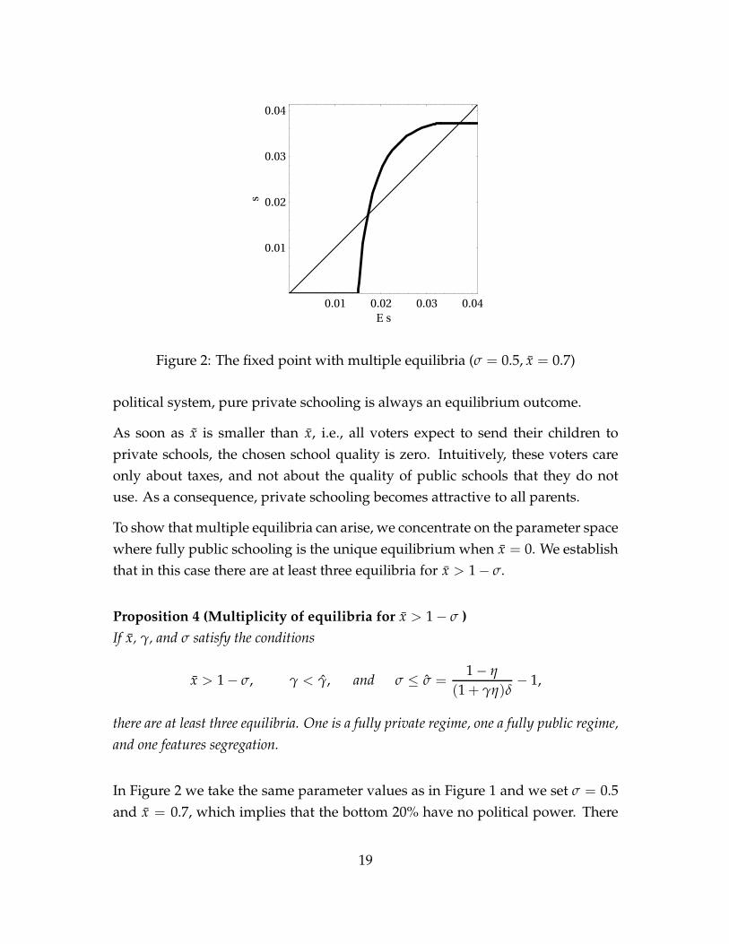
Figure 2: The fixed point with multiple equilibria (σ = 0.5, x = 0.7)

political system, pure private schooling is always an equilibrium outcome.

As soon as x is smaller than x, i.e., all voters expect to send their children toprivate schools, the chosen school quality is zero. Intuitively, these voters careonly about taxes, and not about the quality of public schools that they do notuse. As a consequence, private schooling becomes attractive to all parents.

To show that multiple equilibria can arise, we concentrate on the parameter spacewhere fully public schooling is the unique equilibrium when x = 0. We establishthat in this case there are at least three equilibria for x > 1 − σ.

Proposition 4 (Multiplicity of equilibria for x > 1 − σ )If x, γ, and σ satisfy the conditions

x > 1 − σ, γ < γ, and σ ≤ σ =1 − η

(1 + γη)δ− 1,

there are at least three equilibria. One is a fully private regime, one a fully public regime,and one features segregation.

In Figure 2 we take the same parameter values as in Figure 1 and we set σ = 0.5and x = 0.7, which implies that the bottom 20% have no political power. There

19

are now three fixed points: s = 0, s = 0.017, and s = 0.037, with participationΨ = 0, Ψ = 0.3, and Ψ = 1.

The possibility of multiple equilibria exists because we assume that people haveto decide on fertility and public versus private schooling before the vote on thequality of public education takes place. If all decisions were taken simultane-ously, the voting process would lead to the same outcome as the weighted so-cial planning problem, which is generically unique. Pre-commitment generatesmultiplicity in this setting, but not in the version with equal political weights, be-cause there is now a strategic complementarity between the education choices ofskilled people through the quality of public schools.14 When everyone with po-litical power uses private schools, a given individual does not want to switch tothe public system, since the quality of the public schooling is low. If, however, allvoters were to switch together to the public system, they would vote for a muchhigher quality of public schools, in which case it would be rational to stay in thepublic system. Here, the political bias towards the rich offsets the increased costof taxation resulting from higher participation in public schooling. Provided thatthere is a strong concentration of political power, the model can account for thefact that some countries with similar general characteristics choose very differenteducational systems.15

The next proposition shows that despite the possibility of multiple equilibria, thecoverage of public schooling is never higher in societies dominated by the richthan it is in democracies:

14When actions are strategic complements, the utility of those taking the action depends posi-tively on how many people take the action. Classic examples are Matsuyama (1991) for increasingreturns, Katz and Shapiro (1985) for network externalities, and Diamond and Dybvig (1983) forbank runs.

15A number of authors have derived similar multiplicity results in other applications of votingmodels. In Saint-Paul and Verdier (1997) there is majority voting on a capital income tax. If polit-ical power is unequally distributed, and is biased in favor of households having better access toworld capital markets, expectations-driven multiple equilibria can arise. In a dynamic majorityvoting framework, Hassler, Rodriguez Mora, Storesletten, and Zilibotti (2003) assume that youngagents base their education decisions on expectations over future redistribution. Self-fulfillingexpectations can lead to either high or low redistribution equilibria. Finally, there are other polit-ical economy models that do not have indeterminacy of equilibrium but display multiple steadystates (see for example Benabou 2000 or Doepke and Zilibotti 2005). Initial conditions, as opposedto self-fulfilling expectations, determine which steady state the economy approaches.

20

Proposition 5 (Coverage of public education as a function of x )Let Ψ0 be the equilibrium coverage of public education for x = x0, and v0 the correspond-ing tax rate. If Ψ1 and v1 are an equilibrium coverage and a tax rate for a x = x1 > x0,then we have

Ψ1 ≤ Ψ0,

s1 ≤ s0,

v1 ≤ v0.

In summary, if the rich wield more power than the poor, multiple equilibria mayarise. In any such equilibrium, the coverage, quality of, and spending on publiceducation cannot be higher than in the outcome with equal political weights.Fully private education systems are always possible.

While we have established the results of this section for the extreme case wherehouseholds with an income below x do not wield any political power, the resultsgeneralize to an environment where these households have some positive weightin the political system, but lower than the weight of households with incomeabove x. In particular, it is easy to establish that, for any x, a fully private regimeexists if the weight of low-income people is sufficiently small. As before, if in thiscase the unique equilibrium in the model with an even distribution of politicalpower is pure public schooling, at least three equilibria exist when the poor haveless political power.

5 Outcomes with Government Commitment

So far we have assumed that the level of government spending on education isdetermined after private households have decided whether to send their childrento private or public schools. In this section we analyze an alternative timing as-sumption, namely, the voters elect a government which pre-commits to a givenoverall spending level on education, while households can make their schoolingchoice conditional on this spending. Even though under each timing assump-tion people have perfect foresight, we will see that timing makes an important

21

difference. For the following analysis, we return to the assumption of an evendistribution of political power, i.e. x = 0.

In the new timing, the government sets the tax rate at the beginning of the period.Since the tax base is independent of the schooling choice, this is equivalent to de-termining total spending on public education. After the tax is set, parents choosefertility and public versus private education for their children. Public schoolingper child will then be given by the ratio of pre-committed total spending to thenumber of children in public schools. Since the government has perfect foresight,the problem can be solved backwards by first determining individual decisionsas a function of policies, and then choosing policies taking this dependency intoaccount.

Since fertility choices conditional on schooling are not affected by taxes, fertilityrates will be, as above, determined by equations (3) and (5). Private educationspending is also unaffected by the new timing of decisions and is given by equa-tion (4). The participation decision is determined by the threshold defined inLemma 2, which is now defined in terms of actual schooling quality s:

x[s] =1 − η

δφηs. (17)

We also redefine the endogenous fraction of children participating in the publiceducation system as a function of actual quality:

Ψ[s] =

⎧⎪⎪⎪⎪⎨⎪⎪⎪⎪⎩

0 if x[s] < 1 − σ,x[s] − (1 − σ)

2σif 1 − σ ≤ x[s] ≤ 1 + σ,

1 if x[s] > 1 + σ.

(18)

From Equation (9), the link between taxes and expenditures is given by:

v = Ψ[s]γ

φs. (19)

The objective function modeling the voting process is the same as before, but Ψ

22

and x are now endogenous:

Ω[s] ≡∫ x[s]

0u[x, v, ns, 0, s]g[x]dx +

∫ ∞

x[s]u[x, v, ne, e[x], 0]g[x]dx. (20)

The structure of the problem is similar to a standard Ramsey (1927) problem,where the government chooses optimal taxes taking into account the reaction ofprivate agents. Once again three regimes are possible: fully public (Ψ[s] = 1),segregation (1 > Ψ[s] > 0), and fully private (Ψ[s] = 0). In the segregation case,the first-order condition for optimization is as follows:

∫ x[s]

0

(∂u∂v

∂v∂s

+∂u∂s

)g[x]dx +

∫ ∞

x[s]

(∂u∂v

∂v∂s

+∂u∂s

)g[x]dx

+∫ x[s]

0

∂u∂v

∂v∂Ψ

∂Ψ∂s

g[x]dx +∫ ∞

x[s]

∂u∂v

∂v∂Ψ

∂Ψ∂s

g[x]dx = 0.

The first line of this optimality condition is the same as the one we get in the prob-lem without commitment. The second line is a new term which arises from theendogenous dependency of Ψ on s. This term is always negative. The new neg-ative term implies that under government commitment, the optimal s is lowerthan under no-commitment, as long as the solution for Ψ is interior. Intuitively,the government now takes into account that a marginal increase in s increasesthe number of families who use public schools. On the margin this lowers thevalue of the objective function, since the marginal family is just indifferent be-tween private and public schooling, but imposes a fiscal burden on the rest of thepopulation once it switches from private to public school.

In the fully private and public regimes, participation Ψ[s] is locally independentof s, as long as the marginal family strictly prefers its current schooling choice.The additional term is therefore zero, and hence the optimal schooling choiceof s does not depend on government commitment. The following propositionsummarizes the result.

Proposition 6 (Equilibrium with commitment)An equilibrium with commitment exists. Public school quality is lower than or equal tothe level reached without commitment. The inequality is strict if participation Ψ satisfies:

23

0 < Ψ < 1.

Existence is guaranteed because the objective function is continuous on a com-pact set. The equilibrium is not guaranteed to be unique, however, because theobjective function is not globally concave. In particular, it has kinks at the valuesof s corresponding to x[s] = 1 − σ and x[s] = 1 + σ. However, multiplicity occursonly for knife-edge cases.

If we extend this model to concentrated political power as in Section 4, we nolonger get generic multiplicity of equilibria. Under the original timing, multi-ple equilibria arose as self-fulfilling prophecies. With government commitment,the government moves first and chooses the generically unique equilibrium thatmaximizes the objective function.

We therefore see that the relative timing of the decisions taken by individualhouseholds and by the government has an important bearing on the positive im-plications of our theory. Which timing, then, should be considered the most re-alistic? There is no general answer to this question, as political decision horizonscan vary substantially from country to country. Still, it is useful to consider asa benchmark the common case of a government that adjusts the education bud-get (which determines the quality of public schooling) at an annual frequency.As far as fertility decisions are concerned, the realistic assumption is that house-holds move before the government does. Children generally enter school at agesix, so that at the very minimum, six years pass from the fertility decision untilschooling actually begins. It is hard to imagine that the government commits toa schooling quality more than six years ahead of time, without any possibility oflater adjustments.

In contrast, matters are less clear-cut when it comes to the choice of an educationsystem (i.e., whether to send one’s child to public or private school). We havealready analyzed the case where parents make this choice before the governmentdecides on school quality. What would happen if households chose fertility be-fore the vote on schooling quality, but could adjust their choice of public versusprivate schooling after the vote? As we will see, a framework in which house-holds make at least one decision before the government moves leads to implica-tions similar to those under our original timing, where the government moves

24

last.

In this intermediate case, when households choose fertility, they do so underperfect foresight regarding the future quality of schools. There will be an incomethreshold x below which people have large families (corresponding to the expec-tation of public schooling). The objective of the voting process takes three differ-ent forms depending on how the threshold for private education x[s] comparesto the threshold for small families x. For x < x[s], it is given by:

Ω[s] =∫ x

0u[x, v, ns, 0, s]g[x]dx +

∫ x[s]

xu[x, v, ne, 0, s]g[x]dx

+∫ ∞

x[s]u[x, v, ne, e[x], 0]g[x]dx,

for x = x[s], we have

Ω[s] =∫ x[s]

0u[x, v, ns, 0, s]g[x]dx +

∫ ∞

x[s]u[x, v, ne, e[x], 0]g[x]dx, (21)

and for x > x[s], we have:

Ω[s] =∫ x[s]

0u[x, v, ns, 0, s]g[x]dx +

∫ x

x[s]u[x, v, ns, e[x], 0]g[x]dx

+∫ ∞

xu[x, v, ne, e[x], 0]g[x]dx.

If x = x[s], as in the previous case the first-order condition for optimality hasan additional term related to the marginal impact of s on x[s]. In equilibrium,however, agents have perfect foresight, and x = x[s] will hold. Consider the sthat maximizes the objective function holding x[s] constant at x, as in our origi-nal timing. In Equation (21), in a neighborhood around this s the marginal effectof a change in s on x is zero. The reason is that agents below x have chosen largefamilies in expectation of using public schools, whereas families above x = x[s]have chosen small families in expectation of private schooling. Families close tothe threshold therefore strictly prefer their expected schooling choice to the alter-native. Thus for x = x[s] which occurs in equilibrium, the first-order condition isas in our original timing. If the solution is interior, this implies that the outcome

25

has to be the same.16

To summarize, whether the model generates multiplicity of equilibria dependscrucially on the timing of private decisions relative to the determination of gov-ernment policy. If parents make decisions that lock them into specific choicesfor their children for a long time, whereas the government can adjust the qualityof public education more frequently, multiple equilibria are possible. In the realworld, the strength of these lock-in effects would depend on a number of featuresthat are not modeled explicitly in our theory. For example, in some countries ed-ucational segregation is linked to residential segregation, i.e., there are districtswhere mostly rich people live who use private schools, while poorer districts areserved by public schools. In such an environment, a switch in the type of school-ing would also entail a switch of residence, and maybe even a switch of jobs ifthe distances are large enough. Clearly, in such an environment the lock-in intoa particular schooling type would be much stronger than in a country where pri-vate and public schools are located right next to each other, with few hurdles toswitching schools.

6 Empirical Evidence

Our theory makes predictions about how the quality and extent of private andpublic schooling are determined at the aggregate level, and about how school-ing and fertility choices vary across households within a given political entity.In this section, we compare these predictions to data. We start by focusing onstate-level variation in the extent and quality of public education in the UnitedStates. This setting is well suited to examining the predictions of our theory fordemocratic countries, since all U.S. states operate within the same overall polit-ical framework, while exhibiting considerable variation in schooling policies aswell as the distribution of income. Moreover, we are able to link state-level ev-idence to household data from the U.S. Census to assess the micro implications

16Depending on parameters, however, under the intermediate timing there can also be addi-tional corner solutions. The original and intermediate timing lead to the same equilibria if thelock-in effect through fertility is sufficiently strong. The strength of the lock-in effect, in turn,depends on the fertility differential between parents with children in public and private schools.

26

of our theory. We then extend the analysis to cross-country data, which allowsus to probe the theory’s predictions for non-democratic countries. Here we usedata from the OECD and the World Bank on public and private education spend-ing, as well as micro data from the OECD Programme for International StudentAssessment (PISA).

6.1 Inequality, fertility, and schooling across U.S. states

Our model predicts that in a democracy, the choice of public versus privateschooling and the level of funding of public schooling are driven by income in-equality (see Proposition 3). In particular, a state with higher income inequalityshould exhibit a higher share of private schooling, lower overall spending onpublic schooling, but higher public education spending per student. In addition,the model predicts that a high-inequality state will have a relatively low fertilityrate, because parents who send their children to private school economize on fer-tility. In this section, we examine whether these predictions hold up across U.S.states.

We computed state-level measures of income inequality, average fertility, and theshare of private schooling from the 2000 U.S. Census.17 We correlate these vari-ables with a number of measures of the spending on and the quality of publicschooling. In line with the setup of our theory, we focus on financial measures.18

As an overall spending measure, we use public education spending per capitain each state (this corresponds to the tax rate v in the model). For the qualityof public education (corresponding to the variable s in the model), we considerthree alternative measures. “Total Current Expenditure per Student” is a measureof total spending for day-to-day operation of schools, which includes all expen-ditures of public schools apart from debt repayments, capital outlays, and pro-grams outside of preschool to grade 12. One concern with this broad measure isthat it includes some items that may not have a direct educational impact. There-

17The data is from the one-percent sample of the 2000 U.S. Census, made available atwww.ipums.org by Ruggles et al. (2004).

18There may also be differences in how efficiently a given amount of spending is convertedinto “effective education,” but our theory makes no predictions in this dimension and assumesthat all states are at the efficiency frontier.

27

Table 1: Correlation of Inequality and Share of Private Schooling with Fertility,Education Spending, and the Quality of Public Schooling across U.S. States

Gini coefficient Private school share

Private school share 0.39 (2.98)

Public spending per capita -0.45 (-3.55) -0.10 (-0.68)

Public spending per student 0.26 (1.86) 0.52 (4.31)

Public instruction spending per student 0.18 (1.25) 0.49 (3.92)

Mean teacher salary in public schools 0.25 (1.78) 0.57 (4.80)

Average number of children -0.47 (-3.75) -0.40 (-3.03)

t-Statistics in parentheses. “Gini Coefficient” is computed on 1999 household income by state(data from 2000 U.S. Census). “Share in Private School” is the number of households with at leasthalf of their school-age children in private school as a fraction of the total number of householdswith at least one child in school (data from 2000 U.S. Census). “Number of Children” is theaverage number of children per household in the same data set, where children are counted onlyif the head of household is their parent and if they are currently living in the household. Measuresof education spending and quality of education are defined in the text.

fore, we also use the variable “Total Instruction Expenditure per Student,” whichincludes only expenditures associated directly with student-teacher interactionsuch as teacher salaries and benefits, textbooks and other teaching supplies, andpurchased instructional services. Finally, as an alternative measure of the qualityof instruction we use “Mean Teacher Salary,” an estimate of the average annualsalary of teachers in public elementary and secondary schools.19

Table 1 shows how income inequality (i.e., the Gini coefficient on household in-come by state) and the share of private schooling correlate with fertility and mea-sures of education spending and quality across states. The correlations are in linewith the predictions of Proposition 3. In particular, the correlation between in-equality and the share of private schooling is positive, whereas the correlation be-tween inequality and per-capita spending on public education is negative. Taken

19The expenditure measures are from the National Center for Education Statistics, “Revenuesand Expenditures for Public Elementary and Secondary Education,” School Year 2000-2001. Theteacher salary data is provided by the National Education Association.

28

by themselves, these results might seem to suggest that more inequality leads toless redistribution in the sense of lower support for public education. However,this is not the case when we consider the quality of public education rather thanoverall spending. All three measures of the quality of public education are posi-tively correlated with inequality.20 This verifies the third part of Proposition 3.

The surprising finding that the correlation coefficients of education spending percapita and education spending per student are of opposite sign can be accountedfor by the effect of private schooling on the quality of public schooling. As in-equality rises, more students use private schools, which makes it more affordableto offer a high-quality education to those still in public schools. This effect canbe seen even more clearly when we correlate education quality with the share ofstudents in private school (second column of Table 1). For all three measures, thecorrelation is positive and highly significant. Hence, the theoretical implicationthat as the share of private schooling increases, the quality of the public schoolshould increase as well seems to be well supported in the U.S. data.

The finding has important implications for the relationship of inequality and re-distribution. If one looked only at aggregate spending, one might think that moreinequality leads to less redistribution, as posited by Benabou (2000), among oth-ers. However, the per-person transfer to poorer households (i.e., the educationquality provided to households using public schools) does in fact go up. Thisincrease is possible because more inequality leads to more targeted transfers, asricher households opt out of the public system.

The last row of Table 1 examines predictions for fertility rates. We find that stateswith more inequality and a higher share of private schooling have a lower fer-tility rate. This outcome is in accordance with our model: parents economize onthe number of children if the direct cost of education is high.

20The correlation is significant at the 10 percent level for total expenditure per student as wellas mean teacher salary.

29

6.2 Determinants of fertility and public versus private school-

ing at the household level

We now examine more closely the inner workings of our model with the help ofmicro data from the U.S. Census. We want to establish whether the model paintsa realistic picture of the interaction between household income, private choiceson education and fertility, and the quality of public schooling. This will be usefulto assess whether our model indeed provides a plausible mechanism for gen-erating the observed macro correlations. Here, we draw on data on householdincome, family size (i.e., the household head’s own children living in the house-hold), public versus private schooling (for school-age children), and a number ofdemographic controls from the one-percent sample of the 2000 U.S. Census.

In the model, a household’s decisions on fertility and private versus public school-ing depend on two variables: income and the quality of public schooling (seeLemma 2 and the preceding discussion). In particular, richer households are pre-dicted to be more likely to choose private schools and to have lower fertility rates.The strength of the income effect depends on the quality of public schooling; forexample, if public schooling is of very high quality, even fairly rich householdswill use public schools. To examine these predictions, Tables 2 and 3 show regres-sions of family size and private schooling on household income and a number ofcontrols.21 We use an ordered logit specification for the fertility choice and a logitspecification for the private education choice. All regressions contain dummyvariables for the age of the household head as well as for the state of residence(the effect of further controls is discussed below).

The first column of each table presents results for regressions that include onlyhousehold income in addition to the standard controls. As predicted by the the-ory, an increase in income is associated with a higher probability of using privateschooling and lower fertility.22 However, in this specification the relationship

21In order to be able to include households that report zero income, we add $10 to householdincome before taking logs. The results are qualitatively the same if we shift up incomes by $100or $500 instead.

22The positive effect of income on the probability of private schooling has also been docu-mented by Cohen-Zada and Justman (2003) and Epple, Figlio, and Romano (2004); see alsoNechyba (2006). However, these studies do not consider fertility choices and the interaction ofthe quality of public schooling across states with income effects.

30

Tabl

e2:

Esti

mat

ion

Res

ults

:O

rder

edLo

git

Reg

ress

ion

ofN

umbe

rof

Chi

ldre

non

Inco

me

and

Qua

lity

ofPu

blic

Educ

atio

n

Mea

sure

ofqu

alit

yof

publ

iced

ucat

ion

Tota

lexp

endi

ture

Inst

ruct

ion

expe

ndit

ure

Mea

nte

ache

r

per

stud

ent

per

stud

ent

sala

ry

Log

hous

ehol

din

com

e-0

.012

(-1.

11)

-0.8

08(-

3.15

)-0

.685

(-3.

08)

-0.6

88(-

1.09

)

Inte

ract

ion

inco

me×

qual

ity

0.08

9(3

.15)

0.08

0(3

.07)

0.06

3(1

.07)

Tota

linc

ome

effe

ctat

aver

age

qual

ity-0

.012

(-1.

11)

-0.0

13(-

1.27

)-0

.013

(-1.

26)

-0.0

13(-

1.13

)

t-St

atis

tics

inpa

rent

hese

s(s

tand

ard

erro

rsar

ecl

uste

red

byst

ate)

.D

ata

from

2000

U.S

.Cen

sus.

453,

296

obse

rvat

ions

(hou

seho

lds

wit

hch

ildre

n).S

tate

and

age

ofho

useh

old

dum

mie

sin

allr

egre

ssio

ns.

31

Tabl

e3:

Estim

atio

nR

esul

ts:L

ogit

Reg

ress

ion

ofC

hoic

eof

Priv

ate

Scho

olin

gon

Inco

me

and

Qua

lity

ofPu

blic

Edu-

catio

n

Mea

sure

ofqu

alit

yof

publ

iced

ucat

ion

Tota

lexp

endi

ture

Inst

ruct

ion

expe

ndit

ure

Mea

nte

ache

r

per

stud

ent

per

stud

ent

sala

ry

Log

hous

ehol

din

com

e0.

557

(17.

98)

4.02

1(5

.69)

3.28

0(5

.90)

4.89

4(2

.38)

Inte

ract

ion

inco

me×

qual

ity

-0.3

88(-

4.94

)-0

.323

(-4.

96)

-0.4

06(-

2.09

)

Tota

linc

ome

effe

ctat

aver

age

qual

ity0.

557

(17.

98)

0.56

9(2

8.65

)0.

568

(27.

01)

0.56

5(2

1.76

)

t-St

atis

tics

inpa

rent

hese

s(s

tand

ard

erro

rsar

ecl

uste

red

byst

ate)

.D

ata

from

2000

U.S

.Cen

sus.

311,

625

obse

rvat

ions

(hou

seho

lds

wit

hch

ildre

nin

scho

ol).

Stat

ean

dag

eof

hous

ehol

dd

umm

ies

inal

lreg

ress

ions

.Cho

ice

ofPr

ivat

eSc

hool

ing

vari

able

take

sth

eva

lue

1if

atle

ast

half

ofth

esc

hool

-age

child

ren

inth

eho

useh

old

atte

ndpr

ivat

esc

hool

s.

32

between household income and fertility is not significant at conventional levels.The remaining columns focus on the joint effect of household income and thequality of public schooling in determining private choices. Each regression con-tains an additional interaction term of household income with one of our threemeasures of the quality of public schooling. Notice that schooling quality is mea-sured at the state level, not the household level.23 In essence, we are still esti-mating a micro relationship between household income and private choices, butwe allow the slope of this relationship to vary systematically across states with ahigh and a low quality of public education. We find that in both regressions andfor all three measures of the quality of public schooling, the estimated coefficienton the interaction term is of the opposite sign as the coefficient on income, whichimplies that the effect of income on household choices diminishes as the qualityof public schooling goes up. When the interaction term is included, all parameterestimates are highly significant, with the one exception of the fertility regressionusing mean teacher salary as a quality measure.

The size of the interaction terms implies substantial variation in the steepness ofthe income-fertility and income-private schooling relationships across states witha low and high quality of public schooling. In the states with the highest qualityof public education, these relationships are essentially flat. This is exactly whatone would expect based on the theory: states with high-quality public schoolingare close to a fully public regime, i.e., most parents use public schools regardlessof income, and fertility varies little across income groups.

The regression results are robust with respect to a number of changes to thespecification of the model. We explored sensitivity to racial composition by es-timating the regressions separately by race and by including race dummies; wechecked urban/rural differences by including a metropolitan area dummy; andwe ran the regressions on restricted samples limiting the age range of the in-cluded households. Generally, the sign and significance of the interaction termin the two regressions are robust to these changes, as are the sign and signifi-cance of the total income effect in the education equation. The sign of the total

23The fact that schooling quality is a state-level variable also precludes using it in the regressiondirectly, because our regressions already contain state dummies. As a robustness test, we alsocarried out regressions without state dummies and schooling quality as an included variable,with overall similar results.

33

income effect in the fertility regression turns out to be more sensitive. In partic-ular, for black and Hispanic households the total income effect is strongly neg-ative, whereas for white households it is positive. However, when we restrictthe sample to the ages 25–45, the total income effect once again is negative andsignificant. This suggests that for older white people, the slope of the relationbetween fertility and income can be reversed.24 However, even in the case of apositive slope, the sign of the interaction term remains the same.

6.3 Inequality, fertility, and schooling across countries

We now turn to the determinants of education systems across countries. Com-pared to our analysis of education in U.S. states, cross-country data pose addi-tional challenges. There are substantial differences in the level of developmentand in unobserved variables such as the political system, religious values etc.across countries which could have independent effects on the variables of inter-est.25 Doing full justice to the arising empirical issues is beyond the scope of thispaper. Therefore, we focus on documenting the fundamental correlations andmicro relationships implied by our theory.

The OECD provides internationally comparable data on the relative proportionsof public and private investment in education for the period 1985–1998. In mostcountries, private sector expenditure is comprised mainly of household expen-ditures on tuition and other fees. The exception is Germany, where nearly allprivate expenditure is accounted for by contributions from the business sectorto the system of apprenticeship at the upper secondary level. For primary andlower secondary education, there is little private funding in Germany. In 1998,

24To some extent, this finding could be due to the fact that in the Census, we observe onlychildren who still live in the household. If rich, white households have children relatively latein life, they would appear to have unusually many children in their household at a time whenother parents’ children have already left to form their own households. This type of effect is notpicked up by a simple age dummy, but can be partially addressed by restricting the age range ofhouseholds included in the sample.

25The literature contains few empirical studies on the determinants of the mix between publicand private education across countries. One exception is James (1993), who regresses privateenrollments shares for 50 countries around 1980 on a number of determinants, and concludes thatcultural factors such as religious competition and linguistic heterogeneity play an important role.However, the small number of observations compared to the number of explanatory variablescasts some doubt on the robustness of the results.

34

0

5

10

15

20

25

30

35

40

45

20.0 30.0 40.0 50.0 60.0

Gini circa 1970

Sha

re o

f priv

ate

educ

atio

n 19

98

Figure 3: Inequality and education systems across countries

the data set contains information on a number of non-OECD countries (Israel,Uruguay, Czech Republic, Turkey, Argentina, Indonesia, Chile, Peru, Philippines,and Thailand). With observations on 31 countries, we can investigate whetherinequality is a good predictor of private funding. Computing the correlationbetween the Gini coefficient for income inequality in 1970 (from Deininger andSquire 1996) and the share of private funding in 1998, we find that the correlationis positive and strong with a coefficient of 0.44 (t-stat=2.64).26 The correlation in-creases to 0.55 (t-stat=3.55) if we consider only the primary and secondary levelsof education. Figure 3 presents the cross plot of the private share in primary andsecondary education with the Gini coefficient.

We turn next to micro data from the OECD Programme for International Stu-dent Assessment (PISA), collected in the year 2000 on 15 year-old students inthe principal industrialized countries. It includes a student questionnaire gather-ing information about the student’s family and a school questionnaire coveringinformation on the extent of public funding and the public or private adminis-tration of schools. We focus on four variables in the PISA database. The Inter-

26We use the Gini coefficient in 1970 to address possible reverse causality from schooling toinequality.

35

national Socioeconomic Index (ISEI) captures the attributes of occupations thatconvert parents’ education into income. It was obtained by mapping parents’occupational codes onto an index of occupational status, developed by Ganze-boom, De Graaf, and Treiman (1992). This index provides a rough measure ofhousehold income and human capital (unfortunately, household income itself isnot contained in the data base). Using the index, students are assigned to one offour social classes.27 The second student-specific variable in our data set is thenumber of siblings. At the school level, our data set contains information on thefunding sources of schools and on whether a school is publicly or privately run.For school funding, our variable is the percentage of total funding that stemsfrom government sources, as opposed to fees paid by parents, benefactors, orother sources of income.

For each country, we computed average school characteristics for the four socialclasses. For each group, we report the average share of education spending cov-ered by public sources (the subsidization rate), the share of students in privateschools, and the average fertility rate. The detailed results are provided in Ap-pendix B. Overall, the findings once again are consistent with the theory: in thevast majority of cases, participation in private schooling increases and fertilitydecreases with social status.

An interesting feature of the PISA data is that it covers countries that appear to becharacterized by different schooling regimes. In particular, a number of countriescome close to what could be described as a fully public regime. To investigatethe effects of having a fully public schooling regime, we define countries as fullypublic if the difference in the subsidization rate between the highest and lowestsocial class is less than five percent.28 The remaining countries are classified as

27Typical occupations in the lowest class (between 16 and 35 points on the ISEI scale) includesmall-scale farmer, metalworker, mechanic, taxi or truck driver, and waiter/waitress. Between35 and 53 index points, the most common occupations are bookkeeping, sales, small businessmanagement, and nursing. As the required skills increase, so does the status of the occupation.Between 54 and 70 points, typical occupations are marketing management, teaching, civil engi-neering, and accounting. In the highest class (from 71 to 90 points), occupations include medicine,university teaching, and law.

28This group includes Hungary, the Czech Republic, Denmark, Finland, Germany, Iceland,Latvia, The Netherlands, Norway, Russia and Sweden. Appendix B also provides the propor-tion of students attending private schools. The school type is determined by the question “Isyour school a public or a private school.” Here public schools are those managed by a public

36

Tabl

e4:

Sum

mar

ySt

atis

tics

for

Cou

ntri

esw

ithD

iffer

entE

duca

tion

Reg

imes

Num

ber

ofG

inii

nSh

are

ofFu

ndin

gdi

ffer

ence

Fert

ility

diff

eren

tial

coun

trie

sth

e19

80s

publ

icfu

ndin

gbe

twee

npo

oran

dri

chbe

twee

npo

oran

dri

ch

Fully

publ

icre

gim

e11

24.7

0.96

0.00

0.36

Segr

egat

ion

regi

me

1834

.60.

810.

140.

47

Top

5m

osts

egre

gate

d5

44.6

0.69

0.25

0.69

Cor

rela

tion

wit

hG

ini

-0.5

8(3

.65)

0.76

(5.9

6)0.

53(3

.21)

t-St

atis

tics

inpa

rent

hese

s.

37

being in the segregation regime. We also consider separately the five countrieswith the highest difference in the public subsidization rate of the lowest and thehighest social class (Austria, Australia, Brazil, Mexico, and Spain). In this group,the difference between the subsidization rate of schools attended by members ofthe top and bottom social classes averages 25 percent.

Table 4 provides a number of statistics for the groups of countries with differenteducation regimes. Not surprisingly, in the fully public group the level of publicsubsidization is particularly high, with an average of 96 percent. These countriesare also characterized by low income inequality (average Gini: 24.7), and thefertility differential between the bottom and top social classes is only 0.36.29 Incontrast, the group of countries in the segregation regime has an average Gini of34.6 and a fertility differential of 0.47. The five countries with the highest levelof segregation also top the list in terms of inequality and differential fertility: theaverage Gini coefficient is 44.6 in this group, and the fertility differential betweenthe bottom and top social classes amounts to 0.59. The last row of Table 4 presentscorrelation coefficients between the Gini coefficient and the other variables acrossall countries in the data set. As predicted by the theory, in countries with higherincome inequality average public funding is lower, the subsidization rate is moresensitive to social class, and fertility differentials are larger.30

6.4 Public education spending and democracy

We now turn to the final implication of our theory, the effect of democracy oneducation politics. Given that data on private spending on education is available

education authority, a government agency, or a governing board that is appointed either by thegovernment directly or elected by public franchise. While we could have used this variable todefine countries as fully public, for our purposes the public subsidization rate is a better indica-tor of public versus private schooling than the school type, because “private school” can meandifferent things in different countries. In Belgium, for example, most schools are nominally pri-vate, yet are entirely publicly funded. Nevertheless, using the school type variable instead of theschool funding variable leads to similar results.

29In all the countries we find that the fertility of the lowest social class exceeds the fertility ofthe highest social group. In a majority of countries, the relationship between fertility and socialstatus is monotonically decreasing; in some countries, it is U-shaped.

30One concern here is a reverse causality link whereby school segregation leads to more in-equality. The problem is mitigated by the fact that we use Gini coefficients measured 20 yearsbefore the observed schooling outcomes.

38

Table 5: Public Spending on Education in Democracies and Non-Democracies

Democracy index Observations Mean Variance

Free (= 1) 1020 4.96 3.08

Partially free (1 < x ≤ 4) 836 4.11 7.07

Non-free (4 < x ≤ 7) 644 4.07 8.33

2 4 6 8 10

0.05

0.1

0.15

0.2

0.25

Legend: Free (solid line), partially free (dots), non-free (dashes).Note: Density estimation using the NonParametrix.m Packageby Bernard Gress, 2004

Figure 4: Density of public education spending (percent of GDP)

Table 6: Mean and Variance Tests for Public Education Spending in Democraciesand Non-Democracies

Mean difference test Variance ratio test

Partially free Non-free Partially free Non-free

Free 0.85 (0.00) 0.89 (0.00) 0.44 (0.00) 0.37 (0.00)

Partially free 0.03 (0.82) 0.85 (0.03)

p-values in parentheses.

39

for only a few countries, we focus on public spending on education as a fractionof GDP. Here we have a sample of 158 countries covering the period 1970-2002(with some missing observations; data from World Bank Development Indica-tors). We divide the sample into three groups, based on their level of democracy.As a democracy indicator, we use the political-rights index from the Freedomin the World Country Ratings. The index lies on a one-to-seven scale, with onerepresenting the highest degree of freedom. We assign the countries into threegroups, where “free” countries have an index of one, “partially free” have valuesfrom two to four, and “non-free” countries have values from five to seven.

Table 5 displays the mean and variance of public spending on education for thethree groups of countries. The mean of spending is increasing with democracy,whereas the variance is decreasing. Figure 4 presents a density estimation of theentire distribution of public spending as a share of GDP for the three groups.The density for partially free and non-free countries displays a lower mean anda higher variance. Two-tailed tests of whether the differences are significant areprovided in Table 6. The mean in democratic (free) countries is significantly dif-ferent from the one in the two other groups. The variance in the non-free coun-tries is significantly higher than in the partially free-countries, where the varianceis higher than in the free group. These findings are in line with the predictions ofour theory for the case of an uneven distribution of political power (see Propo-sitions 4 and 5). Our mechanism is not the only possible explanation for theobserved high variance in public educations pending in non-democracies, but itis encouraging that the predictions of the model are in line with data along thisdimension also.

7 Conclusions

The education sector is a main area of government intervention in every countryin the world. At the same time, governments generally are not the sole providersof education; education systems often display a juxtaposition of public and pri-vately funded institutions. The degree of private involvement in the provision ofeducation varies a great deal across countries, ranging from fully public systemsas in some European countries to segregated systems as in parts of the United

40

States. In this paper, we try to understand how countries choose the mix of pub-lic and private education and how the presence of private schools affects thequality of public education.

First, we conclude that high inequality maps into a segregated education system.In our model’s segregated system, the quality of public schools is sufficiently lowto induce rich households to pay for private schools to enhance the education oftheir children. When inequality is low, on the other hand, the rich decide to sendtheir children to public schools, so that they avoid paying for education twice(first through taxes, second through private schools). The prediction of a strongrelationship between inequality and the extent of public schooling is in line withthe empirical evidence. In both cross-country data and cross-state data in theU.S., we find that public spending on education is negatively related to incomeinequality.

Second, we find that as long as the poor have equal weight in the political sys-tem, a larger share of private schooling is associated with a higher quality of pub-lic schooling. While total tax revenue declines as the share of private schoolingincreases, the number of students who use public schools declines even faster,implying that the funding level per student increases. Thus, even though an in-crease in inequality and the associated increase in the share of private schoolingreduce the total amount of redistribution, the transfers to public-school parentsbecome more targeted, leaving the poor better off.

Turning to the role of political power, we find that the quality and extent of publicschooling generally increases with the political weight of the poor. In addition,in societies that are dominated politically by the rich multiple equilibria in thedetermination of education spending may arise. When the rich are in charge,there is a complementarity between the number of rich people participating inpublic schools and their quality. For given initial conditions, such a country mayhave either a high-quality public schooling system in which many or all of therich participate, or a low-quality system with all the rich using private schools.Despite the multiplicity, however, we find that spending on public education isnever higher in a society dominated by the rich than in an otherwise identicaleconomy where the poor have equal power. The model therefore offers an ex-planation for why non-democratic countries spend on average a smaller fraction

41

of GDP on public education than democracies, whereas the variance of spendingacross countries is higher among non-democracies.

An important question for future research is why public education was firstwidely introduced in the nineteenth century during the second phase of the In-dustrial Revolution. Galor and Moav (2006) argue that in this period, capital-ists began to have an interest in public education, because of complementaritiesbetween physical and human capital. Therefore, technological change strength-ening this complementarity may have contributed to the introduction of publicschooling. Galor, Moav, and Vollrath (2006) extend this analysis by distinguish-ing different sources of wealth. If land is less complementary to human capitalthan it is to physical capital, a conflict of interest arises between land-owners andcapitalists. The outcome of this conflict depends on the distribution of wealthand land ownership.

In our model, public schooling always arises if political power is shared equally.The theory therefore points to the expansion of voting rights in the nineteenthcentury as a key explanation for the introduction of public schooling. Yet thequestion of why voting rights were expanded in the first place remains open. Thetheory of Galor and Moav (2006) offers one potential explanation. Acemoglu andRobinson (2000), however, point in a different direction: the rich shared powerin order to avoid the threat of a revolution. In either case, given that the poordid gain political influence, in our model the introduction of public schooling isa necessary consequence. Once the public education system is in place, its sizedepends on the evolution of the income distribution. With this observation, themodel points to the decline in income inequality around the turn of the centuryas a potential explanation for the further expansion of public education after itwas first introduced.

42

References

Acemoglu, Daron and James A. Robinson. 2000. “Why Did the West Extend theFranchise? Democracy, Inequality and Growth in Historical Perspective.”Quarterly Journal of Economics 115 (4): 1167–99.

Alderman, Harold, Peter F. Orazem, and Elizabeth M. Paterno. 2001. “SchoolQuality, School Cost, and the Public/Private School Choices of Low-incomeHouseholds in Pakistan.” Journal of Human Resources 36 (2): 304–326.

Alesina, Alberto and Dani Rodrik. 1994. “Distributive Politics and EconomicGrowth.” Quarterly Journal of Economics 109 (2): 465–90.

Bearse, Peter, Gerhard Glomm, and Debra M. Patterson. 2005. “EndogenousPublic Expenditures on Education.” Journal of Public Economic Theory 7 (4):561–77.

Bedi, Arjun S. and Ashish Garg. 2000. “The Effectiveness of Private versusPublic Schools: The Case of Indonesia.” Journal of Development Economics 61(2): 463–494.

Benabou, Roland. 1996. “Inequality and Growth.” NBER Macroeconomics An-nual, pp. 11–74.

. 2000. “Unequal Societies: Income Distribution and the Social Contract.”American Economic Review 90 (1): 96–129.

Bernheim, Douglas and Michael Whinston. 1986. “Menu Auctions, ResourceAllocation, and Economic Influence.” Quarterly Journal of Economics 101 (1):1–31.

Besley, Timothy and Stephen Coate. 1991. “Public Provision of Private Goodsand the Redistribution of Income.” American Economic Review 81 (4): 979–84.

Cohen-Zada, Danny and Moshe Justman. 2003. “The Political Economy ofSchool Choice: Linking Theory and Evidence.” Journal of Urban Economics54 (2): 277–308.

Coughlin, Peter and Shmuel Nitzan. 1981. “Electoral Outcomes with Proba-bilistic Voting and Nash Social Welfare Maxima.” Journal of Public Economics15 (1): 113–21.

de la Croix, David and Matthias Doepke. 2003. “Inequality and Growth: WhyDifferential Fertility Matters.” American Economic Review 93 (4): 1091–113.

. 2004. “Public versus Private Education when Differential Fertility Mat-ters.” Journal of Development Economics 73 (2): 607–29.

Deininger, Klaus and Lyn Squire. 1996. “Measuring Income Inequality: A NewDatabase.” Development Discussion Paper No. 537, Harvard Institute forInternational Development.

43

Diamond, Douglas W. and Philip H. Dybvig. 1983. “Bank Runs, Deposit Insur-ance, and Liquidity.” Journal of Political Economy 91 (3): 401–19.

Doepke, Matthias and Fabrizio Zilibotti. 2005. “The Macroeconomics of ChildLabor Regulation.” American Economic Review 95 (5): 1492–524.

Epple, Dennis and Richard E. Romano. 1996a. “Ends Against the Middle: Deter-mining Public Service Provision when there are Private Alternatives.” Jour-nal of Public Economics 62 (3): 297–325.

. 1996b. “Public Provision of Private Goods.” Journal of Political Economy104 (1): 57–84.

Epple, Dennis, David Figlio, and Richard Romano. 2004. “Competition BetweenPrivate and Public Schools: Testing Stratification and Pricing Predictions.”Journal of Public Economics 88 (7): 1215–45.

Fernandez, Raquel and Richard Rogerson. 1995. “On the Political Economy ofEducation Subsidies.” Review of Economic Studies 62 (2): 249–62.

Galor, Oded and Omer Moav. 2006. “Das Human-Kapital: A Theory of theDemise of the Class Structure.” Review of Economic Studies 73 (1): 85–117.

Galor, Oded, Omer Moav, and Dietrich Vollrath. 2006. “Inequality in LandOwnership, the Emergence of Human Capital Promoting Institutions andthe Great Divergence.” Unpublished Manuscript, Brown University.

Ganzeboom, Harry B.G., Paul M. De Graaf, and Donald J. Treiman. 1992. “AStandard International Socio-Economic Index of Occupational Status.” SocialScience Research 21 (1): 1–56.

Glomm, Gerhard and B. Ravikumar. 1992. “Public Versus Private Investmentin Human Capital: Endogenous Growth and Income Inequality.” Journal ofPolitical Economy 100 (4): 818–834.

. 1998. “Opting Out of Publicly Provided Services: A Majority VotingResult.” Social Choice and Welfare 15 (2): 197–99.

Goldhaber, Dan D. 1996. “Public and Private High Schools: Is School Choicethe Answer to the Productivity Problem?” Economics of Education Review 15(2): 93–109.

Gradstein, Mark and Moshe Justman. 1997. “Democratic Choice of an Educa-tion System: Implications for Growth and Income Distribution.” Journal ofEconomic Growth 2 (2): 169–83.

Hassler, John, Jose V. Rodriguez Mora, Kjetil Storesletten, and Fabrizio Zilibotti.2003. “The Survival of the Welfare State.” American Economic Review 93 (1):87–112.

44

James, Estelle. 1993. “Why Do Different Countries Choose a Different Public-Private Mix of Educational Sevices?” Journal of Human Resources 28 (3): 571–592.

Katz, Michael L. and Carl Shapiro. 1985. “Network Externalities, Competition,and Compatibility.” American Economic Review 75 (3): 424–440.

Kingdon, Geeta G. 1996. “The Quality and Efficiency of Private and PublicEducation: A Case-study of Urban India.” Oxford Bulletin of Economics andStatistics 58 (1): 55–80.

Matsuyama, Kiminori. 1991. “Increasing Returns, Industrialization, and Inde-terminacy of Equilibrium.” Quarterly Journal of Economics 106 (2): 617–50.

Moav, Omer. 2005. “Cheap Children and the Persistence of Poverty.” EconomicJournal 115 (500): 88–110.

Neal, Derek. 1997. “The Effects of Catholic Secondary Schooling on EducationalAchievement.” Journal of Labor Economics 15 (1): 98–123.

Nechyba, Thomas J. 2006. “Income and Peer Quality Sorting in Public andPrivate Schools.” Chapter 22 of Handbook of the Economics of Education, Vol. 2,edited by Eric A. Hanushek and Finis Welch. Amsterdam: North-Holland.

Persson, Torsten and Guido Tabellini. 1994. “Is Inequality Harmful for Growth?Theory and Evidence.” American Economic Review 84 (3): 600–21.

. 2000. Political Economics: Explaining Economic Policy. Cambridge, Mas-sachusetts: MIT Press.

Ramsey, Frank P. 1927. “A Contribution to the Theory of Taxation.” EconomicJournal 37 (145): 47–61.

Ruggles, Steven, Matthew Sobek, Trent Alexander, Catherine A. Fitch, RonaldGoeken, Patricia Kelly Hall, Miriam King, and Chad Ronnander. 2004.“Integrated Public Use Microdata Series: Version 3.0.” [Machine-readabledatabase]. Minneapolis, MN: Minnesota Population Center.

Saint-Paul, Gilles and Thierry Verdier. 1997. “Power, Distributive Conflicts andMultiple Growth Paths.” Journal of Economic Growth 2 (2): 155–168.

Stiglitz, Joseph E. 1974. “The Demand for Education in Public and PrivateSchool Systems.” Journal of Public Economics 3 (4): 349–85.

Toma, Eugenia F. 1996. “Public Funding and Private Schooling Across Coun-tries.” Journal of Law and Economics 39 (2): 121–48.

45

A Technical Appendix

Proof of Lemma 1: From the budget constraint (2), total spending on childrenis given by xφn + ne. Substituting either n = ns and e = 0 or n = ne and e =ηφx/(1 − η) yields that

xφn + ne =γ

1 + γx.

Taxable income therefore is

x(1 − φn) − ne =1

1 + γx.

�Proof of Lemma 2: We compute the level x such that a household with in-come x is indifferent between public and private by solving u[x, v, ns, 0, [E](s)] =u[x, v, ne, e, 0]:

x =1 − η

δφη[E](s) with: δ = (1 − η)

1η .

x is bigger than zero and depends positively on [E](s). If x is greater (resp.smaller) than x, u[x, v, ns, 0, [E](s)] is smaller (resp. greater) than u[x, v, ne, e, 0],and the household prefers private (resp. public) education, which proves theLemma. �Proof of Proposition 1: The result follows from an application of the Brouwerfixed point theorem. Given (11), the equilibrium expected schooling quality E[s]and actual quality s lie in the interval:

E[s], s ∈[

ηφ

1 + γη, ηφ

](22)

We now define a mapping Δ from E[s] into s which maps this interval into itself.Since an equilibrium requires E[s] = s, a unique equilibrium exists if the mappinghas unique fixed point.

Given expected schooling quality E[s], according to Lemma 2 and equation (7)the fraction of families participating in public education is given by:

Ψ(E[s]) = max{

min{

1 − η

2σδφηE[s] − 1 − σ

2σ, 1

}, 0

}.

This function is (weakly) increasing in E[s]; the higher the expected quality ofpublic education, the more parents are going to prefer using the public sector.

46

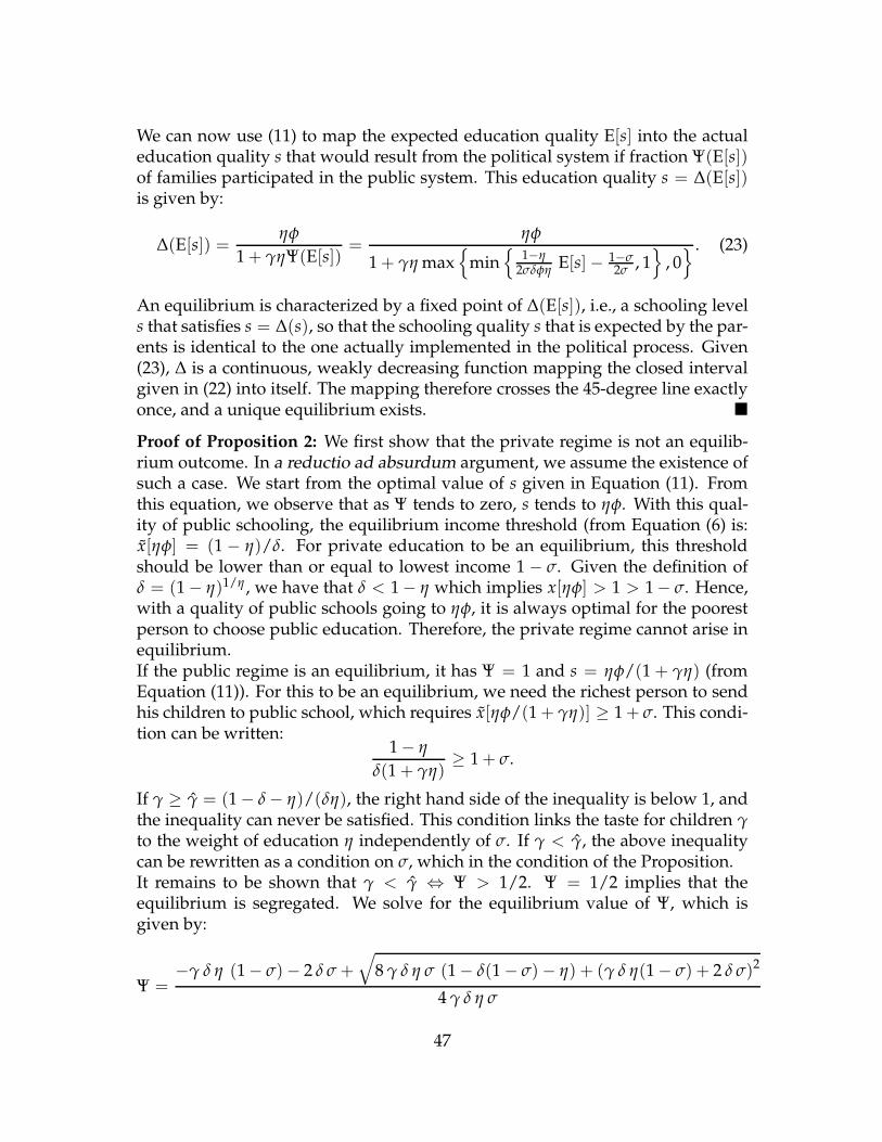
We can now use (11) to map the expected education quality E[s] into the actualeducation quality s that would result from the political system if fraction Ψ(E[s])of families participated in the public system. This education quality s = Δ(E[s])is given by:

Δ(E[s]) =ηφ

1 + γηΨ(E[s])=

ηφ

1 + γη max{

min{

1−η2σδφη E[s] − 1−σ

2σ , 1}

, 0} . (23)

An equilibrium is characterized by a fixed point of Δ(E[s]), i.e., a schooling levels that satisfies s = Δ(s), so that the schooling quality s that is expected by the par-ents is identical to the one actually implemented in the political process. Given(23), Δ is a continuous, weakly decreasing function mapping the closed intervalgiven in (22) into itself. The mapping therefore crosses the 45-degree line exactlyonce, and a unique equilibrium exists. �Proof of Proposition 2: We first show that the private regime is not an equilib-rium outcome. In a reductio ad absurdum argument, we assume the existence ofsuch a case. We start from the optimal value of s given in Equation (11). Fromthis equation, we observe that as Ψ tends to zero, s tends to ηφ. With this qual-ity of public schooling, the equilibrium income threshold (from Equation (6) is:x[ηφ] = (1 − η)/δ. For private education to be an equilibrium, this thresholdshould be lower than or equal to lowest income 1 − σ. Given the definition ofδ = (1 − η)1/η , we have that δ < 1 − η which implies x[ηφ] > 1 > 1 − σ. Hence,with a quality of public schools going to ηφ, it is always optimal for the poorestperson to choose public education. Therefore, the private regime cannot arise inequilibrium.If the public regime is an equilibrium, it has Ψ = 1 and s = ηφ/(1 + γη) (fromEquation (11)). For this to be an equilibrium, we need the richest person to sendhis children to public school, which requires x[ηφ/(1 + γη)] ≥ 1 + σ. This condi-tion can be written:

1 − η

δ(1 + γη)≥ 1 + σ.

If γ ≥ γ = (1 − δ − η)/(δη), the right hand side of the inequality is below 1, andthe inequality can never be satisfied. This condition links the taste for children γto the weight of education η independently of σ. If γ < γ, the above inequalitycan be rewritten as a condition on σ, which in the condition of the Proposition.It remains to be shown that γ < γ ⇔ Ψ > 1/2. Ψ = 1/2 implies that theequilibrium is segregated. We solve for the equilibrium value of Ψ, which isgiven by:

Ψ =−γ δ η (1 − σ) − 2 δ σ +

√8 γ δ η σ (1 − δ(1 − σ) − η) + (γ δ η(1 − σ) + 2 δ σ)2

4 γ δ η σ

47

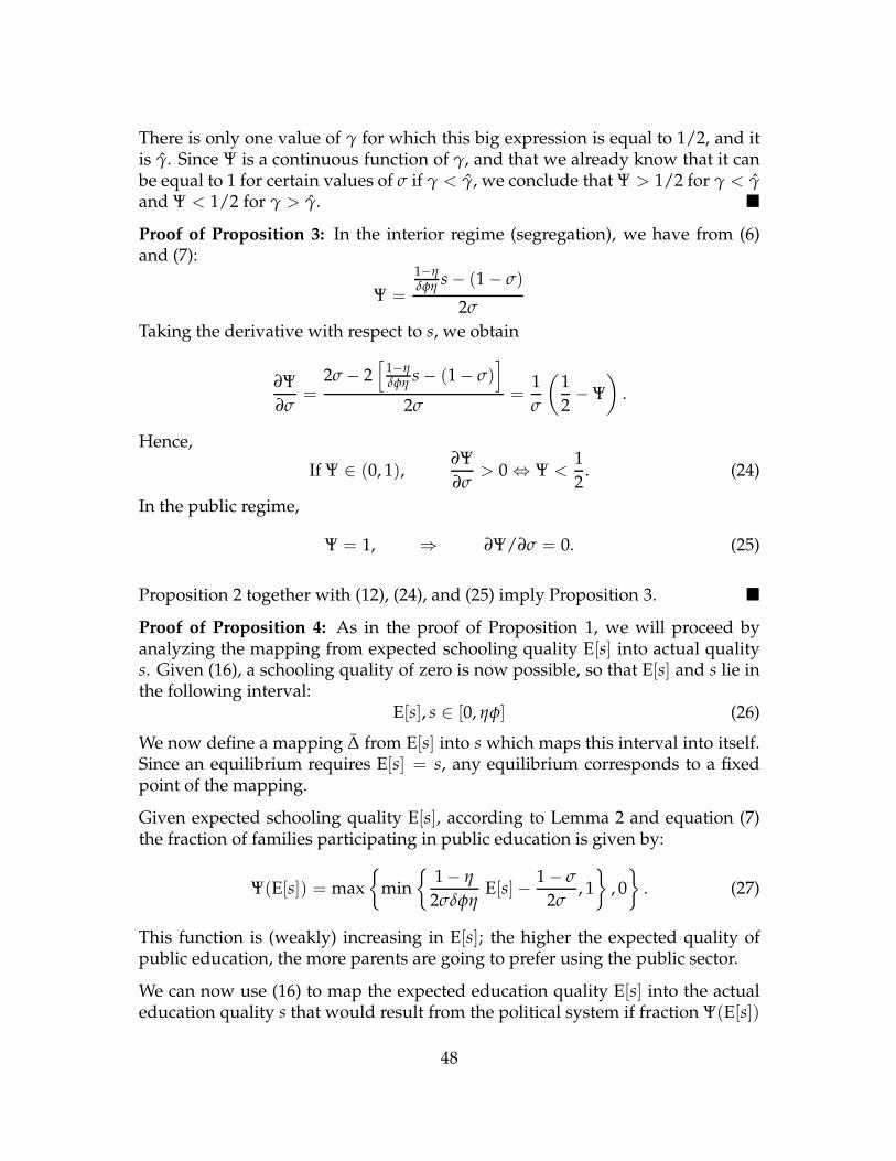
There is only one value of γ for which this big expression is equal to 1/2, and itis γ. Since Ψ is a continuous function of γ, and that we already know that it canbe equal to 1 for certain values of σ if γ < γ, we conclude that Ψ > 1/2 for γ < γand Ψ < 1/2 for γ > γ. �Proof of Proposition 3: In the interior regime (segregation), we have from (6)and (7):

Ψ =1−ηδφη s − (1 − σ)

2σ

Taking the derivative with respect to s, we obtain

∂Ψ∂σ

=2σ − 2

[1−ηδφη s − (1 − σ)

]2σ

=1σ

(12− Ψ

).

Hence,

If Ψ ∈ (0, 1),∂Ψ∂σ

> 0 ⇔ Ψ <12

. (24)

In the public regime,

Ψ = 1, ⇒ ∂Ψ/∂σ = 0. (25)

Proposition 2 together with (12), (24), and (25) imply Proposition 3. �Proof of Proposition 4: As in the proof of Proposition 1, we will proceed byanalyzing the mapping from expected schooling quality E[s] into actual qualitys. Given (16), a schooling quality of zero is now possible, so that E[s] and s lie inthe following interval:

E[s], s ∈ [0, ηφ] (26)

We now define a mapping Δ from E[s] into s which maps this interval into itself.Since an equilibrium requires E[s] = s, any equilibrium corresponds to a fixedpoint of the mapping.

Given expected schooling quality E[s], according to Lemma 2 and equation (7)the fraction of families participating in public education is given by:

Ψ(E[s]) = max{

min{

1 − η

2σδφηE[s] − 1 − σ

2σ, 1

}, 0

}. (27)

This function is (weakly) increasing in E[s]; the higher the expected quality ofpublic education, the more parents are going to prefer using the public sector.

We can now use (16) to map the expected education quality E[s] into the actualeducation quality s that would result from the political system if fraction Ψ(E[s])

48

of families participated in the public system. This education quality s = Δ(E[s])is given by:

Δ(E[s]) = max{

ηφ (1 − σ − x + 2σΨ(E[s]))Ψ(E[s]) (γη (1 − σ − x + 2σΨ(E[s])) + 1 + σ − x)

, 0}

. (28)

An equilibrium is characterized by a fixed point of Δ(E[s]), i.e., a schooling levels that satisfies s = Δ(s), so that the schooling quality s that is expected by the par-ents is identical to the one actually implemented in the political process. GivenΨ(E[s]) and the properties of (16) stated in the text, Δ is a continuous functionmapping the closed interval given in (26) into itself. Due to the Brouwer fixedpoint theorem, at least one equilibrium exists. Also notice that Ψ = 0 is alwaysan equilibrium, since Δ(E[0]) = 0.

Now assume that conditions γ < γ and σ < σ are satisfied. We want to establishthat in this case pure public schooling Ψ = 1 is an equilibrium. In (28), theschooling quality corresponding to Ψ = 1 is s = ηφ/(1 + γη). The first terminside the minimization in (27) satisfies for this s:

1 − η

2σδφηs − 1 − σ

2σ=

1 − η

2σδ(1 + γη)− 1 − σ

2σ

≥ 1

2(

1−ηδ(1+γη) − 1

)(

1 − η

δ(1 + γη)−

(2 − 1 − η

(1 + γη)δ

))

=1

1−ηδ(1+γη) − 1

(1 − η

δ(1 + γη)− 1

)= 1,

where γ < γ guarantees that the right-hand side of the first equation is positive,and the inequality follows from σ ≤ σ. The public education education qualitys = ηφ/(1 + γη) is therefore mapped into Ψ(s) = 1, which, in turn, impliesΨ(s) = s. Therefore, if pure public schooling is an equilibrium under an equaldivision of political power, it is still an equilibrium with a voting threshold x <1 − σ. Since pure private schooling is always an equilibrium, we have at leasttwo equilibria in this case. Next, notice that the slope of Δ(s) is zero at s = 0,since for sufficiently small s we still have Ψ = 0. Also, at s = ηφ/(1 + γη) theslope of Δ(s) is zero as well, since given σ < σ we have Ψ = 1 in a neighborhoodof s = ηφ/(1 + γη). Given that Δ(s) is continuous, it has to cross the 45-degreeline at least one more time in between those values, implying the existence of athird equilibrium, which features segregation. �

49

Proof of Proposition 5: We have established previously that:

max

⎧⎨⎩

ηφ(1+σ−x)Ψ

(1−σ−x+2σΨ) + γηΨ, 0

⎫⎬⎭ ≤ ηφ

1 + γηΨ,

where the left-hand side is the schooling level that arises for a given Ψ as a givenby (16), and the right-hand side is the level that arises with equal political poweras given by (11). Since the reverse mapping from a given schooling quality intoΨ does not depend on the distribution of political power, this inequality impliesthat the mappings Δ and Δ defined in the proofs of Propositions 1 and 4 satisfyΔ(s) ≤ Δ(s). Equilibria in the two environments corresponds to levels of s thatsatisfy s = Δ(s) and s = Δ(s), respectively. It was established in the proof ofProposition 1 that Δ(s) is weakly decreasing and crosses the 45-degree line onlyonce from above. Since Δ(s) ≤ Δ(s), it then follows that Δ cannot cross the45-degree line above the unique crossing point for Δ(s), so that we have s ≤ s.Finally, the relationship between s and v does not depend on the distributionof political power, and taxes are monotonically increasing in s, so that we havev ≤ v. �

50

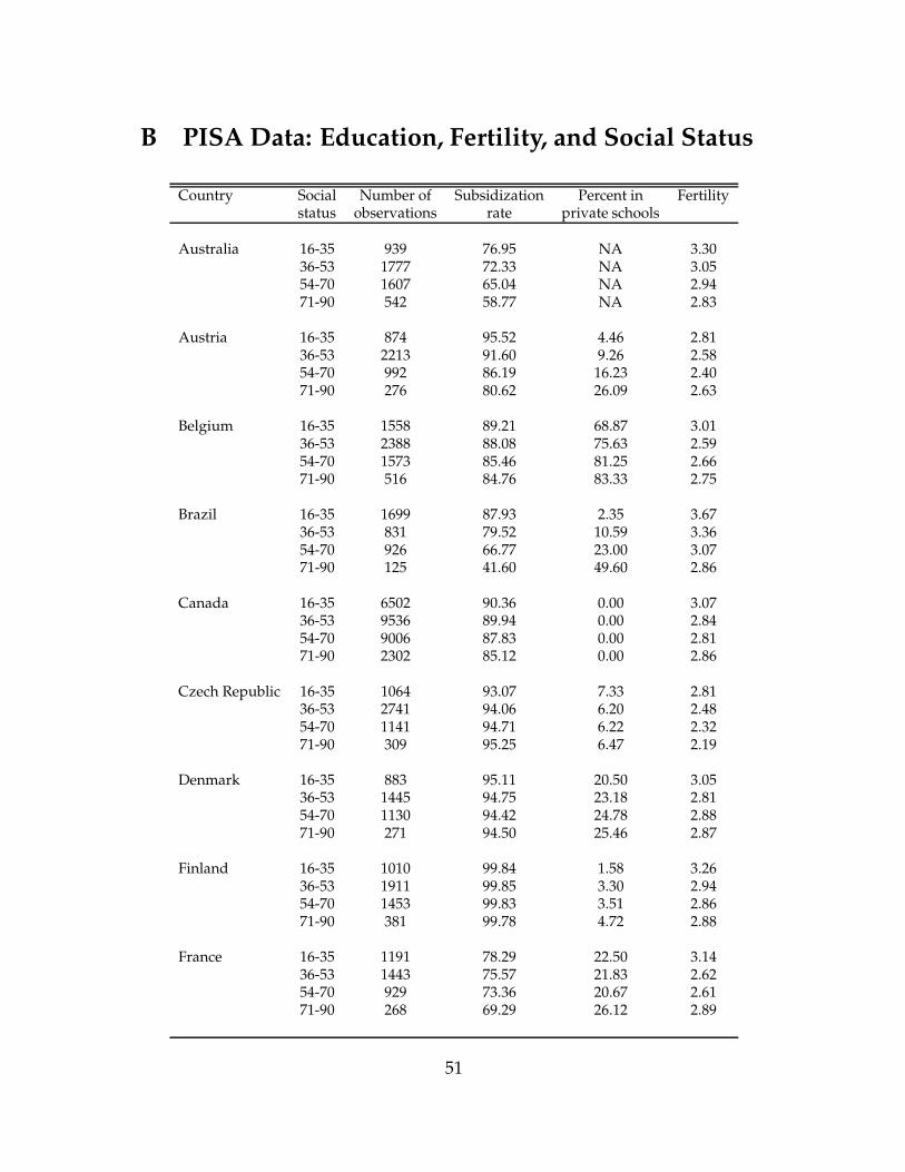
B PISA Data: Education, Fertility, and Social Status

Country Social Number of Subsidization Percent in Fertilitystatus observations rate private schools

Australia 16-35 939 76.95 NA 3.3036-53 1777 72.33 NA 3.0554-70 1607 65.04 NA 2.9471-90 542 58.77 NA 2.83

Austria 16-35 874 95.52 4.46 2.8136-53 2213 91.60 9.26 2.5854-70 992 86.19 16.23 2.4071-90 276 80.62 26.09 2.63

Belgium 16-35 1558 89.21 68.87 3.0136-53 2388 88.08 75.63 2.5954-70 1573 85.46 81.25 2.6671-90 516 84.76 83.33 2.75

Brazil 16-35 1699 87.93 2.35 3.6736-53 831 79.52 10.59 3.3654-70 926 66.77 23.00 3.0771-90 125 41.60 49.60 2.86

Canada 16-35 6502 90.36 0.00 3.0736-53 9536 89.94 0.00 2.8454-70 9006 87.83 0.00 2.8171-90 2302 85.12 0.00 2.86

Czech Republic 16-35 1064 93.07 7.33 2.8136-53 2741 94.06 6.20 2.4854-70 1141 94.71 6.22 2.3271-90 309 95.25 6.47 2.19

Denmark 16-35 883 95.11 20.50 3.0536-53 1445 94.75 23.18 2.8154-70 1130 94.42 24.78 2.8871-90 271 94.50 25.46 2.87

Finland 16-35 1010 99.84 1.58 3.2636-53 1911 99.85 3.30 2.9454-70 1453 99.83 3.51 2.8671-90 381 99.78 4.72 2.88

France 16-35 1191 78.29 22.50 3.1436-53 1443 75.57 21.83 2.6254-70 929 73.36 20.67 2.6171-90 268 69.29 26.12 2.89

51

Country Social Number of Subsidization Percent in Fertilitystatus observations rate private schools

Germany 16-35 887 97.89 2.03 2.7736-53 1970 97.84 3.40 2.4654-70 1105 96.56 6.52 2.3871-90 357 96.11 7.84 2.46

Greece 16-35 1278 85.63 1.10 2.6836-53 1447 87.02 2.07 2.4454-70 1074 82.60 4.38 2.3171-90 280 72.52 15.71 2.24

Hungary 16-35 1022 85.76 3.82 2.7436-53 2070 86.68 4.01 2.4254-70 1281 88.20 3.51 2.3071-90 261 90.18 6.13 2.38

Iceland 16-35 572 99.58 0.00 3.8036-53 1300 99.52 0.62 3.4654-70 926 99.10 1.30 3.3771-90 364 98.82 1.92 3.46

Ireland 16-35 990 94.68 50.71 3.9436-53 1463 91.43 63.98 3.5254-70 1040 87.83 72.21 3.3371-90 183 81.23 78.69 3.25

Italy 16-35 1391 79.47 2.16 2.4536-53 1995 74.50 5.81 2.3054-70 896 74.53 5.80 2.2271-90 281 71.17 6.05 2.34

Korea 16-35 1554 53.63 47.23 2.4636-53 1840 48.12 50.00 2.2554-70 803 46.47 49.69 2.1871-90 96 42.19 45.83 2.20

Mexico 16-35 1607 44.74 3.17 4.3336-53 1134 40.15 17.20 3.7454-70 619 34.52 33.60 3.3971-90 222 29.87 49.55 2.95

Netherlands 16-35 480 94.93 72.92 3.0936-53 739 94.59 77.00 2.8054-70 807 93.86 76.70 2.7971-90 153 94.85 71.90 2.86

52

Country Social Number of Subsidization Percent in Fertilitystatus observations rate private schools

New Zealand 16-35 643 84.82 0.78 3.5636-53 1275 81.16 3.61 3.2054-70 1041 78.20 5.86 3.0771-90 339 73.19 12.39 2.86

Norway 16-35 418 99.57 0.72 3.4036-53 1737 99.71 0.63 2.9854-70 1148 99.53 1.13 2.9971-90 538 99.39 1.12 2.95

Poland 16-35 1052 94.78 0.38 3.0736-53 1449 92.08 2.00 2.7554-70 564 91.24 4.08 2.4971-90 156 82.51 13.46 2.45

Portugal 16-35 1843 89.10 7.27 2.6736-53 1501 86.67 6.46 2.3354-70 747 83.58 8.17 2.2371-90 278 77.73 7.55 2.28

Russia 16-35 1594 94.19 0.00 2.9136-53 2742 93.38 0.00 2.7154-70 1135 92.94 0.00 2.6671-90 828 94.15 0.00 2.44

Spain 16-35 2078 90.92 24.01 2.6036-53 2020 82.93 42.48 2.3654-70 902 73.21 55.21 2.4071-90 387 59.13 68.22 2.50

Switzerland 16-35 1290 98.28 2.56 2.9336-53 2398 96.20 5.50 2.5854-70 1351 93.73 8.44 2.5471-90 582 89.72 13.40 2.68

United Kingdom 16-35 1858 98.24 0.65 3.4436-53 3166 96.50 2.46 2.9954-70 2276 89.99 8.92 2.8271-90 856 84.93 14.02 2.82

United States 16-35 584 94.01 4.11 3.8036-53 840 92.42 5.12 3.5454-70 899 92.84 5.01 3.1071-90 202 87.18 7.92 3.02

53