topological invariants for disordered solid state systemsclosing+2018/...topological invariants for...
TRANSCRIPT

Topological invariants for disordered solid state systems
Topological invariantsfor disordered solid state systems
Hermann Schulz-Baldes, Erlangen
main collaborators:
Emil Prodan (Yeshiva) and Terry Loring (Alberquerque)
Jena, March 2018
Topological invariants for disordered solid state systems
Plan of the talk
• Topological invariant for 1d-chiral Hamiltonian
• Index theorem and physical meaning (bulk-boundary corr.)
• Construction of associated spectral localizer
• Main new result: invariant as signature of spectral localizer
• Proof via spectral flow
• Extension to higher odd dimension
• Implementation of symmetries
• Even dimensional case
• Proof via fuzzy spheres

Topological invariants for disordered solid state systems
Model of SSH type (Su-Schriefer-Heeger)
Quasi-1d one-particle H on `2(Z,C2L) with chiral symmetry
J∗HJ = −H J =
(1L 0
0 −1L
)Due to chirality:
H =
(0 A
A∗ 0
)A on `2(Z,CL)
H insulator with µ = 0 Fermi level: H and hence A invertible
Moreover: H periodic, quasiperiodic or random
and short range so that for position X = X ⊗ 12L
‖[X ,H]‖ < ∞
Topological invariants for disordered solid state systems
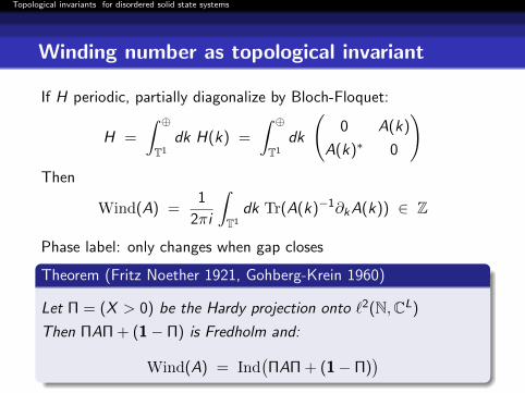
Winding number as topological invariant
If H periodic, partially diagonalize by Bloch-Floquet:
H =
∫ ⊕T1
dk H(k) =
∫ ⊕T1
dk
(0 A(k)
A(k)∗ 0
)Then
Wind(A) =1
2πi
∫T1
dk Tr(A(k)−1∂kA(k)) ∈ Z
Phase label: only changes when gap closes
Theorem (Fritz Noether 1921, Gohberg-Krein 1960)
Let Π = (X > 0) be the Hardy projection onto `2(N,CL)
Then ΠAΠ + (1− Π) is Fredholm and:
Wind(A) = Ind(ΠAΠ + (1− Π)
)
Topological invariants for disordered solid state systems
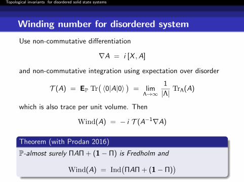
Winding number for disordered system
Use non-commutative differentiation
∇A = i [X ,A]
and non-commutative integration using expectation over disorder
T (A) = EP Tr(〈0|A|0〉
)= lim
Λ→∞
1
|Λ|TrΛ(A)
which is also trace per unit volume. Then
Wind(A) = − i T (A−1∇A)
Theorem (with Prodan 2016)
P-almost surely ΠAΠ + (1− Π) is Fredholm and
Wind(A) = Ind(ΠAΠ + (1− Π)
)
Topological invariants for disordered solid state systems
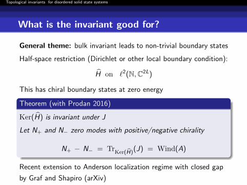
What is the invariant good for?
General theme: bulk invariant leads to non-trivial boundary states
Half-space restriction (Dirichlet or other local boundary condition):
H on `2(N,C2L)
This has chiral boundary states at zero energy
Theorem (with Prodan 2016)
Ker(H) is invariant under J
Let N+ and N− zero modes with positive/negative chirality
N+ − N− = TrKer(H)
(J) = Wind(A)
Recent extension to Anderson localization regime with closed gap
by Graf and Shapiro (arXiv)
Topological invariants for disordered solid state systems
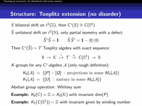
Structure: Toeplitz extension (no disorder)
S bilateral shift on `2(Z), then C∗(S) ∼= C (S1)
S unilateral shift on `2(N), only partial isometry with a defect:
S∗S = 1 S S∗ = 1− |0〉〈0|
Then C∗(S) = T Toeplitz algebra with exact sequence:
0 → K i↪→ T π→ C (S1) → 0
K -groups for any C∗-algebra A (only rough definition):
K0(A) = {[P]− [Q] : projections in some Mn(A)}K1(A) = {[U] : unitary in some Mn(A)}
Abelian group operation: Whitney sum
Example: K0(C) = Z = K0(K) with invariant dim(P)
Example: K1(C (S1)) = Z with invariant given by winding number
Topological invariants for disordered solid state systems
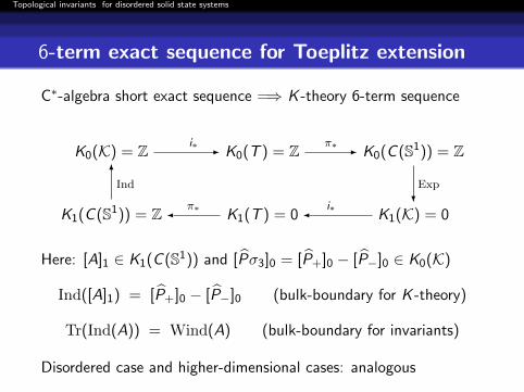
6-term exact sequence for Toeplitz extension
C∗-algebra short exact sequence =⇒ K -theory 6-term sequence
K0(K) = Z i∗ - K0(T ) = Z π∗ - K0(C (S1)) = Z
K1(C (S1)) = Z
Ind6
� π∗K1(T ) = 0 �
i∗K1(K) = 0
Exp?
Here: [A]1 ∈ K1(C (S1)) and [Pσ3]0 = [P+]0 − [P−]0 ∈ K0(K)
Ind([A]1) = [P+]0 − [P−]0 (bulk-boundary for K -theory)
Tr(Ind(A)) = Wind(A) (bulk-boundary for invariants)
Disordered case and higher-dimensional cases: analogous
Topological invariants for disordered solid state systems
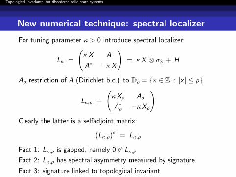
New numerical technique: spectral localizer
For tuning parameter κ > 0 introduce spectral localizer:
Lκ =
(κX A
A∗ −κX
)= κX ⊗ σ3 + H
Aρ restriction of A (Dirichlet b.c.) to Dρ = {x ∈ Z : |x | ≤ ρ}
Lκ,ρ =
(κXρ Aρ
A∗ρ −κXρ
)Clearly the latter is a selfadjoint matrix:
(Lκ,ρ)∗ = Lκ,ρ
Fact 1: Lκ,ρ is gapped, namely 0 6∈ Lκ,ρ
Fact 2: Lκ,ρ has spectral asymmetry measured by signature
Fact 3: signature linked to topological invariant

Topological invariants for disordered solid state systems
Theorem (with Loring 2017)
Let g = ‖A−1‖−1 be the invertibility gap. Provided that
‖[X ,A]‖ ≤ g3
12 ‖A‖κ(*)
and
2 g
κ≤ ρ (**)
the matrix Lκ,ρ is invertible and
12 Sig(Lκ,ρ) = Ind
(ΠAΠ + (1− Π)
)How to use: form (*) infer κ, then ρ from (**)
If A unitary, g = ‖A‖ = 1 and κ = (12‖[D,A]‖)−1 and ρ = 2/κ
Hence small matrix of size ≤ 100 sufficient! Great for numerics!
Topological invariants for disordered solid state systems
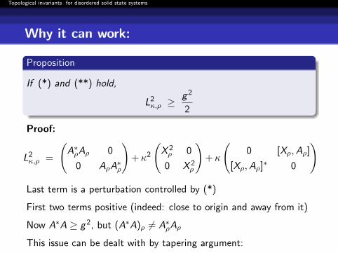
Why it can work:
Proposition
If (*) and (**) hold,
L2κ,ρ ≥
g2
2
Proof:
L2κ,ρ =
(A∗ρAρ 0
0 AρA∗ρ
)+κ2
(X 2ρ 0
0 X 2ρ
)+κ
(0 [Xρ,Aρ]
[Xρ,Aρ]∗ 0
)
Last term is a perturbation controlled by (*)
First two terms positive (indeed: close to origin and away from it)
Now A∗A ≥ g2, but (A∗A)ρ 6= A∗ρAρ
This issue can be dealt with by tapering argument:

Topological invariants for disordered solid state systems
Proposition (Bratelli-Robinson)
For f : R→ R with Fourier transform defined without√
2π,
‖[f (X ),A]‖ ≤ ‖f ′‖1 ‖[X ,A]‖
Lemma
∃ even function f : R→ [0, 1] with f (x) = 0 for |x | ≥ ρand f (x) = 1 for |x | ≤ ρ
2 such that ‖f ′‖1 = 8ρ
With this, f = f (X ) = f (|X |) and 1ρ = χ(|X | ≤ ρ):
A∗ρAρ = 1ρA∗1ρA1ρ ≥ 1ρA
∗f 2A1ρ
= 1ρfA∗Af 1ρ + 1ρ
([A∗, f ]fA + fA∗[f ,A]
)1ρ
≥ g2 f 2 + 1ρ([A∗, f ]fA + fA∗[f ,A]
)1ρ
So indeed A∗ρAρ positive close to origin
Then one can conclude... but TEDIOUS 2
Topological invariants for disordered solid state systems
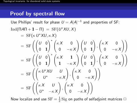
Proof by spectral flow
Use Phillips’ result for phase U = A|A|−1 and properties of SF:
Ind(ΠAΠ + 1− Π) = SF(U∗XU,X )
= SF(κU∗XU, κX )
= SF
((U 0
0 1
)∗(κX 0
0 −κX
)(U 0
0 1
),
(κX 0
0 −κX
))
= SF
((U 0
0 1
)∗(κX 1
1 −κX
)(U 0
0 1
),
(κX 0
0 −κX
))
= SF
((κU∗XU U
U∗ −κX
),
(κX 0
0 −κX
))
= SF
((κX U
U∗ −κX
),
(κX 0
0 −κX
))Now localize and use SF = 1
2 Sig on paths of selfadjoint matrices 2

Topological invariants for disordered solid state systems
Generalization: odd Fredholm model for invertible
Let A ∈ B(H) be invertible with gap g = ‖A−1‖−1
D = D∗ Dirac with compact resolvent and ‖[D,A]‖ <∞Introduce Π = χ(D < 0) and spectral localizer
Lκ =
(κD A
A∗ −κD
)Restriction Lκ,ρ to Ranχ(|D| ≤ ρ) is finite-dimensional matrix
Theorem (with Loring 2017)
If
‖[D,A]‖ ≤ g3
12 ‖A‖κ2 g
κ≤ ρ
then Lκ,ρ is invertible and
12 Sig(Lκ,ρ) = Ind
(ΠAΠ + (1− Π)
)
Topological invariants for disordered solid state systems
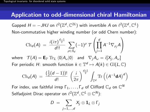
Application to odd-dimensional chiral Hamiltonian
Gapped H = −JHJ on `2(Zd ,C2L) with invertible A on `2(Zd ,CL)
Non-commutative higher winding number (or odd Chern number):
Chd(A) =i(iπ)
d−12
d!!
∑ρ∈Sd
(−1)ρ T
d∏j=1
A−1∇ρjA
where T (A) = EP TrL 〈0|Aω|0〉 and ∇jAω = i [Xj ,Aω]
For periodic H: smooth function k ∈ Td 7→ A(k) ∈ Gl(L,C)
Chd(A) =( 1
2 (d − 1))!
d!
(i
2π
) d+12∫Td
Tr((
A−1dA)d)
For index, use faithful irrep Γ1, . . . , Γd of Clifford Cd on CN
Selfadjoint Dirac operator on `2(Zd ,CL ⊗ CN):
D =∑
j=1,...,d
Xj ⊗ 1L ⊗ Γj
Topological invariants for disordered solid state systems
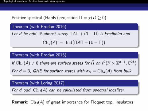
Positive spectral (Hardy) projection Π = χ(D ≥ 0)
Theorem (with Prodan 2016)
Let d be odd. P-almost surely ΠAΠ + (1− Π) is Fredholm and
Chd(A) = Ind(ΠAΠ + (1− Π)
)Theorem (with Prodan 2016)
If Chd(A) 6= 0 there are surface states for H on `2(N× Zd−1,C2L)
For d = 3, QHE for surface states with σH = Chd(A) from bulk
Theorem (with Loring 2017)
For d odd, Chd(A) can be calculated from spectral localizer
Remark: Ch3(A) of great importance for Floquet top. insulators
Topological invariants for disordered solid state systems
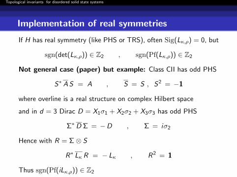
Implementation of real symmetries
If H has real symmetry (like PHS or TRS), often Sig(Lκ,ρ) = 0, but
sgn(det(Lκ,ρ)) ∈ Z2 , sgn(Pf(Lκ,ρ)) ∈ Z2
Not general case (paper) but example: Class CII has odd PHS
S∗ AS = A , S = S , S2 = −1
where overline is a real structure on complex Hilbert space
and in d = 3 Dirac D = X1σ1 + X2σ2 + X3σ3 has odd PHS
Σ∗D Σ = −D , Σ = iσ2
Hence with R = Σ⊗ S
R∗ Lκ R = − Lκ , R2 = 1
Thus sgn(Pf(iLκ,ρ)) ∈ Z2

Topological invariants for disordered solid state systems
Even dimensional pairings
Consider Hamiltonian on `2(Zd ,CL) with d even, no symmetry
For µ in gap of H consider Fermi projection P = χ(H ≤ µ)
Even-dimensional Dirac operator has grading Γd+1 =(1 0
0 −1
)Thus D =
( 0 D′
(D′)∗ 0
)and Dirac phase F = D ′|D ′|−1
Fredholm operator PFP + (1− P) has index = even Chern number
Spectral localizer
Lκ =
(H − µ κD ′
κ (D ′)∗ −(H − µ)
)Theorem (with Loring 2018)
Suppose ‖[H,D ′]‖ <∞ and D ′ normal, and κ, ρ with (*) and (**)
Chd(P) = Ind(PFP + (1− P)
)= 1
2 Sig(Lκ,ρ)
Topological invariants for disordered solid state systems
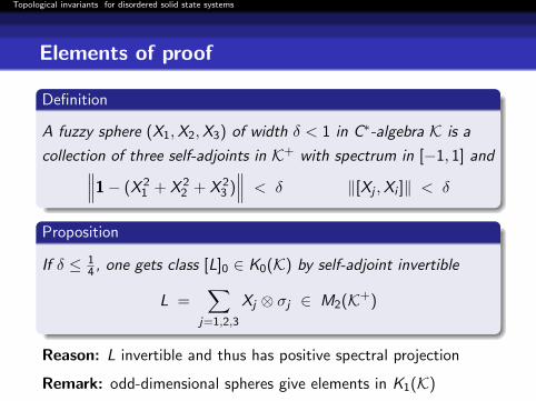
Elements of proof
Definition
A fuzzy sphere (X1,X2,X3) of width δ < 1 in C∗-algebra K is a
collection of three self-adjoints in K+ with spectrum in [−1, 1] and∥∥∥1− (X 21 + X 2
2 + X 23 )∥∥∥ < δ ‖[Xj ,Xi ]‖ < δ
Proposition
If δ ≤ 14 , one gets class [L]0 ∈ K0(K) by self-adjoint invertible
L =∑
j=1,2,3
Xj ⊗ σj ∈ M2(K+)
Reason: L invertible and thus has positive spectral projection
Remark: odd-dimensional spheres give elements in K1(K)
Topological invariants for disordered solid state systems
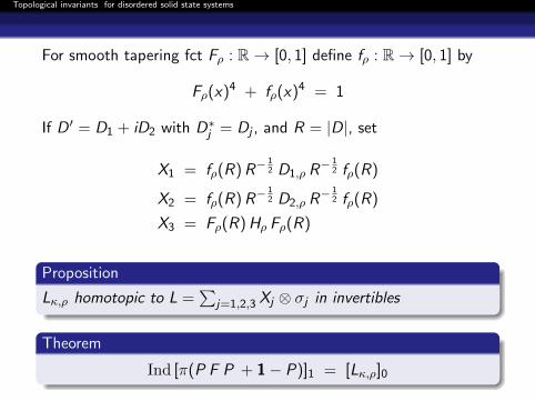
For smooth tapering fct Fρ : R→ [0, 1] define fρ : R→ [0, 1] by
Fρ(x)4 + fρ(x)4 = 1
If D ′ = D1 + iD2 with D∗j = Dj , and R = |D|, set
X1 = fρ(R)R−12 D1,ρ R
− 12 fρ(R)
X2 = fρ(R)R−12 D2,ρ R
− 12 fρ(R)
X3 = Fρ(R)Hρ Fρ(R)
Proposition
Lκ,ρ homotopic to L =∑
j=1,2,3 Xj ⊗ σj in invertibles
Theorem
Ind [π(P F P + 1− P)]1 = [Lκ,ρ]0

Topological invariants for disordered solid state systems
Theorem (General tool)
0→ K ↪→ B π→ Q→ 0 short exact sequence with Q unital
A ∈ B contraction with π(A) ∈ Q invertible, so [π(A)]1 ∈ K1(Q)
Assume A = A1 + i A2 almost normal, namely ‖[A1,A2]‖ < ε
Choose smooth ψ : [0, 1]→ [0, 1] and φ : [0, 1]→ [−1, 1] such that
φ(1) = 1 = −ψ(0) , x2 ψ(x)4 + φ(x)2 = 1
With B = (A21 + A2
2)12 set
Y1 = ψ(B)A1ψ(B) , Y2 = −ψ(B)A2ψ(B) , Y3 = φ(B)
Then (Y1,Y2,Y3) fuzzy sphere in K giving K -theoretic index map:
Ind[π(A)]1 =[ ∑j=1,2,3
Yj ⊗ σj]
0
Topological invariants for disordered solid state systems
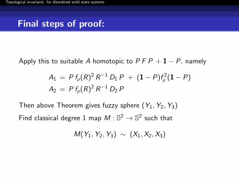
Final steps of proof:
Apply this to suitable A homotopic to P F P + 1− P, namely
A1 = P fρ(R)2 R−1 D1 P + (1− P)f 2ρ (1− P)
A2 = P fρ(R)2 R−1 D2 P
Then above Theorem gives fuzzy sphere (Y1,Y2,Y3)
Find classical degree 1 map M : S2 → S2 such that
M(Y1,Y2,Y3) ∼ (X1,X2,X3)
Topological invariants for disordered solid state systems
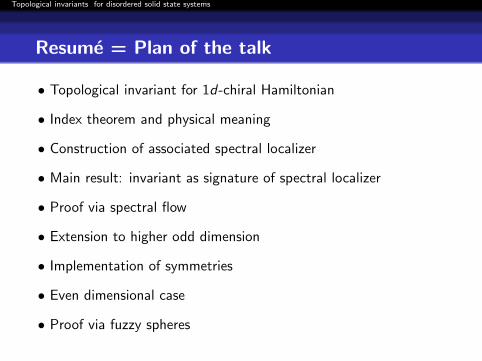
Resume = Plan of the talk
• Topological invariant for 1d-chiral Hamiltonian
• Index theorem and physical meaning
• Construction of associated spectral localizer
• Main result: invariant as signature of spectral localizer
• Proof via spectral flow
• Extension to higher odd dimension
• Implementation of symmetries
• Even dimensional case
• Proof via fuzzy spheres
Topological invariants for disordered solid state systems
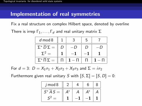
Implementation of real symmetries
Fix a real structure on complex Hilbert space, denoted by overline
There is irrep Γ1, . . . , Γd and real unitary matrix Σ
d mod 8 1 3 5 7
Σ∗D Σ = D −D D −DΣ2 = 1 −1 −1 1
Σ∗Π Σ = Π 1− Π Π 1− Π
For d = 3: D = X1σ1 + X2σ2 + X3σ3 and Σ = iσ2
Furthermore given real unitary S with [S ,Σ] = [S ,D] = 0:
j mod 8 2 4 6 8
S∗ AS = A∗ A A∗ A
S2 = 1 −1 −1 1

Topological invariants for disordered solid state systems
Symmetries of T = ΠAΠ + (1− Π) such that index pairings are:
Ind(2)(T ) j = 2 j = 4 j = 6 j = 8
d = 1 0 2Z Z2 Zd = 3 2Z Z2 Z 0
d = 5 Z2 Z 0 2Zd = 7 Z 0 2Z Z2
where Ind2(T ) = dim(Ker(T ))mod 2 ∈ Z2 (with Großmann 2016)
For spectral localizer follows R∗ Lκ R = s Lκ and R2 = s ′1 with
s = , s ′ = j = 2 j = 4 j = 6 j = 8
d = 1 −1 , −1 1 , −1 −1 , 1 1 , 1
d = 3 1 , −1 −1 , 1 1 , 1 −1 , −1
d = 5 −1 , 1 1 , 1 −1 , −1 1 , −1
d = 7 1 , 1 −1 , −1 1 , −1 −1 , 1
Topological invariants for disordered solid state systems
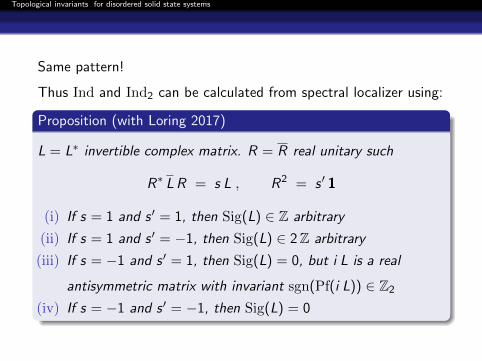
Same pattern!
Thus Ind and Ind2 can be calculated from spectral localizer using:
Proposition (with Loring 2017)
L = L∗ invertible complex matrix. R = R real unitary such
R∗ LR = s L , R2 = s ′ 1
(i) If s = 1 and s ′ = 1, then Sig(L) ∈ Z arbitrary
(ii) If s = 1 and s ′ = −1, then Sig(L) ∈ 2Z arbitrary
(iii) If s = −1 and s ′ = 1, then Sig(L) = 0, but i L is a real
antisymmetric matrix with invariant sgn(Pf(i L)) ∈ Z2
(iv) If s = −1 and s ′ = −1, then Sig(L) = 0