1

Topological dynamics and current-induced motion a

skyrmion lattice

J C Martinez AND M B A Jalil

Computational Nanoelectronics and Nano-device Laboratory

National University of Singapore, 4 Engineering Drive 3, Singapore 117576

We study the Thiele equation for current-induced motion in a skyrmion lattice through two

soluble models of the pinning potential. Comprised by a Magnus term, a dissipative term

and a pinning force, Thiele’s equation resembles Newton’s law but in virtue of the

topological character to the first two, it differs significantly from Newtonian mechanics and

because the Magnus force is dominant, unlike its mechanical counterpart –the Coriolis

force– skyrmion trajectories do not necessarily have mechanical counterparts. This is

important if we are to understand skyrmion dynamics and tap into its potential for data-

storage technology. We identify a pinning threshold velocity for the one-dimensional

pinning potential and for a two-dimensional potential we find a pinning point and the

skyrmion trajectories toward that point are spirals whose frequency (compare Kepler’s

second law) and amplitude-decay depend only on the Gilbert constant and potential at the

pinning point.

PACS numbers: 75.76.+j, 75.78.-n

2

The experimental discovery in 2009 of a hexagonal skyrmion lattice in MnSi under

an external vertical magnetic field generated a convergence of efforts to understand better

the interplay between the ferromagnetic exchange and Dzyaloshinskii-Moriya couplings in

conjunction with crystalline field interactions in B20 compounds, i.e. magnetic materials

lacking inversion symmetry (or chiral magnets)[1, 2]. A skyrmion is a planar topological

spin texture whose spins are distributed in a circularly symmetric and continuous manner

with the spin at the center pointing downward while all spins at the edge are pointing

upward. Of particular interest for its application to information-storage technology,

specifically the racetrack memory [3], is the effect of current on the magnetic texture since

a relatively small current density is able to induce skyrmion motion, thus fueling hopes that

ultra-low current densities might be feasible in the manipulation of magnetic structures [4,

5]. But this hope is not without fears since the mechanisms responsible for pinning and

current-induced skyrmion motion are presently not well understood [6]. Moreover,

experimentally, only very slow translation motion of skyrmions has been observed.

The standard tool of magnetization dynamics is the Landau-Lifshitz-Gilbert (LLG)

equation

(𝜕

𝜕𝑡+ (𝐯𝑠 ∙ 𝛁)) 𝐌 = −𝛾𝐌 × 𝐁eff +

𝛼

𝑀𝐌 × (

𝜕

𝜕𝑡+

𝛽

𝛼(𝐯𝑠 ∙ 𝛁)) 𝐌 (1)

𝐁eff = −1

ℏ𝛾

𝛿ℋ

𝛿𝐌 is the effective field; 𝛾 =

𝑔𝜇𝐵

ℏ> 0 the gyromagnetic ratio, 𝐯𝑠 the spin velocity

parallel to the spin current, ℋthe free energy density, α the Gilbert damping constant, and

β the coupling between the spin-polarized current and local magnetization due to

nonadiabatic effects [7, 8]. An immediate consequence of Eq. (1) is that the magnitude of

the magnetization M2 is conserved in time. The LLG equation has found application in a

3

variety of systems such as ferromagnets, vortex filaments, and moving space curves and

structures such as spin waves and solitons, to name a few [9]. As a time-dependent

nonlinear equation, the LLG equation is arguable the most difficult equation to solve in

theoretical physics. It is natural then to seek simplified versions of it. Since our interest

here is on current-induced forces in a skyrmion lattice, we consider Thiele’s simplification

of it and treat the pinning mechanism phenomenologically [10]. Thiele projected the LLG

equation onto the relevant translational modes [11] and in this way obtained an equation

that could be regarded as a dynamical force equation but derived from a torque equation.

To obtain it, we first assume a steady-state rigid texture 𝐌 = 𝐌(𝒓 − 𝐯𝑑𝑡), 𝐯𝑑 standing for

the skyrmion drift velocity. Then we cross multiply Eq. (1) by M, followed by a scalar

multiplication of the result by 1

𝑀𝜕𝑖𝐌 and finally we integrate over the skyrmion area:

𝐆 × (𝐯𝑠 − 𝐯𝑑) + �⃡� (𝛽𝐯𝑠 − 𝛼𝐯𝑑) = ∇𝑉, (2)

where 𝐺𝑘 = 1

4𝜋휀𝑖𝑗𝑘 ∫ 𝑑2𝑟

1

𝑀3

.

.𝐌 ∙ 𝜕𝑖𝐌 × 𝜕𝑗𝐌 is the dimensionless gryro-coupling vector and

�⃡� 𝑖𝑗 =1

2𝜋∫ 𝑑2𝑟

.

𝑈𝐶

1

𝑀2 𝜕𝑖𝐌 ∙ 𝜕𝑗𝐌 the dissipative dyadic. The gyro-term can be traced back to

the Berry phase and pushes a moving a skyrmion perpendicularly to its direction of motion

and is also referred to as the Magnus force [5, 11, 12]. The Magnus force is the counterpart

of the Coriolis force in dynamics. The latter is a small correction to the dynamical

equations [13], whereas the former, as we will see, dominates the dynamics of our

skyrmion system. The Magnus force makes a spinning ball swerve one way as it passes the

air; the Coriolis force is a fictitious force due to motion in moving noninertial frame. If we

view Eq. (1) as an equation in the reference frame of the current, it seems more fitting to

compare the first term with the Coriolis force. The dissipation term, which sums up the

4

skyrmion’s tendency toward a region of lower energy, originates from Gilbert damping. At

the right-hand side we inserted a term due to a potential V, which models the pinning

potential. Internal details of the skyrmion are ignored. Since the skyrmion is assumed to be

perfectly rigid, it is not possible to deduce the pinning forces due to cancellation of forces

for such a structure. Pinning is important not only in magnetics but also in

superconductivity [14], soliton theory [15] and meteorology. For a skyrmion of winding

number Q = -1 [1], 𝐆 ≡ 𝑔�̂� = −4𝜋�̂�, �̂� being the normal to the thin film and �⃡� 𝑖𝑗 =

5.577𝜋𝛿𝑖𝑗 , i = j = 1, 2.

It is obvious that the Thiele equations are already a vast simplification over the

original LLG equation. Nevertheless it still is nonlinear, albeit one involving only first-order

derivatives. Unlike Newton’s equations of motion, Thiele’s equations are not time-reversal

invariant. Moreover, the quantities g and �⃡� 𝑖𝑗 are of topological origin in contrast with the

dynamical parameters entering into Newton’s equations. It is important then to gain

familiarity with the Thiele equations if we are to understand current-induced motion in

chiral magnets [16]. What is notable about this system is the topological character of the

Magnus and dissipative parameters, a significant departure from mechanical systems. In

the early 90s ideas about a topological quantum mechanics were in vogue [17]; we might

now speak of a topological dynamics for the present system. In this paper, we present two

models for which exact solutions of the Thiele equations can be derived. We find that these

results are in excellent agreement with numerical results. Our findings allow us to identify

key features of the dynamics. Insights from Newtonian mechanics do not necessarily

translate into analogous situations for the Thiele case (for instance Kepler’s second law

5

does not hold in one model; in the other model Coriolis deflection occurs without forward

motion).

We begin with a one-dimensional sinusoidal form for V: V = - V0 cos(2πx/λ) and

assume λ much larger than skyrmion size [18]. Let us also assume constant spin current vs

in the x-direction so v𝑠𝑦 = 0. With v𝑠𝑥 known, the drift velocities 𝑣𝑥𝑑 , 𝑣𝑦

𝑑 can be solved from

𝑣𝑥𝑑 =

𝑔2+𝛼𝛽𝒟2

𝑔2+𝛼2𝒟2 v𝑠𝑥 + 𝑉0𝛼𝒟

𝑔2+𝛼2𝒟2

2𝜋

𝜆sin

2𝜋𝑥

𝜆 (3a)

𝑣𝑦𝑑 =

𝑔(𝛽−𝛼)𝒟

𝑔2+𝛼2𝒟2 v𝑠𝑥 + 𝑉0𝑔

𝑔2+𝛼2𝒟2

2𝜋

𝜆sin

2𝜋𝑥

𝜆 (3b)

Since the solutions are translationally invariant, we take, for simplicity, the initial position

to be the origin. Making use of the formula √𝐴2 − 1 ∫𝑑𝑥

𝐴+sin𝑥= 2tan−1 1+𝐴tan𝑥

2

√𝐴2−1 we find

tan𝜋𝑥

𝜆= 𝑟

sin𝜋

𝜆𝑉√𝑟2−1 𝑡

√𝑟2−1cos𝜋

𝜆𝑉√𝑟2−1 𝑡−sin

𝜋

𝜆𝑉√𝑟2−1 𝑡

, 𝑦 =𝑔

𝛼𝒟(𝑥 − v𝑠𝑥𝑡) (4)

in which ℳ = 𝑔(𝛽−𝛼)𝒟

𝑔2+𝛼2𝒟2 v𝑠𝑥 , 𝒩 =𝑔2+𝛼𝛽𝒟2

𝑔2+𝛼2𝒟2 v𝑠𝑥 , 𝑉 =2𝜋

𝜆𝑉0

𝛼𝒟

𝑔2+𝛼2𝒟2 , 𝑈 =2𝜋

𝜆𝑉0

𝑔

𝑔2+𝛼2𝒟2 have

dimensions of velocity whereas the ratio 𝑟 =𝒩

𝑉 is dimensionless. Equations (4) hold when r

> 1. When r < 1, we must make the replacements sin → i sinh, cos → cosh and tan → i tanh.

Since -1 ≤ arctanh ξ ≤ + 1, x has a limit point when r < 1. This limiting point does not appear

when r > 1.

There is another way to look at the case r = 1. The drift velocity is positive for all x

provided 𝑔2+𝛼𝛽𝒟2

𝑔2+𝛼2𝒟2 v𝑠𝑥 +2𝜋

𝜆𝑉0

𝛼𝒟

𝑔2+𝛼2𝒟2 sin2𝜋𝑥

𝜆≥ 0 so a threshold spin velocity vspin threshold is

required: vspin threshold ≥2𝜋

𝜆𝑉0

𝛼𝒟

𝑔2+𝛼𝛽𝒟2. The case r = 1 corresponds to equality. For this case

6

the second equation of Eq. (4) still holds but the first is replaced by 𝜋𝑥

𝜆= cot−1 (

𝜆

𝜋𝐴𝑡− 1):

one recognizes that pinning still occurs in this instance.

Fig. 1 (a) Skyrmion trajectory for vs = 0.6, V0 =10, α = 0.1, β = α/2 with the origin as starting point: X = x/λ, Y = y/λ. Numerical integration using Mathematica gives the same graph. (b) For the exact solution of Fig. 1(a) we display the position, X(t), Y(t), and velocity �̇�as functions of time. For clarity we plot 2X(t) instead of X. See text for discussion.

Figure 1(a) displays the trajectory and Fig. 1(b) the position-time graphs for spin

velocity vs = 0.6 in the x-direction (this corresponds to r < 1) and V0 =10, α = 0.1, β = α/2.

We use these latter parameters for Figs. 1 - 3. The r = 1 case for the parameters given

corresponds to vs = 0.69037. The starting point is always the origin. Equation (4) and

numerical integration using Mathematica yield the same graphs. The first term of Eq. (2),

which is the Magnus term, shows that the motion along the y-direction is due to the gyro-

term and is large as comparison of the X and Y displacements on Fig. 1(b) indicates.

Figure 1(b) shows that the motion along the x-direction approaches a fixed or

pinning point as the velocity �̇� approaches zero asymptotically; whereas there continues to

be a drift upward. We can think of the first term on the right-hand side of Eq. (3a) as the

force component of the Magnus force opposed by the second term on the right-hand side,

0.1 0.2 0.3 0.4 0.5 0.6 X

1

1

2

3

Y

X 2XY

0.5 1.0 1.5 2.0 T1

1

2

3

NullB

7

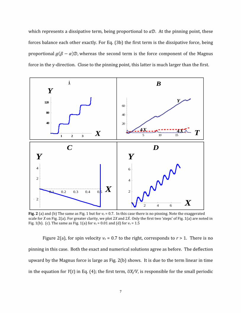
which represents a dissipative term, being proportional to 𝛼𝒟. At the pinning point, these

forces balance each other exactly. For Eq. (3b) the first term is the dissipative force, being

proportional 𝑔(𝛽 − 𝛼)𝒟, whereas the second term is the force component of the Magnus

force in the y-direction. Close to the pinning point, this latter is much larger than the first.

Fig. 2 (a) and (b) The same as Fig. 1 but for vs = 0.7. In this case there is no pinning. Note the exaggerated scale for X on Fig. 2(a). For greater clarity, we plot 2X and 2�̇�. Only the first two ‘steps’ of Fig. 1(a) are noted in Fig. 1(b). (c). The same as Fig. 1(a) for vs = 0.01 and (d) for vs = 1.5

Figure 2(a), for spin velocity vs = 0.7 to the right, corresponds to r > 1. There is no

pinning in this case. Both the exact and numerical solutions agree as before. The deflection

upward by the Magnus force is large as Fig. 2(b) shows. It is due to the term linear in time

in the equation for Y(t) in Eq. (4); the first term, UX/V, is responsible for the small periodic

1 2 3 X

40

80

120

Y

4X4X

Y

5 10 15 T

20

40

60

NullB

0.1 0.2 0.3 0.4 0.5 X2

2

4

Y

C

2 4 6 X

2

4

6

Y

D

8

downward dips in the right-hand plot for Y(t). Each of the almost horizontal steps in Fig. 2a

corresponds to a crossing into the potential barrier (but there is no tunneling here).

Figures 2(c) and (d) show two instances quite removed from the r = 1 case. In the

first where vs = 0.01, the downward line is just the second half of Eq. (4), viz 𝑦 =𝑔

𝛼𝒟(𝑥 −

v𝑠𝑥𝑡). For the upward drift the velocity is −𝑔

𝛼𝒟v𝑠𝑥 > 0, involves the topological quantities

g and 𝒟. It is interesting to see upward motion without horizontal motion, in contrast with

the Coriolis effect. Compared with Fig. 1a the trajectory is here shows sharp change of

direction. In Fig. 2(d) with vs = 1.5, the downward dips correspond to crossings into the

pinning potential. The dips and upward movements are commensurate with each other

unlike the case with Fig. 2(a). For large velocities this trend is maintained.

Consider next the attractive two-dimensional potential

𝑉(𝑥, 𝑦) = −𝑈0 exp (−|𝑥|

𝜆−

|𝑦|

𝜆). (5)

This potential has cusps along the x and y axes. As above we assume a spin current only in

the x-direction. The Thiele equations are

−𝑔𝑣𝑑𝑥 + 𝛼𝒟𝑣𝑑𝑦 = −𝑔𝑣𝑠𝑥 +𝑈0

𝜆𝑒−

|𝑥|

𝜆−

|𝑦|

𝜆 sgn(𝑦) (6a)

𝛼𝒟𝑣𝑑𝑥 + 𝑔𝑣𝑑𝑦 = 𝒟𝛽𝑣𝑠𝑥 +𝑈0

𝜆𝑒−

|𝑥|

𝜆−

|𝑦|

𝜆 sgn(𝑥) (6b)

Let 𝒩 =𝑔2+𝛼𝛽𝒟2

𝑔2+𝛼2𝒟2 v𝑠𝑥, ℳ =𝑔(𝛽−𝛼)𝒟

𝑔2+𝛼2𝒟2 v𝑠𝑥 , and set 𝒶 =𝑔

𝑔2+𝛼2𝒟2, 𝒷 =𝛼𝒟

𝑔2+𝛼2𝒟2. Let 𝑋 = 𝑥/𝜆, 𝑌 =

𝑦/𝜆, measure time with the same magnitude as 𝜆, and define 𝒰 = 𝑈0/𝜆. We find

�̇� = 𝒩 + (𝒷sgn(𝑋) − 𝒶sgn(𝑌))𝒰𝑒−|𝑋|−|𝑌| , �̇� = ℳ + (𝒶sgn(𝑋) + 𝒷sgn(𝑌))𝒰𝑒−|𝑋|−|𝑌| (7)

9

Integrating we have

𝑌 − 𝑌0 =𝒶sgn(𝑋)+𝒷sgn(𝑌)

𝒷sgn(𝑋)−𝒶sgn(𝑌)(𝑋 − 𝑋0) + (ℳ −

𝒶sgn(𝑋)+𝒷sgn(𝑌)

𝒷sgn(𝑋)−𝒶sgn(𝑌)𝒩)𝑡. (8)

This holds for a given quadrant where signs of X and Y stay constant ‘during’ integration.

Again from the first of Eq. (7) we have �̇�sgn(𝑋) = 𝒩sgn(𝑋) + (𝒷 −

𝒶sgn(𝑋)sgn(𝑌))𝒰𝑒−|𝑋|−|𝑌| and from the second, �̇�sgn(𝑌) = ℳ𝑠gn(𝑌) + (𝒶sgn(𝑋)𝑠gn(𝑌) +

𝒷)𝒰𝑒−|𝑋|−|𝑌|; adding and, staying in a fixed quadrant, we obtain |�̇�| + |�̇�| = 𝒩sgn(𝑋) +

ℳ𝑠gn(𝑌) + 2𝒷𝒰𝑒−|𝑋|−|𝑌|. In all cases below 𝒩 > 0 > ℳ. With Z =|𝑋| + |𝑌| we have finally

𝑒𝑍 = 𝑒𝑍0+(𝒩sgn(𝑋)+ℳ𝑠gn(𝑌))𝑡 + 2𝒷𝒰

𝒩sgn(𝑋)+ℳ𝑠gn(𝑌)(𝑒(𝒩sgn(𝑋)+ℳ𝑠gn(𝑌))𝑡 − 1) (9)

where 𝑍0 = |𝑋0| + |𝑌0|. Equations (8) and (9) are the parametric equations of the

trajectory for a given quadrant. For small times the trajectory is clearly straight. When

𝒷𝒰

𝒩sgn(𝑋)+ℳ𝑠gn(𝑌), which is proportional to α, is small we can also expect straight trajectories.

In regions where this is large, we might expect curved trajectories.

Far from the origin the trajectory is straight. To see this, multiply the first equation

of Eq. (7) by Y and the second by X and subtract. Far away from the origin we obtain

𝑑

𝑑𝑡tan−1𝑌

𝑋→

ℳ𝑋−𝒩𝑌

𝑋2+𝑌2, that is, if 𝜙 is the polar angle, then

𝑑𝜙

𝑑𝑡→ 0 as |𝑋|, |𝑌| → ∞.

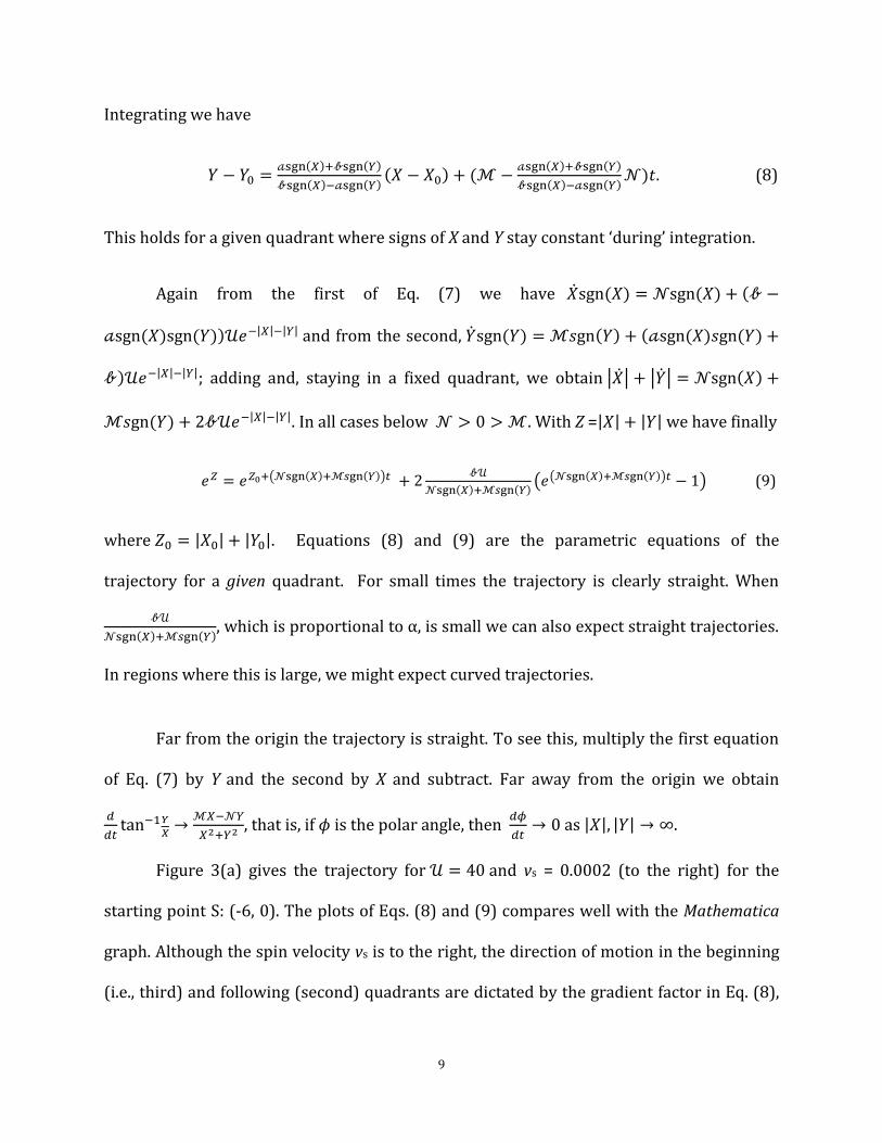
Figure 3(a) gives the trajectory for 𝒰 = 40 and vs = 0.0002 (to the right) for the

starting point S: (-6, 0). The plots of Eqs. (8) and (9) compares well with the Mathematica

graph. Although the spin velocity vs is to the right, the direction of motion in the beginning

(i.e., third) and following (second) quadrants are dictated by the gradient factor in Eq. (8),

10

𝒶sgn(𝑋)+𝒷sgn(𝑌)

𝒷sgn(𝑋)−𝒶sgn(𝑌)=

𝑔sgn(𝑋)+𝛼𝒟sgn(𝑌)

𝛼𝒟sgn(𝑋)−𝑔sgn(𝑌). Note that this is a ratio of quantities of topological origin.

After the motion has entered into the first quadrant, time has now become large (∼ 105, see

Fig. 3b) and the trajectory veers off only to assume a straight path outward to infinity. The

effect of the cusps is evident and occurs only at the coordinate axes. These cusps might be

suitable in modeling line defects.

Fig. 3 (a) Trajectory starting at S: (-6, 0) for 𝒰 = 40 and vs = 0.0002. The red curve is the exact result while the dashed is the one obtain via numerical integration with Mathematica. (b) Position-time graphs, X(T), Y(T). The discontinuities are due to the cusps. The shaded section corresponds to the second quadrant trajectory of Fig. 3(a) and is added for clarity. (c) The same as Fig. 3 (a) for S: (-6, -1) and 𝒰 = 20 and vs =2. (d) Position time graphs corresponding to Fig. 3(c). The inset is a zoom of the turn-around trajectory (circled) about the origin in Fig. 3(c).

Figure 3 (c) shows that trajectory from the starting point S: (-6, -1) for 𝒰 = 20 and

vs = 2. As in Fig. 3(a), the exact and numerical results agree well with each other. The cusps

T

S

6 4 2 2 4 6 8 X

1.0

0.8

0.6

0.4

0.2

Y

C

X

Y2 4 6 8 T

6

4

2

2

4

6

NullD

3.25 3.30 3.35 3.40 3.45 T0.2

0.1

0.1

0.2

0.3

0.4

NullD

11

are again evident. What appears striking here is the turn-around trajectory about the

center of the potential at the origin. In fact a close-up of the trajectory around the origin, as

shown in the inset of Fig. 3(d), indicates that the motion is very much like the first two

parts of Fig. 3(a): they are straight-line segments whose gradients are given by the ratio

𝑔sgn(𝑋)+𝛼𝒟sgn(𝑌)

𝛼𝒟sgn(𝑋)−𝑔sgn(𝑌), which is of topological origin. Because the turn-around occurs much closer to

the source of the potential than in Fig. 3(a) we see a faster reversal of the motion. At the

point T in Fig. 3 (c), the drift is purely horizontal, i.e. the y-velocity vanishes. From the

second equation of Eq. (7) we infer that this is where the dissipative (first term) force

component is balanced by the Magnus (second) term.

Fig. 4 (a) Trajectories starting at S: (0, 1) for 𝒰 = 30 and vs = 0.01 and (b) S: (-7, -1) for 𝒰 = 20 and vs = 1.

Figure 4 shows other scenarios which indicate that whenever particles approach the

origin they are bound to undergo the phenomenon already seen in Fig.3: straight-line

trajectories whose gradients are given by the ratio of topological quantities g and 𝒟.

The LLG equation for the potential (5) does not have a pinning point even though

the origin is clearly a local minimum. This is because of the cusps. To see pinning we take

two identical attractive potentials 𝑉(𝑥, 𝑦), one centered at the origin as in Eq. (5), and another at

S

5 10 X21

123

Y

A

S

6 4 2 2 4 6 X

1.0

0.5

0.5

Y

B

12

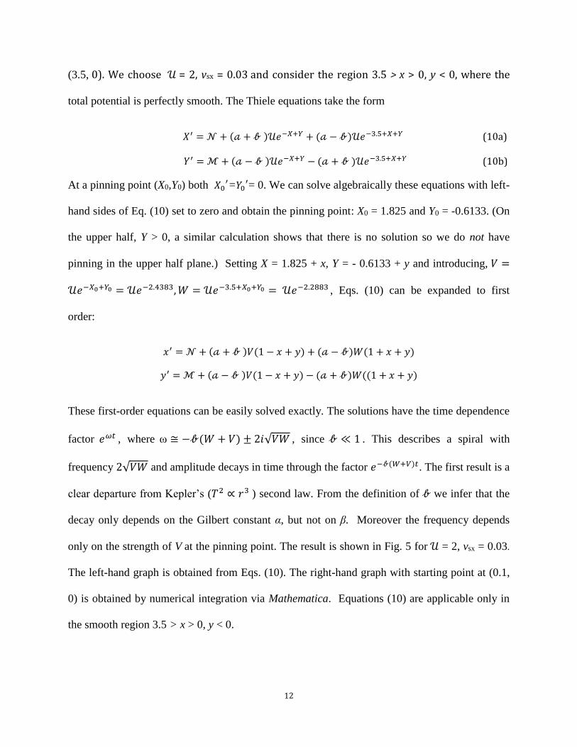
(3.5, 0). We choose 𝒰 = 2, vsx = 0.03 and consider the region 3.5 > x > 0, y < 0, where the

total potential is perfectly smooth. The Thiele equations take the form

𝑋′ = 𝒩 + (𝒶 + 𝒷 )𝒰𝑒−𝑋+𝑌 + (𝒶 − 𝒷)𝒰𝑒−3.5+𝑋+𝑌 (10a)

𝑌′ = ℳ + (𝒶 − 𝒷 )𝒰𝑒−𝑋+𝑌 − (𝒶 + 𝒷 )𝒰𝑒−3.5+𝑋+𝑌 (10b)

At a pinning point (X0,Y0) both 𝑋0′=𝑌0

′= 0. We can solve algebraically these equations with left-

hand sides of Eq. (10) set to zero and obtain the pinning point: X0 = 1.825 and Y0 = -0.6133. (On

the upper half, Y > 0, a similar calculation shows that there is no solution so we do not have

pinning in the upper half plane.) Setting X = 1.825 + x, Y = - 0.6133 + y and introducing, 𝑉 =

𝒰𝑒−𝑋0+𝑌0 = 𝒰𝑒−2.4383, 𝑊 = 𝒰𝑒−3.5+𝑋0+𝑌0 = 𝒰𝑒−2.2883 , Eqs. (10) can be expanded to first

order:

𝑥′ = 𝒩 + (𝒶 + 𝒷 )𝑉(1 − 𝑥 + 𝑦) + (𝒶 − 𝒷)𝑊(1 + 𝑥 + 𝑦)

𝑦′ = ℳ + (𝒶 − 𝒷 )𝑉(1 − 𝑥 + 𝑦) − (𝒶 + 𝒷)𝑊((1 + 𝑥 + 𝑦)

These first-order equations can be easily solved exactly. The solutions have the time dependence

factor 𝑒𝜔𝑡 , where ω ≅ −𝒷(𝑊 + 𝑉) ± 2𝑖√𝑉𝑊 , since 𝒷 ≪ 1 . This describes a spiral with

frequency 2√𝑉𝑊 and amplitude decays in time through the factor 𝑒−𝒷(𝑊+𝑉)𝑡. The first result is a

clear departure from Kepler’s (𝑇2 ∝ 𝑟3 ) second law. From the definition of 𝒷 we infer that the

decay only depends on the Gilbert constant α, but not on β. Moreover the frequency depends

only on the strength of V at the pinning point. The result is shown in Fig. 5 for 𝒰 = 2, vsx = 0.03.

The left-hand graph is obtained from Eqs. (10). The right-hand graph with starting point at (0.1,

0) is obtained by numerical integration via Mathematica. Equations (10) are applicable only in

the smooth region 3.5 > x > 0, y < 0.

13

Fig. 5 With two attractive potentials centered at the origin (0, 0) and at (3.5, 0), it is possible to pin a skyrmion. We choose 𝒰 = 2, vsx = 0.03. On the right we have the result of Eq. (10). For comparison, on the left we use numerical integration with Mathematica from the starting point S = (0.1, 0). Note the effect of the cusps at the axes.

In summary we studied the Thiele equation for current-induced motion in a

skyrmion lattice through two soluble models of the pinning potential. Thiele’s equation is

composed of a Magnus force, responsible for transverse motion relative to the current

velocity, a dissipation force along the current velocity and the pinning force. The first two

have topological origin whereas the third is imposed externally. In the first, one-

dimensional model the Magnus force was found to dominate the dynamics and even

transverse motion without corresponding skyrmion motion in the spin direction was

possible. We saw a threshold velocity below which motion in the current direction is not

allowed and which can be interpreted in terms of balance between the Magnus and the

pinning forces. In the second two-dimensional case we saw the occurrence of straight

trajectories in which the interplay of the Magnus and dissipative forces and, hence, their

topological character are evident. Because of the peculiarities of the model, pinning onto a

point was not possible; however with two potentials separated from each other, a pinning

S2 X

1

Y2, 0.03

0.5 1.0 1.5 2.0 X

1.2

1.0

0.8

0.6

0.4

0.2

Y

14

point could be found. The trajectory close to the pinning point is a spiral whose frequency

and amplitude decay depend only on the Gilbert constant and the strength of the potential

at the pinning point. Kepler’s second law did not hold in this system. We did not inquire

into the effect of mass which can be a natural point for departure in the future [19].

1. N. Nagaosa and Y. Tokura, Nature Nanotech. 8, 899 (2013).

2. N. Nagaosa and Y. Tokura, Phys. Scr. T146, 014020 (2012).

3. A. Fert, V. Cros and J. Sampaio, Nature Nanotech. 8, 152 (2013).

4. T. Schulz et al. Nature Phys. 8, 301 (2012).

5. K. Evershor, M. Garst, R. B. Binz, F. Jonietz, S. Mühlbauer, C. Pfleiderer and A. Rosch, Phys. Rev. B 86,

054432 (2012).

6. Y.-H. Liu and Y.-Q. Li, Chin. Phys. B 24, 017506 (2015).

7. S. Zhang and Z. Li, Phys. Rev. Lett. 93, 127204 (2004)).

8. L. D. Landau and I. M. Lifshitz, Physik. Zeits. Sowjetunion 8, 153 (1935).

9. M. Lakshmanan, Phil. Tran. R. Soc. A 369, 1280 (2011).

10. A. A. Thiele, Phys. Rev. Lett. 30, 230 (1973).

11. K. Evershor, M. Garst, R. A. Duine and A. Rosch, Phys. Rev. B 84, 064401 (2011).

12. K. Everschor and M. Sitte, J. Appl. Phys. 115, 172602 (2014).

13. For new insight on the Coriolis force, see E. van Sebille, Phys. Today 68, 60 (Feb, 2015).

14. J. B. Ketteson and S. N. Song, Superconductivity (Cambridge U. Press, Cambridge UK, 1999).

15. Solitons, edited by S. E. Trullinger, V. E. Zakharov and L. Pokrovsky (North-Holland, Amsterdam,

1986).

16. J. C. Martinez and M. B. A. Jalil, J. Appl. Phys. 117, 17E509 (2015)

17. G. Dunne, R. Jackiw and C. Trugenberger, Phys. Rev. D 41, 661 (1990).

18. R. Troncoso and A. Nunez, Ann. Phys. (NY) 351, 850 (2014).

19. I. Makhfudz, B. Kruger and O. Tchernyshyov, Phys. Rev. Lett. 109, 217201 (2012).