topics in statistical mechanics: the foundations of ...jmschofi/simulation/lecnotes.pdf · topics...
TRANSCRIPT
Topics in Statistical Mechanics:The Foundations of Molecular Simulation
J. Schofield/R. van Zon
CHM1464H Fall 2008, Lecture Notes

2
About the course
The Foundations of Molecular Simulation
This course covers the basic principles involved in simulating chemical and physical systemsin the condensed phase. Simulations are a means to evaluate equilibrium properties such freeenergies as well as dynamical properties such as transport coefficients and reaction rates. Inaddition, simulations allow one to gain insight into molecular mechanisms. After presentingthe theoretical basis of Monte Carlo and molecular dynamics simulations, particular attentionis given to recent developments in this field. These include the hybrid Monte Carlo method,parallel tempering, and symplectic and other integration schemes for rigid, constrained, andunconstrained systems. Time permitting, techniques for simulating quantum systems andmixed quantum-classical systems are also discussed.
Organizational details
Location: WE 76 (Wetmore Hall, New College)Dates and Time: Wednesdays, 3:00 - 5:00 pm
Instructors
• Prof. Jeremy Schofield
– Office: Lash Miller 420E
– Telephone: 978-4376
– Email: [email protected]
– Office hours: Tuesdays, 2:00 pm - 3:00 pm
• Dr. Ramses van Zon
– Office: Lash Miller 423
3
4
– Telephone: 946-7044
– Email: [email protected]
– Office hours: Fridays, 3:00 pm - 4:00 pm
Grading
1. 4 problem sets 70%
2. Short literature report (3500 word limit) 30%or simulation project
Suggested reference books
• D. A. McQuarrie, Statistical Mechanics
• D. Frenkel and B. Smit, Understanding Molecular Dynamics: From Algorithms toApplications (Academic Press, 2002) 2nd ed. Through the UoT library:www.sciencedirect.com/science/book/9780122673511 .
• D. C. Rapaport, The Art of Molecular Dynamics Simulations (Cambridge U. P., 2004).
• W. H. Press, S. A. Teukolvsky, W. T. Vettering, and C. P. Flannery, NumericalRecipes: The Art of Scientific Computing (Cambridge University Press, 1992) 2nd ed.www.nrbook.com/a/bookcpdf.php (c), www.nrbook.com/a/bookfpdf.php (fortran).
Contents
1 Review 91.1 Classical Mechanics . . . . . . . . . . . . . . . . . . . . . . . . . . . . . . . . 91.2 Ensembles and Observables . . . . . . . . . . . . . . . . . . . . . . . . . . . 121.3 Liouville Equation for Hamiltonian Systems . . . . . . . . . . . . . . . . . . 17
1.3.1 Equilibrium (stationary) solutions of Liouville equation . . . . . . . . 201.3.2 Time-dependent Correlation Functions . . . . . . . . . . . . . . . . . 20
2 Numerical integration and importance sampling 232.1 Quadrature . . . . . . . . . . . . . . . . . . . . . . . . . . . . . . . . . . . . 232.2 Importance Sampling and Monte Carlo . . . . . . . . . . . . . . . . . . . . . 242.3 Markov Chain Monte Carlo . . . . . . . . . . . . . . . . . . . . . . . . . . . 28
2.3.1 Ensemble averages . . . . . . . . . . . . . . . . . . . . . . . . . . . . 282.3.2 Markov Chains . . . . . . . . . . . . . . . . . . . . . . . . . . . . . . 282.3.3 Construction of the transition matrix K(y → x) . . . . . . . . . . . . 33
2.4 Statistical Uncertainties . . . . . . . . . . . . . . . . . . . . . . . . . . . . . 36
3 Applications of the Monte Carlo method 413.1 Quasi-ergodic sampling . . . . . . . . . . . . . . . . . . . . . . . . . . . . . . 413.2 Umbrella sampling . . . . . . . . . . . . . . . . . . . . . . . . . . . . . . . . 423.3 Simulated annealing and parallel tempering . . . . . . . . . . . . . . . . . . 43
3.3.1 High temperature sampling . . . . . . . . . . . . . . . . . . . . . . . 433.3.2 Extended state space approach: “Simulated Tempering”, Marinari and
Parisi, 1992 . . . . . . . . . . . . . . . . . . . . . . . . . . . . . . . . 443.3.3 Parallel Tempering or Replica Exchange, C.J. Geyer, 1991 . . . . . . 45
4 Molecular dynamics 474.1 Basic integration schemes . . . . . . . . . . . . . . . . . . . . . . . . . . . . 47
4.1.1 General concepts . . . . . . . . . . . . . . . . . . . . . . . . . . . . . 474.1.2 Ingredients of a molecular dynamics simulation . . . . . . . . . . . . 524.1.3 Desirable qualities for a molecular dynamics integrator . . . . . . . . 564.1.4 Verlet scheme . . . . . . . . . . . . . . . . . . . . . . . . . . . . . . . 60
5
6 CONTENTS
4.1.5 Leap Frog scheme . . . . . . . . . . . . . . . . . . . . . . . . . . . . . 61
4.1.6 Momentum/Velocity Verlet scheme . . . . . . . . . . . . . . . . . . . 62
4.2 Symplectic integrators from Hamiltonian splitting methods . . . . . . . . . . 65
4.3 The shadow or pseudo-Hamiltonian . . . . . . . . . . . . . . . . . . . . . . . 73
4.4 Stability limit of the Verlet scheme for harmonic oscillators . . . . . . . . . . 75
4.5 More accurate splitting schemes . . . . . . . . . . . . . . . . . . . . . . . . . 79
4.5.1 Optimized schemes . . . . . . . . . . . . . . . . . . . . . . . . . . . . 80
4.5.2 Higher order schemes from more elaborate splittings . . . . . . . . . . 82
4.5.3 Higher order schemes using gradients . . . . . . . . . . . . . . . . . . 84
4.5.4 Multiple time-step algorithms . . . . . . . . . . . . . . . . . . . . . . 85
5 Advanced topics 87
5.1 Hybrid Monte Carlo . . . . . . . . . . . . . . . . . . . . . . . . . . . . . . . 87
5.1.1 The Method . . . . . . . . . . . . . . . . . . . . . . . . . . . . . . . . 87
5.1.2 Application of Hybrid Monte-Carlo . . . . . . . . . . . . . . . . . . . 90
5.2 Time-dependent correlations . . . . . . . . . . . . . . . . . . . . . . . . . . . 94
5.3 Event-driven simulations . . . . . . . . . . . . . . . . . . . . . . . . . . . . . 96
5.3.1 Implementation of event-driven dynamics . . . . . . . . . . . . . . . . 99
5.3.2 Generalization: Energy discretization . . . . . . . . . . . . . . . . . . 101
5.4 Constraints and Constrained Dynamics . . . . . . . . . . . . . . . . . . . . . 104
5.4.1 Constrained Averages . . . . . . . . . . . . . . . . . . . . . . . . . . . 104
5.4.2 Constrained Dynamics . . . . . . . . . . . . . . . . . . . . . . . . . . 107
5.5 Statistical Mechanics of Non-Hamiltonian Systems . . . . . . . . . . . . . . . 114
5.5.1 Non-Hamiltonian Dynamics and the Canonical Ensemble . . . . . . . 118
5.5.2 Volume-preserving integrators for non-Hamiltonian systems . . . . . . 124
A Math Appendices 129
A.1 Taylor expansion . . . . . . . . . . . . . . . . . . . . . . . . . . . . . . . . . 129
A.2 Series expansions . . . . . . . . . . . . . . . . . . . . . . . . . . . . . . . . . 130
A.3 Probability theory: . . . . . . . . . . . . . . . . . . . . . . . . . . . . . . . . 130
A.3.1 Discrete systems . . . . . . . . . . . . . . . . . . . . . . . . . . . . . 130
A.3.2 Continuous Systems . . . . . . . . . . . . . . . . . . . . . . . . . . . 131
A.3.3 Gaussian distributions . . . . . . . . . . . . . . . . . . . . . . . . . . 132
A.4 Fourier and Laplace Transforms . . . . . . . . . . . . . . . . . . . . . . . . . 133
A.5 Calculus . . . . . . . . . . . . . . . . . . . . . . . . . . . . . . . . . . . . . . 134
A.5.1 Integration by parts . . . . . . . . . . . . . . . . . . . . . . . . . . . 134
A.5.2 Change of Variable and Jacobians . . . . . . . . . . . . . . . . . . . . 134

CONTENTS 7
B Problem sets 137B.1 Problem Set 1 . . . . . . . . . . . . . . . . . . . . . . . . . . . . . . . . . . . 137B.2 Problem Set 2 . . . . . . . . . . . . . . . . . . . . . . . . . . . . . . . . . . . 139B.3 Problem Set 3 . . . . . . . . . . . . . . . . . . . . . . . . . . . . . . . . . . . 143B.4 Problem Set 4 . . . . . . . . . . . . . . . . . . . . . . . . . . . . . . . . . . . 145

8 CONTENTS
1
Review
1.1 Classical Mechanics
• 1-Dimensional system with 1 particle of mass m
– Newton’s equations of motion for position x(t) and momentum p(t):
x(t) ≡ dx
dtp = mx
F (t) = ma(t) a(t) = x(t)
F (t) = −dV
dx
p(t) = mx(t) = F (t) = −dV
dx
– Define an energy function called the Hamiltonian H(x, p) = p2
2m+ V (x).
– Introduce terminology
p2
2m= kinetic energy V (x) = potential energy
– Newton’s laws can then be expressed as:
x =p
m=
∂H
∂pp = −dV
dx= −∂H
∂x.
– These are coupled ordinary differential equations whose solution is uniquely spec-ified by specifying two conditions, such as x0 = x(0) and p0 = p(0) at somereference time t0 = 0.
9
10 1. REVIEW
• 3-dimensional system of 1 particle
– Notation: r = (x, y, z) and p = (px, py, pz). Also, p · p = p2x + p2
y + p2z.
– The Hamiltonian is: p·p2m
+ V (r).
– The equations of motion are:
r =∂H
∂p=
p
mshorthand for−−−−−−−−−−→
rx
ry
rz
=1
m
px
py
pz
p = −∂H
∂r= −∂V
∂r
• 2 particles in 3-dimensions
– Hamiltonian: H = p1·p1
2m1+ p2·p2
2m2+ V (r1, r2)
– Equations of motion are:
r1 =∂H
∂p1
=p1
m1
r2 =∂H
∂p2
=p2
m2
p1 = −∂H
∂r1
p2 = −∂H
∂r2
– Introduce generalized notation: r(2) = (r1, r2) and p(2) = (p1,p2).
p(2) · p(2) = p1 · p1 + p2 · p2
– Equations of motion in this notation:
r(2) =∂H
∂p(2)p(2) = − ∂H
∂r(2).
• N particle system in 3-D
– Equation of motion in generalized notation:
r(N) =∂H
∂p(N)p(N) = − ∂H
∂r(N).
– A total of 6N equations!
– At each point in time, the system is specified by 6N coordinates (r(N)(t),p(N)(t)) ≡x(N)(t) called the phase point.
– The set of all phase points is called phase space.
– Classical dynamics describes a path through the 6N -Dimensional phase space.
1.1. CLASSICAL MECHANICS 11
– Special properties of path through phase space:
1. Certain quantities remain unchanged during the evolution of system.
∗ Examples: energy, momentum and angular momentum may be conserved(constant) along the path or trajectory of the system.
∗ Path remains on a hyper-surface of constant energy in phase space.
2. Paths never cross in phase space. Each disjoint path, labelled by initialconditions, passes arbitrarily close to any point on the constant energy hy-persurface.
∗ Amount of time for the trajectory of the system from a given initial pointin phase space to pass arbitrarily close to the initial point is called therecurrence time: Absolutely enormous for large, interacting systems.
• Consider an arbitrary function G of the phase space coordinate x(N),
G(r(N),p(N), t) = G(x(N), t).
Taking the time derivative,
dG(x(N), t)
dt=
∂G(x(N), t)
∂t+
∂G(x(N), t)
∂r(N)· r(N) +
∂G(x(N), t)
∂p(N)· p(N)
=∂G(x(N), t)
∂t+
∂G(x(N), t)
∂r(N)· ∂H
∂p(N)− ∂G(x(N), t)
∂p(N)· ∂H
∂r(N).
– We can define the Liouville operator L to be:
L =∂H
∂p(N)· ∂
∂r(N)− ∂H
∂r(N)· ∂
∂p(N)
so that in terms of a general function B
LB =∂B
∂r(N)· ∂H
∂p(N)− ∂B
∂p(N)· ∂H
∂r(N).
– In terms of the Liouville operator,
dG(x(N), t)
dt=
∂G(x(N), t)
∂t+ LG(x(N), t).
– Functions of the phase space coordinate G that are not explicit functions of timet are conserved by the dynamics if LG = 0.
– Formal solution of evolution is then
G(x(N), t) = eLtG(x(N), 0).
12 1. REVIEW
– In particular,
x(N)(t) = eLtx(N)(0).
– Note that LH = 0.
– Can also define the Poisson bracket operator via
A, B ≡ ∂A
∂r(N)· ∂B
∂p(N)− ∂A
∂p(N)· ∂B
∂r(N).
– The relationship between the Poisson bracket and Liouville operators is
LB = B, H sodG(x(N), t)
dt=
∂G(x(N), t)
∂t+ G(x(N), t), H(x(N)).
• Important property:
eLt(A(x(N))B(x(N))
)=(eLtA(x(N))
) (eLtB(x(N))
)= A(x(N)(t))B(x(N)(t)).
1.2 Ensembles and Observables
• Consider some arbitrary dynamical variable G(r(N),p(N)) = G(x(N)) (function of phasespace coordinates and hence possibly evolving in time).
• An experimental measurement of quantity corresponds to a time average of some (pos-sibly short) sampling interval τ .
Gobs(t) = G(t) ≡ 1
τ
∫ τ
0
dσ G(r(N)(t + σ),p(N)(t + σ)
).
– τ τm. where τm is a microscopic time scale. Hence fluctuations on microscopictime scale a smoothed out.
– For most systems, evolution of G(t) cannot be solved analytically and so mustresort to
1. Numerically solving evolution (computer simulation)
2. Developing a new theoretical framework relating time averages to somethingthat can be calculated.
• Ensemble Average: Infinite/long time average of dynamical variable corresponds toan average over a properly weighted set of points of phase space (called an ensemble).The statistical average is called an ensemble average.
– Each point in phase space corresponds to a different configuration of the system.

1.2. ENSEMBLES AND OBSERVABLES 13
– Ensemble average therefore corresponds to a weighted average over different con-figurations of the system.
• Define a probability density for phase space (often loosely called the “distributionfunction’)’:
f(r(N),p(N), t) = distribution function
and hence
f(r(N),p(N), t)dr(N)dp(N) =prob. of finding a system in ensemble withcoordinates between (r(N), r(N)+dr(N)) and(p(N),p(N) + dp(N)) at time t.
– Note that the distribution function is normalized:∫dr(N)dp(N) f(r(N),p(N), t) = 1
• The ensemble average is defined as:
〈G(t)〉 ≡∫
dr(N)dp(N) G(r(N),p(N)) f(r(N),p(N), t).
• microcanonical ensemble: All systems in ensemble have the same total energy.
– All dynamical trajectories with same energy compose a set of states in micro-canonical ensemble.
– Technically, all conserved quantities should also be the same.
What is the connection between the ensemble average and the experimental observation(time average)?
• Quasi-ergodic hypothesis: As t → ∞, a dynamical trajectory will pass arbitrarilyclose to each point in the constant-energy (if only conserved quantity) hypersurface ofphase space (metrically transitive).
– Another statement: For all initial states except for a set of zero measure, thephase space is connected through the dynamics.
– Hypersurfaces of phase space covered by trajectory.
14 1. REVIEW
• So in some sense, as τ →∞ :, we expect
Gobs(t) =1
τ
∫ τ
0
dσ G(r(N)(t + σ),p(N)(t + σ)
)=
1
Ω
∫ ′dr(N)dp(N) G(r(N),p(N))
where
Ω =
∫ ′dr(N)dp(N) =
∫E<H(x(N))<E+δE
dr(N)dp(N)
hence
Gobs(t) = G(t) =
∫G(r(N),p(N))f(r(N),p(N), t) dr(N)dp(N) if f(r(N),p(N), t) = 1/Ω.
– All points on hypersurface have the same weight (equally probable).
– Ensemble analogy: each point in restricted phase space corresponds to a configu-ration of the system with the same macroscopic properties.
• Can utilize an axiomatic approach to find equilibrium distributions: Maximize statis-tical entropy subject to constraints.
• Alternate method: Asymptotic solution of the Boltzmann equation for distributionfunctions - describes collisions of pairs from Newton’s equations and adds an assump-tion of statistical behavior (molecular chaos).
– System naturally evolves from an initial state to states with static macroscopicproperties corresponding to “equilibrium” properties - Can model this with simplespin systems like the Kac ring model.
– Measure of disorder, the statistical entropy, increases as the system evolves: max-imized in equilibrium (H theorem).
Canonical Ensemble
• Remove restriction of defining probability only on constant energy hypersurface.
• Allow total energy of systems in ensemble to vary (hopefully) narrowly around a fixedaverage value.
f(x(N)) =1
N !h3Nexpβ(A−H(x(N)))
• A is the Helmholtz free energy.
1.2. ENSEMBLES AND OBSERVABLES 15
• We define the partition function QN(T, V ) by
QN(T, V ) =1
N !h3N
∫dx(N) exp−βH(x(N)) = exp−βA
so by normalization
f(x(N)) =1
N !h3Nexpβ(A−H(x(N))) =
1
N !H3N
exp−βH(x(N))QN(T, V )
.
• Relation A = −kT ln QN(T, V ) gives thermodynamic connection: For example
1. The pressure is:
P = −(
∂A
∂V
)T
= kT
(∂ ln QN
∂V
)T
.
2. The chemical potential is:
µ =
(∂A
∂N
)T,V
3. The energy is:
E =expβAN !h3N
∫dx(N) H(x(N)) exp−βH(x(N))
=expβAN !h3N
− ∂
∂β
∫dx(N) exp−βH(x(N))
= − 1
QN
∂QN
∂β= −∂ ln QN
∂β.
• We can write the canonical partition function as:
QN(T, V ) =1
N !h3N
∫dx(N) exp−βH(x(N))
=
∫ ∞
0
dE1
N !h3N
∫dx(N) exp−βH(x(N))δ(E −H(x(N)))
=
∫ ∞
0
dE exp−βE(
1
N !h3N
∫dx(N) δ(E −H(x(N)))
)QN(T, V ) =
∫ ∞
0
dE exp−βEN(E)
where
N(E) ≡ 1
N !h3N
∫dx(N) δ(E −H(x(N)))
= density of unique states at energy E (microcanonical partition function).
16 1. REVIEW
Relationship between ensemble averages
• How likely are we to observe a system in the canonical ensemble with an energy verydifferent from the average energy E = 〈H(x(N))〉? From the Tchebycheff inequality,we find that
Pr(∣∣H(x(N))− E
∣∣ ≥ λE)≤ σ2
E
λ2E2
• Now the variance in the energy is:
σ2E =
⟨H(x(N))2
⟩− 〈H(x(N))〉2 =
∂2 ln QN
∂β2= −∂E
∂β= kT 2Cv
and hence
Pr(∣∣H(x(N))− E
∣∣ ≥ λE)≤ kT 2Cv
λ2E2
• For an ideal gas system, E = 3/2NkT and hence Cv = 3/2Nk.
• Typically, E ∼ N and Cv ∼ N .
Pr(∣∣H(x(N))− E
∣∣ ≥ λE)≤ kT 2Cv
λ2E2 ∼ 1
Nλ2
– As N increases, it becomes less and less likely to observe a system with energyvery different from E,
〈B(x(N))〉canon =
∫dE P (E)〈B(x(N))〉micro at E ≈ 〈B(x(N))〉
micro at E(1 + O(1/N)) .
• P (E) is sharply-peaked around E = E: Can show
P (E) ≈ P (E)
(1
2πσ2E
)1/2
exp
−(E − E)2
2kT 2Cv
• Relative spread of energy σE/E ∼ N−1/2.
1.3. LIOUVILLE EQUATION FOR HAMILTONIAN SYSTEMS 17
1.3 Liouville Equation for Hamiltonian Systems
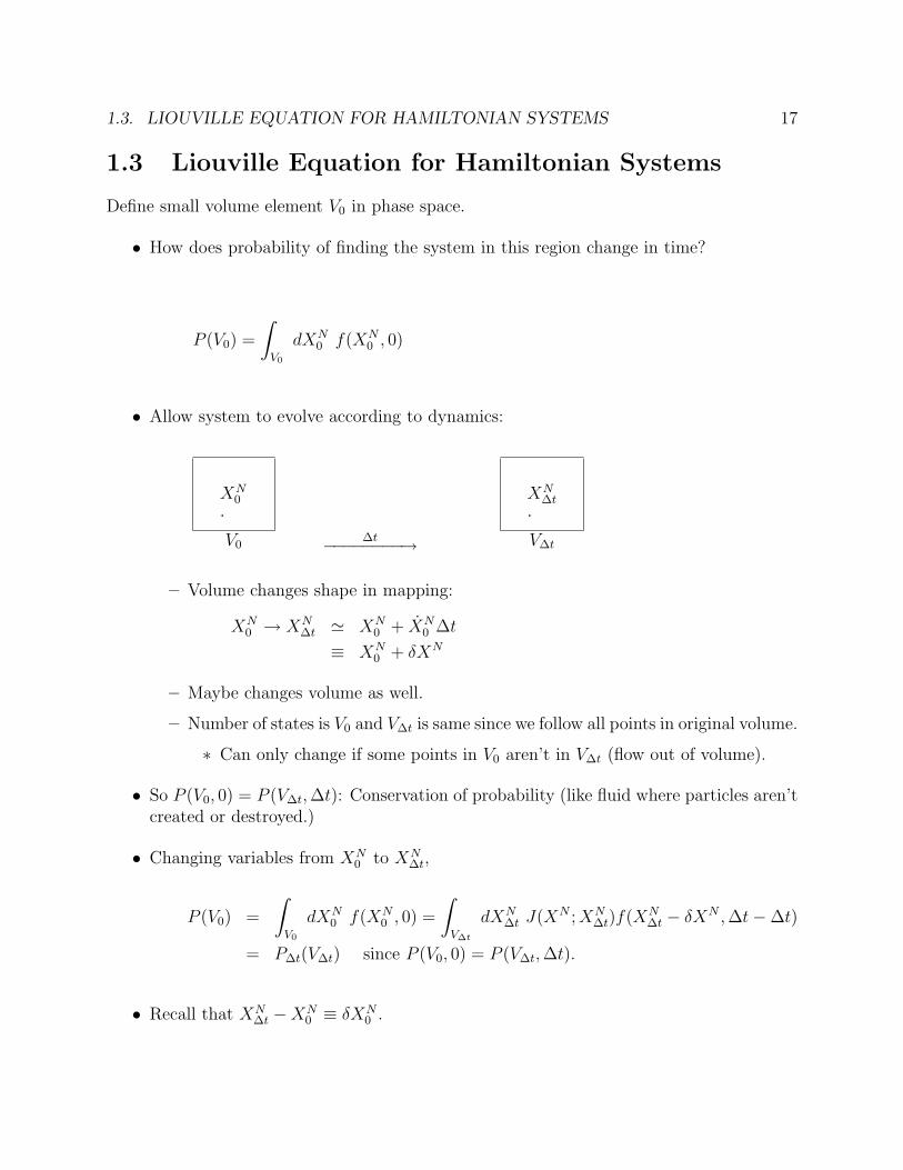
Define small volume element V0 in phase space.
• How does probability of finding the system in this region change in time?
P (V0) =
∫V0
dXN0 f(XN
0 , 0)
• Allow system to evolve according to dynamics:
XN0
·V0
∆t−−−−−−−−→
XN∆t
·V∆t
– Volume changes shape in mapping:
XN0 → XN
∆t ' XN0 + XN
0 ∆t
≡ XN0 + δXN
– Maybe changes volume as well.
– Number of states is V0 and V∆t is same since we follow all points in original volume.
∗ Can only change if some points in V0 aren’t in V∆t (flow out of volume).
• So P (V0, 0) = P (V∆t, ∆t): Conservation of probability (like fluid where particles aren’tcreated or destroyed.)
• Changing variables from XN0 to XN
∆t,
P (V0) =
∫V0
dXN0 f(XN
0 , 0) =
∫V∆t
dXN∆t J(XN ; XN
∆t)f(XN∆t − δXN , ∆t−∆t)
= P∆t(V∆t) since P (V0, 0) = P (V∆t, ∆t).
• Recall that XN∆t −XN
0 ≡ δXN0 .
18 1. REVIEW
• Evaluation of the Jacobian is a bit complicated, but gives
J(XN0 ; XN
∆t) = Jacobian for transform XN0 = XN
∆t − δXN
=
∣∣∣∣ ∂XN0
∂XN∆t
∣∣∣∣ = 1−∇XN · δXN
So
P∆t(V∆t) = P (V0) =
∫V∆t
dXN∆t (1−∇XN · δXN) f
(XN
∆t − δXN , ∆t−∆t)
for small δXN .
• What is δXN?
– For Hamiltonian systems XN∆t ' XN
0 + XN0 ∆t, or δXN = XN
0 ∆t.
– Expanding for small displacements δXN0 and small time intervals ∆t:
f(XN
∆t − δXN , ∆t−∆t)' f
(XN
∆t, ∆t)
−∂f
∂t∆t− (∇XN f) · δXN +
1
2
(∇2
XN f)(δXN)2 + . . .
– Inserting this in previous equation for P∆t(V∆t) = P (V0), we get
P∆t(V∆t) = P∆t(V∆t) +
∫V∆t
dXN∆t(
−∂f
∂t∆t−∇XN · (δXNf) +
1
2∇2
XN f(δXN)2
)or ∫
V∆t
dXN∆t
(−∂f
∂t∆t−∇XN · (δXNf) +
1
2∇2
XN f(δXN)2
)= 0
– Since this holds arbitrary volume V∆t, the integrand must vanish.
∂f
∂t∆t = −∇XN · (δXNf) +
1
2∇2
XN f(δXN)2 + · · ·
– Now, let us evaluate this for δXN = XN0 ∆t
∗ To linear order in ∆t
∇XN ·(XN
0 f)
∆t =(XN · ∇XN f +∇XN · XNf
)∆t
but
∇XN · XN =∂RN
∂RN+
∂PN
∂PN=
∂H
∂RN∂PN− ∂H
∂PN∂RN= 0!
1.3. LIOUVILLE EQUATION FOR HAMILTONIAN SYSTEMS 19
∗ Note that this implies the volume element does not change with normalHamiltonian propagation:
dXN0 = dXN
∆t J(XN ; XN∆t) = dXN
∆t
(1−∇XN · XN∆t
)= dXN
∆t.
– Also, (δXN)2 ∼ O(∆t)2 since δXN ∼ ∆t, so
∂f
∂t∆t = −XN · ∇XN f∆t + O(∆t)2
– In the short-time limit,
∂f
∂t= −XN · ∇XN f
Recall
XN · ∇XN G =(RN · ∇RN + PN · ∇P N
)G
=
(∂H
∂PN· ∇RN − ∂H
∂RN· ∇P N
)G ≡ LG = G,H
So we obtain the Liouville equation:
∂f
∂t= −Lf = −f, H .
• The formal solution is:
f(x(N), t) = e−Ltf(x(N), 0).
• Also note:
∂f
∂t+ XN · ∇XN f =
df(XN , t)
dt= 0.
• Interpretation:
f(r(N)(0),p(N)(0), 0) = f(r(N)(t),p(N)(t), t)
f(r(N)(0),p(N)(0), t) = f(r(N)(−t),p(N)(−t), 0).
• If follow an initial phase point from time 0 to time t, probability density doesn’t change(i.e. you go with the flow).
• Probability density near phase point x(N)(0) at time t is the same as the initial prob-ability density at backward-evolved point x(N)(−t).
20 1. REVIEW
1.3.1 Equilibrium (stationary) solutions of Liouville equation
• Not a function of time, meaning f(RN , PN , t) = f(RN , PN) or
∂f
∂t= −Lf = −f, H = H, f = 0.
• Recall that we showed that energy is conserved by the dynamics so dHdt
= 0.
• Suppose f(RN , PN , t) is an arbitrary function of H(RN , PN).
∂f
∂t= H, f(H) =
∂H
∂RN· ∂f
∂PN− ∂H
∂PN· ∂f
∂RN
but
∂f
∂PN=
∂f
∂H
∂H
∂PN
∂f
∂RN=
∂f
∂H
∂H
∂RN
∂f
∂t=
(∂H
∂RN· ∂H
∂PN− ∂H
∂PN· ∂H
∂RN
)∂f
∂H= 0
Thus any funct. of H is stationary solution of Liouville equation!
• In particular, both the microcanonical and canonical distribution functions are solu-tions of the Liouville equation.
1.3.2 Time-dependent Correlation Functions
Consider the time-dependent correlation function CAB(t) in the canonical ensemble⟨A(x(N), t)B(x(N), 0)
⟩=
∫dx(N)A(x(N), t)B(x(N), 0)f(x(N)).
• From the form of the Liouville operator, for arbitrary functions A and B of the phasespace coordinates
A(x(N), t)B(x(N), t) =(eLtA(x(N), 0)
) (eLtB(x(N), 0)
)= eLt
(A(x(N), 0)B(x(N), 0)
).
• It can be shown by integrating by parts that:⟨(LA(x(N))
)B(x(N))
⟩= −
⟨A(x(N))
(LB(x(N))
)⟩.
1.3. LIOUVILLE EQUATION FOR HAMILTONIAN SYSTEMS 21
• Consequence:⟨A(x(N), t)B(x(N), 0)
⟩=⟨A(x(N))B(x(N),−t)
⟩.
– The autocorrelation function CAA(t) is therefore an even function of time.
• Also, ∫dx(N)
(eLtA(x(N), 0)
)f(x(N), 0) =
∫dx(N)A(x(N), 0)
(e−Ltf(x(N), 0)
)=
∫dx(N)A(x(N), 0)f(x(N), t)
– For an equilbrium system where f(x(N), t) = f(x(N)),
〈A(t)〉 = 〈A(0)〉〈A(t + τ)B(τ)〉 = 〈A(t)B(0)〉 .

22 1. REVIEW
2
Numerical integration and importancesampling
2.1 Quadrature
Consider the numerical evaluation of the integral
I(a, b) =
∫ b
a
dx f(x)
• Rectangle rule: on small interval, construct interpolating function and integrate overinterval.
– Polynomial of degree 0 using mid-point of interval:∫ (a+1)h
ah
dx f(x) ≈ h f ((ah + (a + 1)h)/2) .
– Polynomial of degree 1 passing through points (a1, f(a1)) and (a2, f(a2)): Trape-zoidal rule
f(x) = f(a1) +x− a1
a2 − a1
(f(a2)− f(a1)) −→∫ a2
a1
dx f(x) =
(a2 − a1
2
)(f(a1) + f(a2)) .
– Composing trapezoidal rule n times on interval (a, b) with even sub-intervals[kh, (k + 1)h] where k = 0, . . . , n− 1 and h = (b− a)/n gives estimate∫ b
a
dx f(x) ≈ b− a
n
(f(a) + f(b)
2+
n−1∑k=1
f(a + kh)
).
23
24 2. NUMERICAL INTEGRATION AND IMPORTANCE SAMPLING
• Simpsons rule: interpolating function of degree 2 composed n times on interval (a, b):∫ b
a
dx f(x) ≈ b− a
3n[f(a) + 4f(a + h) + 2f(a + 2h) + 4f(a + 3h) + 2f(a + 4h) + · · ·+ f(b)] .
– Error bounded by
h4
180(b− a)
∣∣f (4)(ξ)∣∣ .
where ξ ∈ (a, b) is the point in the domain where the magnitude of the 4thderivative is largest.
• Rules based on un-even divisions of domain of integration
– w(x) = weight function.
– I(a, b) ≈∑n
i=1 wifi, where wi = w(xi) and fi = f(xi) with choice of xi and wi
based on definite integral of polynomials of higher order.
– Example is Gaussian quadrature with n points based on polynomial of degree2n− 1: well-defined procedure to find xi and wi (see Numerical Recipes).
– Error bounds for n-point Gaussian quadrature are
(b− a)2n+1
(2n + 1)!
(n!)4
[(2n)!]3∣∣f (2n)(ξ)
∣∣ for ξ ∈ (a, b)..
• For multi-dimensional integrals, must place ni grid points along each i dimension.
– Number of points in hyper-grid grows exponentially with dimension.
– Unsuitable for high-dimensional integrals.
2.2 Importance Sampling and Monte Carlo
Suppose integrand f(x) depends on multi-dimensional point x and that integral over hyper-volume
I =
∫V
dx f(x)
is non-zero only in specific regions of the domain.
• We should place higher density of points in region where integrand is large.
• Define a weight function w(x) that tells us which regions are significant.
2.2. IMPORTANCE SAMPLING AND MONTE CARLO 25
– Require property w(x) > 0 for any point x in volume.
– Sometimes use normalized weight function so∫
Vdxw(x) = 1, though not strictly
necessary.
– Re-express integral as:
I =
∫V
dxf(x)
w(x)w(x).
• Idea: Draw a set of N points x1, . . . ,xN from the weight function w(x) then
I =1
N
N∑i=1
f(xi)
w(xi).
• As N →∞, I → I.
• How does this improve the rate of convergence of the calculation of I? We will see thatthe statistical uncertainty is related to the variance σ2
I of the estimate of I, namely
σ2I
=1
N
N∑i
〈∆Ii∆Ii〉 where ∆Ii =f(xi)
w(xi)− I.
and we have assumed that the random variables ∆Ii are statistically independent. Here〈· · · 〉 represents the average over the true distribution of f/w that is obtained in thelimit N →∞.
– Vastly different values of ratio f(xi)/w(xi) lead to large uncertainty.
• The error is minimized by minimizing σ2I.
– If α w(xi) = f(xi), then f(xi)/w(xi) = α and⟨f(xi)
w(xi)
⟩= I = α
⟨(f(xi)
w(xi)
)2⟩
= α2,
and σ2I
= 0.
– Note that writing w(xi) = f(xi)/α requires knowing α = I, the problem we aretrying to solve.
– Generally desire all f(xi)/w(xi) to be roughly the same for all sampled points xi
to mimimize σ2I.
• Example in 1-dimensional integral I =∫ b
adx f(x) =
∫ b
adx f(x)
w(x)w(x).
26 2. NUMERICAL INTEGRATION AND IMPORTANCE SAMPLING
– Monte-Carlo sampling: use random sampling of points x with weight w(x) toestimate ratio f(x)/w(x).
– How do we draw sample points with a given weight w(x)? Consider simplest caseof a uniform distribution on interval (a, b):
w(x) =
1
b−aif x ∈ (a, b).
0 otherwise.
– Use a random number generator that gives a pseudo-random number rand ininterval (0, 1).
xi = a + (b− a)× rand,
then xi are distributed uniformly in the interval (a, b).
– We find that the estimator of f is then:
I =1
N
N∑i=1
f(xi)
w(xi)=
b− a
N
N∑i=1
f(xi) =1
N
N∑k=1
Ik,
where each Ik = (b− a) f(xk) is an independent estimate of the integral.
– Like trapezoidal integration but with randomly sampled points xi from (a, b)each with uniform weight.
• How about other choices of weight function w(x)?
– It is easy to draw uniform yi ∈ (0, 1). Now suppose we map the yi to xi via
y(x) =
∫ x
a
dz w(z).
– Note that y(a) = 0 and y(b) = 1 if w(x) is normalized over (a, b).
– How are the x distributed? Since the y are distributed uniformly over (0, 1), theprobability of finding a value of y in the interval is
dy(x) = w(x) dx,
so the x are distributed with weight w(x).
– It then follows that the one-dimensional integral can be written in the transformedvariables y as:
I =
∫ b
a
dx w(x)f(x)
w(x)=
∫ y(b)
y(a)
dyf(x(y))
w(x(y))=
∫ 1
0
dyf(x(y))
w(x(y))
– Integral easily evaluated by selecting uniform points y and then solving x(y).Must be able to solve for x(y) to be useful.
2.2. IMPORTANCE SAMPLING AND MONTE CARLO 27
• Procedure:
1. Select N points yi uniformly on (0, 1) using yi = rand.
2. Compute xi = x(yi) by inverting y(x) =∫ x
adz w(z).
3. Compute estimator for integral I = 1N
∑Ni=1 f(xi)/w(xi).
• This procedure is easy to do using simple forms of w(x). Suppose the integrand isstrongly peaked around x = x0. One good choice of w(x) might be a Gaussian weight
w(x) =1√
2πσ2e−
(x−x0)2
2σ2 ,
where the variance (width) of the Gaussian is treated as a parameter.
– If I =∫∞−∞ dx f(x) =
∫∞−∞ dx w(x)f(x)/w(x), can draw randomly from the Gaus-
sian weight by:
y(x) =1√
2πσ2
∫ x
−∞dx e−
(x−x0)2
2σ2
=1
2+
1√2πσ2
∫ x
0
dx e−(x−x0)2
2σ2
=1
2+
1√π
∫ x−x0√2σ
0
dw e−w2
=1
2
(1 + erf
(x− x0√
2σ
)).
– Inverting gives xi = x0 +√
2σ ierf(2yi−1), where ierf is the inverse error functionwith series representation
ierf(z) =
√π
2
(z +
π
12z3 +
7π2
480z5 + . . .
)– The estimator of the integral is therefore
I =1
N
√2πσ2
N∑i=1
f(xi)e(xi−x0)2
2σ2 .
– This estimator reduces the variance σ2I
if w(xi) and f(xi) resemble one another.
• Another way to draw from a Gaussian:
– Draw 2 numbers, y1 and y2 uniformly on (0, 1). Define R =√−2 ln y1 and θ =
2πy2. Then x1 = R cos θ and x2 = R sin θ are distributed with density
w(x1, x2) =1
2πe−x2
1e−x22
28 2. NUMERICAL INTEGRATION AND IMPORTANCE SAMPLING
since
dy1dy2 =
∣∣∣∣∣ ∂y1
∂x1
∂y1
∂x2∂y2
∂x1
∂y2
∂x2
∣∣∣∣∣ dx1dx2 = w(x1, x2)dx1dx2
2.3 Markov Chain Monte Carlo
2.3.1 Ensemble averages
• Generally, we cannot find a simple way of generating the xi according to a knownw(xi) for high-dimensional systems by transforming from a uniform distribution.
– Analytical integrals for coordinate transformation may be invertable only for sep-arable coordinates.
– Many degrees of freedom are coupled so that joint probability is complicated andnot the product of single probabilities.
• Typical integrals are ensemble averages of the form:
〈A〉 =1
Z
∫V
dr(N)e−βu(r(N))A(r(N)) =
∫V
dr(N)e−βu(r(N))A(r(N))∫V
dr(N)e−βu(r(N))
– Typical potentials are complicated functions of configuration r(N).
– A good importance sampling weight would set w(r(N)) = e−βu(r(N)).
• How do we sample configurations from a general, multi-dimensional weight?
• Goal: Devise a method to generate a sequence of configurations r(N)1 , . . . , r
(N)n
in which the probability of finding a configuration r(N)i in the sequence is given by
w(r(N)i )dr
(N)i .
• We will do so using a stochastic procedure based on a random walk.
2.3.2 Markov Chains
We will represent a general, multi-dimensional configurational coordinate that identifies thestate by the vector X. We wish to generate a sequence of configurations X1, . . . ,Xn whereeach Xt is chosen with probability density Pt(Xt). To generate the sequence, we use adiscrete-time, time-homogeneous, Markovian random walk.
• Consider the configuration X1 at an initial time labelled as 1 that is treated as arandom variable drawn from some known initial density P1(X).
2.3. MARKOV CHAIN MONTE CARLO 29
• We assume the stochastic dynamics of the random variable is determined by a time-independent transition function K(Y → X), where the transition function defines theprobability density of going from state Y to state X in a time step.
• Since K is a probability density, it must satisfy∫dXK(Y → X) = 1 K(Y → X) ≥ 0.
• The state Xt at time t is assumed to be obtained from the state at time Xt−1 by arealization of the dynamics, where the probability of all transitions is determined byK.
• At the second step of the random walk, the new state X2 is chosen from P2(X|X1) =K(X1 → X). At the third step, the state X3 is chosen from P3(X|X2) = K(X2 → X),and so on, generating the random walk sequence X1, . . . ,Xn.
• If infinitely many realizations of the dynamics is carried out, we find that the distri-bution of Xi for each of the i steps are
P1(X) for X1
P2(X) =∫
dYK(Y → X)P1(Y) for X2
P3(X) =∫
dYK(Y → X)P2(Y) for X3...
...Pt(X) =
∫dYK(Y → X)Pt−1(Y) for Xt.
• The transition function K is ergodic if any state X can be reached from any state Y ina finite number of steps in a non-periodic fashion.
• If K is ergodic, then the Perron-Frobenius Theorem guarantees the existence of a uniquestationary distribution P (X) that satisfies
P (X) =
∫dYK(Y → X)P (Y) and lim
t→∞Pt(X) = P (X).
• Implications
1. From any initial distribution of states P1(X), an ergodic K guarantees that statesXt will be distributed according to the unique stationary distribution P (X) forlarge t (many steps of random walk).
2. P (X) is like an eigenvector of “matrix” K with eigenvalue λ = 1.
3. Goal is then to design an ergodic transition function K so that the stationary orlimit distribution is the Bolztmann weight w(X).
30 2. NUMERICAL INTEGRATION AND IMPORTANCE SAMPLING
Finite State Space
To make the Markov chain more concrete, consider a finite state space in which only mdifferent configurations of the system exist. The phase space then can be enumerated asX1, . . .Xm.
• The transition function is then an m×m matrix K, where the element Kij ≥ 0 is thetransition probability of going from state Xj to state Xi.
• Since the matrix elements represent transition probabilities, for any fixed value of j,
m∑i=1
Kij = 1.
• The distribution Pt(X) corresponds to a column vector Pt = col[a(1)t , . . . a
(m)t ], where
a(i)t is the probability of state Xi at time t.
• The distribution evolves under the random walk as Pt = K ·Pt−1.
• The matrix K is regular if there is an integer t0 such that Kt0 has all positive (non-zero)entries. Then Kt for t ≥ t0 has all positive entries.
• Suppose the matrix K is a regular transition matrix. The following properties hold:
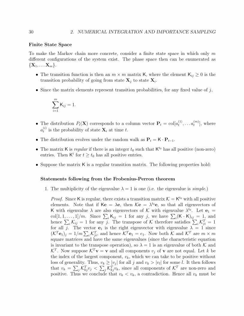
Statements following from the Frobenius-Perron theorem
1. The multiplicity of the eigenvalue λ = 1 is one (i.e. the eigenvalue is simple.)
Proof. Since K is regular, there exists a transition matrix K = Kt0 with all positiveelements. Note that if Ke = λe, then Ke = λt0e, so that all eigenvectors ofK with eigenvalue λ are also eigenvectors of K with eigenvalue λt0 . Let e1 =col[1, 1, . . . , 1]/m. Since
∑i Kij = 1 for any j, we have
∑i(K · K)ij = 1, and
hence∑
iKij = 1 for any j. The transpose of K therefore satisfies∑
iKTji = 1
for all j. The vector e1 is the right eigenvector with eigenvalue λ = 1 since(KTe1)j = 1/m
∑iKT
ji, and hence KTe1 = e1. Now both K and KT are m ×msquare matrices and have the same eigenvalues (since the characteristic equationis invariant to the transpose operation), so λ = 1 is an eigenvalue of both K andKT . Now suppose KTv = v and all components vj of v are not equal. Let k bethe index of the largest component, vk, which we can take to be positive withoutloss of generality. Thus, vk ≥ |vj| for all j and vk > |vl| for some l. It then followsthat vk =
∑j KT
kjvj <∑
j KTkjvk, since all components of KT are non-zero and
positive. Thus we conclude that vk < vk, a contradiction. Hence all vk must be
2.3. MARKOV CHAIN MONTE CARLO 31
the same, corresponding to eigenvector e1. Hence e1 is a unique eigenvector ofKT and λ = 1 is a simple root of the characterstic equation. Hence K has a singleeigenvector with eigenvalue λ = 1.
2. If the eigenvalue λ 6= 1 is real, then |λ| < 1.
Proof. Suppose KTv = λt0v, with λt0 6= 1. It then follows that there is anindex k of vector v such that vk ≥ |vj| for all j and vk > |vl| for some l. Nowλt0vk =
∑j KT
kjvj <∑
j KTkjvk = vk, or λt0vk < vk. Thus λt0 < 1, and hence
λ < 1, since λ is real. Similarly, following the same lines of argument and usingthe fact that −vk < vl for some l, we can establish that λ > −1. Hence |λ| < 1.A similar sort of argument can be used if λ is complex.
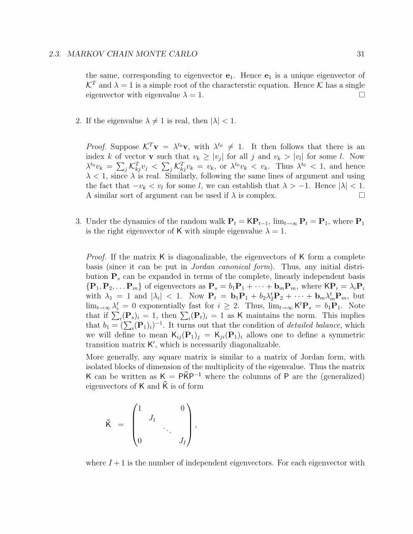
3. Under the dynamics of the random walk Pt = KPt−1, limt→∞ Pt = P1, where P1
is the right eigenvector of K with simple eigenvalue λ = 1.
Proof. If the matrix K is diagonalizable, the eigenvectors of K form a completebasis (since it can be put in Jordan canonical form). Thus, any initial distri-bution Ps can be expanded in terms of the complete, linearly independent basisP1,P2, . . .Pm of eigenvectors as Ps = b1P1 + · · · + bmPm, where KPi = λiPi
with λ1 = 1 and |λi| < 1. Now Pt = b1P1 + b2λt2P2 + · · · + bmλt
mPm, butlimt→∞ λt
i = 0 exponentially fast for i ≥ 2. Thus, limt→∞ KtPs = b1P1. Notethat if
∑i(Ps)i = 1, then
∑i(Pt)i = 1 as K maintains the norm. This implies
that b1 = (∑
i(P1)i)−1. It turns out that the condition of detailed balance, which
we will define to mean Kij(P1)j = Kji(P1)i allows one to define a symmetrictransition matrix K′, which is necessarily diagonalizable.
More generally, any square matrix is similar to a matrix of Jordan form, withisolated blocks of dimension of the multiplicity of the eigenvalue. Thus the matrixK can be written as K = PKP−1 where the columns of P are the (generalized)eigenvectors of K and K is of form
K =
1 0
J1
. . .
0 JI
,
where I +1 is the number of independent eigenvectors. For each eigenvector with
32 2. NUMERICAL INTEGRATION AND IMPORTANCE SAMPLING
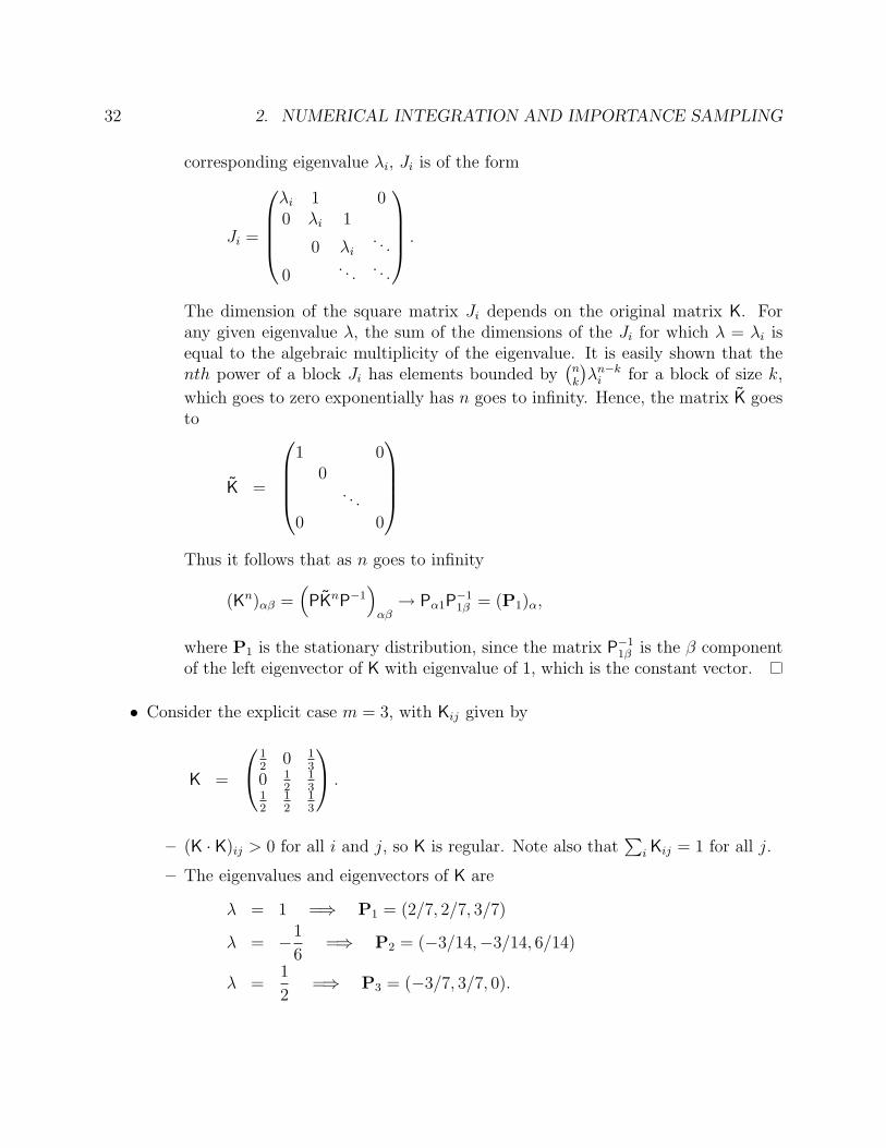
corresponding eigenvalue λi, Ji is of the form
Ji =
λi 1 00 λi 1
0 λi. . .
0. . . . . .
.
The dimension of the square matrix Ji depends on the original matrix K. Forany given eigenvalue λ, the sum of the dimensions of the Ji for which λ = λi isequal to the algebraic multiplicity of the eigenvalue. It is easily shown that thenth power of a block Ji has elements bounded by
(nk
)λn−k
i for a block of size k,
which goes to zero exponentially has n goes to infinity. Hence, the matrix K goesto
K =
1 0
0. . .
0 0
Thus it follows that as n goes to infinity
(Kn)αβ =(PKnP−1
)αβ→ Pα1P
−11β = (P1)α,
where P1 is the stationary distribution, since the matrix P−11β is the β component
of the left eigenvector of K with eigenvalue of 1, which is the constant vector.
• Consider the explicit case m = 3, with Kij given by
K =
12
0 13
0 12
13
12
12
13
.
– (K · K)ij > 0 for all i and j, so K is regular. Note also that∑
i Kij = 1 for all j.
– The eigenvalues and eigenvectors of K are
λ = 1 =⇒ P1 = (2/7, 2/7, 3/7)
λ = −1
6=⇒ P2 = (−3/14,−3/14, 6/14)
λ =1
2=⇒ P3 = (−3/7, 3/7, 0).
2.3. MARKOV CHAIN MONTE CARLO 33
– If initially Ps = (1, 0, 0), then P2 = (1/2, 0, 1/2) and
P10 = (0.28669 · · · , 0.28474 · · · , 0.42857 · · · ),
which differs from P1 by 0.1%.
2.3.3 Construction of the transition matrix K(y → x)
We wish to devise a procedure so that the limiting (stationary) distribution of the randomwalk is the Boltzmann distribution Peq(x).
• Break up the transition matrix into two parts, generation of trial states T(y → x) andacceptance probability of trial state A(y → x)
K(y → x) = T(y → x)A(y → x).
– Will consider definition of acceptance probability given a specified procedure forgenerating trial states with condition probability T(y → x).
• Write dynamics in term of probabilities at time t
Probability of starting in y and ending in x =
∫dy Pt(y) K(y → x)
Probability of starting in x and remaining in x = Pt(x)
(1−
∫dy K(x → y)
)so
Pt+1(x) =
∫dy Pt(y) K(y → x) + Pt(x)
(1−
∫dy K(x → y)
)= Pt(x) +
∫dy
(Pt(y)K(y → x)− Pt(x)K(x → y)
).
• Thus, to get Pt+1(x) = Pt(x), we want∫dy
(Pt(y)K(y → x)− Pt(x)K(x → y)
)= 0.
• This can be accomplished by requiring microscopic reversibility or detailed balance:
Pt(y)K(y → x) = Pt(x)K(x → y)
Pt(y)T(y → x)A(y → x) = Pt(x)T(x → y)A(x → y).
34 2. NUMERICAL INTEGRATION AND IMPORTANCE SAMPLING
– We desire Pt(x) = Pt+1(x) = Peq(x). This places restriction on the acceptanceprobabilities
A(y → x)
A(x → y)=
Peq(x)T(x → y)
Peq(y)T(y → x).
– Note that Peq(x)K(x → y) is the probability of observing the sequence x, y inthe random walk. This must equal the probability of the sequence y, x in thewalk.
• Metropolis Solution: Note that if Peq(x)T(x → y) > 0 and Peq(y)T(y → x) > 0, thenwe can define
A(y → x) = min
(1,
Peq(x)T(x → y)
Peq(y)T(y → x)
)A(x → y) = min
(1,
Peq(y)T(y → x)
Peq(x)T(x → y)
).
– This definition satisfies details balance.
Proof. Verifying explicitly, we see that
Peq(y)T(y → x)A(y → x) = min (Peq(y)T(y → x), Peq(x)T(x → y))
Peq(x)T(x → y)A(x → y) = min (Peq(x)T(x → y), Peq(y)T(y → x))
= Peq(y)T(y → x)A(y → x)
as required.
– Procedure guaranteed to generate states with probability proportional to Boltz-mann distribution if proposal probability T(y → x) generates an ergodic transitionprobability K.
Simple example
• Suppose we want to evaluate the equilibrium average 〈A〉 at inverse temperature βof some dynamical variable A(x) for a 1-dimensional harmonic oscillator system withpotential energy U(x) = kx2/2.
〈A(x)〉 =
∫ ∞
−∞dx Peq(x)A(x) Peq(x) =
1
Ze−βkx2/2
• Monte-Carlo procedure
2.3. MARKOV CHAIN MONTE CARLO 35
1. Suppose the current state of the system is x0. We define the proposal probabilityof a configuration y to be
T(x0 → y) =
1
2∆xif y ∈ [x0 −∆x, x0 + ∆x]
0 otherwise
– ∆x is fixed to some value representing the maximum displacement of the trialcoordinate.
– y chosen uniformly around current value of x0.
– Note that if y is selected, then T(x0 → y) = 1/(2∆x) = T(y → x0) since x0
and y are within a distance ∆x of each other.
2. Accept trial y with probability
A(x0 → y) = min
(1,
T(y → x0)Peq(y)
T(x0 → y)Peq(x0)
)= min
(1, e−β∆U
),
where ∆U = U(y)− U(x0).
– Note that if ∆U ≤ 0 so the proposal has lower potential energy than thecurrent state, A(x0 → y) = 1 and the trial y is always accepted as the nextstate x1 = y.
– If ∆U > 0, then A(x0 → y) = e−β∆U = q. We must accept the trial ywith probability 0 < q < 1. This can be accomplished by picking a randomnumber r uniformly on (0, 1) and then:
(a) If r ≤ q, then accept configuration x1 = y
(b) If r > q, then reject configuration and set x1 = x0 (keep state as is).
3. Repeat steps 1 and 2, and record states xi.
• Markov chain of states (the sequence) xi generated, with each xi appearing in thesequence with probability Peq(xi) (after some number of equilibration steps).
• After collecting N total configurations, the equilibrium average 〈A〉 can be estimatedfrom
〈A〉 =1
N
N∑i=1
A(xi)
since the importance function w(x) = Peq(x).
• Rejected states are important to generate states with correct weight.
• Typically, should neglect the first Ns points of Markov chain since it takes some itera-tions of procedure to generate states with stationary distribution of K(y → x).
36 2. NUMERICAL INTEGRATION AND IMPORTANCE SAMPLING
– Called equilibration or “burn in” time.
– Often have correlation among adjacent states. Can record states every Ncorr
Monte-Carlo steps (iterations).
• Why must rejected states be counted? Recall that K(x → y) must be normalized tobe a probability (or probability density).∫
dy K(x → y) = 1 =
∫dy [δ(x− y) + (1− δ(x− y))] K(x → y)
hence, the probability to remain in the current state is
K(x → x) = 1−∫
dy (1− δ(x− y)) K(x → y)
– K(x → x) is non-zero to insure normalization, so we must see the sequence. . . , x, x, . . . in the Markov chain.
2.4 Statistical Uncertainties
We would like some measure of the reliability of averages computed from a finite set ofsampled data. Consider the average x of a quantity x constructed from a finite set of Nmeasurements x1, . . . , xN, where the xi are random variables drawn from a density ρ(x).
x =1
N
N∑i=1
xi
• Suppose the random variables xi are drawn independently, so that the joint probabilitysatisfies
ρ(x1, . . . xN) = ρ(x1)ρ(x2) · · · ρ(xN).
• Suppose that the intrinsic mean 〈x〉 of the random variable is 〈x〉 =∫
dx xρ(x) andthat the intrinsic variance is σ2, where
σ2 =
∫dx(x− 〈x〉
)2ρ(x).
• A mesaure of reliability is the standard deviation of x, also known as the standarderror σE =
√σ2
E, where σ2E is the variance of the finite average x around 〈x〉 in the
finite set x1, . . . , xN
σ2E = 〈
(x− 〈x〉
)2〉.
2.4. STATISTICAL UNCERTAINTIES 37
• We expect
1. Variance (error) decreases with increasing N
2. Error depends on the intrinsic variance σ2 of the density ρ. Larger variance shouldmean slower convergence of x to 〈x〉.
Suppose all the intrinsic moments 〈xn〉 of ρ(x) exist. If we define the dimensionless variable
z =x− 〈x〉
σE
,
and note that the probability density of z can be written as
P (z) = 〈δ(z − z)〉 =1
2π
∫ ∞
−∞dt 〈e−it(z−z)〉 =
1
2π
∫ ∞
−∞dt eitz〈e−itz〉
=1
2π
∫ ∞
−∞dt eitzχN(t), (2.1)
where χN(t) is the characteristic function of P (z). Using the fact that σE = σ/√
N , as willbe shown shortly, z can be expressed as
z =
√N
N
N∑i=1
xi − 〈x〉σ
=1√N
N∑i=1
(xi − 〈x〉
σ
),
and hence
χN(t) =
⟨e
−it√N
N∑i=1
(xi − 〈x〉
σ
)⟩=(⟨
e−it√
N(x−〈x〉
σ )⟩)N
= χ(t/√
N)N ,
where
χ(u) =⟨e−iu(x−〈x〉)/σ
⟩,
which, for small arguments u can be expanded as χ(u) = 1 − u2/2 + iu3κ3/(6σ3) + . . . ,
where κ3 is the third cumulant of the density ρ(x). Using this expansion, we find ln χN(t) =−t2/2 + O(N−1/2), and hence χN(t) = e−t2/2 for large N . Inserting this form in Eq. (2.1)gives
P (z) =1√2π
e−z2/2
and hence we find the central limit theorem result that the averages x are distributed aroundthe intrinsic mean according to the normal distribution
N(x; 〈x〉, σ2E) =
1√2πσE
e− (x−〈x〉)2
2σ2E ,
38 2. NUMERICAL INTEGRATION AND IMPORTANCE SAMPLING
provided the number of samples N is large and all intrinsic moments (and hence cumulants)of ρ(x) are finite.
• If the central limit theorem holds so that the finite averages are normally distributedas above, then the standard error can be used to define confidence intervals since theprobability p that the deviations in the average, x− 〈x〉, lie within a factor of c timesthe standard error is given by∫ cσE
−cσE
d(x− 〈x〉)N(x; 〈x〉, σ2x) = p.
• If p = 0.95, defining the 95% confidence intervals, then we find that c = 1.96, and hencethe probability that the intrinsic mean 〈x〉 lies in the interval (x− 1.96σE, x + 1.96σE)is P (x− 1.96σE ≤ 〈x〉 ≤ x + 1.96σE) = 0.95.
• If the data are not normally distributed, then higher cumulants of the probabilitydensity may be needed (skewness, kurtosis, ...). The confidence intervals are definedin terms of integrals of the probability density.
• How do we calculate σE or σ2E? We defined the variance as
σ2E = 〈
(x− 〈x〉
)2〉 where x =1
N
∑i
xi
• Expanding the square, we get σ2E = 〈x2〉 − 〈x〉2 but
〈x2〉 =1
N2
∑i,j
〈xixj〉 =1
N2
(∑i
〈x2i 〉+
∑i
∑j 6=i
〈xi〉〈xj〉
)
=1
N2
(N(σ2 + 〈x〉2) + N(N − 1)〈x〉2
)=
σ2
N+ 〈x〉2,
hence σ2E = σ2/N .
• However we don’t really know what σ2 is, so we must estimate this quantity. One wayto do this is to define the estimator of the standard deviation σ2:
σ2 =1
N
∑i
(xi − x)2 .
2.4. STATISTICAL UNCERTAINTIES 39
• The average of this estimator is
〈σ2〉 =1
N
∑i
〈(xi − x)2〉 =1
N
∑i
〈x2i − 2xix + x2〉.
but using the facts that
〈xix〉 =〈x2〉N
+N − 1
N〈x〉2 〈x2〉 =
σ2
N+ 〈x〉2,
we get 〈σ2E〉 = (N − 1)σ2/N and hence σ2 = N〈σ2〉/(N − 1).
• The standard error can therefore be estimated by
σE =
√σ2
√N − 1
• Note that σE decreases as 1/√
N − 1
– Narrowing confidence intervals by a factor of 2 requires roughly 4 times moredata.
– If the xi are not indepenent, then N ∼ Neff , where Neff is the effective number ofindependent configurations. If τc is the correlation length (number of Monte-Carlosteps over which correlation 〈xixj〉 differs from 〈x〉2), then Neff = N/τc.
• Another way to estimate the intrinsic variance σ2 is to use the Jackknife Method: seeB. Efron, The annals of statistics 7, 1 (1979).
– Jackknife procedure is to form N averages from the set x1, . . . , xN by omittingone data point. For example, the jth average is defined to be
x(j) =1
N − 1
N∑i6=j
xi
The result is to form a set of averages x(1), x(2), . . . x(N).– The average x over this Jackknifed set is the same as before since
x =1
N
N∑j=1
x(j) =1
N(N − 1)
N∑j=1
∑i6=j
xi =1
N
N∑i=1
xi.
40 2. NUMERICAL INTEGRATION AND IMPORTANCE SAMPLING
– We define an estimator of the variance Σ2 of the Jackknifed set to be
Σ2 =1
N
N∑j=1
(x(j) − x
)2.
which converges to 〈Σ2〉 as N gets large.
– Inserting the definitions of x(j) and x and using the independence of the xi, wesee that the estimator is related to the intrinsic variance by
〈Σ2〉 =
(1
N − 1− 1
N
)σ2 =
σ2
N(N − 1)σ2 = N(N − 1)〈Σ2〉.
– The standard error can therefore be estimated using the Jackknifed set as
ΣE =
√√√√N − 1
N
N∑j=1
(x(j) − x
)2.
3
Applications of the Monte Carlomethod
3.1 Quasi-ergodic sampling
• Detailed balance condition and ergodic transition matrix imply that random walkMonte-Carlo method correctly generates distribution of configurations.
• Says nothing about the rate of convergence, which depends on implementation (eigen-value spectrum of transition matrix).
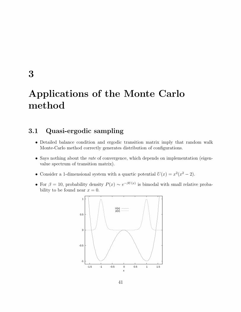
• Consider a 1-dimensional system with a quartic potential U(x) = x2(x2 − 2).
• For β = 10, probability density P (x) ∼ e−βU(x) is bimodal with small relative proba-bility to be found near x = 0.
-1
-0.5
0
0.5
1
-1.5 -1 -0.5 0 0.5 1 1.5
x
U(x)p(x)
41
42 3. APPLICATIONS OF THE MONTE CARLO METHOD
– Note that P (1)/P (0) = e10.
• Consider the simple Metropolis Monte-Carlo scheme discussed previously with:
T(x → y) =
1
2∆xif y ∈ [x−∆x, x + ∆x]
0 otherwise.
– If maximum displacement ∆x is small (∆x 1), then if x is in the region nearx = 1, the probability of proposing y near −1 is zero, and the proposal is veryunlikely to propose a configuration y which is in a different mode from x.
– Random walk dynamics consists of long periods of x being localized in one of themodes, with only rare transitions between the modes (roughly every e10 steps).Overall, an equal amount of time must be spent in both of the modes.
– Rare transitions between modes leads to very slow convergence of distribution ofstates to P (x).
– Easy to fix here since we know where the modes lie: increasing ∆x will allowproposals between modes.
3.2 Umbrella sampling
• Origin of quasi-ergodic sampling problem is poor movement in random walk dynamicsbetween different modes of high probability density.
• Sampling can be improved if one improves the transition probability between modes byeither improving the proposal of trial moves or by modifying the acceptance criterion(i.e. sampling with a different importance function).
• Umbrella sampling is based on using a modified version of the Boltzmann distribu-tion, typically specified by an additional potential energy term that encourages move-ment between modes.
• Consider the quartic system discussed in the last section. We define the umbrellapotential Ub(x) = kx2 and the importance function Π(x) = e−βU(x)e−βUb(x) and definethe transition matrix so that Π is the limit distribution of the random walk.
– Any canonical average can be written as an average over Π
〈A(x)〉 =
∫dx P (x)A(x) =
∫dx Π(x)
(A(x)
P (x)
Π(x)
)provided that Π(x) 6= 0 at any point where P (x) 6= 0.
3.3. SIMULATED ANNEALING AND PARALLEL TEMPERING 43
– Generate Markov chain of states x1, . . . , xN according to Π(x) so that an esti-mator of the average is
〈A(x)〉 =1
N
N∑i=1
A(xi)P (xi)
Π(xi)=
1
N
N∑i=1
A(xi)w(xi) =1
N
N∑i=1
A(xi)eβUb(xi).
– Weight factor w(xi) = eβUb(xi) accounts for bias introduced by the umbrella po-tential. In this case, it will assign greater weight to regions around the modes atx = ±1 since the biased random walk attaches less signficance to these regions.
– The parameter k in the umbrella potential can be adjusted to minimize the sta-tistical uncertainties.
• Disadvantage of umbrella approach: Must know a way in which to enhance movementbetween all modes of system in order to define an effective umbrella potential.
3.3 Simulated annealing and parallel tempering
3.3.1 High temperature sampling
• At high temperatures (β 1), the equilibrium distribution Ph(x) is only weakly bi-modal.
– Transition rate between modes depends exponentially on β∆U , where ∆U is thebarrier height of the potential separating different modes.
– If β is small so that β∆U 1, then the system moves easily between modes.
• Can use high-temperature distribution Ph(x) as an importance function Π(x), resultingin weight function w(xi) given by
w(xi) =P (xi)
Π(xi)= e−(β−βh)U(xi) = e−∆βU(xi).
– If ∆β is large, points near barrier xi = 0 receive little weight since w(xi) 1.
– Advantage of this approach is that we don’t need to know barrier locations sincehigh average potential energy overcomes barriers.
– Disadvantage: For high-dimensional systems, the number of accessible states islarge (high entropy) for high temperatures. Many configurations sampled at hightemperatures therefore receive little weight, leading to sampling inefficiency andlarge statistical uncertainties.
44 3. APPLICATIONS OF THE MONTE CARLO METHOD
3.3.2 Extended state space approach: “Simulated Tempering”,Marinari and Parisi, 1992
• Large temperature gaps in high temperature sampling approach lead to inefficientsampling due to a difference in density of states (entropy), while small temperaturegaps are typically insufficient to enhance the passage between modes.
• Idea of extended state space approaches is to use a ladder of different temperatures (orother parameter) to allow the system to gradually move out of modes in an efficientmanner.
• We augment the phase space point r(N) with a parameter βi from a set of m valuesβi and define a target limit distribution Π(r(N), βi) = Wie
−βiU(r(N)) on the extendedstate space (r(N), βi), where Wi is an adjustable parameter.
• Monte-carlo procedure is standard, but with extended state space:
1. Carry out sequence of a specified number of updates at fixed βi using normalMetropolis scheme.
2. Randomly and uniformly select a temperature index j, with corresponding param-eter βj, for a Monte-Carlo update. Accept change of parameter with probabilityA(i → j), where
A(i → j) = min
(1,
Π(r(N), βj)
Π(r(N), βi)
)= min
(1,
Wj
Wi
e−(βj−βi)U(r(N))
).
– Generate chain of states of extended phase space (r(N)1 , i1), . . . , (r
(N)n , in). If
target average is at temperature β = β1, averages are given by estimator
〈A(r(N))〉 =1
n
n∑k=1
A(r(N)k )
W1
Wik
e−(β1−βik)U(r
(N)k ).
• Drawbacks:
– Must specify the parameter set βi properly to ensure the proper movementbetween modes.
– Must know how to choose weights Wk for a given set of βk. This can be doneiteratively, but requires a fair amount of computational effort.
3.3. SIMULATED ANNEALING AND PARALLEL TEMPERING 45
3.3.3 Parallel Tempering or Replica Exchange, C.J. Geyer, 1991
• Use an extended state space composed of replicas of the system to define a Markovchain X = (r1, . . . rm), where each ri is a complete configuration of the system.
• Design a transition matrix so that limiting distribution is
P (X) = Π1 (r1) . . . Πm (rm)
– The (statistically independent) individual components i of the extended statespace vector can be assigned any weight Πi. One choice is to use a Boltzmanndistribution Πi(ri) = e−βiU(ri) with inverse temperature βi.
• The Monte-Carlo process on the extended state space can be carried out as follows:
1. Carry out a fixed number of updates on all replicas, each with a transition matrixKi that has a limit distribution Πi.
2. Attempt a swap move, in which different components of the extended state spacevector (replicas) are swapped.
– For example, any pair of components, possibly adjacent to one another, canbe selected from a set of all possible pairs with uniform probability. Supposeone picks components 2 and 3, so that the original configuration Xi andproposed configuration Yi are
Xi =
r1
r2
r3...rm
Yi =
r1
r3
r2...rm
– The proposed configuration Yi should be accepted with probability A(Xi →
Yi) given by
A(Xi → Yi) = min
(1,
P (Yi)
P (Xi)
)= min
(1,
Π2(r3)Π3(r2)
Π2(r2)Π3(r3)
)– Note that no adjustable weight factors Wi are needed.
– If Πi = e−βiU(ri), then
Π2(r3)Π3(r2)
Π2(r2)Π3(r3)=
e−β2U(r3)
e−β2U(r2)
e−β3U(r2)
e−β3U(r3)= e−(β2−β3)U(r3)e(β2−β3)U(r2) = e∆β∆U ,
where ∆β = β3 − β2 and ∆U = U(r3)− U(r2).
• Each component of Xi in Markov chain of extended states X(1), . . .X(N) is distributedwith weight Πi
46 3. APPLICATIONS OF THE MONTE CARLO METHOD
• Averages at any of the temperatures are therefore readily computed using
〈A〉βi=
1
N
N∑k=1
A(X(k)i ),
where X(k)i is the ith component of the extended configuration X(k) (the kth configu-
ration in the Markov chain).
• Advantages: Quasi-ergodic sampling is mitigated by using a range of parameters suchas βi. The parameters should be defined such that their extreme values (such as highesttemperature) should demonstrate no trapping in single modes.
• Disadvantages: There must be some overlap in adjacent densities Πi and Πi+1 if a swapmove is to be accepted with significant probability. Ideally, the parameters βi shouldbe chosen so that any given labelled configuration spends an equal amount of time atall parameter values.
– Sometimes requires many replicas, which means that it takes many Monte-Carloexchange moves for a given configuration to cycle through the parameters.
• One of the major advantages of the replica exchange method is the ease with whichone can parallelize the algorithm.
– Normal single-chain algorithm cannot be parallelized efficiently because of sequen-tial nature of random walk procedure.
– Can parallelize the generation of many trial configurations and use an asymmetricproposal procedure to select one preferentially.
– Can parallelize computation of energy, if this is a rate-determining step.
• The exchange frequency between replicas can be optimized to suit the computer archi-tecture.
• Each processor can deal with a single replica, or sub-sets of replicas.
4
Molecular dynamics
4.1 Basic integration schemes
4.1.1 General concepts
• Aim of Molecular Dynamics (MD) simulations:compute equilibrium and transport properties of classical many body systems.
• Basic strategy: numerically solve equations of motions.
• For many classical systems, the equations of motion are of Newtonian form
RN =1
mPN
PN = FN = − ∂U
∂RN,
or
XN = LXN , with LA = A,H,where XN = (RN , PN).
The energy H = P N ·P N
2m+ U(RN) is conserved under this dynamics.
The potential energy is typically of the form of a sum of pair potentials:
U(RN) =∑(i,j)
ϕ(rij) =N∑
i=1
i−1∑j=1
ϕ(rij),
which entails the following expression for the forces FN :
Fi = −∑j 6=i
∂
∂ri
ϕ(rij) = −∑j 6=i
ϕ′(rij)∂rij
∂ri
=∑j 6=i
ϕ′(rij)rj − ri
rij︸ ︷︷ ︸Fij
47
48 4. MOLECULAR DYNAMICS
• Examples of quantities of interest:
1. Radial distribution function (structural equilibrium property)
g(r) =2V
N(N − 1)
∑(i,j)
〈δ(ri − rj − r)〉 ,
where
〈A〉 =
∫dXN A(XN)e−βH(XN )∫
dXN e−βH(XN )(canonical ensemble)
or =
∫dXN A(XN) δ(E −H(XN))∫
dXN δ(E −H(XN))(microcanonical ensemble).
2. Pressure (thermodynamic equilibrium property):
pV = NkT +1
3
∑(i,j)
〈Fij · rij〉
which can be written in terms of g(r) as well.
3. Mean square displacement (transport property):⟨|r(t)− r(0)|2
⟩→ 6Dt for long times t,
where D is the self diffusion coefficient.
4. Time correlation function (relaxation properties)
C(t) = 〈v(t) · v(0)〉
which is related to D as well:
D =1
3limt→∞
limN,V→∞
∫ t
0
C(τ) dτ
• If the system is ergodic then time average equals the microcanonical average:
limtfinal→∞
1
tfinal
∫ tfinal
0
dt A(XN(t)) =
∫dXN A(XN) δ(E −H(XN))∫
dXN δ(E −H(XN)).
• For large N , microcanonical and canonical averages are equal for many quantities A.
• Need long times tfinal!
4.1. BASIC INTEGRATION SCHEMES 49
• The equations of motion to be solved are ordinary differential equations.
• There exist general algorithms to solve ordinary differential equations numerically (seee.g. Numerical Recipes Ch. 16), such as Runge-Kutta and predictor/correction algo-rithms. Many of these are too costly or not stable enough for long simulations ofmany-particle systems. In MD simulations, it is therefore better to use algorithmsspecifically suited for systems obeying Newton’s equations of motion, such as the Ver-let algorithm.
• However, we first want to explore some general properties of integration algorithms.For this purpose, consider a function x of t which satisfies
x = f(x, t). (4.1)
• We want to solve for the trajectory x(t) numerically, given the initial point x(0) attime t = 0.
• Similar to the case of integration, we restrict ourselves to a discrete set of points,separated by a small time step ∆t:
tn = n∆t
xn = x(tn),
where n = 0, 1, 2, 3, . . . .
• To transform equation (4.1) into a closed set of equations for the xn, we need to expressthe time derivative x in terms of the xn. This can only be done approximately.
• Using that ∆t is small:
x(tn) ≈ x(tn + ∆t)− x(tn)
∆t=
xn+1 − xn
∆t.
• Since this should be equal to f(x(t), t) = f(xn, tn):
xn+1 − xn
∆t≈ f(xn, tn) ⇒
xn+1 = xn + f(xn, tn)∆t Euler Scheme. (4.2)
This formula allows one to generate a time series of points which are an approximationto the real trajectory. A simple MD algorithm in pseudo-code could look like this:1
1Pseudo-code is an informal description of an algorithm using common control elements found in mostprogramming language and natural language; it has no exact definition but is intended to make implemen-tation in a high-level programming language straightforward.
50 4. MOLECULAR DYNAMICS
EULER ALGORITHM
SET x to the initial value x(0)
SET t to the initial time
WHILE t < tfinal
COMPUTE f(x,t)
UPDATE x to x+f(x,t)*dt
UPDATE t to t+dt
END WHILE
DO NOT USE THIS ALGORITHM!
• It is easy to show that the error in the Euler scheme is of order ∆t2, since
x(t + ∆t) = x(t) + f(x(t), t)∆t +1
2x(t)∆t2 + . . . ,
so that
xn+1 = xn + f(xn, tn)∆t +O(∆t2)︸ ︷︷ ︸local error
. (4.3)
The strict meaning of the “big O” notation is that if A = O(∆tk) then lim∆t→0 A/∆tk
is finite and nonzero. For small enough ∆t, a term O(∆tk+1) becomes smaller thana term O(∆tk), but the big O notation cannot tell us what magnitude of ∆t is smallenough.
• A numerical prescription such as (4.3) is called an integration algorithm, integrationscheme, or integrator.
• Equation (4.3) expresses the error after one time step; this is called the local truncationerror.
• What is more relevant is the global error that results after a given physical time tf oforder one. This time requires M = tf/∆t MD steps to be taken.
• Denoting fk = f(xk, tk), we can track the errors of subsequent time steps as follows:
x1 = x0 + f0∆t +O(∆t2)
x2 = [x0 + f0∆t +O(∆t2)] + f1∆t +O(∆t2)
= x0 + (f0 + f1)∆t +O(∆t2) +O(∆t2)
...
xM = x0 +M∑
k=1
fk−1∆t +M∑
k=1
O(∆t2);
4.1. BASIC INTEGRATION SCHEMES 51
but as M = tf/∆t:
x(t) = xM = x0 +
tf /∆t∑k=1
fk−1∆t +
tf /∆t∑k=1
O(∆t2)︸ ︷︷ ︸global error
.
• Since tf = O(1), the accumulated error is
tf /∆t∑k=1
O(∆t2) = O(∆t2)O(tf/∆t) = O(tf∆t), (4.4)
which is of first order in the time step ∆t.
• Since the global error goes as the first power of the time step ∆t, we call equation (4.3)a first order integrator.
• In absence of further information on the error terms, this constitutes a general principle:If in a single time step of an integration scheme, the local truncation error is O(∆tk+1),then the globally accumulated error over a time tf is O(tf∆tk) = O(∆tk), i.e., thescheme is kth order.
• Equation (4.4) also shows the possibility that the error grows with physical time tf :Drift.
• Illustration of local and global errors:Let f(x, t) = −αx, so that equation (4.1) reads
x = −αx,
whose solution is exponentially decreasing with a rate α:
x(t) = e−αtx(0). (4.5)
The numerical scheme (4.3) gives for this system
xn+1 = xn − αxn∆t. (4.6)
Note that the true relation is x(t + ∆t) = e−α∆tx(t) = x(t) − α∆tx(t) +O(∆t2), i.e.,the local error is of order ∆t2.
Equation (4.6) is solved by
xn = (1− α∆t)nx0 = (1− α∆t)t/∆t = e[ln(1−α∆t)/∆t]t. (4.7)
52 4. MOLECULAR DYNAMICS
By comparing equations (4.5) and (4.7), we see that the behaviour of the numericalsolution is similar to that of the real solution but with the rate α replaced by α′ =− ln(1−α∆t)/∆t. For small ∆t, one gets for the numerical rate α′ = α+α2∆t/2+· · · =α+O(∆t), thus the global error is seen to be O(∆t), which demonstrates that the Eulerscheme is a first order integrator. Note that the numerical rate diverges at ∆t = 1/α,which is an example of a numerical instability.
4.1.2 Ingredients of a molecular dynamics simulation
1. Boundary conditions
• We can only simulate finite systems.
• A wall potential would give finite size effects and destroy translation invariance.
• More benign boundary conditions: Periodic Boundary Conditions:
• Let all particles lie in a simulation box with coordinates between −L/2 and L/2.
• A particle which exits the simulation box, is put back at the other end.
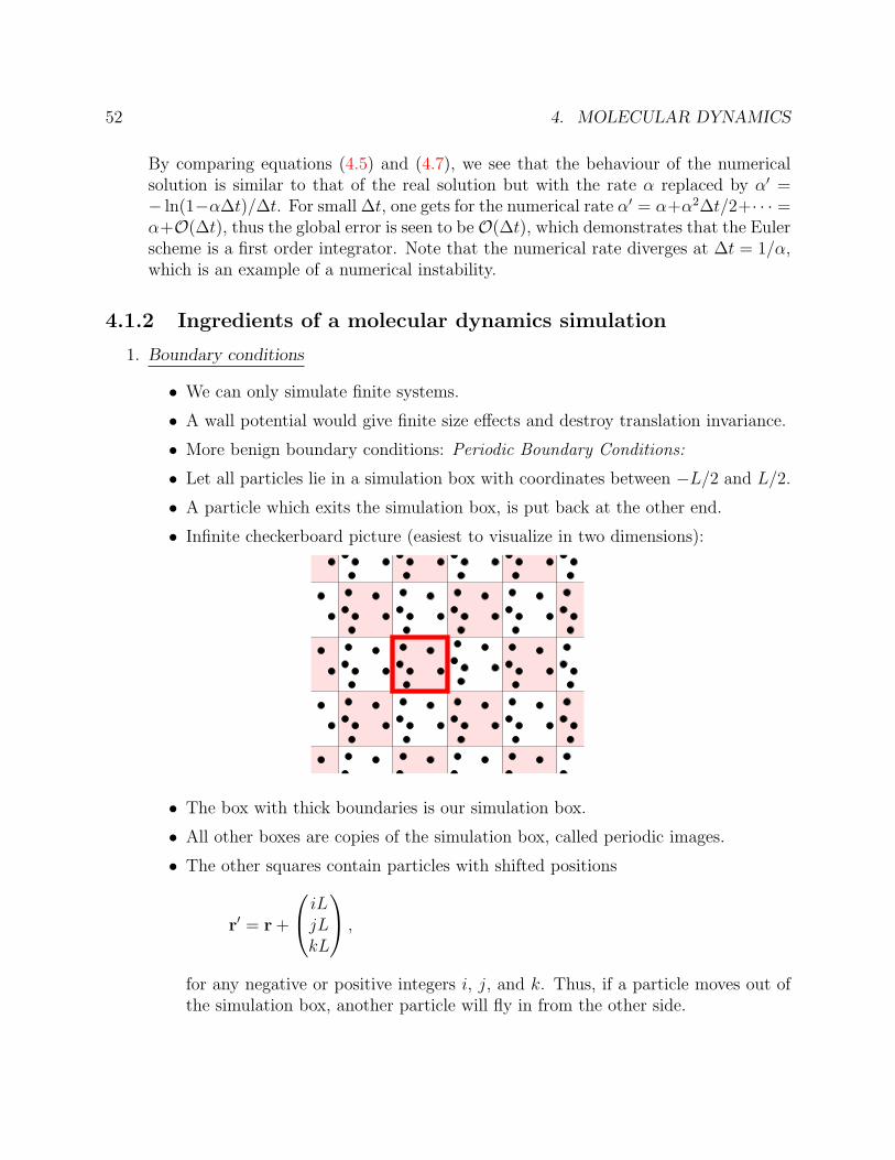
• Infinite checkerboard picture (easiest to visualize in two dimensions):
• The box with thick boundaries is our simulation box.
• All other boxes are copies of the simulation box, called periodic images.
• The other squares contain particles with shifted positions
r′ = r +
iLjLkL
,
for any negative or positive integers i, j, and k. Thus, if a particle moves out ofthe simulation box, another particle will fly in from the other side.
4.1. BASIC INTEGRATION SCHEMES 53
Conversely, for any particle at position r′ not in the simulation box, there is aparticle in the simulation box at
r =
(x′ + L2) mod L− L
2
(y′ + L2) mod L− L
2
(z′ + L2) mod L− L
2
, (4.8)
• Yet another way to view this is to say that the system lives on a torus.
2. Forces
• Usually based on pair potentials.
• A common pair potential is the Lennard-Jones potential
ϕ(r) = 4ε
[(σ
r
)12
−(σ
r
)6]
,
– σ is a measure of the range of the potential.
– ε is its strength.
– The potential is positive for small r: repulsion.
– The potential is negative for large r: attraction.
– The potential goes to zero for large r: short-range.
– The potential has a minimum of −ε at 21/6σ.
• Computing all forces in an N-body system requires the computation of N(N−1)/2(the number of pairs in the system) forces Fij
• Computing forces is often the most demanding part of MD simulations.
• A particle i near the edge of the simulation box will feel a force from the periodicimages, which can be closer to i than their original counter-parts.
• A consistent way to write the potential is
U =∑i,j,k
N∑n=1
n−1∑m=1
ϕ(|rn − rm + iLx + jLy + kLz|). (4.9)
• While this converges for most potentials ϕ, it is very impractical to have to com-pute an infinite sum to get the potential and forces.
• To fix this, one can modify the potential such that it becomes zero beyond acertain cut-off distance rc:
ϕ′(r) =
ϕ(r)− ϕ(rc) if r < rc
0 if r ≥ rc
where the subtraction of ϕ(rc) is there to avoid discontinuities in the potentialwhich would cause violations of energy conservation.
54 4. MOLECULAR DYNAMICS
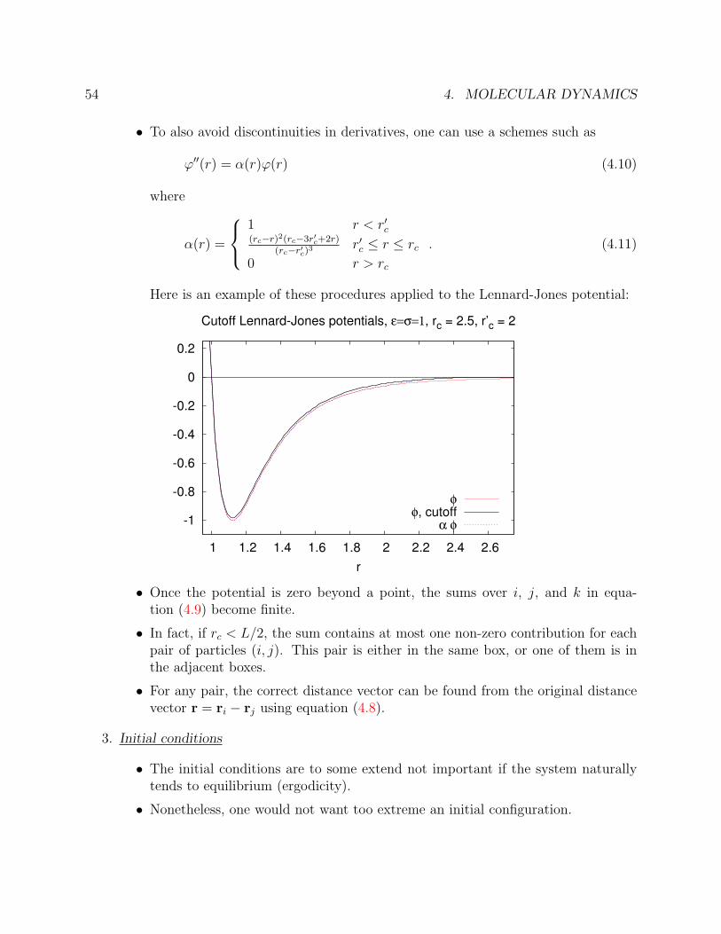
• To also avoid discontinuities in derivatives, one can use a schemes such as
ϕ′′(r) = α(r)ϕ(r) (4.10)
where
α(r) =
1 r < r′c(rc−r)2(rc−3r′c+2r)
(rc−r′c)3 r′c ≤ r ≤ rc
0 r > rc
. (4.11)
Here is an example of these procedures applied to the Lennard-Jones potential:
-1
-0.8
-0.6
-0.4
-0.2
0
0.2
1 1.2 1.4 1.6 1.8 2 2.2 2.4 2.6r
Cutoff Lennard-Jones potentials, ε=σ=1, rc = 2.5, r’c = 2
φφ, cutoff
α φ
• Once the potential is zero beyond a point, the sums over i, j, and k in equa-tion (4.9) become finite.
• In fact, if rc < L/2, the sum contains at most one non-zero contribution for eachpair of particles (i, j). This pair is either in the same box, or one of them is inthe adjacent boxes.
• For any pair, the correct distance vector can be found from the original distancevector r = ri − rj using equation (4.8).
3. Initial conditions
• The initial conditions are to some extend not important if the system naturallytends to equilibrium (ergodicity).
• Nonetheless, one would not want too extreme an initial configuration.
4.1. BASIC INTEGRATION SCHEMES 55
• Starting the system with the particles on a lattice and drawing initial momentafrom a uniform or Gaussian distribution is typically a valid starting point.
• One often makes sure that the kinetic energy has the target value 32NkT , while
the total momentum is set to zero to avoid the system moving as a whole.
4. Integration scheme
• Needed to solve the dynamics as given by the equations of motion.
• Below, we will discuss in detail on how to construct or choose an appropriateintegration scheme.
5. Equilibration/Burn-in
• Since we do not start the system from an equilibrium state, a certain number oftime steps are to be taken until the system has reached an equilibrium.
• One can check for equilibrium by seeing if quantities like the potential energy areno longer changing in any systematic fashion and are just fluctuating around amean values.
• The equilibrium state is microcanonical at a given total energy Etot = Epot +Ekin.
• Since Ekin > 0, the lattice initialization procedure outlined cannot reach all pos-sible values of the energy, i.e. Etot > Epot(lattice).
• To reach lower energies, one can periodically rescale the momenta (a rudimentaryform of a so called thermostat).
• Another way to reach equilibrium is to generate initial conditions using the MonteCarlo method.
6. Measurements
• Construct estimators for physical quantities of interest.
• Since there are correlations along the simulated trajectory, one needs to takesample points that are far apart in time.
• Although when one is interested in dynamical quantities, all points should beused. In the statistical analysis there correlations should be taken into account.
56 4. MOLECULAR DYNAMICS
Given these ingredients, the outline of an MD simulation could look like this:
OUTLINE MD PROGRAM
SETUP INITIAL CONDITIONS
PERFORM EQUILIBRATION by INTEGRATING over a burn-in time B
SET time t to 0
PERFORM first MEASUREMENT
WHILE t < tfinal
INTEGRATE over the measurement interval
PERFORM MEASUREMENT
END WHILE
in which the integration step from t1 to t1+T looks as follows (assuming t=t1 at the start):
OUTLINE INTEGRATION
WHILE t < t1+T
COMPUTE FORCES on all particles
COMPUTE new positions and momenta according to INTEGRATION SCHEME
APPLY PERIODIC BOUNDARY CONDITIONS
UPDATE t to t+dt
END WHILE
Note: we will encounter integration schemes in which the forces need to be computed inintermediate steps, in which case the separation between force computation and integrationis not as strict as this outline suggests.
4.1.3 Desirable qualities for a molecular dynamics integrator
• Accuracy:Accuracy means that the trajectory obeys the equations of motion to good approxima-tion. This is a general demand that one would also impose on integrators for generaldifferential equations. The accuracy in principle improves by decreasing the time step∆t. But because of the exponential separation of near-by trajectories in phase space(Lyapunov instability), this is of limited help.
Furthermore, one cannot decrease ∆t too far in many particle systems for reasons of
• Efficiency:
It is typically quite expensive to compute the inter-particle forces FN , and takingsmaller time steps ∆t requires more force evaluations per unit of physical time.
4.1. BASIC INTEGRATION SCHEMES 57
• Respect physical laws:
– Time reversal symmetry
– Conservation of energy
– Conservation of linear momentum
– Conservation of angular momentum
– Conservation of phase space volume
provided the simulated system also has these properties, of course.
Violating these laws poses serious doubts on the ensemble that is sampled and onwhether the trajectories are realistic.
Unfortunately, there is no general algorithm that obeys all of these conservation lawsexactly for an interacting many-particle system. At best, one can find time-reversible,volume preserving algorithms that conserve linear momentum and angular momentum,but that conserve the energy only approximately.
Note furthermore that with periodic boundary conditions:
– Translational invariance and thus conservation of momentum is preserved.
– There is no wall potential, so the energy conservation is not affected either.
– But rotational invariance is broken: No conservation of angular momentum.
• Stability:Given that the energy is only conserved approximately, when studying dynamics onlarge time scales, or when sampling phase space using MD, it is important that the sim-ulation is stable, i.e., that the algorithm does not exhibit energy drift, since otherwise,it would not even sample the correct microcanonical energy shell.
Remarks:
• Since the computational cost thus limits the time step, the accuracy of the algorithmhas to be assessed at a fixed time step.
• Since ∆t is not necessarily small, higher order algorithms need not be more accurate.
• The most efficient algorithm is then the one that allows the largest possible time stepfor a given level of accuracy, while maintaining stability and preserving conservationlaws.
58 4. MOLECULAR DYNAMICS
• All integration schemes become numerically unstable for large time steps ∆t, even ifthey are stable at smaller time steps. A large step may can the system to a region oflarge potential energy. With infinite precision, this would just cause a large restoringforce that pushes the system back into the low energy region. But with finite precision,the low energies cannot be resolved anymore, and the system remains in the high energystate.
• The dominance of the force evaluations means that the efficiency of a simulation cangreatly be improved by streamlining the evaluation of the forces, using
1. Cell divisions:
– Divide the simulation box into cells larger than the cutoff rc.
– Make a list of all particles in each cell.
– In the sum over pairs in the force computation, only sum pairs of particles inthe same cell or in adjacent cells.
– When ‘adjacent’ is properly defined, this procedure automatically picks outthe right periodic image.
– Draw-backs:1. needs at least three cells in any direction to be of use.2. Still summing many pairs that do not interact (corners).
2. Neighbour lists (also called Verlet lists or Verlet neighbour lists):
– Make a list of pairs of particles that are closer than rc + δr: these are ‘neigh-bours’.
– Sum over the list of pairs to compute the forces.
– The neighbour list are to be used in subsequent force calculations as long asthe list is still valid.
– Invalidation criterion: a particle has moved more than δr/2.
– Therefore, before a new force computation, check if any particle has movedmore than δr/2 since the last list-building. If so, rebuild the Verlet list,otherwise use the old one.
– Notes:1. δr needs to be chosen to balance the cost of rebuilding the list and con-sidering non-interacting particles.2. The building of the list may be sped up by using cell divisions.
For large systems, these methods of computing the interaction forces scale as N insteadof as N2, as the naive implementation of summing over all pairs would give.
4.1. BASIC INTEGRATION SCHEMES 59
Assessing the Euler scheme for the harmonic oscillator
• Consider the Euler scheme applied to x = (r, p), and f(x, t) = (p,−r). i.e., (cf. equa-tion (4.1))
r = p
p = −r.
This is the simple one-dimensional harmonic oscillator with mass 1 and frequency 1,whose solutions are oscillatory
r(t) = r(0) cos t + p(0) sin t (4.12)
p(t) = p(0) cos t− r(0) sin t. (4.13)
The Euler scheme (4.3) gives for this system(rn+1
pn+1
)=
(1 ∆t
−∆t 1
)(rn
pn
). (4.14)
• The eigenvalues of the matrix on the right hand side of equation (4.14) are given byλ± = 1± i∆t, and the solution of equation (4.14) can be expressed as(
rn
pn
)=
(1 ∆t
−∆t 1
)n(r0
p0
)(4.15)
=
(12(λn
+ + λn−) 1
2i(λn
+ − λn−)
−12i
(λn+ − λn
−) 12(λn
+ + λn−)
)(r0
p0
)(4.16)
= (λ+λ−)n/2
(eiω′∆tn+e−iω′∆tn
2eiω′∆tn−e−iω′∆tn
2i
− eiω′∆tn−e−iω′∆tn
2ieiω′∆tn+e−iω′∆tn
2
)(r0
p0
)(4.17)
= (1 + ∆t2)t
2∆t
(cos(ω′t) sin(ω′t)− sin(ω′t) cos(ω′t)
)(r0
p0
), (4.18)
where eiω′∆t = (λ+/λ−)1/2. By comparing equations (4.13) and (4.18), we see that thebehaviour of the numerical solution is similar to that of the real solution but with adifferent frequency, and with a prefactor which is larger than one and grows with time.
• Rather than performing a periodic, circular motion in phase space, the Euler schemeproduces an outward spiral.
• Accuracy: ω′ = ω +O(∆t) so this is only a first order integration scheme.
• Time reversal invariant? No.
60 4. MOLECULAR DYNAMICS
• Conserves energy? No.
• Conserves angular momentum? No.
• Conserves phase space? No.
• Stable? No.
4.1.4 Verlet scheme
• If the system is governed by Newton’s equations:
RN =1
mPN
PN = FN ,
then one can exploit the form of these equations to construct (better) integrators.
• The Verlet scheme is one of these schemes. It can be derived by Taylor expansion
RNn−1 = RN(t−∆t) = RN
n − PNn
∆t
m+ FN
n
∆t2
2m−
...R
N(t)∆t3
6+O(∆t4)
RNn+1 = RN(t + ∆t) = RN
n + PNn
∆t
m+ FN
n
∆t2
2m+
...R
N(t)∆t3
6+O(∆t4).
Adding these two equations leads to
RNn−1 + RN
n+1 = 2RNn + FN
n
∆t2
m+O(∆t4) ⇒
RNn+1 = 2RN
n −RNn−1 + FN
n
∆t2
mPosition-only Verlet Integrator (4.19)
• No momenta!
• Requires positions at the previous step!
• Simple algorithm (r(i) and rprev(i) are particle i’s current and previous position)
VERLET ALGORITHM
SET time t to 0
WHILE t < tfinal
COMPUTE the forces F(i) on all particles
FOR each particle i
COMPUTE new position rnew = 2*r(i)-rprev(i)+F(i)*dt*dt/m
4.1. BASIC INTEGRATION SCHEMES 61
UPDATE previous position rprev(i) to r(i)
UPDATE position r(i) to rnew
END FOR
UPDATE t to t+dt
END WHILE
• Accuracy: This scheme is third order in the positions, so reasonably accurate.
• Respect physical laws?
– Time reversal symmetry? Yes, since
RNn−1 = 2RN
n −RNn+1 + FN
n
∆t2
m.
– Total energy conservation? No momenta, so energy conservation cannot be checked.
– Linear momentum? Also not defined.
– Angular momentum? Not defined.
– Volume preserving? No phase space volume can be defined without momenta.
• Stability: very stable, no energy drift up to relatively large time steps. Why this is sowill become clear later.
4.1.5 Leap Frog scheme
• Is a way to introduce momenta into the Verlet scheme.
• Define momenta at a ’half time step’
PNn+1/2 = PN(t + ∆t/2) = m
RNn+1 −RN
n
∆t. (4.20)
• These momenta are correct up to O(∆t2).
• If we get the positions from the Verlet scheme, then the errors in the momenta do notaccumulate, so that the global order of the momenta in the Leap Frog method is alsoO(∆t2).
• Given the half-step momenta, one may also perform the Leap Frog algorithm as follows:
RNn+1 = RN
n + PNn+1/2
∆t
m(which follows from (4.20)),
62 4. MOLECULAR DYNAMICS
where
PNn+1/2 = m
RNn+1 −RN
n
∆t= m
RNn −RN
n−1 + RNn+1 + RN
n−1 − 2RNn
∆t= PN
n−1/2 + FNn ∆t (as follows from (4.19)).
• The scheme is thus:
PNn+1/2 = PN
n−1/2 + FNn ∆t
RNn+1 = RN
n + PNn+1/2
∆t
m
Leap Frog integrator. (4.21)
• Since the Leap Frog algorithm is derived from the Verlet scheme, it is equally stable.
• The Leap Frog algorithm has the appearance of a first order Taylor expansion, butbecause of the half-step momenta, it is third order in positions and second order inmomenta.
• Since momenta are defined at different time points than positions, conservation laws(energy, momentum,. . . ) can still not be checked.
• The Leap Frog scheme is easy to implement:
LEAP-FROG ALGORITHM
SET time t to 0
WHILE t < tfinal
COMPUTE the forces F(i) on all particles
FOR each particle i
UPDATE momentum p(i) to p(i)+F(i)*dt
UPDATE position r(i) to r(i)+p(i)*dt/m
END FOR
UPDATE t to t+dt
END WHILE
4.1.6 Momentum/Velocity Verlet scheme
• This scheme will integrate positions and momenta (or velocities) at the same timepoints, while keeping the position equivalence with the original Verlet scheme.
• We define the momenta at time t = n∆t as
PNn =
1
2
(PN
n+1/2 + PNn−1/2
).

4.1. BASIC INTEGRATION SCHEMES 63
• Using that the half step momenta are correct to O(∆t2), we see that this is also correctto that order, since
1
2
[PN
(t +
∆t
2
)+ PN
(t− ∆t
2
)]=
1
2
[PN(t) + FN
n
∆t
2+ PN(t)− FN
n
∆t
2+O(∆t2)
]= PN(t) +O(∆t2).
• Using the momentum rule of the Leap Frog algorithm
PNn+1/2 = PN
n−1/2 + FNn ∆t,
and the definition of PNn , one gets
PNn+1/2 = 2PN
n − PNn+1/2 + FN
n ∆t,
or
PNn+1/2 = PN
n + FNn
∆t
2. (4.22)
Substituting Eq. (4.22) into the position rule of the Leap Frog gives the position trans-formation in the momentum-Verlet scheme
RNn+1 = RN
n + PNn
∆t
m+ FN
n
∆t2
2m.
• The corresponding momentum rule is found using the definition of the momentum andthe momentum rule of the Leap Frog:
PNn+1 =
1
2[PN
n+3/2 + PNn+1/2]
=1
2[PN
n+1/2 + FNn+1∆t + PN
n+1/2]
= PNn+1/2 + FN
n+1
∆t
2
= PNn +
FNn+1 + FN
n
2∆t, (4.23)
where (4.22) was used.
• This algorithm is usually called velocity Verlet, and is then expressed in terms of thevelocities V N = PN/m.
64 4. MOLECULAR DYNAMICS
• Summarizing:
RNn+1 = RN
n +PN
n
m∆t +
FNn
2m∆t2
PNn+1 = PN
n +FN
n+1 + FNn
2∆t
Momentum Verlet Scheme (first version).
• The momentum rule appears to pose a problem since FNn+1 is required. But to compute
FNn+1, we need only RN
n+1, which is computed in the integration step as well. That is,given that the forces are known at step n, the next step is can be taken by
STORE all the forces F(i) as Fprev(i)
FOR each particle i
UPDATE position r(i) to r(i)+p(i)*dt/m+F(i)*dt*dt/(2*m)
END FOR
RECOMPUTE the forces F(i) using the updated positions
FOR each particle i
UPDATE momentum p(i) to p(i)+(F(i)+Fprev(i))*dt/2
END FOR
• The extra storage step can be avoided by reintroducing the half step momenta asintermediates. From Eqs. (4.21) (first line), (4.23) and (4.22), one finds
PNn+1/2 = PN
n +1
2FN
n ∆t
RNn+1 = RN
n +PN
n+1/2
m∆t
PNn+1 = PN
n+1/2 +1
2FN
n+1∆t
Momentum Verlet Scheme, second version.
(4.24)
4.2. SYMPLECTIC INTEGRATORS FROM HAMILTONIAN SPLITTING METHODS65
• In pseudo-code:
MOMENTUM-VERLET ALGORITHM
SET time t to 0
COMPUTE the forces F(i)
WHILE t < tfinal
FOR each particle i
UPDATE momentum p(i) to p(i)+F(i)*dt/2
UPDATE position r(i) to r(i)+p(i)*dt/m
END FOR
UPDATE t to t+dt
RECOMPUTE the forces F(i)
FOR each particle i
UPDATE momentum p(i) to p(i)+F(i)*dt/2
END FOR
END WHILE
4.2 Symplectic integrators from Hamiltonian splitting
methods
• For sampling, one wants a long trajectory (formally tf →∞).
• It is therefore important that an integration algorithm be stable.
• The instability of the Euler scheme is general, so generally, one would not use it.
• The momentum Verlet scheme, on the other hand, is much more stable.
• To see why, we will re-derive the momentum Verlet scheme from a completely dif-ferent starting point, using a so-called Hamiltonian splitting method (also known asGeometric integration).
• We return to the formulation of the equations of motion using the Liouville operator:
XN = LXN , (4.25)
where the Liouville operator L acting on a phase space function A was defined in terms
66 4. MOLECULAR DYNAMICS
of the Poison bracket as
LA = A,H
=∂A
∂RN· ∂H
∂PN− ∂H
∂RN· ∂A
∂PN
=
(∂H∂PN
· ∂
∂RN− ∂H
∂RN· ∂
∂PN
)A =
([J · ∂H
∂XN
]T
· ∂
∂XN
)A,
where J is the symplectic matrix
J =
(0 1−1 0
).
• Remembering that the Hamiltonian H was defined as
H =PN · PN
2m+ U(RN), (4.26)
it is easy to show that (4.25) leads to
XN = J · ∂H
∂XN(4.27)
which are just Newton’s equation of motion
RN = PN/m; PN = −FN = − ∂U
∂RN.
• Equations of motion of the form equation (4.27) are called symplectic.
• Symplecticity of the equations of motion has a number of important implications:
1. Symplecticity implies Liouville’s theorem, i.e., conservation of phase space volume,because the rate by which phase space volume changes is given by the divergenceof the flow in phase space, and
∂
∂XN· XN =
∂
∂XN·[J · ∂H
∂XN
]= J :
∂2H∂XNXN
= 0
since J is an antisymmetric matrix and ∂2H∂XNXN is symmetric.
2. If the Hamiltonian is independent of time, symplecticity implies conservation ofenergy H, since
dHdt
=
[∂H
∂XN
]T
· XN =
[∂H
∂XN
]T
· J · ∂H∂XN
= 0,
again using the antisymmetry of J.

4.2. SYMPLECTIC INTEGRATORS FROM HAMILTONIAN SPLITTING METHODS67
3. If the Hamiltonian is invariant under time reversal (i.e., even in momenta), thensymplecticity implies time-reversibility.Time reversal means reversing the momenta, which will be denoted by an operatorT . Time reversal symmetry means that
T eLtT =[eLt]−1
= e−Lt.
The infinitesimal-t version of this is
T LT = −L
When acting on a phase space point XN = (RN , PN), one may also write
T XN = T ·XN ,
where the symmetric matrix
T =
(1 00 −1
).
was defined. Similarly, for derivative one has
T ∂
∂XN= T · ∂
∂XN,
i.e.
T ∂
∂XNA = T · ∂
∂XNT A,
One easily shows that the T matrix and the symplectic matrix anti-commute
T · J = −J · T.
This property, when combined with a T -invariant Hamiltonian, implies time-
68 4. MOLECULAR DYNAMICS
reversal, since
T LT = T(
J · ∂H∂XN
)T
· ∂
∂XNT
= T(
J · ∂H∂XN
)T
· T T · ∂
∂XN
= T T(
J · T · ∂H∂XN
)T
· T · ∂
∂XN
=
(J · T · ∂H
∂XN
)T
· T · ∂
∂XN
= −(
T · J · ∂H∂XN
)T
· T · ∂
∂XN
= −(
J · ∂H∂XN
)T
· TT · T · ∂
∂XN
= −(
J · ∂H∂XN
)T
· ∂
∂XN
= −L q.e.d.
• The idea is now to construct symplectic integrators, such that (by construction), theyconserve phase space volume, conserve momentum and linear momentum when appli-cable and are time-reversible.
• Remember that the formal solution of the equations of motions in equation (4.25) is
XN(t) = eLtXN(0),
but this exponent can only be evaluated explicitly for exceptional forms of L, such asfor
– free particles (e.g. an ideal gas),
– systems with harmonic forces (e.g. particles harmonically bound on a lattice),and
– free rigid bodies.
• Thus, for a Hamiltonian without the potential in (4.26), which is just the kinetic energy
K =PN · PN
2m,
4.2. SYMPLECTIC INTEGRATORS FROM HAMILTONIAN SPLITTING METHODS69
one has
LK =
(J · ∂K
∂XN
)T
· ∂
∂XN=
PN
m· ∂
∂RN,
the exponentiated Liouville operator eLKt corresponds to free motion:
eLKtA(RN , PN) = A
(RN +
PN
mt, PN
).
We call this a free propagation over a time t.
• For a Liouville operator composed of just the potential energy,
LU =
(J · ∂U
∂XN
)T
· ∂
∂XN= FN · ∂
∂PN
one can also evaluate the exponential
eLU tA(RN , PN) = A(RN , PN + FN t
).
We will call this a force propagation over a time t.
• Although we can solve the exponent of the operators LK and LU separately, we cannotexponentiate their sum, because
eX+Y 6= eXeY
when X and Y are non-commuting operators. The operators LK and LU do notcommute since
[LK ,LU ] = LKLU − LULK
= PN · ∂
∂RNFN · ∂
∂PN− FN · ∂
∂PNPN · ∂
∂RN
= PN ·(
∂FN
∂RN
)· ∂
∂PN− FN · ∂
∂RN
6= 0.
• We can however use the Baker-Campbell-Hausdorff (BCH) formula
eXeY = eX+Y + 12[X,Y ]+ 1
12[X,[X,Y ]]+ 1
12[Y,[Y,X]]+further repeated commutators of X and Y . (4.28)
In the current context this is useful if X and Y are small, so that repeated commutatorsbecome successively smaller. This smallness can be achieved by taking M = t/∆t smalltime steps, as follows:
eLt = eL∆t(t/∆t) =[eL∆t
]t/∆t=[eLK∆t+LU∆t
]M. (4.29)
70 4. MOLECULAR DYNAMICS
• Now let X = LU∆t and Y = LK∆t, then [X, Y ] = O(∆t2), [X, [X, Y ]] = O(∆t3) etc.
• Denote any repeated commutators by . . ., then the BCH formula gives
eXeY e−12[X,Y ] = eX+Y + 1
2[X,Y ]+...e−
12[X,Y ]
= eX+Y + 12[X,Y ]− 1
2[X,Y ]+ 1
2[X+Y + 1
2[X,Y ],− 1
2[X,Y ]]+...
= eX+Y + 12[X+Y + 1
2[X,Y ],− 1
2[X,Y ]]+...
= eX+Y +...
• Since . . . = O(∆t3) and [X, Y ] = O(∆t2), we see that
eL∆t = eLU∆teLK∆t +O(∆t2) (4.30)
• Using this in Eq. (4.29) would give a scheme in which alternating force and free prop-agation is performed over small time steps ∆t.
• The accumulated error of this scheme is O(∆t), but the Verlet scheme was O(∆t2).
• The missing ingredient is time reversal. Note that while the true propagation satisfiestime reversal invariance:
T eLU∆t+LK∆tT = [eLU∆t+LK∆t]−1.
Due to the symplecticity of the LU∆t and LK∆t operators separately, the approximateevolution has
T eLU∆teLK∆tT = T eLU∆tT T eLK∆tT = e−LU∆te−LK∆t,
which is not equal to the inverse[eLU∆teLK∆t
]−1= e−LK∆te−LU∆t.
• Time reversal can be restored by taking
eLU∆t+LK∆t = eLU∆t/2eLK∆teLU∆t/2 + . . . , (4.31)
since
T eLU∆t/2eLK∆teLU∆t/2T = T eLU∆t/2T T eLK∆tT T eLU∆t/2T= e−LU∆t/2e−LK∆te−LU∆t/2
=[e−LU∆t/2e−LK∆te−LU∆t/2
]−1
4.2. SYMPLECTIC INTEGRATORS FROM HAMILTONIAN SPLITTING METHODS71
• Equation (4.31) is actually of higher order than equation (4.30), as one sees fromapplying the BCH formula
eLU∆t+LK∆t = eLU∆t/2+LK∆t+LU∆t/2
= eLU∆t/2+LK∆te−12[LU∆t/2+LK∆t,LU∆t/2]+...eLU∆t/2
= eLU∆t/2+LK∆te−14[LK∆t,LU∆t]+...eLU∆t/2
= eLU∆t/2eLK∆te−12[LU∆t/2,LK∆t]+...e−
14[LK∆t,LU∆t]+...eLU∆t/2
= eLU∆t/2eLK∆te−14[LU∆t,LK∆t]+...e−
14[LK∆t,LU∆t]+...eLU∆t/2
= eLU∆t/2eLK∆te...eLU∆t/2
Remember that . . . was O(∆t3), so this scheme has a third order local error andconsequently a second order global error.
• The scheme in equation (4.31) is our momentum Verlet scheme that we had derivedbefore, see equation (4.24). It first performs a half force propagation, a whole freepropagation and then another half force propagation.
• The splitting method is more general than what we have just derived. One does nothave to split up the Hamiltonian into the kinetic and potential part. All that is requiredis that the separate sub-Hamiltonian can be explicitly exponentiated.
• The following general construction of a splitting scheme is as follows
1. Split the Hamiltonian H up into n partial Hamiltonians H1, H2, . . .Hn:
H =n∑
j=1
Hj.
In more advanced splitting schemes, one may in addition define auxiliary Hamil-tonians Hj>n which do not enter in H.
2. Associate with each partial Hamiltonian Hj a partial Liouville operator
Lj = LHj=
[J · ∂Hj
∂XN
]T
· ∂
∂XN
such that the full Liouvillean is given by
L =n∑
j=1
Lj.
72 4. MOLECULAR DYNAMICS
3. One splits up the exponentiated Liouvillean in S factors
eL∆t = ePn
j=1 Lj∆t ≈S∏
s=1
eLjs∆ts , (4.32)
where the product is taken left-to-right, such that the first factor on the left iss = 1 while the last on the right is s = S.
4. Since each Liouvillean is multiplied by a total time interval ∆t in the originalexponent, the separate time intervals for each Liouvillean Lj′ have to add up to∆t as well, at least up to the order of the scheme
S∑s=1
with js = j′
∆ts = ∆t +O(∆tk+1).
for each j′ = 1 . . . n.For auxiliary Hamiltonians Hj>n, their combined time steps should be zero up tothe order of the scheme:
S∑s=1
with js = j′
∆ts = 0 +O(∆tk+1).
for j′ > n.
5. One should take tS+1−s = ts and jS+1−s = ts in order to have time reversalinvariance (we will assume that the Hj are invariant under time reversal).
6. One uses the BCH formula to adjust the ∆ts further, such that
eL∆t =P∏
s=1
eLjs∆ts +O(∆tk+1) (4.33)
which would make this scheme of order k.
• Properties:
– Symplectic ⇒ phase space volume preserving.
– Given 4., also time reversible. Proof:
T
[S∏
s=1
eLjs∆ts
]T =
S∏s=1
[T eLjs∆tsT
]=
S∏s=1
e−Ljs∆ts
=S∏
s=1
[eLjs∆ts
]−1=
[1∏
s=S
eLjs∆ts
]−1
=
[S∏
s=1
eLjs∆ts
]−1
4.3. THE SHADOW OR PSEUDO-HAMILTONIAN 73
– The scheme is of even order: Reason: the scheme is time reversible, so each errorfound by applying the BCH formula must also be time-reversible, i.e., each termX in the exponent satisfies T XT = −X. Thus, the error terms are odd in thepartial Liouvilleans. Since each Liouvillean comes with a factor of ∆t, the localerror terms are odd in ∆t.The resulting global error is then even in ∆t.
– If the full Hamiltonian conserves a quantity Q, i.e. H, Q = 0, and if alsoeach partial Hamiltonian Hj also satisfies Hj, Q = 0, then the quantity Qis conserved in each step in equation (4.32), and thus exactly conserved in theintegration scheme.
4.3 The shadow or pseudo-Hamiltonian
• Energy H is rarely conserved in integration schemes, even symplectic ones.
• Nonetheless, the energy is almost conserved. We will now see in what sense.
• In the derivation of the splitting schemes, we used that repeated commutators of small-time step Liouvilleans are higher order corrections, so that they may be omitted.
• In fact, one can show that the commutator of two Liouvilleans LH1 and LH2 associatedwith two Hamiltonians H1 and H2 is again a Liouvillean of another Hamiltonian:
[LH1 ,LH2 ]A = LH1LH2A− LH2LH1A
= LH1A,H2 − LH2A,H1= A,H2,H1 − A,H1,H2= A,H2,H1+ H1, A,H2.
Using the Jacobi identity for Poisson brackets
A, B, C+ B, C, A+ C, A, B = 0,
we find
[LH1 ,LH2 ]A = H2,H1, A
so that
[LH1 ,LH2 ] = LH2,H1.
74 4. MOLECULAR DYNAMICS
• Consider now the Verlet splitting scheme, writing for brevity X = LU∆t/2 and Y =LK∆t and using the BCH formula to one order further than before:
eXeY eX = eX+Y + 12[X,Y ]+ 1
12[X,[X,Y ]]+ 1
12[Y,[Y,X]]+...eX
= eX+Y + 12[X,Y ]+ 1
12[X,[X,Y ]]+ 1
12[Y,[Y,X]]+X+ 1
2[X+Y + 1
2[X,Y ],X]+ 1
12[X+Y,[X+Y,X]]+ 1
12[X,[X,X+Y ]]+...
= e2X+Y + 12[X,Y ]+ 1
12[X,[X,Y ]]+ 1
12[Y,[Y,X]]+ 1
2[Y + 1
2[X,Y ],X]+ 1
12[X+Y,[Y,X]]+ 1
12[X,[X,Y ]]+...
= e2X+Y + 112
[X,[X,Y ]]+ 112
[Y,[Y,X]]+ 12[ 12[X,Y ],X]+ 1
12[X+Y,[Y,X]]+ 1
12[X,[X,Y ]]+...
= e2X+Y + 112
[X,[X,Y ]]+ 112
[Y,[Y,X]]+ 14[[X,Y ],X]+ 1
12[X,[Y,X]]+ 1
12[Y,[Y,X]]+ 1
12[X,[X,Y ]]+...
= e2X+Y + 112
[X,[X,Y ]]+ 112
[Y,[Y,X]]− 14[X,[X,Y ]]− 1
12[X,[X,Y ]]+ 1
12[Y,[Y,X]]+ 1
12[X,[X,Y ]]+...
= e2X+Y + 112
[X,[X,Y ]]− 14[X,[X,Y ]]+ 1
12[X,[X,Y ]]− 1
12[X,[X,Y ]]+ 1
12[Y,[Y,X]]+ 1
12[Y,[Y,X]]+...
= e2X+Y− 16[X,[X,Y ]]+ 1
6[Y,[Y,X]]+... (4.34)
Re-substituting X and Y , we get
eLU∆t/2eLK∆teLU∆t/2 = eLH∆t− 124
[LU ,[LU ,LK ]]∆t3+ 112
[LK ,[LK ,LU ]]∆t3+O(∆t5)
= eLH−124
[LU ,[LU ,LK ]]∆t2+ 112
[LK ,[LK ,LU ]]∆t2+O(∆t4)∆t
This is the evolution belonging to the following operator
Lshadow = LH −1
24[LU , [LU ,LK ]]∆t2 +
1
12[LK , [LK ,LU ]]∆t2 +O(∆t4)
= LH −1
24[LU ,LK,U]∆t2 +
1
12[LK ,LU,K]∆t2 +O(∆t4)
= LH −1
24LK,U,U∆t2 +
1
12LU,K,K∆t2 +O(∆t4)
= LHpseudo,
where the pseudo-Hamiltonian or shadow Hamiltonian is
Hpseudo = H− 1
24K, U, U∆t2 +
1
12U,K, K∆t2 +O(∆t4).
If H is of the form |PN |2/(2m) + U(RN), one has
K,U, U =∂U
∂RN· ∂2K
∂PN∂PN· ∂U
∂RN=
1
m
∣∣∣∣ ∂U
∂RN
∣∣∣∣2 =1
m|FN |2 (4.35)
U,K, K =∂K
∂PN· ∂2U
∂RN∂RN· ∂K
∂PN=
1
m2PN · ∂2U
∂RN∂RN· PN , (4.36)
so that
Hpseudo = H− 1
24m
∂U
∂RN· ∂U
∂RN+
1
12m2PN · ∂2U
∂RN∂RN· PN +O(∆t4). (4.37)
⇒ The leading correction to the scheme is of Hamiltonian form.
4.4. STABILITY LIMIT OF THE VERLET SCHEME FOR HARMONIC OSCILLATORS75
• This could be worked out to any order in ∆t, and because commutators of Liouvilleansare Liouvilleans themselves, one would always find that the correction terms to theintegration scheme can in principle be taken together into a pseudo-Hamiltonian:
eLU∆t/2eLK∆t/2eLU∆t/2 = eLHpseudo∆t
where
Hpseudo =∞∑
h=0
Hh∆th, (4.38)
with all odd Hh zero and
H0 = K + U = H
H2 = − 1
24K, U, U+
1
12U,K, K.
• For a general splitting scheme (4.33), there is also a pseudo-Hamiltonian, although theexpressions for the Hh differ (except for H0 which is always H).If the scheme is of order k, all Hh with 0 < h < k vanish.
• We conclude that for schemes derived from Hamiltonian splitting schemes, the dynam-ics in the simulation is that corresponding to the pseudo-Hamiltonian rather than thereal Hamiltonian.
• Since the dynamics generated by the splitting scheme is that of the pseudo-Hamiltonian,the value of the pseudo-Hamiltonian is conserved in the dynamics.
• Because the real Hamiltonian and the pseudo-Hamiltonian differ by an amountO(∆tk),the value of the real Hamiltonian varies in the simulation only up to that order.⇒No energy drift.
4.4 Stability limit of the Verlet scheme for harmonic
oscillators
• Despite the theoretical prediction that splitting schemes should be stable, one sees inpractice that large time steps still lead to instabilities.
• To understand that, we will apply the splitting method to a harmonic oscillator.
• Hamiltonian of the harmonic oscillator:
H =1
2p2 +
1
2r2
76 4. MOLECULAR DYNAMICS
• Note: mass and frequency have been set to 1.
• Split the Hamiltonian in a kinetic part K = 12p2 and a potential part U = 1
2r2
• Use the Verlet scheme
eLH∆t = eLU∆t/2eLK∆teLU∆t/2 +O(∆t3)
• Since LK = (J · ∂K∂Γ
)T · ∂∂Γ
, one has
eLK∆tx =
(r + p∆t
p
)=
(1 ∆t0 1
)· x,
where
x =
(rp
),
so the operator eLK∆t acts as a linear operator.
• Similarly, LU = (J · ∂U∂Γ
)T · ∂∂Γ
, and
e12LU∆tx =
(r
p− 12r∆t
)=
(1 0
−12∆t 1
)· x.
• Combining these linear operators in a single Verlet step gives
eLU∆t/2eLK∆teLU∆t/2x =
(1− 1
2∆t2 ∆t
−∆t(1− 14∆t2) 1− 1
2∆t2
)· x. (4.39)
• We saw above that a splitting method conserves a pseudo-Hamiltonian, which is com-posed of the original Hamiltonian plus repeated Poisson brackets of the partial Hamil-tonians.
• To leading order, we had
Hpseudo = H− 1
24K, U, U∆t2 +
1
12U,K, K∆t2 + . . .
• Since K, U = −pr, one finds
K,U, U = r2
U,K, K = p2
4.4. STABILITY LIMIT OF THE VERLET SCHEME FOR HARMONIC OSCILLATORS77
• Thus, the first additional terms in the pseudo-Hamiltonian are of the same form asthose in the Hamiltonian itself.
• Since higher order terms are repeated Poisson brackets, these too are of the same forms,so the full pseudo-Hamiltonian can be written as a renormalized harmonic oscillatorHamiltonian:
Hpseudo =p2
2m+
1
2mω2r2,
where m and ω are a renormalized mass and a renormalized frequency.
• From the leading order terms in the pseudo Hamiltonian, we find
ω = 1 +∆t2
24+O(∆t4)
m = 1− ∆t2
6+O(∆t4)
• As long as m and ω2 are positive quantities, the scheme is stable, since a harmonicoscillator is stable.
• To test whether this is the case, we need to know all the correction terms.
• In this harmonic case, this can be done, as follows:
• We know the general form p2
2m+ 1
2mω2r2 of the Hamiltonian, which we write in matrix
form
Hpseudo = xT · H · x
where
H =
(1
2m0
0 12mω2
).
• The resulting Liouvillean is then
LHpseudox =
[J · ∂Hpseudo
∂x
]T∂
∂xx = J · ∂Hpseudo
∂x= 2J · H︸ ︷︷ ︸
≡L
·x,
so the linear matrix corresponding to the Liouvillian is given by
L =
(0 mω2
− 1m
0
)
78 4. MOLECULAR DYNAMICS
• The solutions of the equations of motion are determined by eL∆t, which is found to be
eL∆t =
(cos(ω∆t) mω sin(ω∆t)
− 1mω
sin(ω∆t) cos(ω∆t)
)This is not a surprising result, since it is just the solution of the classical harmonicoscillator.
• This result should coincide with the form on the right-hand side of equation (4.39).
• We can therefore identify the renormalized frequency and mass in the splitting scheme:
ω =1
∆tarccos(1− 1
2∆t2) (4.40)
m =∆t
ω sin(ω∆t)(4.41)
• Note that the arccos gives a real result for ∆t ≤ 2.
• For larger ∆t, the arccos becomes imaginary, indicating that the scheme has becomeunstable.
• The way the instability limit is approached is illustrated in figure 4.1, where ω and mare plotted as a function of ∆t.
• We see that while the renormalized frequency remains finite up to the limit ∆t = 2,the renormalized mass goes to infinity.
• This divergence shows that the pseudo Hamiltonian is not bounded.
• Only a bounded pseudo-Hamiltonian guarantees a stable algorithm.
• So an instability for large time steps arises even for the simple case of an harmonicoscillator
• The instability arises from an unbounded, diverging pseudo-Hamiltonian.
• Why could the pseudo-Hamiltonian diverge in the first place?
• Consider equation (4.38) again, which gives the pseudo-Hamiltonian as a power seriesin ∆t.
• Generally, power series converge only if ∆t < ∆t∗, where ∆t∗ is the radius of conver-gence.
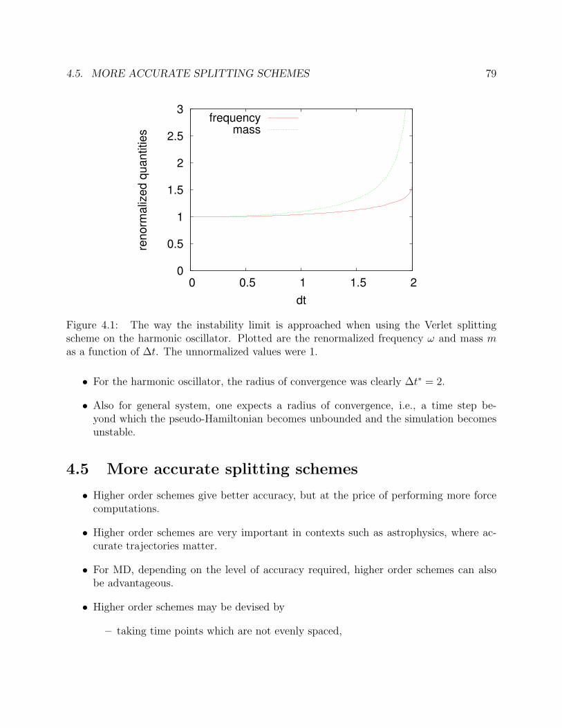
4.5. MORE ACCURATE SPLITTING SCHEMES 79
0
0.5
1
1.5
2
2.5
3
0 0.5 1 1.5 2
reno
rmal
ized
quan
titie
s
dt
frequencymass
Figure 4.1: The way the instability limit is approached when using the Verlet splittingscheme on the harmonic oscillator. Plotted are the renormalized frequency ω and mass mas a function of ∆t. The unnormalized values were 1.
• For the harmonic oscillator, the radius of convergence was clearly ∆t∗ = 2.
• Also for general system, one expects a radius of convergence, i.e., a time step be-yond which the pseudo-Hamiltonian becomes unbounded and the simulation becomesunstable.
4.5 More accurate splitting schemes
• Higher order schemes give better accuracy, but at the price of performing more forcecomputations.
• Higher order schemes are very important in contexts such as astrophysics, where ac-curate trajectories matter.
• For MD, depending on the level of accuracy required, higher order schemes can alsobe advantageous.
• Higher order schemes may be devised by
– taking time points which are not evenly spaced,
80 4. MOLECULAR DYNAMICS
– incorporating leading order correction terms in the pseudo-Hamiltonian
– incorporating more time points,
– or a combination of the above.
All but the first option lead to more force computations per unit of physical time,which decreases the efficiency.
• We will restrict ourselves to symmetric splitting schemes, to ensure time-reversibility.
• To facilitate many of the derivations, we restate the symmetrized BCH formula ofequation (4.34)
eXeY eX = e2X+Y− 16[X,[X,Y ]]+ 1
6[Y,[Y,X]]+fifth repeated X, Y commutators. (4.42)
4.5.1 Optimized schemes
• Given the same Hamiltonian split-up
H = K + U,
L = LK + LU ,
let us now explore a five-fold split up
eL∆t ≈ eηLU∆teLK∆t/2e(1−2η)LU∆teLK∆t/2eηLU∆t. (4.43)
• Note that this is a case of uneven time-intervals.
• Work out the inner three exponentials using equation (4.42)
eηLU∆teLK∆t/2e(1−2η)LU∆teLK∆t/2eηLU∆t
= eηLU∆teLK∆t+(1−2η)LU∆t− (1−2η)∆t3
24[LK ,[LK ,LU ]]+
(1−2η)2∆t3
12[LU ,[LU ,LK ]]+O(∆t5)eηLU∆t
= exp
LK∆t + LU∆t− (1− 2η)∆t3
24[LK , [LK ,LU ]] +
(1− 2η)2∆t3
12[LU , [LU ,LK ]]
− η2∆t3
6[LU , [LU ,LK ]] +
η∆t3
6[LK + (1− 2η)LU , [LK ,LU ]] +O(∆t5)
= eLH∆t+∆t3
„6η−124
[LK ,[LK ,LU ]]+ 1−6η+6η2
12[LU ,[LU ,LK ]]
«+O(∆t5)
= eLH∆t+∆t3(ν1[LK ,[LK ,LU ]]+ν2[LU ,[LU ,LK ]])+O(∆t5)
4.5. MORE ACCURATE SPLITTING SCHEMES 81
where
ν1 =6η − 1
24
ν2 =1− 6η + 6η2
12
• If both ν1 and ν2 were zero, this would give a fourth order scheme.However, this is not possible here: we have one parameter and two prefactors to set tozero.
• Alternatively, one could make the error “as small as possible”, e.g. by minimizingν2
1 + ν22 . This gives
η = 0.1931833275037836 . . . (4.44)
• The scheme in equation (4.43) that uses this value of η is called the Higher-orderOptimized Advanced scheme of second order, or HOA2 for short.
• In general, optimized schemes are based on minimizing the formal error, but this cannotguarantee that the actual error is small: Numerical tests are necessary.
• The HOA2 scheme requires two force computations:
eηLU∆t︸ ︷︷ ︸from previous step
eLK∆t/2 e(1−2η)LU∆t︸ ︷︷ ︸1st force computation
eLK∆t/2 eηLU∆t︸ ︷︷ ︸2nd force computation,
(4.45)
whereas the Verlet scheme requires just one.
• Thus, to compare accuracies at fixed numerical cost, the time step should be takentwice as large in the HOA2 scheme as in the Verlet scheme.
• The HOA2 scheme was tested on a model of water (TIP4P) [Van Zon, Omelyan andSchofield, J. Chem. Phys 128, 136102 (2008)], with the following results:
– As long as it is stable, the HOA2 scheme leads to smaller fluctuations in the totalenergy than the Verlet scheme at the same computational cost.
– In the water simulation, the HOA2 scheme becomes unstable for smaller timesteps than the Verlet scheme.
– The superior stability of the Verlet scheme means that it is the method of choicefor quick and dirty simulations of water with an accuracy less than approximately1.5% (as measured by the energy fluctuations).
82 4. MOLECULAR DYNAMICS
– For more accurate simulations, the HOA2 is more efficient, by about 50%, untilthe HOA2 scheme becomes unstable.
• The higher instability of HOA2 at large time steps, is due to the uneven time-stepsthan are taken.
• The average time step determines the computational cost, but the largest of the timesteps determines the stability.
• Using uneven time steps instead of even time steps (at fixed computational cost) there-fore increases some of the time intervals and decreases other.
• ⇒ uneven time steps become unstable for smaller time steps than even time stepvariants.
4.5.2 Higher order schemes from more elaborate splittings
• While using the HOA2 scheme is beneficial, this could only be known after numericaltests.
• True higher-order schemes are a bit better in that respect: one knows that at least forsmall enough ∆t, they are more efficient.
• The simplest way to get a higher order scheme is to concatenate lower order schemes.
• To understand this, note that if we have a k-th order scheme Sk(∆t) approximatingS(∆t) = eL∆ up to O(∆tk+1), i.e., if
Sk(∆t) = S(∆t) + ∆tk+1δS +O(∆tk+3)
then
Sk(∆s)Sk(∆t− 2∆s)Sk(∆s) (4.46)
= S(∆t) +[2∆sk+1 + (∆t− 2∆s)k+1
]δS +O(∆tk+3) (4.47)
The leading order term can be eliminated by choosing
2∆sk+1 = −(∆t− 2∆s)k+1, (4.48)
which, if k is even, can be solved and gives
∆s =∆t
2− 21/(k+1). (4.49)
4.5. MORE ACCURATE SPLITTING SCHEMES 83
• When Sk = S2 is given by the second Verlet scheme, the corresponding fourth orderscheme becomes
eL∆t ≈ eLU∆s/2eLK∆seLU∆s/2eLU (∆t/2−∆s)eLK(∆t−2∆s)eLU (∆t/2−∆s)eLU∆s/2eLK∆seLU∆s/2
= eLU∆s/2eLK∆seLU (∆t−∆s)/2eLK(∆t−2∆s)eLU (∆t−∆s)/2eLK∆seLU∆s/2 (4.50)
This is called the fourth order Forest-Ruth integration scheme (FR4). Note that it hasseven parts and requires three force evaluations per time step.
• Note that ∆s > ∆t/2, so that ∆t− 2∆s < 0.
• It therefore requires to take a negative time step:This tends to lead to instabilities.
• One can prove that order k splitting schemes using a two-operator split up (such asLU and LK) must have at least one negative time step if k > 2.
• The negative steps thus seem unavoidable.
• One can minimize these however, by allowing more general splitting schemes than thoseconstructed from equation (4.46), i.e., using the general form in equation (4.32).
• This gives more parameters, allowing one to combine this with the higher-order naturewith optimization, i.e. minimizing the leading error terms (cf. the HOA2 scheme).
• A good fourth order scheme of this type is called EFRL4 (Extended Forest-Ruth-likeFourth order scheme) and looks like this:
eL∆t = eLU ξ∆teLK( 12−λ)∆teLUχ∆teLKλ∆teLU (1−2χ−2ξ)∆teLKλ∆teLUχ∆teLK( 1
2−λ)∆teLU ξ∆t
(4.51)
+O(∆t5),
where
ξ = 0.3281827559886160
λ = 0.6563655119772320
χ = −0.09372690852966102
Even though this requires four force evaluations for each time step, it is more efficientthan the FR4 scheme due to a much smaller leading order error.
84 4. MOLECULAR DYNAMICS
4.5.3 Higher order schemes using gradients
• Gradients are, in this context, derivatives and higher-order derivatives of the potential.
• Using gradients as auxiliary Hamiltonians, one can reduce the order of a scheme
• The simplest can be derived by considering once more the five-fold splitting scheme,before optimization:
eηLU∆teLK∆t/2e(1−2η)LU∆teLK∆t/2eηLU∆t = eLH∆t+∆t3(ν1[LK ,[LK ,LU ]]+ν2[LU ,[LU ,LK ]])+O(∆t5)
= eLH∆t+∆t3(ν1LU,K,K+ν2LK,U,U)+O(∆t5)
where
ν1 =6η − 1
24
ν2 =1− 6η + 6η2
12
and let K and U be of the usual form such that (cf. equations (4.35) and (4.36))
K, U, U =∂U
∂RN· ∂2K
∂PN∂PN· ∂U
∂RN=
1
m
∣∣∣∣ ∂U
∂RN
∣∣∣∣2 =1
m|FN |2
U,K, K =∂K
∂PN· ∂2U
∂RN∂RN· ∂K
∂PN=
1
m2PN · ∂2U
∂RN∂RN· PN .
• The former depends only on RN , but the latter is more complicated and depends onboth RN and PN .
• We can eliminate the more complicated term by setting ν1 = 0 ⇒ η = 1/6, leaving uswith
e16LU∆te
12LK∆te
23LU∆te
12LK∆te
16LU∆t = e
LH∆t+∆t3 172m
L|FN |2+O(∆t5)
= e
»LK+L
U+ ∆t272m |FN |2
–∆t+O(∆t5)
• This equation holds for any form of U !
• Thus we may substitute for U the expression
U = U − ∆t2
72m
∣∣FN∣∣2 , (4.52)
4.5. MORE ACCURATE SPLITTING SCHEMES 85
giving
e16LU∆te
12LK∆te
23LU∆te
12LK∆te
16LU∆t = e
»LK+L
U+ ∆t272m |FN |2
–∆t+O(∆t5)
= e[LK+LU ]∆t+O(∆t5) = eLH∆t+O(∆t5)
A fourth order integration scheme!
• Note that no negative time steps were needed.
• The scheme in the current form uses an effective potential U , which differs from the
real potential U by an additional term δU = −∆t2
72m
∣∣FN∣∣2 of order O(∆t2). To leading
order, this term commutes with all factors, so one may also write
eLH∆t+O(∆t5) = e16LU∆te
12LK∆te
23LU∆t+δU∆te
12LK∆te
16LU∆t
= e16LU∆te
12LK∆te
23[LU+ 3
2δU ]∆te
12LK∆te
16LU∆t
= e16LU∆te
12LK∆te
23[L ˜U
]∆te12LK∆te
16LU∆t (4.53)
where the modified potential in the middle step is
˜U = U +3
2δU = U − ∆t2
48m
∣∣FN∣∣2 . (4.54)
• Scheme (4.53) is due to Suzuki.
• To summarize: by taking uneven intervals and incorporating the correction terms(using gradients of the potentials), we get a fourth order scheme which does not requirenegative partial steps and only needs two force evaluations per step.
• Note that to be able to use the modified potentials, the forces have to be well defined,i.e., any cut-off has to be smooth enough.
4.5.4 Multiple time-step algorithms
• Decompose the potential and the corresponding Liouville operator into two parts: onefor fast varying forces and the other for the slow varying forces:
U = Uf + Us (4.55)
• The fast motion could represent e.g. , intermolecular vibrations while the slowly varyingforces might be intermolecular forces.

86 4. MOLECULAR DYNAMICS
• The simplest multiple time-step algorithm is then
e12LUs∆t
(e
12LUf
∆t/MeLK∆t/Me12LUf
∆t/M)M
e12LUs∆t = eL∆t+O(∆t3). (4.56)
• While this is of second order, like the Verlet scheme, the time step for the fast part ofthe motion if M times smaller than that of the slow motion.
5
Advanced topics
5.1 Hybrid Monte Carlo
5.1.1 The Method
One drawback of traditional Monte-Carlo simulation methods is that typically the method ofgenerating trial configurations based on a probability T(x → y) results in trial configurationsy that are highly correlated with the initial configuration x, with only small differencesbetween the configurations.
• As an example, consider a dense liquid system where one could generate trial configu-rations by randomly selecting one of the particles in the fluid and giving the particle arandom displacement.
– Very inefficient since particles are close to one another on average in a dense fluid,so the trial configuration has a high probability of either overlapping with anotherparticle (hard spheres) or being in the strongly repulsive region of the interactionpotential of another particle, resulting in a configuration of high potential energy.
– Molecular dynamics, in contrast, moves all particles in a cooperative fashion, sothat the potential energy undergoes only small fluctuations.
– It is possible to try to move a group or cluster of particles cooperatively usingtricks, but this requires some cleverness.
• Can we devise a dynamical procedure of generating a trial configuration in which a largenumber of degrees of freedom are moved cooperatively in a energetically reasonablefashion?
Suppose we use a dynamical procedure to change a set of coordinates for use as a trialconfiguration in a Monte-Carlo procedure. See S. Duane, A.D. Kennedy, B.J. Pendleton andD. Roweth, Phys. Lett. B 45, 216 (1987).
87
88 5. ADVANCED TOPICS
• We require a momentum coordinate p conjugate to each spatial degree of freedom xwe wish to evolve dynamically.
• Suppose the evolution is a one-to-one mapping (i.e. deterministic evolution) of theinitial phase point (x0,p0) to another phase point (xt,pt)
gt(x0,p0) = (x0(t),p0(t)) = (xt,pt). (5.1)
• The inverse of this mapping is well-defined, so that
g−t(xt,pt) = (x0,p0).
• Consider using this mapping to define a transition matrix in a Markov process somehowso that the transition matrix is defined using the dynamics, K(x0 → xt).
• We want our transition matrix to be stationary with respect to the target distributionP (x), which requires:∫
dx0 P (x0)K(x0 → xt)−∫
dxt P (xt)K(xt → x0) = 0. (5.2)
• How can we define K? Suppose we draw the conjugate momenta p0 randomly from adensity Πm(p0) and then generate the phase point (xt,pt) according to our mappingEq. (5.1). Starting from the initial phase point (x0,p0), the probability of generatingthe phase point (xt,pt) by evolving the system using the deterministic dynamics overa time interval t is therefore
Pg((x0,p0) → (xt,pt)) = δ((x0(t),p0(t))− (xt,pt)) = δ(gt(x0,p0)− (xt,pt)).
• The transition probability K(x0 → xt) is therefore
K(x0 → xt) =
∫dp0dpt Πm(p0)Pg((x0,p0) → (xt,pt)) A((x0,p0) → (xt,pt)), (5.3)
where A((x0,p0) → (xt,pt)) is the acceptance probability for the phase point (xt,pt)if the initial configuration was (x0,p0).
• To define this acceptance probability, let Π(x,p) = P (x)Πm(p) be the probabilitydensity for the augmented coordinate (x,p).
• We then define the acceptance probability to be
A((x0,p0) → (xt,pt)) = min
(1,
Π(xt,pt)
Π(x0,p0)
)
5.1. HYBRID MONTE CARLO 89
• Claim: The transition probability Eq. (5.3) satisfies the stationarity condition Eq. (5.2)provided
1. The dynamics is symplectic, so that the mapping is volume-preserving and time-reversible.
2. The probability density for the conjugate momenta satisfies Πm(−p) = Πm(T p) =Πm(p), where T is the momentum inversion operator T f(p) = f(−p).
Proof. To show Eq. (5.2) is satisfied, we must compute K(xt → x0) under the dynamicalprocedure. Suppose the dynamical mapping is symplectic and hence reversible. Themapping gt therefore satisfies g−t = T gtT and hence if gt(x0,p0) = (x0(t),p0(t)) =(xt,pt), we have T gtT (xt,pt) = (x0,p0) and hence gt(xt, T pt) = (x0, T p0). From thedefinition of the transition probability, we have
K(xt → x0) =
∫d(T p0)d(T pt) Πm(T pt)Pg((xt, T pt) → (x0, T p0))
×A((xt, T pt) → (x0, T p0)) (5.4)
=
∫dp0dpt Πm(pt)δ(g
t(xt, T pt)− (x0, T p0))A((xt,pt) → (x0,p0))
since Πm(T pt) = Πm(pt), Π(xt, T pt) = Π(xt,pt) and Π(x0, T p0) = Π(x0,p0) byassumption. Now
∫dx0 P (x0)K(x0 → xt) =
∫dx0dp0dpt P (x0)Πm(p0)δ(g
t(x0,p0)− (xt,pt))
×min
(1,
Π(xt,pt)
Π(x0,p0)
)=
∫dx0dp0 min
(Π(x0,p0), Π(gt(x0,p0))
), (5.5)
whereas∫dxt P (xt)K(xt → x0) =
∫dxtdp0dpt Π(xt,pt)δ(g
t(xt, T pt)− (x0, T p0))
×min
(1,
Π(x0, T p0)
Π(xt,pt)
)=
∫dxtdpt min
(Π(xt, T pt), Π(gt(xt, T pt))
)(5.6)
90 5. ADVANCED TOPICS
Changing the variables of integration from (xt,pt) to (x0,p0) = T gt(xt, T pt) gives∫dxt P (xt) K(xt → x0) =
∫dx0dp0 J((xt, T pt); (x0,p0)) min
(Π(g−t(x0, T p0)), Π(x0, T p0)
)=
∫dx0dp0 min
(Π(T gt(x0,p0)), Π(x0,p0),
)=
∫dx0dp0 min
(Π(gt(x0,p0)), Π(x0,p0)
)(5.7)
since the Jacobian J((xt, T pt); (x0,p0)) of the transformation is unity due to thevolume-preserving property of the dynamical evolution. Since Eq. (5.5) and Eq. (5.7)are equal, the equilibrium distribution is stationary under the transition matrix K.
5.1.2 Application of Hybrid Monte-Carlo
As an example of a useful application of hybrid Monte-Carlo, consider a bead polymer systemwhere the interaction between monomers is determined by a potential of the form
U(r(N)) =N∑
i=1
N∑j=i+4
Vnb(|ri − rj|) +N∑
i=4
Utor(φi) +N∑
i=3
Ubend(θi) +N∑
i=2
Ubond(|ri − ri−1|).
In this potential, we have the following contributions:
1. A bond-stretching potential Ubond that typically is harmonic.
2. A bond-angle potential Ubend, taken to be harmonic in cos θi, where θi is the bond angledefined by
lili−1 cos θi = (ri − ri−1) · (ri−2 − ri−1),
where li = |ri − ri−1| is the bond distance between monomers i and i + 1.
3. A torsional potential Utor that depends on the torsional angle φi, defined to be theangle between the normal vectors to the planes formed by monomers (i−3, i−2, i−1)and (i − 2, i − 1, i). The torsional angle can be computed readily from the Cartesianpositions of monomers i− 4 through i.
4. A non-bonded potential Unb that describes interactions between monomers separatedfrom one another by at least 4 other monomers. This potential typically is of Lennard-Jones form, and can also include electrostatic interactions.
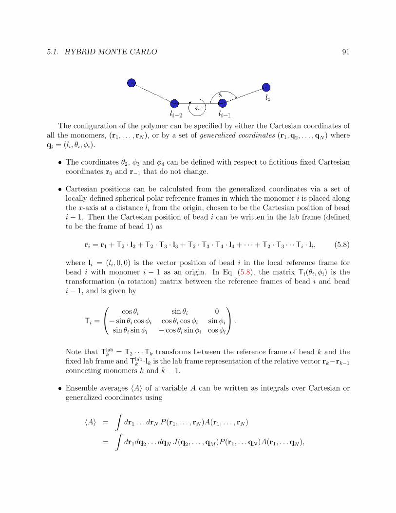
5.1. HYBRID MONTE CARLO 91
The configuration of the polymer can be specified by either the Cartesian coordinates ofall the monomers, (r1, . . . , rN), or by a set of generalized coordinates (r1,q2, . . . ,qN) whereqi = (li, θi, φi).
• The coordinates θ2, φ3 and φ4 can be defined with respect to fictitious fixed Cartesiancoordinates r0 and r−1 that do not change.
• Cartesian positions can be calculated from the generalized coordinates via a set oflocally-defined spherical polar reference frames in which the monomer i is placed alongthe x-axis at a distance li from the origin, chosen to be the Cartesian position of beadi− 1. Then the Cartesian position of bead i can be written in the lab frame (definedto be the frame of bead 1) as
ri = r1 + T2 · l2 + T2 · T3 · l3 + T2 · T3 · T4 · l4 + · · ·+ T2 · T3 · · ·Ti · li, (5.8)
where li = (li, 0, 0) is the vector position of bead i in the local reference frame forbead i with monomer i − 1 as an origin. In Eq. (5.8), the matrix Ti(θi, φi) is thetransformation (a rotation) matrix between the reference frames of bead i and beadi− 1, and is given by
Ti =
cos θi sin θi 0− sin θi cos φi cos θi cos φi sin φi
sin θi sin φi − cos θi sin φi cos φi
.
Note that Tlabk = T2 · · ·Tk transforms between the reference frame of bead k and the
fixed lab frame and Tlabk ·lk is the lab frame representation of the relative vector rk−rk−1
connecting monomers k and k − 1.
• Ensemble averages 〈A〉 of a variable A can be written as integrals over Cartesian orgeneralized coordinates using
〈A〉 =
∫dr1 . . . drN P (r1, . . . , rN)A(r1, . . . , rN)
=
∫dr1dq2 . . . dqN J(q2, . . . ,qM)P (r1, . . .qN)A(r1, . . .qN),
92 5. ADVANCED TOPICS
where J(q2, . . . ,qN) is the Jacobian of the transformation between Cartesian and gen-eralized coordinates. It can be shown that
J(q2, . . . ,qN) =N∏
i=2
l2i cos θi.
• We could construct a Monte-Carlo procedure to generate equilibrium configurations ofthe polymer either
– Randomly displacing Cartesian positions of the monomers and accepting/rejectingtrial configurations based on energy differences. This typically is very inefficientsince the bond-stretching potential greatly restricts the range of displacementsallowed that are accepted.
– Randomly displacing the generalized coordinates qi = (li, θi, φi). This can resultin large conformational changes as small rotations around one of the torsionalangles rotates all the subsequent monomers. In some situations, the drastic changein conformation caused by changing a single dihedral angle can lead to leads totrial configurations with large energies, and hence poor acceptance.
– General problem is we’d like to move the generalized coordinates q together ina cooperative fashion to change the configuration of the polymer in a reasonableway. Ideally, we’d like to keep some degrees of freedom, such as bond lengths,fixed during the generation of a trial configuration. This can be accomplished byusing a dynamical updating scheme on a restricted set of coordinates (θi, φi).
• Implementation: use hybrid Monte-Carlo with fictitious momenta Pθiand Pφi
conju-gate to each of the selected coordinates θi and φi.
– Draw momenta for degrees of freedom of monomer i from Boltzmann weights
Πm(θi, φi) ∼ e−β
P2θi
2mθ e−β
P2φi
2mφ ,
where the effective “masses” mθ and mφ are arbitrary.
– Evolve the configuration (θi, φi, Pθi, Pφi
) for a fixed amount of time τ using a sym-plectic integrator, preferably with a large time step to change the configurationrapidly. The equations to integrate are
θi =Pθi
mθ
φi =Pφi
mφ
Pθi= −∂U
∂θi
˙Pφi= −∂U
∂φi
.
5.1. HYBRID MONTE CARLO 93
∗ A symplectic integrator is easy to construct based on the usual Hamiltoniansplitting scheme of separating the kinetic and potential energy terms anddefining Liouville operators for each of the terms.
∗ The effective forces in the evolution of momenta require evaluation of deriva-tives ∂rj/∂θi and ∂rj/∂φi.
– Track the effective Hamiltonian
He =∑
i
(P 2
θi
mθ
+P 2
φi
mφ
)+ U(r1,q2, . . . ,qN).
– The stationary distribution Π for the phase point in the Monte-Carlo process isproportional to e−βHe , due to the form of the densities of the momenta.
– If the current configuration at the start of the dynamical update is X, accept thetrial configuration Y generated by the trajectory with probability
min
(1,
J(Y)
J(X)e−β∆He
),
where ∆He = He(Y)−He(X).
∗ Note that if the dynamics was integrated perfectly, ∆He = 0 since the effectiveHamiltonian is conserved by the dynamics.
• Comments:
1. The smaller the time step, the smaller the average ∆He and the greater theacceptance probability.
2. The smaller the time step, the smaller the overall change in configuration of thesystem for a fixed number of molecular dynamics steps.
3. The dynamics is fictitious, as the equations of motion are not the Hamiltonianequations for the generalized coordinates. In particular, the kinetic energy in theHamiltonian has a different form.
4. The Jacobian factor is important in the acceptance probability. However, if theli and θi are held fixed and only the torsional angles evolve, the Jacobian factoris constant.
5. Any subset of coordinates can be selected for updating for any trial move. It maybe advantageous to select different groups of coordinates for updating at differenttimes.
94 5. ADVANCED TOPICS
5.2 Time-dependent correlations
We have considered primarily averages of static properties that are constructed out ensembleaverages involving a single phase point at a time. We have seen that these averages may becomputed by either:
1. A Monte-Carlo algorithm that generates ensemble averages by sampling phase pointsfrom the phase space density for the ensemble. Different ensemble averages can becomputed by altering the transition matrix. Within this class of algorithms, we includethe hybrid Monte-Carlo scheme, which uses a dynamical procedure to generate trialconfigurational coordinates.
2. A molecular dynamics procedure that uses the real Hamiltonian dynamics of the systemto compute the time average of a dynamical variable. By hypothesis, the time averageis equal to the micro-canonical ensemble average. In the dynamical evolution, themicro-canonical phase space density and phase space volume are conserved, whichreflects the conservation of probability.
In many physical situations, we are interested in computing quantities that obey some phys-ical law, and which may involve the real dynamics of the system. For example, suppose oneis interested in computing how an initially nonuniform concentration profile (say a drop ofdye in water) is smoothed in the absence of flow or stirring. Such a process is describedphenomenologically by the law of diffusion (Fick’s law), which states that the flux j of thediffusing species is proportional to the negative gradient in the concentration of the species:
j = −D∂c(r, t)
∂r,
where c(r, t) is the local concentration of the species and D is a constant known as thediffusion coefficient. Under Fick’s law, the concentration obeys the equation
∂c(r, t)
∂t= − ∂
∂r· j(r, t)
∂c(r, t)
∂t= D∇2c(r, t). (5.9)
If the initial dye is concentrated in a small region c(r, 0) = δ(r), then the concentrationprofile is
c(r, t) =1
(4πDt)3/2e−r2/(4Dt).
Note that the concentration profile is normalized,∫
dr c(r, t) = 1. This is of the form of aGaussian distribution with a time-dependent width 2Dt. Hence the diffusion coefficient isrelated to the second moment of c(r, t):⟨
r2(t)⟩
=
∫dr r2c(r, t).
5.2. TIME-DEPENDENT CORRELATIONS 95
The second moment can be interpreted to mean the average distance squared that a particlemoves away from the origin in a time interval t. To see how one might compute the coefficientD, we multiply Eq. (5.9) by r2 to compute the second moment to get
∂〈r2(t)〉∂t
= D
∫dr r2∇2c(r, t) = 6D
∫dr c(r, t) = 6D,
after the angular integrals have been carried out using the spherical symmetry of c(r, t).This equation suggests that 〈r2(t)〉 = 6Dt, so that a plot of the average squared distanceversus time should be linear with slope 6D. To compute diffusion coefficient from the time-dependent correlation function 〈r2(t)〉, we must:
1. Draw an initial configuration according to the correct phase space density (i.e. micro-canonical, canonical, etc..).
2. Propagate the system using the correct dynamics and measure the displacement vector∆ri(t) = ri(t)− ri(0) of each particle for a set of different times t.
3. If we ignore any cross-correlation between the motion of particles, we can measure theself-diffusion coefficient Ds by calculating
Ds =〈r2(t)〉
6t=
1
N
N∑i=1
∆ri(t) ·∆ri(t)
6t.
From the equations of motion, ∆ri(t) =∫ t
0dτ vi(τ), and hence the average can be
written as
〈r2(t)〉 =1
N
N∑i=1
∫ t
0
dτ
∫ t
0
dτ ′ vi(τ) · vi(τ′).
• Note that the procedure consists of two different steps, the drawing of the initial phasepoints and then the propagation of the system.
• General time-dependent correlation functions of the form
〈AB(t)〉 =
∫dx(N) f(x(N))A(x(N))B(x(N)(t))
can be computed analogously.
– If the ensemble is not microcanonical, the initial points must be drawn usinga Monte-Carlo algorithm (or with a special dynamical procedure) that generatesphase points according to f(x(N)). Then the system must be evolved using the realdynamics of the system, preferably with a symplectic integrator. This evolutiontherefore evolves the system with constant energy.
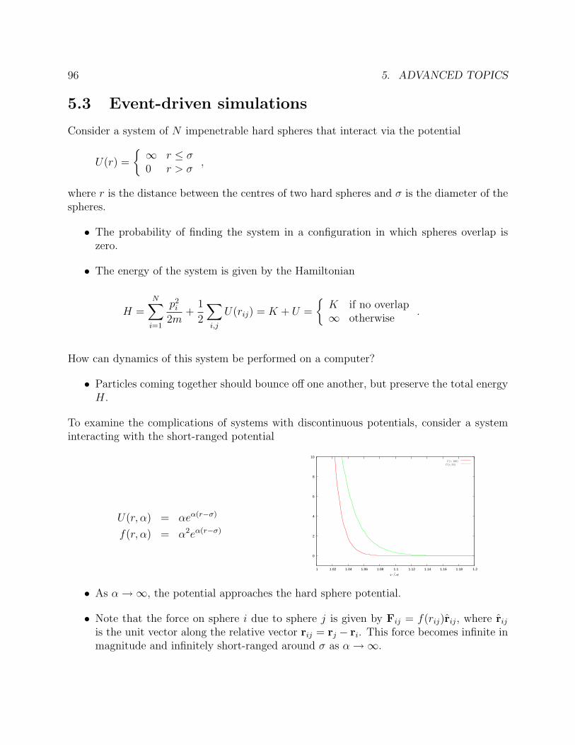
96 5. ADVANCED TOPICS
5.3 Event-driven simulations
Consider a system of N impenetrable hard spheres that interact via the potential
U(r) =
∞ r ≤ σ0 r > σ
,
where r is the distance between the centres of two hard spheres and σ is the diameter of thespheres.
• The probability of finding the system in a configuration in which spheres overlap iszero.
• The energy of the system is given by the Hamiltonian
H =N∑
i=1
p2i
2m+
1
2
∑i,j
U(rij) = K + U =
K if no overlap∞ otherwise
.
How can dynamics of this system be performed on a computer?
• Particles coming together should bounce off one another, but preserve the total energyH.
To examine the complications of systems with discontinuous potentials, consider a systeminteracting with the short-ranged potential
U(r, α) = αeα(r−σ)
f(r, α) = α2eα(r−σ)
0
2
4
6
8
10
1 1.02 1.04 1.06 1.08 1.1 1.12 1.14 1.16 1.18 1.2
r/σ
U(r, 100)U(r, 50)
• As α →∞, the potential approaches the hard sphere potential.
• Note that the force on sphere i due to sphere j is given by Fij = f(rij)rij, where rij
is the unit vector along the relative vector rij = rj − ri. This force becomes infinite inmagnitude and infinitely short-ranged around σ as α →∞.
5.3. EVENT-DRIVEN SIMULATIONS 97
• If integrated by Verlet-scheme, the shadow Hamiltonian Hs to leading order in ∆t is
Hs = H +∆t2
12m2
∑i,j
pi ·∂2U
∂ri∂rj
· pj −∆t2
24m
∑i
Fi · Fi + O(∆t4).
• From form of the potential, we see that the correction term is proportional to (α2∆t)2,and hence the radius of convergence of the shadow Hamiltonian shrinks to zero asα →∞.
– The integrator is unstable for any choice of ∆t.
– In impulsive limit α →∞, force acts discontinuously at a time tc where rij(tc) = σ.
• How can we integrate equations of motion with “impulsive” forces that act at only onetime? Consider the integral form of the equation of motion for the momentum
pi(t + ∆t) = pi(t−∆t) +
∫ t+∆t
t−∆t
dτ Fi(τ).
• In impulsive limit, the force takes the form
Fij = Srijδ(rij − σ)
= Srijδ(t− tc),
where the second equality is obtained by solving the equation rij(tc) = σ and rewritingthe delta function in terms of time.
– S is a constant dependent on the configuration at the moment of collision, to bedetermined.
– Note that the direction of the force is along the relative vector rij for a “centralpotential” that depends only on the magnitude |rij| of the relative vector rij.
• Inserting the impulsive force into the momentum equation gives
∆pi = pi(t + ∆t)− pi(t−∆t) =
Srij if tc ∈ [t−∆t, t + ∆t]0 otherwise.
– In impulsive limit, only one collision at most can occur as ∆t → 0.
• How is the collision time determined? Solve for the collision time by considering whenrij(tc) = σ or rij(tc) · rij(tc) = σ2.
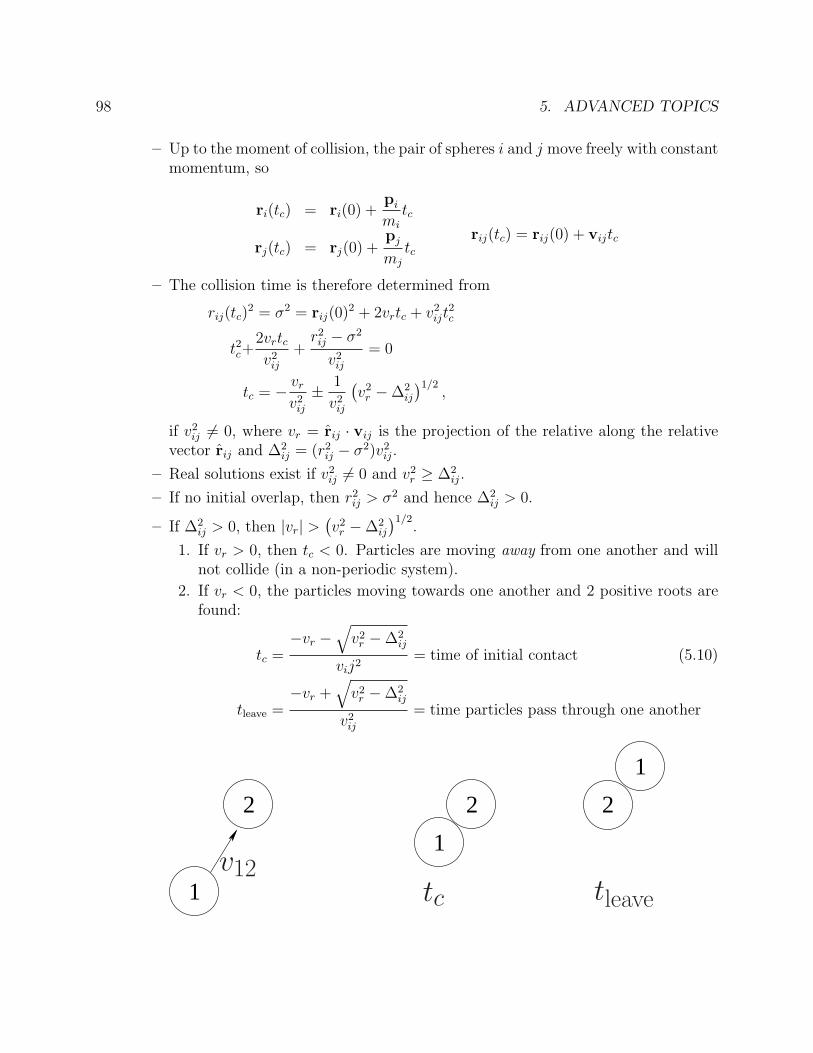
98 5. ADVANCED TOPICS
– Up to the moment of collision, the pair of spheres i and j move freely with constantmomentum, so
ri(tc) = ri(0) +pi
mi
tc
rj(tc) = rj(0) +pj
mj
tcrij(tc) = rij(0) + vijtc
– The collision time is therefore determined from
rij(tc)2 = σ2 = rij(0)
2 + 2vrtc + v2ijt
2c
t2c+2vrtcv2
ij
+r2ij − σ2
v2ij
= 0
tc = − vr
v2ij
± 1
v2ij
(v2
r −∆2ij
)1/2,
if v2ij 6= 0, where vr = rij · vij is the projection of the relative along the relative
vector rij and ∆2ij = (r2
ij − σ2)v2ij.
– Real solutions exist if v2ij 6= 0 and v2
r ≥ ∆2ij.
– If no initial overlap, then r2ij > σ2 and hence ∆2
ij > 0.
– If ∆2ij > 0, then |vr| >
(v2
r −∆2ij
)1/2.
1. If vr > 0, then tc < 0. Particles are moving away from one another and willnot collide (in a non-periodic system).
2. If vr < 0, the particles moving towards one another and 2 positive roots arefound:
tc =−vr −
√v2
r −∆2ij
vij2= time of initial contact (5.10)
tleave =−vr +
√v2
r −∆2ij
v2ij
= time particles pass through one another
2
1
2
1
2
1v12
tc tleave
5.3. EVENT-DRIVEN SIMULATIONS 99
• Determination of magnitude of impulse S is based on conservation principles. If thepotential depends only on the magnitude of the relative vector rij and the Hamiltoniandoes not depend explicitly on time, then linear momentum as well as total energy mustbe conserved once the collision has occurred.
• Conservation of linear momentum implies:
p′i + p′j = pi + pj,
p′i = pi + ∆pi = pi + Srij
p′j = pj + ∆pj = pj − Srij (5.11)
where p′i is the momentum of particle i after the collision with particle j.
• Conservation of energy implies that the post-collisional energy H ′ is equal to the pre-collisional energy H, or
p′i · p′i2mi
+p′j · p′j2mj
=pi · pi
2mi
+pj · pj
2mj
,
which, using Eq. (5.11), gives a condition on the impulse S
S2
2µ− Svr = 0 → S = 2µvr,
where µ = mimj/(mi + mj) is the reduced mass.
• After a collision, the momentum are therefore given by
p′i = pi + 2µvr rij
p′j = pj − 2µvr rij. (5.12)
5.3.1 Implementation of event-driven dynamics
For the hard sphere system, the dynamics can be executed by:
1. Initially calculate all collision events for system using Eq. (5.10).
• Boundary conditions must be properly included: hard walls, periodic system, ...
2. Find first collision event and evolve system (with free evolution) up to that time.
3. For colliding pair, compute the consequences of the collision using Eq. (5.12).
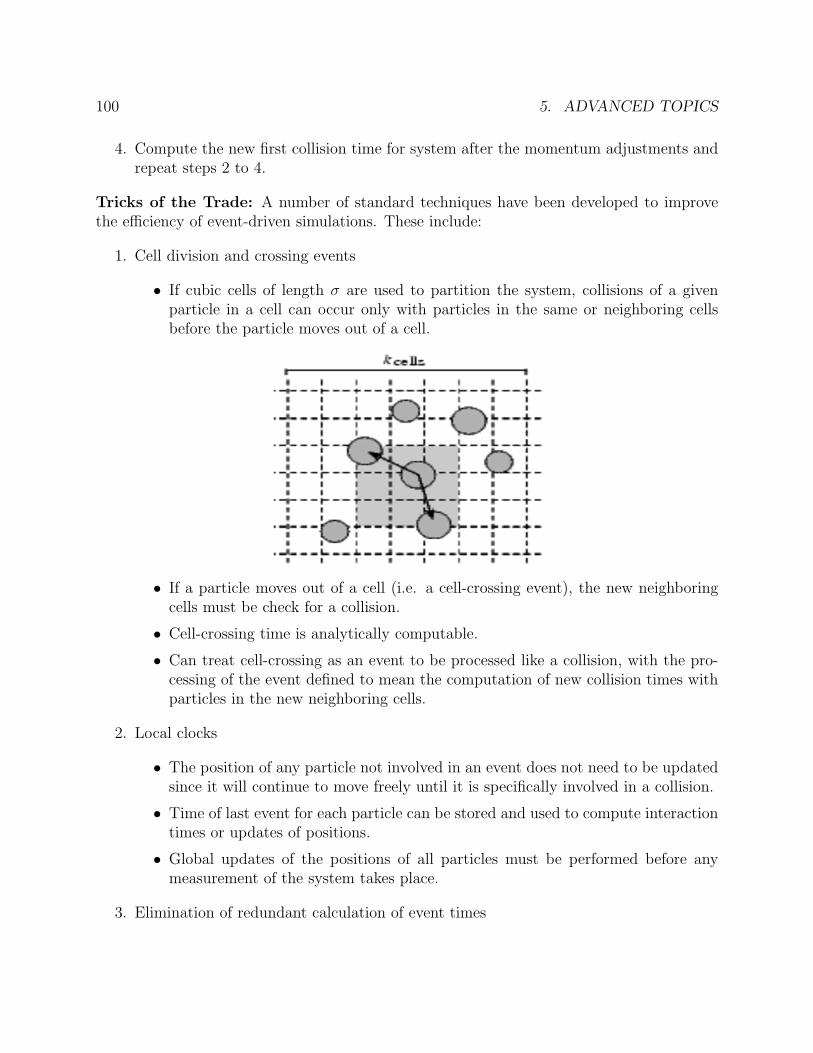
100 5. ADVANCED TOPICS
4. Compute the new first collision time for system after the momentum adjustments andrepeat steps 2 to 4.
Tricks of the Trade: A number of standard techniques have been developed to improvethe efficiency of event-driven simulations. These include:
1. Cell division and crossing events
• If cubic cells of length σ are used to partition the system, collisions of a givenparticle in a cell can occur only with particles in the same or neighboring cellsbefore the particle moves out of a cell.
• If a particle moves out of a cell (i.e. a cell-crossing event), the new neighboringcells must be check for a collision.
• Cell-crossing time is analytically computable.
• Can treat cell-crossing as an event to be processed like a collision, with the pro-cessing of the event defined to mean the computation of new collision times withparticles in the new neighboring cells.
2. Local clocks
• The position of any particle not involved in an event does not need to be updatedsince it will continue to move freely until it is specifically involved in a collision.
• Time of last event for each particle can be stored and used to compute interactiontimes or updates of positions.
• Global updates of the positions of all particles must be performed before anymeasurement of the system takes place.
3. Elimination of redundant calculation of event times
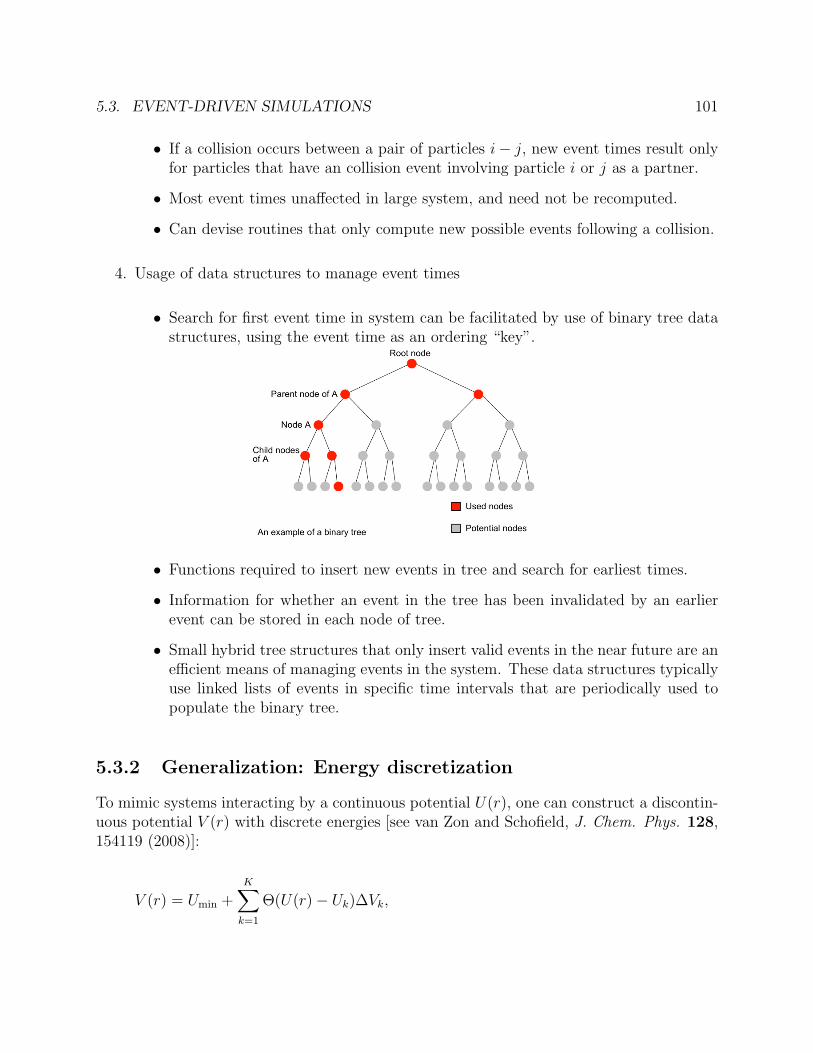
5.3. EVENT-DRIVEN SIMULATIONS 101
• If a collision occurs between a pair of particles i− j, new event times result onlyfor particles that have an collision event involving particle i or j as a partner.
• Most event times unaffected in large system, and need not be recomputed.
• Can devise routines that only compute new possible events following a collision.
4. Usage of data structures to manage event times
• Search for first event time in system can be facilitated by use of binary tree datastructures, using the event time as an ordering “key”.
• Functions required to insert new events in tree and search for earliest times.
• Information for whether an event in the tree has been invalidated by an earlierevent can be stored in each node of tree.
• Small hybrid tree structures that only insert valid events in the near future are anefficient means of managing events in the system. These data structures typicallyuse linked lists of events in specific time intervals that are periodically used topopulate the binary tree.
5.3.2 Generalization: Energy discretization
To mimic systems interacting by a continuous potential U(r), one can construct a discontin-uous potential V (r) with discrete energies [see van Zon and Schofield, J. Chem. Phys. 128,154119 (2008)]:
V (r) = Umin +K∑
k=1
Θ(U(r)− Uk)∆Vk,
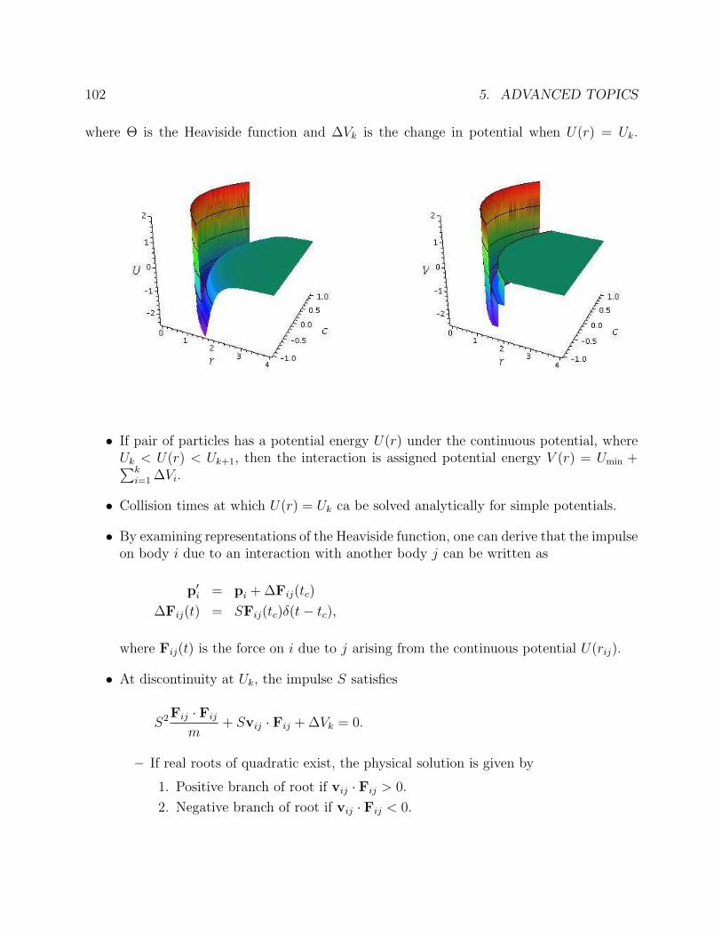
102 5. ADVANCED TOPICS
where Θ is the Heaviside function and ∆Vk is the change in potential when U(r) = Uk.
• If pair of particles has a potential energy U(r) under the continuous potential, whereUk < U(r) < Uk+1, then the interaction is assigned potential energy V (r) = Umin +∑k
i=1 ∆Vi.
• Collision times at which U(r) = Uk ca be solved analytically for simple potentials.
• By examining representations of the Heaviside function, one can derive that the impulseon body i due to an interaction with another body j can be written as
p′i = pi + ∆Fij(tc)
∆Fij(t) = SFij(tc)δ(t− tc),
where Fij(t) is the force on i due to j arising from the continuous potential U(rij).
• At discontinuity at Uk, the impulse S satisfies
S2Fij · Fij
m+ Svij · Fij + ∆Vk = 0.
– If real roots of quadratic exist, the physical solution is given by
1. Positive branch of root if vij · Fij > 0.
2. Negative branch of root if vij · Fij < 0.
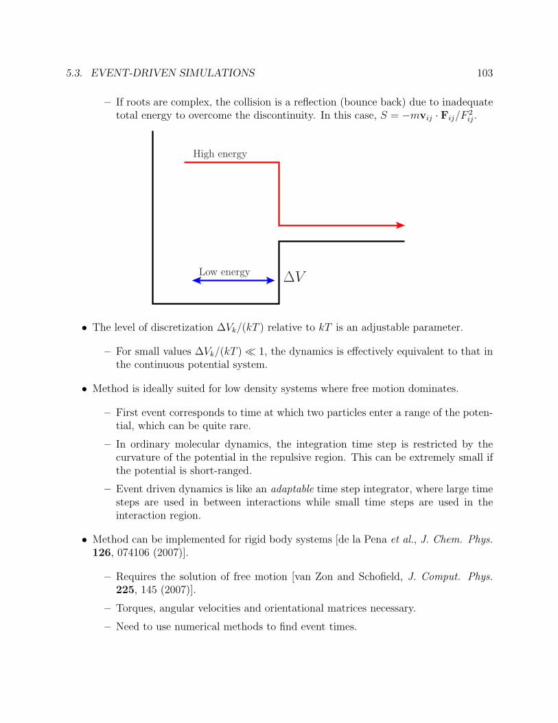
5.3. EVENT-DRIVEN SIMULATIONS 103
– If roots are complex, the collision is a reflection (bounce back) due to inadequatetotal energy to overcome the discontinuity. In this case, S = −mvij · Fij/F
2ij.
High energy
Low energy∆V
• The level of discretization ∆Vk/(kT ) relative to kT is an adjustable parameter.
– For small values ∆Vk/(kT ) 1, the dynamics is effectively equivalent to that inthe continuous potential system.
• Method is ideally suited for low density systems where free motion dominates.
– First event corresponds to time at which two particles enter a range of the poten-tial, which can be quite rare.
– In ordinary molecular dynamics, the integration time step is restricted by thecurvature of the potential in the repulsive region. This can be extremely small ifthe potential is short-ranged.
– Event driven dynamics is like an adaptable time step integrator, where large timesteps are used in between interactions while small time steps are used in theinteraction region.
• Method can be implemented for rigid body systems [de la Pena et al., J. Chem. Phys.126, 074106 (2007)].
– Requires the solution of free motion [van Zon and Schofield, J. Comput. Phys.225, 145 (2007)].
– Torques, angular velocities and orientational matrices necessary.
– Need to use numerical methods to find event times.
104 5. ADVANCED TOPICS
5.4 Constraints and Constrained Dynamics
Typical time scales of most intramolecular motions are 10 to 50 times shorter than thetranslational time scale of a molecule.
• Time step of an integrator determined by shortest relevant time scale.
• Multiple time step methods can be used to deal with differing time scales in dynamicalsimulations.
• Many observables are independent or insensitive to intramolecular motion.
– Molecular conformation is usually only weakly dependent on bond lengths. Bondvibrations are typically restricted to small motions on rapid time scales.
– Some bond angles remain relatively constant, aside from high frequency oscilla-tions.
5.4.1 Constrained Averages
• Suppose a set of ` variables, such as bond lengths, are effectively constant during asimulation.
• We will assume that the constraints are only functions of the positions, and independentof momenta. Such constraints are called holonomic.
• Can specify these constraints by
σ1(r(N)) = 0 such as σ1(r12) = r2
12 − d2
σ2(r(N)) = 0
...
• We write the condition that the set of all constraints σ = (σ1, . . . , σ`) are satisfied inthe compact notation
∏i=1
δ(σi(r(N))) = δ(σ).
• An ensemble average of an observable A(r(N)) that depends only on the configurationof the system can be written as
〈A(r(N))〉 =
∫dr(N)dp(N) P (r(N),p(N))A(r(N)) =
∫dr(N) ρ(r(N))A(r(N)),
5.4. CONSTRAINTS AND CONSTRAINED DYNAMICS 105
where P (r(N),p(N)) is the full phase space density and ρ(r(N)) =∫
dp(N) P (r(N),p(N))is the configurational phase space density.
• If A(r(N)) depends only weakly on the constraints,
〈A(r(N))〉 ≈∫
dr(N)dp(N) P (r(N),p(N))A(r(N))δ(σ)/
∫dr(N) ρ(r(N))δ(σ)
=
∫dr(N) ρcon(r
(N), σ = 0)A(r(N), σ = 0) = 〈A(r(N))〉c
• How can the conditional ensemble average 〈. . . 〉c be computed?
• This can be analyzed most easily by working in generalized coordinates rather thanCartesian coordinates.
• Define a coordinate transformation r = (r1, . . . , rN) → u = (u1, . . . ,uN), where thelast ` coordinates are the ` constraint conditions σα. We can represent u = (qi, σ),where the dimension of the qi is 3N − ` and the dimension of σ is `.
• If p = (p1, . . . ,pn) and the potential of the system is V (r), then the Lagrangian andthe Hamiltonian in the Cartesian coordinates are
L(r, r) =1
2r ·m · r− V (r) H(r,p) =
1
2p ·m−1 · p + V (r),
where mij = miδi,j and m−1ij = m−1
i δi,j.
• Using r(u), the Lagrangian in the generalized coordinates can be written as
L(u, u) =1
2
∑i
miuα∂ri
∂uα
· ∂ri
∂uβ
uβ − V (u) =1
2u · G · u− V (u)
Gαβ =∑
i
mi∂ri
∂uα
· ∂ri
∂uβ
where we have used a notation that repeated Greek indices are summed over. Theconjugate momenta pu to the generalize coordinates are therefore
pu =∂L
∂u= G · u so u = G−1 · pu,
leading to the Hamiltonian
H = pu · q− L =1
2pu · G−1 · pu + U(u).
106 5. ADVANCED TOPICS
– Note from the definition of the matrix G, we have
G−1αβ =
∑i
1
mi
∂uα
∂ri
· ∂uβ
∂ri
.
– Note that the equations of motion in the Cartesian phase space coordinates η =(r,p) and in the generalized phase space coordinates ζ = (u,pu) are in symplecticform
η = J · ∂H
∂ηζ = J · ∂H(ζ)
∂ζ.
Transformations η → ζ that preserve the symplectic form are called canonical.
• Claim: The phase space probability satisfies P (η)dη = P (η(ζ))dζ.
Proof. Consider the transformation of phase space coordinates ζ = ζ(η). The timederivative of this relation gives
ζ =∂ζ
∂η· η = M · η Mαβ =
∂ζα
∂ηβ
.
From the symplectic form of the equation of motion for η, we see that
ζ = M · J · ∂H
∂η.
Considering the inverse of the transformation, η = η(ζ), we find that
∂H
∂ηβ
=∂H
∂ζα
∂ζα
∂ηβ
=∂H
∂ζα
Mαβ so∂H
∂η= MT · ∂H
∂ζ.
Thus we find the equation of motion for the transformed phase space coordinates obeys
ζ =(M · J ·MT
)· ∂H
∂ζ.
This equation maintains symplectic form if M · J ·M = J . Now consider the transfor-mation of the volume element dη = | det M|dζ. If the transformed coordinates preservethe symplectic form, then det
(M · J ·MT
)= det (J ) = det2 (M) det (J ), and hence
det (M) = ±1, and so dη = dζ. If the phase space probability is P (η)dη, it thereforefollows that P (η)dη = P (η(ζ))dζ.
5.4. CONSTRAINTS AND CONSTRAINED DYNAMICS 107
• From this equality, the canonical configurational density can be expressed as
ρ(r)dr =dr
Z
∫dpe−βH =
du
Z
∫dpu e−β/2pu·G−1·pu
e−βV (u)
= c√
det G e−βV (u)du = ρ(u)du,
where c is a normalization constant.
• From our transformation where u = (q, σ), the conditional density is therefore
ρcon(q, σ = 0) = c√
det G e−βV (q,σ=0).
– Note that the factor√
det G is related to the Jacobian of the transform fromCartesian spatial coordinates r to generalized spatial coordinates u.
• Conditional averages can be computed by either
1. Devising a Monte-Carlo procedure that works in the q generalized coordinates.Note trial moves must not violate the constraints σ = 0, which is easy to im-plement if generalized spatial coordinates are used. The transition matrix shouldhave limit density of ρc, and therefore the Jacobian factor must be used in thefinal acceptance criterion of the Monte-Carlo procedure.
2. Carrying out constrained dynamics, which effectively correspond to Hamiltoniandynamics in a lower-dimensional sub-space of the full phase space (r,p) or (u,pu).
5.4.2 Constrained Dynamics
To construct the equations of motion for a constrained system, consider the Lagrangianwritten in the generalized coordinates u while the ` constraints σ = 0 are maintained:
L(u, u) =1
2u · G · u− V (u)
=1
2q · A · q− V (q, σ = 0),
since σ = 0 under the constraint. In this equation, the matrix A is a sub-matrix of G givenby
Aαβ =∑
i
mi∂ri
∂qα
· ∂ri
∂qβ
,
which is of dimension (N−`)×(N−`). From the Lagrangian, we construct the Hamiltonianin generalized coordinates
Hc =1
2pq · A−1 · pq + V (q, σ = 0) pq =
∂L
∂q= A · q.
108 5. ADVANCED TOPICS
• Note that there is no momentum conjugate to the fixed coordinates σ.
• The canonical probability density for this Hamiltonian system is obtained from
ρ(q)dq = dq
∫dpq e−β/2pq ·A−1·pq
e−βV (q,σ=0)
= c′√
det Ae−βV (q,σ=0)dq
ρ(q) = c
√det A√det G
ρcon(q, σ = 0).
• Note that the probability density associated with the Hamiltonian dynamics of theconstrained system is ρ(q), while the targeted constrained density is ρc(q, σ = 0).
– Each configuration generated by constrained dynamics must be weighted by ratioof Jacobian factors
√det G/ det A.
• How can this weight factor be evaluated?
– We write G and its inverse G−1 in block form:
G =
(A B
BT Γ
)A =
∑i
mi∂ri
∂q· ∂ri
∂qB =
∑i
mi∂ri
∂q· ∂ri
∂σΓ =
∑i
mi∂ri
∂σ· ∂ri
∂σ
G−1 =
(∆ E
ET Z
)∆ =
∑i
1
mi
∂q
∂ri
· ∂q
∂ri
E =∑
i
1
mi
∂σ
∂ri
· ∂q
∂ri
Z =∑
i
1
mi
∂σ
∂ri
· ∂σ
∂ri
– We now define a matrix X so that det X = det A:
X =
A 0
BT I
,
where I is the identity matrix.
– Writing X = G · G−1 · X, we get
X = G ·
∆ · A + E · BT E
ET · A + Z · BT Z
G−1 · G =
∆ · A + E · BT ∆ · B + E · Γ
ET · A + Z · BT ET · B + Z · Γ
so ∆ · A + E · BT = I and ET · A + Z · BT = 0, and hence
X = G ·
(I E
0 Z
).
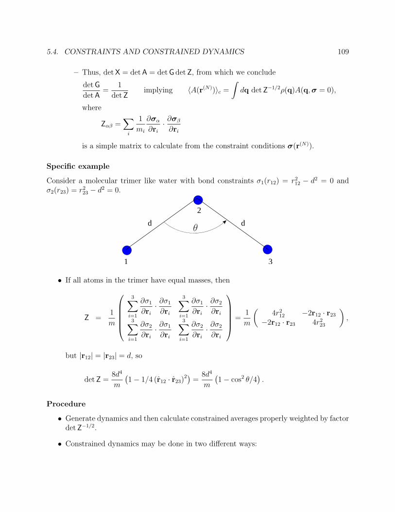
5.4. CONSTRAINTS AND CONSTRAINED DYNAMICS 109
– Thus, det X = det A = det G det Z, from which we conclude
det G
det A=
1
det Zimplying 〈A(r(N))〉c =
∫dq det Z−1/2ρ(q)A(q, σ = 0),
where
Zαβ =∑
i
1
mi
∂σα
∂ri
· ∂σβ
∂ri
is a simple matrix to calculate from the constraint conditions σ(r(N)).
Specific example
Consider a molecular trimer like water with bond constraints σ1(r12) = r212 − d2 = 0 and
σ2(r23) = r223 − d2 = 0.
1
2
3
d dθ
• If all atoms in the trimer have equal masses, then
Z =1
m
3∑
i=1
∂σ1
∂ri
· ∂σ1
∂ri
3∑i=1
∂σ1
∂ri
· ∂σ2
∂ri
3∑i=1
∂σ2
∂ri
· ∂σ1
∂ri
3∑i=1
∂σ2
∂ri
· ∂σ2
∂ri
=1
m
(4r2
12 −2r12 · r23
−2r12 · r23 4r223
),
but |r12| = |r23| = d, so
det Z =8d4
m
(1− 1/4 (r12 · r23)
2) =8d4
m
(1− cos2 θ/4
).
Procedure
• Generate dynamics and then calculate constrained averages properly weighted by factordet Z−1/2.
• Constrained dynamics may be done in two different ways:
110 5. ADVANCED TOPICS
1. Re-writing Hamiltonian in generalized coordinates and using symplectic integratorwith Hamiltonian system.
– Typically, Hamiltonian has complicated form as A−1 is not diagonal.
2. Lagrange multiplier approach: Define Lagrangian with constraints
L′ = L− λασα L =∑
i
mi/2r2i − V (r(N))
• Equation of motion from constrained Lagrangian:
∂
∂t
∂L′
∂r=
∂L′
∂r
miri = −∂V
∂ri
− λα∂σα
∂ri
,
provide the constraints are holonomic (depend only on r and not on p).
• The dynamics in the full phase X = (r,p) is generated by the linear operator L0
L0 = X · ∂
∂X=∑
i
(pi
mi
· ∂
∂ri
+ Fi ·∂
∂pi
− λα
(∂σα
∂ri
)· ∂
∂pi
)dA(X(t))
dt= L0A(X(t))
with formal solution A(X(t)) = exp L0tA(X(0)).
– The effective forces have be re-defined to include a constraint force Gi = −λα∂σα/∂ri.
– The Lagrange multipliers λα typically depend on both r and p, and so the systemis non-Hamiltonian, as the generalized forces depend on p.
– The operator L0 is not obtained from the Poisson bracket of a Hamiltonian.
– Even though the dynamics is not Hamiltonian in the full phase space X, we sawearlier that it is Hamiltonian in a sub-space of the phase space X.
• To solve for the Lagrange multipliers, note that the time-derivatives of the constraintcondition σα = 0 must vanish, so
σα = 0 so∑
i
ri ·∂σα
∂ri
= 0
σα = 0 so∑
i
(ri ·
∂σα
∂ri
+ ri ·∂
∂ri
σα
)= 0.
5.4. CONSTRAINTS AND CONSTRAINED DYNAMICS 111
The equation of motion miri = Fi − λα∂σα/∂ri therefore gives a linear equation forthe Lagrange multipliers∑
i
(Fi
mi
− 1
mi
∂σβ
∂ri
λβ
)· ∂σα
∂ri
+∑i,j
ri ·∂2σα
∂ri∂rj
· rj = 0
or
λα = Z−1αβ (Fβ + Tβ) Fβ =
∑i
Fi
mi
· ∂σβ
∂ri
Tβ =∑i,j
pi
mi
· ∂2σα
∂ri∂rj
·pj
mj
.
and Z is the matrix defined earlier.
– From this expression, one sees an explicit dependence of the Lagrange multipliersλα on the momenta through the T term.
– The equations of motion
L0X =
(ri
pi
)=
pi
mi
Fi −∂σα
∂ri
· Z−1αβ (Fβ + Tβ)
is difficult to solve in the full phase space. One can construct a symplectic integra-tor in a lower dimensional phase space, or resort to an iterative solution methodknown as SHAKE.
Example:
Consider the example of a particle moving on a sphere of radius d centered at the origin.The constraint condition on the position vector r can be written as σ = (r2−d2)/2 = 0. Forthis system, the constraint force G = −λr and Z = r2/m and hence Z−1 = m/r2. We alsofind
F =F
m· ∂σ
∂r=
F · rm
T = r · ∂2σ
∂r2· r = r2.
leading to
λ =m
r2
(F · rm
+ r2
).
If there is no potential, F = 0, and λ = mr2/r2. Noting that the angular velocity of aparticle on a sphere is ω = r/r, we can write the constraint force as G = −mω2r, which isknown as the centripetal force, and the equation of motion can be written as
mr = −λr = −mω2r.
112 5. ADVANCED TOPICS
In finite difference form, this may be written as
r(t + ∆t) = 2r(t)− r(t−∆t)− ω2r(t)∆t2.
How well would the constraint be satisfied at time t + ∆t in this updating scheme if it issatisfied exactly at time t, r2(t) = d2, as well as at time t−∆t? Squaring the left hand sideof the equation above, we get
r2(t + ∆t) = d2(5 + (ω∆t)4 − 4(ω∆t)2 + cos (ω∆t)(2(ω∆t)2 − 4)
)= d2
(1− (ω∆t)4
6+ O(∆t6)
),
where we have used the exact solution r(t) = r(0) cos(ωt)+ r(0) sin ωt/ω. Although the errorin the constraint may appear small, it will build over the course of the simulation and willeventually result in serious violations of the constraint condition. When working with thedifference equations, it turns out to be better to solve the Lagrange multiplier by requiringthat the constraint condition itself is satisfied exactly at each time step (rather than usingthe second derivative condition). Consider the difference equation with an undeterminedLagrange multiplier λ
r(t + ∆t) = ru(t + ∆t)− λ
mr(t),
where ru(t + ∆t) = 2r(t) − r(t − ∆t) = r(t) + r(t)∆t + . . . would be the position of theparticle at time t + ∆t in the absence of the constraint. Imposing the constraint conditionresults in a quadratic equation for λ
d2 = r2(t + ∆t) = r2u(t + ∆t)− 2λ
mr(t) · ru(t + ∆t) +
(λ
mr(t)
)2
,
whose solution is
λ =m
d
(rp(t + ∆t)−
√r2p(t + ∆t)− (r2
u(t + ∆t)− d2))
,
where rp(t + ∆t) = r(t) · ru(t + ∆t) is the projection of the new unconstrained positionru(t + ∆t) along the direction r(t).
• Cannot always solve for the exact λ that satisfies the constraint condition analyticallyif multiple constraints are applied.
• Iterative and efficient numerical solutions of the Lagrange multiplier exist, calledSHAKE.
5.4. CONSTRAINTS AND CONSTRAINED DYNAMICS 113
Basis of SHAKE algorithm
In situations where an analytical solution of the Lagrange multipliers is not possible, anumerical solution can be found by the following procedure:
1. The equation of motion is written as a difference equation to some order in the timestep:
ri(t + ∆t) = rui (t + ∆t)− ∆t2
mi
λα
(∂σα
∂ri
)r(t)
,
where rui (t + ∆t) is the solution of the unconstrained position of component i at time
t + ∆t.
2. We require that all constraints are satisfied at the new time step, σα(t+∆t) = σα(r(t+∆t)) = 0. To enforce this, we use an iterative procedure starting with a guess of
λ(0)α = 0 and taking the positions x
(0)i (t + ∆t) = ru
i (t + ∆t). We then Taylor expand
the constraint condition at the estimated coordinates x(0)i around the difference ∆
(0)i =
ri(t + ∆t)− x(0)i (t + ∆t),
0 = σα(t + ∆t) = σα(x(0)i (t + ∆t)) +
∑i
(∂σα
∂ri
)x
(0)i
·∆(0)i ,
but from the difference equation, we have
∆(0)i =
−∆t2
mi
λ(1)β
(∂σα
∂ri
)ri(t)
+ O(∆t4),
and hence we need
σα(x(0)i ) =
∑i
∆t2
mi
λ(1)β
(∂σα
∂ri
)x
(0)i
·(
∂σβ
∂ri
)ri(t)
= ∆t2Z(0)αβλ
(1)β .
Solving this equation for the new estimate of the Lagrange multipliers λ(1) correspondsto the matrix form
∆t2λ(1)α = Z
(0)−1αβ σβ(x
(0)i (t + ∆t)).
3. Armed with this Lagrange multiplier, we form a new estimate of the constrained posi-tion at time t + ∆t using
x(1)i (t + ∆t) = x
(0)i (t + ∆t)− ∆t2λ
(1)α
mi
(∂σα
∂ri
)ri(t)
114 5. ADVANCED TOPICS
4. We repeat the previous steps to get λ(n+1) by forming Z(n+1)−1 and σ(x(n)i ) until the
x(n)i (t+∆t) converge, at which point ri(t+∆t) = x
(n)i (t+∆t) satisfy all the constraints
to some specified precision.
• It is possible to avoid the matrix inversion step by modifying the algorithm to evaluatethe λα sequentially. In practice, this is carried out by taking only the diagonal termsof the matrix Z−1. This effectively amounts to using the iteration
∆t2λ(n+1)α =
σα(x(n)(t + ∆t))
Z(n)αα
for each constraint in succession.
5.5 Statistical Mechanics of Non-Hamiltonian Systems
In the previous section, we saw that the constrained dynamics generated configurationalstates with a probability density ρ which differs from the constrained probability densityρcon. What ensemble does the constrained dynamics generate?
• Consider the unconstrained Hamiltonian written in the generalized coordinates (u,pu) =(q, σ,pq,pσ),
H(u,pu) =1
2puT · G−1 · pu − V (u),
where we recall the block form of the matrices G and G−1
G =
A B
BT Γ
G−1 =
∆ E
ET Z
,
and from pu = G · u, we see
pq = A · q + B · σ pσ = BT · q + Γ · σ
In the constrained system, we have σ = 0 and σ = 0, and hence the momenta pσ
are no longer independent variables and must be constrained to a specific value thatdepends on (q,pq). In particular, we now have
pq = A · q pσ = BT · q = BT A−1pq = pσ,
where A = A(q, σ = 0) and B = B(q, σ = 0).
5.5. STATISTICAL MECHANICS OF NON-HAMILTONIAN SYSTEMS 115
• Recall that before, the constrained Hamiltonian was written as
Hc =1
2pq · A−1 · pq + V (q, σ = 0),
and the equations of motion in the phase space (q,pq) was of symplectic form (canon-ical). The probability to find the system in a volume dqdpq around (q,pq) for thisHamiltonian system is
ρc(q,pq) dqdpq = ρc
(H(q, σ = 0,pq,pσ = pσ)
)dqdpq.
• In the extended phase space (q, σ,pq,pσ), the probability is therefore
ρc(q,pq)dqdpq δ(σ)δ(pσ − pσ)dσdpσ = ρc
(H(u,pu)
)δ(σ)δ(pσ − pσ) dudpu
= ρc
(H(r,p))δ(σ(r))δ(pσ(r,p)− pσ(r,p)) drdp,
where we have used the fact that the Jacobian for the canonical transformation betweencoordinates (u,pu) and (r,p) is unity.
• To re-write the condition pσ = pσ in terms of the coordinates (r,p), note that
(qσ
)=
∆ E
ET Z
·(
pq
pσ
),
and hence σ = ET · pq + Z · pσ, where A indicates a matrix A evaluated when σ = 0.Multiplying this equality by the matrix Z−1 gives
Z−1(r) · σ(r) = pσ + Z−1 · ET · pq.
From the block forms of G and G−1, we have A·E+B·Z = 0, and hence ET ·AT +ZT ·BT =0. From the definitions of the symmetric matrices A and Z, we see that AT = A andZT = Z, so ET ·A = −Z ·BT , which implies Z−1 ·ET = −BT ·A−1. Finally, when σ = 0,we have
Z−1σ = pσ − B · A−1 · pq = pσ − pσ,
and so δ(pσ − pσ) = δ(Z−1 · σ). Note that Z−1(r)σ(r,p) are easily expressed in theoriginal phase space coordinates (r,p).
116 5. ADVANCED TOPICS
• The probability therefore obeys
ρc(Hc) dqdpqδ(σ)δ(pσ − pσ)dσdpσ = ρc(H(r,p))δ(σ)δ(Z−1 · σ) drdp (5.13)
= ρc(H(r,p))δ(σ) det Z δ(σ) drdp (5.14)
using the fact that δ(Z−1 · σ) = det Z δ(σ).
• In the constrained Hamiltonian system in canonical coordinates (q,pq), the probabilityP (q,pq) = ρcdqdpq is conserved under the evolution of the system by Liouville’stheorem, so that P (q(t),pq(t)) = P (q(0),pq(0)). In addition, it is found that thephase space volume dXq(t) = dXq(0) is also conserved under the flow.
d
dt
(ρc(Hc) dqdpqδ(σ)δ(pσ − pσ)dσdpσ
)= 0 so
d
dt
(ρc(H(r,p)) δ(σ) δ(σ) det Z drdp
)= 0.
• The constrained dynamics conserves H(r,p) = Hc(q,pq) and satisfies the constraintconditions σ = 0 and σ = 0 at all times. Hence, for the full phase space X = (r,p),
d
dt
(det Z dX
)= 0
det Z(r(t)) dX(t) = det Z(r(0)) dX(0).
• Once can therefore interpret dµ(X) = det Z dX as the invariant measure for the phasespace flow.
• To see the connection between the dynamics of the system and the det Z factor, considerthe flow of the standard volume element dX0 under the dynamics to a time t atwhich the volume is dXt = det J(Xt;X0) dX0, where the matrix J has elements Jij =∂Xi(t)/∂Xj(0). To find the evolution of the Jacobian determinant, we use the fact thatdet J = eTr ln J, which follows from the general property of a square matrix, det A = eTr A,with J = eA.
Proof. To establish this fact, note that any square matrix can be written in Jordannormal form as A = P−1 ·D ·P, where D is in Jordan form. Recall that the Jordan formconsists of an upper-triangular matrix with the eigenvalues of A along the diagonal, andthat the determinant of a triangular matrix is the product of the diagonal elements.The exponential of the matrix A can be written as eA = P−1 ·eD ·P, and the determinantof this exponential is det eA = det P−1 det eD det P. Since det P−1 = 1/ det P, we see
5.5. STATISTICAL MECHANICS OF NON-HAMILTONIAN SYSTEMS 117
that det eA = det eD. Since D is in Jordan form, eD is a triangular matrix with diagonalelements 1 + λi + λ2
i /2 + · · · = eλi , where λi = Dii is an eigenvalue of A, where wehave used the fact that Dn
ij =(
nj
)λn−j
i for j ≥ i. Since the determinant of eD is the
product of its diagaonal elements∏
i eλi = e
Pi λi , we see that det eA = eTr A since
Tr A =∑
i λi.
From this property, we have
d det J
dt= eTr ln J d
dt(Tr ln J) = det J Tr
(dJ
dt· J−1
)= det J
(∑i
∂Xi(t)
∂X(0)· ∂X(0)
∂Xi(t)
)= det J
∑i
∂Xi(t)
∂Xi(0)
= det J
(∂
∂X(t)· ˙X(t)
)= det J κ(t),
where κ(t) = ∂/∂X(t) · X(t) is called the phase space compressibility.
– For a Hamiltonian system, phase space volume is conserved and κ = 0 at all times(incompressible phase space).
• The relation between the Jacobian and the compressibility can be written
d ln det J
dt= κ(t)
det J(t) = det J eR t0 dτ κ(τ) = e
R t0 dτ κ(τ).
• From the form of the invariant measure for which dµ(t) = dµ(0), it therefore followsthat
d
dt
(det Z det J
)=
[d det Z
dtdet J
]+ det Z
d det J
dt= 0
κ det Z det J + det Jd det Z
dt= 0,
which implies that
d det Z
dt= −κ det Z
d ln det Z
dt= −κ.
118 5. ADVANCED TOPICS
– This relation can be verified explicitly by evaluating κ = ∇X·X from the equationsof motion
κ = ∇X · X = −∑
i
∂λα(X)
∂pi
· ∂σα
∂ri
= − d
dtln det Z.
– For the holonomically constrained system, we note that κ is the total time deriva-tive of a function of the phase space variable X, ln det Z = ω(X). Thus theintegral
∫ t
0dτ κ(τ) = ω(X(t))− ω(X(0)) and
det J(t)e−ω(X(t)) = det J(0)e−ω(X(0)) = e−ω(X(0)).
– Noting that dX(t) = det J(X(t);X(0)) dX(0), we see that the invariant volumeelement can be written as e−ω(X(t)) dX(t) = e−ω(X(0)) dX(0), and e−ω(X(0)) =det Z(X(0)).
5.5.1 Non-Hamiltonian Dynamics and the Canonical Ensemble
Consider a system with phase space coordinate x that obeys the evolution equation
x(t;x0) =dx
dt= ξ(x(t;x0)
)and suppose the solution of this equation is x(t;x0) subject to the boundary conditionx(0;x0) = x0.
• The time derivative of a dynamical variable B is given by B(x) = ξ ·∇xB(x) = LB(x),where L = ξ · ∇x.
• We assume the dynamics is ergodic so that the time average is equal to an ensembleaverage according to
A(t) = limT→∞
1
T
∫ T
0
dτA(x(t + τ)) = 〈A〉t =
∫dx0 ρ(x0)A(x(t;x0)),
where ρ(x0) is the density at the phase point x0 at time t = 0.
• Noting that
〈A〉t =
∫dxdx0 δ(x− x(t;x0)) ρ(x0)A(x) =
∫dx 〈δ(x− x(t;x0))〉0A(x)
=
∫dx ρ(x, t)A(x),
where ρ(x, t) = 〈δ(x− x(t;x0)〉0 =∫
dx0 ρ(x0)δ(x− x(t;x0)).
5.5. STATISTICAL MECHANICS OF NON-HAMILTONIAN SYSTEMS 119
• The equation of motion for ρ(x, t), the Liouville equation, follows from
∂ρ(x, t)
∂t=
d
dt〈δ(x− x(t;x0))〉0 =
⟨x(t;x0) · ∇x(t)δ(x− x(t;x0))
⟩0
= −∇x · 〈x(t;x0)δ(x− x(t;x0))〉0 = −∇x · 〈ξ(x(t;x0))δ(x− x(t;x0))〉0= −∇x ·
(ξ(x)〈δ(x− x(t;x0))〉0
)= −∇x ·
(ξ(x)ρ(x, t)
).
• We have seen that many dynamics ξ have non-zero phase space compressibilities κ =∇x ·ξ(x), so that the invariant measure, if it exists, assumes the general form dµ(x) =γ(x)dx. We therefore define a density with respect to this measure f(x) by the relationρ(x) = γ(x)f(x), where γ(x) is a positive function of the phase point x.
– Inserting this definition in the Liouville equation, we find
∂f(x, t)
∂t+ ξ(x) · ∇xf(x, t) = −ω(x, t)f(x, t)
ω(x, t) =1
γ(x, t)
(∂γ(x, t)
∂t+∇x · (ξ(x)γ(x, t))
).
– If we choose γ(x, t) to satisfy ω(x, t) = 0, then we find it must satisfy Liouville’sequation,
∂γ
∂t+∇x · (ξγ) = 0
∂γ
∂t+ ξ · ∇xγ = −γ∇x · ξ = −γκ
then
d ln γ(x, t)
dt= −κ
df(x, t)
dt=
∂f(x, t)
∂t+ ξ(x) · ∇xf(x, t) =
∂f(x, t)
∂t+ L0f(x, t) = 0.(5.15)
– If a function w(x) exists that satisfies
κ(x) =dw(x)
dt= ξ(x) · ∇xw(x),
then ln(γ(x, t)/γ(x, 0)) = w(x(t;x0)) − w(x0), and one can define the invariantmeasure to be
dµ(x) = e−w(x)dx.
120 5. ADVANCED TOPICS
– If κ(x) cannot be written as the total time derivative, then
γ(x(t;x0)) = γ(x0)e−
R t0 dτ κ(x(τ,x0))
which is equivalent to solving the full equation for the density ρ(x, t). There isno clear way to define an invariant measure for this type of dynamics.
∗ Note that if we have periodic orbits in the dynamics (only possible in non-Hamiltonian systems) so that x(T ) = x(0), then we must have
w(x(T )) = w(x(0)) or e−R T0 dτκ(τ) = 1.
∗ If the periodic orbit is net contracting or expanding, then we either have thatκ cannot be written as a total time derivative of w(x) or that w(x) is notwell-behaved (singular).
• The formal solution of Eq. (5.15) is
f(X, t) = e−L0tf(X, 0),
as in the normal situation.
• For the special case of a constrained system, since the equations of motion have H(X),σ and σ as constants of motion, we can write the equilibrium phase space distributionfunction, which is a stationary solution of Eq. (5.15), as
feq(X) = Ω(E)−1δ(H(X)− E)δ(σ)δ(σ),
where Ω(E) is a normalizing factor. Note that this result is suggested by Eq. (5.14).
• In non-equilibrium systems, the density f(X, t) has an explicit time dependence, andnon-equilibrium averages can be written as
B(t) =
∫dµ(X) B(X)f(X, t) =
∫dµ(X) B(X)e−L0tf(X, 0),
where f(X, 0) is the initial non-equilibrium density.
– For a canonical Hamiltonian system, the Liouville operator L0 is self-adjoint inthe sense that∫
dXB(X)e−L0tA(X) =
∫dX
(eL0tB(X)
)A(X).
5.5. STATISTICAL MECHANICS OF NON-HAMILTONIAN SYSTEMS 121
– To examine whether this still holds, consider∫dXB(X)L0A(X) =
∫dX
[(−L0 +∇X · X
)B(X)
]A(X)
= −∫
dX
[(L0 + κ) B(X)
]A(X)
by integration by parts. Now note that since L0γ(X) = −κγ(X), it thereforefollows that∫
dµ(X) B(X)L0A(X) =
∫dXγ(X) B(X)L0A(X)
= −∫
dX
[(L0 + κ) γ(X)B(X)
]A(X)
= −∫
dXA(X)
[κγ(X)B(X) + γ(X)
(L0B(X)
)+(L0γ(X)
)B(X)
]= −
∫dX
[L0B(X)
]γ(X)A(X)
= −∫
dµ(X)
[L0B(X)
]A(X).
– Using this result in the expansion of e−L0t, we see that∫dµ(X)B(X)e−L0tA(X) =
∫dµ(X)
(eL0tB(X)
)A(X) =
∫dµ(X) B(X(t))A(X).
– Note that this result also applies for A(X) = f(X), so that the operator L0 isself-adjoint when the invariant measure dµ(X) is used to define the inner-product.This is not the case when the inner product does not include the factor of γ(X)in the measure.
– For Hamiltonian systems, we have γ(X) = 1, and the Liouville operator L0 isself-adjoint with respect to the simple measure dX.
– Note that for the special case of holonomically-constrained systems, we haveγ(X) = det Z(X) as the term in the invariant measure.
122 5. ADVANCED TOPICS
Canonical Dynamics
• Now consider a system with 3N coordinates q and η with corresponding momenta pand pη whose evolution is governed by the equations
q =p
mη = αpη
p = F(q)− αppη − ηKT ′(q) pη =p · pm
− 3NkT (q), (5.16)
where T (q) is a locally-defined temperature and T ′(q) = dT/dq.
– From these equations of motion, we find that
H(q, η,p, pη) =p · p2m
+ φ(q) + αp2
η
2+ 3NηkT (q) = H(q,p, pη) + 3NηkT (q)
is conserved by the dynamics if F(q) = −dφ(q)/dq.
– Suppose the initial conditions set H = E, so that
3Nη =1
kT (q)
(E − p · p
2m− φ(q)− α
p2η
2
)=
1
kT (q)
(E − H
). (5.17)
This allows the system of equations to be simplified by inserting relation (5.17)into Eq. (5.16).
• These dynamics give rise to a phase space compressibility
κ = ∇x · ξ(x) =N∑
i=1
[∂
∂qi
· qi +∂
∂pi
· pi
]+
∂pη
∂pη
+∂η
∂η= −3Nαpη = −3Nη
= − d
dt
[E − H
kT (q)
]
– In this case, the compressibility is equal to a total time derivative, and hence theinvariant measure is
γ(q,p, pη) = e(E−H(q,p,pη))/(kT (q)),
and the dynamics generates an ensemble with probability density
ρ(q, η,p, pη) = δ(E −H(q, η,p, pη)) eE/(kT (q))e−αp2η/(2kT (q)) e−H0(q,p)/(kT (q))/Z,
where H0 = p · p/(2m) + φ(q) and Z is a normalization constant
5.5. STATISTICAL MECHANICS OF NON-HAMILTONIAN SYSTEMS 123
Z =
∫dqdp dηdpη δ(E −H)eE/(kT (q))e−αp2
η/(2kT (q)) e−H0(q,p)/(kT (q))
=
∫dqdp dηdpη
1
3NkT (q)δ(E/(3NkT (q))− η)eE/(kT (q))e−αp2
η/(2kT (q)) e−H0(q,p)/(kT (q))
=
∫dqdp
1
3N
√2πα
kT (q)e−H0/(kT (q)).
• The reduced density ρr(q,p) =∫
dηdpηρ(q, η,p, pη) is therefore
ρr(q,p) =1√
kT (q)e−H0(q,p)/(kT (q))/Zr
Zr =
∫dqdp
1√kT (q)
e−H0(q,p)/(kT (q)).
• Note that when T = T (q) is uniform, the ρr(q,p) is the canonical density for anensemble with temperature T .
• If the system is ergodic, then the dynamics will generate the canonical density, so thata time average of a quantity will correspond to the canonical ensemble average.
• This approach can be extended to include a system with better mixing properties byusing a chain of “thermostat” variables ηi.
• The isobaric-isothermal ensemble can also be sampled using molecular dynamics schemesusing the volume V as a dynamical coordinate with conjugate moment PV .
Systems with no invariant measure
• A different type of system can be defined by the set of equations
q =p
mp = F (q)− αppη pη =
p2
m− kT (q),
– This system does not have an invariant measure as κ = −αpη is not equal to atotal time derivative.
– It has been shown that this system has a fractal steady state and attractingperiodic orbits. [Posch and Hoover, Phys. Rev. E 55, 6803 (1997)]
• Another type of system that has a singular invariant measure is
x = −αx y = βy α > β > 0
124 5. ADVANCED TOPICS
– System has a fixed point at the origin (0, 0) that is net attractive.
– Compressibility is κ = −(α− β) = d/dt (ln |x|+ ln |y|), and hence invariant mea-sure γ = 1/(|x||y|) is singular along the x-axis, y-axis and at the origin.
5.5.2 Volume-preserving integrators for non-Hamiltonian systems
We’d like to develop good integration schemes for non-Hamiltonian systems along the linesused for Hamiltonian systems. Using splitting methods, it turns out that we can sometimesdevelop integrators that
1. are time reversible,
2. preserve the invariant volume (should it exist).
In particular, the preservation of phase space volume is an important property in determiningthe stability of an integrator.
• The idea is to break up the evolution equations x =∑
α x(α) by splitting up theLiouville operator L = x · ∇x into parts L =
∑α Lα so that x(α) = Lαx.
• We have seen that if it exists, the invariant measure dµ(x) = γ(x)dx satisfies thedivergence equation
∇x · (γ(x)x) = 0, (5.18)
under the dynamical evolution determined by x.
• We’d like to find evolution operators Lα that each satisfy Eq. (5.18) and lead to dy-namics that is exactly solvable.
• To see how this can be accomplished, consider the Nose-Hoover system with phasespace x = (q, p, η, pη) and equations of motion
q =p
mη = αpη p = F (q)− αppη pη =
p2
m− kT,
where m, α and kT are constants.
– The full Liouville operator for this system is
L =p
m
∂
∂q+ F (q)
∂
∂p− αppη
∂
∂p+
(p2
m− kT
)∂
∂pη
.
– We now examine a decomposition L =∑
α Lα that satisfies ∇x · (γ(x)x(α)) = 0,where Lαx = x(α).
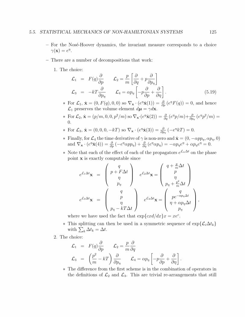
5.5. STATISTICAL MECHANICS OF NON-HAMILTONIAN SYSTEMS 125
– For the Nose-Hoover dynamics, the invariant measure corresponds to a choiceγ(x) = eη.
– There are a number of decompositions that work:
1. The choice:
L1 = F (q)∂
∂pL2 =
p
m
[∂
∂q+ p
∂
∂pη
]L3 = −kT
∂
∂pη
L4 = αpη
[−p
∂
∂p+
∂
∂η
]. (5.19)
∗ For L1, x = (0, F (q), 0, 0) so ∇x · (eηx(1)) = ∂∂p
(eηF (q)) = 0, and henceL1 preserves the volume element dµ = γdx.
∗ For L2, x = (p/m, 0, 0, p2/m) so∇x·(eηx(2)) = ∂∂q
(eηp/m)+ ∂∂pη
(eηp2/m) =0.
∗ For L3, x = (0, 0, 0,−kT ) so ∇x · (eηx(3)) = ∂∂pη
(−eηkT ) = 0.
∗ Finally, for L4 the time derivative of γ is non-zero and x = (0,−αppη, αpη, 0)and ∇x · (eηx(4)) = ∂
∂p(−eηαppη) + ∂
∂η(eηαpη) = −αpηe
η + αpηeη = 0.
∗ Note that each of the effect of each of the propagators eLα∆t on the phasepoint x is exactly computable since
eL1∆tx =
q
p + F∆tηpη
eL2∆tx =
q + p
m∆t
pη
pη + p2
m∆t
eL3∆tx =
qpη
pη − kT∆t
eL4∆tx =
q
pe−αpη∆t
η + αpη∆tpη
,
where we have used the fact that expcxd/dxx = xec.
∗ This splitting can then be used in a symmetric sequence of expLi∆tkwith
∑k ∆tk = ∆t.
2. The choice:
L1 = F (q)∂
∂pL2 =
p
m
∂
∂q
L3 =
(p2
m− kT
)∂
∂pη
L4 = αpη
[−p
∂
∂p+
∂
∂η
].
∗ The difference from the first scheme is in the combination of operators inthe definitions of L2 and L3. This are trivial re-arrangements that still
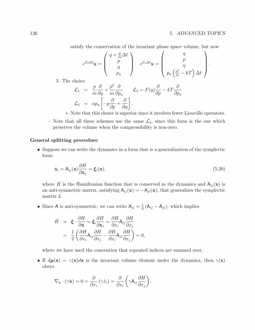
126 5. ADVANCED TOPICS
satisfy the conservation of the invariant phase space volume, but now
eL2∆tx =
q + p
m∆t
pηpη
eL3∆tx =
qpη
pη
(p2
m− kT
)∆t
.
3. The choice
L1 =p
m
∂
∂q+
p2
m
∂
∂pη
L2 = F (q)∂
∂p− kT
∂
∂pη
L4 = αpη
[−p
∂
∂p+
∂
∂η
].
∗ Note that this choice is superior since it involves fewer Liouville operators.
– Note that all these schemes use the same L4, since this form is the one whichpreserves the volume when the compressibility is non-zero.
General splitting procedure
• Suppose we can write the dynamics in a form that is a generalization of the symplecticform:
xi = Aij(x)∂H
∂xj
= ξi(x), (5.20)
where H is the Hamiltonian function that is conserved in the dynamics and Aij(x) isan anti-symmetric matrix, satisfying Aij(x) = −Aji(x), that generalizes the symplecticmatrix J.
• Since A is anti-symmetric, we can write Aij = 12(Aij − Aji), which implies
H = ξ · ∂H
∂x= ξi
∂H
∂xi
=∂H
∂xi
Aij∂H
∂xj
=1
2
(∂H
∂xi
Aij∂H
∂xj
− ∂H
∂xi
Aji∂H
∂xj
)= 0,
where we have used the convention that repeated indices are summed over.
• If dµ(x) = γ(x)dx is the invariant volume element under the dynamics, then γ(x)obeys
∇x · (γx) = 0 =∂
∂xi
(γxi) =∂
∂xi
(γAij
∂H
∂xj
).
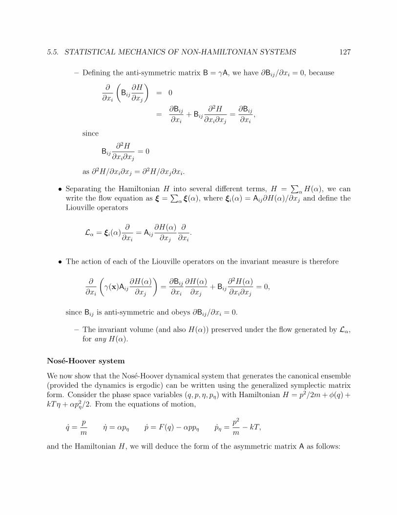
5.5. STATISTICAL MECHANICS OF NON-HAMILTONIAN SYSTEMS 127
– Defining the anti-symmetric matrix B = γA, we have ∂Bij/∂xi = 0, because
∂
∂xi
(Bij
∂H
∂xj
)= 0
=∂Bij
∂xi
+ Bij∂2H
∂xi∂xj
=∂Bij
∂xi
,
since
Bij∂2H
∂xi∂xj
= 0
as ∂2H/∂xi∂xj = ∂2H/∂xj∂xi.
• Separating the Hamiltonian H into several different terms, H =∑
α H(α), we canwrite the flow equation as ξ =
∑α ξ(α), where ξi(α) = Aij∂H(α)/∂xj and define the
Liouville operators
Lα = ξi(α)∂
∂xi
= Aij∂H(α)
∂xj
∂
∂xi
.
• The action of each of the Liouville operators on the invariant measure is therefore
∂
∂xi
(γ(x)Aij
∂H(α)
∂xj
)=
∂Bij
∂xi
∂H(α)
∂xj
+ Bij∂2H(α)
∂xi∂xj
= 0,
since Bij is anti-symmetric and obeys ∂Bij/∂xi = 0.
– The invariant volume (and also H(α)) preserved under the flow generated by Lα,for any H(α).
Nose-Hoover system
We now show that the Nose-Hoover dynamical system that generates the canonical ensemble(provided the dynamics is ergodic) can be written using the generalized symplectic matrixform. Consider the phase space variables (q, p, η, pη) with Hamiltonian H = p2/2m + φ(q) +kTη + αp2
η/2. From the equations of motion,
q =p
mη = αpη p = F (q)− αppη pη =
p2
m− kT,
and the Hamiltonian H, we will deduce the form of the asymmetric matrix A as follows:
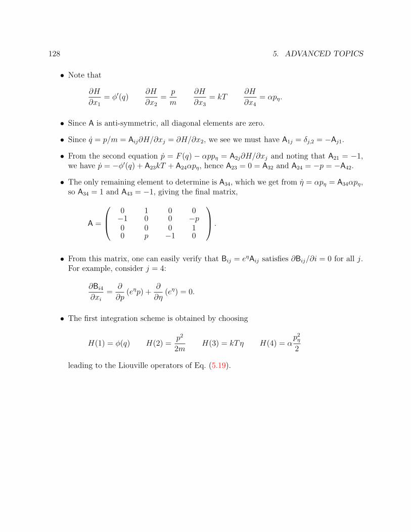
128 5. ADVANCED TOPICS
• Note that
∂H
∂x1
= φ′(q)∂H
∂x2
=p
m
∂H
∂x3
= kT∂H
∂x4
= αpη.
• Since A is anti-symmetric, all diagonal elements are zero.
• Since q = p/m = Aij∂H/∂xj = ∂H/∂x2, we see we must have A1j = δj,2 = −Aj1.
• From the second equation p = F (q) − αppη = A2j∂H/∂xj and noting that A21 = −1,we have p = −φ′(q) + A23kT + A24αpη, hence A23 = 0 = A32 and A24 = −p = −A42.
• The only remaining element to determine is A34, which we get from η = αpη = A34αpη,so A34 = 1 and A43 = −1, giving the final matrix,
A =
0 1 0 0−1 0 0 −p0 0 0 10 p −1 0
.
• From this matrix, one can easily verify that Bij = eηAij satisfies ∂Bij/∂i = 0 for all j.For example, consider j = 4:
∂Bi4
∂xi
=∂
∂p(eηp) +
∂
∂η(eη) = 0.
• The first integration scheme is obtained by choosing
H(1) = φ(q) H(2) =p2
2mH(3) = kTη H(4) = α
p2η
2
leading to the Liouville operators of Eq. (5.19).
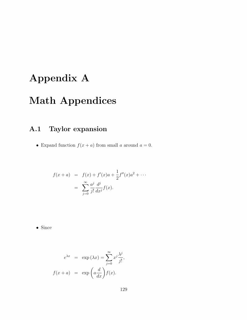
Appendix A
Math Appendices
A.1 Taylor expansion
• Expand function f(x + a) from small a around a = 0.
f(x + a) = f(x) + f ′(x)a +1
2f ′′(x)a2 + · · ·
=∞∑
j=0
aj
j!
dj
dxjf(x).
• Since
eλx = exp (λx) =∞∑
j=0
xj λj
j!,
f(x + a) = exp
(a
d
dx
)f(x).
129
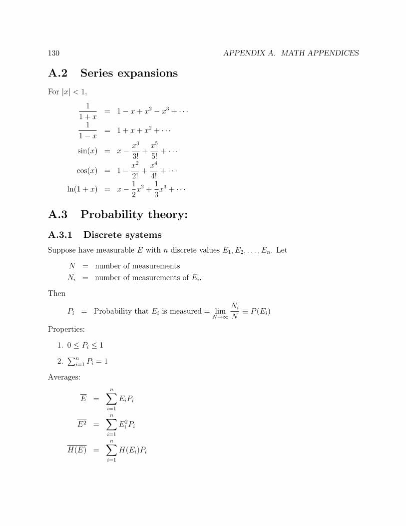
130 APPENDIX A. MATH APPENDICES
A.2 Series expansions
For |x| < 1,
1
1 + x= 1− x + x2 − x3 + · · ·
1
1− x= 1 + x + x2 + · · ·
sin(x) = x− x3
3!+
x5
5!+ · · ·
cos(x) = 1− x2
2!+
x4
4!+ · · ·
ln(1 + x) = x− 1
2x2 +
1
3x3 + · · ·
A.3 Probability theory:
A.3.1 Discrete systems
Suppose have measurable E with n discrete values E1, E2, . . . , En. Let
N = number of measurements
Ni = number of measurements of Ei.
Then
Pi = Probability that Ei is measured = limN→∞
Ni
N≡ P (Ei)
Properties:
1. 0 ≤ Pi ≤ 1
2.∑n
i=1 Pi = 1
Averages:
E =n∑
i=1
EiPi
E2 =n∑
i=1
E2i Pi
H(E) =n∑
i=1
H(Ei)Pi
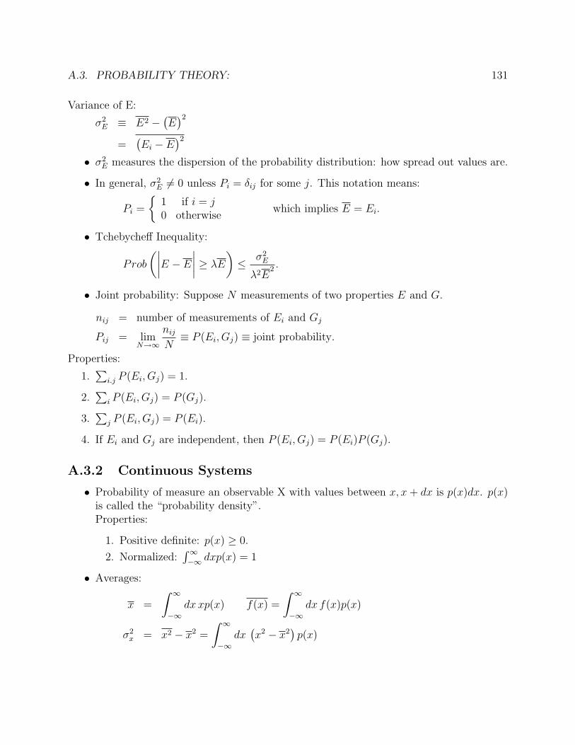
A.3. PROBABILITY THEORY: 131
Variance of E:
σ2E ≡ E2 −
(E)2
=(Ei − E
)2• σ2
E measures the dispersion of the probability distribution: how spread out values are.
• In general, σ2E 6= 0 unless Pi = δij for some j. This notation means:
Pi =
1 if i = j0 otherwise
which implies E = Ei.
• Tchebycheff Inequality:
Prob
(∣∣∣∣E − E
∣∣∣∣ ≥ λE
)≤ σ2
E
λ2E2 .
• Joint probability: Suppose N measurements of two properties E and G.
nij = number of measurements of Ei and Gj
Pij = limN→∞
nij
N≡ P (Ei, Gj) ≡ joint probability.
Properties:
1.∑
i.j P (Ei, Gj) = 1.
2.∑
i P (Ei, Gj) = P (Gj).
3.∑
j P (Ei, Gj) = P (Ei).
4. If Ei and Gj are independent, then P (Ei, Gj) = P (Ei)P (Gj).
A.3.2 Continuous Systems
• Probability of measure an observable X with values between x, x + dx is p(x)dx. p(x)is called the “probability density”.Properties:
1. Positive definite: p(x) ≥ 0.
2. Normalized:∫∞−∞ dxp(x) = 1
• Averages:
x =
∫ ∞
−∞dx xp(x) f(x) =
∫ ∞
−∞dx f(x)p(x)
σ2x = x2 − x2 =
∫ ∞
−∞dx(x2 − x2
)p(x)
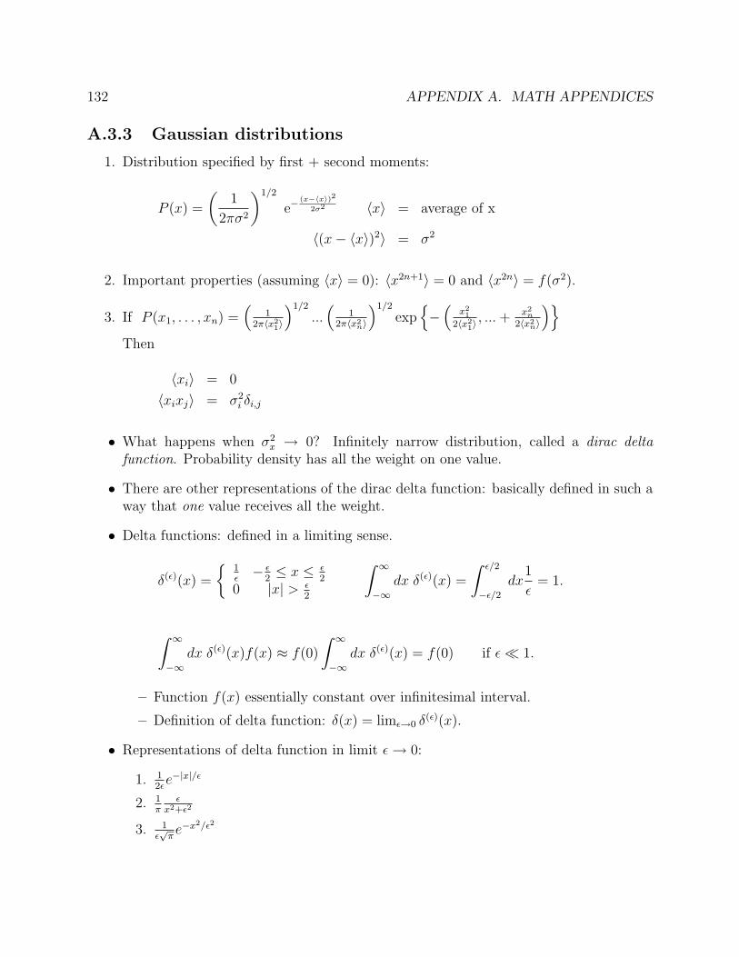
132 APPENDIX A. MATH APPENDICES
A.3.3 Gaussian distributions
1. Distribution specified by first + second moments:
P (x) =
(1
2πσ2
)1/2
e−(x−〈x〉)2
2σ2 〈x〉 = average of x
〈(x− 〈x〉)2〉 = σ2
2. Important properties (assuming 〈x〉 = 0): 〈x2n+1〉 = 0 and 〈x2n〉 = f(σ2).
3. If P (x1, . . . , xn) =(
12π〈x2
1〉
)1/2
...(
12π〈x2
n〉
)1/2
exp−(
x21
2〈x21〉
, ... + x2n
2〈x2n〉
)Then
〈xi〉 = 0
〈xixj〉 = σ2i δi,j
• What happens when σ2x → 0? Infinitely narrow distribution, called a dirac delta
function. Probability density has all the weight on one value.
• There are other representations of the dirac delta function: basically defined in such away that one value receives all the weight.
• Delta functions: defined in a limiting sense.
δ(ε)(x) =
1ε− ε
2≤ x ≤ ε
2
0 |x| > ε2
∫ ∞
−∞dx δ(ε)(x) =
∫ ε/2
−ε/2
dx1
ε= 1.
∫ ∞
−∞dx δ(ε)(x)f(x) ≈ f(0)
∫ ∞
−∞dx δ(ε)(x) = f(0) if ε 1.
– Function f(x) essentially constant over infinitesimal interval.
– Definition of delta function: δ(x) = limε→0 δ(ε)(x).
• Representations of delta function in limit ε → 0:
1. 12ε
e−|x|/ε
2. 1π
εx2+ε2
3. 1ε√
πe−x2/ε2
A.4. FOURIER AND LAPLACE TRANSFORMS 133
4. 1π
sin x/εx
– For any continuous function f of x, for all forms above we get
limε→0
∫ ∞
−∞dx δ(ε)(x− x0)f(x) = f(x0).
Some properties of the delta function
1. δ(−x) = δ(x)
2. δ(cx) = 1|c|δ(x)
3. δ[g(x)] =∑
jδ(x−xj)
|g′(xj)| where g(xj) = 0 and g′(xj) 6= 0.
4. g(x)δ(x− x0) = g(x0)δ(x− x0)
5.∫∞−∞ dx δ(x− y)δ(x− z) = δ(y − z)
6.∫∞−∞ dx dδ(x−x0)
dxf(x) = −
∫∞−∞ dx δ(x− x0)f
′(x) = −f ′(x0)
A.4 Fourier and Laplace Transforms
• Fourier Transform:
f(k) =
∫ ∞
−∞eikxf(x) dx
f(x) =1
2π
∫ ∞
−∞e−ikxf(k) dk
– Properties: ∫ ∞
−∞e−ix(k−k0)dx = 2πδ(k − k0).∫ ∞
−∞f(x− y)g(y) dy =
1
2π
∫ ∞
−∞e−ikxf(k)g(k) dk.
f(x) =
(1
2πσ2
)1/2
e−x2/2σ2 −→ f(k) =
(σ2
2π
)1/2
e−σ2k2/2
f(x) =e−λx
x−→ f(k) =
4π
k2 + λ2
f(x) =1
x−→ f(k) =
4π
k2
134 APPENDIX A. MATH APPENDICES
• Laplace Transform:
f(z) =
∫ −∞
0
e−ztf(t) dt
– Useful properties and transforms:∫ t
0
f(t− τ)g(τ) = f(z)g(z)
f(t) = e−at → f(z) =1
z + a
f(t) =1
tn→ f(z) =
tn−1
(n− 1)!.
A.5 Calculus
A.5.1 Integration by parts
∫udv = uv −
∫vdu
• Example:
∫ b
a
dx f ′(x)g(x) = f(x)g(x)
∣∣∣∣ba
−∫ b
a
dx f(x)g′(x)
A.5.2 Change of Variable and Jacobians
Let I =∫
Rxydxdy f(x, y) be the integral over a connected region Rx,y. Change variables to
u, v via the transform g(u, v) = x and h(u, v) = y. It follows that:
I =
∫Ruv
dudv f(g(u, v), h(u, v))
∣∣∣∣∂(g, h)
∂(u, v)
∣∣∣∣.where the Jacobian ∂(g,h)
∂(u,v)is
∂(g, h)
∂(u, v)≡
∣∣∣∣∣∣∂g∂u
∂g∂v
∂h∂u
∂h∂v
∣∣∣∣∣∣
A.5. CALCULUS 135
• Example: Suppose
I =
∫ ∞
−∞dxdy f(x)g(x− y).
Let u = x and v = x− y. Under this transformation, range of v is (−∞,∞) at a fixedvalue of u (or x). The Jacobian J is
J =
∣∣∣∣ 1 00 −1
∣∣∣∣ = −1
Thus,
I =
∫ ∞
−∞dudv f(u)g(v)| − 1| =
∫ ∞
−∞duf(u)
∫ ∞
−∞dvg(v).

136 APPENDIX A. MATH APPENDICES
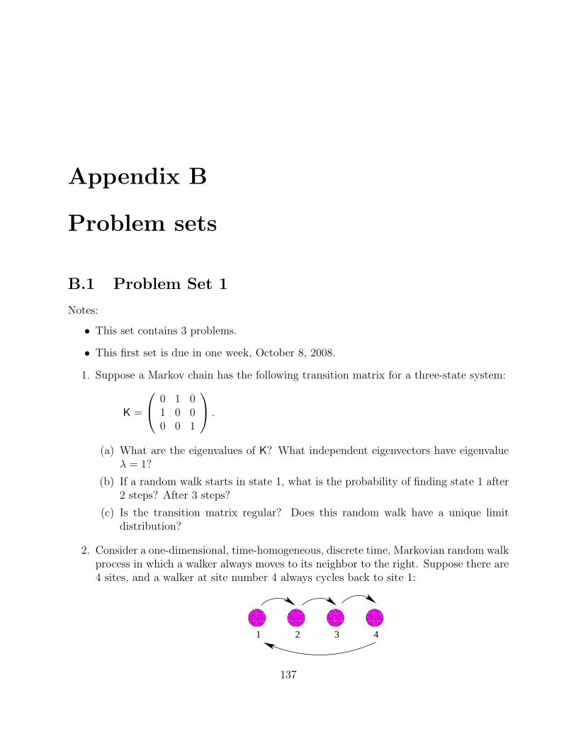
Appendix B
Problem sets
B.1 Problem Set 1
Notes:
• This set contains 3 problems.
• This first set is due in one week, October 8, 2008.
1. Suppose a Markov chain has the following transition matrix for a three-state system:
K =
0 1 01 0 00 0 1
.
(a) What are the eigenvalues of K? What independent eigenvectors have eigenvalueλ = 1?
(b) If a random walk starts in state 1, what is the probability of finding state 1 after2 steps? After 3 steps?
(c) Is the transition matrix regular? Does this random walk have a unique limitdistribution?
2. Consider a one-dimensional, time-homogeneous, discrete time, Markovian random walkprocess in which a walker always moves to its neighbor to the right. Suppose there are4 sites, and a walker at site number 4 always cycles back to site 1:
1 2 3 4
137
138 APPENDIX B. PROBLEM SETS
(a) Write down the transition matrix K(0) for this process and show that the eigen-
values of this matrix are λ(0)k = e−ikπ/2 for k = 1, . . . , 4.
(b) Show that the right eigenvectors of K(0) are e(0)k = 1/2 (eiπk/2, eiπk, eiπ3k/2, eiπ2k)
and that the left eigenvectors are the complex conjugates e(0)∗k .
(c) Now suppose that there is a small but finite probability ε that the walker remainson site 1 and probability 1−ε to step to site 2. What is the form of K = K(0) +∆Know?
(d) The effect of the perturbation ∆K on the eigenvalues can be evaluated usingperturbation theory using
λk = λ(0)k + ∆λk
where ∆λk = e(0)∗k ·∆K · e(0)
k , to first order in ε. Evaluate the effect to first orderin ε of the perturbation on the eigenvalues λk. Does the perturbed system have aunique limit distribution?
(e) What is the effect of the perturbation on the eigenvector e4? What is the physicalmeaning of this eigenvector?
3. Consider a circle of diameter d contained in a square of side length l ≥ d.
(a) Construct an estimator for π using the fraction of uniformly selected points in thesquare that fall in the circle and show that the average of this estimator over thetrue (uniform) distribution is π.
(b) Derive an expression for the standard error in the estimated value of π using thisalgorithm. How does it depend on N (number of points sampled) and the ratiol/d? For fixed l what is the optimal value d that minimizes the standard error?
(c) Write a schematic (or explicit) computer program to compute the value of π usingthis method.
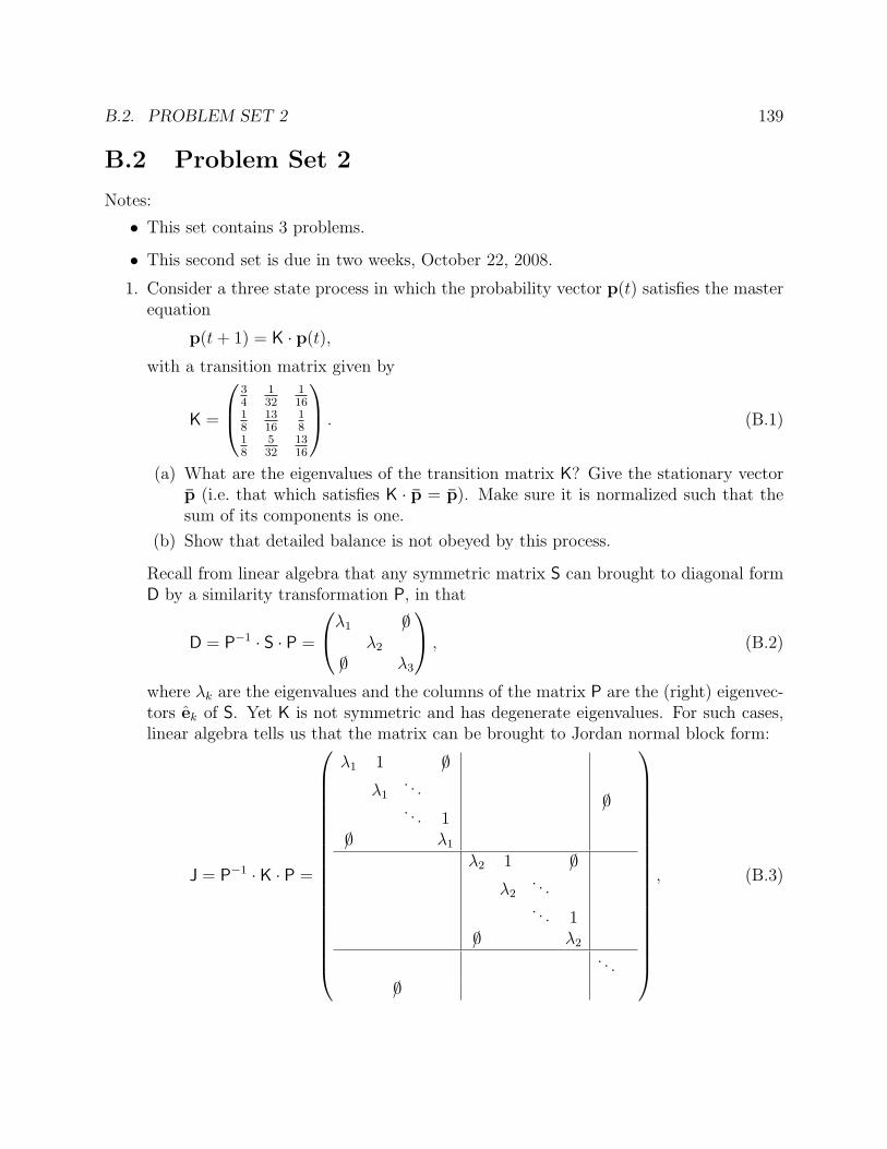
B.2. PROBLEM SET 2 139
B.2 Problem Set 2
Notes:
• This set contains 3 problems.
• This second set is due in two weeks, October 22, 2008.
1. Consider a three state process in which the probability vector p(t) satisfies the masterequation
p(t + 1) = K · p(t),
with a transition matrix given by
K =
34
132
116
18
1316
18
18
532
1316
. (B.1)
(a) What are the eigenvalues of the transition matrix K? Give the stationary vectorp (i.e. that which satisfies K · p = p). Make sure it is normalized such that thesum of its components is one.
(b) Show that detailed balance is not obeyed by this process.
Recall from linear algebra that any symmetric matrix S can brought to diagonal formD by a similarity transformation P, in that
D = P−1 · S · P =
λ1 /0λ2
/0 λ3
, (B.2)
where λk are the eigenvalues and the columns of the matrix P are the (right) eigenvec-tors ek of S. Yet K is not symmetric and has degenerate eigenvalues. For such cases,linear algebra tells us that the matrix can be brought to Jordan normal block form:
J = P−1 · K · P =
λ1 1 /0
λ1. . .. . . 1
/0 λ1
/0
λ2 1 /0
λ2. . .. . . 1
/0 λ2
. . .
/0
, (B.3)
140 APPENDIX B. PROBLEM SETS
where the size gk of each block is equal to the degeneracy of the corresponding eigen-value λk, and P contains the generalized eigenvectors, which follow from the generalizedeigenvalue equation (K− λk1)gk · e(i)
k = 0 (i = 1 . . . gk).
(c) What is the Jordan normal form of the matrix K in equation (1)?
(d) Determine the similarity matrix P that brings it to that form.
The Jordan normal form is possibly a complicating factor because the iterated matrixKt is harder to find.
(e) Show that here
Jt =
1 0 00 λt
2 tλt−12
0 0 λt2
.
(f) Determine the matrix
K∞ = limt→∞
Kt,
and show that it transforms any initial probability vector into the stationaryprobability vector.
2. Consider now a slightly different process with transition matrix
K =
34
116
116
18
1316
18
18
18
1316
. (B.4)
(a) Determine the normalized stationary probability vector p = (p1, p2, p3).
(b) Show that detailed balance is satisfied.
(c) Show that the matrix
K = Q−1 · K · Q
is symmetric, where the similarity transformation Q is defined as
Q =
√p1 00
√p2 0
0 0√
p3
.
(d) What does this imply for the Jordan normal form of K?
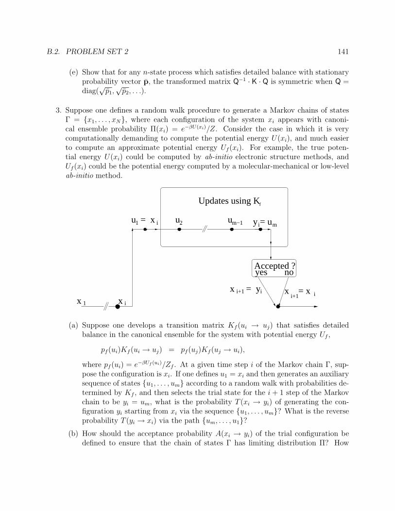
B.2. PROBLEM SET 2 141
(e) Show that for any n-state process which satisfies detailed balance with stationaryprobability vector p, the transformed matrix Q−1 · K · Q is symmetric when Q =diag(
√p1,√
p2, . . .).
3. Suppose one defines a random walk procedure to generate a Markov chains of statesΓ = x1, . . . , xN, where each configuration of the system xi appears with canoni-cal ensemble probability Π(xi) = e−βU(xi)/Z. Consider the case in which it is verycomputationally demanding to compute the potential energy U(xi), and much easierto compute an approximate potential energy Uf (xi). For example, the true poten-tial energy U(xi) could be computed by ab-initio electronic structure methods, andUf (xi) could be the potential energy computed by a molecular-mechanical or low-levelab-initio method.
u = xi1
Updates using Kf
i1
i
Accepted ?
m
i+1 ii+1 i
x xx = x
u2 um−1 y = u
yes no
x = y
(a) Suppose one develops a transition matrix Kf (ui → uj) that satisfies detailedbalance in the canonical ensemble for the system with potential energy Uf ,
pf (ui)Kf (ui → uj) = pf (uj)Kf (uj → ui),
where pf (ui) = e−βUf (ui)/Zf . At a given time step i of the Markov chain Γ, sup-pose the configuration is xi. If one defines u1 = xi and then generates an auxiliarysequence of states u1, . . . , um according to a random walk with probabilities de-termined by Kf , and then selects the trial state for the i + 1 step of the Markovchain to be yi = um, what is the probability T (xi → yi) of generating the con-figuration yi starting from xi via the sequence u1, . . . , um? What is the reverseprobability T (yi → xi) via the path um, . . . , u1?
(b) How should the acceptance probability A(xi → yi) of the trial configuration bedefined to ensure that the chain of states Γ has limiting distribution Π? How
142 APPENDIX B. PROBLEM SETS
does this probability depend on the number of steps m used in the auxiliary chainu1, . . . , um?
(c) What might the advantage be of such a procedure over a simple, symmetrictrial proposal procedure where T (xi → yi) = T (yi → xi)? What conditions areimportant if the auxiliary chain method is to be efficient?
B.3. PROBLEM SET 3 143
B.3 Problem Set 3
Notes:
• This set contains 3 problems.
• This third set is due in two weeks, November 5, 2008.
1. Consider a Hamiltonian of the form
H =|PN |2
2m+ U(RN),
where |PN |2 =∑N
i=1pi·pi
2m. This Hamiltonian is split into a kinetic and potential part
K =|PN |2
2mand U = U(RN).
(a) Compute the action of the partial Liouvillians on a phase point Γ =
(RN
PN
), i.e.
LKΓ = K, Γ and LUΓ = U, Γ and prove that
eLK∆t
(RN
PN
)=
(RN + ∆t
mPN
PN
)eLU∆t
(RN
PN
)=
(RN
PN −∆t ∂U∂RN
)(hint: expand the exponentials.)
(b) Use these relations to show that a single step of the Verlet scheme:
eLU∆t/2eLK∆teLU∆t/2 (B.5)
conserves phase space volume.
(c) Show that applying the Verlet scheme to a harmonic oscillator
H =1
2(p2 + r2).
leads to a linear map: Γ(t + ∆t) = M(∆t) · Γ(t), where M is a 2 × 2 matrixindependent of Γ. Give the explicit form of M.
(d) How can you see that this map conserves phase space volume? What does thisimply for the eigenvalues of the map?
(e) Use the eigenvalues of the map to determine the time step at which the Verletintegrator for the harmonic oscillator becomes unstable.
144 APPENDIX B. PROBLEM SETS
2. The force between two Lennard-Jones particles with a smooth cutoff is given by
ϕ(r) = 4ε
(σ12
r12− σ6
r6
)×
1 r < r′c(rc−r)2(rc−3r′c+2r)
(rc−r′c)3 r′c ≤ r ≤ rc
0 r > rc
. (B.6)
where r = |ri−rj| is the (scalar) distance between two particles at (three-dimensional)positions ri and rj.
(a) Show that the potential is everywhere differentiable.
(b) Derive the force that the two particles feel. What is the sum of these forces?
Consider an N particle system interacting through the smooth Lennard-Jones interac-tion.
(c) How do the momenta and positions of the particles change in a single Verlet step?
(d) Prove that momentum and angular momentum are conserved in a single Verletstep (neglect boundary conditions).
(e) For large enough time steps, the Verlet scheme applied to the N particle Lennard-Jones system starts to exhibit energy drift. Why does this drift go towards higherenergies?
(f) The potential and forces can be computed using cell divisions or a Verlet list.Assuming most of the numerical cost is in computing the potential and forces,which one is more efficient and by how much? Why do these techniques only workfor larger systems?
3. Write a small program to simulate a Lennard-Jones system of 343 particles (cf. Eq. (B.6))in a cubic periodic simulation box, using the Verlet scheme (B.5). Set the mass m,interaction range σ and interaction strength ε to 1 (Lennard-Jones units), and set thedensity at 1. Choose cutoff parameters r′c = 2.5 and rc = 3. (Note: why is there noreason to use cells?) As initial conditions, put the particles on a cubic lattice and drawtheir initial momenta from a Gaussian with a standard deviation of 0.1. For a rangeof time steps, determine
• the appropriate length of the burn-in time,
• the average kinetic temperature Tkin = K/(32N) in equilibrium,
• the total energy in equilibrium, and
• the fluctuations of the total energy in the simulation.
Demonstrate that the fluctuations of the total energy scale as ∆t2 and determine thetime step at which numerical instability sets in.
B.4. PROBLEM SET 4 145
B.4 Problem Set 4
Notes:
• This set contains 3 problems.
• This fourth and final set is due in two weeks, December 3, 2008.
1. For a harmonic oscillator system with Hamiltonian H = 12(p2 + q2), compare the
critical points of instability ∆tc of the Verlet, HOA2, FR4, and 4th-order order Suziki(gradient corrected) integrators.
2. Consider an an-harmonic oscillator system in three dimensions with Hamiltonian
H =p1 · p1
2m1
+p2 · p2
2m2
+ U(r12) U(r12) =k
2r212 +
λ
4r412,
where r12 = |r2 − r1|, k is large and λ is small.
(a) Show that the Hamiltonian can be recast in centre-of-mass R and relative coor-dinates r = r12 as
H =P ·P2M
+p · p2µ
+ U(r) = KP + Kp + U,
where M is the total mass of the system, µ is the relative mass, and P and p arethe momenta conjugate to R and r, respectively.
i. What are the solutions of the equations of motion for R and P?
ii. Construct the Liouville operators LP , Lp and LU and evaluate the commu-tators of these three operators.
(b) Devise a second-order symplectic integrator of this system and find the shadowHamiltonian to order ∆t2.
(c) Suppose one writes the potential U = Uh + ∆U in terms of a harmonic referencepotential Uh(r) = kr2/2 and a difference potential ∆U(r) = λr4/4. Use a splittingscheme to construct a second-order integrator that uses the exact solution ofthe evolution of a harmonic oscillator. To order ∆t2, what does the shadowHamiltonian look like for this integrator? Is it better, or worse, than the integratorin part b?
(d) Suppose the actual potential energy UA(r) and forces are computed using a costlyelectronic structure method. Using the potential U(r) as a reference potential,where UA(r) ≈ U(r), devise an integrator using splitting methods that minimizesthe number of electronic structure calculations over a fixed time interval. Howmight multiple time step methods be used profitably in this integrator?
146 APPENDIX B. PROBLEM SETS
3. An important dynamical property of molecules in a fluid is the self-diffusion coefficientD, that is a measure of how quickly each particle in the fluid moves through space.For a system of N particles, it can be calculated in two different ways:
• One can integrate the velocity autocorrelation function:
D =1
3N
N∑i=1
∫dt′ 〈vi(t) · vi(t + t′)〉 ,
where vi(t) is the velocity of particle i at time t. Note that in a simulation, botht and t + t′ are computed at intervals of the timestep ∆t.
• One can use the relation
D = limt′→∞
N∑i=1
〈|ri(t + t′)− ri(t)|〉6Nt′
,
where ri(t) is the position of particle i at time t. Note that when using this form,one must pay careful attention to how the distance grows in a periodic system.
Modify the code you wrote for a Lennard-Jones system (or modify the sample codeprovided on the class web site) to compute the self-diffusion coefficient D in the twoways mentioned above. The system conditions can be taken to be as described inproblem 3 on problem set 3.