foundations of quantum mechanics - higher...

Foundations of Quantum Mechanics

Dr. H. Osborn1

Michælmas 1997

1LATEXed by Paul Metcalfe – comments and corrections [email protected].

Revision: 2.5Date: 1999-06-06 14:10:19+01

The following people have maintained these notes.

– date Paul Metcalfe

Contents

Introduction v

1 Basics 11.1 Review of earlier work . . . . . . . . . . . . . . . . . . . . . . . . . 11.2 The Dirac Formalism . . . . . . . . . . . . . . . . . . . . . . . . . . 3

1.2.1 Continuum basis .. . . . . . . . . . . . . . . . . . . . . . . 41.2.2 Action of operators on wavefunctions . . . . . . . . . . . . . 51.2.3 Momentum space . . . . . . . . . . . . . . . . . . . . . . . . 61.2.4 Commuting operators . . . . . . . . . . . . . . . . . . . . . 71.2.5 Unitary Operators . . . . . . . . . . . . . . . . . . . . . . . . 81.2.6 Time dependence . . . . . . . . . . . . . . . . . . . . . . . . 8

2 The Harmonic Oscillator 92.1 Relation to wavefunctions . . . . . . . . . . . . . . . . . . . . . . . 102.2 More comments . . . . . . . . . . . . . . . . . . . . . . . . . . . . . 11

3 Multiparticle Systems 133.1 Combination of physical systems .. . . . . . . . . . . . . . . . . . . 133.2 Multiparticle Systems . . .. . . . . . . . . . . . . . . . . . . . . . . 14

3.2.1 Identical particles . . . . . . . . . . . . . . . . . . . . . . . . 143.2.2 Spinless bosons . . . . . . . . . . . . . . . . . . . . . . . . . 153.2.3 Spin1

2 fermions . . . . . . . . . . . . . . . . . . . . . . . . 163.3 Two particle states and centre of mass . . . . . . . . . . . . . . . . . 173.4 Observation . . . . . . . . . . . . . . . . . . . . . . . . . . . . . . . 17

4 Perturbation Expansions 194.1 Introduction .. . . . . . . . . . . . . . . . . . . . . . . . . . . . . . 194.2 Non-degenerate perturbation theory . . . . . . . . . . . . . . . . . . 194.3 Degeneracy . . . . . . . . . . . . . . . . . . . . . . . . . . . . . . . 21

5 General theory of angular momentum 235.1 Introduction .. . . . . . . . . . . . . . . . . . . . . . . . . . . . . . 23

5.1.1 Spin12 particles . . . . . . . . . . . . . . . . . . . . . . . . . 24

5.1.2 Spin1 particles . . . . . . . . . . . . . . . . . . . . . . . . . 255.1.3 Electrons . . . . . . . . . . . . . . . . . . . . . . . . . . . . 25

5.2 Addition of angular momentum . .. . . . . . . . . . . . . . . . . . . 265.3 The meaning of quantum mechanics . . . . . . . . . . . . . . . . . . 27

iii

iv CONTENTS

Introduction

These notes are based on the course “Foundations of Quantum Mechanics” given byDr. H. Osborn in Cambridge in the Michælmas Term 1997. Recommended books arediscussed in the bibliography at the back.

Other sets of notes are available for different courses. At the time of typing thesecourses were:

Probability Discrete MathematicsAnalysis Further AnalysisMethods Quantum MechanicsFluid Dynamics 1 Quadratic MathematicsGeometry Dynamics of D.E.’sFoundations of QM ElectrodynamicsMethods of Math. Phys Fluid Dynamics 2Waves (etc.) Statistical PhysicsGeneral Relativity Dynamical SystemsPhysiological Fluid Dynamics Bifurcations in Nonlinear ConvectionSlow Viscous Flows Turbulence and Self-SimilarityAcoustics Non-Newtonian FluidsSeismic Waves

They may be downloaded from

http://www.istari.ucam.org/maths/ orhttp://www.cam.ac.uk/CambUniv/Societies/archim/notes.htm

or you can [email protected] to get a copy of thesets you require.

v

Copyright (c) The Archimedeans, Cambridge University.All rights reserved.

Redistribution and use of these notes in electronic or printed form, with or withoutmodification, are permitted provided that the following conditions are met:

1. Redistributions of the electronic files must retain the above copyright notice, thislist of conditions and the following disclaimer.

2. Redistributions in printed form must reproduce the above copyright notice, thislist of conditions and the following disclaimer.

3. All materials derived from these notes must display the following acknowledge-ment:

This product includes notes developed by The Archimedeans, CambridgeUniversity and their contributors.

4. Neither the name of The Archimedeans nor the names of their contributors maybe used to endorse or promote products derived from these notes.

5. Neither these notes nor any derived products may be sold on a for-profit basis,although a fee may be required for the physical act of copying.

6. You must cause any edited versions to carry prominent notices stating that youedited them and the date of any change.

THESE NOTES ARE PROVIDED BY THE ARCHIMEDEANS AND CONTRIB-UTORS “AS IS” AND ANY EXPRESS OR IMPLIED WARRANTIES, INCLUDING,BUT NOT LIMITED TO, THE IMPLIED WARRANTIES OF MERCHANTABIL-ITY AND FITNESS FOR A PARTICULAR PURPOSE ARE DISCLAIMED. IN NOEVENT SHALL THE ARCHIMEDEANS OR CONTRIBUTORS BE LIABLE FORANY DIRECT, INDIRECT, INCIDENTAL, SPECIAL, EXEMPLARY, OR CONSE-QUENTIAL DAMAGES HOWEVER CAUSED AND ON ANY THEORY OF LI-ABILITY, WHETHER IN CONTRACT, STRICT LIABILITY, OR TORT (INCLUD-ING NEGLIGENCE OR OTHERWISE) ARISING IN ANY WAY OUT OF THE USEOF THESE NOTES, EVEN IF ADVISED OF THE POSSIBILITY OF SUCH DAM-AGE.

Chapter 1

The Basics of QuantumMechanics

Quantum mechanics is viewed as the most remarkable development in20th centuryphysics. Its point of view is completely different from classical physics. Its predictionsare often probabilistic.

We will develop the mathematical formalism and some applications. We will em-phasize vector spaces (to which wavefunctions belong). These vector spaces are some-times finite-dimensional, but more often infinite dimensional. The pure mathematicalbasis for these is in Hilbert Spaces but (fortunately!) no knowledge of this area isrequired for this course.

1.1 Review of earlier work

This is abrief review of the salient points of the 1B Quantum Mechanics course. Ifyou anything here is unfamiliar it is as well to read up on the 1B Quantum Mechanicscourse. This section can be omitted by the brave.

A wavefunctionψ(x) : R3 �→ C is associated with a single particle in three di-mensions.ψ represents the state of a physical system for a single particle. Ifψ isnormalised, that is

‖ψ‖2 ≡∫

d3x |ψ|2 = 1

then we say thatd3x |ψ|2 is the probability of finding the particle in the infinitesimalregiond3x (atx).

Superposition Principle

If ψ1 andψ2 are two wavefunctions representing states of a particle, then so is thelinear combinationa1ψ1 + a2ψ2 (a1, a2 ∈ C). This is obviously the statement thatwavefunctions live in a vector space. Ifψ′ = aψ (with a �= 0) thenψ andψ′ representthe same physical state. Ifψ andψ′ are both normalised thena = eıα. We writeψ ∼ eıαψ to show that they represent the same physical state.

1

2 CHAPTER 1. BASICS

For two wavefunctionsφ andψ we can define a scalar product

(φ, ψ) ≡∫

d3xφ∗ψ ∈ C.

This has various properties which you can investigate at your leisure.

Interpretative Postulate

Given a particle in a state represented by a wavefunctionψ (henceforth “in a stateψ”) then the probability of finding the particle in stateφ is P = |(φ, ψ)|2 and if thewavefunctions are normalised then0 ≤ P ≤ 1. P = 1 if ψ ∼ φ.

We wish to define (linear) operators on our vector space — do the obvious thing.In finite dimensions we can choose a basis and replace an operator with a matrix.

For a complex vector space we can define the Hermitian conjugate of the operatorAto be the operatorA† satisfying(φ,Aψ) = (A†φ, ψ). If A = A† thenA is Hermitian.Note that ifA is linear then so isA†.

In quantum mechanics dynamical variables (such as energy, momentum or angularmomentum) are represented by (linear) Hermitian operators, the values of the dynam-ical variables being given by the eigenvalues. For wavefunctionsψ(x), A is usuallya differential operator. For a single particle moving in a potentialV (x) we get theHamiltonianH = − �

2

2m∇2 + V (x). Operators may have either a continuous or dis-crete spectrum.

If A is Hermitian then the eigenfunctions corresponding to different eigenvaluesare orthogonal. We assume completeness — that any wavefunction can be expandedas a linear combination of eigenfunctions.

The expectation value forA in a state with wavefunctionψ is 〈A〉ψ , defined to be∑i λi |ai|2 = (ψ,Aψ). We define the square deviation∆A2 to be〈(A− 〈A〉ψ)2〉ψ

which is in general nonzero.

Time dependence

This is governed by the Schr¨odinger equation

ı�∂ψ

∂t= Hψ,

whereH is the Hamiltonian.H must be Hermitian for the consistency of quantummechanics:

ı�∂

∂t(ψ, ψ) = (ψ,Hψ) − (Hψ,ψ) = 0

if H is Hermitian. Thus we can impose the condition(ψ, ψ) = 1 for all time (if ψ isnormalisable).

If we consider eigenfunctionsψi ofH with eigenvaluesEi we can expand a generalwavefunction as

ψ(x, t) =∑

aie− ıEi

�tψi(x).

If ψ is normalised then the probability of finding the system with energyEi is |ai|2.

1.2. THE DIRAC FORMALISM 3

1.2 The Dirac Formalism

This is where we take off into the wild blue yonder, or at least a more abstract form ofquantum mechanics than that previously discussed. The essential structure of quantummechanics is based on operators acting on vectors in some vector space. A wavefunc-tionψ corresponds to some abstract vector|ψ〉, aket vector.|ψ〉 represents the state ofsome physical system described by the vector space.

If |ψ1〉 and|ψ2〉 are ket vectors then|ψ〉 = a1|ψ1〉+a2|ψ2〉 is a possible ket vectordescribing a state — this is the superposition principle again.

We define a dual space ofbra vectors〈φ| and a scalar product〈φ|ψ〉, a complexnumber.1 For any|ψ〉 there corresponds a unique〈ψ| and we require〈φ|ψ〉 = 〈ψ|φ〉∗.We require the scalar product to be linear such that|ψ〉 = a1|ψ1〉 + a2|ψ2〉 implies〈φ|ψ〉 = a1〈φ|ψ1〉 + a2〈φ|ψ2〉. We see that〈ψ|φ〉 = a∗1〈ψ1|φ〉 + a∗2〈ψ2|φ〉 and so〈ψ| = a∗1〈ψ1| + a∗2〈ψ2|.

We introduce linear operatorsA|ψ〉 = |ψ′〉 and we define operators acting on bravectors to the left〈φ|A = 〈φ′| by requiring〈φ′|ψ〉 = 〈φ|A|ψ〉 for all ψ. In general, in〈φ|A|ψ〉, A can act either to the right or the left. We define theadjoint A† of A suchthat if A|ψ〉 = |ψ′〉 then〈ψ|A† = 〈ψ′|. A is said to be Hermitian ifA = A†.

If A = a1A1 + a2A2 thenA† = a∗1A†1 + a∗2A

†2, which can be seen by appealing to

the definitions. We also find the adjoint ofBA as follows:Let BA|ψ〉 = B|ψ′〉 = |ψ′′〉. Then〈ψ′′| = 〈ψ′|B† = 〈ψ|A†B† and the result

follows. Also, if 〈ψ|A = 〈φ′| then|φ′〉 = A†|φ〉.We have eigenvectorsA|ψ〉 = λ|ψ〉 and it can be seen in the usual manner that the

eigenvalues of a Hermitian operator are real and the eigenvectors corresponding to twodifferent eigenvalues are orthogonal.

We assume completeness — that is any|φ〉 can be expanded in terms of the basis ketvectors,|φ〉 =

∑ai|ψi〉 whereA|ψi〉 = λi|ψi〉 andai = 〈ψi|φ〉. If |ψ〉 is normalised

— 〈ψ|ψ〉 = 1 — then the expected value ofA is 〈A〉ψ = 〈ψ|A|ψ〉, which is real ifAis Hermitian.

The completeness relation for eigenvectors ofA can be written as1 =∑

i |ψi〉〈ψi|,which gives (as before)

|ψ〉 = 1|ψ〉 =∑i

|ψi〉〈ψi|ψ〉.

We can also rewriteA =∑

i |ψi〉λi〈ψi| and if λj �= 0 ∀j then we can defineA−1 =

∑i |ψi〉λ−1

i 〈ψi|.We now choose an orthonormal basis{|n〉} with 〈n|m〉 = δnm and the complete-

ness relation1 =∑

n |n〉〈n|. We can thus expand|ψ〉 =∑

n an|n〉 with an = 〈n|ψ〉.We now consider a linear operatorA, and thenA|ψ〉 =

∑n anA|n〉 =

∑m a′m|m〉,

with a′m = 〈m|A|ψ〉 =∑

n an〈m|A|n〉. Further, puttingAmn = 〈m|A|n〉 we geta′m =

∑nAmnan and therefore solvingA|ψ〉 = λ|ψ〉 is equivalent to solving the

matrix equationAa = λa. Amn is called the matrix representation ofA. We also have〈ψ| =

∑n a

∗n〈n|, with a′n

∗ =∑

m a∗mA†mn, whereA†

mn = A∗nm gives the Hermitian

conjugate matrix. This is the matrix representation ofA†.

1bra ket. Who said that mathematicians have no sense of humour?

4 CHAPTER 1. BASICS

1.2.1 Continuum basis

In the above we have assumed discrete eigenvaluesλi and normalisable eigenvectors|ψi〉. However, in general, in quantum mechanics operators often have continuousspectrum — for instance the position operatorx in 3 dimensions.x must have eigen-valuesx for any pointx ∈ R3. There exist eigenvectors|x〉 such thatx|x〉 = x|x〉 foranyx ∈ R3.

As x must be Hermitian we have〈x|x = x〈x|. We define the vector space requiredin the Dirac formalism as that spanned by|x〉.

For any state|ψ〉 we can define a wavefunctionψ(x) = 〈x|ψ〉.We also need to find some normalisation criterion, which uses the 3 dimensional

Dirac delta function to get〈x|x′〉 = δ3(x − x′). Completeness gives∫d3x|x〉〈x| = 1.

We can also recover the ket vector from the wavefunction by

|ψ〉 = 1|ψ〉 =∫

d3x|x〉ψ(x).

Also 〈x|x|ψ〉 = xψ(x); the action of the operatorx on a wavefunction is multipli-cation byx.

Something else reassuring is

〈ψ|ψ〉 = 〈ψ|1|ψ〉 =∫

d3x〈ψ|x〉〈x|ψ〉

=∫

d3x |ψ(x)|2 .

The momentum operatorp is also expected to have continuum eigenvalues. Wecan similarly define states|p〉 which satisfyp|p〉 = p|p〉. We can relatex andp usingthe commutator, which for two operatorsA andB is defined by[

A, B]

= AB − BA.

The relationship betweenx andp is [xi, pj ] = ı�δij . In one dimension[x, p] = ı�.We have a useful rule for calculating commutators, that is:[

A, BC]

=[A, B

]C + B

[A, C

].

This can be easily proved simply by expanding the right hand side out. We can usethis to calculate

[x, p2

].

[x, p2

]= [x, p] p+ p [x, p]= 2ı�p.

It is easy to show by induction that[x, pn] = nı�pn−1.We can define an exponential by

e−ıap

� =∞∑n=0

1n!

(− ıap

�

)n

.


We can evaluate[x, e−

ıap�

]by

[x, e−

ıap�

]=

[x,

∞∑n=0

1n!

(− ıap

�

)n]

=∞∑

n=0

1n!

[x,

(− ıap

�

)n]

=∞∑

n=0

1n!

(− ıa

�

)n

[x, pn]

=∞∑

n=1

1(n− 1)!

(− ıa

�

)n

ı�pn−1

= a

∞∑n=1

(− ıa

�

)n−1

pn−1

= ae−ıap

�

and by rearranging this we get that

xe−ıap

� = e−ıap

� (x+ a)

and it follows thate−ıap

� |x〉 is an eigenvalue ofx with eigenvaluex + a. Thus weseee−

ıap� |x〉 = |x + a〉. We can do the same to the bra vectors with the Hermi-

tian conjugateeıap

� to get〈x + a| = 〈x|e ıap� . Then we also have the normalisation

〈x′ + a|x+ a〉 = 〈x′|x〉.We now wish to consider〈x+a|p〉 = 〈x|e ıap

� |p〉 = eıap

� 〈x|p〉. Settingx = 0 gives〈a|p〉 = e

ıap� N , whereN = 〈0|p〉 is independent ofx. We can determineN from the

normalisation of|p〉.

δ(p′ − p) = 〈p′|p〉 =∫

da 〈p′|a〉〈a|p〉

= |N |2∫

da eıa(p−p′)

�

= |N |2 2π� δ(p′ − p)

So, because we are free to choose the phase ofN , we can setN =(

12π�

) 12 and

thus〈x|p〉 =(

12π�

) 12 e

ıxp� . We coulddefine |p〉 by

|p〉 =∫

dx |x〉〈x|p〉 =(

12π�

) 12

∫dx |x〉e ıxp

� ,

but we then have to check things like completeness.

1.2.2 Action of operators on wavefunctions

We recall the definition of the wavefunctionψ asψ(x) = 〈x|ψ〉. We wish to see whatoperators (the position and momentum operators discussed) do to wavefunctions.

6 CHAPTER 1. BASICS

Now 〈x|x|ψ〉 = x〈x|ψ〉 = xψ(x), so the position operator acts on wavefunctionsby multiplication. As for the momentum operator,

〈x|p|ψ〉 =∫

dp 〈x|p|p〉〈p|ψ〉

=∫

dp p〈x|p〉〈p|ψ〉

=(

12π�

) 12

∫dp pe

ıxp� 〈p|ψ〉

= −ı� ddx

∫dp 〈x|p〉〈p|ψ〉

= −ı� ddx

〈x|ψ〉 = −ı� ddxψ(x).

The commutation relation[x, p] = ı� corresponds to[x,−ı� d

dx

]= ı� (acting on

ψ(x)).

1.2.3 Momentum space

|x〉 �→ ψ(x) = 〈x|ψ〉 defines a particular representation of the vector space. It issometimes useful to use a momentum representation,ψ(p) = 〈p|ψ〉. We observe that

ψ(p) =∫

dx 〈p|x〉〈x|ψ〉

=(

12π�

) 12

∫dx e−

ıxp� ψ(x).

In momentum space, the operators act differently on wavefunctions. It is easy tosee that〈p|p|ψ〉 = pψ(p) and〈p|x|ψ〉 = ı� d

dp ψ(p).We convert the Schr¨odinger equation into momentum space. We have the operator

equationH = p2

2m + V (x) and we just need to calculate how the potential operates onthe wavefunction.

〈p|V (x)|ψ〉 =∫

dx 〈p|V (x)|x〉〈x|ψ〉

=(

12π�

) 12

∫dx e−

ıxp� V (x)〈x|ψ〉

=1

2π�

∫∫dxdp′ V (x)ψ(p′)e

ıx(p′−p)�

=∫

dp′ V (p− p′)ψ(p′),

whereV (p) = 12π�

∫dx e−

ıxp� V (x). Thus in momentum space,

Hpψ(p) =p2

2mψ(p) +

∫dp′ V (p− p′)ψ(p′).


1.2.4 Commuting operators

SupposeA andB are Hermitian and[A, B

]= 0. ThenA andB have simultaneous

eigenvectors.

Proof. SupposeA|ψ〉 = λ|ψ〉 and the vector subspaceVλ is the span of the eigenvec-tors ofA with eigenvalueλ. (If dimVλ > 1 thenλ is said to be degenerate.)

As A andB commute we know thatλB|ψ〉 = AB|ψ〉 and soB|ψ〉 ∈ Vλ. If λ isnon-degenerate thenB|ψ〉 = µ|ψ〉 for someµ. Otherwise we have thatB : Vλ �→ Vλand we can therefore find eigenvectors ofB which lie entirely insideVλ. We can labelthese as|λ, µ〉, and we know that

A|λ, µ〉 = λ|λ, µ〉B|λ, µ〉 = µ|λ, µ〉.

These may still be degenerate. However we can in principle remove this degener-acy by adding more commuting operators until each state is uniquely labeled by theeigenvalues of each common eigenvector. This set of operators is called acompletecommuting set.

This isn’t so odd: for a single particle in 3 dimensions we have the operatorsx1, x2

andx3. These all commute, so for a single particle with no other degrees of freedomwe can label states uniquely by|x〉. We also note from this example that a completecommuting set is not unique, we might just as easily have taken the momentum opera-tors and labeled states by|p〉. To ram the point in more, we could also have taken someweird combination likex1, x2 andp3.

For our single particle in 3 dimensions, a natural set of commuting operators in-volves the angular momentum operator,L = x ∧ p, or Li = εijkxj pk.

We can find commutation relations betweenLi and the other operators we know.These are summarised here, proof is straightforward.

•[Li, xl

]= ı�εilj xj

•[Li, x2

]= 0

•[Li, pm

]= ı�εimkpk

•[Li, p2

]= 0

•[Li, Lj

]= ı�εijkLk

•[Li, L2

]= 0

If we have a HamiltonianH = p2

2m +V (|x|) then we can also see that[L, H

]= 0.

We choose as a commuting setH, L2 and L3 and label states|E, l,m〉, where theeigenvalue ofL2 is l(l+ 1) and the eigenvalue ofL3 ism.

8 CHAPTER 1. BASICS

1.2.5 Unitary Operators

An operatorU is said to beunitary if U †U = 1, or equivalentlyU−1 = U †.SupposeU is unitary andU |ψ〉 = |ψ′〉, U |φ〉 = |φ′〉. Then〈φ′| = 〈φ|U † and

〈φ′|ψ′〉 = 〈φ|ψ〉. Thus the scalar product, which is the probability amplitude of findingthe state|φ〉 given the state|ψ〉, is invariant under unitary transformations of states.

For any operatorA we can defineA′ = U AU †. Then〈φ′|A′|ψ′〉 = 〈φ|A|ψ〉 andmatrix elements are unchanged under unitary transformations. We also note that ifC = AB thenC′ = A′B′.

The quantum mechanics for the|ψ〉, |φ〉, A, B etc. is the same as for|ψ′〉, |φ′〉, A′,B′ and so on. A unitary transform in quantum mechanics is analogous to a canonicaltransformation in dynamics.

Note that ifO is Hermitian thenU = eıO is unitary, asU † = e−ıO†= e−ıO.

1.2.6 Time dependence

This is governed by the Schr¨odinger equation,

ı�∂

∂t|ψ(t)〉 = H |ψ(t)〉.

H is the Hamiltonian and we require it to be Hermitian. We can get an explicitsolution of this ifH does not depend explicitly ont. We set|ψ(t)〉 = U(t)|ψ(0)〉,whereU(t) = e−

ıHt� . As U(t) is unitary,〈φ(t)|ψ(t)〉 = 〈φ(0)|ψ(0)〉.

If we measure the expectation ofA at timet we get〈ψ(t)|A|ψ(t)〉 = a(t). Thisdescription is called the Schr¨odinger picture. Alternatively we can absorb the time de-pendence into the operatorA to get the Heisenberg picture,a(t) = 〈ψ|U †(t)AU(t)|ψ〉.We writeAH(t) = U †(t)AU(t). In this description the operators are time dependent(as opposed to the states).AH(t) is the Heisenberg picture time dependent operator.Its evolution is governed by

ı�∂

∂tAH(t) =

[AH(t), H

],

which is easily proven.For a HamiltonianH = 1

2m p(t)2 + V (x(t)) we can get the Heisenberg equations

for the operatorsxH andpH

ddtxH(t) =

1mpH(t)

ddtpH(t) = −V ′(xH(t)).

These ought to remind you of something.

Chapter 2

The Harmonic Oscillator

In quantum mechanics there are two basic solvable systems, the harmonic oscillatorand the hydrogen atom. We will examine the quantum harmonic oscillator using al-gebraic methods. In quantum mechanics the harmonic oscillator is governed by theHamiltonian

H =1

2mp2 + 1

2mω2x2,

with the condition that[x, p] = ı�. We wish to solveH |ψ〉 = E|ψ〉 to find the energyeigenvalues.

We define a new operatora.

a =(mω

2�

) 12

(x+

ıp

mω

)

a† =(mω

2�

) 12

(x− ıp

mω

).

a and a† are respectively called the annihilation and creation operators. We caneasily obtain the commutation relation

[a, a†

]= 1. It is easy to show that, in terms

of the annihilation and creation operators, the HamiltonianH = 12�ω

(aa† + a†a

),

which reduces to�ω(a†a+ 1

2

). Let N = a†a. Then

[a, N

]= a and

[a†, N

]= −a†.

ThereforeN a = a(N − 1

)andN a† = a†

(N + 1

).

Suppose|ψ〉 is an eigenvector ofN with eigenvalueλ. Then the commutation rela-tions give thatN a|ψ〉 = (λ− 1) a|ψ〉 and therefore unlessa|ψ〉 = 0 it is an eigenvalueof N with eigenvalueλ− 1. Similarly N a†|ψ〉 = (λ+ 1) a†|ψ〉.

But for any|ψ〉, 〈ψ|N |ψ〉 ≥ 0 and equals0 iff a|ψ〉 = 0. Now suppose we have aneigenvalue ofH , λ /∈ {0, 1, 2, . . .}. Then∃n such thatan|ψ〉 is an eigenvector ofNwith eigenvalueλ − n < 0 and so we must haveλ ∈ {0, 1, 2, . . .}. Returning to theHamiltonian we get energy eigenvaluesEn = �ω

(n+ 1

2

), the same result as using the

Schrodinger equation for wavefunctions, but with much less effort.We define|n〉 = Cna

†n|0〉, whereCn is such as to make〈n|n〉 = 1. We can takeCn ∈ R, and evaluate〈0|ana†n|0〉 to findCn.

9

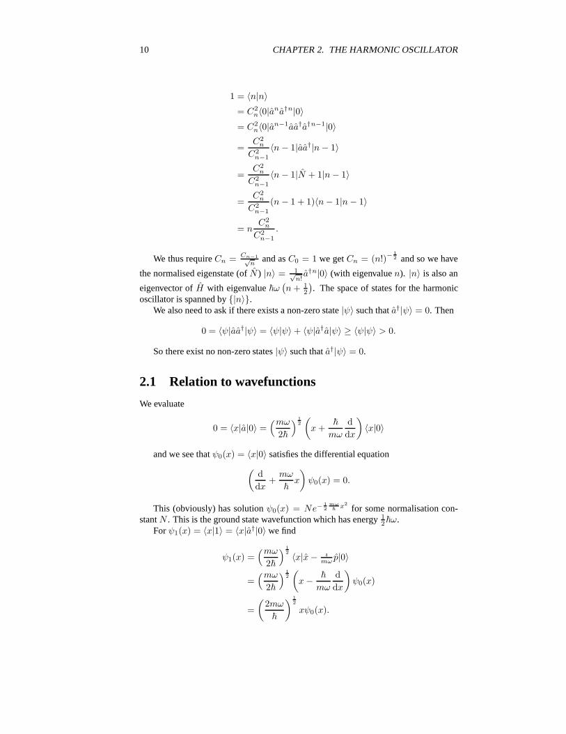
10 CHAPTER 2. THE HARMONIC OSCILLATOR

1 = 〈n|n〉= C2

n〈0|ana†n|0〉= C2

n〈0|an−1aa†a†n−1|0〉

=C2

n

C2n−1

〈n− 1|aa†|n− 1〉

=C2

n

C2n−1

〈n− 1|N + 1|n− 1〉

=C2

n

C2n−1

(n− 1 + 1)〈n− 1|n− 1〉

= nC2

n

C2n−1

.

We thus requireCn = Cn−1√n

and asC0 = 1 we getCn = (n!)−12 and so we have

the normalised eigenstate (ofN ) |n〉 = 1√n!a†n|0〉 (with eigenvaluen). |n〉 is also an

eigenvector ofH with eigenvalue�ω(n+ 1

2

). The space of states for the harmonic

oscillator is spanned by{|n〉}.We also need to ask if there exists a non-zero state|ψ〉 such thata†|ψ〉 = 0. Then

0 = 〈ψ|aa†|ψ〉 = 〈ψ|ψ〉 + 〈ψ|a†a|ψ〉 ≥ 〈ψ|ψ〉 > 0.

So there exist no non-zero states|ψ〉 such thata†|ψ〉 = 0.

2.1 Relation to wavefunctions

We evaluate

0 = 〈x|a|0〉 =(mω

2�

) 12

(x+

�

mω

ddx

)〈x|0〉

and we see thatψ0(x) = 〈x|0〉 satisfies the differential equation(ddx

+mω

�x

)ψ0(x) = 0.

This (obviously) has solutionψ0(x) = Ne−12

mω�

x2for some normalisation con-

stantN . This is the ground state wavefunction which has energy12�ω.

Forψ1(x) = 〈x|1〉 = 〈x|a†|0〉 we find

ψ1(x) =(mω

2�

) 12 〈x|x− ı

mω p|0〉

=(mω

2�

) 12

(x− �

mω

ddx

)ψ0(x)

=(

2mω�

) 12

xψ0(x).

2.2. MORE COMMENTS 11

2.2 More comments

Many harmonic oscillator problems are simplified using the creation and annihilationoperators.1 It is useful to summarise the action of the annihilation and creation opera-tors on the basis states:

a†|n〉 =√n+ 1|n+ 1〉 and a|n〉 =

√n|n− 1〉.

For example

〈m|x|n〉 =(

�

2mω

) 12

〈m|a+ a†|n〉

=(

�

2mω

) 12 (√

n 〈m|n− 1〉 +√n+ 1 〈m|n+ 1〉)

=(

�

2mω

) 12 (√

n δm,n−1 +√n+ 1 δm,n+1

).

This is non-zero only ifm = n±1. We note thatxr contains termsasa†r−s, where0 ≤ s ≤ r and so〈m|xr|n〉 can be non-zero only ifn− r ≤ m ≤ n+ r.

It is easy to see that in the Heisenberg pictureaH(t) = eıHt� ae−ı Ht

� = e−ıωta.Then using the equations forxH(t) andpH(t), we see that

xH(t) = x cosωt+ 1mω p sinωt.

Also, Ha†H(t) = a†H(t)(H + �ω), so if |ψ〉 is an energy eigenstate with eigenvalueE thena†H(t)|ψ〉 is an energy eigenstate with eigenvalueE + �ω.

1And such problemsalways occur in Tripos papers. You have been warned.

12 CHAPTER 2. THE HARMONIC OSCILLATOR

Chapter 3

Multiparticle Systems

3.1 Combination of physical systems

In quantum mechanics each physical system has its own vector space of physical statesand operators, which if Hermitian represent observed quantities.

If we consider two vector spacesV1 andV2 with bases{|r〉1} and {|s〉2} withr = 1 . . .dimV1 ands = 1 . . . dimV2. We define the tensor productV1 ⊗ V2 as thevector space spanned by pairs of vectors

{|r〉1|s〉2 : r = 1 . . .dimV1, s = 1 . . .dimV2}.

We see thatdim(V1 ⊗ V2) = dimV1 dimV2. We also write the basis vectors ofV1⊗V2 as|r, s〉. We can define a scalar product onV1⊗V2 in terms of the basis vectors:〈r′, s′|r, s〉 = 〈r′|r〉1〈s′|s〉2. We can see that if{|r〉1} and{|s〉2} are orthonormalbases for their respective vector spaces then{|r, s〉} is an orthonormal basis forV1⊗V2.

SupposeA1 is an operator onV1 andB2 is an operator onV2 we can define anoperatorA1 × B2 onV1 ⊗ V2 by its operation on the basis vectors:(

A1 × B2

)|r〉1|s〉2 =

(A1|r〉1

) (B2|s〉2

).

We writeA1 × B2 asA1B2.

Two harmonic oscillators

We illustrate these comments by example. Suppose

Hi =p2i

2m+ 1

2mωx2i i = 1, 2.

We have two independent vector spacesVi with bases|n〉i wheren = 0, 1, . . . andai anda†i are creation and annihilation operators onVi, and

Hi|n〉i = �ω(n+ 1

2

) |n〉i.For the combined system we form the tensor productV1 ⊗ V2 with basis|n1, n2〉

and HamiltonianH =∑

i Hi, soH |n1, n2〉 = �ω (n1 + n2 + 1) |n1, n2〉. There areN + 1 ket vectors in theN th excited state.

13

14 CHAPTER 3. MULTIPARTICLE SYSTEMS

The three dimensional harmonic oscillator follows similarly. In general ifH1 andH2 are two independent Hamiltonians which act onV1 andV2 respectively then theHamiltonian for the combined system isH = H1 + H2 acting onV1 ⊗ V2. If {|ψr〉}and {|ψs〉} are eigenbases forV1 andV2 with energy eigenvalues{E1

r} and {E2s}

respectively then the basis vectors{|Ψ〉r,s} for V1⊗V2 have energiesEr,s = E1r +E2

s .

3.2 Multiparticle Systems

We have considered single particle systems with states|ψ〉 and wavefunctionsψ(x) =〈x|ψ〉. The states belong to a spaceH.

Consider anN particle system. We say the states belong toHn = H1 ⊗ · · · ⊗HN

and define a basis of states|ψr1〉1|ψr2〉2 . . . |ψrN 〉N where{|ψri〉i} is a basis forHi.A general state|Ψ〉 is a linear combination of basis vectors and we can define the

N particle wavefunction asΨ(x1,x2, . . . ,xN ) = 〈x1,x2, . . . ,xN |Ψ〉.The normalisation condition is

〈Ψ|Ψ〉 =∫

d3x1 . . . d3xN |Ψ(x1,x2, . . . ,xN )|2 = 1 if normalised.

We can interpretd3x1 . . . d3xN |Ψ(x1,x2, . . . ,xN )|2 as the probability densitythat particlei is in the volume elementd3xi at xi. We can obtain the probabilitydensity for one particle by integrating out all the otherxj ’s.

For time evolution we get the equationı� ∂∂t |Ψ〉 = H |Ψ〉, whereH is an operator

onHN .If the particles do not interact then

H =N∑i=1

Hi

whereHi acts onHi but leavesHj alone forj �= i. We have energy eigenstates in eachHi such thatHi|ψr〉i = Er|ψr〉i and so|Ψ〉 = |ψr1〉1|ψr2〉2 . . . |ψrN 〉N is an energyeigenstate with energyEr1 + · · · + ErN .

3.2.1 Identical particles

There are many such cases, for instance multielectron atoms. We will concentrate ontwo identical particles.

“Identical” means that physical quantities are be invariant under interchange ofparticles. For instance if we haveH = H(x1, p1, x2, p2) then this must equal thepermuted HamiltonianH(x2, p2, x1, p1) if we have identical particles. We introduceU such that

U x1U−1 = x2 U x2U

−1 = x1

U p1U−1 = p2 U p2U

−1 = p1.

We should also haveUHU−1 = H and more generally ifA1 is an operator onparticle 1 thenU A1U

−1 is the corresponding operator on particle 2 (and vice versa).

3.2. MULTIPARTICLE SYSTEMS 15

Note that if|Ψ〉 is an energy eigenstate ofH then so isU |Ψ〉. ClearlyU2 = 1 and werequireU to be unitary, which implies thatU is Hermitian.

In quantum mechanics we require|Ψ〉 andU |Ψ〉 to be the same states (for identicalparticles). This implies thatU |Ψ〉 = λ|Ψ〉 and the requirementU2 = 1 gives thatλ = ±1. In terms of wavefunctions this means thatΨ(x1, x2) = ±Ψ(x2, x1). If wehave a plus sign then the particles are bosons (which have integral spin) and if a minussign then the particles are fermions (which have spin1

2 ,32 , . . . ).

1

The generalisation toN identical particles is reasonably obvious. LetUij inter-change particlesi andj. ThenUijHU

−1ij = H for all pairs(i, j).

The same physical requirement as before gives us thatUij |Ψ〉 = ±|Ψ〉 for all pairs(i, j).

If we have bosons (plus sign) then in terms of wavefunctions we must have

Ψ(x1, . . . , xN ) = Ψ(xp1 , . . . , xpN ),

where(p1, . . . , pN ) is a permutation of(1, . . . , N). If we have fermions then

Ψ(x1, . . . , xN ) = λΨ(xp1 , . . . , xpN ),

whereλ = +1 if we have an even permutation of(1, . . . , N) and−1 if we have an oddpermutation.

Remark for pure mathematicians. 1 and{±1} are the two possible representationsof the permutation group in one dimension.

3.2.2 Spinless bosons

(Which means that the only variables for a single particle arex and p.) Supposewe have two identical non-interacting bosons. ThenH = Hi + H2 and we haveH1|ψr〉i = Er |ψr〉i. The general space with two particles isH1 ⊗ H2 which hasa basis{|ψr〉1|ψs〉2}, but as the particles are identical the two particle state space is(H1 ⊗ H2)S where we restrict to symmetric combinations of the basis vectors. Thatis, a basis for this in terms of the bases ofH1 andH2 is{

|ψr〉1|ψr〉2; 1√2

(|ψr〉1|ψs〉2 + |ψs〉1|ψr〉2) , r �= s}.

The corresponding wavefunctions are

ψr(x1)ψr(x2) and 1√2

(ψr(x1)ψs(x2) + ψs(x1)ψr(x2))

and the corresponding eigenvalues are2Er andEr+Es. The factor of2−12 just ensures

normalisation and

1√2

(1〈ψr′ |2〈ψs′ | + 1〈ψs′ |2〈ψr′ |) 1√2

(|ψr〉1|ψs〉2 + |ψs〉1|ψr〉2)

evaluates toδrr′δss′ + δrs′δr′s.ForN spinless bosons withH =

∑Hi we get

1√N !

(|ψr1〉1 . . . |ψrN 〉N + permutations thereof) if ri �= rj

1Spin will be studied later in the course.


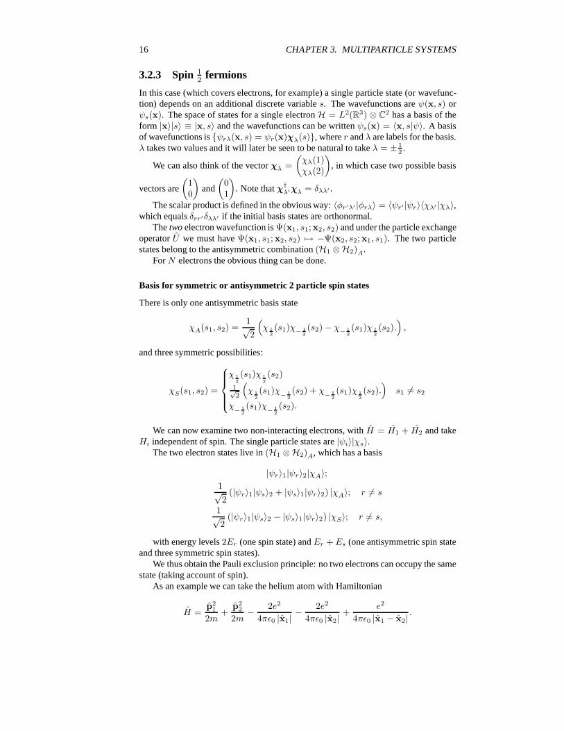
3.2.3 Spin 12

fermions

In this case (which covers electrons, for example) a single particle state (or wavefunc-tion) depends on an additional discrete variables. The wavefunctions areψ(x, s) orψs(x). The space of states for a single electronH = L2(R3) ⊗ C2 has a basis of theform |x〉|s〉 ≡ |x, s〉 and the wavefunctions can be writtenψs(x) = 〈x, s|ψ〉. A basisof wavefunctions is{ψrλ(x, s) = ψr(x)χλ(s)}, wherer andλ are labels for the basis.λ takes two values and it will later be seen to be natural to takeλ = ± 1

2 .

We can also think of the vectorχλ =(χλ(1)χλ(2)

), in which case two possible basis

vectors are

(10

)and

(01

). Note thatχ†

λ′χλ = δλλ′ .

The scalar product is defined in the obvious way:〈φr′λ′ |φrλ〉 = 〈ψr′ |ψr〉〈χλ′ |χλ〉,which equalsδrr′δλλ′ if the initial basis states are orthonormal.

Thetwo electron wavefunction isΨ(x1, s1;x2, s2) and under the particle exchangeoperatorU we must haveΨ(x1, s1;x2, s2) �→ −Ψ(x2, s2;x1, s1). The two particlestates belong to the antisymmetric combination(H1 ⊗H2)A.

ForN electrons the obvious thing can be done.

Basis for symmetric or antisymmetric 2 particle spin states

There is only one antisymmetric basis state

χA(s1, s2) =1√2

(χ 1

2(s1)χ− 1

2(s2) − χ− 1

2(s1)χ 1

2(s2).

),

and three symmetric possibilities:

χS(s1, s2) =

χ 1

2(s1)χ 1

2(s2)

1√2

(χ 1

2(s1)χ− 1

2(s2) + χ− 1

2(s1)χ 1

2(s2).

)s1 �= s2

χ− 12(s1)χ− 1

2(s2).

We can now examine two non-interacting electrons, withH = H1 + H2 and takeHi independent of spin. The single particle states are|ψi〉|χs〉.

The two electron states live in(H1 ⊗H2)A, which has a basis

|ψr〉1|ψr〉2|χA〉;1√2

(|ψr〉1|ψs〉2 + |ψs〉1|ψr〉2) |χA〉; r �= s

1√2

(|ψr〉1|ψs〉2 − |ψs〉1|ψr〉2) |χS〉; r �= s,

with energy levels2Er (one spin state) andEr +Es (one antisymmetric spin stateand three symmetric spin states).

We thus obtain the Pauli exclusion principle: no two electrons can occupy the samestate (taking account of spin).

As an example we can take the helium atom with Hamiltonian

H =p2

1

2m+

p22

2m− 2e2

4πε0 |x1| −2e2

4πε0 |x2| +e2

4πε0 |x1 − x2| .

3.3. TWO PARTICLE STATES AND CENTRE OF MASS 17

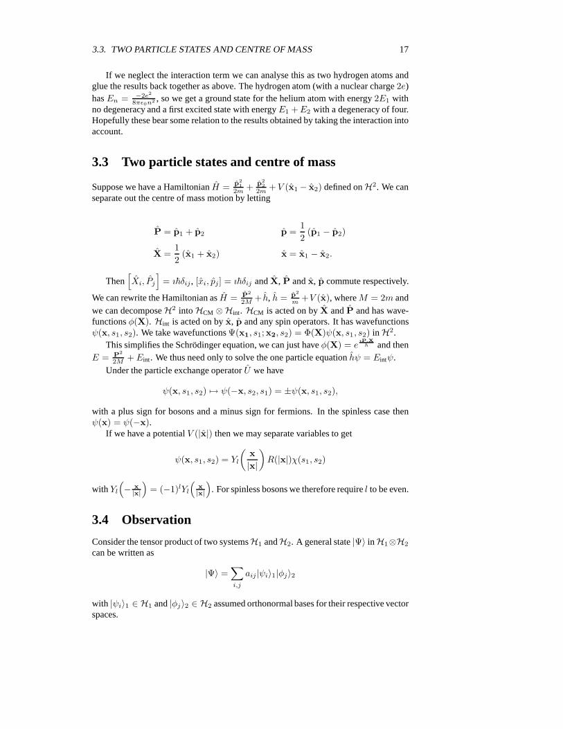
If we neglect the interaction term we can analyse this as two hydrogen atoms andglue the results back together as above. The hydrogen atom (with a nuclear charge2e)hasEn = −2e2

8πε0n2 , so we get a ground state for the helium atom with energy2E1 withno degeneracy and a first excited state with energyE1 +E2 with a degeneracy of four.Hopefully these bear some relation to the results obtained by taking the interaction intoaccount.

3.3 Two particle states and centre of mass

Suppose we have a HamiltonianH = p21

2m + p22

2m +V (x1 − x2) defined onH2. We canseparate out the centre of mass motion by letting

P = p1 + p2 p =12

(p1 − p2)

X =12

(x1 + x2) x = x1 − x2.

Then[Xi, Pj

]= ı�δij , [xi, pj] = ı�δij andX, P andx, p commute respectively.

We can rewrite the Hamiltonian asH = P2

2M + h, h = p2

m +V (x), whereM = 2m and

we can decomposeH2 into HCM ⊗Hint. HCM is acted on byX andP and has wave-functionsφ(X). Hint is acted on byx, p and any spin operators. It has wavefunctionsψ(x, s1, s2). We take wavefunctionsΨ(x1, s1;x2, s2) = Φ(X)ψ(x, s1, s2) in H2.

This simplifies the Schr¨odinger equation, we can just haveφ(X) = eıP.X

� and thenE = P2

2M + Eint. We thus need only to solve the one particle equationhψ = Eintψ.

Under the particle exchange operatorU we have

ψ(x, s1, s2) �→ ψ(−x, s2, s1) = ±ψ(x, s1, s2),

with a plus sign for bosons and a minus sign for fermions. In the spinless case thenψ(x) = ψ(−x).

If we have a potentialV (|x|) then we may separate variables to get

ψ(x, s1, s2) = Yl

(x|x|

)R(|x|)χ(s1, s2)

with Yl(− x

|x|)

= (−1)lYl(

x|x|

). For spinless bosons we therefore requirel to be even.

3.4 Observation

Consider the tensor product of two systemsH1 andH2. A general state|Ψ〉 in H1⊗H2

can be written as

|Ψ〉 =∑i,j

aij |ψi〉1|φj〉2

with |ψi〉1 ∈ H1 and|φj〉2 ∈ H2 assumed orthonormal bases for their respective vectorspaces.

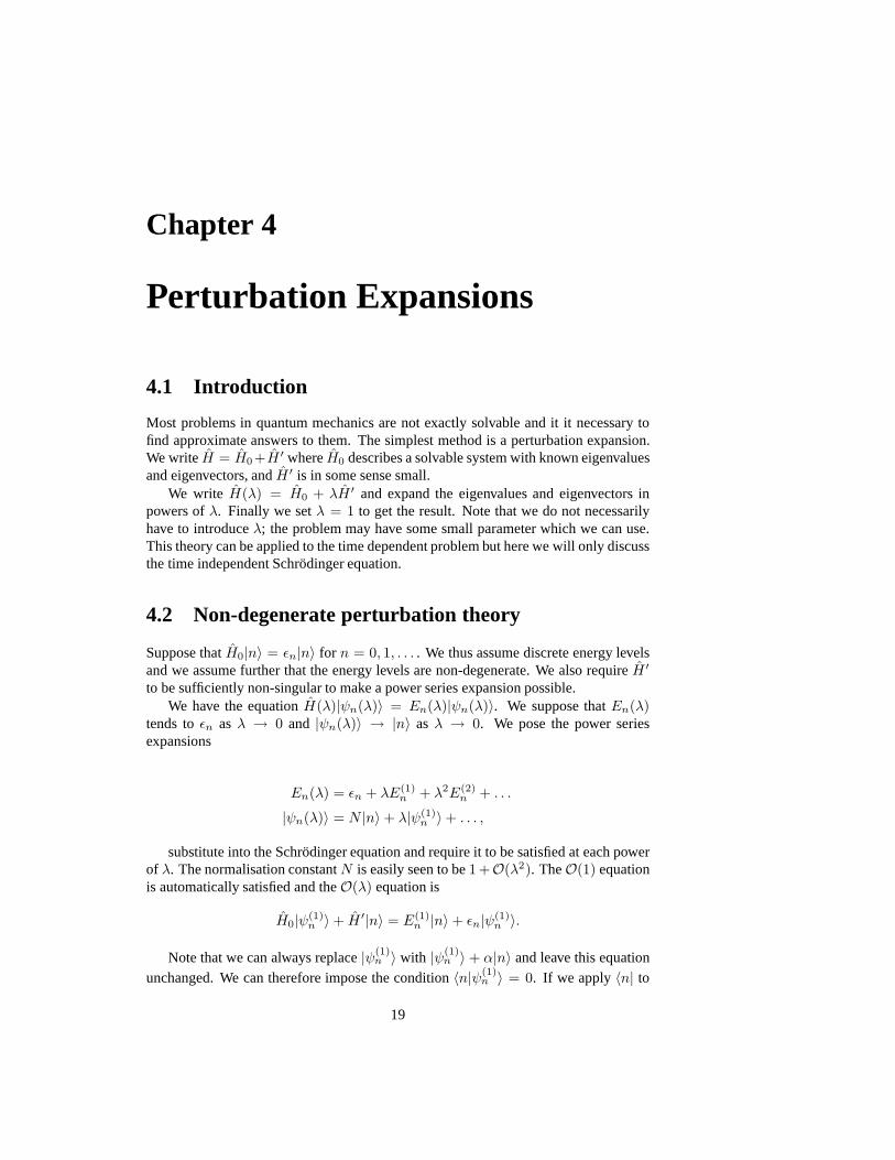
Chapter 4

Perturbation Expansions

4.1 Introduction

Most problems in quantum mechanics are not exactly solvable and it it necessary tofind approximate answers to them. The simplest method is a perturbation expansion.We writeH = H0+H ′ whereH0 describes a solvable system with known eigenvaluesand eigenvectors, andH ′ is in some sense small.

We write H(λ) = H0 + λH ′ and expand the eigenvalues and eigenvectors inpowers ofλ. Finally we setλ = 1 to get the result. Note that we do not necessarilyhave to introduceλ; the problem may have some small parameter which we can use.This theory can be applied to the time dependent problem but here we will only discussthe time independent Schr¨odinger equation.

4.2 Non-degenerate perturbation theory

Suppose thatH0|n〉 = εn|n〉 for n = 0, 1, . . . . We thus assume discrete energy levelsand we assume further that the energy levels are non-degenerate. We also requireH ′

to be sufficiently non-singular to make a power series expansion possible.We have the equationH(λ)|ψn(λ)〉 = En(λ)|ψn(λ)〉. We suppose thatEn(λ)

tends toεn asλ → 0 and |ψn(λ)〉 → |n〉 asλ → 0. We pose the power seriesexpansions

En(λ) = εn + λE(1)n + λ2E(2)

n + . . .

|ψn(λ)〉 = N |n〉 + λ|ψ(1)n 〉 + . . . ,

substitute into the Schr¨odinger equation and require it to be satisfied at each powerof λ. The normalisation constantN is easily seen to be1 +O(λ2). TheO(1) equationis automatically satisfied and theO(λ) equation is

H0|ψ(1)n 〉 + H ′|n〉 = E(1)

n |n〉 + εn|ψ(1)n 〉.

Note that we can always replace|ψ(1)n 〉 with |ψ(1)

n 〉 + α|n〉 and leave this equationunchanged. We can therefore impose the condition〈n|ψ(1)

n 〉 = 0. If we apply〈n| to

19

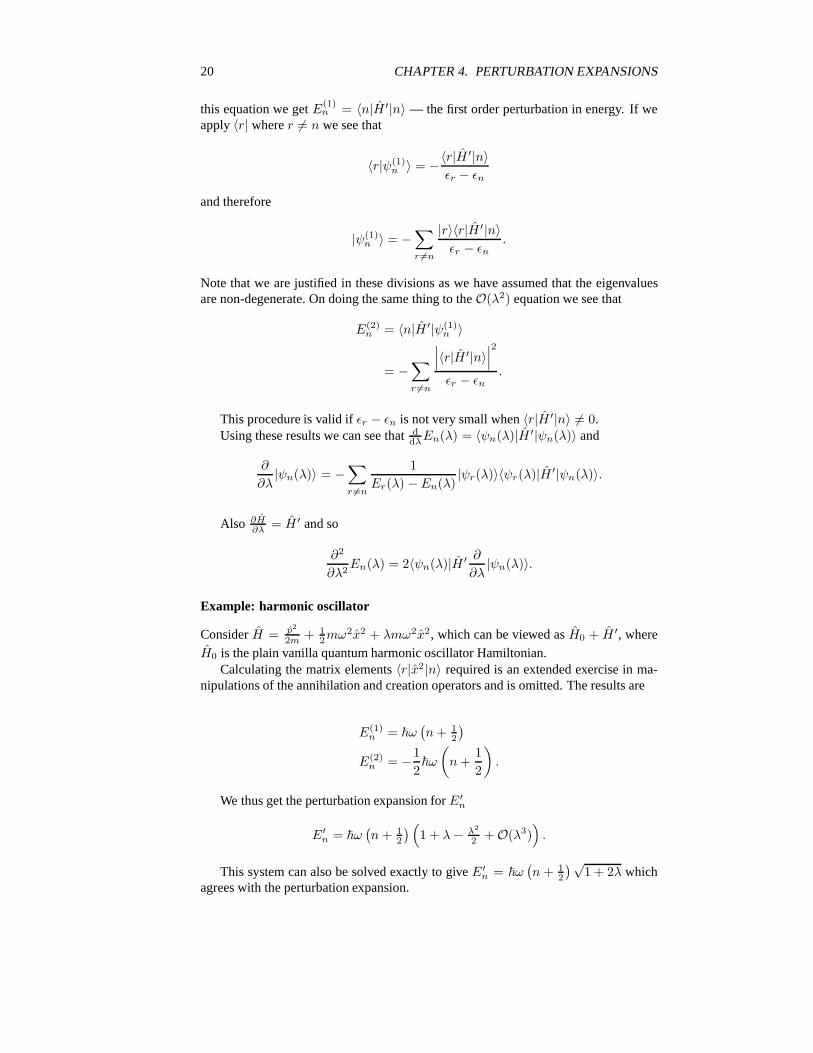
20 CHAPTER 4. PERTURBATION EXPANSIONS

this equation we getE(1)n = 〈n|H ′|n〉 — the first order perturbation in energy. If we

apply〈r| wherer �= n we see that

〈r|ψ(1)n 〉 = −〈r|H ′|n〉

εr − εn

and therefore

|ψ(1)n 〉 = −

∑r �=n

|r〉〈r|H ′|n〉εr − εn

.

Note that we are justified in these divisions as we have assumed that the eigenvaluesare non-degenerate. On doing the same thing to theO(λ2) equation we see that

E(2)n = 〈n|H ′|ψ(1)

n 〉

= −∑r �=n

∣∣∣〈r|H ′|n〉∣∣∣2

εr − εn.

This procedure is valid ifεr − εn is not very small when〈r|H ′|n〉 �= 0.Using these results we can see thatd

dλEn(λ) = 〈ψn(λ)|H ′|ψn(λ)〉 and

∂

∂λ|ψn(λ)〉 = −

∑r �=n

1Er(λ) − En(λ)

|ψr(λ)〉〈ψr(λ)|H ′|ψn(λ)〉.

Also ∂H∂λ = H ′ and so

∂2

∂λ2En(λ) = 2〈ψn(λ)|H ′ ∂

∂λ|ψn(λ)〉.

Example: harmonic oscillator

ConsiderH = p2

2m + 12mω

2x2 + λmω2x2, which can be viewed asH0 + H ′, where

H0 is the plain vanilla quantum harmonic oscillator Hamiltonian.Calculating the matrix elements〈r|x2|n〉 required is an extended exercise in ma-

nipulations of the annihilation and creation operators and is omitted. The results are

E(1)n = �ω

(n+ 1

2

)E(2)

n = −12

�ω

(n+

12

).

We thus get the perturbation expansion forE′n

E′n = �ω

(n+ 1

2

) (1 + λ− λ2

2 + O(λ3)).

This system can also be solved exactly to giveE′n = �ω

(n+ 1

2

)√1 + 2λ which

agrees with the perturbation expansion.

4.3. DEGENERACY 21

4.3 Degeneracy

The method given here breaks down ifεr = εn for r �= n. Perturbation theory can beextended to the degenerate case, but we will consider only the first order shift inεr.We suppose that the states|n, s〉, s = 1 . . .Nn have the same energyεn. Nn is thedegeneracy of this energy level.

As before we pose a HamiltonianH = H0 + λH ′ such thatH0|n, s〉 = εn|n, s〉and look for states|ψ(λ)〉 with energyE(λ) → εn asλ→ 0.

The difference with the previous method is that we expand|ψ(λ)〉 as a power seriesin λ in the basis of eigenvectors of H0. That is

|ψ(λ)〉 =∑s

|n, s〉as + λ|ψ(1)〉.

As theas are arbitrary we can impose the conditions〈n, s|ψ(1)〉 = 0 for eachs andn. We thus have to solveH |ψ(λ)〉 = E(λ)|ψ(λ)〉 with E(λ) = εn +λE(1). If we taketheO(λ) equation and apply〈n, r| to it we get∑

s

as〈n, r|H ′|n, s〉 = arE(1)n

which is a matrix eigenvalue problem. Thus the first order perturbations inεn arethe eigenvalues of the matrix〈n, r|H ′|n, s〉. If all the eigenvalues are distinct thenthe perturbation “lifts the degeneracy”. It is convenient for the purpose of calculationto choose a basis for the space spanned by the degenerate eigenvectors in which thismatrix is “as diagonal as possible”.1

1Don’t ask...

22 CHAPTER 4. PERTURBATION EXPANSIONS

Chapter 5

General theory of angularmomentum

For a particle with position and momentum operatorsx andp with the commutationrelations[xi, pj ] = ı�δij we defineL = x ∧ p. It can be seen thatL is Hermitian and

it is easy to show[Li, Lj

]= ı�εijkLk.

5.1 Introduction

We want to find out if there are other Hermitian operators�J which satisfy this com-mutation relation.1 We ask on what space of states can this algebra of operators berealised, or alternatively, what are the representations?

We want

[Ji, Jj ] = ıεijkJk.

We will choose one component ofJ whose eigenvalues label the states. In accor-dance with convention we chooseJ3. Note that

[J2, J3

]= 0, so we can simultaneously

diagonaliseJ2 andJ3. Denote the normalised eigenbasis by|λ µ〉, so that

J2|λ µ〉 = λ|λ µ〉 and J3|λ µ〉 = µ|λ µ〉.We know thatλ ≥ 0 sinceJ2 is the sum of the squares of Hermitian operators.

Now defineJ± = J1 ± ıJ2. These are not Hermitian, butJ†+ = J−.

It will be useful to note that

[J±, J3] = ±J±[J+, J−] = 2J3

J2 = 12 (J+J− + J−J+) + J2

3

= J+J− − J3 + J23

= J−J+ + J3 + J23 .

1The~ is taken outside - you can put it back in if you want, it is inessential but may or may not appear inexam questions. Since we are now grown up we will omit the hats if they do not add to clarity.

23

24 CHAPTER 5. GENERAL THEORY OF ANGULAR MOMENTUM

Proof of this is immediate.Using the[J±, J3] relation we haveJ3J± = J±J3 ± J3, so that

J3J±|λ µ〉 = (µ± 1)J±|λ µ〉

andJ±|λ µ〉 is an eigenstate ofJ3 with eigenvalueµ ± 1. By similar artifice wecan see thatJ±|λ µ〉 is an eigenstate ofJ2 with eigenvalueλ.

Now evaluate the norm ofJ±|λ µ〉, which is

〈λ µ|J∓J±|λ µ〉 = λ− µ2 ∓ µ ≥ 0.

We can now define states|λ (µ± n)〉 for n = 0, 1, 2, . . . . We can pin them downmore by noting thatλ − µ2 ∓ 2µ ≥ 0 for positive norms. However the formulae wehave are, givenλ, negative for sufficiently large|µ| and so to avoid this we must haveµmax = j such thatJ+|j〉 = 0: henceλ− j2 − j = 0 and soλ = j(j + 1).

We can perform a similar trick withJ−; there must existµmin = −j′ such thatJ−| − j′〉 = 0: thusλ = j′(j′ + 1). Soj′ = j and as−j′ = −j = j − n for somen ∈ {0, 1, 2, . . .} we havej = 0, 1

2 , 1,32 , . . . .

In summary the states can be labelled by|j m〉 such that

J2|j m〉 = j(j + 1)|j m〉J3|j m〉 = m|j m〉J±|j m〉 = ((j ∓m) (j ±m+ 1))

12 |j m± 1〉

with m ∈ {−j,−j + 1, . . . , j − 1, j} andj ∈ {0, 12 , 1,

32 , . . . }. There are2j + 1

states with differentm for the samej. |j m〉 is the standard basis of the angularmomentum states.

We have obtained a representation of the algebra labelled byj. If �J = L = x∧ pwe must havej an integer.

Recall that if we haveA we can define a matrixAλ′λ by A|λ〉 =∑

λ′ |λ′〉Aλ′λ.Note that(BA)λ′λ =

∑µBλ′µAµλ. Given j, we have(J3)m′m = mδm′m and

(J±)m′m =√

(j ∓m) (j ±m+ 1) δm′,m±1, giving us(2j + 1) × (2j + 1) matricessatisfying the three commutation relations[J3, J±] = ±J± and[J+, J−] = 2J3.

If J are angular momentum operators which act on a vector spaceV and we have|ψ〉 ∈ V such thatJ3|ψ〉 = k|ψ〉 and J+|ψ〉 = 0 thenψ is a state with angularmomentumj = k. The other states are given byJn

−|ψ〉, 1 ≤ n ≤ 2k. The conditionsalso giveJ2|ψ〉 = k (k + 1) |ψ〉

5.1.1 Spin 12

particles

This is the simplest non-trivial case. We havej = 12 and a two dimensional state space

with a basis|12 12 〉 and|12 − 1

2 〉. We have the relationsJ3|12 ± 12 〉 = ± 1

2 |12 ± 12 〉 and

J+|12 12 〉 = 0 J−|12 1

2 〉 = |12 − 12 〉

J+|12 − 12 〉 = | 12 1

2 〉 J−|12 − 12 〉 = 0.

5.1. INTRODUCTION 25

It is convenient to introduce explicit matricesσ such that

J|12 m〉 =∑m′

|12 m′〉12 (σ)m′m .

The matricesσ are2 × 2 matrices (called the Pauli spin matrices). Explicitly, theyare

σ+ =(

0 20 0

)σ− =

(0 02 0

)σ3 =

(1 00 −1

)

σ1 =12

(σ+ + σ−) =(

0 11 0

)σ2 =

−ı2

(σ+ − σ−) =(

0 −ıı 0

).

Note thatσ21 = σ2

2 = σ23 = 1 andσ† = σ. These satisfy the commutation relations

[σi, σj ] = 2ıεijkσk (a slightly modified angular momentum commutation relation)and we also haveσ2σ3 = ıσ1 (and the relations obtained by cyclic permutation), soσiσj + σjσi = 2δij1. Thus if n is a unit vector we have(σ.n)2 = 1 and we see thatσ.n has eigenvalues±1.

We define the angular momentum matricess = 12�σ and sos2 = 3

4�21.

The basis states areχ 12

=(

10

)andχ− 1

2=

(01

).

5.1.2 Spin 1 particles

We apply the theory as above to get

S+ =

0

√2 0

0 0√

20 0 0

S3 =

1 0 0

0 0 00 0 −1

andS− = S†+.

5.1.3 Electrons

Electrons are particles with intrinsic spin12 . The angular momentumJ = x ∧ p + s, sare the spin operators for spin12 .

The basic operators for an electron arex, p ands. We can represent these operatorsby their action on two component wavefunctions:

ψ(x) =∑

λ=± 12

ψλ(x)χλ.

In this basisx �→ x, p �→ −ı�∇ ands �→ �

2σ. All other operators are constructedin terms of these, for instance we may have a Hamiltonian

H =p2

2m+ V (x) + U(x)σ.L

whereL = x ∧ p.If V andU depend only on|x| then[J, H ] = 0.


5.2 Addition of angular momentum

Consider two independent angular momentum operatorsJ(1) andJ(2) with J(r) actingon some spaceV (r) andV (r) having spinjr for r = 1, 2.

We now define an angular momentumJ acting onV (1) ⊗V (2) by J = J(1) +J(2).Using the commutation relations forJ(r) we can get[Ji, Jj ] = ıεijkJk.

We want to construct states|J M〉 forming a standard angular momentum basis,that is such that:

J3|J M〉 = M |J M〉J±|J M〉 = N±

J,M |J M ± 1〉

with N±J,M =

√(J ∓M) (J ±M + 1). We look for states inV which satisfy

J+|J J〉 = 0 andJ3|J J〉 = J |J J〉. The maximum value ofJ we can get isj1 + j2;and|j1 + j2 j1 + j2〉 = |j1 j1〉1|j2 j2〉2. ThenJ+|j1 + j2 j1 + j2〉 = 0. Similarly thisis an eigenvector ofJ3 with eigenvalue(j1 + j2). We can now applyJ− repeatedly toform all the|J M〉 states. ApplyingJ− we get

|J M − 1〉 = α|j1 j1 − 1〉1|j2 j2〉2 + β|j1 j1〉1|j2 j2 − 1〉2.

The coefficentsα andβ can be determined from the coefficentsN−a,b, and we must

haveα2 + β2 = 1. If we choose|ψ〉 a state orthogonal to this;

|ψ〉 = −β|j1 j1 − 1〉1|j2 j2〉2 + α|j1 j1〉1|j2 j2 − 1〉2.

J3|ψ〉 can be computed and it shows that|ψ〉 is an eigenvector ofJ3 with eigenvalue� (j1 + j2 − 1). Now

0 = 〈ψ|j1 + j2 j1 + j2 − 1〉 ∝ 〈ψ|J−|j1 + j2 j1 + j2〉

and so〈ψ|J−|φ〉 = 0 for all states|φ〉 in V . ThusJ+|ψ〉 = 0 and

|ψ〉 = |j1 + j2 − 1 j1 + j2 − 1〉.

We can then construct the states|j1 + j2 − 1 M〉 by repeatedly applyingJ−.For eachJ such that|j1 − j2| ≤ J ≤ j1 + j2 we can construct a state|J J〉. We

define the Clebsch-Gordan coefficients〈j1 m1 j2 m2|J M〉, and so

|J M〉 =∑

m1,m2

〈j1 m1 j2 m2|J M〉|j1 m1〉|j2 m2〉.

The Clebsch-Gordan coefficients are nonzero only whenM = m1 +m2.We can check the number of states;

j1+j2∑J=|j1−j2|

(2J + 1) =j1+j2∑

J=|j1−j2|

{(J + 1)2 − J2

}= (2j1 + 1) (2j2 + 1) .

5.3. THE MEANING OF QUANTUM MECHANICS 27

Electrons

Electrons have spin12 and we can represent their spin states withχ± 12(s). Using this

notation we see that two electrons can form a symmetric spin 1 triplet

χm(s1, s2) =

χ 1

2(s1)χ 1

2(s2)

1√2

(χ 1

2(s1)χ− 1

2(s2) + χ− 1

2(s1)χ 1

2(s2)

)χ− 1

2(s1)χ− 1

2(s2)

and an antisymmetric spin 0 singlet;

χ0(s1, s2) =1√2

(χ 1

2(s1)χ− 1

2(s2) − χ− 1

2(s1)χ 1

2(s2)

).

5.3 The meaning of quantum mechanics

Quantum mechanics deals in probabilities, whereas classical mechanics is determin-istic if we have complete information. If we have incomplete information classicalmechanics is also probabilistic.

Inspired by this we ask if there can be “hidden variables” in quantum mechanicssuch that the theory is deterministic. Assuming that local effects have local causes, thisis not possible.

We will take a spin example to show this. Consider a spin12 particle, with two

spin states|↑〉 and|↓〉 which are eigenvectors ofS3 = �

2σ3. If we choose to use twocomponent vectors we have

χ↑ =(

10

)χ↓ =

(01

).

Supposen = (sin θ, 0, cos θ) (a unit vector) and let us find the eigenvectors of

σ.n =(

cos θ sin θsin θ − cos θ

).

As (σ.n)2 = 1 we must have eigenvalues±1 and an inspired guess givesχ↑,n andχ↓,n as

χ↑,n = cos θ2χ↑ + sin θ

2χ↓ and χ↓,n = − sin θ2χ↑ + cos θ

2χ↓.

Thus (reverting to ket vector notation) if an electron is in a state|↑〉 then the prob-ability of finding it in a state|↑,n〉 is cos2 θ

2 and the probability of finding it in a state|↓,n〉 is sin2 θ

2 .Now, suppose we have two electrons in a spin0 singlet state;

|Φ〉 =1√2{|↑〉1|↓〉2 − |↓〉1|↑〉2} .

Then the probability of finding electron 1 with spin up is12 , and after making this

measurement electron 2 must be spin down. Similarly, if we find electron 1 with spindown (probability1

2 again) then electron 2 must have spin up. More generally, supposewe measure electron 1’s spin along directionn. Then we see that the probability for


electron 1 to have spin up in directionn (aligned) is12 and then electron 2 must be in

the state|↓,n〉2.If we have two electrons (say electron 1 and electron 2) in a spin 0 state we may

physically separate them and consider independent experiments on them.We will consider three directions as sketched. For electron 1 there are three vari-

ables which we may measure (in separate experiments);S(1)z = ±1, S(1)

n = ±1 andS

(1)m = ±1. We can also do this for electron 2.

We see that if we find electron 1 hasS(1)z = 1 then electron 2 hasS(2)

z = −1 (etc.).If there exists an underlying deterministic theory then we could expect some prob-

ability distributionp for this set of experiments;

0 ≤ p(S(1)

z , S(1)n , S(1)

m , S(2)z , S(2)

n , S(2)m

)≤ 1

which is nonzero only ifS(1)dirn = −S(2)

dirn and∑{s}

p({s}) = 1.

Bell inequality

Suppose we have a probability distributionp(a, b, c) with a, b, c = ±1. We definepartial probabilitiespbc =

∑a p(a, b, c) and similarly forpac andpab. Then

pbc(1,−1) = p(1, 1,−1) + p(−1, 1,−1)≤ p(1, 1,−1) + p(1, 1, 1) + p(−1, 1,−1) + p(−1,−1,−1)≤ pab(1, 1) + pac(−1,−1).

Applying this to the two electron system we get

P(S(1)

n = 1, S(2)m = 1

)≤ P

(S(1)

z = 1, S(2)n = −1

)+ P

(S(1)

z = −1, S(2)m = 1

).

We can calculate these probabilities from quantum mechanics

P(S(1)

z = 1, S(2)n = −1

)= P

(S(1)

z = 1, S(1)n = 1

)= cos2 θ

2

P(S(1)

z = −1, S(2)m = 1

)= cos2 θ+φ

2 and

P(S(1)

n = 1, S(2)m = 1

)= sin2 θ

2 .

The Bell inequality givessin2 φ2 ≤ cos2 θ

2 + cos2 θ+φ2 which is not in general true.

References

◦ P.A.M. Dirac,The Principles of Quantum Mechanics, Fourth ed., OUP, 1958.

I enjoyed this book as a good read but it is also an eminently suitable textbook.

◦ Feynman, Leighton, Sands,The Feynman Lectures on Physics Vol. 3, Addison-Wesley, 1964.

Excellent reading but not a very appropriate textbook for this course. I read it as acompanion to the course and enjoyed every chapter.

◦ E. Merzbacher,Quantum Mechanics, Wiley, 1970.

This is a recommended textbook for this course (according to the Schedules). I wasn’tparticularly impressed but you may like it.

There must be a good, modern textbook for this course. If you know of one pleasesend me abrief review and I will include it if I think it is suitable. In any case, withthese marvellous notes you don’t need a textbook, do you?

Related courses

There are courses onStatistical Physics andApplications of Quantum Mechanics inPart 2B and courses onQuantum Physics and Symmetries and Groups in QuantumPhysics in Part 2A.

29

foundations of quantum mechanics - higher...

Documents