Steven R. DunbarDepartment of Mathematics203 Avery HallUniversity of Nebraska-LincolnLincoln, NE 68588-0130http://www.math.unl.edu

Voice: 402-472-3731Fax: 402-472-8466

Topics in

Probability Theory and Stochastic ProcessesSteven R. Dunbar

Local Limit Theorems

Rating

Mathematicians Only: prolonged scenes of intense rigor.

1

Section Starter Question

Consider a binomial probability value for a large value of the binomial pa-rameter n. How would you approximate this probability value? Would youexpect this approximation to be uniformly good for all values of k? Explainwhy or why not?

Key Concepts

1. This section gives two estimates of binomial probability values for alarge value of the binomial parameter n in terms of the normal density.Each estimate is uniform in k. These estimates are two forms of theLocal Limit Theorem.

Vocabulary

1. A local limit theorem describes how the probability mass functionof a sum of independent discrete random variables at a particular valueapproaches the normal density.

2

Mathematical Ideas

Introduction

A local limit theorem describes how the probability mass function of a sumof independent discrete random variables approaches the normal density.We observe that the histogram of a sum of independent Bernoulli randomvariables resembles the normal density. From the Central Limit Theorem, wesee that in standard units the area under the one bar of a binomial histogrammay be approximated by the area under a standard normal. Theorems whichcompare the probability of a discrete random variable in terms of the areaunder a bar of a histogram to the area under a normal density are oftencalled local limit theorems. This is illustrated in Figure 1

In a way, Pascal laid the foundation for the local limit theorem whenhe formulated the binomial probability distribution for a Bernoulli randomvariable with p = 1/2 = q. James Bernoulli generalized the distribution tothe case where p 6= 1/2. De Moivre proved the first real local limit theoremfor the case p = 1/2 = q in essentially the form of Lemma 9 in The deMoivre-Laplace Central Limit Theorem. Laplace provided a correct prooffor the case with p 6= 1/2. De Moivre then used the local limit theoremto add up the probabilities that Sn is in an interval of length of order

√n

to prove the Central Limit Theorem. See Lemma 10 and following in Thede Moivre-Laplace Central Limit Theorem. Khintchine, Lyanpunov, andLindeberg proved much more general versions of the Central Limit Theoremusing characteristic functions and Fourier transform methods. Historically,the original Local Limit Theorem was overshadowed by the Central LimitTheorem, and forgotten until its revival by Gnedenko in 1948, [1].

First Form of Local Limit Theorem

Recall that Xk is a Bernoulli random variable taking on the value 1 or 0 withprobability p or 1− p respectively. Then

Sn =n∑k=1

Xi

is a binomial random variable indicating the number of successes in a com-posite experiment.

3

Figure 1: Comparison of the binomial distribution with n = 20, p = 6/10with the normal distribution with mean np and variance np(1− p).

4

In this section, we study the size of Pn [Sn = k] as n approaches infinity.We will give an estimate uniform in k that is a form of the local limit theorem.

Theorem 1 (Local Limit Theorem, First Form).

Pn [Sn = k] =1√

2πp(1− p)n

(exp

(−(k − np)2

2np(1− p)

)+ o(1)

).

uniformly for all k ∈ Z.

Remark. Note that this is stronger than Lemma 9, the de Moivre-LaplaceBinomial Point Mass Limit in the section on the de Moivre-Laplace CentralLimit Theorem. It is stronger in that here the estimate is uniform for allk ∈ Z instead of just an interval of order

√n around the mean.

Proof. 1. Take t = 712

. Note that 12< t < 2

3.

(a) Proposition 1 (the Optimization Extension of the Central LimitTheorem) in The Moderate Deviations Result, says

Pn [Sn = k] =1√

2πp(1− p)nexp

(−(k − np)2

2np(1− p)

)(1 + δn(k)) ,

wherelimn→∞

max|k−np|<n7/12

|δn(k)| = 0.

(b) Rewriting this, we have

Pn [Sn = k] =1√

2πp(1− p)nexp

(−(k − np)2

2np(1− p)

)+

1√2πp(1− p)

exp

(−(k − np)2

2np(1− p)

)δn(k)√n,

where the last term is ou(n−1/2) uniformly in k when |k − np| <

n7/12. Since

1√2πp(1− p)

exp

(−(k − np)2

2np(1− p)

)≤ 1

we can simplify this to

Pn [Sn = k] =1√

2πp(1− p)nexp

(−(k − np)2

2np(1− p)

)+δn(k)√n.

5

2. Theorem 8.1 (the Moderate Deviations Theorem) says that if we take

an = n1/12√p(1−p)

, then limn→∞ an = +∞ and limn→∞ ann−1/6 = 0. Thus,

Pn[Sn ≥ np+ n7/12

]= Pn

[Snn− p ≥ n−5/12

]= Pn

[Snn− p ≥

√p(1− p) ·

n1/12/√p(1− p)

n1/2

]

∼√p(1− p)

n1/12√

2π· exp

(−n1/6

2p(1− p)

)where the last asymptotic limit comes from the Moderate DeviationsTheorem on |k − np| < n7/12.

3. The asymptotic limit implies a weaker estimate:

Pn[Sn ≥ np+ n7/12

]= o

(n−1/2

).

To see this, note that

Pn[Sn ≥ np+ n7/12

]n−1/2

=Pn[Sn ≥ np+ n7/12

]√p(1−p)

n1/12√2π· exp

(−n1/6

2p(1−p)

) ·√p(1−p)

n1/12√2π· exp

(−n1/6

2p(1−p)

)n−1/2

.

Note that the first factor goes to 1 by step 2. So consider n5/12 exp(−n1/6

2p(1−p)

)→

0. This estimate is uniform in k for k − np ≥ n7/12.

4. Note that

exp

(−(k − np)2

2np(1− p)

)≥ exp

(−n14/12

2np(1− p)

)= exp

(−n1/6

2p(1− p)

)so exp

(−(k−np)22np(1−p)

)= o(1).

5. Using step 4, we see that

1√2πp(1− p)n

exp

(−(k − np)2

2np(1− p)

)= o(n−1/2)

uniformly in k with k − np ≥ n7/12.

6

6. Make step 3 look the same as step 1b by putting step 5 into step 3without disturbing the estimate:

Pn [Sn = k] =1√

2πp(1− p)nexp

(−(k − np)2

2np(1− p)

)+ o(n−1/2).

Finally, factor out 1√2πp(1−p)n

and the proof is finished

The Second Form of the Local Limit Theorem

Recall that Yi is a sequence of independent random variables which take val-ues 1 with probability 1/2 and −1 with probability 1/2. This is a mathemat-ical model of a fair coin flip game where a 1 results from “heads” on the ithcoin toss and a−1 results from “tails”. LetHn and Ln be the number of headsand tails respectively in n flips. Then Tn =

∑ni=1 Yi = Hn − Ln = 2Sn − n

counts the difference between the number of heads and tails, an excess ofheads if positive. The second form of the local limit theorem is useful forestimating the probability that Tn takes a value close to its average (2p−1)n.

Remark. The following version of Stirling’s Formula.follows from the state-ment of the First Form of the Local Limit Theorem. However, note that theproof of the Local Limit Theorem uses the Moderate Deviations Theorem.The proof of the Moderate Deviations Theorem uses the Optimization Ex-tension of the de Moivre-Laplace Central Limit Theorem. Step 1 of the proofof the Optimization Extension uses Stirling’s Formula. So this is not a newproof of Stirling’s Formula for binomial coefficients. It is a long way to derivethe asymptotics for binomial coefficients from the usual Stirling Formula.

Corollary 1. (n

k

)=

√2

π

2n√n

exp

(− 2

n(k − n/2)2 + o(1)

)uniformly for k ∈ Z.

Proof. Use p = 1/2 in the First Form of the Local Limit Theorem.

Theorem 2 ( Local Limit Theorem, Second Form). Set Tn = 2Sn− n, then

Pn [Tn = k] =

√2

π

(p

1− p

)k/2 (2√p(1− p)

)n√n

(exp

(−k2

2n

)+ o(1)

)7

uniformly for k ∈ Z such that n+ k is even.

Proof.

Pn [Tn = k] = Pn [2Sn − n = k]

= Pn[Sn =

n+ k

2

]=

(nn+k2

)p

n+k2 (1− p)

n−k2

Using the statement of the Corollary

=

√2

πp

n+k2 (1− p)

n−k2

2n√n

(exp

(− 2

n

(n

2+k

2− n

2

)2)

+ o(1)

)

=

√2

π

(p

1− p

)k/2 (2√p(1− p)

)n√n

(exp

(−k2

2n

)+ o(1)

).

Remark. Note that the First Form and the Second Form of the Local LimitTheorem say the same thing in the symmetric case p = 1/2.

Corollary 2. Let K be a fixed finite subset of Z that contains at least oneeven number and one odd number. Then

limn→∞

1

nln (Pn [Tn ∈ K]) = ln

(2√p(1− p)

).

Proof. The Second Form of the Local Limit Theorem says that the prob-ability that Tn is in a fixed finite subset of Z decreases exponentially as napproaches infinity.

Discussion and Extensions

As the Second Form of the Local Limit Theorem indicates, to state a LocalLimit Theorem for sums of random variables more general than Bernoulli ran-dom variables will take some care. For example, if the summands X1, X2, . . .are all even valued, there is no way the sum X1 + · · · + Xn can be odd so aLocal Limit Theorem will require at least an additional hypothesis while theCentral Limit Theorem will still hold.

8

Definition. We say that h is the maximal span of a density f if h is thelargest integer such that the support of f is contained in the affine subset{b+ kh : k = . . . ,−2,−1, 0, 1, 2, . . . } of Z for some b.

Let φ(x) = 1√2π

e−x2/2 be the standard normal density.

Theorem 3 (Gnedenko’s Local Limit Theorem). Let X1, X2, . . . be indepen-dent random variables with identical density f with finite mean µ and finitevariance σ2 and maximal span equal to 1. Let Sn = X1 + · · ·+Xn. Then

(nσ2)

∣∣∣∣P [Sn = k]− 1

(nσ2)φ((x− nµ)/(nσ2))

∣∣∣∣→ 0

uniformly in k as n→∞.

Proof. This was proved by B. V. Gnedenko in 1948, [1], using characteristicfunctions.

McDonald, [3], has more technical local limit theorems and further refer-ences to other generalizations.

The following example shows that any extension of the Local Limit The-orem to nonidentical random variables illustrates is complicated by the sameproblem of periodicity that already appears in the Second Form of the LocalLimit Theorem above.

Example. Suppose the densities fm are fm(0) = 1/2, fm(1) = 1/2m, fm(2) =1/2 − 1/2m. The first random variable will be either 0 or 1, each withprobability 1/2. For m > 1, the random variables will “essentially” differ by2. That is, the maximal span is “essentially” 2, but Gnedenko’s theoremwill not hold. In fact, consider the histogram of the convolution of thedistributions f1, . . . f20 in Figure 2. This histogram is the distribution ofthe sum of the first 20 of the random variables.

Note that the distribution overall resembles the normal distribution, asexpected from the Lindeberg Central Limit Theorem. However closer inspec-tion show that the value of the distribution at symmetric distances aroundthe mean 20 differ. That is the value of the distribution at 21 is greater thanthe value of the distribution at 19. This suggests that at least the uniformapproach to the normal distribution at integer values will not hold.

9

Figure 2: Distribution of the sum of the first 20 of the random variables withnonidentical independent distributions (1/2, 1/2m, 1/2− 1/2m).

Sources

This section is adapted from: Heads or Tails, by Emmanuel Lesigne, StudentMathematical Library Volume 28, American Mathematical Society, Provi-dence, 2005, Chapter 9, [2]. The historical remarks and the generalizationsof the Local Limit Theorem are adapted from [3].

Algorithms, Scripts, Simulations

Algorithm

The experiment is flipping a coin n times, and repeat the experiment ktimes. Then check the probability of a specific value and compare to the

10

normal probability density. Also compare the logarithmic rate of growth tothe predicted rate.

Scripts

Scripts

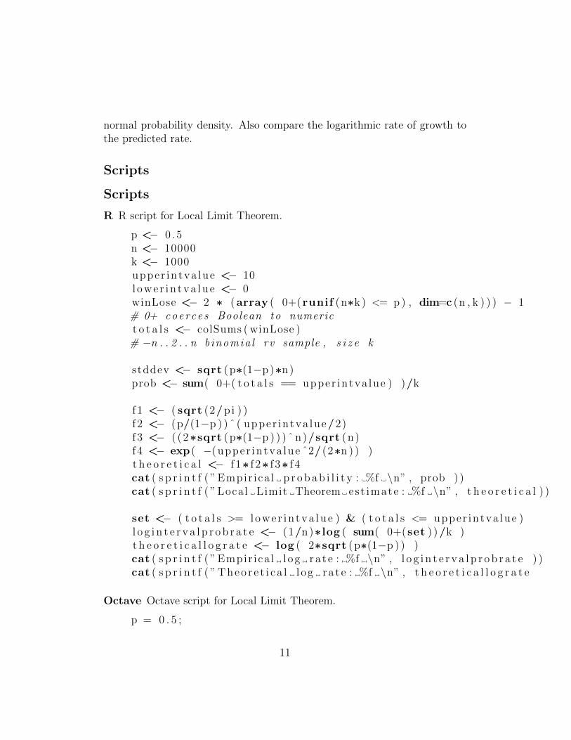
R R script for Local Limit Theorem.

p <− 0 .5n <− 10000k <− 1000upper intva lue <− 10l owe r i n tva lu e <− 0winLose <− 2 ∗ (array ( 0+(runif (n∗k ) <= p ) , dim=c (n , k ) ) ) − 1# 0+ coerces Boolean to numerict o t a l s <− colSums ( winLose )

# −n . . 2 . . n b inomia l rv sample , s i z e k

stddev <− sqrt (p∗(1−p)∗n)prob <− sum( 0+( t o t a l s == upper intva lue ) )/k

f1 <− ( sqrt (2/pi ) )f 2 <− (p/(1−p ) ) ˆ ( upper intva lue/2)f 3 <− ( (2∗sqrt (p∗(1−p ) ) ) ˆ n)/sqrt (n)f 4 <− exp( −(upper intva lue ˆ2/(2∗n ) ) )t h e o r e t i c a l <− f 1∗ f 2∗ f 3∗ f 4cat ( s p r i n t f ( ” Empir ica l p r o b a b i l i t y : %f \n” , prob ) )cat ( s p r i n t f ( ” Local Limit Theorem est imate : %f \n” , t h e o r e t i c a l ) )

set <− ( t o t a l s >= lower i n tva lu e ) & ( t o t a l s <= upper intva lue )l o g i n t e r v a l p r o b r a t e <− (1/n)∗log ( sum( 0+(set ) )/k )t h e o r e t i c a l l o g r a t e <− log ( 2∗sqrt (p∗(1−p ) ) )cat ( s p r i n t f ( ” Empir ica l l og ra t e : %f \n” , l o g i n t e r v a l p r o b r a t e ) )cat ( s p r i n t f ( ” Theo r e t i c a l l og ra t e : %f \n” , t h e o r e t i c a l l o g r a t e

Octave Octave script for Local Limit Theorem.

p = 0 . 5 ;

11

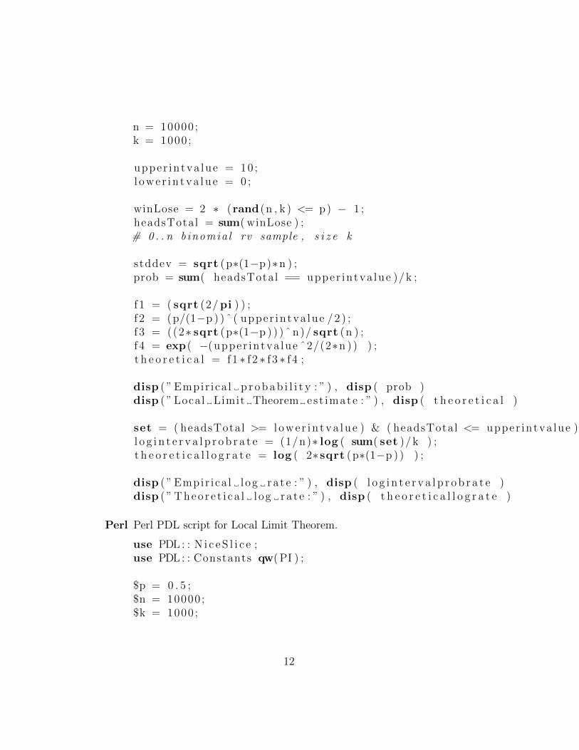
n = 10000;k = 1000 ;

upper intva lue = 10 ;l owe r i n tva lu e = 0 ;

winLose = 2 ∗ (rand (n , k ) <= p) − 1 ;headsTotal = sum( winLose ) ;# 0 . . n b inomia l rv sample , s i z e k

stddev = sqrt (p∗(1−p)∗n ) ;prob = sum( headsTotal == upper intva lue )/k ;

f 1 = ( sqrt (2/pi ) ) ;f 2 = (p/(1−p ) ) ˆ ( upper intva lue / 2 ) ;f 3 = ((2∗ sqrt (p∗(1−p ) ) ) ˆ n)/ sqrt (n ) ;f 4 = exp( −(upper intva lue ˆ2/(2∗n ) ) ) ;t h e o r e t i c a l = f1 ∗ f 2 ∗ f 3 ∗ f 4 ;

disp ( ” Empir ica l p r o b a b i l i t y : ” ) , disp ( prob )disp ( ” Local Limit Theorem est imate : ” ) , disp ( t h e o r e t i c a l )

set = ( headsTotal >= lower i n tva lu e ) & ( headsTotal <= upper intva lue ) ;l o g i n t e r v a l p r o b r a t e = (1/n)∗ log ( sum( set )/k ) ;t h e o r e t i c a l l o g r a t e = log ( 2∗ sqrt (p∗(1−p ) ) ) ;

disp ( ” Empir ica l l og ra t e : ” ) , disp ( l o g i n t e r v a l p r o b r a t e )disp ( ” Theo r e t i c a l l og ra t e : ” ) , disp ( t h e o r e t i c a l l o g r a t e )

Perl Perl PDL script for Local Limit Theorem.

use PDL : : N i c e S l i c e ;use PDL : : Constants qw( PI ) ;

$p = 0 . 5 ;$n = 10000 ;$k = 1000 ;

12

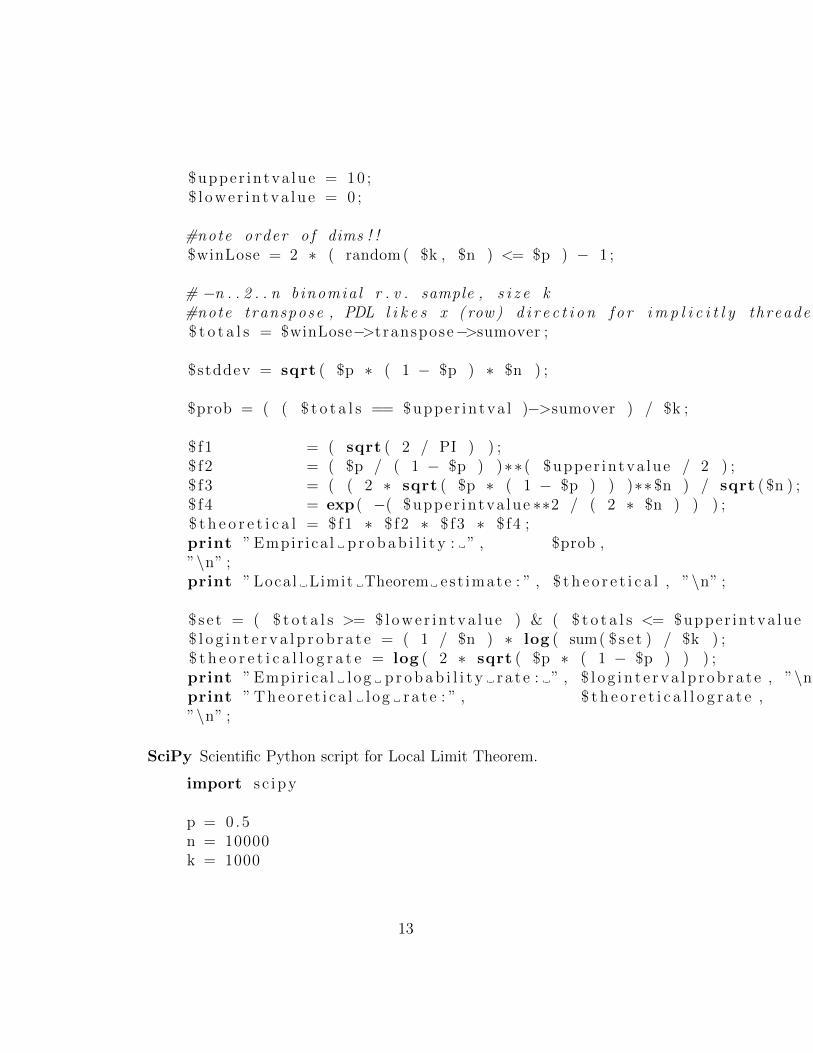
$upper intva lue = 10 ;$ l owe r in tva lue = 0 ;

#note order o f dims ! !$winLose = 2 ∗ ( random ( $k , $n ) <= $p ) − 1 ;

# −n . . 2 . . n b inomia l r . v . sample , s i z e k#note transpose , PDL l i k e s x ( row ) d i r e c t i o n f o r i m p l i c i t l y threaded o p e r a t i o n s$ t o t a l s = $winLose−>transpose−>sumover ;

$stddev = sqrt ( $p ∗ ( 1 − $p ) ∗ $n ) ;

$prob = ( ( $ t o t a l s == $upper in tva l )−>sumover ) / $k ;

$ f1 = ( sqrt ( 2 / PI ) ) ;$ f2 = ( $p / ( 1 − $p ) )∗∗ ( $upper intva lue / 2 ) ;$ f3 = ( ( 2 ∗ sqrt ( $p ∗ ( 1 − $p ) ) )∗∗$n ) / sqrt ( $n ) ;$ f4 = exp( −( $upper intva lue ∗∗2 / ( 2 ∗ $n ) ) ) ;$ t h e o r e t i c a l = $f1 ∗ $ f2 ∗ $ f3 ∗ $ f4 ;print ” Empir ica l p r o b a b i l i t y : ” , $prob ,”\n” ;print ” Local Limit Theorem est imate : ” , $ t h e o r e t i c a l , ”\n” ;

$ s e t = ( $ t o t a l s >= $lower in tva lue ) & ( $ t o t a l s <= $upper intva lue ) ;$ l o g i n t e r v a l p r o b r a t e = ( 1 / $n ) ∗ log ( sum( $s e t ) / $k ) ;$ t h e o r e t i c a l l o g r a t e = log ( 2 ∗ sqrt ( $p ∗ ( 1 − $p ) ) ) ;print ” Empir ica l l og p r o b a b i l i t y ra t e : ” , $ l o g i n t e r v a l p r o b r a t e , ”\n” ;print ” Theo r e t i c a l l og ra t e : ” , $ t h e o r e t i c a l l o g r a t e ,”\n” ;

SciPy Scientific Python script for Local Limit Theorem.

import s c ipy

p = 0 .5n = 10000k = 1000

13

upper intva lue = 10l owe r i n tva lu e = 0

winLose = 2 ∗ ( s c ipy . random . random ( ( n , k))<= p) − 1# Note Booleans True f o r Heads and False f o r T a i l st o t a l s = sc ipy .sum( winLose , a x i s = 0)

# −n . . 2 . . n b inomia l r . v . sample , s i z e k# Note how Booleans ac t as 0 ( Fa lse ) and 1 ( True )

stddev = sc ipy . s q r t ( p ∗ ( 1−p ) ∗n )

prob = ( sc ipy .sum( t o t a l s == upper intva lue ) ) . astype ( ’ f l o a t ’ )/k# Note the c a s t i n g o f i n t e g e r type to f l o a t to g e t f l o a t

f 1 = ( sc ipy . s q r t ( 2 / s c ipy . p i ) ) ;f 2 = ( p / ( 1 − p ) )∗∗ ( upper intva lue / 2 ) ;f 3 = ( ( 2 ∗ s c ipy . s q r t ( p ∗ ( 1 − p ) ) )∗∗n ) / s c ipy . s q r t (n ) ;f 4 = sc ipy . exp ( −( upper intva lue ∗∗2 / ( 2 .0 ∗ n ) ) ) ;# Note the use o f 2 .0 to f o r c e i n t e g e r a r i t h to f l o a t i n g p o i n tt h e o r e t i c a l = f1 ∗ f 2 ∗ f 3 ∗ f 4 ;

print ” Empir ica l p r o b a b i l i t y : ” , probprint ”Moderate Dev iat ions Theorem est imate : ” , t h e o r e t i c a l

set = ( t o t a l s >= lower i n tva lu e ) & ( t o t a l s <= upper intva lue ) ;l o g i n t e r v a l p r o b r a t e = ( 1 / n ) ∗ s c ipy . l og ( ( s c ipy .sum( set ) ) . astype ( ’ f l o a t ’ ) / k ) ;t h e o r e t i c a l l o g r a t e = sc ipy . l og ( 2 ∗ s c ipy . s q r t ( p ∗ ( 1 − p ) ) ) ;print ” Empir ica l l og p r o b a b i l i t y ra t e : ” , l o g i n t e r v a l p r o b r a t eprint ” Theo r e t i c a l l og ra t e : ” , t h e o r e t i c a l l o g r a t e

14

Problems to Work for Understanding

1. Modify the value of p in a script, say to p = 0.51, and investigate theconvergence and the rate of convergence to the normal density function.

2. Modify the value of n in a script to a sequence of values and investigatethe rate of convergence of the logarithmic rate.

Reading Suggestion:

References

[1] B. V. Gnedenko. On the local limit theorem in the theory of probability.Uspekhi Mat. Nauk, 3:187–194, 1948.

[2] Emmanuel Lesigne. Heads or Tails: An Introduction to Limit Theoremsin Probability, volume 28 of Student Mathematical Library. AmericanMathematical Society, 2005.

[3] D. R. McDonald. The local limit theorem: A historical perspective.Journal of the Iranian Statistical Society, 4(2):73–86, 2005.

Outside Readings and Links:

1. L. Breiman, Probability, 1968, Addison-Wesley Publishing, Section 10.4,page 224-227.

15

2. D. R. McDonald, “The Local Limit Theorem: A Historical Perspec-tive”, Journal of the Royal Statistical Society, Vol. 4, No. 2, pp. 73-86.

3. Encyclopedia of Mathematics, Local Limit Theorems

I check all the information on each page for correctness and typographicalerrors. Nevertheless, some errors may occur and I would be grateful if you wouldalert me to such errors. I make every reasonable effort to present current andaccurate information for public use, however I do not guarantee the accuracy ortimeliness of information on this website. Your use of the information from thiswebsite is strictly voluntary and at your risk.

I have checked the links to external sites for usefulness. Links to externalwebsites are provided as a convenience. I do not endorse, control, monitor, orguarantee the information contained in any external website. I don’t guaranteethat the links are active at all times. Use the links here with the same caution asyou would all information on the Internet. This website reflects the thoughts, in-terests and opinions of its author. They do not explicitly represent official positionsor policies of my employer.

Information on this website is subject to change without notice.

Steve Dunbar’s Home Page, http://www.math.unl.edu/~sdunbar1Email to Steve Dunbar, sdunbar1 at unl dot edu

Last modified: Processed from LATEX source on April 26, 2015

16