toanna,mywife - sgoj/baylie/partial differential equations in action... · preface...
TRANSCRIPT

To Anna, my wife

Sandro Salsa
Partial DifferentialEquations in ActionFrom Modellingto Theory
Sandro SalsaDipartimento di MatematicaPolitecnico di Milano
CIP-Code: 2007938891
ISBN 978-88-470-0751-2 Springer Milan Berlin Heidelberg New Yorke-ISBN 978-88-470-0752-9
This work is subject to copyright. All rights are reserved, whether the whole or part of thematerial is concerned, specifically the rights of translation, reprinting, reuse of illustrations,recitation, broadcasting, reproduction on microfilms or in other ways, and storage in data banks.Duplication of this publication or parts thereof is permitted only under the provisions of theItalian Copyright Law in its current version, and permission for use must always ba obtainedfrom Springer. Violations are liable to prosecution under the Italian Copyright Law.
Springer is a part of Springer Science+Business Mediaspringer.comc© Springer-Verlag Italia, Milano 2008Printed in Italy
Cover-Design: Simona Colombo, MilanTypesetting with LATEX: PTP-Berlin, Protago-TEX-Production GmbH, Germany
(www.ptp-berlin.eu)
9 8 7 6 5 4 3 2 1
Springer-Verlag Italia srl – Via Decembrio 28 – 20137 Milano-I
Printing and Binding: Grafiche Porpora , Segrate (MI)

Preface
This book is designed as an advanced undergraduate or a first-year graduate coursefor students from various disciplines like appliedmathematics, physics, engineering.It has evolved while teaching courses on partial differential equations (PDE) duringthe last few years at the Politecnico of Milan.
The main purpose of these courses was twofold: on the one hand, to trainthe students to appreciate the interplay between theory and modelling in prob-lems arising in the applied sciences, and on the other hand to give them a solidtheoretical background for numerical methods, such as finite elements.
Accordingly, this textbook is divided into two parts.
The first one, chapters 2 to 5, has a rather elementary character with the goalof developing and studying basic problems from the macro-areas of diffusion, prop-agation and transport, waves and vibrations. I have tried to emphasize, wheneverpossible, ideas and connections with concrete aspects, in order to provide intuitionand feeling for the subject.
For this part, a knowledge of advanced calculus and ordinary differential equa-tions is required. Also, the repeated use of the method of separation of variablesassumes some basic results from the theory of Fourier series, which are summarizedin appendix A.
Chapter 2 starts with the heat equation and some of its variants in whichtransport and reaction terms are incorporated. In addition to the classical top-ics, I emphasized the connections with simple stochastic processes, such as ran-dom walks and Brownian motion. This requires the knowledge of some elementaryprobability. It is my belief that it is worthwhile presenting this topic as early aspossible, even at the price of giving up to a little bit of rigor in the presentation. Anapplication to financial mathematics shows the interaction between probabilisticand deterministic modelling. The last two sections are devoted to two simple nonlinear models from flow in porous medium and population dynamics.
Chapter 3 mainly treats the Laplace/Poisson equation. The main propertiesof harmonic functions are presented once more emphasizing the probabilistic mo-tivations. The second part of this chapter deals with representation formulas in

Preface
terms of potentials. In particular, the basic properties of the single and doublelayer potentials are presented.
Chapter 4 is devoted to first order equations and in particular to first orderscalar conservation laws. The methods of characteristics and the notion of integralsolution are developed through a simple model from traffic dynamics. In the lastpart, the method of characteristics is extended to quasilinear and fully nonlinearequations in two variables.
In chapter 5 the fundamental aspects of waves propagation are examined, lead-ing to the classical formulas of d’Alembert, Kirchhoff and Poisson. In the final sec-tion, the classical model for surface waves in deep water illustrates the phenomenonof dispersion, with the help of the method of stationary phase.
The main topic of the second part, from chapter 6 to 9, is the development ofHilbert spaces methods for the variational formulation and the analysis of linearboundary and initial-boundary value problems. Given the abstract nature of thesechapters, I have made an effort to provide intuition and motivation about thevarious concepts and results, running the risk of appearing a bit wordy sometimes.
The understanding of these topics requires some basic knowledge of Lebesguemeasure and integration, summarized in appendix B.
Chapter 6 contains the tools from functional analysis in Hilbert spaces, nec-essary for a correct variational formulation of the most common boundary valueproblems. The main theme is the solvability of abstract variational problems, lead-ing to the Lax-Milgram theorem and Fredholm’s alternative. Emphasis is given tothe issues of compactness and weak convergence.
Chapter 7 is divided into two parts. The first one is a brief introduction to thetheory of distributions of L. Schwartz. In the second one, the most used Sobolevspaces and their basic properties are discussed.
Chapter 8 is devoted to the variational formulation of elliptic boundary valueproblems and their solvability. The development starts with one-dimensional prob-lems, continues with Poisson’s equation and ends with general second order equa-tions in divergence form. The last section contains an application to a simplecontrol problem, with both distributed observation and control.
The issue in chapter 9 is the variational formulation of evolution problems, inparticular of initial-boundary value problems for second order parabolic operatorsin divergence form and for the wave equation. Also, an application to a simplecontrol problem with final observation and distributed control is discussed.
At the end of each chapter, a number of exercises is included. Some of themcan be solved by a routine application of the theory or of the methods developedin the text. Other problems are intended as a completion of some arguments orproofs in the text. Also, there are problems in which the student is required to bemore autonomous. The most demanding problems are supplied with answers orhints.
The order of presentation of the material is clearly a consequence of my ...prejudices. However, the exposition if flexible enough to allow substantial changes
VI

Preface
without compromising the comprehension and to facilitate a selection of topics fora one or two semester course.In the first part, the chapters are in practice mutually independent, with the ex-
ception of subsections 3.3.6 and 3.3.7, which presume the knowledge of section 2.6.In the second part, which, in principle, may be presented independently of
the first one, more attention has to be paid to the order of the arguments. Inparticular, the material in chapter 6 and in sections 7.1–7.4 and 7.7–7.10 is neces-sary for understanding chapter 8, while chapter 9 uses concepts and results fromsection 7.11.
Acknowledgments. While writing this book I benefitted from comments,suggestions and criticisms of many collegues and students.Among my collegues I express my gratitude to Luca Dede, Fausto Ferrari, Carlo
Pagani, Kevin Payne, Alfio Quarteroni, Fausto Saleri, Carlo Sgarra, AlessandroVeneziani, Gianmaria A. Verzini and, in particular to Cristina Cerutti, LeonedeDe Michele and Peter Laurence.Among the students who have sat throuh my course on PDE, I would like to
thank Luca Bertagna, Michele Coti-Zelati, Alessandro Conca, Alessio Fumagalli,Loredana Gaudio, Matteo Lesinigo, Andrea Manzoni and Lorenzo Tamellini.
VII

Contents
1 Introduction . . . . . . . . . . . . . . . . . . . . . . . . . . . . . . . . . . . . . . . . . . . . . . . . . . . 11.1 Mathematical Modelling . . . . . . . . . . . . . . . . . . . . . . . . . . . . . . . . . . . . . . 11.2 Partial Differential Equations . . . . . . . . . . . . . . . . . . . . . . . . . . . . . . . . . 21.3 Well Posed Problems. . . . . . . . . . . . . . . . . . . . . . . . . . . . . . . . . . . . . . . . . 51.4 Basic Notations and Facts . . . . . . . . . . . . . . . . . . . . . . . . . . . . . . . . . . . . 71.5 Smooth and Lipschitz Domains . . . . . . . . . . . . . . . . . . . . . . . . . . . . . . . . 101.6 Integration by Parts Formulas . . . . . . . . . . . . . . . . . . . . . . . . . . . . . . . . . 11
2 Diffusion . . . . . . . . . . . . . . . . . . . . . . . . . . . . . . . . . . . . . . . . . . . . . . . . . . . . . . . 132.1 The Diffusion Equation . . . . . . . . . . . . . . . . . . . . . . . . . . . . . . . . . . . . . . 13
2.1.1 Introduction . . . . . . . . . . . . . . . . . . . . . . . . . . . . . . . . . . . . . . . . . . 132.1.2 The conduction of heat . . . . . . . . . . . . . . . . . . . . . . . . . . . . . . . . 142.1.3 Well posed problems (n = 1) . . . . . . . . . . . . . . . . . . . . . . . . . . . . 162.1.4 A solution by separation of variables . . . . . . . . . . . . . . . . . . . . . 192.1.5 Problems in dimension n > 1 . . . . . . . . . . . . . . . . . . . . . . . . . . . 27
2.2 Uniqueness . . . . . . . . . . . . . . . . . . . . . . . . . . . . . . . . . . . . . . . . . . . . . . . . . 302.2.1 Integral method . . . . . . . . . . . . . . . . . . . . . . . . . . . . . . . . . . . . . . . 302.2.2 Maximum principles . . . . . . . . . . . . . . . . . . . . . . . . . . . . . . . . . . . 31
2.3 The Fundamental Solution . . . . . . . . . . . . . . . . . . . . . . . . . . . . . . . . . . . . 342.3.1 Invariant transformations . . . . . . . . . . . . . . . . . . . . . . . . . . . . . . . 342.3.2 Fundamental solution (n = 1) . . . . . . . . . . . . . . . . . . . . . . . . . . . 362.3.3 The Dirac distribution . . . . . . . . . . . . . . . . . . . . . . . . . . . . . . . . . 392.3.4 Fundamental solution (n > 1) . . . . . . . . . . . . . . . . . . . . . . . . . . . 42
2.4 Symmetric Random Walk (n = 1) . . . . . . . . . . . . . . . . . . . . . . . . . . . . . 432.4.1 Preliminary computations . . . . . . . . . . . . . . . . . . . . . . . . . . . . . . 442.4.2 The limit transition probability . . . . . . . . . . . . . . . . . . . . . . . . . 472.4.3 From random walk to Brownian motion . . . . . . . . . . . . . . . . . . 49
2.5 Diffusion, Drift and Reaction . . . . . . . . . . . . . . . . . . . . . . . . . . . . . . . . . 522.5.1 Random walk with drift . . . . . . . . . . . . . . . . . . . . . . . . . . . . . . . . 52
Preface . . . . . . . . . . . . . . . . . . . . . . . . . . . . . . . . . . . . . . . . . . . . . . . . . . . . . . . . . . . . V

Contents
2.5.2 Pollution in a channel . . . . . . . . . . . . . . . . . . . . . . . . . . . . . . . . . . 542.5.3 Random walk with drift and reaction . . . . . . . . . . . . . . . . . . . . 57
2.6 Multidimensional Random Walk . . . . . . . . . . . . . . . . . . . . . . . . . . . . . . . 582.6.1 The symmetric case . . . . . . . . . . . . . . . . . . . . . . . . . . . . . . . . . . . 582.6.2 Walks with drift and reaction . . . . . . . . . . . . . . . . . . . . . . . . . . . 62
2.7 An Example of Reaction−Diffusion (n = 3) . . . . . . . . . . . . . . . . . . . . . 622.8 The Global Cauchy Problem (n = 1) . . . . . . . . . . . . . . . . . . . . . . . . . . . 68
2.8.1 The homogeneous case . . . . . . . . . . . . . . . . . . . . . . . . . . . . . . . . . 682.8.2 Existence of a solution . . . . . . . . . . . . . . . . . . . . . . . . . . . . . . . . . 692.8.3 The non homogeneous case. Duhamel’s method . . . . . . . . . . . 712.8.4 Maximum principles and uniqueness . . . . . . . . . . . . . . . . . . . . . 74
2.9 An Application to Finance . . . . . . . . . . . . . . . . . . . . . . . . . . . . . . . . . . . . 772.9.1 European options . . . . . . . . . . . . . . . . . . . . . . . . . . . . . . . . . . . . . 772.9.2 An evolution model for the price S . . . . . . . . . . . . . . . . . . . . . . 772.9.3 The Black-Scholes equation . . . . . . . . . . . . . . . . . . . . . . . . . . . . . 802.9.4 The solutions . . . . . . . . . . . . . . . . . . . . . . . . . . . . . . . . . . . . . . . . . 832.9.5 Hedging and self-financing strategy . . . . . . . . . . . . . . . . . . . . . . 88
2.10 Some Nonlinear Aspects . . . . . . . . . . . . . . . . . . . . . . . . . . . . . . . . . . . . . . 902.10.1 Nonlinear diffusion. The porous medium equation . . . . . . . . . 902.10.2 Nonlinear reaction. Fischer’s equation . . . . . . . . . . . . . . . . . . . . 93
Problems . . . . . . . . . . . . . . . . . . . . . . . . . . . . . . . . . . . . . . . . . . . . . . . . . . . . . . . 97
3 The Laplace Equation . . . . . . . . . . . . . . . . . . . . . . . . . . . . . . . . . . . . . . . . . . 1023.1 Introduction . . . . . . . . . . . . . . . . . . . . . . . . . . . . . . . . . . . . . . . . . . . . . . . . 1023.2 Well Posed Problems. Uniqueness . . . . . . . . . . . . . . . . . . . . . . . . . . . . . 1033.3 Harmonic Functions . . . . . . . . . . . . . . . . . . . . . . . . . . . . . . . . . . . . . . . . . 105
3.3.1 Discrete harmonic functions . . . . . . . . . . . . . . . . . . . . . . . . . . . . 1053.3.2 Mean value properties . . . . . . . . . . . . . . . . . . . . . . . . . . . . . . . . . 1093.3.3 Maximum principles . . . . . . . . . . . . . . . . . . . . . . . . . . . . . . . . . . . 1103.3.4 The Dirichlet problem in a circle. Poisson’s formula . . . . . . . . 1133.3.5 Harnack’s inequality and Liouville’s theorem . . . . . . . . . . . . . . 1173.3.6 A probabilistic solution of the Dirichlet problem . . . . . . . . . . . 1183.3.7 Recurrence and Brownian motion . . . . . . . . . . . . . . . . . . . . . . . 122
3.4 Fundamental Solution and Newtonian Potential . . . . . . . . . . . . . . . . . 1243.4.1 The fundamental solution . . . . . . . . . . . . . . . . . . . . . . . . . . . . . . 1243.4.2 The Newtonian potential . . . . . . . . . . . . . . . . . . . . . . . . . . . . . . . 1263.4.3 A divergence-curl system.
Helmholtz decomposition formula . . . . . . . . . . . . . . . . . . . . . . . 1283.5 The Green Function . . . . . . . . . . . . . . . . . . . . . . . . . . . . . . . . . . . . . . . . . 132
3.5.1 An integral identity . . . . . . . . . . . . . . . . . . . . . . . . . . . . . . . . . . . . 1323.5.2 The Green function . . . . . . . . . . . . . . . . . . . . . . . . . . . . . . . . . . . . 1333.5.3 Green’s representation formula . . . . . . . . . . . . . . . . . . . . . . . . . . 1353.5.4 The Neumann function . . . . . . . . . . . . . . . . . . . . . . . . . . . . . . . . . 137
3.6 Uniqueness in Unbounded Domains . . . . . . . . . . . . . . . . . . . . . . . . . . . . 1393.6.1 Exterior problems . . . . . . . . . . . . . . . . . . . . . . . . . . . . . . . . . . . . . 139
X
Contents XI
3.7 Surface Potentials . . . . . . . . . . . . . . . . . . . . . . . . . . . . . . . . . . . . . . . . . . . 1413.7.1 The double and single layer potentials . . . . . . . . . . . . . . . . . . . 1423.7.2 The integral equations of potential theory . . . . . . . . . . . . . . . . 146
Problems . . . . . . . . . . . . . . . . . . . . . . . . . . . . . . . . . . . . . . . . . . . . . . . . . . . . . . . 150
4 Scalar Conservation Laws and First Order Equations . . . . . . . . . . . 1564.1 Introduction . . . . . . . . . . . . . . . . . . . . . . . . . . . . . . . . . . . . . . . . . . . . . . . . 1564.2 Linear Transport Equation . . . . . . . . . . . . . . . . . . . . . . . . . . . . . . . . . . . 157
4.2.1 Pollution in a channel . . . . . . . . . . . . . . . . . . . . . . . . . . . . . . . . . . 1574.2.2 Distributed source . . . . . . . . . . . . . . . . . . . . . . . . . . . . . . . . . . . . . 1594.2.3 Decay and localized source . . . . . . . . . . . . . . . . . . . . . . . . . . . . . 1604.2.4 Inflow and outflow characteristics. A stability estimate . . . . . 162
4.3 Traffic Dynamics . . . . . . . . . . . . . . . . . . . . . . . . . . . . . . . . . . . . . . . . . . . . 1644.3.1 A macroscopic model . . . . . . . . . . . . . . . . . . . . . . . . . . . . . . . . . . 1644.3.2 The method of characteristics . . . . . . . . . . . . . . . . . . . . . . . . . . . 1654.3.3 The green light problem . . . . . . . . . . . . . . . . . . . . . . . . . . . . . . . . 1684.3.4 Traffic jam ahead. . . . . . . . . . . . . . . . . . . . . . . . . . . . . . . . . . . . . . 172
4.4 Integral (or Weak) Solutions . . . . . . . . . . . . . . . . . . . . . . . . . . . . . . . . . . 1744.4.1 The method of characteristics revisited . . . . . . . . . . . . . . . . . . . 1744.4.2 Definition of integral solution . . . . . . . . . . . . . . . . . . . . . . . . . . . 1774.4.3 The Rankine-Hugoniot condition . . . . . . . . . . . . . . . . . . . . . . . . 1794.4.4 The entropy condition . . . . . . . . . . . . . . . . . . . . . . . . . . . . . . . . . 1834.4.5 The Riemann problem . . . . . . . . . . . . . . . . . . . . . . . . . . . . . . . . . 1854.4.6 Vanishing viscosity method . . . . . . . . . . . . . . . . . . . . . . . . . . . . . 1864.4.7 The viscous Burger equation . . . . . . . . . . . . . . . . . . . . . . . . . . . . 189
4.5 The Method of Characteristics for Quasilinear Equations . . . . . . . . . 1924.5.1 Characteristics . . . . . . . . . . . . . . . . . . . . . . . . . . . . . . . . . . . . . . . . 1924.5.2 The Cauchy problem . . . . . . . . . . . . . . . . . . . . . . . . . . . . . . . . . . 1944.5.3 Lagrange method of first integrals . . . . . . . . . . . . . . . . . . . . . . . 2024.5.4 Underground flow . . . . . . . . . . . . . . . . . . . . . . . . . . . . . . . . . . . . . 205
4.6 General First Order Equations . . . . . . . . . . . . . . . . . . . . . . . . . . . . . . . . 2074.6.1 Characteristic strips . . . . . . . . . . . . . . . . . . . . . . . . . . . . . . . . . . . 2074.6.2 The Cauchy Problem . . . . . . . . . . . . . . . . . . . . . . . . . . . . . . . . . . 210
Problems . . . . . . . . . . . . . . . . . . . . . . . . . . . . . . . . . . . . . . . . . . . . . . . . . . . . . . . 214
5 Waves and Vibrations . . . . . . . . . . . . . . . . . . . . . . . . . . . . . . . . . . . . . . . . . . 2215.1 General Concepts . . . . . . . . . . . . . . . . . . . . . . . . . . . . . . . . . . . . . . . . . . . . 221
5.1.1 Types of waves . . . . . . . . . . . . . . . . . . . . . . . . . . . . . . . . . . . . . . . . 2215.1.2 Group velocity and dispersion relation . . . . . . . . . . . . . . . . . . . 223
5.2 Transversal Waves in a String . . . . . . . . . . . . . . . . . . . . . . . . . . . . . . . . . 2265.2.1 The model . . . . . . . . . . . . . . . . . . . . . . . . . . . . . . . . . . . . . . . . . . . 2265.2.2 Energy . . . . . . . . . . . . . . . . . . . . . . . . . . . . . . . . . . . . . . . . . . . . . . . 228
5.3 The One-dimensional Wave Equation . . . . . . . . . . . . . . . . . . . . . . . . . . 2295.3.1 Initial and boundary conditions . . . . . . . . . . . . . . . . . . . . . . . . . 2295.3.2 Separation of variables . . . . . . . . . . . . . . . . . . . . . . . . . . . . . . . . . 231

XII Contents
5.4 The d’Alembert Formula . . . . . . . . . . . . . . . . . . . . . . . . . . . . . . . . . . . . . 2365.4.1 The homogeneous equation . . . . . . . . . . . . . . . . . . . . . . . . . . . . . 2365.4.2 Generalized solutions and propagation of singularities . . . . . . 2405.4.3 The fundamental solution . . . . . . . . . . . . . . . . . . . . . . . . . . . . . . 2445.4.4 Non homogeneous equation. Duhamel’s method . . . . . . . . . . . 2465.4.5 Dissipation and dispersion . . . . . . . . . . . . . . . . . . . . . . . . . . . . . . 247
5.5 Second Order Linear Equations . . . . . . . . . . . . . . . . . . . . . . . . . . . . . . . 2495.5.1 Classification . . . . . . . . . . . . . . . . . . . . . . . . . . . . . . . . . . . . . . . . . 2495.5.2 Characteristics and canonical form . . . . . . . . . . . . . . . . . . . . . . 252
5.6 Hyperbolic Systems with Constant Coefficients . . . . . . . . . . . . . . . . . . 2575.7 The Multi-dimensional Wave Equation (n > 1) . . . . . . . . . . . . . . . . . . 261
5.7.1 Special solutions . . . . . . . . . . . . . . . . . . . . . . . . . . . . . . . . . . . . . . 2615.7.2 Well posed problems. Uniqueness . . . . . . . . . . . . . . . . . . . . . . . . 263
5.8 Two Classical Models . . . . . . . . . . . . . . . . . . . . . . . . . . . . . . . . . . . . . . . . 2665.8.1 Small vibrations of an elastic membrane . . . . . . . . . . . . . . . . . . 2665.8.2 Small amplitude sound waves . . . . . . . . . . . . . . . . . . . . . . . . . . . 270
5.9 The Cauchy Problem . . . . . . . . . . . . . . . . . . . . . . . . . . . . . . . . . . . . . . . . 2745.9.1 Fundamental solution (n = 3)
and strong Huygens’ principle . . . . . . . . . . . . . . . . . . . . . . . . . . . 2745.9.2 The Kirchhoff formula . . . . . . . . . . . . . . . . . . . . . . . . . . . . . . . . . 2775.9.3 Cauchy problem in dimension 2 . . . . . . . . . . . . . . . . . . . . . . . . . 2795.9.4 Non homogeneous equation. Retarded potentials . . . . . . . . . . 281
5.10 Linear Water Waves . . . . . . . . . . . . . . . . . . . . . . . . . . . . . . . . . . . . . . . . . 2825.10.1 A model for surface waves . . . . . . . . . . . . . . . . . . . . . . . . . . . . . . 2825.10.2 Dimensionless formulation and linearization . . . . . . . . . . . . . . . 2865.10.3 Deep water waves . . . . . . . . . . . . . . . . . . . . . . . . . . . . . . . . . . . . . 2885.10.4 Interpretation of the solution . . . . . . . . . . . . . . . . . . . . . . . . . . . 2905.10.5 Asymptotic behavior . . . . . . . . . . . . . . . . . . . . . . . . . . . . . . . . . . . 2925.10.6 The method of stationary phase . . . . . . . . . . . . . . . . . . . . . . . . . 293
Problems . . . . . . . . . . . . . . . . . . . . . . . . . . . . . . . . . . . . . . . . . . . . . . . . . . . . . . . 296
6 Elements of Functional Analysis . . . . . . . . . . . . . . . . . . . . . . . . . . . . . . . . 3026.1 Motivations . . . . . . . . . . . . . . . . . . . . . . . . . . . . . . . . . . . . . . . . . . . . . . . . . 3026.2 Norms and Banach Spaces . . . . . . . . . . . . . . . . . . . . . . . . . . . . . . . . . . . . 3076.3 Hilbert Spaces . . . . . . . . . . . . . . . . . . . . . . . . . . . . . . . . . . . . . . . . . . . . . . 3116.4 Projections and Bases . . . . . . . . . . . . . . . . . . . . . . . . . . . . . . . . . . . . . . . . 316
6.4.1 Projections . . . . . . . . . . . . . . . . . . . . . . . . . . . . . . . . . . . . . . . . . . . 3166.4.2 Bases . . . . . . . . . . . . . . . . . . . . . . . . . . . . . . . . . . . . . . . . . . . . . . . . 320
6.5 Linear Operators and Duality . . . . . . . . . . . . . . . . . . . . . . . . . . . . . . . . . 3266.5.1 Linear operators . . . . . . . . . . . . . . . . . . . . . . . . . . . . . . . . . . . . . . 3266.5.2 Functionals and dual space . . . . . . . . . . . . . . . . . . . . . . . . . . . . . 3286.5.3 The adjoint of a bounded operator . . . . . . . . . . . . . . . . . . . . . . 331
6.6 Abstract Variational Problems . . . . . . . . . . . . . . . . . . . . . . . . . . . . . . . . 3346.6.1 Bilinear forms and the Lax-Milgram Theorem . . . . . . . . . . . . . 3346.6.2 Minimization of quadratic functionals . . . . . . . . . . . . . . . . . . . . 339

Contents
6.6.3 Approximation and Galerkin method . . . . . . . . . . . . . . . . . . . . 3406.7 Compactness and Weak Convergence . . . . . . . . . . . . . . . . . . . . . . . . . . 343
6.7.1 Compactness . . . . . . . . . . . . . . . . . . . . . . . . . . . . . . . . . . . . . . . . . 3436.7.2 Weak convergence and compactness . . . . . . . . . . . . . . . . . . . . . 3446.7.3 Compact operators . . . . . . . . . . . . . . . . . . . . . . . . . . . . . . . . . . . . 348
6.8 The Fredholm Alternative . . . . . . . . . . . . . . . . . . . . . . . . . . . . . . . . . . . . 3506.8.1 Solvability for abstract variational problems . . . . . . . . . . . . . . 3506.8.2 Fredholm’s Alternative . . . . . . . . . . . . . . . . . . . . . . . . . . . . . . . . . 354
6.9 Spectral Theory for Symmetric Bilinear Forms . . . . . . . . . . . . . . . . . . 3566.9.1 Spectrum of a matrix . . . . . . . . . . . . . . . . . . . . . . . . . . . . . . . . . . 3566.9.2 Separation of variables revisited . . . . . . . . . . . . . . . . . . . . . . . . . 3576.9.3 Spectrum of a compact self-adjoint operator . . . . . . . . . . . . . . 3586.9.4 Application to abstract variational problems . . . . . . . . . . . . . . 360
Problems . . . . . . . . . . . . . . . . . . . . . . . . . . . . . . . . . . . . . . . . . . . . . . . . . . . . . . . 362
7 Distributions and Sobolev Spaces . . . . . . . . . . . . . . . . . . . . . . . . . . . . . . 3677.1 Distributions. Preliminary Ideas . . . . . . . . . . . . . . . . . . . . . . . . . . . . . . . 3677.2 Test Functions and Mollifiers . . . . . . . . . . . . . . . . . . . . . . . . . . . . . . . . . 3697.3 Distributions . . . . . . . . . . . . . . . . . . . . . . . . . . . . . . . . . . . . . . . . . . . . . . . . 3737.4 Calculus . . . . . . . . . . . . . . . . . . . . . . . . . . . . . . . . . . . . . . . . . . . . . . . . . . . . 377
7.4.1 The derivative in the sense of distributions . . . . . . . . . . . . . . . 3777.4.2 Gradient, divergence, laplacian . . . . . . . . . . . . . . . . . . . . . . . . . . 379
7.5 Multiplication, Composition, Division, Convolution . . . . . . . . . . . . . . 3827.5.1 Multiplication. Leibniz rule . . . . . . . . . . . . . . . . . . . . . . . . . . . . . 3827.5.2 Composition . . . . . . . . . . . . . . . . . . . . . . . . . . . . . . . . . . . . . . . . . . 3847.5.3 Division . . . . . . . . . . . . . . . . . . . . . . . . . . . . . . . . . . . . . . . . . . . . . . 3857.5.4 Convolution . . . . . . . . . . . . . . . . . . . . . . . . . . . . . . . . . . . . . . . . . . 386
7.6 Fourier Transform . . . . . . . . . . . . . . . . . . . . . . . . . . . . . . . . . . . . . . . . . . . 3887.6.1 Tempered distributions . . . . . . . . . . . . . . . . . . . . . . . . . . . . . . . . . 3887.6.2 Fourier transform in S′ . . . . . . . . . . . . . . . . . . . . . . . . . . . . . . . . 3917.6.3 Fourier transform in L2 . . . . . . . . . . . . . . . . . . . . . . . . . . . . . . . . 393
7.7 Sobolev Spaces . . . . . . . . . . . . . . . . . . . . . . . . . . . . . . . . . . . . . . . . . . . . . . 3947.7.1 An abstract construction . . . . . . . . . . . . . . . . . . . . . . . . . . . . . . . 3947.7.2 The space H1 (Ω) . . . . . . . . . . . . . . . . . . . . . . . . . . . . . . . . . . . . . 3967.7.3 The space H10 (Ω) . . . . . . . . . . . . . . . . . . . . . . . . . . . . . . . . . . . . . 3997.7.4 The dual of H10 (Ω) . . . . . . . . . . . . . . . . . . . . . . . . . . . . . . . . . . . . 4017.7.5 The spaces Hm (Ω), m > 1 . . . . . . . . . . . . . . . . . . . . . . . . . . . . . 4037.7.6 Calculus rules . . . . . . . . . . . . . . . . . . . . . . . . . . . . . . . . . . . . . . . . . 4047.7.7 Fourier Transform and Sobolev Spaces . . . . . . . . . . . . . . . . . . . 405
7.8 Approximations by Smooth Functions and Extensions . . . . . . . . . . . . 4067.8.1 Local approximations . . . . . . . . . . . . . . . . . . . . . . . . . . . . . . . . . . 4067.8.2 Estensions and global approximations . . . . . . . . . . . . . . . . . . . . 407
7.9 Traces . . . . . . . . . . . . . . . . . . . . . . . . . . . . . . . . . . . . . . . . . . . . . . . . . . . . . 4117.9.1 Traces of functions in H1 (Ω) . . . . . . . . . . . . . . . . . . . . . . . . . . . 4117.9.2 Traces of functions in Hm (Ω) . . . . . . . . . . . . . . . . . . . . . . . . . . 414
XIII

Contents
7.9.3 Trace spaces . . . . . . . . . . . . . . . . . . . . . . . . . . . . . . . . . . . . . . . . . . 4157.10 Compactness and Embeddings . . . . . . . . . . . . . . . . . . . . . . . . . . . . . . . . 418
7.10.1 Rellich’s theorem . . . . . . . . . . . . . . . . . . . . . . . . . . . . . . . . . . . . . . 4187.10.2 Poincare’s inequalities . . . . . . . . . . . . . . . . . . . . . . . . . . . . . . . . . 4197.10.3 Sobolev inequality in Rn . . . . . . . . . . . . . . . . . . . . . . . . . . . . . . . 4207.10.4 Bounded domains . . . . . . . . . . . . . . . . . . . . . . . . . . . . . . . . . . . . . 422
7.11 Spaces Involving Time . . . . . . . . . . . . . . . . . . . . . . . . . . . . . . . . . . . . . . . 4247.11.1 Functions with values in Hilbert spaces . . . . . . . . . . . . . . . . . . . 4247.11.2 Sobolev spaces involving time . . . . . . . . . . . . . . . . . . . . . . . . . . . 425
Problems . . . . . . . . . . . . . . . . . . . . . . . . . . . . . . . . . . . . . . . . . . . . . . . . . . . . . . . 428
8 Variational Formulation of Elliptic Problems . . . . . . . . . . . . . . . . . . . 4318.1 Elliptic Equations . . . . . . . . . . . . . . . . . . . . . . . . . . . . . . . . . . . . . . . . . . . 4318.2 The Poisson Problem . . . . . . . . . . . . . . . . . . . . . . . . . . . . . . . . . . . . . . . . 4338.3 Diffusion, Drift and Reaction (n = 1) . . . . . . . . . . . . . . . . . . . . . . . . . . 435
8.3.1 The problem . . . . . . . . . . . . . . . . . . . . . . . . . . . . . . . . . . . . . . . . . . 4358.3.2 Dirichlet conditions . . . . . . . . . . . . . . . . . . . . . . . . . . . . . . . . . . . . 4358.3.3 Neumann, Robin and mixed conditions . . . . . . . . . . . . . . . . . . . 439
8.4 Variational Formulation of Poisson’s Problem . . . . . . . . . . . . . . . . . . . 4448.4.1 Dirichlet problem . . . . . . . . . . . . . . . . . . . . . . . . . . . . . . . . . . . . . 4448.4.2 Neumann, Robin and mixed problems . . . . . . . . . . . . . . . . . . . . 4478.4.3 Eigenvalues of the Laplace operator . . . . . . . . . . . . . . . . . . . . . . 4518.4.4 An asymptotic stability result . . . . . . . . . . . . . . . . . . . . . . . . . . . 453
8.5 General Equations in Divergence Form . . . . . . . . . . . . . . . . . . . . . . . . . 4548.5.1 Basic assumptions . . . . . . . . . . . . . . . . . . . . . . . . . . . . . . . . . . . . . 4548.5.2 Dirichlet problem . . . . . . . . . . . . . . . . . . . . . . . . . . . . . . . . . . . . . 4558.5.3 Neumann problem . . . . . . . . . . . . . . . . . . . . . . . . . . . . . . . . . . . . . 4618.5.4 Robin and mixed problems . . . . . . . . . . . . . . . . . . . . . . . . . . . . . 4638.5.5 Weak Maximum Principles . . . . . . . . . . . . . . . . . . . . . . . . . . . . . 465
8.6 Regularity . . . . . . . . . . . . . . . . . . . . . . . . . . . . . . . . . . . . . . . . . . . . . . . . . . 4678.7 Equilibrium of a plate . . . . . . . . . . . . . . . . . . . . . . . . . . . . . . . . . . . . . . . . 4738.8 A Monotone Iteration Scheme for Semilinear Equations . . . . . . . . . . 4758.9 A Control Problem . . . . . . . . . . . . . . . . . . . . . . . . . . . . . . . . . . . . . . . . . . 478
8.9.1 Structure of the problem . . . . . . . . . . . . . . . . . . . . . . . . . . . . . . . 4788.9.2 Existence and uniqueness of an optimal pair . . . . . . . . . . . . . . 4808.9.3 Lagrange multipliers and optimality conditions . . . . . . . . . . . . 4818.9.4 An iterative algorithm . . . . . . . . . . . . . . . . . . . . . . . . . . . . . . . . . 483
Problems . . . . . . . . . . . . . . . . . . . . . . . . . . . . . . . . . . . . . . . . . . . . . . . . . . . . . . . 485
9 Weak Formulation of Evolution Problems . . . . . . . . . . . . . . . . . . . . . . 4929.1 Parabolic Equations . . . . . . . . . . . . . . . . . . . . . . . . . . . . . . . . . . . . . . . . . 4929.2 Diffusion Equation . . . . . . . . . . . . . . . . . . . . . . . . . . . . . . . . . . . . . . . . . . . 493
9.2.1 The Cauchy-Dirichlet problem . . . . . . . . . . . . . . . . . . . . . . . . . . 4939.2.2 Faedo-Galerkin method (I) . . . . . . . . . . . . . . . . . . . . . . . . . . . . . 4969.2.3 Solution of the approximate problem . . . . . . . . . . . . . . . . . . . . . 497
XIV

Contents XV
9.2.4 Energy estimates . . . . . . . . . . . . . . . . . . . . . . . . . . . . . . . . . . . . . . 4989.2.5 Existence, uniqueness and stability . . . . . . . . . . . . . . . . . . . . . . 5009.2.6 Regularity . . . . . . . . . . . . . . . . . . . . . . . . . . . . . . . . . . . . . . . . . . . . 5039.2.7 The Cauchy-Neuman problem. . . . . . . . . . . . . . . . . . . . . . . . . . . 5059.2.8 Cauchy-Robin and mixed problems . . . . . . . . . . . . . . . . . . . . . . 5079.2.9 A control problem . . . . . . . . . . . . . . . . . . . . . . . . . . . . . . . . . . . . . 509
9.3 General Equations . . . . . . . . . . . . . . . . . . . . . . . . . . . . . . . . . . . . . . . . . . . 5129.3.1 Weak formulation of initial value problems . . . . . . . . . . . . . . . 5129.3.2 Faedo-Galerkin method (II) . . . . . . . . . . . . . . . . . . . . . . . . . . . . . 514
9.4 The Wave Equation . . . . . . . . . . . . . . . . . . . . . . . . . . . . . . . . . . . . . . . . . 5179.4.1 Hyperbolic Equations . . . . . . . . . . . . . . . . . . . . . . . . . . . . . . . . . . 5179.4.2 The Cauchy-Dirichlet problem . . . . . . . . . . . . . . . . . . . . . . . . . . 5189.4.3 Faedo-Galerkin method (III) . . . . . . . . . . . . . . . . . . . . . . . . . . . . 5209.4.4 Solution of the approximate problem . . . . . . . . . . . . . . . . . . . . . 5219.4.5 Energy estimates . . . . . . . . . . . . . . . . . . . . . . . . . . . . . . . . . . . . . . 5229.4.6 Existence, uniqueness and stability . . . . . . . . . . . . . . . . . . . . . . 525
Problems . . . . . . . . . . . . . . . . . . . . . . . . . . . . . . . . . . . . . . . . . . . . . . . . . . . . . . . 528
Appendix A Fourier Series . . . . . . . . . . . . . . . . . . . . . . . . . . . . . . . . . . . . . . . 531A.1 Fourier coefficients . . . . . . . . . . . . . . . . . . . . . . . . . . . . . . . . . . . . . . . . . . . 531A.2 Expansion in Fourier series . . . . . . . . . . . . . . . . . . . . . . . . . . . . . . . . . . . 534
Appendix B Measures and Integrals . . . . . . . . . . . . . . . . . . . . . . . . . . . . . 537B.1 Lebesgue Measure and Integral . . . . . . . . . . . . . . . . . . . . . . . . . . . . . . . . 537
B.1.1 A counting problem . . . . . . . . . . . . . . . . . . . . . . . . . . . . . . . . . . . 537B.1.2 Measures and measurable functions . . . . . . . . . . . . . . . . . . . . . . 539B.1.3 The Lebesgue integral . . . . . . . . . . . . . . . . . . . . . . . . . . . . . . . . . 541B.1.4 Some fundamental theorems . . . . . . . . . . . . . . . . . . . . . . . . . . . . 542B.1.5 Probability spaces, random variables and their integrals . . . . 543
Appendix C Identities and Formulas . . . . . . . . . . . . . . . . . . . . . . . . . . . . . 545C.1 Gradient, Divergence, Curl, Laplacian . . . . . . . . . . . . . . . . . . . . . . . . . . 545C.2 Formulas . . . . . . . . . . . . . . . . . . . . . . . . . . . . . . . . . . . . . . . . . . . . . . . . . . . 547
References . . . . . . . . . . . . . . . . . . . . . . . . . . . . . . . . . . . . . . . . . . . . . . . . . . . . . . . . . 549
Index . . . . . . . . . . . . . . . . . . . . . . . . . . . . . . . . . . . . . . . . . . . . . . . . . . . . . . . . . . . . . . 553

1
Introduction
Mathematical Modelling – Partial Differential Equations – Well Posed Problems – Basic
Notations and Facts – Smooth and Lipschitz Domains – Integration by Parts Formulas
1.1 Mathematical Modelling
Mathematical modelling plays a big role in the description of a large part of phe-nomena in the applied sciences and in several aspects of technical and industrialactivity.By a “mathematical model” we mean a set of equations and/or other mathe-
matical relations capable of capturing the essential features of a complex naturalor artificial system, in order to describe, forecast and control its evolution. Theapplied sciences are not confined to the classical ones; in addition to physics andchemistry, the practice of mathematical modelling heavily affects disciplines likefinance, biology, ecology, medicine, sociology.In the industrial activity (e.g. for aerospace or naval projects, nuclear reactors,
combustion problems, production and distribution of electricity, traffic control,etc.) the mathematical modelling, involving first the analysis and the numericalsimulation and followed by experimental tests, has become a common procedure,necessary for innovation, and also motivated by economic factors. It is clear thatall of this is made possible by the enormous computational power now available.In general, the construction of a mathematical model is based on two main
ingredients: general laws and constitutive relations. In this book we shall deal withgeneral laws coming from continuum mechanics and appearing as conservation orbalance laws (e.g. of mass, energy, linear momentum, etc.).The constitutive relations are of an experimental nature and strongly depend
on the features of the phenomena under examination. Examples are the Fourierlaw of heat conduction, the Fick law for the diffusion of a substance or the waythe speed of a driver depends on the density of cars ahead.The outcome of the combination of the two ingredients is usually a partial
differential equation or a system of them.
Salsa S. Partial Differential Equations in Action: From Modelling to Theoryc© Springer-Verlag 2008, Milan

2 1 Introduction
1.2 Partial Differential Equations
A partial differential equation is a relation of the following type:
F (x1, ..., xn, u, ux1, ..., uxn, ux1x1 , ux1x2 ..., uxnxn , ux1x1x1 , ...) = 0 (1.1)
where the unknown u = u (x1, ...xn) is a function of n variables and uxj ,..., uxixj ,...are its partial derivatives. The highest order of differentiation occurring in theequation is the order of the equation.A first important distinction is between linear and nonlinear equations.Equation (1.1) is linear if F is linear with respect to u and all its derivatives,
otherwise it is nonlinear.A second distinction concerns the types of nonlinearity. We distinguish:
– Semilinear equations where F is nonlinear only with respect to u but is linearwith respect to all its derivatives;
– Quasi-linear equations where F is linear with respect to the highest orderderivatives of u;
– Fully nonlinear equations where F is nonlinear with respect to the highest orderderivatives of u.
The theory of linear equations can be considered sufficiently well developed andconsolidated, at least for what concerns the most important questions. On thecontrary, the non linearities present such a rich variety of aspects and complicationsthat a general theory does not appear to be conceivable. The existing results andthe new investigations focus on more or less specific cases, especially interesting inthe applied sciences.To give the reader an idea of the wide range of applications we present a
series of examples, suggesting one of the possible interpretations. Most of them areconsidered at various level of deepness in this book. In the examples, x representsa space variable (usually in dimension n = 1, 2, 3) and t is a time variable.We start with linear equations. In particular, equations (1.2)–(1.5) are fun-
damental and their theory constitutes a starting point for many other equations.
1. Transport equation (first order):
ut + v · ∇u = 0 (1.2)
It describes for instance the transport of a solid polluting substance along a chan-nel; here u is the concentration of the substance and v is the stream speed. Weconsider the one-dimensional version of (1.2) in Section 4.2
2. Diffusion or heat equation (second order):
ut −DΔu = 0, (1.3)
where Δ = ∂x1x1 +∂x2x2 + ...+∂xnxn is the Laplace operator. It describes the con-duction of heat through a homogeneous and isotropic medium; u is the temperatureand D encodes the thermal properties of the material. Chapter 2 is devoted to theheat equation and its variants.

1.2 Partial Differential Equations 3
3. Wave equation (second order):
utt − c2Δu = 0. (1.4)
It describes for instance the propagation of transversal waves of small amplitudein a perfectly elastic chord (e.g. of a violin) if n = 1, or membrane (e.g. of a drum)if n = 2. If n = 3 it governs the propagation of electromagnetic waves in vacuumor of small amplitude sound waves (Section 5.8). Here u may represent the waveamplitude and c is the propagation speed.
4. Laplace’s or potential equation (second order):
Δu = 0, (1.5)
where u = u (x). The diffusion and the wave equations model evolution phenom-ena. The Laplace equation describes the corresponding steady state, in which thesolution does not depend on time anymore. Together with its nonhomogeneousversion
Δu = f ,
called Poisson’s equation, it plays an important role in electrostatics as well. Chap-ter 3 is devoted to these equations.
5. Black-Scholes equation (second order):
ut +1
2σ2x2uxx + rxux − ru = 0.
Here u = u (x,t), x ≥ 0, t ≥ 0. Fundamental in mathematical finance, this equationgoverns the evolution of the price u of a so called derivative (e.g. an Europeanoption), based on an underlying asset (a stock, a currency, etc.) whose price is x.We meet the Black-Scholes equation in Section 2.9.
6. Vibrating plate (fourth order):
utt −Δ2u = 0,
where x ∈R2 and
Δ2u = Δ(Δu) =∂4u
∂x41+ 2
∂4u
∂x21∂x22
+∂4u
∂x42
is the biharmonic operator. In the theory of linear elasticity, it models the transver-sal waves of small amplitude of a homogeneous isotropic plate (see Section 8.7).
7. Schrodinger equation (second order):
−iut = Δu+ V (x)u
where i is the complex unit. This equation is fundamental in quantum mechanicsand governs the evolution of a particle subject to a potential V . The function |u|2

4 1 Introduction
represents a probability density. We will briefly encounter the Schrodinger equationin Problem 6.6.
Let us list now some examples of nonlinear equations
8. Burger’s equation (quasilinear, first order):
ut + cuux = 0 (x ∈ R) .
It governs a one dimensional flux of a non viscous fluid but it is used to modeltraffic dynamics as well. Its viscous variant
ut + cuux = εuxx (ε > 0)
constitutes a basic example of competition between dissipation (due to the termεuxx) and steepening (shock formation due to the term cuux). We will discussthese topics in Section 4.4.
9. Fisher’s equation (semilinear, second order):
ut −DΔu = ru (M − u)
It governs the evolution of a population of density u, subject to diffusion and logis-tic growth (represented by the right hand side). We examine the one-dimensionalversion of Fisher’s equation in Section 2.10.
10. Porous medium equation (quasilinear, second order):
ut = k div (uγ∇u)
where k > 0, γ > 1 are constant. This equation appears in the description offiltration phenomena, e.g. of the motion of water through the ground. We brieflymeet the one-dimensional version of the porous medium equation in Section 2.10.
11. Minimal surface equation (quasilinear, second order):,
div
⎛⎝ ∇u√
1 + |∇u|2
⎞⎠ = 0 (x ∈R2)
The graph of a solution u minimizes the area among all surfaces z = v (x1, x2)whose boundary is a given curve. For instance, soap balls are minimal surfaces.We will not examine this equation (see e.g. R. Mc Owen, 1996).
12. Eikonal equation (fully nonlinear, first order):
|∇u| = c (x)It appears in geometrical optics: if u is a solution, its level surfaces u (x) = tdescribe the position of a light wave front at time t. A bidimensional version isexamined in Chapter 4.

1.3 Well Posed Problems 5
Let us now give some examples of systems.
13. Navier’s equation of linear elasticity: (three scalar equations of secondorder):
�utt = μΔu+ (μ+ λ)grad div u
where u = (u1 (x,t) , u2 (x,t) , u3 (x,t)), x ∈R3. The vector u represents the dis-placement from equilibrium of a deformable continuum body of (constant) density�. We will not examine this system (see e.g. R. Dautray and J. L. Lions, Vol. 1,6,1985).
14. Maxwell’s equations in vacuum (six scalar linear equations of first order):
Et − curl B = 0, Bt + curl E = 0 (Ampere and Faraday laws)
div E =0 div B =0 (Gauss’ law)
where E is the electric field and B is the magnetic induction field. The unit mea-sures are the ”natural” ones, i.e. the light speed is c = 1 and the magnetic perme-ability is μ0 = 1. We will not examine this system (see e.g. R. Dautray and J. L.Lions, Vol. 1, 1985).
15. Navier-Stokes equations (three quasilinear scalar equations of second orderand one linear equation of first order):
{ut + (u·∇)u = −1ρ∇p+ νΔudiv u =0
where u = (u1 (x,t) , u2 (x,t) , u3 (x,t)), p = p (x,t), x ∈R3. This equation governsthe motion of a viscous, homogeneous and incompressible fluid. Here u is the fluidspeed, p its pressure, ρ its density (constant) and ν is the kinematic viscosity,given by the ratio between the fluid viscosity and its density. The term (u·∇)urepresents the inertial acceleration due to fluid transport. We will briefly meet theNavier-Stokes equations in Section 3.4.
1.3 Well Posed Problems
Usually, in the construction of a mathematical model, only some of the generallaws of continuum mechanics are relevant, while the others are eliminated throughthe constitutive laws or suitably simplified according to the current situation. Ingeneral, additional information is necessary to select or to predict the existenceof a unique solution. This information is commonly supplied in the form of initialand/or boundary data, although other forms are possible. For instance, typicalboundary conditions prescribe the value of the solution or of its normal derivative,or a combination of the two. A main goal of a theory is to establish suitableconditions on the data in order to have a problem with the following features:

6 1 Introduction
a) there exists at least one solution;
b) there exists at most one solution;
c) the solution depends continuously on the data.
This last condition requires some explanations. Roughly speaking, property c)states that the correspondence
data→ solution (1.6)
is continuous or, in other words, that a small error on the data entails a smallerror on the solution.This property is extremely important and may be expressed as a local sta-
bility of the solution with respect to the data. Think for instance of usinga computer to find an approximate solution: the insertion of the data and thecomputation algorithms entail approximation errors of various type. A significantsensitivity of the solution on small variations of the data would produce an unac-ceptable result.The notion of continuity and the error measurements, both in the data and
in the solution, are made precise by introducing a suitable notion of distance. Indealing with a numerical or a finite dimensional set of data, an appropriate distancemay be the usual euclidean distance: if x =(x1, x2, ..., xn) ,y =(y1, y2, ..., yn) then
dist (x,y) = ‖x− y‖ =
√√√√n∑k=1
(xk − yk)2 .
When dealing for instance with real functions, defined on a set A, common dis-tances are:
dist (f, g) = maxx∈A
|f (x)− g (x)|
which measures the maximum difference between f and g over A, or
dist (f, g) =
√∫
A
(f − g)2
which is the so called least square distance between f and g.Once the notion of distance has been chosen, the continuity of the correspon-
dence (1.6) is easy to understand: if the distance of the data tends to zero thenthe distance of the corresponding solutions tends to zero.When a problem possesses the properties a), b) c) above it is said to be well
posed. When using a mathematical model, it is extremely useful, sometimes es-sential, to deal with well posed problems: existence of the solution indicates thatthe model is coherent, uniqueness and stability increase the possibility of providingaccurate numerical approximations.As one can imagine, complex models lead to complicated problems which re-
quire rather sophisticated techniques of theoretical analysis. Often, these problems

1.4 Basic Notations and Facts 7
become well posed and efficiently treatable by numerical methods if suitably re-formulated in the abstract framework of Functional Analysis, as we will see inChapter 6.On the other hand, not only well posed problems are interesting for the ap-
plications. There are problems that are intrinsically ill posed because of the lackof uniqueness or of stability, but still of great interest for the modern technology.We only mention an important class of ill posed problems, given by the so calledinverse problems, closely related to control theory, of which we provide simpleexamples in Sections 8.8 and 9.2.
1.4 Basic Notations and Facts
We specify some of the symbols we will constantly use throughout the book andrecall some basic notions about sets, topology and functions.
Sets and Topology.We denote by: N, Z, Q, R, C the sets of natural numbers,integers, rational, real and complex numbers, respectively. Rn is the n−dimensionalvector space of the n−uples of real numbers. We denote by e1,..., en the unit vectorsin the canonical base in Rn. In R2 and R3 we may denote them by i, j and k.The symbol Br (x) denotes the open ball in R
n, with radius r and center at x,that is
Br (x) = {y ∈Rn; |x− y| < r} .If there is no need to specify the radius, we write simply B (x). The volume ofBr (x) and the area of ∂Br (x) are given by
|Br | =ωn
nrn and |∂Br | = ωnrn−1
where ωn is the surface area of the unit sphere1 ∂B1 in R
n; in particular ω2 = 2πand ω3 = 4π.
Let A ⊆ Rn. A point x ∈A is:• an interior point if there exists a ball Br (x) ⊂ A;• a boundary point if any ball Br (x) contains points of A and of its complementRn\A. The set of boundary points of A, the boundary of A, is denoted by ∂A;
• a limit point of A if there exists a sequence {xk}k≥1 ⊂ A such that xk → x.A is open if every point in A is an interior point; the set A = A∪∂A is the closureof A; A is closed if A = A. A set is closed if and only if it contains all of its limitpoints.An open set A is connected if for every couple of points x,y ∈A there exists a
regular curve joining them entirely contained in A. By a domain we mean an openconnected set. Domains are usually denoted by the letter Ω.
1 In general, ωn= nπn/2/Γ(12n+ 1
)where Γ (s) =
∫+∞0
ts−1e−tdt is the Euler gamma
function.

8 1 Introduction
If U ⊂ A, we say that U is dense in A if U = A. This means that any pointx ∈ A is a limit point of U . For instance, Q is dense in R.A is bounded if it is contained in some ball Br (0); it is compact if it is closed
and bounded. If A0 is compact and contained in A, we write A0 ⊂⊂ A and we saythat A0 is compactly contained in A.
Infimum and supremumof a set of real numbers.A set A ⊂ R is boundedfrom below if there exists a number K such that
K ≤ x for every x∈A. (1.7)
The greatest among the numbers K with the property (1.7) is called the infimumor the greatest lower bound of A and denoted by inf A.More precisely, we say that λ = infA if λ ≤ x for every x ∈ A and if, for every
ε > 0, we can find x ∈ A such that x < λ + ε. If infA ∈ A, then infA is actuallycalled the minimum of A, and may be denoted by minA.Similarly, A ⊂ R is bounded from above if there exists a number K such that
x ≤ K for every x∈A. (1.8)
The smallest among the numbers K with the property (1.8) is called the supremumor the lowest upper bound of A and denoted by supA.Precisely, we say that Λ = supA if Λ ≥ x for every x ∈ A and if, for every
ε > 0, we can find x ∈ A such that x > Λ− ε. If supA ∈ A, then supA is actuallycalled the maximum of A, and may be denoted by maxA.
Functions. Let A ⊆ R and u : A→ R be a real valued function defined in A.We say that u is continuous at x ∈A if u (y)→ u (x) as y → x. If u is continuousat any point of A we say that u is continuous in A. The set of such functions isdenoted by C (A).The support of a continuous function is the closure of the set where it is
different from zero. A continuous function is compactly supported in A if it vanishesoutside a compact set contained in A.We say that u is bounded from below (resp. above) in A if the image
u (A) = {y ∈ R, y = u (x) for some x ∈A}
is bounded from below (resp. above). The infimum (supremum) of u (A) is calledthe infimum (supremum) of u and is denoted by
infx∈Au (x) (resp. sup
x∈Au (x)).
We will denote by χA the characteristic function of A: χA = 1 on A andχA = 0 in R
n\A.We use one of the symbols uxj , ∂xju,
∂u
∂xjfor the first partial derivatives of u,
and∇u or grad u for the gradient of u. Accordingly, for the higher order derivativeswe use the notations uxjxk , ∂xjxku,
∂2u
∂xj∂xkand so on.

1.4 Basic Notations and Facts 9
We say that u is of class Ck (Ω), k ≥ 1, or that it is a Ck−function, if u hascontinuous partials up to the order k (included) in the domain Ω. The class ofcontinuously differentiable functions of any order in Ω, is denoted by C∞ (Ω).If u ∈ C1 (Ω) then u is differentiable in Ω and we can write, for x ∈Ω and
h ∈Rn small:u (x + h)− u (x) = ∇u (x) · h+o (h)
where the symbol o (h), “little o of h”, denotes a quantity such that o (h)/ |h| → 0as |h| → 0.The symbol Ck
(Ω)will denote the set of functions in Ck (Ω) whose derivatives
up to the order k included can be extended continuously up to ∂Ω.
Integrals. Up to Chapter 5 included, the integrals can be considered in theRiemann sense (proper or improper). A brief introduction to Lebesgue measureand integral is provided in Appendix B. Let 1 ≤ p < ∞ and q = p/(p − 1), theconjugate exponent of p. The following Holder’s inequality holds
∣∣∣∣∫
Ω
uv
∣∣∣∣ ≤(∫
Ω
|u|p)1/p(∫
Ω
|v|q)1/q
. (1.9)
The case p = q = 2 is known as the Schwarz inequality.
Uniform convergence. A series∑∞
m=1 um, where um : Ω ⊆ Rn → R, is said
to be uniformly convergent in Ω, with sum u if, setting SN =∑N
m=1 um, we have
supx∈Ω
|SN (x) − u (x)| → 0 as N →∞.
Weierstrass test: Let |um (x)| ≤ am, for every m ≥ 1 and x ∈ Ω. If thenumerical series
∑∞m=1 am is convergent, then
∑∞m=1 um converges absolutely and
uniformly in Ω.
Limit and series. Let∑∞m=1 um be uniformly convergent in Ω. If um is contin-
uous at x0 for every m ≥ 1, then u is continuous at x0 and
limx→x0
∞∑m=1um (x) =
∞∑m=1um (x0) .
Term by term integration. Let∑∞
m=1 um be uniformly convergent in Ω. If Ω isbounded and um is integrable in Ω for every m ≥ 1, then:∫
Ω
∞∑m=1um =
∞∑m=1
∫
Ω
um.
Term by term differentiation. Let Ω be bounded and um ∈ C1(Ω)for every
m ≥ 0. If the series ∑∞m=1 um (x0) is convergent at some x0 ∈ A and the series∑∞m=1 ∂xjum are uniformly convergent in Ω for every j = 1, ..., n, then
∑∞m=1 um
converges uniformly in Ω, with sum in C1(Ω)and
∂xj∞∑m=1um (x) =
∞∑m=1∂xjum (x) (j = 1, ..., n).
10 1 Introduction
1.5 Smooth and Lipschitz Domains
We will need, especially in Chapters 7, 8 and 9, to distinguish the domains Ω inRn according to the degree of smoothness of their boundary (Fig. 1.2).
Definition 1.1. We say that Ω is a C1−domain if for every point x ∈ ∂Ω, thereexist a system of coordinates (y1, y2, ..., yn−1, yn) ≡ (y′, yn) with origin at x, a ballB (x) and a function ϕ defined in a neighborhood N ⊂ Rn−1 of y′ = 0′, such that
ϕ ∈ C1 (N ) , ϕ (0′) = 0
and1. ∂Ω ∩B (x) = {(y′, yn) : yn = ϕ (y′) , y′ ∈ N} ,2. Ω ∩B (x) = {(y′, yn) : yn > ϕ (y′) , y′ ∈ N} .
The first condition expresses the fact that ∂Ω locally coincides with the graphof a C1−function. The second one requires that Ω be locally placed on one side ofits boundary.The boundary of a C1−domain does not have corners or edges and for every
point p ∈ ∂Ω, a tangent straight line (n = 2) or plane (n = 3) or hyperplane(n > 3) is well defined, together with the outward and inward normal unit vectors.Moreover these vectors vary continuously on ∂Ω.The couples (ϕ,N ) appearing in the above definition are called local charts. If
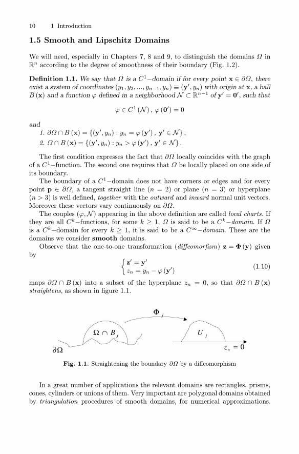
they are all Ck−functions, for some k ≥ 1, Ω is said to be a Ck−domain. If Ωis a Ck−domain for every k ≥ 1, it is said to be a C∞−domain. These are thedomains we consider smooth domains.Observe that the one-to-one transformation (diffeomorfism) z = Φ (y) given
by {z′ = y′
zn = yn − ϕ (y′) (1.10)
maps ∂Ω ∩ B (x) into a subset of the hyperplane zn = 0, so that ∂Ω ∩ B (x)straightens, as shown in figure 1.1.
Fig. 1.1. Straightening the boundary ∂Ω by a diffeomorphism
In a great number of applications the relevant domains are rectangles, prisms,cones, cylinders or unions of them. Very important are polygonal domains obtainedby triangulation procedures of smooth domains, for numerical approximations.

1.6 Integration by Parts Formulas 11
Fig. 1.2. A C1 domain and a Lipschitz domain
These types of domains belong to the class of Lipschitz domains, whose boundaryis locally described by the graph of a Lipschitz function.
Definition 1.2. We say that u : Ω → Rn is Lipschitz if there exists L such that
|u (x)− u(y)| ≤ L |x − y|
for every x,y ∈ Ω. The number L is called the Lipschitz constant of u.Roughly speaking, a function is Lipschitz in Ω if the increment quotients in
every direction are bounded. In fact, Lipschitz functions are differentiable at allpoints of their domain with the exception of a negligible set of points. Precisely,we have (see e.g. Evans and Gariepy, 1997):
Theorem 1.1. (Rademacher). Let u be a Lipschtz function in A ⊆ Rn. Then u isdifferentiable at every point of A, except at a set points of Lebesgue measure zero.
Typical real Lipschitz functions in Rn are f (x) = |x| or, more generally, thedistance function from a closed set, C, defined by
f (x) = dist (x, C) = infy∈C
|x − y| .
We say that a domain is Lipschitz if in Definition 1.1 the functions ϕ areLipschitz or, equivalently, if the map (1.10) is a bi-Lipschitz transformation, thatis, both Φ and Φ−1 are Lipschitz.
1.6 Integration by Parts Formulas
Let Ω ⊂ Rn, be a C1− domain. For vector fields
F =(F1, F2, ..., Fn) : Ω → Rn

12 1 Introduction
with F ∈C1(Ω), the Gauss divergence formula holds:
∫
Ω
divF dx =
∫
∂Ω
F · ν dσ (1.11)
where divF =∑n
j=1 ∂xjFj, ν denotes the outward normal unit vector to ∂Ω, anddσ is the “surface” measure on ∂Ω, locally given in terms of local charts by
dσ =√1 + |∇ϕ (y′)| dy′.
A number of useful identities can be derived from (1.11). Applying (1.11) to vF,with v ∈ C1
(Ω), and recalling the identity
div(vF) = v divF+∇v · F
we obtain the following integration by parts formula:
∫
Ω
v divF dx =
∫
Ω
vF · ν dσ −∫
Ω
∇v · F dx. (1.12)
Choosing F = ∇u, u ∈ C2 (Ω)∩C1(Ω), since div∇u = Δu and ∇u ·ν = ∂νu, the
followingGreen’s identity follows:
∫
Ω
vΔu dx =
∫
∂Ω
v∂νu dσ −∫
Ω
∇v · ∇u dx. (1.13)
In particular, the choice v ≡ 1 yields∫
Ω
Δu dx =
∫
∂Ω
∂νu dσ. (1.14)
If also v ∈ C2 (Ω) ∩ C1(Ω), interchanging the roles of u and v in (1.13) and
subtracting, we derive a second Green’s identity:
∫
Ω
(vΔu− uΔv) dx =∫
∂Ω
(v∂νu− u∂νv) dσ. (1.15)
Remark 1.1. All the above formulas hold for Lipschitz domains as well. In fact, theRademacher theorem implies that at every point of the boundary of a Lipschitzdomain, with the exception of a set of points of surface measure zero, there is awell defined tangent plane. This is enough for extending the formulas (1.12), (1.13)and (1.15) to Lipchitz domains.

2
Diffusion
The Diffusion Equation – Uniqueness – The Fundamental Solution – Symmetric Ran-
dom Walk (n = 1) – Diffusion, Drift and Reaction – Multidimensional Random Walk –
An Example of Reaction−Diffusion (n = 3) – The Global Cauchy Problem (n = 1) –An Application to Finance – Some Nonlinear Aspects
2.1 The Diffusion Equation
2.1.1 Introduction
The one-dimensional diffusion equation is the linear second order partial differ-ential equation
ut −Duxx = fwhere u = u (x, t) , x is a real space variable, t a time variable and D a positiveconstant, called diffusion coefficient. In space dimension n > 1, that is whenx ∈ Rn, the diffusion equation reads
ut −DΔu = f (2.1)
where Δ denotes the Laplace operator:
Δ =
n∑k=1
∂2
∂x2k.
When f ≡ 0 the equation is said to be homogeneous and in this case the su-perposition principle holds: if u and v are solutions of (2.1) and a, b are real (orcomplex) numbers, au+ bv also is a solution of (2.1). More generally, if uk (x,t) isa family of solutions depending on the parameter k (integer or real) and g = g (k)is a function rapidly vanishing at infinity, then
∞∑k=1
uk (x,t) g (k) and
∫ +∞−∞
uk (x,t) g (k) dk
are still solutions.
Salsa S. Partial Differential Equations in Action: From Modelling to Theoryc© Springer-Verlag 2008, Milan

14 2 Diffusion
A common example of diffusion is given by heat conduction in a solid body. Con-duction comes from molecular collision, transferring heat by kinetic energy, withoutmacroscopic material movement. If the medium is homogeneous and isotropic withrespect to the heat propagation, the evolution of the temperature is described byequation (2.1); f represents the intensity of an external distributed source. Forthis reason equation (2.1) is also known as the heat equation.On the other hand equation (2.1) constitutes a much more general diffusion
model, where by diffusion we mean, for instance, the transport of a substance dueto the molecular motion of the surrounding medium. In this case, u could representthe concentration of a polluting material or of a solute in a liquid or a gas (dye ina liquid, smoke in the atmosphere) or even a probability density. We may say thatthe diffusion equation unifies at a macroscopic scale a variety of phenomena, thatlook quite different when observed at a microscopic scale.Through equation (2.1) and some of its variants we will explore the deep con-
nection between probabilistic and deterministic models, according (roughly) to thescheme
diffusion processes ↔ probability density↔ differential equations.The star in this field isBrownian motion, derived from the name of the botanist
Brown, who observed in the middle of the 19th century, the apparently chaoticbehavior of certain particles on a water surface, due to the molecular motion. Thisirregular motion is now modeled as a stochastic process under the terminology ofWiener process or Brownian motion. The operator
1
2Δ
is strictly related to Brownian motion1 and indeed it captures and synthesizes themicroscopic features of that process.Under equilibrium conditions, that is when there is no time evolution, the
solution u depends only on the space variable and satisfies the stationary versionof the diffusion equation (letting D = 1)
−Δu = f (2.2)
(−uxx = f, in dimension n = 1). Equation (2.2) is known as the Poisson equation.When f = 0, it is called Laplace’s equation and its solutions are so important inso many fields that they have deserved the special name of harmonic functions.This equation will be considered in the next chapter.
2.1.2 The conduction of heat
Heat is a form of energy which it is frequently convenient to consider as separatedfrom other forms. For historical reasons, calories instead of Joules are used as unitsof measurement, each calorie corresponding to 4.182 Joules.
1 In the theory of stochastic processes, 12Δ represents the infinitesimal generator of the
Brownian motion.

2.1 The Diffusion Equation 15
We want to derive a mathematical model for the heat conduction in a solidbody. We assume that the body is homogeneous and isotropic, with constant massdensity ρ, and that it can receive energy from an external source (for instance, froman electrical current or a chemical reaction or from external absorption/radiation).Denote by r the time rate per unit mass at which heat is supplied2 by the externalsource.Since heat is a form of energy, it is natural to use the law of conservation of
energy, that we can formulate in the following way:
Let V be an arbitrary control volume inside the body. The time rate of changeof thermal energy in V equals the net flux of heat through the boundary ∂V of V ,due to the conduction, plus the time rate at which heat is supplied by the externalsources.
If we denote by e=e (x, t) the thermal energy per unit mass, the total quantityof thermal energy inside V is given by
∫
V
eρ dx
so that its time rate of change is3
d
dt
∫
V
eρ dx =
∫
V
etρ dx.
Denote by q the heat flux vector4, which specifies the heat flow direction and themagnitude of the rate of flow across a unit area. More precisely, if dσ is an areaelement contained in ∂V with outer unit normal ν, then q · νdσ is the energy flowrate through dσ and therefore the total inner heat flux through ∂V is given by
−∫
∂V
q · ν dσ =(divergence theorem)
−∫
V
divq dx.
Finally, the contribution due to the external source is given by∫
V
rρ dx.
Thus, conservation of energy requires:
∫
V
etρ dx = −∫
V
divq dx+
∫
V
rρ dx. (2.3)
The arbitrariness of V allows us to convert the integral equation (2.3) into thepointwise relation
etρ = − divq+rρ (2.4)
2 Dimensions of r: [r] = [cal]× [time]−1 × [mass]−1 .3 Assuming that the time derivative can be carried inside the integral.4 [q] = [cal]× [lenght]−2 × [time]−1 .

16 2 Diffusion
that constitutes a basic law of heat conduction. However, e and q are unknown andwe need additional information through constitutive relations for these quantities.We assume the following:
• Fourier law of heat conduction. Under “normal” conditions, for many solidmaterials, the heat flux is a linear function of the temperature gradient, that is:
q = −κ∇u (2.5)
where u is the absolute temperature and κ > 0, the thermal conductivity5, dependson the properties of the material. In general, κ may depend on u, x and t, butoften varies so little in cases of interest that it is reasonable to neglect its variation.Here we consider κ constant so that
divq = −κΔu. (2.6)
The minus sign in the law (2.5) reflects the tendency of heat to flow from hotterto cooler regions.
• The thermal energy is a linear function of the absolute temperature:
e = cvu (2.7)
where cv denotes the specific heat6 (at constant volume) of the material. In many
cases of interest cv can be considered constant. The relation (2.7) is reasonablytrue over not too wide ranges of temperature.
Using (2.6) and (2.7), equation (2.4) becomes
ut =κ
cv�Δu+
1
cvr (2.8)
which is the diffusion equation with D = κ/ (cv�) and f = r/cv. As we will see,the coefficient D, called thermal diffusivity, encodes the thermal response time ofthe material.
2.1.3 Well posed problems (n = 1)
As we have mentioned at the end of chapter one, the governing equations in amathematical model have to be supplemented by additional information in order toobtain a well posed problem, i.e. a problem that has exactly one solution, dependingcontinuously on the data.On physical grounds, it is not difficult to outline some typical well posed prob-
lems for the heat equation. Consider the evolution of the temperature u insidea cylindrical bar, whose lateral surface is perfectly insulated and whose length ismuch larger than its cross-sectional area A. Although the bar is three dimensional,
5 [κ] = [cal]× [deg]−1 × [time]−1 × [length]−1 (deg stays for degree, Celsius or Kelvin).6 [cv] = [cal]× [deg]−1 × [mass]−1 .

2.1 The Diffusion Equation 17
we may assume that heat moves only down the length of the bar and that the heattransfer intensity is uniformly distributed in each section of the bar. Thus we mayassume that e = e (x, t) , r = r (x, t), with 0 ≤ x ≤ L. Accordingly, the constitutiverelations (2.5) and (2.7) read
e (x, t) = cvu (x, t) , q = −κuxi.
By choosing V = A× [x, x+Δx] as the control volume in (2.3), the cross-sectionalarea A cancels out, and we obtain
∫ x+Δx
x
cvρut dx =
∫ x+Δx
x
κuxx dx+
∫ x+Δx
x
rρ dx
that yields for u the one-dimensional heat equation
ut −Duxx = f.
We want to study the temperature evolution during an interval of time, say, fromt = 0 until t = T . It is then reasonable to prescribe its initial distribution insidethe bar: different initial configurations will correspond to different evolutions ofthe temperature along the bar. Thus we need to prescribe the initial condition
u (x, 0) = g (x)
where g models the initial temperature profile.This is not enough to determine a unique evolution; it is necessary to know
how the bar interacts with the surroundings. Indeed, starting with a given initialtemperature distribution, we can change the evolution of u by controlling thetemperature or the heat flux at the two ends of the bar7; for instance, we could keepthe temperature at a certain fixed level or let it vary in a certain way, dependingon time. This amounts to prescribing
u (0, t) = h1 (t) , u (L, t) = h2 (t) (2.9)
at any time t ∈ (0, T ]. The (2.9) are called Dirichlet boundary conditions .We could also prescribe the heat flux at the end points. Since from Fourier law
we haveinward heat flow at x = 0 : −κux (0, t)inward heat flow at x = L : κux (L, t)
the heat flux is assigned through the Neumann boundary conditions
−ux (0, t) = h1 (t) , ux (L, t) = h2 (t)
at any time t ∈ (0, T ].7 Remember that the bar has perfect lateral thermal insulation.

18 2 Diffusion
Another type of boundary condition is the Robin or radiation condition.Let the surroundings be kept at temperature U and assume that the inward heatflux from one end of the bar, say x = L, depends linearly on the difference U − u,that is8
κux = γ(U − u) (γ > 0). (2.10)
Letting α = γ/κ > 0 e h = γU/κ, the Robin condition at x = L reads
ux + αu = h.
Clearly, it is possible to assign mixed conditions: for instance, at one end aDirichlet condition and at the other one a Neumann condition.
The problems associated with the above boundary conditions have a corre-sponding nomenclature. Summarizing, we can state the most common problemsfor the one dimensional heat equation as follows: given f = f (x, t) (externalsource) and g = g (x) (initial or Cauchy data), determine u = u (x, t) such that:
⎧⎪⎨⎪⎩
ut −Duxx = f 0 < x < L, 0 < t < T
u (x, 0) = g (x) 0 ≤ x ≤ L+ boundary conditions 0 < t ≤ T
where the boundary conditions may be:
• Dirichlet:u (0, t) = h1 (t) , u (L, t) = h2 (t) ,
• Neumann:−ux (0, t) = h1 (t) , ux (L, t) = h2 (t) ,
• Robin or radiation:
−ux (0, t) + αu (0, t) = h1 (t) , ux (L, t) + αu (L, t) = h2 (t) (α > 0),
ormixed conditions. Accordingly, we have the initial-Dirichlet problem, the initial-Neumann problem and so on. When h1 = h2 = 0, we say that the boundaryconditions are homogeneous.
Remark 2.1. Observe that only a special part of the boundary of the rectangle
QT = (0, L)× (0, T ) ,
called the parabolic boundary of QT , carries the data (see Fig. 2.1). No final con-dition (for t = T, 0 < x < L) is required.
8 Formula (2.10) is based on Newton’s law of cooling : the heat loss from the surface ofa body is a linear function of the temperature drop U −u from the surroudings to thesurface. It represents a good approximation to the radiative loss from a body when|U − u| /u� 1.

2.1 The Diffusion Equation 19
Fig. 2.1. The parabolic boundary of QT
In important applications, for instance in financial mathematics, x varies overunbounded intervals, typically (0,∞) or R. In these cases one has to require thatthe solution do not grow too much at infinity. We will later consider the globalCauchy problem:
⎧⎪⎨⎪⎩
ut −Duxx = f x ∈ R, 0 < t < Tu (x, 0) = g (x) x ∈ R+ conditions as x→ ±∞.
2.1.4 A solution by separation of variables
We will prove that under reasonable hypotheses the initial Dirichlet, Neumann orRobin problems are well posed. Sometimes this can be shown using elementarytechniques like the separation of variables method that we describe below througha simple example of heat conduction. We will come back to this method from amore general point of view in Section 6.9.
As in the previous section, consider a bar (that we can consider one-dimensional)of length L, initially (at time t = 0) at constant temperature u0. Thereafter, theend point x = 0 is kept at the same temperature while the other end x = L iskept at a constant temperature u1 > u0. We want to know how the temperatureevolves inside the bar.Before making any computations, let us try to conjecture what could happen.
Given that u1 > u0, heat starts flowing from the hotter end, raising the temper-ature inside the bar and causing a heat outflow into the cold boundary. On theother hand, the interior increase of temperature causes the hot inflow to decreasein time, while the ouflow increases. We expect that sooner or later the two fluxesbalance each other and that the temperature eventually reaches a steady state

20 2 Diffusion
distribution. It would also be interesting to know how fast the steady state isreached.
We show that this is exactly the behavior predicted by our mathematical model,given by the heat equation
ut −Duxx = 0 t > 0, 0 < x < L
with the initial-Dirichlet conditions
u (x, 0) = g (x) 0 ≤ x ≤ Lu (0, t) = u0, u (L, t) = u1 t > 0.
Since we are interested in the long term behavior of our solution, we leave t un-limited. Notice the jump discontinuity between the initial and the boundary dataat x = L; we will take care of this little difficulty later.
• Dimensionless variables. First of all we introduce dimensionless variables,that is variables independent of the units of measurement. To do that we rescalespace, time and temperature with respect to quantities that are characteristic ofour problem. For the space variable we can use the length L of the bar as rescalingfactor, setting
y =x
L
which is clearly dimensionless, being a ratio of lengths. Notice that
0 ≤ y ≤ 1.
How can we rescale time? Observe that the dimensions of the diffusion coefficientD are
[length]2 × [time]−1.Thus the constant τ = L2/D gives a characteristic time scale for our diffusionproblem. Therefore we introduce the dimensionless time
s =t
τ. (2.11)
Finally, we rescale the temperature by setting
z (y, s) =u (Ly, τ s)− u0u1 − u0
.
For the dimensionless temperature z we have:
z (y, 0) =u (Ly, 0)− u0u1 − u0
= 0, 0 ≤ y ≤ 1
z (0, s) =u (0, τs)− u0u1 − u0
= 0, z (1, s) =u (L, τs) − u0u1 − u0
= 1.

2.1 The Diffusion Equation 21
Moreover
(u1 − u0)zs =∂t
∂sut = τut =
L2
Dut
(u1 − u0)zyy =(∂x
∂y
)2uxx = L
2uxx.
Hence, since ut = Duxx,
(u1 − u0)(zs − zyy) =L2
Dut − L2uxx =
L2
DDuxx − L2uxx = 0.
In conclusion, we findzs − zyy = 0 (2.12)
with the initial conditionz (y, 0) = 0 (2.13)
and the boundary conditions
z (0, s) = 0, z (1, s) = 1. (2.14)
We see that in the dimensionless formulation the parameters L and D have disap-peared, emphasizing the mathematical essence of the problem. On the other hand,we will show later the relevance of the dimensionless variables in test modelling.
• The steady state solution . We start solving problem (2.12), (2.13), (2.14) byfirst determining the steady state solution zSt, that satisfies the equation zyy = 0and the boundary conditions (2.14). An elementary computation gives
zSt (y) = y.
In terms of the original variables the steady state solution is
uSt (x) = u0 + (u1 − u0)x
L
corresponding to a uniform heat flux along the bar given by the Fourier law:
heat flux = −κux = −κ(u1 − u0)L
.
• The transient regime. Knowing the steady state solution, it is convenient tointroduce the function
U (y, s) = zSt (y, s) − z (y, s) = y − z (y, s) .
Since we expect our solution to eventually reach the steady state, U represents atransient regime that should converge to zero as s→∞. Furthermore, the rate ofconvergence to zero of U gives information on how fast the temperature reachesits equilibrium distribution. U satisfies (2.12) with initial condition
U (y, 0) = y (2.15)

22 2 Diffusion
and homogeneous boundary conditions
U (0, s) = 0 and U (1, s) = 0. (2.16)
• The method of separation of variables. We are now in a position to findan explicit formula for U using the method of separation of variables. The mainidea is to exploit the linear nature of the problem constructing the solution bysuperposition of simpler solutions of the form w (s) v (y) in which the variables sand y appear in separated form.
Step 1. We look for non-trivial solutions of (2.12) of the form
U (y, s) = w (s) v (y)
with v (0) = v (1) = 0. By substitution in (2.12) we find
0 = Us − Uyy = w′ (s) v (y) − w (s) v′′ (y)
from which, separating the variables,
w′ (s)w (s)
=v′′ (y)v (y)
. (2.17)
Now, the left hand side in (2.17) is a function of s only, while the right handside is a function of y only and the equality must hold for every s > 0 and everyy ∈ (0, L) . This is possible only when both sides are equal to a common constantλ, say. Hence we have
v′′ (y) − λv (y) = 0 (2.18)
withv (0) = v (1) = 0 (2.19)
andw′ (s) − λw (s) = 0. (2.20)
Step 2. We first solve problem (2.18), (2.19). There are three different possi-bilities for the general solution of (2.18):
a) If λ = 0,v (y) = A+ By (A,B arbitrary constants)
and the conditions (2.19) imply A = B = 0.
b) If λ is a positive real number, say λ = μ2 > 0, then
v (y) = Ae−μy + Beμy
and again it is easy to check that the conditions (2.19) imply A = B = 0.
c) Finally, if λ = −μ2 < 0, then
v (y) = A sinμy + B cos μy.

2.1 The Diffusion Equation 23
From (2.19) we get
v (0) = B = 0
v (1) = A sinμ +B cosμ = 0
from which
A arbitrary, B = 0, μm = mπ, m = 1, 2, ... .
Thus, only in case c) we find non-trivial solutions
vm (y) = A sinmπy. (2.21)
In this context, (2.18), (2.19) is called an eigenvalue problem; the special valuesμm are the eigenvalues and the solutions vm are the corresponding eigenfunctions.With λ = −μ2m = −m2π2, the general solution of (2.20) is
wm (s) = Ce−m2π2s (C arbitrary constant). (2.22)
From (2.21) and (2.22) we obtain damped sinusoidal waves of the form
Um (y, s) = Ame−m2π2s sinmπy.
Step 3. Although the solutions Um satisfy the homogeneous Dirichlet condi-tions, they do not match, in general, the initial condition U (y, 0) = y. As wealready mentioned, we try to construct the correct solution superposing the Umby setting
U (y, s) =
∞∑m=1
Ame−m2π2s sinmπy. (2.23)
Some questions arise:
Q1. The initial condition requires
U (y, 0) =
∞∑m=1
Am sinmπy = y for 0 ≤ y ≤ 1. (2.24)
Is it possible to choose the coefficients Am in order to satisfy (2.24)? In whichsense does U attain the initial data? For instance, is it true that
U (z, s)→ y if (z, s)→ (y, 0)?
Q2. Any finite linear combination of the Um is a solution of the heat equation;can we make sure that the same is true for U? The answer is positive if we coulddifferentiate term by term the infinite sum and get
(∂s − ∂2yy)U (y, s) =∞∑m=1
(∂s − ∂yy)Um (y, s) = 0. (2.25)

24 2 Diffusion
What about the boundary conditions?
Q3. Even if we have a positive answer to questions 1 and 2, are we confidentthat U is the unique solution of our problem and therefore that it describes thecorrect evolution of the temperature?
Q1. Question 1 is rather general and concerns the Fourier series expansion9 ofa function, in particular of the initial data f (y) = y, in the interval (0, 1). Dueto the homogeneous Dirichlet conditions it is convenient to expand f (y) = y in asine Fourier series, whose coefficients are given by the formulas
Am = 2
∫ 10
y sinmπy dy = − 2mπ[y cosmπy]10 +
2
mπ
∫ 10
cosmπy dy =
= −2cosmπmπ
= (−1)m+1 2mπ.
The sine Fourier expansion of f (y) = y is therefore
y =
∞∑m=1
(−1)m+1 2mπsinmπy. (2.26)
Where is the expansion (2.26) valid? It cannot be true at y = 1 since sinmπ = 0for every m and we would obtain 1 = 0. This clearly reflects the jump discontinuityof the data at y = 1.The theory of Fourier series implies that (2.26) is true at every point y ∈ [0, 1)
and that the series converges uniformly in every interval [0, a], a < 1. Moreover,equality (2.26) holds in the leat square sense (or L2 (0, 1) sense), that is
∫ 10
[y−N∑m=1
(−1)m+1 2mπsinmπy]2dy → 0 as N →∞.
From (2.23) and the expression of Am, we obtain the formal solution
U (y, s) =
∞∑m=1
(−1)m+1 2mπe−m
2π2s sinmπy (2.27)
that attains the initial data in the least squares sense, i.e.10.
lims→0+
∫ 10
[U (y, s) − y]2dy = 0. (2.28)
In fact, from Parseval’s equality11, we can write
∫ 10
[U (y, s) − y]2 dy = 4π2
∞∑m=1
(e−m
2π2s − 1)2
m2. (2.29)
9 Appendix A.10 It is also true that U (z, s)→ y in the pointwise sense, when y �= 1 and (z, s)→ (y, 0).We omit the proof.
11 Appendix A.
2.1 The Diffusion Equation 25
Since for s ≥ 0 (e−m
2π2s − 1)2
m2≤ 1
m2
and the series∑1/m2 converges, then the series (2.29) converges uniformly by
the Weierstrass test (see Section 1.4) in [0,∞) and we can take the limit underthe sum, obtaining (2.28).
Q2. The analytical expression of U is rather reassuring: it is a superpositionof sinusoids of increasing frequency m and of strongly damped amplitude becauseof the negative exponential, at least when s > 0. Indeed, for s > 0, the rapidconvergence to zero of each term and its derivatives in the series (2.27) allows usto differentiate term by term. Precisely, we have
∂Um
∂s= (−1)m+2 2mπe−m2π2s sinmπy, ∂
2Um
∂y2= (−1)m+2 2e−m2π2s sinmπy
so that, if s ≥ s0 > 0,∣∣∣∣∂Um
∂s
∣∣∣∣ ≤ 2mπe−m2π2s0 ,
∣∣∣∣∂2Um
∂y2
∣∣∣∣ ≤ 2mπe−m2π2s0 .
Since the numerical series ∞∑m=1
me−m2π2s0
is convergent, we conclude by the Weierstrass test that the series
∞∑m=1
∂Um
∂sand
∞∑m=1
∂2Um
∂y2
converge uniformly in [0, 1] × [s0,∞) so that (2.25) is true and therefore U is asolution of (2.12).It remains to check the Dirichlet conditions: if s0 > 0,
U (z, s)→ 0 as (z, s)→ (0, s0) or (z, s)→ (L, s0) .
This is true because we can take the two limits under the sum, due to the uniformconvergence of the series (2.27) in any region [0, L]× (b,+∞) with b > 0. For thesame reason, U has continuous derivatives of any order, up to the lateral boundaryof the strip [0, L]× (b,+∞) .Note, in particular, that U immediately forgets the initial discontinuity and
becomes smooth at any positive time.
Q3. To show that U is indeed the unique solution, we use the so-called energymethod, that we will develop later in greater generality. Suppose W is anothersolution of problem (2.12), (2.15), (2.16). Then, by linearity,
v = U −W

26 2 Diffusion
satisfiesvs − vyy = 0 (2.30)
and has zero initial-boundary data. Multiplying (2.30) by v, integrating in y overthe interval [0, 1] and keeping s > 0, fixed, we get
∫ 10
vvs dy −∫ 10
vvyy dy = 0. (2.31)
Observe that ∫ 10
vvs dy =1
2
∫ 10
∂s(v2)dy =
1
2
d
ds
∫ 10
v2dy. (2.32)
Moreover, integrating by parts we can write
∫ 10
vvyy dy = [v (1, s) vy (1, s)− v (0, s) vy (0, s)]−∫ 10
(vy)2dy (2.33)
= −∫ 10
(vy)2dy
since v (1, s) = v (0, s) = 0. From (2.31), (2.32) and (2.33) we get
1
2
d
ds
∫ 10
v2dy = −∫ 10
(vy)2 dy ≤ 0 (2.34)
and therefore, the nonnegative function
E (s) =
∫ 10
v2 (y, s) dy
is non-increasing. On the other hand, using (2.28) for v instead of U , we get
E (s)→ 0 as s→ 0which forces E (s) = 0, for every s > 0. But v2 (y, s) is nonnegative and continuousin [0, 1] if s > 0, so that it must be v (y, s) = 0 for every s > 0 or, equivalently,U =W.
• Back to the original variables. In terms of the original variables, our solutionis expressed as
u (x, t) = u0 + (u1 − u0)x
L−
∞∑m=1
(−1)m+1 2mπe−m2π2D
L2t sin
mπ
Lx.
This formula confirms our initial guess about the evolution of the temperaturetowards the steady state. Indeed, each term of the series converges to zero expo-nentially as t→ +∞ and it is not difficult to show12 that
u (x, t)→ u0 + (u1 − u0)x
Las t→ +∞.
12 The Weierstrass test works here for t ≥ t0 > 0.

2.1 The Diffusion Equation 27
Moreover, among the various terms of the series, the first one (m = 1) decays muchmore slowly than the others and very soon it determines the main deviation of ufrom the equilibrium, independently of the initial condition. This leading term isthe damped sinusoid
2
πe−π2DL2
t sinπ
Lx.
In this mode there is a concentration of heat at x = L/2 where the temperaturereaches its maximum amplitude 2 exp(−π2Dt/L2)/π. At time t = L2/D the am-plitude decays to 2 exp(−π2)/π � 3.3 × 10⁻⁵, about 0.005 per cent of its initialvalue. This simple calculation shows that to reach the steady state a time of orderL2/D is required, a fundamental fact in heat diffusion.Not surprisingly, the scaling factor in (2.11) was exactly τ = L2/D. The di-
mensionless formulation is extremely useful in experimental modelling tests. Toachieve reliable results, these models must reproduce the same characteristics atdifferent scales. For instance, if our bar were an experimental model of a muchbigger beam of length L0 and diffusion coefficient D0, to reproduce the same heatdiffusion effects, we must choose material (D) and length (L) for our model barsuch that
L2
D=L20D0.
Figure 2.2 shows the solution of the dimensionless problem (2.12), (2.15), (2.16)for 0 < t ≤ 1.
Fig. 2.2. The solution to the dimensionless problem (2.12), (2.13), ( 2.14)
2.1.5 Problems in dimension n > 1
The formulation of the well posed problems in subsection 2.1.3 can be easily gen-eralized to any spatial dimension n > 1, in particular to n = 2 or n = 3. Supposewe want to determine the evolution of the temperature in a heat conducting bodythat occupies a bounded domain13 Ω ⊂ Rn, during an interval of time [0, T ]. Un-der the hypotheses of subsection 2.1.2, the temperature is a function u = u (x,t)
13 Recall that by domain we mean an open connected set in Rn.
28 2 Diffusion
that satisfies the heat equation ut −DΔu = f , in the space-time cylinder
QT = Ω × (0, T ) .
To select a unique solution we have to prescribe first of all the initial distribution
u (x, 0) = g (x) x ∈Ω,
where Ω = Ω ∪ ∂Ω denotes the closure of Ω.The control of the interaction of the body with the surroundings is modeled
through suitable conditions on ∂Ω. The most common ones are:
Dirichlet condition: the temperature is kept at a prescribed level on ∂Ω; thisamounts to assigning
u (σ, t) = h (σ,t) σ ∈ ∂Ω and t ∈ (0, T ].
Neumann condition: the heat flux through ∂Ω is assigned. To model thiscondition, we assume that the boundary ∂Ω is a smooth curve or surface, havinga tangent line or plane at every point14 with outward unit vector ν. From Fourierlaw we have
q = heat flux = −κ∇uso that the inward heat flux is
−q · ν =κ∇u · ν =κ∂νu.
Thus the Neumann condition reads
∂νu (σ, t) = h (σ,t) σ ∈ ∂Ω and t ∈ (0, T ].
Radiation or Robin condition: the inward (say) heat flux through ∂Ωdepends linearly on the difference15 U − u:
−q · ν =γ (U − u) (γ > 0)
where U is the ambient temperature. From the Fourier law we obtain
∂νu+ αu = h on ∂Ω × (0, T ]
with α = γ/κ > 0, h = γU/κ.
Mixed conditions: the boundary of Ω is decomposed into various parts wheredifferent boundary conditions are prescribed. For instance, a formulation of a mixedDirichlet-Neumann problem is obtained by writing
∂Ω = ∂DΩ ∪ ∂NΩ with ∂DΩ ∩ ∂NΩ = ∅14 We can also allow boundaries with corner points, like squares, cones, or edges, likecubes. It is enough that the set of points where the tangent plane does not exist haszero surface measure (zero length in two dimensions). Lipschitz domains have thisproperty (see Section 1.4).
15 Linear Newton law of cooling.

2.1 The Diffusion Equation 29
where ∂DΩ and ∂NΩ “reasonable” subsets of ∂Ω. Typically ∂NΩ = ∂Ω∩A, whereA is open in Rn. In this case we say that ∂NΩ is a relatively open set in ∂Ω. Thenwe assign
u = h1 on ∂DΩ × (0, T ]∂νu = h2 on ∂NΩ × (0, T ].
Summarizing, we have the following typical problems: given f = f (x, t) andg = g (x), determine u = u (x, t) such that:⎧⎪⎨
⎪⎩
ut −DΔu = f in QT
u (x, 0) = g (x) in Ω
+ boundary conditions on ∂Ω × (0, T ]where the boundary conditions are:
• Dirichlet:u = h,
• Neumann:∂νu = h,
• radiation or Robin:∂νu+ αu = h (α > 0) ,
• mixed:u = h1 on ∂DΩ, ∂νu = h2 on ∂NΩ.
Fig. 2.3. The space-time cylinder QT
Also in dimension n > 1, the global Cauchy problem is important:⎧⎪⎨⎪⎩
ut −DΔu = f x ∈Rn, 0 < t < Tu (x, 0) = g (x) x ∈Rn+ condition as |x| → ∞.

30 2 Diffusion
Remark 2.2. We again emphasize that no final condition (for t = T,x ∈Ω) is re-quired. The data is assigned on the parabolic boundary ∂pQT of QT , given by theunion of the bottom points Ω × {t = 0} and the side points ∂Ω × (0, T ]:
∂pQT =(Ω × {t = 0}
)∪ (∂Ω × (0, T ]) .
2.2 Uniqueness
2.2.1 Integral method
Generalizing the energy method used in subsection 2.1.4, it is easy to show that allthe problems we have formulated in the previous section have at most one solutionunder reasonable conditions on the data. Suppose u and v are solutions of oneof those problems, sharing the same boundary conditions, and let w = u− v; wewant to show that w ≡ 0. For the time being we do not worry about the precisehypotheses on u e v; we assume they are sufficiently smooth in QT up to ∂pQTand observe that w satisfies the homogeneous equation
wt −DΔw = 0 (2.35)
in QT = Ω × (0, T ), with initial condition
w (x,0) = 0
in Ω, and one of the following conditions on ∂Ω × (0, T ]:
w = 0 (Dirichlet) (2.36)
or∂νw = 0 (Neumann) (2.37)
or∂νw + αw = 0 α > 0, (Robin) (2.38)
orw = 0 on ∂DΩ, ∂νw = 0 on ∂NΩ (mixed). (2.39)
Multiply equation (2.35) by w and integrate on Ω; we find∫
Ω
wwt dx = D
∫
Ω
wΔw dx.
Now, ∫
Ω
wwt dx =1
2
d
dt
∫
Ω
w2dx (2.40)
and from Green’s identity (1.13) with u = v = w,∫
Ω
wΔw dx =
∫
∂Ω
w∂νw dσ −∫
Ω
|∇w|2 dx. (2.41)

2.2 Uniqueness 31
Then, letting
E (t) =
∫
Ω
w2dx,
(2.40) and (2.41) give
1
2E′ (t) = D
∫
∂Ω
w∂νw dσ −D∫
Ω
|∇w|2 dx.
If Robin condition (2.38) holds,
∫
∂Ω
w∂νw dσ = −α∫
Ω
w2dx ≤ 0.
If one of the (2.36), (2.37), (2.39) holds, then
∫
∂Ω
w∂νw dσ = 0.
In any case it follows thatE′ (t) ≤ 0
and therefore E is a nonincreasing function. Since
E (0) =
∫
Ω
w2 (x,0) dx =0,
we must have E (t) = 0 for every t ≥ 0 and this implies w (x,t) ≡ 0 in Ω for everyt > 0. Thus u = v.
The above calculations are completely justified if Ω is a sufficiently smoothdomain16 and, for instance, we require that u and v are continuous in QT = Ω ×[0, T ], together with their first and second spatial derivatives and their first ordertime derivatives. We denote the set of these functions by the symbol (not tooappealing...)
C2,1(QT)
and synthesize everything in the following statement.
Theorem 2.1. The initial Dirichlet, Neumann, Robin and mixed problems haveat most one solution belonging to C2,1
(QT).
2.2.2 Maximum principles
The fact that heat flows from higher to lower temperature regions implies thata solution of the homogeneous heat equation attains its maximum and minimumvalues on ∂pQT . This result is known as the maximum principle. Moreover theequation reflects the time irreversibility of the phenomena that it describes, in the
16 C1 or even Lipschitz domains, for instance (see Section 1.4).

32 2 Diffusion
sense that the future cannot have an influence on the past (causality principle).In other words, the value of a solution u at time t is independent of any change ofthe data after t.The following simple theorem translates these principles and holds for functions
in the class C2,1 (QT )∩C(QT). These functions are continuous up to the boundary
of QT , with derivatives continuous in the interior of QT .
Theorem 2.2. Let w ∈ C2,1 (QT ) ∩ C(QT)such that
wt −DΔw = q ≤ 0 in QT . (2.42)
Then w attains its maximum on ∂pQT :
maxQT
w = max∂pQT
w. (2.43)
In particular, if w is negative on ∂pQT , then is negative in all QT .
Proof. We split the proof into two steps.1. Let ε > 0 such that T − ε > 0. We prove that
maxQT−ε
w ≤ max∂pQT
w + εT. (2.44)
Let u = w − εt. Thenut −DΔu = q − ε < 0. (2.45)
We claim that the maximum of u on QT−ε occurs on ∂pQT−ε. Suppose not. Let(x0, t0), x0 ∈ Ω, 0 < t0 ≤ T − ε be a maximum point for u on QT−ε. Fromelementary calculus, we have
Δu (x0, t0) ≤ 0
and eitherut (x0, t0) = 0 if t0 < T − ε
orut (x0, T − ε) ≥ 0.
In both casesut (x0, t0)−Δu (x0, t0) ≥ 0,
contradicting (2.45). Thus
maxQT−ε
u ≤ max∂pQT−ε
u ≤ max∂pQT
w (2.46)
since u ≤ w. On the other hand, w ≤ u+ εT , and therefore, from (2.46) we get
maxQT−ε
w ≤ maxQT−ε
u+ εT ≤ max∂pQT
w + εT
which is (2.44).

2.2 Uniqueness 33
Step 2. Since w is continuous in QT , we deduce that (why?)
maxQT−ε
w→ maxQT
w as ε→ 0.
Hence, letting ε→ 0 in (2.44) we find maxQT w ≤ max∂pQT w which concludes theproof. �As an immediate consequence of Theorem 2.2 (see Problem 2.4) we have that
ifwt −DΔw = 0 in QT
then w attains its maximum and its minimum on ∂pQT . In particular
min∂pQT
w ≤ w (x,t) ≤ max∂pQT
w for every (x,t) ∈ QT .
Moreover:
Corollary 2.1. (Comparison and stability). Let v and w satisfy
vt −DΔv = f1 and wt −DΔw = f2.
Then:
a) If v ≥ w on ∂pQT and f1 ≥ f2 in QT then v ≥ w in all QT .b) The following stability estimate holds
maxQT
|v −w| ≤ max∂pQT
|v −w|+ T maxQT
|f1 − f2| . (2.47)
In particular the initial-Dirichlet problem has at most one solution that, moreover,depends continuously on the data.
For the proof see Problem 2.5.
Remark 2.3. Corollary 2.1 gives uniqueness for the initial-Dirichlet problem undermuch less restrictive hypotheses than Theorem 2.1: indeed it does not require thecontinuity of any derivatives of the solution up to ∂pQT .Inequality (2.47) is a uniform pointwise stability estimate, extremely useful in
several applications. In fact if v = g1, w = g2 on ∂pQT and
max∂pQT
|g1 − g2| ≤ ε and maxQT
|f1 − f2| ≤ ε,
we deducemaxQT
|v − w| ≤ ε (1 + T ) .
Thus, in finite time, a small uniform distance between the data implies smalluniform distance between the corresponding solutions.

34 2 Diffusion
Remark 2.4. Strong maximum principle. Theorem 2.2 is a version of the so calledweak maximum principle, weak because this result says nothing about the possi-bility that a solution achieves its maximum or minimum at an interior point aswell. Actually a more precise result is known as strong maximum principle andstates17 that if a solution of ut −DΔu = 0 achieves its maximumM (minimum)at a point (x1, t1) with x1 ∈ V , 0 < t1 ≤ T , then u =M in V × [0, t1].
Fig. 2.4. The strong maximum principle
2.3 The Fundamental Solution
There are privileged solutions of the diffusion equation that can be used to con-struct many other solutions. In this section we are going to discover one of thesespecial building blocks, the most important one.
2.3.1 Invariant transformations
The homogeneous diffusion equation has simple but important properties. Letu = u (x, t) be a solution of
ut −DΔu = 0. (2.48)
• Time reversal. The function
v(x,t) = u (x,−t) ,
obtained by the change of variable t �−→ −t, is a solution of the adjoint orbackward equation.
vt +DΔv = 0.
17 We omit the rather long proof.
2.3 The Fundamental Solution 35
Coherently, the (2.48) is sometimes called the forward equation. The non-invariance of (2.48) with respect to a change of sign in time is another aspectof time irreversibility.
• Space and time translations invariance. For y,s fixed, the function
v(x,t) = u (x− y, t− s) ,
is still a solution of (2.48). Clearly, for x, t fixed the function u (x− y, t− s) is asolution of the backward equation with respect to y and s.
• Parabolic dilations The transformation
x �−→ ax, t �−→ bt, u �−→ cu (a, b, c > 0)
represents a dilation (or contraction) of the graph of u. Let us check for whichvalues of a, b, c the function
u∗ (x,t) = cu (ax,bt)
is still a solution of (2.48). We have:
u∗t (x,t) −DΔu∗ (x,t) = cbut (ax,bt)− ca2DΔu (ax,bt)
and so u∗ is a solution of (2.48) if
b = a2. (2.49)
The relation (2.49) suggests the name of parabolic dilation for the transformation
x �−→ ax t �−→ a2t (a, b > 0).
Under this transformation the expressions
|x|2Dt
orx√Dt
are left unchanged. Moreover, we already observed that they are dimensionlessgroups. Thus it is not surprising that these combinations of the independent vari-ables occur frequently in the study of diffusion phenomena.
• Dilations and conservation of mass (or energy). Let u = u (x, t) be a solutionof (2.48) in the half-space Rn × (0,+∞) . Then we just checked that the function
u∗ (x,t) = cu(ax,a2t
)(a > 0)
is also a solution in the same set. Suppose u satisfies the condition
∫
Rn
u (x, t) dx =q for every t > 0. (2.50)
36 2 Diffusion
If, for instance, u represents the concentration of a substance (density of mass),equation (2.50) states that the total mass is q at every time t. If u is a temperature,(2.50) says that the total internal energy is constant (= qρcv). We ask for whicha, c the solution u∗ still satisfies (2.50). We have
∫
Rn
u∗ (x, t)dx =c∫
Rn
u(ax, a2t
)dx.
Letting y =ax, so that dy =andx, we find
∫
Rn
u∗ (x, t) dx =ca−n∫
Rn
u(y, a2t
)dy =ca−n
and for (2.50) to be satisfied we must have:
c = qan.
In conclusion, if u = u (x,t) is a solution of (2.48) in the half-space Rn × (0,+∞)satisfying (2.50), the same is true for
u∗ (x,t) = qanu(ax,a2t
). (2.51)
2.3.2 Fundamental solution (n = 1)
We are now in position to construct our special solution, starting with dimensionn = 1. To help intuition, think for instance of our solution as the concentration ofa substance of total mass q and suppose we want to keep the total mass equal toq at any time.We have seen that the combination of variables x/
√Dt is not only invariant
with respect to parabolic dilations but also dimensionless. It is then natural tocheck if there are solutions of (2.48) involving such dimensionless group. Since√Dt has the dimension of a length, the quantity q/
√Dt is a typical order of
magnitude for the concentration, so that it makes sense to look for solutions of theform
u∗ (x,t) =q√DtU
(x√Dt
)(2.52)
where U is a (dimensionless) function of a single variable.Here is the main question: is it possible to determine U = U (ξ) such that u∗ is
a solution of (2.48)? Solutions of the form (2.52) are called similarity solutions18.
18 A solution of a particular evolution problem is a similarity or self-similar solution if itsspatial configuration (graph) remains similar to itself at all times during the evolution.In one space dimension, self-similar solutions have the general form
u (x, t) = a (t)F (x/b (t))
where, preferably, u/a and x/b are dimensionless quantity.

2.3 The Fundamental Solution 37
Moreover, since we are interpreting u∗ as a concentration, we require U ≥ 0and the total mass condition yields
1 =1√Dt
∫
R
U
(x√Dt
)dx =
ξ=x/√Dt
∫
R
U (ξ) dξ
so that we require that ∫
R
U (ξ) dξ = 1. (2.53)
Let us check if u∗ is a solution to (2.48). We have
u∗t =q√D
[−12t−
32U (ξ)− 1
2√Dxt−2U ′ (ξ)
]
= − q
2t√Dt[U (ξ) + ξU ′ (ξ)]
u∗xx =q
(Dt)3/2U ′′ (ξ) ,
hence
u∗t −Du∗xx = −q
t√Dt
{U ′′ (ξ) +
1
2ξU ′ (ξ) +
1
2U (ξ)
}.
We see that for u∗ to be a solution of (2.48), U must be a solution in R of theordinary differential equation
U ′′ (ξ) +1
2ξU ′ (ξ) +
1
2U (ξ) = 0. (2.54)
Since U ≥ 0, (2.53) implies19:
U (−∞) = U (+∞) = 0.
On the other hand, (2.54) is invariant with respect to the change of variables
ξ �→ −ξ
and therefore we look for even solutions: U (−ξ) = U (ξ). Then we can restrictourselves to ξ ≥ 0, asking
U ′ (0) = 0 and U (+∞) = 0. (2.55)
19 Rigorously, the precise conditions are:
lim infx→±∞U (x) = 0.

38 2 Diffusion
To solve (2.54) observe that it can be written in the form
d
dξ
{U ′ (ξ) +
1
2ξU (ξ)
}= 0
that yields
U ′ (ξ) +1
2ξU (ξ) = C (C ∈ R). (2.56)
Letting ξ = 0 in (2.56) and recalling (2.55) we deduce that C = 0 and therefore
U ′ (ξ) +1
2ξU (ξ) = 0. (2.57)
The general integral of (2.57) is
U (ξ) = c0e− ξ24 (c0 ∈ R).
This function is even, positive, integrable and vanishes at infinity. It only remainsto choose c0 in order to ensure (2.53). Since
20
∫
R
e−ξ2
4 dξ =ξ=2z
2
∫
R
e−z2
dz = 2√π
the choice is c0 = (4π)−1/2.
Going back to the original variables, we have found the following solution of(2.48)
u∗ (x, t) =q√4πDt
e−x2
4Dt , x ∈ R, t > 0
positive, even in x, and such that
∫
R
u∗ (x, t)dx = q for every t > 0. (2.58)
The choice q = 1 gives a family of Gaussians, parametrized with time, and it isnatural to think of a normal probability density.
Definition 2.1. The function
ΓD (x, t) =1√4πDt
e−x2
4Dt , x ∈ R, t > 0 (2.59)
is called the fundamental solution of equation (2.48).
20 Recall that ∫
R
e−z2
=√π.
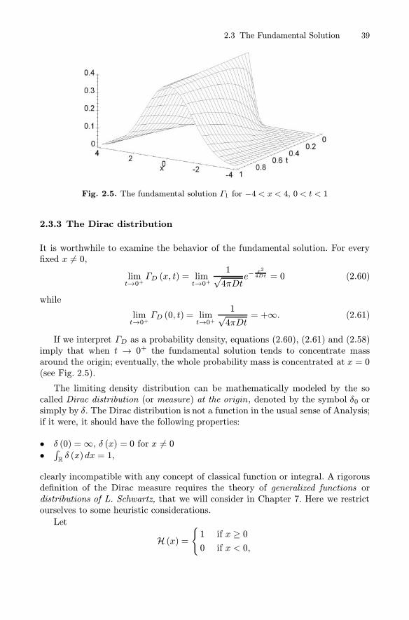
2.3 The Fundamental Solution 39
Fig. 2.5. The fundamental solution Γ1 for −4 < x < 4, 0 < t < 1
2.3.3 The Dirac distribution
It is worthwhile to examine the behavior of the fundamental solution. For everyfixed x �= 0,
limt→0+
ΓD (x, t) = limt→0+
1√4πDt
e−x2
4Dt = 0 (2.60)
while
limt→0+
ΓD (0, t) = limt→0+
1√4πDt
= +∞. (2.61)
If we interpret ΓD as a probability density, equations (2.60), (2.61) and (2.58)imply that when t → 0+ the fundamental solution tends to concentrate massaround the origin; eventually, the whole probability mass is concentrated at x = 0(see Fig. 2.5).
The limiting density distribution can be mathematically modeled by the socalled Dirac distribution (or measure) at the origin, denoted by the symbol δ0 orsimply by δ. The Dirac distribution is not a function in the usual sense of Analysis;if it were, it should have the following properties:
• δ (0) =∞, δ (x) = 0 for x �= 0•∫Rδ (x)dx = 1,
clearly incompatible with any concept of classical function or integral. A rigorousdefinition of the Dirac measure requires the theory of generalized functions ordistributions of L. Schwartz, that we will consider in Chapter 7. Here we restrictourselves to some heuristic considerations.
Let
H (x) ={1 if x ≥ 00 if x < 0,

40 2 Diffusion
Fig. 2.6. Approximation of the Dirac measure
be the characteristic function of the interval [0,∞), known as the Heaviside func-tion. Observe that
H (x+ ε) −H (x− ε)2ε
=
{12ε if − ε ≤ x < ε0 otherwise.
(2.62)
Denote by Iε (x) the quotient (2.62); the following properties hold:
i) For every ε > 0, ∫
R
Iε (x) dx =1
2ε× 2ε = 1.
We can interpret Iε as a unit impulse of extent 2ε (Fig. 2.6).
ii)
limε↓0Iε (x) =
{0 if x �= 0∞ if x = 0.
iii) If ϕ = ϕ (x) is a smooth function, vanishing outside a bounded interval, (atest function), we have
∫
R
Iε (x)ϕ (x) dx =1
2ε
∫ ε
−εϕ (x)dx −→
ε−→0 ϕ (0) .
Properties i) e ii) say that Iε tends to a mathematical object that has precisely theformal features of the Dirac distribution at the origin. In particular iii) suggestshow to identify this object, that is through its action on test functions.
Definition 2.2. We call Dirac measure at the origin the generalized function,denoted by δ, that acts on a test function ϕ as follows:
δ [ϕ] = ϕ (0) . (2.63)
Equation (2.63) is often written in the form 〈δ, ϕ〉 = ϕ (0) or even∫δ (x)ϕ (x) dx = ϕ (0)

2.3 The Fundamental Solution 41
where the integral symbol is purely formal. Observe that property ii) shows that
H′ = δ
whose meaning is given in the following computations, where an integration byparts is used and ϕ is a test function:
∫
R
ϕdH = −∫
R
Hϕ′ = −∫ ∞0
ϕ′ = ϕ (0) , (2.64)
since ϕ vanishes for large21 x .With the notion of Dirac measure at hand, we can say that ΓD satisfies the
initial conditionsΓD (x, 0) = δ.
If the unit mass is concentrated at a point y �= 0, we denote by δy or δ (x− y) theDirac measure at y, defined through the formula
∫δ (x− y)ϕ (x) dx = ϕ (y) .
Then, by translation invariance, the fundamental solution ΓD (x− y, t) is a solutionof the diffusion equation, that satisfies the initial condition
ΓD (x− y, 0) = δ (x− y) .
Indeed it is the unique solution satisfying the total mass condition (2.58) withq = 1.As any solution u of (2.48) has several interpretations (concentration of a sub-
stance, probability density, temperature in a bar) so the fundamental solution canhave several meanings.We can think of it as a unit source solution: ΓD (x, t) gives the concentration
at the point x at time t, generated by the diffusion of a unit mass initially (t = 0)concentrated at the origin. From another point of view, if we imagine a unitmass composed of a large number N of particles, ΓD (x, t) dx gives the probabilitythat a single particle is placed between x and x+ dx at time t or equivalently, thepercentage of particles inside the interval (x, x+ dx) at time t.
Initially ΓD is zero outside the origin. As soon as t > 0, ΓD becomes positiveeverywhere: this amounts to saying that the unit mass diffuses instantaneously allover the x−axis and therefore with infinite speed of propagation. This could be aproblem in using (2.48) as a realistic model, although (see Fig. 2.5) for t > 0, small,ΓD is practically zero outside an interval centered at the origin of length 4D.
21 The first integral in (2.64) is a Riemann-Stieltjes integral, that formally can be writtenas ∫
ϕ (x)H′ (x) dxand interpreted as the action of the generalized function H′ on the test function ϕ.

42 2 Diffusion
2.3.4 Fundamental solution (n > 1)
In space dimension greater than 1, we can more or less repeat the same arguments.We look for positive, radial, self-similar solutions u∗ to (2.48), with total mass equalto q at every time, that is
∫
Rn
u∗ (x,t) dx = q for every t > 0. (2.65)
Since q/ (Dt)n/2is a concentration per unit volume, we set
u∗ (x, t) =q
(Dt)n/2U (ξ) , ξ = |x| /
√Dt.
We have, recalling the expression of the Laplace operator for radial functions (seeAppendix C),
u∗t = −1
2t (Dt)n/2[nU (ξ) + ξU ′ (ξ)]
Δu∗ =1
(Dt)1+n/2
{U ′′ (ξ) +
n− 1ξU ′ (ξ)
}.
Therefore, for u∗ to be a solution of (2.48), U must be a nonnegative solution in(0,+∞) of the ordinary differential equation
ξU ′′ (ξ) + (n− 1)U ′ (ξ) + ξ2
2U ′ (ξ) +
n
2ξU (ξ) = 0. (2.66)
Multiplying by ξn−2, we can write (2.66) in the form
(ξn−1U ′)′ +1
2(ξnU)′ = 0
that gives
ξn−1U ′ +1
2ξnU = C (C ∈ R). (2.67)
Assuming that limξ→0+ of U and U ′ are finite, letting ξ → 0+ into (2.67), wededuce C = 0 and therefore
U ′ +1
2ξU = 0.
Thus we obtain the family of solutions
U (ξ) = c0e− ξ24 .
The total mass condition requires
1 =1
(Dt)n/2
∫
Rn
U
( |x|√Dt
)dx =
c0
(Dt)n/2
∫
Rn
exp
(− |x|
2
4Dt
)dx

2.4 Symmetric Random Walk (n = 1) 43
=y=x/
√Dtc0
∫
Rn
e−|y|2
dy = c0
(∫
R
e−z2
dz
)n= c0 (4π)
n/2
and therefore c0 = (4π)−n/2
. Thus, we have obtained solutions of the form
u∗ (x, t) =q
(4πDt)n/2exp
(− |x|
2
4Dt
), (t > 0) .
Once more, the choice q = 1 is special.
Definition 2.3. The function
ΓD (x, t) =1
(4πDt)n/2exp
(− |x|
2
4Dt
)(t > 0)
is called the fundamental solution of the diffusion equation (2.48).
The remarks after Definition 2.2 can be easily generalized to the multidimen-sional case. In particular, it is possible to define the n− dimensional Dirac measureat a point y through the formula22
∫δ (x − y)ϕ (x) dx = ϕ (y) (2.68)
that expresses the action on the test function ϕ, smooth in Rn and vanishingoutside a compact set. For fixed y, the fundamental solution ΓD (x− y,t) is theunique solution of the global Cauchy problem
{ut −DΔu = 0 x ∈Rn, t > 0u (x, 0) = δ (x− y) x ∈ Rn
that satisfies (2.65) with q = 1.
2.4 Symmetric Random Walk (n = 1)
In this section we start exploring the connection between probabilistic and deter-ministic models, in dimension n = 1. The main purpose is to construct a Brownianmotion, which is a continuous model (in both space and time), as a limit of asimple stochastic process, called random walk, which is instead a discrete model(in both space and time). During the realization of the limiting procedure weshall see how the diffusion equation can be approximated by a difference equa-tion. Moreover, this new perspective will better clarify the nature of the diffusioncoefficient.
22 As in dimension n = 1, in (2.68) the integral has a symbolic meaning only.
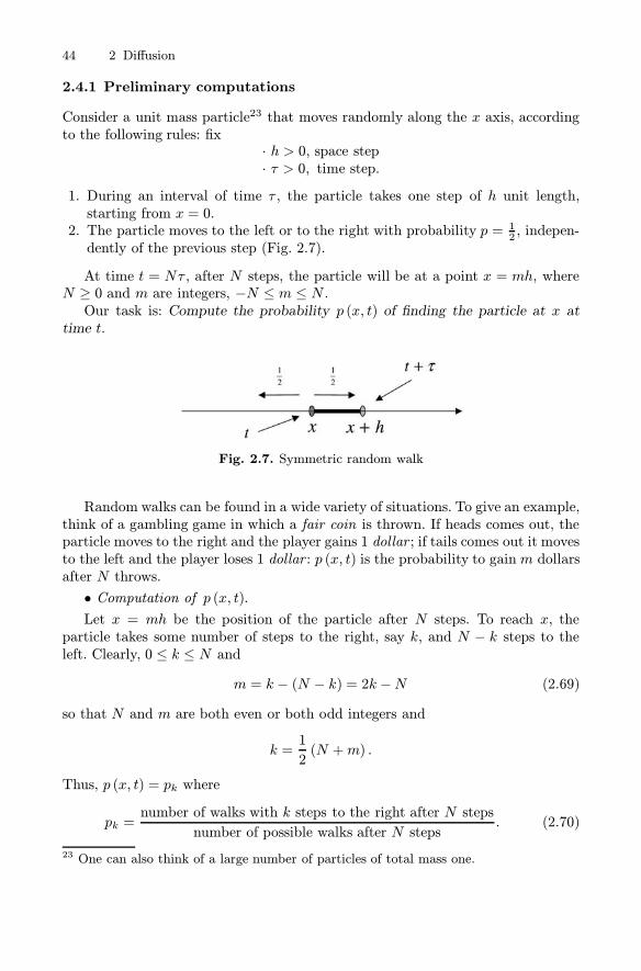
44 2 Diffusion
2.4.1 Preliminary computations
Consider a unit mass particle23 that moves randomly along the x axis, accordingto the following rules: fix
· h > 0, space step· τ > 0, time step.
1. During an interval of time τ , the particle takes one step of h unit length,starting from x = 0.
2. The particle moves to the left or to the right with probability p = 12, indepen-
dently of the previous step (Fig. 2.7).
At time t = Nτ , after N steps, the particle will be at a point x = mh, whereN ≥ 0 and m are integers, −N ≤ m ≤ N .Our task is: Compute the probability p (x, t) of finding the particle at x at
time t.
Fig. 2.7. Symmetric random walk
Random walks can be found in a wide variety of situations. To give an example,think of a gambling game in which a fair coin is thrown. If heads comes out, theparticle moves to the right and the player gains 1 dollar ; if tails comes out it movesto the left and the player loses 1 dollar : p (x, t) is the probability to gainm dollarsafter N throws.
• Computation of p (x, t).Let x = mh be the position of the particle after N steps. To reach x, the
particle takes some number of steps to the right, say k, and N − k steps to theleft. Clearly, 0 ≤ k ≤ N and
m = k − (N − k) = 2k −N (2.69)
so that N and m are both even or both odd integers and
k =1
2(N +m) .
Thus, p (x, t) = pk where
pk =number of walks with k steps to the right after N steps
number of possible walks after N steps. (2.70)
23 One can also think of a large number of particles of total mass one.
2.4 Symmetric Random Walk (n = 1) 45
Now, the number of possible walks with k steps to the right and N − k to the leftis given by the binomial coefficient24
CN,k =
(N
k
)=
N !
k! (N − k)! .
On the other hand, the number of possible walks after N steps is 2N (why?); hence,from (2.70):
pk =CN,k
2Nx = mh, t = Nτ, k =
1
2(N +m) . (2.71)
• Mean displacement and standard deviation of x.Our ultimate goal is to let h and τ go to zero in order to get a continuous
walk, which incorporates the main features of the discrete random walk. This is adelicate point, since, if we want to obtain eventually a continuous faithful copy ofthe random walk, we need to isolate some quantitative parameters able to capturethe essential features of the walk and maintain them unchanged. In our case thereare two key parameters25:
(a) the mean displacement of x after N steps = 〈x〉 = 〈m〉 h(b) the second moment of x after N steps =
⟨x2⟩=⟨m2⟩h2.
The quantity√〈x2〉 =
√〈m2〉h is essentially the average distance from the origin
after N steps.
First observe that, from (2.69), we have
〈m〉 = 2 〈k〉 −N (2.72)
and ⟨m2⟩= 4
⟨k2⟩− 4 〈k〉N +N2. (2.73)
24 The set of walks with k steps to the right and N − k to the left is in one to onecorrespondence with the set of sequences of N binary digits, containing k “1” andN − k “0”, where 1 means right and 0 means left. There are exactly CN,k of thesesequences.
25 If a random variable x takes N possible outcomes x1,..., xN with probability p1, ..., pN ,its moments of (integer) order q ≥ 1 are given by
E (xq) = 〈xq〉 =N∑
j=1
xqjpj .
The first moment (q = 1) is the mean or expected value of x, while
var (x) =⟨x2⟩− 〈x〉2
is the variance of x. The square root of the variance is called standard deviation .

46 2 Diffusion
Thus, to compute 〈m〉 and⟨m2⟩it is enough to compute 〈k〉 and
⟨k2⟩. We have,
by definition and from (2.71),
〈k〉 =N∑k=1
kpk =1
2N
N∑k=1
kCN,k,⟨k2⟩=
N∑k=1
k2pk =1
2N
N∑k=1
k2CN,k. (2.74)
Although it is possible to make the calculations directly from (2.74), it is easier touse the probability generating function, defined by
G (s) =
N∑k=0
pksk =
1
2N
N∑k=0
CN,ksk.
The function G contains in compact form all the information on the moments of kand works for all the discrete random variables taking integer values. In particular,we have
G′ (s) =1
2N
N∑k=1
kCN,ksk−1, G′′ (s) =
1
2N
N∑k=2
k (k − 1)CN,ksk−2. (2.75)
Letting s = 1 and using (2.74), we get
G′ (1) =1
2N
N∑k=1
kCN,k = 〈k〉 (2.76)
and
G′′ (1) =1
2N
N∑k=2
k (k − 1)CN,k = 〈k (k − 1)〉 =⟨k2⟩− 〈k〉 . (2.77)
On the other hand, letting a = 1 and b = s in the elementary formula
(a+ b)N=
N∑k=0
CN,kaN−kbk,
we deduce
G (s) =1
2N(1 + s)
N
and therefore
G′ (1) =N
2and G′′ (1) =
N (N − 1)4
. (2.78)
From (2.78), (2.76) and (2.77) we easily find
⟨k2⟩=N
2and
⟨k2⟩=N (N + 1)
4.
Finally, since m = 2k −N , we have
〈m〉 = 2 〈k〉 −N = 2N2−N = 0

2.4 Symmetric Random Walk (n = 1) 47
and also 〈x〉 = 〈m〉 h = 0, which is not surprising, given the symmetry of the walk.Furthermore
⟨m2⟩= 4
⟨k2⟩− 4N 〈k〉 +N2 = N2 +N − 2N2 +N2 = N
from which √〈x2〉 =
√Nh (2.79)
which is the standard deviation of x, since 〈x〉 = 0. Formula (2.79) contains a keyinformation: at time Nτ , the distance from the origin is of order
√Nh, that is the
order of the time scale is the square of the space scale. In other words,if we want to leave the standard deviation unchanged in the limit process, wemust rescale the time as the square of the space, that is we must use a space-timeparabolic dilation!But let us proceed step by step. The next one is to deduce a difference equation
for the transition probability p = p (x, t). It is on this equation that we will carryout the limit procedure.
2.4.2 The limit transition probability
The particle motion has no memory since each move is independent from theprevious one. If the particle location at time t + τ is x, this means that at time tits location was at x− h or at x+ h, with equal probability. The total probabilityformula then gives
p (x, t+ τ) =1
2p (x− h, t) + 1
2p (x+ h, t) (2.80)
with the initial conditions
p (0, 0) = 1 and p (x, 0) = 0 if x �= 0.
Keeping fixed x and t, let us examine what happens when h → 0, τ → 0. Itis convenient to think of p as a smooth function, defined in the whole half planeR× (0,+∞) and not only at the discrete set of points (mh,Nτ). In addition, bypassing to the limit, we will find a continuous probability distribution so thatp (x, t), being the probability to find the particle at (x, t), should be zero. If weinterpret p as a probability density, this inconvenience disappears. Using Taylor’sformula we can write26
p (x, t+ τ ) = p (x, t) + pt (x, t) τ + o (τ ) ,
p (x± h, t) = p (x, t)± px (x, t)h+1
2pxx (x, t)h
2 + o(h2).
26 The symbol o (z) , (“little o of z”) denotes a quantity of lower order with respect to z;precisely
o (z)
z→ 0 when z → 0.

48 2 Diffusion
Substituting into (2.80), after some simplifications, we find
ptτ + o (τ ) =1
2pxxh
2 + o(h2).
Dividing by τ ,
pt + o (1) =1
2
h2
τpxx + o
(h2
τ
). (2.81)
This is the crucial point; in the last equation we meet again the combination h2
τ !!If we want to obtain something non trivial when h, τ → 0, we must require
that h2/τ has a finite and positive limit; the simplest choice is to keep
h2
τ= 2D (2.82)
for some number D > 0 (the number 2 is there for aesthetic reasons only).Passing to the limit in (2.81), we get for p the equation
pt = Dpxx (2.83)
while the initial condition becomes
limt→0+
p (x, t) = δ. (2.84)
We have already seen that the unique solution of (2.83), (2.84) is
p (x, t) = ΓD (x, t)
since ∫
R
p (x, t)dx = 1.
Thus, the constant D in (2.82) is precisely the diffusion coefficient. Recalling that
h2 =
⟨x2⟩N, τ =
t
N
we haveh2
τ=
⟨x2⟩t= 2D
that means: in unit time, the particle diffuses an average distance of√2D. It is
worthwhile to recall that the dimensions of D are
[D] = [length]2 × [time]−1
and that the combination x2/Dt is dimensionless, not only invariant by parabolicdilations. Also, from (2.82) we deduce
h
τ=2D
h→ +∞. (2.85)
This shows that the average speed h/τ of the particle at each step becomes un-bounded. Therefore, the fact that the particle diffuses in unit time to a finiteaverage distance is purely due to the rapid fluctuations of its motion.

2.4 Symmetric Random Walk (n = 1) 49
2.4.3 From random walk to Brownian motion
What happened in the limit to the random walk? What kind of motion did itbecome? We can answer using some more tools from probability theory. Let xj =x (jτ ) the position of our particle after j steps and let, for j ≥ 1,
hξj = xj − xj−1.
The ξj are independent, identically distributed random variables: each one takes
on value 1 or −1 with probability 12. They have expectation
⟨ξj⟩= 0 and variance⟨
ξ2j⟩= 1. The displacement of the particle after N steps is
xN = h
N∑j=1
ξj.
If we choose
h =
√2Dt
N,
that is h2
τ = 2D, and let N → ∞, the Central Limit Theorem assures that xNconverges in law27 to a random variable X = X (t), normally distributed withmean 0 and variance 2Dt, whose density is ΓD (x, t).
The random walk has become a continuous walk; if D = 1/2, it is called (1-dimensional) Brownian motion orWiener process, that we will characterizelater through its essential features.
Usually the symbol B = B (t) is used to indicate the random position of aBrownian particle. The family of random variables B (t) (where t plays the roleof a parameter) is defined on a common probability space (Ω,�, P ), where Ωis the set of elementary events, � a σ−algebra in Ω of measurable events, andP a suitable probability measure28 in �; therefore the right notation should beB (t, ω), with ω ∈ Ω, but the dependence on ω is usually omitted and understood(for simplicity or laziness).
The family of random variables B (t, ω), with time t as a real parameter, is acontinuous stochastic process. Keeping ω ∈ Ω fixed, we get the real function
t �−→ B (t, ω)
whose graph describes a Brownian path (see Fig. 2.8).
27 That is, if N → +∞,
Prob {a < xN < b} →∫ b
a
ΓD (x, t) dx.
28 See Appendix B.

50 2 Diffusion
Fig. 2.8. A Brownian path
Keeping t fixed, we get the random variable
ω �−→ B (t, ω) .
Without caring too much of what really isΩ, it is important to be able to computethe probability
P {B (t) ∈ I}where I ⊆ R is a reasonable subset of R, (a so called Borel set29). Figure 2.8 showsthe meaning of this computation: fixing t amounts to fixing a vertical straight line,say t = t. Let I be a subset of this line; in the picture I is an interval. P {B (t) ∈ I}is the probability that the particle hits I at time t.
The main properties of Brownian motion are listed below. To be minimalisticwe could synthesize everything in the formula30
dB ∼√dtN (0, 1) = N (0, dt) (2.86)
where N (0, 1) is a normal random variable, with zero mean and variance equal toone.
• Path continuity.With probability 1, the possible paths of a Brownian particleare continuous functions
t �−→ B (t) , t ≥ 0.Since from (2.85) the instantaneous speed of the particle is infinite, their graphsare nowhere differentiable!
29 An interval or a set obtained by countable unions and intersections of intervals, forinstance. See Appendix B.
30 If X is a random variable, we write X ∼ N(μ, σ2
)if X has normal distribution with
mean μ and variance σ2.

2.4 Symmetric Random Walk (n = 1) 51
• Gaussian law for increments. We can allow the particle to start from a pointx �= 0, by considering the process
Bx (t) = x+ B (t) .
With every point x is associated a probability P x, with the following properties(if x = 0, P 0 = P ).
a) P x {Bx (0) = x} = P {B (0) = 0} = 1.b) For every s ≥ 0, t ≥ 0, the increment
Bx (t+ s)− Bx (s) = B (t+ s) −B (s)has normal law with zero mean and variance t, whose density is
Γ (x, t) ≡ Γ 12(x, t) =
1√2πte−
x2
2t .
Moreover it is independent of any event occurred at a time ≤ s. For instance, thetwo events
{Bx (t2)− Bx (t1) ∈ I2} {Bx (t1)− Bx (t0) ∈ I1}t0 < t1 < t2, are independent.
• Transition probability. For each Borel set I ⊆ R, a transition functionP (x, t, I) = P x {Bx (t) ∈ I}
is defined, assigning the probability that the particle, initially at x, belongs to Iat time t. We can write:
P (x, t, I) = P {B (t) ∈ I − x} =∫
I−xΓ (y, t) dy =
∫
I
Γ (y − x, t)dy.
• Invariance. The motion is invariant with respect to translations.• Markov and strong Markov properties. Let μ be a probability measure31 on
R. If the initial position of the particle is random with a probability distributionμ, we can consider a Brownian motion with initial distribution μ, and for it we usethe symbol Bμ. With this motion is associated a probability distribution P μ suchthat, for every Borel set F ⊆ R,
P μ {Bμ (0) ∈ F } = μ (F ) .The probability that the particle belongs to I at time t can be computed throughthe formula
P μ {Bμ (t) ∈ I} =∫
R
P x {Bx (t) ∈ I} dμ (x)
=
∫
R
P (x, t, I)dμ (x) .
31 See Appendix B for the definition of a probability measure μ and of the integral withrespect to the measure μ.

52 2 Diffusion
The Markov property can be stated as follows: given any condition H, related tothe behavior of the particle before time s ≥ 0, the process Y (t) = Bx (t+ s) is aBrownian motion with initial distribution32
μ (I) = P x {Bx (s) ∈ I |H } .
This property establishes the independence of the future process Bx (t+ s) fromthe past (absence of memory) when the present Bx (s) is known and reflects theabsence of memory of the random walk.In the strong Markov property, s is substituted by a random time τ , depending
only on the behavior of the particle in the interval [0, τ ]. In other words, to decidewhether or not the event {τ ≤ t} is true, it is enough to know the behavior of theparticle up to time t. These kinds of random times are called stopping times. Animportant example is the first exit time from a domain, that we will consider inthe next chapter. Instead, the random time τ defined by
τ = inf {t : B (t) > 10 and B (t+ 1) < 10}
is not a stopping time. Indeed (measuring time in seconds), τ is “the smallest”among the times t such that the Brownian path is above level 10 at time t, andafter one second is below 10. Clearly, to decide whether τ ≤ 3, say, it is not enoughto know the path up to time t = 3, since τ involves the behavior of the path up tothe future time t = 4.
• Expectation. Given a sufficiently smooth function g = g (y), y ∈ R, we candefine the random variable
Z (t) = (g ◦Bx) (t) = g (Bx (t)) .
Its expected value is given by the formula
Ex [Z (t)] =
∫
R
g (y)P (x, t, dy) =
∫
R
g (y)Γ (y − x, t) dy.
We will meet this formula in a completely different situation later on.
2.5 Diffusion, Drift and Reaction
2.5.1 Random walk with drift
The hypothesis of symmetry of our random walk can be removed. Suppose our unitmass particle moves along the x axis with space step h > 0, every time interval ofduration τ > 0, according to the following rules (Fig. 2.9).
1. The particle starts from x = 0.2. It moves to the right with probability p0 �= 1
2 and to the left with probabilityq0 = 1− p0, independently of the previous step.

2.5 Diffusion, Drift and Reaction 53
Fig. 2.9. Random walk with drift
Rule 2 breaks the symmetry of the walk and models a particle tendency tomove to the right or to the left, according to the sign of p0 − q0 being positiveor negative, respectively. Again we denote by p = p (x, t) the probability that theparticle location is x =mh at time t = Nτ. From the total probability formula wehave:
p (x, t+ τ ) = p0p (x− h, t) + q0p (x+ h, t) (2.87)
with the usual initial conditions
p (0, 0) = 1 and p (x, 0) = 0 if x �= 0.
As in the symmetric case, keeping x and t fixed, we want to examine what happenswhen we pass to the limit for h→ 0, τ → 0. From Taylor formula, we have
p (x, t+ τ ) = p (x, t) + pt (x, t) τ + o (τ ) ,
p (x± h, t) = p (x, t)± px (x, t)h+1
2pxx (x, t)h
2 + o(h2).
Substituting into (2.87), we get
ptτ + o (τ ) =1
2pxxh
2 + (q0 − p0)hpx + o(h2). (2.88)
A new term appears: (q0 − p0)hpx. Dividing by τ , we obtain
pt + o (1) =1
2
h2
τpxx +
(q0 − p0)hτ
px + o
(h2
τ
). (2.89)
Again, here is the crucial point. If we let h, τ → 0, we realize that the assumption
h2
τ= 2D (2.90)
alone is not sufficient anymore to get something non trivial from (2.89): indeed, ifwe keep p0 and q0 constant, we have
(q0 − p0)hτ
→∞32 P (A |H ) denotes the conditional probability of A, given H .

54 2 Diffusion
and from (2.89) we get a contradiction. What else we have to require? Writing
(q0 − p0)hτ
=(q0 − p0)h
h2
τ
we see we must require, in addition to (2.90), that
q0 − p0h
→ β (2.91)
with β finite. Notice that, since q0 + p0 = 1, (2.91) is equivalent to
p0 =1
2− β2h+ o (h) and q0 =
1
2+β
2h+ o (h) , (2.92)
that could be interpreted as a symmetry of the motion at a microscopic scale.With (2.91) at hand, we have
(q0 − p0)h
h2
τ→ 2Dβ ≡ b
and (2.89) becomes in the limit,
pt = Dpxx + bpx. (2.93)
We already know that Dpxx models a diffusion phenomenon. Let us unmask theterm bpx, by first examining the dimensions of b. Since q0 − p0 is dimensionless,being a difference of probabilities, the dimensions of b are those of h/τ , namely ofa velocity.Thus the coefficient b codifies the tendency of the limiting continuous motion,
to move towards a privileged direction with speed |b|: to the right if b < 0, tothe left if b > 0. In other words, there exists a current of intensity |b| driving theparticle. The random walk has become a diffusion process with drift.The last point of view calls for an analogy with the diffusion of a substance
transported along a channel.
2.5.2 Pollution in a channel
In this section we examine a simple convection-diffusion model of a pollutant onthe surface of a narrow channel. A water stream of constant speed v transports thepollutant along the positive direction of the x axis. We can neglect the depth ofthe water (thinking to a floating pollutant) and the transverse dimension (thinkingof a very narrow channel).Our purpose is to derive a mathematical model capable of describing the evo-
lution of the concentration33 c = c (x, t) of the pollutant. Accordingly, the integral
∫ x+Δx
x
c (y, t) dy (2.94)
33 [c] = [mass] × [length]−1.

2.5 Diffusion, Drift and Reaction 55
gives the mass inside the interval [x, x+Δx] at time t (Fig. 2.10). In the presentcase there are neither sources nor sinks of pollutant, therefore to construct a modelwe use the law of mass conservation: the growth rate of the mass contained inan interval [x, x+Δx] equals the net mass flux into [x, x+Δx] through the endpoints.
Fig. 2.10. Pollution in a narrow channel
From (2.94), the growth rate of the mass contained in an interval [x, x+Δx]is given by 34
d
dt
∫ x+Δx
x
c (y, t) dy =
∫ x+Δx
x
ct (y, t) dy. (2.95)
Denote by q = q (x, t) the mass flux35 entering the interval [x, x+Δx], throughthe point x at time t. The net mass flux into [x, x+Δx] through the end points is
q (x, t)− q (x+Δx, t) . (2.96)
Equating (2.95) and (2.96), the law of mass conservation reads
∫ x+Δx
x
ct (y, t) dy = q (x, t)− q (x+Δx, t) .
Dividing by Δx and letting Δx→ 0, we find the basic law
ct = −qx. (2.97)
At this point we have to decide which kind of mass flux we are dealing with. Inother words, we need a constitutive relation for q. There are several possibilities,for instance:
34 Assuming we can take the derivative inside the integral.35 [q] = [mass]× [time]−1

56 2 Diffusion
a) Convection. The flux is determined by the water stream only. This case cor-responds to a bulk of pollutant that is driven by the stream, without deformationor expansion. Translating into mathematical terms we find
q (x, t) = vc (x, t)
where, we recall, v denotes the stream speed.
b) Diffusion. The pollutant expands from higher concentration regions to lowerones. We have seen something like that in heat conduction, where, according tothe Fourier law, the heat flux is proportional and opposite to the temperaturegradient. Here we can adopt a similar law, that in this setting is known as theFick’s law and reads
q (x, t) = −Dcx (x, t)where the constant D depends on the polluting and has the usual dimensions([D] = [length]
2 × [time]−1).In our case, convection and diffusion are both present and therefore we super-
pose the two effects, by writing
q (x, t) = vc (x, t)−Dcx (x, t) .
From (2.97) we deducect = Dcxx − vcx (2.98)
which constitutes our mathematical model and turns out to be identical to (2.93).
Since D and v are constant, it is easy to determine the evolution of a mass Qof pollutant, initially located at the origin (say). Its concentration is the solutionof (2.98) with initial condition
c (x, 0) = Qδ (x)
where δ is the Dirac measure at the origin. To find an explicit formula, we can getrid of the drift term −vcx by setting
w (x, t) = c (x, t) ehx+kt
with h, k to be chosen suitably. We have:
wt = [ct + kc]ehx+kt
wx = [cx + hc]ehx+kt, wxx = [cxx + 2hcx + h
2c]ehx+kt.
Using the equation ct = Duxx − vcx, we can write
wt −Dwxx = ehx+kt[ct −Dcxx − 2Dhcx + (k −Dh2)c] == ehx+kt[(−v − 2Dh)cx + (k −Dh2)c].
Thus if we choose
h = − v2D
and k =v2
4D,

2.5 Diffusion, Drift and Reaction 57
w is a solution of the diffusion equation wt−Dwxx = 0, with the initial condition
w (x, 0) = c (x, 0) e−v2D x = Qδ (x) e−
v2D x.
In chapter 7 we show that δ (x) e−v2D x = δ (x), so that w (x, t) = QΓD (x, t) and
finally
c (x, t) = Qev2D (x− v2 t)ΓD (x, t) . (2.99)
The concentration c is thus given by the fundamental solution ΓD, “carried” bythe travelling wave exp
{v2D
(x− v
2 t)}, in motion to the right with speed v/2.
In realistic situations, the pollutant undergoes some sort of decay, for instanceby biological decomposition. The resulting equation for the concentration becomes
ct = Dcxx − vcx − γc
where γ is a rate of decay36. We deal with this case in the next section via asuitable variant of our random walk.
2.5.3 Random walk with drift and reaction
We go back to our 1− dimensional random walk, assuming that the particle losesmass at the constant rate γ > 0. This means that in an interval of time from t tot+ τ a percentage of mass
Q (x, t) = τγp (x, t)
disappears. The difference equation (2.87) for p becomes
p (x, t+ τ ) = p0[p (x− h, t)−Q (x− h, t)] + q0[p (x+ h, t)−Q (x+ h, t)]
Since37
p0Q (x− h, t) + q0Q (x+ h, t) = Q (x, t) + (q0 − p0)hQx(x, t) + ...= τγp (x, t) + O (τh) ,
equation (2.88) modifies into
ptτ + o (τ) =1
2pxxh
2 + (q0 − p0)hpx − τγp+ O (τh) + o(h2).
Dividing by τ , letting h, τ → 0 and assuming
h2
τ= 2D,
q0 − p0h
→ β,
we getpt = Dpxx + bpx − γp (b = 2Dβ). (2.100)
36 [γ] = [time]−1 .37 The symbol ”O (k)” (”big O of k”) denotes a quantity of order k.

58 2 Diffusion
The term −γp appears in (2.100) as a decaying term. On the other hand, in im-portant situations, γ could be negative, meaning that this time we have a creationof mass at the rate |γ|. For this reason the last term is called generically a reactionterm and (2.100) is a diffusion equation with drift and reaction.
Going back to equation (2.100), it is useful to look separately at the effect ofthe three terms in its right hand side.
• pt = Dpxx models pure diffusion. The typical effects are spreading and smooth-ing, as shown by the typical behavior of the fundamental solution ΓD.
• pt = bpx is a pure transport equation, that we will consider in detail in chapter3. The solutions are travelling waves of the form g (x+ bt).
• pt = −γp models pure reaction. The solutions are multiples of e−γt, exponen-tially decaying (increasing) if γ > 0 (γ < 0).
So far we have given a probabilistic interpretation for a motion in all R, whereno boundary condition is present. The problems 7 and 8 give a probabilistic in-terpretation of the Dirichlet and Neumann condition in terms of absorbing andreflecting boundaries, respectively.
2.6 Multidimensional Random Walk
2.6.1 The symmetric case
What we have done in dimension n = 1 can be extended without much effort todimension n > 1, in particular n = 2, 3. To define a symmetric random walk, weintroduce the lattice Zn given by the set of points x ∈Rn, whose coordinates aresigned integers. Given the space step h > 0, the symbol hZn denotes the lattice ofpoints whose coordinates are signed integers multiplied by h.Every point x ∈hZn, has a “discrete neighborhood” of 2n points at distance h,
given by
x+hej and x−hej (j = 1, ..., n),
where e1, ..., en is the canonical basis in Rn. Our particle moves in hZn according
to the following rules (Fig. 2.11).
1. It starts from x = 0.
2. If it is located in x at time t, at time t + τ the particle location is at one ofthe 2n points x± hej, with probability p = 1
2n .
3. Each step is independent of the previous one.
As in the 1−dimensional case, our task is to compute the probability p (x, t) offinding the particle at x at time t.Clearly the initial conditions for p are
p (0, 0) = 1 and p (x, 0) = 0 if x �= 0.

2.6 Multidimensional Random Walk 59
Fig. 2.11. Bidimensional random walk
The total probability formula gives
p (x, t+ τ ) =1
2n
n∑j=1
{p (x+hej, t) + p (x−hej, t)} . (2.101)
Indeed, to reach the point x at time t+ τ, at time t the particle must have beenlocated at one of the points in the discrete neighborhood of x and moved fromthere towards x with probability 1/2n. For fixed x and t, we want to examinewhat happens when we let h→ 0, τ → 0. Assuming p defined and smooth in all ofRn × (0,+∞), we use Taylor’s formula to write
p (x, t+ τ) = p (x, t) + pt (x, t) τ + o (τ )
p (x ± hej , t) = p (x, t)± pxj (x, t)h+1
2pxjxj (x, t)h
2 + o(h2).
Substituting into (2.101), after some simplifications, we get
ptτ + o (τ ) =h2
2nΔp+ o
(h2).
Dividing by τ we obtain the equation
pt + o (1) =1
2n
h2
τΔp+ o
(h2
τ
). (2.102)
The situation is quite similar to the 1− dimensional case: still, to obtain eventuallysomething non trivial, we must require that the ratio h2/τ has a finite and positivelimit. The simplest choice is
h2
τ= 2nD (2.103)

60 2 Diffusion
with D > 0. From (2.103), we deduce that in unit time, the particle diffuses atan average distance of
√2nD. The physical dimensions of D have not changed.
Letting h→ 0, τ → 0 in (2.102), we find for p the diffusion equation
pt = DΔp (2.104)
with the initial conditionlimt→0+
p (x, t) = δ. (2.105)
Since∫Rnp (x,t) dx = 1 for every t, the unique solution is given by
p (x, t) = ΓD (x, t) =1
(4πDt)n/2e−
|x|24Dt , t > 0.
The n−dimensional random walk has become a continuous walk ; when D = 12, it
is called n−dimensional Brownian motion. Denote by B (t) = B (t, ω) the randomposition of a Brownian particle, defined for every t > 0 on a probability space(Ω,�, P )38.The family of random variables B (t, ω), with time t as a real parameter, is
a vector valued continuous stochastic process. For ω ∈ Ω fixed, the vectorfunction
t �−→ B (t, ω)describes an n−dimensional Brownian path, whose main features are listed below.• Path continuity. With probability 1, the Brownian paths are continuous for
t ≥ 0.• Gaussian law for increments. The process Bx (t) = x +B (t) defines a Brow-
nian motion with start at x. With every point x is associated a probability P x,with the following properties (if x = 0, P 0 = P ).
a) P x {Bx (0) = x} = P {B (0) = 0} = 1.b) For every s ≥ 0, t ≥ 0, the increment
Bx (t + s) −Bx (s) = B (t + s) −B (s) (2.106)
follows a normal law with zero mean value and covariance matrix equal to tIn,whose density is
Γ (x, t) = Γ 12(x, t) =
1
(2πt)n/2e−
|x|22t .
Moreover, (2.106) is independent of any event occurred at any time less than s.For instance, the two events
{B (t2)−B (t1) ∈ A1} {B (t1)−B (t0) ∈ A2}
are independent if t0 < t1 < t2.
38 See Appendix B.

2.6 Multidimensional Random Walk 61
• Transition function. For each Borel set A ⊆ Rn a transition function
P (x, t, A) = P x {Bx (t) ∈ A}
is defined, representing the probability that the particle, initially located at x,belongs to A at time t. We have:
P (x, t, A) = P {B (t) ∈ A− x} =∫
A−xΓ (y, t) dy =
∫
A
Γ (y − x, t) dy.
• Invariance. The motion is invariantwith respect to rotations and translations.• Markov and strong Markov properties. Let μ be a probability measure39 on
Rn. If the particle has a random initial position with probability distribution μ,we can consider a Brownian motion with initial distribution μ, and for it we usethe symbol Bμ. To Bμ is associated a probability distribution P μ such that
P μ {Bμ (0) ∈ A} = μ (A) .
The probability that the particle belongs to A at time t can be computed throughthe formula
P μ {Bμ (t) ∈ A} =∫
RnP (x, t, A)μ (dx) . (2.107)
The Markov property can be stated as follows: given any condition H, related tothe behavior of the particle before time s ≥ 0, the process Y (t) = Bx (t+ s), is aBrownian motion with initial distribution
μ (A) = P x {Bx (s) ∈ A |H } .
Again, this property establishes the independence of the future process Bx (t+ s)from the past when the present Bx (s) is known and encodes the absence of memoryof the process. In the strong Markov property, a stopping time τ takes the placeof s.
• Expectation. Given any sufficiently smooth real function g = g (y), y ∈ Rn,we can define the real random variable
Z (t) = (g ◦Bx) (t) = g (Bx (t)) .
Its expectation is given by the formula
E [Z (t)] =
∫
Rn
g (y)P (x, t, dy) =
∫
Rn
g (y)Γ (y − x, t) dy.
39 See Appendix B for the definition of a probability measure μ and of the integral withrespect to the measure μ .

62 2 Diffusion
2.6.2 Walks with drift and reaction
As in the 1−dimensional case, we can construct several variants of the symmetricrandom walk. For instance, we can allow a different behavior along each direction,by choosing the space step hj depending on ej. As a consequence the limit processmodels an anisotropic motion, codified in the matrix
D =
⎛⎜⎜⎜⎝
D1 0 · · · 00 D2 0...
. . ....
0 0 · · · Dn
⎞⎟⎟⎟⎠
where Dj = h2j/2nτ is the diffusion coefficient in the direction ej. The resulting
equation for the transition probability p (x,t) is
pt =
n∑j=1
Djpxjxj . (2.108)
We may also break the symmetry by asking that along the direction ej the prob-ability to go to the left (right) is qj (resp. pj). If
qj − pjhj
→ βj and bj = 2Djβj,
the vector b =(b1, ..., bn) plays a role of a drift vector, reflecting the tendency ofmotion to move asymmetrically along each coordinate axis. Adding a reaction termof the form cp, the resulting drift-diffusion-reaction equation is
pt =
n∑j=1
Djpxjxj +
n∑j=1
bjuxj + cp. (2.109)
In problem 2.17 we ask the reader to fill in all the details in the argument leadingto equations (2.108) and (2.109). We will deal with general equations of these typein Chapter 9.
2.7 An Example of Reaction−Diffusion (n = 3)In this section we examine a model of reaction-diffusion in a fissionable material.Although we deal with a greatly simplified model, some interesting implicationscan be drawn.By shooting neutrons into an uranium nucleus it may happen that the nucleus
breaks into two parts, releasing other neutrons already present in the nucleus andcausing a chain reaction. Some macroscopic aspects of this phenomenon can bedescribed by means of an elementary model.

2.7 An Example of Reaction−Diffusion (n = 3) 63
Suppose a cylinder with height h and radius R is made of a fissionable materialof constant density ρ, with total mass
M = π�R2h.
At a macroscopic level, the free neutrons diffuse like a chemical in a porous medium,with a flux proportional and opposite to the density gradient. In other terms, ifN = N (x, y, z,t) is the neutron density and no fission occurs, the flux of neutronsis equal to −k∇N , where k is a positive constant depending on the material. Themass conservation then gives
Nt = kΔN.
When fission occurs at a constant rate γ > 0, we get the equation
Nt = DΔN + γN, (2.110)
where reaction and diffusion are competing: diffusion tends to slow down N, while,clearly, the reaction term tends to exponentially increase N . A crucial question isto examine the behavior of N in the long run (i.e. as t→ +∞).We look for bounded solutions satisfying a homogeneous Dirichlet condition on
the boundary of the cylinder, with the idea that the density is higher at the centerof the cylinder and very low near the boundary. Then it is reasonable to assumethat N has a radial distribution with respect to the axis of the cylinder. Moreprecisely, using the cylindrical coordinates (r, θ, z) with
x = r cos θ, y = r sin θ,
we can write N = N (r, z, t) and the homogeneous Dirichlet condition on theboundary of the cylinder translates into
N (R, z, t) = 0 0 < z < h (2.111)
N (r, 0, t) = N (r, h, t) = 0 0 < r < R
for every t > 0. Accordingly we prescribe an initial condition
N (r, z, 0) = N0 (r, z) (2.112)
such that
N0 (R, z) = 0 for 0 < z < h, and N0 (r, 0) = N0 (r, h) = 0. (2.113)
To solve problem (2.110), (2.111), (2.112), let us first get rid of the reactionterm by setting
N (r, z, t) = N (r, z, t)eγt. (2.114)
Then, writing the Laplace operator in cylindrical coordinates40, N solves
Nt = k[Nrr +
1
rNr +Nzz
](2.115)
40 Appendix C.
64 2 Diffusion
with the same initial and boundary conditions of N . By maximum principle, weknow that there exists only one solution, continuous up to the boundary of thecylinder. To find an explicit formula for the solution, we use the method of sepa-ration of variables, first searching for bounded solutions of the form
N (r, z, t) = u (r) v (z)w (t) , (2.116)
satisfying the homogeneous Dirichlet conditions u (R) = 0 and v (0) = v (h) = 0.Substituting (2.116) into (2.115), we find
u (r) v (z)w′ (t) = k[u′′ (r) v (z)w (t) +1
ru′ (r) v (z)w (t) + u (r) v′′ (z)w (t)].
Dividing by N and rearranging the terms, we get,
w′ (t)kw (t)
−[u′′ (r)u (r)
+1
r
u′ (r)u (r)
]=v′′ (z)v (z)
. (2.117)
The two sides of (2.117) depend on different variables so that they must be equalto a common constant b. Then for v we have the eigenvalue problem
v′′ (z)− bv (z) = 0
v (0) = v (h) = 0.
The eigenvalues are bm ≡ −ν2m = −m2π2
h2 , m ≥ 1 integer, with correspondingeigenfunctions
νm (z) = sin νmz.
The equation for w and u can be written in the form:
w′ (t)kw (t)
+ ν2m =u′′ (r)u (r)
+1
r
u′ (r)u (r)
(2.118)
where the variables r and t are again separated. This forces the two sides of (2.118)to be equal to a common constant μ. Therefore, for w we have the equation
w′ (t) = k(μ− ν2m)w (t)
that gives
w (t) = c exp[k(μ − ν2m
)t]
c ∈ R. (2.119)
Then the equation for u is
u′′ (r) +1
ru′ (r) − μu (r) = 0 (2.120)
with
u (R) = 0 and u bounded in [0, R] . (2.121)

2.7 An Example of Reaction−Diffusion (n = 3) 65
The (2.120) is a Bessel equation of order zero with parameter −μ; conditions(2.121) force41 μ = −λ2 < 0. Then the only bounded solution of (2.120), (2.121)is J0 (λr), where
J0 (x) =
∞∑k=0
(−1)k
(k!)2
(x2
)2k
is the Bessel function of first kind and order zero. To match the boundary conditionu (R) = 0 we require J0 (λR) = 0. Now, J0 has an infinite number of positive simplezeros42 λn, n ≥ 1:
0 < λ1 < λ2 < ... < λn < ...
Thus, if λR = λn, we find infinitely many solutions of (2.120), given by
un (r) = J0
(λnr
R
).
Thus
μ = μn = −λ2nR2.
To summarize, we have determined so far a countable number of solutions
Nmn (r, z, t) = un (r) vm (z)wm,n (t) =
= J0
(λnr
R
)sin νmz exp
[−k(ν2m +
λ2nR2
)t
]
satisfying the homogeneous Dirichlet conditions. It remains to satisfy the initialcondition. Due to the linearity of the problem, we look for a solution obtained bysuperposition of the Nm,n, that is
N (r, z, t) =∞∑
n,m=1
cmnNmn (r, z, t) .
41 In fact, write Bessel’s equation (2.120) in the form
(ru′)′ − μru = 0.
Multiplying by u and integrating over (0, R) , we have
∫ R
0
(ru′)′udr = μ
∫ R
0
u2dr. (2.122)
Integrating by parts and using (2.121), we get
∫ R
0
(ru′)′udr =
[(ru′)u]R0−∫ R
0
(u′)2dr = −∫ R
0
(u′)2dr < 0
and from (2.122) we get μ < 0.42 The zeros of the Bessel functions are known with a considerable degree of accuracy.The first five zeros of J0 are: 2.4048..., 5.5201..., 8.6537..., 11.7915..., 14.9309... .
66 2 Diffusion
Then, we choose the coefficients cmn in order to have
∞∑n,m=1
cmnNmn (r, z, 0) =∞∑
n,m=1
cmnJ0
(λnr
R
)sinmπ
hz = N0 (r, z) . (2.123)
The second of (2.113) and (2.123) suggest an expansion of N0 in sine Fourier serieswith respect to z. Let
cm (r) =2
h
∫ h
0
N (r, z) sinmπ
hz, m ≥ 1,
and
N0 (r, z) =
∞∑m=1
cm (r) sinmπ
hz.
Then (2.123) shows that, for fixed m ≥ 1, the cmn are the coefficients of theexpansion of cm (r) in the Fourier-Bessel series
∞∑n=1
cmnJ0
(λnr
R
)= cm (r) .
We are not really interested in the exact formula for the cmn, however we willcome back to this point in Remark 2.5 below.In conclusion, recalling (2.114), the analytic expression of the solution of our
original problem is the following:
N (r, z, t) =
∞∑n,m=1
cmnJ0
(λnr
R
)exp
{(γ − kν2m − k
λ2nR2
)t
}sin νmz. (2.124)
Of course, (2.124) is only a formal solution, since we should check in which sense theboundary and initial condition are attained and that term by term differentiationcan be performed. This can be done under reasonable smoothness properties ofN0 and we do not pursue the calculations here.Rather, we notice that from (2.124) we can draw an interesting conclusion on
the long range behavior of N . Consider for instance the value of N at the centerof the cylinder, that is at the point r = 0 and z = h/2; we have, since J0 (0) = 1
and ν2m =m2π2
h2 ,
N
(0,h
2, t
)=
∞∑n,m=1
cmn exp
{(γ − km
2π2
h2− k λ
2n
R2
)t
}sinmπ
2.
The exponential factor is maximized for m = n = 1, so the leading term in thesum is
c11 exp
{(γ − kπ
2
h2− k λ
21
R2
)t
}.

2.7 An Example of Reaction−Diffusion (n = 3) 67
If now
γ − k(π2
h2+λ21R2
)< 0,
each term in the series goes to zero as t→ +∞ and the reaction dies out. On theopposite, if
γ − k(π2
h2+λ21R2
)> 0,
that isγ
k>π2
h2+λ21R2, (2.125)
the leading term increases exponentially with time. To be true, (2.125) requiresthat the following relations be both satisfied:
h2 >kπ2
γand R2 >
kλ21γ. (2.126)
The (2.126) gives a lower bound for the height and the radius of the cylinder. Thus,we deduce that there exists a critical mass of material, below which the reactioncannot be sustained.
Fig. 2.12. The Bessel function J0
Remark 2.5. A sufficiently smooth function f , for instance of class C1([0, R]), canbe expanded in a Fourier-Bessel series, where the Bessel functions J0
(λnrR
), n ≥ 1,
play the same role of the trigonometric functions. More precisely, the functionsJ0(λnr) satisfy the following orthogonality relations:
∫ R
0
xJ0(λmx)J0(λnx)dx =
{0 m �= n
R2
2c2n m = n
where
cn =
∞∑k=0
(−1)kk! (k + 1)!
(λn
2R
)2k+1.

68 2 Diffusion
Then
f (x) =
∞∑n=0
fnJ0 (λnx) (2.127)
with the coefficients fn assigned by the formula
fn =2
R2c2n
∫ R
0
xf (x)J0 (λnx) dx.
The series (2.127) converges in the following least square sense: if
SN (x) =N∑n=0
fnJ0 (λnx)
then
limN→+∞
∫ R
0
[f (x)− SN (x)]2 xdx = 0. (2.128)
In Chapter 6, we will interpret (2.128) from the point of view of Hilbert spacetheory.
2.8 The Global Cauchy Problem (n = 1)
2.8.1 The homogeneous case
In this section we consider the global Cauchy problem
{ut −Duxx = 0 in R× (0,∞)u (x, 0) = g (x) in R
(2.129)
where g, the initial data, is given. We will limit ourselves to the one dimensionalcase; techniques, ideas and formulas can be extended without too much effort tothe n−dimensional case.The problem (2.129) models the evolution of the temperature or of the con-
centration of a substance along a very long (infinite) bar or channel, respectively,given the initial (t = 0) distribution.By heuristic considerations, we can guess what could be a candidate solution.
Consider a unit mass composed of a large numberM � 1 of particles and interpretthe solution u as their concentration (or percentage). Then, u (x, t) dx gives themass inside the interval (x, x+ dx) at time t.We want to determine the concentration u (x, y), due to the diffusion of a mass
whose initial concentration is given by g.Thus, the quantity g (y) dy represents the mass concentrated in the interval
(y, y + dy) at time t = 0. As we have seen, Γ (x− y, t) is a unit source solution,

2.8 The Global Cauchy Problem (n = 1) 69
representing the concentration at x at time t, due to the diffusion of a unit mass,initially concentrated in the same interval. Accordingly,
ΓD (x− y, t) g (y) dy
gives the concentration at x at time t, due to the diffusion of the mass g (y) dy.Thanks to the linearity of the diffusion equation, we can use the superposition
principle and compute the solution as the sum of all contributions. In this way,we get the formula
u (x, t) =
∫
R
g (y) ΓD (x− y, t) dy =1√4πDt
∫
R
g (y) e−(x−y)24Dt dy. (2.130)
Clearly, one has to check rigorously that, under reasonable hypotheses on the initialdata g, formula (2.130) really gives the unique solution of the Cauchy problem.This is not a negligible question. First of all, if g grows too much at infinity, morethan an exponential of the type eax
2
, a > 0, in spite of the rapid convergenceto zero of the Gaussian, the integral in (2.130) could be divergent and formula(2.130) loses any meaning. Even more delicate is the question of the uniqueness ofthe solution, as we will see later.
Remark 2.6. Formula (2.130) has a probabilistic interpretation. Let D = 12and let
Bx (t) be the position of a Brownian particle, started at x. Let g (y) be the gainobtained when the particle crosses y. Then, we can write:
u (x, t) = Ex [g (Bx (t))]
where Ex denotes the expected value with respect to the probability P x, withdensity Γ (x− y, t)43.In other words: to compute u at the point (x, t) , consider a Brownian parti-
cle starting at x, compute its position Bx (t) at time t, and finally compute theexpected value of g (Bx (t)).
2.8.2 Existence of a solution
The following theorem states that (2.130) is indeed a solution of the global Cauchyproblem under rather general hypotheses on g, satisfied in most of the interestingapplications44.
Theorem 2.3. Assume that g is a function with a finite number of jump discon-tinuities in R and there exist positive numbers a and c such that
|g (x)| ≤ ceax2 ∀x ∈ R. (2.131)
43 Appendix B.44 We omit the long and technical proof.

70 2 Diffusion
Let u be given by formula (2.130). Then:
i) u ∈ C∞ (R× (0, T )) for T < 1
4Da, and in the strip R× (0, T )
ut −Duxx = 0.
ii) If x0 is a continuity point of g, then
u (y, t)→ g (x0) if (y, t)→ (x0, 0) , t > 0.
iii) There are positive numbers c1 and A such that
|u (x, t)| ≤ CeAx2 ∀ (x, t) ∈ R× (0,∞) .
Remark 2.7. The theorem says that, if we allow an initial data with a controlledexponential growth at infinity expressed by (2.131), then (2.130) is a solution in thestrip R× (0, T ). We will see that, under the stated conditions, (2.130) is actuallythe unique solution.In some applications (e.g. to Finance), the initial data grows at infinity no more
than c1ea1|x|. In this case (2.131) is satisfied by choosing any positive number a
and a suitable c. This means that there is really no limitation on T, since
T <1
4Da
and a can be chosen as small as we like.
Remark 2.8. The property i) shows a typical and important phenomenon con-nected with the diffusion equation: even if the initial data is discontinuous atsome point, immediately after the solution is smooth. The diffusion is therefore asmoothing process. In figure 2.13, this phenomenon is shown for the initial datag (x) = χ(−2,0) (x) + χ(1,4) (x), where χ(a,b) denotes the characteristic function ofthe interval (a, b). By ii), if the initial data g is continuous in all of R, then thesolution is continuous up to t = 0, that is in R×[0, T ).
Fig. 2.13. Smoothing effect of the diffusion equation

2.8 The Global Cauchy Problem (n = 1) 71
2.8.3 The non homogeneous case. Duhamel’s method
The difference equation (or the total probability formula)
p (x, t+ τ) =1
2p (x− h, t) + 1
2p (x+ h, t)
that we found in subsection 2.4.2 during the analysis of the symmetric random walkcould be considered a probabilistic version of the mass conservation principle: thedensity of the mass located at x at time t+ τ is the sum of the densities diffusedfrom x + h and x − h at time t; no mass has been lost or added over the timeinterval [t, t+ τ ]. Accordingly, the expression
p (x, t+ τ ) − [ 12p (x− h, t) + 1
2p (x+ h, t)] (2.132)
could be considered as a measure of the lost/added mass density over the timeinterval from t to t+ τ . Expanding with Taylor’s formula as we did in Section 4.2,keeping h2/τ = 2D, dividing by τ and letting h, τ → 0 in (2.132), we find
pt −Dpxx.
Thus the differential operator ∂t−D∂xx measures the instantaneous densityproduction rate.Suppose now that from time t = 0 until a certain time t = s > 0 no mass is
present and that at time s a unit mass at the point y (infinite density) appears.We know we can model this kind of source by means of a Dirac measure at y, thathas to be time dependent since the mass appears only at time s. We can write itin the form
δ (x− y, t− s) .Thus, we are lead to the non homogeneous equation
pt −Dpxx = δ (x− y, t− s)
with p (x, 0) = 0 as initial condition. What could be the solution? Until t = snothing happens and after s we have δ (x− y, t − s) = 0. Therefore it is likestarting from time t = s and solving the problem
pt −Dpxx = 0, x ∈ R, t > s
with initial condition
p (x, s) = δ (x− y, t − s) .We have solved this problem when s = 0; the solution is ΓD (x− y, t). By the timetranslation invariance of the diffusion equation, we deduce that the solution forany s > 0 is given by
p (x, t) = ΓD (x− y, t− s) . (2.133)

72 2 Diffusion
Consider now a distributed source on the half-plane t > 0, capable to producemass density at the time rate f (x, t). Precisely, f (x, t) dxdt is the mass produced45
between x and x+dx, over the time interval (t, t+dt). If initially no mass is present,we are lead to the non homogeneous Cauchy problem
{vt −Dvxx = f (x, t) in R× (0, T )v (x, 0) = 0 in R.
(2.134)
As in subsection 2.8.1, we motivate the form of the solution at the point (x, t)using heuristic considerations. Let us compute the contribution dv to v (x, t) of amass f (y, s) dyds. It is like having a source term of the form
f∗ (x, t) = f (x, t) δ (x− y, t− s)
and therefore, recalling (2.133), we have
dv (x, t) = ΓD (x− y, t − s) f (y, s) dyds. (2.135)
We obtain the solution v (x, t) by superposition, summing all the contributions(2.135). We split it into the following two steps:
• we sum over y the contributions for fixed s, to get the total density at (x, t) ,due to the diffusion of mass produced at time s. The result is w (x, t, s)ds, where
w (x, t, s) =
∫
R
ΓD (x− y, t − s) f (y, s) dy. (2.136)
• we sum the above contributions for s ranging from 0 to t:
v (x, t) =
∫ t
0
∫
R
ΓD (x− y, t− s) f (y, s) dyds.
The above construction is an example of application of the Duhamel method,that we state below:
Duhamel’s method. The procedure to solve problem (2.134) consists in thefollowing two steps:
1. Construct a family of solutions of homogeneous Cauchy problems, with vari-able initial time s > 0, and initial data f (x, s).
2. Integrate the above family with respect to s, over (0, t).
Indeed, let us examine the two steps.
1. Consider the homogeneous Cauchy problems{wt −Dwxx = 0 x ∈ R, t > sw (x, s, s) = f (x, s) x ∈ R (2.137)
where the initial time s plays the role of a parameter.
45 Negative production (f < 0) means removal.

2.8 The Global Cauchy Problem (n = 1) 73
The function Γ y,s (x, t) = ΓD (x− y, t − s) is the fundamental solution of thediffusion equation that satisfies for t = s, the initial condition
Γ y,s (x, s) = δ (x− y) .
Hence, the solution of (2.137) is given by the function (2.136):
w (x, t, s) =
∫
R
ΓD (x− y, t − s) f (y, s) dy.
Thus, w (x, t, s) is the required family.
2. Integrating w over (0, t) with respect to s, we find
v (x, t) =
∫ t
0
w (x, t, s)ds =
∫ t
0
∫
R
ΓD (x− y, t− s) f (y, s) dyds. (2.138)
Using (2.137) we have
vt −Dvxx = w (x, t, t) +∫ t
0
[wt (x, t, s)−Dwxx (x, t, s)] = f (x, t) .
Moreover, v (x, 0) = 0 and therefore v is a solution to (2.134).
Everything works under rather mild hypotheses on f . More precisely:
Theorem 2.4. If f and its derivatives ft, fx, fxx are continuous and boundedin R×[0, T ), then (2.138) gives a solution v of problem (2.134) in R × (0, T ),continuous up to t = 0, with derivatives vt,vx, vxx continuous in R× (0, T ).
The formula for the general Cauchy problem
{ut −Duxx = f (x, t) in R× (0, T )u (x, 0) = g (x) in R
(2.139)
is obtained by superposition of (2.130) and (2.134):
u (x, t) =
∫
R
ΓD (x− y, t) g (y) dy+∫ t
0
∫
R
Γ (x− y, t− s) f (y, s) dyds (2.140)
Under the hypotheses on f and g stated in Theorems 2.3 and 2.4, (2.140) is asolution of (2.139) in R× (0, T ),
T <1
4Da,
continuous with its derivatives ut, ux, uxx.The initial condition means that u (x, t) → g (x0) as (x, t) → (x0, 0) at any
point x0 of continuity of g. In particular, if g is continuous inR then u is continuousin R×[0,T ).

74 2 Diffusion
2.8.4 Maximum principles and uniqueness
The uniqueness of the solution to the global Cauchy problem is still to be discussed.This is not a trivial question since the following counterexample of Tychonov showsthat there could be several solutions of the homogeneous problem. Let
h (t) =
{e−t
2
for t > 00 for t ≤ 0.
It can be checked46 that the function
T (x, t) =∞∑k=0
x2k
(2k)!
dk
dtkh (t)
is a solution ofut − uxx = 0 in R× (0,+∞)
withu (x, 0) = 0 in R.
Since also u (x, t) ≡ 0 is a solution of the same problem, we conclude that, ingeneral, the Cauchy problem is not well posed.What is wrong with T ? It grows too much at infinity for small times. Indeed
the best estimate available for T is the following:
|T (x, t)| ≤ C exp{x2
θt
}(θ > 0)
that quickly deteriorates when t→ 0+, due to the factor 1/θt.If instead of 1/θt we had a constant A, as in condition iii) of Theorem 2.3,
then we can assure uniqueness.In other words, among the class of functions with growth at infinity controlled
by an exponential of the type CeAx2
for any t ≥ 0 (the so called Tychonov class),the solution to the homogeneous Cauchy problem is unique.This is a consequence of the following maximum principle.
Theorem 2.5 (Global maximum principle). Let z be continuous in R× [0, T ],with derivatives zx, zxx, zt continuous in R × (0, T ), such that, in R × (0, T ) :
zt −Dzxx ≤ 0 (resp. ≥ 0)
andz (x, t) ≤ CeAx2,
(resp. ≥ −CeAx2
)(2.141)
where C > 0. Then
supR×[0,T ]
z (x, t) ≤ supR
z (x, 0)
(resp. inf
R×[0,T ]z (x, t) ≥ inf
R
z (x, 0)
).
46 Not an easy task! See John’s book in the references.

2.8 The Global Cauchy Problem (n = 1) 75
The proof is rather difficult, but if we assume that z is bounded from above orbelow (A = 0 in (2.141)), then the proof relies on a simple application of the weakmaximum principle, Theorem 2.2.In Problem 2.13 we ask the reader to fill in the details of the proof.
We now are in position to prove the following uniqueness result.
Corollary 2.2. Uniqueness I. Suppose u is a solution of{ut −Duxx = 0 in R× (0, T )u (x, 0) = 0 in R,
continuous in R× [0, T ], with derivatives ux, uxx, ut continuous in R× (0, T ). If |u|satisfies (2.141) then u ≡ 0.Proof. From Theorem 2.5 we have
0 = infR
u (x, 0) ≤ infR×[0,T ]
u (x, t) ≤ supR×[0,T ]
u (x, t) ≤ supR
u (x, 0) = 0
so that u ≡ 0. �Notice that if
|g(x)| ≤ ceax2 for every x ∈ R (c, a positive) , (2.142)
we know from Theorem 2.3 that
u (x, t) =
∫
R
ΓD (x− y, t) g (y) dy
satisfies the estimate
|u (x, t)| ≤ CeAx2 in R× (0, T ) (2.143)
and therefore it belongs to the Tychonov class in R× (0, T ), for T < 1/4Da.Moreover, if f is as in Theorem 2.4 and
v (x, t) =
∫ t
0
∫
R
ΓD (x− y, t− s) f (y, s) dyds,
we easily get the estimate
t infR
f ≤ v (x, t) ≤ t supR
f, (2.144)
for every x ∈ R, 0 ≤ t ≤ T. In fact:
v (x, t) ≤ supR
f
∫ t
0
∫
R
ΓD (x− y, t − s) dyds = t supR
f
since ∫
R
ΓD (x− y, t− s) dy = 1
for every x, t, s, t > s. In the same way it can be shown that v (x, t) ≥ t infR f . Asa consequence, we have:

76 2 Diffusion
Corollary 2.3. Uniqueness II. Let g be continuous in R, satisfying (2.143), andlet f be as in Theorem 2.4. Then the Cauchy problem (2.139) has a unique solutionu in R × (0, T ) for T < 1/4Da, belonging to the Tychonov class. This solution isgiven by (2.140) and moreover
infR
g + t infR
f ≤ u (x, t) ≤ supR
g + t supR
f. (2.145)
Proof. If u and v are solutions of the same Cauchy problem (2.139), then w = u−vis a solution of (2.139) with f = g = 0 and satisfies the hypotheses of Corollary2.2. It follows that w (x, t) ≡ 0. �• Stability and comparison. As in Corollary 2.1, inequality (2.145) is a stability
estimate for the correspondence
data �−→ solution.
Indeed, let u1 and u2 be solutions of (2.139) with data g1, f1 and g2, f2, respectively.Under the hypotheses of Corollary 2.2, from (2.145) we can write
supR×[0,T ]
|u1 − u2| ≤ supR
|g1 − g2|+ T supR×[0,T ]
|f1 − f2| .
Therefore if
supR×[0,T ]
|f1 − f2| ≤ ε, supR
|g1 − g2| ≤ ε
also
supR×[0,T ]
|u1 − u2| ≤ ε (1 + T )
that means uniform pointwise stability.
This is not the only consequence of (2.145). We can use it to compare twosolutions. For instance, from the left inequality we immediately deduce that iff ≥ 0 and g ≥ 0, also u ≥ 0.Similarly, if f1 ≥ f2 and g1 ≥ g2, then
u1 ≥ u2.
• Backward equations arise in several applied contexts, from control theory anddynamic programming to probability and finance. An example is the celebratedBlack–Scholes equation we will present in the next section.
Due to the time irreversibility, to have a well posed problem for the backwardequation in the time interval [0, T ] we must prescribe a final condition, that isfor t = T , rather than an initial one. On the other hand, the change of variablet �−→ T − t transforms the backward into the forward equation, so that, fromthe mathematical point of view, the two equations are equivalent. Except for thisremark the theory we have developed so far remains valid.
2.9 An Application to Finance 77
2.9 An Application to Finance
2.9.1 European options
In this section we apply the above theory to determine the price of some financialproducts, in particular of some derivative products, called European options.A financial product is a derivative if its payoff depends on the price behavior of
an asset, in jargon the underlying, for instance a stock, a currency or a commodity.Among the simplest derivatives are the European call and put options, that
are contracts on a prescribed asset between a holder and a subscriber, with thefollowing rules.At the drawing up time of the contract (say at time t = 0) an exercise or
strike price E is fixed.
At an expiry date T , fixed in the future,
• the holder of a call option can (but is not obliged to) exercise the optionby purchasing the asset at the price E. If the holder decides to buy the asset,the subscriber must sell it;
• the holder of a put option can (but is not obliged to) exercise the optionby selling at the price E. If the holder decides to sell the asset, the subscribermust buy it.
Since an option gives to the holder a right without any obligation, the optionhas a price and the basic question is: what is the “right” price that must bepaid at t = 0?This price certainly depends on the evolution of the price S of the underlying,
on the strike price E, on the expiring time T and on the current riskless interestrate r > 0.For instance, for a call, to a lower E corresponds a greater price; the opposite
holds for a put. The price fluctuations of the underlying affect in crucial way thevalue of an option, since they incorporate the amount of risk.To answer our basic question, we introduce the value function V = V (S, t),
giving the proper price of the option if at time t the price of the underlying is S.What we need to know is V (S (0) , 0). When we like to distinguish between calland put, we use the notations C (S, t) and P (S, t), respectively.The problem is then to determine V in agreement with the financial market,
where both the underlying and the option are exchanged. We shall use the Black-Scholes method, based on the assumption of a reasonable evolution model for Sand on the fundamental principle of no arbitrage possibilities.
2.9.2 An evolution model for the price S
Since S depends on more or less foreseeable factors, it is clear that we cannotexpect a deterministic model for the evolution of S. To construct it we assume amarket efficiency in the following sense:

78 2 Diffusion
a) The market responds instantaneously to new information on the asset.
b) The price has no memory: its past history is fully stored in the present price,without further information.
Condition a) implies the adoption of a continuous model. Condition b) basicallyrequires that a change dS of the underlying price has the Markov property, likeBrownian motion.Consider now a time interval from t to t + dt, during which S undergoes a
change from S to S + dS. One of the most common models assumes that thereturn dS/S is given by the sum of two terms.One is a deterministic term, which gives a contribution μdt due to a constant
drift μ, representing the average growth rate of S. With this term alone, we wouldhave
dS
S= μdt
and therefore d logS = μdt, that gives the exponential growth S (t) = S (0) eμt.
The other term is stochastic and takes into account the random aspects of theevolution. It gives the contribution
σdB
where dB is an increment of a Brownian motion and has zero mean and variancedt. The coefficient σ, that we assume to be constant, is called the volatility andmeasures the standard deviation of the return.
Summing the contributions we have
dS
S= μdt+ σdB. (2.146)
Note the physical dimensions of μ and σ: [μ] = [time]−1, [σ] = [time]
− 12 .The (2.146) is a stochastic differential equation (s.d.e.). To solve it one is
tempted to writed logS = μdt+ σdB,
to integrate between 0 e t, and to obtain
logS (t)
S (0)= μt+ σ (B (t) −B (0)) = μt+ σB (t)
since B (0) = 0. However, this is not correct. The diffusion term σdB requires theuse of the Ito formula, a stochastic version of the chain rule. Let us make a fewintuitive remarks on this important formula.
Digression on Ito’s formula. Let B = B (t) the usual Brownian motion. An Itoprocess X = X (t) is a solution of a s.d.e. of the type
dX = a (X, t) dt+ σ (X, t) dB (2.147)
where a is the drift term and σ is the volatility coefficient .

2.9 An Application to Finance 79
When σ = 0, the equation is deterministic and the trajectories can be computedwith the usual analytic methods. Moreover, given a smooth function F = F (x, t),we can easily compute the variation of F along those trajectories. It is enough tocompute
dF = Ftdt+ FxdX = {Ft + aFx} dt.Let now be σ non zero; the preceding computation would give
dF = Ftdt+ FxdX = {Ft + aFx}dt+ σFxdB
but this formula does not give the complete differential of F . Indeed, usingTaylor’s formula, one has, letting X (0) = X0:
F (X, t) = F (X0, 0)+Ftdt+FxdX+1
2
{Fxx (dX)
2+ 2FxtdXdt+ Ftt (dt)
2}+ ....
The differential of F along the trajectories of (2.147) is obtained by selecting in theright hand side of the preceding formula the terms which are linear with respectto dt or dX. We first find the terms
Ftdt+ FxdX = {Ft + aFx} dt+ σFxdB.
The terms 2FxtdXdt and Ftt (dt)2are non linear with respect to dt and dX and
therefore they are not in the differential. Let us now check the term (dX)2. We
have
(dX)2= [adt+ σdB]
2= a2 (dt)
2+ 2aσdBdt+ σ2 (dB)
2.
While a2 (dt)2and 2aσdBdt are non linear with respect to dt and dX, the framed
term turns out to be exactlyσ2dt.
Formally, this is a consequence of the basic formula47 dB ∼√dtN (0, 1) that
assigns√dt for the standard deviation of dB.
Thus the differential of F along the trajectories of (2.147) is given by thefollowing Ito formula:
dF =
{Ft + aFx +
1
2σ2Fxx
}dt+ σFxdB. (2.148)
We are now ready to solve (2.146), that we write in the form
dS = μSdt + σSdB.
Let F (S) = logS. Since
Ft = 0, FS =1
S, Fss = −
1
S2
47 See (2.86), subsection 2.4.3.

80 2 Diffusion
Ito’s formula gives, with X = S, a (S, t) = μS, σ (S, t) = σS,
d logS =
(μ− 12σ2)dt+ σdB.
We can now integrate between 0 and t, obtaining
logS (t) = logS0 +
(μ − 12σ2)t+ σB (t) . (2.149)
The (2.149) shows that the random variable Y = logS has a normal distribution,with mean logS0+
(μ− 1
2σ2)t and variance σ2t. Its probability density is therefore
f (y) =1√2πσ2t
exp
{−(y − logS0 −
(μ − 1
2σ2)t)2
2σ2t
}.
and the density of S is given by
p (s) =1
sf (log s) =
1
s√2πσ2t
{−(log s− logS0 −
(μ− 1
2σ2)t)2
2σ2t
}
which is called a lognormal density.
2.9.3 The Black-Scholes equation
We now construct a differential equation able to describe the evolution of V (S, t).We work under the following hypotheses:
• S follows a lognormal law.• The volatility σ is constant and known.• There are no transaction costs or dividends.• It is possible to buy or sell any number of the underlying asset.• There is an interest rate r > 0, for a riskless investment. This means that 1dollar in a bank at time t = 0 becomes erT dollars at time T .
• The market is arbitrage free.
The last hypothesis is crucial in the construction of the model and means thatthere is no opportunity for instantaneous risk-free profit. It could be considered asa sort of conservation law for money!The translation of this principle into mathematical terms is linked with the
notion of hedging and the existence of self-financing portfolios48. The basic ideais first to compute the return of V through Ito formula and then to construct ariskless portfolio Π , consisting of shares of S and the option. By the arbitrage freehypothesis, Π must grow at the current interest rate r, i.e. dΠ = rΠdt, whichturns out to coincide with the fundamental Black-Scholes equation.
48 A portfolio is a collection of securities (e.g. stocks) holdings.

2.9 An Application to Finance 81
Let us then use the Ito formula to compute the differential of V . Since
dS = μSdt + σSdB,
we find
dV =
{Vt + μSVS +
1
2σ2S2VSS
}dt+ σSVSdB. (2.150)
Now we try to get rid of the risk term σSVSdB by constructing a portfolio Π ,consisting of the option and a quantity49 −Δ of underlying:
Π = V − SΔ.
This is an important financial operation called hedging . Consider now the intervalof time (t, t+ dt) during which Π undergoes a variation dΠ . If we manage to keepΔ equal to its value at t during the interval (t, t+ dt), the variation of Π is givenby
dΠ = dV −ΔdS.This is a key point in the whole construction, that needs to be carefully justified50.Although we content ourselves with an intuitive level, we will come back to thisquestion in the last section of this chapter.Using (2.150) we find
dΠ = dV −ΔdS = (2.151)
=
{Vt + μSVs +
1
2σ2S2VSS − μSΔ
}dt+ σS(VS −Δ)dB.
Thus, if we chooseΔ = VS , (2.152)
meaning that Δ is the value of VS at t, we eliminate the stochastic componentin (2.151). The evolution of the portfolio Π is now entirely deterministic and itsdynamics is given by the following equation:
dΠ =
{Vt +
1
2σ2S2VSS
}dt. (2.153)
The choice (2.152) appears almost .... miraculous, but it is partly justified by thefact that V and S are dependent and the random component in their dynamicsis proportional to S. Thus, in a suitable linear combination of V and S suchcomponent should disappear.
It is the moment to use the no-arbitrage principle. Investing Π at the risklessrate r, after a time dt we have an increment rΠdt. Compare rΠdt with dΠ givenby (2.153).
49 We borrow from finance the use of the greek letter Δ in this context. Clearly here ithas nothing to do with the Laplace operator.
50 In fact, saying that we keep Δ constant for an infinitesimal time interval so that wecan cancel SdΔ from the differential dΠ requires a certain amount of impudence....

82 2 Diffusion
· If dΠ > rΠdt, we borrow an amount Π to invest in the portfolio. The returndΠ would be greater of the cost rΠdt, so that we make an instantaneous risklessprofit
dΠ − rΠdt.· If dΠ < rΠdt, we sell the portfolio Π investing it in a bank at the rate r.
This time we would make an instantaneous risk free profit
rΠdt− dΠ.
Therefore, the arbitrage free hypothesis forces
dΠ =
{Vt +
1
2σ2S2VSS
}dt = rΠdt. (2.154)
SubstitutingΠ = V − SΔ = V − VSS
into (2.154), we obtain the celebrated Black-Scholes equation:
LV = Vt +1
2σ2S2VSS + rSVS − rV = 0. (2.155)
Note that the coefficient μ, the drift of S, does not appear in (2.155). This factis apparently counter-intuitive and shows an interesting aspect of the model. Thefinancial meaning of the Black-Scholes equation is emphasized from the followingdecomposition of its right hand side:
LV = Vt +1
2σ2S2VSS
︸ ︷︷ ︸portfolio return
− r(V − SVS)︸ ︷︷ ︸ .bank investment
The Black-Scholes equation is a little more general than the equations we haveseen so far. Indeed, the diffusion and the drift coefficients are both depending onS. However, as we shall see below, we can transform it into the diffusion equationut = uxx.Observe that the coefficient of VSS is positive, so that (2.155) is a backward
equation. To get a well posed problem, we need a final condition (at t = T ), aside condition at S = 0 and one condition for S → +∞.• Final conditions. We examine what conditions we have to impose at t = T .Call. If at time T we have S > E then we exercise the option, with a profit
S −E. If S ≤ E, we do not exercise the option with no profit. The final payoff ofthe option is therefore
C (S, T ) = max {S − E, 0} = (S − E)+ , S > 0.
Put. If at time T we have S ≥ E, we do not exercise the option, while weexercise the option if S < E. The final payoff of the option is therefore
P (S, T ) = max{E − S, 0} = (E − S)+ , S > 0.

2.9 An Application to Finance 83
• Boundary conditions.We now examine the conditions to be imposed at S = 0and for S → +∞.Call. If S = 0 at a time t, (2.146) implies S = 0 thereafter, and the option has
no value; thereforeC (0, t) = 0 t ≥ 0.
As S → +∞, at time t, the option will be exercised and its value becomes practi-cally equal to S minus the discounted exercise price, that is
C (S, t) − (S − e−r(T−t)E)→ 0 as S →∞.
Put. If at a certain time is S = 0, so that S = 0 thereafter, the final profitis E. Thus, to determine P (0, t) we need to determine the present value of E attime T , that is
P (0, t) = Ee−r(T−t).
If S → +∞, we do not exercise the option, hence
P (S, t) = 0 as S → +∞.
2.9.4 The solutions
Let us summarize our model in the two cases.
Black-Scholes equation
Vt +1
2σ2S2VSS + rSVS − rV = 0. (2.156)
Final payoffs
C (S, T ) = (S − E)+ (call)
P (S, T ) = (E − S)+ (put).
Boundary conditions
C (0, t) = 0, C (S, t)− (S − e−r(T−t)E)→ 0 as S →∞ (call)P (0, t) = Ee−r(T−t), P (S, T ) = 0 as S →∞ (put).
It turns out that the above problems can be reduced to a global Cauchy problemfor the heat equation. In this way it is possible to find explicit formulas for thesolutions. First of all we make a change of variables to reduce the Black-Scholesequation to constant coefficients and to pass from backward to forward in time.Also note that 1/σ2 can be considered an intrinsic reference time while the exerciseprice E gives a characteristic order of magnitude for S and V. Thus, 1/σ2and Ecan be used as rescaling factors to introduce dimensionless variables.Let us set
x = logS
E, τ =
1
2σ2 (T − t) , w (x, τ) = 1
EV
(Eex, T − 2τ
σ2
).

84 2 Diffusion
When S goes from 0 to +∞, x varies from −∞ to +∞. When t = T we haveτ = 0. Moreover:
Vt = −1
2σ2Ewτ
VS =E
Swx, VSS = −
E
S2wx +
E
S2wxx.
Substituting into (2.156), after some simplifications, we get
−12σ2wτ +
1
2σ2 (−wx +wxx) + rwx − rw = 0
orwτ = wxx + (k − 1)wx − kw
where k = 2rσ2is a dimensionless parameter. By further setting51
w (x, τ) = e−k−12 x− (k+1)24 τv (x, τ)
we find that v satisfies
vτ − vxx = 0, −∞ < x < +∞, 0 ≤ τ ≤ T.
The final condition for V becomes an initial condition for v. Precisely, after somemanipulations, we have
v (x, 0) = g (x) =
{e12 (k+1)x − e 12 (k−1)x x > 00 x ≤ 0
for the call option, and
v (x, 0) = g (x) =
{e12 (k−1)x − e 12 (k+1)x x < 00 x ≥ 0
for the put option.Now we can use the preceding theory and in particular Theorem 2.3 and Corol-
lary 2.3. The solution is unique and it is given by formula
v (x, τ) =1√4πτ
∫
R
g (y) e−(x−y)24τ dy.
To have a more significant formula, let y =√2τz + x; then, focusing on the call
option:
v (x, τ) =1√2π
∫
R
g(√2τz + x
)e−
z2
2 dy =
=1√2π
{∫ ∞−x/√2τ
e12 (k+1)(
√2τz+x)−12 z2dz −
∫ ∞−x/√2τ
e12 (k−1)(
√2τz+x)− 12 z2dz
}.
51 See Problem 2.14.

2.9 An Application to Finance 85
After some manipulations in the two integrals52, we obtain
v (x, τ) = e12 (k+1)x+
14 (k+1)
2τN (d+) − e12 (k−1)x+ 14 (k−1)2τN (d−)
where
N (z) =1√2π
∫ z
−∞e−
12y2
dy
is the distribution of a standard normal random variable and
d± =x√2τ+1
2(k ± 1)
√2τ .
Going back to the original variables we have, for the call:
C (S, t) = SN (d+)−Ee−r(T−t)N (d−)
with
d± =log (S/E) +
(r ± 1
2σ2)(T − t)
σ√T − t .
The formula for the put is
P (S, t) = Ee−r(T−t)N (−d−)− SN (−d+) .
It can be shown that53
Δ = CS = N (d+) > 0 for the call
Δ = PS = N (d+)− 1 < 0 for the put.
Note that CS e PS are strictly increasing with respect to S, since N is a strictlyincreasing function and d+ is strictly increasing with S. The functions C, P aretherefore strictly convex functions of S, for every t, namely Css > 0 and Pss > 0.
• Put-call parity. Put and call options with the same exercise price and expirytime can be connected by forming the following portfolio:
Π = S + P −C52 For instance, to evaluate the first integral, complete the square at the exponent, writing
1
2(k + 1)
(√2τz + x
)− 12z2 =
1
2(k + 1) x+
1
4(k + 1)2 τ − 1
2
[z − 12(k + 1)
√2τ
]2.
Then, setting y =1
2(k + 1)
√2τ,
∫ ∞
−x/√2τe12(k+1)(
√2τz+x)− 12 z2dz = e
12(k+1)x+
1
4(k+1)2τ
∫ ∞
−x/√2τ−(k+1)√τ/√2e−
12y2dz.
53 The calculations are rather ... painful.

86 2 Diffusion
where the minus in front of C shows a so called short position (negative holding).For this portfolio the final payoff is
Π (S, T ) = S + (E − S)+ − (S −E)+ .If E ≥ S, we have
Π (S, T ) = S + (E − S) − 0 = Ewhile if E ≤ S,
Π (S, T ) = S + 0− (S − E) = E.Thus at expiry the payoff is always equal to E and it constitutes a riskless profit,whose value at t must be equal to the discounted value of E, because of the noarbitrage condition. Hence we find the following relation (put–call parity)
S + P −C = Ee−r(T−t). (2.157)
Formula (2.157) also shows that, given the value of C (or P ), we can find the valueof P (or C).From (2.157), since Ee−r(T−t) ≤ E and P ≥ 0, we get
C (S, t) = S + P − Ee−r(T−t) ≥ S − Eand therefore, since C ≥ 0,
C (S, t) ≥ (S − E)+ .It follows that the value of C is always greater than the final payoff. It is not sofor a put. In fact
P (0, t) = Ee−r(T−t) ≤ Eso that the value of P is below the final payoff when S is near 0, while it is abovejust before expiring. The figures 2.14 and 2.15 show the behavior of C and P versusS, for some values of T − t up to expiry.
Fig. 2.14. The value function for an European call option
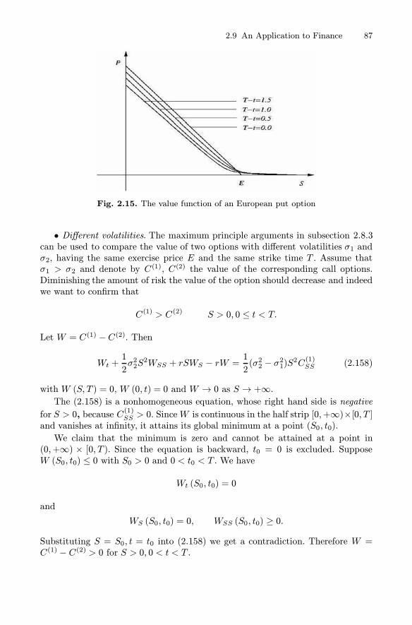
2.9 An Application to Finance 87
Fig. 2.15. The value function of an European put option
• Different volatilities. The maximum principle arguments in subsection 2.8.3can be used to compare the value of two options with different volatilities σ1 andσ2, having the same exercise price E and the same strike time T . Assume thatσ1 > σ2 and denote by C
(1), C(2) the value of the corresponding call options.Diminishing the amount of risk the value of the option should decrease and indeedwe want to confirm that
C(1) > C(2) S > 0, 0 ≤ t < T.
Let W = C(1) −C(2). Then
Wt +1
2σ22S
2WSS + rSWS − rW =1
2(σ22 − σ21)S2C(1)SS (2.158)
with W (S, T ) = 0, W (0, t) = 0 and W → 0 as S → +∞.The (2.158) is a nonhomogeneous equation, whose right hand side is negative
for S > 0, because C(1)SS > 0. SinceW is continuous in the half strip [0,+∞)×[0, T ]
and vanishes at infinity, it attains its global minimum at a point (S0, t0).
We claim that the minimum is zero and cannot be attained at a point in(0,+∞) × [0, T ). Since the equation is backward, t0 = 0 is excluded. SupposeW (S0, t0) ≤ 0 with S0 > 0 and 0 < t0 < T . We have
Wt (S0, t0) = 0
and
WS (S0, t0) = 0, WSS (S0, t0) ≥ 0.
Substituting S = S0, t = t0 into (2.158) we get a contradiction. Therefore W =C(1) − C(2) > 0 for S > 0, 0 < t < T .

88 2 Diffusion
2.9.5 Hedging and self-financing strategy
The mathematical translation of the no arbitrage principle can be made morerigorously than we did in subsection 2.9.2, by introducing the concept of self-financing portfolio. The idea is to “duplicate”V by means of a portfolio consistingof a number of shares of S and a bond Z, a free risk investment growing at therate r, e.g. Z (t) = ert.To this purpose let us try to determine two processes φ = φ (t) e ψ = ψ (t)
such thatV = φS + ψZ (0 ≤ t ≤ T ) (2.159)
in order to eliminate any risk factor. In fact, playing the part of the subscriber (thathas to sell), the risk is that at time T the price S (T ) is greater than E, so that theholder will exercise the option. If in the meantime the subscriber has constructedthe portfolio (2.159), the profit from it exactly meets the funds necessary to paythe holder. On the other hand, if the option has zero value at time T , the portfoliohas no value as well.For the operation to make sense, it is necessary that the subscriber does not put
extra money in this strategy (hedging). This can be assured by requiring that theportfolio (2.159) be self-financing that is, its changes in value be dependentfrom variations of S and Z alone.In formulas, this amount to requiring
dV = φdS + ψdZ (0 ≤ t ≤ T ). (2.160)
Actually, we have already met something like (2.160), when we have constructedthe portfolio Π = V − SΔ or
V = Π + SΔ,
asking that dV = dΠ+ΔdS. This construction is nothing else that a duplication ofV by means of a self-financing portfolio, withΠ playing the role of Z and choosingψ = 1.But, what is the real meaning of (2.160)? We see it better in a discrete setting.
Consider a sequence of times
t0 < t1 < ... < tN
and suppose that the intervals (tj − tj−1) are very small. Denote by Sj e Zj thevalues at tj of S and Z. Consequently, look for two sequences
φj and ψj
corresponding to the quantity of S and Z to be used in the construction of theportfolio (2.159) from tj−1 to tj . Notice that φj and ψj are chosen at time tj−1.Thus, given the interval (tj−1, tj),
Vj = φjSj + ψjZj

2.9 An Application to Finance 89
represents the closing value of the portfolio while
φj+1Sj + ψj+1Zj
is the opening value, the amount of money necessary to buy the new one. Theself-financing condition means that the value Vj of the portfolio at time tj ,determined by the couple
(φj, ψj
), exactly meets the purchasing cost of the port-
folio in the interval (tj , tj+1), determined by(φj+1, ψj+1
). This means
φj+1Sj + ψj+1Zj = φjSj + ψjZj (2.161)
or that the financial gap
Dj = φj+1Sj + ψj+1Zj − Vj
must be zero, otherwise an amount of cash Dj has to be injected to substain thestrategy (Dj > 0) or the same amount of money can be drawn from it (Dj < 0).From (2.161) we deduce that
Vj+1 − Vj = (φj+1Sj+1 + ψj+1Zj+1)− (φjSj + ψjZj)= (φj+1Sj+1 + ψj+1Zj+1)−
(φj+1Sj + ψj+1Zj
)
= φj+1(Sj+1 − Sj) + ψj+1(Zj+1 − Zj)
or
ΔVj = φj+1ΔSj + ψj+1ΔZj
whose continuous version is exactly (2.160).
Going back to the continuous case, by combining formulas (2.150) and (2.160)for dV , we get
{Vt + μSVS +
1
2σ2S2VSS
}dt+ σSVSdB = φ (μSdt+ σSdB) + ψrZdt.
Choosing φ = VS , we rediscover the Black and Scholes equation
Vt +1
2σ2S2VSS + rSVS − rV = 0. (2.162)
On the other hand, if V satisfies (2.162) and
φ = VS , ψ = Z−1(V − VSS) = e−rt(V − VSS),
it can be proved that the self financing condition (2.160) is satisfied for the portfolioφS + ψZ.

90 2 Diffusion
2.10 Some Nonlinear Aspects
All the mathematical models we have examined so far are linear . On the otherhand, the nature of most real problems is nonlinear. For example, nonlinear diffu-sion has to be taken into account in filtration problems, non linear drift terms arequite important in fluid dynamics while nonlinear reaction terms occur frequentlyin population dynamics and kinetics chemistry.
The presence of a nonlinearity in a mathematical model gives rise to manyinteresting phenomena that cannot occur in the linear case; typical instances arefinite speed of diffusion, finite time blow-up or existence of travelling wave solutionsof certain special profiles, each one with its own characteristic velocity.
In this section we try to convey some intuition of what could happen in twotypical and important examples from filtration through a porous medium andpopulation dynamics. In Chapter 4, we shall deal with nonlinear transport models.
2.10.1 Nonlinear diffusion. The porous medium equation
Consider a gas of density ρ = ρ (x, t) flowing through a porous medium. Denoteby v = v (x, t) the velocity of the gas and by κ the porosity of the medium, rep-resenting the volume fraction filled with gas. Conservation of mass reads, in thiscase:
κρt + div (ρv) = 0. (2.163)
Besides (2.163), the flow is governed by the two following constitutive (empirical)laws.
• Darcy’s law:v = −μ
ν∇p (2.164)
where p = p (x, t) is the pressure, μ is the permeability of the medium and ν is the
viscosity of the gas. We assume μ and ν are positive constants.
• Equation of state:
p = p0ρα p0 > 0, α > 0. (2.165)
From (2.164) and (2.165) we have, since p1/α∇p = (1 + 1/α)−1Δ(p1+1/α),
div (ρv) = − μ
(1 + 1/α)νp1/α0
Δ(p1+1/α) = −(m− 1)μp0mν
Δ (ρm)
where m = 1 + α > 1. From (2.163) we obtain
ρt =(m− 1)μp0κmν
Δ(ρm).

2.10 Some Nonlinear Aspects 91
Rescaling time (t �→ (m− 1)μp0κmν
t) we finally get the porous medium equation
ρt = Δ(ρm). (2.166)
SinceΔ(ρm) = div
(mρm−1∇ρ
)
we see that the diffusion coefficient is D (ρ) = mρm−1, showing that the diffusiveeffect increases with the density.The porous medium equation can be written in terms of the pressure variable
u = p/p0 = ρm−1.
It is not difficult to check that the equation for u is given by
ut = uΔu+m
m− 1 |∇u|2
(2.167)
showing once more the dependence on u of the diffusion coefficient.One of the basic questions related to the equation (2.166) or (2.167) is to
understand how an initial data ρ0, confined in a small region Ω, evolves withtime. The key object to examine is therefore the unknown boundary ∂Ω, or freeboundary of the gas, whose speed of expansion we expect to be proportional to|∇u| (from (2.164)). This means that we expect a finite speed of propagation, incontrast with the classical case m = 1.The porous media equation cannot be treated by elementary means, since at
very low density the diffusion has a very low effect and the equation degenerates.However we can get some clue of what happens by examining a sort of fundamentalsolutions, the so called Barenblatt solutions, in spatial dimension 1.The equation is
ρt = (ρm)xx . (2.168)
We look for nonnegative self-similar solutions of the form
ρ (x, t) = t−αU(xt−β
)≡ t−αU (ξ)
satisfying ∫ +∞−∞
ρ (x, t)dx = 1.
This condition requires
1 =
∫ +∞−∞
t−αU(xt−β
)dx = tβ−α
∫ +∞−∞
U (ξ) dξ
so that we must have α = β and∫ +∞−∞ U (ξ) dξ = 1. Substituting into (2.168), we
findαt−α−1(−U − ξU ′) = t−mα−2α(Um)′′.

92 2 Diffusion
Thus, if we choose α = 1/ (m+ 1), we get for U the differential equation
(m+ 1) (Um)′′ + ξU ′ + U = 0
that can be written in the form
d
dξ
[(m+ 1) (Um)′ + ξU
]= 0.
Thus, we have
(m+ 1) (Um)′+ ξU = constant.
Choosing the constant equal to zero, we get
(m+ 1) (Um)′= (m+ 1)mUm−1U ′ = −ξU
or
(m+ 1)mUm−2U ′ = −ξ.
This in turn is equivalent to
(m+ 1)m
m− 1(Um−1
)′= −ξ
whose solution is
U (ξ) =[A− Bmξ2
]1/(m−1)
where A is an arbitrary constant and Bm = (m− 1) /2m (m+ 1) . Clearly, to havea physical meaning, we must have A > 0 and A− Bmξ2 ≥ 0.In conclusion we have found solutions of the porous medium equation of the
form
ρ (x, t) =
⎧⎪⎨⎪⎩
1
tα
[A− Bm
x2
t2α
]1/(m−1)if x2 ≤ At2α/Bm
0 if x2 > At2α/Bm.
(α = 1/ (m+ 1)) .
known as Barenblatt solutions. The points
x = ±√A/Bmt
α ≡ ±r (t)
represent the gas interface between the part filled by gas and the empty part. Itsspeed of propagation is therefore
r (t) = α√A/Bmt
α−1.

2.10 Some Nonlinear Aspects 93
Fig. 2.16. The Barenblatt solution
ρ (x, t) = t−1/5[1− x2t−2/5
]1/3
+
for t = 1, 4, 10, 30
2.10.2 Nonlinear reaction. Fischer’s equation
In 1937 Fisher54 introduced a model for the spatial spread of a so called favoured55
(or advantageous) gene in a population, over an infinitely long one dimensionalhabitat. Denoting by v the gene concentration, Fisher’s equation reads
vτ = Dvyy + rv(1− vM
)τ > 0, y ∈ R, (2.169)
where D, r, andM are positive parameters. An important question is to determinewhether the gene has a typical speed of propagation.Accordingly to the terminology in the introduction, (2.169) is a semilinear
equation where diffusion is coupled with logistic growth through the reaction term
f (v) = rv(1− vM
).
The parameter r represents a biological potential (net birth-death rate, with di-mension [time]−1), while M is the carrying capacity of the habitat. If we rescaletime, space and concentration in the following way
t = rτ , x =√r/Dy, u = v/M,
(2.169) takes the dimensionless form
ut = uxx + u (1− u) , t > 0. (2.170)
Note the two equilibria u ≡ 0 and u ≡ 1. In absence of diffusion, 0 is unstable,and 1 is asymptotically stable. A trajectory with initial data u (0) = u0 between0 and 1 has the typical behavior shown in figure 2.17:
54 Fisher, R. A. (1937), The wave of advance of advantageous gene. Ann. Eugenics, 7,355-69.
55 That is a gene that has an advantage in the struggle for life.

94 2 Diffusion
Fig. 2.17. Logistic curve (r = 0.1, u0 = 1/3)
Therefore, ifu (x, 0) = u0 (x) , x ∈ R, (2.171)
is an initial data for the equation (2.169), with 0 < u0 (x) < 1, we expect acompetitive action between diffusion and reaction, with diffusion trying to spreadand lower u0 against the reaction tendency to increase u towards the equilibriumsolution 1.What we intend to show here is the existence of permanent travelling waves
solutions connecting the two equilibrium states, that is solutions of the form
u (x, t) = U (z) , z = x− ct,
with c denoting the propagation speed, satisfying the conditions
0 < u < 1, t > 0, x ∈ R
andlim
x→−∞u (x, t) = 1 and limx→+∞u (x, t) = 0. (2.172)
The first condition in (2.172), states that the gene concentration is saturated atthe far left end while the second condition denotes zero concentration at the farright end. Clearly, this kind of solutions realize a balance between diffusion andreaction.Since the equation (2.169) is invariant under the transformation x �→ −x, it
suffices to consider c > 0, that is right-moving waves only.Since
ut = −cU ′, ux = U′, uxx = U
′′, (′ = d/dz)
substituting u (x, t) = U (z) into (2.170), we find for U the ordinary differentialequation
U ′′ + cU ′ + U − U2 = 0 (2.173)

2.10 Some Nonlinear Aspects 95
withlim
z→−∞U (z) = 1 and limz→+∞U (z) = 0. (2.174)
Letting U ′ = V , the equation (2.173) is equivalent to the system
dU
dz= V ,
dV
dz= −cV − U + U2 (2.175)
in the phase plane (U, V ). This system has two equilibrium points (0, 0) and (1, 0)corresponding to two steady states. Our travelling wave solution corresponds toan orbit connecting (1, 0) to (0, 0), with 0 < U < 1.We first examine the local behavior of the orbits near the equilibrium points.
The coefficients matrices of the linearized systems at (0, 0) and (1, 0) are, respec-tively,
J (0, 0) =
(0 1−1 −c
)and J (1, 0) =
(0 11 −c
).
The eigenvalues of J (0, 0) are
λ± =1
2
[−c±
√c2 − 4
],
with corresponding eigenvectors
h± =(−c∓
√c2 − 42
).
If c ≥ 2 the eigenvalues are both negative while if c < 2 they are complex. Therefore
(0, 0) is a
{stable node if c ≥ 2stable focus if c < 2.
The eigenvalues of J (1, 0) are
μ± =1
2
[−c ±
√c2 + 4
],
of opposite sign, hence (1, 0) is a saddle point. The unstable and stable separatricesleave (1, 0) along the directions of the two eigenvectors
k+ =
(c +
√c2 + 42
)and k− =
(c−
√c2 + 42
),
respectively.Now, the constraint 0 < U < 1 rules out the case c < 2, since in this case
U changes sign along the orbit approaching (0, 0). For c ≥ 2, all orbits56 in aneighborhood of the origin approach (0, 0) for z → +∞ asymptotically with slope56 Except for two orbits on the stable manifold tangent to h− at (0, 0), in the case c > 2.

96 2 Diffusion
Fig. 2.18. Orbits of the system (2.175)
λ+. On the other hand, the only orbit going to (1, 0) as z → −∞ and remainingin the region 0 < U < 1 is the unstable separatrix γ of the saddle point.
Figure 2.18 shows the orbits configuration in the region of interest (see Problem2.23). The conclusion is that for each c ≥ 2 there exists a unique travelling wavesolution of equation (2.169) with speed c. Moreover U is strictly decreasing .
In terms of original variables, there is a unique travelling wave solution forevery speed c satisfying the inequality c ≥ cmin = 2
√rD.
Thus, we have a continuous “spectrum” of possible speeds of propagation. Itturns out that the minimum speed c = cmin is particularly important.
Indeed, having found a travelling solution is only the beginning of the story.There is a number of questions that arise naturally. Among them, the study of thestability of the travelling waves or of the asymptotic behavior (as t → +∞) of asolution with an initial data u0 of transitional type, that is
u0 (x) =
⎧⎨⎩1 x ≤ a0 < u0 < 1 a < x < b0 x ≥ b.
(2.176)
Should we expect that the travelling wave is insensitive to small perturbations?Does the solution with initial condition (2.176) evolve towards one of the travellingwaves we have just found?
The interested reader can find the answers in the many specialized texts orpapers on the subject57 . Here we only mention that among the travelling wavesolutions we have found, only the minimum speed one can be the asymptotic rep-resentation of solutions with transitional type initial condition. The biological im-plication of this result is that cmin determines the required speed of propagation ofan advantageous gene.
57 See for instance, the books by Murray, vol I, 2001, or Grindrod, 1991.

Problems 97
Problems
2.1. Use the method of separation of variables to solve the following initial-Neumann problem:
⎧⎨⎩ut − uxx = 0 0 < x < L, t > 0u (x, 0) = x 0 < x < Lux (0, t) = ux (L, t) = 0 t > 0.
2.2. Use the method of separation of variables to solve the following non ho-mogeneous initial-Neumann problem:
⎧⎨⎩ut − uxx = tx 0 < x < π, t > 0u (x, 0) = 1 0 ≤ x ≤ πux (0, t) = ux (L, t) = 0 t > 0.
[Hint : Write the candidate solution as u (x, t) =∑
k≥0 ck (t) vk (x) where vkare the eigenfunctions of the eigenvalue problem associated with the homogeneousequation].
2.3. Use the method of separation of variables to solve (at least formally) thefollowing mixed problem:
⎧⎪⎪⎨⎪⎪⎩
ut −Duxx = 0 0 < x < π, t > 0u (x, 0) = g (x) 0 ≤ x ≤ πux (0, t) = 0ux (L, t) + u (L, t) = U
t > 0.
[Answer : u (x, t) =∑
k≥0 cke−Dμ2kt cosμkx, where the numbers μk are the positive
solutions of the equation μ tanμ = 1].
2.4. Prove that, if wt −DΔw = 0 in QT and w ∈ C(QT), then
min∂pQT
w ≤ w (x,t) ≤ max∂pQT
w for every (x,t) ∈ QT .
2.5. Prove Corollary 2.1.
[Hint : b). Let u = v − w, M = maxQT |f1 − f2| and apply Theorem 2.2 toz± = ±u −Mt].
2.6. Let g (t) =M for 0 ≤ t ≤ 1 and g (t) =M − (1− t)4 for 1 < t ≤ 2. Let ube the solution of ut − uxx = 0 in Q2 = (0, 2)× (0, 2) , u = g on ∂pQ2. Computeu (1, 1) and check that it is the maximum of u. Is this in contrast with the strongmaximum principle of Remark 2.4?
2.7. Suppose u = u (x, t) is a solution of the heat equation in a plane domainDT = QT \
(Q1 ∪ Q2
)where Q1 and Q2 are the rectangles in figure 2.19. Assume
that u attains its maximum M at the interior point (x1, t1). Where else u =M?

98 2 Diffusion
Fig. 2.19. At which points (x, t) , u (x, t) = M?
2.8. Find the similarity solutions of the equation ut − uxx = 0 of the formu (x, t) = U
(x/√t)and express the result in term of the error function
erf (x) =2√π
∫ x
0
e−z2
dz.
Find the solution of the problem ut − uxx = 0 in x > 0, t > 0 satisfying theconditions u (0, t) = 1 and u (x, 0) = 0, x > 0.
2.9. Determine for which α and β there exist similarity solutions to ut−uxx =f (x) of the form tαU
(x/tβ
)in each one of the following cases:
(a) f (x) = 0, (b) f (x) = 1, (c) f (x) = x.
[Answer : (a) α arbitrary, β = 1/2. (b) α = 1, β = 1/2. (c) α = 3/2, β = 1/2].
2.10. (Reflecting barriers and Neumann condition). Consider the symmetricrandom walk of Section 2.4. Suppose that a perfectly reflecting barrier is locatedat the point L = mh+ h
2 > 0. By this we mean that if the particle hits the point
L − h2 at time t and moves to the right, then it is reflected and it comes back to
L − h2 at time t + τ . Show that when h, τ → 0 and h2/τ = 2D, p = p (x, t) is a
solution of the problem
⎧⎨⎩pt −Dpxx = 0 x < L, t > 0p (x, 0) = δ x < Lpx (L, t) = 0 t > 0
and moreover∫ L−∞ p (x, t)dx = 1. Compute explicitly the solution.
[Answer : p (x, t) = ΓD (x, t) + ΓD (x− 2L, t)].2.11. (Absorbing barrires and Dirichlet condition). Consider the symmetric
random walk of Section 2.4. Suppose that a perfectly absorbing barrier is locatedat the point L = mh > 0. By this we mean that if the particle hits the point L−h

Problems 99
at time t and moves to the right then it is absorbed and stops at L. Show thatwhen h, τ → 0 and h2/τ = 2D, p = p (x, t) is a solution of the problem
⎧⎨⎩pt −Dpxx = 0 x < L, t > 0p (x, 0) = δ x < Lp (L, t) = 0 t > 0
Compute explicitly the solution.
[Answer : p (x, t) = ΓD (x, t)− ΓD (x− 2L, t).]2.12. Use the partial Fourier transform u (ξ, t) =
∫Re−ixξu (x, t)dx to solve
the global Cauchy problem (2.129) and rediscover formula (2.130).
2.13. Prove Theorem 2.5 under the condition
z (x, t) ≤ C, x ∈ R, 0 ≤ t ≤ T,
using the following steps.a) Let sup
Rz (x, 0) =M0 and define
w (x, t) =2C
L2(x2
2+Dt) +M0.
Check that wt−Dwxx = 0 and use the maximum principle to show that w ≥ z inthe rectangle RL = [−L, L]× [0, T ] .b) Fix an arbitrary point (x0, t0) and choose L large enough to have (x0, t0) ∈
RL. Using a) deduce that z (x0, t0) ≤M0.2.14. Find an explicit formula for the solution of the global Cauchy problem
{ut = Duxx + bux + cu x ∈ R,t > 0u (x, 0) = g (x) x ∈ R.
where D, b, c are constant coefficients. Show that, if c < 0 and g is bounded,u (x, t)→ 0 as t→ +∞[Hint : Choose h, k such that v (x, t) = u (x, t) ehx+kt is a solution of vt = Dvxx].
2.15. Find an explicit formula for the solution of the Cauchy problem⎧⎨⎩ut = uxx x > 0,t > 0u (x, 0) = g (x)u (0, t) = 0
x ≥ 0t > 0.
with g continuous and g (0) = 0.
[Hint : Extend g to x < 0 by odd reflection: g (−x) = −g (x). Solve the correspond-ing global Cauchy problem and write the result as an integral on (0,+∞)].2.16. Let QT = Ω×(0, T ), with Ω bounded domain in Rn. Let u ∈ C2,1 (QT )∩
C(QT)satisfy the equation
ut = DΔu + b (x,t) · ∇u+ c (x,t)u in QT

100 2 Diffusion
where b and c are continuous in QT . Show that if u ≥ 0 (resp. u ≤ 0) on ∂pQTthen u ≥ 0 (resp. u ≤ 0) in QT .[Hint : Assume first that c (x,t) ≤ a < 0. Then reduce to this case by settingu = vekt with a suitable k > 0].
2.17. Fill in the details in the arguments of Section 6.2, leading to formulas(2.108) and (2.109).
2.18. Solve the following initial-Dirichlet problem in B1 ={x ∈R3: |x| < 1
}:
⎧⎨⎩ut = Δu x ∈B1, t > 0u (x, 0) = 0u (σ, t) = 1
x ∈B1σ ∈ ∂B1, t > 0.
Compute limt→+∞ u.[Hint : The solution is radial so that u = u (r, t) , r = |x|. Observe that Δu =urr+
2
rur =
1
r(ru)rr . Let v = ru, reduce to homogeneous Dirichlet condition and
use separation of variables].
2.19. Solve the following initial-Dirichlet problem⎧⎨⎩ut = Δu x ∈K, t > 0u (x, 0) = 0u (σ, t) = 1
x ∈Kσ ∈ ∂K, t > 0.
where K is the rectangular box
K ={(x, y, z)∈R3: 0 < x < a, 0 < y < b, 0 < z < c
}.
Compute limt→+∞ u.
2.20. Solve the following initial-Neumann problem in B1 ={x ∈R3: |x| < 1
}:
⎧⎨⎩ut = Δu x ∈B1, t > 0u (x, 0) = |x|uν (σ, t) = 1
x ∈B1σ ∈ ∂B1 , t > 0.
2.21. Solve the following non homogeneous initial-Dirichlet problem in the unitsphere B1 (u = u (r, t) , r = |x|):
⎧⎪⎨⎪⎩ut − (urr +
2
rur) = qe
−t 0 < r < 1, t > 0
u (r, 0) = Uu (1, t) = 0
0 ≤ r ≤ 1t > 0.
[Answer : The solution is
u (r, t) =2
r
∞∑n=1
(−1)nλn
sin(λnr)
{q
1− λ2n
(e−t − e−λ2nt
)− Ue−λ2nt
}
where λn = nπ].

Problems 101
2.22. Using the maximum principle, compare the values of two call optionsC(1) and C(2) in the following cases:(a) Same exercise price and T1 > T2. (b) Same expiry time and E1 > E2.
2.23. Justify carefully the orbit configuration of figure 2.18 and in particularthat the unstable orbit γ connects the two equilibrium points of system (2.175),by filling in the details in the following steps:
1. Let F = V i+(−cV + U2 − U
)j and n be the interior normal to the bound-
ary of the triangle Ω in figure 2.20. Show that, if β is large enough, F · n > 0 along∂Ω.
2. Deduce that all the orbits of system (2.175) starting at a point in Ω cannotleave Ω (i.e. Ω is a positively invariant region) and converge to the origin asz → +∞.3. Finally, deduce that the unstable separatrix γ of the saddle point (1, 0)
approaches (0, 0) as z → +∞.
Fig. 2.20. Trapping region for the orbits of the vector field F =V i +(−cV + U2 − U) j

3
The Laplace Equation
Introduction – Well Posed Problems. Uniqueness – Harmonic Functions – Fundamental
Solution and Newtonian Potential – The Green Function – Uniqueness in Unbounded
Domains – Surface Potentials
3.1 Introduction
The Laplace equation Δu = 0 occurs frequently in applied sciences, in particularin the study of the steady state phenomena. Its solutions are called harmonicfunctions. For instance, the equilibrium position of a perfectly elastic membraneis a harmonic function as it is the velocity potential of a homogeneous fluid. Also,the steady state temperature of a homogeneous and isotropic body is a harmonicfunction and in this case Laplace equation constitutes the stationary counterpart(time independent) of the diffusion equation.Slightly more generally, Poisson’s equation Δu = f plays an important role in
the theory of conservative fields (electrical, magnetic, gravitational,...) where thevector field is derived from the gradient of a potential.For example, let E be a force field due to a distribution of electric charges in
a domain Ω ⊂ R3. Then, in standard units, div E =4πρ, where ρ represents the
density of the charge distribution. When a potential u exists such that ∇u = −E,then Δu = div∇u = −4πρ, which is Poisson’s equation. If the electric field iscreated by charges located outside Ω, then ρ = 0 in Ω and u is harmonic therein.Analogously, the potential of a gravitational field due to a mass distribution is aharmonic function in a region free from mass.
In dimension two, the theories of harmonic and holomorphic functions arestrictly connected1 . Indeed, the real and the imaginary part of a holomorphic
1 A complex function f = f (z) is holomorphic in an open subset Ω of the complex planeif for every z0 ∈ Ω, the limit
limz→z0
f (z)− f (z0)z − z0 = f ′ (z0)
Salsa S. Partial Differential Equations in Action: From Modelling to Theoryc© Springer-Verlag 2008, Milan

3.2 Well Posed Problems. Uniqueness 103
function are harmonic. For instance, since the functions
zm = rm (cosmθ + i sinmθ) , m ∈ N,
(r, θ polar coordinates) are holomorphic in the whole plane C, the functions
u (r, θ) = rm cosmθ and v (r, θ) = rm sinmθ m ∈ N,
are harmonic in R2 (called elementary harmonics). In Cartesian coordinates, theyare harmonic polynomials; for m = 1, 2, 3 we find
x, y, xy, x2 − y2, x3 − 3xy2, 3x2y − y3.
Other examples are
u (x, y) = eαx cosαy, v (x, y) = eαx sinαy (α ∈ R),
the real and imaginary parts of f (z) = eiαz, both harmonic in R2, and
u (r, θ) = log r, v (r, θ) = θ,
the real and imaginary parts of f (z) = log0 z ≡ log r + iθ, harmonic in R2\ (0, 0)and R2\ {θ = 0} , respectively.In this chapter we present the formulation of the most important well posed
problems and the classical properties of harmonic functions, focusing mainly ondimensions two and three. As in Chapter 2, we emphasize some probabilistic as-pects, exploiting the connection among random walks, Brownian motion and theLaplace operator. A central notion is the concept of fundamental solution, thatwe develop in conjunction with the very basic elements of the so called potentialtheory .
3.2 Well Posed Problems. Uniqueness
Consider the Poisson equation
Δu = f in Ω (3.1)
where Ω ⊂ Rn is a bounded domain. The well posed problems associated withequation (3.1) are the stationary counterparts of the corresponding problems forthe diffusion equation. Clearly here there is no initial condition. On the boundary∂Ω we may assign:
• Dirichlet datau = g, (3.2)
exists and it is finite.

104 3 The Laplace Equation
• Neumann data∂νu = h, (3.3)
where ν is the outward normal unit vector to ∂Ω,
• a Robin (radiation) condition
∂νu+ αu = h (α > 0), (3.4)
• a mixed condition; for instance,
u = g on ΓD (3.5)
∂νu = h on ΓN ,
where ΓD ∪ ΓN = ∂Ω, ΓD ∩ ΓN = ∅, and ΓN is a relatively open subset of ∂Ω.When g = h = 0 we say that the above boundary conditions are homogeneous.
We give some interpretations. If u is the position of a perfectly flexible mem-brane and f is an external distributed load (vertical force per unit surface), then(3.1) models a steady state.The Dirichlet condition corresponds to fixing the position of the membrane at
its boundary. Robin condition describes an elastic attachment at the boundarywhile a homogeneous Neumann condition corresponds to a free vertical motion ofthe boundary.If u is the steady state concentration of a substance, the Dirichlet condition
prescribes the level of u at the boundary, while the Neumann condition assignsthe flux of u through the boundary.
Using Green’s identity (1.13) we can prove the following uniqueness result.
Theorem 3.1. Let Ω ⊂ Rn be a smooth, bounded domain. Then there exists
at most one solution u ∈ C2 (Ω) ∩ C1(Ω)of (3.1), satisfying on ∂Ω one of the
conditions (3.2), (3.4) or (3.5).In the case of the Neumann condition, that is when
∂νu = h on ∂Ω,
two solutions differ by a constant.
Proof. Let u and v be solutions of the same problem, sharing the same boundarydata, and let w = u− v. Then w is harmonic and satisfies homogeneous boundaryconditions (one among (3.2)-(3.5)). Substituting u = v = w into (1.13) we find
∫
Ω
|∇w|2 dx =∫
∂Ω
w∂νw dσ.
If Dirichlet or mixed conditions hold, we have∫
∂Ω
w∂νw dσ = 0.

3.3 Harmonic Functions 105
When a Robin condition holds∫
∂Ω
w∂νw dσ = −∫
∂Ω
αw2dσ ≤ 0.
In any case we obtain that ∫
Ω
|∇w|2 dx ≤0. (3.6)
From (3.6) we infer ∇w = 0 and therefore w = u− v = constant. This concludesthe proof in the case of Neumann condition. In the other cases, the constant mustbe zero (why?), hence u = v. �
Remark 3.1. Consider the Neumann problem Δu = f in Ω, ∂νu = h on ∂Ω.Integrating the equation on Ω and using Gauss’ formula we find
∫
Ω
f dx =
∫
∂Ω
h dσ. (3.7)
The relation (3.7) appears as a compatibility condition on the data f and h, thathas necessarily to be satisfied in order for the Neumann problem to admit a so-lution. Thus, when having to solve a Neumann problem, the first thing to do isto check the validity of (3.7). If it does not hold, the problem does not have anysolution. We will examine later the physical meaning of (3.7).
3.3 Harmonic Functions
3.3.1 Discrete harmonic functions
In Chapter 2 we have examined the connection between Brownian motion anddiffusion equation. We go back now to the multidimensional symmetric randomwalk considered in Section 2.6, analyzing its relation with the Laplace operator Δ.For simplicity we will work in dimension n = 2 but both arguments and conclusionsmay be easily extended to any dimension n > 2. We fix a time step τ > 0, a spacestep h > 0 and denote by hZ2 the lattice of points x =(x1, x2) whose coordinatesare integer multiples of h. Let p (x,t) = p (x1, x2, t) be the transition probabilityfunction, giving the probability to find our random particle at x at time t. Fromthe total probability formula we found a difference equation for p, that we rewritein dimension two:
p (x, t+ τ) =1
4{p (x+he1, t) + p (x−he1, t) + p (x+he2, t) + p (x−he2, t)} .
(3.8)We can write this formula in a more significant way by introducing the mean valueoperator Mh, whose action on a function u = u(x) is defined by the following

106 3 The Laplace Equation
formula:
Mhf (x) =1
4{u (x+he1) + u (x−he1) + u (x+he2) + u (x−he2)}
=1
4
∑|x−y|=h
u (y) .
Note that Mhu (x) gives the average of u over the points of the lattice hZ2 at
distance h from x. We say that these points constitute the discrete neighborhoodof x of radius h.It is clear that (3.8) can be written in the form
p (x, t+ τ ) =Mhp (x,t) . (3.9)
In (3.9) the probability p at time t + τ is determined by the action of Mh at theprevious time, and then it is natural to interpret the mean value operator as thegenerator of the random walk.Now we come to the Laplacian. If u is twice continuously differentiable, it is
not difficult to show that2
limh→0Mhu (x)− u (x)
h2→ 14Δu (x) . (3.10)
The formula (3.10) induces to define, for any fixed h > 0, a discrete Laplaceoperator through the formula
Δ∗h =Mh − I
where I denotes the identity operator (i.e. Iu = u). The operator Δ∗h acts onfunctions u defined in the whole lattice hZ2 and, coherently, we say that u isd-harmonic (d for discrete) if Δ∗hu = 0.Thus, the value of a d-harmonic function at any point x is given by the average
of the values at the points in the discrete neighborhood of x of radius h.We can proceed further and define a discrete Dirichlet problem. Let A be a
subset of hZ2.We say that A is connected if, given any couple of points x0, x1 in A, it is
possible to connect them by a walk3 on hZ2 entirely contained in A.Moreover, we say that x ∈A is an interior point of A if its h−neighborhood
is contained in A. The points of A that are not interior are called boundary points(Fig. 3.1). The set of the boundary points of A, the boundary of A, is denoted by∂A.
2 Using a second order Taylor’s polynomial, after some simplifications, we get:
Mhu (x) = u (x) +h2
4{ux1x1 (x) + ux2x2 (x)}+ o
(h2)
from which formula (3.10) comes easily.3 Recall that consecutive points in a walk have distance h.

3.3 Harmonic Functions 107
Fig. 3.1. A domain for the discrete Dirichlet problem
Discrete Dirichlet problem. Let A be a bounded connected subset of hZ2
and g be a function defined on the boundary ∂A of A. We want to determine u,defined on A, such that
{Δ∗hu = 0 at the interior points of Au = g on ∂A.
(3.11)
We deduce immediately three important properties of a solution u:
1. Maximum principle: If u attains its maximum or its minimum at an interiorpoint then u is constant. Indeed, suppose x ∈A is an interior point and u (x) =M ≥ u (y) for every y ∈A. Since u (x) is the average of the four values of u atthe points at distance h from x, at all these points u must be equal to M . Letx1 �= x be one of these neighboring points. By the same argument, u (y) =Mfor every y in the h−neighborhood of x1. Since A is connected, proceeding inthis way we prove that u (y) =M at every point of A.
2. u attains its maximum and its minimum on ∂A. This is an immediate conse-quence of 1.
3. The solution of the discrete Dirichlet problem is unique (exercise).
The discrete Dirichlet problem (3.11) has a remarkable probabilistic interpre-tation that can be used to construct its solution. Let us go back to our randomparticle. First of all, we want to show that whatever its starting point x ∈A is, theparticle hits the boundary ∂A with probability one.For every Γ ⊆ ∂A, we denote by
P (x,Γ )
the probability that the particle starting from x ∈A hits ∂A for the first time at apoint y ∈Γ . We have to prove that P (x, ∂A) = 1 for every x ∈A.
108 3 The Laplace Equation
Clearly, if x ∈Γ we have P (x,Γ ) = 1, while if x ∈∂A\Γ , P (x,Γ ) = 0. It turnsout that, for fixed Γ , the function
wΓ (x) = P (x,Γ )
is d-harmonic in the interior of A, that is Δ∗wΓ = 0. To see this, denote by
p (1,x,y)
the one step transition probability, i.e. the probability to go from x to y in onestep. Given the symmetry of the walk, we have p (1,x,y) = 1/4 if |x− y| = 1 andp (1,x,y) = 0 otherwise.Now, to hit Γ starting from x, the particle first hits a point y in its h−neigh-
borhood and from there it reaches Γ , independently of the first step. Then, by thetotal probability formula we can write
wΓ (x) = P (x,Γ ) =∑y∈hZ2
p (1,x,y)P (y,Γ ) =MhP (x,Γ ) =MhwΓ (x) ,
which entails
(I −Mh)wΓ = Δ∗hwΓ = 0.
Thus, wΓ is d − harmonic in A. In particular w∂A (x) = P (x,∂A) is d − harmonicin A and w∂A = 1 on ∂A. On the other hand, the function z (x) ≡ 1 satisfies thesame discrete Dirichlet problem, so that, by the uniqueness property 3 above,
w∂A (x) = P (x,∂A) ≡ 1 in A. (3.12)
This means that the particle hits the boundary ∂A with probability one. As aconsequence, observe that the set function
Γ �→ P (x,Γ )
defines a probability measure on ∂A, for any fixed x ∈A.We construct now the solution u to (3.11). Interpret the boundary data g as a
payoff : if the particle starts from x and hits the boundary for the first time at y,it wins g (y). We have:
Theorem 3.2. The value u (x) is given by the expected value of the winnings g (·)with respect to the probability P (x, ·). That is
u (x) =∑y∈∂A
g (y)P (x, {y}) . (3.13)
Proof. Each term
g (y)P (x, {y}) = g (y)w{y} (x)

3.3 Harmonic Functions 109
is d−harmonic in A and therefore u is d−harmonic in A as well. Moreover, ifx ∈∂A then u (x) = g (x) since each term in the sum is equal to g (x) if y = x orto zero if y �= x. �As h→ 0, formula (3.10) shows that, formally, d−harmonic functions“become”
harmonic. Thus, it seems reasonable that appropriate versions of the above prop-erties and results should hold in the continuous case. We start with the mean valueproperties.
3.3.2 Mean value properties
Guided by their discrete characterization, we want to establish some fundamen-tal properties of harmonic functions. To be precise, we say that a function u isharmonic in a domain Ω ⊆ Rn if u ∈ C2 (Ω) and Δu = 0 in Ω.Since d−harmonic functions are defined through a mean value property, we
expect that harmonic functions inherit a mean value property of the followingkind: the value at the center of any ball B ⊂⊂ Ω, i.e. compactly contained in Ω,equals the average of the values on the boundary ∂B. Actually, something more istrue.
Theorem 3.3. Let u be harmonic in Ω ⊆ Rn. Then, for any ball BR (x) ⊂⊂ Ω
the following mean value formulas hold:
u (x) =n
ωnRn
∫
BR(x)
u (y) dy (3.14)
u (x) =1
ωnRn−1
∫
∂BR(x)
u (σ) dσ (3.15)
where ωn is the measure of ∂B1 .
Proof (for n = 2). Let us start from the second formula. For r < R define
g (r) =1
2πr
∫
∂Br(x)
u (σ) dσ.
Perform the change of variables σ = x+rσ′. Then σ′ ∈ ∂B1 (0), dσ = rdσ′ and
g (r) =1
2π
∫
∂B1(0)
u (x+rσ′) dσ′.
Let v (y) = u (x+ry) and observe that
∇v (y) = r∇u (x+ry)Δv (y) = r2Δu (x+ry) .

110 3 The Laplace Equation
Then we have
g′ (r) =1
2π
∫
∂B1(0)
d
dru (x+rσ′) dσ′ =
1
2π
∫
∂B1(0)
∇u (x+rσ′) · σ′dσ′
=1
2πr
∫
∂B1(0)
∇v (σ′) · σ′dσ′ = (divergence theorem)
=1
2πr
∫
B1(0)
Δv (y) dy =r
2π
∫
B1(0)
Δu (x+ry) dy = 0.
Thus, g is constant and since g (r)→ u (x) for r→ 0, we get (3.15).To obtain (3.14), let R = r in (3.15), multiply by r and integrate both sides
between 0 and R. We find
R2
2u (x) =
1
2π
∫ R
0
dr
∫
∂Br(x)
u (σ) dσ=1
2π
∫
BR(x)
u (y) dy
from which (3.14) follows. �
Even more significant is a converse of Theorem 3.2. We say that a continuousfunction u satisfies the mean value property in Ω, if (3.14) or (3.15) holds forany ball BR (x) ⊂⊂ Ω. It turns out that if u is continuous and possesses themean value property in a domain Ω, then u is harmonic in Ω. Thus we obtain acharacterization of harmonic functions through a mean value property, as in thediscrete case. As a by product we deduce that every harmonic function in a domainΩ is continuously differentiable of any order in Ω, that is, it belongs to C∞ (Ω).Notice that this is not a trivial fact since it involves derivatives not appearingin the expression of the Laplace operator. For instance, u (x, y) = x + y |y| is asolution of uxx + uxy = 0 in all R
2 but it is not twice differentiable with respectto y at (0, 0).
Theorem 3.4. Let u ∈ C (Ω). If u satisfies the mean value property, then u ∈C∞ (Ω) and it is harmonic in Ω.
We postpone the proof to the end of the Section 3.4.
3.3.3 Maximum principles
As in the discrete case, a function satisfying the mean value property in a domain4
Ω cannot attain its maximum or minimum at an interior point of Ω, unless itis constant. In case Ω is bounded and u (non constant) is continuous up to theboundary of Ω, it follows that u attains both its maximum and minimum onlyon ∂Ω. This result expresses a maximum principle that we state precisely in thefollowing theorem.
4 Recall that a domain is an open connected set.

3.3 Harmonic Functions 111
Theorem 3.5. Let u ∈ C (Ω), Ω ⊆ Rn. If u has the mean value property and
attains its maximum or minimum at p ∈ Ω, then u is constant. In particular, if Ωis bounded and u ∈ C(Ω) is not constant, then, for every x ∈Ω,
u (x) < max∂Ωu and u (x) > min
∂Ωu (from strong maximum principle).
Proof. (n = 2). Let p be a minimum point5 for u:
m = u(p) ≤ u(y), ∀y ∈Ω.
We want to show that u ≡ m in Ω. Let q be another arbitrary point in Ω. SinceΩ is connected, it is possible to find a finite sequence of circles B (xj) ⊂⊂ Ω,j = 0, ..., N , such that (Fig. 3.2):
• xj ∈ B (xj−1) , j = 1, ..., N• x0 = p, xN = q.
Fig. 3.2. A sequence of overlapping circles connecting the points p and q
The mean value property gives
m = u (p) =1
|B (p)|
∫
B(p)
u (y) dy.
Suppose there exists z ∈B (p) such that u (z) > m. Then, given a circle Br (z) ⊂B (p), we can write:
m =1
|B (p)|
∫
B(p)
u (y)dy (3.16)
=1
|B (p)|
{∫
B(p)\Br(z)u (y) dy +
∫
Br(z)
u (y) dy
}.
5 The argument for the maximum is the same.

112 3 The Laplace Equation
Since u (y) ≥ m for every y and, by the mean value again,∫
Br(z)
u (y) dy =u (z) |Br (z)| > m |Br (z)| ,
continuing from (3.16) we obtain
>1
|B (p)| {m |B (p) \Br (z)|+m |Br (z)|} = m
and therefore the contradiction m > m.Thus it must be that u ≡ m in B (p) and in particular u(x1) = m. We repeat
now the same argument with x1 in place of p to show that u ≡ m in B (x1)and in particular u(x2) = m. Iterating the procedure we eventually deduce thatu(xN) = u(q) =m. Since q is an arbitrary point of Ω, we conclude that u ≡ m inΩ. �An important consequence of the maximum principle is the following corollary.
Corollary 3.1. Let Ω ⊂ Rn be a bounded domain and g ∈ C (∂Ω). The problem{Δu = 0 in Ωu = g on ∂Ω.
(3.17)
has at most a solution ug∈C2 (Ω) ∩ C(Ω). Moreover, let ug1 and ug2 be the
solutions corresponding to the data g1, g2 ∈ C (∂Ω). Then:(a) (Comparison). If g1 ≥ g2 on ∂Ω and g1 �= g2, then
ug1 > ug2 in Ω. (3.18)
(b) (Stability).
|ug1 (x) − ug2 (x)| ≤ max∂Ω
|g1 − g2| for every x ∈Ω. (3.19)
Proof. We first show (a) and (b). Let w = ug1 − ug2 . Then w is harmonic andw = g1 − g2 ≥ 0 on ∂Ω. Since g1 �= g2, w is not constant and from Theorem 3.5
w (x) > min∂Ω(g1 − g2) ≥ 0 for every x ∈Ω.
This is (3.18). To prove (b), apply Theorem 3.5 to w and −w to find±w (x) ≤ max
∂Ω|g1 − g2| for every x ∈Ω
which is equivalent to (3.19).Now if g1 = g2, (3.19) implies w = ug1 −ug2 ≡ 0, so that the Dirichlet problem
(3.17) has at most one solution. �
Remark 3.2. Inequality (3.19) is a stability estimate. Indeed, suppose g is knownwithin an absolute error less than ε, or, in other words, suppose g1 is an approxi-mation of g and max∂Ω |g − g1| < ε; then (3.19) gives
maxΩ|ug1 − ug| < ε
so that the approximate solution is known within the same absolute error.
3.3 Harmonic Functions 113
3.3.4 The Dirichlet problem in a circle. Poisson’s formula
To prove the existence of a solution to one of the boundary value problems weconsidered in Section 3.2 is not an elementary task. In Chapter 8, we solve thisquestion in a general context, using the more advanced tools of Functional Analysis.However, in special cases, elementary methods, like separation of variables, work.We use it to compute the solution of the Dirichlet problem in a circle. Precisely, letBR = BR (p) be the circle of radius R centered at p =(p1, p2) and g ∈ C (∂BR).We want to prove the following theorem.
Theorem 3.6. The unique solution u ∈ C2 (BR) ∩C(BR)of the problem
{Δu = 0 in BRu = g on ∂BR.
(3.20)
is given by Poisson’s formula
u (x) =R2 − |x− p|2
2πR
∫
∂BR(p)
g (σ)
|x− σ|2dσ. (3.21)
In particular, u ∈ C∞ (BR).
Proof. The symmetry of the domain suggests the use of polar coordinates
x1 = p1 + r cos θ x2 = p2 + r sin θ.
Accordingly, let
U (r, θ) = u (p1 + r cos θ, p2 + r sin θ) , G (θ) = g (p1 +R cos θ, p2 + R sin θ) .
The Laplace equation becomes6
Urr +1
rUr +
1
r2Uθθ = 0, 0 < r < R, 0 ≤ θ ≤ 2π, (3.22)
with the Dirichlet condition
U (R, θ) = G (θ) , 0 ≤ θ ≤ 2π.
Since we ask that u be continuous in BR, then U and G have to be continuousin [0, R]× [0, 2π] and [0, 2π], respectively; moreover both have to be 2π−periodicwith respect to θ.We use now the method of separation of variables, by looking first for solutions
of the form
U (r, θ) = v (r)w (θ)
6 Appendix B.

114 3 The Laplace Equation
with v, w bounded and w 2π−periodic. Substitution in (3.22) gives
v′′ (r)w (θ) +1
rv′ (r)w (θ) +
1
r2v (r)w′′ (θ) = 0
or, separating the variables,
−r2v′′ (r) + rv′ (r)
v (r)=w′′ (θ)w (θ)
.
This identity is possible only when the two quotients have a common constantvalue λ. Thus we are lead to the ordinary differential equation
r2v′′ (r) + rv′ (r)− λv (r) = 0 (3.23)
and to the eigenvalue problem
{w′′ (θ)− λw (θ) = 0w (0) = w (2π) .
(3.24)
We leave to the reader to check that problem (3.24) has only the zero solutionfor λ ≥ 0. If λ = −μ2, μ > 0, the differential equation in (3.24) has the generalintegral
w (θ) = a cosμθ + b sinμθ (a, b ∈ R) .The 2π−periodicity forces μ = m, a nonnegative integer.The equation (3.23), with λ = m, has the general solution7
v (r) = d1r−m + d2rm (d1, d2 ∈ R) .
Since v has to be bounded we exclude r−m, m > 0 and hence d1 = 0.We have found a countable number of 2π−periodic harmonic functions
rm {am cosmθ + bm sinmθ} m = 0, 1, 2, .... (3.25)
We superpose now the (3.25) by writing
U (r, θ) = a0 +
∞∑m=1
rm {am cosmθ + bm sinmθ} (3.26)
with the coefficients am and bm still to be chosen in order to satisfy the boundarycondition
lim(r,θ)→(R,ξ)
U(r, θ) = G (ξ) ∀ξ∈ [0, 2π] . (3.27)
7 It is an Euler equation. The change of variables s = log r reduces it to the equation
v′′ (s)−m2v (s) = 0.
3.3 Harmonic Functions 115
Case G ∈ C1 ([0, 2π]). In this case G can be expanded in a uniformly con-vergent Fourier series
G (ξ) =α02+
∞∑m=1
{αm cosmξ + βm sinmξ}
where
αm =1
π
∫ 2π0
G (ϕ) cosmϕ dϕ, βm =1
π
∫ 2π0
G (ϕ) sinmϕ dϕ.
Then, the boundary condition (3.27) is satisfied if we choose
a0 =α0
2, am = R
−mαm, bm = R−mβm.
Substitution of these values of a0, am, bm into (3.26) gives, for r ≤ R,
U (r, θ) =α0
2+1
π
∞∑m=1
( rR
)m ∫ 2π0
G (ϕ) {cosmϕ cosmθ + sinmϕ sinmθ} dϕ
=1
π
∫ 2π0
G (ϕ)
[1
2+
∞∑m=1
( rR
)m{cosmϕ cosmθ + sinmϕ sinmθ}
]dϕ
=1
π
∫ 2π0
G (ϕ)
[1
2+
∞∑m=1
( rR
)mcosm(ϕ − θ)
]dϕ.
Note that in the second equality above, the exchange of sum and integration ispossible because of the uniform convergence of the series. Moreover, for r < R, wecan differentiate under the integral sign and then term by term as many times aswe want (why?). Therefore, since for every m ≥ 1 the functions
( rR
)mcosm(ϕ − θ)
are smooth and harmonic, also U ∈ C∞ (BR) and is harmonic for r < R.To obtain a better formula, observe that
∞∑m=1
( rR
)mcosm(ϕ − θ) = Re
[ ∞∑m=1
(ei(ϕ−θ)
r
R
)m].
Since
Re
∞∑m=1
(ei(ϕ−θ)
r
R
)m= Re
1
1− ei(ϕ−θ) rR− 1 = R2 − rR cos (ϕ − θ)
R2 + r2 − 2rR cos (ϕ − θ) − 1
=rR cos (ϕ − θ)− r2
R2 + r2 − 2rR cos (ϕ− θ)

116 3 The Laplace Equation
we find
1
2+
∞∑m=1
( rR
)mcosm(ϕ − θ) = 1
2
R2 − r2R2 + r2 − 2rR cos (ϕ− θ) . (3.28)
Inserting (3.28) into the formula for U , we get Poisson’s formula in polar coor-dinates:
U (r, θ) =R2 − r22π
∫ 2π0
G (ϕ)
R2 + r2 − 2Rr cos (θ − ϕ)dϕ. (3.29)
Going back to Cartesian coordinates8 we obtain Poisson’s formula (3.21). Corollary3.1 assures that (3.29) is indeed the unique solution of the Dirichlet problem (3.20).
Case G ∈ C ([0, 2π]). We drop now the additional hypothesis that G (θ) iscontinuously differentiable. Even with G only continuous, formula (3.29) makesperfect sense and defines a harmonic function in BR and it can be shown that
9
lim(r,θ)→(R,ξ)
U (r, θ) = G (ξ) , ∀ξ∈ [0, 2π] .
Therefore (3.29) is the unique (by Corollary 3.1) solution to (3.20). �
• Poisson’s formula in dimension n > 2. Theorem 3.6 has an appropriateextension in any number of dimensions. When BR = BR (p) is an n− dimensionalball, the solution of the Dirichlet problem (3.20) is given by (see subsection 3.5.3,for the case n = 3)
u (x) =R2 − |x− p|2ωnR
∫
∂BR(p)
g (σ)
|x− σ|n dσ. (3.30)
An important consequence of Poisson’s formula is the possibility to control thederivatives of any order of a harmonic function u at a point p by the maximum ofu in a small ball centered at p. We show it for first and second derivatives in thefollowing corollary.
Corollary 3.2. Let u be a harmonic function in a domain Ω and BR (p) ⊂⊂ Ω.Then ∣∣uxj (p)
∣∣ ≤ nRmax∂BR(p)
|u| ,∣∣uxjxk (p)
∣∣ ≤ c (n)R2
max∂BR(p)
|u| . (3.31)
8 With σ = R(cosϕ, sinϕ), dσ = Rdϕ and
|x− σ|2 = (r cos θ − R cosϕ)2 + (r sin θ − R sinϕ)2= R2 + r2 − 2Rr (cosϕ cos θ + sinϕ sin θ)= R2 + r2 − 2Rr cos (θ − ϕ) .
9 See Problem 3.20.

3.3 Harmonic Functions 117
Proof. From (3.30) we have
u (x) =R2 − |x− p|2ωnR
∫
∂BR(p)
u (σ)
|x− σ|n dσ.
Since we want to compute the derivatives at p, we can differentiate under theintegral obtaining:
uxj (x) =−2 (xj − pj)ωnR
∫
∂BR(p)
u (σ)
|x− σ|n dσ
−nR2 − 2 |x − p|2ωnR
∫
∂BR(p)
xj − σj|x − σ|n+2
u (σ) dσ.
Now, at x = p we have|pj − σj ||p− σ|n+2
≤ R−n−1.
Therefore, since |∂BR (p)| = ωnRn−1,
∣∣uxj (p)∣∣ ≤ nRωn
∫
∂BR(p)
|pj − σj ||p− σ|n+2
|u (σ)|dσ ≤ nRmax∂BR(p)
|u| .
Similarly we get the estimates for the second derivatives; we leave the details tothe reader. �
We are now in position to prove Theorem 3.4, the converse of the mean valueproperty (m.v.p.).
• Proof of Theorem 3.4. First observe that if two functions satisfy the m.v.p. ina domainΩ, their difference satisfies this property as well. Let u ∈ C (Ω) satisfyingthe m.v.p. and consider a circle B ⊂⊂ Ω. We want to show that u is harmonic andinfinitely differentiable in Ω. Denote by v the solution of the Dirichlet problem
{Δv = 0 in Bv = u on ∂B.
From Theorem 3.6 we know that v ∈ C∞ (B) ∩ C(B)and, being harmonic, it
satisfies the m.v.p. in B. Then, also w = v − u satisfies the m.v.p. in B andtherefore (Theorem 3.4) it attains its maximum and minimum on ∂B. Since w = 0on ∂B, we conclude that u = v in B. Since B is arbitrary, u ∈ C∞ (Ω) and isharmonic in Ω. �
3.3.5 Harnack’s inequality and Liouville’s theorem
From the mean value and Poisson’s formulas we deduce another maximum princi-ple, known as Harnack’s inequality :

118 3 The Laplace Equation
Theorem 3.7. Let u be harmonic and nonnegative in the ball BR = BR (0) ⊂ Rn.Then for any x ∈BR,
Rn−2 (R− |x|)(R+ |x|)n−1
u (0) ≤ u (x) ≤ Rn−2 (R+ |x|)(R− |x|)n−1
u (0) . (3.32)
Proof (n = 3). From Poisson’s formula:
u (x) =R2 − |x|24πR
∫
∂BR
u (σ)
|σ − x|3dσ.
Observe that R−|x| ≤ |σ − x| ≤ R+ |x| and R2−|x|2 = (R−|x|)(R+ |x|). Then,by the mean value property,
u (x) ≤ R+ |x|(R− |x|)2
1
4πR
∫
∂BR
u (σ) dσ =R (R+ |x|)(R − |x|)2
u (0) .
Analogously,
u (x) ≥ R(R− |x|)(R+ |x|)2
1
4πR2
∫
∂BR
u (σ) dσ =R (R− |x|)(R+ |x|)2
u (0) .
�Harnack’s inequality has an important consequence: the only harmonic func-
tions in Rn bounded from below or above are the constant functions.
Corollary 3.3. (Liouville′s Theorem). If u is harmonic in Rn and u (x) ≥ M ,then u is constant.
Proof (n = 3). The function w = u −M is harmonic in R3 and nonnegative.Fix x ∈R3 and choose R > |x|; Harnack’s inequality gives
R (R− |x|)(R+ |x|)2
w (0) ≤ w (x) ≤ R (R + |x|)(R− |x|)2
w (0) . (3.33)
Letting R →∞ in (3.33) we get
w (0) ≤ w (x) ≤ w (0)
whence w (0) = w (x). Since x is arbitrary we conclude that w, and therefore alsou, is constant. �
3.3.6 A probabilistic solution of the Dirichlet problem
In Section 3.1 we solved the discrete Dirichlet problem via a probabilistic method.The key ingredients in the construction of the solution, leading to formula (3.13),were the mean value property and the absence of memory of the random walk (each
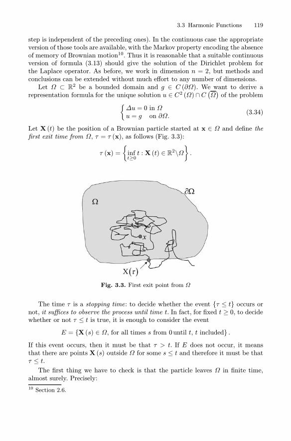
3.3 Harmonic Functions 119
step is independent of the preceding ones). In the continuous case the appropriateversion of those tools are available, with the Markov property encoding the absenceof memory of Brownian motion10. Thus it is reasonable that a suitable continuousversion of formula (3.13) should give the solution of the Dirichlet problem forthe Laplace operator. As before, we work in dimension n = 2, but methods andconclusions can be extended without much effort to any number of dimensions.Let Ω ⊂ R
2 be a bounded domain and g ∈ C (∂Ω). We want to derive arepresentation formula for the unique solution u ∈ C2 (Ω)∩C
(Ω)of the problem
{Δu = 0 in Ωu = g on ∂Ω.
(3.34)
Let X (t) be the position of a Brownian particle started at x ∈ Ω and define thefirst exit time from Ω, τ = τ (x), as follows (Fig. 3.3):
τ (x) =
{inft≥0t : X (t) ∈ R2\Ω
}.
Fig. 3.3. First exit point from Ω
The time τ is a stopping time: to decide whether the event {τ ≤ t} occurs ornot, it suffices to observe the process until time t. In fact, for fixed t ≥ 0, to decidewhether or not τ ≤ t is true, it is enough to consider the event
E = {X (s) ∈ Ω, for all times s from 0until t, t included} .If this event occurs, then it must be that τ > t. If E does not occur, it meansthat there are points X (s) outside Ω for some s ≤ t and therefore it must be thatτ ≤ t.The first thing we have to check is that the particle leaves Ω in finite time,
almost surely. Precisely:
10 Section 2.6.

120 3 The Laplace Equation
Lemma 3.1. For every x ∈ Ω, τ (x) is finite with probability 1, that is:
P {τ (x) <∞} = 1.
Proof. It is enough to show that our particle remains inside any circle Br =Br (x) ⊂ Ω with zero probability. If we denote by τ r the first exit time from Br ,we have to prove that P {τ r =∞} = 0.Suppose X (t) ∈ Br until t = k (k integer). Then, for j = 1, 2, ..., k, it must be
that|X (j)−X (j − 1)| < 2r.
Thus (the occurrence of) the event {τ r > k} implies (the occurrence of) all theevents
Ej = {|X (j) −X (j − 1)| < 2r} j = 1, 2, ..., k
and therefore also of their intersection. As a consequence
P {τ r > k} ≤ P{∩kj=1Ej
}. (3.35)
On the other hand, the increments X (j) − X (j − 1) are mutually independentand equidistributed according to a standard normal law, hence we can write
P {Ej} =1
2π
∫
{|z|<2r}exp
(−|z|
2
2
)dz ≡γ < 1
and
P{∩kj=1Ej
}=
k∏j=1
P {Ej} = γk. (3.36)
Since {τ r =∞} implies {τ r > k}, from (3.35) and (3.36) we have
P {τ r =∞} ≤ P {τ r > k} ≤ γk.
Letting k → +∞ we get P {τ r =∞} = 0. �Lemma 3.1 implies that X (τ ) hits the boundary ∂Ω in finite time, with prob-
ability 1. We can therefore introduce on ∂Ω a probability distribution associatedwith the random variable X(τ ) by setting
P (x,τ , F ) = P {X(τ ) ∈ F } (τ = τ (x) ),
for every “reasonable” subset F ⊂ ∂Ω11. P (x,τ , F ) is called the escape probabilityfrom Ω through F . For fixed x in Ω, the set function
F �−→ P (x,τ (x) , F )
defines a probability measure on ∂Ω, since P (x,τ (x) , ∂Ω) = 1, according toLemma 3.1.
11 Precisely, for every Borel set (Appendix B).

3.3 Harmonic Functions 121
By analogy with formula (3.13), we can now guess the type of formula we expectfor the solution u of problem (3.34). To get the value u (x), let a Brownian particlestart from x, and let X (τ ) ∈ ∂Ω its first exit point from Ω. Then, compute therandom“gain”g (X (τ )) and take its expected value with respect to the distributionP (x,τ , ·). This is u (x). Everything works if ∂Ω is not too bad. Precisely, we have:Theorem 3.8. Let Ω be a bounded Lipschitz domain and g ∈ C (∂Ω). The uniquesolution u ∈ C2 (Ω) ∩ C
(Ω)of problem (3.34) is given by
u (x) = Ex [g (X (τ ))] =
∫
∂Ω
g (σ)P (x, τ (x) , dσ) . (3.37)
Proof (sketch). For fixed F ⊆ ∂Ω, consider the function
uF : x �−→P (x, τ (x) , F )).
We claim that uF is harmonic in Ω. Assuming that uF is continuous12 in Ω, from
Theorem 3.4, it is enough to show that uF satisfies the mean value property. LetBR = BR (x) ⊂⊂ Ω. If τR = τR (x) is the first exit time from BR, then X (τR) hasa uniform distribution on ∂BR, due to the invariance by rotation of the Brownianmotion.This means that, starting from the center, the escape probability from BR
through any arc K ⊂ ∂BR is given bylength of K
2πR.
Now, before reaching F , the particle must hit ∂BR. Since τR is a stopping time,we may use the strong Markov property. Thus, after τR, X (t) can be consideredas a Brownian motion with uniform initial distribution on ∂BR , expressed by theformula (Fig. 3.4)
μ (ds) =ds
2πR,
where ds is the length element on ∂BR. Therefore, the particle escapes ∂BRthrough some arc of length ds centered at a point s and from there it reachesF with probability P (s, τ (s) , F )μ (ds). By integrating this probability on ∂BR weobtain P (x,τ (x),F ), namely:
P (x, τ (x) , F ) =
∫
∂BR(x)
P (s, τ (s) , F )μ (ds) =1
2πR
∫
∂BR(x)
P (s, τ (s) , F )ds.
which is the mean value property for uF .Observe now that if σ∈∂Ω then τ (σ) = 0 and hence
P (σ, τ (σ) , F ) =
{1 if σ ∈F0 if σ ∈∂Ω\F.
12 Which should be at least intuitively clear.
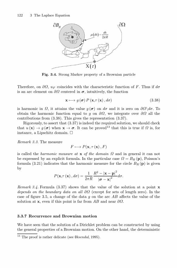
122 3 The Laplace Equation
Fig. 3.4. Strong Markov property of a Brownian particle
Therefore, on ∂Ω, uF coincides with the characteristic function of F . Thus if dσis an arc element on ∂Ω centered in σ, intuitively, the function
x �−→ g (σ)P (x,τ (x) , dσ) (3.38)
is harmonic in Ω, it attains the value g (σ) on dσ and it is zero on ∂Ω\dσ. Toobtain the harmonic function equal to g on ∂Ω, we integrate over ∂Ω all thecontributions from (3.38). This gives the representation (3.37).Rigorously, to assert that (3.37) is indeed the required solution, we should check
that u (x) → g (σ) when x → σ. It can be proved13 that this is true if Ω is, forinstance, a Lipschitz domain. �
Remark 3.3. The measureF �−→ P (x, τ (x) , F )
is called the harmonic measure at x of the domain Ω and in general it can notbe expressed by an explicit formula. In the particular case Ω = BR (p), Poisson’sformula (3.21) indicates that the harmonic measure for the circle BR (p) is givenby
P (x,τ (x) , dσ) =1
2πR
R2 − |x− p|2
|σ − x|2dσ.
Remark 3.4. Formula (3.37) shows that the value of the solution at a point xdepends on the boundary data on all ∂Ω (except for sets of length zero). In thecase of figure 3.5, a change of the data g on the arc AB affects the value of thesolution at x, even if this point is far from AB and near ∂Ω.
3.3.7 Recurrence and Brownian motion
We have seen that the solution of a Dirichlet problem can be constructed by usingthe general properties of a Brownian motion. On the other hand, the deterministic
13 The proof is rather delicate (see ∅ksendal, 1995).

3.3 Harmonic Functions 123
Fig. 3.5. A modification of the Dirichlet data on the arc AB, affects the value of thesolution at x
solution of some Dirichlet problems can be used to deduce interesting propertiesof Brownian motion. We examine two simple examples. Recall from Section 3.1that ln |x| is harmonic in the plane except x = 0.Let a, R be real numbers, R > a > 0. It is easy to check that the function
uR (x) =ln |R| − ln |x|lnR− lna
is harmonic in the ring Ba,R ={x ∈R2; a < |x| < R
}and moreover
uR (x) = 1 on ∂Ba (0) , uR (x) = 0 on ∂BR (0) .
Thus u (x) represents the escape probability from the ring through ∂Ba (0), start-ing at x:
uR (x) = PR (x,τ (x) , ∂Ba (0)) .
Letting R → +∞, we get
PR (x,τ (x) , ∂Ba (0)) =ln |R| − ln |x|lnR− ln a → 1 = P∞ (x,τ (x) , ∂Ba (0)) .
This means that, starting at x, the probability we (sooner or later) enter thecircle Ba (0), is 1. Due to the invariance by translations of the Brownian motion,the origin can be replaced by any other point without changing the conclusions.Moreover, since we have proved in Lemma 3.1 that the exit probability from anycircle is also 1, we can state the following result: given any point x and any circlein the plane, a Brownian particle started at x enters the circle and exit from it aninfinite number of times, with probability 1. We say that a bidimensional Brownianmotion is recurrent.
In three dimensions a Brownian motion is not recurrent. In fact (see the nextsection), the function
u (x) =
1|x| − 1
R
1a − 1
R
is harmonic in the spherical shell Ba,R ={x ∈R3; a < |x| < R
}and
u (x) = 1 on ∂Ba (0) , u (x) = 0 on ∂BR (0) .
124 3 The Laplace Equation
Then u (x) represents the escape probability from the shell through ∂Ba (0), start-ing at x:
uR (x) = PR (x,τ (x) , ∂Ba (0)) .
This time, letting R→ +∞, we find
PR (x,τ (x) , ∂Ba (0)) =
1|x| − 1
R
1a − 1
R
→ a
|x| = P∞ (x,τ (x) , ∂Ba (0)) .
Thus, the probability to enter, sooner or later, the sphere Ba (0) is not 1 and itbecomes smaller and smaller as the distance of x from the origin increases.
3.4 Fundamental Solution and Newtonian Potential
3.4.1 The fundamental solution
The (3.37) is not the only representation formula for the solution of the Dirichletproblem. We shall derive deterministic formulas involving various types of poten-tials, constructed using a special function, called the fundamental solution of theLaplace operator.As we did for the diffusion equation, let us look at the invariance properties
characterizing the operator Δ: the invariances by translations and by rotations.Let u = u (x) be harmonic in Rn. Invariance by translations means that the
function v (x) = u (x− y), for each fixed y, is also harmonic, as it is immediate tocheck.Invariance by rotations means that, given a rotation in Rn, represented by an
orthogonal matrix M (i.e. MT = M−1), also v (x) = u (Mx) is harmonic in Rn.To check it, observe that, if we denote by D2u the Hessian of u, we have
Δu = TrD2u = trace of the Hessian of u.
SinceD2v (x) =MTD2u (Mx)M
andM is orthogonal, we have
Δv (x) = Tr[MTD2u (Mx)M] = TrD2u (Mx) = Δu (Mx) = 0
and therefore v is harmonic.Now, a typical rotation invariant quantity is the distance function from a point,
for instance from the origin, that is r = |x|. Thus, let us look for radially symmetricharmonic functions u = u (r).Consider first n = 2; using polar coordinates and recalling (3.22), we find
∂2u
∂r2+1
r
∂u
∂r= 0

3.4 Fundamental Solution and Newtonian Potential 125
so thatu (r) = C log r +C1.
In dimension n = 3, using spherical coordinates (r, ψ, θ), r > 0, 0 < ψ < π,0 < θ < 2π, the operator Δ has the following expression14:
Δ =∂2
∂r2+2
r
∂
∂r︸ ︷︷ ︸radial part
+1
r2
{1
(sinψ)2∂2
∂θ2+∂2
∂ψ2+ cotψ
∂
∂ψ
}
︸ ︷︷ ︸.
spherical part (Laplace-Beltrami operator)
The Laplace equation for u = u (r) becomes
∂2u
∂r2+2
r
∂u
∂r= 0
whose general integral is
u (r) =C
r+ C1 C,C1 arbitrary constants.
Choose C1 = 0 and C =14π if n = 3, C = − 1
2π if n = 2. The function
Φ (x) =
⎧⎪⎨⎪⎩
− 12πlog |x| n = 21
4π |x| n = 3(3.39)
is called the fundamental solution for the Laplace operator Δ. As we shall provein Chapter 7, the above choice of the constant C is made in order to have
ΔΦ (x) = −δ (x)
where δ (x) denotes the Dirac measure at x = 0.The physical meaning of Φ is remarkable: if n = 3, in standard units, 4πΦ
represents the electrostatic potential due to a unitary charge located at the originand vanishing at infinity15.Clearly, if the origin is replaced by a point y, the corresponding potential is
Φ (x − y) andΔxΦ (x−y) = −δ (x− y) .
By symmetry, we also have ΔyΦ (x − y) = −δ (x− y).
Remark 3.5. In dimension n > 3, the fundamental solution of the Laplace operatoris Φ (x) = ω−1n |x|2−n.14 Appendix D.15 In dimension 2,
2πΦ (x1, x2) = − log√x21 + x
22
represents the potential due to a charge of density 1, distributed along the x3 axis.

126 3 The Laplace Equation
3.4.2 The Newtonian potential
Suppose that f (x) is the density of a charge located inside a compact set in R3.Then Φ (x − y) f (y) dy represents the potential at x due to the charge f (y) dyinside a small region of volume dy around y. The full potential is given by thesum of all the contributions; we get
u (x) =
∫
R3
Φ (x− y) f (y) dy = 14π
∫
R3
f (y)
|x − y|dy (3.40)
which is the convolution between f and Φ and it is called the Newtonian poten-tial of f . Formally, we have
Δu (x) =
∫
R3
ΔxΦ (x− y) f (y) dy = −∫
R3
δ (x− y) f (y) dy = −f (x) . (3.41)
Under suitable hypotheses on f , (3.41) is indeed true (see Theorem 3.9 below).Clearly, u is not the only solution of Δv = −f , since u+c, c constant, is a solutionas well. However, the Newtonian potential is the only solution vanishing at infinity.All this is stated precisely in the theorem below, where, for simplicity, we assumef ∈ C2
(R3)with compact support16. We have:
Theorem 3.9. Let f ∈ C2(R3)with compact support. Let u be the Newtonian
potential of f , defined by (3.40). Then, u is the only solution in R3 of
Δu = −f (3.42)
belonging to C2(R3)and vanishing at infinity.
Proof. The uniqueness part follows from Liouville’s Theorem. Let v ∈ C2(R3)
another solution to (3.42), vanishing at infinity. Then u−v is a bounded harmonicfunction in all R3 and therefore is constant. Since it vanishes at infinity it must bezero; thus u = v.To show that (3.40) belongs to C2
(R3)and satisfies (3.42), observe that we
can write (3.40) in the alternative form
u (x) =
∫
R3
Φ (y) f (x− y) dy = 14π
∫
R3
f (x− y)|y| dy.
Since 1/ |y| is integrable near the origin and f is zero outside a compact set, wecan take first and second order derivatives under the integral sign to get
uxjxk (x) =
∫
R3
Φ (y) fxjxk (x − y) dy. (3.43)
16 Recall that the support of a continuous function f is the closure of the set where f isnot zero.

3.4 Fundamental Solution and Newtonian Potential 127
Since fxjxk ∈ C(R3), formula (3.43) shows that also uxjxk is continuous and
therefore u ∈ C2(R3).
It remains to prove (3.42). Since Δxf (x− y) = Δyf (x− y), from (3.43), wehave
Δu(x) =
∫
R3
Φ (y)Δxf (x− y) dy =∫
R3
Φ (y)Δyf (x− y) dy.
We want to integrate by parts using formula (1.13) but since Φ has a singularityat y = 0, we have first to isolate the origin, by choosing a small ball Br = Br (0)and writing
Δu(x) =
∫
Br(0)
· · · dy+∫
R3\Br(0)· · · dy ≡ Ir+Jr. (3.44)
We have, using spherical coordinates,
|Ir| ≤max |Δf |4π
∫
Br(0)
1
|y| dy =max |Δf |∫ r
0
ρ dρ =max |Δf |2
r2
so thatIr → 0 if r→ 0.
Keeping in mind that f vanishes outside a compact set, we can integrate Jr byparts (twice), obtaining
Jr =1
4πr
∫
∂Br
∇σf (x − σ) · νσ dσ−∫
R3\Br(0)∇Φ (y) · ∇yf (x− y) dy
=1
4πr
∫
∂Br
∇σf (x − σ) · νσ dσ−∫
∂Br
f (x− σ)∇Φ (σ) · νσ dσ
since ΔΦ = 0 in R3\Br (0). We have:
1
4πr
∣∣∣∣∫
∂Br
∇σf (x− σ) · νσ dσ∣∣∣∣ ≤ rmax |∇f | → 0 as r→ 0.
On the other hand, ∇Φ (y) = −y |y|−3 and the outward pointing17 unit normalon ∂Br is νσ = −σ/r, so that∫
∂Br
f (x− σ)∇Φ (σ) · νσ dσ=1
4πr2
∫
∂Br
f (x− σ) dσ→ f (x) as r→ 0.
Thus, Jr → −f (x) as r → 0. Passing to the limit as r → 0 in (3.44) we getΔu (x) = −f (x). �
Remark 3.6. Theorem 3.9 actually holds under much less restrictive hypotheses onf . For instance, it is enough that f ∈ C1
(R3)and |f (x)| ≤ C |x|−3−ε , ε > 0.
17 With respect to R3\Br .

128 3 The Laplace Equation
Remark 3.7. An appropriate version of Theorem 3.9 holds in dimension n = 2,with the Newtonian potential replaced by the logarithmic potential
u (x) =
∫
R2
Φ (x − y) f (y) dy = − 12π
∫
R2
log |x − y| f (y) dy. (3.45)
The logarithmic potential does not vanish at infinity; its asymptotic behavior is(see Problem 3.11)
u (x) = −M2πlog |x|+O
(1
|x|
)as |x| → +∞ (3.46)
where
M =
∫
R2
f (y)dy.
Indeed, the logarithmic potential is the only solution of Δu = −f in R2 satisfying(3.46).
3.4.3 A divergence-curl system. Helmholtz decomposition formula
Using the properties of the Newtonian potential we can solve the following twoproblems, that appear in several applications e.g. to linear elasticity, fluid dynamicsor electrostatics.
(1) Reconstruction of a vector field in R3 from the knowledge of its curl anddivergence. Precisely, given a scalar f and a vector field ω, we want to find avector field u such that {
div u =fcurl u = ω
in R3.
We assume that u has continuous second derivatives and vanishes at infinity, as itis required in most applications.
(2) Decomposition of a vector field u ∈R3 into the sum of a divergence freevector field and a curl free vector field. Precisely, given u, we want to find ϕ anda vector field w such that the following Helmholtz decomposition formula holds
u =∇ϕ+ curl w. (3.47)
Consider problem (1). First of all observe that, since div curl u =0, a necessarycondition for the existence of a solution is div ω =0.Let us check uniqueness. If u1 and u2 are solutions sharing the same data f
and ω, their difference w = u1− u2 vanishes at infinity and satisfies
div w =0 and curl w = 0 in R3.
From curl w = 0 we infer the existence of a scalar function U such that
∇U = w.

3.4 Fundamental Solution and Newtonian Potential 129
From div w =0 we deduce
div∇U = ΔU = 0.Thus U is harmonic. Hence its derivatives, i.e. the components wj of w, are
bounded harmonic functions in R3. Liouville’s theorem implies that each wj isconstant and therefore identically zero since it vanishes at infinity. We concludethat, under the stated assumptions, the solution of problem (1) is unique.To find u, split it into u = v + z and look for v and z such that
div z = 0 curl z = ω
div v = f curl v = 0.
As before, from curl v = 0 we infer the existence of a scalar function ϕ such that∇ϕ = v, while div v =f implies Δϕ = f . We have seen that, under suitablehypotheses on f , ϕ is given by the Newtonian potential of f , that is:
ϕ (x) = − 14π
∫
R3
1
|x − y|f (y) dy
and v =∇ϕ. To find z, recall the identity
curl curl z =∇(div z)−Δz.
Since div z =0, we get
Δz = −curl curl z =curl ωso that
z (x) =1
4π
∫
R3
1
|x− y|curl ω (y)dy.
Let us summarize the conclusions in the next theorem, also specifying the hypothe-ses18 on f and ω.
Theorem 3.10. Let f ∈ C1(R3), ω ∈ C2
(R3)such that div ω =0 and, for |x|
large,
|f (x)| ≤ M
|x|3+ε, |curlω (x)| ≤ M
|x|3+ε(ε > 0) .
Then, the unique solution vanishing at infinity of the system
{div u =fcurl u = ω
in R3
is given by vector field
u (x) =
∫
R3
1
4π |x − y|curl ω (y) dy −∇∫
R3
1
4π |x − y|f (y) dy. (3.48)
18 See Remark 3.6.

130 3 The Laplace Equation
Consider now problem (2). If u, div u and curl u satisfy the hypotheses oftheorem 3.10, we can write
u(x) =
∫
R3
1
4π |x − y|curl curl u (y) dy −∇∫
R3
1
4π |x − y| div u (y) dy.
Since u is rapidly vanishing at infinity, we have19
∫
R3
1
|x− y|curl curl u (y) dy = curl∫
R3
1
|x − y|curl u (y) dy. (3.49)
We conclude that
u =∇ϕ + curl wwhere
ϕ (x) = −∫
R3
1
4π |x− y|div u (y) dy
and
w (x) =
∫
R3
1
4π |x − y|curl u (y) dy.
• An application to fluid dynamics. Consider the three dimensional flow of anincompressible fluid of constant density ρ and viscosity μ, subject to a conservativeexternal force20 F = ∇f . If u = u (x,t) denotes the velocity field and p = p (x,t) isthe hydrostatic pressure, the laws of conservation of mass and linear momentumgive for u and p the celebrated Navier-Stokes equations:
div u = 0 (3.50)
and
Du
Dt= ut + (u·∇)u = −
1
ρ∇p+ νΔu+1
ρ∇f (ν = μ/ρ). (3.51)
We look for solution of (3.50), (3.51) subject to a given initial condition
u (x,0) = g (x) x ∈R3, (3.52)
where g is also divergence free:
div g =0.
19 In fact, if |g (x)| ≤ M|x|3+ε , one can show that
∂
∂xj
∫
R3
1
|x− y|g (y) dy =∫
R3
1
|x− y|∂g
∂yjdy.
20 Gravity, for instance.

3.4 Fundamental Solution and Newtonian Potential 131
The quantity DuDt is called the material derivative of u, given by the sum of ut,
the fluid acceleration due to the non-stationary character of the motion, and of(u·∇)u, the inertial acceleration due to fluid transport21.In general, the system (3.50), (3.51) is extremely difficult to solve. In the case
of slow flow, for instance due to high viscosity, the inertial term becomes negligible,compared for instance to νΔu, and (3.51) simplifies to the linearized equation
ut = −1
ρ∇p+ νΔu+∇f. (3.53)
It is possible to find an explicit formula for the solution of (3.50), (3.52), (3.53)by writing everything in terms of ω =curl u. In fact, taking the curl of (3.53) and(3.52), we obtain, since curl(∇p+ νΔu+∇f) = νΔω,
{ωt = νΔω x ∈R3, t > 0ω (x,0) = curl g (x) x ∈R3.
This is a global Cauchy problem for the heat equation. If g ∈C2(R3)and curl g
is bounded, we have
ω (x,t) =1
(4πνt)3/2
∫
R3
exp
(−|y|
2
4νt
)curl g (x− y) dy. (3.54)
Moreover, for t > 0, we can take the divergence operator under the integral in(3.54) and deduce that div ω =0. Therefore, if curl g (x) vanishes rapidly at infin-ity22, we can recover u by solving the system
curl u = ω, div u =0,
according to formula (3.48) with f = 0.Finally to find the pressure, from (3.53) we have
∇p = −ρut + μΔu−∇f. (3.55)
Since ωt = νΔω, the right hand side has zero curl; hence (3.55) can be solved anddetermines p up to an additive constant (as it should be).
In conclusion: Let, f ∈ C1(R3), g ∈C2
(R3), with div g = 0 and curl g rapidly
vanishing at infinity. There exist a unique u ∈C2(R3), with curl u vanishing at
infinity, and p ∈C1(R3)unique up to an additive constant, satisfying the system
(3.50), (3.52), (3.53).
21 The i−component of (v·∇) v is given by∑3j=1 vj ∂vi∂xj. Let us compute Dv
Dt, for example,
for a plane fluid uniformly rotating with angular speed ω. Then v (x, y) = −ωyi+ωxj.Since vt = 0, the motion is stationary and
Dv
Dt= (v·∇) v =
(−ωy ∂
∂x+ωx
∂
∂y
)(−ωyi+ωxj) = −ω2 (−xi+yj)
which is centrifugal acceleration.22 |curl g (x)| ≤M/ |x|3+ε , ε > 0, it is enough.

132 3 The Laplace Equation
3.5 The Green Function
3.5.1 An integral identity
Formula (3.40) gives a representation of the solution to Poisson’s equation in allR3. In bounded domains, any representation formula has to take into account theboundary values, as indicated in the following theorem.
Theorem 3.11. Let Ω ⊂ Rn be a smooth, bounded domain and u ∈ C2
(Ω).
Then, for every x ∈Ω,
u (x) = −∫
Ω
Φ (x− y)Δu (y) dy+
+
∫
∂Ω
Φ (x− σ) ∂νσu (σ) dσ−∫
∂Ω
u (σ) ∂νσΦ (x − σ) dσ(3.56)
The last two terms in the right hand side of (3.56) are called single and doublelayer potentials, respectively. We are going to examine these surface potentialslater. The first one is the Newtonian potential of −Δu in Ω.Proof. We give it for n = 3. Fix x ∈Ω, and consider the fundamental solution
Φ (x− y) = 1
4πrxyrxy = |x− y|
as a function of y: we write Φ (x− ·).We would like to apply Green’s identity (1.15)
∫
Ω
(vΔu− uΔv)dx =∫
∂Ω
(v∂νu −u∂νv)dσ (3.57)
to u and Φ (x− ·). However, Φ (x − ·) has a singularity in x, so that it cannot beinserted directly into (3.57). Let us isolate the singularity inside a ball Bε (x), withε small. In the domain Ωε = Ω\Bε (x), Φ (x − ·) is smooth and harmonic.Thus, replacing Ω with Ωε, we can apply (3.57) to u and Φ (x − ·). Since
∂Ωε = ∂Ω ∪ ∂Bε (x) ,and ΔyΦ (x− y) = 0, we find:
∫
Ωε
1
rxyΔu dy =
∫
∂Ωε
(1
rxσ
∂u
∂νσ−u ∂
∂νσ
1
rxσ
)dσ
=
∫
∂Ω
(· · · ) dσ +∫
∂Bε(x)
1
rxσ
∂u
∂νσdσ −
∫
∂Bε(x)
u∂
∂νσ
1
rxσdσ.
(3.58)
We let now ε→ 0 in (3.58). We have:∫
Ωε
1
rxσΔu dy→
∫
Ω
1
rxσΔu dy as ε→ 0 (3.59)
since Δu ∈ C(Ω)and r−1xσ is positive and integrable in Ω.

3.5 The Green Function 133
On ∂Bε (x), we have rxσ = ε and |∂νu| ≤M , since |∇u| is bounded; then∣∣∣∣∣∫
∂Bε(x)
1
rxσ
∂u
∂νσdσ
∣∣∣∣∣ ≤ 4πεM → 0 as ε→ 0. (3.60)
The most delicate term is∫
∂Bε(x)
u∂
∂νσ
1
rxσdσ.
On ∂Bε (x), the outward pointing (with respect to Ωε) unit normal at σ isνσ=
x−σε , so that
∂
∂νσ
1
rxσ= ∇y
1
rxσ· νσ=
x − σε3x − σε=1
ε2.
As a consequence,
∫
∂Bε(x)
u∂
∂νσ
1
rxσdσ =
1
ε2
∫
∂Bε(x)
u dσ→ 4π u (x) (3.61)
as ε→ 0, by the continuity of u.Letting ε→ 0 in (3.58), from (3.59), (3.60), (3.61) we obtain (3.56). �
3.5.2 The Green function
The function Φ defined in (3.39) is the fundamental solution for the Laplace op-erator Δ in all Rn (n = 2, 3). We can also define a fundamental solution for theLaplace operator in any open set and in particular in any bounded domainΩ ⊂ Rn,representing the potential due to a unit charge placed at a point x ∈ Ω and equalto zero on ∂Ω.This function, that we denote by G (x,y), is called the Green function in Ω,
for the operator Δ; for fixed x ∈Ω, G satisfies
ΔyG (x,y) = −δx in Ω
andG (x,σ) = 0, σ ∈ ∂Ω.
More explicitly, the Green’s function can be written in the form
G (x,y) = Φ (x − y)− ϕ (x,y)
where ϕ, for fixed x ∈Ω, solves the Dirichlet problem{
Δyϕ = 0 in Ω
ϕ (x,σ) = Φ (x − σ) on ∂Ω.(3.62)

134 3 The Laplace Equation
Two important properties of the Green function are the following (see Prob-lem 3.14):
(a) Positivity: G (x,y) > 0 for every x,y ∈ Ω, with G (x,y) → +∞ whenx− y→ 0;(b) Symmetry: G (x,y) = G (y,x).
The existence of the Green function for a particular domain depends on thesolvability of the Dirichlet problem (3.62). From Theorem 3.8, we know that thisis the case if Ω is a Lipschitz domain, for instance.Even if we know that the Green function exists, explicit formulas are available
only for special domains. Sometimes a technique known as method of electrostaticimages works. In this method ϕ (x, ·) is considered as the potential due to animaginary charge q placed at a suitable point x∗, the image of x, in the complementof Ω. The charge q and the point x∗ have to be chosen so that ϕ (x, ·) on ∂Ω isequal to the potential created by the unit charge in x.The simplest way to illustrate the method is to find the Green function for the
upper half-space, although this is an unbounded domain. Clearly, we require thatG vanishes at infinity.
• Green’s function for the upper half space in R3. Let R3+ be the upper halfspace :
R3+ = {(x1, x2, x3) : x3 > 0} .
Fix x =(x1, x2, x3) and observe that if we choose x∗=(x1, x2,−x3) then, on y3 = 0
we have|x∗ − y| = |x − y| .
Thus, if x ∈R3+, x∗ belongs to the complement of R3+, the function
ϕ (x,y) = Φ (x∗−y) = 1
4π |x∗ − y|is harmonic in R3+ and ϕ (x,y) = Φ (x− y) on the plane y3 = 0. In conclusion,
G (x,y) =1
4π |x− y| −1
4π |x∗ − y| (3.63)
is the Green function for the upper half space.
• Green function for sphere. Let Ω = BR = BR (0) ⊂ R3. To find the Greenfunction for BR, set
ϕ (x,y) =q
4π |x∗ − y| ,
x fixed in BR, and try to determine x∗, outside BR, and q, so that
q
4π |x∗ − y| =1
4π |x − y| (3.64)
when |y| = R. The (3.64) gives
|x∗ − y|2 = q2 |x − y|2 (3.65)
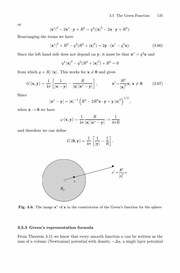
3.5 The Green Function 135
or|x∗|2 − 2x∗ · y + R2 = q2(|x|2 − 2x · y +R2).
Rearranging the terms we have
|x∗|2 + R2 − q2(R2 + |x|2) = 2y · (x∗ − q2x). (3.66)
Since the left hand side does not depend on y, it must be that x∗ = q2x and
q4 |x|2 − q2(R2 + |x|2) +R2 = 0
from which q = R/ |x| . This works for x �= 0 and gives
G (x,y) =1
4π
[1
|x− y| −R
|x| |x∗ − y|
], x∗=
R2
|x|2x, x �= 0. (3.67)
Since
|x∗ − y| = |x|−1(R4 − 2R2x · y + y |x|2
)1/2,
when x→ 0 we have
ϕ (x,y) =1
4π
R
|x| |x∗ − y| →1
4πR
and therefore we can define
G (0,y) =1
4π
[1
|y| −1
R
].
Fig. 3.6. The image x∗ of x in the construction of the Green’s function for the sphere
3.5.3 Green’s representation formula
From Theorem 3.11 we know that every smooth function u can be written as thesum of a volume (Newtonian) potential with density −Δu, a single layer potential
136 3 The Laplace Equation
of density ∂νu and a double layer potential of moment u. Suppose u solves theDirichlet problem {
Δu = f in Ωu = g on ∂Ω.
(3.68)
Then (3.56) gives, for x ∈Ω,
u (x) = −∫
Ω
Φ (x − y) f (y) dy+
+
∫
∂Ω
Φ (x− σ) ∂νσu (σ) dσ−∫
∂Ω
g (σ) ∂νσΦ (x− σ) dσ.(3.69)
This representation formula for u is not satisfactory, since it involves the data fand g but also the normal derivative ∂νσu, which is unknown. To get rid of ∂νσu,let G (x,y) = Φ (x − y) − ϕ (x,y) be the Green function in Ω. Since ϕ (x, ·) isharmonic in Ω, we can apply (3.57) to u and ϕ (x, ·); we find
0 =
∫
Ω
ϕ (x,y) f (y) dy +
−∫
∂Ω
ϕ (x,σ) ∂νσu (σ) dσ +
∫
∂Ω
g (σ) ∂νσϕ (x,σ) dσ.(3.70)
Adding (3.69), (3.70) and recalling that ϕ (x,σ) = Φ (x− σ) on ∂Ω, we obtain:
Theorem 3.12. Let Ω be a smooth domain and u be a smooth solution of (3.68).Then:
u (x) = −∫
Ω
f (y)G (x,y) dy−∫
∂Ω
g (σ) ∂νσG (x,σ) dσ. (3.71)
Thus the solution of the Dirichlet problem (3.68) can be written as the sum ofthe two Green potentials in the right hand side of (3.71) and it is known as soonas the Green function in Ω is known. In particular, if u is harmonic, then
u (x) = −∫
∂Ω
g (σ) ∂νσG (x,σ) dσ. (3.72)
Comparing with (3.37), we deduce that
−∂νσG (x,σ) dσ
represents the harmonic measure in Ω. The function
P (x,σ) = −∂νσG (x,σ)
is called Poisson’s kernel. Since G (·,σ) > 0 inside Ω and vanishes on Ω, P isnonnegative (actually positive).On the other hand, the formula
u (x) = −∫
Ω
f (y)G (x,y) dy

3.5 The Green Function 137
gives the solution of the Poisson equation Δu = f in Ω, vanishing on ∂Ω. Fromthe positivity of G we have that:
f ≥ 0 in Ω implies u ≤ 0 in Ω,which is another form of the maximum principle.
• Poisson’s kernel and Poisson’s formula. From (3.67) we can compute Pois-son’s kernel for the sphere BR (0). We have, recalling that x
∗=R2 |x|−2 x, if x �= 0,
∇y[1
|x − y| −R
|x| |x∗ − y|
]=x − y|x− y|3
− R|x|x∗−y|x∗ − y|3
.
If σ ∈∂BR (0), from (3.65) we have |x∗ − σ| = R |x|−1 |x− σ| , therefore
∇yG (x,σ) =1
4π
[x− σ|x − σ|3
− |x|2
R2x∗−σ|x− σ|3
]=
−σ4π |x− σ|3
[1− |x|
2
R2
].
Since on ∂BR (0) the exterior unit normal is νσ= σ/R, we have
P (x,σ) = −∂νσG (x,σ) = −∇yG (x,σ) · νσ =R2 − |x|24πR
1
|x − σ|3.
As a consequence, we obtain Poisson’s formula
u (x) =R2 − |x|24πR
∫
∂BR(0)
g (σ)
|x− σ|3dσ (3.73)
for the unique solution of the Dirichlet problem Δu = 0 in BR (0) and u = g on∂BR (0) .
3.5.4 The Neumann function
We can find a representation formula for the solution of a Neumann problem aswell. Let u be a smooth solution of the problem
{Δu = f in Ω
∂νu = h on ∂Ω(3.74)
where f and h have to satisfy the solvability condition∫
∂Ω
h (σ) dσ=
∫
Ω
f (y) dy, (3.75)
keeping in mind that u is uniquely determined up to an additive constant. FromTheorem 3.11 we can write
u (x) = −∫
Ω
Φ (x − y) f (y) dy+
+
∫
∂Ω
h (σ)Φ (x− σ) dσ−∫
∂Ω
u (σ) ∂νσΦ (x− σ) dσ.(3.76)

138 3 The Laplace Equation
and this time we should get rid of the second integral, containing the unknowndata u on ∂Ω. Mimicking what we have done for the Dirichlet problem, we try tofind an analog of the Green function, that is a function N = N (x,y) given by
N (x,y) = Φ (x − y)− ψ (x,y)where, for x fixed, ψ is a solution of
{Δyψ = 0 in Ω
∂νσψ (x,σ) = ∂νσΦ (x− σ) on ∂Ω,
in order to have ∂νσN (x,σ) = 0 on ∂Ω. But this Neumann problem has nosolution because the compatibility condition∫
∂Ω
∂νσΦ (x− σ) dσ = 0
is not satisfied. In fact, letting u ≡ 1 in (3.56), we get∫
∂Ω
∂νσΦ (x− σ) dσ = −1. (3.77)
Thus, taking into account (3.77), we require ψ to satisfy{Δyψ = 0 in Ω
∂νσψ (x,σ) = ∂νσΦ (x− σ) + 1|∂Ω| on ∂Ω.
(3.78)
In this way, ∫
∂Ω
(∂νσΦ (x− σ) +
1
|∂Ω|
)dσ = 0
and (3.78) is solvable. Note that, with this choice of ψ, we have
∂νσN (x,σ) = −1
|∂Ω| on ∂Ω. (3.79)
Apply now (3.57) to u and ψ (x, ·); we find:
0 = −∫
∂Ω
ψ (x,σ) ∂νσu (σ) dσ+
∫
∂Ω
h (σ) ∂νσψ (σ) dσ +
∫
Ω
ψ (y) f (y) dy.
(3.80)Adding (3.80) to (3.76) and using (3.79) we obtain:
Theorem 3.13. Let Ω be a smooth domain and u be a smooth solution of (3.74).Then:
u (x)− 1
|∂Ω|
∫
∂Ω
u (σ) dσ =
∫
∂Ω
h (σ)N (x,σ) dσ −∫
Ω
f (y)N (x,y) dy.
Thus, the solution of the Neumann problem (3.74) can also be written as thesum of two potentials, up to the additive constant c = 1
|∂Ω|∫∂Ωu (σ) dσ, the mean
value of u.The function N is called Neumann’s function (also Green’s function for the
Neumann problem) and it is defined up to an additive constant.
3.6 Uniqueness in Unbounded Domains 139
3.6 Uniqueness in Unbounded Domains
3.6.1 Exterior problems
Boundary value problems in unbounded domains occur in important applications,for instance in the motion of fluids past an obstacle, capacity problems or scatteringof acoustic or electromagnetic waves.As in the case of Poisson’s equation in all Rn, a problem in an unbounded
domain requires suitable conditions at infinity to be well posed.Consider for example the Dirichlet problem
{Δu = 0 in |x| > 1u = 0 on |x| = 1. (3.81)
For every real number a,
u (x) = a log |x| and u (x) = a (1− 1/ |x|)
are solutions to (3.81) in dimension two and three, respectively. Thus there is nouniqueness.To restore uniqueness, a typical requirement in two dimensions is that u be
bounded, while in three dimensions that u (x) has a limit, say u∞, as |x| → ∞:under these conditions, in both cases we select a unique solution.Problem (3.81) is an exterior Dirichlet problem. Given a bounded domain Ω,
we call exterior of Ω the setΩe = R
n\Ω.Without loss of generality we will assume that 0 ∈Ω and for simplicity, we willconsider only connected exterior sets, i.e. exterior domains. Note that ∂Ωe = ∂Ω.As we have seen in several occasions, maximum principles are very useful to
prove uniqueness. In exterior three dimensional domains we have (for n = 2 seeProblem 3.16):
Theorem 3.14. Let Ωe ⊂ R3 be an exterior domain and u ∈ C2 (Ωe) ∩ C(Ωe),
be harmonic in Ωe and vanishing as |x| → ∞. If u ≥ 0 (resp. u ≤ 0) on ∂Ωe thenu ≥ 0 (resp. u ≤ 0) in Ωe.Proof. Let u ≥ 0 on ∂Ωe. Fix ε > 0 and choose r0 so large that Ω ⊂ {|x| < r}
and u ≥ −ε on {|x| = r} , for every r ≥ r0. In the bounded set
Ωe,r = Ωe ∩ {|x| < r}
we can apply Theorem 3.5 and we get u ≥ −ε in this set. Since ε is arbitrary andr may be taken as large as we like, we deduce that u ≥ 0 in Ωe.The argument for the case u ≤ 0 on ∂Ωe is similar and we leave the details to
the reader. �An immediate consequence is the following uniqueness result in dimension n =
3 (for n = 2 see Problem 3.16):
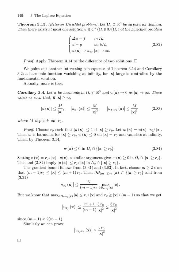
140 3 The Laplace Equation
Theorem 3.15. (Exterior Dirichlet problem). Let Ωe ⊂ R3 be an exterior domain.Then there exists at most one solution u ∈ C2 (Ωe)∩C(Ωe) of the Dirichlet problem
⎧⎪⎨⎪⎩
Δu = f in Ωe
u = g on ∂Ωe
u (x)→ u∞ |x| → ∞.(3.82)
Proof. Apply Theorem 3.14 to the difference of two solutions. �
We point out another interesting consequence of Theorem 3.14 and Corollary3.2: a harmonic function vanishing at infinity, for |x| large is controlled by thefundamental solution.Actually, more is true:
Corollary 3.4. Let u be harmonic in Ωe ⊂ R3 and u (x)→ 0 as |x| → ∞. Thereexists r0 such that, if |x| ≥ r0,
|u (x)| ≤ M|x| ,∣∣uxj (x)
∣∣ ≤ M
|x|2,
∣∣uxjxk (x)∣∣ ≤ M
|x|3(3.83)
where M depends on r0.
Proof. Choose r0 such that |u (x)| ≤ 1 if |x| ≥ r0. Let w (x) = u(x)−r0/ |x|.Then w is harmonic for |x| ≥ r0, w (x) ≤ 0 on |x| = r0 and vanishes at infinity.Then, by Theorem 3.14,
w (x) ≤ 0 in Ωe ∩ {|x| ≥ r0} . (3.84)
Setting v (x) = r0/ |x|−u(x), a similar argument gives v (x) ≥ 0 in Ωe∩{|x| ≥ r0}.This and (3.84) imply |u (x)| ≤ r0/ |x| in Ωe ∩ {|x| ≥ r0} .The gradient bound follows from (3.31) and (3.83). In fact, choose m ≥ 2 such
that (m − 1)r0 ≤ |x| ≤ (m+ 1) r0. Then ∂B(m−1)r0 (x) ⊂ {|x| ≥ r0} and from(3.31) ∣∣uxj (x)
∣∣ ≤ 3
(m− 1)r0max
∂Bmr0(x)|u| .
But we know that max∂Bmr0(x) |u| ≤ r0/ |x| and r0 ≥ |x| / (m+ 1) so that we get
∣∣uxj (x)∣∣ ≤ m+ 1
(m− 1)3 r0
|x|2≤ 6 r0|x|2
since (m+ 1) < 2(m− 1).Similarly we can prove ∣∣uxjxk (x)
∣∣ ≤ c r0|x|3
�

3.7 Surface Potentials 141
The estimates (3.83) assure the validity of the Green identity∫
Ωe
∇u · ∇v dx =∫
∂Ωe
v∂νu dσ (3.85)
for any pair u, v ∈ C2 (Ωe)∩C1(Ωe), harmonic in Ωe and vanishing at infinity. Tosee this, apply the identity (3.85) in the bounded domain Ωe,r = Ωe ∩ {|x| < r} .Then let r→∞ to get (3.85) in Ωe.In turn, via the Green identity (3.85), we can prove an appropriate version of
Theorem 3.15 for the exterior problem⎧⎪⎨⎪⎩
Δu = f in Ωe
∂νu+ ku = g on ∂Ωe, (k ≥ 0)u→ u∞ as |x| → ∞.
(3.86)
Observe that k �= 0 corresponds to the Robin problem while k = 0 corresponds tothe Neumann problem.
Theorem 3.16. (Exterior Neumann and Robin problems). Let Ωe ⊂ R3 be an
exterior domain. Then there exists at most one solution u ∈ C2 (Ωe) ∩ C1(Ωe) ofproblem (3.86).
Proof. Suppose u, v are solutions of (3.86) and let w = u−v. Then w is harmonicΩe, ∂νw + kw = 0 on ∂Ωe and w→ 0 as |x| → ∞.Apply the identity (3.85) with u = v = w. Since ∂νw = −kw on ∂Ωe we have:
∫
Ωe
|∇w|2 dx =∫
∂Ωe
w∂νw dσ = −∫
∂Ωe
kw2dσ ≤ 0.
Thus ∇w = 0 and w is constant, because Ωe is connected. But w vanishes atinfinity so that w = 0. �
3.7 Surface Potentials
In this section we go back to examine the meaning and the main properties of thesurface potentials appearing in the identity (3.56). A remarkable consequence isthe possibility to convert a boundary value problem into a boundary integralequation. This kind of formulation can be obtained for more general operatorsand more general problems as soon as a fundamental solution is known. Thus itconstitutes a flexible method with important implications. In particular, it consti-tutes the theoretical basis for the so called boundary element method, which mayoffer several advantages from the point of view of the computational cost in numer-ical approximations, due to a dimension reduction. Here we present the integralformulations of the main boundary value problems and state some basic results.The reader can find complete proofs and the integral formulation of more generalor different problems in the literature at the end of the book (e.g. Dautrait-Lions,vol 3, 1985).

142 3 The Laplace Equation
3.7.1 The double and single layer potentials
The last integral in (3.56) is of the form
D (x;μ) =∫
∂Ω
μ (σ) ∂νσΦ (x − σ) dσ (3.87)
and it is called the double layer potential of μ. In three dimensions it representsthe electrostatic potential generated by a dipole distribution23 of moment μ on ∂Ω.To get a clue of the main features ofD (x;μ), it is useful to look at the particular
case μ (σ) ≡ 1, that is
D (x;1) =∫
∂Ω
∂νσΦ (x− σ) dσ. (3.88)
Inserting u ≡ 1 into (3.56) we get
D (x;1) = −1 for every x ∈Ω. (3.89)
On the other hand, if x ∈Rn\Ω is fixed, Φ (x− ·) is harmonic in Ω and can beinserted into (3.57) with u ≡ 1; the result is
D (x;1) = 0 for every x ∈Rn\Ω. (3.90)
What happens for x ∈ ∂Ω? First of all we have to check that D (x;1) is well defined(i.e. finite) on ∂Ω. Indeed the singularity of ∂νσΦ (x− σ) becomes critical whenx ∈ ∂Ω since as σ → x the order of infinity equals the topological dimension of∂Ω. For instance, in the two dimensional case we have
D (x;1) = − 12π
∫
∂Ω
∂νσ log |x− σ|dσ = −1
2π
∫
∂Ω
(x− σ) · νσ|x− σ|2
dσ.
The order of infinity of the integrand is one and the boundary ∂Ω is a curve, aone dimensional object. In the three dimensional case we have
D (x;1) = 14π
∫
∂Ω
∂
∂νσ
1
|x − σ|dσ =1
4π
∫
∂Ω
(x − σ) · νσ|x − σ|3
dσ.
23 For every σ ∈ ∂Ω, let −q (σ), q (σ) two charges placed at the points σ, σ+hνσ,respectively. If h > 0 is very small, the pair of charges constitutes a dipole of axis νσ.The induced potential at x is given by
u (x,σ) = q (σ) [Φ (x− (σ+hν)) − Φ (x− σ)] = q (σ) h
[Φ (x− (σ+hν)) − Φ (x− σ)
h
].
Since h is very small, setting q (σ)h = μ (σ), we can write, at first order of approxi-mation,
uh (x) � μ (σ)∂νσΦ (x− σ) .Integrating on ∂Ω we obtain D (x;μ).

3.7 Surface Potentials 143
The order of infinity of the integrand is two and ∂Ω is a bidimensional surface.However, if we assume that Ω is a C2 domain, then it can be proved that
D (x;1) is well defined on ∂Ω.To compute the value of D (x;1) on ∂Ω we first observe that formulas (3.89)
and (3.90) follow immediately from the geometric interpretation of the integrand inD (x;1). Precisely, set rxσ = |x − σ| and, in dimension two, consider the quantity
dσ∗ = −(x − σ) · νσr2xσ
dσ =(σ − x) · νσr2xσ
dσ.
We have (see Fig. 3.7),(σ − x)rxσ
·νσ = cosϕ
and therefore
dσ′ =(σ − x) · νσrxσ
dσ = cosϕ dσ
is the projection of the length element dσ on the circle ∂Brxσ (x), up to an errorof lower order. Then
dσ∗ =dσ′
rxσ
is the projection of dσ on ∂B1 (x).Integrating on ∂Ω, the contributions to dσ∗ sum up to 2π if x ∈ Ω (case a)
of figure 3.8) and to 0 if x ∈Rn\Ω, due to the sign compensations induced by theorientation of νσ (case c) of figure 3.8). Thus
∫
∂Ω
dσ∗ ={2π if x ∈Ω0 if x ∈R2\Ω
Fig. 3.7. Geometrical interpretation of the integrand in D (x, 1) (n = 2)

144 3 The Laplace Equation
which are equivalent to (3.89) and (3.90), since
D (x;1) = − 12π
∫
∂Ω
dσ∗.
The case b) in figure 3.8 corresponds to x ∈ ∂Ω. It should be now intuitively clearthat the point x “ sees” a total angle of only π radiants and D (x;1) = −1/2.The same kind of considerations hold in dimension three; this time, the quantity
(see Fig. 3.9)
dσ∗ = −(x − σ) · νσr3xσ
dσ =(σ − x) · νσr3xσ
dσ
is the projection on ∂B1 (x) (solid angle) of the surface element dσ. Integratingover ∂Ω, the contributions to dσ∗ sum up to 4π if x ∈Ω and to 0 if x ∈R3\Ω.If x ∈ ∂Ω, it “ sees” a total solid angle of measure 2π. Since
D (x;1) = − 14π
∫
∂Ω
dσ∗,
we find again the values −1, 0,−1/2 in the three cases, respectively.
Fig. 3.8. Values of∫∂Ω
dσ∗ for n = 2
We gather the above results in the following Lemma.
Lemma 3.2 (Gauss). Let Ω ⊂ Rn be a bounded, C2-domain. Then
D (x;1) =∫
∂Ω
∂νσΦ (x − σ) dσ =
⎧⎪⎪⎪⎨⎪⎪⎪⎩
−1 x ∈Ω
−12
x ∈∂Ω
0 x ∈ Rn\Ω.
Thus, when μ ≡ 1, the double layer potential is constant outside ∂Ω and hasa jump discontinuity across ∂Ω. Observe that if x ∈∂Ω,
limz→x, z∈Rn\Ω
D (z;1) = D (x;1) + 12

3.7 Surface Potentials 145
Fig. 3.9. The solid angle dσ∗, projected from dσ
and
limz→x, z∈Ω
D (z;1) = D (x;1)− 12.
These formulas are the key for understanding the general properties of D (x;μ),that we state in the following theorem.
Theorem 3.17. Let Ω ⊂ Rn be a bounded, C2 domain and μ a continuous func-tion on ∂Ω. Then, D (x;μ) is harmonic in Rn\∂Ω and the following jump relationshold for every x ∈ ∂Ω :
limz→x, z∈Rn\Ω
D (z;μ) = D (x;μ) + 12μ (x) (3.91)
and
limz→x, z∈Ω
D (z;μ) = D (x;μ)− 12μ (x) . (3.92)
Proof (Sketch). If x /∈ ∂Ω there is no problem in differentiating under theintegral sign and, for σ fixed on ∂Ω, the function
∂νσΦ (x − σ) = ∇σΦ (x− σ) · νσis harmonic. Thus D (x;μ) is harmonic in Rn\∂Ω.Consider (3.91). This is not an elementary formula and we cannot take the
limit under the integral sign, once more because of the critical singularity of∂νσΦ (x − σ) when x ∈ ∂Ω.Let z ∈Rn\Ω. From Gauss Lemma 3.2
μ (x)
∫
∂Ω
∂νσΦ (z − σ) dσ = 0
and we can write
D (z;μ) =∫
∂Ω
∂νσΦ (z− σ) [μ (σ) − μ (x)]dσ. (3.93)

146 3 The Laplace Equation
Now, when σ is near x, the smoothness of ∂Ω and the continuity of μ mitigatethe singularity of ∂νσΦ (x− σ) and allow to take the limit under the integral sign.Thus
limz→x
∫
∂Ω
∂νσΦ (z− σ) [μ (σ) − μ (x)] dσ =∫
∂Ω
∂νσΦ (x − σ) [μ (σ)− μ (x)]dσ.
Exploiting once more Gauss lemma, we have
=
∫
∂Ω
∂νσΦ (x− σ) μ (σ) dσ − μ (x)∫
∂Ω
∂νσΦ (x− σ) dσ
= D (x;μ) + 12μ (x) .
The proof of (3.92) is similar. �The second integral in (3.56) is of the form
S (x,ψ) =∫
∂Ω
Φ (x − σ)ψ (σ) dσ
and it is called the single layer potential of ψ.In three dimensions it represents the electrostatic potential generated by a
charge distribution of density ψ on ∂Ω. If Ω is a C2−domain and ψ is continuouson ∂Ω, then S is continuous across ∂Ω and
ΔS = 0 in Rn\∂Ω,because there is no problem in differentiating under the integral sign.Since the flux of an electrostatic potential undergoes a jump discontinuity
across a charged surface, we expect a jump discontinuity of the normal deriva-tive of S across ∂Ω. PreciselyTheorem 3.18. Let Ω ⊂ Rn be a bounded, C2-domain and ψ a continuous func-tion on ∂Ω. Then, S (x;ψ) is harmonic in Rn\∂Ω, continuous across ∂Ω and thefollowing jump relations hold for every x ∈ ∂Ω :
limz→x, z∈Rn\Ω
∂νxS (z;ψ) =∫
∂Ω
∂νxΦ (x− σ)ψ (σ) dσ −1
2ψ (x) (3.94)
and
limz→x, z∈Ω
∂νxS (z;ψ) =∫
∂Ω
∂νxΦ (x − σ)ψ (σ) dσ +1
2ψ (x) . (3.95)
3.7.2 The integral equations of potential theory
By means of the jump relations (3.92)-(3.95) of the double and single layer poten-tials we can reduce the main boundary value problems of potential theory into inte-gral equations of a special form. Let Ω ⊂ Rn be a smooth domain and g ∈ C (∂Ω).We first show the reduction procedure for the interior Dirichlet problem
{Δu = 0 in Ω
u = g on ∂Ω.(3.96)

3.7 Surface Potentials 147
The starting point is once more the identity (3.56), which gives for the solutionu of (3.96) the representation
u (x) =
∫
∂Ω
Φ (x− σ) ∂νσu (σ) dσ−∫
∂Ω
g (σ) ∂νσΦ (x − σ) dσ.
In subsection 3.5.3 we used the Green function to get rid of the single layer potentialcontaining the unknown ∂νσu. Here we adopt a different strategy: we forget thesingle layer potential and try to represent u in the form of a double layer potential,by choosing an appropriate density. In other words, we seek a continuous functionμ on ∂Ω, such that the solution u of (3.96) is given by
u (x) =
∫
∂Ω
μ (σ) ∂νσΦ (x − σ) dσ = D (x;μ) . (3.97)
The function u given by (3.97) is harmonic in Ω so that we have only to checkthe boundary condition
limx→z∈∂Ω
u (x) = g (z) .
Letting x→ z ∈ ∂Ω and taking into account the jump relation (3.91), we obtainfor μ the integral equation
∫
∂Ω
μ (σ) ∂νσΦ (z − σ) dσ −1
2μ (z) = g (z) z ∈ ∂Ω. (3.98)
If μ ∈ C (∂Ω) solves (3.98), then (3.97) is a solution of (3.96) in C2 (Ω) ∩ C(Ω).
The following theorem holds.
Theorem 3.19. Let Ω ⊂ Rn be a bounded, C2 domain and g a continuous func-tion on ∂Ω. Then, the integral equation (3.98) has a unique solution μ ∈ C (∂Ω)and the solution u ∈ C2 (Ω) ∩ C
(Ω)of the Dirichlet problem (3.96) can be rep-
resented as the double layer potential of μ.
We consider now the interior Neumann problem
{Δu = 0 in Ω
∂νu = g on ∂Ω(3.99)
where g ∈ C(∂BR) satisfies the solvability condition∫
∂BR
g dσ = 0. (3.100)
This time we seek a continuous function ψ on ∂Ω, such that the solution u of(3.99) is given in the form
u (x) =
∫
∂Ω
ψ (σ)Φ (x − σ) dσ = S (x,ψ) . (3.101)

148 3 The Laplace Equation
The function u given by (3.101) is harmonic in Ω, so that we have only to checkthe boundary condition
limx→z∈∂Ω
∂νzu (x) = g (z) .
Letting x→ z ∈ ∂Ω and taking into account the jump relation (3.95), we obtainfor ψ the integral equation
∫
∂Ω
ψ (σ) ∂νzΦ (z − σ) dσ +1
2ψ (z) = g (z) z ∈ ∂Ω. (3.102)
If ψ ∈ C (∂Ω) solves (3.102), then (3.101) is a solution of (3.99) in C2 (Ω)∩C1(Ω).
It turns out that the general solution of (3.102) has the form
ψ = ψ +C0ψ0 C0 ∈ R,
where ψ is a particular solution of (3.102) and ψ0 is a solution of the homogeneousequation
∫
∂Ω
ψ0 (σ) ∂νzΦ (z − σ) dσ +1
2ψ0 (z) = 0 z ∈ ∂Ω. (3.103)
As expected, we have infinitely many solutions to the Neumann problem. Observethat
S (x,ψ0) =∫
∂Ω
ψ0 (σ)Φ (x− σ) dσ
is harmonic in Ω with vanishing normal derivative on ∂Ω, because of (3.95) and(3.103). Consequently, S (x,ψ0) is constant and the following theorem holds.
Theorem 3.20. Let Ω ⊂ Rn be a bounded, C2-domain and g a continuous func-tion on ∂Ω satisfying (3.100). Then, the Neumann problem (3.99) has infinitelymany solutions u ∈ C2 (Ω) ∩ C1
(Ω)of the form
u (x) = S(x,ψ
)+C,
where ψ is a particular solution of (3.102) andC is an arbitrary constant.
Another advantage of the method is that, in principle, exterior problems canbe treated as the interior problems, with the same level of difficulty. It is enoughto use the exterior jump conditions (3.91), (3.94) and proceed in the same way(see Problem 3.16).As an example of an elementary application of the method we solve the interior
Neumann problem for the circle.
• The Neumann problem for the circle. Let BR = BR (0) ⊂ R2 and consider
the Neumann problem {Δu = 0 in BR
∂νu = g on ∂BR

3.7 Surface Potentials 149
where g ∈ C(∂BR) satisfies the solvability condition (3.100). We know that u isunique up to an additive constant. We want to express the solution as a singlelayer potential:
u (x) = − 12π
∫
∂BR
ψ (σ) log |x − σ| dσ. (3.104)
The Neumann condition ∂νu = g on ∂BR translates into the following integralequation for the density ψ:
− 12π
∫
∂BR
(z − σ) · νz|z − σ|2
ψ (σ) dσ +1
2ψ (z) = g (z) (z ∈ ∂BR). (3.105)
On ∂BR we have
νz= z/R and (z− σ) · z =R2 − z · σ
and
|z− σ|2 = 2(R2 − z ·σ
)
so that (3.105) becomes
− 1
4πR
∫
∂BR
ψ (σ) dσ +1
2ψ (z) = g (z) (z ∈ ∂BR). (3.106)
The solutions of the homogeneous equation (g = 0) are constant functions ψ0 (x) =C (why?). A particular solution ψ with
∫
∂BR
ψ (σ) dσ = 0
is given by
ψ (z) = 2g (z) .
Thus, the general solution of (3.106) is
ψ (z) = 2g (z) + C C ∈ R
and up to an additive constant, the solution of the Neumann problem is given by
u (x) = − 1π
∫
∂BR
g (σ) log |x − σ| dσ.
Remark 3.8. The integral equations (3.98) and (4.114) are of the form
∫
∂Ω
K (z,σ) ρ(σ)dσ ± 12ρ (z) = g (z) (3.107)

150 3 The Laplace Equation
and are called Fredholm integral equations of the first kind . Their solution is basedon the following so called Fredholm alternative: either equation (3.107) hasexactly one solution for every g ∈ C(∂Ω), or the homogeneous equation
∫
∂Ω
K (z,σ)φ(σ)dσ ± 12φ (z) = 0
has a finite number φ1, ..., φN of non trivial, linearly independent solutions.
In this last case equation (3.107) is not always solvable and we have:
(a) the adjoint homogeneous equation
∫
∂Ω
K (σ, z)φ∗(σ)dσ ± 12φ∗ (z) = 0
has N non trivial linearly independent solutions φ∗1, ..., φ∗N ;
(b) equation (3.107) has a solution if and only if g satisfies the following Ncompatibility conditions:
∫
∂Ω
φ∗j (σ)g (σ) dσ = 0, j = 1, ..., N (3.108)
(c) if g satisfies (3.108), the general solution of (3.107) is given by
ρ = ρ+C1φ1 + ...CNφN
where ρ is a particular solution of equation (3.107) and C1, ..., CN are arbitraryreal constants.
The analogy with the solution of a system of linear algebraic equations shouldbe evident. We will come back to Fredholm’s alternative in Chapter 6.
Problems
3.1. Show that if u is harmonic in a domain Ω, also the derivatives of u of anyorder are harmonic in Ω.
3.2. We say that a function u ∈ C2(Ω), Ω ⊆ Rn is subharmonic (resp. super-harmonic) in Ω if Δu ≥ 0 (Δu ≤ 0) in Ω. Show that:a) If u is subharmonic, then, for every BR (x) ⊂⊂ Ω,
u (x) ≤ n
ωnRn
∫
BR(x)
u (y) dy
and
u (x) ≤ 1
ωnRn−1
∫
∂BR(x)
u (y) dy.
If u is superharmonic, the reverse inequalities hold.

Problems 151
b) If u ∈ C(Ω)is subharmonic, (superharmonic), the maximum (minimum)
of u is attained on ∂Ω.
c) If u is harmonic in Ω then u2 is subharmonic.
d) Let u be subharmonic in Ω and F : R→ R, smooth. Under which conditionson F is F ◦ u subharmonic?3.3. Let Ω ⊂ R2 be a bounded domain and v ∈ C2 (Ω)∩C1
(Ω)be a solution
of (torsion problem) {vxx + vyy = −2 in Ω
v = 0 on ∂Ω.
Show that u = |∇v|2 attains its maximum on ∂Ω.3.4. Let BR be the unit circle centered at (0, 0). Use the method of separation
of variables to solve the problem{Δu = f in BR
u = 1 on ∂BR.
Find an explicit formula when f (x, y) = y.
[Hint : Use polar coordinates; expand f = f (r, ·) in sine Fourier series in [0, 2π]and derive a set of ordinary differential equations for the Fourier coefficients ofu (r, ·)].3.5. Let B1,2 =
{(r, θ) ∈ R2; 1 < r < 2
}. Examine the solvability of the Neu-
mann problem⎧⎨⎩Δu = −1 in B1,2uν = cos θ on r = 1uν = λ(cos θ)
2 on r = 2(λ ∈ R)
and write an explicit formula for the solution, when it exists.
3.6 (Schwarz’s reflection principle). Let
B+1 ={(x, y) ∈ R2 : x2 + y2 < 1, y > 0
}
and u ∈ C2(B+1)∩ C(B+1 ), harmonic B+1 , u (x, 0) = 0. Show that the function
U (x, y) =
{u (x, y) y ≥ 0−u (x,−y) y < 0
obtained from u by odd reflection with respect to y, is harmonic in all B1.
[Hint : Let v be the solution of Δv = 0 in B1, v = U on ∂B1. Define
w (x, y) = v (x, y) + v (x,−y)
and show that w ≡ 0 ...].

152 3 The Laplace Equation
Fig. 3.10. Interior circle condition at x0
3.7. State and prove the Schwarz reflection principle in dimension three.
3.8. Let u be harmonic in R3 such that∫
R3
|u (x)|2 dx <∞.
Show that u ≡ 0.[Hint. Write the mean formula in a ball BR (0) for u. Use the Schwarz inequalityand let R → +∞].3.9. Let u be harmonic in Rn and M an orthogonal matrix of order n. Using
the mean value property, show that v (x) = u (Mx) is harmonic in Rn.
3.10. (Hopf’s maximum principle). Let Ω be a domain in R2 and u ∈ C1(Ω),harmonic and positive in Ω. Assume that u (x0) = 0 at a point x0∈ ∂Ω and thatat x0 the following interior circle condition holds (see Fig. 3.10): there exists acircle CR (p) ⊂ Ω such that
CR (p) ∩ ∂Ω = {x0} .
(a) Show that the exterior normal derivative of u at x0 is (strictly) negative:uν (x0) < 0.
(b) Generalize to any number of dimensions.
[Hint. (a) Use the maximum principle to compare u with the function
w (x) =ln |R| − ln |x− p|lnR− ln(R/2) min
∂CR/2(p)u
in the ringA = CR (p)\CR/2 (p) .
Then, compare the normal derivatives at x0].
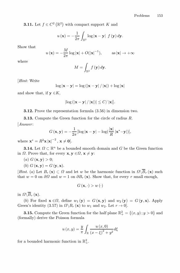
Problems 153
3.11. Let f ∈ C2(R2)with compact support K and
u (x) = − 12π
∫
R2
log |x− y| f (y) dy.
Show that
u (x) = −M2πlog |x|+O(|x|−1), as |x| → +∞
where
M =
∫
R2
f (y)dy.
[Hint: Writelog |x− y| = log (|x − y| / |x|) + log |x|
and show that, if y ∈K,
|log (|x− y| / |x|)| ≤ C/ |x|].
3.12. Prove the representation formula (3.56) in dimension two.
3.13. Compute the Green function for the circle of radius R.
[Answer :
G (x,y) = − 12π[log |x − y| − log( |x|
R|x∗−y|)],
where x∗ = R2x |x|−2 , x �= 0].3.14. Let Ω ⊂ Rn be a bounded smooth domain and G be the Green function
in Ω. Prove that, for every x,y ∈Ω, x �= y:(a) G (x,y) > 0;
(b) G (x,y) = G (y,x).
[Hint. (a) Let Br (x) ⊂ Ω and let w be the harmonic function in Ω\Br (x) suchthat w = 0 on ∂Ω and w = 1 on ∂Br (x). Show that, for every r small enough,
G (x, ·) > w (·)
in Ω\Br (x).(b) For fixed x ∈Ω, define w1 (y) = G (x,y) and w2 (y) = G (y,x). Apply
Green’s identity (3.57) in Ω\Br (x) to w1 and w2. Let r→ 0].3.15. Compute the Green function for the half plane R2+ = {(x, y) ; y > 0} and
(formally) derive the Poisson formula
u (x, y) =y
π
∫
R
u (x, 0)
(x− ξ)2 + y2dξ
for a bounded harmonic function in R2+.

154 3 The Laplace Equation
3.16. Prove that the exterior Dirichlet problem in the plane has a uniquebounded solution u ∈ C2 (Ωe) ∩ C
(Ωe), through the following steps. Let w be
the difference of two solutions. Then w is harmonic Ωe, vanishes on ∂Ωe and isbounded, say |w| ≤M .1) Assume that the 0 ∈ Ω. Let Ba (0) and BR (0) such that
Ba (0) ⊂ Ω ⊂ BR (0)
and define
uR (x) =Mln |x| − ln |a|lnR− ln a .
Use the maximum principle to conclude that w ≤ uR, in the ring
Ba,R ={x ∈R2; a < |x| < R
}.
2) Let R→∞ and deduce that w ≤ 0 in Ωe.3) Proceed similarly to show that w ≥ 0 in Ωe.3.17. Find the Poisson formula for the circle BR, by representing the solution
of Δu = 0 in BR, u = g on ∂BR, as a double layer potential.
3.18. Consider the exterior Neumann-Robin problem in R3
⎧⎪⎨⎪⎩
Δu = 0 in Ωe
∂νu+ ku = g on ∂Ωe, (k ≥ 0)u→ 0 as |x| → ∞.
(3.109)
(a) Show that the condition∫
∂Ω
gdσ = 0
is necessary for the solvability of (3.109) if k = 0.
(b) Represent the solution as a single layer potential and derive the integralequations for the unknown density.
[Hint. (a) Show that, for R large,∫
∂Ω
g dσ =
∫
{|x|=R}∂νu dσ.
Then let R→∞ and use Corollary 3.2].3.19. Solve (formally) the Neumann problem in the half space R3+, using a
single layer potential.
3.20. Let B = B1 (0) ⊂ R2. To complete the proof of Theorem 3.6 we must
show that, if g ∈ C (∂B) and u is given by formula (3.21) with R = 1 and p = 0,then
limx→ξu (x) = g (ξ) for every ξ ∈ ∂B.

Problems 155
Fill in the details in the following steps and conclude the proof.
1. First show that:
1− |x|22π
∫
∂B
1
|x− σ|2dσ = 1
and that therefore
u (x) − g (ξ) = 1− |x|2
2π
∫
∂B
g (σ) − g (ξ)|x− σ|2
dσ.
2. For δ > 0, write
u (x) − g (ξ) = 1− |x|2
2π
∫
∂B∩{|σ−ξ|<δ}· · ·dσ + 1− |x|
2
2π
∫
∂B∩{|σ−ξ|>δ}· · ·dσ
≡ I + II.Fix ε > 0, and use the continuity of g to show that, if δ is small enough, then
|I| < ε.3. Show that, if |x − ξ| < δ/2 and |σ − ξ| > δ, then |x− σ| > δ/2 and therefore
limx→ξII = 0.
3.21. Consider the equation
Lu ≡ Δu+ k2u = 0 in R3
called Helmoltz or reduced wave equation.
(a) Show that the radial solutions u = u (r), r = |x|, satisfying the outgoingSommerfeld condition
ur + iku = O
(1
r2
)as r→∞,
are of the form
ϕ (r; k) = ce−ikr
rc ∈ C.
(b) For f smooth and compactly supported in R3 define the potential
U (x) = c0
∫
R3
f (y)e−ik|x−y|
|x− y| dy .
Select the constant c0 such that
LU (x) = −f (x) .
[Answer (b): c0 = (4π)−1].
4
Scalar Conservation Laws and First Order
Equations
Introduction – Linear Transport Equation – Traffic Dynamics – Integral (or Weak) Solu-
tions – The Method of Characteristics For Quasilinear Equations – General First Order
Equations
4.1 Introduction
In the first part of this chapter we consider equations of the form
ut + q (u)x = 0, x ∈ R, t > 0. (4.1)
In general, u = u (x, t) represents the density or the concentration of a physicalquantity Q and q (u) is its flux function1. Equation (4.1) constitutes a link betweendensity and flux and expresses a (scalar) conservation law for the followingreason. If we consider a control interval [x1, x2], the integral∫ x2
x1
u (x, t)dx
gives the amount of Q between x1 and x2 at time t. A conservation law statesthat, without sources or sinks, the rate of change of Q in the interior of [x1, x2]is determined by the net flux through the end points of the interval. If the flux ismodelled by a function q = q (u) , the law translates into the equation
d
dt
∫ x2
x1
u (x, t)dx = −q (u (x2, t)) + q (u (x1, t)) , (4.2)
where we assume that q > 0 (q < 0) for a flux along the positive (negative)direction of the x axes. If u and q are smooth functions, equation (4.2) can berewritten in the form ∫ x2
x1
[ut (x, t) + q (u (x, t))x] dx = 0
which implies (4.1), due to the arbitrariness of the interval [x1, x2].
1 The dimensions of q are [mass]× [time]−1.
Salsa S. Partial Differential Equations in Action: From Modelling to Theoryc© Springer-Verlag 2008, Milan
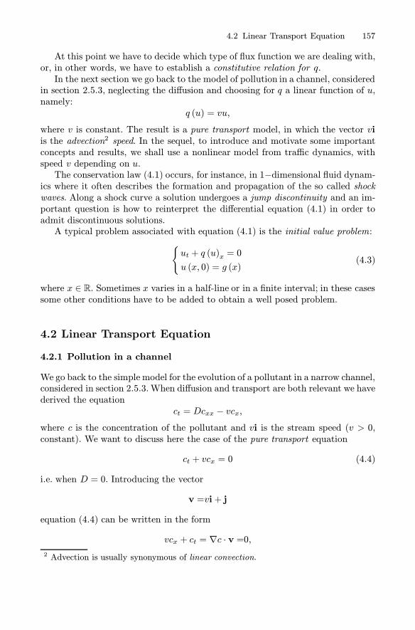
4.2 Linear Transport Equation 157
At this point we have to decide which type of flux function we are dealing with,or, in other words, we have to establish a constitutive relation for q.In the next section we go back to the model of pollution in a channel, considered
in section 2.5.3, neglecting the diffusion and choosing for q a linear function of u,namely:
q (u) = vu,
where v is constant. The result is a pure transport model, in which the vector viis the advection2 speed. In the sequel, to introduce and motivate some importantconcepts and results, we shall use a nonlinear model from traffic dynamics, withspeed v depending on u.The conservation law (4.1) occurs, for instance, in 1−dimensional fluid dynam-
ics where it often describes the formation and propagation of the so called shockwaves. Along a shock curve a solution undergoes a jump discontinuity and an im-portant question is how to reinterpret the differential equation (4.1) in order toadmit discontinuous solutions.A typical problem associated with equation (4.1) is the initial value problem:
{ut + q (u)x = 0
u (x, 0) = g (x)(4.3)
where x ∈ R. Sometimes x varies in a half-line or in a finite interval; in these casessome other conditions have to be added to obtain a well posed problem.
4.2 Linear Transport Equation
4.2.1 Pollution in a channel
We go back to the simple model for the evolution of a pollutant in a narrow channel,considered in section 2.5.3.When diffusion and transport are both relevant we havederived the equation
ct = Dcxx − vcx,where c is the concentration of the pollutant and vi is the stream speed (v > 0,constant). We want to discuss here the case of the pure transport equation
ct + vcx = 0 (4.4)
i.e. when D = 0. Introducing the vector
v =vi + j
equation (4.4) can be written in the form
vcx + ct = ∇c · v =0,2 Advection is usually synonymous of linear convection.

158 4 Scalar Conservation Laws and First Order Equations
pointing out the orthogonality of ∇c and v. But ∇c is orthogonal to the level linesof c, along which c is constant. Therefore the level lines of c are the straight linesparallel to v, of equation
x = vt + x0.
These straight lines are called characteristics. Let us compute c along the char-acteristic x = vt + x0 letting
w (t) = c (x0 + vt, t) .
Since3
w (t) = vcx (x0 + vt, t) + ct(x0 + vt, t),
equation (4.4) becomes the ordinary differential equation w (t) = 0 which impliesthat c is constant along the characteristic.We want to determine the evolution of the concentration c, by knowing its
initial profilec (x, 0) = g (x) . (4.5)
Fig. 4.1. Characteristic line for the linear transport problem
The method to compute the solution at a point (x, t), t > 0, is very simple.Let x = vt + x0 be the equation of the characteristic passing through (x, t).Go back in time along this characteristic from (x, t) until the point (x0, 0), of
intersection with the x− axes (see Fig. 4.1).Since c is constant along the characteristic and c (x0, 0) = g (x0), it must be
c (x, t) = g (x0) = g (x− vt) .Thus, if g ∈ C1 (R), the solution of the initial value problem (4.4), (4.5) is givenby
c (x, t) = g (x− vt) . (4.6)
The solution (4.6) represents a travelling wave, moving with speed v in thepositive x−direction. In figure 4.2, an initial profile g (x) = sin (πx)χ[0,1] (x) istransported in the plane x, t along the straight-lines x − t = constant, i.e. withspeed v = 1.
3 The dot denotes derivative with respect to time.

4.2 Linear Transport Equation 159
Fig. 4.2. Travelling wave solution of the linear transport equation
4.2.2 Distributed source
The equationct + vcx = f (x, t) , (4.7)
with the initial conditionc (x, 0) = g (x) , (4.8)
describes the effect of an external distributed source along the channel. The func-tion f represents the intensity of the source, measured in concentration per unittime.Again, to compute the value of the solution u at a point (x, t) is not difficult.
Let x = x0 + vt be the characteristic passing through (x, t) and compute u alongthis characteristic, setting w (t) = c (x0 + vt, t). From (4.7), w satisfies the ordinarydifferential equation
w (t) = vcx (x0 + vt, t) + ct(x0 + vt, t) = f (x0 + vt, t)
with the initial conditionw (0) = g (x0) .
Thus
w (t) = g (x0) +
∫ t
0
f (x0 + vs, s) ds.
Letting t = t and recalling that x0 = x− vt, we get
c (x, t) = w (t) = g (x− vt) +∫ t
0
f (x− v(t − s), s) ds. (4.9)
Since (x, t) is arbitrary, if g and f are reasonably smooth functions, (4.9) is oursolution.
Proposition 4.1. Let g ∈ C1 (R) and f, fx ∈ C (R× R+). The solution of theinitial value problem
{ct + vcx = f (x, t) x ∈ R, t > 0c(x, 0) = g (x) x ∈ R

160 4 Scalar Conservation Laws and First Order Equations
is given by the formula
c (x, t) = g (x− vt) +∫ t
0
f (x− v(t − s), s) ds. (4.10)
Remark 4.1. Formula (4.10) can be derived using the Duhamel method, as in sec-tion 2.2.8 (see Problem 4.1.)
4.2.3 Decay and localized source
Suppose that, due to biological decomposition, the pollutant decays at the rate
r (x, t) = −γc (x, t) γ > 0.
Without external sources and diffusion, the mathematical model is
ct + vcx = −γc,
with the initial conditionc (x, 0) = g (x) .
Setting
u (x, t) = c (x, t) eγv x, (4.11)
we have
ux =(cx +
γ
vc)eγv x and ut = cte
γv x
and therefore the equation for u is
ut + vux = 0
with the initial condition
u (x, 0) = g (x) eγv x.
From Proposition 4.1, we get
u (x, t) = g (x− vt) e γv (x−vt)
and from (4.11)c (x, t) = g (x− vt) e−γt
which is a damped travelling wave.
We now examine the effect of a source of pollutant placed at a certain pointof the channel, e.g. at x = 0. Typically, one can think of waste material fromindustrial machineries. Before the machines start working, for instance before timet = 0, we assume that the channel is clean. We want to determine the pollutantconcentration, supposing that at x = 0 it is kept at a constant level β > 0, fort > 0.

4.2 Linear Transport Equation 161
To model this source we introduce the Heaviside function
H (t) ={1 t ≥ 00 t < 0,
with the boundary conditionc (0, t) = βH (t) (4.12)
and the initial condition
c (x, 0) = 0 for x > 0. (4.13)
As before, let u (x, t) = c (x, t) eγv x, which is a solution of ut + vux = 0. Then:
u (x, 0) = c (x, 0) eγv x = 0 x > 0
u (0, t) = c (0, t) = βH (t) .
Since u is constant along the characteristics it must be of the form
u (x, t) = u0 (x− vt) (4.14)
where u0 is to be determined from the boundary condition (4.12) and the initialcondition (4.13).To compute u for x < vt, observe that a characteristic leaving the t−axis from
a point (0, t) carries the data βH (t). Therefore, we must have
u0 (−vt) = βH (t) .
Letting s = −vt we getu0 (s) = βH
(−sv
)
and from (4.14),
u (x, t) = βH(t− xv
).
This formula gives the solution also in the sector
x > vt, t > 0,
since the characteristics leaving the x−axis carry zero data and hence we deduceu = c = 0 there. This means that the pollutant has not yet reached the point x attime t, if x > vt.Finally, recalling (4.11), we find
c (x, t) = βH(t− xv
)e−
γv x.
Observe that in (0, 0) there is a jump discontinuity which is transported along thecharacteristic x = vt. Figure 4.3 shows the solution for β = 3, γ = 0.7, v = 2.
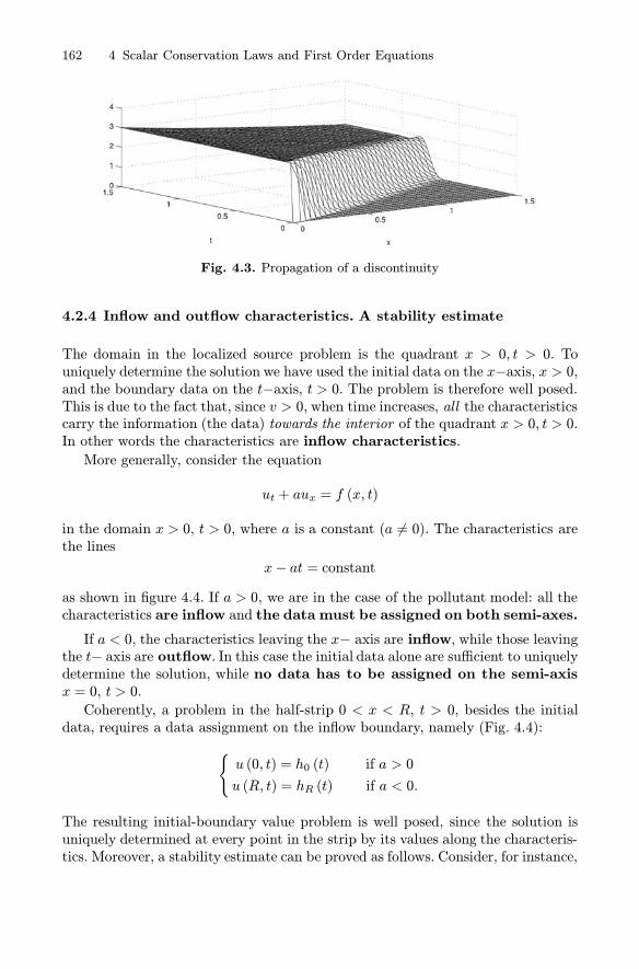
162 4 Scalar Conservation Laws and First Order Equations
Fig. 4.3. Propagation of a discontinuity
4.2.4 Inflow and outflow characteristics. A stability estimate
The domain in the localized source problem is the quadrant x > 0, t > 0. Touniquely determine the solution we have used the initial data on the x−axis, x > 0,and the boundary data on the t−axis, t > 0. The problem is therefore well posed.This is due to the fact that, since v > 0, when time increases, all the characteristicscarry the information (the data) towards the interior of the quadrant x > 0, t > 0.In other words the characteristics are inflow characteristics.
More generally, consider the equation
ut + aux = f (x, t)
in the domain x > 0, t > 0, where a is a constant (a �= 0). The characteristics arethe lines
x− at = constant
as shown in figure 4.4. If a > 0, we are in the case of the pollutant model: all thecharacteristics are inflow and the data must be assigned on both semi-axes.
If a < 0, the characteristics leaving the x− axis are inflow, while those leavingthe t− axis are outflow. In this case the initial data alone are sufficient to uniquelydetermine the solution, while no data has to be assigned on the semi-axisx = 0, t > 0.
Coherently, a problem in the half-strip 0 < x < R, t > 0, besides the initialdata, requires a data assignment on the inflow boundary, namely (Fig. 4.4):
{u (0, t) = h0 (t) if a > 0
u (R, t) = hR (t) if a < 0.
The resulting initial-boundary value problem is well posed, since the solution isuniquely determined at every point in the strip by its values along the characteris-tics. Moreover, a stability estimate can be proved as follows. Consider, for instance,

4.2 Linear Transport Equation 163
Fig. 4.4. The arrows indicate where the data should be assigned
the case a > 0 and the problem4
⎧⎪⎨⎪⎩
ut + aux = 0 0 < x < R, t > 0
u (0, t) = h (t) t > 0
u (x, 0) = g (x) 0 < x < R.
(4.15)
Multiply the differential equation by u and write
uut + auux =1
2
d
dtu2 +
a
2
d
dxu2 = 0.
Integrating in x over (0, R) we get:
d
dt
∫ R
0
u2 (x, t)dx+ a[u2 (R, t)− u2 (0, t)
]= 0.
Now use the data u (0, t) = h (t) and the positivity of a to obtain
d
dt
∫ R
0
u2 (x, t)dx ≤ ah2 (t) .
Integrating in t we have, using the initial condition u (x, 0) = g (x),
∫ R
0
u2 (x, t)dx ≤∫ R
0
g2 (x) dx+ a
∫ t
0
h2 (s) ds. (4.16)
Now, let u1 and u2 be solutions of problem (4.15) with initial data g1, g2 andboundary data h1, h2 on x = 0. Then, by linearity, w = u1 − u2 is a solution4 For the case ut + aux = f �= 0, see Problem 4.2.

164 4 Scalar Conservation Laws and First Order Equations
of problem (4.15) with initial data g1− g2 and boundary data h1− h2 on x = 0.Applying the inequality (4.16) to w we have
∫ R
0
[u1 (x, t)− u2 (x, t)]2dx ≤∫ R
0
[g1 (x)− g2 (x)]2dx+ a∫ t
0
[h1 (s) − h2 (s)]2ds.
Thus, a least-squares approximation of the data controls a least-squares approxi-mation of the corresponding solutions. In this sense, the solution of problem (4.15)depends continuously on the initial data and on the boundary data on x = 0.Wepoint out that the values of u on x = R do not appear in (4.16).
4.3 Traffic Dynamics
4.3.1 A macroscopic model
From far away, an intense traffic on a highway can be considered as a fluid flowand described by means of macroscopic variables such as the density of cars5 ρ,their average speed v and their flux6 q. The three (more or less regular) functionsρ, u and q are linked by the simple convection relation
q = vρ.
To construct a model for the evolution of ρ we assume the following hypotheses.
1. There is only one lane and overtaking is not allowed. This is realistic forinstance for traffic in a tunnel (see Problem 4.7). Multi-lanes models with overtak-ing are beyond the scope of this introduction. However the model we will presentis often in agreement with observations also in this case.
2. No car“sources”or“sinks”.We consider a road section without exit/entrancegates.
3. The average speed is not constant and depends on the density alone, that is
v = v (ρ) .
This rather controversial assumption means that at a certain density the speed isuniquely determined and that a density change causes an immediate speed varia-tion. Clearly
v′ (ρ) =dv
dρ≤ 0
since we expect the speed to decrease as the density increases.
As in Section 4.1, from hypotheses 2 and 3 we derive the conservation law:
ρt + q(ρ)x = 0 (4.17)
5 Number of cars per unit length.6 Cars per unit time.

4.3 Traffic Dynamics 165
where
q(ρ) = v (ρ) ρ.
We need a constitutive relation for v = v (ρ). When ρ is small, it is reasonableto assume that the average speed v is more or less equal to the maximal velocityvm, given by the speed limit. When ρ increases, traffic slows down and stops at themaximum density ρm (bumper-to-bumper traffic). We adopt the simplest modelconsistent with the above considerations7, namely
v (ρ) = vm
(1− ρ
ρm
),
so that
q (ρ) = vmρ
(1− ρ
ρm
). (4.18)
Since
q(ρ)x = q′ (ρ) ρx = vm
(1− 2ρρm
)ρx
equation (4.17) becomes
ρt + vm
(1− 2ρρm
)
︸ ︷︷ ︸q′(ρ)
ρx = 0. (4.19)
According to the terminology in Section 1.1, this is a quasilinear equation. Wealso point out that
q′′ (ρ) = −2vmρm< 0
so that q is strictly concave. We couple the equation (4.19) with the initial condition
ρ (x, 0) = g (x) . (4.20)
4.3.2 The method of characteristics
We want to solve the initial value problem (4.19), (4.20). To compute the density ρat a point (x, t) we follow the idea we used in the linear transport case: to connectthe point (x, t) with a point (x0, 0) on the x−axis, through a curve along which ρis constant (Fig. 4.5).Clearly, if we manage to find such a curve, that we call characteristic based
at (x0, 0), the value of ρ at (x, t) is given by ρ (x0, 0) = g (x0). Moreover, if thisprocedure can be repeated for every point (x, t), x ∈ R, t > 0, then we cancompute ρ at every point and the problem is completely solved. This is the methodof characteristics.
7 And in good agreement with experimental data.

166 4 Scalar Conservation Laws and First Order Equations
Fig. 4.5. Characteristic curve
Adopting a slightly different point of view, we can implement the above ideaas follows: assume that x = x (t) is the equation of the characteristic based at thepoint (x0, 0); along x = x (t) we observe always the same initial density g (x0) . Inother words
ρ (x (t) , t) = g (x0) (4.21)
for every t > 0. If we differentiate identity (4.21), we get
d
dtρ (x (t) , t) = ρx (x (t) , t)x
′ (t) + ρt (x (t) , t) = 0 (t > 0). (4.22)
On the other hand, (4.19) yields
ρt (x (t) , t) + q′ (g (x0)) ρx (x (t) , t) = 0
so that, subtracting (4.23) from (4.22), we obtain
ρx (x (t) , t) [x (t)− q′ (g (x0))] = 0. (4.23)
Assuming ρx (x (t) , t) �= 0, we deduce
x (t) = q′ (g (x0)) .
Since x (0) = x0 we find
x (t) = q′ (g (x0)) t+ x0. (4.24)
Thus, the characteristics are straight lines with slope q′ (g (x0)). Different valuesof x0 give, in general, different values of the slope.We can now derive a formula for ρ. To compute ρ (x, t), t > 0, go back in time
along the characteristic through (x, t) until its base point (x0, 0). Then ρ (x, t) =g (x0). From (4.24) we have, since x (t) = x,
x0 = x− q′ (g (x0)) t
and finally
ρ (x, t) = g (x− q′ (g (x0)) t) . (4.25)

4.3 Traffic Dynamics 167
Fig. 4.6. Characteristic straight line (g0 = g (x0))
Formula (4.25) represents a travelling wave propagatingwith speed q′ (g (x0))along the positive x−direction.We emphasize that q′ (g (x0)) is the local wave speed and it must not be confused
with the traffic velocity. In fact, in general,
dq
dρ=d (ρv)
dρ= v + ρ
dv
dρ≤ v
since ρ ≥ 0 and dvdρ ≤ 0.
The different nature of the two speeds becomes more evident if we observethat the wave speed may be negative as well. This means that, while the trafficadvances along the positive x−direction, the disturbance given by the travellingwave may propagate in the opposite direction. Indeed, in our model (4.18), dqdρ < 0
when ρ > ρm2.
Formula (4.25) seems to be rather satisfactory, since, apparently, it gives thesolution of the initial value problem (4.19), (4.20) at every point. Actually, a moreaccurate analysis shows that, even if the initial data g are smooth, the solutionmay develop a singularity in finite time (e.g. a jump discontinuity). When thisoccurs, the method of characteristics does not work anymore and formula (4.25) isnot effective. A typical case is described in figure 4.7: two characteristics based atdifferent points (x1, 0) e (x2, 0) intersect at the point (x, t) and the value u (x, t)is not uniquely determined as soon as g (x1) �= g (x2).
Fig. 4.7. Intersection of characteristics

168 4 Scalar Conservation Laws and First Order Equations
In this case we have to weaken the concept of solution and the computationtechnique. We will come back on these questions later. For the moment, we analyzethe method of characteristics in some particularly significant cases.
4.3.3 The green light problem
Suppose that bumper-to-bumper traffic is standing at a red light, placed at x = 0,while the road ahead is empty. Accordingly, the initial density profile is
g (x) =
{ρm for x ≤ 00 for x > 0.
At time t = 0 the traffic light turns green and we want to describe the car flowevolution for t > 0. At the beginning, only the cars nearer to the light start movingwhile most remain standing.
Since q′ (ρ) = vm(1− 2ρ
ρm
), the local wave speed is given by
q′ (g (x0)) ={−vm for x0 ≤ 0vm for x0 > 0
and the characteristics are the straight lines
x = −vmt+ x0 if x0 < 0
x = vmt+ x0 if x0 > 0.
The lines x = vmt and x = −vmt partition the upper half-plane in the three regionsR, S and T , shown in figure 4.8.
Fig. 4.8. Characteristics for the green light problem
Inside R we have ρ (x, t) = ρm, while inside T we have ρ (x, t) = 0. Considerthe points on the horizontal line t = t. At the points
(x, t)∈ T the density is zero:
the traffic has not yet arrived in x at time t = t. The front car is located at thepoint
x = vmt
which moves at the maximum speed, since ahead the road is empty.

4.3 Traffic Dynamics 169
The cars placed at the points(x, t)∈ R are still standing. The first car that
starts moving at time t = t is at the point
x = −vmt.
In particular, it follows that the green light signal propagates back through thetraffic at the speed vm.What is the value of the density inside the sector S? No characteristic extends
into S due to the discontinuity of the initial data at the origin, and the method asit stands does not give any information on the value of ρ inside S.A strategy that may give a reasonable answer is the following:a) approximate the initial data by a continuous function gε, which converges
to g as ε→ 0 at every point x, except 0;b) construct the solution ρε of the ε−problem by the method of characteristics;c) let ε→ 0 and check that the limit of ρε is a solution of the original problem.Clearly we run the risk of constructing many solutions, each one depending on
the way we regularize the initial data, but for the moment we are satisfied if weconstruct at least one solution.
a) Let us choose as gε the function (Fig. 4.9)
gε (x) =
⎧⎪⎨⎪⎩
ρm x ≤ 0ρm(1 −
x
ε) 0 < x < ε
0 x ≥ ε.
When ε→ 0, gε (x)→ g (x) for every x �= 0.
Fig. 4.9. Smoothing of the initial data in the green light problem
b) The characteristics for the ε−problem are:
x = −vmt+ x0 if x0 < 0
x = −vm(1− 2x0
ε
)t+ x0 if 0 ≤ x0 < ε
x = vmt+ x0 if x0 ≥ ε
since, for 0 ≤ x0 < ε,
q′ (gε (x0)) = vm
(1− 2gε (x0)
ρm
)= −vm
(1− 2x0
ε
).

170 4 Scalar Conservation Laws and First Order Equations
The characteristics in the region −vmt < x < vmt + ε form a rarefaction fan(Fig. 4.10).
Fig. 4.10. Fanlike characteristics
Clearly, ρε (x, t) = 0 for x ≥ vmt +ε and ρε (x, t) = ρm for x ≤ −vmt. Let now(x, t) belong to the region
−vmt < x < vmt+ ε.
Solving for x0 in the equation of the characteristic x = −vm(1− 2x0
ε
)t+ x0, we
find
x0 = εx+ vmt
2vmt+ ε.
Then
ρε (x, t) = gε (x0) = ρm(1−x0
ε) = ρm
(1− x+ vmt2vmt+ ε
). (4.26)
c) Letting ε→ 0 in (4.26) we obtain
ρ (x, t) =
⎧⎪⎪⎨⎪⎪⎩
ρm for x ≤ −vmtρm2
(1− x
vmt
)for − vmt < x < vmt
0 for x ≥ vmt. (4.27)
It is easy to check that ρ is a solution of the equation (4.19) in the regions R, S, T .For fixed t, the function ρ decreases linearly from ρm to 0 as x varies from −vmtto vmt. Moreover, ρ is constant on the fan of straight lines
x = ht − vm < h < vm.
These type of solutions are called rarefaction or simple waves (centered at theorigin).The formula for ρ (x, t) in the sector S can be obtained, a posteriori, by a formal
procedure that emphasizes its structure. The equation of the characteristics canbe written in the form
x = vm
(1− 2g (x0)
ρm
)t + x0 = vm
(1− 2ρ (x, t)
ρm
)t + x0.

4.3 Traffic Dynamics 171
Fig. 4.11. Characteristics in a rarefaction wave
Fig. 4.12. Profile of a rarefaction wave at time t
because ρ (x, t) = g (x0). Inserting x0 = 0 we obtain
x = vm
(1− 2ρ (x, t)
ρm
)t.
Solving for ρ we find exactly
ρ (x, t) =ρm2
(1− x
vmt
)(t > 0). (4.28)
Since vm
(1− 2ρ
ρm
)= q′ (ρ), we see that (4.28) is equivalent to
ρ (x, t) = r(xt
)
where r = (q′)−1 is the inverse function of q′. Indeed this is the general form of ararefaction wave (centered at the origin) for a conservation law.
We have constructed a continuous solution ρ of the green light problem, con-necting the two constant states ρm and 0 by a rarefaction wave. However, it isnot clear in which sense ρ is a solution across the lines x = ±vmt, since, there,its derivatives undergo a jump discontinuity. Also, it is not clear whether or not(4.27) is the only solution. We will return on these important points.
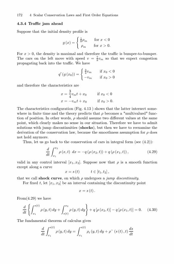
172 4 Scalar Conservation Laws and First Order Equations
4.3.4 Traffic jam ahead
Suppose that the initial density profile is
g (x) =
{18ρm for x < 0
ρm for x > 0.
For x > 0, the density is maximal and therefore the traffic is bumper-to-bumper.The cars on the left move with speed v = 7
8vm so that we expect congestion
propagating back into the traffic. We have
q′ (g (x0)) =
{34vm if x0 < 0
−vm if x0 > 0
and therefore the characteristics are
x =3
4vmt + x0 if x0 < 0
x = −vmt+ x0 if x0 > 0.
The characteristics configuration (Fig. 4.13 ) shows that the latter intersect some-where in finite time and the theory predicts that ρ becomes a "multivalued" func-tion of position. In other words, ρ should assume two different values at the samepoint, which clearly makes no sense in our situation. Therefore we have to admitsolutions with jump discontinuities (shocks), but then we have to reexamine thederivation of the conservation law, because the smoothness assumption for ρ doesnot hold anymore.Thus, let us go back to the conservation of cars in integral form (see (4.2)):
d
dt
∫ x2
x1
ρ (x, t) dx = −q (ρ (x2, t)) + q (ρ (x1, t)) , (4.29)
valid in any control interval [x1, x2]. Suppose now that ρ is a smooth functionexcept along a curve
x = s (t) t ∈ [t1, t2] ,that we call shock curve, on which ρ undergoes a jump discontinuity.For fixed t, let [x1, x2] be an interval containing the discontinuity point
x = s (t) .
From(4.29) we have
d
dt
{∫ s(t)
x1
ρ (y, t) dy +
∫ x2
s(t)
ρ (y, t) dy
}+ q [ρ (x2, t)]− q [ρ (x1, t)] = 0. (4.30)
The fundamental theorem of calculus gives
d
dt
∫ s(t)
x1
ρ (y, t) dy =
∫ s(t)
x1
ρt (y, t) dy + ρ− (s (t) , t)
ds
dt

4.3 Traffic Dynamics 173
Fig. 4.13. Expecting a shock
andd
dt
∫ x2
s(t)
ρ (y, t) dy =
∫ x2
s(t)
ρt (y, t) dy − ρ+ (s (t) , t)ds
dt,
where
ρ− (s (t) , t) = limy↑s(t)
ρ (y, t) , ρ+ (s (t) , t) = limy↓s(t)
ρ (y, t) .
Hence, equation (4.30) becomes
∫ x2
x1
ρt (y, t) dy +[ρ− (s (t) , t)− ρ+ (s (t) , t)
]s (t) = q [ρ (x1, t)]− q [ρ (x2, t)] .
Letting x2 ↓ s (t) and x1 ↑ s (t) we obtain[ρ− (s (t) , t)− ρ+ (s (t) , t)
]s (t) = q
[ρ− (s (t) , t)
]− q
[ρ+ (s (t) , t)
]
that is:
s =q [ρ+ (s, t)]− q [ρ− (s, t)]ρ+ (s, t)− ρ− (s, t) . (4.31)
The relation (4.31) is an ordinary differential equation for s and it is known asRankine-Hugoniot condition. The discontinuity propagating along the shockcurve is called shock wave. The Rankine-Hugoniot condition gives the shock speeds (t) as the quotient of the flux jump over the density jump. To determine the shockcurve we need to know its initial point and the values of ρ from both sides of thecurve.
Let us apply the above considerations to our traffic problem8. We have
ρ+ = ρm, ρ− =ρm8
8 In the present case the following simple formula holds:
q (w)− q (z)w − z = vm
(1− w + z
ρm
).

174 4 Scalar Conservation Laws and First Order Equations
while
q[ρ+]= 0 q
[ρ−]=7
64vmρm
and (4.31) gives
s (t) =q [ρ+]− q [ρ−]ρ+ − ρ− = −1
8vm.
Since clearly s (0) = 0, the shock curve is the straight line
x = −18vmt.
Note that the slope is negative: the shock propagates back with speed −18vm, as itis revealed by the braking of the cars, slowing down because of a traffic jam ahead.
As a consequence, the solution of our problem is given by the following formula(Fig. 4.14)
ρ (x, t) =
{18ρm x < −1
8vmt
ρm x > −18vmt.
This time the two constant states 18ρm and ρm are connected by a shock wave.
Fig. 4.14. Shock wave
4.4 Integral (or Weak) Solutions
4.4.1 The method of characteristics revisited
The method of characteristics applied to the problem{ut + q (u)x = 0
u (x, 0) = g (x)(4.32)
gives the travelling wave (see (4.25) with x0 = ξ)
u(x, t) = g [x− q′ (g (ξ)) t](q′ =
dq
du
)(4.33)

4.4 Integral (or Weak) Solutions 175
with local speed q′ (g (ξ)), in the positive x−direction. Since u (x, t) ≡ g (ξ) alongthe characteristic based at (ξ, 0), from (4.33) we obtain that u is implicitly definedby the equation
G (x, t, u) ≡ u− g [x− q′ (u) t] = 0. (4.34)
If g and q′ are smooth, the Implicit Function Theorem, implies that equation (4.34)defines u as a function of (x, t), as long as the condition
Gu (x, t, u) = 1 + tq′′(u)g′ [x− q′ (u) t] �= 0 (4.35)
holds. An immediate consequence is that if q′′ and g′ have the same sign, thesolution given by the method of characteristics is defined and smooth for all timest ≥ 0. Precisely, we have:
Proposition 4.2. Suppose that q ∈ C2 (R), g ∈ C1 (R) and g′q′′ ≥ 0 in R. Thenformula (4.34) defines the unique solution u of problem (4.32) in the half-planet ≥ 0. Moreover, u (x, t) ∈ C1 (R× [0,∞)).
Thus, if q′′ and g′ have the same sign, the characteristics do not intersect. Notethat in the ε−approximation of the green light problem, q is concave and gε isdecreasing. Although gε is not smooth, the characteristics do not intersect and ρεis well defined for all times t > 0. In the limit as ε → 0, the discontinuity of greappears and the fan of characteristics produces a rarefaction wave.
What happens if q′′ and g′ have a different sign in an interval [a, b]? Proposition4.2 still holds for small times, since Gu ∼ 1 if t ∼ 0, but when time goes on weexpect the formation of a shock. Indeed, suppose, for instance, that q is concaveand g is increasing. The family of characteristics based on a point in the interval[a, b] is
x = q′ (g (ξ)) t+ ξ ξ ∈ [a, b] . (4.36)
When ξ increases, g increases as well, while q′ (g (ξ)) decreases so that we expectintersection of characteristics along a shock curve. The main question is to findthe positive time ts (breaking time) and the location xs of first appearance ofthe shock.
According to the above discussion, the breaking time must coincide with thefirst time t at which the expression
Gu (x, t, u) = 1 + tq′′(u)g′ [x− q′ (u) t]
becomes zero. Computing Gu along the characteristic (4.36), we have u = g (ξ)and
Gu (x, t, u) = 1 + tq′′(g (ξ))g′(ξ).
Assume that the nonnegative function
z (ξ) = −q′′(g(ξ))g′(ξ)

176 4 Scalar Conservation Laws and First Order Equations
attains its maximum only at the point ξM ∈ [a, b]. Then z (ξM) > 0 and
ts = minξ∈[a,b]
1
z (ξ)=
1
z (ξM ). (4.37)
Since xs belongs to the characteristics x = q′ (g (ξM )) t+ ξM , we find
xs =q′ (g (ξM ))z (ξM )
+ ξM . (4.38)
The point (xs, ts) has an interesting geometrical meaning. In fact, it turns out thatif q′′g′ < 0, the family of characteristics (4.36) admits an envelope9 and (xs, ts) isthe point on the envelope with minimum time coordinate (see Problem 4.8).
Fig. 4.15. Breaking time for problem (4.39)
Example 4.1. Consider the initial value problem{ut + (1− 2u)ux = 0u (x, 0) = arctanx.
(4.39)
We have q (u) = u − u2, q′ (u) = 1 − 2u, q′′ (u) = −2, and g (ξ) = arctan ξ,g′ (ξ) = 1/
(1 + ξ2
). Therefore, the function
z (ξ) = −q′′(g(ξ))g′(ξ) = 2(1 + ξ2
)
9 Recall that the envelope of a family of curves φ (x, t, ξ) = 0, depending on the pa-rameter ξ, is a curve ψ (x, t) = 0 tangent at each one of its points to a curve of thefamily. If the family of curves φ (x, t, ξ) = 0 has an envelope, its parametric equationsare obtained by solving the system
{φ (x, t, ξ) = 0φξ (x, t, ξ) = 0
with respect to x and t.

4.4 Integral (or Weak) Solutions 177
has a maximum at ξM = 0 and z (0) = 2. The breaking-time is tS = 1/2 andxS = 1/2. Thus, the shock curve starts from (1/2, 1/2) . For 0 ≤ t < 1/2 thesolution u is smooth and implicitly defined by the equation
u− arctan [x− (1− 2u) t] = 0. (4.40)
After t = 1/2, equation (4.40) defines u as a multivalued function of (x, t) anddoes not define a solution anymore. Figure 4.15 shows what happens for t = 1/4,1/2 and 1. Note that the common point of intersection is (1/2, tan1/2) which isnot the first shock point.
How does the solution evolve after t = 1/2?We have to insert a shock wave intothe multivalued graph in figure 4.15 in such a way the conservation law is preserved.We will see that the correct insertion point is prescribed by the Rankine-Hugoniotcondition. It turns out that this corresponds to cutting off from the multivaluedprofile two equal area lobesA and B as described in figure 4.16 (G. B. Whithamequal area rule10).
Fig. 4.16. Inserting a shock wave by the Whitham equal-area rule
4.4.2 Definition of integral solution
We have seen that the method of characteristics is not sufficient, in general, todetermine the solution of an initial value problem for all times t > 0. In the greenlight problem a rarefaction wave was used to construct the solution in a region notcovered by characteristics. In the traffic jam case the solution undergoes a shock,propagating according to the Rankine-Hugoniot condition.
10 The equal-area rule holds for a general conservation law (see Whitham, 1974).

178 4 Scalar Conservation Laws and First Order Equations
Some questions arise naturally.
Q1. In which sense is the differential equation satisfied across a shock or, moregenerally, across a separation curve where the constructed solution is not differen-tiable?One way to solve the problem is simply to not care about those points. However,
in this case it would be possible to construct solutions that do not have anythingto do with the physical meaning of the conservation law.
Q2. Is the solution unique?
Q3. If there is no uniqueness, is there a criterion to select the “physicallycorrect” solution?To answer, we need first of all to introduce a more flexible notion of solution,
in which the derivatives of the solution are not directly involved. Let us go backto the problem {
ut + q (u)x = 0 x ∈ R, t > 0u (x, 0) = g (x) x ∈ R (4.41)
and assume for the moment that u is a smooth solution, at least of class C1 inR×[0,∞). We say that u is a classical solution.Let v be a smooth function in R×[0,∞), with compact support. We call v a
test function. Multiply the differential equation by v and integrate on R×(0,∞).We get ∫ ∞
0
∫
R
[ut + q (u)x] v dxdt = 0. (4.42)
The idea is to carry the derivatives onto the test function v via an integration byparts. If we integrate by parts the first term with respect to t we obtain11:
∫ ∞0
∫
R
utv dxdt = −∫ ∞0
∫
R
uvt dxdt−∫
R
u (x, 0)v (x, 0)dx
= −∫ ∞0
∫
R
uvt dxdt−∫
R
g (x)v (x, 0)dx.
Integrating by parts the second term in (4.42) with respect to x, we have:
∫ ∞0
∫
R
q (u)x v dxdt = −∫ ∞0
∫
R
q(u)vx dxdt.
Then, equation (4.42) becomes
∫ ∞0
∫
R
[uvt + q(u)vx]dxdt+
∫
R
g (x) v (x, 0)dx = 0. (4.43)
We have obtained an integral equation, valid for every test function v. Observethat no derivative of u appears in (4.43).
11 Since v is compactly supported and u, v are smooth, there is no problem in exchangingthe order of integration.
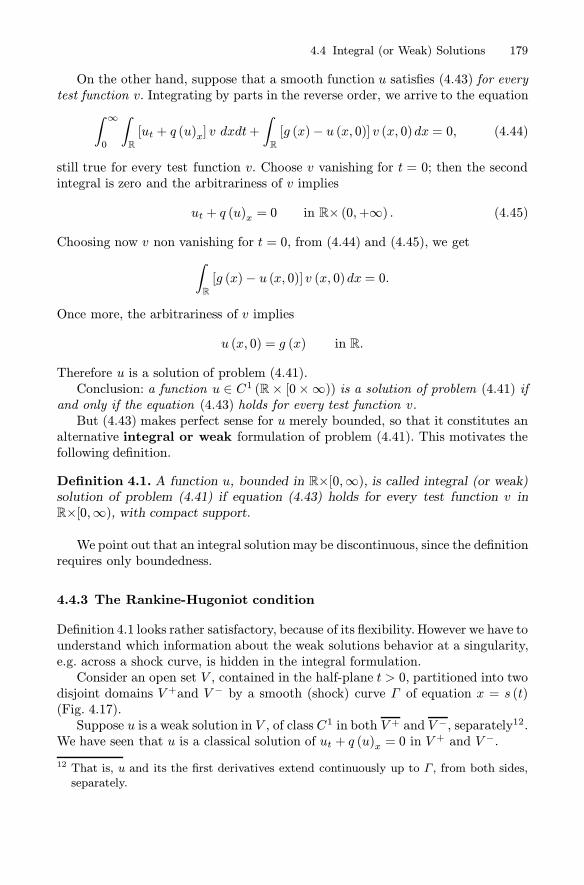
4.4 Integral (or Weak) Solutions 179
On the other hand, suppose that a smooth function u satisfies (4.43) for everytest function v. Integrating by parts in the reverse order, we arrive to the equation
∫ ∞0
∫
R
[ut + q (u)x] v dxdt+
∫
R
[g (x)− u (x, 0)] v (x, 0)dx = 0, (4.44)
still true for every test function v. Choose v vanishing for t = 0; then the secondintegral is zero and the arbitrariness of v implies
ut + q (u)x = 0 in R× (0,+∞) . (4.45)
Choosing now v non vanishing for t = 0, from (4.44) and (4.45), we get
∫
R
[g (x)− u (x, 0)] v (x, 0)dx = 0.
Once more, the arbitrariness of v implies
u (x, 0) = g (x) in R.
Therefore u is a solution of problem (4.41).Conclusion: a function u ∈ C1 (R× [0×∞)) is a solution of problem (4.41) if
and only if the equation (4.43) holds for every test function v.But (4.43) makes perfect sense for u merely bounded, so that it constitutes an
alternative integral or weak formulation of problem (4.41). This motivates thefollowing definition.
Definition 4.1. A function u, bounded in R×[0,∞), is called integral (or weak)solution of problem (4.41) if equation (4.43) holds for every test function v inR×[0,∞), with compact support.
We point out that an integral solutionmay be discontinuous, since the definitionrequires only boundedness.
4.4.3 The Rankine-Hugoniot condition
Definition 4.1 looks rather satisfactory, because of its flexibility. However we have tounderstand which information about the weak solutions behavior at a singularity,e.g. across a shock curve, is hidden in the integral formulation.Consider an open set V , contained in the half-plane t > 0, partitioned into two
disjoint domains V +and V − by a smooth (shock) curve Γ of equation x = s (t)(Fig. 4.17).Suppose u is a weak solution in V , of class C1 in both V + and V −, separately12.
We have seen that u is a classical solution of ut + q (u)x = 0 in V+ and V −.
12 That is, u and its the first derivatives extend continuously up to Γ , from both sides,separately.

180 4 Scalar Conservation Laws and First Order Equations
Fig. 4.17. A shock curve dividing a domain V
Choose now a test function v, supported in a compact set K ⊂ V , such thatK ∩ Γ is non empty. Since v (x, 0) = 0, we can write:
0 =
∫ ∞0
∫
R
[uvt + q(u)vx] dxdt
=
∫
V+[uvt + q(u)vx]dxdt+
∫
V −[uvt + q(u)vx] dxdt.
Integrating by parts and observing that v = 0 on ∂V +\Γ , we have:∫
V +[uvt + q(u)vx]dxdt =
= −∫
V +[ut + q(u)x] v dxdt+
∫
Γ
[u+ n2 + q(u+)n1] v dl
=
∫
Γ
[u+ n2 + q(u+)n1] v dl
where u+ denotes the value of u on Γ from the V+ side, n = (n1, n2) is the outward
unit normal vector on ∂V + and dl denotes the arc length on Γ . Similarly, since nis inward with respect to V −:
∫
V−[uvt + q(u)vx]dxdt = −
∫
Γ
[u− n2 + q(u−)n1] v dl
where u− denotes the value of u on Γ from the V − side. Therefore we deduce that∫
Γ
{[q(u+)− q(u−)]n1 + [u+ − u−]n2} v dl = 0.
The arbitrariness of v yields
[q(u+)− q(u−)]n1 + [u+ − u−]n2 = 0 (4.46)

4.4 Integral (or Weak) Solutions 181
on Γ . If u is continuous across Γ , (4.46) is automatically satisfied. If u+ �= u− wewrite the relation (4.46) more explicitly. Since x = s (t) on Γ , we have
n =(n1, n2) =1√
1 + (s (t))2(−1, s (t)) .
Hence (4.46) becomes, after simple calculations,
s =q [u+ (s, t)]− q [u− (s, t)]u+ (s, t)− u− (s, t)
(4.47)
which is the Rankine-Hugoniot condition for the shock curve Γ .
In general, functions constructed by connecting classical solutions and rarefac-tion waves in a continuous way are weak solutions. The same is true for shockwaves satisfying the Rankine-Hugoniot condition. Then, the solutions of the greenlight and of the traffic jam problems are precisely integral solutions.Thus, Definition 4.1 gives a satisfactory answer to question Q1. The other two
questions require a deeper analysis as the following example shows.
Fig. 4.18. The rarefaction wave of example 4.3
Example 4.2. (Non uniqueness). Imagine a flux of particles along the x−axis, eachone moving with constant speed. Suppose that u = u (x, t) represents the velocityfield, which gives the speed of the particle located at x at time t. If x = x (t) is thepath of a particle, its velocity at time t is given by
x (t) = u (x (t) , t) ≡ constant.Thus, we have
0 =d
dtu (x (t) , t) = ut (x (t) , t) + ux (x (t) , t) x (t)
= ut (x (t) , t) + ux (x (t) , t) u (x (t) , t) .
Therefore u = u (x, t) satisfies Burger’s equation
ut + uux = ut +
(u2
2
)
x
= 0 (4.48)
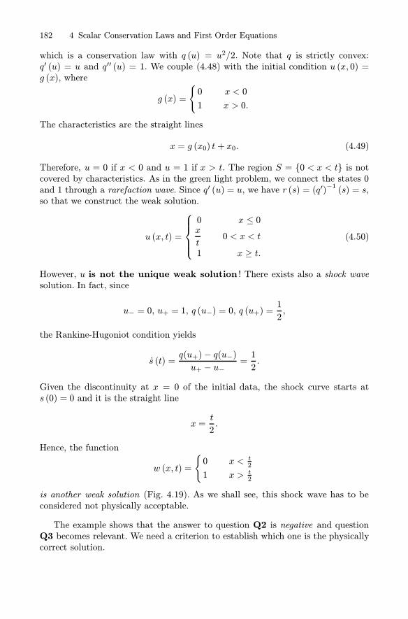
182 4 Scalar Conservation Laws and First Order Equations
which is a conservation law with q (u) = u2/2. Note that q is strictly convex:q′ (u) = u and q′′ (u) = 1. We couple (4.48) with the initial condition u (x, 0) =g (x), where
g (x) =
{0 x < 0
1 x > 0.
The characteristics are the straight lines
x = g (x0) t + x0. (4.49)
Therefore, u = 0 if x < 0 and u = 1 if x > t. The region S = {0 < x < t} is notcovered by characteristics. As in the green light problem, we connect the states 0and 1 through a rarefaction wave. Since q′ (u) = u, we have r (s) = (q′)−1 (s) = s,so that we construct the weak solution.
u (x, t) =
⎧⎪⎪⎨⎪⎪⎩
0 x ≤ 0x
t0 < x < t
1 x ≥ t.(4.50)
However, u is not the unique weak solution ! There exists also a shock wavesolution. In fact, since
u− = 0, u+ = 1, q (u−) = 0, q (u+) =1
2,
the Rankine-Hugoniot condition yields
s (t) =q(u+)− q(u−)u+ − u−
=1
2.
Given the discontinuity at x = 0 of the initial data, the shock curve starts ats (0) = 0 and it is the straight line
x =t
2.
Hence, the function
w (x, t) =
{0 x < t
2
1 x > t2
is another weak solution (Fig. 4.19). As we shall see, this shock wave has to beconsidered not physically acceptable.
The example shows that the answer to question Q2 is negative and questionQ3 becomes relevant. We need a criterion to establish which one is the physicallycorrect solution.

4.4 Integral (or Weak) Solutions 183
Fig. 4.19. A non physical shock
4.4.4 The entropy condition
From Proposition 4.2 we have seen that the equation
G (x, t, u) ≡ u− g [x− q′ (u) t] = 0
defines the unique classical solution u of problem (4.41), at least for small times.The Implicit Function Theorem gives
ux = −GxGu=
g′
1 + tg′q′′.
If we assume g′ > 0, q′′ ≥ C > 0, we get
ux ≤E
t
where13 E = 1C . Using the mean value theorem we deduce the following condition,
called entropy condition: there exists E ≥ 0 such that14, for every x, z ∈ R,z > 0, and every t > 0,
u (x+ z, t)− u (x, t) ≤ Etz. (4.51)
The denomination comes from an analogy with gas dynamics, where a condi-tion like (4.51) implies that entropy increases across a shock. The entropy conditiondoes not involve any derivative of u and makes perfect sense for discontinuous solu-tions as well. A weak solution satisfying (4.51) is said to be an entropy solution.A number of consequences follows directly from (4.51).
13 In the case g′ < 0 and q′′ ≤ C < 0 we already have ux < 0.14
u (x+ z, t)− u (x, t) = ux (x+ z∗) z
with a suitable z∗ between 0 e z.

184 4 Scalar Conservation Laws and First Order Equations
• The function
x �−→ u (x, t)− Etx
is decreasing. In fact, let x + z = x2, x = x1 and z > 0. Then x2 > x1 and(4.51) is equivalent to
u (x2, t)−E
tx2 ≤ u (x1, t)−
E
tx1. (4.52)
• If x is a discontinuity point for u (·, t), then
u+ (x, t) < u− (x, t) (4.53)
where u± (x, t) = limy→x± u (y, t). In fact, choose x1 < x < x2 and let x1 andx2 both go to x in (4.52).
If q is strictly convex, (4.53) yields
q′ (u+) <q(u+)− q(u−)u+ − u−
< q′(u−).
Then, the Rankine-Hugoniot implies that, if x = s (t) is a shock curve,
q′ (u+ (x, t)) < s (t) < q′ (u− (x, t)) (4.54)
that is called entropy inequality. The geometrical meaning of (4.54) is remark-able: the slope of a shock curve is less than the slope of the left-characteristics andgreater than the slope of the right-characteristics. Roughly, the characteristics hitforward in time the shock line, so that it is not possible to go back in time alongcharacteristics and hit a shock line, expressing a sort of irreversibility after a shock.
The above considerations lead us to select the entropy solutions as the onlyphysically meaningful ones. On the other hand, if the characteristics hit a shockcurve backward in time, the shock wave is to be considered non-physical.
Thus, in the non-uniqueness Example 4.3, the solution w represents a non-physical shock since it does not satisfy the entropy condition. The correct solutionis therefore the simple wave (4.50). The following important result holds (see e.g.Smoller, 1983).
Theorem 4.1. If q ∈ C2 (R) is convex (or concave) and g is bounded, there existsa unique entropy solution of the problem
{ut + q (u)x = 0 x ∈ R, t > 0u (x, 0) = g (x) x ∈ R. (4.55)

4.4 Integral (or Weak) Solutions 185
4.4.5 The Riemann problem
We apply Theorem 4.1 to solve explicitly problem (4.55) with initial data
g (x) =
{u+ x > 0
u− x < 0,(4.56)
where u+and u− are constants, u+ �= u−. This problem is known as Riemannproblem, and it is particularly important for the numerical approximation of morecomplex problems.
Theorem 4.2. Let q ∈ C2 (R) be strictly convex and q′′ ≥ h > 0.a) If u+ < u−, the unique entropy solution is the shock wave
u (x, t) =
{u+
xt > s
′ (t)
u− xt< s′ (t)
(4.57)
where
s (t) =q(u+)− q(u−)u+ − u−
.
b) If u+ > u−, the unique entropy solution is the rarefaction wave
u (x, t) =
⎧⎪⎪⎨⎪⎪⎩
u− xt < q
′ (u−)
r(xt
)q′ (u−) < x
t < q′ (u+)
u+xt > q
′ (u+)
where r = (q′)−1, is the inverse function of q′.
Proof. a) The shock wave (4.57) satisfies the Rankine Hugoniot condition andtherefore it is clearly a weak solution. Moreover, since u+ < u− the entropy con-dition holds as well, and u is the unique entropy solution of problem (4.56) byTheorem 4.1.b) Since
r (q′ (u+)) = u− and r (q′ (u−)) = u−,
u is continuous in the half-plane t > 0 and we have only to check that u satisfiesthe equation ut + q (u)x = 0 in the region
S ={(x, t) : q′ (u−) <
x
t< q′ (u+)
}.
Let u (x, t) = r(xt
).We have:
ut + q (u)x = −r′(xt
) xt2+ q′ (r) r′
(xt
) 1t= r′
(xt
) 1t
[q′ (r) − x
t
]≡ 0.
Thus, u is a weak solution in the upper half-plane.
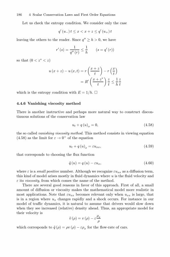
186 4 Scalar Conservation Laws and First Order Equations
Let us check the entropy condition. We consider only the case
q′ (u−) t ≤ x < x+ z ≤ q′ (u+) t
leaving the others to the reader. Since q′′ ≥ h > 0, we have
r′ (s) =1
q′′ (r)≤ 1h
(s = q′ (r))
so that (0 < z∗ < z)
u (x+ z)− u (x, t) = r(x+ z
t
)− r
(xt
)
= R′(x+ z∗
t
)z
t≤ 1h
z
t
which is the entropy condition with E = 1/h. �
4.4.6 Vanishing viscosity method
There is another instructive and perhaps more natural way to construct discon-tinuous solutions of the conservation law
ut + q (u)x = 0, (4.58)
the so called vanishing viscosity method. This method consists in viewing equation(4.58) as the limit for ε→ 0+ of the equation
ut + q (u)x = εuxx, (4.59)
that corresponds to choosing the flux function
q (u) = q (u) − εux, (4.60)
where ε is a small positive number. Although we recognize εuxx as a diffusion term,this kind of model arises mostly in fluid dynamics where u is the fluid velocity andε its viscosity, from which comes the name of the method.There are several good reasons in favor of this approach. First of all, a small
amount of diffusion or viscosity makes the mathematical model more realistic inmost applications. Note that εuxx becomes relevant only when uxx is large, thatis in a region where ux changes rapidly and a shock occurs. For instance in ourmodel of traffic dynamics, it is natural to assume that drivers would slow downwhen they see increased (relative) density ahead. Thus, an appropriate model fortheir velocity is
v (ρ) = v (ρ) − ερxρ
which corresponds to q (ρ) = ρv (ρ) − ερx for the flow-rate of cars.

4.4 Integral (or Weak) Solutions 187
Another reason comes from the fact that shocks constructed by the vanishingviscosity method are physical shocks, since they satisfy the entropy inequality.As for the heat equation, in principle we expect to obtain smooth solutions
even with discontinuous initial data. On the other hand, the nonlinear term mayforce the evolution towards a shock wave.Here we are interested in solutions of (4.59) connecting two constant states uL
and uR, that is, satisfying the conditions
limx→−∞u (x, t) = uL, lim
x→+∞u (x, t) = uR. (4.61)
Since we are looking for shock waves, it is reasonable to seek a solution dependingonly on a coordinate ξ = x− vt moving with the (unknown) shock speed v. Thus,let us look for bounded travelling waves solution of (4.59) of the form
u (x, t) = U (x− vt) ≡ U (ξ)
withU (−∞) = uL and U (+∞) = uR (4.62)
and uL �= uR. We have
ut = −vdU
dξ, ux =
dU
dξ, uxx =
d2U
dξ2
so that we obtain for U the ordinary differential equation
(q′ (U)− v) dUdξ= εd2U
dξ2
which can be integrated to yield
q (U)− vU + A = εdUdξ
where A is an arbitrary constant. Assuming thatdU
dξ→ 0 as ξ → ±∞ and using
(4.62) we get
q (uL)− vuL + A = 0 and q (uR) − vuR + A = 0. (4.63)
Subtracting these two equations we find
v =q (uR)− q (uL)uR − uL
≡ v. (4.64)
and then A =−q (uR)uL + q (uL)uR
uR − uL≡ A.
Thus, if there exists a travelling wave solution satisfying conditions (4.61), itmoves with a speed v predicted by the Rankine-Hugoniot formula. Still it is not
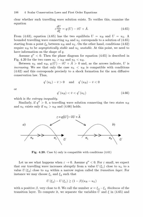
188 4 Scalar Conservation Laws and First Order Equations
clear whether such travelling wave solution exists. To verifies this, examine theequation
εdU
dξ= q (U)− vU + A. (4.65)
From (4.63), equation (4.65) has the two equilibria U = uR and U = uL. Abounded travelling wave connecting uR and uL corresponds to a solution of (4.65)starting from a point ξ0 between uR and uL. On the other hand, conditions (4.62)require uR to be asymptotically stable and uL unstable. At this point, we need tohave information on the shape of q.Assume q′′ < 0. Then the phase diagram for equation (4.65) is described in
Fig. 4.20 for the two cases uL > uR and uL < uR.Between uL and uR, q (U) − vU + A > 0 and, as the arrows indicate, U is
increasing. We see that only the case uL < uR is compatible with conditions(4.62) and this corresponds precisely to a shock formation for the non diffusiveconservation law. Thus,
q′ (uL) − v > 0 and q′ (uR)− v < 0
orq′ (uR) < v < q′ (uL) (4.66)
which is the entropy inequality.Similarly, if q′′ > 0, a travelling wave solution connecting the two states uR
and uL exists only if uL > uR and (4.66) holds.
Fig. 4.20. Case b) only is compatible with conditions (4.61)
Let us see what happens when ε → 0. Assume q′′ < 0. For ε small, we expectthat our travelling wave increases abruptly from a value U (ξ1) close to uL to avalue U (ξ2) close to uR within a narrow region called the transition layer. Forinstance we may choose ξ1 and ξ2 such that
U (ξ2)− U (ξ1) ≥ (1− β)(uR − uL)
with a positive β, very close to 0. We call the number κ = ξ2− ξ1 thickness of thetransition layer. To compute it, we separate the variables U and ξ in (4.65) and

4.4 Integral (or Weak) Solutions 189
integrate over (ξ1, ξ2); this yields
ξ2 − ξ1 = ε∫ U(ξ2)
U(ξ1)
ds
q (s) − vs + A .
Thus, the thickness of the transition layer is proportional to ε. As ε → 0, thetransition region becomes more and more narrow and eventually a shock wavethat satisfies the entropy inequality is obtained.This phenomenon is clearly seen in the important case of viscous Burger’s
equation that we examine in more details in the next subsection.
Example 4.3. Burger’s shock solution. Let us determine a travelling wave solutionof the viscous Burger equation
ut + uux = εuxx (4.67)
connecting the states uL = 1 and uR = 0. Note that q (u) = u2/2 is convex. Then
v = 1/2 and A = 0. Equation (4.65) becomes
2εdU
dξ= U2 − U
that can be easily integrated to give
U (ξ) =1
1 + exp
(ξ
2ε
) .
Thus the travelling wave is given by
u (x, t) = U
(x− t2
)=
1
1 + exp
(2x− t4ε
) . (4.68)
When ε→ 0,u (x, t)→ w (x, t) =
{0 x > t/21 x < t/2
which is the entropy shock solution for the non viscous Burger equation with initialdata 1 if x < 0 and 0 if x > 0.
4.4.7 The viscous Burger equation
The viscous Burger equation is one of the most celebrated examples of nonlineardiffusion equation. It arose (Burger, 1948) as a simplified form of the Navier-Stokesequation, in an attempt to study some aspects of turbulence. It appears also ingas dynamics, in the theory of sound waves and in traffic flow modelling and
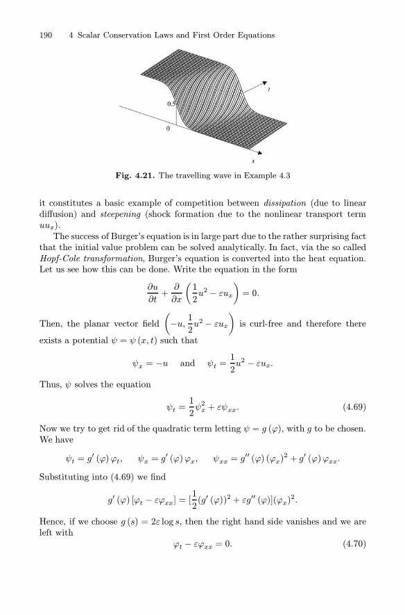
190 4 Scalar Conservation Laws and First Order Equations
Fig. 4.21. The travelling wave in Example 4.3
it constitutes a basic example of competition between dissipation (due to lineardiffusion) and steepening (shock formation due to the nonlinear transport termuux).The success of Burger’s equation is in large part due to the rather surprising fact
that the initial value problem can be solved analytically. In fact, via the so calledHopf-Cole transformation, Burger’s equation is converted into the heat equation.Let us see how this can be done. Write the equation in the form
∂u
∂t+∂
∂x
(1
2u2 − εux
)= 0.
Then, the planar vector field
(−u, 12u2 − εux
)is curl-free and therefore there
exists a potential ψ = ψ (x, t) such that
ψx = −u and ψt =1
2u2 − εux.
Thus, ψ solves the equation
ψt =1
2ψ2x + εψxx. (4.69)
Now we try to get rid of the quadratic term letting ψ = g (ϕ), with g to be chosen.We have
ψt = g′ (ϕ)ϕt, ψx = g
′ (ϕ)ϕx, ψxx = g′′ (ϕ) (ϕx)
2 + g′ (ϕ)ϕxx.
Substituting into (4.69) we find
g′ (ϕ) [ϕt − εϕxx] = [1
2(g′ (ϕ))2 + εg′′ (ϕ)](ϕx)
2.
Hence, if we choose g (s) = 2ε log s, then the right hand side vanishes and we areleft with
ϕt − εϕxx = 0. (4.70)

4.4 Integral (or Weak) Solutions 191
Thusψ = 2ε logϕ
and from u = −ψx we obtainu = −2εϕx
ϕ(4.71)
which is the Hopf-Cole transformation. An initial data
u (x, 0) = u0 (x) (4.72)
transforms into an initial data of the form15
ϕ0 (x) = exp
{−∫ x
a
u0 (z)
2εdz
}(a ∈ R). (4.73)
If (see Theorem 2.4)
1
x2
∫ x
a
u0 (z) dz → 0 as |x| → ∞,
the initial value problem (4.70), (4.73) has a unique smooth solution in the half-plane t > 0, given by formula (2.137):
ϕ (x, t) =1√4πεt
∫ +∞−∞
ϕ0 (y) exp
(−(x− y)
2
4εt
)dy.
This solution is continuous with its x−derivative16 up to t = 0 at any continuitypoint of u0. Consequently, from (4.71), problem (4.67) has a unique smooth solu-tion in the half-plane t > 0, continuous up to t = 0 at any continuity point of u0,given by
u (x, t) =
∫ +∞−∞
x− ytϕ0 (y) exp
(−(x− y)
2
4εt
)dy
∫ +∞−∞
ϕ0 (y) exp
(−(x− y)
2
4εt
)dy
. (4.74)
We use formula (4.74) to solve an initial pulse problem.
Example 4.4. Initial pulse. Consider problem (4.67), (4.67) with the initial condi-tion
u0 (x) =Mδ (x)
where δ denotes the Dirac density at the origin. We have, choosing a = 1,
ϕ0 (x) = exp
{−∫ x
1
u0 (y)
2εdy
}=
⎧⎨⎩1 x > 0
exp
(M
2ε
)x < 0.
15 The choice of a is arbitrary and does not affect the value of u.16 Check it.

192 4 Scalar Conservation Laws and First Order Equations
Formula (4.74), gives, after some routine calculations,
u (x, t) =
√4ε
πt
exp
(− x
2
4εt
)
2
exp (M/2ε)− 1 +√π
2
[1− erf
(x√4εt
)]
where
erf(x) =
∫ x
0
e−z2
dz
is the error function.
Fig. 4.22. Evolution of an initial pulse for the viscous Burger’s equation (M = 1, ε =0.04)
4.5 The Method of Characteristics for QuasilinearEquations
In this section we apply the characteristics method to general quasilinear equations.We consider mainly the case of two independent variables, where the intuition issupported by the geometric interpretation. However, the generalization to anynumber of dimensions should not be too difficult for the reader.
4.5.1 Characteristics
We consider equations of the form
a (x, y, u)ux + b (x, y, u)uy = c (x, y, u) (4.75)

4.5 The Method of Characteristics for Quasilinear Equations 193
whereu = u (x, y)
and a, b, c are continuously differentiable functions.The solutions of (4.75) can be constructed via geometric arguments. The tan-
gent plane to the graph of a solution u at a point (x0, y0, z0) has equation
ux (x0, y0) (x− x0) + uy (x0, y0) (y − y0) − (z − z0) = 0
and the vectorn0 = (ux (x0, y0) , uy (x0, y0) ,−1)
is normal to the plane. Introducing the vector
v0 = (a (x0, y0, z0) , b (x0, y0, z0) , c (x0, y0, z0)) ,
equation (4.75) implies thatn0 · v0 = 0.
Thus, v0 is tangent to the graph of u (Fig. 4.23). In other words, (4.75) says that,at every point (x, y, z), the graph of any solution is tangent to the vector field
v (x, y, z)= (a (x, y, z) , b (x, y, z) , c (x, y, z)) .
In this case we say that the graph of a solution is an integral surface of thevector field v.
Fig. 4.23. Integral surface
Now, we may construct integral surfaces of v as union of integral curves ofv, that is curves tangent to v at every point. These curves are solutions of the

194 4 Scalar Conservation Laws and First Order Equations
systemdx
dt= a (x, y, z) ,
dy
dt= b (x, y, z) ,
dz
dt= c (x, y, z) (4.76)
and are called characteristics. Note that
z = z (t)
gives the values u along a characteristic, that is
z (t) = u (x (t) , y (t)) . (4.77)
In fact, differentiating (4.77) and using (4.76) and (4.75), we have
dz
dt= ux (x (t) , y (t))
dx
dt+ uy (x (t) , y (t))
dy
dt= a (x (t) , y (t) , z (t))ux (x (t) , y (t)) + b((x (t) , y (t) , z (t))uy (x (t) , y (t))
= c (x (t) , y (t) , z (t)) .
Thus, along a characteristic the partial differential equation (4.75) degeneratesinto an ordinary differential equation.In the case of a conservation law (with t = y)
uy + q′ (u)ux = 0
(q′ (u) =
dq
du
),
we have introduced the notion of characteristic in a slightly different way, but weshall see later that there is no contradiction.
The following proposition is a consequence of the above geometric reasoningand of the existence and uniqueness theorem for system of ordinary differentialequations17.
Proposition 4.3. a) Let the surface S be the graph of a C1 function u = u (x, y).If S is union of characteristics then u is a solution of the equation (4.75).b) Every integral surface S of the vector field v is union of characteristics.
Namely: every point of S belongs exactly to one characteristic, entirely containedin S.c) Two integral surfaces intersecting at one point intersect along the whole
characteristic passing through that point.
4.5.2 The Cauchy problem
Proposition 4.3 gives a characterization of the integral surfaces as a union of char-acteristics. The problem is how to construct such unions to get a smooth surface.One way to proceed is to look for solutions u whose values are prescribed on acurve γ0, contained in the x, y plane.
17 We leave the details of the proof to the reader.

4.5 The Method of Characteristics for Quasilinear Equations 195
In other words, suppose that
x (s) = f (s) , y (s) = g (s) s ∈ I ⊆ R
is a parametrization of γ0. We look for a solution u of (4.75) such that
u (f (s) , g (s)) = h (s) , s ∈ I, (4.78)
where h = h (s) is a given function. We assume that I is a neighborhood of s = 0,and that f, g, h are continuously differentiable in I.
The system (4.75), (4.78) is called Cauchy problem. If we consider the three-dimensional curve Γ0 given by the parametrization
x (s) = f (s) , y (s) = g (s) , z (s) = h (s) ,
then, solving the Cauchy problem (4.75), (4.78) amounts to determining an integralsurface containing Γ0 (Fig. 4.24).
The data are often assigned in the form of initial values
u (x, 0) = h (x) ,
with y playing the role of "time". In this case, γ0 is the axis y = 0 and x plays therole of the parameter s. Then a parametrization of Γ0 is given by
x = x, y = 0, z (x) = h (x) .
By analogy, we often refer to Γ0 as to the initial curve. The strategy to solve aCauchy problem comes from its geometric meaning: since the graph of a solution
Fig. 4.24. Characteristics flowing out of Γ0

196 4 Scalar Conservation Laws and First Order Equations
u = u (x, y) is a union of characteristics, we determine those flowing out from Γ0,by solving the system
dx
dt= a (x, y, z) ,
dx
dt= b (x, y, z) ,
dx
dt= c (x, y, z) , (4.79)
with the family of initial conditions
x(0) = f (s) , y(0) = g (s) , z(0) = h (s) , (4.80)
parametrized by s ∈ I. The union of the characteristics of this family should give18u. Why only should? We will come back to this question.Under our hypotheses, the Cauchy problem (4.79), (4.80) has exactly one so-
lutionx = X (s, t) , y = Y (s, t) , z = Z (s, t) . (4.81)
in a neighborhood of t = 0, for every s ∈ I.A couple of questions arise:
a) Do the three equations (4.81) define a function z = u (x, y)?
b) Even if the answer to question a) is positive, is z = u (x, y) the uniquesolution of the Cauchy problem?
Let us reason in a neighborhood of s = t = 0, setting
X (0, 0) = f (0) = x0, Y (0, 0) = g (0) = y0, Z (0, 0) = h (0) = z0.
The answer to question a) is positive if we can solve for s and t the first two equa-tions in (4.81), and find s = S (x, y) e t = T (x, y) of class C1 in a neighborhoodof (x0, y0), such that
S (x0, y0) = 0, T (x0, y0) = 0.
Then, from the third equation z = Z (s, t), we get
z = Z (S (x, y) , T (x, y)) = u (x, y) . (4.82)
From the Inverse Function Theorem, the system
{X (s, t) = xY (s, t) = y
definess = S (x, y) and t = T (x, y)
in a neighborhood of (x0, y0) if
J (0, 0) =
∣∣∣∣∣Xs (0, 0) Ys (0, 0)
Xt (0, 0) Yt (0, 0)
∣∣∣∣∣ �= 0. (4.83)
18 Identifying u with its graph.

4.5 The Method of Characteristics for Quasilinear Equations 197
From (4.79) and (4.80) we have
Xs (0, 0) = f′ (0) , Ys (0, 0) = g′ (0)
andXt (0, 0) = a (x0, y0, z0) , Yt (0, 0) = b (x0, y0, z0) ,
so that (4.83) becomes
J (0, 0) =
∣∣∣∣∣f ′ (0) g′ (0)
a (x0, y0, z0) b (x0, y0, z0)
∣∣∣∣∣ �= 0 (4.84)
orb (x0, y0, z0) f
′ (0) �= a (x0, y0, z0) g′ (0) . (4.85)
Condition (4.85) means that the vectors
(a (x0, y0, z0) , b (x0, y0, z0)) and (f ′ (0) , g′ (0))
are not parallel.In conclusion: if condition (4.84) holds, then (4.82) is a well defined C1−function.Now consider question b). The above construction of u implies that the surface
z = u (x, y) contains Γ0 and all the characteristics flowing out from Γ0, so thatu is a solution of the Cauchy problem. Moreover, by Proposition 4.5 c), two in-tegral surfaces containing Γ0 must contain the same characteristics and thereforecoincide.We summarize everything in the following theorem, recalling that
(x0, y0, z0) = (f (0) , g (0) , h (0)) .
Theorem 4.3. Let a, b, c be C1−functions in a neighborhood of (x0, y0, z0) andf, g, h be C1−functions in I. If J (0, 0) �= 0, then, in a neighborhood of (x0, y0),there exists a unique C1−solution u = u (x, y) of the Cauchy problem
{a (x, y, u)ux + b (x, y, u)uy = c (x, y, u)
u (f (s) , g (s)) = h (s) .(4.86)
Moreover, u is defined by the parametric equations (4.81).
Remark 4.2. If a, b, c and f, g, h are Ck−functions, k ≥ 2, then u is a Ck−functionas well.
It remains to examine what happens when J (0, 0) = 0, that is when the vectors(a (x0, y0, z0) , b (x0, y0, z0)) and (f
′ (0) , g′ (0)) are parallel.Suppose that there exists a C1−solution u of the Cauchy problem (4.86). Dif-
ferentiating the second equation in (4.86) we get
h′ (s) = ux (f (s) , g (s)) f ′ (s) + uy (f (s) , g (s)) g′ (s) . (4.87)

198 4 Scalar Conservation Laws and First Order Equations
Computing at x = x0, y = y0, z = z0 and s = 0, we obtain
{a (x0, y0, z0)ux (x0, y0) + b (x0, y0, z0)uy (x0, y0) = c (x0, y0, z0)
f ′ (0)ux (x0, y0) + g′ (0)uy (x0, y0) = h′ (0) .(4.88)
Since u is a solution of the Cauchy problem, the vector (ux (x0, y0) , uy (x0, y0)) isa solution of the algebraic system (4.88). But then, from Linear Algebra, we knowthat the condition
rank
(a (x0, y0, z0) b (x0, y0, z0) c (x0, y0, z0)
f ′ (0) g′ (0) h′ (0)
)= 1 (4.89)
must hold and therefore the two vectors
(a (x0, y0, z0) b (x0, y0, z0) , c (x0, y0, z0)) and (f ′ (0) , g′ (0) , h′ (0)) (4.90)
are parallel. This is equivalent to saying that Γ0 is parallel to the characteristiccurve at (x0, y0, z0). When this occurs, we say that Γ0 is characteristic at thepoint (x0, y0, z0).
Conclusion: If J (0, 0) = 0, a necessary condition for the existence of aC1−solution u = u (x, y) of the Cauchy problem in a neighborhood of (x0, y0)is that Γ0 be characteristic at (x0, y0, z0).
Now, assume Γ0 itself is a characteristic and let P0 = (x0, y0, z0) ∈ Γ0. If wechoose a curve Γ ∗ transversal19 to Γ0 at P0, by Theorem 4.3 there exists a uniqueintegral surface containing Γ ∗ and, by Proposition 4.3 c), this surface contains Γ0.In this way we can construct infinitely many smooth solutions.
We point out that the condition (4.89) is compatible with the existence of aC1−solution only if Γ0 is characteristic at P0. On the other hand, it may occurthat J (0, 0) = 0, that Γ0 is non characteristic at P0 and that solutions of theCauchy problem exist anyway; clearly, these solutions cannot be of class C1.
Let us summarize the steps to solve the Cauchy problem (4.86):
Step 1. Determine the solution
x = X (s, t) , y = Y (s, t) , z = Z (s, t) (4.91)
of the characteristic system
dx
dt= a (x, y, z) ,
dy
dt= b (x, y, z) ,
dz
dt= c (x, y, z) (4.92)
with initial conditions
X (s, 0) = f (s) , Y (s, 0) = g (s) , Z (s, 0) = h (s) , s ∈ I.19 Not tangent.

4.5 The Method of Characteristics for Quasilinear Equations 199
Step 2. Compute J (s, t) on the initial curve Γ0 i.e.
J (s, 0) =
∣∣∣∣∣f ′ (s) g′ (s)Xt (s, 0) Yt (s, 0)
∣∣∣∣∣ .
The following cases may occur:
2a. J (s, 0) �= 0, for every s ∈ I. This means that Γ0 does not have char-acteristic points. Then, in a neighborhood of Γ0, there exists a unique solutionu = u (x, y) of the Cauchy problem, defined by the parametric equations (4.91).
2b. J (s0, 0) = 0 for some s0 ∈ I and Γ0 is characteristic at the pointP0 = (f (s0) , g (s0) , h (s0)). A C
1−solution may exist in a neighborhood of P0only if the rank condition (4.89) holds at P0.
2c. J (s0 , 0) = 0 for some s0 ∈ I and Γ0 is not characteristic at P0.There are no C1−solutions in a neighborhood of P0. There may exist less regularsolutions.
2d. Γ0 is a characteristic. Then there exist infinitely many C1−solutions
in a neighborhood of Γ0.
Example 4.5. Consider the non-homogeneous Burger equation
uux + uy = 1. (4.93)
As in Example 4.2, if y is the time variable y, u = u (x, y) represents a velocity fieldof a flux of particles along the x−axis. Equation (4.93) states that the accelerationof each particle is equal to 1. Assume
u (x, 0) = h (x) , x ∈ R.
The characteristics are solutions of the system
dx
dt= z,
dy
dt= 1,
dz
dt= 1
and the initial curve Γ0 has the parametrization
x = f (s) = s, y = g (s) = 0, z = h (s) s ∈ R.
The characteristics flowing out from Γ0 are
X (s, t) = s+t2
2+ th (s) , Y (s, t) = t, Z (s, t) = t + h (s) .
Since
J (s, t) =
∣∣∣∣∣1 + th′ (s) 0
t+ h (s) 1
∣∣∣∣∣ = 1 + th′ (s) ,

200 4 Scalar Conservation Laws and First Order Equations
we have J (s, 0) = 1 and we are in the case 2a: in a neighborhood of Γ0 there existsa unique C1−solution. If, for instance, h (s) = s, we find the solution
u = y +2x− y22 + 2y
(x ∈ R, y ≥ −1) .
Now consider the same equation with initial condition
u
(y2
4, y
)=y
2,
equivalent to assigning the values of u on the parabola x = y2
4 . A parametrizationof Γ0 is given by
x = s2, y = 2s, z = s, s ∈ R.Solving the characteristic system with these initial conditions, we find
X (s, t) = s2 + ts+t2
2, Y (s, t) = 2s+ t, Z (s, t) = s+ t. (4.94)
Observe that Γ0 does not have any characteristic point, since its tangent vector(2s, 2, 1) is never parallel to the characteristic direction (s, 1, 1). However
J (s, t) =
∣∣∣∣2s+ t 2s+ t 1
∣∣∣∣ = −t
which vanishes for t = 0, i.e. exactly on Γ0. We are in the case 2c. Solving for sand t, t �= 0, in the first two equations (4.94), and substituting into the third one,we find
u (x, y) =y
2±√x− y
2
4.
We have found two solutions of the Cauchy problem, satisfying the differential
equation in the region x > y2
4 . However, these solutions are not smooth in aneighborhood of Γ0, since on Γ0 they are not differentiable.
• Conservation laws. According to the new definition, the characteristics of theequation
uy + q′ (u)ux = 0
(q′ (u) =
dq
du
),
with initial conditionsu (x, 0) = g (x) ,
are the three-dimensional solution curves of the system
dx
dt= q′ (z) ,
dy
dt= 1,
dz
dt= 0
with initial conditions
x (s, 0) = s, y (s, 0) = 0, z (s, 0) = g (s) , s ∈ R.

4.5 The Method of Characteristics for Quasilinear Equations 201
Integrating, we find
z = g (s) , x = q′ (g (s)) t + s, y = t.
The projections of these straight-lines on the x, y plane are
x = q′ (g (s)) y + s.
which are the “old characteristics”, called projected characteristics in the generalquasilinear context.
• Linear equations. Consider a linear equation
a (x, y) ux + b (x, y)uy = 0. (4.95)
Introducing the vector w =(a, b), we may write the equation (4.95) in the form
Dwu = ∇u ·w =0.
Thus, every solution of the (4.95) is constant along the integral lines of the vectorw, i.e. along the projected characteristics, solutions of the reduced characteristicsystem
dx
dt= a (x, y) ,
dy
dt= b (x, y) , (4.96)
locally equivalent to the ordinary differential equation
b (x, y) dx− a (x, y) dy = 0.
If a first integral20 ψ = ψ (x, y) of the system (4.96) is known, then the family ofthe projected characteristics is given in implicit form by
ψ (x, y) = k, k ∈ R
and the general solution of (4.95) is given by the formula
u (x, y) = G (ψ (x, y)) ,
where G = G (r) is an arbitrary C1−function, that can be determined by theCauchy data.
Example 4.6. Let us solve the problem
{yux + xuy = 0u (x, 0) = x4.
20 We recall that a first integral (also called constant of motion) for a system of o.d.e.dx
dt= f (x), is a C1−function ϕ = ϕ (x) which is constant along the trajectories of the
system, i.e. such that ∇ϕ · f ≡0.

202 4 Scalar Conservation Laws and First Order Equations
Here w = (y, x) and the reduced characteristic system is
dx
dt= y,
dy
dt= x
locally equivalent toxdx− ydy = 0.
Integrating we find that the projected characteristics are the hyperbolas
ψ (x, y) = x2 − y2 = k
and therefore ψ (x, y) = x2 − y2 is a first integral. Then, the general solution ofthe equation is
u (x, y) = G(x2 − y2).Imposing the Cauchy condition, we have
G(x2) = x4
from which G (r) = r2. The solution of the Cauchy problem is
u (x, y) = (x2 − y2)2.
Example 4.7. An interesting situation occurs when we want to find a solution ofthe equation (4.95) in a smooth domain Ω ⊂ R2, that assumes prescribed valueson a subset of the boundary γ = ∂Ω. Figure 4.25 shows a possible situation. Inanalogy with the problems in subsection 4.2.4, for the solvability of the problemwe have to assign the Cauchy data only on the so called inflow boundary γidefined by
γi = {σ ∈ γ : w · ν <0}where ν is the outward unit normal to γ. If a smooth Cauchy data is prescribed onγi, a smooth solution is obtained by defining u to be constant along the projectedcharacteristics like l1 and piecewise constant on those like l2. Observe that thepoints at which w is tangent to γ are characteristic.
4.5.3 Lagrange method of first integrals
We have seen that, in the linear case, we can construct a general solution, depend-ing on an arbitrary function from the knowledge of a first integral for the reducedcharacteristic system. The method can be extended to equations of the form
a (x, y, u)ux + b (x, y, u)uy = c (x, y, u) . (4.97)
We say that two first integrals ϕ = ϕ (x, y, u) are independent if ∇ϕ and ∇ψ arenowhere colinear. Then:

4.5 The Method of Characteristics for Quasilinear Equations 203
Fig. 4.25. Cauchy problem in a domain
Theorem 4.4. Let ϕ = ϕ (x, y, u), ψ = ψ (x, y, u) be two independent first inte-grals of the characteristic system and F = F (h, k) be a C1−function. If
Fhϕu + Fkψu �= 0,
the equationF (ϕ (x, y, u) , ψ (x, y, u)) = 0
defines the general solution of (4.97) in implicit form.
Proof. It is based on the following two observations. First, the function
w = F (ϕ (x, y, u) , ψ (x, y, u)) (4.98)
is a first integral. In fact,∇w = Fh∇ϕ+ Fk∇ψ
so that∇w · (a, b, c) = Fh∇ϕ · (a, b, c) + Fk∇ψ · (a, b, c) ≡ 0
since ϕ and ψ are first integrals. Moreover, by hypothesis,
wu = Fhϕu + Fkψu �= 0.
Second, if w is a first integral and wu �= 0, then equation
w (x, y, u) = 0 (4.99)
defines implicitly an integral surface u = u (x, y) of (4.97). In fact, since w is a firstintegral it satisfies the equation
a (x, y, u)wx + b (x, y, u)wy + c (x, y, u)wu = 0. (4.100)

204 4 Scalar Conservation Laws and First Order Equations
Moreover, from the Implicit Function Theorem, we have
ux = −wxwu, uy = −
wywu
and from (4.100) we get easily (4.97). �
Remark 4.3. As a by-product of the proof, we have that the general solution of thethree-dimensional homogeneous equation (4.100) is given by (4.98).
Remark 4.4. The search for first integrals is sometimes simplified by writing thecharacteristic system in the form
dx
a (x, y, u)=
dy
b (x, y, u)=
du
c (x, y, u).
Example 4.8. Consider again the nonhomogeneous Burger equation
uux + uy = 1
with initial condition
u
(1
2y2, y
)= y.
A parametrization of the initial curve Γ0 is
x =1
2s2 , y = s, z = s
and therefore Γ0 is a characteristic. We are in the case 2d.Let us use the Lagrange method. To find two independent first integrals, we
write the characteristic system in the form
dx
z= dy = dz
ordx = zdz, dy = dz.
Integrating the two equations, we get
x− 12z2 = c2, y − z = c1
so that
ϕ (x, y, z) = x− 12z2, ψ (x, y, z) = y − z
are two first integral. Since
∇ϕ (x, y, z) = (1, 0,−z)

4.5 The Method of Characteristics for Quasilinear Equations 205
and
∇ψ (x, y, z) = (0, 1,−1)we see that they are also independent.Thus, the general solution of Burger equation is given by
F
(x− 12z2, y− z
)= 0
where F is an arbitrary C1−function.Finally, to satisfy the Cauchy condition, it is enough to choose F such that
F (0, 0) = 0. As expected, there exist infinitely many solutions of the Cauchyproblem.
4.5.4 Underground flow
Consider the underground flow of a fluid (like water). In the wet region, only afraction of any control volume is filled with fluid. This fraction, denoted by φ, iscalled porosity and, in general, it depends on position, temperature and pressure.Here, we assume φ depends on position only: φ = φ (x, y, z).If ρ is the fluid density and q =(q1, q2, q3) is the flux vector (the volumetric
flow rate of the fluid), the conservation of mass yields, in this case,
φρt + div(ρq) = 0.
For q the following modified Darcy law is commonly adopted:
q =− kμ(∇p+ ρg)
where p is the pressure and g is the gravity acceleration; k > 0 is the permeabilityof the medium and μ is the fluid viscosity21. Thus, we have:
φρt − div[ρk
μ(∇p+ ρg)
]= 0. (4.101)
Now, suppose that two immiscible fluids, of density ρ1 and ρ2, flow under-ground. Immiscible means that the two fluids cannot dissolve one into the other orchemically interact. In particular, the conservation law holds for the mass of eachfluid. Thus, if we denote by S1 and S2 the fractions (saturations) of the availablespace filled by the two fluids, respectively, we can write
φ (S1ρ1)t + div(ρ1q1) = 0 (4.102)
φ (S2ρ2)t + div(ρ2q2) = 0. (4.103)
21 For water: μ = 1.14 · 103 Kg ×m × s−1.

206 4 Scalar Conservation Laws and First Order Equations
We assume that S1+S2 = 1, i.e. that the medium is completely saturated andthat capillarity effects are negligible. We set S1 = S and S2 = 1 − S. The Darcylaw for the two fluids becomes
q1=− kk1
μ1(∇p+ ρ1g)
q2=− kk2
μ2(∇p+ ρ2g)
where k1, k2 are the relative permeability coefficients, in general depending on S.We make now some other simplifying assumptions:
– gravitational effects are negligible,
– k, φ, ρ1, ρ2, μ1, μ2 are constant,
– k1 = k1 (S) , k2 = k2 (S) are known.
Equations (4.103) and (4.102) become:
φSt + div q1 = 0, −φSt + div q2 = 0 (4.104)
while the Darcy laws take the form
q1= − kk1μ1∇p, q2=− k
k2μ2∇p. (4.105)
Letting q = q1 + q2 and adding the two equations in (4.104) we have
div q =0.
Adding the two equations in (4.105) yields
∇p = −1k
(k1μ1+k2μ2
)−1q
from which
div ∇p = Δp = −1kq·∇
(k1μ1+k2μ2
)−1.
From the first equations in (4.104) and (4.105) we get
φSt = − divq1 = k∇(k1
μ1
)· ∇p+ k k1
μ1Δp
= −(k1
μ1+k2
μ2
)−1q·∇
(k1
μ1
)− k1μ1q·∇
(k1
μ1+k2
μ2
)−1
= q·∇H (S) = H ′ (S) q·∇S
where
H (S) = −k1 (S)μ1
(k1 (S)
μ1+k2 (S)
μ2
)−1.

4.6 General First Order Equations 207
When q is known, the resulting quasilinear equation for the saturation S is
φSt = H′ (S)q·∇S,
known as the Bukley-Leverett equation.In particular, if q can be considered one-dimensional and constant, i.e. q =qi,
we haveqH ′ (S) Sx + φSt = 0
which is of the form (4.97), with u = S and y = t. The characteristic system is(see Remark 4.10)
dx
qH ′ (S)=dt
φ=dS
0.
Two first integrals arew1 = φx− qH ′ (S) t
and w2 = S. Thus, the general solution is given by
F (φx− qH ′ (S) t, S) = 0.
The choiceF (w1, w2) = w2 − f (w1) ,
yieldsS = f (φx− qH ′ (S) t)
that satisfies the initial condition S (x, 0) = f (φx) .
4.6 General First Order Equations
4.6.1 Characteristic strips
We extend the characteristic method to nonlinear equations of the form
F (x, y, u, ux, uy) = 0 (4.106)
We assume that F = F (x, y, u, p, q) is a smooth function of its arguments and, toavoid trivial cases, that F 2p + F
2q �= 0. In the quasilinear case,
F (x, y, u, p, q) = a (x, y, u) p+ b (x, y, u) q − c (x, y, u)
andFp = a (x, y, u) , Fq = b (x, y, u) (4.107)
so that F 2p + F2q �= 0 says that a and b do not vanish simultaneously.
Equation (4.106) has a geometrical interpretation as well. Let u = u (x, y) bea smooth solution and consider a point (x0, y0, z0) on its graph. Equation (4.106)constitutes a link between the components ux and uy of the normal vector
n0 = (−ux (x0, y0) ,−uy (x0, y0) , 1)
208 4 Scalar Conservation Laws and First Order Equations
but it is a little more complicated than in the quasilinear case22 and it is not apriori clear what a characteristic system for equation (4.106) should be. Reasoningby analogy, from (4.107) we are lead to the choice
dx
dt= Fp (x, y, z, p, q)
dy
dt= Fq (x, y, z, p, q) .
(4.108)
where z (t) = u (x (t) , y (t)) and
p = p (t) = ux (x (t) , y (t)) , q = q (t) = uy (x (t) , y (t)) . (4.109)
Thus, taking account of (4.108), the equation for z is:
dz
dt= ux
dx
dt+ uy
dy
dt= pFp + qFq (4.110)
Equations (4.110) and (4.108) correspond to the characteristic system (4.76), butwith two more unknown functions: p (t) e q (t).We need two more equations. Proceeding formally, from (4.108) we can write
dp
dt= uxx (x (t) , y (t))
dx
dt+ uxy (x (t) , y (t))
dy
dt= uxx (x (t) , y (t))Fp + uxy (x (t) , y (t))Fq.
We have to get rid of the second order derivatives. Since u is a solution of (4.106),the identity
F (x, y, u (x, y) , ux (x, y) , uy (x, y)) ≡ 0.holds. Partial differentiation with respect to x yields, since uxy = uyx:
Fx + Fuux + Fpuxx + Fquxy ≡ 0.
Computing along x = x (t), y = y (t), we get
uxx (x (t) , y (t))Fp + uxy (x (t) , y (t))Fq = −Fx − p (t)Fu. (4.111)
22 If, for instance Fq �= 0, by the Implicit Function Theorem, the equationF (x0, y0, z0, p, q) = 0 defines q = q (p) so that
F (x0, y0, z0, p, q (p)) = 0.
Therefore, the possible tangent planes to u at (x0, y0, z0) form a one parameter familyof planes, given by
p (x − x0) + q (p) (y − y0)− (z − z0) = 0.This family, in general, envelopes a cone with vertex at (x0, y0, z0) , calledMonge cone.Each possible tangent plane touches the Monge cone along a generatrix.

4.6 General First Order Equations 209
Thus, we deduce for p the following differential equation:
dp
dt= −Fx (x, y, z, p, q)− pFu (x, y, z, p, q) .
Similarly, we find
dq
dt= −Fy (x, y, z, p, q)− qFu (x, y, z, p, q) .
In conclusion, we are lead to the following characteristic system of five au-tonomous equations
dx
dt= Fp,
dy
dt= Fq,
dz
dt= pFp + qFq (4.112)
and
dp
dt= −Fx − pFu,
dq
dt= −Fy − qFu. (4.113)
Observe that F = F (x, y, u, p, q) is a first integral of (4.112), (4.113). In fact
d
dtF (x (t) , y (t) , z (t) , p (t) , q (t))
= Fxdx
dt+ Fy
dy
dt+ Fu
dz
dt+ Fp
dp
dt+ Fq
dq
dt= FxFp + FyFq + Fu (pFp + qFq) + Fp (−Fx − pFp) + Fq (−Fy − qFq)≡ 0
and therefore, if F (x (t0) , y (t0) , z (t0) , p (t0) , q (t0)) = 0 at some t0, then
F (x (t) , y (t) , z (t) , p (t) , q (t)) ≡ 0. (4.114)
Thus, the curve,
x = x (t) , y = y (t) , z = z (t) ,
still called a characteristic curve, is contained in an integral surface, while
p = p (t) , q = q (t)
give the normal vector at each point, and can be associated with a piece of thetangent plane, as shown in figure 4.26.For this reason, a solution (x (t) , y (t) , z (t) , p (t) , q (t)) of (4.112), (4.113) is
called characteristic strip (Fig. 4.26).
Fig. 4.26. Characteristic strip
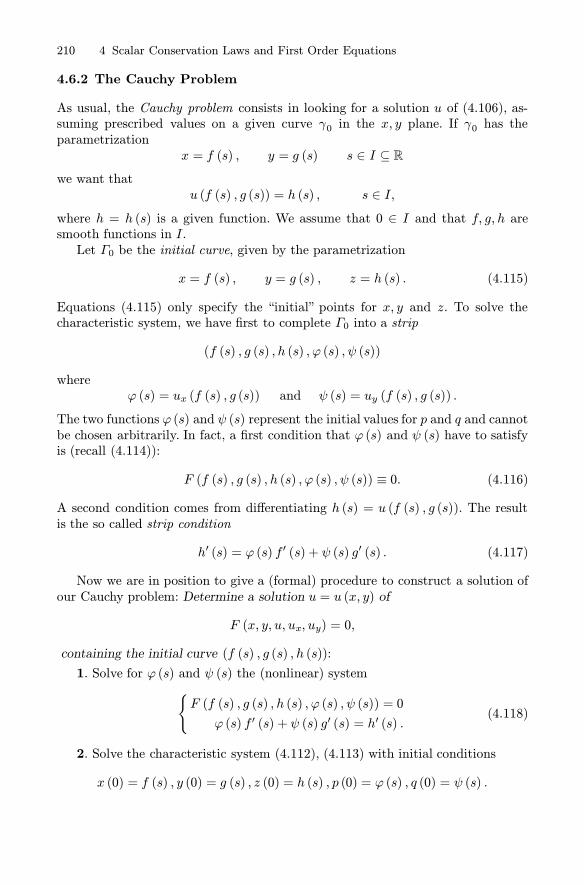
210 4 Scalar Conservation Laws and First Order Equations
4.6.2 The Cauchy Problem
As usual, the Cauchy problem consists in looking for a solution u of (4.106), as-suming prescribed values on a given curve γ0 in the x, y plane. If γ0 has theparametrization
x = f (s) , y = g (s) s ∈ I ⊆ Rwe want that
u (f (s) , g (s)) = h (s) , s ∈ I,where h = h (s) is a given function. We assume that 0 ∈ I and that f, g, h aresmooth functions in I.Let Γ0 be the initial curve, given by the parametrization
x = f (s) , y = g (s) , z = h (s) . (4.115)
Equations (4.115) only specify the “initial” points for x, y and z. To solve thecharacteristic system, we have first to complete Γ0 into a strip
(f (s) , g (s) , h (s) , ϕ (s) , ψ (s))
whereϕ (s) = ux (f (s) , g (s)) and ψ (s) = uy (f (s) , g (s)) .
The two functions ϕ (s) and ψ (s) represent the initial values for p and q and cannotbe chosen arbitrarily. In fact, a first condition that ϕ (s) and ψ (s) have to satisfyis (recall (4.114)):
F (f (s) , g (s) , h (s) , ϕ (s) , ψ (s)) ≡ 0. (4.116)
A second condition comes from differentiating h (s) = u (f (s) , g (s)). The resultis the so called strip condition
h′ (s) = ϕ (s) f ′ (s) + ψ (s) g′ (s) . (4.117)
Now we are in position to give a (formal) procedure to construct a solution ofour Cauchy problem: Determine a solution u = u (x, y) of
F (x, y, u, ux, uy) = 0,
containing the initial curve (f (s) , g (s) , h (s)):
1. Solve for ϕ (s) and ψ (s) the (nonlinear) system
{F (f (s) , g (s) , h (s) , ϕ (s) , ψ (s)) = 0
ϕ (s) f ′ (s) + ψ (s) g′ (s) = h′ (s) .(4.118)
2. Solve the characteristic system (4.112), (4.113) with initial conditions
x (0) = f (s) , y (0) = g (s) , z (0) = h (s) , p (0) = ϕ (s) , q (0) = ψ (s) .

4.6 General First Order Equations 211
Suppose we find the solution
x = X (s, t) , y = Y (s, t) , z = Z (s, t) , p = P (s, t) , q = Q (s, t) .
3. Solve x = X (s, t) , y = Y (s, t) for s, t in terms of x, y. Substitute s = S (x, y)and t = T (x, y) into z = Z (t, s) to yield a solution z = u (x, y).
Example 4.9.We want to solve the equation
u = u2x − 3u2ywith initial condition u (x, 0) = x2. We have F (p, q) = p2 − 3q2 − u and thecharacteristic system is
dx
dt= 2p,
dy
dt= −6q, dz
dt= 2p2 − 6q2 = 2z (4.119)
dp
dt= p,
dq
dt= q. (4.120)
A parametrization of the initial line Γ0 is
f (s) = s, g (s) = 0, h (s) = s2 .
To complete the initial strip we solve the system (4.118):{ϕ2 − 3ψ2 = s2ϕ = 2s.
There are two solutions:
ϕ (s) = 2s, ψ (s) = ±s.
The choice of ψ (s) = s yields, integrating equations (4.120),
P (s, t) = 2set, Q (s, t) = set
whence, from (4.119),
X (s, t) = 4s(et − 1) + s, Y (s, t) = −6s(et − 1), Z (s, t) = s2e2t.
Solving the first two equations for s, t and substituting into the third one, we get
u (x, y) =(x+y
2
)2.
The choice of ψ (s) = −s yields
u (x, y) =(x− y2
)2.
As the example shows, in general there is no uniqueness, unless system (4.118)has a unique solution. On the other hand, if this system has no (real) solution,then the Cauchy problem has no solution as well.

212 4 Scalar Conservation Laws and First Order Equations
Furthermore, observe that if (x0, y0, z0) = (f (0) , g (0) , h (0)) and (p0, q0) is asolution of the system
{F (x0, y0, z0, p0, q0) = 0
p0f′ (0) + q0g′ (0) = h′ (0) ,
by the Implicit Function Theorem, the condition
∣∣∣∣∣f ′ (0) Fp(x0, y0, z0, p0, q0)
g′ (0) Fq(x0, y0, z0, p0, q0)
∣∣∣∣∣ �= 0 (4.121)
assures the existence of a solution ϕ (s) and ψ (s) of (4.118), in a neighborhood ofs = 0. Condition (4.121) corresponds to (4.84) in the quasilinear case.The following theorem summarizes the above discussion on the Cauchy problem
F (x, y, u, ux, uy) = 0 (4.122)
with initial curve Γ0 given by
x = f (s) , y = g (s) , z = h (s) . (4.123)
Theorem 4.5. Assume that:
i) F is twice continuously differentiable in a domain D ⊆ R5 and F 2p +F 2q �= 0;ii) f, g, h are twice continuously differentiable in a neighborhood of s = 0.
iii) (p0, q0) is a solution of the system (5.30) and condition (4.121) holds.
Then, in a neighborhood of (x0, y0), there exists a C2 solution z = u (x, y) of
the Cauchy problem (4.122), (4.123).
• Geometrical optics. The equation
c2(u2x + u
2y
)= 1 (c > 0) (4.124)
is called eikonal equation and arises in (two dimensional) geometrical optics. Thelevel lines γt of equation
u (x, y) = t (4.125)
represent the “wave fronts” of a wave perturbation (i.e. light) moving with time tand c denotes the propagation speed, that we assume to be constant. An orthogonaltrajectory to the wave fronts coincides with a light ray. A point (x (t) , y (t)) on aray satisfies the identity
u (x (t) , y (t)) = t (4.126)
and its velocity vector v =(x, y) is parallel to ∇u. Therefore
∇u · v = |∇u| |v| = c |∇u| .

4.6 General First Order Equations 213
On the other hand, differentiating (4.126) we get
∇u · v =uxx+ uyy = 1from which
c2 |∇u|2 = 1.Geometrically, if we fix a point (x0, y0, z0), equation c
2(p2+ q2) = 1 states thatthe family of planes
z − z0 = p (x− x0) + q (y − y0) ,tangent to an integral surface at (x0, y0, z0), all make a fixed angle θ = arctan |∇u|−1 =arctan c with the z−axis. This family envelopes the circular cone (exercise)
(x− x0)2 + (y − y0)2 = c2(z − z0)2
called the light cone, with opening angle 2θ.The eikonal equation is of the form (4.106) with23
F (x, y, u, p, q) =1
2
[c2(p2 + q2)− 1
].
The characteristic system is24:
dx
dτ= c2p,
dy
dτ= c2q,
dz
dτ= c2p2 + c2q2 = 1 (4.127)
anddp
dτ= 0,
dq
dτ= 0. (c3)
An initial curve Γ0
x = f (s) , y = g (s) , z = h (s) ,
can be completed into an initial strip by solving for φ and ψ the system{φ (s)
2+ ψ (s)
2= c−2
φ (s) f ′ (s) + ψ (s) g′ (s) = h′ (s) .(4.128)
This system has two real distinct solutions if
f ′ (s)2 + g′ (s)2 > c2h′ (s)2 (4.129)
while it has no real solutions if25
f ′ (s)2 + g′ (s)2 < c2h′ (s)2 . (4.130)
23 The factor 12 is there for esthetic reasons.24 Using τ as a parameter along the characteristics.25 System (4.128) is equivalent to finding the intersection between the circle ξ2+η2 = c−2
and the straight line f ′ξ + g′η = h′. The distance of the center (0, 0) from the line isgiven by
d =|h′|
√(f ′)2 + (g′)2
so that there are 2 real intersections if d < c−1, while there is no real intersection ifd > c−1.

214 4 Scalar Conservation Laws and First Order Equations
If (4.129) holds, Γ0 forms an angle greater than θ with the z−axis and thereforeit is exterior to the light cone (Fig. 4.22). In this case we say that Γ0 is space-likeand we can find two different solutions of the Cauchy problem. If (4.130) holds,Γ0 is contained in the light cone and we say it is time-like. The Cauchy problemdoes not have any solution.Given a space-like curve Γ0 and φ, ψ solutions of the system (4.128), the cor-
responding characteristic strip is, for s fixed,
x (t) = f (s) + c2φ (s) t, y (t) = g (s) + c2ψ (s) t, z (t) = h (s) + t
p (t) = φ (s) , q (t) = ψ (s) .
Observe that the point (x (t) , y (t)) moves along the characteristic with speed
√x2 (t) + y2 (t) =
√φ2 (s) + ψ2 (s) = c
with direction (φ (s) , ψ (s)) = (p (t) , q (t)). Therefore, the characteristic lines arecoincident with the light rays. Moreover, we see that the fronts γt can be con-structed from γ0 by shifting any point on γ0 along a ray at a distance ct. Thus,the wave fronts constitute a family of “parallel” curves.
Fig. 4.27. Space-like and time-like initial curves
Problems
4.1. Using Duhamel’s method (see subsection 2.8.3) solve the problem
{ct + vcx = f (x, t) x ∈ R, t > 0c(x, 0) = 0 x ∈ R.
Find an explicit formula when f (x, t) = e−t sinx.

Problems 215
[Hint. For fixed s ≥ 0 and t > s, solve{wt + vwx = 0
w (x, s; s) = f (x, s) .
Then, integrate w with respect to s over (0, t)].
4.2. Consider the following problem (a > 0):
⎧⎪⎨⎪⎩
ut + aux = f (x, t) 0 < x < R, t > 0
u (0, t) = 0 t > 0
u (x, 0) = 0 0 < x < R.
Prove the stability estimate
∫ R
0
u2 (x, t) dx ≤ et∫ t
0
∫ R
0
f2 (x, s) dxds, t > 0.
[Hint. Multiply by u the equation. Use a > 0 and the inequality 2fu ≤ f2 + u2 toobtain
d
dt
∫ R
0
u2 (x, t) dx ≤∫ R
0
f2 (x, t) dx+
∫ R
0
u2 (x, t)dx.
Prove that if E (t) satisfies
E′ (t) ≤ G (t) +E (t) , E (0) = 0
then E (t) ≤ et∫ t0G (s) ds].
4.3. Solve Burger’s equation ut + uux = 0 with initial data
g (x) =
⎧⎨⎩1 x ≤ 01− x 0 < x < 10 x ≥ 1.
[Answer : See figure 4.28].
4.4. In the Green light problem (subsection 4.3.3) compute:
a) the car density at the light for t > 0.
b) The time that a car located at the point x0 = −vmt0 at time t0 takes toreach the light.
[Hint. b) If x = x (t) is the position of the car at time t, show that dxdt =vm2 +
x(t)2t ].
4.5. Consider equation (4.19) in section 4.3.1, with initial density
ρ0 (x) =
{ρ1 x < 0
ρm x > 0.
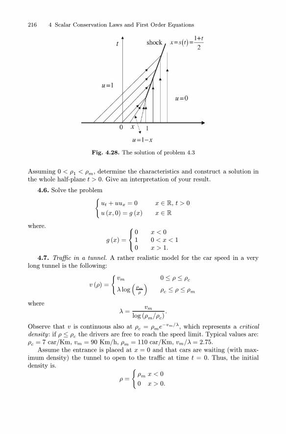
216 4 Scalar Conservation Laws and First Order Equations
Fig. 4.28. The solution of problem 4.3
Assuming 0 < ρ1 < ρm, determine the characteristics and construct a solution inthe whole half-plane t > 0. Give an interpretation of your result.
4.6. Solve the problem{ut + uux = 0 x ∈ R, t > 0u (x, 0) = g (x) x ∈ R
where.
g (x) =
⎧⎨⎩0 x < 01 0 < x < 10 x > 1.
4.7. Traffic in a tunnel. A rather realistic model for the car speed in a verylong tunnel is the following:
v (ρ) =
{vm 0 ≤ ρ ≤ ρcλ log
(ρmρ
)ρc ≤ ρ ≤ ρm
whereλ =
vmlog (ρm/ρc)
.
Observe that v is continuous also at ρc = ρme−vm/λ, which represents a critical
density : if ρ ≤ ρc the drivers are free to reach the speed limit. Typical values are:ρc = 7 car/Km, vm = 90 Km/h, ρm = 110 car/Km, vm/λ = 2.75.Assume the entrance is placed at x = 0 and that cars are waiting (with max-
imum density) the tunnel to open to the traffic at time t = 0. Thus, the initialdensity is.
ρ =
{ρm x < 0
0 x > 0.

Problems 217
a) Determine density and car speed; draw their graphs as a function of time.b) Determine and draw in the x, t plane the trajectory of a car initially at
x = x0 < 0, and compute the time it takes to enter the tunnel.
4.8. Consider the equation
ut + q′ (u)ux = 0
with initial condition u (x, 0) = g (x). Assume that g, q′ ∈ C1 ([a, b]) and g′q′′ < 0in [a, b] . Show that the family of characteristics
x = q′ (u) t+ ξ, ξ ∈ [a, b] (4.131)
admits an envelope and that the point (xs, ts) of shock formation, given by formulas(4.37) and (4.38), is the point on this envelope with minimum time coordinate(Fig. 4.29).
Fig. 4.29. Envelope of characteristics and point of shock formation
4.9. Find the solutions of the problems{ut ± uux = 0 t > 0, x ∈ Ru (x, 0) = x x ∈ R.
4.10. Draw the characteristics and describe the evolution for t → +∞ of thesolution of the problem
⎧⎨⎩ut + uux = 0 t > 0, x ∈ R
u (x, 0) =
{sinx0
0 < x < πx ≤ 0 or x ≥ π
4.11. Show that, for every α > 1, the function
uα (x, t) =
⎧⎪⎪⎨⎪⎪⎩
−1 2x < (1− α) t−α (1− α) t < 2x < 0α 0 < 2x < (α− 1) t1 (α− 1) t < 2x

218 4 Scalar Conservation Laws and First Order Equations
is a weak solution of the problem
⎧⎨⎩ut + uux = 0 t > 0, x ∈ R
u (x, 0) =
{−11
x < 0x > 0.
Is it also an entropy solution, at least for some α?
4.12. Using the Hopf-Cole transformation, solve the following problem for theviscous Burger equation
{ut + uux = εuxx t > 0, x ∈ Ru (0, x) = H (x) x ∈ R.
where H is the Heaviside function.Show that, as t→ +∞, u (x, t) converges to a travelling wave similar to (4.68).
[Answer. The solution is
u (x, t) =1
1 +erfc
(−x/
√4εt)
erfc((x− t)/
√4εt) exp
(x− t/22ε
)
where
erfc (s) =
∫ +∞s
exp(−z2
)dz
is the complementary error function].
4.13. Find the solution of the linear equation
ux + xuy = y
satisfying the initial condition u (0, y) = g (y), y ∈ R, with
(a) g (y) = cos y and (b) g (y) = y2.
[Answer of (a):
u = xy − x3
3+ cos
(y − x
2
2
)].
4.14. Consider the linear equation
aux + buy = c (x, y) ,
where a, b are constants (b �= 0), and the initial condition u (x, 0) = h (x).1) Show that
u (x, y) = h (x− γy) +∫ y/b
0
c (aτ + x− γy, bτ ) dτ γ = a/b.

Problems 219
2) Deduce that a jump discontinuity at x0 of h, propagates into a jump of thesame size for u along the characteristic of equation x− γy = x0.4.15. Let D =
{(x, y) : y > x2
}and a = a (x, y) be a continuous function in
D.
1) Check the solvability of the problem{a (x, y)ux − uy = −u (x, y) ∈ Du(x, x2
)= g (x) x ∈ R.
2) Examine the case
a (x, y) = y/2 and g (x) = exp(−γx2
),
where γ is a real parameter.
4.16. Solve the Cauchy problem{xux − yuy = u− y x > 0, y > 0
u(y2, y
)= y y > 0.
May a solution exist in a neighborhood of the origin?
[Answer.
u (x, y) =(y + x2/3y−1/3
)/2.
In no neighborhood of (0, 0) a solution can exist].
4.17. Consider a cylindrical pipe with axis along the x−axis, filled with afluid moving along the positive direction. Let ρ = ρ (x, t) and q = 1
2ρ2 be the
fluid density and the flux function. Assume the walls of the pipe are composed byporous material, from which the fluid leaks at the rate H = kρ2.a) Following the derivation of the conservation law given in the introduction,
show that ρ satisfies the equation.
ρt + ρρx = −kρ2
b) Solve the Cauchy problem with ρ (x, 0) = 1.
[Answer. b) ρ (x, t) = 1/ (1 + kt)].
4.18. Solve the Cauchy problem{ux = −(uy)2 x > 0, y ∈ Ru (0, y) = 3y y ∈ R. ,
4.19. Solve the Cauchy problem{u2x + u
2y = 4u
u (x,−1) = x2 x ∈ R.
[Answer : u (x, y) = x2 + (y + 1)2]

220 4 Scalar Conservation Laws and First Order Equations
4.20. Solve the Cauchy problem
{c2(u2x + u
2y
)= 1
u (cos s, sin s) = 0 s ∈ R.
[Answer : There are two solutions
u± (x, y) =±1c
{1−
√x2 + y2
}
whose wave fronts are shown in figure 4.30].
Fig. 4.30. Solutions of problem 4.20

5
Waves and Vibrations
General Concepts – Transversal Waves in a String – The One-dimensional Wave Equa-
tion – The d’Alembert Formula – Second Order Linear Equations – Hyperbolic Systems
With Constant Coefficients – The Multi-dimensional Wave Equation (n > 1) – Two Clas-
sical Models – The Cauchy Problem – Linear Water Waves
5.1 General Concepts
5.1.1 Types of waves
Our dayly experience deals with sound waves, electromagnetic waves (as radio orlight waves), deep or surface water waves, elastic waves in solid materials. Oscil-latory phenomena manifest themselves also in contexts and ways less macroscopicand known. This is the case, for instance, of rarefaction and shock waves in trafficdynamics or of electrochemical waves in human nervous system and in the regula-tion of the heart beat. In quantum physics, everything can be described in termsof wave functions, at a sufficiently small scale.Although the above phenomena share many similarities, they show several dif-
ferences as well. For example, progressive water waves propagate a disturbance,while standing waves do not. Sound waves need a supporting medium, while elec-tromagnetic waves do not. Electrochemical waves interact with the supportingmedium, in general modifying it, while water waves do not.Thus, it seems too hard to give a general definition of wave, capable of covering
all the above cases, so that we limit ourselves to introducing some terminology andgeneral concepts, related to specific types of waves. We start with one-dimensionalwaves.
a. Progressive or travelling waves are disturbances described by a functionof the following form:
u (x, t) = g (x− ct) .For t = 0, we have u (x, 0) = g (x), which is the “initial”profile of the perturbation.This profile propagates without change of shape with speed |c|, in the positive
Salsa S. Partial Differential Equations in Action: From Modelling to Theoryc© Springer-Verlag 2008, Milan

222 5 Waves and Vibrations
(negative) x−direction if c > 0 (c < 0). We have already met this kind of waves inChapters 2 and 4.
b. Harmonic waves are particular progressive waves of the form
u (x, t) = A exp {i (kx− ωt)} , A, k, ω ∈ R. (5.1)
It is understood that only the real part (or the imaginary part)
A cos (kx− ωt)
is of interest, but the complex notation may often simplify the computations. In(5.1) we distinguish, considering for simplicity ω and k positive:
• The wave amplitude |A|;
• The wave number k, which is the number of complete oscillations in the spaceinterval [0, 2π], and the wavelength
λ =2π
k
which is the distance between successive maxima (crest) or minima (troughs)of the waveform;
• The angular frequency ω, and the frequency
f =ω
2π
which is the number of complete oscillations in one second (Hertz) at a fixedspace position;
• The wave or phase speed
cp =ω
k
which is the crests (or troughs) speed;
Fig. 5.1. Sinusoidal wave

5.1 General Concepts 223
c. Standing waves are of the form
u (x, t) = B cos kx cosωt.
In these disturbances, the basic sinusoidal wave, cos kx, is modulated by the timedependent oscillationB cosωt. A standing wave may be generated, for instance, bysuperposing two harmonic waves with the same amplitude, propagating in oppositedirections:
A cos(kx− ωt) + A cos(kx+ ωt) = 2A cos kx cosωt. (5.2)
Consider now waves in dimension n > 1.
d. Plane waves. Scalar plane waves are of the form
u (x,t) = f (k · x−ωt) .
The disturbance propagates in the direction of k with speed cp = ω/ |k|. Theplanes of equation
θ (x,t) = k · x−ωt = constantconstitute the wave-fronts.Harmonic or monochromatic plane waves have the form
u (x, t) = A exp {i (k · x−ωt)} .
Here k is the wave number vector and ω is the angular frequency. The vector kis orthogonal to the wave front and |k| /2π gives the number of waves per unitlength. The scalar ω/2π still gives the number of complete oscillations in onesecond (Hertz) at a fixed space position.
e. Spherical waves are of the form
u (x,t) = v (r, t)
where r = |x− x0| and x0 ∈ Rn is a fixed point. In particular u (x,t) = eiωtv (r)represents a stationary spherical wave, while u (x,t) = v (r − ct) is a progressivewave whose wavefronts are the spheres r − ct = constant, moving with speed |c|(outgoing if c > 0, incoming if c < 0).
5.1.2 Group velocity and dispersion relation
Many oscillatory phenomena can be modelled by linear equations whose solutionsare superpositions of harmonic waves with angular frequency depending on thewave number:
ω = ω (k) . (5.3)
A typical example is the wave system produced by dropping a stone in a pond.If ω is linear, e.g. ω (k) = ck, c > 0, the crests move with speed c, independent
of the wave number. However, if ω (k) is not proportional to k, the crests move with

224 5 Waves and Vibrations
speed cp = ω (k) /k, that depends on the wave number. In other words, the crestsmove at different speeds for different wavelengths. As a consequence, the variouscomponents in a wave packet given by the superposition of harmonic waves ofdifferent wavelengths will eventually separate or disperse. For this reason, (5.3) iscalled dispersion relation.In the theory of dispersive waves, the group velocity, given by
cg = ω′ (k)
is a central notion, mainly for the following three reasons.
1. It is the speed at which an isolated wave packet moves as a whole. A wavepacket may be obtained by the superposition of dispersive harmonic waves, forinstance through a Fourier integral of the form
u (x, t) =
∫ +∞−∞
a (k) ei[kx−ω(k)t]dk (5.4)
where the real part only has a physical meaning. Consider a localized wave packet,with wave number k ≈ k0, almost constant, and with amplitude slowly varyingwith x. Then, the packet contains a large number of crests and the amplitudes|a (k)| of the various Fourier components are negligible except that in a smallneighborhood of k0, (k0 − δ, k0 + δ), say.Figure 5.2 shows the initial profile of a Gaussian packet,
Reu (x, 0) =3√2exp
{−x
2
32
}cos 14x,
slowly varying with x, with k0 = 14, and its Fourier transform:
a (k) = 6 exp{−8 (k − 14)2}.
As we can see, the amplitudes |a (k)| of the various Fourier components are negli-gible except when k is near k0.
Fig. 5.2. Wave packet and its Fourier transform
Then we may write
ω (k) ≈ ω (k0) + ω′ (k0) (k − k0) = ω (k0) + cg (k − k0)

5.1 General Concepts 225
and
u (x, t) ≈ ei{k0x−ω(k0)t}∫ k0+δ
k0−δa (k) ei(k−k0)(x−cgt)dk. (5.5)
Thus, u turns out to be well approximated by the product of two waves. The firstone is a pure harmonic wave with relatively short wavelength 2π/k0 and phasespeed ω (k0) /k0. The second one depends on x, t through the combination x− cgt,and is a superposition of waves of very small wavenumbers k−k0, which correspondto very large wavelengths. We may interpret the second factor as a sort of envelopeof the short waves of the packet, that is the packet as a whole, which thereforemoves with the group speed.
2. An observer that travels at the group velocity sees constantly waves of thesame wavelength 2π/k, after the transitory effects due to a localized initial per-turbation (e.g. a stone thrown into a pond). In other words, cg is the propagationspeed of the wave numbers.Imagine dropping a stone into a pond. At the beginning, the water pertur-
bation looks complicated, but after a sufficiently long time, the various Fouriercomponents will be quite dispersed and the perturbation will appear as a slowlymodulated wave train, almost sinusoidal near every point, with a local wave num-ber k (x, t) and a local frequency ω (x, t). If the water is deep enough, we expectthat, at each fixed time t, the wavelength increases with the distance from thestone (longer waves move faster, see subsection 5.10.4) and that, at each fixedpoint x, the wavelength tends to decrease with time.Thus, the essential features of the wave system can be observed at a relatively
long distance from the location of the initial disturbance and after some time haselapsed.Let us assume that the free surface displacement u is given by a Fourier integral
of the form (5.4). We are interested on the behavior of u for t � 1. An impor-tant tool comes from the method of stationary phase1 which gives an asymptoticformula for integrals of the form
I (t) =
∫ +∞−∞
f (k) eitϕ(k)dk (5.6)
as t→ +∞. We can put u into the form (5.6) by writing
u (x, t) =
∫ +∞−∞
a (k) eit[kxt −ω(k)]dk,
then by moving from the origin at a fixed speed V (thus x = V t) and defining
ϕ (k) = kV − ω (k) .
Assume for simplicity that ϕ has only one stationary point k0, that is
ω′ (k0) = V ,1 See subsection 5.10.6

226 5 Waves and Vibrations
and that ω′′ (k0) �= 0. Then, according to the method of stationary phase, we canwrite
u (V t, t) =
√π
|ω′′(k0)|a(k0)√texp {it [k0V − ω (k0)]}+O
(t−1). (5.7)
Thus, if we allow errors of order t−1, moving with speed V = ω′ (k0) = cg, thesame wave number k0 always appears at the position x = cgt. Note that theamplitude decreases like t−1/2 as t→ +∞. This is an important attenuation effectof dispersion.
3. Energy is transported at the group velocity by waves of wavelength 2π/k.In a wave packet like (5.5), the energy is proportional to2
∫ k0+δ
k0−δ|a (k)|2 dk � 2δ |a (k0)|2
so that it moves at the same speed of k0, that is cg.Since the energy travels at the group velocity, there are significant differences
in the wave system according to the sign of cg − cp, as we will see in Section 10.
5.2 Transversal Waves in a String
5.2.1 The model
We derive a classical model for the small transversal vibrations of a tightlystretched horizontal string (e.g. a string of a guitar). We assume the followinghypotheses:
1. Vibrations of the string have small amplitude. This entails that the changes inthe slope of the string from the horizontal equilibrium position are very small.
2. Each point of the string undergoes vertical displacements only. Horizontal dis-placements can be neglected, according to 1.
3. The vertical displacement of a point depends on time and on its position onthe string. If we denote by u the vertical displacement of a point located atx when the string is at rest, then we have u = u (x, t) and, according to 1,|ux (x, t)| � 1.
4. The string is perfectly flexible. This means that it offers no resistance to bend-ing. In particular, the stress at any point on the string can be modelled bya tangential3 force T of magnitude τ , called tension. Figure 5.3 shows howthe forces due to the tension acts at the end points of a small segment of thestring.
5. Friction is negligible.
Under the above assumptions, the equation of motion of the string can bederived from conservation of mass and Newton law.
2 See A. Segel, 1987.3 Consequence of absence of distributed moments along the string.

5.2 Transversal Waves in a String 227
Fig. 5.3. Tension at the end points of a small segment of a string
Let ρ0 = ρ0 (x) be the linear density of the string at rest and ρ = ρ (x, t) be itsdensity at time t. Consider an arbitrary part of the string between x and x+Δxand denote by Δs the corresponding length element at time t. Then, conservationof mass yields
ρ0 (x)Δx = ρ (x, t)Δs. (5.8)
To write Newton law of motion we have to determine the forces acting on our smallpiece of string. Since the motion is vertical, the horizontal forces have to balance.On the other hand they come from the tension only, so that if τ (x, t) denotes themagnitude of the tension at x at time t, we can write (Fig. 5.3):
τ (x+Δx, t) cosα (x+Δx, t)− τ (x, t) cosα (x, t) = 0.
Dividing by Δx and letting Δx→ 0, we obtain
∂
∂x[τ (x, t) cosα (x, t)] = 0
from whichτ (x, t) cosα (x, t) = τ0 (t) (5.9)
where τ0 (t) is positive4.
The vertical forces are given by the vertical component of the tension and bybody forces such as gravity and external loads.Using (5.9), the scalar vertical component of the tension at x, at time t, is given
by:
τvert (x, t) = τ (x, t) sinα (x, t) = τ0 (t) tanα(x, t) = τ0 (t) ux (x, t) .
4 It is the magnitude of a force.

228 5 Waves and Vibrations
Therefore, the (scalar) vertical component of the force acting on our small pieceof string, due to the tension, is
τvert (x+Δx, t)− τvert (x, t) = τ0 (t) [ux (x+Δx, t)− ux (x, t)].
Denote by f (x, t) the magnitude of the (vertical) body forces per unit mass. Then,using (5.8), the magnitude of the body forces acting on the string segment is givenby: ∫ x+Δx
x
ρ (y, t) f (y, t) ds =
∫ x+Δx
x
ρ0 (y) f (y, t) dy.
Thus, using (5.8) again and observing that utt is the (scalar) vertical acceleration,Newton law gives:
∫ x+Δx
x
ρ0 (y) utt (y, t) dy = τ0 (t) [ux (x+Δx, t)−ux (x, t)]+∫ x+Δx
x
ρ0 (y) f (y, t) dy.
Dividing by Δx and letting Δx→ 0, we obtain the equation
utt − c2 (x, t)uxx = f (x, t) (5.10)
where c2 (x, t) = τ0 (t) /ρ0 (x).
If the string is homogeneous then ρ0 is constant. If moreover it is perfectlyelastic5 then τ0 is constant as well, since the horizontal tension is nearly the sameas for the string at rest, in the horizontal position. We shall come back to equation(5.10) shortly.
5.2.2 Energy
Suppose that a perfectly flexible and elastic string has length L at rest, in thehorizontal position. We may identify its initial position with the segment [0, L] onthe x axis. Since ut(x, t) is the vertical velocity of the point at x, the expression
Ecin (t) =1
2
∫ L
0
ρ0u2t dx (5.11)
represents the total kinetic energy during the vibrations. The string storespotential energy too, due to the work of elastic forces. These forces stretch anelement of string of length Δx at rest by6
Δs−Δx =∫ x+Δx
x
√1 + u2x dx−Δx =
∫ x+Δx
x
(√1 + u2x − 1
)dx ≈ 1
2u2xΔx
5 For instance, guitar and violin strings are nearly homogeneous, perfectly flexible andelastic.
6 Recall that, at first order, if ε� 1, √1 + ε − 1 � ε/2.
5.3 The One-dimensional Wave Equation 229
since |ux| � 1. Thus, the work done by the elastic forces on that string element is
dW =1
2τ0u
2xΔx.
Summing all the contributions, the total potential energy is given by:
Epot (t) =1
2
∫ L
0
τ0u2x dx. (5.12)
From (5.11) and (5.12) we find, for the total energy:
E (t) =1
2
∫ L
0
[ρ0u2t + τ0u
2x] dx. (5.13)
Let us compute the variation of E. Taking the time derivative under the integral,we find (remember that ρ0 = ρ0 (x) and τ0 is constant),
E (t) =
∫ L
0
[ρ0ututt + τ0uxuxt]dx.
By an integration by parts we get
∫ L
0
τ0uxuxt dx = τ0[ux (L, t)ut (L, t)− ux (0, t)ut (0, t)]− τ0∫ L
0
utuxxdx
whence
E (t) =
∫ L
0
[ρ0utt − τ0uxx]utdx+ τ0[ux (L, t)ut (L, t)− ux (0, t)ut (0, t)].
Using (5.10), we find:
E (t) =
∫ L
0
ρ0fut dx+ τ0[ux (L, t)ut (L, t)− ux (0, t)ut (0, t)]. (5.14)
In particular, if f = 0 and u is constant at the end points 0 and L (thereforeut (L, t) = ut (0, t) = 0) we deduce E (t) = 0. This implies
E (t) = E (0)
which expresses the conservation of energy.
5.3 The One-dimensional Wave Equation
5.3.1 Initial and boundary conditions
Equation (5.10) is called the one-dimensional wave equation. The coefficient c hasthe dimensions of a speed and in fact, we will shortly see that it represents the wave

230 5 Waves and Vibrations
propagation speed along the string. When f ≡ 0, the equation is homogeneous andthe superposition principle holds: if u1 and u2 are solutions of
utt − c2uxx = 0 (5.15)
and a, b are (real or complex) scalars, then au1 + bu2 is a solution as well. Moregenerally, if uk (x,t) is a family of solutions depending on the parameter k (integeror real) and g = g (k) is a function rapidly vanishing at infinity, then
∞∑k=1
uk (x,t) g (k) and
∫ +∞−∞
uk (x,t) g (k) dk
are still solutions of (5.15).Suppose we are considering the space-time region 0 < x < L, 0 < t < T . In
a well posed problem for the (one-dimensional) heat equation it is appropriate toassign the initial profile of the temperature, because of the presence of a first ordertime derivative, and a boundary condition at both ends x = 0 and x = L, becauseof the second order space derivative.By analogy with the Cauchy problem for second order ordinary differential
equations, the second order time derivative in (5.10) suggests that not only theinitial profile of the string but the initial velocity has to be assigned as well.Thus, our initial (or Cauchy) data are
u (x, 0) = g (x) , ut (x, 0) = h (x) , x ∈ [0, L] .The boundary data are formally similar to those for the heat equation. Typi-
cally:
Dirichlet data describe the displacement of the end points of the string:
u (0, t) = a (t) , u (L, t) = b (t) , t > 0.
If a (t) = b (t) ≡ 0 (homogeneous data), both ends are fixed, with zero displace-ment.
Neumann data describe the applied (scalar) vertical tension at the end points.As in the derivation of the wave equation, we may model this tension by τ0ux sothat the Neumann conditions take the form
τ0ux (0, t) = a (t) , τ0ux (L, t) = b (t) , t > 0.
In the special case of homogeneous data, a (t) = b (t) ≡ 0, both ends of the stringare attached to a frictionless sleeve and are free to move vertically.
Robin data describe a linear elastic attachment at the end points. One way torealize this type of boundary condition is to attach an end point to a linear spring7
whose other end is fixed. This translates into assigning
τ0ux (0, t) = ku (0, t) , τ0ux (L, t) = −ku (L, t) , t > 0,
where k (positive) is the elastic constant of the spring.
7 Which obeys Hooke’s law: the strain is a linear function of the stress.
5.3 The One-dimensional Wave Equation 231
In several concrete situations, mixed conditions have to be assigned. For in-stance, Robin data at x = 0 and Dirichlet data at x = L.
Global Cauchy problem. We may think of a string of infinite length and assignonly the initial data
u (x, 0) = g (x) , ut (x, 0) = h (x) , x ∈ R.
Although physically unrealistic, it turns out that the solution of the global Cauchyproblem is of fundamental importance. We shall solve it in Section 5.4.Under reasonable assumptions on the data, the above problems are well posed.
In the next section we use separation of variables to show it for a Cauchy-Dirichletproblem.
Remark 5.1. Other kinds of problems for the wave equation are the so called Gour-sat problem and the characteristic Cauchy problem. Some examples are given inProblems 5.9, 5.10.
5.3.2 Separation of variables
Suppose that the vibration of a violin chord is modelled by the following Cauchy-Dirichlet problem
⎧⎨⎩utt − c2uxx = 0 0 < x < L, t > 0u (0, t) = u (L, t) = 0 t ≥ 0u (x, 0) = g (x) , ut (x, 0) = h (x) 0 ≤ x ≤ L
(5.16)
where c2 = τ0/ρ0 is constant.We want to check whether this problem is well posed, that is, whether a solution
exists, is unique and it is stable (i.e. it depends “continuously” on the data g andh). For the time being we proceed formally, without worrying too much about thecorrect hypotheses on g and h and the regularity of u.
• Existence. Since the boundary conditions are homogeneous8, we try to con-struct a solution using separation of variables.Step 1. We start looking for solutions of the form
U (x, t) = w (t) v (x)
with v (0) = v (L) = 0. Inserting U into the wave equation we find
0 = Utt − c2Uxx = w′′ (t) v (x) − c2w (t) v′′ (x)
or, separating the variables,
1
c2w′′ (t)w (t)
=v′′ (x)v (x)
. (5.17)
8 Remember that this is essential for using separation of variables.

232 5 Waves and Vibrations
We have reached a familiar situation: (5.17) is an identity between two functions,one depending on t only and the other one depending on x only. Therefore the twosides of (5.17) must be both equal to the same constant, say λ. Thus, we are leadto the equation
w′′ (t)− λc2w (t) = 0 (5.18)
and to the eigenvalue problem
v′′ (x)− λv (x) = 0 (5.19)
v (0) = v (L) = 0. (5.20)
Step 2. Solution of the eigenvalue problem. There are three possibilities for thegeneral integral of (5.19).
a) If λ = 0, then v (x) = A+ Bx and (5.20) imply A = B = 0.
b) If λ = μ2 > 0, then v (x) = Ae−μx+Beμx and again (5.20) implyA = B = 0.c) If λ = −μ2 < 0, then v (x) = A sinμx+B cosμx. From (5.20) we get
v (0) = B = 0
v (1) = A sinμL +B cosμL = 0
whence
A arbitrary, B = 0, μL = mπ, m = 1, 2, ... .
Thus, in case c) only we find non trivial solutions, of the form
vm (x) = Am sinμmx, μm =mπ
L. (5.21)
Step 3. Insert λ = −μ2m = −m2π2/L2 into (5.18). Then, the general solutionis
wm (t) = Cm cos (μmct) +Dm sin (μmct) . (5.22)
From (5.21) and (5.22) we construct the family of solutions
Um (x, t) = [am cos (μmct) + bm sin(μmct)] sinμmx, m = 1, 2, ...
where am and bm are arbitrary constants.Um is called the m
th−normal mode of vibration or mth − harmonic, andis a standing wave with frequency m/2L. The first harmonic and its frequency1/2L, the lowest possible, are said to be fundamental. All the other frequenciesare integral multiples of the fundamental one. Because of this reason it seems thata violin chord produces good quality tones, pleasant to the ear (this is not so, forinstance, for a vibrating membrane like a drum, as we will see shortly).
Step 4. If the initial conditions are
u (x, 0) = am sinμmx ut (x, 0) = cbmμm sinμmx
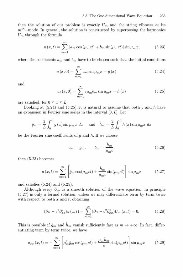
5.3 The One-dimensional Wave Equation 233
then the solution of our problem is exactly Um and the string vibrates at itsmth−mode. In general, the solution is constructed by superposing the harmonicsUm through the formula
u (x, t) =
∞∑m=1
[am cos (μmct) + bm sin(μmct)] sinμmx, (5.23)
where the coefficients am and bm have to be chosen such that the initial conditions
u (x, 0) =
∞∑m=1
am sinμmx = g (x) (5.24)
and
ut (x, 0) =
∞∑m=1
cμmbm sinμmx = h (x) (5.25)
are satisfied, for 0 ≤ x ≤ L.Looking at (5.24) and (5.25), it is natural to assume that both g and h have
an expansion in Fourier sine series in the interval [0, L]. Let
gm =2
L
∫ L
0
g (x) sinμmx dx and hm =2
L
∫ L
0
h (x) sinμmx dx
be the Fourier sine coefficients of g and h. If we choose
am = gm, bm =hm
μmc, (5.26)
then (5.23) becomes
u (x, t) =
∞∑m=1
[gm cos(μmct) +
hmμmc
sin(μmct)
]sinμmx (5.27)
and satisfies (5.24) and (5.25).Although every Um is a smooth solution of the wave equation, in principle
(5.27) is only a formal solution, unless we may differentiate term by term twicewith respect to both x and t, obtaining
(∂tt − c2∂2xx)u (x, t) =∞∑m=1
(∂tt − c2∂2xx)Um (x, t) = 0. (5.28)
This is possible if gm and hm vanish sufficiently fast as m → +∞. In fact, differ-entiating term by term twice, we have
uxx (x, t) = −∞∑m=1
[μ2mgm cos(μmct) +
μmhmcsin(μmct)
]sinμmx (5.29)

234 5 Waves and Vibrations
and
utt (x, t) = −∞∑m=1
[μ2mgmc
2 cos(μmct) + μmhmc sin(μmct)]sinμmx. (5.30)
Thus, if, for instance,
|gm| ≤C
m4and
∣∣∣hm∣∣∣ ≤ C
m3, (5.31)
then
∣∣μ2mgm cos(μmct)∣∣ ≤ Cπ2
L2m2, and
∣∣∣μmhmc sin(μmct)∣∣∣ ≤ cC
Lm2
so that, by the Weierstrass test, the series in (5.29), (5.30) converge uniformlyin [0, L] × [0,+∞). Since also the series (5.27) is clearly uniformly convergent in[0, L]× [0,+∞), differentiation term by term is allowed and u is a C2 solution ofthe wave equation.Under which assumptions on g and h do the (5.31) hold?Let g ∈ C4 ([0, L]), h ∈ C3 ([0, L]) and assume the following compatibility
conditions:
g (0) = g (L) = g′′ (0) = g′′ (L) = 0h (0) = h (L) = 0.
Then (5.31) hold9.Moreover, under the same assumptions, it is not difficult to check that
u (y, t)→ g (x) , ut (y, t)→ h (x) , as (y, t)→ (x, 0) (5.32)
for every x ∈ [0, L] and we conclude that u is a smooth solution of (5.16).• Uniqueness. To show that (5.27) is the unique solution of problem (5.16), we
use conservation of energy. Let u and v be solutions of (5.16). Then w = u− v isa solution of the same problem with zero initial and boundary data. We want toshow that w ≡ 0.Formula (5.13) gives, for the total mechanical energy,
E (t) = Ecin (t) +Epot (t) =1
2
∫ L
0
[ρ0w2t + τ0w
2x] dx
9 It is an exercise on integration by parts. For instance, if f ∈ C4 ([0,L]) and f (0) =f (L) = f ′′ (0) = f ′′ (L) = 0, then, integrating by parts four times, we have
fm =
∫ L
0
f (x) sin(mπL
)dx =
1
m4
∫ L
0
f (4) (x) sin(mπL
)dx
and ∣∣∣fm∣∣∣ ≤ max
∣∣∣f (4)
∣∣∣L
m4.

5.3 The One-dimensional Wave Equation 235
and in our case we haveE (t) = 0
since f = 0 and wt (L, t) = wt (0, t) = 0, whence
E (t) = E (0)
for every t ≥ 0. Since, in particular, wt (x, 0) = wx (x, 0) = 0, we haveE (t) = E (0) = 0
for every t ≥ 0. On the other hand, Ecin (t) ≥ 0, Epot (t) ≥ 0, so that we deduceEcin (t) = 0, Epot (t) = 0
which force wt = wx = 0. Therefore w is constant and since w (x, 0) = 0, weconclude that w (x, t) = 0 for every t ≥ 0.• Stability. We want to show that if the data are slightly perturbed, the cor-
responding solutions change only a little. Clearly, we need to establish how weintend to measure the distance for the data and for the corresponding solutions.For the initial data, we use the least square distance, given by10
‖g1 − g2‖0 =(∫ L
0
|g1 (x)− g2 (x)|2 dx)1/2
.
For functions depending also on time, we define
‖u− v‖0,∞ = supt>0
(∫ L
0
|u (x, t)− v (x, t)|2 dx)1/2
which measures the maximum in time of the least squares distance in space.Now, let u1 and u2 be solutions of problem (5.16) corresponding to the data
g1, h1 and g2, h2, respectively. Their difference w = u1− u2 is a solution of thesame problem with Cauchy data g = g1− g2 and h = h1− h2. From (5.27) weknow that
w (x, t) =
∞∑m=1
[gm cos(μmct) +
hmμmc
sin(μmct)
]sinμmx.
From Parseval’s identity11 and the elementary inequality (a+ b)2 ≤ 2(a2 + b2),
a, b ∈ R, we can write∫ L
0
|w (x, t)|2 dx = L2
∞∑m=1
[gm cos(μmct) +
hm
μmcsin(μmct)
]2
≤ L∞∑m=1
⎡⎣g2m +
(hmμmc
)2⎤⎦ .
10 The symbol ‖g‖ denotes a norm of g. See Chapter 6.11 Appendix A.

236 5 Waves and Vibrations
Since μm ≥ π/L, using Parseval’s equality again, we obtain∫ L
0
|w (x, t)|2 dx ≤ Lmax{1,
(L
πc
)2} ∞∑m=1
[g2m + h
2m
]
= 2max
{1,
(L
πc
)2}[‖g‖20 + ‖h‖
20
]
whence the stability estimate
‖u1 − u2‖20,∞ ≤ 2max{1,
(L
πc
)2}[‖g1 − g2‖20 + ‖h1 − h2‖
20
]. (5.33)
Thus, “close” data produce “close” solutions.
Remark 5.2. From (5.27), the chord vibration is given by the superposition of har-monics corresponding to the non-zero Fourier coefficients of the initial data. Thecomplex of such harmonics determines a particular feature of the emitted sound,known as the timbre, a sort of signature of the musical instrument!
Remark 5.3. The hypotheses we have made on g and h are unnaturally restrictive.For example, if we pluck a violin chord at a point, the initial profile is continuousbut has a corner at that point and cannot be even C1. A physically realisticassumption for the initial profile g is continuity.Similarly, if we are willing to model the vibration of a chord set into motion
by a strike of a little hammer, we should allow discontinuity in the initial velocity.Thus it is realistic to assume h bounded.Under these weak hypotheses the separation of variables method does not work.
On the other hand, we have already faced a similar situation in Chapter 4, wherethe necessity to admit discontinuous solutions of a conservation law has lead to amore general and flexible formulation of the initial value problem. Also for the waveequation it is possible to introduce suitable weak formulations of the various initial-boundary value problems, in order to include realistic initial data and solutionswith a low degree of regularity. A first attempt is shown in subsection 5.4.2. Aweak formulation more suitable for numerical methods is treated in Chapter 9.
5.4 The d’Alembert Formula
5.4.1 The homogeneous equation
In this section we establish the celebrated formula of d’Alembert for the solutionof the following global Cauchy problem:
{utt − c2uxx = 0 x ∈ R, t > 0u (x, 0) = g (x) , ut (x, 0) = h (x) x ∈ R. (5.34)

5.4 The d’Alembert Formula 237
To find the solution, we first factorize the wave equation in the following way:
(∂t − c∂x) (∂t + c∂x)u = 0. (5.35)
Now, letv = ut + cux. (5.36)
Then v solves the linear transport equation
vt − cvx = 0
whencev (x, t) = ψ (x+ ct)
where ψ is a differentiable arbitrary function. From (5.36) we have
ut + cux = ψ (x+ ct)
and formula (4.10) in subsection 4.2.2 yields
u (x, t) =
∫ t
0
ψ (x− c (t − s) + cs) ds+ ϕ (x− ct) ,
where ϕ is another arbitrary differentiable function.Letting x− ct+ 2cs = y, we find
u (x, t) =1
2c
∫ x+ct
x−ctψ (y) dy+ ϕ (x− ct) . (5.37)
To determine ψ and ϕ we impose the initial conditions:
u (x, 0) = ϕ (x) = g (x) (5.38)
andut (x, 0) = ψ (x)− cϕ′ (x) = h (x)
whenceψ (x) = h (x) + cg′ (x) . (5.39)
Inserting (5.39) and (5.38) into (5.37) we get:
u (x, t) =1
2c
∫ x+ct
x−ct[h (y) + cg′ (y)] dy + g (x− ct)
=1
2c
∫ x+ct
x−cth (y) dy +
1
2[g (x+ ct) − g (x− ct)] + g (x− ct)
and finally the d’Alembert formula
u (x, t) =1
2[g(x+ ct) + g (x− ct)] + 1
2c
∫ x+ct
x−cth (y) dy. (5.40)

238 5 Waves and Vibrations
If g ∈ C2(R) and h ∈ C1 (R), formula (5.40) defines a C2−solution in the half-plane R×[0,+∞). On the other hand, a C2−solution u in R×[0,+∞) has to begiven by (5.40), just because of the procedure we have used to solve the Cauchyproblem. Thus the solution is unique. Observe however, that no regularizing effecttakes place here: the solution u remains no more than C2 for any t > 0. Thus, thereis a striking difference with diffusion phenomena, governed by the heat equation.Furthermore, let u1 and u2 be the solutions corresponding to the data g1, h1
and g2, h2, respectively. Then, the d’Alembert formula for u1−u2 yields, for everyx ∈ R and t ∈ [0, T ],
|u1 (x, t)− u2 (x, t)| ≤ ‖g1 − g2‖∞ + T ‖h1 − h2‖∞where
‖g1 − g2‖∞ = supx∈R
|g1 (x)− g2 (x)| , ‖h1 − h2‖∞ = supx∈R
|h1 (x)− h2 (x)| .
Therefore, we have stability in pointwise uniform sense, at least for finite time.
Rearranging the terms in (5.40), we may write u in the form12
u (x, t) = F (x+ ct) +G (x− ct) (5.41)
which gives u as a superposition of two progressive waves moving at constant speedc in the negative and positive x−direction, respectively. Thus, these waves are notdispersive.The two terms in (5.41) are respectively constant along the two families of
straight lines γ+ and γ− given by
x+ ct = constant, x− ct = constant.
These lines are called characteristics13 and carry important information, as wewill see in the next subsection.An interesting consequence of (5.41) comes from looking at figure 5.4. Consider
the characteristic parallelogram with vertices at the point A,B, C,D. From (5.41)we have
F (A) = F (C) , G (A) = G (B)
F (D) = F (B) , G (D) = G (C) .
12 For instance:
F (x + ct) =1
2g (x+ ct) +
1
2c
∫ x+ct
0
h (y) dy
and
G (x − ct) = 12g (x− ct) + 1
2c
∫ 0
x−cth (y) dy.
13 In fact they are the characteristics for the two first order factors in the factorization(5.35).
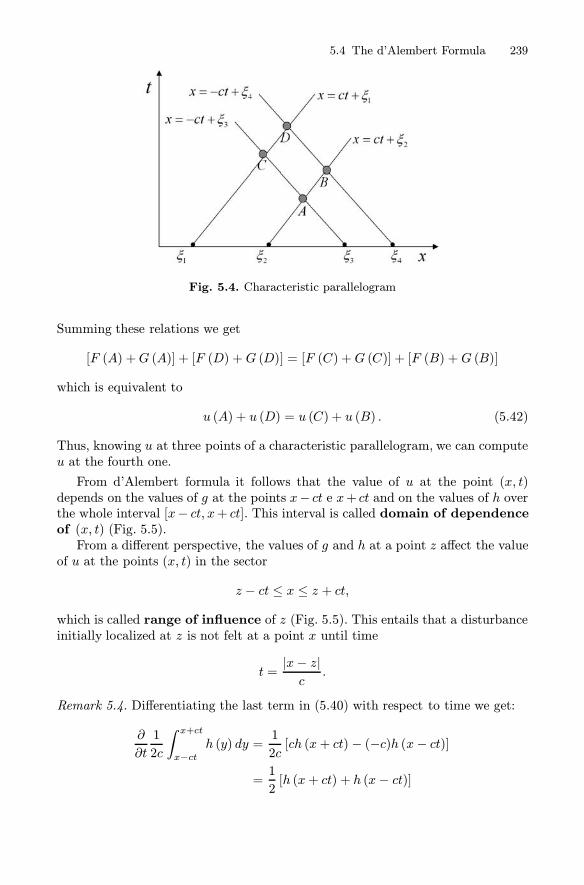
5.4 The d’Alembert Formula 239
Fig. 5.4. Characteristic parallelogram
Summing these relations we get
[F (A) +G (A)] + [F (D) +G (D)] = [F (C) +G (C)] + [F (B) +G (B)]
which is equivalent to
u (A) + u (D) = u (C) + u (B) . (5.42)
Thus, knowing u at three points of a characteristic parallelogram, we can computeu at the fourth one.
From d’Alembert formula it follows that the value of u at the point (x, t)depends on the values of g at the points x− ct e x+ ct and on the values of h overthe whole interval [x− ct, x+ ct]. This interval is called domain of dependenceof (x, t) (Fig. 5.5).From a different perspective, the values of g and h at a point z affect the value
of u at the points (x, t) in the sector
z − ct ≤ x ≤ z + ct,
which is called range of influence of z (Fig. 5.5). This entails that a disturbanceinitially localized at z is not felt at a point x until time
t =|x− z|c.
Remark 5.4. Differentiating the last term in (5.40) with respect to time we get:
∂
∂t
1
2c
∫ x+ct
x−cth (y) dy =
1
2c[ch (x+ ct) − (−c)h (x− ct)]
=1
2[h (x+ ct) + h (x− ct)]

240 5 Waves and Vibrations
Fig. 5.5. Domain of dependence and range of influence
which has the form of the first term with g replaced by h. It follows that if whdenotes the solution of the problem
{wtt − c2wxx = 0 x ∈ R, t > 0w (x, 0) = 0, wt (x, 0) = h (x) . x ∈ R (5.43)
then, d’Alembert formula can be written in the form
u (x, t) =∂
∂twg (x, t) +wh (x, t) . (5.44)
Actually, (5.44), can be established without reference to d’Alembert formula, aswe will see later.
5.4.2 Generalized solutions and propagation of singularities
In Remark 5.3 we have emphasized the necessity of a weak formulation to includephysically realistic data. On the other hand, observe that d’Alembert formulamakes perfect sense even for g continuous and h bounded. The question is inwhich sense the resulting function satisfies the wave equation, since, in principle,it is not even differentiable, only continuous. There are several ways to weaken thenotion of solution to include this case; here, for instance, we mimic what we didfor conservation laws.
Assuming for the moment that u is a smooth solution of the global Cauchyproblem, we multiply the wave equation by a C2−test function v, defined inR× [0,+∞) and compactly supported. Integrating over R× [0,+∞) we obtain
∫ ∞0
∫
R
[utt− c2uxx]v dxdt = 0.

5.4 The d’Alembert Formula 241
Fig. 5.6. Chord plucked at the origin (c = 1)
Now we integrate by parts both terms twice, to transfer all the derivatives from uto v. This yields, being v zero outside a compact subset of R× [0,+∞),
∫ ∞0
∫
R
c2uxxv dxdt =
∫ ∞0
∫
R
c2uvxx dxdt
and∫ ∞0
∫
R
uttv dxdt = −∫
R
ut (x, 0)v (x, 0)dx−∫ ∞0
∫
R
utvt dxdt
= −∫
R
[ut (x, 0)v (x, 0)− u (x, 0)vt (x, 0)]dx+∫ ∞0
∫
R
uvttdxdt.
Using the Cauchy data u (x, 0) = g (x) and ut (x, 0) = h (x), we arrive to theintegral equation
∫ ∞0
∫
R
u[vtt − c2vxx] dxdt−∫
R
[h (x) v (x, 0)− g (x) vt (x, 0)]dx = 0. (5.45)
Note that (5.45) makes perfect sense for u continuous, g continuous and h bounded,only. Conversely, if u is a C2 function that satisfies (5.45) for every test functionv, then it turns out14 that u is a solution of problem (5.34).Thus we may adopt the following definition.
Definition 5.1. Let g ∈ C (R) and h be bounded in R. We say that u ∈C (R × [0,+∞)) is a generalized solution of problem (5.34) if (5.45) holds forevery test function v.
If g is continuous and h is bounded, it can be shown that formula (5.41) con-stitutes precisely a generalized solution.
14 Check it.

242 5 Waves and Vibrations
Figure 5.6 shows the wave propagation along a chord of infinite length, pluckedat the origin and originally at rest, modelled by the solution of the problem
{utt − uxx = 0 x ∈ R, t > 0u (x, 0) = g (x) , ut (x, 0) = 0 x ∈ R
where g has a triangular profile. As we see, this generalized solution displays linesof discontinuities of the first derivatives, while outside these lines it is smooth.
We want to show that these lines are characteristics. More generally, considera region G ⊂ R× (0,+∞), divided into two domainsG(1) e G(2) by a smooth curveΓ of equation x = s (t), as in figure 5.7. Let
ν = ν1i+ν2j =1√
1 + (s (t))2(−i + s (t) j) (5.46)
be the unit normal to Γ , pointing inward to G(1).
Given any function f defined in G, we denote by
f(1) and f(2)
its restriction to the closure of G(1) and G(2), respectively, and we use the symbol
[f (s (t) , t)] = f(1) (s (t) , t)− f(2) (s (t) , t) .
for the jump of f across Γ , or simply [f ] when there is no risk of confusion.
Now, let u be a generalized solution of our Cauchy problem, of class C2 both inthe closure15 of G(1) and G(2), whose first derivatives undergo a jump discontinuityon Γ . We want to prove that:
Proposition 5.1. Γ is a characteristic.
Proof. First of all observe that, from our hypotheses, we have [u] = 0 and[ux] , [ut] �= 0. Moreover, the jumps [ux] and [ut] are continuous along Γ .By analogy with conservation laws, we expect that the integral formulation
(5.45) should imply a sort of Rankine-Hugoniot condition, relating the jumps ofthe derivatives with the slope of Γ and expressing the balance of linear momentumacross Γ .
In fact, let v be a test function with compact support in G. Inserting v into(5.45), we can write
0 =
∫
G
(c2uvxx − uvtt
)dxdt =
∫
G(2)(...)dxdt+
∫
G(1)(...) dxdt. (5.47)
15 That is, the first and second derivatives of u extend continuously up to Γ , from bothsides, separately.
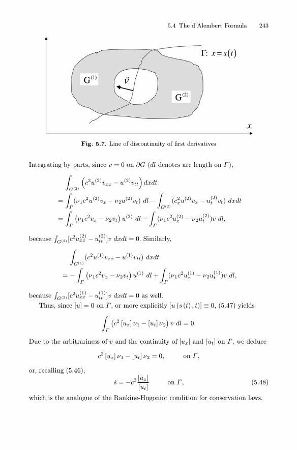
5.4 The d’Alembert Formula 243
Fig. 5.7. Line of discontinuity of first derivatives
Integrating by parts, since v = 0 on ∂G (dl denotes arc length on Γ ),
∫
G(2)
(c2u(2)vxx − u(2)vtt
)dxdt
=
∫
Γ
(ν1c2u(2)vx − ν2u(2)vt) dl−
∫
G(2)(c2xu
(2)vx − u(2)t vt) dxdt
=
∫
Γ
(ν1c
2vx − ν2vt)u(2) dl−
∫
Γ
(ν1c2u(2)x − ν2u(2)t )v dl,
because∫G(2)[c2u
(2)xx − u(2)tt ]v dxdt = 0. Similarly,
∫
G(1)(c2u(1)vxx − u(1)vtt) dxdt
= −∫
Γ
(ν1c
2vx − ν2vt)u(1) dl+
∫
Γ
(ν1c2u(1)x − ν2u(1)t )v dl,
because∫G(2) [c
2u(1)xx − u(1)tt ]v dxdt = 0 as well.
Thus, since [u] = 0 on Γ , or more explicitly [u (s (t) , t)] ≡ 0, (5.47) yields∫
Γ
(c2 [ux] ν1 − [ut] ν2
)v dl = 0.
Due to the arbitrariness of v and the continuity of [ux] and [ut] on Γ , we deduce
c2 [ux] ν1 − [ut] ν2 = 0, on Γ ,
or, recalling (5.46),
s = −c2 [ux][ut]
on Γ , (5.48)
which is the analogue of the Rankine-Hugoniot condition for conservation laws.

244 5 Waves and Vibrations
On the other hand, differentiating [u (s (t) , t)] ≡ 0 we obtaind
dt[u (s (t) , t)] = [ux (s (t) , t)]s (t) + [ut (s (t) , t)] ≡ 0
or
s = − [ut][ux]
on Γ . (5.49)
Equations (5.48) and (5.49) entail
s (t) = ±cwhich yields
s (t) = ±ct+ constantshowing that Γ is a characteristic. �
5.4.3 The fundamental solution
It is rather instructive to solve the global Cauchy problem with g ≡ 0 and a specialh: the Dirac delta at a point ξ, that is h (x) = δ(x− ξ). For instance, this modelsthe vibrations of a violin string generated by a unit impulse localized at ξ (a strikeof a sharp hammer). The corresponding solution is called fundamental solutionand plays the same role of the fundamental solution for the diffusion equation.Certainly, the Dirac delta is a quite unusual data, out of reach of the theory
we have developed so far. Therefore, we proceed formally.Thus, letK = K (x, ξ, t) denote our fundamental solution and apply d’Alembert
formula; we find
K (x, ξ, t) =1
2c
∫ x+ct
x−ctδ (y − ξ) dy (5.50)
which at first glance looks like a mathematical UFO.To get a more explicit formula, we first compute
∫ x−∞ δ (y) dy. To do it, recall
that (subsection 2.3.3), if H is the Heaviside function and
Iε (y) =H (y + ε) −H (y − ε)
2ε=
{ 12ε − ε ≤ y < ε
0 everywhere else(5.51)
is the unit impulse of extent ε, then limε↓0 Iε (y) = δ (y). Then it seems appropriateto compute
∫ x−∞ δ (y) dy by means of the formula
∫ x
−∞δ (y) dy = lim
ε↓0
∫ x
−∞Iε (y) dy.
Now, we have:
∫ x
−∞Iε (y) dy =
⎧⎪⎪⎨⎪⎪⎩
0 x ≤ −ε(x+ ε) /2ε − ε < x < ε1 x ≥ ε.

5.4 The d’Alembert Formula 245
Letting ε → 0 we deduce that (the value at zero is irrelevant)∫ x
−∞δ (y) dy = H (x) , (5.52)
which actually is not surprising, if we remember that H′ = δ. Everything worksnicely.Let us go back to our mathematical UFO, by now ... identified; we write
∫ x+ct
x−ctδ (y − ξ) dy = lim
ε↓0
∫ x+ct
−∞Iε (y − ξ) dy − lim
ε↓0
∫ x−ct
−∞Iε (y − ξ) dy.
Then, using (5.50), (5.51) and (5.52), we conclude:
K (x, ξ, t) =1
2c{H (x− ξ + ct) −H (x− ξ − ct)} . (5.53)
Figure 5.8 shows the graph of K (x, ξ, t), with c = 1
Fig. 5.8. The fundamental solution K (x, ξ, t)
Note how the initial discontinuity at x = ξ propagates along the characteristics
x = ξ ± t.
We have found the fundamental solution (5.53) through d’Alembert formula.Conversely, using the fundamental solution we may derive d’Alembert formula.

246 5 Waves and Vibrations
Namely, consider the solution wh of the Cauchy problem (5.43), that is with data(see Remark 5.4)
w (x, 0) = 0, wt (x, 0) = h (x) , x ∈ R.
We may write
h (x) =
∫ +∞−∞
δ (x− ξ)h (ξ) dξ
looking at h (x) as a superposition of impulses δ (x− ξ)h (ξ), concentrated at ξ.Then, we may construct wh by superposing the solutions of the same problem withdata δ (x− ξ)h (ξ) instead of h. But these solutions are given by
K (x, ξ, t)h (ξ)
and therefore we obtain
wh (x, t) =
∫ +∞−∞
K (x, ξ, t)h (ξ) dξ.
More explicitly, from (5.53):
wh (x, t) =1
2c
∫ +∞−∞
{H (x− ξ + ct)−H (x− ξ − ct)} h (ξ) dξ
=1
2c
∫ x+ct
−∞h (ξ) dξ − 1
2c
∫ x−ct
−∞h (ξ) dξ
=1
2c
∫ x+ct
x−cth (y) dy.
At this point, (5.44) yields d’Alembert formula.We shall use this method to construct the solution of the global Cauchy problem
in dimension 3.
5.4.4 Non homogeneous equation. Duhamel’s method
To solve the nonhomogeneous problem
{utt − c2uxx = f (x, t) x ∈ R, t > 0u (x, 0) = 0, ut (x, 0) = 0 x ∈ R. (5.54)
we use the Duhamel’s method (see subsection 2.2.8). For s ≥ 0 fixed, let w =w (x, t; s) be the solution of problem
{wtt − c2wxx = 0 x ∈ R, t ≥ sw (x, s; s) = 0, wt (x, s; s) = f (x, s) x ∈ R. (5.55)

5.4 The d’Alembert Formula 247
Since the wave equation is invariant under (time) translations, from (5.40) we get
w (x, t; s) =1
2c
∫ x+c(t−s)
x−c(t−s)f (y, s) dy.
Then, the solution of (5.54) is given by
u (x, t) =
∫ t
0
w (x, t; s) ds =1
2c
∫ t
0
ds
∫ x+c(t−s)
x−c(t−s)f (y, s) dy.
In fact, u (x, 0) = 0 and
ut (x, t) = w (x, t; t) +
∫ t
0
wt (x, t; s) ds =
∫ t
0
wt (x, t; s) ds
since w (x, t; t) = 0. Thus ut (x, 0) = 0. Moreover,
utt (x, t) = wt (x, t; t)+
∫ t
0
wtt (x, t; s) ds = f (x, t) +
∫ t
0
wtt (x, t; s) ds
and
uxx (x, t) =
∫ t
0
wxx (x, t; s) ds.
Therefore, since wtt − c2wxx = 0,
utt (x, t)− c2uxx (x, t) = f (x, t) +∫ t
0
wtt (x, t; s) ds− c2∫ t
0
wxx (x, t; s) ds
= f (x, t) .
Everything works and gives the unique solution in C2(R × [0,+∞)), under rathernatural hypotheses on f : we require f and fx be continuous in R× [0,+∞).Finally note that the value of u at the point (x, t) depends on the values of the
forcing term f in all the triangular sector Sx,t in figure 5.5.
5.4.5 Dissipation and dispersion
Dissipation and dispersion effects are quite important in wave propagation phe-nomena. Let us go back to our model for the vibrating string, assuming that itsweight is negligible and that there are no external loads.
• External damping. External factors of dissipation like friction due to themedium may be included into the model through some empirical constitutive law.Wemay assume, for instance, a linear law of friction expressing a force proportionalto the speed of vibration. Then, a force given by −kρ0utΔxj, where k > 0 is adamping constant, acts on the segment of string between x and x+Δx. The finalequation takes the form
ρ0utt − τ0uxx + kρ0ut = 0. (5.56)

248 5 Waves and Vibrations
For a string with fixed end points, the same calculations in subsection 5.2.2 yield
E (t) = −∫ L
0
kρ0u2t dx = −kEcin (t) ≤ 0 (5.57)
which shows a rate of energy dissipation proportional to the kinetic energy.For equation (5.56), the usual initial-boundary value problems are still well
posed under reasonable assumptions on the data. In particular, the uniqueness ofthe solution follows from (5.57), since E (0) = 0 implies E (t) = 0 for all t > 0.
• Internal damping. The derivation of the wave equation in subsection 5.2.1leads to
ρ0utt = (τvert)x
where τvert is the (scalar) vertical component of the tension. The hypothesis ofvibrations of small amplitude corresponds to taking
τvert � τ0ux, (5.58)
where τ0 is the (scalar) horizontal component of the tension. In other words, weassume that the vertical forces due to the tension at two end points of a stringelement are proportional to the relative displacement of these points. On the otherhand, the string vibrations convert kinetic energy into heat, because of the frictionamong the particles. The amount of heat increases with the speed of vibrationwhile, at the same time, the vertical tension decreases. Thus, the vertical tensiondepends not only on the relative displacements ux, but also on how fast thesedisplacements change with time16. Hence, we modify (5.58) by inserting a termproportional to uxt:
τvert = τux + γuxt (5.59)
where γ is a positive constant. The positivity of γ follows from the fact that energydissipation lowers the vertical tension, so that the slope ux decreases if ux > 0 andincreases if ux < 0. Using the law (5.59) we derive the third order equation
ρ0utt − τuxx − γuxxt = 0. (5.60)
In spite of the presence of the term uxxt, the usual initial-boundary value prob-lems are again well posed under reasonable assumptions on the data. In particular,uniqueness of the solution follows once again from dissipation of energy, since, inthis case17 ,
E (t) = −∫ L
0
γρ0u2xt ≤ 0.
• Dispersion. When the string is under the action of a vertical elastic restoringforce proportional to u, the equation of motion becomes
utt − c2uxx + λu = 0 (λ > 0) (5.61)
16 In the movie The Legend of 1900 there is a spectacular demo of this phenomenon.17 Check it.

5.5 Second Order Linear Equations 249
known as the linearized Klein-Gordon equation. To emphasize the effect of thezero order term λu, let us seek for harmonic waves solutions of the form
u (x, t) = Aei(kx−ωt).
Inserting u into (5.61) we find the dispersion relation
ω2 − c2k2 = λ =⇒ ω (k) = ±√c2k2 + λ.
Thus, this waves are dispersive with phase and group velocities given respectivelyby
cp (k) =
√c2k2 + λ
|k| , cg =dω
dk=
c2 |k|√c2k2 + λ
.
Observe that cg < cp.A wave packet solution can be obtained by an integration over all possible wave
numbers k :
u (x, t) =
∫ +∞−∞
A (k) ei[kx−ω(k)t]dk (5.62)
where A (k) is the Fourier transform of the initial condition:
A (k) =
∫ +∞−∞
u (x, 0) e−ikxdx.
This entails that, even if the initial condition is localized inside a small interval, allthe wavelength contribute to the value of u. Although we have seen in subsection5.1.2 that we observe a decaying in amplitude of order t−1/2 (see formula (5.7)),these dispersive waves do not dissipate energy. For example, if the ends of thestring are fixed, the total mechanical energy is given by
E (t) =ρ02
∫ L
0
(u2t + c
2u2x + λu2)dx
and one may check that E (t) = 0, t > 0.
5.5 Second Order Linear Equations
5.5.1 Classification
To derive formula (5.41) we may use the characteristics in the following way. Wechange variables by setting
ξ = x+ ct, η = x− ct (5.63)
or
x =ξ + η
2, t =
ξ − η2c

250 5 Waves and Vibrations
and define
U (ξ, η) = u
(ξ + η
2,ξ − η2c
).
Then
Uξ =1
2ux +
1
2cut
and since utt = c2uxx
Uξη =1
4uxx −
1
4cuxt +
1
4cuxt −
1
4c2utt = 0.
The equationUξη = 0 (5.64)
is called the canonical form of the wave equation; its solution is immediate:
U (ξ, η) = F (ξ) +G (η)
and going back to the original variables (5.41) follows.Consider now a general equation of the form:
autt + 2buxt + cuxx + dut + eux + hu = f (5.65)
with x, t varying, in general, in a domain Ω. We assume that the coefficientsa, b, c, d, e, h, f are smooth functions18 in Ω. The sum of second order terms
a (x, t)utt + 2b (x, t)uxt + c (x, t)uxx (5.66)
is called principal part of equation (5.65) and determines the type of equationaccording to the following classification. Consider the algebraic equation
H (p, q) = ap2 + 2bpq + cq2 = 1 (a > 0). (5.67)
in the plane p, q. If b2−ac < 0, (5.67) defines a hyperbola, if b2−ac = 0 a parabolaand if b2 − ac < 0 an ellipse. Accordingly, equation (5.65) is called:a) hyperbolic when b2 − ac < 0,b) parabolic when b2 − ac = 0,c) elliptic when b2 − ac > 0.
Note that the quadratic form H (p, q) is, in the three cases, indefinite, nonnegative,positive, respectively. In this form, the above classification extends to equations inany number of variables, as we shall see later on.It may happen that a single equation is of different type in different subdomains.
For instance, the Tricomi equation xutt − uxx = 0 is hyperbolic in the half planex > 0, parabolic on x = 0 and elliptic in the half plane x < 0.Basically all the equations in two variables we have met so far are particular
cases of (5.65). Specifically,
18 E.g. C2 functions.

5.5 Second Order Linear Equations 251
• the wave equationutt − c2uxx = 0
is hyperbolic: a (x, t) = 1, c (x, t) = −c2, and the other coefficients are zero;• the diffusion equation
ut −Duxx = 0is parabolic: c (x, t) = −D, d (x, t) = 1, and the other coefficients are zero;• Laplace equation (using y instead of t)
uxx + uyy = 0
is elliptic: a (x, y) = 1, c (x, y) = 1, and the other coefficients are zero.
May we reduce to a canonical form, similar to (5.64), the diffusion and theLaplace equation? Let us briefly examine why the change of variables (5.63) worksfor the wave equation. Decompose the wave operator as follows
∂tt − c2∂xx = (∂t + c∂x) (∂t − c∂x). (5.68)
If we introduce the vectors v =(c, 1) and w = (−c, 1), then (5.68) can be writtenin the form
∂tt − c2∂xx = ∂v∂w.On the other hand, the characteristics
x+ ct = 0, x− ct = 0
of the two first order equations
φt − cφx = 0 and ψt + cψt = 0,
corresponding to the two factors in (5.68), are straight lines in the direction of wand v, respectively. The change of variables
ξ = φ (x, t) = x+ ct η = ψ (x, t) = x− ct
maps these straight lines into ξ = 0 and η = 0 and
∂ξ =1
2c(∂t + c∂x) =
1
2c∂v, ∂η =
1
2c(∂t − c∂x) =
1
2c∂w.
Thus, the wave operator is converted into a multiple of its canonical form:
∂tt − c2∂xx = ∂v∂w = 4c2∂ξη .
Once the characteristics are known, the change of variables (5.63) reduces the waveequation to the form (5.64).Proceeding in the same way, for the diffusion operator we would have
∂xx = ∂x∂x.

252 5 Waves and Vibrations
Therefore we find only one family of characteristics, given by
t = constant.
Thus, no change of variables is necessary and the diffusion equation is already inits canonical form.For the Laplace operator we find
∂xx + ∂yy = (∂y + i∂x) (∂y − i∂x)
and there are two families of complex characteristics given by
φ (x, y) = x+ iy = constant, ψ (x, y) = x− iy = constant.
The change of variables
z = x+ iy, z = x− iy
leads to the equation∂zzU = 0
whose general solution is
U (z, z) = F (z) +G (z) .
This formula may be considered as a characterization of the harmonic function inthe complex plane.It should be clear, however, that the characteristics for the diffusion and the
Laplace equations do not play the same relevant role as they do for the waveequation.
5.5.2 Characteristics and canonical form
Let us go back to the equation in general form (5.65). Can we reduce to a canonicalform its principal part? There are at least two substantial reasons to answer thequestion.The first one is tied to the type of well posed problems associated with (5.65):
which kind of data have to be assigned and where, in order to find a uniqueand stable solution? It turns out that hyperbolic, parabolic and elliptic equationsshare their well posed problems with their main prototypes: the wave, diffusionand Laplace equations, respectively. Also the choice of numerical methods dependsvery much on the type of problem to be solved.The second reason comes from the different features the three types of equation
exhibit. Hyperbolic equations model oscillatory phenomena with finite speed ofpropagation of the disturbances, while for parabolic equation, “information”travelswith infinite speed. Finally, elliptic equations model stationary situations, with noevolution in time.

5.5 Second Order Linear Equations 253
To obtain the canonical form of the principal part we try to apply the ideasat the end of the previous subsection. First of all, note that, if a = c = 0, theprincipal part is already in the form (5.64), so that we assume a > 0 (say). Nowwe decompose the differential operator in (5.66) into the product of two first orderfactors, as follows19:
a∂tt + 2b∂xt + c∂xx = a(∂t − Λ+∂x
) (∂t − Λ−∂x
)(5.69)
where
Λ± =−b±
√b2 − aca
.
Case 1: b2 − ac > 0, the equation is hyperbolic. The two factors in (5.69)represent derivatives along the direction fields
v (x, t) =(−Λ+ (x, t) , 1
)and w (x, t) =
(−Λ− (x, t) , 1
)
respectively, so that we may write
a∂tt + 2b∂xt + c∂xx = a∂v∂w.
The vector fields v and w are tangent at any point to the characteristics
φ (x, t) = k1 and ψ (x, t) = k2 (5.70)
of the following quasilinear first-order equations
φt − Λ+φx = 0 and ψt − Λ−ψx = 0. (5.71)
Note that we may write the two equations (5.71) in the compact form
av2t + 2bvxvt + cv2x = 0. (5.72)
By analogy with the case of the wave equation, we expect that the change ofvariables
ξ = φ (x, t) , η = ψ (x, t) (5.73)
should straighten the characteristics, at least locally, converting ∂v∂w into a mul-tiple of ∂ξη .First of all, however, we have to make sure that the transformation (5.73)
is non-degenerate, at least locally, or, in other words, that the Jacobian of thetransformation does not vanish:
φtψx − φxψt �= 0. (5.74)
19 Remember thatax2 + 2bxy + cy2 = a (x− x1) (x− x2)
wherex1,2 =
[−b±
√b2 − ac
]/a.
254 5 Waves and Vibrations
On the other hand, this follows from the fact that the vectors ∇φ and ∇ψ areorthogonal to v and w, respectively, and that v, w are nowhere colinear (sinceb2 − ac > 0).Thus, at least locally, the inverse transformation
x = Φ (ξ, η) , t = Ψ (ξ, η)
exists. LetU (ξ, η) = u (Φ (ξ, η) , Ψ (ξ, η)) .
Thenux = Uξφx + Uηψx, ut = Uξφt + Uηψt
and moreover
utt = φ2tUξξ + 2φtψtUξη + ψ
2tUηη + φttUξ + ψttUη
uxx = φ2xUξξ + 2φxψxUξη + ψ
2xUηη + φxxUξ + ψxxUη
uxt = φtφxUξξ + (φxψt + φtψx)Uξη + ψtψxUηη + φxtUξ + ψxtUη.
Thenautt + 2buxy + cuxx = AUξξ + 2BUξη + CUηη +DUξ + EUη
where20
A = aφ2t + 2bφtφx + cφ2x, C = aψ2t + 2bψtψx + cψ
2x
B = aφtψt + b(φxψt + φtψx) + cφxψx
D = aφtt + 2bφxt + cφxx, E = aψtt + 2bψxt + cψxx.
Now, A = C = 0, since φ and ψ both satisfy (5.72), so that
autt + 2buxt + cuxx = 2BUξη +DUξ + EUη .
We claim that B �= 0; indeed, recalling that Λ+Λ− = c/a, Λ+ + Λ+ = −2b/a and
φt = Λ+φx, ψt = Λ
−ψx,
after elementary computations we find
B =2
a
(ac − b2
)φxψx.
From (5.71) and (5.74) we deduce that B �= 0. Thus, (5.65) assumes the form
Uξη = F (ξ, η, U, Uξ, Uη)
which is its canonical form.
20 It is understood that all the functions are evaluated at x = Φ (ξ, η) and t = Ψ (ξ, η) .

5.5 Second Order Linear Equations 255
The curves (5.70) are called characteristics for (5.65) and are the solutioncurves of the ordinary differential equations
dx
dt= −Λ+, dx
dt= −Λ−, (5.75)
respectively. Note that the two equations (5.75) can be put into the compact form
a
(dx
dt
)2− 2bdx
dt+ c = 0. (5.76)
Example 5.1. Consider the equation
xutt −(1 + x2
)uxt = 0. (5.77)
Since b2 − ac =(1 + x2
)/4 > 0, (5.77) is hyperbolic. Equation (5.76) is
x
(dx
dt
)2+(1 + x2
) dxdt= 0
which yields, for x �= 0,dx
dt= −1 + x
2
xand
dx
dt= 0 .
Thus, the characteristics curves are:
φ (x, t) = e2t(1 + x2
)= k1 and ψ (x, t) = x = k2.
We setξ = e2t
(1 + x2
)and η = x.
After routine calculations, we find D = E = 0 so that the canonical form is
Uξη = 0.
The general solution of (5.77) is therefore
u (x, t) = F(e2t(1 + x2
))+G (x)
with F and G arbitrary C2 functions.
Case 2: b2−ac ≡ 0, the equation is parabolic. There exists only one familyof characteristics, given by φ (x, t) = k, where φ is a solution of the first orderequation
aφt + bφx = 0,
since Λ+ = Λ− = −b/a. If φ is known, choose any smooth function ψ such that∇φ and ∇ψ are linearly independent and
aψ2t + 2bψtψx + cψ2x = C �= 0.
256 5 Waves and Vibrations
Set
ξ = φ (x, t) , η = ψ (x, t)
and
U (ξ, η) = u (Φ (ξ, η) , Ψ (ξ, η)) .
For the derivatives of U we can use the computations done in case 1. However,observe that, since b2 − ac = 0 and aφt + bφx = 0, we have
B = aφtψt + b(φtψx + φxψt) + cφxψx = ψt(aφt + bφx) + ψx(bφt + cφx)
= bψx
(φt +
c
bφx
)= bψx
(φt +
b
aφx
)=b
aψx(aφt + bφx) = 0.
Thus, the equation for U becomes
CUηη = F (ξ, η, U, Uξ, Uη)
which is the canonical form.
Example 5.2. The equation
utt − 6uxt + 9uxx = u
is parabolic. The family of characteristics is
φ (x, t) = 3t+ x = k.
Choose ψ (x, t) = x and set
ξ = 3t+ x, η = x.
Since ∇φ = (3, 1) and ∇ψ = (1, 0), the gradients are independent and we set
U (ξ, η) = u
(ξ − η3, η
).
We have, D = E = 0, so that the equation for U is
Uηη − U = 0
whose general solution is
U (ξ, η) = F (ξ) e−η +G (ξ) eη
with F and G arbitrary C2 functions. Finally, we find
u (x, t) = F (3t+ x) e−x +G (3t+ x) ex.

5.6 Hyperbolic Systems with Constant Coefficients 257
Case 3: b2 − ac < 0, the equation is elliptic. In this case there are no realcharacteristics. If the coefficients a, b, c are analytic functions21 we can proceed asin case 1, with two families of complex characteristics. This yields the canonicalform
Uzw = G (z, w, U, Uz, Uw) z, w ∈ C.Letting
z = ξ + iη, w = ξ − iηand U (ξ, η) = U (ξ + iη, ξ − iη) we can eliminate the complex variables arrivingat the real canonical form
Uξξ + Uηη = G(ξ, η, U, Uξ, Uη
).
5.6 Hyperbolic Systems with Constant Coefficients
In principle, it is always possible and often convenient, to reduce second orderequations to first order systems. For instance, the change of variables
ux = w1 and ut = w2
transforms the wave equation utt − c2uxx = f into the system
wt +Awx = f , (5.78)
where22 w = (w1, w2)�, f =(0, f)
�and
A =
(0 −1−c2 0
).
Note that the matrix A has the two real distinct eigenvalues λ± = ±c, witheigenvectors
v+ = (1,−c)� and v− = (1, c)�
normal to the characteristics, reflecting the hyperbolic nature of the wave equation.More generally, consider the linear system
ut +Aux +Bu = f (x, t) x ∈ R, t > 0,
where u and f are column vectors in Rm and A,B are constant m×m matrices,with the initial condition
u (x, 0) = g (x) x ∈ R.
We say that the system is hyperbolic if A has m real distinct eigenvalues λ1,λ2, ..., λm.
21 I.e. they can be locally expanded in Taylor series.22 The symbol � denotes transposition .

258 5 Waves and Vibrations
In this case, we can solve our initial value problem, extending the method ofcharacteristics. Namely, there exists in Rm a base of m (column) eigenvectors
V1, V2, ...,Vm.
If we introduce the non singular matrix
Γ =(V1 | V2 | ... | Vm
)
thenΓ−1AΓ = Λ = diag (λ1, λ2, ..., λm) .
Now, letting v = Γ−1u, we discover that v solves the system
vt +Λvx = B∗v + f∗ x ∈ R, t > 0 (5.79)
where B∗ = Γ−1BΓ and f ∗= Γ−1f , with initial condition
v (x, 0) = g∗ (x) = Γ−1g (x) x ∈ R.
The left hand side of system (5.79) is uncoupled and the equation for the componentvk of v takes the form:
(vk)t + λk(vk)x =
m∑j=1
b∗kjvj + f∗k k = 1, ..., m.
Note that if b∗kj = 0 for j �= k, then the right hand side is uncoupled as well. Thusthe above equation becomes
(vk)t + λk(vk)x = b∗kkvk + f
∗k k = 1, ..., m (5.80)
and can be solved by the method of characteristic, as described in Chapter 4.Coherently, we call characteristics the straight lines γk
x− λkt = k, k = 1, ..., m.
In the particular case of homogeneous systems, that is
ut +Aux = 0 x ∈ R, t > 0, (5.81)
equation (5.80) is (vk)t + λk(vk)x = 0 and its general solution is the travellingwave vk (x, t) = wk(x − λkt), with wk arbitrary and differentiable. Then, sinceu = Γv, the general solution of (5.81) is given by the following linear combinationof travelling waves:
u (x, t) =
m∑k=1
wk(x− λkt)Vk. (5.82)
Choosing wk = g∗k we find the unique solution satisfying u (x, 0) = g (x).

5.6 Hyperbolic Systems with Constant Coefficients 259
• The telegrapher’s system. Systems of first order equations arise in many areasof applied sciences. A classical example is
LIt + Vx +RI = 0, (5.83)
CVt + Ix +GV = 0 (5.84)
which describes the flow of electricity in a line, such as a coaxial cable. The variablex is a coordinate along the cable. I = I (x, t) and V (x, t) represent the currentin the inner wire and the voltage across the cable, respectively. The electricalproperties of the line are encoded by the constants C, capacitance to ground, R,resistance and G, conductance to ground, all per unit length.We assign initial conditions
I (x, 0) = I0 (x) , V (x, 0) = V0 (x) .
Introducing the column vector u =(V, I)�and the matrices
A =
(0 1/L1/C 0
)M =
(−R/L 00 −G/L
),
we may write the system in the form
ut +Aux =Mu. (5.85)
Also in this case the matrix A has real distinct eigenvalues λ1,2 = ±1/√LC, with
corresponding eigenvectors
v1 =(√C,√L)�
v2 =(√C,−
√L)�.
Thus, system (5.85) is hyperbolic. Let
Γ =
(√C√C√
L −√L
)
and
w = Γ−1u =1
2
(1/√C 1/
√L
1/√C −1/
√L
)(u1u2
).
Then w solveswt +Λux = Dw (5.86)
where
Λ =
(1/√LC 0
0 −1/√LC
), D = Γ−1MΓ = − 1
2LC
(RC +GL RC −GLRC −GL RC +GL
).
The left hand side of (5.86) is uncoupled. In the special case RC = GL (seeProblem 5.13), the full system is uncoupled and reduces to the equations
w±t ±1√LCw±x = −
R
Lw± (5.87)
260 5 Waves and Vibrations
with initial conditions
w± (x, 0) =1
2
[I0 (x)√C± V0 (x)√
L
]≡ w±0 (x) .
Applying to both equations (5.87) the method of characteristics, we find (Section4.2.3.)
w± (x, t) = w±0
(x± 1√
LCt
)e−
RL t.
Finally, formula (5.82) gives
u (x, t) =
{w+0 (x+ t/
√LC)
(√C√L
)+w−0 (x− t/
√LC)
( √C
−√L
)}e−
RL t.
Thus, the solution is given by the superposition of two damped travelling waves. IfRC �= GL there is no explicit formulas and one has to resort to numerical methods.
Remark 5.5. When the relevant domain is a quadrant, say x > 0, t > 0, or a half-strip (a, b)× (0 +∞), some caution is necessary to get a well posed problem. Forinstance, consider the problem
ut +Aux = 0 x ∈ [0, R] , t > 0 (5.88)
with the initial condition
u (x, 0) = g (x) x ∈ [0, R] .
Which kind of data and where should they be assigned to uniquely determine u?Look at the k−th equation of the uncoupled problem
(vk)t + λk(vk)x = 0.
Suppose λk > 0, so that the characteristic γk is inflow on x = 0 and outflow onx = R. Guided by the scalar case (subsection 4.2.4), we must assign the value ofvk only on x = 0. On the contrary, if λk < 0, the value of vk has to be assignedon x = R.The conclusion is: suppose that r eigenvalues (say λ1, λ2, ..., λr) are positive
and the other m − r eigenvalues are negative. Then the values of v1, ..., vr haveto be assigned on x = 0 and the values of vr+1, ..., vm on x = R. In terms ofthe original unknown u, this amounts to assign, on x = 0, r independent linearcombinations of the u components:
(Γ−1u
)k=
m∑j=1
cjkuj k = 1, 2, ..., r,
while other m− r have to be assigned on x = R.

5.7 The Multi-dimensional Wave Equation (n > 1) 261
5.7 The Multi-dimensional Wave Equation (n > 1)
5.7.1 Special solutions
The wave equationutt − c2Δu = f, (5.89)
constitutes a basic model for describing a remarkable number of oscillatory phe-nomena in dimension n > 1. Here u = u (x,t), x ∈Rn and, as in the one-dimensionalcase, c is the speed of propagation. If f ≡ 0, the equation is said homogeneous andthe superposition principle holds. Let us examine some relevant solutions of (5.89).
• Plane waves. If k ∈Rn and ω2 = c2 |k|2, the function
u (x,t) = w (x · k−ωt)
is a solution of the homogeneous (5.89). Indeed,
utt (x,t) − c2Δu (x,t) = ω2w′′ (x · n−ωt)− c2 |k|2 w′′ (x · n−ωt) = 0.
We have already seen in subsection 5.1.1 that the planes
x · k−ωt = constant
constitute the wave fronts, moving at speed cp = ω/ |k| in the k direction. Thescalar λ = 2π/ |k| is the wavelength. If w (z) = Aeiz , the wave is said monochro-matic or harmonic.
• Cylindrical waves (n = 3) are of the form
u (x,t) = w (r, t)
where x =(x1, x2, x3), r =√x21 + x
22. In particular, solutions like u (x,t) =
eiωtw (r) represent stationary cylindrical waves, that can be found solving the ho-mogeneous version of equation (5.89) using the separation of variables, in axiallysymmetric domains.If the axis of symmetry is the x3 axis, it is appropriate to use the cylindrical
coordinates x1 = r cos θ, x2 = r sin θ, x3. Then, the wave equation becomes23
utt − c2(urr +
1
rur +
1
r2uθθ + ux3x3
)= 0.
Looking for standing waves of the form u (r, t) = eiλctw (r), λ ≥ 0, we find, afterdividing by c2eiλct,
w′′ (r) +1
rw′ + λ2w = 0.
This is a Bessel equation of zero order. We know that the only solutions boundedat r = 0 are
w (r) = aJ (λr) , a ∈ R23 Appendix C.

262 5 Waves and Vibrations
where, we recall,
J0 (x) =
∞∑k=0
(−1)k
(k!)2
(x2
)2k
is the Bessel function of first kind of zero order. In this way we obtain waves ofthe form
u (r, t) = aJ0 (λr) eiλct.
• Spherical waves (n = 3) are of the form
u (x,t) = w (r, t)
where x =(x1, x2, x3), r = |x| =√x21 + x
22 + x
23. In particular u (x,t) = e
iωtw (r)represent standing spherical waves and can be determined by solving the homoge-neous version of equation (5.89) using separation of variables in spherically sym-metric domains. In this case, spherical coordinates
x1 = r cos θ sinψ, x2 = r sin θ sinψ, x3 cosψ,
are appropriate and the wave equation becomes24
1
c2utt − urr −
2
rur −
1
r2
{1
(sinψ)2uθθ + uψψ +
cosψ
sinψuψ
}= 0. (5.90)
Let us look for solutions of the form u (r, t) = eiλctw (r), λ ≥ 0. We find, aftersimplifying out c2eiλct,
w′′ (r) +2
rw′ + λ2w = 0
which can be written25
(rw)′′ + λ2rw = 0.
Thus, v = rw is solution ofv′′ + λ2v = 0
which gives v (r) = a cos (λr)+b sin (λr) and hence the attenuated spherical waves
w (r, t) = aeiλctcos (λr)
r, w (r, t) = beiλct
sin (λr)
r. (5.91)
Let us now determine the general form of a spherical wave in R3. Insertingu (x,t) = w (r, t) into (5.90) we obtain
wtt − c2{wrr (r) +
2
rwr
}= 0
24 Appendix C.25 Thanks to the miraculous presence of the factor 2 in the coefficient of w′!
5.7 The Multi-dimensional Wave Equation (n > 1) 263
which can be written in the form
(rw)tt − c2 (rw)rr = 0. (5.92)
Then, formula (5.41) gives
w (r, t) =F (r + ct)
r+G (r − ct)r
≡ wi (r, t) +wo (r, t) (5.93)
which represents the superposition of two attenuated progressive spherical waves.The wave fronts of uo are the spheres r−ct = k, expanding as time goes on. Hence,wo represents an outgoing wave. On the contrary, the wave wi is incoming, sinceits wave fronts are the contracting spheres r + ct = k.
5.7.2 Well posed problems. Uniqueness
The well posed problems in dimension one, are still well posed in any number ofdimensions. Let
QT = Ω × (0, T )a space-time cylinder, where Ω is a bounded C1−domain26 in Rn. A solutionu (x,t) is uniquely determined by assigning initial data and appropriate boundaryconditions on the boundary ∂Ω of Ω.More specifically, we may pose the following problems: Determine u = u (x, t)
such that:⎧⎪⎪⎨⎪⎪⎩
utt − c2Δu = f in QT
u (x, 0) = g (x) , ut (x,0) = h (x) in Ω
+ boundary conditions on ∂Ω × [0, T )(5.94)
where the boundary conditions are:
(a) u = h (Dirichlet),
(b) ∂νu = h (Neumann),
(c) ∂νu+ αu = h (α > 0, Robin),
(d) u = h1 on ∂DΩ and ∂νu = h2 on ∂NΩ (mixed problem) with ∂NΩ arelatively open subset of ∂Ω and ∂DΩ = ∂Ω\∂NΩ.The global Cauchy problem
{utt − c2Δu = f x ∈Rn, t > 0u (x, 0) = g (x) , ut (x,0) = h (x) x ∈Rn (5.95)
is quite important also in dimension n > 1. We will examine it with some detailslater on. Particularly relevant are the different features that the solutions exhibitfor n = 2 and n = 3.26 As usual we can afford corner points (e.g. a triangle or a cone) and also some edges(e.g. a cube or a hemisphere).

264 5 Waves and Vibrations
Under rather natural hypotheses on the data, problem (5.94) has at most onesolution. To see it, we may use once again the conservation of energy, which isproportional to:
E (t) =1
2
∫
Ω
{u2t + c
2 |∇u|2}dx.
The growth rate is:
E (t) =
∫
Ω
{ututt + c
2∇ut · ∇u}dx.
Integrating by parts, we have∫
Ω
c2∇ut · ∇u dx =c2∫
∂Ω
uνut dσ −∫
Ω
c2utΔu dx
whence, since utt − c2Δu = f ,
E (t) =
∫
Ω
{utt − c2Δu
}ut dx+c
2
∫
∂Ω
uνut dσ =
∫
Ω
fut dx+c2
∫
∂Ω
uνut dσ.
Now it is easy to prove the following result, where we use the symbol Ch,k (D)to denote the set of functions h times continuously differentiable with respect tospace and k times with respect to time in D.
Theorem 5.1. Problem (5.94), coupled with one of the boundary conditions (a)−(d) above, has at most one solution in C2,2 (QT ) ∩ C1,1
(QT).
Proof. Let u1 and u2 be solutions of the same problem, sharing the same data.Their difference w = u1− u2 is a solution of the homogeneous equation, with zerodata. We show that w (x,t) ≡ 0.In the case of Dirichlet, Neumann and mixed conditions, since either wν = 0
or wt = 0 on ∂Ω × [0, T ), we have E (t) = 0. Thus, since E (0) = 0, we infer:
E (t) =1
2
∫
Ω
{w2t + c
2 |∇w|2}dx =0, ∀t > 0.
Therefore, for each t > 0, both wt and |∇w (x,t)| vanish so that w (x,t) is constant.Then w (x,t) ≡ 0, since w (x, 0) = 0.For the Robin problem
E (t) = −c2∫
∂Ω
αwwt dσ = −c2
2
d
dt
∫
∂Ω
αw2 dσ
that isd
dt
{E (t) +
c2
2
∫
∂Ω
αw2 dσ
}= 0.
Hence,
E (t) +c2
2
∫
∂Ω
αw2dσ = constant

5.7 The Multi-dimensional Wave Equation (n > 1) 265
Fig. 5.9. Retrograde cone
and, being zero initially, it is zero for all t > 0. Since α > 0, we again concludethat w ≡ 0. �Uniqueness for the global Cauchy problem follows from another energy inequal-
ity, with more interesting consequences.First a remark. For sake of clarity, let n = 2. Suppose that a disturbance
governed by the homogeneous wave equation (f = 0) is felt at x0 at time t0. Sincethe disturbances travel with speed c, u (x0, t0) is, in principle, only affected by thevalues of the initial data in the circle Bct0 (x0). More generally, at time t0 − t,u (x0, t0) is determined by those values in the circle Bc(t0−t) (x0). As t varies from0 to t0, the union of the circles Bc(t0−t) (x0) in the x,t space coincides with the socalled backward or retrograde cone with vertex at (x0, t0) and opening θ = tan
−1 c,given by (see Fig. 5.9):
Cx0,t0 = {(x,t) : |x− x0| ≤ c(t0 − t), 0 ≤ t ≤ t0} .Thus, given a point x0, it is natural to introduce an energy associated with itsbackward cone by the formula
e (t) =1
2
∫
Bc(t0−t)(x0)(u2t + c
2 |∇u|2)dx.
It turns out that e (t) is a decreasing function. Namely:
Lemma 5.1. Let u be a C2−solution of the homogeneous wave equation in Rn ×[0,+∞). Then
e (t) ≤ 0.Proof. We may write
e (t) =1
2
∫ c(t0−t)
0
dr
∫
∂Br(x0)
(u2t + c2 |∇u|2)dσ

266 5 Waves and Vibrations
so that
e (t) = − c2
∫
∂Bc(t0−t)(x0)(u2t + c
2 |∇u|2)dσ +∫
Bc(t0−t)(x0)
(ututt + c
2∇u · ∇ut)dx.
An integration by parts yields
∫
Bc(t0−t)(x0)∇u · ∇ut dx =
∫
∂Bc(t0−t)(x0)utuν dσ −
∫
Bc(t0−t)(x0)utΔu dx
whence
e (t) =
∫
Bc(t0−t)(x0)ut(utt − c2Δu)dx+
c
2
∫
∂Bc(t0−t)(x0)(2cutuν − u2t − c2 |∇u|2)dσ
=c
2
∫
∂Bc(t0−t)(x0)(2cutuν − u2t − c2 |∇u|2)dσ
Now
|utuν | ≤ |ut| |∇u|so that
2cutuν − u2t − c2 |∇u|2 ≤ 2c |ut| |∇u| − u2t − c2 |∇u|2 = − (ut − c |∇u|)2 ≤ 0
and therefore e (t) ≤ 0. �Two almost immediate consequences are stated in the following theorem:
Theorem 5.2. Let u ∈ C2 (Rn × [0,+∞)) be a solution of the Cauchy problem(5.95). Then:
(a) If g ≡ h ≡ 0 in Bct0 (x0) and f ≡ 0 in Cx0,t0 then u ≡ 0 in Cx0,t0.(b) Problem (5.95) has at most one solution in C2 (Rn × [0,+∞)) .
5.8 Two Classical Models
5.8.1 Small vibrations of an elastic membrane
In subsection 5.2.3 we have derived a model for the small transversal vibrations ofa string. Similarly, we may derive the governing equation of the small transversalvibrations of a highly stretched membrane (think e.g. of a drum), at rest in thehorizontal position. We briefly sketch the derivation leaving it to the reader to fillin the details. Assume the following hypotheses.
1. The vibrations of the membrane are small and vertical. This means that thechanges from the plane horizontal shape are very small and horizontal dis-placements are negligible.

5.8 Two Classical Models 267
2. The vertical displacement of a point of the membrane depends on time andon its position at rest. Thus, if u denotes the vertical displacement of a pointlocated at rest at (x, y), we have u = u (x, y, t).
3. The membrane is perfectly flexible and elastic. There is no resistance to bend-ing. In particular, the stress in the membrane can be modelled by a tangentialforce T of magnitude τ , called tension27. Perfect elasticity means that τ is aconstant.
4. Friction is negligible.
Under the above assumptions, the equation of motion of the membrane can bederived from conservation of mass and Newton’s law.Let ρ0 = ρ0 (x, y) be the surface mass density of the membrane at rest and
consider a small “rectangular” piece of membrane, with vertices at the pointsA,B, C,D of coordinates (x, y), (x + Δx, y), (x, y+Δy) and (x+Δx, y+Δy),respectively. Denote by ΔS the corresponding area at time t. Then, conservationof mass yields
ρ0 (x, y)ΔxΔy = ρ (x, y, t)ΔS. (5.96)
To write Newton’s law of motion we have to determine the forces acting on oursmall piece of membrane. Since the motion is vertical, the horizontal forces haveto balance.The vertical forces are given by body forces (e.g. gravity and external loads)
and the vertical component of the tension.Denote by f (x, y, t)k the resultant of the body forces per unit mass. Then, us-
ing (5.96), the body forces acting on the membrane element are well approximatedby:
ρ (x, y, t) f (x, y, t)ΔS k = ρ0 (x, y) f (x, y, t)ΔxΔy k.
Along the edges AB and CD, the tension is perpendicular to the x−axis andalmost parallel to the y−axis. Its (scalar) vertical components are respectivelygiven by
τvert (x, y, t) � τuy (x, y, t)Δx, τvert (x, y +Δy, t) � τuy (x, y+Δy, t)Δx.
Similarly, along the edge AC, the tension is perpendicular to the y−axis and almostparallel to the x−axis. Its (scalar) vertical components are respectively given by
τvert (x, y, t) � τux (x, y, t)Δy, τvert (x+Δx, y, t) � τux (x+Δx, y, t)Δy.27 The tension T has the following meaning. Consider a small region on the membrane,delimited by a closed curve γ. The material on one side of γ exerts on the material onthe other side a force per unit length T (pulling) along γ. A constitutive law for T is
T (x, y,t)=τ (x, y,t)N (x, y,t) (x, y)∈ γwhere N is the outward unit normal vector to γ, tangent to the membrane.Again, the tangentiality of the tension force is due to the absence of distributed
moments over the membrane.

268 5 Waves and Vibrations
Thus, using (5.96) again and observing that utt is the (scalar) vertical acceleration,Newton’s law gives:
ρ0 (x, y)ΔxΔy utt =
= τ [uy (x, y+Δy, t)− uy (x, y, t)]Δx+ τ [ux (x+Δx, y, t)− ux (x, y, t)]Δy++ρ0 (x, y) f (x, y, t)ΔxΔy.
Dividing for ΔxΔy and letting Δx,Δy→ 0, we obtain the equation
utt − c2(uyy + uxx) = f (x, y, t) (5.97)
where c2 (x, y, t) = τ/ρ0 (x, y).
• Square Membrane. Consider a membrane occupying at rest a square of sidea, pinned at the boundary. We want to study its vibrations when the membraneis initially horizontal, with speed h = h (x, y). If there is no external load and theweight of the membrane is negligible, the vibrations are governed by the followinginitial-boundary value problem:
⎧⎪⎪⎪⎪⎨⎪⎪⎪⎪⎩
utt − c2Δu = 0 0 < x < a, 0 < y < a, t > 0
u (x, y, 0) = 0, ut (x, y, 0) = h (x, y) 0 < x < a, 0 < y < a
u (0, y, t) = u (a, y, t) = 0u (x, 0, t) = u (x, a, t) = 0
0 ≤ y ≤ a, t ≥ 00 ≤ x ≤ a, t ≥ 0.
The square shape of the membrane and the homogeneous boundary conditionssuggest the use of separation of variables. Let us look for solution of the form
u (x, y, t) = v (x, y) q (t)
with v = 0 at the boundary. Substituting into the wave equation we find
q′′ (t) v (x, y) − c2q (t)Δv (x, y) = 0
and, separating the variables,
q′′ (t)c2q (t)
=Δv (x, y)
v (x, y)= −λ2
whence28 the equationq′′ (t) + c2λ2q (t) = 0. (5.98)
and the eigenvalue problemΔv + λ2v = 0 (5.99)
v (0, y) = v (a, y) = v (x, 0) = v (x, a) = 0, 0 ≤ x, y ≤ a.28 The two ratios must be equal to the same constant. The choice of −λ2 is guided byour former experience....

5.8 Two Classical Models 269
We first solve the eigenvalue problem, using once more separation of variables andsetting v (x, y) = X (x)Y (y), with the conditions
X (0) = X (a) = 0, Y (0) = Y (a) = 0.
Substituting into (5.99), we obtain
Y ′′ (y)Y (y)
+ λ2 = −X′′ (x)X (x)
= μ2
where μ is a new constant.Letting ν2 = λ2 − μ2, we have to solve the following two one-dimensional
eigenvalue problems, in 0 < x < a and 0 < y < a, respectively:{X′′ (x) + μ2X (x) = 0X (0) = X (a) = 0
{Y ′′ (y) + ν2Y (y) = 0Y (0) = Y (a) = 0.
The solutions are:
X (x) = Am sinμmx, μm =mπ
a
Y (y) = Bn sin νny, νn =nπ
a
where m, n = 1, 2, ... . Since λ2 = ν2 + μ2, we have
λ2mn =π2
a2(m2 + n2
), m, n = 1, 2, ... (5.100)
corresponding to the eigenfunctions
vmn (x, y) = Cmn sinμmx sinνny.
For λ = λmn, the general integral of (5.98) is
qmn (t) = amn cos cλmnt + bm sin cλmnt.
Thus we have found infinitely many special solutions to the wave equations, of theform,
umn = (amn cos cλmnt+ bmn sin cλmnt) sinμmx sin νny.
which, moreover, vanish on the boundary.Every umn is a standing wave and corresponds to a particular mode of vi-
bration of the membrane. The fundamental frequency is f11 = c√2/2a, while the
other frequencies are fmn = c√m2 + n2/2a, which are not integer multiple of the
fundamental one (as they do for the vibrating string).
Going back to our problem, to find a solution which satisfies the initial condi-tions, we superpose the modes umn defining
u (x, y, t) =
∞∑m,n=1
(amn cos cλmnt+ bmn sin cλmnt) sinμmx sinνny.

270 5 Waves and Vibrations
Since u (x, y, 0) = 0 we choose amn = 0 for every m, n ≥ 1. From ut (x, y, 0) =h (x, y) we find the condition
∞∑m,n=1
cbmnλmn sinμmx sinνnx = h (x, y) . (5.101)
Therefore, we assume that h can be expanded in a double Fourier sine series asfollows:
h (x, y) =
∞∑m,n=1
hmn sinμmx sin νny,
where the coefficients hmn are given by
hmn =4
a2
∫
Q
h (x, y) sinmπ
ax sin
nπ
ay dxdy.
Then, if we choose bmm = hmm/cλmn, (5.101) is satisfied. Thus, we have con-structed the formal solution
u (x, y, t) =
∞∑m,n=1
hmncλmn
sin cλmnt sinμmx sin νny. (5.102)
If the coefficients hmm/cλmn vanish fast enough as m, n → +∞, it can be shownthat (5.102) gives the unique solution29.
5.8.2 Small amplitude sound waves
Sound waves are small disturbances in the density and pressure of a compressiblegas. In an isotropic gas, their propagation can be described in terms of a singlescalar quantity. Moreover, due to the small amplitudes involved, it is possible tolinearize the equations of motion, within a reasonable range of validity. Three arethe relevant equations: two of them are conservation of mass and balance of linearmomentum, the other one is a constitutive relation between density and pressure.Conservation of mass expresses the relation between the gas density ρ = ρ (x,t)
and its velocity v = v (x,t):
ρt + div (ρv) = 0. (5.103)
The balance of linear momentum describes how the volume of gas occupying aregion V reacts to the pressure exerted by the rest of the gas. Assuming that theviscosity of the gas is negligible, this force is given by the normal pressure −pν onthe boundary of V (ν is the exterior normal to ∂V ).
29 We leave it the reader to find appropriate smoothness hypotheses on h, in order toassure that (5.102) is the unique solution.

5.8 Two Classical Models 271
Thus, if there are no significant external forces, the linear momentum equationis
Dv
Dt≡ vt + (v·∇)v = −
1
ρ∇p. (5.104)
The last equation is an empirical relation between p and ρ. Since the pressurefluctuations are very rapid, the compressions/expansions of the gas are adiabatic,without any loss of heat .In these conditions, if γ = cp/cv is the ratio of the specific heats of the gas
(γ ≈ 1.4 in air) then p/ργ is constant, so that we may writep = f (ρ) = Cργ (5.105)
with C constant.The system of equations (5.103), (5.104), (5.105) is quite complicated and it
would be extremely difficult to solve it in its general form. Here, the fact thatsound waves are only small perturbation of normal atmospheric conditions allowsa major simplification. Consider a static atmosphere, where ρ0 and p0 are constantdensity and pressure, with zero velocity field. We may write
ρ = (1 + s) ρ0 ≈ ρ0where s is a small dimensionless quantity, called condensation and representingthe fractional variation of the density from equilibrium. Then, from (5.105), wehave
p− p0 ≈ f ′ (ρ0) (ρ− ρ0) = sρ0f ′ (ρ0) (5.106)
and∇p ≈ ρ0f ′ (ρ0)∇s.
Now, if v is also small, we may keep only first order terms in s and v. Thus,we may neglect the convective acceleration (v·∇)v and approximate (5.104) and(5.103) by the linear equations
vt= −c20∇s (5.107)
andst + div v =0 (5.108)
where we have set c20 = f′ (ρ0) = Cγρ
γ−10 .
Let us pause for a moment to examine which implications the above lineariza-tion has. Suppose that V and S are average values of |v| and s, respectively.Moreover, let L and T typical order of magnitude for space and time in the wavepropagation, such as wavelength and period. Rescale v, s, x and t as follows:
ξ =x
L, τ =
t
T, U (ξ, τ) =
v (Lξ, T τ)
V, σ (ξ, τ) =
s (Lξ, T τ)
S. (5.109)
Substituting (5.109) into (5.107) and (5.108) we obtain
V
TUτ +
c20S
L∇σ = 0 and
S
Tστ +
V
LdivU =0.

272 5 Waves and Vibrations
In this equations the coefficients must be of the same order of magnitude, therefore
V
T≈ c
20S
Land
S
T≈ VL
which impliesL
T≈ c0.
As we see, c0 is a typical propagation speed, namely it is the sound speed. Now,the convective acceleration is negligible with respect to (say) vt, if
V 2
LU·∇U�V
TUτ
or V � c0.Thus if the gas speed is much smaller than the sound speed, our linearization
makes sense. The ratio M = V/c0 is calledMach number.
We want to derive from (5.107) and (5.108) the following theorem in which weassume that both s and v are smooth functions.
Theorem 5.3. a) The condensation s is a solution of the wave equation
stt − c20Δs = 0 (5.110)
where c0 =√f ′ (ρ0) =
√γp0/ρ0 is the speed of sound.
b) If v (x,0) = 0, there exists an acoustic potential φ such that v =∇φ. More-over φ satisfies (5.110) as well.
Proof. a) Taking the divergence on both sides of (5.107) and the t−derivativeon both sides of (5.108) we get, respectively:
div vt= −c20Δs
andstt= −(div v)t.
Since (div v)t = div vt, equation (5.110) follows.
b) From (5.107) we havevt= −c20∇s.
Let
φ (x,t) = −c20∫ t
0
s (x,z) dz.
Thenφt = −c20s
and we may write (5.107) in the form
∂
∂t[v−∇φ] = 0.

5.8 Two Classical Models 273
Hence, since φ (x,0) = 0, v (x,0) = 0, we infer
v (x,t)−∇φ (x,t) = v (x,0)−∇φ (x,0) = 0.
Thus v =∇φ. Finally, from (5.108),
φtt = −c20st = c20div v =c20Δφ
which is (5.110). �Once the potential φ is known, the velocity field v, the condensation s and the
pressure fluctuation p− p0 can be computed from the following formulas:
v =∇φ, s = − 1c20φt, p− p0 = −ρ0φt.
Consider, for instance, a plane wave represented by the following potential:
φ (x,t) = w (x · k−ωt) .
We know that if c20 |k|2 = ω2, φ is a solution of (5.110). In this case, we have:
v =w′k, s =ω
c20w′, p − p0 = ρ0ωw′.
Example 5.3. Motion of a gas in a tube. Consider a straight cylindrical tube withaxis along the x1−axis, filled with gas in the region x1 > 0. A flat piston, whoseface moves according to x1 = h (t), sets the gas into motion. We assume that|h (t)| � 1 and |h′ (t)| � c0. Under these conditions, the motion of the pistongenerates sound waves of small amplitude and the acoustic potential φ is a solutionof the homogeneous wave equation. To compute φ we need boundary conditions.The continuity of the normal velocity of the gas at the contact surface with thepiston gives
φx1 (h (t) , x2, x3, t) = h′ (t) .
Since h (t) ∼ 0, we may approximate this condition by
φx1 (0, x2, x3, t) = h′ (t) . (5.111)
At the tube walls the normal velocity of the gas is zero, so that, if ν denotes theoutward unit normal vector at the tube wall, we have
∇φ · ν =0. (5.112)
Finally since the waves are generated by the piston movement, we may look foroutgoing plane waves30 solution of the form:
φ (x,t) = w (x · n−ct)30 We do not expect incoming waves, which should be generated by sources placed farfrom the piston.

274 5 Waves and Vibrations
where n is a unit vctor. From (5.112) we have
∇φ · ν =w′ (x · n−ct)n · ν =0
whence n · ν =0 for every ν orthogonal to the wall tube. Thus, we infer n = (1, 0, 0)and, as a conseguence,
φ (x,t) = w (x1−ct) .From (5.111) we get
w′ (−ct) = h′ (t)so that (assuming h (0) = 0),
w (s) = −ch(−sc
).
Hence, the acoustic potential is given by
φ (x,t) = −ch(t− x1c
)
which represents a progressive wave propagating along the tube. In this case:
v =ci, s =1
ch′(t− x1c
), p = cρ0h
′(t− x1c
)+ p0.
5.9 The Cauchy Problem
5.9.1 Fundamental solution (n = 3) and strong Huygens’ principle
In this section we consider the global Cauchy problem for the three-dimensionalhomogeneous wave equation:
{utt − c2Δu = 0 x ∈R3, t > 0u (x, 0) = g (x) , ut (x,0) = h (x) x ∈R3. (5.113)
We know from Theorem 5.2 that problem (5.113) has at most one solution u ∈C2(R3 × [0,+∞)
). Our purpose here is to show that the solution u exists and
to find an explicit formula for it, in terms of the data g and h. Our derivation israther heuristic so that, for the time being, we do not worry too much about thecorrect hypotheses on h and g, which we assume as smooth as we need to carryout the calculations.First we need a lemma that reduces the problem to the case g = 0 (and which
actually holds in any dimension). Denote by wh the solution of the problem
{wtt − c2Δw = 0 x ∈R3, t > 0w (x, 0) = 0, wt (x,0) = h (x) x ∈R3.
(5.114)

5.9 The Cauchy Problem 275
Lemma 5.2. If wg has continuous third-order partials, then v = ∂twg solves theproblem {
wtt − c2Δw = 0 x ∈R3, t > 0w (x, 0) = g (x) , wt (x,0) = 0 x ∈R3.
(5.115)
Therefore the solution of (5.113) is given by
u = ∂twg +wh. (5.116)
Proof. Let v = ∂twg. Differentiating the wave equation with respect to t wehave
0 = ∂t(∂ttwg − c2Δwg) = (∂tt − c2Δ)∂twg = vtt − c2Δv.Moreover,
v (x,0) = ∂twg (x,0) = g (x) , vt (x,0) = ∂ttwg (x,0) = c2Δwg (x,0) = 0.
Thus, v is a solution of (5.115) and u = v + wh is the solution of (5.113). �
The lemma shows that, once the solution of (5.114) is determined, the solutionof the complete problem (5.113) is given by (5.116).Therefore, we focus on the solution of (5.114), first with a special h, given by the
three-dimensional Dirac measure at y, δ (x− y). For example, in the case of soundwaves, this initial data models a sudden change of the air density, concentrated ata point y. If w represents the density variation with respect to a static atmosphere,then w solves the problem
{wtt − c2Δw = 0 x ∈R3, t > 0w (x, 0) = 0, wt (x,0) = δ (x− y) x ∈R3. (5.117)
The solution of (5.117), which we denote by K (x,y,t), is called fundamentalsolution of the three-dimensional wave equation. To solve (5.117) we use ... theheat equation (!), approximating the Dirac measure with the fundamental solutionof the three-dimensional diffusion equation. Indeed, from section 2.3.4, (choosingt = ε, D = 1, n = 3) we know that
Γ (x − y,ε) = 1
(4πε)3/2exp
{−|x− y|
2
4ε
}→ δ (x− y)
as ε → 0. Denote by wε the solution of (5.117) with δ (x − y) replaced byΓ (x− y,ε). Since Γ (x− y,ε) is radially symmetric with pole at y, we expectthat wε shares the same type of symmetry and is a spherical wave of the formwε = wε (r, t), r = |x − y|. Thus, from (5.93) we may write
wε (r, t) =F (r + ct)
r+G (r − ct)r
. (5.118)

276 5 Waves and Vibrations
The initial conditions require
F (r) +G (r) = 0 and c(F ′ (r) −G′ (r)) = rΓ (r,ε)or
F = −G and G′ (r) = −rΓ (r,ε) /2c.Integrating the second relation yields
G (r) = − 1
2c(4πε)3/2
∫ r
0
s exp
{−s2
4ε
}ds =
1
4πc
1√4πε
(exp
{− r2
4ε
}− 1)
and finally
wε (r, t) =1
4πcr
{1√4πεexp
{−(r − ct)
2
4ε
}− 1√4πεexp
{−(r + ct)
2
4ε
}}.
Now observe that the function
Γ (r, ε) =1√4πεexp
{− r2
4ε
}
is the fundamental solution of the one-dimensional diffusion equation with x = rand t = ε. Letting ε→ 0 we find31
wε (r, t)→1
4πcr{δ(r − ct)− δ(r + ct)} .
Since r + ct > 0 for every t > 0, we deduce that δ(r + ct) = 0 and therefore weconclude that
K (x,y,t) =δ(r − ct)4πcr
r = |x − y| . (5.119)
Thus, the fundamental solution is an outgoing travelling wave, initially concen-trated at y and thereafter on
∂Bct (y) = {x : |x− y| = ct} .The union of the surfaces ∂Bct (y) is called the support of K and coincides withthe boundary of the forward space-time cone, with vertex at (y, 0) and openingθ = tan−1 c, given by
C∗y,0 = {(x, t): |x− y| ≤ ct, t > 0} .In the terminology of Section 4, ∂C∗y,0 constitutes the range of influence of thepoint y.The fact that the range of influence of the point y is only the boundary of
the forward cone and not the full cone has important consequences on the natureof the disturbances governed by the three-dimensional wave equation. The moststriking phenomenon is that a perturbation generated at time t = 0 by a pointsource placed at y is felt at the point x0 only at time t0 = |x0−y| /c (Fig. 5.10).This is known as strong Huygens’ principle and explains why sharp signals arepropagated from a point source.We will shortly see that this is not the case in two dimensions.
31 Here δ is one-dimensional.

5.9 The Cauchy Problem 277
Fig. 5.10. Huygens principle
5.9.2 The Kirchhoff formula
Using the fundamental solution as in subsection 5.4.3, we may derive a formulafor the solution of (5.114) with a general h. Since
h (x) =
∫
R3
δ (x− y)h (y) dy,
we may see h as a superposition of impulses δ (x− y)h (y) localized at y, ofstrength h (y). Accordingly, the solution of (5.114) is given by the superpositionof the corresponding solutions K (x,y,t)h (y), that is
wh (x,t) =
∫
R3
K (x,y,t)h (y) dy =
∫
R3
δ(|x− y| − ct)4πc |x− y| h (y) dy =
=
∫ ∞0
δ(r − ct)4πcr
dr
∫
∂Br(x)
h (σ) dσ =1
4πc2t
∫
∂Bct(x)
h (σ) dσ.
where we have used the formula∫ ∞0
δ (r − ct) f (r) dr = f (ct) .
Lemma 5.2 and the above intuitive argument lead to the following theorem:
Theorem 5.4. (Kirchhoff′s formula). Let g ∈ C3(R3)and h ∈ C2
(R3). Then,
u (x,t) =∂
∂t
[1
4πc2t
∫
∂Bct(x)
g (σ) dσ
]+
1
4πc2t
∫
∂Bct(x)
h (σ) dσ (5.120)
is the unique solution u ∈ C2(R3 × [0,+∞)
)of problem (5.113)
Proof. Letting σ = x+ctω, where ω ∈ ∂B1 (0), we have dσ = c2t2dω and wemay write
wg (x,t) =1
4πc2t
∫
∂Bct(x)
g (σ) dσ =t
4π
∫
∂B1(0)
g (x+ctω) dω.

278 5 Waves and Vibrations
Since g ∈ C3(R3), this formula shows that wg satisfies the hypotheses of Lemma
5.2. Therefore it is enough to check that
wh (x,t) =1
4πc2t
∫
∂Bct(x)
h (σ) dσ =t
4π
∫
∂B1(0)
h (x+ctω) dω
solves problem (5.114). We have:
∂twh (x,t) =1
4π
∫
∂B1(0)
h (x+ctω) dω +ct
4π
∫
∂B1(0)
∇h (x+ctω) · ω dω. (5.121)
Thus,wh (x,0) = 0 and ∂twh (x,0) = h (x) .
Moreover, by Gauss’ formula, we may write
ct
4π
∫
∂B1(0)
∇h (x+ctω) · ω dω = 1
4πct
∫
∂Bct(x)
∂νh (σ) dσ
=1
4πct
∫
Bct(x)
Δh (y) dy
=1
4πct
∫ ct
0
dr
∫
∂Br(x)
Δh (σ) dσ
whence, from (5.121),
∂ttwh (x,t) =c
4π
∫
∂B1(0)
∇h (x+ctω) ·ω dω − 1
4πct2
∫
Bct(x)
Δh (y) dy
+1
4πt
∫
∂Bct(x)
Δh (σ) dσ
=1
4πt
∫
∂Bct(x)
Δh (σ) dσ.
On the other hand,
Δwh (x,t) =t
4π
∫
∂B1(0)
Δh (x+ctω) dω =1
4πc2t
∫
∂Bct(x)
Δh (σ) dσ
and therefore∂ttwh−c2Δwh = 0.
�Using the calculations in the proof of the above theorem, we may write the
Kirchhoff formula in the following form:
u (x,t) =1
4πc2t2
∫
∂Bct(x)
{g (σ) +∇g (σ) · (σ − x) + th (σ)} dσ. (5.122)

5.9 The Cauchy Problem 279
The presence of the gradient of g in (5.122) suggests that, unlike the one-dimensional case, the solution u may be more irregular than the data. Indeed,if g ∈ Ck
(R3)and h ∈ Ck−1
(R3), k ≥ 2, then we can only guarantee that u is
Ck−1 and ut is Ck−2 at a later time.Formula (5.122) makes perfect sense also for g ∈ C1
(R3)and h bounded.
Clearly, under these weaker hypotheses, (5.122) satisfies the wave equation in anappropriate generalized sense, as in subsection 5.4.2, for instance.
In this case, scattered singularities in the initial data h may concentrate atlater time on smaller sets, giving rise to stronger singularities (focussing effect, seeproblem 5.17).
According to (5.122), u (x, t) depends upon the data g and h only on the surface∂Bct (x), which therefore coincides with the domain of dependence for (x,t).
Assume that the support of g and h is the compact set D. Then u (x, t) isdifferent from zero only for tmin < t < tmax where tmin and tmax are the first andthe last time t such that D ∩ ∂Bct (x) �= ∅. In other words, a disturbance, initiallylocalized inside D, starts affecting the point x at time tmin and ceases to affect itafter time tmax. This is another way to express the strong Huygens’ principle.
Fix t and consider the union of all the spheres ∂Bct (ξ) as ξ varies on ∂D. Theenvelope of these surfaces constitutes the wave front and bounds the support ofu, which spreads at speed c (see Problem 5.16).
5.9.3 Cauchy problem in dimension 2
The solution of the Cauchy problem in two dimensions can be obtained fromKirchhoff’s formula, using the so called Hadamard’s method of descent. Considerfirst the problem
{wtt − c2Δw = 0 x ∈R2, t > 0w (x, 0) = 0, wt (x,0) = h (x) x ∈R2.
(5.123)
The key idea is to “immerse” the two-dimensional problem (5.123) in a three-dimensional setting. More precisely, write points in R3 as (x,x3) and set h (x,x3) =h (x). The solution U of the three-dimensional problem is given by Kirchhoff for-mula:
U (x, x3, t) =1
4πc2t
∫
∂Bct(x,x3)
h dσ. (5.124)
We claim that, since h does not depend on x3, U is independent of x3 as well, andtherefore the solution of (5.123) is given by (5.124) with, say, x3 = 0.
To prove the claim, note that the spherical surface ∂Bct (x,x3) is a union ofthe two hemispheres whose equation are
y3 = F± (y1, y2) = x3 ±√c2t2 − r2,

280 5 Waves and Vibrations
where r2 = (y1 − x1)2 + (y2 − x2)2. On both hemispheres we have:
dσ =
√1 + |∇F±|2 dy1dy2
=
√1 +
r2
c2t2 − r2 dy1dy2 =ct√
c2t2 − r2dy1dy2
so that we may write (dy = dy1dy2)
U (x, x3, t) =1
2πc
∫
Bct(x)
h (y)√c2t2 − |x− y|2
dy
and U is independent of x3 as claimed. From the above calculations and recallingLemma 5.2 we deduce the following theorem.
Theorem 5.5. (Poisson′s formula). Let g ∈ C3(R2)and h ∈ C2
(R2). Then,
u (x,t) =1
2πc
⎧⎨⎩∂
∂t
∫
Bct(x)
g (y) dy√c2t2 − |x− y|2
+
∫
Bct(x)
h (y) dy√c2t2 − |x− y|2
⎫⎬⎭ .
is the unique solution u ∈ C2(R2 × [0,+∞)
)of the problem
{utt − c2Δu = 0 x ∈R2, t > 0u (x, 0) = g (x) , ut (x,0) = h (x) x ∈R2.
Also Poisson’s formula can be written in a somewhat more explicit form. In-deed, letting y − x = ctz, we have
dy =c2t2dz, |x − y|2 = c2t2 |z|2
whence ∫
Bct(x)
g (y)√c2t2 − |x − y|2
dy = ct
∫
B1(0)
g (x+ctz)√1− |z|2
dz.
Then
∂
∂t
∫
Bct(x)
g (y)√c2t2 − |x − y|2
dy
= c
∫
B1(0)
g (x+ctz)√1− |z|2
dz+c2t
∫
B1(0)
∇g (x+ctz) · z√1− |z|2
dz
and, going back to the original variables, we obtain
u (x,t) =1
2πct
∫
Bct(x)
g (y) +∇g (y) · (y − x) + th (y)√c2t2 − |x− y|2
dy. (5.125)

5.9 The Cauchy Problem 281
Poisson’s formula displays an important difference with respect to its three-dimensional analogue, Kirkhhoff’s formula. In fact the domain of dependence forthe point (x,t) is given by the full circle Bct (x) = {y: |x− y| < ct}. This entailsthat a disturbance, initially localized at ξ, starts affecting the point x at timetmin = |x − ξ| /c. However, this effect does not vanish for t > tmin, since ξ stillbelongs to the circle Bct (x) after tmin.
It is the phenomenon one may observe by placing a cork on still water anddropping a stone not too far away. The cork remains undisturbed until it is reachedby the wave front but its oscillations persist thereafter.
Thus, sharp signals do not exist in dimension two and the strong Huygensprinciple does not hold.
Remark 5.6. An examination of Poisson’s formula reveals that the fundamentalsolution for the two dimensional wave equation is given by
K (x,y,t) =1
2πc
H (ct− r)√c2t2 − r2
where r2 = |x− y| and H is the Heaviside function. For y fixed, its support is thefull forward space-time cone, with vertex at (y, 0) and opening θ = tan−1 c, givenby
C∗y,0 = {(x, t): |x− y| ≤ ct, t > 0} .
5.9.4 Non homogeneous equation. Retarded potentials
The solution of the non-homogeneous Cauchy problem can be obtained viaDuhamel’s method. We give the details for n = 3 only (for n = 2 see Problem5.18). By linearity it is enough to derive a formula for the solution of the problemwith zero initial data:
{utt − c2Δu = f (x,t) x ∈R3, t > 0u (x, 0) = 0, ut (x,0) = 0 x ∈R3. (5.126)
Assume that f ∈ C2(R3 × [0,+∞
)). For s ≥ 0 fixed, let w = w (x, t; s) be the
solution of the problem
{wtt − c2Δw = 0 x ∈ R3, t ≥ sw (x, s; s) = 0, wt (x, s; s) = f (x, s) x ∈ R3.
Since the wave equation is invariant under time translations, w is given byKirkhhoff’s formula with t replaced by t− s:
w (x, t; s) =1
4πc2(t− s)
∫
∂Bc(t−s)(x)f (σ, s) dσ.
282 5 Waves and Vibrations
Then,
u (x, t) =
∫ t
0
w (x, t; s) ds =1
4πc2
∫ t
0
ds
(t − s)
∫
∂Bc(t−s)(x)f (σ, s) dσ (5.127)
is the unique solution u ∈ C2(R3 × [0,+∞
)) of (5.126)32.
Formula (5.126) shows that u (x,t) depends on the values of f in the full back-ward cone
Cx,t = {(z,s) : |z− x| ≤ c(t− s), 0 ≤ s ≤ t} .Note that (5.126) may be written in the form
u (x,t) =1
4π
∫
Bct(x)
1
|x− y|f(y,t− |x− y|
c
)dy (5.128)
which is a so called retarded potential. Indeed, u (x,t) depends on the values of thesource f at the earlier times
t′ = t− |x− y|c.
5.10 Linear Water Waves
A great variety of interesting phenomena occurs in the analysis of water waves.Here we briefly analyze surface water waves, that is disturbances of the free surfaceof an incompressible fluid, resulting from the balance between a restoring force,due to gravity and/or surface tension, and fluid inertia due to an external action(such as wind, passage of a ship, sub-sea earthquakes). We will focus on the specialcase of linear waves, whose amplitude is small compared to wavelength, analyzingthe dispersive relations in the approximation of deep water.
5.10.1 A model for surface waves
We start deriving a basic model for surface water waves, assuming the followinghypotheses:
1. The fluid has constant density ρ and negligible viscosity. In particular, the forceexerted on a control fluid volume V by the rest of the fluid is given by thenormal pressure33 −pν on ∂V .
2. The motion is laminar (no breaking waves or turbulence) and two dimensional.This means that in a suitable coordinate system x, z, where the coordinate xmeasures horizontal distance and z is a vertical coordinate, we can describethe free surface by a function z = h (x, t), while the velocity vector has theform w =u (x, z, t) i+v (x, z, t)k.
32 Check it, mimicking the proof in dimension one (subsection 5.4.4).33 ν is the exterior normal unit vector to ∂V .

5.10 Linear Water Waves 283
3. The motion is irrotational, so that there exists a (smooth) scalar potentialφ = φ (x, z, t) such that:
w =∇φ = φxi+φzk.We need equations for the unknowns h and φ, together with initial conditions and
Fig. 5.11. Vertical section of the fluid region
suitable conditions at the boundary of our relevant domain, composed by the freesurface, the lower boundary and the lateral sides.We assume that the side boundaries are so far apart that their influence can
be neglected. Therefore x varies all along the real axis.Furthermore, we assume, for simplicity, that the lower boundary is flat, at the
level z = −H .Two equations for h and φ come from conservation of mass and balance of
linear momentum, taking into account hypotheses 2 and 3 above.
Mass conservation gives:
div w =Δφ =0 x ∈ R, −H < z < h (x, t) . (5.129)
Thus, φ is a harmonic function.
Balance of linear momentum yields:
wt + (w·∇)w = g−1
ρ∇p (5.130)
where g is the gravitational acceleration.Let us rewrite (5.130) in terms of the potential φ. From the identity
w× curl w =12∇(|w|2)− (w·∇)w
we get, being curl w = 0,
(w·∇)w =12∇(|∇φ|2).
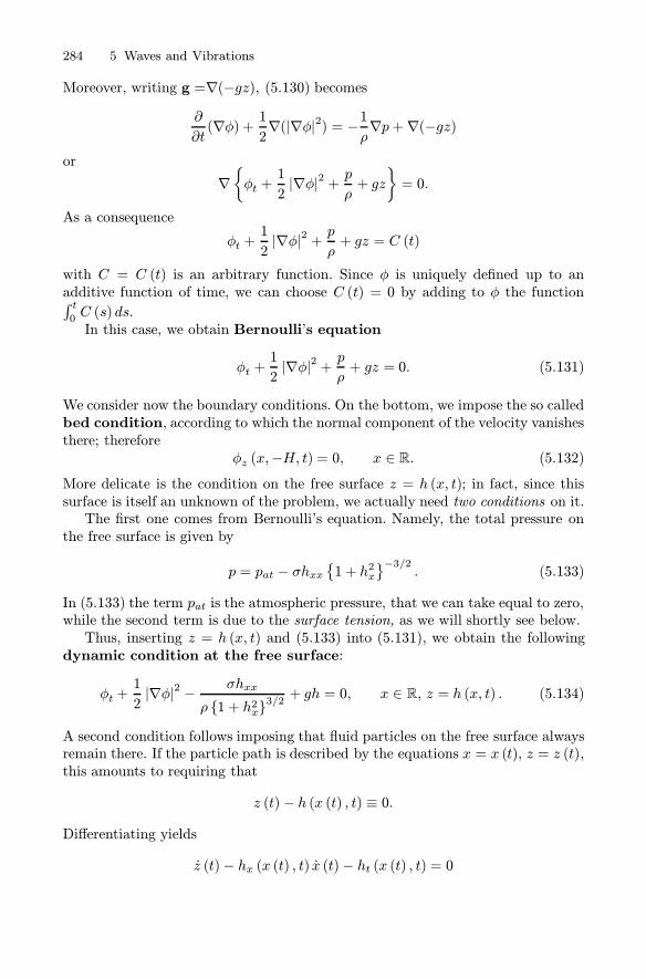
284 5 Waves and Vibrations
Moreover, writing g =∇(−gz), (5.130) becomes∂
∂t(∇φ) + 1
2∇(|∇φ|2) = −1
ρ∇p+∇(−gz)
or
∇{φt +
1
2|∇φ|2 + p
ρ+ gz
}= 0.
As a consequence
φt +1
2|∇φ|2 + p
ρ+ gz = C (t)
with C = C (t) is an arbitrary function. Since φ is uniquely defined up to anadditive function of time, we can choose C (t) = 0 by adding to φ the function∫ t0C (s) ds.In this case, we obtain Bernoulli’s equation
φt +1
2|∇φ|2 + p
ρ+ gz = 0. (5.131)
We consider now the boundary conditions. On the bottom, we impose the so calledbed condition, according to which the normal component of the velocity vanishesthere; therefore
φz (x,−H, t) = 0, x ∈ R. (5.132)
More delicate is the condition on the free surface z = h (x, t); in fact, since thissurface is itself an unknown of the problem, we actually need two conditions on it.The first one comes from Bernoulli’s equation. Namely, the total pressure on
the free surface is given by
p = pat − σhxx{1 + h2x
}−3/2. (5.133)
In (5.133) the term pat is the atmospheric pressure, that we can take equal to zero,while the second term is due to the surface tension, as we will shortly see below.Thus, inserting z = h (x, t) and (5.133) into (5.131), we obtain the following
dynamic condition at the free surface:
φt +1
2|∇φ|2 − σhxx
ρ {1 + h2x}3/2+ gh = 0, x ∈ R, z = h (x, t) . (5.134)
A second condition follows imposing that fluid particles on the free surface alwaysremain there. If the particle path is described by the equations x = x (t), z = z (t),this amounts to requiring that
z (t) − h (x (t) , t) ≡ 0.
Differentiating yields
z (t)− hx (x (t) , t) x (t)− ht (x (t) , t) = 0
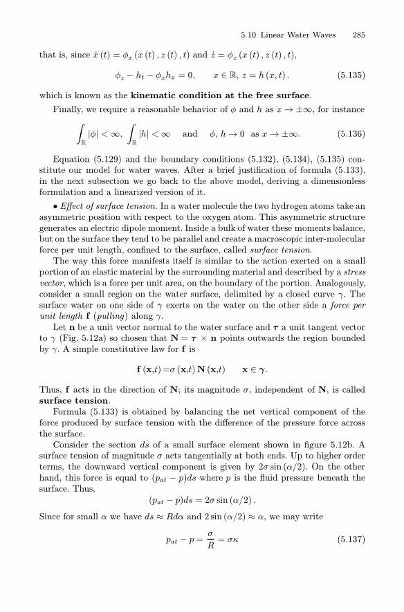
5.10 Linear Water Waves 285
that is, since x (t) = φx (x (t) , z (t) , t) and z = φz (x (t) , z (t) , t),
φz − ht − φxhx = 0, x ∈ R, z = h (x, t) . (5.135)
which is known as the kinematic condition at the free surface.
Finally, we require a reasonable behavior of φ and h as x→ ±∞, for instance∫
R
|φ| <∞,∫
R
|h| <∞ and φ, h→ 0 as x→ ±∞. (5.136)
Equation (5.129) and the boundary conditions (5.132), (5.134), (5.135) con-stitute our model for water waves. After a brief justification of formula (5.133),in the next subsection we go back to the above model, deriving a dimensionlessformulation and a linearized version of it.
• Effect of surface tension. In a water molecule the two hydrogen atoms take anasymmetric position with respect to the oxygen atom. This asymmetric structuregenerates an electric dipole moment. Inside a bulk of water these moments balance,but on the surface they tend to be parallel and create a macroscopic inter-molecularforce per unit length, confined to the surface, called surface tension.The way this force manifests itself is similar to the action exerted on a small
portion of an elastic material by the surrounding material and described by a stressvector, which is a force per unit area, on the boundary of the portion. Analogously,consider a small region on the water surface, delimited by a closed curve γ. Thesurface water on one side of γ exerts on the water on the other side a force perunit length f (pulling) along γ.Let n be a unit vector normal to the water surface and τ a unit tangent vector
to γ (Fig. 5.12a) so chosen that N = τ × n points outwards the region boundedby γ. A simple constitutive law for f is
f (x,t)=σ (x,t)N (x,t) x ∈ γ.
Thus, f acts in the direction of N; its magnitude σ, independent of N, is calledsurface tension.Formula (5.133) is obtained by balancing the net vertical component of the
force produced by surface tension with the difference of the pressure force acrossthe surface.Consider the section ds of a small surface element shown in figure 5.12b. A
surface tension of magnitude σ acts tangentially at both ends. Up to higher orderterms, the downward vertical component is given by 2σ sin (α/2). On the otherhand, this force is equal to (pat − p)ds where p is the fluid pressure beneath thesurface. Thus,
(pat − p)ds = 2σ sin (α/2) .Since for small α we have ds ≈ Rdα and 2 sin (α/2) ≈ α, we may write
pat − p =σ
R= σκ (5.137)
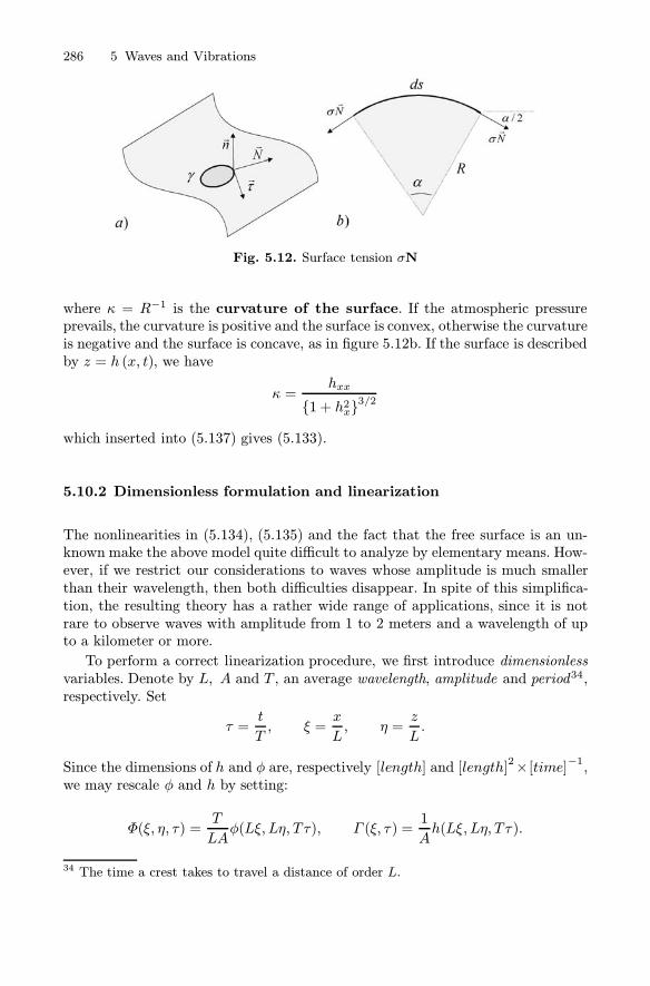
286 5 Waves and Vibrations
Fig. 5.12. Surface tension σN
where κ = R−1 is the curvature of the surface. If the atmospheric pressureprevails, the curvature is positive and the surface is convex, otherwise the curvatureis negative and the surface is concave, as in figure 5.12b. If the surface is describedby z = h (x, t), we have
κ =hxx
{1 + h2x}3/2
which inserted into (5.137) gives (5.133).
5.10.2 Dimensionless formulation and linearization
The nonlinearities in (5.134), (5.135) and the fact that the free surface is an un-known make the above model quite difficult to analyze by elementary means. How-ever, if we restrict our considerations to waves whose amplitude is much smallerthan their wavelength, then both difficulties disappear. In spite of this simplifica-tion, the resulting theory has a rather wide range of applications, since it is notrare to observe waves with amplitude from 1 to 2 meters and a wavelength of upto a kilometer or more.
To perform a correct linearization procedure, we first introduce dimensionlessvariables. Denote by L, A and T , an average wavelength, amplitude and period34,respectively. Set
τ =t
T, ξ =
x
L, η =
z
L.
Since the dimensions of h and φ are, respectively [length] and [length]2× [time]−1,
we may rescale φ and h by setting:
Φ(ξ, η, τ) =T
LAφ(Lξ, Lη, Tτ), Γ (ξ, τ) =
1
Ah(Lξ, Lη, Tτ).
34 The time a crest takes to travel a distance of order L.

5.10 Linear Water Waves 287
In terms of these dimensionless variables, our model becomes, after elementarycalculations:
ΔΦ = 0, −H0 < η < εΓ (ξ, τ), ξ ∈ R
Φτ +ε2 |∇Φ|
2+F
{Γ −BΓξξ
{1 + ε2Γ 2ξ
}3/2}= 0, η = εΓ (ξ, τ), ξ ∈ R
Φη − Γτ − εΦξΓξ = 0, η = εΓ (ξ, τ), ξ ∈ RΦη (ξ,−H0, τ) = 0, ξ ∈ Rwhere we have emphasized the four dimensionless combinations35
ε =A
L, H0 =
H
L, F = gT
2
L, B = σ
ρgL2. (5.138)
The parameter B, called Bond number, measures the importance of surfacetension while F , the Froude number, measures the importance of gravity.At this point, the assumption of small amplitude compared to the wavelength,
translates simply into
ε =A
L� 1
and the linearization of the above system is achieved by letting ε = 0 :
ΔΦ = 0, −H0 < η < 0, ξ ∈ RΦτ +F {Γ − BΓξξ} = 0, η = 0, ξ ∈ RΦη − Γτ = 0, η = 0, ξ ∈ RΦη (ξ,−H0, τ) = 0, ξ ∈ R.
Going back to the original variables, we finally obtain the linearized system⎧⎪⎪⎪⎪⎪⎨⎪⎪⎪⎪⎪⎩
Δφ = 0, −H < z < 0, x ∈ R (Laplace)
φt + gh− σρhxx = 0, z = 0, x ∈ R (Bernoulli)
φz − ht = 0, z = 0, x ∈ R (kinematic)
φz (x,−H, t) = 0, x ∈ R (bed condition)
(5.139)
It is possible to obtain an equation for φ only. Differentiate twice with respect tox the kinematic equation and use φxx = −φzz; this yields
htxx = φzxx = −φzzz. (5.140)
Differentiate Bernoulli’s equation with respect to t , then use ht = φz and (5.140).The result is:
φtt + gφz +σ
ρφzzz = 0, z = 0, x ∈ R. (5.141)
35 Note the reduction of the number of relevant parameters from seven (A,L, T, H, g, σ, ρ)to four.

288 5 Waves and Vibrations
5.10.3 Deep water waves
We solve now system (5.139) with the following initial conditions:
φ (x, z, 0) = 0, h (x, 0) = h0 (x) , ht (x, 0) = 0. (5.142)
Thus, initially (t = 0) the fluid velocity is zero and the free surface has been per-turbed into a non horizontal profile h0, that we assume (for simplicity) smooth,even (i.e. h0 (−x) = h0 (x)) and compactly supported. In addition we consider thecase of deep water (H≫ 1) so that the bed condition can be replaced by36
φz (x, z, t)→ 0 as z → −∞. (5.143)
The resulting initial-boundary value problem is not of the type we considered sofar, but we are reasonably confident that it is well posed. Since x varies over allthe real axis, we may use the Fourier transform with respect to x, setting
φ (k, z, t) =
∫
R
e−ikxφ (x, z, t)dx, h (k, t) =
∫
R
e−ikxh (x, t) dx.
Note that, the assumptions on h0 implies that h0 (k) = h0 (k, 0) rapidly vanishes as
|k| → ∞ and h0 (−k) = h0 (k). Moreover, since φxx = −k2φ, the Laplace equationtransforms into the ordinary differential equation
φzz − k2φ = 0
whose general solution is
φ (k, z, t) = A (k, t) e|k|z + B (k, t) e−|k|z.
From (5.143) we deduce B (k, t) = 0, so that
φ (k, z, t) = A (k, t) e|k|z. (5.144)
Trasforming (5.141) we get
φtt + gφz +σ
ρφzzz = 0, z = 0, k ∈ R
and (5.144) yields for A the equation
Att +
(g |k|+ σ
ρ|k|3)A = 0.
Thus, we obtain
A (k, t) = a (k) eiωt + b (k) e−iωt
36 For the case of finite depth see Problem 5.19.

5.10 Linear Water Waves 289
where (dispersion relation)
ω (k) =
√g |k|+ σ
ρ|k|3,
and
φ (k, z, t) ={a (k) eiω(k)t + b (k) e−iω(k)t
}e|k|z.
To determine a (k) e b (k), observe that the Bernoulli condition gives
φt (k, 0, t) +
{g +σ
ρk2}h (k, t) = 0, k ∈ R (5.145)
from which
iω (k){a (k) eiω(k)t − b (k) e−iω(k)t
}+
(g +σ
ρk2)h (k, t) = 0, k ∈ R
and for t = 0
iω (k) {a (k)− b (k)}+(g +σ
ρk2)h0 (k) = 0. (5.146)
Similarly, the kinematic condition gives
φz (k, 0, t) + ht (k, t) = 0, k ∈ R. (5.147)
We have
φz (k, 0, t) = |k|{a (k) eiω(k)t + b (k) e−iω(k)t
}
and since ht (k, 0) = 0, we get, from (5.147) for t = 0 and k �= 0,
a (k) + b (k) = 0. (5.148)
From (5.146) and (5.148) we have (k �= 0)
a (k) = −b (k) =i(g + σ
ρk2)
2ω (k)h0 (k)
and therefore
φ (k, y, t) =i(g + σ
ρk2)
2ω (k)
{eiω(k)t − e−iω(k)t
}e|k|zh0 (k) .
From (5.145) we deduce:
h (k, t) =
(g +σ
ρk2)−1φt (k, 0, t) =
1
2
{eiω(k)t + e−iω(k)t
}h0 (k)

290 5 Waves and Vibrations
and finally, transforming back37
h (x, t) =1
4π
∫
R
{ei(kx−ω(k)t) + ei(kx+ω(k)t)
}h0 (k) dk. (5.149)
5.10.4 Interpretation of the solution
The surface displacement appears in wave packet form. The dispersion relation
ω (k) =
√g |k|+ σ
ρ|k|3
shows that each Fourier component of the initial free surface propagates bothin the positive and negative x−directions. The phase and group velocities are(considering only k > 0, for simplicity)
cp =ω
k=
√g
k+σk
ρ
and
cg =g + 3σk2/ρ
2√gk + σk3/ρ
.
Thus, we see that the speed of a wave of wavelength λ = 2π/k depends on itswavelength. The fundamental parameter is
B∗ = 4π2B=σk2
ρg
where B is the Bond number. For water, under “normal” conditions,
ρ = 1 gr/cm3, σ = 72 gr/sec2, g = 980 cm/sec2 (5.150)
so that B∗ = 1 for wavelengths λ � 1.7 cm. When λ � 1.7 cm, then B∗ < 1,k = 2π
λ � 1 and surface tension becomes negligible. This is the case of gravitywaves (generated e.g. by dropping a stone into a pond) whose phase speed is wellapproximated by
cp =
√g
k=
√gλ
2π
while their group velocity is
cg =1
2
√g
k=1
2cp.
37 Note that, since also ω (k) is even, we may write
h (x, t) =1
2π
∫
R
cos [kx− ω (k) t] h0 (k) dk.

5.10 Linear Water Waves 291
Thus, longer waves move faster and energy is slower than the crests.On the other hand, if λ � 1.7 cm, then B∗ > 1, k = 2π
λ � 1 and this timesurface tension prevails over gravity. In fact, short wavelengths are associated withrelative high curvature of the free surface and high curvature is concomitant withlarge surface tension effects. This is the case of capillarity waves (generated e.g.by raindrops in a pond) and their speed is well approximated by
cp =
√σk
ρ=
√2πσ
λρ
while the group velocity is
cg =3
2
√σk
ρ=3
2cp.
Thus shorter waves move faster and energy is faster than the crests.When both gravity and surface tension are relevant, figure 5.13 shows the graph
of c2p versus λ, for water, with the values (5.150):
c2p = 156. 97 λ+452. 39
λ.
The main feature of this graph is the presence of the minimum
cmin = 23 cm/sec
corresponding just to the value λ = 1.7 cm. The consequence is curious: lineargravity and capillarity deep water waves can appear simultaneously only when thespeed is greater than 23 cm/sec. A typical situation occurs when a small obstacle(e.g. a twig) moves at speed v in still water. The motion of the twig results in theformation of a wave system that moves along with it, with gravity waves behindand capillarity waves ahead. In fact, the result above shows that this wave systemcan actually appear only if v > 23 cm/sec.
Fig. 5.13. c2p versus λ

292 5 Waves and Vibrations
5.10.5 Asymptotic behavior
As we have already observed, the behavior of a wave packet is dominated for shorttimes by the initial conditions and only after a relatively long time it is possibleto observe the intrinsic features of the perturbation. For this reason, informationabout the asymptotic behavior of the packet as t→ +∞ are important. Thus, weneed a good asymptotic formula for the integral in (5.149) when t� 1.For simplicity, consider gravity waves only, for which
ω (k) =√g |k|.
Let us follow a particle x = x (t) moving along the positive x−direction withconstant speed v > 0, so that x = vt. Inserting x = vt into (5.149) we find
h (vt, t) =1
4π
∫
R
eit(kv−ω(k))h0 (k) dk +1
4π
∫
R
eit(kv+ω(k))h0 (k) dk
≡ h1 (vt, t) + h2 (vt, t) .
According to Theorem 5.6 in the next subsection (see also Remark 5.10), with
ϕ (k) = kv − ω (k) ,
if there exists exactly one stationary point for ϕ, i.e. only one point k0 such that
ω′ (k0) = v and ϕ′′ (k0) = −ω′′ (k0) �= 0,
we may estimate h1 for t� 1 by the following formula:
h1 (vt, t) =A (k0)
texp {it[k0v − ω (k0)]}+ O
(t−1)
(5.151)
where
A (k0) = h0 (k0)
√1
8π |ω′′ (k0)|exp i
{−π4sign ω′′(k0)
}.
We have
ω′ (k) =1
2
√g |k|−1/2 sign (k)
and
ω′′ (k) = −√g
4|k|−3/2 .
Since v > 0, equation ω′ (k0) = v gives the unique point of stationary phase
k0 =g
4v2=gt2
4x2.
Moreover,
k0v − ω (k0) = −g
4v= − gt4x
5.10 Linear Water Waves 293
and
ω′′(k0) = −2v3
g= −2x
3
gt3< 0
so that from (5.151) we find
h1 (vt, t) =1
4h0
( g4v2
)√ g
πtv3exp i
{− gt4v+π
4
}+O
(t−1)
Similarly, sinceh0 (k0) = h0 (−k0) ,
we find
h2 (vt, t) =1
4h0
( g4v2
)√ g
πtv3exp i
{gt
4v− π4
}+O
(t−1).
Finally,
h (vt, t) = h1 (vt, t) + h2 (vt, t)
= h0
( g4v2
)√ g
4πv3tcos
{gt
4v− π4
}+O
(t−1).
This formula shows that, for large x and t, with x/t = v, constant, the wave packetis locally sinusoidal with wave number
k (x, t) =gt
4vx=gt2
4x2.
In other words, an observer moving at the constant speed v = x/t sees a domi-nant wavelength 2π/k0, where k0 is the solution of ω
′ (k0) = x/t. The amplitudedecreases as t−1/2. This is due to the dispersion of the various Fourier componentsof the initial configuration, after a sufficiently long time.
5.10.6 The method of stationary phase
The method of stationary phase, essentially due to Laplace, gives an asymptoticformula for integrals of the form
I (t) =
∫ b
a
f (k) eitϕ(k)dk (−∞ ≤ a < b ≤ ∞)
as t → +∞. Actually, only the real part of I (t), in which the factor cos[tϕ (k)]appears, is of interest. Now, as t increases and ϕ (k) varies, cos[tϕ (k)] oscillatesmore and more and eventually much more than f . For this reason, the contributionsof the intervals where cos[tϕ (k)] > 0 will balance those in which cos[tϕ (k)] < 0,so that we expect that I (t)→ 0 as t→ +∞, just as the Fourier coefficients of anintegrable function tend to zero as the frequency goes to infinity.

294 5 Waves and Vibrations
To obtain information on the vanishing speed, assume ϕ is constant on a certaininterval J . On this interval cos[tϕ (k)] is constant as well and hence there are neitheroscillations nor cancellations. Thus, it is reasonable that, for t � 1, the relevantcontributions to I (t) come from intervals where ϕ is constant or at least almostconstant. The same argument suggests that eventually, a however small interval,containing a stationary point k0 for ϕ, will contribute to the integral much morethan any other interval without stationary points.The method of stationary phase makes the above argument precise through
the following theorem.
Theorem 5.6. Let f and ϕ belong to C2 ([a, b]). Assume that
ϕ′ (k0) = 0, ϕ′′(k0) �= 0 and ϕ′ (k) �= 0 for k �= k0.
Then, as t→ +∞∫ b
a
f (k) eitϕ(k)dk =
√2π
|ϕ′′(k0)|f(k0)√texp
{i[tϕ(k0) +
π
4signϕ′′(k0)
]}+O
(t−1)
First a lemma.
Lemma 5.3. Let f, ϕ as in Theorem 5.6. Let [c, d] ⊆ [a, b] and assume that|ϕ′ (k)| ≥ C > 0 in (c, d). Then
∫ d
c
f (k) eitϕ(k)dk = O(t−1)
t→ +∞. (5.152)
Proof. Integrating by parts we get (multiplying and dividing by ϕ′):
∫ d
c
f
ϕ′ϕ′eitϕdk =
1
it
{f (d) eitϕ(d)
ϕ′ (d)− f (c) e
itϕ(c)
ϕ′ (c)−∫ d
c
f ′ϕ′ − fϕ′′(ϕ′)2
eitϕdk
}.
Thus, from∣∣eitϕ(k)∣∣ ≤ 1 and our hypotheses, we have
∣∣∣∣∣∫ d
c
f eitϕdk
∣∣∣∣∣ ≤1
Ct
{|f (d)|+ |f (c)|+ 1
C
∫ d
c
|f ′ϕ′ − fϕ′′| dk}
≤ Kt
which gives (5.152). �Proof of Theorem 5.6. Without loss of generality, we may assume k0 = 0, so
that ϕ′ (0) = 0, ϕ′′ (0) �= 0. From Lemma 5.3, it is enough to consider the integral∫ ε
−εf (k) eitϕ(k)dk
where ε > 0 is as small as we wish. We distinguish two cases.

5.10 Linear Water Waves 295
Case 1: ϕ is a quadratic polynomial, that is
ϕ (k) = ϕ (0) +Ak2, A =1
2ϕ′′ (0) .
Then, write
f (k) = f (0) +f (k)− f (0)
kk ≡ f (0) + q (k) k,
and observe that, since f ∈ C2 ([−ε, ε]), q′ (k) is bounded in [−ε, ε]. Then, we have:∫ ε
−εf (k) eitϕ(k)dk = 2f(0)eitϕ(0)
∫ ε
0
eitAk2
dk + eitϕ(0)∫ ε
−εq (k) keitAk
2
dk.
Now, an integration by parts shows that the second integral is O (1/t) as t → ∞(the reader should check the details).In the first integral, if A > 0, let
tAk2 = y2 .
Then ∫ ε
0
eitAk2
dk =1√tA
∫ ε√tA
0
eiy2
dy.
Since38 ∫ ε√tA
0
eiy2
dy =
√π
2eiπ4 +O
(1
ε√tA
),
we get
∫ ε
0
f (k) eitϕ(k)dk =
√2π
|ϕ′′(0)|f(0)√texp
{i[ϕ(0)t+
π
4
]}+ O
(1
t
),
which proves the theorem when A > 0. The proof is similar if A < 0.Case 2. General ϕ. By a suitable change of variable we reduce case 2 to case 1.
First we write
ϕ (k) = ϕ (0) +1
2a (k) k2 (5.153)
where
a (k) = 2
∫ 10
(1− r)ϕ′′ (rk)dr.
38 Recall that eiπ/4 =(√2 + i
√2)/2. Moreover, the following formulas hold:
∣∣∣∣
√π
2√2−∫ λ
0
cos(y2)dy
∣∣∣∣ ≤√π
λ∣∣∣∣
√π
2√2−∫ λ
0
sin(y2)dy
∣∣∣∣ ≤√π
λ.
296 5 Waves and Vibrations
Equation (5.153) follows by applying to ψ (s) = ϕ (sk) the following Taylor for-mula:
ψ (1) = ψ (0) + ψ′ (0) s+1
2
∫ 10
(1− r)ψ′′ (r) dr.
Note that a (0) = ϕ′′ (0). Consider the function
p (k) = k√a (k) /ϕ′′ (0).
We have p (0) = 0 and p′ (0) = 1. Therefore, p is invertible near zero. Let
k = p−1 (y) .
Then, since
ϕ (k) = ϕ (0) +ϕ′′ (0)2[p (k)]
2,
we have,
ϕ (y) ≡ ϕ(p−1 (y)
)
= ϕ (0) +ϕ′′ (0)2
[p(p−1 (y)
)]2
= ϕ (0) +ϕ′′ (0)2y2
and ∫ ε
−εf (k) eitϕ(k)dk =
∫ p−1(ε)
p−1(−ε)F (y) eitϕ(y)dy
where
F (y) =f(p−1 (y)
)p′ (p−1 (y))
.
Since F (0) = f (0) and ϕ is a quadratic polynomial with ϕ (0) = ϕ (0), ϕ′′ (0) =ϕ′′ (0), case 2 follows from case 1. �
Remark 5.7. Theorem 5.6 holds for integrals extended over the whole real axis aswell (actually this is the most interesting case) as long as, in addition, f is bounded,
|ϕ′ (±∞)| ≥ C > 0, and∫R|f ′ϕ′ − fϕ′′| (ϕ′)−2 dk <∞. Indeed, it is easy to check
that Lemma 5.3 is true under these hypotheses and then the proof of Theorem 5.6is exactly the same.
Problems
5.1. The chord of a guitar of length L is plucked at its middle point and thenreleased. Write the mathematical model which governs the vibrations and solve it.Compute the energy E (t).

Problems 297
5.2. Solve the problem
⎧⎨⎩utt − uxx = 0 0 < x < 1, t > 0u (x, 0) = ut (x, 0) = 0 0 ≤ x ≤ 1ux (0, t) = 1, u (1, t) = 0 t ≥ 0.
5.3. Forced vibrations. Solve the problem.
⎧⎨⎩utt − uxx = g (t) sinx 0 < x < π, t > 0u (x, 0) = ut (x, 0) = 0 0 ≤ x ≤ πu (0, t) = u (π, t) = 0 t ≥ 0
[Answer. u (x, t) = sinx∫ t0g (t − τ ) sin τ dτ ].
5.4. Equipartition of energy. Let u = u (x, t) be the solution of the globalCauchy problem for the equation utt− cuxx = 0, with initial data u (x, 0) = g (x),ut (x, 0) = h (x). Assume that g and h are smooth functions with compact supportcontained in the interval (a, b). Show that there exists T such that, for t ≥ T ,
Ecin (t) = Epot (t) .
5.5. Solve the global Cauchy problem for the equation utt− cuxx = 0, with thefollowing initial data:
a) u (x, 0) = 1 if |x| < a, u (x, 0) = 0 if |x| > a; ut (x, 0) = 0b) u (x, 0) = 0; ut (x, 0) = 1 if |x| < a, ut (x, 0) = 0 if |x| > a.5.6. Check that formula (5.42) may be written in the following form:
u (x+ cξ − cη, t+ ξ + η)− u (x+ cξ, t+ ξ)− u (x− cη, t+ η) + u (x, t) = 0.(5.154)
Show that if u is a C2 function and satisfies (5.154), then
utt − c2uxx = 0.
Thus, (5.154) can be considered as a weak formulation of the wave equation.
5.7. The small longitudinal free vibrations of an elastic bar are governed bythe following equation
ρ (x)σ (x)∂2u
∂t2=∂
∂x
[E (x)σ (x)
∂u
∂x
](5.155)
where u is the longitudinal displacement, ρ is the linear density of the material, σis the cross section of the bar and E is its Young’s modulus39.
39 E is the proportionality factor in the strain-stress relation given by Hooke’s law: T(strain) = E ε (stress). Here ε � ux. For steel, E = 2×10¹¹ dine/cm2, for alluminium,E = 7× 10¹² dine/cm2.

298 5 Waves and Vibrations
Assume the bar has constant cross section but it is constructed by weldingtogether two bars, of different (constant) Young’s modulus E1, E2 and densityρ1, ρ2, respectively.Since the two bars are welded together, the displacement u is continuous across
the junction, which we locate at x = 0. In this case:
(a) Give a weak formulation of the global initial value problem for equation(5.155).
(b) Deduce that the following jump condition must hold at x = 0:
E1u(0−, t) = E2u(0+, t) t > 0. (5.156)
(c) Let cj = Ej/ρj, j = 1, 2. A left incoming wave uinc (x, t) = exp [i (x− c1t)]produces at the junction a reflected wave uref (x, t) = a exp [i (x+ c1t)] and atransmitted wave utr (x, t) = b exp [i (x− c2t)] . Determine a, b and interpret theresult.
[Hint. (c) Look for a solution of the form
u = uinc + uref
for x < 0 and u = utr for x > 0. Use the continuity of u and the jump condition(5.156)].
5.8. Determine the characteristics of Tricomi equation
utt − tuxx = 0.
[Answer : 3x± 2t3/2 = k, for t > 0].5.9. Classify the equation
t2utt + 2tuxt + uxx − ux = 0and find the characteristics. After a reduction to canonical form, find the generalsolution.[Answer :
u (x, t) = F(te−x
)+G
(te−x
)ex,
with F , G arbitrary].
5.10. Consider the following characteristic Cauchy problem40 for the waveequation in the half-plane x > t:
⎧⎨⎩utt − uxx = 0 x > tu (x, x) = f (x) x ∈ Ruν (x, x) = g (x) x ∈ R
where ν =(1,−1) /√2. Establish whether or not this problem is well posed.
40 Note that the data are the values of u and of the normal derivative on the characteristicy = x.

Problems 299
5.11. Consider the following so called Goursat problem41 for the wave equationin the sector −t < x < t:
⎧⎨⎩utt − uxx = 0 − t < x < tu (x, x) = f (x) , u (x,−x) = g (x) x > 0f (0) = g (0) .
Establish whether or not this problem is well posed.
5.12. Ill posed non-characteristic Cauchy problem for the heat equation. Checkthat for every integer k, the function
uk (x, t) =1
k[cosh kx cos kx cos 2k2t− sinhkx sin kx sin 2k2t]
solves ut = uxx and the (non characteristic) initial conditions:
u (0, t) =1
kcos 2k2t, ux (0, t) = 0.
Deduce that the corresponding Cauchy problem in the half-plane x > 0 is illposed.
5.13. Consider the telegrapher’s system (5.83), (5.84).(a) By elementary manipulations derive the following second order equation
for the inner current I:
Itt −1
LCIxx +
RC +GL
LCIt +
RG
LCI = 0.
(b) LetI = e−ktv
and choose k in order for v to satisfy an equation of the form
vtt −1
LCvxx + hv = 0.
Check that the condition RC = GL is necessary to have non dispersive waves(distorsionless transmission line).
5.14. Circular membrane. A perfectly flexible and elastic membrane at resthas the shape of the circle B1 =
{(x, y) : x2 + y2 ≤ 1
}. If the boundary is fixed
and there are no external loads, the vibrations of the membrane are governed bythe following system:
⎧⎪⎪⎨⎪⎪⎩
utt − c2(urr +
1rur +
1r2 uθθ
)= 0 0 < r < 1, 0 ≤ θ ≤ 2π, t > 0
u (r, θ, 0) = g (r, θ) , ut (r, 0) = h (r, θ) 0 < r < 1, 0 ≤ θ ≤ 2πu (1, θ, t) = 0 0 ≤ θ ≤ 2π, t ≥ 0.
41 Note that the data are the values of u on the characteristics y = x and y = −x, forx > 0.

300 5 Waves and Vibrations
In the case h = 0 e g = g (r), use the method of separation of variables to find thesolution
u (r, t) =∞∑n=1
anJ0 (λnr) cosλnt
where J0 is the Bessel function of order zero, λ1, λ2, ... are the zeros of J0 and thecoefficients an are given by
an =2
c2n
∫ 10
sg (s) J0 (λns) ds
where
cn =
∞∑n=1
(−1)kk! (k + 1)!
(λn
2
)2k+1
(see Remark 2.2.5).
5.15. Circular waveguide. Consider the equation utt−c2Δu = 0 in the cylinder
CR = {(r, θ, z) : 0 ≤ r ≤ R, 0 ≤ θ ≤ 2π, −∞ < z < +∞} .
Determine the axially symmetric solutions of the form
u (r, z, t) = v (r)w (z)h (t)
satisfying the Neumann condition ur = 0 on r = R.
[Answer.
un (r, z, t) = exp {−i (ωt− kz)} J0 (μnr/R) , n ∈ N.
where J0 is the Bessel function, μn are its stationary points (J′0 (μn) = 0) and
ω2
c2= k2 +
μ2nR2].
5.16. Let u be the solution of utt − c2Δu = 0 in R3 × (0,+∞) with data
u (x, 0) = g (x) and ut (x, 0) = h (x) ,
both supported in the sphere Bρ (0). Describe the support of u for t > 0.
[Answer : The spherical shell B�+ct (0) \ B�−ct (0), of width 2ρ, which expands atspeed c].
5.17. Focussing effect. Solve the problem
{wtt − c2Δw = 0 x ∈R3, t > 0w (x, 0) = 0, wt (x,0) = h (|x|) x ∈R3

Problems 301
where (r = |x|)
h (r) =
{1 0 ≤ r ≤ 10 r > 1.
Check that w (r, t) displays a discontinuity at the origin at time t = 1/c.
5.18. Show that the solution of the two-dimensional non-homogeneous Cauchyproblem with zero initial data is given by
u (x, t) =1
2πc
∫ t
0
∫
Bc(t−s)(x)
1√c2 (t− s)2 + |x − y|2
f(y,s) dyds.
5.19. For linear gravity waves (σ = 0), examine the case of uniform finitedepth, replacing condition (5.143) by
φz (x,−H, t) = 0
under the initial conditions (5.142).
(a) Write the dispersion relation.
Deduce that:
(b) The phase and group velocity have a finite upper bound.
(c) The square of the phase velocity in deep water (H � λ) is proportional tothe wavelength.
(d) Linear shallow water waves (H � λ) are not dispersive.[Answer: (a) ω2 = gk tanh (kH),
(b) cpmax =√kH ,
(c) c2p ∼ gλ/2π,(d) c2p ∼ gH ].5.20. Determine the travelling wave solutions of the linearized system (5.139)
of the formφ (x, z, t) = F (x− ct)G (z) .
Rediscover the dispersion relation found in Problem 5.19 (a).[Answer:
φ (x, z, t) = cosh k (z +H) {A cos k (x− ct) +B sin k (x− ct)} ,
A, B arbitrary constants and c2 = g tanh (kH) /k].

6
Elements of Functional Analysis
Motivations – Norms and Banach Spaces – Hilbert Spaces – Projections and Bases – Lin-
ear Operators and Duality – Abstract Variational Problems – Compactness and Weak
Convergence – The Fredholm Alternative – Spectral Theory for Symmetric Bilinear
Forms
6.1 Motivations
The main purpose in the previous chapters has been to introduce part of the basicand classical theory of some important equations of mathematical physics. Theemphasis on phenomenological aspects and the connection with a probabilisticpoint of view should have conveyed to the reader some intuition and feeling aboutthe interpretation and the limits of those models.
The few rigorous theorems and proofs we have presented had the role of bring-ing to light the main results on the qualitative properties of the solutions andjustifying, partially at least, the well-posedness of the relevant boundary and ini-tial/boundary value problems we have considered.
However, these purposes are somehow in competition with one of the mostimportant role of modern mathematics, which is to reach a unifying vision of largeclasses of problems under a common structure, capable not only of increasingtheoretical understanding, but also of providing the necessary flexibility to guidethe numerical methods which will be used to compute approximate solutions.
This conceptual jump requires a change of perspective, based on the introduc-tion of abstract methods, historically originating from the vain attempts to solvebasic problems (e.g. in electrostatics) at the end of the 19th century. It turns outthat the new level of knowledge opens the door to the solution of complex problemsin modern technology.
These abstract methods, in which analytical and geometrical aspects fuse, arethe core of the branch of Mathematics, called Functional Analysis.
Salsa S. Partial Differential Equations in Action: From Modelling to Theoryc© Springer-Verlag 2008, Milan

6.1 Motivations 303
It could be useful for understanding the subsequent development of the theory,to examine in an informal way how the main ideas come out, working on a coupleof specific examples.Let us go back to the derivation of the diffusion equation, in subsection 2.1.2. If
the body is heterogeneous or anisotropic, may be with discontinuities in its thermalparameters (e.g. due to the mixture of two different materials), the Fourier law ofheat conduction gives for the flux function q the form
q = −A (x)∇u,
where the matrix A satisfies the condition
q·∇u = −A (x)∇u · ∇u ≤ 0 (ellipticity condition),
reflecting the tendency of heat to flow from hotter to cooler regions. If ρ = ρ (x)and cv = cv (x) are the density and the specific heat of the material, and f = f (x)is the rate of external heat supply per unit volume, we are led to the diffusionequation
ρcvut − div (A (x)∇u) = f.In stationary conditions, u (x,t) = u (x), and we are reduced to
−div (A (x)∇u) = f. (6.1)
Since the matrix A encodes the conductivity properties of the medium, we expecta low degree of regularity of A, but then a natural question arises: what is themeaning of equation (6.1) if we cannot compute the divergence of A?We have already faced similar situations in subsections 4.4.2, where we have
introduced discontinuous solutions of a conservation law, and in subsection 5.4.2,where we have considered solutions of the wave equation with irregular initial data.Let us follow the same ideas.Suppose we want to solve equation (6.1) in a bounded domain Ω, with zero
boundary data (Dirichlet problem). Formally, we multiply the differential equationby a smooth test function vanishing on ∂Ω, and we integrate over Ω:
∫
Ω
−div (A (x)∇u) v dx =∫
Ω
fv dx.
Since v = 0 on ∂Ω, using Gauss’ formula we obtain
∫
Ω
A (x)∇u · ∇v dx =∫
Ω
fv dx (6.2)
which is called weak or variational formulation of our Dirichlet problem.Equation (6.2) makes perfect sense for A and f bounded (possibly discontinu-
ous) and u, v ∈ C1(Ω), the set of of functions in C1
(Ω), vanishing on ∂Ω. Then,
we may say that u ∈ C1(Ω)is a weak solution of our Dirichlet problem if (6.2)

304 6 Elements of Functional Analysis
holds for every v ∈ C1(Ω). Fine, but now we have to prove the well-posedness of
the problem so formulated!Things are not so straightforward, as we have experienced in section 4.4.3 and,
actually, it turns out that C1(Ω)is not the proper choice, although it seems to
be the natural one. To see why, let us consider another example, somewhat morerevealing.Consider the equilibrium position of a stretched membrane having the shape
of a square Ω, subject to an external load f (force per unit mass) and kept at levelzero on ∂Ω.Since there is no time evolution, the position of the membrane may be described
by a function u = u (x), solution of the Dirichlet problem
{−Δu = f in Ωu = 0 on ∂Ω.
(6.3)
For problem (6.3), equation (6.2) becomes
∫
Ω
∇u · ∇v dx =∫
Ω
fv dx ∀v ∈ C1(Ω). (6.4)
Now, this equation has an interesting physical interpretation. The integral in theleft hand side represents the work done by the internal elastic forces, due to avirtual displacement v. On the other hand
∫Ωfv expresses the work done by the
external forces.Thus, the weak formulation (6.4) states that these two works balance, which
constitutes a version of the principle of virtual work.There is more, if we bring into play the energy. In fact, the total potential energy
is proportional to
E (v) =
∫
Ω
|∇v|2 dx︸ ︷︷ ︸
internal elastic energy
−∫
Ω
fv dx
︸ ︷︷ ︸.
external potential energy
(6.5)
Since nature likes to save energy, the equilibrium position u corresponds to theminimizer of (6.5) among all the admissible configurations v. This fact is closelyconnected with the principle of virtual work and, actually, it is equivalent to it(see subsection 8.4.1).Thus, changing point of view, instead of looking for a weak solution of (6.4)
we may, equivalently, look for a minimizer of (6.5).However there is a drawback. It turns out that the minimum problem does not
have a solution, except for some trivial cases. The reason is that we are looking inthe wrong set of admissible functions.Why C1
(Ω)is a wrong choice? To be minimalist, it is like looking for the
minimizer of the functionf (x) = (x− π)2
among the rational numbers!
6.1 Motivations 305
Anyway, the answer is simple: C1(Ω)is not naturally tied to the physical
meaning of E (v), which is an energy and only requires the gradient of u to besquare integrable, that is |∇u| ∈ L2 (Ω). There is no need of a priori continuityof the derivatives, actually neither of u. The space C1
(Ω)is too narrow to have
any hope of finding the minimizer there. Thus, we are forced to enlarge the set ofadmissible functions and the correct one turns out to be the so called Sobolev spaceH10 (Ω), whose elements are exactly the functions belonging to L
2 (Ω), togetherwith their first derivatives, vanishing on ∂Ω. We could call them functions of finiteenergy!
Although we feel we are on the right track, there is a price to pay, to puteverything in a rigorous perspective and avoid risks of contradiction or non-senses.In fact many questions arise immediately.
For instance, what do we mean by the gradient of a function which is onlyin L2(Ω), maybe with a lot of discontinuities? More: a function in L2(Ω) is, inprinciple, well defined except on sets of measure zero. But, then, what does it mean“vanishing on ∂Ω”, which is precisely a set of measure zero?
We shall answer these questions in Chapter 7. We may anticipate that, for thefirst one, the idea is the same we used to define the Dirac delta as a derivativeof the Heaviside function, resorting to a weaker notion of derivative (we shall sayin the sense of distributions), based on the miraculous formula of Gauss and theintroduction of a suitable set of test function.
For the second question, there is a way to introduce in a suitable coherent waya so called trace operator which associates to a function u ∈ L2 (Ω), with gradientin L2 (Ω), a function u|∂Ω representing its values on ∂Ω (see subsection 6.6.1).The elements of H10 (Ω) vanish on ∂Ω in the sense that they have zero trace.
Another question is what makes the space H10 (Ω) so special. Here the con-junction between geometrical and analytical aspects comes into play. First of all,although it is an infinite-dimensional vector space, we may endow H10 (Ω) with astructure which reflects as much as possible the structure of a finite dimensionalvector space like Rn, where life is obviously easier.
Indeed, in this vector space (thinking of R as the scalar field) we may introducean inner product given by
(u, v)1 =
∫
Ω
∇u · ∇v
with the same properties of an inner product in Rn. Then, it makes sense to talkabout orthogonality between two functions u and v in H10 (Ω), expressed by thevanishing of their inner product:
(u, v)1 = 0.
Having defined the inner product (·, ·)1, we may define the size (norm) of u by
‖u‖1 =√(u, u)1

306 6 Elements of Functional Analysis
and the distance between u and v by
dist (u, v) = ‖u− v‖1 .
Thus, we may say that a sequence {un} ⊂ H10 (Ω) converges to u in H10 (Ω) if
dist (un, u)→ 0 as n→∞.
It may be observed that all of this can be done, even more comfortably, in thespace C1
(Ω). This is true, but with a key difference.
Let us use an analogy with an elementary fact. The minimizer of the function
f (x) = (x− π)2
does not exist among the rational numbers Q, although it can be approximated asmuch as one likes by these numbers. If from a very practical point of view, rationalnumbers could be considered satisfactory enough, certainly it is not so from thepoint of view of the development of science and technology, since, for instance,no one could even conceive the achievements of Calculus without the real numbersystem.As R is the completion of Q, in the sense that R contains all the limits of
sequences in Q that converge somewhere, the same is true for H10 (Ω) with respectto C1
(Ω). This makes H10 (Ω) a so called Hilbert space and gives it a big advantage
with respect to C1(Ω), which we illustrate going back to our membrane problem
and precisely to equation (6.4). This time we use a geometrical interpretation.In fact, (6.4) means that we are searching for an element u, whose inner product
with any element v of H10 (Ω) reproduces “the action of f on v”, given by the linearmap
v �−→∫
Ω
fv.
This is a familiar situation in Linear Algebra. Any function F : Rn → R, which islinear, that is such that
F (ax+ by) = aF (x) + bF (y) ∀a, b ∈ R, ∀x,y ∈Rn,
can be expressed as the inner product with a unique representative vector zF∈Rn(Representation Theorem). This amounts to saying that there is exactly one solu-tion zF of the equation
z · y = F (y) for every y ∈Rn. (6.6)
The structure of the two equations (6.4), (6.6) is the same: on the left hand sidethere is an inner product and on the other one a linear map.Another natural question arises: is there any analogue of the Representation
Theorem in H10 (Ω)?The answer is yes (see Riesz’s Theorem 6.3), with a little effort due to the
infinite dimension of H10 (Ω). The Hilbert space structure of H10 (Ω) plays a key

6.2 Norms and Banach Spaces 307
role. This requires the study of linear functionals and the related concept of dualspace. Then, an abstract result of geometric nature, implies the well-posedness ofa concrete boundary value problem.
What about equation (6.2)? Well, if the matrix A is symmetric and strictlypositive, the left hand side of (6.2) still defines an inner product in H10 (Ω) andagain Riesz’s Theorem yields the well-posedness of the Dirichlet problem.If A is not symmetric, things change only a little. Various generalizations of
Riesz’s Theorem (e.g. the Lax-Milgram Theorem 6.4) allow the unified treatmentof more general problems, through their weak or variational formulation. Actually,as we have experienced with equation (6.2), the variational formulation is often theonly way of formulating and solving a problem, without losing its original features.
The above arguments should have convinced the reader of the existence of ageneral Hilbert space structure underlying a large class of problems, arising in theapplications. In this chapter we develop the tools of Functional Analysis, essentialfor a correct variational formulation of a wide variety of boundary value problems.The results we present constitute the theoretical basis for numerical methods suchas finite elements or more generally,Galerkin’s methods, and this makes the theoryeven more attractive and important.More advanced results, related to general solvability questions and the spectral
properties of elliptic operators are included at the end of this chapter.
A final comment is in order. Look again at the minimization problem above. Wehave enlarged the class of admissible configurations from a class of quite smoothfunctions to a rather wide class of functions. What kind of solutions are we find-ing with these abstract methods? If the data (e.g. Ω and f , for the membrane)are regular, could the corresponding solutions be irregular? If yes, this does notsound too good! In fact, although we are working in a setting of possibly irregularconfigurations, it turns out that the solution actually possesses its natural degreeof regularity, once more confirming the intrinsic coherence of the method.It also turns out that the knowledge of the optimal regularity of the solution
plays an important role in the error control for numerical methods. However, thispart of the theory is rather technical and we do not have much space to treat itin detail. We shall only state some of the most common results.
The power of abstract methods is not restricted to stationary problems. As weshall see, Sobolev spaces depending on time can be introduced for the treatmentof evolution problems, both of diffusive or wave propagation type (see Chapter 7).Also, in this introductory book, the emphasis is mainly to linear problems.
6.2 Norms and Banach Spaces
It may be useful for future developments, to introduce norm and distance inde-pendently of an inner product, to emphasize better their axiomatic properties.Let X be a linear space over the scalar field R or C. A norm in X, is a real
function‖·‖ : X → R (6.7)

308 6 Elements of Functional Analysis
such that, for each scalar λ and every x,y ∈ X, the following properties hold:
1. ‖x‖ ≥ 0; ‖x‖ = 0 if and only if x = 0 (positivity)
2. ‖λx‖ = |λ| ‖x‖ (homogeneity)
3. ‖x+ y‖ ≤ ‖x‖+ ‖y‖ (triangular inequality).
A norm is introduced to measure the size (or the“length”) of each vector x ∈ X,so that properties 1, 2, 3 should appear as natural requirements.A normed space is a linear space X endowed with a norm ‖·‖. With a norm is
associated the distance between two vectors given by
d (x, y) = ‖x− y‖
which makes X a metric space and allows to define a topology in X and a notionof convergence in a very simple way.We say that a sequence {xn} ⊂ X converges to x in X, and we write xm → x
in X, ifd (xm, x) = ‖xm − x‖ → 0 as m→∞.
An important distinction is between convergent and Cauchy sequences. A sequence{xm} ⊂ X is a Cauchy sequence if
d (xm, xk) = ‖xm − xk‖ → 0 as m, k→∞.
If xm → x in X, from the triangular inequality, we may write
‖xm − xm‖ ≤ ‖xm − x‖+ ‖xk − x‖ → 0 as m, k→∞
and therefore
{xm} convergent implies that {xm} is a Cauchy sequence. (6.8)
The converse in not true, in general. Take X = Q, with the usual norm given by|x| . The sequence of rational numbers
xm =
(1 +
1
m
)m
is a Cauchy sequence but it is not convergent in Q, since its limit is the irrationalnumber e.A normed space in which every Cauchy sequence converges is called complete
and deserves a special name.
Definition 6.1. A complete, normed linear space is called Banach space.
The notion of convergence (or of limit) can be extended to functions from anormed space into another, always reducing it to the convergence of distances,that are real functions.

6.2 Norms and Banach Spaces 309
Let X, Y linear spaces, endowed with the norms ‖·‖X and ‖·‖Y , respectively,and let F : X → Y . We say that F is continuous at x ∈ X if
‖F (y) − F (x)‖Y → 0 when ‖y − x‖X → 0
or, equivalently, if, for every sequence {xm} ⊂ X,
‖xm − x‖X → 0 implies ‖F (xm)− F (x)‖Y → 0.
F is continuous in X if it is continuous at every x ∈ X. In particular:
Proposition 6.1. Every norm in a linear space X is continuous in X.
Proof. Let ‖·‖ be a norm in X. From the triangular inequality, we may write
‖y‖ ≤ ‖y − x‖+ ‖x‖ and ‖x‖ ≤ ‖y − x‖+ ‖y‖
whence|‖y‖ − ‖x‖| ≤ ‖y − x‖ .
Thus, if ‖y − x‖ → 0 then |‖y‖ − ‖x‖| → 0, which is the continuity of the norm.�Some examples are in order.
Spaces of continuous functions. Let X = C (A) be the set of (real orcomplex) continuous functions on A, where A is a compact subset of Rn, endowedwith the norm (called maximum norm)
‖f‖C(A) = maxA |f | .
A sequence {fm} converges to f in C (A) if
maxA|fm − f | → 0,
that is, if fm converges uniformly to f in A. Since a uniform limit of continuousfunctions is continuous, C (A) is a Banach space.Note that other norms may be introduced in C (A), for instance the least
squares or L2 (A) norm
‖f‖L2(A) =(∫
A
|f |2)1/2
.
Equipped with this norm C (A) is not complete. Let, for example A = [−1, 1] ⊂ R.The sequence
fm(t) =
⎧⎪⎨⎪⎩
0 t ≤ 0mt 0 < t ≤ 1
m
1 t > 1m
(m ≥ 1) ,

310 6 Elements of Functional Analysis
contained in C ([−1, 1]), is a Cauchy sequence with respect to the L2 norm. In fact(letting m > k),
‖fm − fk‖2L2(A) =∫ 1−1|fm(t)− fk(t)|2 dt = (m− k)2
∫ 1/m0
t2dt+
∫ 1/k0
(1− kt)2 dt
=(m− k)23m3
+1
3k<1
3
(1
m+1
k
)→ 0 as m, k→ ∞.
However, fn converges in L2 (−1, 1)−norm (and pointwise) to the Heaviside func-
tion
H(t) ={1 t ≥ 00 t < 0,
which is discontinuous at t = 0 and therefore does not belong to C ([−1, 1]).More generally, letX = Ck (A), k ≥ 0 integer, the set of functions continuously
differentiable in A up to order k, included.To denote a derivative of order m, it is convenient to introduce an n− uple of
nonnegative integers, α = (α1, ..., αn), called multi-index, of length
|α| = α1 + ...+ αn =m,
and set
Dα =∂α1
∂xα11...∂αn
∂xαnn.
We endow Ck (A) with the norm (maximum norm of order k)
‖f‖Ck(A) = ‖f‖C(A) +k∑
|α|=1‖Dαf‖C(A) .
If {fn} is a Cauchy sequence in Ck (A), all the sequences {Dαfn} with 0 ≤ |α| ≤ kare Cauchy sequences in C (A). From the theorems on term by term differentiationof sequences, it follows that the resulting space is a Banach space.
Remark 6.1. With the introduction of function spaces we are actually making astep towards abstraction, regarding a function from a different perspective. Incalculus we see it as a point map while here we have to consider it as a singleelement (or a point or a vector) of a vector space.
Summable and bounded functions. Let Ω be an open set in Rn and p ≥ 1a real number. Let X = Lp (Ω) be the set of functions f such that |f |p is Lebesgueintegrable in Ω. Identifying two functions f and g when they are equal a.e.1 in Ω,
1 A property is valid almost everywhere in a set Ω, a.e. in short, if it is true at all pointsin Ω, but for a subset of measure zero (Appendix B).
6.3 Hilbert Spaces 311
Lp (Ω) becomes a Banach space2 when equipped with the norm (integral norm oforder p)
‖f‖Lp(Ω) =(∫
Ω
|f |p)1/p
.
The identification of two functions equal a.e. amounts to saying that an elementof Lp (Ω) is not a single function but, actually, an equivalence class of functions,different from one another only on subsets of measure zero. At first glance, thisfact could be annoying, but after all, the situation is perfectly analogous to con-sidering a rational number as an equivalent class of fractions (2/3, 4/6, 8/12 ....represent the same number). For practical purposes one may always refer to themore convenient representative of the class.
Let X = L∞ (Ω) the set of essentially bounded functions in Ω. Recall3 thatf : Ω → R (or C) is essentially bounded if there exists M such that
|f (x)| ≤M a.e. in Ω. (6.9)
The infimum of all numbersM with the property (6.9) is called essential supremumof f , and denoted by
‖f‖L∞(Ω) = ess supΩ|f | .
If we identify two functions when they are equal a.e., ‖f‖L∞(Ω) is a norm inL∞ (Ω), and L∞ (Ω) becomes a Banach space.Holder inequality (1.9) mentioned in chapter 1, may be now rewritten in terms
of norms as follows: ∣∣∣∣∫
Ω
fg
∣∣∣∣ ≤ ‖f‖Lp(Ω) ‖g‖Lq(Ω) , (6.10)
where q = p/(p− 1) is the conjugate exponent of p, allowing also the case p = 1,q =∞.Note that, if Ω has finite measure and 1 ≤ p1 < p2 ≤∞, from (6.10) we have,
choosing g ≡ 1, p = p2/p1 and q = p2/(p2 − p1):∣∣∣∣∫
Ω
|f |p1∣∣∣∣ ≤ |Ω|1/q ‖f‖p1Lp2(Ω)
and therefore Lp2 (Ω) ⊂ Lp1 (Ω). If the measure of Ω is infinite, this inclusion isnot true, in general; for instance, f ≡ 1 belongs to L∞ (R) but is not in Lp (R) for1 ≤ p <∞.
6.3 Hilbert Spaces
Let X be a linear space over R. An inner or scalar product in X is a function
(·, ·) : X ×X → R
2 See e.g. Yoshida, 1965.3 Appendix B.
312 6 Elements of Functional Analysis
with the following three properties. For every x, y, z ∈ X and scalars λ, μ ∈ R:1. (x, x) ≥ 0 and (x, x) = 0 if and only if x = 0 (positivity)
2. (x, y) = (y, x) (symmetry)
3. (μx+ λy, z) = μ (x, z) + λ (y, z) (bilinearity).
A linear space endowed with an inner product is called an inner product space.Property 3 shows that the inner product is linear with respect to its first argument.From 2, the same is true for the second argument as well. Then, we say that (·, ·)constitutes a symmetric bilinear form in X. When different inner product spacesare involved it may be necessary the use of notations like (·, ·)X , to avoid confusion.
Remark 6.2. If the scalar field is C, then
(·, ·) : X ×X → C
and property 2 has to be replaced by
2bis. (x, y) = (y, x) where the bar denotes complex conjugation. As a consequence,
we have(z, μx+ λy) = μ (z, x) + λ (z, y)
and we say that (·, ·) is antilinear with respect to its second argument or that itis a sesquilinear form in X.
An inner product induces a norm, given by
‖x‖ =√(x, x) (6.11)
In fact, properties 1 and 2 in the definition of norm are immediate, while thetriangular inequality is a consequence of the following quite important theorem.
Theorem 6.1. Let x, y ∈ X. Then:(1) Schwarz’s inequality:
|(x, y)| ≤ ‖x‖ ‖y‖ . (6.12)
Moreover equality holds in (6.12) if and only if x and y are linearly dependent.
(2) Parallelogram law:
‖x+ y‖2 + ‖x− y‖2 = 2 ‖x‖2 + 2 ‖y‖2 .
The parallelogram law generalizes an elementary result in euclidean plane ge-ometry: in a parallelogram, the sum of the squares of the sides length equals thesum of the squares of the diagonals length. The Schwarz inequality implies thatthe inner product is continuous; in fact, writing
(w, z)− (x, y) = (w − x, z) + (x, z − y)

6.3 Hilbert Spaces 313
we have
|(w, z)− (x, y)| ≤ ‖w − x‖ ‖z‖+ ‖x‖ ‖z − y‖so that, if w→ x and z → y, then (w, z)→ (x, y).Proof. (1) We mimic the finite dimensional proof. Let t ∈ R and x, y ∈ X.
Using the properties of the inner product and (6.11), we may write:
0 ≤ (tx+ y, tx+ y) = t2 ‖x‖2 + 2t (x, y) + ‖y‖2 ≡ P (t) .
Thus, the second degree polynomial P (t) is always nonnegative, whence
(x, y)2 − ‖x‖2 ‖y‖2 ≤ 0
which is the Schwarz inequality. Equality is possible only if tx+y = 0, i.e. if x andy are linearly dependent.(2) Just observe that
‖x± y‖2 = (x± y, y ± y) = ‖x‖2 ± 2 (x, y) + ‖y‖2 . (6.13)
�
Definition 6.2. Let H be an inner product space. We say that H is a Hilbertspace if it is complete with respect to the norm (6.11), induced by the innerproduct.
Two Hilbert spaces H1 and H2 are isomorphic if there exists a linear mapL : H1 → H2 which preserves the inner product, i.e.:
(x, y)H1 = (Lx, Ly)H2 ∀x, y ∈ H1.
In particular
‖x‖H1 = ‖Lx‖H2Example 6.1. Rn is a Hilbert space with respect to the usual inner product
(x,y)Rn= x · y =
n∑j=1
xjyj, x = (x1, ..., xn) , y =(y1, ..., yn).
The induced norm is
|x| = √x · x =n∑j=1
x2j .
More generally, if A =(aij)i,j=1,...,n is a square matrix of order n, symmetric andpositive,
(x,y)A = x ·Ay = Ax · y =n∑i=1
aijxiyj (6.14)

314 6 Elements of Functional Analysis
defines another scalar product in Rn. Actually, every inner product in Rn may bewritten in the form (6.14), with a suitable matrix A.
Cn is a Hilbert space with respect to the inner product
x · y =n∑j=1
xjyj x = (x1, ..., xn) ,y =(y1, ..., yn).
It is easy to show that every real (resp. complex) linear space of dimension nis isomorphic to Rn (resp. Cn).
Example 6.2. L2(Ω) is a Hilbert space (perhaps the most important one) withrespect to the inner product
(u, v)L2(Ω) =
∫
Ω
uv.
If Ω is fixed, we will simply use the notations (u, v)0 instead of (u, v)L2(Ω)and ‖u‖0 instead of ‖u‖L2(Ω).
Example 6.3. Let l2Cbe the set of complex sequences x = {xm} such that
∞∑i=1
|xm|2 <∞.
For x = {xm} and y = {ym}, define
(x,y)l2C
=
∞∑i=1
xiyj, x = {xn} ,y = {yn} .
Then (x,y)l2C
is an inner product which makes l2Ca Hilbert space over C (see
Problem 6.3). This space constitutes the discrete analogue of L2(0, 2π). Indeed,each u ∈ L2 (0, 2π) has an expansion in Fourier series (Appendix A)
u(x) =∑m∈Zume
imx,
where
um =1
2π
∫ 2π0
u (x) e−imxdx.
Note that um = u−m, since u is a real function. From Parseval’s identity, we have
(u, v)0 =
∫ 2π0
uv = 2π∑m∈Zumv−m
and (Bessel’s equation)
‖u‖20 =∫ 2π0
u2 = 2π∑m∈Z
|um|2 .

6.3 Hilbert Spaces 315
Example 6.4. A Sobolev space. It is possible to use the frequency space introducedin the previous example to define the derivatives of a function in L2 (0, 2π) in aweak or generalized sense. Let u ∈ C1 (R), 2π−periodic. The Fourier coefficientsof u′ are given by
u′m = imum
and we may write
‖u′‖20 =∫ 2π0
(u′)2 = 2π∑m∈Zm2 |um|2 . (6.15)
Thus, both sequences {um} and {mum} belong to l2C. But the right hand side in(6.15) does not involve u′ directly, so that it makes perfect sense to define
H1per (0, 2π) ={u ∈ L2 (0, 2π) : {um} , {mum} ∈ l2
}
and introduce the inner product
(u, v)1,2 = (2π)∑m∈Z
[1 +m2
]umv−m
which makes H1per (0, 2π) into a Hilbert space. Since
{mum} ∈ l2C,
with each u ∈ H1per (0, 2π) is associated the function v ∈ L2 (0, 2π) given by
v(x) =∑m∈Zimume
imx.
We see that v may be considered as a generalized derivative of u and H1per (0, 2π)as the space of functions in L2 (0, 2π), together with their first derivatives. Let u ∈H1per (0, 2π) and
u(x) =∑m∈Zume
imx.
Since ∣∣umeimx∣∣ = 1mm |um| ≤
1
2
(1
m2+m2 |um|2
)
the Weierstrass test entails that the Fourier series of u converges uniformly in R.Thus u has a continuous, 2π−periodic extension to all R. Finally observe that, ifwe use the symbol u′ also for the generalized derivative of u, the inner product inH1per (0, 1) can be written in the form
(u, v)1,2 =
∫ 10
(u′v′ + uv).
316 6 Elements of Functional Analysis
6.4 Projections and Bases
6.4.1 Projections
Hilbert spaces are the ideal setting to solve problems in infinitely many dimensions.They unify through the inner product and the induced norm, both an analyticaland a geometric structure. As we shall shortly see, we may coherently introducethe concepts of orthogonality, projection and basis, prove a infinite-dimensionalPythagoras’ Theorem (an example is just Bessel’s equation) and introduce otheroperations, extremely useful from both a theoretical and practical point of view.As in finite-dimensional linear spaces, two elements x, y belonging to an inner
product space are called orthogonal or normal if (x, y) = 0, and we write x⊥y.Now, if we consider a subspace V of Rn, e.g. a hyperplane through the origin,
every x ∈ Rn has a unique orthogonal projection on V . In fact, if dimV = k andthe unit vectors v1,v2, ...,vk constitute an orthonormal basis in V , we may alwaysfind an orthonormal basis in Rn, given by
v1,v2, ...,vk,wk+1, ...,wn,
where wk+1, ...,wn are suitable unit vectors. Thus, if
x =
k∑j=1
xjvj +
n∑j=k+1
xjwj ,
the projection of x on V is given by
PV x =
k∑j=1
xjvj.
On the other hand, the projection PV x can be characterized through the follow-ing property, which does not involve a basis in Rn: PV x is the point in V thatminimizes the distance from x, that is
|PV x− x| = infy∈V
|y − x| . (6.16)
In fact, if y =∑k
j=1 yjvj , we have
|y − x|2 =k∑j=1
(yj − xj)2 +n∑
j=k+1
x2j ≥N∑
j=k+1
x2j = |PV x − x|2 .
In this case, the “infimum” in (6.16) is actually a “minimum”.The uniqueness of PV x follows from the fact that, if y
∗ ∈ V and
|y∗−x| = |PV x − x| ,

6.4 Projections and Bases 317
then we must havek∑j=1
(y∗j − xj)2 = 0,
whence y∗j = xj for j = 1, ..., k, and therefore y∗ = PV x. Since
(x − PV x)⊥v, ∀v ∈ V
every x ∈ Rn may be written in a unique way in the form
x = y + z
with y ∈ V and z ∈ V ⊥, where V ⊥ denotes the subspace of the vectors orthogonalto V .Then, we say that Rn is direct sum of the subspaces V and V ⊥ and we write
Rn = V ⊕ V ⊥.
Finally,|x|2 = |y|2 + |z|2
which is the Pythagoras’ Theorem in Rn.
Fig. 6.1. Projection Theorem
We may extend all the above consideration to infinite-dimensional Hilbertspaces H , if we consider closed subspaces V of H . Here closed means withrespect to the convergence induced by the norm. More precisely, a subset U ⊂ His closed in H if it contains all the limit points of sequences in U . Observe that ifV has finite dimension k, it is automatically closed, since it is isomorphic to Rk
(or Ck). Also, a closed subspace of a Hilbert space is a Hilbert space as well, withrespect to the inner product in H .Unless stated explicitly, from now on we consider Hilbert spaces over R
(real Hilbert spaces), endowed with inner product (·, ·) and induced norm ‖·‖.
318 6 Elements of Functional Analysis
Theorem 6.2. (Projection Theorem). Let V be a closed subspace of a Hilbertspace H. Then, for every x ∈ H, there exists a unique element PV x ∈ V such that
‖PV x− x‖ = infv∈V
‖v − x‖ . (6.17)
Moreover, the following properties hold:
1. PV x = x if and only if x ∈ V .2. Let QV x = x− PV x. Then QV x ∈ V ⊥ and
‖x‖2 = ‖PV x‖2 + ‖QV x‖2 .
Proof. Letd = inf
v∈V‖v − x‖ .
By the definition of least upper bound, we may select a sequence {vm} ⊂ V , suchthat ‖vm − x‖ → d asm→∞. In fact, for every integerm ≥ 1 there exists vm ∈ Vsuch that
d ≤ ‖vm − x‖ < d+1
m. (6.18)
Letting m→∞ in (6.18), we get ‖vm − x‖ → d.We now show that {vm} is a Cauchy sequence. In fact, using the parallelogram
law for the vectors vk − x and vm − x, we obtain
‖vk + vm − 2x‖2 + ‖vk − vm‖2 = 2 ‖vk − x‖2 + 2 ‖vm − x‖2 . (6.19)
Since vk+vm2
∈ V , we may write
‖vk + vm − 2x‖2 = 4∥∥∥∥vk + vm2
− x∥∥∥∥2
≥ 4d2
whence, from (6.19):
‖vk − vm‖2 = 2 ‖vk − x‖2 + 2 ‖vm − x‖2 − ‖vk + vm − 2x‖2
≤ 2 ‖vk − x‖2 + 2 ‖vm − x‖2 − 4d2.
Letting k,m→∞, the right hand side goes to zero and therefore
‖vk − vm‖ → 0
as well. This proves that {vm} is a Cauchy sequence.Since H is complete, vm converges to an element w ∈ H which belongs to V ,
because V is closed . Using the norm continuity (Proposition 6.1) we deduce
‖vm − x‖ → ‖w − x‖ = d
so that w realizes the minimum distance from x among the elements in V .

6.4 Projections and Bases 319
We have to prove the uniqueness of w. Suppose w ∈ V is another element suchthat ‖w − x‖ = d. The parallelogram law, applied to the vectors w−x and w− x,yields
‖w − w‖2 = 2 ‖w − x‖2 + 2 ‖w − x‖2 − 4∥∥∥∥w + w
2− x∥∥∥∥2
≤ 2d2 + 2d2 − 4d2 = 0
whence w = w.
We have proved that there exists a unique element w = PV x ∈ V such that
‖x− PV x‖ = d.
To prove 1, observe that, since V is closed, x ∈ V if and only if d = 0, which meansx = PV x.To show 2, let QV x = x− PV x, v ∈ V e t ∈ R. Since PV x+ tv ∈ V for every
t, we have:
d2 ≤ ‖x− (PV x+ tv)‖2 = ‖QV x− tv‖2
= ‖QV x‖2 − 2t (QV x, v) + t2 ‖v‖2
= d2 − 2t (QV x, v) + t2 ‖v‖2 .
Erasing d2 and dividing by t > 0, we get
(QV x, v) ≤t
2‖v‖2
which forces (QV x, v) ≤ 0; dividing by t < 0 we get
(QV x, v) ≥t
2‖v‖2
which forces (QV x, v) ≥ 0. Thus (QV x, v) = 0 which means QV x ∈ V ⊥ andimplies that
‖x‖2 = ‖PV x+QV x‖2 = ‖PV x‖2 + ‖QV x‖2 ,concluding the proof. �
The elements PV x, QV x are called orthogonal projections of x on V andV ⊥, respectively. The least upper bound in (6.17) is actually a minimum.Moreoverthanks to properties 1, 2, we say that H is direct sum of V and V ⊥ :
H = V ⊕ V ⊥.
Note that
V ⊥ = {0} if and only if V = H.
320 6 Elements of Functional Analysis
Remark 6.3. Another characterization of PV x is the following (see Problem 6.4):u = PV x if and only if
{1. u ∈ V2. (x− u, v) = 0, ∀v ∈ V.
Remark 6.4. It is useful to point out that, even if V is not a closed subspace of H ,the subspace V ⊥ is always closed. In fact, if yn → y and {yn} ⊂ V ⊥, we have, forevery x ∈ V ,
(y, x) = lim(yn, x) = 0
whence y ∈ V ⊥.
Example 6.5. Let Ω ⊂ Rn be a set of finite measure. Consider in L2 (Ω) the
1−dimensional subspace V of constant functions (a basis is given by f ≡ 1, forinstance). Since it is finite-dimensional, V is closed in L2 (Ω) . Given f ∈ L2 (Ω),to find the projection PV f , we solve the minimization problem
minλ∈R
∫
Ω
(f − λ)2.
Since ∫
Ω
(f − λ)2 =∫
Ω
f2 − 2λ∫
Ω
f + λ2 |Ω| ,
we see that the minimizer is
λ =1
|Ω|
∫
Ω
f.
Therefore
PV f =1
|Ω|
∫
Ω
f and QV f = f −1
|Ω|
∫
Ω
f.
Thus, the subspace V ⊥ is given by the functions g ∈ L2 (Ω) with zero mean value.In fact these functions are orthogonal to f ≡ 1:
(g, 1)0 =
∫
Ω
g = 0.
6.4.2 Bases
A Hilbert space is said to be separable when there exists a countable dense subsetof H . An orthonormal basis in a separable Hilbert space H is sequence {wk}k≥1 ⊂H such that4 {
(wk, wj) = δkj k, j ≥ 1, ...‖wk‖ = 1 k ≥ 1
4 δjk is the Kronecker symbol.

6.4 Projections and Bases 321
and every x ∈ H may be expanded in the form
x =
∞∑k=1
(x, wk)wk. (6.20)
The series (6.20) is called generalized Fourier series and the numbers ck =(x, wk) are the Fourier coefficients of x with respect to the basis {wk}. Moreover(Pythagoras again!):
‖x‖2 =∞∑k=1
(x, wk)2.
Given an orthonormal basis {wk}k≥1, the projection of x ∈ H on the subspace Vspanned by, say, w1, ..., wN is given by
PV x =
N∑k=1
(x, wk)wk.
An example of separable Hilbert space is L2 (Ω), Ω ⊆ Rn. In particular, the set offunctions
1√2π,cosx√π,sinx√π,cos 2x√π,sin 2x√π, ...,
cosmx√π,sinmx√π, ...
constitutes an orthonormal basis in L2 (0, 2π) (see Appendix A).It turns out that:
Proposition 6.2. Every separable Hilbert space H admits an orthonormal basis.
Proof (sketch). Let {zk}k≥1 be dense in H . Disregarding, if necessary, thoseelements which are spanned by other elements in the sequence, we may assumethat {zk}k≥1 constitutes an independent set, i.e. every finite subset of {zk}k≥1 iscomposed by independent elements.Then, an orthonormal basis {wk}k≥1 is obtained by applying to {zk}k≥1 the
following so called Gram-Schmidt process. First, construct by induction a sequence{w}k≥1 as follows. Let w1 = z1. Once wk−1 is known, we construct wk by sub-tracting from zk its components with respect to w1, ..., wk−1:
wk = zk −(zk, wk−1)‖wk−1‖2
wk−1 − · · · −(zk, w1)
‖w1‖2w1.
In this way, wk is orthogonal to w1, ..., wk−1. Finally, set wk = wk/ ‖wk−1‖. Since{zk}k≥1 is dense in H , then {wk}k≥1 is dense in H as well. Thus {wk}k≥1 is anorthonormal basis. �In the applications, orthonormal bases arise from solving particular boundary
value problems, often in relation to the separation of variables method. Typicalexamples come form the vibrations of a non homogeneous string or from diffusion

322 6 Elements of Functional Analysis
in a rod with non constant thermal properties cv, ρ, κ. The first example leads tothe wave equation
ρ (x)utt − τuxx = 0.Separating variables (u(x, t) = v (x) z (t)), we find for the spatial factor the equa-tion
τv′′ + λρv = 0.
In the second example we are led to
(κv′)′ + λcvρv = 0.
These equations are particular cases of a general class of ordinary differentialequations of the form
(pu′)′ + qu+ λwu = 0 (6.21)
called Sturm-Liouville equations. Usually one looks for solutions of (6.21) in aninterval (a, b), −∞ ≤ a < b ≤ +∞, satisfying suitable conditions at the endpoints. The natural assumptions on p and q are p �= 0 in (a, b) and p, q, p−1 locallyintegrable in (a, b). The function w plays the role of a weight function, continuousin [a, b] and positive in (a, b) .In general, the resulting boundary value problem has non trivial solutions only
for particular values of λ, called eigenvalues. The corresponding solutions are calledeigenfunctions and it turns out that, when suitably normalized, they constitute anorthonormal basis in the Hilbert space L2w (a, b), the set of Lebesgue measurablefunctions in (a, b) such that
‖u‖2L2w =∫ b
a
u2 (x)w (x) dx <∞,
endowed with the inner product
(u, v)L2w=
∫ b
a
u (x) v (x)w (x) dx.
We list below some examples5.
• Consider the problem{(1− x2
)u′′ − xu′ + λu = 0 in (−1, 1)
u (−1) <∞, u (1) <∞.
The differential equation is known as Chebyshev’s equation and may be written inthe form (6.21):
((1− x2)1/2u′)′ + λ(1− x2
)−1/2u = 0
5 For the proofs, see Courant-Hilbert, vol. I, 1953.
6.4 Projections and Bases 323
which shows the proper weight function w (x) =(1− x2
)−1/2. The eigenvalues
are λn = n2, n = 0, 1, 2, .... The corresponding eigenfunctions are the Chebyshev
polynomials Tn, recursively defined by T0 (x) = 1, T1 (x) = x and
Tn+1 = 2xTn − Tn−1 (n > 1) .
For instance:
T2 (x) = 2x2 − 1, T3 (x) = 4x3 − 3x, T4 (x) = 8x4 − 8x2 − 1.
The normalized polynomials√1/πT0,
√2/πT1, ...,
√2/πTn, ... constitute an
orthonormal basis in L2w (−1, 1).• Consider the problem6
((1− x2
)u′)′+ λu = 0 in (−1, 1)
with weighted Neumann conditions
(1− x2
)u′ (x)→ 0 as x→ ±1.
The differential equation is known as Legendre’s equation. The eigenvalues areλn = n (n+ 1), n = 0, 1, 2, ... The corresponding eigenfunctions are the Legendrepolynomials, defined by L0 (x) = 1, L1 (x) = x,
(n+ 1)Ln+1 = (2n + 1)xLn − nLn−1 (n > 1)
or by Rodrigues’ formula
Ln (x) =1
2nn!
dn
dxn(x2 − 1
)n(n ≥ 0) .
For instance, L2 (x) = (3x2 − 1)/2, L3 (x) = (5x3 − 3x)/2. The normalized poly-
nomials √2n+ 1
2Ln
constitute an orthonormal basis in L2 (−1, 1) (here w (x) ≡ 1). Every functionf ∈ L2 (−1, 1) has an expansion
f (x) =∞∑n=0
fnLn (x)
where fn =2n+12
∫ 1−1 f (x)Ln (x) dx, with convergence in L
2 (−1, 1).• Consider the problem
{u′′ − 2xu′ + 2λu = 0 in (−∞,+∞)e−x
2/2u (x)→ 0 as x→ ±∞.6 See also Problem 8.5.

324 6 Elements of Functional Analysis
The differential equation is known as Hermite’s equation (see Problem 6.6) andmay be written in the form (6.21):
(e−x2
u′)′ + 2λe−x2
u = 0
which shows the proper weight function w (x) = e−x2
. The eigenvalues are λn =n, n = 0, 1, 2, .... The corresponding eigenfunctions are the Hermite polynomialsdefined by Rodrigues’ formula
Hn (x) = (−1)n ex2 dn
dxne−x
2
(n ≥ 0) .
For instance
H0 (x) = 1, H1 (x) = 2x, H2 (x) = 4x2 − 2, H3 (x) = 8x3 − 12x.
The normalized polynomials π−1/4 (2nn!)−1/2Hn constitute an orthonormal basisin L2w (R), with w (x) = e
−x2 . Every f ∈ L2w (R) has an expansion
f (x) =
∞∑n=0
fnHn (x)
where fn = [π1/22nn!]−1
∫Rf (x)Hn (x) e
−x2dx, with convergence in L2w (R).
• After separating variables in the model for the vibration of a circular mem-brane the following parametric Bessel equation of order p arises (see Problem 6.8):
x2u′′ + xu′ +(λx2 − p2
)u = 0 x ∈ (0, a) (6.22)
where p ≥ 0, λ ≥ 0, with the boundary conditions
u (0) finite, u (a) = 0. (6.23)
Equation (6.22) may be written in Sturm-Liouville form as
(xu′)′ +(λx− p
2
x
)u = 0
which shows the proper weight function w (x) = x. The simple rescaling z =√λx
reduces (6.22) to the Bessel equation of order p
z2d2u
dz2+ zdu
dz+(z2 − p2
)u = 0 (6.24)
where the dependence on the parameter λ is removed. The only bounded solutionsof (6.24) are the Bessel functions of first kind and order p, given by
Jp (z) =
∞∑k=0
(−1)kΓ (k + 1)Γ (k + p+ 1)
(z2
)p+2k

6.4 Projections and Bases 325
Fig. 6.2. Graphs of J0,J1 and J2
where
Γ (s) =
∫ ∞0
e−tts−1dt (6.25)
is the Euler Γ− function. In particular, if p = n ≥ 0, integer:
Jn (z) =
∞∑k=0
(−1)kk! (k + n)!
(z2
)n+2k.
For every p, there exists an infinite, increasing sequence {αpj}j≥1 of positive zeroesof Jp:
Jp (αpj) = 0 (j = 1, 2, ...).
Then, the eigenvalues of problem (6.22), (6.23) are given by λpj =(αpja
)2, with
corresponding eigenfunctions upj (x) = Jp
(αpjax). The normalized eigenfunctions
√2
aJp+1 (αpj)Jp
(αpjax)
constitute an orthonormal basis in L2w (0, a), with w (x) = x. Every function f ∈L2w (0, a) has an expansion in Fourier-Bessel series
f (x) =
∞∑j=1
fjJp
(αpjax),
where
fj =2
a2J2p+1 (αpj)
∫ a
0
xf (x)Jp
(αpjax)dx,
convergent in L2w (0, a).

326 6 Elements of Functional Analysis
6.5 Linear Operators and Duality
6.5.1 Linear operators
Let H1 and H2 be Hilbert spaces. A linear operator from H1 into H2 is afunction
L : H1 → H2such that7, ∀α, β ∈ R and ∀x, y ∈ H1
L(αx+ βy) = αLx + βLy.
For every linear operator we define its Kernel, N (L) and Range, R (L), as follows:
Definition 6.3. The kernel of L, is the pre-image of the null vector in H2:
N (L)= {x ∈ H1 : Lx = 0} .
The range of L is the set of all outputs from points in H1:
R (L) = {y ∈ H2 : ∃x ∈ H1, Lx = y} .
N (L) and R (L) are linear subspaces of H1 and H2, respectively.Our main objects will be linear bounded operators.
Definition 6.4. A linear operator L : H1 → H2 is bounded if there exists anumber C such that
‖Lx‖H2 ≤ C ‖x‖H1 , ∀x ∈ H1. (6.26)
The number C controls the expansion rate operated by L on the elements ofH1. In particular, if C < 1, L contracts the sizes of the vectors in H1.If x �= 0, using the linearity of L, we may write (6.26) in the form
∥∥∥∥∥L(x
‖x‖H1
)∥∥∥∥∥H2
≤ C
which is equivalent to
sup‖x‖H1=1
‖Lx‖H2 = K <∞, (6.27)
since x/ ‖x‖H1 is a unit vector in H1. Clearly K ≤ C.
Proposition 6.3. A linear operator L : H1 → H2 is bounded if and only if it iscontinuous.
7 Notation: if L is linear, when no confusion arises, we may write Lx instead of L (x).

6.5 Linear Operators and Duality 327
Proof. Let L be bounded. From (6.26) we have, ∀x, x0 ∈ H1,
‖L (x− x0)‖H2 ≤ C ‖x− x0‖H1so that, if ‖x− x0‖H1 → 0, also ‖Lx− Lx0‖H2 = ‖L (x− x0)‖H2 → 0. This showsthe continuity of L.Let L be continuous. In particular, L is continuous at x = 0 so that there exists
δ such that‖Lx‖H2 ≤ 1 if ‖x‖H1 ≤ δ.
Choose now y ∈ H1 with ‖y‖H1 = 1 and let z = δy. We have ‖z‖H1 = δ whichimplies
δ ‖Ly‖H2 = ‖Lz‖H2 ≤ 1or
‖Ly‖H2 ≤1
δ
and (6.27) holds with K ≤ C = 1δ . �
Given two Hilbert spaces H1 and H2, we denote by
L (H1, H2)
the family of all linear bounded operators from H1 into H2. If H1 = H2 we simplywrite L (H). L (H1, H2) becomes a linear space if we define, for x ∈ H1 and λ ∈ R,
(G+ L) (x) = Gx+ Lx
(λL)x = λLx.
Also, we may use the number K in (6.27) as a norm in L (H1, H2):
‖L‖L(H1,H2) = sup‖x‖H1=1
‖Lx‖H2 . (6.28)
When no confusion arises we will write simply ‖L‖ instead of ‖L‖L(H1,H2). Thus,for every L ∈ L (H1, H2), we have
‖Lx‖H2 ≤ ‖L‖ ‖x‖H1 .
The resulting space is complete, so that:
Proposition 6.4. Endowed with the norm (6.28), L (H1, H2) is a Banach space.
Example 6.6. Let A be an m× n real matrix. The map
L : x �−→ Ax
is a linear operator from Rn into Rm. To compute ‖L‖, note that
‖Ax‖2 = Ax ·Ax = A�Ax · x.

328 6 Elements of Functional Analysis
The matrix A�A is symmetric and nonnegative and therefore, from Linear Alge-bra,
sup‖x‖=1
A�Ax · x =ΛM
where ΛM is the maximum eigenvalue of A�A. Thus, ‖L‖ = √ΛM .
Example 6.7. Let V be a closed subspace of a Hilbert space H . The projections
x �−→ PV x, x �−→ QV x,
defined in Theorem 6.2, are bounded linear operators from H intoH . In fact, from‖x‖2 = ‖PV x‖2 + ‖QV x‖2, it follows immediately that
‖PV x‖ ≤ ‖x‖ , ‖QV x‖ ≤ ‖x‖
so that (6.26) holds with C = 1. Since PV x = x when x ∈ V and QV x = x whenx ∈ V ⊥, it follows that ‖PV ‖ = ‖QV ‖ = 1. Finally, observe that
N (PV ) = R (QV ) = V ⊥ and N (QV ) = R (PV ) = V.
Example 6.8. Let V andH be Hilbert spaces with8 V ⊂ H . Considering an elementin V as an element of H , we define the operator IV→H : V → H ,
IV→H (u) = u,
which is called embedding of V into H . IV→H is clearly a linear operator and itis also bounded if there exists a constant C such that
‖u‖H ≤ C ‖u‖V , for every u ∈ V
In this case, we say that V is continuously embedded in H and we write
V ↪→ H.
For instance, H1per (0, 2π) ↪→ L2 (0, 2π) .
6.5.2 Functionals and dual space
When H2 = R (or C, for complex Hilbert spaces), a linear operator L : H → R
takes the name of functional.
Definition 6.5. The collection of all bounded linear functionals on a Hilbert spaceH is called dual space of H and denoted by H∗ (instead of L (H,R)).8 The inner products in V and H may be different.
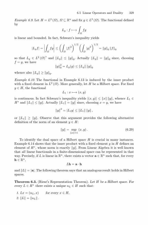
6.5 Linear Operators and Duality 329
Example 6.9. Let H = L2 (Ω), Ω ⊆ Rn and fix g ∈ L2 (Ω). The functional definedby
Lg : f �−→∫
Ω
fg
is linear and bounded. In fact, Schwarz’s inequality yields
|Lgf | =∣∣∣∣∫
Ω
fg
∣∣∣∣ ≤(∫
Ω
|f |2)1/2(∫
Ω
|g|2)1/2
= ‖g‖0 ‖f‖0
so that Lg ∈ L2 (Ω)∗ and ‖Lg‖ ≤ ‖g‖0. Actually ‖Lg‖ = ‖g‖0 since, choosingf = g, we have
‖g‖20 = Lg(g) ≤ ‖Lg‖ ‖g‖0whence also ‖Lg‖ ≥ ‖g‖0.
Example 6.10. The functional in Example 6.13 is induced by the inner productwith a fixed element in L2 (Ω). More generally, let H be a Hilbert space. For fixedy ∈ H , the functional
L1 : x �−→ (x, y)is continuous. In fact Schwarz’s inequality yields |(x, y)| ≤ ‖x‖ ‖y‖, whence L1 ∈H∗ and ‖L1‖ ≤ ‖y‖. Actually ‖L1‖ = ‖y‖ since, choosing x = y, we have
‖y‖2 = |L1y| ≤ ‖L1‖ ‖y‖ ,
or ‖L1‖ ≥ ‖y‖. Observe that this argument provides the following alternativedefinition of the norm of an element y ∈ H :
‖y‖ = sup‖x‖=1
(x, y) . (6.29)
To identify the dual space of a Hilbert space H is crucial in many instances.Example 6.14 shows that the inner product with a fixed element y in H defines anelement of H∗, whose norm is exactly ‖y‖. From Linear Algebra it is well knownthat all linear functionals in a finite-dimensional space can be represented in thatway. Precisely, if L is linear in Rn, there exists a vector a ∈ Rn such that, for everyh ∈ Rn,
Lh = a · hand ‖L‖ = |a|. The following theorem says that an analogous result holds in Hilbertspaces.
Theorem 6.3. (Riesz′s Representation Theorem). Let H be a Hilbert space. Forevery L ∈ H∗ there exists a unique uL ∈ H such that:
1. Lx = (uL, x) for every x ∈ H,2. ‖L‖ = ‖uL‖ .

330 6 Elements of Functional Analysis
Proof. Let N be the kernel of L. If N = H , then L is the null operator anduL = 0. If N ⊂ H , then N is a closed subspace of H . In fact, if {xn} ⊂ N andxn → x, then 0 = Lxn → Lx so that x ∈ N ; thus N contains all its limit pointsand therefore is closed.Then, by the Projection Theorem, there exists z ∈ N⊥, z �= 0. Thus Lz �= 0
and, given any x ∈ H , the element
w = x− LxLzz
belongs to N . In fact
Lw = L
(x− LxLzz
)= Lx− Lx
LzLz = 0.
Since z ∈ N⊥, we have
0 = (z, w) = (z, x)− LxLz‖z‖2
which entails
Lx =L (z)
‖z‖2(z, x) .
Therefore if uL = L (z) ‖z‖−2 z, then Lx = (uL, x).For the uniqueness, observe that, if v ∈ H and
Lx = (v, x) for every x ∈ H,
subtracting this equation from Lx = (uL, x), we infer
(uL − v, x) = 0 for every x ∈ H
which forces v = uL.
To show ‖L‖ = ‖uL‖, use Schwarz’s inequality
|(uL, x)| ≤ ‖x‖ ‖uL‖
to get‖L‖ = sup
‖x‖=1|Lx| = sup
‖x‖=1|(uL, x)| ≤ ‖uL‖ .
On the other hand,
‖uL‖2 = (uL, uL) = LuL ≤ ‖L‖ ‖uL‖
whence‖uL‖ ≤ ‖L‖ .
Thus ‖L‖ = ‖uL‖. �

6.5 Linear Operators and Duality 331
The Riesz’s map R : H∗ → H given by
L �−→ uL
is a canonical isometry, since it preserves the norm:
‖L‖ = ‖uL‖ .
We say that uL is the Riesz element associated with L, with respect to the scalarproduct (·, ·). Moreover, H∗ endowed with the inner product
(L1, L2)H∗ = (uL1 , uL2)
is clearly a Hilbert space. Thus, in the end, the Representation Theorem allowsthe identification of a Hilbert space with its dual.Typically, L2 (Ω) or l2 are identified with their duals.
Remark 6.5.Warning: there are situations in which the above canonical identifi-cation requires some care. A typical case we shall meet later occurs when dealingwith a pair of Hilbert spaces V , H such that
V ↪→ H and H∗ ↪→ V ∗.
As we will see in subsection 6.8.1, in this conditions it is possible to identify Hand H∗ and write
V ↪→ H ↪→ V ∗,but at this point the identification of V with V ∗ is forbidden, since it would giverise to nonsense!
Remark 6.6. A few words about notations. The symbol (·, ·) or (·, ·)H denotesthe inner product in a Hilbert space H . Let now L ∈ H∗. For the action of thefunctional L on an element x ∈ H we used the symbol Lx. Sometimes, when it isuseful or necessary to emphasize the duality (or pairing) between H and H∗, weshall use the notation 〈L, x〉∗ or even H∗〈L, x〉H .
6.5.3 The adjoint of a bounded operator
The concept of adjoint operator extends the notion of transpose of an m × nmatrix A and plays a crucial role in determining compatibility conditions for thesolvability of several problems. The transpose A� is characterized by the identity
(Ax,y)Rm=(x,A�y)
Rn, ∀x ∈Rn, ∀y ∈Rm.
We extend precisely this relation to define the adjoint of a bounded linear operator.Let L ∈ L(H1, H2). If y ∈ H2 is fixed, the real map
Ty : x �−→ (Lx,y)H2

332 6 Elements of Functional Analysis
defines an element of H∗1 . In fact
|Tyx| =∣∣(Lx,y)H2
∣∣ ≤ ‖Lx‖H2 ‖y‖H2 ≤ ‖L‖L(H1,H2) ‖y‖H2 ‖x‖H1so that ‖Ty‖ ≤ ‖L‖L(H1,H2) ‖y‖H2 .From Riesz’s Theorem, there exists a unique w ∈ H1 depending on y, which
we denote by w = L∗y, such that
Tyx = (x,L∗y)H1 ∀x ∈ H1, ∀y ∈ H2.
This defines L∗ as an operator from H2 into H1, which is called the adjoint of L.Precisely:
Definition 6.6. The operator L∗ : H2 → H1 defined by the identity
(Lx,y)H2 =(x,L∗y)H1 , ∀x ∈ H1, ∀y ∈ H2 (6.30)
is called the adjoint of L.
Example 6.11. Let R : H∗ → H the Riesz operator. Then R∗ = R−1 : H → H∗.In fact, for every F ∈ H∗ and v ∈ H , we have:
(RF, v)H = 〈F, v〉∗ =(F,R−1v
)H∗ .
Example 6.12. Let T : L2 (0, 1)→ L2 (0, 1) be the linear map
Tu (x) =
∫ x
0
u (t) dt.
Schwarz’s inequality gives ∣∣∣∣∫ x
0
u
∣∣∣∣2
≤ x∫ x
0
u2,
whence
‖Tu‖20 =∫ 10
|Tu|2 =∫ 10
∣∣∣∣∫ x
0
u
∣∣∣∣2
dx ≤∫ 10
(x
∫ x
0
u2)dx ≤ 12
∫ 10
u2 ≤ 12‖u‖20
and therefore T is bounded. To compute T ∗, observe that
(Tu,v)0 =
∫ 10
[v (x)
∫ x
0
u (y) dy] dx = exchanging the order of integration
=
∫ 10
[u (y)
∫ 1x
v (x) dx] dy = (u, T ∗v)0 .
Thus,
T ∗v (x) =∫ 1x
v (t) dt.
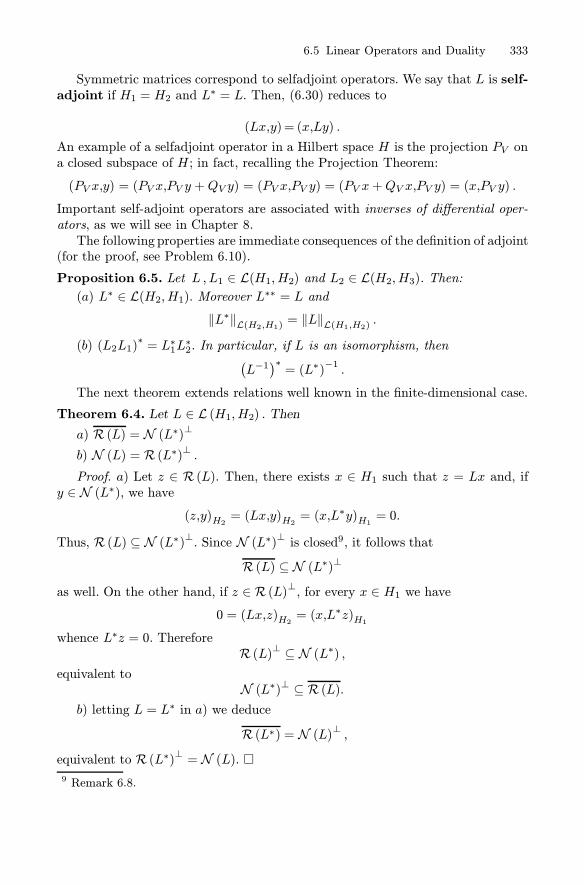
6.5 Linear Operators and Duality 333
Symmetric matrices correspond to selfadjoint operators. We say that L is self-adjoint if H1 = H2 and L
∗ = L. Then, (6.30) reduces to
(Lx,y)= (x,Ly) .
An example of a selfadjoint operator in a Hilbert space H is the projection PV ona closed subspace of H ; in fact, recalling the Projection Theorem:
(PV x,y) = (PV x,PV y +QV y) = (PV x,PV y) = (PV x+QV x,PV y) = (x,PV y) .
Important self-adjoint operators are associated with inverses of differential oper-ators, as we will see in Chapter 8.The following properties are immediate consequences of the definition of adjoint
(for the proof, see Problem 6.10).
Proposition 6.5. Let L , L1 ∈ L(H1, H2) and L2 ∈ L(H2, H3). Then:(a) L∗ ∈ L(H2, H1). Moreover L∗∗ = L and
‖L∗‖L(H2,H1) = ‖L‖L(H1,H2) .(b) (L2L1)
∗= L∗1L∗2. In particular, if L is an isomorphism, then(
L−1)∗= (L∗)−1 .
The next theorem extends relations well known in the finite-dimensional case.
Theorem 6.4. Let L ∈ L (H1, H2) . Thena) R (L) = N (L∗)⊥
b) N (L) = R (L∗)⊥ .Proof. a) Let z ∈ R (L). Then, there exists x ∈ H1 such that z = Lx and, if
y ∈ N (L∗), we have(z,y)H2 = (Lx,y)H2 = (x,L
∗y)H1 = 0.
Thus, R (L) ⊆ N (L∗)⊥. Since N (L∗)⊥ is closed9, it follows thatR (L) ⊆ N (L∗)⊥
as well. On the other hand, if z ∈ R (L)⊥, for every x ∈ H1 we have0 = (Lx,z)H2 = (x,L
∗z)H1whence L∗z = 0. Therefore
R (L)⊥ ⊆ N (L∗) ,equivalent to
N (L∗)⊥ ⊆ R (L).b) letting L = L∗ in a) we deduce
R (L∗) = N (L)⊥ ,equivalent to R (L∗)⊥ = N (L). �9 Remark 6.8.

334 6 Elements of Functional Analysis
6.6 Abstract Variational Problems
6.6.1 Bilinear forms and the Lax-Milgram Theorem
In the variational formulation of boundary value problems a key role is played bybilinear forms. Given two linear spaces V1, V2, a bilinear form in V1 × V2 is afunction
a : V1 × V2 → R
satisfying the following properties:
i) For every y ∈ V2, the function
x �−→ a(x, y)
is linear in V1.
ii) For every x ∈ V1, the function
y �−→ a(x, y)
is linear in V2.
When V1 = V2, we simply say that a is a bilinear form in V .
Remark 6.7. In complex inner product spaces we define sesquilinear forms, insteadof bilinear forms, replacing ii) by:
iibis) for every x ∈ V1, the function
y �−→ a(x, y)
is anti-linear10 in V2.
Here are some examples.
• A typical example of bilinear form in a Hilbert space is its inner product.• The formula
a (u, v) =
∫ b
a
(p(x)u′v′ + q(x)u′v + r(x)uv) dx
where p, q, r are bounded functions, defines a bilinear form in C1 ([a, b]).More generally, if Ω is a bounded domain in Rn,
a(u,v) =
∫
Ω
(α ∇u · ∇v + ub (x) · ∇v + a0 (x)uv) dx (α > 0) ,
10 That is
a (x, αy + βz) = αa (x, y) + βa (x, z)

6.6 Abstract Variational Problems 335
or
a(u,v) =
∫
Ω
α ∇u · ∇v dx+∫
∂Ω
huv dσ (α > 0) ,
(b, a0, h bounded) are bilinear forms in C1(Ω).
• A bilinear form in C2(Ω)involving higher order derivatives is
a (u, v) =
∫
Ω
Δu Δv dx.
Let V be a Hilbert space, a be a bilinear form in V and F ∈ V ∗. Consider thefollowing problem, called abstract variational problem:
⎧⎨⎩
Find u ∈ Vsuch that
a (u, v) = 〈F, v〉∗ ∀v ∈ V.(6.31)
As we shall see, many boundary values problems can be recast in this form.The fundamental result is:
Theorem 6.5. (Lax−Milgram). Let V be a real Hilbert space endowed withinner product (·, ·) and norm ‖·‖. Let a = a (u, v) be a bilinear form in V . If:i) a is continuous, i.e. there exists a constant M such that
|a(u, v)| ≤M ‖u‖ ‖v‖ , ∀u, v ∈ V ;
ii) a is V−coercive, i.e. there exists a constant α > 0 such that
a(v, v) ≥ α ‖v‖2 , ∀v ∈ V, (6.32)
then there exists a unique solution u ∈ V of problem (6.31). Moreover, thefollowing stability estimate holds:
‖u‖ ≤ 1α‖F ‖V ∗ . (6.33)
Remark 6.8. The coercivity inequality (6.32) may be considered as an abstractversion of the energy or integral estimates we met in the previous chapters. Usually,it is the key estimate to prove in order to apply Theorem 6.5. We shall come backto the general solvability of a variational problem in Section 6.8, when a is notV−coercive.
Remark 6.9. Inequality (6.61) is called stability estimate for the following reason.The functional F, element of V ∗, encodes the “data” of the problem (6.31). Sincefor every F there is a unique solution u(F ), the map
F �−→ u(F )

336 6 Elements of Functional Analysis
is a well defined function from V ∗ onto V . Also, everything here has a linearnature, so that the solution map is linear as well. To check it, let λ, μ ∈ R, F1,F2 ∈ V ∗ and u1, u2 the corresponding solutions. The bilinearity of a, gives
a(λu1 + μu2, v) = λa(u1, v) + μa(u2, v) =
= λF1v + μF2v.
Therefore, the same linear combination of the solutions corresponds to a linearcombination of the data; this expresses the principle of superposition for problem(6.31). Applying now (6.33) to u1− u2, we obtain
‖u1 − u2‖ ≤1
α‖F1 − F2‖V ∗ .
Thus, close data imply close solutions. The stability constant 1/α plays an im-portant role, since it controls the norm-variation of the solutions in terms of thevariations on the data, measured by ‖F1 − F2‖V ∗ . This entails, in particular, thatthe more the coercivity constant α is large, the more “stable” is the solution.
Proof of theorem 6.5. We split it into several steps.
1. Reformulation of problem (6.31). For every fixed u ∈ V , by the continuityof a, the linear map
v �→ a (u, v)is bounded in V and therefore it defines an element of V ∗. From Riesz’s Represen-tation Theorem, there exists a unique A [u] ∈ V such that
a (u, v) = (A[u],v) , ∀v ∈ V. (6.34)
Since F ∈ V ∗ as well, there exists a unique zF ∈ V such that
Fv = (zF ,v) ∀v ∈ V
and moreover ‖F ‖V ∗ = ‖zF ‖. Then, problem (6.31) can be recast in the followingway: ⎧⎨
⎩Find u ∈ Vsuch that
(A [u] ,v) = (zF ,v) , ∀v ∈ Vwhich, in turn, is equivalent to finding u such that
A [u] = zF . (6.35)
We want to show that (6.35) has exactly one solution. To do this we show that
A : V → V
is a linear, continuous, one-to-one, surjective map.

6.6 Abstract Variational Problems 337
2. Linearity and continuity of A. We repeatedly use the definition of A and thebilinearity of a. To show linearity, we write, for every u1, u2, v ∈ V and λ1, λ2 ∈ R,
(A [λ1u1 + λ2u2] ,v) = a (λ1u1 + λ2u2, v) = λ1a (u1, v) + λ2a (u2, v)
= λ1 (A [u1] ,v) + λ2 (A [u2] ,v) = (λ1A [u1] + λ2A [u2] ,v)
whence
A [λ1u1 + λ2u2] = λ1A [u1] + λ2A [u2] .
Thus A is linear and we may write Au instead of A [u]. For the continuity, observethat
‖Au‖2 = (Au,Au) = a(u, Au)≤M ‖u‖ ‖Au‖
whence
‖Au‖ ≤M ‖u‖ .3. A is one-to-one and has closed range, i.e.
N (A) = {0} and R (A) is a closed subspace of V.
In fact, the coercivity of a yields
α ‖u‖2 ≤ a (u, u) = (Au, u) ≤ ‖Au‖ ‖u‖
whence
‖u‖ ≤ 1α‖Au‖ . (6.36)
Thus, Au = 0 implies u = 0 and hence N (A) = {0}.To prove that R (A) is closed we have to consider a sequence {ym} ⊂ R (A)
such that
ym → y ∈ Vas m → ∞, and show that y ∈ R (A). Since ym ∈ R (A) , there exists um suchthat Aum = ym. From (6.36) we infer
‖uk − um‖ ≤1
α‖yk − ym‖
and therefore, since {ym} is convergent, {um} is a Cauchy sequence. Since V iscomplete, there exists u ∈ V such that
um → u
and the continuity of A yields ym = Aum → Au. Thus Au = y, so that y ∈ R (A)and R (A) is closed.

338 6 Elements of Functional Analysis
4. A is surjective, that is R (A) = V . Suppose R (A) ⊂ V . Since R (A) is aclosed subspace, by the Projection Theorem there exists z �= 0, z ∈ R (A)⊥. Inparticular, this implies
0 = (Az, z) = a (z, z) ≥ α ‖z‖2
whence z = 0. Contradiction. Therefore R (A) = V .5. Solution of problem (6.31). Since A is one-to-one and R (A) = V , there
exists exactly one solution u ∈ V of equation
Au = zF .
From point 1, u is the unique solution of problem (6.31) as well.
6. Stability estimate. From (6.36) with u = u, we obtain
‖u‖ ≤ 1α‖Au‖ = 1
α‖zF ‖ =
1
α‖F ‖V ∗
and the proof is complete. �
Remark 6.10. Some applications require the solution to be in some Hilbert spaceW , while asking the variational equation
a (u, v) = 〈F, v〉∗to hold for every v ∈ V , with V �= W . A variant of Theorem 6.5 deals with thisasymmetric situation. Let F ∈ V ∗ and a = a (u, v) be a bilinear form in W × Vsatisfying the following three hypotheses:
i) there exists M such that
|a(u, v)| ≤M ‖u‖W ‖v‖V , ∀u ∈W, ∀v ∈ V ;ii) there exists α > 0 such that
sup‖v‖V =1
a(u, v) ≥ α ‖u‖W , ∀u ∈W ;
iii)supw∈Wa(w, v) > 0, ∀v ∈ V.
Condition ii) is an asymmetric coercivity, while iii) assures that, for every fixedv ∈ V , a (v, ·) is positive at some point in W . We have (for the proof see Problem6.11):
Theorem 6.6. (Necas). If i), ii), iii) hold, there exists a unique u ∈ W such that
a (u, v) = 〈F, v〉∗ ∀v ∈ V.
Moreover
‖u‖W ≤ 1α‖F ‖V ∗ . (6.37)

6.6 Abstract Variational Problems 339
6.6.2 Minimization of quadratic functionals
When a is symmetric, i.e. if
a (u, v) = a (v, u) ∀u, v ∈ V,
the abstract variational problem (6.31) is equivalent to a minimization problem.In fact, consider the quadratic functional
E (v) =1
2a (v, v) − 〈F, v〉∗ .
We have:
Theorem 6.7. Let a be symmetric. Then u is solution of problem (6.31) if andonly if u is a minimizer of E, that is
E (u) = minv∈VE (v) .
Proof. For every ε ∈ R and every “variation” v ∈ V we have
E (u+ εv) −E (u)
=
{1
2a (u+ εv, u+ εv) − 〈F, u+ εv〉∗
}−{1
2a (u, u)− 〈F, u〉∗
}
= ε {a (u, v)− 〈F, v〉∗}+1
2ε2a (v, v) .
Now, if u is the solution of problem (6.31), then a (u, v) − 〈F, v〉∗ = 0. Therefore
E (u+ εv) − E (u) = 12ε2a (v, v) ≥ 0
so that u minimizes E. On the other hand, if u is a minimizer of E, then
E (u+ εv) −E (u) ≥ 0,
which entails
ε {a (u, v) − 〈F, v〉∗}+1
2ε2a (v, v) ≥ 0.
This inequality forces (why?)
a (u, v) − 〈F, v〉∗ = 0 ∀v ∈ V (6.38)
and u is a solution of problem (6.31)). �
Letting ϕ (ε) = E (u+ εv), from the above calculations we have
ϕ′(0) = a (u, v) − 〈F, v〉∗ .

340 6 Elements of Functional Analysis
Thus, the linear functional
v �−→ a (u, v)− 〈F, v〉∗appears as the derivative of E at u along the direction v and we write
E′ (u) v = a (u, v)− 〈F, v〉∗ . (6.39)
In Calculus of Variation E′ is called first variation and denoted by δE.If a is symmetric, the variational equation
E′ (u)v = a (u, v) − 〈F, v〉∗ = 0, ∀v ∈ V (6.40)
is called Euler equation for the functional E.
Remark 6.11. A bilinear form a, symmetric and coercive, induces in V the innerproduct
(u, v)a = a (u, v) .
In this case, existence, uniqueness and stability for problem (6.31) follow directlyfrom Riesz’s Representation Theorem. In particular, there exists a unique mini-mizer u of E.
6.6.3 Approximation and Galerkin method
The solution u of the abstract variational problem (6.31), satisfies the equation
a (u, v) = 〈F, v〉∗ (6.41)
for every v in the Hilbert space V . In concrete applications, it is important tocompute approximate solutions with a given degree of accuracy and the infinitedimension of V is the main obstacle. Often, however, V may be written as a unionof finite-dimensional subspaces, so that, in principle, it could be reasonable toobtain approximate solutions by “projecting” equation (6.41) on those subspaces.This is the idea of Galerkin’s method. In principle, the higher the dimensionof the subspace the better should be the degree of approximation. More precisely,the idea is to construct a sequence {Vk} of subspaces of V with the followingproperties:
a) Every Vk is finite-dimensional : dimVk = k,
b) Vk ⊂ Vk+1 (actually, not strictly necessary),c) ∪Vk = V.To realize the projection, assume that the vectors ψ1, ψ2, ..., ψk span Vk. Then,
we look for an approximation of the solution u in the form
uk =
k∑j=1
cjψj, (6.42)

6.6 Abstract Variational Problems 341
by solving the projected problem
a (uk, v) = 〈F, v〉∗ ∀v ∈ Vk. (6.43)
Since {ψ1, ψ2, ..., ψk} constitutes a basis in Vk, (6.43) amounts to requiring
a (uk, ψr) = 〈F, ψr〉∗ r = 1, ..., k. (6.44)
Substituting (6.42) into (6.44), we obtain the k linear algebraic equations
k∑j=1
cja(ψj, ψr
)= 〈F, ψr〉∗ r = 1, 2, ..., k (6.45)
for the unknown coefficients c1, c2, ..., ck. Introducing the vectors
c =
⎛⎜⎜⎜⎝
c1c2...ck
⎞⎟⎟⎟⎠ , F =
⎛⎜⎜⎜⎝
〈F, ψ1〉∗〈F, ψ2〉∗...〈F, ψk〉∗
⎞⎟⎟⎟⎠
and the matrix A =(arj), with entries
arj = a(ψj, ψr
), j, r = 1, ..., k,
we may write (6.45) in the compact form
Ac = F. (6.46)
The matrixA is called stiffness matrix and clearly plays a key role in the numericalanalysis of the problem.If the bilinear form a is coercive, A is strictly positive. In fact, let ξ ∈Rk. Then,
by linearity and coercivity:
Aξ · ξ =k∑
r,j=1
arjξrξj =
k∑r,j=1
a(ψj, ψr
)ξrξj
=
k∑r,j=1
a(ξjψj, ξrψr
)= a
⎛⎝
k∑i=1
ξjψj ,
k∑j=1
ξrψr
⎞⎠
≥ α ‖v‖2
where
v =
k∑j=1
ξjψj∈Vk.
Since {ψ1, ψ2, ..., ψk} is a basis in Vk, we have v = 0 if and only if ξ = 0. ThereforeA is strictly positive and, in particular, non singular.

342 6 Elements of Functional Analysis
Thus, for each k ≥ 1, there exists a unique solution uk ∈ Vk of (6.46). We wantto show that uk → u, as k → ∞, i.e. the convergence of the method, and give acontrol of the approximation error.For this purpose, we prove the following lemma, which also shows the role of
the continuity and the coercivity constants (M and α, respectively) of the bilinearform a.
Lemma 6.1. (Cea). Assume that the hypotheses of the Lax-Milgram Theoremhold and let u be the solution of problem (6.31). If uk is the solution of problem(6.44), then
‖u− uk‖ ≤M
αinfv∈Vk
‖u− v‖ . (6.47)
Proof. We havea (uk, v) = 〈F, v〉∗ , ∀v ∈ Vk
anda (u, v) = 〈F, v〉∗ , ∀v ∈ Vk.
Subtracting the two equations we obtain
a (u− uk, v) = 0, ∀v ∈ Vk.In particular, since v − uk ∈ Vk, we have
a (u− uk, v − uk) = 0, ∀v ∈ Vkwhich implies
a (u− uk, u− uk) = a (u− uk, u− v) + a (u− uk, v − uk)= a (u− uk, u− v) .
Then, by the coercivity of a,
α ‖u− uk‖2 ≤ a (u− uk, u− uk) ≤M ‖u− uk‖ ‖u− v‖whence,
‖u− uk‖ ≤M
α‖u− v‖ . (6.48)
This inequality holds for every v ∈ Vk, with Mα independent of k. Therefore (6.48)
still holds if we take in the right hand side the infimum over all v ∈ Vk. �Convergence of Galerkin’s method. Since we have assumed that
∪Vk = V,there exists a sequence {wk} ⊂ Vk such that wk → u as k → ∞. Cea’s Lemmagives, for every k:
‖u− uk‖ ≤M
αinfv∈Vk
‖u− v‖ ≤ Mα‖u−wk‖
whence‖u− uk‖ → 0.
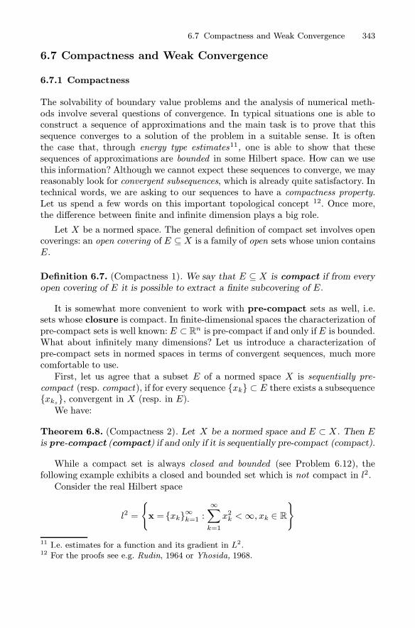
6.7 Compactness and Weak Convergence 343
6.7 Compactness and Weak Convergence
6.7.1 Compactness
The solvability of boundary value problems and the analysis of numerical meth-ods involve several questions of convergence. In typical situations one is able toconstruct a sequence of approximations and the main task is to prove that thissequence converges to a solution of the problem in a suitable sense. It is oftenthe case that, through energy type estimates11, one is able to show that thesesequences of approximations are bounded in some Hilbert space. How can we usethis information? Although we cannot expect these sequences to converge, we mayreasonably look for convergent subsequences, which is already quite satisfactory. Intechnical words, we are asking to our sequences to have a compactness property.Let us spend a few words on this important topological concept 12. Once more,the difference between finite and infinite dimension plays a big role.
Let X be a normed space. The general definition of compact set involves opencoverings: an open covering of E ⊆ X is a family of open sets whose union containsE.
Definition 6.7. (Compactness 1). We say that E ⊆ X is compact if from everyopen covering of E it is possible to extract a finite subcovering of E.
It is somewhat more convenient to work with pre-compact sets as well, i.e.sets whose closure is compact. In finite-dimensional spaces the characterization ofpre-compact sets is well known: E ⊂ Rn is pre-compact if and only if E is bounded.What about infinitely many dimensions? Let us introduce a characterization ofpre-compact sets in normed spaces in terms of convergent sequences, much morecomfortable to use.First, let us agree that a subset E of a normed space X is sequentially pre-
compact (resp. compact), if for every sequence {xk} ⊂ E there exists a subsequence{xks}, convergent in X (resp. in E).We have:
Theorem 6.8. (Compactness 2). Let X be a normed space and E ⊂ X. Then Eis pre-compact (compact) if and only if it is sequentially pre-compact (compact).
While a compact set is always closed and bounded (see Problem 6.12), thefollowing example exhibits a closed and bounded set which is not compact in l2.Consider the real Hilbert space
l2 =
{x = {xk}∞k=1 :
∞∑k=1
x2k <∞, xk ∈ R}
11 I.e. estimates for a function and its gradient in L2.12 For the proofs see e.g. Rudin, 1964 or Yhosida, 1968.

344 6 Elements of Functional Analysis
endowed with
(x,y) =
∞∑k=1
xkyk and ‖x‖2 =∞∑k=1
x2k.
Let E ={ek}k≥1, where e
1 = {1, 0, 0, ...}, e2 = {0, 1, 0, ...}, etc.. Observe that Econstitutes an orthonormal basis in l2. Then, E is closed and bounded in l2.However, E is not sequentially compact. Indeed,
∥∥ej − ek∥∥ = √2, if j �= k, andtherefore no subsequence of
{ek}k≥1 can be convergent.
Thus, in infinite-dimensions, closed and bounded does not imply compact. Ac-tually, this can only happen in finite-dimensional spaces. In fact:
Theorem 6.9. Let B be a Banach space. B is finite-dimensional if and only if theunit ball {x : ‖x‖ ≤ 1} is compact.
Criterion of compactness in L2. To recognize that a subset of a Hilbertspace is compact is usually a hard task. The following theorem gives a criterionfor recognizing pre-compact sets S ⊂ L2(Ω).
Theorem 6.10. Let Ω ⊂ Rn be a bounded domain and S ⊂ L2(Ω). If:i) S is bounded: i.e. there exists K such that ‖u‖L2(Ω) ≤ K, ∀u ∈ S,ii) there exist α and L, positive, such that, if u is extended by zero outside Ω,
‖u (·+ h)− u (·)‖L2(Ω) ≤ L |h|α, for every h ∈Rn and u ∈ S,
then S is pre-compact.
The second condition expresses an equicontinuity in norm of all the elementsin S. We shall meet this condition in subsection 7.10.1.
6.7.2 Weak convergence and compactness
We have seen that the compactness in a normed space is equivalent to sequentialcompactness. In the applications, this translates into a very strong requirementfor approximating sequences.Fortunately, in normed spaces, and in particular in Hilbert spaces, there is
another notion of convergence, much more flexible, which turns out to be perfectlyadapted to the variational formulation of boundary value problems.Let H be a Hilbert space with inner product (·, ·) and norm ‖·‖. If F ∈ H∗, we
know that 〈F, xk〉∗ → 〈F, x〉∗ when ‖xk − x‖ → 0. However, it could be that
〈F, xk〉∗ → 〈F, x〉∗for every F ∈ H∗, even if ‖xk − x‖ � 0. Then, we say that xk converges weaklyto x. Precisely:

6.7 Compactness and Weak Convergence 345
Definition 6.8. A sequence {xk} ⊂ H converges weakly to x ∈ H, and wewrite
xk ⇀ x
(with an “half arrow”), if
〈F, xk〉∗ → 〈F, x〉∗ , ∀F ∈ H∗.The convergence in norm is then called strong convergence. From Riesz’s Rep-
resentation Theorem, it follows that {xk} ⊂ H converges weakly to x ∈ H if andonly if
(xk, y)→ (x, y) , ∀y ∈ H.The weak limit is unique, since xk ⇀ x and xk ⇀ z implies
(x− z, y) = 0 ∀y ∈ H,whence x = z. Moreover, Schwarz’s inequality gives
|(xk − x, y)| ≤ ‖xk − x‖ ‖y‖so that strong convergence implies weak convergence, which should not be surpris-ing.The two notions of convergence are equivalent in finite-dimensional spaces. It
is not so in infinite dimensions, as the following example shows.
Example 6.13. Let H = L2 (0, 2π). The sequence vk (x) = cos kx, k ≥ 1, is weaklyconvergent to zero. In fact, for every f ∈ L2 (0, 2π) , the Riemann-Lebesgue The-orem on the Fourier coefficients of f implies that
(f, vk)0 =
∫ 2π0
f (x) cos kx dx→ 0
as k→∞. However‖vk‖0 =
√π
and therefore {vk}k≥1 does not converge strongly.Remark 6.12. If L ∈ L (H1, H2) and xk ⇀ x in H1 we cannot say that Lxk → Lxin H2. However, by definition of weak convergence, Lxk ⇀ Lx is true. Thus, if Lis (strongly) continuous then it is weakly continuous as well.
Remark 6.13.Warning: Not always strong implies weak ! Take a strongly closedset E ⊂ H . Can we deduce that E is weakly closed as well? The answer is no. In-deed, “strongly closed”means that E contains all the limits of strongly convergentsequences {xk} ⊂ E. But suppose that xk ⇀ x (only weakly); since the conver-gence is not strong, we can not affirm that x ∈ E. Thus, E is not weakly closed,in general13.For instance, let E = {vk} where vk (x) = cos kx, as in Example 6.23. Then,
E is a strongly closed subset of L2 (0, 2π) and contained in the set {‖v‖0 =√π}.
However vk ⇀ 0 /∈ E, so that E is not weakly closed.13 See Problem 6.14.

346 6 Elements of Functional Analysis
We have observed that the norm in a Hilbert space is strongly continuous. Withrespect to weak convergence, the norm is only lower semicontinuous, as property2 in the following theorem shows.
Theorem 6.11. Let {xk} ⊂ H such that xk ⇀ x. Then1) {xk} is bounded,2) ‖x‖ ≤ lim infk→∞ ‖xk‖.
We omit the proof of 1. For the second point, it is enough to observe that
‖x‖2 = limk→∞
(xk, x) ≤ ‖x‖ lim infk→∞
‖xk‖
and simplify by ‖x‖.The usefulness of weak convergence is revealed by the following compactness
result. Basically, it says that if we substitute strong with weak convergence, anybounded sequence in a Hilbert space is weakly pre-compact. Precisely:
Theorem 6.12. Every bounded sequence in a Hilbert space H contains a subse-quence which is weakly convergent to an element x∈H .
Proof. We give it under the additional hypothesis that H is separable. Thus,there exists a sequence {zk} dense inH . Let now {xj} ⊂ H be a bounded sequence:‖xj‖ ≤M , ∀j ≥ 1. We split the proof into three steps.1. Using a “diagonal”process, we construct a subsequence {x(s)s } such that the
real sequence (x(s)s , zk) is convergent for every fixed zk. To do this, observe that
the sequence(xj, z1)
is bounded in R and therefore there exists {x(1)j } ⊂ {xj} such that
(x(1)j , z1)
is convergent. For the same reason, from {x(1)j } we may extract a subsequence{x(2)j } such that
(x(2)j , z2)
is convergent. By induction, we construct {x(k)j } such that
(x(k)j , zk)
converges. Consider the diagonal sequence {x(s)s }, obtained by selecting x(1)1 from{x(1)j }, x
(2)2 from {x(2)j } and so on. Then,
(x(s)s , zk)

6.7 Compactness and Weak Convergence 347
is convergent for every fixed k ≥ 1.2. We use the density of {zk} to show that (x(s)s , zk) converges for every z ∈ H .
In fact, for fixed ε > 0 and z ∈ H , we may find zk such that ‖z − zk‖ < ε. Write
(x(s)s − x(m)m , z) = (x(s)s − x(m)m , z − zk) + (x(s)s − x(m)m , zk).
If j and m are large enough∣∣∣(x(s)s − x(m)m , zk)
∣∣∣ < ε
since (x(s)s , zk) is convergent. Moreover, from Schwarz’s inequality,
∣∣∣(x(s)s − x(m)m , z − zk)∣∣∣ ≤
∥∥∥x(s)s − x(m)m
∥∥∥ ‖z − zk‖ ≤ 2Mε.
Thus, if j and m are large enough, we have∣∣∣(x(s)s − x(m)m , z)
∣∣∣ ≤ (2M + 1)ε,
hence the sequence (x(s)s − x(m)m , z) is a Cauchy sequence in R and therefore con-
vergent.3. From 2, we may define a linear functional T in H by setting
Tz = lims→∞(x
(s)s , z).
Since∥∥∥x(s)s
∥∥∥ ≤M , we have|Tz| ≤M ‖z‖
whence T ∈ H∗. From the Riesz Representation theorem, there exists a uniquex∞ ∈ H such that
Tz = (x∞, z) , ∀z ∈ H.Thus
(x(s)s , z)→ (x∞, z) , ∀z ∈ Hor
x(s)s ⇀ x∞.
�
Example 6.14. Let H = L2 (Ω), Ω ⊆ Rn and consider a sequence {uk}k≥1 ⊂
L2 (Ω). To say that {uk} is bounded means that
‖uk‖0 ≤M, for every k ≥ 1.
Theorem 6.11 implies the existence of a subsequence {ukm}m≥1 and of u ∈ L2 (Ω)such that, as m→ +∞,
∫
Ω
ukmv →∫
Ω
uv, for every v ∈ L2 (Ω) .
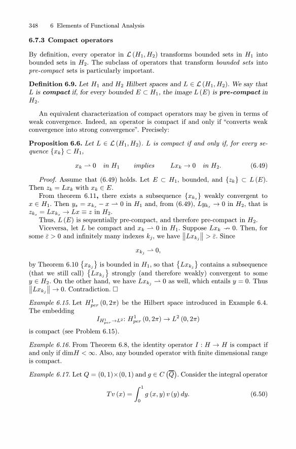
348 6 Elements of Functional Analysis
6.7.3 Compact operators
By definition, every operator in L (H1, H2) transforms bounded sets in H1 intobounded sets in H2. The subclass of operators that transform bounded sets intopre-compact sets is particularly important.
Definition 6.9. Let H1 and H2 Hilbert spaces and L ∈ L (H1, H2). We say thatL is compact if, for every bounded E ⊂ H1, the image L (E) is pre-compact inH2.
An equivalent characterization of compact operators may be given in terms ofweak convergence. Indeed, an operator is compact if and only if “converts weakconvergence into strong convergence”. Precisely:
Proposition 6.6. Let L ∈ L (H1, H2). L is compact if and only if, for every se-quence {xk} ⊂ H1,
xk ⇀ 0 in H1 implies Lxk → 0 in H2. (6.49)
Proof. Assume that (6.49) holds. Let E ⊂ H1, bounded, and {zk} ⊂ L (E).Then zk = Lxk with xk ∈ E.From theorem 6.11, there exists a subsequence {xks} weakly convergent to
x ∈ H1. Then ys = xks − x ⇀ 0 in H1 and, from (6.49), Lyks → 0 in H2, that iszks = Lxks → Lx ≡ z in H2.Thus, L (E) is sequentially pre-compact, and therefore pre-compact in H2.Viceversa, let L be compact and xk ⇀ 0 in H1. Suppose Lxk � 0. Then, for
some ε > 0 and infinitely many indexes kj, we have∥∥Lxkj
∥∥ > ε. Sincexkj ⇀ 0,
by Theorem 6.10{xkj}is bounded in H1, so that
{Lxkj
}contains a subsequence
(that we still call){Lxkj
}strongly (and therefore weakly) convergent to some
y ∈ H2. On the other hand, we have Lxkj ⇀ 0 as well, which entails y = 0. Thus∥∥Lxkj∥∥→ 0. Contradiction. �
Example 6.15. Let H1per (0, 2π) be the Hilbert space introduced in Example 6.4.The embedding
IH1per→L2 : H1per (0, 2π)→ L2 (0, 2π)
is compact (see Problem 6.15).
Example 6.16. From Theorem 6.8, the identity operator I : H → H is compact ifand only if dimH <∞. Also, any bounded operator with finite dimensional rangeis compact.
Example 6.17. Let Q = (0, 1)×(0, 1) and g ∈ C(Q). Consider the integral operator
Tv (x) =
∫ 10
g (x, y) v (y) dy. (6.50)

6.7 Compactness and Weak Convergence 349
We want to show that T is compact from L2 (0, 1) into L2 (0, 1). In fact, for everyx ∈ (0, 1), Schwarz’s inequality gives
|Tv (x)| ≤∫ 10
|g (x, y) v (y)|dy ≤ ‖g (x, ·)‖L2(0,1) ‖v‖L2(0,1) , (6.51)
whence ∫ 10
|Tv (x)|2 dx ≤ ‖g‖2L2(Q) ‖v‖2L2(0,1)
which implies that Tv ∈ L2 (0, 1) and that T is bounded.To check compactness, we use Proposition 6.7. Let {vk} ⊂ L2 (0, 1) such that
vk ⇀ 0, that is ∫ 10
vkw → 0, for every w ∈ L2 (0, 1) . (6.52)
We have to show that Tvk → 0 in L2 (0, 1). Being weakly convergent, {vk} isbounded so that
‖vk‖L2(0,1) ≤M, (6.53)
for some M and every k. From (6.51) we have
|Tvk (x)| ≤M ‖g (x, ·)‖L2(0,1) .
Moreover, inserting w (·) = g (x, ·) into (6.52), we infer that
Tvk (x) =
∫ 10
g (x, y) vk (y) dy → 0 for every x ∈ (0, 1) .
From the Dominated Convergence Theorem14 we infer that Tvk → 0 inL2 (0, 1). Therefore T is compact.
The following proposition is useful.
Proposition 6.7. Let L : H1 → H2 be compact. Then:a) L∗ : H2 → H1 is compact;b) if G ∈ L (H2, H3) or G ∈ L (H0, H1), the operator G◦L or L◦G is compact.
Proof . a). We use Proposition 6.7. Let {xk} ⊂ H2 and xk ⇀ 0. Let us showthat ‖L∗xk‖H1 → 0. We have:
‖L∗xk‖2H1 = (L∗xk, L∗xk)H1 = (xk, LL
∗xk)H2 .
Since L∗ ∈ L (H2, H1), we have
L∗xk ⇀ 014 Appendix B.

350 6 Elements of Functional Analysis
in H1 and the compactness of L entails LL∗xn → 0 in H2. Since ‖xk‖ ≤ M , we
finally have
‖L∗xk‖2H1 = (xk, LL∗xk)H2 ≤M ‖LL∗xk‖2H2 → 0.
b). We leave it as an exercise. �
6.8 The Fredholm Alternative
6.8.1 Solvability for abstract variational problems
Let us go back to the variational problem
a (u, v) = 〈F, v〉∗ ∀v ∈ V, (6.54)
and suppose that Lax-Milgram Theorem cannot be applied, since, for instance, ais not V−coercive. In this situation it may happen that the problem does not havea solution, unless certain compatibility conditions on F are satisfied. A typicalexample is given by the Neumann problem
{−Δu = f in Ω
∂νu = g on ∂Ω.
A necessary and sufficient solvability condition is given by.
∫
Ω
f +
∫
∂Ω
g = 0. (6.55)
Moreover, if (6.55) holds, there are infinitely many solutions, differing among eachother by an additive constant. Condition (6.55) has both a precise physical inter-pretation in terms of a resultant of forces at equilibrium and a deep mathematicalmeaning, with roots in Linear Algebra!
Indeed, the results we are going to present are extensions of well known factsconcerning the solvability of linear algebraic systems of the form
Ax = b (6.56)
where A is an n × n matrix and b ∈Rn. The following dichotomy holds: either(6.56) has a unique solution for every b or the homogeneous equation Ax = 0 hasnon trivial solutions.More precisely, system (6.56) is solvable if and only if b belongs to the column
space of A, which is the orthogonal complement of ker(A�). If w1, ...,ws spanker(A�), this amounts to asking the s compatibility conditions, 0 ≤ s ≤ n,
b ·wj = 0 j = 1, ..., s.

6.8 The Fredholm Alternative 351
Finally, ker (A) and ker(A�) have the same dimension and if v1, ...,vs spanker (A), the general solution of (6.56) is given by
x =x+
s∑j=1
cjvj
where x is a particular solution of (6.56) and c, ..., cs are arbitrary constants.The extension to infinite-dimensional spaces requires some care. In particular,
in order to state an analogous dichotomy theorem for the variational problem(6.54), we need to clarify the general setting, to avoid confusion.The problem involves two Hilbert spaces: V , the space where we seek the so-
lution, and V ∗, which the data F belongs to. Let us introduce a third space H ,intermediate between V and V ∗. In boundary value problems, usuallyH = L2 (Ω),with Ω bounded domain in Rn, while V is a Sobolev space. In practice, we oftenmeet a pair of Hilbert spaces V , H with the following properties:
1. V ↪→ H , i.e. V is continuously embedded in H. Recall that this simply meansthat the identity operator IV→H , from V intoH , is continuous or, equivalentlythat there exists C such that
‖u‖H ≤ C ‖u‖V ∀u ∈ V. (6.57)
2. V is dense in H .
Using Riesz’s Theorem, we may identify H with H∗. Also, we may continuouslyembed H into V ∗, so that any element in H can be thought as an element of V ∗.It is enough to observe that, for any fixed u ∈ H , the functional Tu defined by
〈Tu, v〉∗ = (u, v)H v ∈ V, (6.58)
is continuous in V . In fact, Schwarz’s inequality and (6.57) give
|(u, v)H | ≤ ‖u‖H ‖v‖H ≤ C ‖u‖H ‖v‖V . (6.59)
Then, we have a continuous map u→ Tu, from H into V ∗, with ‖Tu‖V ∗ ≤ C ‖u‖H .If Tu = 0 then
(u, v)H = 0 ∀v ∈ Vwhich forces u = 0, by the density of V in H .Thus, the map u �−→ Tu is one to one and defines a continuous embedding
IH→V ∗ . This allows the identification of u with an element of V ∗, which meansthat, instead of (6.58), we can write
〈u, v〉∗ = (u, v)H ∀v ∈ V,regarding u on the left as an element of V ∗ and on the right as an element of H .Finally, it can be shown that V and H are dense in V ∗. Thus, we have
V ↪→ H ↪→ V ∗
with dense embeddings. We call (V,H, V ∗) a Hilbert triplet.

352 6 Elements of Functional Analysis
This is the right setting. We use the symbols
(·, ·) = (·, ·)H , ‖·‖ = ‖·‖Hto denote inner product and norm in H , respectively, while 〈·, ·〉∗ = V ∗〈·, ·〉V isreserved for the duality between V ∗ and V .To state the main result we need to introduce weakly coercive forms and their
adjoints.
Definition 6.10. We say that the bilinear form a (u, v) is weakly coercive withrespect to the pair (V,H) if there exist λ0 ∈ R and α > 0 such that
a (v, v) + λ0 ‖v‖2 ≥ α ‖v‖2V ∀v ∈ V.
The adjoint form a∗ of a is given by
a∗ (u, v) = a (v, u) ,
obtained by interchanging the arguments in the analytical expression of a. In theapplications to boundary value problems, a∗ is associated with the so called formaladjoint of a differential operator (see subsection 8.5.1).We shall denote by N (a) and N (a∗), the set of solutions u and w, respectively,
of the variational problems
a (u, v) = 0, ∀v ∈ V and a∗ (w, v) = 0, ∀v ∈ V.
Observe that N (a) and N (a∗) are both subspaces of V , playing the role of kernelsfor a and a∗
Theorem 6.13. Let (V,H, V ∗) be a Hilbert triplet, with V compactly embeddedin H . Let F ∈ V ∗ and a be a bilinear form in V , continuous and weakly coercivewith respect to (V,H). Then:a) Either equation
a (u, v) = 〈F, v〉∗ ∀v ∈ V (6.60)
has a unique solution u and
‖u‖ ≤ C ‖F ‖V ∗ (6.61)
b) ordimN (a) = dimN (a∗) = d <∞.
and (6.60) is solvable if and only if 〈F, w〉∗ = 0 for every w ∈ N (a∗).The proof of Theorem 6.12 relies on a more general result, known as Fredholm’s
Alternative, presented in the next section.
Some comments are in order. The following dichotomy holds: either (6.60) hasa unique solution for every F ∈ V ∗ or the homogeneous equation a (u, v) = 0 hasnon trivial solutions. The same conclusions hold for the adjoint equation
a∗ (u, v) = 〈F, v〉∗, ∀v ∈ V.

6.8 The Fredholm Alternative 353
If w1, w2, ..., wd span N (a∗), (6.60) is solvable if and only if the d compatibilityconditions
〈F, wj〉∗ = 0, j = 1, ..., d
hold. In this case, equation (6.60) has infinitely many solutions given by
u = u+
d∑j=1
cjzj
where u is a particular solution of (6.60), z1, ..., zd span N (a) and c1, ..., cd arearbitrary constants.We shall apply Theorem 6.12 to boundary value problems in Chapter 8. Here
is however a preliminary example.
Example 6.18. Let V = H1per (0, 2π), H = L2 (0, 2π) and assume that w = w (t)
is a positive, continuous function in [0, 2π]. We know (Example 6.27) that V iscompactly embedded in H. Moreover, it can be shown that V is dense in H .Thus (V,H, V ∗) is a Hilbert triplet.Given f ∈ H , consider the variational problem
∫ 2π0
u′v′wdt =∫ 2π0
fv dt, ∀v ∈ V. (6.62)
The bilinear form a (u, v) =∫ 2π0 u
′v′wdt is continuous in V but it is not V −coercive.In fact
|a (u, v)| ≤ wmax ‖u′‖0 ‖v′‖0 ≤ wmax ‖u‖1 ‖v‖1 ,but a (u, u) = 0 if u is constant. However it is weakly coercive with respect to(V,H), since
a (u, u) + ‖u‖20 =∫ 2π0
(u′)2wdt+∫ 2π0
u2dt ≥ min{wmin, 1} ‖u‖21,2 .
Moreover, ∣∣∣∣∫ 2π0
fv dt
∣∣∣∣ ≤ ‖f‖0 ‖v‖0 ≤ ‖f‖0 ‖v‖1,2
hence the functional F : v �→∫ 2π0fv dt defines an element of V ∗.
We are under the hypotheses of Theorem 6.12. The bilinear form is symmetric,so that N (a) = N (a∗). The solutions of the homogeneous equation
a (u, v) =
∫ 2π0
u′v′wdt = 0, ∀v ∈ V (6.63)
are the constant functions. In fact, letting v = u in (6.63) we obtain
∫ 2π0
(u′)2wdt = 0
354 6 Elements of Functional Analysis
which forces u (t) ≡ c, constant, since w > 0. Then, dimN (a) = 1. Thus, fromTheorem 6.11 we can draw the following conclusions: equation (6.62) is solvable ifand only if
〈F, 1〉∗ =∫ 2π0
fdt = 0.
Moreover, in this case, (6.62) has infinitely many solutions of the form u = u+ c.The variational problem has a simple interpretation as a boundary value prob-
lem. By an integration by parts, recalling that v (0) = v (2π), we may rewrite(6.62) as
∫ 2π0
[(−wu′)′ − f ]vdt + v (0) [w (2π)u′ (2π)− w (0)u′ (0)] = 0, ∀v ∈ V.
Choosing v vanishing at 0 we are left with
∫ 2π0
[−(wu′)′ − f ]vdt = 0, ∀v ∈ V , v (0) = v (2π) = 0.
which forces(u′w)′ = −f.
Thenv (0) [w (2π)u′ (2π)− w (0)u′ (0)] = 0, ∀v ∈ V
which, in turn, forcesw (2π)u′ (2π) = w (0)u′ (0) .
Thus, problem (6.62) constitutes the variational formulation of the followingboundary value problem:
⎧⎨⎩(wu′)′ = −f in (0, 2π)u (0) = u (2π)w (2π)u′ (2π) = w (0)u′ (0) .
It is important to point out that the periodicity condition u (0) = u (2π) is forcedby the choice of the space V while the Neuman type periodicity condition is en-coded in the variational equation (6.62).
6.8.2 Fredholm’s Alternative
We introduce some terminology. Let V1, V2 Hilbert spaces and Φ : V1 → V2. Wesay that Φ is a Fredholm operator if N (Φ) and R (Φ)⊥ have finite dimension. Theindex of Φ is the integer
ind (Φ) = dimN (Φ)− dimR (Φ)⊥ = dimN (Φ)− dimN (Φ∗) .
We have15:
15 For the proof, see e.g. Brezis, 1983.

6.8 The Fredholm Alternative 355
Theorem 6.14. (Fredholm′s Alternative). Let V be a Hilbert space and K ∈L (V ) be a compact operator. Then
Φ = I −K
is a Fredholm operator with zero index. Moreover Φ∗ = I −K∗,
R (Φ) = N (Φ∗)⊥ (6.64)
and
N (Φ) = {0} ⇐⇒ R (Φ) = V. (6.65)
The last formula shows that Φ is one-to-one if and only if it is onto. In otherwords, uniqueness for the equation
x−Kx = f (6.66)
is equivalent to existence for every f ∈ V and viceversa. The same thing holds forthe adjoint Φ∗ = I −K∗ and the associated equation
y −K∗y = g.
Let d = dimR (Φ)⊥ = dimN (Φ∗) > 0. Then, (6.64) says that equation (6.66)is solvable if and only if f ⊥ N (Φ∗), that is, if and only if (f, y) = 0 for everysolution y of
y −K∗y = 0. (6.67)
If y1, y2, ..., yd span N (Φ∗), this amounts to asking the d compatibility relations
(f, yj) = 0, j = 1, ..., d
as necessary and sufficient conditions for the solvability of (6.66).
Remark 6.14. Clearly, Theorem 6.13 holds for operators K − λI with λ �= 0. Thecase λ = 0 cannot be included. Trivially, for the operator K = 0 (which is com-pact), we have N (K) = V , hence, if dimV = ∞, Theorem 6.13 does not hold. Amore significant example is the one-dimensional range operator
Kx = L (x)x0
where L ∈ L (V ) and x0 is fixed in V . Assume dimV =∞. From Riesz’s Theorem,there exists z ∈ V such that Lx = (z, x) for every x ∈ V . Thus, N (K) is givenby the subspace of the elements in V orthogonal to z, which has infinitely manydimensions.
• Proof of Theorem 6.12 (sketch). The strategy is to write equation
a (u, v) = 〈F, v〉∗ (6.68)

356 6 Elements of Functional Analysis
in the form(IV −K)u = g.
where IV is the identity operator in V and K : V → V is compact.Let J : V → V ∗ the embedding of V into V ∗. Recall that J is the composition
of the embeddings IV→H and IH→V ∗ . Since IV→H is compact and IH→V ∗ is con-tinuous, we infer from Proposition 6.8 that J is compact. We write (6.68) in theform
aλ0 (u, v) ≡ a (u, v) + λ0 (u, v)H = 〈λ0Ju+ F, v〉∗where λ0 > 0 is such that aλ0 (u, v) is coercive. Since, for fixed u ∈ V , the linearmap
v �→ aλ0 (u, v)is continuous in V , there exists L ∈ L (V, V ∗) such that
〈Lu, v〉∗ = aλ0 (u, v) ∀u, v ∈ V.
Thus, equation a (u, v) = 〈F, v〉∗ is equivalent to
〈Lu, v〉∗ = 〈λ0Ju+ F, v〉∗ ∀v ∈ V
and therefore toLu = λ0Ju+ F. (6.69)
Since aλ0 is V−coercive, from the Lax-Milgram Theorem, the operator L is anisomorphism between V and V ∗ and (6.69) can be written in the form
u− λ0L−1Ju = L−1F.
Letting g = L−1F ∈ V and K = λ0L−1J , (6.69) becomes
(IV −K)u = g.
where K:V → V.Since J is compact and L−1 is continuous, K is compact (Proposition 6.8).
Applying the Fredholm Alternative Theorem and rephrasing the conclusions interms of bilinear forms we conclude the proof16. �
6.9 Spectral Theory for Symmetric Bilinear Forms
6.9.1 Spectrum of a matrix
Let A be an n× n matrix and λ ∈ C. Then, either the equation
Ax−λx = b16 We omit the rather long and technical details.

6.9 Spectral Theory for Symmetric Bilinear Forms 357
has a unique solution for every b or there exists u �= 0 such that
Au =λu.
In the last case we say that λ,u constitutes an eigenvalue-eigenvector pair. Theset of eigenvalues of A is called spectrum of A, denoted by σP (A). If λ /∈ σP (A)the resolvent matrix (A−λI)−1 is well defined. The set
ρ (A) = C\σP (A)
is called the resolvent of A. If λ ∈ σP (A), the kernel N (A−λI) is the subspacespanned by the eigenvectors corresponding to λ and it is called the eigenspace ofλ. Note that σP (A) = σP (A
ᵀ).The symmetric matrices are particularly important: all the eigenvalues λ1, ...λn
are real (possibly of multiplicity greater than 1) and there exists in Rn an orthonor-mal basis of eigenvectors u1, ...,un.We are going to extend these concepts in the Hilbert space setting. A motivation
is .... the method of separation of variables.
6.9.2 Separation of variables revisited
Using the method of separation of variables, in the first chapters we have con-structed solutions of boundary value problems by superposition of special solu-tions. However, explicit computations can be performed only when the geometryof the relevant domain is quite particular. What may we say in general? Let usconsider an example from diffusion.Suppose we have to solve the problem
⎧⎨⎩ut = Δu (x, y) ∈ Ω, t > 0u (x, y, 0) = g (x, y) (x, y) ∈ Ωu (x, y, t) = 0 (x, y) ∈ ∂Ω, t > 0
where Ω is a bounded bi-dimensional domain. Let us look for solutions of the form
u (x, y, t) = v (x, y)w (t) .
Substituting into the differential equation, with some elementary manipulations,we obtain
w′ (t)w (t)
=Δv (x, y)
v (x, y)= −λ,
where λ is a constant, which leads to the two problems
w′ + λw = 0 t > 0 (6.70)
and {−Δv = λv in Ωv = 0 on ∂Ω.
(6.71)

358 6 Elements of Functional Analysis
A number λ such that there exists a non trivial solution v of (6.71) is called aDirichlet eigenvalue of the operator −Δ in Ω and v is a corresponding eigen-function. Now, the original problem can be solved if the following two propertieshold:
a) There exists a sequence of (real) eigenvalues λk with corresponding eigen-vectors uk. Solving (6.70) for λ = λk yields
wk (t) = ce−λkt c ∈ R.
b) The initial data g can be expanded is series of eigenfunctions:
u(x, y) =∑gkuk (x, y) .
Then, the solution is given by
u (x, y, t) =∑gke
−λktuk (x, y)
where the series converges in some suitable sense.
Condition b) requires that the set of Dirichlet eigenfunctions of −Δ constitutesa basis in the space of initial data. This leads to the problem of determining thespectrum of a linear operator in a Hilbert space and, in particular, of self-adjointcompact operators. Indeed, it turns out that the solution map of a symmetricvariational boundary value problem is often a self-adjoint compact operator. Wewill go back to the above problem in subsection 8.4.3.
6.9.3 Spectrum of a compact self-adjoint operator
We define resolvent and spectrum for a bounded linear operator. Although thenatural setting is the complex field C, we limit ourselves to R, mainly for simplicitybut also because this is the interesting case for us.
Definition 6.11. Let H be a Hilbert space, L ∈ L (H), and I the identity in H .a) The resolvent set ρ (L) of L is the set of real numbers λ such that L− λI is
one-to-one and onto:
ρ (L) = {λ ∈ R: L − λI is one-to-one and onto} .
b) The (real) spectrum σ (L) of L is
σ (L) = R\ρ (L) .
Remark 6.15. If λ ∈ ρ (L), the resolvent (L − λI)−1 is bounded17.17 It is a consequence of the Closed Graph Theorem: If the graph of a linear operatorA : H1 → H2 is closed in H1 ×H2 then A is bounded.

6.9 Spectral Theory for Symmetric Bilinear Forms 359
IfH has finite dimension, any linear operator is represented by a matrix, so thatits spectrum is given by the set of its eigenvalues. In infinitely many dimensionsthe spectrum may be divided in three subsets. In fact, if λ ∈ σ (L), different thingscan go wrong with (L − λI)−1.First of all, it may happen that L − λI is not one-to-one so that (L− λI)−1
does not even exist. This means that N (L − λI ) �= ∅, i.e. that the equation
Lx = λx (6.72)
has non trivial solutions. Then, we say that λ is an eigenvalue of L and that thenon zero solutions of (6.72) are the eigenvectors corresponding to λ. The linearspace spanned by these eigenvectors is called the eigenspace of λ and denoted byN (L− λI ).
Definition 6.12. The set σP (L) of the eigenvalues of L is called the point spec-trum of L.
Other things can occur. L − λI is one-to-one, R(L − λI ) is dense in H , but(L−λI)−1 is unbounded. Then, we say that λ belongs to the continuous spectrumof L, denoted by σC (L) .Finally, L − λI is one-to-one but R(L − λI ) is not dense in H. This defines
the residual spectrum of L.
Example 6.19. Let H = l2 and L : l2 → l2 be the shift operator which mapsx = {x1, x2, ...} ∈ l2 into y = {0, x1, x2, ...}. We have
(L − λI)x = {−λx1, x1 − λx2, x2 − λx3, ...} .
If λ �= 0, then λ ∈ ρ (L). In fact for every z = {z1, z2, ...} ∈ l2,
(L − λI)−1 z ={−z1λ,−z2λ+z1
λ2, ...
}.
Since R(L) contains only sequences whose first element is zero, R(L) is not densein l2, therefore 0 ∈ σR (L) = σ (L).
We are mainly interested in the spectrum of a compact self-adjoint operator.The following theorem is fundamental18.
Theorem 6.15. Let K be a compact, self-adjoint operator on a separable Hilbertspace H. Then:
a) 0 ∈ σ (K) and σ (K) \ {0} = σP (K) \ {0}.b) H has an orthonormal basis {um} consisting of eigenvectors for K.c) If dim H =∞, the corresponding eigenvalues different from zero {λm} can
be arranged in a decreasing sequence |λ1| ≥ |λ2| ≥ · · · , with λm → 0, as m→∞.18 For the proof, see Brezis, 1983.

360 6 Elements of Functional Analysis
Thus, the spectrum of a compact self-adjoint operator contains always λ = 0,which is not necessarily an eigenvalue. The other elements in σ (L) are eigenvalues,arranged in a sequence converging to zero if H is infinite dimensional.If λ �= 0 is an eigenvalue, Fredholm’s Alternative applies to L− λI, so that, in
particular, the eigenspace N (L − λI) has finite dimension.A consequence of Theorem 6.15 is the spectral decomposition formula forK. If
x ∈ H and {um}m≥1 is an orthonormal set of eigenvectors corresponding to allnon-zero eigenvalues {λm}m≥1, we can describe the action of K as follows:
Kx =∑m≥1(Kx, um)um =
∑m≥1λm (x, um)um, ∀x ∈ H . (6.73)
6.9.4 Application to abstract variational problems
We now apply theorems 6.13 and 6.14 to our abstract variational problems. Thesetting is the same of theorem 6.12, given by a Hilbert triplet (V,H, V ∗), withcompact embedding of V into H . We assume that H is also separable. Let a be abilinear form in V , continuous and weakly coercive; in particular:
aλ0 (u, v) ≡ a (v, v) + λ0 ‖v‖2 ≥ α ‖v‖2V ∀v ∈ V
The notion of resolvent and spectrum can be easily defined. Consider the problem
a (u, v) = λ (u, v) + 〈F, v〉∗ ∀v ∈ V. (6.74)
The resolvent ρ (a) is the set of real numbers λ such that (6.74) has a uniquesolution u (F ) ∈ V for every F ∈ V ∗ and the solution map
Sλ : F �−→ u (F )
is an isomorphism between V ∗ and V .The (real) spectrum is σ (a) = R\ρ (a), while the point spectrum σP (a) is the
subset of the spectrum given by the eigenvalues, i.e. the numbers λ such that thehomogeneous problem
a (u, v) = λ (u, v) ∀v ∈ V (6.75)
has non-trivial solutions (eigenfunctions). We call eigenspace of λ the spacespanned by the corresponding eigenfunctions and we denote it by N (a, λ).The following theorem is a consequence of the Fredholm Alternative and The-
orem 7.4. and it is based on the following relation between σP (Sλ0) and σP (aλ0).Note that 0 /∈ σ (Sλ0) and that σ (aλ0 ) ⊂ (0,+∞).Let μ ∈ σP (Sλ0) and f be a corresponding eigenvector, that is,
Sλ0f = μf.

6.9 Spectral Theory for Symmetric Bilinear Forms 361
Thus, necessarily f ∈ V and
aλ0 (Sλ0f, v) = μaλ0 (f, v) = (f, v)
or
aλ0 (f, v) =1
μ(f, v)
for all v ∈ V . Therefore λ = 1/μ is an eigenvalue of aλ0 , with the same eigenspace.As a consequence
N (aλ0 ) = N (Sλ0 ) ⊂ V.Moreover, since the eigenvalues of aλ0 are all positive, if follows that μ > 0 as well.
Theorem 6.16. Let (V,H, V ∗) be a Hilbert triplet with H separable and V com-pactly embedded in H. Let F ∈ V ∗ and a be a symmetric bilinear form in V,continuous and weakly coercive. We have:
(a) σ (a) = σP (a) ⊂ (−λ0,+∞).Moreover, if the sequence of eigenvalues {λm}is infinite, then λm → +∞.(b) If u, v are eigenfunctions corresponding to different eigenvalues, then
a (u, v) = (u, v) = 0. Moreover, H has an orthonormal basis of eigenvectors um.
(c){um/
√λm + λ0
}constitutes an orthonormal basis in V , with respect to
the scalar product
((u, v)) = a (u, v) + λ0 (u, v) . (6.76)
Proof. By hypothesis, Sλ0 is an isomorphism between V∗ and V . In particular,
it is well defined as a map from H into V ⊂ H . Since the embedding of V inH is compact, then Sλ0 is compact as an operator from H into H . Also, by thesymmetry of a, Sλ0 is selfadjoint, that is
(Sλ0f, g) = (f, Sλ0g) for all f, g ∈ H .
In fact, let u = Sλ0f and w = Sλ0g. Then, for every v ∈ V ,
aλ0 (u, v) = (f, v) and aλ0 (w, v) = (g, v) .
In particular,
aλ0 (u, w) = (f, w) and aλ0 (w, u) = (g, u)
so that, since aλ0 (u, w) = aλ0 (w, u) and (g, u) = (u, g), we can write
(Sλ0f, g) = (u, g) = (f, w) = (f, Sλ0g) .
Since 0 /∈ σ (Sλ0), from Theorem 6.15 it follows that σ (Sλ0) = σP (Sλ0) andthe eigenvalues form a sequence {μm} with μm ↓ 0. Using Theorem 6.15 and therelation between σP (Sλ0) and σP (aλ0), (a) and (b) follow easily.

362 6 Elements of Functional Analysis
Finally if {um} is an orthonormal basis of eigenvectors for a in H , then19
a (um, uk) = λm (um, uk) = λmδmk
so that((um, uk)) ≡ aλ0 (um, uk) = (λm + λ0) δmk
which easily gives (c). �
Problems
6.1. Heisenberg Uncertainty Principle. Let ψ ∈ C1 (R) such that x [ψ (x)]2 → 0as |x| → ∞ and
∫R[ψ (x)]
2dx = 1. Show that
1 ≤ 2∫
R
x2 |ψ (x)|2 dx∫
R
∣∣ψ′ (x)∣∣2 dx.
(If ψ is a Schrodinger wave function, the first factor in the right hand sidemeasures the spread of the density of a particle, while the second one measuresthe spread of its momentum).
6.2. Let H be a Hilbert space and a (u, v) be a symmetric and non negativebilinear form in H :
a (u, v) = a (v, u) and a (u, v) ≥ 0 ∀u, v ∈ H .Show that
|a (u, v)| ≤√a (u, u)
√a (v, v).
[Hint. Mimic the proof of Schwarz’s inequality].
6.3. Show the completeness of l2.
[Hint. Take a Cauchy sequence{xk}where xk =
{xkm}. In particular,
∣∣xkm − xhm∣∣→
0 as h, k → ∞ and therefore xhm → xm for every m. Define x = {xm} and showthat xk → x in l2].6.4. LetH be a Hilbert space and V a closed subspace ofH . Show that u = PV x
if and only if {1. u ∈ V2. (x− u, v) = 0, ∀v ∈ V.
6.5. Let f ∈ L2 (−1, 1). Find the polynomial of degree ≤ n that gives thebest approximation of f in the least squares sense, that is, the polynomial p thatminimizes ∫ 1
−1(f − q)2
among all polynomials q with degree ≤ n.19 δmk is Kronecker symbol.

Problems 363
[Answer: p (x) = a0L0 (x) + a1L1 (x) + ... + anLn (x), where Ln is the n − thLegendre polynomials and aj = (n+ 1/2) (f, Ln)L2(−1,1)].
6.6. Hermite’s equation and the quantum mechanics harmonic oscillator. Con-sider the equation
w′′ +(2λ+ 1− x2
)w = 0 x ∈ R (6.77)
with w (x)→ 0 as x→ ±∞.a) Show that the change of variables z = wex
2/2 transforms (6.77) into Her-mite’s equation for z :
z′′ − 2xz′ + 2λz = 0with e−x
2/2z (x)→ 0 as x→ ±∞.b) Consider the Schrodinger wave equation for the harmonic oscillator
ψ′′ +8π2m
h2(E − 2π2mν2x2
)ψ = 0 x ∈ R
where m is the mass of the particle, E is the total energy, h is the Plank constantand ν is the vibrational frequency. The physically admissible solutions are thosesatisfying the following conditions:
ψ → 0 as x→ ±∞ and ‖ψ‖L2(R) = 1.
Show that there is a solution if and only if
E = hν
(n+1
2
)n = 0, 1, 2....
and, for each n, the corresponding solution is given by
ψn (x) = knHn
(2π√νm/hx
)exp
(−2π
2νm
hx2)
where kn =
(4πνm
22n (n!)2h
)1/2and Hn is the n − th Hermite polynomial.
6.7. Using separation of variables, solve the following steady state diffusionproblem in three dimensions (r, θ, ϕ spherical coordinates, 0 ≤ θ ≤ 2π, 0 ≤ ϕ ≤ π):
{Δu = 0 r < 1, 0 < ϕ < π
u (1, ϕ) = g (ϕ) 0 ≤ ϕ ≤ π.
[Answer:
u (r, ϕ) =
∞∑n=0
anrnLn (cosϕ) ,

364 6 Elements of Functional Analysis
where Ln is the n− th Legendre polynomial and
an =2n+ 1
2
∫ 1−1g(cos−1 x
)Ln (x) dx.
At a certain point, the change of variable x = cosϕ is required].
6.8. The vertical displacement u of a circular membrane of radius a satisfiesthe bidimensional wave equation utt = Δu, with boundary condition u (a, θ, t) = 0.Supposing the membrane initially at rest, write a formal solution of the problem.
[Hint:
u (r,θ, t) =
∞∑p,j=0
Jp (αpjr) {Apj cos pθ+ Bpj sin pθ} cos(√αpjt)
where the coefficients Apj and Bpj are determined by the expansion of the initialcondition u (r, θ, 0) = g (r, θ)].
6.9. In calculus, we say that f : Rn → R is differentiable at x0 if there existsa linear mapping L : Rn → R such that
f (x0 + h)− f (x0) = Lh+o (‖h‖) as h→ 0.
Determine the Riesz elements associated with L, with respect to the inner prod-ucts:
a) (x,y) = x · y =∑nj=1 xjyj , b) (x,y)A = Ax · y =
∑ni,j=1 aijxiyj ,
where A = (aij) is a positive and symmetric matrix (see Example 6.3).
6.10. Prove Proposition 6.5.
[Hint. First show that‖L∗‖L(H2,H1) ≤ ‖L‖L(H1,H2)
and then that L∗∗ = L. Reverse the role of L and L∗ to show that ‖L∗‖L(H2,H1) ≥‖L‖L(H1,H2)].6.11. Prove Necas Theorem 6.6.
[Hint. Try to follow the same steps in the proof of the Lax-Milgram Theorem].
6.12. Let E ⊂ X, X Banach space. Prove the following facts:a) If E is compact, then it is closed and bounded.
b) Let E ⊂ F and F be compact; if E closed then E is compact.6.13. Projection on a closed convex set. Let H be a Hilbert space and E ⊂ H ,
closed and convex.a) Show that, for every x ∈ H , there is a unique element PEx ∈ E (the
projection of x on E) such that
‖PEx− x‖ = infv∈E
‖v − x‖ . (6.78)

Problems 365
b) Show that x∗ = PEx if and only if
(x∗ − x, v − x∗) ≥ 0 for every v ∈ E. (6.79)
c) Give a geometrical interpretation of (6.79).
[Hint. a) Follow the proof of the Projection Theorem 6.2. b) Let 0 ≤ t ≤ 1 anddefine
ϕ (t) = ‖x∗ + t(v − x∗)− x‖2 v ∈ E.Show that x∗ = PEx if and only if ϕ′ (0) ≥ 0. Check that ϕ′ (0) ≥ 0 is equivalentto (6.79)].
6.14. Let H be a Hilbert space and E ⊂ H be closed and convex. Show thatE is weakly closed.
[Hint. Let {xk} ⊂ E such that xk ⇀ x. Use (6.79) to show that PEx = x, so thatx ∈ E].6.15. Show that the embedding of H1per (0, 2π) into L
2 (0, 2π) is compact.
[Hint. Let {uk} ⊂ H1per (0, 2π) with
‖uk‖2 =∑m∈Z
(1 +m2
)|ukm|2 < M.
Show that, by a diagonal process, it is possible to select indexes kj such that, foreach m, ukjm converges to some number Um. Let
u (x) =∑m∈ZUme
imx
and show that ukj → u in L2 (0, 2π)].9.16. Let L : L2 (R) → L2 (R) be defined by Lv (x) = v (−x) . Show that
σ (L) = σP (L) = {1}.6.17. Let V and W be two closed subspaces of a Hilbert space H , with inner
product (·, ·). Let x0 ∈ H and define the following sequence of projections (seeFig. 6.3):
x2n+1 = PW (x2n), x2n+2 = PV (x2n+1) , n ≥ 0.
Prove that:
(a) If V ∩W = {0} then xn → 0.(b) If V ∩W �= {0}, then xn → PV ∩W (x0)
by filling in the details in the following steps.
1. Observe that‖xn+1‖2 = (xn+1, xn) .
Computing ‖xn+1 − xn‖2, show that ‖xn‖ is decreasing (hence ‖xn‖ ↓ l ≥ 0) and‖xn+1 − xn‖ → 0.
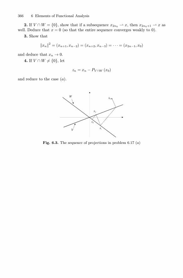
366 6 Elements of Functional Analysis
2. If V ∩W = {0}, show that if a subsequence x2nk ⇀ x, then x2nk+1 ⇀ x aswell. Deduce that x = 0 (so that the entire sequence converges weakly to 0).
3. Show that
‖xn‖2 = (xn+1, xn−2) = (xn+2, xn−3) = · · · = (x2n−1, x0)
and deduce that xn → 0.4. If V ∩W �= {0}, let
zn = xn − PV ∩W (x0)
and reduce to the case (a).
Fig. 6.3. The sequence of projections in problem 6.17 (a)

7
Distributions and Sobolev Spaces
Distributions. Preliminary Ideas – Test Functions and Mollifiers – Distributions – Calcu-
lus – Multiplication, Composition, Division, Convolution – Fourier Transform – Sobolev
Spaces – Approximations by Smooth Functions and Extensions – Traces – Compactness
and Embeddings – Spaces Involving Time
7.1 Distributions. Preliminary Ideas
We have seen the concept of Dirac measure arising in connection with the fun-damental solutions of the diffusion and the wave equations. Another interestingsituation is the following, where the Dirac measure models a mechanical impulse.
Fig. 7.1. Elastic collision at time t = t0
Consider a mass m moving along the x−axis with constant speed vi (seeFig. 7.1). At time t = t0 an elastic collision with a vertical wall occurs. Afterthe collision, the mass moves with opposite speed −vi. If v2, v1 denote the scalarspeeds at times t1, t2, t1 < t2, by the laws of mechanics we should have
m(v2 − v1) =∫ t2
t1
F (t) dt,
Salsa S. Partial Differential Equations in Action: From Modelling to Theoryc© Springer-Verlag 2008, Milan

368 7 Distributions and Sobolev Spaces
where F denotes the intensity of the force acting on m. When t1 < t2 < t0 ort0 < t1 < t2, then v2 = v1 = v or v2 = v1 = −v and therefore F = 0: no forceis acting on m before and after the collision. However, if t1 < t0 < t2, the lefthand side is equal to 2mv �= 0. If we insist to model the intensity of the force by afunction F , the integral in the right hand side is zero and we obtain a contradiction.
Indeed, in this case, F is a force concentrated at time t0, of intensity 2mv, thatis
F (t) = 2mv δ (t− t0) .
In this chapter we see how the Dirac delta is perfectly included in the theory ofdistributions or Schwartz generalized functions. We already mentioned in subsec-tion 2.3.3 that the key idea in this theory is to describe a mathematical objectthrough its action on smooth test functions ϕ, with compact support. In the caseof the Dirac δ, such action is expressed by the formula (see Definition 2.2)
∫δ (x)ϕ (x) dx = ϕ (0)
where, we recall, the integral symbol is purely formal. As we shall shortly see, theappropriate notation is 〈δ, ϕ〉 = ϕ (0).Of course, by a principle of coherence, among the generalized functions we
should be able to recover the usual functions of Analysis. This fact implies thatthe choice of the test functions cannot be arbitrary. In fact, let Ω ⊆ R
n be adomain and take for instance a function u ∈ L2 (Ω). A natural way to define theaction of u on a test ϕ is
〈u, ϕ〉 = (u, ϕ)0 =∫
Ω
uϕ dx.
If we let ϕ be varying over all L2 (Ω), we know from the last chapter, that 〈u, ϕ〉identifies uniquely u. Indeed, if v ∈ L2 (Ω) is such that 〈u, ϕ〉 = 〈v, ϕ〉 for everyϕ ∈ L2 (Ω), we have
0 = 〈u− v, ϕ〉 =∫
Ω
(u− v)ϕ dx ∀ϕ ∈ L2 (Ω) (7.1)
which forces (why?) u = v a.e. in Ω.
On the other hand, we cannot use L2−functions as test functions since, forinstance, 〈δ, ϕ〉 = ϕ (0) does not have any meaning.We ask: is it possible to reconstruct u from the knowledge of (u, ϕ)0, when ϕ
varies on a set of nice functions?
Certainly this is impossible if we use only a restricted set of test functions.However, it is possible to recover u from the value of (u, ϕ)0, when ϕ varies in adense set in L2 (Ω). In fact, let (u, ϕ)0 = (v, ϕ)0 for every test function. Givenψ ∈ L2 (Ω), there exists a sequence of test functions {ϕk} such that ‖ϕk − ψ‖0 →

7.2 Test Functions and Mollifiers 369
0. Then1,
0 =
∫
Ω
(u− v)ϕk dx→∫
Ω
(u− v)ψ dx
so that (7.1) still holds for every ψ ∈ L2 (Ω) and (u, ϕ)0 identifies a unique elementin L2 (Ω).
Thus, the set of test functions must be dense in L2 (Ω) if we want L2−functionsto be seen as distributions. In the next section we construct an appropriate set oftest functions.However, the main purpose of introducing the Schwartz distributions is not re-
stricted to a mere extension of the notion of function but it relies on the possibilityof broadening the domain of calculus in a significant way, opening the door to anenormous amount of new applications. Here the key idea is to use integration byparts to carry the derivatives onto the test functions. Actually, this is not a newprocedure. For instance, we have used it in subsection 2.3.3, when have interpretedthe Dirac delta at x = 0 as the derivative of the Heaviside function H, (see formula(2.63) and footnote 24).Also, the weakening of the notion of solution of conservation laws (subsection
4.4.2) or of the wave equation (subsection 5.4.2) follows more or less the samepattern.
In the first part of this chapter we give the basic concepts of the theory ofSchwartz distributions, mainly finalized to the introduction of Sobolev spaces.The basic reference is the book of L. Schwartz, 1966, to which we refer for theproofs we do not present here.
7.2 Test Functions and Mollifiers
Recall that, given a continuous function v, defined in a domain Ω ⊆ Rn, the
support of v is given by the closure of the set of points where v is different fromzero:
supp(v) = Ω ∩ closure of {x ∈Ω : v (x) �= 0} .Actually, the support or, better, the essential support, is defined also for measurablefunctions, not necessarily continuous in Ω. Namely, let Z be the union of the opensets on which v = 0 a.e. Then, Ω\Z is called the essential support of v and we usethe same symbol supp(v) to denote it.
We say that v is compactly supported in Ω, if supp(v) is a compact subset of Ω.
Definition 7.1. Denote by C∞0 (Ω) the set of functions belonging to C∞ (Ω),compactly supported in Ω. We call test functions the elements of C∞0 (Ω) .
1 From ∣∣∣∣
∫
Ω
(u− v) (ϕk − ψ) dx∣∣∣∣ ≤ ‖u− v‖0 ‖ϕk − ψ‖0 .

370 7 Distributions and Sobolev Spaces
Example 7.1. The reader can easily check that the function given by
η (x) =
{c exp
(1
|x|2−1)0 ≤ |x| < 1
0 |x| ≥ 1 (c ∈ R). (7.2)
belongs to C∞0 (Ω).
The function (7.2) is a typical and important example of test function. Indeed,we will see below that many other test functions can be generated by convolutionwith (7.2).Let us briefly recall the definition and the main properties of the convolution
of two functions. Given two functions u and v defined in Rn, the convolution u ∗ vof u and v is given by the formula:
(u ∗ v) (x) =∫
Rn
u (x − y) v (y) dy =∫
Rn
u (y) v (x− y) dy.
It can be proved that (Young’s Theorem): if u ∈ Lp(Rn) and v ∈ Lq(Rn), p, q ∈[1,∞], then u ∗ v ∈ Lr(Rn) where 1r = 1
p +1q − 1 and
‖u ∗ v‖Lr(Rn) ≤ ‖u‖Lp(Rn) ‖u‖Lq(Rn) .
The convolution is a very useful device to regularize “wild functions”. Indeed,consider the function η defined in (7.2). We have:
η ≥ 0 and supp (η) = B1 (0)
where, we recall, BR (0) = {x ∈ Rn: |x| < R}. Choose
c =
(∫
B1(0)
exp
(1
|x|2 − 1
)dx
)−1
so that∫Rnη = 1. Set, for ε > 0,
ηε (x) =1
εnη
( |x|ε
). (7.3)
This function belongs to C∞0 (Rn) (and therefore to all Lp (Rn)), with supportequal to Bε (0), and still
∫Rnηε = 1.
Let now f ∈ Lp(Ω). If we set f ≡ 0 outside Ω, we obtain a function in Lp(Rn),still denoted by f , for which the convolution f ∗ ηε is well defined in all Rn:
fε (x) = (f ∗ ηε) (x) =∫
Ω
ηε (x− y) f (y) dy
=
∫
Bε(0)
η (z) f (x − z) dz.
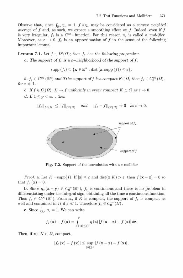
7.2 Test Functions and Mollifiers 371
Observe that, since∫Rnηε = 1, f ∗ ηε may be considered as a convex weighted
average of f and, as such, we expect a smoothing effect on f . Indeed, even if fis very irregular, fε is a C
∞−function. For this reason ηε is called a mollifier.Moreover, as ε → 0, fε is an approximation of f in the sense of the followingimportant lemma.
Lemma 7.1. Let f ∈ Lp(Ω); then fε has the following properties:a. The support of fε is a ε−neighborhood of the support of f:
supp (fε) ⊆ {x ∈ Rn : dist (x, supp (f)) ≤ ε} .
b. fε ∈ C∞ (Rn) and if the support of f is a compactK⊂Ω, then fε ∈ C∞0 (Ω) ,for ε� 1.c. If f ∈ C (Ω), fε → f uniformly in every compact K ⊂ Ω as ε→ 0.d. If 1 ≤ p <∞ , then
‖fε‖Lp(Ω) ≤ ‖f‖Lp(Ω) and ‖fε − f‖Lp(Ω) → 0 as ε→ 0.
Fig. 7.2. Support of the convolution with a ε-mollifier
Proof. a. Let K =supp(f). If |z| ≤ ε and dist(x,K) > ε, then f (x− z) = 0 sothat fε (x) = 0.
b. Since ηε (x − y) ∈ C∞0 (Rn), fε is continuous and there is no problem indifferentiating under the integral sign, obtaining all the time a continuous function.Thus fε ∈ C∞ (Rn). From a., if K is compact, the support of fε is compact aswell and contained in Ω if ε� 1. Therefore fε ∈ C∞0 (Ω) .c. Since
∫Rnηε = 1, We can write
fε (x)− f (x) =∫
{|z|≤ε}η (z) [f (x − z) − f (x)] dz.
Then, if x ∈K ⊂ Ω, compact,
|fε (x) − f (x)| ≤ sup|z|≤ε
|f (x− z)− f (x)| .

372 7 Distributions and Sobolev Spaces
Since f is uniformly continuous inK we have that sup|z|≤ε |f (x − z)− f (x)| → 0,uniformly in x, as ε→ 0. Thus fε → f uniformly in K.d. From Holder’s inequality, we have, for q = p/ (p− 1),
fε (x) =
∫
Ω
ηε (x− y) f (y) dy =∫
Ω
ηε (x− y)1/q ηε (x − y)1/p f (y) dy
≤(∫
Ω
ηε (x− y) |f (y)|p dy)1/p
.
This inequality and Fubini’s Theorem2 yield
‖fε‖Lp(Ω) ≤ ‖f‖Lp(Ω) . (7.4)
In fact:
‖fε‖pLp(Ω) =∫
Ω
|fε (x)|p dx ≤∫
Ω
(∫
Ω
ηε (x− y) |f (y)|p dy)dx
=
∫
Ω
|f (y)|p(∫
Ω
ηε (x − y) dx)dy ≤
∫
Ω
|f (y)|p dy = ‖f‖pLp(Ω) .
FromTheorem B.6, given any δ > 0, there exists g ∈ C0 (Ω) such that ‖g − f‖Lp(Ω) <δ. Then, (7.4) implies
‖gε − fε‖Lp(Ω) ≤ ‖g − f‖Lp(Ω) < δ.
Moreover, since the support of g is compact, gε → g uniformly in Ω, by c, so that,we have, in particular, ‖gε − g‖Lp(Ω) < δ, for ε small. Thus,
‖f − fε‖Lp(Ω) ≤ ‖f − g‖Lp(Ω) + ‖g − gε‖Lp(Ω) + ‖gε − fε‖Lp(Ω) ≤ 3δ.
This shows that ‖f − fε‖Lp(Ω) → 0 as ε→ 0. �
Remark 7.1. Let f ∈ L1loc(Ω), i.e. f ∈ L1(Ω′) for every3 Ω′ ⊂⊂ Ω. The convolutionfε (x) is well defined if x stays ε−away from ∂Ω, that is if x belongs to the set
Ωε = {x ∈Ω: dist (x,∂Ω) > ε} .
Moreover, fε ∈ C∞ (Ωε) .
Remark 7.2. In general ‖f − fε‖L∞(Ω) � 0 as ε → 0. However ‖fε‖L∞(Ω) ≤‖f‖L∞(Ω) is clearly true.
2 Appendix B.3 Ω′ ⊂⊂ Ω means that the closure of Ω′ is a compact subset of Ω.

7.3 Distributions 373
Example 7.2. Let Ω′ ⊂⊂ Ω and f = χΩ′ be the characteristic function of Ω′.Then, fε = χΩ′ ∗ ηε ∈ C∞0 (Ω) as long as ε < dist(Ω′, ∂Ω). Note that 0 ≤ fε ≤ 1.In fact
fε (x) =
∫
Ω
ηε (x − y)χΩ′ (y) dy =∫
Ω′∩Bε(x)ηε (x − y) dy =
∫
Ω′∩Bε(0)ηε (y) dy≤1.
Moreover, f ≡ 1 in Ω′ε . In fact, if x ∈Ω′ε, the ball Bε (x) is contained in Ω′ andtherefore ∫
Ω′∩Bε(x)ηε (x− y) dy =
∫
Bε(0)
ηε (y) dy =1.
A consequence of Lemma 7.1 is the following approximation theorem.
Theorem 7.1. C∞0 (Ω) is dense in Lp (Ω) for every 1 ≤ p <∞.Proof. Denote by Lpc (Ω) the space of functions in L
p (Ω) , with (essential)support compactly contained in Ω. Let f ∈ Lpc (Ω) andK = supp(f). From Lemma7.1.a, we know that supp(fε) is a ε−neighborhood of K, which is still a compactsubset of Ω, for ε small.Since by Lemma 7.1.d, fε → f in Lp (Ω), we deduce that C∞0 (Ω) is dense in
Lpc (Ω), if 1 ≤ p < ∞. On the other hand, Lpc (Ω) is dense in Lp (Ω); in fact, let{Km} be a sequence of compact subsets of Ω such that
Km ⊂ Km+1 and ∪Km = Ω.Denote by χ
Kmthe characteristic function of Km. Then, we have
{χKmf}⊂ Lpc (Ω) and
∥∥∥χKmf − f
∥∥∥Lp→ 0 as m→ +∞
by the Dominated Convergence Theorem4, since∣∣∣χKmf∣∣∣ ≤ |f |. �
7.3 Distributions
We now endow C∞0 (Ω) with a suitable notion of convergence. Recall that thesymbol
Dα =∂α1
∂xα11...∂αn
∂xαnn, α = (α1, ..., αn) ,
denotes a derivative of order |α| = α1 + ...+ αn.Definition 7.2. Let {ϕk} ⊂ C∞0 (Ω) and ϕ ∈ C∞0 (Ω) . We say that
ϕk → ϕ in C∞0 (Ω) as k → +∞if:1. Dαϕk → Dαϕ uniformly in Ω, ∀α = (α1, ..., αn);2. there exists a compact set K ⊂ Ω containing the support of every ϕk.
4 Appendix B.

374 7 Distributions and Sobolev Spaces
It is possible to show that the limit so defined is unique. The space C∞0 (Ω) isdenoted by D (Ω), when endowed with the above notion of convergence.Following the discussion in the first section, we focus on the linear functionals
in D (Ω). If L is one of those, we shall use the bracket (or pairing) 〈L, ϕ〉 to denotethe action of L on a test function ϕ.
We say that linear functional
L : D (Ω)→ R
is continuous in D (Ω) if
〈L, ϕk〉 → 〈L, ϕ〉, whenever ϕk → ϕ in D (Ω) . (7.5)
Note that, given the linearity of L, it would be enough to check (7.5) in the caseϕ = 0.
Definition 7.3. A distribution in Ω is a linear continuous functional in D (Ω).The set of distributions is denoted by D′ (Ω).
Two distributions F and G coincide when their action on every test functionis the same, i.e. if
〈F, ϕ〉 = 〈G, ϕ〉, ∀ϕ ∈ D (Ω) .To every u ∈ L2 (Ω) corresponds the functional Iu whose action on ϕ is
〈Iu, ϕ〉 =∫
Ω
uϕ dx,
which is certainly continuous in D (Ω). Therefore Iu is a distribution in D′ (Ω)and we have seen at the end of Section 7.1 that Iu may be identified with u.
Thus, the notion of distribution generalizes the notion of function (in L2 (Ω))and the pairing 〈·, ·〉 between D (Ω) and D′ (Ω) generalizes the inner product inL2 (Ω).
The same arguments show that every function u ∈ L1loc (Ω) belongs to D′ (Ω)and
〈u, ϕ〉 =∫
Ω
uϕ dx.
On the other hand, if u /∈ L1loc, u cannot represent a distribution. A typicalexample is u (x) = 1/x which does not belongs to L1loc (R). However, there is adistribution closely related to 1/x as we show in Example 7.6.
Example 7.3. (Dirac delta). The Dirac delta at the point y, i.e. δy : D (Rn)→ R,whose action is
〈δy, ϕ〉 = ϕ (y) ,is a distribution D′ (Rn), as it is easy to check.
7.3 Distributions 375
D′ (Ω) is a linear space. Indeed if α, β are real (or complex) scalars, ϕ ∈ D (Ω)and L1, L2 ∈ D′ (Ω), we define αL1 + βL2 ∈ D′ (Ω) by means of the formula
〈αL1 + βL2, ϕ〉 = α〈L1, ϕ〉 + β〈L2, ϕ〉.In D′ (Ω) we may introduce a notion of (weak) convergence: {Lk} converges to Lin D′ (Ω) if
〈Lk, ϕ〉 → 〈L, ϕ〉, ∀ϕ ∈ D (Ω) .If 1 ≤ p ≤∞, we have the continuous embeddings:
Lp (Ω) ↪→ L1loc (Ω) ↪→ D′ (Ω) .This means that, if uk → u in Lp (Ω) or in L1loc (Ω), then5 uk → u in D′ (Ω) aswell.With respect to this convergence, D′ (Ω) possesses a completeness property
that may be used to construct a distribution or to recognize that some linearfunctional in D (Ω) is a distribution. Precisely, one can prove the following result.Proposition 7.1. Let {Fk} ⊂ D′ (Ω) such that
limk→∞
〈Fk, ϕ〉
exists and is finite for all ϕ ∈ D (Ω). Call F (ϕ) this limit. Then, F ∈ D′ (Ω) andFk → F in D′ (Ω) .In particular, if the numerical series
∞∑k=1
〈Fk, ϕ〉
converges for all ϕ ∈ D (Ω), then ∑∞k=1 Fk = F ∈ D′ (Ω).Example 7.4. (Dirac comb). For every ϕ ∈ D (R), the numerical series
∞∑k=−∞
〈δ (x− k) , ϕ〉 =∞∑
k=−∞ϕ (k)
is convergent, since only a finite number of terms is different from zero6 . FromProposition 7.1, we deduce that the series
comb (x) =
∞∑k=−∞
δ (x− k) . (7.6)
5 For instance, let ϕ ∈ D (Ω). We have, by Holder’s inequality:∣∣∣∣
∫
Ω
(uk − u)ϕdx∣∣∣∣ ≤ ‖uk − u‖Lp(Ω) ‖ϕ‖Lq(Ω)
where q = p/(p − 1). Then, if ‖uk − u‖Lp(Ω) → 0, also∫Ω(uk − u)ϕdx→0, showing
the convergence of {uk} in D′ (Ω) .6 Only a finite number of integers k belongs to the support of ϕ.
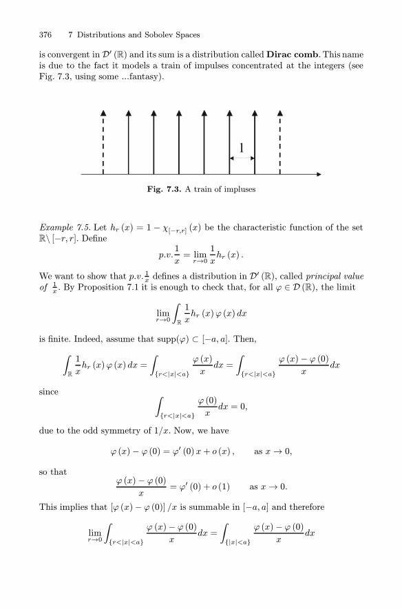
376 7 Distributions and Sobolev Spaces
is convergent in D′ (R) and its sum is a distribution calledDirac comb. This nameis due to the fact it models a train of impulses concentrated at the integers (seeFig. 7.3, using some ...fantasy).
Fig. 7.3. A train of impluses
Example 7.5. Let hr (x) = 1 − χ[−r,r] (x) be the characteristic function of the setR\ [−r, r]. Define
p.v.1
x= lim
r→01
xhr (x) .
We want to show that p.v. 1x defines a distribution in D′ (R), called principal valueof 1x . By Proposition 7.1 it is enough to check that, for all ϕ ∈ D (R), the limit
limr→0
∫
R
1
xhr (x)ϕ (x) dx
is finite. Indeed, assume that supp(ϕ) ⊂ [−a, a]. Then,∫
R
1
xhr (x)ϕ (x) dx =
∫
{r<|x|<a}
ϕ (x)
xdx =
∫
{r<|x|<a}
ϕ (x)− ϕ (0)x
dx
since ∫
{r<|x|<a}
ϕ (0)
xdx = 0,
due to the odd symmetry of 1/x. Now, we have
ϕ (x)− ϕ (0) = ϕ′ (0)x+ o (x) , as x→ 0,
so thatϕ (x)− ϕ (0)
x= ϕ′ (0) + o (1) as x→ 0.
This implies that [ϕ (x)− ϕ (0)] /x is summable in [−a, a] and therefore
limr→0
∫
{r<|x|<a}
ϕ (x)− ϕ (0)x
dx =
∫
{|x|<a}
ϕ (x)− ϕ (0)x
dx
7.4 Calculus 377
is a finite number. Thus, p.v. 1x ∈ D′ (R) and the above computations yield
〈p.v. 1x, ϕ〉 = lim
r→0
∫
{r<|x|}
ϕ (x)
xdx ≡ p.v.
∫
R
ϕ (x)
xdx
where p.v. stays for principal value7.
• Support of a distribution. The Dirac δ is concentrated at a point. More pre-cisely, we say that its support coincides with a point. The support of a generaldistribution F may be defined in the following way. We want to characterize thesmallest closed set outside of which F vanishes. However, we cannot proceed as inthe case of a function, since a distribution is defined on the elements of D (Ω), noton subsets of Rn.Thus, let us start saying that F ∈ D′ (Ω) vanishes in an open set A ⊂ Ω if
〈F, ϕ〉 = 0
for every ϕ ∈ D (Ω) whose support is contained in A. Let A be the union of allopen sets where F vanishes. A is open. Then, we define:
supp (F ) = Ω\A.
For example, supp(comb) = Z.
Remark 7.3. Let F ∈ D′ (Ω) with compact support K. Then the bracket 〈F, v〉 iswell defined for all v ∈ C∞ (Ω), not necessarily with compact support. Infact, let ϕ ∈ D (Ω), 0 ≤ ϕ ≤ 1, such that ϕ ≡ 1 in an open neighborhood of K(see Remark 7.4). Then vϕ ∈ D (Ω) and we can define
〈F, v〉 = 〈F, vϕ〉 .
Note that 〈F, vϕ〉 is independent of the choice of ϕ. Indeed if ψ has the sameproperty of ϕ, then
〈F, vϕ〉 − 〈F, vψ〉 = 〈F, v(ϕ− ψ)〉 = 0
since ϕ − ψ = 0 in an open neighborhood of K.
7.4 Calculus
7.4.1 The derivative in the sense of distributions
A central concept in the theory of the Schwartz distributions is the notion of weakor distributional derivative. Clearly we have to abandon the classical definition,
7 Whence the symbol p.v. 1x .

378 7 Distributions and Sobolev Spaces
since, for instance, we are going to define the derivative for a function u ∈ L1loc ,which may be quite irregular.The idea is to carry the derivative onto the test functions, as if we were using
the integration by parts formula.Let us start from a function u ∈ C1 (Ω). If ϕ ∈ D (Ω), denoting by ν =(ν1, ..., νn)
the outward normal unit vector to ∂Ω, we have∫
Ω
ϕ∂xiu dx =
∫
∂Ω
ϕu νi dx−∫
Ω
u∂xiϕ dx
= −∫
Ω
u∂xiϕ dx
since ϕ = 0 on ∂Ω. The equation∫
Ω
ϕ ∂xiu dx = −∫
Ω
u ∂xiϕ dx,
interpreted in D′ (Ω), becomes〈∂xiu, ϕ〉 = −〈u, ∂xiϕ〉. (7.7)
Formula (7.7) shows that the action of ∂xiu on the test function ϕ equals theaction of u on the test function −∂xiϕ. On the other hand, formula (7.7) makesperfect sense if we replace u by any F ∈ D′ (Ω) and it is not difficult to checkthat it defines a continuous linear functional in D (Ω). This leads to the followingfundamental notion:
Definition 7.4. Let F ∈ D′ (Ω). The derivative ∂xiF is the distribution definedby the formula
〈∂xiF, ϕ〉 = −〈F, ∂xiϕ〉, ∀ϕ ∈ D (Ω) .From (7.7), if u ∈ C1 (Ω) its derivatives in the sense of distributions coincide
with the classical ones. This is the reason we keep the same notations in the twocases.
Note that the derivative of a distribution is always defined! Moreover, sinceany derivative of a distribution is a distribution, we deduce the convenient factthat every distribution possesses derivatives of any order (in D′ (Ω)):
〈DαFk, ϕ〉 = (−1)|α|〈Fk, Dαϕ〉.For example, the second order derivative
∂xixkF = ∂xi (∂xkF )
is defined by〈∂xixkF, ϕ〉 = 〈F, ∂xixkϕ〉. (7.8)
Not only. Since ϕ is smooth, then ∂xixkϕ = ∂xkxiϕ so that (7.8) yields
∂xixkF = ∂xkxiF.
Thus, for all F ∈ D′ (Ω) we may always reverse the order of differentiation withoutany restriction.

7.4 Calculus 379
Example 7.6. Let u (x) = H (x), the Heaviside function. In D′ (R) we have H′ = δ.In fact, let ϕ ∈ D (R) . By definition,
〈H′, ϕ〉 = −〈H, ϕ′〉.On the other hand, H ∈ L1loc (R), hence
〈H, ϕ′〉 =∫
R
H (x)ϕ′ (x) dx =∫ ∞0
ϕ′ (x) dx = −ϕ (0)
whence〈H′, ϕ〉 = ϕ (0) = 〈δ, ϕ〉
or H′ = δ.Another aspect of the idyllic relationship between calculus and distributions is
given by the following theorem, which expresses the continuity in D′ (Ω) of everyderivative Dα.
Proposition 7.2. If Fk → F in D′ (Ω) then DαFk → DαF in D′ (Ω) for anymulti-index α.
Proof. Fk → F in D′ (Ω) means that 〈Fk, ϕ〉 → 〈F, ϕ〉, ∀ϕ ∈ D (Ω).In particular, since Dαϕ ∈ D (Ω),
〈DαFk, ϕ〉 = (−1)|α|〈Fk, Dαϕ〉 → (−1)|α|〈F,Dαϕ〉 = 〈DαF, ϕ〉.
�As a consequence, if
∑∞k=1 Fk = F in D′ (Ω), then∞∑k=1
DαFk = DαF in D′ (Ω) .
Thus, term by term differentiation is always permitted in D′ (Ω).More difficult is the proof of the following theorem, which expresses a well
known fact for functions.
Proposition 7.3. Let Ω be a domain in Rn. If F ∈ D′ (Ω) and ∂xjF = 0 forevery j = 1, ..., n, then F is a constant function.
7.4.2 Gradient, divergence, laplacian
There is no problem to define vector valued distributions. The space of test func-tions is D (Ω;Rn), i.e. the set of vectors ϕ =(ϕ1, ..., ϕn) whose components belongto D (Ω).A distribution F ∈D′ (Ω;Rn) is given by F = (F1, ..., Fn) with Fj ∈ D′ (Ω),
j = 1, ..., n. The pairing between D (Ω;Rn) and D′ (Ω;Rn) is defined by
〈F,ϕ〉 =n∑i=1
〈Fi,ϕi〉. (7.9)

380 7 Distributions and Sobolev Spaces
• The gradient of F ∈ D′ (Ω), Ω ⊂ Rn, is simply
∇F = (∂x1F, ∂x2F, ..., ∂xnF ) .
Clearly ∇F ∈ D′ (Ω;Rn). If ϕ ∈ D (Ω;Rn), we have
〈∇F ,ϕ〉 =n∑i=1
〈∂xiF, ϕi〉 = −n∑i=1
〈F, ∂xiϕi〉 = −〈F, divϕ〉
whence〈∇F ,ϕ〉 = −〈F, divϕ〉 (7.10)
which shows the action of ∇F on ϕ.• For F ∈ D′ (Ω;Rn), we set
divF =
n∑i=1
∂xiFi.
Clearly divF ∈D′ (Ω). If ϕ ∈ D (Ω), then
〈divF,ϕ〉 = 〈n∑1=1
∂xiFi,ϕ〉 = −n∑1=1
〈Fi,∂xiϕ〉 = −〈F,∇ϕ〉
whence〈divF,ϕ〉 = −〈F,∇ϕ〉. (7.11)
• The Laplace operator is defined in D′ (Ω) by
ΔF =
n∑i=1
∂xixiF.
If ϕ ∈ D (Ω), then〈ΔF,ϕ〉 = 〈F ,Δϕ〉 .
Using (7.10), (7.11) we get
〈ΔF,ϕ〉 = 〈F ,div∇ϕ〉 = −〈∇F ,∇ϕ〉 = 〈div∇F ,ϕ〉
whence Δ =div∇ also in D′ (Ω).
Example 7.7. Consider the fundamental solution for the Laplace operator in R3
u (x) =1
4π
1
|x| .
Observe that u ∈ L1loc(R3)so that u ∈ D′
(R3).We want to show that, in D′
(R3),
−Δu = δ. (7.12)

7.4 Calculus 381
First of all, if Ω ⊂ R3 and 0 /∈Ω, we know that u is harmonic in Ω, that is
Δu = 0 in Ω
in the classical sense and therefore also in D′(R3). Thus, let ϕ ∈ D
(R3)with
0 ∈supp(ϕ). We have, since u ∈ L1loc(R3):
〈Δu,ϕ〉 = 〈u,Δϕ〉 = 14π
∫
R3
1
|x|Δϕ (x) dx. (7.13)
We would like to carry the laplacian onto 1/ |x|. However, this cannot be donedirectly, since the integrand is not continuous at 0. Therefore we exclude a smallsphere Br = Br (0) from our integration region and write
∫
R3
1
|x|Δϕ (x) dx = limr→0∫
BR\Br
1
|x|Δϕ (x) dx (7.14)
where BR = BR (0) is a sphere containing the support of ϕ. An integration byparts in the spherical shell CR,r = BR\Br yields8
∫
CR,r
1
|x|Δϕ (x) dx =∫
∂Br
1
r∂νϕ (x) dσ−
∫
CR,r
∇(1
|x|
)· ∇ϕ (x) dx
where ν = − x|x| is the outward normal unit vector on ∂Br . Integrating once more
by parts the last integral, we obtain:
∫
CR,r
∇(1
|x|
)· ∇ϕ (x) dx =
∫
∂Br
∂ν
(1
|x|
)ϕ (x) dσ−
∫
CR,r
Δ
(1
|x|
)ϕ (x) dx
=
∫
∂Br
∂ν
(1
|x|
)ϕ (x) dσ,
since Δ(1|x|)= 0 inside CR,r . From the above computations we infer
∫
CR,r
1
|x|Δϕ (x) dx =∫
∂Br
1
r∂νϕ (x) dσ−
∫
∂Br
∂ν
(1
|x|
)ϕ (x) dσ. (7.15)
We have:
1
r
∣∣∣∣∫
∂Br
∂νϕ (x) dσ
∣∣∣∣ ≤1
r
∫
∂Br
|∂νϕ (x)| dσ ≤ 4πrmaxR3|∇ϕ|
and therefore
limr→0
∫
∂Br
1
r∂νϕ (x) dσ = 0.
8 Recall that ϕ = 0 and ∇ϕ = 0 on ∂BR.

382 7 Distributions and Sobolev Spaces
Moreover, since
∂ν
(1
|x|
)= ∇
(1
|x|
)·(− x|x|
)=
(− x|x|3
)·(− x|x|
)=1
|x|2,
we may write
∫
∂Br
∂ν
(1
|x|
)ϕ (x) dσ = 4π
1
4πr2
∫
∂Br
ϕ (x) dσ → 4πϕ (0) .
Thus, from (7.15) we get
limr→0
∫
BR\Br
1
|x|Δϕ (x) dx = −4πϕ (0)
and finally (7.13) yields
〈Δu,ϕ〉 = −ϕ (0) = −〈δ, ϕ〉
whence −Δu=δ.
7.5 Multiplication, Composition, Division, Convolution
7.5.1 Multiplication. Leibniz rule
Let us analyze the multiplication between two distributions. Does it make anysense to define, for instance, the product δ · δ = δ2 as a distribution in D′ (R)?Things are not so smooth. An idea for defining δ2 may be the following: take
a sequence {uk} of functions in L1loc (R) such that uk → δ in D′(R), compute u2kand set
δ2 = limk→∞
u2k in D′(R).
Since we may approximate δ in D′(R) in many ways (see Problem 7.1), it is neces-sary that the definition does not depend on the approximating sequence. In otherwords, to compute δ2 we must be free to choose any approximating sequence.However, this is illusory. Indeed choose
uk = kχ[0,1/k].
We have uk → δ in D′ (R) but, if ϕ ∈ D (R), by the Mean Value Theorem we have∫
R
u2kϕ = k2
∫ 1/k0
ϕ = kϕ (xk)
for some xk ∈ [0, 1/k]. Now, if ϕ (0) > 0, say, we deduce that∫
R
u2kϕ→ +∞, k → +∞
7.5 Multiplication, Composition, Division, Convolution 383
so that{u2k}does not converge in D′ (R).
The method does not work and it seems that there is no other reasonable wayto define δ2. Thus, we simply give up defining δ2 as a distribution or, in general,the product of a pair of distributions. However, if F ∈ D′ (Ω) and u ∈ C∞ (Ω),we may define the product uF by the formula
〈uF, ϕ〉 = 〈F, uϕ〉 , ∀ϕ ∈ D (Ω) .
First of all, this makes sense since uϕ ∈ D (Ω). Also, if ϕk → ϕ in D (Ω), thenuϕk → uϕ in D (Ω) and
〈uF, ϕk〉 = 〈F, uϕk〉 → 〈F, uϕ〉 = 〈uF, ϕ〉 .
so that uF is a well defined element of D′ (Ω).
Example 7.8. Let u ∈ C∞ (R). We have
uδ = u (0) δ.
Indeed, if ϕ ∈ D (R),
〈uδ, ϕ〉 = 〈δ, uϕ〉 = u (0)ϕ (0) = 〈u (0) δ, ϕ〉 .
Note that the product uδ makes sense even if u is only continuous. In particular
xδ = 0.
The Leibniz rule holds: let F ∈ D′ (Ω) and u ∈ C∞ (Ω) ; then
∂xi (uF ) = u ∂xiF + ∂xiu F . (7.16)
In fact, let ϕ ∈ D (Ω); we have:
〈∂xi (uF ) , ϕ〉 = −〈uF, ∂xiϕ〉 = −〈F, u∂xiϕ〉
while
〈u ∂xiF + ∂xiu F, ϕ〉 = 〈∂xiF, uϕ〉 + 〈F, ϕ∂xiu〉= −〈F, ∂xi (uϕ)〉+ 〈F, ϕ∂xiu〉 = 〈F, u∂xiϕ〉
and (7.16) follows.
Example 7.9. From xδ = 0 and Leibniz formula we obtain
δ + xδ′ = 0.
More generally,xmδ(k) = 0 in D′ (R) , if 0 ≤ k < m.

384 7 Distributions and Sobolev Spaces
7.5.2 Composition
Composition in D′ (R) requires caution as well. For instance, if F = δ and u (x) =x3, is there a natural way to define F ◦ u as a distribution in D′ (R)?As above, consider the sequence uk = kχ[0,1/k] and compute wk = uk ◦ u. If
ϕ ∈ D′ (R), we have∫
R
wkϕ = k
∫
R
χ[0,1/k](x3)ϕ (x) dx = k
∫ k−1/3
0
ϕ (x) dx = k2/3ϕ (xk)
for some xk ∈ [0, 1/k]. Then, if ϕ (0) > 0,∫Rwkϕ→ +∞ and F ◦ u does not make
any sense. Thus, it seems hard to define the composition between two generaldistributions. To see what can be done, let us start analyzing the case of twofunctions.Let ψ : Ω′ → Ω be one to one, with ψ and ψ−1 of class C∞. If F : Ω → R
is a C1−function we may consider the composition
w = F ◦ ψ.
For ϕ ∈ D (Ω), we have, using the change of variables y = ψ (x):∫
Ω′w (x)ϕ (x) dx =
∫
Ω′F (ψ(x))ϕ (x) dx =
∫
Ω
F (y))ϕ(ψ−1(y)
) ∣∣det Jψ−1 (y)∣∣ dy
which becomes, in terms of distributions,
〈F ◦ ψ, ϕ〉 = 〈F, ϕ ◦ ψ−1 ·∣∣det Jψ−1
∣∣〉. (7.17)
This formula makes sense also if F ∈ D′ (Ω) and leads to the following
Definition 7.5. If F ∈ D′ (Ω) and ψ : Ω′ → Ω is one to one, with ψ and ψ−1of class C∞, then formula (7.17) defines the composition F ◦ ψ as an element ofD′ (Ω).
Abuses of notation are quite common, like F (ψ (x)) to denote F ◦ ψ. For in-stance, we have repeatedly used the (comfortable and incorrect) notation δ (x − x0)instead of the (uncomfortable and correct....) notation δ ◦ ψ, with ψ (x) = x− x0.
Example 7.10. In D′ (Rn), we have
δ (ax) =1
|a|n δ (x) .
Using formula (7.17) we may extend to distributions some properties, typical offunctions. We list some of them.
We say that F ∈ D′ (Rn) is:

7.5 Multiplication, Composition, Division, Convolution 385
• radial, if
F (Ax) = F (x) , for every orthogonal matrix A;
• homogeneous of degree λ, if
F (tx) = tλF (x) , ∀t > 0;
• even, odd if, respectively,
F (−x) = F (x) , F (−x) = −F (x) ;
• periodic with period P, if
F (x+P) = F (x) .
Example 7.11. a. δ ∈ D′ (Rn) is radial, even and homogeneous of degree λ = −n.b. v.p. 1x ∈ D′ (R) is odd and homogeneous of degree λ = −1.c. In D′ (R), comb is periodic with period 1.
7.5.3 Division
The division in D′ (Ω) is rather delicate, even restricting to F ∈ D′ (Ω) and u ∈C∞ (Ω). To divide F by u means to find G ∈ D′ (Ω) such that uG = F . If u nevervanishes there is no problem, since in this case 1/u ∈ C∞ (Ω) and the answer issimply
G =1
uF.
If u vanishes somewhere, things get complicated. We only consider a particularcase in one dimension.
Let I ⊆ R be an open interval and u ∈ C∞ (I). If u vanishes at z, we say thatz is a zero of order m (z) if the derivatives of u up to order m (z) − 1, included,vanish at z, while the derivative of order m (z) does not vanish at z.For instance, z = 0 is a zero of order 3 for u (x) = sinx− x.One can prove the following theorem.
Proposition 7.4. Assume that u vanishes at isolated points z1, z2, ... with orderm (z1) , m (z2),.... Then, the equation
uG = 0
has infinitely many solutions in D′ (I), given by the following formula:
G =∑j
m(zj)−1∑k=0
cjkδ(k) (x− zj) (7.18)
where cjk are arbitrary constants and δ(k) is the derivative of δ of order k.

386 7 Distributions and Sobolev Spaces
Example 7.12. The solutions in D′ (R) of the equation
xG = 0.
are the distributions of the form G = cδ, with c ∈ R. To solve the equation
xG = 1 (7.19)
we add to the solutions of the homogeneous equation xG = 0 a particular solutionof (7.19). It turns out that one of these is
G1 = v.p.1
x.
In fact, if ϕ ∈ D (R), from Example 7.6 we get
〈x · (v.p. 1x), ϕ〉 = 〈v.p. 1
x, xϕ〉 =
= v.p.
∫
R
xϕ (x)
xdx =
∫
R
ϕ (x)dx = 〈1, ϕ〉
whence
x · (v.p. 1x) = 1.
Therefore, the general solution of (7.19) is
G = v.p.1
x+ cδ, c ∈ R.
7.5.4 Convolution
The convolution of two distributions may be defined with some restrictions as well.Let us see why. If u, w ∈ L1 (Rn) and ϕ ∈ D (Rn) we may write:
〈u ∗ w, ϕ〉 = 〈∫
Rn
u (x − y)w (y) dy,ϕ〉 =
=
∫
Rn
[∫
Rn
u (x− y)w (y) dy]ϕ(x) dx =
=
∫
Rn
∫
Rn
u (x)w (y)ϕ(x+ y) dydx.
Now, the question is: may we give any meaning to this formula if u and v aregeneric distributions? The answer is negative, mainly because the function
φ (x,y) = ϕ(x+ y)
does not have compact support9 in Rn ×Rn (unless ϕ ≡ 0).9 For instance: if ϕ ∈ D′ (R) and supp(ϕ) = [a, b], then the support of ϕ (x+ y) in R2 isthe unbounded strip a ≤ x+ y ≤ b.

7.5 Multiplication, Composition, Division, Convolution 387
However, a small modification of the above formula would give the possibil-ity to define the convolution between two distributions, if at least one of themhas compact support. Here we limit ourselves to define the convolution betweena distribution T and a C∞−function u. For x fixed, let ψx (y) = x− y so thatu (x − y) = u ◦ ψx.If T ∈ L1 (Rn), with compact support, then the usual definition of convolution
is
(T ∗ u) (x) =∫
Rn
T (y)u (x− y) dy = 〈T, u ◦ ψx〉 . (7.20)
Since u ◦ψx is a C∞−function, recalling Remark 7.4, the last bracket makes senseif T is a distribution with compact support as well. Precisely, we have:
Proposition 7.5. Let T ∈ D′ (Rn), with compact support, and u ∈ C∞ (Rn).Then, the following formula
(T ∗ u) (x) = 〈T, u ◦ ψx〉 (7.21)
defines a C∞−function called convolution of T and u.
Example 7.13. Let u ∈ C∞0 (Rn). Then
(δ ∗ u) (x) = 〈δ, u (x − ·)〉 = u (x)
i.eδ ∗ u = u. (7.22)
Thus, the Dirac distribution at zero, acts as the identity with respect to theconvolution. Formula (7.22) actually holds for all u ∈ D′ (Rn). In particular:
δ ∗ δ = δ.
Proposition 7.6. The convolution commutes with derivatives. Actually, we have:
∂xj (T ∗ u) = ∂xjT ∗ u = T ∗ ∂xju.
The last equality is easy to prove, under the hypotheses of Proposition 7.5:
(∂xjT ∗ u) (z) =⟨∂xjT, u ◦ ψz
⟩= −
⟨T, ∂xj(u ◦ ψz)
⟩
=⟨T, ∂xju ◦ ψz
⟩=(T ∗ ∂xju
)(z) .
In particular, if T = H and u ∈ D (R),
(H ∗ u)′ = (H′ ∗ u) = δ ∗ u = u.
Warning: The convolution of functions is associative. For distributions, theconvolution is, in general, not associative. In fact, consider the three distributions1, δ′,H; we have (formally):
δ′ ∗ 1 = (δ ∗ 1)′ = 1′ = 0

388 7 Distributions and Sobolev Spaces
whence
H ∗(δ′ ∗ 1
)= H ∗ 0 = 0.
However, (H ∗ δ′
)∗ 1 = (H′ ∗ δ) ∗ 1 = (δ ∗ δ) ∗ 1 = 1.
The problem is that two out of three factors (1 and H) have non compact support.If at least two factors have compact support one can show that the convolution isassociative.
7.6 Fourier Transform
7.6.1 Tempered distributions
We introduce now the Fourier transform F of a distribution. As usual, the ideais to define the action of F by carrying the transform onto the test functions.However a problem immediately arises: if ϕ ∈ D(Rn) is not identically zero, then
ϕ (ξ) =
∫
Rn
e−ix·ξϕ (x) dx
cannot belong10 to D(Rn). Thus, it is necessary to choose a larger space of testfunctions. It turns out that the correct one consists in the set of functions rapidlyvanishing at ∞, which obviously contains D(Rn). It is convenient to considerfunctions and distributions with complex values.
Definition 7.6. Denote by S (Rn) the space of functions v ∈ C∞(Rn) rapidlyvanishing at infinity, i.e. such that
Dαv (x) = o(|x|−m
), |x| → ∞,
for all m ∈ N and every multi-index α.10 Let n = 1 and ϕ ∈ D (R) . Assume that
supp (ϕ) ⊂ (−a, a) .We may write
ϕ (ξ) =
∫ a
−ae−ixξϕ (x) dx =
∫ a
−a
∞∑
n=0
(−ixξ)nn!
ϕ (x) dx =
∞∑
n=0
(−iξ)nn!
∫ a
−axnϕ (x) dx.
Since ∣∣∣∣
∫ a
−axnϕ (x) dx
∣∣∣∣ ≤ max |ϕ| an,
it follows that ϕ is an analytic function in all C. Therefore ϕ cannot vanish outside acompact interval, unless ϕ ≡ 0. But then ϕ ≡ 0 as well.

7.6 Fourier Transform 389
Example 7.14. The function v (x) = e−|x|2
belongs to S (Rn) while v (x) =e−|x|
2
sin(e|x|2
) does not (why?).
We endow S (Rn) with an “ad hoc” notion of convergence. If β = (β1, ..., βn) is amulti-index, we set
xβ = xβ11 · · · xnn1 .
Definition 7.7. Let {vk} ⊂ S (Rn) and v ∈ S (Rn). We say that
vk → v in S (Rn)
if for every pair of multi-indexes α, β,
xβDαvk → xβDαv, uniformly in Rn.
Remark 7.4. If {vk} ⊂ D (Rn) and vk → v in D (Rn), then
vk → v in S (Rn)
as well, since each vk vanishes outside a common compact set so that the multi-plication by xβ does not have any influence.
The Fourier transform will be defined for distributions in D′ (Rn), continuouswith respect to the convergence in Definition 7.7. These are the so called tempereddistributions. Precisely:
Definition 7.8. We say that T ∈ D′ (Rn) is a tempered distribution if
〈T, vk〉 → 0
for all sequences {vk} ⊂ D (Rn) such that vk → 0 in S (Rn). The set of tempereddistributions is denoted by S′ (Rn) .
So far, a tempered distribution T is only defined on D (Rn). To define T onS (Rn), first we observe that D (Rn) is dense in S (Rn).In fact, given v ∈ S (Rn), let
vk (x) = v (x) ρ (|x| /k)
where ρ = ρ (s), s ≥ 0, is a non-negative C∞−function, equal to 1 in [0, 1] andzero for s ≥ 2 (see Fig. 7.4). We have {vk} ⊂ D (Rn) and vk → v in S (Rn), sinceρ (|x| /k) is equal to 1 for {|x| < k} and zero for {|x| > 2k}.Then, we set
〈T, v〉 = limk→∞
〈T, vk〉 . (7.23)
It can be shown that this limit exists and is finite, and it is independent of theapproximating sequence {vk} . Thus, a tempered distribution is a continuousfunctional on S (Rn).

390 7 Distributions and Sobolev Spaces
Fig. 7.4. A smooth decreasing and nonnegative function, equal to 1 in [0, 1] and vanishingfor s ≥ 2
Example 7.15.We leave it as an exercise to show that the following distributionsare tempered.a. Any polynomial.b. Any compactly supported distribution.c. Any periodic distribution (e.g. the Dirac comb).d. Any function u ∈ Lp (Rn), 1 ≤ p ≤ ∞. Thus, we have
S (Rn) ⊂ Lp (Rn) ⊂ S′ (Rn) .On the contrary:
e. ex /∈ S′ (R) (why?).Like D′ (Ω), S′ (Rn) possesses a completeness property that may be used to
construct a tempered distribution or to recognize that some linear functional inD (Rn) is a tempered distribution. First, we say that a sequence {Tk} ⊂ S′ (Rn)converges to T in S′ (Rn) if
〈Tk, v〉 → 〈T, v〉 , ∀v ∈ S (Rn) .We have:
Proposition 7.7. Let {Tk} ⊂ S′ (Rn) such thatlimk→∞
〈Tk, v〉 exists and is finite, ∀v ∈ S (Rn) .
Then, this limit defines T ∈ S′ (Rn) and Tk converges to T in S′ (Rn) .Example 7.16. The Dirac comb is a tempered distribution. In fact, if v ∈ S(R), wehave
〈comb (x) , v〉 =∞∑
k=−∞v (k)
and the series is convergent since v (k) → 0 more rapidly than |k|−m for everym > 0. From Proposition 7.7, comb(x) ∈ S′(R).Remark 7.5. Convolution. If T ∈ S′(Rn) and v ∈ S(Rn), the convolution is welldefined by formula (7.21). Then, T ∗ v ∈ S′(Rn) and coincides with a function inC∞ (Rn).

7.6 Fourier Transform 391
7.6.2 Fourier transform in S′
If u ∈ L1 (Rn), its Fourier transform is given by
u (ξ) = F [u] (ξ) =∫
Rn
e−ix·ξu (x) dx.
It could be that, even if u is compactly supported, u /∈ L1 (Rn). For instance, ifpa (x) = χ[−a,a] (x) then
p (ξ) = 2sin (aξ)
ξ
which is not11 in L1 (R). When also u ∈ L1 (Rn), u can be reconstructed from uthrough the following inversion formula:
Theorem 7.2. Let u ∈ L1 (Rn), u ∈ L1 (Rn). Then
u (x) =1
(2π)n
∫
Rn
eix·ξu(ξ)dξ ≡F−1 [u] (x) . (7.24)
In particular, the inversion formula (7.24) holds for u ∈ S(Rn), since (exercise)u ∈ S(Rn) as well. Moreover, it may be proved that
uk → u in S (Rn)
if and only if
uk → u in S (Rn) ,which means that
F , F−1 : S(Rn)→ S(Rn)are continuous operators
Now observe that, if u, v ∈ S(Rn),
〈u, v〉 = 〈∫
Rn
e−ix·ξu(x)dx,v〉 =∫
Rn
(∫
Rn
e−ix·ξu(x)dx)v (ξ) dξ
=
∫
Rn
(∫
Rn
e−ix·ξv (ξ) dξ)u(x)dx = 〈u, v〉
so that (weak Parseval identity):
〈u, v〉 = 〈u, v〉 . (7.25)
The key point is that the last bracket makes sense for u = T ∈ S′(Rn) as well,and defines a tempered distribution. In fact:
11 Appendix B.

392 7 Distributions and Sobolev Spaces
Lemma 7.2. Let T ∈ S′(Rn). The linear functional
v �→ 〈T, v〉 , ∀v ∈ S(Rn)
is a tempered distribution.
Proof. Let vk → v in D(Rn). Then vk → v and vk → v in S(Rn) as well. SinceT ∈ S′(Rn), we have
limk→∞
〈T, vk〉 = 〈T, v〉
so that v �→ 〈T, v〉 defines a distribution. If vk → 0 in S(Rn), then vk → 0 inS(Rn) and 〈T, vk〉 → 0. Thus, v �→ 〈T, v〉 is a tempered distribution. �We are now in position to define the Fourier transform of T ∈ S′(Rn).
Definition 7.9. Let T ∈ S′(Rn). The Fourier transform T = F [T ] is the tempereddistribution defined by
〈T , v〉 = 〈T, v〉 , ∀v ∈ S(Rn).
We see that the transform has been carried onto the test function v ∈ (Rn). Asa consequence, all the properties valid for functions, continue to hold for tempereddistributions. We list some of them. Let T ∈ S′(Rn) and v ∈ S(Rn).1. Translation. If a ∈ Rn,
F [T (x − a)] = e−ia·ξT and F[eia·xT
]= T (ξ − a) .
In fact (v = v (ξ)):
〈F [T (x − a)] , v〉 = 〈T (x− a) , v〉 = 〈T, v (x + a)〉=⟨T,F
[e−ia·ξv
]⟩= 〈T , e−ia·ξv〉 = 〈e−ia·ξT , v〉.
2. Rescaling. If h ∈ R, h �= 0,
F [T (hx)] = 1
|h|n T(ξ
h
).
In fact:
〈F [T (hx)] , v〉 = 〈T (hx) , v〉 = 〈T, 1|h|n v(xh
)〉
= 〈T,F [v (hξ)]〉 = 〈T , v (hξ)〉 = 〈 1|h|n T(ξ
h
), v〉.
In particular, choosing h = −1, it follows that if T is even (odd) then T is even(odd).
3. Derivatives:
a) F[∂xjT
]= iξj T and b) F [xjT ] = i∂ξj T .
7.6 Fourier Transform 393
Namely:⟨F[∂xjT
], v⟩=⟨∂xjT, v
⟩= −
⟨T, ∂xj v
⟩
=⟨T,F
[iξjv
]⟩= 〈iξjT , v〉.
For the second formula, we have:
〈F [xjT ] , v〉 = 〈xjT, v〉 = 〈T, xj v〉=⟨T,−iF [∂ξjv]
⟩= 〈−iT , ∂ξjv〉 = 〈i∂ξj T , v〉.
4. Convolution12. If T ∈ S′(Rn) and v ∈ S(Rn),
F [T ∗ v] = T · v.Example 7.17.We know that δ ∈ S′(Rn). We have:
δ = 1, 1 = (2π)nδ.
In fact
〈δ, v〉 = 〈δ, v〉 =∫
Rn
v (x) dx = 〈1, v〉 .
For the second formula, using (7.24) we have:
〈1, v〉 = 〈1, v〉 =∫
Rn
v (ξ) dξ = (2π)nv (0)
= 〈(2π)n δ, v〉 .Example 7.18. Transform of xj :
xj = i (2π)n∂ξj δ.
Indeed, from 3, b) and Example 7.20, we may write
xj = F [xj · 1] = i∂ξj 1 = i (2π)n∂ξjδ.
7.6.3 Fourier transform in L2
Since L2 (Rn) ⊂ S′ (Rn), the Fourier transform is well defined for all functions inL2 (Rn) . The following theorem holds, where v denotes the complex conjugate ofv.
Theorem 7.3. u ∈ L2 (Rn) if and only if u ∈ L2 (Rn). Moreover, if u, v ∈ L2 (Rn),the following strong Parseval identity holds:
∫
Rn
u · v = (2π)n∫
Rn
u · v. (7.26)
In particular‖u‖2L2(Rn) = (2π)
n ‖u‖2L2(Rn) . (7.27)
12 We omit the proof.

394 7 Distributions and Sobolev Spaces
Formula (7.27) shows that the Fourier transform is an isometry in L2 (Rn)(but for the factor (2π)
n).
Proof. Since S (Rn) is dense in L2 (Rn), it is enough to prove (7.26) for u, v ∈S (Rn). Let w = v. From (7.25) we have
∫
Rn
u · w =∫
Rn
u · w.
On the other hand,
w (x) =
∫
Rn
e−ix·yv (y)dy = (2π)nF−1 [v] (x) = (2π)n v (x)
and (7.26) follows. �
Example 7.19. Let us compute
∫
R
(sinx
x
)2dx.
We know that the Fourier transform of p1 = χ[−1,1] is p1 (ξ) = 2 sin ξ/ξ, whichbelongs to L2 (R). Thus, (7.27) yields
4
∫
R
(sin ξ
ξ
)2dξ = 2π
∫
R
(χ[−1,1] (x)
)2dx = 4π
whence ∫
R
(sinx
x
)2dx = π.
7.7 Sobolev Spaces
7.7.1 An abstract construction
Sobolev spaces constitute one of the most relevant functional settings for the treat-ment of boundary value problems. Here, we will be mainly concerned with Sobolevspaces based on L2 (Ω), developing only the theoretical elements we will need inthe sequel13.The following abstract theorem is a flexible tool for generating Sobolev Spaces.
The ingredients of the construction are:
• The space D′ (Ω;Rn), in particular, for n = 1, D′ (Ω).13 We omit the most technical proofs, that can be found, for instance, in the classicalbooks of Adams, 1975, or Mazja, 1985.

7.7 Sobolev Spaces 395
• Two Hilbert spaces H and Z with Z ↪→ D′ (Ω;Rn) for some n ≥ 1. In particularvk → v in Z implies vk → v in D′ (Ω;Rn) . (7.28)
• A linear continuous operator L : H → D′ (Ω;Rn) (such as a gradient or adivergence).
We have:
Theorem 7.4. DefineW = {v ∈ H : Lv ∈ Z}
and(u, v)W = (u, v)H + (Lu, Lv)Z . (7.29)
Then W is a Hilbert space with inner product given by (7.29). The embedding ofW in H is continuous and the restriction of L to W is continuous from W into Z.
Proof. It is easy to check that (7.29) has all the properties of an inner product,with induced norm
‖u‖2W = ‖u‖2H + ‖Lu‖
2Z .
Thus W is an inner-product space. It remains to check its completeness. Let {vk}a Cauchy sequence in W. We must show that there exists v ∈ H such that
vk → v in H and Lvk → Lv in Z.Observe that {vk} and {Lvk} are Cauchy sequences in H and Z, respectively.Thus, there exist v ∈ H and z ∈ Z such that
vk → v in H and Lvk → z in Z.The continuity of L and (7.28) yield
Lvk → Lv in D′ (Ω;Rn) and Lvk → z in D′ (Ω;Rn) .Since the limit of a sequence in D′ (Ω;Rn) is unique, we infer that
Lv = z.
Therefore Lvk → Lv in Z and W is a Hilbert space.The continuity of the embedding W ⊂ H follows from
‖u‖H ≤ ‖u‖Wwhile the continuity of L|W :W → Z follows from
‖Lu‖Z ≤ ‖u‖W .Thus, the proof is complete. �Remark 7.6. The norm induced by the inner product (7.29) is
‖u‖W =√‖u‖2H + ‖Lu‖
2Z
which is called the graph norm of L.
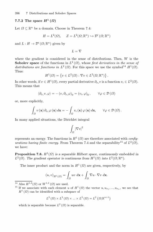
396 7 Distributions and Sobolev Spaces
7.7.2 The space H1 (Ω)
Let Ω ⊆ Rn be a domain. Choose in Theorem 7.4:
H = L2(Ω), Z = L2(Ω;Rn) ↪→D′ (Ω;Rn)
and L : H → D′ (Ω;Rn) given by
L = ∇
where the gradient is considered in the sense of distributions. Then, W is theSobolev space of the functions in L2 (Ω), whose first derivatives in the sense ofdistributions are functions in L2 (Ω). For this space we use the symbol14 H1(Ω).Thus:
H1(Ω) ={v ∈ L2(Ω) : ∇v ∈ L2(Ω;Rn)
}.
In other words, if v ∈ H1(Ω), every partial derivative ∂xiv is a function vi ∈ L2(Ω).This means that
〈∂xiv, ϕ〉 = − (v, ∂xiϕ)0 = (vi, ϕ)0 , ∀ϕ ∈ D (Ω)
or, more explicitly,
∫
Ω
v (x) ∂xiϕ (x) dx = −∫
Ω
vi (x)ϕ (x) dx, ∀ϕ ∈ D (Ω) .
In many applied situations, the Dirichlet integral
∫
Ω
|∇v|2
represents an energy. The functions in H1 (Ω) are therefore associated with config-urations having finite energy. From Theorem 7.4 and the separability15 of L2(Ω),we have:
Proposition 7.8. H1(Ω) is a separable Hilbert space, continuously embedded inL2(Ω). The gradient operator is continuous from H1(Ω) into L2(Ω;Rn).
The inner product and the norm in H1 (Ω) are given, respectively, by
(u, v)H1(Ω) =
∫
Ω
uv dx+
∫
Ω
∇u · ∇v dx.
14 Also H1,2(Ω) or W 1,2 (Ω) are used.15 If we associate with each element u of H1 (Ω) the vector u, ux1 , ..., uxn , we see thatH1 (Ω) can be identified with a subspace of
L2 (Ω)× L2 (Ω)× ...× L2 (Ω) = L2 (Ω;Rn+1)
which is separable because L2 (Ω) is separable.
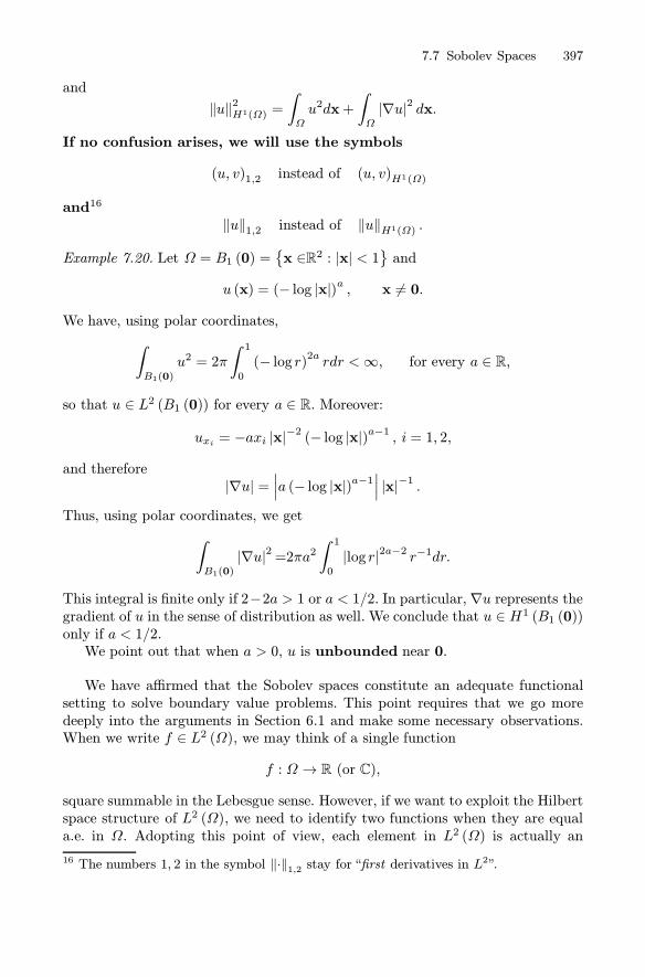
7.7 Sobolev Spaces 397
and
‖u‖2H1(Ω) =∫
Ω
u2dx+
∫
Ω
|∇u|2 dx.
If no confusion arises, we will use the symbols
(u, v)1,2 instead of (u, v)H1(Ω)
and16
‖u‖1,2 instead of ‖u‖H1(Ω) .
Example 7.20. Let Ω = B1 (0) ={x ∈R2 : |x| < 1
}and
u (x) = (− log |x|)a , x �= 0.
We have, using polar coordinates,
∫
B1(0)
u2 = 2π
∫ 10
(− log r)2a rdr <∞, for every a ∈ R,
so that u ∈ L2 (B1 (0)) for every a ∈ R. Moreover:
uxi = −axi |x|−2 (− log |x|)a−1 , i = 1, 2,
and therefore|∇u| =
∣∣∣a (− log |x|)a−1∣∣∣ |x|−1 .
Thus, using polar coordinates, we get
∫
B1(0)
|∇u|2=2πa2∫ 10
|log r|2a−2 r−1dr.
This integral is finite only if 2−2a > 1 or a < 1/2. In particular,∇u represents thegradient of u in the sense of distribution as well. We conclude that u ∈ H1 (B1 (0))only if a < 1/2.We point out that when a > 0, u is unbounded near 0.
We have affirmed that the Sobolev spaces constitute an adequate functionalsetting to solve boundary value problems. This point requires that we go moredeeply into the arguments in Section 6.1 and make some necessary observations.When we write f ∈ L2 (Ω), we may think of a single function
f : Ω → R (or C),
square summable in the Lebesgue sense. However, if we want to exploit the Hilbertspace structure of L2 (Ω), we need to identify two functions when they are equala.e. in Ω. Adopting this point of view, each element in L2 (Ω) is actually an
16 The numbers 1, 2 in the symbol ‖·‖1,2 stay for “first derivatives in L2”.

398 7 Distributions and Sobolev Spaces
equivalence class of which f is a representative. The drawback here is that it doesnot make sense anymore to compute the value of f at a single point, since a pointis a set with measure zero!The same considerations hold for “functions” in H1 (Ω), since
H1 (Ω) ⊂ L2 (Ω) .
On the other hand, if we deal with a boundary value problem, it is clear that wewould like to compute the solution at any point in Ω!Even more important is the question of the trace of a function on the boundary
of a domain. By trace of f on ∂Ω we mean the restriction of f to ∂Ω. In a Dirichletor Neumann problem we assign precisely the trace of the solution or of its normalderivative on ∂Ω, which is a set with measure zero. Does this make any sense ifu ∈ H1 (Ω)?It could be objected that, after all, one always works with a single representative
and that the numerical approximation of the solution, only involves a finite numberof points, making meaningless the distinction between functions in L2 (Ω) or inH1 (Ω) or continuous. Then, why do we have to struggle to give a precise meaningto the trace of a function in H1 (Ω)?One reason comes from numerical analysis, in particular from the need to keep
under control the approximation errors and to give stability estimates.Let us ask, for instance: if a Dirichlet data is known within an error of order ε
in L2−norm on ∂Ω, can we estimate in terms of ε the corresponding error in thesolution?If we are satisfied with an L2 or an L∞ norm in the interior of the domain,
this kind of estimate may be available. But often, an energy estimate is required,involving the norm inL2 (Ω) of the gradient of the solution. In this case, theL2 norm of the boundary data is not sufficient and it turns out that the exactinformation on the data, necessary to restore an energy estimate, is encoded in thetrace characterization of Section 7.9.We shall introduce the notion of trace on ∂Ω for a function in H1 (Ω), using
an approximation procedure with smooth functions. However, there are two cases,in which the trace problem may be solved quite simply: the one-dimensional caseand the case of functions with zero trace. We start with the first case.
• Characterization of H1(a, b). As Example 7.26 shows, a function in H1 (Ω)may be unbounded. In dimension n = 1 this cannot occur. In fact, the elementsin H1 (a, b) are continuous functions17 in [a, b].
Proposition 7.9. Let u ∈ L2 (a, b) . Then u ∈ H1 (a, b) if and only if u is contin-uous in [a, b] and there exists w ∈ L2 (a, b) such that
u(y) = u(x) +
∫ y
x
w (s) ds, ∀x, y ∈ [a, b]. (7.30)
Moreover u′ = w (both a.e. and in the sense of distribution).17 Rigorously: every equivalence class in H1 (a, b) has a representative continuous in [a, b].

7.7 Sobolev Spaces 399
Proof. Assume that u is continuous in [a, b] and that (7.30) holds with w ∈L2 (a, b). Choose x = a. Replacing, if necessary, u by u − u (a), we may assumeu (a) = 0, so that
u(y) =
∫ y
a
w (s) ds, ∀x, y ∈ [a, b].
Let v ∈ D (a, b). We have:
〈u′, v〉 = −〈u, v′〉 = −∫ b
a
u (s) v′ (s) ds = −∫ b
a
[∫ s
a
w (t) dt
]v′ (s) ds =
(exchanging the order of integration)
= −∫ b
a
[∫ b
t
v′ (s) ds
]w (t) dt =
∫ b
a
v (t)w (t) dt = 〈w, v〉 .
Thus u′ = w in D′ (a, b) and therefore u ∈ H1 (a, b). From the Lebesgue Differen-tiation Theorem18 we deduce that u′ = w a.e. as well.Viceversa, let u ∈ H1 (a, b). Define
v (x) =
∫ x
c
u′ (s) ds, x ∈ [a, b]. (7.31)
The function v is continuous in [a, b] and the above proof shows that v′ = u′ inD′ (a, b). Then (Proposition 7.3) u = v + C, C ∈ R and therefore u is continuousin [a, b] as well. Moreover, (7.31) yields
u(y) − u (x) = v(y) − v (x) =∫ y
x
u′ (s) ds
which is (7.30). �Since a function u ∈ H1 (a, b) is continuous in [a, b], the value u (x0) at every
point x0 ∈ [a, b] makes perfect sense. In particular the trace of u at the end pointsof the interval is given by the values u (a) and u (b).
7.7.3 The space H10 (Ω)
Let Ω ⊆ Rn. We introduce an important subspace of H1 (Ω).Definition 7.10. We denote by H10 (Ω) the closure of D (Ω) in H1 (Ω).Thus u ∈ H10(Ω) if and only if there exists a sequence {ϕk} ⊂ D (Ω) such that
ϕk → u in H1 (Ω), i.e. both ‖ϕk − u‖0 → 0 and ‖∇ϕk −∇u‖0 → 0 as k →∞.Since the test functions in D (Ω) have zero trace on ∂Ω, every u ∈ H10 (Ω)
“inherits” this property and it is reasonable to consider the elements H10 (Ω) as thefunctions in H1 (Ω) with zero trace on ∂Ω. Clearly, H10(Ω) is a Hilbert subspaceof H1 (Ω).An important property that holds in H10 (Ω), particularly useful in the solution
of boundary value problems, is expressed by the following inequality of Poincare.
18 Appendix B.
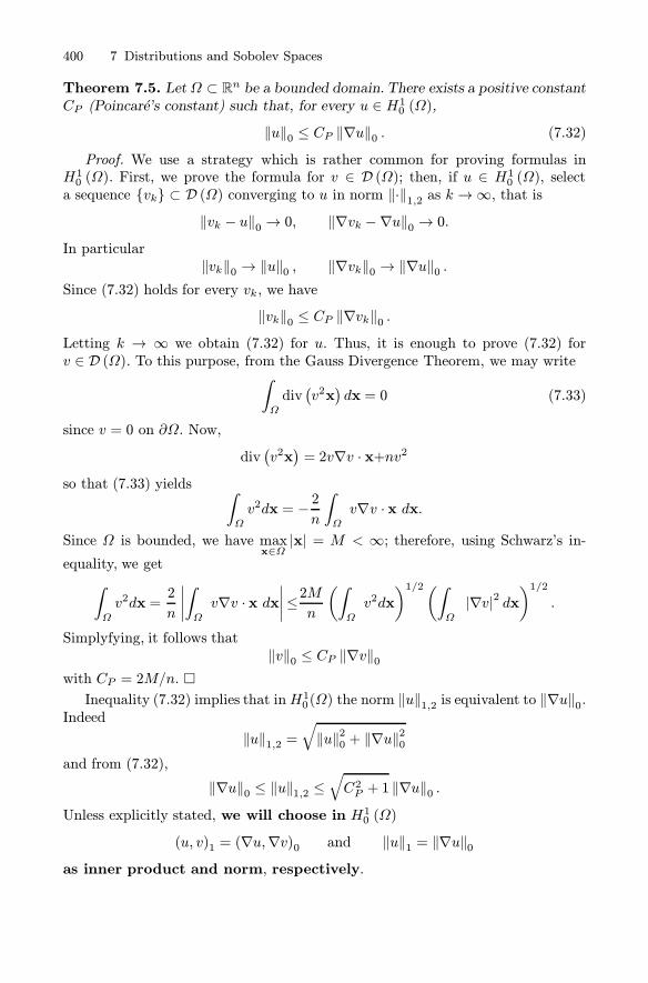
400 7 Distributions and Sobolev Spaces
Theorem 7.5. Let Ω ⊂ Rn be a bounded domain. There exists a positive constantCP (Poincare’s constant) such that, for every u ∈ H10 (Ω),
‖u‖0 ≤ CP ‖∇u‖0 . (7.32)
Proof. We use a strategy which is rather common for proving formulas inH10 (Ω). First, we prove the formula for v ∈ D (Ω); then, if u ∈ H10 (Ω), selecta sequence {vk} ⊂ D (Ω) converging to u in norm ‖·‖1,2 as k →∞, that is
‖vk − u‖0 → 0, ‖∇vk −∇u‖0 → 0.In particular
‖vk‖0 → ‖u‖0 , ‖∇vk‖0 → ‖∇u‖0 .Since (7.32) holds for every vk, we have
‖vk‖0 ≤ CP ‖∇vk‖0 .Letting k → ∞ we obtain (7.32) for u. Thus, it is enough to prove (7.32) forv ∈ D (Ω). To this purpose, from the Gauss Divergence Theorem, we may write
∫
Ω
div(v2x
)dx = 0 (7.33)
since v = 0 on ∂Ω. Now,
div(v2x)= 2v∇v · x+nv2
so that (7.33) yields ∫
Ω
v2dx = − 2n
∫
Ω
v∇v · x dx.
Since Ω is bounded, we have maxx∈Ω
|x| = M < ∞; therefore, using Schwarz’s in-equality, we get
∫
Ω
v2dx =2
n
∣∣∣∣∫
Ω
v∇v · x dx∣∣∣∣≤2M
n
(∫
Ω
v2dx
)1/2(∫
Ω
|∇v|2 dx)1/2
.
Simplyfying, it follows that‖v‖0 ≤ CP ‖∇v‖0
with CP = 2M/n. �Inequality (7.32) implies that inH10(Ω) the norm ‖u‖1,2 is equivalent to ‖∇u‖0.
Indeed
‖u‖1,2 =√‖u‖20 + ‖∇u‖
20
and from (7.32),
‖∇u‖0 ≤ ‖u‖1,2 ≤√C2P + 1 ‖∇u‖0 .
Unless explicitly stated, we will choose in H10 (Ω)
(u, v)1 = (∇u,∇v)0 and ‖u‖1 = ‖∇u‖0as inner product and norm, respectively.
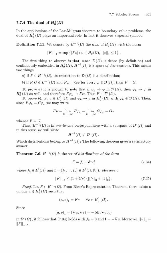
7.7 Sobolev Spaces 401
7.7.4 The dual of H10(Ω)
In the applications of the Lax-Milgram theorem to boundary value problems, thedual of H10 (Ω) plays an important role. In fact it deserves a special symbol.
Definition 7.11. We denote by H−1(Ω) the dual of H10(Ω) with the norm
‖F ‖−1 = sup{|Fv| : v ∈ H10(Ω), ‖v‖1 ≤ 1
}.
The first thing to observe is that, since D (Ω) is dense (by definition) andcontinuously embedded in H10 (Ω), H
−1(Ω) is a space of distributions. This meanstwo things:
a) if F ∈ H−1(Ω), its restriction to D (Ω) is a distribution;b) if F,G ∈ H−1(Ω) and Fϕ = Gϕ for every ϕ ∈ D (Ω), then F = G.To prove a) it is enough to note that if ϕk → ϕ in D (Ω), then ϕk → ϕ in
H10 (Ω) as well, and therefore Fϕk → Fϕ. Thus F ∈ D′ (Ω).To prove b), let u ∈ H10 (Ω) and ϕk → u in H10 (Ω), with ϕk ∈ D (Ω). Then,
since Fϕk = Gϕk we may write
Fu = limk→+∞
Fϕk = limk→+∞
Gϕk = Gu
whence F = G.Thus, H−1(Ω) is in one-to-one correspondence with a subspace of D′ (Ω) and
in this sense we will writeH−1(Ω) ⊂ D′ (Ω) .
Which distributions belong to H−1(Ω)? The following theorem gives a satisfactoryanswer.
Theorem 7.6. H−1(Ω) is the set of distributions of the form
F = f0 + divf (7.34)
where f0 ∈ L2(Ω) and f =(f1, ..., fn) ∈ L2(Ω;Rn). Moreover:
‖F ‖−1 ≤ (1 + CP ) {‖f0‖0 + ‖f‖0} . (7.35)
Proof. Let F ∈ H−1(Ω). From Riesz’s Representation Theorem, there exists aunique u ∈ H10 (Ω) such that
(u, v)1 = Fv ∀v ∈ H10 (Ω) .
Since(u, v)1 = (∇u,∇v) = −〈div∇u, v〉
in D′ (Ω) , it follows that (7.34) holds with f0 = 0 and f = −∇u.Moreover, ‖u‖1 =‖F ‖−1.

402 7 Distributions and Sobolev Spaces
Viceversa, let F = f0+div f , with f0 ∈ L2(Ω) and f =(f1, ..., fn) ∈ L2(Ω;Rn).Then F ∈ D′ (Ω) and, letting Fv = 〈F, v〉, we have;
Fv =
∫
Ω
f0v dx+
∫
Ω
f ·∇v dx ∀v ∈ D (Ω) .
From the Schwarz and Poincare inequalities, we have
|Fv| ≤ (CP + 1) {‖f0‖0 + ‖f‖0} ‖v‖1 . (7.36)
Thus, F is continuous in the H10− norm. It remains to show that F has a uniquecontinuous extension to all H10 (Ω). Take u ∈ H10 (Ω) and {vk} ⊂ D (Ω) such that‖vk − u‖1 → 0. Then, (7.36) yields
|Fvk − Fvh| ≤ (1 +CP ) {‖f0‖0 + ‖f‖0} ‖vk − vh‖1 .
Therefore {Fvk} is a Cauchy sequence in R and converges to a limit which isindependent of the sequence approximating u (why?) and which we may denoteby Fu. Finally, since
|Fu| = limk→∞
|Fvk| and ‖u‖1 = limk→∞‖vk‖1 ,
from (7.36) we get:
|Fu| ≤ (1 +CP ) {‖f0‖0 + ‖f‖0} ‖u‖1showing that F ∈ H−1 (Ω). �Theorem 7.6 says that the elements of H−1(Ω) are represented by a linear
combination of functions in L2(Ω) and their first derivatives (in the sense of dis-tributions). In particular, L2(Ω) ↪→ H−1(Ω).Example 7.21. If n = 1, the Dirac δ belongs toH−1(−a, a). Indeed, we have δ = H′where H is the Heaviside function, and H ∈ L2(−a, a).However, if n ≥ 2 and 0 ∈ Ω, δ /∈ H−1(Ω). For instance, let n = 2 and
Ω = B1 (0). Assume δ ∈ H−1(Ω). Then we may write
δ = f0 + div f
for some f0∈L2(Ω) and f ∈L2(Ω;R2). Thus, for every ϕ ∈ D (Ω),
ϕ (0) = 〈δ, ϕ〉 = 〈f0 + div f , ϕ〉 =∫
Ω
[f0ϕ− f ·∇ϕ]dx.
From Schwarz’s inequality, it follows that
|ϕ (0)|2 ≤{‖f0‖20 + ‖f‖
20
}‖ϕ‖21,2
and, using the density of D (Ω) in H10 (Ω), this estimate should hold for any ϕ ∈H10(Ω) as well. But this is impossible, since in H
10 (Ω) there are functions which
are unbounded near the origin, as we have seen in Example 7.26.

7.7 Sobolev Spaces 403
Example 7.22. Let Ω be a smooth, bounded domain in Rn. Let u = χΩ be itscharacteristic function. Since χΩ ∈ L2 (Rn), the distribution F = ∇χΩ belongs toH−1 (Rn;Rn). The support of F = ∇χΩ coincides with ∂Ω and its action on atest ϕ ∈ D (Rn;Rn) is described by the following formula:
〈∇χΩ,ϕ〉 = −∫
Rn
χΩdiv ϕ dx = −∫
∂Ω
ϕ · ν dσ.
We may regard F as a “delta uniformly distributed on ∂Ω”.
Remark 7.7. It is important to avoid confusion between H−1 (Ω) and H1 (Ω)∗,the dual of H1 (Ω). Since, in general, D (Ω) is not dense in H1 (Ω), the spaceH1 (Ω)
∗is not a space of distributions. Indeed, although the restriction to D (Ω)
of every T ∈ H1 (Ω)∗ is a distribution, this restriction does not identifies T . As asimple example, take f ∈L2 (Ω;Rn) with |f | ≥ c > 0 a.e. and div f = 0. Define
Tϕ =
∫
Ω
f · ∇ϕ dx.
Since |Tϕ| ≤ ‖f‖0 ‖∇ϕ‖0, we infer that T ∈ H1 (Ω)∗. However, the restriction of
T to D (Ω) is the null operator, since in D′ (Ω) we have
〈T, ϕ〉 = −〈div f ,ϕ〉 = 0 ∀ϕ ∈ D (Ω) .
7.7.5 The spaces Hm (Ω), m > 1
Involving higher order derivatives, we may construct new Sobolev spaces. Let Nbe the number of multi-indexes α = (α1, ..., αn) such that |α| =
∑ni=1 αi ≤ m.
Choose in Theorem 7.4
H = L2(Ω), Z = L2(Ω;RN) ⊂ D′(Ω;RN
),
and L : L2(Ω)→ D′(Ω;RN
)given by
Lv = {Dαv}|α|≤m .
Then W is the Sobolev space of the functions in L2 (Ω), whose derivatives (inthe sense of distributions) up to order m included, are functions in L2 (Ω). Forthis space we use the symbol Hm(Ω). Thus:
Hm(Ω) ={v ∈ L2(Ω) : Dαv ∈ L2(Ω), ∀α : |α| ≤ m
}.
From Theorem 7.4 and the separability of L2 (Ω), we deduce:
Proposition 7.10. Hm(Ω) is a separable Hilbert space, continuously embeddedin L2(Ω). The operators Dα, |α| ≤ m, are continuous from Hm(Ω) into L2(Ω).

404 7 Distributions and Sobolev Spaces
The inner product and the norm in Hm are given, respectively, by
(u, v)Hm(Ω) = (u, v)m,2 =∑|α|≤m
∫
Ω
DαuDαv dx
and
‖u‖2Hm(Ω) = ‖u‖2m,2 =
∑|α|≤m
∫
Ω
|Dαu|2 dx.
If u ∈ Hm (Ω), any derivative of u of order k belongs toHm−k (Ω); more generally,if |α| = k ≤ m, then
Dαu ∈ Hm−k (Ω)
and Hm(Ω) ↪→ Hm−k (Ω), k ≥ 1.
Example 7.23. Let B1 (0) ⊂ R3 and consider u (x) = |x|−a . It is easy to check (seeProblem 7.15) that u ∈ H1 (B1 (0)) if a < 1/2. The second order derivatives of uare given by:
uxixj = a (a+ 2)xixj |x|−a−4 − aδij |x|−a−2 .Then ∣∣uxixj
∣∣ ≤ |a (a+ 2)| |x|−a−2so that uxixj ∈ L2 (B1 (0)) if 2a + 4 < 3, or a < −12 . Thus u ∈ H2 (B1 (0)) ifa < −1/2.
7.7.6 Calculus rules
Most calculus rules in Hm are formally similar to the classical ones, although theirproofs are not so trivial. We list here a few of them:
Derivative of a product. Let u ∈ H1(Ω) and v ∈ D (Ω) . Then uv ∈ H1(Ω)and
∇ (uv) = u∇v + v∇u. (7.37)
Formula (7.37) holds if both u, v ∈ H1(Ω) as well. In this case, however,
uv ∈ L1 (Ω) and ∇ (uv) ∈ L1 (Ω;Rn) .
Composition I. Let u ∈ H1(Ω) and g : Ω′ → Ω be one-to-one and Lipschitz.Then, the composition
u ◦ g : Ω′ → R
belongs to H1 (Ω′) and
∂xi [u ◦ g] (x) =n∑k=1
∂xku (g (x)) ∂xigk (x) (7.38)
both a.e. in Ω and in D′ (Ω). In particular, the Lipschitz change of variablesy =g (x) transforms H1 (Ω) into H1 (Ω′).

7.7 Sobolev Spaces 405
Composition II. Let u ∈ H1(Ω) and f : R→R be Lipschitz. Then, thecomposition
f ◦ u : Ω → R
belongs to H1 (Ω) and
∂xi [f ◦ u] (x) = f ′ (u (x)) ∂xiu (x) (7.39)
both a.e. in Ω and in D′ (Ω).In particular, choosing respectively
f (t) = |t| , f (t) = max {t, 0} and f (t) = −min {t, 0} ,
it follows that the following functions:
|u| , u+ = max{u, 0} , and u− = −min{u, 0}
all belong to H1(Ω). For these functions, (7.39) yields
∇u+ ={∇u if u > 00 if u ≤ 0 , ∇u
− ={0 if u ≥ 0
−∇u if u < 0
and ∇(|u|) = ∇u++∇u−, ∇u = ∇u+−∇u−. As a consequence, if u ∈ H1 (Ω) isconstant in a set K ⊆ Ω, then ∇u = 0 a.e. in K.
7.7.7 Fourier Transform and Sobolev Spaces
The spaces Hm (Rn), m ≥ 1, may be defined in terms of the Fourier transform. Infact, by Theorem 7.3,
u ∈ L2 (Rn) if and only if u ∈ L2 (Rn)
and
‖u‖2L2(Rn) = (2π)−n ‖u‖2L2(Rn) .
It follows that, for every multi-index α with |α| ≤m,
Dαu ∈ L2 (Rn) if and only if ξαu ∈ L2 (Rn)
and
‖Dαu‖2L2(Rn) = (2π)−n ‖ξαu‖2L2(Rn) .
Finally, observe that
|ξα|2 ≤ |ξ|2|α| ≤ C(1 + |ξ|2)m
whence we obtain the following result.
406 7 Distributions and Sobolev Spaces
Proposition 7.11. Let u ∈ L2 (Rn) . Then:i) u ∈ Hm (Rn) if and only if (1 + |ξ|2)m/2u ∈ L2 (Rn) .ii) The norms
‖u‖Hm(Rn) and∥∥∥(1 + |ξ|2)m/2u
∥∥∥L2(Rn)
are equivalent.
• Sobolev spaces of real order. The norm
‖u‖Hm(Rn) =∥∥∥(1 + |ξ|2)m/2u
∥∥∥L2(Rn)
makes perfect sense even if m is not an integer and we are led to the followingdefinition.
Definition 7.12. Let s ∈ R, 0 < s < ∞. We denote by Hs (Rn) the space offunctions u ∈ L2 (Rn) such that |ξ|s u ∈ L2 (Rn).
Intuitively, the functionF−1
[(iξj)su]
represents a “derivative of order s” of u. Then,
u ∈ Hs (Rn)
if the “derivatives of order s” of u belong to L2 (Rn). We have:
Proposition 7.12. Hs (Rn) is a Hilbert space with inner product and norm givenby
(u, v)Hs(Rn) =
∫
Rn
(1 + |ξ|2
)su v dξ
and
‖u‖Hs(Rn) =∥∥∥∥(1 + |ξ|2
)s/2u
∥∥∥∥L2(Rn)
.
The space H1/2 (Rn) of the L2−functions possessing “half derivatives” inL2 (Rn) plays an important role in Section 7.9.
7.8 Approximations by Smooth Functions and Extensions
7.8.1 Local approximations
The functions in H1(Ω) may be quite irregular. However, using mollifiers, anyu ∈ H1(Ω) may be approximated locally by smooth functions, in the sense thatthe approximation holds in every compact subset of Ω.

7.8 Approximations by Smooth Functions and Extensions 407
Denote by ηε =1εnη(|x|ε
)the mollifier introduced in section 7.2 and by Ωε the
set of points ε−away from ∂Ω, i.e. (see Remark 7.2):
Ωε = {x ∈Ω: dist (x,∂Ω) > ε} .
We have:
Theorem 7.7. Let u ∈ H1(Ω) and, for ε > 0, small, define
uε = u ∗ ηε.
Then
1. uε∈ C∞ (Ωε) ,2. if ε→ 0, uε → u in H1 (Ω′) for every Ω′ ⊂⊂ Ω.
Proof. Property 1 follows from Remark 7.2. To prove 2, recall that, for everyi = 1, 2, ..., n, we have
∂xiuε = ∂xiu ∗ ηε. (7.40)
Then, 2 follows from property d of Lemma 7.1, applied to any Ω′ ⊂⊂ Ω. �
7.8.2 Estensions and global approximations
By Theorem 7.7, we may approximate a function inH1 (Ω) by smooth functions, aslong as we stay at positive distance from ∂Ω. We wonder whether an approximationis possible in all Ω. First we give the following definition.
Definition 7.13. Denote by D(Ω)the set of restrictions to Ω of functions in
D (Rn).Thus, ϕ ∈ D
(Ω)if there is ψ ∈ D (Rn) such that ϕ = ψ in Ω. Clearly,
D(Ω)⊂ C∞
(Ω). We want to establish whether
D(Ω)is dense in H1 (Ω) . (7.41)
The case Ω = Rn is special, since D (Ω) coincides with D(Ω). We have:
Theorem 7.8. D (Rn) is dense in H1 (Rn). In particular H1 (Rn) = H10 (Rn).Proof. First observe that H1c (R
n), the subspace of functions with compact(essential) support in Rn, is dense in H1(Rn). In fact, let u ∈ H1 (Rn) and v ∈D (Rn), such that 0 ≤ v ≤ 1 and v ≡ 1 if |x| ≤ 1. Define
us (x) = v(xs
)u (x) .
Then us ∈ H1c (Rn) and
∇us (x) = v(xs
)∇u (x) + 1
su (x)∇v
(xs
).

408 7 Distributions and Sobolev Spaces
From the Dominated Convergence Theorem19, it follows that
us → u in H1(Rn) as s→∞.On the other hand D (Rn) is dense in H1c (Rn). In fact, if u ∈ H1c (Rn), we have
uε = u ∗ ηε ∈ D (Rn)and uε → u in H1(Rn). �However, in general (7.41) is not true, as the following example shows.
Example 7.24. Consider, for instance,
Ω = {(ρ, θ) : 0 < ρ < 1, 0 < θ < 2π} .The domain Ω coincides with the open unit circle, centered at the origin, withoutthe radius
{(ρ, θ) : 0 < ρ < 1, θ = 0} .The closure Ω is given by the full closed circle. Let
u (ρ, θ) = ρ1/2 cos(θ/2).
Then u ∈ L2 (Ω), since u is bounded. Moreover20,
|∇u|2 = u2ρ +1
ρ2u2θ =
1
4ρin Ω,
so that u ∈ H1 (Ω). However, u (ρ, 0+) = ρ1/2 while u (ρ, 2π−) = −ρ1/2. Thus, uhas a jump discontinuity across θ = 0 and no sequence of smooth functions canconverge to u in H1 (Ω).
The difficulty in Example 7.24 is that the domain Ω lies on both sides of partof its boundary (the radius 0 < ρ < 1, θ = 0). Thus, to have a hope that (7.41) istrue we have to avoid domains with this anomaly and consider domains with somedegree of regularity.Thus, assume Ω is a C1 or even a Lipschitz domain. Theorem 7.8 suggests a
strategy to prove (7.41): given u ∈ H1(Ω), extend the definition of u to all Rn inorder to obtain a function in H1(Rn) and then apply Theorem 7.8. The first thingto do is to introduce an extension operator :
Definition 7.14. We say that a linear operator E : H1(Ω) → H1(Rn) is anextension operator if, ∀u ∈ H1(Ω):1. E (u) = u in Ω,
2. if Ω is bounded, E (u) is compactly supported,
3. E is continuous:
‖Eu‖H1(Rn) ≤ c (n,Ω) ‖u‖H1(Ω) .19 Observe that |us| ≤ |u| and |∇us| ≤ |∇u|+M |u| where M = max |∇v| .20 Appendix C.

7.8 Approximations by Smooth Functions and Extensions 409
How do we construct E? The first thing that comes into mind is to defineEu = 0 outside Ω (trivial extension). This certainly works if u ∈ H10 (Ω). In fact:u ∈ H10 (Ω) if and only if its trivial extension belongs to H1 (Rn).However, the trivial extension works in this case only. For instance, let u ∈
H1 (0,∞) with u (0) = a �= 0. Let Eu be the trivial extension of u. Then, inD′ (R), (Eu)′ = u′ + aδ which is not even in L2 (R).Thus, we have to use another method. If Ω is a half space. i.e.
Ω = Rn+ = {(x1, ..., xn) : xn > 0}an extension operator can be defined by a reflection method as follows:
• Reflection method. Let H1(Rn+
). Write x = (x′, xn). We reflect in an even
way with respect to the hyperplane xn = 0, by setting Eu = u where
u (x) = u (x′, |xn|) .Then, it is possible to prove that, in D′ (Rn):
uxj (x) =
{uxj (x
′, |xn|) j < n
uxn (x′, |xn|) sign xn j = n.
(7.42)
It is now easy to check that E has the properties 1,2,3 listed above. In particular,
‖Eu‖2H1(Rn) = 2 ‖u‖2H1(Rn+)
.
• Extension operator for Lipschitz domains. Suppose now that Ω is a boundedLipschitz domain. To construct an extension operator we use two rather generalideas, which may be applied in several different contexts: localization and reductionto the half space.
Localization. It is based on the following lemma. Given a set K, by opencovering of K we mean a collection U of open sets, such that K ⊂ ∪U∈UU .Lemma 7.3. (Partition of unity). Let K ⊂ Rn be a compact set and U1, ..., UN bean open covering of K. There exist functions ψ1, ..., ψN with the following proper-ties:
1. For every j = 1, ..., N , ψj ∈ C∞0 (Uj) and 0 ≤ ψj ≤ 1.2. For every x ∈K, ∑N
j=1 ψj (x) = 1.
Proof (sketch). Since K ⊂ ∪Nj=1Uj and each Uj is open, we can find open setsKj ⊂⊂ Uj such that
K ⊂ ∪Nj=1Kj .Let χKj be the characteristic function of Kj and ηε the mollifier (7.3). Defineϕj,ε = ηε ∗χKj . According to Example 7.2, we may fix ε so small in order to haveϕj,ε ∈ C∞0 (Uj) and ϕj,ε > 0 on Kj . Then the functions
ψj =ϕj,ε∑Ns=1 ϕs,ε
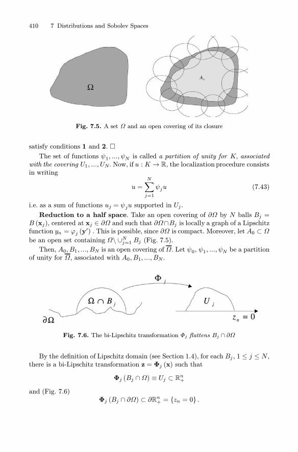
410 7 Distributions and Sobolev Spaces
Fig. 7.5. A set Ω and an open covering of its closure
satisfy conditions 1 and 2. �The set of functions ψ1, ..., ψN is called a partition of unity for K, associated
with the covering U1, ..., UN. Now, if u : K → R, the localization procedure consistsin writing
u =
N∑j=1
ψju (7.43)
i.e. as a sum of functions uj = ψju supported in Uj .
Reduction to a half space. Take an open covering of ∂Ω by N balls Bj =B (xj), centered at xj ∈ ∂Ω and such that ∂Ω∩Bj is locally a graph of a Lipschitzfunction yn = ϕj (y
′) . This is possible, since ∂Ω is compact. Moreover, let A0 ⊂ Ωbe an open set containing Ω\ ∪Nj=1 Bj (Fig. 7.5).Then, A0, B1, ..., BN is an open covering of Ω. Let ψ0, ψ1, ..., ψN be a partition
of unity for Ω, associated with A0, B1, ..., BN .
Fig. 7.6. The bi-Lipschitz transformation Φj flattens Bj ∩ ∂Ω
By the definition of Lipschitz domain (see Section 1.4), for each Bj , 1 ≤ j ≤ N ,there is a bi-Lipschitz transformation z = Φj (x) such that
Φj (Bj ∩Ω) ≡ Uj ⊂ Rn+and (Fig. 7.6)
Φj (Bj ∩ ∂Ω) ⊂ ∂Rn+ = {zn = 0} .

7.9 Traces 411
Let u ∈ H1 (Ω) and uj = ψju. Then, wj = uj ◦Φ−1j is supported in Uj, so that,
extending it to zero in Rn+\Uj , we have wj ∈ H1(Rn+
).
The functionEwj = wj, obtained by the reflection method, belongs toH1 (Rn).
Now we go back defining
Euj = wj ◦Φj , 1 ≤ j ≤ N ,
in Bj and Euj = 0 outside Bj . Finally, let u0 = ψ0u0 and let Eu0 be the trivialextension of u0. Set
Eu =
N∑j=0
Euj .
At this point, it is not difficult to show that E satisfies the requirements 1, 2, 3 ofDefinition 7.14. We have proved the following
Theorem 7.9. Let Ω be either Rn+ or a bounded, Lipschitz domain. Then, thereexists an extension operator E : H1(Ω)→ H1(Rn).An immediate consequence of Theorems 7.8 and 7.9 is the following global
approximation result:
Theorem 7.10. Let Ω be either Rn+ or a bounded, Lipschitz domain. Then
D(Ω)is dense in H1 (Ω). In other words, if u ∈ H1 (Ω), there exists a se-
quence {um} ⊂ D(Ω)such that
‖um − u‖1,2 → 0 as m→ +∞.
7.9 Traces
7.9.1 Traces of functions in H1 (Ω)
The possibility of approximating any element u ∈ H1 (Ω) by smooth functions inΩ represents a key tool for introducing the notion of restriction of u on Γ = ∂Ω.Such restriction is called the trace of u on Γ and it will be an element of L2 (Γ ).Observe that if Ω = Rn+, then Γ = ∂R
n+ = R
n−1 and L2 (Γ ) is well defined.If Ω is a Lipschitz domain, we define L2 (Γ ) by localization. More precisely, letB1, ..., BN be an open covering of Γ by balls centered at points on Γ , as in sub-section 7.8.2. If g : Γ → R, write
g =N∑j=1ψjg
where ψ1, ..., ψN is a partition of unity for Γ , associated with B1, ..., BN . SinceΓ ∩ Bj is the graph of a Lipschitz function yn = ϕj (y′), on Γ ∩ Bj there is anatural notion of “area element”, given by
dσ=
√1 +
∣∣∇ϕj∣∣2dy′.

412 7 Distributions and Sobolev Spaces
Thus, we say that g ∈ L2 (Γ ) if21
‖g‖2L2(Γ) =N∑j=1
∫
Γ∩Bjψj |g|2 dσ<∞. (7.44)
L2 (Γ ) is a Hilbert space with respect to the inner product
(g, h)L2(Γ) =N∑j=1
∫
Γ∩Bjψj gh dσ.
Let us go back to our trace problem. We may consider n > 1, since there is noproblem if n = 1. The strategy consists in the following two steps.
Let τ 0 : D(Ω)→ L2 (Γ ) be the operator that associates to every function v
its restriction v|Γ to Γ : τ 0v = v|Γ . This makes perfect sense, since each v ∈ D(Ω)
is continuous on Γ .First step: show that ‖τ 0u‖L2(Γ) ≤ c (Ω, n) ‖u‖1,2. Thus, τ 0 is continuous from
D(Ω)⊂ H1(Ω) into L2 (Γ ).
Second step: extend τ 0 to all H1(Ω) using the density of D
(Ω)in H1(Ω).
An elementary analogy may be useful. Suppose we have a function f : Q→ R
and we want to define the value of f at an irrational point x. What do we do?Since Q is dense in R, we select a sequence {rk} ⊂ Q such that rk → x. Then wecompute f (rk) and set f (x) = limk→∞ f (rk). Of course, we have to prove thatthe limit exists, by showing, for example, that {f (rn)} is a Cauchy sequence andthat the limit does not depend on the approximating sequence {rn}.Theorem 7.11. Let Ω be either Rn+ or a bounded, Lipschitz domain. Then thereexists a linear operator (trace operator) τ 0 : H
1(Ω)→ L2 (Γ ) such that:1. τ 0u = u|Γ if u ∈ D
(Ω),
2. ‖τ 0u‖L2(Γ) ≤ c (Ω, n)‖u‖1,2 .
Proof. Let Ω = Rn+. First, we prove inequality 2 for u ∈ D(Ω). In this case
τ 0u = u(x′, 0) and we must show that there is a constant c such that∫
Rn−1|u(x′, 0)|2 dx′ ≤ c ‖u‖2H1(Rn+) ∀u ∈ D
(Ω). (7.45)
For every xn ∈ (0, 1) we may write:
u(x′, 0) = u(x′, xn) −∫ xn
0
uxn (x′, t)dt.
Since by Schwarz’s inequality(∫ 10
|uxn (x′, t)|dt)2≤∫ 10
|uxn (x′, t)|2dt,
21 Observe that the norm (7.44) depends on the particular covering and partition ofunity. However, norms corresponding to different coverings and partitions of unity areall equivalent and induce the same topology on L2 (Γ ).

7.9 Traces 413
we deduce that (recalling the elementary inequality (a+ b)2 ≤ 2a2 + 2b2)
|u(x′, 0)|2 ≤ 2 |u(x′, xn)|2 + 2(∫ 10
|uxn (x′, t)| dt)2
≤ 2 |u(x′, xn)|2 + 2∫ 10
|uxn (x′, t)|2dt
≤ 2 |u(x′, xn)|2 + 2∫ 10
|∇u (x′, t)|2 dt
Integrating both sides in Rn−1 with respect to x′ and in (0, 1) with respect to xnwe easily obtain (7.45) with c = 2.Assume now u ∈ H1
(Rn+
). Since D
(Ω)is dense in H1
(Rn+
), we can select
{uk} ⊂ D(Ω)such that uk → u in H1
(Rn+
).
The linearity of τ 0 and estimate (7.45) yield
‖τ 0uh − τ 0uk‖L2(Rn−1) ≤√2 ‖uh − uk‖H1(Rn+) .
Since {uk} is a Cauchy sequence in H1(Rn+
), we infer that {τ 0uk} is a Cauchy
sequence in L2(Rn−1). Therefore, there exists u0 ∈ L2(Rn−1) such that
τ 0uk → u0 in L2(Rn−1).
The limiting element u0 does not depend on the approximating sequence {uk}. Infact, if {vk} ⊂ D
(Ω)and vk → u in H1
(Rn+
), then
‖vk − uk‖H1(Rn+) → 0.
From‖τ 0vk − τ 0uk‖L2(Rn−1) ≤
√2 ‖vk − uk‖H1(Rn+)
it follows that τ 0vk → u0 in L2(Rn−1) as well.Thus, if u ∈ H1
(Rn+
), it makes sense to define τ 0u = u0. It should be clear
that τ 0 has the properties 1, 2.If Ω is a bounded Lipschitz domain, the theorem can be proved once more by
localization and reduction to a half space. We omit the details. �Definition 7.15. The function τ 0u, also denoted by u|Γ , is called the trace ofu on Γ .
The following integration by parts formula for functions in H1 (Ω) is a conse-quence of the trace theorem 7.11.
Corollary 7.1. Assume Ω is either Rn+ or a bounded, Lipschitz domain. Letu ∈ H1 (Ω) and v ∈H1 (Ω;Rn). Then
∫
Ω
∇u · v dx = −∫
Ω
u divv dx+
∫
Γ
(τ 0u) (τ 0v) · ν dσ. (7.46)
where ν is the outward unit normal to Γ and τ 0v =(τ 0v1, ..., τ0vn) .

414 7 Distributions and Sobolev Spaces
Proof. Formula (7.46) holds if u ∈ D(Ω)and v ∈D
(Ω;Rn
). Let u ∈ H1 (Ω)
and v ∈H1 (Ω;Rn) . Select {uk} ⊂ D(Ω), {vk} ⊂ D
(Ω;Rn
)such that uk → u in
H1 (Ω) and vk → v in H1 (Ω;Rn). Then:∫
Ω
∇uk · vk dx = −∫
Ω
uk div vk dx+
∫
Γ
(τ 0uk) (τ 0vk) · ν dσ.
Letting k →∞, by the continuity of τ 0, we obtain (7.46). �It is not surprising that the kernel of τ 0 is precisely
22 H10 (Ω):
τ 0u = 0 ⇐⇒ u ∈ H10 (Ω) .In similar way, we may define the trace of u ∈ H1 (Ω) on a relatively open
subset Γ0 ⊂ Γ .Theorem 7.12. Assume Ω is either Rn+ or a bounded, Lipschitz domain. Let Γ0be an open subset of Γ.Then there exists a trace operator τ Γ0 : H
1(Ω)→ L2 (Γ0) such that:1. τΓ0u = u|Γ0 if u ∈ D
(Ω),
2. ‖τ Γ0u‖L2(Γ0) ≤ c (Ω, n) ‖u‖1,2.The function τΓ0u is called the trace of u on Γ0, often denoted by u|Γ0 . The
kernel of τ Γ0 is denoted by H10,Γ0(Ω):
τΓ0u = 0 ⇐⇒ u ∈ H10,Γ0 (Ω) .
This space can be characterized in another way. Let V0,Γ0 be the set of functionsin D
(Ω)vanishing in a neighborhood of Γ 0. Then:
Proposition 7.13. H10,Γ0(Ω) is the closure of V0,Γ0 in H1 (Ω).
7.9.2 Traces of functions in Hm (Ω)
We have seen that u ∈ Hm(Rn+), m ≥ 1, has a trace on Γ = ∂Rn+. However, ifm = 2, every derivative of u belongs to H1(Rn+), so that it has a trace on Γ . Inparticular, we may define the trace of ∂xnu on Γ . Let
τ 1u = (∂xnu)|Γ .
In general, for m ≥ 2, we may define the trace on Γ of the derivatives ∂jxnu = ∂ju
∂xjnfor j = 0, 1, ...,m− 1 and set
τ ju = (∂jxnu)|Γ .
In this way, we construct a linear operator τ : Hm(Rn+)→ L2 (Γ ;Rm), given byτu = (τ 0u, ..., τm−1u) .
22 However, only the proof of the “ ⇐= ” part is trivial. The proof of the “ =⇒ ” part israther tecnical and we omit it.
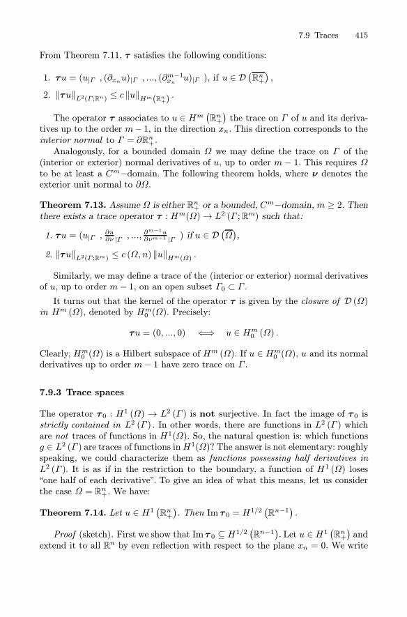
7.9 Traces 415
From Theorem 7.11, τ satisfies the following conditions:
1. τu = (u|Γ , (∂xnu)|Γ , ..., (∂m−1xn u)|Γ ), if u ∈ D(Rn+
),
2. ‖τu‖L2(Γ ;Rn) ≤ c ‖u‖Hm(Rn+) .
The operator τ associates to u ∈ Hm(Rn+
)the trace on Γ of u and its deriva-
tives up to the order m− 1, in the direction xn. This direction corresponds to theinterior normal to Γ = ∂Rn+.Analogously, for a bounded domain Ω we may define the trace on Γ of the
(interior or exterior) normal derivatives of u, up to order m− 1. This requires Ωto be at least a Cm−domain. The following theorem holds, where ν denotes theexterior unit normal to ∂Ω.
Theorem 7.13. Assume Ω is either Rn+ or a bounded, Cm−domain, m ≥ 2. Then
there exists a trace operator τ : Hm(Ω)→ L2 (Γ ;Rm) such that:
1. τu = (u|Γ , ∂u∂ν |Γ , ...,∂m−1u∂νm−1 |Γ ) if u ∈ D
(Ω),
2. ‖τu‖L2(Γ ;Rm) ≤ c (Ω, n)‖u‖Hm(Ω) .
Similarly, we may define a trace of the (interior or exterior) normal derivativesof u, up to order m− 1, on an open subset Γ0 ⊂ Γ .It turns out that the kernel of the operator τ is given by the closure of D (Ω)
in Hm (Ω), denoted by Hm0 (Ω). Precisely:
τu = (0, ..., 0) ⇐⇒ u ∈ Hm0 (Ω) .
Clearly, Hm0 (Ω) is a Hilbert subspace of H
m (Ω). If u ∈ Hm0 (Ω), u and its normal
derivatives up to order m− 1 have zero trace on Γ .
7.9.3 Trace spaces
The operator τ 0 : H1 (Ω) → L2 (Γ ) is not surjective. In fact the image of τ 0 is
strictly contained in L2 (Γ ) . In other words, there are functions in L2 (Γ ) whichare not traces of functions in H1(Ω). So, the natural question is: which functionsg ∈ L2 (Γ ) are traces of functions inH1(Ω)? The answer is not elementary: roughlyspeaking, we could characterize them as functions possessing half derivatives inL2 (Γ ). It is as if in the restriction to the boundary, a function of H1 (Ω) loses“one half of each derivative”. To give an idea of what this means, let us considerthe case Ω = Rn+. We have:
Theorem 7.14. Let u ∈ H1(Rn+
). Then Im τ 0 = H
1/2(Rn−1) .
Proof (sketch). First we show that Imτ 0 ⊆ H1/2(Rn−1). Let u ∈H1 (Rn+
)and
extend it to all Rn by even reflection with respect to the plane xn = 0. We write
416 7 Distributions and Sobolev Spaces
the points in Rn as x =(x′, xn), with x′ = (x1, ..., xn). Define g (x′) = u (x′, 0).We show that g ∈ H1/2
(Rn−1), that is
‖g‖2H1/2(Rn−1) =∫
Rn−1(1 +
∣∣ξ′∣∣2)1/2 ∣∣g (ξ′)∣∣2 dξ′ <∞.
First, we consider u ∈ D (Rn) and express g in terms of u. By the Fourier inversionformula, we may write
u (x′, xn) =1
(2π)n
∫
Rn−1eix
′·ξ′(∫
R
u(ξ′, ξn
)eixnξndξn
)dξ′
so that
g (x′) =1
(2π)n−1
∫
Rn−1eix
′·ξ′(1
2π
∫
R
u(ξ′, ξn
)dξn
)dξ′.
This shows that
g(ξ′)=1
2π
∫
R
u(ξ′, ξn
)dξn.
Thus:
‖g‖2H1/2(Rn−1) =1
(2π)2
∫
Rn−1(1 +
∣∣ξ′∣∣2)1/2∣∣∣∣∫
R
u(ξ′, ξn
)dξn
∣∣∣∣2
dξ′.
Note now the following two facts. First, from Schwarz’s inequality, we may write∣∣∣∣∫
R
u(ξ′, ξn
)dξn
∣∣∣∣ ≤∫
R
(1 + |ξ|2)−1/2(1 + |ξ|2)1/2∣∣u (ξ′, ξn
)∣∣dξn
≤(∫
R
(1 + |ξ|2)∣∣u (ξ′, ξn
)∣∣2 dξn)1/2(∫
R
(1 + |ξ|2)−1dξn)1/2
.
Second,23
∫
R
(1 + |ξ|2)−1dξn =∫
R
(1 +∣∣ξ′∣∣2 + ξ2n)−1dξn =
π
(1 +∣∣ξ′∣∣2)1/2
.
Thus,
‖g‖2H1/2(Rn−1) ≤1
4π
∫
Rn
(1 + |ξ|2) |u (ξ)|2 dξ = 14π‖u‖2H1(Rn) =
1
2π‖u‖2H1(Rn+) <∞.
Therefore, g ∈ H1/2(Rn−1). By the usual density argument, this is true for everyu ∈ H1 (Rn) and shows that Imτ 0 ⊆ H1/2
(Rn−1).
To prove the opposite inclusion, take any g ∈ H1/2(Rn−1) and define
u (x′, xn) =1
(2π)n−1
∫
Rn−1e−(1+|ξ′|)xn g
(ξ′)eix
′·ξ′dξ′, xn ≥ 0.
23∫R(a2 + t2)−1dt =
[1
aarctan
(t
a
)]+∞
−∞=π
a(a > 0) .
7.9 Traces 417
Then, clearly u (x′, 0) = g (x′) and it can be proved that u ∈ H1(Rn+
). Therefore,
g ∈ Imτ 0 so that H1/2(Rn−1) ⊆ Im τ 0. �
If Ω is a bounded, Lipschitz domain, it is possible to define H1/2 (Γ ) by local-ization and reduction to the half space, as we did for L2 (Γ ). In this way we canendow H1/2 (Γ ) with an inner product that makes it a Hilbert space, continuouslyembedded in L2 (Γ ). It turn out that H1/2 (Γ ) coincides with Im τ 0:
H1/2 (Γ ) ={u|Γ : u ∈ H1(Ω)
}. (7.47)
Actually, changing slightly our point of view, we could take (7.47) as a definitionof H1/2 (Γ ) and endow H1/2 (Γ ) with the equivalent norm
‖g‖H1/2(Γ) = inf{‖u‖H1(Ω) : u ∈ H1(Ω), u|Γ = g
}. (7.48)
This norm is equal to the smallest among the norms of all elements in H1(Ω)sharing the same trace g on Γ and takes into account that the trace operator τ 0is not injective, since we know that Ker τ 0 = H
10 (Ω). In particular, the following
trace inequality holds: ∥∥u|Γ∥∥H1/2(Γ)
≤ ‖u‖1,2 , (7.49)
which means that the trace operator τ 0 is continuous from H1(Ω) onto H1/2 (Γ ) .
In similar way, if Γ0 is a relatively open subset of Γ , by localization and reduc-tion to the half space, we may define the space H1/2 (Γ0) and make it a Hilbertspace, continuously embedded in L2 (Γ0). H
1/2 (Γ0) coincides with ImτΓ0 , that is
H1/2 (Γ0) ={u|Γ0 : u ∈ H1(Ω)
},
and can be endowed with the norm
‖g‖H1/2(Γ0) = inf{‖u‖H1(Ω) : u ∈ H1(Ω), u|Γ0 = g
}.
In particular, the following trace inequality holds:
∥∥u|Γ0∥∥H1/2(Γ0)
≤ ‖u‖H1(Ω) . (7.50)
which means that the trace operator τ Γ0 is continuous from H1(Ω) in H1/2 (Γ0) .
Finally, if Ω is Rn+ or a bounded Cm− domain,m ≥ 2, the space of the traces of
functions inHm(Ω) is the fractional order Sobolev space Hm−1/2 (Γ ), still showinga loss of “half derivative”. Coherently, the trace of a normal derivative undergoesa loss of one more derivative and belongs to Hm−3/2 (Γ ); the derivatives of orderm− 1 have traces in H1/2 (Γ ). Thus we obtain:
τ : Hm(Ω)→(Hm−1/2 (Γ ) , Hm−3/2 (Γ ) , ..., H1/2 (Γ )
).
The kernel of τ is Hm0 (Ω).
418 7 Distributions and Sobolev Spaces
7.10 Compactness and Embeddings
7.10.1 Rellich’s theorem
Since
‖u‖0 ≤ ‖u‖1,2 ,
H1 (Ω) is continuously embedded in L2 (Ω) i.e., if a sequence {uk} converges to uin H1 (Ω) it converges to u in L2 (Ω) as well.If we assume that Ω is a bounded, Lipschitz domain, then the embedding
of H1 (Ω) in L2 (Ω) is also compact. Thus, a bounded sequence {uk} ⊂ H1 (Ω)has the following important property:
There exists a subsequence{ukj}and u ∈ H1 (Ω), such that
a. ukj → u in L2 (Ω) ,b. ukj ⇀ u in H
1 (Ω) (i.e. ukj converges weakly24 to u in H1 (Ω)).
Actually, only property a follows from the compactness of the embedding.Property b expresses a general fact in every Hilbert space H : every boundedsubset E ⊂ H is sequentially weakly compact (Theorem 6.11).
Theorem 7.15. Let Ω be a bounded, Lipschitz domain. Then H1 (Ω) is com-pactly embedded in L2 (Ω).
Proof. We use the compactness criterion expressed in Theorem 6.9. First, ob-serve that, for every v ∈ D (Rn) we may write
v (x+ h)− v (x) =∫ 10
d
dtv (x+th) dt =
∫ 10
∇v (x+th) · h dt
whence
|v (x+ h) − v (x)|2 =∣∣∣∣∫ 10
∇v (x+th) · h dt∣∣∣∣2
≤ |h|2∫ 10
|∇v (x+th)|2 dt.
Integrating on Rn we find
∫
Rn
|v (x+ h)− v (x)|2 dx ≤ |h|2∫
Rn
dx
∫ 10
|∇v (x+th)|2 dt ≤ |h|2 ‖∇v‖2L2(Rn)
so that ∫
Rn
|v (x+ h) − v (x)|2 dx ≤ |h|2 ‖∇v‖2L2(Rn) . (7.51)
Since D (Rn) is dense in H1 (Rn), we infer that (7.51) holds for every u ∈ H1 (Rn)as well.
24 Section 6.7.
7.10 Compactness and Embeddings 419
Let now S ⊂ H1 (Ω) be bounded, i.e. there exists a number M such that:
‖u‖H1(Ω) ≤M, ∀u ∈ S.
By Theorem 7.9, every u ∈ S has an extension u ∈ H1 (Rn), with support cotainedin an open set Ω′ ⊃⊃ Ω. Thus, u ∈ H10 (Ω′) and moreover,
‖∇u‖L2(Ω′) ≤ c ‖∇u‖L2(Ω) ≤ cM.
Denote by S the set of such extensions. Then (7.51) holds for every u ∈ S :∫
Ω′|u (x+ h) − u (x)|2 dx ≤ |h|2 ‖∇u‖2L2(Rn) ≤ c2M2 |h|
2.
Theorem 6.9 implies that S is precompact in L2 (Ω′), which implies that S isprecompact in L2 (Ω). �
7.10.2 Poincare’s inequalities
Under suitable hypotheses, the norm ‖u‖1,2 is equivalent to ‖∇u‖0. This meansthat there exists a constant CP , depending only on n and Ω, such that
‖u‖0 ≤ CP ‖∇u‖0 . (7.52)
Inequalities like (7.52) are called Poincare’s inequalities and play a big rolein the variational treatment of boundary value problems, as we shall realize inthe next chapter. We have already proved (Theorem 7.5) that (7.52) holds if u ∈H10 (Ω), i.e. for functions vanishing on ∂Ω.On the other hand, (7.52) cannot hold if u = constant �= 0. Roughly speaking,
the hypotheses that guarantee the validity of (7.52) require that u vanishes in some“non trivial set”. For instance, under each one of the following conditions, (7.52)holds:
i) u ∈ H10,Γ0 (Ω) (u vanishes on a non empty relatively open subset Γ0 ⊂ ∂Ω);ii) u ∈ H1 (Ω) and u = 0 on a set E ⊂ Ω with positive measure: |E| = a > 0;iii) u ∈ H1(Ω) and
∫Ωu = 0 (u has mean value zero in Ω).
Theorem 7.16. Let Ω be a bounded Lipschitz domain. Assume that u satisfiesone among the hypotheses i), ii), iii) above. Then, there exists CP such that
‖u‖0 ≤ CP ‖∇u‖0 . (7.53)
Proof. Assume i) holds. By contradiction suppose (7.53) is not true. This meansthat for every integer j ≥ 1, there exists uj ∈ H10,Γ0 (Ω) such that
‖uj‖0 > j ‖∇uj‖0 . (7.54)

420 7 Distributions and Sobolev Spaces
Normalize uj in L2 (Ω) by setting
wj =uj
‖uj‖0.
Then, from (7.54),
‖wj‖0 = 1 and ‖∇wj‖0 <1
j≤ 1.
Thus {wj} is bounded in H1 (Ω) and by Rellich’s Theorem there exists a subse-quence {wjk} and w ∈ H10,Γ0 (Ω) such that• wjk → w in L2 (Ω) ,• ∇wjk ⇀ ∇w in L2 (Ω).The continuity of the norm gives
‖w‖0 = limj→∞ ‖wj‖0 = 1.
On the other hand, the weak semicontinuity of the norm (Theorem 6.10) yields,
‖∇w‖0 ≤ lim infj→∞‖∇wj‖0 = 0
so that ∇w = 0. Since Ω is connected, w is constant and since w ∈ H10,Γ0 (Ω), weinfer w = 0, in contradiction to ‖w‖0 = 1.The proof in the other cases is identical. �
Remark 7.8. If u ∈ H1 (Ω), let1
|Ω|
∫
Ω
u = uΩ. (7.55)
Then w = u − uΩ has zero mean value and (7.53) holds for w. Thus, in general,the Poincare inequality takes the form:
‖u− uΩ‖0 ≤ CP ‖∇u‖0 .
7.10.3 Sobolev inequality in Rn
From Proposition 7.9 we know that the elements of H1 (R) are continuous and(Problem 7.19) vanish as x→ ±∞. Moreover, if u ∈ D (R), we may write
u2 (x) =
∫ x
−∞
d
dsu2 (s) ds = 2
∫ x
−∞u (s) u′ (s) ds.
Using Schwarz’s inequality and 2ab ≤ 2a2 + 2b2, we getu (x)
2 ≤ 2 ‖u‖L2(R) ‖u′‖L2(R) ≤ ‖u‖2L2(R) + ‖u′‖
2L2(R) = ‖u‖
2H1(R) .
Since D (R) is dense in H1 (R) , this inequality holds if u ∈ H1 (R) as well. Wehave proved:

7.10 Compactness and Embeddings 421
Proposition 7.14. Let u ∈ H1 (R). Then u ∈ L∞ (R) and
‖u‖L∞(R) ≤ ‖u‖H1(R) .
On the other hand, Example 7.26 implies that, when Ω ⊆ Rn, n ≥ 2,
u ∈ H1(Ω)� u ∈ L∞ (Ω) .
However, it is possible to prove that u is actually p−summable with a suitablep > 2. Moreover, the Lp−norm of u can be estimated by the H1−norm of u.To realize which exponent p is the correct one, assume that the inequality
‖u‖Lp(Rn) ≤ c ‖∇u‖L2(Rn) (7.56)
is valid for every u ∈ D (Rn), where c may depend on p and n but not on u.We now use a typical “dimensional analysis” argument.Inequality (7.56) must be invariant under dilations in the following sense. Let
u ∈ D (Rn) and for λ > 0 set
uλ (x) = u (λx) .
Then uλ ∈ D (Rn) so that inequality (7.56) must be true for uλ, with c indepen-dent of λ:
‖uλ‖Lp(Rn) ≤ c ‖∇uλ‖L2(Rn) . (7.57)
Now, ∫
Rn
|uλ|p dx =∫
Rn
|u (λx)|p dx = 1λn
∫
Rn
|u (y)|p dy
while ∫
Rn
|∇uλ|2 dx =∫
Rn
|∇u (λx)|2 dx = 1
λn−2
∫
Rn
|∇u (y)|2 dy.
Therefore, (7.57) becomes
1
λn/p
(∫
Rn
|u|p dy)1/p
≤c (n, p) 1
λ(n−2)/2
(∫
Rn
|∇u|2 dy)1/2
or‖u‖Lp(Rn) ≤ cλ1−
n2 +
np ‖∇u‖L2(Rn) .
The only way to get a constant independent of λ is to choose p such that
1− n2+n
p= 0.
Hence, if n > 2, the correct p is given by
p∗ =2n
n− 2which is called the Sobolev exponent for H1 (Rn). The following theorem of Sobolev,Gagliardo, Nirenberg holds:

422 7 Distributions and Sobolev Spaces
Theorem 7.17. Let u ∈ H1 (Rn) , n ≥ 3. Then u ∈ Lp∗ (Rn) with p∗ = 2nn−2 , and
the following inequality holds.
‖u‖Lp∗(Rn) ≤ c ‖∇u‖L2(Rn) (7.58)
where c = c (n).
In the case n = 2 the correct statement is:
Proposition 7.15. Let u ∈ H1(R2). Then u ∈ Lp (R) for 2 ≤ p <∞, and
‖u‖Lp(R2) ≤ c (p) ‖u‖H1(R2) .
7.10.4 Bounded domains
We now consider bounded domains. In dimension n = 1, the elements of H1 (a, b)are continuous in [a, b] and therefore bounded as well. Furthermore, the followinginequality holds:
‖v‖L∞(a,b) ≤ C∗ ‖v‖H1(a,b) (7.59)
withC∗ =
√2max
{(b− a)−1/2 , (b− a)1/2
}.
Indeed, by Schwarz’s inequality we have, for any x, y ∈ [a, b], y > x:
u (y) = u (x) +
∫ y
x
u′ (s) ds
≤ u (x) +√b− a‖u′‖L2(a,b)
whence, using the elementary inequality (A+ B)2 ≤ 2A2 + 2B2,
u (y)2 ≤ 2u (x)2 + 2 (b− a) ‖u′‖2L2(a,b) .
Integrating over (a, b) with respect to x we get
(b− a)u (y)2 ≤ 2 ‖u‖2L2(a,b) + 2 (b− a)2 ‖u′‖2L2(a,b)
from which (7.59) follows easily.
In dimension n ≥ 2, the improvement in summability is indicated in the fol-lowing theorem.
Theorem 7.18. Let Ω be a bounded, Lipschitz domain. Then:
1. If n > 2, H1(Ω) ↪→ Lp (Ω) for 2 ≤ p ≤ 2nn−2 . Moreover, if 2 ≤ p < 2n
n−2 , theembedding of H1(Ω) in Lp (Ω) is compact.
2. If n = 2, H1(Ω) ↪→ Lp (Ω) for 2 ≤ p <∞, with compact embedding.

7.10 Compactness and Embeddings 423
In the above cases
‖u‖Lp(Ω) ≤ c(n, p, Ω) ‖u‖H1(Ω) .
For instance, in the important case n = 3, we have
p∗ =2n
n − 2 = 6.
HenceH1(Ω) ↪→ L6 (Ω)
and‖u‖L6(Ω) ≤ c(Ω) ‖u‖H1(Ω) .
When the embedding of H1(Ω) in Lp (Ω) is compact, the Poincare inequality inTheorem 7.16 may be replaced by (see Problem 7.20)
‖u‖Lp(Ω) ≤ c (n, p, Ω)‖∇u‖L2(Ω) . (7.60)
Theorem 7.18 shows what we can conclude about a H1−function with regards tofurther regularity. It is natural to expect something more for Hm−functions, withm > 1. In fact:
Theorem 7.19. Let Ω be a bounded, Lipschitz domain, and m > n/2. Then
Hm(Ω) ↪→ Ck(Ω), for 0 ≤ k < m− n
2
with compact embedding. In particular,
‖u‖Ck(Ω) ≤ c(n, k, Ω) ‖u‖Hm(Ω) .
Theorem 7.19 implies that, in dimension n = 2,
H2(Ω) ⊂ C0(Ω).
In fact, if m = 2, n = 2 then m− n/2 = 1, so that k = 0. Similarly
H3(Ω) ⊂ C1(Ω),
since m− n/2 = 3− 1 = 2.Also in dimension n = 3, we have
H2(Ω) ⊂ C0(Ω)and H3(Ω) ⊂ C1
(Ω),
as it is easy to check.
Remark 7.9. If u ∈ Hm(Ω) for any m ≥ 1, then u ∈ C∞(Ω). This kind of results
is very useful in the regularity theory for boundary value problems.

424 7 Distributions and Sobolev Spaces
7.11 Spaces Involving Time
7.11.1 Functions with values in Hilbert spaces
The natural functional setting for evolution problems requires spaces which involvetime. Given a function u = u(x,t), it is often convenient to separate the roles ofspace and time adopting the following point of view. Assume that t ∈ [0, T ] andthat for every t, or at least for a.e. t, the function u (·, t) belongs to a Hilbert spaceV (e.g. L2 (Ω) or H1 (Ω)).Then, we may consider u as a function of the real variable t with values in V :
u: [0, T ]→ V.When we adopt this convention, we write u (t) and u (t) instead of u(x,t) andut (x,t).We can extend to these types of functions the notions of measurability and
integral, without too much effort, following more or less the procedure outlined inAppendix B. First, we introduce the set of functions s: [0, T ] → V which assumeonly a finite number of values. These functions are called simple and are of theform
s (t) =
N∑j=1
χEj (t)uj (0 ≤ t ≤ T ) (7.61)
where, u1, ..., uN ∈ V and E1, ..., EN are Lebesgue measurable, mutually disjointsubsets of [0, T ].We say that f : [0, T ] → V is measurable if there exists a sequence of simple
functions sk: [0, T ]→ V such that, as k→∞,‖sk (t)− f (t)‖V → 0, a.e. in [0, T ] .
It is not difficult to prove that, if f is measurable and v ∈ V , the (real) functiont �−→ (f (t) , v)V is Lebesgue measurable in [0, T ].The notion of integral is defined first for simple functions. If s is given by (7.61),
we define ∫ T
0
s (t) dt =
N∑j=1
|Ej| uj.
Then:
Definition 7.16. We say that f : [0, T ]→ V is summable in [0, T ] if there exists asequence sk: [0, T ]→ V of simple functions such that
∫ T
0
‖sk (t)− f (t)‖V dt→ 0 as k→ +∞. (7.62)
If f is summable in [0, T ], we define the integral of f as follows:∫ T
0
f (t) dt = limk→+∞
∫ T
0
sk (t) dt as k→ +∞. (7.63)
7.11 Spaces Involving Time 425
Since (check it)∥∥∥∥∥∫ T
0
[sh (t)− sk (t)] dt∥∥∥∥∥V
≤∫ T
0
‖sh (t) − sk (t)‖V dt
≤∫ T
0
‖sk (t) − f (t)‖V dt+∫ T
0
‖sk (t)− f (t)‖V dt
it follows from (7.62) that the real sequence
{∫ T
0
sk (t) dt
}
is a Cauchy sequence so that the limit (7.63) is well defined and does not depend onthe choice of the approximating sequence {sk}. Moreover, the following importanttheorem holds:
Theorem 7.20. (Bochner). A measurable function f : [0, T ] → V is summable in[0, T ] if and only if the real function t �−→ ‖f (t)‖V is summable in [0, T ].Moreover
∥∥∥∥∥∫ T
0
f (t) dt
∥∥∥∥∥V
≤∫ T
0
‖f (t)‖V dt (7.64)
and (u,
∫ T
0
f (t) dt
)
V
=
∫ T
0
(u, f (t))V dt, ∀u ∈ V. (7.65)
The inequality (7.64) is well known in the case of real or complex functions.By Riesz’s Representation Theorem, (7.65) shows that the action of any elementof V ∗ commutes with the integrals.
7.11.2 Sobolev spaces involving time
Once the definition of integral has been given, we can introduce the spacesC ([0, T ]; V ) and Lp (0, T ; V ), 1 ≤ p ≤∞. The symbol C ([0, T ]; V ) denotes the setof continuous functions u: [0, T ]→ V. Endowed with the norm
‖u‖L∞(0,T ;V ) = max0≤t≤T‖u (t)‖V ,
C ([0, T ]; V ) is a Banach space.
We define Lp (0, T ; V ) as the set of measurable functions u: [0, T ] → V suchthat:if 1 ≤ p <∞
‖u‖Lp(0,T ;V ) =(∫ T
0
‖u (t)‖pV dt)1/p
<∞ (7.66)
426 7 Distributions and Sobolev Spaces
while if p =∞
‖u‖L∞(0,T ;V ) = ess sup0≤t≤T
‖u (t)‖V <∞.
Endowed with the above norms, Lp (0, T ; V ) becomes a Banach space for 1 ≤ p ≤∞. If p = 2, the norm (7.66) is induced by the inner product
(u, v)L2(0,T ;V ) =
∫ T
0
(u (t) , v (t))V dt
that makes L2 (0, T ; V ) a Hilbert space.To define Sobolev spaces, we need to give the notion of derivative in the sense
of distributions for functions u∈L1loc (0, T ; V ).We say that u∈L1loc (0, T ; V ) is the derivative in the sense of distribution (or
the weak derivative) of u if
∫ T
0
ϕ (t) u (t) dt = −∫ T
0
ϕ (t)u (t) dt
for every ϕ ∈ D (0, T ) or, equivalently, if∫ T
0
ϕ (t) (u (t) , v)V dt = −∫ T
0
ϕ (t) (u (t) , v)V dt ∀v ∈ V . (7.67)
Then, we can introduce the following spaces:
a)We denote by W 1,p (0, T ; V ) the Sobolev space of the functions u∈Lp (0, T ; V )whose weak derivative
u ∈ Lp (0, T ; V ) .With the norm
‖u‖W1,p(0,T ;V ) =
(∫ T
0
‖u (t)‖pV dt+∫ T
0
‖u (t)‖pV dt)1/p
, if 1 ≤ p <∞
and‖u‖W1,∞(0,T ;V ) = sup
0≤t≤T‖u (t)‖V + sup
0≤t≤T‖u (t)‖V , if p =∞
these spaces are all Banach spaces.
b) If p = 2, we may write H1 (0, T ; V ) instead of W 1,2 (0, T ; V ). This is aHilbert space with inner product
(u, v)H1(0,T ;V ) =
∫ T
0
{(u (t) , v (t))V + (u (t) , u (t))V } dt.
Since functions in H1 (a, b) are continuous in [a, b], it makes sense to considerthe value of u at any point of [a, b]. In a certain way, the functions inW 1,p (0, T ; V )depends only on the real variable t, so that the following theorem is not surprising.

7.11 Spaces Involving Time 427
Theorem 7.21. Let u∈H1 (0, T ; V ). Then, u ∈ C ([0, T ]; V ) andmax0≤t≤T
‖u (t)‖V ≤ C (T ) ‖u‖H1(0,T ;V ) .
Moreover, the fundamental theorem of calculus holds:
u (t) = u (s) +
∫ t
s
u (r) dr 0 ≤ s ≤ t ≤ T.
The typical functional setting for the applications to initial-boundary valueproblems is a Hilbert triplet (V,H, V ∗),
V ↪→ H ↪→ V ∗,with V separable. It is necessary to deal with functions u ∈ L2 (0, T ; V ) whosederivative u belongs to L2 (0, T ; V ∗). This means that in the left hand side of(7.67), the inner product (u (t) , v)V has to be replaced by the duality 〈u (t) , v〉∗.The following result is fundamental25.
Theorem 7.22. Let u∈L2 (0, T ; V ), with u∈L2 (0, T ; V ∗) . Then :a) u ∈ C ([0, T ] ;H) and
max0≤t≤T
‖u (t)‖H ≤ C{‖u‖L2(0,T ;V ) + ‖u‖L2(0,T ;V ∗)
}. (7.68)
b) If also v∈L2 (0, T ; V ) and v∈L2 (0, T ; V ∗), the following integration by partsformula holds:∫ t
s
{〈u (r) , v (r)〉∗ + 〈u (r) , v (r)〉∗} dr = (u (t) , v (t))H − (u (s) , v (s))H (7.69)
for all s, t ∈ [0, T ].Remark 7.10. From (7.69) we infer,
d
dt(u (t) , v (t))H = 〈u (t) , v (t)〉∗ + 〈u (t) , v (t)〉∗
a.e. t ∈ [0, T ] and (letting u = v)∫ t
s
d
dt‖u (r)‖2H dt = ‖u (t)‖
2H − ‖u (s)‖
2H . (7.70)
We conclude this chapter with a useful result (see Problem 7.25): the weakconvergence in L2 (0, T ; V ) “preserves boundedness in L∞ (0, T ; V )”.
Proposition 7.16. Let {uk} ⊂ L2 (0, T ; V ), weakly convergent to u. Assume thatsupt∈[0,T ]
‖uk (t)‖V ≤ C
with C independent of k. Then, also,
supt∈[0,T ]
‖u (t)‖V ≤ C.
25 For the proof, see Dautray-Lions, volume 5, chapter XVIII, 1985.

428 7 Distributions and Sobolev Spaces
Problems
7.1. Approximations of δ.
(a) Let Br = Br (0) ⊂ Rn. Show that, if χBr is the characteristic function of
Br ,
limr→0
1
|Br|χBr = δ in D′ (Rn) .
(b) Let ηε be the mollifier in (7.3). Show that limε→0 ηε = δ, in D′ (Rn) .(c) Let ΓD (x, t) be the fundamental solution of the heat equation ut = DΔu.
Show thatΓD (·, t)→ δ, in D′ (Rn)
as t→ 0+.7.2. Let {xk} ⊂ R, xk → +∞. Show that ∑∞k=1 ckδ (x− xk) converges in
D′(R) for all {ck} ⊂ R.7.3. Show that the series ∞∑
k=1
ck sin kx
converges in D′(R) if the numerical sequence {ck} is slowly increasing, i.e. if thereexists p ∈ R such that ck = O (kp) as k→∞.7.4. Show that if F ∈ D′(Rn), v ∈ D(Rn) and v vanishes in an open set
containing the support of F, then 〈F, v〉 = 0. Is it true that 〈F, v〉 = 0 if v vanishesonly on the support of F ?
7.5. Let u (x) = |x| and S (x) = sign(x). Prove that u′ = S in D′ (R) .7.6. Prove that xmδ(k) = 0 in D′ (R), if 0 ≤ k < m.7.7. Let u (x) = ln |x|. Then, u′ = p.v. 1
x, in D′ (R) .
[Hint. Write
〈u′, ϕ〉 = −〈u, ϕ′〉 = −∫
R
ln |x|ϕ′ (x) dx = − limε→0
∫
{|x|>ε}ln |x|ϕ′ (x) dx
and integrate by parts].
7.8. Let n = 3 and F ∈ D′(Ω;R3
). Define curl F ∈ D′
(Ω;R3
)by the formula
curl F =(∂x2F3 − ∂x3F2, ∂x3F1 − ∂x1F3, ∂x1F2 − ∂x2F1) .
Check that, for all ϕ =(ϕ1, ϕ2, ϕ3) ∈ D(Ω;R3
),
〈curl F,ϕ〉 = 〈F,curl ϕ〉 .7.9. Show that if
u (x1, x2) = −1
2πln(x21 + x
22)

Problems 429
then−Δu = δ, in D′
(R2).
7.10. Show that if uk → u in Lp(Rn) then uk → u in S′(Rn).7.11. Solve the equation x2δ = 0 in D′ (R) .7.12. Let u ∈ C∞ (R) with compact support in [0, 1]. Compute comb ∗ u.
[Answer.∑+∞
k=−∞ u (x− k)].7.13. Let H = H (x) be the Heaviside function. Prove that
a) F [signx] = 2ip.v.1
ξ, b) F [H] = πδ + 1
ip.v.1
ξ.
[Hint. a) Let u (x) =sign(x) . Note that u′ = 2δ. Transform this equation to obtain
ξu (ξ) = −2i.
Solve this equation using formula (7.18), and recall that u is odd while δ is even.
b) Write H (x) = 12+ 12signx and use a)].
7.14. Compute the Fourier transform of comb.
7.15. Let Ω = B1 (0) ⊂ Rn, n > 2, and u (x) = |x|−a, x �= 0. Determine for
which values of a, u ∈ H2 (Ω).7.16. Choose in Theorem 7.4,
H = L2(Ω;Rn), Z = L2(Ω) ⊂ D′ (Ω)
and L : H → D′ (Ω) given by L = div. Identify the resulting space W .7.17. Let X and Z be Banach spaces with Z ↪→ D′ (Ω;Rn) (e.g. Lp(Ω) or
Lp(Ω;Rn)).Let L : X → D′ (Ω;Rn) be a linear continuous operator (e.g. a gradient or a
divergence). DefineW = {v ∈ X : Lv ∈ Z}
with norm‖u‖2W = ‖u‖
2X + ‖Lu‖
2Z .
Prove that W is a Banach space, continuously embedded in X.
[Hint : Follow the proof of Theorem 7.4].
7.18. The Sobolev spaces W 1,p. Let Ω ⊆ Rn be a domain. For p ≥ 1. Define
W 1,p(Ω) = {v ∈ Lp(Ω) : ∇v ∈ Lp(Ω;Rn)} .
Using the result of Problem 7.17, show that W 1,p(Ω) is a Banach space.
7.19. Let u ∈ Hs (R). Prove that, if s > 1/2, u ∈ C (R) and u (x) → 0 asx→ ±∞.[Hint : Show that u ∈ L1 (R)].

430 7 Distributions and Sobolev Spaces
7.20. Let u and Ω satisfy the hypotheses of Theorem 7.16. Prove that, if theembedding H1(Ω) ↪→ Lp (Ω) is compact, then
‖u‖Lp(Ω) ≤ c (n, p, Ω)‖∇u‖L2(Ω) .
7.21. Let Ω be a bounded domain (not necessarily Lipschitz). Show thatH10 (Ω) is compactly embedded in L
2 (Ω).
[Hint: Extend u by zero outside Ω].
7.22. LetH10,a (a, b) =
{u ∈ H1 (a, b) : u (a) = 0
}.
Show that Poincare’s inequality holds in H10,a (a, b).
7.23. Let n > 1 and
Ω ={(x′, xn) : x′ ∈ Rn−1, 0 < xn < d
}.
Show that in H10 (Ω) a Poincare inequality holds.
7.24. Let Ω be a bounded, Lipschitz domain and let Γ = ∂Ω.
a) Show that
(u, v)1,∂ =
∫
Γ
u|Γ v|Γ dσ+∫
Ω
∇u · ∇v dx
is an inner product in H1 (Ω) .
b) Show that the norm
‖u‖1,∂ =(∫
∂Ω
u2|Γ dσ+∫
Ω
|∇u|2 dx)1/2
(7.71)
is equivalent to ‖u‖1,2.[Hint: b) Let u|Γ = g. By the Projection Theorem 6.2, it is possible to write in aunique way
u = u0 + g,
with u0 ∈ H10 (Ω), g ∈ H1 (Ω) and (u0, g)1,2 = 0. Using (7.48), show that‖g‖H1/2(Γ) = ‖g‖1,2].7.25. Prove Proposition 7.16.
[Hint. Recall that a sequence of real functions {gk} convergent to g in L1 (0, T ),has a subsequence converging a.e. to the same limit (Theorem B.4).Apply this result to the sequence gk (t) = (uk (t) , v)V and observe that
|gk (t)| ≤ C ‖v‖V ].

8
Variational Formulation of Elliptic Problems
Elliptic Equations – The Poisson Problem – Diffusion, Drift and Reaction (n = 1) –
Variational Formulation of Poisson’s Problem – General Equations in Divergence Form –
Regularity – Equilibrium of a plate – A Monotone Iteration Scheme for Semilinear Equa-
tions – A Control Problem
8.1 Elliptic Equations
Poisson’s equation Δu = f is the simplest among the elliptic equations, accordingto the classification in Section 5.5, at least in dimension two. This type of equationsplays an important role in the modelling of a large variety of phenomena, oftenof stationary nature. Typically, in drift, diffusion and reaction models, like thoseconsidered in Chapter 2, a stationary condition corresponds to a steady state, withno more dependence on time.
Elliptic equations appear in the theory of electrostatic and electromagneticpotentials or in the search of vibration modes of elastic structures as well (e.g.through the method of separation of variables for the wave equation).
Let us define precisely what we mean by elliptic equation in dimension n.
Let Ω ⊆ Rn be a domain, A (x) = (aij (x)) a square matrix of order n, b(x) =(b1 (x) , ..., bn (x)), c(x) = (c1 (x) , ..., cn (x)) vector fields in R
n, a0 = a0(x) andf = f(x) real functions. An equation of the form
−n∑
i,j=1
∂xi(aij (x)uxj
)+
n∑i=1
∂xi (bi(x)u) +
n∑i=1
ci(x)uxi + a0 (x)u = f (x) (8.1)
or
−n∑
i,j=1
aij (x)uxixj +
n∑i=1
bi (x) uxi + a0 (x)u = f (x) (8.2)
Salsa S. Partial Differential Equations in Action: From Modelling to Theoryc© Springer-Verlag 2008, Milan

432 8 Variational Formulation of Elliptic Problems
is said to be elliptic in Ω if A is positive in Ω, i.e. if the following ellipticitycondition holds:
n∑i,j=1
aij (x) ξiξj > 0, ∀x ∈Ω, ∀ξ ∈Rn, ξ �= 0.
We say that (8.1) is in divergence form since it mat be written as
−div(A (x)∇u)︸ ︷︷ ︸diffusion
+ div(b(x)u) + c (x) · ∇u︸ ︷︷ ︸transport
+ a0 (x)u︸ ︷︷ ︸reaction
= f (x)︸ ︷︷ ︸external source
(8.3)
which emphasizes the particular structure of the higher order terms. Usually, thefirst term models the diffusion in heterogeneous or anisotropic media, when theconstitutive law for the flux function q is given by the Fourier or Fick law:
q = −A∇u.
Here u may represent a temperature or the concentration of a substance. Thus, theterm −div(A∇u) is associated with thermal or molecular diffusion. The matrix Ais called diffusion matrix ; the dependence of A on x denotes anisotropic diffusion.The examples in Chapter 2 explain the meaning of the other terms in equation
(8.3). In particular, div(bu) models convection or transport and corresponds to aflux function given by
q = bu.
The vector b has the dimensions of a velocity. Think, for instance, of the fumesemitted by a factory installations, which diffuse and are transported by the wind.In this case b is the wind velocity. Note that, if divb = 0, then div(bu) reduces tob · ∇u which is of the same form of the third term c · ∇u.The term a0u models reaction. If u is the concentration of a substance, a0
represents the rate of decomposition (a0 > 0) or growth (a0 < 0).Finally, f represents an external action, distributed in Ω, e.g. the rate of heat
per unit mass supplied by an external source.If the entries aij of the matrix A and the component bj of b are all differen-
tiable, we may compute the divergence of both A∇u and bu, and reduce (8.1) tothe non-divergence form
−n∑
i,j=1
aij (x)uxixj +
n∑k=1
bk (x)uxk + c (x)u = f (x)
where
bk (x) =
n∑i=1
∂xiaik (x) + bk (x) + ck (x) and c (x) = divb (x) + a0 (x) .
However, when the aij or the bj are not differentiable, we must keep the divergenceform and interpret the differential equation (8.3) in a suitable weak sense.

8.2 The Poisson Problem 433
A non-divergence form equation is also associated with diffusion phenomenathrough stochastic processes which generalize the Brownian motion, called diffu-sion processes. In simple cases, we may proceed as in Section 2.6. For example,considering a random walk in hZ2, separately symmetric along each axis, and pass-ing to the limit in a suitable way as h and the time step τ go to zero, we obtainan equation of the form
ut = D1 (x, y)uxx +D2 (x, y)uyy
with diffusion matrix
A (x, y) =
(D1 (x, y) 00 D2 (x, y)
)
where D1 (x, y) > 0, D2 (x, y) > 0. Thus, the steady state case is a solution of anon-divergence form equation.
In the next section we give a brief account of the various notions of solutionavailable for these kinds of equations, using the Poisson equation as a model.We develop the basic theory of elliptic equations in divergence form, recasting
the most common boundary value problems within the functional framework ofthe abstract variational problems of Section 6.6.
8.2 The Poisson Problem
Assume we are given a domain Ω ⊂ Rn, a constant α > 0 and two real functionsa0, f : Ω → R. We want to determine a function u satisfying the equation
−αΔu+ a0u = f in Ω
and one of the usual boundary conditions on ∂Ω.
Let us examine what we mean by solving the above Poisson problem. Theobvious part is the final goal: we have to show existence, uniqueness and stabilityof the solution; then, based on these results, we want to compute the solution byNumerical Analysis methods.Less obvious is the meaning of solution. In fact, in principle, every problem
may be formulated in several ways and a different notion of solution is associatedwith each way. What is important in the applications is to select the“most efficientnotion” for the problem under examination, where “efficiency” may stand for thebest compromise between simplicity of both formulation and theoretical treatment,sufficient flexibility and generality, adaptability to numerical methods.Here is a (non exhaustive!) list of various notions of solution for the Poisson
problem.
• Classical solutions are twice continuously differentiable functions; the dif-ferential equation and the boundary conditions are satisfied in the usual pointwisesense.

434 8 Variational Formulation of Elliptic Problems
• Strong solutions belong to the Sobolev space H2 (Ω). Thus, they possessderivatives in L2(Ω) up to the second order, in the sense of distributions.
The differential equation is satisfied in the pointwise sense, a.e. with respect tothe Lebesgue measure in Ω, while the boundary condition is satisfied in the senseof traces.
• Distributional solutions belong to L1loc (Ω) and the equation holds in thesense of distributions, i.e.:
∫
Ω
{−αuΔϕ+ a0(x)uϕ}dx =∫
Ω
fϕdx, ∀ϕ ∈ D (Ω) .
The boundary condition is satisfied in a very weak sense.
• Weak or variational solutions belong to the Sobolev space H1 (Ω). Theboundary value problem is recast within the framework of the abstract variationaltheory developed in Section 6.6. Often the new formulation represents a version ofthe principle of virtual work.
Clearly, all these notions of solutionmust be connected by a coherence principle,which may be stated as follows: if all the data (domain, boundary data, forcingterms) and the solution are C∞, all the above notions must be equivalent. Thus,the non-classical notions constitute a generalization of the classical one.
An important task, with consequences in the error control in numerical meth-ods, is to establish the optimal degree of regularity of a non-classical solution.
More precisely, let u be a non-classical solution of the Poisson problem. Thequestion is: how much does the regularity of the data a0, f and of the domain Ωaffect the regularity of the solution?
An exhaustive answer requires rather complicated tools. In the sequel we shallindicate only the most relevant results.
The theory for classical and strong solutions is well established and can befound, e.g. in the book of Gilbarg-Trudinger, 1998. From the numerical point ofview, the method of finite differences best fits the differential structure of theproblem and aims at approximating classical solutions.
The distributional theory is well developed, is quite general, but is not the mostappropriate framework for solving boundary value problems.
Indeed, the sense in which the boundary values are attained is one of the mostdelicate points, when one is willing to widen the notion of solution.
For our purposes, the most convenient notion of solution is the last one: it leadsto a quite flexible formulation with a sufficiently high degree of generality and abasic theory solely relying on the Lax-Milgram Theorem (Section 6.6). Moreover,the analogy (and often the coincidence) with the principle of virtual work indicatesa direct connection with the physical interpretation.
Finally, the variational formulation is the most natural to implement theGalerkin method (finite elements, spectral elements, etc...), widely used in thenumerical approximation of the solutions of boundary value problems.

8.3 Diffusion, Drift and Reaction (n = 1) 435
To present the main ideas behind the variational formulation, we start fromone-dimensional problems with an equation slightly more general than Poisson’sequation.
8.3 Diffusion, Drift and Reaction (n = 1)
8.3.1 The problem
We shall derive the variational formulation of the following problem:
⎧⎪⎨⎪⎩
−(p(x)u′)′︸ ︷︷ ︸diffusion
+ q (x)u′︸ ︷︷ ︸transport
+ r(x)u︸ ︷︷ ︸reaction
= f (x) , in the interval (a, b)
boundary conditions at x = a and x = b.
(8.4)
We may interpret (8.4) as a stationary problem of diffusion, drift and reaction.
The main steps for the weak formulation are the following:
a. Select a space of smooth test functions, adapted to the boundary conditions.
b. Multiply the differential equation by a test function and integrate over (a, b) .
c. Carry one of the derivatives in the divergence term onto the test function viaan integration by parts, using the boundary conditions and obtaining an integralequation.
d. Interpret the integral equation as an abstract variational problem (Section 6.6)in a suitable Hilbert space. In general, this is a Sobolev space, given by the closureof the space of test functions.
8.3.2 Dirichlet conditions
We start by analyzing homogeneous Dirichlet conditions:
{−(p(x)u′)′ + q (x)u′ + r(x)u = f (x) , in (a, b)
u (a) = u (b) = 0.(8.5)
Assume first that p ∈ C1 ([a, b]), with p > 0, and q, r, f ∈ C ([a, b]).Let u ∈ C2 (a, b)∩ C ([a, b]) be a classical solution of (8.5). We select C10 (a, b)
as the space of test functions. These test functions have a continuous derivativeand compact support in (a, b). In particular, they vanish at the end points.
Now we multiply the equation by an arbitrary v ∈ C10 (a, b) and integrate over(a, b). We find:
−∫ b
a
(pu′)′vdx+∫ b
a
[qu′ + ru]vdx =∫ b
a
fvdx. (8.6)

436 8 Variational Formulation of Elliptic Problems
Integrating by parts the first term and using v (a) = v (b) = 0, we get:
−∫ b
a
(pu′)′vdx =∫ b
a
pu′v′dx− [pu′v]ba =∫ b
a
pu′v′dx.
From (8.6) we derive the integral equation
∫ b
a
[pu′v′ + qu′v + ruv]dx =∫ b
a
fvdx, ∀v ∈ C10 (a, b) . (8.7)
Thus, (8.5) implies (8.7).On the other hand, assume that (8.7) is true. Integrating by parts in the reverse
order, we recover (8.6), which can be written in the form
∫ b
a
{−(pu′)′ + q (x)u′ + r(x)u− f (x)} vdx = 0 ∀v ∈ C10 (a, b) .
The arbitrariness of v entails1
−(p(x)u′)′ + q (x)u′ + r(x)u− f (x) = 0 in (a, b)
i.e. the original differential equation.Thus, for classical solutions, the two formulations (8.5) e (8.7) are
equivalent. Observe that equation (8.7)
• involves only one derivative of u, instead of two,• makes perfect sense even if p, q, r and f are merely locally integrable,• has transformed (8.5) into an integral equation, valid on an infinite-dimensionalspace of test functions.
These features lead to the following functional setting:
a) we enlarge the class of test functions to H10 (a, b), which is the closure ofC10 (a, b) in H
1−norm;b) we look for a solution belonging to H10 (a, b), in which the homogeneous
Dirichlet conditions are already included.
Thus, the weak or variational formulation of problem (8.5) is:
Determine u ∈ H10(a, b) such that∫ b
a
{pu′v′ + qu′v + ruv} dx =∫ b
a
fvdx, ∀v ∈ H10 (a, b). (8.8)
If we introduce the bilinear form
B (u, v) =
∫ b
a
{pu′v′ + qu′v + ruv} dx
1 If g ∈ C ([a, b]) and ∫ bagvdx = 0 for every v ∈ C10 (a, b), then g ≡ 0 (exercise).

8.3 Diffusion, Drift and Reaction (n = 1) 437
and the linear functional
Lv =
∫ b
a
fv dx,
equation (8.8) can be recast as
B (u, v) = Lv, ∀v ∈ H10 (a, b).Then existence, uniqueness and stability follow from the Lax-Milgram Theorem6.5, under rather natural hypotheses on p, q, r, f . Recall that, by Poincare’s in-equality (7.32) we have
‖u‖0 ≤ CP ‖u′‖0 ,so that we may choose in H10 (a, b) the norm
‖u‖1 = ‖u′‖0equivalent to ‖u‖1,2 = ‖u‖0 + ‖u′‖0Proposition 8.1. Assume that p, q, q′, r ∈ L∞(a, b) and f ∈ L2(a, b). If
p (x) ≥ α > 0 and − 12q′ (x) + r (x) ≥ 0 a.e. in (a, b), (8.9)
then (8.8) has a unique solution u ∈ H10(a, b). Moreover
‖u′‖0 ≤CP
α‖f‖0 . (8.10)
Proof. Let us check that the hypotheses of the Lax-Milgram Theorem hold,with V = H10(a, b).
Continuity of the bilinear form B. We have:
|B (u, v)| ≤∫ b
a
{‖p‖L∞ |u′v′|+ ‖q‖L∞ |u′v|+ ‖r‖L∞ |uv|}dx.
Using the Schwarz and Poincare inequalities, we obtain
|B (u, v)| ≤ ‖p‖L∞ ‖u′‖0 ‖v′‖0 + ‖q‖L∞ ‖u′‖0 ‖v‖0 + ‖r‖L∞ ‖u‖0 ‖v‖0≤(‖p‖L∞ +CP ‖q‖L∞ +C2P ‖r‖L∞
)‖u′‖0 ‖v′‖0
so that B is continuous in V .
Coercivity of B. We may write:
B (u, u) =
∫ b
a
{p(u′)2 + qu′u + ru2
}dx
≥ α ‖u′‖20 +1
2
∫ b
a
q(u2)′dx+
∫ b
a
ru2dx
(integrating by parts) = α ‖u′‖20 +∫ b
a
{−12q′ + r
}u2dx
(from (8.9)) ≥ α ‖u′‖20and therefore B is V−coercive.

438 8 Variational Formulation of Elliptic Problems
Continuity of L in V . The Schwarz and Poincare inequalities yield
|Lv| =∣∣∣∣∣∫ b
a
fv dx
∣∣∣∣∣ ≤ ‖f‖0 ‖v‖0 ≤ CP ‖f‖0 ‖v′‖0 .
so that ‖L‖V ∗ ≤ CP ‖f‖0.Then, the Lax-Milgram Theorem gives existence, uniqueness and the stability
estimate (8.10). �
Remark 8.1. The hypotheses on the coefficient q are rather restrictive; a betterresult can be achieved using the Fredholm Alternative Theorem and a weak maxi-mum principle, as we will show later on. This remark holds for the other types ofboundary value problems as well.
Remark 8.2. If q = 0, the bilinear form B is symmetric. From Proposition 6.6, inthis case the weak solution minimizes in H10 (a, b) the “energy functional”
J (u) =
∫ b
a
{p (u′)2 + ru2 − 2fu
}dx.
Then, equation (8.8) coincides with the Euler equation of J :
J ′ (u) v = 0, ∀v ∈ H10 (a, b) .
Remark 8.3. In the case of nonhomogeneous Dirichlet conditions, e.g. u (a) = A,u (b) = B, set w = u − y, where y = y (x) is the straight line through the points(a, A), (b, B), given by
y (x) = A+ (x− a) B −Ab− a .
Then, the variational problem for w is
∫ b
a
[pw′v′ + qw′v + rwv]dx =∫ b
a
(Fv +Gv′) dx ∀v ∈ H10 (a, b) (8.11)
with
F (x) = f (x) +B − Ab− a q (x)− r(x)
(A+ (x− a) B − A
b− a
)
and
G (x) =B − Ab− a p (x) .
Proposition 8.1 still holds with small adjustments (see Problem 8.1).
Remark 8.4. In subsection 6.6.3. we presented the Galerkin approximation methodin an abstract setting. In this case, we have to construct a sequence {Vk} of sub-spaces of H10 (a, b) such that:
8.3 Diffusion, Drift and Reaction (n = 1) 439
a) Every Vk is finite-dimensional (for instance, but not necessarily, of dimensionk);
b) Vk ⊂ Vk+1 (this is actually not strictly necessary);c) ∪Vk = H10(a, b).Given a basis ψ1, ψ2, ..., ψk for Vk, we write
uk =
k∑j=1
cjψj
and determine c1, c2, ..., ck by solving the k linear algebraic equations
k∑i=1
aijcj = Lψi, i = 1, 2, ..., k,
where the elements aij of the stiffness matrix are given by
aij = B(ψj, ψi) =
∫ b
a
[pψ′jψ′i + qψ
′jψi + rψjψi]dx, i = 1, 2, ..., k.
Observe that, for the approximations, Cea’s Lemma 6.1 yields the estimate
‖u− uk‖1 ≤‖p‖L∞ + CP ‖q‖L∞ +C2P ‖r‖L∞
αinf
vk∈Vk‖u− vk‖1 .
This inequality shows the relative influence of diffusion, transport and reactionon the approximation. In principle, the Galerkin approximation works as long as‖q‖L∞ + ‖r‖L∞ is not much greater than a0 and ‖p‖L∞ /α is not large. In theopposite case, one needs suitably stabilized numerical methods (see Quarteroni-Valli, 2000). Clearly, this remark extends to the other types of boundary conditionsas well.
8.3.3 Neumann, Robin and mixed conditions
We now derive the weak formulation of the Neumann problem{−(p(x)u′)′ + q (x)u′ + r(x)u = f (x) , in (a, b)
−p (a)u′ (a) = A, p (b)u′ (b) = B. (8.12)
The boundary conditions prescribe the outward flux at the end points. This way ofwriting the Neumann conditions, with the presence of the factor p in front of thederivative, is naturally associated with the divergence structure of the diffusionterm.Again, assume first that p ∈ C1 ([a, b]), with p > 0, and q, r, f ∈ C0 ([a, b]).
A classical solution u has a continuous derivative up to the end points so thatu ∈ C2 (a, b) ∩ C1 ([a, b]).
440 8 Variational Formulation of Elliptic Problems
As space of test functions, we choose C1 ([a, b]). Multiplying the equation byan arbitrary v ∈ C1 ([a, b]) and integrating over (a, b), we find again
−∫ b
a
(pu′)′vdx+∫ b
a
[qu′ + ru]vdx =∫ b
a
fvdx. (8.13)
Integrating by parts the first term and using the Neumann conditions, we get
−∫ b
a
(pu′)′vdx =∫ b
a
pu′v′dx− [pu′v]ba =∫ b
a
pu′v′dx− v (b)B − v (a)A.
Then (8.13) becomes
∫ b
a
[pu′v′ + qu′v + ruv]dx− v (b)B − v (a)A =∫ b
a
fvdx, (8.14)
for every v ∈ C1 ([a, b]).Thus, (8.12) implies (8.14). If the choice of the test functions is correct, we
should be able to recover the classical formulation from (8.14).Indeed, let us start recovering the differential equation. Since
C10 (a, b) ⊂ C1 ([a, b]) ,
(8.14) clearly holds for every v ∈ C10 (a, b). Then, (8.14) reduces to (8.7) and wededuce, as before,
−(pu′)′ + qu′ + ru− f = 0, in (a, b) . (8.15)
Let us now use the test functions which do not vanish at the end points. Integratingby parts the first term in (8.14) we have:
∫ b
a
pu′v′dx = −∫ b
a
(pu′)′v dx+ p (b) v (b)u′ (b) − p (a) v (a)u′ (a) .
Inserting this expression into (8.14) and taking into account (8.15) we find:
v (b) [p (b)u′ (b)− B]− v (a) [p (a)u′ (a) + A] = 0.
The arbitrariness of the values v (b) and v (a) forces
p (b)u′ (b) = B, −p (a)u′ (a) = A,
recovering the Neumann conditions as well.Thus, for classical solutions, the two formulations (8.12) and (8.14) are
equivalent.Enlarging the class of test functions to H1(a, b), which is the closure of
C1 ([a, b]) in H1−norm, we may state the weak or variational formulation ofproblem (8.12) as follows:

8.3 Diffusion, Drift and Reaction (n = 1) 441
Determine u ∈ H1(a, b) such that, ∀v ∈ H1(a, b),∫ b
a
{pu′v′ + qu′v + ruv} dx =∫ b
a
fv dx+ v (b)B + v (b)A. (8.16)
We point out that the Neumann conditions are encoded in equation (8.16), ratherthan forced by the choice of the test functions, as in the Dirichlet problem.Introducing the bilinear form
B (u, v) =
∫ b
a
{pu′v′ + qu′v + ruv} dx
and the linear functional
Lv =
∫ b
a
fv dx+ v (b)B + v (a)A,
equation (8.16) can be recast in the abstract form
B (u, v) = Lv, ∀v ∈ H1(a, b).Again, existence, uniqueness and stability of a weak solution follow from the Lax-Milgram Theorem, under rather natural hypotheses on p, q, r, f .Recall that if v ∈ H1(a, b), inequality (7.59) yields
v(x) ≤ C∗ ‖v‖1,2
(8.17)
for every x ∈ [a, b], with C∗ =√2max
{(b− a)−1/2, (b− a)1/2
}.
Proposition 8.2. Assume that:
i) p, q, r ∈ L∞(a, b) and f ∈ L2(a, b)ii) p (x) ≥ α0 > 0, r (x) ≥ c0 > 0 a.e. in (a, b) and
K0 ≡ min{α0, c0} −1
2‖q‖L∞ > 0.
Then, (8.8) has a unique solution u ∈ H1(a, b). Furthermore‖u‖1,2 ≤ K−10 {‖f‖0 +C∗(|A|+ |B|)} . (8.18)
Proof. Let us check that the hypotheses of the Lax-Milgram Theorem hold,with V = H1(a, b).
Continuity of the bilinear form B. We have:
|B (u, v)| ≤∫ b
a
{‖p‖L∞ |u′v′|+ ‖q‖L∞ |u′v|+ ‖r‖L∞ |uv|}dx.
Using Schwarz’s inequality, we easily get
|B (u, v)| ≤ (‖p‖L∞ + ‖q‖L∞ + ‖r‖L∞) ‖u‖1,2 ‖v‖1,2so that B is continuous in V .

442 8 Variational Formulation of Elliptic Problems
Coercivity of B. We have
B (u, u) =
∫ b
a
{p(u′)2 + qu′u + ru2
}dx.
The Schwarz inequality gives∣∣∣∣∣∫ b
a
qu′u dx
∣∣∣∣∣ ≤ ‖q‖L∞ ‖u′‖0 ‖u‖0 ≤
1
2‖q‖L∞
{‖u′‖20 + ‖u‖
20
}.
Then, by ii),
B (u, u) ≥ (α0 −1
2‖q‖L∞) ‖u′‖
20 + (c0 −
1
2‖q‖L∞) ‖u‖
20 ≥ K0 ‖u‖
21,2
so that B is V −coercive.Continuity of L in V . Schwarz’s inequality and (8.17) yield
|Lv| ≤ ‖f‖0 ‖v‖0 + |v (b)B + v (a)A| ≤≤ {‖f‖0 + C∗ (|A|+ |B|)} ‖v‖1,2
whence ‖L‖V ∗ ≤ ‖f‖0 + C∗ (|A|+ |B|).Then, the Lax-Milgram Theorem gives existence, uniqueness and the stability
estimate (8.18). �
Remark 8.5. Suppose, p = 1, q = r = 0. The problem reduces to
{u′′ = f in (a, b)
−u′ (a) = A, u′ (b) = B.
Hypothesis ii) is not satisfied (since r = 0). If u is a solution of the problem andk ∈ R, also u+ k is a solution of the same problem. We cannot expect uniqueness.Not even we may prescribe f , A, B arbitrarily, if we want that a solution exists.In fact, integrating the equation u′′ = f over (a, b), we deduce that the Neumanndata and f must satisfy the compatibility condition
B +A =
∫ b
a
f (x) dx. (8.19)
If (8.19) does not hold, the problem has no solution. Thus, to have existence anduniqueness we must require that (8.19) holds and select a solution (e.g.) withzero mean value in (a, b). We will return on this kind of solvability questions inChapter 9.
Robin conditions. Suppose that the boundary conditions in problem (8.12)are:
−p (a)u′ (a) = A, p (b)u′ (b) + hu (b) = B (h > 0, constant)

8.3 Diffusion, Drift and Reaction (n = 1) 443
where, for simplicity, the Robin condition is imposed at x = b only. With smalladjustments, we may repeat the same computations made for the Neumann con-ditions (see Problem 8.3 ). The weak formulation is:
Determine u ∈ H1 (a, b) such that, ∀v ∈ H1 (a, b) ,∫ b
a
{pu′v′ + qu′v + ruv} dx+ hu (b) v (b) =∫ b
a
fvdx + v (b)B + v (a)A. (8.20)
Introducing the bilinear form
B (u, v) =
∫ b
a
{pu′v′ + qu′v + ruv} dx+ hu (b) v (b)
we may write our problem in the abstract form
B (u, v) = Lv ∀v ∈ H1 (a, b) .We have:
Proposition 8.3. Assume that i) and ii) of Proposition 8.2 hold and that h > 0.Then (8.20) has a unique solution u ∈ H1(a, b). Furthermore
‖u‖1,2 ≤ K−10 {‖f‖0 +C∗(|A|+ |B|)} .
Proof. Let V = H1(a, b). Since
B (u, u) = B (u, u) + hu2 (b) ≥ K0 ‖u‖21,2and ∣∣∣B (u, v)
∣∣∣ ≤ |B (u, v)|+ h |u (b) v (b)|≤(‖p‖L∞ + ‖q‖L∞ + ‖r‖L∞ + h(C∗)2
)‖u‖1,2 ‖v‖1,2 ,
B is continuous and V−coercive. The conclusion follows easily. �Mixed conditions. The weak formulation of mixed problems does not present
particular difficulties. Suppose, for instance, we assign at the end points the con-ditions
u (a) = 0, p (b)u′ (b) = B.
Thus, we have a mixed Dirichlet-Neumann problem. The only relevant observationis the choice of the functional setting. Since u (a) = 0, we have to choose V = H10,a,the space of functions v ∈ H1 (a, b), vanishing at x = a. The Poincare inequalityholds in H10,a (see Problem 7.21), so that we may choose ‖u′‖0 as the norm inH10,a. Moreover, the following inequality
v(x) ≤ C∗∗ ‖v′‖0 (8.21)
holds2 for every x ∈ [a, b], with C∗∗ = (b− a)1/2.2 Since v (a) = 0, we have v (x) =
∫ xav′ so that |v (x)| ≤ √b− a ‖v′‖0.

444 8 Variational Formulation of Elliptic Problems
The weak formulation is: Determine u ∈ H10,a such that∫ b
a
{pu′v′ + qu′v + ruv} dx =∫ b
a
fvdx + v (b)B, ∀v ∈ H10,a. (8.22)
We have:
Proposition 8.4. Assume that i) and ii) of Proposition 8.2 hold. Then, (8.22)has a unique solution u ∈ H10,a. Furthermore
‖u′‖0 ≤ K−10 {CP ‖f‖0 + C∗∗ |B|} .
We leave the proof as an exercise.
8.4 Variational Formulation of Poisson’s Problem
Guided by the one-dimensional case, we now analyze the variational formulationof Poisson’s problem in dimension n > 1, starting with a Dirichlet condition.
8.4.1 Dirichlet problem
Let Ω ⊂ Rn be a bounded domain. We examine the following problem:{−αΔu+ a0 (x)u = f in Ω
u = 0 on ∂Ω(8.23)
where α > 0, constant. To achieve a weak formulation, we first assume that a0and f are smooth and that u ∈ C2 (Ω) ∩ C0
(Ω)is a classical solution of (8.23).
We select C10 (Ω) as the space of test functions, having continuous first derivativesand compact support in Ω. In particular, they vanish in a neighborhood of ∂Ω.Let v ∈ C10 (Ω) and multiply the Poisson equation by v. We get
∫
Ω
{−αΔu+ a0u− f } v dx = 0. (8.24)
Integrating by parts and using the boundary condition, we obtain
∫
Ω
{α∇u · ∇v + a0uv} dx =∫
Ω
fv dx, ∀v ∈ C10 (Ω) . (8.25)
Thus (8.23) implies (8.25).On the other hand, assume (8.25) is true. Integrating by parts in the reverse
order we return to (8.24), which entails −αΔu+ a0u −f = 0 in Ω.Thus, for classical solutions, the two formulations (8.23) and (8.25) are
equivalent.
8.4 Variational Formulation of Poisson’s Problem 445
Observe that (8.25) only involves first order derivatives of the solution and ofthe test function. Then, enlarging the space of test functions to H10 (Ω), closure ofC10 (Ω) in the norm ‖u‖1 = ‖∇u‖0, we may state the weak formulation of problem(8.5) as follows:
Determine u ∈ H10 (Ω) such that∫
Ω
{α∇u · ∇v + a0uv} dx =∫
Ω
fv dx, ∀v ∈ H10 (Ω) . (8.26)
Introducing the bilinear form
B (u, v) =
∫
Ω
{α∇u · ∇v + a0uv} dx
and the linear functional
Lv =
∫
Ω
fv dx,
equation (8.26) corresponds to the abstract variational problem
B (u, v) = Lv, ∀v ∈ H10 (Ω) .Then, the well-posedness of this problem follows from the the Lax-Milgram The-orem under the hypothesis a0 ≥ 0. Precisely:Theorem 8.1. Assume that f ∈ L2 (Ω) and that 0 ≤ a0 (x) ≤ γ0 a.e. in Ω. Then,problem (8.26) has a unique solution u ∈ H10 (Ω). Moreover
‖∇u‖0 ≤CPα‖f‖0 .
Proof. We check that the hypotheses of the Lax-Milgram Theorem hold, withV = H10 (Ω).
Continuity of the bilinear form B. The Schwarz and Poincare inequalities yield:
|B (u, v)| ≤ α ‖∇u‖0 ‖∇v‖0 + γ0 ‖u‖0 ‖v‖0≤(α+C2P γ0
)‖∇u‖0 ‖∇v‖0
so that B is continuous in H10 (Ω).
Coercivity of B. It follows from
B (u, u) =
∫
Ω
α |∇u|2 dx+∫
Ω
a0u2dx ≥ α ‖∇u‖20
since a0 ≥ 0.Continuity of L. The Schwarz and Poincare inequalities give
|Lv| =∣∣∣∣∫
Ω
fv dx
∣∣∣∣ ≤ ‖f‖0 ‖v‖0 ≤ CP ‖f‖0 ‖∇v‖0 .
Hence L ∈ H−1 (Ω) and ‖L‖H−1(Ω) ≤ CP ‖f‖0. The conclusions follow from theLax-Milgram Theorem. �

446 8 Variational Formulation of Elliptic Problems
Remark 8.6. Suppose that c = 0 and that u represents the equilibrium position ofan elastic membrane. Then B (u, v) represents the work done by the elastic internalforces, due to a virtual displacement v. On the other hand Lv expresses the workdone by the external forces. The weak formulation (8.26) states that these twoworks balance, which constitutes a version of the principle of virtual work.Furthermore, due to the symmetry of B, the solution u of the problem mini-
mizes in H10 (Ω) the Dirichlet functional
E (u) =
∫
Ω
α |∇u|2 dx︸ ︷︷ ︸
internal elastic energy
−∫
Ω
fu dx
︸ ︷︷ ︸external potential energy
which represents the total potential energy. Equation (8.26) constitutes theEuler equation for E.Thus, in agreement with the principle of virtual work, u minimizes the potential
energy among all the admissible configurations.Similar observations can be made for the other types of boundary conditions.
• Non homogeneous Dirichlet conditions. Suppose that the Dirichlet conditionis u = g on ∂Ω. If Ω is a Lipschitz domain and g ∈ H1/2 (∂Ω), then g is the traceon ∂Ω of a (non unique) function g ∈ H1(Ω), called extension of g to Ω. Then,setting
w = u− gwe are reduced to homogeneous boundary conditions. In fact, w ∈ H10 (Ω) and isa solution of the equation
∫
Ω
{α∇w · ∇v dx+ a0wv} dx =∫
Ω
Fv dx, ∀v ∈ H10 (Ω)
where F = f − α∇g − a0g ∈ L2(Ω). The Lax-Milgram Theorem yields existence,uniqueness and the stability estimate
‖∇w‖0 ≤CP
α{‖f‖0 + (α+ a0) ‖g‖1,2} (8.27)
for any extension g of g. Since ‖u‖1,2 ≤ ‖w‖1,2 + ‖g‖1,2 and recalling that (sub-section 7.9.3)
‖g‖H1/2(∂Ω) = inf{‖g‖1,2 : g ∈ H1(Ω), g|∂Ω = g
},
taking the lowest upper bound with respect to g, from (8.27) we deduce, in termsof u:
‖u‖1,2 ≤ C (α, γ0, n, Ω){‖f‖0 + ‖g‖H1/2(∂Ω)
}.

8.4 Variational Formulation of Poisson’s Problem 447
8.4.2 Neumann, Robin and mixed problems
Let Ω ⊂ Rn be a bounded, Lipschitz domain. We examine the following problem:{−αΔu+ a0 (x)u = f in Ω
∂νu = g on ∂Ω(8.28)
where α > 0 is constant and ν denotes the outward normal unit vector to ∂Ω. Asusual, to derive a weak formulation, we first assume that a0, f and g are smoothand that u ∈ C2 (Ω) ∩ C1
(Ω)is a classical solution of (8.28). We choose C1
(Ω)
as the space of test functions, having continuous first derivatives up to ∂Ω. Letv ∈ C1
(Ω), arbitrary, and multiply the Poisson equation by v. Integrating over
Ω, we get ∫
Ω
{−αΔu+ a0u} v dx =∫
Ω
fv dx. (8.29)
An integration by parts gives
−∫
∂Ω
α∂νu vdσ +
∫
Ω
{α∇u · ∇v + a0uv} dx =∫
Ω
fv dx, ∀v ∈ C1(Ω).
(8.30)Using the Neumann condition we may write∫
Ω
{α∇u · ∇v + a0uv} dx =∫
Ω
fv dx+α
∫
∂Ω
gv dσ ∀v ∈ C1(Ω). (8.31)
Thus (8.28) implies (8.31).On the other hand, suppose that (8.31) is true. Integrating by parts in the
reverse order, we find∫
Ω
{−αΔu+ a0u− f } v dx+∫
∂Ω
α∂νu vdσ = α
∫
∂Ω
gv dσ, (8.32)
for every ∀v ∈ C1(Ω). Since C10 (Ω) ⊂ C1
(Ω)we may insert any v ∈ C10 (Ω) into
(8.32), to get ∫
Ω
{−αΔu+ a0u− f } v dx = 0.
The arbitrariness of v ∈ C10 (Ω) entails −αΔu+ a0u −f = 0 in Ω. Therefore (8.32)becomes ∫
∂Ω
∂νu vdσ =
∫
∂Ω
gv dσ ∀v ∈ C1(Ω)
and the arbitrariness of v ∈ C1(Ω)forces ∂νu = g, recovering the Neumann
condition as well.Thus, for classical solutions, the two formulations (8.28) and (8.31) are
equivalent.Recall now that, by Theorem 7.10, C1
(Ω)is dense in H1 (Ω), which therefore
constitutes the natural Sobolev space for the Neumann problem. Then, enlarg-ing the space of test functions to H1 (Ω), we may give the weak formulation ofproblem (8.5) as follows:

448 8 Variational Formulation of Elliptic Problems
Determine u ∈ H1 (Ω) such that∫
Ω
{α∇u · ∇v + a0uv} dx =∫
Ω
fvdx+α
∫
∂Ω
gvdσ, ∀v ∈ H1 (Ω) . (8.33)
Again we point out that the Neumann condition is encoded in (8.33) and notexplicitly expressed as in the case of Dirichlet boundary conditions. Since we usedthe density of C1
(Ω)in H1 (Ω) and the trace of v on ∂Ω, some regularity of
the domain (Lipschitz is enough) is needed, even in the variational formulation.Introducing the bilinear form
B (u, v) =
∫
Ω
{α∇u · ∇v + a0uv} dx (8.34)
and the linear functional
Lv =
∫
Ω
fv dx+α
∫
∂Ω
gvdσ, (8.35)
(8.33) may be formulated as the abstract variational problem
B (u, v) = Lv, ∀v ∈ H10 (Ω) .
The following theorem states the well-posedness of this problem under reasonablehypotheses on the data. Recall from Theorem 7.11 the trace inequality
‖v‖L2(∂Ω) ≤ C (n,Ω) ‖v‖1,2 . (8.36)
Theorem 8.2. Let Ω ⊂ Rn be a bounded, Lipschitz domain, f ∈ L2 (Ω), g ∈
L2 (∂Ω) and 0 < c0 ≤ a0 (x) ≤ γ0 a.e. in Ω.Then, problem (8.33) has a unique solution u ∈ H1 (Ω). Moreover,
‖u‖1,2 ≤1
min{α, c0}{‖f‖0 +Cα ‖g‖L2(∂Ω)
}.
Proof. We check that the hypotheses of the Lax-Milgram Theorem hold, withV = H1(Ω).
Continuity of the bilinear form B. The Schwarz inequality yields:
|B (u, v)| ≤ α ‖∇u‖0 ‖∇v‖0 + γ0 ‖u‖0 ‖v‖0≤ (α+ γ0) ‖u‖1,2 ‖v‖1,2
so that B is continuous in H1 (Ω).
Coercivity of B. It follows from
B (u, u) =
∫
Ω
α |∇u|2 dx+∫
Ω
a0u2dx ≥ min{α, c0} ‖u‖21,2
since a0 (x) ≥ c0 > 0 a.e. in Ω.

8.4 Variational Formulation of Poisson’s Problem 449
Continuity of L. From Schwarz’s inequality and (8.36) we get:
|Lv| ≤∣∣∣∣∫
Ω
fv dx
∣∣∣∣+ α∣∣∣∣∫
∂Ω
gv dσ
∣∣∣∣ ≤ ‖f‖0 ‖v‖0 + α ‖g‖L2(∂Ω) ‖v‖L2(∂Ω)≤{‖f‖0 +Cα ‖g‖L2(∂Ω)
}‖v‖1,2 .
Therefore L is continuous in H1 (Ω) with
‖L‖H1(Ω)∗ ≤ ‖f‖L2(Ω) +Cα ‖g‖L2(∂Ω) .
The conclusion follows from the Lax-Milgram Theorem. �
Remark 8.7. As in the one-dimensional case, without the condition a0 (x) ≥ c0 >0, neither the existence nor the uniqueness of a solution is guaranteed. Let, forexample, a0 = 0. Then two solutions of the same problem differ by a constant. Away to restore uniqueness is to select a solution with, e.g., zero mean value, thatis ∫
Ω
u (x) dx =0.
The existence of a solution requires the following compatibility condition on thedata f and g: ∫
Ω
f dx+α
∫
∂Ω
g dσ = 0, (8.37)
obtained by substituting v = 1 into the equation
∫
Ω
α∇u · ∇v dx =∫
Ω
fv dx+α
∫
∂Ω
gv dσ.
Note that, since Ω is bounded, the function v = 1 belongs to H1 (Ω).If a0 = 0 and (8.37) does not hold, problem (8.28) has no solution. Viceversa,
we shall see later that, if this condition is fulfilled, a solution exists.If g = 0, (8.37) has a simple interpretation. Indeed problem (8.28) is a model for
the equilibrium configuration of a membrane whose boundary is free to slide alonga vertical guide. The compatibility condition
∫Ωfdx = 0 expresses the obvious
fact that, at equilibrium, the resultant of the external loads must vanish.
Robin problem. The same arguments leading to the weak formulation of theNeumann problem (8.28) may be used for the problem
{−αΔu+ a0 (x)u = f in Ω
∂νu+ hu = g on ∂Ω.(8.38)
The weak formulation comes from (8.30), observing that
∂νu = −hu + g on ∂Ω.

450 8 Variational Formulation of Elliptic Problems
We obtain the following variational formulation:
Determine u ∈ H1 (Ω) such that∫
Ω
{α∇u · ∇v + a0uv} dx+α∫
∂Ω
huv dσ =
∫
Ω
fv dx+α
∫
∂Ω
g dσ ∀v ∈ H1 (Ω) .
We have:
Theorem 8.3. Let Ω, f, g and a0 be as in Theorem 8.2 and 0 ≤ h (x) ≤ h0 a.e.on ∂Ω. Then, problem (8.38) has a unique weak solution u ∈ H1 (Ω). Moreover
‖u‖1,2 ≤1
min{α, c0}{‖f‖0 +Cα ‖g‖L2(∂Ω)
}.
Proof. Introducing the bilinear form
B (u, v) = B (u, v) + α
∫
∂Ω
huv dσ
the variational formulation becomes
B (u, v) = Lv ∀v ∈ H1 (Ω)
where B and L are defined in (8.34) and (8.35), respectively.From the Schwarz inequality and (8.36), we infer
∣∣∣∣∫
∂Ω
huv dσ
∣∣∣∣ ≤ h0 ‖u‖L2(∂Ω) ‖v‖L2(∂Ω) ≤ C2h0 ‖u‖1,2 ‖v‖1,2 .
On the other hand, the positivity of α, a0 and h entails that
B (u, u) ≥ B (u, u) ≥ min {α, c0} ‖u‖21,2 .
The conclusions follow easily. �
Mixed Dirichlet-Neumann problem. Let ΓD be a non empty relativelyopen subset of ∂Ω. Set ΓN = ∂Ω\ΓD and consider the problem
⎧⎨⎩−αΔu+ a0 (x)u = f in Ω
u = 0 on ΓD∂νu = g onΓN .
The correct functional setting is H10,ΓD (Ω), i.e. the set of functions in H1 (Ω) with
zero trace on ΓD. From Theorem 7.16, the Poincare inequality holds in H10,ΓD(Ω)
and therefore we may choose the norm
‖u‖H10,ΓD (Ω) = ‖∇u‖0 .

8.4 Variational Formulation of Poisson’s Problem 451
From (8.29) and the Gauss formula, we obtain, since u = 0 on ΓD,
−∫
ΓN
α∂νu vdσ +
∫
Ω
{α∇u · ∇v + a0uv} dx =∫
Ω
fv dx, ∀v ∈ C1(Ω).
The Neumann condition on ΓN , yields the following variational formulation:
Determine u ∈ H10,ΓD (Ω) such that, ∀v ∈ H10,ΓD (Ω),∫
Ω
α∇u · ∇v dx+∫
Ω
a0uv dx =
∫
Ω
fv dx+α
∫
ΓN
gv dσ.
Using the trace inequality (Theorem 7.12)
‖v‖L2(ΓN ) ≤ C ‖v‖1,2 , (8.39)
the proof of the next theorem follows the usual pattern.
Theorem 8.4. Let Ω ⊂ Rn be a bounded Lipschitz domain. Assume f ∈ L2 (Ω),g ∈ L2 (ΓN) and 0 ≤ a0 (x) ≤ γ0 a.e. in Ω. Then the mixed problem has a uniquesolution u ∈ H10,ΓD (Ω). Moreover:
‖∇u‖0 ≤1
α‖f‖0 + C ‖g‖L2(ΓN ) .
8.4.3 Eigenvalues of the Laplace operator
In subsection 6.9.2 we have seen how the efficacy of the separation of variablesmethod for a given problem relies on the existence of a basis of eigenfunctionsassociated with that problem. The abstract results in subsection 6.9.4, concern-ing the spectrum of a weakly coercive bilinear form, constitute the appropriatetools for analyzing the spectral properties of uniformly elliptic operators and inparticular of the Laplace operator. It is important to point out that the spectrumof a differential operator must be associated with specific homogeneousboundary conditions.Thus, for instance, we may consider the Dirichlet eigenfunctions for the Laplace
operator in a domain Ω, i.e. the non trivial solutions of the problem
{−Δu = λu in Ωu = 0 on ∂Ω.
(8.40)
A weak solution of problem (8.40) is a function u ∈ H10 (Ω) such that
a (u, v) ≡ (∇u,∇v)0 = λ (u, v)0 ∀v ∈ H10 (Ω) .
If Ω is bounded, the bilinear form is H10 (Ω)−coercive so that Theorem 6.15 gives:
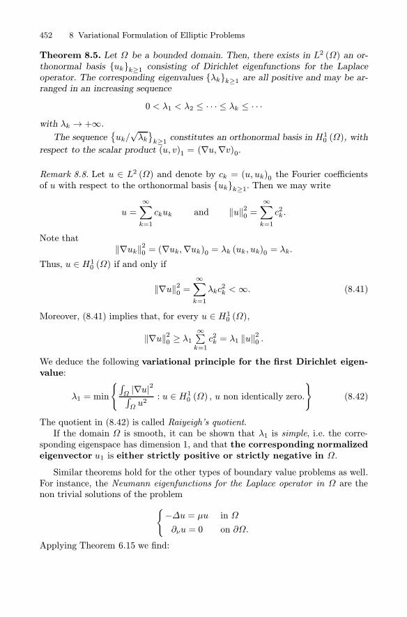
452 8 Variational Formulation of Elliptic Problems
Theorem 8.5. Let Ω be a bounded domain. Then, there exists in L2 (Ω) an or-thonormal basis {uk}k≥1 consisting of Dirichlet eigenfunctions for the Laplaceoperator. The corresponding eigenvalues {λk}k≥1 are all positive and may be ar-ranged in an increasing sequence
0 < λ1 < λ2 ≤ · · · ≤ λk ≤ · · ·with λk → +∞.The sequence
{uk/
√λk}k≥1 constitutes an orthonormal basis in H
10 (Ω), with
respect to the scalar product (u, v)1 = (∇u,∇v)0.
Remark 8.8. Let u ∈ L2 (Ω) and denote by ck = (u, uk)0 the Fourier coefficientsof u with respect to the orthonormal basis {uk}k≥1. Then we may write
u =
∞∑k=1
ckuk and ‖u‖20 =∞∑k=1
c2k.
Note that‖∇uk‖20 = (∇uk,∇uk)0 = λk (uk, uk)0 = λk.
Thus, u ∈ H10 (Ω) if and only if
‖∇u‖20 =∞∑k=1
λkc2k <∞. (8.41)
Moreover, (8.41) implies that, for every u ∈ H10 (Ω),
‖∇u‖20 ≥ λ1∞∑k=1
c2k = λ1 ‖u‖20 .
We deduce the following variational principle for the first Dirichlet eigen-value:
λ1 = min
{∫Ω|∇u|2∫Ωu2
: u ∈ H10 (Ω) , u non identically zero.}
(8.42)
The quotient in (8.42) is called Raiyeigh’s quotient.If the domain Ω is smooth, it can be shown that λ1 is simple, i.e. the corre-
sponding eigenspace has dimension 1, and that the corresponding normalizedeigenvector u1 is either strictly positive or strictly negative in Ω.
Similar theorems hold for the other types of boundary value problems as well.For instance, the Neumann eigenfunctions for the Laplace operator in Ω are thenon trivial solutions of the problem
{−Δu = μu in Ω
∂νu = 0 on ∂Ω.
Applying Theorem 6.15 we find:

8.4 Variational Formulation of Poisson’s Problem 453
Theorem 8.6. If Ω is a bounded Lipschitz domain, there exists in L2 (Ω) anorthonormal basis {uk}k≥1 consisting of Neumann eigenfunctions for the Laplaceoperator. The corresponding eigenvalues form a non decreasing sequence {μk}k≥1,with μ1 = 0 and μk → +∞.Moreover, the sequence {uk/
√μk + 1}k≥1 constitutes an orthonormal basis in
H1 (Ω), with respect to the scalar product (u, v)1,2 = (u, v)0+ (∇u,∇v)0.
8.4.4 An asymptotic stability result
The results in the last subsection may be used sometimes to prove the asymptoticstability of a steady state solution of an evolution equation as time t→ +∞.As an example consider the following problem for the heat equation. Suppose
that u ∈ C2,1(Ω × [0,+∞)
)is the (unique) solution of
⎧⎪⎨⎪⎩
ut −Δu = f (x) x ∈Ω, t > 0u (x,0) = u0 (x) x ∈Ωu (σ,t) = 0 σ ∈ ∂Ω, t > 0
where Ω is a smooth, bounded domain. Denote by u∞ = u∞ (x) the solution ofthe stationary problem {
−Δu∞ = f in Ω
u∞ = 0 on ∂Ω.
Proposition 8.5. For t ≥ 0, we have
‖u (·, t)− u∞‖0 ≤ e−λ1t{C2P ‖f‖0 + ‖u0‖0
}(8.43)
where λ1 is the first Dirichlet eigenvalue for the Laplace operator in Ω.
Proof. Set g (x) = u0 (x) − u∞ (x). The function w (x,t) = u (x,t) − u∞ (x)solves the problem
⎧⎪⎨⎪⎩
wt −Δw = 0 x ∈Ω, t > 0w (x,0) = g (x) x ∈Ωw (σ,t) = 0 σ ∈ ∂Ω, t > 0.
(8.44)
Let us use the method of separation of variables and look for solutions of the formw (x,t) = v (x) z (t). We find
z′ (t)z (t)
=Δv (x)
v (x)= −λ
with λ constant. Thus we are lead to the eigenvalue problem
{−Δv = λv in Ωv = 0 on ∂Ω.

454 8 Variational Formulation of Elliptic Problems
From Theorem 8.5, there exists in L2 (Ω) an orthonormal basis {uk}k≥1 consistingof eigenvectors, corresponding to a sequence of non decreasing eigenvalues {λk},with λ1 > 0 and λk → +∞. Then, if gk = (g, uk)0, we can write
g =∞∑1
gkuk and ‖g‖20 =∞∑k=1
g2k.
As a consequence, we find zk (t) = e−λkt and finally
w (x,t) =
∞∑1
e−λktgkuk (x) .
Thus,
‖u (·, t)− u∞‖20 = ‖w (·, t)‖20
=
∞∑k=1
e−2λktg2k
and since λk > λ1 for every k, we deduce that
‖u (·, t)− u∞‖20 ≤∞∑k=1
e−2λ1tg2k = e−2λ1t ‖g‖20 .
Theorem 8.1 yields, in particular
‖u∞‖0 ≤ C2P ‖f‖0 ,and hence
‖g‖0 ≤ ‖u0‖0 + ‖u∞‖0≤ ‖u0‖0 +C2P ‖f‖0
giving (8.43). �Proposition 8.5 implies that the steady state u∞ is asymptotically stable in
L2 (Ω)−norm as t → +∞. The speed of convergence is exponential3 and it isdetermined by the first eigenvalue λ1.
8.5 General Equations in Divergence Form
8.5.1 Basic assumptions
In this section we consider boundary value problems for elliptic operators withgeneral diffusion and transport terms. Let Ω ⊂ R
n be a bounded domain andset
Eu = −div (A (x)∇u− b (x) u) + c (x) ·∇u+ a0 (x)u (8.45)
where A =(aij)i,j=1,...,n, b = (b1, ..., bn), c = (c1, ..., cn) and a0 is a real function.
3 Compare with subsection 2.1.4.
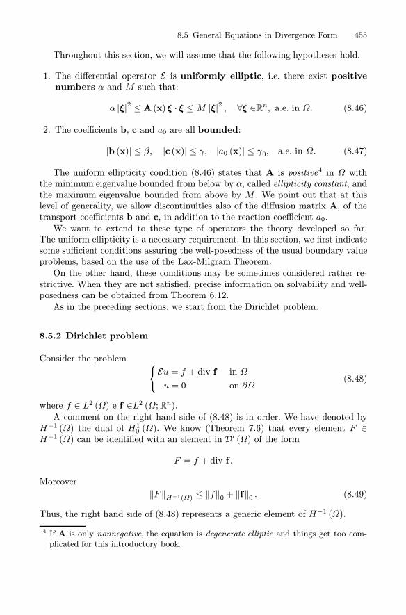
8.5 General Equations in Divergence Form 455
Throughout this section, we will assume that the following hypotheses hold.
1. The differential operator E is uniformly elliptic, i.e. there exist positivenumbers α and M such that:
α |ξ|2 ≤ A (x) ξ · ξ ≤ M |ξ|2 , ∀ξ ∈Rn, a.e. in Ω. (8.46)
2. The coefficients b, c and a0 are all bounded:
|b (x)| ≤ β, |c (x)| ≤ γ, |a0 (x)| ≤ γ0, a.e. in Ω. (8.47)
The uniform ellipticity condition (8.46) states that A is positive4 in Ω withthe minimum eigenvalue bounded from below by α, called ellipticity constant, andthe maximum eigenvalue bounded from above by M . We point out that at thislevel of generality, we allow discontinuities also of the diffusion matrix A, of thetransport coefficients b and c, in addition to the reaction coefficient a0.
We want to extend to these type of operators the theory developed so far.The uniform ellipticity is a necessary requirement. In this section, we first indicatesome sufficient conditions assuring the well-posedness of the usual boundary valueproblems, based on the use of the Lax-Milgram Theorem.
On the other hand, these conditions may be sometimes considered rather re-strictive. When they are not satisfied, precise information on solvability and well-posedness can be obtained from Theorem 6.12.
As in the preceding sections, we start from the Dirichlet problem.
8.5.2 Dirichlet problem
Consider the problem {Eu = f + div f in Ω
u = 0 on ∂Ω(8.48)
where f ∈ L2 (Ω) e f ∈L2 (Ω;Rn).A comment on the right hand side of (8.48) is in order. We have denoted by
H−1 (Ω) the dual of H10 (Ω). We know (Theorem 7.6) that every element F ∈H−1 (Ω) can be identified with an element in D′ (Ω) of the form
F = f + div f .
Moreover
‖F ‖H−1(Ω) ≤ ‖f‖0 + ‖f‖0 . (8.49)
Thus, the right hand side of (8.48) represents a generic element of H−1 (Ω).
4 If A is only nonnegative, the equation is degenerate elliptic and things get too com-plicated for this introductory book.

456 8 Variational Formulation of Elliptic Problems
As in Section 8.4, to derive a variational formulation of (8.48), we first assumethat all the coefficients and the data f , f are smooth. Then, we multiply theequation by a test function v ∈ C10 (Ω) and integrate over Ω:
∫
Ω
[−div(A∇u− bu) v] dx+∫
Ω
[c·∇u+ a0u] v dx =∫
Ω
[f + divf ] vdx.
Integrating by parts, we find, since v = 0 on ∂Ω:∫
Ω
[−div(A∇u− bu) v] dx =∫
Ω
[A∇u · ∇v − bu · ∇v] dx
and ∫
Ω
v div f dx = −∫
Ω
f ·∇v dx.
Thus, the resulting equation is:∫
Ω
{A∇u · ∇v − bu · ∇v + cv·∇u + a0uv} dx =∫
Ω
{fv − f ·∇v } dx (8.50)
for every v ∈ C10 (Ω).It is not difficult to check that for classical solutions, the two formulations
(8.48) and (8.50) are equivalent.
We now enlarge the space of test functions toH10 (Ω) and introduce the bilinearform
B (u, v) =
∫
Ω
{A∇u · ∇v − bu · ∇v + cv·∇u + a0uv} dx
and the linear functional
Fv =
∫
Ω
{fv − f ·∇v } dx.
Then, the weak formulation of problem (8.48) is the following:
Determine u ∈ H10 (Ω) such that
B (u, v) = Fv, ∀v ∈ H10 (Ω) . (8.51)
A set of hypotheses that ensure the well-posedness of the problem is indicated inthe following proposition.
Proposition 8.6. Assume that hypotheses (8.46) and (8.47) hold and that f ∈L2 (Ω), f ∈ L2 (Ω;Rn). Then if b and c have Lipschitz components and
1
2div (b− c) + a0 ≥ 0, a.e. in Ω, (8.52)
problem (8.51) has a unique solution. Moreover, the following stability estimateholds:
‖u‖1 ≤1
α{‖f‖0 + ‖f‖0} . (8.53)
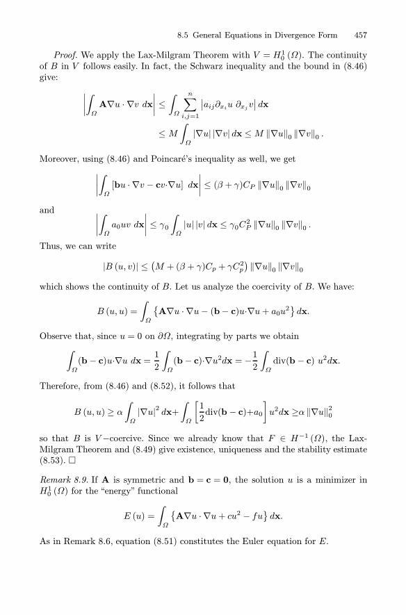
8.5 General Equations in Divergence Form 457
Proof. We apply the Lax-Milgram Theorem with V = H10 (Ω). The continuityof B in V follows easily. In fact, the Schwarz inequality and the bound in (8.46)give:
∣∣∣∣∫
Ω
A∇u · ∇v dx∣∣∣∣ ≤
∫
Ω
n∑i,j=1
∣∣aij∂xiu ∂xjv∣∣ dx
≤ M∫
Ω
|∇u| |∇v| dx ≤M ‖∇u‖0 ‖∇v‖0 .
Moreover, using (8.46) and Poincare’s inequality as well, we get
∣∣∣∣∫
Ω
[bu · ∇v − cv·∇u] dx∣∣∣∣ ≤ (β + γ)CP ‖∇u‖0 ‖∇v‖0
and ∣∣∣∣∫
Ω
a0uv dx
∣∣∣∣ ≤ γ0∫
Ω
|u| |v| dx ≤ γ0C2P ‖∇u‖0 ‖∇v‖0 .
Thus, we can write
|B (u, v)| ≤(M + (β + γ)Cp + γC
2p
)‖∇u‖0 ‖∇v‖0
which shows the continuity of B. Let us analyze the coercivity of B. We have:
B (u, u) =
∫
Ω
{A∇u · ∇u− (b− c)u·∇u+ a0u2
}dx.
Observe that, since u = 0 on ∂Ω, integrating by parts we obtain
∫
Ω
(b− c)u·∇u dx = 12
∫
Ω
(b− c)·∇u2dx = −12
∫
Ω
div(b− c) u2dx.
Therefore, from (8.46) and (8.52), it follows that
B (u, u) ≥ α∫
Ω
|∇u|2 dx+∫
Ω
[1
2div(b− c)+a0
]u2dx ≥α ‖∇u‖20
so that B is V −coercive. Since we already know that F ∈ H−1 (Ω), the Lax-Milgram Theorem and (8.49) give existence, uniqueness and the stability estimate(8.53). �
Remark 8.9. If A is symmetric and b = c = 0, the solution u is a minimizer inH10 (Ω) for the “energy” functional
E (u) =
∫
Ω
{A∇u · ∇u+ cu2 − fu
}dx.
As in Remark 8.6, equation (8.51) constitutes the Euler equation for E.

458 8 Variational Formulation of Elliptic Problems
Remark 8.10. If the Dirichlet condition is nonhomogeneous, i.e.
u = g on ∂Ω,
with g ∈ H1/2 (∂Ω), we consider an extension g of g in H1 (Ω) and set w = u− g.In this case we require that Ω is at least a Lipschitz domain, to ensure the existenceof g. Then w ∈ H10 (Ω) and solves the equation
Ew = f + div (f+A∇g − bg) − c ·∇g − cg.
From (8.46) and (8.47) we have
c·∇g + cg ∈ L2 (Ω) and A∇g − bg ∈L2 (Ω;Rn) .
Therefore, the Lax-MilgramTheorem yields existence, uniqueness and the estimate
‖u‖1,2 ≤ C (α, n,M, β, γ, γ0, Ω){‖f‖0 + ‖f‖0 + ‖g‖H1/2(∂Ω)
}.
Fig. 8.1. The solution of problem (8.54)
Example 8.1. Figure 8.1 shows the solution of the following Dirichlet problem inthe upper half circle:
⎧⎨⎩−uρρ − ρ−1uρ − ρuθ = 0 ρ < 1, 0 < θ < πu(1, θ) = sin(θ/2) 0 ≤ θ ≤ π
u (ρ, 0) = 0, u (ρ, π) = ρ ρ ≤ 1(8.54)
where (ρ, θ) denotes polar coordinates. Note that, in rectangular coordinates,
−ρuθ = yux − xuy (8.55)
so that it represents a transport term of the type c·∇u with c = (y,−x). Sincedivb =0, Proposition 8.6 ensures the well posedness of the problem.

8.5 General Equations in Divergence Form 459
Alternative for the Dirichlet problem. We will see later that problem(8.48) is actually well posed under the condition
divb+a0 ≥ 0,
which does not involve the coefficient c.In particular, this condition is fulfilled if a0 (x) ≥ 0 and b (x) = 0 a.e. in Ω. In
general however, we cannot prove that the bilinear form B is coercive. What wemay affirm is that B is weakly coercive, i.e. there exists λ0 ∈ R such that:
B (u, v) = B (u, v) + λ0 (u, v)0 ≡ B (u, v) + λ0∫
Ω
uv dx
is coercive. In fact, from the elementary inequality
|ab| ≤ εa2 + 14εb2, ∀ε > 0,
we get
∣∣∣∣∫
Ω
(b− c)u·∇u dx∣∣∣∣ ≤ (β + γ)
∫
Ω
|u·∇u|dx ≤ε ‖∇u‖20 +(β + γ)2
4ε‖u‖20 .
Therefore:
B (u, u) ≥ α ‖∇u‖20+λ0 ‖u‖20 − ε ‖∇u‖
20 −
((β + γ)
2
4ε+ γ
)‖u‖20 . (8.56)
If we choose ε = α/2 and λ0 = (β + γ)2/4ε+ γ, we obtain
B (u, u) ≥ α2‖∇u‖20
which shows the coercivity of B. Introduce now the Hilbert triplet
V = H10 (Ω) , H = L2 (Ω) , V ∗ = H−1 (Ω)
and recall that, since Ω is a bounded, Lipschitz domain, H10 (Ω) is dense andcompactly embedded in L2 (Ω). Finally, define the adjoint bilinear form of B by
B∗ (u, v) ≡∫
Ω
{(A�∇u+ cu) · ∇v − bv · ∇u+ a0uv
}dx =B (v, u) ,
associated with the formal adjoint of E
E∗u = −div(A�∇u+ cu
)− b · ∇u+ a0u.
We are now in position to apply Theorem 6.12 to our variational problem. Theconclusions are:

460 8 Variational Formulation of Elliptic Problems
1) The subspaces NB and NB∗ of the solutions of the homogeneous problems
B (u, v) = 0, ∀v ∈ H10 (Ω)
and
B∗ (w, v) = 0, ∀v ∈ H10 (Ω)
share the same dimension d, 0 ≤ d <∞.2) The problem
B (u, v) = Fv, ∀v ∈ H10 (Ω)
has a solution if and only if Fw = 0 for every w ∈ NB∗ .Let us translate the statements 1) and 2) into a less abstract language:
Theorem 8.7. LetΩ be a bounded, Lipschitz domain, f ∈ L2 (Ω) and f ∈L2 (Ω;Rn).Assume (8.46) and (8.47) hold. Then, we have the following alternative:
a) Either E is an isomorphism between H10 (Ω) and H−1 (Ω) and thereforeproblem (8.48) has a unique weak solution, with
‖∇u‖0 ≤ C (n, a,K, β, γ) {‖f‖0 + ‖f‖0}
or the homogeneous and the adjoint homogeneous problems
{Eu = 0 in Ω
u = 0 on ∂Ω,and
{E∗w = 0 in Ω
w = 0 on ∂Ω
have each d linearly independent solutions.
b) Moreover, problem (8.48) has a solution if and only if
∫
Ω
{fw − f ·∇w} dx =0 (8.57)
for every solution w of the adjoint homogeneous problem.
Theorem 8.7 implies that if we can show the uniqueness of the solution ofproblem (8.48), then automatically we infer both the existence and the stabilityestimate.
To show uniqueness, the weak maximum principles in subsection 8.5.5 are quiteuseful. We will be back to this argument there.
The conditions (8.57) constitute d compatibility conditions that the data haveto satisfy in order for a solution to exists.
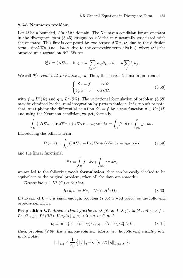
8.5 General Equations in Divergence Form 461
8.5.3 Neumann problem
Let Ω be a bounded, Lipschitz domain. The Neumann condition for an operatorin the divergence form (8.45) assigns on ∂Ω the flux naturally associated withthe operator. This flux is composed by two terms: A∇u · ν, due to the diffusionterm −divA∇u, and −bu·ν, due to the convective term div(bu), where ν is theoutward unit normal on ∂Ω. We set
∂Eν u ≡ (A∇u− bu)·ν =n∑
i,j=1
aij∂xju νi − u∑j
bjνj .
We call ∂Eν u conormal derivative of u. Thus, the correct Neumann problem is:{Eu = f in Ω
∂Eν u = g on ∂Ω.(8.58)
with f ∈ L2 (Ω) and g ∈ L2 (∂Ω). The variational formulation of problem (8.58)may be obtained by the usual integration by parts technique. It is enough to note,that, multiplying the differential equation Eu = f by a test function v ∈ H1 (Ω)and using the Neumann condition, we get, formally:
∫
Ω
{(A∇u− bu)∇v + (c·∇u)v + a0uv} dx =∫
Ω
fv dx+
∫
∂Ω
gv dσ.
Introducing the bilinear form
B (u, v) =
∫
Ω
{(A∇u− bu)∇v + (c·∇u)v + a0uv} dx (8.59)
and the linear functional
Fv =
∫
Ω
fv dx+
∫
∂Ω
gv dσ,
we are led to the following weak formulation, that can be easily checked to beequivalent to the original problem, when all the data are smooth:
Determine u ∈ H1 (Ω) such thatB (u, v) = Fv, ∀v ∈ H1 (Ω) . (8.60)
If the size of b− c is small enough, problem (8.60) is well-posed, as the followingproposition shows.
Proposition 8.7. Assume that hypotheses (8.46) and (8.47) hold and that f ∈L2 (Ω), g ∈ L2 (∂Ω). If a0 (x) ≥ c0 > 0 a.e. in Ω and
α0 ≡ min{α− (β + γ)/2, c0 − (β + γ)/2} > 0, (8.61)
then, problem (8.60) has a unique solution. Moreover, the following stability esti-mate holds:
‖u‖1,2 ≤1
α0
{‖f‖0 +C (n,Ω)‖g‖L2(∂Ω)
}.

462 8 Variational Formulation of Elliptic Problems
Proof (sketch). Since
|B (u, v)| ≤ (M + β + γ + γ0) ‖u‖1,2 ‖v‖1,2B is continuous in H1 (Ω). Moreover, we may write
B (u, u) ≥ α∫
Ω
|∇u|2 dx−∣∣∣∣∫
Ω
[(b− c)·∇u] u dx∣∣∣∣+∫
Ω
a0u2dx.
From Schwarz’s inequality and the inequality 2ab ≤ a2 + b2, we obtain∣∣∣∣∫
Ω
[(b− c)·∇u] u dx∣∣∣∣ ≤ (β + γ) ‖∇u‖0 ‖u‖0 ≤
(β + γ)
2‖u‖21,2 .
Thus, if (8.61) holds, we get B (u, u) ≥ α0 ‖u‖21,2 and therefore B is coercive.Finally, using (8.36), it is not difficult to check that F ∈ H1 (Ω)∗, with
‖F ‖H1(Ω)∗ ≤ ‖f‖0 + C (n,Ω)‖g‖L2(∂Ω) .
�Alternative for the Neumann problem. The bilinear form B is coercive
also under the conditions
(b− c) · ν ≤0 a.e. on ∂Ω and1
2div(b− c)+a0 ≥ c0 > 0 a.e in Ω,
as it can be checked following the proof of Proposition 8.6.However, in general the bilinear formB is only weakly coercive. In fact, choosing
in (8.56) ε = α/2 and λ0 = (β + γ)2/2ε+ 2γ + 2γ0, we easily get
B (u, u) = B (u, u) + λ0 ‖u‖20 ≥α
2‖∇u‖20 +
((β + γ)
2
4ε+ γ + γ0
)‖u‖20
and therefore B is coercive. Applying theorem 6.12, we obtain the following alter-native:
Theorem 8.8. Let Ω be a bounded, Lipschitz domain. Assume that (8.46) and(8.47) hold. Then, if f ∈ L2 (Ω) and g ∈ L2 (∂Ω):a) Either problem (8.58) has a unique solution u ∈ H1 (Ω) and
‖u‖1,2 ≤ C (n, α,M, β, γ, γ0){‖f‖0 + ‖g‖L2(∂Ω)
}
or the homogeneous and the adjoint homogeneous problems
{Eu = 0 in Ω
(A∇u− bu) · ν = 0 on ∂Ωand
{E∗w = 0 in Ω
(A�∇w + cw) · ν = 0 on ∂Ω
have each d linearly independent solutions.

8.5 General Equations in Divergence Form 463
b) Moreover, problem (8.60) has a solution if and only if
Fw =
∫
Ω
fw dx+
∫
∂Ω
gw dσ = 0 (8.62)
for every solution w of the adjoint homogeneous problem.
Remark 8.11. Again, uniqueness implies existence. Note that if b = c = 0 anda0 = 0, then the solutions of the adjoint homogeneous problem are the constantfunctions. Therefore d = 1 and the compatibility condition (8.62) reduces to thewell known equation ∫
Ω
f dx+
∫
∂Ω
g dσ = 0.
Remark 8.12. Note that in the right hand side of (8.58) there is no term of theform div f , as was the case in the Dirichlet problem. Indeed, it is better to avoidterms of that form for the following reason. Consider, for instance, the problem−Δu =divf , ∂νu = 0. A weak formulation would be, after the usual integrationby parts,
∫
Ω
∇u · ∇v dx =∫
∂Ω
(f · ν) vdσ−∫
Ω
f ·∇v dx ∀v ∈ H1 (Ω) . (8.63)
However, even if f is smooth, (8.63) is equivalent to div(∇u+f ) =0 in the senseof distributions, but with
(∇u+ f ) · ν =0 on ∂Ω,
giving rise to a different problem.
8.5.4 Robin and mixed problems
Robin problem. The variational formulation of the problem
{Eu = f in Ω
∂Eν u+hu = g on ∂Ω.(8.64)
is obtained by replacing the bilinear form B in problem (8.60), by
B (u, v) = B (u, v) +
∫
∂Ω
huv dσ
If 0 ≤ h (x) ≤ h0 a.e. on ∂Ω, Proposition 8.7 still holds for problem (8.64).As for the Neumann problem, in general the bilinear form B is only weakly
coercive and a theorem perfectly analogous to Theorem 8.8 holds. We leave thedetails as an exercise.
464 8 Variational Formulation of Elliptic Problems
Mixed Dirichlet-Neumann problem. Let ΓD be a non empty relativelyopen subset of ∂Ω and ΓN = ∂Ω\ΓD. Consider the mixed problem
⎧⎨⎩Eu = f in Ωu = 0 on ΓD
∂Eν u = g on ΓN
As in subsection 8.4.2, the correct functional setting is H10,ΓD (Ω) with the norm‖u‖H10,ΓD (Ω) = ‖∇u‖0. Introducing the linear functional
Fv =
∫
Ω
fv dx+
∫
ΓN
gv dσ,
the variational formulation is the following: Determine u ∈ H10,ΓD (Ω) suchthat
B (u, v) = Fv, ∀v ∈ H10,ΓD (Ω) . (8.65)
Proceeding as in Proposition 8.6, we may prove the following result:
Proposition 8.8. Assume that hypotheses (8.46) and (8.47) hold and that f ∈L2 (Ω), g ∈ L2 (ΓN). If b and c have Lipschitz components and
(b− c) · ν ≤ 0 a.e. on ΓN ,1
2div (b− c) + a0 ≥ 0, a.e. in Ω,
then problem (8.65) has a unique solution u ∈ H10,ΓD (Ω). Moreover, the followingstability estimate holds:
‖u‖1 ≤1
α
{‖f‖0 + C ‖g‖L2(ΓN )
}.
Remark 8.13. If u = g0 on ΓD, i.e. if the Dirichlet data are nonhomogeneous, setw = u − g0, where g0 ∈ H1(Ω) is an extension of g0. Then w ∈ H10,ΓD (Ω) andsolves
B (w, v) = B (g0, v) +
∫
Ω
fv dx+
∫
ΓN
gv dσ ∀v ∈ H10,ΓD (Ω) .
For the mixed problem as well, in general the bilinear form is only weaklycoercive and we may resort to the alternative theorem, achieving a result similarto Theorems 8.7. Only note that the compatibility conditions (8.60) take the form
Fw =
∫
Ω
fw dx+
∫
ΓN
gw dσ = 0
for every solution w of the adjoint problem⎧⎨⎩
E∗w = 0 in Ωw = 0 on ΓD(
A�∇w + cw)· ν = 0 onΓN .

8.5 General Equations in Divergence Form 465
8.5.5 Weak Maximum Principles
In Chapter 2 we have given a version of the maximum principle for the Laplaceequation. This principle has an extension valid for general divergence form opera-tors. First, some remarks.Let Ω be a bounded, Lipschitz domain and u ∈ H1 (Ω). Since C1
(Ω)is dense
in H1 (Ω), u ≥ 0 on ∂Ω if there exists a sequence {vk}k≥1 ⊂ C1(Ω)such that
vk → u in H1 (Ω) and vk ≥ 0. It is as if the trace of u on ∂Ω “inherits” thenonnegativity from the sequence {vk}k≥1.Since vk ≥ 0 on ∂Ω is equivalent to saying that5 the negative part v−k =
max{−vk, 0} has zero trace on ∂Ω, it then turns out that u ≥ 0 on ∂Ω if and onlyif u− ∈ H10 (Ω). Similarly, u ≤ 0 on ∂Ω if and only if u+ ∈ H10 (Ω).Other inequalities follow in a natural way. For instance, we have u ≤ v on ∂Ω
if u− v ≤ 0 on ∂Ω. Thus, we may define:
sup∂Ωu = inf {k ∈ R : u ≤ k on ∂Ω} , inf
∂Ωu = sup {k ∈ R : u ≥ k on ∂Ω}
which coincide with the usual greatest lower bound and lowest upper bound whenu ∈ C(∂Ω).Consider the equation
B (u, v) =
∫
Ω
{(A∇u− bu)∇v + cv·∇u+ a0uv} dx = 0, (8.66)
for every v ∈ H10 (Ω). We have:
Theorem 8.9. (Weak maximum principle). Assume that u ∈ H1 (Ω) satisfies(8.66) and that (8.46) and (8.47) hold. Moreover, let b Lipschitz and
divb+ a0 ≥ 0 a.e. in Ω. (8.67)
ThensupΩu ≤ sup
∂Ωu+ and inf
Ω≥ inf
∂Ωu−. (8.68)
Proof . For simplicity, we give the proof only for b = c = 0, and therefore a0 ≥ 0a.e. in Ω. We have:
∫
Ω
A∇u · ∇v dx = −∫
Ω
a0uv dx, ∀v ∈ H10 (Ω) .
Letl = sup
∂Ωu+
We may assume that l < ∞, otherwise there is nothing to be proved. Select as atest function v = max{u− l, 0} ≥ 0, which belongs to H10 (Ω).5 Recall from subsection 7.5.2 that, if u ∈ H1 (Ω) then its positive and negative part,u+ = max {u, 0} and u− = max{−u, 0}, belong to H1 (Ω) as well.

466 8 Variational Formulation of Elliptic Problems
Now, observe that in the set {u > l}, where v > 0 a.e., we have ∇v = ∇u sothat, using the uniform ellipticity condition and (8.67), we obtain
α
∫
{u>l}|∇v|2 dx ≤
∫
Ω
A∇u · ∇v dx = −∫
{u>l}a0u (u− l) dx ≤0.
Thus, either |{u > l}| = 0 or ∇v = 0. In any case, since v ∈ H10 (Ω), we inferv = 0, whence u ≤ l.The second inequality in (8.68) may be proved in similar way. �
Remark 8.14. Note that Theorem 8.9 implies that if u ≤ 0 or u ≥ 0 on ∂Ω, thenu ≤ 0 or u ≥ 0 in Ω. In particular, if u = 0 on ∂Ω then u = 0 in Ω.Also, it is not possible to substitute sup∂Ω u
+ by sup∂Ω u or inf∂Ω u− with
inf∂Ω u in (8.68). A counterexample in dimension one is shown in figure 8.2. Thesolution of −u′′ + u = 0 in (0, 1), u (0) = u (1) = −1, has a negative maximumwhich is greater than −1.
Fig. 8.2. The solution of −u′′ + u = 0 in (0, 1), u (0) = u (1) = −1
Using Theorem 6.12, we have:
Corollary 8.1. Under the hypotheses of Theorem 8.9, the Dirichlet problem{Eu = f + divf in Ωu = 0 on ∂Ω
has a unique solution u ∈ H10 (Ω) and‖∇u‖0 ≤ C (n, α,K, β, γ) {‖f‖0 + ‖f‖0} .
A similar maximum principle holds for Robin or mixed conditions, yieldinguniqueness and therefore well-posedness, for the corresponding problems.Suppose for instance that u ∈ H1 (Ω) satisfies the equation
B (u, v)=0, ∀v ∈ H10,ΓD (Ω) . (8.69)
Then u is a solution of a mixed problem with f = g = 0. We may prove thefollowing result (compare with Example 8.18).

8.6 Regularity 467
Theorem 8.10. Let ΓD ⊂ ∂Ω, open, ΓD �= ∅. Assume that u ∈ H1 (Ω) satisfies(8.69) and that (8.46) and (8.47) hold. Moreover, let b be Lipschitz and
b · ν ≤ 0 a.e. on ΓN , divb+ a0 ≥ 0 a.e. in Ω.
Then
supΩu ≤ sup
ΓD
u+ and infΩ≥ inf
ΓDu−.
8.6 Regularity
An important task, in general technically rather complicated, is to establish theoptimal regularity of a weak solution in relation to the degree of smoothness ofthe data: the domain Ω, the boundary data, the coefficients of the operator and theforcing term. To get a clue of what happens, consider for example the followingPoisson problem: {
−Δu+ u = F in Ω
u = 0 on ∂Ω
where F ∈ H−1 (Ω). Under this hypothesis, the Lax-Milgram Theorem yields asolution u ∈ H10 (Ω) and we cannot get much more, in terms of smoothness. Indeed,from Sobolev inequalities (see subsection. 7.10.4) it follows that u ∈ Lp(Ω) withp = 2n
n−2 , if n ≥ 3, or u ∈ Lp (Ω), with 2 ≤ p <∞, if n = 2. However, this gain inintegrability does not seriously increase the smoothness of u.Reversing our point of view, we may say that, starting from a function in
H10 (Ω) and applying to it a second order operator “two orders of differentiabilityare lost”: the loss of one order drives from H10 (Ω) into L
2 (Ω) while a further lossleads to H−1 (Ω). It is as if the upper index −1 indicates a “lack” of one order ofdifferentiability.
Nevertheless, consider the case in which u ∈ H1 (Rn) is a solution of the equa-tion
−Δu+ u = f in Rn. (8.70)
We ask: if f ∈ L2 (Rn) what is the optimal regularity of u?Following the above argument, our conclusions would be: it is true that we
start from u ∈ H1 (Rn), but applying the second order operator −Δ + I, whereI denotes the identity operator, we find f ∈ L2(R). Thus we conclude that thestarting function should actually be in H2 (Rn) rather than H1 (Rn). Indeed thisis true and can be easily proved using the Fourier transform. Since
∂xiu (ξ) = iξiu (ξ) , ∂xixju (ξ) = −ξiξj u (ξ)
we have
−Δu (ξ) = |ξ|2 u (ξ)

468 8 Variational Formulation of Elliptic Problems
and equation (8.70) becomes
(1 + |ξ|2)u (ξ) = f (ξ)
whence
u (ξ) =f (ξ)
1 + |ξ|2. (8.71)
From (8.71) we easily draw the information we were looking for: every secondderivative of u belongs to L2 (Rn). This comes from the following facts:
• formula (7.27):
‖v‖2L2(Rn) = (2π)n ‖v‖2L2(Rn) ,
• the elementary inequality
2∣∣ξiξj
∣∣ < 1 + |ξ|2 , ∀i, j = 1, ..., n,
• the simple computation
∫
Rn
∣∣∂xixju (x)∣∣2 dx =
∫
Rn
ξ2i ξ2j |u (ξ)|2 dξ =
∫
Rn
ξ2i ξ2j
(1 + |ξ|2)2∣∣∣f (ξ)
∣∣∣2
dξ
<1
4
∫
Rn
∣∣∣f (ξ)∣∣∣2
dξ =(2π)
n
4
∫
Rn
|f (x)|2 dx.
Thus, u ∈ H2 (Rn) and moreover, we have obtained the estimate
‖u‖H2(Rn) ≤ C ‖f‖L2(Rn) .
We may go further. If f ∈ H1 (Rn), i.e. if f has first partials in L2 (Rn), asimilar computation yields u ∈ H3 (Rn). Iterating this argument, we concludethat for every m ≥ 0,
if f ∈ Hm (Rn) then u ∈ Hm+2 (Rn) .
Using the Sobolev embedding theorems of subsection 7.10.4, we infer that, if m issufficiently large, u is a classical solution. In fact, if u ∈ Hm+2 (Rn) then
u ∈ Ck (Rn) for k < m+ 2− n2,
and therefore it is enough thatm > n2to have u at least in C2 (Rn). An immediate
consequence is:
if f ∈ C∞ (Rn) then u ∈ C∞(Rn).
This kind of results can be extended to uniformly elliptic operators E in diver-gence form and to the solutions of the Dirichlet, Neumann and Robin problems.

8.6 Regularity 469
The regularity for mixed problems is more delicate and requires compatibility con-ditions along the border between ΓD and ΓN . We will not insist on this subject.There are two kinds of regularity results, concerning interior regularity and
global regularity, respectively. Since the proofs are quite technical (see Evans,1998), we only state the main results.In all the theorems below u is a weak solution of
Eu = f in Ω.
We keep the hypotheses (8.46) and (8.47).
• Interior regularity. The next theorem is a H2−interior regularity result. Notethat the boundary of the domain does not play any role. We have:
Theorem 8.11. (H2 interior regularity). Let the coefficients aij be Lipschitz inΩ. Then u ∈ H2loc (Ω) and if Ω′ ⊂⊂ Ω,
‖u‖H2(Ω′) ≤ C{‖f‖L2(Ω) + ‖u‖L2(Ω)
}. (8.72)
Thus, u is a strong solution (see Section 8.2) in Ω. The constant C depends onall the relevant parameters α, β, γ, γ0,M and also on the distance of Ω
′ from ∂Ωand the Lipschitz constant of aij and bj, i, j = 1, ..., n.
Remark 8.15. The presence of the norm ‖u‖L2(Ω) in the right hand side of (8.72)is necessary6 and due to the fact that the bilinear form B associated to E is onlyweakly coercive.
If we increase the regularity of the coefficients, the smoothness of u increasesaccording to the following theorem:
Theorem 8.12. (Higher interior regularity). Let aij, bj ∈ Cm+1 (Ω) and cj, a0 ∈Cm (Ω), m ≥ 1, i, j = 1, ..., n. Then u ∈ Hm+2
loc (Ω) and if Ω′ ⊂⊂ Ω,
‖u‖Hm+2(Ω′) ≤ C{‖f‖Hm(Ω) + ‖u‖L2(Ω)
}.
As a consequence, if aij, bj, cj, a0, f ∈ C∞ (Ω) , then u ∈ C∞ (Ω) as well.
• Global regularity.We focus on the optimal regularity of a solution (non neces-sarily unique!) of the boundary value problems we have considered in the previoussections.Consider first H2−regularity. If u ∈ H2 (Ω), its trace on ∂Ω belongs to
H3/2 (∂Ω) so that a Dirichlet data gD has to be taken in this space. On theother hand, the trace of the normal derivative belongs to H1/2 (∂Ω) and hence wehave to assign a Neumann or a Robin data gN in this space. Also, the domain hasto be smooth enough, say C2, in order to define the traces of u and ∂νu.
6 For instance, u (x) = sinx is a solution of the equation u′′ + u = 0. Clearly we cannotcontrol any norm of u with the norm of the right hand side alone!

470 8 Variational Formulation of Elliptic Problems
Thus, assume that u is a solution of Eu = f in Ω, with one of the followingboundary conditions:
u =gD ∈ H3/2 (∂Ω)or
∂Eν+hu= gN ∈ H1/2 (∂Ω) ,with
0 ≤ h (σ) ≤ h0 a.e. on ∂Ω.
We have:
Theorem 8.13. Let Ω be a bounded, C2−domain. Assume that aij, bj, i, j =1, ..., n, are Lipschitz in Ω and f ∈ L2 (Ω). Then u ∈ H2(Ω) and
‖u‖H2(Ω) ≤ C{‖u‖0 + ‖f‖0 + ‖gD‖H3/2(∂Ω)
}(Dirichlet),
‖u‖H2(Ω) ≤ C{‖u‖0 + ‖f‖0 + ‖gR‖H1/2(∂Ω)
}(Neumann/Robin).
If we increase the regularity of the domain, the coefficients and the data, thesmoothness of u increases accordingly to the following theorem.
Theorem 8.14. Let Ω be a bounded Cm+2−domain. Assume that aij, bj ∈Cm+1
(Ω), cj, a0 ∈ Cm
(Ω), i, j = 1, ..., n, f ∈ Hm (Ω). If gD ∈ Hm+3/2 (∂Ω)
or gN ∈ Hm+1/2 (∂Ω) and h ∈ Cm+1 (∂Ω), then u ∈ Hm+2(Ω) and moreover,
‖u‖Hm+2(Ω) ≤ C{‖u‖0 + ‖f‖Hm(Ω) + ‖gD‖Hm+3/2(∂Ω)
}(Dirichlet),
‖u‖Hm+2(Ω) ≤ C{‖u‖0 + ‖f‖Hm(Ω) + ‖gR‖Hm+1/2(∂Ω)
}(Neumann, Robin).
In particular, if Ω is a C∞−domain, all the coefficients are in C∞(Ω)and the
boundary data are in C∞ (∂Ω), then u ∈ C∞(Ω).
• A particular case. Let Ω be a C2−domain and f ∈ L2 (Ω). The Lax-MilgramTheorem and Theorem 8.11 imply that the solution of the Dirichlet problem
{−Δu = f in Ω
u = 0 on ∂Ω
belongs to H2(Ω) ∩H10 (Ω) and that
‖u‖H2(Ω) ≤ C ‖f‖0 = C ‖Δu‖0 . (8.73)
Since clearly we have‖Δu‖0 ≤ ‖u‖H2(Ω)
we draw the following important conclusion:

8.6 Regularity 471
Corollary 8.2. If u ∈ H2(Ω) ∩H10(Ω), then
‖Δu‖0 ≤ ‖u‖H2(Ω) ≤ Cb ‖Δu‖0 .
In other words, ‖Δu‖0 and ‖u‖H2(Ω) are equivalent norms in H2(Ω) ∩H10(Ω).
In the next section, we will see an application of Corollary 8.2 to an equilibriumproblem for a bent plate.
• Domains with corners. The above regularity results hold for smooth domains.However, in several applied situations, Lipschitz domains are the relevant ones.For these domains the regularity theory is not elementary and goes beyond thepurposes of the present book. Thus, we only give an idea of what happens bymeans of two examples.
Fig. 8.3. The case α =3
2π in Example 8.17
Example 8.2. Consider the plane sector:
Sα = {(r, θ) : 0 < r < 1,− α/2 < θ < α/2} (0 < α < 2π).
The functionu (r, θ) = r
πα cos
π
αθ
is harmonic in Sα, since it is the real part of f (z) = zπα , which is holomorphic in
Sα. Furthermore,
u (r,−α/2) = u (r, α/2) = 0, 0 ≤ r ≤ 1 (8.74)
andu (1, θ) = cos
π
αθ, 0 ≤ θ ≤ α. (8.75)
We focus on a neighborhood of the origin. If α = π, Sα is a semicircle and
u (r, θ) = Rez = x ∈ C∞(Sα).
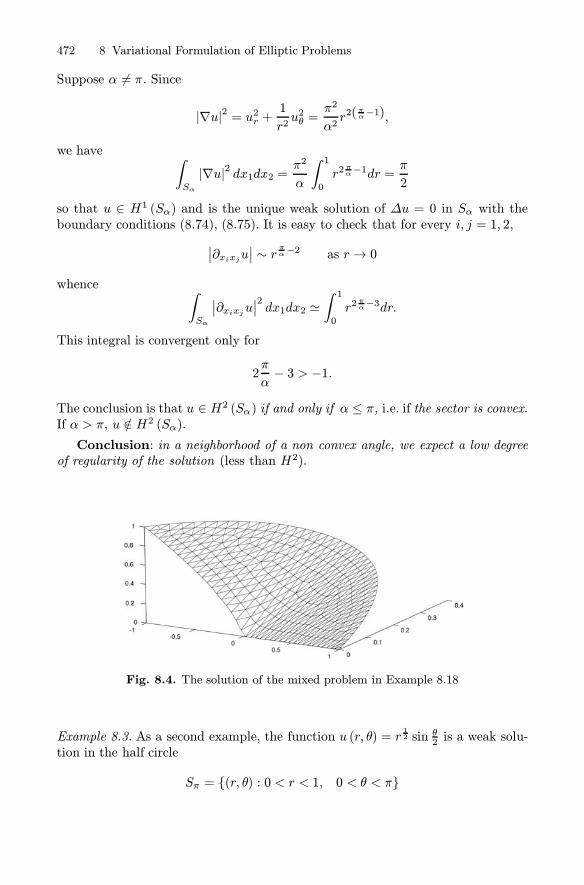
472 8 Variational Formulation of Elliptic Problems
Suppose α �= π. Since
|∇u|2 = u2r +1
r2u2θ =
π2
α2r2(
πα−1),
we have ∫
Sα
|∇u|2 dx1dx2 =π2
α
∫ 10
r2πα−1dr =
π
2
so that u ∈ H1 (Sα) and is the unique weak solution of Δu = 0 in Sα with theboundary conditions (8.74), (8.75). It is easy to check that for every i, j = 1, 2,
∣∣∂xixju∣∣ ∼ r πα−2 as r→ 0
whence ∫
Sα
∣∣∂xixju∣∣2 dx1dx2 �
∫ 10
r2πα−3dr.
This integral is convergent only for
2π
α− 3 > −1.
The conclusion is that u ∈ H2 (Sα) if and only if α ≤ π, i.e. if the sector is convex.If α > π, u /∈ H2 (Sα).Conclusion: in a neighborhood of a non convex angle, we expect a low degree
of regularity of the solution (less than H2).
Fig. 8.4. The solution of the mixed problem in Example 8.18
Example 8.3. As a second example, the function u (r, θ) = r12 sin θ2 is a weak solu-
tion in the half circle
Sπ = {(r, θ) : 0 < r < 1, 0 < θ < π}

8.7 Equilibrium of a plate 473
of the mixed problem⎧⎨⎩
Δu = 0 in Sπu (1, θ) = sin θ
20 < θ < π
u (r, 0) = 0 and ∂x2u (r, π) = 0 0 ≤ r < 1.
Namely,
|∇u|2 = 14r,
so that ∫
Sπ
|∇u|2 dx1dx2 =π
4
whence u ∈ H1 (Sπ). Moreover,
∂x2u = ur sin θ +1
ruθ cos θ =
1
2√rcosθ
2
hence∂x2u (r, π) = 0.
However, along the half-line θ = π/2, for example, we have
∣∣∂xixju∣∣ ∼ r− 32 r ∼ 0
so that ∫
Sα
∣∣∂xixju∣∣2 dx1dx2 ∼
∫ 10
r−2dr =∞.
and therefore u /∈ H2 (Sπ) .Thus, the solution has a low order of regularity near the origin, even though
the boundary of Sπ is flat there. Note that the origin separates the Dirichlet andNeumann regions (see Fig. 8.4).
Conclusion: in general, the optimal regularity of the solution of a mixed prob-lem is less than H2 near the boundary between the Dirichlet and Neumann regions.
8.7 Equilibrium of a plate
The range of application of the variational theory is not confined to second orderequations. In this section we consider the vertical deflection u = u (x, y) of a bentplate of small thickness (compared with the other dimensions) under the action ofa normal load. If Ω ⊂ R2 represents the transversal section of the plate, it can beshown that u is governed by the fourth order equation
ΔΔu = Δ2u =q
D≡ f in Ω,
where q is the density of loading and D encodes the elastic properties of the mate-rial. The operator Δ2 is called biharmonic or bi-laplacian and the solutions of

474 8 Variational Formulation of Elliptic Problems
Δ2u = 0 are called biharmonic functions. In two dimensions, the explicit expres-sion of Δ2 is given by7
Δ2 =∂4
∂x4+ 2
∂4
∂x2∂y2+∂4
∂y4.
If the plate is rigidly fixed along its boundary (clamped plate), then u and itsnormal derivative must vanish on ∂Ω. Thus, we are led to the following boundaryvalue problem: {
Δ2u = f in Ωu = ∂νu = 0 on ∂Ω.
(8.76a)
We want to derive a variational formulation. To obtain it, choose C20 (Ω) as space of
test functions, i.e. the set of functions in C2 (Ω), compactly supported in Ω. Thischoice takes into account the boundary conditions. Now, multiply the biharmonicequation by a function v ∈ C20(Ω) and integrate over Ω:
∫
Ω
Δ2u v dx =
∫
Ω
f v dx. (8.77)
Integrating by parts twice and using the conditions v = ∂νv = 0 on ∂Ω, we get:∫
Ω
Δ2u v dx =
∫
Ω
(div∇Δu)v dx =∫
∂Ω
∂ν (Δu)v dσ−∫
Ω
∇Δu · ∇v dx
= −∫
∂Ω
Δu∂νv dσ+
∫
Ω
ΔuΔv dx =
∫
Ω
ΔuΔv dx.
Thus, (8.77) becomes ∫
Ω
ΔuΔv dx =
∫
Ω
fv dx. (8.78)
Now we enlarge the space of test functions by taking the closure of C20(Ω) inH2 (Ω), which isH20 (Ω). Note that (see subsection 7.9.2) this is precisely the spaceof functions u such that u and ∂νu have zero trace on ∂Ω.Since H20 (Ω) ⊂ H10 (Ω)∩H2 (Ω), from Corollary 8.2 we know that in this space
we may choose ‖u‖2 = ‖Δu‖0 as a norm. We are led to the following variationalformulation:
7 It is possible to give the definition of ellipticity for an operator of order higher thantwo (see Renardy-Rogers, 2004). For instance, consider the linear operator with con-stant coefficients L =∑|α|=m aαD
α, m ≥ 2, where α = (α1, ..., αn) is a multi-index.Associate with L its symbol, given by
SL (ξ) =∑
|α|=maα (iξ)
α .
Then L is said to be elliptic if SL (ξ) �= 0 for every ξ ∈Rn, ξ �= 0. The symbol ofL = Δ2 in 2 dimensions is −ξ41− 2ξ21ξ22− ξ42, which is negative if (ξ1, ξ2) �= (0, 0). ThusΔ2 is elliptic. Note that, for m = 2, we recover the usual definition of ellipticity.

8.8 A Monotone Iteration Scheme for Semilinear Equations 475
Determine u ∈ H20 (Ω) such that∫
Ω
ΔuΔv dx =
∫
Ω
fv dx, ∀v ∈ H20 (Ω) . (8.79)
The following result holds:
Proposition 8.9. If f ∈ L2 (Ω), there exists a unique solution u ∈ H20 (Ω) of(8.79). Moreover,
‖Δu‖0 ≤ Cb ‖f‖0 .
Proof. Note that the bilinear form
B (u, v) =
∫
Ω
Δu ·Δv dx
coincides with the inner product in H20 (Ω). On the other hand, setting,
Lv =
∫
Ω
fv dx,
from Corollary 8.2, we have:
|L (v)| =∫
Ω
|fv| dx ≤‖f‖0 ‖v‖0 ≤ Cb ‖f‖0 ‖Δv‖0
so that L ∈ H20 (Ω)∗. We conclude the proof directly from the Riesz RepresentationTheorem. �
Remark 8.16. Let u be the solution of problem (8.79). Setting w = Δu, we haveΔw = f with f ∈ L2 (Ω). Thus, Corollary 8.2 implies w ∈ H2 (Ω) which, in turn,yields u ∈ H4 (Ω).
8.8 A Monotone Iteration Scheme for Semilinear Equations
The weak maximumprinciple can be used to construct iteration schemes for solvingnonlinear boundary value problems. We consider here the following problem:
{−Δu = f (u) in Ωu = g on ∂Ω.
(8.80)
We assume that Ω is a smooth domain and that f ∈ C1 (R), g ∈ H1/2 (∂Ω). Aweak solution of problem (8.80) is a function u ∈ H1 (Ω) such that u = g on ∂Ωand ∫
Ω
∇u · ∇v dx =∫
Ω
f (u) v dx ∀v ∈ H10 (Ω) . (8.81)

476 8 Variational Formulation of Elliptic Problems
We need to introduce weak sub and super solutions. We say that u∗ ∈ H1 (Ω) is aweak subsolution of problem (8.80) if u∗ ≤ g on ∂Ω and
∫
Ω
∇u∗ · ∇v dx ≤∫
Ω
f (u∗) v dx ∀v ∈ H10 (Ω) , v ≥ 0 a.e. in Ω.
Similarly, we say that u∗ ∈ H1 (Ω) is a weak supersolution of problem (8.80) ifu∗ ≥ g on ∂Ω and
∫
Ω
∇u∗ · ∇v dx ≥∫
Ω
f (u∗) v dx ∀v ∈ H10 (Ω) , v ≥ 0 a.e. in Ω.
We want to prove the following theorem.
Theorem 8.15. Assume that g is bounded on ∂Ω and that there exist a weaksubsolution u∗ and a weak supersolution u∗ of problem (8.80) such that:
a ≤ u∗ ≤ g ≤ u∗ ≤ b a, b ∈ R.
Then, there exists a solution u of problem (8.80) such that
u∗ ≤ u ≤ u∗.
Proof. Let M = max[a,b] |f ′|. Then the function F (s) = f (s) +Ms is nonde-creasing. Write Poisson’s equation in the form
−Δu+Mu = F (u) .
The idea is to exploit the linear theory to define recursively the following sequence{uk}k≥1 of functions: let u1 be the solution of
{−Δu1 +Mu1 = F (u∗) in Ω
u1 = g on ∂Ω.
Given uk, let uk+1 be the solution of
{−Δuk+1 +Muk+1 = F (uk) in Ω
uk = g on ∂Ω.(8.82)
We claim that uk is non decreasing and trapped between u∗ and u∗:
u∗ ≤ uk ≤ uk+1 ≤ u∗ a.e. in Ω.
Assuming the claim, we deduce that uk converges a.e in Ω to some bounded func-tion u, as k → +∞. Since F (a) ≤ F (uk) ≤ F (b), by the Dominated ConvergenceTheorem we infer that
∫
Ω
F (uk) vdx→∫
Ω
F (u) vdx as k→∞,

8.8 A Monotone Iteration Scheme for Semilinear Equations 477
for every v ∈ H10 (Ω). Now it is enough to show that there is a subsequence {ukj}which converges weakly inH1 (Ω) to u, in order to pass to the limit in the equation
∫
Ω
(∇ukj+1 · ∇v +Mukj+1v) dx =∫
Ω
F (ukj)v dx ∀v ∈ H10 (Ω)
and obtain (8.81).We now prove the claim. Let us check that u∗ ≤ u1 a.e in Ω. Set h0 = u∗−u1.
Then sup∂Ω h+0 = 0 and
∫
Ω
(∇h0 · ∇v +Mh0v)dx ≤0, ∀v ∈ H10 (Ω) , v ≥ 0 a.e. in Ω.
From the proof of Theorem 8.9 we deduce h0 ≤ 0. Similarly, we infer that u1 ≤ u∗.Now assume inductively that
u∗ ≤ uk−1 ≤ uk ≤ u∗ a.e. in Ω.
We prove that u∗ ≤ uk ≤ uk+1 ≤ u∗ a.e. in Ω. Let wk = uk − uk+1. We havewk = 0 on ∂Ω and∫
Ω
(∇wk · ∇v +Mwkv) dx =∫
Ω
[F (uk−1) − F (uk)]v dx ∀v ∈ H10 (Ω) .
Since F is nondecreasing, we deduce that F (uk−1)− F (uk) ≤ 0 a.e. in Ω so that∫
Ω
(∇wk · ∇v +Mwkv) dx ≤0 ∀v ∈ H10 (Ω) , v ≥ 0 a.e. in Ω.
Again, the proof of Theorem 8.9 yields wk ≤ 0 a.e. in Ω. Similarly, we infer thatu∗ ≤ uk and uk+1 ≤ u∗.To complete the proof we have to show that uk ⇀ u, weakly in H
1 (Ω). Thisfollows from the estimate for the nonhomogeneous Dirichlet problem (8.82):
‖uk‖1,2 ≤ C (n,M,Ω){‖F (uk−1)‖0 + ‖g‖H1/2(∂Ω)
}
≤ C1 (n,M,Ω){F (b) + ‖g‖H1/2(∂Ω)
}.
Since {uk} is bounded in H1 (Ω), there exists a subsequence weakly convergent tou. �The functions u∗ and u∗ in the above theorem are called lower and upper
barrier, respectively. Thus, Theorem 8.17 reduces the solvability of problem (8.80)to finding a lower and an upper barrier. In general we cannot assert that thesolution is unique. Here is an example of non uniqueness.
Example 8.4. Consider the following problem for the stationary Fisher equation:{−Δu = u (1− u) in Ω
u = 0 on ∂Ω.

478 8 Variational Formulation of Elliptic Problems
Clearly, u∗ ≡ 0 is a solution. If we assume that the domain Ω is smooth and thatthe first Dirichlet eigenvalue for the Laplace operator is λ1 < 1, we can show thatthere exists a solution which is positive in Ω. In fact, u∗ ≡ 1 is an upper barrier.We now exhibit a positive lower barrier. Let w1 be the nonnegative normalizedeigenfunction corresponding to λ1. From Remark 8.8 we know that w1 > 0 insideΩ and from elliptic regularity,w1 is smooth up to ∂Ω. Let u∗ = σw1. We claim that,if σ is positive and small enough, u∗ is a lower barrier. Indeed, since −Δw1 = λ1w1,we have,
−Δu∗ − u∗ (1− u∗) = σw1(λ1 − 1 + σw1). (8.83)
If m = maxΩ w1 and σ < (1 − λ1)/m, then the right hand side of (8.83) isnegative and u∗ is a lower barrier.From Theorem 8.17 we infer the existence of a solution u such that w1 ≤ u ≤ 1.
�
The uniqueness of the solution of problem (8.80) is guaranteed if, for instance,f is nonincreasing:
f ′ (s) ≤ 0, s ∈ R.Then, if u1 and u2 are two solutions of (8.80), we have w = u1− u2 ∈ H10 (Ω) andwe can write
−Δw = f (u1) − f (u2) = c (x)wwhere c (x) = f ′ (u (x)), for a suitable u between u1 and u2. Since c ≤ 0 weconclude from the maximum principle that w ≡ 0 or u1 = u2.
8.9 A Control Problem
Control problems are more and more important in modern technology. We givehere an application of the variational theory we have developed so far, to a fairlysimple temperature control problem.
8.9.1 Structure of the problem
Suppose that the temperature u of a homogeneous body, occupying a smoothbounded domain Ω ⊂ R3, satisfies the following stationary conditions:
{Eu ≡ −Δu+ div (bu) = z in Ω
u = 0 on ∂Ω.(8.84)
where b ∈C1(Ω;R3
)is given, with divb ≥0 in Ω.
In (8.84) we distinguish two types of dependent variables: the control variablez, that we take in H = L2 (Ω), and the state variable u.Coherently, (8.84) is called the state system. Given a control z, from Corollary
8.1, (8.84) has a unique weak solution
u [z] ∈ V = H10 (Ω) .
8.9 A Control Problem 479
Thus, setting
a (u, v) =
∫
Ω
(∇u · ∇v − ub·∇v) dx,
u [z] satisfies the state equation
a (u [z] , v) = (z, v)0 ∀v ∈ V (8.85)
and‖u [z]‖1 ≤ ‖z‖0 . (8.86)
From elliptic regularity (Theorem 8.13) it follows that u ∈ H2 (Ω) ∩ H10 (Ω), sothat u is a strong solution of the state equation and satisfies it in the a.e. pointwisesense as well.Our problem is to choose the source term z in order to minimize the
“distance” of u from a given target state ud.Of course there are many ways to measure the distance of u from ud. If we are
interested in a distance which involves u and ud over an open subset Ω0 ⊆ Ω, areasonable choice may be
J (u, z) =1
2
∫
Ω0
(u− ud)2 dx+β
2
∫
Ω
z2dx (8.87)
where β > 0.J (u, z) is called cost functional or performance index. The second term
in (8.87) is called penalization term; its role is, on one hand, to avoid using “toolarge” controls in the minimization of J , on the other hand, to assure coercivityfor J , as we shall see later on.Summarizing, we may write our control problem in the following way:
Find (u∗, z∗) ∈ H × V , such that⎧⎪⎪⎪⎨⎪⎪⎪⎩
J (u∗, z∗) = min(u,z)∈V ×H
J (u, z)
under the conditions
Eu = z in Ω, u = 0 on ∂Ω
(8.88)
If (u∗, z∗) is a minimizing pair, u∗ and z∗ are called optimal state and optimalcontrol, respectively.
Remark 8.17. When the control z is defined in an open subset Ω0 of Ω, we saythat it is a distributed control. In some cases, z may be defined only on ∂Ω andthen is called boundary control.Similarly, when the cost functional (8.87) involves the observation of u in Ω0 ⊆
Ω, we say that the observation is distributed. On the other hand, one may observe uor ∂νu on Γ ⊆ ∂Ω. These cases correspond to boundary observations and the costfunctional has to take an appropriate form. Some examples are given in Problems8.20–8.22.

480 8 Variational Formulation of Elliptic Problems
The main questions to face in a control problem are:
• Establish existence and/or uniqueness of an optimal pair (u∗, z∗).• Derive necessary and/or sufficient optimality conditions.
• Construct algorithms for the numerical approximation of (u∗, z∗).
8.9.2 Existence and uniqueness of an optimal pair
Given z ∈ H , we may substitute into J the unique solution u = u [z] of (8.85) toget the functional
J (z) = J (u [z] , z) =1
2
∫
Ω0
(u [z]− ud)2 dx+β
2
∫
Ω
z2dx,
depending only on z. Thus, our minimization problem (8.88) is reduced to find anoptimal control z∗ ∈ H such that
J (z∗) = minz∈HJ (z) . (8.89)
Once z∗ is known, the optimal state is given by u∗ = u [z∗].The strategy to prove existence and uniqueness of an optimal control is to use
the relationship between minimization of quadratic functionals and abstract vari-ational problems corresponding to symmetric bilinear forms, expressed in Propo-sition 6.4. The key point is to write J (z) in the following way:
J (z) =1
2b (z, z) + Lz + q (8.90)
where q ∈ R (irrelevant in the optimization) and:• b (z, w) is a bilinear form in H , symmetric, continuous and H−coercive;• L is a linear, continuous functional in H .
Then, by Proposition 6.4, there exists a unique minimizer z∗ ∈ H . Moreover z∗ isthe minimizer if and only if z∗ satisfies the Euler equation (see (6.40))
J ′ (z∗)w = b (z∗, w)− Lw = 0 ∀w ∈ H. (8.91)
This procedure yields the following result.
Theorem 8.16. There exists a unique optimal control z∗ ∈ H . Moreover, z∗ isoptimal if and only if the following Euler equation holds (u∗ = u [z∗]):
J ′ (z∗)w =∫
Ω0
(u∗ − ud)u [w] dx+β∫
Ω
z∗w = 0 ∀w ∈ H. (8.92)
8.9 A Control Problem 481
Proof. According to the above strategy, we write J (z) in the form (8.90).First note that the map z �→ u [z] is linear. In fact, if α1, α2 ∈ R, then
u [α1z1 + α2z2] is the solution of Eu [α1z1 + α2z2] = α1z1 + α2z2u1. Since E islinear,
E (α1u [z1] + α2u [z2]) = α1Eu [z1] + α2Eu [z2] = α1z1 + α2z2
and therefore, by uniqueness, u [α1z1 + α2z2] = α1u [z1] + α2u [z2].As a consequence,
b (z, w) =
∫
Ω0
u [z] u [w] dx+β
∫
Ω
zw (8.93)
is a bilinear form and
Lw =
∫
Ω0
u [w]ud dx (8.94)
is a linear functional in H .Moreover, b is symmetric (obvious), continuous and H−coercive. In fact, from
(8.86) and the Schwarz and Poincare inequalities, we have, since Ω0 ⊆ Ω,
|b (z, w)| ≤ ‖u [z]‖L2(Ω0) ‖u [w]‖L2(Ω0) + β ‖z‖0 ‖w‖0≤ (C2P + β) ‖z‖0 ‖w‖0
which gives the continuity of b. The H−coercivity of b follows from
b (z, z) =
∫
Ω0
u2 [z]dx+β
∫
Ω
z2 ≥ β ‖z‖20 .
Finally, from (8.86) and Poincare’s inequality,
|Lw| ≤ ‖ud‖L2(Ω0) ‖u [w]‖L2(Ω0) ≤ CP ‖ud‖0 ‖w‖0 ,
and we deduce that L is continuous in H .Now, if we set: q =
∫Ω0u2d dx, it is easy to check that
J (z) =1
2b (z, z)− Lz + q.
Then, Proposition 6.4 yields existence and uniqueness of the optimal control andEuler equation (8.91) translates into (8.92) after simple computations. �
8.9.3 Lagrange multipliers and optimality conditions
The Euler equation (8.92) gives a characterization of the optimal control z∗ but itis not suitable for its computation.To obtain more manageable optimality conditions, let us change point of view
by regarding the state equation Eu [z] = −Δu+div(bu) = z, with u = 0 on ∂Ω,

482 8 Variational Formulation of Elliptic Problems
as a constraint for our minimization problem. Then, the key idea is to introduce amultiplier p ∈ V , to be chosen suitably later on, and write J (z) in the augmentedform
1
2
∫
Ω0
(u [z]− ud)2 dx+β
2
∫
Ω
z2dx+
∫
Ω
p (z − Eu [z]) dx. (8.95)
In fact, we have just added zero. Since z �−→ u [z] is a linear map,
Lz =
∫
Ω
p (z − Eu [z]) dx
is a linear functional in H and therefore Theorem 8.15 yields the Euler equation:
J ′ (z∗)w =∫
Ω0
(u∗ − ud)u [w] dx+∫
Ω
(p+βz∗)w dx−∫
Ω
p Eu [w]dx = 0 (8.96)
for every w ∈ H . Now we integrate twice by parts the last term, recalling thatu [w] = 0 on ∂Ω. We find:
∫
Ω
pEu [w]dx =∫
∂Ω
p (−∂νu [w] + (b · ν)u [w]) dσ +∫
Ω
(−Δp− b · ∇p)u [w] dx
= −∫
∂Ω
p ∂νu [w] dσ +
∫
Ω
E∗p u [w] dx,
where the operator E∗ = −Δ− b · ∇ is the formal adjoint of E .Now we choose the multiplier: let p∗ be the solution of the following adjoint
problem: {E∗p = (u∗ − ud)χΩ0 in Ω
p = 0 on ∂Ω.(8.97)
Using (8.97), the Euler equation (8.96) becomes
J ′ (z∗)w =∫
Ω
(p∗ + βz∗)w dx =0 ∀w ∈ H, (8.98)
equivalent to p∗ + βz∗ = 0.Summarizing, we have proved the following result:
Theorem 8.17. The control z∗ and the state u∗ = u (z∗) are optimal if and onlyif there exists a multiplier p∗ ∈ V such that z∗, u∗ and p∗ satisfy the followingoptimality conditions:
⎧⎪⎨⎪⎩
Eu∗ = −Δu∗ + div (bu∗) = z∗ in Ω, u∗ = 0 on ∂ΩE∗p∗ = −Δp∗ − b · ∇p∗ = (u∗ − ud)χΩ0 in Ω, p∗ = 0 on ∂Ωp∗ + βz∗ = 0. (Euler equation).
Remark 8.18. The optimal multiplier p∗ is also called adjoint state.

8.9 A Control Problem 483
Remark 8.19. We may generate the state and the adjoint equations in weak form,introducing the Lagrangian L = L (u, z, p), given by
L (u, z, p) = J (u, z)− a (u, p) + (z, p)0.
Notice that L is linear in p, therefore8
L′p (u∗, z∗, p∗) v = −a (u∗, v) + (z∗, v)0 = 0
corresponds to the state equation. Moreover
L′u (u∗, z∗, p∗)ϕ = J ′u (u∗, z∗)ϕ− a(ϕ, p∗)= (u∗ − ud, ϕ)L2(Ω0) − a
∗(p∗, ϕ) = 0
generates the adjoint equation, while
L′z (u∗, z∗, p∗)w = β (w, z∗)0 + (w, p∗)0 = 0
constitutes Euler equation.
Remark 8.20. It is interesting to examine the behavior of J (z∗) as β → 0. In ourcase it is possible to show that J (z∗)→ 0 as β → 0.
8.9.4 An iterative algorithm
From Euler equation (8.98) and the Riesz Representation Theorem, we infer that
p∗ + βz∗ is the Riesz element associated with J ′ (z∗) ,
called the gradient of J at z∗ and denoted by the usual symbol ∇J (z∗) or byδz (z∗, p∗). Thus, we have
∇J (z∗) = p∗ + βz∗.It turns out that −∇J (z∗) plays the role of the steepest descent direction for J ,as in the finite-dimensional case. This suggests an iterative procedure to computea sequence of controls {zk}k≥0, convergent to the optimal one.Select an initial control z0. If zk is known (k ≥ 0), then zk+1 is computed
according to the following scheme.
1. Solve the state equation a (uk, v) = (zk, v)0, ∀v ∈ V.2. Knowing uk, solve the adjoint equation
a∗ (pk, ϕ) = (uk − ud, ϕ)L2(Ω0) ∀ϕ ∈ V.
3. Setzk+1 = zk − τk∇J (zk) (8.99)
8 L′p, L′z and L′u denote the derivatives of the quadratic functional L with respect top, z,u, respectively.

484 8 Variational Formulation of Elliptic Problems
and select the relaxation parameter τk in order to assure that
J (zk+1) < J (zk) . (8.100)
Clearly, (8.100) implies the convergence of the sequence {J (zk)}, though ingeneral not to zero. Concerning the choice of the relaxation parameter, there areseveral possibilities. For instance, if β � 1, we know that the optimal value J (z∗)is close to zero (Remark 8.23) and then we may chose
τk = J (zk) |∇J (zk)|−2 .
With this choice, (8.99) is a Newton type method:
zk+1 = zk −∇J (zk)|∇J (zk)|2
J (zk) .
Also τk = τ , constant, may work, as in the following example, where τ = 10.
Example 8.20. Let Ω = (0, 4) × (0, 4) ⊂ R2 and Ω0 = (2.5, 3.5)× (2.5, 3.5).
Consider problem (8.88), with ud = χΩ0 , β = 10−4 and state system
−Δu+ 3.5ux + 1.5uy = z, in Ω and u = 0 on ∂Ω.
According to Theorem 8.16, there exists a unique optimal control z∗. The adjointsystem is
−Δp− 3.5px − 1.5py = (u− 1)χΩ0 , in Ω and p = 0 on ∂Ω.
Figures 8.5 and 8.6 show the optimal state and the optimal control, respectively,with their isolines. Note the hole at the center of Ω0 in the graph of z
∗, in whichz∗ attains a negative minimum. This is due to the fact that, without control, the
Fig. 8.5. Optimal state u∗ in Example 8.20

Problems 485
Fig. 8.6. Optimal control z∗ in Example 8.20
solution of the state equation tends to be smooth and greater than one on Ω0 sothat the control has to counterbalance this effect.9
Problems
8.1. Consider the Dirichlet problem{−(a(x)u′)′ + b (x)u′ + a0(x)u = f (x) , a < x < b)
u (a) = A, u (b) = B.
State and prove an existence, uniqueness and stability theorem.
[Hint: use Remark 8.3].
8.2. Write the weak formulation of the following problem:{(x2 + 1)u′′ − xu′ = sin 2πx 0 < x < 1
u (0) = u (1) = 0.
Show that there exists a unique solution u ∈ H10 (0, 1) and that ‖u′‖L2(0,1) ≤ 1/√2.
8.3. Fill in the details of the weak formulations of the Robin and mixed prob-lem, in subsection 8.3.3.
8.4. Write the weak formulation of the following problem:{cosx u′′ − sinx u′ − xu = 1 0 < x < 1
u′ (0) = −u (0) , u (π/4) = 0Discuss existence and uniqueness and derive a stability estimates.
9 For more on control theory see e.g. A.K. Aziz, J.W. Wingate and M.J. Balas eds, Con-trol Theory of Systems Governed by Partial Differential Equations, Academic Press,1977.

486 8 Variational Formulation of Elliptic Problems
8.5. Legendre equation. Let
X ={v ∈ L2 (−1, 1) :
(1− x2
)1/2 ∈ L2 (−1, 1)}
with inner product
(u, v)X =
∫ 1−1
[uv +
(1− x2
)u′v′
]dx.
a) Check that (u, v)X is indeed an inner product and that X is a Hilbert space.
b) Study the variational problem
(u, v)V =
∫ 1−1fv dx for every v ∈ X (8.101)
where f ∈ L2 (−1, 1).c) Determine the boundary value problem whose variational formulation is
(8.101).
[a) Hint: Use Theorem 7.4, with V = L2 (−1, 1) and Z = L2w (−1, 1), w (x) =(1− x2
)1/2. Check that Z ↪→ D (−1, 1) .
b) Hint: Use the Lax-Milgram Theorem.
c) Answer: The boundary value problem is
{−[(1 − x2)u′
]′+ u = f − 1 < x < 1
(1− x2)u′ (x)→ 0 as x→ ±1.
This is a Legendre equation with the natural Neumann conditions at both endpoints].
8.6. Let V = H1per (0, 2π) ={u ∈ H1 (0, 2π) : u (0) = u (2π)
}and F be the
linear functional
F : v �−→∫ 2π0
tv (t) dt.
(a) Check that F ∈ V ∗.(b) According to Riesz’s Theorem, there is a unique element u ∈ V such that
(u, v)1,2 = 〈F, v〉∗, for every v ∈ V . Determine explicitly u.8.7. Transmission conditions (I). Consider the problem
{(p (x)u′)′ = f in (a, b)u (a) = u (b) = 0
(8.102)
where f ∈ L2 (a, b), p (x) = p1 > 0 in (a, c) and p (x) = p2 > 0 in (c, b).

Problems 487
Show that problem (8.102) has a unique weak solution in H1 (a, b), satisfyingthe conditions: ⎧⎨
⎩p1u
′′ = f in (a, c)p2u
′′ = f in (c, b)p1u
′ (c−) = p2u′ (c+) .Observe the jump of the derivative of u at x = c (Fig. 8.7).
Fig. 8.7. The solution of the transmission problem (p (x)u′)′ = −1, u (0) = u (3) = 0,
with p (x) = 3 in (0, 1) and p (x) = 1/2 in (1, 3)
8.8. Let Ω = (0, 1)× (0, 1) ⊂ R2. Prove that the functional
E (v) =1
2
∫
Ω
{|∇v|2 − xv
}dxdy
has a unique minimizer u ∈ H10 (Ω). Write the Euler equation and find an explicitformula for u.
8.9. Consider the following subspace of H1 (Ω):
V =
{u ∈ H1 (Ω) : 1|Ω|
∫
Ω
u dx = 0
}.
a) Show that V is a Hilbert space with inner product (·, ·)1 and find which boundaryvalue problem has the following weak formulation:∫
Ω
∇u · ∇v dx =∫
Ω
fv dx, ∀v ∈ V.
b) Show that if f ∈ L2(Ω) there exists a unique solution.8.10. Consider the following subspace of H1 (Ω):
V =
{u ∈ H1 (Ω) : 1|∂Ω|
∫
∂Ω
u dσ = 0
}.
Show that V is a Hilbert space with inner product (·, ·)1,2 and find which boundaryvalue problem has the following weak formulation:∫
Ω
{∇u · ∇v + uv} dx =∫
Ω
fv dx, ∀v ∈ V.
May we apply the Lax-Milgram Theorem?
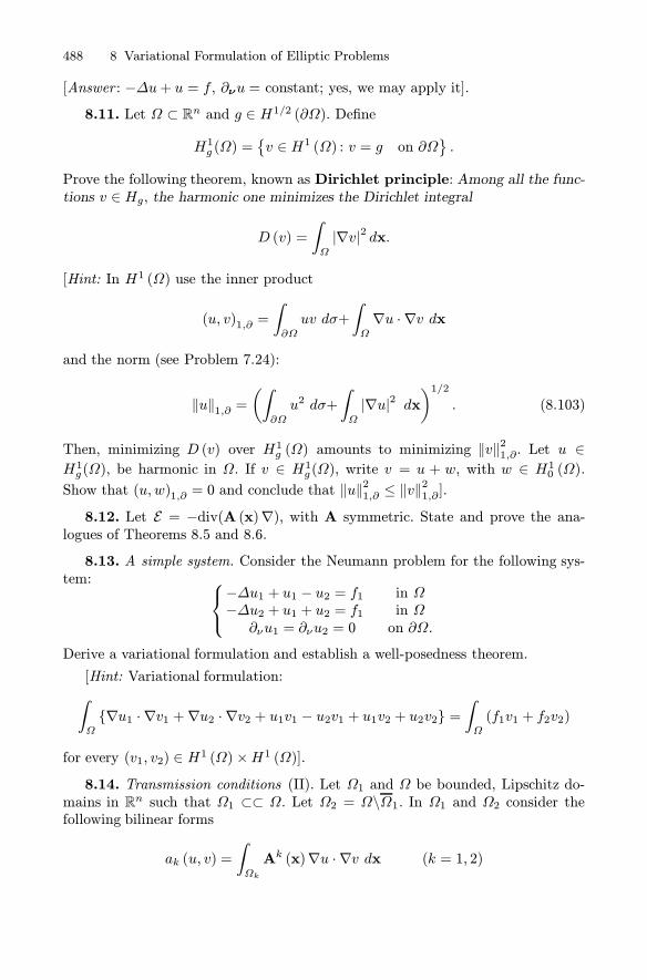
488 8 Variational Formulation of Elliptic Problems
[Answer : −Δu+ u = f , ∂νu = constant; yes, we may apply it].8.11. Let Ω ⊂ Rn and g ∈ H1/2 (∂Ω). Define
H1g (Ω) ={v ∈ H1 (Ω) : v = g on ∂Ω
}.
Prove the following theorem, known as Dirichlet principle: Among all the func-tions v ∈ Hg, the harmonic one minimizes the Dirichlet integral
D (v) =
∫
Ω
|∇v|2 dx.
[Hint: In H1 (Ω) use the inner product
(u, v)1,∂ =
∫
∂Ω
uv dσ+
∫
Ω
∇u · ∇v dx
and the norm (see Problem 7.24):
‖u‖1,∂ =(∫
∂Ω
u2 dσ+
∫
Ω
|∇u|2 dx)1/2
. (8.103)
Then, minimizing D (v) over H1g (Ω) amounts to minimizing ‖v‖21,∂. Let u ∈H1g(Ω), be harmonic in Ω. If v ∈ H1g(Ω), write v = u + w, with w ∈ H10 (Ω).Show that (u, w)1,∂ = 0 and conclude that ‖u‖
21,∂ ≤ ‖v‖
21,∂].
8.12. Let E = −div(A (x)∇), with A symmetric. State and prove the ana-logues of Theorems 8.5 and 8.6.
8.13. A simple system. Consider the Neumann problem for the following sys-tem: ⎧⎨
⎩−Δu1 + u1 − u2 = f1 in Ω−Δu2 + u1 + u2 = f1 in Ω∂νu1 = ∂νu2 = 0 on ∂Ω.
Derive a variational formulation and establish a well-posedness theorem.
[Hint: Variational formulation:
∫
Ω
{∇u1 · ∇v1 +∇u2 · ∇v2 + u1v1 − u2v1 + u1v2 + u2v2} =∫
Ω
(f1v1 + f2v2)
for every (v1, v2) ∈ H1 (Ω) ×H1 (Ω)].8.14. Transmission conditions (II). Let Ω1 and Ω be bounded, Lipschitz do-
mains in Rn such that Ω1 ⊂⊂ Ω. Let Ω2 = Ω\Ω1. In Ω1 and Ω2 consider thefollowing bilinear forms
ak (u, v) =
∫
Ωk
Ak (x)∇u · ∇v dx (k = 1, 2)

Problems 489
with Ak uniformly elliptic. Assume that the entries of Ak are continuous in Ωk,but that the matrix
A (x) =
{A1 (x) in Ω1A2 (x) in Ω2
may have a jump across Γ = ∂Ω1. Let u ∈ H10 (Ω) be the weak solution of theequation
a (u, v) = a1 (u, v) + a2 (u, v) = (f, v)0 ∀v ∈ H10 (Ω) ,
where f ∈ L2 (Ω).a) Which boundary value problem does u satisfy?
b) Which conditions on Γ do express the coupling between u1 and u2?
[Hint: b) u1|Γ = u2|Γ and A1∇u1 · ν = A2∇u2 · ν, where ν points outward
with respect to Ω1].
8.15. Find the mistake in the following argument. Consider the Neumann prob-lem {
−Δu+ c·∇u = f in Ω
∂νu = 0 on ∂Ω(8.104)
with Ω smooth, c ∈C1(Ω)and f ∈ L2 (Ω). Let V = H1 (Ω) and
B (u, v) =
∫
Ω
{∇u · ∇v + (c·∇u)v} .
If divc = 0, we may write
∫
Ω
(c · ∇u)u dx =12
∫
Ω
c · ∇(u2) dx =∫
∂Ω
u2c · ν dσ.
Thus, if c · ν ≥c0 > 0 then, recalling Problem 8.11,
B(u, u) ≥ ‖∇u‖20 + c0‖u‖2L2(∂Ω) ≥ C ‖u‖21,2so that B is V −coercive and problem (8.104) has a unique solution!!8.16. Let Ω = (0, π)× (0, π). Study the solvability of the Dirichlet problem
{Δu+ 2u = f in Q
u = 0 on ∂Q.
In particular, examine the cases f (x, y) = 1 and f (x, y) = x− π/2.8.17. Let B+1 =
{(x, y) ∈ R2: x2 + y2 < 1, y > 0
}. Examine the solvability of
the Robin problem {−Δu = f in B+1
∂νu+ yu = 0 on ∂B+1 .

490 8 Variational Formulation of Elliptic Problems
8.18. Let Ω = (0, 1) × (0, 1), a0 ∈ R. Examine the solvability of the mixedproblem ⎧
⎨⎩Δu+ a0u = 1 in Ω
u = 0 on ∂Ω\ {y = 0}∂νu = x on {y = 0} .
8.19. Derive a variational formulation of the following problem
{Δ2u = f in Ω
Δu+ ρ∂νu = 0 on ∂Ω
where ρ is a positive constant.Show that the right functional setting is H2 (Ω) ∩ H10 (Ω), i.e. the space of
functions in H2 (Ω) with zero trace. Prove the well-posedness of the resultingproblem.
[Hint: The variational formulation is
∫
Ω
Δu ·Δv dx+∫
∂Ω
ρ∂νu · ∂νv dσ=∫
Ω
fv dx, ∀v ∈ H2 (Ω) ∩H10 (Ω) .
To show the well-posedness, use ‖∂νv‖L2(∂Ω) ≤ ‖Δv‖0, ∀v ∈ H2 (Ω) ∩H10 (Ω)].8.20. Distributed observation and control, Neumann conditions. Let Ω ⊂ R
n
be a bounded, smooth domain and Ω0 an open (non empty) subset of Ω. SetV = H1 (Ω) , H = L2 (Ω) and consider the following control problem:
Minimize the cost functional
J (u, z) =1
2
∫
Ω0
(u− ud)2 dx+β
2
∫
Ω
z2dx
over (u, z) ∈ H1 (Ω)× L2 (Ω), with state system{Eu = −Δu+ a0u = z in Ω
∂νu = g on ∂Ω(8.106)
where a0 is a positive constant, g ∈ L2 (∂Ω) and z ∈ L2 (Ω).a) Show that there exists a unique minimizer.
b) Write the optimality conditions: adjoint problem and Euler equations.
[a) Hint: Follow the proof of Theorem 8.15, observing that, if u [z] is the solutionof (8.106) the map z �−→ u [z]− u [0] is linear. Then write
J (z) = 12
∫
Ω0
(u [z]− u [0] + u[0]− ud)2 dx+ β2
∫
Ω
z2dx
and adjust the bilinear form (8.93) accordingly.
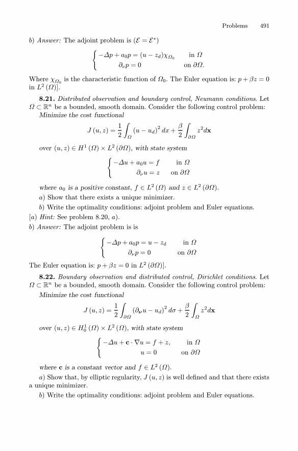
Problems 491
b) Answer: The adjoint problem is (E = E∗){−Δp+ a0p = (u− zd)χΩ0 in Ω
∂νp = 0 on ∂Ω.
Where χΩ0 is the characteristic function of Ω0. The Euler equation is: p+ βz = 0in L2 (Ω)].
8.21. Distributed observation and boundary control, Neumann conditions. LetΩ ⊂ Rn be a bounded, smooth domain. Consider the following control problem:Minimize the cost functional
J (u, z) =1
2
∫
Ω
(u− ud)2 dx+β
2
∫
∂Ω
z2dx
over (u, z) ∈ H1 (Ω)× L2 (∂Ω), with state system{−Δu+ a0u = f in Ω
∂νu = z on ∂Ω
where a0 is a positive constant, f ∈ L2 (Ω) and z ∈ L2 (∂Ω).a) Show that there exists a unique minimizer.
b) Write the optimality conditions: adjoint problem and Euler equations.
[a) Hint: See problem 8.20, a).
b) Answer: The adjoint problem is is
{−Δp+ a0p = u− zd in Ω
∂νp = 0 on ∂Ω
The Euler equation is: p+ βz = 0 in L2 (∂Ω)].
8.22. Boundary observation and distributed control, Dirichlet conditions. LetΩ ⊂ Rn be a bounded, smooth domain. Consider the following control problem:Minimize the cost functional
J (u, z) =1
2
∫
∂Ω
(∂νu− ud)2 dσ +β
2
∫
Ω
z2dx
over (u, z) ∈ H10 (Ω)× L2 (Ω), with state system{−Δu+ c · ∇u = f + z, in Ω
u = 0 on ∂Ω
where c is a constant vector and f ∈ L2 (Ω).a) Show that, by elliptic regularity, J (u, z) is well defined and that there exists
a unique minimizer.
b) Write the optimality conditions: adjoint problem and Euler equations.

9
Weak Formulation of Evolution Problems
Parabolic Equations – Diffusion Equation – General Equations – The Wave Equation
9.1 Parabolic Equations
In Chapter 2 we have considered the diffusion equation and some of its generaliza-tions, as in the reaction-diffusion model (Section 2.5) or in the Black-Scholes model(Section 2.9). This kind of equations belongs to the class of parabolic equations,that we have already classified in spatial dimension 1, in subsection 2.4.1 and thatwe are going to define in a more general setting.
Fig. 9.1. Space-time cylinder
Let Ω ⊂ Rn be a bounded domain, T > 0 and consider the space-time cylinderQT = Ω × (0, T ). Let A = A (x,t) be a square matrix of order n, b = b(x,t),c = c (x, t) vectors in Rn, a0 = a0(x,t) and f = f(x,t) real functions. Equationsin divergence form of the type
ut − div(A∇u− bu) + c · ∇u+ a0u = f (9.1)
Salsa S. Partial Differential Equations in Action: From Modelling to Theoryc© Springer-Verlag 2008, Milan
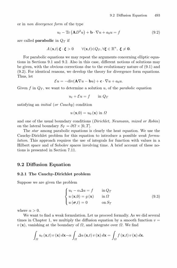
9.2 Diffusion Equation 493
or in non divergence form of the type
ut −Tr(AD2u
)+ b · ∇u+ a0u = f (9.2)
are called parabolic in QT if
A (x,t) ξ · ξ > 0 ∀(x,t)∈QT , ∀ξ ∈ Rn, ξ �= 0.
For parabolic equations we may repeat the arguments concerning elliptic equa-tions in Sections 9.1 and 9.2. Also in this case, different notions of solutions maybe given, with the obvious corrections due to the evolutionary nature of (9.1) and(9.2). For identical reasons, we develop the theory for divergence form equations.Thus, let
Eu = −div(A∇u− bu) + c · ∇u+ a0u.Given f in QT , we want to determine a solution u, of the parabolic equation
ut + Eu = f in QT
satisfying an initial (or Cauchy) condition
u (x,0) = u0 (x) in Ω
and one of the usual boundary conditions (Dirichlet, Neumann, mixed or Robin)on the lateral boundary ST = ∂Ω × [0, T ].The star among parabolic equations is clearly the heat equation. We use the
Cauchy-Dirichlet problem for this equation to introduce a possible weak formu-lation. This approach requires the use of integrals for function with values in aHilbert space and of Sobolev spaces involving time. A brief account of these no-tions is presented in Section 7.11.
9.2 Diffusion Equation
9.2.1 The Cauchy-Dirichlet problem
Suppose we are given the problem⎧⎪⎨⎪⎩
ut − αΔu = f inQT
u (x,0) = g (x) inΩ
u (σ,t) = 0 onST
(9.3)
where α > 0.We want to find a weak formulation. Let us proceed formally. As we did several
times in Chapter 1, we multiply the diffusion equation by a smooth function v =v (x), vanishing at the boundary of Ω, and integrate over Ω. We find
∫
Ω
ut (x,t) v (x) dx−α∫
Ω
Δu (x,t) v (x) dx =
∫
Ω
f (x,t) v (x) dx.

494 9 Weak Formulation of Evolution Problems
Integrating by parts the second term, we get∫
Ω
ut (x,t) v (x) dx+α
∫
Ω
∇u (x,t) · ∇v (x) dx =∫
Ω
f (x,t) v (x) dx. (9.4)
This looks like what we did for elliptic equations, except for the presence of ut.Moreover, here we will have somehow to take into account the initial condition.Which could be a correct functional setting?First of all, since we are dealing with evolution equations, it is convenient to
adopt the point of view of section 7.11, and consider u = u (x, t) as a function oft with values into a suitable Hilbert space V :
u: [0, T ]→ V.When we adopt this convention, we write u (t) instead of u (x, t) and u insteadof ut. Accordingly, we write f (t) instead of f (x, t). With these notations, (9.4)becomes ∫
Ω
u (t) v dx+α
∫
Ω
∇u (t) · ∇v dx =∫
Ω
f (t) v dx. (9.5)
The homogeneous Dirichlet condition, i.e. u (t) = 0 on ∂Ω for t ∈ [0, T ], suggeststhat the natural space for u (t) is V = H10 (Ω), at least for a.e. t ∈ [0, T ]. As usual,in H10 (Ω) we use the inner product
(w, v)1 = (∇w,∇v)0with corresponding norm ‖·‖1. Thus, the second integral in (9.5) may be writtenin the form
(∇u (t) ,∇v)0 .Also, it would seem to be appropriate that u (t) ∈ L2 (Ω), looking at the firstintegral. This however is not coherent with the choice u (t)∈H10 (Ω), since we haveΔu (t) ∈ H−1 (Ω) and
u (t) = αΔu (t) + f (t) (9.6)
from the diffusion equation. Thus, we deduce that H−1 (Ω) is the natural spacefor u as well. Consequently, the first integral in (9.5) has to be interpreted as
〈u (t) , v〉∗where 〈·, ·〉∗ denotes the pairing between H−1 (Ω) and H10 (Ω).A reasonable hypothesis on f is f ∈ L2 (QT ), which in the new notations
becomes1
f ∈ L2(0, T ;L2 (Ω)
).
Coherently, from (9.6) we require u∈L2(0, T ;H10 (Ω)
)and u∈L2
(0, T ;H−1 (Ω)
).
Now, from Theorem 7.22 we know that
u∈ C([0, T ] ;L2 (Ω)
)
so that the initial condition u (0) = g makes perfect sense if we choose g ∈ L2 (Ω).
1 Also f ∈ L2 (0, T ; V ∗) is fine.

9.2 Diffusion Equation 495
The above arguments motivate the following definition. Consider the Hilberttriplet (V,H, V ∗), where V = H10 (Ω), H = L2 (Ω) and V ∗ = H−1 (Ω). Recall thatPoincare’s inequality holds in V :
‖v‖0 ≤ CP ‖v‖1 .Finally, let
a (w, v) = α(∇w,∇v)0Definition 9.1. A function u∈L2 (0, T ; V ) is called weak solution of problem(9.3) if u∈L2 (0, T ; V ∗) and:1. for every v ∈ V ,
〈u (t) , v〉∗+a (u (t) , v)= (f (t) , v)0 a.e. t ∈ [0, T ] . (9.7)
2. u (0) = g.
Remark 9.1. Equation (9.7) may be interpreted in the sense of distributions. Tosee this, observe that, for every v ∈ V , the real function
w (t) = 〈u (t) , v〉∗is a distribution in D′ (0, T ) and
〈u (t) , v〉∗ =d
dt(u (t) , v)0 in D′ (0, T ) . (9.8)
This means that, for every ϕ ∈ D (0, T ), we have∫ T
0
〈u (t) , v〉∗ ϕ (t) dt = −∫ T
0
(u (t) , v) ϕ (t) dt.
In fact, since u (t) ∈ V , by Bochner’s Theorem 7.20 and the definition of u, wemay write
∫ T
0
〈u (t) , v〉∗ ϕ (t) dt = 〈∫ T
0
u (t)ϕ (t) dt, v〉∗ = 〈−∫ T
0
u (t) ϕ (t) dt, v〉∗.
On the other hand,∫ T0u (t) ϕ (t) dt ∈ V so that 2
〈−∫ T
0
u (t) ϕ (t) dt, v〉∗ = (−∫ T
0
u (t) ϕ (t) dt , v)0 = −∫ T
0
(u (t) , v)0 ϕ (t) dt.
Thus w ∈ L1loc(0, T ) ⊂ D′ (0, T ) and (9.8) is true. As a consequence, equation (9.7)may be written in the form
d
dt(u (t) , v)0 + a (u (t) ,v) = (f, v)0 (9.9)
in the sense of distributions in D′ (0, T ), for all v ∈ V .Remark 9.2. We leave it to the reader to check that if a weak solution u is smooth,i.e. u ∈ C2,1
(QT), then u is a classical solution.
2 Recall from Section 6.8 that if u ∈ H and v ∈ V , 〈u, v〉∗ = (u, v)0.

496 9 Weak Formulation of Evolution Problems
9.2.2 Faedo-Galerkin method (I)
We want to show that problem (9.3) has exactly one weak solution, which dependscontinuously on the data in a suitable norm.Although there are variants of the Lax-Milgram Theorem perfectly adapted to
solve evolution problems, we shall use the so-called Faedo-Galerkin method, alsomore convenient for numerical approximations. Let us describe the main strategy.
1. We select a sequence of smooth functions {wk}∞k=1 constituting3
an orthogonal basis in V = H10 (Ω)
andan orthonormal basis in H = L2 (Ω) .
In particular, we can write
g =
∞∑k=1
gkwk
where gk = (g, wk)0 and the series converges in H .
2. We construct the sequence of finite-dimensional subspaces
Vm = span {w1, w2, ..., wm} .Clearly
Vm ⊂ Vm+1 and ∪Vm = V.For m fixed, let
um (t) =
m∑k=1
ck (t)wk, Gm =
m∑k=1
gkwk. (9.10)
We solve the following approximate problem: Determine um ∈ H1 (0, T ; V ), satis-fying, for every s = 1, ..., m,{
(um (t) , ws)0 + a (um (t) , ws) = (f (t) ,ws)0 , a.e t ∈ [0, T ]um (0) = Gm.
(9.11)
Note that the differential equation in (9.11) is true for each element of the basisws, s = 1, ..., m, if and only if it is true for every v ∈ Vm. Moreover, since um ∈L2 (0, T ; V ), we have
(um (t) , v)0 = 〈um (t) , v〉∗ .We call um a Galerkin approximation of the solution u.
3. We show that {um} and {um} are bounded in L2 (0, T ; V ) and L2 (0, T ; V ∗),respectively (energy estimates). Then, the weak compactness Theorem 6.11 impliesthat a subsequence {umk} converges weakly in L2 (0, T ; V ) to some element u, while{umk} converges weakly in L2 (0, T ; V ∗) to u.4. We prove that u in step 3 is the unique weak solution of problem (9.3).
3 This is possible since V is a separable Hilbert space. In particular, here we can chooseas wk the Dirichlet eigenfunctions of the Laplace operator, normalized with respect tothe norm in H (see Theorem 8.5).

9.2 Diffusion Equation 497
9.2.3 Solution of the approximate problem
The following lemma holds:
Lemma 9.1. For all m, there exists a unique solution um of problem (9.11). Inparticular, since um ∈ H1 (0, T ; Vm), we have um ∈ C ([0, T ]; Vm).
Proof. Since w1, ..., wm are mutually orthonormal in L2 (Ω), we have
(um (t) , ws)0 =
(m∑k=1
ck (t)wk, ws
)
0
= cs (t) .
Also, w1, ..., wm is an orthogonal system in Vm, hence
a
(m∑k=1
ck (t)wk, ws
)= α (∇ws,∇ws)0 cs (t) = α ‖∇ws‖
20 cs (t) .
LetFs (t) = (f (t) , ws) , Fm (t) = (F1 (t) , ..., Fm (t))
andCm (t) = (c1 (t) , ..., cm (t)) , gm = (g1, ..., gm) .
If we introduce the diagonal matrix
W = diag{‖∇w1‖20 , ‖∇w2‖
20 , ..., ‖∇wm‖
20
}
of order m, problem (9.11) is equivalent to the following system of m uncoupledlinear ordinary differential equations, with constant coefficients:
Cm (t) = −αWCm (t) + Fm (t) , a.e. t ∈ [0, T ] (9.12)
with initial conditionCm (0) = gm.
Since F ∈ L2 (0, T ;Rm), there exists a unique solution Cm (t) ∈ H1(0, T ;Rm).From
um (t) =m∑k=1
ck (t)wk,
we deduce that um ∈ H1 (0, T ; Vm). �
Remark 9.3. We have chosen a basis {wk} orthonormal in L2 and orthogonal inH10 because with respect to this base, the Laplace operator becomes a diagonaloperator, as it is reflected by the approximate problem (9.12). However, the methodworks using any countable basis for both spaces. Problem (9.11) becomes
Cm (t) = −M−1WCm (t) +M−1Fm (t) a.e. t ∈ [0, T ]

498 9 Weak Formulation of Evolution Problems
where4
M =(Msk) , Msk = (ws, wk)0 ,
W =(Wsk) , Wsk = α (∇ws,∇wk)0 .This is particularly important in the numerical implementation of the method,where, in general, the elements of the basis in Vm are not mutually orthogonal.
9.2.4 Energy estimates
Our purpose is to show that we can extract from the sequence of Galerkin approx-imations {um} a subsequence converging in some sense to a solution of problem(9.3). This is a typical compactness problem in Hilbert spaces. The key tool isTheorem 6.11: let H be a Hilbert space and {xm} ⊂ H a bounded sequence. Then,{xm} has a subsequence {xmk} weakly convergent to x ∈ H . Moreover
‖x‖ ≤ lim infk→∞
‖xmk‖ . (9.13)
Thus, what we need is to show that suitable Sobolev norms of um can beestimated by suitable norms of the data, and the estimates are independentof m. Moreover, these estimates must be powerful enough in order to pass to thelimit as m→ +∞ in the approximating equation
(um, v)0 + α (∇um,∇v)0 = (f, v)0 .
In our case we will be able to control the norms of um in L∞ (0, T ;H) and
L2 (0, T ; V ), and the norm of um in L2 (0, T ; V ∗), that is the norms
maxt∈[0,T ]
‖um (t)‖0 ,∫
Ω
‖um (t)‖21 dt and∫
Ω
‖um (t)‖2∗ dt
Thus, let um =∑m
k=1 ck (t)wk be the solution of problem (9.11).
Theorem 9.1. (Estimate of um). For every t ∈ [0, T ], the following estimateholds:
‖um (t)‖20 + α∫ t
0
‖um (s)‖21 ds ≤ ‖g‖20 +C2Pα
∫ t
0
‖f (s)‖20 ds. (9.14)
Note in particular how estimate (9.14) deteriorates as α approaches to zero.An alternative estimate is given in Problem 9.3.
Proof. Multiplying equation (9.11) by ck (t) and summing for k = 1, ..., m, weget
(um (t) , um (t))0 + a (um (t) , um (t)) = (f (t) ,um (t))0 (9.15)
4 Since w1, ...,wm is a basis in Vm, the matrix M is positive, hence non singular.

9.2 Diffusion Equation 499
for a.e. t ∈ [0, T ]. Now, note that
(um (t) , um (t))0 =1
2
d
dt‖um (t)‖20 , a.e. t ∈ (0, T )
anda (um (t) , um (t)) = α ‖∇um (t)‖20 = α ‖um (t)‖
21 .
From the inequalities of Schwarz and Poincare and the elementary inequality
|ab| ≤ a2
2ε+ε
2b2 ∀a, b ∈ R, ∀ε > 0 (9.16)
with ε = α, we deduce
(f (t) ,um (t))0 ≤ ‖f (t)‖0 ‖um (t)‖0 ≤ CP ‖f (t)‖0 ‖um (t)‖1≤ C
2P
2α‖f (t)‖20 +
α
2‖um (t)‖21 .
Thus, from (9.15) we obtain
d
dt‖um (t)‖20 + α ‖um (t)‖
21 ≤C2Pα‖f (t)‖20 .
We now integrate over (0, t), using formula (7.70) in Remark 7.34. Since um (0) =Gm and observing that
‖Gm‖20 ≤ ‖g‖20
by the orthogonality of w1, ..., wm in L2 (Ω), we may write:
‖um (t)‖20 + α∫ t
0
‖um (s)‖21 ds ≤ ‖Gm‖20 +C2Pα
∫ t
0
‖f (s)‖20 ds (9.17)
≤ ‖g‖20 +C2Pα
∫ t
0
‖f (s)‖20 ds
which is (9.14). �
We now give an estimate of the norm of um in L2 (0, T ; V ∗).
Theorem 9.2. (Estimate of um). The following estimate holds:
∫ T
0
‖um (t)‖2∗ dt ≤ 2α ‖g‖20 + 4C
2P
∫ T
0
‖f (t)‖20 dt (9.18)
Proof. Let v ∈ V and writev = w + z
where w ∈ Vm and z ∈ V ⊥m . We have
‖w‖1 ≤ ‖v‖1 .
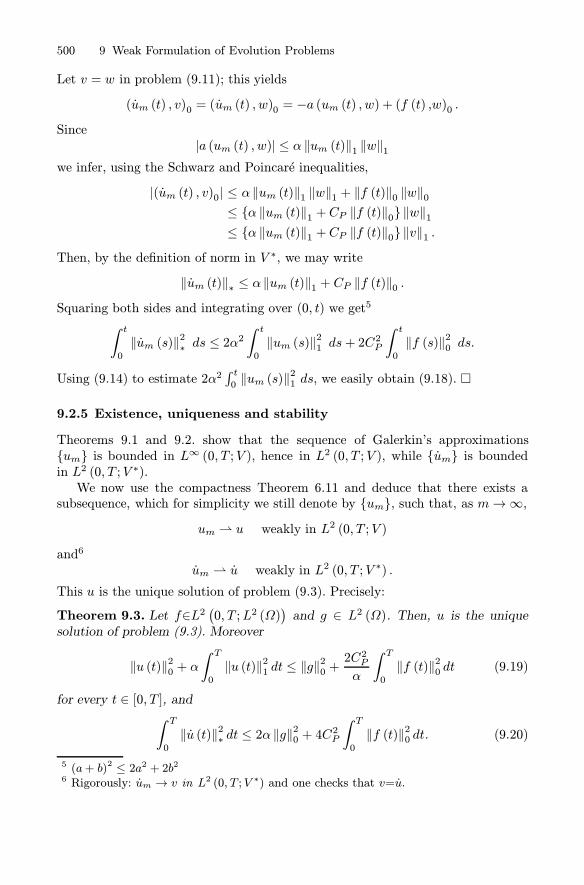
500 9 Weak Formulation of Evolution Problems
Let v = w in problem (9.11); this yields
(um (t) , v)0 = (um (t) , w)0 = −a (um (t) , w) + (f (t) ,w)0 .Since
|a (um (t) , w)| ≤ α ‖um (t)‖1 ‖w‖1we infer, using the Schwarz and Poincare inequalities,
|(um (t) , v)0| ≤ α ‖um (t)‖1 ‖w‖1 + ‖f (t)‖0 ‖w‖0≤ {α ‖um (t)‖1 +CP ‖f (t)‖0} ‖w‖1≤ {α ‖um (t)‖1 +CP ‖f (t)‖0} ‖v‖1 .
Then, by the definition of norm in V ∗, we may write
‖um (t)‖∗ ≤ α ‖um (t)‖1 + CP ‖f (t)‖0 .Squaring both sides and integrating over (0, t) we get5
∫ t
0
‖um (s)‖2∗ ds ≤ 2α2∫ t
0
‖um (s)‖21 ds+ 2C2P∫ t
0
‖f (s)‖20 ds.
Using (9.14) to estimate 2α2∫ t0‖um (s)‖21 ds, we easily obtain (9.18). �
9.2.5 Existence, uniqueness and stability
Theorems 9.1 and 9.2. show that the sequence of Galerkin’s approximations{um} is bounded in L∞ (0, T ; V ), hence in L2 (0, T ; V ), while {um} is boundedin L2 (0, T ; V ∗).We now use the compactness Theorem 6.11 and deduce that there exists a
subsequence, which for simplicity we still denote by {um}, such that, as m→∞,um ⇀ u weakly in L2 (0, T ; V )
and6
um ⇀ u weakly in L2 (0, T ; V ∗) .
This u is the unique solution of problem (9.3). Precisely:
Theorem 9.3. Let f∈L2(0, T ;L2 (Ω)
)and g ∈ L2 (Ω). Then, u is the unique
solution of problem (9.3). Moreover
‖u (t)‖20 + α∫ T
0
‖u (t)‖21 dt ≤ ‖g‖20 +2C2Pα
∫ T
0
‖f (t)‖20 dt (9.19)
for every t ∈ [0, T ], and∫ T
0
‖u (t)‖2∗ dt ≤ 2α ‖g‖20 + 4C
2P
∫ T
0
‖f (t)‖20 dt. (9.20)
5 (a+ b)2 ≤ 2a2 + 2b26 Rigorously: um → v in L2 (0, T ;V ∗) and one checks that v=u.

9.2 Diffusion Equation 501
Proof. Existence. To say that um ⇀ u, weakly in L2 (0, T ; V ) as m → ∞,
means that∫ T
0
(∇um (t) ,∇v (t))0 dt→∫ T
0
(∇u (t) ,∇v (t))0 dt
for all v∈L2 (0, T ; V ). Similarly, um ⇀ u, weakly in L2 (0, T ; V ∗), means that∫ T
0
(um (t) , v (t))0 dt =
∫ T
0
〈um (t) , v (t)〉∗ dt→∫ T
0
〈u (t) , v (t)〉∗ dt
for all v∈L2 (0, T ; V ).We want to use these properties to pass to the limit as m → +∞ in problem
(9.11), keeping in mind that the test functions have to be chosen in Vm. Fixv∈L2 (0, T ; V ); we may write
v (t) =
∞∑k=1
bk (t)wk
with the series convergent in V , for a.e. t ∈ [0, T ]. Let
vN (t) =
N∑k=1
bk (t)wk (9.21)
and keep N fixed, for the time being. If m ≥ N , then vN ∈ L2 (0, T ; Vm). Multi-plying equation (9.11) by bk (t) and summing for k = 1, ..., N , we get
(um (t) , vN (t))0 + α (∇um (t) ,∇vN (t))0 = (f (t) ,vN (t))0 .
An integration over (0, T ) yields
∫ T
0
{(um, vN)0 + α (∇um,∇vN)0} dt =∫ T
0
(f, vN)0 dt. (9.22)
Thanks to the weak convergence of um and um in their respective spaces, we canlet m→ +∞. Since
∫ T
0
(um, vN)0 dt =
∫ T
0
〈um, vN〉∗ dt→∫ T
0
〈u, vN 〉∗ dt,
we obtain ∫ T
0
{〈u, vN〉∗ + α (∇u,∇vN)0} dt =∫ T
0
(f, vN )0 dt.
Now, let N → ∞ observing that vN → v in L2 (0, T ; V ) and in particular weaklyin this space as well. We obtain
∫ T
0
{〈u, v〉∗ + α (∇u,∇v)0} dt =∫ T
0
(f, v)0 dt. (9.23)

502 9 Weak Formulation of Evolution Problems
Then, (9.23) is valid for all v ∈ L2 (0, T ; V ). This entails7
〈u (t) , v〉∗ + α (∇u (t) ,∇v)0 dt = (f (t) , v)0for all v∈V and a.e. t ∈ [0, T ]. Therefore u satisfies (9.7). From Theorem 7.22, weknow that u∈C ([0, T ] ;H).It remains to check that u (t) satisfies the initial condition u (0) = g. Let
v∈C1 ([0, T ] ;V ) with v (T ) = 0. Integrating by parts (see Theorem 7.22, b)), weobtain ∫ T
0
(um, vN)0 dt = (Gm, vN (0))0 −∫ T
0
(um, vN )0 dt
so that, from (9.22) we find
−∫ T
0
{(um, vN)0 + α (∇um,∇vN )0} dt = − (Gm, vN (0))0 +∫ T
0
(f, vN)0 dt.
Let first m→ ∞ and then N →∞; we get
−∫ T
0
{(u, v)0 + α (∇u,∇v)0} dt = − (g, v (0))0 +∫ T
0
(f, v)0 dt. (9.25)
On the other hand, integrating by parts in formula (9.23) (see again Theorem 7.22,b)) we find
−∫ T
0
{(u, v)0 + α (∇u,∇v)0} dt = (u (0) , v (0))0 +∫ T
0
(f (t) , v (t))0 dt. (9.26)
Subtracting (9.25) from (9.26), we deduce
(u (0) , v (0))0 = (g, v (0))0
and the arbitrariness of v (0) forces
u (0) = g.
Uniqueness. Let u1 and u2 be weak solutions of the same problem. Then,w = u1 − u2 is a weak solution of
〈w (t) , v〉∗ + α (∇w (t) ,∇v)0 = 0
for all v∈V and a.e. t ∈ [0, T ], with initial data w (0) = 0. Choosing v = w (t) wehave7 Precisely: equation (9.23) is valid, in particular, for v (t) of the form wkϕ (t), withϕ ∈ L2 (0, T ). Therefore, for each k there is a set Ek of measure zero, such that
〈u (t) , wk〉∗ + α (∇u (t) ,∇wk)0 dt = (f (t) , wk)0 (9.24)
for all t /∈ Ek.Then, (9.24) holds for every k, as long as t /∈ ∪k≥1Ek. Since |∪k≥1Ek| = 0and {wk} is a basis in V , we conclude that (9.24) holds for all v ∈ V , a.e. t ∈ [0, T ].

9.2 Diffusion Equation 503
〈w (t) , w (t)〉∗ + α (∇w (t) ,∇w (t))0 = 0or, using Remark 7.34,
1
2
d
dt‖w (t)‖20 = −α ‖w (t)‖
21
whence, since ‖w (0)‖20 = 0,
‖w (t)‖20 = −∫ T
0
−α ‖w (t)‖21 dt < 0
which entails w (t) = 0 for all t ∈ [0, T ]. This gives uniqueness of the weak solution.Stability estimates. Letting m → +∞ in (9.14) and (9.18) we get, using
(9.13) and Proposition 7.16,
‖u‖2L∞(0,T ;H) , ‖u‖2L2(0,T ;V ) ≤ ‖g‖
20 +C2Pα
∫ T
0
‖f‖20 dt
and
‖u‖2L(0,T ;V ∗) ≤ 2α ‖g‖20 + 4C
2P
∫ T
0
‖f‖20 dt
which give (9.19) and (9.20). �
Remark 9.4. As a by-product of the above proof, we deduce that, if f=0, u satisfiesthe equation
d
dt‖u (t)‖20 = −2α ‖u (t)‖
21 ≤ 0
which shows the dissipative nature of the diffusion equation.
9.2.6 Regularity
As in the elliptic case, the regularity of the solution improves with the regularityof the data. Precisely, we have:
Theorem 9.4. Let Ω be a C2−domain and u be the weak solution of problem(9.3). If g ∈ V , then u ∈ L2(0, T ;H2 (Ω)) ∩ L∞ (0, T ; V ) and u ∈ L2 (0, T ;H).Moreover
‖u‖L2(0,T ;H2(Ω)) + ‖u‖L∞(0,T ;V ) + ‖u‖L2(0,T ;H) ≤ C (α){‖g‖V + ‖f‖L2(0,T ;H)
}.
(9.27)
Proof. Multiplying equation (9.11) by ck (t) and summing for k = 1, ..., m, weget
‖um (t)‖20 + α (∇um (t) ,∇um (t))0 = (f (t) ,um (t))0 (9.28)
504 9 Weak Formulation of Evolution Problems
for a.e. t ∈ [0, T ]. Now, note that
(∇um (t) ,∇um (t))0 =1
2
d
dt‖∇um (t)‖20 , a.e. t ∈ (0, T )
and that, from Schwarz’s inequality
(f (t) ,um (t))0≤‖f (t)‖0 ‖um (t)‖0 ≤1
2‖f (t)‖20 +
1
2‖um (t)‖20 .
From this inequality and (9.28), we infer
αd
dt‖∇um (t)‖20 + ‖um (t)‖
20 ≤ ‖f (t)‖
20 a.e. t ∈ (0, T ) .
An integration over (0, t) yields
α ‖∇um (t)‖20 +∫ t
0
‖um (s)‖20 ds ≤∫ t
0
‖f (s)‖20 ds+ ‖gm‖21 . (9.29)
Passing to the limit as m → ∞ along an appropriate subsequence, we deducethat the same estimate holds for u and therefore, that u ∈ L∞ (0, T ; V ) and u ∈L2 (0, T ;H). In particular, we may write (9.7) in the form:
α (∇u (t) ,∇v)0 = (f (t)− u (t) , v)0 a.e. t ∈ [0, T ]
for all v ∈ V .Now, the regularity theory for elliptic equations (Theorem 8.13) implies that
u (t) ∈ H2(Ω) for a.e. t ∈ [0, T ] and that
‖u (t)‖2H2(Ω) ≤ C (α,Ω){‖g‖21 + ‖f (t)‖
20 + ‖u (t)‖
20
}.
Integrating and using (9.29), we obtain
u ∈ L2(0, T ;H2 (Ω))
and the estimate (9.27). �Further regularity requires compatibility conditions on f and g. We limit our-
selves to consider the following situation in the case f = 0. Suppose we haveu ∈ C∞
(QT). Since u = 0 on the lateral side, we have
u = ∂tu = · · · = ∂jt u = · · · = 0, ∀j ≥ 0, on ∂Ω × (0,∞)
which hold, by continuity, also for t = 0. On the other hand, the heat equationgives
∂tu = αΔu, ∂2t u = αΔ(∂tu) = αΔ2u
and, in general,∂jt u = αΔ
ju, ∀j ≥ 0, in QT .

9.2 Diffusion Equation 505
Since u ∈ C∞(QT), these equations still hold for t = 0. As a consequence, we
conclude that
g = Δg = · · · = Δjg = · · · = 0 ∀j ≥ 0, on ∂Ω. (9.30)
Thus, conditions (9.30) are necessary in order to have u ∈ C∞(QT). It turns
out that they are sufficient as well, as stated by the following theorem8.
Theorem 9.5. Let u be the weak solution of problem (9.3). If g ∈ Hm (Ω), forevery m ≥ 1, and conditions (9.30) hold, then u ∈ C∞
(QT).
9.2.7 The Cauchy-Neuman problem
The Faedo-Galerkin method works with the other common boundary conditions,with small adjustments. Let us examine the weak formulation of the diffusionequation,
〈u (t) , v〉∗+a (u (t) , v)= (f (t) , v)0 , (9.31)
which must be true for all v ∈ V and a.e. in [0, T ]. For the Cauchy-Dirichletproblem, the bilinear form a is
a (w, v) = α (∇w,∇v)0which is a multiple of the inner product in V = H10(Ω). Thus, a is continuous butalso V−coercive, which is crucial for the method, as in the elliptic case.However, once the relevant Hilbert triplet (V,H, V ∗) has been selected, for
parabolic equation it is enough that a be weakly coercive i.e that there existsα > 0, λ ≥ 0 such that
a (v, v) + λ ‖v‖2H ≥ α ‖v‖2V ∀v ∈ V. (9.32)
Indeed, if (9.32) holds, setw (t)=e−λtu (t) .
Then,w (t)=e−λtu (t)− λe−λtu (t) = e−λtu (t) − λw (t)
so that, if u solves (9.31), w solves
〈w (t) , v〉∗+a (w (t) , v) + λ (w (t) , v)H =(e−λtf (t) , v
)H
which is an equation of the same type, with the coercive bilinear form
a (w, v) = a (w, v) + λ (w, v)H
and forcing term e−λtf (t). In other words, if the bilinear form a is only weaklycoercive, by a simple change of variable we may reduce ourselves to an equivalent
8 For the proof, see Evans, 1998.

506 9 Weak Formulation of Evolution Problems
equation, associated with a modified coercive bilinear form (see however Problem9.4).For instance, consider the following Cauchy-Neumann problem9:
⎧⎪⎨⎪⎩
ut − αΔu = f inQT
u (x,0) = g (x) in Ω
∂νu (σ,t) = 0 on ST .
(9.33)
where f ∈ L2 (QT ) and g ∈ L2 (Ω). For the weak formulation choose H = L2 (Ω)and V = H1 (Ω) , where, we recall, inner product and norm are given by
(u, v)1,2 = (∇u,∇v)0 + (u, v)0 , ‖u‖21,2 = ‖∇u‖20 + ‖u‖
20 .
A weak formulation of the Cauchy-Neumann problem may be stated as follows:
Find u∈L2 (0, T ; V ) such that u∈L2 (0, T ; V ∗) and
1. for all v ∈ V and a.e. t ∈ [0, T ],
〈u (t) , v〉∗+a (u (t) , v)= (f (t) , v)0 ,
2. u (0) = g.
The bilinear form
a (u, v) = α (∇u,∇v)0is weakly coercive: any λ > 0 works.For simplicity, let λ = α; then
a (w, v) = α {(∇u,∇v)0 + (u, v)0} .
With the change of variable
w (t)= e−αtu (t)
we are reduced to the following equivalent formulation:
Find w∈L2 (0, T ; V ) such that
w∈L2 (0, T ; V ∗)
and
1. for all v ∈ V and a.e. t ∈ [0, T ],
〈w (t) , v〉∗+a (w (t) , v) =(e−αtf (t) , v
)0,
2. w (0) = g.
9 For nonhomogeneous Neumann conditions, see Problem 9.2.

9.2 Diffusion Equation 507
With small adjustments, the technique used for Dirichlet boundary conditionsyields existence and uniqueness of a unique solution w of the above Cauchy-Neumann problem and therefore of the original problem. The stability estimatesfor w take the form
‖w (t)‖20 +∫ t
0
‖w (s)‖21,2 ds ≤ c(α){‖g‖20 +
∫ t
0
e−2αs ‖f (s)‖20 ds}
and ∫ t
0
‖w (s)‖2∗ ds ≤ c(α){‖g‖20 +
∫ t
0
e−2αs ‖f (s)‖20 ds}
for all t ∈ [0, T ]. Going back to u, we obtain the following theorem.
Theorem 9.6. There exists a unique weak solution u of (9.31) satisfying the initialcondition u (0) = g. Moreover
∫ T
0
{‖u (s)‖21,2 + ‖u (s)‖
2∗}ds ≤ C
{‖g‖20 +
∫ T
0
‖f (s)‖20 ds}
(9.34)
where C = C (α, T ).
9.2.8 Cauchy-Robin and mixed problems
Consider the problem
⎧⎪⎨⎪⎩
ut − αΔu = f inQT
u (x,0) = g (x) inΩ
∂νu (σ,t) + h (σ)u (σ,t) = 0 onST
where h ∈ L∞ (∂Ω) and h ≥ 0. For the weak formulation we choose H = L2 (Ω)and V = H1 (Ω). As in the elliptic case, we consider the bilinear form
a (u, v) = α (∇u,∇v)0 +∫
∂Ω
huv dσ. (9.35)
A weak formulation is the following:
Determine u∈L2 (0, T ; V ) such that u∈L2 (0, T ; V ∗) and
1. for all v ∈ V and a.e. t ∈ [0, T ],
〈u (t) , v〉∗+a (u (t) , v)= (f (t) , v) ,
2. u (0) = u0.
The following theorem holds.

508 9 Weak Formulation of Evolution Problems
Theorem 9.7. There exists a unique weak solution u of the Cauchy-Robin prob-lem. Moreover, the inequality (9.34) holds for u, with C = C(α,Ω, ‖h‖L∞(∂Ω)).
Proof. We may argue as in the case of Neumann conditions. The bilinear form(9.35) is continuous and weakly coercive for any λ > 0, since10 h ≥ 0 on ∂Ω.Choosing λ = α, we have
a (u, v) = α {(∇u,∇v)0 + (u, v)0}+∫
∂Ω
huv dσ ≥ α (u, v)1,2 .
Moreover, thanks to the trace inequality (see Theorem 7.11)
‖u‖L2(∂Ω) ≤ C∗ ‖u‖1,2 (9.36)
we may write
|a (u, v)| ≤ α ‖u‖1,2 ‖v‖1,2 + ‖h‖L∞(∂Ω) ‖u‖L2(∂Ω) ‖v‖L2(∂Ω)≤ (α+ C∗ ‖h‖L∞(∂Ω)) ‖u‖1,2 ‖v‖1,2
whence a is continuous as well. Setting
w (t)=e−αtu (t) ,
we are led to determine w∈L2 (0, T ; V ) such that w∈L2 (0, T ; V ∗) and
1. for all v ∈ V and a.e. t ∈ [0, T ],
〈w (t) , v〉∗+a (w (t) , v)=(e−αtf (t) , v
),
2. w (0) = u0.
Then, the energy inequalities follow as in the case of the Dirichlet problem.For the existence and uniqueness of the weak solution, we need only to observethat the trace inequality (9.36) gives, for the Galerkin approximations {um}, theestimate
∫ T
0
‖um (t)‖2L2(∂Ω) dt ≤ C2∗∫ T
0
‖um (t)‖21,2 dt ≤ C(α, T ){‖g‖20 +
∫ T
0
‖f (s)‖20 ds}.
Thus, {um} has a subsequence weakly convergent in L2 (∂Ω). Therefore we canpass to the limit as m→ +∞ in the term
∫
∂Ω
hum (t) vdσ
as well. �10 If |h| ≤M on ∂Ω, a is weakly coercive for λ large enough (check it).

9.2 Diffusion Equation 509
Finally, we consider the mixed problem
⎧⎪⎪⎪⎨⎪⎪⎪⎩
ut − αΔu = f inQT
u (x,0) = g (x) in Ω
∂νu (σ,t) = 0u (σ,t) = 0
on ΓN × [0, T ]on ΓD × [0, T ].
where ΓD is a relatively open subset of ∂Ω and ΓN = ∂Ω\ΓD. For the weakformulation we choose H = L2 (Ω) and V = H10,ΓD (Ω), with inner product
(u, v)1 = (∇u,∇v)0and norm ‖·‖1. Recall that in H10,ΓD (Ω) Poincare’s inequality holds:
‖v‖0 ≤ CP ‖v‖1 .
The bilinear forma (w, v) = α (∇w,∇v)0
is continuous and V−coercive. Reasoning as in the case of the Dirichlet condition,we conclude that:
Theorem 9.8. There exists a unique weak solution u of the initial-mixed problem.Moreover, the inequalities (9.19) and (9.20) hold.
9.2.9 A control problem
Using the same techniques of Section 8.8, we may solve simple control problemsfor the diffusion equation. Consider, for instance, the problem of minimizing thecost functional
J (u, z) =1
2
∫
Ω
|u (T )− ud|2 dx+β
2
∫
QT
z2dxdt
under the condition (state system)
⎧⎨⎩ut −Δu = z in QTu = 0 onSTu (x,0) = g (x) in Ω.
(9.37)
Thus, we want to control the distributed heat flux in QT , given by z, in order tominimize the distance from ud of the final observation of u, given byu (T ).
If g ∈ L2 (Ω) and the class of admissible controls is L2 (QT ), we know from The-orem 9.3 that problem (9.37) has a unique weak solution u = u [z] for every controlz. Moreover, we assume that Ω is a C2−domain and that g ∈ H10 (Ω), so that The-orem 9.4 implies that, actually, u ∈ L2
(0, T ;H2 (Ω)
)and u ∈ L2
(0, T ;L2 (Ω)
).

510 9 Weak Formulation of Evolution Problems
Substituting u [z] into J , we obtain the functional
J (z) = J (u [z] , z) =1
2
∫
Ω
(u [T ; z]− ud)2 dx+β
2
∫
QT
z2dxdt, (9.38)
where we have set u [t; z] = u[z] (t).Since the mapping z �→ u [z]− u [0] is linear (why?), we write
J (z) =1
2
∫
Ω
(u [T ; z]− u [T ; 0] + u [T ; 0]− ud)2 dx+β
2
∫
QT
z2dxdt,
and then it is easy to check that J has the form
J (z) =1
2b (z, z) + Lz + q
where
b (z, w) =
∫
Ω
(u [T ; z]− u [T ; 0]) (u [T ;w]− u [T ; 0]) dx+β∫
QT
zw dxdt
and
Lz =
∫
Ω
(u [T ; z]− u [T ; 0]) (u [T ; 0]− ud) dx
with q = 12
∫Ω(u [T ; 0]− ud)2 dx.
Following the proof of Theorem 8.15 we deduce that there exists a uniqueoptimal control z∗, with corresponding optimal state u∗ = u[z∗]. Moreover, theoptimal control is characterized by the following Euler equation:
J ′ (z∗) [w] = b (z∗, w) + Lw = 0
which, after some adjustments becomes
J ′ (z∗) [w] =∫
Ω
(u∗ (T ) − ud) (u [T ;w]− u [T ; 0]) dx+ β∫
QT
z∗w dxdt =0
for every w ∈ L2 (QT ).Using the method of Lagrange multiplier as in subsection 8.8.3 we may obtain
a more manageable set of optimality conditions. In fact, let us write the costfunctional (9.38) in the following augmented form, highlighting the role of thelinear map z �→ u [z]− u [0]:
J (z) =1
2
∫
Ω
(u [T ; z]− ud)2 dx+β
2
∫
QT
z2dxdt
+
∫
QT
p {z − (u [z]− u [0]) +Δ(u [z]− u [0])} dxdt
where p is a multiplier. Note that we have just added zero to J .

9.2 Diffusion Equation 511
The Euler equation for the augmented functional becomes:
J ′ (z∗) [w] =∫
Ω
(u∗ (T )− ud) (u [T ;w]− u [T ; 0]) dx+∫
QT
(βz∗ + p)w dxdt +
−∫
QT
p {(u [w]− u [0]) −Δ(u [w]− u [0])} dxdt=0
for all w ∈ L2 (QT ). We now integrate by parts the last integral. We have, sinceu [0;w]− u [0; 0] = g − g = 0:
∫
QT
p (u [w]− u [0])dxdt =∫ T
0
∫
Ω
p (u [w]− u [0])dxdt
=
∫
Ω
p (T ) (u [T ;w]− u [T ; 0])dx−∫
QT
p (u [w]− u [0])dxdt.
Furthermore, since u [w]− u [0] = 0 on ST ,∫
QT
p Δ(u [w]− u [0])dxdt =∫
ST
p (uν [w]− uν [0]) dσdt−∫
QT
∇p · ∇(u [w]− u [0])dxdt
=
∫
ST
p (uν [w]− uν [0]) dσdt+∫
QT
Δp (u [w]− u [0])dxdt.
Let the multiplier p be the unique solution of the following adjoint problem:
⎧⎨⎩pt +Δp = 0 in QTp = 0 onSTp (x,T ) = − (u∗ (T )− ud) in Ω.
(9.39)
Then the Euler equation reduces to
J ′ (z∗) [w] =∫
QT
(βz∗ + p)w dxdt = 0 ∀w ∈ L2 (QT )
whence
βz∗ + p = 0. (9.40)
Let us summarize the above results. The control z∗and the state u∗ [z∗] areoptimal if and only if there exist a multiplier p∗ ∈ L2
(0, T ;H2 (Ω)
), with p∗ ∈
L2(0, T ;L2 (Ω)
), such that z∗, u∗ and p∗ satisfy the state system (9.37), the
adjoint system (9.39) and the Euler equation (9.40).
Remark 9.5. Note that the adjoint system is a final value problem for the backwardheat equation, which is a well posed problem.

512 9 Weak Formulation of Evolution Problems
9.3 General Equations
9.3.1 Weak formulation of initial value problems
We now consider divergence form operators11
Eu = −divA∇u+ c·∇u+ a0u.
The matrix A =(ai,j (x,t)), in general different from a multiple of the identity ma-trix, encodes the anisotropy of the medium with respect to diffusion. For instance,(see subsection 2.6.2) a matrix of the type
⎛⎝α 0 00 ε 00 0 ε
⎞⎠
with α � ε > 0, denotes higher propensity of the medium towards diffusionalong the x1−axis, than along the other directions. As in the stationary case, forthe control of the stability of numerical algorithms, it is important to compare theeffects of the drift, reaction and diffusion terms. We make the following hypotheses:
(a) the coefficients c, a0 are bounded (i.e. all belong to L∞(QT )), with
|c| ≤ γ, |a0| ≤ γ0, a.e. in QT .
(b) E is uniformly elliptic:
α |ξ|2 ≤ A (x,t) ξ · ξ ≤ K |ξ|2 for all ξ ∈Rn, ξ �= 0, a.e. (x,t) ∈ QT .
We consider initial value problems of the form:
⎧⎪⎨⎪⎩
ut + Eu = f inQT
u (x,0) = g (x) x ∈ ΩBu (σ,t) = 0 (σ,t) ∈ ST
(9.41)
where Bu stands for one of the usual homogeneous boundary conditions. For in-stance, Bu = ∂νu for the Neumann condition.The weak formulation of problem (9.41) follows the pattern of the previous
sections. Let us briefly review the main ingredients.
Functional setting. The functional setting is constituted by a Hilbert triplet(V,H, V ∗), where H = L2 (Ω) and H10 (Ω) ⊆ V ⊆ H1(Ω). The choice of V dependson the type of boundary condition we are dealing with. The familiar choices areV = H10 (Ω) for the homogeneous Dirichlet condition, V = H
1(Ω) for the Neumannor Robin condition, V = H10,ΓD(Ω) in the case of mixed conditions.
11 For simplicity we consider b = 0, but the extension of the results to the case b �= 0 isstraightforward,
9.3 General Equations 513
The bilinear form. We set
a (u, v; t) =
∫
Ω
{A∇u · ∇v + (c·∇u) v + a0uv} dx
and, in the case of Robin condition,
a (u, v; t) =
∫
Ω
{A∇u · ∇v + (c·∇u)v + a0uv} dx+∫
∂Ω
huv dσ
where we require h ∈ L∞ (∂Ω), h ≥ 0 an ∂Ω. Notice that a is time dependent, ingeneral.Under the stated hypotheses, it is not difficult to show that
|a (u, v; t)| ≤M ‖u‖V ‖v‖Vso that a is continuous in V . The constant M depends on K, γ, γ0 that is, onthe size of the coefficients aij, cj , a0 (and on ‖h‖L∞(∂Ω) in the case of Robincondition).Also, a is weakly coercive. In fact from (9.16), we have, for every ε > 0:
∫
Ω
(c·∇u)u dx ≥ −γ ‖∇u‖0‖u‖0
≥ −γ2
[ε ‖∇u‖20 +
1
ε‖u‖20
]
and ∫
Ω
a0u2dx ≥ −γ0 ‖u‖20
whence, as h ≥ 0 a.e. on ∂Ω,
a (u, u; t) ≥[α− γ0ε
2
]‖∇u‖2
0−[ γ2ε+ γ0
]‖u‖20 . (9.42)
We distinguish three cases:
If γ = 0 and γ0 = 0 the bilinear form is V−coercive when V = H10 (Ω). IfH10(Ω) ⊆ V ⊆ H1(Ω),
a (u, v; t) = a (u, v; t) + λ0 (u, v)0 (9.43)
is V −coercive for any λ0 > 0.If γ = 0 and γ0 > 0, (9.43) is V −coercive for any λ0 > γ.If γ > 0, choose in (9.42)
ε =α
γand λ0 = 2
[ γ2ε+ γ0
]= 2
[γ2
2α+ γ0
].
Then
a (u, v; t) ≥ α2‖∇u‖20 +
λ0
2‖u‖20 ≥ min
{α
2,λ0
2
}‖u‖21,2
so that a is weakly coercive.

514 9 Weak Formulation of Evolution Problems
The data g and f . We assume g ∈ H and f∈L2 (0, T ; V ∗)The solution. We look for u such that u (t) ∈ V , at least a.e. t ∈ [0, T ]. Since
v �−→ a (u,v;t)
and f (t) are elements of V ∗, a.e. t ∈ [0, T ], we ask u (t) ∈ V ∗ a.e. in [0, T ] as well.Moreover we require that ‖u (t)‖V and ‖u (t)‖V ∗ belongs to L2 (0, T ).The weak formulation. The above considerations lead to the following weak
formulation of the initial-boundary value problem:
Given f∈L2 (0, T ; V ∗) and g ∈ L2 (Ω), determine u∈L2 (0, T ; V ) such thatu∈L2 (0, T ; V ∗) and that:1. for all v ∈ V and a.e. t ∈ [0, T ],
〈u (t) , v〉∗ + a (u (t) ,v; t) = 〈f (t) , v〉∗ , (9.44)
2. u (0) = g.
Again, since u ∈ C ([0, T ] ;H), condition 2 means ‖u (t) − g‖0 → 0 when t →0+. As for the heat equation, (9.44) may be written in the equivalent form
d
dt(u (t) , v) + a (u (t) ,v; t) = 〈f (t) , v〉∗
for all v ∈ V and in the sense of distributions in D′ [0, T ].If a is not coercive, we make the change of variable
w (t)=e−λ0tu (t)
and (9.44) becomes
〈u (t) , v〉∗ + a (u (t) ,v; t) = 〈e−λ0tf (t) , v〉∗with the coercive bilinear form
a (u, v; t) = a (u, u; t)+ λ0 (u, v)0 .
Every stability estimate for w translates into a corresponding estimate for u, timesthe factor eλ0t.
9.3.2 Faedo-Galerkin method (II)
We want to show that our initial value problem has a unique weak solution, whichcontinuously depends on the data, in the appropriate norms. The method of Faedo-Galerkin may be used also in this case, as in the previous sections, with smallcorrections only.Choose an orthonormal basis {wk} in H , orthogonal in V , and let
Vm = span {w1, w2, ..., wm} .

9.3 General Equations 515
Look at the projected equation
〈um, v〉∗ + a (um,v; t) = 〈f, v〉∗ ∀v ∈ Vm (9.45)
where um = um (t) =∑m
k=1 ck (t)wk.
Galerkin approximations. Inserting v = ws, s = 1, ..., m, into (9.45) we areled to the following linear system of ordinary differential equations:
{C′m (t) = −W (t)Cm (t) +F (t) , a.e. t ∈ [0, T ] ,Cm (0) = gm.
(9.46)
where Cm (t) = (c1 (t) , ..., cm (t)), the entries of the matrixW are
Wsk (t) = a (wk, ws, t)
andFs (t) = 〈f (t) , ws〉∗ , Fm (t) = (F1 (t) , ..., Fm (t)) ,
gs = (g, ws) , gm = (g1, ..., gm) .
Since F ∈L2 (0, T ;Rm) and Wsk∈L∞ (0, T ), for every m ≥ 1 there exists a uniquesolution um ∈ H1 (0, T ; Vm) of Problem (9.46).The energy estimates for um and their proofs, necessary to pass to the limit in
(9.45), are perfectly analogous to those indicated in Theorems 9.1 and 9.2.If a is not coercive, we make the change of variable
w (t)=e−λ0tu (t)
and (9.44) becomes
〈u (t) , v〉∗ + a [(u (t) ,v; t)] = 〈e−λ0tf (t) , v〉∗with the coercive bilinear form
a (u, v; t) = a (u, u; t)+ λ0 (u, v)0 .
Every stability estimate for w translates into a corresponding estimate for u, timesthe factor eλ0t. Precisely, we have:
Estimates of um and um. Let um be the solution of problem (9.46). Then
maxt∈[0,T ]
‖um (t)‖20 + α∫ T
0
‖um‖2V dt ≤ C{∫ T
0
‖f‖2∗ dt+ ‖g‖20
}(9.47)
and
∫ T
0
‖um‖2∗ dt ≤ C{∫ T
0
‖f‖2∗ dt+ ‖g‖20
}(9.48)
where C depends only on Ω, α,K, β, γ, T .

516 9 Weak Formulation of Evolution Problems
Existence and uniqueness. From (9.47), the sequence {um} of Galerkinapproximations is bounded in L2 (0, T ; V ), while, from (9.48), {um} is bounded inL2 (0, T ; V ∗). Thus, there exists a subsequence of {um}, which we still denote by{um}, such that, for m→∞,
um ⇀ u weakly in L2 (0, T ; V )
and
um ⇀ u weakly in L2 (0, T ; V ∗) .
Then:
Theorem 9.9. If f∈L2(0, T ;L2 (Ω)
)and g ∈ L2 (Ω), u is the unique weak solu-
tion of problem (9.41). Moreover
maxt∈[0,T ]
‖u (t)‖20 + α∫ T
0
‖u‖2V dt ≤ C{∫ T
0
‖f‖2∗ dt+ ‖g‖20
}
∫ T
0
‖u (t)‖2∗ dt ≤ C{∫ T
0
‖f‖2∗ dt+ ‖g‖20
}
where C depends only on Ω, α,K, β, γ, T .
Fig. 9.2. The solution of problem (9.49) in Example 9.1
Remark 9.6. The method works with non homogeneous boundary conditions aswell. For instance, for the initial-Dirichlet problem, if the data is the trace of afunction ϕ ∈ L2
(0, T ;H1 (Ω)
)with ϕ ∈ L2
(0, T ;L2 (Ω)
), the change of variable
w = u− ϕ reduces the problem to homogeneous boundary conditions.

9.4 The Wave Equation 517
Example 9.1. Figure 9.2 shows the graph of the solution of the Cauchy-Dirichletproblem ⎧⎪⎨
⎪⎩
ut − uxx + 2ux = 0.2tx 0 < x < 5, t > 0
u (x,0) = max (2− 2x, 0) 0 < x < 5
u (0, t) = 2− t/6, u (5, t) = 0 t > 0
(9.49)
Note the tendency of the drift term 2ux, to “transport to the right” initial dataand the effect of the source term 0.2tx to increase the solution near x = 5, moreand more with time.
9.4 The Wave Equation
9.4.1 Hyperbolic Equations
The wave propagation in a nonhomogeneous and anisotropic medium leads tosecond order hyperbolic equations. With the same notations of section 9.1, anequation in divergence form of the type
utt − div(A (x,t)∇u) + b(x,t) · ∇u+ c (x,t)u = f (x,t) (9.50)
or in non-divergence form of the type
utt − tr(A (x,t)D2u) + b(x,t) · ∇u+ c (x,t)u = f (x,t) (9.51)
is called hyperbolic in QT = Ω × (0, T ) if
A (x,t) ξ · ξ > 0 a.e. (x,t)∈QT , ∀ξ ∈ Rn, ξ �= 0.
The typical problems for hyperbolic equations are those already considered for thewave equation. Given f in QT , we want to determine a solution u of (9.50) or(9.51) satisfying the initial conditions
u (x,0) = g (x) , ut (x,0) = h (x) in Ω
and one of the usual boundary conditions (Dirichlet, Neumann, mixed or Robin)on the lateral boundary ST = ∂Ω × [0, T ].Even if from the phenomenological point of view, the hyperbolic equations dis-
play substantial differences from the parabolic ones, for divergence form equationsit is possible to give a similar weak formulation,which can be analyzed by means ofFaedo-Galerkin method. We will limit ourselves to the Cauchy-Dirichlet problemfor the wave equation. For general equations, the theory is more complicated, un-less we assume that the coefficients ajk, entries of the matrix A, are continuouslydifferentiable with respect to both x and t.

518 9 Weak Formulation of Evolution Problems
9.4.2 The Cauchy-Dirichlet problem
Consider the problem
⎧⎪⎨⎪⎩
utt − c2Δu = f inQT
u (x,0) = g (x) , ut (x,0) = g1 (x) x ∈Ω
u (σ,t) = 0 (σ,t) ∈ ST .(9.52)
To find an appropriate weak formulation, multiply the wave equation by a functionv = v (x), vanishing at the boundary, and integrate over Ω. We find
∫
Ω
utt (x,t) v (x) dx−c2∫
Ω
Δu (x,t) v (x) dx =
∫
Ω
f (x,t) v (x) dx.
Integrating by parts the second term, we get
∫
Ω
utt (x,t) v (x) dx+c2
∫
Ω
∇u (x,t) · ∇v (x) dx =∫
Ω
f (x,t) v (x) dx (9.53)
which becomes, in the notations of the previous sections,
∫
Ω
u (t) v dx+α
∫
Ω
∇u (t) · ∇v dx =∫
Ω
f (t) v dx
where u stays for utt. Again the natural space for u is L2(0, T ;H10 (Ω)
). Thus, a.e.
t > 0, u (t)∈V=H10 (Ω), and Δu (t) ∈ V ∗ = H−1 (Ω). On the other hand, fromthe wave equation we have
utt = c2Δu+ f.
If f∈L2 (0, T ;H), with H = L2 (Ω), it is natural to require u∈L2 (0, T ; V ∗).Accordingly, a reasonable assumption for u is u ∈ L2 (0, T ;H), an intermediate
space between L2 (0, T ; V ) and L2 (0, T ; V ∗). Thus, we look for solutions u suchthat
u ∈ L2 (0, T ; V ) , u ∈ L2 (0, T ;H) , u∈L2 (0, T ; V ∗) . (9.54)
It can be shown12 that, if u satisfies (9.54), then,
u ∈ C ([0, T ]; V ) and u ∈ C ([0, T ] ;H) .
Thus, it is reasonable to assume u (0) = g ∈ V , u (0) = g1 ∈ H .The above considerations lead to the following weak formulation.
Given f∈L2 (0, T ; V ∗) and g ∈ V , g1 ∈ H , determine u∈L2 (0, T ; V ) such that
u ∈ L2 (0, T ;H) , u∈L2 (0, T ; V ∗)
and that:
12 Lions-Magenes, Chapter 3, 1972.

9.4 The Wave Equation 519
1. for all v ∈ V and a.e. t ∈ [0, T ],
〈u (t) , v〉∗ + c2 (∇u (t) ,∇v)0 = (f (t) , v)0 , (9.55)
2. u (0) = g, u (0) = g1
Remark 9.7. Equation (9.55) may be interpreted in the sense of distributions inD′ (0, T ). First observe that, for every v ∈ V , the real function
w (t) = 〈u (t) , v〉∗
is a distribution D′ (0, T ) and
w (t) =d2
dt2(u (t) , v)0 in D′ (0, T ) . (9.56)
This means that for every ϕ ∈ D (0, T ) we have∫ T
0
w (t)ϕ (t) dt =
∫ T
0
(u (t) , v) ϕ (t) dt.
In fact, since u (t) ∈ V ∗, we may write, thanks to Bochner’s Theorem,∫ T
0
w (t)ϕ (t) dt =
∫ T
0
〈u (t) , v〉∗ ϕ (t) dt =⟨∫ T
0
u (t)ϕ (t) dt, v
⟩
∗
=
(∫ T
0
u (t) ϕ (t) dt , v
)
0
=
∫ T
0
(u (t) , v))0ϕ (t) dt.
for all ϕ ∈ D (0, T ) . Since the last integral is well defined, w ∈ L1loc (0, T ) andtherefore w ∈ D′ (0, T ). Moreover, by definition,
∫ T
0
(u (t) , v) ϕ (t) dt =
∫ T
0
d2
dt2(u (t) , v) ϕ (t) dt
in D′ (0, T ), which is (9.56). As a consequence, (9.55) may be written in the form
d2
dt2(u (t) , v)0 + c
2 (∇w (t) ,∇v)0 = (f (t) , v)0 (9.57)
for all v ∈ V and in the sense of distributions in [0, T ].
Remark 9.8. We leave it to the reader to check that if a weak solution u is smooth,i.e. u ∈ C2
(QT), then u is a classical solution.

520 9 Weak Formulation of Evolution Problems
9.4.3 Faedo-Galerkin method (III)
We want to show that problem (9.52) has a unique weak solution, which con-tinuously depends on the data, in appropriate norms. Once more, we are goingto use the method of Faedo-Galerkin, so that we briefly review the main steps,emphasizing the differences with the parabolic case.
1. We select a sequence of smooth functions {wk}∞k=1 constituting
an orthogonal basis in V
and
an orthonormal basis in H.
In particular, we can write
g =
∞∑k=1
gkwk, g1 =
∞∑k=1
g1kwk
where gk = (g, wk)0, g1k =
(g1, wk
)0, with the series converging in H .
2. Let
Vm = span {w1, w2, ..., wm}and
um (t) =
m∑k=1
rk (t)wk, Gm =
m∑k=1
gkwk, G1m =
m∑k=1
g1kwk.
We construct the sequence of Galerkin approximations um by solving the followingprojected problem:
Determine um ∈ H2 (0, T ; V ) such that, for all s = 1, ..., m,{(um (t) , ws)0 + c
2 (∇um (t) ,∇ws)0 = (f (t) ,ws)0 , 0 ≤ t ≤ Tum (0) = Gm, um (0) = G
1m.
(9.58)
Note that the differential equation in (9.58) is true for each element of thebasis ws, s = 1, ..., m, if and only if it is true for every v ∈ Vm. Moreover, sinceum ∈ H2 (0, T ; V ) we have um ∈ L2 (0, T ; V ), so that
(um (t) , v)0 = 〈um (t) , v〉∗ .
3. We show that {um}, {um} and {um} are bounded inL2 (0, T ; V ),L2 (0, T ;H)and L2 (0, T ; V ∗), respectively (energy estimates). Then, the weak compactnessTheorem 6.11 implies that a subsequence {umk} converges weakly in L2 (0, T ; V )to u, while {umk} and {umk} converge weakly in L2 (0, T ;H) and L2 (0, T ; V ∗) tou and u.
4. We prove that u in step 3 is the unique weak solution of problem (9.52).

9.4 The Wave Equation 521
9.4.4 Solution of the approximate problem
The following lemma holds.
Lemma 9.2. For all m ≥ 1, there exists a unique solution to problem (9.58). Inparticular, since um ∈ H2 (0, T ; V ) , we have um ∈ C1 ([0, T ]; V ).
Proof. Observe that, since w1, w2, ...,wm are orthonormal in H ,
(um (t) , ws)0 =
(m∑k=1
rk (t)wk, ws
)
0
= rk (t)
and since they are orthogonal in V ,
c2
(m∑k=1
rk (t)∇wk,∇ws)
0
= c2 (∇ws,∇ws)0 rs (t) = c2 ‖∇ws‖20 rs (t) .
Set
Fs (t) = (f (t) , ws) , F (t) = (F1 (t) , ..., Fm (t))
and
Rm (t) = (r1 (t) , ..., rm (t)) , gm = (g1, ..., gm) , g1m =
(g11 , ..., g
1m
).
If we introduce the diagonal matrix
W = diag{‖∇w1‖20 , ‖∇w2‖
20 , ..., ‖∇wm‖
20
}
of order m, problem (9.58) is equivalent to the following system of m uncoupledlinear ordinary differential equations, with constant coefficients:
Rm (t) = −c2WRm (t) +Fm (t) , a.e. t ∈ [0, T ] (9.59)
with initial conditions
Rm (0) = gm. Rm (0) = g1m.
Since Fs ∈ L2 (0, T ), for all s = 1, ..., m, system (9.59) has a unique solutionRm (t) ∈ H2(0, T ;Rm). From
um (t) =
m∑k=1
rk (t)wk,
we deduce um ∈ H2 (0, T ; V ). �
522 9 Weak Formulation of Evolution Problems
9.4.5 Energy estimates
We want to show that from the sequence of Galerkin approximations {um} it ispossible to extract a subsequence converging to the weak solution of the originalproblem. As in the parabolic case, we are going to prove that the relevant Sobolevnorms of um can be controlled by the norms of the data, in a way that doesnot depend on m. Moreover, the estimates must be powerful enough in order topass to the limit as m→ +∞ in the approximating equation.
(um (t) , v)0 + c2 (∇um (t) ,∇v)0 = (f (t) , v)0 .
In this case we can give a bound of the norms of um in L∞ (0, T ; V ), of um in
L∞ (0, T ;H) and of u in L2 (0, T ; V ∗), that is the norms
maxt∈[0,T ]
‖um‖1 , maxt∈[0,T ]
‖um‖0 and
∫ T
0
‖um (t)‖2∗ dt.
For the proof, we shall use the following elementary but very useful lemma.
Lemma 9.3. (Gronwall). Let Ψ , G be continuous in [0, T ], with G nondecreasingand γ > 0. If
Ψ (t) ≤ G (t) + γ∫ t
0
Ψ (s) ds, for all t ∈ [0, T ]
then
Ψ (t) ≤ G (t) eγt, for all t ∈ [0, T ] .
Proof. Let
R (s) = γ
∫ s
0
Ψ (r) dr.
Then, for all t ∈ [0, T ],
R′ (s) = γΨ (s) ≤ γ[G (s) + γ
∫ s
0
Ψ (r) dr
]= γ [G (s) + R (s)] .
Multiplying both sides by exp (−γt), we can write the above inequality in the form
d
ds[R (s) exp (−γt)] ≤ γG (s) exp (−γt) .
Integrating over (0, t) gives (R (0) = 0):
R (t) ≤ γ∫ t
0
G (s) eγ(t−s)ds ≤ G (t) eγt, for all t ∈ [0, T ] .
�

9.4 The Wave Equation 523
Theorem 9.10. (Estimate of um, um). Let um be the solution of problem (9.58).Then
maxt∈[0,T ]
{‖um (t)‖20 + 2c2 ‖um (t)‖
21
}≤ eT
{‖g‖21 +
∥∥g1∥∥20+ ‖f‖2L2(0,T ;H)
}. (9.60)
Proof. Since um ∈ H2 (0, T ; V ), we may choose v = um (t) as a test function in(9.58). We find
(um (t) , um (t))0 + c2 (∇um (t) ,∇um (t))0 = (f (t) , um (t))0 (9.61)
for a.e. t ∈ [0, T ]. Observe that
(um (t) , um (t))0 =1
2
d
dt‖um (t)‖20 , a.e. t ∈ (0, T )
and
(∇um (t) ,∇um (t))0 = c2d
dt‖∇um (t)‖20 .
By Schwarz’s inequality,
(f (t) , um (t))0≤‖f (t)‖0 ‖um (t)‖0 ≤1
2‖f (t)‖20 +
1
2‖um (t)‖20
so that, from (9.61) we deduce
d
dt
{‖um (t)‖20 + 2c2 ‖um (t)‖
21
}≤ ‖f (t)‖20 + ‖um (t)‖
20 .
Integrating over (0, t) we get (Remark 7.34 applied to um and ∇um)
‖um (t)‖20 + 2c2 ‖um (t)‖21
≤ ‖Gm‖21 +∥∥G1m
∥∥20+
∫ t
0
‖f (s)‖20 ds+∫ t
0
‖um (s)‖20 ds
≤ ‖g‖21 +∥∥g1∥∥2
0+
∫ t
0
‖f (s)‖20 ds+∫ t
0
‖um (s)‖20 ds,
since‖Gm‖21 ≤ ‖g‖
21 ,
∥∥G1m∥∥20≤∥∥g1∥∥2
0.
Let
Ψ (t) = ‖um (t)‖20 + 2c2 ‖um (t)‖21 , G (t) = ‖g‖
21 +
∥∥g1∥∥20+
∫ t
0
‖f (s)‖20 ds.
Note that both Ψ and G are continuous in [0, T ]. Then
Ψ (t) ≤ G (t) +∫ t
0
Ψ (s) ds
524 9 Weak Formulation of Evolution Problems
and Gronwall Lemma yields, for every t ∈ [0, T ],
‖um (t)‖20 + 2c2 ‖um (t)‖21 ≤ et
{‖g‖21 + ‖h‖
20 +
∫ t
0
‖f‖20 ds}
�
We now give a control of the norm of um in L2 (0, T ; V ∗).
Theorem 9.11. (Estimate of um). Let um be the solution of problem (9.58).Then
∫ T
0
‖um (t)‖2∗ dt ≤ C(c, T ){‖g‖21 +
∥∥g1∥∥20+
∫ T
0
‖f (s)‖20 ds.}
(9.62)
Proof. Let v ∈ V and writev = w + z
with w ∈ Vm = span{w1, w2, ..., wm} and z ∈ V ⊥m . Since w1, ..., wk are orthogonalin V , we have
‖w‖1 ≤ ‖v‖1 .
Choosing w as a test function in problem (9.58), we obtain
(um (t) , v)0 = (um (t) , w)0 = −c2 (∇um (t) ,∇w)0 + (f (t) ,w)0 .
Since
|(∇um (t) ,∇w)0| ≤ ‖um (t)‖1 ‖w‖1we may write
|(um (t) , v)0| ≤{c2 ‖um (t)‖1 + ‖f (t)‖0
}‖w‖1
≤{c2 ‖um (t)‖1 + ‖f (t)‖0
}‖v‖1 .
Thus, by the definition of norm in V ∗, we infer
‖um (t)‖∗ ≤ c2 ‖um (t)‖1 + ‖f (t)‖0 .
Squaring and integrating over (0, T ) we obtain
∫ T
0
‖um (t)‖2∗ dt ≤ 2c4∫ T
0
‖um (t)‖21 dt+ 2∫ T
0
‖f (t)‖20 dt
and Theorem 9.10 gives (9.62). �

9.4 The Wave Equation 525
9.4.6 Existence, uniqueness and stability
Theorem 9.10 shows that the sequence {um} of Galerkin approximations isbounded in L∞ (0, T ; V ), hence, in particular, in L2 (0, T ; V ), while the sequence{um} is bounded in L2 (0, T ; V ∗).Theorem 6.11 implies that there exists a subsequence, which for simplicity we
still denote by {um}, such that, as m→∞,
um ⇀ u weakly in L2 (0, T ; V )
um ⇀ u weakly in L2 (0, T ;H)
um ⇀ u weakly in L2 (0, T ; V ∗) .
The following theorem holds:
Theorem 9.12. Let f∈L2 (0, T ;H), g ∈ V , g1 ∈ H. Then u is the unique weaksolution of problem (9.52). Moreover,
‖u‖2L∞(0,T ;V ) + ‖u‖2L∞(0,T ;H) + ‖u‖
2L2(0,T ;V ∗) ≤ C
{‖f‖2L2(0,T ;H) + ‖g‖
21 +
∥∥g1∥∥20
}
with C = C (c, T ).
Proof . Existence. We know that:
∫ T
0
(∇um (t) ,∇v (t))0 dt→∫ T
0
(∇u (t) ,∇v (t))0 dt
for all v∈L2 (0, T ; V ),∫ T
0
(um (t) , w (t))0 dt→∫ T
0
(u (t) , w (t))0 dt
for all w∈L2 (0, T ;H), and∫ T
0
(um (t) , v (t))0 =
∫ T
0
〈um (t) , v (t)〉∗ dt→∫ T
0
〈u (t) , v (t)〉∗ dt
for all v∈L2 (0, T ; V ),We want to use these properties to pass to the limit as m → +∞ in problem
(9.58), keeping in mind that the test functions have to be chosen in Vm. Fixv∈L2 (0, T ; V ); we may write
v (t) =
∞∑k=1
bk (t)wk
where the series converges in V for a.e. t ∈ [0, T ]. Let
vN (t) =
N∑k=1
bk (t)wk (9.63)

526 9 Weak Formulation of Evolution Problems
and keep N fixed, for the time being. If m ≥ N , then vN ∈ L2 (0, T ; Vm) . Multi-plying equation (9.58) by bk (t) and summing for k = 1, ..., N , we get
(um (t) , vN (t))0 + c2 (∇um,∇vN )0 = (f (t) ,vN (t))0 .
An integration over (0, T ) yields
∫ T
0
{(um, vN)0 + c
2 (∇um,∇vN)0}dt =
∫ T
0
(f, vN)0 dt. (9.64)
Thanks to the weak convergence of um and um in their respective spaces, we canlet m→ +∞. Since
(um (t) , vN (t))0 = 〈um (t) , vN (t)〉∗ → 〈u (t) , vN (t)〉∗ ,
we obtain ∫ T
0
{〈u, vN〉∗ + c2 (∇u,∇vN )0
}dt =
∫ T
0
(f, vN)0 dt.
Now, let N →∞, observing that vN → v in L2 (0, T ; V ) and, in particular, weaklyin this space as well. We obtain
∫ T
0
{〈u (t) , v (t)〉∗ + c2 (∇u (t) ,∇v (t))0
}dt =
∫ T
0
(f (t) , v (t))0 dt. (9.65)
Then, (9.65) is valid for all v ∈ L2 (0, T ; V ). This entails, in particular (see footnote7),
〈u (t) , v〉∗ + c2 (∇u (t) ,∇v)0 dt = (f (t) , v)0for all v∈V and a.e. t ∈ [0, T ]. Therefore u satisfies (9.55) and we know thatu∈C ([0, T ] ;V ), u∈C ([0, T ] ;H).To check the initial conditions, we proceed as in Theorem 9.3. We choose any
function v ∈ C2 ([0, T ]; V ), with v (T ) = v (T ) = 0. Integrating by parts twice in(9.65), we find
∫ T
0
{〈u (t) , v (t)〉∗ + c2 (∇u (t) ,∇v (t))0
}dt (9.66)
=
∫ T
0
(f (t) , v (t))0 dt+ (u (0) , v (0))− (u (0) , v (0)) .
On the other hand, integrating by parts twice in (9.64), and letting first m→ +∞,then N →∞, we deduce
∫ T
0
{〈u (t) , v (t)〉∗ + c2 (∇u (t) ,∇v (t))0
}dt (9.67)
=
∫ T
0
(f (t) , v (t))0 dt+(g1, v (0)
)− (g, v (0)) .

9.4 The Wave Equation 527
Comparing (9.66) and (9.67), we conclude
(u (0) , v (0))− (u (0) , v (0)) =(g1, v (0)
)− (g, v (0))
for every v ∈ C2 ([0, T ]; V ), with v (T ) = v (T ) = 0. The arbitrariness of v (0) andv (0) gives
u (0) = g1 and u (0) = g.
Uniqueness. Assume g = g1 ≡ 0 and f ≡ 0. We want to show that u ≡ 0. Theproof would be easy if we could choose u as a test function in (9.55), but u (t) doesnot belong to V . Thus, for fixed s, set13
v (t) =
{∫ st u (r) dr if 0 ≤ t ≤ s0 if s ≤ t ≤ T .
We have v (t) ∈ V for all t ∈ [0, T ], so that we may insert it into (9.55). After anintegration over (0, T ), we deduce
∫ s
0
{〈u (t) , v (t)〉∗ + c2 (∇u (t) ,∇v (t))0
}dt = 0. (9.68)
An integration by parts yields
∫ s
0
〈u (t) , v (t)〉∗ dt = −∫ s
0
(u (t) , v (t))0 dt =
∫ s
0
(u (t) , u (t))0 dt
=1
2
∫ s
0
d
dt‖u (t)‖20 dt
since v (s) = u (0) = 0 and v (t) = −u (t) if 0 < t < s. On the other hand,∫ s
0
(∇u (t) ,∇v (t))0 dt = −∫ s
0
(∇v (t) ,∇v (t))0 dt = −1
2
∫ s
0
d
dt‖∇v (t)‖20 dt.
Hence, from (9.68),
∫ s
0
d
dt
{‖u (t)‖20 − c2 ‖∇v (t)‖
20
}dt = 0
or
‖u (s)‖20 + c2 ‖∇v (0)‖20 = 0
which entails u (s) ≡ 0.Stability. To prove the estimate in Theorem 9.12, use Proposition 7.16. to pass
to the limit asm→∞ in (9.60). This gives the estimates for u and u. The estimatefor u follows from the weak lower semicontinuity of the norm in L2 (0, T ; V ∗). �13 We follow Evans, 1998.

528 9 Weak Formulation of Evolution Problems
Problems
9.1. Consider the problem⎧⎪⎨⎪⎩
ut − (a (x)ux)x + b (x)ux + c(x)u = f (x, t) 0 < x < 1, 0 < t < T
u (x,0) = g (x) , 0 ≤ x ≤ 1u (0, t) = 0, u (1, t) = k (t) . 0 ≤ t ≤ T .
1) Modifying u suitably, reduce the problem to homogeneous Dirichlet condi-tions.
2) Write a weak formulation for the new problem.
3) Prove the well-posedness of the problem, under suitable hypotheses on thecoefficients a, b, c and the data f, g. Write a stability estimate for the original u.
9.2. Consider the Neumann problem (9.33) with non-homogeneous boundarycondition ∂νu = h, with h ∈ L2 (ST ).a) Give a weak formulation of the problem and derive the main estimates for
the Galerkin approximations.b) Deduce existence and uniqueness of the solution.
9.3. Prove a variant of the energy estimate in Theorem 9.1, by showing firstthat
d
dt‖um (t)‖20 + 2α ‖um (t)‖
21 ≤ ‖f (t)‖
20 + ‖um (t)‖
20
and then using Gronwall’s Lemma.
9.4. Derive the energy estimate for the Galerkin approximations um of thesolution of the Cauchy-Neumann problem, whithout using the change of variablew (t) = e−λtu (t).[Hint. Add and subtract λ ‖um (t)‖2H ; use the weak coercivity of a and Gron-
wall’s Lemma.]
9.5. H2−regularity. State and prove a H2−regularity result for the heat equa-tion with homogeneous Neumann boundary conditions.
9.6. Consider the problem⎧⎪⎨⎪⎩
utt − c2Δu = f in Ω × (0, T )u (x,0) = g (x) , ut (x, 0) = h (x) in Ω
uν (0, t) = 0. on ∂Ω × [0, T ] .Write a weak formulation of the problem and prove the analogues of Theorems9.10, 9.11 and 9.12.
9.7. Concentrated reaction. Consider the problem⎧⎪⎨⎪⎩
utt − uxx + u (x, t) δ (x) = 0 − 1 < x < 1, 0 < t < Tu (x,0) = g (x) , ut (x, 0) = h (x) − 1 ≤ x ≤ 1u (−1, t) = u (1, t) = 0. 0 ≤ t ≤ T .

Problems 529
where δ (x) denotes the Dirac δ at the origin.
a) Write a weak formulation for the problem.
b) Prove the well-posedness of the problem, under suitable hypotheses on g andh.
[Hint. a) Let V = H10 (−1, 1) and H = L2 (−1, 1). The weak formulation is: findu ∈ C ([−1, 1] , V ), with u ∈ C ([−1, 1] , H) and u ∈ C ([−1, 1] , V ∗), such that, forevery v ∈ V ,
〈u (t) , v〉∗ + (ux (t) , vx) + u (0, t)v (0) = 0 for a.e. t ∈ (0, T )
and ‖u (t)− g‖V → 0, ‖u (t) − h‖H → 0 as t→ 0 ].9.8. Consider the minimization of the cost functional
J (u, z) =1
2
∫
Ω
|u (T )− ud|2 +β
2
∫
QT
z2dxdt
under the condition (state system)
⎧⎪⎨⎪⎩
utt −Δu = f + z in QT
u = 0 onST
u (x,0) = ut (x,0) = 0 in Ω
where Ω is a C2−domain and f ∈ L2 (QT ). Show that there exists a unique optimalcontrol z∗ ∈ L2 (QT ) and determine the optimality conditions (adjoint equationand Euler equation).

Appendix A
Fourier Series
Fourier coefficients – Expansion in Fourier series
A.1 Fourier coefficients
Let u be a 2T -periodic function in R and assume that u can be expanded in atrigonometric series as follows:
u (x) = U +∞∑k=1
{ak cos kωx+ bk sin kωx} (A.1)
where ω = π/T .First question: how u and the coefficients U , ak and bk are related to each
other? To answer, we use the following so called orthogonality relations, whoseproof is elementary:
∫ T
−Tcos kωx cosmωx dx =
∫ T
−Tsin kωx sinmωx dx = 0 if k �= m
∫ T
−Tcos kωx sinmωx dx = 0 for all k,m ≥ 0.
Moreover ∫ T
−Tcos2 kωx dx =
∫ T
−Tsin2 kωx dx = T. (A.2)
Now, suppose that the series (A.1) converges uniformly in R. Multiplying (A.1)by cos nωx and integrating term by term over (−T, T ), the orhogonality relationsand (A.2) yield, for n ≥ 1,
∫ T
−Tu (x) cosnωx dx = Tan
Salsa S. Partial Differential Equations in Action: From Modelling to Theoryc© Springer-Verlag 2008, Milan

532 Appendix A Fourier Series
or
an =1
T
∫ T
−Tu (x) cosnωx dx. (A.3)
For n = 0 we get ∫ T
−Tu (x) dx = 2UT
or, setting U = a0/2,
a0 =1
T
∫ T
−Tu (x) dx (A.4)
which is coherent with (A.3) as n = 0.
Similarly, we find
bn =1
T
∫ T
−Tu (x) sinnωx dx. (A.5)
Thus, if u has the uniformly convergent expansion (A.1), the coefficients an, bn(with a0 = 2U) must be given by the formulas (A.3) and (A.5). In this case wesay that the trigonometric series
a02+∞∑k=1
{ak cos kωx+ bk sin kωx} (A.6)
is the Fourier series of u and the coefficients (A.3), (A.4) and (A.5) are called theFourier coefficients of u.
• Odd and even functions. If u is an odd function, i.e. u (−x) = −u (x), wehave ak = 0 for every k ≥ 0, while
bk =2
T
∫ T
0
u (x) sin kωx dx.
Thus, if u is odd, its Fourier series is a sine Fouries series:
u (x) =∞∑k=1
bk sin kωx.
Similarly, if u is even, i.e. u (−x) = u (x), we have bk = 0 for every k ≥ 1, while
ak =2
T
∫ T
0
u (x) cos kωx dx.
Thus, if u is even, its Fourier series is a cosine Fouries series:
u (x) =a02+∞∑k=1
ak cos kωx.

A.1 Fourier coefficients 533
• Fourier coefficients of a derivative. Let u ∈ C1 (R) be 2T−periodic. Thenwe may compute the Fourier coefficients a′k and b
′k of u
′. We have, integrating byparts, for k ≥ 1:
a′k =1
T
∫ T
−Tu′ (x) cos kωx dx
=1
T[u (x) cos kωx]
T−T +
kω
T
∫ T
−Tu (x) sin kωx dx
=kω
T
∫ T
−Tu (x) sin kωx dx
= kωbk
and
b′k =1
T
∫ T
−Tu′ (x) sin kωx dx
=1
T[u (x) sin kωx]T−T −
kω
T
∫ T
−Tu (x) cos kωx dx
= −kωT
∫ T
−Tu (x) cos kωx dx
= −kωak.
Thus, the Fourier coefficients a′k and b′k are related to ak and bk by the following
formulas:a′k = kωbk, b
′k = −kωak. (A.7)
• Complex form of a Fourier series. Using the Euler identities
e±ikωx = cos kωx± i sin kωx
the Fourier series (A.6) can be expressed in the complex form
∞∑k=−∞
ckeikωx,
where the complex Fourier coefficients ck are given by
ck =1
2T
∫ T
−Tu (z) e−ikωzdz.
The relations among the real and the complex Fourier coefficients are:
c0 =1
2a0
and
ck =1
2(ak − bk) , c−k = ck for k > 0.

534 Appendix A Fourier Series
A.2 Expansion in Fourier series
In the above computations we started from a function u admitting a uniformconvergent expansion in Fourier series. Adopting a different point of view, let u bea 2T−periodic function and assume we can compute its Fourier coefficients, givenby formulas (A.3) and (A.5). Thus, we can associate with u its Fourier series andwrite
u ∼ a02+∞∑k=1
{ak cos kωx+ bk sin kωx} .
The main questions are now the following:
1. Which conditions on u do assure “the convergence” of its Fourier series?Of course there are several notions of convergence (e.g pointwise, uniform, leastsquares).
2. If the Fourier series is convergent in some sense, does it always have sum u?
A complete answer to the above questions is not elementary. The convergenceof a Fourier series is a rather delicate matter. We indicate some basic results (forthe proofs, see e.g. Rudin, 1964 and 1974,Royden, 1988, or Zygmund and Wheeden,1977.
• Least squares or L2 convergence. This is perhaps the most natural type ofconvergence for Fourier series (see subsection 6.4.2). Let
SN (x) =a02+
N∑k=1
{ak cos kωx+ bk sin kωx}
be the N−partial sum of the Fourier series of u. We haveTheorem A.1 Let u be a square integrable function1 on (−T, T ). Then
limN→+∞
∫ T
−T[SN (x)− u (x)]2 dx = 0.
Moreover, the following Parseval relation holds:
1
T
∫ T
−Tu2 =
a202+∞∑k=1
(a2k + b
2k
). (A.8)
Since the numerical series in the right hand side of (A.8) is convergent, we deducethe following important consequence:
Corollary A.1 (Riemann-Lebesgue).
limk→+∞
ak = limk→+∞
bk = 0
• Pointwise convergence. We say that u satisfies the Dirichlet conditions in[−T, T ] if it is continuous in [−T, T ] except possibly at a finite number of points1 That is
∫ T−T u
2 <∞.

A.2 Expansion in Fourier series 535
of jump discontinuity and moreover if the interval [−T, T ] can be partitioned in afinite numbers of subintervals such that u is monotone in each one of them.The following theorem holds.
Theorem A.2. If u satisfies the Dirichlet conditions in [−T, T ] then theFourier series of u converges at each point of [−T, T ]. Moreover2:
a02+∞∑k=1
{ak cos kωx+ bk sin kωx} =
⎧⎪⎪⎨⎪⎪⎩
u (x+) + u (x−)2
x ∈ (−T, T )
u (T−) + u (−T+)2
x = ±T
In particular, under the hypotheses of Theorem A.2, at every point x of continuityof u the Fourier series converges to u (x).
• Uniform convergence. A simple criterion of uniform convergence is providedby the Weierstrass test (see Section 1.4). Since
|ak cos kωx+ bk sin kωx| ≤ |ak|+ |bk|
we deduce: If the numerical series
∞∑k=1
|ak| and∞∑k=1
|bk|
are convergent, then the Fourier series of u is uniformly convergent in R, with sumu.
This is the case, for instance, if u ∈ C1 (R) and is 2T periodic. In fact, from(A.7) we have for every k ≥ 1,
ak = −1
ωkb′k and bk =
1
ωka′k.
Therefore
|ak| ≤1
ωk2+ (b′k)
2
and
|bk| ≤1
ωk2+ (a′k)
2.
Now, the series∑
1k2 is convergent. On the other hand, also the series
∞∑k=1
(a′k)2 and
∞∑k=1
(b′k)2
are convergent, by Parseval’s relation (A.8) applied to u′ in place of u. The conclu-sion is that if u ∈ C1 (R) and 2T periodic, its Fourier series is uniformly convergentin R with sum u.
2 We set f (x±) = limy→±x f (y).

536 Appendix A Fourier Series
Another useful result is a refinement of Theorem A.2.
Theorem A.3 Assume u satisfies the Dirichlet conditions in [−T, T ]. Then:a) If u is continuous in [a, b] ⊂ (−T, T ), then its Fourier series converges
uniformly in [a, b] .
b) If u is continuous in [−T, T ] and u (−T ) = u (T ), then its Fourier seriesconverges uniformly in [−T, T ] (and therefore in R).

Appendix B
Measures and Integrals
Lebesgue Measure and Integral
B.1 Lebesgue Measure and Integral
B.1.1 A counting problem
Two persons, that we denote by R and L, must compute the total value of Mcoins, ranging from 1 to 50 cents. R decides to group the coins arbitrarily in pilesof, say, 10 coins each, then to compute the value of each pile and finally to sumall these values. L, instead, decides to partition the coins according to their value,forming piles of 1-cent coins, of 5-cents coins and so on. Then he computes thevalue of each pile and finally sums all their values.In more analytical terms, let
V :M → N
a value function that associates to each element of M (i.e. each coin) its value.R partitions the domain of V in disjoint subsets, sums the values of V in suchsubsets and then sums everything. L considers each point p in the image of V(the value of a single coin), considers the inverse image V −1 (p) (the pile of coinswith the same value p), computes the corresponding value and finally sums overevery p.These two ways of counting correspond to the strategy behind the definitions
of the integrals of Riemann and Lebesgue, respectively. Since V is defined on adiscrete set and is integer valued, in both cases there is no problem in summing itsvalues and the choice is determined by an efficiency criterion. Usually, the methodof L is more efficient.In the case of a real (or complex) function f , the“sums of its values”corresponds
to an integration of f . While the construction of R remains rather elementary, theone of L requires new tools.
Salsa S. Partial Differential Equations in Action: From Modelling to Theoryc© Springer-Verlag 2008, Milan

538 Appendix B Measures and Integrals
Let us examine the particular case of a bounded and positive function, definedon an interval [a, b] ⊂ R. Thus, let
f : [a, b]→ [inf f, sup f ] .
To construct the Riemann integral, we partition [a, b] in subintervals I1, ..., IN(the piles of R), then we choose in each interval Ik a point ξk and we computef (ξk) l (Ik), where l(Ik) is the length of Ik, (i.e. the value of the k− th pile). Nowwe sum the values f (ξk) l(Ik) and set
(R)∫ b
a
f = limδ→0
N∑k=1
f (ξk) l(Ik),
where δ = max{l (I1) , ..., l (IN)}. If the limit is finite and moreover is independentof the choice of the points ξk, then this limit defines the Riemann integral of f in[a, b].Now, let us examine the Lebesgue strategy. This time we partition the interval
[inf f, sup f ] in subintervals [yk−1, yk] (the values of each coin for L) with
inf f = y0 < y1 < ... < yN−1 < yN = sup f.
Then we consider the inverse images Ek = f−1 ([yk−1, yk]) (the piles of homoge-
neous coins) and we would like to compute their .... length. However, in generalEk is not an interval or a union of intervals and, in principle, it could be a veryirregular set so that it is not clear what is the “length” of Ek.Thus, the need arises to associate with every Ek a measure, which replaces the
length when Ek is an irregular set. This leads to the introduction of the Lebesguemeasure of (practically every) set E ⊆ R, denoted by |E| .Once we know how to measure Ek (the number of coins in the k− th pile), we
choose an arbitrary point αk ∈ [yk−1, yk] and we compute αk |Ek| (the value ofthe k − th pile). Then, we sum all the values αk |Ek| and set
(L)
∫ b
a
f = limρ→0
N∑k=1
αk |Ek| .
where ρ is the maximum among the lengths of the intervals [yk−1, yk]. It can beseen that under our hypotheses, the limit exists, is finite and is independent of thechoice of αk. Thus, we may always choose αk = yk−1. This remark leads to thedefinition of the Lebesgue integral in subsection B.3: the number
∑Nk=1 yk−1 |Ek|
is nothing else that the integral of a simple function, which approximates f frombelow and whose range is the finite set y0 < ... < yN−1 . The integral of f is thesupremum of these numbers.
The resulting theory has several advantages with respect to that of Riemann.For instance, the class of integrable functions is much wider and there is no needto distinguish among bounded or unbounded functions or integration domains.
B.1 Lebesgue Measure and Integral 539
Especially important are the convergence theorems presented in subsectionB.1.4, which allow the possibility of interchanging the operation of limit and inte-gration, under rather mild conditions.Finally, the construction of the Lebesgue measure and integral can be greatly
generalized as we will mention in subsection B.1.5.For the proofs of the theorems stated in this Appendix, the interested reader
can consult Rudin, 1964 and 1974, Royden, 1988, or Zygmund and Wheeden, 1977.
B.1.2 Measures and measurable functions
A measure in a set Ω is a set function, defined on a particular class of subsets ofΩ called measurable set which “behaves well” with respect to union, intersectionand complementation. Precisely:
Definition B.1 A collection F of subsets of Ω is called σ−algebra if:(i) ∅, Ω ∈ F ;(ii) A ∈ F implies Ω\A ∈ F ;(iii) if {Ak}k∈N ⊂ F then also ∪Ak and ∩Ak belong to F .
Example B.1. If Ω = Rn, we can define the smallest σ−algebra containing all theopen subsets of Rn, called the Borel σ−algebra. Its elements are called Borel sets,typically obtained by countable unions and/or intersections of open sets.
Definition B.2 Given a σ−algebra F in a set Ω, a measure on F is a function
μ : F → R
such that:
(i) μ (A) ≥ 0 for every A ∈ F ;(ii) if A1, A2, ...are pairwise disjoint sets in F , then
μ (∪k≥1Ak) =∑k≥1μ (Ak) (σ − additivity).
The elements of F are called measurable sets.The Lebesgue measure in Rn is defined on a σ−algebraM containing the Borel
σ−algebra, through the following theorem.Theorem B.1 There exists in Rn a σ−algebraM and a measure
|·|n :M→ [0,+∞]
with the following properties:
1. Each open and closed set belongs to M.2. If A ∈ M and A has measure zero, every subset of A belongs to M and hasmeasure zero.

540 Appendix B Measures and Integrals
3. IfA = {x ∈Rn : aj < xj < bj; j = 1, ..., n}
then |A| =∏nj=1 (bj − aj) .
The elements ofM are called Lebesgue measurable sets and |·|n (or simply |·| ifno confusion arises) is called the n−dimensional Lebesgue measure. Unless explic-itly said, from now on, measurable means Lebesgue measurable and the measure isthe Lebesgue measure.Not every subset of Rn is measurable. However, the nonmeasurable ones are
quite ... pathological1 !The sets of measure zero are quite important. Here are some examples: all
countable sets, e.g. the set Q of rational numbers; straight lines or smooth curvesin R2; straight lines, hyperplanes, smooth curves and surfaces in R3.Notice that a straight line segment has measure zero in R2 but, of course not
in R.We say that a property holds almost everywhere in A ∈ M (in short, a.e. in A)
if it holds at every point of A except that in a subset of measure zero.For instance, the sequence fk (x) = exp
(−n sin2 x
)converges to zero a.e. in
R, a Lipschitz function is differentiable a.e. in its domain (Rademacher’s Theorem1.1).
The Lebesgue integral is defined for measurable functions, characterized by thefact that the inverse image of every closed set is measurable.
Definition B.3 Let A ⊆ Rn be measurable, and f : A→ R. We say that f ismeasurable if
f−1 (C) ∈ Ffor any closed set C ⊆ R.If f is continuous, is measurable. The sum and the product of a finite num-
ber of measurable functions is measurable. The pointwise limit of a sequence ofmeasurable functions is measurable.If f : A → R, is measurable, we define its essential supremum or least upper
bound by the formula:
ess sup f = inf {K : f ≤ K a.e. in A} .Note that, if f = χ
Q, the characteristic functions of the rational numbers, we have
sup f = 1, but esssup f = 0, since |Q| = 0.Every measurable function may be approximated by simple functions.A func-
tion s : A ⊆ Rn → R is said to be simple if its range is constituted by a finite
number of values s1, ..., sN , attained respectively on measurable sets A1, ..., AN ,contained in A. Introducing the characteristic functions χAj , we may write
s =
N∑j=1
sjχAj .
1 See e.g. Rudin, 1974.

B.1 Lebesgue Measure and Integral 541
We have:
Theorem B.2. Let f : A → R, be measurable. There exists a sequence {sk}of simple functions converging pointwise to f in A. Moreover, if f ≥ 0, we maychoose {sk} increasing.
B.1.3 The Lebesgue integral
We define the Lebesgue integral of a measurable function on a measurable set A.
For a simple function s =∑N
j=1 sjχAj we set:
∫
A
s =
N∑j=1
sj |Aj|
with the convenction that, if sj = 0 and |Aj| = +∞, then sj |Aj | = 0.If f ≥ 0 is measurable, we define
∫
A
f = sup
∫
A
s
where the supremum is computed over the set of all simple functions s such thats ≤ f in A.In general, if f is measurable, we write f = f+ − f−, where f+ = max{f, 0}
and f− = max{−f, 0} are the positive and negative parts of f , respectively. Thenwe set: ∫
A
f =
∫
A
f+ −∫
A
f−
under the condition that at least one of the two integrals in the righthand side is finite.If both these integrals are finite, the function f is said to be integrable or
summable in A. From the definition, it follows immediately that a measurablefunctions f is integrable if and only if |f | is integrable.All the functions Riemann integrable in a set A are Lebesgue integrable as
well. An interesting example of non integrable function in (0,+∞) is given byh (x) = sinx/x. In fact2 ∫ +∞
0
|sinx|xdx = +∞.
On the contrary, it may be proved that
limN→+∞
∫ N
0
sinx
xdx =
π
2.
and therefore the improper Riemann integral of h is finite.
2 We may write∫ +∞
0
|sin x|x
dx =
∞∑
k=1
∫ kπ
(k−1)π
|sinx|x
dx ≥∞∑
k=1
1
kπ
∫ kπ
(k−1)π|sinx| dx =
∞∑
k=1
2
kπ= +∞.

542 Appendix B Measures and Integrals
The set of the integrable functions in A is denoted by L1 (A). If we identifytwo functions when they agree a.e. in A, L1 (A) becomes a Banach space with thenorm3
‖f‖L1(A) =∫
A
|f | .
We denote by L1loc (A) the set of locally summable functions, i.e. of the functionswhich are summable in every compact subset of A.
B.1.4 Some fundamental theorems
The following theorems are among the most important and useful in the theory ofintegration.
Theorem B.3 (Dominated Convergence Theorem). Let {fk} be a sequenceof summable functions in A such that fk → f a.e.in A. If there exists g ≥ 0,summable in A and such that |fk| ≤ g a.e. in A, then f is summable and
‖fk − f‖L1(A) → 0 as k→ +∞.
In particular
limk→∞
∫
A
fk =
∫
A
f.
Theorem B.4 Let {fk} be a sequence of summable functions in A such that‖fk − f‖L1(A) → 0 as k → +∞. Then there exists a subsequence
{fkj}such that
fkj → f a.e. as j → +∞.Theorem B.5 (Monotone Convergence Theorem). Let {fk} be a sequence of
nonnegative, measurable functions in A such that
f1 ≤ f2 ≤ ... ≤ fk ≤ fk+1 ≤ ... .
Then
limk→∞
∫
A
fk =
∫
A
limk→∞
fk.
Example B.2. A typical situation we often encounter in this book is the following.Let f ∈ L1 (A) and, for ε > 0, set Aε = {|f | > ε}. Then, we have
∫
Aε
f →∫
A
f as ε→ 0.
This follows from Theorem B.4 since, for every sequence εj → 0, we have |f | χAεj ≤|f | and therefore ∫
Aεj
f =
∫
A
fχAεj→∫
A
f as ε→ 0.
3 See Chapter 6.

B.1 Lebesgue Measure and Integral 543
Let C0 (A) be the set of continuous functions in A, compactly supported inA. An important fact is that any summable function may be approximated by afunction in C0 (A).
Theorem B.6. Let f ∈ L1 (A). Then, for every δ > 0, there exists a continuousfunction g ∈ C0 (A) such that
‖f − g‖L1(A) < δ.
The fundamental theorem of calculus extends to the Lebesgue integral in thefollowing form:
Theorem B.7. (Differentiation). Let f ∈ L1loc (R). Thend
dx
∫ x
a
f (t) dt = f (x) a.e. x ∈ R.
Finally, the integral of a summable function can be computed via iteratedintegrals in any order. Precisely, let
I1 = {x ∈Rn : −∞ ≤ ai < xi < bi ≤ ∞; i = 1, ..., n}
andI2 = {y ∈Rm : −∞ ≤ aj < yj < bj ≤ ∞; j = 1, ..., m} .
Theorem B.8 (Fubini). Let f be summable in I = I1 × I2 ⊂ Rn ×Rm. Then1. f (x, ·) ∈ L1 (I2) for a.e. x ∈I1, and f (·,y) ∈ L1 (I1) for a.e. y ∈I2,2.∫I2f (·,y) dy ∈ L1 (I1) and
∫I1f (x, ·) dx ∈ L1 (I2),
3. the following formulas hold:∫
I
f (x,y) dxdy =
∫
I1
dx
∫
I2
f (x,y) dy =
∫
I2
dx
∫
I1
f(x,y)dy.
B.1.5 Probability spaces, random variables and their integrals
Let F be a σ−algebra in a set Ω. A probability measure P on F is a measure inthe sense of definition B.2, such that P (Ω) = 1 and
P : F → [0, 1] .
The triplet (Ω,F , P ) is called a probability space. In this setting, the elements ωof Ω are sample points, while a set A ∈ F has to be interpreted as an event . P (A)is the probability of (occurrence of) A.A typical example is given by the triplet
Ω = [0, 1] , F =M∩ [0, 1] , P (A) = |A|
which models a uniform random choice of a point in [0, 1].

544 Appendix B Measures and Integrals
A 1−dimensional random variable in (Ω,F , P ) is a function
X : Ω → R
such that X is F−measurable, that is
X−1 (C) ∈ F
for each closed set C ⊆ R.
Example B.3. The number k of steps to the right after N steps in the random walkof Section 2.4 is a random variable. Here Ω is the set of walks of N steps.
By the same procedure used to define the Lebesgue integral we can define theintegral of a random variable with respect to a probability measure. We sketch themain steps.If X is simple, i.e. X =
∑Nj=1 sjχAj , we define
∫
Ω
X dP =
N∑j=1
sjP (Aj).
If X ≥ 0 we set∫
Ω
X dP = sup
{∫
Ω
Y dP : Y ≤ X, Y simple}.
Finally, if X = X+ −X− we define∫
Ω
X dP =
∫
Ω
X+ dP −∫
Ω
X− dP
provided at least one of the integral on the right hand side is finite.In particular, if ∫
Ω
|X| dP <∞,
then
E (X) = 〈X〉 =∫
Ω
X dP
is called the expected value (or mean value or expectation) of X, while
Var (X) =
∫
Ω
(X −E (X))2 dP
is called the variance of X.Analogous definitions can be given componentwise for n−dimensional random
variablesX : Ω → R
n.
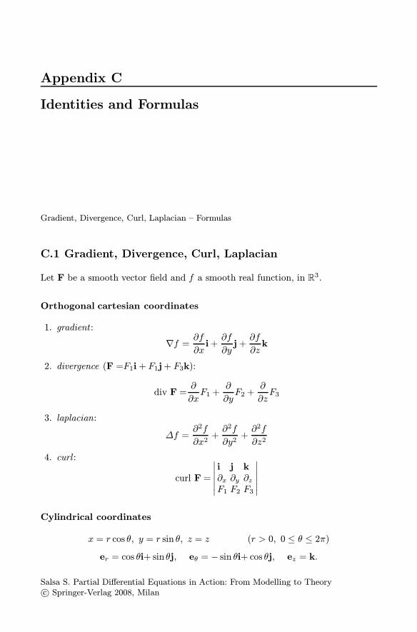
Appendix C
Identities and Formulas
Gradient, Divergence, Curl, Laplacian – Formulas
C.1 Gradient, Divergence, Curl, Laplacian
Let F be a smooth vector field and f a smooth real function, in R3.
Orthogonal cartesian coordinates
1. gradient :
∇f = ∂f∂xi+∂f
∂yj+∂f
∂zk
2. divergence (F =F1i + F1j+ F3k):
div F =∂
∂xF1 +
∂
∂yF2 +
∂
∂zF3
3. laplacian:
Δf =∂2f
∂x2+∂2f
∂y2+∂2f
∂z2
4. curl :
curl F =
∣∣∣∣∣∣i j k∂x ∂y ∂zF1 F2 F3
∣∣∣∣∣∣
Cylindrical coordinates
x = r cos θ, y = r sin θ, z = z (r > 0, 0 ≤ θ ≤ 2π)er = cos θi+ sin θj, eθ = − sin θi+ cos θj, ez = k.
Salsa S. Partial Differential Equations in Action: From Modelling to Theoryc© Springer-Verlag 2008, Milan

546 Appendix C Identities and Formulas
1. gradient :
∇f = ∂f∂rer +
1
r
∂f
∂θeθ +
∂f
∂zez
2. divergence (F =Frer + Fθeθ + Fzk):
div F =1
r
∂
∂r(rFr) +
1
r
∂
∂θFθ +
∂
∂zFz
3. laplacian:
Δf =1
r
∂
∂r
(r∂f
∂r
)+1
r2∂2f
∂θ2+∂2f
∂z2=∂2f
∂r2+1
r
∂f
∂r+1
r2∂2f
∂θ2+∂2f
∂z2
4. curl :
curl F =1
r
∣∣∣∣∣∣er reθ ez∂r ∂θ ∂zFr rFθ Fz
∣∣∣∣∣∣
Spherical coordinates
x = r cos θ sinψ, y = r sin θ sinψ, z = r cosψ (r > 0, 0 ≤ θ ≤ 2π, 0 ≤ ψ ≤ π)
er = cos θ sinψi+sin θ sinψj+cosψk
eθ = − sin θi+ cos θjeψ = cos θ cosψi+ sin θ cosψj− sinψk.
1. gradient :
∇f = ∂f∂rer +
1
r sinψ
∂f
∂θeθ +
1
r
∂f
∂ψeψ
2. divergence (F =Frer + Fθeθ + Fψeψ):
div F =∂
∂rFr +
2
rFr
︸ ︷︷ ︸radial part
+1
r
[1
sinψ
∂
∂θFθ +
∂
∂ψFψ + cotψFψ
]
︸ ︷︷ ︸spherical part
3. laplacian:
Δf =∂2f
∂r2+2
r
∂f
∂r︸ ︷︷ ︸radial part
+1
r2
{1
(sinψ)2∂2f
∂θ2+∂2f
∂ψ2+ cotψ
∂f
∂ψ
}
︸ ︷︷ ︸spherical part (Laplace-Beltrami operator)
4. curl :
rot F =1
r2 sinψ
∣∣∣∣∣∣∣
er reψ r sinψeθ
∂r ∂ψ ∂θ
Fr rFψ r sinψFz
∣∣∣∣∣∣∣.
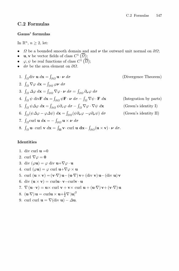
C.2 Formulas 547
C.2 Formulas
Gauss’ formulas
In Rn, n ≥ 2, let:
• Ω be a bounded smooth domain and and ν the outward unit normal on ∂Ω;• u,v be vector fields of class C1
(Ω);
• ϕ, ψ be real functions of class C1(Ω);
• dσ be the area element on ∂Ω.
1.∫Ωdiv u dx =
∫∂Ωu · ν dσ (Divergence Theorem)
2.∫Ω ∇ϕ dx =
∫∂Ω ϕν dσ
3.∫ΩΔϕ dx =
∫∂Ω∇ϕ · ν dσ =
∫∂Ω∂νϕ dσ
4.∫Ωψ divF dx =
∫∂ΩψF · ν dσ −
∫Ω∇ψ ·F dx (Integration by parts)
5.∫Ω ψΔϕ dx =
∫∂Ω ψ∂νϕ dσ −
∫Ω ∇ϕ · ∇ψ dx (Green’s identity I)
6.∫Ω(ψΔϕ− ϕΔψ) dx =
∫∂Ω(ψ∂νϕ −ϕ∂νψ) dσ (Green’s identity II)
7.∫Ωcurl u dx = −
∫∂Ωu× ν dσ
8.∫Ωu· curl v dx =
∫Ωv· curl u dx−
∫∂Ω(u× v) · ν dσ.
Identities
1. div curl u =0
2. curl ∇ϕ = 03. div (ϕu) = ϕ div u+∇ϕ · u4. curl (ϕu) = ϕ curl u+∇ϕ× u5. curl (u× v) = (v·∇)u− (u·∇)v+(div v)u− (div u)v6. div (u× v) = curlu · v−curlv · u7. ∇ (u · v) = u× curl v + v× curl u+ (u·∇)v+(v·∇)u8. (u·∇)u = curlu× u+12∇ |u|
2
9. curl curl u = ∇(div u)−Δu.
References
Partial Differential Equations
E. DiBenedetto, Partial Differential Equations. Birkhauser, 1995.
L.C. Evans, Partial Differential Equations. A.M.S., Graduate Studies in Math-ematics, 1998.
A. Friedman, Partial Differential Equations of parabolic Type. Prentice-Hall, En-glewood Cliffs, 1964.
D. Gilbarg and N. Trudinger, Elliptic Partial Differential Equations of SecondOrder. II edition, Springer-Verlag, Berlin Heidelberg, 1998.
R.B. Guenter and J.W. Lee, Partial Differential Equations of MathematicalPhysics and Integral Equations. Dover Publications, Inc., New York, 1998.
F. John, Partial Differential Equations (4th ed.). Springer-Verlag, New York,1982.
O. Kellog, Foundations of Potential Theory. Springer-Verlag, New York, 1967.
G.M. Lieberman, Second Order Parabolic Partial Differential Equations.WorldScientific, Singapore, 1996.
J. L. Lions and E. Magenes, Nonhomogeneous Boundary Value Problems andApplications. Springer-Verlag, New York, 1972.
R. McOwen, Partial Differential Equations: Methods and Applications. Prentice-Hall, New Jersey, 1996.
M. Protter and H. Weinberger, Maximum Principles in Differential Equa-tions. Prentice-Hall, Englewood Cliffs, 1984.
M. Renardy and R.C. Rogers, An Introduction to Partial Differential Equa-tions. Springer-Verlag, New York, 1993.
J. Rauch, Partial Differential Equations. Springer-Verlag, Heidelberg 1992.
J. Smoller, Shock Waves and Reaction-Diffusion Equations. Springer-Verlag, NewYork, 1983.

550 References
W. Strauss, Partial Differential Equation: An Introduction. Wiley, 1992.
D.V. Widder, The Heat Equation. Academic Press, New York, 1975.
Mathematical Modelling
A. J. Acheson, Elementary Fluid Dynamics. Clarendon Press-Oxford, 1990.
J. Billingham and A.C. King, Wave Motion. Cambridge University Press,2000.
R. Courant and D. Hilbert,Methods of Mathematical Phisics. Vol. 1 e 2. Wiley,New York, 1953.
R. Dautray and J. L. Lions,Mathematical Analysis and Numerical Methods forScience and Technology, Vol. 1-5. Springer-Verlag, Berlin Heidelberg, 1985.
C.C. Lin and L.A. Segel. Mathematics Applied to Deterministic Problems inthe Natural Sciences. SIAM Classics in Applied Mathematics, (4th ed.) 1995.
J.D. Murray, Mathematical Biology. Springer-Verlag, Berlin Heidelberg, 2001.
L.A. Segel, Mathematics Applied to Continuum Mechanics. Dover Publications,Inc., New York, 1987.
G.B. Whitham, Linear and Nonlinear Waves. Wiley-Interscience, 1974.
Analysis and Functional Analysis
R. Adams, Sobolev Spaces. Academic Press, New York, 1975.
H. Brezis, Analyse Fonctionnelle. Masson, 1983.
L.C. Evans and R.F. Gariepy, Measure Theory and Fine properties of Func-tions. CRC Press, 1992.
V.G. Maz’ya, Sobolev Spaces. Springer-Verlag, Berlin Heidelberg, 1985.
W. Rudin, Principles of Mathematical Analysis (3th ed.). Mc Graw-Hill, 1976.
W. Rudin, Real and Complex Analysis (2th ed). Mc Graw-Hill, 1974.
L. Schwartz, Theorie des Distributions. Hermann, Paris, 1966.
K. Yoshida, Functional Analysis. Springer-Verlag, Berlin Heidelberg, 1965.
Numerical Analysis
R. Dautray and J.L. Lions, Mathematical Analysis and Numerical Methodsfor Science and Technology. Vol. 4 and 6. Springer-Verlag, Berlin Heidelberg,1985.
A. Quarteroni and A. Valli, Numerical Approximation of Partial DifferentialEquations. Springer-Verlag, Berlin Heidelberg, 1994.

References 551
Stochastic Processes and Finance
M. Baxter and A. Rennie, Financial Calculus: An Introduction to DerivativePricing. Cambridge U. Press, 1996.
L.C. Evans, An Introduction to Stochastic Differential Equations, Lecture Notes,http://math.berkeley.edu/∼evans/
B.K. Øksendal, Stochastic Differential Equations: An Introduction with Appli-cations. (4th ed.), Springer-Verlag, Berlin Heidelberg, 1995.
P. Wilmott, S. Howison and J. Dewinne, The Mathematics of FinancialDerivatives. A Student Introduction. Cambridge U. Press, 1996.

Index
Absorbing barriers 98Adjoint problem 482Advection 157Arbitrage 80
Barenblatt solutions 91Bernoulli’s equation 284Bond number 287Boundary conditions 17Dirichlet 17, 28Mixed 28mixed 18Neumann 17, 28Robin 18, 28
Breaking time 175Brownianmotion 49path 49
Canonical form 254, 256Canonical isometry 331Capillarity waves 291Cauchy sequence 308Characteristic 158, 194, 258parallelogram 238strip 209system 209
Chebyshev polynomials 323Classical solution 433Closure 7Compactoperator 348set 8
Condition
compatibility 105Conjugate exponent 9Conormal derivative 461Convection 56Convergenceleast squares 24uniform 9weak 344
Convolution 370, 386Cost functional 479Critical mass 67Cylindrical waves 261
d’Alembert formula 237Darcy’s law 90Diffusion 14coefficient 48
Direct sum 317Dirichlet eigenfunctions 451Dispersion relation 224, 249, 289Distributionalderivative 378solution 434
Domain 7Domain of dependence 239, 279DomainsLipschitz 11smooth 10
Drift 54, 78
Eigenfunction 322, 358, 359Eigenvalues 322, 358, 359Elliptic equation 431Entropy condition 183Equal area rule 177

554 Index
Equationbackward heat 34Bessel 65Bessel (of order p) 324Black-Scholes 3, 82Bukley-Leverett 207Burger 4diffusion 2, 13Eiconal 4eikonal 212elliptic 250Euler 340Fisher 4fully non linear 2hyperbolic 250Klein-Gordon 249Laplace 3linear elasticity 5linear, nonlinear 2Maxwell 5minimal surface 4Navier Stokes 5, 130parabolic 250partial differential 2Poisson 3, 102porous media 91porous medium 4quasilinear 2reduced wave 155Schrodinger 3semilinear 2stochastic differential 78Sturm-Liouville 322transport 2vibrating plate 3wave 3
Escape probability 120Essentialsupport 369supremum 311
European options 77Expectation 52, 61Expiry date 77Extension operator 409ExteriorDirichlet problem 139domain 139Robin problem 141, 154
Fick’s law 56
Final payoff 82Firstexit time 119integral 201, 203variation 340
Flux function 156Forward cone 276Fouriercoefficients 321law 16series 24transform 388, 405
Fourier-Bessel series 66, 325Froude number 287FunctionBessel (of order p) 324characteristic 8compactly supported 8continuous 8d-harmonic 106Green’s 133harmonic 14, 102Heaviside 40test 43, 369
Fundamental solution 39, 43, 125, 244,275
Gaussian law 51, 60Global Cauchy problem 19, 29, 68non homogeneous 72
Gram-Schmidt process 321Gravity waves 290Green’s identity 12Gronwall Lemma 522Group velocity 224
Harmonicmeasure 122oscillator 363waves 222
Helmholtz decomposition formula 128Hermite polynomials 324Hilbert triplet 351Hopf’s maximum principle 152Hopf-Cole transformation 191
Incoming/outgoing wave 263Infimum 8Inflow/outflowboundary 201

Index 555
characteristics 162Inner product space 312Integralnorm (of order p) 311surface 193
integration by parts 12Inward heat flux 28Ito’s formula 78
Kernel 326Kinematic condition 285Kinetic energy 228
Lattice 58, 105Least squares 24Legendre polynomials 323Light cone 213Linear waves 282little o of 9Localchart 10wave speed 167
Logarithmic potential 128Logistic growth 93Lognormal density 80
Mach number 272Markov properties 51, 61Mass conservation 55Maximum principle 31, 74, 107Mean value property 110Method 19Duhamel 72electrostatic images 134characteristics 165descent 279Faedo-Galerkin 496, 514, 520Galerkin 340stationary phase 226separation of variables 19, 22, 231, 268,357, 453
vanishing viscosity 186Metric space 308Mollifier 371Multidimensional symmetric random walk
58
Neumanneigenfunctions 452function 138
Normal probability density 38
Normed space 308
Open covering 409Operatoradjoint 332discrete Laplace 106linear, bounded 326mean value 105
Optimalcontrol 479state 479
Parabolicdilations 35equation 492
Parallelogram law 312Partition of unity 410Phase speed 222Plane waves 223, 261Poincare’s inequality 399, 419Point 7boundary 7interior 7limit 7
Poisson formula 116Potential 102double layer 142Newtonian 126single layer 146
Potential energy 229Pre-compact set 343Problemeigenvalue 23well posed 6, 16
Projected characteristics 201Put-call parity 85
Randomvariable 49walk 43walk with drift 52
Range 326of influence 239, 276
Rankine-Hugoniot condition 173, 181Rarefaction/simple waves 170Reaction 58Reflecting barriers 98Reflection method 409Resolvent 357, 358Retarded potential 282Retrograde cone 265
556 Index
Riemann problem 185Rodrigues’ formula 323, 324
Schwarzinequality 312reflection principle 151
Self-financing portfolio 80, 88Selfadjoint operator 333Sets 7Shockcurve 172speed 173wave 173
Similarity, self-similar solutions 36Sobolev exponent 421Solution 21self-similar 91steady state 21unit source 41
Sommerfeld condition 155Spectrum 357, 358Spherical waves 223Standing wave 223, 232Steepest descent 483Stiffness matrix 341Stochastic process 49, 60Stopping time 52, 119Strike price 77Strong Huygens’ principle 276, 279Strong Parseval identity 393Strong solution 434Superposition principle 13, 69, 230Support 8of a distribution 377
Tempered distribution 389Term by termdifferentiation 9integration 9
Topology 7Trace 411inequality 417
Traffic in a tunnel 216Transitionfunction 61layer 188probability 51
Travelling wave 158, 167, 187, 221Tychonov class 74
Uniform ellipticity 455Unit impulse 40
Value function 77Variational formulationBiharmonic equation 474Dirichlet problem 436, 445, 456Mixed problem 444, 451, 464Neumann problem 440, 447, 461Robin problem 443, 450solution 434
Volatility 78
Wavenumber 222packet 224
Weak coerciveness 459Weak formulationCauchy-Dirichlet problem 495Cauchy-Neumann problem 506Cauchy-Robin problem 507General initial-boundary problem 514Initial-Dirichlet problem (wave eq.)518
Weak Parseval identity 391Weakly coercive (bilinear form) 505, 513Weierstrass test 9, 25

End of printing December 2007