To Trade or Not to Trade:

Oil Leases, Information Asymmetry, and Coase

Paul A. Brehm*1 and Eric Lewis∗2

1University of Michigan2US Department of Justice

December 5, 2016

Please click here for the most recent version.

Abstract

We exploit a federal oil lease lottery to examine how markets correct for

initial misallocation. Lottery participants included oil companies, as well as

individuals without the capital or expertise to drill for oil. In the absence

of reallocation, we expect less drilling on leases won by individuals. We find

that leases won by firms and individuals have similar short- and long-term

outcomes, suggesting that secondary markets rapidly and efficiently correct for

misallocation to individuals. However, the small subset of parcels with nearby

oil production have 50% less drilling when they are won by firms. We develop

a simple model to demonstrate how information asymmetry adversely affects

firms to a greater degree. Because individuals have larger gains from trade, they

are less likely to have their decision to trade affected by asymmetric information

and are more likely to trade with a nearby producing firm.

∗pabrehm@umich.edu and erickyle@umich.edu. We are very grateful for financial assistance pro-vided by Rackham Graduate School, MITRE, and the National Science Foundation GRFP. Forhelpful comments and discussions, we thank Ryan Kellogg, Catie Hausman, Hoyt Bleakley, ShaunMcRae, Jeremy West, Akshaya Jha, Arthur van Benthem, Kelsey Jack, Yiyuan Zhang, Sarah John-ston, Chris Sullivan, Julian Hsu, Andrew Litten, Maggie (O’Rourke) Brehm, Berkeley’s EnergyCamp attendees, and seminar participants at the University of Michigan. This paper does notrepresent the views of the Department of Justice. All errors are our own.

1

1 Introduction

The Coase Theorem (Coase, 1960) suggests that, in the absence of frictions, initial

asset misallocation should be corrected through secondary market trading. Informa-

tion asymmetry is one type of friction that can disrupt reallocation (Akerlof, 1970;

Myerson and Satterthwaite, 1983; Hendricks and Porter, 1988). Our paper seeks to

answer two related questions. First, in the absence of large frictions, can we find

evidence that initially misallocated assets can quickly and efficiently be reallocated,

as the Coase Theorem predicts? Second, does the presence of information asymmetry

change our results?

We examine a 1970’s oil (and gas) lease lottery that only cost $10 per lease

to enter1, allowing many different individuals and firms to enter the lottery. While

winning oil firms had the capacity to exploit their leases, winning individuals likely

lacked the necessary capital and expertise. Many of these individuals entered the

lottery with the intent of flipping their winnings to firms and securing a quick profit,

but were likely poor initial matches for the drilling rights. We hypothesize that in

the absence of secondary markets, parcels won by firms would have seen much more

development.

We test whether initial misallocation to individuals (instead of firms) as a re-

sult of the lottery led to short- and medium-run differences in drilling and production.

While assignment via lottery provides exogenous variation conditional on entry, we

also need to correct for potential bias from endogenous entry. Indeed, our data show

that firms and individuals submit entries for different types of leases at different rates.

We use two strategies to control for bias from endogenous entry.

Our first strategy uses the fact that each lease had three “winners”, a first-place

winner that actually claimed the lease, as well as two back-up winners. We examine a

restricted set of parcels where exactly one of the three winners is a firm. Within this

1$10 in 1975-1978 is worth about $41 in 2015.

2

subsample, knowing the identity of the initial winner provides no information about

the underlying characteristics of a lease. As a result, we can estimate an unbiased

treatment effect from having a firm win a lease. Our second strategy uses the full set

of parcels and relies on observables to control for bias from endogenous entry. Results

are broadly consistent across our two specifications.

Consistent with the Coase Theorem, we find that leases without information

asymmetry are likely to be reallocated, resulting in similar ex-post probabilities of

drilling and production for leases won by firms and those won by individuals. This

finding provides evidence in favor of the efficiency of secondary markets that contrasts

with a recent literature (Bleakley and Ferrie, 2014; Akee, 2009). Their papers show

that correcting for initial market mismatches takes anywhere from 20 to 100 years,

while our paper shows that reallocation can allow outcomes to be very similar in the

immediate term.

Our findings likely differ from the existing literature because of the relative

ease of correcting for initial misallocation in our setting. Underlying lease charac-

teristics in our sample started out identical, in expectation; the previous literature

examined convergence when assets started out with different underlying characteris-

tics. Additionally, the deep pool of interested parties, reliable (if limited) information

about leases, and the relative ease of contacting lessees all likely aided secondary

market reallocation.

A subset of leases in our sample have nearby oil production. This nearby oil

production provides private information to the nearby producer about the quality

of their land, as well as the quality of nearby land. Private information creates a

lemons problem and makes it difficult for parties to agree on a fair transfer price.

Indeed, Wiggins and Libecap (1985) find that information asymmetry from nearby

production impedes unitization on oil fields that are being developed because parties

are unable to agree on how to share oil production.

3

We find that leases with nearby production have about twice as much drilling

and production if they are initially allocated to individuals, as opposed to firms. This

result is likely caused by individuals’ greater propensity to reassign their leases to

nearby producing firms that can make the best decisions about whether to drill on

the land. Analysis of reassignment patterns confirms that firms are less likely than

individuals to trade with nearby producing firms.

In order to more formally understand our results, we develop a simple theoret-

ical model of lease reassignment and drilling that is based in part on Myerson (1985);

Samuelson (1985). Information asymmetry in the model works to prevent trade be-

cause uninformed parties know that informed parties will only agree to a trade if the

latter are paying a price at or below the fair market value – there is limited upside to

engaging in trade for the uninformed party. The intuition of the model is that gains

from trading with a nearby producing firm are larger for individuals, causing them to

be more likely to overcome information asymmetry. Because nearby producing firms

have information about the quality of the lease, they are better able to identify the

best leases to drill. On the other hand, firms that retain leases they initially win are

unable to internalize the nearby firms’ information about their lease, causing them

to be less likely to drill.

Our work improves the understanding of how (mineral lease) secondary mar-

kets reallocate assets. This is particularly relevant today because current fracking

hotspots have a similar structure to the Wyoming oil lease lottery. For example,

oil deposits in the Bakken shale were allocated haphazardly, from the perspective

of farmers who were not expecting to drill for oil. In addition to similarities in the

allocation process, the reallocation process remains comparable - direct negotiations

between landowners and firms interested in buying drilling rights.

We also contribute to the understanding how asymmetric information can

impede otherwise efficient market design. In the absence of information asymmetry

4

and in the presence of a robust secondary market, our work suggests that initial

allocations may not be important. However, the presence of information asymmetry

suggests that it is better to initially allocate an asset to somebody who cannot use it

than it is to allocate the same asset to a random firm (if there is a robust secondary

market). While the former allocation type is initially worse, secondary markets are

better able to correct for this mismatch because the gains from trade are larger. This

ties to theoretical work by Myerson and Satterthwaite (1983) showing that when the

range of typical seller valuations does not overlap with the range of typical buyer

valuations, efficient trade can occur that is both individually rational and incentive

compatible—even though buyers and sellers still have uncertainty about each other’s

valuations. Our results demonstrate a novel way of avoiding information asymmetry

problems – allocate assets to owners who must trade them.2

Finally, we demonstrate that under certain conditions (information symmetry

and a robust secondary market), lotteries can be a relatively efficient way of allocating

public resources. In addition to oil and gas, many other natural resources (timber,

coal, water, etc.), as well as spectrum, Internet domain names, and carbon permits are

public resources that could be allocated via lottery.3 Many economists would suggest

that an auction is a superior method of allocating resources. Our results suggest

that the efficiency cost of lotteries is lower than expected in some settings. Indeed,

lotteries with a robust secondary market could be a preferable form of allocation if

they are less costly to implement than an auction, if they are seen as a more equitable

way of distributing public resources, or if they generate higher revenues.4

2Our work also ties to a strand of corporate finance literature showing that information asymme-try problems can be mitigated by bank-imposed opacity (for example, Dang, Gorton, Holmstrom,and Ordonez (2016) show that bank-imposed opacity promotes asset liquidity).

3One example with a similar reallocation process is highlighted in a recent Wall Street Journalarticle highlighting how 30 of 104 entrants into a wireless spectrum auction were individuals takingadvantage of a 25% discount designed to encourage new entrants. Successful bidders who qualifyfor discounts are allowed to lease all their airwaves to larger companies and sell the airwaves after 5years.

4Many state-run lotteries (like “Powerball”) generate more revenue than the value of the prize.Additionally, auctions can generate substantially less revenue than the expected value of the prize

5

Our paper proceeds as follows. Section 2 discusses background for our em-

pirical setting, including the lottery system and leasing rules. Section 3 describes

our data. Section 4 explains our empirical specification and main results. Section 5

develops our model and Section 6 discusses and concludes.

2 Background: Oil Lottery and Reallocation

This paper focuses on oil and gas leasing, drilling, and production activity on United

States Federal Government owned land. The Bureau of Land Management (BLM),

a division of the Department of the Interior, allocates leases to drill for and produce

oil and gas. We focus our study on Wyoming, where approximately 52% of the land

is owned by the federal government, and where there has been significant oil and gas

production (Fairfax and Yale, 1987).

Our analysis uses leases that were allocated by the BLM via lottery, providing

randomization that is key to our identification strategy. The BLM began using a

lottery system for “non-competitive” land in 1960 as a way to provide an orderly and

fair allocation (Bureau of Land Management, 1983).5 “Non-competitive” land was

designated as such if it was on the site of a lapsed lease, the previous lease was not

known to be productive, and the land was at least one mile away from known oil or

gas production (Fairfax and Yale, 1987).6 The lottery system ended in 1987 when

the BLM switched to using auctions for this type of land.7,8

if competition is limited.5“Before 1960, these tracts were offered on a first-come, first-served basis. When particularly

promising tracts were due to be posted as available, long lines formed at the land offices. Fightsoften broke out, disrupting business and, in some instances, injuring employees trying to control thecrowds. The simultaneous oil and gas lease drawing was developed to establish an orderly and fairsystem of awarding these noncompetitive leases.” (Bureau of Land Management, 1983).

6For land closer to known production, the government used an auction. For land that had neverbeen leased, it used a first-come first-serve system.

7One of the main reasons for this change was to combat middlemen from “filing services” whocharged excessive fees to file entry cards on behalf of unsophisticated parties. For example, a $250filing fee might be charged to a retiree in Florida (with the middleman keeping $240 and sendingthe $10 fee in to the BLM).

8The BLM still uses lotteries for parcels that receive no bids in the auction.

6

Lottery specifics remained constant during our sample period (1975 through

1978), though they changed slightly during later lotteries. Each month, regional

BLM offices would compile a list of the parcels that would be offered in the lottery.9

Interested individuals and firms typically had about a week to submit an entry card

to the regional BLM office for each lottery they wanted to enter (Bureau of Land

Management, 1983). Many entrants filed multiple cards, one per plot for multiple

plots, with a $10 filing fee for each entry card submitted. As this entry fee was

very low, it was unlikely to restrict individuals who had less industry experience and

capital from entering.

The regional BLM office would then draw three entry cards – one for the first-

place winner, along with two runner-ups – which we refer to as the first-, second-,

and third-place winners. The holder of the first place winning entry card had 30 days

to submit a rental payment, equal to $1 per acre, in order to secure the lease. If the

first-place winner did not respond with a rental payment within 30 days, the BLM

contacted the second-place winner with a notification that the first-place winner had

not responded and that the second-place winner was now eligible to submit the rental

payment and obtain the lease. In the case of no response, the BLM then turned to

the third-place winner.10 Lottery losers were informed of their loss by the return of

their entrance cards (Bureau of Land Management, 1983).

In order to retain leases after winning, new lessees were required to continue

to comply with BLM leasing rules. Lessees paid a rental fee of $1 per acre per year

in the years prior to any oil or gas production. After leases began production they

paid a royalty, typically 12.5 percent, on revenues from production. If a lease had

oil or gas production within 10 years of the lease start date, the lease continued

until production ended. If there was no production within 10 years and if qualifying

9The Cheyenne office’s region included Wyoming, as well as small parts of Nebraska, Kansas,etc. We exclude leases outside of Wyoming due to data limitations.

10By matching winner records with transactions records, we estimate that approximately 98% ofleases were claimed by the first-place winner.

7

drilling operations were not in progress, leases generally expired and were returned

to the BLM. A lease also ended if the lessee formally abandoned it or failed to pay

rental fees (Fairfax and Yale, 1987). These expired and abandoned leases were then

re-offered through lottery–or via auction, if they expired after 1987.

Two institutional features helped leases to be reallocated to the optimal own-

ers. First, there were low search costs: the BLM maintains an open records office

where anyone can easily look up the name and contact information of current lessees.

Low search costs increase the number of potential buyers who might contact a lessee.

More potential buyers may increase buyer willingness to sell both by raising the price

via competition, as well as by giving the individual additional signals about the ex-

pected value of the lease.

Additionally, misallocation is easily observed. When firms visit the BLM open

records office, it is easy for them to determine whether a current lessee is an oil and

gas firm or an individual. Firms were very aware that many individuals entered the

lotteries hoping to strike it rich, which they could likely only do if they transferred

their lease to a firm. In these cases, the individuals’ valuations of leases in the absence

of transfer was likely very low, and possibly negative, as the lease required paying

annual rental fees. In contrast, firms typically had positive valuations.

3 Data Description & Summary Statistics

3.1 Data Description

Our lottery sample is compiled from Bureau of Land Management (BLM) lease data.

Lotteries were held monthly from January 1975 to December 1978, with roughly

225 parcels for lease per month. We drop a small number of parcels (<1%) due to

illegibility in the raw data or for having fewer than three winners. This leaves a total

sample of 10,762 parcels offered over 48 months. The data include information on the

8

boundaries of the leases, allowing us to match the leases to drilling and production

activity. The data also include the total number of entry cards submitted for each

parcel to be leased, as well as the names of the first-, second-, and third-place winners.

Appendix A discusses this data in greater detail.

The winners’ names allow us to determine whether the winner was a firm

or an individual. We first search the names for terms like “Inc.”, “Production”,

or “Corporation.” We then reviewed each lease’s winners by hand to ensure that

they were accurately categorized. Most firms appear to be oil and gas production

companies. Some individuals only appear once or twice and appear to not have

connections to the oil industry. Other individuals appear to be more “sophisticated”,

winning frequently and having close connections with the oil industry.11

Our primary outcomes of interest, drilling and production activity, use data

from the Wyoming Oil and Gas Conservation Commission. These data have been

lightly edited to improve quality by the United States Geological Survey (Biewick,

2011). It includes both the date and Public Land Survey System location for each

well drilled within Wyoming. This allows us to determine whether a lease had nearby

production when it was listed in the lottery, as well as whether drilling or production

occurred on the lease itself.12

We define nearby production to be an oil-producing well drilled within five

years of a lease’s start and located within 2.6 miles of the lease.13 In Appendix D we

11We discuss individuals entering on behalf of firms and other potential manipulations in Ap-pendix A.

12Production data are only available starting in 1978. The fact that our first leases begin in 1975but our first production does not appear until 1978 could be problematic. If, for example, a well wasdrilled in 1975 and production finished before 1978 we would be unable to capture this production.However, this is very unlikely for two reasons. First, immediate drilling was rare because permitsneeded to be secured and infrastructure (such as roads) frequently needed to be built before drillingcould occur. Second, even if drilling happened within 3 years of the start date, most wells have longproduction lifespans, such that we would still observe the well producing by 1978. For example,we find that of all wells drilled in Wyoming between 1979 and 1985, less than 10% of wells have alifespan less than 3 years.

13We exclude gas-producing wells because most participants in the colloquially known “oil leaselottery” were looking for oil, as it was much more profitable. In 1984, oil accounted for about 95%of the energy produced from hydrocarbons in Wyoming (Fairfax and Yale, 1987). Additionally, the

9

consider a variety of alternative definitions of nearby production and find that our

results are broadly consistent.

We also compile lease transfer outcome data from the BLM’s LR2000, an

administrative database of federal leases. The LR2000 includes detailed information,

including leases transfers, lease terminations, and lease partners. This dataset allows

us to measure how quickly markets correct for misallocation. One limitation of the

LR2000 is that a selection of leases are not included because they expired prior to

the digitization of their data. However, we find that approximately 95% of leases

from our lottery data can be linked to the LR2000. Unfortunately, increasing this

match rate to 100% is not possible as paper records of leases and lease transfers are

destroyed fifteen years after lease expiration.14

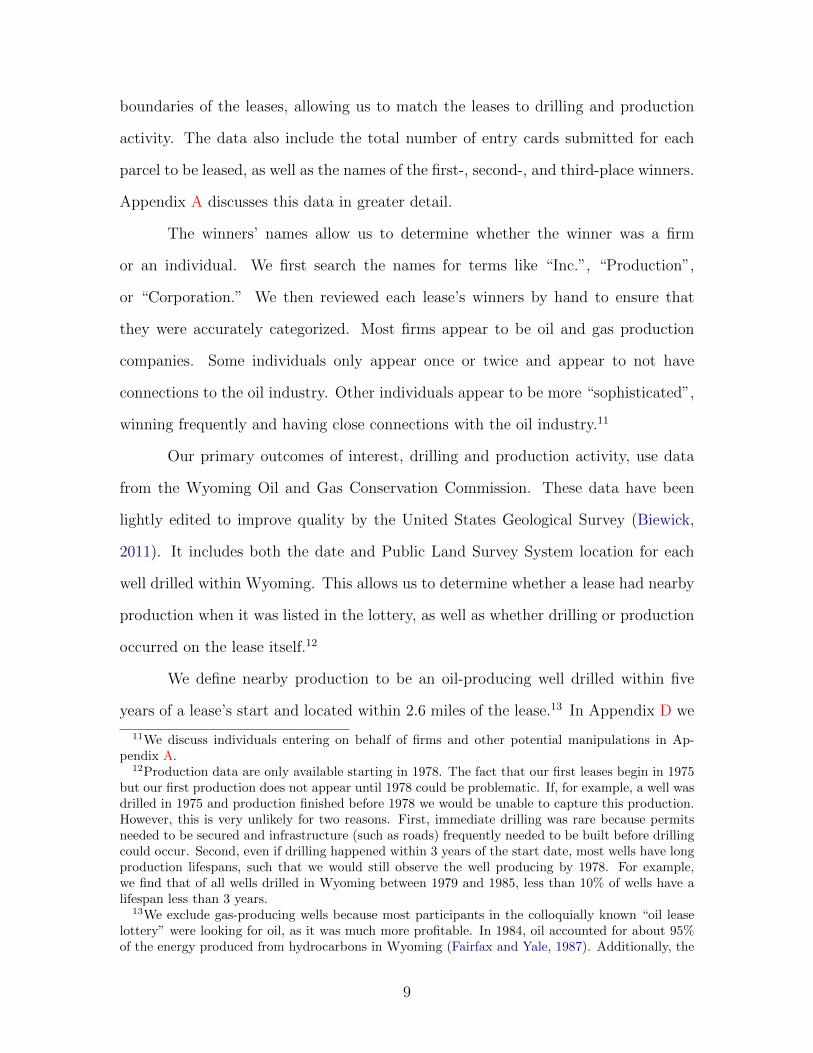
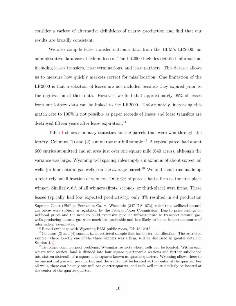
Table 1 shows summary statistics for the parcels that were won through the

lottery. Columns (1) and (2) summarize our full sample.15 A typical parcel had about

600 entries submitted and an area just over one square mile (640 acres), although the

variance was large. Wyoming well spacing rules imply a maximum of about sixteen oil

wells (or four natural gas wells) on the average parcel.16 We find that firms made up

a relatively small fraction of winners. Only 6% of parcels had a firm as the first place

winner. Similarly, 6% of all winners (first-, second-, or third-place) were firms. These

leases typically had low expected productivity, only 3% resulted in oil production

Supreme Court (Phillips Petroleum Co. v. Wisconsin (347 U.S. 672)) ruled that wellhead naturalgas prices were subject to regulation by the Federal Power Commission. Due to price ceilings onwellhead prices and the need to build expensive pipeline infrastructure to transport natural gas,wells producing natural gas were much less profitable and less likely to be an important source ofinformation asymmetry.

14E-mail exchange with Wyoming BLM public room, Feb 13, 2015.15Columns (3) and (4) summarize a restricted sample that has better identification. The restricted

sample, where exactly one of the three winners was a firm, will be discussed in greater detail inSection 4.1).

16To reduce common pool problems, Wyoming restricts where wells can be located. Within eachsquare mile section, land is divided into four square quarter-mile sections and further subdividedinto sixteen sixteenth-of-a-square-mile squares known as quarter-quarters. Wyoming allows there tobe one natural gas well per quarter, and the wells must be located at the center of the quarter. Foroil wells, there can be only one well per quarter-quarter, and each well must similarly be located atthe center of the quarter-quarter.

10

within twelve years; only 5% had production within thirty years.17

Full SampleOne FirmWinner

mean st.dev. mean st.dev.Number of entries 598.09 824.27 427.32 644.99Area (sq. miles) 1.11 1.09 0.97 1.05Number of firms among winners 0.19 0.42 1.00 0.00Firm is first place winner 0.06 0.25 0.34 0.48Nearby production indicator 0.22 0.42 0.21 0.41Any drilling within 5 years 0.04 0.20 0.03 0.18Any drilling within 12 years 0.08 0.28 0.07 0.26Any drilling within 30 years 0.15 0.35 0.13 0.33Any production within 5 years 0.02 0.12 0.01 0.11Any production within 12 years 0.03 0.18 0.03 0.17Any production within 30 years 0.05 0.23 0.04 0.21

Table 1: Summary statistics at the lease level. The first two columns describe theentire sample (10,762 parcels). The second two columns describe the restricted samplewhere exactly one of the three winners was a corporation (1,800 parcels). The numberof parcels is a round number (1,800) by chance, no sampling has occurred.

3.2 Ruling out Corruption & Testing for Randomness

Our identification strategy could be threatened if the lottery was not truly random

– either because of corruption or other factors. If, for example, firms bribed BLM

officials to win desirable parcels, that would invalidate our assumption that the un-

derlying parcels were ex-ante identical. We now check whether there is evidence of

lottery manipulation.18

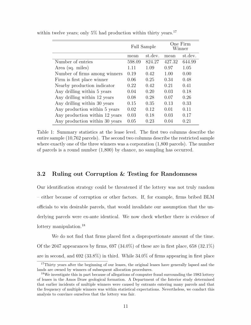
We do not find that firms placed first a disproportionate amount of the time.

Of the 2047 appearances by firms, 697 (34.0%) of these are in first place, 658 (32.1%)

are in second, and 692 (33.8%) in third. While 34.0% of firms appearing in first place

17Thirty years after the beginning of our leases, the original leases have generally lapsed and thelands are owned by winners of subsequent allocation procedures.

18We investigate this in part because of allegations of computer fraud surrounding the 1983 lotteryof leases in the Amos Draw geological formation. A Department of the Interior study determinedthat earlier incidents of multiple winners were caused by entrants entering many parcels and thatthe frequency of multiple winners was within statistical expectations. Nevertheless, we conduct thisanalysis to convince ourselves that the lottery was fair.

11

is slightly above the 33.3% that we would expect, the binomial distribution predicts

that there is a 24% chance of observing 697 or more firms in first place, given 2047

total appearances. Within the restricted sample of 1,800 parcels we have a similar

distribution of firms across winners (619 in first place), with a 16% chance that at

least 619 firms appear in first place.

Table 2 tests whether parcels won by firms are similar on observables to those

won by individuals. We restrict the sample to parcels where exactly one firm was

amongst the three winners and compare parcel characteristics. Within this restricted

sample, we find that parcels won by individuals and firms are very similar; those won

by individuals have slightly more offers and are slightly larger, but the differences

are well within the type of statistical variation we would expect to see. We therefore

proceed under the assumption that the lottery was fair.

Individuals FirmsDifference(p-value)

Offers Mean 430.99 420.33 0.74Offers Variance 647.17 641.28 0.80Acreage Mean 628.33 610.32 0.59Acreage Variance 676.40 663.68 0.59Nearby Production Mean 0.20 0.23 0.19Nearby Production Variance 0.40 0.42 0.19

Table 2: We restrict the sample to the 1,800 parcels where exactly one firm appearedamongst the three winners. Statistics for parcels won by individuals are reported incolumn (1), while column (2) reports those won by firms. Column (3) reports thep-value from an equality test.

4 Analysis

We first detail our empirical strategies and how we correct for endogenous entry. We

then look at lease transactions data to see how quickly secondary markets transferred

leases. Next, we examine whether there is evidence that the initial winner’s identity

affects drilling and production. Throughout our analysis we compare firms with

12

individual winners.

4.1 Empirical Strategy

4.1.1 Primary Specification

A simple comparison of leases won by firms with leases won by individuals will not

correct for lottery participants endogenously choosing which lotteries to enter. Table 3

shows that the total number of entries for a given lease is negatively correlated with

the probability that the winner is a firm. It also shows that the number of entries

is positively correlated with both ex-ante (total acreage) and ex-post (probability of

drilling) measures of profitability. That is, individuals tend to crowd out firms on

parcels with higher expected productivity. As a result, firms are less likely to win

leases that eventually had drilling or production.

1 2 3 4 5 6 71: Number of entries 1.002: Area 0.41 1.003: Nearby production 0.14 -0.14 1.004: Drilling within 12 years 0.20 0.08 0.18 1.005: Production within 12 years 0.17 0.02 0.16 0.63 1.006: Number of winning firms -0.10 -0.06 -0.02 -0.03 -0.02 1.007: Firm is first place winner -0.06 -0.04 0.00 -0.02 -0.02 0.58 1.00

Table 3: Correlations between selected variables for each observation using the unre-stricted sample with all 10,762 parcels.

To illustrate the effects of a naıve comparison, suppose we ran the following

regression where the probability of drilling at time t (Yi) is regressed on a constant

and an indicator for whether the winner was a firm (Fi):

Yi = α0 + β1Fi + εi (1)

In this specification, β1 estimates the naıve treatment effect of a firm winning a lease:

13

it will be biased because εi is correlated with Fi. Our specification would not control

for the fact that plots won by firms are disproportionately low quality.

Our primary specification breaks the correlation between εi and Fi by restrict-

ing our sample to the set of leases where exactly one firm was among the first-,

second-, and third-place winners. Within this subsample, a firm is no more likely to

be in first place than they are to be in second- or third-place. Therefore, the treat-

ment effect of a firm winning a lease will be uncorrelated with unobservables and we

obtain an unbiased estimate. All differences in outcomes are therefore attributable

to differential behavior by different classes of winners.19

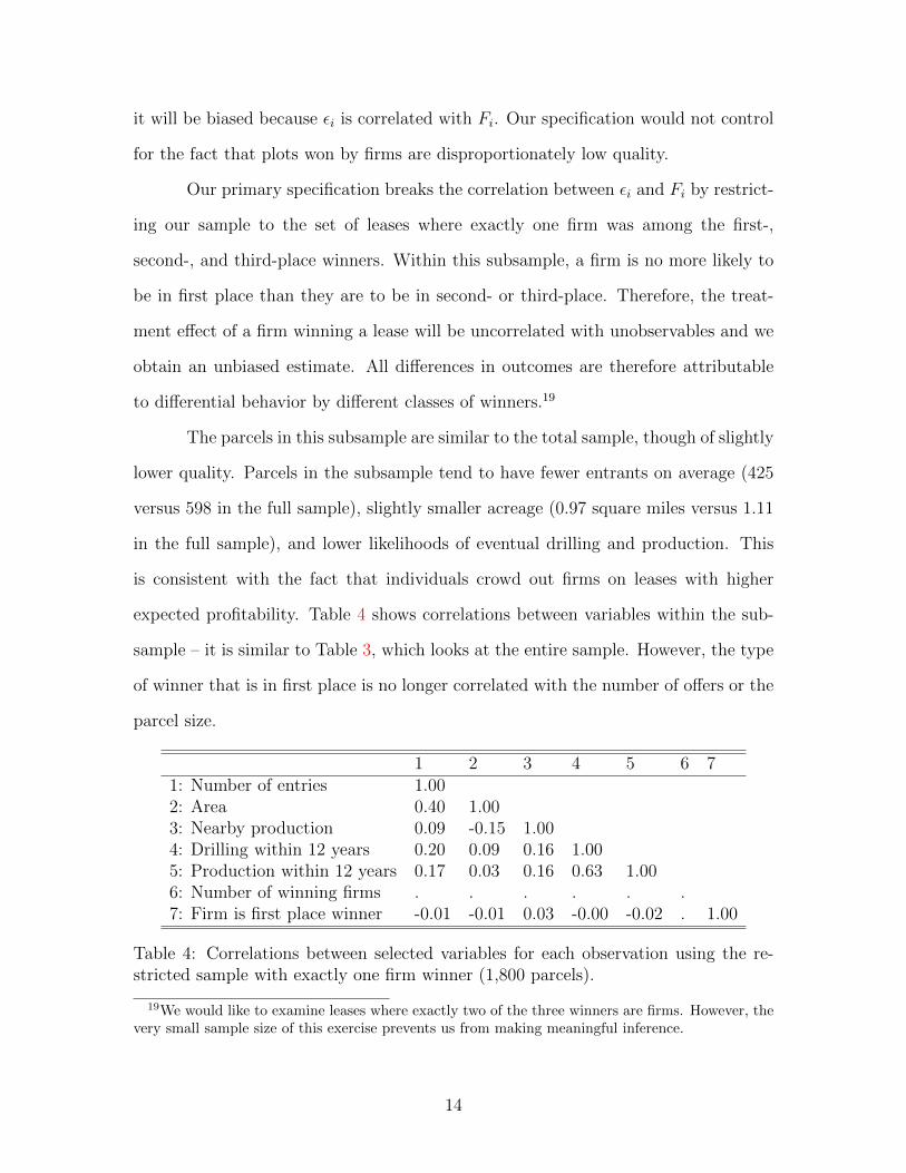
The parcels in this subsample are similar to the total sample, though of slightly

lower quality. Parcels in the subsample tend to have fewer entrants on average (425

versus 598 in the full sample), slightly smaller acreage (0.97 square miles versus 1.11

in the full sample), and lower likelihoods of eventual drilling and production. This

is consistent with the fact that individuals crowd out firms on leases with higher

expected profitability. Table 4 shows correlations between variables within the sub-

sample – it is similar to Table 3, which looks at the entire sample. However, the type

of winner that is in first place is no longer correlated with the number of offers or the

parcel size.

1 2 3 4 5 6 71: Number of entries 1.002: Area 0.40 1.003: Nearby production 0.09 -0.15 1.004: Drilling within 12 years 0.20 0.09 0.16 1.005: Production within 12 years 0.17 0.03 0.16 0.63 1.006: Number of winning firms . . . . . .7: Firm is first place winner -0.01 -0.01 0.03 -0.00 -0.02 . 1.00

Table 4: Correlations between selected variables for each observation using the re-stricted sample with exactly one firm winner (1,800 parcels).

19We would like to examine leases where exactly two of the three winners are firms. However, thevery small sample size of this exercise prevents us from making meaningful inference.

14

Our primary specification using this subsample is:

Yi = α0 + β1Fi + β2NearbyProdi + β3NearbyProdi ∗ Fi + ΩXi + εi (2)

Our primary specification includes an indicator for nearby production, as well

as an interaction term between the identity of the lessee and the presence of nearby

production. We also include control variables (a spline in the number of offers, total

acreage, and month-of-lottery fixed effects) that are not necessary but may improve

precision.20,21

In this specification, β1 informs us about the effect of assigning a lease to an

individual or a firm. This coefficient will help us to answer our first research question

– in the absence of large frictions, can we find evidence that initial asset allocations

do not matter? A large and positive β1 will tell us that leases won by individuals

are not being reassigned to optimal owners - and that leases won by firms have more

drilling and production.

β2 informs us about the overall effect of having nearby production on a lease.

Note that this will capture several effects. Because nearby oil and gas increases the

chances of oil and gas on one’s own land, we expect that drilling and production

will be more common when there is nearby production. However, this effect may be

diminished to the extent that information asymmetry from nearby production inhibits

optimal asset reallocation for both firms and individuals.

β3 captures the differential effect of nearby production on firms versus individ-

uals. Because firms are in a better initial position to exploit leases that they win, we

might expect this coefficient to be positive. To the extent that this interaction effect

is negative, it must be because individuals are better able to reassign their parcels to

20We use a linear probability model, which is appropriate for calculating average treatment effects(Angrist and Pischke, 2008). The AIC and BIC suggest a linear probability model is a better fit forour data than a logit or probit.

21Results without the control variables are similar.

15

firms with the highest value.

We analyze several outcome variables (Yi) of interest; we look at lease reas-

signment by time t, drilling by time t, production by time t, probability of production

given drilling by time t, days to well completion, and total production from producing

wells.

Throughout our analysis, we use (Conley, 1999) spatial standard errors. We

allow εi and εj to be correlated if section i and section j are within twenty miles of

each other.22

4.1.2 Secondary Specification

We also consider a specification using our entire sample, which increases the precision

of our estimates, but relies on the assumption that control variables eliminate bias

from endogenous entry.

We rely on the number of offers for a lease, the total acreage of a lease, and

a set of month-of-lottery fixed effects to control for unobservables that are correlated

with the probability a firm wins a lease. The number of offers is highly correlated

with ex-post measures of profitability like drilling and production. This is because

entrants know that not all parcels are equal – they know the exact location of each

parcel, which gives them important information about how far away the nearest road

is, limited geological information, and the ability to find out limited information

about the productivity of nearby plots. The least desirable parcels received less than

ten entries, while the most desirable received several thousand. This kind of variance

is not random and is possible because people have different expectations about the

profitability of different plots.23

22Lewis (2015) shows that information about parcels in section j, more than 20 miles away fromsection i, do not provide information about how productive section i will be.

23Indeed, under certain conditions the ex-ante expected value of a parcel can be exactly determinedby the number of entries. Suppose, for example, that the value of winning a plot is $1,000. The costof entering the lottery is $10. Therefore, the expected value of entering a lottery is 1/N * $1,000 -$10. One would want to enter the lottery for a plot if they expected N to be less than 100 and would

16

Our secondary specification is run on the full sample of leases:

Yi = α0 + β1Fi + β2NearbyProdi + β3NearbyProdi ∗ Fi

+ β4TotalAcreagei + s(NumOffers) + δMi + εi (3)

We use a cubic spline, s(), with six knot points to allow for flexibility in the

relationship between outcome variables and the number of offers. Mi are month-of-

lottery fixed effects. Our coefficients of interest remain β1 and β3; their interpretation

is the same as in our primary specification. Results using our second specification are

very similar to results using our primary specification.

4.2 Lease Transactions: Results

We first examine lease transactions in order to understand how firms and individuals

treated their drilling rights. This will help to inform expectations about whether they

are looking to drill on the parcels they have won, or perhaps are looking to flip the

parcels for a quick profit.24 Figure 1 uses our restricted sample with exactly one firm

winner and displays how long it took for leases to be transferred for the first time.25,26

not want to enter if they expected more than 100 entries. If there were 200 potential entrants, onepotential Nash equilibrium of an entry game involves all participants flipping a coin to determineif they enter. The expected number of entrants will be 100 and no party will find it profitable todeviate from the coin-flip entry strategy.

24One concern with the LR2000 is that the digitization of lease records began in the late 1980’s;however, we are able to match over 95% of the leases because paper records were transcribed duringthat time. Importantly, we do not find a substantial difference in match rates between individualsand corporations. We believe that leases that do not appear in the LR2000 are most likely to havebeen passed over by the winner or to have expired early, though we cannot conclusively rule outother possibilities.

25Note that not all “first transfers” were to corporations. Indeed, our examination of the ad-ministrative database indicates many winning individuals first transferred portions of their leasesto family members or other individuals. Many of these leases were re-transferred at later points intime, frequently to firms. We focus on “first transfers” because the administrative database onlyidentifies parties by shorthand. Interpreting the type of party (firm vs. individual) is straightforwardon a case-by-case basis. However, doing so systematically would be a major undertaking and almostcertainly would not change our conclusions.

26Appendix B presents regression results presents regressions using Equation 2 and our restrictedsample to analyze years until initial lease reassignment.

17

Figure 1: Histogram of the amount of time, in years, until a lease is transferred.Graph limited to leases where exactly one firm appeared among the first-, second-,and third-place winners. Individuals are in black outlines and firms are in green.Leases that do not have a recorded transfer are in the “Never”category, while leasesthat could not be linked to the LR2000 data are in the category “No Match”.

We find that lease transfers were an important part of lease development.

Nearly 30% of leases won by individuals were transferred within the first year of a

lease. In contrast, firms were 22% less likely to transfer leases during the first year.

Instead, firms were the most likely to hold on to the lease without ever transferring

it —firms did this 22% more frequently than individuals. Therefore, the secondary

market was an important mechanism to correct for misallocation and individuals were

more likely to take advantage of the secondary market. Not only were a large fraction

of leases initially allocated to individuals eventually transferred, but there was also a

significant number of transfers from firms.

18

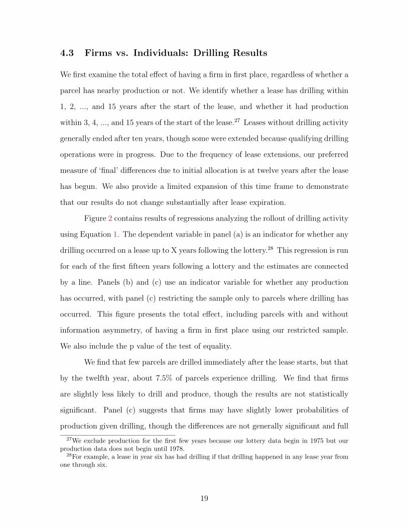
4.3 Firms vs. Individuals: Drilling Results

We first examine the total effect of having a firm in first place, regardless of whether a

parcel has nearby production or not. We identify whether a lease has drilling within

1, 2, ..., and 15 years after the start of the lease, and whether it had production

within 3, 4, ..., and 15 years of the start of the lease.27 Leases without drilling activity

generally ended after ten years, though some were extended because qualifying drilling

operations were in progress. Due to the frequency of lease extensions, our preferred

measure of ‘final’ differences due to initial allocation is at twelve years after the lease

has begun. We also provide a limited expansion of this time frame to demonstrate

that our results do not change substantially after lease expiration.

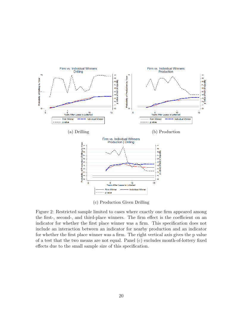
Figure 2 contains results of regressions analyzing the rollout of drilling activity

using Equation 1. The dependent variable in panel (a) is an indicator for whether any

drilling occurred on a lease up to X years following the lottery.28 This regression is run

for each of the first fifteen years following a lottery and the estimates are connected

by a line. Panels (b) and (c) use an indicator variable for whether any production

has occurred, with panel (c) restricting the sample only to parcels where drilling has

occurred. This figure presents the total effect, including parcels with and without

information asymmetry, of having a firm in first place using our restricted sample.

We also include the p value of the test of equality.

We find that few parcels are drilled immediately after the lease starts, but that

by the twelfth year, about 7.5% of parcels experience drilling. We find that firms

are slightly less likely to drill and produce, though the results are not statistically

significant. Panel (c) suggests that firms may have slightly lower probabilities of

production given drilling, though the differences are not generally significant and full

27We exclude production for the first few years because our lottery data begin in 1975 but ourproduction data does not begin until 1978.

28For example, a lease in year six has had drilling if that drilling happened in any lease year fromone through six.

19

(a) Drilling (b) Production

(c) Production Given Drilling

Figure 2: Restricted sample limited to cases where exactly one firm appeared amongthe first-, second-, and third-place winners. The firm effect is the coefficient on anindicator for whether the first place winner was a firm. This specification does notinclude an interaction between an indicator for nearby production and an indicatorfor whether the first place winner was a firm. The right vertical axis gives the p valueof a test that the two means are not equal. Panel (c) excludes month-of-lottery fixedeffects due to the small sample size of this specification.

20

sample results do not support this conclusion.

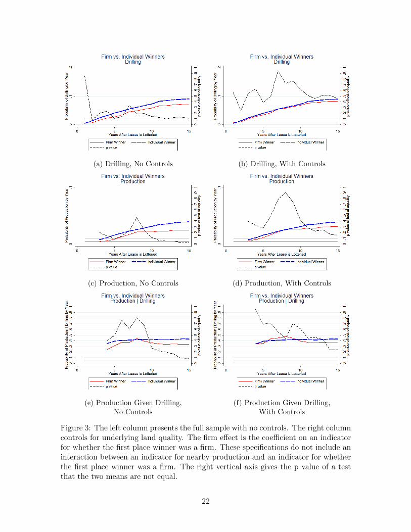
We also examine drilling and production outcomes over time using our full

sample of 10,762 parcels. Figure 3 reports results without controlling for endogenous

entry in the left column, while the right hand column includes variables like the

number of offers for a lease to control for land quality (detailed in Equation 3).

The left column suggests that leases won by firms are less likely to have drilling or

production. However, when we control for land quality on the right, most of the

differences disappear. Indeed, results with controls look very similar to those in

Figure 2. Point estimates suggest that firms may have lower likelihoods of drilling

and production, though the results are not statistically significant. Overall, we find

that initial assignment does not affect drilling and production outcomes.29

4.4 Nearby Production

We now investigate whether firms or individuals perform differentially better in the

presence of nearby production. Table 5 presents the coefficients from regressions using

Equation 2 results after the twelfth year of a lease (Table 9 presents the full sample

analog in Appendix C). The first row of Table 5 indicates that the presence of nearby

production is associated with much higher rates of drilling and production (columns

(3) and (4)). This is to be expected, as nearby oil is one of the best predictors of

oil underfoot. Row 2 shows that leases won by firms and individuals, absent nearby

production, have similar outcomes. It is similar to results in the previous section; we

will briefly expand on this in the following section.

The third row, an interaction between nearby production and whether the

initial winner was a firm, shows that leases won by firms have differentially lower rates

of drilling and production than those won by individuals when nearby production

is present. Figures 4 uses our restricted sample and presents results for each year

29Appendix E looks at drilling time and production quantities. However, due to a lack of precision,we do not find these results to be substantive. They are included for completeness.

21

(a) Drilling, No Controls (b) Drilling, With Controls

(c) Production, No Controls (d) Production, With Controls

(e) Production Given Drilling,No Controls

(f) Production Given Drilling,With Controls

Figure 3: The left column presents the full sample with no controls. The right columncontrols for underlying land quality. The firm effect is the coefficient on an indicatorfor whether the first place winner was a firm. These specifications do not include aninteraction between an indicator for nearby production and an indicator for whetherthe first place winner was a firm. The right vertical axis gives the p value of a testthat the two means are not equal.

22

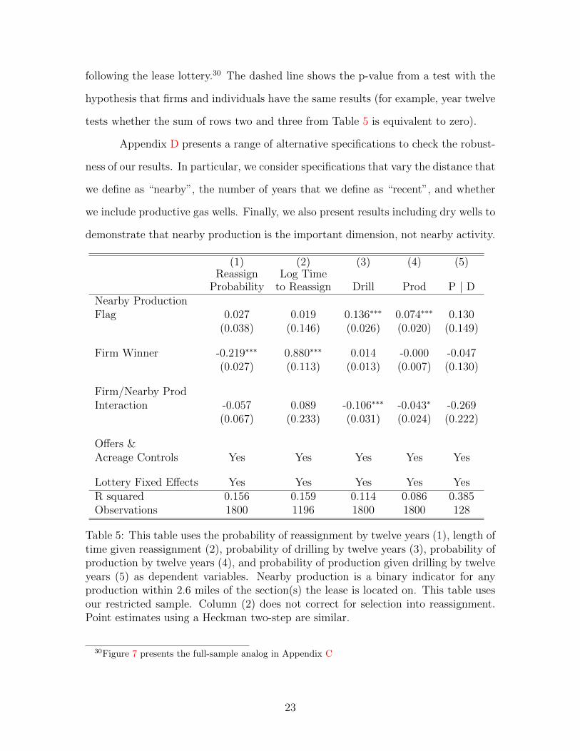
following the lease lottery.30 The dashed line shows the p-value from a test with the

hypothesis that firms and individuals have the same results (for example, year twelve

tests whether the sum of rows two and three from Table 5 is equivalent to zero).

Appendix D presents a range of alternative specifications to check the robust-

ness of our results. In particular, we consider specifications that vary the distance that

we define as “nearby”, the number of years that we define as “recent”, and whether

we include productive gas wells. Finally, we also present results including dry wells to

demonstrate that nearby production is the important dimension, not nearby activity.

(1) (2) (3) (4) (5)Reassign

ProbabilityLog Time

to Reassign Drill Prod P | DNearby ProductionFlag 0.027 0.019 0.136∗∗∗ 0.074∗∗∗ 0.130

(0.038) (0.146) (0.026) (0.020) (0.149)

Firm Winner -0.219∗∗∗ 0.880∗∗∗ 0.014 -0.000 -0.047(0.027) (0.113) (0.013) (0.007) (0.130)

Firm/Nearby ProdInteraction -0.057 0.089 -0.106∗∗∗ -0.043∗ -0.269

(0.067) (0.233) (0.031) (0.024) (0.222)

Offers &Acreage Controls Yes Yes Yes Yes Yes

Lottery Fixed Effects Yes Yes Yes Yes YesR squared 0.156 0.159 0.114 0.086 0.385Observations 1800 1196 1800 1800 128

Table 5: This table uses the probability of reassignment by twelve years (1), length oftime given reassignment (2), probability of drilling by twelve years (3), probability ofproduction by twelve years (4), and probability of production given drilling by twelveyears (5) as dependent variables. Nearby production is a binary indicator for anyproduction within 2.6 miles of the section(s) the lease is located on. This table usesour restricted sample. Column (2) does not correct for selection into reassignment.Point estimates using a Heckman two-step are similar.

30Figure 7 presents the full-sample analog in Appendix C

23

(a) Drilling (b) Production

(c) Production Given Drilling

Figure 4: Restricted sample with one firm winner. Estimates are reported for parcelswith nearby production. The firm effect is the sum of the coefficient on an indicatorfor whether the first place winner was a firm, plus the coefficient on an interactionbetween the firm winner indicator and an indicator for nearby production. Theright vertical axis gives the p value of a test that the two means are not equal.Panel (c) excludes month-of-lottery fixed effects due to the small sample size of thisspecification.

24

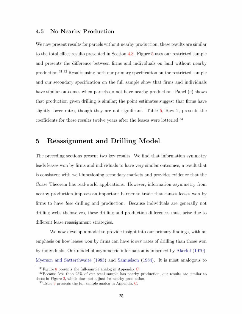
4.5 No Nearby Production

We now present results for parcels without nearby production; these results are similar

to the total effect results presented in Section 4.3. Figure 5 uses our restricted sample

and presents the difference between firms and individuals on land without nearby

production.31,32 Results using both our primary specification on the restricted sample

and our secondary specification on the full sample show that firms and individuals

have similar outcomes when parcels do not have nearby production. Panel (c) shows

that production given drilling is similar; the point estimates suggest that firms have

slightly lower rates, though they are not significant. Table 5, Row 2, presents the

coefficients for these results twelve years after the leases were lotteried.33

5 Reassignment and Drilling Model

The preceding sections present two key results. We find that information symmetry

leads leases won by firms and individuals to have very similar outcomes, a result that

is consistent with well-functioning secondary markets and provides evidence that the

Coase Theorem has real-world applications. However, information asymmetry from

nearby production imposes an important barrier to trade that causes leases won by

firms to have less drilling and production. Because individuals are generally not

drilling wells themselves, these drilling and production differences must arise due to

different lease reassignment strategies.

We now develop a model to provide insight into our primary findings, with an

emphasis on how leases won by firms can have lower rates of drilling than those won

by individuals. Our model of asymmetric information is informed by Akerlof (1970);

Myerson and Satterthwaite (1983) and Samuelson (1984). It is most analogous to

31Figure 8 presents the full-sample analog in Appendix C.32Because less than 25% of our total sample has nearby production, our results are similar to

those in Figure 2, which does not adjust for nearby production.33Table 9 presents the full sample analog in Appendix C.

25

(a) Drilling (b) Production

(c) Production Given Drilling

Figure 5: Restricted sample with one firm winner. Estimates are reported for parcelswithout nearby production. The firm effect is the coefficient on an indicator forwhether the first place winner was a firm. The right vertical axis gives the p valueof a test that the two means are not equal. Panel (c) excludes month-of-lottery fixedeffects due to the small sample size of this specification.

26

results derived in Myerson (1985) and Samuelson (1985). One departure from the

previous literature is that their models assume the seller is the party with private

information. In our setting, the buyer will have superior information due to their

nearby production.

5.1 Model Preliminaries

Our stylized model has three types of agents: firms that initially win a lease (F),

individuals that initially win a lease (I), and the lowest cost firm that is interested in

purchasing a lease (LCF). All parties are risk neutral. The lease has an underlying

true value of production, θ ∼ U[0,1]. In the base version of our model there is no

information asymmetry and all agents can only form expectations about the true

value of θ. In the absence of private information, E[θ] is the same for all parties.

Each type of lessee has a specific cost of drilling, Cj, j ∈ I, F, that is public

knowledge and known with certainty. The LCF’s cost of drilling, CLCF , is also public

knowledge and known with certainty. We assume that CI > CF ≥ CLCF . Note

that the cost difference between firms and individuals is the only assumed difference

between firms and individuals. It is reasonable for individuals to have the highest

costs, as they generally do not have the capital and expertise to drill oil wells. Firms

that are initial lessees and LCFs are likely to have similar costs when there is no

nearby production.

The game proceeds in two stages. First, the lessee and LCF bargain over the

lease. Bargaining happens via a take-it-or-leave-it offer, Oj, made by the LCF.34

Following the reassignment stage, the lease owner decides whether or not drill. Ex-

pected payoffs from drilling equal the expected value of θ less the cost of drilling (Cj).

34In our basic framework, results are not sensitive to the type of bargaining framework. When weintroduce information asymmetry, results will become sensitive to the choice of bargaining frame-work. This model demonstrates how information asymmetry can lead to worse outcomes for leaseswon by firms. We do not find that information asymmetry always leads to worse outcomes for leaseswon by firms.

27

Drilling happens if this value is positive.

5.2 Model Solution

The model solution without information asymmetry is quite simple. Because all

information is public, parties do not learn anything as the bargaining process plays

out. All parties will evaluate the expected value of drilling at 1/2. If 1/2 > CLCF

and Cj > CLCF then there are gains from trade. The LCF will look to buy the lease

and drill on it. They will offer the minimum price such that the lessee will accept,

the lease will be traded, and drilling will occur. If a lease is initially won by a firm,

1/2 > CF and CF = CLCF , no trade will occur, but the initial lessee will make the

same drilling decision that the LCF would.

Our setup yields predictions that are realized in the data. The eventual out-

comes in terms of drilling and production will be similar, regardless of who wins the

lease. Additionally, firms will be less likely to trade their lease than individuals. This

is because the winning firm may be the lowest cost firm. We might also expect small

transaction costs (not explicitly modeled) to inhibit trade between firms with similar

drilling costs. We now turn to a richer model that explains our results on information

asymmetry.

5.3 Information Asymmetry

Information asymmetry requires two adjustments to our assumptions. First, the LCF

is replaced by a nearby production firm (NPF). The NPF is the potential buyer; their

existing production allows them to know the true θ of the lease in question. Lease

winners still do not have private information and can only form expectations about

the value of θ. However, lessees are able to update these expectations based on offers

they receive from the NPF. Notice that this will lead to a pooling equilibrium; a

separating equilibrium is impossible because the NPF has no credible way to signal

28

the true θ of the lease. Second, let costs be CI > CF > CNPF . It is reasonable for

the NPF to have the lowest costs, as they are already producing in the area.35

We now solve for the equilibrium of our simple bargaining model. The primary

complication is that the lessee will update their expectations about the parcel’s value

as soon as an offer is made by the nearby producing firm.

If the initial lessee retains the lease after receiving an offer, Oj, it will receive

their updated expectation of θ less their costs of drilling: E[θ|Oj]−Cj. Thus, it will

only trade if the offer is welfare improving: Oj > E[θ|Oj]−Cj. Notice that there is no

profitable deviation – if the initial lessee rejects an offer when Oj > E[θ|Oj]−Cj (or

accepts an offer when Oj < E[θ|Oj]−Cj), it will be worse off. E[θ|Oj] is determined

by realizing that an offer of Oj indicates that the true value of θ lies somewhere

between Oj +CNPF (adding CNPF to account for the cost of drilling a well) and 1.36

The uniform distribution means that E[θ|Oj] =(Oj+CNPF+1)

2.

Thus, the initial lessee will accept a trade if Oj >(Oj+CNPF+1)

2− Cj, which

reduces to:37

Oj > 1 + CNPF − 2Cj (4)

The NPF will be willing to offer a trade if the true value of θ is greater than its cost

of acquisition plus the cost of drilling:

θ −Oj − CNPF > 0 (5)

The NPF will find the minimum Oj such that the Equation 4 is satisfied and

then offer this minimum Oj if it satisfies Equation 5. Substituting the first inequality

35Due to the randomized nature of the lottery and the fact that most leases with nearby productionhad a mean (median) of more than 750 (325) offers, firms that win leases are unlikely to be the nearbyproducing firm.

36If an offer is made, this interval will always be of the form [X,1], where X is between 0 and 1.Neither Oj nor CNPF can be less than 0; a lessee would never accept a negative offer and drillingcosts are assumed to be positive. Additionally, the NPF will not make an offer such that Oj +CNPF

is greater than 1, as this will result in a negative payoff for all possible values of θ.37Oj >

(Oj+CNPF+1)2 − Cj ⇒ 2Oj > Oj + CNPF + 1− 2Cj ⇒ Oj > 1 + CNPF − 2Cj .

29

into the second, we find that trade will happen when:38

θ > 1 + 2CNPF − 2Cj (6)

For all θs that satisfy Equation 6, the NPF will make the same bid, the minimum

Oj that satisfies Equation 4.39 Drilling will necessarily occur.40 Notice that the

individual’s higher cost of drilling leads to a greater range of θs that are traded.

When trade does not occur, the lessee decides whether or not to drill based on

whether E[θ|no offer]−Cj > 0. In this situation, the lessee knows that θ lies between 0

and 1+2CNPF−2Cj. Thus, E[θ|no offer]−Cj =0+1+2CNPF−2Cj

2−Cj = 1

2+CNPF−2Cj.

Notice that the expected gains from drilling are positive only when drilling costs are

low (Cj <14

+ CNPF

2). When drilling costs are high (Cj >

14

+ CNPF

2), the lessee will

choose not to drill. Note that the firm will be in a better position to drill a retrained

lease. However, individuals are more likely to trade leases, and traded leases are

always drilled.

In equilibrium, drilling will happen whenever there is trade (when θ ∈ [1 +

2CNPF −2Cj, 1]. If θ < 1 + 2CNPF −2Cj, trade will not happen and drilling will only

occur if 12

+ CNPF − 2Cj > 0.

5.4 Empirical Predictions

We are now able to examine our empirical findings. Is it possible for leases won by

individuals to have more drilling than those won by firms? The answer depends on

38θ − (1 + CNPF − 2Cj)− CNPF > 0⇒ θ − 1− 2CNPF + 2Cj > 0⇒ θ > 1 + 2CNPF − 2Cj .39Again, note that there are no profitable deviations from this strategy. If the NPF offers more

than the minimum Oj , it will not increase the range of θs that are accepted. If the NPF offers lessthan the minimum Oj , its offer will be rejected.

40We have not discussed what happens when θ is below the threshold. It is possible that the NPFcould make an offer, knowing that it will not be accepted. This possibility can be rejected by eitherassigning a small transaction cost to making an offer, or by arguing that the NPF may not wish toprovide information (in the form of an offer) to a competing nearby firm if it will not benefit fromdoing so.

30

the costs of drilling.

Suppose that we are in an environment where the firm has low drilling costs

and the individual lessee has high drilling costs (CI >14

+ CNPF

2> CF ). For example,

CNPF = 0, CF = 0.1, and CI = 0.5. If our data are actually represented by θ ∼ U[0,1],

our model predicts that trade and drilling will occur 90% of the time if individuals

win all of the leases. In contrast, our model predicts trade will occur 20% of the

time and drilling will occur 100% of the time when firms win. The higher level of

drilling for parcels won by firms results from a high expected θ when there is no trade,

combined with a low CF .

On the other hand, consider when both firms and individuals have relatively

high costs (CI > CF > 14

+ CNPF

2). For example, CNPF = 0.5, CF = 0.6, and CI =

1.0. If individuals win all the leases, trade and drilling will occur 50% of the time.

If firms win all of the leases, trade will occur 20% of the time and drilling will also

occur 20% of the time. In this situation, assigning the leases to individuals will result

in a higher proportion of them being drilled – consistent with our empirical findings.

5.5 Testing Trade with Nearby Producing Firms

We now turn to examining the primary finding of our model: due to their lower

drilling costs, firms will be less willing than individuals to trade their leases to nearby

producing firms.41 We scraped the identities of nearby producing well operators

and matched these nearby operators to firms in the LR2000 lease history. We then

estimate how frequently leases won by firms (relative to individuals) are traded with

nearby producing firms using the following regression:

TradeNPFi = α0 + β1Fi + ΩXi + εi (7)

41Note that our earlier results demonstrate firms are less likely to transfer overall. This may notaffect drilling frequency in the absence of information asymmetry because many firms are similar.However, failing to trade to nearby producers can have long-term consequences because they arelikely to use their proprietary information to make different drilling decisions than the initial lessees.

31

The dependent variable is whether we have matched a lessee as trading with

a nearby producing well operator. The primary coefficient of interest, β1, tells us

whether firms are differentially less likely to trade with a nearby producing well

operator. For this analysis, our sample is the set of leases with nearby production.

Our analysis is primarily limited because we cannot perfectly identify whether

trade happened with the nearby producing firm. This leads to attenuation bias.42

This imperfect match identification arises from four sources. First, our available well

operator data does not also identify the nearby lessee. Any trades with a nearby

lessee different from the operator will not be correctly matched.43 Second, both the

assignment data and the nearby operator data are incomplete. In particular, nearby

operators are unavailable before 1978. Both datasets are likely missing observations,

with greater completeness in later years. Third, neither dataset identifies corporate

relationships. This means we will fail to identify a trade to a subsidiary or former

employee of a nearby operator as a match. Finally, our analysis will be limited by

imperfect identification of the “nearby” wells. For example, a well drilled outside of

our five-year drilling window may have an owner that will be able to make the correct

drilling decision, but we will not flag this type of match.44,45

42Because the dependent variable is binary, measurement error is non-classical and results inattenuation bias.

43In future work, we hope to incorporate some nearby owner data. Extracting the available nearbyowners is a non-trivial task.

44Our analysis will also be limited because we are matching text strings. Abbreviations andtypos introduce measurement error and lower our match rate. For example, “Gulf” can be matchedwith “Petrogulf Corporation” or “Gulf Oil”. We use “Gulf” as the basis for matching becauseabbreviations are ubiquitous in the LR2000. Matching only with full names will cause many falsenegatives.

45Finally, we note that our preferred analysis looks at whether parcels are ever reassigned tothe current nearby producing firm. In Appendix F we examine whether parcels are traded to thecurrent nearby operator before drilling has begun. We prefer our primary analysis because of theopaque nature of firm relationships. If nearby production is listed by “Conoco”, it is possible thatthe nearby production was actually by Philips Oil Company, which was then bought by Conoco.However, we may not observe Philips as a nearby producer. Therefore, a lease traded to Philips,and subsequently to Conoco, would yield a false negative. The main drawback to this approach isthat our analysis will occasionally identify matches not suggested by our model – where the tradeshappen after drilling. Fortunately, both approaches yield similar results as most matches are priorto drilling.

32

Sample withNearby Firms

Sample withDistant Firms

(1) (2) (3) (4)Firm Winner -0.079∗∗∗ -0.077∗∗∗ -0.023 -0.005

(0.029) (0.018) (0.025) (0.019)

intercept 0.049∗∗ 0.044∗∗ 0.027 0.000(0.024) (0.021) (0.024) (0.015)

Full Sample No Yes No Yes

Offers &Acreage Controls Yes Yes Yes Yes

Lottery Year Fixed Effects No Yes No YesR squared 0.069 0.038 0.034 0.018Observations 376 2399 443 2644

Table 6: We examine how frequently leases are reassigned to firms that have nearbyproduction. Column (1) uses our restricted sample and Column (2) uses the fullsample. Columns (3) and (4) look at how frequently leases are reassigned to distantfirms with production in the area. We allow reassignments to happen at any pointduring the lease. A pooled regression testing whether the ‘Firm Winner’ coefficient isdifferent in columns (1) and (3) yields a p-value of 0.128. A pooled regression testingwhether the ‘Firm Winner’ coefficient is different in columns (2) and (4) yields ap-value of 0.003.

Table 6 reports our primary results. In columns (1) and (2), we look at the set

of leases with nearby production and examine whether leases are ever reassigned to a

nearby producing firm. We find that firm winners about 7.5% less likely to have their

parcels ever reassigned to a nearby producing firms. Columns (3) and (4) use a sample

without nearby production within 2.6 miles, but with production between 2.6 and 5.2

miles away from the lease. Here, we find that firms and individuals have similar rates

of reassignment. These results show that when there is nearby production, firms are

differentially less likely to reassign parcels to nearby producing firms.46

46Note that it is unclear whether we should expect the magnitude of the coefficients to be differentbetween columns (1) and (3). On the one hand, firms are less likely to want to reassign to nearbyproducing firms than distant producing firms because it is likely that the nearby firms have adifferential information advantage. On the other hand, distant producing firms may not have a costadvantage over the initial lessee. This would suggest that there are limited gains from trade. Thefact that we see evidence of a differential suggests that there are reassignment gains due to cost

33

Is the magnitude of this effect large enough to explain the full drilling differ-

ences we find between leases won by firms and those won by individuals? By itself,

no. However, it does demonstrate that firms are reassigning their leases differently

than individuals. Additionally, we expect that attenuation bias from measurement

error causes the coefficients to be smaller than their true values. These differing

reassignment processes appear to be the primary cause of different lease outcomes.

6 Discussion and Conclusion

Overall, the accumulation of evidence suggests two facts. First, leases without in-

formation asymmetry are efficiently reallocated via a robust secondary market. The

secondary market allows for similar drilling and production outcomes, regardless of

initial allocation. Second, information asymmetry inhibits trade between firms and

nearby producing firms. This leads to worse outcomes for these types of leases when

they are initially assigned to firms. In our setting, we can conclude that it is better

to initially have a bad match than it is to have a mediocre match. Because the mech-

anism – information asymmetry – is not specific to our setting, our findings are likely

more broadly applicable.

Our finding that information asymmetry affected firms more severely than

individuals may seem surprising at first. However, our theoretical model, combined

with analysis of the transaction histories, reveals that our results are actually intuitive.

Because the average firm is already a mediocre match for any given lease, the gains

from trading that parcel are lower than the gains for an individual. As a result, many

firms (in contrast to individuals) are insufficiently incentivized to trade their leases

in the presence of information asymmetry.

One important policy implication is that lotteries can be a relatively efficient

mechanism for allocating assets under certain conditions. For example, nature’s “lot-

differentials.

34

tery” that allocated oil deposits to farmers in the Bakken shale formation likely does

not seriously impede the efficient outcome. Indeed, the Bakken’s mineral rights real-

location process is very similar to the process in our setting; oil firms employ landmen

to purchase the rights from individuals without the capital or expertise to develop

the resources. Thus, our results provide evidence in favor of the United States’ policy

of allocating both surface rights and mineral rights to property owners.

Additionally, market designers should carefully evaluate whether information

asymmetry is likely to be present. If it is, taking steps to ensure that assets are not

allocated to intermediate-quality matches can yield tangible benefits. Potential ap-

plications include wireless spectrum auctions and electricity transmission markets. In

electricity markets, for example, information asymmetry may arise due to proprietary

information about generation costs. Our results suggest that assigning transmission

rights to generating firms is inferior to auctioning the rights or assigning them ran-

domly via lottery to individuals.

Our work suggests one primary avenue of further research. While lotteries can

be an efficient way of allocating public resources, we do not yet understand how they

affect government revenue. One of the government’s primary goals when allocating

a public resource is to raise funds.47 We will compare lotteries and auctions run by

the BLM to determine which allocation method raised more revenue. There are two

possible ways for us to explore this question. We can match auctioned parcels with

similar parcels that were lotteried at the same time. Additionally, we can compare

revenues before and after the BLM switched to an auction for all parcels in 1987.

Answering this question will give us a fuller picture of the relative welfare effects of

auctions and lotteries.

47Li (2014) finds that auctions generate greater social welfare than lotteries for Chinese licenseplate distributions. However, China does not allow for reallocation of licenses, reducing their effi-ciency.

35

References

Akee, R. (2009, May). Checkerboards and Coase: The effect of property institutions

on efficiency in housing markets. Journal of Law and Economics 52 (2), 395–410.

Akerlof, G. A. (1970). The market for “lemons”: Quality uncertainty and the market

mechanism. The Quarterly Journal of Economics , 488–500.

Angrist, J. D. and J.-S. Pischke (2008). Mostly harmless econometrics: An empiri-

cist’s companion. Princeton university press.

Biewick, L. R. (2011). Geodatabase of wyoming statewide oil and gas drilling activity

to 2010. U.S. Geological Survey Data Series 625.

Bleakley, H. and J. Ferrie (2014). Land openings on the Georgia frontier and

the Coase theorem in the short- and long-run. http://www-personal.umich.edu/

~hoytb/Bleakley_Ferrie_Farmsize.pdf.

Bureau of Land Management (1983). The Federal Simultaneous Oil and Gas Leasing System:

Important Information about The “Government Oil and Gas Lottery ”. Bureau of Land

Management.

Coase, R. H. (1960). The problem of social cost. The Journal of Law and Economics 3,

1–44.

Conley, T. G. (1999). GMM estimation with cross sectional dependence. Journal of econo-

metrics 92 (1), 1–45.

Dang, T. V., G. Gorton, B. Holmstrom, and G. Ordonez (2016). Banks as secret keepers.

http://economics.mit.edu/files/9776.

Fairfax, S. K. and C. E. Yale (1987). Federal Lands: A Guide to Planning, Management,

and State Revenues. Island Press.

36

Hendricks, K. and R. H. Porter (1988). An empirical study of an auction with asymmetric

information. The American Economic Review 78, 865–863.

Lewis, E. (2015). Federal environmental protection and the distorted search for oil and gas.

Li, S. (2014). Better lucky than rich? welfare analysis of automobile license allocations in

beijing and shanghai. Welfare Analysis of Automobile License Allocations in Beijing and

Shanghai (March 1, 2014).

Myerson, R. B. (1985). Analysis of two bargaining problems with incomplete mechanisms.

In A. E. Roth (Ed.), Game-theoretic models of bargaining, Chapter 7, pp. 115–147. Cam-

bridge University Press.

Myerson, R. B. and M. A. Satterthwaite (1983). Efficient mechanisms for bilateral trading.

Journal of Economic Theory 29, 265–281.

Samuelson, W. (1984). Bargaining under asymmetric information. Econometrica: Journal

of the Econometric Society , 995–1005.

Samuelson, W. (1985). A comment on the coase theorem. In A. E. Roth (Ed.), Game-

theoretic models of bargaining, Chapter 15, pp. 321–339. Cambridge University Press.

Wiggins, S. N. and G. D. Libecap (1985). Oil field unitization: contractual failure in the

presence of imperfect information. The American Economic Review , 368–385.

37

Appendices

A Data Sources and Identification of Firm and In-

dividual

Records on lotteries were scanned from paper records at the BLM office in Laramie

Wyoming. These records include first information on parcels that would be offered in

the lottery, with an example from June 1975 in Figure 6. These records also contain

information on the first-, second-, and third-place winners as well as the total number

of entries. The first place winner has information both on name as well as address;

the second- and third-place winners only have names.

This data is publicly available from the Wyoming BLM. The Michigan IRB

panel ruled that this data is not regulated.

Data were double-blind entered using a data digitization service and are guar-

anteed to be 99.95% accurate.

We identify firms from whether words such as “Co.”, “Corp. ”, “Corpora-

tion”, “Co.”, “Inc. ”, “Ltd.”, “Limited ”, “Associates”, “Oil”, “Gas”, and “Indus-

tries”appear in the name of the winner. We also include as firms those that are

obviously firms but not easily categorized from this rule (for example, “Michigan

Wisconsin Pipe Line”).

We also explicitly list first-place individuals as individuals rather than firms

even if their address information suggests that they are associated with a firm (e.g.,

John Doe, Acme Co., Acme Wyoming 80000) We do this for two reasons. First,

if these individuals had appeared as second- or third-place winners, we would not

observe the address/firm information, and we would categorize them as individuals.

Second, we cannot determine whether these individuals were entering the lottery on

behalf of the firm or merely using the firm as a personal address. To the extent that

38

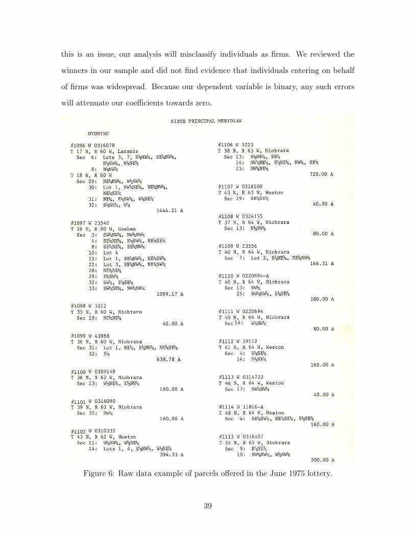
this is an issue, our analysis will misclassify individuals as firms. We reviewed the

winners in our sample and did not find evidence that individuals entering on behalf

of firms was widespread. Because our dependent variable is binary, any such errors

will attenuate our coefficients towards zero.'\ 'i-.

SIXTIT PRINCIPAI MERIDIAN

WYOI.IING

#l-096 I 03l-6078 llrt06 w 5223T 17 N, R 50 I, Laramle T 38 N' R 63 I'l ' Nlobrara

Sec 6t Lots 3, 7 , StNEt, SE,6]'lWk' Sec 13 : SttNEll' SEkELswt, NksEt L4" Nwli,IEk, slNEk, NWL' sEk

8: NtNl.lk 231 NW]61'lEk

T 18 N, R 60 w 720.00 ASec 29: NElNwk, I.Ilrsl.lk

30: Ior 1, NwLNEk, NELl,lwL, /11107 I.r 0316100NEr6SEk T 43 N, R 63 I' Weston

31: NEt, Elrswrr, t,IksEk Sec 29: SEltsEt32- StrNEk, Wl5 40.00 A

L444.21 A/11108 r^r 0324L55

llLg7 W 23542 T 37 N' R 64 l' NlobraraT 26 N, R 50 W, Goshen Sec 13: NLSwt

Sec 3: SWLllWrl, NI,ILSWI 80.00 A4z SErdEt, ELSWI6, NErSEk8: SEli.IEl4, SELlrw,4 //l-l-09 w 23556

10: Lor 4 T 40 N, R 54 w, Nlobrara15: Lot 1, sEU.Itk, NEtswt Sec 7: Lot 3, STNEL' NEkswtzzt Lor 3, sEllI^lk, NEksllrk 166.31 AZ8z NEIISEL29t Etswt /11L10 i 0220694-A322 Swk, S'SEL T 40 N' R 64 w' Nlobrara33: SIrtlNEt, NwtSEk Sec 13: Swt

LO99.L7 A 25. swklwt, ELSEL280,00 A

111098 w 5212T 35 N, R 60 w, Nioblara /I111f W 0220694

sec 18: NEli'lEk T 40 N, R 54 W, NLobrara40.00 A Sec 14: I^lrrNI.IL

80.00 A/i1099 I,l 43988T 36 N, R 60 !,r, Niobrara llLLLz W 39IL2

sec 31: Lor 1, NEk, ELIVrk, NELSEL T 41 N, R 64 W, I,leston32. St Sec 4: SkSEt

538.78 A 14: SkSEt160.00 A

/11100 n 0309148T 36 N, R 62 W, Nlobrara /11113 W 03L4722

Sec 13: wLNEk, ELNWT T 46 N, R 64 lJ' Weston150.00 A Sec 17: Nw'dII.Il

40.00 A/11101 w 0315090T 39 N, R 62 W, Nlobrara //1114 W 11816-4

sec 35: NWk T 48 N, R 64 W, Wesron160.00 A Sec 4t sELSwk, NELSE,6' SttSEt

160.00 AllLLOz w 0310335T 43 N, R 62 i'1, tJeston /11115 i 0316107

Sec 11: WLSW,6, WISEL T 35 N, R 55 W, NlobraraL4z Lots 1, 4, E*NWL, WISEL Sec 9: ELSET

394.53 A l0: sI^IlNwt6, I.rtsl,,200.00 A

#10: Irl 18309-8, cT 58 N, R 62 W, Crook /11115 !J 0316108-A, W 0315109, I 0316110

Sec 25: Lots 1, 2,3,4,5, 15, 16 T 37 N, R 65 I, Nlobrara283.97 A sec 9: SElllili, Sl

L7 z SEtNEl4, NWt#11-04 w 0316096 18: Lot 4, SLNEL, SEtswt? 37 N, R 53 W, Nlobrara 7L9.66 A

Sec 3: Lot 3, 4, Swktlrt118.55 A /i1117 t,l 0321841

T 39 N, R 65 W, Nl.obrara/iu05 w 0316097 Sec 28: lrLNWtT 37 N, R 63 W, NLobrara 80.00 A

Sec 25: Etifi:150.00 A -1-

Figure 6: Raw data example of parcels offered in the June 1975 lottery.

39

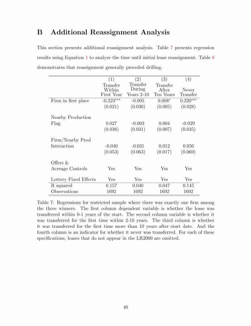
B Additional Reassignment Analysis

This section presents additional reassignment analysis. Table 7 presents regression

results using Equation 1 to analyze the time until initial lease reassignment. Table 8

demonstrates that reassignment generally preceded drilling.

(1) (2) (3) (4)TransferWithin

First Year

TransferDuring

Years 2-10

TransferAfter

Ten YearsNever

TransferFirm in first place -0.223∗∗∗ -0.005 0.008∗ 0.220∗∗∗

(0.021) (0.030) (0.005) (0.028)

Nearby ProductionFlag 0.027 -0.003 0.004 -0.029

(0.038) (0.031) (0.007) (0.035)

Firm/Nearby ProdInteraction -0.040 -0.031 0.012 0.056

(0.053) (0.063) (0.017) (0.069)

Offers &Acreage Controls Yes Yes Yes Yes

Lottery Fixed Effects Yes Yes Yes YesR squared 0.157 0.040 0.047 0.145Observations 1692 1692 1692 1692

Table 7: Regressions for restricted sample where there was exactly one firm amongthe three winners. The first column dependent variable is whether the lease wastransferred within 0-1 years of the start. The second column variable is whether itwas transferred for the first time within 2-10 years. The third column is whetherit was transferred for the first time more than 10 years after start date. And thefourth column is an indicator for whether it never was transferred. For each of thesespecifications, leases that do not appear in the LR2000 are omitted.

40

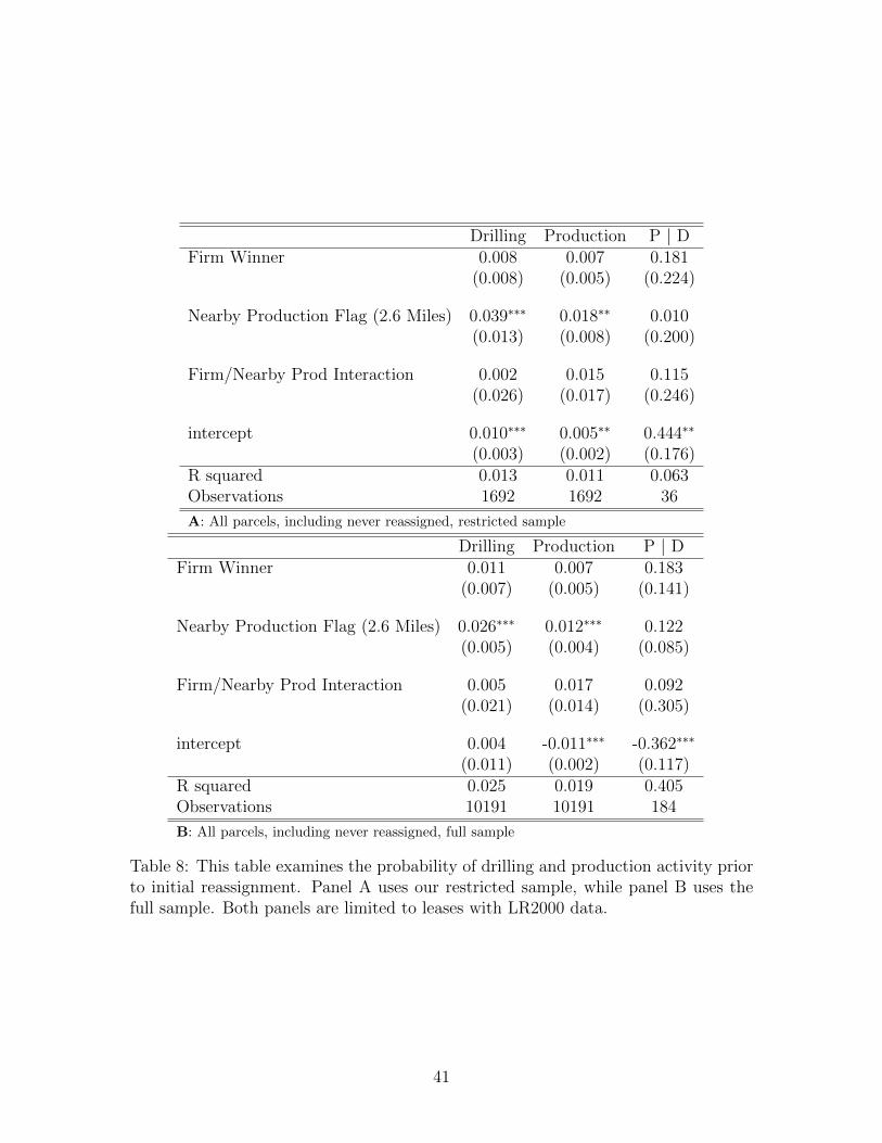
Drilling Production P | DFirm Winner 0.008 0.007 0.181

(0.008) (0.005) (0.224)

Nearby Production Flag (2.6 Miles) 0.039∗∗∗ 0.018∗∗ 0.010(0.013) (0.008) (0.200)

Firm/Nearby Prod Interaction 0.002 0.015 0.115(0.026) (0.017) (0.246)

intercept 0.010∗∗∗ 0.005∗∗ 0.444∗∗

(0.003) (0.002) (0.176)R squared 0.013 0.011 0.063Observations 1692 1692 36

A: All parcels, including never reassigned, restricted sample

Drilling Production P | DFirm Winner 0.011 0.007 0.183

(0.007) (0.005) (0.141)

Nearby Production Flag (2.6 Miles) 0.026∗∗∗ 0.012∗∗∗ 0.122(0.005) (0.004) (0.085)

Firm/Nearby Prod Interaction 0.005 0.017 0.092(0.021) (0.014) (0.305)

intercept 0.004 -0.011∗∗∗ -0.362∗∗∗

(0.011) (0.002) (0.117)R squared 0.025 0.019 0.405Observations 10191 10191 184

B: All parcels, including never reassigned, full sample

Table 8: This table examines the probability of drilling and production activity priorto initial reassignment. Panel A uses our restricted sample, while panel B uses thefull sample. Both panels are limited to leases with LR2000 data.

41

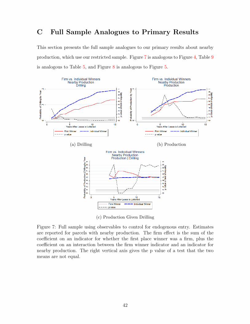
C Full Sample Analogues to Primary Results

This section presents the full sample analogues to our primary results about nearby

production, which use our restricted sample. Figure 7 is analogous to Figure 4, Table 9

is analogous to Table 5, and Figure 8 is analogous to Figure 5.

(a) Drilling (b) Production

(c) Production Given Drilling

Figure 7: Full sample using observables to control for endogenous entry. Estimatesare reported for parcels with nearby production. The firm effect is the sum of thecoefficient on an indicator for whether the first place winner was a firm, plus thecoefficient on an interaction between the firm winner indicator and an indicator fornearby production. The right vertical axis gives the p value of a test that the twomeans are not equal.

42

(1) (2) (3) (4) (5)Reassign

ProbabilityLog Time

to Reassign Drill Prod P | DNearby ProductionFlag 0.017 -0.070 0.111∗∗∗ 0.058∗∗∗ 0.079∗

(0.014) (0.073) (0.026) (0.011) (0.046)

Firm Winner -0.211∗∗∗ 0.875∗∗∗ 0.011 -0.000 -0.074(0.026) (0.086) (0.011) (0.005) (0.069)

Firm/Nearby ProdInteraction -0.056 0.219 -0.083∗∗∗ -0.029 0.092

(0.056) (0.176) (0.026) (0.018) (0.116)

Offers &Acreage Controls Yes Yes Yes Yes Yes

Lottery Fixed Effects Yes Yes Yes Yes YesR squared 0.130 0.123 0.078 0.061 0.151Observations 10762 8097 10762 10762 904

Table 9: This table uses the probability of reassignment by twelve years (1), length oftime given reassignment (2), probability of drilling by twelve years (3), probability ofproduction by twelve years (4), and probability of production given drilling by twelveyears (5) as dependent variables. Nearby production is a binary indicator for anyproduction within 2.6 miles of the section(s) the lease is located on. This table usesour full sample. Column (2) does not correct for selection into reassignment. Pointestimates using a Heckman two-step are similar.

43

(a) Drilling (b) Production

(c) Production Given Drilling

Figure 8: Full sample using observables to control for endogenous entry. Estimatesare reported for parcels without nearby production. The firm effect is the coefficienton an indicator for whether the first place winner was a firm. The right vertical axisgives the p value of a test that the two means are not equal.

44

D Alternative Nearby Production Specifications

In this Appendix we consider a variety of alternative nearby production specifica-

tions. Figures 9 and 10 define nearby production as occurring over the last 10 years.

Figures 11 and 12 define nearby production as occurring within 1.7 miles. Figures 13

and 14 define nearby production as occurring within 3.2 miles. Figures 15 and 16

use an alternate data source that includes productive gas wells and defines recent by

the first production year, not the drilling year. Figures 17 and 18 repeat the exercise

in Figures 15 and 16, but define nearby production as occurring within 3.2 miles.

Our central results about nearby production are broadly consistent over this range of

alternative specifications.

Figures 19 and 20 look at nearby drilling instead of nearby production. We

limit “nearby” to only include the closest 1.7 miles as well over half of leases have had

unsuccessful wells within 2.6 miles. The results are qualitatively similar to our main

results, though the magnitudes are smaller and not always statistically significant.

This finding is unsurprising. Unproductive wells will have two important differences

from productive ones. First, the owner of an unproductive well will be less eager to

purchase nearby leases – they have already determined that the area is dry. Second,

the information asymmetry from an unproductive well is likely not as large. Both

parties will be able to agree that the nearby firm has not found oil – considerably easier

than agreeing about the quantity and quality of production from a nearby producing

well. As the quality of information causing information asymmetry decreases, the

negative effects from information asymmetry should dissipate.

45

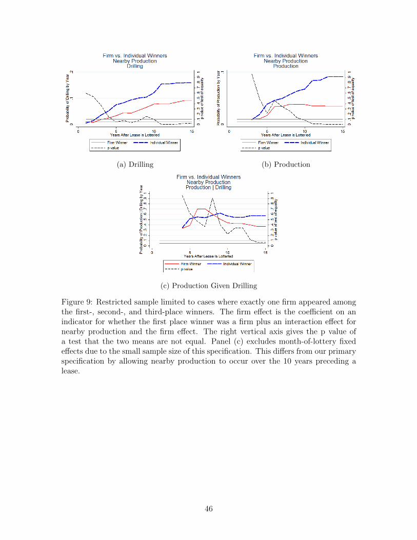
(a) Drilling (b) Production

(c) Production Given Drilling

Figure 9: Restricted sample limited to cases where exactly one firm appeared amongthe first-, second-, and third-place winners. The firm effect is the coefficient on anindicator for whether the first place winner was a firm plus an interaction effect fornearby production and the firm effect. The right vertical axis gives the p value ofa test that the two means are not equal. Panel (c) excludes month-of-lottery fixedeffects due to the small sample size of this specification. This differs from our primaryspecification by allowing nearby production to occur over the 10 years preceding alease.

46

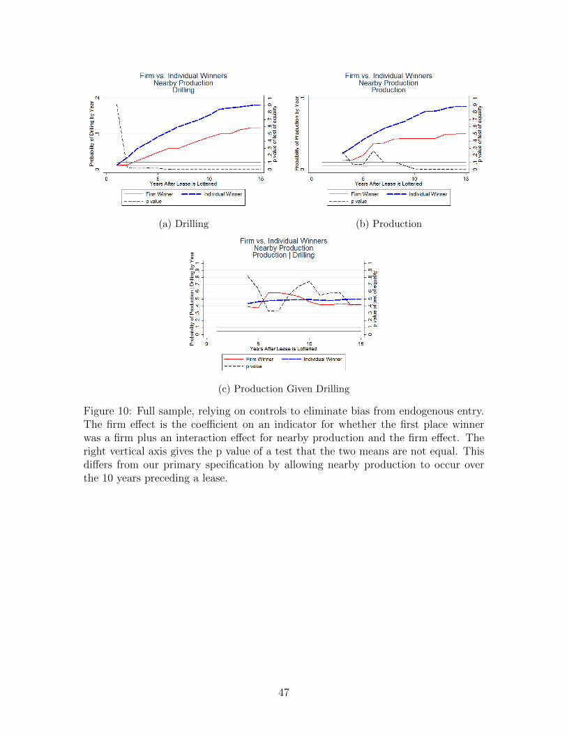
(a) Drilling (b) Production

(c) Production Given Drilling

Figure 10: Full sample, relying on controls to eliminate bias from endogenous entry.The firm effect is the coefficient on an indicator for whether the first place winnerwas a firm plus an interaction effect for nearby production and the firm effect. Theright vertical axis gives the p value of a test that the two means are not equal. Thisdiffers from our primary specification by allowing nearby production to occur overthe 10 years preceding a lease.

47

(a) Drilling (b) Production

(c) Production Given Drilling

Figure 11: Restricted sample limited to cases where exactly one firm appeared amongthe first-, second-, and third-place winners. The firm effect is the coefficient on anindicator for whether the first place winner was a firm plus an interaction effect fornearby production and the firm effect. The right vertical axis gives the p value ofa test that the two means are not equal. Panel (c) excludes month-of-lottery fixedeffects due to the small sample size of this specification. This differs from our primaryspecification by defining nearby production as occurring within 1.7 miles of a lease.

48

(a) Drilling (b) Production

(c) Production Given Drilling

Figure 12: Full sample, relying on controls to eliminate bias from endogenous entry.The firm effect is the coefficient on an indicator for whether the first place winner wasa firm plus an interaction effect for nearby production and the firm effect. The rightvertical axis gives the p value of a test that the two means are not equal. This differsfrom our primary specification by defining nearby production as occurring within 1.7miles of a lease.

49

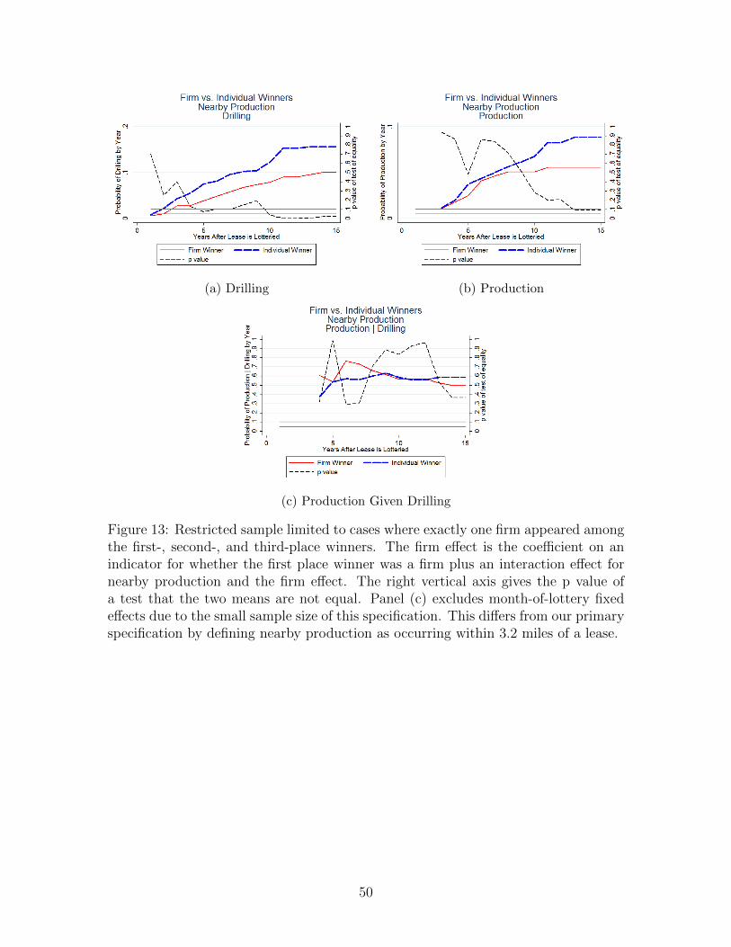
(a) Drilling (b) Production

(c) Production Given Drilling

Figure 13: Restricted sample limited to cases where exactly one firm appeared amongthe first-, second-, and third-place winners. The firm effect is the coefficient on anindicator for whether the first place winner was a firm plus an interaction effect fornearby production and the firm effect. The right vertical axis gives the p value ofa test that the two means are not equal. Panel (c) excludes month-of-lottery fixedeffects due to the small sample size of this specification. This differs from our primaryspecification by defining nearby production as occurring within 3.2 miles of a lease.

50

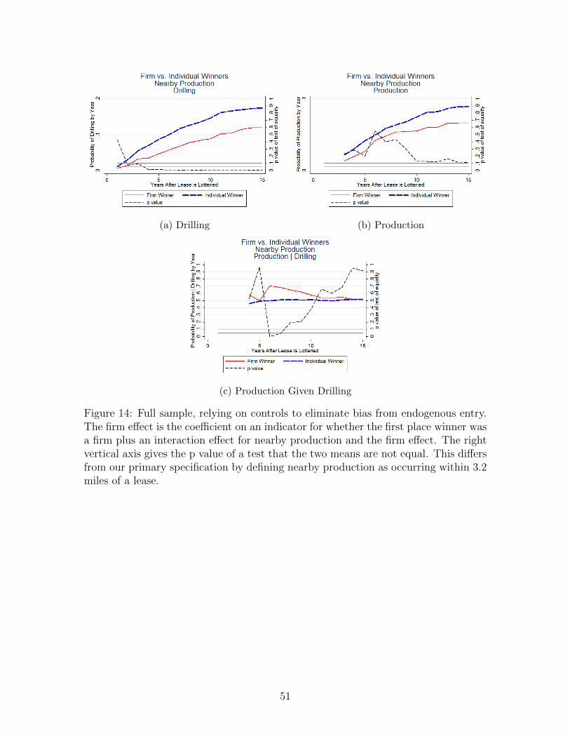
(a) Drilling (b) Production

(c) Production Given Drilling

Figure 14: Full sample, relying on controls to eliminate bias from endogenous entry.The firm effect is the coefficient on an indicator for whether the first place winner wasa firm plus an interaction effect for nearby production and the firm effect. The rightvertical axis gives the p value of a test that the two means are not equal. This differsfrom our primary specification by defining nearby production as occurring within 3.2miles of a lease.

51

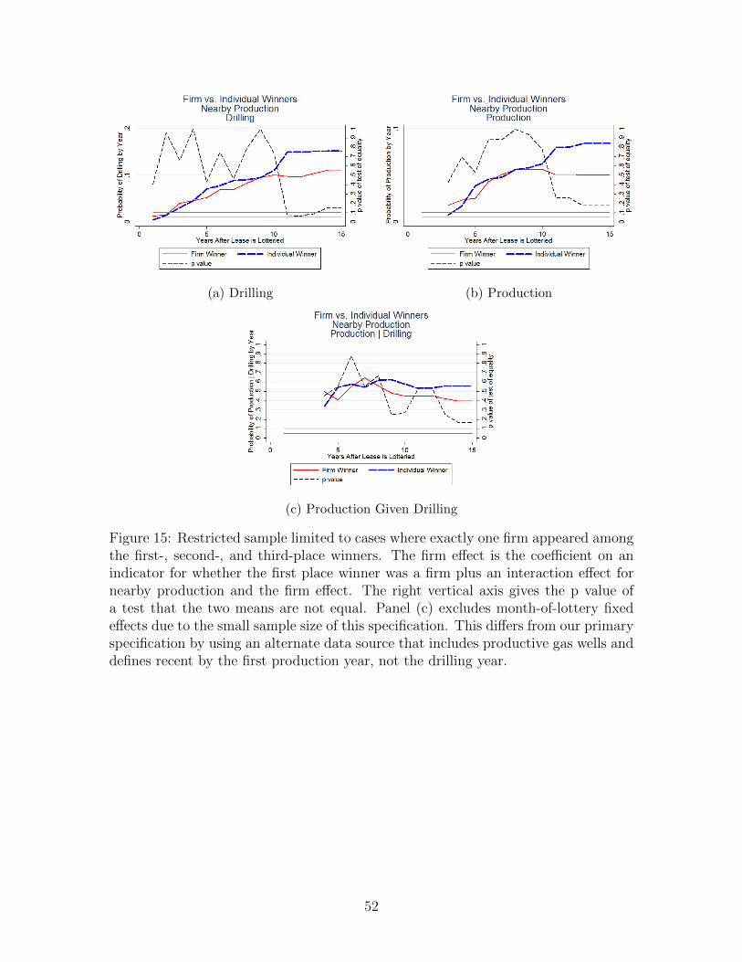
(a) Drilling (b) Production

(c) Production Given Drilling

Figure 15: Restricted sample limited to cases where exactly one firm appeared amongthe first-, second-, and third-place winners. The firm effect is the coefficient on anindicator for whether the first place winner was a firm plus an interaction effect fornearby production and the firm effect. The right vertical axis gives the p value ofa test that the two means are not equal. Panel (c) excludes month-of-lottery fixedeffects due to the small sample size of this specification. This differs from our primaryspecification by using an alternate data source that includes productive gas wells anddefines recent by the first production year, not the drilling year.

52

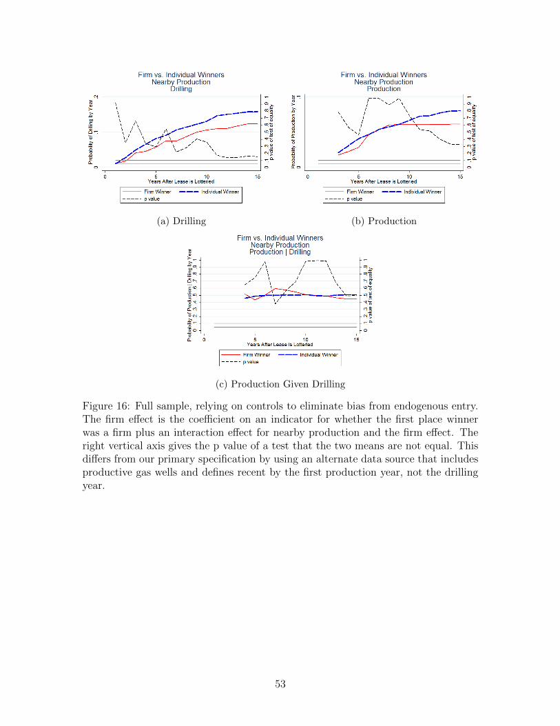
(a) Drilling (b) Production

(c) Production Given Drilling

Figure 16: Full sample, relying on controls to eliminate bias from endogenous entry.The firm effect is the coefficient on an indicator for whether the first place winnerwas a firm plus an interaction effect for nearby production and the firm effect. Theright vertical axis gives the p value of a test that the two means are not equal. Thisdiffers from our primary specification by using an alternate data source that includesproductive gas wells and defines recent by the first production year, not the drillingyear.

53

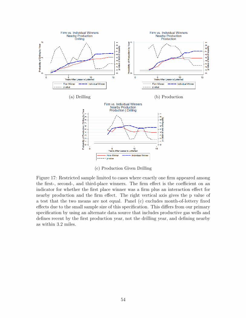
(a) Drilling (b) Production

(c) Production Given Drilling

Figure 17: Restricted sample limited to cases where exactly one firm appeared amongthe first-, second-, and third-place winners. The firm effect is the coefficient on anindicator for whether the first place winner was a firm plus an interaction effect fornearby production and the firm effect. The right vertical axis gives the p value ofa test that the two means are not equal. Panel (c) excludes month-of-lottery fixedeffects due to the small sample size of this specification. This differs from our primaryspecification by using an alternate data source that includes productive gas wells anddefines recent by the first production year, not the drilling year, and defining nearbyas within 3.2 miles.

54

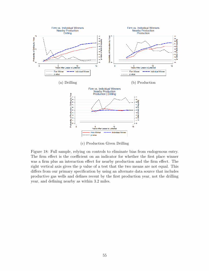
(a) Drilling (b) Production

(c) Production Given Drilling

Figure 18: Full sample, relying on controls to eliminate bias from endogenous entry.The firm effect is the coefficient on an indicator for whether the first place winnerwas a firm plus an interaction effect for nearby production and the firm effect. Theright vertical axis gives the p value of a test that the two means are not equal. Thisdiffers from our primary specification by using an alternate data source that includesproductive gas wells and defines recent by the first production year, not the drillingyear, and defining nearby as within 3.2 miles.

55

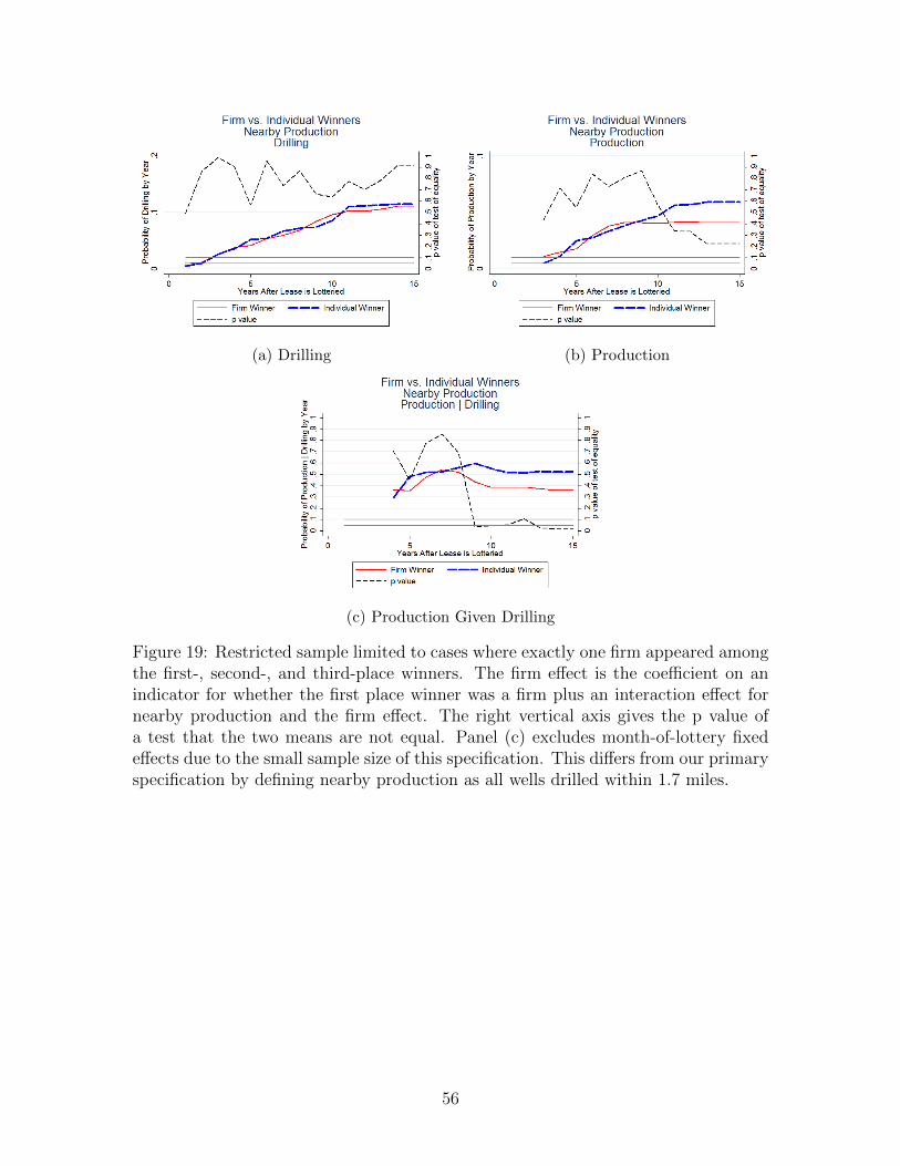
(a) Drilling (b) Production

(c) Production Given Drilling

Figure 19: Restricted sample limited to cases where exactly one firm appeared amongthe first-, second-, and third-place winners. The firm effect is the coefficient on anindicator for whether the first place winner was a firm plus an interaction effect fornearby production and the firm effect. The right vertical axis gives the p value ofa test that the two means are not equal. Panel (c) excludes month-of-lottery fixedeffects due to the small sample size of this specification. This differs from our primaryspecification by defining nearby production as all wells drilled within 1.7 miles.

56

(a) Drilling (b) Production

(c) Production Given Drilling

Figure 20: Full sample, relying on controls to eliminate bias from endogenous entry.The firm effect is the coefficient on an indicator for whether the first place winnerwas a firm plus an interaction effect for nearby production and the firm effect. Theright vertical axis gives the p value of a test that the two means are not equal. Thisdiffers from our primary specification by defining nearby production as all wells drilledwithin 1.7 miles.

57

E Drilling Time and Production Quantities

This appendix includes regressions that look at drilling time and production quanti-

ties. Because many drilling rigs are rented out by the day, the number of days spent

drilling is a rough proxy for drilling costs. Production quantities are a rough proxy

for revenue. Due to the highly variable nature of these measures, our results are not

precise. Table 10 presents the results of this analysis.

The first row shows that drilling time (Columns 1 & 2) and production quanti-

ties (Columns 3 & 4 ) do not have statistically significant differences depending on the

initial lease winner’s identity. The point estimates suggest firms had lower average

production, but they are insignificant; we do not interpret them as meaningful. We

do not have a reason to expect that these types of wells would have lower quantities

produced.48

The third row looks at how drilling time and production quantities differ by

winner’s identity in the presence of nearby production. Again, the point estimates are

not statistically significant. Point estimates suggest that leases won by firms produce

relatively larger quantities. This would be consistent with information asymmetry

decreasing the frequency of marginal wells, but these results are difficult to interpret

in the context of the coefficients from the first row. Taken together, we do not believe

we have enough precision for this set of results to be substantively interpreted.

48One explanation could be crowding out. However, leases won by firms do not appear to havedrilled wells more frequently.

58

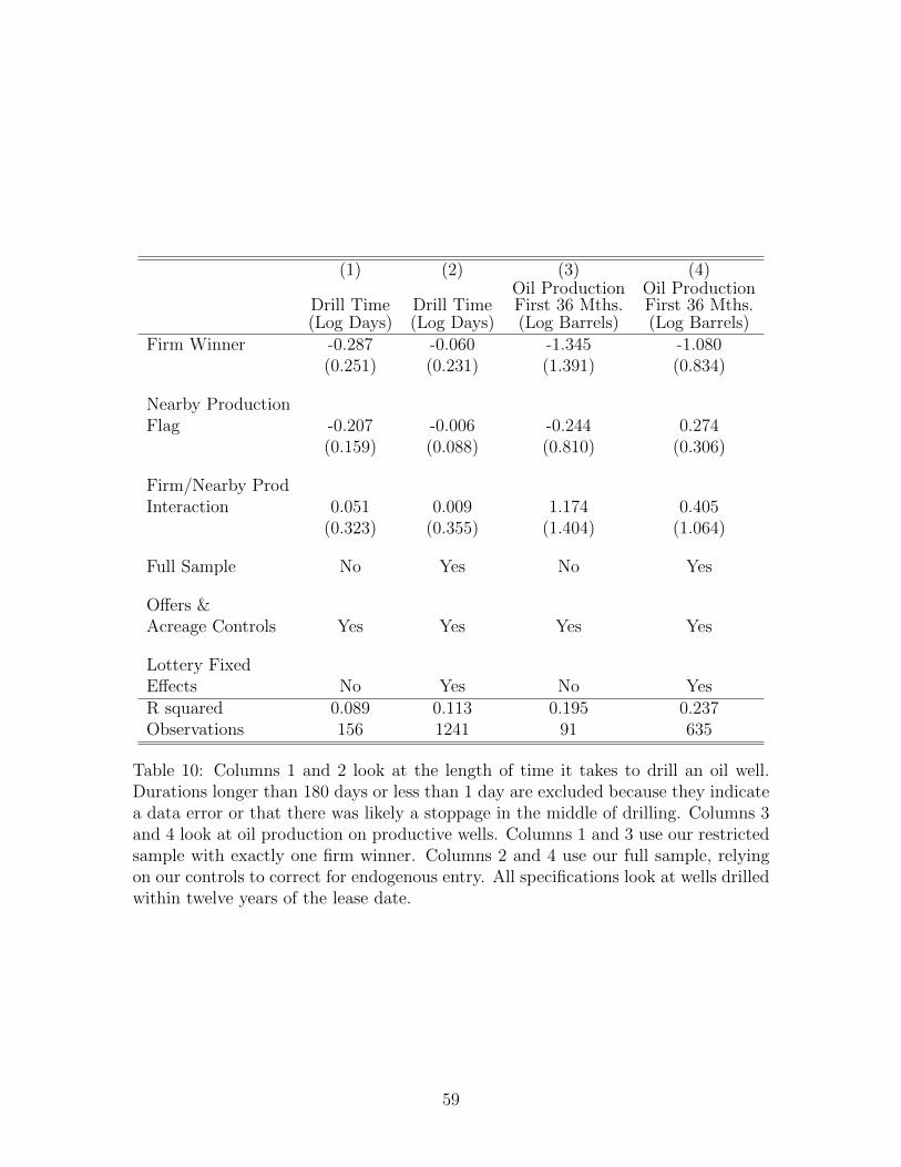
(1) (2) (3) (4)

Drill Time(Log Days)

Drill Time(Log Days)

Oil ProductionFirst 36 Mths.(Log Barrels)

Oil ProductionFirst 36 Mths.(Log Barrels)

Firm Winner -0.287 -0.060 -1.345 -1.080(0.251) (0.231) (1.391) (0.834)

Nearby ProductionFlag -0.207 -0.006 -0.244 0.274

(0.159) (0.088) (0.810) (0.306)

Firm/Nearby ProdInteraction 0.051 0.009 1.174 0.405

(0.323) (0.355) (1.404) (1.064)

Full Sample No Yes No Yes

Offers &Acreage Controls Yes Yes Yes Yes

Lottery FixedEffects No Yes No YesR squared 0.089 0.113 0.195 0.237Observations 156 1241 91 635

Table 10: Columns 1 and 2 look at the length of time it takes to drill an oil well.Durations longer than 180 days or less than 1 day are excluded because they indicatea data error or that there was likely a stoppage in the middle of drilling. Columns 3and 4 look at oil production on productive wells. Columns 1 and 3 use our restrictedsample with exactly one firm winner. Columns 2 and 4 use our full sample, relyingon our controls to correct for endogenous entry. All specifications look at wells drilledwithin twelve years of the lease date.

59

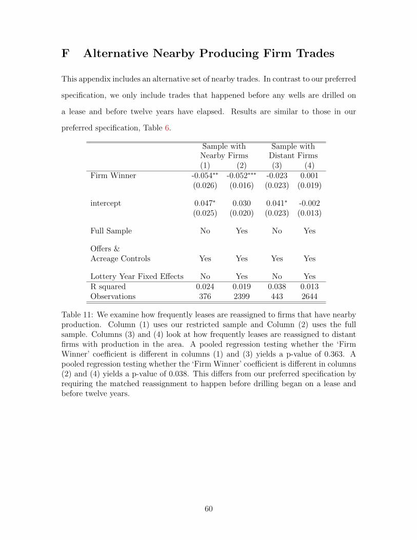
F Alternative Nearby Producing Firm Trades

This appendix includes an alternative set of nearby trades. In contrast to our preferred

specification, we only include trades that happened before any wells are drilled on

a lease and before twelve years have elapsed. Results are similar to those in our

preferred specification, Table 6.

Sample withNearby Firms

Sample withDistant Firms

(1) (2) (3) (4)Firm Winner -0.054∗∗ -0.052∗∗∗ -0.023 0.001

(0.026) (0.016) (0.023) (0.019)

intercept 0.047∗ 0.030 0.041∗ -0.002(0.025) (0.020) (0.023) (0.013)

Full Sample No Yes No Yes

Offers &Acreage Controls Yes Yes Yes Yes

Lottery Year Fixed Effects No Yes No YesR squared 0.024 0.019 0.038 0.013Observations 376 2399 443 2644

Table 11: We examine how frequently leases are reassigned to firms that have nearbyproduction. Column (1) uses our restricted sample and Column (2) uses the fullsample. Columns (3) and (4) look at how frequently leases are reassigned to distantfirms with production in the area. A pooled regression testing whether the ‘FirmWinner’ coefficient is different in columns (1) and (3) yields a p-value of 0.363. Apooled regression testing whether the ‘Firm Winner’ coefficient is different in columns(2) and (4) yields a p-value of 0.038. This differs from our preferred specification byrequiring the matched reassignment to happen before drilling began on a lease andbefore twelve years.

60