tmdl and plrg modeling of the lower st. johns river...
TRANSCRIPT

TMDL and PLRG Modeling of the
Lower St. Johns River
Technical Report Series Volume 1:
Calculation of the External Load
By:
John Hendrickson, Environmental Scientist
St. Johns River Water Management District
Nadine Trahan, GIS Analyst
Jones, Edmunds and Assoc.
Emily Stecker, Environmental Scientist
BCI Engineers and Scientists
Ying Ouyang, Ph.D., Environmental Scientist
St. Johns River Water Management District
May 2002
2
Table of Contents
INTRODUCTION AND APPROACH ........................................................................................................ 7
Project Area Description ........................................................................................................................... 8
Justification of the Conceptual Approach to the LSJR External Load .................................................... 10
Distinction of Labile and Refractory Organic Nutrients and Carbon ...................................................... 12
Organic Matter Composition Effects on Biodegradability And Nutrient Bioavailability ....................... 13
Objectives ................................................................................................................................................ 16
METHODS ................................................................................................................................................. 17
Separation of Labile and Refractory Organic Carbon, Nitrogen and Phosphorus .................................. 17
Overview ............................................................................................................................................. 17
Calculation of the External Load For the Lower St. Johns River ............................................................ 27
Point Source Load Estimation ............................................................................................................. 28
Non-Point Source Load Estimation ..................................................................................................... 29
Determination of the Upstream Load to the LSJR .............................................................................. 46
Determination of the Atmospheric Deposition Load ........................................................................... 53
RESULTS ................................................................................................................................................... 56
Tributary Organic Carbon and Nutrients ................................................................................................. 56
Calibration Data Set Summary ............................................................................................................ 56
Watershed Model Calibration .............................................................................................................. 58
Point Source Organic Carbon and Nutrients ........................................................................................... 70
Upstream Concentrations of Organic Carbon and Nutrients ................................................................... 72
Reconstruction Of The Upstream Natural Background Load ................................................................. 81
Natural Background Concentrations of Small Order, Undeveloped Streams ...................................... 81
Role of Spring Inputs ........................................................................................................................... 85
Historic Data for the St. Johns River ................................................................................................... 89
Total LSJR Load Estimates ..................................................................................................................... 97
Atmospheric Deposition ........................................................................................................................ 105
DISCUSSION ........................................................................................................................................... 106
Literature Cited ......................................................................................................................................... 113

3
FIGURES
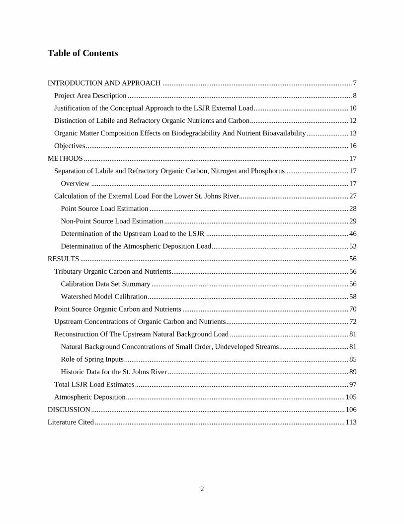
1. The Lower St. Johns River Basin ....................................................................................9
2. Comparison of Inorganic and Non-Inorganic Nutrient Fractions for Black Creek and
the Lower St. Johns River at Racy Point .......................................................................13
3. Rates of Exertion of BOD for Organic Substrates Typical of Northeast Florida Surface
Waters ............................................................................................................................19
4. Tributary Water Quality Sampling Stations for Watershed Modeling Set-up and Skill
Assessment ....................................................................................................................20
5. Organic Carbon:Nitrogen Ratio as a Function of the Percent Labile Organic Carbon
.......................................................................................................................................25
6. Organic Carbon:Phosphorus Ratio as a Function of the Percent Labile Organic
Carbon ...........................................................................................................................26
7. Relationship Between PLSM Predicted Runoff:Observed Runoff Ratio and Measured
Seasonal Whole Watershed Runoff Coefficient ............................................................34
8. Relative Position of the 1995-1999 Time Interval in the Historic Long Term Flow
Record ...........................................................................................................................35
9. Development of Hydrologic Correction Factors for the PLSM Runoff Coefficient .....38
10. Comparison of Original, Seasonal-fixed and Long-Term Rain Ratio Adjusted Runoff
Coefficients ...................................................................................................................39
11. Comparison of Original PLSM-Predicted, Long-Term Rain Ratio Adjusted and
Observed Cumulative Discharge Curves for LSJRB Calibration Watersheds, 1995-99
.......................................................................................................................................40
12. Monthly Mean Concentrations and 95% Confidence Intervals for Color and Total
Organic Carbon for 24 Unimpacted Blackwater Streams in Northeast Florida ............43
13. Watershed Model Input Areas for Nutrient Load Compilation ....................................46
14. Tributaries Forming the Lower St. Johns River ............................................................48
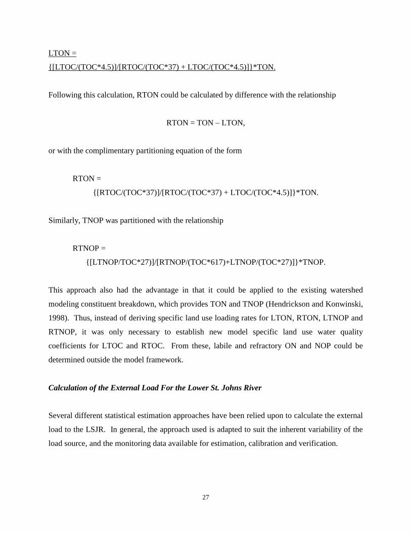
15. Flow chart for differentiation of laboratory analytical fractions into CE-QUAL-ICM
state variables for the lower St. Johns River upstream boundary at Dunns Creek and
Buffalo Bluff .................................................................................................................50
16. Comparison of Corrected Chlorophyll a and Algal Biovolume for Combined LSJR
Freshwater Water Quality and Plankton Analysis, 1995 – 2001 ..................................52

4
17. Comparison of POC:Algal Biovolume (a) and POC:Total Chlorophyll a Ratios to
Total Biovolume and Total Chlorophyll a Concentration for LSJR Freshwater Samples
.......................................................................................................................................54
18. Relationship Between Refractory Dissolved Organic Carbon and Color for Blackwater
Streams of the LSJR Basin ............................................................................................55
19. Comparison of Observed to Simulated Flow-Weighted Concentrations of Carbon,
Nitrogen and Phosphorus Forms for the December through March Season .................61
20. Comparison of Observed to Simulated Flow-Weighted Concentrations of Carbon,
Nitrogen and Phosphorus Forms for the April through July Season .............................63
21. Comparison of Observed to Simulated Flow-Weighted Concentrations of Carbon,
Nitrogen and Phosphorus Forms for the August through November Season ...............65
22. Partitioned Nitrogen Concentrations at (a) Buffalo Bluff and (b) Dunns Creek, Dec.
1994 - Nov. 1999 ...........................................................................................................74
23. Partitioned Phosphorus Concentrations at (a) Buffalo Bluff and (b) Dunns Creek, 1995
– 1999 ............................................................................................................................75
24. Partitioned Organic Carbon Concentrations at Buffalo Bluff and Dunns Creek, 1995 –
1999 ...............................................................................................................................76
25. Loads of Nitrogen Forms Entering the Lower St. Johns River at Buffalo Bluff and
Dunns Creek, 1995-99 ...................................................................................................79
26. Loads of Phosphorus Forms Entering the Lower St. Johns River at Buffalo Bluff and
Dunns Creek, 1995-99 ...................................................................................................80
27. Continuous Probability Density Functions for Total and Inorganic Nutrient Mean
Concentrations for Streams in Northeast Florida ..........................................................84
28. Time-Series Concentrations of Nitrate+Nitrite-N and Orthophosphate-P in Major
Springs Discharging to the St. Johns River That Exhibit Nitrate+Nitrite Trends .........86
29. Comparison of Present Day and Predicted Natural Background Concentrations of
Total Nitrogen and Total Phosphorus in the Lower St. Johns at Buffalo Bluff, 1995-99
.......................................................................................................................................88
30. Population growth within the 14 Counties of the St. Johns River Basin, 1890 – 2000
.......................................................................................................................................90
31. Comparison of Monthly Mean Water Quality Parameters for 1995-99 (solid boxes) to
the Data Collected by Pierce (1947) in 1939-40 (open diamonds) for the St. Johns
River near Buffalo Bluff................................................................................................95

5
32. Comparison of Total and Bioavailable Nitrogen Forms in Runoff from Natural
Forested and Mixed Urban/Commercial/Residential Watersheds ..............................108

6
TABLES
1. Tributary Water Quality Station Locations Employed in Determination of Labile and
Refractory Organic Nutrients ........................................................................................22
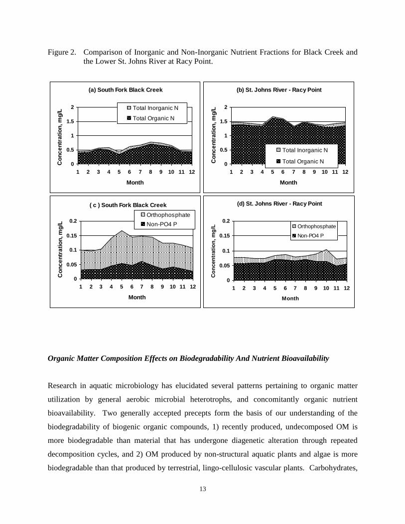
2. Point Source Facilities Included in the Calculation of the Lower St. Johns River
External Load ................................................................................................................23
3. Seasonal Runoff Coefficients for Application of the Pollution Load Screening Model
to the LSJR Basin ..........................................................................................................33
4. Seasonal Water Quality Coefficients Used in the PLSM to Predict Non-Point Source
Loads to the LSJR .........................................................................................................41
5. Total Organic, Labile Total Organic and Refractory Total Organic Carbon Land Use
Category Concentration Coefficients ............................................................................45
6. Mean Total, Inorganic, and Calculated Labile and Refractory Organic Nutrient and
Carbon Mean Annual Flow-Weighted Concentrations for Tributaries sampled within
the lower St. Johns River Basin .....................................................................................57
7. Pearson Correlations, Slopes, and Confidence Intervals of the Slopes for Intercept-Fit
Regressions Between Calibration Station Measured Flow-Weighted Concentrations
and Contributing Area Modeled Runoff-Weighted Concentrations .............................68
8. Summary of Point Source Mean Effluent Water Quality Concentrations ....................71
9. Total Phosphorus Concentrations Determined for Selected Locations in St. Johns
River Basin in 1952 .......................................................................................................92
10. Summary of Mean Annual Loads to the Lower St. Johns River, 1995 .........................98
11. Summary of Mean Annual Loads to the Lower St. Johns River, 1996 .........................99
12. Summary of Mean Annual Loads to the Lower St. Johns River, 1997 .......................100
13. Summary of Mean Annual Loads to the Lower St. Johns River, 1998 .......................101
14. Summary of Mean Annual Loads to the Lower St. Johns River, 1999 .......................102
15. Summary of Overall Mean Annual Loads to the Lower St. Johns River, 1995-99 ....103

7
INTRODUCTION AND APPROACH
Accelerated eutrophication arising from nutrient enrichment of estuaries represents one of the
most significant water quality problems faced by near coastal waters worldwide (National
Research Council, 2000). Within the United States, part of this problem rests in the standards-
based approach to water quality control, in which the potential harm incurred by sources is
evaluated based upon effluent and near-field concentrations of pollutants. In this approach,
cumulative loads of substances, in particular nutrients, have been overlooked, with the result that
receiving water assimilative capacities have been overwhelmed. This situation has increasingly
lead water managers to resort to the TMDL process (CWA Section 303(d)) as a means of
eutrophication control. To address problems associated with accelerated eutrophication in the
lower St. Johns River estuary (LSJR), both the Florida Department of Environmental Protection
(FDEP) and the St. Johns River Water Management District (SJRWMD) are jointly executing a
strategy for nutrient pollution control that fulfills their respective responsibilities for the
establishment of TMDLs for impaired water bodies and stormwater PLRGs (F.A.C. Chapter 62-
40).
A generally accepted approach has evolved for addressing estuarine eutrophication in which the
sources, magnitude and timing of the external nutrient load are linked to the effects of the
receiving water body. Because of the temporal and spatial disconnect between the entry of
nutrient loads and the manifestation of eutrophication effects, and the need to predict the levels
of expected improvement with various nutrient reduction strategies, dynamic water quality
process models have become invaluable tools in estuarine nutrient management efforts. Such
models “process” the external load in a time-sequential fashion in a 2 or 3-dimensional
discretized grid that approximates the morphology of the water body. In the context of
eutrophication, relevant “processes” are the biological processes photosynthesis and algal carbon
fixation, community respiration (as both a loss of organic carbon and exertion of oxygen
demand), and organic nutrient re-mineralization, as well as physical processes such as oxygen
reaeration, substance advection, molecular dispersion, solar light absorption, and sedimentation.

8
In this modeling approach to the establishment of nutrient pollution reductions, two large
investigative efforts must be undertaken: one to quantify the timing, magnitude, and spatial
nature of the incoming nutrient load, referred to as the “external load”, and another to determine
the effect of this load on the receiving water body. This report describes the first element of this
intricate undertaking for the Lower St. Johns River, that of the derivation of the external load.
Project Area Description
The St. Johns River is one of the largest blackwater rivers of the southeast U.S. The river is
located in northeast Florida and drains about 1/5th
of the state, encompassing a 9,562 square mile
drainage area. The river is slow moving, with a slope of only 1.4 in/mi (Toth, 1993), and is
essentially at sea level for its final 125 mi. The lower St. Johns is the estuarine portion of the
river, formed at the confluence of the middle St. Johns and the Ocklawaha River, and
encompassing a 2,750 square mile area (Figure 1). Within this reach, the St. Johns River is
slightly more that 100 miles long and has a water surface area, including tributary mouths below
head of tide, of 85,000 acres. The lower St. Johns can be differentiated into three riverine
salinity and limnologic zones: a fresh tidal lacustrine zone which extends from the city of Palatka
north to approximately the mouth of Black Creek; a predominantly oligohaline, lacustrine zone
extending from the mouth of Black Creek northward to the Fuller Warren Bridge (I-95) in
Jacksonville; and a mesohaline/polyhaline, riverine zone downstream to the mouth. The slow
moving, lacustrine nature of the river facilitates phytoplankton primary production, and spring
and summer algal blooms in this nutrient-rich river often exhibit chlorophyll a concentrations
exceeding 100 g/L.
The southern portion of the lower basin is largely rural, with predominant land uses in forestry
and row crop agriculture. The northern portion of the basin is distinguished by the heavily
urbanized cities of Jacksonville, Orange Park and Middleburg. Roughly three quarters (64 to 82
percent) of the basin’s highly developed land uses (medium and high residential, high intensity
commercial and industrial) drain to the oligohaline and mesohaline lower St. Johns. In contrast,
62 to 98 percent of the basin’s agricultural land uses drain to the fresh tidal reach.
9
Figure 1. The Lower St. Johns River Basin.

10
The existence of poor water quality in the LSJR has been identified in a number of reports dating
back to at least 1947 (Florida State Board of Health 1947). Because of these problems, the
establishment of TMDLs and PLRGs for the lower St. Johns River are a high priority, and an
aggressive schedule has been established that seeks the identification of river assimilative
capacity and general allocation to major sources by the end of 2002.
Comprehensive external nutrient load assessments have been performed twice previously for the
LSJR. In 1976, the firm of Atlantis Scientific (Atlantis Scientific, 1976), under authorization of
the 1972 Clean Water Act Section 315, undertook a computation of the external load and
concluded that point source comprised the majority of this load. Hendrickson and Konwinski
(1998) also computed the external load to the river for 1993-94, and concluded that nitrogen and
phosphorus were 2.5 and 6 times greater than natural background, with augmented nutrient loads
(that load above natural background) approximately evenly split between point and nonpoint
sources.
Justification of the Conceptual Approach to the LSJR External Load
By virtue of its long term presence in the St. Johns River and its frequent project partnerships
with the SJRWMD, the U.S. Army Corps Jacksonville District has brought valuable assistance to
the river TMDL and PLRG development. This partnership has provided the assistance of the
U.S. Army Engineer Research and Development Center (ERDC) at Vicksburg, MS, to assist in
the examination of the nature of the interaction between river processes and the external load.
To quantify this interaction, the ERDC has adapted its water quality model, CE-QUAL-ICM
(Corps of Engineers Water Quality Integrated Compartment Model), to the LSJR. CE-QUAL-
ICM (hereafter referred to as just ICM) was developed to study eutrophication processes in
Chesapeake Bay (Cerco and Cole, 1994), however, as ICM simulates the fundamental processes
related to algal (and plant) growth, death and decomposition, its robust model formulation is
applicable to a wide range of water bodies and even wetlands. ICM differs from another widely
used water quality model, WASP, in that it predicts eutrophication effects – transparency loss,
dissolved oxygen sags, and sedimentation - through the use of a carbon budget, rather that

11
relying on the input and internal formation of biochemical oxygen demand and chlorophyll a.
Because ICM allows for the distinction of carbon and nutrients compartmentalized within labile
and refractory forms, it is in theory particularly useful for applications in blackwater river
estuaries.
Along with the mixture of inorganic and nutrient-bearing organic substrates (such as animal and
human waste, industrial process effluents, and algae or algal detritus) that are the focus of
anthropogenic nutrient enrichment, blackwater rivers and streams also exhibit significant nutrient
content of natural origin. Large portions of this natural nutrient load, as much as 40 percent of
the phosphorus, and over 90 percent of nitrogen, are contained within the organic fraction.
Strong relationships between total organic carbon and color suggest that the majority of this
natural, organic nutrient load is contained within colored, dissolved organic matter (CDOM) of
terrestrial and riparian vascular plant origin. Although natural CDOM is generally believed to be
resistant to microbial decomposition and largely unavailable for utilization by phytoplankton in
typical estuarine residence times, these heterogeneous, humic substances contain a substantial
amount of nitrogen (N) and phosphorus (P) in their structures (DeBusk et al, 2001), and hence
the sheer volume of the material with respect to other OM pools dictates its relevance be
considered.
With the capabilities of ICM come fairly rigorous requirements on the detail of the external
nutrient and carbon load that must be input for model simulations. The most difficult of these
determinations is the separation of the external organic nutrient and carbon load into labile
(easily decomposed and utilized) and refractory (slowly decomposed) components based upon
readily available water quality monitoring data. This technique for separation needs to extend
also to the river water quality monitoring calibration data set for ICM. In order to predict the
changes in the external load with various nutrient reduction strategies, it is not sufficient to only
characterize the incoming labile and refractory carbon and nutrient load; the relationship between
land development and organic carbon and nutrient bioavailability must also be described. An
additional relationship must be addressed between the concentration of colored dissolved organic
matter (CDOM) and water column transparency in order for the appropriate functioning of the
ICM light attenuation algorithm in the algal photosynthesis calculation.

12
Distinction of Labile and Refractory Organic Nutrients and Carbon
It is generally understood that dissolved, inorganic forms of nutrients (NO2+3, NH4, and PO4), as
well as some low molecular weight organic compounds such as urea, are immediately available
for algal growth, while organic nutrient forms, which must first undergo desorption (if
particulate bound), hydrolysis, bacterial decomposition or photo-decomposition (Bushaw et al.
1996) for inorganic nutrient regeneration and subsequent utilization by phytoplankton, are less
readily available. Organic nutrient bio-availability for aquatic primary production is dependent
upon the utilization preference of the parent organic substrate by general microbial heterotrophs
(DeBusk et al., 2001), which must first decompose this substrate in order to liberate mineral
nutrient forms. With regard to organic carbon and nutrient bioavailability, a general working
hypothesis has evolved that partitions organic carbon and nutrients into two pools: a labile pool,
that can be utilized in time frames relevant to water quality processes of interest in the receiving
water, and a refractory pool, that is decomposed very slowly and essentially inert for relevant
time frames (Wetzel, 1983). The bioavailablility of the organic nutrient pool represents an
important issue in the assessment of nutrient enrichment in blackwater rivers of the southeast
U.S. coastal plain, as much of the total phosphorus (TP) and most of the total nitrogen (TN)
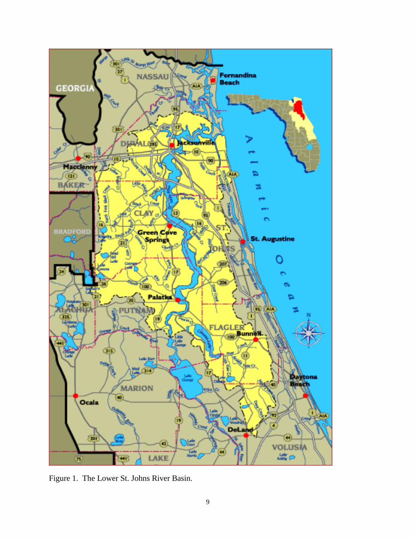
enters the river as an organic or non-inorganic form (Figure 2).
Relatively little attention has been paid to differences in organic nutrient bioavailability in
assessments of external loads to eutrophic water bodies (Stepanauskas et al., 1998). This may be
due to the predominance of inorganic nutrients in river flow to intensely studied temperate
estuaries, leading most authors to not further differentiate the organic nutrient pool (Magnien et
al. 1992; Goolsby et al. 2001) or even to distinguish it from the inorganic nutrient-dominated
total nutrient pool (Boynton et al. 1995; Jaworski et al. 1992; Valiela et al. 1992). This lack of
differentiation extends also to land use-loading rates applied in watershed load indexing models
(Hartigan et al., 1982; Adamus and Bergman, 1995; Harper, 1994; EPA, 1984), to the commonly
used, process-based watershed models such as HSPF, to agronomic field scale models such as
GLEAMS, and to water quality process models such as WASP.
13
Figure 2. Comparison of Inorganic and Non-Inorganic Nutrient Fractions for Black Creek and
the Lower St. Johns River at Racy Point.
Organic Matter Composition Effects on Biodegradability And Nutrient Bioavailability
Research in aquatic microbiology has elucidated several patterns pertaining to organic matter
utilization by general aerobic microbial heterotrophs, and concomitantly organic nutrient
bioavailability. Two generally accepted precepts form the basis of our understanding of the
biodegradability of biogenic organic compounds, 1) recently produced, undecomposed OM is
more biodegradable than material that has undergone diagenetic alteration through repeated
decomposition cycles, and 2) OM produced by non-structural aquatic plants and algae is more
biodegradable than that produced by terrestrial, lingo-cellulosic vascular plants. Carbohydrates,
(a) South Fork Black Creek
0
0.5
1
1.5
2
1 2 3 4 5 6 7 8 9 10 11 12
Month
Co
nc
en
tra
tio
n, m
g/L
Total Inorganic N
Total Organic N
(b) St. Johns River - Racy Point
0
0.5
1
1.5
2
1 2 3 4 5 6 7 8 9 10 11 12
Month
Co
nc
en
tra
tio
n, m
g/L
Total Inorganic N
Total Organic N
( c ) South Fork Black Creek
0
0.05
0.1
0.15
0.2
1 2 3 4 5 6 7 8 9 10 11 12
Month
Co
nc
en
tra
tio
n, m
g/L
Orthophosphate
Non-PO4 P
(d) St. Johns River - Racy Point
0
0.05
0.1
0.15
0.2
1 2 3 4 5 6 7 8 9 10 11 12
Month
Co
ncen
trati
on
, m
g/L Orthophosphate
Non-PO4 P

14
proteins, lipids, nucleic acids and pigments are decomposed in relatively short time frames, while
humic substances are less readily decomposed and in some cases essentially inert (Wetzel, 1983;
Moran and Hodson, 1990; although this assertion is contradicted in the work of Volk et al., 1997,
who find similar utilization of humic substances). The biodegradability of natural OM that
occurs in aquatic systems and its bioavailability of incorporated C, N and P can be viewed as
dependent largely upon two factors: 1) whether the material is allochthonous or autochthonous in
origin, and 2) whether or not the OM has undergone some degree of decomposition and
diagenetic alteration prior to its entry to surface waters. Thus it generally holds that
autochthonous OM is more labile than allochthonous OM, and that the humic fraction of DOM is
less bioavailable on a mole carbon than non-humic DOM (Kaplan and Newbold 1995; Moran
and Hodson, 1990; Moran et al., 1999). In their work on piedmont and blackwater river OM in
the southeast U.S., Sun et al. (1997) demonstrate that the compositional changes that accompany
diagenetic condensation relate directly to bioavailability, with blackwater stream OM appearing
the most refractory per mole carbon. This assertion is in congruity with work that has shown
some forms of soil humus in the allochthonous organic carbon pool to be decades to hundreds of
years old (Raymond and Bauer, 2001).
Surprisingly, this difference in OM bioavailability runs contrary to the “smaller is better”
nutrient utilization paradigm, in that particulate organic nutrients in surface waters, in the form of
algal cells or relatively undecomposed plant detritus, are generally more readily available than
dissolved forms. Within the dissolved organic matter pool (<0.45 m diameter), high molecular
weight organic compounds (> 10,000 nMW) also have been to found to be more bioavailable
(Tranvik, 1990; Amon and Benner 1996; Gardner et al., 1996; Mannino and Harvey 2000) than
low molecular weight DOM (< 1000 nMW). In the Amazon River, Hedges et al. (1994)
considered DOM to be the most profoundly degraded material, hence the most refractory,
mobilized through a process of “selective solubilization”.
Also fundamental to the bioavailability of organic nutrients for primary production is whether or
not OM decomposition will result in nutrient regeneration (e.g., an increase in water column
inorganic nutrients) or nutrient immobilization to meet bacterial growth needs. Goldman et al.
(1987) postulated that if the substrate C:N and C:P ratios are sufficiently low such that, when

15
corrected for carbon gross growth efficiency (the fraction of the total carbon decomposed that is
retained as bacterial biomass), N and P remain in excess of bacterial growth needs, then these
nutrients will be regenerated in the inorganic form and be potentially available for incorporation
by phytoplankton. Because labile OM is high in proteins, amino acids and cellular metabolic
organic compounds that exhibit relatively low C:N and C:P ratios, decomposition of labile
substrates in the aquatic environment tends to lead to the regeneration of N and P. Conversely,
substrates with a high C:N, such as aquatic humic OM (averaging 50:1 molar; Thurman, 1985),
will tend to immobilize inorganic N and P (Mann, 1988; Strauss and Lamberti, 2000). Not
surprisingly, organic substrates with high C:N ratios that typically exist in the aquatic
environment exhibit low biological availability, and concomitantly a low likelihood that bacterial
decomposition of this substrate can regenerate mineral nutrients for autotrophs (Bushaw et al.,
1996). Because of these general differences, C:N and C:P ratios have been a commonly used
proxy for bioavailability of OM.
No clear definition exists on what constitutes labile verses refractory, and whether or not the
range between the two extremes exists as a continuum or as discrete states. Labile substrates
have been described as those utilized within timeframes of one to two weeks (Sondergaard and
Middelboe, 1995); as utilization through the exponential growth phase to the stationary phase
(approximately 2 days; Stepanauskas et al., 1999; approximately 4 days for DON of the
Delaware River (Seitzinger and Sanders 1997)); or in-situ bioreactor residence time (4 to 18
hours; Volk et al., 1997). The first order decay coefficient of 0.075 day-1
used by ICM (Cerco
and Cole, 1995) yields a duration of 9.2 days for 50% utilization of the original labile substrate,
and 30 days for 90% utilization. Moran and Hodson (1989), in their investigation of fresh and
salt marsh plant ligno-cellulose, observed what appeared to be distinct rates of utilization,
suggesting distinct, uniform chemical classes driving separate utilization rates. Similarly, Ogura
(1975) determined that two distinct pools of dissolved organic compounds existed in most
aquatic systems.
In various examinations of surface waters exhibiting a range of human impact, the biodegradable
percent of the total OC pool has been found to vary between 1 and 86 percent (Sun et al., 1997).
For most rivers dominated by allochthonous OC, the range is closer to between 7% to 25%

16
(Sondergaard and Middelboe, 1995; Volk et al., 1997), with blackwater rivers exhibiting the
lowest relative amounts of labile OC (Moran et al., 1999). Stepanauskas et al. (2000), in their
study of Scandinavian rivers, estimated the percent of labile dissolved organic nitrogen (DON) as
between 19 and 55%.
Objectives
The objectives of this report are
1) describe the approach to partitioning organic carbon and nutrients in the external load to
the LSJR, for the purpose of distinguishing the relative bioavailability of these forms and
hence the impact on eutrophication;
2) determine the relationship between land development factors and the relative
bioavailability of carbon and nutrient forms in runoff at a watershed scale, for the
purpose of modeling the external carbon and nutrient load, and predicting the changes in
this load with changes in land development patterns;
3) determine the load to the LSJR from all sources – upstream, within basin point and non-
point sources, and atmospheric sources – in order to assess the relative effects of these
sources on eutrophication; and
4) reconstruct the natural background load to the LSJR, for the purpose of putting present-
day loading rates in perspective, and for gauging the baseline level of productivity of the
LSJR in its pre-development state.

17
METHODS
Separation of Labile and Refractory Organic Carbon, Nitrogen and Phosphorus
Overview
To partition labile and refractory organic carbon and nutrients in the external load calculation, a
two-step empirical approach was developed. First, a conceptual model was developed relating
the rate of oxygen consumption during decomposition to total organic carbon to determine
overall decomposition rate, based upon partial decomposition rates for labile and refractory
organic material already established within ICM. This model was then applied to a water quality
data base of tributary sampling stations and point source effluents to partition labile and
refractory organic carbon. A multiple regression approach was employed to establish specific
land use, labile and refractory organic carbon runoff concentrations, and these specific land use
organic carbon concentrations are then applied to a watershed model to develop whole-basin
labile and refractory organic carbon loads. The second step partitioned organic N and P based
upon the relative amounts of labile and refractory organic carbon. Again employing the tributary
water quality monitoring and point source effluent data, C:N and C:P ratios were related to the
percent of labile organic carbon, and this relationship used to predict refractory and labile C:N
and C:P ratios. These ratios were then used to sub-divide the previously modeled organic
nitrogen and non-orthophosphate phosphorus (TP-PO4) loads into labile and refractory fractions.
Model for Organic Carbon Partitioning
Organic carbon found in surface waters is borne in a mix of organic matter from multiple
sources. This complex mix of organic substrates is assumed to be composed of fractions that are
readily available for microbial decomposition (labile) and relatively unavailable (refractory).
The degree of organic carbon lability in oxygenated surface waters should, in theory, be reflected
in carbonaceous biochemical oxygen demand (CBOD), with labile substrates consuming more
oxygen per mole of carbon in the test period (typically 5 days) than refractory substrates.

18
Consumption of organic carbon by bacterial heterotrophs has generally been found to adhere to
first-order exponential decay. Chapra (1977) provides this relationship in the following form, in
which the maximum amount of CBOD that can be exerted on a substrate, CBODultimate, is related
to that amount consumed in time t, by the relationship:
Ct = Co(1-e-kt
)
where Ct is the oxygen (or carbon) consumed at time t, Co is the BODultimate, and k is the
substrate-specific decomposition coefficient.
In practice, measurements of ultimate BOD are rarely performed, although total organic carbon,
a frequently measured constituent, should in theory be related to ultimate BOD. The molar rate
of O2 consumption per CO2 production has typically been set at 1:1 in computations of
community respiration (Wetzel and Likens, 1990; as per the respiratory quotient (RQ) of
Strickland, 1960). In the computations here, a RQ of 1 mole O2 consumed per 1 mole of OC
consumed, or mass ratio of 2.67:1, was used.
Figure 3 demonstrates the theoretical rate of change in BOD exerted over time for various
homogeneous categories of substrates common to surface waters of northeast Florida, and their
associated decay coefficients. Algal biomass and domestic waste organic matter appear to be
highly labile substrates, while pulp mill effluent and colored dissolved organic matter in runoff
of native, undeveloped blackwater streams appear to be relatively refractory. Decay coefficients
established in the CE-QUAL-ICM model of 0.075 day-1
for labile substrates and 0.001 day-1
for
refractory substrates appear representative of the range in decay coefficients for the aquatic
organic substrates in Figure 3. In comparison, decay rates determined by Moran et al. (1999) for
5 rivers of the southeast U.S., expressed as first order decay coefficients, ranged from 0.003 day-1
to 0.001 day-1
.

19
Figure 3. Rates of Exertion of BOD for Organic Substrates Typical of Northeast Florida
Surface Waters. Model of the form Ct = Cu(1-e-Kt), adapted from Chapra (1997). Cu
= ultimate BOD exertion, estimated from TOC from 2.67:1 mass ratio of O2
consumption to OC consumption and respiratory quotient =1. Algae: Determined
from mean BOD data from lake Dora, FL; phytoplankton organic carbon determined
form 50:1 carbon:chlorophyll a. Value should be considered the sum of algal
respiration and bacterial decomposition. Secondary WWTP effluent from a sampling
of 23 point sources of the lower St. Johns River basin. Pulp and paper determined
form a large mill in the lower St. Johns River basin. Native DOM developed from the
mean of undeveloped blackwater streams in northeast Florida.
Determination of Labile and Refractory Organic Carbon
To partition labile and refractory organic carbon, tributary runoff and point source effluent water
quality monitoring data collected between 1993 to 1999 within the lower St. Johns River basin
were compiled to create a data base of BOD, nutrients and organic carbon. Tributary station
descriptions and number of events sampled are included in Table 1, and the locations of these
tributaries and their contributing areas are shown in Figure 4. Point sources are listed in Table 2.
Stations were included in the analysis if the sample constituent suite included CBOD, total
0
10
20
30
40
50
60
70
80
90
100
0 10 20 30 40 50 60
Time, days
Pe
rce
nt
of
Ult
ima
te B
OD
Exe
rted
, o
r P
erc
en
t o
f
To
tal
Org
an
ic C
arb
on
Co
ns
um
ed Algae
K = 0.094 day-1
2ndary STP
K = 0.0386 day-1
Pulp & Paper Eff.
K = 0.0096 day-1
Native DOM
K = 0.0022 day-1

20
Figure 4. Tributary Water Quality Sampling Stations for Watershed Modeling Set-up and Skill
Assessment.

21
organic carbon, total phosphorus, orthophosphate, total ammonia and total nitrate+nitrite
nitrogen. In all, 789 samples were available for 28 surface water stations and 22 point sources.
Sample total organic carbon was considered to be the sum of carbon within labile substrates
(labile total organic carbon, or LTOC) and refractory substrates (refractory total organic carbon,
or RTOC), the proportions of which can be determined through the simultaneous expression of
their rates of decomposition, as indicated by oxygen consumption in the 5-day biochemical
oxygen demand (BOD5) test. Using the rates of decomposition of the first-order decay model of
0.075 day-1
for labile substrates, and 0.001 day-1
for refractory, a pair of equations for the
simultaneous solution of labile and refractory portions can be set up in the form:
(1) TOCt=5 = RTOC(1-e-(0.001)*5
) + LTOC(1-e-(0.075)*5
)
(2) TOCt= = RTOC(1-e-(0.001)* ) + LTOC(1-e
-(0.075)* )
where RTOC = refractory total organic carbon, and LTOC = labile TOC. In equation (1), the
moles of TOC decomposed at t=5 was assumed to be in unity (RQ = 1) with the moles of oxygen
consumed (CBOD5) and was converted to TOC consumed by dividing by 2.67. When all TOC is
consumed, at t = , (analogoug to ultimate BOD) the exponent term in parenthesis goes to zero,
and TOC = RTOC + LTOC. The above paired equations were simplified for computation
through the following steps:
(1) (CBOD5/2.67) = RTOC*(0.005) + LTOC*(0.3127)
(2) TOC = RTOC*(1) + LTOC*(1)
(1) 200*[(CBOD5/2.67) = RTOC*(0.005) + LTOC*(0.3127)]
(2) TOC = RTOC*(1) + LTOC*(1)
(1) CBOD5*74.906 - LTOC*(62.54) = RTOC
(2) TOC - LTOC = RTOC

22
Table 1. Tributary Water Quality Station Locations Employed in Determination of Labile and Refractory Organic Nutrients
Station
Abbreviation Station Description Latitude Longitude
River
Mile
Entry
Point Samp. No.
Urban,
Commercial,
Residential
Fraction
High
Intensity,
Livestock
Fraction
Row Crop,
Citrus, Low
Intensity
Fraction
Forested
Fraction
16MCRK 16 Mile Creek at Deep Crk Rd. W 293932.27 812741.76 11 0.0 0.0 84.9 15.1
ARLRM Arlington River Near Mouth Below Pottsburg Ck 301917.00 813558.00 20 6 57.8 0.1 10.9 27.7
BC218 BRADLEY CREEK @ 218 300035.28 814824.12 7 0.0 0.0 0.9 99.1
BC739 BRADLEY CREEK @ 739 300246.86 814705.10 20 5.6 0.0 25.2 69.2
BLC Black Creek at Hwy 209 300455.00 814835.00 44 47
BRDRM Broward River Near Mouth at Hecksher Drive 302500.00 813608.00 3 5
BSF South Fork of Black Creek at Hwy 218 300337.00 815218.00 44 44 3.5 1.1 9.8 84.8
CCR Clarkes Creek at US 17 295242.00 813950.00 56 5
CEDSJ Cedar River Above San Juan Blvd 301654.00 814426.00 26 19 67.5 0.2 12.8 17.7
DBR Dog Branch 50 meters downstr. County Rd. 207 A 294143.00 813450.00 67 29 4.4 0.0 81.5 13.8
DCH Deep Creek headwaters 294034.00 812800.00 19 0.0 0.0 73.4 26.0
DPB Deep Creek at Railroad Bridge 294345.00 812914.00 67 47 0.7 0.0 74.1 24.6
DUNCM Dunn Creek Near Mouth at Hecksher Drive 302516.00 813509.00 3 4
GC16 Governors Creek at Hwy 16 Near Green Cove 295902.00 814211.00 22 8.8 0.4 24.0 66.8
GC315 Green's Creck above County Rd. 315 295438.00 814740.00 3 0.0 0.9 3.6 95.5
GOV Governors Ck Near Mouth @ Seaboard Coast Rr Bridge 300014.00 814133.00 6
ML209 MILL LOG @ 209 300344.72 814525.66 15 0.6 3.6 28.1 67.2
MLRMC Mill Log Creek @ Russell Missionary 300305.00 814546.00 19 0.4 7.5 50.9 40.0
MOB Moccasin Branch On SR 13 294617.00 812850.00 30 1.3 0.3 39.5 58.7
NBC North Fork of Black Creek at SR 21 300432.00 815150.00 44 48 4.6 1.1 13.5 79.2
OHD Outlet of Hastings Drainage District 294249.00 813243.00 31 1.3 0.0 38.8 59.7
ORTCR Ortega River @ Collins Road 301203.00 814351.00 1
ORTTM Ortega River Above Timaquana Road 301451.00 814236.00 26 13 35.0 0.2 14.8 48.5
PCRHR Peters Creek at Rosemary Hill Rd 300025.00 814454.00 24 1.1 0.8 5.5 92.6
PTC Peters Creek at Hwy 209 300200.00 814329.00 44 82 1.5 4.7 13.3 79.9
SMC Sixmile Creek at SR 13 295732.00 813237.00 51 56 2.0 2.1 20.4 75.1
TRC Trout Creek at SR 13 295905.00 813358.00 51 12 1.6 0.1 9.1 88.5
TRTRM Trout River Near Mouth Below Main St Bridge 302337.00 813856.00 15 4
Total 629
23
Table 2. Point Source Facilities Included in the Calculation of the Lower St. Johns River External Load
Facility ID Facility Name Data
Freq.
Service Area
(Ac.)
Design
Capacity
(MGD)
1997-98
Mean Flow
(MGD)
Connect % Facility
Latitude
Facility
Longitude
Model Grid
#
IC JC
R-Seg.
FL0023493 MANDARIN WWTF Daily 30690 7.50 4.81 57.0 30.17903 -81.62241 1504 100 28 Oligohal
FL0026000 BUCKMAN STREET WWTF Daily 73143 52.50 33.06 79.0 30.35232 -81.62898 1121 55 24 Mesohal
FL0026441 ARLINGTON EAST WWTF Daily 63576 11.00 10.85 49.0 30.34665 -81.54316 1061 39 48 Mesohal
FL0026450 JAX DISTRICT II WWTF Daily 67105 10.00 4.32 89.0 30.42293 -81.61842 338 36 24 Mesohal
FL0026468 SOUTHWEST DISTRICT WWTF Daily 48194 10.00 5.86 43.0 30.23276 -81.72250 1422 90 20 Oligohal
FL0000400 STONE CONTAINER CORPORATION Monthly 20.00 8.85 N/A 30.41900 -81.60420 183 28 21 Mesohal
FL0000892 JEFFERSON SMURFIT CORPORATION Monthly 7.00 5.79 N/A 30.36670 -81.62500 1035 51 24 Mesohal
FL0002763 GEORGIA PACIFIC, PALATKA Monthly N/A 50.00 34.24 N/A 29.68247 -81.68278 2027 171 20 Fresh
FL0020231 JACKSONVILLE BEACH Monthly 3.07 874 31 81 Mesohal
FL0020427 NEPTUNE BEACH WWTF Monthly 1321 1.50 0.94 97.0 30.31558 -81.42007 874 31 81 Mesohal
FL0020915 GREEN COVE SPRINGS, CITY OF Monthly 4083 0.75 0.46 85.0 30.00724 -81.69646 1679 121 20 Fresh
FL0022489 WESLEY MANOR RETIRMNT VILL-JAX Monthly 0.1 0.05 30.11390 -81.60610 1573 110 31 Oligohal
FL0023248 BUCCANEER WWTF Monthly 1785 1.30 1.00 95.0 30.36976 -81.41157 874 31 81 Mesohal
FL0023604 MONTEREY WWTF Monthly 3684 3.60 3.02 55.0 30.33060 -81.60116 1158 59 27 Mesohal
FL0023621 HOLLY OAKS SUBDIVISION Monthly 3803 1.00 0.00 72.0 30.35752 -81.52208 1105 43 54 Mesohal
FL0023663 SAN JOSE SUBDIVISION Monthly 2225 2.25 2.09 88.0 30.24698 -81.62258 1430 94 28 Oligohal
FL0023671 JACKSONVILLE HEIGHTS Monthly 2.50 1.19 30.24100 -81.75670 1384 86 12 Oligohal
FL0023922 ORANGE PARK, TOWN OF Monthly 2694 2.50 1.34 99.5 30.18241 -81.70981 1511 103 21 Oligohal
FL0024767 SAN PABLO WWTF Monthly 1260 0.50 0.46 84.0 30.27763 -81.43065 1343 53 78 Mesohal
FL0025151 MILLER STREET WWTP Monthly 8471 5.00 3.41 65.0 30.17820 -81.71228 1511 103 21 Oligohal
FL0025828 ORTEGA HILLS SUBDIVISION Monthly 191 0.22 0.14 89.0 30.21869 -81.70962 1452 92 12 Oligohal
FL0026751 ROYAL LAKES Monthly 2.40 2.33 30.21389 -81.54440 1458 96 29 Oligohal
FL0026778 BEACON HILLS WWTF Monthly 2266 1.30 0.75 98.0 30.38379 -81.52166 750 31 57 Mesohal
FL0026786 WOODMERE SUBDIVISION Monthly 1106 0.50 0.35 97.0 30.37987 -81.60245 712 44 27 Mesohal
FL0030210 SOUTH GREEN COVE SPRINGS WWTF Monthly 3526 0.50 0.27 85.0 29.98259 -81.66759 1723 125 21 Fresh
FL0032875 FLEMING OAKS WWTP Monthly 5159 0.49 0.30 65.0 30.07463 -81.70457 1629 115 22 Oligohal
FL0038776 ATLANTIC BEACH WWTF Monthly 2218 3.00 1.70 92.0 30.33551 -81.40882 874 31 81 Mesohal
FL0040061 PALATKA, CITY OF Monthly 4724 3.00 2.76 95.0 29.61582 -81.65123 2175 182 42 Fresh
FL0041530 ANHEUSER BUSCH MAIN ST. LAND APP. Monthly 1.46 30.45278 -81.65000 89 29 11 Mesohal
FL0042315 CITY OF HASTINGS Monthly 0.06 29.72500 -81.50000 1927 154 29 Fresh
FL0043591 JULINGTON CREEK WWTP Monthly 6141 1.00 0.21 56.0 30.10634 -81.62597 1613 113 30 Oligohal
FL0043834 FLEMING ISLAND SYSTEM WWTP Monthly 8878 1.50 0.69 65.0 30.09279 -81.71982 1616 113 22 Oligohal
FL0117668 UNITED WATER FL - ST. JOHNS NORTH Monthly 0.00 30.09556 -81.61089 1613 113 30 Oligohal
FLA011427 USN NS MAYPORT Monthly 0.98 30.39690 -81.39750 558 31 94 Mesohal
FLA011429 USN NAS JACKSONVILLE Monthly 1.09 30.24138 -81.67580 1432 91 20 Oligohal
Brierwood S/D - Beauclerc STP Monthly 0.78 0.00 1445 95 29 Oligohal

24
Solving these 2 equations for LTOC produces:
LTOC = (CBOD5*74.906-TOC)/61.54
And;
RTOC = TOC – LTOC
In calculations, 2 of the 88 point source samples and 6 of the 702 tributary samples had CBOD5
values that indicated decay rates less than 0.001 day-1
; conversely, 3 point source samples in the
data set exhibited CBOD5 values that when converted to TOC exceeded the TOC at the
maximum decomposition rate of 0.075 day-1
. These values were omitted from subsequent
calculations.
Determination of Labile and Refractory Organic Nutrients
To determine labile and refractory organic nitrogen and phosphorus in tributary runoff and point
source effluents, the relationships between labile organic C content and organic C:N and C:P
ratios were examined to partition organic nitrogen (TON = TKN – NH4) and non-orthophosphate
P (TNOP = TP – PO4) into these respective pools. In this partitioning scheme, it is assumed that
the majority of nitrogen not accounted for in the separate analysis of inorganic nitrogen (NH4
and NOX) is in either dissolved or particulate organic matter. The same cannot be said for non-
orthophosphate phosphorus forms, as a significant proportion of this analytical fraction may in
the form of calcium or magnesium phosphates. For this reason, in fraction of total P not in
orthophosphate is referred to as “total non-PO4-phosphorus”, and abbreviated as TNOP.
Organic C:N and C:TNOP ratios for the tributary and point source data set were plotted against
percent labile organic carbon [(LTOC/TOC)*100] to determine the relationship between
proportional nutrient content and lability. One data point from stream runoff draining a large
dairy and intensive pasture lands in which the TOC:TNOP was 4225:1 was omitted from this
analysis. These log – log plots (Figure 5 and 6) demonstrate significant partitioning of carbon to
nutrient ratios based upon their content of labile organic carbon, with samples high in labile
organic carbon exhibiting low organic C:N and C:TNOP ratios.

25
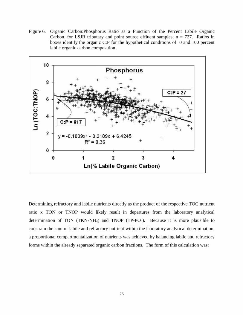
To determine the TOC:TON and TOC:TNOP for hypothetical, purely labile or refractory
substrates, polynomial regressions of these log – log relationships were solved for the TOC:TON
and TOC:TNOP values corresponding to the %LTOC = 0% and when %LTOC = 100% (Figures
5 and 6). This yielded an TOC:TON mass ratio of 37 for a completely refractory substrate, and a
ratio of 4.5 for a completely labile substrate. In the case of non-orthophosphate phosphorous, the
TOC:TNOP mass ratios obtained were 617 for refractory OM and 27 for labile.
Figure 5. Organic Carbon:Nitrogen Ratio as a Function of the Percent Labile Organic Carbon.
for LSJR tributary and point source effluent samples; n = 763. Ratios in boxes
identify the organic C:N for the hypothetical conditions of 0 and 100 percent labile
organic carbon composition.
26
Figure 6. Organic Carbon:Phosphorus Ratio as a Function of the Percent Labile Organic
Carbon. for LSJR tributary and point source effluent samples; n = 727. Ratios in
boxes identify the organic C:P for the hypothetical conditions of 0 and 100 percent
labile organic carbon composition.
Determining refractory and labile nutrients directly as the product of the respective TOC:nutrient
ratio x TON or TNOP would likely result in departures from the laboratory analytical
determination of TON (TKN-NH4) and TNOP (TP-PO4). Because it is more plausible to
constrain the sum of labile and refractory nutrient within the laboratory analytical determination,
a proportional compartmentalization of nutrients was achieved by balancing labile and refractory
forms within the already separated organic carbon fractions. The form of this calculation was:
27
LTON =
{[LTOC/(TOC*4.5)]/[RTOC/(TOC*37) + LTOC/(TOC*4.5)]}*TON.
Following this calculation, RTON could be calculated by difference with the relationship
RTON = TON – LTON,
or with the complimentary partitioning equation of the form
RTON =
{[RTOC/(TOC*37)]/[RTOC/(TOC*37) + LTOC/(TOC*4.5)]}*TON.
Similarly, TNOP was partitioned with the relationship
RTNOP =
{[LTNOP/TOC*27)]/[RTNOP/(TOC*617)+LTNOP/(TOC*27)]}*TNOP.
This approach also had the advantage in that it could be applied to the existing watershed
modeling constituent breakdown, which provides TON and TNOP (Hendrickson and Konwinski,
1998). Thus, instead of deriving specific land use loading rates for LTON, RTON, LTNOP and
RTNOP, it was only necessary to establish new model specific land use water quality
coefficients for LTOC and RTOC. From these, labile and refractory ON and NOP could be
determined outside the model framework.
Calculation of the External Load For the Lower St. Johns River
Several different statistical estimation approaches have been relied upon to calculate the external
load to the LSJR. In general, the approach used is adapted to suit the inherent variability of the
load source, and the monitoring data available for estimation, calibration and verification.

28
Point Source Load Estimation
To perform the point source load estimation, six separate data sets were utilized to gain available
information on concentration, flow, point of discharge and service area. These data sets included
1) hard copy monthly operating report files maintained at the FDEP Northeast District Office; 2)
NPDES electronic files obtained from FDEP Tallahassee; 3) Discharge quality data maintained
by the Jacksonville Electric Authority; 4) Fifth-year synoptic surveys performed by FDEP
Tallahassee or by contractor as part of permit renewal process or WQBEL studies; 5) a special 2
year sampling program conducted jointly by FDEP-NED, SJRWMD and Duval County RESD;
and 6) a GIS data base of locational information compiled by contractor. Table 2 lists the point
source facilities included in the data base, their permitted volume, and location of entry into the
WQ model grid.
Point source data were compiled into two files based on sampling frequency. The JEA data base
in most cases contained daily data on flow and water quality concentration for the 5 largest
facilities in Jacksonville, and these data were the core of one data set. Remaining facilities with
monthly or quarterly reporting data were compiled into a second data base.
Data coverage for the JEA facilities was excellent, with almost complete daily coverage for the
entire 1995 through 1999 time interval. Data coverage for the remaining facilities was fair to
good, with data coverage increasing through time as permit monitoring requirements increased to
cover nutrients in effluent. The most serious data deficiency occurred for total organic carbon,
and data from a short term, joint sampling program from 1995 through 1996 were heavily relied
upon to supply typical values for this constituent.
To calculate daily loads for facilities with monthly reporting data, mean monthly flow was
multiplied by monthly grab sampling or flow composite water quality data when available.
Generally, monthly nutrient concentrations were not available, as quarterly nutrient sampling
was typically the case for these facilities, so the mean of the sampling record was used. Some
questions arose regarding data representation, as many nutrient values were recorded in the
FDEP WAFER data base as “monthly maximum value”. However, after conferring with FDEP-

29
NED staff, it was concluded that these data were invariably fixed-interval grab sampling data,
and could be used to generate representative mean values.
Non-Point Source Load Estimation
Unlike point source effluent loads, nonpoint source loads enter at so many locations and exhibit
such large temporal variation that a direct monitoring approach is infeasible except for the
largest, most significant inputs. At all other nonpoint entry points, statistical watershed modeling
is relied upon to complete the external load budget.
Land development influences the delivery of water quality constituents to surface waters in two
fundamental ways. Through fertilization, lawn maintenance, manure spreading, septic tank
operation, vehicular use, etc., nutrients and other pollutants are added to the land surface or to
shallow groundwater in excess of natural land cover conditions (i.e., native forest, wetland).
Unlike the situation that tends to predominate on developed lands, natural land covers are highly
conservative of essential growth nutrients, and thus labile nutrient forms tend to be retained
within these terrestrial ecosystems. In addition, the creation of impervious surfaces, drainage
development, and the destruction of near stream wetlands increases the amount of rainfall that
ultimately ends up as runoff, thus increasing the pollutant exporting capability in developed
landscapes. Thus, the process of nonpoint source pollution has both chemical and hydrologic
components.
The watershed modeling approach used for the LSJR TMDL and PLRG development utilizes the
relationship between land use development and alteration in water quality and quantity to
perform a spatial extrapolation of whole basin nonpoint source load. The formulation of this
statistical model has its roots in the spreadsheet watershed load screening model, referred to as
the Pollution Load Screening Model (acronym PLSM; Adamus and Bergman 1995), which
utilizes a computer-driven geographic information system framework to calculate constituent
loads as the product of water quality concentration associated with certain land use practices, and
runoff water volume associated with those same practices. The model’s nonpoint source

30
pollutant export concentrations are specific to one of 15 different land use classes. Water
quantity is determined through a hybrid of the SCS curve number method, and is the product of
rain volumes and a coefficient (referred to as the runoff coefficient, or RC, with values ranging
from 0 to 0.9) relating the propensity of various land use and soil hydrologic group combinations
to generate runoff. The computational approach of the PLSM is similar to that of the Surface
Water Management Model (SWMM) screening level tool.
In the initial application of the PLSM to the LSJRB, Hendrickson and Konwinski (1999) made 4
major modifications to the model’s original framework: 1) the model time step was shortened to
seasonal, rather than annual average loading rates, to account for seasonal differences in specific
land use export concentrations and runoff quantity; 2) total nutrient forms were subdivided to
provide orthophosphate and total inorganic nitrogen, and by difference, TON and TNOP; 3)
land-use loading rates were adjusted to monitoring data collected within the LSJR basin using a
linear multiple regression best-fit approach based on contributing land-use fractions in
calibration watersheds; and 4) runoff coefficients were varied by season to account for intra-
annual variation in rainfall and evapotranspiration patterns. In the original application,
nonpoint source loads were predicted for the time period from 1993 to 1995, relying on land use
information compiled from 1989-90.
In this application of the PLSM, the modifications described above were maintained, and in
addition 1) LTOC and RTOC, were added to the specific land-use loading rate water quality
coefficients; and 2) runoff water quantity was varied based upon deviations in the long term
rainfall patterns. From the model output of labile and refractory organic carbon, LTON, RTON,
LTNOP and RTNOP were differentiated based on the proportional nutrient ratio weighting
described previously. A parameter referred to as the long-term rain ratio (LTRR) was developed
as a weighting factor to adjust the PLSM runoff coefficient based on antecedent watershed soil
water conditions, and is described below. Two versions of the PLSM were utilized. One version
ran within ARC Info, and calculated loads directly as the sum within contributing areas of
overlying grid coverage-products of runoff and water quality concentration. A second version
was run within Microsoft Excel, and calculates area-weighted runoff coefficient and runoff-
weighted concentration based upon the area within contributing watersheds of unique land us

31
and soil hydrologic group combinations. Though different in computational approach, both
models are theoretically identical and provided only slightly different results owing to the areal
weighting applied to rainfall input data in the Excel model application.
Watershed NPS Hydrologic Set-Up and Calibration
One of the principal deficiencies of the original PLSM hydrologic algorithm for predicting time-
varying load is its inability to account for short term changes in antecedent soil moisture
conditions that lead to changes in the propensity for rainfall to generate runoff. To account for
patterns in antecedent soil moisture associated with normal intra-annual patterns in rainfall and
evapotranspiration, the previous PLSM application to the LSJR utilized a set of runoff
coefficients for each land use-soil hydrologic group combination that varied by season (Table 3).
While this adjustment helped to simulate seasonal runoff patterns, model responsiveness to long-
term deviations from the normal seasonal rainfall pattern, for which model runoff coefficients
were originally established, was still poor. The underlying nature of this insufficiency is readily
shown in Figure 7, which plots the ratio of the PLSM-predicted runoff to measured runoff to the
seasonal whole-watershed water yield (the ratio of the measured runoff volume to the watershed
seasonal incident rainfall volume). When watershed water yield is low, resulting from prevailing
drier than normal conditions, the fixed runoff coefficient of the PLSM formulation over-predicts
measured volume (PLSM/observed > 1). When watershed yield is high due to high rainfall
seasons, the opposite is observed (PLSM/observed < 1). Because of the large range in flow
conditions occurring in the 1995-99 TMDL/PLRG modeling time window (the relative ranking
of mean annual flow rates for the 1995 – 1999 is shown in Figure 8), it was critical to obtain a
better time-varying estimate of runoff, and hence, load.
To adjust for this model insensitivity, a correction factor was developed based upon two
concepts. First, as rainfall and runoff patterns deviate form the long term norm, the ratio of the
fixed, PLSM runoff coefficient to the measured, basin yield (rain volume/runoff) varies in a
predictable manner, as was shown in Figure 7. Because extended drought-induced changes in
the rainfall-runoff relationship may occur over several seasons, the calculation to devise what is

32
referred to as the long-term rain ratio (LTRR) incorporated rain excess or deficit for one year (3
seasons) with the following equation:
LTRR = [RAINCS/LT RAINCS + (RAINCS-1/LT RAINCS-1)/2 +
(RAINCS-2/LT RAINCS-2)/3]/LT RAINCS
where:
RAINCS, RAINCS-1, and RAINCS-2 = current season rain, the previous season’s rain, and rain of
season prior to previous season; and LT RAINCS, LT RAINCS-1, and LT RAINCS-2 = 30-year,
long term mean rain for the corresponding seasons above (Rao et al., 1997).
Second, the rate of deviation of the ratio of PLSM runoff : Measured runoff with drought or
wetness is a function of the degree of impervious surface area of the basin. Under extended
durations of low rain, basins with a large degree of impervious surface area are less affected by
dry soil moisture conditions, and as a result still return a relatively large amount of their rainfall
as runoff.

33
Table 3. Seasonal Runoff Coefficients for Application of the Pollution Load Screening Model
to the LSJR Basin. Values represent the fraction of that produces runoff.
Land Use Soil Hydrologic Group
A B C D
Well Poorly
Drained Drained
Season 1: December through March
Low Density Residential 0.05 0.12 0.18 0.25
Medium Density Residential 0.5 0.6 0.7 0.8
High Density Residential 0.6 0.7 0.8 0.9
Low Density Commercial 0.5 0.6 0.7 0.8
High Density Commercial 0.7 0.8 0.9 1
Industrial 0.5 0.6 0.7 0.8
Mining 0.05 0.12 0.18 0.25
Miscellaneous Agriculture 0.05 0.12 0.18 0.25
Pasture 0.05 0.12 0.18 0.25
Row Crop 0.401 0.401 0.401 0.401
Citrus 0.05 0.12 0.18 0.25
Livestock Feedlots 0.05 0.12 0.18 0.25
Forestry, Silviculture, Range, Barren 0.05 0.12 0.18 0.25
Water Surfaces 1 1 1 1
Wetlands 0.95 0.95 0.95 0.95
Season 2: April through July
Low Density Residential 0 0 0.05 0.1
Medium Density Residential 0.2 0.3 0.4 0.5
High Density Residential 0.3 0.4 0.5 0.6
Low Density Commercial 0.2 0.3 0.4 0.5
High Density Commercial 0.4 0.5 0.6 0.7
Industrial 0.2 0.3 0.4 0.5
Mining 0 0 0.05 0.1
Miscellaneous Agriculture 0 0 0.05 0.1
Pasture 0 0 0.05 0.1
Row Crop 0.392 0.392 0.392 0.392
Citrus 0 0 0.05 0.1
Livestock Feedlots 0 0 0.05 0.1
Forestry, Silviculture, Range, Barren 0 0 0.05 0.1
Water Surfaces 1 1 1 1
Wetlands 0.75 0.75 0.75 0.75
Season 3: August through November
Low Density Residential 0.05 0.15 0.25 0.35
Medium Density Residential 0.55 0.65 0.75 0.85
High Density Residential 0.65 0.75 0.85 0.95
Low Density Commercial 0.55 0.65 0.75 0.85
High Density Commercial 0.7 0.8 0.9 1
Industrial 0.55 0.65 0.75 0.85
Mining 0.05 0.15 0.25 0.35
Miscellaneous Agriculture 0.05 0.15 0.25 0.35
Pasture 0.05 0.15 0.25 0.35
Row Crop 0.512 0.512 0.512 0.512
Citrus 0.05 0.15 0.25 0.35
Livestock Feedlots 0.05 0.15 0.25 0.35
Forestry, Silviculture, Range, Barren 0.05 0.15 0.25 0.35
Water Surfaces 1 1 1 1
Wetlands 1 1 1 1

34
Figure 7. Relationship Between PLSM Predicted Runoff:Observed Runoff Ratio and Measured
Seasonal Whole Watershed Runoff Coefficient. Seasonal Whole Watershed Runoff
Coefficient = Incident Rainfall Volume/Runoff Volume
Figure 7. Relationship Between PLSM Predicted Runoff:Observed Runoff Ratio and
Measured Seasonal Whole Watershed Runoff Coefficient. Seasonal Whole
Watershed Runoff Coefficient = Incident Rainfall Volume/Runoff Volume
0.00
0.20
0.40
0.60
0.80
1.00
1.20
1.40
1.60
0.00 2.00 4.00 6.00 8.00 10.00 12.00 14.00
PLSM Q/Observed Seasonal Q
Ob
serv
ed
Seaso
nal W
ho
le W
ate
rsh
ed
Rain
Vo
lum
e/R
un
off
PLSM =
Measured Q

35
Figure 8. Relative Position of the 1995-1999 Time Interval in the Historic Long Term Flow
Record. (From Hendrickson and Magley, 2002.)
St. Johns R. at Deland Nth.Fork Black Creek1960 7463.8 1964 447.1
1953 5402.8 1959 411.5
1959 4896.4 1947 363.6
1947 4835.8 1948 356.1
1941 4800.1 1979 338.5
19 9 5 4 70 4 .1 1966 316.5
1966 4628.4 1953 299
1964 4458.3 1960 283.8
1948 4376.9 1970 283.4
19 9 8 4 2 2 8 .4 1965 273.3
1979 4149.8 1991 272.8
1945 4095.5 1983 268.8
1994 4054.1 1992 267
1982 3970.3 1969 266.5
1968 3926 1968 261.1
1969 3918.6 1994 260.7
1934 3910 1984 242.6
1983 3851.6 1973 242.3
1978 3662.8 1944 238.9
1949 3649.1 19 9 5 237.4
1991 3481 19 9 8 236
19 9 6 3 3 4 3 .6 1946 232
1974 3259.5 1963 228
1954 3212.3 1974 224
1992 3202.6 1950 222.3
1957 3195.9 19 9 6 220.6
1984 3152.6 1933 220.5
1944 3148.8 1949 218
1936 3111.6 1987 208.8
1985 3026.9 1972 206
1942 2984.2 19 9 7 203.9
1963 2980.1 1982 199.8
1973 2968 1961 198
1946 2895 1988 197.7
1970 2842.7 1980 194.9
1952 2795.5 1941 191
1943 2704 1942 189
1988 2688.5 1945 187.3
1950 2654.3 1978 186.5
1976 2610.9 1967 175.2
1951 2597.7 1958 170.2
1987 2573.6 1937 156.4
1958 2573.1 1985 151.1
1956 2562.4 1986 150.7
1965 2383.3 1957 143.1
1935 2362.5 1971 142.8
1937 2360 1934 140.8
1967 2326.4 1956 137.8
19 9 7 2271 1993 134.3
1939 2259.6 1989 130.2
19 9 9 2226 1938 120.8
1972 2186.5 1975 120.7
1993 2122.3 1977 117
1955 2107.2 1940 115
1975 2103.6 1962 107.4
1986 2094.4 1939 107.3
1940 1958.1 1976 99.6
1938 1920.7 1935 92.9
1977 1920 1952 89
1989 1804 1932 86.4
1962 1715.4 1981 85.6
1961 1714.2 1943 84.2
1990 1505.4 1955 60
1971 1307.7 1951 58.1
1980 1174.2 19 9 9 48.9
1981 859.3 1954 48
1990 41.9
1931 12.5
1995
1998
1996
1997
1999

36
Figure 9 demonstrates this 2-step analysis process. Analysis was confined to the 4 most reliable
flow gauging stations; the Deep Creek gauge, due to poor performance of the acoustic flow
meter at this site, was excluded. The original model-predicted, area-weighted PLSM runoff
coefficient for each season and year for these four calibration watersheds (60 seasonal values
total) were placed into 4 runoff coefficient classes. The rate of change (slope) in the measured
yield : PLSM predicted runoff coefficient ratio as a function of the LTRR2 was determined for
each of these classes through zero-intercept simple linear regression (Figure 9(a)). As PLSM-
predicted runoff coefficient class increases, the rate of change of the observed:PLSM runoff
coefficient ratio, as LTRR increases, declines. Stated more simply, as watershed impervious
surface area increases, the degree to which variation in the long term rainfall pattern leads to
deviations in the fixed, PLSM runoff coefficients, decreases. To account for lower response in
watersheds with higher amounts of impervious surface, regression was again used to quantify the
rate of PLSM runoff coefficient deviation with changes in watershed impervious area,
approximated by the original PLSM runoff coefficient (Figure 9(b)). This relationship was then
integrated into an adjustment for the PLSM fixed, seasonal runoff coefficients based on the
LTRR of the form:
Observed RC/PLSM RC = LTRR2*(0.3228*PLSM-RC
0.6206)
This relationship was multiplied through by the PLSM-predicted runoff coefficient to derive a
long term, rain-adjusted runoff coefficient:
RUNOFF COEFFICIENTadj = PLSM-RC*[LTRR2*(0.3228*PLSM-RC
0.6206)]
Figure 10 compares the original and adjusted PLSM runoff coefficient and seasonal flow volume
to the measured watershed yields and seasonal flows. The adjustment removes bias and
improves precision in both the PLSM runoff coefficients and flows, moving slopes of the
regressions between observed and simulated to near one and zero, respectively. The correlation
coefficient improves from 0.12 to 0.43 in the case of runoff coefficient and from 0.59 to 0.80 in
the case of seasonal flow volume. Cumulative discharge curves for the seasons from December
1994 through November 1999 for the measured, original PLSM and PLSM-adjusted discharge

37
volumes (Figure 11) show that, with the exception of the South Fork of Black Creek, the long
term rain-ratio adjustment of PLSM seasonal simulations greatly reduces the cumulative over-
prediction of the measured flow.
Water Quality Set-Up and Calibration
In the original application of the PLSM to the LSJR basin, specific land use water quality
coefficients were developed for total nitrogen (TN), total inorganic nitrogen (TIN, or NOX +
NH4), total phosphorus (TP), orthophosphate (PO4), biochemical oxygen demand (BOD), and
total suspended solids (TSS). These coefficients, shown in Table 4, were left unchanged from
the earlier application, so the comparison of measured to simulated values here represents a skill
assessment for these constituents. (The term skill assessment is used here, rather than
verification, as the calculated flow-weighted concentrations that are used to compare to
watershed model simulations encompass the data used in the original calibration, collected from
1990-95, and newer data from 1996-2000.) New to this iteration of model development are total
organic carbon (TOC), labile total organic carbon (LTOC), and refractory total organic carbon
(RTOC). To calculate the labile and refractory portions of organic nitrogen and non-PO4-
phosphorus, the proportioning equations described earlier were applied utilizing the simulated
LTOC or RTOC operating on the difference of simulated TN-TIN and TP-PO4. The use of the
simulated TON and TOP values assures that TIN+RTON+LTON and PO4+LTOP+RTOP will be
equal to TN and TP.

38
Figure 9. Development of Hydrologic Correction Factors for the PLSM Runoff Coefficient. (a)
Linear regressions relating changes in seasonal rainfall pattern, expressed as
(LTRR)2, the ratio of observed watershed yield to PLSM predicted. (b) Relationship
between the slope of the (LTRR)2 and the watershed area-weighted runoff coefficient.
(b) Slope LTRR2 x OBS/PLS vs. Mean WS Runoff Coefficient
y = 0.3228x-0.6206
R2 = 0.9065
0
0.1
0.2
0.3
0.4
0.5
0.6
0.7
0.8
0.9
0.000 0.100 0.200 0.300 0.400 0.500 0.600 0.700
Watershed Area Weighted RC
Slo
pe L
TR
R x
O
bs/P
LS
M
(a) Long Term Rain Ratio x PLSM RC/Observed Yield
y = 0.8024x
R2 = 0.3786
y = 0.6152x
R2 = 0.486
y = 0.4596x
R2 = 0.2111
y = 0.4534x
R2 = 0.8376
0
0.5
1
1.5
2
2.5
3
0 1 2 3 4 5 6
LTRR2
OB
S/P
LS
RC=.199-.288
RC=.344-.402
RC=.441-.510
RC=.607-.674

39
Figure 10. Comparison of Original, Seasonal-fixed and Long-Term Rain Ratio Adjusted
Runoff Coefficients (a) and Total Seasonal Discharge (b) for Flow Calibration
Watersheds Within the LSJRB.
(a) Observed vs. Predicted Runoff Coefficient
y = 0.2588x + 0.3423
R2 = 0.1236
y = 0.9155x + 0.0423
R2 = 0.434
0.000
0.200
0.400
0.600
0.800
1.000
1.200
1.400
0.000 0.200 0.400 0.600 0.800 1.000
Observed Watershed RC
Pre
dic
ted
RC
PLSM Original
Adjusted RC
(b) Measured x Simulated Seasonal Flow - All Stations
y = 0.9654x + 1E+06
R2 = 0.8037
y = 0.6602x + 2E+07
R2 = 0.5881
0.E+00
5.E+07
1.E+08
2.E+08
2.E+08
3.E+08
0.E+00 5.E+07 1.E+08 2.E+08 2.E+08
Observed
Sim
ula
ted
Adjusted Runoff
Original PLSM

40
Figure 11. Comparison of Original PLSM-Predicted, Long-Term Rain Ratio Adjusted and
Observed Cumulative Discharge Curves for LSJRB Calibration Watersheds, 1995-
99.
Big Davis Creek
0
2
4
6
8
10
12
14
95s1
95s3
96s2
97s1
97s3
98s2
99s1
99s3
Cu
mu
lati
ve M
ean
Dis
ch
ag
e, m
3/s Observed
PLSM
PLSM-Adjusted
Deep Creek
0
5
10
15
20
25
30
35
40
95s1
95s3
96s2
97s1
97s3
98s2
99s1
99s3
Cu
mu
lati
ve M
ean
Dis
ch
arg
e, m
3/s
Ortega River
0
5
10
15
20
25
30
35
95s1
95s3
96s2
97s1
97s3
98s2
99s1
99s3
Cu
mu
lati
ve M
ean
Dis
ch
arg
e, m
3/s
Rice Creek
0
5
10
15
20
25
30
35
95s1
95s3
96s2
97s1
97s3
98s2
99s1
99s3
Cu
mu
lati
ve M
ean
Dis
ch
arg
e, m
3/s
South Fork Black Creek
0
10
20
30
40
50
60
70
80
95s1
95s3
96s2
97s1
97s3
98s2
99s1
99s3
Cu
mu
lati
ve M
ean
Dis
ch
arg
e, m
3/s
North Fork Black Creek
0
20
40
60
80
100
120
95s1
95s3
96s2
97s1
97s3
98s2
99s1
99s3
Cu
mu
lati
ve M
ean
Dis
ch
arg
e, m
3/s

41
Table 4. Seasonal Water Quality Coefficients Used In the PLSM to Predict Non-Point Source
Loads to the LSJR. All Values represent flow-weighted concentrations in mg/L.
Season 1: Dec. 1 through Mar. 31
Land Use TN TP BOD SS TIN TPO4
Low Density Res. 0.8 0.08 1 6 0.04 0.06
Medium Density Res. 1.4 0.25 2 15 0.35 0.1
High Density Res. 1.8 0.3 4 20 0.4 0.13
Low Dens. Commercial 1.1 0.2 2 15 0.35 0.1
High Dens. Commercial 1.2 0.3 4 25 0.4 0.13
Industrial 1.2 0.25 2 25 0.4 0.1
Forest, Range/Open, Barren 0.7 0.06 1 25 0.02 0.04
Pasture 3.9 0.75 4 15 1 0.6
Row Crop, Misc. Ag 2 0.38 1 15 0.7 0.2
Livestock 4.5 1.3 6 15 1.5 1
Water (Atmos. Wetfall) 0.28 0.017 0 0 0.28 0.015
Wetlands 0.7 0.06 1 3 0.02 0.04
Season 2: Apr. 1 through Jul. 31
Land Use TN TP BOD SS TIN TPO4
Low Density Res. 0.8 0.07 1 6 0.04 0.05
Medium Density Res. 1.6 0.3 2 30 0.2 0.1
High Density Res. 2 0.5 4 40 0.3 0.12
Low Dens. Commercial 1.2 0.3 2 30 0.3 0.1
High Dens. Commercial 2 0.5 4 50 0.4 0.12
Industrial 1.2 0.3 2 40 0.4 0.1
Forest, Range/Open, Barren 0.7 0.05 1 40 0.04 0.03
Pasture 3 1.1 4 10 1 0.85
Row Crop, Misc. Ag 10.7 1.8 1 54 4.7 0.6
Livestock 6 1.3 6 30 1.2 1
Water (Atmos. Wetfall) 0.49 0.014 0 0 0.49 0.014
Wetlands 0.7 0.05 1 3 0.04 0.03
Season 3: Aug. 1 through Nov. 30
Land Use TN TP BOD SS TIN TPO4
Low Density Res. 0.8 0.09 1 5 0.06 0.07
Medium Density Res. 1.5 0.35 2 25 0.41 0.16
High Density Res. 1.7 0.53 4 35 0.55 0.22
Low Dens. Commercial 1.3 0.22 2 15 0.3 0.13
High Dens. Commercial 1.7 0.53 4 35 0.55 0.22
Industrial 1.3 0.22 2 25 0.3 0.13
Forest, Range/Open, Barren 0.8 0.09 1 3 0.04 0.05
Pasture 3 2 4 15 1.2 2.1
Row Crop, Misc. Ag 4.4 2.2 1 26 0.55 1.6
Livestock 5 2.6 6 30 1.7 2.4
Water (Atmos. Wetfall) 0.47 0.028 0 0 0.47 0.016
Wetlands 0.7 0.07 1 3 0.04 0.05

42
Following the calculation of LTOC and RTOC for the water quality data set, specific land use
flow-weighted mean concentrations were developed following the procedure outlined in
Hendrickson and Konwinski (1998). Mean flow-weighted concentrations for LTOC and RTOC
were computed by sub-dividing water quality samples for each season and station into low flow
(samples collected within the 1 – 50th
percentile flow days) and high flow (samples collected
within the 51 – 100th
percentile flow days) and multiplying mean concentrations within flow
class by the proportion of total seasonal flow volume occurring within the class, and summing
these two products. Seasonal, flow-weighted concentrations were used to set specific loading
rates, as observations from blackwater stream monitoring stations suggest that TOC
concentrations in runoff change significantly due to season (Figure 12). Seasons used were not
the Julian seasons but modified seasons corresponding to hydrologic and meteorological patterns
of northeast Florida, and were comprised of a cool, moderately wet winter season from
December through March characterized by regular frontal storm events; a hot, dry
spring/summer from April through July; and a hot, wet summer/fall from August through
November characterized by afternoon convective thunderstorms and tropical systems.
A multiple regression approach was then used to objectively assign seasonal, specific land-use
concentrations. Land uses were aggregated into four broad classes: 1) row crop agriculture, of
which the majority was cabbage and potatoes on seepage-irrigated flatwoods soils; 2) dairy,
including associated feedlots, loafing areas, improved pastures and manure spray-fields; 3)
medium to high intensity residential, commercial and industrial; and 4) silviculture, native forest
and wetlands. Multiple regression models for each season were set up in the form:
1*LU-FR + 2*LU-FD + 3*LU-FU + 4*LU-FF = [TOC, LTOC, RTOC],

43
Figure 12. Monthly Mean Concentrations and 95% Confidence Intervals for Color and Total
Organic Carbon for 24 Unimpacted Blackwater Streams in Northeast Florida.
(a) Color
0
50
100
150
200
250
300
350
400
450
500
1 2 3 4 5 6 7 8 9 10 11 12
MONTH
ME
AN
CO
LO
R,
Pt-
Co
Un
its
(b) Total Organic Carbon
0
5
10
15
20
25
30
35
40
1 2 3 4 5 6 7 8 9 10 11 12
MONTH
ME
AN
TO
C,
mg
/L

44
where LU-FR, LU-FD, LU-FU, and LU-FF were the fractions of watershed area upstream of
sampling stations in the aggregated row crop, dairy, urban and forested categories. Regression
statistics were developed using Minitab Statistical Software. Determination of water quality
coefficients in this manner generally produces concentrations lower than those determined from
specific land use monitoring on small catchments of homogeneous land use, such as the type
developed for the National Urban Runoff Program monitoring (U.S. EPA, 1984), presumably
due to instream assimilation and sedimentation that leads to an attenuation of concentration from
source to mouth. However, such “implicitly attenuated” loading rates are viewed as superior for
whole watershed determinations of constituent loads, as would be required for input to a
receiving water body eutrophication model.
TOC, LTOC and RTOC concentrations within these aggregated land use categories were then
disaggregated into a broader set of land uses corresponding to those employed in the PLSM
framework of Adamus and Bergman (1995). The set of final water quality coefficients for all
land uses is shown in Table 5.
In their development of the EFDC hydrodynamic model for the lower St. Johns, Sucsy and
Morris (2002) identified 63 discrete entry points and their contributing areas for water volumes
entering the model grid (Figure 13), and these have been retained for the nonpoint source load
entry points to ICM.

45
Table 5. Total organic, labile total organic, and refractory total organic carbon land use category concentration coefficients.
Aggregated class model coefficients in bold, with individual class concentrations estimated by the trend with land use
intensity. RTOC concentrations determined from TOC - LTOC. Values in parenthesis are regression model coefficients.
Constit-
uent
Urban
Great
Class
Med.
Dens.
Resi-
dential
High
Dens.
Resi-
dential
Low
Intens.
Comm.
High
Intens.
Comm.
Indus-
trial
Dairy
Great
Class
Feed-
lot,
Loafing
Pas-
ture
Row
Crop
Great
Class
Row
Crop
Citrus,
Tree
Crops
Miscel.
Ag.
Forest
Great
Class
Low
Dens.
Resi-
dential Mining
Range/
Open
Space
Upland
Forest
Silvi-
culture
Wet-
lands Barren
F
Statistic
Season 1
TOC 11.7 14 11 12 9 12 34.3 45 34 17.3 17.3 17.3 17.3 18.0 16 16 18 20 22 30 14 43.8
LTOC 4.6 3 4 5 6 5 4.6 15 4 1.5 1.5 1.5 1.5 0.5 1 0.5 1 0.5 0.5 1 0.5 43
RTOC 7.1
(11.6)
11 7 7 3 7 29.7
(27.5)
30 30 15.8
(13.4)
15.8 15.8 15.8 17.5
(15.9)
15 15.5 17 19.5 21.5 29 13.5 36.5
Season 2
TOC 8.7 12 8 10 7 10 18.4 30 18 11.4 11.4 11.4 11.4 18.1 16 16 18 20 22 30 14 47.5
LTOC 5.1 4 5 5 6 5 2.6 15 3 2.7 2.7 2.7 2.7 1.4 2 1 2 1 1 2 1 15.2
RTOC 3.6
(4.1)
8 3 5 1 5 15.8
(17.6)
15 15 8.7
(6.5)
8.7 8.7 8.7 16.7
(13.9)
14 15 16 19 21 28 13 20.8
Season 3
TOC 7.8 10 7 8 7 10 47.2 55 45 27.5 27.5 27.5 27.5 22.1 20 20 22 20 24 30 18 58.9
LTOC 3.4 3 3 3 4 4 4.4 14 4 2.4 2.4 2.4 2.4 0.9 1.5 1 1.5 0.5 1 2 0.5 15.9
RTOC 4.4
(6.5)
7 4 5 3 6 42.8
(45.1)
41 41 25.1
(25.2)
25.1 25.1 25.1 21.2
(19.8)
18.5 19 20.5 19.5 23 28 17.5 32.3
Notes:2) Loading rates for forested land covers increased slightly due to: a) dry conditions of the calibration data set, and b) the preponderance of sandy ridge sampling sites.3) Specific land use breakouts based on 2 premises: a) Forested covers export more TOC than grassed or annual plant covers; and b) Suwannee River WAM BOD loading rates were used to proportion LTOC on the development intensity continuum.

46
Figure 13. Watershed Model Input Areas for Nutrient Load Compilation.

47
Determination of the Upstream Load to the LSJR
Background
The upstream load is composed of the three large tributaries that make up the lower St. Johns:
the middle St. Johns River, the Ocklawaha River, and Dunns Creek (Figure 14). These three
tributaries make up approximately 61, 21, and 18 percent of the long-term annual mean river
discharge at Palatka. Because of autochthonous production in upstream lakes, the upstream load
differs greatly from watershed loads that enter within the LSJR basin.
Because of the large amount of the entire LSJR flow that enters upstream (roughly 60%), a direct
monitoring approach, featuring continuous measurement of discharge, and bi-weekly collection
of water quality samples, has been used to determine its constituent load. This is in contrast to
the watershed modeling approach that has been used to develop the downstream tributary load.
Along with water quality monitoring, phytoplankton (algae) monitoring has also been performed
at these inputs to determine the amounts and types of algae entering the LSJR, and how they
change throughout the year and from year to year.
The presence of phytoplankton, and the preponderance of nutrients and carbon that is contained
in phytoplankton, is the single most important feature that separates the upstream inputs in the
whole LSJR external load. This poses an additional level of difficulty in the
compartmentalization of nutrients and carbon. Other tributaries to the LSJR (with the exception
of Doctors Lake, which in the LSJR TMDL modeling is included within the model grid) contain
insignificant amounts of algae, and distinguishing algal-borne nutrients and carbon in the
particulate labile organic pool has not been done in the calculation of the watershed nonpoint
source load.

48
Figure 14. Tributaries Forming the Lower St. Johns River.
Crescent
Lake
Lake
George
Lake
Ocklawaha
Palatka
Dunns Creek
Station
Buffalo Bluff
Station
Jacksonville
Middle St.
Johns R.
Ocklawaha R.
Dunns Cr.
Lower St.
Johns R.
Approach to Upstream Boundary Nutrient and Carbon Partitioning
The combined incoming load from the middle and upper St. Johns and Ocklawaha River was
determined from the LSJR sampling station at Buffalo Bluff, a location 11 miles downstream of
the Ocklawaha River mouth. Direct monitoring was also used to characterize the load entering
the LSJR from the Crescent Lake Basin, at the sampling location in Dunns Creek, just
downstream of the Buffalo Bluff site. Both locations are instrumented with acoustic Doppler
current profilers, capable of measuring velocity and discharge in conditions of reversing flows.
Biweekly water quality monitoring has been performed at these locations under two programs,
with only slight differences in constituents. An ambient monitoring program, collecting samples
during the second week of each month, includes BOD in its suite, necessary for the empirical
separation of labile and refractory organic carbon. A second monitoring network samples these
locations on the fourth week of the month, and includes the analysis of particulate organic

49
carbon, and a complete plankton analysis featuring taxonomic classification, cell densities and
cell biovolume for major algal taxonomic groups. Both programs analyze complete suites of
chlorophyll and dissolved and total organic and inorganic nutrients and carbon.
The flow chart of Figure 15 illustrates the mapping of water quality chemical analysis results to
respective biological compartments of the LSJR WQ model. In this calculation cascade, one of
the most important determinations that must be made (and that distinguishes this boundary
determination from downstream tributary inputs) is the content of the total nutrient and carbon
load in phytoplankton. In this approach, the inorganic forms (for nitrogen or phosphorus) are
distinguished from the organic forms directly through laboratory analysis as shown. Next,
organic carbon is subdivided into labile or refractory forms based upon the procedure described
previously for tributary nonpoint sources, utilizing BOD converted to carbon units and the
established first-order decomposition rates. Labile organic carbon and nutrients are then further
subdivided into algal and non-algal, under the assumption that all algal organic matter is labile.
The determination of algal carbon content is described below, and algal nutrient composition was
determined from this algal carbon estimate, assuming adherence to the Redfield stoichiometric
proportions of 106:16:1 C:N:P molar.
50
Figure 15. Flow chart for differentiation of laboratory analytical fractions into CE-QUAL-ICM state variables for the lower St.
Johns River upstream boundary at Dunns Creek and Buffalo Bluff.
Total Form
TN, TP, TOC
Inorganic
(NOX, NH3, PO4)
Organic
(TKN-NH3, TP-PO4, POC+DOC)
Labile
(TOC consumption rate = 0.075/day)
Refractory
(TOC consumption rate = 0.001/day)
Particulate
(RTOC - RDOC; nutrients by
stoichiometric partitioning)
Dissolved
(RDOC determined by Color; nutrients by stoichiometric
partitioning)
Particulate
(LTOC - LDOC; nutrients by
stoichiometric partitioning)
Dissolved
(DOC - RDOC; nutrients by
stoichiometric partitioning)
Non-algal
(LPOC - Algal POC)
Algal
(By biovolume or chlorophyll a;nutrients by Redfield ratio)
Cyanobacteria Diatoms Other algal sp.

51
A data set of coincidently collected particulate organic carbon, nitrogen and phosphorus,
chlorophyll a, and algal biovolume (Phlips and Cichra, 2001) were relied upon to determine algal
carbon content and confirm nutrient ratios. Direct measurements of particulate organic carbon
using the high temperature combustion coulombmetric method were used to establish algal
C:chlorophyll a and C:algal biovolume ratios. Estimation of POC by difference of TOC – DOC
with measurements performed by the carbon gas analyzer were not used due to their much lower
precision and poor fit with algal biomass. Coulombmetric POC data are limited in coverage,
having been performed only once monthly from August 1998 to the present. Thus, to calculate
TOC for subsequent compartmentalization to labile and refractory forms for dates on which POC
was not determined, TOC was considered to be at least equal to DOC + algal POC, with algal
POC determined either through algal biovolume or chlorophyll a, preferentially selecting
biovolume data in the calculation when available. At most, TOC was considered to be equal to
DOC + (total suspended solids 0.4), representing a situation in which all TSS were organic
particles with a 40% composition by weight of carbon.
Comparison of algal biovolume to corrected chlorophyll a for LSJR freshwater sampling stations
(Figure 16) shows a strong correlation between these two variables, as would be expected.
Regression R2 values for the relationship range from 0.75 to 0.83 for the 6 stations examined,
and intercepts are near zero. A similar correlation is obtained in regressions between
uncorrected chlorophyll a and biovolume, with the exception that the intercept values are higher,
suggesting the presence of chlorophyll-containing algal detritus that is not accounted for in the
biovolume determination.

52
Figure 16. Comparison of Corrected Chlorophyll a and Algal Biovolume for Combined LSJR
Freshwater Water Quality and Plankton Analysis, 1995 – 2001. Plankton taxonomy
and biovolume determinations performed by Phlips and Cichra, 2001.
Both chlorophyll a and algal biovolume were strongly correlated to measurements of particulate
organic carbon, though linear regression R2 values were typically driven by a small number of
large values in the data set associated with algal bloom events, when a large amount of the POC
is expected to be in algal biomass. To help distinguish carbon to biomass relationships, sample
C:chlorophyll and C:biovolume ratios were viewed as boundary relationships, in which the
approach of POC:biomass values the true C:biomass measure occurs as non-algal carbon
declines (Figure 17). In these boundary relationships, it can be seen that minimum C:chlorophyll
ratios approach the commonly cited carbon:chlorophyll a ratio of 50:1, shown in red in Figure
17(a). In the case of the biovolume comparison, a similar boundary analysis yields an estimate
of 3.3 m3/ml per mg/L POC.
Buffalo Bluff
Chla = 0.0034*(Biov) + 9.5556
R2 = 0.8188
Federal Pt.
Chla = 0.005*(Biov) + 3.3355
R2 = 0.8258
Crescent L.
Chla = 0.0051*(Biov) + 5.3773
R2 = 0.8212
Deep Cr. Cove
Chla = 0.0045*(Biov) + 5.706
R2 = 0.7664
L. George
Chla = 0.0036*(Biov) + 8.739
R2 = 0.8104
Palatka
Chla = 0.0056*(Biov) + 5.2055
R2 = 0.7508
0
20
40
60
80
100
120
140
160
0.0 5000.0 10000.0 15000.0 20000.0 25000.0 30000.0
Total Biovolume, (micro-m3/ml)*1000
Co
rrecte
d C
hlo
rop
hyll a
, m
g/m
3
Buffalo Bluff
Deep Cr. Cove
Federal Point
L. George
Palatka
Crescent L.

53
To perform the partitioning of organic carbon when reliable TOC measurements were not
available, RDOC was first derived through a relationship with color (Figure 18), and LDOC
determined as the DOCmeasured – RDOCcolor-derived. LTOC and RTOC were then calculated by
way of the carbon equivalency BOD decomposition-derivation described in the watershed model
coefficient development, using a TOC estimated by DOC + algal OC. For Dunns Creek, this
approach suggested that a large fraction of the organic carbon pool is contained in RDOC. In the
case of the Buffalo Bluff station, however, RDOC concentrations were lower, hence relatively
large amounts of DOC were attributed to the LDOC partition. These high LDOC concentrations
(mean = 3.7 mg/L; range = 0 to 6.1 mg/L) in most cases exceeded the calculated non-algal
LTOC concentration when non-algal LTOC was calculated as TOCmin – RTOC – algal LTOC.
To adjust for this inconsistency, LTOC concentration was increased such that non-algal LTOC =
LDOC, resulting in non-algal LPOC = 0. In cases where the sum of LTOC + RTOC exceeded
DOC + TSS*0.4 (TOCmax; occurring in 12 of the 51 sampling events in between Nov. 1996
through Dec. 1998), RTOC was adjusted downward.
Determination of the Atmospheric Deposition Load
The calculation of the atmospheric deposition load to the lower St. Johns River was performed
by the private consulting firm Tetra Tech, Inc. (Pollman, 2003). Estimates were derived for total
wet and dry deposition of nitrogen and phosphorus species. Wet nitrogen deposition
concentration was determined by the monthly mean of the 3 nearest National Atmospheric
Deposition Program (NADP) sites to the LSJR, FL99 (Kennedy Space Center), FL03 (Bradford
Forest), and GA09 (Okeefenokee Swamp). Volumes were computed as the product of the
monthly Thiessen rainfall polygon rainfall volumes (the same spatial rainfall data set as that used
for watershed modeling) directly falling on the ICM grid surface area. Monthly dry deposition
nitrogen flux estimates were developed using the method of Poor et al. (2001). Phosphorus wet
deposition was determined by the volume weighted mean deposition estimates collected at the
Lake Barco monitoring station, approximately 20 miles west of Palatka.

54
Figure 17. Comparison of POC:Algal Biovolume (a) and POC:Total Chlorophyll a Ratios to
Total Biovolume and Total Chlorophyll a Concentration for LSJR Freshwater
Samples. Red Lines in graph (a) correspond to a C:chlorophyll a of 50:1, and in
graph (b) corresponds to C:biovolume of 0.0003 (for biovolume expressed as
µm3/ml x 1000).
(a ) POC:Total Chlorophyll a
0
20
40
60
80
100
120
140
160
0 100 200 300 400 500
POC:Chlorophyll a ratio
To
tal
Ch
loro
ph
yll
a,
mg
/m3
(b) POC:Algal Biovolume
0
5000
10000
15000
20000
25000
30000
0 0.002 0.004 0.006 0.008 0.01 0.012
C:Biovolume Ratio
Bio
vo
lum
e,
mic
ro-m
3/m
l x
10
00

55
Figure 18. Relationship Between Refractory Dissolved Organic Carbon and Color for
Blackwater Streams of the LSJR Basin. From Hendrickson et al., 2001.
Color = 0.4125(RDOC)2 + 4.633(RDOC)
R2 = 0.9939
0
200
400
600
800
1000
1200
1400
1600
0 10 20 30 40 50 60 70
Mean RDOC by Color Class, mg/L
Co
lor,
Pt-
Co
Un
its
Cuthbert and del
Georgio, 1992
Pulp Mill
Eff luent
Rasmussen et al 1989
56
RESULTS
Tributary Organic Carbon and Nutrients
Calibration Data Set Summary
Calculated seasonal flow-weighted concentrations of organic carbon, nitrogen and phosphorus
forms in field sampling data of tributary runoff are listed in Table 6. Organic carbon in samples
was considered to be primarily allochthonous in origin. Of the 789 total samples available, 570
were also analyzed for chlorophyll a. Of these, 82% had chlorophyll a concentrations less than 5
g/L, suggesting low contributions to the total organic carbon pool of internally-derived,
autochthonous organic carbon. Of the 103 samples with chlorophyll a concentrations above 5
g/L, 71 were obtained at on two tributaries, Sixmile and Peters Creeks, with sampling sites in
quiescent, open embayments below the head of tide, where autochthonous production potential
was high.
Using the BOD partitioning approach, labile total organic carbon (LTOC) was found to comprise
a relatively small fraction of the TOC pool in stream runoff. This is not surprising, as southeast
U.S. coastal plain blackwater streams are by nature high in refractor, colored dissolved organic
matter. The highest absolute concentrations of LTOC were found to occur in tributaries draining
urbanized Jacksonville. These tributaries also exhibited lower TOC concentrations, presumably
do to the increase in impervious surface area and the concomitant reduction in runoff leached
through soils on the flow-path to the stream, as well as a reduction in the amount of natural forest
cover in the basin to supply organic detritus. Catchments with high contributions of dairy land
use exhibited relatively high LDOC concentrations, but had calculated RDOC concentrations
similar to undeveloped watersheds.

57
Table 6. Mean Total, Inorganic, and Calculated Labile and Refractory Organic Nutrient and Carbon Mean Annual Flow-Weighted Concentrations for Tributaries sampled within
the lower St. Johns River Basin. Sorted in order of increasing land use intensity. Values in boxes lacked BOD sampling data and were calculated using simulated
values.
Land Use Percent in Class
Forest Dominated n Urban Dairy
Row
Crop Forest TN TIN
Labile
TON
Refrac.
TON TP TPO4
Labile
TNOP
Refrac.
TONP TOC
Labile
TOC
Refrac.
TOC
Bradley Creek Upstr. 7 | 1 6 0 93 | 0.490393 0.013565 0.085395 0.391433 0.017946 0.01022 0.002321 0.003883 15.42371 0.401154 15.02256
Peters CreekUpstr. 24 | 3 4 1 92 | 0.640559 0.027803 0.155494 0.456867 0.029919 0.013087 0.008189 0.008642 21.23662 0.833601 20.06556
Black Creek No. Fork. 48 | 4 1 1 92 | 0.802675 0.119433 0.195487 0.487386 0.059442 0.026052 0.018489 0.014363 24.08545 1.030466 20.64633
Black Creek So. Fork 44 | 13 5 1 81 | 0.7094 0.054821 0.169452 0.484908 0.115486 0.070977 0.0225 0.021265 23.20996 0.892373 20.70435
Trout Creek 12 | 4 2 8 86 | 1.162648 0.081714 0.342241 0.738693 0.073858 0.027308 0.030129 0.024262 24.89197 1.253613 22.77622
0.76 0.059 0.190 0.512 0.06 0.030 0.016 0.014 21.77 0.88 19.84
Dairy Dominated
Peters Creek Dwnstr. 82 | 4 8 7 80 | 1.073664 0.282677 0.323955 0.467032 0.210378 0.143282 0.04446 0.022637 17.00254 1.325701 15.53925
Bradley Cr. Dwnstr. 20 | 5 24 0 70 | 4.113989 3.439598 0.35236 0.386799 0.093123 0.049962 0.03238 0.010782 11.23281 1.171885 10.06092
Trout River 82 | 22 20 2 56 | 1.77 0.391 0.766 0.618 0.43 0.398 0.023 0.001 27.03 2.29 17.25
Mill Log Br. Dwnstr. 15 | 2 25 0 73 | 1.988097 0.547011 0.651904 0.789182 0.96523 0.76857 0.136757 0.059903 28.76962 2.595772 26.17384
Mill Log Br. Upstr. 19 | 1 54 0 45 | 2.872906 0.801499 0.995905 1.075502 1.715412 1.534645 0.129663 0.051104 32.63283 3.372127 29.26071
Governors Creek 22 | 10 24 0 66 | 3.319618 2.144658 0.685129 0.489831 0.218639 0.157146 0.049441 0.012694 18.46127 2.684303 15.70752
2.52 1.268 0.629 0.638 0.60 0.509 0.069 0.026 22.52 2.24 19.00
Row Crop Dominated
Hastings Drainage Dist. 31 | 2 13 26 59 | 1.808419 0.473851 0.697115 0.63843 0.472736 0.281731 0.141746 0.049259 23.18233 2.693788 21.05455
Moccasin Branch 30 | 7 6 28 59 | 1.86147 0.553435 0.758721 0.547453 0.468344 0.304752 0.128775 0.034816 31.36513 3.420644 22.59039
Deep Creek Dwnstr. 47 | 2 33 30 35 | 1.942408 0.688538 0.480799 0.777022 0.557594 0.420494 0.081452 0.047354 24.37006 1.732058 23.70844
Dog Branch 29 | 12 4 72 13 | 2.500268 1.123014 0.958052 0.570389 0.525746 0.276305 0.202008 0.047432 17.08496 2.863868 13.35062
2.03 0.710 0.724 0.633 0.51 0.321 0.138 0.045 24.00 2.68 20.18
Urban Dominated
Cedar Creek 78 | 25 9 4 62 | 1.021877 0.136099 0.398539 0.487238 0.09942 0.06413 0.024671 0.010619 13.93 1.277845 12.65216
Ortega River 13 | 38 8 5 50 | 0.965428 0.154752 0.279993 0.530465 0.125436 0.064639 0.041893 0.028275 18.45483 1.190488 18.6259
Arlington River 6 | 68 3 2 27 | 1.008321 0.183998 0.549518 0.266673 0.153877 0.077913 0.062494 0.013487 13.58393 2.755236 11.10736
Cedar River Dwnstr. 19 | 67 9 1 24 | 1.166174 0.328866 0.638752 0.195467 0.190901 0.097539 0.086623 0.009593 12.38027 3.446573 8.667477
McCoy's Creek 69 | 89 7 0 4 | 1.659184 0.43134 1.112342 0.115503 0.430823 0.169996 0.251564 0.009263 7.863333 4.075591 3.787743
1.16 0.247 0.596 0.319 0.20 0.095 0.093 0.014 13.24 2.55 10.97
OVERALL AVERAGE 17 6 11 66 1.64 0 .60 0.53 0.53 0.348 0.248 0.076 0.024 20.31 2.07 17.44

58
Based on the empirical partitioning scheme derived here, organic N was on average evenly split
between labile and refractory forms, while non-orthophosphate P tended to predominate in labile
forms. These proportions differed widely based upon the level and type of development within a
sampling basin. For undeveloped basins, with over 90% of their area in natural land covers or
silviculture, LTON was on average 27% of TON. For these same basins, LTNOP was, at 51%,
on average a higher proportion of TNOP. It should though be noted that these streams exhibited
such low concentrations of TP that absolute LTNOP values are very low, and the precision of the
partitioning approach should also be considered low. Conversely, for tributaries draining basins
with over 30% of urban land area, LTON averaged 70% of TON, and LTNOP was on average
86% of TNOP. Despite relatively low TOC concentrations in comparison to streams draining
undeveloped watersheds, urban development-dominated watersheds exhibit some of the highest
concentrations of LTOC, LTON, and LTNOP.
Streams draining agriculture-dominated watersheds also exhibited proportionally high levels of
LTOC, LTON and LTNOP. Within this category, several streams draining watersheds with
large areas of dairy land use exhibited some extremely high concentrations of TP and TN. The
high levels of these nutrients were not consistent within any given stream, suggesting various
unidentified dairy practices influence water quality in different ways. Bradley Creek and
Governor’s Creek exhibited high TN levels, at 6.39 and 5.13 mg/L, respectively, with a large
portion of this as nitrate+nitrite-N, but had relatively low (for dairy runoff) TP concentrations.
Another dairy-influenced stream, Mill Log Branch, had elevated but much lower levels of TN, at
2 mg/L, while mean TP concentration was 1.36 mg/L! This lack of consistent pattern with
respect to elevated nutrient concentrations led to difficulties in establishing model concentration
parameters.
Watershed Model Calibration
Hydrologic and water quality coefficients were calibrated separately and together (as load) to
provide a relative sense of their individual and combined precision. Hydrologic calibration was

59
discussed in the previous methods section, therefore only the quality and load calibration are
covered here. As TN, TIN, TP, and PO4 were calibrated in the first LSJR development of the
PLSM (Hendrickson and Konwinski, 1998) and remain the same in this application, the results
can be viewed as a verification of the established model coefficients. For the newly created
constituents TOC, RTOC and LTOC, this comparison represents an assessment of the
performance of the coefficient assignment process through the multiple regression approach.
Figures 19, 20 and 21 compare the seasonal measured and simulated flow-weighted
concentrations of relevant water quality variables. Large differences are evident for monitoring
stations downstream of dairy land uses (shown as open squares in Figures 19 - 21. Part of this
appeared to be due to the inconsistencies identified in the previous section with regard to the
appearance of N or P in runoff. However, the consistent under-prediction suggests that either 1)
water quality concentrations assigned to improved pasture and confined animal feeding zones are
too low; 2) runoff coefficients assigned to these areas are too low; or 3) the area dedicated to
dairy is under-reported in the GIS land use layer. As the present PLSM nutrient concentrations
assigned to improved pasture and concentrated feeding areas range from 3.0 - 3.9 mg/L and 4.5 –
6.0 mg/L for TN and from 0.75 – 2.0 mg/L and 1.3 – 2.6 mg/L for TP, considerably greater that
the 2.48 TN and 0.349 TP mg/L mean concentrations reported by Harper (1994) for central and
south Florida, it does not appear at first that model concentrations are too low. After some
inspection, it was discovered that the GIS land use data in many cases either incorrectly coded
land cover associated with dairy, identifying intensive pasture or manure sprayfields as row crop
or miscellaneous agriculture, or failed to account for it at all. Also, as the PLSM in its present
form assigns the same runoff coefficients to pasture and dairy as undeveloped land use, this too
may be a source of under-representation. Darkened squares in Figures 19 - 21 identify these
simulated values for these same watersheds derived by assigning all land are under the
“miscellaneous agriculture” category to dairy, and increasing runoff coefficients to the same
values observed for the tri-county agricultural area. These modifications appear to bring organic
nutrient concentrations more in line with observed data, but still leave simulated inorganic
nutrient concentrations (and hence, total nutrient) low. Because these manipulations are
hypothetical, the sampling stations within the three watersheds with substantial dairy

60
development (Governors Creek, Mill Log Branch and Bradley Creek) are excluded from the
quantitative calibration described below.

61
Figure 19. Comparison of Observed to Simulated Flow-Weighted Concentrations of Carbon,
Nitrogen and Phosphorus Forms for the December through March Season. All units
in mg/L. Open squares represent existing dairy watershed predictions, and solid
squares represent miscellaneous agriculture added to dairy land and runoff
coefficients increased to match tri-county ag area row crop values.
Total N
0
1
2
3
4
5
0 1 2 3 4 5Observed
Sim
ula
ted
Total Inorganic N
0
0.5
1
1.5
2
2.5
3
3.5
0 0.7 1.4 2.1 2.8 3.5
ObservedS
imu
late
d
Total P
0
0.4
0.8
1.2
1.6
2
0 0.5 1 1.5 2
Observed
Sim
ula
ted
Total PO4
0
0.3
0.6
0.9
1.2
1.5
1.8
0 0.3 0.6 0.9 1.2 1.5 1.8
Observed
Sim
ula
ted
Total Organic C
0
5
10
15
20
25
30
35
40
45
0 5 10 15 20 25 30 35 40 45
Observed
Sim
ula
ted
Total Suspended Solids
0
10
20
30
40
0 10 20 30 40
Observed
Sim
ula
ted
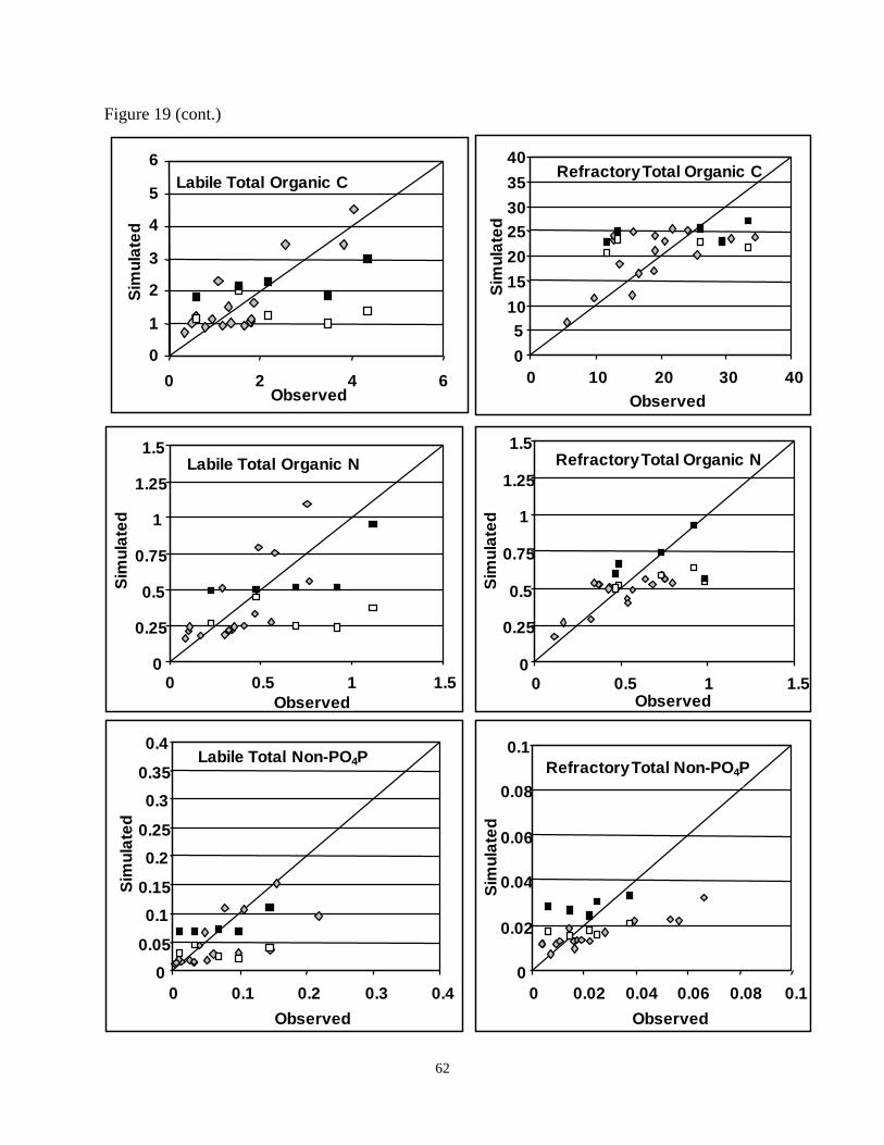
62
Figure 19 (cont.)
Labile Total Organic C
0
1
2
3
4
5
6
0 2 4 6Observed
Sim
ula
ted
Refractory Total Organic C
0
5
10
15
20
25
30
35
40
0 10 20 30 40
Observed
Sim
ula
ted
Labile Total Organic N
0
0.25
0.5
0.75
1
1.25
1.5
0 0.5 1 1.5
Observed
Sim
ula
ted
Refractory Total Organic N
0
0.25
0.5
0.75
1
1.25
1.5
0 0.5 1 1.5Observed
Sim
ula
ted
Labile Total Non-PO4P
0
0.05
0.1
0.15
0.2
0.25
0.3
0.35
0.4
0 0.1 0.2 0.3 0.4
Observed
Sim
ula
ted
Refractory Total Non-PO4P
0
0.02
0.04
0.06
0.08
0.1
0 0.02 0.04 0.06 0.08 0.1
Observed
Sim
ula
ted

63
Figure 20. Comparison of Observed to Simulated Flow-Weighted Concentrations of Carbon,
Nitrogen and Phosphorus Forms for the April through July Season. All units in
mg/L. Open squares represent existing dairy watershed predictions, and solid
squares represent miscellaneous agriculture added to dairy land and runoff
coefficients increased to match tri-county ag area row crop values.
Total N
0
1
2
3
4
5
0 1 2 3 4 5
Observed
Sim
ula
ted
Outlier:Dog BranchSim. = 2.8Obs. = 7.2
Total Inorganic N
0
0.5
1
1.5
2
2.5
3
3.5
0 0.7 1.4 2.1 2.8 3.5
ObservedS
imu
late
d
Total P
0
0.4
0.8
1.2
1.6
2
0 0.5 1 1.5 2
Observed
Sim
ula
ted
Total PO
0
0.3
0.6
0.9
1.2
1.5
1.8
0 0.3 0.6 0.9 1.2 1.5 1.8
Observed
Sim
ula
ted
Total Organic C
0
5
10
15
20
25
30
35
40
45
0 5 10 15 20 25 30 35 40 45
Observed
Sim
ula
ted
Total Suspended Solids
0
10
20
30
40
0 10 20 30 40
Observed
Sim
ula
ted

64
Figure 20 (cont.)
Labile Total Organic C
0
1
2
3
4
5
6
0 1 2 3 4 5 6Observed
Sim
ula
ted
Refractory Total Organic C
0
5
10
15
20
25
30
35
40
0 10 20 30 40
Observed
Sim
ula
ted
Labile Total Organic N
0
0.25
0.5
0.75
1
1.25
1.5
0 0.5 1 1.5Observed
Sim
ula
ted
Dog Br.Calc = 1.0Sim = 2.9
Refractory Total Organic N
0
0.25
0.5
0.75
1
1.25
1.5
0 0.5 1 1.5Observed
Sim
ula
ted
Labile Total Non-PO4P
0
0.05
0.1
0.15
0.2
0.25
0.3
0.35
0.4
0 0.1 0.2 0.3 0.4Observed
Sim
ula
td
Dog Br.
Calc = 0.2
Sim = 0.7
Refractory Total Non-PO4P
0
0.02
0.04
0.06
0.08
0.1
0 0.02 0.04 0.06 0.08 0.1
Observed
Sim
ula
ted

65
Figure 21. Comparison of Observed to Simulated Flow-Weighted Concentrations of Carbon,
Nitrogen and Phosphorus Forms for the August through November Season. All
units in mg/L. Open squares represent existing dairy watershed predictions, and
solid squares represent miscellaneous agriculture added to dairy land and runoff
coefficients increased to match tri-county ag area row crop values.
Total N
0
1
2
3
4
5
0 1 2 3 4 5
Observed
Sim
ula
ted
Total Inorganic N
0
0.5
1
1.5
2
2.5
3
3.5
0 1 2 3Observed
Sim
ula
ted
Total P
0
0.4
0.8
1.2
1.6
2
0 0.5 1 1.5 2
Observed
Sim
ula
ted
Total PO4
0
0.3
0.6
0.9
1.2
1.5
1.8
0 0.3 0.6 0.9 1.2 1.5 1.8
Observed
Sim
ula
ted
Total Organic C
0
5
10
15
20
25
30
35
40
45
0 5 10 15 20 25 30 35 40 45
Observed
Sim
ula
ted
Total Suspended Solids
0
9
18
27
36
45
0 10 20 30 40
Observed
Sim
ula
ted

66
Figure 21 (cont.)
Labile Total Organic C
0
1
2
3
4
5
6
0 1 2 3 4 5 6
Observed
Sim
ula
ted
Refractory Total Organic C
0
5
10
15
20
25
30
35
40
45
0 10 20 30 40 50
Observed
Sim
ula
ted
Labile Total Organic N
0
0.2
0.4
0.6
0.8
1
1.2
1.4
1.6
0 0.5 1 1.5 2
Observed
Sim
ula
ted
Refractory Total Organic N
0
0.2
0.4
0.6
0.8
1
1.2
1.4
0 0.25 0.5 0.75 1 1.25 1.5
Observed
Sim
ula
ted
Labile Total Non-PO4P
0
0.05
0.1
0.15
0.2
0.25
0.3
0.35
0.4
0 0.1 0.2 0.3 0.4
Observed
Sim
ula
ted
Refractory Total Non-PO4P
0
0.01
0.02
0.03
0.04
0.05
0.06
0.07
0.08
0.09
0.1
0 0.02 0.04 0.06 0.08 0.1
Observed
Sim
ula
ted

67
Two statistical tests were performed to characterize the level of agreement between the
calculated flow-weighted concentrations and the PLS model simulated, runoff-weighted
concentrations, and the results of these are shown in Table 7. Pearson product-moment
correlations were calculated to estimate general agreement between observed and simulated
values, and zero-intercept regression slopes and confidence intervals, in which the observed
flow-weighted concentration represented the independent variable, were calculated to assess
potential bias in model water quality coefficients. Variables exhibiting the poorest correlations
between the calculated flow weighted and simulated values include TPO4 for the December –
March season, RTON for the April – July.

68
Table 7. Pearson Correlations, Slopes, and Confidence Intervals of the Slopes for Intercept-Fit Regressions Between Calibration
Station Measured Flow-Weighted Concentrations and Contributing Area Modeled Runoff-Weighted Concentrations. Boxed
confidence bounds indicate seasons and constituents for which agreement between measured (independent) and modeled
(dependent) concentrations are significantly different than 1:1. Parameter TN TIN LTON RTON TP TPO4 LTNOP RTNOP TOC LTOC RTOC TSS
December - March
Pearson Correlation 0.656 0.796 0.73 0.754 0.638 0.399 0.7 0.907 0.62 0.846 0.6 0.657
p-value 0.004 0.000 0.001 0.000 0.006 0.113 0.002 0.000 0.008 0.000 0.011 0.004
Slope 0.742 0.400 0.982 0.870 0.625 0.545 0.611 0.521 1.095 0.986 0.992 0.870
Slope Standard Error 0.066 0.051 0.104 0.056 0.080 0.102 0.088 0.050 0.057 0.076 0.074 0.100
Slope Upper 95% C.I. 0.601 0.292 0.762 0.751 0.454 0.328 0.424 0.416 0.973 0.824 0.836 0.657
Slope Lower 95% C.I. 0.882 0.508 1.201 0.989 0.795 0.761 0.798 0.627 1.216 1.148 1.149 1.082
April - July
Pearson Correlation 0.892 0.947 0.648 0.365 0.827 0.794 0.697 0.828 0.636 0.684 0.653 0.76
p-value 0.000 0.000 0.007 0.164 0.000 0.000 0.003 0.000 0.008 0.003 0.006 0.001
Slope 1.625 1.800 1.315 1.390 1.517 0.922 1.837 2.307 1.150 1.106 1.410 1.421
Slope Standard Error 0.161 0.136 0.182 0.215 0.163 0.104 0.291 0.430 0.082 0.099 0.125 0.171
Slope Upper 95% C.I. 1.284 1.513 0.928 0.934 1.171 0.702 1.219 1.396 0.976 0.896 1.146 1.058
Slope Lower 95% C.I. 1.965 2.088 1.702 1.846 1.862 1.142 2.455 3.217 1.324 1.316 1.674 1.784
August - November
Pearson Correlation 0.698 0.541 0.685 0.43 0.754 0.76 0.698 0.123 0.713 0.351 0.71 0.315
p-value 0.002 0.025 0.002 0.097 0.000 0.000 0.003 0.650 0.001 0.168 0.001 0.218
Slope 0.764 0.651 0.630 0.783 0.722 0.701 0.896 0.861 0.853 0.570 0.894 0.661
Slope Standard Error 0.062 0.105 0.072 0.103 0.094 0.096 0.134 0.242 0.060 0.092 0.068 0.142
Slope Upper 95% C.I. 0.633 0.428 0.478 0.564 0.523 0.497 0.612 0.347 0.726 0.375 0.750 0.361
Slope Lower 95% C.I. 0.895 0.873 0.782 1.001 0.921 0.905 1.179 1.375 0.980 0.764 1.039 0.962
Overall
Pearson Correlation 0.600 0.695 0.577 0.348 0.692 0.774 0.597 0.172 0.648 0.534 0.638 0.512
p-value 0.000 0.000 0.000 0.014 0.000 0.000 0.000 0.237 0.000 0.000 0.000 0.000
Slope 1.020 1.019 0.924 0.920 0.844 0.715 1.162 0.871 0.987 0.808 1.006 0.929
Slope Standard Error 0.081 0.110 0.083 0.074 0.075 0.057 0.134 0.146 0.041 0.062 0.052 0.094
Slope Upper 95% C.I. 0.857 0.799 0.757 0.772 0.695 0.601 0.894 0.580 0.905 0.684 0.902 0.742
Slope Lower 95% C.I. 1.182 1.239 1.091 1.068 0.993 0.829 1.430 1.162 1.070 0.933 1.110 1.117

69
season, RTON, RTNOP, LTOC and TSS for the August – November season, and RTNOP for the
overall, all season comparison. In all other comparisons, Pearson correlation p-values are less
than 0.05. In 22 of the possible 36 (3 seasons x 12 constituents) seasonal comparisons, the slope
of the regression line relating the observed, flow-weighted concentration to the simulated value
was found to be significantly greater than or less than 1, suggesting some bias in the model
seasonal water quality coefficients. Many of the seasonal biases are compensating, and when all
seasons are combined, 9 of the 12 constituent slope confidence intervals contain 1, and the
remaining 3, TP, PO4 and LTOC, upper confidence bounds are close to 1. Seasonal oscillation
in observed verses simulated slopes in several cases results from a few data points belonging to
streams (principally Dog Branch and Deep Creek) draining the tri-county agricultural area that
exhibit much higher concentrations and thus heavily influence the regression line. When high
flow samples from these streams, influential in the flow-weighting calculation, were recorded
near the end of the December – March WQ coefficient seasonal break, observed concentrations
are high relative to model predictions, producing a observed x simulated slope of less that 1.
In most cases, the newly-added model constituents for TOC, LTOC and RTOC perform well,
however, it should be kept in mind that in the case of these constituents the same data set was
used for assigning land use water quality coefficients and calibration, so statistics only reflect the
skill in assigning coefficients.
To assess the accuracy of load prediction (the product of concentration and discharge volume),
daily loads calculated at water quality sampling stations that also have established stream-flow
gauging installations were compared to watershed model simulated daily loads. Actual daily
load was assumed to be equivalent to the product of the instantaneous water quality sampling
concentration and the daily discharge. Because water quality concentrations can vary within a
day, this should be considered to be an estimate of daily load. Simulated daily load was
calculated as the seasonal, watershed area-weighted constituent concentration x seasonal water
quantity x the daily flow fraction. Daily flow fraction is the fraction of the given daily flow of
the total seasonal flow, and was the statistic used to disaggregate seasonal watershed model loads
to daily loads for input to the LSJR water quality processes model.
70
Three tributary stations in the LSJR meet the criteria of having both water quality and quantity
monitoring, and comparison of their simulated and observed daily loads are shown in Figure 21.
The plots demonstrate the tendency for baseflow conditions to be over-sampled relative to
stormflow or high-flow conditions in fixed-interval ambient monitoring data. This phenomena is
manifested in the plots by many sampling points clustered near the origin, with few high-flow
(and thus high load) data points to discern the relationship between observed and simulated.
Considering the uncertainty associated with estimating the true value of the daily load, and with
fractionating a daily load from the watershed model seasonal load, simulated and observed daily
loads are in good agreement. Of particular interest are the dual data points of Figure 21. Open
diamonds represent the comparison using the North Fork’s daily flow fractions to disaggregate
the seasonal load, while the solid triangles represent the simulated daily load disaggregated with
the daily flow fractions from the South Fork. This latter condition is a closer representation to
the approach used for most sub-basins, which did not have flow gauging stations, and were
disaggregated with nearest-neighbor daily flow fractions. In general, inorganic nutrient fractions
appear to be more variable than total, and larger, homogeneous watersheds (exemplified by
South Fork Black Creek) have better agreement than heterogeneous watersheds with varying
land uses and management that leads to variations in pollution runoff (exemplified by Deep
Creek).
Point Source Organic Carbon and Nutrients
Mean point source effluent discharge volumes and water quality concentrations for 1997-98 are
summarized in Table 8. On average, 135.4 million gallons per day of treated domestic waste,
and 59.9 million gallons per day of treated industrial waste were discharged during that time
period, with the majority of this entering the oligohaline and mesohaline portions of the river
north of Julington Creek.

71
Table 8. Summary of Point Source Mean Effluent Water Quality Concentrations
Facility Name
Mean
Monthly
Discharge
(MGD)
CBOD
(mg/l)
TIN
(mg/L)
TN
(mg/L)
LTON
(mg/L)
RTON
(mg/L)
Ortho-P
(mg/l)
Total P
(mg/l)
Labile,
Non-
ortho P
(mg/L)
Refract.
Non-
ortho P
(mg/L)
TOC
(mg/l)
LTOC
(mg/L)
RTOC
(mg/L)
TSS
(mg/l)
Inorg. SS
(mg/L)
Buckman Street 32.5 11.7 8.869 11.617 2.477 0.271 3.652 4.621 0.938 0.031 17.77 14.01 3.76 20.08 2.46
Arlington East 10.8 8.6 12.157 14.492 2.229 0.106 2.072 2.593 0.515 0.006 12.40 10.26 2.14 14.11 1.18
Southwest 5.8 5.1 7.214 10.469 2.748 0.507 1.226 1.436 0.200 0.009 12.71 5.99 6.72 18.36 5.23
Mandarin 4.8 4.7 8.962 10.835 1.554 0.319 2.022 2.458 0.410 0.026 10.99 5.54 5.45 4.78 0.10
District II 4.3 2.6 21.867 23.601 1.325 0.409 4.537 5.788 1.132 0.119 10.00 3.05 6.95 6.76 0.08
Miller St. 3.4 3.3 3.627 4.343 0.622 0.094 2.022 2.226 0.193 0.010 8.56 3.82 4.74 6.57 0.00
Jacksonville Beach Average 3.1 2.5 7.368 9.664 1.700 0.596 1.779 2.136 0.320 0.036 11.27 2.89 8.38 2.73 0.00
Monterey 3.0 2.4 9.866 11.021 0.890 0.266 1.488 1.908 0.383 0.037 9.55 2.72 6.84 9.38 0.00
City of Palatka 2.8 6.1 15.193 16.538 1.237 0.073 2.251 2.409 0.155 0.003 9.86 7.23 2.64 7.27 0.00
Royal Lakes 2.3 4.4 6.600 7.800 1.112 0.088 2.833 3.564 0.713 0.018 8.65 5.22 3.43 6.55 0.00
San Jose 2.1 3.9 10.782 12.285 1.324 0.179 1.700 2.000 0.287 0.013 9.48 4.61 4.87 7.30 0.00
Atlantic Beach 1.7 2.1 8.859 10.136 0.990 0.288 1.518 1.845 0.300 0.028 8.87 2.44 6.43 2.64 0.00
Orange Park 1.4 2.6 9.936 10.391 0.407 0.048 1.859 2.688 0.798 0.031 5.82 3.05 2.77 3.21 0.00
Julington Creek 1.2 2.8 7.400 7.800 0.365 0.035 2.299 2.839 0.525 0.016 5.66 3.29 2.38 2.19 0.00
Jacksonville Heights 1.2 1.1 9.060 10.000 0.589 0.351 2.285 2.596 0.262 0.049 7.83 1.21 6.61 0.45 0.00
USN Naval Air Station 1.1 2.4 10.887 11.883 0.766 0.230 1.192 1.350 0.143 0.015 8.07 2.78 5.29 1.61 0.00
Atlantic Beach - Buccanneer 1.0 5.1 8.814 10.817 1.845 0.159 1.839 2.259 0.409 0.011 10.66 6.00 4.66 3.11 0.00
Mayport Naval Air Station Average 1.0 5.6 6.727 7.937 1.078 0.131 1.620 1.903 0.272 0.011 10.61 6.67 3.94 28.52 13.48
Neptune Beach 0.9 4.9 7.254 8.285 0.988 0.043 1.618 1.934 0.311 0.004 8.13 5.87 2.26 3.95 0.00
Beacon Hills 0.8 2.8 9.933 11.335 1.160 0.242 1.821 2.215 0.369 0.025 9.21 3.24 5.98 3.71 0.00
Anheuser Busch Land App. 0.7 8.2 2.889 5.297 2.353 0.054 3.132 3.976 0.839 0.005 11.58 9.79 1.79 21.93 0.00
Fleming Island 0.6 3.9 2.530 6.100 2.319 1.251 2.185 2.660 0.391 0.083 14.24 4.56 9.68 2.52 0.00
Holly Oaks 0.5 3.7 7.505 8.774 1.105 0.164 2.433 2.686 0.241 0.011 9.66 4.29 5.37 11.43 0.00
San Pablo 0.5 1.1 5.200 6.350 0.701 0.449 2.268 2.810 0.450 0.092 8.50 1.25 7.25 1.72 0.00
Green Cove Springs 0.5 3.0 9.351 11.690 1.850 0.489 1.915 2.371 0.420 0.036 11.38 3.52 7.87 7.16 0.00
Woodmere 0.3 3.0 10.496 12.396 1.499 0.401 1.203 1.402 0.181 0.018 10.43 3.46 6.97 6.06 0.00
Brierwood S/D - Beauclerc 0.3 2.9 6.697 7.778 0.967 0.115 1.447 1.730 0.273 0.010 7.16 3.40 3.76 4.70 0.00
Fleming Oaks 0.3 4.0 2.586 3.201 0.534 0.080 1.890 2.283 0.373 0.020 7.62 4.69 2.93 1.90 0.00
South Green Cove Springs 0.3 2.5 11.745 12.434 0.599 0.090 1.852 2.229 0.359 0.017 6.90 2.99 3.91 2.95 0.00
St. Johns North - United Water 0.2 5.5 11.043 11.240 0.196 0.000 2.390 2.977 0.587 0.000 6.63 6.59 0.04 11.10 0.00
Orteg Hills 0.1 2.2 16.600 17.601 0.803 0.197 1.795 2.153 0.332 0.026 8.03 2.55 5.47 2.50 0.00
City of Hastings 0.1 5.5 6.764 9.330 2.111 0.455 0.513 0.560 0.043 0.004 12.21 6.53 5.68 11.80 0.00
Wesley Manor Retirement Village 0.1 5.1 3.776 6.094 2.108 0.209 1.276 1.505 0.222 0.007 11.32 6.08 5.24 5.02 0.00
Domestic Waste Average 135.4 4.1 8.744 10.289 1.289 0.254 1.998 2.427 0.404 0.025 9.75 4.84 4.91 7.40 0.68
%Bioav. TN %Bioav. TP
Georgia Pacific Corp. 34.4 10.8 1.419 4.427 1.654 1.354 0.546 1.136 0.464 0.126 93.31 11.68 81.63 15.62 0.00 69.4142877 88.9007792
Stone Container Corp. 8.8 18.5 1.112 6.038 4.163 0.762 0.493 0.911 0.394 0.024 51.45 21.73 29.73 23.91 0.00 87.3726384 97.4117881
Jefferson Smurfit Corp. 5.4 30.5 8.567 14.135 4.802 0.767 0.959 1.497 0.508 0.030 65.34 36.06 29.28 125.22 3.86 94.5744953 97.9804699
Industrial Waste Average 59.9 20.0 3.699 8.200 3.540 0.961 0.666 1.181 0.455 0.060 70.03 23.16 46.88 54.92 1.29

72
In contrast to tributary surface waters, inorganic nutrients are the predominant form of domestic
waste effluent TN and TP concentrations. Based upon the BOD-partitioning of the organic
nutrient fraction, domestic waste exhibits a high proportion in the labile form, on average 84%
for LTON and 87% for LTNOP.
Pulp and paper processing waste is the only industrial effluent (excluding dairy runoff)
discharged directly to the lower St. Johns River. During the TMDL and PLRG water quality
model calibration time period, three pulp and paper mills were operating within the basin,
however, since this time one has ceased operation (Jefferson Smurfit), and another, Georgia
Pacific, has considerably reduced its effluent volume. Thus it should be understood that these
statistics are in transition, and relevant only for calibration of the water quality model and for the
starting point in subsequent load allocation calculations.
The most noteworthy characteristic of pulp and paper process waste is the very high levels of
TOC. While largely refractory, LTOC concentrations are quite high, suggesting high potential
oxygen demand. These effluents also appear to carry a large proportion of their organic nutrient
forms in the labile fraction, with 78% of TON as LTON, and 88% of TNOP as LTNOP.
Upstream Concentrations of Organic Carbon and Nutrients
Nutrients and organic carbon entering the lower St. Johns (Figure 14) exhibit an annual pattern in
compartmentalization linked to algal production and upstream runoff. Lake George is the
predominant hyro-morphological feature that shapes the upstream load entering at Buffalo Bluff,
and the co-occurrence of increased residence time and increased day length and temperature in
the spring and early summer transforms the river from an allochthonous (external carbon-
supplied) system to one which is principally autochthonous (internally-generated carbon supply).
This pattern results in a sequence of nutrient sequestration within the lake that starts with
inorganic nitrogen disappearance in the spring, leading quickly to nitrogen-fixing blue green
algal dominance.

73
Figures 22, 23, and 24 show the patterns in N, P and organic C form concentrations at Buffalo
Bluff and Dunns Creek from 1995 through 1999. Algal organic carbon concentrations increase
each year in May, and remain elevated through August. Peak algal organic carbon
concentrations coincide with refractory organic carbon (largely composed of allochthonous
colored dissolved organic matter) annual minimums. Annual peak algal organic carbon
concentrations range between 2.4 mg/L (June 1995) to 5.9 mg/L (July 1999) at Buffalo Bluff,
and between 2.0 mg/L (July 1995) and 4.0 mg/L (May 1999) at Dunns Creek. Low inorganic N
concentrations exiting Lake George and at Buffalo Bluff suggest a condition of low N stress on
the algal community is a normal occurrence by late spring. If this is the case, then the drawdown
of non-algal labile N that occurs in May and June may be an important regulator of algal growth
at this time.
By June of most years, evidence for blue-green algal nitrogen fixation can be seen at Buffalo
Bluff. These can be sees as peaks in non-algal LTON, absent of flow events that would be
expected to import allochthonous organic N. In 1996, the summer total Kjeldahl nitrogen peak is
2.05 mg/L, occurring on June 12; in 1997, it is 2.32 mg/L on July 23; and in 1999, it is 2.8 mg/L
on May 25. Peaks in LTON in Figure 22 near these events suggest either low C:N ratios due to
luxury acquisition of nitrogen (in which case this should more correctly be attributed to the algal
N compartment), exudation of labile N by the actively-growing N-fixing community, or the
presence of a large amount of algal detritus.

74
Figure 22. Partitioned Nitrogen Concentrations at (a) Buffalo Bluff and (b) Dunns Creek, Dec.
1994 - Nov. 1999.
(a) Buffalo Bluff
0.000
0.200
0.400
0.600
0.800
1.000
1.200
1.400
1.600O
ct-
94
Jan
-95
Ap
r-95
Jul-
95
Oct-
95
Jan
-96
Ap
r-96
Jul-
96
Oct-
96
Jan
-97
Ap
r-97
Jul-
97
Oct-
97
Jan
-98
Ap
r-98
Jul-
98
Oct-
98
Jan
-99
Ap
r-99
Jul-
99
Oct-
99
Jan
-00
Co
nc
en
tra
tio
n, m
g/L
as
N
Non-Algal LTON
Algal ON
TIN
RTON
(b) Dunns Creek
0.000
0.200
0.400
0.600
0.800
1.000
1.200
1.400
1.600
Oct-
94
Jan
-95
Ap
r-95
Jul-
95
Oct-
95
Jan
-96
Ap
r-96
Jul-
96
Oct-
96
Jan
-97
Ap
r-97
Jul-
97
Oct-
97
Jan
-98
Ap
r-98
Jul-
98
Oct-
98
Jan
-99
Ap
r-99
Jul-
99
Oct-
99
Jan
-00
Co
ncen
trati
on
, m
g/L
as N
Non-Algal LTON
Algal ON
TIN
RTON

75
Figure 23. Partitioned Phosphorus Concentrations at (a) Buffalo Bluff and (b) Dunns Creek,
1995 - 1999.
(a) Buffalo Bluff
0.000
0.010
0.020
0.030
0.040
0.050
0.060
0.070
0.080
Oct-
94
Jan
-95
Ap
r-95
Jul-
95
Oct-
95
Jan
-96
Ap
r-96
Jul-
96
Oct-
96
Jan
-97
Ap
r-97
Jul-
97
Oct-
97
Jan
-98
Ap
r-98
Jul-
98
Oct-
98
Jan
-99
Ap
r-99
Jul-
99
Oct-
99
Jan
-00
Co
nc
en
tra
tio
n, m
g/L
as
P
Non-Algal LTNOP
Algal OP
PO4
RTNOP4/11/95, 0.102
5/2/95, 0.107
(b) Dunns Creek
0.000
0.010
0.020
0.030
0.040
0.050
0.060
0.070
0.080
Oct-
94
Jan
-95
Ap
r-95
Jul-
95
Oct-
95
Jan
-96
Ap
r-96
Jul-
96
Oct-
96
Jan
-97
Ap
r-97
Jul-
97
Oct-
97
Jan
-98
Ap
r-98
Jul-
98
Oct-
98
Jan
-99
Ap
r-99
Jul-
99
Oct-
99
Jan
-00
Co
nc
en
tra
tio
n, m
g/L
as
P
Non-Algal LTNOP
Algal OP
PO4
RTNOP10/18/95,
0.088

76
Figure 24. Partitioned Organic Carbon Concentrations at Buffalo Bluff and Dunns Creek, 1995
- 1999.
(a) Buffalo Bluff
0
3
6
9
12
15
18
21
24
27
30
33
Oct-
94
Jan
-95
Ap
r-95
Ju
l-95
Oct-
95
Jan
-96
Ap
r-96
Ju
l-96
Oct-
96
Jan
-97
Ap
r-97
Ju
l-97
Oct-
97
Jan
-98
Ap
r-98
Ju
l-98
Oct-
98
Jan
-99
Ap
r-99
Ju
l-99
Oct-
99
Jan
-00
Co
nce
ntr
ati
on
, m
g/L
as
C
Non-Algal LTOC
Algal OC
RTOC
(b) Dunns Creek
0
3
6
9
12
15
18
21
24
27
30
33
Oct-
94
Jan
-95
Ap
r-95
Ju
l-95
Oct-
95
Jan
-96
Ap
r-96
Ju
l-96
Oct-
96
Jan
-97
Ap
r-97
Ju
l-97
Oct-
97
Jan
-98
Ap
r-98
Ju
l-98
Oct-
98
Jan
-99
Ap
r-99
Ju
l-99
Oct-
99
Jan
-00
Co
nce
ntr
ati
on
, m
g/L
as
C
Non-Algal LTOC
Algal OC
RTOC
77
Algal organic carbon at Buffalo Bluff as a fraction of TOC peaks during the months of July and
August, when algal biomass accounts for roughly 20 to 25% of water column TOC, and RTOC
reaches its annual minimum (Figure 24). A decrease in allochthonous OC import, dilution with
artesian spring flow, and perhaps photodecomposition, are suspected to be the principle factors
leading to the annual summer decline in RTOC. On average, total labile OC (algal plus non-
algal labile OC) represents 23 percent of the total organic carbon concentration entering the
lower St. Johns at Buffalo Bluff. In contrast, LTOC concentration was on average 10 percent of
TOC exiting the Crescent Lake Basin (Dunns Creek).
While not shown in Figure 24, the further partitioning of Buffalo Bluff LTOC into dissolved
(LDOC) and particulate (LPOC) forms resulted in assigning nearly all of the non-algal labile
carbon in the dissolved form, as a consequence of maintaining LDOC = DOC – RDOC. It
cannot be determined if this exists as an artifact of the carbon partitioning process, or represents
a real phenomena. The presence of high concentrations of LDOC might be possible if the source
of the LDOC was algal exudates associated with high levels of algal production. Between July
and September, peak Buffalo Bluff LTOC (algal + non-algal) concentration ranges between 5
and 9 mg/L, exceeding the maximum concentrations calculated for any of the tributary sampling
stations used in the development of watershed model water quality coefficients by 2-fold. In
comparison to the regression-determined specific land-use loading rate LTOC concentrations,
the Buffalo Bluff LTOC is comparable to runoff from the highly urbanized tributaries of
Jacksonville and northern Clay County. These high LTOC concentrations should be viewed in
context with the low dissolved oxygen concentrations in this reach of the lower St. Johns, which
can exhibit frequent and prolonged excursions below 5 mg/L between July and October. From
this analysis, it appears that the capability for generation of LTOC from river autochthonous
production far exceeds that of terrestrial export in watershed runoff.
Incoming nutrients and organic carbon to the lower St. Johns River from Dunns Creek appears to
resemble that of a large blackwater stream, with algal productivity in the upstream Crescent Lake
exerting less influence over carbon and nutrient partitioning that is observed for Lake George.
RTOC concentrations of Dunns Creek are much higher than that of Buffalo Bluff, exceeding 30

78
mg/L in the aftermath of the 1997-98 El Nino winter. In March of 1998, a color measurement of
800 Pt Co units was recorded, however, this value stands alone as an outlier, and most color
measurements during this period were between 400 – 500 Pt-Co units – still very highly colored.
In the dry-down following the El Nino 1997-98 winter, RTOC levels fall to a low of around 10
mg/L in September. Mean bio-available TP (PO4 + LTNOP) concentration of Dunns Creek is
similar to that of Buffalo Bluff, 0.057 mg/L, compared to0.056 mg/L. Mean total bio-available
nitrogen (TIN + LTON), at 0.732 mg/L, is somewhat less than that for Buffalo Bluff, which was
1.072 mg/L.
Figures 24 – 26 compare 1995-99 time series loads entering the LSJR from Buffalo Bluff and
Dunns Creek. Because of the much greater flow from the mid and upper St. Johns and
Ocklawaha Rivers, the Buffalo Bluff load dominates the total upstream load to the LSJR. From
April 1998 through November 1999, the net discharge from Dunns Creek was zero, resulting in
no net load to the LSJR.

79
Figure 25. Loads of Nitrogen Forms Entering the Lower St. Johns River at Buffalo Bluff and
Dunns Creek, 1995-99.
(a) Buffalo Bluff
-10
-5
0
5
10
15
20
25
30
35
40
Oct-
94
Jan
-95
Ap
r-9
5
Ju
l-95
Oct-
95
Jan
-96
Ap
r-9
6
Ju
l-96
Oct-
96
Jan
-97
Ap
r-9
7
Ju
l-97
Oct-
97
Jan
-98
Ap
r-9
8
Ju
l-98
Oct-
98
Jan
-99
Ap
r-9
9
Ju
l-99
Oct-
99
Jan
-00
Me
an
Da
ily L
oa
d,
MT
Non-Algal LTON
Algal ON
Total Inorganic N
Refractory TON
(b) Dunns Creek
-10.0
-5.0
0.0
5.0
10.0
15.0
20.0
25.0
30.0
35.0
40.0
Oct-
94
Jan
-95
Ap
r-95
Ju
l-95
Oct-
95
Jan
-96
Ap
r-96
Ju
l-96
Oct-
96
Jan
-97
Ap
r-97
Ju
l-97
Oct-
97
Jan
-98
Ap
r-98
Ju
l-98
Oct-
98
Jan
-99
Ap
r-99
Ju
l-99
Oct-
99
Jan
-00
Me
an
Da
ily L
oa
d,
MT
Non-Algal LTON
Algal ON
Total Inorganic N
Refractory TON
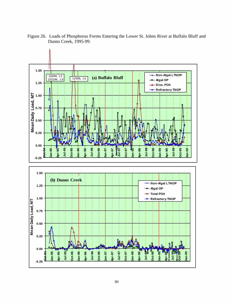
80
Figure 26. Loads of Phosphorus Forms Entering the Lower St. Johns River at Buffalo Bluff and
Dunns Creek, 1995-99.
(a) Buffalo Bluff
-0.25
0.00
0.25
0.50
0.75
1.00
1.25
1.50
Oct-
94
Jan
-95
Ap
r-95
Ju
l-95
Oc
t-95
Jan
-96
Ap
r-96
Ju
l-96
Oc
t-96
Jan
-97
Ap
r-97
Ju
l-97
Oct-
97
Jan
-98
Ap
r-98
Ju
l-98
Oct-
98
Jan
-99
Ap
r-99
Ju
l-99
Oct-
99
Jan
-00
Me
an
Da
ily L
oa
d,
MT
Non-Algal LTNOP
Algal OP
Diss. PO4
Refractory TNOP
12/6/94, 1.5
12/21/94, 1.9 11/5/95, 1.6
(b) Dunns Creek
-0.25
0.00
0.25
0.50
0.75
1.00
1.25
1.50
Oct-
94
Jan
-95
Ap
r-95
Ju
l-95
Oct-
95
Jan
-96
Ap
r-96
Ju
l-96
Oct-
96
Jan
-97
Ap
r-97
Ju
l-97
Oct-
97
Jan
-98
Ap
r-98
Ju
l-98
Oct-
98
Jan
-99
Ap
r-99
Ju
l-99
Oct-
99
Jan
-00
Me
an
Daily L
oad
, MT
Non-Algal LTNOP
Algal OP
Total PO4
Refractory TNOP

81
Reconstruction Of The Upstream Natural Background Load
To provide the endpoint for the continuum in water quality responses to nutrient enrichment, it is
necessary to estimate or reconstruct the characteristics of the natural background load. It should
be emphasized that achieving the natural background condition is not the objective of the TMDL
process per se, though it is assumed to be a desirable condition. Rather, the quantification of this
condition anchors one end of the water quality impairment – development continuum and allows
for the interpolation to the point of water quality criteria adherence and hence tolerable
anthropogenic load. Estimation of the natural background condition is also desirable as it helps
in envisioning the estuarine ecosystem prior to human impacts, which can help define restoration
goals and set realistic water quality targets.
To estimate the natural background load of nitrogen, phosphorus and organic carbon that enters
the lower St. Johns from within the immediate (i.e., lower St. Johns) basin, the watershed
modeling approach use was followed, with all present-day developed land used reverted to
natural forest cover. Because similar modeling has not been performed for the Ocklawaha and
St. Johns River basins upstream of the lower St. Johns, and perhaps more importantly, water
quality modeling has not been performed to estimate the transformation of this load that would
occur in the numerous, large upstream lakes, estimation of the upstream boundary natural
background load is more difficult. In the following analysis, the load delivered to the inlet of the
lower St. Johns Basin is estimated through a simple source-proportionality approach and by
applying a Vollenweider model phosphorus settling term for Lake George. This estimate is then
corroborated by comparison to available historic water quality data.
Natural Background Concentrations of Small Order, Undeveloped Streams
Nitrogen, phosphorus and carbon forms engage in almost continuous flux in surface waters from
the moment of dissolution or detachment from the terrestrial environment. In streams
contributing to the St. Johns River, the time between export from the terrestrial environment to
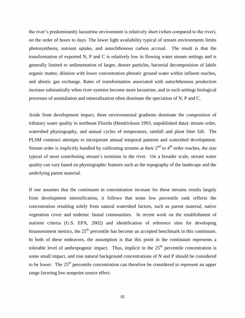
82
the river’s predominantly lacustrine environment is relatively short (when compared to the river),
on the order of hours to days. The lower light availability typical of stream environments limits
photosynthesis, nutrient uptake, and autochthonous carbon accrual. The result is that the
transformation of exported N, P and C is relatively low in flowing water stream settings and is
generally limited to sedimentation of larger, denser particles, bacterial decomposition of labile
organic matter, dilution with lower concentration phreatic ground water within influent reaches,
and abiotic gas exchange. Rates of transformation associated with autochthonous production
increase substantially when river systems become more lacustrine, and in such settings biological
processes of assimilation and mineralization often dominate the speciation of N, P and C.
Aside from development impact, three environmental gradients dominate the composition of
tributary water quality in northeast Florida (Hendrickson 1993, unpublished data): stream order,
watershed physiography, and annual cycles of temperature, rainfall and plant litter fall. The
PLSM construct attempts to incorporate annual temporal patterns and watershed development.
Stream order is implicitly handled by calibrating streams at their 2nd
to 4th
order reaches, the size
typical of most contributing stream’s terminus in the river. On a broader scale, stream water
quality can vary based on physiographic features such as the topography of the landscape and the
underlying parent material.
If one assumes that the continuum in concentration increase for these streams results largely
from development intensification, it follows that some low percentile rank reflects the
concentration resulting solely from natural watershed factors, such as parent material, native
vegetation cover and endemic faunal communities. In recent work on the establishment of
nutrient criteria (U.S. EPA, 2002) and identification of reference sites for developing
bioassessment metrics, the 25th
percentile has become an accepted benchmark in this continuum.
In both of these endeavors, the assumption is that this point in the continuum represents a
tolerable level of anthropogenic impact. Thus, implicit in the 25th
percentile concentration is
some small impact, and true natural background concentrations of N and P should be considered
to be lower. The 25th
percentile concentration can therefore be considered to represent an upper
range favoring low nonpoint source effect.

83
The 25th
percentile rank (Figure 27(a)) for streams of the type within the LSJR basin corresponds
to 0.77 mg/L of total nitrogen (TN) for Pleistocene Ridge streams (streams that drain the higher,
sandy ridges that predominate on the western banks of the St. Johns valley), and 0.88 mg/L TN
for Atlantic Coast Flatwoods streams (streams draining the low-lying region on the eastern banks
of the St. Johns). For total inorganic nitrogen (TIN = NH4 + NO2+3), the 25th
percentile value for
Pleistocene Ridge streams is 0.041 mg/L, and for Atlantic Coast Flatwoods streams is 0.058
mg/L. Total phosphorus (TP) and orthophosphate (PO4), concentrations corresponding to the
25th
percentile for Pleistocene Ridge and Atlantic Coast Flatwoods streams are, respectively:
0.038 mg/L TP, 0.023 mg/L PO4, and 0.066 mg/L TP and 0.039 mg/L PO4 (Figure 27(b)). In
comparison, concentrations assigned to undeveloped land uses (timberlands included) in
watershed model development for the lower St. Johns River Basin (Hendrickson and Konwinski,
1998; Hendrickson et al. 2002), shown in Table 4, are similar, producing a somewhat lower
concentrations of 0.7 mg/L for TN and values of between 0.02 and 0.04 mg/L for TIN, but
comparable and values between 0.05 to 0.07 mg/L for TP and between 0.03 and 0.05 mg/L for
PO4. Recent draft nutrient criteria developed by the EPA’s convened National Expert’s
Workshop places criteria thresholds (considered upper acceptable levels and thus incorporating
some anthropogenic contribution) for streams and rivers of this ecoregion (Region 12, northern
peninsular Florida) at 0.9 mg/L for TN and 0.04 mg/L TP.

84
Figure 27. Continuous Probability Density Functions for Total and Inorganic Nutrient Mean
Concentrations for Streams in Northeast Florida. ACF = Atlantic Coast Flatwoods
Streams; PPR = Plio-Pleistocene Ridge Streams; TN = Total Nitrogen; TIN = Total
Inorganic N (NOX+NH4); TP = Total Phosphorus; PO4 = Orthophosphate.
(a) Nitrogen
0
10
20
30
40
50
60
70
80
90
100
2 3 4 5 6 7 8 9 10
Ln(Total N, mg/m3as N)
Pe
rce
nti
le R
an
k
ACF - TN
PPR - TN
ACF - TIN
PPR - TIN
TN 25th %ile =
0.77 - 0.88 mg/L
TIN 25th %ile =
0.041 - 0.058 mg/L
(b) Phosphorus
0
10
20
30
40
50
60
70
80
90
100
0 1 2 3 4 5 6 7 8
Ln(TP, mg/m 3as P)
Pe
rce
nti
le R
an
k ACF - TP
PPR - TP
ACF - PO4
PPR - PO4
TP 25th %ile =
0.038 - 0.066 mg/L
PO4 25th %ile =
0.023 - 0.039 mg/L

85
Role of Spring Inputs
Artesian spring flow represents a significant proportion of the baseflow of the St. Johns,
comprising approximately 38% of the mean annual discharge at the basin’s inlet at Buffalo
Bluff. Thus, the influence of artesian spring N and P concentrations cannot be ignored in the
present-day and natural background levels of river and estuary productivity.
Today, many springs exhibit elevated concentrations of nutrients as a result of contamination of
deep Floridian ground water over the past half century. This contamination has occurred by
several means, including percolation of surficial aquifer water that has been enriched through
fertilization, land application of waste and nitrogen-enriched atmospheric deposition; stormwater
drainage wells; and sinkhole inputs of eutrophic surface waters. In most cases this enrichment
has resulted in increases in spring concentrations of the highly soluble and mobile nitrate-
nitrogen form (Figure 28), though in some cases direct entry through drainage wells and
sinkholes may have also resulted in elevated nitrogen and phosphorus concentrations (Figure
28). Trends in nutrient concentrations suggest that spring contamination via direct entry through
storm drain wells may be on the decline (as in the case of Rock and Wekiva Springs, Figure 28),
while nitrate contamination through surficial aquifer downward percolation may still be
increasing (as in the case of DeLeon, Blue, Silver and Gemini Springs). Presumably, because of
the tendency for phosphorus to be depleted in deep percolating groundwater from adsorbtion and
assimilation in surface soils, downward percolation does not represent a significant pathway for
phosphorus contamination.

86
Figure 28. Time-Series Concentrations of Nitrate+Nitrite-N and Orthophosphate-P in Major
Springs Discharging to the St. Johns River That Exhibit Nitrate+Nitrite Trends.
Data From USGS, Odum (1953) and SJRWMD.
(a) Nitrate + Nitrite
0.000
0.500
1.000
1.500
2.000
2.500
Fe
b-6
3
Fe
b-6
6
Fe
b-6
9
Fe
b-7
2
Fe
b-7
5
Fe
b-7
8
Fe
b-8
1
Fe
b-8
4
Fe
b-8
7
Fe
b-9
0
Jan
-93
Jan
-96
Jan
-99
Jan
-02
NO
X, m
g/L
Blue
DeLeon
Gemini
Rock
Silver
Wekiva
(b) Orthophosphate
0.000
0.020
0.040
0.060
0.080
0.100
0.120
0.140
Feb-6
3
Feb-6
6
Feb-6
9
Feb-7
2
Feb-7
5
Feb-7
8
Feb-8
1
Feb-8
4
Feb-8
7
Feb-9
0
Jan-9
3
Jan-9
6
Jan-9
9
Jan-0
2
To
tal P
O4, m
g/L
Blue
DeLeon
Gemini
Ro ck
Silver
Wekiva

87
Because of the absence of trends in orthophosphate concentrations for major springs contributing
to the St. Johns River (Wekiva and Rock Springs excluded), the present day, flow-weighted
orthophosphate concentration of 0.041 mg/L has been used to represent the natural background
concentration. For nitrate+nitrite-N, the 25th
percentile occurrence of all springs has been used,
which corresponds to a concentration of 0.01 mg/L. Spring TP and TKN data are also available,
though in lower numbers and temporal coverage. Spring-flow mean TP concentration was found
to be 0.061 mg/L, while the mean concentration of dissolved TP was 0.04 mg/L, suggesting
particulate P as a large component of non-PO4-phosphorus. The mean concentration of total
Kjeldahl nitrogen was 0.081 mg/L. Fourteen of the 35 available measurements for TKN were
remarked as below the method detection limit of approximately 0.08 mg/L. Due to the
uncertainty regarding the concentrations of TP and TKN, the relatively low concentrations, and
the possibility for organic N and non-PO4-phosphorus to arise from spring source other that the
artesian boil, the nitrate+nitrite and orthophosphate concentration have been used to represent
total N and total P from artesian springs.
Using the 25th
percentile values of TN and TP observed for ridge and flatwoods tributary runoff
to represent background terrestrial flow concentrations, the 25th
and percentile concentration of
spring NO2+3, and the mean flow-weighted spring PO4 concentration, natural background
concentrations of TN and TP were projected for the St. Johns River at Buffalo Bluff (Figure 29).
The proportions of surface and groundwater were determined through a relationship between
present-day refractory total organic carbon and the calculated ratio of terrestrial:artesian flow
occurring during the 2 week period prior to the time of sampling. This approach was used to
dampen the oscillations in discharge that occur at the Buffalo Bluff due to intermittent and
extended reverse flows (Sucsy and Morris, 2001). TP concentration was reduced by the
sedimentation rate for Lake George by applying the Vollenweider calculation using the
formulation of Chapra (1997). Calculated Lake George TP sedimentation rate was found to be
1.0 m/yr, and although unusually low, is in agreement with the sedimentation rate determined for
Lake Apopka, another large, shallow sub-tropical lake (Coveney, 1997). The final natural
background annual mean TP concentration delivered to Buffalo Bluff was determined to be
0.037 mg/L, for the hydrologic conditions existing from 1995-99. The actual 1995-99 mean TP
concentration at Buffalo Bluff was 0.063 mg/L.
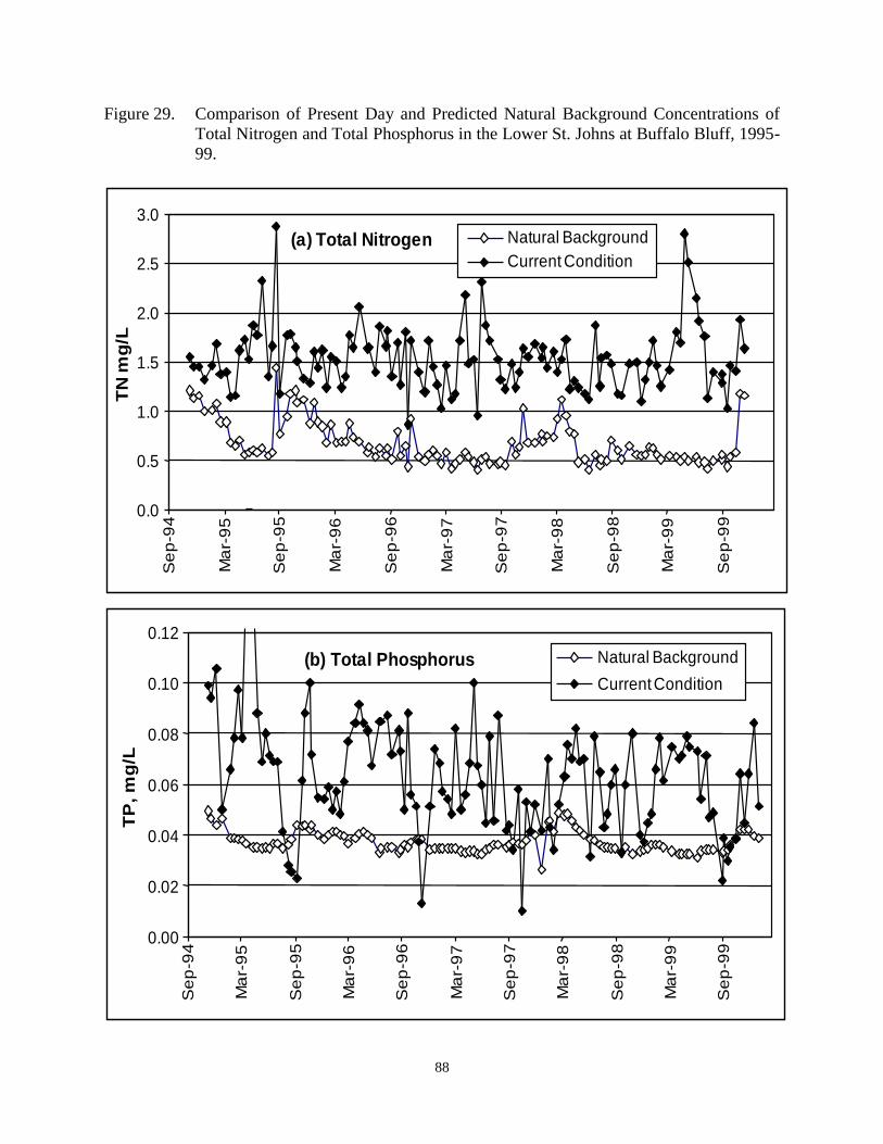
88
Figure 29. Comparison of Present Day and Predicted Natural Background Concentrations of
Total Nitrogen and Total Phosphorus in the Lower St. Johns at Buffalo Bluff, 1995-
99.
(a) Total Nitrogen
0.0
0.5
1.0
1.5
2.0
2.5
3.0
Se
p-9
4
Ma
r-9
5
Se
p-9
5
Ma
r-9
6
Se
p-9
6
Ma
r-9
7
Se
p-9
7
Ma
r-9
8
Se
p-9
8
Ma
r-9
9
Se
p-9
9
TN
mg
/L
Natural Background
Current Condition
(b) Total Phosphorus
0.00
0.02
0.04
0.06
0.08
0.10
0.12
Se
p-9
4
Ma
r-9
5
Se
p-9
5
Ma
r-9
6
Se
p-9
6
Ma
r-9
7
Se
p-9
7
Ma
r-9
8
Se
p-9
8
Ma
r-9
9
Se
p-9
9
TP
, m
g/L
Natural Background
Current Condition

89
To develop an estimate for natural background TN concentration, the terrestrial to spring flow
ratio approach was again used, for both bioavailable (considered to be the sum of inorganic,
labile organic and algal fractions) and refractory nitrogen partitions. Labile and refractory
nitrogen concentrations were separately estimated to account for phytoplankton bio-available
nitrogen deficit that would presumably be made up through algal nitrogen fixation.
Concentrations were calculated corresponding to each sampling day of the bi-weekly sampling
record between 1995-99. RTON was assumed to be the same as the present day concentration,
while time-varying LTON was calculated using the present-day RTON-LTON relationship,
reduced by the mean ratio of historic to present day LTON. Natural background estimated algal
P was used to determine an algal ON based on Redfield stoichiometric equivalency (7.2:1 N:P
mass ratio), and for days on which the labile N was less than algal ON, the difference was added
to the labile N concentration. Labile and refractory N concentrations for each day were then
summed, to produce a mean 1995-99 natural background mean TN concentration of 0.687 mg/L.
By comparison, the actual 1995-99 mean TN concentration at Buffalo Bluff was 1.54 mg/L.
Mean natural background chlorophyll a concentration was estimated to be 14.0 mg/m3, while the
actual 1995-99 mean corrected chlorophyll a was 26.6 mg/m3.
Historic Data for the St. Johns River
Few water quality data exist for the St. Johns River prior to substantial levels of development.
While the point at which the St. Johns River Basin became developed to a degree that it exerted a
significant effect on water quality is difficult to ascertain, the sharp increase in the State’s
population that began subsequent to World War II appears to correspond the earliest reports of
water quality degradation (Figure 30). Population density within the basin upstream of
Jacksonville remained relatively low until 1940. Between 1940 and 1950, population within the
basin increased by 39% (Fl. State Board of Health, 1951).

90
Figure 30. Population growth within the 14 Counties of the St. Johns River Basin, 1890 –
2000. Data from Dietrich (1978) and University of Florida (2000). Significant
events with likely impact on nutrient status identified.
0.0
0.5
1.0
1.5
2.0
2.5
3.0
3.5
4.0
4.5
1880 1900 1920 1940 1960 1980 2000
Po
pu
lati
on
, mill
ion
s o
f p
ers
on
s
Water hyacinth
introduced
First of 5 major
Jacksonville Harbor
dredging projects
Upper St. Johns marsh
encroachment begun w /
Fellsmere grade
Earliest
WQ data
2,4-D First used to
control w ater hyacinth
Upper St. Johns Marsh
1/3rd of its original area
Rodman Dam
completed
Water hyacinth eliminated
follow ing operation “Clean Sw eep”
– Era of algal blooms begins
Blount Island
Cut Completed
Upstream point
source direct
discharge
eliminated
By the time of the earliest, regular surface water quality monitoring efforts, beginning in the late
1960’s, water quality in the middle St. Johns River appears to have already declined. Moody
(1970) attributed this decline in Lake George to the occurrence of regular, severe algal blooms.
Principle factors leading to these algal blooms were believed to be: 1) upstream development and
its concomitant nutrient enrichment through point and non-point source pollution, and 2) aquatic
weed spraying to eliminate floating water hyacinth. Moody notes that concentrations of blue-
green algae were in 1967, “present in much greater numbers . . . “ than reported in an earlier
study in 1939-40 (by E. Lowe Pierce (1947)). Two water quality sample events for Lake
George, which were collected in July of 1967 and December of 1969, are contained in his report.

91
The July sample contained 2.28 mg/L TN and 0.13 mg/L TP, while the December sample
contained 1.3 mg/L TN and again, 0.13 mg/L TP.
Three data sets have been identified that can help in understanding the nutrient status and hence
open water ecology of the St. Johns prior to substantial development. The first of these is a study
conducted by E. Lowe Pierce (1947) reporting on several aspects of the water quality and
plankton in the St. Johns River at locations in the Ocklawaha River mouth, in the river upstream
and downstream of the Ocklawaha from September 1939 to November 1940. The second is the
work of Odum (1953) characterizing the phosphorus concentrations of waters of the State. The
third study was published by the Florida State Board of Health in1948 to determine the effect of
untreated waste discharge in and around the City of Jacksonville.
The objective of the Florida State Board of Health study was to determine the effect of the
discharge of untreated sewage in the vicinity of Jacksonville, and sampling stations were
established in the St. Johns River near the city of Green Cove Springs to characterize upstream,
background conditions. Two surveys were performed, the first conducted in May and June of
1945, and a second conducted from September 1945 to May of 1946. Though nutrient analysis
was not performed, BOD and dissolved oxygen were examined and may be used to infer trophic
status. Many of the reports’ sampling stations were located in Jacksonville, which at the time
was already significantly impacted, principally from the discharge of raw sewage. However,
comparing the report’s BOD data from the upstream, “un-impacted” site near the Shands Bridge
to present day concentrations at the same location suggests that water column biodegradable
organic matter has increased over time. The May to June survey produced what was referred to a
“highest average” (statistical methods are not explained in the report) of 0.83 mg/L; in
comparison, the May - June mean BOD concentration at Shands Bridge from 1996 to 2000 was
2.14 mg/L. The Sept. 1945 to May 1946 survey produced a highest average concentration of 0.82
mg/L, while the 1996-2000 average is 1.43 mg/L.
Under present-day conditions in the LSJR, algal biomass is accounts for the majority of labile
organic carbon in the river, and the relationship between BOD and chlorophyll a is highly
significant, with chlorophyll a concentrations explaining over 70% of the variation in BOD (Chl-

92
a = 14.39*(BOD) – 4.11; R2 = 0.71). Based on this relationship, the 0.83 mg/L BOD measured
in 1945 corresponds to a chlorophyll a of about 8 mg/m3. Converting the present day mean river
color for this location to refractory organic nitrogen (assumes color has not changed; in reality,
river color probably has declined somewhat due to basin development), and adding in the
nitrogen content of algal biomass at 8 mg/m3 chlorophyll a, a mean total organic nitrogen content
of 0.48 mg/L can be calculated. With the inclusion of inorganic nitrogen, it would be expected
from these BOD data that total nitrogen was in the neighborhood of 0.6 mg/L, comparable to the
reconstructed historic Buffalo Bluff mean TN concentration of 0.687 mg/L. It should be noted
that Green Cove Springs is located downstream of where, even in 1946, potentially significant
inputs of nutrients from the city of Palatka (20 miles upstream, at that time with a population of
approximately 8,000) and the tri-county agricultural area, may have occurred.
The Odum (1953) report to the Florida Geological Survey extensively surveyed orthophosphate
and total phosphorus in surface waters around the State. Samples were collected at one time
from many different locations, so annual trends cannot be inferred. These data for locations in
the St. Johns River and its contributing streams are listed in Table 9. Because a significant
amount of development had begun to occur at the time of this study, these data must be viewed
selectively for the potential of anthropogenic nutrient contamination. For locations that likely
still represented unimpacted reaches of the lower St. Johns River in 1952 (assumed to be Lake
George and Crescent Lake), these data suggest a concentration of total phosphorus of around
0.04 mg/L. Upstream of Lake Monroe, the Odum data suggests a St. Johns River that was
remarkably low in phosphorus.
Table 9. Total Phosphorus Concentrations Determined for Selected Locations in St. Johns
River Basin in 1952. Data from Odum (1953).
Location Date Total P, mg/L
Black Creek, Route 17 Aug. 9, 1952 0.04
Deep Creek, Hastings, Route 207 Jul. 14, 1952 0.54
Crescent Lake, Andalusia Jul. 19, 1952 0.033

93
Doctor’s Lake, Route 17 Aug. 9, 1952 0.065
Lake George at Silver Glen Springs Aug. 14, 1952 0.044
Lake Monroe, Sanford Jun. 23, 1952 0.18
Ortega River, Route 21 Aug. 9, 1952 0.044
St. Johns R., Crows Bluff, Volusia Co. Sep. 3, 1952 0.117
St. Johns R., Palatka Jul 19, 1952 0.061
St. Johns R., Route 192 (Brevard Co.) Jun. 23, 1952 0.007
St. Johns R., Route 50 (Orange Co.) Jun. 23, 1952 0.015
St. Johns R., Green Cove Springs Jul. 16, 1952 0.119
The data of Pierce (1947), due to the length of his study and the comparatively large suite of
measurements, provide compelling evidence of a river that was dramatically lower in nutrients
and algal biomass. The graphs of Figure 31 compare the results of this study with the present
day mean concentrations observed from 1995-99. In 1939-40, Pierce reported blue green algae
(of the genera Anabaena, Raphidiopsis and Microcystis) ranging from too few to count for most
months, to 36,000 cells/ml in August of 1940. In comparison, the annual mean peak blue-green
cell count exiting Lake George for 1997-2000 (Phlips and Cichra, 2001) was 518,893 cells/ml.
The Pierce study also suggests a shift in the dominance of phytoplankton groups, with diatoms
(primarily the genera Coscinodiscus and Melosira) formerly making up a much greater relative
portion of the plankton.
The Pierce study also provides data on nitrogen forms throughout the year. (Unfortunately,
analysis for phosphorus forms was not performed.) Due to some differences in methodology and
uncertainties regarding sample handling and preservation techniques, only total nitrogen
concentrations are compared. Pierce reported mean annual TN as 0.41 mg/L in Little Lake
George (upstream of the Ocklawaha mouth), and 0.37 mg/L at Welaka (downstream of the
Ocklawaha), values that are roughly 1/4th
of present day concentrations. The Pierce TN numbers
are similar to the present day estimated mean concentration refractory total organic N at Buffalo
Bluff, of 0.46 mg/L. Because RTON theoretically reflects a relatively constant natural supply of

94
organic nitrogen, its concentration would be expected to remain constant, or perhaps even
decrease due to development, over time.

95
Figure 31. Comparison of Monthly Mean Water Quality Parameters for 1995-99 (solid boxes)
to the Data Collected by Pierce (1947) in 1939-40 (open diamonds) for the St. Johns
River near Buffalo Bluff. Error bars on 1995-99 data represent 95% C.I. Pierce
chlorophyll estimated from cell counts.
a) Total Chloride
0
90
180
270
360
450
Jul-39 Sep-39 Nov-39 Dec-39 Feb-40 Mar-40 May-40 Jul-40 Aug-40 Oct-40
mg
/L
b) Dissolved Oxygen
0
2
4
6
8
10
12
Jul-39 Sep-39 Nov-39 Dec-39 Feb-40 Mar-40 May-40 Jul-40 Aug-40 Oct-40
mg
/L
c) Total Nitrogen
0.0
0.5
1.0
1.5
2.0
2.5
Jul-39 Sep-39 Nov-39 Dec-39 Feb-40 Mar-40 May-40 Jul-40 Aug-40 Oct-40
mg
/l
d) Secchi Depth
0
0.5
1
1.5
2
Jul-39 Sep-39 Nov-39 Dec-39 Feb-40 Mar-40 May-40 Jul-40 Aug-40 Oct-40
me
ters
e) Chlorophyll-a (corrected)
0
20
40
60
80
100
Jul-39 Sep-39 Nov-39 Dec-39 Feb-40 Mar-40 May-40 Jul-40 Aug-40 Oct-40
mg
/m3

96
The Pierce (1947) total N concentrations are low when compared to those reconstructed here,
which suggest an annual mean concentration of 0.65 – 0.70 mg/L. Similarly, mean annual
chlorophyll a estimated from cell densities in the Pierce work, at 2 mg/m3, are considerably
lower than the reconstructed annual mean of 14 mg/m3. However, unaccounted for in the water
column measurements of these studies, but theoretically included in the runoff delivery
approach, is the sequestration of nutrient in water hyacinth (Eichornia crassipes). Water
hyacinth, introduced to the St. Johns shortly before 1900, quickly spread through the river, and
anecdotal accounts prior to 1940 (Rawlings, 193_) indicate widespread coverage. Annual
reports to Congress on the progress of hyacinth control in the St. Johns (USACE Annual Reports
to Congress, 1930 - 1967) indicate that between 3000 to 13,000 acres of hyacinth were removed
annually, suggesting that at least 5 to 10 % (based on the sum of lake surface areas of the St.
Johns from Lake Winder through Little Lake George) of the rivers water surface area typically
may have been covered.
To estimate the potential sequestration of nitrogen in water hyacinth, literature values for organic
matter dry weight and percent N and P content were combined with areal coverage estimates
determined by the U.S. Army Corps of Engineers. Using an 8% areal hyacinth coverage
estimate (U.S. Army Corps estimate from the only available comprehensive survey of hyacinth,
conducted in November of 1948, of 9,500 acres (USACE, 1948)) and assuming 1000 g/m2
organic matter, with 1% as N, 0.05% as P (Reddy and DeBusk, 1987; values represent minimum
in the areal organic matter and nutrient content ranges, as would be expected for uncultivated
hyacinth growing under natural and assumed nutrient-limited conditions), an additional 0.27
mg/L N can be calculated as sequestered in hyacinth tissue. Adding this concentration to the
Pierce mean TN concentration for the St. Johns below the Ocklawaha mouth produces a mean
total N concentration of 0.64 mg/L.
Differences in analysis methodology, the relatively short study durations, possibly different
hydrologic conditions, and assumptions in the conversion procedures warrant that these estimates
of background concentrations be used with caution. However, these studies suggest substantially
lower water column nitrogen and algal biomass, and marginally lower phosphorus concentrations
prevailed in the pre-development St. Johns River. If the concentrations of TN of 0.6 mg/L and

97
TP of 0.04 mg/L are accepted as representative of water column (including floating
macrophytes) natural background levels, then nutrients flowing into the lower St. Johns River
from the upper and middle St. Johns and Ocklawaha Rivers today appear to be elevated between
1.5 to 4 times above pre-development conditions.
Total LSJR Load Estimates
With the estimated of upstream, natural background loads, it is possible to estimate the total
incoming anthropogenic nutrient and organic carbon load to the Lower St. Johns River. Tables
10 - 15 summarize the mean annual loads from source categories to the LSJR by river ecozone
from 1995 through 1999, and the over all average. When comparing this compilation of loads to
that performed earlier by Hendrickson and Konwinski (1998) it should be noted that in this
assessment, the portion of river identified as predominantly oligohaline has been moved
upstream, to encompass all loads entering from Black Creek northward to the Ortega River. In
the previous assessment, loads entering from Orange Park northward were considered to
contribute directly to the oligohaline reach, and Black Creek loads were added to the freshwater
river. The reason for the move was the prevailing drier conditions encountered during the 1995-
99 assessment period, particularly for 1998 and 1999.
The separation of labile and refractory organic carbon and nutrients performed in this version of
the external load provides a dramatically different conclusion on the relative sources of problem
nutrients leading to algal blooms in the lower St. Johns. In the previous compilation of the LSJR
external load, Hendrickson and Konwinski (1998), in lieu of information on the utilization of
organic nitrogen and non-orthophosphate phosphorus forms by river algal communities,
estimated the bioavailable load as that composed of only inorganic nutrient (NH4, NOX, and PO4)
forms. The addition of labile organic forms to the “total bioavailable pool” of nutrients greatly
increases the apparent influence of upstream loads. Accounting for labile organic forms also
increases the relative importance of urban nonpoint source runoff in potential contribution of
problem nutrient loads.

98
Table 10. Summary of Mean Annual Loads to the Lower St. Johns River, 1995. All values in metric tons per year.
Total N Labile TON
Refractory
TON
Total
Inorganic N Total P Labile TNOP
Refractory
TNOP Total PO4
Total
Organic C Labile TOC Refractory TOC
Buffalo Bluff Total 10765.1 4336.2 5373.0 1056.0 511.2 207.3 96.9 207.0 138347.0 12976.2 125370.9
Natural Background 6659.7 1006.7 5432.5 220.5 290.8 97.9 97.3 95.6 131539.8 5727.6 125812.3
Dunns Creek Total 1372.5 290.7 919.0 162.8 108.2 33.6 35.4 39.1 23100.5 718.7 22381.9
Natural Background 915.7 112.0 779.9 23.7 61.3 15.0 31.4 14.9 19272.6 636.9 18635.7
Upstream Total 12137.7 4627.0 6291.9 1218.8 619.3 240.9 132.3 246.1 161447.5 13694.8 147752.7
Fresh Tidal NP Total 1068.4 371.7 505.6 191.1 211.2 54.9 22.7 133.6 23875.4 1709.8 22165.6
Natural Nonpoint 626.3 203.8 387.9 34.6 56.8 11.1 6.7 38.9 23213.7 1255.7 21957.9
Agriculture Contribution 384.1 126.1 124.7 133.4 136.9 35.4 13.4 88.1 217.9 173.7 44.2
Urban Contribution 53.2 39.3 -3.5 17.4 15.4 8.5 1.7 5.2 -507.8 171.4 -679.2
Other Nonpoint 4.7 2.5 -3.5 5.7 2.1 -0.1 0.9 1.3 951.7 109.0 842.7
Point Source 306.7 151.5 12.0 143.2 70.2 32.0 0.8 37.4 1417.6 814.6 603.0
Oligohaline NP Total 1141.3 517.8 447.3 176.3 186.8 79.2 16.7 90.9 25692.0 2584.6 23107.4
Natural Nonpoint 746.3 236.9 468.9 40.5 65.6 13.0 8.3 44.2 26852.0 1413.6 25438.4
Agriculture Contribution 26.2 10.7 2.0 13.5 10.9 2.1 0.5 8.3 1.5 46.5 -45.0
Urban Contribution 370.7 269.2 -10.1 111.6 110.0 64.0 7.8 38.2 -2062.9 1028.6 -3091.5
Other Nonpoint -1.8 1.0 -13.5 10.7 0.5 0.0 0.2 0.3 901.5 96.0 805.5
Point Source 333.5 49.6 3.9 279.9 72.1 11.2 0.3 60.6 287.1 165.0 122.1
Meso-Polyhaline NP Total 440.2 223.2 120.6 96.4 92.0 44.0 6.6 41.4 6524.5 1002.8 5521.6
Natural Nonpoint 218.4 68.0 138.5 11.9 19.8 3.8 2.5 13.6 7509.0 385.0 7124.1
Agriculture Contribution 13.4 5.3 1.1 7.0 5.3 1.2 0.2 4.0 17.4 20.2 -2.8
Urban Contribution 209.9 151.9 -10.7 68.8 66.6 39.2 3.8 23.6 -1238.7 567.6 -1806.3
Other Nonpoint -1.5 -2.1 -8.2 8.8 0.2 -0.2 0.2 0.2 236.7 30.1 206.6
Point Source 1147.4 238.9 18.9 889.6 294.4 46.9 1.2 246.2 1920.7 1103.7 817.0
Total Atmospheric Dep. 219.5 2.8
LSJRB Summary
Total Natural Nonpoint 1591.0 508.7 995.3 86.9 142.2 28.0 17.5 96.7 57574.7 3054.3 54520.4
Total Augmented Nonpoint 1059.0 603.9 78.2 376.8 347.9 150.2 28.6 169.1 -1482.8 2243.0 -3725.8
Total Point Source 1787.6 440.0 34.9 1312.7 436.6 90.2 2.3 344.2 3625.4 2083.3 1542.1
Grand Total 16794.8 6179.6 7400.4 2995.2 1548.8 509.2 180.6 856.1 221164.9 21075.5 200089.4
Notes: N= Nitrogen; P=Phosphorus; C=Carbon. NP=Nonpoint Sources. LSJRB Summary sums loads for only the lower St. Johns Basin downstream of Dunns Creek.

99
Table 11. Summary of Mean Annual Loads to the Lower St. Johns River, 1996. All values in metric tons per year.
Total N Labile TON
Refractory
TON
Total
Inorganic N Total P Labile TNOP
Refractory
TNOP Total PO4
Total
Organic C Labile TOC Refractory TOC
Buffalo Bluff Total 8609.9 4828.1 3252.4 529.4 385.0 241.4 48.1 95.3 103597.6 17027.1 86570.5
Natural Background 4451.6 1100.3 3252.4 98.9 221.1 122.7 48.1 50.4 92828.8 6258.3 86570.5
Dunns Creek Total 898.0 172.5 595.7 129.8 42.5 11.8 13.7 17.1 16639.5 523.2 16116.3
Natural Background 716.0 85.8 595.7 34.5 34.1 9.6 13.7 10.9 16604.5 488.2 16116.3
Upstream Total 9507.9 5000.6 3848.1 659.2 427.5 253.2 61.7 112.5 120237.1 17550.3 102686.8
Fresh Tidal NP Total 578.6 187.5 289.3 101.8 93.6 25.7 11.5 56.4 13718.0 869.5 12848.4
Natural Nonpoint 365.6 105.5 243.7 16.5 32.0 6.0 4.5 21.5 13597.2 623.4 12973.8
Agriculture Contribution 177.0 56.0 49.7 71.3 51.8 15.0 5.6 31.2 -24.3 88.7 -113.0
Urban Contribution 30.8 25.7 -5.1 10.2 8.6 4.7 0.9 2.9 -334.6 118.2 -452.8
Other Nonpoint 5.2 0.3 1.0 3.9 1.3 0.0 0.6 0.7 479.7 39.2 440.4
Point Source 285.6 144.6 11.5 129.6 66.0 30.5 0.8 34.7 1340.4 770.2 570.1
Oligohaline NP Total 676.8 300.0 264.0 112.8 113.7 47.0 10.1 56.6 14393.1 1440.3 12952.7
Natural Nonpoint 427.3 124.3 281.9 21.0 38.3 7.1 5.2 26.1 15176.5 707.0 14469.4
Agriculture Contribution 18.0 7.2 1.8 9.0 6.6 1.2 0.2 5.1 8.0 29.6 -21.5
Urban Contribution 230.5 51.4 -13.5 77.0 68.0 38.6 4.5 24.9 -1383.4 645.9 -2029.3
Other Nonpoint 1.0 117.0 -6.2 5.8 0.8 0.1 0.2 0.4 592.0 57.8 534.2
Point Source 322.5 42.3 3.4 276.8 65.6 10.5 0.3 54.9 351.8 202.2 149.7
Meso-Polyhaline NP Total 422.7 210.3 119.2 93.2 87.2 39.6 6.3 41.3 6400.3 949.3 5451.0
Natural Nonpoint 211.3 62.5 137.7 11.0 19.6 3.5 2.5 13.5 7243.0 345.8 6897.3
Agriculture Contribution 17.8 6.6 1.8 9.4 7.5 1.6 0.3 5.6 42.9 25.0 17.9
Urban Contribution 193.3 141.7 -14.2 65.8 59.4 34.5 3.3 21.6 -1161.2 545.2 -1706.4
Other Nonpoint 0.4 -0.6 -6.2 7.1 0.8 -0.1 0.3 0.6 275.6 33.3 242.3
Point Source 1144.4 251.6 20.0 872.9 328.9 50.8 1.3 276.9 2199.7 1264.0 935.7
Total Atmospheric Dep. 203.7 2.7
LSJRB Summary
Total Natural Nonpoint 1004.2 292.3 663.4 48.5 89.8 16.6 12.1 61.2 36016.7 1676.3 34340.5
Total Augmented Nonpoint 673.9 405.5 9.1 259.3 204.6 95.7 15.8 93.1 -1505.4 1582.9 -3088.3
Total Point Source 1752.5 438.5 34.8 1279.3 460.5 91.7 2.3 366.5 3891.9 2236.4 1655.4
Grand Total 13142.2 6136.9 4555.3 2246.3 1185.2 457.1 91.9 633.2 158640.3 23045.9 135594.5
Notes: N= Nitrogen; P=Phosphorus; C=Carbon. NP=Nonpoint Sources. LSJRB Summary sums loads for only the lower St. Johns Basin downstream of Dunns Creek.

100
Table 12. Summary of Mean Annual Loads to the Lower St. Johns River, 1997. All values in metric tons per year.
Total N Labile TON
Refractory
TON
Total
Inorganic N Total P Labile TNOP
Refractory
TNOP Total PO4
Total
Organic C Labile TOC Refractory TOC
Buffalo Bluff Total 4849.3 3606.6 1061.3 181.4 173.2 148.6 12.9 11.6 55541.4 17236.2 38305.2
Natural Background 1880.2 792.5 1061.3 26.4 117.5 85.7 12.9 18.8 42814.0 4508.8 38305.2
Dunns Creek Total 933.4 318.0 564.3 51.2 59.9 27.1 15.6 17.2 17202.9 996.6 16206.3
Natural Background 711.2 133.1 564.3 13.8 35.8 15.2 15.6 4.9 16963.6 757.3 16206.3
Upstream Total 5782.7 3924.6 1625.5 232.6 233.1 175.7 28.6 28.8 72744.4 18232.8 54511.5
Fresh Tidal NP Total 992.8 341.2 430.4 221.2 158.4 54.4 20.6 83.4 20214.2 1522.6 18691.6
Natural Nonpoint 532.7 181.2 321.9 29.6 44.8 9.7 5.5 29.5 20183.5 1163.8 19019.7
Agriculture Contribution 405.3 122.0 109.6 173.7 97.5 35.5 12.1 49.9 -112.0 132.2 -244.1
Urban Contribution 49.1 39.2 -1.0 10.9 14.4 9.0 2.0 3.4 -439.7 167.9 -607.6
Other Nonpoint 5.7 -1.2 0.0 7.0 1.7 0.1 1.0 0.5 582.3 58.7 523.6
Point Source 299.6 86.6 73.1 139.7 69.1 24.0 7.0 38.1 4789.3 585.6 4203.6
Oligohaline NP Total 728.4 325.9 302.4 100.1 110.4 46.5 10.8 53.0 17709.8 1684.1 16025.7
Natural Nonpoint 501.7 163.3 310.9 27.4 42.8 8.9 5.4 28.4 18268.7 996.5 17272.1
Agriculture Contribution 16.4 6.8 1.3 8.4 6.9 1.3 0.3 5.3 -8.7 30.0 -38.7
Urban Contribution 211.9 156.1 -1.4 57.3 60.6 36.3 5.0 19.3 -1101.0 602.7 -1703.7
Other Nonpoint -1.6 -0.3 -8.3 7.0 0.1 0.0 0.1 0.0 550.9 54.9 496.0
Point Source 341.3 45.9 9.8 285.6 73.6 11.5 0.7 61.5 321.6 143.8 177.8
Meso-Polyhaline NP Total 342.7 182.4 88.7 71.6 69.6 35.1 4.7 29.8 4914.8 822.6 4092.2
Natural Nonpoint 162.7 52.0 101.9 8.8 13.9 2.9 1.8 9.2 5644.2 300.8 5343.4
Agriculture Contribution 9.9 4.0 0.4 5.5 3.5 0.6 0.0 2.9 -8.1 14.7 -22.8
Urban Contribution 170.9 128.3 -8.5 51.1 52.0 31.6 2.7 17.7 -865.4 490.0 -1355.4
Other Nonpoint -0.8 -1.9 -5.0 6.1 0.2 0.1 0.2 -0.1 144.1 17.0 127.1
Point Source 1187.7 251.1 33.7 902.9 334.6 71.4 3.1 260.1 2233.5 1354.5 879.0
Total Atmospheric Dep. 235.0 3.0
LSJRB Summary
Total Natural Nonpoint 1197.1 396.5 734.6 65.9 101.4 21.5 12.7 67.2 44096.4 2461.2 41635.2
Total Augmented Nonpoint 867.0 453.0 87.0 327.0 236.9 114.6 23.3 99.0 -1257.7 1568.1 -2825.7
Total Point Source 1828.6 383.6 116.6 1328.2 477.4 106.9 10.8 359.7 7344.4 2083.9 5260.5
Grand Total 9910.4 5157.8 2563.7 1953.6 1051.8 418.7 75.4 554.7 122927.4 24346.0 98581.5
Notes: N= Nitrogen; P=Phosphorus; C=Carbon. NP=Nonpoint Sources. LSJRB Summary sums loads for only the lower St. Johns Basin downstream of Dunns Creek.

101
Table 13. Summary of Mean Annual Loads to the Lower St. Johns River, 1998. All values in metric tons per year.
Total N
Labile TON
Refractory TON
Total Inorganic
N
Total P Labile TNOP
Refractory TNOP Total PO4
Total Organic C
Labile TOC
Refractory TOC
Buffalo Bluff Total 8561.5 4942.4 3175.9 443.1
341.8 201.8 42.5 97.4
127323.1 21218.1 106105.0
Natural Background 4428.1 1189.7 3175.9 62.5
246.4 140.0 42.5 63.9
112873.9 6768.9 106105.0
Dunns Creek Total 971.2 217.6 681.9 71.7
51.3 15.8 15.9 19.7
21379.6 778.7 20600.9
Natural Background 813.6 108.2 681.9 23.5
39.4 11.1 15.9 12.4
21216.6 615.7 20600.9
Upstream Total 9532.7 5160.0 3857.8 514.9
393.1 217.6 58.4 117.1
148702.7 21996.9 126705.9
Fresh Tidal NP Total 1652.2 480.2 935.0 237.0
222.9 53.8 31.1 138.0
44053.4 2272.1 41781.4
Natural Nonpoint 1188.3 284.7 864.2 39.4
103.4 17.3 16.7 69.4
43976.7 1525.1 42451.6
Agriculture Contribution 350.3 111.7 93.9 144.7
92.2 27.3 11.9 53.0
-257.6 256.3 -513.9
Urban Contribution 110.4 92.5 -21.4 39.4
25.8 13.4 2.8 9.6
-817.6 443.8 -1261.4
Other Nonpoint 3.1 -8.7 -1.7 13.6
1.5 -4.2 -0.2 5.9
1151.9 47.0 1105.0
Point Source 274.2 82.4 57.1 134.5
62.1 21.9 5.1 35.0
4154.4 582.3 3572.2
Oligohaline NP Total 1236.9 492.7 565.8 178.4
171.8 63.8 18.4 89.6
28792.1 2331.6 26460.5
Natural Nonpoint 830.1 199.7 601.6 28.8
72.4 12.1 11.6 48.7
29623.8 1041.0 28582.8
Agriculture Contribution 35.9 17.9 9.5 8.5
8.7 5.9 2.4 0.5
-51.2 53.9 -105.1
Urban Contribution 374.4 282.0 -33.2 125.6
90.6 50.4 6.3 33.9
-1540.4 1200.2 -2740.6
Other Nonpoint -3.5 -6.9 -12.1 15.4
0.1 -4.5 -1.9 6.5
759.8 36.5 723.3
Point Source 301.3 53.7 9.6 238.0
81.4 13.2 0.7 67.5
363.5 184.3 179.2
Meso-Polyhaline NP Total 867.0 436.2 254.1 176.7
152.0 68.5 11.4 72.1
13343.1 1966.9 11376.3
Natural Nonpoint 426.5 109.6 299.9 17.0
37.7 6.5 5.7 25.5
14672.1 570.9 14101.2
Agriculture Contribution 38.3 7.3 -1.5 32.5
11.8 -3.1 -1.1 16.1
29.8 49.8 -20.0
Urban Contribution 404.1 315.7 -40.2 128.6
101.5 59.8 4.8 36.9
-1741.7 1310.4 -3052.1
Other Nonpoint -1.8 3.6 -4.1 -1.3
0.9 5.3 2.0 -6.3
382.9 35.8 347.1
Point Source 1267.0 279.4 38.3 949.3
341.5 70.7 3.3 267.6
2468.4 1500.7 967.7
Total Atmospheric Dep. 278.2
3.8 LSJRB Summary
Total Natural Nonpoint 2444.9 594.0 1765.7 85.2
213.5 35.8 34.0 143.6
88272.7 3137.0 85135.7
Total Augmented Nonpoint 1311.2 815.2 -10.8 506.8
333.2 150.3 26.8 156.1
-2084.0 3433.6 -5517.6
Total Point Source 1842.4 415.5 105.1 1321.8
485.0 105.8 9.1 370.1
6986.3 2267.2 4719.1
Grand Total 15409.4 6984.7 5717.8 2428.7
1428.5 509.5 128.4 786.9
241877.7 30834.6 211043.1
Notes: N= Nitrogen; P=Phosphorus; C=Carbon. NP=Nonpoint Sources. LSJRB Summary sums loads for only the lower St. Johns Basin downstream of Dunns Creek.
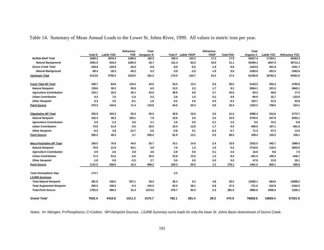
102
Table 14. Summary of Mean Annual Loads to the Lower St. Johns River, 1999. All values in metric tons per year.
Total N Labile TON
Refractory
TON
Total
Inorganic N Total P Labile TNOP
Refractory
TNOP Total PO4
Total
Organic C Labile TOC Refractory TOC
Buffalo Bluff Total 5280.2 3876.3 1268.0 182.0 183.4 150.2 17.2 17.9 62627.4 17164.1 45463.3
Natural Background 2091.0 815.0 1250.3 25.7 121.3 83.3 16.9 21.1 50350.1 4637.0 45713.1
Dunns Creek Total -166.6 -120.9 -45.0 -0.8 -8.9 -6.5 -1.9 -0.6 -1443.5 -401.8 -1041.7
Natural Background -80.4 -35.3 -45.2 0.2 -3.9 -2.0 -1.9 0.0 -1263.6 -201.0 -1062.6
Upstream Total 5113.6 3755.4 1223.0 181.2 174.5 143.7 15.3 17.4 61183.8 16762.3 44421.6
Fresh Tidal NP Total 248.7 84.8 119.4 44.5 54.5 13.4 5.6 35.5 5143.3 352.4 4790.9
Natural Nonpoint 139.6 39.3 93.9 6.5 13.2 2.3 1.7 9.2 5064.1 221.0 4843.1
Agriculture Contribution 103.1 35.0 35.1 33.0 38.9 9.6 3.7 25.6 64.3 46.8 17.5
Urban Contribution 9.3 7.6 -1.4 3.2 2.6 1.5 0.2 0.9 -90.9 32.7 -123.5
Other Nonpoint -3.3 3.0 -8.1 1.8 -0.2 0.0 0.0 -0.3 105.7 51.9 53.8
Point Source 275.3 144.0 11.4 119.8 64.5 30.3 0.8 33.4 1232.2 708.0 524.1
Oligohaline NP Total 236.9 103.3 93.4 40.2 40.8 16.0 3.6 21.2 5286.4 512.6 4773.7
Natural Nonpoint 162.4 45.3 109.1 7.9 15.6 2.6 2.0 10.9 5700.0 247.9 5452.1
Agriculture Contribution 5.9 2.3 0.5 3.1 2.6 0.5 0.1 2.0 9.5 10.2 -0.8
Urban Contribution 74.9 51.9 -3.5 26.5 23.4 12.8 1.7 9.0 -494.5 197.1 -691.6
Other Nonpoint -6.3 3.8 -12.7 2.6 -0.8 0.1 -0.2 -0.7 71.4 57.3 14.0
Point Source 305.2 46.3 3.7 255.2 81.9 13.1 0.3 68.5 249.4 143.3 106.1
Meso-Polyhaline NP Total 156.5 76.9 44.0 35.7 33.1 14.9 2.4 15.9 2332.0 342.7 1989.3
Natural Nonpoint 79.9 21.9 54.1 3.9 7.6 1.3 1.0 5.4 2719.0 116.0 2603.0
Agriculture Contribution 6.9 2.6 0.8 3.6 2.8 0.6 0.1 2.0 16.6 9.6 7.0
Urban Contribution 71.4 51.6 -5.6 25.5 22.8 13.0 1.2 8.5 -451.4 195.3 -646.7
Other Nonpoint -1.8 0.8 -5.3 2.7 0.0 0.0 0.0 0.0 47.9 21.8 26.1
Point Source 1121.5 206.0 16.3 899.2 330.3 50.0 1.2 279.1 1401.0 805.1 595.9
Total Atmospheric Dep. 174.7 2.5
LSJRB Summary
Total Natural Nonpoint 381.9 106.5 257.1 18.3 36.4 6.2 4.8 25.5 13483.1 584.9 12898.2
Total Augmented Nonpoint 260.2 158.5 -0.3 102.0 92.0 38.1 6.8 47.0 -721.5 622.8 -1344.2
Total Point Source 1702.0 396.4 31.4 1274.2 476.7 93.4 2.3 381.0 2882.5 1656.4 1226.1
Grand Total 7632.4 4416.8 1511.2 1575.7 782.1 281.4 29.2 470.9 76828.0 19626.4 57201.6
Notes: N= Nitrogen; P=Phosphorus; C=Carbon. NP=Nonpoint Sources. LSJRB Summary sums loads for only the lower St. Johns Basin downstream of Dunns Creek.

103
Table 15. Summary of Overall Mean Annual Loads to the Lower St. Johns River, 1995 - 1999. All values in metric tons per year.
Total N Labile TON
Refractory
TON
Total
Inorganic N Total P Labile TNOP
Refractory
TNOP Total PO4
Total
Organic C Labile TOC Refractory TOC
Buffalo Bluff Total 7613.2 4317.9 2826.1 478.4 318.9 189.9 43.5 85.9 97487.3 17124.3 80363.0
Natural Background 3902.1 980.8 2834.5 86.8 199.4 105.9 43.5 50.0 86081.3 5580.1 80501.2
Dunns Creek Total 801.7 175.6 543.2 82.9 50.6 16.3 15.7 18.5 15375.8 523.1 14852.7
Natural Background 615.2 80.8 515.3 19.1 33.3 9.8 14.9 8.6 14558.7 459.4 14099.3
Upstream Total 8414.9 4493.5 3369.3 561.3 369.5 206.2 59.3 104.4 112863.1 17647.4 95215.7
Fresh Tidal NP Total 908.1 293.1 455.9 159.1 148.1 40.4 18.3 89.4 21400.9 1345.3 20055.6
Natural Nonpoint 570.5 162.9 382.3 25.3 50.0 9.3 7.0 33.7 21207.1 957.8 20249.2
Agriculture Contribution 283.9 90.1 82.6 111.2 83.5 24.5 9.3 49.6 -22.3 139.5 -161.9
Urban Contribution 50.6 40.9 -6.5 16.2 13.4 7.4 1.5 4.4 -438.1 186.8 -624.9
Other Nonpoint 3.1 -0.8 -2.5 6.4 1.3 -0.8 0.4 1.6 654.3 61.2 593.1
Point Source 288.3 121.8 33.0 133.4 66.4 27.7 2.9 35.7 2586.8 692.2 1894.6
Oligohaline NP Total 804.1 347.9 334.6 121.5 124.7 50.5 11.9 62.3 18374.7 1710.7 16664.0
Natural Nonpoint 533.5 153.9 354.5 25.1 46.9 8.7 6.5 31.7 19124.2 881.2 18243.0
Agriculture Contribution 20.5 9.0 3.0 8.5 7.1 2.2 0.7 4.2 -8.2 34.0 -42.2
Urban Contribution 252.5 185.2 -12.3 79.6 70.5 40.4 5.0 25.1 -1316.5 734.9 -2051.3
Other Nonpoint -2.4 -0.2 -10.6 8.3 0.1 -0.9 -0.3 1.3 575.1 60.5 514.6
Point Source 320.8 47.6 6.1 267.1 74.9 11.9 0.4 62.6 314.7 167.7 147.0
Meso-Polyhaline NP Total 445.8 225.8 125.3 94.7 86.8 40.4 6.3 40.1 6702.9 1016.9 5686.1
Natural Nonpoint 219.7 62.8 146.4 10.5 19.7 3.6 2.7 13.4 7557.5 343.7 7213.8
Agriculture Contribution 17.3 5.2 0.5 11.6 6.2 0.2 -0.1 6.1 19.7 23.9 -4.1
Urban Contribution 209.9 157.9 -15.9 67.9 60.5 35.6 3.2 21.7 -1091.7 621.7 -1713.4
Other Nonpoint -1.1 0.0 -5.7 4.7 0.4 1.0 0.5 -1.1 217.4 27.6 189.8
Point Source 1173.6 245.4 25.5 902.8 325.9 58.0 2.0 266.0 2044.6 1205.6 839.1
Total Atmospheric Dep. 222.2 222.2 3.0 3.0
LSJRB Summary
Total Natural Nonpoint 1323.8 379.6 883.2 61.0 116.7 21.6 16.2 78.8 47888.7 2182.7 45706.0
Total Augmented Nonpoint 834.2 487.2 32.6 314.4 242.9 109.8 20.3 112.9 -1410.3 1890.1 -3300.3
Total Point Source 1782.6 414.8 64.6 1303.2 467.2 97.6 5.3 364.3 4946.1 2065.5 2880.6
Grand Total 12577.8 5775.1 4349.7 2462.1 1199.3 435.2 101.1 663.3 164287.7 23785.7 140502.0
Notes: N= Nitrogen; P=Phosphorus; C=Carbon. NP=Nonpoint Sources. LSJRB Summary sums loads for only the lower St. Johns Basin downstream of Dunns Creek.

104
In the upstream nutrient load, total N and P in the 1995-99 load summary are similar to that of
1993-94, at 8,415 MT/yr TN and 370 MT/yr TP, compared to 7209 MT/yr TN and 317 MT/yr
TP. Upstream TIN load from 1995-99 was considerably less than that in 1993-94, at 414 MT/yr
compared to 639 MT/yr. Total PO4 load was marginally less in 1997-98, at 73 MT/yr as
compared to 99 MT/yr in 1993-94. The generally lower upstream inorganic nutrient loads may
be attributed to lower flow conditions that prevailed during the 1997-98 period, resulting in
longer residence time in upstream lakes and greater incorporation of inorganic forms in algal
biomass. Although the el Nino winter of 1997-98 resulted in one of the highest mean annual
flow rates for the St. Johns River at the upstream Deland gauging station, this extremely wet
interval was short, and immediately followed by one of the longest droughts in Florida
meteorological history. Hence the tendency for low algal standing stock associated with a high
flow/short residence time hydrologic pattern was not seen in 1998.
Within-LSJR basin anthropogenic loads are still predominantly attributable to point source
discharges. From 1995-99, point sources accounted for 1,783 MT/yr of TN and 467 MT/yr of
TP, as compared to the 1993-94 estimate of 1,886 MT/yr of TN and 530 MT/yr of TP. Applying
the labile/refractory partitioning algorithm to point source effluents suggests that most of the
organic nutrient portion of these effluents is in the bioavailable form.
Within-LSJR basin nonpoint source loads are lower that that assessed for the 1993-94 time
period, owing largely to the prevailing dry condition that decreased nonpoint source runoff in
general. An additional factor leading to this decrease is a substantial decline in tri-county row
crop area. In the previous assessment, the within-basin, nonpoint TN mean annual load was
determined to be 3,528 MT/yr, with 1,243 MT/yr of this representing the above background load.
In this assessment, the mean annual 1995-99 nonpoint TN load was determined to be 2,158
MT/yr, with 834 MT/yr of that the above-background load. For TP, the 1993-94 nonpoint load
was determined to be 665 MT/yr, with 468 MT/yr of this the above-background load, while for
1995-99, the mean load was determined to be 360 MT/yr, with 243 MT/yr of this the augmented,
above-background load. However, the relevance of the nonpoint source load as it relates to the
contribution of bioavailable nutrients, is considerably increased in this assessment, owing to the
distinction of labile organic pool. In the 1993-94 assessment, in which only the TIN load was

105
considered to represent the “bioavailable” load, total anthropogenic bioavailable nonpoint load
was assessed as 488 MT/yr of TIN and 248 MT/yr of PO4. With the inclusion of labile organic
nutrient forms, the 1995-99 augmented nonpoint source bioavailable N load increases to 802
MT/yr. The 1995-99 augmented nonpoint bioavailable P load was estimated as 223 MT/yr, less
than the estimated PO4 load of 1993-94; however, the inclusion of the labile organic fraction
represents a 97 percent increase over an estimate based upon PO4 alone.
Atmospheric Deposition
The estimate of directly-intercepted atmospheric deposition load has been considerably reduced
in the 1995-99 total load assessment. Using three NADP gauges, rather than the one used in the
1993-94 assessment, including dry deposition, and relying on tower measurements to determine
the P load, Pollman and Roy (2003) provided data that demonstrates the directly-intercepted
rainfall load to the LSJR to be roughly 222 MT/yr of TN, of which most is inorganic N, and 3
MT/yr of P. Thus, direct atmospheric deposition represents only 2.8 percent of the total
bioavailable N load and 0.5 percent of the bioavailable P load to the LSJR. The discrepancy
between this estimate and the earlier estimate, which found atmospheric deposition to comprise
14.7% of the bioavailable N load and 0.8% of the bioavailable P load can be attributed to two
factors. The first is the inclusion of labile organic N and P in the assessment of bioavailable
point and nonpoint source loads. The second can be traced to a units error in the Hendrickson
and Konwinski (1998) assessment, in which atmospheric deposition NO3 concentrations that
were reported as mg/L NO3, were assumed to be as mg/L N. The result was a 443 percent
overestimate in atmospheric N load.
Accounting for indirect deposition, that portion of wet deposition falling on terrestrial areas and
entering surface waters un-attenuated in runoff, can in some cases substantially increase the
contribution of atmospheric nitrogen. Timpe (1999) concluded that 28% of the non-point source
nitrogen loading from mixed urban and residential watersheds in the Tampa Bay Watershed
could be attributed to wet atmospheric deposition. Rushton (1997) found a significant
correlation between precipitation nitrogen concentration and the concentration of parking lot

106
runoff for individual storm events in a study of wet detention pond effectiveness. Employing
the wet deposition retention factors (the proportion of wet deposition that arrives in surface
waters for various land covers) of Paerl et al. (2001), the 1995-99 mean annual indirect
atmospheric deposition added by land areas in the lower St. Johns River basin is estimated at and
additional 222 MT/year. This doubles the overall contribution of atmospheric nitrogen to the
total N load of the LSJR to 5.5 percent. However, an arguably more relevant way to view the
contribution is to view it in the context of the urban nonpoint nitrogen pollution. If atmospheric
nitrogen deposition has roughly doubled over the past 150 years due to anthropogenic inputs
(Pollman, pers. comm.), then 84 MT per year of the indirect atmospheric deposition that is
exported from urban areas can well be viewed as anthropogenic atmospheric contribution. This
represents 15 percent of the anthropogenic labile nitrogen that enters the lower St. Johns River in
an average year.
DISCUSSION
In order to develop ecologically relevant nutrient budgets for estuaries, that portion of the
organic nutrient pool that is biologically available must be quantified (Seitzinger and Sanders,
1997). The results of this analysis suggest that a potentially wide range in bioavailability may
exist in the organic carbon and nutrient pools of tributary runoff from different land uses. For
the watersheds employed in the calibration of PLSM coefficients, LTOC was on average 10% of
TOC, ranging from 4% in waters draining undeveloped, forested streams to 54% for a highly
urbanized streams. In a study of mixed urban/ag/forested watersheds in southeast Pennsylvania,
Volk et al. (1997) found bioavailable DOC to constitute on average 25 % of DOC. As southeast
US blackwater streams would be expected to exhibit higher levels of RDOC, the values obtained
here appear consistent with that study. Due to the tendency for labile organic matter to possess
higher relative amounts of N and P, the fractions of labile nutrient within total organic nutrient
forms are higher than labile carbon fractions, on average 50% for LTON and 75% for LTNOP.
LTON ranged from 28% of TON for largely undeveloped watersheds to 78% for urbanized
streams. Due to the very low levels of TNOP observed in undeveloped watershed runoff, it
cannot be said with certainty what percent is composed of LTNOP, although it appears that
concentrations are probably less than 10 g/L. For urbanized streams, TNOP was found to be

107
92% composed of LTNOP. Thus it can be seen that anthropogenic nutrient loading, due to its
relatively greater amount of labile nutrient content, has a proportionally greater effect on
eutrophication than would be surmised by the absolute increase in total nutrient (Figure 32).

108
Figure 32. Comparison of Total and Bioavailable Nitrogen Forms in Runoff from Natural
Forested and Mixed Urban/Commercial/Residential Watersheds. Due to the higher
relative amounts of labile nutrients in developed landscapes, deleterious nutrient
load often exceeds that which would be inferred by absolute increases in nutrients
alone. Reductions in refractory organic nutrient-bearing colored dissolved organic
matter may also increase algal productivity by increasing transparency.
0.0
0.2
0.4
0.6
0.8
1.0
1.2
1.4
1.6
Natural Urban
Co
ncen
trati
on
. m
g/L
Total Inorg. N
Labile Org. N
Refractory Org. N
214%
Increase
in TN
663% Increase in
Bio-available N

109
The addition of organic carbon and nutrient forms provides the necessary enhancement to our
understanding of the external load to permit the development of hypothesis related to the natural
and altered productivity states of the LSJR estuary, in particular as it relates to the TMDL
response variables: dissolved oxygen, chlorophyll a and turbidity. The analysis here suggests
that in its natural state, the LSJR saw considerably lower levels of labile organic carbon and
nutrients. The un-altered condition of forested landscapes and contiguous riparian areas also
probably resulted in a river that was more darkly colored. Based on 1995-99 annual averages,
the present anthropogenic load of total labile nitrogen of 6,407 MT/yr represents a 374 percent
increase over the natural background labile nitrogen load of 1,720 MT/yr. For labile
phosphorus, the 1995-99 mean annual anthropogenic load of 820 MT/yr represents a 297 percent
increase over the natural background load of 276 MT/yr. One would assume that this degree of
loading over background would result in much higher levels of internal algal production,
although the amount of this increased production cannot be determined from the annual average
external load alone. With regard to the pre-development oxygen regime that the estuary
experienced, not only would lower levels of algal production have a positive effect, but the lower
incoming load of LTOC would also be expected to result in lower imported BOD.
A significant, seasonal component exists in the concentrations of organic carbon forms that occur
in runoff, and such seasonal effects have been observed elsewhere. In Scandinavian boreal
forests, DON concentrations were observed to increase as spring snow melt-induced water table
rise brings water table to surface (Stepanauskas et al., 2000), and Leff and Meyer (1991), in an
examination of DOC patterns in the Ogeechee River in Georgia, found concentrations to
increases with increasing flow. With regard to bioavailability, Moran et al. (1999) found the
highest per mole C rates of utilization in August for the Satilla River in Georgia. McLatchey and
Reddy (1998) attribute such seasonal changes as largely due to the annual pattern in soil
temperature and soil redox changes owing to saturation and decomposition. With declining free
energy (redox potential) there is decreased OM decomposition, hence greater OM export; greater
P mobilization; higher substrate quality of the exported organic matter; and enhanced NH4
mobilization. Other important factors may include the timing of forest litterfall, the timing of

110
temperatures leading to litter decomposition, or the occurrence of leaching rains following
litterfall.
In the examination of multiple regression-developed land use loading rates, it is clear (and
perhaps intuitive) that intensification in land use, in particular associated with urbanization, leads
to an increase in the concentration and export of labile organic matter and a decrease in the
refractory form. While the increase in labile organic matter is clearly detrimental, the
implications of a decrease in RTOC are less clear. RTOC is assumed to be synonymous with
colored dissolved organic matter, and the effects of CDOM on aquatic systems are to increase
color, decrease pH, as well as to possibly exert some antibacterial properties. Higher prevailing
color levels in the lower St. Johns River has been suggested to favor the dominance of the low-
light adapted native submersed grass Vallisneria americana (Dean Dobberfuhl, pers.
communication) allowing it to fix carbon at lower light levels and thus out compete
phytoplankton for nutrients.
While the high concentrations calculated for LTOC in dairy runoff are probably not surprising,
the relatively higher concentrations calculated for urban runoff are. Possible sources in the urban
and residential environment could include malfunctioning septic tanks, sanitary sewer line leaks,
pump station overflows, animal feces, grass clippings, industrial waste or perhaps even
hydrocarbons. The implications of this are that while urban runoff tends to exhibit moderate
levels of organic nutrient concentrations, it is likely that much of this is in the labile fraction and
hence potentially more detrimental to receiving waters. The differentiation and inclusion of
labile organic carbon and nutrients into the total bioavailable pool increases the relative harm
that this form of land use development perpetrates over what was previously believed.
The greatest change in our understanding of the relative sources of bioavailable nutrients to the
lower St. Johns that comes with the inclusion of labile carbon and nutrients is the apparent huge
contribution of the upper and middle St. Johns. Based on only inorganic nutrient concentrations,
Hendrickson and Konwinski (1998) estimated its contribution to be much lower, providing only
20% of TIN and 11% of PO4. With the inclusion of labile organic N and P, the upper and middle
St. Johns can be seen to contribute 61% of the whole LSJR bioavailable N and 28% of

111
bioavailable P. Much of this bioavailable N is produced internally through atmospheric nitrogen
fixation by blue-green algae in Lake George (Paerl, 2002; Phlips and Cichra, 2001) during long
residence times that favor the depletion of bioavailable N stores. Thus, while nitrogen control
has been one of the most widely touted management strategies in the oligohaline and mesohaline
portions of the LSJR to reduce the potential for nuisance algal blooms in this nitrogen-limited
estuary, the most successful approach to reducing nitrogen in the upstream load delivered to the
estuary may well be reduction in phosphorus load to the upper and middle St. Johns River.
The discovery of the potential sequestration of the greater part of the historic bioavailable
nitrogen (and presumably also phosphorus) supply to the St. Johns by water hyacinth
(Eichhornia crassipes) necessitates a fundamental re-definition of the “natural background” load
to the LSJR. Even prior to the introduction of water hyacinth, Bartram (1792) noted in his
travels of Florida in 1774, in the reach of the LSJR between Green Cove Springs and Palatka,
vast quantities of the floating aquatic plant water lettuce (Pistia stratiotes). He wrote:
“I set sail on early, and saw, this day, vast quantities of Pistia stratiotes . . .
forming most delightful green plains, several miles in length, and in some
places a quarter of a mile in breadth”
Accounts such as this indicate that vast areas of floating aquatic plants existed in the pre-colonial
LSJR, and that river ecology was based upon the substantial utilization of nutrients by
macrophytes, rather than phytoplankton.
Beginning in 1949, chemical aquatic weed spraying with 2,4-D began in an effort to eradicate
water hyacinth. It was not until the late 1960’s that the exotic weed, by this time wildly out of
control due no doubt by the increased nutrient load to which the river was now subjected, was
reduced to manageable levels. Today, hyacinth is kept in check through continuous aquatic
weed spraying. This undertaking, along with continued urban, industrial and agricultural
development within the basin, has undoubtedly transformed the river into the phytoplankton-
dominated system that it is today. The characterization of the incoming, natural background load
to the LSJR as phytoplankton-dominated should be viewed as a device to establish a common

112
currency for evaluating nutrient enrichment and control efforts against established,
phytoplankton chlorophyll-a based standards. The apparent importance of water lettuce in the
pre-colonial LSJR suggests that a balanced ecosystem restoration approach should not only
address nutrient reduction to reduce the severity of algal blooms, but should also assess to the
role of floating and submersed, rooted aquatic macrophytes in maintaining water quality and
organism health and diversity.
113
Literature Cited
Adamus, C.L. and M.J. Bergman. 1995. Estimating nonpoint source pollution loads with a GIS
screening model. Wat. Res. Bull. 31(4): 647-655.
Amon, R.M.W. and R. Benner. 1996. Bacterial utilization of different size classes of dissolved
organic matter. Limnol. Oceanogr. 41(1) 41-51.
Boynton, W.R., J.H. Garber, R. Summers and W.M. Kemp. 1995. Inputs, transformations and
transport of nitrogen and phosphorus in Chesapeake Bay and selected tributaries. Estuaries
18(1B): 285-314.
Bushaw, K.L et al. 1996. Photochemical release of biologically available nitrogen from dissolved
organic matter. Nature 381:404-407.
Cerco, C. F. and T. Cole. 1995. Users Guide to the CE-QUAL-ICM Eutrophication Model.
U.S. Army Corps of Engineers Waterways Experiment Station, Vicksburg, MS.
Chapra, S.C. 1997. Surface Water Quality Modeling. McGraw Hill, New York. 844 pp.
Coveney, M. 1997. P sedimentation rate for L. Apopka.
DeBusk, W.F., J.R. White and K.R. Reddy. 2001. Carbon and nitrogen dynamics in wetland
soils, In, Modeling Carbon and Nitrogen Dynamics for Soil Management , M.J. Shaffer, L.
Ma and S. Hansen, eds. CRC Press, Boca Raton, FL.
Dietrich, T.S. 1978. The urbanization of Florida’s population: A historical perspective on county
growth 1830-1970. Bureau of Economic and Business Research, University of Florida,
Gainesville, FL.
Florida State Board of Health. 1948. Report on the St. Johns River pollution survey. Bureau of
Sanitary Engineering, Jacksonville, Fla. 59 pp.
Florida State Board of Health. 1951. One River, One Plan – St. Johns River Basin: Report on
Water Pollution Control. Water Pollution Series #27. Tallahassee, FL.
Gardner, W.S., R. Benner, R.M.W. Amon, J.B. Cotner Jr., J.F. Cavaleto and F.R. Johnson. 1996.
Effects of high molecular weight dissolved organic matter on nitrogen dynamics in the
Mississippi River plume. Mar. Ecol Prog Ser. 133: 287-297.
Goldman, J.C., D.A. Caron and M.R. Dennett. 1987. Regulation of gross growth efficiency and
ammonium regeneration in bacteria by substrate C:N ratio. Limnol. Oceanogr. 32(6):
1239-1252.
Goolsby, D.A., W.A. Battaglin, B.T. Aulenbach and R. P. Hooper. 2001. Nitrogen input to the
Gulf of Mexico. J. Environ. Qual. 30: 329-336.

114
Harper, H. 1994. Estimation of Stormwater Loading Rate Parameters for Central and South
Florida. Environmental Research and Design, Inc. Orlando, FL.
Hartigan, J.P., T.M. Quasebarth and E. Southerland. 1982. Calibration of NPS loading factors.
J. Env. Eng. 109(6): 1259-1272.
Hedges, J.I., G.L. Cowie, J.E. Richey, P.D. Quay, R. Benner, M. Strom, B.R. Forsberg. 1994.
Origins and processing of organic matter in the Amazon River as indicated by
carbohydrates and amino acids. Limnol. Oceanogr. 39(4): 743-761.
Hendrickson, J.C. and J. Konwinski. 1998. Seasonal Nutrient Import-Export Budgets for the
Lower St. Johns River, Florida. Final report for Contract WM598, Florida Department of
Environmental Protection. 109 pp.
Hendrickson, J.C., C. Cerco and J. L. Martin. 2001. Photo-decomposition model for colored
dissolved organic matter in a blackwater estuary. In, Warrick, J.J., (Editor), American
Water Resources Association Annual Spring Specialty Conference Proceedings. “Water
Quality Monitoring and Modeling.” American Water Resources Association Conference,
Middleburg, Virginia, TPS-01-1, 284 pp.
Hendrickson, J., E. Lowe, D. Dobberfuhl, P. Sucsy and D. Campbell. 2003. Characteristics of
Accelerated Eutrophication in the Lower St. Johns River Estuary and Recommendation of
Targets for the Achievement of Water Quality Goals to Fulfill TMDL and PLRG
Objectives. Water Resources Department Technical Memorandum No. __, St. Johns River
Water Management District, Palatka, FL.
Jaworski, N.A., P.M. Groffman, A.A. Keller, J.C. Prager. 1992. A watershed nitrogen and
phosphorus balance: The upper Potomac river basin. Estuaries 15(1): 83-95.
Kaplan, L.A. and J.D. Newbold. 1995. Measurement of streamwater biodegradable dissolved
organic carbon with a plug-flow bioreactor. Water Res. 29:2696-2706.
Magnien, R.E., R.M. Summers and K.G. Sellner. 1992. External nutrient sources, internal
nutrient pools, and phytoplankton production in Chesapeake Bay. Estuaries 15(4): 497-
516.
Mann, K.H. 1988. Production and use of detritus in various freshwater, estuarine, and coastal
marine ecosystems. Limnol. Oceanogr. 33(4) 910-930.
Mannino, A. and H.R. Harvey. 2000. Biochemical composition of particles and dissolved
organic matter along an estuarine gradient: Sources and implications for DOM reactivity.
Limnol. Oceanogr. 45(4): 775-788.
McLatchey, G. P. and K. R. Reddy. 1998. Regulation of Organic Matter Decomposition and
Nutrient Release in a Wetland Soil. J. Env. Qual. 27: 1268-1274.

115
Meyer, J.L., R.T. Edwards, R. Risley. 1987. Bacterial Growth on Dissolved Organic Carbon
from a Blackwater River. Microb. Ecol. (1987) 13: 13-29.
Moody, 1970.
Moran, M.A., R.E. Hodson. 1989. Formation and bacterial utilization of dissolved organic
carbon derived from detrital lignocellulose. Limnol. Oceanogr. 34 (6):1034-1047.
Moran, M.A., R.E. Hodson. 1990. Bacterial production on humic and nonhumic components of
dissolved organic carbon. Limnol. Oceanogr. 35(8): 1744-1756.
Moran, M.A., W.M. Sheldon Jr., J.E. Sheldon. 1999. Biodegradation of Riverine Dissolved
Organic Carbon in Five Estuaries of the Southeastern United States. Estuaries 22(1): 55-
64.
National Research Council. 2000. Clean Coastal Waters: Understanding and Reducing the
Effects of Nutrient Pollution. Ocean Studies Board and Water Science and Technology
Board, Commission on Geosciences, Environment, and Resources. National Academy
Press, Washington D.C. 405 pp.
Odum, H.T. 1953. Dissolved Phosphorus in Florida Waters. Report to the Florida Geological
Survey, Report of Investigations, No. 9. Tallahassee, FL.
Ogura, N. 1975. Further studies on decomposition of dissolved organic matter in coastal
seawater. Mar. Biol. 31: 60-62.
Paerl, H.W. 2001. Production and Nutrient Limitation of Harmful Algal Blooms in the St. Johns
River. Progress report to the St. Johns River Water Management District under Contract
No. SD154RA.
Paerl, H.W., R.L. Dennis, D.R. Whitall. 2002. Atmospheric deposition of nitrogen: Implications
for nutrient over-enrichment of coastal waters. Estuaries 25(4b): 677-693.
Phlips, E.J. and M.F. Cichra. 2001. Plankton Communities of the Lower St. Johns River.
Annual Report to the St. Johns River Water Management District, Contract #97W165.
University of Florida Department of Fisheries and Aquatic Sciences, Gainesville, FL.
Pierce, E.L. 1947.
Pollman, C.D. and S. Roy. 2003. Examination Of Atmospheric Deposition Chemistry and Its
Potential Effects On The Lower St. Johns Estuary: Final Report Submitted To St. Johns
River Water Management District, Contract No. SE706AA. Tetra Tech, Inc. Gainesville,
FL.
Poor, N, R. Pribble, and H. Greening. 2001. Direct wet and dry deposition of ammonia, nitric
acid, ammonium, and nitrate to the Tampa Bay Estuary, FL, USA. Atmos. Environ. 35:
3947 – 3955.
116
Rao, D.V., S.A. Jenab and D. Clapp. 1997. Rainfall Analysis for Northeast Florida: Summary of
Monthly and Annual Rainfall Data Through 1995. St. John River Special Publication SJ97-
SP22.
Rawlings, M.K. 193_ . Hyacinth Drift.
Raymond, P.A. and J.E. Bauer. 2001. DOC cycling in a temperate estuary: A mass balance
approach using natural 14C and 13C isotopes. Limnol. Oceanogr. 46(3): 655-667.
Reddy, R. and _ Debusk. 1987. Hyacinth N content.
Rushton, B. 1997. Processes that effect stormwater pollution. Proceedings, 5th
Biennial
Stormwater Research Conference. Southwest Florida Water Management District,
Brooksville, FL.
Seitzinger, S.P. and R.W. Sanders. 1997. Contribution of dissolved organic nitrogen from rivers
to estuarine eutrophication. Mar. Ecol. Prog. Ser. 159: 1-12.
Sondergaard, M. and M. Middelboe. 1995. A cross-system analysis of labile dissolved organic
carbon. Mar. Ecol. Prog. Ser. 118: 283-294.
Stepanauskas, R., L. Leonardson and L.J. Tranvik. 1998. Bioavailability of wetland derived
DON to freshwater and marine bacterioplankton. Limnol. Oceanogr. 44(6): 1477-1485.
Stepanauskas, R., H. Laudon and N. O. G. Jorgensen. 2000. High DON bioavailability in boreal
streams during a spring flood. Limnol. Oceanogr., 45(6): 1298-1307.
Strauss, E. A. and G. A. Lamberti. 2000. Regulation of Nutrification in Aquatic Sediments by
Organic Carbon. Limnol. Oceanogr. 45(8):1854-1859.
Strickland, J.D.H. 1960. Measuring the production of marine phytoplankton. Bull. Fish. Res.
Bd. Canada 122. 172 pp.
Sucsy, P and F. Morris. 2001. Hydrodynamics report.
Sun, L., E.M. Perdue, J.L. Meyer and J. Weis. 1997. Use of elemental composition to predict
bioavailability of dissolved organic matter in a Georgia river. Limnol. Oceanogr. 42(4):
714-721.
Timpe, M.P. 1999. Impacts of atmospheric deposition on stormwater quality. Proceedings, 6th
Biennial Stormwater Research and Watershed Management Conference. Southwest
Florida Water Management District, Brooksville, FL.
Toth, D.J. 1993. Volume 1 of the Lower St. Johns River Basin Reconnaissance: Hydrogeology.
Technical Report SJ93-7, St. Johns River Water Management District, Palatka, Florida.

117
Tranvik, L.J. 1990. Bacterioplankton Growth on Fractions of Dissolved Organic Carbon of
Different Molecular Weights from Humic and Clear Waters. Applied and Environmental
Microbiology, 56(6):1672-1677.
Thurman, E.M. 1985. Organic Geochemistry of Natural Waters. Junk, Boston.
U.S.A.C.E. Annual Reports to Congress, 1930 – 1967.
U.S.A.C.E. 1948, November 1. Comprehensive Survey for Removal of Water Hyacinths and
Other Marine Vegetable Growths Interim Report, Serial No. 32. United States Army Corps
of Engineers South Atlantic Division Field Committee, Office, Division Engineer, South
Atlantic Division, Atlanta, Georgia.
U.S. EPA. 1984. Result of the Nationwide Urban Runoff Program: Volume 1 Final Report.
Water Planning Division Report No. PB84-185552.
U.S. EPA, 2002. Nutrient Criteria for SE Ecoregion Streams.
University of Florida. 2000. Florida Estimates of Population. Bureau of Economic and Business
Research. Gainesville, FL.
Valiela, I., K. Foreman, M. LaMontagne, D. Hersh, J. Costa, P. Peckol, B. DeMeo-Andreson, C.
D’Avanzo, M. Babione, C. Sham, J. Brawley and K. Lajtha. 1992. Couplings of watersheds
and coastal waters: Sources and consequences of nutrient enrichment in Waquiot Bay,
Massachusetts. Estuaries 15(4): 443-457.
Volk, C.J., C.B. Volk and L.A. Kaplan. 1997. Chemical composition of biodegradable dissolved
organic matter in streamwater. Limnol. Oceanogr. 42(1): 39-44.
Wetzel, R.G. 1983. Limnology. Second Ed., CBS College Publishing, New York, NY. 767 pp.
Wetzel, R.A. and G.E. Likens. 1990. Limnological Analyses. 2nd
Ed. Springer-Verlag, New
York. 391 pp.