title pageelectric vehicle charging impact on distribution
TRANSCRIPT

Title Page
Electric Vehicle Charging Impact on Distribution Conductor Model and Mitigation
Techniques
by
Jenna DeLozier
B.S. in Electrical Engineering, University of Pittsburgh, 2018
Submitted to the Graduate Faculty of
The Swanson School of Engineering in partial fulfillment
of the requirements for the degree of
Master of Science in Electrical and Computer Engineering
University of Pittsburgh
2019
ii
COMMITTEE PAGE
UNIVERSITY OF PITTSBURGH
SWANSON SCHOOL OF ENGINEERING
This thesis was presented
by
Jenna DeLozier
It was defended on
November 11, 2019
and approved by
Gregory Reed, PhD, Professor, Department of Electrical and Computer Engineering
Brandon Grainger, PhD, Assistant Professor, Department of Electrical and Computer
Engineering
Masoud Barati, PhD, Assistant Professor, Department of Electrical and Computer Engineering
Thesis Advisor: Gregory Reed, PhD, Professor, Department of Electrical and Computer
Engineering

iii
Copyright © by Jenna DeLozier
2019
iv
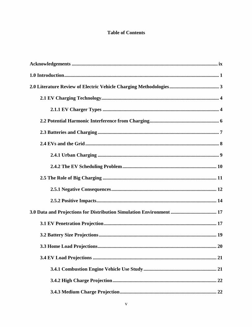
Abstract
Abstract
Electric Vehicle Charging Impact on Distribution Conductor Model and Mitigation
Techniques
Jenna DeLozier, M.S.
University of Pittsburgh, 2019
Electric Vehicle (EV) charging is one of the largest growing electricity demand sectors that
is being added into the electric grid. The bulk electric system, which will carry the majority of the
current load, is a specific infrastructure which is regularly monitored for load changes. In contrast,
distribution systems do not have the same supervision and therefore can be treated as a black box.
The distribution system is important for stability of the grid and in order to predict how much EVs
will impact the main grid, a simulator for a distribution line was created to determine substation
transformer loading and line loading. In addition, four charging cases for the EVs were created to
investigate different charging scenarios. Finally, load mitigation techniques were investigated to
offer potential solutions for the overloading of aged infrastructure.
v
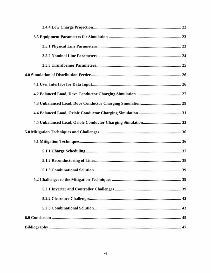
Table of Contents
Acknowledgements ...................................................................................................................... ix
1.0 Introduction ............................................................................................................................. 1
2.0 Literature Review of Electric Vehicle Charging Methodologies ........................................ 3
2.1 EV Charging Technology ............................................................................................... 4
2.1.1 EV Charger Types .............................................................................................. 4
2.2 Potential Harmonic Interference from Charging ........................................................ 6
2.3 Batteries and Charging .................................................................................................. 7
2.4 EVs and the Grid ............................................................................................................ 8
2.4.1 Urban Charging .................................................................................................. 9
2.4.2 The EV Scheduling Problem ............................................................................ 10
2.5 The Role of Big Charging ............................................................................................ 11
2.5.1 Negative Consequences ..................................................................................... 12
2.5.2 Positive Impacts ................................................................................................. 14
3.0 Data and Projections for Distribution Simulation Environment ..................................... 17
3.1 EV Penetration Projection ........................................................................................... 17
3.2 Battery Size Projections ............................................................................................... 19
3.3 Home Load Projections ................................................................................................ 20
3.4 EV Load Projections .................................................................................................... 21
3.4.1 Combustion Engine Vehicle Use Study ........................................................... 21
3.4.2 High Charge Projection .................................................................................... 22
3.4.3 Medium Charge Projection .............................................................................. 22
vi
3.4.4 Low Charge Projection ..................................................................................... 22
3.5 Equipment Parameters for Simulation ...................................................................... 23
3.5.1 Physical Line Parameters ................................................................................. 23
3.5.2 Nominal Line Parameters ................................................................................ 24
3.5.3 Transformer Parameters .................................................................................. 25
4.0 Simulation of Distribution Feeder ....................................................................................... 26
4.1 User Interface for Data Input ...................................................................................... 26
4.2 Balanced Load, Dove Conductor Charging Simulation ........................................... 27
4.3 Unbalanced Load, Dove Conductor Charging Simulation ....................................... 29
4.4 Balanced Load, Oriole Conductor Charging Simulation ......................................... 31
4.5 Unbalanced Load, Oriole Conductor Charging Simulation..................................... 33
5.0 Mitigation Techniques and Challenges ............................................................................... 36
5.1 Mitigation Techniques .................................................................................................. 36
5.1.1 Charge Scheduling ............................................................................................ 37
5.1.2 Reconductoring of Lines ................................................................................... 38
5.1.3 Combinational Solution .................................................................................... 39
5.2 Challenges to the Mitigation Techniques ................................................................... 39
5.2.1 Inverter and Controller Challenges ................................................................ 39
5.2.2 Clearance Challenges ........................................................................................ 42
5.2.3 Combinational Solution .................................................................................... 43
6.0 Conclusion ............................................................................................................................. 45
Bibliography ................................................................................................................................ 47
vii
List of Tables
Table 1 EV Purchase Rates through 2018 [34] ............................................................................. 18
Table 2: Battery Size Historical [35] ............................................................................................ 19
Table 3: Physical Line Parameters [37] ........................................................................................ 24
Table 4: Nominal Line Parameters ............................................................................................... 24
viii
List of Figures
Figure 1: EV Charging Levels [4] .................................................................................................. 5
Figure 2: Harmonic Distortion Example [10] ................................................................................. 7
Figure 3: Example Electricity Use Chart [16] .............................................................................. 10
Figure 4: Duck Curve of Overgeneration [28] .............................................................................. 15
Figure 5: Distribution Simulator Interface .................................................................................... 27
Figure 6: 13.2 kV Dove Conductor Balanced System .................................................................. 28
Figure 7: 2.4 kV Dove Conductor Balanced System .................................................................... 29
Figure 8: 13.2 kV Dove Conductor Unbalanced System .............................................................. 30
Figure 9: 2.4 kV Dove Conductor Unbalanced System ................................................................ 31
Figure 10: 13.2 kV Oriole Conductor Balanced System .............................................................. 32
Figure 11: 2.4 kV Oriole Conductor Balanced System ................................................................ 33
Figure 12: 13.2 kV Oriole Conductor Unbalanced System .......................................................... 34
Figure 13: 2.4 kV Oriole Conductor Unbalanced System ............................................................ 35
Figure 14: Potential Logic Diagram for Charge Scheduling ........................................................ 37
Figure 15: Harmonic Distorition Limits for Current [7] ............................................................... 41

ix
Acknowledgements
Firstly, I would like to thank my parents, Paula and Dale DeLozier for being so supportive
of everything I do and work towards. Engineering school was a challenge I needed to rise up to in
order to accomplish this greatest task so far in my life. I would next like to thank my brother
Matthew for always going with me to church when classwork became overwhelming. I would also
like to thank Jack, whom I have shared many meals and conversations with. Next, I would like to
thank my advisor, Dr. Gregory Reed, for giving me the opportunity to continue my studies at the
University of Pittsburgh and help cultivate my interest in electric power systems. I would also like
to thank Dr. Katrina Kelly-Pitou for exposing me to community-based research. It was a humbling
experience and really showed me how important the community is for energy and power research.
The research is done for them, not just for the advancement of the field.
I would also like to thank my lab mates, Santino, Adam, Ryan, Alvaro, Zach, Aryana, Tom,
Thibaut, Christian, Erick, Corey, John, Alekhya, and Peter for the culture I experienced in graduate
school. My memories will be of you all, not the times sitting in the classes. In addition to my
student counterparts, I would like to thank Dr. Brandon Grainger and Dr. Masoud Barati for the
guidance through my thesis. When I was looking for an academic perspective, they were always
there and supportive. In addition to my academic electric power contacts, I would also like to thank
the distribution engineering department at Duquesne Light. Without their guidance, I would not
have learned practical distribution techniques for my simulations.
I finally would like to thank my wonderful boyfriend, Daniel Mueller. He always reassured
me throughout the process of getting my bachelors and master’s degrees, and was nothing but
supportive. I am so thankful to have you in my life.

1
1.0 Introduction
Electric Vehicles (EV) are a mode of transportation in which electric torque provides a
clean and exciting way to travel. An increase of these vehicles being integrated onto the national
electric grid is occurring in not only in the United States but in other countries worldwide, this
large amount of charging, or big charging, will become a prevalent issue due to aging
infrastructure, lack of capacity on distribution lines, and transformer overloading. These are long-
term issues which will need to be addressed with or without the EV revolution. Many research
articles describe the effect on the bulk electric system, while the distribution system is not as
researched. Typical distribution systems are not monitored in the way the transmission system is
currently monitored and yet this will most likely be where the bottleneck in power consumption
will occur. These systems can be extremely unique due to the age and design differences through
the years; therefore, simulations of individual lines are required to determine the impact. Section
two of this thesis contains a relevant literature review of EV charging, encompassing harmonic
considerations and loading scenarios. Section three describes the creation of the simulator used in
this research and the parameters input to create the loading charts. Next, the simulator takes into
account four peak charging scenarios and compares them to line and transformer limits, while also
considering the potential for two-way power flow in section four. Section five investigates two
mitigation techniques: charge scheduling and reconductoring. The charge scheduling section
creates a potential algorithm that would be implemented using a master-slave configuration and
the associated IEEE standards. Then, the reconductoring section describes the steps and
considerations needed for completing this task with reference to the National Electric Safety Code.

2
Finally, in section six, the conclusions are presented and the best-case scenario for EV charge
mitigation is presented.

3
2.0 Literature Review of Electric Vehicle Charging Methodologies
A review of relevant literature is necessary to facilitate the research method required to
perform a research on EVs and distribution systems. Therefore, a survey of academic literature
covering topics such as the EV charging technology and consequences of large-scale power
consumption is paramount. The following three subsections stipulate current methodologies
present in the previous categories. With the advent of EVs came an influx on information about
research, application, and projections on this technology. In the last year alone, 2018, over 6,828
articles were published within the IEEEXplore article archive, exhibiting a large volume of
publications [1]. These articles cover different facets of EVs, particularly the technological
application. Using the Google Trends application, the term 'EV Charging' did not start to see a
spike in popularity until 2010, while its counterpart 'Electric Vehicles' has seen a steady interest
since data collection started in 2004 [2]. EVs are not only focused heavily upon in academia, but
also in the government and sector. A number of cities in the United States (US) are beginning to
create legislation for EV charging, and also states are attempting to create legislation with a focus
on charging locations, such as in Pennsylvania with Senate Bill 596 [3]. This bill is directed toward
utility response to transportation electrification. The working title, "An Act amending Title 66
(Public Utilities) of the Pennsylvania Consolidated Statutes, in restructuring of electric utility
industry, providing for transportation fueling infrastructure development," describes exactly what
the goal is: create the ability to refuel (charge) EVs and other alternative fuel vehicles. As EV
penetration increases, potentially more problems could arise in terms of technology and
application. Utility-scale phase balancing and infrastructure capabilities are two of the main
concerns with EV charging, and many electric utilities are facing a similar problem as more EVs
4
penetrate their service areas. Big charging, which is the focus of this thesis, will be defined as the
phenomena of large power draw that an electrified fleet will require to continue consistent
operation. Electric power utilities constantly need to be ahead of technological revolutions within
the industry. Therefore, there is a need for these utilities to create simulation cases for potential
impacts on the future. EVs are no different, and the rate of penetration onto these distribution grids
as well as the number of vehicles charging simultaneously will become imperative in mitigating
the effects of the technology change to create and maintain a safe and reliable system.
2.1 EV Charging Technology
The first step to understanding the complexities of big charging is to understand the
technology behind the charging itself. The type of charger is critical because the voltage level of
the charger directly influences the amount of output power the device can provide. These chargers
can also have design problems that can be described as potential harmonic interference. Finally,
the component that is being charged, the battery, also needs to be studied at a high-level.
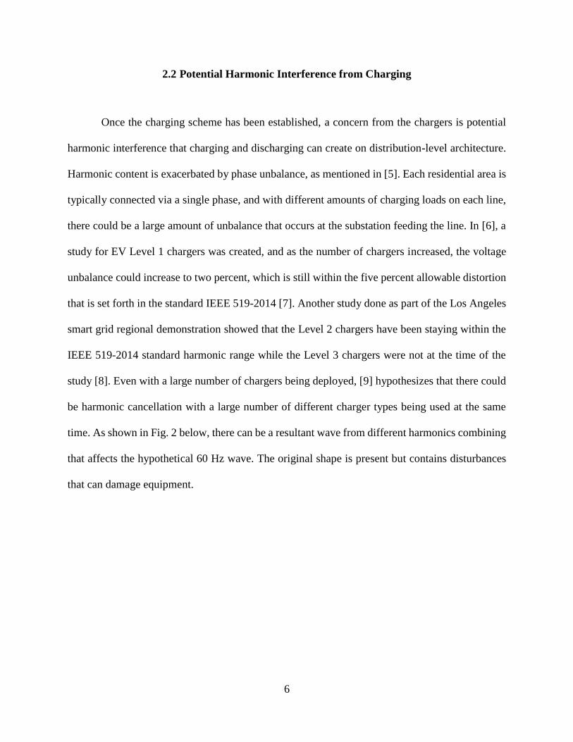
2.1.1 EV Charger Types
In order to enable the EV to operate, its batteries have to be charged beforehand. Although
that sounds simple, this step already presents a first big challenge, the missing standardization of
the charging plugs. For example, Tesla vehicles use a different charger than a Chevrolet Bolt. In
addition, there is no standardization between countries either. In the US, there are four main
5
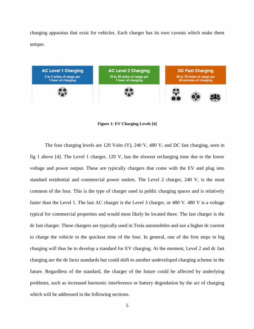
charging apparatus that exist for vehicles. Each charger has its own caveats which make them
unique.
Figure 1: EV Charging Levels [4]
The four charging levels are 120 Volts (V), 240 V, 480 V, and DC fast charging, seen in
fig 1 above [4]. The Level 1 charger, 120 V, has the slowest recharging time due to the lower
voltage and power output. These are typically chargers that come with the EV and plug into
standard residential and commercial power outlets. The Level 2 charger, 240 V, is the most
common of the four. This is the type of charger used in public charging spaces and is relatively
faster than the Level 1. The last AC charger is the Level 3 charger, or 480 V. 480 V is a voltage
typical for commercial properties and would most likely be located there. The last charger is the
dc fast charger. These chargers are typically used in Tesla automobiles and use a higher dc current
to charge the vehicle in the quickest time of the four. In general, one of the first steps in big
charging will thus be to develop a standard for EV charging. At the moment, Level 2 and dc fast
charging are the de facto standards but could shift to another undeveloped charging scheme in the
future. Regardless of the standard, the charger of the future could be affected by underlying
problems, such as increased harmonic interference or battery degradation by the act of charging
which will be addressed in the following sections.
6
2.2 Potential Harmonic Interference from Charging
Once the charging scheme has been established, a concern from the chargers is potential
harmonic interference that charging and discharging can create on distribution-level architecture.
Harmonic content is exacerbated by phase unbalance, as mentioned in [5]. Each residential area is
typically connected via a single phase, and with different amounts of charging loads on each line,
there could be a large amount of unbalance that occurs at the substation feeding the line. In [6], a
study for EV Level 1 chargers was created, and as the number of chargers increased, the voltage
unbalance could increase to two percent, which is still within the five percent allowable distortion
that is set forth in the standard IEEE 519-2014 [7]. Another study done as part of the Los Angeles
smart grid regional demonstration showed that the Level 2 chargers have been staying within the
IEEE 519-2014 standard harmonic range while the Level 3 chargers were not at the time of the
study [8]. Even with a large number of chargers being deployed, [9] hypothesizes that there could
be harmonic cancellation with a large number of different charger types being used at the same
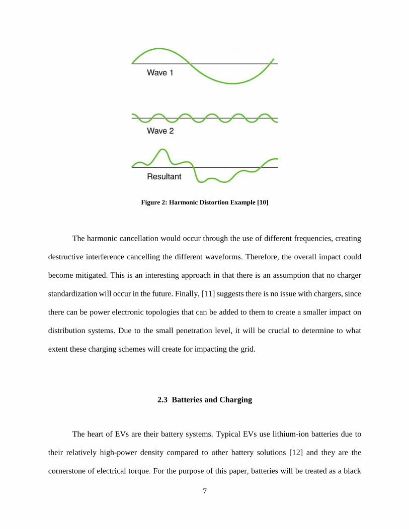
time. As shown in Fig. 2 below, there can be a resultant wave from different harmonics combining
that affects the hypothetical 60 Hz wave. The original shape is present but contains disturbances
that can damage equipment.
7
Figure 2: Harmonic Distortion Example [10]
The harmonic cancellation would occur through the use of different frequencies, creating
destructive interference cancelling the different waveforms. Therefore, the overall impact could
become mitigated. This is an interesting approach in that there is an assumption that no charger
standardization will occur in the future. Finally, [11] suggests there is no issue with chargers, since
there can be power electronic topologies that can be added to them to create a smaller impact on
distribution systems. Due to the small penetration level, it will be crucial to determine to what
extent these charging schemes will create for impacting the grid.
2.3 Batteries and Charging
The heart of EVs are their battery systems. Typical EVs use lithium-ion batteries due to
their relatively high-power density compared to other battery solutions [12] and they are the
cornerstone of electrical torque. For the purpose of this paper, batteries will be treated as a black
8
box power source and the chemical properties will not be investigated. Nevertheless, these
batteries need a steady power supply in order to charge properly, as stated in [12] since batteries
are sensitive in regard to charging, and the stochastic nature of some renewable resources can be
damaging. For example article [13] addresses there is a load scheduling problem with wind power,
a stochastic renewable source. The amount of charging that the battery can do in this situation
requires a large amount of computational power, which is undesirable when attempting to predict
a random-nature energy source. The large amount of computational power is due to the
randomness of the charge and the inability to count the charge after a period of battery degradation.
Direct stochastic renewable energy charging is not ideal, and therefore requires a direct connection
to a stable power source, such as the grid or a filtering intermediary step.
One of the largest challenges to current battery technology is the degradation of the lithium-
ion batteries. Repeated charging and discharging at deep levels (greater than 50 percent) can
damage the batteries. To combat this, EVs usually contain twice as many batteries as to not
discharge greater than half of the total capacity [12]. Although the doubling of battery size
completes the task, the added weight also has an impact on the efficiency of the EV. Therefore,
charging becomes even more important with the weight of the batteries and total potential charge.
Heavier EVs can show a decreased range but still contain a large number of batteries. A balance
between weight and capacity is necessary for the most economical vehicle operation.
2.4 EVs and the Grid
Once the charging technique has been determined, the next crucial step is determining the
affect big charging will have on the grid. There have been quite a few different studies created for
9
the EV impact and the grid, but for brevity, urban charging and the EV scheduling problem will
be reviewed. Urban charging is becoming more and more critical due to the ongoing trend of cities
transforming into megacities, which means a population of ten million people or more. Having
more places gain a higher penetration of EV’s creates a scheduling problem for charging to ensure
the grid will not become overloaded at a certain time of the day. Both of these topics are described
in the following sections.
2.4.1 Urban Charging
Urban charging can be considered the charging of EVs in densely populated areas, such as
in a city. Most of the data that has been collected for the EV scheduling problem comes from urban
charging studies. A study that was done on the University of California Los Angeles (UCLA)
campus [14] shows that there are peaks for charging amounts that occur around the start of the
workday and at the end of the workday. These times are not surprising as these are times that
people have finished commutes and errands during the day and are looking to charge while being
busy in buildings. Fig. 3 shows the energy consumption trend from the study. Another article, [15],
provides a similar study but in the Toronto area, where the same result was achieved for typical
plug-in times. Understanding where the demand for charging is located and its peak will help
predict load distributions for utilities and power generation quantities. Figure three shows a
consumption chart similar to the other research articles. The peak time is in the morning, which is
consistent with when residential load increases due to people waking up. The only inconsistency
with the previous research with this graph is the lack of an evening peak for when people report
home. One explanation is that this could be on a weekend day, where the people could be home
during the day and not at work or completing errands.

10
Figure 3: Example Electricity Use Chart [16]
2.4.2 The EV Scheduling Problem
Once the different load profiles are created in an urban setting, the necessity for load
scheduling arises. From previous data collections, there are peaks in consumption in the morning
and evening, in proximity to the start and end times of a typical workday. These peak loads can
then be extended in time if the EV chargers are then activated in locations of work or retail. The
EV scheduling problem is focused upon in [13], [17], [18], and [19]. These four articles give a
brief overview of the problem and potential solutions. [11] describes the scheduling necessary to
charge with a wind turbine, while [17] described the use of a fuzzy controller to schedule when to
charge or discharge with a centralized controller. The article [18] uses hardware-in-the-loop (HIL)
as well as real-time digital simulation (RTDS) to simulate power flow using three states (charging,
discharging, and no charging) and ranks the power flow by priority of low charge. Finally, [19]
11
describes a control algorithm that can be used for parking garages with two cases for charging: all
vehicles charge at the same time or stagger the charging. These four articles give a brief look into
the EV scheduling problem of when to charge the vehicles if there is a large influx of power
demand in a relatively small amount of time caused by these vehicles. With big charging, the
scheduling problem is going to become critical in redirecting the amount of power needed for the
charging of a large fleet of EVs. The most common control is the centralized controller which
determines the power flow needed for all of the vehicles and evenly distributes power to vehicles
in an order determined by their individual state of charge on each battery. This approach not only
smartly charges the vehicles but does so in a manner that the utilities should not become
overwhelmed by a large fluctuation of required power on local infrastructure.
2.5 The Role of Big Charging
With a large penetration of EVs on the road, there will be a large power demand as well.
This is the EV charging conundrum: how will the exponentially increased power demand be
handled in technological and governmental realms? There will be negative consequences to the
increased demand, as well as positive impacts. Negative consequences can include large
generation mismatch, phase balancing problems, overutilized infrastructure, and increased
emissions impact. On the other hand, there are still some positive impacts to the large-scale topic.
Positive impacts can include grid stability and duck curve mitigation using the batteries as a
distributed energy resource (DER). Both of these sides will be discussed in the following sections.

12
2.5.1 Negative Consequences
Negative consequences are just as they sound: they have a negative impact on the affected
subject matter. The four main problems that can be seen include large generation mismatch, phase
balancing problems, unavailable infrastructure, and increased emissions impact. Generation
mismatch comes from the inability for a generation source and a load to be able to be matched, so
there is neither a lack nor excess of power [20]. With the data collection on EV charging habits,
generation providers will be able to ramp to the desired generation level depending on trends. This
is not unlike current energy market predictions, where historical data is used to predict what the
load will be the next day.
Phase balancing problems and harmonic problems are intertwined issues. The phase
unbalance that can be created by EV charging is created through different penetration levels
throughout a distribution system. For example, a single phase of a three-phase distribution network
could have 20 EV chargers that activate at relatively similar times. Another phase of the same
network could have no chargers activating at that time, leading to the first phase having a much
larger power draw [10]. Power is transmitted from the substation in the three phases and if one
phase is heavily loaded, there could be power quality issues closer to the sources. As years have
progressed, this has been a concern for residential feeders before the wide-scale adoptions of EVs
[21]. One way to mitigate this would be to use the EV scheduling problem to even the distribution
feeders to create a better power factor. The power factor is a factor which relates the total power
in watts to the apparent power in volt-amps. The closer to one the power factor is, the better power
quality becomes, and lower losses occur. If the factor is pushed closer to one, then the generation
and quality problems should desist.
13
Another major problem that could happen is overutilized infrastructure [22]. On the East
Coast of the US, the infrastructure tends to be older due to the West Coast settlements being newer
and initial technological implementation on the East Coast. For example, this is why states such
as California have such advanced utility power programs with solar photovoltaics (solar PV) and
EV integration. The main problem will be the aged grids of the East, not necessarily the West.
Power lines can only handle so much current, so there is a push to create higher voltage distribution
lines to allow for more current and power transfer. This will be a long process, due to the amount
of distribution lines and associated equipment (such as transformers, circuit breakers, and
insulators) being replaced to accommodate the voltage change as well as the associated costs. In
order to conquer the infrastructural issues, change is inevitable. More lines, generation, and overall
equipment will be necessary in order to handle the load that will be to come with the advent of big
charging.
The last major problem that could occur is increased emissions impact [23]. Internal
combustion engines will have emissions due to combustion of fuel no matter what type of fuel or
catalytic converters are used. With the switch to EVs, there is still a cost to the electricity
consumption. Nuclear energy, a low-emission source, has an undecided future in more than one
country. With nuclear closures potentially occurring in the US, the current fuel replacement is with
natural gas. Natural gas releases half the emissions as a similar coal fuel, but if the electricity is
from a fossil fuel, one emissions source is just replaced with another. This creates a need for low-
carbon sourced fuels to become more needed. Not all renewable energy sources can be considered
clean, creating the important distinction between the renewable resources. As low-carbon
renewables are needed, their impact will also be felt, leading to positive consequences.

14
2.5.2 Positive Impacts
Consequences do not necessarily need to be negative, so positive consequences can exist.
Two main positive outcomes from EV charging are grid stability and duck curve mitigation. Both
of these come from using batteries as a distributed energy resource (DER). With increased loading
on the power system, a method of peak shaving using the EV batteries could be used [22(28)].
Peak shaving is an operation occurring at high load demand intervals in which batteries can be
deployed, creating a lower demand on traditional generation sources. Peak shaving has two main
benefits: stability and money saving. The article [24] describes the financial benefits of time-of-
day pricing, meaning at high demand times that the price of electricity will increase and discourage
people from using it at that time. Peak shaving can help with the financial side by storing energy
in the EV battery and using the battery during high-priced electricity times. Technology-wise, peak
shaving allows for power equalizing over time. This can be accomplished using a vehicle-to-grid
(V2G) electronics topology, as described in [25]. This will allow for the power to flow into and
out of the EV batteries to create a more stable grid. The paper [26] also proposes a similar approach
to stabilizing the grid by injecting more power in times of fluctuations or peak consumption times.
Battery types also need to be considered when creating stabilization methods, as different
configurations can create different responses, as mentioned in [27]. One example of different
responses would be the difference between lithium-ion batteries and lead acid. Lead acid batteries
typically have a slower response time than the lithium-ion, so an immediate power gap closure
would not be satisfied as fully as with the original battery.
In addition to grid stabilization techniques, the duck curve could potentially also be
mitigated by battery technology. The duck curve is the penetration curve of solar energy over time,
and how it can create a steep ramp of baseline generation coming online as more solar PV is
15
introduced [28]. One way to approach the duck curve is to think of it as an inverted peak, and
baseline generation is generation that typically does not turn off, such as nuclear, natural gas, and
other non-stochastic generation fuel sources. Figure 4 shows the visualization of the duck curve.
Figure 4: Duck Curve of Overgeneration [28]
As shown, there is an over-generation of solar which causes the dip in baseline and
increases for every year when more solar PV is introduced into the system. Once there is a
fluctuation in irradiation of the panels, the generation can sharply drop off or ramp up, creating
non-ideal situations where the baseline generation cannot compensate for the load [28]. One way
the batteries in EVs could help mitigate this problem would be to use the V2G adaptation and push
energy back onto the grid until the baseline generation can reach an equilibrium with the loads on
the system. The mitigation of the duck curve can also be considered a grid stabilization effort. Grid

16
stabilization is crucial to provide safe and reliable service to customers and having more
stabilization techniques will help with the transition from traditional generation to stochastic
sourced energy production.
17
3.0 Data and Projections for Distribution Simulation Environment
EVs have more positive consequences than negative consequences, as determined in the
literature review. Since they will be integrating into the grid in the upcoming years, an analysis of
load growth and impact is necessary to ease into a smooth transition. In order to create a simulation,
a determination of regressions and predictions is necessary in order to project the potential loading
of the distribution lines.
3.1 EV Penetration Projection
EV penetration rates are not unlike the rates presented from the integration of cellular
devices. The curve begins slowly as the first adopters push the technology forward. As time goes
on, the adoption takes on an exponential curve. This curve was created using penetration amounts
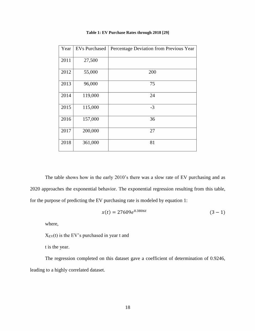
already seen through 2018 and reflects the current trend. These can be seen in Table 1, shown
below.
18
Table 1: EV Purchase Rates through 2018 [29]
Year EVs Purchased Percentage Deviation from Previous Year
2011 27,500
2012 55,000 200
2013 96,000 75
2014 119,000 24
2015 115,000 -3
2016 157,000 36
2017 200,000 27
2018 361,000 81
The table shows how in the early 2010’s there was a slow rate of EV purchasing and as
2020 approaches the exponential behavior. The exponential regression resulting from this table,
for the purpose of predicting the EV purchasing rate is modeled by equation 1:
𝑥(𝑡) = 27609𝑒0.3806𝑡 (3 − 1)
where,
XEV(t) is the EV’s purchased in year t and
t is the year.
The regression completed on this dataset gave a coefficient of determination of 0.9246,
leading to a highly correlated dataset.

19
3.2 Battery Size Projections
A similar process in determining the EV purchasing projections can also apply to the
battery size of the vehicles in the future. Table 2 describes the trend for miles per battery from the
years 2015 until 2019.
Table 2: Battery Size Historical [30]
Year Miles per Battery
2015 119
2016 122
2017 156
2018 159
2019 190
Unlike the EV purchase rate, the batteries have not been growing as exponentially, but
rather linearly. Every four years sees an increase in seventy miles per battery. Therefore, in 2030,
the average battery can hold approximately 400 miles worth of charge. The dataset for this
conclusion is statistically insignificant due to such a small population, but the assumption will be
used moving forward. Therefore, the battery projection for capacity can be estimated using
equation 2:
𝑥𝐵𝑎𝑡𝑡𝑒𝑟𝑦(𝑡) = 190 +70𝑡
4 (3 − 2)

20
where,
XBattery(t) is the EV battery capacity in miles per battery in year t + 2019 and
t is the year after 2019.
3.3 Home Load Projections
In this specific simulation, the average home will contain a load of size 15 kVA for the
peak. This number was achieved through estimating the load of a medium-large home which uses
electricity to heat. This is a potential overestimation, but the worst-case is necessary to stress the
system. Each year the simulation adds a compounded three-percent increase in base load in
addition to the EV load which is added due to additional loads and efficiency gains. Therefore, the
home load projection can be modeled as in equation 3:
𝑥𝐻𝑜𝑚𝑒(𝑡) = 15,000(1 + 0.03)𝑡 (3 − 3)
where,
XHome(t) is the home baseload in year t + 2019 and
t is the year after 2019.
This projection equation will be used in conjunction with the EV load equations, which are
determined in section 3.4. Distribution circuits also use a multiplier called a diversity factor. This
factor assumes that no two loads are the same and is multiplied to get the load at a certain time.
21
Over ten loads, the diversity factor approaches 0.54, which is the factor used in this distribution
line simulation.
3.4 EV Load Projections
EV chargers in the public right-of-way are typically a level two charger, which charges at
a maximum of 7.2 kW. Therefore, this charging level will be used in order to determine the peak
charging level that the EV fleet will create. The EV load projections are then projected using three
charges cases: low, medium, and high. Before these three cases are determined, the use of
combustion engine vehicles is studied to apply to EV use.
3.4.1 Combustion Engine Vehicle Use Study
In a medium-size city such as Pittsburgh, a typical commute for a vehicle is 20 miles one
way, as determined in the Siemens City Tool analysis from 2018 [31]. Therefore, the round-trip
average for driving is 40 miles per day. Typical combustion engine vehicles typically show ‘low
fuel’ at the eighth tank level which is no different than in EVs. With this information, the three
cases for charging will be after one trip (360 miles left), half a battery (200 miles left), and at one-
eighth of a battery (50 miles left). In addition, the average number of cars per household in the
Pittsburgh region is approximately two, and it can be assumed then that each load center will house
two vehicles. In order to determine the actual number of EVs per line, the average number of
vehicles bought per year is used with the number of EVs bought per year. The number of total

22
vehicles per year is around 17 million, while the EV penetration rate changes. Using this
relationship, the number of EV’s per line can be projected.
3.4.2 High Charge Projection
The high charge projection assumes that each EV will be recharged at the end of the day,
after completing one trip. In order to create the worst-case scenario for loading of the distribution
lines, this case is considered the highest and most severe due to the entire EV fleet charging at the
same time.
3.4.3 Medium Charge Projection
The medium charge projection decides that the EVs are charged only when half the battery
is left, and not every load is on at the same time. The time for half battery, assuming only daily
commute, is every five days, so the EV load is assumed to be at one-fifth on any given day. This
is a considerable decrease compared to the high charging case, and still high compared to the low
charging case in 3.4.4.
3.4.4 Low Charge Projection
The low charging projection assumes that the owner will only charge when one-eighth of
the battery remains, or one daily commute. This assumes that the charging will occur every eight
or nine days, so the load is at one-ninth of its maximum potential. This is the best case for highly

23
loaded lines as it spreads the amount of charging needed to the last minute and can be scheduled
easier for line congestion relief.
3.5 Equipment Parameters for Simulation
Line parameters needed for the simulations are outlined in the sections below. There are
two categories of parameters: physical and nominal. The physical parameters describe the physical
properties of the cables, such as radius and resistance. The other type of parameter, nominal,
describes the voltage levels and line lengths that are used in the simulation. In addition to the line
parameters, equipment on the system also needs parameters. The last piece needing a value is that
of the transformer feeding the line from the substation. The individual transformers on the line are
not considered since they can be arbitrarily added.
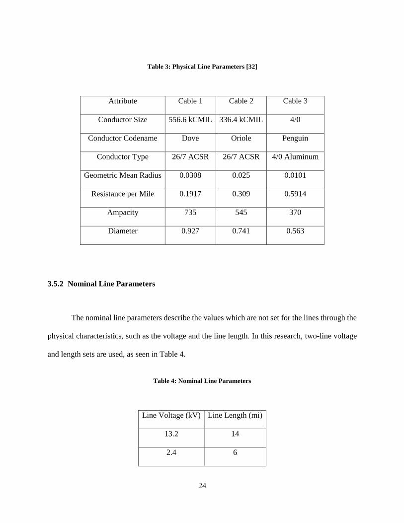
3.5.1 Physical Line Parameters
In order to simulate the different distribution lines that could be used, three cables of
interest were selected. These three cables have parameters outlined in Table 3. Common cable
sizes have a bird-themed codename which they can be easily referred. The first cable of interest
has the highest power transfer of the three and has the codename of Dove. The second cable,
codename Oriole, has a lower amount of power that can be transferred due to a lower ampacity.
The third cable, codename Penguin, acts as the common neutral for the other two cables in the
simulation. In theory, there should not be current on the neutral, but it acts as a pathway for line
faults and helps with balancing the loads.
24
Table 3: Physical Line Parameters [32]
Attribute Cable 1 Cable 2 Cable 3
Conductor Size 556.6 kCMIL 336.4 kCMIL 4/0
Conductor Codename Dove Oriole Penguin
Conductor Type 26/7 ACSR 26/7 ACSR 4/0 Aluminum
Geometric Mean Radius 0.0308 0.025 0.0101
Resistance per Mile 0.1917 0.309 0.5914
Ampacity 735 545 370
Diameter 0.927 0.741 0.563
3.5.2 Nominal Line Parameters
The nominal line parameters describe the values which are not set for the lines through the
physical characteristics, such as the voltage and the line length. In this research, two-line voltage
and length sets are used, as seen in Table 4.
Table 4: Nominal Line Parameters
Line Voltage (kV) Line Length (mi)
13.2 14
2.4 6
25
These two combinations can be seen as the average line length in a system and the voltages
are in line-to-ground, typical for distribution applications.
3.5.3 Transformer Parameters
Distribution lines need a source of power, and this is typically provided by a substation.
Each line has its own specific circuit breaker and not necessarily its own transformer. For the
intents of this research, the line will be afforded its own transformer at the size of 10 MVA. This
is not uncommon for a single-line size. Transformers can be run at higher power output than the
size that is specified, but this will shorten the life instead of creating failure conditions at the
onslaught of the high-power output.
26
4.0 Simulation of Distribution Feeder
This section describes the simulation results using the simulator and parameters outlined
in section 3. In total, 64 charging and discharging simulation cases were completed in total.
Constants throughout the simulations include the pole geometry, transformer rating, load sizes,
and neutral conductor type. This helped to reduce the number of variables to allow for a closer
comparison of different simulation cases.
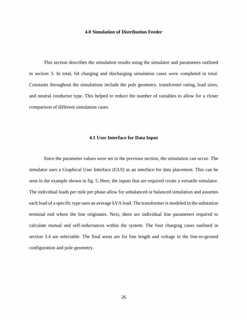
4.1 User Interface for Data Input
Since the parameter values were set in the previous section, the simulation can occur. The
simulator uses a Graphical User Interface (GUI) as an interface for data placement. This can be
seen in the example shown in fig. 5. Here, the inputs that are required create a versatile simulator.
The individual loads per mile per phase allow for unbalanced or balanced simulation and assumes
each load of a specific type uses an average kVA load. The transformer is modeled in the substation
terminal end where the line originates. Next, there are individual line parameters required to
calculate mutual and self-inductances within the system. The four charging cases outlined in
section 3.4 are selectable. The final areas are for line length and voltage in the line-to-ground
configuration and pole geometry.
27
Figure 5: Distribution Simulator Interface
4.2 Balanced Load, Dove Conductor Charging Simulation
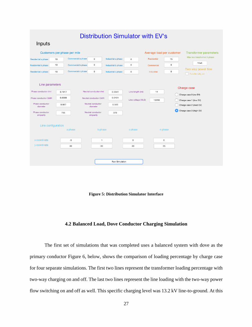
The first set of simulations that was completed uses a balanced system with dove as the
primary conductor Figure 6, below, shows the comparison of loading percentage by charge case
for four separate simulations. The first two lines represent the transformer loading percentage with
two-way charging on and off. The last two lines represent the line loading with the two-way power
flow switching on and off as well. This specific charging level was 13.2 kV line-to-ground. At this
28
voltage level, the two-way flow does not make much difference, as seen in the chart. This could
be attributed to a large load existing on the lines before the charging is accounted for. Charge case
three shows overloading conditions in both the transformer and line loading, and the bottleneck is
in both. The step from case two to three shows a large increase in load, which is expected for the
amount of increased charging.
Figure 6: 13.2 kV Dove Conductor Balanced System
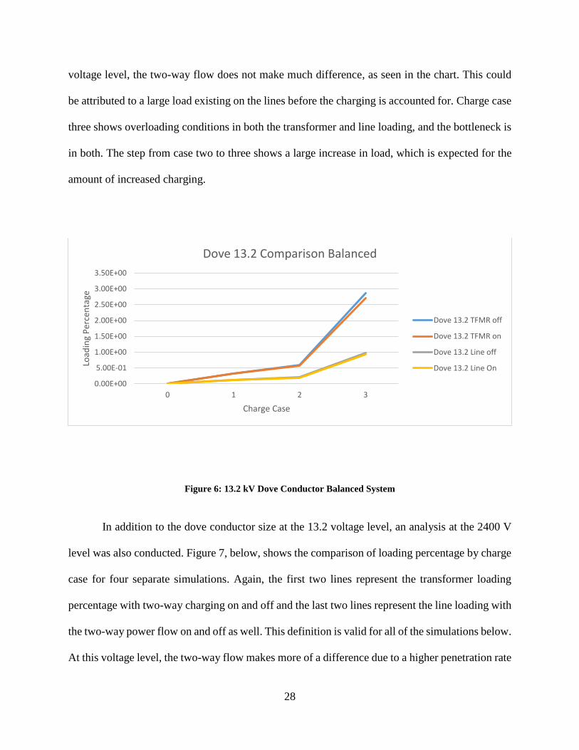
In addition to the dove conductor size at the 13.2 voltage level, an analysis at the 2400 V
level was also conducted. Figure 7, below, shows the comparison of loading percentage by charge
case for four separate simulations. Again, the first two lines represent the transformer loading
percentage with two-way charging on and off and the last two lines represent the line loading with
the two-way power flow on and off as well. This definition is valid for all of the simulations below.
At this voltage level, the two-way flow makes more of a difference due to a higher penetration rate
0.00E+00
5.00E-01
1.00E+00
1.50E+00
2.00E+00
2.50E+00
3.00E+00
3.50E+00
0 1 2 3
Load
ing
Per
cen
tage
Charge Case
Dove 13.2 Comparison Balanced
Dove 13.2 TFMR off
Dove 13.2 TFMR on
Dove 13.2 Line off
Dove 13.2 Line On
29
and lower loading allowances. The graph shows that at lower voltage, the penetration levels are
much higher due to the lower loads that already existed. Two-way power flow has a much greater
impact due to a combination of lower existing load and higher EV loads. In this case, a two-way
power flow existing on the line would be beneficial for total line loading since the line loading in
this case is so relatively high.
Figure 7: 2.4 kV Dove Conductor Balanced System
4.3 Unbalanced Load, Dove Conductor Charging Simulation
The second set of simulations that was completed uses an unbalanced system with dove as
the primary conductor. Figure 8, below, shows the comparison of loading percentage by charge
case for four separate simulations. This specific charging level was 13.2 kV line-to-ground. At this
0.00E+00
1.00E-01
2.00E-01
3.00E-01
4.00E-01
5.00E-01
6.00E-01
7.00E-01
8.00E-01
9.00E-01
0 1 2 3
Load
ing
Per
cen
tage
Charge Case
Dove 2.4 Comparison Balanced
Dove 2.4 TFMR off
Dove 2.4 TFMR on
Dove 2.4 Line off
Dove 2.4 Line On

30
voltage level, the two-way flow makes more of a difference than the balanced case. As with the
balanced case, the two-way power flow is not as effective at the already high line loadings that
occur in the 13.2 kV case even with the newly added EV loads. The unbalance does not make
much of a difference compared to the balanced simulation due to the number of loads that occur
and the rebalancing that can occur with larger commercial and industrial loads on each circuit.
Figure 8: 13.2 kV Dove Conductor Unbalanced System
In addition to the dove conductor size at the 13.2 voltage level, an analysis at the 2400 V
level was also conducted. Figure 9, below, shows the comparison of loading percentage by charge
case for four separate simulations. As with the balanced case, the two-way power flow is more
effective at the line loadings that occur in the 2400 V case with the added EV loads. In this case,
the unbalance is much more pronounced due to the smaller loads that can occur on the lower level
power lines.
0.00E+00
5.00E-01
1.00E+00
1.50E+00
2.00E+00
2.50E+00
3.00E+00
0 1 2 3
Load
ing
Per
cen
tage
Charge Case
Dove 13.2 Comparison Unbalanced
Dove 13.2 TFMR off
Dove 13.2 TFMR on
Dove 13.2 Line off
Dove 13.2 Line On

31
Figure 9: 2.4 kV Dove Conductor Unbalanced System
4.4 Balanced Load, Oriole Conductor Charging Simulation
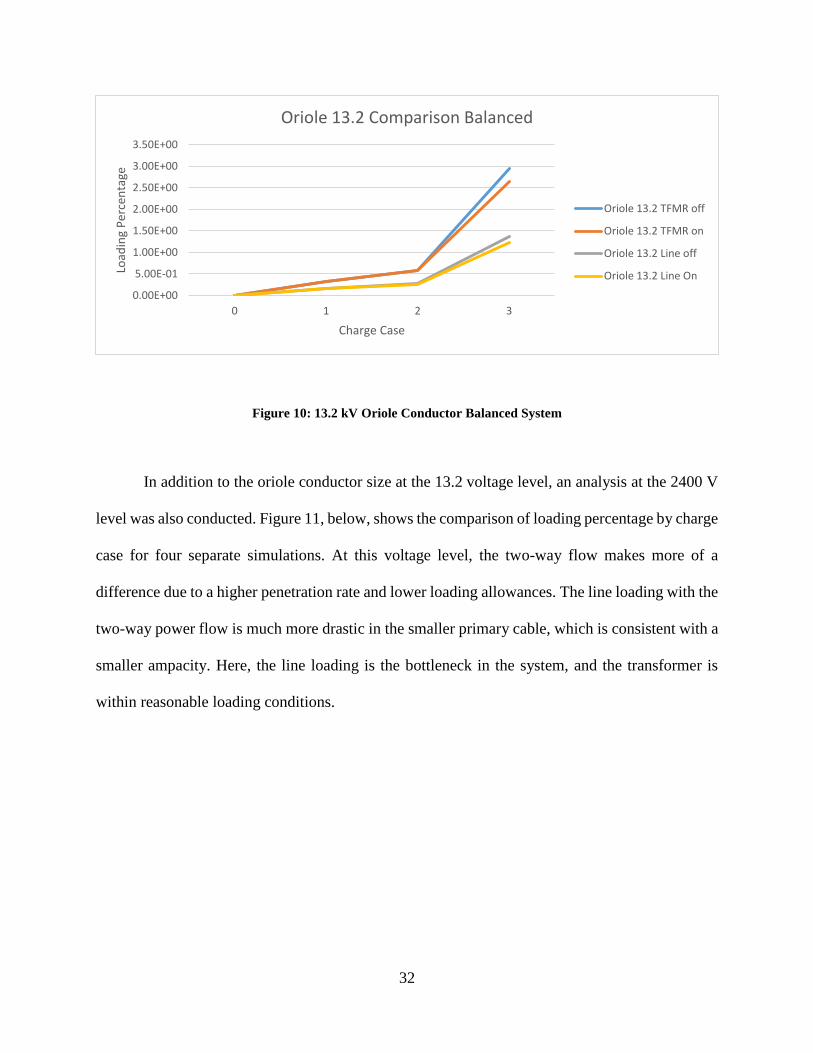
The third set of simulations that was completed use a balanced system with oriole as the
primary conductor. Figure 10, below, shows the comparison of loading percentage by charge case
for four separate simulations. This specific charging level was 13.2 kV line-to-ground. This is a
similar result to the dove conductor in section 4.3. The lines are overloaded, and overloads create
burnouts. The transformer is also at a high overload percentage, almost 2.5 times the rated load.
Once again at this voltage level, the two-way flow does not make much difference in the circuit
due to the high rate of base load the buildings already harbor.
0.00E+00
2.00E-01
4.00E-01
6.00E-01
8.00E-01
1.00E+00
1.20E+00
1.40E+00
1.60E+00
0 1 2 3
Load
ing
Per
cen
tage
Charge Case
Dove 2.4 Comparison Unbalanced
Dove 2.4 TFMR off
Dove 2.4 TFMR on
Dove 2.4 Line off
Dove 2.4 Line On
32
Figure 10: 13.2 kV Oriole Conductor Balanced System
In addition to the oriole conductor size at the 13.2 voltage level, an analysis at the 2400 V
level was also conducted. Figure 11, below, shows the comparison of loading percentage by charge
case for four separate simulations. At this voltage level, the two-way flow makes more of a
difference due to a higher penetration rate and lower loading allowances. The line loading with the
two-way power flow is much more drastic in the smaller primary cable, which is consistent with a
smaller ampacity. Here, the line loading is the bottleneck in the system, and the transformer is
within reasonable loading conditions.
0.00E+00
5.00E-01
1.00E+00
1.50E+00
2.00E+00
2.50E+00
3.00E+00
3.50E+00
0 1 2 3
Load
ing
Per
cen
tage
Charge Case
Oriole 13.2 Comparison Balanced
Oriole 13.2 TFMR off
Oriole 13.2 TFMR on
Oriole 13.2 Line off
Oriole 13.2 Line On

33
Figure 11: 2.4 kV Oriole Conductor Balanced System
4.5 Unbalanced Load, Oriole Conductor Charging Simulation
The final set of simulations that was completed use an unbalanced system with primary
conductor oriole. Figure 12, below, shows the comparison of loading percentage by charge case
for four separate simulations. This specific charging level was 13.2 kV line-to-ground. At this
voltage level, the two-way flow makes more of a difference than the balanced case, but only
slightly. As seen in the previous sections, the two-way power flow is most impactful in lower-level
power systems and here there is no discernable overloading conditions.
0.00E+00
2.00E-01
4.00E-01
6.00E-01
8.00E-01
1.00E+00
1.20E+00
1.40E+00
0 1 2 3
Load
ing
Per
cen
tage
Charge Case
Oriole 2.4 Comparison Balanced
Oriole 2.4 TFMR off
Oriole 2.4 TFMR on
Oriole 2.4 Line off
Oriole 2.4 Line On

34
Figure 12: 13.2 kV Oriole Conductor Unbalanced System
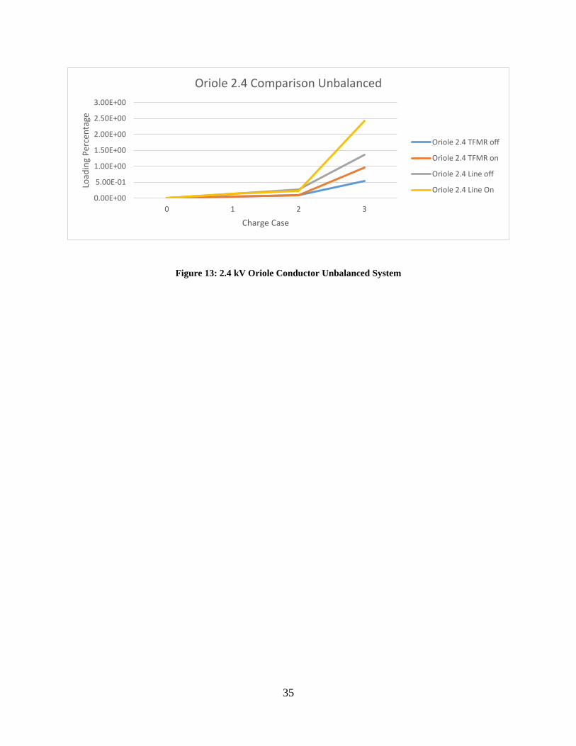
In addition to the oriole conductor size at the 13.2 voltage level, an analysis at the 2400 V
level was also conducted. Figure 13, below, shows the comparison of loading percentage by charge
case for four separate simulations. As seen in the dove conductor, the lower level unbalanced
system has more impact in terms of charging and the two-way power flow. The previous four cases
in this scheme have the same trend, where the lower voltage power systems are more affected by
unbalance and the two-way power flow than the higher-voltage systems.
0.00E+00
2.00E-01
4.00E-01
6.00E-01
8.00E-01
1.00E+00
0 1 2 3
Load
ing
Per
cen
tage
Charge Case
Oriole 13.2 Comparison Unbalanced
Oriole 13.2 TFMR off
Oriole 13.2 TFMR on
Oriole 13.2 Line off
Oriole 13.2 Line On
35
Figure 13: 2.4 kV Oriole Conductor Unbalanced System
0.00E+00
5.00E-01
1.00E+00
1.50E+00
2.00E+00
2.50E+00
3.00E+00
0 1 2 3
Load
ing
Per
cen
tage
Charge Case
Oriole 2.4 Comparison Unbalanced
Oriole 2.4 TFMR off
Oriole 2.4 TFMR on
Oriole 2.4 Line off
Oriole 2.4 Line On
36
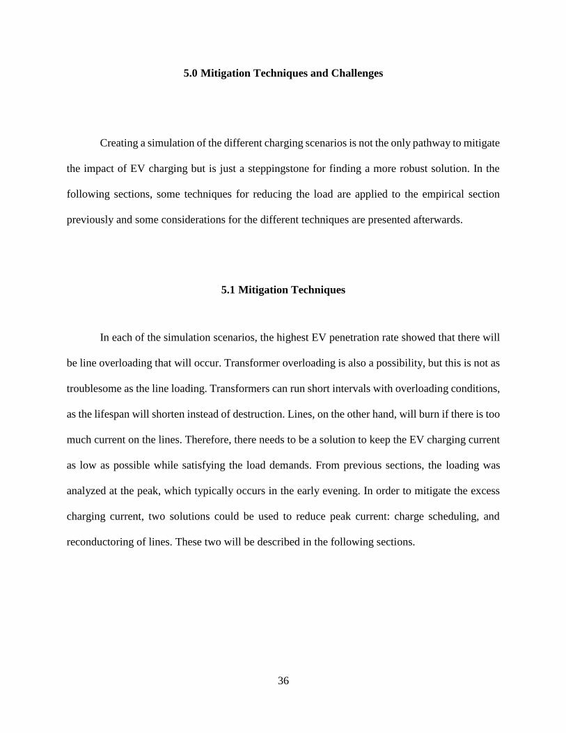
5.0 Mitigation Techniques and Challenges
Creating a simulation of the different charging scenarios is not the only pathway to mitigate
the impact of EV charging but is just a steppingstone for finding a more robust solution. In the
following sections, some techniques for reducing the load are applied to the empirical section
previously and some considerations for the different techniques are presented afterwards.
5.1 Mitigation Techniques
In each of the simulation scenarios, the highest EV penetration rate showed that there will
be line overloading that will occur. Transformer overloading is also a possibility, but this is not as
troublesome as the line loading. Transformers can run short intervals with overloading conditions,
as the lifespan will shorten instead of destruction. Lines, on the other hand, will burn if there is too
much current on the lines. Therefore, there needs to be a solution to keep the EV charging current
as low as possible while satisfying the load demands. From previous sections, the loading was
analyzed at the peak, which typically occurs in the early evening. In order to mitigate the excess
charging current, two solutions could be used to reduce peak current: charge scheduling, and
reconductoring of lines. These two will be described in the following sections.

37
5.1.1 Charge Scheduling
The first of two solutions to reduce the line current is to schedule the EVs for off-peak
times. This could be, for example, completed when a threshold on a line has been met and charging
can occur. A potential charging algorithm could be used, as seen in fig. 14, below.
Figure 14: Potential Logic Diagram for Charge Scheduling
Here, the logic begins with when the line current is approaching peak. This can be set by
the line properties and the current transformers that exist in the substation end of the distribution
line. If the line is very close to the threshold, the charging will not commence. Next, knowing how
many vehicles are requesting charging is necessary to know if the line will be overloaded. If it is
38
not, the vehicle may charge. If the line is close to the threshold, a loop commences taking the
charging request and the line data and when there is available room or the state of charge (SOC)
is so low that it is critical to charge, the charging will commence or wait. Once the charging starts,
the vehicle will continue charging until complete and finally more room will appear on the system
for more vehicles. This logic diagram does not consider neither more advanced charging
techniques nor two-way power flow. The controller that would be used for such an application
would need to be built for the conditions that occur on the individual lines. This approach would
be costly, as it would require a master-slave controller system with a controller on each individual
EV as well as a SOC charge estimator for the decision making.
5.1.2 Reconductoring of Lines
The second of the two solutions would be to reconductor the lines for higher amperage.
The bottleneck in EV charging is the lines, as determined previously. Reconductoring would be
the first half of this solution, as the larger cables can have higher amp throughput while the other
half would be setting the line to a higher voltage. The higher voltage would create a lower current,
and more power can be moved through the distribution lines. This solution would not be as costly
as creating scheduled charging, but it would still have costs due to the individual equipment
needing to be changed to accommodate different voltage levels. This is a quick and direct way to
allow more charging capabilities compared to the controller installation.
39
5.1.3 Combinational Solution
In addition to the two individual solutions, these solutions can be combined to create a
more robust solution than the two separately. The charge scheduling can allow for off-peak
charging tied to time of day pricing while the lines will not get close to the limit with new
conductors.
5.2 Challenges to the Mitigation Techniques
There are challenges to the two solutions that are not necessarily technically challenging
but regulatory challenging. The two-way power flow requires inverters for the individual vehicles,
and this can lead to harmonic issues, briefly described in section 2.1.2. On the other hand,
reconductoring has its own challenges with archaic infrastructure and national electric safety codes
(NESC) surrounding any new construction and rehabilitations. In the next section, each of these
are discussed as to why mitigating high currents for EV charging can be such a challenging topic.
5.2.1 Inverter and Controller Challenges
Two-way power was a consideration in this research, where at peak times, the attached
EVs would immediately place the amount of energy they pulled back onto the grid to decrease the
amount of loading at peak conditions. Two of the main challenges with this idea are controllers
and inverters. Controllers will be a costly solution. As described in 5.1.1, each vehicle will require
a slave controller that is controlled by a master taking data from each vehicle and each power line
40
in a system. This would need to be tied to a supervisory control and data acquisition (SCADA)
system, which is already tracking the status of different power systems locations of interest.
Connecting individual controllers brings another question to the table: cyber security. This is a
problem already being seen with the introduction of wi-fi enabled smart meters, which are also
tied to utility networks. This work does not consider cyber security but it is necessary to mention
as it is becoming a relevant topic for both government, academia, and industry. These individual
controllers in the future can be combined into home charging and public charging stations, so each
car will not be required to maintain more electronic equipment. These stations would then require
internet connectivity in order to transfer the data for commands and therefore public spaces would
need to not only receive upgraded electric connections but data connections as well. The electric
connections are already required as part of the charger infrastructure and in the future the data
connection can be installed in parallel or retroactively.
Inverters for the DC to AC conversion were not as strictly regulated until the IEEE 1547-
2018 standard was updated for 2018 [33]. This standard was revised due to a blackout which
happened in Southern California, when solar photovoltaic cells tripped off the grid, causing a large
shedding of load. This inverter standard can be applied to tripping hazards to the two-way power
flow problem, but due to the revised standard, there are many inverters that were sold without the
specific thresholds for voltage stability. This can be a challenge until the standard is fully
implemented across the system.
The next standard of note is IEEE 519-2014, which describes the harmonic content of a
power system and its limits. The official title, “IEEE Recommended Practice and Requirements
for Harmonic Control in Electrical Power Systems,” describes exactly what the standard outlines:
acceptable harmonic contents and limits [7]. The standard, originally released in 1981, began the

41
quantification of harmonics on the system, since electronics were becoming popular and power
needed to be regulated. The 1960s and 1970s were littered with blackouts due to voltage collapse
and part of the standard which addressed this problem. A first update was released in 1992 and
addressed harmonic distortion and set the limits for this phenomenon. The latest edition, 2014,
describes statistical analysis on the systems and updates on limits due to the shift to stochastic
power sources and high amounts of DC current penetration into the system. Figure 15 below shows
the acceptable limits for harmonic contents for currents specifically.
Figure 15: Harmonic Distorition Limits for Current [7]
Figure 15, pulled from the standard edition 2014, only shows odd harmonics due to the
cancellation of even harmonics in power systems. Harmonics above the eleventh are typically
small and not necessarily considered in such power systems, and the total distortion allowed is five
percent for most systems. This could become a challenge due to inverters placing energy onto the
system at different times due to potentially asynchronous behavior. This behavior could create
42
problems since the waveforms could create destructive or constructive harmonics and therefore
decrease the voltage peaks to outside of and above acceptable limits for power systems. One way
to mitigate this would be to inject the inverter current at specific points in the system’s frequency
and therefore mitigate the interference. Just as in other cases, this adds cost to the already costly
system and cannot guarantee anything.
The final standard of note ties both controllers and harmonic problems together, IEEE 518-
1982 [34]. This standard describes the harmonic allowances for controllers. Since one of the
components of the controller solution is to check the state of charge of a vehicle, the harmonic
output from the vehicle could potentially disrupt the controller. This is an unlikely scenario, but
one that is still necessary to address. The standard is from 1982, which is close to being out of date
for current applications, but the outlining prerogatives still apply to these chargers. Both of these
challenges are only the beginning for technological solutions and are not considered in-depth. Due
to the high cost of implementation and technical considerations, the solution in section 5.2.2 is
more reasonable with the technology and costs of 2019.
5.2.2 Clearance Challenges
Reconductoring power lines, however inexpensive compared to its technological
counterpart, can still be costly. In the United States, there are a set of codes called the National
Electric Safety Code (NESC) which dictates how far power lines need to be away from different
structures [35]. These distances are called clearances and the code describes many different cases
that power lines can exist in, such as near buildings, swimming pools, highways, and other man-
made sites. One of the stipulations of this code is that if any work is being done on a pole, it needs
to be brought up to the current standard (which is updated every four years) and one pole on each

43
side is typically also needed to be brought up to the current code. This is not unlike other building
codes where if any type of renovation is completed, the entire building must be brought up to
whatever applicable code there is. Reconductoring is one of the actions that can be taken on an
electric utility pole where the clearances would need to be changed in order to be legal. This
problem becomes prevalent where old infrastructure is dominant: in older cities with aged
infrastructure. The NESC, which is updated every four years, has increased distances for
conductors since the 1980’s, which is new for much of the infrastructure in the United States. A
simple reconductoring, which would consist of changing cables, insulators, jumpers, and other
wire-related equipment could suddenly change to an entire pole replacement and pole movement.
There would not be a route to avoid this potential problem and it would become not just costly but
challenging to get the same equipment back into the areas where it once was located. Of course,
reconductoring would not be a problem for certain areas where large clearances are already
existing but as stated, it will be a main challenge in cities where the lines can be close to buildings
or where space prohibits pole movement.
5.2.3 Combinational Solution
The best solutions are typically a compromise between systems, such as the two solutions
from section 5.2.1 and section 5.2.2 combined. One way to do this would be to allow areas to be
reconductored if the spacing allowed a conversion, while more congested areas adopt a charge
scheduler. Dense areas would favor this idea because the main conductors to the area could be
replaced for higher current throughput since it would be a main feeder. The smaller offshoots could
use a scheduler per each feed and therefore have a smaller cost associated. No solution is the catch-

44
all for the EV charging, but having multiple solutions working together will have more leniency
for future growth.
45
6.0 Conclusion
Electric Vehicles are a technology which could be likened to the cell phone revolution in
the early 2000’s. The rate of adoption increased exponentially for phones in the 1990’s and early
2000’s, and now it is now commonplace for most people to have one just twenty years later. If
EV’s continue their exponential growth curve, there will be a similar outcome. An exponential
adoption curve has already been plotted, as seen in the regression of cars being purchased. There
is no sign of slowing and this provides a basis for EV charging analysis for the future. A line
simulator is necessary for checking how much current will be needed for a specific distribution
line. After analysis of line loading cases, the main constraint that will occur is required amps in
the highest charge case in every scenario creating an overload and destroying the distribution lines.
In the more realistic charging scenarios, the distribution lines will not become overloaded from
charging at the half battery and eighth battery levels. Even if the highest charge case becomes the
scenario, three ways can decrease the charging load on each of the lines. Two-way power can
inject current back onto the distribution line at peak loading conditions in order to decrease the
peak amps. Then, the car can charge at off-peak times. The second solution is to schedule the
charging for a time where there is available current on the system to charge the vehicles. This ties
into the two-way power flow which would require the electronics to facilitate this solution. The
third solution is to reconductor the distribution lines at a higher voltage, which would allow for
more current to pass through the system. The final and best solution is a compromise between the
three aforementioned solutions, replacing main conductors while the offshoots would be controlled
by the charge scheduler and two-way charging. There is no perfect solution to the EV charging

46
problem which will occur and the best way to combat this problem is to create a combinational
system with as much flexibility as possible.
47
Bibliography
[1] IEEEXplore: Electric Vehicles, IEEEXplore, 2019. [Online]. Available:
https://ieeexplore.ieee.org/search/searchresult.jsp?newsearch=true&queryText=ElectricVe
hicles.
[2] Google, Google Trends: Electric Vehicle, 2019. [Online]. Available:
https://trends.google.com/trends/explore?q=EV&geo=US.
[3] S. Mensch et al, SB 596 PA, Pennsylvania General Assembly, 2019.
[4] Tips General, “What to Consider Before Buying an Electric Car,” Tips General. [Online].
Available: http://tipsgeneral.com/how-to/what-to-consider-before-buying-an-electric-
car.html.
[5] J. Guo et al., Research on Harmonic Characteristics and Harmonic Counteraction Problem
of EV Charging Station, 2nd IEEE Conf. Energy Internet Energy Syst. Integr. EI2 2018 –
Proc., pp. 15, 2018.
[6] T. Klayklueng and S. Dechanupaprittha, Impact analysis on voltage unbalance of EVs
charging on a low voltage distribution system, 2014 Int. Electr. Eng. Congr. iEECON 2014,
pp. 14, 2014.
[7] IEEE, IEEE 519-2014, 2014.
[8] M. Di Paolo, Analysis of Harmonic Impact of Electric Vehicle Charging Impact on the
Electric Power Grid, 2017 IEEE Green Energy Smart Syst. Conf., pp. 15, 2017.
[9] L. Kutt, E. Saarijarvi, M. Lehtonen, H. Molder, and J. Niitsoo, Harmonic distortions of
multiple power factor compensated EV chargers, 2014 16th Eur. Conf. Power Electron.
Appl. EPE-ECCE Eur. 2014, pp. 39, 2014.
[10] OpenStax, “Physics,” Lumen. [Online]. Available:
https://courses.lumenlearning.com/physics/chapter/16-10-superposition-and-interference/.
[11] E. Basu,et al., Harmonic distortion caused by EV battery chargers in the distribution systems
network and its remed, 39th Int. Univ. Power Eng. Conf., 2004.
[12] M. S. Islam, N. Mithulananthan, and K. Bhumkittipich, Feasibility of PV and battery energy
storage based EV charging in different charging stations, 2016 13th Int. Conf. Electr. Eng.
Comput. Telecommun. Inf. Technol. ECTI-CON 2016, pp. 16, 2016.
48
[13] Q. Huang, Q. S. Jia, and X. Guan, A Review of EV Load Scheduling with Wind Power
Integration, IFAC-PapersOnLine, vol. 48, no. 28, pp. 223228, 2015.
[14] Z. Jiang, H. Tian, M. J. Beshir, R. Sibagatullin, and A. Mazloomzadeh, Statistical analysis
of Electric Vehicles charging, station usage and impact on the grid, 2016 IEEE Power
Energy Soc. Innov. Smart Grid Technol. Conf. ISGT 2016, 2016.
[15] Z. Wei, Y. Li, Y. Zhang, and L. Cai, Intelligent parking garage EV charging scheduling
considering battery charging characteristic, IEEE Trans. Ind. Electron., vol. 65, no. 3, pp.
28062816, 2018.
[16] “Solar energy storage key to savings for Central West feedlot,” AgInnovators. [Online].
Available: https://www.aginnovators.org.au/initiatives/sustainability/case-studies/solar-
energy-storage-key-savings-central-west-feedlot.
[17] R. R. Deshmukh and M. S. Ballal, An energy management scheme for grid connected EVs
charging stations, Proc. 2018 IEEE Int. Conf. Power, Instrumentation, Control Comput.
PICC 2018, pp. 16, 2018.
[18] V. Lakshminarayanan, V. G. S. Chemudupati, S. Pramanick, and K. Rajashekara, Real-time
Optimal Energy Management Controller for Electric Vehicle Integration in Workplace
Microgrid, IEEE Trans. Transp. Electrif., vol. PP, no. c, pp. 11, 2018.
[19] S. Faisal, S. Ahmed, and S. Ur Rehman, Distributed power mismatchestimation in
smart grid,ICET 2016 - 2016 Int. Conf. Emerg. Technol.,pp. 15, 2017.
[20] M. Zhang, Q. Chen, J. Xu, W. Yang, and S. Niu, Study on influence of large-scale electric
vehicle charging and discharging load on distribution system, China Int. Conf. Electr.
Distrib. CICED, vol. 2016-Septe, no. Ciced, pp. 14, 2016.
[21] IEEE, Smart Grid Research: Power - IEEE Grid Vision 2050 Roadmap, 2013.
[22] M. Striebg, Bradley, Ogundipe, Adebayo, Papadakis, Engineering Applications in
Sustainable Engineering Design, 1st ed. Cengage, 2016.
[23] J. Cui, Y. Li, W. Zhang, and C. Chen, Research on impact and utilization of electric vehicle
integration into power grid, Proc. 30th Chinese Control Decis. Conf. CCDC 2018, pp.
15941597, 2018.
[24] P. Xu, J. Li, X. Sun, W. Zheng, and H. Liu, Dynamic Pricing at Electric Vehicle Charging
Stations for Queueing Delay Reduction, Proc. - Int. Conf. Distrib. Comput. Syst., pp.
25652566, 2017.
[25] V. Monteiro, J. G. Pinto, and J. L. Afonso, Experimental Validation of a Three-Port
Integrated Topology to Interface Electric Vehicles and Renewables with the Electrical
Grid, IEEE Trans. Ind. Informatics, vol. 14, no. 6, pp. 23642374, 2018.

49
[26] S. Y. Ge, L. Wang, H. Liu, and L. Feng, The impact of discharging electric vehicles on the
distribution grid, 2012 IEEE Innov. Smart Grid Technol. - Asia, ISGT Asia 2012, no.
51107085, pp. 14, 2012.
[27] D. Seetharam, et al., Hidden Costs of Power Cuts and Battery Backups, Proceedings of the
fourth international conference on Future energy systems, 2013.
[28] P. Denholm, et al., Overgeneration from Solar Energy in California: A Field Guide to the
Duck Chart, 2013.
[29] R. Irle, “USA Plug-in sales for the first half of 2019,” EV-volumes. [Online]. Available:
http://www.ev-volumes.com/country/usa/
[30] “ US Electric Car Range Will Average 275 Miles By 2022, 400 Miles By 2028 - New
Research (Part 1),” Cleantechnica. [Online]. Available:
https://cleantechnica.com/2018/10/27/us-electric-car-range-will-average-275-miles-by-
2022-400-miles-by-2028-new-research-part-1/
[31] “A Technology Roadmap for Pittsburgh: Linking Climate and Innovation,” Siemens.
[Online]. Available: https://assets.new.siemens.com/siemens/assets/api/uuid:a31d7c2c-
8c2c-4836-998a-097fe3e10bf0/version:1561154658/2019-cypt-report-pittsburgh-
lowres.pdf
[32] “Ampacities for Aluminum & ACSR Overhead Electrical Conductors,” The Aluminum
Association. [Online]. Available:
https://www.aluminum.org/sites/default/files/Ampacities%20for%20Aluminum%20%26
%20ACSR%20Overhead%20Electrical%20Conductors.pdf
[33] IEEE, IEEE 1547-2018, 2018.
[34] IEEE, IEEE 519-1982, 1982.
[35] IEEE, IEEE SA - The National Electrical Safety Code (NESC), 2016.