impact of electric vehicle charging on the distribution ...1130512/fulltext01.pdf · impact of...

Impact of electric vehicle charging on the

distribution grid in Uppsala 2030

EMIL GUSTAFSSON

FREDRIK NORDSTROM

Master of Science Thesis

Stockholm, Sweden 2017

This page intentionally left blank

Impact of electric vehicle charging on the

distribution grid in Uppsala 2030

Emil Gustafsson, Fredrik Nordstrom

Stockholm, Sweden, May 29th, 2017

Industrial Engineering and Management

ITM

Royal Institute of Technology

Abstract

Planning of distribution grids is based on statistically estimating the max-

imum load that will occur given a certain range of criteria (location, household

types, district / electric heating etc.) Charging of electric vehicles is not one

of these criteria. However, given the expected ‘boom’ in sales of Chargeable

Electric Vehicles (CEVs), and the lengthy planning process of distribution

grids (¿10 years) the knowledge gap is becoming a more pressing issue.

This research has been conducted to investigate if Vattenfall, a Swedish

electric utility company with distribution assets in both Sweden and Ger-

many, needs to take action to react to the expected increase in CEVs in the

near term. The study has been conducted with Uppsala Municipality as a

showcase and 2030 as the time frame.

The findings of this study show that Vattenfall should incorporate CEV

usage into distribution planning to avoid overload of power stations in Up-

psala by 2030. The findings shows that 1) we can expect a ’boom’ in sales

of CEVs in the near future and that 73% of cars in traffic in Uppsala may

be CEVs by 2030 and 2) that CEV charging is expected to have a signifi-

cant impact on the distribution grid, with certain power stations in Uppsala

seeing a peak load increase of up to 30%. The recommended actions are the

following:

• Monitor specific areas with a high concentration of cars and low energy

consumption per household that already have substations with capacity

below the recommended dimensions

i

• Monitor CEV sales to reevaluate current projections on CEV development

in Uppsala

• Monitor trends of car ownership and evaluate whether this will affect CEV

charging behaviour

• Reconstruct Velander constants, used for grid planning, to take the CEV

load into consideration

• Investigate smart charging solutions, to shift the CEV load peak to a dif-

ferent time of the day

Key Words: Chargeable Electric Vehicles, Load Profiles, Distribution grid,

Driving Patterns

ii


iii

Sammanfattning

Dimensionering av distributionsnat baseras pa att statistiskt uppskatta

den maximala lasten som kommer att intraffa pa natet, givet olika faktorer

(geografiskt lage, hushallstyp, fjarrvarme / elvarme etc.). Laddning av elbilar

ar inte en av de faktorer som man tar hansyn till. Givet en vantat kraftig

okning av laddningsbara bilar, samt den langa planeringshorisonten for distri-

butionsnat (¿10 ar), blir dock fragan hur elbilar kommer att paverka elnatet

valdigt aktuell.

Denna studie har bedrivits for att avgora hur Vattenfall, ett statligt,

svenskt elbolag med distributionsnat i Sverige och Tyskland, behover age-

ra for att anpassa sig till den forvantade okningen av elbilar. Den har studien

har genomforts som en fallstudie pa Uppsala Kommun med ar 2030 som

tidsram.

Resultaten fran studien visar att Vattenfall bor ta hansyn till laddning av

elbilar vid dimensionering av distributionsnat for att undvika overbelastning

pa natstationer i Uppsala ar 2030. Resultaten visar dels att 1) man kan

forvanta sig en kraftig okning av forsaljning av laddningsbara fordon inom

en snar framtid och uppemot 73 % av alla bilar i trafik i Uppsala kommer

att vara laddningsbara ar 2030 samt att 2) laddningsbara fordon kommer att

ha en signifikant paverkan pa distributionsnatet med okningar pa upp till

30 % av maxlasten for vissa natstationer. Foljande atgarder rekommenderas

saledes:

• Overvaka specifika omraden med hog biltathet och lag energianvandning

per hushall som ar anslutna till natstationer som ar underdimensionerade

iv

• Folj utvecklingen av forsaljning av laddbara fordon for att omvardera ge-

nomforda projektioner over laddningsbara bilar i Uppsala

• Overvaka trender inom bilagande och utvardera hur detta paverkar ladd-

ningsbeteende

• Gor om Velanderkonstanter sa att de tar hansyn till lasten fran laddbara

fordon vid planering av elnat

• Utvardera smarta laddningslosningar for att flytta last fran elbilsladdning

till en annan tidpunkt pa dygnet

Nyckelord: Elbilar, Lastprofiler, Distributionsnat, Kormonster

v

Declaration

’We declare that all material in this thesis is entirely our own work and

has not been previously submitted to this or any other institution. All material

in this thesis that is not our own work has been acknowledged and we have

stored all material used in this research, including research data, preliminary

analysis, notes, interviews, and drafts, and can produce them on request.’

Emil Gustafsson

Signature

May 29th, 2017Date

Fredrik Nordstrom

Signature

May 29th, 2017Date

vi

Acknowledgements

First of all, we are grateful for the opportunity to write this thesis, which

will be the end of a five year journey towards a degree. We would like to thank

our supervisor and mentor at Vattenfall, Strategy Manager at Strategic Plan-

ning, Alicia Bjornsdotter Abrams, Strategy Manager at Strategic Planning,

without whom this thesis would have reached nowhere near the quality that

it did. We would also like to thank our supervisor and our examiner at KTH,

PhD Student Omar Shafqat and Professor Per Lundqvist for their guidance

throughout the duration of the thesis work. Additionally, we would like to

record a sincere thanks to Vattenfall and the employees there for providing us

with means to complete this thesis. Lastly, but perhaps most importantly, we

would like thank all the institutions and organisations that have, at no cost,

been willing to help and provide us with the information that we needed.

Big thank you to Lindholmen Science Park, The Swedish Energy Agency and

Uppsala Municipality.

vii


viii

Contents

1 Introduction 2

1.1 Background . . . . . . . . . . . . . . . . . . . . . . . . . . . . . . . 2

1.2 Problem Formulation . . . . . . . . . . . . . . . . . . . . . . . . . . 3

1.3 Purpose and Aim . . . . . . . . . . . . . . . . . . . . . . . . . . . . 4

1.4 Research Questions . . . . . . . . . . . . . . . . . . . . . . . . . . . 4

1.5 Delimitations . . . . . . . . . . . . . . . . . . . . . . . . . . . . . . 5

1.6 Contribution to Science . . . . . . . . . . . . . . . . . . . . . . . . . 5

1.7 Disposition . . . . . . . . . . . . . . . . . . . . . . . . . . . . . . . 6

2 Method 9

2.1 Research approach . . . . . . . . . . . . . . . . . . . . . . . . . . . 9

2.2 Research process . . . . . . . . . . . . . . . . . . . . . . . . . . . . 9

2.3 Collection of data . . . . . . . . . . . . . . . . . . . . . . . . . . . . 11

2.4 Analysis of data and model outcome . . . . . . . . . . . . . . . . . 13

2.5 Validity and Reliability . . . . . . . . . . . . . . . . . . . . . . . . . 14

3 Literature Review 17

3.1 Chargeable Electric Vehicles . . . . . . . . . . . . . . . . . . . . . . 17

3.2 Driving Patterns . . . . . . . . . . . . . . . . . . . . . . . . . . . . 27

3.3 The Electric Grid . . . . . . . . . . . . . . . . . . . . . . . . . . . . 31

3.4 Previous Research . . . . . . . . . . . . . . . . . . . . . . . . . . . . 39

3.5 Summary of Literature Review . . . . . . . . . . . . . . . . . . . . 41

4 CEV projections 2030 44

4.1 Assumptions . . . . . . . . . . . . . . . . . . . . . . . . . . . . . . . 44

4.2 Calculations . . . . . . . . . . . . . . . . . . . . . . . . . . . . . . . 45

4.3 Findings . . . . . . . . . . . . . . . . . . . . . . . . . . . . . . . . . 47

5 Analysis of Driving Patterns 2030 52

5.1 Assumptions . . . . . . . . . . . . . . . . . . . . . . . . . . . . . . . 52

5.2 Calculations . . . . . . . . . . . . . . . . . . . . . . . . . . . . . . . 53

ix

5.3 Findings . . . . . . . . . . . . . . . . . . . . . . . . . . . . . . . . . 54

6 CEVs’ impact on the Uppsala grid 2030 61

6.1 Assumptions . . . . . . . . . . . . . . . . . . . . . . . . . . . . . . . 61

6.2 Calculations . . . . . . . . . . . . . . . . . . . . . . . . . . . . . . . 64

6.3 Findings . . . . . . . . . . . . . . . . . . . . . . . . . . . . . . . . . 66

6.4 Sensitivity Analysis . . . . . . . . . . . . . . . . . . . . . . . . . . . 76

7 Results 81

7.1 SQ 1 - How many CEVs and of what kind will there be in Uppsala

and in relevant nearby areas in 2030? . . . . . . . . . . . . . . . . . 81

7.2 SQ 2 - How will CEVs impact the distribution grid in Uppsala in 2030? 81

7.3 MRQ - Which measures should Vattenfall take in order to sustainably

react to the expected increase in CEVs in Uppsala by 2030? . . . . 83

8 Discussion 87

8.1 Discussion of our Results . . . . . . . . . . . . . . . . . . . . . . . . 87

8.2 Discussion of our Assumptions . . . . . . . . . . . . . . . . . . . . . 93

8.3 Externalities unaccounted for . . . . . . . . . . . . . . . . . . . . . 95

9 Conclusion 101

9.1 MRQ . . . . . . . . . . . . . . . . . . . . . . . . . . . . . . . . . . . 101

9.2 Future Work . . . . . . . . . . . . . . . . . . . . . . . . . . . . . . . 101

References 104

A Appendix - Interview take-aways 113

A.1 CEV Charging . . . . . . . . . . . . . . . . . . . . . . . . . . . . . 113

A.2 Driving Patterns . . . . . . . . . . . . . . . . . . . . . . . . . . . . 113

A.3 Grid Infrastructure . . . . . . . . . . . . . . . . . . . . . . . . . . . 113

B Appendix - Projections 116

C Appendix - Results 119

x

List of Figures

1 Problem solving break down . . . . . . . . . . . . . . . . . . . . . . 10

2 Research process . . . . . . . . . . . . . . . . . . . . . . . . . . . . 11

3 EV global growth . . . . . . . . . . . . . . . . . . . . . . . . . . . . 17

4 CEV market share by country . . . . . . . . . . . . . . . . . . . . . 18

5 Development of cars by fuel type, Sweden . . . . . . . . . . . . . . 19

6 Development of cars by fuel type, Uppsala Municipality . . . . . . . 19

7 Development of CEVs, Sweden . . . . . . . . . . . . . . . . . . . . 20

8 Development of CEVs, Uppsala Municipality . . . . . . . . . . . . . 20

9 CEV market share development, Sweden . . . . . . . . . . . . . . . 21

10 CEV market share development, Norway . . . . . . . . . . . . . . . 22

11 Charging power vs battery SOC . . . . . . . . . . . . . . . . . . . . 26

12 Seasonal change in driving patterns . . . . . . . . . . . . . . . . . . 30

13 Break-down of the electric grid . . . . . . . . . . . . . . . . . . . . 33

14 Average daily load profile, Sweden . . . . . . . . . . . . . . . . . . . 34

15 Vattenfall’s grid in Uppsala County . . . . . . . . . . . . . . . . . . 36

16 Projected electricity usage . . . . . . . . . . . . . . . . . . . . . . . 38

17 Historic and planed BEV models . . . . . . . . . . . . . . . . . . . 47

18 Projection number of CEVs and non CEVs, Sweden . . . . . . . . . 48

19 Projection CEV market share, Sweden . . . . . . . . . . . . . . . . 48

20 Projection number of CEVs and non CEVs, Uppsala Municipality . 49

21 Projection CEV market share, Uppsala Municipality . . . . . . . . 50

22 Histogram of distance driven . . . . . . . . . . . . . . . . . . . . . . 55

23 Daily variation in driving patterns . . . . . . . . . . . . . . . . . . . 55

24 Monthly variation in driving patterns . . . . . . . . . . . . . . . . . 56

25 Histogram of last stop of the day, all data points . . . . . . . . . . . 57

26 Histogram of last stop of the day, day of the week . . . . . . . . . . 57

27 Histogram of last stop of the day, month of the year . . . . . . . . . 58

28 Average electricity load, houses, day of the week . . . . . . . . . . . 67

29 Average electricity load, apartments, day of the week . . . . . . . . 67

xi

30 Average electricity load, houses, certain months . . . . . . . . . . . 68

31 Average electricity load, apartments, certain months . . . . . . . . . 68

32 Worst case daily usage of electricity . . . . . . . . . . . . . . . . . . 69

33 CEV load, day of the week . . . . . . . . . . . . . . . . . . . . . . . 69

34 CEV load, month . . . . . . . . . . . . . . . . . . . . . . . . . . . . 70

35 CEV load, worst case . . . . . . . . . . . . . . . . . . . . . . . . . . 71

36 Household load combined with CEV load, house . . . . . . . . . . . 72

37 Household load combined with CEV load, apartment . . . . . . . . 72

38 Power grid illustration, without CEVs . . . . . . . . . . . . . . . . 75

39 Power grid illustration, with CEVs . . . . . . . . . . . . . . . . . . 76

40 Power grid illustration, with CEVs and added houses . . . . . . . . 79

41 Mobile Industry projections . . . . . . . . . . . . . . . . . . . . . . 89

List of Tables

1 Charging options . . . . . . . . . . . . . . . . . . . . . . . . . . . . 25

2 Selection of cars in BRD 1 . . . . . . . . . . . . . . . . . . . . . . . 28

3 Assumptions, CEV projections . . . . . . . . . . . . . . . . . . . . . 45

4 Assumptions, driving pattern modeling . . . . . . . . . . . . . . . . 53

5 Assumptions, household load analysis . . . . . . . . . . . . . . . . . 62

6 Assumptions, charging of CEVs combined with household load . . . 64

7 Increase in max load per household, in selected areas . . . . . . . . 74

8 Sensitivity analysis, driving distance . . . . . . . . . . . . . . . . . 77

9 Sensitivity analysis, charging power . . . . . . . . . . . . . . . . . . 78

10 Externalities, risk analysis . . . . . . . . . . . . . . . . . . . . . . . 99

11 Projections CEV development 1, Sweden, all figures . . . . . . . . . 116

12 Projections CEV development 2, Sweden, all figures . . . . . . . . . 116

13 Projections CEV development 1, Uppsala, all figures . . . . . . . . 117

14 Projections CEV development 2, Uppsala, all figures . . . . . . . . 117

15 Increase in max load, all areas . . . . . . . . . . . . . . . . . . . . . 120

16 Number of cars per household in Uppsala areas . . . . . . . . . . . 121

xii

Abbreviations

BRD 1 Bilrorelsedata 1.

CEVs Chargeable Electric Vehicles. See Glossary: CEVs.

CTR Centre for Traffic Research.

ECS External Charging Strategies.

EVC Electric Vehicle Charging.

ICEs Internal Combustion Engines. See Glossary: ICEs.

ICS Individual Charging Strategies.

IVA Kungl. Ingenjorsvetenskapsakademien.

LSP Lindholmen Science Park.

MRQ Main Research Question.

SCB Statistiska Centralbyran.

SOC State of Charge.

SVK Svenska Kraftnat.

TSS Test Site Sweden.

UCC Uncontrolled Charging.

Glossary

CEVs All cars that can charge and run on electricity. Two sub-categories to

CEV are BEV (Battery Electric Vehicle) and PHEV (Plug-in Hybrid Electric

Vehicle). EHV (Electric Hybrid Vehicle) is not considered a sub-category in

this definition because it can not be re-charged with electricity through a plug.

Grid Load The electrical consumption on the electrical grid.

ICEs All cars that have an engine that work by burning fossil fuels such as petroleum

and diesel.

Passenger Cars A car that is intended for people and a maximum of eight seats

in addition to the driver’s seat.

xiii

Power Train The mechanism that transmits the drive from the engine of a vehicle

to its axle.

Velander Constants Constants that are used to statistically help dimension dis-

tribution grids. They are based on electricity consumption habits to determine

the annual peak load..

xiv


1

1 Introduction

This section introduces the background of the thesis and presents the problem for-

mulation. The purpose and aim as well as definition of research questions, delimi-

tations and scientific contribution of the thesis is included in this section. Finally,

the contribution to science that this research brings and a disposition of the report

is accounted for.

1.1 Background

’A shift is under way that will lead to widespread adoption of electric vehicles in

the next decade’

(Randall 2016)

The energy industry is facing a vast transformation. Energy production and stor-

age are becoming increasingly decentralised and renewable energy production is

becoming competitive with conventional generation. Industrial processes are shift-

ing towards using electricity as the supply of energy and we are phasing out fossil

fuels such as oil.

As a part of this transformation there has been a surge in demand for Chargeable

Electric Vehicles (CEVs). Large investments and significant political incentives are

driving the production costs down, leading to an eventual tipping point for sales of

CEVs. This will cause a shift in energy distribution, putting a larger strain on the

distribution grid and lead to a decreased demand in energy sources such as gas and

diesel (Randall 2016).

To put this in perspective, Sweden’s total secondary energy consumption amounted

to 375 TWh in 2015, of which 85 TWh came from the transport sector (accounting

for cars, trucks and trains but not aviation). According to the Swedish Energy

Agency, roughly half of the 85 TWh per year is consumed within the combustion

engine of a car. Thus, roughly 11% of Sweden’s energy consumption is on the verge

of taking a new route (The Swedish Energy Agency 2015).

As of December 31st 2016 there were roughly 27,000 vehicles in Sweden that

could be charged with electricity. 29%, or 7,532, of these vehicles run on electricity

2

only (BEVs as opposed to PHEVs), compared with the total number of passenger

cars in Sweden which was approximately 4.8 million in 2016 (Power Circle 2016c).

During 2016 there was an increase of 65% in sold CEVs and, if historical sales

are extrapolated, it is projected that by the end of 2020, the number of chargeable

vehicles in Sweden will reach 152,000 (Power Circle 2016c). If the rate of newly

bought CEVs will continue as it has, 58,000 new CEVs will be sold in 2020 (Power

Circle 2016a). To put this in perspective, 388,000 new cars in total were sold in

Sweden in 2016 (Transport Analysis 2017a).

On average, a passenger car in Sweden travels 34 km per day, varying depend-

ing on where in Sweden you live (Myhr 2016b). Given these 34 km, an electric

car like a Nissan Leaf would have to charge approximately 6 kWh per day (Nissan

2016). As a comparison, a typical refrigerator has a power usage of 50 W which,

during the course of a day, amounts to 1.2 kWh or a fifth of the consumption of a

CEV (Electolux 2016).

Electricity producers are constantly working to match the supply and demand

in the system and this process has been relatively unchanged and consistent. People

sleep at night, wake up in the morning, eat breakfast, go to work, return from work,

make dinner and go to bed - people’s daily routines are the primary driver for the

electricity demand on a local level and it is from this behaviour, together with

criteria such as geographic location and type of household, that the distribution

grid is dimensioned today. The planning process for distribution grids is long (¿10

years) and needs to account for changes in demand expected in the future. While

there is uncertainty in terms of what will happen when, the electrification of the

transport sector is inevitably going to affect grid planning activities.

1.2 Problem Formulation

A major and dramatic increase in CEVs will not happen overnight, however, it is

likely that all actors in the Swedish electric grid will see effects in the upcoming 5

- 10 years (see Section 3.1). Given that the total energy consumed by passenger

cars is comparable to the total amount of energy consumed in Sweden, it is relevant

3

to evaluate increased variations of the grid load. These variations may be very

compatible with the current load profiles, resulting in a flatter demand profile,

or they may, conversely and more likely, cause extreme load peaks and put an

unsustainable strain on the grid. Since charging of electric vehicles is not one of

the criteria that is taken into consideration when dimensioning distribution grids,

and the planning process is long, the knowledge gap of CEVs impact on the grid is

becoming a more pressing issue.

Specifically, there is little knowledge of how this will affect specific urban areas,

such as Uppsala. The problem is not primarily regarding the average demand and

the average capacity, but rather what will happen in certain extreme scenarios.

For example, during the end of the day when people come home from work, on

holidays taken by car, etc. The current unpredictability and uncertainty may cause

distress in the electric grid once sales of CEVs start to pick up. This distress may

cause larger load peaks in the grid, requiring a need to expand the distribution and

transmission capacity, which is very costly. The increased demand may however end

up causing a better balance in the demand, for example, by CEVs charging during

low peak demand hours. Whether the increased loads from the CEVs mismatch

with the current load profiles or not, it can be assumed that actors such as Vattenfall

will benefit from knowing which.

1.3 Purpose and Aim

The purpose of this thesis is to map out and investigate the effects of CEVs on the

distribution grid in Uppsala. The aim is to evaluate if Vattenfall need to take action

to react to an increase in CEVs and, if so, determine which measures Vattenfall

should take.

1.4 Research Questions

The research questions have been structured through a Main Research Question

(MRQ) with two sub-questions (SQ). These are as follows:

MRQ Which measures should Vattenfall take in order to sustainably react to the

4

expected increase in CEVs in Uppsala by 2030?

SQ 1 How many CEVs and of what kind will there be in Uppsala and in relevant

nearby areas in 2030?

SQ 2 How will CEVs impact the distribution grid in Uppsala in 2030?

1.5 Delimitations

This thesis will geographically be limited to investigating the MRQ in Uppsala

Municipality due to its relevance and interest to Vattenfall as grid owner. The

results will therefore be most relevant in Uppsala Municipality but will be valid as

an indication to other municipalities.

When collecting and using different data there are limits to what is accessible.

This makes it necessary to adjust the data in order to fit Uppsala and CEVs by

making assumptions and generalizations. This is described further in Section 2.

As projections of CEVs primarily regard passenger cars, this study will focus

only on the driving patterns of those. Passenger cars leased through employ-

ers/companies, taxis and other commercial passenger cars will all be included as

they are not excluded in current reporting systems and databases (Myhr 2016a).

When looking at Electric Vehicle Charging (EVC), the limitation that the charg-

ing is to be 100% done at home is made. This for two reasons, firstly, because

evidence points to home charging being the absolutely most common way to charge

your electric vehicle, and secondly, to ensure that the ’worst case’ scenario from a

distribution grid perspective is covered in the study. More on this in Section 8.

Finally, since this thesis is conducted together with Vattenfall, the suggested

measures to be taken will be be tailored to Vattenfall and Uppsala Municipality,

but will be applicable to other energy companies and municipalities as well.

1.6 Contribution to Science

Previous studies conducted in the area of CEVs’ impact on the grid load mainly

focus on the present situation as opposed to taking a longer projection into account.

Existing literature examines national grid effects from different perspectives and

5

what implications CEVs will have on a country as whole. This thesis will have a

more narrow perspective and assess the effects on a specific municipally (Uppsala),

at specific times and the implications different future CEV scenarios will have on

the local grid in terms of supply and infrastructure.

Also, this study is unique in the sense that it uses detailed transport data to

translate peoples’ driving patterns into load profiles. This methodology has not

been found in other research.

1.7 Disposition

This report presents the conducted research and it is structured in the following

way.

Introduction This chapter starts by giving the reader of this report a back-

ground and problem formulation of the chosen area of research. The chapter

then includes the purpose and aim and the specific research questions followed

by the delimitations of the study and the research’s contribution to science. The

chapter ends with describing the disposition of the report.

Method This chapter describes how the research have been conducted in order

to achieve the purpose and aim of the study and to answer the research questions.

The chapter starts with describing the research approach and the research process,

followed by explaining how the collection of data and the analysis of the model

outcome will be done. The chapter then ends with describing how the research

will ensure validity and reliability.

Literature Review This chapter aims to provide the needed knowledge and

theory in different areas, in order to conduct the research in a good way. The

chapter includes research on the development of chargeable electric vehicles, mod-

elling of driving patterns and how the electric grid works.

Proceeding these generic chapters, the results of this study will be presented ac-

cordingly.

6

CEV Projections 2030 This chapter presents the findings regarding the CEV

projections that have been compiled for this study

Analysis of Driving Patterns This chapter presents the findings regarding

the analysis of driving patterns to present a hypothesis on when and how much

CEVs will need to charge.

CEVs’ Impact on the Uppsala Grid 2030 This chapter combines previously

presented results with the current grid load to be able to isolate the impact due to

CEVs. This chapter also includes a sensitivity analysis to illustrate how possible

errors in the collected data might affect the findings.

Results This chapter summarizes previously presented findings and answers the

research questions asked in the beginning of the report.

Proceeding the results, the report ends with the following generic chapters.

Discussion This chapter discusses the reliability of the empirical findings and

the impact that the results have. It also discusses scenarios and externalities that

might affect the results as well as discusses some of the assumptions that have

been made.

Conclusion This chapter concludes the research by answering the main research

question. It also leaves suggestions regarding future research to be done in order

to expand the field of knowledge.

7


8

2 Method

This section presents the chosen methodology used in this thesis. The section in-

cludes a description of the research approach and the research process and presents

the chosen data sources and modelling method. The section ends with a reflection

on the quality of the research design.

2.1 Research approach

In order to fulfill the purpose and aim of this thesis there was, firstly, a need to model

and simulate both CEV development, grid load patterns and travel patterns to

determine how these, together, will impact the electric grid in Uppsala Municipality

2030. Secondly, there was a need to identify potential measures for Vattenfall to

take given this insight.

To be able to achieve the first part we’ve had to identify the needed data in order

to create the necessary model to simulate the situation in Uppsala in 2030. This

was done both together with Vattenfall and other institutions (see Section 2.3). We

then chose to compare the current situation (in terms of electricity usage today)

with our analysis of how CEVs will affect the grid in 2030. This was done in terms

looking at the change in needed power.

Furthermore, once the necessary data was in place and analyzed, we were able to

propose recommendations on how Vattenfall should further monitor and be proac-

tive to the expected increase in CEVs.

2.2 Research process

The driving factor behind this thesis idea has been our interest in the CEV area

combined with Vattenfall’s interest to learn more about how they will be affected

by the expected CEV development. Vattenfall wanted a better understanding of

how CEVs will affect them as grid owners in the future and what actions they need

to take to be proactive.

After discussions and a better understanding of both previous research (together

with supervisors at KTH) and Vattenfall’s need of insight in the area, the MRQ

9

was established.

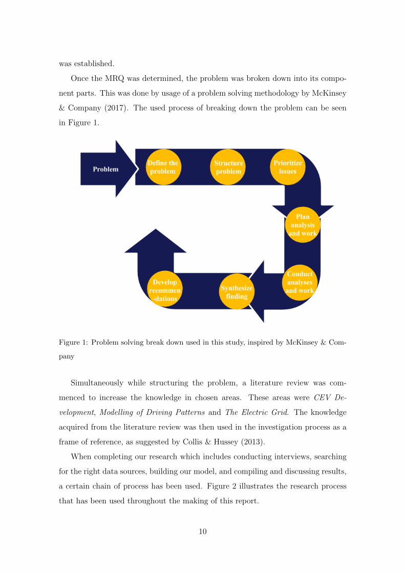
Once the MRQ was determined, the problem was broken down into its compo-

nent parts. This was done by usage of a problem solving methodology by McKinsey

& Company (2017). The used process of breaking down the problem can be seen

in Figure 1.

Figure 1: Problem solving break down used in this study, inspired by McKinsey & Com-

pany

Simultaneously while structuring the problem, a literature review was com-

menced to increase the knowledge in chosen areas. These areas were CEV De-

velopment, Modelling of Driving Patterns and The Electric Grid. The knowledge

acquired from the literature review was then used in the investigation process as a

frame of reference, as suggested by Collis & Hussey (2013).

When completing our research which includes conducting interviews, searching

for the right data sources, building our model, and compiling and discussing results,

a certain chain of process has been used. Figure 2 illustrates the research process

that has been used throughout the making of this report.

10

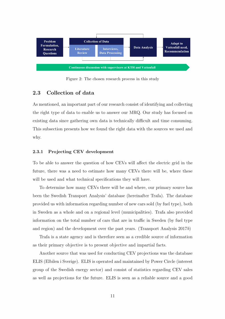
Figure 2: The chosen research process in this study

2.3 Collection of data

As mentioned, an important part of our research consist of identifying and collecting

the right type of data to enable us to answer our MRQ. Our study has focused on

existing data since gathering own data is technically difficult and time consuming.

This subsection presents how we found the right data with the sources we used and

why.

2.3.1 Projecting CEV development

To be able to answer the question of how CEVs will affect the electric grid in the

future, there was a need to estimate how many CEVs there will be, where these

will be used and what technical specifications they will have.

To determine how many CEVs there will be and where, our primary source has

been the Swedish Transport Analysis’ database (hereinafter Trafa). The database

provided us with information regarding number of new cars sold (by fuel type), both

in Sweden as a whole and on a regional level (municipalities). Trafa also provided

information on the total number of cars that are in traffic in Sweden (by fuel type

and region) and the development over the past years. (Transport Analysis 2017b)

Trafa is a state agency and is therefore seen as a credible source of information

as their primary objective is to present objective and impartial facts.

Another source that was used for conducting CEV projections was the database

ELIS (Elbilen i Sverige). ELIS is operated and maintained by Power Circle (interest

group of the Swedish energy sector) and consist of statistics regarding CEV sales

as well as projections for the future. ELIS is seen as a reliable source and a good

11

way of validating our own projections. (Power Circle 2016b)

2.3.2 Modelling drive patterns

The next step was to gather data on how people in Sweden and Uppsala are using

their cars, to be able to say how the usage of cars will affect the grid when replaced

by CEVs. When acquiring this data, collaboration with Lindholmen Science Park

(LSP) and Test Site Sweden (TSS) was crucial for our research. LSP is an inter-

national collaboration for research and innovation based in Gothenburg, Sweden.

LSP have three focus areas which are Media, ICT and Transport, the later is where

the TSS-program is situated. (Lindholmen Science Park 2017)

Within the TSS-program is the so called National Car Movement database

that consists information on different car monitoring projects. The database is

financed by The Swedish Energy Agency (Energimyndigheten) and the purpose of

the database is to gather information on how CEVs and ICEs actually are being

used (Test Site Sweden 2017). This database is open for non-profit organisations

and research and it is from this database that we gathered data to determine driving

patterns. Both LSP and TSS are seen as credible sources of information as they

are publicly funded, non-profit and share the unmanipulated raw data.

Two other important sources in modelling driving patterns was Uppsala Mu-

nicipaity and Trafa. These sources provided statistics on where in Uppsala there

are many cars (demographic statistics) and what the average driving distance in

specifically Uppsala is. This information helped translate the data from the TSS

database to be applicable for the drivers in Uppsala.

2.3.3 Understanding the grid

Lastly there was a need to acquire data about the local electric grid in Uppsala,

to understand the components that make up the grid and what the implications

to change these would be. We needed to understand how the grid is constructed

and how the different system components interact with one another and understand

how the grid load is today and how it might change.

The necessary information was retrieved by reaching out to people at Vattenfall

12

and other organisations to gain the specific and expert insights needed. According

to Blomkvist & Hallin (2015), semi-structured interviews is a good method to collect

qualitative data and thus this strategy was adopted in these meetings.

There was also a need to compare the load from CEVs to detailed household

load. This was our chosen method when investigating the effects on the grid due to

CEVs because the relatvie change from today’s household indicates how the current

infrastructure may need to be upgrade.

We simulated the CEV load by combining the driving patterns data of when

and how much the CEVs would need to charge with our research on technical speci-

fications of CEVs and CEV chargers. The household load profiles were constructed

using historical data provided by The Swedish Energy Agency. The data was pro-

vided as Excel sheets with information on different types of households, different

sources of electricity usage and for different time periods. This made it possible for

us to conduct our analysis in a good way.

The data from The Swedish Energy Agency is deemed as reliable, since it comes

from a public agency and since acquiring the data was done under strict regulations

and measurement rules.

2.4 Analysis of data and model outcome

When all the necessary data had been collected we had to compile the different data

sources into one to be able to analyze the data and produce results. This subsection

describes the methodology for doing this in the best way.

2.4.1 Software choice

We used Microsoft Excel as our primary software for compiling the data, creating

our model and making our analysis. Excel was deemed to be the best tool as it is

easy to handle large amounts of data in and since we have a good understanding of

the software and its functions. Add-ins such as PowerPivot was used to handle the

databases and VBA-Macros was used to extract final results.

13

2.4.2 Value-creating results

Ultimately, the purpose of this study was to find what actions Vattenfall should take

in order to, in a sustainable way, react to the effects CEV charging could have on

the electric grid i Uppsala by 2030. Thus, it was important to constantly have this

in mind during the length of the study so that we did not drift from that purpose.

In order to assure this, constant feedback and weekly sessions with supervisors at

Vattenfall was held.

2.5 Validity and Reliability

To ensure that the report is conducted in a proper way we made sure to check the

validity and reliability thoroughly throughout the entire length of the study. This

is crucial to be able to guarantee that an external and objective party would be

able to conduct the same research as we have and reach the same results (Collis

& Hussey 2013). This was done by presenting all the results that were generated

including notes from interviews and meetings to ensure complete transparency. By

ensuring this the research becomes more reliable and useful to those reading this

report.

According to Blomkvist & Hallin (2015), validity is to make sure that the con-

ducted research is about the right thing and reliability is to ensure that the research

is done in the right way. Since this study consists of both gathering of data and

simulation of results, it is important to ensure validity and reliability of the input

data to be able to ensure validity and reliability in the results themselves. To make

sure that the collected data is both valid and reliable the data was analyzed by

triangulating the data points using different independent sources (Trafa and ELIS

as well as TSS, Uppsala Muncipality and The Swedish Energy Agency). This is

encouraged, according to Easterby-Smith et al. (2012).

Since we simulated scenarios to obtain the results the most important factor

threatening the reliability and validity of the results is the quality of the data

and the number of parameters included in the model. However, we ran the risk

of the validity conflicting with the reliability since an increase in the number of

14

parameters could compromise the accuracy of the results. We aimed to calibrate

this in collaboration with experts on the subject of modelling as well as experts in

each sub-area of the study.

Normally, interviews can cause risks with the reliability of the results, however

for this report, the interviews were primarily a source of objective information on

how things are. Thus, no personal opinion was expected to effect the outcome.

15


16

3 Literature Review

This section presents the required background and relevant conducted research for

this thesis. Firstly a general background is provided on the CEV market, different

CEV models and the CEV charging infrastructure. Further, the chapter will look

into how driving patterns are identified and quantified as well as make a deep dive

into the electric grid and what current load profiles look like. Finally the chapter

summarize previous research that is specifically relevant to this thesis.

3.1 Chargeable Electric Vehicles

This subsection brings to light the development within the CEV industry. This

includes the sales trends, development from different car manufacturers and the

charging infrastructure.

3.1.1 Market for Charging Electric Vehicles

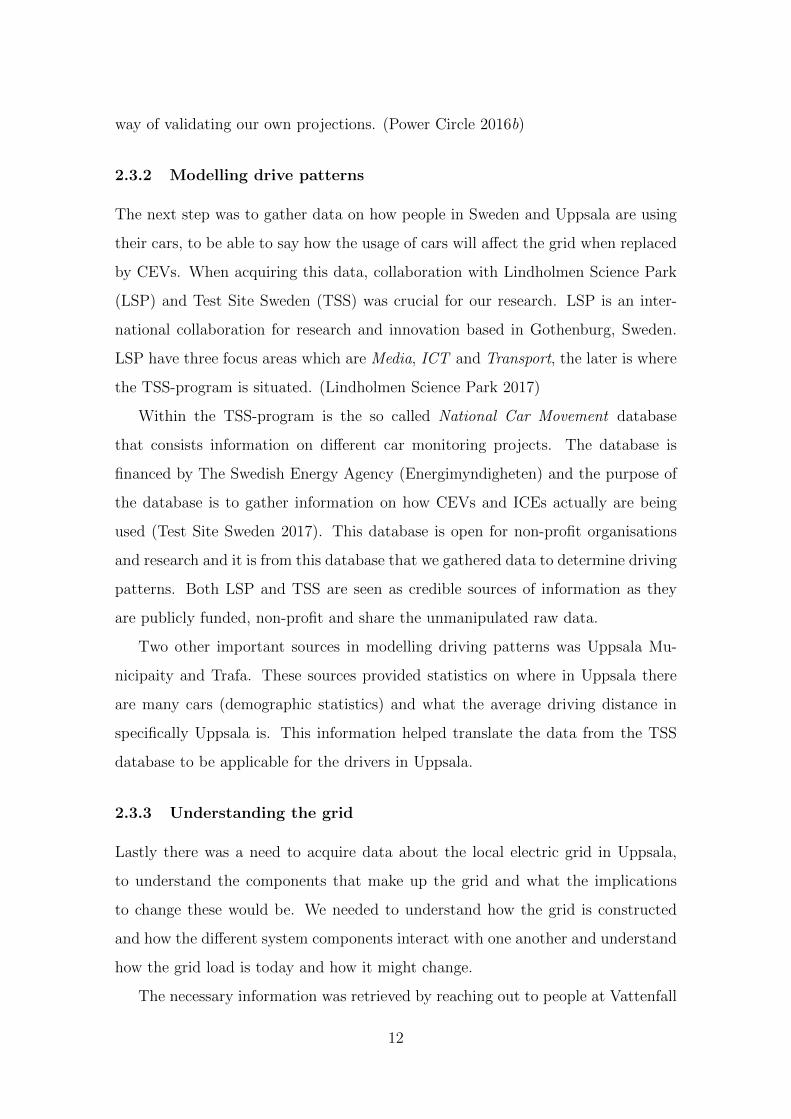
The market for CEVs is nearing a tipping point. In 2015 the global CEV market

surpassed 1 million CEVs globally on the streets. This is illustrated in Figure 3.

China is today the biggest CEV market in terms of number of cars sold with roughly

half of all new CEV (350,000) sold in 2016 (Alestig & Hjalmarson-Neideman 2017).

Figure 3: CEV global growth (International Energy Agency 2016)

17

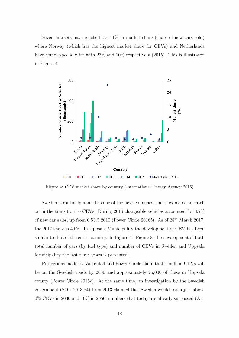
Seven markets have reached over 1% in market share (share of new cars sold)

where Norway (which has the highest market share for CEVs) and Netherlands

have come especially far with 23% and 10% respectively (2015). This is illustrated

in Figure 4.

Figure 4: CEV market share by country (International Energy Agency 2016)

Sweden is routinely named as one of the next countries that is expected to catch

on in the transition to CEVs. During 2016 chargeable vehicles accounted for 3.2%

of new car sales, up from 0.53% 2010 (Power Circle 2016b). As of 28th March 2017,

the 2017 share is 4.6%. In Uppsala Municipality the development of CEV has been

similar to that of the entire country. In Figure 5 - Figure 8, the development of both

total number of cars (by fuel type) and number of CEVs in Sweden and Uppsala

Municipality the last three years is presented.

Projections made by Vattenfall and Power Circle claim that 1 million CEVs will

be on the Swedish roads by 2030 and approximately 25,000 of these in Uppsala

county (Power Circle 2016b). At the same time, an investigation by the Swedish

government (SOU 2013:84) from 2013 claimed that Sweden would reach just above

0% CEVs in 2030 and 10% in 2050, numbers that today are already surpassed (An-

18

Figure 5: Development of cars in Sweden by fuel type (Transport Analysis 2017a)

Figure 6: Development of cars in Uppsala Municipality by fuel type (Transport Analysis

2017a)

dersson & Ribbing 2016). A new study by Bloomberg New Energy Finance predicts

that 35% of new cars sales worldwide will be chargeable by 2040 (Randall 2016).

In the middle of the 2000’s, cars driven by ethanol were strongly subsidised by

the Swedish government (tax deductions on both the car and on the fuel). This

resulted in massive growth in sales for a couple of years, which later stopped com-

pletely, mainly due to the subsidies being withdrawn in 2011 (Saxton 2016). The

19

Figure 7: Development of CEVs in Sweden (Transport Analysis 2017a)

Figure 8: Development of CEVs in Uppsala Municipality (Transport Analysis 2017a)

development of ethanol cars sales shows how strong incentives, like subsidies, have

a powerful effect on peoples buying behaviour.

CEV sales have also been driven mainly by governmental subsidies. Both Nor-

way and the Netherlands offer significant tax cuts as incentive for buying a CEV

instead of a traditional petrol driven vehicles (Kihlstrom 2015). In Sweden the

so called supermiljobilspremien gives CEV buyers a discount of up to 40,000 SEK

(Finansdepartementet 2016). The Swedish government recently extended the super-

miljobilspremien in waiting for the Bonus-malus-system, designed to penalize cars

20

with high emissions. The Bonus-malus-system is expected to be in working order

by July 1st, 2018, and with that the supermiljobilspremien will cease to exist. (Fi-

nansdepartementet 2016). There are other factors expected to fuel the growth such

as decreased prices of CEVs, longer driving range and improved access to charging

infrastructure.

When comparing the CEV development in Sweden and Norway, it looks like

CEV development in Sweden is following a similar development, only three years

later. This is seen in Figure 9 and Figure 10. The comparison between the two

countries is a relevant as the two countries are very similar from as economical,

geographical and social perspective.

Figure 9: CEV market share development in Sweden (Transport Analysis 2017a)

3.1.2 Car model development of Electric Vehicles

Car model development of CEVs and increased sales is in a positive spiral, driving

down prices and increasing the number of available car models. Increased demand is

driving down the cost for the batteries used in the cars which is especially important

because it accounts for roughly 75% of the total power train cost (Wolfram & Lutsey

2016). Since 2010, battery prices have dropped 65% and in 2016 alone they dropped

35% (Randall 2016). According to Randall (2016), price parity will be reached by

2022, at which point the life time cost for owning a CEV will be equivalent to

21

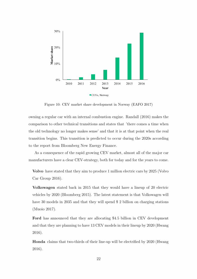
Figure 10: CEV market share development in Norway (EAFO 2017)

owning a regular car with an internal combustion engine. Randall (2016) makes the

comparison to other technical transitions and states that ’ there comes a time when

the old technology no longer makes sense’ and that it is at that point when the real

transition begins. This transition is predicted to occur during the 2020s according

to the report from Bloomberg New Energy Finance.

As a consequence of the rapid growing CEV market, almost all of the major car

manufacturers have a clear CEV-strategy, both for today and for the years to come.

Volvo have stated that they aim to produce 1 million electric cars by 2025 (Volvo

Car Group 2016).

Volkswagen stated back in 2015 that they would have a lineup of 20 electric

vehicles by 2020 (Bloomberg 2015). The latest statement is that Volkswagen will

have 30 models in 2035 and that they will spend $ 2 billion on charging stations

(Muoio 2017).

Ford has announced that they are allocating $4.5 billion in CEV development

and that they are planning to have 13 CEV models in their lineup by 2020 (Hwang

2016).

Honda claims that two-thirds of their line-up will be electrified by 2020 (Hwang

2016).

22

Daimler is spending $500 million on a new battery factory to support their CEV

cars (Hwang 2016).

Tesla is building their ’Giga factory’ for battery production in Nevada and are

hoping to cut their battery costs with over 30% when finished in 2018. Tesla

estimates that the factory will be able to produce an annual battery capacity of

35 GWh (Tesla Motors 2017).

Besides what is mentioned above, the Asian market (with China leading the way

as mentioned earlier) is growing rapidly. Manufacturers such as Warren Buffett’s

BYD, BAIC, and Volvo-owner Geely is putting a lot of effort in CEV development

with the government subsidising CEV manufacturers since the government is bet-

ting that CEVs will solve the smog-problem in big cities across the country (Alestig

& Hjalmarson-Neideman 2017). Even though the government is reducing the subsi-

dies (due to a number of corrupt CEV start-ups), subsidies are likely to remain high

for the big CEV manufacturers (such as BYD, BAIC and Geely) as the Chinese

government has an ambition to sell 3 million CEVs per year by 2025 (Bloomberg

News 2016).

3.1.3 Charging of Electric Vehicles

An ever debated problem with the transition to CEVs has been the required in-

frastructure, namely charging stations. The debate has two primary dimensions -

1) access to charging stations (i.e. the number of charging stations) and 2) time

to charge (i.e. power output of the charging stations). Both these dimensions are

something that have seen significant improvements just in the past years.

Access to charging stations seems to be less and less of an obstacle when

considering buying a CEV. Japan, for example, now has more charging stations

than petrol stations, although many are private (McCurry 2016). According to

Uppladdning.nu (2016), there are currently around 30 stations in and nearby

the town of Uppsala (compared to 250 in Stockholm). These charging stations

all have at least one charging plug but can have up to ten plugs. If looking at

the entire Uppsala County there are 41 charging points as of March 2017 and

23

this is only counting the public charging points (Laddinfra 2017). Overall there

are 2,756 public charging points in Sweden and the most common power type is

3.7 kW (41%) followed by 22 kW (21%) (Laddinfra 2017). A noteworthy new

regulation, that will affect charging of CEVs, is the new EU directive that will

require new and refurbished houses to sport charging stations for CEVs. This

directive is expected to come into effect 2019 (Neslen 2016). On a more local

level, Sweden has decided on charging with mode 3 and type 2-plug as standard

at all public charging stations, with start 2017. This will be of great importance

for CEV retailers since lack of a joint standard have been holding back the spread

of CEVs in Sweden (Svensk Energi 2013).

Time to charge a CEV has been seen as one of biggest problems when moving

to an electrified car fleet. Mainly because refueling a fossil fuel driven car takes

only a couple of minutes while recharging a CEV has historically taken at least

a couple of hours. The slowest charging alternative currently being used, is that

which corresponds to the power available in a normal socket. In Sweden this is

230 volts and 10 ampere, thus 2.3 kW of available power. The available charging

options today are many in the range 2.3 kW - 145 kW (see Table 1 for more

detail on today’s charging options). In order to make charging of CEVs less of an

issue, BMW, Daimler’s Mercedes, Ford, and Volkswagen are, in a joint venture,

exploring the possibilities of a 350 kW charger. More than twice that of Tesla’s

supercharger of 145 kW. A 350 kW charger would recharge a 100 kWh battery

in under 20 minutes (Lambert 2016).

Important to mention when talking about the time to charge, is how the

charging power supplied to the battery varies with different factors such as size,

supplied power, temperature, etc. According to Tollin (2016), the power supplied

to the battery varies drastically with the State of Charge (SOC) of the battery

when charging at high power. At high power the battery will receive the stated

power only at a low SOC, but then the supplied power eventually decline as

the SOC increases. At approximately 35-80% SOC (depending on the supplied

power), the charging power will drop fairly linearly, as seen in Figure 11. Ac-

cording to Tollin (2016), even factors such as the condition of the battery (inner

24

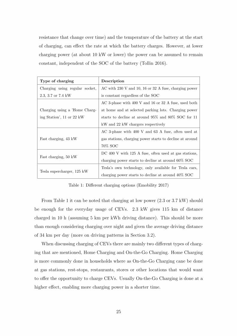
resistance that change over time) and the temperature of the battery at the start

of charging, can effect the rate at which the battery charges. However, at lower

charging power (at about 10 kW or lower) the power can be assumed to remain

constant, independent of the SOC of the battery (Tollin 2016).

Type of charging Description

Charging using regular socket,

2.3, 3.7 or 7.4 kW

AC with 230 V and 10, 16 or 32 A fuse, charging power

is constant regardless of the SOC

Charging using a ’Home Charg-

ing Station’, 11 or 22 kW

AC 3-phase with 400 V and 16 or 32 A fuse, used both

at home and at selected parking lots. Charging power

starts to decline at around 95% and 80% SOC for 11

kW and 22 kW chargers respectively

Fast charging, 43 kW

AC 3-phase with 400 V and 63 A fuse, often used at

gas stations, charging power starts to decline at around

70% SOC

Fast charging, 50 kWDC 400 V with 125 A fuse, often used at gas stations,

charging power starts to decline at around 60% SOC

Tesla supercharger, 125 kWTesla’s own technology, only available for Tesla cars,

charging power starts to decline at around 40% SOC

Table 1: Different charging options (Emobility 2017)

From Table 1 it can be noted that charging at low power (2.3 or 3.7 kW) should

be enough for the everyday usage of CEVs. 2.3 kW gives 115 km of distance

charged in 10 h (assuming 5 km per kWh driving distance). This should be more

than enough considering charging over night and given the average driving distance

of 34 km per day (more on driving patterns in Section 3.2).

When discussing charging of CEVs there are mainly two different types of charg-

ing that are mentioned, Home Charging and On-the-Go Charging. Home Charging

is more commonly done in households where as On-the-Go Charging cane be done

at gas stations, rest-stops, restaurants, stores or other locations that would want

to offer the opportunity to charge CEVs. Usually On-the-Go Charging is done at a

higher effect, enabling more charging power in a shorter time.

25

Figure 11: Charging power of a BMW i3 vs battery SOC. Different colours represent

charging at different days and charging stations (Electrify Atlanta 2017)

Grahn (2014) has categorized the type of charging strategies or typologies according

to Uncontrolled Charging (UCC), External Charging Strategies (ECS) and Individ-

ual Charging Strategies (ICS). These are described further bellow.

Uncontrolled Charging means that the owner of the CEV will charge without

a third party incentive / input or individual strategy. The owner will charge

according to its charging behaviour however without the driver being influenced

by certain parameters (see below).

Individual Charging Strategies means that the owner of the CEV will charge

based on or influenced by, certain factors affecting the owner’s charging behaviour.

This could for example be an owner that is price sensitive, thus choosing to charge

during low price hours. Or a driver choosing certain routes to accommodate for

charging at a certain station.

External Charging Strategies means that the owner of the CEV will charge

based on what a third party dictates. This could for example be letting Vattenfall

choose when the CEV should be charged based on the current and future strain

on the grid.

26

In this study, Home Charging and Uncontrolled Charging will be assumed as

the choice for all charging. This to focus the potential impact on the grid at a

residential level. As for charging strategy, primarily ECS will be considered as a

possible solution to the impacts that CEVs could have on the grid.

3.2 Driving Patterns

This subsection accounts for current data and research in modelling driving patterns

that will be used in this research, both at a national level but also especially for

Uppsala.

3.2.1 Modelling of Drive Patterns

As mentioned in Section 2, a part of this research will be to analyse and use data on

driving patterns from data collected by LSP and TSS. The main project from TSS

that will be used is the one called Bilrorelsedata 1 (BRD 1) that was commenced

in 2010. The project has a final report written by Karlsson (2013) (in this section

referred to as, the study) and was conducted in Vastra Gotaland (VG), Sweden,

with GPS-tracking of over 700 ICE cars.

The aim for the BRD 1 study was to get a better understanding of how cars

are being used in order to understand how to facilitate for more CEVs in a nearby

future (Karlsson 2013). The author of the final report states that data on driving

patterns has previously been unavailable and that countries’ (Sweden included)

travel surveys never reach anywhere near the same level of detail as what the BRD

1 study has achieved. Instead the national gathering of data was heavily dependent

on questionnaires and interviews, which can give an underestimate in terms of

number of trips due to the nature and inaccuracy of surveys and interviews (Wolf

et al. 2003, Stopher et al. 2007).

In the study, the goal was to gather data of 500 different vehicles for 30 days

or more. In the final report it is stated that data from 714 cars was logged in the

database. 528 cars logged data for more than 30 days and 450 cars logged data for

more than 50 days (Karlsson 2013). The selection of cars was conducted by the

27

Swedish motor-vehicle register from cars matching the criteria in Table 2. Requests

were sent out randomly to owners with cars that matched the criteria. In total the

study received 932 positive responses from a total of 12 357 inquisitions.

Parameter Chosen selection

Vehicle type Passenger car of type 11

Usage Non-commercial

Model year 2002 or newer

Geographic area Registered in VG county or

Kungssbacka municipality

Table 2: Selection of cars in BRD 1

At the start for the study, the area in which the selection of cars was made

consisted of approximately 17% of the total number of cars in Sweden and 17%

of Sweden’s inhabitants. Average driving distance and cars per 1,000 inhabitants

had almost a one-to-one ratio between the chosen area and the Sweden average

(Karlsson 2013).

To be able to log the movement of the cars the study chose to use a GPS logger

with a GSM modem and a memory card to be able to store data. The device (MX3

from Host Mobility) was connected to the 12V outlet in the cars. Some of the

logged data include:

• Device (i.e. Car)

• Trip ID

• Final velocity

• Average velocity

• Distance

• Pause before & after

• Duration

• Start and stop date & time

The data was then collected by TSS and analyzed for errors that were removed

upon finding (e.g. trips with speed under 0,1 km/h for more then 10 min) (Karlsson

1A car that is mainly used for person transport and that holds the maximum capacity of 8

people (including the driver) and with a maximum weight of 3.5 tons

28

2013). From the database the study was able to analyse the results and draw

conclusions regarding, e.g. number of trips per day and length per trip. For more

details regarding the study contact TSS and LSP. There as some remarks on this

study that need to be mentioned, these are stated bellow

• The data used in this research is slightly different from the one used in the final

report by Karlsson (2013). This because since the final report was completed,

TSS has made some small additional corrections in the database.

• Some data points have mistakes in them and have to be manipulated in order

to be useful (see Section 4 on how this was done)

• There are some delays in when the GPS tracker starts, giving a different

location on the start of a trip versus where the last trip ended. This delay

varies and is in the final report accounted for by removing certain data points.

After adjusting for loss of data, 460 cars with data logged for more than 30

days remained (compared to 528).

• The author of the study states that one disadvantage with tracking only

through GPS is that the reason behind the trip is not recorded.

• The author of the study claims that driving patterns of the cars in the study

might not be equal that of future CEVs, due to big difference in range. This

is something that this report disagree with, partly due to the rapid advance-

ments made in CEV range but also due to the average driving distance per

day being significantly under the maximum range of the CEVs that already

exist today (more of this in Section 5).

3.2.2 Seasonal Influence on Driving Patterns

According to Borjesson (2017) at Centre for Traffic Research (CTR), an important

factor when analyzing driving patterns is the seasonal variation. Seasonal variation

means that there are differences in people’s driving behaviour depending on the

time of year.

One way to estimate the seasonal variation is by looking at the registered con-

gestion charge of cars (trangselskatt). This gives a good overview of how many trips

are made on a monthly basis. It should be noted that a trip in this sense is defined

29

by a car passing the point of registration and being registered for payment in the

system. According to the study the seasonal effects are significant when modeling

driving patterns. These differences are presented in Figure 12.

Figure 12: Index of seasonal change in driving patterns according to registered congestion

fees2 (Transportstyrelsen 2017)

Notable from Figure 12 is that there are most registrations of cars during the

time April to June and that there is a significant difference compared to the number

of registrations during the winter months (November to February). More on how

seasons affect driving patterns and how this will be taken into account in Section 5

3.2.3 Driving in Uppsala Municipality

When looking at driving patterns on a specific regional level (Uppsala), there is little

available information. The primary source of national driving statistics is Trafa. As

mentioned in Section 2, Trafa gathers and presents statistics on the traffic situation

in Sweden, both at a national level and at a more local level (municipality being

the highest level of detail). By gathering information from the odometer of vehicles

(done at yearly inspections of all registered cars in Sweden) Trafa is able to present

statistics of total driving distance over the past year (Transport Analysis 2017a).

2No congestion fee is taken in July

30

According to the latest Trafa compilation by Myhr (2016b), the average driving

distance of a car in Sweden was 12,240 km per year (2016). The distance however

varies depending on where in Sweden you live and in Uppsala the same number

was 12 570 km per year, thus slightly above average (Myhr 2016b). Per day, these

figures give an average driving distance of 33.5 km and 34.4 km per day respectively

for Sweden and Uppsala. When looking historically, the average driving distance in

Sweden has been more less constant since 2005 (12,980 km) (Myhr 2016b).

To be able to make reasonable assumptions regarding driving patterns in Up-

psala, demographic statistics of inhabitants and their behavior is needed. Upp-

sala Municipality (the office of Kommunledningskontoret) provides this information

upon request in from of Excel sheets (SCB 2016b). Some key insights form this data

is regarding inhabitants, number of households andnumber of cars per households.

The data on the above mentioned is given on detailed geographic level, providing the

opportunity to make high quality assumptions on where there will be a big impact

from CEVs. The following data points were given per area in Uppsala Municipality,

as of December 31st 2015 (SCB 2016b).

• Number of cars

• Number of houses and apartments

• Number of inhabitants

• Number of people working within/outside the area

• Average income

3.3 The Electric Grid

This subsection will account for the background information that is needed to un-

derstand how the electric grid in Sweden and Uppsala works and what implications

there are to load variations.

3.3.1 The electric grid in Sweden

In 2011, Sweden was divided into 4 electric grid areas where Uppsala Municipally

is a part of the third area, SE3. The division of the grid was a result of the

31

European Commission’s accusation that Sweden’s transmission regulations were

discriminating to foreign costumers (Svensk Energi 2016b). The electric grid in

Sweden is also divided into different levels according to local grid, regional grid and

national grid, where the number of actors are by far the most on the local grid level

with approximately 160 actors (Svensk Energi 2016a). On the regional grid there

are three major actors (E.ON Elnat Sverige AB, Vattenfall Eldistribution AB and

Ellevio AB) and the national grid only has one owner, Svenska Kraftnat (SVK)

(Kjellman 2007). See Figure 13 for a break-down of the electric grid in Sweden.

The grid in Figure 13 is divided into transmission grid and distribution grid.

The distribution grid in Sweden is what is refereed to as the local grid, where the

transmission grid both consists of regional grid (110 kV) and national grid (265-275

kV).

According to Svensk Energi (2016a), the Swedish grid has a delivery reliability

of 99.98% and on average the capacity of the grid and its transformers is well above

the consumed load (Tollin 2016).

3.3.2 Current Load

Traditionally, the household load of consumed electricity has a relatively consistent

pattern. People wake up, turn on e.g. their coffee maker and the load increases,

go to work and the load decreases, come home and start to cook food and turn on

other electric appliances which makes the load increase again, and then they go to

sleep and the load decreases. The household load is driven by human behaviour

and other factors such as the weather (especially affecting the need for heating).

Sweden

In 2015 the total usage of electricity in Sweden was 136 TWh. This was the second

lowest usage in the 21th century (mostly due to warm weather and thus low heating

needs). Roughly 50% of the electricity was used in the sector households and

services and 37% was used in the industry. The net export of electricity was record

high in 2015 with 22.6 TWh being exported. (Andersson & Arvidsson 2016)

According to Byman (2016), the electricity usage in Sweden has been fairly con-

32

Figure 13: Break-down of the electric grid (Wikipedia 2017)

sistent at around 130-140 TWh per year for the last 25 years. This is due to more

energy efficient appliances in households and machines in the industry have been

able to make up for a growing population and an increasing number of households

(Byman 2016).

33

On average, the home usage of electricity per person in Sweden was around 3.1

MWh in 2015, with variations in the northern parts of Sweden 4.2 MWh per per-

son) and in the southern parts (2.6 MWh per person) (SCB 2016a). In Figure 14,

a daily average electricity load profiles for houses and apartments are presented.

Figure 14: Average daily load profile in Sweden (The Swedish Energy Agency 2010)

The load curves follow the behaviour described above. The time between 18:00-

19:00, what is normally referred to as Peak Hour, is when the load is highest during

the day.

When looking at a more granular level, there is a need to, not only divide

electricity usage by type of household, but also by month and day. This since there

is great variation in electricity usage over the year. Through The Swedish Energy

Agency and the so called Hushallseldatabasen, this information is distributed upon

request, by signing an agreement not to hand out the raw data to others. The

data consists of measurements done in both detached houses and apartments over

a longer period of time and the data includes the different electrical devices there

are in a household. (The Swedish Energy Agency 2010)

The database consists of 201 households of the type detached house (single

building with own supply of energy) and 188 households of the type apartment (a

household that is part of a bigger building with mutual heating and water supply

34

for all the households in the building). The database consists of over 200 million

data points and can give a comprehensive overview of how electricity is used in

Sweden. The different households that are measured are selected from a wide range

of demographic groups and vary in size, number of inhabitants and income. Some

of the households in the database are measured on a monthly basis and some on a

12 month basis. The measurements are done with 10 minutes intervals and stretch

from 2005 to 2008. (The Swedish Energy Agency 2010)

According to Niklas Notstrand, Principal Statistician at The Swedish Energy

Agency, there are some problems with the database. However, these problems

mainly refer to statistical insignificance when using the database on a detailed level

such as ’do apartments less 100 square meters, with 3 or more inhabitants, use more

warm water than on average?’. In a report by Zimmermann (2009), these types of

questions are attempted to be answered where various results of electricity usage in

Sweden are determined based on the data from Hushallseldatabasen. However, in

these detailed cases / questions, the database is not comprised of enough samples

to be able to provide statistically significant results and thus be representative for

Sweden as a whole (Notstrand 2016).

There is also a somewhat skewed geographical selection of the households. As

stated by Zimmermann (2009), this database was, at the time of creation, by far the

most comprehensive database of its kind in the world. The goal was to collect data

from 400 households that was selected using statistics from Statistiska Centralbyran

(SCB), and this goal was achieved. However when some of the selected households

declined the offer to participate, they were replaced with a group of overrepresented

households from the area of Malardalen, giving the database a geographic imbalance

(Notstrand 2016).

However, according to Notstrand (2016), the database will still provide results

of high statistical significance when used not to split the data points into several

different sub-groups. When looking at how average total energy usage differ during

the days and months of the year and only divide by type of household (house or

apartment), the database will provide reliable results (Notstrand 2016).

35

Uppsala

In Uppsala Municipality, Vattenfall owns most of the local grid and owns the entire

grid in the town of Uppsala, as seen in Figure 15. The black stripes in the area

Bjorklinge represents electric grid that is not owned by Vattenfall. Besides that

area, Vattenfall owns all of the grid inside the green line (representing Uppsala

Municipality) as well as the majority of the grid in the closest outskirts of Uppsala

Municipality. This means that Vattenfall are responsible for all power stations, on

all levels, as well as transmission lines from the regional grid all the way to each

household.

Figure 15: Vattenfall’s grid in Uppsala County (Natomraden.se 2016)

In Uppsala, the average home usage of electricity per person was 3.0 MWh in

2015 thus slightly bellow the national average (SCB 2016a).

3.3.3 Future load

As mentioned above, the electricity consumption has been relatively constant for the

past 25 years. Kungl. Ingenjorsvetenskapsakademien (IVA) has recently completed

a report on how the energy system might look beyond the year 2030. In that report,

it is predicted that the electricity usage will be between 128-165 TWh annually.

The report states that it is difficult to predict usage of electricity more than 5 years

into the future and refers to previous projections that are usually accurate when

36

conducted only a couple of years in advance but tend to be further from reality

when done with greater time scale. (Liljeblad 2016)

An increase to 165 TWh by 2030 is equal to an increase with 22% from today,

or a yearly increase by roughly 4%. When breaking down the electricity usage

it is done in three major segments, Housing and Service, Industry and Transport

(Liljeblad 2016). Since this report focuses on how the electricity load in households

will be affected by CEV growth, the predicted electricity usage in the Housing and

Service segment, which includes electricity heating, is particularly interesting.

Housing and Service will have a usage of 65-85 TWh, compared to today’s usage

of 71 TWh. The biggest increase is predicted to be in the service sector (30-40

TWh compared to 31 TWh today) due to an increased demand in service related

products. An increase in e-shopping is predicted to lead to a growing number of

warehouses that will need more electricity than the reduced need in regular stores.

The household electricity is predicted to be at 20-25 TWh, compared to today’s

usage of 21 TWh and is largely dependent on the predicted increase in population

(and number of households). Energy efficient appliances and new technology is

predicted to hold back the usage need. Finally, the required need for electric heating

is predicted to be lower in 2030 (15-20 TWh compared to 19 TWh today). This

is due to a warmer climate and more efficient heating system (larger share of heat

pumps that have a high efficiency).

Assuming a ’worst case’ scenario with electricity heating remaining constant

at 19 TWh and household electricity increasing from 21 to 25 TWh gives a yearly

increase of approximately 0.79% and a total increase with 12.5% until 2030. In areas

where heating is supplied from other sources than electricity (e.g. district heating)

the relative change will be even greater assuming that the grid in these areas are

not dimensioned for the heating supply. These areas will see a 19% increase until

2030 or a 1.2% annual increase, in a ’worst case’ scenario. Noteworthy is that the

increase in the Transport segment (which is predicted to be mostly due to growth of

electric vehicles) is separate and thus not accounted for in the Housing and Service

segment.

Overall Liljeblad (2016), mentions four major factors to how much and how fast

37

the electricity demand will change within the different segment above. These are:

• Economical development

• Population growth

• Technical development

• Political decisions and regulations

Examples of these factors is GDP development, price on batteries, migration

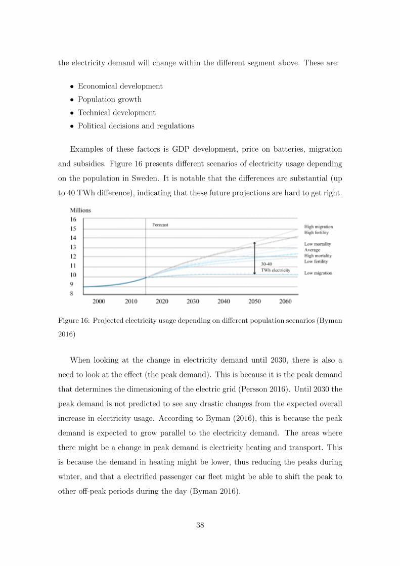
and subsidies. Figure 16 presents different scenarios of electricity usage depending

on the population in Sweden. It is notable that the differences are substantial (up

to 40 TWh difference), indicating that these future projections are hard to get right.

Figure 16: Projected electricity usage depending on different population scenarios (Byman

2016)

When looking at the change in electricity demand until 2030, there is also a

need to look at the effect (the peak demand). This is because it is the peak demand

that determines the dimensioning of the electric grid (Persson 2016). Until 2030 the

peak demand is not predicted to see any drastic changes from the expected overall

increase in electricity usage. According to Byman (2016), this is because the peak

demand is expected to grow parallel to the electricity demand. The areas where

there might be a change in peak demand is electricity heating and transport. This

is because the demand in heating might be lower, thus reducing the peaks during

winter, and that a electrified passenger car fleet might be able to shift the peak to

other off-peak periods during the day (Byman 2016).

38

3.4 Previous Research

In order to make sure that this thesis will contribute to science and the general

research in this area, different studies that have been conducted in similar fields as

this report will be examined. This to confirm that the research questions in this

report have not yet been answered. This subsection presents the findings.

3.4.1 Research study #1

This research was conducted in 2013 as a PhD thesis at Royal Institute of Technol-

ogy, Stockholm.

The purpose of the thesis was to complete certain knowledge gaps in the area

of how CEVs will impact the grid load. The aim was to investigate the impact of

different types of electric vehicles charging on load profiles and load variations in

Sweden.

The thesis uses a stochastic model based on transport and load data to be able

to simulate how charging of CEVs would affect the load given five different charging

scenarios.

The thesis establishes that there are three key factors that determine how the

load will be affected. These are charging location, charging need and charging

moment. The thesis also establishes that the model gains accuracy as the quality

and amount of data increases.

The results of the thesis indicate that during ’unoptimized’ scenarios, with full

adaption to CEVs, there can be significant increases in peak load. (Grahn 2013)


This research was conducted in 2011 for the Institute of Electrical and Electronics

Engineers, New York.

This study aims to model and analyze the demand of grid load in a distribution

system due to battery charging of electric vehicles. The study is conducted on a

distribution system in the United Kingdom and uses a stochastic formulated method

and different charging scenarios to model how the load is effected. The study

39

simulates four charging scenarios, with and without optimized smart-charging, and

different types of batteries with different needs.

One conclusion from the study is that with a CEV market share of 20%, the

daily increase in the load will be 36% in a ’worst-case’ scenario. (Qian et al. 2011)


This research was published in Elsevier in 2008 for their Transport and Environment

section.

This study models driving patterns and identifies driving cycles in large Chinese

cities. The study presents a method to collect data by a so called car-chase technique

and by identifying the most important factors in drive patterns.

The study indicates that among the important factors that define driving pat-

terns are local road infrastructure and driving behaviour. (Wang et al. 2008)

3.4.4 Research Study #4

This study was conducted in 2015 for the Electrical Engineering School as a master

thesis at The Royal Institute of Technology.

The study was done in collaboration with Ellevio with the purpose to investi-

gate how many CEVs that can be charged at the same time in different areas in

Stockholm.

The study uses a standardised charging case (effect and time), combined with

internal knowledge on grid components capacity and load for five different areas in

Stockholm, to determine at what percentage of the areas’ parking lots the charging

could cause a problem.

The study finds that cable overload could case a major problem due to CEVs

charging and that the areas that are most vulnerable are rural areas with small

houses. The study also finds that much of the problem can be solved by giving the

consumers the incentive to charge at night. (Persson-Gode 2016)

3.4.5 Conclusion from previous research

From the research studies the following conclusions can be drawn:

40

• It is a reconfirmation that the research questions in this report are valid and

in need of answers

• In the existing research on CEVs’ impact on the grid, focus is not on actual

driving patterns and driving behaviour

• There is a need to conduct this type of study with a higher level of granularity,

i.e. Uppsala Municipally instead of Sweden and the U.K

• Several of the studies focus on the Effect from different types of charging

strategies

• The theses uses data input and sources that can possibly be re-used in this

thesis or at least be used as inspiration to where and how data can be found

and generated

• Only one of the theses focus on how the distribution and transmission capacity

of the electric grid are affected by CEVs. The other focus on load profiles in

general and production related issues

• None of the theses have a future approach regarding CEV development, future

electricity usage and the future mobility need

3.5 Summary of Literature Review

The literature review conducted in this report will, as mentioned in Section 2, serve

as a frame of reference when completing this research. The theory in Section 3.1 will

help making projections on the CEV market development in Sweden and Uppsala

as well as provide the needed technical knowledge regarding charging and battery

capacity. Section 3.2, will help provide data sources and modelling techniques for

driving patterns in order to create a model to simulate driving patterns in and

around the Uppsala area. Thirdly, Section 3.3 gives the necessary knowledge to

incorporate the modelling of driving patterns to existing load curves. It also helps

understanding how the electric grid might be affected by CEVs and what actions is

needed to account for this. Finally Section 3.4 ensures that the research is relevant

and that the MRQ is correctly formulated. Bellow are the overall key take aways

from the conducted literature review.

Firstly, the literature review establishes what is well-known, namely that the

41

CEV market is seeing explosive growth based on sales figures, car manufacturer’s

strategic planning/investments and developments in charging technology.

Secondly, the literature review helps to understand how driving patterns will

affect the need and character of CEV charging and how this can be modeled.

Thirdly, the literature review provides the initial background information re-

quired in order to understand how load variations impact grid infrastructure.

Finally, the literature shows that previous research conducted in this area needs

to be supplemented, which confirms that the research questions in this study are

valid and in need of answers.

42


43

4 CEV projections 2030

This section accounts for all the projections that have been made using the data

described in Section 2 and presented in Section 3.1. The assumptions and calcu-

lations that have been made are accounted for in this section. This section finally

presents the findings regarding development of CEV models in the world as well as

projections of CEVs market share in Sweden and in Uppsala.

4.1 Assumptions

When conducting the different projections in this section, some assumptions had to

be made. These assumptions are presented in Table 3.

Assumption Description Motivation

Continued growth The growth of CEV sales is as-

sumed to continue at a similar

pace as it has between between

2012 and 2016

It is reasonable as long as the influ-

encing factors are the same. Such

as politics, economics, etc.

Declined growth Even if sales are assumed to con-

tinue to grow, it has been assumed

that the growth rate will decline to

30% between 2017 and 2022

The CAGR between 2013 and 2016

was 207% thus, 30% is an under-

statement for at least the first cou-

ple of years of the projection

Price parity According to Randall (2016), it

is assumed that CEVs will reach

price parity with ICEs in 2022

Randall (2016)

Dramatic shift After 2022 it is assumed to be a

dramatic growth in CEV sales due

to price parity being reached and

that all new cars that are sold will

be CEVs within three years

Assuming all else stays the same,

there will be no reason not to

buy an CEV. Also if price par-

ity is reached, governments can

more easily work towards com-

pletely banning sales of ICEs

44

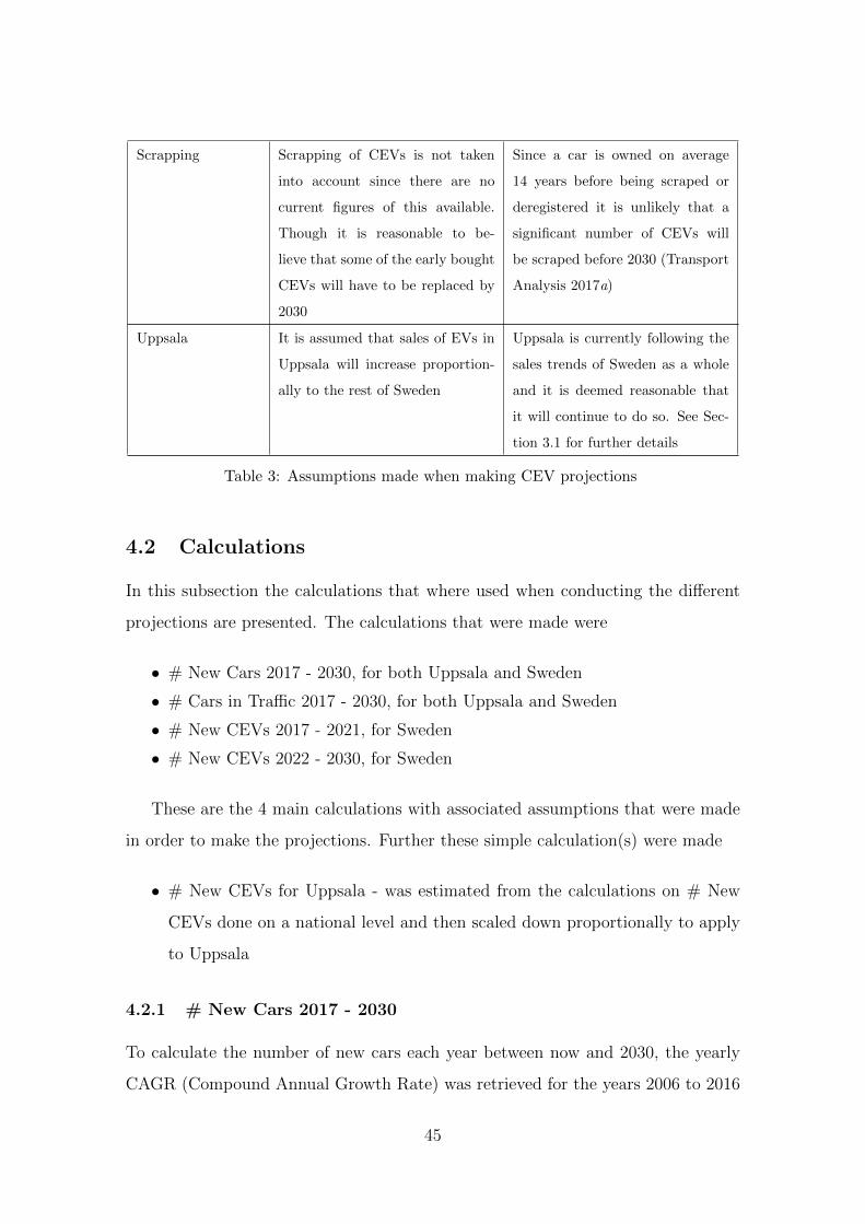
Scrapping Scrapping of CEVs is not taken

into account since there are no

current figures of this available.

Though it is reasonable to be-

lieve that some of the early bought

CEVs will have to be replaced by

2030

Since a car is owned on average

14 years before being scraped or

deregistered it is unlikely that a

significant number of CEVs will

be scraped before 2030 (Transport

Analysis 2017a)

Uppsala It is assumed that sales of EVs in

Uppsala will increase proportion-

ally to the rest of Sweden

Uppsala is currently following the

sales trends of Sweden as a whole

and it is deemed reasonable that

it will continue to do so. See Sec-

tion 3.1 for further details

Table 3: Assumptions made when making CEV projections

4.2 Calculations

In this subsection the calculations that where used when conducting the different

projections are presented. The calculations that were made were

• # New Cars 2017 - 2030, for both Uppsala and Sweden

• # Cars in Traffic 2017 - 2030, for both Uppsala and Sweden

• # New CEVs 2017 - 2021, for Sweden

• # New CEVs 2022 - 2030, for Sweden

These are the 4 main calculations with associated assumptions that were made

in order to make the projections. Further these simple calculation(s) were made

• # New CEVs for Uppsala - was estimated from the calculations on # New

CEVs done on a national level and then scaled down proportionally to apply

to Uppsala

4.2.1 # New Cars 2017 - 2030

To calculate the number of new cars each year between now and 2030, the yearly

CAGR (Compound Annual Growth Rate) was retrieved for the years 2006 to 2016

45

(Myhr 2016a). This was done as shown in Equation 1

# New Cars CAGR =

(# New Cars 2016

# New Cars 2006

) 12016−2006

(1)

Further, the succeeding years were calculated by multiplying ’# New Cars 2016’

with the ’# New Cars CAGR’, compounded by the number of years surpassing 2016.

For example, # New Cars 2020 was calculated according to Equation 2

# New Cars 2020 = # New Cars 2016 ∗ # New Cars CAGR2020−2016 (2)

4.2.2 # Cars in Traffic 2017 - 2030

To calculate the # Cars in Traffic 2017 - 2030, the same equation as in the previous

section was used. This is shown in Equations 3 and 4

# Cars in Traffic CAGR =

(# Cars in Traffic 2016

# Cars in Traffic 2006

) 12016−2006

(3)

# Cars in Traffic 2020 = # Cars in Traffic 2016 ∗# Cars in Traffic CAGR2020−2016

(4)

4.2.3 # New CEVs 2017 - 2021

To calculate # New CEVs per year between 2017 - 2021, the previous year’s # New

CEVs per year is multiplied by 30%, as assumed. This is shown in Equation 5.

# New CEVs year X = # New CEVs year (X − 1) ∗ (1 + 30%),

where 2017 ≤ X ≥ 2021(5)

4.2.4 # New CEVs 2022 - 2030

To calculate # New CEVs per year 2022 - 2030, it is assumed that CEVs will reach

100% market share within 3 years. This means that all New Cars 2024 will be

CEVs. The market share 2021 has been calculated to roughly 13 %. The market

share is therefore estimated to be 40% in 2022 and 80% in 2023.

46

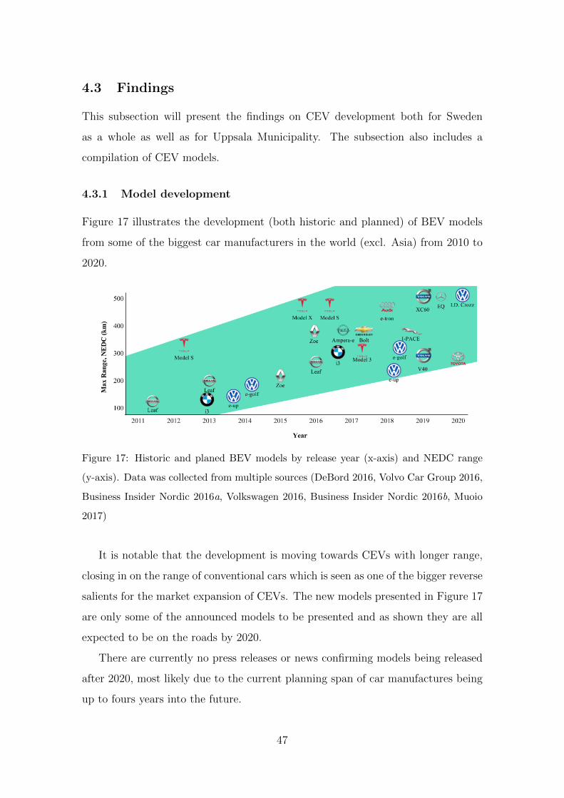
4.3 Findings

This subsection will present the findings on CEV development both for Sweden

as a whole as well as for Uppsala Municipality. The subsection also includes a

compilation of CEV models.

4.3.1 Model development

Figure 17 illustrates the development (both historic and planned) of BEV models

from some of the biggest car manufacturers in the world (excl. Asia) from 2010 to

2020.

Figure 17: Historic and planed BEV models by release year (x-axis) and NEDC range

(y-axis). Data was collected from multiple sources (DeBord 2016, Volvo Car Group 2016,

Business Insider Nordic 2016a, Volkswagen 2016, Business Insider Nordic 2016b, Muoio

2017)

It is notable that the development is moving towards CEVs with longer range,

closing in on the range of conventional cars which is seen as one of the bigger reverse

salients for the market expansion of CEVs. The new models presented in Figure 17

are only some of the announced models to be presented and as shown they are all

expected to be on the roads by 2020.

There are currently no press releases or news confirming models being released

after 2020, most likely due to the current planning span of car manufactures being

up to fours years into the future.

47

4.3.2 Sweden

The projections indicate that Sweden is on track to reach 10% CEVs of new sales

in 2020, and 1 million CEVs in traffic by some time during 2024. These projections

can be seen in Figure 18 and Figure 19.

Figure 18: Projection of the number of CEVs in Sweden

Figure 19: Projection of the market share of CEVs in Sweden

The projections suggest that 4 million CEVs are projected to be in traffic by

the year 2030 and that Sweden in total will have 5.7 million cars in traffic. The

48

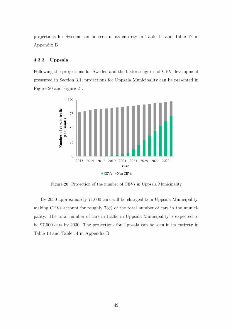
projections for Sweden can be seen in its entirety in Table 11 and Table 12 in

Appendix B

4.3.3 Uppsala

Following the projections for Sweden and the historic figures of CEV development

presented in Section 3.1, projections for Uppsala Municipality can be presented in

Figure 20 and Figure 21.

Figure 20: Projection of the number of CEVs in Uppsala Municipality

By 2030 approximately 71,000 cars will be chargeable in Uppsala Municipality,

making CEVs account for roughly 73% of the total number of cars in the munici-

pality. The total number of cars in traffic in Uppsala Municipality is expected to

be 97,000 cars by 2030. The projections for Uppsala can be seen in its entirety in

Table 13 and Table 14 in Appendix B

49

Figure 21: Projection of the market share of CEVs in Uppsala Municipality

50


51

5 Analysis of Driving Patterns 2030

In this section the analysis of the gathered data on driving patterns is presented.

The section describes the assumptions and calculations that have been made and

presents the findings from the analysis.

5.1 Assumptions

To be able to use the TSS database in a way that is useful to this research, some

assumptions, corrections and simplifications have been made, these are presented

in Table 4.


Day of week aggre-

gation

When aggregating the data, it is

chosen not to distinguish between

the days of the week between dif-

ferent weeks of the month. Thus,

the first Monday in January is not

distinct from the second Monday

in January, and so on

There may be some extremes that

are averaged out due to this as-

sumption. However, those ex-

tremes cannot be pinpointed in

this database either way as the

database size is to small. Thus,

these extremes will have to be sim-

ulated in a sensitivity analysis in-

stead

Data cleansing Errors were corrected in line with

the study by Karlsson (2013).

Trips with a stop under 10 sec-

onds were made into one trip. All

trips with under 0.1 km/h speed

for more then 10 minutes were dis-

carded. Data from before 2005,

after 2014 and all duplicates were

discarded

It is reasonable to make some point

incisions in databases of this size.

Guidelines provided by (Karlsson

2013) were used

52

No distinction be-

tween cars

The TSS database provides the

data tag ’Device’ which allows to

separate each analysis on a car by

car basis. However, to deal with

a bigger sample size each car is

treated anonymously and on an

aggregated level

Given that the sample size consists

of 39,700 days of which the car was

registered and roughly 700 vehi-

cles, most major deviations should

be averted

Unchanged driving

behaviour

The data in the TSS database is

from 2010 but the assumption is

made that driving patterns will

not change significantly by 2030

Available data on driving dis-

tances indicate that driving dis-

tances have been relatively un-

changed since 2005 as described

in Section 3.2. Thus the evidence

points toward consistent driving

habits, but it is not conclusive 3

Table 4: Assumptions made when analyzing TSS data and modeling driving patterns

5.2 Calculations

The data that was acquired consisted of the following data points (as described in

Section 3.2.1)

• Device (i.e. Car)

• Trip ID

• Final velocity

• Average velocity

• Distance

• Pause before & after

• Duration

• Start and stop date & time

The following calculations had to be made in order to aggregate the database

into numbers that could be used to produce the findings in the next section.

3Note that there are few studies on how driving habits have changed and the few studies that

do exists are on an aggregated level

53

• Retrieve the distance travelled per day and map against histogram groups

(Figure 22)

• Retrieve the distance travelled per day and the number of trips made per day,

for each day of the week (Figure 23)

• Retrieve the distance travelled per day and the number of trips made per day,

for each month of the year (Figure 24)

• Retrieve the last stop time of the day per device (car) and map against 24

hours with 10 minute intervals (Figure 25)

• Retrieve the last stop of the day per device (car) and map against 24 hours

with 10 minute intervals, for each day of the week (Figure 26)

• Retrieve the last stop of the day per device (car) and map against 24 hours

with 10 minute intervals, for each month of the year (Figure 27)

5.3 Findings

This subsection presents the findings found from compiling the TSS database. The

findings are presented as figures, showing variations in driving distance and stopping

time of vehicles.

5.3.1 Driving distance

Figure 22 shows that the most frequent average distance driven per day (including

days where no driving occurs) is 25 to 30 km per day. The average in Figure 22 is

38.0 km per day per vehicle however this assuming each car was under registration

for equally many days. Taking into account the fact that the monitored cars were

not tracked for equally many days, the calculated weighted average distance per

day per vehicle is 32.4 km.

Figure 23 shows that the driving patterns vary with the days of the week. It

shows that there are significantly fewer trips made during the weekend as well as

less distance driven. The peak driving day in terms of distance driven is Thursdays

at 35.1 km per day as opposed to the day with the least distance driven, Saturdays

at 28.1 km. The number of trips made per day overall correlate with the distance

54

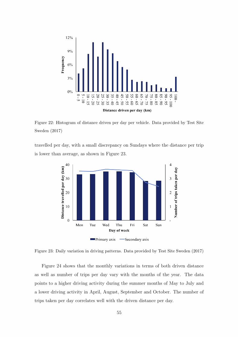
Figure 22: Histogram of distance driven per day per vehicle. Data provided by Test Site

Sweden (2017)

travelled per day, with a small discrepancy on Sundays where the distance per trip

is lower than average, as shown in Figure 23.

Figure 23: Daily variation in driving patterns. Data provided by Test Site Sweden (2017)

Figure 24 shows that the monthly variations in terms of both driven distance

as well as number of trips per day vary with the months of the year. The data

points to a higher driving activity during the summer months of May to July and

a lower driving activity in April, August, September and October. The number of

trips taken per day correlates well with the driven distance per day.

55

Figure 24: Monthly variation in driving patterns. Data provided by Test Site Sweden

(2017)

5.3.2 Final stopping time

Figure 25 shows that there is a peak of cars arriving home (presumably) between

16:00 and 19:00. The data is aggregated from a sample of 39,700 unique cars &

days and on 10 minute intervals. Thus, the peak of 1.6% at 18:00 translates to 1.6%

of any given sample. This means that if there are 1,000 cars in an area, this data

suggests that 16 cars would arrive home between 18:00 and 18:10.

Figure 26 shows that there are variations in what was presented in Figure 25,

when it comes to the day of the week. Figure 26 indicates that the last stop of

the day varies between weekdays and weekends. There is a smaller peak and lower

concentration of the number of vehicles that make their last stop of the day during

weekend than during the weekdays. The difference between the peak on Tuesdays

(highest weekly peak) and Saturdays (lowest weekly peak) is 75% (with Tuesdays

having a 75% higher peak than Saturdays). Figure 26 also shows that looking at

each day of the week separately compromises the number of data points available

to produce the histogram, resulting in less ’smooth’ histograms. Given that the

database in itself contains 39,700 days that can be considered and that there are 7

days in a week, there are on average roughly 5,700 data points per day of the week,

that need to be mapped onto the 10 minute intervals of which there 144 in a day.

56

Figure 25: Histogram over last stop of the day aggregated for all data points. Data also

aggregated over 10 minute intervals. Data provided by Test Site Sweden (2017)

That means that there are on average roughly 40 data points per each 10 minute

interval. Thus, the relative standard deviation is much higher as you inspect the

data on a higher detail level. Or differently phrased, the sample size for each curve

is a seventh of that which it is for the average.

Figure 26: Histogram of last stop of the day aggregated for per each day of the week.

Data aggregated over 10 minute intervals. Data provided by Test Site Sweden (2017)

Figure 27 shows that there are variations in what was presented in Figure 25,

when it comes to the month of the year. Figure 27 indicates that the last stop of

57

the day varies depending on which month of the year it is. Due to big variations

it is difficult to see in Figure 27 which month has the highest peak of number of

vehicles making their last stop of the day at the same time. However, from the

calculation it can be extracted that the highest peak (December) is 47% higher

than the lowest peak (April). Figure 27 also shows that looking at each month of

the year separately compromises the number of data points available to produce

the histogram, resulting in less ’smooth’ histograms. Given that the database in

itself contains 39,700 days that can be considered and that there are 12 months in

a year, there are on average roughly 3,300 data points per each month, that need to

be mapped onto the 10 minute intervals of which there 144 in a day. That means

that there are on average roughly 23 data points per each 10 minute interval. Thus,

the relative standard deviation is much higher as you inspect the data on a higher

detail level. Or differently phrased, the sample size for each curve is a twelfth of

that which it is for the average.

Figure 27: Histogram of last stop of the day aggregated for per each month of the year.

Data also aggregated over 10 minute intervals. Data provided by Test Site Sweden (2017)

These findings derive from the raw data provided by TSS database and thus

the findings are not Uppsala specific. This has been taken into account by looking

at the average driven distance in Uppsala and compared it to the average driving

distance in the TSS database. The average distance driven per day in Uppsala is

58

34.3 km and the average distance driven per day in the TSS Database is 32.4 km.

Thus, the Uppsala average distance driven per data is roughly 6% more than in the

TSS database. This will be taken into account in Section 6.

59


60

6 CEVs’ impact on the Uppsala grid 2030

In this section the effect on the electric grid from CEVs is presented. The section

starts by looking at how the load varies during the day/year today, followed by an

analysis of how the future share of CEVs will impact the household load.

6.1 Assumptions

To be able to use the database from The Swedish Energy Agency in a useful way

and to adjust current data to future scenarios, some assumptions had to be made.

These are presented in Table 5.


Statistically signifi-

cant

By aggregating the data in the

database, a statistically big

enough sample of houses and

apartments can be obtained to be

representative for households in

Sweden.

This assumption is backed by Not-

strand (2016), and the fact that

the average electricity usage per

household in the database is close

to the known average household

electricity usage of Swedish house-

holds.

Future electricity

consumption

To be able to determine how the

electricity usage in households will

be in 2030 (in order to compare

with the CEV load 2030), projec-

tions on the development of elec-

tricity usage in households pro-

vided by IVA is used. These pro-

jections are used to adjust the cre-

ated load curves from the database

IVA is viewed as a reliable source

due to their many publications and

good reputation in the academic

community. However, IVA also

states that there is uncertainty in

their projections.

61

Sweden = Uppsala The assumption that the elec-

tricity usage in Uppsala is the

same as what is represented in the

database is made to be able to ap-

ply the data to Uppsala

Since the database is deemed big

enough to represent households

in Sweden and since the average

household electricity consumption

in Uppsala is almost the exact

same as the average for entire Swe-

den, this assumptions is deemed as

reasonable

Table 5: Assumptions made when using and analysing the data from The Swedish Energy

Agency

Further, Table 6 summarizes the assumptions that were made in order to com-

bine the driving patterns data from TSS with the data provided from The Swedish

Energy Agency.


ICE = CEV In the TSS database, logged vehi-

cles were all ICEs. Thus, to make

this data usable, it is assumed that

CEVs will be driven same way that

ICEs are driven today

Range of CEVs are projected to in-

crease as to accommodate what is

expected today. See Section 8 for

further discussion

Charging starts at

last stop and last

stop only

It is assumed that all charging will

be started precisely at the last reg-

istered stop of the day and that

this stop is at home. It is also as-

sumed that no charging is done be-

fore the last stop

That Home Charging would be

the most common charging be-

haviour is deemed most likely as

the charging technology available

today can accommodate the charg-

ing needs in a standard socket (see

Section 3.1.3). Heesterman (2017)

also points out that a vast ma-

jority of costumers start to charge

when they arrive home. See Sec-

tion 8 for further discussion re-

garding this

62

Charging speed The assumption that all charging

is done at home makes it reason-

able to also assume that charging

will not be done at high power

(fast charging). Thus the average

charging power is assumed at 3.7

kW

Since fast charging equipment is

expensive and that 99% of all

drivers will suffice with charging

at low power during the night (see

Section 3.1.3)

Uncontrolled charg-

ing

The assumption that all charging

is done uncontrolled, i.e. without

strategy from the owner or involve-

ment from a third part is made

(See Section 3.1.3)

Without clear incentives and / or

benefits there is little that moti-

vate people to change their be-

haviour. This report also seeks to

investigate the worst case scenario

kWh per km It is assumed that a an average

CEV can travel 5 km on one kWh

From a holistic perspective

throughout the literature review

this seem like a fair figure. It is

also the current energy usage of

the Nissa Leaf (Nissan 2016)

24-hour days A simplification to segment the

driving days to start at 00:00 and

end at 23:59 is made. This cre-

ates the assumption that all trips

starting after 00:00 end ending be-

fore 23:59 is done the same ’driving

day’, leaving an error when trips

that start before 23:59 but end af-

ter 00:00 (the next day)

The assumption is made to be able

to handle the large number of data

points and to be able to use the

data in a productive way. Identify-

ing the ’actual driving days’ rather

than the time-defined days would

also be complex and possibly inac-

curate. This possible error is dis-

cussed further in Section 8

63

Always fully

charged battery

The assumption that drivers al-

ways want to charge there bat-

tery to its fullest is made and thus

the model simulate that drivers al-

ways recharge their battery after

the last stop of the day

This assumption is made for two

reasons. Firstly because people

want to be prepared for unex-

pected events where it might be

necessary to have a fully charged

car and thus it is believed that this

will be the natural charging be-

haviour. Secondly, because if there

are no incentives not to charge the

battery to its fullest people will

not care to spend effort and time

to plan their charging behaviour.

The possible error is discussed fur-

ther in Section 8

Table 6: Assumptions made when combining data from TSS with the data from The

Swedish Energy Agency

6.2 Calculations

This subsection presents the calculations that were used to assess CEVs’ impact

on the grid. The calculations consist of three parts. Firstly, the calculations that

were made in order to compile the data provided by The Swedish Energy Agency.

Secondly, the calculations that were made in order to translate the impact of driving

patterns (see Section 5) into a grid load that can be compared to the data provided

by the Swedish Energy Agency. Lastly the CEV load needs to be adjusted to

parameters that apply in Uppsala.

6.2.1 Calculations household load

The data that was acquired from The Swedish Energy Agency consisted of the

following data points (as described in Section 3.3.2)

• Date & time (per 10 minute intervals)

• Appliance identifier

• House identifier

64

• Energy consumed (per 10 minute interval)

The following calculations had to be made in order to aggregate the database

into numbers that could be used to produce the findings in the next section. The

calculations made are each on a average per household basis and have all been

adjusted according to a 2030 scenario as described in Table 5.

• Retrieve and aggregate the consumed energy per each 10 minute interval of a

day and for each household, per day of the week, for houses (Figure 28)


day and for each household, per day of the week, for apartments (Figure 29)


day and for each household, per month, for houses (Figure 30)


day and for each household, per month, for apartments (Figure 31)

• Retrieve the day of the week and the month of the year with the highest load

peak, for houses and apartments (Figure 32)

6.2.2 Calculations CEV load

Given that the outcome of Section 5 is a ’when’ and a ’how far’, the only calculation

that needs to be made to be able to map the driving patterns onto the household

load, is to convert the ’how far’ to a measurement of energy. This is done according

to Equation 6. The adjustment to convert to distance driven in Uppsala is also

made by multiplying the distance driven by the relative difference in distance, as

mentioned in Section 5.

Distance travelled (km) ∗ Energy needed per distance(kWh

km

)= Energy needed (kWh)

(6)

Further, to calculate when a CEV will be done charging, which is essential to

calculating the load curves due to CEVs, Equation 7 translate the needed energy

to time.

65

Energy needed (kWh)

Charging power (kW)= Time until fully charged (h) (7)

Given the time until fully charged and the chosen charging power, the CEV load

curves can be produced.

6.3 Findings

In this subsection all findings on CEVs impact on the electric grid are presented.

That includes the findings on household load, driving patterns translated to charg-

ing need and the combined impact on the grid.

6.3.1 Household load

By analysing the data in the database Hushallseldatabasen from The Swedish En-

ergy Agency, the load curves in Figure 28 to Figure 32 are compiled. As the relevant

Uppsala adjustments have been made, the findings of how electricity is being used,

are Uppsala specific.

Figure 28 and Figure 29 show that there is a significant variation in power

consumption between the days of the week, in both houses and apartments. Both

figures show that the household load is fairly similar during the weekdays as well

fairly similar during the weekend. Both figures also showcase a significant difference

in the household load between weekends and weekdays. This difference is most likely

explained by different energy related behaviours in the household that vary with

the days of the week.

Figure 30 and Figure 31 show that there is a significant variation in power con-

sumption between the months of the year, in both houses and apartments. Months

with high power consumption are months in the winter (January and February) and

months with low power power consumption are months in the summer (June and

July). This is most likely due the need of more heating and lighting power during

the winter months. The two figures also show that there is a bigger relative varia-

tion in houses than there is in apartments. This is most likely due the dependency

that houses have on their heating systems.

66

Figure 28: Electricity load in houses per day of the week. Data provided by The Swedish

Energy Agency (2010)

Figure 29: Electricity load in apartments per day of the week. Data provided by The

Swedish Energy Agency (2010)

Figure 32 shows the worst case household load for both houses and apartments.

The figures show that the peak load for houses occurs at 18:10 on a Saturday in

January with a peak load of 6,193 W, and that the peak load for apartments occurs

at 19:50 on a Saturday in March with a peak load of 1,549 W.

67

Figure 30: Average electricity load in houses, per day for certain months. Data provided

by The Swedish Energy Agency (2010)

Figure 31: Average electricity load in apartments, per day for certain months. Data

provided by The Swedish Energy Agency (2010)

6.3.2 CEV load

By combining the analysis made on the TSS data (as presented in Section 5) with

the assumptions and calculations regarding CEV charging the findings shown in

Figure 33 to Figure 35 are obtained, illustrating the CEV load. The data presented

shows the CEV load per CEV, thus the household type and number of vehicles per

68

Figure 32: Worst case daily usage of electricity. Data provided by The Swedish Energy

Agency (2010)

household has not been taken into account. As the relevant Uppsala adjustments

have been made, the findings are Uppsala specific.

Figure 33 illustrates how the load due to charging of CEVs differ during the days

of the week. Figure 33 shows that the CEV load peak is higher during weekdays

compared to weekends (approximately 920 W compared to 620 W) but that the

peak occurs at roughly the same time. The highest peak (Monday, 940 W) is 71%

higher than the lowest peak (Saturday, 550 W)

Figure 33: CEV load charging per day of the week

69

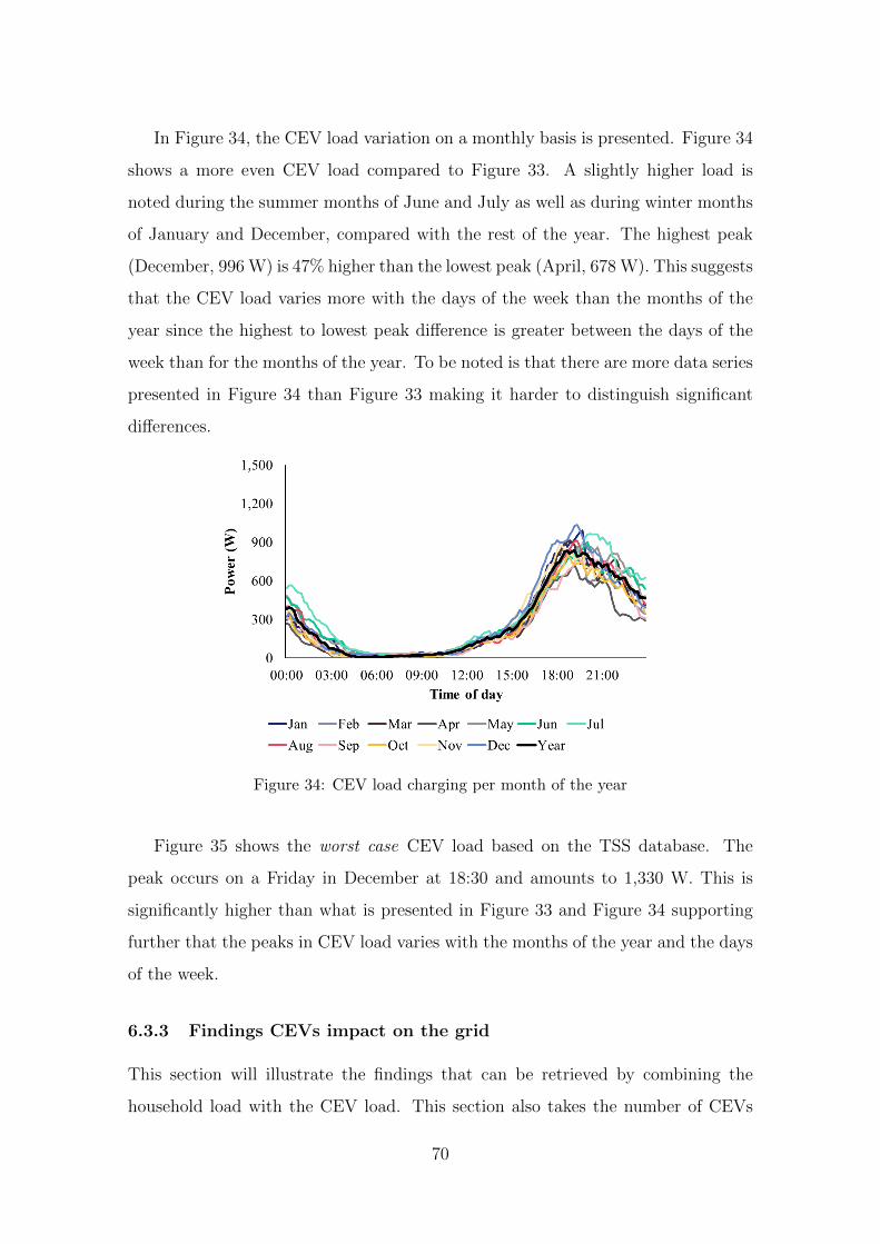
In Figure 34, the CEV load variation on a monthly basis is presented. Figure 34

shows a more even CEV load compared to Figure 33. A slightly higher load is

noted during the summer months of June and July as well as during winter months

of January and December, compared with the rest of the year. The highest peak

(December, 996 W) is 47% higher than the lowest peak (April, 678 W). This suggests

that the CEV load varies more with the days of the week than the months of the

year since the highest to lowest peak difference is greater between the days of the

week than for the months of the year. To be noted is that there are more data series

presented in Figure 34 than Figure 33 making it harder to distinguish significant

differences.

Figure 34: CEV load charging per month of the year

Figure 35 shows the worst case CEV load based on the TSS database. The

peak occurs on a Friday in December at 18:30 and amounts to 1,330 W. This is

significantly higher than what is presented in Figure 33 and Figure 34 supporting

further that the peaks in CEV load varies with the months of the year and the days

of the week.

6.3.3 Findings CEVs impact on the grid

This section will illustrate the findings that can be retrieved by combining the

household load with the CEV load. This section also takes the number of CEVs

70

Figure 35: Worst case scenario of CEV charging during one day

into account with respect to the number of vehicles per household as well as share

of vehicles that are CEVs.

Figure 36 shows household load in a house with the added CEV load. With

the parameters that apply for Figure 36, the max peak is 6,131 W which is an

increase of 12% compared to the max peak if considering only the household load

without CEVs that day. With regards to the worst case max house load as shown in

Figure 32 (Saturday, January), the peak in Figure 36 is 99% of the max load. This

means that on a Monday in February, if there is a market penetration of 75% CEVs,

with an average of 1 vehicle per household, the max load that is to be expected on

that day will increase by 12%. It also means that, in this scenario, the previous

worst case load was almost reached, but on a different day and month than before.

Figure 37 shows household load in an apartment with the added CEV load.

With the parameters that apply for Figure 37, the max peak is 1,699 W which

is an increase of 10% more than the max peak if considering only the household

load without CEVs. With regards to the worst case max apartment load, shown

in Figure 32, the peak in Figure 37 is 10% higher (the selected day and month

coincides with that of the worst case scenario). This means that on a Saturday in

March, if there is a market penetration of 25% CEVs, with an average of 0.5 vehicle

per household, the max load that is to be expected on that day will increase by 10%.

71

Figure 36: An average household load on a Monday in February in a house combined

with an average CEV load. This assumes 1 vehicle(s) per household and a 75% CEV

market penetration implying 0.75 CEVs per household. The day and month was chosen

at random

It also means that, in this scenario, the previous worst case load was proceeded by

10%.

Figure 37: An average household load on a Saturday in March in a apartment combined

with an average CEV load. This assumes 0.5 vehicles per household and a 25% CEV

market penetration implying 0.125 CEVs per household. The day and month was chosen

at random

72

Given that the above data points can be extracted for each scenario of CEV

market penetration and for a varying number of vehicles in a household, a model can

be run to evaluate the impact on the grid from CEVs with the following parameters

being changeable.

• Day of the week and month of the year for both the household data (apart-

ments and houses) as well as the driving patterns data

• Share of CEVs

• Number of vehicles in apartments and houses in the different areas in Uppsala

Municipality (provided by SCB (2016b))

Extracting and searching the for biggest increase in max peak load relative the

previous max peak load (as shown in Figure 32), generates Table 7. Table 7 is

a preview of the data points that were extracted. The table in its entirety can

be found in Table 15 in Appendix C. Table 7 shows that the increase in max

load increases almost linearly with the share of CEVs of cars in traffic. The table

also shows that apartments are expected to see a bigger increase in max load than

houses. Through this simulation, it can be found that Kungsangen is the area that

is expected to see the highest increase in max load. This is true for all share of

CEVs of cars in traffic 2030 scenarios. As this is on a household basis, the results

correlates directly with the number of cars per household as showed in Table 16

in Appendix C. Using these results, simple case examples can be constructed, as

shown in Figure 38 and Figure 39.

Figure 38 illustrates a fictional example of a neighbourhood with three streets

and 23 houses, connected to a power station. The shown loads per street have

been calculated by assuming that each house has an average maximum load that

corresponds to the day that what was found in Table 7 for Almungebygden at 75%

CEVs in houses; a load of 4,951 W excluding the CEV load (which occurred at 19:10

on a December in Tuesday). This gives the total load for Street A of 45 kW, 4,951 W

x 9 houses. The same load was assumed for the other streets and houses. Figure 38

further shows that this particular neighbourhood’s load aggregates up to 115 kW

during this particular time, day and month (19:10 on a December in Tuesday).

73

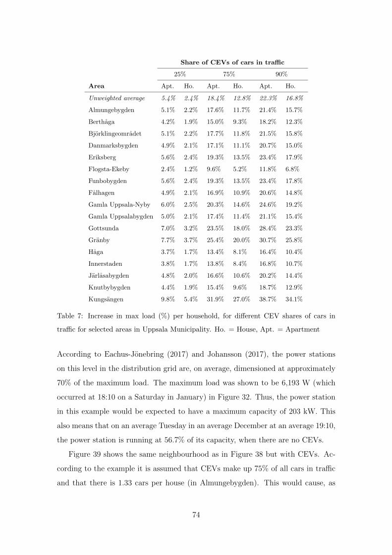
Share of CEVs of cars in traffic

25% 75% 90%

Area Apt. Ho. Apt. Ho. Apt. Ho.

Unweighted average 5.4% 2.4% 18.4% 12.8% 22.3% 16.8%

Almungebygden 5.1% 2.2% 17.6% 11.7% 21.4% 15.7%

Berthaga 4.2% 1.9% 15.0% 9.3% 18.2% 12.3%

Bjorklingeomradet 5.1% 2.2% 17.7% 11.8% 21.5% 15.8%

Danmarksbygden 4.9% 2.1% 17.1% 11.1% 20.7% 15.0%

Eriksberg 5.6% 2.4% 19.3% 13.5% 23.4% 17.9%

Flogsta-Ekeby 2.4% 1.2% 9.6% 5.2% 11.8% 6.8%

Funbobygden 5.6% 2.4% 19.3% 13.5% 23.4% 17.8%

Falhagen 4.9% 2.1% 16.9% 10.9% 20.6% 14.8%

Gamla Uppsala-Nyby 6.0% 2.5% 20.3% 14.6% 24.6% 19.2%

Gamla Uppsalabygden 5.0% 2.1% 17.4% 11.4% 21.1% 15.4%

Gottsunda 7.0% 3.2% 23.5% 18.0% 28.4% 23.3%

Granby 7.7% 3.7% 25.4% 20.0% 30.7% 25.8%

Haga 3.7% 1.7% 13.4% 8.1% 16.4% 10.4%

Innerstaden 3.8% 1.7% 13.8% 8.4% 16.8% 10.7%

Jarlasabygden 4.8% 2.0% 16.6% 10.6% 20.2% 14.4%

Knutbybygden 4.4% 1.9% 15.4% 9.6% 18.7% 12.9%

Kungsangen 9.8% 5.4% 31.9% 27.0% 38.7% 34.1%

Table 7: Increase in max load (%) per household, for different CEV shares of cars in

traffic for selected areas in Uppsala Municipality. Ho. = House, Apt. = Apartment

According to Eachus-Jonebring (2017) and Johansson (2017), the power stations

on this level in the distribution grid are, on average, dimensioned at approximately

70% of the maximum load. The maximum load was shown to be 6,193 W (which

occurred at 18:10 on a Saturday in January) in Figure 32. Thus, the power station

in this example would be expected to have a maximum capacity of 203 kW. This

also means that on an average Tuesday in an average December at an average 19:10,

the power station is running at 56.7% of its capacity, when there are no CEVs.

Figure 39 shows the same neighbourhood as in Figure 38 but with CEVs. Ac-

cording to the example it is assumed that CEVs make up 75% of all cars in traffic

and that there is 1.33 cars per house (in Almungebygden). This would cause, as

74

Figure 38: Neighbourhood and power grid illustration without CEVs of 23 houses with a

house load of 4,951 W each

shown in Table 7, an increase, relative the max load, of 15.7%. Thus, a household

max load of 6,193 W * 1.157 = 7,165 W or a total neighbourhood load of 164 kW

which would be 81% of the power station’s capacity. Thus, the previous highest

running rate, after which the power station was dimensioned, has increased from

70% to 81% which is an increase of 15.7%. This means that the power stations

will, if you have aggregated enough houses under one power station, see an increase

in their highest running rate corresponding to that which is presented in Table 7.

A second important finding is that the previous max peak for the household load

used to be at 18:10 on a Saturday in January but is now expected to occur at 19:10

on a Friday in December. Thirdly, the max load that day, Friday in December,

increased from 115 kW to 164 kW which is an increase of 43%. Fourthly, these

results are on top of the expected increase in household load projcted by Liljeblad

(2016), thus the total increase household load compared to the data in the database

provided by the Swedish Energy Agency is even higher (by a factor of an additional

12.5%. See Table 5) Important to note is that if too few houses are connected to

one power station the results are likely to vary so much that deviations of 100% of

the expected value is not unthinkable.

75

Figure 39: Neighbourhood and power grid illustration with CEVs of 23 houses with a

house load (incl. a CEV load) of 7,165 W each

6.4 Sensitivity Analysis

The findings presented in this section are built on a model that allows each con-

tributing factor to be modified, both to allow different scenarios to be procured as

well as to facilitate investigating which factors have a big and small impact on the

end result.

Further is an investigation into how the following three factors affect the final

result (increase in max load). This analysis has been done by looking at houses and

apartments in Almungebygden separately.

• Distance driven per day on average (compared to the national average)

• Charging power (W)

• Number of households per power station

Table 8 shows how and increase or decrease in the average driving distance po-

tentially increases the max load. The tables shows the relative increase or decrease

to the results presented in Table 7 for Almungebygden. As the table shows, if the

average distance driven is less in an area in Uppsala, the increase in max load is

expected to be smaller, and vice versa. The table also shows that the impact of

the factor driving distance does not always have a linear impact on the end result,

but rather that it depends on the presumed relative (to the household load) impact

76

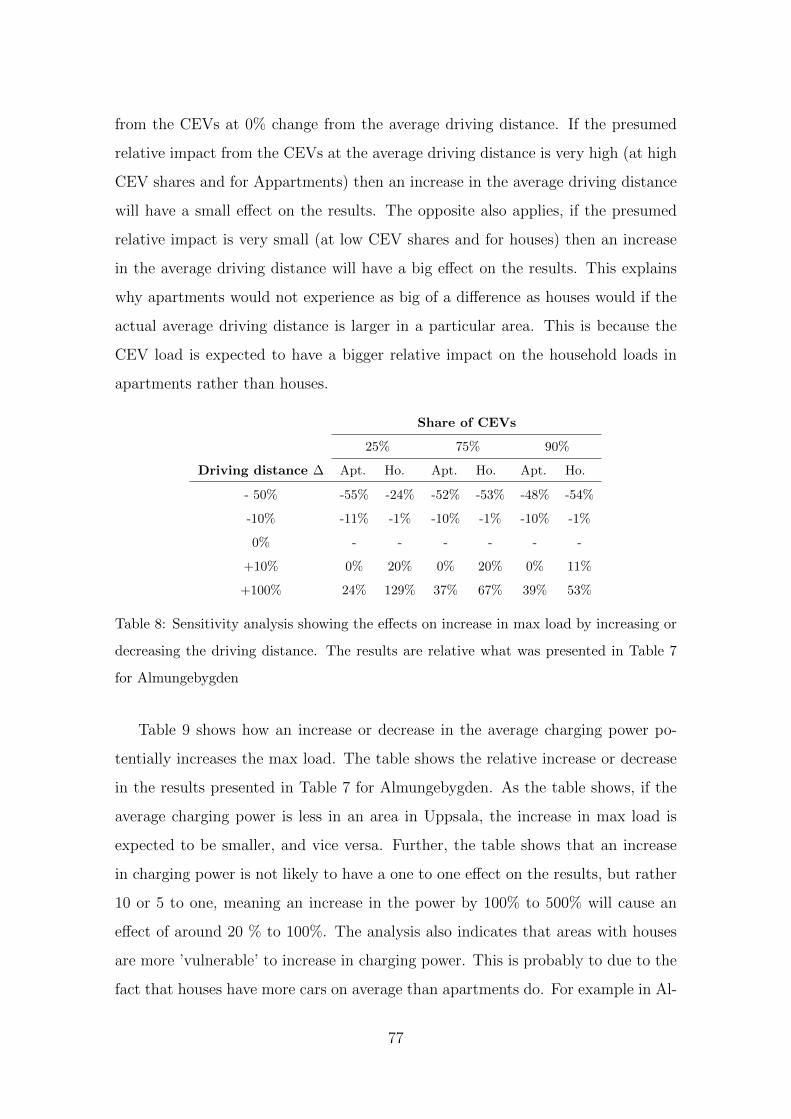
from the CEVs at 0% change from the average driving distance. If the presumed

relative impact from the CEVs at the average driving distance is very high (at high

CEV shares and for Appartments) then an increase in the average driving distance

will have a small effect on the results. The opposite also applies, if the presumed

relative impact is very small (at low CEV shares and for houses) then an increase

in the average driving distance will have a big effect on the results. This explains

why apartments would not experience as big of a difference as houses would if the

actual average driving distance is larger in a particular area. This is because the

CEV load is expected to have a bigger relative impact on the household loads in

apartments rather than houses.

Share of CEVs

25% 75% 90%

Driving distance ∆ Apt. Ho. Apt. Ho. Apt. Ho.

- 50% -55% -24% -52% -53% -48% -54%

-10% -11% -1% -10% -1% -10% -1%

0% - - - - - -

+10% 0% 20% 0% 20% 0% 11%

+100% 24% 129% 37% 67% 39% 53%

Table 8: Sensitivity analysis showing the effects on increase in max load by increasing or

decreasing the driving distance. The results are relative what was presented in Table 7

for Almungebygden

Table 9 shows how an increase or decrease in the average charging power po-

tentially increases the max load. The table shows the relative increase or decrease

in the results presented in Table 7 for Almungebygden. As the table shows, if the

average charging power is less in an area in Uppsala, the increase in max load is

expected to be smaller, and vice versa. Further, the table shows that an increase

in charging power is not likely to have a one to one effect on the results, but rather

10 or 5 to one, meaning an increase in the power by 100% to 500% will cause an

effect of around 20 % to 100%. The analysis also indicates that areas with houses

are more ’vulnerable’ to increase in charging power. This is probably to due to the

fact that houses have more cars on average than apartments do. For example in Al-

77

mungebygden there are 1.33 cars per house and 0.35 cars per apartments, meaning

there are 3.8 more cars in houses than in apartments in Almungebygden.

An interesting data point in Table 9 is the ’-11%’ in apartments, at 25% CEVs

and a charging power of 7.36 kW. Here, an increase in charging power is expected

to cause a smaller increase in max load than if the charging power was 3.68 kW.

This is likely explained by the few number of CEVs, due to the few number of cars

in apartments and the low share of CEVs. It means that at this charging rate,

the overlap from multiple CEVs charging at the same time is smaller (because the

CEVs finish charging quicker) and thus lowering the overall max load. However, as

the table also shows, this is only applicable at 25% CEVs and in apartments.

Share of CEVs

25% 75% 90%

Charging power ∆ (kW) Apt. Ho. Apt. Ho. Apt. Ho.

-38% (2.30) -36% 22% -25% -15% -23% -21%

0% (3.68) - - - - - -

+100% (7.36) -11% 53% 22% 34% 24% 30%

+200% (11.04) 17% 60% 55% 68% 60% 66%

+500% (22.08) 45% 76% 57% 101% 58% 99%

Table 9: Sensitivity analysis showing the effects on increase in max load by increasing or

decreasing the driving distance. The results are relative what was presented in Table 7

for Almungebygden

Lastly, to investigate the effect of number of households per power station,

i.e. if new houses are being built, Figure 40 illustrates an example. Given that

power stations are dimensioned according to 70% of the expected max load in

a neighbourhood, Figure 40 aims to investigate and illustrate the effects if the

number of households per an existing power station was to increase. Figure 40

is based on the same example as in Figure 39 but with another house built (4%

increase compared to the 23 houses in the figure).

Figure 40 shows that the total load would increase from 115 kW, as shown in

Figure 38, to 171 kW. This would correspond to a running rate of 84% of the power

station’s capacity. The increase from 115 kW to 171 kW on that day, that month

78

and that time is due to both the added house as well as the expected CEV load.

The added house would increase the max load from 70% of the capacity to 73%

(increase by 4%). Further the CEV load would increase the max load by the same

15.7% as described previously. Thus, 73% * 1.157 = 84%. This means that if more

houses are added to existing power stations the effect will be the product of the

increase in number of houses multiplied by the expected increase in max load due

to CEVs per house.

Figure 40: Neighbourhood and power grid illustration with CEVs of 23 + 1 houses with

a house load (incl. a CEV load) of 7,165 W each

79


80

7 Results

This section presents the results that answer the two SQs that in turn help answer

the MRQ.

7.1 SQ 1 - How many CEVs and of what kind will there be

in Uppsala and in relevant nearby areas in 2030?

Section 4 presents the findings on what the development of CEVs will look like in

Uppsala 2030.

In Figure 20 it is shown that there will be roughly 71,000 CEVs on the road by

2030, according to the projections. This corresponts to a vehicle fleet share of 73%

of the total number of cars (that is projected to be roughly 96,000).

Regarding the development of CEV models, Figure 17 indicates that 1) All

major car manufacturers have already made or are planing on a CEV debut and

2) The car models will, within nearby releases, have an EPA range of 300+ km

and likely to continue improving well into the 2020’s. The range improvements are

likely to continue to soon reach the same range capacities as those in traditional

ICEs today. The research behind Section 4 also indicates that the sub-category to

CEVs, BEVs, will be the most prominent CEV type as the PHEV is considered a

’transition’ vehicle to fully adopting BEVs.

The findings regarding charging infrastructure suggest that home charging will

be the most common CEV charging behaviour. This is due to the fact that the

lower power charging options, that are available at a low or no cost, will suffice for

the average daily driven distance.

7.2 SQ 2 - How will CEVs impact the distribution grid in

Uppsala in 2030?

As presented in Section 6, the expected impact on the distribution grid due to

charging by CEVs is measured by simulating the CEV load and comparing its size

to the current household loads.

81

Firstly, the findings show that the household load in apartments is much lower

than in houses (as seen in Figure 32), and that the overall household load is much

lower in the summer than it is in the winter (as seen in Figure 30 and Figure 31).

Secondly, the findings show how the driving patterns, presented in Section 5,

translate into a load that is comparable to the household load of both houses and

apartments. The findings shows that the highest load due to CEVs is not expected

to succeed 1,400 W per car (as shown in Figure 35). This means that less than half

of the cars in a sample are expected to charge at the same time when the peak is

the highest. This is assuming a charging rate of 3.7 kW and that the sample size is

sufficiently large.

Thirdly, once the household loads and the CEV loads were compared to each

other the findings show that the CEV load can, during a certain times of the day,

certain days of the week and certain months of year, cause an increase to the max

load expected in the distribution grid. This is shown in Figure 36 and in Figure 37.

Lastly, the findings summarize the above three points, by extracting and search-

ing for biggest increase in max load expected throughout day, day of the week and

month of the year. This is presented in Table 7. The findings, presented in Ta-

ble 7, are illustrated with an example in Figure 38 and Figure 39. This final finding

showed that the expected increase in max load varies with the different areas in

Uppsala as well as with different CEV share of cars in traffic scenarios. The figures

helped illustrate that the increase in max load per household will have a direct

impact on the power stations capacity.

Further, a sensitivity analysis was conducted that showed the following three

things.

• The change in average driving distance in an area has an impact on the

increase in max load depending on the CEVs overall relative impact on the

household load

• The change in average charging power in an area has impact on the increase

in max load that is proportional to the increase or decrease in charging power,

but the impact is smaller than one to one

82

• If more houses were build in an area, the impact due to CEVs would be even

greater, by a factor proportional to the increase in number of houses

Overall the results have led to the following conclusions regarding what effect

CEVs will have on the distribution grid in Uppsala 2030.

• CEVs are expected to a have a significant impact on the household load and

therefore, by extension, on the distribution grid and its power stations

• CEVs will have a bigger relative impact on the household load in households

where the energy consumption is small such as as apartments but also, by

extension, households with direct heating

• CEVs will have a bigger impact on the household load in areas where the

number of cars per household is high

• The higher the CEV load is, the smaller the difference will be in impact on

houses compared to apartments. Also, the higher the CEV load is, the closer

the ’worst peak load day’ gets to the day of the worst CEV load as the CEV

load will be the more determinant factor in the household load

7.3 MRQ - Which measures should Vattenfall take in order

to sustainably react to the expected increase in CEVs

in Uppsala by 2030?

Given the findings presented in Section 7.1 and 7.2 that are supported by Section 4

to Section 6, the following measures should be taken by Vattenfall in order to

sustainably react to the expected increase in CEVs in Uppsala by 2030.

Monitor specific areas with a high concentration of cars, low energy consump-

tion per household and that already have substations with a capacity that is be-

low the typical dimensions. These are factors that have big impact on how CEVs

will affect the grid and therefore these are the areas that are most likely to first

encounter problems when CEV sales start to increase.

Follow CEV sales to reevaluate the projections made in this study. By doing

this Vattenfall will know if the development is moving faster or slower then pro-

jected and can plan actions accordingly. This should be done by subscribing to

83

Trafas publications that are published every month. It can also be done together

with e.g. Power Circle, to develop a tool that monitors the development at a

detailed geographic level. This would allow for Vattenfall to monitor CEV devel-

opment on a more detailed geographical level than what has been done in this

study.

Monitor trends of car ownership to be able to evaluate if it will affect peo-

ple’s CEV charging behaviour and render the model completely incorrect. These

trends include for example joint car ownership (carpools or otherwise) and au-

tonomous vehicles that if widely adopted would change people’s charging be-

haviour dramatically. This would make the prediction of how CEVs will impact

the distribution grid wrong, drastically affecting the results in this study.

Review Velander constants to make grid planning take the load due to CEVs

into consideration (This is explained further in Section 9.2.3). This should be

done by looking at transport data and travel patterns to incorporate how, when

and where people travel as a part of how they use electricity. Given the current

situation and the expected increase in CEVs, it is believed that transportation

in general will have a significant impact on how electricity is consumed in the

future. When reconstructing Velander constants it is important to understand

that the findings in this study are applicable when looking at a specific level in

the distribution grid. When taking actions based on these findings there is a

need to understand that at lower levels in the grid, with samples of only a few

households, there will be bigger variations in the impact and actions must be

adjusted accordingly. The opposite also applies, namely that at regional level,

the effects of the CEV load are not expected to be at all significant.

Investigate smart charging as a possible solution, to shift the CEV load peak

to a different time of day (presumably during night). The recommendation is to

adopt a simple use of smart charging where the starting time of charging is moved

a couple of hours to ’shave’ the worst peak. This could be done by providing a

technical solution to supplement the existing charging solutions that only ask

when you want to use the car in the morning and then adjusts the charging

84

to start as late as possible given this information and the SOC of the battery.

The value of this would be highly motivated by the alternative cost of upgrading

infrastructure due to an increase max load.

85


86

8 Discussion

This section consists of a discussion of the impacts and reliability of the various re-

sults that our model has provided. The section also discusses the recommendations

that we give and what scenarios that might impact the recommendations. Further-

more the section also discusses some of the assumptions we have made when creating

our model and what implications these assumptions have had on the final results.

8.1 Discussion of our Results

This subsection discusses the results presented in Section 7. The results are reviewed

as to whether or not they are likely and reasonable.

8.1.1 SQ 1

Our estimation of 71,000 CEVs in Uppsala by 2030 is based on roughly 4 million

CEVs in Sweden by the same year. This number may seem high, considering the

low share of CEVs today and that Power Circle project only 1 million CEVs on

the road by 2030. However, as pointed out throughout this report, projections

stretching far into the future (5+ years) are extremely hard get right.

If we look at the projections for CEVs both in Sweden and Uppsala (Figure 18

and Figure 20), there is a notable acceleration in the market share after the year

2022. This is due to the projected price parity that Randall (2016) predicts that in

turn implies that there will be few or no incentives not to by a CEV instead of an

ICE.

When comparing the projected and historical CEV sales in Sweden with the

CEV sales in Norway seen in Figure 10, it is notable that currently Sweden is ’lag-

ging’ behind Norway by 3-4 years. When comparing the projections presented in

Figure 19, this ’lag’ would be 7 years in 2021 compared to Norway. This suggests,

if assuming all else equal, that these projections are modest and underestimating

until the year of 2021. The same argument applies when comparing Sweden to the

CEV market share in the Netherlands as shown in Figure 4. After 2021, assump-

tions of price parity have been applied and thus these types of historic comparisons

87

are unreasonable, as the growth is expected to be far from linear.

An interesting point of discussion, is the implication of the ’tipping point’ in CEV

sales happening sooner or later than what we have projected and what the impli-

cations would be to our results. We have predicted this ’tipping point’ to happen

2022, when Randall (2016) predicts price parity to be reached. What would the

implications be if this happens later (or sooner) than when we have assumed? The

answer to this is quite simple, assuming that CEVs will be the dominant vehicle

type at one point in time. If that can be assumed, the implication of when this

’tipping point’ will occur will simply shift the year when 100% of new vehicles will

be CEVs. Once that has occurred, it is reasonably a matter of enduring the average

scrapping time (14 years in Sweden) until the entire fleet of personal vehicles will

have shifted to CEVs.

From 2016 to 2030 it is projected that the number of new cars that will be

sold will increase from 388,000 to 520,000. That means that for every year that

the boom is ’off’ from our projections, the total stock of CEVs in Sweden will be

roughly 430 000 cars greater or smaller. If, for example, the boom is delayed by

2 years to 2024 there will be almost 1 million CEVs less in Sweden by 2030 (and

15,000 CEVs less in Uppsala). This highlights the importance of identifying when

the ’tipping point’ will be reached.

There are several factors that could contribute to reaching the ’tipping point’ in

the near future. There is the introduction of the Bonus-Malus system as discussed

in Section 3.1.1 that could fuel the shift to CEVs. There is the development of

new models that are becoming more and more price competitive as well as the

development of the necessary infrastructure.

We believe that the projections made by Power Circle (2016a) are very modest,

primarily because their projections show that the most explosive shift in the CEV

market has already occurred and that they project that the acceleration is decreas-

ing. To be noted is that our projections are in line with what Power Circle (2016a)

have projected until 2021, however after we assume price parity our projections

diverge.

88

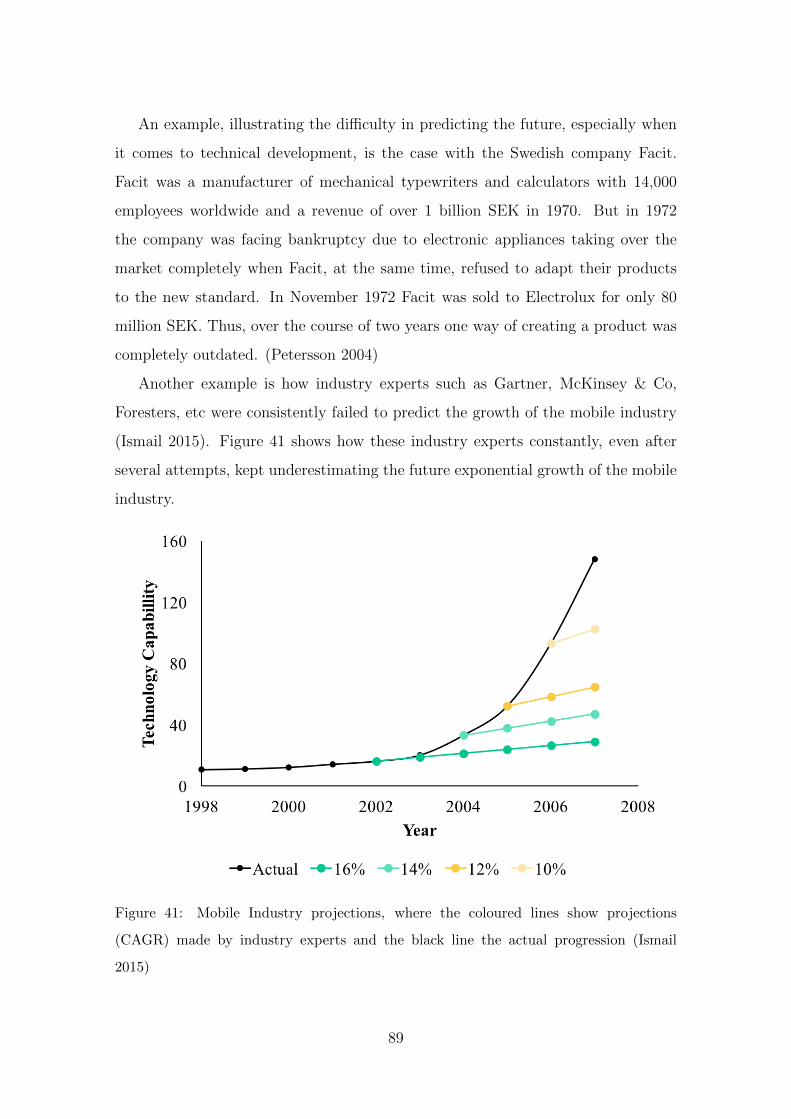
An example, illustrating the difficulty in predicting the future, especially when

it comes to technical development, is the case with the Swedish company Facit.

Facit was a manufacturer of mechanical typewriters and calculators with 14,000

employees worldwide and a revenue of over 1 billion SEK in 1970. But in 1972

the company was facing bankruptcy due to electronic appliances taking over the

market completely when Facit, at the same time, refused to adapt their products

to the new standard. In November 1972 Facit was sold to Electrolux for only 80

million SEK. Thus, over the course of two years one way of creating a product was

completely outdated. (Petersson 2004)

Another example is how industry experts such as Gartner, McKinsey & Co,

Foresters, etc were consistently failed to predict the growth of the mobile industry

(Ismail 2015). Figure 41 shows how these industry experts constantly, even after

several attempts, kept underestimating the future exponential growth of the mobile

industry.

Figure 41: Mobile Industry projections, where the coloured lines show projections

(CAGR) made by industry experts and the black line the actual progression (Ismail

2015)

89

In summary it can be said that these type of projections are hard to get right.

However, for our intents and purposes the exact number of CEVs in Sweden and

in Uppsala 2030 is not crucial to the results of this study. The overall take-away is

that the sales of CEVs is likely to continue increasing and that an eventual ’tipping

point’ is likely to occur before 2030.

8.1.2 SQ 2

Our findings from Section 5 and Section 6 is what lays the foundation for our results

and answering of SQ 2.

Our findings regarding driving patterns are generated from the TSS database.

The overall findings on driving distance per day can be compared with the national

statistics from Trafa, to verify the quality of the database. According to Trafa,

the driving distance per day in Vastra Gotaland was 34.3 km in 2012. When we

compiled the data points we calculate these figures to be 32.4 km per day, consisting

of data between 2010-2012, indicating that the data is reliable. This is important

since we rely on the driving pattern data when we estimate the needed charging

power and by comparing it to national statistics we get a confirmation that the

data seems correct.

The assumptions that we have made to be able to conduct the analysis of the

driving pattern data is described in Section 5 and some are discussed later in this

section. The assumption that affects the result on SQ 2 in the biggest way is that

we assume that driving patterns found by analysing measurements of ICEs in the

TSS database will be transferable to driving patterns of CEVs in 2030. Since CEVs

of today have a shorter driving range than ICEs it is reasonable to think that CEVs

will drive shorter distances. However, since we want to look at the impact from

CEVs in 2030, and since the development of CEVs point to rapid increase in range,

we believe that these differences can be neglected for 2030. Also, to look at the driv-

ing patterns of CEVs today would incorrectly depict how the average CEV driver

in 2030 would drive. This is because the owners of CEVs today are considered

’early adopters’ and thus would not be a fair representation of 2030 when CEVs are

likely to be the standard. We believe that a more correct estimate of CEVs driving

90

patterns in 2030 is obtained by looking at the standard today, which is why we look

at how ICEs drive today.

Regarding the generic finding on household electricity usage, there is no need for

discussion as they are 1) only used as a point of reference in this study and 2) widely

discussed in other forums.

However, the fact that the CEV load curves seem to closely follow the household

load curves is more interesting. This is somewhat expected as the electricity load

in households is driven by people being at home which coincides with people’s

driving habits. The fact that the household load peaks at 18:00 - 19:00 is most

likely explained by people returning home from work or school at that time which

gives the load from CEVs a similar ’shape’ to that of the household load. Since

our model is focused on the last stop of the day and that charging starts at that

point it gives the curve a shape that translates to when people arrive at home. We

have, throughout the length of the report, stated that we have chosen this method

to simulate a ’worst case’ scenario of the impact on the grid from CEVs’ charging,

and since we believe that this charging pattern will be dominant in 2030 (more on

this in Section 8.2.3).

The result that the highest load due to CEVs charging is not expected to be

above 1,400 W per car is also noteworthy as the model has assumed 3.7 kW as

charging power. This means that, on average, for a larger sample, there is less than

half of all cars charging at the same time (at max peak) even if all cars would be

CEVs. This result is key, as it explicitly translates into how grids in the future can

and should be dimensioned by taking the CEV load into consideration. This type

of statistical indication of how to dimension a grid, according to how electricity is

consumed, is exactly the same as how Velander constants are used in current grid

dimensioning methodologies Eachus-Jonebring (2017).

Our final result of the different areas in Uppsala Municipality and the increase

in max load given different CEV share of cars in traffic, gives a more detailed view

of how CEVs will affect the grid. The results indicate that there are differences in

the impact on the grid depending on the types of households and number of vehicles

91

per household. The results also show that there are differences in the impact on

the grid between apartments and houses.

Our results, in terms of increase of the max peak load, range from 2% to 39%

depending on CEV share, household typ and area. These number are in the same

order of magnitude as the projected increase in household electricity usage, provided

by IVA. IVA predicts a 12.5% increase in max load by 2030. We can also look at the

study conducted in the United Kingdom by Qian et al. (2011), where the author

finds that at only 20% CEV share, the daily increase of electricity usage can be 36%,

in a ’worst case’ scenario. This study is conducted with a different methodology

and was made in 2011. In the same way as by comparing with IVAs figures of future

electricity usage, the figures point in the same direction and in the same order of

magnitude as our results.

Further we have showed how these results would impact a single power station

by aggregating the households’ loads into one junction. As shown in Section 6,

the effects on the power stations are in direct proportion to the effects per each

household, which is discussed above. This type of example case gives a good and

real indication of how our result will directly impact the grid.

8.1.3 MRQ

The final recommendations that we give Vattenfall answers our MRQ and is pre-

sented in Section 7.3. The rationale and motivation behind our recommendations

are based on our results presented to answer SQ 1 and SQ 2. In terms of how

reasonable our recommendations are, we believe that given that the sales and de-

velopment of CEVs is expected to ’boom’ (SQ 1) and that the load due to CEVs is

expected to have a significant impact on the distribution grid (SQ 2), it is justifiable

to attribute a high focus to take action on this matter. We believe that Vattenfall

should do this in accordance with our recommendations. We support this by our

case example over Uppsala Municipality 2030, however the recommendations can

and should be applied in a more general sense.

92

8.2 Discussion of our Assumptions

Throughout the time of our research we have made several assumptions and sim-

plifications in order to create a working model and to be able to generate results.

In this subsection the implications on the results of the most drastic assumptions

and simplifications are discussed.

8.2.1 CEV projections 2030

There are mainly two assumptions when making the projections on the number of

CEVs that need to be discussed further. Other assumptions are accounted for in

Section 4.

The first assumption is that we have chosen not to take scrapping of CEVs into

account. This assumption has been made because 1) the average life cycle of a

car in Sweden is 14 years, (thus, a significant number CEVs will not start being

scrapped until the late 2030’s) and 2) CEVs are assumed to have a longer life span

(due to the possibility of changing the battery and not the entire car). Thus, this

gives an aggregated number of CEVs that consist of all CEVs sold in Sweden from

now until 2030. This suggests that the ’actual’ number of CEVs 2030 might be

slightly smaller.

We also assume that there will not be a change in buying behaviour when

the predicted ’tipping point’ of CEV sales has been reached. By this we mean

that the number of new cars sold per year will continue according to historical

sales figures. However, it is not unreasonable that a dramatic shift to CEVs, and

therefore significant advantages in price and maintenance, will cause an even more

dramatic shift to CEVs than the previously linear historical sales data may indicate.

Or to put it differently, if CEVs become attractive enough for consumers, they may

consider buying a new car before they need to, making the transition to CEVs in

Sweden even faster than what we have predicted.

The discussion of these two assumptions point in two different directions. Over-

all, our belief is that our projections are optimistic but that there is still room for

the final number of CEVs 2030 to be even higher than what we suggest. The as-

93

sumption that have larger effects on our projections is the effects when price parity

is in place, which is discussed in Section 8.1.

8.2.2 Analysis of Driving Patterns 2030

When producing the driving patterns model, there are two assumptions that need

to be addressed in more detail.

The first assumption is that each registered vehicle is treated in an aggregate

form. This means that all data points for all cars have been summed up. This is

logical since we are not interested in distinguishing different cars or drivers from

each other, but are rather interested in a statistical average. In doing this there is a

risk of certain vehicles and drivers being overrepresented in the statistical average.

However, as the average driving distance of the aggregated data is close to that of

Trafa’s presented figures, the aggregation seems fair. We recognize that this is not

conclusive evidence.

The second assumption is that the data that has been processed has been pro-

cessed assuming that a ’driving day’ starts at 00:00 and ends at 23:59 with not

overlap allowed. This creates a possible error if the ’last stop of the day’ is in fact

after 23:59 (someone arriving home after midnight). In this case our model will

register the second to last stop of the day as being the last stop. The model will

then compile the distance driven up until that stop and disclose that the amount

of kWh that needs to be charged will correspond to that distance. The actual last

stop (maybe at 00:25) is instead registered to the next day. This means that the

total distance driven (and thus the connected power needed to be charged) will not

be wrong but the charging starting time may be shifted. However, according to the

raw data, this possible ’mistake’ happens less than 0.5% of the registered days, thus

having a very small impact overall which makes it reasonable for us to discard.

8.2.3 CEVs’ impact on the Uppsala grid 2030

When analyzing the data of grid impact there are two assumptions that we have

made that need to be addressed in more detail.

The first assumption is that charging of CEVs is done at the last stop of the

94

day and that this stop is at home. We made this assumption since evidence point

to home charging being the most common way to charge and that it is reasonable

to assume that a driver is at home when the driver stops for the last time. This

assumption is also verified by Heesterman (2017), Associated Manager at Home

Charging Installations at Tesla Motors. This assumption made the large number

of data points much more manageable. There is one major possible flaw in this

assumption. If people charge a lot of the needed power on locations that is not at

home (the office, stores, etc.), our model will be skewed, showing a larger charging

need than what would be realistic. Since we want to have a ’worst case’ approach

on the implications and since most drivers will cope with only charging at home,

we have chosen to discard this possibility.

The second assumption is that CEVs are always charged until they have a ’full

tank’. Regardless if this assumption is unrealistic or not, it doesn’t matter. As

the data behind the model is aggregated to always show a 24h period and encloses

data from the entire year, the charging need per day will correspond to the average

distance travelled that day. Thus, on a daily basis where each sequential day is

similar, this assumption is fair. However, in cases such as Friday night to Saturday

morning or Sunday night to Monday morning, this might cause a bigger problem

as those sequential days have been shown to vary a lot more than say Tuesday to

Wednesday. This is not believed to be a huge source of error but is yet recognized

as a possible one.

8.3 Externalities unaccounted for

This subsection discusses several scenarios that have intentionally not been taken

into account in this study but could completely change the way our MRQ is an-

swered.

8.3.1 Car ownership 2030

One of the big questions that arise when evaluating the results and implications

presented in this report is what the future of car ownership will look like.

95

In our research we have assumed that there will be a continued increase in

number of vehicles in Sweden, following the development of the past 10 years. This

is reasonable since there are today no signs of car ownership changing. Both number

of new cars per year and the total number of cars are increasing and we have assumed

that this development will continue to 2030. However, there are several factors that

might change that.

One example is joint car ownership and carpools. BMW’s Drive Now and Volvo’s

Sun Fleet are current examples of this. This type of car ownership means that there

is more than one household that own the car that the household uses which will

result in fewer cars per household and fewer cars in total. There is today a relatively

small number of households that have adopted this type of car ownership and those

that have often use it as a ’secondary car’, owning the firs car in a conventional

way. However, with new business models and changed needs in car usage, this might

change.

If carpools and joint ownership was to increase the impact on our findings will

be mostly regarding number of cars per household, which we have seen have a big

impact on the load from CEVs charging. Fewer cars per household will mean fewer

cars charging at peak time and thus a smaller impact on the max load.

Another factor related to how we will use cars in 2030 is the concept of ’peak

car’. Peak car refers to the time when we start using the car less and less and driv-

ing shorter distances than before. The biggest driver is expected to be urbanisation,

i.e. people moving into cities and not needing a car to get around.

We have assumed that driving patterns will not change from today to 2030 and

that CEVs will be driven the same way as ICEs are driven today. If ’peak car’ was

to happen it would mean that the usage of cars would drop and thus resulting in

fewer and shorter trips.

If this is the case, the parameter that will impact our findings that is going to

change is driven distance. If fewer and shorter trips are made (but the total number

of cars still increases), the needed charging distance per car is going to be lower.

This will affect the maximum load peak, however, less compared to if number of

96

cars per household were to decrease.

Thirdly, a factor that might drastically change how we will use cars in 2030 is

autonomous vehicles. Autonomous cars will, most likely, be electric vehicles and

have the ability to charge themselves (through induction). Since cars in this case

can drive themselves there is reason to believe that the number of cars will decrease

and that the cars that exist will drive practically non-stop (as a form of taxi service).

In this case the parameters in our model that will be affected is both number of cars

per household (decrease) and distance driven (increase). However, if or when self

driving CEVs become the norm it is less likely that they will charge in someones

home but rather a station dedicated for that purpose rendering the results of the

report close to irrelevant.

8.3.2 Electric vehicles are outperformed by other technology

Another factor that we have chosen to overlook in this study is the competition

from other fuel types that may replace fossil fuels, instead of CEVs.

One of these are fuel cell driven cars that run on electricity but without the need

of a battery. The big advantage with fuel cell cars is that it will only take 5 minutes

to refill the tank (with hydrogen) compared to 20-30 min (at best) for CEVs. The

primary thing that speaks against fuel cell driven cars is the economic factor, that

is, if it ever will be cost efficient enough to produce and sell, compared to ICEs

and especially CEVs. Today it is mainly only Asian car manufacturers (Toyota and

Hyundai) that manufactures fuel cells cars and they might sell at a loss, when also

factoring in the cost of building the infrastructure for hydrogen fuel stations (Ayre

2014).

8.3.3 Electricity consumption is different in 2030

In our model we have looked at the household electricity usage today and, by

using projections of future electricity usage made by IVA, adjusted the load curves

to be accurate for 2030. These projections, like with the ones we make on CEV

development, are hard to get right but since IVA have broken down the usage in

97

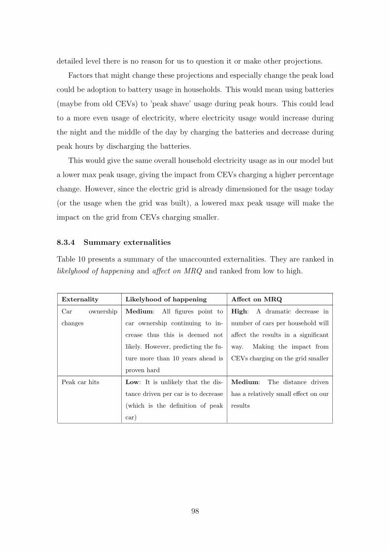
detailed level there is no reason for us to question it or make other projections.

Factors that might change these projections and especially change the peak load

could be adoption to battery usage in households. This would mean using batteries

(maybe from old CEVs) to ’peak shave’ usage during peak hours. This could lead

to a more even usage of electricity, where electricity usage would increase during

the night and the middle of the day by charging the batteries and decrease during

peak hours by discharging the batteries.

This would give the same overall household electricity usage as in our model but

a lower max peak usage, giving the impact from CEVs charging a higher percentage

change. However, since the electric grid is already dimensioned for the usage today

(or the usage when the grid was built), a lowered max peak usage will make the

impact on the grid from CEVs charging smaller.

8.3.4 Summary externalities

Table 10 presents a summary of the unaccounted externalities. They are ranked in

likelyhood of happening and affect on MRQ and ranked from low to high.

Externality Likelyhood of happening Affect on MRQ

Car ownership

changes

Medium: All figures point to

car ownership continuing to in-

crease thus this is deemed not

likely. However, predicting the fu-

ture more than 10 years ahead is

proven hard

High: A dramatic decrease in

number of cars per household will

affect the results in a significant

way. Making the impact from

CEVs charging on the grid smaller

Peak car hits Low: It is unlikely that the dis-

tance driven per car is to decrease

(which is the definition of peak

car)

Medium: The distance driven

has a relatively small effect on our

results

98

Autonomous cars

take over

Low: It is deemed unlikely that

self driven cars will have a big pen-

etration by 2030. They will proba-

bly exist (they already do exist to-

day) but the belief is that due to

regulations they will not have re-

placed regular driven cars by 2030

High: The impact on our model

if autonomous cars take over will

be large. This is because both the

number of cars and driving pat-

terns would change drastically

CEVs are outper-

formed by other

technology

Low: It is deemed highly unlikely

that other technology will surpass

CEVs. Investment by all the ma-

jor car manufacturers is in CEV

model development

High: If, e.g. fuel cell cars would

replace CEVs our entire model

is irrelevant since charging cars

would not be needed at all

Electricity usage

change

Low: The projections made by

IVA is deemed as reliable

High: If the change means low-

ered max peak the affect on our

model will be high since we look

at how CEVs affect the max peak

in households

Table 10: Different externalities’ risk and affect on our MRQ

Looking at Table 10, we see that all but one of the investigated externalities

have a low chance of happening, making it reasonable not to include them in our

model at this stage. We can also see that factors that implicate number of cars per

household have a higher impact on our results and that there are externalities that,

if they occur, make our model completely irrelevant. Overall it should be stated

that if changes are to happen by 2030 it is probably in the area of how we will own

and use cars overall. Looking to the future, it points to fewer cars in total and that

the driving distance per car will increase.

99


100

9 Conclusion

This section presents the conclusion of this thesis. It also answers the research ques-

tion with the final recommendations as well as leaves suggestions of improvement

for future work.

9.1 MRQ

We believe that given that the sales and development of CEVs is expected to ’boom’

(SQ 1) and that the load due to CEVs is expected to have a significant impact on

the distribution grid (SQ 2), it is justifiable to attribute a high focus to take action

on this matter. We believed that Vattenfall should do this in accordance with the

recommendations in this report. We support this by our case example over Uppsala

Municipality 2030, however the recommendations can and should be applied in a

more general sense.

• Monitor specific areas with a high concentration of cars, low energy consumption

per household and that already have substations with a capacity that is below

the typical dimensions

• Follow CEV sales to reevaluate the projections

• Monitor trends of car ownership to be able to evaluate if it will affect people’s

CEV charging behaviour and drastically affect the results in this study

• Reconstruct Velander constants to make grid planning take the CEV load into

consideration

• Investigate smart charging as a possible solution, to shift the CEV load peak to

a different time of day

9.2 Future Work

This subsection presents the proposed changes and follow ups that future work in

this area should include. This comprises of both improvements to the work in this

study as well as perpetuating work that could be done.

101

9.2.1 CEV projections

The CEV projections made in this study are, as stated previously, used as a point

of reference to be able to generate relevant results from the model. As previously

stated, Power Circle (2016b) predict 25% market share of cars in traffic by 2030, this

study predict 75%. As car manufactures release their responses to the predicted

CEV ’boom’ in the upcoming 2-3 years, these projections can likely be made a lot

more accurate. This would help ’zero in’ which of the scenarios, 25%, 75% or 90%

(or a completely different one) market share of cars in traffic by 2030 is the most

relevant.

9.2.2 Improved model

There are several areas where assumptions and simplifications have been made in

the model used in this thesis. These are all described in detail in Sections 4 to

Section 6. All of these could be improved by more detailed and reliable data sets.

For example, all data used has been adjusted to fit Uppsala and the year 2030,

the supporting evidence for those assumptions could be improved as more data is

produced and made available. As discussed in Section 8, the fact that it is assumed

that CEVs will drive the same way as ICEs and that CEVs will charge the way

that have been assumed, has a big impact on the outcome of the model. Thus,

a suggestion for future work would be to build a model based on actual charging

behaviours, rather than assumptions based on driving patterns. However, this has

to be done under the premises that the charging behaviours reflect how the average

CEV owner will charge in 2030 and not how the early adopter CEV owner will

charge. This is why the presently available charging behaviour data have not been

used, as stated in Section 6.1, because it would assume that all CEV owners will

charge like the early adopters in 2030.

9.2.3 Velander constants

Velander constants are used to statistically help dimension distribution grids. The

constants are tailored based on different customer behaviours, i.e. electricity con-

102

sumption habits. These constants take things such as geographical location, electric

or district heating and size of household into account to be able to statistically en-

sure that the load in the grid will not surpass a certain desired percentage (Haglund

& Johansson 2002). Thus, the suggested future work would be to procure new Ve-

lander constants that take the CEV load into consideration.

9.2.4 Business opportunity in grid impact

The desire from the beginning of the research was to be able to investigate the

economical opportunities for Vattenfall in knowing the impact on the grid from

CEVs charging.

Since specific information, on both the exact specification on the grid in Uppsala

(capacity and load) as well as the financial implications of changing / rebuilding

the grid, were unsuccessfully gathered, the possible economical costs from knowing

the impact on the grid could not be calculated.

For future work it is therefore suggested that Vattenfall investigate what the

implication are of our findings. This should be done 1) to better predict the needed

grid investments and 2) to better understand what services and products are needed,

both to benefit the consumers (CEV owners) as well as Vattenfall (by for example

shifting the load to even out the max peak).

103


104

References

Alestig, P. & Hjalmarson-Neideman, M. (2017), ‘Kina tvingar

varlden att skifta till elbilar’, SvD . https://www.svd.se/

kina-tvingar-varlden-skifta-till-elbilar Accessed: 2017-02-10.

Andersson, A. & Arvidsson, M. (2016), ‘2015 var ett ar med stor

elproduktion och rekordstor export av el’, The Swedish Energy

Agency . http://www.energimyndigheten.se/nyhetsarkiv/2016/

2015-var-ett-ar-med-stor-elproduktion-och-rekordstor-export-av-el/

Accessed: 2017-02-21.

Andersson, J. & Ribbing, P. (2016), ‘”prognosen for elbilar ar

ett skamt”’, Ny Teknik . http://www.nyteknik.se/opinion/

prognosen-for-elbilar-ar-ett-skamt-6579495 Accessed: 2017-02-10.

Ayre, J. (2014), ‘Toyota to lose $100,000 on every hydrogen fcv

sold?’, Clean Technica . https://cleantechnica.com/2014/11/19/

toyota-lose-100000-every-hydrogen-fcv-sold/.

Blomkvist, P. & Hallin, A. (2015), Method for Engineering Students, Studentlitter-

atur.

Bloomberg (2015), ‘Vw to reinvent itself as a maker of smartphones on

wheels’. https://www.bloomberg.com/news/articles/2015-09-14/

vw-to-reinvent-itself-as-a-maker-of-smartphones-on-wheels Accessed:

2016-12-01.

Bloomberg News (2016), ‘95% of china’s electric ve-

hicle startups face wipeout’, Bloomberg Technology .

https://www.bloomberg.com/news/articles/2016-08-28/

most-of-china-s-electric-car-startups-face-wipeout-by-new-rules

Accessed: 2017-02-10.

Business Insider Nordic (2016a), ‘Bmw is striking back at tesla and mer-

cedes with at least 2 new electric cars’. http://nordic.businessinsider.

com/bmw-launching-electric-cars-by-2020-2016-10?r=US&IR=T Accessed:

2016-12-01.

105

Business Insider Nordic (2016b), ‘Here’s the electric car audi is

building to take on tesla’. http://www.businessinsider.com/

audis-electric-vs-tesla-2016-9?r=US&IR=T&IR=T Accessed: 2016-12-01.

Byman, K. (2016), ‘Fem vagval for sverige - syntesrapport iva-projektet vagval

el, isbn: 978-91-7082-930-7’, IVA . http://www.iva.se/globalassets/

rapporter/vagval-el/201606-iva-vagvalel-slutrapport-j.pdf Accessed:

2017-03-15.

Borjesson, M. (2017). Interview by telephone at Vattenfall, 2017-01-10.

Collis, J. & Hussey, R. (2013), Business research: A practical guide for undergrad-

uate and postgraduate students, 4th ed., Palgrave macmillan.

DeBord, M. (2016), ‘Electric cars could be nearing a critically important tipping

point for explosive growth’, Business Insider .

Eachus-Jonebring, P. A. (2017). Personal meeting at Sweco, 2017-04-04.

EAFO (2017), ‘Norway’. http://www.eafo.eu/content/norway Accessed: 2017-

03-24.

Easterby-Smith, M., Thorpe, R. & Jackson, P. (2012), Management research,

SAGE, London, UK.

Electolux (2016), ‘Fristaende kylskap erf3703mow’. http://www.electrolux.

se/kitchen/cooling/refrigerators/free-standing-refrigerator/

erf3703mow2/ Accessed: 2016-11-15.

Electrify Atlanta (2017), ‘Dc fast charging’. http://electrifyatlanta.com/wp/

?page_id=357 Accessed: 2017-03-29.

Emobility (2017), ‘Snabbladdning?’. http://emobility.

se/startsida/laddstationsguiden/forberedelser/

1-2-snabbladdning-eller-normalladdning/ Accessed: 2017-03-08.

Finansdepartementet (2016), ‘Utgiftsomrade 22 - kommunikationer’, Sveriges

Regering .

Grahn, P. (2013), ‘Electric vehicle charging impact on load profile’, School of Elec-

trical Engineering, Royal Institute of Technology .

Grahn, P. (2014), ‘Electric vehicle charging modeling’, School of Electrical Engi-

neering, Royal Institute of Technology .

106

Haglund, C. & Johansson, D. (2002), ‘Utredning av sammanlagringsberakningar

i netbas’, Institutionen for teknik - Hogskolan Trollhattan Uddevalla . http:

//www.diva-portal.org/smash/get/diva2:214923/FULLTEXT01.pdf.

Heesterman, R. (2017). Mail correspondence, 2017-04-07.

Hwang, R. (2016), ‘Future of electric vehicles is bright’, NRDC . https://

www.nrdc.org/experts/roland-hwang/future-electric-vehicles-bright

Accessed: 2017-02-10.

International Energy Agency (2016), ‘Global ev outlook - beyond one mil-

lion electric cars’. https://www.iea.org/publications/freepublications/

publication/Global_EV_Outlook_2016.pdf Accessed: 2016-11-28.

Ismail, S. (2015), ‘Exponential organizations’. https://www.youtube.com/watch?

v=FNQSM4ipZog&feature=youtu.be Accessed: 2017-04-26.

Johansson, M. (2017). Personal meeting at Vatenfall, 2017-02-13.

Karlsson, S. (2013), ‘The swedish car movement data project - final report’,

Chalmers University of Technology, Division of Physical resource Theory De-

partment of Energy and Environment .

Kihlstrom, L.-M. (2015), ‘Continued electric car boom in norway’,

News from Vattenfall . http://news.vattenfall.com/sv/article/

fortsatt-elbilsboom-i-norge Accessed: 2016-12-02.

Kjellman, S. (2007), ‘Forhandsprovning av nattariffer m.m.’, Statens Of-

fentliga Utredningar, pp. 81 . https://data.riksdagen.se/fil/

E47F8264-9B72-4B29-BF23-023374CA78B0 Accessed: 2016-12-05.

Laddinfra (2017), ‘Statistik?’. http://laddinfra.se/start/statistik/ Ac-

cessed: 2017-03-08.

Lambert, F. (2016), ‘5 major automakers join forces to deploy

400 ultra-fast (350 kw) charging stations for electric vehicles in

europe’, The Guardian . https://electrek.co/2016/11/29/

ultra-fast-charging-electric-car-network-bmw-mercedes-ford-vw/

Accessed: 2016-12-01.

Liljeblad, A. (2016), ‘Framtidens elanvandning - en delrapport

inom iva-projektet vagval el, isbn: 978-91-7082-908-6’, IVA .

107

https://www.iva.se/globalassets/info-trycksaker/vagval-el/

vagvalel-framtidens-elanvandning-delrapport.pdf Accessed: 2017-03-14.

Lindholmen Science Park (2017), ‘About us’. http://www.lindholmen.se/en/

about-us Accessed: 2017-02-24.

McCurry, J. (2016), ‘Japan now has more electric car charge points than petrol

stations’, The Guardian . https://www.theguardian.com/world/2016/may/

10/japan-electric-car-charge-points-petrol-stations Accessed: 2016-

12-01.

McKinsey & Company (2017), ‘Problem solving grand slam: 7 steps to mas-

ter’. http://gsl.mit.edu/media/programs/ghana-summer-2013/materials/

problem_solving_grand_slam_7_steps_to_master_training_deck.pdf Ac-

cessed: 2017-03-27.

Muoio, D. (2017), ‘Volkswagen just unveiled an electric

suv concept that could challenge tesla’s model y’, Busi-

ness Insider Nordic . http://nordic.businessinsider.com/

volkswagen-electric-crossover-suv-id-crozz-photos-2017-4?r=US&

IR=T.

Myhr, A. (2016a), ‘Fordon pa vag 2015’, Trafikanalys .

Myhr, A. (2016b), ‘Korstrackor for svenskregistrerade vagfordon 1999-2015’, Trafik-

analys .

Neslen, A. (2016), ‘Plans for an electric car charging point

in every new home in europe’, The Guardian . https:

//www.theguardian.com/sustainable-business/2016/oct/11/

electric-car-charging-point-new-home-europe-renault Accessed: 2016-

12-01.

Nissan (2016), ‘Performance nissan leaf’. http://www.nissanusa.com/

electric-cars/leaf/versions-specs/version.s.html Accessed: 2016-11-15.

Notstrand, N. (2016). Telephone meeting at Vattenfall, 2017-03-13.

Natomraden.se (2016), ‘Natomrade vattenfall’. http://www.natomraden.se/ Ac-

cessed: 2016-12-05.

Persson-Gode, H. (2016), ‘Network planning for charging electric vehicles in stock-

108

holm’, KTH Royal Institute of Technology, School of Electrical Engineering .

Persson, J. (2016). Personal meeting at Vattenfall, 2016-12-13.

Petersson, T. (2004), ‘Att vilja men inte kunna - perspektiv pa facitkrisen’, Bruk-

skultur . http://www.brukskultur.se/uploadedFiles/71_facitkris.pdf.

Power Circle (2016a), ‘Elbilsstatistik’. http://elbilsstatistik.se/startsida/

se-statistik/ Accessed: 2016-12-01.

Power Circle (2016b), ‘Elis - elbilen i sverige’.

Power Circle (2016c), ‘Fortsatt dominans for laddhybrider’. http://powercircle.

org/nyhet/fortsatt-dominans-for-laddhybrider/ Accessed: 2016-11-15.

Qian, K., Zhou, C., Allan, M. & Yuan, Y. (2011), ‘Modeling of load demand due

to ev battery charging in distribution systems’, IEEE Transactions on power

systems, Vol. 26, No. 2 . http://ieeexplore.ieee.org.focus.lib.kth.se/

stamp/stamp.jsp?arnumber=5535237&tag=1 Accessed: 2016-12-07.

Randall, T. (2016), ‘Here’s how electric cars will cause the next oil crisis’,

Bloomberg. http://www.bloomberg.com/features/2016-ev-oil-crisis/ Ac-

cessed: 2016-11-14.

Saxton, B. (2016), ‘Personbilsparkens fossiloberoende - utveckling och styrmedel’,

Trafikanalys .

SCB (2016a), ‘Elforbrukning i bostader 2015, mwh per invanare’. Pro-

vided by Regionsfakta, http://www.regionfakta.com/Gotlands-lan/Energi/

Elforbrukning-i-bostader/ Accessed: 2017-02-21.

SCB (2016b), ‘Uppsala mun.’, Provided by Uppsala Municipality .

Stopher, P., FitzGerald, C. & Xu, M. (2007), ‘Assessing the accuracy of the sydney

household travel survey with gps’, Transportation Vol 34, 723-741 .

Svensk Energi (2013), ‘Nationell standard for laddsta-

tioner’. http://www.svenskenergi.se/Pressrum/Nyheter/

Nationell-standard-for-laddstationer-Nu-har-Sverige-bestamt-sig-/

Accessed: 2017-02-13.

Svensk Energi (2016a), ‘Elnatet’. http://www.svenskenergi.se/Elfakta/

Elnatet/ Accessed: 2016-12-04.

Svensk Energi (2016b), ‘Elomraden’. http://www.svenskenergi.se/Elfakta/

109

Elomraden/ Accessed: 2016-12-04.

Tesla Motors (2017), ‘Tesla gigafactory’. https://www.tesla.com/gigafactory

Accessed: 2017-03-02.

Test Site Sweden (2017), ‘Nationell databas’. http://database.testsitesweden.

com./info/index Accessed: 2017-02-24.

The Swedish Energy Agency (2010), ‘Export fran hushallsdatabasen’.

The Swedish Energy Agency (2015), ‘Energianvandning och energitillforsel -

underlag till energikommissionen’. http://www.energikommissionen.se/

app/uploads/2015/12/Underlagsrapport-till-Energikommissionen_anv%

C3%A4ndning-och-tillf%C3%B6rsel_Energimyndigheten.pdf Accessed:

2016-11-14.

Tollin, J. (2016). Personal meeting at Vattenfall, 2016-12-02.

Transport Analysis (2017a), ‘Statistik’. http://www.trafa.se/vagtrafik/ Ac-

cessed: 2017-02-17.

Transport Analysis (2017b), ‘Trafikanalys – en kunskapsmyndighet for transport-

politiken’. http://www.trafa.se/sidor/om-trafikanalys/ Accessed: 2017-

02-22.

Transportstyrelsen (2017), ‘Statistik trangselskatt, stockholm 2016’. https:

//www.transportstyrelsen.se/sv/vagtrafik/statistik-och-strada/Vag/

trangselskatt11/stockholm/statistik-2016/ Accessed: 2017-03-28.

Uppladdning.nu (2016), ‘Karta over laddplatser’. http://www.uppladdning.nu/

Map.aspx?ln=sv Accessed: 2016-12-01.

Volkswagen (2016), ‘E-golf’. http://showroom.volkswagen.se/e-golf/ Ac-

cessed: 2016-12-01.

Volvo Car Group (2016), ‘Volvo cars announces new target of 1 million electrified

cars sold by 2025’. https://www.media.volvocars.com/global/en-gb/media/

pressreleases/189874/ Accessed: 2016-12-01.

Wang, Q., Huo, H., He, K., Yao, Z. & Zhang, Q. (2008), ‘Characterization of vehicle

driving patterns and development of driving cycles in chinese cities’, Elsevier,

Transportation research part D: transport and environment 13(5), 289–297.

Wikipedia (2017), ‘Electrical grid?’. https://en.wikipedia.org/wiki/

110

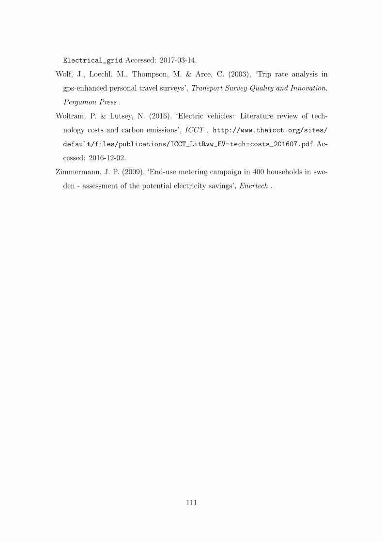
Electrical_grid Accessed: 2017-03-14.

Wolf, J., Loechl, M., Thompson, M. & Arce, C. (2003), ‘Trip rate analysis in

gps-enhanced personal travel surveys’, Transport Survey Quality and Innovation.

Pergamon Press .

Wolfram, P. & Lutsey, N. (2016), ‘Electric vehicles: Literature review of tech-

nology costs and carbon emissions’, ICCT . http://www.theicct.org/sites/

default/files/publications/ICCT_LitRvw_EV-tech-costs_201607.pdf Ac-

cessed: 2016-12-02.

Zimmermann, J. P. (2009), ‘End-use metering campaign in 400 households in swe-

den - assessment of the potential electricity savings’, Enertech .

111


112

A Appendix - Interview take-aways

A.1 CEV Charging

Johan Tollin, Vattenfall & Rombout Heesterman, Tesla

• When charging at high effects, the SOC of the battery has an affect on the

supplied power

– High effects is generally viewed as over 20 kW

• When charging at low effects the supplied power can be assumed as constant

– Low effects is everything bellow 10 kW

• The majority of customers start charging when they arrive home

• A majority of customers charge at a rate bellow 11 kW when at home

A.2 Driving Patterns

Maria Borjesson, CTR

• Drive patterns varies with the seasons

• Seasonal variations can be modeled from congestion charge fees

A.3 Grid Infrastructure

Jonas Persson and Martin Johansson, Vattenfall & Per-Arne Eachus

Jonebring, Sweco

• Average house load is between 2-3 kW

• Velander constants are used when dimensioning the grid in different areas.

– Velander constants need to be updated when CEVs are a factor in the

household electricity usage

• Rural areas are fed from substations of approximately 200 kVA

– Approximately 20-30 households per substation

113

• Urban areas are fed from substations of approximately 800 kVA

– Approximately 100 households per substation

• The distribution grid is generally dimensioned at 70% of the expected max

load

• A new substation costs approximately SEK 400,000

• Cables cost somewhere between SEK 200-700 per meter

• Cost of digging in preparation for new/expanded grid is approximately SEK

1000 per meter

114


115

B Appendix - Projections

Year # CEVs in traf-

fic

# New CEVs # New Cars # Cars in traffic

2008 276,344 4,278,995

2010 308,734 4,335,182

2012 1,254 301,335 4,447,165

2014 7,094 4,447 324,037 4,585,519

2016 26,824 12,283 388,014 4,768,060

2018 73,229 26,229 404,840 4,890,005

2020 151,653 44,327 422,395 5,015,068

2022 385,562 176,284 440,711 5,143,330

2024 1,205,516 459,822 459,822 5,274,872

2026 2,154,963 479,761 479,761 5,409,779

2028 3,145,582 500,565 500,565 5,548,136

2030 4,179,157 522,272 522,272 5,690,031

Table 11: Our projections of the CEV development in Sweden, based on historic figures

from Myhr (2016a) and own assumptions described in Section 4. Table 1 of 2

Year % CEVs of cars

in traffic

% CEVs of new

cars

% Non-CEVs of

new cars

% Increase in

new CEVs

2008 0% 0% 100%

2010 0% 0% 100%

2012 0% 0% 100%

2014 0% 1% 99% 219%

2016 1% 3% 97% 65%

2018 1% 6% 94% 30%

2020 3% 10% 90% 30%

2022 7% 40% 60%

2024 23% 100% 0%

2026 40% 100% 0%

2028 57% 100% 0%

2030 73% 100% 0%

Table 12: Our projections of the CEV development in Sweden, based on historic figures

from Myhr (2016a) and own assumptions described in Section 4. Table 2 of 2

116

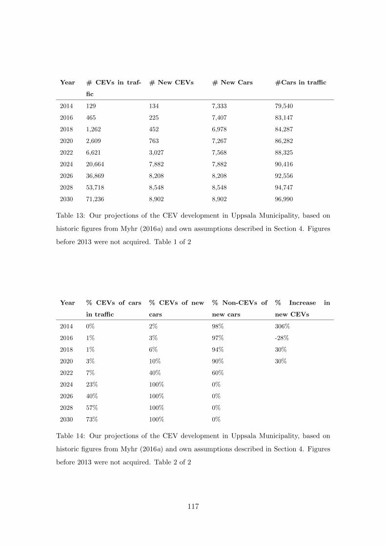
Year # CEVs in traf-

fic

# New CEVs # New Cars #Cars in traffic

2014 129 134 7,333 79,540

2016 465 225 7,407 83,147

2018 1,262 452 6,978 84,287

2020 2,609 763 7,267 86,282

2022 6,621 3,027 7,568 88,325

2024 20,664 7,882 7,882 90,416

2026 36,869 8,208 8,208 92,556

2028 53,718 8,548 8,548 94,747

2030 71,236 8,902 8,902 96,990

Table 13: Our projections of the CEV development in Uppsala Municipality, based on

historic figures from Myhr (2016a) and own assumptions described in Section 4. Figures

before 2013 were not acquired. Table 1 of 2

Year % CEVs of cars

in traffic

% CEVs of new

cars

% Non-CEVs of

new cars

% Increase in

new CEVs

2014 0% 2% 98% 306%

2016 1% 3% 97% -28%

2018 1% 6% 94% 30%

2020 3% 10% 90% 30%

2022 7% 40% 60%

2024 23% 100% 0%

2026 40% 100% 0%

2028 57% 100% 0%

2030 73% 100% 0%

Table 14: Our projections of the CEV development in Uppsala Municipality, based on

historic figures from Myhr (2016a) and own assumptions described in Section 4. Figures

before 2013 were not acquired. Table 2 of 2

117


118

C Appendix - Results

Share of CEVs of cars in traffic

25% 75% 90%

Area Apt. Ho. Apt. Ho. Apt. Ho.

Unweighted average 5.4% 2.4% 18.4% 12.8% 22.3% 16.8%

Almungebygden 5.1% 2.2% 17.6% 11.7% 21.4% 15.7%

Berthaga 4.2% 1.9% 15.0% 9.3% 18.2% 12.3%

Bjorklingeomradet 5.1% 2.2% 17.7% 11.8% 21.5% 15.8%

Danmarksbygden 4.9% 2.1% 17.1% 11.1% 20.7% 15.0%

Eriksberg 5.6% 2.4% 19.3% 13.5% 23.4% 17.9%

Flogsta-Ekeby 2.4% 1.2% 9.6% 5.2% 11.8% 6.8%

Funbobygden 5.6% 2.4% 19.3% 13.5% 23.4% 17.8%

Falhagen 4.9% 2.1% 16.9% 10.9% 20.6% 14.8%

Gamla Uppsala-Nyby 6.0% 2.5% 20.3% 14.6% 24.6% 19.2%

Gamla Uppsalabygden 5.0% 2.1% 17.4% 11.4% 21.1% 15.4%

Gottsunda 7.0% 3.2% 23.5% 18.0% 28.4% 23.3%

Granby 7.7% 3.7% 25.4% 20.0% 30.7% 25.8%

Haga 3.7% 1.7% 13.4% 8.1% 16.4% 10.4%

Innerstaden 3.8% 1.7% 13.8% 8.4% 16.8% 10.7%

Jarlasabygden 4.8% 2.0% 16.6% 10.6% 20.2% 14.4%

Knutbybygden 4.4% 1.9% 15.4% 9.6% 18.7% 12.9%

Kungsangen 9.8% 5.4% 31.9% 27.0% 38.7% 34.1%

Kvarnbo 4.6% 2.0% 16.1% 10.2% 19.6% 13.7%

Kvarngardet 5.4% 2.3% 18.6% 12.7% 22.5% 16.9%

Kabo 3.3% 1.5% 12.3% 7.2% 14.9% 9.3%

Libroback 6.0% 2.5% 20.2% 14.4% 24.5% 19.0%

Luthagen 3.6% 1.6% 13.0% 7.8% 15.9% 10.0%

Loten 8.0% 3.9% 26.3% 21.0% 31.8% 26.9%

Norby 3.9% 1.8% 14.1% 8.7% 17.2% 11.2%

Norra Rasbobygden 5.1% 2.2% 17.8% 11.8% 21.6% 15.9%

Nantuna-Vilan 4.3% 1.9% 15.3% 9.5% 18.6% 12.7%

Rickomberga 8.3% 4.1% 27.1% 21.8% 32.7% 27.9%

Sala backe 7.6% 3.7% 25.3% 19.9% 30.6% 25.6%

Skyttorpsbygden 4.8% 2.1% 16.7% 10.6% 20.2% 14.5%

Stenhagen 5.5% 2.3% 18.7% 12.9% 22.7% 17.1%

Storvretabygden 4.9% 2.1% 17.2% 11.2% 20.9% 15.1%

119

Sunnersta 4.6% 2.0% 16.2% 10.2% 19.7% 13.9%

Svartbacken 5.9% 2.4% 19.9% 14.1% 24.1% 18.6%

Savja-Bergsbrunna 5.6% 2.3% 19.1% 13.3% 23.2% 17.7%

Sodra Hagundabygden 5.1% 2.2% 17.7% 11.8% 21.5% 15.9%

Sodra Rasbobygden 5.4% 2.3% 18.5% 12.6% 22.4% 16.8%

Tuna backar 6.2% 2.5% 20.9% 15.1% 25.3% 19.9%

Ulleraker 8.1% 4.0% 26.6% 21.3% 32.2% 27.3%

Ultuna 2.3% 1.2% 9.3% 4.9% 11.4% 6.5%

Vaksalabygden 5.6% 2.3% 19.1% 13.3% 23.2% 17.7%

Valsatra 5.0% 2.1% 17.2% 11.2% 20.9% 15.2%

Vattholmabygden 5.0% 2.1% 17.4% 11.4% 21.1% 15.4%

Vardsatra 5.1% 2.2% 17.6% 11.7% 21.4% 15.7%

Vangebygden 5.2% 2.2% 18.0% 12.0% 21.8% 16.1%

Vastra Balingebygden 5.3% 2.2% 18.3% 12.4% 22.2% 16.5%

Arsta 6.8% 3.0% 22.9% 17.3% 27.7% 22.5%

Ostra Balingebygden 5.3% 2.2% 18.1% 12.2% 22.0% 16.4%

Table 15: Increase in max load (%) for different CEV shares of cars in traffic for all areas

in Uppsala Municipality. Ho. = House, Apt. = Apartment

Cars per

Area Apt. Ho.

Unweighted average 0.37 1.39

Almungebygden 0.35 1.33

Berthaga 0.30 1.14

Bjorklingeomradet 0.36 1.34

Danmarksbygden 0.34 1.29

Eriksberg 0.39 1.45

Flogsta-Ekeby 0.20 0.76

Funbobygden 0.39 1.45

Falhagen 0.34 1.28

Gamla Uppsala-Nyby 0.41 1.52

Gamla Uppsalabygden 0.35 1.31

Gottsunda 0.46 1.74

Granby 0.50 1.88

Haga 0.28 1.03

Innerstaden 0.28 1.06

Jarlasabygden 0.34 1.26

120

Knutbybygden 0.31 1.17

Kungsangen 0.62 2.34

Kvarnbo 0.33 1.22

Kvarngardet 0.37 1.40

Kabo 0.25 0.95

Libroback 0.40 1.51

Luthagen 0.27 1.01

Loten 0.52 1.95

Norby 0.29 1.08

Norra Rasbobygden 0.36 1.34

Nantuna-Vilan 0.31 1.16

Rickomberga 0.53 2.00

Sala backe 0.50 1.87

Skyttorpsbygden 0.34 1.26

Stenhagen 0.37 1.41

Storvretabygden 0.35 1.30

Sunnersta 0.33 1.23

Svartbacken 0.40 1.49

Savja-Bergsbrunna 0.38 1.44

Sodra Hagundabygden 0.36 1.34

Sodra Rasbobygden 0.37 1.39

Tuna backar 0.42 1.56

Ulleraker 0.52 1.97

Ultuna 0.20 0.74

Vaksalabygden 0.38 1.44

Valsatra 0.35 1.30

Vattholmabygden 0.35 1.31

Vardsatra 0.35 1.33

Vangebygden 0.36 1.35

Vastra Balingebygden 0.37 1.38

Arsta 0.45 1.70

Ostra Balingebygden 0.36 1.37

Table 16: Number of cars per household in Uppsala areas. Ho. = House, Apt. =

Apartment

121

impact of electric vehicle charging on the distribution ...1130512/fulltext01.pdf · impact of...

Documents