Data Science and Service Research

Discussion Paper

Discussion Paper No. 38

Time Series Residual

Momentum

Hongwei Chuang

March, 2015

Center for Data Science and Service Research

Graduate School of Economic and Management

Tohoku University

27-1 Kawauchi, Aobaku

Sendai 980-8576, JAPAN

Time Series Residual Momentum

Hongwei Chuanga,∗

aGraduate School of Economics and Management, Tohoku University27-1 Kawauchi, Aoba Ward, Sendai 980-8576, Japan

Abstract

The momentum strategy as described in the seminal work of Jegadeesh and Tit-man (1993) leads to stream of studies on theoretical work of momentum effectand empirical analysis in different financial assets and markets of several countries.However, the characteristics displayed by the momentum strategy have often beingargued that was associated with risk exposures to pricing factors and time-varyingrisk. Especially, the investment portfolio’s performance endanger profound draw-down risk when the market rebounds after financial crisis. In this study, I proposedthe time series residual momentum strategy to mitigate the magnitude of losses. Ifthe stock positively (negatively) deviates from predicted intrinsic values during ashort-term period, it is denoted as over-valuation (under-valuation). Through inves-tigating the U.S. stock market, the empirical results show the proposed strategy cannot only achieve significant improvement for the conventional momentum strategy,but also can substantially reduce the drastic losses from financial crises.

Key words: Momentum; Fama-French Factors; Asset Pricing; Financial Crisis

JEL classification: C3; G2

1. Introduction

As Isaac Newton said “What goes up must come down.” Everything inearth should obey the law of gravity. Therefore, it is natural to assume thelaw of gravity can also be applied in financial market. However, academicstudies have found out that stocks which perform better than the other stocksin recent past will continue for a certain period. The phenomenon is called“momentum” effect. Past studies also have confirmed that this effect has beenobserved not only in the stock market but also in commodity and currencymarkets. The profit cannot be explained away by saying that high-performancestocks are more risky, or by arguing that the trading cost would eat up all theprofit, instead they are considered potential profitable.

This anomaly also drives a juggernaut through one of the tenets in finan-cial theory, which is the efficient market hypothesis. In the weak-form efficientmarket hypothesis, the past price movements should provide no guide to fu-

1

ture price changes. Investors should have no logical reasons to prefer the pastwinners to the past losers. Therefore, we are going to revisit the conventionalmomentum strategy in the U.S. stock market by using the residual analy-sis over a longer period from January 1930 to December 2010. Our proposedstrategy can control the short-term behavior and intermediate continuation ofa stock.

The intermediate-horizon return continuations are first reported by Je-gadeesh and Titman (1993). They propose the momentum strategy, whichbuys the past winning stocks over the previous three to twelve months andsells the past losing stocks over the same period exhibits substantial profit.Although these results have been widely accepted, researchers are still in de-bate over the sources of the profit and the interpretation of the evidence. Themomentum effect is not only remarkably persistent in stock market but also incommodity and currency markets. Okunev and White (2003) find momentumeffect in currencies. Erb and Harvey (2006) find momentum effect in com-modities. Moskowitz, Ooi and Pedersen (2012) find momentum effect in ex-change traded futures contracts. Moreover, the momentum effect is worldwide.Rouwenhorst (1998) finds evidence of momentum effect in developed stockmarkets, and Rouwenhorst (1999) documents momentum effect in emergingmarkets.

Although the momentum strategy tends to work well on the winners andthe losers over the past three-to-twelve months, the momentum effect disap-pears for longer periods in three or five year. Just as trees do not grow tothe sky, share prices do not rise forever. Many investigators have argued themomentum strategies to display characteristics that are often associated withfactors of price risk. Chordia and Shivakumar (2002) reveal the profits of mo-mentum strategies to exhibit strong variation across the business cycle. Intheir study, they show the conventional momentum strategy earns 14.70% an-nualized return during expansions and loses 8.70% during recessions over theperiod from January 1930 to December 2009. Cooper, Gutierrez and Hameed(2004) further examine the variation of average returns to the U.S. equity mo-mentum strategies. They find in “UP” states, which are defined by the laggedthree-year return of the market, the historical mean of returns of a equally-weighted momentum strategy is 0.93% per month. In “DOWN” states, thehistorical mean of returns of a equally-weighted momentum strategy is -0.37%per month. It means those losers often experience strong gains after the marketcollapses. In such circumstances, implementation of the momentum strategywill result in persistent strings of negative returns. It leads to a momentumcrash.

In this paper, we propose a more effective strategy, time series residualmomentum, which ranks all eligible stocks based on their total returns andresidual returns in the recent past months. The advantage of the time series

2

momentum strategy is not only to reduce the time-varying exposures but alsoto eliminate the “value risk,” which occurs when a stock is overvalued. There-fore, this time series residual momentum strategy performs better than theconventional momentum strategy and the the residual momentum strategy.Most important of all, it can avoid the huge loss of the conventional momen-tum strategy after 2000.

To sum, in past decades, financial academics and practitioners have rec-ognized that the momentum strategy can generate significant profit and thatthe momentum effect exists in many financial markets. But, fewer people no-tice the collapse of the momentum is profound especially after the financialcrisis. In this study, we adjust the conventional momentum strategy in theU.S. stock market by using the residual analysis over the period from Jan-uary 1930 to December 2010. The modification we proposed can take care ofthe short-term behavior and the intermediate continuation of a stock. Theempirical results show the modification can largely improve the conventionalmomentum strategy.

2. Momentum Crash

We first examine the conventional momentum strategy over a longer pe-riod in the U.S. stock market from January 1930 to December 2010. Mostof time, the market appears to underreact to the public information andresults in consistent price momentum. However, in extreme conditions, thepast losers of the momentum strategy often comprise a very high premium.When the market conditions are going better, those past losers will experiencestrong gains. This leads to a “momentum crash.” It is because the returns ofthe conventional momentum strategies are highly-skewed. Therefore, investorswho implement the conventional momentum strategy will experience stringsof negative returns, especially after the market collapses.

Data and Portfolio Formation

The data for the study is from CRSP monthly files. Our data consists ofall domestic, primary stocks listed on the New York Stock Exchange (NYSE),American Stock Exchange (AMEX), and Nasdaq (NASDAQ) stock marketsduring the period from January 1929 to December 2010. We utilize only thereturns on common shares with a 10 or 11 CRSP share-code. Close-end funds,Real Estate Investment Trust (REITs), unit trusts, American Depository Re-ceipts (ADRs), and foreign stocks are excluded from the analysis. We alsoexclude stocks with price below $1 during the formation periods to reduce themicrostructure effect associated with low-price stocks.

Following most of the literature, we rank the stocks based on their pasttwelve-month returns excluding the most recent month. Then we assign thesestocks into 10 equally weighted portfolios at the end day of each formation

3

Fig. 1. Momentum Portfolio Formation

month. Each portfolio is held for one month following the formation month.The reason why we focus on their past twelve-month returns excluding themost recent month is that this momentum definition is currently most broadlyused and readily available through the PR1YR factor of Carhart (1997). Themomentum strategy is typically to disentangle the intermediate horizon mo-mentum effect from the short reversal effect documented by Jegadeesh (1993)and Lehmann (1990).

Figure 1 illustrates time line of the portfolio formation process for themomentum returns in May 2009. The ranking period returns are the cumula-tive returns from the close of the last trading day in April 2008 to the closeof the last trading day in March 2009. We sort all firms that meet the datarequirements into 10-decile portfolios which are labeled P1 to P10 accordingto their cumulative returns over the ranking period. The 10% of firms withthe highest ranking period returns go into portfolio P10, the “[W]inner”-decileportfolio, and those with the lowest ranking period returns go into portfolioP1, the “[L]oser”-decile portfolio. The return on a zero investment “Winner-Minus-Loser” (WML) portfolio is the difference of the return on the Winnerand the return on the Loser portfolio in each period.

The monthly returns of the decile portfolios are based on the equally-weighted returns. Decile membership does not change in a month, except forthe case of delisting. We also consider the overlapping portfolios approach,which is a strategy that holds a series of portfolios selected in the currentmonth and the previous month. The market return we used is Dow JonesIndustry Average (DJIA) index downloaded from Yahoo! Finance. 1 The risk-free rate and the cross-sectional Fama-French three factors are downloadedfrom the data library of Kenneth R. French. 2

Momentum Portfolio Performance

Table 1 presents the moments of the momentum decile portfolios fromJanuary 1930 to December 2010. For all portfolios, Mean, Std, Skew and Kurt

1 We use DJIA instead of S&P 500 because the first trading day of S&P 500 is Jan3, 1950.2 http://mba.tuck.dartmouth.edu/pages/faculty/ken.french

4

denote the full-period realized mean, stand deviation, skewness and kurtosisof the monthly returns to the portfolios. The average return of the winnerportfolio is 1.63% per month and is 0.69% of the loser portfolio. A self-financingstrategy that buys the top 10%, Winner, and sells the bottom 10%, Loser,produces profits of 0.94% per month. The result is consistent with the existingliterature, which states that there is a strong momentum premium over thepast 80-year period.

Table 1Twelve-Month Momentum Portfolio Characteristics, January 1930-December 2010

Portfolio Mean Std Skew Kurt

P1 (Past Loser) 0.69% 0.1067 2.3866 17.9023

P2 0.82% 0.0819 1.6241 14.4532

P3 1.01% 0.0781 2.1760 20.5349

P4 1.06% 0.0719 1.5558 15.7259

P5 1.15% 0.0690 1.1678 13.2865

P6 1.20% 0.0663 0.9465 12.3870

P7 1.28% 0.0645 0.4184 7.8186

P8 1.41% 0.0676 0.6713 9.8730

P9 1.54% 0.0718 0.3366 6.9300

P10 (Past Winner) 1.63% 0.0870 1.0294 13.4764

WML 0.94% 0.0701 -2.7992 22.7026

The skewness of the past loser portfolio is 2.3866, and the skewness ofthe past winner portfolio is 1.0294. The skewness of the past loser portfolio ismore than twice of the skewness of the past winner portfolio. One should notethat the past loser portfolios are considerably positively-skewed than the pastwinner portfolios. Therefore, the skewness of WML portfolio is -2.7992, whichis largely negative-skewed. Another thing we should note is that the kurtosisof WML portfolio is 22.7026, which is also considerably large than usual.

The skewness of returns on momentum portfolios is not surprising. Forexample, Wall Street calls a high momentum stock that suddenly collapsesas a “torpedo.” A torpedoed stock is a stock hit by new negative informationafter a long period of positive information. As the stock price has continuouslyincreased in the past, investors may expect that the company’s business is ingood conditions. Hence, the upward trend in earnings will more likely con-tinue. However, it remains possible that the trend of increasing earnings maysuddenly reverse. When it occurs, the positive effect on the stock’s earningsmay also be reversed, ex. some stocks in the technology sector, where new in-novations make existing technologies obsolete. Those fast-growing companies

5

Fig. 2. Cumulative Monthly Returns of WML, DJIA and Risk-free, January1930-December 2010

which depend on existing technologies might be affected. The growth of thesefirms suddenly stop.

Figure 2 presents the cumulative monthly returns 3 for investing $1 ini-tially in (1) the risk-free asset; (2) the DJIA index; and (3) the zero investmentportfolio, WML portfolio, respectively, over the period from January 1930 toDecember 2010. On the right side of the plot, we present the final dollar valuesfor each of the three portfolios. We can see the final value of WML is $448.73,DJIA is $46.59, and the risk-free asset is $17.78. The momentum strategy doesearn a significant return.

Momentum Crashes

Good things don’t last long. The momentum strategy appears to loosetheir profitability in the recent years. Again, we plot the cumulative monthlyreturns for investments in the risk-free asset, the DJIA index, and the WMLportfolio from January 2000 to December 2010 as shown in Figure 3. Wecan find the WML portfolio loses almost 70% at the end of 2010. In fact,it lost 1.46% per annum over the period from January 2000 to December2010. The large losses of the WML portfolio occured in the first half of 2009,

3 The cumulative return on an implementable strategy is an investment at time 0and fully reinvested at each time point. During the period, there is no cash put inor taken out. R(t, T ) denotes the cumulative return between time t to T , R(t, T ) =∏Ts=t+1(1 + Rs).

6

Fig. 3. Cumulative Monthly Returns of WML, DJIA and Riskfree, January 2000-De-cember 2010

especially in March, April, and May. The losses were 18.22%, 39.52%, and14.29% respectively. The rough under-performance appears when the marketrebounds from the bottom. We argue that the large negative skewness of theWML portfolio can cause the momentum crash.

Table 2Top 10 Worst-Month WML Portfolio Returns

Rank Month Past Loser Past Winner WML DJIA

1 1932/07 77.76% 15.58% -62.18% 25.79%

2 2001/01 78.79% 17.74% -61.05% 0.92%

3 1932/08 100.08% 43.18% -56.91% 35.76%

4 1939/09 81.67% 24.78% -56.89% 11.72%

5 2009/04 48.12% 8.61 % -39.52% 7.35%

6 2002/11 37.68% 8.26 % -29.42% 5.94%

7 1932/01 29.66% 5.14 % -24.53% -1.73%

8 1975/01 44.12% 20.02% -24.10% 14.19%

9 1938/06 38.84% 16.52% -22.32% 24.26%

10 1974/01 24.72% 4.84 % -19.88% 0.55%

Table 2 presents the top ten worst-month returns of the WML strat-egy over the periods from January 1930 to December 2010. The table also

7

gives the contemporaneous monthly returns of DJIA. These returns often oc-cur when the market has dramatic downturns, and during a month wherethe market gradually rises. For example, during the two-month period fromJuly to August in 1932, the DJIA increased 61.55%, but the return of theWML portfolio decreased 119.09%. As we can also see from the Table 2, dur-ing the two-month period, returns of the Past Loser deciles are 77.76% and100.08% outperform the returns of the Past Winner deciles which are 15.58%and 43.18% respectively. Thus, the strong momentum reversals can be charac-terized as a momentum crash. The momentum crash happens in the short sideof the portfolio, the past losers portfolios, which are crashing up rather thandown. We should also notice that these momentum crashes are also clusteredas shown in Figure 4. The strong performance of the past losers occurs overthe span of multiple months.

Robustness Check

For robustness check, we also plot the cumulative monthly WML portfolioreturns over the period from January 1930 to December 2010 by consideringdifferent formation periods, i.e., we rank the stocks based on the past j-monthreturn, where j=3, 6, and 9. The result is shown as Figure 5. We can see thecumulative monthly WML return based on the past 3-month return is $2.79.The cumulative monthly WML return basing on the past 6-month return is$7.11. And the cumulative monthly WML return basing on the past 9-monthreturn is $17.11. The best performance of cumulative monthly WML returnis based on past 12-month return, which reaches $448.73. Thus, we focus onthe 12-month formation period as our momentum strategy analysis hereafter.

Table 3 presents the moments of the momentum decile portfolios fromJanuary 1930 to December 2010 based on the past 3-month return. The skew-ness of the past loser portfolios is 1.5887, and the skewness of the past win-ner portfolios is 0.3401. The skewness of WML portfolios is -2.8086, which isnegative. The kurtosis of WML portfolios is 22.8985. Table 4 presents the mo-ments of the momentum decile portfolios from January 1930 to December 2010based on the past 6-month return. The skewness of the past loser portfoliosis 2.0914, and the skewness of the past winner portfolios is 0.0396. The skew-ness of WML portfolios is -2.6249, which is negative. The kurtosis of WMLportfolios is 19.7919. Table 5 presents the moments of the momentum decileportfolios from January 1930 to December 2010 based on the past 9-monthreturn. The skewness of the past loser portfolios is 2.1495, and the skewnessof the past winner portfolios is 0.8497. The skewness of WML portfolios is-3.1013, which is negative. The kurtosis of WML portfolios is 22.4271.

Further, we plot the cumulative monthly WML portfolio returns over theperiod from January 2000 to December 2010 by considering different formationperiods as shown in Figure 6. We can see the cumulative monthly WML return

8

Fig. 4. Momentum Portfolio Performance, January 1930-December 2010

9

Table 3Characteristics of 3-month Momentum Portfolios, January 1930-December 2010

Portfolio Mean Std Skew Kurt

P1 (Past Loser) 0.91% 0.1013 1.5887 10.4791

P2 1.09% 0.0871 1.8941 15.8793

P3 1.23% 0.0807 2.1182 19.4230

P4 1.19% 0.0719 1.2167 13.2133

P5 1.15% 0.0671 0.6108 8.6659

P6 1.17% 0.0664 0.7823 11.5043

P7 1.15% 0.0644 0.3849 7.1533

P8 1.16% 0.0664 0.3782 7.8832

P9 1.16% 0.0700 0.2545 6.3014

P10 (Past Winner) 1.24% 0.0805 0.3401 6.3945

WML 0.33% 0.0613 -2.8086 22.8985

Table 4Characteristics of 6-month Momentum Portfolios, January 1930-December 2010

Portfolio Mean Std Skew Kurt

P1 (Past Loser) 0.95% 0.1073 2.0914 13.6075

P2 1.02% 0.0878 2.0454 16.3411

P3 1.06% 0.0794 1.7692 15.2567

P4 1.16% 0.0761 2.1912 20.9869

P5 1.16% 0.0692 1.3928 14.3128

P6 1.18% 0.0680 1.0820 13.3095

P7 1.17% 0.0641 0.3624 7.9755

P8 1.18% 0.0644 -0.1076 5.2800

P9 1.35% 0.0689 -0.0565 5.1462

P10 (Past Winner) 1.44% 0.0811 0.0396 4.4203

WML 0.49% 0.0691 -2.6249 19.7919

based on the past 3-month return is $0.51. The cumulative monthly WMLreturn based on the past 6-month return is $0.47. And the cumulative monthlyWML return based on the past 9-month returns is $0.2. It shows that themomentum crash won’t eliminate no matter how many months of the pastj-month return we consider, where j=3, 6, 9, and 12.

10

Fig. 5. j-Month Momentum Portfolios Performance, January 1930-December 2010

11

Table 5Characteristics of 9-month Momentum Portfolios, January 1930-December 2010

Portfolio Mean Std Skew Kurt

P1 (Past Loser) 0.82% 0.1066 2.1495 15.7713

P2 0.97% 0.0870 2.2791 19.8423

P3 1.02% 0.0780 1.6489 15.1072

P4 1.07% 0.0713 1.2550 12.4999

P5 1.09% 0.0686 1.1951 12.7131

P6 1.19% 0.0665 1.0374 12.1164

P7 1.28% 0.0668 0.8437 10.9467

P8 1.28% 0.0673 0.4746 10.1607

P9 1.44% 0.0717 0.4868 8.7271

P10 (Past Winner) 1.48% 0.0852 0.8497 11.3598

WML 0.66% 0.0736 -3.1013 22.4271

3. Time Series Residual Momentum Strategy

Many investigators have argued that the characteristics displayed by themomentum strategy are often associated with factors of price risk. Chordia andShivakumar (2002) show that the profits of momentum strategies to exhibitstrong variation across the business cycle. They report that the conventionalmomentum strategy earns 14.70% annualized return during expansions andloses 8.70% during recessions over the period from January 1930 to December2009.

In addition, Blitz, Huij and Martens (2011) also argue that the con-ventional momentum strategies exhibit the time-varying exposures to Fama-French three factors. To counter this drawback, they propose the “residualmomentum strategy” to reduce the time-varying exposures by ranking allstocks based on its own residual returns instead of the total returns. Blitz,Huij and Martens (2011) show that the residual momentum strategy can earnprofits that are about twice as large as the conventional momentum strategywith more consistency over time.

The literature on momentum strategies focus on the relative performanceof securities in cross-sectional perspective. Moskowitz, Ooi and Pedersen (2012)propose the “time series momentum strategy” in equity index, currency, com-modity, and bond futures. They only focus on a security’s past returns. Theyfound that the past twelve-month returns of a security to show strong positiveinfluence on its future return with persistent effect for about one year, followedby partially-reversed role over longer horizons. This strategy can also deliver

12

Fig. 6. Cumulative Monthly Returns of j-Month Momentum Portfolios, January2000-December 2010

substantial abnormal returns with little exposure to the standard asset pricingfactor to perform well during extreme market condition.

The advantage of cross-sectional residual momentum is to reduce the time-

13

varying exposures. On the other hand, the advantage of the time series momen-tum is that the security’s past returns provide strong positive predictability toits future returns. Hence, it is natural to combine the cross-sectional residualmomentum strategy and time series momentum strategy into the “time seriesresidual momentum strategy.” Our empirical evidence shows the strategy canavoid the huge loss in recent years.

Cross-Sectional Residual Momentum

The residual momentum strategy proposed by Blitz, Huij and Martens(2011) is also known as a “cross-sectional” residual momentum strategy, sincetheir approach focused on the cross-sectional relative performance in residualreturns of securities. Their formula is shown as follows. In each month t, theresidual returns are estimated by using Fama-French three factors model, thatis,

rit = αi + βi1MKTt + βi2SMBt + βi3HMLt + εit (1)

where rit is the excess return of stock i in month t. MKTt, SMBt, and HMLtare the excess returns of factor-mimicking portfolios for the market, size and,value in month t. αi, βi1, β

i2 and βi3 are parameters to be estimated. And εit is

the residual return.

Only the stocks with complete return history of over 36-month rollingregression window were included. The purpose of using 36-month rolling win-dows is to ensure having a sufficient number of return observations to obtainaccurate estimates for stock exposures to the market, size, and value. In orderto obtain the residual return, the regression over 36-month rolling windows,was run, i.e., over the period from t− 36 to t− 1 to get the estimated param-eters αi, βi1, β

i2 and βi3 of each stock i. The estimated residual return of stock

i in month t is

eit = rit − (βi1MKTt + βi2SMBt + βi3HMLt), (2)

where the estimated αi is not included, since the intercept of regression servedas a general control for the misspecification in the model for expected stockreturns.

At each formation month t, they rank all eligible stocks into 10-decileportfolios according to the estimated residual returns from past twelve months,standardized by the standard deviation over the same period of time. The cu-mulative monthly returns of the residual momentum strategy and total returnmomentum strategy are plotted by Blitz, Huij and Martens (2011) in Figure7.

As a result, the highest value of the residual momentum strategy overthe period from January 1930 to December 2010 was about $10,000, largerthan those of total return momentum. This suggested that the performance of

14

Fig. 7. Cumulative monthly returns plot by Blitz, Huij and Martens (2011), January1930-December 2010

the residual momentum strategy is more consistent in compared to the con-ventional momentum strategy. In addition, this also exposed how poorly theconventional momentum strategy has performed during “The Great Depres-sion” that started from 1929 and lasted until the late 1930s or early 1940s.

Time Series Momentum

The literature on momentum strategies focus on the relative performanceof securities in cross-sectional perspective. Moskowitz, Ooi and Pedersen (2012)propose the “time series momentum strategy” in equity index, currency, com-modity, and bond futures, with focus on past returns of a security. In theirstudy, they first examine the time series predictability of future returns acrossdifferent time horizons. In other words, they regress the excess return rt in themonth t on its lagged h months return, rt−h. Both of the returns are scaledby their ex-ante volatilities, σ2

t−1 and σ2t−h−1,

rtσ2t−1

= α + βhrt−hσ2t−h−1

+ εt, (3)

where the ex-ante volatility is annualized as follows:

σ2t = 261

∞∑i=0

(1− δ)δi(rt−1−i − rt)2. (4)

261 is the factor which scales the variance to be annual, rt is the exponentialweighted average return, and the weight (1− δ)δi add up to 1. The parameterδ is chosen so that the center of mass of the weight is 60 days. The way toadjust futures returns by their ex-ante volatilities is similar to use the Gener-alized Least Squares instead of Ordinary Least Squares. They find a positive

15

Fig. 8. Time Series Predictability by Moskowitz, Ooi and Pedersen (2010)

t-statistic for the first twelve months, indicating the significant continuationand trend in its return.

Figure 8 shows that t-statistics are positive in twelve months. This indi-cates the significant return continuation or trends. In their study, the moststrong time series momentum effect are on the properties of the past twelve-month time series momentum and one month holding period. The time seriesmomentum strategy is defined to take a long position if the past twelve-monthcumulative excess return is positive and a short position if the past twelve-month cumulative excess return is negative. The position is scaled by theex-ante annualized volatility that is 0.60%. Therefore, the return of the timeseries momentum strategy for security i from time t to t+ 1 is as follow:

sign(rit−12,t)0.06%

σitrit,t+1, (5)

where σit is defined as same as (4) and rit,t+1 is the return of security i fromtime t to t+ 1.

Time Series Residual Momentum

Previous literatures have generally attributed the momentum effect tofirm-specific returns, arguing that investors have either under-reacted or be-latedly overreacted to the firm-specific returns. Recently, Lewellen (2002) stud-ied the momentum effect in focusing on the role of industry, size, and B/Mfactors. Lewellen (2002) argued that it is impossible to explain the signifi-cant component of momentum through firm-specific returns with behavioral

16

model. Instead, that the excess covariance, not underreaction, can explain themomentum effect in the portfolios.

It is well known that the momentum effect is a cross-sectional result andit is not the same as positive autocorrelation. As Lo and MacKinlay (1990)showed in 1990, the possibility of momentum effect been caused by the auto-correlation in returns, the lead-lag relation among stocks (cross-serial correla-tion) or the cross-sectional dispersion in unconditional means. Later, Lewellen(2002) has also proposed a simpler strategy based on Lo and Mackinlay’stheory to consider holding assets in proportion to the market-adjust returns,shown as followed.

The proportion weight of asset i in month t is

wit =1

N(rit−1 − rmt−1), (6)

where rit−1 is the asset’s return in month t−1, rmt−1 is the corresponding returnon the equally-weighted index, and N is the total number of stocks. Assumingthat returns have unconditional mean µ ≡ E[rt] and autocovariance matrixΩ ≡ E[(rt−1 − µ)(rt − µ)′]. Therefore, the portfolio return in month t equals

πt =∑i

witrit =

1

N

∑i

(rit−1 − rmt−1)rit, (7)

and the expected profit is

E[πt] =1

NE[

∑i

(rit−1rit)]−

1

NE[

∑i

(rmt−1rit)]

=1

N

∑i

(ρi + µ2i )− (ρm + µ2

m), (8)

where ρi and ρm are the autocovariances of asset i and the equally-weightedindex m. (8) shows that the profit of the portfolio depends on the magnitudeof asset autocovariances relative to market’s auto-covariance. (8) can also bewritten into a matrix notation. Let the average autocovariance equal tr(Ω)/Nand the autocovariance of the market portfolio equal 1′Ω1/N2. tr(·) denotesthe sum of the diagonals and 1′ is a vector of ones. Therefore, (4.8) equals

E[πt] =1

Ntr(Ω)− 1

N21′Ω1 + σ2

µ

=N − 1

N2tr(Ω)− 1

N2[1′Ω1− tr(Ω)] + σ2

µ, (9)

where σ2µ is the cross-sectional variance of unconditional expected returns [col-

lecting the µ2i and µ2

m terms in (8)].

The decompositions of Lewellen (2002) suggest the profit of momentum

17

Table 6Categories of Momentum Strategy

Momentum Residual Momentum

Cross Section Jegadeesh and Titman (1993), ... Blitz, Huij and Martens (2011)

Time Series Moskowitz, Ooi and Pedersen (2012) Our study

to rise in three ways as followed. First, stocks are positively autocorrelated,so firms currently with high returns are expected to have high returns inthe future. Second, since the stock returns are negatively correlated to thelagged returns of other stocks, high future returns can be predicted by theother stocks’ poor performances. Third, stocks simply have high unconditionalexpected returns relative to the other stocks. Overall, the empirical finding ofLewellen (2002) has concluded the lead-lag relations to play an important roleamong stocks.

One of the advantages in cross-sectional residual momentum is that itconsists of the ability to reduce the time-varying exposure effect of the con-ventional momentum strategies. This time series momentum shows that thefuture returns of a stock can be forecast by its past returns. In addition,in the decomposition of Lewellen (2002), it is natural to combine the cross-sectional residual momentum strategy with time series momentum strategyinto the “time series residual momentum strategy.” Summary of the differentcategories in current momentum strategy is shown in Table 6.

Methodology

Without loss of generality, we assume that there are n securities with Ti tobe the length of security i. To implement the time series residual momentumstrategy, the first step is to estimate the time series residual returns of eachsecurity. In following with Blitz, Huij and Martens (2011), we ran the followingregression through the same equation as equation (1) in month t, for eachsecurity i, where the residual returns eit is obtained by equation (2).

We propose a measure of value risk, denoting qit(j) for security i based onits own past j-month time series residual return in the month t. The qit(j) is

18

Fig. 9. Q-Q plot

defined as:

qit(j) = Φ(

∑t−j+1t eit√j × σ2

t

), (10)

where σ2t is the variance of eit over the same period, j is the strength of value

risk over the past j months ( j = 3, 6, 9 or 12), and Φ is the cumulativefunction of a standard Normal distribution.

qit(j) can be viewed as a proxy measure of the present value relative to itslong-term equilibrium level. qit(j) is used to describe whether or not a stock’srecent j -month return has been overvalued. Through this formula, we can formthe portfolios based on independently sort all eligible stocks by their own past12-month accumulative monthly return and j -month value-risk measure, qit(j)at each formation month t.

In argument regarding to whether or not∑t−j+1

teit√

j×σ2t

follows a Standard

Normal distribution can be confirmed by a Q-Q plot of∑t−j+1

teit√

j×σ2t

for a stock

19

with its permno number 10006, as shown in Figure 9. The Q-Q plot wasconstructed using different j -month, j=3, 6, 9 and 12. In j=3, the samplequantiles were approvimate to the Standard Normal distribution, confirmingthat it is not inappropriate to use Φ as the transformation.

In order to form the portfolios, the stocks were first assigned into one of 10portfolios based on their cumulative returns over the previous twelve months.The top 10% of firms with the highest ranking period returns were filed intoportfolio P10, the “[W]inner” decile portfolio. On the other hand, the bottom10% of firms with the lowest ranking period returns were filed into portfolioP1, the “[L]oser” decile portfolio. Besides, the stocks are also independentlyassigned into one of the 3 portfolios with the categories of [U]nder, [M]iddleand [O]ver, based on the value-risk measures over the same period of time.In combination of the two separately arranged ranking methods, up to 30value-risk momentum portfolios were obtained. “WU-LO” was defined as themonthly portfolio return of the “[W]inner that is [U]nder-valued minus the[L]oser that is [O]ver-valued.” A return on a zero investment of a WU-LOportfolio is the difference between the return in the undervalued winner andovervalued loser portfolio in each time period. In this study, only monthlyreturn over next one month was focused based on a equally-weighted averageof the portfolio returns.

Empirical results

The results are shown in Table 7, where the standard deviations are in theparentheses. As seen from the table, when j = 3, the monthly average returnof the WU-LO portfolio is 2.44% that is equal to 33.57% annual return. For j= 6, the monthly average return of the WU-LO portfolio is 1.67% that is equalto 22.06% annual return. For j = 9, the monthly average return of the WU-LOportfolio is 1.74% that is equal to 23.01% annual return. Overall, the returnsof these three WU-LO portfolios outperformed the conventional momentumstrategy. We further use one-tailed t-test to examine the difference betweenthe returns of WU-LO portfolio and WML. For j = 3, the t-test statistic ofWU-LO portfolio to WML is 3.4675 with p-value < 0.01. For j = 6, the t-teststatistic of WU-LO portfolio to WML is 1.4003 with p-value < 0.1. For j = 9and j = 12, the t-test statistics are not significant at 5% significant level.

Initially, our study focused on the consideration of short-termed contrar-ian and the continuation in intermediate momentum of each stock. As a result,the improvement in conventional momentum strategy with value risk was ob-served, mainly due to the undervaluing of a firm at its high momentum. At thiscircumstance, the stock price will tend to rise instead of fall in the followingmonth. Thus, our strategy was aimed at controlling the short-term behaviorof a stock and the persistent intermediate momentum.

20

21

Figure 10 plot the monthly portfolio return of the time series momentumstrategy (j = 3) over the period from July 1967 to December 2010. As a re-sult, the time series momentum strategy was shown to perform better thanthe conventional momentum strategy as shown in Figure 3.4. In addition, theWU-LO portfolio returns were observed to be more stable than the returns ofconventional momentum portfolio, though we also recognized the imperfectionof our strategy with incapability of avoiding a huge loss of -37.86% in April2009. Further plotting on the cumulative monthly return of conventional mo-mentum strategy and time series residual momentum strategy over the timeperiod from July 1967 to December 2010 was also shown in Figure 11. As aresult, the cumulative monthly return of WU-LO is $116,926.2; whereas thecumulative monthly return of WML was shown to be $69.09. In consideringthe performance after 2000, the cumulative monthly return was also plotted forconventional momentum strategy and time series residual momentum strategyover the time period from January 2000 to December 2010, as shown in Figure12. The WML was shown to lose about 70% in December 2010 compared toits initial investment in January 2000. As for the value using our strategy,217.10% was observed in December 2010 comparing to its initial investmentin January 2000.

4. Conclusions and Future Researches

The momentum effect has been widely accepted in financial market. But,fewer people notice the collapse of the momentum is profound especially afterfinancial crisis. There are “momentum crashes.” Just as trees do not growto the sky, likewise, share prices do not rise forever. The momentum crashis because that conventional momentum strategy exhibits substantial time-varying exposures to the market.

In this study, we revisit the conventional momentum strategy in the U.S.stock market by the residual analysis and the price-risk adjustment over a longperiod of time, from January 1930 to December 2010. Such time-varying expo-sures of the conventional momentum strategy can be reduced by the residualanalysis and the price-risk adjustment. The idea was when a firm is under-valued (under-priced) at its high momentum; the stock price tends to riseinstead of fall in the following month. Conversely, when a firm is overvalued(over-priced) at its low momentum, the stock price tends to fall instead ofrise. The strategies that we proposed can control the short-term behavior ofa stock and the intermediate continuation.

Overall, our empirical results showed that through these two strategies,significant improvement was observed in compared to the conventional mo-mentum strategy, suggesting it to be a better way for portfolios managementin future studies. Even more, this new concept of residual analysis can also befurther applied to other financial markets as commodities and currencies.

22

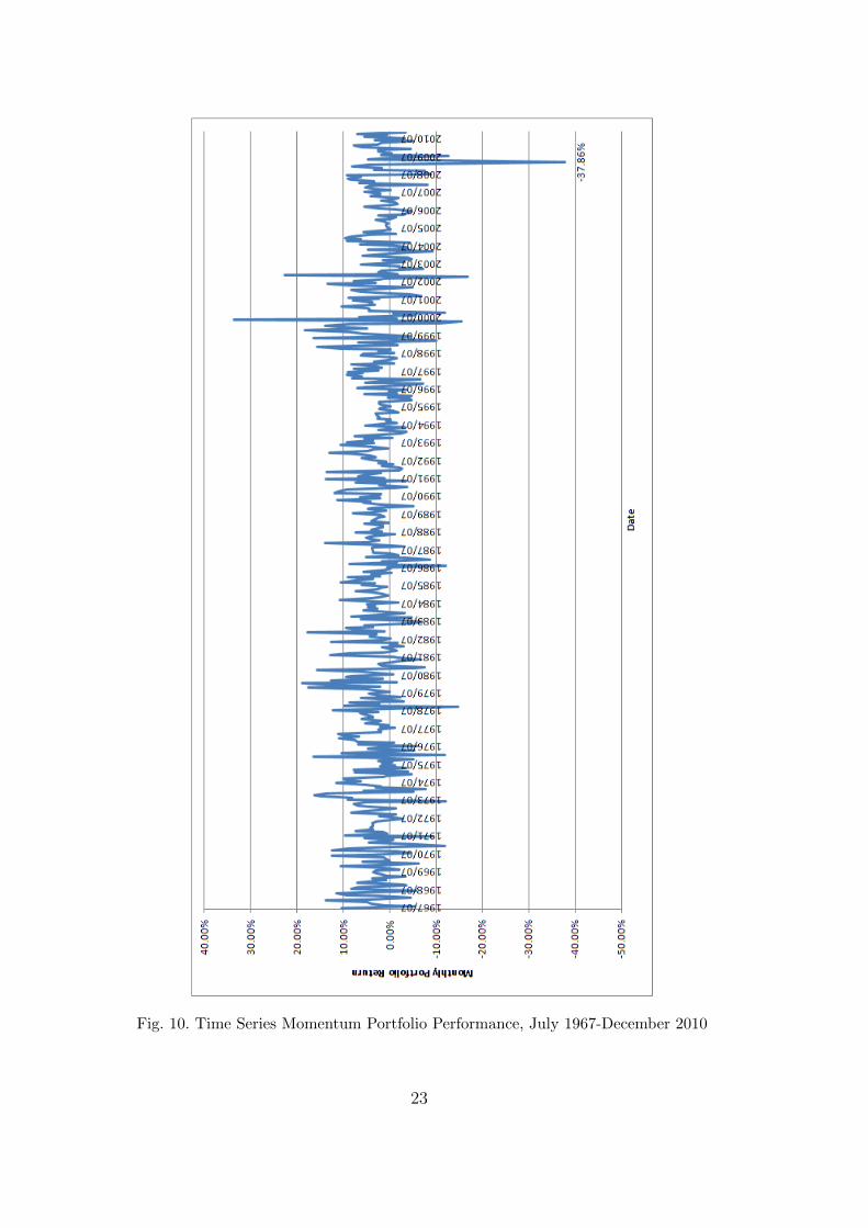
Fig. 10. Time Series Momentum Portfolio Performance, July 1967-December 2010

23

Fig. 11. Cumulative Monthly Returns of WML, WU-LO, July 1967-December 2010

24

Fig. 12. Cumulative Monthly Returns of WML, WU-LO, January 2000-December2010

References

Asness, C.S., Moskowitz, T.J. and Pedersen, L.H. (2013) Value and momentumeverywhere, Journal of Finance 68, 929–985.

Carhart, M. (1997) On persistence in mutual fund performance, Journal ofFinance 52, 57–82.

Chordia, T., and L. Shivakumar (2002) Momentum, business cycle, and time-varying expected returns, Journal of Finance 57, 985–1019.

Cooper, M., R. Gutierrez, and A. Hameed (2004) Market states and momen-tum, Journal of Finance 59, 1345–1365.

Daniel, K., and T. Moskowitz (2013) Momentum crashes, Swiss Finance In-stitute Research Paper, 13–61

Erb, C., and C. Harvey (2006) The strategic and tactical value of commodityfutures, Financial Analysts Journal 62, 69–97.

George, T.J. and Hwang, C.Y. (2004) The 52-week high and momentum in-vesting, Journal of Finance 59, 2145–2176.

Grundy, B.D. and Martin, J.S. (2001) Understanding the nature of the risksand the source of the rewards to momentum investing, Review of FinancialStudies 14, 29–78.

Jegadeesh, N. (1990) Evidence of predictable behavior of security returns,Journal of Finance 45, 881–898.

Jegadeesh, N., and S. Titman (1993) Returns to buying winners and sellinglosers: Implications for stock market efficiency, Journal of Finance 48, 65–91.

25

Lehmann, B. (1990) Fads, martingales, and market efficiency, The QuarterlyJournal of Economics 105, 1–28.

Lehmann, J. (2002) Momentum and autocorrelation in stock returns, Reviewof Financial Studies 15, 533–564.

Lo, Andrew W., and Archie Craig MacKinlay (1990) When are contrarianprofits due to stock market overreaction?, Review of Financial Studies 3,175–205.

Moskowitz, T. and Ooi, Y.H. and Pedersen, L.H. (2012) Time series momen-tum, Journal of Financial Economics 104, 228–250.

Okunev, J., and D. White (2003) Do momentum-based strategies still work inforeign currency markets?, Journal of Financial and Quantitative Analysis38, 425–447.

Rouwenhorst, K. (1998) International momentum strategies, Journal of Fi-nance 53, 267–284.

Rouwenhorst, K. (1999) Local return factors and turnover in emerging stockmarkets, Journal of Finance 54, 1439–1464.

26