SYSTEMS-LEVEL QUALITY IMPROVEMENT

Time Series Modelling and Forecasting of EmergencyDepartment Overcrowding

Farid Kadri & Fouzi Harrou & Sondès Chaabane &

Christian Tahon

Received: 15 January 2014 /Accepted: 7 July 2014 /Published online: 23 July 2014# Springer Science+Business Media New York 2014

Abstract Efficient management of patient flow (demand) inemergency departments (EDs) has become an urgent issue formany hospital administrations. Today, more and more atten-tion is being paid to hospital management systems to optimal-ly manage patient flow and to improve management strate-gies, efficiency and safety in such establishments. To this end,EDs require significant human and material resources, butunfortunately these are limited. Within such a framework,the ability to accurately forecast demand in emergency depart-ments has considerable implications for hospitals to improveresource allocation and strategic planning. The aim of thisstudy was to develop models for forecasting daily attendancesat the hospital emergency department in Lille, France. Thestudy demonstrates how time-series analysis can be used toforecast, at least in the short term, demand for emergencyservices in a hospital emergency department. The forecastswere based on daily patient attendances at the paediatricemergency department in Lille regional hospital centre,France, from January 2012 to December 2012. Anautoregressive integrated moving average (ARIMA) methodwas applied separately to each of the two GEMSA categoriesand total patient attendances. Time-series analysis was shownto provide a useful, readily available tool for forecastingemergency department demand.

Keywords Emergency department . Overcrowding . Timeseries . ARMA . Forecasting

Introduction

Emergency departments (EDs) are an important component ofhealthcare systems because they provide immediate and es-sential medical care for patients, but they are also the mostovercrowding component. Unfortunately, the role of the ED asa safety net is now under the threat of overcrowding [1, 2].The causes of this overcrowding are i) inadequate staffing,hospital bed shortages and inpatient boarding [3, 4], ii) in-crease in demand (patient flow) for EDs services [5, 6], and iii)influenza season (epidemic period) [7] which often generatesa large flows of patients. So, the influx of patients is one of thecauses of this overcrowding. The problem of the influx ofpatients, which is a direct cause of ED overcrowding inseveral nations [8–11, 6], affects both private and publichealth-care systems.

The management of patient flow is a challenge faced bymany hospitals, in particular emergency departments. Oneapproach to alleviate and mitigate problems associated withED overcrowding is to forecast levels of demand for ED carein advance (hours, days) in order to give health-care staff anopportunity to prepare for this demand.

The ability to predict demand in emergency departments iscrucial for designing strategies aimed at avoiding overcrowd-ing that may lead to strain situations in these establishments.Time series can be used by managers to make current deci-sions and plans based on long and/or short-term forecasting.

The main objective of this work was to propose a statisticalmodel based on univariate time series, which was then used topredict daily patient attendances at the paediatric emergencydepartment (PED) in Lille regional hospital centre, France.For this, in addition to the total daily arrivals (expected and

This article is part of the Topical Collection on Systems-Level QualityImprovement

F. Kadri : S. Chaabane :C. TahonUniv. Lille Nord de France, 59000 Lille, France

F. Kadri (*) : S. Chaabane :C. TahonUVHC, TEMPO Lab., “Production, Services, Information” Team,59313 Valenciennes, Francee-mail: farid.kadri@univ-valenciennes.fr

F. HarrouChemical Engineering Program, Texas A&M University at Qatar,Doha, Qatar

J Med Syst (2014) 38:107DOI 10.1007/s10916-014-0107-0

unexpected arrivals) at the PED, we considered two signifi-cant categories from the GEMSA (Groupes d’EtudeMulticentrique des Services d’Accueil, MulticentricEmergency Department Study Group in English) classifica-tion: unplanned patients (unexpected arrivals) that returnhome after PED care, and unplanned patients that are hospi-talized after emergency care.

The results yielded by these models will assist hospitalmanagers in their decision-making process to utilize and allo-cate medical staff better, taking the fluctuant demand on thesystem and individual zones in the emergency department intoconsideration. The remainder of this paper is organized asfollows: the context and the problem to be resolved in thisstudy are presented in the next two subsections. In secondsection presents the time-series modelling and how it can beused for forecasting demand in hospital emergency depart-ments. Third section presents the modelling technique used inthis work. Fourth section presents a brief description of thedata used. The data analysis and validation of the modelsusing real data are presented in Fifth section. Finally, sixthsection reviews the main points discussed in this work andconcludes the study.

Context of the study

Nowadays, with the growing demand for emergency medicalcare, the management of hospital emergency departments(EDs) has become increasingly important. For example, ac-cording to the reports by the Institute of Medicine of theNational Academies (2006) [12], between 1993 and 2003,visits to emergency departments in the United States increasedby 26 % while the number of EDs were reduced by 9 % [13].In France, as well as abroad, much effort has been made overthe past few decades to improve emergency department man-agement. However, the number of visits to EDs in France hasrapidly increased. Between 1996 and 1999, the annual numberof visits to EDs increased by 5.8 %, and increased by 43 %between 1990 and 1998 [14]. In addition, according to theannual public report published by the Medical EmergenciesCourt of Auditors, the annual number of ED visits doubledfrom 7 million to 14 million between 1990 and 2004 [15].Increasing patient demand in EDs is due to many factors,including proximity to these establishments, a need for exam-inations and to obtain rapid expert medical advice [16].

Modelling and forecasting daily patient volumes providesuseful information for hospital emergency departments whichmay be utilized for allocating resources and planning futureexpansion. Accurate prediction of patient attendances in anemergency department will help ED management to planbetter for the future. For example, organisation of the staffroster and efficient allocation of the resources required toprovide a good service in emergency departments. In addition,accurate prediction of daily patient attendances may provide

useful information to improve ED efficiency by reducing thenumber of patients waiting for treatment and health care, aswell as increasing the total number of patients treated. It iscritical for hospital emergency departments to plan and createstrategies to cope with the large number of patients arrivingmore effectively, and make the best use of the availableresources.

Problem to be solved

The anticipation and/or management of patient influx is one ofthe most crucial problems in emergency departments (EDs)throughout the world [17]. To deal with this influx of patients,emergency departments require significant human and mate-rial resources, as well as a high degree of coordination amonghuman and material elements [18, 19]. Unfortunately, theseresources are limited. The consequences of this influx ofpatients has resulted in problems of emergency departmentovercrowding [11, 2]. ED overcrowding affects i) patients:very lengthy waits, patients leave the ED without beingtreated, violence of angry patients against staff, reducedaccess to emergency medical services and increase inpatient mortality [20, 21], and ii) the quality of treat-ment and prognosis by medical staff who are oftenoverloaded thus leading to a decrease in physician jobsatisfaction [22, 23]. Consequently, ED managers mustcontrol the problems related to the care load flow(demand) to improve the organization and the manage-ment of resources and the internal restructuring reflectedby resource pooling, including technical platforms.

Time series and emergency department admissions

Due to the importance of forecasting the number of patientarrivals in the hospital system to maintain performance and tohelp enhance the management of hospital establishments,several forecasting techniques have been developed. Thesetechniques can be broadly divided into two categories: qual-itative and quantitative methods. Qualitative-based forecast-ing methods predict the future, usually using opinion andmanagement judgment of experts in specified fields [24].Quantitative methods [25], on the other hand, rely on mathe-matical models. These approaches are based on the analysis ofhistorical data and assume that past data patterns can be usedto forecast future data points. Techniques in this category aremostly based on time-series methods [26]. The advantage oftime-series techniques is their simplicity and effectiveness,and they are more attractive for practical applications. Manytime-series forecasting techniques are referenced in the bibli-ography, and they can be broadly categorized into two mainclasses: univariate and multivariate techniques. Univariate

107, Page 2 of 20 J Med Syst (2014) 38:107

techniques involve the analysis of a single variable whilemultivariate analysis examines two or multiple variablessimultaneously.

In the field of health care systems, increasing attention hasbeen accorded to time-series models to predict patient arrivalsin hospital establishments [27–30]. The literature reviewshows that time-series analysis has been largely applied inthe hospital sector to forecast patient arrivals, length of stay,and for projecting the utilization of inpatient days. In thisregard, some of the research efforts made by previous re-searchers deserve mentioning [31] presented Holt-Wintersexponential-smoothing and autoregressive integrated movingaverage models for forecasting monthly discharges and dif-ferences in occupancy in several hospitals [32] used threestatistical methods (moving averages and seasonal decompo-sition methods) to predict the number of ED visits at any timeof the week to a university hospital in New Mexico. Theyfound that simple models can be used to describe the numberof ED visits for each hour of the week [33] developed astatistical model for an emergency department at a hospitalin Israel based on 3 years of daily time-series data. They useda regression model with a linear trend, and 3 types of seasonalfactor representing the effects of the day of the week, themonth of the year, and the type of day (holiday, half workingday, or full working day) [34] employed two univariate time-series analysis methods (Box–Jenkins method and ad hocapproach) to model and forecast monthly patient volumesbetween 1986 and 1996 at King Faisal University familyand community medicine primary health care clinic, Al-Khobar, Saudi Arabia [35] used Box–Jenkins models to fore-cast the number of daily emergency admissions and the num-ber of beds occupied by emergency admissions on a dailybasis at Bromley Hospitals NHS Trust in the United Kingdom[36] studied ED patterns in a hospital in Tenerife, Spain. Theiranalysis was based on a time series of the number of EDpresentations every hour over a 6-year period (1997 to 2002)[37] used autoregressive (AR) and Welch spectral estimationmethods to analyze the electroencephalogram (EEG) signals.The parameters of autoregressive (AR) method were estimat-ed by using Yule–Walker. The results demonstrate superiorperformance of the covariance methods over Yule–walker ARand Welch methods [38] used ARIMA models to forecastward occupancy, due to SARS infection, for up to 3 days inadvance. The authors used seasonal decomposition methodsto obtain detailed estimates of the effects of the hour of day,the day of week, and the week of the year on attendances [39]reviewed the past 25 years of research into time-series fore-casting covering the period 1982–2005. The authors dividedthe time-series models into linear and nonlinear models. Theydiscussed the strengths and weaknesses of each method [40]used two statistical methods: i) exponential smoothing and ii)Box–Jenkins Method, to forecast the number of patients pres-ent each month from 2000 to 2005 at the ED of a regional

hospital in Victoria, Australia [41] applied an Adaptive AutoRegressive-Moving Average (A-ARMA) to analyze the elec-tromyographic (EMG) signals. The author found that A-ARMA present good models with few parameters and theirability to, with small p and q, represent a very rich set ofstationary time series in a parsimonious way [28] evaluatedthe use of four statistical methods (Box–Jenkins, time-seriesregression, exponential smoothing, and artificial neural net-work models) to predict daily ED patient volumes over27 months (from 2005 to 2007) in three different hospitalEDs in Utah and southern Idaho (USA). The authors com-pared four models with a benchmark multiple linear regres-sion model already available in the emergency medicine liter-ature. They claim that regression-based models incorporatingcalendar variables account for site-specific special-day effects,and allow for residual autocorrelation providing a more ap-propriate, informative, and consistently accurate approach forforecasting daily ED patient volumes [42] studied the tempo-ral relationships between the demands for key resources in theemergency department (ED) and the inpatient hospital in2006, and developed multivariate forecasting models. Theauthors compared the ability of the models they developed(multivariate models) to provide out-of-sample forecasts ofED census and the demands for diagnostic resources with aunivariate benchmarkmodel [43] used a time-series method topredict daily emergency department attendances. The authorsapplied an autoregressive integrated moving average(ARIMA) method separately to three acuity categories andtotal patient attendances at the ED of an acute care regionalgeneral hospital from July 2005 to March 2008. They con-cluded that time-series analysis provides a useful, readilyavailable tool for predicting emergency department workloadthat can be used for staff roster and resource planning [44]presented a hybrid system (called Online Multi-AgentMonitoring System) to solve the patient’s critical state moni-toring problems in real time. The medical monitoring systemcombines multi-agent approaches with time-series models(ARIMA).

There are also Autoregressive Moving Average modelswith eXternal inputs (ARMAX) and their variants (ARX,ARIMAX, SARIMAX…), which take into account the ex-planatory variables [26, 45]. The explanatory variables mayrepresent meteorological measurements (temperature,wind direction…), or epidemics. Finally, multiple time-series models, which are natural extensions of the uni-variate ARMA models in the sense that a vector ofdependent variables replaces the dependent variable,can be found in the literature. These models includevector autoregression (VAR), and its extensions (VMA,VARMA…), which is one of the most successful formultivariate time-series modelling [46, 47]. Thesemodels allow measurements from several time series tobe processed simultaneously.

J Med Syst (2014) 38:107 Page 3 of 20, 107

Time-series methods are interesting tools for predictingemergency department demand (number of patient arrivals).They are very useful as an initial significant analysis of patientflow because of their ease of use, implementation and inter-pretation within the framework of modelling and forecastingof emergency department overcrowding caused by the influxof patients.

In the next section, we present the method used in thisstudy to analyze and forecast demand in the paediatric emer-gency department in Lille hospital centre, France.

Univariate time-series forecasting

ED patient arrivals are defined as a temporal pattern; thenumber of patient arrivals in the ED varies considerablyaccording to the hour of day, the day of week, the week of

month and the month of year. To deal with the large influx ofpatients, we need a modelling approach that can give decision-makers a reliable estimate of future patient arrivals based oncurrent known levels.

A time series is a sequence of measurements indexed overtime or a set of chronologically ordered observations, andtime-series forecasting is the practice of using past and presentvalues of one ormore time series to predict future values of thetime series. Generally, time-series analysis has two main ob-jectives: one is to identify the nature of the phenomenonrepresented by the sequence of observations, the other is toforecast (or predict) future values of the time-series variable.Time-series forecasting methods assume that historical data isa good indicator of future demand.

In this paper, the main time series of interest is dailyattendances in an emergency department. We wished to ex-plore the practical problem of how well ED demand can be

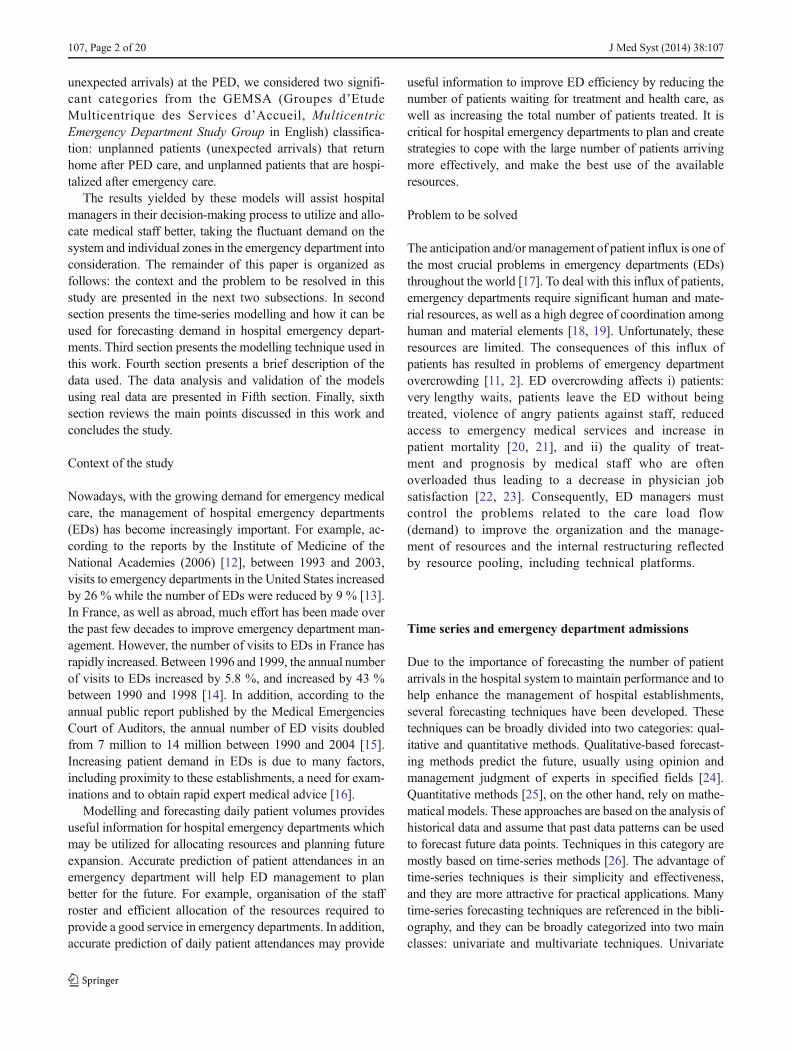
Fig. 1 Time-series modelling using ARIMA (Box and Jenkins) procedure

107, Page 4 of 20 J Med Syst (2014) 38:107

forecast, at least in the short term i.e., one day, using only thistime-series data. Hence, in this study we focused on time-series analysis methods. The use of observations available attime t of the number of patient arrivals at the emergencydepartment from a time series to forecast its value at somefuture time t + l can provide a basis for a variety of applica-tions such as: customer demand, medication inventory con-trol, economic and business planning, and general control ofhealth-care systems.

The results presented in the literature show that ARMAmodels [48, 49] provide a very accessible time-series analyticaltool both in terms of methodological constraints and the level ofmathematical models used that are less complex linear

stochastic equations. This analysis tool is mainly used forpredicting future values and identifying the structure of the timeseries. For this purpose, in this studywe used ARMAmodels toanalyze and forecast daily patient arrivals at the paediatricemergency department in Lille regional hospital centre, France.

Univariate time series: ARIMA modelling

In practice, most phenomena present a time dimension that isusually dissimulated but should be taken into account. This isthe case of patient flow data for which the patient flow Y t attime t depends on previous values (Y t�1; Y t�2;… ). The threeunivariate time-series models widely applied to model patient

0

250

500

750

1000

1250

1500

1750

2000

2250

2500

January February March April May June July August September October November December

Arriv

al

nu

mb

er

Month

0

20

40

60

80

100

1 8 15 22 29 36 43 50 57 64 71 78 85 92 99 106

113

120

127

134

141

148

155

162

169

176

183

190

197

204

211

218

225

232

239

246

253

260

267

274

281

288

295

302

309

316

323

330

337

344

351

358

365

Arr

ival

num

ber

Day

J Med Syst (2014) 38:107 Page 5 of 20, 107

Fig. 2 Actual number of arrivals per month from January 2012 to December 2012

Fig. 3 Daily paediatric emergency department arrivals from January to December 2012

volume in emergency departments are autoregressive process-es (AR), moving average processes (MA), and autoregressivemoving average processes (ARMA). Adding non-stationarymodels to the mix leads to the integrated ARMA orautoregressive integrated moving average (ARIMA) modelpopularized in the work by [48]. ARMA models are verycomprehensive linear models and can represent many typesof linear relationships, such as autoregressive (AR), movingaverage (MA), and mixed AR and MA time-series structures.

The AR model is intuitively appealing because it describeshow an observation directly depends upon one or more pre-vious measurements plus white noise. For time-seriesobservationsY t , the AR model of order p, which is alsowritten as AR(p), is defined by:

Y t ¼Xp

i¼1aiY t − i þ εt ð1Þ

where aj are non-seasonal AR parameters, and εt is zero-mean Gaussian noise εteNð0;σ2Þ .

MAmodels describe how an observation depends upon thecurrent white noise term as well as one or more previouserrors. An MA model of order q, also denoted by MA(q), isdefined as:

Y t ¼ εt þXq

j¼1bjεt− j ð2Þ

where bj are non-seasonal MA parameters. The ARMAmodel was first presented by Box and Jenkins [48]. ARMAmodels are more sophisticated stochastic models that combineelements of moving average methods and regression methods.One advantage of an ARMA process is that it involves fewerparameters than an MA or AR process alone [50]. The mixedAR and MA or ARMA model of order (p, q), also denotedautoregressive moving average, ARMA(p,q) is written as:

0

0,1

0,2

0,3

0,4

0,5

0,6

0,7

0,8

0,9

1

34 36 38 40 42 44 46 48 50 52 54 56 58 60 62 64 66 68 70 72 74 76 78 80 82 84 86 88 90 92 94 96

)F

DC(

noitc

nu

Fn

oitu

b ir tsiD

evit

alu

mu

C

Number of Patients

Monday Tuesday Wednsday Thursday Friday Saturday Sunday

Table 1 Patient category and admission mode according to the GEMSA classification

GEMSA classification Admission mode Description

GEMSA 1 (G1) Unplanned Patient dead on arrival or died before any resuscitation

GEMSA 2 (G2) Unplanned Patient not convened, unexpected arrival, returned home after emergency care

GEMSA 3 (G3) Planned Patient convened, expected arrival, returned home after emergency care

GEMSA 4 (G4) Unplanned Patient not convened, unexpected arrival, hospitalized after emergency care

GEMSA 5 (G5) Planned Patient convened, expected arrival, hospitalized after emergency care

GEMSA 6 (G6) Unplanned Patient requiring immediate or prolonged care (intensive care)

107, Page 6 of 20 J Med Syst (2014) 38:107

Fig. 4 Distribution function per day of the week of the number of patients received at the PED for the period of 2012

Y t ¼Xp

i¼1aiY t − i þ

Xq

j¼1bjεt − j þ εt ð3Þ

where Y t is the variable to be predicted using previous sam-ples of the time series, εt is a sequence of i.i.d. (independentand identically distributed) terms which have zero mean. Themodel parameters ai (auto-regressive part) establish a linearrelationship between the value predicted by the model at time tand the past values of the time series. Themodel parameters bj

(moving average part) establish a linear relationship betweenthe value predicted by the model at time k and a Gaussiandistribution of i.i.d. samples [51].

In time series analysis, the lag operator or backshift oper-

ator (B) defined as BkYt ¼ Yt�k; operates on an element of atime series to produce the previous element. Using backshiftoperator B, we can define the Eq. (3) as follow:

∅ Bð Þ Y t ¼ θ Bð Þ εt;∅ Bð Þ ¼ 1−a1B−a2B2−…−apBp

� �θ Bð Þ ¼ 1−bqB−bqB2−…− bqB

q� � ð4Þ

In relation to ARMA models, ARIMA models are extend-ed to include differencing. ARIMA processing has beenshown to be the most successful approach to model a broadvariety of time series [29, 48, 49]. In many cases it is a veryuseful method to fit time-series data. However, a lot of phe-nomena tend to vary from one season to another, thus theseasonal fluctuations may cause problems when fitting anARIMAmodel. The main feature of seasonal data is that thereare high correlations among observations from a certain timespan (day, week, month or quarter). When a time seriesexhibits seasonality, it is useful to try to exploit the correlationbetween the data at successive periods of time. SARIMAmodels will allow us to do that. If the data series containseasonal fluctuations, the SARIMA model can be used tomeasure the seasonal effect or eliminate seasonality.

Identification of ARIMA models

The main steps required to obtain the orders (p, q) and param-eters (ai , b j ) that appear in Eq. 3 are recalled below [48, 49](see Fig. 1):

0

19100

1683

2556

50912

0

2000

4000

6000

8000

10000

12000

14000

16000

18000

20000

22000

G1 G2 G3 G4 G5 G6

Arr

ival

num

ber

GEMSA classification

J Med Syst (2014) 38:107 Page 7 of 20, 107

Fig. 5 Distribution of visits to the PED according to the GEMSA classification recorded from database 2012

Fig. 6 Daily G2 arrivals at the paediatric emergency department from January 2012 to December 2012

& Time Series stationarity: Identification of the order ofdifferentiation

The identification of the structure of a time seriesstarts with the observation of its stationarity. Thenon-stationarity of a time series can be seen on thegraph of the series (the increase or decrease in thetrend) and through patterns of the autocorrelationfunction (ACF) of the series. To make a stationaryseries, Box proposed applying a differentiation term,i.e. replacing the original series with the series ofdifferences of adjacent points.

& Model estimation: identification of AR and MA ordersThe order of both the AR and the MA parts must

be estimated. Autocorrelation and partial autocorre-lation computation is used to obtain these orders.The order of the autoregressive term present in thefinal ARIMA model is equal to p, which corre-sponds to the number of significant peaks in thePartial autocorrelation function (PACF). The orderof the moving average term in the final ARIMAmodel is equal to q, which is the number of signif-icant peaks in the Autocorrelation function (ACF).

The estimated autoregressive parameters AR(p)and moving average MA(q) may be established usinga non-linear estimation method of maximum likeli-hood (maximum likelihood estimator). This calcula-tion is performed according to the orders of theARIMA parameters defined in the model identifica-tion phase.

& Selection and validation of the ARIMA modelsThe most suitable models chosen should offer

adequate predictions. Generally, in order to evaluatemodels, the data used are split into two groups: i)the training group, used to build the ARIMA model,

and ii) the validation group, to evaluate the ARIMAmodel. The post-verification of the model isachieved using two tests: i) testing of the signifi-cance of the parameters and ii) validation of thewhite noise residue hypothesis. Model validationrefers to various statistical specification tests tocheck the validity of the model.

To evaluate the predictive abilities of the models,several measures of a model’s ability to fit data havebeen developed. The following can be cited: percent-age variability in regression analyses (R2), RootMean Square Error (RMSE), Mean AbsolutePercentage Error (MAPE) [49], Absolute Deviation(MAD), Mean Square Error (MSE) [52], BayesianInformation Criterion (BIC) [53].

Residual analysis is the most important step inmodel validation. Several statistical tests (Jarque-Bera, Lilliefors test…) and plots of the residuals(histogram, Henry’s line, probability–probability plotor PP plot, and the normal Quantile-Quantile plot or

Fig. 7 Daily G4 arrivals at the paediatric emergency department from January 2012 to December 2012

Table 2 Descriptive statistics of the two GEMSA categories (G2 and G4arrivals)

Statistics Category G2 Category G4

Mean 53 8

Median 52 7

Standard deviation 10.88 3.10

Maximum 82 19

Minimum 22 1

First quartile 45 5

Third quartile 60 9

107, Page 8 of 20 J Med Syst (2014) 38:107

QQ plot…) can be used to examine the goodness offit to the historical data of the model selected. Themodel residuals are described as good if they havevarious properties: normality, homoscedasticity, andindependence.

Data analysis

In this section we describe the data sources and the data onwhich we based our analysis and the forecasting models thatwe used.

Description of the data used

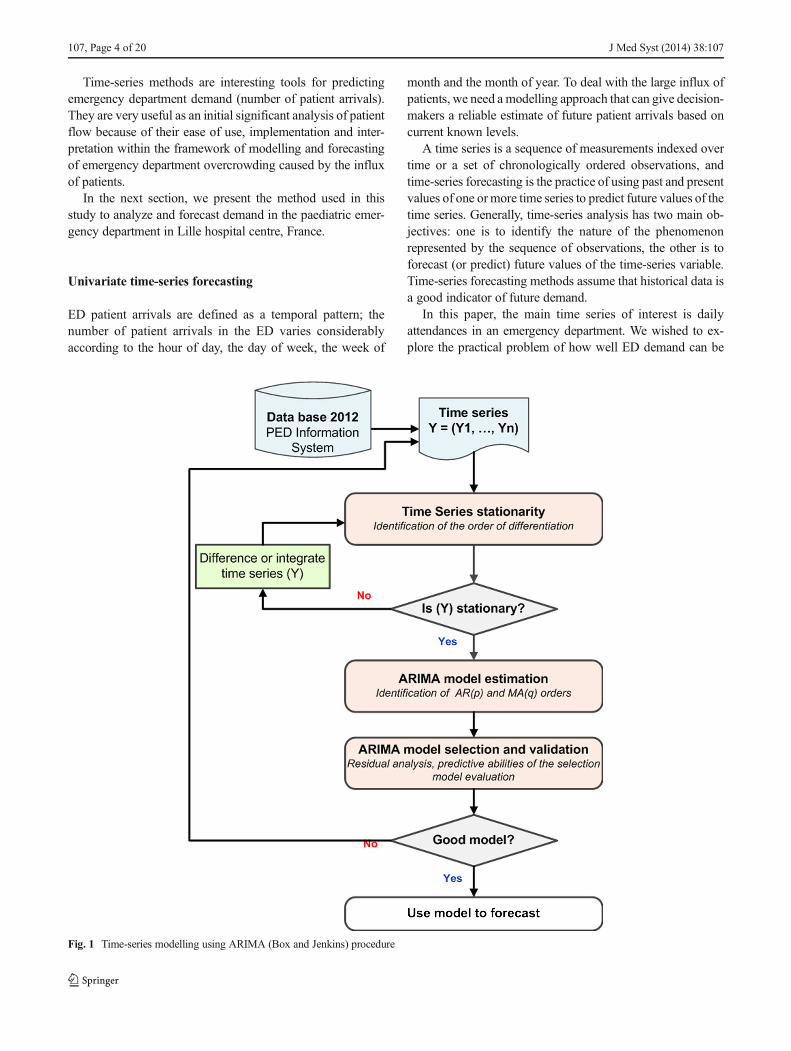
Lille Regional Hospital Centre (CHRU) serves fourmillion inhabitants in Nord-Pas-de-Calais, a region char-acterized by one of the largest population densities inFrance (7 % of the French population). The paediatricemergency department (PED) in Lille regional hospitalcentre (CHRU) is open 24 h a day and receives 23 900

patients a year on average. Besides its internal capacity,the PED shares many resources, such as administrativepatient registration, clinical laboratory, scanner, magneticresonance imaging (MRI), X-rays and blood bank, withother hospital departments.

This retrospective study was conducted utilizing a datasetextracted from the database of Lille regional hospital centrepaediatric emergency department (PED). The data used in thispaper are the time series of daily patient attendances at Lilleregional hospital centre PED, from January 2012 to December2012.

The purpose of this paper is to describe how statisticalforecasting methods were used to make short-term (i.e.one day) predictions for daily ED attendances at Lilleregional hospital centre. Before any attempt to modeland forecast three times series (G2, G4 of GEMSA clas-sification and total daily attendances, described in the nextsection), it was critical to conduct preliminary descriptiveanalyses of the data, paying particular attention to theidentification of important features such as seasonal pat-terns, cyclical variations, trends, outliers, and any othernoteworthy fluctuations in the series.

Fig. 8 Daily attendances at the paediatric emergency department of G2, G4 and total arrivals from January 2012 to December 2012

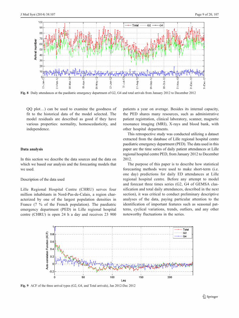
Fig. 9 ACF of the three arrival types (G2, G4, and Total arrivals), Jan 2012-Dec 2012

J Med Syst (2014) 38:107 Page 9 of 20, 107

Analysis of the data used

Descriptive account of arrivals

Figure 2 provides the actual total number of patient arrivalsper month from January 2012 to December 2012. In general,the flow of patients varied between winter and/or epidemicperiods (November – March) and normal periods (April –October). It appears that the traffic was relatively light fromJuly to September, as shown in this figure.

Figure 3 presents the daily arrivals at the paediatric emer-gency department over the entire period (from January 2012to December 2012). This figure shows that the daily arrivalsdo not tend to increase or decrease over the duration of thedata set. So, on average over the entire period of year (fromJanuary to December 2012), it appears that there is no trend inthis time series. The number of patients arriving at the PEDvaries considerably according to the day of the week, asshown by the height of individual spikes in Fig. 3. This couldbe explained by:

& More daily arrivals on certain days of the week: morearrivals were observed on Sundays and Mondays thanthe rest of the week, as shown in Fig. 4. According to thisFigure, with the cumulative distribution function, CDF=0.5, a difference of 11 patients per day of the week wasrecorded, with arrival numbers of 59 patients registered onWednesday and 71 patients on Monday. Also, in 80 % ofcases (CDF=0.8), a difference of 15 patients was recordedbetween Wednesday and Monday.

& Special event days that may lead to abnormally high PEDarrivals, like holidays, sporting events and festivals in theregion.

Classification of patients in emergency departments

Two main schemes exist by which such patients may becategorized: the Multicentric Emergency Department Study

Group (Groupes d'Etude Multicentrique des Servicesd’Accueil, GEMSA), and the clinical classification of emer-gency patients called CCMU (Classification Clinique desmaladies des Urgences) [54]. This paper only focuses on theGEMSA classification, which was developed by theCommission of Emergency Medicine of the FrenchResuscitation Society (Commission de Médecine d’Urgencede la Société de Réanimation de langue Française). TheGEMSA classification identifies six groups of patients accord-ing to the outcome on leaving the ED, as summarized inTable 1. Each group is associated with a different care load.The classification criteria were established according to theinput and output mode of the patients, and the programming ornot of the care activity. The GEMSA classification can pro-vide useful information about the patient’s arrival, which maybe planned or unplanned, and/or significant and prolongedsupport. In addition, GEMSA classification traces the organi-zation of the care activities and the patient’s pathway withinthe emergency department. This classification could be usedto predict resource consumption in an ED. Groups G4 and G6are characterized by an intense workload (heavyworkload) forthe medical and nursing staff and the utilization of significantradiological as well as biological means.

Figure 5 shows the distribution of visits according to theGEMSA classification recorded from January to December2012. As it can be seen in Fig. 4, over 80 % of patients whoarrived in the PED were unplanned, G2; these patients usuallyreturned home after treatment at the PED. G4, unexpectedarrivals, accounted for over 10.7 %; most of these patientswere hospitalized after treatment in the PED.

Fig. 10 Auto-scaled daily attendances of the three time series

Table 3 Parameters of the three models

Parameters G2, ARMA (2,1) G4, ARMA (1,1) Total, ARMA (2,1)

a1 0.36±0.013 0.24±0.016 0.22±0.070

a2 0.07±0.012 – 0.01±0.069

b1 0.4±0.030 0.235±0.031 0.23±0.030

107, Page 10 of 20 J Med Syst (2014) 38:107

Figures 6 and 7 present the daily arrivals at the paediatricemergency department from January 2012 to December 2012,for the two patient categories, i.e. G2 and G4, respectively.According to Figs. 6 and 7, it can be observed that the timeseries do not exhibit a significant trend. It can be noted that itis important to predict the total number of arrivals at the PED

and the number of arrivals of patients in these two categories(G2 and G4), in order to avoid overcrowding, to organizeresources better and to reduce the need for care servicesdownstream of the PED.

The catalogue of descriptive statistics for the twocategories (G2 and G4) is presented in Table 2.

Fig. 11 Observed and predicted daily attendances at the emergency department per patient category, Jan 2012 - Dec 2012

J Med Syst (2014) 38:107 Page 11 of 20, 107

According to this table, the maximum daily patient arrivals atthe PED were 82 and 19 for G2 and G4 respectively. Also, theinterquartile range (difference between the first and the thirdquartile) was equal to 15 and 4 for the categories G2 and G4respectively. In the case of category G4, the number of pa-tients arriving at the PED varied between 5 and 9 in case of thefirst quartile and the third quartile respectively (see Table 2).

The challenge in this study was to determine and validateforecasting models for daily patient attendances at the paedi-atric emergency department (PED) in Lille regional hospitalcentre, France. For this, we considered the two patient cate-gories (G2 and G4) presented above, and total daily atten-dances at the PED. In the next section, we present the time-series forecasting method used in this study.

0 2 4 6 8 10 12 14 16 18 20

0

2

4

6

8

10

12

14

16

18

20

Num ber of daily ED attendances

Num

ber o

f p

redic

ted d

aily E

D a

ttendances

y = 1*x + 0.0028

2.99993 32.962.98

33.02 G4

30 40 50 60 70 80 90 100

30

40

50

60

70

80

90

100

Numbers of daily PED attendances

Nu

mb

ers o

f p

re

dic

ted

da

ily P

ED

atte

nd

an

ce

s

y = 1*x - 0.0061

Total

20 30 40 50 60 70 80 90

20

30

40

50

60

70

80

90

Numbe r of da ily PED a tte nda nce s

Nu

mb

er

of p

red

icte

d d

aily P

ED

atte

nd

an

ce

s

y = 0.99*x + 0.14

G 2

Fig. 12 Scatter plot of daily attendances at the emergency department per patient category, observed versus predicted, Jan 2012-Dec 2012

107, Page 12 of 20 J Med Syst (2014) 38:107

Experimental results

According to the GEMSA classification admission mode(Table 1), we considered two main types of patient arrivals:G 2 and G 4 unplanned admission modes, and total arrivals atthe PED.

Fig. 13 Residuals of the three ARMA models selected: G2, G4, and Total time series

Table 4 Statistical validation measures applied to data from Fig. 8

Parameters G2, ARMA (2,1) G4, ARMA (1,1) Total, ARMA (2,1)

R2 0.99 0.99 0.99

RMSE 0.781 0.015 0.141

J Med Syst (2014) 38:107 Page 13 of 20, 107

The first step in any time-series analysis is to plot the obser-vations against time to obtain simple descriptive measures of themain properties of the series. Time-series plots provide a pre-liminary understanding of the time behaviour of the series. Thegraph should highlight important features of the series, such astrends and seasonality. The data series of daily attendances inemergency departments of GEMSA patient categories (i.e. G2,G4, and total patient attendances), collected from January 2012to December 2012, were firstly used to develop a descriptivemodel. It is important to verify beforehand the periodicity (orseasonality) of the time series that needs to be modelled. To thisend, the autocorrelation function analysis (ACF), also calledcorrelogram, is usually used to determine the periodicity in thetime series analyzed. It is well known that the distance betweenextremum points in the autocorrelation functions gives the peri-od of the time series. Plots of these times series and the

corresponding auto-correlation functions (ACF) are shown inFigs. 8 and 9, respectively.

From the time-series plot depicted in Fig. 8, it is apparent thatthe series does not have a long-term trend or seasonality. Thestationarity of these three series was confirmed by the Phillips-Perron Test, i.e. p-value of the test=0.01, which is lower than5% [55]. This led us to study stationary series with ARMA(p,q),(i.e. ARIMA(p,0,q)), According to Fig. 9, no apparent periodic-ity can be observed in the ACF. The similarity between theautocorrelation functions of the daily attendances time seriescan also be seen. The ACF also decreases exponentially to 0as the lag increases. The presence of a significant short-termdependence (short-memory) can also be observed in all the timeseries. The short-memory property, or short-term dependence,describes the low-order correlation structure of a series. It is wellknown that the ARMA processes, also termed short memory,

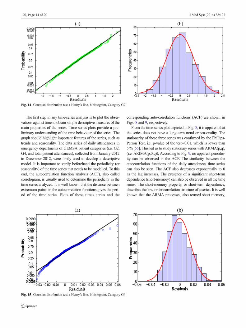
Fig. 14 Gaussian distribution test a Henry’s line, b histogram, Category G2

Fig. 15 Gaussian distribution test a Henry’s line, b histogram, Category G4

107, Page 14 of 20 J Med Syst (2014) 38:107

developed by Box and Jenkins, model short-term correlations ina time series.

These data, which are shown in Fig. 8, were scaled to bezero mean with a unit variance, and then used to develop amodel using the following equation:

bY i ¼ Y i−μY i

σY i

� �ð5Þ

These operations were reversed (multiplied by st.dev,σY i ,and mean added, μY i , for each time series) after the forecast-ing procedures so that the predictions correspond to the orig-inal series. The three transformed time series (G2, G4 andtotal) are depicted in Fig. 10.

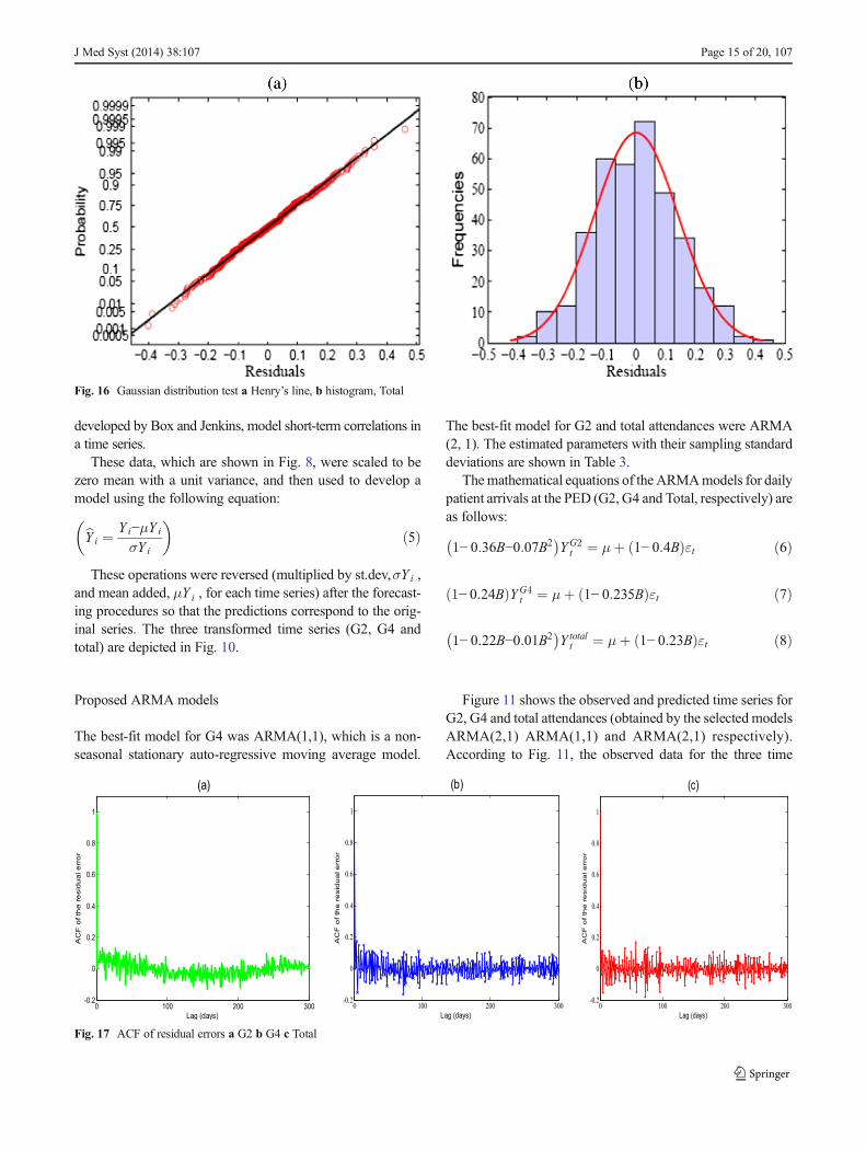
Proposed ARMA models

The best-fit model for G4 was ARMA(1,1), which is a non-seasonal stationary auto-regressive moving average model.

The best-fit model for G2 and total attendances were ARMA(2, 1). The estimated parameters with their sampling standarddeviations are shown in Table 3.

Themathematical equations of the ARMAmodels for dailypatient arrivals at the PED (G2, G4 and Total, respectively) areas follows:

1− 0:36B−0:07B2� �

YG2t ¼ μþ 1− 0:4Bð Þεt ð6Þ

1− 0:24Bð ÞYG4t ¼ μþ 1− 0:235Bð Þεt ð7Þ

1− 0:22B−0:01B2� �

Y totalt ¼ μþ 1− 0:23Bð Þεt ð8Þ

Figure 11 shows the observed and predicted time series forG2, G4 and total attendances (obtained by the selected modelsARMA(2,1) ARMA(1,1) and ARMA(2,1) respectively).According to Fig. 11, the observed data for the three time

Fig. 16 Gaussian distribution test a Henry’s line, b histogram, Total

0 100 200 300-0.2

0

0.2

0.4

0.6

0.8

1

AC

F o

f th

e r

esid

ua

l e

rro

r

Lag (days)

(a)

0 100 200 300-0.2

0

0.2

0.4

0.6

0.8

1

AC

F o

f th

e re

sid

ua

l e

rro

r

Lag (days)

(b)

0 100 200 300-0.2

0

0.2

0.4

0.6

0.8

1

AC

F o

f th

e re

sid

ua

l e

rro

r

Lag (days)

(c)

Fig. 17 ACF of residual errors a G2 b G4 c Total

J Med Syst (2014) 38:107 Page 15 of 20, 107

series are well-adjusted by the three models selected (Total,G2 and G4). Furthermore, to illustrate the quality of theARMA-based models selected, one common and simple ap-proach is to regress predicted versus observed values (or viceversa). Ideally, on a plot of observed versus predicted values,the points should be scattered around a diagonal straight line(Y ¼ Y ). This plot can be used directly to present a goodnessof fit as vertical deviations from the ‘perfect’ line indicate anybiases present (either overall, or in certain sections of the data).

The scatter plots of observed versus predicted attendancesfor the three best-fit models selected, and the regression lineare shown in Fig. 12. It shows that the points are distributedalong the regression line, i.e. for the three studied times series,the slope of the regression line between observed and predict-ed values is not significantly different from 1 and the y-intercept is not significantly different from 0. Therefore, themodels were successful in accounting for most of the signif-icant autocorrelations present in the data, and there is noindication of a curvature or other anomalies. This type ofgraph presents very similar information to a residuals versuspredicted plot, widely used in statistical diagnostics [50].According to Fig. 12, it can be seen that the scatter plots ofobserved and predicted daily attendances, or patient arrivals,at the paediatric emergency department (PED) indicate areasonable performance of the selected models.

Model selection and validation

The models were selected and validated according to thereviewing criteria used for assessing model performance(“Identification of ARIMA Models” section). In this paperthe models selected were evaluated by calculating the perfor-

mance metrics RMSE and R2 . The quality of fit of the ARMAmodels selected was first evaluated in terms of the RMSEcriterion, which represents the mean deviation of the predictedvalues with respect to the observed ones. RMSE is defined as:

RMSE ¼

ffiffiffiffiffiffiffiffiffiffiffiffiffiffiffiffiffiffiffiffiffiffiffiffiffiX bY−Y� �2

n

vuutð9Þ

where Y are the measured values, Y are the correspondingpredicted values and n is the number of samples. This statisticis easier to interpret since it has the same units as the valuesplotted on the vertical axis. Low RMSE values indicate goodmodel performance, that is, a good match between predictedand measured values. The RMSE value depends on the meanvalue of the variable, which hinders comparisons betweenmodels for predicting variables that have different meanvalues. Lower RMSE values (RMSE< 1) are indicative of amodel that represents the observed values better.

Fig. 18 ARMA (2,1) fitted total series (01 Nov–22 Dec 2012) and forecasted (22 Dec to 28 Dec 2012)

Fig. 19 ARMA (2,1) fitted G2 series (01 Nov–22 Dec 2012) and forecasted (22 Dec–28-Dec 2012)

107, Page 16 of 20 J Med Syst (2014) 38:107

We also evaluated the goodness of fit using the coefficient

of determination, or R2 , which corresponds to the percentageof variability explained by the model. A higher R2 indicatesbetter model accuracy. The latter is defined as:

R2 ¼ 1−SSR

SSYð10Þ

where SSR is the sum of squared residuals, also known as thesum of squared errors of prediction. It is a measure of thediscrepancy between the data observed and an estimationmodel (predicted values):

SSR ¼XN

i¼1Y i−bY i

� �2ð11Þ

Here, Y i are the observed values, and Y i are the predictedvalues obtained from the selectedmodel. A small SSR indicates aclose fit of themodel to the data. IfRSS is equal to zero themodelis perfect, i.e. for allN samples the observed values coincidewiththe predicted values. SSY is the sum of the squared differencesbetween the observed values and the average observed data:

SSY ¼XN

i¼1Y i− Y� �2 ð12Þ

where Y i are the observed values, and Y is the mean of theobserved data. SSY is assumed to be a theoretical referencemodel where for each experimental response (observed data) a

constant value is calculated as the average experimental re-sponse. The coefficient of determination R2 is also defined asthe square of the correlation between the response values and thepredicted response values. This statistic measures how success-ful the fit is in explaining the variation of the data. A value ofR2¼ 1 , upper bound and desired value, denotes that the modelfits the data perfectly. The degree of fit declines the further thestatistics are from one. For example, a value of R2¼ 0:99

means that 99 % of the total sum of squares in the training setis explained by the model, and that only 1 % is in the residuals.

As shown in Table 4, the high R2 and the low RMSE of thebest-fit models show that all three models closely representedthe observed time series.

Residual analysis

The diagnostic verification of model adequacy is the last taskin ARMA model building. Firstly, it is necessary to checkwhether the residual distribution follows a Gaussian distribu-tion. To this end, the residual normality hypothesis was veri-fied in this study by examining Henry’s line and the histo-gram. The latter is the simplest graphical tool that allows us tovisually check the normality of the residuals. It can be recalledthat for the line of Henry, the normality of the residual distri-bution can be recognized by the quality of the alignment of thepoints. If residuals are distributed according to a normaldistribution then the points should be aligned.

Fig. 20 ARMA (1,1) fitted G4 series (01 Nov–22 Dec 2012) and forecasted (22 Dec–28 Dec 2012)

Table 5 Comparison between the observed data and the predicted data obtained by fitting January to December 2012

Horizon H Total Forecast Total error G2 Forecast G2 error G4 Forecast G4 error

1 76 73.5237 2.4763 66 62.8051 3.1949 7 8.8255 1.8255

2 71 69.2891 1.7109 65 62.4135 2.5865 6 8.3917 2.3917

3 69 67.9322 1.0678 60 62.0918 2.0918 7 8.5370 1.5370

4 65 66.4108 1.4108 57 61.7788 4.7788 5 8.6298 3.6298

5 73 66.4114 6.5886 62 61.4768 0.5232 8 8.6511 0.6511

6 66 65.6456 0.3544 56 61.1853 5.1853 8 8.6524 0.6524

7 71 65.9898 5.0102 56 60.9041 4.9041 5 8.6535 3.6535

J Med Syst (2014) 38:107 Page 17 of 20, 107

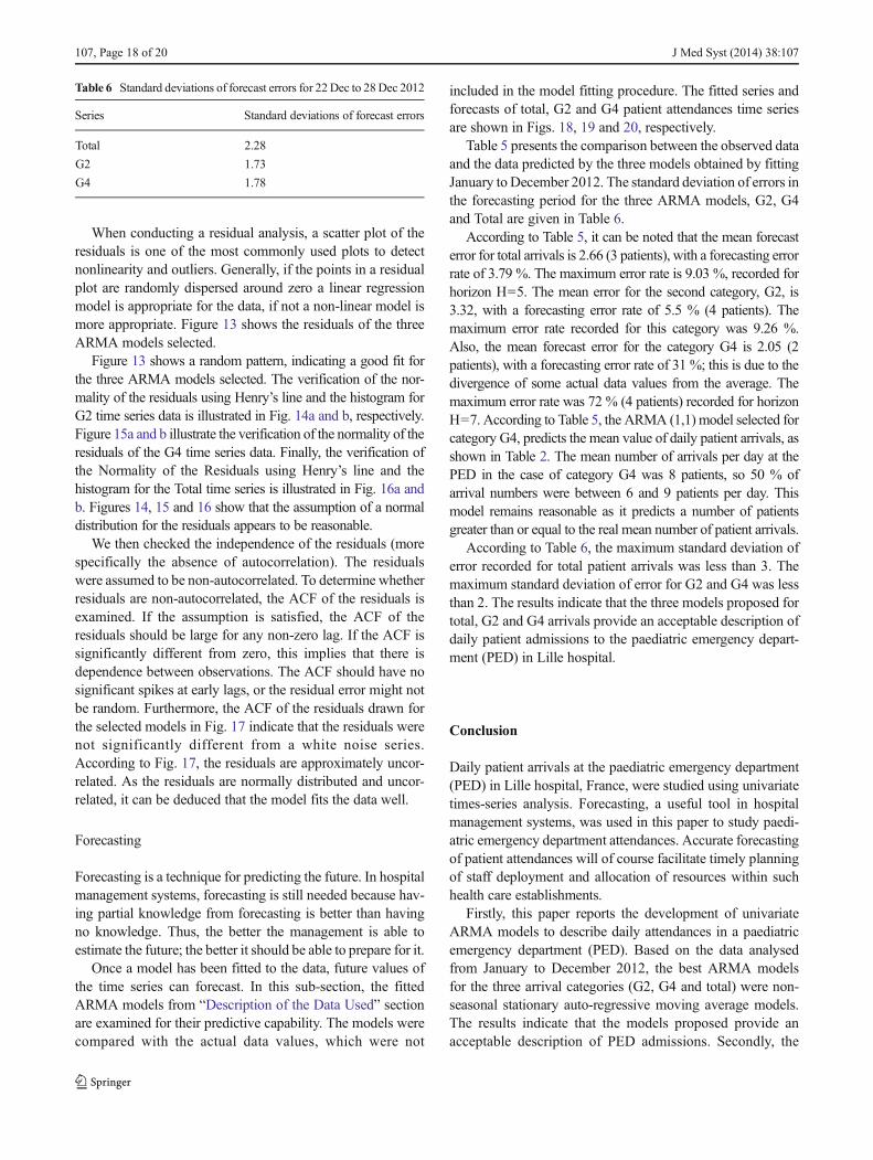
When conducting a residual analysis, a scatter plot of theresiduals is one of the most commonly used plots to detectnonlinearity and outliers. Generally, if the points in a residualplot are randomly dispersed around zero a linear regressionmodel is appropriate for the data, if not a non-linear model ismore appropriate. Figure 13 shows the residuals of the threeARMA models selected.

Figure 13 shows a random pattern, indicating a good fit forthe three ARMA models selected. The verification of the nor-mality of the residuals using Henry’s line and the histogram forG2 time series data is illustrated in Fig. 14a and b, respectively.Figure 15a and b illustrate the verification of the normality of theresiduals of the G4 time series data. Finally, the verification ofthe Normality of the Residuals using Henry’s line and thehistogram for the Total time series is illustrated in Fig. 16a andb. Figures 14, 15 and 16 show that the assumption of a normaldistribution for the residuals appears to be reasonable.

We then checked the independence of the residuals (morespecifically the absence of autocorrelation). The residualswere assumed to be non-autocorrelated. To determine whetherresiduals are non-autocorrelated, the ACF of the residuals isexamined. If the assumption is satisfied, the ACF of theresiduals should be large for any non-zero lag. If the ACF issignificantly different from zero, this implies that there isdependence between observations. The ACF should have nosignificant spikes at early lags, or the residual error might notbe random. Furthermore, the ACF of the residuals drawn forthe selected models in Fig. 17 indicate that the residuals werenot significantly different from a white noise series.According to Fig. 17, the residuals are approximately uncor-related. As the residuals are normally distributed and uncor-related, it can be deduced that the model fits the data well.

Forecasting

Forecasting is a technique for predicting the future. In hospitalmanagement systems, forecasting is still needed because hav-ing partial knowledge from forecasting is better than havingno knowledge. Thus, the better the management is able toestimate the future; the better it should be able to prepare for it.

Once a model has been fitted to the data, future values ofthe time series can forecast. In this sub-section, the fittedARMA models from “Description of the Data Used” sectionare examined for their predictive capability. The models werecompared with the actual data values, which were not

included in the model fitting procedure. The fitted series andforecasts of total, G2 and G4 patient attendances time seriesare shown in Figs. 18, 19 and 20, respectively.

Table 5 presents the comparison between the observed dataand the data predicted by the three models obtained by fittingJanuary to December 2012. The standard deviation of errors inthe forecasting period for the three ARMA models, G2, G4and Total are given in Table 6.

According to Table 5, it can be noted that the mean forecasterror for total arrivals is 2.66 (3 patients), with a forecasting errorrate of 3.79 %. The maximum error rate is 9.03 %, recorded forhorizon H=5. The mean error for the second category, G2, is3.32, with a forecasting error rate of 5.5 % (4 patients). Themaximum error rate recorded for this category was 9.26 %.Also, the mean forecast error for the category G4 is 2.05 (2patients), with a forecasting error rate of 31 %; this is due to thedivergence of some actual data values from the average. Themaximum error rate was 72 % (4 patients) recorded for horizonH=7. According to Table 5, the ARMA (1,1) model selected forcategory G4, predicts the mean value of daily patient arrivals, asshown in Table 2. The mean number of arrivals per day at thePED in the case of category G4 was 8 patients, so 50 % ofarrival numbers were between 6 and 9 patients per day. Thismodel remains reasonable as it predicts a number of patientsgreater than or equal to the real mean number of patient arrivals.

According to Table 6, the maximum standard deviation oferror recorded for total patient arrivals was less than 3. Themaximum standard deviation of error for G2 and G4 was lessthan 2. The results indicate that the three models proposed fortotal, G2 and G4 arrivals provide an acceptable description ofdaily patient admissions to the paediatric emergency depart-ment (PED) in Lille hospital.

Conclusion

Daily patient arrivals at the paediatric emergency department(PED) in Lille hospital, France, were studied using univariatetimes-series analysis. Forecasting, a useful tool in hospitalmanagement systems, was used in this paper to study paedi-atric emergency department attendances. Accurate forecastingof patient attendances will of course facilitate timely planningof staff deployment and allocation of resources within suchhealth care establishments.

Firstly, this paper reports the development of univariateARMA models to describe daily attendances in a paediatricemergency department (PED). Based on the data analysedfrom January to December 2012, the best ARMA modelsfor the three arrival categories (G2, G4 and total) were non-seasonal stationary auto-regressive moving average models.The results indicate that the models proposed provide anacceptable description of PED admissions. Secondly, the

Table 6 Standard deviations of forecast errors for 22 Dec to 28Dec 2012

Series Standard deviations of forecast errors

Total 2.28

G2 1.73

G4 1.78

107, Page 18 of 20 J Med Syst (2014) 38:107

models developed were used to forecast the number of dailyarrivals at the PED. The results in the case studied indicate thatthe forecasting performance of the models proposed is accept-able. The approach proposed and lessons learned from thisstudy may assist other regional hospitals and their emergencydepartments in carrying out their own analyses to aid plan-ning. The results have also shown the suitability of our ap-proach in predicting the number of patient arrivals at the PEDin Lille. The time series is essentially linear and thereforeARMA modelling offered robust predictions in many cases.

However, this study raises several questions about relatedseries. The forecasting of ED visits on a finer time scale, suchas hourly, would be very interesting. Accurate forecasting ofthese series would facilitate planning of nursing rosters andallocation of staff within the department, and could potentiallyassist in bed occupancy prediction. It may be possible to find abetter model using other fitting techniques, which would leadto more accurate forecasts. The scope can be expanded tomultivariate forecasting models. We could also forecast dailyattendances at the PED using other explanatory variables suchas meteorological measurements (temperature…), and epidem-ic events. To this end, the Autoregressive Moving Averagemodel with eXternal inputs (ARMAX) could be used.

References

1. Gordon, J. A., Billings, J., Asplin, B. R., and Rhodes, K. V., Safetynet research in emergency medicine: proceedings of the AcademicEmergency Medicine Consensus Conference on “The UnravelingSafety Net”. Acad. Emerg. Med. Off. J. Soc. Acad. Emerg. Med.8(11):1024–1029, 2001.

2. Boyle, A., Beniuk, K., Higginson, I., and Atkinson, P., Emergencydepartment crowding: Time for interventions and policy evaluations.Emerg. Med. Int. 2012:2012.

3. Cooke, M. W., Wilson, S., Halsall, J., and Roalfe, A., Total time inEnglish accident and emergency departments is related to bed occu-pancy. Emerg. Med. J. EMJ 21(5):575–576, 2004.

4. Sun, B. C., Mohanty, S. A., Weiss, R., Tadeo, R., Hasbrouck, M.,Koenig, W., Meyer, C., and Asch, S., Effects of hospital closures andhospital characteristics on emergency department ambulance diver-sion, Los Angeles County, 1998 to 2004. Ann. Emerg. Med. 47(4):309–316, 2006.

5. Howard, M. S., Davis, B. A., Anderson, C., Cherry, D., Koller, P.,and Shelton, D., Patients’ perspective on choosing the emergencydepartment for nonurgent medical care: a qualitative study exploringone reason for overcrowding. J. Emerg. Nurs. JEN Off. Publ. Emerg.Dep. Nurses Assoc. 31(5):429–435, 2005.

6. Kadri, F., Chaabane, S., Harrou, F., et Tahon, C., Modélisation etprévision des flux quotidiens des patients aux urgences hospitalièresen utilisant l’analyse de séries chronologiques. In: 7ème conférencede Gestion et Ingénierie des Systèmes Hospitaliers (GISEH), Liège,Belgique, 2014, pp. 8.

7. Schull, M. J., Mamdani, M. M., and Fang, J., Influenza and emer-gency department utilization by elders. Acad. Emerg. Med. Off. J.Soc. Acad. Emerg. Med. 12(4):338–344, 2005.

8. Espinosa, G., Miró, O., Sánchez, M., Coll-Vinent, B., and Millá, J.,Effects of external and internal factors on emergency departmentovercrowding. Ann. Emerg. Med. 39(6):693–695, 2002.

9. Li, G., Lau, J. T., McCarthy, M. L., Schull, M. J., Vermeulen, M., andKelen, G. D., Emergency department utilization in the United Statesand Ontario, Canada. Acad. Emerg. Med. Off. J. Soc. Acad. Emerg.Med. 14(6):582–584, 2007.

10. Bair, A. E., Song, W. T., Chen, Y.-C., and Morris, B. A., The impactof inpatient boarding on ED efficiency: a discrete-event simulationstudy. J. Med. Syst. 34(5):919–929, 2010.

11. Kolker, A., Process modeling of emergency department patient flow:effect of patient length of stay on ED diversion. J. Med. Syst. 32(5):389–401, 2008.

12. IMNA, Institute of Medicine Committee on the Future of EmergencyCare in theU.S. Health System. Hospital- based emergency care: at thebreaking point. TheNational Academies Press,Washington, DC, 2006.

13. Kellermann, A. L., Crisis in the emergency department. N. Engl. J.Med. 355(13):1300–1303, 2006.

14. Baubeau, D., Deville, A., et M. Joubert, Les passages aux urgences de1990 à 1998: une demande croissante de soins non programmés. 72, 2000.

15. Cours des comptes, Les urgences médicales, constats et évolutionrécente, rapport public annuel—08 février 2007. 2007.

16. Roh, C.-Y., Lee, K.-H., and Fottler, M. D., Determinants of hospitalchoice of rural hospital patients: the impact of networks, servicescopes, and market competition. J. Med. Syst. 32(4):343–353, 2008.

17. Kadri, F., Pach, C., Chaabane, S., Berger, T., Trentesaux, D., Tahon,C., and Sallez, Y., Modelling and management of the strain situationsin hospital systems using un ORCA approach, IEEE IESM, 28–30October », RABAT - MOROCCO, 2013, p. 10.

18. Kadri, F., Chaabane, S., and Tahon, C., A simulation-based decisionsupport system to prevent and predict strain situations in emergencydepartment systems. Simul. Model. Pract. Theory 42:32–52, 2014.

19. El-Masri, S., and Saddik, B., An emergency system to improve am-bulance dispatching, ambulance diversion and clinical handover com-munication—a proposedmodel. J. Med. Syst. 36(6):3917–3923, 2012.

20. Sprivulis, P. C., Da Silva, J.-A., Jacobs, I. G., Frazer, A. R. L., andJelinek, G. A., The association between hospital overcrowding andmortality among patients admitted viaWestern Australian emergencydepartments. Med. J. Aust. 184(5):208–212, 2006.

21. Alexandrescu, R., Bottle, A., Jarman, B., and Aylin, P., Classifyinghospitals as mortality outliers: logistic versus hierarchical logisticmodels. J. Med. Syst. 38(5):1–7, 2014.

22. Rondeau, K. V., and Francescutti, L. H., Emergency departmentovercrowding: the impact of resource scarcity on physician jobsatisfaction. J. Healthc. Manag. Am. Coll. Healthc. Exec. 50(5):327–340, 2005. discussion 341–342.

23. Lin, B. Y.-J., Hsu, C.-P. C., Chao,M.-C., Luh, S.-P., Hung, S.-W., andBreen, G.-M., Physician and nurse job climates in hospital-basedemergency departments in Taiwan: management and implications.J. Med. Syst. 32(4):269–281, 2008.

24. Pope, C., van Royen, P., and Baker, R., Qualitative methods inresearch on healthcare quality. Qual. Saf. Health Care 11(2):148–152, 2002.

25. Ozcan, Y. A., Quantitative methods in health care management:techniques and applications. John Wiley & Sons, 2005.

26. Shumway, R. H., and Stoffer, D., Time series analysis and its appli-cations with R examples. Springer Texts in Statistics, New York, 2011.

27. Hisnanick, J. J., Forecasting the demand for inpatient services forspecific chronic conditions. J. Med. Syst. 18(1):9–21, 1994.

28. Jones, S. S., Thomas, A., Evans, R. S., Welch, S. J., Haug, P. J., andSnow, G. L., Forecasting daily patient volumes in the emergencydepartment. Acad. Emerg. Med. Off. J. Soc. Acad. Emerg. Med.15(2):159–170, 2008.

29. McGee, V. E., Jenkins, E., and Rawnsley, H. M., Statistical forecast-ing in a hospital clinical laboratory. J. Med. Syst. 3(3–4):161–174,1979.

J Med Syst (2014) 38:107 Page 19 of 20, 107

30. Xu, M., Wong, T. C., and Chin, K. S., Modeling daily patient arrivalsat Emergency Department and quantifying the relative importance ofcontributing variables using artificial neural network. Decis. SupportSyst. 2013.

31. Lin, W. T., Modeling and forecasting hospital patient movements:univariate and multiple time series approaches. Int. J. Forecast. 5(2):195–208, 1989.

32. Tandberg, D., and Qualls, C., Time series forecasts of emergencydepartment patient volume, length of stay, and acuity. Ann. Emerg.Med. 23(2):299–306, 1994.

33. Rotstein, Z., Wilf-Miron, R., Lavi, B., Shahar, A., Gabbay, U., andNoy, S., The dynamics of patient visits to a public hospital ED: astatistical model. Am. J. Emerg. Med. 15(6):596–599, 1997.

34. Abdel-Aal, R. E., and Mangoud, A. M., Modeling and forecastingmonthly patient volume at a primary health care clinic using univar-iate time-series analysis. Comput. Methods Programs Biomed. 56(3):235–247, 1998.

35. Jones, S. A., Joy, M. P., and Pearson, J., Forecasting demand ofemergency care. Health Care Manag. Sci. 5(4):297–305, 2002.

36. Martín Rodríguez, G., and Cáceres Hernández, J. J., A method forascertaining the seasonal pattern of hospital emergency departmentvisits. Rev. Esp. Salud Pública 79(1):5–15, 2005.

37. Alkan, A., and Kiymik, M. K., Comparison of AR and Welchmethods in epileptic seizure detection. J. Med. Syst. 30(6):413–419,2006.

38. Earnest, A., Chen, M. I., Ng, D., and Sin, L. Y., Usingautoregressive integrated moving average (ARIMA) modelsto predict and monitor the number of beds occupied duringa SARS outbreak in a tertiary hospital in Singapore. BMCHealth Serv. Res. 5(1):36, 2005.

39. Gooijer, J. G. D., and Hyndman, R. J., Twenty five years of timeseries forecasting. Int. J. Forecast. p. 2006.

40. Champion, R., Kinsman, L. D., Lee, G. A., Masman, K. A., May, E.A., Mills, T. M., Taylor, M. D., Thomas, P. R., and Williams, R. J.,Forecasting emergency department presentations. Aust. Health Rev.Publ. Aust. Hosp. Assoc. 31(1):83–90, 2007.

41. Barişçi, N., The adaptive ARMA analysis of EMG signals. J. Med.Syst. 32(1):43–50, 2008.

42. Jones, S. S., Evans, R. S., Allen, T. L., Thomas, A., Haug, P. J.,Welch, S. J., and Snow, G. L., A multivariate time series approach tomodeling and forecasting demand in the emergency department.J. Biomed. Inform. 42(1):123–139, 2009.

43. Sun, Y., Heng, B., Seow, Y., and Seow, E., Forecasting daily atten-dances at an emergency department to aid resource planning. BMCEmerg. Med. 9(1):1, 2009.

44. Nouira, K., and Trabelsi, A., Intelligent monitoring system for inten-sive care units. J. Med. Syst. 36(4):2309–2318, 2012.

45. Lim, C., McAleer, M., and Min, J. C. H., ARMAX modelling ofinternational tourism demand. Math. Comput. Simul. 79(9):2879–2888, 2009.

46. Lütkepohl, H., Forecasting cointegrated VARMA processes. In:Clements, M. P., and Hendry, D. F., (Ed.), A Companion toEconomic Forecasting. Blackwell Publishing Ltd, 2007, p. 179–205.

47. Reinsel, G. C., Elements of multivariate time series analysis.Springer, 2003.

48. Box, G. E. P., and Jenkins, G. M., Time series analysis: forecastingand control. Holden-Day, 1976.

49. Makridakis, S. G., Wheelwright, S. C., and Hyndman, R. J.,Forecasting: methods and applications, 3rd Edition. 1998.

50. Draper, N., and Smith, H., Applied regression analysis. Wiley, NewYork, 1966.

51. Balaguer, E., Palomares, A., Soria, E., and Martín-Guerrero, J. D.,Predicting service request in support centers based on nonlineardynamics, ARMA modeling and neural networks. Expert Syst.Appl. 34(1):665–672, 2008.

52. Windhorst, U., and Johansson, H., Modern techniques in neurosci-ence research, 1st edition. Springer, New York, 1999.

53. Mayer, D. G., and Butler, D. G., Statistical validation. Ecol. Model.68(1–2):21–32, 1993.

54. Berthier, F., Andreü, M., Bourjac, M., Baron, D., Branger, B., andTurbide, A., Analysis of cost and of non-medical care load of patientsseen in an accident and emergency department—the importance ofclinical classification of emergency patients. Eur. J. Emerg. Med. Off.J. Eur. Soc. Emerg. Med. 5(2):235–240, 1998.

55. Banerjee, A., Co-integration, error correction, and the econometricanalysis of non-stationary data. Oxford University Press, 1993.

107, Page 20 of 20 J Med Syst (2014) 38:107