time-resolved adaptive fem simulation of the dlr … adaptive fem simulation of the ... high-lift...

Time-resolved adaptive FEM simulation of the

DLR-F11 aircraft model at high Reynolds number

Johan Hoffman∗

Computational Technology Laboratory, School of Computer Science and Communication, KTH

Johan Jansson†


Basque Center for Applied Mathematics, Bilbao, Spain

Niclas Jansson‡

RIKEN Advanced Institute for Computational Science

Rodrigo Vilela de Abreu§


Linne FLOW Centre, KTH

We present a time-resolved, adaptive finite element method for aerodynamics, togetherwith the results from the HiLiftPW-2 workshop, where this method is used to compute theflow past a DLR-F11 aircraft model at realistic Reynolds number. The mesh is automat-ically constructed by the method as part of the computation, and no explicit turbulencemodel is used. The effect of unresolved turbulent boundary layers is modeled by a simpleparametrization of the wall shear stress in terms of the skin friction. In the extreme case ofvery high Reynolds numbers we approximate the small skin friction by zero skin friction,corresponding to a free slip boundary condition, which results in a computational modelwithout any model parameter that needs tuning. Thus, the simulation methodology by-passes the main challenges posed by high Reynolds number CFD: the design of an optimalcomputational mesh, turbulence (or subgrid) modeling, and the cost of boundary layer res-olution. The results from HiLiftPW-2 presented in this report show good agreement withexperimental data for a range of different angles of attack, while using orders of magnitudefewer degrees of freedom than what is needed in state of the art methods such as RANS.

I. Introduction

In this paper, we present computational results obtained for the 2nd AIAA CFD High-Lift PredictionWorkshop (HiLiftPW-2), realized in San Diego, California, in 2013, of the flow past a complex geometry,high-lift aircraft model (DLR-F11), see Figure 1. One of the main objectives of the workshop was to “assessnumerical prediction capability”1 of current Computational Fluid Dynamics (CFD) codes and methods.

This is, of course, the main goal of similar past and ongoing workshop efforts, such as the BANCworkshop series for the aeroacoustics community.2 The objective of our participation in the HiLiftPW-2 isalso connected to this “benchmarking” aspect of such workshops, and is, in this particular regard, in line

∗Professor, Computational Technology Laboratory, School of Computer Science and Communication, KTH, SE-10044 Stock-holm, Sweden.†Research line leader, Computational Technology Laboratory, CSC, KTH, SE-10044 Stockholm, Sweden and Basque Center

for Applied Mathematics, Bilbao, Spain.‡Postdoctoral Researcher, RIKEN Advanced Institute for Computational Science, Chuo-ku, Kobe, 650-0047, Japan§PhD candidate, Computational Technology Laboratory, School of Computer Science and Communication, KTH, SE-10044

Stockholm, Sweden.

1 of 13

American Institute of Aeronautics and Astronautics

with the objectives of the other workshop participants: we want to compare our computational results withexperiments. We believe these comparisons are, per se, of great scientific value.

However, we have other, long-term goals with our participation, which are perhaps more ambitious, andcertainly more difficult to achieve: we would like to present a new methodology for computational aerody-namics, and we would like this methodology to establish a new direction for the field.

The basis for our new methodology is an adaptive finite element method without boundary layer reso-lution. The mesh is automatically constructed by the method as part of the computation, and no explicitturbulence model is needed. The effect of unresolved turbulent boundary layers is modeled by a simpleparametrization of wall shear stress in terms of the skin friction. In the extreme case of very high Reynoldsnumbers (Re) we approximate the small skin friction by zero skin friction, corresponding to a free slipboundary condition, which results in a computational model without any model parameters that need tun-ing. Thus, the simulation methodology bypasses the main challenges posed by high Re CFD: the design of anoptimal computational mesh, turbulence (or subgrid) modeling, and the cost of boundary layer resolution.

In this paper we present the main components of the simulation methodology and our results from theHiLiftPW-2 workshop, where we highlight the non-standard aspects of the methodology and discuss theresults in relation to the experiments. We find that the simulation results compare well with experimentaldata for all angles of attack, while using orders of magnitude less degrees of freedom than other participantsof the workshop. The low computational cost also allows for a time-resolved simulation, which providesadditional results that cannot be obtained from a stationary simulation, such as the ones based on Reynolds-averaged Navier-Stokes equations (RANS).

Figure 1. Overview of the domain and of the DLR-F11 aircraft model (upper) and detail of wing pressureside (lower). On the detail snapshot of the wing pressure side, slat tracks and flap fairings are seen.

II. Simulation Methodology

The mathematical framework for the simulation method is functional analysis and the concept of weaksolutions to the Navier-Stokes equations (NSE), introduced by the mathematician Jean Leray in 1934. Lerayproved that there exist weak solutions (or turbulent solutions in the terminology of Leray) that satisfy NSEin variational form, that is NSE integrated against a family of test functions. A finite element method (FEM)is based on the variational form of NSE, and one can show that, if the formulation of the method satisfies

2 of 13


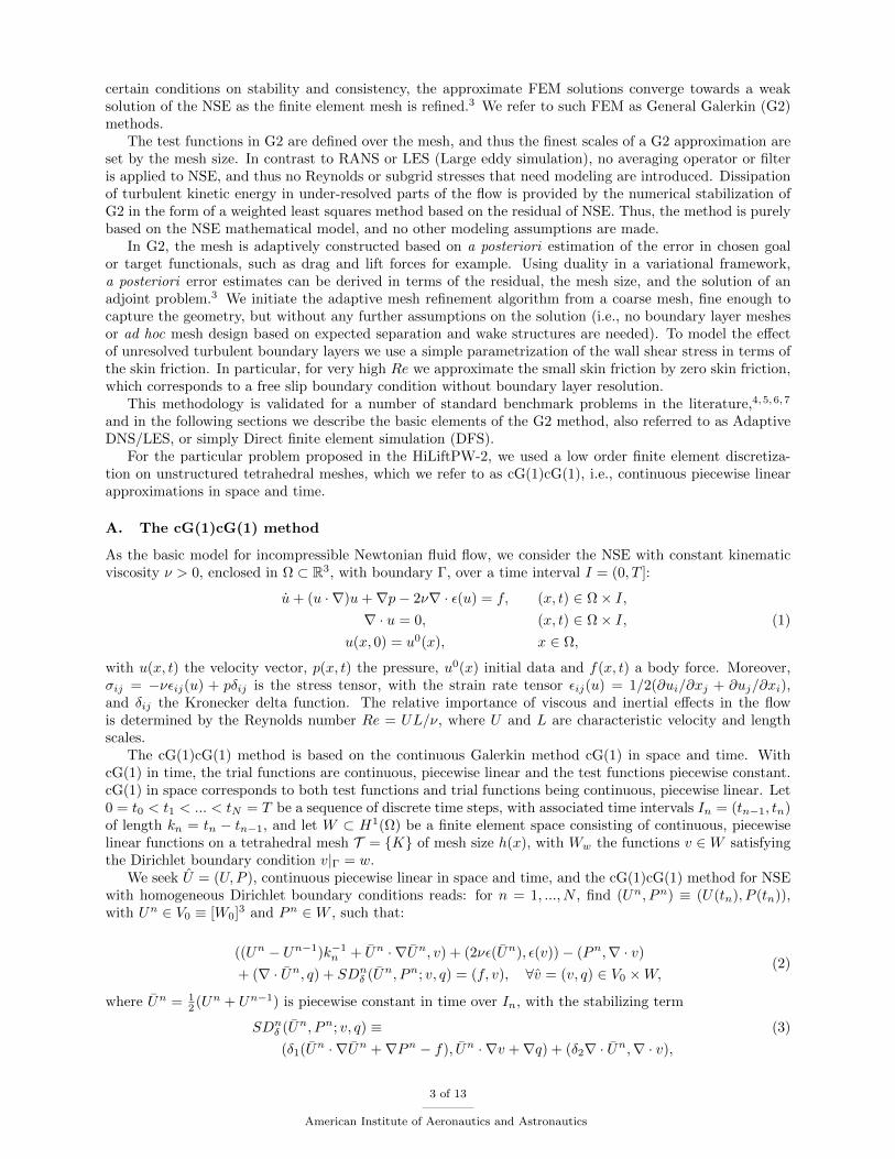
certain conditions on stability and consistency, the approximate FEM solutions converge towards a weaksolution of the NSE as the finite element mesh is refined.3 We refer to such FEM as General Galerkin (G2)methods.

The test functions in G2 are defined over the mesh, and thus the finest scales of a G2 approximation areset by the mesh size. In contrast to RANS or LES (Large eddy simulation), no averaging operator or filteris applied to NSE, and thus no Reynolds or subgrid stresses that need modeling are introduced. Dissipationof turbulent kinetic energy in under-resolved parts of the flow is provided by the numerical stabilization ofG2 in the form of a weighted least squares method based on the residual of NSE. Thus, the method is purelybased on the NSE mathematical model, and no other modeling assumptions are made.

In G2, the mesh is adaptively constructed based on a posteriori estimation of the error in chosen goalor target functionals, such as drag and lift forces for example. Using duality in a variational framework,a posteriori error estimates can be derived in terms of the residual, the mesh size, and the solution of anadjoint problem.3 We initiate the adaptive mesh refinement algorithm from a coarse mesh, fine enough tocapture the geometry, but without any further assumptions on the solution (i.e., no boundary layer meshesor ad hoc mesh design based on expected separation and wake structures are needed). To model the effectof unresolved turbulent boundary layers we use a simple parametrization of the wall shear stress in terms ofthe skin friction. In particular, for very high Re we approximate the small skin friction by zero skin friction,which corresponds to a free slip boundary condition without boundary layer resolution.

This methodology is validated for a number of standard benchmark problems in the literature,4,5, 6, 7

and in the following sections we describe the basic elements of the G2 method, also referred to as AdaptiveDNS/LES, or simply Direct finite element simulation (DFS).

For the particular problem proposed in the HiLiftPW-2, we used a low order finite element discretiza-tion on unstructured tetrahedral meshes, which we refer to as cG(1)cG(1), i.e., continuous piecewise linearapproximations in space and time.

A. The cG(1)cG(1) method

As the basic model for incompressible Newtonian fluid flow, we consider the NSE with constant kinematicviscosity ν > 0, enclosed in Ω ⊂ R3, with boundary Γ, over a time interval I = (0, T ]:

u+ (u · ∇)u+∇p− 2ν∇ · ε(u) = f, (x, t) ∈ Ω× I,∇ · u = 0, (x, t) ∈ Ω× I, (1)

u(x, 0) = u0(x), x ∈ Ω,

with u(x, t) the velocity vector, p(x, t) the pressure, u0(x) initial data and f(x, t) a body force. Moreover,σij = −νεij(u) + pδij is the stress tensor, with the strain rate tensor εij(u) = 1/2(∂ui/∂xj + ∂uj/∂xi),and δij the Kronecker delta function. The relative importance of viscous and inertial effects in the flowis determined by the Reynolds number Re = UL/ν, where U and L are characteristic velocity and lengthscales.

The cG(1)cG(1) method is based on the continuous Galerkin method cG(1) in space and time. WithcG(1) in time, the trial functions are continuous, piecewise linear and the test functions piecewise constant.cG(1) in space corresponds to both test functions and trial functions being continuous, piecewise linear. Let0 = t0 < t1 < ... < tN = T be a sequence of discrete time steps, with associated time intervals In = (tn−1, tn)of length kn = tn − tn−1, and let W ⊂ H1(Ω) be a finite element space consisting of continuous, piecewiselinear functions on a tetrahedral mesh T = K of mesh size h(x), with Ww the functions v ∈W satisfyingthe Dirichlet boundary condition v|Γ = w.

We seek U = (U,P ), continuous piecewise linear in space and time, and the cG(1)cG(1) method for NSEwith homogeneous Dirichlet boundary conditions reads: for n = 1, ..., N , find (Un, Pn) ≡ (U(tn), P (tn)),with Un ∈ V0 ≡ [W0]3 and Pn ∈W , such that:

((Un − Un−1)k−1n + Un · ∇Un, v) + (2νε(Un), ε(v))− (Pn,∇ · v)

+ (∇ · Un, q) + SDnδ (Un, Pn; v, q) = (f, v), ∀v = (v, q) ∈ V0 ×W,

(2)

where Un = 12 (Un + Un−1) is piecewise constant in time over In, with the stabilizing term

SDnδ (Un, Pn; v, q) ≡ (3)

(δ1(Un · ∇Un +∇Pn − f), Un · ∇v +∇q) + (δ2∇ · Un,∇ · v),

3 of 13


and

(v, w) =∑K∈T

∫K

v · w dx,

(ε(v), ε(w)) =

3∑i,j=1

(εij(v), εij(w)),

with the stabilization parameters δ1 = κ1(k−2n + |Un−1|2h−2)−1/2 and δ2 = κ2h|Un−1|, where κ1 and κ2 are

positive constants of unit size. We choose a time step size kn = CCFL minx∈Ω h/|Un−1|, with CCFL typicallyin the range [0.5, 20]. The resulting non-linear algebraic equation system is solved with a robust Schur-typefixed-point iteration method.8

B. The Adaptive Algorithm

A simple description of the adaptive algorithm, starting from k = 0, reads:

1. For the mesh Tk: compute primal and (linearized) adjoint problem.

2. If∑K∈Tk EK < TOL then stop, else:

3. Mark 10% of the elements with highest EK for refinement.

4. Generate the refined mesh Tk+1, and goto 1.

Here, EK is the error indicator for each cell K, which we describe in Section C. For now, it suffices tosay that EK is a function of the residual of the NSE and of the solution of a linearized adjoint problem. Theformulation of the adjoint problem includes the definition of a target functional for the refinement, whichusually enters the adjoint equations as a boundary condition or as a volume source term. This functionalshould be chosen according to the problem we are solving. In other words, one needs to ask the right questionin order to obtain the correct answer from the algorithm. In this paper our target functional is chosen to bethe mean value in time of the aerodynamic forces.

Apart from a suitable formulation of the adjoint problem, the only other input required from the user isan initial discretization of the geometry, T0. Since our method is designed for tetrahedral meshes that donot require any special treatment of the near wall region (no need for a boundary-layer mesh), the initialmesh can be easily created with any standard mesh generation tool.

C. A posteriori error estimate for cG(1)cG(1)

The a posteriori error estimate is based on the following theorem (for a detailed proof, see Chapter 30 here3):

Theorem 1 If U = (U,P ) solves (2), u = (u, p) is a weak NSE solution, and ϕ = (ϕ, θ) solves an associatedadjoint problem with data M(·), then we have the following a posteriori error estimate for the target functionalM(U) with respect to the reference functional M(u):

|M(u)−M(U)| ≤N∑n=1

[

∫In

∑K∈Tn

|R1(U)|K · ω1 dt

+

∫In

∑K∈Tn

|R2(U)|K ω2 dt+

∫In

∑K∈Tn

|SDnδ (U ; ϕ)K | dt ] =:

∑K∈Tn

EK

with

R1(U) = U + (U · ∇)U +∇P − 2ν∇ · ε(u)− f,R2(U) = ∇ · U, (4)

where SDnδ (·; ·)K is a local version of the stabilization form (3), and the stability weights are given by

ω1 = C1hK |∇ϕ|K ,ω2 = C2hK |∇θ|K ,

4 of 13


where hK is the diameter of element K in the mesh Tk, and C1,2 represent interpolation constants. Moreover,

|w|K ≡ (‖w1‖K , ‖w2‖K , ‖w3‖K), with ‖w‖K = (w,w)1/2K , and the dot denotes the scalar product in R3.

For simplicity, it is here assumed that the time derivatives of the dual variables φ = (φ, θ) can be boundedby their spatial derivatives. Given Theorem 1, we can understand the adaptive algorithm. As mentionedabove, the error indicator, EK , is a function of the residual of the NSE and of (the gradients of) the solutionof a linearized adjoint problem (a detailed formulation of the adjoint problem is given in Chapter 14 ofHoffman and Johnson3). Thus, on a given mesh, we must first solve the NSE to compute the residuals,R1(U) and R2(U), and then a linearized adjoint problem to compute the weights multiplying the residuals,ω1 and ω2. With that information, we are able to compute

∑K∈Tk EK and check it against the given stop

criterion. This procedure of solving the forward and backward problems for the NSE is closely related to anoptimization loop and can be understood as the problem of finding the “optimal mesh” for a given geometryand boundary conditions, i.e., the mesh with the least possible number of degrees of freedom for computingM(u) within a given degree of accuracy.

D. Turbulent boundary layers

In our work on high Reynolds number turbulent flow,9,10,11 we have chosen to apply a skin friction stressas wall layer model. That is, we append the NSE with the following boundary conditions:

u · n = 0, (5)

βu · τk + nTστk = 0, k = 1, 2, (6)

for (x, t) ∈ Γsolid× I, with n = n(x) an outward unit normal vector, and τk = τk(x) orthogonal unit tangentvectors of the solid boundary Γsolid. We use matrix notation with all vectors v being column vectors andthe corresponding row vector is denoted vT .

With skin friction boundary conditions, the rate of kinetic energy dissipation in cG(1)cG(1) has a con-tribution of the form:

2∑k=1

∫ T

0

∫Γsolid

|β1/2U · τk|2 ds dt, (7)

from the kinetic energy which is dissipated as friction in the boundary layer. For high Re, we modelRe→∞ by β → 0, so that the dissipative effect of the boundary layer vanishes with large Re. In particular,we have found that a small β does not influence the solution.9 For the present simulations we used theapproximation β = 0, which can be expected to be a good approximation for real high-lift configurations,where Re is typically much larger than in a wind tunnel experiment.

III. Results

This section is divided in four parts: in the first and second ones, a detailed comparison of the computedaerodynamic force and pressure coefficients with their corresponding experimental values is presented. Inthe third part, different flow visualizations are presented and discussed. Here, we would like to make it clearthat the results shown in Sections A through C were all obtained with the geometry designated as “config4” by the organizing committee,1 which includes “slat tracks” and “flap track fairings”, but no “pressuretube bundles”. Finally, we close the section with preliminary results for the geometry including pressuretube bundles, which is the one designated as “config 5” by the organizing committee.

A. Aerodynamic Forces

As discussed in Section II, our simulation methodology is an iterative process, where the mesh is refined ineach iteration based on an a posteriori error estimate. Therefore, we could say that the classical mesh study– an essential part of any thoroughly conducted CFD analysis – is a “by-product” of our method, i.e., themethod automatically requires the computation of the aerodynamic forces on a series of successively refinedmeshes.

Figure 2(a) shows the lift coefficient, CL, as a function of the angle of attack, α, for the finest meshobtained for each angle. The approach we chose was, starting from the same coarse mesh, to execute the

5 of 13


adaptive algorithm for each angle of attack separately, resulting in a different “family of meshes” for eachangle a.

0 5 10 15 20 251

1.2

1.4

1.6

1.8

2

2.2

2.4

2.6

2.8

3

α [degrees]

CL

exp

sim

(a) Lift vs. α, last iteration (finest mesh).

0 5 10 15 20 251

1.2

1.4

1.6

1.8

2

2.2

2.4

2.6

2.8

3

α [degrees]

CL

exp

iter0

iter1

iter2

iter3

iter4

(b) Lift vs. α, all iterations.

0 0.5 1 1.5 2 2.5 3 3.5 4 4.5

x 106

1.9

2

2.1

2.2

2.3

2.4

2.5

number of mesh points

CL

sim

exp

(c) Lift vs. number of mesh points, α = 12 .

0 0.5 1 1.5 2 2.5 3 3.5

x 106

2.2

2.3

2.4

2.5

2.6

2.7

2.8

2.9

3


CL

sim

exp

(d) Lift vs. number of mesh points, α = 22.4 .

Figure 2. Lift coefficient, CL, vs. angle of attack, α, and vs. number of mesh points.

Convergence results are shown in Figure 2(b), where CL is again plotted as a function of α, this timefor all five iterations of the adaptive algorithms for α = 12 , 22.4 . Although no definite convergence canbe observed, neither for α = 12 nor α = 22.4 , we clearly see that the computational result “approaches”the experimental curve as the number of iterations (or points in the mesh) increases. Figures 2(c) and 2(d)reinforce this trend, showing how CL varies with the number of mesh points, approaching the experimentalvalue for both angles. Similar results for the drag coefficient are shown in Figures 3.

Comparisons with experimental values of both CL and CD are shown in Table 1. For α = 12 , weobtained CL = 2.24 with our finest mesh, which corresponds to a relative error of 5.1%, when compared tothe experimental value. For α = 22.4 , the relative error in lift coefficient amounts to 4.2%.

Also shown in the table is a comparison of the lift to drag ratio of our simulation estimates with corre-sponding wind-tunnel values. The results here are of mixed quality: whereas for α = 12 the error is lessthan 5%, the error for α = 22.4 surpasses 20%.

The timestep k is chosen to be proportional to the mesh size, h, according to kn = CCFL minK∈Tk h/|Un−1|,and thus refining h implicitly also refines k. Since k is given by a minimum of h divided by U , the timestepmay be constrained by small mesh cells determined by detailed geometrical features, which may not have asignificant effect on the average global aerodynamic quantities. To quantify this, we performed computationson the coarsest mesh of “config 5”, for an angle of attack α = 22.4, using 3 different timesteps given byCCFL = 4, 8, 16. The corresponding CL– and CD–values vary within ≤ 1%, giving an indication that thesequantities are not sensitive to the timestep size in this range. Additionally, the additional cost in average

aHowever, due to lack of time, we were only able to obtain adaptive iterations for α = 12 , 22.4 ; the results for theremaining angles in the figure were computed with the mesh for α = 22.4 .

6 of 13


0 5 10 15 20 250.1

0.15

0.2

0.25

0.3

0.35

0.4

0.45

0.5

0.55

0.6

α [degrees]

CD

exp

sim

(a) Drag, last iteration (finest mesh).

0 5 10 15 20 250.1

0.15

0.2

0.25

0.3

0.35

0.4

0.45

0.5

0.55

0.6

α [degrees]

CD

exp

iter0

iter1

iter2

iter3

iter4

(b) Drag, all iterations.

0 0.5 1 1.5 2 2.5 3 3.5 4 4.5

x 106

0.17

0.18

0.19

0.2

0.21

0.22

0.23


CD

sim

exp

(c) Drag vs. number of mesh points, α = 12 .

0 0.5 1 1.5 2 2.5 3 3.5

x 106

0.3

0.32

0.34

0.36

0.38

0.4

0.42


CD

sim

exp

(d) Drag vs. number of mesh points, α = 22.4 .

Figure 3. Drag coefficient, CD, vs. angle of attack, α, and vs. number of mesh points.

wall-clock time per timestep is 24% for CCFL = 16 compared to CCFL = 8 and 7% for CCFL = 8 comparedto CCFL = 4, indicating a significant saving of computational cost when using the larger timesteps in therange.

(a) α = 12 .

sim. exp. relative error

lift 2.24 2.36 5.1%

drag 0.220 0.221 < 1%

ratio 10.2 10.7 4.8%

(b) α = 22.4 .

sim. exp. relative error

lift 2.80 2.69 4.2%

drag 0.357 0.412 13.4%

ratio 7.85 6.52 20.3%

Table 1. Comparison of drag and lift coefficients and lift over drag ratio, L/D, against experiments.

B. Pressure coefficients

Mean pressure coefficients, CP , were measured at different distances from the aircraft body along the wingin order to verify how lift is generated over the wing surface and how and where it breaks down after stall.Here, we present CP distributions for selected measurement stations and for the angles of attack for whichwe have performed adaptive iterations, i.e. α = 12 , 22.4 .

Figure 4 shows CP at four measurement locationsb for α = 12 , one close to the aircraft body, PS01, one

bOmitted locations show similar trends.

7 of 13


0 0.5 1

−4

−2

0

2

x/c

cp

PS01 y = 0.20967m

simexp

0 0.5 1

−6

−4

−2

0

2

x/c

cp

PS05 y = 0.7603m

0 0.5 1

−6

−4

−2

0

2

x/c

cp

PS07 y = 1m

0 0.5 1

−6

−4

−2

0

2

x/c

cp

PS11 y = 1.3488m

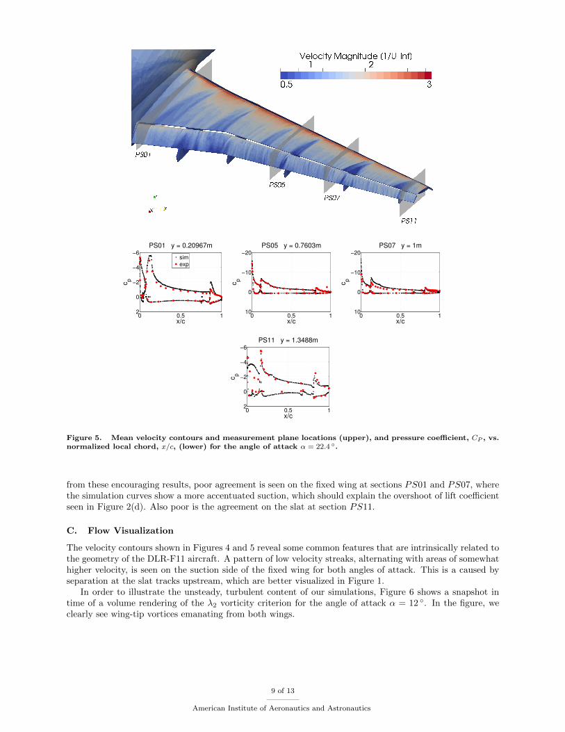
Figure 4. Mean velocity contours and measurement plane locations (upper), and pressure coefficient, CP , vs.normalized local chord, x/c, (lower) for the angle of attack α = 12 .

at half wing-span, PS05, and two others on the outboard side, closer to the wing tip, PS07 and PS11. Inthe figure it is also possible to see the location of these measurement stations together with velocity contourson the wing surface (similar to a “limiting streamlines” plot).

The degree of agreement is good on all three elements (slat, fixed wing and flap) on both pressure andsuction sides for measurements up to half wing-span. The only difference is a slightly steeper pressuregradient towards the trailing edge of the fixed wing in the simulation at half wing-span and also a strongersuction peak on the flap suction side at the measurement station closest to the aircraft body (PS01). Aswe approach the wing tip, however, this agreement deteriorates. On the fixed wing, e.g., the simulationresult shows consistently lower suction than the measured curve. This should partially explain the lower liftcoefficient obtained in the simulation, as seen in Figure 2(a). However, we expect this difference to becomeless pronounced as the mesh is further refined, at least if the trend indicated in Figure 2(b) and 2(c) holds.

Similar results are shown in Figure 5 for α = 22.4 . A comparison with Figure 4 reveals strongersuction peaks for this angle of attack in both simulation and measurements, which is in accordance with thehigher lift obtained for α = 22.4 in both campaigns. In the examination of Figure 5 alone, we find thatthe agreement between measured and computed pressure coefficients is excellent at half wing-span on allthree wing elements. Moreover, a good match is also seen for the suction peaks on the slat at the inboardmeasurement section (PS01) and on the main wing at the outboard measurement section (PS11). Apart

8 of 13


0 0.5 1

−6

−4

−2

0

2

x/c

cp

PS01 y = 0.20967m

simexp

0 0.5 1

−20

−10

0

10

x/c

cp

PS05 y = 0.7603m

0 0.5 1

−20

−10

0

10

x/c

cp

PS07 y = 1m

0 0.5 1

−6

−4

−2

0

2

x/c

cp

PS11 y = 1.3488m

Figure 5. Mean velocity contours and measurement plane locations (upper), and pressure coefficient, CP , vs.normalized local chord, x/c, (lower) for the angle of attack α = 22.4 .

from these encouraging results, poor agreement is seen on the fixed wing at sections PS01 and PS07, wherethe simulation curves show a more accentuated suction, which should explain the overshoot of lift coefficientseen in Figure 2(d). Also poor is the agreement on the slat at section PS11.

C. Flow Visualization

The velocity contours shown in Figures 4 and 5 reveal some common features that are intrinsically related tothe geometry of the DLR-F11 aircraft. A pattern of low velocity streaks, alternating with areas of somewhathigher velocity, is seen on the suction side of the fixed wing for both angles of attack. This is a caused byseparation at the slat tracks upstream, which are better visualized in Figure 1.

In order to illustrate the unsteady, turbulent content of our simulations, Figure 6 shows a snapshot intime of a volume rendering of the λ2 vorticity criterion for the angle of attack α = 12 . In the figure, weclearly see wing-tip vortices emanating from both wings.

9 of 13


Figure 6. Volume rendering of λ2 vorticity criterion for the angle of attack α = 12 , snapshot in time.

D. Preliminary results for “config 5”

We are currently working on a set of simulations for future publications, where we intend to compare resultsobtained with “config 4” against results obtained with “config 5”. These two configurations differ somewhat,the latter being slightly closer to the experimental model due to the presence of pressure tube bundles nearthe slat tracks.

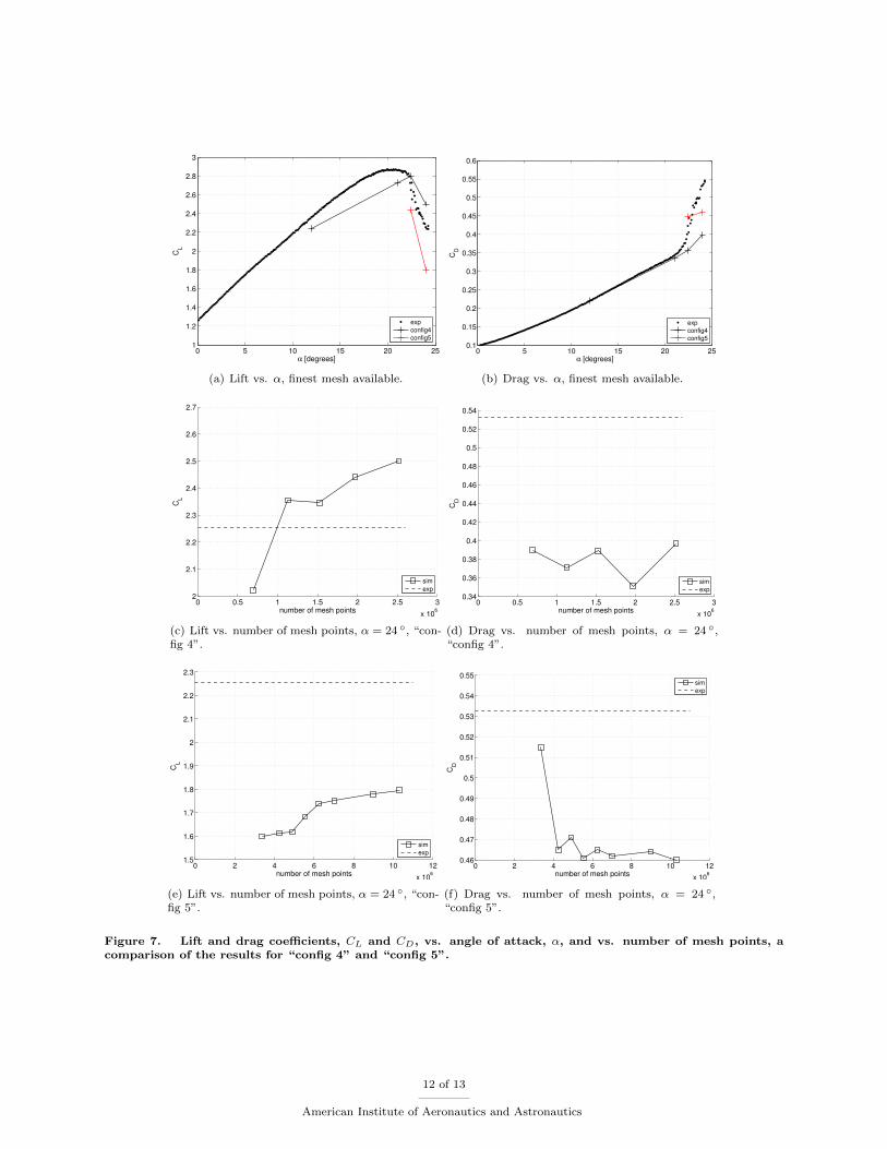
Figures 7(a) and 7(b) show a comparison of the results obtained with “config 4” and “config 5” for theangles of attack α = 22.4 , 24 . The computed values obtained for CL and CD with “config 5” (the redcurves) indicate that the flow is indeed stalled: we have a clear lift break when moving from α = 22.4 to24 , which is consistently followed by an increase in drag force. For “config 4”, a similar drop in the liftcurve observed; the drag coefficient, however, does not increase to the levels observed in the experiments,which indicates that simulations performed with “config 4” are not suitable for direct comparisons withmeasurements near stall. Figures 7(c)–7(f) show CL and CD as a function of the number of mesh cells forthe both angles and both “config’s”. The trends observed for CL and CD as the mesh is refined reinforcethe results illustrated in Figures 7(a) and 7(b).

Next, we compare the stalled angle, α = 24 , with the non-stalled angle, α = 22.4 , for “config 5”, bya volume rendering of the magnitude of the velocity at a snapshot in time in Figure 8. The velocity valuesin the range U = [0.6, 1.4] have zero opacity to reveal the high velocity in red on the leading edges of thewing components and the low velocity in blue in the wake. We clearly see a separated wake region appearingaround the trailing edge of the flap for α = 22.4 , but covering almost the entire surface of the main wingand flap for the stall case at α = 24 (except close to the aicraft body, where no clear wake region is seen).

IV. Conclusions

This paper contains the results obtained with the G2 method for the HiLiftPW-2 held in San Diego,California, in 2013. G2 is a time-resolved FEM for turbulent flows with no turbulence modeling, and withan automatic mesh generation algorithm based on an a posteriori error estimate. These features of G2characterize it as a parameter-free method, where no a priori knowledge of the flow is needed during theproblem formulation stage, nor during the mesh generation process. Moreover, in G2, turbulent boundarylayers are modeled by a slip with friction boundary condition, and thus no boundary layer mesh is needed.

10 of 13


We believe the results presented in this report are “very promising”. Although no definite convergenceis shown in Figures 2 and 3, our results approach the experimental values as the mesh is refined. Moreover,we were able to predict stall for “config 5” at similar angles of attack as in the experiments, which is asignificant physical outcome of our simulations.

Acknowledgments

The authors would like to acknowledge the financial support from the Swedish Foundation for StrategicResearch, the European Research Council and the Swedish Research Council. The simulations were per-formed on resources provided by the Swedish National Infrastructure for Computing (SNIC) at PDC – Centerfor High-Performance Computing and on resources provided by the “Red Espanola de Supercomputacion”and the “Barcelona Supercomputing Center - Centro Nacional de Supercomputacion”.

The initial volume mesh was generated with ANSA from Beta-CAE Systems S. A., who generouslyprovided an academic license for this project.

References

1Rumsey, C., “2nd AIAA CFD High Lift Prediction Workshop (HiLiftPW-2) (http://hiliftpw.larc.nasa.gov/),” 2013.2Choudhari, M. and Visbal, M., “Second Workshop on Benchmark problems for Airframe Noise Computations (BANCII)

(https://info.aiaa.org/tac/ASG/FDTC/DG/BECAN files /BANCII.htm),” 2012.3Hoffman, J. and Johnson, C., Computational Turbulent Incompressible Flow , Vol. 4 of Applied Mathematics: Body and

Soul , Springer, 2007.4Hoffman, J., “Computation of mean drag for bluff body problems using Adaptive DNS/LES,” SIAM J. Sci. Comput.,

Vol. 27(1), 2005, pp. 184–207.5Hoffman, J., “Adaptive simulation of the turbulent flow past a sphere,” J. Fluid Mech., Vol. 568, 2006, pp. 77–88.6Hoffman, J. and Johnson, C., “A new approach to Computational Turbulence Modeling,” Comput. Methods Appl. Mech.

Engrg., Vol. 195, 2006, pp. 2865–2880.7Hoffman, J., “Efficient computation of mean drag for the subcritical flow past a circular cylinder using General Galerkin

G2,” Int. J. Numer. Meth. Fluids, Vol. 59(11), 2009, pp. 1241–1258.8Houzeaux, G., Vazquez, M., Aubry, R., and Cela, J., “A massively parallel fractional step solver for incompressible flows,”

Journal of Computational Physics, Vol. 228, No. 17, 2009, pp. 6316–6332.9Hoffman, J. and Jansson, N., A computational study of turbulent flow separation for a circular cylinder using skin friction

boundary conditions, Ercoftac, series Vol.16, Springer, 2010.10Hoffman, J. and Johnson, C., “Resolution of d’Alembert’s Paradox,” J. Math. Fluid Mech., Published Online First at

www.springerlink.com: 10 December 2008.11Vilela de Abreu, R., Jansson, N., and Hoffman, J., “Adaptive computation of aeroacoustic sources for a rudimentary

landing gear,” Int. J. Numer. Meth. Fluids, Vol. 74, No. 6, 2014, pp. 406–421.

11 of 13


0 5 10 15 20 251

1.2

1.4

1.6

1.8

2

2.2

2.4

2.6

2.8

3

α [degrees]

CL

exp

config4

config5

(a) Lift vs. α, finest mesh available.

0 5 10 15 20 250.1

0.15

0.2

0.25

0.3

0.35

0.4

0.45

0.5

0.55

0.6

α [degrees]

CD

exp

config4

config5

(b) Drag vs. α, finest mesh available.

0 0.5 1 1.5 2 2.5 3

x 106

2

2.1

2.2

2.3

2.4

2.5

2.6

2.7


CL

sim

exp

(c) Lift vs. number of mesh points, α = 24 , “con-fig 4”.

0 0.5 1 1.5 2 2.5 3

x 106

0.34

0.36

0.38

0.4

0.42

0.44

0.46

0.48

0.5

0.52

0.54


CD

sim

exp

(d) Drag vs. number of mesh points, α = 24 ,“config 4”.

0 2 4 6 8 10 12

x 106

1.5

1.6

1.7

1.8

1.9

2

2.1

2.2

2.3


CL

sim

exp

(e) Lift vs. number of mesh points, α = 24 , “con-fig 5”.

0 2 4 6 8 10 12

x 106

0.46

0.47

0.48

0.49

0.5

0.51

0.52

0.53

0.54

0.55


CD

sim

exp

(f) Drag vs. number of mesh points, α = 24 ,“config 5”.

Figure 7. Lift and drag coefficients, CL and CD, vs. angle of attack, α, and vs. number of mesh points, acomparison of the results for “config 4” and “config 5”.

12 of 13


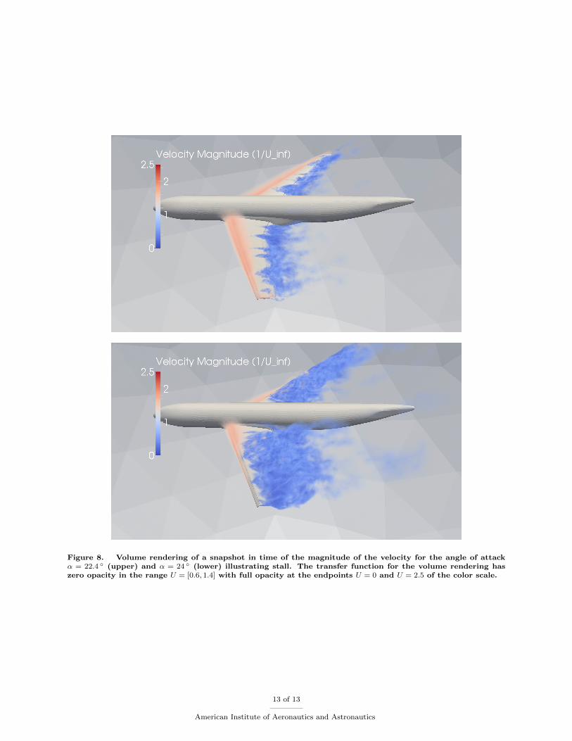
Figure 8. Volume rendering of a snapshot in time of the magnitude of the velocity for the angle of attackα = 22.4 (upper) and α = 24 (lower) illustrating stall. The transfer function for the volume rendering haszero opacity in the range U = [0.6, 1.4] with full opacity at the endpoints U = 0 and U = 2.5 of the color scale.

13 of 13


time-resolved adaptive fem simulation of the dlr … adaptive fem simulation of the ... high-lift...

Documents