TIME-FREQUENCY DUAL AND QUANTIZATION

Anna Marie Maeser

A Thesis Submitted to theUniversity of North Carolina Wilmington in Partial Fulfillment

of the Requirements for the Degree ofMaster of Science

Department of Mathematics and Statistics

University of North Carolina Wilmington

2009

Approved by

Advisory Committee

James Blum Russell Herman

Mark Lammers

Chair

Accepted by

Dean, Graduate School

This thesis has been prepared in the style and format

Consistent with the journal

American Mathematical Monthly.

ii

TABLE OF CONTENTS

ABSTRACT . . . . . . . . . . . . . . . . . . . . . . . . . . . . . . . . . . iv

DEDICATION . . . . . . . . . . . . . . . . . . . . . . . . . . . . . . . . . v

ACKNOWLEDGMENTS . . . . . . . . . . . . . . . . . . . . . . . . . . . vi

LIST OF TABLES . . . . . . . . . . . . . . . . . . . . . . . . . . . . . . . vii

LIST OF FIGURES . . . . . . . . . . . . . . . . . . . . . . . . . . . . . . viii

1 INTRODUCTION . . . . . . . . . . . . . . . . . . . . . . . . . . . . ix

2 MATHEMATICAL BACKGROUND AND MOTIVATION . . . . . . 3

2.1 Fourier Analysis . . . . . . . . . . . . . . . . . . . . . . . . . . 3

2.2 Sampling Theory . . . . . . . . . . . . . . . . . . . . . . . . . 8

2.3 Finite Frames and Duals . . . . . . . . . . . . . . . . . . . . . 12

2.4 Sigma-Delta Quantization . . . . . . . . . . . . . . . . . . . . 18

2.4.1 First-Order Schemes . . . . . . . . . . . . . . . . . . 19

2.4.2 Second-Order Schemes . . . . . . . . . . . . . . . . . 26

2.5 The Finite Heisenberg Product and Sum . . . . . . . . . . . . 27

3 TIME-FREQUENCY DUAL AND QUANTIZATION . . . . . . . . . 31

3.1 Time-Frequency Dual . . . . . . . . . . . . . . . . . . . . . . . 31

3.2 Σ∆ Quantization with TF Noise Shaper . . . . . . . . . . . . 36

4 APPLICATIONS OF THE TF DUAL WITH AUDIO . . . . . . . . . 37

4.1 Applying the Time-Frequency Quantization Scheme . . . . . . 38

4.2 Applying the Second Order Σ∆ Scheme . . . . . . . . . . . . 40

5 CONCLUSION . . . . . . . . . . . . . . . . . . . . . . . . . . . . . . 43

REFERENCES . . . . . . . . . . . . . . . . . . . . . . . . . . . . . . . . . 45

6 APPENDIX . . . . . . . . . . . . . . . . . . . . . . . . . . . . . . . . 47

6.1 MATLAB Program Used for Results in Section 4.1 . . . . . . 47

6.2 MATLAB Program Used for Results in Section 4.2 . . . . . . 52

iii

ABSTRACT

It is often necessary to convert analog signals into digital ones to make use

of modern technology in terms of transmission, storage, and recovery of signals.

Frames, duals, and quantization each play a role in this process and are discussed

in depth in this paper. The Time-Frequency dual, motivated by the Heisenberg

sum, is developed and it is shown that this dual minimizes the Heisenberg sum,

‖DH∗‖2F + ‖DFH∗‖2F . We find that the Time-Frequency dual outperforms the

canonical dual and the Blackman filter as it yields a higher Signal-to-Noise Ratio

and a lower Mean Square Error, resulting in minimal signal reconstruction error in

comparison. This is shown through the use of MATLAB to analyze an audio signal.

iv

DEDICATION

I dedicate this thesis to all of my friends and family who have always stood by

me and encouraged me to do my best. I don’t know what I would do without you.

v

ACKNOWLEDGMENTS

I would like to thank all of my committee members, Dr. Mark Lammers, Dr.

Russell Herman, and Dr. James Blum, for their countless hours of advising and

help. You all have been amazing and there is no way I could have done this without

you.

vi

LIST OF TABLES

1 A summary of MSE and SNR for the Blackman filter, canonical dual,

and the time-frequency dual using the time-frequency quantization

scheme. Through these calculations, we see that the time-frequency

dual minimizes the error. . . . . . . . . . . . . . . . . . . . . . . . . . 40

2 A summary of MSE and SNR for the Blackman filter, canonical

dual, and the time-frequency dual using the second order Σ∆ scheme.

Through these calculations, we see that the time-frequency dual min-

imizes the error. . . . . . . . . . . . . . . . . . . . . . . . . . . . . . . 42

vii

LIST OF FIGURES

1 (a) shows a signal with its Fourier transform in (b). We can see that (b)

is band-limited because the Fourier transform vanished outside a finite

interval (i.e., [−ω, ω]). In (c), the signal is sampled and the transform

becomes periodic in (d). . . . . . . . . . . . . . . . . . . . . . . . . . . 9

2 The blackman filter with N = 32. . . . . . . . . . . . . . . . . . . . . . 18

3 Left: The block filter of length 32. Right: The Fourier transform of the

block filter, resulting in the sinc function. . . . . . . . . . . . . . . . . . 30

4 The original audio signal prior to any filtering and reconstruction. . . . . 38

5 A graph of the difference between the original signal in Figure 4 and the

reconstruction with the Blackman filter with MSE = 8.319. . . . . . . . . 39

6 A graph of the difference between the original signal in Figure 4 and the

reconstruction with the canonical dual fram with MSE = 8.471. . . . . . . 39

7 A graph of the difference between the original signal in Figure 4 and the

reconstruction with the time-frequency dual developed in this paper. The

MSE is slightly less than that of Figure 5 and Figure 6 is 7.699. . . . . . . 39

8 A graph of the difference between the original signal in Figure 4 and the

reconstruction with the Blackman filter with MSE = 0.372. . . . . . . . . 41

9 A graph of the difference between the original signal in Figure 4 and the

reconstruction with the canonical dual frame with MSE = 5.555. . . . . . 41

10 A graph of the difference between the original signal in Figure 4 and the

reconstruction with the time-frequency dual developed in this paper. The

MSE is much less than that of Figure 8 and Figure 6 and is 0.277. . . . . 41

viii

1 INTRODUCTION

Technology has become such a part of everyday life that it is now common to

simply download your favorite movie or put thousands of songs onto your MP3

player at the drop of a hat. Signal processing, including compression, filtering, and

denoising, make all of these luxuries possible. Three underlying mathematical ideas

involved in this process include frames, duals, and quantization, all of which will be

discussed in depth in this paper.

Frames and duals became popular shortly after the discovery of the Sampling

Theorem by Claude Shannon in 1948 [19]. In essence, The Sampling Theorem says

that a continuous band-limited signal can be replaced by a discrete sequence of

samples from the signal without losing any information [13]. It is remarkable that

certain continuous functions can be completely reconstructed from discrete sets of

samples. This is important in practice because it is often necessary to convert analog

models into digital ones to make use of modern technology in terms of transmission,

storage, and recovery of signals.

The term analog describes a waveform that can take on a continuous range of

values. On the other hand, the term digital describes a waveform that corresponds

to a discrete sequence of values used to represent a discrete or continuous signal.

In real-world applications, the first step in the process of converting analog signals

to digital is measuring the signal over a discrete set of values. Specifically, a discrete

representation of a signal x over a finite set of numbers, or a dictionary, {an}n∈[0,d],

is given as x =d∑

n=1

~enan, where the vectors, ~en, are real or complex. If the choice of

~en is not unique, then the dictionary is said to be redundant [18]. Although these

ideas along with frames and duals provide discrete representations of a signal, it is

not quite digital because digital representations consist of a finite alphabet. This is

where quantization comes into play [18].

Two types of quantization are pulse code modulation and sigma-delta quanti-

zation. Pulse Code Modulation (PCM) is an industry standard for turning analog

audio signals into digital audio signals. During PCM, we sample a signal at a very

low oversampling rate and it is usually quantized into a series of binary codes, which

makes the technique useful for large alphabets. A large number of bits, such as 16,

would correspond to a large alphabet with a dictionary of 216 in size. The average

human ear can hear at a frequency of 40 Hz. PCM oversamples at 10%, or 44Hz [3].

Sigma-delta quantization (Σ∆ quantization), discussed in Section 2.4, is a low-

bit method (i.e., 1 to 2 bits), that samples at 3200%, a vast oversampling that is

often implemented by engineers in applications because PCM is generally expensive

and does not have strong error correction [11]. Σ∆ quantization takes the error into

account at each stage of quantization and smooths this out from the beginning. In

PCM, if a large error is made in the beginning, the error can not be corrected.

In this paper, we develop the Time-Frequency dual (TF dual), motivated in

part by the finite Heisenburg sum [8], used to minimize error in both time and

frequency. We also develop a quantization scheme that proves to exhibit less error

in signal reconstructions and Signal-to-Noise Ratio (SNR) when compared to the

Blackman filter and the canonical dual. In Section 2, mathematical background will

be given for Fourier analysis, sampling theory, duals and frames, quantization, and

the Heisenberg sum. This will be followed by an explanation of the time-frequency

dual, it’s properties, and the TF quantization scheme influenced by Σ∆ quantization.

In the last section we will show the advantage to the TF dual by comparing it to

both the Blackman filter and the canonical dual frame in terms of Mean Square

Error (MSE) and SNR. We find that the TF dual outperforms the canonical dual

and the Blackman filter as it yields a higher SNR and a lower MSE, resulting in

minimal signal reconstruction error in comparison.

2

2 MATHEMATICAL BACKGROUND AND MOTIVATION

2.1 Fourier Analysis

Although not the main topic of this paper, it is beneficial to understand the

basics of Fourier analysis as a useful mathematical tool that paved the way for

many advances in signal processing. Joseph Fourier (1768 - 1830) developed the

Fourier series in order to expand a periodic function in terms of the specific set of

functions {1, cosx, cos 2x, cos 3x, ..., sinx, sin 2x, sin 3x, ...}. This is captured with

the following definition.

Definition 1. A Trigonometric Fourier Series expansion of a function f on

x ∈ [−π, π] can be expressed as

f(x) = a0 +∞∑n=1

(an cosnx+ bn sinnx), (1)

where the coefficients an and bn are called Fourier coefficients of f and are given

by the following formulae:

a0 =1

2π

∫ π

−πf(x) dx,

an =1

π

∫ π

−πf(x) cosnx dx, (n = 1, 2, ...), (2)

bn =1

π

∫ π

−πf(x) sinnx dx, (n = 1, 2, ...).

The functions cos x and sin x can be written using complex exponentials as

cos x =eix + e−ix

2, sin x =

eix − e−ix

2i,

which allows us to define the Fourier series in the complex form.

3

Definition 2. Let f be a 2p-periodic piecewise smooth function. The Complex

Exponential Fourier Series is

f(x) =∞∑

n=−∞

cneinπpx, x ∈ [−p, p], (3)

where the Fourier coefficients cn are given by

cn =1

2p

∫ p

−pf(x)e−i

nπpx dx, (n = 0,±1,±2, ...). (4)

Problems of convergence of the Fourier series is a delicate issue that has been

studied immensely. We will be dealing with finite cases in this paper and will be less

concerned with convergence issues; however, these are discussed in depth in [14].

The continuous Fourier Transform is denoted f(ω) and is a generalization of the

complex Fourier series. The Fourier series deals with functions that are periodic in

the interval [−p, p]; however, we use the Fourier transform for non-periodic func-

tions by allowing p → ∞. The continuous Fourier Transform defines a relationship

between a signal in the time domain and its representation in the frequency domain.

Definition 3. The Fourier Transform of a function, f , defined in [2], is given

by

f(ω) =1√2π

∫ ∞−∞

f(x)e−iωx dx, (−∞ < ω <∞). (5)

ω is the angular frequency in the Fourier transform, which is generally defined as

nπp

= n∆ω. The angular frequency is generally related to the period, T , by ∆ω = 2πT

.

In this case, the period is T = 2p, which implies that ω = πp. As a result, ω is related

to the complex Fourier series coefficients in that ω = nπp

and is a discrete set of ω’s.

4

Example 1. A Fourier Transform

Given a signal, f(x) we can find the Fourier transform, f(ω).

f(x) =

e−x, ifx > 0

0, ifx ≤ 0

f(ω) =1√2π

∫ ∞0

e−xe−iωxdx

=1√2π

∫ ∞0

e−(x+iωx)dx

=1√2π

∫ ∞0

e−x(1+iω)dx

=−1√

2π(1 + iω)e−x(1+iω)

∣∣∣∞0

Since limx→∞

e−x(1+iω) = 0, we get

f(ω) = 0− −1√2π(1 + iω)

=1√

2π(1 + 1ω)

=1− iω√

2π(1 + ω2).

Definition 4. The Inverse Fourier Transform, defined in [2], is given as

f(x) =1√2π

∫ ∞−∞

f(ω)eiωx dω, (−∞ < x <∞). (6)

If we started with f(ω) from Example 1, we could use (6) to obtain our original

f(x) in Example 1.

As described previously, it is often necessary to sample a continuous function to

obtain a discrete representation. The next important definition, the Discrete Fourier

5

Transform, denoted X(j), can be viewed as sampling from the continuous Fourier

transform.

Definition 5. Given an N-sequence x=((x(0), x(1),...,x(N-1)), the N-point Dis-

crete Fourier Transform of x is defined by

X(j) =1√N

N−1∑k=0

x(k)e2πijk/N , j = 0, 1, ..., N − 1. [2] (7)

Example 2. A Discrete Fourier Transform

We will compute the DFT of a simple 2-point sequence x = (0, 1).

X2(j) =1√2

1∑k=0

x(k)e2πijk2 , j = 0, 1.

Replacing x(k) with it’s sequential value, we get the first term,

X2(0) =1√2

1∑k=0

x(k)

=1√2

(0 + 1) =1√2

The second term becomes

X2(1) =1√2

1∑k=0

x(k)eikπ2

=1√2

(0 + eiπ2 )

=1√2i.

Therefore, we have the DFT of x = (0, 1) is X = ( 1√2, 1√

2i).

Like the Fourier transform, the discrete Fourier transform also has an inverse.

6

Definition 6. The Inverse Discrete Fourier Transform (IDFT) is given by

x(k) =1√N

N−1∑j=0

X(j)e−2πij kN , k = 0, 1, ..., N − 1. (8)

The Fourier transform and the inverse Fourier transform are considered to be a

transform pair. Similarly, the DFT and the IDFT are a transform pair. This simply

means that the inverse transform is a method to give you back your original signal

or sequence.

We will prove that the DFT and IDFT are inverses of each other. In other

words, we will show that for any N sequence x, F−1N (FN(x))(k)(k) = x(k) for k =

0, 1, ..., N − 1. F−1N stands for the inverse Fourier transform and FN is the Fourier

transform [2]. This can be done similarly for the continuous Fourier transform and

the inverse Fourier transform.

Proof. We first define an interesting identity. For j, k = 0, 1, 2, ..., N − 1, we have

N−1∑n=0

e2πnj−kN =

0, if j 6= k

N, if j = k(9)

Clearly, the second part is true because j = k, resulting in e0 = 1 summed N times.

To show why the first part holds, we let

e2πinj−kN = zn, (10)

where z = e2πij−kN . We then see that the sum in (9) is a geometric sum that equals

1−zN1−z . We know that zN = e2πi(j−k) = 1, so we obtain a sum of zero for j 6= k or

7

z 6= 1. Using (7) and (8), we get

F−1N (FN(x))(k) =

1√N

N−1∑n=0

X(n)︷ ︸︸ ︷1√N

N−1∑j=0

x(j)e2πijnN e−2πin k

N

=1

N

N=1∑j=0

x(j)N−1∑n=0

e2πi(j−k)nN .

Using the knowledge from (9), we complete the proof with

F−1N (FN(x))(k) =

1

Nx(k)N = x(k). (11)

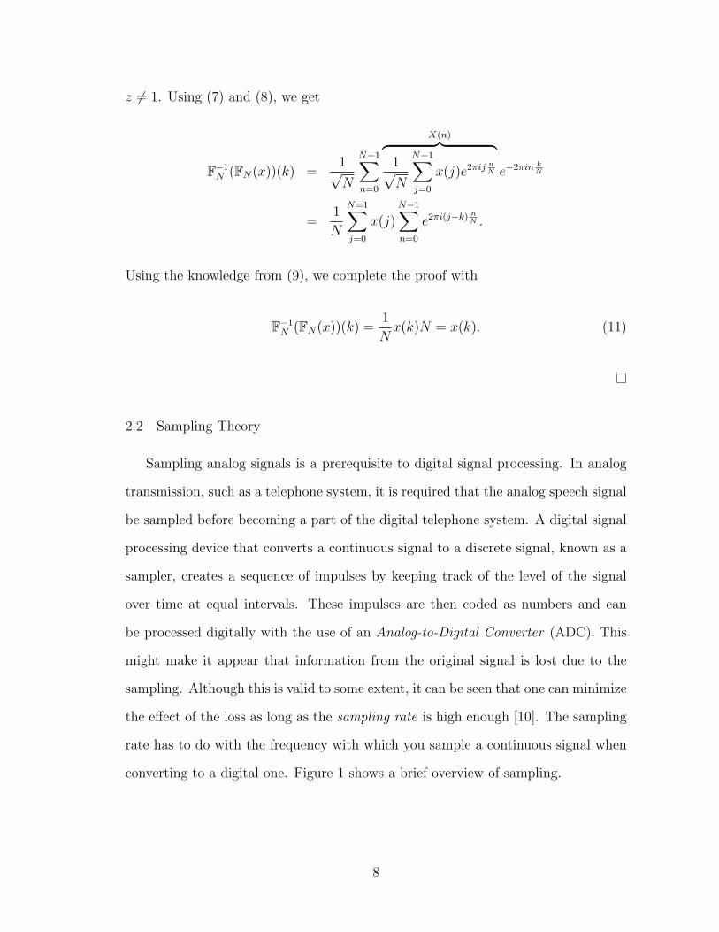
2.2 Sampling Theory

Sampling analog signals is a prerequisite to digital signal processing. In analog

transmission, such as a telephone system, it is required that the analog speech signal

be sampled before becoming a part of the digital telephone system. A digital signal

processing device that converts a continuous signal to a discrete signal, known as a

sampler, creates a sequence of impulses by keeping track of the level of the signal

over time at equal intervals. These impulses are then coded as numbers and can

be processed digitally with the use of an Analog-to-Digital Converter (ADC). This

might make it appear that information from the original signal is lost due to the

sampling. Although this is valid to some extent, it can be seen that one can minimize

the effect of the loss as long as the sampling rate is high enough [10]. The sampling

rate has to do with the frequency with which you sample a continuous signal when

converting to a digital one. Figure 1 shows a brief overview of sampling.

8

Figure 1: (a) shows a signal with its Fourier transform in (b). We can see that (b) isband-limited because the Fourier transform vanished outside a finite interval (i.e., [−ω, ω]).In (c), the signal is sampled and the transform becomes periodic in (d).

This brings us to the idea of band-limited functions and band width, which will

be useful in understanding the Short-Time Fourier Transform (STFT), defined in

Equation (12), and the sampling theorem for band-limited functions.

Definition 7. A function f(x) is band-limited if its Fourier transform (5) vanishes

outside a finite interval. Then there exists a positive number W such that f(ω) = 0

for all |ω| > W. The number W is called the band width of f .

The majority of functions are not considered band-limited; however, most functions

can be approximated by band-limited functions [2]. This is a natural extension of

the range of human hearing. Humans can only hear up to about 40 Hz, a finite

interval, and all hearing disappears outside of these frequencies.

We examined the continuous Fourier transform and the discrete Fourier transform

in Section 2.1 and can now discuss the Short-Time Fourier Transform, also known

as the Gabor transform, which is dependent upon the band width of the function

[5]. This transform is used to determine how long a specific frequency will last.

The STFT is a technique in which Fourier transforms are taken of short consecutive

segments of a signal. This transform provides a clear representation of the signal

9

and a frequency image of the signal locally in time and has been an inspiration to

the Time-Frequency Dual [5].

Definition 8. The Short-time Fourier Transform is defined as

Vgf(x, ω) =1√2π

∫ ∞−∞

f(t)g(t− x)e−iωt dt, (12)

where t represents time and ω represents the band width of the signal. g is the filter

window which is commonly represented by a Gaussian, f(x) = e−x2, or an indicator

function, f(x) = 1 if |x| < a and 0 otherwise. The bar represents the complex

conjugate.

The definition of a band-limited function allows for an important representation.

Basically, every band-limited function with band width W can be written as a linear

combination of basis functions where the coefficients in this sum are function values

at a discrete set of equally spaced sample points. The sampling theorem for band-

limited functions and it’s proof results [2].

Theorem 1. The Sampling Theorem for Band-Limited Functions Suppose

that f is band-limited with band width W. Then for all x,

f(x) =∞∑

n=−∞

f(nπ

W)sin(Wx− nπ)

(Wx− nπ), n = 0,±1,±2, .... (13)

The proof of the sampling theorem is found in [2] and given below.

Proof. By definition, we know that f vanishes outside [−W,W ] [2]. By the Inverse

Fourier Transform (6), we have

f(x) =1√2π

∫ ∞−∞

f(ω)eiωx dω

=1√2π

∫ W

−Wf(ω)eiωx dω. (14)

10

f can be written as a Fourier series on [−ω, ω] due to the fact that f vanishes out-

side [−W,W ]. Using the complex form of the Fourier series (3), f can be represented

as

f(ω) =∞∑

n=−∞

cneinπWω (|ω| < W ) (15)

=∞∑

n=−∞

c−ne−inπ

Wω.

Using Equation (4), the complex Fourier coefficients are written

c−n =1

2W

∫ W

−Wf(ω)ei

nπWω dω. (16)

Noticing the relationship between c−n and f(x) in (14) and (16), we can simplify

the c−n’s and get

c−n =

√2π

2Wf(nπ

W). (17)

One more integral must be computed before continuing the proof. The solution

(18) uses the identity eix = cosx+ i sinx.

1

2W

∫ W

−We−i

nπWωeiωx dω =

1

2W

∫ W

−Wei(Wx−nπ)ω/W dω

=1

2W

∫ W

−Wcos(

Wx− nπW

ω) dω

=sin(Wx− nπ)

Wx− nπ. (18)

We can now complete the proof using f(x) in Equation (14), f(ω) in Equation

(15), and c−n in Equation (17).

11

f(x) =1√2π

∫ W

−W

f(ω)︷ ︸︸ ︷∞∑

n=−∞

c−ne−inπ

Wω eiωx dω

=1√2π

∫ W

−W

f(ω)︷ ︸︸ ︷∞∑

n=−∞

c−n︷ ︸︸ ︷√2π

2Wf(nπ

W) e−i

nπWω eiωx dω.

Interchanging the order of the integral and sum, we obtain

f(x) =∞∑

n=−∞

f(nπ

W)

1

2W

∫ W

−We−i

nπWωeiωx dω

=∞∑

n=−∞

f(nπ

W)sin(Wx− nπ)

Wx− nπ

from (18).

We can see from this theorem that f is completely determined by its sample

values f(nπW

). Harold Nyquist recognized that the larger the band width, the more

sample points per unit length are required for (13) to hold. As a result, the minimum

number of sample points per unit length in ~x required for (13) to be true is known

as the Nyquist Sampling Rate. This rate corresponds to the smallest band width

of the function and is twice the band width of the signal, or 2W [2]. We will

explore sampling at a rate much greater than the Nyquist rate, exemplifying an

advantageous property of frames. This significantly greater sampling rate is known

as oversampling.

2.3 Finite Frames and Duals

The theory of frames is due to Duffin and Schaeffer who introduced the idea in

the 1950s [7]. They were not utilized greatly until the 1980s when Stephane Mallat

12

and Ingrid Daubechies used them for wavelet analysis. We use frames in order to

implement sampling techniques described previously and in this case, to achieve an

oversampled representation of a signal. This is the first step to converting an analog

signal to digital.

The Euclidean norm and the inner product are two concepts that should be

understood prior to defining a frame. They are defined as follows:

Definition 9. The Euclidean Norm or L2-Norm of a vector in RN is given by

||~x|| =√x2

1 + x22 + x2

3 + ...+ x2N . (19)

The Inner Product is defined as

〈~x, ~y〉 =N∑i=1

xiyi. (20)

The inner product is related to the Euclidean norm by

〈~x, ~x〉 = ||~x||2. (21)

The Euclidean norm and the inner product will be used often throughout the rest

of this paper, especially when defining frames and duals. Before offically defining

a frame, the relationship between a basis and a frame should be clear. A basis is

commonly referred to as a linearly independent spanning set because each matrix

column in RN can not be written as a linear combination of other columns and each

vector in the vector space can be written as a unique linear combination of basis

elements. An example of a standard basis in R3 is given by vectors ~e1 = (1, 0, 0)T ,

~e2 = (0, 1, 0)T , and ~e3 = (0, 0, 1)T . Taking each vector to be a column in a matrix,

the following basis, G, results.

13

G =

1 0 0

0 1 0

0 0 1

. (22)

A frame is a generalization of a basis that may consist of linearly dependent

columns. By adding a fourth column to the above matrix, we get a simple frame,

R, which is a linearly dependent spanning set of R3.

R =

1 0 0 0

0 1 0 0

0 0 1 1

. (23)

The precise definition of a frame for Rd follows.

Definition 10. A finite collection of vectors {~en}n∈[0,d], where ~en ∈ Rd is a Frame

with frame bounds 0 < A ≤ B <∞ if d ≤ N and

∀~x ∈ Rd, A||~x||2 ≤N∑n=1

| 〈~x,~en〉 |2 ≤ B||~x||2. (24)

|| · || is the Euclidean norm. The frame is tight if A=B. If ||~en|| = 1 for each n then

the frame is said to be a unit-norm frame. A similar definition holds for infinite

dimensions.

Definition 11. A dual frame, {~mn}Nn=1 ⊆ Rd to a frame ~en ∈ Rd, is defined by

~x =N∑n=1

〈~x,~en〉 ~mn =N∑n=1

〈~x, ~mn〉~en, ∀~x ∈ Rd. (25)

A dual frame is unique if d = N , meaning that it is a critically sampled collection.

When d < N , a dual frame is not unique and oversampling occurs. It is important

to note that if ~en is a dual to ~mn then ~mn is also a dual to ~en.

14

The definition of a frame given in (24) can also be given in terms of matrices.

Before this can be done, a frame matrix must be defined.

Definition 12. A frame matrix is the d × N matrix containing ~ej as the jth

column. We will call this frame matrix E. E must have rank d for its columns to

form a frame for Rd. As a result, (25) can be rewritten with corresponding frame

matrices E and M as

EM∗ = ME∗ = Id, (26)

where E∗ and M∗ are the adjoints of their corresponding matrices and Id is the d×d

identity matrix [3].

The frame inequality in (24) can then be re-written in terms of matrices as

∀~x ∈ Rd, A||~x||2 ≤ ||EE∗~x||2 ≤ B||~x||2. (27)

Many different dual frames have been developed. We will concentrate on the

canonical dual, the Sobolev dual, and the Blackman filter as different dual frames to

the sampling frame, a repetition of a canonical orthonormal basis. An example of a

sampling frame can be found in (44).

Definition 13. The Canonical Dual Frame is given as C = (EE∗)−1E.

This dual frame results in the following property:

CE∗ = (EE∗)−1EE∗ = I. (28)

The Sobolev dual minimizes ||ED∗|| and it can be used along with appropriate

dual frames to minimize reconstruction error when compared to the canonical dual.

Let {~en}Nn=1 ∈ R be a frame for R and let E be the corresponding d × N frame

matrix.

15

Before officially defining the Sobolev dual, we must first define two forms for the

first order difference matrix. The first order circulant difference matrix is defined as

Dc =

1 −1 0 0 . . . 0

0 1 −1 0 . . . 0

0 0 1 −1 . . . 0

. . . . . .

0 0 . . . 0 1 −1

−1 0 . . . 0 0 1

. (29)

In theory, the circulant matrix is advantageous because it works well with the

Fourier transform. In other words, we obtain nice diagonal matrices when applying

a Fourier transform matrix to Dc. On the other hand, for the sake of applications,

we use the ’code-friendly’, non-circulant, difference matrix, D, as shown in [3] be-

cause it is invertible. This property will be used later in this paper for the sake of

implementing an iterative quantization scheme in which each step depends on the

previous one. D is defined as

D =

1 −1 0 0 . . . 0

0 1 −1 0 . . . 0

0 0 1 −1 . . . 0

. . . . . .

0 0 . . . 0 1 −1

0 0 . . . 0 0 1

. (30)

Using D as defined above, we can now define the Sobolev dual.

Definition 14. The Sobolev dual {~Sn}Nn=1 ∈ R is given by

S = (E∇−1E∗)−1E∇−1, (31)

16

where ∇ = D∗D and D is the non-circulant difference matrix from (30).

The benefits to the Sobolev dual will be discussed further in Section 2.4.1. The

Blackman filter is related to the canonical and Sobolev duals in that its translates

form a dual matrix. There are many different filtering techniques that can be used

in signal processing. Common filters include lowpass, highpass, bandpass, bandstop,

and allpass filters. We will be concerned with the Blackman lowpass filter. Low-

pass filters reduce the amplitude of frequencies above a certain cutoff frequency and

allows those below the cutoff to pass through. Every lowpass filter has a stopband

associated with it. A stopband is a band of frequencies in which the filter does not

let signals through. Any frequency between the upper and lower limits are not trans-

mitted. The minimum stopband associated with the Blackman filter is 74 dB. The

filter works by taking a sum of translates to obtain a discrete, but representative,

depiction of the continuous signal.

The Blackman filter is created using the expression

w(n) = a0 − a1 cos(2πn

N − 1) + a2 cos(

4πn

N − 1), (n = 0, ..., N − 1).

The coefficients are given by the following formulae:

a0 =1− α

2(32)

a1 =1

2

a2 =α

2.

α is typically taken to be 0.16 in the Blackman filter, which results in

w(n) = .42− .5 cos(2πn

N − 1) + .08 cos(

4πn

N − 1), (33)

17

where N is the length of the filter and 0 ≤ n ≤ N − 1.

Figure 2: The blackman filter with N = 32.

All of these duals will be compared to the time-frequency dual in Section 4.

2.4 Sigma-Delta Quantization

Digital processing and signal transmission are heavily reliant upon quantization.

The frame decompositions in Section 2.3 allow us to have oversampled discrete sig-

nal decompositions in relation to the frame coefficients, 〈~x,~en〉. Oversampling is

important because it allows for error correction during quantization. These frame

coefficients can take on any value in R and are therefore not digital. A method is

needed to replace these arbitrary frame coefficient values with a finite set of numbers

defined by our quantization alphabet (i.e., {-1,1}). This leads us to the definition of

quantization:

Definition 15. Quantization is the process of replacing the real-valued frame co-

efficients, 〈~x,~en〉, of a continuous variable with elements of a discrete-valued set of

numbers, A, called the Quantization Alphabet.

In order to develop or use a quantization scheme, the scalar quantizer should be

understood.

18

Definition 16. A scalar quanitizer is defined as

Q(u) = argmin{q∈A}|u− q|, (34)

where argmin is the value that minimizes the function, u is an internal state variable

and the q′ns are the desired output coefficients [3],[11].

2.4.1 First-Order Schemes

Sigma-delta quantization is a method that has the ability to produce high pre-

cision quantization through combining dual theory, scalar quantizers, and frame

coefficients to run an iterative routine. This iterative routine is meant to obtain

a robust digital representation. To begin, we let ~x ∈ RN with frame coefficients

xn = 〈~x,~en〉. We also let {~en}Nn=1 ⊂ RN be a frame for RN .

A general first-order iteration of the sigma-delta algorithm is given by the fol-

lowing formulae.

qn = Q(un−1 + xn),

un = un−1 + xn − qn, n = 1, ..., N. (35)

u0 is usually taken to be within the bounds of the state variables. For the purposes

of this paper, we will take u0 = 0.

A signal ~x is deconstructed by generating its frame coefficients xn = 〈~x,~en〉 and

quantizing as qn = Q(〈~x,~en〉). The signal is reconstructed using the dual frame,

{~mn}Nn=1, with the reconstruction given as

x =N∑n=1

qn ~mn. (36)

19

We can determine the error, ~x− x, between the original signal, ~x, and the recon-

structed signal, as follows:

~x− x =N∑n=1

xn ~mn −N∑n=1

qn ~mn

=N∑n=1

(xn − qn)~mn (37)

=N∑n=1

(un − un−1)~mn (38)

=N∑n=1

∆un ~mn (39)

We continue with an application of summation by parts to get

~x− x =N∑n=1

un(~mn − ~mn−1) + u0 ~m1 − uN ~mN (40)

Now we can use the matrix notation described in Section 2.3. Recall that D is

the invertible version of the first-order difference matrix, or the discrete version of

the first derivative, given by

D =

1 −1 0 0 . . . 0

0 1 −1 0 . . . 0

0 0 1 −1 . . . 0

. . . . . .

0 0 . . . 0 1 −1

0 0 . . . 0 0 1

, (41)

and define the vector of state variables,

20

~u =

u1

u2

u3

u4

...

uN

, (42)

Then, we compute a bound on the error using the Frobenis norm, denoted ||A||F ,

and defined later in Section 3.

The bound on the error is computed with the following:

‖~x− x‖ = ‖N∑n=1

(un − un−1)~mn‖ (43)

= ‖MD∗~u‖

≤ ‖MD∗‖F ‖~u‖L2

where D∗ = DT , the conjugate transpose, M is a d × n matrix, and ~u is an N × 1

vector. This error is small if ||MD∗|| is small and ~u is bounded. The Sobelov dual

minimizes this norm and, as a result, yields minimal error.

Our goal is to achieve a small error, that is, to minimize the magnitude of the

error, ‖~x− x‖. A simple example follows.

Example 3.

We will begin with an original signal, ~x and a sampling frame, E. We will show

how to obtain the magnitude of the error between the original signal, ~x, and the

reconstructed signal, x, through the use of a first-order quantization scheme. Let

~x =

13

−14

be an original signal and E be the sampling frame matrix such that

21

the rows of E correspond to en and

E =

1 0

1 0

1 0

0 1

0 1

0 1

. (44)

We apply E to ~x to achieve an oversampled representation of ~x, a vector originally

in R2 and now in R6. The result follows:

E~x =

13

13

13

−14

−14

−14

. (45)

We then apply the first order quantization scheme defined in (35) to send each

of our xn’s to a member of our quantization alphabet, {−1, 1}, while keeping track

of the error between each xn and qn as we proceed.

u0 = 0

q1 = Q(u0 + x1) = Q(0 +1

3) = 1

u1 = u0 + x1 − q1 = 0 +1

3− 1 = −2

3

q2 = Q(u1 + x2) = Q(−1

3) = −1

22

u2 = u1 + x2 − q2 = −1

3+ 1 =

2

3

q3 = Q(u2 + x3) = 1

u3 = u2 + x3 − q3 = 1− 1 = 0 (46)

q4 = Q(u3 + x4) = Q(−1

4) = −1

u4 = u3 + x4 − q4 =3

4

q5 = Q(u4 + x5) = Q(1

2) = 1

u5 = u4 + x5 − q5 = −1

2

q6 = Q(u5 + x6) = Q(−3

4) = −1

u6 = u5 + x6 − q6 =1

4.

Now, the quantized vector consisting of the q′ns, or quantized coefficients, from above

is shown as ~q below. The vector of state variables is also shown below and is defined

as ~u.

~q =

1

−1

1

−1

1

−1

~u =

0

−23

23

0

34

−12

13

Stability is the task of keeping the state variables bounded. Notice that stability

conditions are met in this example because the state vector, ~u, is bounded above by

1 and below by −1.

We will now reconstruct the signal. This can be done using any dual frame

matrix. In this case, we will use the canonical dual from (28).

23

To find the canonical dual, we use the property E∗cE = Id.

Ec =

13

0

13

0

13

0

0 13

0 13

0 13

. (47)

We then calculate E∗cE using Ec from (47) and our sampling frame matrix, E, from

(44).

E∗cE =

13

13

13

0 0 0

0 0 0 13

13

13

1 0

1 0

1 0

0 1

0 1

0 1

=

1 0

0 1

. (48)

24

Applying E∗c to ~q, we get

E∗c~q =

13

13

13

0 0 0

0 0 0 13

13

13

1

−1

1

−1

1

−1

(49)

=

13

−13

= x. (50)

Then, we calculate the magnitude of the error by

‖~x− x‖ =

∥∥∥∥∥∥∥ 1

3

−14

− 1

3

−13

∥∥∥∥∥∥∥ .

=

∥∥∥∥∥∥∥ 0

112

∥∥∥∥∥∥∥

=

√02 +

(1

12

)2

=1

12. (51)

We see through the above example that Σ∆ quantization keeps track of the error

with the use of the state variables, ~u. The error that results between the original

signal, ~x and the quantized signal, x is about 8.3%, which is relatively low considering

the low oversampling rate in this example.

Stability is the task of keeping the state variables, ~u and ~v, bounded. Stability

is met in this example because each state variable is less than one, exemplifying

the ability of Σ∆ to smooth out quantization error over time. We observe that

stability conditions are met in the following illustration: Let |un−1| ≤ 1, |xn| ≤ 1

25

and qn = {−1, 1}.

Then |un−1 + xn| ≤ 2 by the triangle inequality.

Case 1: −2 ≤ un−1 + xn ≤ 0

Then, we know Q(un−1 + xn) = qn = −1. The distance between −1 and any point

in the interval, (−2, 0), is at most 1.

Case 2: Similarly, when 0 ≤ un−1 + xn ≤ 2, qn = 1 and the distance between 1 and

any point in the interval, (0, 2), is at most 1.

Hence, |(xn + un−1)− qn| < 1.

2.4.2 Second-Order Schemes

In order to achieve better decay, second-order Σ∆ schemes are useful. Daubechies

and Devore discuss second-order schemes in [6]. A general second-order recursion is

as follows.

vn = vn−1 + xn − qn

un = un−1 + vn (52)

qn = sign[F (un−1, vn−1, xn)].

F is a specific function; for example, F (u, v, x) = γu + v + x, where γ is a fixed

parameter. Stability conditions must still be met and are often more difficult to

achieve due to imperfect quantizers and imprecisions in the definition of F . The

second-order schemes quantize based on differences of differences. In other words,

we would obtain

∆2un = ∆un −∆un−1 = un − un−1 − (un−1 − un−2)

= un − 2un−1 + un−2.

26

This second-order scheme helps to motivate the time-frequency scheme discussed

in later sections.

2.5 The Finite Heisenberg Product and Sum

The Heisenberg Uncertainty Principle, given in [8], is defined as

(4π2)

∫ ∞−∞

x2|h(x)|2dx∫ ∞−∞

ω2|h(ω)|2dω ≥ ||h||4

4, (53)

formalizes the concept that two particular variables cannot occur with extreme pre-

cision at the same time [12]. In this principle, h is the original function or signal

while h is it’s Fourier transform.

This principle is important in physics as well as signal processing. In physics,

position and momentum are the two variables that cannot be measured with great

precision simultaneously. In signal processing, we deal with time and frequency. So

in this case, it is not possible to simultaneously obtain both exceptional time and

frequency resolution [12]. This is also related to the idea that if f(x) is localized

then f(ω) is not and vice versa. This idea is illustrated later in Figure 3.

A reasonable finite analog of the Heisenberg product in (53), given in [9], is

d2(‖Dcf‖2‖DcFf‖2) (54)

where d2 = N is the length of the signal since

d2(‖Dcf‖2‖DcFf‖2) = 4d2

d2−1∑j=0

sin2(πj/d2)|(Ff)(j)|2d2−1∑j=0

sin2(πj/d2)|f(j)|2

≈ 4d2

d2−1∑j=0

(πj/d2)2|(Ff)(j)|2d2−1∑j=0

(πj/d2)2|f(j)|2

27

≈ 4d2

b(d2−1)/2c∑j=−bd2/2c

(πj/d2)2| h(j/d)√d|2b(d2−1)/2c∑j−bd2/2c

(πj/d2)2|h(j/d)√d|2

= 4d2π2

d2

b(d2−1)/2c∑j=−bd2/2c

(j/d)2|h(j/d)|2 1

d

b(d2−1)/2c∑j−bd2/2c

(πj/d)2|h(j/d)|2 1

d

≈ 4π2

∫Rw2|h(w)|2 dw

∫Rx2|h(x)|2 dx

= 4π2‖wh(w)‖2‖xh(x)‖2.

Similarly, we can obtain the Heisenberg sum.

Definition 17. The Heisenberg sum is defined as

HS(f) = ||Dcf ||2 + ||DcFf ||2. (55)

Since ||Dcf ||2 = 〈Dcf,Dcf〉 = 〈D∗cDcf, f〉, the finite Laplacian, ∆c = D∗cDc can

be introduced [8].

∆c = D∗cDc =

2 −1 0 0 . . . −1

−1 2 −1 0 . . . 0

0 −1 2 −1 . . . 0

. . . . . .

0 0 . . . −1 2 −1

−1 0 . . . 0 −1 2

. (56)

We will mainly be concerned with the Heisenberg sum as a motivation for the

time-frequency dual. The Heisenberg sum can be written in terms of the Laplacian

as

28

HS(f) = 〈Dcf,Dcf〉+ 〈DcFf,DcFf〉

= 〈D∗cDcf, f〉+ 〈F ∗D∗cDcFf, f〉

= 〈∆cf, f〉+ 〈F ∗∆cFf, f〉

= 〈(∆c + F ∗∆cF )f, f〉 . (57)

The standard matrix representation of ∆c + F ∗∆cF found in [8] is defined as

∆c + F ∗∆cF =

4− 2c0 −1 0 0 −1

−1 4− 2c1 −1 . . . 0

0 −1 4− 2c2 −1 0

.... . .

...

−1 0 0 −1 4− 2c−1

, (58)

where cn = cos(2πnN

), ∀n ∈ Z [8].

The Balian-Low Theorem (BLT) was developed by Roger Balian and Francis

E. Low and is related to the Heisenberg Uncertainty Principle. This theorem simply

says one cannot obtain a time-frequency localized orthonormal basis. [4].

Theorem 2. If a Gabor System, gmn = g(x − n)e2πimx, where g is a Gabor

window (i.e., any non trivial function that forms an orthonormal basis in L2(R)),

then (∫ ∞−∞|tg(t)|2dt

)(∫ ∞−∞|xg(x)|2dx

)= +∞. (59)

A proof of this theorem can be found in [4].

It is beneficial to find a filter in which the filter itself and the Fourier transform of

the filter decays quickly in both time and frequency. The block filter, shown in Figure

3 is an example of a filter that does not provide high time-frequency localization due

29

to the fact that it’s Fourier transform is the sinc function, f(ω) = sin(ω)ω

, which has

slow decay as shown in Figure 3.

Figure 3: Left: The block filter of length 32. Right: The Fourier transform of the blockfilter, resulting in the sinc function.

30

3 TIME-FREQUENCY DUAL AND QUANTIZATION

3.1 Time-Frequency Dual

All of the information found in Section 2 has motivated the development of what

we call the time-frequency dual. In this section, we combine the theories developed

by Fourier, Heisenberg, and Shannon, to introduce this new type of alternative dual

frame that is driven by error reduction with the use of Σ∆ quantization.

We must first discuss positive definite matrices before using them to define the

time-frequency dual. We defined the inner product of a vector in Section 2.3. Now,

we will use the Frobenius inner product to generalize this inner product to matrices.

Definition 18. The Frobenius Inner Product for matrices is written as

〈A,B〉 = Tr(AB∗) (60)

where B∗ denotes the conjugate transpose of a matrix, B, and Tr[·] denotes the trace

of a matrix, or the sum of the diagonal entries [1].

Similar to the Euclidean norm, the Frobenius norm and the inner product are

closely related.

Definition 19. The Frobenius Norm of a matrix A is written as

‖A‖F =√

Tr(AA∗) (61)

Definition 20. Any matrix A is positive definite if ∃ a matrix P such that A =

P ∗P and A is invertible. Equivalently, ∀~x ∈ Rn, 〈A~x, ~x〉 > 0. A is semipositive

definite if ∀~x ∈ Rn, 〈A~x, ~x〉 ≥ 0.

Theorem 3. The sum of two positive definite matrices is positive definite.

31

With the understanding of what it means to be positive definite and Theorem 3,

we can prove the following property.

Proposition 1. For any positive integer N , ∆c +Xc is a positive definite matrix.

Proof. We begin with the time-frequency frame, ||xf(x)||2+||ωf(ω)||2 from the finite

Heisenberg sum. This can be written in terms of matrices as ||DcH∗||2 + ||DcFH

∗||2,

as shown in Section 2.5, whereDc is the first order difference matrix defined in (29), F

is the Fourier transform matrix, and H is the frame matrix. H∗ is the corresponding

conjugate transpose matrix. H 6= 0.

0 < ‖DcH∗‖2 + ‖DcFH

∗‖2

= 〈DcH∗, DcH

∗〉+ 〈DcFH∗, DcFH

∗〉

= Tr[(DcH∗)∗DcH

∗] + Tr[(DcFH∗)∗DcFH

′]

= Tr[HD∗cDcH∗] + Tr[HF ∗D∗cDcFH

∗]

= Tr[(D∗cDcH∗)∗H∗] + Tr[(F ∗D∗cDcFH

∗)∗H∗]

= 〈∆cH∗, H∗〉+ 〈XcH

∗, H∗〉 ,

where ∆c = 〈Dc, Dc〉 = D∗cDc and ∆c is invertible. ∆c is then positive definite

because it satisfies Definition 20 in that ∆c = P ∗P and P = Dc.

Xc = 〈DcF,DcF 〉

= (DcF )∗DcF

= F ∗D∗cDcF.

As a result, Xc is also positive definite because Xc = (DcF )∗(DcF ) and Xc is invert-

ible. This also satisfies Definition 20 where P = DcF . Knowing that both

32

∆c and Xc are positive definite, we know that ∆c +Xc is positive definite based on

Theorem 3.

We can now define the time-frequency dual. We note that we will refer to Dc

defined in (29). This circulant matrix is advantageous because it works well with

the Fourier transform.

Definition 21. Let {~en}Nn=1 ∈ Rd be a frame for Rd and let E be the associated

d × N frame matrix. The Time-Frequency Dual (TF dual), {~hn}Nn=1 ∈ Rd, is

defined so that ~hi is the ith column of the matrix

H = [E(T ∗f )−1T−1f E∗]−1[E(T ∗f )−1T−1

f ], (62)

where Tf is ∆ +X; ∆ = D∗cDc, where Dc is the circulant difference matrix; and, X

= F ∗D∗cDcF where F is the Fourier transform matrix.

The matrix Tf is a slight perturbation of the matrix in (58). Asymptotically,

this provides very little change for large windows and is similar to the simplification

of Dc given in [3]. Tf is defined as follows:

Tf = ∆ + F ∗∆F =

4− 2c0 −1 0 0 0

−1 4− 2c1 −1 . . . 0

0 −1 4− 2c2 −1 0

.... . .

...

0 0 0 −1 4− 2c−1

, (63)

where cn = cos(2πnN

), ∀n ∈ Z.

The major result of the time-frequency dual is that it minimizes the sum, ‖DH∗‖2F+

‖DFH∗‖2F . To show this, we first look to a theorem from [16], a lemma from [3],

and define the operator norm.

33

Definition 22. Let {εi} be the set of eigenvalues of A∗A. The Operator Norm

of a matrix A applied to a vector ~x is

‖A‖op = sup‖~x=1‖‖A~x‖ =√

max{εi}. (64)

Theorem 4. Any dual frame F is of the form F = H +G for some G that satisfies

HG∗ = GH∗ = 0. [16]

Lemma 1. Let E be a d × N matrix and let F be an arbitrary dual frame to E.

The Frobenius norm, ‖F‖F , and the operator norm, ‖F‖op, are minimized when

F = (EE∗)−1E, the canonical dual frame of E. [3]

Proof. Let H = (EE∗)−1E be the canonical dual of E. Given Theorem 3.1, we get

‖F‖2F = ‖H +G‖2F = Tr[(H +G)(H +G)∗] = Tr(HH∗) + Tr(GG∗). (65)

Since HH∗ and GG∗ are positive semidefinite matrices, it follows that the Frobenius

norm is minimized when G = 0. Similarly, we see that

‖F‖op = sup‖~x‖=1‖F~x‖ = sup‖~x‖=1

√‖H~x+G~x‖2 =

√‖H~x‖2 + ‖G~x‖2 (66)

is also minimized when G = 0 (i.e., when F = H is the canonical dual frame).

Following this result, we can now prove that the TF dual is a minimizer of

‖DH∗‖2F + ‖DFH∗‖2F .

Theorem 5. Let E be a d×N frame matrix. The time-frequency dual, H, defined

in (62), is the dual frame of E for which ‖DH∗‖2F + ‖DFH∗‖2F is minimal.

34

Proof. First let us note that

HE∗ = ([E(T ∗f )−1T−1f E∗]−1[E(T ∗f )−1T−1

f ])E∗

= (E∗)−1TfT∗f

Id︷ ︸︸ ︷E−1E(T ∗f )−1T−1

f E∗

= (E∗)−1Tf

Id︷ ︸︸ ︷T ∗f (T ∗f )−1 T−1

f E∗

= (E∗)−1

Id︷ ︸︸ ︷TfT

−1f E∗

= (E∗)−1E∗ = Id.

Thus, H is a dual frame for E.

Since Tf is invertible, we have that K is a dual frame to E if and only if

KT ∗f (T ∗f )−1E∗ = KE∗ = Id if and only if KT ∗f is a dual frame to ET−1f . We

recall from the proof of Proposition 1 that

‖DcH∗‖2 + ‖DcFH

∗‖2 = 〈∆H∗, H∗〉+ 〈XH∗, H∗〉

= 〈(∆ +X)H∗, H∗〉

= ‖(∆ +X)12H∗‖2.

We already know that HE∗ = Id. Then we also know that EH∗ = E(∆+X)−12 (∆+

X)12H∗ = Id. We essentially want to create a new frame and find its canonical dual.

We take E(∆ +X)−12 as our new frame. We then get

H(∆ +X)12 = (E(∆ +X)−1E∗)−1E(∆ +X)−

12 )

H = (E(∆ +X)−1E∗)−1E(∆ +X)−1.

We can now see that (E(∆ + X)−1E∗)−1E(∆ + X)−12 ) is the canonical dual to our

frame E(∆ +X)−12 with minimal Frobenius and operator norm. It also follows that

35

the TF dual, H, is the dual frame of E that minimizes ‖DH∗‖2F + ‖DFH∗‖2F .

3.2 Σ∆ Quantization with TF Noise Shaper

Quantization schemes have been developed for classic Σ∆ schemes and will be

done in this section for the time-frequency noise shaper. The creation of this scheme

is based upon the second-order Σ∆ algorithms [6] and stability requirements. A

second-order Σ∆ quantization scheme for the time-frequency dual is given in (67)

with Q(u) defined as in (34).

q1 = Q(x1)

u1 = x1 − q1

q2 = Q(x2 + u1)

u2 = x2 − q2 + u1

q3 = Q(x3 + u2)

u3 = x3 − q3 + (α3u1 − u2)/8.

For i = 4, ..., N, the scheme continues,

qi = Q(xi + ui−1) (67)

ui = xi−1 − qi−1 + (αi−2ui−2 − ui−1 − ui−3)/8,

where αi is the athii component of the matrix in (58).

36

4 APPLICATIONS OF THE TF DUAL WITH AUDIO

The quantization scheme discussed in Section 3.2 will be applied to an audio

signal in an effort to reconstruct the signal with minimal error. The scheme will

be used to compare the time-frequency dual with two commonly used filters, the

Blackman, defined in (33) and the canonical dual, defined in (28). It will be shown

that the TF dual has a higher signal-to-noise ratio than both the blackman filter

and the canonical dual. We will use each of these methods to reconstruct an audio

signal.

We will compare each using the signal-to-noise ratio and the mean-square error,

or MSE. SNR is the ratio of a signal to the noise corrupting the signal. The higher

the ratio, the less intrusive the noise. We compute the SNR as follows:

Definition 23. Digital Signal-to-Noise Ratio is defined as

SNR = 10 log10

σ2

σ2e

, (68)

where σ2 and σ2e are the variances of the original signal and the error of the quanti-

zation, respectively. [15].

For design purposes, it is common in practice for engineers to make a white noise

assumption. We use the MSE definition below in this setting based upon the White

Noise Hypothesis (WNH), which has proven to be very successful [15]. The state

variables, uN , are treated as if they are independently and identically distributed.

This is not true; however, the WNH is still quite appropriate because it produces

desired results and is approximately true in certain cases (i.e. mean zero) [15]. This

results in the mean-square error being calculated as the expectation of the square of

the Euclidean norm of the difference between the original signal, ~x, and the quantized

37

signal, x. Mathematically, we define MSE as in [15].

MSE = E[||~x− x||2] . (69)

4.1 Applying the Time-Frequency Quantization Scheme

We begin our comparison by reading a wav file into Matlab and creating each of

our filter banks. We then run the quantization scheme found in (67). At a window

length of 128 and an oversampling rate of 16, the SNR calculated from the Blackman

filter and canonical dual were found to be 17.238 dB and 17.160 dB, respectively.

The time-frequency dual has a SNR of 17.576 dB, which is higher than both the

canonical and blackman techniques. This means that the signal reconstruction done

using the TF dual contains slightly less obtrusive noise as shown by the amount of

mean square error in the following figures.

Figure 4: The original audio signal prior to any filtering and reconstruction.

38

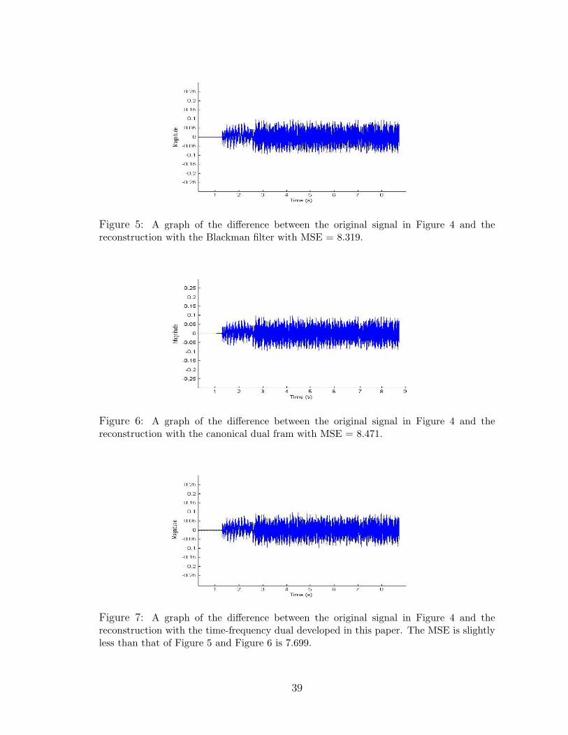
Figure 5: A graph of the difference between the original signal in Figure 4 and thereconstruction with the Blackman filter with MSE = 8.319.

Figure 6: A graph of the difference between the original signal in Figure 4 and thereconstruction with the canonical dual fram with MSE = 8.471.

Figure 7: A graph of the difference between the original signal in Figure 4 and thereconstruction with the time-frequency dual developed in this paper. The MSE is slightlyless than that of Figure 5 and Figure 6 is 7.699.

39

As is seen in the previous figures, the signal-to-noise ratios and mean square

errors found when doing signal construction with the Blackman filter, canonical dual,

and time-frequency dual are quite close. It can be seen that the time-frequency

quantization scheme minimizes error consistently and is not dependent upon the

filter bank being used. These results are summarized in Table 1.

Blackman Canonical Time-FrequencySNR 17.238 17.160 17.576MSE 8.319 8.471 7.699

Table 1: A summary of MSE and SNR for the Blackman filter, canonical dual, andthe time-frequency dual using the time-frequency quantization scheme. Throughthese calculations, we see that the time-frequency dual minimizes the error.

4.2 Applying the Second Order Σ∆ Scheme

We will now compare the SNR and MSE using the Blackman filter, the canon-

ical dual, and the time-frequency dual with the second-order quantization scheme

developed by Daubechies and Devore in Section 2.4.2 using the same signal in Sec-

tion 4.1. We discover that the time-frequency dual has a much greater advantage in

this setting. The signal-to-noise ratios for the Blackman filter, canonical dual, and

time-frequency dual are 30.727, 18.990, and 32.003 respectively.

The time-frequency dual demonstrates a higher SNR and lower error through

signal reconstruction when compared to the canonical dual and Blackman filter using

this scheme. We can see that the advantage to using a specific dual is dependent

upon which quantization scheme is used. In this section we distinguish between the

results from the second-order scheme developed by Daubechies and Devore and the

time-frequency scheme. The time-frequency scheme yields a similar error and SNR

when using any of the three duals while the scheme in this section shows a definite

advantage to the time-frequency dual. The results are summarized in Table 2.

40

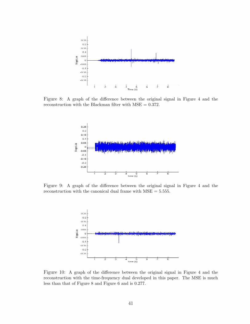
Figure 8: A graph of the difference between the original signal in Figure 4 and thereconstruction with the Blackman filter with MSE = 0.372.

Figure 9: A graph of the difference between the original signal in Figure 4 and thereconstruction with the canonical dual frame with MSE = 5.555.

Figure 10: A graph of the difference between the original signal in Figure 4 and thereconstruction with the time-frequency dual developed in this paper. The MSE is muchless than that of Figure 8 and Figure 6 and is 0.277.

41

Blackman Canonical Time-FrequencySNR 30.727 18.990 32.003MSE 0.372 5.555 0.277

Table 2: A summary of MSE and SNR for the Blackman filter, canonical dual,and the time-frequency dual using the second order Σ∆ scheme. Through thesecalculations, we see that the time-frequency dual minimizes the error.

42

5 CONCLUSION

The sampling theorem and Fourier analysis paved the way for many advances in

signal processing. The idea that a continuous band-limited signal can be replaced by

a discrete sequence of samples without losing any information led to the development

of frames and duals. These concepts along with quantization are important as it is

often necessary in practice to convert analog signals to digital ones.

Σ∆ quantization is used as a basis for the time-frequency quantization scheme

developed in this paper. This method was chosen over Pulse Code Modulation

because PCM does not have strong error correction and Σ∆ quantization smooths

out error over time. We see that through this quantization, the state variables, ~u

and ~v, must be less than one to achieve stability.

When F is a dual frame to E, we find that the Frobenis norm, ‖F‖F and the

operator norm, ‖F‖op are minimized when F = (EE∗)−1E is the canonical dual

frame of E. Using this method, we find that the time frequency dual is a minimizer

of the Heisenberg sum, ‖DH∗‖2F + ‖DFH∗‖2F . From this, we see that even though

the Balian Low Theorem says that a signal and it’s Fourier transform cannot be

localized for an orthonormal basis, we can generate duals in the finite setting that

are, in fact, well localized in time and frequency. Along the same lines, we see

that even if the frame and frame coefficients have poor time-frequency localization,

such as the block function, we can find a dual frame and frame matrix with good

time-frequency localization.

Applying our time-frequency quantization scheme to the canonical dual, Black-

man filter, and the time-frequency dual, we see that the time-frequency dual outper-

forms the others. This is shown through a higher signal-to-noise ratio and a lower

mean square error. It is interesting to notice that the time-frequency quantization

scheme seems to provide similar results among all three duals tested; however, the

43

scheme developed by Daubechies and Devore shows a much wider range of values.

The time-frequency dual has only been tested with the two quantization schemes

in this paper. As a result, future research to develop new schemes would be beneficial

and may show that the TF dual outperforms the canonical dual and the Blackman

filter in a larger magnitude. Also, many signals were tested with these duals and

schemes; however, it may be the case that a specific type of signal, that has not been

tested, works best with the Time-Frequency dual/quantization scheme.

44

REFERENCES

[1] A.R. Amir-Moez and C. Davis. Generalized Frobenius inner products. (Math.

Annalen 141), 107, 1960.

[2] N.H. Asmar. Partial Differential Equations with Fourier Series and Boundary

Value Problems. (Pearson Education, Inc.), 398:546-571, 2005.

[3] J. Blum, M. Lammers, A.M. Powell, and O. Yilmaz. Sobolev Duals in Frame

Theory and Sigma-Delta Quantization. (Submitted to JFAA), 2009.

[4] J.J. Benedetto, C. Heil, and D.F. Walnut. Differentiation and the Balian-Low

Theorem. (CRC Press, Inc.), 355-359, 1995.

[5] J.S. Byrnes and J.L. Byrnes. Recent Advances in Fourier Analysis and Its Ap-

plications. (Kluwer Academic Publishers), 436:441-442, 1990.

[6] I. Daubechies and R. Devore. Approximating a bandlimited function using very

coarsely quantized data: A family of stable sigma-delta modulators of arbitrary

order. (Annals of Mathematics), 679-710, 2003.

[7] R. J. Duffin and A. C. Schaeffer. A class of nonharmonic Fourier series (Trans.

Amer. Math. Soc.), 341-366, 1952.

[8] M. Fickus. Notes on a Discrete Uncertainty Principle.(Preprint), 6-7, 2007.

[9] M. Fickus and M.C. Lammers. Finite Balian Low. (Preprint), 2009.

[10] C. Gasquet and P. Witomski. Fourier Analysis and Applications: Filtering,

Numerical Computation, Wavelets. (Springer-Verlag New York Inc.), 343-360,

1999.

[11] C.S. Gunturk. One-Bit Sigma-Delta Quantization with Exponential Accuracy.

(Wiley Periodicals, Inc.), 1608-1616, 2003.

45

[12] W. Heisenberg, ber den anschaulichen Inhalt der quantentheoretischen Kine-

matik und Mechanik, (Zeitschrift fr Physik), 43, pp. 172-198, 1927.

[13] A.J. Jerri. The Shannon Sampling Theorem-It’s Various Extensions and Ap-

plications: A tutorial Review. (The Institute of Electrical and Electronics Engi-

neers, Inc.), 1565-1567, 1977.

[14] Y. Katznelson. An introduction to Harmonic Analysis. (Dover Publications,

Inc.), 46-61, 1976.

[15] M.C. Lammers, A.M. Powell, O. Yilmaz. On Quantization of Finite Frame

Expansions: Sigma-Delta Schemes of Arbitrary Order.

[16] S. Li. On General Frame Decompositions. (Numerical Functional Analysis and

Optimization 16) no. 9, 1181-1191, 1995.

[17] R.J. Marks II. Introduction to Shannon Sampling and Interpolation Theory.

(Springer-Verlag New York Inc.), 1-5:37, 1991.

[18] A.M. Powell, J.J. Benedetto, and O. Yilmaz. Sigma-Delta Quantization and

Finite Frames.

[19] C. E. Shannon. Communication in the presence of noise. (Proc. Institute of

Radio Engineers), vol. 37, no.1, 10-21, 1949.

[20] A. Teolis. Computational Signal Processing with Wavelets. (Birkhauser

Boston), 36-37, 1998.

[21] E. W. Weisstein. Hilbert Space/ Complete Metric Space. From MathWorld-(A

Wolfram Web Resource.), http://mathworld.wolfram.com/HilbertSpace.html.

[22] A.I. Zayed. Advances in Shannon’s Sampling Theory. (CRC Press, Inc.), 1-5:19,

1993.

46

6 APPENDIX

6.1 MATLAB Program Used for Results in Section 4.1

clear all

K=3; %bit rate

delt= 1/(K-.5);%%% quantizer stepsize

y = wavread(’boxachoc.wav’); L = length(y);%signal stereo

s=1;c=1/4;

y=y(:,1)/s;% convert Mono

part=.1;

L=floor(part*L);% change part to run shorter pieces of the signal

d=128;% window length -must be even

n=16;% oversampling rate

N=n*d;

j=0:n*d-1;

for m=1:d; %repeated on basis

E(m,(m-1)*n+1:n*m)=ones(1,n);

end

%create duals

T=diag(ones(1,N-1),1);

T(N,1)=1;

% Blackman Window %

w = .42 - .5*cos(2*pi*(0:n-1)/(n-1)) ...

+ .08*cos(4*pi*(0:n-1)/(n-1));

w=w/sum(w);

for m=1:d;

Ed(m,(m-1)*n+1:n*m)=w;

47

end

% Sobelov Dual %

DS = diag(ones(1,N),0) + diag(-ones(1,N-1),1);

DS(N,N) = 1;

%DS(N,1)=0;

D=DS;

Dinv=inv(D);

M = Dinv*(Dinv.’);

S = ((E*M*(E.’))^(-1))*(E*M);

% Canonical dual %

C = (E*E’)^(-1)*E;

% Time-Frequency Dual %

D1 = diag(ones(1,N),0) + diag(-ones(1,N-1),1) + diag(-ones(1,1),-(N-1));

D1(N,N) = 1;

D=D1;

pre_f = (eye(N))/sqrt(N);

F = fft(pre_f);

X = F’*D’*D*F;

Delt=D’*D;

TF = Delt+X^(1);

TF(N,1)=0;

TF(1,N)=0;

M=inv(TF’)*inv(TF);

H = ((E*M*(E.’))^(-1))*(E*M);

pc=0;

sec=floor(L/d);

for j=1:sec %windowed frame transform, i.e. coefficient set

48

yt=y(pc+1:pc+d);

YH(:,j)=E’*yt;

pc=pc+d;

end

stability=max(max(YH)) %check stability <1 good

%clear E %for memory

alpha = diag(TF);

gamma=1.6;

uN=0;vN=YH(1,1)/gamma;

q = zeros(N,sec);

for m =1:sec

x = YH(:,m);

u = zeros(N,1);

q(1,m)=Q(x(1),delt,K);

u(1)=x(1)-q(1,m);

q(2,m)=Q(x(2)+u(1),delt,K);

u(2)=x(2)-q(2,m)+u(1)/8;

q(3,m)=Q(x(3)+u(2),delt,K);

u(3)=x(3)-q(3)+(alpha(3)*u(1)-u(2))/8;

for j = 4:N

q(j,m)=Q((u(j-1)+x(j)),delt,K);

u(j)=(x(j-1)-q(j-1,m))+(-u(j-3)+alpha(j-2)*u(j-2)-u(j-1))/8;

U(m)=max(abs(u));

mU(m)=min(u);

end

end

stability=max(U)

49

clear x YH; %clean up for memory

pc=0; %reconstrution

YA=zeros(L,1);

YC=zeros(L,1);

YS=zeros(L,1);

YCAN=zeros(L,1);

for j=1:sec-1

YA(pc+1:pc+d)=H*q(:,j)+YA(pc+1:pc+d);

YC(pc+1:pc+d)=Ed*q(:,j)+YC(pc+1:pc+d);

YS(pc+1:pc+d)=S*q(:,j)+YS(pc+1:pc+d);

YCAN(pc+1:pc+d)=C*q(:,j)+YCAN(pc+1:pc+d);

pc=pc+d;

end

b=300;

L=floor(.9*L);

clf

figure(1)

hold on

plot(y(b:L)-YC(b:L),’k’)

axis([b L -.3 .3])

hold off

figure(2)

clf

hold on

plot(y(b:L)-YA(b:L),’b’)

axis([b L -.3 .3])

figure(3)

50

clf

hold on

plot(y(b:L)-YS(b:L),’b’)

axis([b L -.3 .3])

figure(4)

clf

hold on

plot(y(b:L)-YCAN(b:L),’b’)

axis([b L -.3 .3])

figure(5)

clf

hold on

plot(y(b:L),’b’)

axis([b L -.8 1])

errblack=norm(y(b:L)-YC(b:L))

errTF=norm(y(b:L)-YA(b:L))

errsob=norm(y(b:L)-YS(b:L))

errcan=norm(y(b:L)-YCAN(b:L))

mseblack=errblack^2

mseTF=errTF^2

msesob=errsob^2

msecan=errcan^2

vce=var(y(b:L)-YC(b:L));

vae=var(y(b:L)-YA(b:L));

vse=var(y(b:L)-YS(b:L));

vcanse=var(y(b:L)-YCAN(b:L));

vy=var(y(b:L));

51

SNR_black_and_SNR_TF_and_SNR_SOB_and_SNR_CAN=

[10*log(vy/vce)/log(10), 10*log(vy/vae)/log(10),

10*log(vy/vse)/log(10), 10*log(vy/vcanse)/log(10)]

wavplay(YC,11000) %play signals

wavplay(real(YA),11000)

improve=(10*log(vy/vae)/log(10)-

10*log(vy/vce)/log(10))/(10*log(vy/vce)/log(10))

6.2 MATLAB Program Used for Results in Section 4.2

clear all

K=3; %bit rate

delt= 1/(K-.5);%%% quantizer stepsize

y = wavread(’boxachoc.wav’); L = length(y);%signal stereo

s=1;c=1/2;

y=y(:,1)/s;% convert Mono

part=.1;

L=floor(part*L);% change part to run shorter pieces of the signal

d=128;% window length -must be even

n=16;% oversampling rate

N=n*d;

j=0:n*d-1;

for m=1:d; %repeated on basis

E(m,(m-1)*n+1:n*m)=ones(1,n);

end

%create duals

T=diag(ones(1,N-1),1);

T(N,1)=1;

52

% Blackman Window %

w = .42 - .5*cos(2*pi*(0:n-1)/(n-1)) ...

+ .08*cos(4*pi*(0:n-1)/(n-1));

w=w/sum(w);

for m=1:d;

Ed(m,(m-1)*n+1:n*m)=w;

end

% Sobelov Dual %

DS = diag(ones(1,N),0) + diag(-ones(1,N-1),1);

DS(N,N) = 1;

D=DS;

Dinv=inv(D);

M = Dinv*(Dinv.’);

S = ((E*M*(E.’))^(-1))*(E*M);

% Canonical dual %

C = (E*E’)^(-1)*E;

% Time-Frequency Dual %

D1 = diag(ones(1,N),0) + diag(-ones(1,N-1),1) + diag(-ones(1,1),-(N-1));

D1(N,N) = 1;

D=D1;

pre_f = (eye(N))/sqrt(N);

F = fft(pre_f);

X = F’*D’*D*F;

Delt=D’*D;

TF = real(Delt+X);

TF(N,1)=0;

TF(1,N)=0;

53

M=inv(TF’)*inv(TF);

H = ((E*M*(E.’))^(-1))*(E*M);

pc=0;

sec=floor(L/d);

for j=1:sec %windowed frame transform, i.e. coefficient set

yt=y(pc+1:pc+d);

YH(:,j)=E’*yt;

pc=pc+d;

end

stability=max(max(YH)) %check stability <1 good

%clear E %for memory

alpha = diag(TF);

gamma=1.6;

uN=0;vN=YH(1,1)/gamma;

q = zeros(N,sec);

for m =1:sec %%% 2nd oreder Sigma-Delta (Daub -Devore paper)

x = YH(:,m);

u = zeros(N,1);

v = zeros(N,1);

q(1,m) = Q(uN+ x(1),delt,K);

v(1)=x(1)-q(1);

u(1) = uN + v(1);

for j = 2:N

q(j,m) = Q(u(j-1)+ gamma*v(j-1),delt,K);

v(j) = v(j-1)+ x(j) - q(j,m);

u(j)= u(j-1) +v(j);

end

54

U(m)=max(u);

mU(m)=min(u);

end

stability=max(U)

clear x YH; %clean up for memory

pc=0; %reconstrution

YA=zeros(L,1);

YC=zeros(L,1);

YS=zeros(L,1);

YCAN=zeros(L,1);

for j=1:sec-1

YA(pc+1:pc+d)=H*q(:,j)+YA(pc+1:pc+d);

YC(pc+1:pc+d)=Ed*q(:,j)+YC(pc+1:pc+d);

YS(pc+1:pc+d)=S*q(:,j)+YS(pc+1:pc+d);

YCAN(pc+1:pc+d)=C*q(:,j)+YCAN(pc+1:pc+d);

pc=pc+d;

end

b=300;

L=floor(.9*L);

clf

figure(1)

hold on

plot(y(b:L)-YC(b:L),’k’)

axis([b L -.3 .3])

hold off

figure(2)

clf

55

hold on

plot(y(b:L)-YA(b:L),’b’)

axis([b L -.3 .3])

figure(3)

clf

hold on

plot(y(b:L)-YS(b:L),’b’)

axis([b L -.3 .3])

figure(4)

clf

hold on

plot(y(b:L)-YCAN(b:L),’b’)

axis([b L -.3 .3])

figure(5)

clf

hold on

plot(y(b:L),’b’)

axis([b L -.8 1])

errblack=norm(y(b:L)-YC(b:L))

errTF=norm(y(b:L)-YA(b:L))

errsob=norm(y(b:L)-YS(b:L))

errcan=norm(y(b:L)-YCAN(b:L))

mseblack=errblack^2

mseTF=errTF^2

msesob=errsob^2

msecan=errcan^2

vce=var(y(b:L)-YC(b:L));

56

vae=var(y(b:L)-YA(b:L));

vse=var(y(b:L)-YS(b:L));

vcanse=var(y(b:L)-YCAN(b:L));

vy=var(y(b:L));

SNR_black_and_SNR_TF_and_SNR_SOB_and_SNR_CAN

=[10*log(vy/vce)/log(10), 10*log(vy/vae)/log(10),

10*log(vy/vse)/log(10), 10*log(vy/vcanse)/log(10)]

wavplay(YC,11000) %play signals

wavplay(real(YA),11000)

improve=(10*log(vy/vae)/log(10)-

10*log(vy/vce)/log(10))/(10*log(vy/vce)/log(10))

57