tight coupling ufmarcgis for simulating inundation depth in densely area s. h. kang

Nat. Hazards Earth Syst. Sci., 10, 1523–1530, 2010www.nat-hazards-earth-syst-sci.net/10/1523/2010/doi:10.5194/nhess-10-1523-2010© Author(s) 2010. CC Attribution 3.0 License.

Natural Hazardsand Earth

System Sciences

Tight coupling UFMArcGIS for simulating inundation depth indensely area

S. H. Kang

Dept. of Civil Engineering, Kangwon National University, Samcheok, Republic of Korea

Received: 18 September 2008 – Revised: 11 June 2010 – Accepted: 29 June 2010 – Published: 14 July 2010

Abstract. The integration of hydrological models and Geo-graphical Information Systems (GIS) usually takes two ap-proaches: loose coupling and tight coupling. This paperpresents a tight coupling approach within a GIS environmentthat is achieved by integrating the urban flood model with themacro language of GIS. Such an approach affords an uncom-plicated way to capitalize on the GIS visualization and spa-tial analysis functions, thereby significantly supporting thedynamic simulation process of hydrological modeling. Thetight coupling approach is illustrated by UFMArcGIS (Ur-ban Flood Model with ArcGIS), which is a realization of anurban flood model integrated with the VBA (visual basic ofapplication) language of ArcGIS. Within this model, majorstages of model structures are created from the initial param-eter input and transformation of datasets, intermediate mapsare then visualized, and the results are finally presented invarious graphical formats in their geographic context. Thisapproach provides a convenient and single environment inwhich users can visually interact with the model, e.g. by ad-justing parameters while simultaneously observing the corre-sponding results. This significantly facilitates users in the ex-ploratory data analysis and decision-making stages in termsof the model applications.

1 Introduction

In recent years, the introduction of various hydraulic and hy-drological modeling techniques has enabled users of GIS togo beyond the data inventory and management stage to con-duct sophisticated modeling and simulation. In terms of hy-drological modeling, GIS has provided modelers with new

Correspondence to:S. H. Kang([email protected])

platforms for data management and visualization, particu-larly through its powerful capabilities to process topographi-cal data. The rapid distribution of GIS techniques to a widerpopulation has the potential to make various hydrologicalmodels more transparent and to enable the communicationof GIS operations and results to a large group of users. At-tempts have been made to integrate various models into GISin order to meet the increasing need to enhance its functional-ity in environmental modeling (Bishop and Karadaglis, 1996;Vivoni et al., 2005), urban modeling (Nie, 2004; Hosoya-mada, 2005; Takayama et al., 2006) and, in a more generalsense, analytical tools (Horritt and Bates, 2001a, b; Yangand Rystedt, 2002; Haile and Rientjes, 2005; Sayama et al.,2006).

Consequently, while able to simplify reality, models canstill involve complex mathematical and analytical exercises.While some of these calculations are possible within a GIS,others require greater computational abilities than are cur-rently available in a GIS. Models can be implemented withina GIS in a number of ways (Sui and Maggio, 1999). Themodel and the GIS can be loosely coupled, whereby the GISis used to prepare data for use in a separate computationalmodel. The GIS can alternatively be used simply to visualizethe model output. The model can also be implemented usingthe functionality of the GIS, for example in calculating to-pographic factors for a hydrological model. The advantagesof this latter approach lie in the fact that both systems caneither be developed or used independently. However, the ex-change of data files, which usually involves taking text filesas a link between two systems, is inherently cumbersomeand not user-friendly. Alternatively, the model and the GIScan be tightly computationally coupled, whereby the GIS isused for both the input and the visualization of the output. Itshould be noted that differences in data models have a signif-icant impact on the computational manipulation of data in theabove coupling process. Compared with the loose coupling

Published by Copernicus Publications on behalf of the European Geosciences Union.

http://creativecommons.org/licenses/by/3.0/

1524 S. H. Kang: Tight coupling UFMArcGIS for simulating inundation depth in densely area

method used in the earlier development of GIS, tight cou-pling is considered to be a more effective integration methodwhen a transparent interface is required for the data struc-tures of GIS, which is rarely provided by GIS developers.

Previously employed for mapping analysis results, visu-alization is nowadays considered an important tool for spa-tial analysis (Bourget, 2004). Various new terms have beenused to reflect this change, such as spatial data explorationand exploratory visualization. When hydraulic models arefully integrated into GIS, the analytical processes can besimulated, thereby making visual exploration more straight-forward. With such a highly interactive platform, users areable to obtain a comprehensive perception of reality throughits counterpart in computer systems. Despite these conve-niences, few attempts have been made to tightly link a GISbased model to simulate inundation depth. This is due to thecomplex topographic features in urban areas.

In this study, an urban flood model – overland flow, ur-ban flood flow and sewer flow – was combined and devel-oped with ArcGIS in order to simulate inundation depth inSamcheok city, South Korea. The intention is to provide anexample to illustrate the advantages of using such a tight in-tegration method for modeling and visualization.

2 Description of study site

The Oship River of Samcheok city, Kangwon Province,in the Republic of Korea is located about 100 km to theeast of Seoul (128◦30′

∼ 128◦40′ E; 37◦25′∼ 37◦49′ N). The

drainage area of the Oship River basin is 384 km2, with amean annual precipitation of 1550 mm over the last 10 years(1998–2007; data are only available for this period). Over80% of the annual mean rainfall area was concentrated inheavy showers that occurred several times during the rainyseason from May to September during this period (WAMIS,2009; on-line available athttp://www.wamis.go.kr/).

The basin has a large forested area (87%) and an area foragricultural use (7.5%). The main channel length of the Os-hip River is 59 km and the channel slope ranges from 0.037to 0.801%. Samcheok city is situated in the downland areaof the Oship River basin, with a population of approximately30 000 inhabitants. The total area of the city is 2.79 km2 withcontours ranging from 0 to 30 m for an urban flood simu-lation of 1.32 km2. The area has a well known history offloods due to heavy rainfall (Kang, 2007). From 31 Au-gust to 1 September 2002, the basin endured a large flooddue to heavy rainfall caused by Typhoon Rusa. The typhoonclaimed the lives of 13 people and inundated 3639 housesand 200 ha of farmland. The maximum hourly and total pre-cipitation was 64 mm h−1 and 582 mm, respectively. Thisdevastation extended further when another typhoon hit thesame region in 2003, resulting in serious damage. The suc-cessive disasters isolated the public, separating people fromother towns, and paralyzed personal infrastructures, while

causing wide-spread destruction of property and numeroushuman casualties. In order to reduce the loss of life and prop-erty caused by floods, the Flood Mitigation Project was ini-tiated by the municipality of Samcheok city in 2004. Theproject was designed to protect against the 100-year floodfrequency. The major components for reducing flood damagein the urban area include: drainage pumping stations, a sewerdrainage system, and channel improvement. Other cities inthe world have been developed similar projects. For exam-ple in Barcelona city (Spain) the damages produced by flashfloods have considerably diminished during the last years ba-sically due to the development of a dense network of pump-ing station within the city (Barrera et al., 2006).

3 Model structure

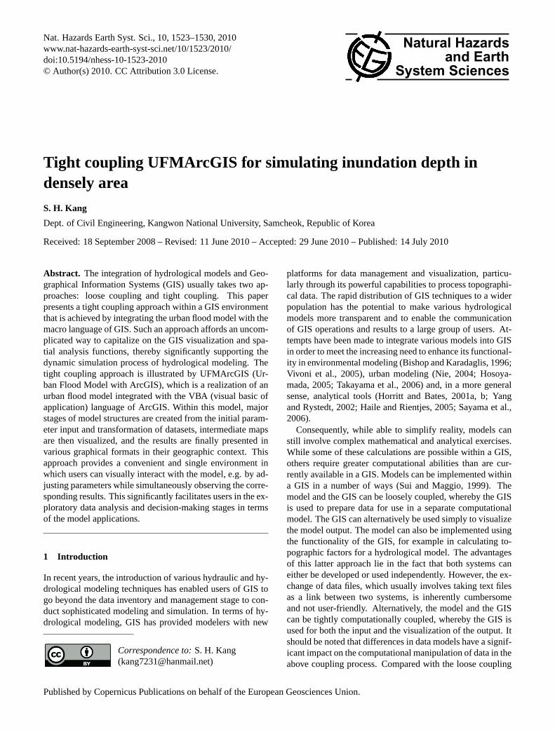
The overall model structure with ArcGIS is represented asshown in Fig. 1. Following the transformation of rainfallto effective runoff by interception and depression storagesimulation, surface runoff is handled in two parallel simu-lation modules. The sub-routine module for hydrologic sur-face runoff is applied to areas where there is surface floodingas well as interaction between surface flow and sewer flow.Here, surface runoff enters the sewer system at defined inlets.

3.1 Overland flow from watershed

The drainage area of Oship River basin is 393 km2 and hasmany tributaries. Among them, the study area for the surfacerunoff is 344.8 km2 and the channel slope ranges from 0.071to 0.40. The governing equations based on the kinematicwave model are as follows:

3.1.1 Slope flow

∂h

∂t+

∂q

∂x= re (1)

q = αhm (2)

Here,x is a one-dimensional spatial coordinate;t is time;qis the discharge per unit width on the slope;re is the effectiverainfall; h is the water depth;α andm are constants, respec-tively (m′=5/3;α =

√sinθ/N ; θ is the slope gradient; andN

is the Manning’s roughness coefficient in the slope).

3.1.2 River flow

∂h

∂t+

∂q ′

∂x=

q

B(3)

q ′= αhm′

(4)

Here,q ′ is the discharge per unit width on the mountainousriver; q is the lateral inflow per unit width from the slope;B is the mountainous river width;α and m′ are constants

Nat. Hazards Earth Syst. Sci., 10, 1523–1530, 2010 www.nat-hazards-earth-syst-sci.net/10/1523/2010/

http://www.wamis.go.kr/

S. H. Kang: Tight coupling UFMArcGIS for simulating inundation depth in densely area 1525

19

1

2

3

4

5

6

7

8

9

10

11

12

13

14

15

16

Fig. 2. Concept of buildings sharing

(A1) and (A2) in each grid

Fig. 3. Share rate of building per unit grid

Fig. 1. Urban flood model structure on ArcGIS Fig. 1. Urban flood model structure on ArcGIS.

(α =√

sinθr/n; θr is the river bed slope;n is the Manning’sroughness coefficient; andm′=5/3).

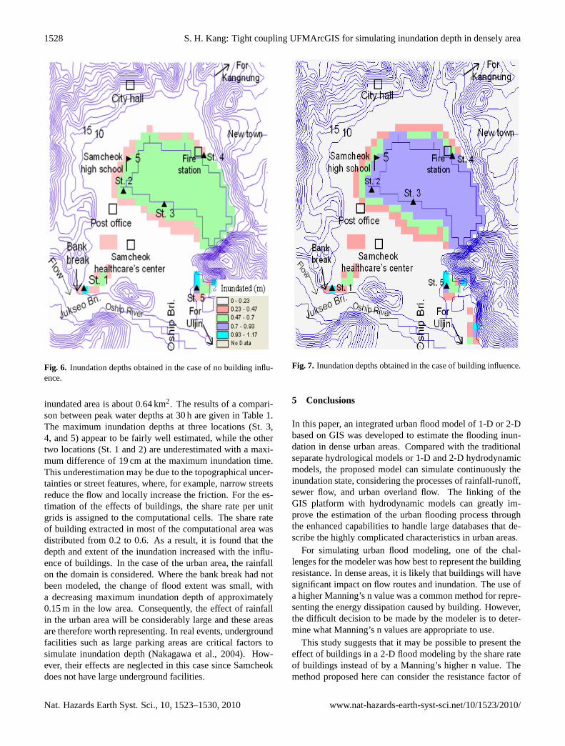
The lateral inflow from the slope of the river is calcu-lated using the characteristics method and the runoff dis-charge along the river is calculated using the finite differencemethod, which uses the Leap-Frog method. For the bound-ary condition in the down stream of the bank break point, thewater-level flux of the sides of the grid is assigned using thedischarge hydrograph as shown in Fig. 5.

3.1.3 Sewer flow

The rainwater in the sewer pipe is calculated in the followingcontinuity and momentum equations:

∂A

∂t+

∂Q

∂x= q (5)

∂Q

∂t+

∂(uQ)

∂x= gA

∂H

∂x−

gn2|Q|Q

R4/3A, (6)

whereA is the cross sectional area of flow;Q is the dis-charge;q is the lateral inflow;u is the flow velocity;H is thewater level (H = h+ z); andz is the elevation of the sewerpipe from the bottom (Abbott et al., 1998; Franz, 1997). Forthis study, the interaction between surface flow and sewerflow is as described by Schmitt et al. (2004). The value ofManning’s roughness coefficient is 0.015 s m−1/3 and it isassumed that the cross sectional shape of the pipes is rect-angular.

3.2 Urban flood flow

The governing equations for 2-D, gradually varied, unsteadyflow can be derived from mass conservation and momentumequations. Overland flow equations are the 2-D expansion ofSt. Venant’s 1-D open channel flow equations, as follows:

Continuity equation (mass conservation equation)

∂h

∂t+

∂M

∂x+

∂M

∂y= re−qout+qover (7)

Momentum equations

∂M

∂t+

∂(uM)

∂x+

∂(vM)

∂y= −gh

∂H

∂x−

τbx

ρw(8)

∂N

∂t+

∂(uN)

∂x+

∂(vN)

∂y= −gh

∂H

∂y−

τby

ρw

, (9)

whereh is the water depth;u andv are the velocities of flowin the x- and y-directions, respectively;M and N are thefluxes of discharge in the x- and y-directions, respectively(M=uh, N=vh); qout is the drainage discharge from the urbanarea to the sewer line in each grid; andqover is the overtop-ping flow discharge per unit area of the computational gridfrom the down stream.

H is the water level, written asH = h+z, wherez is thebed elevation.τbx andτby are the x- and y-components, re-spectively, of shear stress on the water bottom, as follows:

τbx =ρwgn2u

√u2+v2

h1/3(10)

www.nat-hazards-earth-syst-sci.net/10/1523/2010/ Nat. Hazards Earth Syst. Sci., 10, 1523–1530, 2010


19

1

2

3

4

5

6

7

8

9

10

11

12

13

14

15

16




Fig. 1. Urban flood model structure on ArcGIS

Fig. 2. Concept of buildings sharing (A1) and (A2) in each grid.

τby =ρwgn2v

√u2+v2

h1/3, (11)

whereρw is the water density;g is the gravity acceleration;andn is Manning’s roughness coefficient.

4 Application of model

4.1 Influence of buildings

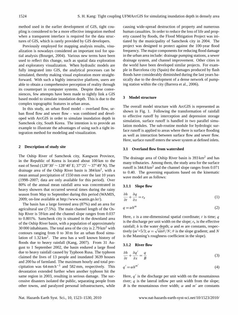
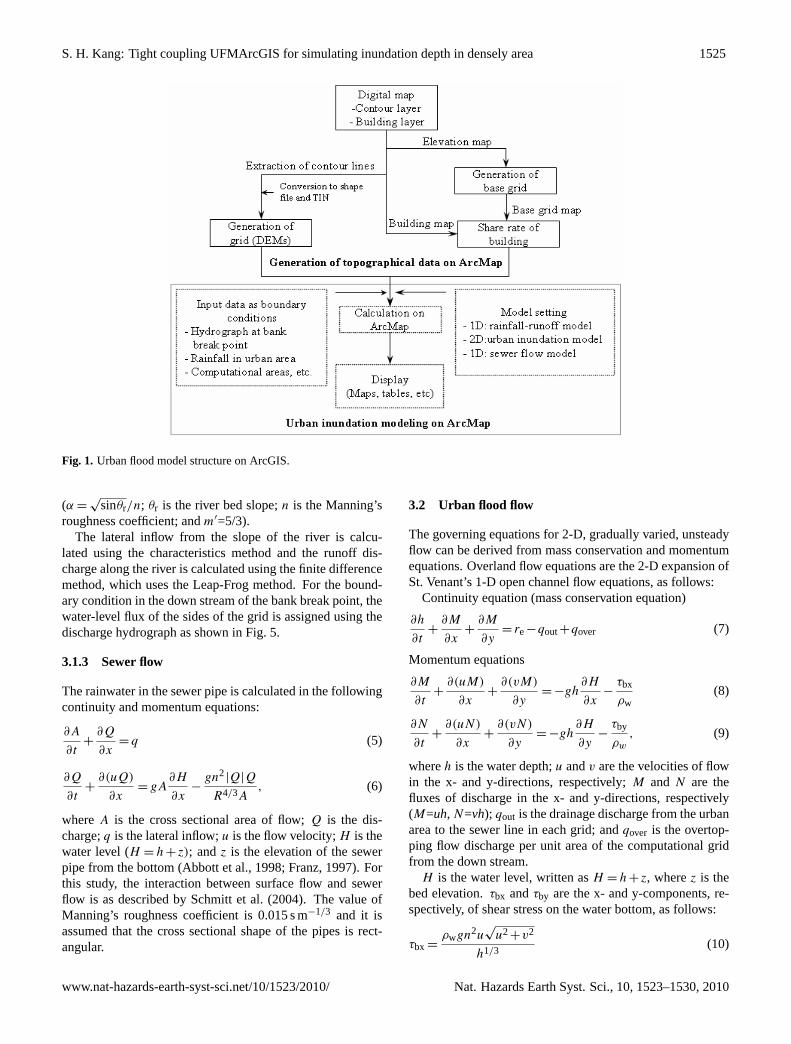
In order to simulate urban flooding, the influence of build-ings should be carefully specified according to the needs ofan application. GIS-based hydrological modeling is appliedin order to distinguish the basic hydrological elements froma DEM (Digital Elevation Model). When considering the in-fluence of buildings, the method of determining the share rateof a building is used as described in Eqs. (13) and (14). Thepossible representations of buildings for the model are illus-trated in Fig. 2. In order to extract building properties, GIStechniques were applied as shown in Fig. 3. The data relat-ing to building areas is converted into an image, which is thenconverted into a polygon using a geo-concept image. For ex-tracting buildings, a minimum filter method by Arc-info wasused.

In order to estimate the effect of a building, the share ofthe buildingλi,j in each grid, and the transmissivity of thebuildingβi,j =

√1−λi,j are applied (Takahashi et al., 1986).

In this study, buildings are represented as independently solidobjects. For the calculation, the values of 1.0 for buildingsand 0.0 for areas without buildings are assigned. The flux ofdischarge can then be defined as:

M∗= βM, N∗

= βN (12)

whereM∗ andN∗ are the flux of discharge which are cor-rected boundary conditions in the x- and y-components perunit width, respectively. If we considerM∗, N∗ andλ, thecontinuity equation can be written as:

(1−λ)∂h

∂t+

∂M∗

∂x+

∂N∗

∂y= re−qout+qover (13)

19

1

2

3

4

5

6

7

8

9

10

11

12

13

14

15

16




Fig. 1. Urban flood model structure on ArcGIS

Fig. 3. Share rate of building per unit grid with contour lines.

whereu andv are the x- and y-components of flow veloc-ity, respectively;M∗

= βM andN∗= βN are the x- and y-

components, respectively, of the corrected discharge per unitwidth; M andN are the x- and y-components per unit width,respectively;qout is the drainage discharge per unit area fromthe computational mesh into the sewer system; andqover isthe overtopping discharge flow per unit area of the compu-tational grid from the river network. If there are non-linearareas due to the difference of elevation, the discharge flux,M0 flows by drop-water as:

M0 = µhh√

ghh (14)

Based on the hydraulic model test, the discharge coefficientµ is estimated to beµ = (2/3)3/2; andhh is the water depthwhere the elevation is the highest by over-topping water as(Thang et al., 2004):

M0 = µ′h1√

gh1 (15)

whereµ′ is the discharge coefficient estimated asµ′= 0.35;

andh1 is the water depth at the lowest elevation. The mini-mum depth for moving waters is given as 0.001 m (Iwasa etal., 1980).

4.2 Initial values and model validation

The Samcheok city selected for urban inundation modelingis surrounded by mountains; it mostly consists of low-lyingland, where the river flows into the sea through the outside ofthe city. Following the floods, a field investigation team led



20

1

2

3

4

Fig. 5. Discharge hydrograph at bank break point (rainfall data : WAter Management Information System, http://www.wamis.go.kr/)

Fig. 4. A inundated depths after flooding

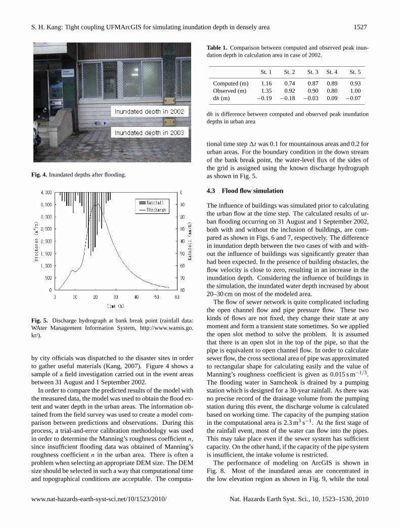
Fig. 4. Inundated depths after flooding.

20

1

2

3

4

Fig. 5. Discharge hydrograph at bank break point (rainfall data : WAter Management Information System, http://www.wamis.go.kr/)

Fig. 4. A inundated depths after flooding

Fig. 5. Discharge hydrograph at bank break point (rainfall data:WAter Management Information System,http://www.wamis.go.kr/).

by city officials was dispatched to the disaster sites in orderto gather useful materials (Kang, 2007). Figure 4 shows asample of a field investigation carried out in the event areasbetween 31 August and 1 September 2002.

In order to compare the predicted results of the model withthe measured data, the model was used to obtain the flood ex-tent and water depth in the urban areas. The information ob-tained from the field survey was used to create a model com-parison between predictions and observations. During thisprocess, a trial-and-error calibration methodology was usedin order to determine the Manning’s roughness coefficientn,since insufficient flooding data was obtained of Manning’sroughness coefficientn in the urban area. There is often aproblem when selecting an appropriate DEM size. The DEMsize should be selected in such a way that computational timeand topographical conditions are acceptable. The computa-

Table 1. Comparison between computed and observed peak inun-dation depth in calculation area in case of 2002.

St. 1 St. 2 St. 3 St. 4 St. 5

Computed (m) 1.16 0.74 0.87 0.89 0.93Observed (m) 1.35 0.92 0.90 0.80 1.00dh (m) −0.19 −0.18 −0.03 0.09 −0.07

dh is difference between computed and observed peak inundationdepths in urban area

tional time step1t was 0.1 for mountainous areas and 0.2 forurban areas. For the boundary condition in the down streamof the bank break point, the water-level flux of the sides ofthe grid is assigned using the known discharge hydrographas shown in Fig. 5.

4.3 Flood flow simulation

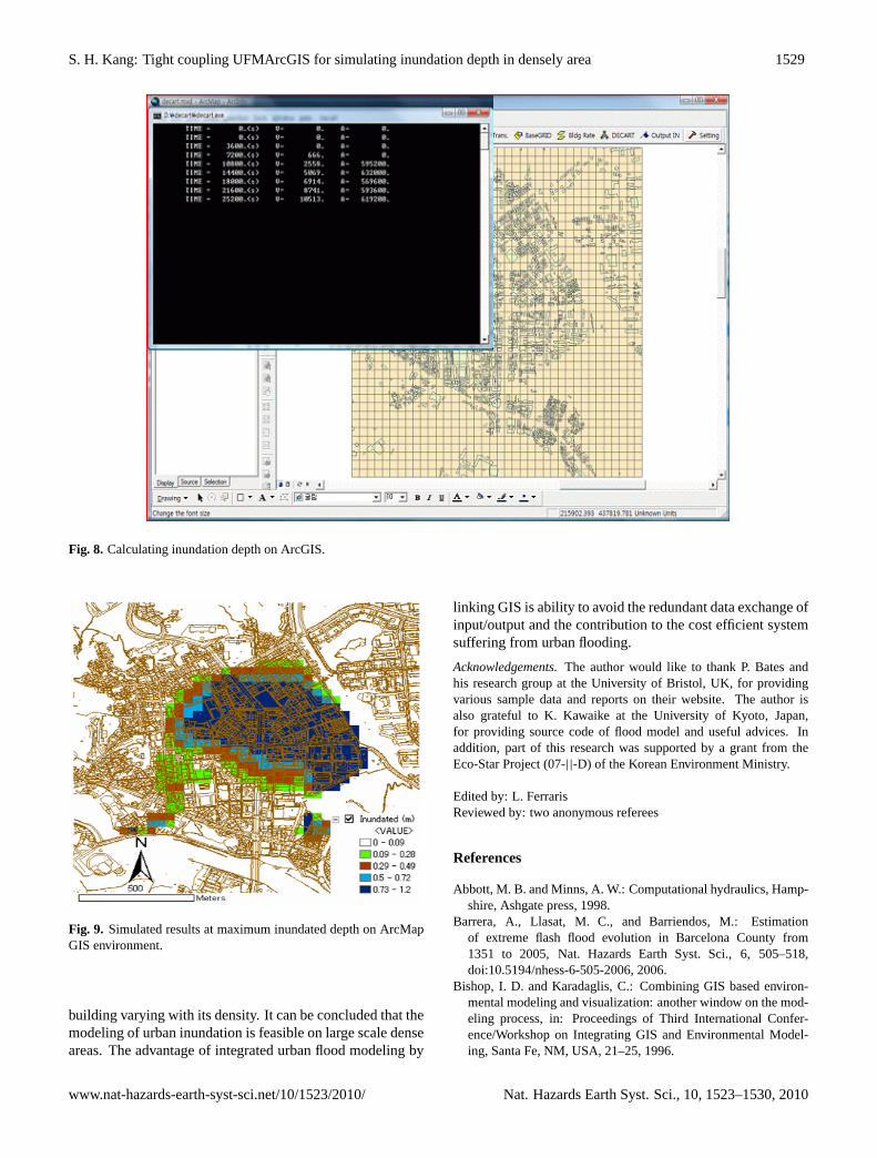
The influence of buildings was simulated prior to calculatingthe urban flow at the time step. The calculated results of ur-ban flooding occurring on 31 August and 1 September 2002,both with and without the inclusion of buildings, are com-pared as shown in Figs. 6 and 7, respectively. The differencein inundation depth between the two cases of with and with-out the influence of buildings was significantly greater thanhad been expected. In the presence of building obstacles, theflow velocity is close to zero, resulting in an increase in theinundation depth. Considering the influence of buildings inthe simulation, the inundated water depth increased by about20–30 cm on most of the modeled area.

The flow of sewer network is quite complicated includingthe open channel flow and pipe pressure flow. These twokinds of flows are not fixed, they change their state at anymoment and form a transient state sometimes. So we appliedthe open slot method to solve the problem. It is assumedthat there is an open slot in the top of the pipe, so that thepipe is equivalent to open channel flow. In order to calculatesewer flow, the cross sectional area of pipe was approximatedto rectangular shape for calculating easily and the value ofManning’s roughness coefficient is given as 0.015 s m−1/3.The flooding water in Samcheok is drained by a pumpingstation which is designed for a 30-year rainfall. As there wasno precise record of the drainage volume from the pumpingstation during this event, the discharge volume is calculatedbased on working time. The capacity of the pumping stationin the computational area is 2.3 m3 s−1. At the first stage ofthe rainfall event, most of the water can flow into the pipes.This may take place even if the sewer system has sufficientcapacity. On the other hand, if the capacity of the pipe systemis insufficient, the intake volume is restricted.

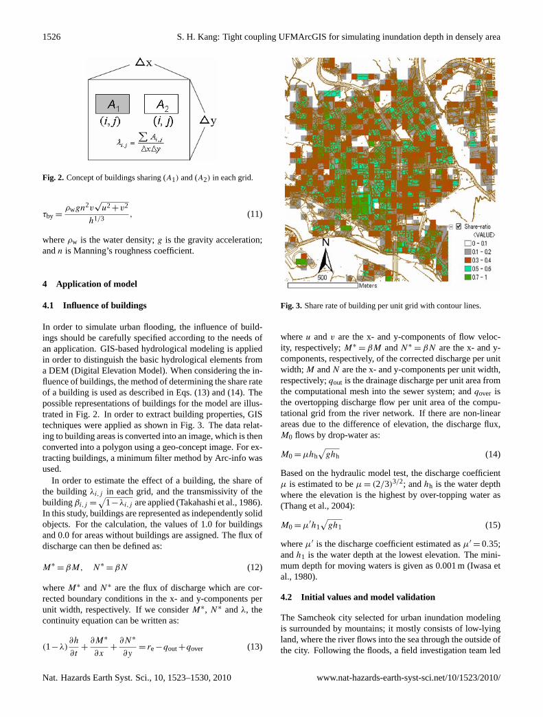
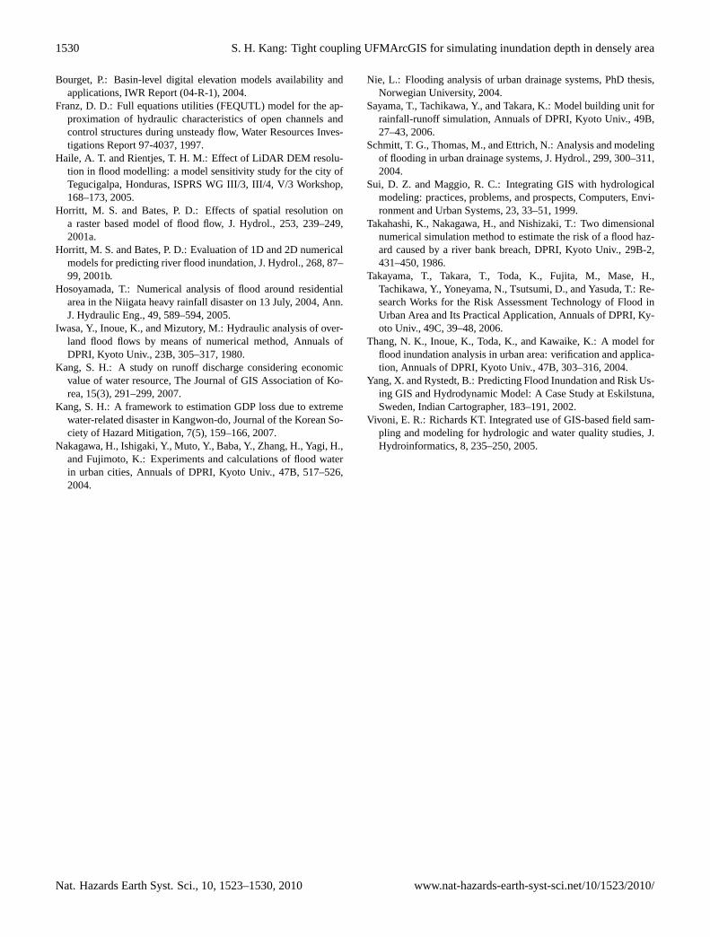
The performance of modeling on ArcGIS is shown inFig. 8. Most of the inundated areas are concentrated inthe low elevation region as shown in Fig. 9, while the total





21

1

2

3

4

Fig. 8. Calculating inundation depth on ArcGIS

Fig. 6. Inundation depths obtained in the

case of no building influence


case of building influence

Fig. 6. Inundation depths obtained in the case of no building influ-ence.

inundated area is about 0.64 km2. The results of a compari-son between peak water depths at 30 h are given in Table 1.The maximum inundation depths at three locations (St. 3,4, and 5) appear to be fairly well estimated, while the othertwo locations (St. 1 and 2) are underestimated with a maxi-mum difference of 19 cm at the maximum inundation time.This underestimation may be due to the topographical uncer-tainties or street features, where, for example, narrow streetsreduce the flow and locally increase the friction. For the es-timation of the effects of buildings, the share rate per unitgrids is assigned to the computational cells. The share rateof building extracted in most of the computational area wasdistributed from 0.2 to 0.6. As a result, it is found that thedepth and extent of the inundation increased with the influ-ence of buildings. In the case of the urban area, the rainfallon the domain is considered. Where the bank break had notbeen modeled, the change of flood extent was small, witha decreasing maximum inundation depth of approximately0.15 m in the low area. Consequently, the effect of rainfallin the urban area will be considerably large and these areasare therefore worth representing. In real events, undergroundfacilities such as large parking areas are critical factors tosimulate inundation depth (Nakagawa et al., 2004). How-ever, their effects are neglected in this case since Samcheokdoes not have large underground facilities.

21

1

2

3

4





case of building influence Fig. 7. Inundation depths obtained in the case of building influence.

5 Conclusions

In this paper, an integrated urban flood model of 1-D or 2-Dbased on GIS was developed to estimate the flooding inun-dation in dense urban areas. Compared with the traditionalseparate hydrological models or 1-D and 2-D hydrodynamicmodels, the proposed model can simulate continuously theinundation state, considering the processes of rainfall-runoff,sewer flow, and urban overland flow. The linking of theGIS platform with hydrodynamic models can greatly im-prove the estimation of the urban flooding process throughthe enhanced capabilities to handle large databases that de-scribe the highly complicated characteristics in urban areas.

For simulating urban flood modeling, one of the chal-lenges for the modeler was how best to represent the buildingresistance. In dense areas, it is likely that buildings will havesignificant impact on flow routes and inundation. The use ofa higher Manning’s n value was a common method for repre-senting the energy dissipation caused by building. However,the difficult decision to be made by the modeler is to deter-mine what Manning’s n values are appropriate to use.

This study suggests that it may be possible to present theeffect of buildings in a 2-D flood modeling by the share rateof buildings instead of by a Manning’s higher n value. Themethod proposed here can consider the resistance factor of



21

1

2

3

4





case of building influence

Fig. 8. Calculating inundation depth on ArcGIS.

22

1

2

3

4

5

6

7

8

9

Table 1. Comparison between computed and observed peak inundation depth in calculation area in case of 2002 St. 1 St. 2 St. 3 St. 4 St. 5 Computed (m) Observed (m) dh (m)

1.16 1.35 -0.19

0.74 0.92 -0.18

0.87 0.90 -0.03

0.89 0.80 0.09

0.93 1.00 -0.07

dh is difference between computed and observed peak inundation depths in urban area

Fig. 9. Simulated results at maximum inundated depth

on ArcMap GIS environment Fig. 9. Simulated results at maximum inundated depth on ArcMapGIS environment.

building varying with its density. It can be concluded that themodeling of urban inundation is feasible on large scale denseareas. The advantage of integrated urban flood modeling by

linking GIS is ability to avoid the redundant data exchange ofinput/output and the contribution to the cost efficient systemsuffering from urban flooding.

Acknowledgements.The author would like to thank P. Bates andhis research group at the University of Bristol, UK, for providingvarious sample data and reports on their website. The author isalso grateful to K. Kawaike at the University of Kyoto, Japan,for providing source code of flood model and useful advices. Inaddition, part of this research was supported by a grant from theEco-Star Project (07-||-D) of the Korean Environment Ministry.

Edited by: L. FerrarisReviewed by: two anonymous referees

References

Abbott, M. B. and Minns, A. W.: Computational hydraulics, Hamp-shire, Ashgate press, 1998.

Barrera, A., Llasat, M. C., and Barriendos, M.: Estimationof extreme flash flood evolution in Barcelona County from1351 to 2005, Nat. Hazards Earth Syst. Sci., 6, 505–518,doi:10.5194/nhess-6-505-2006, 2006.

Bishop, I. D. and Karadaglis, C.: Combining GIS based environ-mental modeling and visualization: another window on the mod-eling process, in: Proceedings of Third International Confer-ence/Workshop on Integrating GIS and Environmental Model-ing, Santa Fe, NM, USA, 21–25, 1996.



Bourget, P.: Basin-level digital elevation models availability andapplications, IWR Report (04-R-1), 2004.

Franz, D. D.: Full equations utilities (FEQUTL) model for the ap-proximation of hydraulic characteristics of open channels andcontrol structures during unsteady flow, Water Resources Inves-tigations Report 97-4037, 1997.

Haile, A. T. and Rientjes, T. H. M.: Effect of LiDAR DEM resolu-tion in flood modelling: a model sensitivity study for the city ofTegucigalpa, Honduras, ISPRS WG III/3, III/4, V/3 Workshop,168–173, 2005.

Horritt, M. S. and Bates, P. D.: Effects of spatial resolution ona raster based model of flood flow, J. Hydrol., 253, 239–249,2001a.

Horritt, M. S. and Bates, P. D.: Evaluation of 1D and 2D numericalmodels for predicting river flood inundation, J. Hydrol., 268, 87–99, 2001b.

Hosoyamada, T.: Numerical analysis of flood around residentialarea in the Niigata heavy rainfall disaster on 13 July, 2004, Ann.J. Hydraulic Eng., 49, 589–594, 2005.

Iwasa, Y., Inoue, K., and Mizutory, M.: Hydraulic analysis of over-land flood flows by means of numerical method, Annuals ofDPRI, Kyoto Univ., 23B, 305–317, 1980.

Kang, S. H.: A study on runoff discharge considering economicvalue of water resource, The Journal of GIS Association of Ko-rea, 15(3), 291–299, 2007.

Kang, S. H.: A framework to estimation GDP loss due to extremewater-related disaster in Kangwon-do, Journal of the Korean So-ciety of Hazard Mitigation, 7(5), 159–166, 2007.

Nakagawa, H., Ishigaki, Y., Muto, Y., Baba, Y., Zhang, H., Yagi, H.,and Fujimoto, K.: Experiments and calculations of flood waterin urban cities, Annuals of DPRI, Kyoto Univ., 47B, 517–526,2004.

Nie, L.: Flooding analysis of urban drainage systems, PhD thesis,Norwegian University, 2004.

Sayama, T., Tachikawa, Y., and Takara, K.: Model building unit forrainfall-runoff simulation, Annuals of DPRI, Kyoto Univ., 49B,27–43, 2006.

Schmitt, T. G., Thomas, M., and Ettrich, N.: Analysis and modelingof flooding in urban drainage systems, J. Hydrol., 299, 300–311,2004.

Sui, D. Z. and Maggio, R. C.: Integrating GIS with hydrologicalmodeling: practices, problems, and prospects, Computers, Envi-ronment and Urban Systems, 23, 33–51, 1999.

Takahashi, K., Nakagawa, H., and Nishizaki, T.: Two dimensionalnumerical simulation method to estimate the risk of a flood haz-ard caused by a river bank breach, DPRI, Kyoto Univ., 29B-2,431–450, 1986.

Takayama, T., Takara, T., Toda, K., Fujita, M., Mase, H.,Tachikawa, Y., Yoneyama, N., Tsutsumi, D., and Yasuda, T.: Re-search Works for the Risk Assessment Technology of Flood inUrban Area and Its Practical Application, Annuals of DPRI, Ky-oto Univ., 49C, 39–48, 2006.

Thang, N. K., Inoue, K., Toda, K., and Kawaike, K.: A model forflood inundation analysis in urban area: verification and applica-tion, Annuals of DPRI, Kyoto Univ., 47B, 303–316, 2004.

Yang, X. and Rystedt, B.: Predicting Flood Inundation and Risk Us-ing GIS and Hydrodynamic Model: A Case Study at Eskilstuna,Sweden, Indian Cartographer, 183–191, 2002.

Vivoni, E. R.: Richards KT. Integrated use of GIS-based field sam-pling and modeling for hydrologic and water quality studies, J.Hydroinformatics, 8, 235–250, 2005.


tight coupling ufmarcgis for simulating inundation depth in densely area s. h. kang

Documents

gis visualization

gis environmentthat

withina gis

users of gis togo

themacro language of

communicationof gis

model applications

various models