Celest Mech Dyn Astr (2013) 116:109–140DOI 10.1007/s10569-013-9482-y

ORIGINAL ARTICLE

Tidal synchronization of close-in satellitesand exoplanets. A rheophysical approach

Sylvio Ferraz-Mello

Received: 17 April 2012 / Revised: 4 February 2013 / Accepted: 23 March 2013 /Published online: 28 April 2013© Springer Science+Business Media Dordrecht 2013

Abstract This paper presents a new theory of the dynamical tides of celestial bodies. It isfounded on a Newtonian creep instead of the classical delaying approach of the standardviscoelastic theories and the results of the theory derive mainly from the solution of a non-homogeneous ordinary differential equation. Lags appear in the solution but as quantitiesdetermined from the solution of the equation and are not arbitrary external quantities pluggedin an elastic model. The resulting lags of the tide components are increasing functions oftheir frequencies (as in Darwin’s theory), but not small quantities. The amplitudes of thetide components depend on the viscosity of the body and on their frequencies; they arenot constants. The resulting stationary rotations (often called pseudo-synchronous) have anexcess velocity roughly proportional to 6ne2/(χ2 + χ−2) (χ is the mean-motion in units ofone critical frequency—the relaxation factor—inversely proportional to the viscosity) insteadof the exact 6ne2 of standard theories. The dissipation in the pseudo-synchronous solutionis inversely proportional to (χ + χ−1); thus, in the inviscid limit, it is roughly proportionalto the frequency (as in standard theories), but that behavior is inverted when the viscosity ishigh and the tide frequency larger than the critical frequency. For free rotating bodies, thedissipation is given by the same law, but now χ is the frequency of the semi-diurnal tide inunits of the critical frequency. This approach fails, however, to reproduce the actual tidal lagson Earth. In this case, to reconcile theory and observations, we need to assume the existenceof an elastic tide superposed to the creeping tide. The theory is applied to several Solar Systemand extrasolar bodies and currently available data are used to estimate the relaxation factorγ (i.e. the critical frequency) of these bodies.

Keywords Creep tide · Pseudo-synchronous rotation · Energy dissipation · Solar system ·Extrasolar planets · Geodetic lag

S. Ferraz-Mello (B)Instituto de Astronomia Geofísica e Ciências Atmosféricas,Universidade de São Paulo, São Paulo, Brazile-mail: sylvio@astro.iag.usp.br

123

110 S. Ferraz-Mello

1 Introduction

During the twentieth century, many versions of the Darwin theory, or of what has been calledDarwin theory, were used in the study of the tidal evolution of satellites and planets (seereviews in Ogilvie and Lin 2004; Efroimsky and Williams 2009). Those versions were notexempt of problems, the more important appearing when they are used to study solutions nearthe spin-orbit resonance. All of them, consistently, show the existence of a stationary solution,which is synchronous when the two bodies move in circular orbits or super-synchronous oth-erwise (that is, a solution in which the time average of the rotation angular velocity is constantand slightly higher than the orbital mean motion; it is often called pseudo-synchronous). Theexcess of angular velocity in the stationary solution when the bodies are in elliptical orbitsis physically expected. The torques acting on the bodies are inversely proportional to a greatpower of the distance and, therefore, much larger when the body is at the pericenter of therelative orbit than in other parts of the orbit. As a consequence, the angular velocity near thepericenter will enter in the time averages with a larger weight and will dominate the resultleading to averages larger than the mean motion n. Then, in the case of a planet or satellitemoving around its primary in an elliptic orbit, we should not expect the synchronizationof the two motions. Pure tidal theories lead to synchronous stationary solutions only in thecircular approximation. In standard Darwin theories,1 in the usual approximation in whichonly the main zonal harmonic is considered, the average excess of angular velocity of thebody is given by ∼ 6ne2 (e is the orbit eccentricity) (see Goldreich and Peale 1966, Eq. 24).This is a quantity independent of the nature of the body and therefore one important difficultyof these theories.

This prediction is, however, not confirmed by the observation of planetary satellites. Titan,for example, should then have a synodic rotation period of about 8.5 years (i.e. ∼43◦ per year)while the radar observations done with the space probe Cassini over several years showedthat the actual rotation differs from the synchronous spin by a shift of ∼ 0.12◦ per year inapparent longitude (Stiles et al. 2008, 2010)2. In the case of Europa, the value predictedby the standard theory is less than 20 years. The present position of some cycloidal cracksconfirms a non-synchronous rotation, but the comparison of Voyager and Galileo imagesindicate a synodic period less than 12000 years (Hoppa et al. 1999; Greenberg et al. 2002;Hurford et al. 2007). The most striking case is the Moon whose average rotation and orbitare synchronous notwithstanding an orbital eccentricity 0.055.

The only way to conciliate theory and observation is to assume that in all these cases anextra torque able to counterbalance the tidal torque is acting on the body, and the most obviousassumption concerning this extra torque is the existence of a permanent equatorial asymmetryof the body (Greenberg 1984). This can explain the case of the Moon and a quick calculationincluding the tides raised by the Earth and the C31 component of the lunar potential result in aspin-orbit synchronous solution; the net effect of the tides is just a deviation of the symmetryaxis which is not pointing to the Earth but shows a small offset [see Ferraz-Mello et al. (2008),Eq. 46]. In the case of Titan and Europa, the situation is more complex. In both cases, wemay assume a permanent equatorial asymmetry, but the resulting solution is then an exactsynchronization, not a slightly non-synchronous rotation as some observations seem to show.

1 I will have to refer often in this paper to theories derived from Darwin’s theory. To use a simple label, I willuse the word “standard Darwin theories”, or, for short, “standard theories”, to denote all Darwin-like theoriesin which an elastic tide is delayed by lags assumed small and proportional to frequencies.2 A re-analysis of the data by Meriggiola and Iess (Meriggiola 2012) has not showed discrepancy from asynchronous motion larger than 0.02◦ per year

123

Tidal synchronization of close-in satellites and exoplanets 111

Several attempts were made to explain these differences either by assuming ad hoc massdistributions inside these bodies, or by modifying the Darwinian theories. Since the 6ne2 lawresults from the theory when the lags are assumed to be small and proportional to the frequencyof the tide components, one immediate idea is to substitute the linear dependence by a powerlaw (see Sears et al. 1993). However, without physical grounds to support the assumption,the result will depend on the ad hoc fixed powers and remain only speculative. Efroimskyand Lainey (2007) have proposed to substitute the linear law by an inverse power law. Thegrounds for their proposal are some laboratory measurements and also the determination ofthe dissipation affecting the Earth’s seismic waves at different frequencies. An inverse powerlaw brings with it an additional difficulty because any quantity inversely proportional to thefrequency tends to infinity when the frequency goes to zero. Efroimsky and Williams (2009)and Efroimsky (2012) claim that this difficulty can be circumvented, but it is done at theprice of an extremely complex modeling. The results of this paper (Sect. 10) may help theunderstanding of what happens in the immediate neighborhood of the frequency zero andwhy no actual singularity exists.

A different approach was presented in Ferraz-Mello et al. (2008)(hereafter FRH) in whichthe lags remain proportional to the frequencies, but the non-instantaneous response of thebody to the tidal potential is taken into account. In that approach, the resulting excess ofangular velocity is given by ∼ 6ne2(k1/k0) where k0 and k1 denote the response factors ofthe body to the semi-diurnal and the monthly components of the tide, respectively3. Theseresponse factors are not equal. In the stationary condition, the frequency of the semi-diurnalcomponent approaches 0 and k0 approaches its maximum, the fluid Love number k f . On itsturn, the response of the monthly component of the tide will depend on the viscosity of thebody. If the viscosity is small, the body will respond faster and k1/k0 ∼ 1. The result is again∼ 6ne2. However, if the viscosity is large, the deformation of the body does not attain itsmaximum theoretical extent; that is, k1/k0 < 1 and the resulting excess of angular velocity issmaller than 6ne2. However, as in the discussion above, without physical grounds to supportthe chosen value of k1, the result will depend on ad hoc fixed values.

A difference in the response factors was also considered by Darwin (1880), but it was onlysporadically considered in some papers (e.g. Alexander 1973; Wahr 1981; Efroimsky andWilliams 2009). However, the differences among their response factors were not sufficient tosolve the problem highlighted above, mainly because those differences disappear when theso-called “weak friction approximation” (Alexander 1973) is introduced.

One structural difficulty comes from the use of Love’s theory of elasticity. The use ofLove’s theorem as a shortcut to obtain the potential of the field spanned by the tidally deformedbody without having to calculate beforehand its figure of equilibrium introduces the constantLove numbers as response factors for all terms issued from the same spherical harmonic ofthe tidal potential. The only free parameters are, then, the ad hoc introduced phase lags. AfterDarwin (1879), the tangents of the phase lags are proportional to the frequencies of the tidecomponents, one result also found in this paper. However, since the lags are introduced instandard theories as arbitrary ad hoc quantities, different laws can be postulated. They canbe freely postulated or, as in some more elaborated investigations, suggested from the studyof delays in damped oscillators (see, for instance, Greenberg 2009).

However, in most of the standard theories, the viscosity of the body is never explicitlyconsidered and strictly speaking the so-called “viscoelastic” approaches are more adequatelydescribed as “elastic” and “delayed”, their actual ingredients.

3 We use in this paper the same tide component names used for fast rotating bodies (Type I of FRH) regardlessof its actual rotation speed. In next sections we use the names monthly and/or annual for tidal componentswith the same period as the orbital motion.

123

112 S. Ferraz-Mello

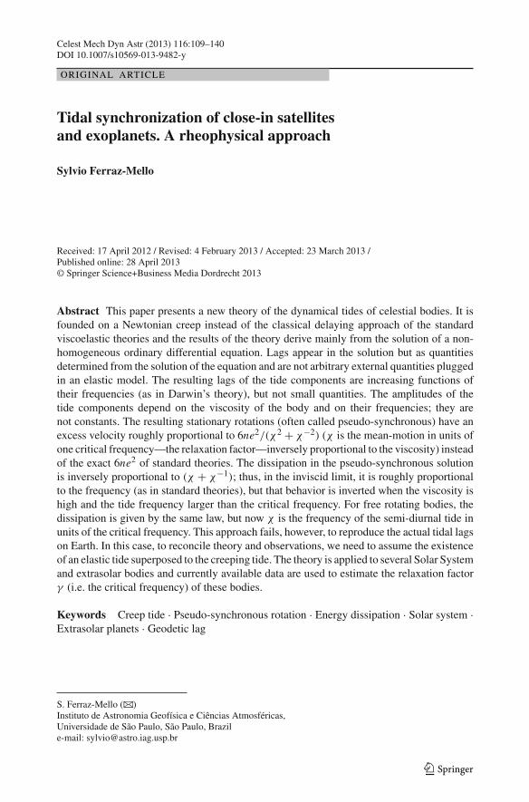
Fig. 1 Elements of the model:ζ is a section of the surface of thebody at the time t; ρ is a sectionof the surface of the equilibriumspheroid at the same time

We did not consider in this short account theories based on energy dissipation instead ofphase delays, because they follow a different line of thought (for a comprehensive account ofthem, see Eggleton 2006, Chap. 4, and Migaszewski 2012; see also Bambusi and Haus 2012).The results issued from these theories are formally equivalent to Darwin’s theory when lagsare assumed proportional to the frequencies and lead to the same pseudo-synchronous resultsdiscussed in the beginning of this Introduction.

This paper introduces a new rheophysical approach in which the body tends always tocreep towards the equilibrium by the only action of the gravitational forces acting on it (self-gravitation and tidal potential) and does it with a rate inversely proportional to its viscosity.The adopted creep law is Newtonian (linear), and at every instant the stress is assumed tobe proportional to the distance from the equilibrium. This leads to Eq. (2) and with onlyone exception every result in the paper is a direct consequence of this first-order differentialequation. The exception occurs when studying the shape of the tide in hard bodies as theEarth. In this case, in order to conciliate theory and observation, it is necessary to assumethat a purely elastic tide (see Sect. 10) exists, superposed to the creep tide.

The physical model is presented in Sect. 2 and developed in Sects. 3 and 4. Section 2also presents a short application to the case of bodies in circular motion with results equalto those obtained by Darwin (1879) and which served as the basis for the introduction ofa lag proportional to the tide frequency in his 1880 theory. The next sections are devotedto the calculation of the perturbations: First, the perturbations on the rotation of the tidallydeformed body (Sect. 5) and its synchronization (or pseudo-synchronization) (Sect. 6); then,the perturbations on the semi-major axis (energy dissipation; Sect. 7) and on the eccentricity(Sect. 8). Section 9 discusses the value of the relaxation factor γ on the basis of our currentknowledge of the tidal evolution of stars, planets and planetary satellites. The theory iscompleted, in Sect. 10, by the introduction of an additional elastic tide, necessary to reproducethe observed shape of tidally deformed bodies.

2 A simple rheophysical model

The usual standard model considers an elastic tide and delays the tidal bulge by an ad hocphase lag in order to take into account the body anelasticity. In this theory, we propose insteadof that, a simple rheophysical model, the basis of which is shown in Fig. 1. We consider onebody of mass m and assume that, at a given time t , the surface of the body is a functionζ = ζ(ϕ∗,θ∗, t) where ζ is the distance of the surface points to the center of gravity of thebody and ϕ∗,θ∗ their longitudes and co-latitudes with respect to a reference system rotatingwith the body. In the same instant t , the body is under the action of a tidal potential due to

123

Tidal synchronization of close-in satellites and exoplanets 113

one second body of mass M situated in its neighborhood. No hypothesis is being done onthe relative importance of the two bodies. Both may play the role of the central body andits satellite or hot planet. In actual applications, both cases have to be considered (see FRHSect. 18).

Would the body m be inviscid, it would immediately change its shape to the equilibriumconfiguration. In the simplest case, the figure of equilibrium of it under the action of thetidal potential is a prolate Jeans spheroid ρ = ρ(ϕ∗,θ∗, t) (see Chandrasekhar 1969) whosemajor axis is directed along the line joining the centers of gravity of the two bodies. If ae, be

are the principal equatorial axes of the spheroid, its prolateness is

ερ = ae

be− 1 = 15

4

(

M

m

) (

Re

r

)3

(1)

(Tisserand et al. 1891) where Re is the mean equatorial radius of m and r the distance fromM to m. Terms of second order with respect to ερ are neglected in this and in the followingcalculations.

The adopted model is founded on the law

ζ = γ (ρ − ζ ). (2)

The basic idea supporting this law is that because of the forces acting on the body (self-gravitation plus tide), its surface will tend to the equilibrium spheroid, but not instantaneously,and its instantaneous response (measured by ζ ) will be proportional to the radial separationbetween it and the equilibrium spheroid, ρ − ζ . Equation (2) is the equation of a Newtoniancreep (see Oswald 2009, Chap. 5) where the distance to the equilibrium is considered asproportional to the stress. It does not consider inertia or azimuthal motions, which may existand should be considered in further studies. The superposed elastic tide whose existencestems from the comparison of the observed shape of the tidal deformations and the theory, isnot included in the equations of the model because the force due to the elastic tide is radialand its torque is zero; it does not affect the rotation or the averaged work and eccentricity.

The relaxation factor γ is a radial deformation rate gradient and has dimension T−1. It isγ = 0 in the case of a solid body and γ → ∞ in the case of an inviscid fluid. Between thesetwo extremes, we have the viscous bodies, which, under stress relax towards the equilibrium,but not instantaneously.

We shall mention here the very similar equation used by Darwin in his first paper on theprecession of a viscous Earth (Darwin 1877)4 to define its rate of adjustment to a new form ofequilibrium, soon extended to the study of tides (Darwin 1879) by means of a law similar toEq. (2). However, in the later paper, he was rather interested in the ocean tides upon a yieldingnucleus and was not satisfied with the results that he classed as fallacious. For unless theviscosity [of the Earth] was much larger than that of pitch, the viscous sphere would comportitself sensibly like a perfect fluid, and the ocean tides would be quite insignificant. This isperhaps the reason for which he never went beyond the circular approximation later used(Darwin 1880) to introduce the tide lag and the tide height in the Earth model in the study ofthe secular changes of the orbit of the Moon and the changing rotation of the Earth.

4 We may paraphrase one of Darwin’s statements by just changing the symbols used in it by those showninside brackets: But because of the Earth’s viscosity, [ζ ] always tends to approach [ρ]. The stresses introducedin the Earth by the want of coincidence of [ζ ] with [ρ] vary as [ρ − ζ ]. Also the amount of flow of a viscousfluid, in a small interval of time, varies jointly as that interval and the stress. Hence the linear velocity (on themap), with which [ζ ] approaches [ρ], varies as [ρ − ζ ]. Let this velocity be [γ (ρ − ζ )], where [γ ] dependson the viscosity of the Earth, decreasing as the viscosity increases.

123

114 S. Ferraz-Mello

It is also possible to obtain Eq. (2) by integrating a spherical approximation of the Navier–Stokes equation of a radial flow across the two surfaces, for very low Reynolds number(Stokes flow), a case in which the inertia terms can be neglected and the stress due to thenon-equilibrium may be absorbed into the pressure terms (see Happel and Brenner 1973).The boundary conditions are ζ = 0 at ζ = ρ. The pressure due to the body gravitation isgiven by the weight of the mass which lies above (or is missing below5) the equilibriumsurface, that is, −w(ζ − ρ); the modulus of the pressure gradient is the specific weight w.

This comparison allows us to see that the relaxation factor γ is related to the viscositycoefficient η through

γ = wR

2η= 3gm

8π R2η, (3)

where g is the gravity at the surface of the body and R is its mean radius.6 This equation isimportant because it allows us to estimate the range of possible values of γ for the celestialbodies to be considered in the applications.

2.1 The creep equation

The function ρ may be written as

ρ = Re

(

1 + 1

2ερ cos 2Ψ

)

(4)

(to the order O(ερ)), where Ψ is the angular distance of one generic point on the surface ofthe equilibrium ellipsoid to the axis of the tidal bulge (that is, the direction of M).

If we restrict the present study to the case of a “planar” problem, in which the orbitalplane of the tide generating body M cuts the body m symmetrically (i.e. m is symmetricalwith respect to an equator, and M lies on the same plane as the equator of m), the differentialequation of the adopted model for the creep becomes

ζ + γ ζ = γρ = γ R′ + 1

2γ Reερ sin2

θ∗ cos(2ϕ∗ − 2� − 2v) (5)

where θ∗ is the co-latitude (introduced through cos Ψ = cos α sinθ∗), R′ =Re(1 − 1

2ερ cos2θ∗) and

ϕ∗ = � + v + α (6)

(see Fig. 2).In the solution of this equation, we have to consider that dϕ∗

dt = Ω , angular velocity ofrotation of the body m, which is assumed to rotate in the same direction as the orbital motionof M.

5 This does not mean that a negative mass is being assigned to void spaces; it means just that the forcesincluded in the calculation of the equilibrium figure need to be subtracted when the masses creating them areno longer there.6 Darwin (1879) used a very complete construction of the Navier–Stokes equations and, in his results, thenumerical factor is 3/38 instead of 3/8. His numerical factor is determined by the spheroidal form of the tidalpotential, but the intensity of the potential does not appear in the result. So, his result would hold even for aninfinitesimal tide!

123

Tidal synchronization of close-in satellites and exoplanets 115

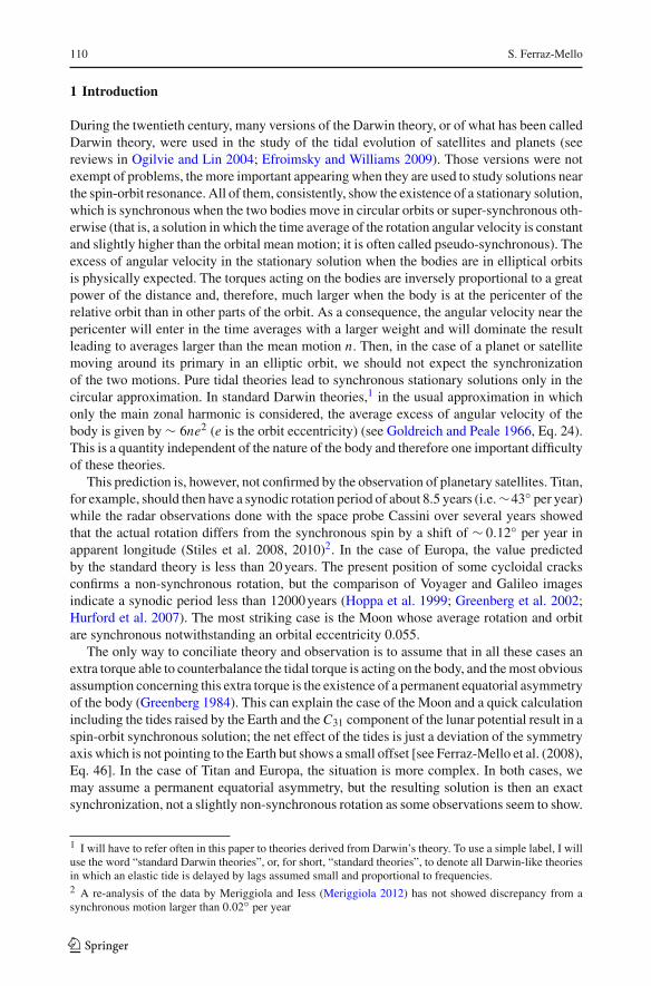
Fig. 2 Equatorial section of theequilibrium spheroidcorresponding to the tidegenerated by M on m. Angles:α is the distance from the genericsurface point to the vertex of thespheroid; v is the true anomaly ofM; � is the angle between theorigin meridian of the body andthe pericenter of the orbit ofM; ϕ∗ = � + v + α

2.2 The circular approximation

For the sake of making clear which are the main consequences of the proposed rheophysicalmodel, before considering the full model, we consider first the simple case in which therelative motion of the two bodies is circular. In such case, r = a (semi-major axis) andv = � = nt (mean anomaly).

The resulting equation is a trivial non-homogeneous first-order differential equation withconstant coefficients whose solution is

ζ = Ce−γ t + R′ + A cos(2α − σ0) (7)

where C is an integration constant. A, σ0 are undetermined coefficients which may be obtainedby simple substitution in the differential equation and identification as

σ0 = arctanν

γ, (8)

A = 1

2Reε

′ρ cos σ0 =

12 Reγ ε′

ρ√

γ 2 + ν2(9)

where ε′ρ = ερ sin2

θ∗ and ν is the semi-diurnal frequency

ν = 2α = 2Ω − 2n. (10)

The integration constant C depends on ϕ∗ (the integration was done with respect to t) andmay be related to the initial surface ζ0 = ζ(ϕ∗,θ∗, 0) through

C = ζ0 − R′ − A cos(2α(0) − σ0). (11)

The solution depends on θ∗ via its influence on the constants R′ and A.

3 Tidal deformation of the body

In order to develop the theory, we have to consider the two-body equations and introduce

r = a(1 − e2)

1 + e cos v(12)

123

116 S. Ferraz-Mello

and

v = � +(

2e − e3

4

)

sin � + 5e2

4sin 2� + 13e3

12sin 3� + O(e4) (13)

into Eq. (5). The resulting creep equation is

ζ + γ ζ = γ R′ + 15γ Re sin2θ∗

8

(

M

m

) (

Re

a

)3(

cos(2ϕ∗ − 2� − 2�)

+ e

2

(

7 cos(2ϕ∗ − 2� − 3�) − cos(2ϕ∗ − 2� − �))

+ e2

2

(

− 5 cos(2ϕ∗ − 2� − 2�) + 17 cos(2ϕ∗ − 2� − 4�))

+ e3

16

(

− 123 cos(2ϕ∗ − 2� − 3�) + cos(2ϕ∗ − 2� − �)

+ 845

3cos(2ϕ∗ − 2� − 5�) + 1

3cos(2ϕ∗ − 2� + �)

)

)

+ · · · (14)

or

ζ + γ ζ = γ R′ + 15γ Re sin2θ∗

8

(

M

m

)(

Re

a

)3 N∑

k=−N

E2,k(e) cos(2ϕ∗ − 2� + (k − 2)�)

(15)

where N is the adopted order of approximation of the Fourier series and the E2,k(e) arethe eccentricity functions appearing as coefficients in Eq. (14). They are some of the Cay-ley expansions (Cayley 1861). An elementary calculation using simple concepts of Fourieranalysis shows that

E2,k(e) = 1

2π

2π∫

0

(a

r

)3cos

(

2v + (k − 2)�)

d�. (16)

(see “Appendix”).The integration of Eq. (15) is trivial. If we write ζ +γ ζ = F(t), we know that the general

solution is

ζ = e−γ t∫

t

F(t)eγ t dt (17)

or

ζ = Ce−γ t + Re + R′′(θ∗, t)

+15γ Re sin2θ∗

8

(

M

m

)(

Re

a

)3 N∑

k=−N

E2,k(e) cos(2α + k� − σk)√

γ 2 + (ν + kn)2(18)

where α = ϕ∗ − � − � (N.B. α − α = v − �),

R′′ = −1

2γ Re cos2

θ∗e−γ t∫

t

ερeγ t dt

123

Tidal synchronization of close-in satellites and exoplanets 117

and

σk = arctan

(

kn + ν

γ

)

. (19)

It is worth emphasizing that the σk are not ad hoc lags plugged by hand, but constantsintroduced during the (exact) integration of the creep equation just to allow us to write thesolution in simpler form. However the σk play a role similar to the εk introduced as ad hocdelays in FRH.7 From their definition, it is also clear that the σk are not small quantities asthe lags are assumed to be in standard Darwin theories.

The solution of the differential equation can also be written as

ζ = Ce−γ t + Re + R′′ + 1

2Re sin2

θ∗N

∑

k=−N

εk(e) cos(2α + k� − σk), (20)

where we have introduced

εk = 15

4E2,k(e) cos σk

(

M

m

)(

Re

a

)3

. (21)

ζ is formed by the superposition to one sphere of the bulges of several spheroids the prolate-nesses of which are the εk .

4 The attraction of the tidally deformed body

In order to proceed, we assume that the potential of m is the sum of the potential of onesphere plus the potentials due to various ellipsoid bulges the intersections of which with theequatorial plane are given by the sum of terms in Eq. (20).

For instance, when sinθ∗ = 1, the main component of ζ(α) corresponds to

Re + 1

2Reε0(e)cos(2α − σ0), (22)

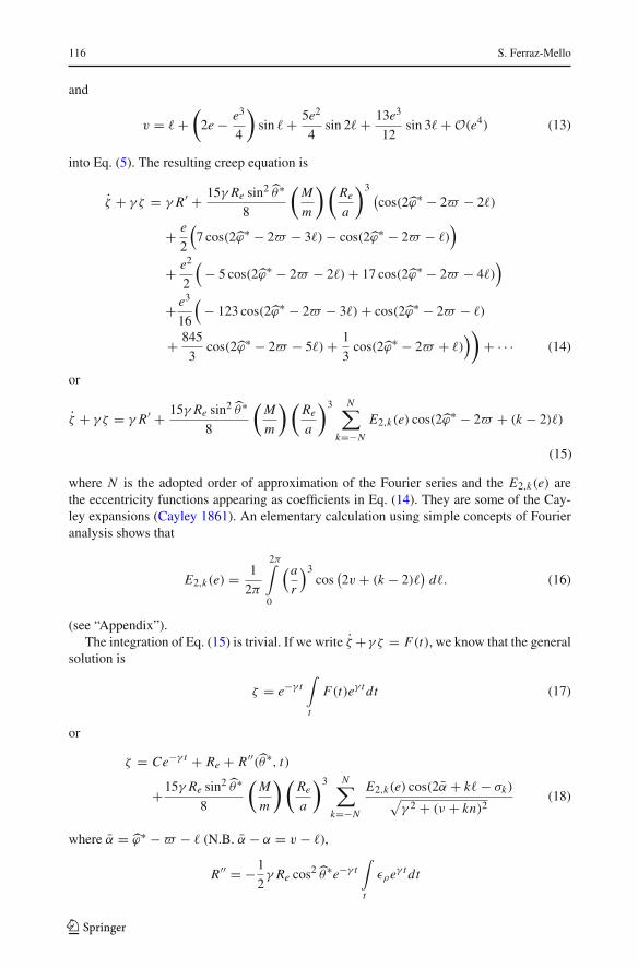
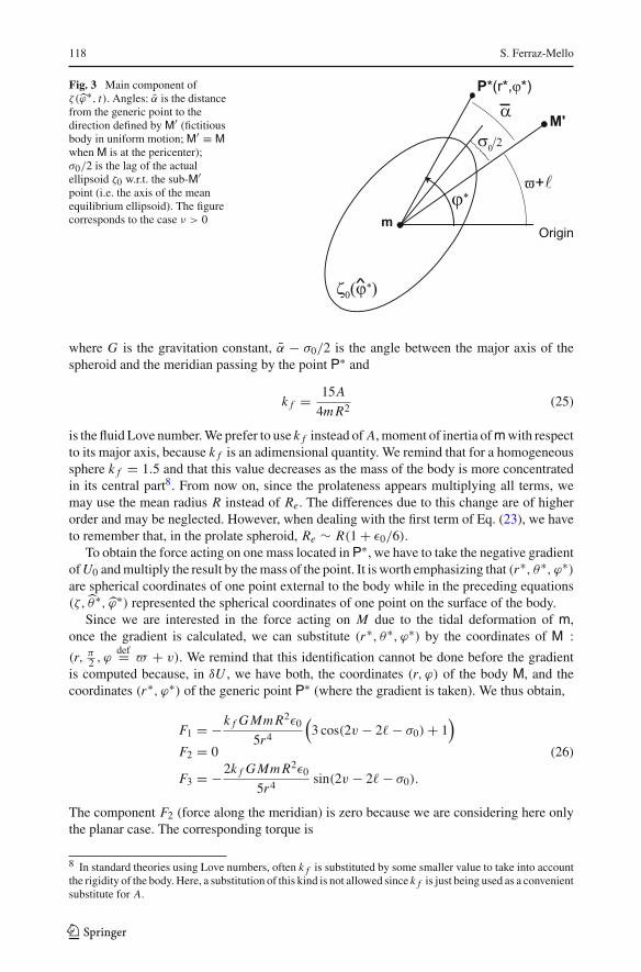
which is the equatorial boundary of a spheroid of mean equatorial radius Re and prolatenessε0 displaced of an angle σ0/2 with respect to the direction of M′ (fictitious body in uniformmotion; M′ ≡ M when M is at pericenter) (see Fig. 3).

The equation of this spheroid is

ζ0 = Re

(

1 + 1

2ε0 cos 2Ψ0

)

= Re

(

1 − 1

2ε0 cos2

θ∗ + 1

2ε0 sin2

θ∗ cos(2α − σ0)

)

. (23)

where Ψ0 is the angular distance from the generic point to the vertex of the spheroid.ζ0 differs from the component k = 0 of Eq. (20) by the additional term − 1

2ε0 cos2θ∗; as

discussed in Sect. 4.1, the contribution of this additional term can be neglected in the planarapproximation of this study.

The disturbing potential (i.e. the potential to be added to the potential of a sphere) due toζ0, on an external point P∗(r∗, θ∗, ϕ∗), is

δU0 = −2k f Gm R2ε0

15r∗3

(

3 cos2 Ψ0 − 1)

= −k f Gm R2ε0

15r∗3

(

sin2 θ∗(3 cos(2α − σ0) + 1) − 2 cos2 θ∗) (24)

7 The subscripts used for the σk are not the same subscripts used in FRH for their homologous lags εk .

123

118 S. Ferraz-Mello

Fig. 3 Main component ofζ(ϕ∗, t). Angles: α is the distancefrom the generic point to thedirection defined by M′ (fictitiousbody in uniform motion; M′ ≡ Mwhen M is at the pericenter);σ0/2 is the lag of the actualellipsoid ζ0 w.r.t. the sub-M′point (i.e. the axis of the meanequilibrium ellipsoid). The figurecorresponds to the case ν > 0

where G is the gravitation constant, α − σ0/2 is the angle between the major axis of thespheroid and the meridian passing by the point P∗ and

k f = 15A

4m R2 (25)

is the fluid Love number. We prefer to use k f instead of A, moment of inertia of m with respectto its major axis, because k f is an adimensional quantity. We remind that for a homogeneoussphere k f = 1.5 and that this value decreases as the mass of the body is more concentratedin its central part8. From now on, since the prolateness appears multiplying all terms, wemay use the mean radius R instead of Re. The differences due to this change are of higherorder and may be neglected. However, when dealing with the first term of Eq. (23), we haveto remember that, in the prolate spheroid, Re ∼ R(1 + ε0/6).

To obtain the force acting on one mass located in P∗, we have to take the negative gradientof U0 and multiply the result by the mass of the point. It is worth emphasizing that (r∗, θ∗, ϕ∗)are spherical coordinates of one point external to the body while in the preceding equations(ζ,θ∗, ϕ∗) represented the spherical coordinates of one point on the surface of the body.

Since we are interested in the force acting on M due to the tidal deformation of m,once the gradient is calculated, we can substitute (r∗, θ∗, ϕ∗) by the coordinates of M :(r, π

2 , ϕdef= � + v). We remind that this identification cannot be done before the gradient

is computed because, in δU , we have both, the coordinates (r, ϕ) of the body M, and thecoordinates (r∗, ϕ∗) of the generic point P∗ (where the gradient is taken). We thus obtain,

F1 = −k f G Mm R2ε0

5r4

(

3 cos(2v − 2� − σ0) + 1)

F2 = 0

F3 = −2k f G Mm R2ε0

5r4 sin(2v − 2� − σ0).

(26)

The component F2 (force along the meridian) is zero because we are considering here onlythe planar case. The corresponding torque is

8 In standard theories using Love numbers, often k f is substituted by some smaller value to take into accountthe rigidity of the body. Here, a substitution of this kind is not allowed since k f is just being used as a convenientsubstitute for A.

123

Tidal synchronization of close-in satellites and exoplanets 119

M1 = 0

M2 = 2k f G Mm R2ε0

5r3 sin(2v − 2� − σ0)

M3 = 0.

(27)

For the other terms of ζ(ϕ∗) we have similar expressions having just to pay attention that, inthese terms, k� appears added to the arguments. We can proceed in the same way as abovebecause the operations done involve only geometric quantities. We thus have

δU =N

∑

k=−N

−k f Gm R2εk

15r∗3

(

sin2 θ∗(3 cos(2α + k� − σk) + 1) − 2 cos2 θ∗) (28)

where the εk are the prolatenesses defined by Eq. (21). The corresponding force and torqueare

F1 =N

∑

k=−N

−k f G Mm R2εk

5r4

(

3 cos(

2v + (k − 2)� − σk) + 1

)

F3 =N

∑

k=−N

−2k f G Mm R2εk

5r4 sin(

2v + (k − 2)� − σk)

M2 =N

∑

k=−N

2k f G Mm R2εk

5r3 sin(

2v + (k − 2)� − σk)

.

(29)

4.1 The axial terms

At last, we have to consider the term R′′, not yet considered, and the terms 12 Reεk cos2

θ∗subtracted from the parts of ζ to complete the equation of the spheroids. Putting then together,we obtain

δaxζ = 1

2γ Re

( N∑

k=−N

εk − e−γ t∫

t

ερeγ t dt

)

cos2θ∗. (30)

r = R + δaxζ is the equation of a spheroid with symmetry axis perpendicular to the orbitand whose prolateness is given by the bracket in the above equation. As is well-known, theresulting field is axial. The force on M is central and its contribution to the torque is null.It will be important in the general non-planar problem because it will contribute for theprecession of the axis of the body. Because of its sign, it will counteract the effects due to theoblateness of the body (not considered in the present study). It will contribute short-periodvariations in the semi-major axis and eccentricity, which will be averaged to zero over oneorbit. Hence, they can be neglected in the planar case.

5 Rotation of close-in companions

We use the equation CΩ = M2 (≡ −Mz) (see FRH Sect. 7–8). The time average of Ω overone period is

〈Ω〉 = 1

2πC

2π∫

0

M2 d�.

123

120 S. Ferraz-Mello

Hence, using the approximation A � C in k f and simplifying:

〈Ω〉 = −45G M2 R3

16ma6

[(

1 − 5e2 + 63

8e4 − 155

36e6

)

sin 2σ0

+(

1

4e2 − 1

16e4 + 13

768e6

)

sin 2σ1 +(

49

4e2 − 861

16e4 + 21975

256e6

)

sin 2σ−1

+(

289

4e4 − 1955

6e6

)

sin 2σ−2 + 1

2304e6 sin 2σ3 + 714025

2304e6 sin 2σ−3

]

. (31)

It is worth mentioning that only squares will contribute to the average and the above resultmay be written as

〈Ω〉 = −45G M2 R3

16ma6

N∑

k=−N

E22,k(e) sin 2σk . (32)

In order to have an explicit equation in terms of the relaxation parameter γ and the involvedfrequencies, the definitions given by Eqs. (19) may be introduced into the above equationthrough the trigonometric relation sin 2X = 2 tan X/(1 + tan2 X), that is

sin 2σk = 2γ (ν + kn)

γ 2 + (ν + kn)2 . (33)

The resulting expression can be used to study the tidal despining of close-in companionsand/or central bodies.

6 Synchronization: spin-orbit resonance

The immediate consequence of Eq. (31) is that the synchronous rotation is not a stationarysolution of the system when the orbital eccentricity is not zero. Indeed, introducing Eq. (33)and making ν = 0, there results, in the first approximation,

〈Ω〉∣

∣

∣

ν=0� 135G M2 R3nγ e2

2ma6(n2 + γ 2). (34)

The equality to zero is not possible if γ e �= 0. In the synchronous state, the torque is positive,meaning that the rotation is being accelerated by the tidal torque. The stationary solution canonly be reached at a supersynchronous rotation. Indeed, solving the equation 〈Ω〉 = 0, weobtain

Ω = n + 6nγ 2

n2 + γ 2 e2 + 3nγ 2 226n6 + 1453n4γ 2 + 28n2γ 4 + γ 6

8(n2 + γ 2)3(4n2 + γ 2)e4 + O(e6). (35)

The result corresponds to a supersynchronous rotation. However, at variance with the standardtheories, the stationary rotation speed is not independent of the body rheology. It depends onthe viscosity η through the relaxation factor γ .

In the quasi-inviscid limit, η → 0, then γ n and γ 2

γ 2+n2 � 1. We then obtain

Ωlim � n

(

1 + 6e2 + 3

8e4

)

. (36)

Thus, in the quasi-inviscid limit, the result is the same obtained with Darwin’s theory whenwe neglect the differences in the response factors ki and assume that the ad hoc lags of tidecomponents with equal frequencies are equal (see Laskar and Correia 2004; FRH, Sect. 9).

123

Tidal synchronization of close-in satellites and exoplanets 121

On the contrary, in the solid limit, γ � n and then Ω ≈ n (the stationary solution issynchronous).

7 Energy dissipation

The rate of the work done by the tidal forces is Worb = Fv.The components of v in the adopted 3D spherical coordinates are

v1 = nae sin v√1 − e2

v2 = 0 (37)

v3 = na2√

1 − e2

r.

The result, time-averaged over one period, is:

〈W 〉orb = 3k f G M2 R5n

4a6

[(

1 − 5e2 + 63

8e4 − 155

36e6

)

sin 2σ0

+(

1

8e2− 1

32e4 + 13

1536e6

)

sin 2σ1 +(

147

8e2 − 2583

32e4 + 65925

512e6

)

sin 2σ−1

+(

289

2e4 − 1955

3e6

)

sin 2σ−2 − e6

4608sin 2σ3 + 3570125e6

4608sin 2σ−3

]

(38)

or

〈W 〉orb = 3k f G M2 R5n

8a6

N∑

k=−N

(2 − k)E22,k(e) sin 2σk . (39)

In the pseudo-synchronous stationary rotation, we may use ν as given by Eq. (35). Hence,using the sin 2σk values given in Eq. (33) and neglecting terms of order higher than O(e2),

〈W 〉orb (stat) � −75k f G M2 R5ne2

8a6

γ n

γ 2 + n2 . (40)

In addition, we have to consider the work done by the tidal torque on the rotating body:〈W 〉rot = CΩ〈Ω〉, that is,

〈W 〉rot = −3k f G M2 R5Ω

4a6

N∑

k=−N

E22,k(e) sin 2σk . (41)

(Since W ∝ Ω , the work associated with the rotation of the body vanishes when it reachesthe stationary state.)

The rate of the mechanical energy released inside the body is

〈E〉 = −(〈W 〉orb + 〈W 〉rot)

> 0. (42)

From Eq. (38), since Worb = −GmM

2a, we obtain a = 2a2

GmMWorb, i.e. the secular

variation of the semi-major axis

〈a〉 = 3k f M R5n

4ma4

N∑

k=−N

(2 − k)E22,k(e) sin 2σk . (43)

123

122 S. Ferraz-Mello

The interpretation, neglecting the terms in e2, is easy. If the body is rotating faster than theorbital motion, then ν > 0, σ0 > 0, and a > 0. The tide in m causes the bodies M and m torecede one from another. Otherwise they are falling one on another.

Two approximations of this formula are useful:

(i) The free rotating approximation

〈a〉free � 3k f M R5nγ ν

ma4(γ 2 + ν2)(44)

and

(ii) The pseudo-synchronous approximation

〈a〉stat � −75k f M R5ne2

4ma4

γ n

γ 2 + n2 . (45)

7.1 The quality factor of standard theories

The quality factor Q is a parameter originally introduced to characterize damped oscilla-tors. It expresses the quality of the oscillator in keeping free oscillations alive. It is pro-portional to the proper frequency of the oscillator and vanishes when no elastic force isacting. Its extension to forced oscillations is not done without ambiguities and we do notuse it in this theory. Nevertheless, the quality factor Q is widely used and, in the appli-cations, we need to know how to express it in terms of the rheophysical parameters usedhere. However, it is worth emphasizing that the formulas given in this section are obtainedby mere comparison of some equations of this theory with their equivalents in standardDarwin theories and are not valid out of the particular conditions in which they wereestablished.

We recall that, in standard theories, the quality factor Q and the tidal Love number k2

cannot be separated one from another; in the following equations, k2 is the tidal Love numberand k f is the fluid Love number.

In standard theories, two different definitions of Q are used, one when the body is freerotating and another when it is trapped in a stationary pseudo-synchronous state.

7.1.1 Bodies in free rotation

In classical theory, in this case, we have

〈W 〉 � 3k2G M2 R5n

2a6 Q

(see FRH Eqs. 48) where Q is the inverse of the lag of the semi-diurnal tide (ε0). Comparingto the eccentricity-independent term of Eq. (38), we obtain the equivalence formula (validonly for small eccentricities):

Q = k2

k f

(γ 2 + ν2)

γ ν= k2

k f

[

1

2sin 2σ0

]−1

= k2

k f

(

χ + 1

χ

)

(46)

where we have introduced χ = νγ

(χ is the frequency of the semi-diurnal tide in units of γ ).

123

Tidal synchronization of close-in satellites and exoplanets 123

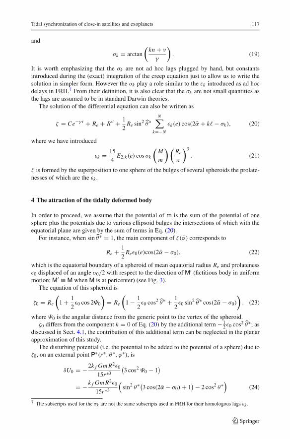
It is important to note that Q goes to infinity when χ (or ν) goes to zero. This is so alsoin the standard theories and is just a consequence of the inadequacy of the quality factor Qto measure dissipation. One may note that the dissipation itself, given by Eq. (39), is notsingular for ν = 0.

7.1.2 Bodies in pseudo-synchronous stationary rotation

In standard theories we have, in this case,

〈W 〉 � −75k2G M2 R5ne2

8a6 Q− 9k2G M2 R5ne2

8a6 ε5

(see FRH Eqs. 48–51) where, now, Q is the inverse of the lag of the monthly/annual tide(ε2). In FRH, we have considered the lag of the radial tide (ε5) as equal to the lag of themonthly/annual tide (ε2) since both have the same period in the case of a stationary rotatingbody. If we compare only the first part of the above equation to Eq. (40), we obtain againEq. (46). However, when the complete equation is considered, there results

Qstat = k2

k f

(γ 2 + n2)

γ n= 28

25

k2

k f

[

1

2sin 2σ1

]−1

= 28

25

k2

k f

(

χ + 1

χ

)

(47)

where now χ = nγ

(χ is the frequency of the monthly/annual tide in units of γ ).This duality in the actually used definitions of Q in standard theories is a big nuisance.

In the case of planetary satellites, eccentricities are low and either the system is rotatingor nearly synchronous and we may consider the two cases separately. However, in the caseof exoplanets, eccentricities are often high and the choice of one of the two formulas todetermine Q is a problem. Indeed, in the standard approach, if the eccentricity is large,the stationary rotation may have a period much smaller than the orbital period and thedissipation due to the semi-diurnal tide will not vanish as in true synchronous companions.As a consequence, tidal components with frequencies ν and n will contribute to the energydissipation on the same foot making impossible to privilege one of them to define onequality factor.

8 Circularization

The variation of the remaining elements can be obtained straightforwardly using Gaussequations (see Beutler 2005, Sect. 6.3.5). As discussed in FRH (Sect. 18.1), in order to takeinto account correctly the reaction on M of its tidal action on m, the accelerations R′, S′, W ′of those equations need to be multiplied by (M +m)/m or, equivalently, by n2a3/Gm. Withthe forces calculated in Sect. 4, we thus get

〈e〉 = −3k f M R5ne

8ma5

[(

1 − 21

4e2 + 9e4 − 3299

576e6

)

sin 2σ0

+(

1

4− 1

16e2 − 35

768e4 − 175

18432e6

)

sin 2σ1

+(

− 49

4+ 1253

16e2 − 50311

256e4 + 508651

2048e6

)

sin 2σ−1

123

124 S. Ferraz-Mello

+(

− 289

2e2 + 10421

12e4 − 310463

144e6

)

sin 2σ−2

+(

1

768e4 + 17

18432e6

)

sin 2σ3 −(

714025

768e4 − 105299675

18432e6

)

sin 2σ−3

+ e6

144sin 2σ4 − 284089e6

64sin 2σ−4

]

(48)

or

〈e〉 = −3k f M R5n

8ma5e

N∑

k=−N

(

2√

1 − e2 − (2 − k)(1 − e2))

E22,k(e) sin 2σk . (49)

Taking into account Eqs. (33), we may also write

〈e〉=−3k f M R5neγ

16ma5

(

4ν

γ 2 + ν2 − 49(ν − n)

γ 2 + (ν − n)2 + (ν + n)

γ 2 + (ν + n)2

)

+ O(e3). (50)

In the case of a stationary or near-stationary rotation, ν = O(e2) and the above equation isreduced to

〈e〉 � −75

8

k f M R5neγ

ma5

n

γ 2 + n2 . (51)

9 Dissipation parameters in stars, planets and satellites

In this section we determine the values of γ for several Solar System and extrasolar bodies.We use for that sake the values published in the literature usually obtained using standardtidal evolution theories. One problem common to most of the given examples is that theinversion of the equivalence formulas relating γ to Q has two solutions. The choice of oneof the two solutions is done after comparing the values of the equivalent uniform viscosityin each solution.

9.1 Io

The tidal evolutions of the Galilean satellites of Jupiter are among the best studied in ourSolar System. From the satellites accelerations, Lainey et al. (2009) have determined thedissipations of Io and Jupiter. For Io, they have found k2/Q = 0.015 ± 0.003. Introducingthis value in the formulas given in Sect. 7.1, we obtain γ = 4.9 ± 1.0 × 10−7 Hz. It is worthmentioning that this result is independent of the individual values of k2 and Q, which arenot well known. The calculated value of γ depends only on the value of k2/Q and on themoment of inertia (0.378 m R2).

With the results given in Sect. 6 (Eq. 35), we obtain for the synodic rotation period (a.k.a.length of the day) Psyn = 3300+1800

−1000 year. We may compare this value with the minimumvalue 1400 years determined by Milazzo et al. (2001) from the comparison of Galileo andVoyager images taken 17 years apart.

The equivalent viscosity corresponding to this determination may be obtained usingEq. (3). The result, 1.2 ± 0.3 × 1016 Pa s, is in good agreement with the value used bySegatz et al. (1999): 2 × 1016 Pa s, in their models for Io’s tidal dissipation.

123

Tidal synchronization of close-in satellites and exoplanets 125

Fig. 4 The low-eccentricityequivalent of the quality factors(in units of k2/k f ) as functionsof the frequency (in units of γ ).For rotating bodies, χ = ν/γ

(solid line); for bodies instationary rotation, χ = n/γ

(dashed line)

0.01 0.1 1 10 1001

10

100Q

χ

We note that the adopted value of γ corresponds to χ = 94, that is, to the ascendingbranch of the curve shown in Fig. 4 (Darwin’s theory corresponds to the descending branch).Therefore, we are in the regime proposed by Efroimsky and Lainey (2007) in which Qincreases with the frequency of the tide component. The solution corresponding to Darwin’sregime gives γ = 0.003 and η = 1.7 × 1012, which is 2 − 3 orders of magnitude below theknown viscosity of ice and silicates (resp. 1.5 × 1014 Pa s and 3 × 1015 Pa s cf. Sotin et al.2004).

9.2 Europa

The basic information that we have on Europa is its non-synchronous rotation. The synodicperiod is constrained by the lower limit 12000 years obtained from the comparison of Galileoand Voyager images, and the upper limit 250000 years, obtained by comparing the presentposition of some cycloidal cracks with the longitudes at which their shapes should havebeen formed (see Greenberg et al. 2002). Using the results given in Sect. 6, we obtainγ = 1.8 − 8.0 × 10−7 Hz and k2/Q between 0.01 and 0.045 (if we adopt k2 = 0.26, weobtain Q in the range 6–26). The equivalent uniform viscosity corresponding to these resultsis η = 4 − 18 × 1015 Pa s.

The same indetermination discussed above occurs here since the excess of rotation speedis approx. proportional to χ2 + χ−2. As before, we have to look to the viscosity to decidebetween the two mathematically possible solutions. The solution corresponding to Darwin’sregime gives γ = 0.0005 − 0.002 and η = 1.3 − 6 × 1012 Pa.s, which is less than expected,but not so much as in other cases.

We note that the indetermination is as more difficult to solve as Q is small.

9.3 The Moon

The quality factor of the Moon has been determined for two tidal frequencies. For the monthlytide, Q = 30 ± 4 and for the annual tide Q ∼ 35 (Williams et al. 2005; Williams 2008).The values of Q for the monthly tide (combined with the very low k2 of the Moon, 0.0301cf. Williams et al.) gives γ = 2.0 ± 0.3 × 10−9 Hz. The synodic period of the Mooncorresponding to the above determinations of γ is larger than 5 Myr and indistinguishablefrom a true synchronous spin-orbit resonance.

The problem with this determination is the value found for the uniform viscosity:η = 2.3 ± 0.3 × 1018 Pa s, 4–5 orders of magnitude smaller than the values reported inthe literature, which refer to the solid lithosphere. This seems to be one more indication in

123

126 S. Ferraz-Mello

favor of the role played by a plastic lunar asthenosphere in tidal dissipation and is in agree-ment with the dramatic decrease of the seismic Q below the deep moonquake source regionindicating the presence of a partial melt below this depth and that, likely, most of the solidbody dissipation in the Moon occurs below 1150 km (see Wieczorek 2006). The alternativesolution, corresponding to Darwin’s regime, gives viscosity values yet smaller and may beexcluded. The adoption of a more realistic value for the viscosity leads to a much smaller γ

and a much larger synodic period, even when a permanent equatorial asymmetry of the Moonis neglected. The resulting γ is small enough to compensate the fact that n and e may havebeen larger in the past and to give a result consistent with the rotation indicated by the distrib-ution of the craters on the Moon: a synchronous attitude lasting since the formation of the lastgreat basin, 3.8 Gyrs ago (see Wieczorek and Le Feuvre 2009). However, a larger viscositywould also imply a larger Q, in contradiction with the above-mentioned determinations.9

Let us add that the annual tide cannot be studied with the Keplerian model used in thispaper. It is clearly related to the motion of the Earth–Moon system around the Sun and aperturbed model is necessary to interpret it.

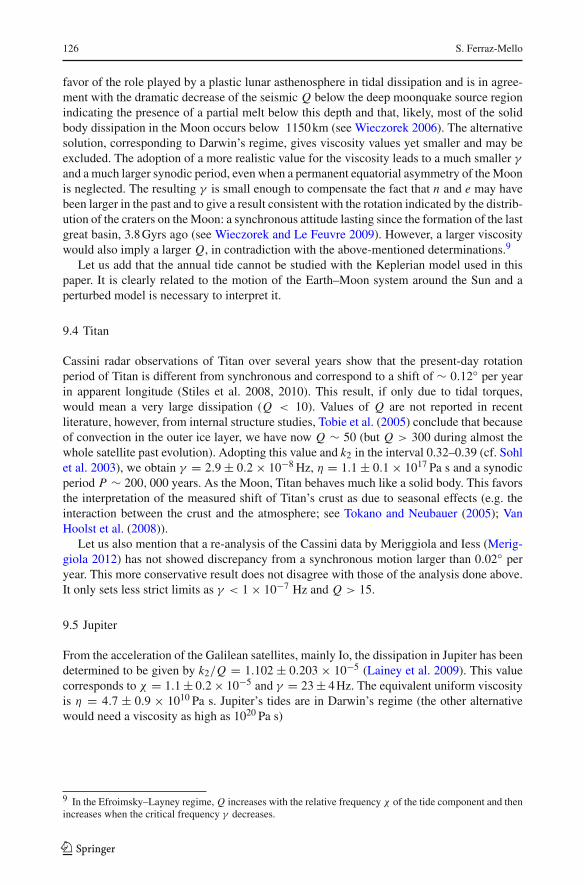
9.4 Titan

Cassini radar observations of Titan over several years show that the present-day rotationperiod of Titan is different from synchronous and correspond to a shift of ∼ 0.12◦ per yearin apparent longitude (Stiles et al. 2008, 2010). This result, if only due to tidal torques,would mean a very large dissipation (Q < 10). Values of Q are not reported in recentliterature, however, from internal structure studies, Tobie et al. (2005) conclude that becauseof convection in the outer ice layer, we have now Q ∼ 50 (but Q > 300 during almost thewhole satellite past evolution). Adopting this value and k2 in the interval 0.32–0.39 (cf. Sohlet al. 2003), we obtain γ = 2.9 ± 0.2 × 10−8 Hz, η = 1.1 ± 0.1 × 1017 Pa s and a synodicperiod P ∼ 200, 000 years. As the Moon, Titan behaves much like a solid body. This favorsthe interpretation of the measured shift of Titan’s crust as due to seasonal effects (e.g. theinteraction between the crust and the atmosphere; see Tokano and Neubauer (2005); VanHoolst et al. (2008)).

Let us also mention that a re-analysis of the Cassini data by Meriggiola and Iess (Merig-giola 2012) has not showed discrepancy from a synchronous motion larger than 0.02◦ peryear. This more conservative result does not disagree with those of the analysis done above.It only sets less strict limits as γ < 1 × 10−7 Hz and Q > 15.

9.5 Jupiter

From the acceleration of the Galilean satellites, mainly Io, the dissipation in Jupiter has beendetermined to be given by k2/Q = 1.102 ± 0.203 × 10−5 (Lainey et al. 2009). This valuecorresponds to χ = 1.1 ± 0.2 × 10−5 and γ = 23 ± 4 Hz. The equivalent uniform viscosityis η = 4.7 ± 0.9 × 1010 Pa s. Jupiter’s tides are in Darwin’s regime (the other alternativewould need a viscosity as high as 1020 Pa s)

9 In the Efroimsky–Layney regime, Q increases with the relative frequency χ of the tide component and thenincreases when the critical frequency γ decreases.

123

Tidal synchronization of close-in satellites and exoplanets 127

9.6 Saturn

From the maximum possible past evolution of Mimas, Meyer and Wisdom (2007) obtainedfor Saturn, the limit Q > 18, 000. If we use Saturn’s Love number, k2 = 0.341, we obtainχ < 2.4 × 10−5 (Darwin’s regime) and γ > 13 Hz. The equivalent uniform viscosity isη < 1.5 × 1010 Pa s.

9.7 Neptune

Founded on previous studies of the Neptunian satellites, Zhang and Hamilton (2008) proposedthe value Q ∼ 18000 (with an error factor 2). If we adopt the Love number, k2 = 0.41 (Burša1992), there follows γ = 9.4 Hz and η = 2.4 × 1010 Pa s. The factor 2 of incertitude in Qis reproduced in the values of γ and η.

9.8 Solid Earth

The tidal dissipation in the solid Earth was estimated from satellite tracking and altimetry(Ray et al. 1996) as Q = 370 with an error factor ∼ 2 (lag angle 0.16 ± 0.09 degrees).Considering the Love number k2 = 0.46, there follows χ = 770, γ = 1.8 × 10−7 Hzand η = 9 × 1017 Pa s. All these values have error factors ∼ 2. The viscosity found isseveral orders of magnitude smaller than the viscosity of the Earth’s lower mantle (seeKarato 2008). This uniform value does not make a distinction between the various parts ofthe solid Earth and is expected to be smaller than the viscosity of the mantle. The result,however, allows us to solve the two-solution indetermination in the inversion of Q(χ). Forinstance, in the present case, the root corresponding to a Darwin’s tide regime (γ ∼ 0.1Hz) leads to viscosity values 6 orders of magnitude smaller than the above given one andcan be excluded. The low viscosity found is an indication that the given γ is too large andthat we should look for a creeping law leading to more dissipation in high frequencies, asit happens when the Andrade model is plugged in the modified standard theory as proposedby Efroimsky (2012).

9.9 Hot Jupiters

A first assessment of the values of γ for hot Jupiters may be done using the values foundby Hansen (2010) from an analysis of the survival of some short-period exoplanets of mass∼ 0.5MJup. The comparison of our results to the formulas used by Hansen adapted to thecase of a planet trapped in a stationary rotation (i.e. pseudo-synchronous), gives

γ = 25Gk f

42R5σp(52)

where σp is the planetary dissipation parameter used by Hansen.Using his mean results for WASP-17 b, Corot-5 b and Kepler-6 b, transiting planets whose

radii have been determined, we obtain values γ in the range 8–50 Hz, the smaller valuecorresponding to the bloated WASP-17 b (radius ∼ 2RJup). The results are also sensitive tothe moment of inertia of the planets (via k f ) and were obtained using A > 0.1m R2. If thecentral concentration is yet larger (i.e. if A is smaller), γ may be smaller.

123

128 S. Ferraz-Mello

Fig. 5 Simulation of the tidalevolution of the orbit of planetCoRoT 5b using γ = 200 Hz(black) for initial eccentricities0.05, 0.09 and 0.18. Thecorresponding results with theDarwin–Mignard approach usingQ = 3.4 × 106 are also shown(blue). Vertical lines show t = 0and the age of the star range(5.5–8.3 Gyr). Horizontal lines:Observed eccentricity at t = 0(limits of the error bar cf. Raueret al. 2009)

Another possibility is to use the known value of Jupiter’s Q and some scaling laws: (i) Ifn � γ, Q scales with the period of the main tidal component (see Sect. 7.1); (ii) Q scaleswith R−5 (see Eggleton et al. 1998; Ogilvie and Lin 2004; Hansen 2010). For instance, wemay consider one hot Jupiter with a mass of 2–3 MJup in a 5-day orbit. The period of the maintide raised on it is 29.4 times the period of the semi-diurnal tide of Jupiter (raised by Io) andplanets of this mass range have radii 1.2 ± 0.2RJup. With these data we obtain Q ∼ 420, 000and, then, γ = 15 Hz.

The very existence of hot Jupiters around old stars in significantly non-circular orbits isan important test for tidal theories. Indeed, all general mechanisms responsible for importanteccentricity enhancement are related to events expected to occur in the early stages of theformation of the system (see Malmberg and Davies 2009). Therefore, in older systems, ifeccentricities were not damped to zero, the variations due to the tidal evolution may have beenbelow some limits. We note that the existence of several planets in these conditions10 playsagainst hypothesizing that exceptional sources of significant enhancement may have existedin the recent story of each one of them. However, we emphasize that the two parametersconsidered in this analysis, age and eccentricity, are of difficult determination.

We have studied some of the CoRoT hot Jupiters in elliptic orbit. On one hand, transit-ing planets have better determined eccentricities11, and, on the other hand, their ages weredetermined with some confidence.

Figure 5 shows the tidal evolution of the hot Jupiter CoRot-5 b calculated using theapproach developed in this paper (black lines) and the standard Darwin theory (blue lines),respectively. In order to avoid well-known truncation errors associated with expansions, wehave used N = 150 in the expansions, which allows dealing with eccentricities in the rangeof the solutions shown (e < 0.85) without serious truncation errors (see the “Appendix”).The evolution predicted by Darwin’s theory was simulated by numerical integration of one2-body model using Mignard’s expression for the tidal force in closed form.

10 e.g. CoRot-5 b (M = 0.47MJup, e = 0.09+0.09−0.04), CoRoT-12 b (M = 0.9MJup, e = 0.07+0.06

−0.04) andCoRoT-23 b (M = 2.8MJup, e = 0.16 ± 0.07)11 The true longitude must be 90 degrees at the minimum light of the transit. This constraint added to the radialvelocity measurements, allows a better determination of the eccentricity and the longitude of the pericenter thanin the case of non-transiting planets where these parameters are to be determined based on hard-to-measureasymmetries of the radial velocity curve.

123

Tidal synchronization of close-in satellites and exoplanets 129

Figure 5 shows the good agreement of the rheophysical theory of this paper and Darwin’sstandard theory in the study of the evolution of giant planets. The solutions shown in Fig. 5correspond to γ = 200 Hz and its equivalent Q = 3.4 × 106, respectively.

9.10 Hot super-Earths

The few known transiting planets in the 1–10 Earth mass range are in circular orbits and thememory of their past evolution is erased. There is only one case among the currently knownones that may give us some information. It is 55 Cnc e for which e = 0.057+0.064

−0.041. It belongsto a somewhat hierarchized system of 5 planets whose past evolution may be simulated fromad hoc initial conditions able to bring the system to its present situation.

Simulations with the standard theory (Mignard’s torque) starting with arbitrary excitedeccentricities showed that dissipation in 55 Cnc e drives the innermost planets (55 Cnc e and55 Cnc b) to a stationary solution with aligned pericenters (secular mode I of Michtchenkoand Ferraz-Mello 2001) and the eccentricity of 55 Cnc e falls to ∼ 0.003 in a time muchshorter than the age of the system (which is 10.2 ± 2.5 Gyr). If Q > 5500 (dissipation factorof the current “annual” tide), the damping to the equilibrium center of the secular dynamicsis much slower allowing 55 Cnc e to be found at a larger eccentricity now.

The only other possible guess comes from the viscosity of CoRoT-7 b estimated by Légeret al. (2011): η > 1018 Pa s. Using the physical data of that planet, we obtain γ < 5×10−7 Hzand Q = 100. This result means that for CoRoT-7 b, χ > 1 and Q grows with the frequency(Efroimsky–Lainey regime), one fact that should be taken into account in the simulations ofthe evolution of the system. If k2 = 0.46 as for the Earth, then Q′ = 3Q/2k2 = 300, whichis of the same order as the value 100 adopted by Rodríguez et al. (2011) in the study of thetidal evolution of the CoRoT-7 planets.

9.11 Solar type stars

Dissipation values of solar type stars have been estimated by Hansen (2010) from an analysisof the survival of some short-period exoplanets. The comparison of the equations used inHansen’s evolution model to ours allows us to write:

γ = 2Gk f star

3R5starσstar

(53)

where σstar is the stellar dissipation parameter used by Hansen. Using his mean result σstar =8.3 × 10−64 g−1 cm−2 s−1, we obtain for M and G stars, γ ∼ 3 − 25 Hz. This variation ismainly due to important dependence on the radius and the upper limit correspond to starshaving half of the radius of the Sun. For one star equal to the Sun, the result is γ = 7 Hz.

An approximated calculation gives for the corresponding kinematic viscosity, 109 −1010m2s−1, which are much larger than the value 108m2s−1 used by Ogilvie and Lin (2007)in their models of tidal dissipation in stars.

However, in the study of transiting hot Jupiters mentioned in Sect. 9.9, we have found thatγ < 30 Hz often implies a too large exchange of angular momentum between the orbit andthe star rotation. As a consequence, we needed to assume extremely low values for the starrotation in the past to be able to reproduce current observed values.

The limit γ > 30 Hz given in Table 1 is more or less the same obtained by Jackson (2011)from the analysis of the distribution of the putative remaining lifetime of hot Jupiters. We

123

130 S. Ferraz-Mello

Table 1 Summary of the values adopted and/or obtained in this section

Body γ (Hz) 2π/γ η (Pa s) Q equivalent

Moon 2.0 ± 0.3 × 10−9 36000 d 2.3 ± 0.3 × 1018 30 ± 4

Titan 2.9 ± 0.2 × 10−8 2500 d 1.1± 0.1 × 1017 ∼50

Solid Earth 0.9–3.6 × 10−7 200–800 d 4.5−18 × 1017 200–800

Io 4.9 ± 1.0 × 10−7 150 d 1.2± 0.3 × 1016 50–80

Europa 1.8–8.0× 10−7 90–400 d 4−18 × 1015 6–26

Neptune 2.7–19 <2 s 1.2–4.8 × 1010 9000–36000

Saturn >7.2 <0.9 s <15 × 1010 >18000

Jupiter 23 ± 4 ∼ 0.3 s 4.7 ± 0.9 × 1010 ∼ 36000

hot Jupiters 8–50 0.1–0.8 s 5 × 1010−1012 2 × 105−2 × 106

solar-type stars >30 <0.2 s < 2 × 1012 > 2 × 106

Fig. 6 Binary stars: Distributionof the angular velocity of rotationin function of the eccentricity(with data made available byG. Torres)

0 0.1 0.2 0.3

ECCENTRICITY

0

1

2

0

1

2

Ω/n

note that the corresponding limit for the viscosity is 30 times larger than that adopted byOgilvie and Lin (2007).

9.12 Binary stars

We may use a sample of data on detached binary stars selected from those collected by Torreset al. (2010), to investigate their rotations. If we fit a law λe2 through the points shown inFig. 6, we obtain a coefficient close to 8. However, a further analysis shows that this valueis strongly determined by the few points corresponding to e > 0.2; when these points arenot included the coefficients falls to 2. The concentration of the measured values around thesynchronous rotation is clearly seen; we may also see that among the stars in elliptic orbitsa majority shows rotation above the synchronous value (i.e. they are super-synchronous).However, the high dispersion of the points does not allow us to fix the value of λ, nor todiscard the coefficient corresponding to a standard solution (λ = 6), which may prevailbecause of the low viscosity (and consequently high γ ) of normal stars.

123

Tidal synchronization of close-in satellites and exoplanets 131

10 The elastic tide

The shape of the body deformation due to the creep tide is given by Eq. (20). After thetransient phase (i.e. for γ t 1), only the forced terms matter and it is dominated by thesemi-diurnal component

δζ = 15Re sin2θ∗

8

(

M

m

) (

Re

a

)3

E2,0(e) cos σ0 cos(2α − σ0), (54)

the maximum of which is reached when 2α − σ0 = 0, i.e. the angle between the vertex ofthis component and the sub-M′ point is σ0/2. We remind that σ0 is a constant determinedby the integration of the creep equation and not an ad hoc lag; it is not necessarily small. Inaddition, tan σ0 is proportional to the semi-diurnal frequency ν and inversely proportional tothe relaxation factor γ (i.e. it is proportional to the viscosity).

In the case of an inviscid body, the response to the tidal action is instantaneous, γ → ∞and σ0 → 0; the tide highest point remains aligned with the mean direction of the tide raisingbody M (as shown in Fig. 2).

However, when γ � ν, as in rocky planets and satellites, σ0 will approach 90◦ (in therigid body limit, γ = 0 and σ0 = 90◦). This result is in contradiction with the observations.For instance, the observed geodetic lag of the Earth’s body semi-diurnal tide is very small(0.16 ± 0.09 degrees cf. Ray et al. 1996). In addition, some authors (see Efroimsky 2012)claim that in these bodies the actual lags do not obey the weak friction approximation wherelag tangents are proportional to the frequencies, but have lags proportional to a negativepower of the frequency.

In order to conciliate the theory and the observed tidal bulges in the Earth, we have toassume that the actual tide is not restricted to the component due to the creeping of the bodyunder the tidal action, but has also a pure elastic component. No matter how empirical thishypothesis seems to be, it explains well the observed behavior.

Let this elastic component be defined at each point by its height over the sphere and begiven by δζel(φ

∗,θ∗) = λ(ρ(φ∗,θ∗) − R′) where ρ is the radius vector of the equilibriumspheroid surface and λ is a quantity related to the maximum height of the tide (see Sect. 10.2).For the Earth, for instance, λ ∼ 0.2, which is the ratio of the observed maximum height of thelunar tide (26 cm after Melchior 1983) to the maximum height of the equilibrium spheroidalfigure (1.34 m).

The sum of the (local) heights of the elastic tide and of the main term of the creep tide is

δζ = 1

2Reερ

(

λ cos 2α + cos σ0 cos(2α − σ0))

(55)

where, for the sake of simplicity, we have set r = a, E2,0(e) = 1 and sinθ∗ = 1 (equator).There is some similarity between this composite model and the model studied by Remus

et al. (2012) and due to Zahn (1966). The elastic tide of this paper is, in principle, the sameas Zahn’s adiabatic tide. However, the creeping tide is very different from Zahn’s dissipativetide. The physical setting of the two models is not the same and the results are different;for instance, the creeping tide is not in quadrature with the exciting potential, as Zahn’sdissipative tide.

123

132 S. Ferraz-Mello

10.1 The geodetic lag

In the circular approximation, the maximum tide height (i.e., the maximum of δζ ) is no longerreached at α = σ0/2 as the creep tide, but at

α = 1

2ε0 (56)

where

ε0 = arctansin 2σ0

1 + 2λ + cos 2σ0. (57)

This function is shown in Fig. 7a. We see that, as far as λ �= 0, ε0 → 0 when σ0 → π2 ,

that is, when γ → 0. As a bonus, we also have near the rigid limit (i.e. near σ0 = π2 ) ε0

decreasing when σ0 increases, that is, when the frequency ν increases. This is exactly thebehavior that is being advocated by Efroimsky and collaborators (Efroimsky and Lainey2007; Efroimsky and Williams 2009; Castillo-Rogez et al. 2011; Efroimsky 2012) for theEarth and the planetary satellites. This is best seen if we plot these curves using as independentvariable the semi-diurnal frequency χ (in units of γ ). See Fig. 7b. We see that for χ small,ε0 grows with χ (as in Darwin’s theory). However, in this model, it only grows up to reacha maximum and then decreases. We may compare these curves to the curve Q(χ) presentedin Fig. 4 and remind of the popular use of the relation Q = 1/ε0 in Darwinian theories.However, the matching is very imperfect: The minimum of Q happens for χ = 1 while themaximum of ε0 happens for values of χ larger than 1, which increase indefinitely as λ tendsto zero.

It is worth recalling that one of the difficulties created by the assumption that the actualtide lag is proportional to a negative power of the frequency happens when the frequencychanges of sign. If no additional assumption is done, we just have a singularity with the tidelag tending to infinity or, at least, abrupt jumps between positive and negative values. Thisis not the case with the solution that results from the superposition of the elastic and creeptides. In this case, the transition from one side to another is smooth. The tide angle increaseswhen the frequency decreases up to reach a maximum; after that point it quickly decreasesup to cross zero with a finite derivative. The behavior in the negative side is just symmetrical(see Fig. 7c).

In addition, the agreement of Fig. 7c with the red curve of Fig. 1 of Efroimsky (2012) isnoteworthy. Efroimsky’s curve corresponds to the left half of Fig. 7c. The only differences arethe reversed direction (Fig. 7c is drawn assuming that the frequency is decreasing as the timeincreases) and the use, by Efroimsky, of logarithmic scales. The two figures show exactly thesame behavior notwithstanding the fact that they arise from two completely different models.

10.2 Tide maximum height

The maximum height of the creep tide (after the transient phase is over) can be determinedas a function of the semi-diurnal frequency and the relaxation factor. It is given by the valueof h = ζ − R′ at α = αmax , that is

hmax = ζ(αmax ) − R′. (58)

123

Tidal synchronization of close-in satellites and exoplanets 133

(a) (b)

(c) (d)

Fig. 7 a Geodetic lag of the semi-diurnal tide as a function of σ0. b Same as (a), but as a function of χ = ν/γ

(χ = tan σ0). c Time evolution of the geodetic tide lag when the frequency of the semi-diurnal tide crosses0 and the tidal bulge changes of side with respect to the sub-M point. d Maximum height of the tide in units12 Rερ . The blue lines correspond to λ = 0.2 (Earth)

Hence, for γ t 1 and θ∗ = 90◦ (i.e. at the equator of m), in this approximation:

hmax = 1

2Rερ cos σ0 =

12 Rερ

√

1 + tan2 σ0

=12 Rγ ερ

√

γ 2 + ν2. (59)

This result is the same obtained by Darwin (1879) for the tides of a viscous spheroid, wheninertia is neglected.

In the case of one solid body, γ = 0 and the creep tide height vanishes. In the case of aninviscid body, γ → ∞, σ0 → 0, and we get the value hmax = 1

2 Rερ .It is worth noting that the latest results appear clearly in the solution of the differential

equation (Eq. 7) when it is written as

ζ = Ce−γ t + R′ + 1

2Rε′

ρ cos σ0 cos(2α − σ0). (60)

When an instantaneous elastic tide is added to the creep tide, the maximum height of thegeodetic (or composite) tide is the value of the function δζeq (Eq. 55) at its maximum:

hmax = 1

2Rερ

√

λ2 + (1 + 2λ) cos2 σ0. (61)

Hence, it is almost unchanged when the viscosity is low (ν � γ i.e. σ0 � 1), but thedifference becomes significant in the case of viscous bodies, when σ0 is high. The relativevalue of the maximum height of the actual tide is shown in Fig. 7d. In that figure, theunit is the maximum height of the equilibrium spheroid ( 1

2 Rερ). One may note that when

123

134 S. Ferraz-Mello

γ � ν, σ0 → π/2, the height of the creep tide tends to zero and the maximum height of thecomposite tide is the maximum height of the instantaneous elastic tide: 1

2λRερ .It is important to emphasize that the frequency-dependent height of the tide has not been

taken into account in the majority of modern tide theories (Jeffreys 1961; MacDonald 1964;Kaula 1964; Singer 1968; Mignard 1979; Hut 1981; Murray and Dermott 1999; Laskar andCorreia 2004). In these theories, Love’s elasticity theory is used to calculate the potential of thetidally deformed body, which is proportional to the frequency-independent Love number k2

(or, in higher-orders, made of spherical harmonics proportional to the frequency-independentk j , j = 2, . . .). They consider the tides on an elastic body and, to take into account theimperfect elasticity, just delay the potential introducing by hand a phase lag.

10.3 Dynamical consequences of the elastic tide

This empirical introduction of an elastic tide is necessary to have the theory conform to themeasurements of Earth’s bodily tides. It is however important to stress the fact that, beingelastic, it does not present a lag. The major axis of the prolate spheroid corresponding to theelastic tide is permanently oriented towards M.

It then follows,

F1el = −4k f G Mm R2λε′ρ

5r4 , F2el = F3el = 0. (62)

The force due to the empirical elastic tide is radial and its torque is equal to zero. Thereforeit does not contribute to the variation in the rotation discussed in Sect. 5. Its contribution to thedissipation also vanishes since the term added to Fv is proportional to r−7 sin v whose timeaverage is zero. So, its introduction does not affect any of the results presented in previoussections.

11 Conclusions

We will be brief in these conclusions. The rheophysical theory presented in this paper isyet incipient to justify a long discussion. However, even at this early stage, some results arenoteworthy.

The first result concerns the problem that served as motivation for this investigation: theso-called pseudo-synchronous stationary rotation. In this theory, it is given by a law thatdepends on the viscosity of the body. In the limit γ → ∞ (or η → 0), the body behaves likea perfect fluid and the pseudo-synchronous stationary rotation happens exactly as in classicalDarwin’s theory. However, when γ � n (e.g. in rocky bodies), no matter if the eccentricity islarge or small, the stationary rotation is close to the true synchronous rotation. In the case ofrocky bodies, the monthly/annual tide (due to eccentricity) does not create the strong torqueresponsible for the super-synchronicity of fluid bodies.

In the case of natural satellites, the reophysical theory allows us to obtain the excess ofthe rotation period and to determine the “length-of-day” (a.k.a synodic rotation period). Theresults are in agreement with the observed values. They were obtained without adding anytorque due to some “permanent” equatorial asymmetry, which may indeed exist, but is notnecessary to counterbalance the tidal torque.

123

Tidal synchronization of close-in satellites and exoplanets 135

The second result concerns dissipation. Energy dissipation appears proportional to (ν

γ+

γ

ν)−1. The maximum dissipation of a tide component is reached when its frequency equals

γ and decreases symmetrically when ν is different of γ no matter if larger or smaller. Whenν � γ the energy dissipation is proportional to ν. This is what happens in giant planetsand stars. When ν γ , the energy dissipation is inversely proportional to ν. This is thebehavior of dissipation in rocky bodies as extensively discussed by Efroimsky and Lainey(2007), Efroimsky and Williams (2009), Castillo-Rogez et al. (2011) and Efroimsky (2012).We have taken some care writing these sentences to avoid privileging γ or ν. In fact, therelaxation factor γ plays a role of critical frequency and one body may behave in differentways under the action of two tidal components of different frequencies if one is larger andthe other is smaller than the critical frequency γ . In Table 1 we have included in one columnthe inverse of γ , to indicate the location of this bifurcation, which, in some cases, is not veryfar from the periods of the actual stresses acting on the body.

At this point, I would like to stress that we have not used the quality factor Q in thepresent theory. In standard theories, the quality factor Q is an ambiguously defined parame-ter. It is defined using the semi-diurnal tide in the case of a freely rotating body, but usingthe monthly/annual tide in the case of a pseudo-synchronous companion. In classical appli-cations, these two cases are very distinct and we can handle the two different definitions.However, in the case of high-eccentricity exoplanets, this separation no longer occurs. Thedissipation is shared in comparable parts by the semi-diurnal and the monthly/annual tideand we get different values of Q following we consider one tide component or another. Thelow-eccentricity equivalence formulas relating Q to γ and the values listed in Table 1 onlyappear in this paper because it is important to have a bridge between standard theories andthis new one. However, it is necessary to stress the fact that these formulas are just numericalbridges valid for low eccentricities and for the rotational states assumed to establish them.Strictly speaking, a universal relation between Q and γ does not exist. We also note that thetidal Love number k2 has not been used in the equations of the creeping tide.

Section 9 presents a short inventory of bodies in the Solar System and extrasolar. For eachof them, the values of the relaxation factor γ and the uniform equivalent viscosity are derivedon the grounds of the results obtained for them with standard theories. We stress the fact thatthe results shown allow the studied bodies to be divided into two groups. One group, includingthe planetary satellites and the terrestrial planets, in which the dissipation decreases whenthe frequency increases (Efroimsky–Lainey regime), and the other, including giant planets,hot Jupiters and stars, following Darwin’s regime in which dissipation increases with thefrequency.

At last, the “Appendix” discusses some accuracy problems involved in tidal evolutiontheories. The warning included in FRH stating that long series expansions by themselves arenot improvements of a physical theory has been several times misunderstood and criticized(e.g. Leconte et al. 2010). However, we repeat it. Very-high-order expansions did create, inthe past, the feeling that the results of standard Darwin theory were exact notwithstandingthe fact that we cannot yet say that we understand the Physics ruling bodily tides. Indeed,the results of the standard Darwin theory for the pseudo-synchronous stationary rotation ofclose-in companions, independent of the viscosity of the body, cannot be correct, even whenwritten using endless series.

On the negative side, the main question is that the rheophysical theory failed to givethe actual shape of the bodily tide observed in the Earth. This failure forced us to admitthe existence of a superposed elastic tide, which affects the shape of the observed tide butwhich is torque free and thus does not change the results of the rheophysical theory in what

123

136 S. Ferraz-Mello

concerns the rotation of the bodies and the average energy dissipation. This superposition ofthe creeping tide and an elastic tide is a question that certainly needs to be stated in terms ofPhysics.

In addition, we can devise many other points in which the theory needs to be improved.We list a few of them: We have considered only homogeneous bodies; we have considereda non-rotating model for the equilibrium tide (a Jeans spheroid); we have considered onlythe planar (two-dimensional) problem; we have disregarded inertia and the non-linearityof actual creep laws; we have assumed tidal deformations small enough so as to allow asuperposition principle to be used in the calculation of the potential spanned by the tidallydeformed body, etc. In that sense, the presented theory is yet a proposed model. Each of thecited points deserves now to be taken into consideration, and shall be taken into considerationif we want to apply the theory to bodies as intricate as some planetary satellites. One positivepoint to be mentioned is that the theory opens the way for the construction of very complexmodels and to adopt laws more complete than the Newtonian creep law. Once the basicequations are given, they can be solved numerically. This means that we may adopt physicalmodels as complex as necessary, no matter if their equations can be solved analytically ornot.

At last, we have to emphasize that the approach developed in this paper is a new andcomplete theory of the bodily tide problem, whose results derive from only one physicallaw: the Newtonian creep. There are no ad hoc lags plugged by hand as in the standardtheories. The constants σi appearing in the arguments of the trigonometric functions, whichcan be physically interpreted as delays, are well determined parameters of the exact solutionof simple ordinary differential equations. The results show some discrepancies with respectto the classical theories, but also some coincidences. The way in which creep and elastictides combine to give rise to geodetic lags increasing when the frequency decreases, for hardbodies, is appealing and may serve as a justification to the modern theories of Efroimskyand collaborators. In what concerns the discrepancies, it is important to know if they referto observable phenomena or not. When observational data do not exist, it is impossible toknow whether a proposed theory is or not correct.

Acknowledgments I wish to acknowledge the visiting fellowship granted by the Isaac Newton Institutefor Mathematical Sciences, University of Cambridge (UK), where the basic ideas of this theory were firstdeveloped. I thank Michael Efroimsky for our fruitful endless discussions about tides, rheology and dissipation,Rudi Dvorak and the Wien Universität, where parts of this paper were written, and Dr. G.Torres for kindlysending me the data used to construct Fig. 6. I am also indebted to Adrián Rodríguez and Hugo Folonier forhaving pointed out many mistakes in the previous versions of this paper. This investigation was supported byCNPq, grants 302783/2007-5 and 306146/2010-0.

Appendix: Higher-order approximations

The eccentricity functions introduced in Sect. 3 are the Cayley expansions for the solutionsof the Keplerian motion (see Cayley 1861; Fernandes 1996) corresponding to the entries(r/a)−3[sin | cos]2 f in Cayley’s tables.

The approximations adopted in Sect. 3 may be enough for most purposes. They are cer-tainly enough for low eccentricities. For high eccentricities, however, a different approach isnecessary. Cayley expansions include in their derivation the Taylor expansion of the solutionof Kepler’s equation, whose convergence radius is e∗ = 0.6627434 . . . (see Wintner 1941).Some simple comparisons allow us to see that for eccentricities of the order of 0.5, or evenless, the results are not accurate.

123

Tidal synchronization of close-in satellites and exoplanets 137

Since the equations appearing in this paper are written in terms of one of the families ofCayley expansions, the power series may be substituted by Eq. 16 in the form

E2,k(e) = 1

2π√

1 − e2

2π∫

0

a

rcos

(

2v + (k − 2)�)

dv. (63)

We may note that the function under the integral involves both the mean (�) and the true (v)anomalies, but can be easily handled numerically. The only difference with Eq. (16) is thepreference in having the integration done over the true anomaly instead of being done overthe mean anomaly (via the classical expression r2dv = a2

√1 − e2d�) to avoid having to

solve the Kepler equation, which is operationally expensive.The integral solves the problem of the accuracy in the determination of the Cayley coef-

ficients (see Table 2), but not that of the Fourier series giving the variation of the elements.To obtain approximations valid in high eccentricities, it is necessary to use expansions notaffected by the singularities of the Keplerian motion (see Ferraz-Mello and Sato 1989). How-ever, one preliminary guess can be done comparing different approximations. Figure 8 shows

Fig. 8 log |de/dt | obtained withthe series of Eq. (49) truncated atN = 7, 20, 50 and 100. Arbitraryunits

Table 2 Comparison of thecalculated values of E2,k (e) fore = 0.4

k Eq. (63) Series to e7

−4 0.54807 0.49883

−3 0.74504 0.74853

−2 0.91810 0.92062

−1 0.94573 0.94571

0 0.62029 0.62030

1 −0.19615 −0.19615

2 0. 0.

3 0.00150 0.00150

4 0.00120 0.00119

123

138 S. Ferraz-Mello

the value of |e| for close-in companions in pseudo-synchronous stationary rotation, in arbi-trary units, considering the sum of the eccentricity-dependent terms of Eq. 49 truncated atN = 7, 20, 50 and 100, respectively. The abrupt changes of the curves with respect to the nextone show a limiting eccentricity in each case. For instance the series truncated at N = 7 (theusual cutoff of Cayley series) give wrong results for eccentricities above 0.4. It is importantto stress that the calculations showed in Fig. 5, concerning the tidal evolution predicted bythe standard Darwin theory are not affected by truncation effects since for that sake we haveused Mignard’s formulation whose basic equations are given in closed form (Mignard 1979)without resorting to any expansions.

References

Alexander, M.E.: The weak friction approximation and tidal evolution in close binary systems. Astrophys.Space Sci. 23, 459–510 (1973)

Bambusi, D., Haus, E.: Asymptotic stability of synchronous orbits for a gravitating viscoelastic sphere. Celes.Mech. Dyn. Astron. 114, 255–277 (2012)

Beutler, G.: Methods of Celestial Mechanics, vol. I. Springer, Berlin (2005)Burša, M.: Secular Love numbers of the major planets. Earth Moon Planets 59, 239–244 (1992)Castillo-Rogez, J.C., Efroimsky, M., Lainey, V.: The tidal history of Iapetus. Spin dynamics in the light of a

refined dissipation model. J. Geophys. Res. 116, E9008 (2011)Cayley, A.: Tables of developments of functions in the theory of elliptic motion. Mem. Roy. Astron. Soc. 29,

191–306 (1861)Chandrasekhar, S.: Ellipsoidal Figures of Equilibrium, Chap. VIII. Yale University Press, New Haven (1969)Darwin, G.H.: On the influence of geological changes on the Earth’s axis of rotation. Philos. Trans. 167,

271–312 (1877)Darwin, G.H.: On the bodily tides of viscous and semi-elastic spheroids and on the ocean tides upon a yielding

nucleus. Philos. Trans. 170, 1–35 (1879) (repr. Scientific Papers, Cambridge, Vol. II, 1908)Darwin, G.H.: On the secular change in the elements of the orbit of a satellite revolving about a tidally distorted

planet. Philos. Trans. 171, 713–891 (1880) (repr. Scientific Papers, Cambridge, Vol. II, 1908)Efroimsky, M., Lainey, V.: Physics of bodily tides in terrestrial planets and the appropriate scales of dynamical

evolution. J. Geophys. Res. 112, E12003 (2007)Efroimsky, M., Williams, J.G.: Tidal torques. I. A critical review of some techniques. Celes. Mech. Dyn.

Astron. 104, 257–289 (2009)Efroimsky, M.: Bodily tides near spin-orbit resonances. Celes. Mech. Dyn. Astron. 112, 283–330 (2012)Eggleton, P.P., Kiseleva, L.G., Hut, P.: The equilibrium tide model for tidal friction. Astrophys. J. 499, 853–870

(1998)Eggleton, P.P.: Evolutionary processes in binary and multiple stars. Cambridge University Press, Cambridge

(2006)Fernandes, S.S.: Expansions of (r/a)m cos jv and (r/a)m sin jv to high eccentricities. Celest. Mech. Dyn.

Astron. 63, 375–408 (1996)Ferraz-Mello, S., Sato, M.: The very-high-eccentricity asymmetric expansion of the disturbing function near

resonances of any order. Astron. Astrophys. 225, 541–547 (1989)Ferraz-Mello, S., Rodríguez, A., Hussmann, H.: Tidal friction in close-in satellites and exoplanets.The Darwin

theory re-visited. Celest. Mech. Dyn. Astron. 101, 171–201 (2008) and Errata: Celest. Mech. Dyn. Astron.104, 319–320 (2009). (ArXiv: 0712.1156 astro-ph.EP) (FRH)

Goldreich, P., Peale, S.: Spin-orbit coupling in the soalr system. Astron. J. 71, 425–438 (1966)Greenberg, R.: Frequency dependence of tidal Q. Astron. J. 698, L42–L45 (2009)Greenberg, R., Hoppa, G.V., Geissler, P., Sarid, A., Tufts, B.R.: The rotation of Europa. Celest. Mech. Dyn.

Astron. 83, 35–47 (2002)Greenberg, R., Weidenschilling, S.J.: How fast do Galilean satellites spin? Icarus 58, 186–196 (1984)Hansen, B.M.S.: Calibration of equilibrium tide theory for extrasolar planetary systems. Astroph. J. 723,

285–299 (2010)Happel, J., Brenner, H.: Low Reynolds Number Hydrodynamics. Kluwer, Dordrecht (1973)Hoppa, G.V., Greenberg, R., Geissler, P., Tufts, B.R., Plassmann, J., Durda, D.: Rotation of Europa: constraints

from terminator and limb positions. Icarus 137, 341–347 (1999)

123

Tidal synchronization of close-in satellites and exoplanets 139

Hurford, T.A., Sarid, A.R., Greenberg, R.: Cycloidal cracks on Europa: improved modeling and non-synchronous rotation implications. Icarus 186, 218–233 (2007)

Hut, P.: Tidal evolution in close binary systems. Astron. Astrophys. 99, 126–140 (1981)Jackson, B., Penev, K., Barnes, R.: Constraining tidal dissipation in stars and destruction rates of exoplanets.

Bull. Am. Astron. Soc. 43, # 402.06 (2011)Jeffreys, H.: The effect of tidal friction on eccentricity and inclination. Mon. Not. R. Astron. Soc. 122, 339–343

(1961)Karato, S.-I.: Deformation of Earth Materials. An Introduction to the Rheology of Solid Earth. Cambridge

University Press, Cambridge (2008)Kaula, W.M.: Tidal dissipation by solid friction and the resulting orbital evolution. Rev. Geophys. 3, 661–685

(1964)Laskar, J., Correia, A.C.M.: The Rotation of Extra-solar Planets. In: Extrasolar Planets: Today and Tomorrow,

ASP Conference Series, vol. 321, pp. 401–410 (2004)Lainey, V., Arlot, J.-E., Karatekin, Ö., Van Hoolst, T.: Strong tidal dissipation in Io and Jupiter from astrometric

observations. Nature 459, 959–967 (2009)Leconte, J., Chabrier, G., Baraffe, I.: Uncertainties in tidal theory. IAU Symp. 276, 248–251 (2010)Léger, A., Grasset, O., Fegley, B., Codron, F., Albarede, A.F., et al.: The extreme physical properties of the

CoRoT-7b super-Earth. Icarus 213, 1–11 (2011)MacDonald, G.F.: Tidal friction. Rev. Geophys. 2, 467–541 (1964)Malmberg, D., Davies, M.B.: On the origin of eccentricities among extrasolar planets. Mon. Not. R. Astron.

Soc. 394, L26–L30 (2009)Meriggiola, R.: The Determination of the Rotational State of Celestial Bodies. Ph.D.Thesis, La Sapienza,

Roma (2012)Melchior, P.: The Tides of the Planet Earth. Pergamon Press, Oxford (1983)Meyer, J., Wisdom, J.: Tidal heating in Enceladus. Icarus 188, 535–539 (2007)Michtchenko, T.A., Ferraz-Mello, S.: Modeling the 5:2 mean-motion resonance in the Jupiter-Saturn planetary

system. Icarus 149, 357–374 (2001)Migaszewski, C.: The generalized non-conservative model of a 1-planet system revisited. Celest. Mech. Dyn.

Astron. 113, 169–203 (2012)Mignard, F.: The evolution of the lunar orbit revisited. I. Moon Planets 20, 301–315 (1979)Milazzo, M.P., Geissler, P.E., Greenberg, R., et al.: Non-Synchronous Rotation of Io? Conference Jupiter: The

Planet. Satellites and Magnetosphere, Boulder (2001)Murray, C.D., Dermott, S.F.: Solar System Dynamics. Cambridge University Press, Cambridge (1999)Ogilvie, G.I., Lin, D.N.C.: Tidal dissipation in rotating giant planets. Astrophys. J. 610, 477–509 (2004)Ogilvie, G.I., Lin, D.N.C.: Tidal dissipation in rotating solar-type stars. Astrophys. J. 661, 1180–1191 (2007)Oswald, P.: Rheophysics: The Deformation and Flow of Matter. Cambridge University Press, Cambridge

(2009)Rauer, H., Queloz, D., Csizmadia, S.Z., Deleuil, M., Alonso, R., et al.: Transiting exoplanets from the CoRoT

space mission VII. The hot-Jupiter-type planet CoRoT-5b. Astron. Astrophys. 506, 281–286 (2009)Ray, R.D., Eanes, R.J., Chao, B.F.: Detection of tidal dissipation in the solid Earth by satellite tracking and

altimetry. Nature 381, 595–597 (1996)Remus, F., Mathis, S., Zahn, J.-P.: The equilibrium tide in stars and giant planets. I. The coplanar case. Astron.

Astrophys. 544, A.132 (2012)Rodríguez, A., Ferraz-Mello, S., Michtchenko, T.A., Beaugé, C., Miloni, O.: Tidal decay and orbital circular-

ization in close-in two-planet systems. Mon. Not. R. Astron. Soc. 415, 2349–2358 (2011)Sears, W.D., Lunine, J.I., Greenberg, R.: Equilibrium nonsynchronous rotation of Titan. Icarus 105, 259–262

(1993)Segatz, M., Spohn, T., Ross, M.N., Schubert, G.: Tidal dissipation, surface heat flow, and figure of viscoelastic

models of Io. Icarus 75, 187–206 (1988)Singer, S.F.: The origin of the Moon and geophysical consequences. Geophys. J. R. Astron. Soc. 15, 205–226

(1968)Sohl, F., Hussmann, H., Schwentker, B., Spohn, T., Lorenz, R.D.: Interior structure models and tidal Love

numbers of Titan. J. Geophys. Res. 108(E12), 5130 (2003)Sotin, C., Choblet, G., Head, J.W., Mocquet, A., Tobie, G.: Thermal evolution of Europa’s icy crust. www.lpi.

usra.edu/meetings/europa2004/pdf/7017.pdf (2004)Stiles, B.W., Kirk, R.L., Lorenz, R.D., Hensley, S., Lee, E., et al.: Determining Titan’s Spin State from Cassini

RADAR Images. Astron. J. 135, 1669–1680 (2009) and Erratum: Astron. J. 139, 311 (2011)Tisserand, F.: Traité de Mécanique Céleste, tome II, Chap. VIII. Gauthier-Villars, Paris (1891)Tobie, G., Grasset, O., Lunine, J.I., Mocquet, A., Sotin, C.: Titan’s internal structure inferred from a coupled

thermal-orbital model. Icarus 175, 496–502 (2005)

123

140 S. Ferraz-Mello

Tokano, T., Neubauer, F.M.: Wind-induced seasonal angular momentum exchange at Titan’s surface and itsinfluence on Titan’s length-of-day. Geophys. Res. Lett. 32(L24), 203 (2005)

Torres, G., Andersen, J., Giménez, A.: Accurate masses and radii of normal stars: modern results and appli-cations. Astron. Astrophys. Rev. 18, 67–126 (2010)

Van Hoolst, T., Rambaux, N., Karatekin, O., Dehant, V., Rivoldini, A.: The effect of gravitational and pressuretorques on Titan’s length-of-day variations. Icarus 200, 256–264 (2008)

Wahr, J.M.: Body tides on an elliptical, rotating, elastic and oceanless Earth. Geophys. J. R. Astron. Soc. 64,677–703 (1981)

Wieczorek, M.A., Jolliff, B.L., Khan, A., et al.: The constitution and structure of the lunar interior. Rev. Miner.Geochem. 60, 221–364 (2006)

Wieczorek, M.A., Le Feuvre, M.: Did a large impact reorient the Moon? Icarus 200, 358–366 (2009)Williams, J.G., Boggs, D.H.: Lunar Core and Mantle. What Does LLR See? In: Proceedings of the 16th

Internat. Workshop on Laser Ranging (Poznan) (2008)Williams, J.G., Boggs, D.H., Ratcliff, J.T.: Lunar Fluid Core and solid-body tides. In: Lunar and Planetary

Science Conference, XXXVI, 1503.pdf (2005)Wintner, A.: The analytical foundations of Celestial Mechanics, Princeton. (Chap, IV) (1941)Zahn, J.P.: Les marées dans une étoile double serrée. Ann. Astrophys. 29, 313–330 (1966)Zhang, K., Hamilton, D.P.: Orbital resonances in the inner neptunian system II. Resonant history of Proteus,

Larissa, Galatea, and Despina. Icarus 193, 267–282 (2008)

123