tick size reduction and market quality
TRANSCRIPT

THE STOCKHOLM SCHOOL OF ECONOMICS
Department of Finance
Bachelor Thesis
Spring 2011
Tick Size Reduction and Market Quality
The Stockholm Stock Exchange
Fredrik Herslow ′ Dan Parksjö ″
Abstract
The implementation of the FESE tick size table 2 on June 7 2010 meant a reduction in the
minimum tick size for all Large Cap stocks on the Stockholm Stock Exchange. By using order
data from Nasdaq OMX, this study investigates the impact of the tick size reduction on market
quality by examining quoted bid-ask spread, quoted depth, trading volume and volatility. The
performed Wilcoxon rank-sum tests and difference-in-difference regressions provide signifi-
cant empirical results of a reduction in bid-ask spread and depth along with an increase in trad-
ing volume. The reduction of the bid-ask spread is greatest for low-priced and high-volume
stocks, for which the tick size is is more likely to be a binding constraint. These findings are
similar to much of the findings presented by previous research. This study concludes that this
particular tick size reduction meant an enhanced market quality for small investors while the
effect for large investors remained ambiguous. No significant findings were made regarding
how the return volatility was effected by the tick size reduction.
Keywords: Market quality, liquidity, bid-ask spread, depth, trading volume
Tutor: Francesco Sangiorgi
′ [email protected] ″ [email protected]
We would like to thank our tutor Francesco Sangiorgi, and Johannes Breckenfelder for their valuable help and support.

2
Contents
1. Introduction .............................................................................................................................................................. 3
2 Background ................................................................................................................................................................ 4
3. Previous Research .................................................................................................................................................... 5
4. Theory & Hypotheses ............................................................................................................................................. 6
4.1 Bid-Ask Spread .................................................................................................................................................. 7
4.2 Depth .................................................................................................................................................................. 8
4.3 Volatility ............................................................................................................................................................. 8
4.4 Trading volume ................................................................................................................................................. 9
5. Data .......................................................................................................................................................................... 10
6. Methodology........................................................................................................................................................... 11
6.1 The Parameters................................................................................................................................................ 12
6.1.1 Bid-Ask Spread ........................................................................................................................................ 12
6.1.2 Depth ........................................................................................................................................................ 12
6.1.3 Volatility .................................................................................................................................................... 12
6.1.4 Volume ...................................................................................................................................................... 13
6.2 Wilcoxon Rank-Sum Test .............................................................................................................................. 13
6.3 Regressions ...................................................................................................................................................... 14
6.3.1 Difference-in-Difference Regressions ................................................................................................. 14
6.3.3 Control Variables .................................................................................................................................... 15
6.4 Endogeneity Problem ..................................................................................................................................... 16
7. Results ..................................................................................................................................................................... 16
7.1 Bid-Ask Spread ................................................................................................................................................ 16
7.2 Depth ................................................................................................................................................................ 18
7.3 Volatility ........................................................................................................................................................... 19
8. Implications and Conclusion ............................................................................................................................... 21
9. Further Research .................................................................................................................................................... 23
10. References ............................................................................................................................................................. 24
11. Appendix ............................................................................................................................................................... 26

3
1. Introduction
Throughout the last couple of decades, stock exchanges all over the world have followed a trend of re-
ducing the tick sizes for traded equities. By reducing the tick size they hope to attract more listed compa-
nies, investors and capital, and thereby increasing the trading activity. On June 7, 2010, as part of the
harmonization of tick size tables within the European equity market, the FESE tick size table 2 extended
to apply from only OMXS30 to all stocks on the Large Cap list at the Stockholm Stock Exchange. For
the affected stocks, this new tick size table meant a reduction in the minimum tick size. This thesis aims
to investigate how the market quality for these stocks has been affected by the decrease in tick size, and
whether this change has resulted in any significant difference in traded volume.
The tick size of a stock refers to the minimum possible price movement that a stock can experience. For
example, a Large Cap stock trading at SEK 160 with the old tick size table had a minimum tick size of
0.5. It could therefore assume prices such as 160.0, 160.5, 161.0 and so forth. As a result of the new table,
the stock’s tick size would have been reduced to 0.1, enabling it to take the prices 160.0, 160.1, 160.2 and
so on. A reduced tick size like the one presented here ought to affect the market quality in several ways.
We believe that the quoted bid-ask spread will decline as a direct result of the reduced tick size, as traders
seek to exploit the fact that the cost for immediacy has decreased. A reduction in the bid-ask spread is
also likely to reduce the liquidity in terms of reduced quoted market depth. Since it is now less expensive
to step in front of an already submitted order, traders will be more hesitant to post large orders as the risk
of other traders stealing their possible transactions has increased. Considering the fact that the jumps
between stock prices now are smaller, we also hypothesize that a tick size reduction should result in lower
volatility. Taken together it is our last hypothesis that the tick size reduction will have a positive effect on
traded volume. This we base on the fact that the lower cost of trading should result in higher volumes.
To conclude whether the stated hypotheses are correct we will perform an empirical examination of the
different parameters as to see whether there has been any significant change in the variable related to the
event. First of all we will conduct a Wilcoxon rank-sum test to see if there has been any change in the
means around the event. Secondly, we will run two different regression set-ups in order to control for
other factors and verify that the potential change is attributable to the tick size reduction and not some-
thing else. In order to more clearly distinguish the tick size effect we choose to exclude certain stocks that
could impede our results After having applied the restrictions that each stock has got to have at least one
transaction per day and not change price bands for any time during the study, as well as be listed for the
entire period, we end up with a treatment sample of 25 affected companies and a control sample of 145
companies. Out of these, 25 stocks are chosen to act as the control sample, where each treatment stock is
assigned a matched control stock that is similar with respect to market capitalization and trading turnover.
This matching procedure is necessary in order to run one of the regressions which make use of the differ-
ence between the treatment and its control in the regression. It also allows for better comparability be-
tween the treatment and control group.

4
Looking at the results of the regressions and the Wilcoxon rank-sum tests we can see that our results are
much in line with the findings of previous research. When it comes to the bid-ask spread we notice a
substantial decrease of around 25 percent. The decline is apparent also when it comes to the market
depth, which has experienced a decrease of about 75 percent, whereof around 70 percent of those 75
percent can be attributable to the tick size reduction. The volatility has decreased with 27 percent for the
treatment group. Hence it seems as though the volatility should have decreased due to the tick size intro-
duction. However, we find no clear evidence supporting this claim as the regressions leave us with mostly
insignificant results. In addition to this, the volatility for the control group has decreased with 27 percent
as well. As a final result we notice that the volume for all firms has decreased during the examined period.
Nevertheless we find proof, although a bit week, for that the relative decrease is less for the treatment
companies than for the control companies. In sum we conclude that the market quality has increased for
small investors who are not limited by the shares available at the highest order book level. For larger in-
vestors who now have to divide their orders between several order levels, the effect on market quality is
ambiguous.
Our contribution to this field of study is primarily that we study a tick size change that has never been
examined as of today. Hence, we are able to come up with results showing how this particular change in
tick size impacted the market quality. Since research has failed to establish one universally optimal tick
size, it becomes necessary to study the effects of each individual tick size change separately to see if the
market quality has been further improved. We furthermore apply a methodology that is more robust than
many previous studies, that more often than not settles for just one regression with one definition of the
parameters in question.
2 Background
The FESE1 tick table 2 was first introduced for the OMXS30, an index containing the 30 most liquid
stocks on the Stockholm Stock Exchange (henceforth SSE), on October 26, 2009. This tick size table was
then implemented for its counterparties in Helsinki (OMXH25) and Copenhagen (OMXC20). On June 7,
2010, the tick table was extended to apply for all stocks trading on the Large Cap lists on these three ex-
changes. The implementation of the FESE tick size table 2 was a result of an agreement met between the
FESE, the London Investment Banking Association and several Multilateral Trading Facilities including
NASDAQ Europe. The new table is a step toward harmonizing and reducing the tick size regimes in
Europe in order to create benefits for the markets and the market participants. The harmonization of tick
size tables was initiated to prevent trading venues to undercut each other with regard to tick size. When
tick sizes get too small it will harm liquidity by decreasing the market depth, and in turn lead to increased
costs for market participants.
1 Federation of European Securities Exchanges
5
Despite the supposed positive effects of FESE tick size table 2, the harmonization was not conducted for
all stocks at the same time on SSE. Stocks trading on the Mid Cap and Small Cap lists were left unaffect-
ed and continued to trade according to the old tick size table. Compared to the old one, the new tick size
table meant both increases and decreases in tick size depending on the price of the stock. Stocks that
were priced up to SEK 499.50 experienced a decrease in tick size, companies trading between SEK 1,000-
9,995 were left unaffected, while companies trading above SEK 10,000 experienced an increase tick size.
However, as all affected Large Cap stocks on SSE fell into the first price category, they were all subject to
a decrease in tick size.
3. Previous Research
A lot of research has been put into the field of tick sizes without reaching a conclusion of what consti-
tutes an optimal tick size. Instead the previous research often focuses on the effects of one particular tick
size change and its effect on market quality. Some papers even try to forecast the effects of a possible tick
size change. Many of the studies examining tick size changes look at the impact on the bid-ask spread,
market depth and trading volume. Although the results from these studies vary somewhat, they generally
show a positive correlation between a reduction in tick size and bid-ask spread along with market depth.
The trading volume however is more often than not found to have a negative correlation with tick size
reductions.
Following an hypothesized reduction of the tick size from 1/8 to 1/16 dollar for U.S. exchange-listed
stocks, Harris (1994) presents empirical results predicting a decrease in both bid-ask spreads and depths,
making it difficult to determine the total effect on liquidity. In addition he also notices an increase in daily
traded volume. The results of Harris (1994) represent in general what many subsequent studies conclude
as well, even though there are some differences. Bacidore (1997) in contrast concludes that the trading
volume remained unchanged following a change from 12.5 cents to 5 cents for stocks trading above 5
dollars on the Toronto Stock Exchange. He does however also find evidence in line with Harris’ results,
such as narrower bid-ask spreads and decreased depths. Bacidore especially points out that the decrease in
depths does not bring negative implications for liquidity considering the simultaneous decrease in spreads.
Goldstein and Kavajecz (2000) also find proof of decreased quoted bid-ask spreads and cumulative
depths, when examining an actual tick size reduction from 1/8 to 1/16 dollar on the New York Stock
Exchange.
Several empirical studies show that a smaller tick size is more favourable for low priced and/or frequently
traded stocks. The converse is true for high priced and/or infrequently traded stocks, for which a large
tick size may be preferable. Harris (1994) provides an explanation when he states that the minimum tick
size seems to be a binding constraint for low-priced and frequently traded stocks, while it is rarely binding
for high-priced and infrequently traded stocks. Bessembinder (2003) documents such findings, showing

6
that the quoted bid-ask spread and quoted depth decline in particular for high volume stocks with large
market capitalization.
Some of the conducted research within the area of tick size changes distinguishes between the effects for
two different groups, namely liquidity demanders trading small orders and liquidity demanders trading
large orders. Harris (1994) argues that small traders would benefit from a reduction in tick size that re-
duces bid-ask spreads and depth, since they most likely will be able to find sufficient liquidity at the high-
est order book level. Goldstein and Kavajecz (2000) present evidence that suggest a decline in execution
costs for smaller orders while the execution costs for larger orders of infrequently traded stocks rose.
They did not notice any substantial difference for large orders of frequently traded stocks.
Several studies also account for return volatility when examining the effect of a tick size change upon
market quality. The effect on volatility does not seem to be as clear cut as the effect on bid-ask spread
since different articles reach different conclusions. Ronen and Weaver (1998) and Bessembinder (2003)
for example find that return volatility decreases as an effect of a tick size reduction. Van Ness et al. (2000)
on the other hand present results showing an increase in volatility on NYSE following an implementation
of a 1/16 dollar tick size.
When it comes to SSE, findings from existing studies on tick size are much in line with the findings from
other exchanges arround the world. Niemeyer and Sandås (1994) provide evidence showing a positive
relation between tick size and bid-ask spread, market depth and a negative relationship to trading vol-
umes. They discuss the ambiguous effect on market quality given these results and conclude that the tick
size reduction primarily benefits small traders. In their thesis, Bennemark and Chen (2007) investigate the
effects on market quality of a tick size change on SSE in 2006. They show that bid-ask spread, breadth,
depth and return volatility decreases. Bennemark and Chen believe the reduction in bid-ask spread out-
weighs the negative effects associated with the decrease in depth, therefore resulting in an enhanced mar-
ket quality.
4. Theory & Hypotheses
When taking a broader perspective, the research conducted within the field of tick size changes originates
from the theories of market microstructure. Market microstructure is defined as “the study of the process
of exchanging assets under explicit trading rules” (O’Hara 1995, p.1). Instead of focusing on the mecha-
nisms of trading, the area of market microstructure specifically analyzes how the price formation process
is influenced by different trading mechanisms (O’Hara 1995). Liquid markets are said to offer trading
without causing any impact on the price. It is widely established in literature and previous research that
the bid-ask spread and depth are important constituents of liquidity, which together with volatility are
three central components that give indications regarding market quality. An effect of market liquidity is
how much is traded on the exchange. If the market quality is high, there will be more trades taking place,

7
generating volume. It is therefore these four measures we aim to look at when trying to decipher the ef-
fect of the tick size reduction on SSE.
4.1 Bid-Ask Spread
The bid-ask spread is the difference between the highest price a buyer wants to pay for a security, and the
lowest price a seller is willing to sell the same security for. The bid-ask spread has an important role in
financial markets and is commonly viewed as a central determinant of liquidity. For traders who demand
immediacy, the bid-ask spread is the cost they have to pay in order to trade directly. If they want to buy
the share immediately they have to pay the lowest ask price, and conversely if they want to sell it straight
away they will have to pay the highest bid price. In contrast, dealers look upon the bid-ask spread as the
benefit they receive for providing immediacy in a market (Harris 2003). A dealer is an actor who mediates
trades in at stock market Harris (2003). Consequently, traders who value immediacy prefer smaller bid-ask
spreads since it minimizes their cost of trading, while dealers prefer larger bid-ask spreads since it will
maximize their profits.
Harris (2003) divides the bid-ask spread into a transaction component, including the operating and inven-
tory risk part, and an adverse selection component. The bid-ask spread would equal the transaction cost
component if all traders knew the true value of the share, that is, if there was perfect information in the
market. Since this is not the case, informed traders can buy (sell) the share when the price is lower (high-
er) than the true value (O’Hara 1995). To compensate for the loss dealers suffer when trading with in-
formed traders, they set broader bid-ask spreads to gain from the uninformed traders.
As seen in studies such as Harris (1994), Goldstein and Kavajecz (2000) and Jones and Lipson (2001)
there is strong empirical evidence for that a reduction in tick size leads to narrower bid-ask spreads. We
thereby expect the quoted bid-ask spread to decrease following a decrease in the tick size.
Hypothesis 1(a): A decrease of the tick size will lead to a decrease of the quoted bid-ask spread
It is commonly found in earlier studies that the bid-ask spread is beneficial for stocks that are low-priced
and frequently traded (see Porter and Weaver (1997) and Goldstein and Kavajecz (2000)). Harris (1994)
states that the tick size tends to be a binding constraint for low-priced, frequently traded stocks and that
the bid-ask spread should decrease more for stocks where the tick size is a binding constraint. According-
ly, we have reason to expect a more observable decrease in the quoted bid-ask spread for high-volume
stocks and low-priced stocks.
Hypothesis 1(b): A decrease of the tick size will lead to a relatively larger decrease in the quoted bid-ask
spread for high-volume stocks
Hypothesis 1(c): A decrease of the tick size will lead to a relatively larger decrease in the quoted bid-ask
spread for low-priced stocks

8
4.2 Depth
Market depth is a significant component of liquidity, where larger depths are considered to be liquidity
enhancing. The depth is defined as the quantity of shares that can be traded at a given cost of liquidity
(Harris 2003). Market depth is widely described as the ability of the securities in a market to absorb rela-
tively large orders without dramatically impacting the price.
The depths are often affected when tick sizes are reduced. One of the reasons is that traders who reveal
their orders are exposed to the risk that other investors can take advantage of their position and place an
order at a slightly higher level in the order book. Consider an example where a large institutional investor
puts a large buy order at the second order book level. Other traders might believe that the institutional
investor possess some private information, since the institution is demanding large quantities. The other
traders can utilize this situation by placing an order at the order level just above the institutional investor.
In this case they could quite cheaply gain precedence over the large order from the institutional inves-
tor.(Harris 2003) Thus, when the tick size gets smaller, the cost of getting order priority through price
decreases. As a result, the quoted depths are likely to fall, as investors want to safeguard themselves
against this behavior. Another reason why depth could decrease due to a tick size reduction, is that such a
reductions is mostly followed by a decrease in the bid-ask spread. As the bid-ask spread is the benefit
dealers obtain from providing liquidity, the dealers are now forced to move down their orders in the or-
der book to compensate for the narrower spread.(Goldstein and Kavajecz 2000) Prior studies generally
show a decrease in the quoted depth after a tick size reduction, which for example are the findings of
Harris (1994) and Bacidore (1997).
Because of the above theory combined with the empirical findings of previous research on the area, we
expect the quoted depth to decrease.
Hypothesis 2(a): A decrease of the tick size till lead to a decrease in quoted depth
Hypothesis 2(b): A decrease of the tick size will lead to a relatively larger decrease in quoted depth for
high-volume stocks
Hypothesis 2(c): A decrease of the tick size will lead to a relatively larger decrease in quoted depth for
low-priced stocks
4.3 Volatility
Volatility is the variation of the price of a particular stock or financial instrument over a given period of
time, and is commonly measured in standard deviation. Volatility can be divided into two components:
fundamental volatility, reflecting the unexpected changes in the value of a share, and the transitory volatil-
ity which is caused by uninformed traders (Harris 2003). The fundamental volatility as such cannot be
affected by a tick size change, since it depends on external shocks. The transitory volatility on the other
hand can be affected by the bid-ask bounce, which is when the price jumps slightly up and down as impa-

9
tient traders looks for immediacy (Harris 2003). As the bid-ask spread gets smaller, this variation should
decrease as well, thereby reducing the overall volatility.
An opposing theory suggests that the volatility should increase as a result of decreased quoted depth.
With fewer shares available at each order book level, the price is more likely to jump between different
order book levels, therefore increasing the volatility (Porter and Weaver 1997).
Considering the contrasting theories and empirical findings, it is difficult to hypothesize about exactly
how the volatility will be affected by this tick size change. As a result of a tick size reduction, Ronen and
Weaver (1998) and Bessembinder (2003) shows that the return volatility decreases, while Van Ness et al.
(2000) finds both an increases and decreases in volatility at different stock exchanges. Since Bennemark
and Chen (2007) find evidence of a decrease in volatility following a previous tick size reduction on SSE,
we have reason to expect a decrease in volatility for the examined tick size reduction.
Hypothesis 3(a): A decrease of the tick size will lead to a decrease in volatility
Hypothesis 3(b): A decrease of the tick size will lead to a relatively larger decrease in volatility for high-
volume stocks
Hypothesis 3(c): A decrease of the tick size will lead to a relatively larger decrease in volatility for low-
priced stocks
4.4 Trading volume
The trading volume is defined as the number of trades that are executed for a security during a defined
time period. The bid-ask spread is an element of the cost of trading and will therefore affect the trading
volume. Hence a reduced bid-ask spread following the tick size reduction would cause the trading volume
to increase. Here it is possible to apply demand theory, since there ought to be a negative relationship
between bid-ask spread (cost) and trading volume (quantity). Thus, if the bid-ask spread decreases, vol-
ume should increase. One should however be aware of the contrary relationship as well. If the volume
increases exogenously then the bid-ask spread could decrease as a result since more traders and higher
demand will tighten the spread. After a tick size reduction, Harris (1994) finds an increase in trading vol-
ume in contrast to Bacidore (1997) who shows that the trading volume is left unchanged. With regard to
the theory that the cost of trading declines, we believe that the trading volume should increase.
Hypothesis 4(a): A decrease of the tick size till lead to an increase in trading volume.
Hypothesis 4(b): A decrease of the tick size will lead to a relatively larger increase in trading volume for
high-volume stocks
Hypothesis 4(c): A decrease of the tick size will lead to a relatively larger increase in trading volume for
low-priced stocks

10
5. Data
The primary data used in this thesis has been provided by NASDAQ OMX from their quotation data-
base, which comprises all individual orders on financial instruments traded on SSE. The data contains the
bid and ask prices, corresponding volumes and the number of orders at each level, for the 20 highest
order book levels. Each financial instrument is uniquely identified through an ”IdCode” while each order
is given a unique “identifier” and is time stamped down to the closest millisecond. To complement this
data, we have collected historical data from the NASDAQ OMX Nordic’s website (NASDAQ OMX
Nordic 2011) on the highest, lowest, closing and average prices, as well as volume and trading turnover.
Thomson Datastream has been used to find the number of shares outstanding for all firms, and the vari-
ables necessary for calculating the distance metric mentioned below.
This study will use a time period that spans from April 19 to July 23, 2010, surrounding the tick size
change on June 7. The sample period between April 19 and May 31 will act as a 6 week long pre-event
estimation window, while the period between June 14 to July 23 will represent as a 6 week long post-
event estimation window. We consider this estimation period sufficient to capture the effects of the
event, being at least equal or even longer than the periods used by for example Porter & Weaver (1997),
Ronen & Weaver (1998) and Bennemark & Chen (2007). Similar to many other studies, we choose to
exclude a period just before and after the event to avoid any unusual trading behavior related to the event
(see for example Bacidore (1997) and Ronen & Weaver (1998)). We set this period of exclusion to a peri-
od of one week before and after the introduction of the event. To cope with the high-frequency nature of
the data, we have averaged it for each quarter of an hour throughout each trading day, which gives a total
of 34 observations for each stock per day. The multiple observations per firm over time define this data
as a panel dataset. In order to avoid some of the problems caused by extreme observations in the dataset,
we have winsorized the dependent variables at the 98 percent level. This means that the values below the
1st percentile are assigned the value of the 1st percentile, and that values above the 99th percentile are as-
signed the values of the 99th percentile. By doing this the extreme values are “smoothed” instead of
trimmed away. Thus, the impact of the extreme values is reduced at the same time as the number of ob-
servations is kept constant, which we consider to be preferable over losing some observations. See Tables
1 and 2 for descriptive statistics on original and winsorized data.
The initial total sample (whereof treatment firms) consists of the 293(37) stocks listed at SSE at the time
of the event. In order to avoid biased results, the test will exclude companies that trade within two differ-
ent price bands (see Table 3 for price band tables) during the period of interest. Hence, if a stock for
example trades between SEK 145-155 during the pre-event period, it will be excluded from the sample
since it during the time of interest trades within two different price bands (SEK 50-150 and SEK 150-
500). It may appear quite harsh to exclude a stock that trades within a range of SEK 10, but the shifts
between price bands will cause the stock to be trading with different tick sizes, independent of the event
we are examining. We furthermore exclude companies that have less than one transaction per day, since

11
the illiquidity of these stocks could cause them to behave in an irrational way. Lastly we exclude stocks
that have become publicly traded or delisted during the study since they inevitably lack data for some part
of the examined period. All these exclusions render us with a final of 170 (25) firms. See Table 4 for ex-
cluded companies and the reason for their exclusion.
To be able to infer conclusion regarding the (b) and (c)-parts of our hypotheses, we have chosen to parti-
tion both the treatment and control samples into high/low volume stocks and high/low priced stocks.
Each firm will therefore exist in one of the volume groups and in one of the price groups simultaneously.
The division is conducted so that the high and low groups are about equal in size. The calculation of
which group a company should belong to is based on the average of that parameter through the pre-event
period.
Inspired by Boehmer et al.(2009), the control group for the regressions are chosen so that a similar unaf-
fected company matches each company in the treatment group, thus creating a control group of equal
size as the treatment group. In our case this means that the 25 treatment companies are matched with 25
control companies. See Table 5 for disclosure of which control company is matched to which treatment
company. The matching company is found by creating a distance metric based on market capitalization
and trading turnover collected for the time period starting October 16, 2009, and ending April 16, 2010.
The distance metric is calculated as the sum of the proportional absolute difference in market capitaliza-
tion and trading turnover between the affected and unaffected companies. The control company is cho-
sen as to minimise the total distance measure. By following this approach, the control group will possess
as similar characteristics as the treatment group as possible, which hopefully will improve our results and
allow us to run the second type of regression.
6. Methodology
Conducting an investigation of the effects on market quality by a tick size event is not as straightforward
as many other tests. Since there are several aspects that need to be accounted for, we have chosen to
weigh in the effects of a few different variables, all directly or indirectly related to market quality. In our
attempt to distinguish how the market has been affected we will examine how spreads, depths, volatility
and volume have changed due to the event. Volume in itself is not a constituent of liquidity, but should
be affected through changes in the three other parameters. Hence, looking for any potential difference in
volume can be seen as a way of “double-checking” how the market has changed, since a higher market
quality ought to result in increased trading and therefore higher volume. To obtain as robust results as
possible, we will first implement a Wilcoxon rank-sum test comparing the means of each parameter be-
fore and after the tick size reduction, and thereafter run two different types of regressions. We attempt to
further increase robustness through the use of two different definitions of the dependent variable for
each measure.

12
6.1 The Parameters
The parameters, and their respective definitions, that will be used in the empirical tests are presented
below.
6.1.1 Bid-Ask Spread
There are two commonly used measures of bid-ask spread, effective and quoted spread. The data availa-
ble to us only allow us to look at the quoted bid-ask spread. The bid-ask spread is defined as the differ-
ence between the highest bid-price and the lowest ask-price. Because to its nature, the bid-ask spread will
per definition always be positive. Consider a situation where the best ask-price would have been 105 and
the best bid-price 110 (creating a bid-ask spread of -5), then a transaction would have taken place some-
where between 105 and 110, thus eliminating those orders and re-establishing a positive equilibrium,
where the ask-price is higher than the bid-price. To ascertain robust results we will use two different defi-
nitions of bid-ask spread – absolute and relative. The absolute quoted spread is defined as the lowest ask-
price minus the highest bid-price, measured in SEK:
The relative spread is defined as the absolute spread divided by the midpoint of the best ask- and bid-
prices, measured in basis points:
6.1.2 Depth
The second liquidity measure of interest is the quoted depth, which again is measured in both absolute
and relative terms. The absolute depth is obtained by summing up the volumes at the best bid and ask
level:
The relative measure has been calculated as the absolute depth divided by outstanding shares to give a
reasonable idea of the proportion of the security’s shares that are available at the best order book level
and is measured in basis points:
6.1.3 Volatility
The volatility is measured as the standard deviation of the logarithmic 15-minutes return. The logarithmic
return is created through the use of a price variable that is equal to the midpoint of the highest bid- and
lowest ask-price. The standard deviation is annualized to allow for easier interpretation. When we annual-

13
ize the return, we assume 252 trading days in a year and 34 quarters of an hour per day. The method
therefore follows this order:
√
The volatility is quoted in decimal form and calculated per day, which gives this measure a lower frequen-
cy than the two previous ones.
The second definition of volatility that we make use of is the proportional daily range of transaction pric-
es, which is given by the difference between the highest and lowest price paid during the day divided by
the midpoint of the two:
6.1.4 Volume
This measure is very straight-forward as we use the traded volume and trading turnover before and after
the event. The traded volume is simply the number of shares that have been bought and sold during a
time period. The trading turnover is the sum of the number of shares traded multiplied by the average
price per share for a given time period. In this case the time-period for both measures will be one day
since we do not have any intraday data for them.
6.2 Wilcoxon Rank-Sum Test
The first empirical test conducted is the Wilcoxon rank-sum test, which we hope will give an indication of
how the parameter in question has been affected by the tick size change. The test is constructed to test
whether there is any significant difference in means between the pre- and post-event period. If there is an
effect on the studied parameter caused by the event, then the means of the post-period should be differ-
ent from the mean from the pre-period. One should however be aware of that this test only tests the
difference in means. It cannot distinguish whether it is the event that has caused the change or if it is just
a trend. We have chosen to use the Wilcoxon rank-sum test over the t-test since we want to avoid the
assumption of normality that the t-test prescribes (Newbold et al 2007). Furthermore, as Sawilowsky
(2005) points out, the t-test only possesses a slight power advantage over the Wilcoxon rank-sum test
even in those cases where normality occurs. The use of the Wilcoxon rank-sum test is also common in
articles within this field of research, which can be seen in for example Ronen and Weaver (1998), Ahn et

14
al. (2007) and Van Ness et al. (2000). The Wilcoxon rank-sum test assumes that the two populations are
identical in all aspects, apart from differences in locations (Newbold et al. 2007). This assumption should
hold as the populations should be identical apart from the difference in mean caused by the event. How-
ever, since we do not proof that this is true we will be careful when drawing conclusions from this test.
Furthermore, these tests should only be seen as a preliminary test as to whether the parameter in question
has been affected. To allow for better inferences, the results from these tests will be interpreted in con-
junction with the regression results.
6.3 Regressions
6.3.1 Difference-in-Difference Regressions
To ascertain that the changes in means stem from the tick size reduction and not any ongoing short- or
long-term trend we will run regressions controlling for other variables. Since not all stocks on SSE are
subject to the tick table change, it becomes natural to run a difference-in-difference regression where the
affected firms will act as the treatment group and the unaffected firms as the control group. A difference-
in-difference regression estimates the effect on the treatment companies by controlling for changes in the
control group:
( )
A difference-in-difference regression requires two dummy variables. The dummy “Treatment” is assigned
a value of 1 if the stock is affected by the tick size reduction, and 0 otherwise. In the same manner a
dummy, “Event”, is created taking on the value of 1 if the time period is after the tick table change, and 0
if it is before the introduction of the new table. The difference-in-difference variable is then created
through multiplying the two dummy variables. Hence, the most basic difference-in-difference regression
is:
(1.1)
where is the liquidity measure of interest; is a dummy which is assigned the value of 1 if the
time period is post the tick table change and 0 if it is before; is a dummy variable that takes
on the value of 1 if it is an affected firm and 0 otherwise, and DiD is the difference-in-difference estima-
tor that is 1 if the firm is treatment firm and the time period is post the event.
Consider the example where equals the bid-ask spread for stock A. If the tick size is reduced for only
that stock, everything else equal, and the actual spread does indeed decrease we would expect to be
negative. It is therefore this difference-in-difference effect we are interested in when running regressions
of this type.

15
To add robustness to the results, this regression will be run in three different set-ups, where we increase
the number of controls in each step. The first equation will be equation (1.1) stated above. In a next step
we will add both time and company fixed effects which gives us the second equation:
(1.2)
where is calendar day dummies for each trading day controlling for time fixed effects, and are
dummies for each individual company controlling for company fixed effects. The “Event” and “Treat-
ment” variables fall away since they are now controlled for under the fixed effects.
In the last step we will also add different control variables:
(1.3)
where is a vector consisting of betas for control variables in vector . Hence, the control variables
will be slightly different depending on which the dependent variable is. For all regressions we have aver-
aged the quarterly data so that each company has one observation per day, thus giving us a panel dataset.
This is done in order to avoid data with different frequencies, which would have biased our results.
6.3.2 Matched Companies Difference Regressions
Another type of regression that we will run is one inspired by Bohemer, Jones & Zhang (2009). It makes
use of the difference between a treatment and its matched control company and will also be run in two
different steps for increased robustness. The first being:
(2.1)
where is the liquidity measure of interest; is a dummy variable that is assigned 1 for the post
event period and 0 for the pre-event period; is a vector of betas for , and is a vector of the
pairwise differences between the treatment and control companies for the control variables. The second
regression also controls for time and company fixed effects. This regression is given as:
(2.2)
where are the matched pair fixed effect, and are calendar day dummies for each trading day.
Using this type of regression makes the “Event” the variable of interest. Since all variables already are
made up of differences, there is no need for a difference-in-difference variable to account for the differ-
ence in effect between the treatment and control group.
6.3.3 Control Variables
For the bid-ask spread and depth regressions the same control variables will be used. For regressions (1.1-
1.3) the applicable control variables are logarithmic market cap, logarithmic volume and the annualized

16
standard deviation of return. The second type of regression (2.1-2.2) will make use of the difference of
the following variables: volume, proportional daily range of transaction prices, market capitalization, and
volume-weighted average price.
The control variables for regressions (1.1-1.3) for the volatility regressions are the number of transactions,
logarithmic market capitalization and one lagged volatility parameter. The regressions (2.1-2.2) will make
use of the difference between market capitalization, number of transactions and the volume-weighted
average price.
Lastly, the control variables for the volume regressions (1.1-1.3) are the volatility (annualized standard
deviation of return), logarithmic market capitalization and the quoted absolute bid-ask spread. For the
regressions (2.1-2.2) the corresponding control variables are the differences of: proportional daily range of
transaction prices, market capitalization and quoted absolute bid-ask spread.
6.4 Endogeneity Problem
We can identify endogeneity problems in our regressions in form of simultaneous equations and omitted
variables. The simultaneous equations problems arise when we regress bid-ask spread on volume and vice
versa, and also when we regress volume on bid-ask spread and depth. One way to handle the simultane-
ous equations problem is to specify instrumental variables for the endogenous variables in a two stage
least squares (Wooldridge 2009). However, Harris (1994) shows that the endogeneity problem due to the
simultaneous equations bias does not have any impact on the results, whereupon we do not feel the ne-
cessity of controlling for this. The regressions might also be endogenous due to the omitted variable bias,
where an explanatory variable is left out of the regression (Wooldridge 2009). Harris (1994) suggests that
one omitted variable is skilled traders who through their knowledge manage to obtain narrower bid-ask
spreads. If the variable of skilled traders explains the bid-ask spread and it is left out, the results would be
biased. As this cannot be ruled out, some caution has to be taken when interpreting the results.
7. Results
This section will present the outcome of the empirical tests that have been undertaken in our aim to ex-
amine our previously stated hypotheses. The section will look at each liquidity measure in turn, intertwin-
ing the results from the Wilcoxon rank-sum test and regression results, and finally comparing the out-
come to our hypotheses. Graphs visualizing the effects on the parameters are found in the appendix.
7.1 Bid-Ask Spread
The effect of the tick size reduction on spreads can be seen in Table 6 and Table 7. Looking at the abso-
lute spread, found in Table 6, it is apparent that the absolute spread has decreased for each treatment
subgroup and for the treatment group as a whole, and that all figures are significant at the one percent
level. Overall, the absolute spread has decreased with about SEK 0.13, or roughly 24 percent. Since the

17
average tick size reduction according to the tick size table for the studied treatment companies being ap-
proximately 74 percent, it seems as though the potential of the tick size reduction is not fully realized.
Using the control group as a comparison, it is noticeable that the control group’s companies’ absolute
spreads were left more or less unaffected by the tick change. This is of course in line with our expecta-
tions, since they were not subject to the reduction. Therefore, with the treatment group being affected
and the control ditto being unaffected it is plausible to assert that the reduction in absolute spread is due
to the examined tick size reduction.
The reduction in quoted absolute spread is supplemented by a reduction in relative spread as well, thereby
corroborating our initial findings. For the treatment group we observe very similar results compared to
the absolute spread with a reduction of 10.6 basis points, which corresponds to a decrease of 26 percent.
For the control companies it appears as though the relative bid-ask spread has increased by 5 percent,
which is slightly higher than the decrease of 0.6 percent that the same group experienced in absolute
spread. However, these changes are both quite small in magnitude and it is debatable whether these
changes stem from the examined event.
Turning the attention to the results of the regression gives an indication that the control group actually
has not experienced a significant change in spread due to the tick size reduction. Looking at regression
(1.1) in Table 14 , it is observable that the “event”-variable is not significant neither for the absolute
spread nor the relative spread. In addition, the magnitude of the coefficients is relatively small. Had the
control group been subject to an effect during this time, then the “event”-variable would have been sig-
nificant and different from zero.
A regressor that does show significance is the variable of interest of this test, namely the difference-in-
difference-variable in regressions (1.1-1.3) and the “event”-variable in regressions (2.1-2.2). Beginning
with the simple difference-in-difference regression (1.1) we can see that the difference-in-difference -
variable is highly significant and has a negative beta coefficient just as expected. Reassuringly, the differ-
ence-in-difference -variable continues to be significant at the one percent level throughout regressions
(1.2-1.3). Moreover, the coefficient remains similar in magnitude of around SEK 0.12 for the absolute
spread and 7-9 basis points for the relative spread. Comparing the outcome of regression (1.3) with the
result from the difference in means shows that the reduction in spreads for affected companies are rough-
ly equal in size. For the absolute (relative) spread the difference in means witnesses about a reduction of
SEK 0.13 (10.6 bp), while regression (1.3) shows a reduction of SEK 0.117 (9.16 bp). Performing the
second type of regression gives quite similar results, with the absolute (relative) spread decreasing with
SEK 0.119 (11.84 bp) in regression (2.2).
Because of the apparent reduction in the means combined with the highly significant negative betas for
the difference-in-difference variable for both measures of spread, we consider the results to be robust.
18
Therefore can conclude that hypothesis 1(a) was correct, a decrease in tick size does lead to a decreased
bid-ask spread.
Having confirmed that the bid-ask spread decreases, we continue our examination of spreads, and wheth-
er high volume stocks experience a bigger shock than low volume stocks. In Table 6, there seems to be
evidence pointing in this direction. The absolute spread for the high volume stocks has decreased with
SEK 0.17, which is equivalent to 47 percent. This should be compared to the low volume stocks which
see a drop of SEK 0.09, equivalent to a decrease of 12 percent.
Looking at the equivalent numbers for the relative spread, the findings are the same. The high volume
stocks decrease with 16.75 bp (52%), while the low volume group decreases with only 3.92 bp (7.6%),
thereby supporting our findings in absolute spread. Hence, we can conclude that hypothesis 1(b) was
correct, a decrease in tick size reduces the bid-ask spread more for high volume stocks.
In a similar manner we expect lower priced stocks to be affected to a larger degree than low priced stocks.
Results in Table 6 show that for the absolute spread, the lower priced companies experience bigger drops
in spread than do their higher priced counterparties. The lower priced companies experience a drop of
32.6 percent in absolute spread while the corresponding figure for the higher priced companies is a drop
of 21 percent. The same trend can be found when looking at the relative spreads in Table 7, where low
priced firms show a decrease of 36 percent, while high priced firms witness about a decrease of 15 per-
cent. As a result, we accept hypothesis 1(c), meaning that low priced stocks are effected to a greater extent
than high priced stocks.
7.2 Depth
The rather strong significance levels evident for the spreads are a theme that continues throughout this
subsection regarding depths too. As can be seen from Table 8, the absolute depth has decreased for each
subgroup and for the treatment group as a whole. The decrease in depths for all treatment groups taken
together is 11367 shares, which is equivalent to a decrease of 78 percent. This of course constitutes quite
a dramatic change in quoted depth. Comparing these figures to the control group, we can see that the
control group suffers a decrease of 3813 shares, which in relative terms equals a decline of 36 percent.
The significant decrease in depth for the control group is a bit puzzling, since these firms were not sub-
ject to the tick size reduction. A conceivable theory is that there is some sort of trend going on with de-
creased depths. On top of that, the new tick size table is introduced, which further reduces the depths of
the treatment group.
The treatment group is more affected than the control group when looking at the alternative measure of
depth, relative depth, as well. As can be seen from Table 9, the relative depth of the treatment group de-
creases with 0.71 bp (69%) while the control group decreases with 0.05 bp (11%). Hence, the means seem
to suggest that the depth has decreased for the treatment companies.

19
Taking a look at regression (1.1) showing the simple difference-in-difference regression gives us an early
indication that the tick size reduction has caused a decrease in depth, as both the beta-coefficients for
absolute and relative depth are negative and significant at the one percent level. Observable in the same
table is that the “event”-variable is negative and significant which signals an overall trend of decreased
depth.
As more control variables are added to throughout regressions (1.1-1.3), the difference-in-difference -
variable starts to stabilize around a coefficient of -10,000 shares for the absolute depth and -0.67 for the
relative depth. Furthermore, the difference-in-difference -variables for the depth measures are significant
at the one percent level through regressions all the regressions. The magnitude of the coefficient for abso-
lute depth in regression (1.3), -10089, is relatively similar to the one found in the Wilcoxon rank-sum test,
-11367. The difference between these two numbers can probably be explained by the trend of decreased
depths as we noticed previously. For the relative spread, the figures between the two are quite similar as
well, which indicates that the relative spread has decreased with about 0.70 basis points.
Looking at the second type of regression confirms the effect of reduced absolute depth both in regression
(2.1) and (2.2). Regression (2.2) gets a slightly larger effect on absolute depth compared to regressions
(1.1-1.3), with a value of -13356. However, this is still an effect with the expected sign and high signifi-
cance, whereby we find it logical to claim that the absolute depth decreases when tick size is reduced.
Especially when considering that the relative depth regressions corroborate these findings, as can be seen
in Tables 16 and 17.
Considering that eight all ten regressions, plus the results from the Wilcoxon rank-sum tests, suggest that
depth decreases following a tick size reduction, we would be inclined to accept hypothesis 2(a), thereby
acknowledging a reduction in depth.
The reduction in depth is, as hypothesized, greater for high volume stocks than for low volume stocks
which is evident in Tables 8 and 9. For the absolute (relative) depth, the decrease is 81 percent (73%)
compared to the low volume stocks that only experience a drop of 54 percent (54%). Hence, with signifi-
cant t-statistics we claim that high volume stocks experience a bigger decrease in depth than low volume
stocks when faced with a tick size reduction.
In a similar manner, and as can be seen in Tables 8 and 9, the depth for low priced stocks experience a
decrease in absolute (relative) depth of 81 percent (72%) compared to the high priced stocks’ decrease of
65 percent (63%). Therefore we find that we were right in hypothesis 2(c), low priced stocks are exposed
to higher drops in depth than high priced stocks are.
7.3 Volatility
Discerning the effects on volatility by the tick size reduction is of particular interest, since neither previ-
ous research nor theory point in one single direction as to what might happen with this market quality

20
measure. Approaching this problem with the Wilcoxon rank-sum test available in Table 12, shows that
for the treatment companies the annualized volatility decreases with 10.2 percentage points, which equals
27 percent. Yet again however, there is a possibility of a downward sloping trend in volatility. This also
seems to be the case, since the control group’s overall volatility decreases with 11.3 percentage points, or
27 percent after the event. The trend of lower volatility could for example be attributable to either a pre-
event period with high volatility or a post-event period of low volatility. The regressions (1.1-1.3 and 2.1-
2.2) fail to provide any significant coefficient for the difference-in-difference estimator, which implies that
the effect is not significantly different from zero.
Looking at the alternative definition of volatility, the proportional daily range of transaction prices, it is
noticeable that only one out of five regressions for this measure, and only one of ten for all volatility re-
lated regressions, shows any significance. The significant regression, (1.3) for the proportional daily range
of transaction prices, has a negative coefficient of small magnitude for the difference-in-difference regres-
sor. Considering the insignificant findings and the very small effect in the significant regression, we can-
not conclude that there has been any change in volatility, whereupon we fail to reject hypothesis 3(a).
Having established that the volatility does neither increase nor decrease for treatment firms, it is really
superfluous to further investigate hypothesis 3(b) and 3(c). For the sake of argument however we still
make a swift overlook of the results.
From Table 12 we can see that high volume stocks experience a drop in volatility of 29 percent, while the
low volume stocks experience a decrease of 24 percent. Thus there does not seem to be any big differ-
ence between high and low volume stocks, even though there is a slight sign that high volume stocks are
more affected.
Turning our attention to price level of the stock instead we notice that this classification fails to deliver
any major difference either. The low priced stocks witness about a decline in volatility of 29 percent. The
high priced stocks on the other hand show a decline of 24 percent. Yet again there is such a small differ-
ence that we refrain from making any grandiose statement about the potential difference between the two
groups.
7.4 Volume
Table 10, presenting the results of the difference of means for volume, shows slightly surprising results.
The volume for the treatment group as a whole has decreased by 29 percent, which is the exact opposite
of our hypothesised outcome. This would mean that the reduction in tick size has decreased trading activ-
ity which seems a bit counterintuitive since a lower spread reduces the costs of trading. Making it less
expensive to trade should according to basic economic theory increase the quantity, that is increase the
volume, which appears not to have been the case. Turning the attention to the control group shows a
similar effect. For the control groups there is an even more substantial decrease in volume of 51 percent.

21
The story is the same for trading turnover with decreases of 31 percent and 38 percent for the treatment
and control group respectively.
The reduction in both treatment and control groups raises the question whether it is the event in itself
that has caused the changes with different magnitude, or if all companies have been affected equally much
by another factor. Trading volume is a measure that varies a lot over time and it would be interesting
considering a situation where trading volume in general decreased with about 50 percent for all stocks on
SSE during the examined period. If that is the case then a reduction of 30 percent for the treatment com-
panies should rather be looked upon as a 20 percent increase in volume compared to the new base.
From the regressions in Table 18 it is possible to deduce that the treatment companies did get increased
trading volume as a result of the reduced tick size. All regressions for the trading volume are significant at
the one percent level, and it appears as though the event caused an increase of around 190,000 shares
being traded each day on average. For the trading turnover, the case is not as convincing, with results
being significant only at the ten percent level for regressions (1.1-1.3). Regressions (2.1-2.2) fail to show
significance for both the trading volume and turnover which puts the results in some doubts. However,
given the strong significance for trading volume in regressions 1.1-1.3, we are inclined to conclude that
the tick size reduction has increased the volume despite the weakness.
For the high (low) volume companies, we can notice a decrease in volume of 294189 (45409) shares,
which is equivalent to 28 percent (41%). Thus, in this case, low volume stocks seem to experience a larger
decrease in volume than high volume stocks. Hence, hypothesis 4(b) is rejected.
Having the same look at the price level hypothesis, no substantial difference between low priced and high
priced stocks can be deduced. The low (high) priced stocks decrease in volume with 28 percent (29%).
Due to the limited differences between the two groups we fail to draw any conclusion regarding hypothe-
sis 4(c), indicating that the price level does not change how much the stock in question is affected by the
tick size reduction when it comes to volume.
8. Implications and Conclusion
This section aims to discuss and analyze the results obtained in the previous section.
The results of this thesis are mostly in line with previous research, with an observable decrease in the
quoted bid-ask spread for the affected companies following the tick size reduction implemented through
the FESE tick size table 2. The same results has been found by the majority of other research undertaken
in this field of study (see e.g. Harris (1994), Goldstein and Kavajecz (2000) and Jones and Lipson (2001)).
A decrease in spreads follows quite intuitively from a reduced tick size. One reason for a stock not to
decrease in spread when the tick size has been reduced is that it is not constrained by the tick size and
trades independently of it. This however does not seem to be the case for the examined sample in general

22
as the spreads decreased substantially. The narrower spread seen in isolation means that this particular
tick size reduction has lowered the costs of trading through decreasing the cost of execution. As a result,
liquidity, and in the wider context market quality has been enhanced. We also present evidence for that
low-priced and high-volume stocks experience the greatest reductions in bid-ask spread after the tick size
change. This finding agrees with the previous research of, among others, Porter and Weaver (1997) and
Goldstein and Kavajecz (2000).
Our findings regarding the decreased quoted depth are also in line with much of the previously conducted
research, such as by Harris (1994) and Bacidore (1997). The decline in depth harms liquidity and might
force some investors to split their orders over several order book levels to get the number of shares they
demand. The lower depths can also be a result of dealers moving away from the best quotes in order to
ensure their benefits for providing liquidity. The reduced depths constitute a decrease in liquidity and
therefore also a deterioration of market quality. This reduction of market quality could possibly strike
hardest against large institutional investors who usually demand large volumes and now are forced to
trade over several order levels. For small traders however, the reduction in depths might not even be
noticeable, for in which case the reduction has had very limited effect on their view of market quality.
The weak findings regarding volatility make us hesitant on drawing any conclusions regarding the volatili-
ty. It seems as though there is a slight decrease even though we cannot establish it at a reasonable signifi-
cance level. Therefore it is possible that the reduction in bid-ask spread did not affect the transitory vola-
tility to a large extent, or that the transitory volume only makes up a small part of the volatility. Consider-
ing the different effects on volatility found in different papers, and the non-existing effect in our and
other’s cases, we believe that the effect on volatility by a tick size change is at best very limited. We are
doubtful if there exists an effect besides in theory, where predictions are made for both a positive and
negative correlation. Thus, the volatility seems to have a very limited effect on market quality in this case.
This study can also conclude that the trading volume increased as a result of the tick size reduction, which
is in line with findings of for example Bacidore (1997) and Niemeyer and Sandås (1994). The finding is
also supported by theory which suggests that a lower bid-ask spread means a decrease in the cost of trad-
ing which subsequently should attract investors and increase the number of trades.
The empirical results from this study imply that the overall effect on market quality is ambiguous. In
terms of market quality it is difficult to judge if the improvements in bid-ask spread are large enough to
compensate for the decline in depth. However, given that the volume increases after the new tick table
has been introduced, supports the suggestion that the market quality overall has benefited from the im-
plementation. Increased trading should indicate that market participants are more willing to act on the
market, which in turn must be a sign of improved market quality. This must not however be the case for
all the actors in the market. Large institutional investors might very well be adversely affected if the reduc-
tion in the bid-ask spread is not enough to outweigh the cost of having to divide their orders over several

23
order depths. Using a similar reasoning, a small investor has most likely gained from the tick size reduc-
tion as he or she probably is less dependent on large order depths.
The policy makers should be cautious if considering a further reduction in tick size, since an even larger
drop in depths could scare away large investors, which would be harmful for the overall liquidity. On the
other hand it would be interesting to see whether a further decrease could decrease trading costs even
more, which is ought to be positive for all involved parties.
9. Further Research
This study leaves space for additional studies on tick size in general and the tick size reduction on June 7,
2010, on SSE in particular. One aspect that would be interesting to divulge is how a tick size change af-
fect different type of investors, through investigating how the behavior of large versus small traders
change. Such an investigation would be able to reduce the speculation around this importance of the
trader’s size and instead give hard facts about the effects. Furthermore, it could be interesting to look at
some parameters that we have been impossible for us to look at given the data set we had. Effective
spread could be an example of such a variable that many studies look at, but we have been unable to do.
Therefore, there is lapse of knowledge surrounding that matter in the context of this particular tick size
reduction.

24
10. References
Ahn, H., Cai, J., Chan, K., Hamao, Y. (2007), “Tick size change and liquidity provision on the Tokyo
Stock Exchange”, J. Japanese Int. Economies 21, 173-194.
Bacidore, J.M. (1997), “The Impact of Decimalization on Market Quality: An Empirical Investigation of
the Toronto Stock Exchange”, Journal of Financial Intermediation 6, 92-120.
Bennemark, K., Chen, J. (2007), “Does Tick Size Matter? – Evidence from the Stockholm Stock Ex-
change”, Master thesis. Stockholm School of Economics.
Bessembinder, H. (2003), “Trade Execution Costs and Market Quality after Decimalization”, The Journal
of Financial and Quantitative Analysis 38 (4), 747-777.
Boehmer, E., Jones, C.M., X., Zhang (2009), ” Shackling Short Sellers: The 2008 Shorting Ban”, Working
paper. University of Oregon, Columbia Business School, Cornell University.
Federation of European Securities Exchanges (2011), Tick Size Regimes, Available [online]:
http://www.fese.be/en/?inc=cat&id=34 [2011-06-05].
Goldstein, M.A., Kavajecz, K.A. (2000), ”Eighths, sixteenths, and market depth: changes in tick size and
liquidity provision on the NYSE”, Journal of Financial Economics 56, 125-149.
Harris, L.E. (1994), ”Minimum Price Variations, Discrete Bid-Ask Spreads, and Quotation Sizes”, The
Review of Financial Studies 7 (1), 149-178.
Harris, L. (2003), Trading and Exchanges: Market Microstructure for Practitioners. New York, Oxford University
Press, Inc.
Jones, C.M., Lipson, M.L. (2001), “Sixteenths: direct evidence on institutional execution costs”, Journal of
Financial Economics 59, 253-278.
NASDAQ OMX Nordic (2011), Historical Prices. Available [online]:
http://www.nasdaqomxnordic.com/shares/historicalprices/ [2011-06-05].
NASDAQ OMX (2011), Global Data Products – Nordic Weekly Newsletter. Available [online]:
http://nordic.nasdaqomxtrader.com/digitalAssets/72/72734_global_data_products_newsletter_2011-
03.pdf [2011-06-05].
Newbold, P., Carlson, W.L., Thorne B. (2007), Statistics for Business and Economics. New Jersey, Pearson
Education, Inc.
Niemeyer, J., Sandås, P. (1995), “An Empirical Analysis of the Trading Structure at the Stockholm Stock
Exchange”, Working Paper 44. Stockholm School of Economics.

25
O’Hara, M. (1995), Market Microstructure Theory. Cambridge Massachusetts, Blackwell Publishers.
Porter, D.C., Weaver, D.G. (1997), ”Tick Size and Market Quality”, Financial Management 26 (4), 5-26.
Ronen, T., Weaver, D.G. (1998), ”The Effect of Tick Size on Volatility, Trader Behavior, and Market
Quality” Working paper. Rutgers University and Baruch College
Sawilowsky, S.S. (2005), “Misconceptions Leading to Choosing the t Test Over the Wilcoxon Mann-
Whitney Test for Shift in Location Parameter”, Journal of Modern Applied Statistical Methods 4 (2), 598-600.
Van Ness, B.F., Van Ness, R.A., Pruitt, S.W. (2000), ” The Impact of the Reduction in Tick Increments in
Major U.S. Markets on Spreads, Depth, and Volatility”, Review of Quantitative Finance and Accounting 15, 153-
167.
Wooldridge, J.M. (2009), Introductory Econometrics: A Modern Apptroach. Canada, South-Western.

26
11. Appendix
Tables 1 & 2 Descriptive statistics
Tables 1 and 2 below present descriptive statistics for all the independent variables used in the tests. The
winsorized data is cut at the 1 percent level at each tail. Table 1 presents the statistics for the 25 treatment
companies before and after the introduction of the new tick size table. Table 2 presents the same statistics
for the 25 control companies. The spread and depth parameters are measured in 15-minutes intervals,
creating a maximum of 34 observations per day. The volume- and volatility-related parameters are meas-
ured on a daily basis.

27
Table 1. Descriptive Statistics for Treatment Firms
Variable Descriptives Before After
Unwinsorized Winsorized Unwinsorized Winsorized
Absolute Bid-Ask Spread Mean 0.5499 0.5459
0.4335 0.4131
Median 0.4392 0.4392
0.2500 0.2500
Max 9.1996 2.2414
10.5661 2.2414
Min 0.0000 0.0220
0.0112 0.0220
StdDev 0.4302 0.4048
0.5807 0.4509
N 21990 21990
23740 23740
Relative Bid-Ask Spread Mean 41.8125 41.7140
31.9906 31.0797
Median 33.9559 33.9559
18.0291 18.0291
Max 524.8169 237.1541
823.6575 237.1541
Min 0.0000 6.5737
1.9287 6.5737
StdDev 29.2522 28.3194
44.0620 36.3854
N 21990 21990
23740 23740
Absolute Depth Mean 14772 14585
3216 3218
Median 5603 5603
1880 1880
Max 336496 134108
61393 61393
Min 20 283
11 283
StdDev 23744 22408
4120 4118
N 21990 21990
23740 23740
Relative Depth Mean 1.2423 1.0288
0.3234 0.3237
Median 0.6042 0.6042
0.1897 0.1897
Max 34.9211 5.0671
5.7892 5.0671
Min 0.0017 0.0377
0.0011 0.0377
StdDev 2.1763 1.1725
0.4891 0.4879
N 21990 21990
23740 23740
Volume Mean 609178 609182
434400 434407
Median 256675 256675
191102 191102
Max 8121154 8121154
7022074 7022074
Min 750 1340
365 1340
StdDev 1071076 1071073
773285 773281
N 725 725
725 725
Trading Turnover Mean 66800000 64000000
44600000 44100000
Median 33100000 33100000
26800000 26800000
Max 991000000 413000000
741000000 413000000
Min 82167 148725
48765 148725
StdDev 99700000 82900000
58900000 54100000
N 725 725
725 725
Volatility Mean 0.3884 0.3831
0.2814 0.2816
Median 0.3130 0.3130
0.2432 0.2432
Max 2.6531 1.5230
1.5294 1.5230
Min 0.0563 0.1080
0.0796 0.1080
StdDev 0.2844 0.2540
0.1515 0.1512
N 725 725
725 725
Proportional Daily Range Mean 0.0342 0.0340
0.0258 0.0257
of Transaction Prices Median 0.0306 0.0306
0.0226 0.0226
Max 0.1397 0.0897
0.1438 0.0897
Min 0.0044 0.0074
0.0023 0.0074
StdDev 0.0181 0.0172
0.0147 0.0139
N 725 725 725 725

28
Table 2. Descriptive Statistics for Control Firms
Variable Descriptives Before After
Unwinsorized Winsorized Unwinsorized Winsorized
Absolute Bid-Ask Spread Mean 0.3678 0.3583
0.3615 0.3561
Median 0.2500 0.2500
0.2500 0.2500
Max 8.7500 2.2414
6.0833 2.2414
Min 0.0000 0.0220
0.0060 0.0220
StdDev 0.4496 0.3748
0.3997 0.3618
N 25098 25098
26864 26864
Relative Bid-Ask Spread Mean 47.7136 45.8102
44.6237 43.5924
Median 31.4187 31.4187
32.6334 32.6334
Max 1021.8980 237.1541
779.4985 237.1541
Min 0.0000 6.5737
0.5346 6.5737
StdDev 56.7597 45.0139
46.9672 40.0027
N 25098 25098
26864 26864
Absolute Depth Mean 73776 10564
6752 6752
Median 4687 4687
4652 4652
Max 6514417 134108
125400 125400
Min 12 283
22 283
StdDev 404584 24441
7923 7923
N 25098 25098
26864 26864
Relative Depth Mean 0.4779 0.4775
0.4262 0.4261
Median 0.3228 0.3228
0.3173 0.3173
Max 6.6002 5.0671
6.5644 5.0671
Min 0.0003 0.0377
0.0042 0.0377
StdDev 0.5045 0.4998
0.3647 0.3627
N 25098 25098
26864 26864
Volume Mean 2541243 1061337
477334 477344
Median 350422 350422
189415 189415
Max 127000000 8121154
6950054 6950054
Min 51 1340
51 1340
StdDev 10400000 1856984
692644 692636
N 724 724
724 724
Trading Turnover Mean 74200000 65600000
41400000 40700000
Median 20700000 20700000
11500000 11500000
Max 2040000000 413000000
756000000 413000000
Min 4149 148725
4133 148725
StdDev 149000000 94500000
68300000 63200000
N 724 724
724 724
Volatility Mean 0.4399 0.4275
0.3909 0.3144
Median 0.3385 0.3385
0.2752 0.2752
Max 3.1749 1.5230
56.0904 1.5230
Min 0.0845 0.1080
0.0624 0.1080
StdDev 0.3581 0.2953
2.0795 0.1768
N 725 725
725 725
Proportional Daily Range Mean 0.0376 0.0371
0.0298 0.0297
of Transaction Prices Median 0.0338 0.0338
0.0271 0.0271
Max 0.1630 0.0897
0.1212 0.0897
Min 0.0031 0.0074
0.0000 0.0074
StdDev 0.0200 0.0179
0.0145 0.0140
N 724 724 724 724

29
Table 3. FESE Tick Size Table 2 and the Previous Tick Size Table
FESE Tick Size Table 2 Previous tick size table
Price Intervall (SEK) Tick Size Price Intervall (SEK Tick Size
0-0.4999 0.0001
0.00 - 4.99 0.01
0.5-0.9995 0.0005
5.00 - 14.95 0.05
1-4.999 0.001
15.00 - 49.90 0.1
5-9.995 0.005
50.00 – 149.75 0.25
10-49.99 0.01
150.00 - 499.50 0.5
50-99.95 0.05
500.00 - 4999.00 1
100-499.9 0.1
5000.00 - 5
500-999.5 0.5 1000-4999 1 5000-9995 5 10000- 10
The FESE Tick Size Table 2 was implemented on the OMXS30 on October 26 2009. It was extended to apply for all Large Cap stocks on June 7 2010
The previous tick size table continued to be in use for all Small Cap and Mid Cap stocks after June 7 2010. Stocks in the price interval 0.00-499.50 experienced a reduction in tick size, stocks in the price interval 1000-9995 were unaffected while stocks above 10000 experienced an increase in tick size

30
Table 4. Excluded Companies
Excluded Company (A-G) 1 2 3
Excluded Company (H-O) 1 2 3
Aarhus Karlshamn x
Havsfrun Investments B x
Acap Invest A x
Heba B x
Acap Invest B x
Hemtex x
Alfa Laval x
Hexagon x
Anoto Group x
HL Display x
Arise Windpower
x
Holmen A x
Atlas Copco A x
HQ x
Atlas Copco B x
Hufvudstaden C x x
Atrium Ljungberg x
Husqvarna A x
Balder B x
Husqvarna C x
BE Group x
Indl & Finl Systems x
Beijer Electronics x x
Intellecta B x
Billerud x
ITAB Shop Concept x
Boliden x
Jeeves Infosystems x
Bong Ljungdahl x
Kabe Husvagnar B x
Borås Väveri x
KappAhl x
BTS Group x
Karo Bio x
Byggmax
x
Kungsleden x
Catena x
Lammhults Design Group x x
Cellavision x
LBI International x
Consilium B x
Ledstiernan B
x
Corem Pref
x
Luxonen x
CTT Systems x
Malmbergs Elektriska x
Dagon x
Mekonomen x
Duni x
Micronic Mydata x
Duroc B x
Midsona A x
Electra x
Midway Holdings A x
Electrolux A x
Modul 1 x
Elektronikgruppen B x
MSC Konsult B x
Elos B x
MTG A x
Eniro x
Munters x
Enquest
x
Nederman Holding x
Ework Scandinavia x
Netonnet x
Fabege x
Nokia x
Fagerhult x
Novestra x
Fast Partner x
Novotek x x
Fenix Outdoor x x
OEM International x
Formpipe x
Orc Software x
G& L Beijer x
Ortivus A x x
Geveko B x
Ortivus B x x
Global Health Partner x Oxygene x
1. Excluded due to movement between price bands
2. Excluded due to less than one transaction per day
3. Excluded due to recently being listed/delisted

31
Excluded Company (P-X) 1 2 3
PA Resources x
Pfizer x
Poolia B x
Prevas B x
Probi x
Profilgruppen x x
Ratos A x
Ratos B x
Reijlerkoncernen x x
Rottneros x
Saab B x
Sagax x
SäkI x
Sandvik x
SCA A x
SCA B x
SEB A x
SEB C x
Sectra B x
Sigma B x x
Sintercast x
Softronic x
SSAB B x
Stora Enso A x
Sweco A x
Sweco B x
Svedbergs x
Swedol B x
Svolder A x
Tele2 A x
TeliaSonera x
Tieto x
Tilgin x
Traction B x
Trelleborg x
Unibet x
VBG Group x
Wihlborgs x
XANO Industri B x
1. Excluded due to movement between price bands
2. Excluded due to less than one transaction per day
3. Excluded due to recently being listed/delisted

32
Table 5. Matched Control Companies
Treatment Company Control Company
Autoliv SSAB A
Industrivärden A Active Biotech
Industrivärden C SAS
Holmen B JM
Elekta B Volvo A
Hufvudstaden A PEAB B
NCC A Niscayah
NCC B Intrum Justitia
Seco Tools B Wallenstam
Latour B Systemair
Meda A Ericsson A
Castellum Loomis
Kinnevik A Brinova
Kinnevik B Securitas
Lundbergsföretagen B Black Earth Farming
Stora Enso R Getinge
Axfood Nobia
Oriflame Swedish Orphan Biovitrum
Millicom Scania B
Lundin Mining MTG B
Hakon Invest Öresund
Lindab International Höganäs
Melker Schörling SKF A
Alliance Oil Lundin Petroleum
Swedbank Pref Axis
The above table shows pairwise matched treatment and control companies. The companies are matched so that they are as similar as possible with regards to market capitalization and trading turnover.

33
Graphs 1-4 Bid-Ask Spread
Graphical illustration of bid-ask spread means around the event day of June 7 2010. The absolute spread is defined as the differ-
ence between the lowest ask price and the highest bid price and is measured in SEK. The relative bid-ask spread is defined as the
absolute spread divided by the midpoint of the lowest ask price and the highest bid price, and is measured in basis points.

34
Graphs 5-8 Depth
Graphical illustration of depth means around the event day of June 7 2010. The absolute depth is defined as the sum of the
shares available at the highest bid price and lowest ask price. The relative depth is defined as the absolute depth divided by the
amount of outstanding shares, and is measured in basis points.

35
Graphs 9-12 Trading Volume and Trading Turnover
Graphical illustration of trading volume and trading turnover means around the event day of June 7 2010. The trading volume is
defined as the amount of shares that are traded for each security over the course of a day. The trading turnover is defined as the
volume multiplied by the daily volume-weighted average share price and is measured in SEK.

36
Graphs 12-16 Volatility and Proportional Daily Range of Transaction Prices
Graphical illustration of volatility and proportional daily range of transaction prices means around the event day of June 7 2010.
The volatility is defined as the annualized standard deviation of logarithmic daily returns, and is measured in decimal form. The
proportional daily range of transaction prices is defined as the difference between the highest and lowest price paid for a security
over a day, divided by the midpoint of the two.

37
Table 6. Absolute Bid-Ask Spread
This table presents the means of the pre- and post-event periods, and the change between the two for the absolute bid-ask spread. The bid-ask spread is defined as the difference between the lowest ask price and the highest bid price, expressed in SEK. The Z-value is obtained through the Wilcoxon rank-sum test. The data for the 25 treatment companies and their matched control compa-nies, is on a 15-minute basis for each trading day. The partition into high/low volume and high/low-priced stocks is made so that "high" groups contain 13 companies and the "low" groups contain 12 companies each. Thus each company exists simultaneously in both a volume and a price group.
Event Group Stock Type Pre Post Change Change (%) Z-value N (Pre) N (Post)
Treatment Group High Volume 0.3555 0.1871 -0.1685*** -47.4% -84.60 11485 12406
Low Volume 0.7539 0.6606 -0.0933*** -12.4% -24.11 10505 11334
High Price 0.7381 0.5828 -0.1554*** -21.0% -44.27 11419 12396
Low Price 0.3382 0.2278 -0.1104*** -32.6% -63.04 10571 11344
Overall 0.5459 0.4131 -0.1327*** -24.3% -63.90 21990 23740
Control Group High Volume 0.1719 0.1765 0.0046*** 2.7% 5.23 12366 13357
Low Volume 0.5393 0.5337 -0.0056*** -1.0% -2.69 12732 13507
High Price 0.3974 0.4050 0.0076*** 1.9% 3.49 12377 13313
Low Price 0.3202 0.3080 -0.0122*** -3.8% -3.25 12721 13551
Overall 0.3583 0.3561 -0.0022 -0.6% -0.64 25098 26864
*** p<0.01, **p<0.05, *p<0.10
Table 7. Relative Bid-Ask Spread
This table presents the means of the pre- and post-event periods, and the change between the two for the relative bid-ask spread. The relative bid-ask spread is defined as the difference between the lowest ask price and the highest bid price, divided by the mid-point of the two, expressed in basis points. The Z-value is obtained through the Wilcoxon rank-sum test. The data for the 25 treat-ment companies and their matched control companies, is on a 15-minute basis for each trading day. The partition into high/low volume and high/low-priced stocks is made so that "high" groups contain 13 companies and the "low" groups contain 12 compa-nies each. Thus each company exists simultaneously in both a volume and a price group.
Event Group Stock Type Pre Post Change Change (%) Z-value N (Pre) N (Post)
Treatment Group High Volume 32.35 15.60 -16.75*** -51.8% -106.91 11485 12406
Low Volume 51.95 48.03 -3.92*** -7.6% -23.06 10505 11334
High Price 39.62 33.66 -5.96*** -15.0% -51.27 11419 12396
Low Price 43.98 28.26 -15.72*** -35.7% -75.18 10571 11344
Overall 41.71 31.08 -10.63*** -25.5% -85.13 21990 23740
Control Group High Volume 31.29 28.07 -3.21*** -10.3% -3.01 12366 13357
Low Volume 59.92 58.94 -0.98*** -1.6% -4.65 12732 13507
High Price 30.05 31.50 1.45*** 4.8% 2.94 12377 13313
Low Price 61.14 55.47 -5.67*** -9.3% -4.56 12721 13551
Overall 45.81 43.59 -2.22 -4.8% -0.03 25098 26864
*** p<0.01, **p<0.05, *p<0.10

38
Table 8. Absolute Depth
This table presents the means of the pre- and post-event periods, and the change between the two for the absolute depth. The absolute depth is the sum of the number of shares available at the lowest ask price and highest bid price. The Z-value is obtained through the Wilcoxon rank-sum test. The data for the 25 treatment companies and their matched control companies, is on a 15-minute basis for each trading day. The partition into high/low volume and high/low-priced stocks are made so that "high" groups contain 13 companies and the "low" groups contains 12 companies each. Thus each company exists simultaneously in both a vol-ume and a price group.
Event Group Stock Type Pre Post Change Change (%) Z-value N (Pre) N (Post)
Treatment Group High Volume 24894 4754 -20140*** -80.9% -93.14 11485 12406
Low Volume 3315 1536 -1778*** -53.6% -52.03 10505 11334
High Price 5091 1784 -3307*** -65.0% -64.32 11419 12396
Low Price 24841 4785 -20056*** -80.7% -69.28 10571 11344
Overall 14585 3218 -11367*** -77.9% -86.06 21990 23740
Control Group High Volume 17502 9923 -7579 -43.3% -1.19 12366 13357
Low Volume 3826 3616 -211** -5.5% -2.20 12732 13507
High Price 4248 4313 64 1.5% 0.21 12377 13313
Low Price 16710 9149 -7561*** -45.3% -4.22 12721 13551
Overall 10564 6752 -3813* -36.1% -1.95 25098 26864
*** p<0.01, **p<0.05, *p<0.10
Table 9. Relative Depth
This table presents the means of the pre- and post-event periods, and the change between the two for the relative depth. The rela-tive depth is the sum of the number of shares available at the lowest ask price and highest bid price, divided by the number of out-standing shares, and is expressed in basis points. The Z-value is obtained through the Wilcoxon rank-sum test. The data for the 25 treatment companies and their matched control companies, is on a 15-minute basis for each trading day. The partition into high/low volume and high/low-priced stocks is made so that "high" groups contain 13 companies and the "low" groups contain 12 compa-nies each. Thus each company exists simultaneously in both a volume and a price group.
Event Group Stock Type Pre Post Change Change (%) Z-value N (Pre) N (Post)
Treatment Group High Volume 1.5013 0.4026 -1.0987*** -73.2% -104.02 11485 12406
Low Volume 0.5122 0.2372 -0.2749*** -53.7% -46.15 10505 11334
High Price 0.7227 0.2700 -0.4527*** -62.6% -69.84 11419 12396
Low Price 1.3595 0.3823 -0.9772*** -71.9% -73.32 10571 11344
Overall 1.0288 0.3237 -0.7051*** -68.5% -100.91 21990 23740
Control Group High Volume 0.4684 0.3909 -0.0775* -16.5% -1.79 12366 13357
Low Volume 0.4863 0.4609 -0.0253*** -5.2% -3.07 12732 13507
High Price 0.3924 0.3858 -0.0066 -1.7% -1.34 12377 13313
Low Price 0.5602 0.4657 -0.0945*** -16.9% -5.34 12721 13551
Overall 0.4775 0.4261 -0.0513*** -10.8% -4.30 25098 26864
*** p<0.01, **p<0.05, *p<0.10
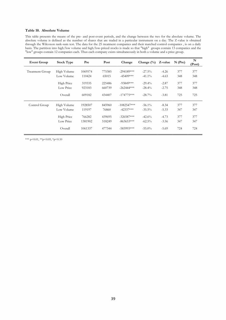
39
Table 10. Absolute Volume
This table presents the means of the pre- and post-event periods, and the change between the two for the absolute volume. The absolute volume is defined as the number of shares that are traded in a particular instrument on a day. The Z-value is obtained through the Wilcoxon rank-sum test. The data for the 25 treatment companies and their matched control companies , is on a daily basis. The partition into high/low volume and high/low-priced stocks is made so that "high" groups contain 13 companies and the "low" groups contain 12 companies each. Thus each company exists simultaneously in both a volume and a price group.
Event Group Stock Type Pre Post Change Change (%) Z-value N (Pre)
N (Post)
Treatment Group High Volume 1069574 775385 -294189*** -27.5% -4.26 377 377
Low Volume 110424 65015 -45409*** -41.1% -4.63 348 348
High Price 319335 225486 -93849*** -29.4% -2.87 377 377
Low Price 923183 660739 -262444*** -28.4% -2.75 348 348
Overall 609182 434407 -174775*** -28.7% -3.81 725 725
Control Group High Volume 1928507 845960 -1082547*** -56.1% -8.34 377 377
Low Volume 119197 76860 -42337*** -35.5% -5.33 347 347
High Price 766282 439695 -326587*** -42.6% -4.73 377 377
Low Price 1381902 518249 -863653*** -62.5% -3.56 347 347
Overall 1061337 477344 -583993*** -55.0% -5.69 724 724
*** p<0.01, **p<0.05, *p<0.10
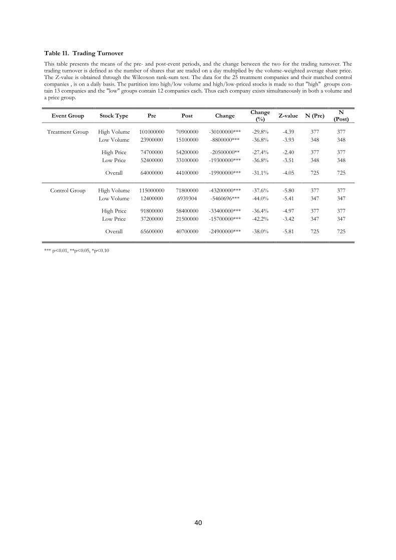
40
Table 11. Trading Turnover
This table presents the means of the pre- and post-event periods, and the change between the two for the trading turnover. The trading turnover is defined as the number of shares that are traded on a day multiplied by the volume-weighted average share price. The Z-value is obtained through the Wilcoxon rank-sum test. The data for the 25 treatment companies and their matched control companies , is on a daily basis. The partition into high/low volume and high/low-priced stocks is made so that "high" groups con-tain 13 companies and the "low" groups contain 12 companies each. Thus each company exists simultaneously in both a volume and a price group.
Event Group Stock Type Pre Post Change
Change (%)
Z-value N (Pre) N
(Post)
Treatment Group High Volume 101000000 70900000 -30100000*** -29.8% -4.39 377 377
Low Volume 23900000 15100000 -8800000*** -36.8% -3.93 348 348
High Price 74700000 54200000 -20500000** -27.4% -2.40 377 377
Low Price 52400000 33100000 -19300000*** -36.8% -3.51 348 348
Overall 64000000 44100000 -19900000*** -31.1% -4.05 725 725
Control Group High Volume 115000000 71800000 -43200000*** -37.6% -5.80 377 377
Low Volume 12400000 6939304 -5460696*** -44.0% -5.41 347 347
High Price 91800000 58400000 -33400000*** -36.4% -4.97 377 377
Low Price 37200000 21500000 -15700000*** -42.2% -3.42 347 347
Overall 65600000 40700000 -24900000*** -38.0% -5.81 725 725
*** p<0.01, **p<0.05, *p<0.10

41
Table 12. Volatility
This table presents the means of the pre- and post-event periods, and the change between the two for the volatility. The volatility is defined as annualized standard deviation of logarithmic daily returns, and is expressed in decimal form. The Z-value is obtained through the Wilcoxon rank-sum test. The data for the 25 treatment companies and their matched control companies, is on a daily basis. The partition into high/low volume and high/low-priced stocks is made so that "high" groups contain 13 companies and the "low" groups contain 12 companies each. Thus each company exists simultaneously in both a volume and a price group.
Event Group Stock Type Pre Post Change Change (%) Z-value N (Pre) N (Post)
Treatment Group High Volume 0.3882 0.2764 -0.1118*** -28.8% -8.51 377 377
Low Volume 0.3776 0.2872 -0.0904*** -23.9% -5.98 348 348
High Price 0.3559 0.2691 -0.0868*** -24.4% -7.47 377 377
Low Price 0.4125 0.2950 -0.1175*** -28.5% -7.00 348 348
Overall 0.3831 0.2816 -0.1015*** -26.5% -10.21 725 725
Control Group High Volume 0.4160 0.3114 -0.1046*** -25.1% -5.12 377 377
Low Volume 0.4400 0.3175 -0.1225*** -27.8% -7.11 348 348
High Price 0.4106 0.3002 -0.1104*** -26.9% -6.78 377 377
Low Price 0.4459 0.3297 -0.1162*** -26.1% -5.58 348 348
Overall 0.4275 0.3144 -0.1131*** -26.5% -8.67 725 725
*** p<0.01, **p<0.05, *p<0.10
Table 13. Proportional Daily Range of Transaction Prices
This table presents the means of the pre- and post-event periods, and the change between the two for the proportional daily range of transaction prices. It is defined as the difference between the highest price paid on a day minus the lowest price paid divided by the midpoint of the two. The Z-value is obtained through the Wilcoxon rank-sum test. The data for the 25 treatment companies and their matched control companies, is on a daily basis. The partition into high/low volume and high/low-priced stocks is made so that "high" groups contain 13 companies and the "low" groups contain 12 companies each. Thus each company exists simultaneously in both a volume and a price group.
Event Group Stock Type Pre Post Change Change (%) Z-value N (Pre) N (Post)
Treatment Group High Volume 0.0337 0.0273 -0.0064*** -19.0% -6.13 377 377
Low Volume 0.0343 0.0241 -0.0102*** -29.7% -8.47 348 348
High Price 0.0321 0.0235 -0.0086*** -26.8% -8.55 377 377
Low Price 0.0361 0.0282 -0.0079*** -21.8% -6.16 348 348
Overall 0.0340 0.0257 -0.0083*** -24.3% -10.30 725 725
Control Group High Volume 0.0383 0.0319 -0.0064*** -16.7% -5.14 377 377
Low Volume 0.0357 0.0274 -0.0083*** -23.2% -6.50 347 347
High Price 0.0361 0.0286 -0.0075*** -20.8% -6.56 377 377
Low Price 0.0381 0.0310 -0.0071*** -18.6% -5.06 347 347
Overall 0.0371 0.0297 -0.0074*** -19.9% -52.76 25093 26859
*** p<0.01, **p<0.05, *p<0.10

42
Table 14. Dependent Variables: Absolute and Relative Spread
This table presents the results of OLS regressions using robust standard errors. The dataset is a panel with daily observations for the 25 treatment and 25 control firms. The independent variable absolute spread is defined as the lowest ask price minus the highest bid price and measured in SEK, while the relative spread is defined as the absolute spread divided by the midpoint of the best bid and ask prices and measured in basis points. The "Event"-variable is a dummy variable that is assigned a 1 if the time period is after the tick size reduction and 0 if it is before the reduction. "Treatment" is also a dummy variable that is given a 1 if the firm is a treatment firm, and 0 if it is a control firm. The "Diff-in-diff" variable is obtained through multiplying the two dummy variables with each other. Hence, it is 1 if the firm is a treatment firm and the time period is post the event. In all other cases it will be 0. Log (Market Cap) is the logarithmic market capitalization on a daily basis calculated through multiplying the volume-weighted average share prices with the number of outstanding shares. Log (Volume) is the logarithmic value of all traded stocks on a given day for each company. The volatility is measured as the annualized standard deviation of logarithmic returns and is presented in decimal form. Where time dummy variables are used it refers to the use of daily calendar day dummies for each trading day, and company fixed effects control for company-specific effects.
Absolute Spread Relative Spread
Variable Reg (1.1) Reg (1.2) Reg (1.3) Reg (1.1) Reg (1.2) Reg (1.3)
Diff-in-Diff -0.124*** -0.124*** -0.117***
-7.769*** -7.769*** -9.163***
(-4.52) (-11.82) (-11.23)
(-2.91) (-7.24) (-8.90)
Event 0.0111
-0.802
(0.57)
(-0.37)
Treatment 0.171***
-3.248*
(9.01)
(-1.73)
Log (Market Cap)
-0.0217***
-21.43***
(-2.86)
(-21.74)
Log (Volume)
-0.0425***
-3.942***
(-6.92)
(-6.44)
Volatility
0.00616
0.574
(1.45)
(1.29)
Constant 0.308*** 0.354*** 1.368***
38.93*** 31.76*** 577.3***
(22.07) (16.32) (5.69)
(23.81) (13.42) (20.48)
Time Dummy Variables No Yes Yes
No Yes Yes
Company Fixed Effects No Yes Yes
No Yes Yes
R2 0.033 0.864 0.869
0.017 0.847 0.862
N 2900 2900 2898 2900 2900 2898
t-statistics in parantheses
*** p<0.01, **p<0.05, *p<0.10

43
Table 15. Dependent Variables: Absolute Diff Spread and Relative Diff Spread
This table presents the results of OLS regressions using robust standard errors. The dataset is a panel with daily observations for the 25 treatment and 25 control firms. Each variable is a difference between the treatment company and its matched control company. The independent variable Diff Spread is therefore the difference in spread, which in turn is defined as the lowest ask price minus the highest bid price and measured in SEK, while the Relative Spread, which is used in the Relative Diff Spread is defined as the Abso-lute Spread divided by the midpoint of the best bid and ask prices and measured in basis points. The "Event"-variable is a dummy variable that is assigned a 1 if the time period is after the tick size reduction and 0 if it is before the reduction. Diffvol is the differ-ence in volume, where volume is defined as the sum shares traded during one day. Diffpropdaily is the difference between the pro-portional daily range of transaction prices, where that in turn is defined as the highest price paid during a day minus the lowest price paid divided by the midpoint of the two. Diffmarketcap is the difference in market capitalization, which is measured as the number of outstanding shares multiplied by the daily volume-weighted average share price. Where time dummy variables are used it refers to the use of daily calendar day dummies for each trading day, and company fixed effects control for company-specific effects.
Absolute Diff Spread Relative Diff Spread
Variable Reg (2.1) Reg (2.2) Reg (2.1) Reg (2.2)
Event -0.125*** -0.119**
-8.729*** -11.84**
(-7.57) (-2.36)
(-4.97) (-2.31)
diffvol -1.40e-09*** -1.39e-09**
0.000000553*** 0.000000355***
(-2.60) (-2.56)
(6.20) (4.07)
diffpropdaily 1.568*** 1.250***
346.0*** 171.7***
(3.36) (4.03)
(7.07) (5.44)
diffaverage 0.00158*** -0.00240***
-0.0216*** -0.117***
(38.91) (-4.83)
(-5.82) (-2.61)
diffmarketcap 1.83e-13 1.11e-11***
-1.72e-10*** -3.04e-10
(0.57) (4.66)
(-5.48) (-1.46)
Constant 0.0806*** 0.267***
0.756 5.185
(6.59) (5.38)
(0.55) (1.01)
Time Dummy Variables No Yes
No Yes
Company Fixed Effects No Yes
No Yes
R2 0.453 0.782
0.131 0.689
N 1448 1448 1448 1448
t-statistics in parantheses
*** p<0.01, **p<0.05, *p<0.10
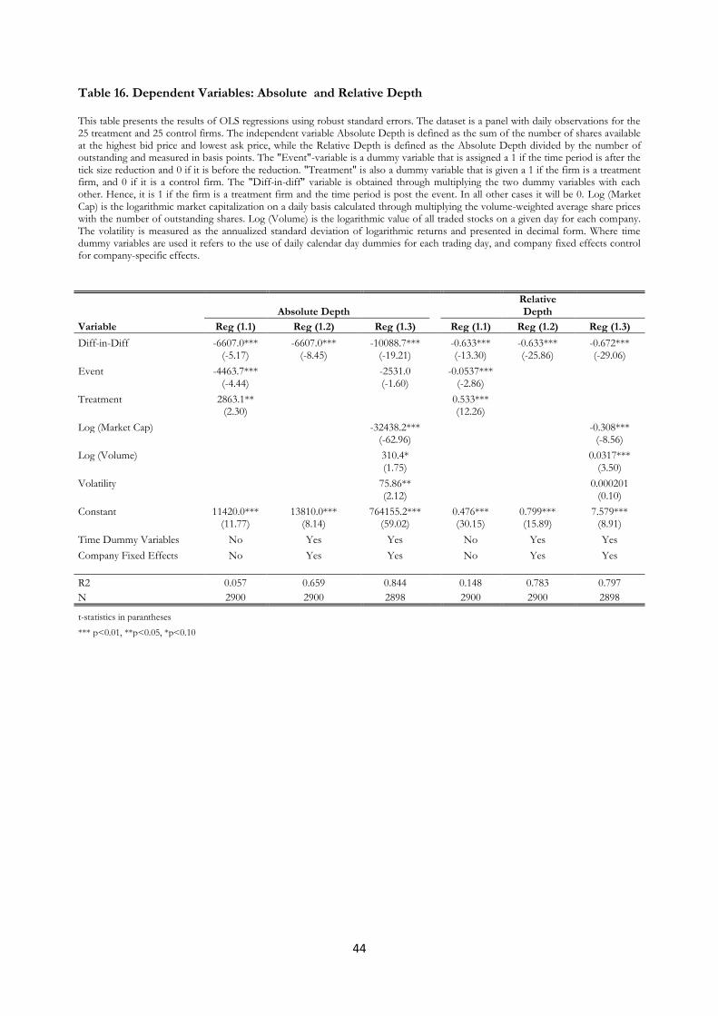
44
Table 16. Dependent Variables: Absolute and Relative Depth
This table presents the results of OLS regressions using robust standard errors. The dataset is a panel with daily observations for the 25 treatment and 25 control firms. The independent variable Absolute Depth is defined as the sum of the number of shares available at the highest bid price and lowest ask price, while the Relative Depth is defined as the Absolute Depth divided by the number of outstanding and measured in basis points. The "Event"-variable is a dummy variable that is assigned a 1 if the time period is after the tick size reduction and 0 if it is before the reduction. "Treatment" is also a dummy variable that is given a 1 if the firm is a treatment firm, and 0 if it is a control firm. The "Diff-in-diff" variable is obtained through multiplying the two dummy variables with each other. Hence, it is 1 if the firm is a treatment firm and the time period is post the event. In all other cases it will be 0. Log (Market Cap) is the logarithmic market capitalization on a daily basis calculated through multiplying the volume-weighted average share prices with the number of outstanding shares. Log (Volume) is the logarithmic value of all traded stocks on a given day for each company. The volatility is measured as the annualized standard deviation of logarithmic returns and presented in decimal form. Where time dummy variables are used it refers to the use of daily calendar day dummies for each trading day, and company fixed effects control for company-specific effects.
Absolute Depth Relative Depth
Variable Reg (1.1) Reg (1.2) Reg (1.3) Reg (1.1) Reg (1.2) Reg (1.3)
Diff-in-Diff -6607.0*** -6607.0*** -10088.7***
-0.633*** -0.633*** -0.672***
(-5.17) (-8.45) (-19.21)
(-13.30) (-25.86) (-29.06)
Event -4463.7***
-2531.0
-0.0537***
(-4.44)
(-1.60)
(-2.86)
Treatment 2863.1**
0.533***
(2.30)
(12.26)
Log (Market Cap)
-32438.2***
-0.308***
(-62.96)
(-8.56)
Log (Volume)
310.4*
0.0317***
(1.75)
(3.50)
Volatility
75.86**
0.000201
(2.12)
(0.10)
Constant 11420.0*** 13810.0*** 764155.2***
0.476*** 0.799*** 7.579***
(11.77) (8.14) (59.02)
(30.15) (15.89) (8.91)
Time Dummy Variables No Yes Yes
No Yes Yes
Company Fixed Effects No Yes Yes
No Yes Yes
R2 0.057 0.659 0.844
0.148 0.783 0.797
N 2900 2900 2898 2900 2900 2898
t-statistics in parantheses
*** p<0.01, **p<0.05, *p<0.10

45
Table 17. Dependent Variables: Absolute Diff Depth and Relative Diff Depth
This table presents the results of OLS regressions using robust standard errors. The dataset is a panel with daily observations for the 25 treatment and 25 control firms. Each variable is a difference between the treatment company and its matched control company. The independent variable Diff Depth is therefore the difference in depth, which in turn is defined as the sum of shares available at the lowest ask price and highest bid price, while the Relative Depth, which is used in the Relative Diff Depth is defined as the Abso-lute Depth divided by the number of outstanding shares, and measured in basis points. The "Event"-variable is a dummy variable that is assigned a 1 if the time period is after the tick size reduction and 0 if it is before the reduction. Diffvol is the difference in volume, where volume is defined as the sum shares traded during one day. Diffpropdaily is the difference between the proportional daily range of transaction prices, where that in turn is defined as the highest price paid during a day minus the lowest price paid divided by the midpoint of the two. Diffmarketcap is the difference in market capitalization, which is measured as the number of outstanding shares multiplied by the daily volume-weighted average share price. Where time dummy variables are used it refers to the use of daily calendar day dummies for each trading day, and company fixed effects control for company-specific effects.
Absolute Diff Depth Relative Diff Depth
Variable Reg (2.1) Reg (2.2) Reg (2.1) Reg (2.2)
Event -10389.9*** -13356.3***
-0.684*** -0.813***
(-11.61) (-3.65)
(-15.10) (-6.37)
diffvol 0.00205*** 0.00137***
2.83e-08*** 2.38e-08***
(7.31) (5.99)
(7.48) (6.95)
diffpropdaily 57471.9** -6578.1
0.621 -1.158*
(2.40) (-0.37)
(0.64) (-1.81)
diffaverage -31.87*** 42.38
-0.00129*** 0.00407**
(-12.17) (1.06)
(-8.58) (2.07)
diffmarketcap 4.98e-08*** -0.000000460
5.66e-13 1.32e-11
(3.79) (-1.59)
(0.57) (1.54)
Constant 8847.3*** 7649.4**
0.667*** 0.444***
(9.72) (2.01)
(14.20) (2.90)
Time Dummy Variables No Yes
No Yes
Company Fixed Effects No Yes
No Yes
R2 0.483 0.760
0.224 0.800
N 1448 1448 1448 1448
t-statistics in parantheses
*** p<0.01, **p<0.05, *p<0.10

46
Table 18. Dependent Variables: Trading Volume and Trading Turnover
This table presents the results of OLS regressions using robust standard errors. The dataset is a panel with daily observations for the 25 treatment and 25 control firms. The independent variable Volume is defined as the number of shares that are traded for the security during a day, while the Trading Turnover is defined as the Volume multiplied by the volume-weighted average share price and therefore measured in SEK. The "Event"-variable is a dummy variable that is assigned a 1 if the time period is after the tick size reduction and 0 if it is before the reduction. "Treatment" is also a dummy variable that is given a 1 if the firm is a treatment firm, and 0 if it is a control firm. The "Diff-in-diff" variable is obtained through multiplying the two dummy variables with each other. Hence, it is 1 if the firm is a treatment firm and the time period is post the event. In all other cases it will be 0. Log (Market Cap) is the logarithmic market capitaliza-tion on a daily basis calculated through multiplying the volume-weighted average share prices with the number of outstanding shares. The volatility is measured as the annualized standard deviation of logarithmic returns and presented in decimal form. The bid-ask Spread is defined as the difference between the lowest ask price and the highest bid price. Where time dummy variables are used it refers to the use of daily calendar day dummies for each trading day, and company fixed effects control for company-specific effects.
Trading Vo-
lume Trading Turnover
Variable Reg (1.1) Reg (1.2) Reg (1.3) Reg (1.1) Reg (1.2) Reg (1.3)
Diff-in-Diff 409218.1*** 409452.7*** 189941.5***
10666803.1 5045388.8* 4979456.0*
(4.62) (7.58) (4.75)
(1.43) (1.72) (1.69)
Event -583993.0***
-32865464.2***
(-7.93)
(-5.41)
Treatment -452155.3***
-7417951.9
(-5.68)
(-1.12)
Volatility
28106.4*
1337068.8
(1.92)
(1.37)
Log (Market Cap)
-2063074.1***
1177666.0
(-55.54)
(0.51)
Bid-ask Spread
-61188.9**
-4546769.8**
(-2.34)
(-2.12)
Constant 1061337.4*** 610913.0*** 48583612.2***
74231965.7*** 53709513.8*** 27379684.6
(15.38) (6.97) (56.12)
(13.45) (10.52) (0.51)
Time Dummy Varia-bles No Yes Yes
No Yes Yes
Company Fixed Ef-fects No Yes Yes
No Yes Yes
R2 0.042 0.657 0.811
0.019 0.741 0.742
N 2898 2898 2898 2898 2898 2898
t-statistics in parantheses
*** p<0.01, **p<0.05, *p<0.10

47
Table 19. Dependent Variables: Diff Volume and Diff Trading Turnover
This table presents the results of OLS regressions using robust standard errors. The dataset is a panel with daily observations for the 25 treatment and 25 control firms. Each variable is a difference between the treatment company and its matched control company. The independent variable Diff Volume is therefore the difference in volume which in turn is defined as the sum shares traded during one day, while the Trading Turnover which is used in the Diff Trading Turnover is defined as the daily volume multiplied by the daily volume-weighted average price. The "Event"-variable is a dummy variable that is assigned a 1 if the time period is after the tick size reduction and 0 if it is before the reduction. Diffspread is the difference in spread, where the spread is measured as the differ-ence between the lowest ask price and the highest bid price. Diffpropdaily is the difference between the proportional daily range of transaction prices, where that in turn is defined as the highest price paid during a day minus the lowest price paid divided by the midpoint of the two. Diffmarketcap is the difference in market capitalization, which is measured as the number of outstanding shares multiplied by the daily volume-weighted average share price. Where time dummy variables are used it refers to the use of daily calen-dar day dummies for each trading day, and company fixed effects control for company-specific effects.
Diff Volume Diff Trading Turnover
Variable Reg (2.1) Reg (2.2) Reg (2.1) Reg (2.2)
Event 378117.5*** 207435.9
4512122.3 6032220.8
(4.79) (0.88)
(1.37) (0.48)
diffpropdaily 22305915.8*** 11978137.8***
271205585.0*** 647923635.6***
(8.57) (7.27)
(3.11) (7.15)
diffmarketcap -0.00000474*** -0.000118***
0.000304*** 0.00157*
(-2.98) (-5.40)
(2.91) (1.91)
diffspread -740378.3*** -214264.4***
-10952689.8*** -8776892.7***
(-9.96) (-4.61)
(-4.01) (-3.32)
Constant -295160.3*** -54083.4
-56160.0 12572886.1
(-4.22) (-0.32)
(-0.02) (1.60)
Time Dummy Variables No Yes
No Yes
Company Fixed Effects No Yes
No Yes
R2 0.161 0.670
0.020 0.401
N 1448 1448 1448 1448
t-statistics in parantheses
*** p<0.01, **p<0.05, *p<0.10

48
Table 20. Dependent Variables: Volatility and Proportional Daily Range of Transaction Prices
This table presents the results of OLS regressions using robust standard errors. The dataset is a panel with daily observations for the 25 treatment and 25 control firms. The independent variable volatility is measured as the annualized standard deviation of logarithmic returns presented in decimal form, while the Proportional Daily Range of Transaction Prices is defined as the highest priced paid during the day minus the lowest, divided by the midpoint of the two. The "Event"-variable is a dummy variable that is assigned a 1 if the time period is after the tick size reduction and 0 if it is before the reduction. "Treatment" is also a dummy variable that is given a 1 if the firm is a treatment firm, and 0 if it is a control firm. The "Diff-in-diff" variable is obtained through multiplying the two dum-my variables with each other. Hence, it is 1 if the firm is a treatment firm and the time period is post the event. In all other cases it will be 0. Transactions corresponds to the number of transactions that have taken place during a day. Log (Market Cap) is the loga-rithmic market capitalization on a daily basis calculated through multiplying the volume-weighted average share prices with the num-ber of outstanding shares. L.1 Volatility is the lagged volatility of one period, i.e. one day, and L.1 Prop Daily Range is the counterpar-ty for the proportional daily range of transaction prices. Where time dummy variables are used it refers to the use of daily calendar day dummies for each trading day, and company fixed effects control for company-specific effects.
Volatility Prop. Daily Range
Variable Reg (1.1) Reg (1.2) Reg (1.3) Reg (1.1) Reg (1.2) Reg (1.3)
Diff-in-Diff 0.0116 0.0116 -0.0136
-0.000926 -0.000923 -0.00286***
(0.69) (1.01) (-1.03)
(-0.79) (-0.99) (-2.67)
Event -0.113***
-0.00733***
(-8.85)
(-8.68)
Treatment -0.0444***
-0.00309***
(-3.07)
(-3.35)
Transactions
0.0000571***
0.00000520***
(5.24)
(8.89)
Log (Market Cap)
-0.0315***
-0.00416***
(-2.62)
(-2.95)
L1 Volatility
0.119***
(3.73)
L1 Prop Daily Range
0.109***
(4.39)
Constant 0.428*** 0.230*** 0.852***
0.0371*** 0.0262*** 0.133***
(38.99) (10.47) (2.97)
(55.74) (13.94) (4.04)
Time Dummy Variables No Yes Yes
No Yes Yes
Company Fixed Effects No Yes Yes
No Yes Yes
R2 0.060 0.577 0.640
0.068 0.435 0.488
N 2900 2900 2198 2898 2898 2196
t-statistics in parantheses
*** p<0.01, **p<0.05, *p<0.10

49
Table 21. Dependent Variables: Diff Volatility and Diff Prop. Daily Range
This table presents the results of OLS regressions using robust standard errors. The dataset is a panel with daily observations for the 25 treatment and 25 control firms. Each variable is a difference between the treatment company and its matched control company. The independent variable Diff Volatility is therefore the difference in volatility, which in turn is defined as the annualized standard deviation of logarithmic daily returns, while the Prop. Daily Range of Transaction Prices which is used in the Diff Prop. Daily Range is defined as the difference between the highest price paid during the day and the lowest price for the same security, divided by the midpoint of the two. The "Event"-variable is a dummy variable that is assigned a 1 if the time period is after the tick size reduction and 0 if it is before the reduction. Diffmarketcap is the difference in market capitalization, which is measured as the number of outstanding shares multiplied by the daily volume-weighted average share price. Difftransactions is the difference in amount of transactions that has taken place on each day. The diffaverage is the difference in volume-weighted average share price for the day in question. Where time dummy variables are used it refers to the use of daily calendar day dummies for each trading day, and company fixed effects control for company-specific effects.
Diff Volatility and Diff Proportional Daily Range of Transaction Prices
Diff Volatility Diff Prop. Daily Range
Variable Reg (2.1) Reg (2.2) Reg (2.1) Reg (2.2)
Event 0.00425 0.0377
-0.00169 0.00536
(0.32) (0.88)
(-1.61) (1.02)
diffmarketcap 1.21e-12*** 3.83e-12
-2.16e-14 -3.65e-13
(3.23) (1.00)
(-0.71) (-1.15)
difftransactions 0.0000192** 0.0000590***
0.00000240*** 0.00000694***
(2.37) (5.74)
(4.67) (9.75)
diffaverage -0.000368*** -0.000399
-0.0000317*** -0.0000475
(-9.27) (-0.56)
(-10.58) (-0.80)
Constant -0.0166 -0.0363
-0.000361 -0.00194
(-1.47) (-0.71)
(-0.45) (-0.38)
Time Dummy Variables No Yes
No Yes Company Fixed Effects No Yes
No Yes
R2 0.068 0.291
0.098 0.335
N 1448 1448 1448 1448
t-statistics in parantheses
*** p<0.01, **p<0.05, *p<0.10