1

ÉCOLE DOCTORALE DES SCIENCES DE LA TERRE ET DE L’ENVIRONNEMENT (ED 413)

Laboratoire d’Hydrologie et de Géochimie de Strasbourg (LHyGeS) UMR 7517 (Université de Strasbourg / ENGEES – CNRS)

THÈSE

Présentée par :

Marie LEFRANCQ

soutenue le : 11 Avril 2014

pour obtenir le grade de : Docteur de l’université de Strasbourg

Discipline/ Spécialité: Science de l’environnement

Transport and attenuation of pesticides in runoff from agricultural headwater catchments:

from field characterisation to modelling

THÈSE dirigée par :

M. IMFELD Gwenaël Chargé de recherche CNRS, France

RAPPORTEURS :

M. BROWN Colin Professeur, Université de York, Royaume-Uni M.STAMM Christian Directeur de recherche, Eawag, Suisse

AUTRES MEMBRES DU JURY : Mme GASCUEL-ODOUX Chantal Directrice de recherche, INRA Rennes, France M. JETTEN Victor Professeur, Université de Twente, Pays Bas M. PAYRAUDEAU Sylvain Maître de conférences, ENGEES, France

UNIVERSITÉ DE STRASBOURG

2

3

“A PhD thesis is like riding a bike, to keep your balance you must keep moving” Adapted from Albert Einstein

4

5

Acknowledgements

This Ph.D. thesis was carried out at the Laboratory of Hydrology and Geochemistry of Strasbourg (LHyGeS), France. It was supported by the Interreg IV PhytoRet project (E.U./The Rhin Meuse French national water agency fellowship). I want to thank all persons and institutions who have directly or indirectly contributed to this work. I had been considering the project of achieving a PhD for a while: The only missing thing was an interesting subject in an exciting context! Sylvain Payraudeau and Gwenaël Imfeld allowed me to get this chance: thanks to both of them for that. I am very grateful to them for their continuous support in the form of discussions, feedbacks and ideas, which definitively contributed to the completion of this project. I also thank them for their help in reviewing this thesis tirelessly and preparing the peer-reviewed publications. I am grateful to the jury members who kindly accepted to evaluate my work: Pr. Colin Brown, Pr. Victor Jetten, Dr. Chantal Gascuel Odoux and Dr. Christian Stamm. I particularly wish to thank all the German partners of the ‘PhytoRet project’. Herzlichen Dank an Dr. Habil. Jens Lange, Prof. Klaus Kümmerer, Dr. Oliver Olson und Barbara Herbstritt. Ich möchte auch Romy Durst and Brian Sweeney for their great help in the field danken. Thanks as well to the PhD students of the Phytoret project, Matthias Gassmann and Lukasz Gutowski, for the interactive skype sessions, I will remember as well the nice touristic tours of Lüneburg and of the ‘Hamburg fish market’.Thanks also to Caroline Grégoire who made possible this Phytoret project. My heartfelt thanks to Victor Jetten for his precious time and his welcoming to the Faculty of Geo-Information Science and Earth Observation (ITC) in Twente for two stays. Heel hartelijk bedankt! I have really appreciated the teachings, the tips and the secrets on OpenLisem and Qt creator you provided me. Thanks as well to Paul Van Dijk for his invaluable advice on all the parameters of LISEM and his advices in agronomical aspect. I am immensely grateful to Eric Pernin, Nicolas Tissot and Benoit Guyot for their daily help in the field experiment setting up, the sample collection and their analytical support in the lab.I am very grateful to René Boutin, Sophie Gangloff, Carole Lutz and Marie-Pierre Ottermatte for their precious advice, and analytical support in the lab work. I specially acknowledge Martine Trauttmann for her dedication to the soil laboratory and analyses! I would like to thank as well all the bachelor and master students who contributed to this work: Maxime, Jeanne, Thomas, Célia, Antonio, Diogo, Arthur and Matthieu. Thank you for your deep involvement in these field and modelling experiments. I would like to warmly thank the farmers who responded to the surveys and made these experimental studies possible; especially for their allowance for the experimental plot study and, for their invaluable help in filling or digging using their agricultural machines when building the experiment sites in the field. Thanks as well to all my colleagues at the LHyGeS. I want to especially name Sylvain Weill, “my hydrological father”, Marie Claire Pierret for her interest in studying rare earth elements transport in the arable crop catchment, Anne Véronique Auzet for her help in understanding agricultural erosion, Raphaël Di Chiara for his motivation in solving numerical problems, Cyrielle Regazonni for the usefull advices in GIS, Alain Clement for solving all kinds of informatic bugs, the colleagues from IMFS for their advice on the Doppler installation or hydraulic calculations, Lauriane and Fanilo for their advices in maths, Joëlle for all her special touches and naturally,

6

Maurice Millet for his great help in pesticides quantification and for teaching me the bases of chemistry that I had completely forgotten. I also benefited from the precious help of Philippe Ackerer who provided invaluable advices for resolving my mass balance errors and finding alternative ways to implement the mixing layer concept! Thanks for your permanent good mood, patience and encouragements. Many thanks to Richard Coupe for proof-reading my manuscript. A special thanks to Roger Moussa for having the good words at the right time. ‘The day will come for the firework”. But… These 3 years have also been so nice for many non-academic reasons: My deepest thanks go to all the Ph.D students from the LHyGeS, and especially to my colleagues and friends Elodie, Benoit, Nicolas and Omniea for the coffee and beer times. They greatly contributed to the nice atmosphere which has been prevailed throughout those three years. Thanks as well to the ‘third floor’ PhD students: Adrien (the golden Palm), Izabella (the Hungarian dancer), the Italian team including Ivan, Eleonora and Clio, Thieb’ (the best “pétanque” player), Nicolas (for the crazy Tuesday), Philippe (for the numerous croissants) and the new PhD students Marion (from Arzviller ) and Bastien ! Thanks to Marianne for sharing the flat for so long! Thanks to the Strasbourg team for the weekly meetingS at the “Grincheux” or the “Marché bar”, and also for the soccer games in the Orangerie park. Thanks as well to the “2009 Cemagref wedding agency” from Lyon. Enfin, merci à toute ma famille, surtout aux petiots qui ont grandi ou sont nés pendant ces trois dernières années … Sans oublier Damien pour m’avoir soutenue jusque-là! De nombreux cols à passer nous attendent encore …

7

Table of Contents

Table of Figures ........................................................................................................................................................................... 10 Table of Tables ............................................................................................................................................................................. 13 Abbreviations ............................................................................................................................................................................... 15 Abstract ........................................................................................................................................................................................... 17

Chapter I. Introduction & context ........................................................................................................... 37 1. Pesticides in the environment ............................................................................................................................... 37

1.1. Impact and diversity ......................................................................................................................................... 37 1.2. Environmental distribution of pesticides ................................................................................................ 39

2. Pesticide transport from agro-ecosystems to surface waters ................................................................. 41 2.1. Agro-ecosystems, definition and specificity ........................................................................................... 41 2.2. Pesticide transport and attenuation from agricultural sources to sinks ................................... 42

2.2.1 Processes affecting pesticides amount at the source area (Asource) ................................................ 43 2.2.2 Processes affecting pesticide transport in agro-ecosystems (Aactive and Aconnected) ................ 47 2.2.3 Relevance of combining emerging analytical tools for assessing pesticide degradation .... 49 2.2.4 Usefulness and complementarity of modelling following a characterisation phase ............. 50

3. Relevance of headwater catchments for pesticide transport in surface water ............................... 56 3.1. Definition and role of headwater catchments in downstream water quality .......................... 56 3.2. Importance of combining plot- and catchment-scale observations............................................. 57 3.3. Models for predicting pesticide transport in headwater catchments ......................................... 58

Chapter II. Research focus and objectives ............................................................................................. 59 1. Research focus .............................................................................................................................................................. 59 2. Thesis objectives .......................................................................................................................................................... 60 3. Thesis layout.................................................................................................................................................................. 63 4. References ...................................................................................................................................................................... 65

Chapter III. Fungicides drift and mobilisation via runoff and erosion in vineyard ................. 76

Section 1. Kresoxim methyl deposition, drift and runoff in a vineyard catchment ............. 78 1. Abstract ............................................................................................................................................................................ 78 2. Introduction ................................................................................................................................................................... 80 3. Material and methods................................................................................................................................................ 81

3.1. Description of the vineyard catchment .................................................................................................... 81 3.2. KM properties and application ..................................................................................................................... 82 3.3. Sampling procedure .......................................................................................................................................... 83 3.4. KM analysis ........................................................................................................................................................... 84 3.5. Data analysis ......................................................................................................................................................... 85

4. Results and discussion .............................................................................................................................................. 86 4.1. KM deposition ...................................................................................................................................................... 86 4.2. KM drift ................................................................................................................................................................... 88 4.3. Runoff-associated KM ....................................................................................................................................... 90

5. Conclusion ...................................................................................................................................................................... 91 6. References ...................................................................................................................................................................... 92

Section 2. Fungicides transport in runoff from vineyard plot and catchment: contribution of non-target areas .................................................................................................................................................... 94

1. Abstract ............................................................................................................................................................................ 94 2. Introduction ................................................................................................................................................................... 95 3. Material and methods................................................................................................................................................ 96

3.1. Chemicals ............................................................................................................................................................... 96 3.2. Description of the vineyard catchment .................................................................................................... 97 3.3. Description of the experimental plot ......................................................................................................... 98

8

3.4. Pesticide applications and soil deposition ........................................................................................... 101 3.5. Runoff discharge measurement and water sampling procedure ............................................... 101 3.6. Soil sampling and characterization ......................................................................................................... 102 3.7. Chemical analysis ............................................................................................................................................ 102 3.8. Data analysis and calculation ..................................................................................................................... 103

4. Results ........................................................................................................................................................................... 104 4.1. Hydrology............................................................................................................................................................ 104 4.2. Hydrochemistry ............................................................................................................................................... 104 4.3. Deposition of KM and CY on soil ............................................................................................................... 105 4.4. KM and CY mobilisation in the runoff dissolved phase (< 0.7 µm) ........................................... 105 4.5. Partitioning of KM and CY in runoff ........................................................................................................ 109

5. Discussion .................................................................................................................................................................... 110 6. Conclusion ................................................................................................................................................................... 112 7. References ................................................................................................................................................................... 113

Chapter IV. Herbicides transport and attenuation via runoff and erosion in arable crop catchment …………………………………………………………………………………………………………………… ..117

Section 1. Transport and attenuation of chloroacetanilides in an agricultural headwater catchment ……………………………………………………………………………………………………………………. .119

1. Abstract ......................................................................................................................................................................... 119 2. Introduction ................................................................................................................................................................ 120 3. Material and methods............................................................................................................................................. 121

3.1. Description of the study site ....................................................................................................................... 121 3.2. Herbicides characteristics and applications ........................................................................................ 123 3.3. Hydrological measurements and sampling procedure ................................................................... 124 3.4. Hydrochemical and soil analysis .............................................................................................................. 125 3.5. Chloroacetanilide analysis ........................................................................................................................... 125

3.5.1 Chemicals ................................................................................................................................................................ 125 3.5.2 Extraction ................................................................................................................................................................ 125 3.5.3 Quantification of the chloroacetanilides and their degradation products .............................. 126 3.5.4 Enantiomer analysis of S-metolachlor ...................................................................................................... 127 3.5.5 Data analysis .......................................................................................................................................................... 127

4. Results and discussion ........................................................................................................................................... 128 4.1. Chloroacetanilide attenuation in the plot soil .................................................................................... 128 4.2. Influence of hydrology and hydrochemistry on chloroacetanilide export and partitioning ……………………………………………………………………………………………………………………………….130

4.2.1 Hydrochemical and chloroacetanilide load variations...................................................................... 130 4.2.2 Chloroacetanilide partitioning ...................................................................................................................... 135

4.3. ESA and OXA degradation products dynamics ................................................................................... 136 4.4. S-metolachlor enantiomeric signatures as indicator of in-situ degradation ........................ 137

5. Conclusion ................................................................................................................................................................... 140 6. Acknowledgement ................................................................................................................................................... 141 7. References ................................................................................................................................................................... 142

Chapter V. Modelling pesticide runoff at the headwater catchment scale ..............................146

Section 1. Agronomical insights for improving runoff prediction in headwater agricultural catchments ........................................................................................................................................148

1. Abstract ......................................................................................................................................................................... 148 2. Introduction ................................................................................................................................................................ 150 3. Material and methods............................................................................................................................................. 152

3.1. Model description............................................................................................................................................ 152 3.2. Continuous agronomical model: IDR ........................................................................................................ 153 3.3. Study case ........................................................................................................................................................... 154

3.3.1 Description of the study site .......................................................................................................................... 154 3.3.2 Hydrological procedure and experimental results ............................................................................. 155 3.3.3 Erosion characterisation .................................................................................................................................. 158

9

3.4. Input parameters ............................................................................................................................................. 159 3.5. Calibration strategy ........................................................................................................................................ 161 3.6. Model calibration and sensitivity analysis ........................................................................................... 162 3.7. Evaluation criteria and data analysis ..................................................................................................... 162

4. Results ........................................................................................................................................................................... 163 4.1. Basic calibration method (BCM) ............................................................................................................... 163 4.2. Constraint calibration method (CCM) .................................................................................................... 166 4.3. Sensitivity analysis of input parameters ............................................................................................... 168 4.4. Erosion characterisation and prediction: focus on May 21 .......................................................... 169

5. Discussion and conclusion ................................................................................................................................... 170 6. Acknowledgements ................................................................................................................................................. 172 7. References ................................................................................................................................................................... 172

Section 2. A comprehensive mathematical model for mobilisation and transport of dissolved pesticide from the soil surface to runoff: the mixing layer approach. .............................177

1. Introduction ................................................................................................................................................................ 177 2. Mathematical theory and approach ................................................................................................................. 180

2.1. Openlisem ........................................................................................................................................................... 180 2.2. Mixing model ..................................................................................................................................................... 182 2.3. Numerical resolution with operator splitting (LISEM-psni) ........................................................ 183 2.4. Pseudo-analytical resolution (LISEM-pa) ............................................................................................. 185 2.5. Mass balance errors calculations ............................................................................................................. 187 2.6. Case study scenarios ...................................................................................................................................... 188

3. Results and discussion ........................................................................................................................................... 189 3.1. Steady test case ................................................................................................................................................ 189 3.2. Dynamic test case: an experimental plot .............................................................................................. 191 3.3. A study case in an agricultural headwater catchment: Alteckendorf ....................................... 194

4. Conclusion ................................................................................................................................................................... 197 5. Acknowledgement ................................................................................................................................................... 198 6. References ................................................................................................................................................................... 199

Chapter VI. General conclusions and perspectives ...........................................................................201 1. Summary and conclusion ....................................................................................................................201

1.1. The spatial variability of pesticides deposition during application impacts pesticide runoff ……………………………………………………………………………………………………………………………….203 1.2. Combining plot and catchment scales observations is critical for assessing off-site exports of pesticides ......................................................................................................................................................................... 205 1.3. Predicting pesticide transport processes in the agricultural catchments ............................. 207 1.4. Pesticides partitioning is crucial for pesticide export under field condition........................ 208 1.5. Combining analytical approaches helps the evaluation of pesticide degradation within agricultural headwater catchment ............................................................................................................................ 210

2. Implications and perspectives ..........................................................................................................212 2.1. How to address the variability of pesticides deposition during application in pesticides runoff studies? .................................................................................................................................................................... 213 2.2. How to improve the evaluation the pesticides partitioning in runoff water? ...................... 213 2.3. How to evaluate the degradation of chiral pesticides under field conditions? .................... 214

3. References ................................................................................................................................................216

Chapter VII. Appendices................................................................................................................................222

10

Table of Figures

Chapter I

Figure I-1. Structures of the four stereoisomers of metolachlor (Kabler and Chen, 2006) .................................. 38 Figure I-2. Pesticide movement in the hydrological system (Barbash, 2014)............................................................ 40 Figure I-3. Bio-physical-chemical processes related to pesticide transport and attenuation in agro-

ecosystems ...................................................................................................................................................................................... 45 Figure I-4. Degradation pathways of acetochlor in soil (Roberts et al., 1999). Acetochlor was

metabolised in soil mainly by two primary pathways. The first pathway involved the hydrolytic/oxidative displacement of chlorine to form the alcohol 2 and the oxidation of the alcohol 2 to oxanilic acid 3. N-dealkylation of 3 yielded oxanilic acid 4. The second pathway involved the displacement of chlorine by glutathione and the further secondary catabolism of the glutathione conjugate 5 to the various sulfinylacteic and sulfonic acid products (6-9)....................... 46

Figure I-5. Processes for transferring pesticides from the soil surface to runoff water ........................................ 48 Figure I-6. Existing physically based pesticide transport models according to their spatial and

temporal discretisations. .......................................................................................................................................................... 51 Figure I-7. Relationship between catchment size and aqueous non-point sources of insecticide

contamination detected in samples of surface waters (Schultz, 2004) ............................................................... 57

Chapter II

Figure II-1. Locations and schemes of the study catchments (Alsace, France) .......................................................... 62 Figure II-2. Graphical outline of the PhD thesis ....................................................................................................................... 64

Chapter III

Figure III-1. Graphical outline of the PhD thesis (Chapter III) .......................................................................................... 77 Figure III-2. Graphical abstract ........................................................................................................................................................ 79 Figure III-3. Location of the kresoxim methyl collectors in the vineyard catchment (Rouffach, Alsace,

France) on May 24, 2011. ......................................................................................................................................................... 82 Figure III-4. Kresoxim methyl soil deposition of the nine collectors normalised by corresponding Thiessen

area in the vineyard catchment (Rouffach, Alsace, France) during the three periods P1, P2 and P3 on May 24, 2011. ................................................................................................................................................................................. 87

Figure III-5. Scheme of the catchment (A) and the experimental plot (B) (Rouffach, Alsace, France). The geographical coordinates of the meteorological station are 47°57'9N, 07°17'3E. ......................................... 99

Figure III-6. Temporal changes in the hydrological conditions (A and B), the fungicides application (green bars for KM, orange bars for CY) and the concentrations in runoff water (C and D), the specific loads (green bars for KM, orange bars for CY) in runoff water (E and and F), with the cumulated amount (markers) and fungicides concentrations in soil (G) at the catchment scale (left) and at the plot scale (right) from May 24 to August 31 2011. = KM and = CY. Figure III-6C and III-6D: error bars show the analytical uncertainty of pesticides measurements. Figure III-6E and III-6F: error bars show the total uncertainty associated with the pesticides measurement and the discharge measurement. ........................................................................................................................................................................................................... 108

Figure III-7. Load distribution between the dissolved and particulate phases in runoff water at the catchment and plot scales (Rouffach, France). The total loads exported are reported at the top of the barplots. ......................................................................................................................................................................................... 109

Chapter IV

Figure IV-1. Graphical outline of the PhD thesis (Chapter IV) ........................................................................................ 118 Figure IV-2. Scheme of the catchment (Alteckendorf, Alsace, France). ...................................................................... 122 Figure IV-3. Chemical structure of S-metolachlor, acetochlor and their degradation products: ethane

sulfonic (ESA) and oxanilic acids (OXA) metabolites of metolachlor (MESA and MOXA) and acetochlor (AcESA and AcOXA) .................................................................................................................................................................. 123

11

Figure IV- 4. Temporal changes of S-metolachlor concentration in soil and dissolved runoff water samples at the plot scale .......................................................................................................................................................................... 129

Figure IV-5. Temporal changes of rainfall (A), the chloroacetanilide application (B), the dissolved exported loads (< 0.7 μm) of the parent compound (C), those of the degradation products (D) and the particulate loads (> 0.7 μm) of the parent compounds (E) at the catchment outlet (Alteckendorf, Alsace, France) with red bars for acetochlor and purple bars for S-metolachlor. For chloroacetanilide and metabolite loads, error bars were calculated via error propagation, incorporating analytical uncertainties as well as the uncertainty of suspended solids and water volume measurements. ....... 131

Figure IV-6. Distribution of enantiomeric excess of S-metolachlor in dissolved and solid bound surface water samples from the drain (DW), plot (PW) and catchment (CW) outlets and in soil (plot) and sediment (catchment) samples. .......................................................................................................................................... 138

Figure IV- 7. Temporal changes of the enantiomeric excess of metolachlor at the plot outlet (A) and at the catchment outlet (B) in different environmental compartments. ....................................................................... 139

Chapter V

Figure V-1. Graphical outline of the PhD thesis (Chapter V) ........................................................................................... 147 Figure V-2. Graphical abstract....................................................................................................................................................... 149 Figure V-3. Scheme of the study catchment (Alteckendorf, Alsace, France). ........................................................... 154 Figure V-4. Temporal changes of calibrated initial water content, saturated hydraulic conductivity

and manning coefficient related to the daily rainfall from May 2 to July 10 2012. ..................................... 167 Figure V-5. Relative sensitivity of total discharge [%] for 20% variation of each input parameter

separately. Only parameters for which total discharge sensitivity exceeded 1% were represented. Abbreviations for the input parameters are explained in the nomenclature. Plus or minus symbol indicates 20% increase or decrease respectively. Errors bars represent the temporal variability of the sensitivity within the 9 runoff events. ..................................................................... 168

Figure V-6. Conceptual mixing layer model for pesticides mobilisation ................................................................... 183 Figure V-7. Schemes of the three case study scenarios ..................................................................................................... 188 Figure V-8. Influence of Qlim value (left) and time step (right) on the pesticide concentration in

runoff water during the transient period ....................................................................................................................... 190 Figure V-9. Observed and simulated runoff on the experimental plot (A) and associated pesticides

concentration in runoff water (B) ..................................................................................................................................... 193 Figure V-10. Simulated pesticides concentration in soil water (CM). .......................................................................... 194 Figure V-11. Measured and simulated runoff and associated pesticides concentration in runoff

water at the catchment outlet ............................................................................................................................................. 196 Figure V- 12. Spatial pattern of pesticides runoff in the study catchment on May 21 ......................................... 197

Chapter VII

Figure VII-1. 3D orthophotography (A) and topography and water pathways (B) which drained at least 0.5 ha of the vineyard catchment. ........................................................................................................................... 232

Figure VII-2. Four Metolachlor stereoisomers (2 diastereomers and 2 enantiomers) (Kabler and Chen, 2006) .................................................................................................................................................................................. 233

Figure VII-3. Examples of GC-MS/MS chromatograms showing the enantiomeric separation for racemic metolachlor (A) and S-metolachlor (B). The stereoisomer elution was aS1’S; aS1’R; aR1’S; aR1’R. ................................................................................................................................................................................ 234

Figure VII-4. Relative loads of solid-bound (> 0.7 μm) and dissolved (< 0.7 μm) for S-metolachlor and acetochlor at the catchment outlet from March 12 and August 14. .......................................................... 238

Figure VII-5. Temporal changes of the percentage of total loads of chloroacetanilides and their metabolites expressed in molar load equivalent for S-metolachlor at the plot (A) and catchment outlet (B) and for acetochlor at the catchment outlet (C) from March 12 to July 10 2012. ..................... 239

Figure VII- 6. Soil map of the catchment................................................................................................................................... 245 Figure VII- 7. Example of deposition pattern with topography change (A), in headlands (B), behind a

vegetal barrier (C) and example of rills erosion (D) and diffusive erosion (E). ............................................ 247 Figure VII-8. Total discharge as a function of Ksat and Ψ for the event June 7 2012. ............................................ 247 Figure VII-9. Accumulated runoff pathways and predicted hydrograph for two different parameters

set for the event June 7 2012. For configuration A, Ksat corn and Ksat wheat were set to 18 and 60 mm h-1 respectively and for configuration B, 55 and 7 mm h-1. ........................................................................... 248

12

Figure VII-10. Rainfall, discharge and drain water height together with predicted discharge according to the both calibration methods for the nine runoff events within the headwater catchment. .................................................................................................................................................................................... 254

Figure VII-11. Comparison of the predicted runoff pathways for May 21 with the pictures of that day within the headwater catchment. ............................................................................................................................. 255

Figure VII-12. Predicted and observed erosion rates for each plot within the agricultural catchment. ..... 255

13

Table of Tables

Chapter I

Table I-1. Summary of catchment-scale hydrological and pesticide transport models in surface water; “dynamic” may represent different erosion equations for erosion splash, rill erosion and/or transport capacity. ....................................................................................................................................................... 53

Chapter III

Table II-1. Physical-chemical properties of the four study compounds (PPDB, 2009). ......................................... 61 Table II-2. Main characteristics of both study catchments (Alsace, France) ............................................................... 62

Chapter III

Table III-1. KM, application and meteorological characteristics of May 24 2011 in Rouffach ............................ 83 Table III-2. Kresoxim methyl deposition along the transect at the vineyard catchment (Rouffach,

Alsace, France) the May 24 2011. ......................................................................................................................................... 89 Table III-3. Physico-chemical properties of kresoxim-methyl and cyazofamid. Data were obtained

from PPDB (2011) ....................................................................................................................................................................... 97 Table III-4. Geomorphology and land use, hydrology and hydrochemistry from May 24 to August 31

2011 in the experimental plot and the vineyard catchment (Rouffach, France). ......................................... 100 Table III-5. Kresoxim methyl and cyazofamid application and transport from May 24 to August 31

2011 in the experimental plot and the vineyard catchment (Rouffach, France). Values are provided as the mean and ranges. ..................................................................................................................................... 107

Chapter IV

Table IV-1. Hydrological characteristics from March 12 to August 14 2012 in the catchment (Alsace, France). Values are provided as the mean and ranges. ............................................................................................ 130

Table IV-2. Hydrochemistry characteristics from March 12 to August 14 2012 in the plot, drain and catchment's outlet (Alsace, France). Values are provided as the mean and ranges. Bold number corresponds to May 21. .......................................................................................................................................................... 133

Table IV-3. Chloroacetanilides concentrations and occurrences from March 12 to August 14 2012 in the plot, drain and catchment's outlet (Alsace, France). Values are provided as the mean and ranges. Bold number corresponds to May 21............................................................................................................... 134

14

Chapter V Table V-1. Meteorological and hydrological characteristics of the 9 runoff events yielding at least 10 m3 at

the outlet of the catchment and occurring from May 2 to August 15 2012. ................................................... 157 Table V-2. Description of the LISEM input parameters and their spatial and temporal discretisation for the

both calibration methods: BCM and CCM. “Spatialised” indicates that input parameters are discretised for each cell, “crop” that input parameters are homogeneous according to each 11 landuses and “homogeneous” that the input parameters were lumped for the catchment. “Fixed” indicates that input parameters are fixed over time, “temporally” that input parameters were fixed but may vary over time and “calibrated” indicates that the input parameters were calibrated. ...................................... 160

Table V-3. LISEM erosion parameters related to each crop for May 21. .................................................................... 161 Table V-4. Comparisons of measured and predicted runoff events in terms of total discharge [m3], peak

time discharge [min], peak discharge [L s-1] and performance criteria for each runoff events. ........... 165 Table V-5. Measured and predicted total erosion and deposition [ton] within the catchment and the total

soil loss at the outlet of the catchment. ........................................................................................................................... 170 Table V-6. Parameters involved in the pesticides mobilisation and transport resolution and their physical

range. .............................................................................................................................................................................................. 187 Table V-7. Description of the input parameters of LISEM-psni and LISEM-pa in the three different study

scenarios ....................................................................................................................................................................................... 189

Chapter VII

Table VII-1. Interpolation methods for estimating the total KM deposition at the catchment scale. ........... 223 Table VII-2. Kresoxim methyl soil deposition as a percentage of the applied dose for each

integrative petri dish. .............................................................................................................................................................. 225 Table VII-3. Meteorological data for each transect and kresoxim methyl soil deposition as a

percentage of the applied dose. .......................................................................................................................................... 226 Table VII-4. Deposition loads on plot margins in the catchment according to the distances. Values

are provided as a range. ......................................................................................................................................................... 227 Table VII-5. Commercial products composition (Stroby DF © and Mildicut ©). ................................................... 228 Table VII-6. Application dose and frequency of all the synthetic active substances applied in the

catchment during the wine growing season of 2011 (substances representing > 2% of the total pesticide mass applied). Values for the catchment are provided as mean of plots values ± standard deviation according to the plots. The substances marked in grey were used on the study plot. ....................................................................................................................................................................... 229

Table VII-7. Number of applications and pesticides use in the catchment during the 2011 wine growing season. Values for the catchment are provided as mean of plots values ± standard deviation. ...................................................................................................................................................................................... 230

Table VII-8. Methods and standards for pedological analysis. ....................................................................................... 230 Table VII-9. Hydrochemical comparison of runoff water outflowing from the plot and the catchment

using the Wilcoxon Signed Rank test. .............................................................................................................................. 231 Table VII-10. Methods and standards for soil hydrodynamic properties analysis. .............................................. 235 Table VII-11. Analytical data of the GC-MS/MS quantification of metolachlor and acetochlor and the

LC-MS/MS quantification of their degradation products metolachlor ESA (MESA), metolachlor OXA (MOXA), acetochlor ESA(AcESA) and acetochlor OXA (AcOXA). ............................................................... 236

Table VII-12. Hydrochemical comparison of water outflowing from the drain, the plot and the catchment using the Wilcoxon Signed Rank test. ....................................................................................................... 237

15

Abbreviations

Aactive: Hydrologically active area

AcESA: Ethane sulfonic degradates of acetochlor

AcOXA: Oxanilic acids degradates of acetochlor

Aconnected: Area that is hydrological connected to a stream

AM: Arithmetic Mean

ARAA: Association for agronomic advances in Alsace

Asource: Area where pesticides are applied and/or deposit

BCM: Basic calibration method

BIAS: Bias indicator

CCM: Constraint calibration method

COFRAC: French national accreditation authority

CSA: Critical source areas

CSIA: Compound specific isotope analysis

CY: Cyazofamid

DAA: Days after application

DE: Diastereoisomer excess

DIC: Dissolved inorganic carbon

DOC: Dissolved organic carbon

DT50: half-life time

EE: enantiomeric excess

ESA: Ethane sulfonic acid

GC-MS: Gas chromatography-mass spectrometry

GML: Gauss-Marquardt-Levenberg algorithm

HESI: Heated electrospray ionisation

HRUs: Hydrological responses units

IDR: Agronomical continuous model

IDW: Inverse distance squared weighting

LC-MS: Liquid chromatography-mass spectrometry

Kd: Soil water partition coefficient

KGE: Kling-Gupta efficiency

KM: Kresoxim methyl

Koc: Soil organic carbon water partitioning coefficient

Kow: Octanol–water partition coefficient

Ksat: Saturated hydraulic conductivity

16

Ksat2: Saturated hydraulic conductivity for the second layer

LISEM: Limbourg Soil Erosion Model

LOQ: Limit of quantification

MELP: Mass equivalent load of the parent compound

MESA: Ethane sulfonic degradates of metolachlor

MOXA: Oxanilic acids degradates of metolachlor

MS: Mass spectrometer

MWP: Molecular weight

n: Manning’s coefficient

NSE: Nash Suttcliff efficiency

OKri: Ordinary kriging

OXA: Oxanilic acid

POC: Particulate organic carbon

PPDB: Pesticide properties data base

RMSE: Root mean square errors

RR: Random roughness

SEC: Seasonal export coefficient

soildep1,2: Soil depth for layer 1 or 2

SPE: Solid phase extraction

SRM: Selected reaction monitoring

TCRP: Tillage-controlled runoff pattern model

TIC: Total inorganic carbon

TOC: Total organic carbon

TM: Thiessen method

TSS: Total suspended solids

USLE: Universal soil loss equation

θi1,2: Initial water content for layer 1 or 2

θsat1,2: Saturated water content for layer 1 or 2

Ψ1,2: Wetting front for layer 1 or 2

17

Abstract

Understanding the transport and attenuation of pesticides in agricultural areas is crucial to

evaluate their ecological impact on non-target ecosystems. Intensive agricultural headwater

catchments (0 – 1 km²) play a dominant role in pesticide transport and thus, can have major

impacts on downstream water quality. However, surface pesticide transport in headwater

catchments has received little attention. In-depth experimental knowledge on off-site pesticide

transport is required for the prediction of pesticide transport grounded on physically-based

models. In particular, current knowledge at the catchment scale on (i) the spatial variability of

pesticide deposition during application, (ii) the impact of erosion on pesticide export, and (iii)

the extent of pesticide attenuation in both soil and runoff is very limited.

In this context, this thesis aimed at gaining knowledge about pesticide transport and attenuation

in agricultural headwater catchments. Interlocked scales and analytical approaches were

combined to evaluate the pesticide transport and degradation from the plot application area to

the catchment’s outlet in contrasting agricultural catchments (vineyard versus arable crops),

representative of temperate agro-ecosystems. The results show that (i) non-target areas within

catchment may largely contribute (> 40%) to the overall load of runoff-associated fungicides

depending on the hydrological forcing. (ii) For both sites, pesticide partitioning between

suspended solids and runoff water largely varied over time and according to the molecules and

was shown to be linked to suspended solid concentrations. More than 40% of the total export in

the runoff water occurred in the particulate phase (> 0.7 µm) for both chloroacetanilides in the

arable crop catchment, suggesting that erosion may represent a primary mode of mobilisation

and transport of pesticides in runoff. Runoff and erosion are largely influenced by drastic

changes in the soil surface states and the hydrodynamic parameters during the growing season

in agro-ecosystems. (iii) The need for an event based, spatially distributed pesticides transport

model at the catchment scale which integrate temporal changes in soil surface characteristics

and soil hydrodynamic parameters has been underlined. A mathematical formalism was

therefore developed to predict pesticide mobilisation and transport in runoff, in the dissolved

phase, assuming a thin layer of soil-runoff interaction. The developed formalism was integrated

in a hydrological and erosion model LISEM (Limbourg Soil Erosion Model), which was designed

to explicitly describe the soil surface structures including crusted and compacted zones. The

promising preliminary results of the model can be anticipated as a starting point for better

predicting pesticide export in runoff during rainfall-runoff events in agricultural catchments. (iv)

Based on molar equivalent load calculations, an export coefficient of two chloroacetanilides

18

degradation products loads of 7% of their total mass applied was estimated underscoring the

importance of degradation processes, which may be reflected in enantiomer analyses.

Enantiomeric excess of the S-enantiomer negatively correlated with S-metolachlor

concentrations in soil, suspended solids and runoff water samples suggesting enantioselective

biodegradation in the different environmental compartments. These results demonstrated that

enantiomer analyses may be relevant for assessing biodegradation of chiral pesticides at

catchment scale.

Overall, the results provide quantitative field data and insights coupled with a physically-based

model on pesticide transport and attenuation processes in runoff at the catchment scale, with

further implications for the delineation of critical sources areas that most contribute to pesticide

runoff export and for the ecotoxicological risks associated with chiral compounds. The work

carried out in this thesis demonstrated that combining different approaches at the catchment

scale enables a better understanding of pesticide transport and attenuation.

19

Atténuation et transport par ruissellement des pesticides dans les têtes de bassins

versants agricoles:

De la caractérisation sur le terrain à la modélisation

Résumé étendu en Français

Introduction

De nombreuses études scientifiques soulignent les problèmes sanitaires et écologiques générés

par plus de 50 ans d’utilisation de pesticides (Kohler and Triebskorn, 2013; Schwarzenbach et

al., 2006). Les pesticides sont intentionnellement et massivement appliqués dans le monde

entier et sont donc considérés comme une source importante de pollution de l'environnement

(Mostafalou and Abdollahi, 2013). L'utilisation de pesticides est connue pour avoir des effets

néfastes sur tous les compartiments environnementaux: atmosphère, sol, eau, flore et faune

(Andresen et al., 2012; Aufauvre et al., 2012; Bunemann et al., 2006; Imfeld and Vuilleumier,

2012; Miguens et al., 2007). Malgré leurs impacts écotoxicologiques, les pesticides sont de plus

en plus utilisés dans le monde entier (EPA, 2011). La recherche de traitements plus rapides et

plus efficaces et l'augmentation des coûts des pesticides ont stimulé le développement de

nouvelles technologies conduisant à l’arrivée sur le marché de molécules aux structures de plus

en plus complexe (Ye et al., 2010). Vingt-cinq pour cent des pesticides sont chiraux, c'est à dire

qu’ils présentent deux (ou plusieurs) isomères, appelés énantiomères, qui sont des images non

superposables l'une de l'autre (Kurt-Karakus et al., 2010). Par exemple, la Figure 1 montre les

énantiomères du métolachlore. Les énantiomères d’un même pesticide possèdent des propriétés

physico-chimiques identiques mais peuvent se comporter différemment dans l’environnement.

Les énantiomères peuvent en effet subir des processus, dits énantioselectifs, conduisant par

exemple à la biodégradation préférentielle d’un énantiomère par rapport à l’autre (Ye et al.,

2010).

20

Figure 1. Structures des quatre stéréoisomères du métolachlore (Kabler and Chen, 2006)

L’exportation des pesticides dans les eaux de surface, i.e., les cours d'eau, rivières et lacs,

représente de 1 à 10% de la masse totale appliquée (Schulz, 2004), ce qui est d’intérêt majeur

étant donné que les masses d'eau de surface représentent une source d'eau potable importante

dans le monde entier (Arnold et al., 2013). Les eaux de surface sont particulièrement

vulnérables à la contamination par les pesticides en raison de leur proximité avec les zones

contaminées et la mobilisation rapide des pesticides lors d'événements pluvieux (Botta et al.,

2012; Tang et al., 2012). Par conséquent, les zones d’agriculture intensive présentent souvent

des niveaux élevés de pollution des eaux de surface par les pesticides (Blann et al., 2009;

Vorosmarty et al., 2010).

Comprendre le transport par ruissellement et l’atténuation des pesticides dans les

agroécosystèmes est donc primordial pour évaluer leurs impacts écologiques sur les

écosystèmes aquatiques. Les têtes de bassin versant (0 - 1 km²) correspondent aux surfaces

drainées par les premiers cours d'eau des réseaux hydrographiques. Ces petits bassins assurent

de nombreuses fonctionnalités essentielles à l'équilibre dynamique d'un hydrosystème

21

contribuant de manière significative au volume d’eau et aux flux de nutriments ou de pesticides

des zones avales. Les têtes de bassins versants agricoles (0 - 1 km²) jouent un rôle dominant sur

le transport de pesticides et donc peuvent avoir des impacts importants sur la qualité de l’eau en

aval (Salmon-Monviola et al., 2013). Cependant, les processus associés au transport des

pesticides dans les eaux de surface restent peu compris. Ainsi, nous disposons de peu

d’informations sur la variabilité spatiale du dépôt des pesticides à l’échelle du bassin versant,

influençant pourtant significativement leur transport par ruissellement. Les études disponibles

portent surtout sur le transport des pesticides dans le ruissellement en phase dissoute.

Cependant, le transport des pesticides hydrophobiques s’opère principalement sur la phase

particulaire, associés aux colloïdes et/ou au carbone organique dissous. Par conséquent, pour

évaluer le transport des pesticides dans le ruissellement agricole, les deux phases, dissoutes et

particulaires, doivent être prises en compte. Enfin, il reste difficile de quantifier la dégradation in

situ des pesticides sur le terrain. En effet, les estimations classiques de vitesse de dégradation

des pesticides déterminées en laboratoire dans des conditions statiques peuvent ne pas être

appropriées pour des conditions expérimentales de terrain (Fenner et al., 2013). En effet, les

équilibres d’adsorption sont rarement atteints sur le terrain du à la grande dynamique des

conditions hydrologiques et hydrochimiques.

L'objectif général de cette thèse est donc d’améliorer la compréhension et la prédiction du

transport des pesticides par ruissellement dans les phases dissoutes et particulaires au sein des

têtes de bassins versants agricoles. Deux échelles élémentaires, i.e. la parcelle et le bassin

versant, ont été combinées afin de répondre aux objectifs suivants:

(i) caractériser la variabilité spatiale des dépôts de fongicides lors de leurs

applications à l’échelle du vignoble et l’impact de cette variabilité sur le

ruissellement.

(ii) évaluer et comparer la répartition des pesticides entre les phases particulaires et

dissoutes dans le ruissellement dans les deux contextes agricoles différents.

(iii) évaluer la dégradation in situ du S-métolachlore en combinant analyses

énantiomériques et analyses des produits de dégradation.

(iv) élaborer et valider un modèle physique pour la prédiction de la mobilisation et

du transport des pesticides dans le ruissellement.

22

L'approche à deux échelles a été appliquée sur deux têtes de bassins versants agricoles de 50 ha

représentatifs de la région du Rhin supérieur. Les bassins versants diffèrent en termes de

cultures (vigne et grandes cultures), topographie, caractéristiques des sols, forçages

hydrologiques et pesticides appliqués. Quatre pesticides différents ont été étudiés en raison de

leur large utilisation, de leur toxicité et de leur large gamme de propriétés physico-chimiques: le

krésoxim-méthyl (KM) et le cyazofamid (CY) (fongicides), l’acétochlore et une

molécule chirale, le S-métolachlore (herbicides).

Le plan de la thèse est décrit ci-dessous et dans la représentation graphique (Figure 2). Il

comprend deux articles publiés et deux articles en préparation.

Figure 2. Représentation graphique du plan de la thèse

23

Chapitre 3. Dérive et transport des fongicides via le ruissellement et l’érosion dans un

vignoble

Les vignobles sont des agrosystèmes fortement anthropisés qui présentent une forte densité de

routes et chemins sujets au ruissellement et potentiellement au transport de fongicides.

L'application foliaire en vigne est effectuée à 2 m de hauteur et peut donc conduire à une dérive

significative des pesticides. Dans un premier chapitre, nous avons donc étudié la dérive et le

transport de fongicides via le ruissellement dans les vignobles. La dérive et la variabilité spatiale

du dépôt de deux fongicides (KM et CY) ont été étudiées dans des conditions d'application réelle

dans un bassin versant de 42,7 ha (Rouffach, Alsace, France). Après leur déposition, leur

transport par ruissellement et leur répartition entre la phase dissoute et particulaire ont été

évalués conjointement à l’échelle du vignoble et d’une parcelle représentative pendant une

saison viticole, i.e., de mai à août 2011 (Figure 3).

Figure 3. Schéma du bassin versant (A) et de la parcelle expérimentale (B) (Rouffach, Alsace, France).

24

Les résultats ont montré que le dépôt des fongicides sur le sol varie spatialement et

temporellement de manière significative. Le dépôt total de fongicides sur le sol des parcelles à

l’échelle du vignoble a été estimé par différentes méthodes d'interpolation et est en moyenne de

60 g (7% de la masse totale appliquée) pour le KM et 18 g (2%) pour le CY. La quantité de

fongicides déposée sur les routes était 50 fois supérieure à celle dans les eaux de ruissellement

recueillies à l’exutoire du bassin versant. Les observations combinées aux deux échelles

montrent que les coefficients d'exportation du KM et du CY étaient plus importants au bassin

versant qu’à la parcelle. Les estimations montrent que 85 et 62% des charges mesurées à la

sortie du bassin versant ne peuvent pas être expliqués par une contribution des parcelles de

vigne. Cela souligne que les éléments inter-parcellaires pourraient largement contribuer à la

charge totale de fongicides exportées par ruissellement. La répartition du KM et du CY entre

trois fractions, à savoir les matières en suspension (> 0,7 µm) et deux fractions dissoutes (i.e. <

0,22 µm et entre 0,22 et 0,7 µm) dans l'eau de ruissellement étaient similaires aux deux échelles.

Le KM a été principalement détecté en dessous de 0,22 µm, alors que le CY a été principalement

détecté dans la fraction comprise entre 0,22 et 0,7 µm. Bien que le KM et le CY aient des

propriétés physico-chimiques similaires et sont supposés se comporter de façon similaire, ces

résultats montrent que leur répartition entre les deux fractions au sein de la phase dissoute

diffère largement.

Pour une meilleure compréhension du transport des pesticides par l'érosion, nous avons étudié

le transport de pesticides dans un bassin versant sujet à l'érosion.

25

Chapitre 4. Le transport et l’atténuation des chloroacetanilides dans un bassin versant en

grandes cultures

Dans un deuxième chapitre, l'approche de suivi à deux échelles a donc également été appliquée

dans un bassin versant en grandes cultures en Alsace (Alteckendorf, Alsace, France), sujet à des

coulées d’eaux boueuses fréquentes. L’acétochlore et le S-métolachlore, un herbicide chiral sont

mondialement utilisés sur la betterave et le maïs. Le S-métolachlore dispose de quatre stéréo-

isomères stables avec un atome de carbone asymétrique et une chiralité axiale. Sa dégradation

dans les sols agricoles peut conduire à un enrichissement d’un énantiomère spécifique

(Milosevic et al., 2013). Les objectifs de cette étude étaient i) d'évaluer l'exportation de deux

herbicides de la famille des chloroacétanilides (le S-métolachlore et l’acétochlore) à la fois dans

la phase dissoute et particulaire et de quatre produits de dégradation (l’éthane sulfonique acide

(ESA) et l'acide oxanilique (OXA), les produits de dégradation du métolachlore (MESA et MOXA)

et de l’acétochlore (ACESA et AcOXA)) dans un bassin versant agricole pendant une saison

agricole et ii) de tester le potentiel des analyses énantiomériques pour évaluer la biodégradation

du S-métolachlore. Le bassin versant et l'une de ses parcelles de betteraves à sucre ont été

étudiés conjointement en termes de ruissellement, d'érosion, d'hydrochimie et d’exportation de

chloroacetanilides au cours d'une saison culturale, i.e. de mars à août 2012.

Nos résultats indiquent que la répartition des chloroacetanilides varie significativement en

fonction du temps et des concentrations en matières en suspensions et des caractéristiques des

évènements ruisselants. La grande variabilité temporelle des coefficients de répartition du S-

métolachlore et de l’acétochlore peut être reliée à leur grande solubilité par rapport à leur log

Kow (Boithias et al., 2014) et la nature des adsorbants (taille des particules, aromaticité et

polarité), qui peut changer avec le temps et selon différents événements érosifs (Boithias et al.,

2014; Si et al., 2009). Un seul épisode ruisselant a été responsable de 53% du volume ruisselé

total à l’exutoire, de 92% des matières en suspension totales exportées et de 96% du total des

charges du S-métolachlore et de l’acétochlore exportées à l’exutoire du bassin versant au cours

de la saison culturale (Figure 4). Le taux d'exportation du S-métolachlore et de l’acétochlore à

l'échelle du bassin versant a été de 3,4% et 5,8% de la masse totale appliquée avec plus de 40%

des charges totales sous forme particulaire.

Les produits de dégradation du S-métolachlore se sont montrés beaucoup plus persistants dans

les eaux de ruissellement que ceux de l'acétochlore. Pour quantifier le transport de la charge

totale des chloroacétanilides (composés parents et produits de dégradation) au sein du bassin

versant agricole, les charges d’ESA et d’OXA ont été exprimés en équivalent molaire de la masse

26

du composé parent. La charge équivalent-molaire de la molécule mère (P) (MELP) a été calculée

selon l'équation 1.

{ [

]} { [

]} (Eq. 1)

Basé sur ce calcul (Eq 1), un coefficient d'exportation de l'ESA et de l’OXA de 7,3% et de 6,7% de

la masse totale appliquée pour le S-métolachlore et acétochlore, respectivement, ont été estimés,

ce qui indique une contribution majeure des charges des produits de dégradation de l'ESA et

OXA (Figure 4).

27

Figure 4. Variabilité temporelles des charges du S-métolachlore, de l’acétochlore et de

leurs produits de dégradation dans la phase dissoute (<0,7 µm) et dans la phase

particulaire (> 0,7 µm) à l’exutoire du bassin versant (Alteckendorf, Alsace, France).

L’erreur totale a été estimée par propagation d’erreurs basée sur les incertitudes

analytiques, ainsi que sur les incertitudes liées aux mesures des matières en suspension

et des mesures de volume d’eau.

28

Les quatres isomères du métolachlore peuvent se regrouper en deux paires d’énantiomères, où

aS1’S et aR1’S constitue la première paire, appelée S-métolachlore et aS1’R et aR1’R constitue la

seconde, appelée R-métolachlore. Pour observer la différence de signature chirale au cours du

temps, l’excés énantiomérique (EE) a été défini. EE est calculé par l'excédent des 1'S isomères

sur les 1'R isomères (Buser et al., 2000) (Eq. 2).

( ) ( )

( ) (Eq. 2)

Le produit commercial appliqué, le Mercantor Gold, a une signature énantiomérique comprise

entre 0,72 et 0,74. EE a augmenté de 0,6 à 0,75 et de -0,02 à 0,75 dans la phase dissoute à

l’échelle de la parcelle et du bassin versant juste après les applications. Dans l'ensemble, pour les

échantillons de sol, de matières en suspension et d’eau de ruissellement, une légère corrélation a

été montré entre les valeurs de EE et les concentrations de S-métolachlore [ppm] (rho = 0,22,

p <0,05, n = 94). Ce résultat suggère qu’il y a un enrichissement en R-métolachlore pour les

échantillons à faible concentration, indiquant une possible dégradation énantiosélective. Il s'agit

de la première étude qui combine les analyses de produits de dégradation et des énantiomère du

S-métolachlore dans différentes matrices environnementales à l’échelle d’un bassin versant

agricole. Même si peu d'études ont été menées sur la stéréosélectivité du métolachlore, la

dégradation stéréosélective du S-métolachlore reste un sujet controversé (Buser et al., 2000;

Klein et al., 2006; Kurt-Karakus et al., 2010). Ces résultats représentent donc un point de départ

pour une meilleure compréhension et prévision du transport et de la dégradation des

chloroacétanilides à l'échelle des bassins versants agricoles.

Dans cette thèse, le ruissellement de pesticides dans deux contextes différents représentatifs des

têtes de bassins versants agricoles de la région du Rhin supérieur a été étudié. Cependant, les

processus physico-chimiques observés dans un contexte agricole pendant une saison

particulière ne peuvent être ni validés, ni extrapolés sans l'aide de la modélisation.

29

Chapitre 5. Modéliser le ruissellement de pesticides à l’échelle de petits bassins versants

agricoles

La première étape pour modéliser le ruissellement des pesticides est de correctement prédire le

ruissellement et l’érosion au sein de petits bassins versants agricoles. Les états de surface du sol,

principalement la couverture du sol, la structure et l'encroûtement des sols, sont connus pour

significativement influencer la répartition des précipitations entre l’infiltration et le

ruissellement (Pare et al., 2011; Ulrich et al., 2013). Au cours d'une saison agricole, les

changements temporels des paramètres hydrodynamiques du sol et des états de surface des sols

peuvent être très rapides et importants (Alaoui et al., 2011; O'Hare et al., 2010). La connaissance

des états de surface du sol et des paramètres hydrodynamiques est cruciale pour comprendre et

prévoir les processus de transport des pesticides dans les agroécosystèmes. Actuellement, peu

de modèles de transport des pesticides prennent en compte les effets des pratiques agricoles sur

les paramètres hydrodynamiques et sur les caractéristiques de la surface du sol. Un seul

événement pluvieux peut être à l’origine de plus de la moitié du taux d’érosion mesuré dans un

bassin versant sur toute la saison culturale. Une compréhension détaillée de la génération du

ruissellement et de la dynamique et des voies de transfert du ruissellement est donc essentielle à

une échelle évènementielle. Or, la plupart des modèles de transport de pesticide sont

inappropriés pour étudier à l’échelle de petits bassins versants agricoles le transport des

pesticides avec une résolution temporelle très fine (≤ 1 min). En outre, les modèles de transport

de pesticides par ruissellement intègrent rarement les processus d'érosion et négligent donc le

transport des pesticides sur la phase particulaire. Pour toutes ces raisons, il est nécessaire de

développer un modèle de transport de pesticides, (i) qui soit complètement distribué, (ii) soit

conçu pour des petits bassins versants agricoles, (iii) qui ait une résolution temporelle fine à

échelle évènementielle, et (iv) qui soit basé sur une approche dynamique pour évaluer les

processus d'érosion et pouvoir prendre en compte le transport des pesticides dans la phase

particulaire. Un formalisme mathématique a donc été développé pour prédire la mobilisation

des pesticides et le transport par ruissellement dans la phase dissoute dans un premier temps

basé sur la théorie de la couche de mélange (Wallender et al., 2008). Les pesticides présents

dans la couche superficielle du sol interagissent avec l'eau de ruissellement (Wallender et al.,

2008).

La première étape pour prédire le transport des pesticides par ruissellement est de

correctement simuler la dynamique et les parcours de l’eau avec un ensemble de paramètres

d’entrée physiques et cohérents. Une nouvelle approche de calibration a donc été développée

pour prédire les processus de ruissellement et d'érosion avec LISEM afin de prendre en compte

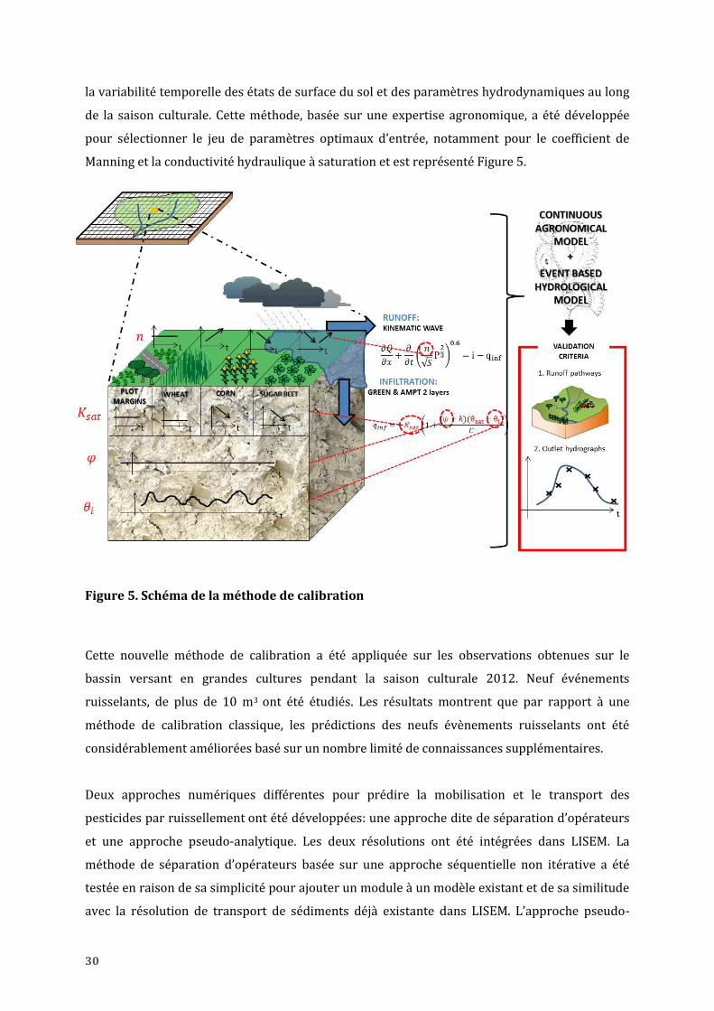
30

la variabilité temporelle des états de surface du sol et des paramètres hydrodynamiques au long

de la saison culturale. Cette méthode, basée sur une expertise agronomique, a été développée

pour sélectionner le jeu de paramètres optimaux d’entrée, notamment pour le coefficient de

Manning et la conductivité hydraulique à saturation et est représenté Figure 5.

Figure 5. Schéma de la méthode de calibration

Cette nouvelle méthode de calibration a été appliquée sur les observations obtenues sur le

bassin versant en grandes cultures pendant la saison culturale 2012. Neuf événements

ruisselants, de plus de 10 m3 ont été étudiés. Les résultats montrent que par rapport à une

méthode de calibration classique, les prédictions des neufs évènements ruisselants ont été

considérablement améliorées basé sur un nombre limité de connaissances supplémentaires.

Deux approches numériques différentes pour prédire la mobilisation et le transport des

pesticides par ruissellement ont été développées: une approche dite de séparation d’opérateurs

et une approche pseudo-analytique. Les deux résolutions ont été intégrées dans LISEM. La

méthode de séparation d’opérateurs basée sur une approche séquentielle non itérative a été

testée en raison de sa simplicité pour ajouter un module à un modèle existant et de sa similitude

avec la résolution de transport de sédiments déjà existante dans LISEM. L’approche pseudo-

31

analytique utilisée sur un schéma implicite présente plusieurs avantages. L'intérêt de cette

approche est que la conservation de la masse n'est pas altérée et que la sensibilité au pas de

temps est négligeable (Jacques et al., 2006).

Ces deux résolutions ont été testées sur 3 niveaux d’échelles: une seule cellule (1 m²), une

parcelle expérimentale (4,5 m²) disposant de données observées et à l’échelle du bassin versant

en grandes cultures précédemment présenté (470,000 m²) (Figure 6).

Figure 6. Schéma des trois différents cas test

L’instabilité numérique de la méthode de séparation d’opérateurs a été démontrée dès le

premier cas test. Cette résolution ne semble donc pas appropriée pour prédire le transport des

pesticides à l’échelle de bassins versants agricoles. La résolution pseudo-analytique a été

évaluée et validée sur les trois échelles. La dynamique d’exportation de pesticides et les bilans

de masses ont été validés à l’échelle de la parcelle expérimentale. Ce formalisme s’est montré

robuste à la fois en fonction de différents pas de temps et conditions de déclenchement de

ruissellement et en fournissant des ordres de grandeur raisonnables à l’échelle du bassin

versant. Ces résultats préliminaires sont donc encourageants mais nécessitent des études

supplémentaires, notamment avec (i) une validation dynamique des concentrations de

pesticides à l’exutoire d’un bassin versant disposant d’une discrétisation temporelle fine des

concentration en pesticides, (ii) une validation spatiale des concentrations de pesticides en

utilisant des points de contrôle interne de mesures, (iii) une réflexion sur l'évaluation des

concentrations initiales spatiales des pesticides dans le sol et l'eau du sol, et (iv) l'évaluation de

l'influence des paramètres d’entrées. La prédiction des pesticides sur la phase particulaire fera

l'objet d'une étude future.

32

Conclusion

Cette thèse vise à améliorer les connaissances sur le transport des pesticides par ruissellement

dans deux contextes agricoles différents: vignoble et grandes cultures, et se concentre plus

particulièrement sur la répartition des pesticides dans la phase dissoute et particulaire dans les

eaux de ruissellement. Les observations combinées des pesticides transportés via le

ruissellement à la fois à l’échelle du bassin versant et de la parcelle ont permis d’identifier les

zones à l’origine d’une exportation de pesticides. Le travail effectué dans cette thèse a souligné

l'importance de la dérive des pesticides sur des surfaces imperméables. Cette dérive devrait être

prise en compte dans le futur dans les modèles de transport des pesticides via le ruissellement

pour les bassins versants fortement anthropisés. La répartition des pesticides dans la phase

dissoute et particulaire diffère significativement sur les deux bassins versants selon les

molécules, même si leurs propriétés physico-chimiques sont similaires. Ceci souligne la

complexité de prédire la répartition « dissous-particulaire » des pesticides dans des conditions

dynamiques de terrain. En effet, l’équilibre d’adsorption des pesticides est rarement atteint sur

le terrain et l'affinité des pesticides avec des particules dépend fortement de la nature des

adsorbants. L'étude de terrain a aussi démontré que les analyses énantiomériques peuvent être

pertinentes pour évaluer les processus de dégradation des pesticides chiraux in situ dans les

eaux de surface à l'échelle des bassins versants. Il est maintenant crucial de quantifier les

conditions et l’étendue de cette dégradation énantioselective du S-métolachlore en laboratoire

pour pouvoir comparer les données de terrain avec des études de référence qui sont

actuellement manquantes. D'autre part, il est essentiel d'interpréter ces données de terrain plus

profondément avec des modèles physiques qui prennent en compte l’énantioselectivité.

Cette étude a démontré que la combinaison de différentes approches à l'échelle du bassin

versant permet une meilleure compréhension du transport des pesticides et de leur atténuation.

33

Références

Alaoui, A., Lipiec, J., Gerke, H.H., 2011. A review of the changes in the soil pore system due to soil deformation: A hydrodynamic perspective. Soil & Tillage Research. 115, 1-15.

Andresen, L.C., Nothlev, J., Kristensen, K., Navntoft, S., Johnsen, I., 2012. The wild flora biodiversity in pesticide free bufferzones along old hedgerows. Journal of Environmental Biology. 33, 565-572.

Arnold, S.M., Clark, K.E., Staples, C.A., Klecka, G.M., Dimond, S.S., Caspers, N., Hentges, S.G., 2013. Relevance of drinking water as a source of human exposure to bisphenol A. Journal of Exposure Science and Environmental Epidemiology. 23, 137-144.

Aufauvre, J., Biron, D.G., Vidau, C., Fontbonne, R., Roudel, M., Diogon, M., Vigues, B., Belzunces, L.P., Delbac, F., Blot, N., 2012. Parasite-insecticide interactions: a case study of Nosema ceranae and fipronil synergy on honeybee. Scientific Reports. 2.

Blann, K.L., Anderson, J.L., Sands, G.R., Vondracek, B., 2009. Effects of Agricultural Drainage on Aquatic Ecosystems: A Review. Critical Reviews in Environmental Science and Technology. 39, 909-1001.

Boithias, L., Sauvage, S., Merlina, G., Jean, S., Probst, J.-L., Sánchez Pérez, J.M., 2014. New insight into pesticide partition coefficient Kd for modelling pesticide fluvial transport: Application to an agricultural catchment in south-western France. Chemosphere. 99, 134-142.

Botta, F., Fauchon, N., Blanchoud, H., Chevreuil, M., Guery, B., 2012. Phyt'Eaux Cites: Application and validation of a programme to reduce surface water contamination with urban pesticides. Chemosphere. 86, 166-176.

Bunemann, E.K., Schwenke, G.D., Van Zwieten, L., 2006. Impact of agricultural inputs on soil organisms - a review. Australian Journal of Soil Research. 44, 379-406.

Buser, H.R., Poiger, T., Muller, M.D., 2000. Changed enantiomer composition of metolachlor in surface water following the introduction of the enantiomerically enriched product to the market. Environmental Science & Technology. 34, 2690-2696.

EPA, 2011. Pesticide Industry Sales and Usage: 2006 and 2007 Market Estimates. US Environmental Protection Agency, Washington (DC).

Fenner, K., Canonica, S., Wackett, L.P., Elsner, M., 2013. Evaluating Pesticide Degradation in the Environment: Blind Spots and Emerging Opportunities. Science. 341, 752-758.

Imfeld, G., Vuilleumier, S., 2012. Measuring the effects of pesticides on bacterial communities in soil: A critical review. European Journal of Soil Biology. 49, 22-30.

Jacques, D., Simunek, J., Mallants, D., van Genuchten, M.T., 2006. Operator-splitting errors in coupled reactive transport codes for transient variably saturated flow and contaminant transport in layered soil profiles. Journal of Contaminant Hydrology. 88, 197-218.

Kabler, A.K., Chen, S.M., 2006. Determination of the 1 ' S and 1 ' R diastereomers of metolachlor and S-metolachlor in water by chiral liquid chromatography - Mass spectrometry/mass spectrometry (LC/MS/MS). Journal of Agricultural and Food Chemistry. 54, 6153-6158.

Klein, C., Schneider, R.J., Meyer, M.T., Aga, D.S., 2006. Enantiomeric separation of metolachlor and its metabolites using LC-MS and CZE. Chemosphere. 62, 1591-1599.

Kohler, H.R., Triebskorn, R., 2013. Wildlife Ecotoxicology of Pesticides: Can We Track Effects to the Population Level and Beyond? Science. 341, 759-765.

Kurt-Karakus, P.B., Bidleman, T.F., Muir, D.C.G., Struger, J., Sverko, E., Cagampan, S.J., Small, J.M., Jantunen, L.M., 2010. Comparison of concentrations and stereoisomer ratios of mecoprop, dichlorprop and metolachlor in Ontario streams, 2006-2007 vs. 2003-2004. Environmental Pollution. 158, 1842-1849.

Miguens, T., Leiros, M.C., Gil-Sotres, F., Trasar-Cepeda, C., 2007. Biochemical properties of vineyard soils in Galicia, Spain. Science of The Total Environment. 378, 218-222.

Mostafalou, S., Abdollahi, M., 2013. Pesticides and human chronic diseases: Evidences, mechanisms, and perspectives. Toxicology and Applied Pharmacology. 268, 157-177.

O'Hare, M.T., McGahey, C., Bissett, N., Cailes, C., Henville, P., Scarlett, P., 2010. Variability in roughness measurements for vegetated rivers near base flow, in England and Scotland. Journal of Hydrology. 385, 361-370.

Pare, N., Andrieux, P., Louchart, X., Biarnes, A., Voltz, M., 2011. Predicting the spatio-temporal dynamic of soil surface characteristics after tillage. Soil & Tillage Research. 114, 135-145.

Salmon-Monviola, J., Moreau, P., Benhamou, C., Durand, P., Merot, P., Oehler, F., Gascuel-Odoux, C., 2013. Effect of climate change and increased atmospheric CO2 on hydrological and nitrogen cycling in an intensive agricultural headwater catchment in western France. Climatic Change. 120, 433-447.

34

Schulz, R., 2004. Field studies on exposure, effects, and risk mitigation of aquatic nonpoint-source insecticide pollution: A review. Journal of Environmental Quality. 33, 419-448.

Schwarzenbach, R.P., Escher, B.I., Fenner, K., Hofstetter, T.B., Johnson, C.A., von Gunten, U., Wehrli, B., 2006. The challenge of micropollutants in aquatic systems. Science. 313, 1072-1077.

Si, Y.B., Takagi, K., Iwasaki, A., Zhou, D.M., 2009. Adsorption, desorption and dissipation of metolachlor in surface and subsurface soils. Pest Management Science. 65, 956-962.

Tang, X.Y., Zhu, B., Katou, H., 2012. A review of rapid transport of pesticides from sloping farmland to surface waters: Processes and mitigation strategies. Journal of Environmental Sciences-China. 24, 351-361.

Ulrich, U., Dietrich, A., Fohrer, N., 2013. Herbicide transport via surface runoff during intermittent artificial rainfall: A laboratory plot scale study. Catena. 101, 38-49.

Vorosmarty, C.J., McIntyre, P.B., Gessner, M.O., Dudgeon, D., Prusevich, A., Green, P., Glidden, S., Bunn, S.E., Sullivan, C.A., Liermann, C.R., Davies, P.M., 2010. Global threats to human water security and river biodiversity (vol 467, pg 555, 2010). Nature. 468, 334-334.

Wallender, W.W., Joyce, B.A., Ginn, T.R., 2008. Modeling the Transport of Spray-Applied Pesticides from Fields with Vegetative Cover. Transactions of the Asabe. 51, 1963-1976.

Ye, J., Zhao, M.R., Liu, J., Liu, W.P., 2010. Enantioselectivity in environmental risk assessment of modern chiral pesticides. Environmental Pollution. 158, 2371-2383.

35

36

Chapter I. Introduction & context

37

Chapter I. Introduction & context

1. Pesticides in the environment

1.1. Impact and diversity

Multiple scientific reports emphasise the health and ecological problems created by over

50 years of anthropogenic pollutant contamination (Kohler and Triebskorn, 2013;

Schwarzenbach et al., 2006). Nearly 80% of the world's population is threatened by water

contamination arising from many different stressors (Vörösmarty et al., 2010). Because

pesticides are intentionally and massively applied worldwide, pesticides are considered a major

source of environmental pollution (Mostafalou and Abdollahi, 2013). Pesticide use is known to

have prejudicial impacts in all environmental compartments: atmosphere, soil, water, flora and

fauna. For example, pesticide contamination has been reported to affect soil biogeochemical

activity (Miguens et al., 2007) and living organisms, such as animals (Aufauvre et al., 2012;

Bunemann et al., 2006), bacteria (Imfeld and Vuilleumier, 2012) and plants (Andresen et al.,

2012). Ecotoxicological tests are fundamental tools for assessing the toxicity of pesticides to

organisms and have demonstrated the acute and/or chronic toxicity of a wide range of

pesticides (Alves et al., 2013). The toxicity of a specific pesticide can be assessed by its LC50

value, corresponding to the concentration at which half of the population dies following a given

exposure time. For example, the widely used fungicide kresoxim methyl is considered highly

toxic to aquatic crustaceans and aquatic invertebrates, with an acute, 96-hour LC50 of 47 μg L−1

(PPDB, 2009). Residues of pesticides have been reported to exceed the European Union’s

maximum residue level in food, causing concern regarding their possible effects on public

health; such concerns exist for the fungicide cyazofamid in grapes, for example (Gonzalez-

Rodriguez et al., 2011). Several pesticides, such as chlorinated, organophosphate and carbamate

insecticides, as well as phenoxy acid and triazine herbicides have demonstrated significant

exposure-response associations in human-health studies, such as studies regarding specific

human cancers (Alavanja and Bonner, 2012; Bassil et al., 2007) and Parkinson’s disease

(Fitzmaurice et al., 2013).

Despite their ecotoxicological impacts, numerous pesticides are increasingly used worldwide

(EPA, 2011). In general, pesticides comprise three main subgroups, i.e., fungicides, herbicides

and insecticides, and more than 20 other types, such as rodenticides, molluscicides, and

Chapter I. Introduction & context

38

algaecides (EPA, 2011). In 2007, 250 different synthetic pesticides were commercialised

(Directive 91/414/EEC; EPA, 2011). Since then, every year, 2.4 million tons of pesticides have

been sold worldwide, with world pesticide expenditure growing to more than $39.4 billion in

2007 (EPA, 2011). While herbicides are the most applied pesticide group in the world,

comprising 39% of total worldwide pesticide use (EPA, 2011), fungicides are the most used in

Europe, constituting an annual amount of approximately 107,574 tons of active ingredient and

comprising 49% of European pesticide use (Eurostat, 2007). The worldwide use of pesticides

has increased, as have the complexities of molecular structures allowed on the market (Ye et al.,

2010). The steadily growing need for more rapid and efficient treatment and the increased cost

of pesticides has stimulated development of new technologies, such as nano-pesticides. Nano-

pesticides include entities in the nanometer size range that enhance pesticide properties, for

instance, increasing apparent solubility (Kah et al., 2013). Twenty-five percent of pesticides are

chiral (Kurt-Karakus et al., 2010), i.e. pesticides presenting two (or more) isomers, called

enantiomers, which are non-superimposable mirror images of each other; for example, Figure I-

2 shows the enantiomers for metolachlor. Enantiomers behave differently in different

environments, and bioaccumulation, persistence and/or toxicity may demonstrate

enantioselectivity (Ye et al., 2010).

Figure I-2. Structures of the four stereoisomers of metolachlor (Kabler and Chen, 2006)

Chapter I. Introduction & context

39

Apart from the new generation compounds, there are a number of concerns regarding the

detrimental effects of pesticides on the environment. Ancient and complex molecules still cause

serious water quality issues (Kümmerer, 2010). Despite being banned more than 40 years ago,

some pesticides, such as DDT, are still very persistent in soil and groundwater (Kümmerer,

2010). Surfactants are a diverse group of chemicals that are often added to commercial pesticide

formulations designed to benefit solubilisation properties (Ying, 2006). The fate of such

surfactants, which often constitute the major part of the mass applied, is almost entirely

unknown (Oliver-Rodriguez et al., 2013). Pesticide degradation may lead to the formation of

unknown metabolites that may be more harmful and/or persistent than the parent compounds.

Pesticides, surfactants and their metabolites are among the most relevant environmental

contaminants. Understanding pesticide distribution among environmental compartments has

therefore become of utmost importance.

1.2. Environmental distribution of pesticides

Figure I-3 illustrates the diversity of pathways by which pesticides are dispersed in the various

compartments of the environment, including atmosphere, soil, water and vegetation. Pesticides

are either released intentionally, through application processes (i.e., diffuse pollution), or

unintentionally, occurring during an accident (i.e., point-source pollution). Sprayed pesticide

may drift and reach non-target areas during pesticide application. Spray drift may account for 1

to 75% of the total mass of pesticides applied, depending on the meteorological conditions,

application methods and pesticide characteristics (Barbash, 2014). Once pesticides are applied,

off-site losses through volatilisation may reach 90% (Bedos et al., 2002). Pesticides can be

transported and persist over long distances in the atmosphere; such an example is

organochlorines, which were detected in the Artic (Sadiki and Poissant, 2008). Pesticide

deposition can be caused by precipitation (wet deposition) or by gaseous and particle deposition

(dry deposition) (Coupe et al., 2000; Messing et al., 2013). Following deposition, pesticides may

be dispersed within hydrosystems, particularly groundwater systems and surface water bodies.

Losses due to leaching in groundwater may represent a few percent of the total pesticide mass

for moderately mobile pesticides such as atrazine (Farlin et al., 2013). Pesticide losses into

surface water, which includes streams, rivers and lakes, have been shown to range between 1 to

10% (Schulz, 2004). Due to their close connections with contaminated areas and the fast

mobilisation of pesticides during rainfall-runoff events, surface waters are particularly and

rapidly vulnerable to contamination (Botta et al., 2012; Tang et al., 2012), which is of serious

concern given that surface water bodies represent drinking water sources worldwide (Arnold et

Chapter I. Introduction & context

40

al., 2013). Diffuse input paths by which pesticides contaminate surface waters are as follows: tile

drain outflow, baseflow seepage, surface and subsurface runoff and soil erosion from

contaminated areas (Reichenberger et al., 2007).

Figure I-3. Pesticide movement in the hydrological system (Barbash, 2014)

The majority of offsite pesticide movements enter streams as a result of their close connections

to agricultural areas, where most pesticides are applied. Therefore, areas with intensive

agriculture can exhibit high degrees of water pollution (Vörösmarty et al., 2010); for example,

83% of American monitored streams from farmland areas had at least one pesticide for which

the concentration exceeded USEPA guidelines for aquatic life (Blann et al., 2009). Agricultural

streams may receive highly contaminated water and be incapable of fully attenuating the

impacts of concentrated pesticide contamination, underscoring the necessity of limiting threats

at their source rather than via costly remediation of symptoms (Vörösmarty et al., 2010). Hence,

understanding pesticide transport from agricultural systems to surface water ecosystems

represents a major challenge.

Chapter I. Introduction & context

41

2. Pesticide transport from agro-ecosystems to surface waters

2.1. Agro-ecosystems, definition and specificity

An ecosystem is “a functional system of complementary relations between living organisms and

their environment, delimited by arbitrarily chosen boundaries, which in space and time appear

to maintain a steady yet dynamic equilibrium” (Gliessman, 2007). An agro-ecosystem is an

ecosystem that integrates agricultural production (e.g., the farm or, on a larger scale, the region

impacted by agricultural activity). Due to anthropogenic activities, an agro-ecosystem is often

characterised by a reduction of biological diversity and by an alteration in natural energy flow

(harvest period) and an alteration of biogeochemical cycles (nutrient saturation) compared to a

natural ecosystem (Gliessman, 2007). Nitrogen (N) and phosphorus (P) are the two most

important nutrients limiting biological production and are the most extensively applied

nutrients in agricultural areas, mainly via soluble inorganic fertilisers (Drinkwater and Snapp,

2007).

An agricultural landscape is divided into arable lands (e.g., cereals, cotton, vegetables),

permanent crops (e.g., orchards, vineyards) and permanent pastures (FAO, 2011). Arable land

and permanent crops represent 28% and 3%, respectively, of the total agricultural area

worldwide. Although vineyards cover a small percentage of agricultural land surfaces, they

contribute a major share to European pesticide use (Eurostat, 2007). Vineyards are risky

agricultural contamination ‘hotspots’ due to the large quantities and diversity of pesticides

applied in addition to the vulnerability of the soil to erosion. Vineyards undergo ten to a

thousand tons of soil loss per hectare per year due to shallow soil depth and steep slopes

(Gómez et al., 2011; Quiquerez et al., 2014). Vineyards are strongly impacted by anthropogenic

forcing, including the planting of vine rows along the fall line or the presence of impermeable

tracks, thereby creating favourable conditions for water runoff and concomitant sediment and

pesticide losses (Novara et al., 2011).

In arable crop areas, simplified rotations, through the replacement of a variety of spring and

winter-sown crops with winter-sown cereals, have been possible through the use of nutrient and

carbon inputs. These simplified rotations lead to the prevalence of bare land during some part of

the year. Farmers are often advised to apply non-selective herbicides during pre-sowing and/or

pre-emergence (Lodovichi et al., 2013). Pre-sowing and/or pre-emergence herbicides are

applied to the soil surface and can thus be easily mobilised by runoff and erosion. Vineyard and

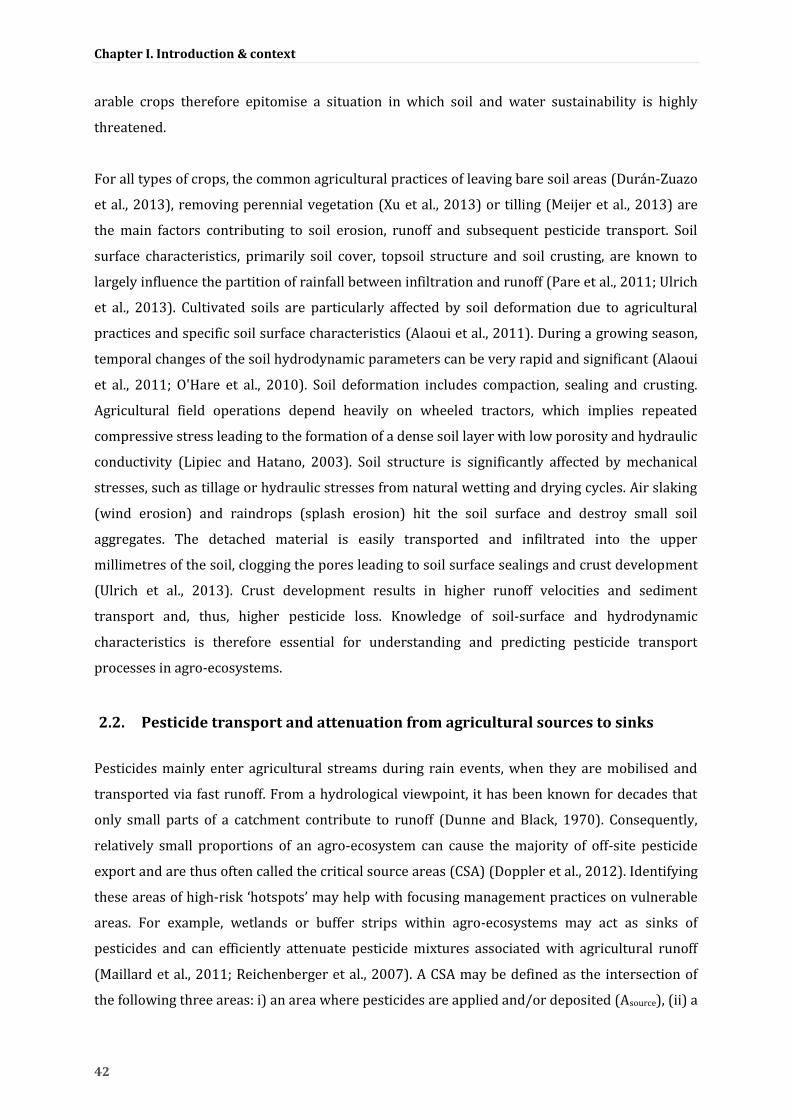
Chapter I. Introduction & context

42

arable crops therefore epitomise a situation in which soil and water sustainability is highly

threatened.

For all types of crops, the common agricultural practices of leaving bare soil areas (Durán-Zuazo

et al., 2013), removing perennial vegetation (Xu et al., 2013) or tilling (Meijer et al., 2013) are

the main factors contributing to soil erosion, runoff and subsequent pesticide transport. Soil

surface characteristics, primarily soil cover, topsoil structure and soil crusting, are known to

largely influence the partition of rainfall between infiltration and runoff (Pare et al., 2011; Ulrich

et al., 2013). Cultivated soils are particularly affected by soil deformation due to agricultural

practices and specific soil surface characteristics (Alaoui et al., 2011). During a growing season,

temporal changes of the soil hydrodynamic parameters can be very rapid and significant (Alaoui

et al., 2011; O'Hare et al., 2010). Soil deformation includes compaction, sealing and crusting.

Agricultural field operations depend heavily on wheeled tractors, which implies repeated

compressive stress leading to the formation of a dense soil layer with low porosity and hydraulic

conductivity (Lipiec and Hatano, 2003). Soil structure is significantly affected by mechanical

stresses, such as tillage or hydraulic stresses from natural wetting and drying cycles. Air slaking

(wind erosion) and raindrops (splash erosion) hit the soil surface and destroy small soil

aggregates. The detached material is easily transported and infiltrated into the upper

millimetres of the soil, clogging the pores leading to soil surface sealings and crust development

(Ulrich et al., 2013). Crust development results in higher runoff velocities and sediment

transport and, thus, higher pesticide loss. Knowledge of soil-surface and hydrodynamic

characteristics is therefore essential for understanding and predicting pesticide transport

processes in agro-ecosystems.

2.2. Pesticide transport and attenuation from agricultural sources to sinks

Pesticides mainly enter agricultural streams during rain events, when they are mobilised and

transported via fast runoff. From a hydrological viewpoint, it has been known for decades that

only small parts of a catchment contribute to runoff (Dunne and Black, 1970). Consequently,

relatively small proportions of an agro-ecosystem can cause the majority of off-site pesticide

export and are thus often called the critical source areas (CSA) (Doppler et al., 2012). Identifying

these areas of high-risk ‘hotspots’ may help with focusing management practices on vulnerable

areas. For example, wetlands or buffer strips within agro-ecosystems may act as sinks of

pesticides and can efficiently attenuate pesticide mixtures associated with agricultural runoff

(Maillard et al., 2011; Reichenberger et al., 2007). A CSA may be defined as the intersection of

the following three areas: i) an area where pesticides are applied and/or deposited (Asource), (ii) a

Chapter I. Introduction & context

43

hydrologically active area (Aactive), i.e., where surface or subsurface runoff has occurred and (iii)

an area that is hydrologically connected to a stream (Aconnected) (Doppler et al., 2012). In other

words, a CSA can be represented by the following spatial intersection:

⋂ ⋂ (1)

The amount of substance that is available for transport via runoff or erosion may be attenuated

by sorption and degradation between two runoff events. Finally, various factors, including

farming practices, intrinsic physical-chemical properties of pesticide compounds, soil and

vegetation characteristics and hydrological and biogeochemical conditions, govern pesticide

transport and attenuation within agro-ecosystems.

2.2.1 Processes affecting pesticides amount at the source area (Asource)

When pesticides are applied, some of the spray may move beyond the intended area and reach a

non-target ecosystem. Chlorpyrifos and metalaxyl drift, for example, have occurred at distances

as great as 24 m in the vineyard (Vischetti et al., 2008). Such pesticide drift largely depends on

the equipment, application techniques and farming practices used. Nozzle height, nozzle

pressure, droplet size and driving speed are main factors influencing pesticide drift (Arvidsson

et al., 2011; Nuyttens et al., 2009). Climatic conditions, such as wind speed, temperature or

atmospheric humidity, also play a major role in the spatial variability of pesticide deposition. For

example, lower atmospheric humidity results in greater pesticide drift (Nuyttens et al., 2007).

Vegetation may act as a barrier and intercept pesticide drift (Ohliger and Schulz, 2010). Finally,

chemical factors, i.e., formulation, presence of additives, density, viscosity and volatility, also

affect pesticide drift (Nuyttens et al., 2009). However, studies have often focused on the distance

that pesticides drift from the spray origin, and very little is known with regard to the spatial

variability of pesticide application within and surrounding the application area (Lazzaro et al.,

2008). Spatial variability of pesticide deposition within the application area can be observed due

to the micro-scale variability in local conditions (Gregorio et al., 2014). It is therefore crucial to

investigate the spatial patterns of deposited pesticides to understand and predict which

pesticide is available for transport. Given that considerable amounts of impermeable surfaces

are present, pesticide deposition via drift in vineyards may be particularly prone to fast runoff.

Chapter I. Introduction & context

44

Once pesticides are deposited, pesticide attenuation in agro-ecosystems involves destructive

processes, e.g., photolysis, hydrolysis and biodegradation, and non-destructive processes, e.g.,

plant uptake and sorption (Figure I-3).

Among the non-destructive processes, plant uptake occurs via the following two major

pathways: (i) desorption from the soil followed by root uptake from the soil solution and (ii)

deposition on plant surfaces followed by uptake into the inner parts of the plant (Juraske et al.,

2009). Root uptake generally increases in relation to the affinity of the pesticide to lipids

(Barbash, 2014) and varies considerably between individual plant species and root depths

(Fantke et al., 2013). The octanol–water partition coefficient (Kow) is often used to estimate the

absorptive properties of the rhizodermis. Because of their hydrophilic properties, pesticides

with low log Kow values (i.e., < 1) will hardly penetrate the lipid-containing root epidermis. On

the contrary, pesticides with log Kow values > 3 will be increasingly retained by the lipids in the

root epidermis and the organic matter surrounding the root (Verkleij et al., 2009).

Sorption/desorption processes govern pesticide leaching into the deeper soil layer and the

timing and amount of pesticides mobilised by runoff. Sorption is influenced by soil texture, soil

particle size distribution, soil moisture, soil organic carbon content, pH, temperature, and

compound characteristics (Wauchope et al., 2002). Increased contact time between pesticides

and sorbents may result in the formation of stronger bonds (Gevao et al., 2000). Pesticides can

remain strongly sorbed on the soil particles, depending on their affinities with natural organic

carbon and/or mineral surfaces. The affinity of a compound with soil is often estimated based on

the soil/solution distribution coefficient (Kd). The Kd values vary greatly among soils and

sediments and may span an order of magnitude for a single active ingredient (Barbash, 2014).

The Kd values are often strongly correlated with the soil’s organic matter content and lead to the

development of Koc, the organic-carbon water partition coefficient that is defined as the ratio of

Kd and the mass fraction of organic carbon (Barbash, 2014). For most pesticides, log Koc ranges

between 1 and 4 (Calvet, 2005).

Chapter I. Introduction & context

45

Figure I-4. Bio-physical-chemical processes related to pesticide transport and attenuation in agro-ecosystems

Different degradation processes co-exist in the environment and can be classified into two main

categories, biotic and abiotic processes (processes in pink in Figure I-3). Abiotic processes

involve non-living chemical and physical factors in the environment, such as photolysis,

hydrolysis and chemical transformations (e.g., redox reactions). Pesticides may also be

transformed by living organisms via biotic processes, as in the case of microbial transformation.

The soil ecosystem is inhabited by billions of microorganisms and numerous other organisms,

including fungi, algae, insects and plants (Jacobsen and Hjelmsø, 2014). Plants, animals and fungi

typically transform pesticides for environmental detoxification purposes, whereas bacteria more

commonly metabolise pesticides for assimilation and energy (Fenner et al., 2013).

Biodegradation is generally identified as the most important manner, mass-balance-wise, of

pesticide degradation (Fenner et al., 2013). It is often impossible to distinguish between biotic

and abiotic processes because all of these processes may occur simultaneously or sequentially,

making a mechanistic understanding difficult, especially under field conditions. Except for

complete mineralisation, transformation processes lead often to the presence of degradation

products in the environment, as illustrated by the degradation pathways of acetochlor in soil

(Figure I-4) (Roberts et al., 1999). Degradation products may behave differently in the

environment compared with the parent compound (la Farre et al., 2008). For example,

Chapter I. Introduction & context

46

enantiomers of chiral pesticides have identical physical-chemical properties and are expected to

undergo similar abiotic processes, such as sorption or volatilisation. Conversely, due to their

spatial configurations, enantiomers can behave differently during biological processes, such as

plant uptake or microbial degradation; the term ‘enantioselective process’ is used to describe

this phenomenon (Celis et al., 2013).

Figure I-5. Degradation pathways of acetochlor in soil (Roberts et al., 1999). Acetochlor was metabolised in soil mainly by two primary pathways. The first pathway involved the hydrolytic/oxidative displacement of chlorine to form the alcohol 2 and the oxidation of the alcohol 2 to oxanilic acid 3. N-dealkylation of 3 yielded oxanilic acid 4. The second pathway involved the displacement of chlorine by glutathione and the further secondary catabolism of the glutathione conjugate 5 to the various sulfinylacteic and sulfonic acid products (6-9)

The half-life time (DT50) corresponds to the time required to degrade half of the quantity of a

molecule. Pesticide half-life times are widely used to quantify the persistence of a compound in

the environment for registration procedures (Farlin et al., 2013). However, classical estimates of

pesticide degradation rates determined in the laboratory may not be relevant under the dynamic

conditions that exist in the field (Papiernik et al., 2009) and may therefore inaccurately predict

pesticide transformation in agro-ecosystems (Gassmann et al., 2014). Thus, approaches capable

of measuring the in situ extent of degradation at catchment scales must be developed (Turner et

al., 2006).

The spatial variability of pesticide deposition during application and processes of degradation

and sorption considerably influence pesticide mobilisation and transport via runoff (Barbash,

2014; Doppler et al., 2012; Gascuel-Odoux et al., 2009).

Chapter I. Introduction & context

47

2.2.2 Processes affecting pesticide transport in agro-ecosystems (Aactive and Aconnected)

Depending on the time that elapses between pesticide application and the next rainfall event,

pesticides may be mobilised in the course of a rainfall-runoff event from vegetation or soil

surfaces (processes in blue in Figure I-3). Studies of pesticide washoff generally indicate that a

large fraction of pesticides deposited on foliage can be mobilised by rain (up to 100% for highly

soluble pesticides) (Wauchope et al., 2004).

On soil surfaces, runoff and erosion mobilise pesticides in a thin, near-surface soil layer

(McGrath et al., 2008). This soil layer is often called the ‘mixing layer’ and has been found to be

in the millimetre to centimetre range (Ahuja et al., 1981). Erosion may be caused by rainfall or

surface runoff and may lead to subsequent transport of sorbed pesticides. Different types of

erosion exist, including sheet erosion, rill erosion and gully erosion. Sheet erosion is the uniform

removal of soil in thin layers by the forces of raindrops and overland flow. Rill erosion is the

removal of soil by concentrated water running through little streams. Gully erosion is an

advanced stage of rill erosion (Toy et al., 2002). Pesticide transfer from the soil surface is

difficult to predict because various processes occur simultaneously (Shi et al., 2011). These

processes include pesticide diffusion induced by the concentration gradient between water

runoff and soil water (1 in Figure I-5), ejection of soil water by rainfall (2 in Figure I-5), erosion

of contaminated sediment by rainfall and concentrated flow (3 in Figure I-5) and pesticide

adsorption-desorption (4 in Figure I-5) (Shi et al., 2011).

Chapter I. Introduction & context

48

Figure I-6. Processes for transferring pesticides from the soil surface to runoff water (Shi et al., 2011)

As previously stated (§2.1), soil surface characteristics and hydrodynamic parameters are

essential for triggering runoff, erosion and pesticide transport. Various additional factors affect

the mobilisation of pesticides in runoff and erosion, including rainfall intensity, topography,

initial water content and pesticide characteristics (Shi et al., 2011). Rainfall variability within a

storm event can also have a significant impact on pesticide losses via runoff (McGrath et al.,

2008). Pesticide transfer occurs in both soluble and particulate phases and depends primarily on

the physical-chemical characteristics of the compound and the nature of the sorbent, e.g.,

organic matter or mineral surfaces (Rodriguez-Liebana et al., 2011). Erosion processes may

therefore contribute to pesticide transport (Bereswill et al., 2013; Taghavi et al., 2011). To date,

most studies have focused on dissolved pesticide transport. Hydrophobic pesticides are mainly

transported in runoff in association with colloids and dissolved organic carbon (DOC) (Chen et

al., 2010; Maillard et al., 2011). Hence, erosion processes and pesticides in particulate phases

should be considered when evaluating pesticide transport in agricultural runoff.

Chapter I. Introduction & context

49

2.2.3 Relevance of combining emerging analytical tools for assessing pesticide degradation

Approaches capable of measuring in situ the extent of pesticide degradation are required for

deciphering attenuation processes, such as sorption, dilution or degradation at catchment scales

(Turner et al., 2006). Indeed, quantitative chemical analysis of the parent pesticide is not

sufficient for distinguishing degradation from sorption and/or dilution. Evidence of in situ

degradation may be determined via degradation products quantification, enantiomeric analysis

or CSIA (Compound Specific Isotope Analysis) methods. These alternative approaches may be

combined to gain mechanistic insights into pesticide transformation processes (Milosevic et al.,

2013) and can be used to evaluate pesticide transformation under the dynamic conditions that

exist in the field.

Degradation product analysis is one of the most used methods for assessing the occurrence of

pesticide degradation in the environment. Quantitative chemical analyses of the degradation

products are often challenging because they are often unstable compounds (Andreu and Pico,

2004). Furthermore, the degradation products must be known, and standards must be available

for developing analytical methods. The absence of one type of degradation-product analysis does

not exclude other degradation pathways involving other degradation products.

Chiral pesticide biodegradation may lead to the enrichment of the remaining fraction of non-

degraded pesticides in one or another enantiomer. A shift, compared with the initial

enantiomeric signature of the commercial product, can indicate preferential degradation of one

enantiomer (Celis et al., 2013). Enantiomeric analyses of chiral pesticides have been successfully

used to assess pesticide degradation, for instance, for metalaxyl in batch experiments (Celis et

al., 2013), phenoxyacid herbicides in a groundwater system (Milosevic et al., 2013), metolachlor

in surface water (Buser et al., 2000) or chlordane in soil and vegetation (White et al., 2002).

Enantiomeric analyses may fail if both enantiomers are equally degraded by the same enzyme or

if enantiomer-preferential enzymes are simultaneously present in the environment.

CSIA analysis, which is based on an approach that is similar to enantiomeric analysis, may

provide additional information regarding possible in-situ degradation. CSIA measures the

isotopic composition, i.e., the ratio between the abundance of the heavy isotope against the light

stable isotope of an element like oxygen or carbon in a molecule (Thullner et al., 2012).

Compared with the isotopic ratio of the commercial compound, biodegradation may lead to

Chapter I. Introduction & context

50

enrichment in heavy isotopes because molecules with light isotopes tend to degrade more

quickly (Elsner, 2010).

So far, degradation product analyses and enantiomer and isotope approaches have not been

combined to assess degradation in runoff water in agro-ecosystems. Combining analytical

methods can provide advantages that are beyond the reach of any of the methods applied alone.

Based on the weaknesses and strengths of each method, combined approaches may complement

each other in their assessment of pesticide degradation. Models may then validate mechanistic

hypotheses based on field experimentation.

2.2.4 Usefulness and complementarity of modelling following a characterisation phase

A model is “a mathematical description of a simplified conceptual representation of a certain

fragment of the real world” (Alvarez-Benedi and Munoz-Carpena, 2004). Because environmental

processes are complex and mathematically describing every process is logistically impossible,

model conceptualisations are always simplifications. “Essentially, all models are wrong, but

some are useful” (Box and Draper, 1987). Once it has been established that a model can

reproduce reality with sufficient accuracy, the model may be used to prognosticate the impacts

of environmental scenarios under different meteorological or hydrological conditions or

agricultural contexts at significantly lower cost and in much less time than experimental field

trials require (Alvarez-Benedi and Munoz-Carpena, 2004; Quilbe et al., 2006). Pesticide

transport models in agro-ecosystems are therefore crucial to achieving sustainability of current

agriculture practices. Predictive models are used to (i) assess the extent of pesticide dispersion,

(ii) evaluate possible mitigating management practices and regulatory policies (Payraudeau and

Grégoire, 2012) and (iii) prognosticate future potential problems (Alvarez-Benedi and Munoz-

Carpena, 2004). Modelling may also confirm or negate a hypothesis regarding physical

mechanisms based on a comprehensive field characterisation study (Lutz et al., 2013).

A large number of models describing pesticide transport in agro-ecosystems have been

developed over the last 40 years for various scales and contexts and have been already used for

intercomparisons and/or in reviews (Borah and Bera, 2003b; Holvoet et al., 2007; Kohne et al.,

2009; Payraudeau and Grégoire, 2012; Quilbe et al., 2006). Numerical models, including those

that are empirical, stochastic, conceptual and physically based, have been used to describe

pesticide transport processes (Payraudeau and Grégoire, 2012). Physically based models can be

differentiated based on their ability to decipher the contribution of each physical process and to

Chapter I. Introduction & context

51

estimate pesticide concentrations under different hydrological conditions and with different

pesticide characteristics (Berenzen et al., 2005). The existing physically based models designed

for predicting pesticide transport in surface water in agro-ecosystems for various spatial and

temporal scales are detailed in Table I-1. Obviously, this brief census is not exhaustive and only

models for cases in which sufficient information has been obtained were included in this

analysis. The 32 selected physically based models for pesticide behaviours in surface water are

presented in Figure I-6 according to their spatial and temporal discretisations. Catchment

representations, spatial and temporal discretisations and processes are detailed for various

existing pesticide-fate models in Table I-1.

Figure I-7. Existing physically based pesticide transport models according to their spatial and temporal discretisations.

Chapter I. Introduction & context

52

To date, no single pesticide-fate model has proved to be a satisfactory tool for all purposes

(Alvarez-Benedi and Munoz-Carpena, 2004). Currently, few models account for the effects of

agricultural practices on hydrodynamic parameters and soil surface characteristics (Pare et al.,

2011).

Distributed models may consider the variability in contributing areas in catchments and are

useful for delineating critical-source areas for pesticide runoff (Frey et al., 2009). Fully

distributed models, such as AGNPS (Merritt et al., 2003), describe the landscape on the scale of a

grid cell, whereas semi-distributed models define homogeneous elements, such as Hydrological

Responses Units (HRUs) for the model SWAT (Boithias et al., 2011) (Table I-1). Fully distributed

models may help decipher the contributions of small features, such as roads or buffer strips, in

agro-ecosystems.

Chapter I. Introduction & context

53

Table I-1. Summary of catchment-scale hydrological and pesticide transport models in surface water; “dynamic” may represent different erosion equations for erosion splash, rill erosion and/or transport capacity.

Model name References Time step Spatial scale Discretisation Erosion Particulate

pesticide

ACTMO (Frere et al., 1975) hourly < 100 km²

hydrological units

USLE Yes

ADAPT (Gowda et al., 2012) daily field -100 km² hydrological

units USLE Yes

(Ann-)AGNPS (Merritt et al., 2003)

(Bingner and Theurer, 2001) hourly/daily 1- 200 km² square grid cell RUSLE Yes

ARM (Donigian and Crawford, 1976) hourly/daily < 5 km² ? dynamic Yes

BASINS (Tong and Chen, 2002) daily no specific size

hydrological units

dynamic Yes

CATCHIS/SWATCHCATCH (Brown et al., 2002) daily/weekly > 100 km² subcatchments No No

CATFLOW (Zehe et al., 2001) < 1 hour field - 100 km² hillslope elements

dynamic Yes

CHU model (Chu and Marino, 2004) monthly > 100 km² grid cell MUSLE Yes

CPM (Haith and Loehr, 1979) monthly < 100 km² ? USLE ?

DRIPS (Röpke et al., 2004) daily no specific size grid cell No No

DWSM (Borah et al., 2004) seconds no specific size segments dynamic Yes

EPIC-PST (Sabbagh et al., 1991) hourly/daily field - 100 ha grid cell MUSLE ?

GIBSI (Rousseau et al., 2000) daily >100 km² hydrological

units RUSLE Yes

GLEAMS/CREAMS (Leonard et al., 1991) hourly/daily field grid cell USLE No

HSPF (Borah and Bera, 2003a)

(Donigian et al., 1995) hourly/daily no specific size

hydrological units

dynamic Yes

HYDROGEOSPHERE (Rosenbom et al., 2009) hourly/daily > 100 km² grid cell No No

Chap I. Introduction & context

54

Model name References Time step Spatial scale Discretisation Erosion Particulate

pesticide

MHYDAS (Moussa et al., 2002) seconds < 100 km² hydrological units dynamic Yes

MIKE-SHE (Fauser et al., 2008) hourly/daily < 100 km² square grid cell dynamic ?

OPUS (Bogena et al., 2003) hourly/daily Field hillslope elements MUSLE No

PELMO (Huber et al., 2000) daily Field grid cell No No

PESTDRAIN (Branger et al., 2009) < 1 hour Field conceptual No No

PRZM (Centofanti et al., 2008) (Luo and Zhang, 2010)

daily field/catchment grid cell USLE Yes

RIVWQ (Karpouzas and Capri, 2006) daily field/catchment grid cell ? Yes

SHETRAN (Ewen et al., 2000) seconds hourly

1 - 2000 km² grid cell dynamic Yes

SPIDER (Renaud et al., 2008) hourly 0-10 km² stream segment No No

SWAT (Boithias et al., 2011) daily 30-15000 km² hydrological units MUSLE Yes

SWMM (Park et al., 2008) < 1 hour no specific size subcatchments ? ?

SWRRBWQ (SWRRBWQ manual, 1993) daily > 100 km² subcatchments MUSLE ?

WARMF (Dayyani et al., 2010) daily > 100 km² compartments dynamic ?

WASP6/DYNHYD5 (Ekdal et al., 2011) < 1 hour river/field compartments ? Yes

WEPP-UI (Singh et al., 2009) daily no specific size hillslope segments dynamic Yes

ZIN-AgriTra (Gassmann et al., 2013) seconds Field/catchment square grid cell USLE Yes

Chapter I. Introduction & context

55

In agro-ecosystems, soil surface characteristics and hydrodynamic parameters may change very

rapidly due to agricultural practices (§2.1), and rainfall variability within a storm event can have

a significant impact on pesticide losses via runoff (§2.2.2). In parallel, a significant short-term

pesticide export may occur within one single storm in agricultural catchments (McGrath et al.,

2010). Consequently, predicting the generation and dynamics of pesticide transport at the event

scale is essential for better understanding fast transport processes, such as contaminated runoff.

An event-based model that employs a very small time step (≤ 1 min) and very high resolution

rainfall data seems more appropriate when the goal is to better understand the detailed

dynamics of pesticide export. In this context, event-based models, such as DWSM, are

particularly designed to use fine temporal discretisations (Borah et al., 2004).

In pesticide-fate models, erosion processes are often predicted based on the Universal Soil Loss

Equation (USLE) or its revisions, RUSLE and MUSLE (Kinnell, 2010); examples are the cases of

ZIN-AgriTra (Gassmann et al., 2013) or CREAMS (Leonard et al., 1991)(Table I-1). Theoretically,

USLE was designed to predict long-term (e.g., annual) average soil losses at field scale. Despite

numerous revisions to extend these results to the entire catchment at event scale, the USLE

equations do not consider runoff explicitly for determining erosion (Kinnell, 2010). Pesticide-

fate models rarely integrate erosion processes with dynamic approaches (Table I-1).

Agro-ecosystems provide a foundation for evaluating and understanding the interactions of

physical-chemical processes and agricultural practices affecting the transport and fate of

pesticides. Combining emerging analytical tools and modelling may be a valuable approach to

investigate pesticide transport in agro-ecosystems. Changes in agricultural practices occur

locally at farm and agricultural plot levels. In contrast, different measures for water protection

are defined on the scale of hydrological areas (> 10,000 km²) (Macary et al., 2014). Agricultural

regional areas integrate numerous catchments, making difficult a comprehensive understanding

of pesticide transport. Among the agro-ecosystems, headwater agricultural catchments (0 - 1

km²) represent an intermediary scale between agricultural plot and agricultural regional area,

where ongoing processes affecting pesticide transport remain poorly known.

Chap I. Introduction & context

56

3. Relevance of headwater catchments for pesticide transport in surface water

3.1. Definition and role of headwater catchments in downstream water quality

Headwater catchments are the initial drainage areas that catch water and direct it into surface

water features such as creeks and streams. Headwater streams are often defined as first- and

second-order streams according to the Horton-Strahler method (Brutsaert, 2005). In aggregate,

headwater streams compose the majority of the total stream length in a river network and often

represent small hydrological catchments (0 – 1 km²) (Dodds and Oakes, 2008). Because these

catchments are not large, headwater streams are easily influenced by small-scale differences in

local conditions (Meyer et al., 2007). Headwater streams dominate surface water drainage

networks and may have a major impact on downstream water quality (Dodds and Oakes, 2008;

Freeman et al., 2007; Salmon-Monviola et al., 2013). This is due to several factors, including (i)

the major contribution of headwater streams to the mean water volume and flux in higher-order

streams (Alexander et al., 2007), (ii) the greatest capacity of headwater streams for interaction

between water and contaminated areas due to their proximity with agricultural land and (iii) the

potential for rapid in-stream uptake and retention of pesticides due to riparian vegetation

(Dodds and Oakes, 2008). Furthermore, because of their high habitat diversity, headwater

streams significantly contribute to the biodiversity of the overall stream system and are

essential for the successful dispersal of species among stream networks (Meyer et al., 2007;

Rasmussen et al., 2013). Headwater catchments therefore play a dominant role in pesticide

transport and the resulting downstream water quality.

Headwater catchments located in agricultural areas are identified as high-risk ‘hotspots’ of

pesticide contamination. For example, small Swiss streams have clearly shown higher pesticide-

mixture concentrations (150 compounds) than medium or large rivers and represent more than

70% of Swiss streams (Munz et al., 2012). Reported insecticide concentrations in surface water

worldwide have been shown to be negatively correlated with catchment size (Figure I-7)

(Schulz, 2004).

Chapter I. Introduction & context

57

Figure I-8. Relationship between catchment size and aqueous non-point sources of insecticide contamination detected in samples of surface waters (Schultz, 2004)

However, due to their small size, hydrological headwater catchments are often not qualified as

significant surface water bodies and are generally disregarded and poorly investigated, despite

their importance for supporting higher ecological quality in higher order streams (Munz et al.,

2012; Rasmussen et al., 2013). For example, implementation of the Water Framework Directive

in the European Union encourages member states to obtain “good ecological and chemical

status” of surface waters. However, these objectives exclude headwater catchments and only

consider larger surface water bodies (Rasmussen et al., 2013). There is, therefore, a lack of

knowledge concerning water quality in headwater catchments, which are often less monitored

and highly contaminated and may have major impacts on water quality downstream.

3.2. Importance of combining plot- and catchment-scale observations

Combining different control points within a study area is useful for the delineation of critical

source areas for pesticide runoff (Freitas et al., 2008). Furthermore, considering the complexity

of interactions of the processes, several measurement points within a study area are necessary

to validate a distributed model (Lee et al., 2012). Pesticide transport is often evaluated on a plot-

or catchment-scale (Viglizzo et al., 2011) but has rarely been evaluated with regard to both

scales simultaneously. Combining experimental information obtained using different scales

within the same catchment is necessary to identify the critical source areas of off-site pesticide

transport and to evaluate how pesticide runoff varies for different scales.

Chap I. Introduction & context

58

3.3. Models for predicting pesticide transport in headwater catchments

A previous analysis of existing pesticide-fate models (§2.2.4) emphasized that a fully distributed

event-based model that considers erosion processes with a dynamic approach may facilitate our

understanding of the generation, dynamics and pathways of pesticide transport in agro-

ecosystems. Based on this analysis, only the following four models have been designed for

assessing pesticide transport using very fine temporal resolutions (≤ 1 min) in headwater

catchments: CATFLOW (Zehe et al., 2001), ZIN-AgriTra (Gassmann et al., 2013), MHYDAS

(Moussa et al., 2002) and DWSM (Borah et al., 2004). None of these models are fully distributed,

and use a dynamic approach to evaluate erosion processes (Table I-1).

For all the reasons stated above, there is need for a pesticide transport model that (i) is fully

distributed, (ii) is designed for considerations on the agricultural headwater-catchment scale

and (iii) the rainfall-runoff event scale, and (iv) is based on a dynamic approach to assess

erosion processes to predict pesticide transport in the particulate phase.

The hydrological and erosion model LISEM (Limbourg Soil Erosion Model) (DeRoo et al., 1996)

seems to be a good candidate for fulfilling the above four criteria. Admittedly, LISEM does not

predict pesticide mobilisation and transport in runoff. However, it is an event-based model that

is fully distributed for headwater catchments. Sediment detachment is generated by rainfall

splash based on rainfall kinetic energy (Sanchez-Moreno et al., 2012) and/or overland flow.

Flow erosion is calculated with a stream-power-based transport capacity (Morgan et al., 1998).

LISEM is specifically designed to describe agricultural landscape components containing crusted

and compacted zones and soil surface structures. Furthermore, LISEM was validated for various

agricultural contexts and hydrological conditions (Baartman et al, 2012; Hessel, 2006; Hessel et

al, 2007; Sheikh et al, 2010).

Chapter II. Aim and thesis approach

59

Chapter II. Research focus and objectives

1. Research focus

Several scientific gaps and challenges have been identified in the previous chapter, and these

must still be addressed if we are to understand, characterise and predict pesticide transport into

surface water in headwater catchments. This PhD thesis attempts to provide evidence that

partially addresses these remaining issues.

Vineyard and arable crops epitomise a situation where soil and water sustainability is highly

threatened. Headwater catchments located in those areas are identified as high-risk ‘hotspots’ of

pesticide contamination. From a management perspective, the headwater-catchment scale is

suitable for more readily implementing remediation actions by local groups. In addition, limiting

threats as closely as possible to their source may be more efficient than the costly remediation of

symptoms downstream. From a scientific viewpoint, the ongoing processes affecting pesticide

transport remain poorly understood with regard to the intermediate scale between agricultural

plot and regional-scale catchment. Thus, understanding pesticide transport and attenuation in

headwater catchments implies the combination of different approaches (characterisation and

modelling), analytical methods (degradation products and enantiomeric analyses) and scales

(plot and catchment). Such a comprehensive approach may help us understand the processes of

pesticide transport and attenuation in headwater catchments.

During the course of this study, the following several questions have arisen, highlighting major

gaps in our current ability to understand, model and predict pesticide transport and attenuation

in agricultural headwater catchments:

What are the spatial patterns of fungicide deposition following a vineyard application, and

how does the spatial variability of fungicide deposition influence off-site movement in

runoff?

Chapter II. Aim and thesis approach

60

How are pesticides distributed between the dissolved and particulate phases in runoff

water in relation to each compound’s characteristics and the hydrological and

hydrochemical conditions?

What is the potential contribution of analytical approaches, such as enantiomer analysis of

chiral pesticides, to identifying, characterising and quantifying the in situ degradation of

pesticides on the headwater-catchment scale?

Finally, how is it possible to predict the impact of erosion processes and pesticide

partitioning between the dissolved and particulate phases on pesticide transport into

surface water?

2. Thesis objectives

The overall aim of this thesis is to evaluate and predict pesticide transport in runoff water in the

dissolved and particulate phases within headwater agricultural catchments. Two contrasting

agricultural catchments, one in a vineyard and one in an arable crop, were investigated on two

elemental scales, i.e., agricultural-plot and headwater-catchment, to meet the following

objectives:

(i) Characterise the spatial variability of fungicide deposition during application in the

vineyard catchment and its impact on subsequent runoff.

(ii) Evaluate and compare pesticide partitioning of four model compounds between the

dissolved and particulate phases in runoff in both model agricultural catchments.

(iii) Evaluate the in-situ degradation of a major pre-emergence herbicide, S-metolachlor,

in the arable crop catchment by combining analytical approaches.

(iv) Develop and validate a physically based model for predicting pesticide mobilisation

in runoff water that is applicable to both agricultural catchments.

The PhD approach is to combine characterisation and modelling for assessing pesticide

transport. Two 50-ha catchments representative of agricultural headwater catchments in

temperate areas have been investigated in terms of runoff, erosion, hydrochemistry and

pesticide transport. The catchments differ in terms of crops (grape and corn), topography, soils,

Chapter II. Aim and thesis approach

61

hydrological processes and applied pesticides (Table II-2). Both catchments are located in Alsace

in the east of France (Figure II-1). Four different model pesticides were selected owing to their

wide usage, their toxicity and their large range of physical-chemical properties. Kresoxim-

methyl (KM) and cyazofamid (CY) are both fungicides applied in vineyards, and acetochlor and

S-metolachlor are both herbicides that are widely used on corn and sugar beet. Their main

physical-chemical characteristics are presented in Table II-1. In parallel, a mathematical

formalism has been developed to predict dissolved pesticide mobilisation and transport in

runoff, which is applicable to both agricultural catchments. This formalism has then been

integrated into LISEM (Limbourg Soil Erosion Model) (DeRoo et al., 1996). Extension of the

mathematical formalism for assessing pesticide transport in the particulate phase is further

discussed below and will be the topic of future investigations.

Table II-1. Physical-chemical properties of the four study compounds (PPDB, 2009).

a(Fenoll et al., 2010);b(http://toxnet.nlm.nih.gov/); c (Alletto et al., 2013)

Pesticides groups Fungicides Herbicides

Active substance Kresoxim - methyl Cyazofamid S-metolachlor Acetochlor

Family Strobilurin Cyanoimidazole Chloroacetamides Chloroacetamides

Chemical formula C18H19NO4 C13H13ClN4O2S C15H22ClNO2 C14H20ClNO2

Chemical structure

Molecular mass [g mol-1] 313.4 324.8 283.8 269.8

Water solubility [g L-1] 2 0.11 480 282

Log Kow [-] 3.4 3.2 3.05 4.14

Log Koc [-] 2.5a 2.8 – 3.2b 1.8 – 2.6c 2.2

DT50 soil [days] 16 10 15 14

DT50 Hydrolysis in

water (20°C, pH 7) [days] 35 25 stable Stable

Aquatic invertebrates

48 h EC50 [mg L-1] 0.19 0.19 26 8.6

Chapter II. Aim and thesis approach

62

Figure II-1. Locations and schemes of the study catchments (Alsace, France) Table II-2. Main characteristics of both study catchments (Alsace, France)

ROUFFACH ALTECKENDORF

Catchment area [ha] 42.7 47

Elevation [m] 230 – 379 190 - 230

Slope [% ] 15 7

Crops Vine Corn, sugar-beet,

wheat

Crops ratio [%] 59 88

Studied plot area [m²] 880 77.2

Annual precipitation [mm] 563 ± 174 704 ± 151

Chapter II. Aim and thesis approach

63

3. Thesis layout

The dissertation outline is described below and in the following diagram outline (Figure II-2).

Chapter 3 investigates fungicide drift and related runoff in vineyards and is divided into two

sections. Evaluation of drift and spatial variability in the deposition of two fungicides (KM and

CY) as formulated products were first investigated under foliar application conditions in the

vineyard catchment (Rouffach, Alsace, France) (Section 1; published in Science of the Total

Environment, 2013). Following deposition of the fungicides, their transport in runoff water and

their partitioning within the dissolved and particulate phases were jointly evaluated for the

vineyard catchment and a representative plot during wine-growing season (i.e., May to August

2011) (Section 2; published in Environmental Science and Pollution Research, 2013).

To better understand pesticide transport via erosion, Chapter 4 explores pesticide transport in

a corn catchment, where erosion may occur much more often compared with the vineyard

catchment. The transport of two herbicides, i.e., metolachlor and acetochlor, was evaluated in

both the dissolved and particulate phases. An integrative approach combining analyses of the

parent compound, degradation products and enantiomers was used to investigate the in-situ

transformation of S-metolachlor and acetochlor in water, suspended solids and soil (publication

in prep).

Mobilisation and transport of pesticides observed in one agricultural context during one season

could only be confirmed and further extended with the help of modelling. Chapter 5 focuses on

pesticide transport modelling in runoff from headwater catchments and is divided into two

sections. The first step for correctly predicting pesticide transport into surface water is to

accurately predict runoff and erosion dynamics and pathways. A new approach was developed

for choosing a suitable and meaningful set of input parameters for calibrating an event-based

model to predict runoff and erosion in the arable crop catchment during a crop-growing season

(Section 1; publication in prep). A mathematical formalism was then developed and integrated

in LISEM to predict dissolved pesticide mobilisation and transport in runoff. This formalism is

applicable to both agricultural catchments (Section 2).

The final chapter summarises the main findings and conclusions derived from this research. It

concludes by suggesting future research directions to investigate pesticide contamination of

surface water in headwater agricultural catchments.

Chapter II. Aim and thesis approach

64

Figure II-2. Graphical outline of the PhD thesis

Chapter II. Aim and thesis approach

65

4. References

Ahuja, L.R., Sharpley, A.N., Yamamoto, M., Menzel, R.G., 1981. The Depth of Rainfall-Runoff-Soil Interaction

as Determined by P-32. Water Resources Research. 17, 969-974.

Alaoui, A., Lipiec, J., Gerke, H.H., 2011. A review of the changes in the soil pore system due to soil

deformation: A hydrodynamic perspective. Soil & Tillage Research. 115, 1-15.

Alavanja, M.C.R., Bonner, M.R., 2012. Occupational Pesticide Exposures and Cancer Risk: A Review. Journal

of Toxicology and Environmental Health-Part B-Critical Reviews. 15, 238-263.

Alexander, R.B., Boyer, E.W., Smith, R.A., Schwarz, G.E., Moore, R.B., 2007. The role of headwater streams in

downstream water quality. Journal of the American Water Resources Association. 43, 41-59.

Alletto, L., Benoit, P., Bolognesi, B., Couffignal, M., Bergheaud, V., Dumeny, V., Longueval, C., Barriuso, E.,

2013. Sorption and mineralisation of S-metolachlor in soils from fields cultivated with different

conservation tillage systems. Soil & Tillage Research. 128, 97-103.

Alvarez-Benedi, J., Munoz-Carpena, R., 2004. Soil-Water-Solute Process Characterization: An Integrated

Approach, Vol., Taylor & Francis.

Alves, P.R.L., Cardoso, E.J.B.N., Martines, A.M., Sousa, J.P., Pasini, A., 2013. Earthworm ecotoxicological

assessments of pesticides used to treat seeds under tropical conditions. Chemosphere. 90, 2674-

2682.

Andresen, L.C., Nothlev, J., Kristensen, K., Navntoft, S., Johnsen, I., 2012. The wild flora biodiversity in

pesticide free bufferzones along old hedgerows. Journal of Environmental Biology. 33, 565-572.

Andreu, V., Pico, Y., 2004. Determination of pesticides and their degradation products in soil: critical

review and comparison of methods. Trac-Trends in Analytical Chemistry. 23, 772-789.

Arnold, S.M., Clark, K.E., Staples, C.A., Klecka, G.M., Dimond, S.S., Caspers, N., Hentges, S.G., 2013. Relevance

of drinking water as a source of human exposure to bisphenol A. Journal of Exposure Science

and Environmental Epidemiology. 23, 137-144.

Arvidsson, T., Bergstrom, L., Kreuger, J., 2011. Spray drift as influenced by meteorological and technical

factors. Pest Management Science. 67, 586-598.

Aufauvre, J., Biron, D.G., Vidau, C., Fontbonne, R., Roudel, M., Diogon, M., Vigues, B., Belzunces, L.P., Delbac,

F., Blot, N., 2012. Parasite-insecticide interactions: a case study of Nosema ceranae and fipronil

synergy on honeybee. Scientific Reports. 2.

Barbash, J.E., 2014. The Geochemistry of Pesticides. In: Treatise on Geochemistry (Second Edition). Vol.,

H.D. Holland, K.K. Turekian, eds. Elsevier, Oxford, pp. 535-572.

Baartman, J.E.M., Jetten, V.G., Ritsema, C.J., de Vente, J., 2012. Exploring effects of rainfall intensity and

duration on soil erosion at the catchment scale using openLISEM: Prado catchment, SE Spain.

Hydrological Processes. 26, 1034-1049.

Bassil, K.L., Vakil, C., Sanborn, M., Cole, D.C., Kaur, J.S., Kerr, K.J., 2007. Cancer health effects of pesticides -

Systematic review. Canadian Family Physician. 53, 1705-1711.

Bedos, C., Cellier, P., Calvet, R., Barriuso, E., Gabrielle, B., 2002. Mass transfer of pesticides into the

atmosphere by volatilization from soils and plants: overview. Agronomie. 22, 21-33.

Chapter II. Aim and thesis approach

66

Berenzen, N., Lentzen-Godding, A., Probst, M., Schulz, H., Schulz, R., Liess, M., 2005. A comparison of

predicted and measured levels of runoff-related pesticide concentrations in small lowland

streams on a landscape level. Chemosphere. 58, 683-91.

Bereswill, R., Golla, B., Streloke, M., Schulz, R., 2013. Entry and toxicity of organic pesticides and copper

in.vineyard streams: Erosion rills jeopardise the efficiency of riparian buffer strips (vol 146, pg

81, 2012). Agriculture Ecosystems & Environment. 172, 49-50.

Bingner, R.L., Theurer, F.D., 2001. Topographic factors for RUSLE in the continuous-simulation watershed

model for predicting agricultural, non-point source pollutants (AnnAGNPS). Soil Erosion

Research for the 21st Century, Proceedings. 619-622.

Blann, K.L., Anderson, J.L., Sands, G.R., Vondracek, B., 2009. Effects of Agricultural Drainage on Aquatic

Ecosystems: A Review. Critical Reviews in Environmental Science and Technology. 39, 909-

1001.

Bogena, H., Diekkruger, B., Klingel, K., Jantos, K., Thein, J., 2003. Analysing and modelling solute and

sediment transport in the catchment of the Wahnbach River. Physics and Chemistry of the Earth.

28, 227-237.

Boithias, L., Sauvage, S., Taghavi, L., Merlina, G., Probst, J.L., Perez, J.M.S., 2011. Occurrence of metolachlor

and trifluralin losses in the Save river agricultural catchment during floods. Journal of

Hazardous Materials. 196, 210-219.

Borah, D.K., Bera, M., 2003a. Watershed scale hydrologic and nonpoint source pollution models for long-

term continuous and storm event simulations. Total Maximum Daily Load (Tmdl):

Environmental Regulations Ii, Proceedings. 161-167.

Borah, D.K., Bera, M., 2003b. Watershed-scale hydrologic and nonpoint-source pollution models: Review

of mathematical bases. Transactions of the Asae. 46, 1553-1566.

Borah, D.K., Bera, M., Xia, R., 2004. Storm event flow and sediment simulations in agricultural watersheds

using DWSM. Transactions of the Asae. 47, 1539-1559.

Botta, F., Fauchon, N., Blanchoud, H., Chevreuil, M., Guery, B., 2012. Phyt'Eaux Cites: Application and

validation of a programme to reduce surface water contamination with urban pesticides.

Chemosphere. 86, 166-176.

Box, G.E.P., Draper, N.R., 1987. Empirical model-building and response surfaces, Vol., Wiley.

Branger, F., Tournebize, J., Carluer, N., Kao, C., Braud, I., Vauclin, M., 2009. A simplified modelling approach

for pesticide transport in a tile-drained field: The PESTDRAIN model. Agricultural Water

Management. 96, 415-428.

Brown, C.D., Bellamy, P.H., Dubus, I.G., 2002. Prediction of pesticide concentrations found in rivers in the

UK. Pest Management Science. 58, 363-373.

Brutsaert, W., 2005. Hydrology: An Introduction, Vol., Cambridge University Press.

Bunemann, E.K., Schwenke, G.D., Van Zwieten, L., 2006. Impact of agricultural inputs on soil organisms - a

review. Australian Journal of Soil Research. 44, 379-406.

Buser, H.R., Poiger, T., Muller, M.D., 2000. Changed enantiomer composition of metolachlor in surface

water following the introduction of the enantiomerically enriched product to the market.

Environmental Science & Technology. 34, 2690-2696.

Chapter II. Aim and thesis approach

67

Calvet, R., 2005. Les pesticides dans le sol: conséquences agronomiques et environnementales, Vol.,

Editions France Agricole.

Celis, R., Gamiz, B., Adelino, M.A., Hermosin, M.C., Cornejo, J., 2013. Environmental behavior of the

enantiomers of the chiral fungicide metalaxyl in Mediterranean agricultural soils. Science of The

Total Environment. 444, 288-297.

Centofanti, T., Hollis, J.M., Blenkinsop, S., Fowler, H.J., Truckell, I., Dubus, I.G., Reichenberyer, S., 2008.

Development of agro-environmental scenarios to support pesticide risk assessment in Europe.

Science of The Total Environment. 407, 574-588.

Chen, G.A., Lin, C., Chen, L.A., Yang, H., 2010. Effect of size-fractionation dissolved organic matter on the

mobility of prometryne in soil. Chemosphere. 79, 1046-1055.

Chu, X.F., Marino, M.A., 2004. Semidiscrete pesticide transport modeling and application. Journal of

Hydrology. 285, 19-40.

Coupe, R.H., Manning, M.A., Foreman, W.T., Goolsby, D.A., Majewski, M.S., 2000. Occurrence of pesticides in

rain and air in urban and agricultural areas of Mississippi, April-September 1995. Science of The

Total Environment. 248, 227-240.

Dayyani, S., Prasher, S.O., Madani, A., Madramootoo, C.A., 2010. Development of DRAIN-WARMF model to

simulate flow and nitrogen transport in a tile-drained agricultural watershed in Eastern Canada.

Agricultural Water Management. 98, 55-68.

DeRoo, A.P.J., Wesseling, C.G., Ritsema, C.J., 1996. LISEM: A single-event physically based hydrological and

soil erosion model for drainage basins .1. Theory, input and output. Hydrological Processes. 10,

1107-1117.

Dodds, W.K., Oakes, R.M., 2008. Headwater influences on downstream water quality. Environmental

Management. 41, 367-377.

Donigian, A., Crawford, N., 1976. Modelling pesticides and nutrients on agricultural lands. U.S.

Environmental Protection Agency, EPA-600/2-76-043, Athens, Ga.

Donigian, A., Bicknell, B., Imhoff, J., 1995. Hydrological simulation program – Fortran (HSPF). Computer

models of watershed hydrology. Water Resources Publications, Higlands Ranch, Colo., 396-442.

Doppler, T., Camenzuli, L., Hirzel, G., Krauss, M., Luck, A., Stamm, C., 2012. Spatial variability of herbicide

mobilisation and transport at catchment scale: insights from a field experiment. Hydrology and

Earth System Sciences. 16, 1947-1967.

Drinkwater, L.E., Snapp, S.S., 2007. Nutrients in agroecosystems: Rethinking the management paradigm.

Advances in Agronomy, Vol 92. 92, 163-186.

Dunne, T., Black, R.D., 1970. Partial Area Contributions to Storm Runoff in a Small New England

Watershed. Water Resources Research. 6, 1296-1311.

Durán-Zuazo, V.H., Francia-Martínez, J.R., García-Tejero, I., Tavira, S.C., 2013. Implications of land-cover

types for soil erosion on semiarid mountain slopes: Towards sustainable land use in

problematic landscapes. Acta Ecologica Sinica. 33, 272-281.

Ekdal, A., Gurel, M., Guzel, C., Erturk, A., Tanik, A., Gonenc, I.E., 2011. Application of WASP and SWAT

models for a Mediterranean Coastal Lagoon with Limited Seawater Exchange. Journal of Coastal

Research. 1023-1027.

Chapter II. Aim and thesis approach

68

Elsner, M., 2010. Stable isotope fractionation to investigate natural transformation mechanisms of organic

contaminants: principles, prospects and limitations. Journal of Environmental Monitoring. 12,

2005-2031.

EPA, 2011. Pesticide Industry Sales and Usage: 2006 and 2007 Market Estimates. US Environmental

Protection Agency, Washington (DC).

Eurostat, 2007. The use of plant protection products in the European Union: data 1992–2003. Statistical

book. European Communities, Luxembourg.

Ewen, J., Parkin, G., O'Connell, P.E., 2000. Shetran: Distributed River Basin Flow and Transport Modeling

System. Journal of Hydrologic Engineering. 5, 250-258.

Fantke, P., Wieland, P., Wannaz, C., Friedrich, R., Jolliet, O., 2013. Dynamics of pesticide uptake into plants:

From system functioning to parsimonious modeling. Environmental Modelling & Software. 40,

316-324.

FAO, 2011. Food and agriculture organization of the united nations. http://faostat.fao.org.

Farlin, J., Galle, T., Bayerle, M., Pittois, D., Braun, C., El Khabbaz, H., Lallement, C., Leopold, U., Vanderborght,

J., Weihermueller, L., 2013. Using the long-term memory effect of pesticide and metabolite soil

residues to estimate field degradation half-life and test leaching predictions. Geoderma. 207, 15-

24.

Fauser, P., Thomsen, M., Sorensen, P.B., Petersen, S., 2008. Predicted concentrations for pesticides in

drainage dominated catchments. Water Air and Soil Pollution. 187, 149-156.

Fenner, K., Canonica, S., Wackett, L.P., Elsner, M., 2013. Evaluating Pesticide Degradation in the

Environment: Blind Spots and Emerging Opportunities. Science. 341, 752-758.

Fenoll, J., Ruiz, E., Flores, P., Hellin, P., Navarro, S., 2010. Leaching potential of several insecticides and

fungicides through disturbed clay-loam soil columns. International Journal of Environmental

Analytical Chemistry. 90, 276-285.

Fitzmaurice, A.G., Rhodes, S.L., Lulla, A., Murphy, N.P., Lam, H.A., O'Donnell, K.C., Barnhill, L., Casida, J.E.,

Cockburn, M., Sagasti, A., Stahl, M.C., Maidment, N.T., Ritz, B., Bronstein, J.M., 2013. Aldehyde

dehydrogenase inhibition as a pathogenic mechanism in Parkinson disease. Proceedings of the

National Academy of Sciences of the United States of America. 110, 636-641.

Freeman, M.C., Pringle, C.M., Jackson, C.R., 2007. Hydrologic connectivity and the contribution of stream

headwaters to ecological integrity at regional scales. Journal of the American Water Resources

Association. 43, 5-14.

Freitas, L.G., Singer, H., Muller, S.R., Schwarzenbach, R.P., Stamm, C., 2008. Source area effects on herbicide

losses to surface waters - A case study in the Swiss Plateau. Agriculture Ecosystems &

Environment. 128, 177-184.

Frere, M.H., Onstad, C.A., Holtan, H.N., 1975. ACTMO, an agricultural chemical transport model. U.S. Dept. of

Agr., Agr. Res. Ser, ARS-H-3. U.S. Govt Printing Oft., Washington, D.C. . 54 pp.

Frey, M.P., Schneider, M.K., Dietzel, A., Reichert, P., Stamm, C., 2009. Predicting critical source areas for

diffuse herbicide losses to surface waters: Role of connectivity and boundary conditions. Journal

of Hydrology. 365, 23-36.

Chapter II. Aim and thesis approach

69

Gascuel-Odoux, C., Aurousseau, P., Cordier, M.O., Durand, P., Garcia, F., Masson, V., Salmon-Monviola, J.,

Tortrat, F., Trepos, R., 2009. A decision-oriented model to evaluate the effect of land use and

agricultural management on herbicide contamination in stream water. Environmental Modelling

& Software. 24, 1433-1446.

Gassmann, M., Stamm, C., Olsson, O., Lange, J., Kümmerer, K., Weiler, M., 2013. Model-based estimation of

pesticides and transformation products and their export pathways in a headwater catchment.

Hydrology and Earth System Science. 17, 5213-5228.

Gassmann, M., Khodorkovsky, M., Friedler, E., Dubowski, Y., Olsson, O., 2014. Uncertainty in the river

export modelling of pesticides and transformation products. Environmental Modelling &

Software. 51, 35-44.

Gevao, B., Semple, K.T., Jones, K.C., 2000. Bound pesticide residues in soils: a review. Environmental

Pollution. 108, 3-14.

Gliessman, S.R., 2007. Agroecology: The Ecology of Sustainable Food Systems, Vol., CRC Press.

Gómez, J.A., Llewellyn, C., Basch, G., Sutton, P.B., Dyson, J.S., Jones, C.A., 2011. The effects of cover crops and

conventional tillage on soil and runoff loss in vineyards and olive groves in several

Mediterranean countries. Soil Use and Management. 27, 502-514.

Gonzalez-Rodriguez, R.M., Cancho-Grande, B., Simal-Gandara, J., 2011. Decay of fungicide residues during

vinification of white grapes harvested after the application of some new active substances

against downy mildew. Food Chemistry. 125, 549-560.

Gowda, P.H., Mulla, D.J., Desmond, E.D., Ward, A.D., Moriasi, D.N., 2012. Adapt: Model Use, Calibration, and

Validation. Transactions of the Asabe. 55, 1345-1352.

Gregorio, E., Rosell-Polo, J.R., Sanz, R., Rocadenbosch, F., Solanelles, F., Garcerá, C., Chueca, P., Arnó, J., del

Moral, I., Masip, J., Camp, F., Viana, R., Escolà, A., Gràcia, F., Planas, S., Moltó, E., 2014. LIDAR as an

alternative to passive collectors to measure pesticide spray drift. Atmospheric Environment. 82,

83-93.

Haith, D., Loehr, R., 1979. Effectiveness of soil and water conservation practices for pollution control. U.S.

Environmental Protection Agency, EPA-600/3-82-024, Athens, Ga.

Hessel, R., van den Bosch, R., Vigiak, O., 2006. Evaluation of the LISEM soil erosion model in two

catchments in the East African Highlands. Earth Surface Processes and Landforms. 31, 469-486.

Hessel, R., Jetten, V., 2007. Suitability of transport equations in modelling soil erosion for a small Loess

Plateau catchment. Engineering Geology. 91, 56-71.

Holvoet, K.M.A., Seuntjens, P., Vanrolleghem, P.A., 2007. Monitoring and modeling pesticide fate in surface

waters at the catchment scale. Ecological Modelling. 209, 53-64.

Huber, A., Bach, M., Frede, H.G., 2000. Pollution of surface waters with pesticides in Germany: modeling

non-point source inputs. Agriculture Ecosystems & Environment. 80, 191-204.

Imfeld, G., Vuilleumier, S., 2012. Measuring the effects of pesticides on bacterial communities in soil: A

critical review. European Journal of Soil Biology. 49, 22-30.

Jacobsen, C.S., Hjelmsø, M.H., 2014. Agricultural soils, pesticides and microbial diversity. Current Opinion

in Biotechnology. 27, 15-20.

Chapter II. Aim and thesis approach

70

Juraske, R., Castells, F., Vijay, A., Munoz, P., Anton, A., 2009. Uptake and persistence of pesticides in plants:

Measurements and model estimates for imidacloprid after foliar and soil application. Journal of

Hazardous Materials. 165, 683-689.

Kabler, A.K., Chen, S.M., 2006. Determination of the 1'S and 1'R diastereomers of metolachlor and S-

metolachlor in water by chiral liquid chromatography - Mass spectrometry/mass spectrometry

(LC/MS/MS). Journal of Agricultural and Food Chemistry. 54, 6153-6158.

Kah, M., Beulke, S., Tiede, K., Hofmann, T., 2013. Nanopesticides: State of Knowledge, Environmental Fate,

and Exposure Modeling. Critical Reviews in Environmental Science and Technology. 43, 1823-

1867.

Karpouzas, D.G., Capri, E., 2006. Risk analysis of pesticides applied to rice paddies using RICEWQ 1.6.2v

and RIVWQ 2.02. Paddy and Water Environment. 4, 29-38.

Kinnell, P.I.A., 2010. Event soil loss, runoff and the Universal Soil Loss Equation family of models: A review.

Journal of Hydrology. 385, 384-397.

Kohler, H.R., Triebskorn, R., 2013. Wildlife Ecotoxicology of Pesticides: Can We Track Effects to the

Population Level and Beyond? Science. 341, 759-765.

Kohne, J.M., Kohne, S., Simunek, J., 2009. A review of model applications for structured soils: b) Pesticide

transport. Journal of Contaminant Hydrology. 104, 36-60.

Kümmerer, K., 2010. Emerging contaminants in waters. Hydrologie und Wasserbewirtschaftung. 54, 349-

359.

Kurt-Karakus, P.B., Bidleman, T.F., Muir, D.C.G., Struger, J., Sverko, E., Cagampan, S.J., Small, J.M., Jantunen,

L.M., 2010. Comparison of concentrations and stereoisomer ratios of mecoprop, dichlorprop and

metolachlor in Ontario streams, 2006-2007 vs. 2003-2004. Environmental Pollution. 158, 1842-

1849.

la Farre, M., Perez, S., Kantiani, L., Barcelo, D., 2008. Fate and toxicity of emerging pollutants, their

metabolites and transformation products in the aquatic environment. Trac-Trends in Analytical

Chemistry. 27, 991-1007.

Lazzaro, L., Otto, S., Zanin, G., 2008. Role of hedgerows in intercepting spray drift: Evaluation and

modelling of the effects. Agriculture Ecosystems & Environment. 123, 317-327.

Lee, G., Tachikawa, Y., Sayama, T., Takara, K., 2012. Catchment responses to plausible parameters and

input data under equifinality in distributed rainfall-runoff modeling. Hydrological Processes. 26,

893-906.

Leonard, R.A., Knisel, W.G., Truman, C.C., Davis, F.M., 1991. The Gleams Model-a Computer Tool for

Evaluating Agrochemical Fate. Abstracts of Papers of the American Chemical Society. 201, 93-

Agro.

Lipiec, J., Hatano, R., 2003. Quantification of compaction effects on soil physical properties and crop

growth. Geoderma. 116, 107-136.

Lodovichi, M.V., Blanco, A.M., Chantre, G.R., Bandoni, J.A., Sabbatini, M.R., Vigna, M., Lopez, R., Gigon, R.,

2013. Operational planning of herbicide-based weed management. Agricultural Systems. 121,

117-129.

Chapter II. Aim and thesis approach

71

Luo, Y.Z., Zhang, M.H., 2010. Spatially distributed pesticide exposure assessment in the Central Valley,

California, USA. Environmental Pollution. 158, 1629-1637.

Lutz, S.R., van Meerveld, H.J., Waterloo, M.J., Broers, H.P., van Breukelen, B.M., 2013. A model-based

assessment of the potential use of compound-specific stable isotope analysis in river monitoring

of diffuse pesticide pollution. Hydrology and Earth System Science. 17, 4505-4524.

Macary, F., Morin, S., Probst, J.L., Saudubray, F., 2014. A multi-scale method to assess pesticide

contamination risks in agricultural watersheds. Ecological Indicators. 36, 624-639.

Maillard, E., Payraudeau, S., Faivre, E., Grégoire, C., Gangloff, S., Imfeld, G., 2011. Removal of pesticide

mixtures in a stormwater wetland collecting runoff from a vineyard catchment. Science of The

Total Environment. 409, 2317-2324.

SWRRBWQ manual, S., 1993. SWRRBWQ Window’s Interface User's Guide (1993). Office of Science and

Technology Standards and Applied Science Division U. S. Environmental Protection Agency.

McGrath, G.S., Hinz, C., Sivapalan, M., 2008. Modeling the effect of rainfall intermittency on the variability

of solute persistence at the soil surface. Water Resources Research. 44.

McGrath, G.S., Hinz, C., Sivapalan, M., Dressel, J., Putz, T., Vereecken, H., 2010. Identifying a rainfall event

threshold triggering herbicide leaching by preferential flow. Water Resources Research. 46.

Meijer, A.D., Heitman, J.L., White, J.G., Austin, R.E., 2013. Measuring erosion in long-term tillage plots using

ground-based lidar. Soil & Tillage Research. 126, 1-10.

Merritt, W.S., Letcher, R.A., Jakeman, A.J., 2003. A review of erosion and sediment transport models.

Environmental Modelling & Software. 18, 761-799.

Messing, P., Farenhorst, A., Waite, D., Sproull, J., 2013. Influence of usage and chemical-physical properties

on the atmospheric transport and deposition of pesticides to agricultural regions of Manitoba,

Canada. Chemosphere. 90, 1997-2003.

Meyer, J.L., Strayer, D.L., Wallace, J.B., Eggert, S.L., Helfman, G.S., Leonard, N.E., 2007. The contribution of

headwater streams to biodiversity in river networks. Journal of the American Water Resources

Association. 43, 86-103.

Miguens, T., Leiros, M.C., Gil-Sotres, F., Trasar-Cepeda, C., 2007. Biochemical properties of vineyard soils in

Galicia, Spain. Science of The Total Environment. 378, 218-222.

Milosevic, N., Qiu, S., Elsner, M., Einsiedl, F., Maier, M.P., Bensch, H.K.V., Albrechtsen, H.J., Bjerg, P.L., 2013.

Combined isotope and enantiomer analysis to assess the fate of phenoxy acids in a

heterogeneous geologic setting at an old landfill. Water Research. 47, 637-649.

Morgan, R.P.C., Quinton, J.N., Smith, R.E., Govers, G., Poesen, J.W.A., Chisci, G., Torri, D., 1998. The EUROSEM

model. Modelling Soil Erosion by Water. 55, 389-398.

Mostafalou, S., Abdollahi, M., 2013. Pesticides and human chronic diseases: Evidences, mechanisms, and

perspectives. Toxicology and Applied Pharmacology. 268, 157-177.

Moussa, R., Voltz, M., Andrieux, P., 2002. Effects of the spatial organization of agricultural management on

the hydrological behaviour of a farmed catchment during flood events. Hydrological Processes.

16, 393-412.

Chapter II. Aim and thesis approach

72

Munz, N., Wittmer, I., Leu, C., 2012. Biocide Monitoring in Switzerland. . Workshop on environmental

monitoring of biocides in Europe - from prioritisation to measurements. . Berlin (DE), 5-6

November 2012.

Novara, A., Gristina, L., Saladino, S.S., Santoro, A., Cerda, A., 2011. Soil erosion assessment on tillage and

alternative soil managements in a Sicilian vineyard. Soil & Tillage Research. 117, 140-147.

Nuyttens, D., De Schampheleire, M., Baetens, K., Sonck, B., 2007. The influence of operator-controlled

variables on spray drift from field crop sprayers. Transactions of the Asabe. 50, 1129-1140.

Nuyttens, D., De Schampheleire, M., Verboven, P., Brusselman, E., Dekeyser, D., 2009. Droplet Size and

Velocity Characteristics of Agricultural Sprays. Transactions of the Asabe. 52, 1471-1480.

O'Hare, M.T., McGahey, C., Bissett, N., Cailes, C., Henville, P., Scarlett, P., 2010. Variability in roughness

measurements for vegetated rivers near base flow, in England and Scotland. Journal of

Hydrology. 385, 361-370.

Ohliger, R., Schulz, R., 2010. Water body and riparian buffer strip characteristics in a vineyard area to

support aquatic pesticide exposure assessment. Science of The Total Environment. 408, 5405-

5413.

Oliver-Rodriguez, B., Zafra-Gomez, A., Camino-Sanchez, F.J., Conde-Gonzalez, J.E., Perez-Trujillo, J.P.,

Vilchez, J.L., 2013. Multi-residue method for the analysis of commonly used commercial

surfactants, homologues and ethoxymers, in marine sediments by liquid chromatography-

electrospray mass spectrometry. Microchemical Journal. 110, 158-168.

Papiernik, S.K., Koskinen, W.C., Yates, S.R., 2009. Solute Transport in Eroded and Rehabilitated Prairie

Landforms. 2. Reactive Solute. Journal of Agricultural and Food Chemistry. 57, 7434-7439.

Pare, N., Andrieux, P., Louchart, X., Biarnes, A., Voltz, M., 2011. Predicting the spatio-temporal dynamic of

soil surface characteristics after tillage. Soil & Tillage Research. 114, 135-145.

Park, S.Y., Lee, K.W., Park, I.H., Ha, S.R., 2008. Effect of the aggregation level of surface runoff fields and

sewer network for a SWMM simulation. Desalination. 226, 328-337.

Payraudeau, S., Grégoire, C., 2012. Modelling pesticides transfer to surface water at the catchment scale: a

multi-criteria analysis. Agronomy for Sustainable Development. 32, 479-500.

PPDB, 2009. The Pesticide Properties DataBase (PPDB) developed by the Agriculture & Environment

Research Unit (AERU) at the University of Hertfordshire, from the database that originally

accompanied the EMA (Environmental Management for Agriculture) software (also developed

by AERU), with additional input from the EU–funded FOOTPRINT project (FP6–SSP–022704).

http://www.herts.ac.uk/aeru/footprint.

Quilbe, R., Rousseau, A.N., Lafrance, P., Leclerc, J., Amrani, M., 2006. Selecting a pesticide fate model at the

watershed scale using a multi-criteria analysis. Water Quality Research Journal of Canada. 41,

283-295.

Quiquerez, A., Chevigny, E., Allemand, P., Curmi, P., Petit, C., Grandjean, P., 2014. Assessing the impact of

soil surface characteristics on vineyard erosion from very high spatial resolution aerial images

(Côte de Beaune, Burgundy, France). Catena. 116, 163-172.

Chapter II. Aim and thesis approach

73

Rasmussen, J.J., McKnight, U.S., Loinaz, M.C., Thomsen, N.I., Olsson, M.E., Bjerg, P.L., Binning, P.J., Kronvang,

B., 2013. A catchment scale evaluation of multiple stressor effects in headwater streams. Science

of The Total Environment. 442, 420-431.

Reichenberger, S., Bach, M., Skitschak, A., Frede, H.G., 2007. Mitigation strategies to reduce pesticide inputs

into ground- and surface water and their effectiveness; A review. Science of The Total

Environment. 384, 1-35.

Renaud, F.G., Bellamy, P.H., Brown, C.D., 2008. Simulating pesticides in ditches to assess ecological risk

(SPIDER): I. Model description. Science of The Total Environment. 394, 112-123.

Roberts, T.R., Hutson, D.H., Services, R.S.o.C.I., 1999. Metabolic Pathways of Agrochemicals: Insecticides

and fungicides, Vol., Royal Society of Chemistry.

Rodriguez-Liebana, J.A., Mingorance, M.D., Pena, A., 2011. Sorption of hydrophobic pesticides on a

Mediterranean soil affected by wastewater, dissolved organic matter and salts. Journal of

Environmental Management. 92, 650-654.

Röpke, B., Bach, M., Frede, H.G., 2004. DRIPS - a DSS for estimating the input quantity of pesticides for

German river basins. Environmental Modelling & Software. 19, 1021-1028.

Rosenbom, A.E., Therrien, R., Refsgaard, J.C., Jensen, K.H., Ernstsen, V., Klint, K.E.S., 2009. Numerical

analysis of water and solute transport in variably-saturated fractured clayey till. Journal of

Contaminant Hydrology. 104, 137-152.

Rousseau, A.N., Mailhot, A., Turcotte, R., Duchemin, M., Blanchette, C., Roux, M., Etong, N., Dupont, J.,

Villeneuve, J.P., 2000. GIBSI - An integrated modelling system prototype for river basin

management. Hydrobiologia. 422, 465-475.

Sabbagh, G.J., Geleta, S., Elliott, R.L., Williams, J.R., Griggs, R.H., 1991. Modification of Epic to Simulate

Pesticide Activities - Epic-Pst. Transactions of the Asae. 34, 1683-1692.

Sadiki, M., Poissant, L., 2008. Atmospheric concentrations and gas-particle partitions of pesticides:

Comparisons between measured and gas-particle partitioning models from source and receptor

sites. Atmospheric Environment. 42, 8288-8299.

Salmon-Monviola, J., Moreau, P., Benhamou, C., Durand, P., Merot, P., Oehler, F., Gascuel-Odoux, C., 2013.

Effect of climate change and increased atmospheric CO2 on hydrological and nitrogen cycling in

an intensive agricultural headwater catchment in western France. Climatic Change. 120, 433-

447.

Sanchez-Moreno, J.F., Mannaerts, C.M., Jetten, V., Loffler-Mang, M., 2012. Rainfall kinetic energy-intensity

and rainfall momentum-intensity relationships for Cape Verde. Journal of Hydrology. 454, 131-

140.

Schulz, R., 2004. Field studies on exposure, effects, and risk mitigation of aquatic nonpoint-source

insecticide pollution: A review. Journal of Environmental Quality. 33, 419-448.

Schwarzenbach, R.P., Escher, B.I., Fenner, K., Hofstetter, T.B., Johnson, C.A., von Gunten, U., Wehrli, B., 2006.

The challenge of micropollutants in aquatic systems. Science. 313, 1072-1077.

Sheikh, V., van Loon, E., Hessel, R., Jetten, V., 2010. Sensitivity of LISEM predicted catchment discharge to

initial soil moisture content of soil profile. Journal of Hydrology. 393, 174-185.

Chapter II. Aim and thesis approach

74

Shi, X.N., Wu, L.S., Chen, W.P., Wang, Q.J., 2011. Solute Transfer from the Soil Surface to Overland Flow: A

Review. Soil Science Society of America Journal. 75, 1214-1225.

Singh, P., Wu, J.Q., McCool, D.K., Dun, S., Lin, C.H., Morse, J.R., 2009. Winter Hydrologic and Erosion

Processes in the US Palouse Region: Field Experimentation and WEPP Simulation. Vadose Zone

Journal. 8, 426-436.

Taghavi, L., Merlina, G., Probst, J.L., 2011. The role of storm flows in concentration of pesticides associated

with particulate and dissolved fractions as a threat to aquatic ecosystems Case study: the

agricultural watershed of Save river (Southwest of France). Knowledge and Management of

Aquatic Ecosystems. 400-06.

Tang, X.Y., Zhu, B., Katou, H., 2012. A review of rapid transport of pesticides from sloping farmland to

surface waters: Processes and mitigation strategies. Journal of Environmental Sciences-China.

24, 351-361.

Thullner, M., Centler, F., Richnow, H.H., Fischer, A., 2012. Quantification of organic pollutant degradation in

contaminated aquifers using compound specific stable isotope analysis - Review of recent

developments. Organic Geochemistry. 42, 1440-1460.

Tong, S.T.Y., Chen, W.L., 2002. Modeling the relationship between land use and surface water quality.

Journal of Environmental Management. 66, 377-393.

Toy, T.J., Foster, G.R., Renard, K.G., 2002. Soil Erosion: Processes, Prediction, Measurement, and Control,

Vol., Wiley.

Turner, J., Albrechtsen, H.J., Bonell, M., Duguet, J.P., Harris, B., Meckenstock, R., McGuire, K., Moussa, R.,

Peters, N., Richnow, H.H., Sherwood-Lollar, B., Uhlenbrook, S., van Lanen, H., 2006. Future trends

in transport and fate of diffuse contaminants in catchments, with special emphasis on stable

isotope applications. Hydrological Processes. 20, 205-213.

Ulrich, U., Dietrich, A., Fohrer, N., 2013. Herbicide transport via surface runoff during intermittent artificial

rainfall: A laboratory plot scale study. Catena. 101, 38-49.

Verkleij, J.A.C., Golan-Goldhirsh, A., Antosiewisz, D.M., Schwitzguebel, J.P., Schroder, P., 2009. Dualities in

plant tolerance to pollutants and their uptake and translocation to the upper plant parts.

Environmental and Experimental Botany. 67, 10-22.

Viglizzo, E.F., Ricard, M.F., Jobbagy, E.G., Frank, F.C., Carreno, L.V., 2011. Assessing the cross-scale impact of

50 years of agricultural transformation in Argentina. Field Crops Research. 124, 186-194.

Vischetti, C., Cardinali, A., Monaci, E., Nicelli, M., Ferrari, F., Trevisan, M., Capri, E., 2008. Measures to

reduce pesticide spray drift in a small aquatic ecosystem in vineyard estate. Science of The Total

Environment. 389, 497-502.

Vörösmarty, C.J., McIntyre, P.B., Gessner, M.O., Dudgeon, D., Prusevich, A., Green, P., Glidden, S., Bunn, S.E.,

Sullivan, C.A., Liermann, C.R., Davies, P.M., 2010. Global threats to human water security and

river biodiversity. Nature. 467, 555-561.

Wauchope, R.D., Yeh, S., Linders, J.B.H.J., Kloskowski, R., Tanaka, K., Rubin, B., Katayama, A., Kordel, W.,

Gerstl, Z., Lane, M., Unsworth, J.B., 2002. Pesticide soil sorption parameters: theory,

measurement, uses, limitations and reliability. Pest Management Science. 58, 419-445.

Chapter II. Aim and thesis approach

75

Wauchope, R.D., Johnson, W.C., Sumner, H.R., 2004. Foliar and soil deposition of pesticide sprays in

peanuts and their washoff and runoff under simulated worst-case rainfall conditions. Journal of

Agricultural and Food Chemistry. 52, 7056-7063.

White, J.C., Mattina, M.J.I., Eitzer, B.D., Iannucci-Berger, W., 2002. Tracking chlordane compositional and

chiral profiles in soil and vegetation. Chemosphere. 47, 639-646.

Xu, Q.X., Wang, T.W., Cai, C.F., Li, Z.X., Shi, Z.H., Fang, R.J., 2013. Responses of Runoff and Soil Erosion to

Vegetation Removal and Tillage on Steep Lands. Pedosphere. 23, 532-541.

Ye, J., Zhao, M.R., Liu, J., Liu, W.P., 2010. Enantioselectivity in environmental risk assessment of modern

chiral pesticides. Environmental Pollution. 158, 2371-2383.

Ying, G.G., 2006. Fate, behavior and effects of surfactants and their degradation products in the

environment. Environment International. 32, 417-431.

Zehe, E., Maurer, T., Ihringer, J., Plate, E., 2001. Modeling water flow and mass transport in a loess

catchment. Physics and Chemistry of the Earth Part B-Hydrology Oceans and Atmosphere. 26,

487-507.

Chapter III. Fungicide drift and mobilisation via runoff and erosion in vineyard

76

Chapter III. Fungicides drift and mobilisation via runoff and erosion in vineyard

Viticulture represents an important agricultural practice in the world and the long-term use of

organic and inorganic pesticides in vineyards leads to contamination of aquatic ecosystems.

Vineyards are agro-systems which are strongly impacted by anthropogenic forcing and present

impermeable surfaces which are easily prone to fungicides runoff. Moreover, foliar application

in vineyards is carried out at 2 m height and can therefore lead to significant pesticide drift.

Fungicides represent 80% of the total amount of pesticides used in French vineyards. Farmers

are advised to apply different groups of pesticide in sequence in order to avoid fungal

resistances, which increase the variety of fungicides used at a single production site. Kresoxim

methyl (KM) and cyazofamid (CY) are recent fungicide compounds used in the treatment of

downy (Plasmopara viticola) and powdery (Uncinula necator) mildews. These pesticides directly

inhibit essential fungal functions such as respiration (for KM) or energy production (for CY).

The drift and the spatial variability of the deposition of these two fungicides as formulated

products were investigated under real application condition in a vineyard (Section 1). Following

their deposition, their transport in runoff water and partitioning within the dissolved and

particulate phases were jointly evaluated from the vineyard catchment and a representative plot

(Section 2).

Chapter III. Fungicide drift and mobilisation via runoff and erosion in vineyard

77

Figure III-1. Graphical outline of the PhD thesis (Chapter III)

Chapter III. Fungicide drift and mobilisation via runoff and erosion in vineyard

78

Section 1. Kresoxim methyl deposition, drift and runoff in a vineyard catchment

Marie Lefrancq, Gwenaël Imfeld, Sylvain Payraudeau, Maurice Millet

(Section published in Science of the Total Environment 442: 503-508; Appendices are given in

Chapter VII)

1. Abstract

Surface runoff and spray drift represent a primary mode of pesticide mobilisation from

agricultural land to ecosystem. Though pesticide drift has mainly been studied at small scale

(< 1 ha), pesticide transport by drift and runoff have rarely been compared in the same

agricultural catchment. Here kresoxim methyl (KM) drift during foliar application was evaluated

in a vineyard catchment (Rouffach, Alsace, France), and KM deposition on non-target surfaces

was compared to KM runoff. KM was detected on 55% of the collectors and concentration

reached 18% of the applied dose (i.e. 1.5 mg m−2). Our results indicated that KM soil deposition

greatly varied in space and time. The total KM soil deposition in the vineyard plots was

estimated by four different interpolation methods (arithmetic mean, Thiessen method, inverse

weighting distance and ordinary kriging) and ranged between 53 g and 61 g (5.8 and 6.6% of the

total mass applied). The amount of KM drifted on roads was 50 times larger than that in runoff

water collected at the outlet of the catchment. Although KM application was carried out under

regular operational and climatic conditions, its deposition on non-target surfaces may be

significant and lead to pesticide runoff. These results can be anticipated as a starting point for

assessing pesticide deposition during spray application and corresponding pesticide runoff in

agricultural catchments.

Highlights

- We evaluated kresoxim methyl (KM) drift in a vineyard catchment

- KM deposition at the catchment scale widely varied in space and time

- KM concentration represented up to 18% of the applied dose (1.5 mg m−2)

- KM soil deposition represented between 5.8 and 6.6% of the total mass applied

- KM road deposition (0.6 to 5.2 g) was 50 times larger than KM in runoff.

Keywords: Soil; Catchment; Transport; Pesticide; Vine; Fungicide

Chapter III. Fungicide drift and mobilisation via runoff and erosion in vineyard

79

Figure III-2. Graphical abstract

Chapter III. Fungicide drift and mobilisation via runoff and erosion in vineyard

80

2. Introduction

Pesticide loss represents the portion of applied pesticides that does not reach the intended

target during or after an application event. Pesticides are directly lost during air spraying, or

indirectly, via surface runoff, leaching in soil, drain flow, volatilisation from soil and plants

and/or wind erosion (Felsot et al., 2011; McGrath et al., 2010; Oliver et al., 2012). Pesticide drift

is defined as droplets, dry particles or vapour sprays moving beyond the target zone during or

immediately after an application (Carlsen et al., 2006), and can affect soil or aquatic ecosystems

(Vischetti et al., 2008). Following application, surface runoff and the associated transport of

suspended solids represent a primary mode of pesticide mobilisation from agricultural land to

aquatic ecosystems (Brady et al., 2006). However, quantitative knowledge on pesticide loss by

drift and runoff at the catchment scale is scarce. Pesticide loss largely depends on the farming

practices, and hydrological and climatic conditions, although the diversity of experimental

approaches, agricultural contexts and modes of application render an inter-comparison difficult.

During foliar application, 6% of chlorpyrifos and 1.6% of the metalaxyl doses were found on soil

3 m beyond the application zone (Vischetti et al., 2008). For folpet and tebuconazole, loss on soil

during spray drift reached 41.1 and 88.8% of the applied dose, respectively (Druart et al., 2011).

In another study, loss of ten herbicides by spray drift ranged from 0.1 to 9% of the applied

amount close to the sprayed area (up to 2 m) (Carlsen et al., 2006). Though climatic factors, such

as wind speed, temperature or atmospheric humidity, influence pesticide drift, the vegetation

(i.e. cover, height) (Lazzaro et al., 2008), chemical factors (i.e. formulation, presence of additives,

density, viscosity and volatility), the type of application (i.e. sprayer type, nozzle pressure and

size, release height) (Arvidsson et al., 2011; Nuyttens et al., 2009) and the topography also play a

crucial role (Carlsen et al., 2006; Gil and Sinfort, 2005). However, little is known about the drift

of widely used pesticides at the catchment scale.

Fungicides represent 80% of the total amount of pesticides used in vineyards (Provost et al.,

2007), and may affect beneficial fungi (Bunemann et al., 2006) and bacteria (Imfeld and

Vuilleumier, 2012). The fungicide kresoxim methyl (KM) has been widely used for treating

downy (Plasmopara viticola) and powdery (Uncinula necator) mildews (Abreu et al., 2006). KM

is toxic to aquatic crustaceans and aquatic invertebrates, with an acute 96 hour lethal

concentration for half of the population (LC50) of 47 μg L−1 (PPDB, Pesticide Properties Data

Base, 2009). The KM acid, one of the KM degradation products, has a high risk index and is part

of the priority list for the source drinking water protection in Great Britain (Sinclair et al., 2006).

KM is preventatively applied on vine leaves during the critical period for mildews infections,

generally from May to August in Alsace (France). KM deposition on vineyard soil is therefore

Chapter III. Fungicide drift and mobilisation via runoff and erosion in vineyard

81

considered as a loss. In this study, deposition is defined as KM losses on vineyard soil, and drift

is defined as KM losses beyond the application area, i.e. outside the plots. Although KM is

increasingly used and potentially toxic, to the best of our knowledge, KM losses by drift,

deposition and surface runoff at the agricultural catchment scale have not been quantified yet.

Such evaluation is required to better evaluate the source of pesticide losses during and following

an application in agricultural catchments. Therefore, this study aims (1) to quantify in a vineyard

catchment the KM deposition and drift on non-target areas, and (2) to compare the KM losses

with KM runoff collected at the outlet of the catchment.

3. Material and methods

3.1. Description of the vineyard catchment

The experiment was performed in a 42.7 ha vineyard catchment in Rouffach (Alsace, France,

latitude 47°57′9″ N; longitude 007°17′3″ E). The catchment was described previously (Grégoire

et al., 2010) and a scheme with its land use is provided in Figure III-3. Briefly, vineyards cover

59% of the catchment and forest and pasture 29%. The main soil type is calcareous clay loam

with medium infiltration capacity. A meteorological station located in the catchment provided

air temperature, relative humidity, wind velocity and rainfall data with a resolution of 6 min. The

mean annual precipitation is 605 ± 115 mm (period from 1998 to 2011). Rainfall events do not

generate a permanent stream at the catchment and runoff events statistically occur every week

through the year. The road network is dense and accounts for 4.6% of the catchment area and

represents the principal route of water flow (Figure III-3). The vineyard plots are grass covered

every two vine rows.

Chapter III. Fungicide drift and mobilisation via runoff and erosion in vineyard

82

Figure III-3. Location of the kresoxim methyl collectors in the vineyard catchment (Rouffach, Alsace, France) on May 24, 2011.

3.2. KM properties and application

Kresoxim-methyl (methyl-α-(methoxyimino)-2-[(2-methylphenoxy)-methyl]phenyl acetate)

belongs to the strobilurin family. The physicochemical characteristics of KM are summarised in

Table III-1. KM has a log Koc of 2.5 (Fenoll et al., 2010), an aqueous hydrolysis half-life of 35 days

(20 °C, pH 7) and a half-life in soil of 16 days. The application of KM in the form of STROBY DF®

was conducted between 6:10 am and 3:45 pm on May 24, 2011. Detailed meteorological and

application characteristics are provided in Table III-1. KM application rate was 0.08 kg ha−1

sprayed using a broadcast air assisted by a dragged sprayer VICAR (600 L), with a nozzle

pressure of 8.5 bars and a maximum nozzle height of 1.8 m. The driving speed ranged between 5

and 6 km h−1 and the application headed from east to west (Figure III-3). KM is applied only on

11.5 ha of vineyard plots corresponding to a total mass applied of KM of 920 g.

Chapter III. Fungicide drift and mobilisation via runoff and erosion in vineyard

83

Table III-1. KM, application and meteorological characteristics of May 24 2011 in Rouffach (Alsace, France). Values are provided as the mean and ranges.

a Obtained from the PPDB Pesticide Properties DataBase (2009). b Data from Mayenheim meteorological station at 8 km from Rouffach.

3.3. Sampling procedure

At the vineyard catchment, 51 glass circular Petri dishes (150 ID×25 mm, 176.71 cm2) were used

to collect surface fungicide droplets to quantify KM deposition and drift, according to Mathers et

al. (2000). The dishes were located using a differential global positioning system. Nine dishes,

named “integrative”, were distributed within the investigated plots to estimate the direct KM

deposition on the vineyard soil (Figure III-3). In the eastern part of the catchment, which is the

largest, two dishes were placed at each plot strip (dishes I1, I2, I3, I4, I5 and I6). Only one dish

was placed at each plot strip in the western part (dishes I7, I8 and I9) because the covered area

was lower. The collector density at the catchment scale was 1.3 ha−1. The dishes were replaced

three times every 4 h during the application period to limit photolytic degradation. Exposure

Kresoxim methyl

Chemical formula C18H19NO4

Chemical structure

Molecular weight [g mol-1]a 313.35

Henry constant [ Pa m3 mol-1] (25 °C)a 3.60 10 -7

Log Kowa 3.40

Application

Maximum nozzle height [m] 2

Nozzle pressure [bars] 8.5

Application rate of kresoxim methyl [kg ha-1] 0.08

Amount applied [kg] 0.92

Driving speed [km h-1] 5 - 6

Meteorology

Wind velocity (2m) [m.s-1] 1. 9 (0.8 - 3.3)

Mean wind direction (10 m) [°] b 187 (20 - 320)

Air temperature (2 m) [°C] 24 (16.7 - 27.2)

Relative humidity (2 m) [%] 39.9 (25 - 73)

Global radiation [kJ m-2] 252.8 (132 - 344)

Chapter III. Fungicide drift and mobilisation via runoff and erosion in vineyard

84

time for each Petri dish and for each period were (mean h ± SE h; n=9): period 1 (P1): 4.05 ±

0.19; period 2 (P2): 4.04 ± 0.18 and period 3 (P3): 2.01 ± 0.15. In parallel, seven transects

outside the vineyard plots, encompassing 42 dishes, were deployed to estimate the drift extent.

Dishes were placed along the transect at 0, 1, 5, 10, 25 and 40 m from the vineyard plot in the

downwind direction and in other directions to encircle the catchment (Figure III-3). Dishes on

each transect were immediately collected after KM application on the plot containing the first

dish. KM on the dishes was extracted by three successive washings with ethyl acetate with a

recovery rate assumed to be 100%. Samples were transferred in glass flasks, placed on ice

during transport to the laboratory and stored in the dark at −20 °C until analysis. At the

catchment outlet (Figure III-3), runoff discharges were continuously monitored following the

application. Water depth was measured using flow bubbler modules with a precision of 1 mm

(Hydrologic, Sainte- Foy, Quebec, Canada) combined with a Venturi channel

(ENDRESS+HAUSER, Switzerland). 300 mL of water were collected every 3 m3 using a 4010

Hydrologic automatic sampler (Sainte-Foy, Quebec, Canada).

The detailed procedure of sample collection and storage ensuring reliable pesticide

measurements was previously tested and discussed (Domange and Grégoire, 2006). Briefly,

water samples were collected in glass jars, stored in the dark at 4 °C until collection on June 1,

2011, and placed on ice during transportation to the laboratory. Water samples were filtered

through 0.7 μm glass fibre filters within 1 day and stored in the dark at −20 °C until analysis.

Suspended solids were considered as the fraction of runoff solids larger than 0.7 μm.

3.4. KM analysis

Eluates of ethyl acetate with KM were concentrated to 1 mL using a rotary evaporator (45 °C,

240 mbar). Before injection, metolachlor D6 was spiked in each sample as an internal standard

at 100 μg L−1. Analysis was carried out using a Focus-ITQ 700 GC–MS/MS (Thermo Scientific les

Ulis, France). Pulsed injection (3 μL at 3 mL min−1 for 1 min) was done in splitless mode with an

Optima 5MS column (30 m×0.25 mm ID, 0.25 mm OD; MN, Hoerdt, France). The GC temperature

programme was held to 50 °C (2min), ramped at 30 °C min−1 until 150 °C, at 5 °C min−1 until 250

°C and finally increased at 30 °C min−1 until 300 °C. Helium at 1 mL min−1 was used as carrier gas.

Injector and transfer line temperatures were 280 °C and 300 °C, respectively. Mass

spectrometric detection was done in electronic impact ionisation mode with source and the trap

temperature set at 210 °C. Quantification was based on the daughter ion 89 and identification on

the parent ion 116. KM was never detected in blank samples. Each sample was measured at least

three times. Detection limit was 0.1 μg L−1 with an analytical uncertainty of 10%.

Chapter III. Fungicide drift and mobilisation via runoff and erosion in vineyard

85

𝑇 = 𝑅𝑗

𝑛

𝑗=1

𝑆𝑗

KM analysis in water samples was performed according to the NF XPT 90–210 French standards

at the Pasteur Institute of Lille (France), which is a service of pesticide residue analysis

accredited by the French National Accreditation Authority (COFRAC). The COFRAC calibration

certificate is recognized by other European calibration services (EA - European Cooperation for

Accreditation). KM in water samples was extracted by solid phase extraction (SPE) and

quantified using liquid chromatography coupled to tandem mass spectrometry (LC–MS/MS).

Limits of quantification were 0.1 μg L−1 with a mean uncertainty of 23% and a recovery rate

ranging from 80 to 90%.

3.5. Data analysis

Reported concentrations were normalised by the size of the Petri dishes [kg ha−1] and provided

as a percent of the KM applied dose. The total amount of KM deposited within the plots during

application was estimated using four different spatial interpolation methods to evaluate biases

when interpolating deposited concentrations at the catchment scale. Deposition loads were

estimated based on (1) an arithmetic mean, (2) the classical Thiessen method (TM) generally

applied for rain gauges (Fiedler, 2003), (3) inverse distance squared weighting (IDW), and (4)

ordinary kriging (OKri) using a spherical semi variance function which were previously applied

for estimating soil contamination (Xie et al., 2011). The interpolations were done using the

ArcGIS software (version 10.1). The TM consisted in allocating a portion of the catchment's

surface (Pi [ha]) using TM for each Petri dish i. The total amount directly deposited on plot soil, T

[kg] is given by:

(1)

where Di is the dose [kg ha−1] of the Petri dishes i. The IDW and OKri methods provided a mean

rate Rj [kg ha−1] for each plot j with a surface Sj. The total amount deposited on plot soil, T [kg] is

given by:

(2)

where n is the number of plots in the application zone. Detailed description and root mean

square errors (RMSE) for each method are provided in Table VII-1 in the Appendices. The

amount of KM deposited along transects were compared with an empirical decreasing power

𝑇 = 𝐷𝑖 𝑃𝑖

14

𝑖=1

Chapter III. Fungicide drift and mobilisation via runoff and erosion in vineyard

86

𝑀𝑖𝑗 = 𝑆𝑖𝑗

𝐶𝑖 + 𝐶𝑗

2

function for drift in vineyards (Rautmann et al., 1999). The total amount of KM deposited on plot

margins between two distances i and j from the plot (Mij) was calculated as a range according to

the following equation:

(3)

where Mij is the minimum (or maximum respectively) amount of KM deposited on plot margins,

Sij is the surface of roads between i and j meters from the plot, and Ci and Cj are the minimum (or

maximum respectively) deposition concentrations among all transects at the distance i and j,

respectively.

4. Results and discussion

4.1. KM deposition

KM soil deposition was defined in this study as the deposition on the vineyard plots,

corresponding to losses for the intended target, i.e. vine leaves in our case. Detailed results for

the integrative Petri dishes are provided in Table VII-2. KM was detected in at least one of the

three dishes at each location. KM was detected in 41% of the 27 integrative Petri dishes within

the vineyard plots. The spatial and temporal variability of KM deposition is shown for the three

periods P1, P2 and P3 and for the entire day in 0. The daily deposition of KM, i.e. summing KM

concentrations on dishes at the same location and changed three times during the day, ranged

between 0.09 and 1.20 mg m−2, which corresponded maximally to 15% of the applied dose

(dish I8, see Figure III-3). Mean deposited load on the catchment soil and standard deviation was

2.91 ± 4.39, 1.17 ± 1.92 and 1.59 ± 4.69% ha−1 for the period P1, P2 and P3, respectively, and

5.66 ± 5.13% ha−1 for the entire period.

Chapter III. Fungicide drift and mobilisation via runoff and erosion in vineyard

87

Figure III-4. Kresoxim methyl soil deposition of the nine collectors normalised by corresponding Thiessen area in the vineyard catchment (Rouffach, Alsace, France) during the three periods P1, P2 and P3 on May 24, 2011.

These results clearly emphasise that KM depositions on the vineyard soil largely varied in space

and time. Spatial variation of KM deposition is to be related to the interception of spray

application by the vine plants. Collectors were systematically placed in the middle of the inter-

rows, and thus only intercepted the KM fraction that passed through the vine plants during

application. The height of vine plants ranged from 35 to 200 cm and the distance between vine

rows was 170 cm for 77% of the vineyard area, whereas it varied between 140 or 280 cm in the

remaining area. The third period was shorter than the two others, explaining less KM deposition

compared to the first two periods. During the third period, application occurred in the western

part of the catchment (Figure III-4), which was smaller, thus implying lower frequency of

sprayer runs. The mean value of air humidity during the first period was 51.7 ± 2.0% whereas it

was 30.2 ± 0.2% and 30.4 ± 0.3% during the two other periods. The lower the absolute humidity,

the greater the pesticide drift. This is due to smaller droplet with high drift potential during

evaporation (Nuyttens et al., 2007). Consequently, less pesticide drift is expected when humidity

is high, explaining larger amounts of KM deposited directly on the vine plots during the first

period.

The total amount of KM deposition on the vineyard soil is estimated to be 53 g (5.8% of the total

mass applied) using an arithmetic mean (AM), 58 g (6.2%) based on the OKri, 59 g (6.4%) using

the IDW and 61 g (6.6%) using the TM. Estimation of total deposited amount is associated with

Chapter III. Fungicide drift and mobilisation via runoff and erosion in vineyard

88

an uncertainty, which depends on the number of samples, the distance between sampling

locations and the choice of interpolation methods (Kravchenko, 2003). In this study, an

opportunity sampling approach (i.e. placing dishes in representative plots) was used. This choice

was selected because the spatial variability of KM deposition could not be predicted before the

application. Cross validation consisted in removing consecutively a sampling point, before

interpolating the value based on the remaining observations and comparing the estimated value

with the observed one. Cross validation was used for each interpolation method to evaluate at

each sampling point the difference between observed and interpolated KM deposition. The root

mean square error (RMSE) ranged from 530 (AM) to 847% (TM) (see Table VII-1). The error

calculation shows that errors at each sampling site may be large, which emphasises that the

accuracy of deposition estimates can largely vary. Nevertheless, these results also show that the

four interpolation methods result in similar estimates of total KM deposition. Therefore their

combined use may confer a more accurate estimation range of total KM deposition on vineyard

soil (Table VII-1).

4.2. KM drift

KM drift was defined in this study as KM deposition in areas located beyond the vineyard plots.

The location and characteristics of the transects used for evaluating KM drift are provided in

Figure III-3 and Table III-2. Detailed results of KM drift along the transects are provided in

Table VII-3. The distance at which KM could not be detected differed among transects and

ranged between 1 m and beyond 40 m from the vineyard plots. KM concentrations along the

transect 2 (T2) reached 1.5 mg m−2, which represents 18.2% of the applied dose between 6:33

and 9:10 am. The maximum drift distance was beyond 40 m for T2, with a concentration

representing 0.1% of the applied dose. This is in agreement with previous studies, showing that

chlorpyrifos and metalaxyl drift occurred up to 24 m in vineyard (Vischetti et al., 2008). Drift on

40 m surrounding plot margins, such as grass strips, vegetated ditches or road networks ranged,

according to the interpolation method used (see Eq. (3)), from 2.4 to 20.0 g, which corresponds

to 0.3 to 2.2% of the total mass applied respectively. The detailed results of KM load estimates

on plot margins are provided in Table VII-4.

Between 0 and 5 m, KM concentrations were significantly lower than those found using a

Rautmann model, which results in RMSE between the observed and the estimated quantities for

each transect larger than four orders of magnitude. In contrast, values above 5 m from the plot

were closer to the modelled values (RMSE = 20.2%). However, exposure time for each transect

varied according to the application time at each plot (mean min ± SE min; n = 7: 86 min ± 37).

Chapter III. Fungicide drift and mobilisation via runoff and erosion in vineyard

89

Varying exposure time at each plot may have influenced the amount of KM recovered on the

dishes, mainly due to different lengths of photolytic period. Moreover, KM concentrations at the

plot border of transects 6 and 7 (Figure III-3) were lower than those at 1 m suggesting that

dishes were not directly exposed to application owing to partial or total interception of KM by

the vine plants. While our results highlight the interest of mitigation measures such as grass

strips for intercepting pesticide drift during application, the large variability in KM drift along

transects may limit an accurate estimation of the drift distance.

Table III-2. Kresoxim methyl deposition along the transect at the vineyard catchment (Rouffach, Alsace, France) the May 24 2011.

T1 T2 T3 T4 T5 T6 T7

Characteristics

Opening time 11:54 am 6:33 am 9:05 am 8:41 am 9:10 am 2:22 pm 1:43 pm

Closing time 12:26 pm 9:10 am 10:24 am 10:05 am 10:05 am 3:51 pm 2:50 pm

Orientation [°] 8 125 109 130 109 101 73

Meteorology

Mean relative humidity [%] 29.3 58.4 35.6 39.1 42.8 28.9 29.5

Mean temperature [°C] 26.7 20.7 25.7 25.2 24.5 24.8 25.4

Mean wind speed [m s-1] 1.8 1.6 1.3 1.3 1.3 2.6 2.8

Mean wind orientation [°] 225 185 225 177 210 165 170

Kresoxim methyl

Maximum of KM deposit [%a] 2.26 18.24 3.66 10.06 8.12 2.8 17.98

Last KM deposit [%a] 0.06 0.11 0.21 5.16 3.35 0.4 0.15

D50% [m] b 2.59 0.88 3.03 1.1 0.85 7.28 3.47

D100% [m] c 10-25 > 40 5-10 1-5 1-5 > 25 > 25

a in [%] of the application rate. b Estimated distance to measure half the largest amount of KM. c Distance at which KM was not detected.

Chapter III. Fungicide drift and mobilisation via runoff and erosion in vineyard

90

4.3. Runoff-associated KM

Rainfall events in the week following KM application occurred on May 27 (2.0 mm) and 31

(10.5 mm) yielding a total runoff volume of 66.3 m3. KM concentration in runoff water at the

catchment outlet was 0.17 μg L−1, which corresponded to a KM load of 11 mg and an export

coefficient of 0.001%. Even the minimum estimated KM load via drift found on plot margins

(i.e. 2.4 g) was 200 times larger than the KM load in runoff water collected at the catchment's

outlet. No KM could be detected in suspended solids. Two weeks after KM application, KM was

no longer detected in runoff generated by the six successive rainfall events, which, in total,

accounted for a rainfall depth of 8.6 mm and a total runoff volume of 51.7 m3. This indicates that

deposited and drifted KM was mobilised from the catchment over the course of the two rainfall

runoff events that directly followed KM application. Two weeks after the first KM application, a

new KM application occurred on the vineyard catchment. This new application prevented

further estimation of KM export by runoff related to the target application event.

Due to its low sorption potential in soils and its high solubility, KM is expected to be prone to

runoff when a significant rainfall event directly follows an application. Since KM drifted on roads

may be mobilised during rainfall–runoff events, the portion of KM on roads requires specific

consideration. Estimated amount of KM drifted on roads ranged from 0.6 to 5.2 g (Table VII-4),

which corresponds to a KM amount 50 times larger than that found in runoff. This suggests that,

following drift, various KM attenuation processes can simultaneously act at the catchment scale

and control KM transport by runoff. Dissipation of KM following its application on the vineyard

can be partly due to photolysis and sorption on both soil particles and road surfaces (Navarro et

al., 2009; Ramwell, 2005). KM photolysis and sorption on soil or road surfaces has not been

reported yet. This lack of information precludes a compound-specific estimation of attenuation

at the catchment scale. Nevertheless, half-life of KM during photolysis in leaching water from

lysimeters was estimated to be 0.04 days (Navarro et al., 2009), which suggests that KM drifted

onto roads may be degraded rapidly if no rainfall–runoff event occurs in the meanwhile. The fate

of pesticides applied on road surfaces also depends on the extent of sorption. KM and the

herbicide diuron have similar Koc values (316 and 334 respectively) suggesting that the

sorption behaviour of these two compounds is similar (Ramwell, 2005). A previous study

showed that 23% of diuron remained sorbed to the asphalt during 6 days (Ramwell, 2005).

Using this value, the contribution of KM sorption on roads estimated for this study would range

between 0.49 and 3.98 g, which is still 43 times larger than the KM load measured in runoff at

the outlet.

Chapter III. Fungicide drift and mobilisation via runoff and erosion in vineyard

91

The low export of KM observed in runoff in the present study is to be related to the low runoff

coefficient and hydrological connectivity between vineyard plots and the road network during

rainfall-runoff events. Hydrological connectivity between vineyard plots and roads was

previously observed in the study catchment during two runoff events on June 29, 2005

(18.6 mm; maximum intensity of 8 mm 6 min−1) and 2006 (13 mm; maximum intensity of

6.6 mm 6 min−1). These observations showed that, despite larger rainfall depths and intensities,

only 12% of the catchment effectively contributed to runoff discharge that reaches the

catchment outlet. Assuming that only 12% of the catchment was involved in the discharge

produced at the catchment outlet, the KM load which can be mobilised from connected roads is

estimated to be 36 times larger than the KM load recorded in runoff at the outlet of the

catchment (Table VII-4). This suggests that only a small fraction of KM drifted onto roads was

exported from the catchment. Our results also highlight that further experiments are required to

more accurately quantify and predict under environmental conditions KM sorption, photolysis

and mobilisation.

5. Conclusion

This study was designed to evaluate and compare in a small vineyard catchment KM deposition

and drift during application as well as KM export in runoff following KM application. KM losses

were quantified on non-target zones, including vineyard soil and roads. The daily soil deposition

of KM on the vineyard plots ranged between 0.09 and 1.20 mg m−2, which corresponds to

maximally 15% of the applied dose. KM drift on non-target areas ranged between 0 and

1.5 mg m−2, i.e. 18% of the applied dose. The results indicated that KM depositions on soil widely

varied in space and time, depending on soil and meteorological conditions. The total estimated

amount of KM deposition in the study catchment ranged from 53 g (5.8% of the total mass

applied) to 61 g (6.6%), depending on the interpolation method used. KM loads on roads

represented between 0.07 and 0.57% of the total mass applied, i.e. about 50 times more than the

KM load in runoff during the week following the application. Though the KM application was

carried out under controlled and climatically favourable conditions, KM deposition and drift on

non-target zones, and especially on roads, may lead to significant KM transport by runoff that

eventually reaches downstream aquatic ecosystems. We anticipate our results to be a starting

point for assessing in agricultural catchments pesticide deposition and drift during pesticide

application and following runoff.

Chapter III. Fungicide drift and mobilisation via runoff and erosion in vineyard

92

6. Acknowledgements

This research has been funded by the PhytoRET project (C.21) of the European INTERREG IV

program Upper Rhine. Marie Lefrancq is supported by the European INTERREG IV program

Upper Rhine and by the water agency of Rhin Meuse. The authors wish to thank the Agricultural

and Viticulture College of Rouffach, the City of Rouffach and the farmers of the Hohrain domain,

Rouffach, France for their contribution. Special appreciation goes to Thibault Coll, Thomas

Dreidemy, Romy Durst, Elodie Maillard, Julien Moronval, Angela Mutschler, Cyrielle Regazzoni

and Izabella Babcsányi for their support in sampling, measurement and analysis.

7. References

Abreu SD, Caboni P, Cabras P, Garau VL, Alves A. Validation and global uncertainty of a liquid

chromatographic with diode array detection method for the screening of azoxystrobin,

kresoxim-methyl, trifloxystrobin, famoxadone, pyraclostrobin and fenamidone in grapes and

wine. Anal Chim Acta 2006; 573: 291-297.

Arvidsson T, Bergstrom L, Kreuger J. Spray drift as influenced by meteorological and technical factors. Pest

Manag Sci 2011; 67: 586-598.

Brady JA, Wallender WW, Werner I, Fard BM, Zalom FG, Oliver MN, et al. Pesticide runoff from orchard

floors in Davis, California, USA: A comparative analysis of diazinon and esfenvalerate. Agr

Ecosyst Environ 2006; 115: 56-68.

Bunemann EK, Schwenke GD, Van Zwieten L. Impact of agricultural inputs on soil organisms - a review.

Aust J Soil Res 2006; 44: 379-406.

Carlsen SCK, Spliid NH, Svensmark B. Drift of 10 herbicides after tractor spray application. 2. Primary drift

(droplet drift). Chemosphere 2006; 64: 778-786.

Domange N, Grégoire C. Quality of in situ data about pollutant concentration. TrAC 2006;25:179–89.

Druart C, Millet M, Scheifler R, Delhomme O, Raeppel C, de Vaufleury A. Snails as indicators of pesticide

drift, deposit, transfer and effects in the vineyard. Sci Total Environ 2011; 409: 4280-4288.

Felsot AS, Unsworth JB, Linders JBHJ, Roberts G, Rautman D, Harris C, et al. Agrochemical spray drift;

assessment and mitigation - A review. J Environ Sci Heal B 2011; 46: 1-23.

Fenoll J, Ruiz E, Flores P, Hellin P, Navarro S. Leaching potential of several insecticides and fungicides

through disturbed clay-loam soil columns. Int J Environ An Ch 2010; 90: 276-285.

Fiedler FR. Simple, practical method for determining station weights using Thiessen polygons and

isohyetal maps. J Hydrol Eng 2003; 8: 219-221.

Gil Y, Sinfort C. Emission of pesticides to the air during sprayer application: A bibliographic review. Atmos

Environ 2005; 39: 5183-5193.

Chapter III. Fungicide drift and mobilisation via runoff and erosion in vineyard

93

Grégoire C, Payraudeau S, Domange N. Use and fate of 17 pesticides applied on a vineyard catchment. Int J

Environ An Ch 2010; 90: 406-420.

Imfeld G, Vuilleumier S. Measuring the effects of pesticides on bacterial communities in soil: A critical

review. Eur J Soil Biol 2012; 49: 22-30.

Kravchenko AN. Influence of spatial structure on accuracy of interpolation methods. Soil Sci Soc Am J

2003; 67: 1564-1571.

Lazzaro L, Otto S, Zanin G. Role of hedgerows in intercepting spray drift: Evaluation and modelling of the

effects. Agr Ecosyst Environ 2008; 123: 317-327.

Mathers JJ, Wild, S. A., and Glass, C. R. Comparison of ground deposit collection media in field drift studies.

Aspects appl Biol 2000; 57: 242-248.

McGrath GS, Hinz C, Sivapalan M, Dressel J, Putz T, Vereecken H. Identifying a rainfall event threshold

triggering herbicide leaching by preferential flow. Water Resour Res 2010; 46: W02513.

Navarro S, Fenoll J, Vela N, Ruiz E, Navarro G. Photocatalytic degradation of eight pesticides in leaching

water by use of ZnO under natural sunlight. J Hazard Mater 2009; 172: 1303-1310.

Nuyttens D, De Schampheleire M, Baetens K, Sonck B. The influence of operator-controlled variables on

spray drift from field crop sprayers. T Asabe 2007; 50: 1129-1140.

Nuyttens D, De Schampheleire M, Verboven P, Brusselman E, Dekeyser D. Droplet Size and Velocity

Characteristics of Agricultural Sprays. T Asabe 2009; 52: 1471-1480.

Oliver DP, Kookana RS, Anderson JS, Cox JW, Waller N, Smith LH. Off-site transport of pesticides in

dissolved and particulate forms from two land uses in the Mt. Lofty Ranges, South Australia. Agr

Water Manage 2012; 106: 78-85.

PPDB, Pesticide Properties DataBase. Agriculture & Environment Research Unit (AERU) at the University

of Hertfordshire. http://www.herts.ac.uk/aeru/footprint. 2009.

Provost D, Cantagrel A, Lebailly P, Jaffre A, Loyant V, Loiseau H, et al. Brain tumours and exposure to

pesticides: a case-control study in southwestern France. Occup Environ Med 2007; 64: 509-14.

Ramwell CT. Herbicide sorption to concrete and asphalt. Pest Manag Sci 2005; 61: 144-150.

Rautmann D, Streloke M, Winkler R. New basic drift values in the authorization procedure for plant

protection products. In: Forster, R., Streloke, M. (Eds), Workshop on Risk Assessment and Risk

Mitigation Measures in the Context of Authorization of plant protection (WORMM) organised by

Federal Biological Research Centre for Agriculture and Forestry, Biology Division,

Braunschweig, Germany. Parey. Mitt. Biol. Bundesanst. Land- Forstwirtsch., Berlin. 27-29

September 1999; 383: 133-141.

Sinclair CJ, Boxall ABA, Parsons SA, Thomas MR. Prioritization of pesticide environmental transformation

products in drinking water supplies. Environ Sci Technol 2006; 40: 7283-7289.

Vischetti C, Cardinali A, Monaci E, Nicelli M, Ferrari F, Trevisan M, et al. Measures to reduce pesticide spray

drift in a small aquatic ecosystem in vineyard estate. Sci Total Environ 2008; 389: 497-502.

Xie YF, Chen TB, Lei M, Yang J, Guo QJ, Song B, et al. Spatial distribution of soil heavy metal pollution

estimated by different interpolation methods: Accuracy and uncertainty analysis. Chemosphere

2011; 82: 468-476.

Chapter III. Fungicide drift and mobilisation via runoff and erosion in vineyard

94

Section 2. Fungicides transport in runoff from vineyard plot and catchment: contribution of non-target areas

Marie Lefrancq, Sylvain Payraudeau, Antonio Joaquín García Verdú, Elodie Maillard, Maurice

Millet, Gwenaël Imfeld

(Section published in Environmental Science and Pollution Research; Appendices are given in

Chapter VII)

1. Abstract

Surface runoff and erosion during the course of rainfall events are major processes of pesticide

transport from agricultural land to aquatic ecosystem. These processes are generally evaluated

either at the plot or the catchment scale. Here, we compared at both scales the transport and

partitioning in runoff water of two widely used fungicides, i.e., kresoxim methyl (KM) and

cyazofamid (CY). The objective was to evaluate the relationship between fungicide runoff from

the plot and from the vineyard catchment. The results show that seasonal export for KM and CY

at the catchment were larger than those obtained at the plot. This underlines that non-target

areas within the catchment largely contribute to the overall load of runoff-associated fungicides.

Estimations show that 85 and 62 % of the loads observed for KM and CY at the catchment outlet

cannot be explained by the vineyard plots. However, the partitioning of KM and CY between

three fractions, i.e., the suspended solids (> 0.7 μm) and two dissolved fractions (i.e., between

0.22 and 0.7 μm and < 0.22 μm) in runoff water was similar at both scales. KM was

predominantly detected below 0.22 μm, whereas CY was mainly detected in the fraction

between 0.22 and 0.7 μm. Although KM and CY have similar physicochemical properties and are

expected to behave similarly, our results show that their partitioning between two fractions of

the dissolved phase differs largely. It is concluded that combined observations of pesticide

runoff at both the catchment and the plot scales enable to evaluate the sources areas of pesticide

off-site transport.

Keywords: Pesticide; Scale; Sorption; Partitioning; Deposition

Chapter III. Fungicide drift and mobilisation via runoff and erosion in vineyard

95

2. Introduction

Pesticides are transported in the environment through different pathways, such as surface

runoff and/or erosion (Oliver et al. 2012a). Pesticide transport is often evaluated at the plot

scale or at the catchment scales (Viglizzo et al. 2011) but more rarely at both scales

simultaneously. Combining experimental information obtained at different scales within the

same catchment is necessary to identify the areas of off-site pesticide transport and to evaluate

how pesticide runoff varies at different scales. At the plot scale, studies are generally conducted

to identify the climatic or chemical factors affecting pesticide transport. These factors include

the physicochemical properties of pesticides (Dores et al. 2009; Rice et al. 2010), rainfall and

irrigation patterns (Candela et al. 2010; Silburn et al. 2013), or agricultural management

(Warnemuende et al. 2007). At the catchment scale, studies generally focus on the temporal

change of pesticide concentrations in relation to hydrological events (Davis et al. 2012; Oliver et

al. 2012b) or on the transport pathways of pesticides based on hydrograph separation (Duffner

et al. 2012; Taghavi et al. 2011). Several studies have shown that diffuse herbicide loss to surface

waters may originate from a limited part of a catchment (Freitas et al. 2008; Frey et al. 2009).

Spatial arrangement of the plots and agricultural practices also influence pesticide loss

(Wohlfahrt et al. 2010). Studies including different observation scales have emphasised that

pesticide dilution and re-infiltration processes occurred from field edges to the outlet of the

catchment (Leu et al. 2004; Louchart et al. 2001). Overall, quantitative knowledge on pesticide

transport in runoff combining plot and catchment scales at the same study site remains scarce.

Pesticide transport in runoff occurs either in the dissolved phase or sorbed onto suspended

solids, depending mainly on the physico-chemical characteristics of the compound. Most studies

to date focus on dissolved pesticide transport. However, more than 50 % of total pesticide

loading in runoff can be accounted for by sorption to suspended solids depending on the

chemical properties (Dores et al. 2009; Boithias et al. 2011). Hydrophobic pesticides are mainly

transported in runoff in association with colloids and dissolved organic carbon (DOC) (Chen et

al. 2010; Maillard et al. 2011). Hence, both dissolved and particulate loads should be accounted

for when evaluating pesticide transport in agricultural runoff. The presence of pesticides in

agricultural runoff due to intensive use in vineyards is a current environmental concern.

Fungicides represent 80% of pesticide use in French viticulture (Provost et al. 2007). Kresoxim-

methyl (KM) and cyazofamid (CY) are two systemic fungicides which are widely used in foliar

spray applications to control grapevine downy mildew (Plasmopara viticola) for arable crops,

fruit tree crops, and vine. KM and CY are known to be toxic for aquatic crustaceans and

mammals, respectively (Table III-3). KM acid, one of the KM transformation products, is on the

Chapter III. Fungicide drift and mobilisation via runoff and erosion in vineyard

96

priority list of the UK drinking water source protection (Sinclair et al. 2006). Residues of CY in

grapes have been reported to exceed the European Union maximum residue level, which

underline possible effects on public health (Gonzalez-Rodriguez et al. 2011). Although KM and

CY are widely used in Europe (Eurostat, 2007) and may cause ecotoxicological effects, to the best

of our knowledge, the transport in runoff of these fungicides has not been reported yet in

vineyards. In this study, transport of KM and CY in runoff from a vineyard catchment of 42.7 ha

and a representative plot of 878 m2 was jointly evaluated and compared with respect to rainfall

and hydrochemical patterns. The dissolved and particle-associated loads of KM and CY were

quantified during a vine-growing season (i.e., May to August 2011) at the plot and the catchment

scales in order to compare fungicide runoff and to evaluate the contribution of non-target areas

to total pesticide losses at the catchment scale. In this study, non-target areas are defined as the

areas where no pesticide applications are intended, such as forests, orchards, or road networks.

3. Material and methods

3.1. Chemicals

Physical and chemical characteristics of KM and CY are provided in Table III-3. KM (methyl (E)-

methoxyimino[α-(otolyloxy)-o-tolyl]acetate) belongs to the strobilurin family and is the active

substance of the Stroby DF© commercial formulation (BASF). CY, (4-chloro-2-cyano-N,N-

dimethyl-5-ptolylimidazole-1-sulfonamide) belongs to the cyanoimidazole family and it is the

active substance of the Mildicut© commercial formulation (ISK Biosciences Europe S.A.). The

detailed composition of commercial preparations is provided in Table VII-5 in the Appendices.

KM and CY have low vapor pressure (2.3 and 13.3×10−3 mPa, respectively) and a log Kow in the

same order of magnitude (3.4 and 3.2, respectively) (see Table III-3). In soil leaching studies, KM

and CY were shown to be moderately mobile (Fenoll et al. 2010; Suciu et al. 2011). However, less

is known about the environmental behaviour of KM and CY.

Chapter III. Fungicide drift and mobilisation via runoff and erosion in vineyard

97

Table III-3. Physico-chemical properties of kresoxim-methyl and cyazofamid. Data were obtained from PPDB (2011)

3.2. Description of the vineyard catchment

The 42.7 ha vineyard catchment is located in Rouffach, Alsace, France (47°57′9 N, 07°17′3 E)

and was described previously (Grégoire et al. 2010). The scheme and detailed characteristics of

the catchment are provided in Figure III-5 and Table III-4. The study was carried out between 24

May and 31 August 2011, because KM and CY use mainly proceeds during the mildew outbreak,

i.e., between the end of May and middle of July. Briefly, 59% of the catchment is covered by

vineyards and the main soil type is a calcareous clay loam with medium infiltration capacity.

According to the hydrologic soil groups classification of USDA-SCS (1972), the soil surface

distribution per soil type is 30% for B (moderately low runoff potential), 43% for C (moderately

high runoff potential), and 27% for D (high runoff potential). The mean slope of the catchment is

15%.

The catchment is equipped with a meteorological station providing rainfall data with a

resolution of 6 min. The mean precipitation value from 24 May to 31 August was 216 ± 75 mm

Kresoxim methyl Cyazofamid

Chemical structure

Chemical formula

C18H19NO4 C13H13ClN4O2S

Family

Strobilurin Cyanoimidazole

Molecular mass [g mol-1] 313.35 324.78

Water solubility [g L-1] 2 0.1

Vapour pressure at 25°C [10-3 mPa] 2.3 13.3

Henry's law constant at 25°C [Pa m3 mol-1] 3.60 10-4 4.03 10-2

Log Kow [-] 3.4 3.2

Log Koc [-] 2.5 2.8

Soil degradation DT50 [d] 16 10

Water-Sediment DT50 [d] 1 14

Aqueous hydrolysis DT50 (20°C, pH 7) [d] 35 25

Aqueous photolysis DT50 (pH 7) [d] 18.2 0.1

Daphnia toxicity Acute 48 hour EC50 [mg L-1] 0.2 0.2

Oncorhynchus mykiss toxicity Chronic 21 day NOEC [mg L-1] 0.013 0.13

Rat toxicity short term dietary NOEL [mg kg-1] > 146 29.5

Chapter III. Fungicide drift and mobilisation via runoff and erosion in vineyard

98

(1998 - 2011). Grass cover of vine plots in every two rows has been favoured since the 1980s as

a means to reduce erosion and runoff (Tournebize et al. 2012). Hydrological surface connectivity

is very low in the catchment due to the grass cover and concave grass strip. Previous

observations showed that only 12 % of the catchment effectively contributes to runoff

discharges that reach the outlet of the catchment. Rainfall-runoff events statistically occur every

week and do not generate a permanent stream in the catchment. The road network accounts for

5% of the catchment area and represents the principal route of water flow within the catchment.

Topography and flow direction have been provided in Figure VII-1 in the Appendices. Runoff

coefficients ranged from 0.01 to 2.60% (2009 - 2010). Lower runoff coefficients are

characteristic for vineyards with grass cover, such as Lolium perenne (L.) in the inter-rows

(Novara et al. 2011).

3.3. Description of the experimental plot

The 878 m2 plot (68.6 × 12.8 m) encompassed seven vine rows and was separated from adjacent

rows with a 30 cm high border to ensure hydraulic separation from other plots (Figure III-5).

This plot was cultivated with a Vitis vinifera Cv Riesling “Grand crus”, and was covered every two

rows with interrow grass consisting mainly of Lolium perenne (L.) (covering 90%), Galium

mollugo (L.) (5%), and Medicago lupulina (L.) (5%). Inter-rows spacing were 280 cm for grass

row and 140 cm for weeded rows. Vine feet were spaced about 140 cm each in a row. The vine

training system was called single and/or double “Guyot.” Overland flow generated from the plot

flowed to a road through a 2 m grass strip, at which point it reached the outlet of the catchment

(see Figure III-5).

The representativeness of the selected plot is based on (1) the slope (18%; the mean value for

the vineyard plots is 14.4 ± 7.6%), (2) the hydrologic soil group (C; i.e., representing 45% of the

vineyard soil of the catchment), (3) the occurrence of grass coverage every two vine plant rows

(a crop management technique currently applied in France and applied on 69% of the vineyard

catchment surface), and (4) the typical pattern of pesticide use (similar to that of the other plots

in terms of chemicals, doses, and frequencies (see Tables VII-6 and VII-7 in the Appendices). This

plot was therefore considered representative of the vineyard area for evaluating KM and CY

transport.

Chapter III. Fungicide drift and mobilisation via runoff and erosion in vineyard

99

Figure III-5. Scheme of the catchment (A) and the experimental plot (B) (Rouffach, Alsace, France). The geographical coordinates of the meteorological station are 47°57'9N, 07°17'3E.

Chapter III. Fungicide drift and mobilisation via runoff and erosion in vineyard

100

Table III-4. Geomorphology and land use, hydrology and hydrochemistry from May 24 to August 31 2011 in the experimental plot and the vineyard catchment (Rouffach, France). Values are provided as the mean and ranges.

Parameter Unit Catchment Plot

Geomorphology

Area [ha] 42.7 0.088

Elevation [m] 230 - 379 246 – 252

Slope [%] 15 18

Landuse

Vineyard ratio [%] 59 100

Road network [%] 5 0

Forest/pasture [%] 29 0

Others (headland, …) [%] 7 0

Hydrology

Number of runoff

events [-] 38 15

Runoff coefficient [%] 1.76 (0.32 - 3.97) 0.13 (0.006 - 0.43)

Normalised runoff

volume [m3 ha-1] 37.27 4.89

Quiescent period [d] 2.13 (0.03 - 7.56) 5.02 (0.16 - 14.96)

Hydrochemistry

pH [-] 7.22 (6.69 - 7.81) 7.67 (7.10 - 8.35)

DOC [mg C L-1] 22.76 (10.15 - 38.77) 23.80 (9.60 - 55.96)

TOC [mg C L-1] 24.79 (11.63 - 37.74) 28.31 (9.46 - 57.74)

NO3- [mg L-1] 0.74 (0 - 2.47) 6.40 (0 - 29.90)

PO43- [mg L-1] 1.96 (1.26 - 2.51) 4.46 (1.56 - 10.17)

NH4+ [mg L-1] 0.08 (0 - 0.15) 0.64 (0 - 1.27)

NO2- [mg L-1] 0.07 (0 - 0.19) 0.17 (0 - 0.42)

SO42- [mg L-1] 7.82 (3.61 - 14.10) 17.81 (0 - 49.48)

K [mg L-1] 5.27 (2.03 - 10.96) 16.15 (6.90 - 38.00)

Fet [mg L-1] 0.45 (0 - 2.02) 0.94 (0.14 - 2.07)

Fe II [mg L-1] 0.27 (0 - 1.80) 0.48 (0.12 - 1.41)

Mn [mg L-1] 0.07 (0 - 0.22) 0.10 (0.01 - 0.32)

Cu [mg L-1] 0.038 (0.014 - 0.076) 0.135 (0.043 - 0.283)

Chapter III. Fungicide drift and mobilisation via runoff and erosion in vineyard

101

3.4. Pesticide applications and soil deposition

The amount and time of KM and CY use were estimated based on surveys addressed to the vine

growers which covered 83% of the total vineyard area in the catchment. Both compounds were

applied in the same way and in similar amounts, 1,133 g for KM and 1,387 g for CY in the whole

catchment. The soil deposition of fungicides reported in the present study result from the largest

application of the vine growing season, and accounted for 97% of the total mass applied for KM

on 24 May and 89% for CY on 9 June on 46% of the vineyard area. Additional applications of KM

(on 1.2% of the vineyard) and CY (on 4.8% of the vineyard) (Figure III-6C) occurred between 3

June and 4 July. These additional applications (one for KM and two for CY) were carried out at

more than 170 m from the experimental plot. Therefore, KM and CY drift on the experimental

plot corresponding to these applications was assumed to account for a negligible fraction of the

pesticide mass balance. However, these additional applications were taken into account to

quantify the total fungicide export at the catchment scale. Fungicide amounts used per vineyard

surface were 1.77 and 1.44 times larger at the plot scale than at the catchment scale for KM and

CY, respectively (see Table III-5; Figure III-6C, D). Fifty one Petri dishes were used to collect

fungicide droplets deposited on the soil surface of vineyard plots and plot margins, such as road

networks or grass strips. The sampling procedure for characterising KM deposition on soil has

been described previously (Lefrancq et al. 2013) and was identical for CY.

3.5. Runoff discharge measurement and water sampling procedure

At the plot outlet, runoff water was collected in a polyethylene gutter that conducted water into

three connected stainless steel collectors of 68 L (Figure III-5). The collectors were covered to

keep water in the dark. This volumetric measurement was retained instead of dynamic

discharge measurement because of a large uncertainty for low outflow. For each runoff event,

water height was recorded on a limnimetric scale and converted to runoff volume (uncertainty

of 0.01 L). Manual samples were taken within an average of 1.9 days after the runoff event. At

the catchment outlet (Figure III-5), runoff discharges were continuously monitored from 24 May

to 31 August 2011. The water depth was measured using bubbler flow modules with a precision

of 1 mm (Hydrologic, Sainte-Foy, Quebec, Canada) combined with a Venturi channel. Three

hundred millilitres of water were sampled for every 3 m3 of discharge using a 4010 Hydrologic

automatic sampler (Sainte-Foy, Quebec, Canada). The detailed procedure of sample collection

and storage in order to ensure reliable pesticide measurements was tested and described

previously (Domange and Grégoire 2006). Briefly, water samples were collected in glass jars,

stored in the dark at 4 °C until collection, and placed on ice during transportation to the

Chapter III. Fungicide drift and mobilisation via runoff and erosion in vineyard

102

laboratory. The series of discrete flow-proportional water samples taken during each week were

combined in a single composite sample prior to analysis.

Water samples collected at the plot and the catchment outlet were sequentially filtered

maximally within 12 h after collection. Filtrates were obtained following sequential filtration

through 0.7 and 0.22 μm filters. Filtrates were stored at −20 °C in the dark until analysis.

Fungicides in both filtrates were analysed and fungicides transported in the fraction between 0.7

and 0.22 μm were determined by difference. Total suspended solids (TSS) were considered as

the fraction larger than 0.7 μm.

3.6. Soil sampling and characterization

Dissipation and/or sorption of KM and CY in soil were evaluated in the near-surface layer of soil

which is strongly correlated with fungicide mobilisation in runoff (McGrath et al. 2008). Topsoil

(0 - 3 cm) samples were collected weekly at the plot scale to measure soil water content and

monthly to measure pH and organic matter. Soil samples for fungicide quantification were

collected according to a pre-established logarithmic time scale: 0, 1, 3, 8, 14, 21, 34, 50, and 84

days after pesticide application. During each sampling campaign, five soil samples were

randomly taken every 10 m from each unweeded vine row to avoid grass removal in the weeded

vine row. Soil samples were taken from the weeded row 5 days after application (DAA).

Differences on fungicides concentrations between weeded and unweeded rows remained below

the analysis uncertainties and were therefore neglected. On the application day, soil samples

were additionally analysed every 10 m to evaluate the intra-plot variability of fungicide

application. Samples were collected using a stainless steel spoon and were then pooled into a

single composite sample. Physicochemical characteristics of the topsoil were (in per cent):

organic carbon, 8.2; SiO2, 37.2; Al2O3, 6.2; MgO, 1.8; CaO, 21.8; Fe2O3, 3.5; MnO, 0.1; Na2O, 0.4;

K2O, 1.7; P2O5, 0.3; and pH 7.1. Detailed norms and methods for pedological measurements are

described in Table VII-8 in the Appendices. For fungicides quantification, soil samples were

stored in the dark at −20 °C until analysis.

3.7. Chemical analysis

For the deposition experiment, samples were concentrated using a rotary evaporator and

analysed with a GC-MS/MS for KM and reverse phase HPLC at 280 nm for CY. The quantification

limit (LOQ) was 8.10−3 μg m−2 for KM and 2 μg m−2 for CY, and analytical uncertainties were 10%

for KM and 2% for CY.

Chapter III. Fungicide drift and mobilisation via runoff and erosion in vineyard

103

Hydrologic processes control the export of organic matter and nutrients from the agricultural

land to aquatic ecosystem (Stieglitz et al. 2003; Thompson et al. 2012). The use of nutrients as

hydrological tracers could therefore provide information on the hydrological connectivity and

the relative contribution of plot margins versus agricultural plots. Concentrations of DOC,

dissolved inorganic carbon, total organic carbon, total inorganic carbon, NH4+, NO3−, NO2

−, PO43-,

SO42−, Na, K, Mg, Ca, Al, Mn, Fe, Cu, Si, and Cl− in water were determined following FR EN ISO

standards and laboratory procedures. pH was measured using a WTW multi-350i portable

sensors (WTW, Weilheim, Germany).

KM and CY in dissolved water, suspended solids, and soil were analysed according to the

NF XPT 90 - 210. Briefly, KM and CY in water were analysed by online SPE LC-MS/MS. Both

compounds had a LOQ of 0.10 μg L−1 with uncertainties of 23% for KM and 24% for CY and a

recovery rate of 85 ± 5%. Extraction efficiencies of pesticides were obtained for each water

sample set by spiking active substances in runoff water. Further quality control was achieved by

using a blank for each set of samples.

KM and CY in soil and TSS were ultrasonically extracted by methanol with a contact time of 30

min, yielding a recovery rate of 65 ± 5% and were analysed by LC-MS/MS. LOQ was determined

to be 10 μg kgdried−1 with analytical uncertainties of 28% for KM and 33% for CY.

3.8. Data analysis and calculation

Hydrological and hydrochemical concentrations at the plot and catchment outlets were

compared using the paired nonparametric Wilcoxon signed rank test and the Spearman rank

correlation test. Statistical tests were performed using the R software (R development Core

Team, 2008; version 2.6.2). When hydrochemical or fungicide concentrations were lower than

the LOQ, sample concentration was set to zero for calculating the KM and CY mean

concentrations, occurrences, and loadings. To evaluate seasonal load export of KM and CY, a

seasonal export coefficient (SEC) was calculated with the quotient of the total load exported over

the total mass applied during the season. The runoff coefficients associated with each runoff

event were calculated using the entire area of the plot and the catchment. KM and CY

applications and loads were normalised by the total vineyard area and expressed in grams per

hectare of vineyard to distinguish non-target areas from application areas, such as forests,

orchards, and roads, which comprise 41% of the catchment.

Chapter III. Fungicide drift and mobilisation via runoff and erosion in vineyard

104

4. Results

4.1. Hydrology

Hydrological characteristics from 24 May through 31 August 2011 are provided in Table III-4

and Figure III-6A, B. Daily mean temperature varied between 10.6 and 27.6 °C and potential

daily evapotranspiration ranged from 1.5 to 6.9 mm. Rainfall events were defined by a minimal

interruption of 2 h with dry period. Fifty four rainfall events were monitored from 24 May to 31

August 2011, which amounted to 214.9 mm. These events varied in terms of range of total

rainfall amounts (0.2 - 23.9 mm), durations (6 - 690 min), and intensities (0.03 - 1.00 mm min−1).

Among these rainfall events, 38 produced runoff at the catchment scale (95% of the total rainfall

during the investigation period) and among them, only 15 at the plot scale (79% of the total

rainfall). Runoff events occurred at the plot scale with a minimum rainfall intensity threshold of

0.33 mm min−1. At the plot outlet runoff volume varied between 2 and 84 L (mean ± SD,

27 ± 29 L) (Figure III-6b; Table III-4). Runoff coefficients ranged between 0.006 and 0.429 %

(mean ± SD, 0.130 ± 0.134). The quiescent period between two runoff events had a range of 0.16

to 14.96 days (mean ± SD, 5.02 ± 4.60 days) during the investigation period. The gravimetric

water content in the plot soil samples ranged from 2 to 33% for the study period. A significant

negative correlation was observed between water content and number of days without rainfall

(p < 0.01).

At the catchment outlet, runoff events occurred with a minimum rainfall intensity threshold of

0.10 mm min−1. The runoff volume for each event during the investigation period had a range of

1.91 to 195.41 m3 (mean ± SD, 41.88 ± 50.23 m3) (Figure III-6A; Table III-4) generating a total

volume of 1591.28 m3. Runoff coefficients varied between 0.32 and 3.97% (mean ± SD,

1.76 ± 0.73%). The mean quiescent period between two runoff events ranged from 0.03 to 7.56

days (mean ± SD, 2.13 ± 2.42 days) during the investigation period. Hydrochemical patterns of

runoff generated from the plot and the catchment were also compared.

4.2. Hydrochemistry

Detailed hydrochemical characteristics are provided in Table III-4. Comparison of

hydrochemical conditions between the plot and the catchment revealed no significant changes in

either organic carbon, inorganic carbon, nitrites or sulphate concentrations during the

investigation period (p > 0.05) (see Table VII-9 in the Appendices). The concentration of DOC did

not significantly differ between the plot and the catchment (p > 0.05). The total DOC mass

exported during the investigation period reached 151 g ha−1 at the plot and 680 g ha−1 at the

Chapter III. Fungicide drift and mobilisation via runoff and erosion in vineyard

105

catchment scales. In contrast, nutrients, i.e., NO3−, NH4

+, PO43−, and major elements, i.e., Cu, Al, Si,

K, Na, Mg, and pH differed significantly between the plot and catchment samples (see Table VII-9

in the Appendices). Concentrations of nutrients and major element were generally higher at the

plot scale than at the catchment scale (Table III-4).

4.3. Deposition of KM and CY on soil

KM and CY deposition on the vineyard soil varied widely in space and time. For the study plot,

KM concentration reached 0.12 mg m−2. Deposition concentrations ranged between 0.09 and

1.20 mg m−2 in the catchment. CY deposition for 9 June resulted in a concentration of 0.27 mg

m−2 at the study plot, and ranged between 0.02 and 0.30 mg m−2 in the catchment. At the

catchment scale, the total mass of fungicides deposited on the vineyard plots was estimated to

be 60 g (7% of the total mass applied) for KM and 18 g (2% of the total mass applied) for CY.

Fungicide losses on plot margins were estimated by linear interpolation at maximally 20 g (2%

of the total mass applied) for KM and 6 g (1% of the total mass applied) for CY with 5.2 g for KM

and 1.4 g for CY only on roads. Details on KM deposition, estimates, and interpolation

calculations have been described previously for KM (Lefrancq et al. 2013). A similar approach

has been applied for CY deposition. This deposition resulted in a fungicide pool in the top layer

of soil that could be mobilised during runoff.

4.4. KM and CY mobilisation in the runoff dissolved phase (< 0.7 µm)

At the plot scale, KM and CY were not detected in the soil before applications. Following

application, KM and CY concentrations in the soil were detected and gradually decreased down

to no detection after 8 days for KM and 11 days for CY (see Table III-5; Figure III-6G). The spatial

variability of fungicide concentrations observed directly after application in the plot area

remained below analytical uncertainties.

Of the 15 water samples collected at the plot outlet, 28 and 50% had KM and CY concentrations

above the LOQ. The first runoff events that occurred 8 and 6 days following application

accounted for 3% of the total mass exported for KM and 50% for that of CY. KM and CY

concentrations in runoff reached 1.20 and 12.00 μg L−1, respectively (Table III-5; Figure III-6D).

The maximum pesticide concentration in runoff was observed 30 DAA for KM and 6 DAA for CY.

The last runoff event in which KM and CY was quantified occurred 50 DAA for KM and 34 DAA

for CY, though at this point KM and CY concentrations in the soil could not be quantified

(Figure III-6G). Admittedly, the LOQ for pesticides analysis in water was two orders of

Chapter III. Fungicide drift and mobilisation via runoff and erosion in vineyard

106

magnitude lower than for soil. Runoff events recorded at the plot scale yielded a total load of

0.06 and 0.17 mg, corresponding to a SEC of 0.01‰ for KM and 0.02‰ for CY (Table III-5;

Figure III-6F). When the concentrations below the LOQ were set to the LOQ for water (< 0.7 μm),

the corresponding SEC estimates were 0.01 for KM and 0.03‰ for CY.

At the catchment outlet, 28 (KM) and 21% (CY) of water samples collected (n=16) contained

concentrations above the LOQ. KM and CY concentrations in runoff at the catchment scale

rapidly decreased in 8 DAA (Figure III-6C); 16% for KM and 54% for CY of the total mass

exported in runoff were already exported 8 DAA. Concentrations reached 0.17 μg L−1 for KM and

0.60 μg L−1 for CY. Maximum concentrations were measured in the first runoff event following

the application of both compounds (see Table III-5; Figure III-6C). Runoff events yielded a total

load of 72.01 and 57.44 mg corresponding to a SEC of 0.06‰ for KM and 0.04‰ for CY

(Figure III-6E). When the concentrations were below the LOQ for water (< 0.7 μm) and were set

to the LOQ after the application, the corresponding SEC was estimated to 0.14‰ for KM and

0.13‰ for CY. KM and CY concentrations in runoff did not significantly differ between the plot

and the catchment (p > 0.05). KM loads were 0.68 mg havineyard−1 at the plot and 2.86 mg

havineyard−1 at the catchment. CY loads were 1.93 mg havineyard−1 at the plot and 2.28 mg havineyard−1

at the catchment’s outlet. These results underline that larger amounts of KM were exported at

the catchment compared with those of CY, whereas at the plot scale the opposite trend was

observed (Table III-5). These results underscore the different behaviour in KM and CY export in

runoff, which may be reflected in the partitioning of KM and CY between suspended solids and

two fractions of the dissolved phase.

Chapter III. Fungicide drift and mobilisation via runoff and erosion in vineyard

107

Table III-5. Kresoxim methyl and cyazofamid application and transport from May 24 to August 31 2011 in the experimental plot and the vineyard catchment (Rouffach, France). Values are provided as the mean and ranges.

Parameter Unit Catchment Plot

Kresoxim-

methyl Cyazofamid

Kresoxim-

methyl Cyazofamid

Application Amount [g havineyard-1] 45.06 55.17 79.55 79.55

Soil

Soil concentration [mg kg-1] - - (0 - 0.14) (0 - 0.17)

Last detection after

application [d] - - 4-8 7-11

Water in

dissolved

phase

(< 0.7 µm)

Occurrence (n) [%] 28 (16) 21 (16) 28 (15) 50 (15)

Concentration [µg L-1] (0 - 0.17) (0 - 0.60) (0 - 1.20) (0 - 12.00)

Load [mg havineyard-1] 2.86 2.28 0.68 1.93

Load [mg ha-1] 1.69 1.35 0.68 1.93

Seasonal Export

Coefficient (SEC) [‰] 0.06 0.04 0.01 0.02

Chapter III. Fungicide drift and mobilisation via runoff and erosion in vineyard

108

Figure III-6. Temporal changes in the hydrological conditions (A and B), the fungicides application (green bars for KM, orange bars for CY) and the concentrations in runoff water (C and D), the specific loads (green bars for KM, orange bars for CY) in runoff water (E and and F), with the cumulated amount (markers) and fungicides concentrations in soil (G) at the catchment scale (left) and at the plot scale (right) from May 24 to August 31 2011. = KM and = CY. Figure III-6C and III-6D: error bars show the analytical uncertainty of pesticides measurements. Figure III-6E and III-6F: error bars show the total uncertainty associated with the pesticides measurement and the discharge measurement.

Chapter III. Fungicide drift and mobilisation via runoff and erosion in vineyard

109

4.6. Partitioning of KM and CY in runoff

KM and CY were not detected in suspended solids (> 0.7 μm) at plot or catchment scales for the

duration of the study; 64.1 (0.04 mg) and 91.8% (66.10 mg) of total KM load occurred in the

dissolved fraction of runoff below 0.22 μm at both the plot and the catchment scale, respectively

(see Figure III-7). KM concentrations below 0.22 μm reached 0.55 μg L−1 at the plot scale and

0.27 μg L−1 at the catchment scale. Concerning CY, 98.7 (0.17 mg) and 100% (57.44 mg) of the

exported load occurred in the dissolved fraction between 0.22 and 0.7 μm for the plot and

catchment scale, respectively (see Figure III-7). CY concentrations in the dissolved fraction

below 0.22 μm reached 0.3 μg L−1 at the plot scale, although it was not detected in this fraction at

the catchment scale.

Figure III-7. Load distribution between the dissolved and particulate phases in runoff water at the catchment and plot scales (Rouffach, France). The total loads exported are reported at the top of the barplots.

Chapter III. Fungicide drift and mobilisation via runoff and erosion in vineyard

110

5. Discussion

The off-site transport of fungicides in both dissolved and particulate phases needs to be better

understood for an identification of environmental factors controlling fungicide runoff. Therefore,

information obtained at both plot and catchment scales can be combined to evaluate the relative

contribution of the plots and the plot margins to fungicide runoff.

At both scales, SEC remains very low and was lower than the values obtained in previous studies

(Grégoire et al. 2010). However, previous studies showed lower pesticide concentrations at the

catchment scale than at the plot scale, which indicates a dilution effect on pesticide

concentrations due to non-treated areas, such as plot margins, and infiltration to groundwater

(Leu et al. 2004; Louchart et al. 2001). The latter results differ from our observations in so far, as

no significant difference could be observed between fungicide concentrations in runoff at the

plot and catchment scales. In addition, loads normalised per vineyard area were larger at the

catchment scale than at the plot scale. Fungicide loads at the catchment outlet can be estimated

by extrapolating pesticide export observed at the experimental plot to the entire pesticide

application area of the catchment. This estimation shows that 85 and 62% of the loads observed

at the catchment outlet cannot be explained by an export from the vineyard plots. This result

underscores that non-target areas within the catchment, such as plot margins, largely contribute

to overall fungicide loads in runoff. In this study, only small storm events generating runoff

occurred during the period close to the application. If larger storms were to occur shortly after

the application of pesticides, the contribution of the plots to the overall pesticide loads at the

catchment’s outlet is expected to be higher. The different contributions from plots and plot

margins to runoff-associated fungicide export at the catchment scale is discussed in the

following with respect to hydrological and hydrochemical conditions, as well as fungicide

deposition.

Lower occurence and amount of runoff at the plot compared with the catchment scale can be

explained by the grass cover on plots and the dense impermeable road network within the

catchment. Consequently, the areas prone to generate runoff, and thus pesticide runoff,

encompass the road network directly connected to the catchment outlet and plots when the

runoff threshold is exceeded. At the catchment scale, hydrological connectivity between fields

and plot margins is a major factor which determines the transport of pesticides from fields to the

catchment outlet (Wohlfahrt et al. 2010). The decrease of nutrients and major ion

concentrations such as Cu, Na, K, Si, and Al from the plot to the catchment outlet underlines the

attenuation and/or dilution effect on hydrochemical concentrations between the scales

Chapter III. Fungicide drift and mobilisation via runoff and erosion in vineyard

111

(Haygarth et al. 2005). The provision of DOC from the forest, dirt road or from bare soil plots

likely led to higher DOC loads observed at the catchment compared with that at the plot. In

addition, significant amounts of KM and CY deposited on non-target areas attested that fungicide

drift represents a critical source of contamination leading to fungicide runoff. The higher

deposited mass of KM on the plot margins (2.2% of the total mass applied) compared with that

of CY (0.6% of the total mass applied) resulted in larger KM export at the catchment scale

compared with CY, while at the plot scale, the opposite trend was observed. Our results also

highlight that a similar partitioning of KM and CY within the dissolved phase of runoff occured at

both scales. KM was mainly found below 0.22 μm, whereas CY was mostly found in the fraction

between 0.22 and 0.7 μm. Although KM and CY have similar physico-chemical properties, these

results show that their partitioning in the dissolved phase in field samples differs. However,

these properties are often specific for the active ingredient and given soil characteristics and

may not be appropriate for understanding sorption of commercial products on suspended solids

and/or DOC (Pose-Juan et al. 2011; Vryzas et al. 2007). This suggests that the physico-chemical

properties are insufficient to quantitatively evaluate and predict the in situ partitioning of KM

and CY within the dissolved phase. Besides, theoretical partitioning coefficients are often

obtained under equilibrium conditions using static sorption experiments (Wauchope et al.

2002). However, under field conditions, sorption equilibrium is rarely reached because

agricultural systems are highly dynamic and hydrological and chemical conditions are likely to

vary over time and space (Lafrance and Caron 2012).

In pesticide transport studies, data collection and process knowledge mostly originate from the

plot scale (Viglizzo et al. 2011), whereas transport models and management actions for

pesticides often operate at the catchment and/or the regional scale (Reichenberger et al. 2007).

Down or upscaling of experimental data or physicochemical processes are therefore considered

to be critical in hydrology, hydrochemistry, and pesticide transport studies (Capel et al. 2001;

Cerdan et al. 2004; Haygarth et al. 2005). Several studies have emphasised that runoff and

pesticide losses were statistically similar for different plot size (Mounirou et al. 2012; Wauchope

et al. 2004), and the results obtained at the smaller scale may be extrapolated for larger areas.

However, these studies do not integrate different landscape elements typically found in

agricultural catchments, such as plot margins and roads. A representative surface unit for off-

site pesticide transport extrapolation at the catchment scale should include the different

agricultural landscape elements, such as roads and plot boundaries. The inter-annual variability

of off-site pesticide transport may be reduced with increasing scale size (Capel et al. 2001). This

result can be explained by the fact that the catchment integrates pesticide runoff from tens to

thousands of agricultural plots and plot margins, which may compensate pesticide loads from

Chapter III. Fungicide drift and mobilisation via runoff and erosion in vineyard

112

year to year. In contrast, variability in meteorological conditions and application time largely

accounts for changes in pesticide losses at the plot scale. The accuracy of an extrapolation of

pesticide loads across the scales highly depends on pesticide properties. For pesticides with

short half-life in the soil, such as KM and CY, it is difficult to predict across scales a common

export pattern, because they are generally less detected in surface water at larger scale due to

fast degradation (Capel et al. 2001). Studies at complementary scales multiply the cost, the time,

and the measurements and may lead to methodological inconsistencies (Viglizzo et al. 2011).

However, combining hydrological and chemical observations at different scales of an

agricultural catchment can improve the knowledge on the respective contribution of plots and

plot margins in the off-site transport of pesticides. The latter approach may consolidate

predictions of pesticide transport at a particular scale.

6. Conclusion

Our results provide quantitative field data of transport and partitioning of KM and CY in runoff

in both particulate and dissolved phases. Combining observations of pesticide runoff at both the

catchment and plot scales enables to evaluate the source areas of off-site transport of

agricultural pesticides. Altogether, our results highlight that (1) plots were not the main

contributors of KM and CY load exports at the catchment scale during the investigated growing

season, (2) fungicide drift on roads is a major transport pathway of KM and CY to the outlet of

the catchment, (3) catchment complexity cannot be restricted to a group of individual

agricultural plots generating pesticide loads for predicting off-site pesticide transport, and (4)

that fungicide partitioning within the dissolved phase may greatly differ according to chemicals.

Quantitative estimates of off-site pesticide transport may support the design and adaptation of

mitigation strategies, including reducing pesticide drift on boundary areas.

Chapter III. Fungicide drift and mobilisation via runoff and erosion in vineyard

113

7. Acknowledgements

The authors are members of REALISE, the Network of Laboratories in Engineering and Science

for the Environment in the Alsace Region (France) (http://realise.u-strasbg.fr), from which

support is gratefully acknowledged. This research has been funded by the Research Program

EC2CO (CNRS-INSU) and the PhytoRET project (C.21) of the European INTERREG IV program

Upper Rhine. Marie Lefrancq and Elodie Maillard were supported by a fellowship of the Rhine-

Meuse Water Agency and the Alsace Region, respectively. The authors wish to thank the

Agricultural and Viticulture College of Rouffach, the City of Rouffach and the farmers of the

Hohrain domain, Rouffach, France. Special appreciation goes to the soil laboratory EOST

UMS830 CNRS with Martine Trautmann for the soil analysis. We specially acknowledge as well

René Boutin, Thomas Dreidemy, Romy Durst, Sophie Gangloff, Agnès Herrmann, Carole Lutz,

Marie-Pierre Ottermatte, Eric Pernin, Brian Sweeney and Nicolas Tissot for their support in

sampling, analysis or/and writing.

8. References

Boithias L, Sauvage S, Taghavi L, Merlina G, Probst JL, Perez JMS (2011) Occurrence of metolachlor and

trifluralin losses in the Save river agricultural catchment during floods. J Hazard Mater 196:

210-219

Candela L, Caballero J, Ronen D (2010) Glyphosate transport through weathered granite soils under

irrigated and non-irrigated conditions - Barcelona, Spain. Sci Total Environ 408: 2509-2516

Capel PD, Larson SJ, Winterstein TA (2001) The behaviour of 39 pesticides in surface waters as a function

of scale. Hydrol Process 15: 1251-1269

Cerdan O, Le Bissonnais Y, Govers G, Lecomte V, van Oost K, Couturier A, King C, Dubreuil N (2004) Scale

effect on runoff from experimental plots to catchments in agricultural areas in Normandy. J

Hydrol 299: 4-14

Chen GA, Lin C, Chen LA, Yang H (2010) Effect of size-fractionation dissolved organic matter on the

mobility of prometryne in soil. Chemosphere 79: 1046-1055

Davis AM, Lewis SE, Bainbridge ZT, Glendenning L, Turner RDR, Brodie JE (2012) Dynamics of herbicide

transport and partitioning under event flow conditions in the lower Burdekin region, Australia.

Mar Pollut Bull 65: 182-193

Domange N, Grégoire C (2006) Quality of in situ data about pollutant concentration. Trac-Trend Anal

Chem 25: 179-189

Dores EFGC, Spadotto CA, Weber OLS, Carbo L, Vecchiato AB, Pinto AA (2009) Environmental Behaviour of

Metolachlor and Diuron in a Tropical Soil in the Central Region of Brazil. Water Air Soil Poll 197:

175-183

Chapter III. Fungicide drift and mobilisation via runoff and erosion in vineyard

114

Duffner A, Ingwersen J, Hugenschmidt C, Streck T (2012) Pesticide Transport Pathways from a Sloped

Litchi Orchard to an Adjacent Tropical Stream as Identified by Hydrograph Separation. J Environ

Qual 41: 1315-1323

Eurostat (2007 Edition) The use of plant protection products in the European Union: Data 1992-2003.

statistical book.

Fenoll J, Ruiz E, Flores P, Hellin P, Navarro S (2010) Leaching potential of several insecticides and

fungicides through disturbed clay-loam soil columns. Int J Environ An Ch 90: 276-285

Freitas LG, Singer H, Muller SR, Schwarzenbach RP, Stamm C (2008) Source area effects on herbicide

losses to surface waters - A case study in the Swiss Plateau. Agr Ecosyst Environ 128: 177-184

Frey MP, Schneider MK, Dietzel A, Reichert P, Stamm C (2009) Predicting critical source areas for diffuse

herbicide losses to surface waters: Role of connectivity and boundary conditions. J Hydrol 365:

23-36

Gonzalez-Rodriguez RM, Cancho-Grande B, Simal-Gandara J (2011) Decay of fungicide residues during

vinification of white grapes harvested after the application of some new active substances

against downy mildew. Food Chem 125: 549-560

Grégoire C, Payraudeau S, Domange N (2010) Use and fate of 17 pesticides applied on a vineyard

catchment. Int J Environ Anal Chem 90: 406-420

Haygarth PM, Wood FL, Heathwaite AL, Butler PJ (2005) Phosphorus dynamics observed through

increasing scales in a nested headwater-to-river channel study. Sci Total Environ 344: 83-106

Lafrance P, Caron E (2012) Impact of vegetated filter strips on sorbed herbicide concentrations and

sorption equilibrium in agricultural plots. J Environ Sci Health B 47: 967-974

Lefrancq M, Imfeld G, Payraudeau S, Millet M (2013) Kresoxim methyl deposition, drift and runoff in a

vineyard catchment. Sci Total Environ 442: 503-508

Leu C, Singer H, Stamm C, Muller SR, Schwarzenbach RP (2004) Variability of herbicide losses from 13

fields to surface water within a small catchment after a controlled herbicide application. Environ

Sci Technol 38: 3835-3841

Louchart X, Voltz M, Andrieux P, Moussa R (2001) Herbicide Transport to Surface Waters at Field and

Watershed Scales in a Mediterranean Vineyard Area. J Environ Qual 30: 982-991

Maillard E, Payraudeau S, Faivre E, Grégoire C, Gangloff S, Imfeld G (2011) Removal of pesticide mixtures

in a stormwater wetland collecting runoff from a vineyard catchment. Sci Total Environ 409:

2317-2324

McGrath GS, Hinz C, Sivapalan M (2008) Modeling the effect of rainfall intermittency on the variability of

solute persistence at the soil surface. Water Resour Res 44: W09432

Mounirou LA, Yacouba H, Karambiri H, Paturel JE, Mahe G (2012) Measuring runoff by plots at different

scales: Understanding and analysing the sources of variation. Cr Geosci 344: 441-448

Novara A, Gristina L, Saladino SS, Santoro A, Cerda A (2011) Soil erosion assessment on tillage and

alternative soil managements in a Sicilian vineyard. Soil Till Res 117: 140-147

Oliver DP, Kookana RS, Anderson JS, Cox JW, Waller N, Smith LH (2012a) Off-site transport of pesticides in

dissolved and particulate forms from two land uses in the Mt. Lofty Ranges, South Australia. Agr

Water Manage 106: 78-85

Chapter III. Fungicide drift and mobilisation via runoff and erosion in vineyard

115

Oliver DP, Kookana RS, Anderson JS, Cox J, Waller N, Smith L (2012b) The off-site transport of pesticide

loads from two land uses in relation to hydrological events in the Mt. Lofty Ranges, South

Australia. Agr Water Manage 106: 70-77

Pose-Juan E, Rial-Otero R, Paradelo M, Lopez-Periago JE (2011) Influence of the adjuvants in a commercial

formulation of the fungicide "Switch" on the adsorption of their active ingredients: Cyprodinil

and fludioxonil, on soils devoted to vineyard. J Hazard Mater 193: 288-295

Provost D, Cantagrel A, Lebailly P, Jaffre A, Loyant V, Loiseau H, et al. (2007) Brain tumours and exposure

to pesticides: a case-control study in southwestern France. Occup Environ Med 64: 509-14.

Reichenberger S, Bach M, Skitschak A, Frede HG (2007) Mitigation strategies to reduce pesticide inputs

into ground- and surface water and their effectiveness; A review. Sci Total Environ 384: 1-35

Rice PJ, Horgan BP, Rittenhouse JL (2010) Pesticide Transport with Runoff from Creeping Bentgrass Turf:

Relationship of Pesticide Properties to Mass Transport. Environ Toxicol Chem 29: 1209-1214

Silburn DM, Foley JL, deVoil RC (2012) Managing runoff of herbicides under rainfall and furrow irrigation

with wheel traffic and banded spraying. Agr Ecosyst Environ (in press)

Sinclair CJ, Boxall ABA, Parsons SA, Thomas MR (2006) Prioritization of pesticide environmental

transformation products in drinking water supplies. Environ Sci Technol 40: 7283-7289

Stieglitz M, Shaman J, McNamara J, Engel V, Shanley J, Kling GW (2003) An approach to understanding

hydrologic connectivity on the hillslope and the implications for nutrient transport. Global

Biogeochem Cy 17

Suciu NA, Ferrari T, Ferrari F, Trevisan M, Capri E (2011) Pesticide removal from waste spray-tank water

by organoclay adsorption after field application to vineyards. Environ Sci Pollut R 18: 1374-

1383

Taghavi L, Merlina G, Probst JL (2011) The role of storm flows in concentration of pesticides associated

with particulate and dissolved fractions as a threat to aquatic ecosystems Case study: the

agricultural watershed of Save river (Southwest of France). Knowl Manag Aquat Ec 400: 06

Thompson JJD, Doody DG, Flynn R, Watson CJ (2012) Dynamics of critical source areas: Does connectivity

explain chemistry? Sci Total Environ 435, 499-508

Tournebize J, Grégoire C, Coupe RH, Ackerer P (2012) Modelling nitrate transport under row

intercropping system: Vines and grass cover. J Hydrol 440: 14-25

USDA-SCS (1972) National Engineering Handbook. Part 360. Government Printing Office: Washington, D.C.

Viglizzo EF, Ricard MF, Jobbagy EG, Frank FC, Carreno LV (2011) Assessing the cross-scale impact of 50

years of agricultural transformation in Argentina. Field Crop Res 124: 186-194

Vryzas Z, Papadopoulou-Mourkidou E, Soulios G, Prodromou K (2007) Kinetics and adsorption of

metolachlor and atrazine and the conversion products (deethylatrazine, deisopropylatrazine,

hydroxyatrazine) in the soil profile of a river basin. Eur J Soil Sci 58: 1186-1199

Wauchope RD, Yeh S, Linders JBHJ, Kloskowski R, Tanaka K, Rubin B, Katayama A, Kordel W, Gerstl Z, Lane

M, Unsworth JB (2002) Pesticide soil sorption parameters: theory, measurement, uses,

limitations and reliability. Pest Manag Sci 58: 419-445

Wauchope RD, Truman CC, Johnson AW, Sumner HR, Hook JE, Dowler CC, Chandler LD, Gascho GJ, Davis JG

(2004) Fenamiphos losses under simulated rainfall: Plot size effects. T Asae 47: 669-676

Chapter III. Fungicide drift and mobilisation via runoff and erosion in vineyard

116

Warnemuende EA, Patterson JP, Smith DR, Huang CH (2007) Effects of tilling no-till soil on losses of

atrazine and glyphosate to runoff water under variable intensity simulated rainfall. Soil Till Res

95: 19-26

Wohlfahrt J, Colin F, Assaghir Z, Bockstaller C (2010) Assessing the impact of the spatial arrangement of

agricultural practices on pesticide runoff in small catchments: Combining hydrological modeling

and supervised learning. Ecol Indic 10: 826-839

Overall, the investigation of drift and transport of fungicides in vineyard catchment

demonstrated that (i) pesticide drift onto roads is not negligible and represents a major

transport pathway to surface water in such vineyard catchments strongly impacted by

anthropogenic forcing, (ii) erosion was negligible in such a catchment where grass cover of vine

plots in every two rows has been favoured since the 1980s, (iii) fungicide partitioning within the

dissolved phase may greatly differ according to chemical properties and (iv) combined

observations of pesticide runoff at both the catchment and the plot scales enable to evaluate the

sources areas of pesticide off-site transport.

Chapter IV. Herbicide transport and attenuation via runoff and erosion in arable crop catchment

117

Chapter IV. Herbicide transport and attenuation via runoff and erosion in arable crop catchment

For better understanding of pesticide transport via erosion, we studied pesticide transport in a

corn catchment where erosion may occur significantly compared to the vineyard catchment. The

two scales approach was therefore likewise applied in an arable crop catchment in Alsace

(Alteckendorf, Alsace, France), prone to frequent mudflows.

Chloroacetanilide herbicides are used to control annual grasses and broad-leaved weeds on a

variety of crops including corn, sugar beet and sunflower. They are applied pre-emergence to

row crops which are therefore easily prone to runoff and erosion. S-metolachlor and acetochlor

are among the ten most commonly used herbicides in the European Union and the United States.

The transport and partitioning of S-metolachlor and acetochlor were evaluated. S-metolachlor

comprises of four stable stereoisomers with an asymmetric carbon atom and an axial chirality.

Its degradation in agricultural soil may lead to an enrichment of the heavier isotope and/or one

specific enantiomer, which might be reflected during pesticide transport.

The transport by runoff and erosion of these two herbicides was evaluated in a headwater

agricultural catchment and a combination of three methods was tested to assess the in situ

degradation of S-metolachlor in runoff water at catchment scale: analysis of (i) parent and (ii)

daughter compound concentrations, (iii) enantiomer ratios.

Chapter IV. Herbicide transport and attenuation via runoff and erosion in arable crop catchment

118

Figure IV-1. Graphical outline of the PhD thesis (Chapter IV)

Chapter IV. Herbicide transport and attenuation via runoff and erosion in arable crop catchment

119

Section 1. Transport and attenuation of chloroacetanilides in an agricultural headwater catchment

Marie Lefrancq, Gwenaël Imfeld, Benoit Guyot, Maurice Millet, Sylvain Payraudeau

(This part is in preparation for publication, Appendices are given in Chapter VII)

1. Abstract

Chloroacetanilides are pre-emergent herbicides used on corn and sugar beet and are applied to

bare soil, which is prone to runoff and erosion. Determination of their transport in the dissolved

and particulate phases of runoff water and degradation in agricultural catchments is currently

lacking. The objectives of this study were i) to assess the export of two chloroacetanilides (S-

metolachlor and acetochlor) and four degradation products (ethane sulfonic (ESA) and oxanilic

acid (OXA) degradates of metolachlor (MESA and MOXA) and acetochlor (AcESA and AcOXA)) in

an agricultural catchment to account for both the dissolved and particulate phases over an

agriculture season, and ii) to apply enantiomer analyses to evaluate S-metolachlor

biodegradation. Runoff, erosion, hydrochemistry and chloroacetanilide transport were

evaluated at both the plot and catchment scales. Partitioning between the dissolved and

particulate chloroacetanilide phases largely varied over time and was dependent on the

suspended solid concentrations and rainfall-runoff event characteristics. S-metolachlor

degradation products strongly persisted in the runoff water compared to the acetochlor

degradation products. Enantiomeric fractionation was observed at the catchment outlet with

low concentrations of S-metolachlor, suggesting that S-enantioselective degradation occurred.

Thus far, this is the first investigation that has combined the degradation products and

enantiomer analyses of S-metolachlor in different environmental matrices (soil, suspended

solids and water) within an agricultural catchment. We anticipate that our results will be a

starting point for the improved understanding and prediction of the transport and degradation

of chloroacetanilides at the agricultural catchment scale.

Keywords:

Runoff; Sorption; Herbicides; Enantiomeric fractionation; Biodegradation; Partitioning

Chapter IV. Herbicide transport and attenuation via runoff and erosion in arable crop catchment

120

2. Introduction

Pre-emergent herbicides are applied to bare soil, which is prone to runoff and erosion.

Chloroacetanilides are primary pre-emergent herbicides used on corn and sugar beet (Eurostat,

2007) and have a moderate to high chronic toxicity for aquatic vertebrates, invertebrates, and

aquatic plants (Cai et al., 2007; He et al., 2013; Liu and Xiong, 2009; Zhang et al., 2013). The

acetochlor and metolachlor chemical structures differ only in their alkoxyalkyl moiety attached

to the N-atom in the acetanilide group, resulting in differences in terms of toxicity, transport and

degradation (Figure IV-3) (Barbash, 2014; Elsayed et al., 2014; Saha et al., 2012). S-metolachlor

is a chiral molecule and presents four stable stereoisomers (two pairs of enantiomers and two

pairs of diastereomers) resulting from two chiral elements: one from an asymmetrically

substituted carbon and the other from a hindered rotation around the C-N axis (Figure VII-2)

(Buser et al., 2000). Among chloroacetanilides, metolachlor and acetochlor have been observed

as being more highly sorbed in soil (Liu et al., 2000). Chloroacetanilides exported in both the

dissolved and particulate phases should be accounted for in catchments prone to hard runoff

and erosion (Oliver et al., 2012). S-metolachlor and acetochlor are frequently detected along side

their degradation products in global surface waters (Freitas et al., 2008; Steele et al., 2008; Ye,

2003). Chloroacetanilides undergo degradation that results in the production of more than 30

and 25 different degradation products for S-metolachlor and acetochlor, respectively (Hladik et

al., 2008b; Roberts et al., 1999; Steele et al., 2008). The ethane sulfonic (ESA) and oxanilic acid

(OXA) degradates of metolachlor (MESA and MOXA) and acetochlor (AcESA and AcOXA) are the

most prevalent S-metolachlor and acetochlor degradation products and were frequently

detected in laboratory studies, groundwater systems and surface water bodies (Baran and

Gourcy, 2013; Dictor et al., 2008; Steele et al., 2008). However, the analysis of the degradation

products may have limitations when used to quantify the degradation processes. In particular,

the degradation of the commercial formulation results in the formation of degradation products

that are mostly unknown and for which few analytical standards are currently available, limiting

their identification (Boxall et al., 2004; Hladik et al., 2008a). Therefore, alternative approaches

are required to evaluate the relative contribution of different attenuation processes, such as

sorption, dilution or degradation in the environment (Turner et al., 2006).

Although the enantiomer ratios are not affected by abiotic attenuation processes for chiral

compounds, biological processes, such as microbial degradation, may be enantioselective. Thus,

enantiomer analyses may indicate the occurrence of biodegradation and have already been

successfully applied to assess the biodegradation of various pesticides, such as metalaxyl in

batch experiments (Celis et al., 2013) or phenoxyacid herbicides in groundwater systems

Chapter IV. Herbicide transport and attenuation via runoff and erosion in arable crop catchment

121

(Milosevic et al., 2013). However, little is known of the fate of metolachlor stereoisomers in the

environment, and the enantioselective biodegradation of metolachlor in various environmental

compartments remains controversial (Buser et al., 2000; Klein et al., 2006; Kurt-Karakus et al.,

2010). The objectives of this study were i) to assess the export of two chloroacetanilides, i.e., S-

metolachlor and acetochlor, and four degradation products (ethane sulfonic (ESA) and oxanilic

acid (OXA) degradates of metolachlor (MESA and MOXA) in an agricultural catchment to account

for both the dissolved and particulate phases over an agriculture season, and ii) to apply

enantiomer analyses to evaluate S-metolachlor biodegradation. The transport of

chloroacetanilide in the surface water at the outlet of a drain, plot and catchment was jointly

evaluated and compared to the rainfall and hydrochemical patterns. The study was carried out

between March 12 and August 14, 2012 because the use of S-metolachlor and acetochlor

proceeds in March-April for the pre-emergence control of weeds and because springtime is a

mudslide risk period resulting from extensive bare soil.

3. Material and methods

3.1. Description of the study site

The 47-ha catchment is located 30 km north of Strasbourg (Alteckendorf, Alsace, France)

(Figure IV-2). The mean slope is 6.7% (± 4.8%), and the altitude ranges between 190 and 230 m.

Geological features of the lower hills of the Vosges include Mesozoic marls and limestone that

are overlain by silty material assumed to have originated from loess alteration.

The spatial variability of the soil was characterised by 48 soil surface samples (0 - 20 cm) in

April 2011 and six 2-m soil profiles in November 2012. The main soil type is calcareous brown

earth, and there are calcic soils on hillsides and calcic colluvial soils in the central thalweg. The

grain size distributions of 6 soil profiles presented low variation (n = 30) (mean ± SD in

percent): clay 29.5 ± 5.8, silt 64.2 ± 6.5 and sand 6.4 ± 2.9. The soil characteristics (mean ± SD)

were CaCO3 10.7 ± 8.1%, organic matter 1.1 ± 0.8%, pH 7.2 ± 0.6, phosphorus 0.04 ± 0.04 g kg-1

and CEC 12.7 ± 2.8 cmol+ kg-1. The detailed norms and methods of the soil measurements are

described in Table VII-10 in the Appendices.

Chapter IV. Herbicide transport and attenuation via runoff and erosion in arable crop catchment

122

Figure IV-2. Scheme of the catchment (Alteckendorf, Alsace, France).

Water was conducted to the outlet of the catchment via ditches to a 50 cm diameter pipe under

the road (Figure IV-2). A drainage system has existed since 1950; one drain (D1, see Figure IV-2)

was detected as active during the campaign and flowed to a ditch 102 m from the outlet. No flow

was observed for the other drains during the study period. The mean precipitation from March

12 to August 14 was 295 ± 69 mm (2005 - 2011). The catchment was intensively cultivated;

88% was arable land, and corn (68%), winter wheat (16%) and sugar beet (4%) were the

principal crops in 27 farming plots. Corn and sugar beet are usually sown between mid-March

and the end of May, leading to the prevalence of bare soil during this period. The catchment

study area is prone to significant mudslides every two years (Heitz et al., 2012). In 2009, five

vegetal barriers were installed on the water pathways to decrease the water velocity and to

retain sediments during large rainfall-runoff events (Figure IV-2). Within the catchment, a 77.2-

m² sugar beet plot was located in the uphill region and hydrologically isolated from the adjacent

plots by a 60-cm high HDPE border at 30-cm soil depth (Figure IV-2). The plot slope was 4.7%,

and the plot instrumentation was removed on July 10, 2012 as a result of agricultural

operations.

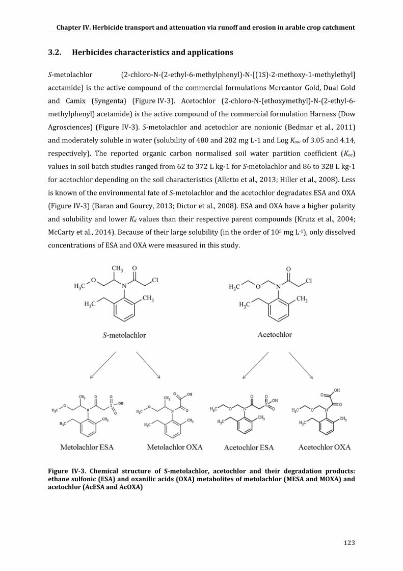
Chapter IV. Herbicide transport and attenuation via runoff and erosion in arable crop catchment

123

3.2. Herbicides characteristics and applications

S-metolachlor (2-chloro-N-(2-ethyl-6-methylphenyl)-N-[(1S)-2-methoxy-1-methylethyl]

acetamide) is the active compound of the commercial formulations Mercantor Gold, Dual Gold

and Camix (Syngenta) (Figure IV-3). Acetochlor (2-chloro-N-(ethoxymethyl)-N-(2-ethyl-6-

methylphenyl) acetamide) is the active compound of the commercial formulation Harness (Dow

Agrosciences) (Figure IV-3). S-metolachlor and acetochlor are nonionic (Bedmar et al., 2011)

and moderately soluble in water (solubility of 480 and 282 mg L-1 and Log Kow of 3.05 and 4.14,

respectively). The reported organic carbon normalised soil water partition coefficient (Koc)

values in soil batch studies ranged from 62 to 372 L kg-1 for S-metolachlor and 86 to 328 L kg-1

for acetochlor depending on the soil characteristics (Alletto et al., 2013; Hiller et al., 2008). Less

is known of the environmental fate of S-metolachlor and the acetochlor degradates ESA and OXA

(Figure IV-3) (Baran and Gourcy, 2013; Dictor et al., 2008). ESA and OXA have a higher polarity

and solubility and lower Kd values than their respective parent compounds (Krutz et al., 2004;

McCarty et al., 2014). Because of their large solubility (in the order of 105 mg L-1), only dissolved

concentrations of ESA and OXA were measured in this study.

Figure IV-3. Chemical structure of S-metolachlor, acetochlor and their degradation products: ethane sulfonic (ESA) and oxanilic acids (OXA) metabolites of metolachlor (MESA and MOXA) and acetochlor (AcESA and AcOXA)

Chapter IV. Herbicide transport and attenuation via runoff and erosion in arable crop catchment

124

Racemic metolachlor and acetochlor were applied in the study site from the early and late

1990s, respectively. Since 1998-2000, metolachlor has been replaced by S-metolachlor (the

herbicidally active enantiomer), which is isomerically enriched in the enantiomer-S (80/20%)

(Blaser, 2002). The amounts, timing and location of the acetochlor and S-metolachlor

applications were estimated based on surveys addressed to the farmers who covered 88% of the

catchment crop area, and identical application practices were assumed for the remaining area. A

total of 10.44 and 10.95 kg of acetochlor and S-metolachlor, respectively, were applied for the

10 days following corn and sugar beet sowing in the catchment during the study period

(Figure IV-4). The Mercantor Gold commercial formulation (Syngenta) was applied twice

(April 12 and May 1) on the plot, and no acetochlor was applied.

3.3. Hydrological measurements and sampling procedure

Two tipping buckets and 3 cumulative rain gauges were installed within the study catchment

(Figure IV-2) and read every week to evaluate spatial variation in rainfall. At the catchment

outlet (Figure IV-2), water discharge was measured using a Doppler flowmeter (2150 Isco,

Lincoln, Nebraska, USA). Flow proportional water samples were systematically collected every

20 m3 using a cooled automatic sampler (Isco Avalanche, Lincoln, Nebraska, USA). A punctual

water sample at the catchment outlet was collected in November 2012.

At the plot scale, runoff water was collected by a polyethylene gutter. Water level measurements

(Op in Figure IV-2) were conducted using a Venturi channel combined with a surface water level

sensor (ISMA, Forbach, France). Because of plot border overflowing, the water mass balance

could not be precisely estimated at the plot scale. Flow proportional water samples were

collected every 7 L by a cooled automatic sampler (Isco Avalanche, Lincoln, Nebraska, USA).

Point water sampling was collected weekly at the drain (D1, Figure IV-2) until July 10. The water

samples were collected in glass flasks, stored in the dark at 4 °C after each runoff event and

placed on ice during transportation to the laboratory for chemical analysis.

Sediments were collected monthly at the outlet of the catchment for chemical and granulometric

analyses. At the plot scale, the topsoil (0 - 3 cm) samples were collected before the application

and 5, 12, 20, 27, 33, 40, 47, 60, 75 and 89 days following the application. On July 10, one 1-m

depth core were extracted at the plot scale to estimate the vertical herbicide transport. The soil

samples were kept frozen at -20 °C until pesticide analysis.

Chapter IV. Herbicide transport and attenuation via runoff and erosion in arable crop catchment

125

3.4. Hydrochemical and soil analysis

The conductivity, pH, dissolved oxygen and redox potential were continuously measured at the

catchment outlet using Acteon 3000 sensors (Ponsel, Caudan, France). Nine hydrochemical

parameters (TIC, DIC, TOC, DOC, PO43−, Ptot, NO3−, NO2− and NH4+) were determined by FR EN

ISO standards and laboratory procedures. The water samples were filtered through 0.7-μm glass

fibre filters to separate the dissolved and particulate phases. Organic matter, pH and water

content of the soil samples were determined over time according to FR EN ISO standards and

internal procedures (Table VII-10).

3.5. Chloroacetanilide analysis

3.5.1 Chemicals

Chromasolv Plus methylene chloride, methanol and ethyl acetate at analytical grade purity (≥

99.9%) (Sigma Aldrich, St Quentin Fallavier, France) were used for the chloroacetanilide

analyses. Metolachlor-d6 and alachlor-d13 were obtained from Dr. Ehrenstorfer GmbH

(Augsburg, Germany) and used as internal standards for the chloroacetanilide quantification.

The analytical standards of metolachlor, acetochlor and the ethane sulfonic (ESA) and oxanilic

acids (OXA) degradates of metolachlor (MESA and MOXA) and acetochlor (AcESA and AcOXA)

(Pestanal, analytical grade purity >95%; Sigma Aldrich, St Quentin Fallavier, France) were used

to develop the analytical method.

3.5.2 Extraction

The chloroacetanilide quantification was conducted on the suspended solid (4 ± 9 g), sediment

(5 g) and soil (5 g) samples with 4 mL of ACN/pure water (v:v 60/40) by shaking for 1 min

(Vortex), incubating for 30 min at 115 °C, shaking for an additional 1 min and centrifuging for 10

min at 3500 rpm. The supernatant was then collected, and a second extraction was carried out

using the same protocol with the addition of 0.1% H3PO4. The supernatant was then filtered

using a 0.2-µm PTFE filter, concentrated with rotary evaporation to one droplet, resuspended in

50 mL of pure water and extracted by solid-phase extraction (SPE).

The SPE of the water, suspended solids, sediments and soil samples were performed using SolEx

C18 cartridges and an AutoTrace 280 SPE system (Dionex, CA, USA). The extraction cartridges

were washed with 5 mL of ethyl acetate, followed by 5 mL of methylene chloride and

Chapter IV. Herbicide transport and attenuation via runoff and erosion in arable crop catchment

126

sequentially conditioned by 10 mL of methanol and 10 mL of deionised water. The conditioned

cartridges were then loaded with the samples and dried with nitrogen for 10 min. The elution of

the chloroacetanilide herbicides and their degradation products was performed successively

with 3 mL of ethyl acetate and 2 mL of methylene chloride. Samples were concentrated under

nitrogen flux to 1 droplet, and 2 mL of methylene chloride were added.

3.5.3 Quantification of the chloroacetanilides and their degradation products

The chloroacetanilides were quantified by a GC-MS/MS (ITQ 700 model, Thermo Fisher

Scientific, Les Ulis, France) using metolachlor-d6 and alachlor-d13 as internal standards

(100 µg L-1) for S-metolachlor and acetochlor, respectively. The chloroacetanilide separation was

conducted on a 5% phenyl - 95% dimethylpolysiloxane fused-silica capillary column using a 30

m x 0.25 mm ID, and 0.25-µm film thickness OPTIMA 5MS (Macherey Nagel GmbH, Düren,

Germany) with helium as a carrier gas at a flow rate of 1 mL min-1. The quantification limits for

the water samples were 0.02 and 0.05 µg L-1 with a recovery efficiency of 96% and 43% for

metolachlor and acetochlor, respectively, with a mean analytical uncertainty of 8%. The

detection limits, retention times and selected ions used for identification are detailed in

Table VII-11. The quantification limits of the solid samples were 0.01 and 0.05 mg kg−1 with a

recovery efficiency of 74% and 63% and analysis uncertainty of 16% and 22% for metolachlor

and acetochlor, respectively.

MESA, MOXA, AcESA and AcOXA were analysed using a TSQ Quantum ACCESS LC-MS/MS

equipped with a Thermo Scientific Accela autosampler with a temperature-controlled sample

tray (15 °C) (Thermo Fisher, Les Ulis, France). The analytical column was an EC 150/3

Nucleodur Polar Tec (particle size 3 µm, length 150 mm and internal diameter 3 mm) and a

precolumn EC 4/3 Polar Tec 30 mm (Macherey Nagel, France). The mass spectrometer (MS) was

a Thermo TSQ Quantum triple quadrupole mass spectrometer (Thermo Fisher, Les Ulis, France)

operated using a heated electrospray ionisation (HESI) source. The best sensitivity in the

multiple reaction monitoring operation was achieved through the acquisition of selected

reaction monitoring (SRM) transitions with the MRM mode. For the identification of the studied

compounds, two SRM transitions and the correct ratio between the abundances of the two

optimised SRM transitions (SRM1/SRM2) were used along with retention time matching. The

quantification limits were 0.10 and 0.06 µg L-1 for MOXA and MESA, respectively, and 0.10 and

0.02 µg L-1 for AcOXA and AcESA, respectively. Information on the SRM transitions, detection

limits and analytical uncertainties are provided in Table VII-11.

Chapter IV. Herbicide transport and attenuation via runoff and erosion in arable crop catchment

127

3.5.4 Enantiomer analysis of S-metolachlor

Chiral analyses were performed with a GC-MS (Trace GC 2000 series, Thermo Scientific, Les Ulis,

France) using a 30 m x 0.25 mm ID, 0.25-µm film with 20% tert-butyldimethylsilyl-beta-

cyclodextrin dissolved in a 15% phenyl - 85% methylpolysiloxane column (BGB Analytik,

Boeckten, Switzerland) with helium as a carrier gas at a flow rate of 1.0 mL min-1. The

stereoisomer elution was aS1’S; aS1’R; aR1’S; and aR1’R (Figure VII-3). The four isomers can be

grouped into two pairs of enantiomers whereby the aS1‘S- and aR1’S-isomers constitute one pair

of enantiomers, and the aS1’R- and aR1’R-isomers constitute the other pair. The enantiomeric

excess (EE) was defined as the excess of the 1’S-isomers over the 1’R-isomers (Buser et al., 2000)

as follows:

( 𝑆 𝑆 𝑅 𝑆) ( 𝑆 𝑅 𝑅 𝑅)

( 𝑆 𝑅 𝑅 𝑆 𝑆 𝑅 𝑅 𝑅) (4)

The diastereoisomer excess (DE) was similarly defined as the excess of one pair of

diastereomers (aS1’S and aR1’R) over the other pair (aR1’S and aS1’R) as follows:

𝐷 ( 𝑆 𝑆 𝑅 𝑅) ( 𝑅 𝑆 𝑆 𝑅)

( 𝑆 𝑆 𝑅 𝑅 𝑅 𝑆 𝑆 𝑅) (5)

The EE and DE from the commercial product Mercantor Gold were 0.73 ± 0.01 and 0.07 ± 0.02,

respectively (n = 8). The racemic metolachlor spiked at 9 different concentrations (25 –

2500 µg L-1) was injected 3 times each to determine the precision in EE measurements. The

mean and standard deviations were 0.01 ± 0.03 (n = 27), indicating that there were no

concentration effects on the EE values. In addition, no enantiomeric fractionation occurred

during the extraction and dilution procedures (data not shown).

3.5.5 Data analysis

Herbicide concentrations below the quantification limit were set to zero. The runoff coefficients,

herbicide exported loads and export coefficient were calculated as previously explained

(Grégoire et al., 2010). Data were compared using the paired non-parametric Wilcoxon signed

rank test and Spearman rank correlation test. Statistical tests were performed using the R

software (R development Core Team, 2008; version 2.6.2). The partition coefficient of the

chloroacetanilides between the dissolved and particulate phases (Kd) were calculated as the

ratio of the particulate concentration against the dissolved concentration when both

concentrations exceeded the quantification limits. The soil organic carbon water partitioning

coefficient (Koc) was calculated based on the ratio of Kd against the particulate organic carbon

Chapter IV. Herbicide transport and attenuation via runoff and erosion in arable crop catchment

128

(POC). The field half-life in the soil was estimated assuming an exponential decrease of the soil

concentration over time. To quantify the transport of the total chloroacetanilide loading within

the agricultural catchment, ESA and OXA, as chloroacetanilide-derived compounds, were

expressed as a parent compound mass equivalence. The mass equivalent load of the parent

compound (P) (MELP) was calculated according to the following equation:

{ [

]} { [

]} (1)

where MWP is the molecular weight of S-metolachlor (283.8 g mol-1) or acetochlor

(269.8 g mol-1), MWOXA is the molecular weight of MOXA (279.3 g mol-1) or AcOXA

(265.30 g mol-1), and MWESA is the molecular weight of MESA (329.1 g mol-1) or AcESA (314.37 g

mol-1). The relationship between the chloroacetanilides and degradation products were

evaluated by calculating the %OXA (ESA) as a percentage of the total loads of the

chloroacetanilides, ESA and OXA according to the following equations:

𝑃 𝑆 (2)

𝑆 𝑆

𝑃 𝑆 (3)

where [ESA], [OXA] and [P] are the respective molar loadings of ESA, OXA and the parent

compounds in water. A %OXA (ESA) equal to zero indicates that either ESA, OXA and the parent

compound were below the quantification limit or that only OXA (resp. ESA) was below the limit.

4. Results and discussion

4.1. Chloroacetanilide attenuation in the plot soil

The concentration of S-metolachlor in the topsoil from the experimental plot was

6.0 µg kgdry-1 (Figure IV-4), and no acetochlor was detected before the applications because an

acetochlor application had not occurred in the previous 5 years at the plot scale. The soil

concentrations of S-metolachlor after Mercantor Gold application gradually decreased from 2.1

mg kgdry-1 to 0.5 mg kgdry-1 at 89 days after application (Figure IV-4). The field half-life in the soil

was estimated at 54 days following an exponential decrease (R² = 0.75, p < 0.001) (Figure IV-4),

which was consistent with the values of previous field and modelling studies (half-lives from 13

to > 90 days) (Boithias et al., 2011; Cabrera et al., 2012; Leu et al., 2010; Shaner et al., 2006).

S-metolachlor leached up to a 1 m depth on July 10 with concentrations of 4 × 10-3 mg kg-1dry.

The dissolved S-metolachlor concentrations in the runoff water at the plot scale decreased over

time and were correlated with concentrations of the soil surface samples (rho=0.93, p < 0.001)

Chapter IV. Herbicide transport and attenuation via runoff and erosion in arable crop catchment

129

(Figure IV-4), emphasising that the lower S-metolachlor amount could be mobilised over time

for surface transport.

Figure IV- 4. Temporal changes of S-metolachlor concentration in soil and dissolved runoff water samples at the plot scale

Chapter IV. Herbicide transport and attenuation via runoff and erosion in arable crop catchment

130

4.2. Influence of hydrology and hydrochemistry on chloroacetanilide export and partitioning

4.2.1 Hydrochemical and chloroacetanilide load variations

Based on the five rain gauges, rainfall showed a low spatial variation (± 3.5 mm on a weekly

basis) and was considered homogeneous at the catchment scale. Eighty-eight rainfall events

were monitored from March 12 to August 14 and amounted to 316 mm. A total outflow water

volume of 17,419 m3 was measured at the catchment outlet (Figure IV-5). The meteorological,

hydrological, and hydrochemical characteristics during the study period are provided in

Tables IV-1 and IV-2 and Figure IV-5 A and C.

Table IV-1. Hydrological characteristics from March 12 to August 14 2012 in the catchment (Alsace, France). Values are provided as the mean and ranges. Bold number corresponds to May 21.

Parameter Unit

Met

eoro

logy

Daily mean temperature [°C] 15.8 ± 4.8 (4.9 – 26.0)

Daily mean humidity [%] 68.2 ± 10.9 (37.8 - 89.4)

Daily potential evapotranspiration [mm] 3.8 ± 1.2 (1.3 - 7.4)

Rainfall events amounts [mm] 3.6 ± 6.4 (0.4 - 54.4)

Maximal rainfall events intensities [mm h-1

] 4 ± 4 (2 - 18)

Rainfall events duration [mn] 114 ± 114 (8 - 462)

Hyd

rolo

gy

(even

ts >

10 m

3) Outflow volume [m

3] 1314 ± 3472 (22 - 10568)

Event duration [mn] 136 ± 116 (38 - 413)

Runoff coefficient [%] 7.8 ± 12.6 (0.2 - 40.8)

Maximum outflow [mm h-1

] 1.17 ± 1.72 (0 – 5.56)

Estimation of the drainage contribution to

the runoff volume [%] 8.6 ± 6.7 (1.5 - 22.5)

Chapter IV. Herbicide transport and attenuation via runoff and erosion in arable crop catchment

131

Figure IV-5. Temporal changes of rainfall (A), the chloroacetanilide application (B), the dissolved exported loads (< 0.7 μm) of the parent compound (C), those of the degradation products (D) and the particulate loads (> 0.7 μm) of the parent compounds (E) at the catchment outlet (Alteckendorf, Alsace, France) with red bars for acetochlor and purple bars for S-metolachlor. For chloroacetanilide and metabolite loads, error bars were calculated via error propagation, incorporating analytical uncertainties as well as the uncertainty of suspended solids and water volume measurements.

Chapter IV. Herbicide transport and attenuation via runoff and erosion in arable crop catchment

132

During the growing season, a total of 581 tons of TSS, 0.33 tons of dissolved organic carbon

(DOC) and 44 tons of POC were exported at the outlet of the catchment (Figure IV-5). The TSS

export represented 1006 t km-2 and corresponded to a soil loss of 0.4 mm over the catchment.

This severe soil loss was in the range of the regional annual erosion (Neboit, 1991). Based on

linear hydrograph separation, the drainage contribution from drain D1 (Figure IV-2) was

estimated at 33% of the total outflowing water during the growing season. Compared to the

hydrochemical conditions of the drain, plot and catchment water during the investigation

period, the drain had significantly different concentrations of TIC, DIC, TOC, DOC, PO43−, Ptot,

NO2− and NH4+ (p < 0.05) (see Table IV-2 and Table VII-12 in Appendices). Drainage water

typically has lower concentrations of pesticides (14 to 96 times) than surface runoff from a

catchment or plot (Table IV-3), which was previously shown (Brown and van Beinum, 2009). At

the catchment scale, the total chloroacetanilide concentrations differed between high and low

flow periods (p < 0.01). This suggests a higher contribution of surface runoff during the high

flow conditions to discharge and to chloroacetanilide export at the catchment scale.

A total export coefficient of 3.4% and 5.8% for S-metolachlor and acetochlor were estimated for

both the particulate and dissolved phases at the catchment outlet. A 40-year return period

rainfall event on May 21 corresponded to 20% of the total rainfall and 53% of the total outflow

volume. This major event accounted for 92% of the TSS, 42% of the DOC, 87% of the POC and

96% of the chloroacetanilides exported during the study period (Figure IV-5). The May 21 event

occurred 7 days after and 16 days after the final applications of S-metolachlor and acetochlor,

respectively. Therefore, the period that included the days following the chloroacetanilide

application when bare soil was prevalent appeared to be risky for chloroacetanilide export.

More than 40% of the total chloroacetanilide export occurred in the particulate phase for both

S-metolachlor and acetochlor (Figure VII-4), ranging according to error propagation between 38

and 53%, emphasising that a large portion of exported chloroacetanilides occurred in

association with particles. Not counting this extreme event, the total exported load in the

dissolved phase was 85 and 13% of the total loads exported for S-metolachlor and acetochlor

respectively, emphasising the large temporal variability of the chloroacetanilide partitioning

between the dissolved and particulate phase.

Chapter IV. Herbicide transport and attenuation via runoff and erosion in arable crop catchment

133

Table IV-2. Hydrochemistry characteristics from March 12 to August 14 2012 in the plot, drain and catchment's outlet (Alsace, France). Values are provided as the mean and ranges. Bold number corresponds to May 21.

Parameter Unit Plot Drain Catchment

Samples number [ - ] 10 16 33

Ero

sio

n

Total suspended solids (> 0.7µm) [mg L-1] 1.70 ± 2.57 (0.05 - 7.66) 0.16 ± 0.29 (0 – 1.00) 5.85 ± 11.27 (0.02 - 59.70)

Volatile organic carbon (> 0.7µm) [%] 18.73 ± 12.9 (11.04 - 46.32) 24.27 ± 22.62 (3.03 - 75.76) 11.1 ± 5.16 (4.76 - 30.16)

Hy

dro

chem

istr

y

Nitrite (NO2-) [mg L-1] 0.50 ± 0.36 (0.11 - 1.22) 0.13 ± 0.03 (0.11 - 0.19) 0.83 ± 1.31 (0.11 - 5.60)

Nitrate (NO3-) [mg L-1] 114.05 ± 157.02 (10.17 - 425.15) 31.52 ± 12.87 (18.75 - 62.66) 27.16 ± 20.71 (2.32 - 92.18)

Ammonium (NH4+) [mg L-1] 12.11 ± 23.95 (0.42 - 69.45) 1.16 ± 1.63 (0.12 - 3.04) 4.14 ± 7.39 (0.12 - 29.59)

Ion phosphate (PO43-) [mg P L-1] 1.85 ± 2.32 (0.13 - 6.38) 0.36 ± 0.39 (0.01 - 1.05) 0.44 ± 0.37 (0.01 - 1.61)

Total inorganic carbon (TIC) [mg C L-1] 22.51 ± 35.43 (1.46 - 93.4) 87.37 ± 2.79 (82.32 - 91.42) 74.9 ± 18.47 (18.71 - 107.77)

Total organic carbon (TOC) [mg C L-1] 64.86 ± 78.55 (10.43 - 221.51) 2.87 ± 1.08 (1.72 - 5.23) 20.44 ± 28.10 (1.20 - 120.42)

Dissolved inorganic carbon (DIC) [mg C L-1] 23.97 ± 38.55 (0.09 - 87.44) 80.07 ± 22.76 (3.74 - 92.31) 58.42 ± 27.26 (0.12 - 93.17)

Dissolved organic carbon (DOC) [mg C L-1] 50.11 ± 75.65 (3.16 - 228.90) 4.12 ± 3.85 (1.84 - 14.46) 21.6 ± 26.45 (1.30 - 111.80)

Total phosphorus (P) [mg L-1] 2.87 ± 1.90 (1.44 - 6.20) 0.64 ± 0.38 (0.35 - 1.26) 7.43 ± 7.20 (0.84 – 29.00)

Chapter IV. Herbicide transport and attenuation via runoff and erosion in arable crop catchment

134

Table IV-3. Chloroacetanilides concentrations and occurrences from March 12 to August 14 2012 in the plot, drain and catchment's outlet (Alsace, France). Values are provided as the mean and ranges. Bold number corresponds to May 21.

n.a. not analysed

Parameter Unit Plot Drain Catchment

Ru

no

ff W

ate

r

Samples number [ - ] 10 16 33

S-metolachlor

(< 0.7 µm)

Occurrence [%] 100 63 64

Dissolved concentration [µg L-1

] 26.98 ± 20.21 (0.36 - 64.10) 0.28 ± 0.53 (0 - 2.21) 4.14 ± 12.79 (0 - 62.09)

Enantiomeric excess (EE) [ - ] 0.72 ± 0.05 (0.6 - 0.75) 0.68 ± 0.12 (0.34 - 0.74) 0.71 ± 0.15 (-0.02 - 0.77)

Diastereisomer excess (DE) [ - ] 0.09 ± 0.03 (0.04 – 0.14) 0.11 ± 0.02 (0.07 – 0.16) 0.10 ± 0.02 (0.07 – 0.13)

S-metolachlor

(> 0.7 µm)

Occurence [%] 70 54 44

Particulate concentration [mg kg-1

] 0.77 ± 1.50 (0 - 4.83) 0.62 ±1.65 (0 - 6.35) 1.14 ± 6.05 (0 - 34.29)

Enantiomeric excess (EE) [ - ] 0.74 ± 0.04 (0.67 - 0.77) 0.74 ± 0.04 (0.64 - 0.77) 0.70 ± 0.13 (0.28 - 0.75)

Diastereisomer ratio (DR) [ - ] 0.11 ± 0.02 (0.07 - 0.14) 0.19 ± 0.05 (0.10 - 0.25) 0.11 ± 0.04 (0.00 - 0.16)

Metolachlor

(< 0.7 µm)

ESA -OXA

Occurence (MESA) [%] 56 n.a 29

Occurence (MOXA) [%] 89 n.a 53

S-metolachlor ESA [µg L-1

] 28.66 ± 67.03 (0 - 199.94) n.a 41.64 ± 82.30 (0 - 316.17)

S-metolachlor OXA [µg L-1

] 122.33 ± 208.46 (0 - 659.32) n.a 6.52 ± 18.84 (0 - 91.84)

Acetochlor

(< 0.7 µm)

Occurence [%] 40 38 45

Dissolved concentration [µg L-1

] 0.28 ± 0.55 (0 - 1.75) 0.15 ± 0.24 (0 - 0.85) 3.86 ± 12.32 (0 - 59.33)

Acetochlor

(> 0.7 µm)

Occurence [%] 25 38 22

Particulate concentration [mg kg-1

] 3.69 ± 11.78 (0 - 41.03) 1.70 ± 5.47 (0 - 21.94) 3.28 ± 14.57 (0 - 82.95)

Acetochlor

(< 0.7 µm)

ESA-OXA

Occurence (AcESA) [%] 0 n.a 12

Occurence (AcOXA) [%] 0 n.a 21

Acetochlor ESA [µg L-1

] 0 ± 0 (0 - 0) n.a 1.35 ± 4.17 (0 - 17.51)

Acetochlor OXA [µg L-1

] 0 ± 0 (0 - 0) n.a 10.01 ± 23.55 (0 - 96.25)

So

il

Samples number [ - ] 11 n.a n.a

Metolachlor Concentration [mg kg-1

] 0.86 ± 0.52 (0.00 - 1.36) n.a n.a

Enantiomeric excess (EE) [ - ] 0.73 ± 0.04 (0.62 - 0.78) n.a n.a

Diastereisomer ratio (DR) [ - ] 0.09 ± 0.01 (0.07 - 0.11) n.a n.a

Chapter IV. Herbicide transport and attenuation via runoff and erosion in arable crop catchment

135

4.2.2 Chloroacetanilide partitioning

Rainfall intensities were correlated with the total suspended solid (TSS) concentrations

(rho=0.6; p < 0.001) as well as the S-metolachlor and acetochlor concentrations in both the

dissolved and particulate phases (rho=0.39, p < 0.001). This underscores the impact of intensive

events on TSS and chloroacetanilide export. The herbicide concentrations and loads during the

study period are provided in Figure IV-5 and Table IV-3. Drastic changes in S-metolachlor and

acetochlor partitioning between the dissolved and particulate phases were observed over time

(Figure VII-4). The Kd values of S-metolachlor and acetochlor were significantly correlated

together (rho=0.85, p < 0.05), suggesting that these two herbicides were similarly mobilised

over time. The Koc values ranged between 71 and 9395 L kg-1 for S-metolachlor and between 97

and 137,818 L kg-1 for acetochlor. Higher Koc values for acetochlor compared to S-metolachlor

were consistent with its higher hydrophobicity and lower solubility. The Kd values of both

chloroacetanilides presented significant negative correlations with the suspended solid flux

(rho=-0.92 and rho=-0.54, p < 0.001 and p < 0.05 for S-metolachlor and acetochlor, respectively),

indicating that chloroacetanilide adsorption onto particles decreased with increasing TSS

concentrations. It is further supported by the decrease of POC together with the increase of TSS

(rho=-0.55, p < 0.001). These observations are consistent with other studies and highlight the

impoverishment in organic carbon of eroded materials (Boithias et al., 2014; Cerro et al., 2014).

The TSS concentrations may also impact the required level of Gibbs free energy during

partitioning, which may largely affect the partitioning coefficient over time (Goss and

Schwarzenbach, 2003). Large variations of S-metolachlor and acetochlor partitioning over time

may be related to their large solubility relative to their log Kow (Boithias et al., 2014) and the

nature of the sorbents (size of the particles, aromaticity and polarity), which may change over

time and under different erosive events (Boithias et al., 2014; Si et al., 2009). The conductivity

and pH appear to have no influence on the Kd values, most likely because the pH (7.9 ± 0.2) and

conductivity (633 ± 239 µS cm-1) were relatively constant during the study period.

Few studies have focused on partitioning coefficients, such as Kd or Koc, stemming from runoff

pesticide concentration measurements (Boithias et al., 2014; Taghavi et al., 2011). The

calculated Koc values were five orders of magnitude lower than the chloroacetanilide Koc values

estimated in the Save River in the western France (Boithias et al., 2014) and one to two orders of

magnitude larger than those in soil-water batch studies at equilibrium (Alletto et al., 2013; Hiller

et al., 2008). The diversity of the experimental approaches, equilibrium sorption time and

sorbent characteristics make it difficult to compare the partitioning coefficients.

Chapter IV. Herbicide transport and attenuation via runoff and erosion in arable crop catchment

136

4.3. Dynamics of ESA and OXA degradation products

Although ESA and OXA were less frequently detected than their parent compounds (Table IV-3),

they often presented larger molar concentrations than their parent compounds (70% and 47%

of the samples at the plot and catchment scales, respectively), indicating that the degradation

process occurred during the study period. At the plot scale, dissolved AcESA and AcOXA could

not be detected in the water because acetochlor had not been applied in the previous 5 years.

Eighty-six percent of the plot water samples presented higher molar concentrations of MOXA

than MESA (Figure VII-5). At the catchment scale, MESA, MOXA, AcESA and AcOXA correlated

over time (rho=0.68, p < 0.001), suggesting that they had similar transformation and

transportation pathways, as previously shown in batch studies (Graham et al., 1999). On a

weekly basis, 41% and 100% of the catchment samples presented greater OXA concentrations

than ESA concentrations for S-metolachlor and acetochlor, respectively (Figure VII-5). Based on

the MELp calculation (Eq.1), an export coefficient of ESA and OXA parent compound mass

equivalent loads of 7.3% and 6.7% of the total mass applied for S-metolachlor and acetochlor,

respectively, were estimated, indicating the large relative contributions of the ESA and OXA

loads.

Only the S-metolachlor degradation products could be detected at the catchment scale from

March 12 to March 15, although both S-metolachlor and acetochlor were used during this period

(Figure IV-5). The occurrence of metolachlor degradation products can be explained by the rapid

degradation from earlier and smaller applications of S-metolachlor (April 12 and May 1) or by

the large quantities of S-metolachlor that had accumulated in soils because of the 10 additional

years of metolachlor use within the study site. From May 15 to July 3, 5 runoff events larger than

10 m3 occurred and led to a high detection frequency and larger exported loads of the

chloroacetanilides ESA and OXA. Among the runoff events, the event of May 21 explained 9%

and 94% of the total exported loads for ESA and OXA of S-metolachlor and acetochlor,

respectively, suggesting that a smaller amount of ESA was available in the soil surface or that

MOXA was more mobile than ESA, which is still controversial (Baran and Gourcy, 2013; Bayless

et al., 2008; Krutz et al., 2004). The persistence of S-metolachlor degradation products compared

to those of acetochlor were observed at the catchment outlet at the end of the study period

(from July 3 to August 14), whereas the acetochlor degradation products were not detected

(Figure IV-5), which is consistent with other studies (Steele et al., 2008).

Chloroacetanilide degradation may occur both biotically (Field and Thurman, 1996; McCarty et

al., 2014) and abiotically (Bian et al., 2009; Zeng et al., 2012). It is commonly supposed that ESA

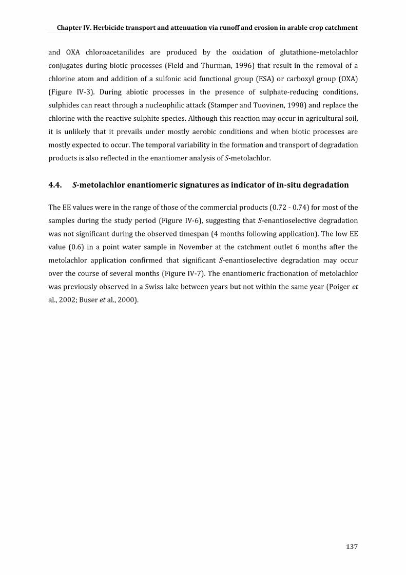
Chapter IV. Herbicide transport and attenuation via runoff and erosion in arable crop catchment

137

and OXA chloroacetanilides are produced by the oxidation of glutathione-metolachlor

conjugates during biotic processes (Field and Thurman, 1996) that result in the removal of a

chlorine atom and addition of a sulfonic acid functional group (ESA) or carboxyl group (OXA)

(Figure IV-3). During abiotic processes in the presence of sulphate-reducing conditions,

sulphides can react through a nucleophilic attack (Stamper and Tuovinen, 1998) and replace the

chlorine with the reactive sulphite species. Although this reaction may occur in agricultural soil,

it is unlikely that it prevails under mostly aerobic conditions and when biotic processes are

mostly expected to occur. The temporal variability in the formation and transport of degradation

products is also reflected in the enantiomer analysis of S-metolachlor.

4.4. S-metolachlor enantiomeric signatures as indicator of in-situ degradation

The EE values were in the range of those of the commercial products (0.72 - 0.74) for most of the

samples during the study period (Figure IV-6), suggesting that S-enantioselective degradation

was not significant during the observed timespan (4 months following application). The low EE

value (0.6) in a point water sample in November at the catchment outlet 6 months after the

metolachlor application confirmed that significant S-enantioselective degradation may occur

over the course of several months (Figure IV-7). The enantiomeric fractionation of metolachlor

was previously observed in a Swiss lake between years but not within the same year (Poiger et

al., 2002; Buser et al., 2000).

Chapter IV. Herbicide transport and attenuation via runoff and erosion in arable crop catchment

138

Figure IV-6. Distribution of enantiomeric excess of S-metolachlor in dissolved and solid bound surface water samples from the drain (DW), plot (PW) and catchment (CW) outlets and in soil (plot) and sediment (catchment) samples.

The EE ranged between -0.02 and 0.77 in the dissolved phase of runoff and 0.28 and 0.77 in the

particulate phase (Figure IV-7 and Table IV-3). The EE increased from 0.6 to 0.75 and from -0.02

to 0.75 in the runoff water at the plot and catchment scales just after application (Figure IV-7).

S-metolachlor could not be quantified on suspended solids before the application, which

prevented an enantiomeric analysis. At the catchment scale, the EE in the dissolved and

particulate phases revealed a significant correlation with the S-metolachlor concentration in

those phases (rho=0.64 and 0.87, p < 0.001). The EE values increased from 0.62 to 0.74 in the

plot soil samples just after the first application (Figure IV-7). Afterwards, the EE average was

0.74 ± 0.02, which suggested that S-metolachlor was not degraded enantioselectively within the

observed time span (71 days after last application) (Figure IV-7). The EE decreased from 0.80 to

0.64 over the soil depth and was correlated with the S-metolachlor concentration (rho=0.88, p <

0.05). The EE decreased from 0.75 to 0.66 (n = 3) over time in the sediments in front of the dike

at the catchment outlet (Figure IV-7). Overall, a slight correlation existed between the EE values

in the different environmental samples and S-metolachlor concentrations [ppm] (rho=0.22, p

<0.05, n=94). There was no significant difference between the EE values among the

environmental compartments (p > 0.1), suggesting that the environmental compartments could

Chapter IV. Herbicide transport and attenuation via runoff and erosion in arable crop catchment

139

not be distinguished based on their enantiomers signatures. The DE in nearly all of the samples

(water, suspended solids and soils) did not show significant shifts, suggesting that metolachlor

biodegradation was not diastereoisomer-selective under the environmental conditions

described in this study (Table IV-3).

Figure IV- 7. Temporal changes of the enantiomeric excess of metolachlor at the plot outlet (A) and at the catchment outlet (B) in different environmental compartments.

Chapter IV. Herbicide transport and attenuation via runoff and erosion in arable crop catchment

140

Although few studies of the stereoselectivity of metolachlor have been conducted, the

stereoselective degradation of S-metolachlor is still a controversial topic (Buser et al., 2000;

Klein et al., 2006; Kurt-Karakus et al., 2010). In a laboratory study, spiked soil samples presented

stereoselective degradation of racemic metolachlor with a decrease in the aR1’S isomer (Polcaro

et al., 2004). In this study, the ratio (aSS-aRS)/(aSS+aRS) did not significantly change and was

not significantly correlated with the S-metolachlor concentration, suggesting that only

enantiomers were subject to isomer-selective degradation. Samples with lower concentrations

of S-metolachlor were associated with an enrichment in the R-enantiomer, indicating

S-enantioselective degradation. No correlation was observed between the EE and MOXA or

MESA concentrations, which might partially be a result of the different contributions of other

commercial formulations (Dual Gold and Camix) that have different isomeric signatures.

Contrary to the EE, the DE of a chiral compound can vary largely depending on the batch and

conditions during synthesis (Buser et al., 2000). Variations of the EE according to the different

commercial products are unlikely to occur (Kurt-Karakus et al., 2010). In addition,

S-enantioselective degradation may not involve the formation of such degradation products, and

the presence of enzymes capable of degrading the enantiomers or/and interconversion reaction

cannot be excluded (Milosevic et al., 2013; Polcaro et al., 2004), interfering with the

enantiomeric signatures of the bulk sample.

5. Conclusion

The transport and degradation of the widely used chloroacetanilides S-metolachlor and

acetochlor were evaluated at both the plot and catchment scales using different analytical

approaches, which included the quantification of the chloroacetanilides and four of their

degradation products and enantiomer analyses. Our results showed that an important amount of

the pesticide load is missed when only the dissolved concentration of the parent compound is

analysed. The total export coefficients for S-metolachlor and acetochlor and their degradation

products were 11.4 and 11.8%, respectively, which includes both the dissolved and particulate

loads. The partitioning of S-metolachlor and acetochlor between the dissolved and particulate

phases varied widely over time and was linked to the suspended solid concentrations. The

concentration dynamics of acetochlor, S-metolachlor and their metabolites (ESA and OXA) in

runoff were similar within the agricultural catchment. MESA and MOXA were found to be more

persistent than AcESA and AcOXA. However, an evaluation of the amount of degradation

products in the soil is lacking within the catchment, and such an evaluation would help

determine the formation mechanisms of the degradation products in the field prior to their

export in runoff. These measurements will be the topic of future investigations. Our results show

Chapter IV. Herbicide transport and attenuation via runoff and erosion in arable crop catchment

141

that S-enantioselective biodegradation occurs and is negatively correlated with S-metolachlor

concentrations. However, no relationship could be found between the EE values and MESA and

MOXA concentrations. The present field study indicates the potential of enantiomer analyses for

assessing chloroacetanilide biodegradation and could be efficiently complemented with future

laboratory benchmark studies on enantiomeric fractionation during chloroacetanilide

degradation combined with an analysis of the degradation products to determine the extent of

biodegradation in agro-ecosystems.

6. Acknowledgements

The authors are members of REALISE, the Network of Laboratories in Engineering and Science

for the Environment in the Alsace Region (France; http://realise.unistra.fr), and the support of

REALISE is gratefully acknowledged. This research was funded by the research program EC2CO

(CNRS-INSU) and the PhytoRET project (C.21) of the European INTERREG IV program in the

Upper Rhine. Marie Lefrancq was supported by a fellowship of the Rhine-Meuse Water Agency

and Alsace Region. The authors wish to thank the farmers for their support. We acknowledge the

soil laboratory EOST UMS830 CNRS and Martine Trautmann, Anne Véronique Auzet, Tristan

Meyer, Diogo Reis, Jeanne Dollinger, Thomas Dreidemy, Célia Kennel, René Boutin, Sophie

Gangloff, Marie-Pierre Ottermatte, Eric Pernin and Brian Sweeney for their support in sampling,

analysis and/or writing.

Chapter IV. Herbicide transport and attenuation via runoff and erosion in arable crop catchment

142

7. References

Alletto, L., Benoit, P., Bolognesi, B., Couffignal, M., Bergheaud, V., Dumeny, V., Longueval, C., Barriuso, E.,

2013. Sorption and mineralisation of S-metolachlor in soils from fields cultivated with different

conservation tillage systems. Soil & Tillage Research. 128, 97-103.

Baran, N., Gourcy, L., 2013. Sorption and mineralization of S-metolachlor and its ionic metabolites in soils

and vadose zone solids: Consequences on groundwater quality in an alluvial aquifer (Ain Plain,

France). Journal of Contaminant Hydrology. 154, 20-28.

Barbash, J.E., 2014. The Geochemistry of Pesticides. In: Treatise on Geochemistry (Second Edition). Vol.,

H.D. Holland, K.K. Turekian, eds. Elsevier, Oxford, pp. 535-572.

Bayless, E.R., Capel, P.D., Barbash, J.E., Webb, R.M.T., Hancock, T.L.C., Lampe, D.C., 2008. Simulated fate and

transport of metolachlor in the unsaturated zone, Maryland, USA. Journal of Environmental

Quality. 37, 1064-1072.

Bedmar, F., Daniel, P.E., Costa, J.L., Gimenez, D., 2011. Sorption of Acetochlor, S-Metolachlor, and Atrazine

in Surface and Subsurface Soil Horizons of Argentina. Environmental Toxicology and Chemistry.

30, 1990-1996.

Bian, H.T., Chen, J.W., Cai, X.Y., Liu, P., Wang, Y., Huang, L.P., Qiao, X.L., Hao, C., 2009. Dechlorination of

chloroacetanilide herbicides by plant growth regulator sodium bisulfite. Water Research. 43,

3566-3574.

Blaser, H.U., 2002. The chiral switch of (S)-metolachlor: A personal account of an industrial odyssey in

asymmetric catalysis. Advanced Synthesis & Catalysis. 344, 17-31.

Boithias, L., Sauvage, S., Taghavi, L., Merlina, G., Probst, J.L., Perez, J.M.S., 2011. Occurrence of metolachlor

and trifluralin losses in the Save river agricultural catchment during floods. Journal of

Hazardous Materials. 196, 210-219.

Boithias, L., Sauvage, S., Merlina, G., Jean, S., Probst, J.-L., Sánchez Pérez, J.M., 2014. New insight into

pesticide partition coefficient Kd for modelling pesticide fluvial transport: Application to an

agricultural catchment in south-western France. Chemosphere. 99, 134-142.

Boxall, A.B.A., Sinclair, C.J., Fenner, K., Kolpin, D., Maud, S.J., 2004. When synthetic chemicals degrade in the

environment. Environmental Science & Technology. 38, 368a-375a.

Brown, C.D., van Beinum, W., 2009. Pesticide transport via sub-surface drains in Europe. Environmental

Pollution. 157, 3314-3324.

Buser, H.R., Poiger, T., Muller, M.D., 2000. Changed enantiomer composition of metolachlor in surface

water following the introduction of the enantiomerically enriched product to the market.

Environmental Science & Technology. 34, 2690-2696.

Cabrera, A., Papiernik, S.K., Koskinen, W.C., Rice, P.J., 2012. Sorption and dissipation of aged metolachlor

residues in eroded and rehabilitated soils. Pest Management Science. 68, 1272-1277.

Cai, X.Y., Sheng, G.Y., Liu, W.P., 2007. Degradation and detoxification of acetochlor in soils treated by

organic and thiosulfate amendments. Chemosphere. 66, 286-292.

Chapter IV. Herbicide transport and attenuation via runoff and erosion in arable crop catchment

143

Celis, R., Gamiz, B., Adelino, M.A., Hermosin, M.C., Cornejo, J., 2013. Environmental behavior of the

enantiomers of the chiral fungicide metalaxyl in Mediterranean agricultural soils. Science of The

Total Environment. 444, 288-297.

Cerro, I., Sanchez-Perez, J.M., Ruiz-Romera, E., Antigüedad, I., 2014. Variability of particulate (SS, POC) and

dissolved (DOC, NO3) matter during storm events in the Alegria agricultural watershed.

Hydrological Processes. 28, 2855-2867.

Dictor, M.C., Baran, N., Gautier, A., Mouvet, C., 2008. Acetochlor mineralization and fate of its two major

metabolites in two soils under laboratory conditions. Chemosphere. 71, 663-670.

Elsayed, O.F., Maillard, E., Vuilleumier, S., Nijenhuis, I., Richnow, H.H., Imfeld, G., 2014. Using compound-

specific isotope analysis to assess the degradation of chloroacetanilide herbicides in lab-scale

wetlands. Chemosphere. 99, 89-95.

Eurostat, 2007. The use of plant protection products in the European Union: data 1992–2003. Statistical

book. European Communities, Luxembourg.

Field, J.A., Thurman, E.M., 1996. Glutathione conjugation and contaminant transformation. Environmental

Science & Technology. 30, 1413-1418.

Freitas, L.G., Singer, H., Muller, S.R., Schwarzenbach, R.P., Stamm, C., 2008. Source area effects on herbicide

losses to surface waters - A case study in the Swiss Plateau. Agriculture Ecosystems &

Environment. 128, 177-184.

Goss, K.U., Schwarzenbach, R.P., 2003. Rules of thumb for assessing equilibrium partitioning of organic

compounds: Successes and pitfalls. Journal of Chemical Education. 80, 450-455.

Graham, W.H., Graham, D.W., Denoyelles, F., Smith, V.H., Larive, C.K., Thurman, E.M., 1999. Metolachlor and

alachlor breakdown product formation patterns in aquatic field mesocosms. Environmental

Science & Technology. 33, 4471-4476.

Grégoire, C., Payraudeau, S., Domange, N., 2010. Use and fate of 17 pesticides applied on a vineyard

catchment. International Journal of Environmental Analytical Chemistry. 90, 406-420.

He, H.Z., Chen, G.K., Yu, J., He, J.B., Huang, X.L., Li, S.F., Guo, Q., Yu, T.H., Li, H.S., 2013. Individual and Joint

Toxicity of Three Chloroacetanilide Herbicides to Freshwater Cladoceran Daphnia carinata.

Bulletin of Environmental Contamination and Toxicology. 90, 344-350.

Heitz, C., Flinois, G., Glatron, S., 2012. Protection against muddy floods: perception for local actors in Alsace

(France) of a protection measure (fascines). International Disaster Risk Conference, Davos,

Suisse, 26-30 Août 2012.

Hiller, E., Krascsenits, Z., Cernansky, S., 2008. Sorption of acetochlor, atrazine, 2,4-D, chlorotoluron, MCPA,

and trifluralin in six soils from Slovakia. Bulletin of Environmental Contamination and

Toxicology. 80, 412-416.

Hladik, M.L., Bouwer, E.J., Roberts, A.L., 2008a. Neutral degradates of chloroacetamide herbicides:

Occurrence in drinking water and removal during conventional water treatment. Water

Research. 42, 4905-4914.

Hladik, M.L., Bouwer, E.J., Roberts, A.L., 2008b. Neutral chloroacetamide herbicide degradates and related

compounds in Midwestern United States drinking water sources. Science of The Total

Environment. 390, 155-165.

Chapter IV. Herbicide transport and attenuation via runoff and erosion in arable crop catchment

144

Klein, C., Schneider, R.J., Meyer, M.T., Aga, D.S., 2006. Enantiomeric separation of metolachlor and its

metabolites using LC-MS and CZE. Chemosphere. 62, 1591-9.

Krutz, L.J., Senseman, S.A., Dozier, M.C., Hoffman, D.W., Tierney, D.P., 2004. Infiltration and adsorption of

dissolved metolachlor, metolachlor oxanilic acid, and metolachlor ethanesulfonic acid by

buffalograss (Buchloe dactyloides) filter strips. Weed Science. 52, 166-171.

Kurt-Karakus, P.B., Bidleman, T.F., Muir, D.C.G., Struger, J., Sverko, E., Cagampan, S.J., Small, J.M., Jantunen,

L.M., 2010. Comparison of concentrations and stereoisomer ratios of mecoprop, dichlorprop and

metolachlor in Ontario streams, 2006-2007 vs. 2003-2004. Environmental Pollution. 158, 1842-

1849.

Leu, C., Schneider, M.K., Stamm, C., 2010. Estimating Catchment Vulnerability to Diffuse Herbicide Losses

from Hydrograph Statistics. Journal of Environmental Quality. 39, 1441-1450.

Liu, H.J., Xiong, M.Y., 2009. Comparative toxicity of racemic metolachlor and S-metolachlor to Chlorella

pyrenoidosa. Aquatic Toxicology. 93, 100-106.

Liu, W.P., Gan, J.Y., Papiernik, S.K., Yates, S.R., 2000. Structural influences in relative sorptivity of

chloroacetanilide herbicides on soil. Journal of Agricultural and Food Chemistry. 48, 4320-4325.

McCarty, G.W., Hapeman, C.J., Rice, C.P., Hively, W.D., McConnell, L.L., Sadeghi, A.M., Lang, M.W., Whitall,

D.R., Bialek, K., Downey, P., 2014. Metolachlor metabolite (MESA) reveals agricultural nitrate-N

fate and transport in Choptank River watershed. Science of The Total Environment. 473–474,

473-482.

Milosevic, N., Qiu, S., Elsner, M., Einsiedl, F., Maier, M.P., Bensch, H.K.V., Albrechtsen, H.J., Bjerg, P.L., 2013.

Combined isotope and enantiomer analysis to assess the fate of phenoxy acids in a

heterogeneous geologic setting at an old landfill. Water Research. 47, 637-649.

Neboit, R., 1991. L'homme et l'érosion: l'érosion des sols dans le monde, Vol., Association des Publications

de la Faculté des Lettres et Sciences Humaines de Clermont-Ferrand.

Oliver, D.P., Kookana, R.S., Anderson, J.S., Cox, J.W., Waller, N., Smith, L.H., 2012. Off-site transport of

pesticides in dissolved and particulate forms from two land uses in the Mt. Lofty Ranges, South

Australia. Agricultural Water Management. 106, 78-85.

Poiger, T., Muller, M.D., Buser, H.R., 2002. Verifying the chiral switch of the pesticide metolachlor on the

basis of the enantiomer composition of environmental residues. Chimia. 56, 300-303.

Polcaro, C.M., Berti, A., Mannina, L., Marra, C., Sinibaldi, M., Viel, S., 2004. Chiral HPLC resolution of neutral

pesticides. Journal of Liquid Chromatography & Related Technologies. 27, 49-61.

Roberts, T.R., Hutson, D.H., Services, R.S.o.C.I., 1999. Metabolic Pathways of Agrochemicals: Insecticides

and fungicides, Vol., Royal Society of Chemistry.

Saha, S., Dutta, D., Karmakar, R., Ray, D.P., 2012. Structure-toxicity relationship of chloroacetanilide

herbicides: Relative impact on soil microorganisms. Environmental Toxicology and

Pharmacology. 34, 307-314.

Shaner, D.L., Brunk, G., Belles, D., Westra, P., Nissen, S., 2006. Soil dissipation and biological activity of

metolachlor and S-metolachlor in five soils. Pest Management Science. 62, 617-623.

Si, Y.B., Takagi, K., Iwasaki, A., Zhou, D.M., 2009. Adsorption, desorption and dissipation of metolachlor in

surface and subsurface soils. Pest Management Science. 65, 956-962.

Chapter IV. Herbicide transport and attenuation via runoff and erosion in arable crop catchment

145

Stamper, D.M., Tuovinen, O.H., 1998. Biodegradation of the acetanilide herbicides alachlor, metolachlor,

and propachlor. Critical Reviews in Microbiology. 24, 1-22.

Steele, G.V., Johnson, H.M., Sandstrom, M.W., Capel, P.D., Barbash, J.E., 2008. Occurrence and fate of

pesticides in four contrasting agricultural settings in the United States. Journal of Environmental

Quality. 37, 1116-32.

Taghavi, L., Merlina, G., Probst, J.L., 2011. The role of storm flows in concentration of pesticides associated

with particulate and dissolved fractions as a threat to aquatic ecosystems Case study: the

agricultural watershed of Save river (Southwest of France). Knowledge and Management of

Aquatic Ecosystems 400-06.

Turner, J., Albrechtsen, H.J., Bonell, M., Duguet, J.P., Harris, B., Meckenstock, R., McGuire, K., Moussa, R.,

Peters, N., Richnow, H.H., Sherwood-Lollar, B., Uhlenbrook, S., van Lanen, H., 2006. Future trends

in transport and fate of diffuse contaminants in catchments, with special emphasis on stable

isotope applications. Hydrological Processes. 20, 205-213.

Ye, C., 2003. Environmental behavior of the herbicide acetochlor in soil. Bulletin of Environmental

Contamination and Toxicology. 71, 919-923.

Zeng, T., Chin, Y.P., Arnold, W.A., 2012. Potential for Abiotic Reduction of Pesticides in Prairie Pothole

Porewaters. Environmental Science & Technology. 46, 3177-3187.

Zhang, J.N., Liang, W.J., Wu, X., Jiang, S.W., Li, Q., 2013. Toxic Effects of Acetochlor on Mortality,

Reproduction and Growth of Caenorhabditis elegans and Pristionchus pacificus. Bulletin of

Environmental Contamination and Toxicology. 90, 364-368.

Chapter V. Modelling pesticide runoff at the headwater catchment scale

146

Chapter V. Modelling pesticide runoff at the headwater catchment scale

Overview

Pesticide runoff in two different agricultural contexts representative of headwater catchments of

the Rhineland area were investigated in this thesis. However, physico-chemical processes

observed from one agricultural context during one season could only be confirmed and further

extended with the help of modelling.

Runoff and erosion in agro-ecosystems are largely influenced by drastic changes of the dynamics

of soil surface state and hydrodynamic parameters during the growing season (Alaoui et al.,

2011). Knowledge of soil surface state and hydrodynamic parameters is crucial for

understanding and predicting pesticide transport processes in agro-ecosystems. Currently, few

pesticide transport models account for the effects of agricultural practices on hydrodynamic

parameters and soil surface characteristics and most of them are deemed inappropriate for

investigating headwater catchments with a very fine temporal resolution (≤ 1 min, see Chapter

1, §2.2.4). Furthermore, pesticide-runoff models rarely integrate erosion processes, and thus

neglect pesticide transport in the particulate phase. This underscores that an event based,

spatially distributed pesticide-fate model at the headwater catchment scale is needed to address

pesticide mobilisation and transport in agricultural headwater catchments.

A new calibration approach was developed for predicting runoff and erosion processes with

meaningful input parameters based on an hydrological and erosion model LISEM (Limbourg Soil

Erosion Model) (DeRoo et al., 1996) in order to account for the temporal variability of the soil

surface and hydrodynamic parameters along the growing season (Section 1, in prep). A

mathematical formalism was developed to predict pesticide mobilisation and transport via

runoff in the dissolved phase based on the distributed mixing layer theory (Wallender et al.,

2008) (Section 2). This formalism was integrated in LISEM.

Chapter V. Modelling pesticide runoff at the headwater catchment scale

147

Figure V-1. Graphical outline of the PhD thesis (Chapter V)

Chapter V. Modelling pesticide runoff at the headwater catchment scale

148

Section 1. Agronomical insights for improving runoff prediction in headwater agricultural catchments

Marie Lefrancq, Paul Van Dijk, Matthieu Schwob, Sylvain Payraudeau

(This part is in preparation for publication, Appendices are given in Chapter VII)

1. Abstract

Predicting runoff and erosion in agricultural areas is inherently difficult because of rapid

changes in soil surface characteristics, hydrodynamic parameters and vegetation. Obtaining

distributed input parameters for mechanistic approaches remains difficult, and model

calibration often leads to “equifinality” as a result of over-parameterisation. In this study, a novel

approach was developed for reducing the dimensionality of calibration issues to improve runoff

prediction at the event scale within headwater agricultural catchments. The originality of this

approach is the combination of the event-based hydrological model LISEM (Limbourg Soil

Erosion Model) and agronomic continuous model IDR to provide the temporal variability of soil

surface characteristics, soil hydrodynamic parameters and vegetation changes during a growing

season. Applied at a study site located in eastern France, the approach developed in this work

showed that runoff prediction at the outlet and within the catchment was enhanced during a

growing season based on limited supplementary knowledge of the input parameters. Combining

a hydrological event-based model and agronomic continuous model provided an accurate spatial

prediction of erosion for the largest observed erosive event. The sensitivity of 21 input

parameters of LISEM was assessed and differed according to the intensity and volume of the 9

significant runoff events observed during the growing season. Simulated runoff volume was less

sensitive to the initial water content and saturated hydraulic conductivity during intensive

runoff events. The sensitivity analysis showed that the Green and Ampt infiltration parameters,

i.e., saturated and initial water content, suction at the wetting front and saturated hydraulic

conductivity, were major factors influencing the total runoff volume for the 9 runoff events. The

full coupling of a distributed hydrological event-based model with an agronomic model should

be further developed to account for spatial and temporal variation of the initial soil surface

characteristics and hydrodynamic parameters.

Key words: Erosion; Soil hydraulic properties; Equifinality; Temporal variability; Soil surface

characteristics; Tillage

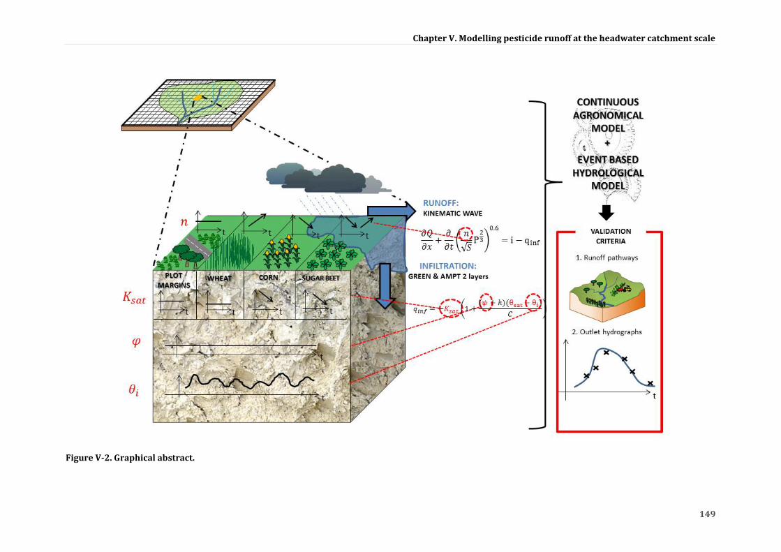
Chapter V. Modelling pesticide runoff at the headwater catchment scale

149

Figure V-2. Graphical abstract.

Chapter V. Modelling pesticide runoff at the headwater catchment scale

150

2. Introduction

Agricultural practices strongly impact the generation, dynamics and pathways of both runoff and

erosion worldwide (Dotterweich, 2013). Common agricultural practices of removing perennial

vegetation (Xu et al., 2013), maintaining areas of bare soil (Durán-Zuazo et al., 2013), and tilling

(Meijer et al., 2013) promote soil erosion and runoff and the subsequent transport of pesticides.

Cultivated soils have specific soil surface characteristics such as soil cover, topsoil structure and

soil crusting that are known to largely influence the partitioning of rainfall between infiltration

and runoff (Pare et al., 2011). Hortonian runoff prevails in agricultural areas in the early growth

stages (spring and early summer) (Armand et al., 2009; Van den Putte et al., 2013), and soil

hydrodynamics significantly change over time during a growing season (Alaoui et al., 2011; Ali,

2008; O'Hare et al., 2010). For example, surface soil hydraulic conductivity (Ksat) may exhibit

higher values immediately after tillage (e.g., 30-35 mm h-1) and gradually decrease from April to

September (e.g., 5-10 mm h-1) for loess soils (Ali, 2008) as a result of the breakdown of

aggregates caused by rainfall and the clogging of larger pores (Zeng et al., 2013). Manning’s

coefficient (n) is influenced by soil surface characteristics, which are rendered smoother by the

rainfall events, and the friction dissipation from crop growth that maintains resistance for the

water flow (Augustin et al., 2009; Li and Zhang, 2001). Determining the soil surface

characteristics and hydrodynamics is crucial for predicting hydrological processes in

agricultural catchments. However, few studies have attempted to develop predictive models that

emphasise the impact of agricultural practices on hydrodynamic parameters and soil surface

characteristics (Green et al., 2003; Pare et al., 2011).

Erosion and hydrological models have been steadily improving throughout recent decades

(Aksoy and Kavvas, 2005; Mitasova et al., 2013). A single rainfall event can cause more than half

of the annual measured erosion within a catchment (Edwards and Owens, 1991), and only parts

of a catchment might contribute to runoff (Dunne and Black, 1970). Determining the generation,

dynamics and pathways of both surface runoff and sediment transport at an event scale is

therefore essential (Evrard et al., 2009; Fiener et al., 2011). Continuous models are not usually

designed to detail the runoff from single events and generally lack sufficient spatial and

temporal details (Merritt et al., 2003). Event-based models are often simpler because they do

not account for all of the processes required in a continuous model, such as evapotranspiration,

water redistribution and plant growth (Berthet et al., 2009), and enable finer temporal and

spatial discretisation. However, reducing the gap between measurement availability and

parameter estimation for physically based models still remains a challenge.

Chapter V. Modelling pesticide runoff at the headwater catchment scale

151

The initial conditions in event-based models are set from additional external information

(Tramblay et al., 2010) and often require calibration for each rainfall-runoff event (Baartman et

al., 2012). Calibration steps may hamper the selection of unique spatial parameter sets that best

describe catchment dynamics and may lead to “equifinality“ as a result of over-parameterisation

(Beven, 2006; Kirchner, 2006). Several approaches have been developed to tackle the issue of

non-unique parameter sets (Efstratiadis and Koutsoyiannis, 2010; Gupta et al., 2009; Wallner et

al., 2013). These approaches include multi-objective calibrations with different types and/or

locations of observations. Considering the complexity of interactions between physical

processes, several observation locations within the catchment can significantly improve the

calibration and validation of a distributed model (Lee et al., 2012). Because sediment transport

is conditioned by runoff dynamics (Aksoy and Kavvas, 2005), additional erosion characterisation

within the catchment may assist in the spatial validation of predicted runoff velocities and flow

depths.

The objective of this study was to develop a novel approach to improve runoff prediction at the

event scale during a growing season within headwater agricultural catchments. The novelty of

the approach was in the combination of the event-based hydrological model LISEM (DeRoo et al.,

1996) and the continuous agronomic model IDR (Van Dijk et al., in prep.) to provide the temporal

variability of soil surface characteristics, soil hydrodynamic parameters and vegetation changes

during a growing season. A constraint calibration method (CCM) was developed and tested using

the IDR model outputs to improve the consistency and to reduce the equifinality of the LISEM

parameters calibrated for an event based on a growing season. To quantify the benefit in terms

of the consistency and equifinality of the CCM approach, a basic calibration method (BCM) of the

LISEM parameters was applied for each event without considering the evolution of the

agronomical properties along the growing season. The consistency of the model prediction was

evaluated by the ability of LISEM to i) simulate the runoff dynamics at the outlet and runoff

patterns within the catchment and ii) predict the amount of eroded soil at the outlet and erosion

patterns within the catchment for intensive event. The CCM approach was tested for a case study

located 30 km northeast of Strasbourg (Alsace, France).

Chapter V. Modelling pesticide runoff at the headwater catchment scale

152

3. Material and methods

3.1. Model description

The hydrological model used for the calibration testing was LISEM (Limbourg Soil Erosion

Model) (DeRoo et al., 1996), which is a physically based runoff and soil erosion model for event-

based predictions in small agricultural catchments (<10,000 ha).

The selection of LISEM was motivated by 3 main reasons. The first reason was to select an event-

based model that was fully distributed for headwater catchments and that considered erosion

processes. The second reason was that LISEM was designed to describe agricultural landscape

components with crusted and compacted zones and soil surface structure (Liu et al., 2003). The

third reason was that this model was validated in various agricultural contexts and hydrological

conditions (Baartman et al., 2012; Hessel et al., 2006; Hessel and Jetten, 2007; Sheikh et al.,

2010). The theory and structures of LISEM were previously described (Baartman et al., 2012).

Briefly, rainfall interception by vegetation is first calculated based on a canopy storage function

(de Jong and Jetten, 2007). Then, the water partitioning between infiltration and the surface is

calculated by the Green and Ampt equations for one or two soil layers (Kutílek and Nielsen,

1994) (Eq. 1):

( ( )( )

) (Eq. 1)

where qinf is the infiltration rate [m s-1], Ksat is the saturated hydraulic conductivity [m s-1], F is

the cumulative infiltration from the beginning of the event [m], is the average matrix suction

at the wetting front [m], h is the overpressure depth of the water layer at the soil surface [m],

is the saturated water content [-], and is the initial water content of the layer [-]. The

maximum depression storage in the micro-relief was estimated based on an empirical equation

from Kamphorst et al. (2000). Once the maximum depression storage was exceeded, runoff was

generated. Erosion detachment was generated by rainfall splash based on rainfall kinetic energy

(Sanchez-Moreno et al., 2012) and/or overland flow. Flow detachment was calculated with a

stream-power based transport capacity based on the EUROSEM formalism (Morgan et al., 1998).

Sediment traps can be used to represent the vegetal barriers as observed within the catchment.

The flow velocity was calculated with the Manning equation, and surface runoff was routed over

the landscape with the 1D kinetic wave equation (Eq. 2) (Chow et al., 2013).

[𝑛

√𝑆𝑃

]

(Eq. 2)

Chapter V. Modelling pesticide runoff at the headwater catchment scale

153

where Q is the discharge [m3 s-1], n is the Manning coefficient [-], S is the sine of the slope

gradient [-], P is the wet perimeter [m], and qsur is the infiltration surplus [m² s-1]. Equations 1

and 2 indicate that the compensation in rainfall-runoff model parameters may occur in one cell

during the water partitioning between runoff and infiltration (Eq. 1) or spatially between the

cells during the transport step (Eq. 2). Transport equations (water and sediment) are solved in

one spatial dimension and routed from upstream to downstream over a predefined flow

network that connects cells in 8 directions (quasi 2D). In this study, LISEM refers to version 1.79

of OpenLISEM (http://blogs.itc.nl/lisem/). For each predicted runoff event, the initial surface soil

characteristics, hydrodynamic parameters and initial water content were required for the

hydrological predictions with LISEM and were provided by the continuous agronomic model IDR.

3.2. Continuous agronomic model: IDR

Soil surface and vegetation characteristics, including vegetation and crop residue cover, random

roughness and saturated hydraulic conductivity, vary in space during the crop growing season.

IDR, or indicator of runoff dynamics, is a continuous field scale model. IDR predicts the soil surface

state and hydrodynamic parameters as a function of the cropping system, e.g., crop, tillage,

climate and soil type (Van Dijk et al., in prep.). Physical processes and equations included in IDR

are detailed in the Appendices. Briefly, Ksat is determined in two steps: the saturated hydraulic

conductivity of the soil matrix is estimated based on the pedotransfer function (Cosby et al.,

1984), which only depends on the soil texture, and then the soil tillage and progressive soil

clogging under the influence of rainfall are considered. The approach for estimating soil

moisture in the topsoil layer is based on the soil moisture depletion model from Kohler and

Linsley (1951). Vegetation cover is calculated according to a sigmoidal curve based on the

growth equation of Hunt (1982). Random roughness (RR) is calculated based on the equations of

Potter (1990).

Chapter V. Modelling pesticide runoff at the headwater catchment scale

154

3.3. Case study

3.3.1 Description of the study site

The 47-ha catchment is located 30 km northeast of Strasbourg (Alsace, France) and has a mean

annual temperature of 11.7 °C, mean annual rainfall of 605 mm (± 141 mm) and

evapotranspiration of 820 mm (± 28 mm) (2005-2011, Meteo France station in Waltenheim sur

Zorn, which is located 7 km from the study site).

The mean slope is 6.7% (± 4.8%), and the altitude ranges between 190 and 230 m. The

catchment outlet forms a retention basin (maximum capacity of 6700 m3) during large runoff

events, and water is conducted to the catchment outlet (P0 in Figure V-3) via ditches into a 50-

cm diameter pipe under the road, which yields a maximum outflow of 550 L s-1. A pipe (P1 in

Figure V-3) was constructed to conduct the runoff under a track. The catchment is intensively

cultivated, and 88% is arable land with corn (68%), winter wheat (16%) and sugar beet (4%) as

principal crops. A drainage system has existed since 1950, and one drain (Figure V-3) was active

during the study period and flowing in a ditch. No flow was observed in the other drains during

the study period.

Figure V-3. Scheme of the study catchment (Alteckendorf, Alsace, France).

Chapter V. Modelling pesticide runoff at the headwater catchment scale

155

The spatial variability of the soil was characterised by 48 soil surface samples (0 - 20 cm) in

April 2011 and six 2-m soil profiles in November 2012. The main soil type is calcareous brown

earths and calcic soils on hillsides and colluvial calcic soils in the central thalweg (Figure VII-6 in

the Appendices). The grain size distributions of the soil profiles presented low variations (n =

30) (mean ± SD in percent): clay 29.5 ± 5.8, silt 64.2 ± 6.5 and sand 6.4 ± 2.9. The soil

characteristics (mean ± SD) were CaCO3 10.7 ± 8.1%, organic matter 1.1 ± 0.8%, pH 7.2 ± 0.6,

phosphorus 0.04 ± 0.04 g kg-1 and CEC 12.7 ± 2.8 cmol+ kg-1. The detailed norms and methods for

the soil measurements are described in Table VII-10. The soil characteristics showed little

variability within the studied catchment (Figure VII-6) and were considered homogeneous in

this study. A compacted layer was observed at a depth between 20 and 30 cm along the soil

profiles corresponding to the plough base. Undisturbed soil samples of 100 cm3 were taken at 6

depths along the 2 m depth profile to characterise the hydrodynamic properties.

The saturated hydraulic conductivity of the soil matrix was determined under steady conditions

(Table VII-10), and it was measured at 6.3 ± 8.8 mm h-1 in the soil samples from the first depth

(0 - 10 cm) (n = 6). The study catchment was prone to significant muddy flows nearly every year

(Heitz et al., 2012), and the soil was sensitive to soil crusting and compaction. In 2009, five

vegetal barriers were installed in the flow path to decrease the water velocity and to retain the

soil particles during large events (Figure V-3). Springtime is a muddy flow risk period because of

the extensive bare soil. Runoff discharges were continuously monitored between March 12 and

August 14, 2012 and corresponded to the crop-growing season.

3.3.2 Hydrological procedure and experimental results

The catchment area was equipped with two tipping bucket rain gauges and 3 cumulative rain

gauges to measure the weekly rainfall spatial variability (Figure V-3). Based on the five rain

gauges, a low spatial variation of the rainfall was observed within the catchment (± 3.5 mm on a

weekly basis). Therefore, the rainfall was considered to be homogeneous for the simulation.

Water discharge was measured at the catchment outlet (P0 in Figure V-3) using a Doppler

flowmeter (2150 Isco, Lincoln, Nebraska, USA) with a volume precision of 3%. Within the

catchment, 2 runoff detectors were installed at P1 and P2 to indicate the runoff pathways within

the catchment (see Figure V-3). The water level was measured using a pressure-sensor

datalogger (Orpheus mini, OTT, Kempten, Germany) in a pipe (P1) in which the water was

conducted from a ditch. P2 was located at the outlet of a sugar beet plot upstream in the

catchment; it was left as a bare area from March to May like 72% of the crop area. The runoff

Chapter V. Modelling pesticide runoff at the headwater catchment scale

156

water was collected by a polyethylene gutter, and the water level was measured with a Venturi

channel combined with a surface water level sensor (ENDRESS and HAUSER, Huninge, France)

(P2 in Figure V-3).

Each week, topsoil samples (0 - 3 cm) were collected in the sugar beet plot (P2), and water

content, organic carbon and pH of the samples were measured. To allow for the spatial

validation of the simulated patterns, field observations were performed on runoff pathways and

erosion and deposition patterns after the most intense events on May 2 and May 21 because the

traces of surface runoff and erosion were visible.

Nine rainfall events that each yielded more than 10 m3 of runoff at the outlet of the catchment

were observed during the study period (Table V-1). The largest event was on May 21 and

corresponded to 20% of the total rainfall and 53% of the total discharge during the study period.

For this event, the water retention in front of the dike began 130 min after the beginning of the

rainfall and reached 1.8 m, which modified the water velocities and peak outflow. After this

event, the soil surface of the arable land was completely crusted, facilitating the production of

runoff during subsequent rainfall events (Table V-1).

Chapter V. Modelling pesticide runoff at the headwater catchment scale

157

Table V-1. Meteorological and hydrological characteristics of the 9 runoff events yielding at least 10 m3 at the outlet of the catchment and occurring from May 2 to August 15 2012.

* Flood retention

** Time after beginning of rainfall event

Unit May 2 May 21 May 23 June 7 June 11 June 12 July 10 July 08 July10

Rainfall amount [mm] 16.2 54.4 3.8 10.8 5.8 10.8 12.8 11.0 6.2

Rainfall duration [min] 179 204 29 106 20 180 30 164 41

Rainfall effective duration [min] 45 106 12 24 10 53 27 49 11

6 min-peak rainfall intensity [mm h-1]

38 72 26 56 50 20 40 16 46

Total discharge [m3] 22.2 10567.9 143.6 208.0 147.6 408.3 227.4 79.0 23.2

Drainage contribution [%] 22.5 1.5 13.7 3.5 5.3 6.2 4.8 13.3 6.5

Runoff event duration [min] 75 413 55 98 84 193 91 179 38

Runoff coefficient [%] 0.2 40.8 7.0 4.0 6.5 5.8 3.6 1.3 0.7

Maximum outflow [L s-1] 11.2 * 105.0 131.0 0.7 125.0 229.0 30.5 20.2

Peak time discharge** [min] 184 * 27 84 19 53 34 90 10

Chapter V. Modelling pesticide runoff at the headwater catchment scale

158

3.3.3 Erosion characterisation

Because sediment transport is sensitive to flow hydraulics, erosion characterisation could help

to validate runoff predictions. At the outlet of the plot and catchment (P2 and P0, respectively, in

Figure V-3), flow-proportional water samples were systematically collected every 7 L and 20 m3,

respectively, using an automatic sampler (Isco Avalanche, Lincoln, Nebraska, USA). The water

samples were filtered through 0.7-μm glass fibre filters for the quantification of total suspended

solids (TSS). On average during the study period, 90% of the water was sampled each week,

excluding the week of May 21, in which only 4% of the water discharge volume was sampled

because of the automatic sampling strategy and large amount of discharge.

Erosion characteristics were mapped on May 21 because the rill patterns and deposition

enabled the measurement and quantification of erosion. Along a representative length profile of

the plots, the width and depth measurements of the rills were performed for each plot and

extrapolated to the whole plots as proposed by Takken et al. (1999). The deposited soil volume

was measured below each vegetal barrier; the sediment amount stored in numerous small

deposition areas was much harder to measure in the field and may have been proportionally

important, which rendered the quantification uncertain. The erosion and deposition mass

budget was quantified assuming a homogeneous bulk density of the sediment. The bulk density

of the deposited material was measured below each vegetal barrier within the catchment in

triplicate, and on average it was 2200 ± 77 kg m-3.

At the outlet of the catchment, a total amount of TSS of 433 t was exported during the May 21

event. Assuming the homogeneity of the erosion and bulk density in the catchment, the total

amount of exported TSS corresponded to an erosion rate of 9 t ha-1 and represented a soil loss

depth of 0.4 mm over the catchment. The sediment deposition occurred in the (i) main flow path

in front of the vegetal barriers, (ii) plots, as a result of slope changes, and (iii) downslope areas

where the flow direction suddenly changed, as a result of tillage perpendicular to the flow

direction (headlands) or at the interface between corn and grass strips. No sign of erosion could

be observed for the wheat and barley fields characterised by dense vegetation cover. The main

erosion and deposition processes are illustrated in Figure VII-7. The rill erosion rates were

estimated for each plot and ranged between 0 and 382 t ha-1. The erosion and deposition budget

estimates are detailed in Table V-5.

Chapter V. Modelling pesticide runoff at the headwater catchment scale

159

3.5. Input parameters

The input parameters for the hydrological modelling are detailed in Table V-2. The catchment

boundary was determined with ArcGIS 10.1 (ESRI, Redlands, United States) based on airborne

lidar measurements (8 points per m² with a vertical accuracy of 15 cm). The catchment was

discretised over 4-m² cells to describe the smallest agricultural element, i.e., a grass strip. The

soil profile was discretised in two layers at 0-25 and 25-175 cm to represent the observed

compacted layers corresponding to the plough base. The input parameters for each layer are

noted with subscripts 1 (0-25 cm) or 2 (25-175 cm).

Eleven different land uses were determined: corn crop, cereal crop (wheat, alfalfa and oat),

sugar beet crop, dirt road, asphalt road, grass road, grass strip, ditch, fallow land, orchard and

hedge. The initial and saturated water content (θi1,2 and θsat1,2), average suction at the wetting

front (Ψ1,2), soil depth for both layers (soildep1,2) and saturated hydraulic conductivity for the

second layer (Ksat2) were assumed to be homogeneous within the catchment. Parameter values

and estimation methods are detailed in Table V-2. The measured topsoil water content (0 - 3 cm)

could not be used directly in the model because it represents the water content of a very thin soil

surface layer compared to the topsoil layer (0 - 25 cm) represented in LISEM; however, temporal

variations in measured topsoil water content were compared with the calibrated initial water

content. The surface parameters, i.e., random roughness (RR), n, Ksat and vegetation parameters,

were assumed to only vary according to the crops because the spatial variations of the soil types

and the slope were limited within the catchment. The vegetation parameters and RR were

determined using IDR for each crop (Table V-2). The erosion input parameters for May 21 are

detailed for each crop in Table V-3.

Chapter V. Modelling pesticide runoff at the headwater catchment scale

160

Table V-2. Description of the LISEM input parameters and their spatial and temporal discretisation for the both calibration methods: BCM and CCM. “Spatialised” indicates that input parameters are discretised for each cell, “crop” that input parameters are homogeneous according to each 11 landuses and “homogeneous” that the input parameters were lumped for the catchment. “Fixed” indicates that input parameters are fixed over time, “temporally” that input parameters were fixed but may vary over time and “calibrated” indicates that the input parameters were calibrated.

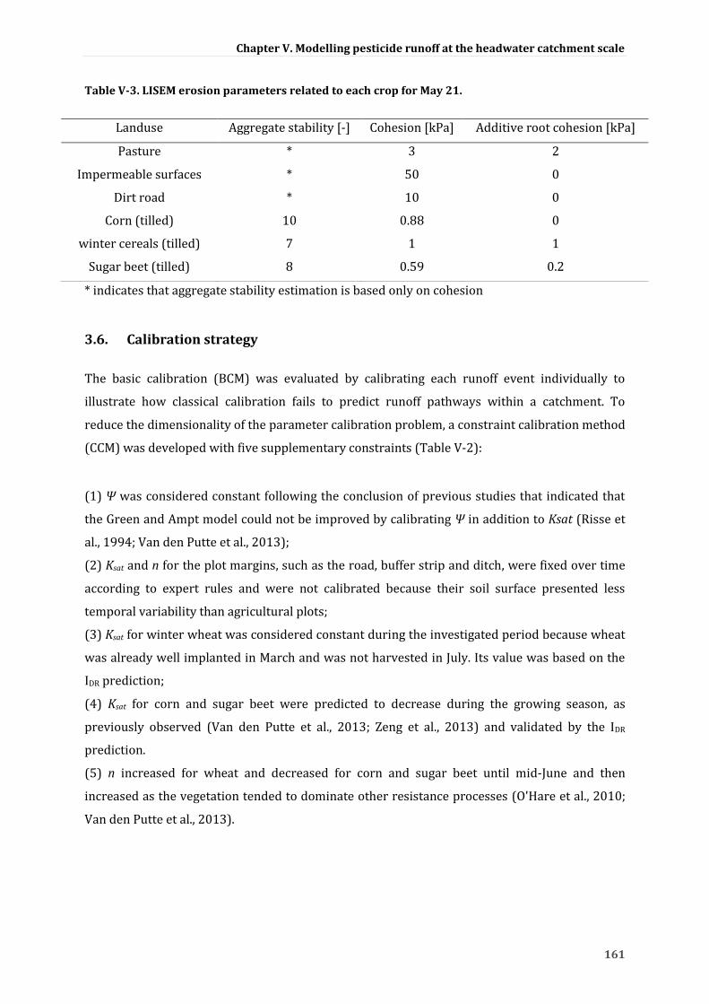
Chapter V. Modelling pesticide runoff at the headwater catchment scale

161

Table V-3. LISEM erosion parameters related to each crop for May 21.

* indicates that aggregate stability estimation is based only on cohesion

3.6. Calibration strategy

The basic calibration (BCM) was evaluated by calibrating each runoff event individually to

illustrate how classical calibration fails to predict runoff pathways within a catchment. To

reduce the dimensionality of the parameter calibration problem, a constraint calibration method

(CCM) was developed with five supplementary constraints (Table V-2):

(1) Ψ was considered constant following the conclusion of previous studies that indicated that

the Green and Ampt model could not be improved by calibrating Ψ in addition to Ksat (Risse et

al., 1994; Van den Putte et al., 2013);

(2) Ksat and n for the plot margins, such as the road, buffer strip and ditch, were fixed over time

according to expert rules and were not calibrated because their soil surface presented less

temporal variability than agricultural plots;

(3) Ksat for winter wheat was considered constant during the investigated period because wheat

was already well implanted in March and was not harvested in July. Its value was based on the

IDR prediction;

(4) Ksat for corn and sugar beet were predicted to decrease during the growing season, as

previously observed (Van den Putte et al., 2013; Zeng et al., 2013) and validated by the IDR

prediction.

(5) n increased for wheat and decreased for corn and sugar beet until mid-June and then

increased as the vegetation tended to dominate other resistance processes (O'Hare et al., 2010;

Van den Putte et al., 2013).

Landuse Aggregate stability [-] Cohesion [kPa] Additive root cohesion [kPa]

Pasture * 3 2

Impermeable surfaces * 50 0

Dirt road * 10 0

Corn (tilled) 10 0.88 0

winter cereals (tilled) 7 1 1

Sugar beet (tilled) 8 0.59 0.2

Chapter V. Modelling pesticide runoff at the headwater catchment scale

162

3.7. Model calibration and sensitivity analysis

Except for the May 21 event, the calibration was based on the outflow dynamics at the outlet of

the catchment for both calibration methods. Because ponding occurred in the retention basin

and modified the peak flow, the calibration for the May 21 event was based on the first 150 min

of the hydrograph and total exported discharge volume. The calibration and sensitivity analyses

were conducted using the PEST algorithm (Doherty, 2002). PEST uses a classical optimisation

approach based on the minima in error surfaces and incorporates the Gauss-Marquardt-

Levenberg (GML) algorithm. PEST minimises an objective function that is the sum of the

weighted square deviation between the measured and predicted outflow (Doherty, 2002). The

drawback of this method is that the algorithm might converge to a local minima depending on

the error surface and start values for the optimisation run (Cullmann et al., 2011). The initial

value for calibration is therefore crucial and must be accurately estimated before calibration.

To assess the input parameters that most significantly influenced the model results, a sensitivity

analysis that varied one factor at a time was performed using the SENSAN component of PEST

(Doherty, 2002). It was performed by increasing and decreasing each individual input variable

and parameter by 20% and examining the model output in terms of total discharge. Although the

one factor-at-a-time method overlooks the interactions and non-linear effects of the input

parameters (Saltelli et al., 2004), it provides a preliminary appreciation of the primary influence

of the input parameters on the total discharge predictions and emphasises the input parameters

for which measurement and calibration efforts are most required.

3.8. Evaluation criteria and data analysis

The predicted and observed total discharge, peak discharge and peak time discharge were first

compared at the outlet of the catchment. Comparisons of the predicted and observed

hydrographs were assessed qualitatively (visual comparison) and quantitatively based on a

multi-criteria analysis. Three criteria were calculated: (i) the Nash Suttcliff coefficient (NSE), (ii)

Kling-Gupta efficiency (KGE), and (iii) bias indicator (BIAS) (Milella et al, 2012). The NSE and

KGE assess the consistency of the peak flow with respect to the timing and discharge peaks

(Eq. 3):

𝑆 ∑ (

)

∑ (

)

(Eq. 3)

Chapter V. Modelling pesticide runoff at the headwater catchment scale

163

where i is the time step, is the observed outflow at i, is the predicted outflow at i, and

is the average observed outflow during the event. KGE (Gupta et al., 2009) is estimated as

follows (Eq. 4):

√( ) ( ) ( ) (Eq. 4)

where r is the linear correlation coefficient between the simulated and observed discharge. α

and β are determined as follows:

;

; where σ is the standard deviation, μ is the

mean value, subscript ‘s’ represents simulations, and ‘o’ represents observations. BIAS produces

a global concept of the overestimation or underestimation (Eq. 5):

𝑆

∑ (

)

∑

(Eq. 5)

Considering the complexity of the interactions among physical processes, performing the

validation at the outlet can mask important spatial variation in the catchment (Lee et al., 2012).

Therefore, for each runoff event, the predicted runoff pathways were compared to the runoff

detectors within the catchments (P1 and P2, Figure V-3) and the spatial observations after the 2

largest events on May 2 and May 21. The percentage of the catchment area where runoff

occurred and the percentage of such area hydrologically connected to the outlet via surface

runoff were calculated based on LISEM output maps with ArcGIS 10.1.

The calibrated parameters and their sensitivity were compared to the measured system

properties using the paired nonparametric Wilcoxon signed rank test and the Spearman rank

correlation test. Statistical tests were performed using the R software (R development Core

Team, 2008; version 2.6.2).

4. Results

4.1. Basic calibration method (BCM)

The basic calibration method (BCM) was first assessed by calibrating the LISEM parameters

independently for each runoff event. For the 9 runoff events, measured hydrographs were

systematically under-predicted by the BCM, as shown by the negative BIAS values (Table V-4).

The observed hydrographs were fitted by LISEM with the BCM approach (Figure VII-10),

resulting in NSE and KGE values ranging from 0.4 to 0.97 (Table V-4). On the contrary, runoff

pathways were not adequately simulated, particularly for May 2 and May 21. Although observed

runoff occurred at the two internal control points (P1 and P2) for these 2 events, only the runoff

at internal control point P1 was predicted by the BCM. According to the LISEM predictions for

Chapter V. Modelling pesticide runoff at the headwater catchment scale

164

the 9 runoff events, an average of 63% of the cereal surfaces triggered runoff and were

hydrologically connected via surface runoff to the outlet of the catchment, whereas the field

observations revealed that runoff mostly occurred on the bare soil.

As expected for the event-based calibrations (Van den Putte et al., 2013), equifinality occurred. A

clear compensation between the Ksat and Ψ parameters was observed during the partitioning

between the runoff and infiltration (Figure VII-8), and there was also a compensation between

the Ksat parameters for the different land uses. For example, the calibrated Ksat wheat increased

from 4 to 60 mm h-1 between June 11 and June 12, whereas in the same time period, Ksat corn

decreased from 60 to 6 mm h-1; This is clearly unrealistic in only one day. Contrasting runoff

pathways were predicted for a similarly predicted hydrograph at the outlet with different Ksat for

wheat and corn (Figure VII-9). The parameters obtained with BCM are therefore poorly

constrained, highly interdependent and not consistent with agronomical knowledge. These

results highlighted the weakness of calibrations performed independently for each event.

Chapter V. Modelling pesticide runoff at the headwater catchment scale

165

Table V-4. Comparisons of measured and predicted runoff events in terms of total discharge [m3], peak time discharge [min], peak discharge [L s-1] and performance criteria for each runoff events.

Total discharge [m3]

Peak discharge [L s-1]

Peak time discharge [min]

Obs CCM % Diff

Obs CCM % Diff

Obs CCM % Diff

May 2 17 26.2 54.1

16 16.6 3.6

184 188.6 2.5

May 21 10411 5800.4 -44.3

* 1929.0 *

* 235.3 *

May 23 124 165.2 33.3

105 96.6 -8.7

27 26.5 -1.9

June 7 201 179.8 -10.5

131 156.0 16.0

84 82.3 -2.0

June 11 140 137.1 -2.1

129 127.8 -0.9

19 20.5 7.9

June 12 383 177.4 -53.7

125 125.1 0.1

53 57.2 7.9

July 7 217 232.6 7.2

229 228.1 -0.4

34 33.8 -0.6

July 8 69 40.0 -42.0

30 30.0 0.0

90 111.6 24.0

July 10 22 8.1 -63.2

37 7.6 -79.5

10 13.2 32.0

BIAS KGE Nash coefficient

BCM CCM BCM CCM BCM CCM

May 2 -38.87 11.30 0.45 0.55 0.57 0.02

May 21 -0.97** 4.49** 0.69** 0.44** 0.94** 0.10**

May 23 -2.12 -0.62 0.85 0.84 0.78 0.68

June 7 -3.31 -14.70 0.96 0.82 0.97 0.82

June 11 8.88 -7.80 0.75 0.82 0.76 0.68

June 12 -28.60 -56.45 0.70 0.35 0.73 0.21

July 7 -15.17 1.81 0.52 0.76 0.53 0.52

July 8 -19.56 -48.04 0.75 0.40 0.82 -0.01

July 10 -10.85 -75.36 0.45 -0.28 0.40 -0.17

*flood retention

**between the beginning of the rainfall event and the flooding of the pipe

Chapter V. Modelling pesticide runoff at the headwater catchment scale

166

4.2. Constraint calibration method (CCM)

To overcome the limitation of the BCM strategy, the more constrained CCM approach was

developed and tested on the study site. In general, the BIAS criteria indicated that the

predictions underestimated the runoff water volume. The adequacies for the total discharge,

peak discharge, and peak time discharge between predicted and measured runoff and the NSE

are presented for the 9 runoff events (Figure VII-10). The KGE ranged between -0.28 and 0.84,

and the NSE obtained with the CCM were always lower than those obtained by the BCM;

however, certain events presented a better KGE for the CCM than the BCM (Table V-4). For May

2 and July 10, the LISEM could reproduce two peaks with the CCM compared to the BCM method

(Figure VII-10), indicating that the hydrological processes and their spatial amplitudes were

better represented. This improvement could only be confirmed with KGE for May 2 (Table V-4).

The runoff pathways were significantly improved because the runoff was observed for the

9 events at the 2 internal control points P1 and P2, which were simulated by LISEM. Moreover,

for the largest event (May 21), the predicted runoff pathways corresponded to the observations

(Figure VII-11). Fifty-four percent of the catchment surface was hydrologically connected to the

outlet via surface runoff according to the LISEM runoff mapping during the crop growing season.

As observed in the field, wheat, alfalfa and oat plots were not primary contributors to the

predicted runoff, and only 2% of the cereal areas were hydrologically connected. The slight

decrease of the criteria based on the discharge fitting was counterbalanced by a clear

improvement of the runoff pathways within the catchment.

The temporal variation of the calibrated value of θi1 (0 - 25 cm) follows the same tendency as the

measured topsoil water content (0 - 3 cm) (Figure V-4). The calibrated Ksat values varied

between 0.7 and 1.5 mm h-1 and were in the range of values obtained in previous studies for

similar agricultural catchments in temperate areas (Risse et al., 1995). Despite the constraint

rules, a small increase of Ksat for corn and sugar beet values was necessary for June 7 to improve

the predictions of runoff at P0 (Figure V-4). An increase of Ksat was previously observed during

the cropping seasons (Mubarak et al., 2009) and could partly be a result of the restructuring of

the soil 17 days after the intensive rainfall event of May 21 and the soil drying cycle (Mubarak et

al., 2009) because no rainfall occurred between May 23 and June 2.

Chapter V. Modelling pesticide runoff at the headwater catchment scale

167

Figure V-4. Temporal changes of calibrated initial water content, saturated hydraulic conductivity and manning coefficient related to the daily rainfall from May 2 to July 10 2012.

Chapter V. Modelling pesticide runoff at the headwater catchment scale

168

4.3. Sensitivity analysis of input parameters

A sensitivity analysis was conducted for each event to observe the influence of input parameters

over time on the model results and to allocate efforts in the calibration method focused on the

most influential input parameter. A sensitivity analysis of the 21 parameters of LISEM was

assessed for the CCM calibrated input parameters. The results showed that the Green and Ampt

parameters, i.e., θsat1, θi1, Ksat1, and Ψ1, were the major factors that influenced the total discharge

for the 9 runoff events (Figure V-5), which was previously shown (Sheikh et al., 2010; Zeng et al.,

2013).

Figure V-5. Relative sensitivity of total discharge [%] for 20% variation of each input parameter separately. Only parameters for which total discharge sensitivity exceeded 1% were represented. Abbreviations for the input parameters are explained in the nomenclature. Plus or minus symbol indicates 20% increase or decrease respectively. Errors bars represent the temporal variability of the sensitivity within the 9 runoff events.

Ksat2, Ψ2, and soildep2 were relatively insensitive to the total discharge (from -2 to 2% of the total

discharge for 20% of the change) (Figure V-5), suggesting the importance of the topsoil layers

for Hortonian runoff generation. The impact of vegetation interception ranged from 0.8% of the

total rainfall for the May 21 event to 19.8% for the July 10 event. The sensitivity of the leaf area

index of corn was significantly correlated with the corn coverage fractions (ρ = 0.9, p < 0.001)

and indicated that the sensitivity of the vegetation increased with the vegetation growth at the

end of the season. The sensitivity analysis of the 21 parameters did not significantly differ

Chapter V. Modelling pesticide runoff at the headwater catchment scale

169

between the 9 runoff events (p > 0.5). The sensitivity of the initial moisture on the total

discharge was lower (between 10 to 300 times less important) for intensive events, such as on

May 21, compared to other events, which was previously shown by Sheikh (Sheikh et al., 2010).

The observed runoff coefficient presented a significant negative correlation with the sensitivity

of Ksat1 to the total discharge (ρ = -0.98, p < 0.001), suggesting that Ksat1 was also less sensitive

during intensive runoff events. These results showed that conducting a sensitivity analysis on a

single event was definitely not representative of the sensitivity over a crop-growing season.

4.4. Erosion characterisation and prediction: focus on May 21

The event on May 21 was the largest event of the study period, and calibration was only possible

at the beginning of its hydrograph because discharge was not limited by the discharge capacity

of the outlet pipe. The erosion observations may help to validate the predicted runoff pathways.

The predicted deposits and eroded masses were clearly underestimated, which was expected

because of the underestimation of the total discharge (Table V-4 and V-5). However, the

simulated deposition in the vegetal barrier compared to the simulated total deposition was in

the same range as the field measurements following the event. Similarly, an identical proportion

of the flow detachment erosion compared to the total erosion was found between the field

measurements and simulations. The predicted erosion rates ranged between 6 and 82 ton ha-1

according to each plot and were represented against the observations (Figure VII-12). LISEM

strongly over-predicted the erosion rates in cereal fields and under-predicted the erosion rates

in plots 20, 21 and 22 (Figure V-3 and Figure VII-12). This result was confirmed by Takken

(1999), who observed that the spatial variation in erosion rates for different crop types was not

well-predicted. The poor spatial agreement of the spatial erosion prediction with the

observations may be partly due to the fact that the effect of tillage on the runoff pattern was not

taken into account, which may have had an important effect on the predicted local erosion rates

(Takken et al., 1996) or by an incomplete or incorrect predictive impact of vegetation on the

erosion processes. The predicted suspended solid concentrations obtained by LISEM were in the

same order of magnitude as the measured results (Table V-5).

Chapter V. Modelling pesticide runoff at the headwater catchment scale

170

Table V-5. Measured and predicted total erosion and deposition [ton] within the catchment and the total soil loss at the outlet of the catchment.

** Deposition in the plot in front of the dike was included in topographical deposition

5. Discussion and conclusion

Predicting runoff in agricultural areas is inherently difficult because of rapid changes in the

surface characteristics, hydrodynamic parameters and vegetation. Advances in model accuracy

can be achieved by investing more effort in calibration methods based on agronomical

information, spatial validation and erosion prediction.

The LISEM parameters were calibrated independently for each event (BCM approach); however,

predictions did not correctly represent the runoff pathways within the catchment despite

constraining the input parameters within their physical extent. Furthermore, the temporal

variations of the input parameters were unlikely to occur. The developed constraint calibration

approach (CCM) clearly showed that considering the temporal variability of hydrodynamic

parameters along the growing season helped to enhance the model prediction from a limited

amount of supplementary information despite a slight degradation of evaluation criteria of the

prediction at the catchment outlet. Therefore, our results confirm the observations of Risse et al.

Measured Predicted

Mass budget [ton] [%] [ton] [%]

Erosion

Rill/interrill 2414 91

Flow detachment 1445 95

Diffusive No quantified : ≈250 9

Splash detachment 78 5

Deposition

Vegetal barrier 1482 67

Sediment traps 795 63

Topography** 666 30

Other type of deposition 458 37

Headlands 63 3

Soil loss at the outlet

433 246

Mean TSS concentrations [g L-1] [g L-1]

Plot (P2) 2.9 7

Catchment (P0) 59.7 46

Chapter V. Modelling pesticide runoff at the headwater catchment scale

171

(1994) and Van den Putte et al. (2013), who stated that the performance of the Green and Ampt

model could not be improved by calibrating Ψ in addition to Ksat.

We anticipate that the CCM method is readily transposable for agricultural areas where a similar

soil surface evolution is observed. Because the main factors influencing the runoff were the

Green and Ampt parameters, the main initial assumptions regarding the homogeneity of the

initial and saturated water content (θi1 and θsat1) within the catchment and the homogeneity of

the permeability for each crop may be relaxed in future studies. The spatial variability of the soil

moisture content could have a major impact on the predictions (Craig et al., 2010; Kale and

Sahoo, 2011). Spatial variations of θi1 can be estimated with a simple soil water balance model

that can be used in continuous time periods to predict each pre-event θi (Sheikh et al., 2009).

The constant under-estimation of the total discharge, shown by the BIAS parameters for both

the BCM and CCM, could be partly explained by the drainage contribution. Drainage could also

explain the wider shape of the observed hydrographs compared to the predicted hydrographs.

The peak rainfall intensity presented a significant negative correlation with the drainage

contribution (ρ = -0.73; p < 0.05), which suggested that the drainage contribution was important

for smaller events. The observed drainage contribution showed a significant correlation with the

sensitivity of θi2 (ρ = 0.81, p < 0.05), suggesting that the humidity of the deeper layers and the

low flow component prevailed when the drainage was dominant compared to the runoff. The

frequency of significant muddy flows observed in the catchment, which were prone to soil

crusting and compaction, confirmed the major role of surface runoff.

Erosion predictions may help to validate runoff predictions. Runoff velocity reduction and

sediment deposition in headlands, when the tillage orientation changed, was not predicted by

LISEM. The impact of tillage direction on runoff and erosion pathways may be improved by the

Tillage-Controlled Runoff Pattern model (TCRP) because it can change the local flow direction

according to the tillage practices (Takken et al., 2001; van Dijk et al., 2005).

The full coupling of a distributed hydrological event-based model with an agronomical model

should be further investigated when considering the dynamics of the initial soil surface

characteristics and hydrodynamic parameters. This coupling should enhance the model

accuracy and reduce the equifinality. This future approach may help to bridge the gap between

events and continuous-based modelling.

Chapter V. Modelling pesticide runoff at the headwater catchment scale

172

6. Acknowledgements

The authors are members of REALISE, the Network of Laboratories in Engineering and Science

for the Environment in the Alsace Region (France; http://realise.unistra.fr), and the support from

REALISE is gratefully acknowledged. This research was funded by the PhytoRET project (C.21)

of the European INTERREG IV program in the Upper Rhine. Marie Lefrancq was supported by

the European INTERREG IV program in the Upper Rhine and Water Agency of Rhine Meuse. We

acknowledge, in particular, Anne-Véronique Auzet for her considerable knowledge of erosion

and soil surface states, the soil laboratory UMS830 EOST/CNRS, Martine Trautmann for the soil

analysis and Jean-Bernard Bardiaux for his hydraulic expertise. We would like to thank Gwenaël

Imfeld for helpful comments.

7. References

Aksoy, H., Kavvas, M.L., 2005. A review of hillslope and watershed scale erosion and sediment transport

models. Catena. 64, 247-271.

Alaoui, A., Lipiec, J., Gerke, H.H., 2011. A review of the changes in the soil pore system due to soil

deformation: A hydrodynamic perspective. Soil & Tillage Research. 115, 1-15.

Ali, B., 2008. Typologie fonctionnelle des états de surface du sol [EDS] pour l’extrapolation des propriétés

hydro-érosives. . Thèse, Université Louis Pasteur de Strasbourg – CNRS. Institut de Mécanique

des Fluides et des Solides. 206 pp.

Armand, R., Bockstaller, C., Auzet, A.V., Van Dijk, P., 2009. Runoff generation related to intra-field soil

surface characteristics variability Application to conservation tillage context. Soil & Tillage

Research. 102, 27-37.

Augustin, L.N., Irish, J.L., Lynett, P., 2009. Laboratory and numerical studies of wave damping by emergent

and near-emergent wetland vegetation. Coastal Engineering. 56, 332-340.

Baartman, J.E.M., Jetten, V.G., Ritsema, C.J., de Vente, J., 2012. Exploring effects of rainfall intensity and

duration on soil erosion at the catchment scale using openLISEM: Prado catchment, SE Spain.

Hydrological Processes. 26, 1034-1049.

Berthet, L., Andreassian, V., Perrin, C., Javelle, P., 2009. How crucial is it to account for the antecedent

moisture conditions in flood forecasting? Comparison of event-based and continuous

approaches on 178 catchments. Hydrology and Earth System Sciences. 13, 819-831.

Beven, K., 2006. A manifesto for the equifinality thesis. Journal of Hydrology. 320, 18-36.

Chow, V., Maidment, D., Mays, L., 2013. Applied Hydrology, 2nd Edition, Vol., McGraw-Hill

Companies,Incorporated.

Cosby, B.J., Hornberger, G.M., Clapp, R.B., Ginn, T.R., 1984. A Statistical Exploration of the Relationships of

Soil-Moisture Characteristics to the Physical-Properties of Soils. Water Resources Research. 20,

682-690.

Chapter V. Modelling pesticide runoff at the headwater catchment scale

173

Craig, J.R., Liu, G., Soulis, E.D., 2010. Runoff-infiltration partitioning using an upscaled Green-Ampt

solution. Hydrological Processes. 24, 2328-2334.

Cullmann, J., Krausse, T., Saile, P., 2011. Parameterising hydrological models - Comparing optimisation and

robust parameter estimation. Journal of Hydrology. 404, 323-331.

de Jong, S.M., Jetten, V.G., 2007. Estimating spatial patterns of rainfall interception from remotely sensed

vegetation indices and spectral mixture analysis. International Journal of Geographical

Information Science. 21, 529-545.

DeRoo, A.P.J., Wesseling, C.G., Ritsema, C.J., 1996. LISEM: A single-event physically based hydrological and

soil erosion model for drainage basins .1. Theory, input and output. Hydrological Processes. 10,

1107-1117.

Doherty, J., 2002. PEST Model-Independent Parameter Estimation. Watermark Numerical Computing.

Dotterweich, M., 2013. The history of human-induced soil erosion: Geomorphic legacies, early descriptions

and research, and the development of soil conservation-A global synopsis. Geomorphology. 201,

1-34.

Dunne, T., Black, R.D., 1970. Partial Area Contributions to Storm Runoff in a Small New England

Watershed. Water Resources Research. 6, 1296-1311.

Durán-Zuazo, V.H., Francia-Martínez, J.R., García-Tejero, I., Tavira, S.C., 2013. Implications of land-cover

types for soil erosion on semiarid mountain slopes: Towards sustainable land use in

problematic landscapes. Acta Ecologica Sinica. 33, 272-281.

Edwards, W.M., Owens, L.B., 1991. Large Storm Effects on Total Soil-Erosion. Journal of Soil and Water

Conservation. 46, 75-78.

Efstratiadis, A., Koutsoyiannis, D., 2010. One decade of multi-objective calibration approaches in

hydrological modelling: a review. Hydrological Sciences Journal-Journal Des Sciences

Hydrologiques. 55, 58-78.

Evrard, O., Cerdan, O., van Wesemael, B., Chauvet, M., Le Bissonnais, Y., Raclot, D., Vandaele, K., Andrieux,

P., Bielders, C., 2009. Reliability of an expert-based runoff and erosion model: Application of

STREAM to different environments. Catena. 78, 129-141.

Fiener, P., Auerswald, K., Van Oost, K., 2011. Spatio-temporal patterns in land use and management

affecting surface runoff response of agricultural catchments-A review. Earth-Science Reviews.

106, 92-104.

Green, T.R., Ahuja, L.R., Benjamin, J.G., 2003. Advances and challenges in predicting agricultural

management effects on soil hydraulic properties. Geoderma. 116, 3-27.

Gupta, H.V., Kling, H., Yilmaz, K.K., Martinez, G.F., 2009. Decomposition of the mean squared error and NSE

performance criteria: Implications for improving hydrological modelling. Journal of Hydrology.

377, 80-91.

Heitz, C., Flinois, G., Glatron, S., 2012. Protection against muddy floods: perception for local actors in

Alsace

(France) of a protection measure (fascines). International Disaster Risk Conference, Davos,

Suisse, 26-30 Août 2012.

Chapter V. Modelling pesticide runoff at the headwater catchment scale

174

Hessel, R., van den Bosch, R., Vigiak, O., 2006. Evaluation of the LISEM soil erosion model in two

catchments in the East African Highlands. Earth Surface Processes and Landforms. 31, 469-486.

Hessel, R., Jetten, V., 2007. Suitability of transport equations in modelling soil erosion for a small Loess

Plateau catchment. Engineering Geology. 91, 56-71.

Hunt, R., 1982. Plant growth curves. Edward Arnold, London, 248.

Kale, R.V., Sahoo, B., 2011. Green-Ampt Infiltration Models for Varied Field Conditions: A Revisit. Water

Resources Management. 25, 3505-3536.

Kamphorst, E.C., Jetten, V., Guerif, J., Pitkanen, J., Iversen, B.V., Douglas, J.T., Paz, A., 2000. Predicting

depressional storage from soil surface roughness. Soil Science Society of America Journal. 64,

1749-1758.

Kirchner, J.W., 2006. Getting the right answers for the right reasons: Linking measurements, analyses, and

models to advance the science of hydrology. Water Resources Research. 42.

Kohler, M.A., Linsley, R.K., 1951. Predicting the runoff from storm rainfall. US weather Bureau Res.

Kutílek, M., Nielsen, D.R., 1994. Soil hydrology, Vol., Catena Verlag.

Lee, G., Tachikawa, Y., Sayama, T., Takara, K., 2012. Catchment responses to plausible parameters and

input data under equifinality in distributed rainfall-runoff modeling. Hydrological Processes. 26,

893-906.

Li, Z., Zhang, J.T., 2001. Calculation of field Manning's roughness coefficient. Agricultural Water

Management. 49, 153-161.

Liu, G.B., Xu, M.X., Ritsema, C., 2003. A study of soil surface characteristics in a small watershed in the hilly,

gullied area on the Chinese Loess Plateau. Catena. 54, 31-44.

Meijer, A.D., Heitman, J.L., White, J.G., Austin, R.E., 2013. Measuring erosion in long-term tillage plots using

ground-based lidar. Soil & Tillage Research. 126, 1-10.

Merritt, W.S., Letcher, R.A., Jakeman, A.J., 2003. A review of erosion and sediment transport models.

Environmental Modelling & Software. 18, 761-799.

Milella, P., Bisantino, T., Gentile, F., Iacobellis, V., Liuzzi, G.T., 2012. Diagnostic analysis of distributed input

and parameter datasets in Mediterranean basin streamflow modeling. Journal of Hydrology.

472, 262-276.

Mitasova, H., Barton, M., Ullah, I., Hofierka, J., Harmon, R.S., 2013. 3.9 GIS-Based Soil Erosion Modeling. In:

Treatise on Geomorphology. Vol., J.F. Shroder, ed.^eds. Academic Press, San Diego, pp. 228-258.

Morgan, R.P.C., Quinton, J.N., Smith, R.E., Govers, G., Poesen, J.W.A., Chisci, G., Torri, D., 1998. The EUROSEM

model. Modelling Soil Erosion by Water. 55, 389-398.

Mubarak, I., Mailhol, J.C., Angulo-Jaramillo, R., Ruelle, P., Boivin, P., Khaledian, M., 2009. Temporal

variability in soil hydraulic properties under drip irrigation. Geoderma. 150, 158-165.

O'Hare, M.T., McGahey, C., Bissett, N., Cailes, C., Henville, P., Scarlett, P., 2010. Variability in roughness

measurements for vegetated rivers near base flow, in England and Scotland. Journal of

Hydrology. 385, 361-370.

Pare, N., Andrieux, P., Louchart, X., Biarnes, A., Voltz, M., 2011. Predicting the spatio-temporal dynamic of

soil surface characteristics after tillage. Soil & Tillage Research. 114, 135-145.

Chapter V. Modelling pesticide runoff at the headwater catchment scale

175

Potter, K.N., 1990. Soil Properties Effect on Random Roughness Decay by Rainfall. Transactions of the

Asae. 33, 1889-1892.

Risse, L.M., Nearing, M.A., Savabi, M.R., 1994. Determining the Green-Ampt Effective Hydraulic

Conductivity from Rainfall-Runoff Data for the Wepp Model. Transactions of the Asae. 37, 411-

418.

Risse, L.M., Nearing, M.A., Zhang, X.C., 1995. Variability in Green-Ampt Effective Hydraulic Conductivity

under Fallow Conditions. Journal of Hydrology. 169, 1-24.

Saltelli, A., Tarantola, S., Campolongo, F., Ratto, M., 2004. Sensitivity Analysis in Practice: A Guide to

Assessing Scientific Models, Vol., Wiley.

Sanchez-Moreno, J.F., Mannaerts, C.M., Jetten, V., Loffler-Mang, M., 2012. Rainfall kinetic energy-intensity

and rainfall momentum-intensity relationships for Cape Verde. Journal of Hydrology. 454, 131-

140.

Sheikh, V., Visser, S., Stroosnijder, L., 2009. A simple model to predict soil moisture: Bridging Event and

Continuous Hydrological (BEACH) modelling. Environmental Modelling & Software. 24, 542-

556.

Sheikh, V., van Loon, E., Hessel, R., Jetten, V., 2010. Sensitivity of LISEM predicted catchment discharge to

initial soil moisture content of soil profile. Journal of Hydrology. 393, 174-185.

Takken, I., Beuselinck, L., Nachtergaele, J., Govers, G., Poesen, J., Degraer, G., 1999. Spatial evaluation of a

physically-based distributed erosion model (LISEM). Catena. 37, 431-447.

Takken, I., Govers, G., Jetten, V., Nachtergaele, L., Steegen, A., Poesen, J., 2001. Effects of tillage on runoff

and erosion patterns. Soil & Tillage Research. 61, 55-60.

Tramblay, Y., Bouvier, C., Martin, C., Didon-Lescot, J.F., Todorovik, D., Domergue, J.M., 2010. Assessment of

initial soil moisture conditions for event-based rainfall-runoff modelling. Journal of Hydrology.

387, 176-187.

Van den Putte, A., Govers, G., Leys, A., Langhans, C., Clymans, W., Diels, J., 2013. Estimating the parameters

of the Green-Ampt infiltration equation from rainfall simulation data: Why simpler is better.

Journal of Hydrology. 476, 332-344.

Van Dijk, P., Villerd, J., Koller, R., Bockstaller, C., in prep. A predictive indicator for overland flow potential

of cropping systems: accounting for farmers’ control on key variables.

Van Dijk, P.M., Auzet, A.V., Lemmel, M., 2005. Rapid assessment of field erosion and sediment transport

pathways in cultivated catchments after heavy rainfall events. Earth Surface Processes and

Landforms. 30, 169-182.

Wallner, M., Haberlandt, U., Dietrich, J., 2013. A one-step similarity approach for the regionalization of

hydrological model parameters based on Self-Organizing Maps. Journal of Hydrology. 494, 59-

71.

Xu, Q.X., Wang, T.W., Cai, C.F., Li, Z.X., Shi, Z.H., Fang, R.J., 2013. Responses of Runoff and Soil Erosion to

Vegetation Removal and Tillage on Steep Lands. Pedosphere. 23, 532-541.

Zeng, C., Wang, Q.J., Zhang, F., Zhang, J., 2013. Temporal changes in soil hydraulic conductivity with

different soil types and irrigation methods. Geoderma. 193, 290-299.

Chapter V. Modelling pesticide runoff at the headwater catchment scale

176

LISEM provided consistent prediction i) of discharge, volume at the outlet of the studied crop

catchment and ii) of the runoff pathways within the catchment associated to runoff events along

a crop growing season. A mathematical formalism for assessing dissolved pesticide runoff

transport was therefore developed and integrated in LISEM to evaluate different study case

scenarios. The mathematical formalism is introduced in the following section.

Chapter V. Modelling pesticide runoff at the headwater catchment scale

177

Section 2. A comprehensive mathematical model for

mobilisation and transport of dissolved pesticide from the soil surface to runoff: the mixing layer approach.

1. Introduction

On soil surfaces, runoff and associated erosion represent a primary mode of mobilisation and

transfer of pesticides from agricultural land to surface water (Oliver et al., 2012). Pesticide

mobilisation from soil into runoff involves complex combination of various transport

mechanisms including raindrop-driven processes, diffusion induced by the pesticide

concentration gradient, erosion of sediment with adsorbed pesticide and adsorption/desorption

of pesticides in soil-water systems (Gao et al., 2005; Shi et al., 2011; Wallach et al., 2001). Many

models have been developed for predicting pesticide transfer between soil-water and runoff

(Borah and Bera, 2003; Holvoet et al., 2007; Kohne et al., 2009; Payraudeau and Grégoire, 2012;

Quilbe et al., 2006).

Predicting runoff, erosion and the subsequent transport of pesticides in agricultural areas is

inherently difficult because of rapid changes in soil surface characteristics and hydrodynamic

parameters. Currently, few pesticide runoff models account for the effects of agricultural

practices on hydrodynamic parameters and soil surface characteristics and most of them are

deemed inappropriate for investigating headwater catchment scale with a very fine temporal

resolution (≤ 1 min) (Chap. I. §2.2.4). This emphasises the need for an event based, spatially

distributed pesticide transport model at the catchment scale integrating changes in soil surface

characteristics and soil hydrodynamic parameters (Payraudeau and Grégoire, 2012). LISEM

(Limbourg Soil Erosion Model), an event based model, that is fully distributed, was designed to

explicitly describe the soil surface structures including crusted and compacted zones, and the

diversity of agricultural landscape components, i.e. plots and plots margins in headwater

catchments (Liu et al., 2003). An additional reason, which has motivated the selection of LISEM,

lies in its consideration for erosion processes which opens doors for further investigation on

solid-bound pesticide prediction. The objective of this study was therefore to predict the

mobilisation and the transport of dissolved pesticide in runoff.

Pesticide mobilisation between soil, soil water and runoff is usually modelled as either a

diffusion-like process or a mixing model (Gao et al., 2005; Shi et al., 2011). In the diffusion

Chapter V. Modelling pesticide runoff at the headwater catchment scale

178

models, a boundary layer is described as an interfacial diffusion-controlled process driven by the

concentration gradient. The mixing layer concept is probably the most commonly used in

pesticide fate models due to its numerical simplicity and its realistic representation, as

hortonian runoff processes have repeatedly been shown to be initiated as a near-surface process

(Gao et al., 2004; McGrath et al., 2008; Wallender et al., 2008). This concept assumes that the

transport is controlled by a mixing layer below the soil surface, in which rainwater, soil solution

and runoff water completely and instantaneously mix (Havis et al., 1992). The soil depth

interacting with runoff water is variable ranging from 0.25 to 2 cm according to various

experimental and modelling studies (Ahuja et al., 1981; Havis et al., 1992; Wallender et al.,

2008). Previous studies have shown that the effective depth of interaction is related to the

degree of soil aggregation and increases with soil slope, kinetic energy of raindrops and rainfall

intensity (Havis et al., 1992). In fact, the observed mixing-layer depth is often much shallower

than the depth required for fitting models to field data (Gao et al., 2004). In reality, rainfall water

and soil water are incompletely mixed because soil water inside soil aggregates is partly

inaccessible and the hydraulic turbulences produced by rainfall impact decrease with depth (Shi

et al., 2011). The concept of a ‘film transport coefficient’ was therefore introduced to describe

the transfer rate between soil water and runoff water (Havis et al., 1992; Shi et al., 2011). In

dynamic conditions existing in the field, pesticide sorption equilibrium could take several hours

(Lafrance and Caron, 2012). Given the short time steps used in the model (≤ 1 min), a first-order

kinetic reaction was used to describe pesticide sorption/desorption in the mixing zone

(Wallender et al., 2008).

Combining chemical processes, i.e. sorption and diffusion, and transport processes requires

significant computational effort due to the non-linearity of the equations (Wallach et al., 2001).

Two main approaches exist to solve the coupled equations for transient flow and solute

transport: (i) the operator splitting approach, in which the transport via runoff and the

chemistry are solved sequentially, and (ii) the one-step global implicit approach in which the

transport and the chemistry equations are solved simultaneously (Jacques et al., 2006). Operator

splitting techniques are often used to solve complex equation systems by splitting the governing

equations into sub-equations, wherein each subset of equations capture a portion of the physics

present in the system (Ren et al., 2014). Among the operator splitting techniques, the sequential

non-iterative approach (SNIA) consists in solving sequentially the transport then the chemistry

part of the problem without iteration (Carrayrou et al., 2004). Operator splitting techniques

provide efficient numerical approaches for developing resolution modules separately and

including them in an existing physically based-model (Lagneau and van der Lee, 2010).

However, the operator splitting techniques often lead to mass balance errors and impose small

Chapter V. Modelling pesticide runoff at the headwater catchment scale

179

time steps during fast chemical kinetics (Carrayrou et al., 2004). In contrast, the main

advantages of the global implicit method are that all processes are solved simultaneously, the

method is mass-conservative and the approach is less sensitive to the large time step (Jacques et

al., 2006), which may be an important consideration to address pesticide mobilisation and

transport at catchment scale. However, this method is generally more complex mathematically

and may require large computing memory (Jacques et al., 2006). To the best of our knowledge,

very few studies used (pseudo-)analytical resolution, i.e. an analytical solution after spatial

differentiation, to solve the implicit numerical schemes. This type of resolution may reduce the

computing errors due to discretisation errors associated with the operator approximations

(Carrayrou et al., 2004).

Two different numerical approaches were therefore tested and compared in order to (i)

evaluate the influence of the solution procedure, (ii) retain the best approach for evaluating

pesticides mobilisation and transport in runoff at catchment scale, and (iii) ensure an acceptable

mass balance both for water and pesticide. First, an operator splitting approach (SNIA) was used

to solve the pesticide mobilisation and transport equations (LISEM-psni model). The second

approach considered a pseudo-analytical solution of the global implicit method (LISEM-pa

model). Accuracy and robustness of LISEM-psni and LISEM-pa models were estimated by

comparing results against the theoretical tests and the experimental data. By using a mass

balance formulation and testing their stability over different time steps, both schemes were

compared on three test cases: (i) steady state flow on one cell (1m²), (ii) an experimental case

under constant rainfall at plot scale (4.5 m²) (Joyce, 2008) and (iii) a rainfall-runoff event in the

Alteckendorf study catchment (470,000 m²) (previously presented in Chapter IV).

Chapter V. Modelling pesticide runoff at the headwater catchment scale

180

2. Mathematical theory and approach

2.1. Openlisem

Openlisem is an accessible and easy-to-use version of the soil erosion model LISEM

(DeRoo et al., 1996). Openlisem is implemented in C++. Version 1.79 was used and modified

under the cross-platform Qt version 4.8.3 (http://qt-project.org/) and the Visual Studio

debugging tool 2010 (http://msdn.microsoft.com). The theory and structures of LISEM were

described previously (Chap.V - Section 1-§2.4 and Annex 1). Only hydrological equations and

numerical schemes, which are needed for the pesticide-water coupling are detailed here. Briefly,

the water partitioning between infiltration and surface runoff was calculated with the Green and

Ampt equations solved explicitly (Eq. 1) (Kutílek and Nielsen, 1994).

sat iθ θ

1inf sat

hq K

F

(Eq. 1)

where qinf is the infiltration rate [m s-1], Ksat the saturated hydraulic conductivity [m s-1], F the

cumulative infiltration from the beginning of the event [m], the average matrix suction at the

wetting front [m], h the overpressure depth of the water layer at the soil surface [m], sat the

saturated water content [-] and i the initial water content of the soil layer [-]. Flow velocity was

calculated for the infiltration surplus, i.e. surface runoff, with the Manning equation and surface

runoff was routed over the landscape with the 1D kinetic wave equation (quasi 2D) (Eq. 2). The

kinematic wave method is based on Chow et al. (2013) which combines the momentum and

mass conservation equations in a classic way:

A Q

qt x

(Eq. 2)

where A is the wet cross section [m²], Q the discharge [m3 s-1], q the infiltration surplus [m² s-1]

and x and t the localisation [m] and time [s]. When surface runoff was routed over a grid cell that

still had the capacity to infiltrate inside the kinematic wave routine, infiltration took place. The

relation between A and Q is given by:

23

A Q

nP

S

(Eq. 3)

where P is the wet perimeter [m], n the Manning’s coefficient [-], S the sine of the slope gradient

and β is a constant (0.6). Differentiation and combination of equations 2 and 3 gave the implicit

Chapter V. Modelling pesticide runoff at the headwater catchment scale

181

numerical scheme (Eq. 4) which was solved using a Newton backward-difference method (Chow

et al., 2013).

1

1 1 11 11 1 1

1

1 with

2

n n n nn ni i i ii i

Q QQ q

t x

Q Q Q QQ q Q Q Q

t x

(Eq. 4)

where n is the current time step, n+1 the end of the time step, i the upstream side of a grid cell,

i+1 the downstream side of grid cell,

11

niQ the new discharge [m3 s-1], 1n

iQ the new discharge at

the “upstream end” of the grid cell which is the sum of all incoming water generated by the

kinematic wave [m3 s-1], 1

niQ the discharge of the previous time step which is outflowing the grid

cell [m3 s-1], Q the diagonal average discharge in a space time diagram [m3 s-1], q the average

infiltration surplus over the length of the grid cell [m² s-1]. At each time step, the grid cells were

re-arranged in order to start the flow calculation at the top of the branches of the drainage

network and progress towards the outlet, using as input for the downstream grid cell the sum of

the discharges of the upstream grid cells at the end of the time step.

As a future objective is to predict solid-bound pesticide transport, consistency with the

numerical scheme used to solve the sediment and pesticide transport equations was targeted.

Before computing the kinematic wave, splash, flow detachment and sediment deposition were

solved separately based on rainfall intensity and updated velocity calculated with effective

rainfall depth. Erosion procedures give an intermediate sediment concentration noted *C

(calculations are not detailed here). Suspended sediment in runoff is then routed using a similar

equation as equation 2:

0sQ CA

x t (Eq. 5)

where sQ is the sediment flux [kg s-1] and C the sediment concentration [kg m-3]. After

differentiation and discretisation, we have:

Chapter V. Modelling pesticide runoff at the headwater catchment scale

182

1 1 1 * 11, 1 , 1 1 1 1

1 1 1 * 11, 1 1 1 1 1

1 *, , 1

11

where and

s

n n n n ns i s i i i i i

n n n n ns i i i i i i

ns i s i

ni i

Q C AA C e d

x t t

Q Q C C Q QA C Q e d

x t t

Q Qs C C Q QQ C Q e d

x t t

Q QA Q C

Q Q

n

(Eq. 6)

Where * indicates that concentration and flux are intermediary and yet considering the erosion

or deposition processes of the new time step. Therefore, equation 6 was rewritten to calculate

the new sediment flux (Eq. 7).

*1 1 1, 1

, 1 11 1

, 1

11

( )n n ns is i i in

n is i

ni

QQ x tQ C Q x Q Q

QQ

xt Q

Q

(Eq. 7)

2.2. Mixing model

Pesticide mobilisation at the soil/surface runoff interface was predicted by assuming

that a very thin layer at the soil surface exists where water from infiltration, runoff and soil pore

mix instantaneously (Wallender et al., 2008). The developed conceptual model is shown in

Figure V-6.

Pesticide loss below the mixing zone was considered as a sink term as the modelling focused on

pesticide transport in runoff. The governing equations describing pesticide transport in runoff

water were as follows:

film M inf

film M inf M b

1=K (C -C)-q C+

x

= K (C-C )+q (C-C )- ( )

( )

p

Ms r D M s

sr D M s

QAC

x t

Ck K C C

t

Ck K C C

t

(Eq. 8)

Where Qp is pesticide flux [kg s-1], A the wet cross section [m2], qinf the infiltration rate [m s-1],

Kfilm the film transport coefficient [m s-1], kr the rate of desorption [s-1], KD soil water partition

coefficient [m3 kg-1], C the pesticide concentration in runoff [kg m3], CM the pesticide

Chapter V. Modelling pesticide runoff at the headwater catchment scale

183

concentration in the soil water in the mixing zone [kg m3], Cs the mass of pesticides adsorbed per

dry unit weight of soil in the mixing zone [kg kg-1], θs the soil porosity [m3 m-3], ε the mixing layer

depth [m] and ρb the soil bulk density [kg m-3]. This three equations’ system is valid only if runoff

occurs. Two hydrological cases were therefore considered: (1) runoff and (2) no runoff. The

numerical limit (Qlim) for considering runoff has been defined as a minimum condition on the

discharge outflowing the grid cell (Q) and its value is discussed further. The case without runoff

was treated similarly in both resolution approaches. When Q < Qlim during runoff recession,

exchanges via the Kfilm coefficient between runoff and mixing layer were interrupted and

pesticide mass currently in runoff was infiltrated and transported over the system until

pesticide runs out.

Figure V- 6. Conceptual mixing layer model for pesticide mobilisation (Adapted from Wallender (2008))

2.3. Numerical resolution with operator splitting (LISEM-psni)

The transport and chemical set of equations were first solved similarly to the sediment transport

resolution in LISEM leading to the development of LISEM-psni. The resolution consisted in the

sequential resolution of the chemical set of equations, noted with χ-subscript (Eq. 9) and

transport equations, noted with T-subscript (Eq. 10).

film M inf

film M inf M b

C=K (C -C)-q C

1= (K (C-C )+q (C-C )- ( ))

( )

Mr D M s

s

sr D M s

t

Ck K C C

t

Ck K C C

t

(Eq. 9)

Chapter V. Modelling pesticide runoff at the headwater catchment scale

184

CA

x

p

T

Q

t (Eq. 10)

For the case of runoff, equations concerning pesticides in the soil water and the solid-phase of

soil were equivalent to the differential equations system in matrix form (Eq. 11):

inf inf( ).

0

Mfilm b r D filmb r

M

s s s

ss

r D r

bA

C K q k K K q CkCt

CCk K k

t

(Eq. 11)

If pesticide concentration in runoff water (C) was supposedly constant over a time step and

known from the previous time step (Cn), the system (11) is a system of first-order linear

differential equations and has therefore an unique vector-values solution (C,CM,CS) for any given

initial vector-values (C0,CM0,CS0). Analytical expressions for CS and CM were therefore computed

with Maple 17©. A potential mass of pesticide in runoff (Mrunoff) was then calculated as

follows:

( 1)

1inf( ) ² ²

runoff runoff

n t

n n nfilm film M

n t

M M K q x tC K x C dt (Eq. 12)

Where Δt is the time step, Δx the spatial resolution, (n+1)Δt the new time of the calculation and

nΔt the precedent time of calculation. Large time steps may lead to the calculation of negative

pesticide masses in runoff. To avoid numerical problems during simulations, negative 1nrunoffM

values were artificially set to zero which may lead to inaccuracy in predicted pesticide

concentrations. The obtained mass of pesticide leads to the calculation of an intermediate

pesticide concentration in runoff C* by considering the water volume in the cell at time n+1. This

calculation is performed for all cells before moving to the next time step. Since the resolution

was done from upstream to downstream, the transport equation (Eq. 10) was developed using

the approach used for sediment transport resolution. Therefore, pQ is the pesticide flux [kg s-1]

defined by (Eq. 14).

0pQAC

t x

(Eq. 13)

*p, 11 1 1

p, 1 11 1

p, 1

11

( )in n ni i in

n ii

ni

QtQ Q x C Q x Q Q

QQ

xt Q

Q

(Eq. 14)

Chapter V. Modelling pesticide runoff at the headwater catchment scale

185

2.4. Pseudo-analytical resolution (LISEM-pa)

The transport and chemical set of equations were solved analytically after spatial discretisation

leading to the development of LISEM-pa. The first equation of the system (10) was transformed

by differentiating the temporal derivation and by assuming that the wetted section, A, was

constant over a time step (Eq. 15).

inf

inf

p

M

p

M

QACx K C C q C

t x

QCA x K C C q C

t x

(Eq. 15)

The system of ordinary differential equations is then:

1 1 1

inf

1 1 1

inf

11

inf

(

(

1)

n n n

upstream upstream

film M film

n n n

upstream upstream

film M film

nnfilm upstream

film M upstr

Q C Q CCK C C K qA x

t x

Q C Q CCK C C K qQ x

t x

K x QC QK x q x C C C

t Q x Q Q x

1n

eam

(Eq. 16)

Therefore, the system (1) and the development (16) can be converted in the following matrix

form:

inf

inf inf

0

0

0 0

1where ) ;

;

;

MM

ss

bA

film

film

film film b r D

s s

b rr D

s

C

t Ca b kC

Cd e ft

Ch iC

t

K xQa K x q x b

Q x Q

K q K q k Kd e

kf h k K

1

1 ; ; k=nupstream n

r upstream

Qi k C

Q x

(Eq. 17)

Chapter V. Modelling pesticide runoff at the headwater catchment scale

186

The entries of the matrix A are constant over each time step. The system (17) has an unique

vector-values solution (C, CM, CS) for any given initial vector-values (C0, CM0, CS0). In order to

compute the vector-values solution, eigenvalues and eigenvectors of the matrix A were

calculated. The eigenvalues of the matrix A are the roots of the characteristic polynomial which

is a cubic real polynomial. These eigenvalues are the solutions of equation 18:

3 2

3 2

( ) (i ) ( ) 0P x x e a x hf ie ia db ea x hfa idb iea

x x x

(Eq. 18)

The nature of the roots of P depends on the sign of its discriminant defined by:

2 2 3 3 218 4 4 27 (Eq. 19)

According to the sign of Δ, it leads to three cases:

Case 1: If Δ= 0, the polynomial P has a multiple root and all roots are real (λ0, λ0, λ0) or (λ0, λ0, λ1)

Case 2: If Δ > 0, the polynomial P has three real roots in the form (λ1, λ2, λ3)

Case 3: If Δ < 0, the polynomial P has one real root and two non-real conjugate roots (λ1, λ2,2 ).

A particular solution of the equation system is noted xp. For the case 1, general solutions are

detailed in Annex 1. For case 2, the general solution is:

31 2

1 2 31 2 3( ) ( ) tt tp p p px t C v e C v e C v e x t (Eq. 20)

And for case 3, the general solution is:

1 2

1 2 2

2

2 2

1 2

3

( ) ( cos( ) sin( ))

( sin( ) cos( )) ( )

t tp r p i p

tr p i p p

x t C v e C e v bt v bt

C e v bt v bt x t (Eq. 21)

where jrpv denotes the real part of the eigenvector related to j and

jipv denotes the complex

part. As the sign of Δ was not known, the three cases were implemented in the model. The sign

of Δ was tested using 100,000 Monte Carlo simulations within the physical extent of each

parameter involved in the matrix A entries. These parameters and their physical extent are

detailed in Table V-6. The results showed that the sign of Δ remains positive for all the Monte

Carlo simulations, which indicates that the general solution (20) is mostly to occur.

Chapter V. Modelling pesticide runoff at the headwater catchment scale

187

Table V-6. Parameters involved in the pesticides mobilisation and transport resolution and their physical range.

Parameters units range

Spatial discretisation (Δx) [m] 1 - 10

Pe

stic

ide

s

Film transport coefficient (Kfilm) [m s-1] 0 - 10-3

Desorption rate (kr) [s-1] 0 - 1

Porosity [-] 0.2 - 0.6

Depth of the mixing layer (ε) [m] 10-3 - 10-1

Soil water partition coefficient (KD) [m3 kg-1] 0 - 10-1

Soil bulk density (ρ) [kg m-3] 1200 - 1800

Hy

dro

log

y

Manning coefficient [-] 0.01 - 0.5

Water height (h) [m] 10-10 - 10-1

Slope [m m-1] 0.001 - 0.8

infiltration rate (qinf) [m s-1] 0 - 10-4

2.5. Mass balance errors calculations

Mass balance errors were calculated at every time step. For both numerical approaches, LISEM-

pnsi and LISEM-pa, a cumulative mass balance error (Merr) was calculated within the same

approach (Eq 22):

1 1 1 1

, ,Pesticides

in runoff waterPesticides in Pesticides sorbed soil water on the soil

( 1)

inf,

Pesticides leav

( ² ²

²

n n n nerr applied M s s b runoff

i j i j

n t

Mn i j n t

M M C x C x M

q x C dt

( 1)

1

ing Pesticides leaving the system by infiltration the system by surface runoff

² ) 100n t

noulet applied

n n t

Q x Cdt M

(Eq. 22)

Where appliedM is the pesticide mass initially present in the system [kg], i and j refer to the space

coordinated, n refers to the time step.

Chapter V. Modelling pesticide runoff at the headwater catchment scale

188

2.6. Case study scenarios

Three test cases were analysed for evaluating both numerical schemes, i.e. LISEM-psni and

LISEM-pa (Figure V-7).

Figure V- 7. Schemes of the three case study scenarios

Specific input parameters for each test case were detailed in Table V-7.

The first test considered the transport and the mobilization of one hypothetical pesticide

through one cell (1 m²) in steady state flow and upstream runoff conditions. The cell was

subjected to constant rainfall and constant flux of pesticides [kg s-1]

6 3 6 3 1(50 10 9 10 )kg m m s until reaching the steady state of pesticide

concentrations in the three compartments (runoff, soil and soil water). This test case was

used to evaluate the influence of time step and of the Qlim value on the predicted

concentrations and to verify the accuracy of the algorithms, as the exact steady state

solution is known.

The second test consisted in predicting pesticide mobilisation and transport from the

soil surface under experimental conditions in a plot of 4.5 m² under artificial rainfall

published by Wallender et al., (2008). The accuracy of the model was evaluated against

experimental data.

The last test consisted in predicting pesticide mobilisation and transport from a

contaminated soil surface based on non-homogeneous pesticide application

(S-metolachlor was applied on 29.8% of the catchment area) on the study catchment of

Alteckendorf (470,000 m²). Predictions were grounded on the hydrological modelling

previously explained (Chap V -Section 1) and compared with the experimental data

Chapter V. Modelling pesticide runoff at the headwater catchment scale

189

previously presented (Chap IV). Two runoff events, May 21 and June 7, were selected for

two reasons: (i) the selected runoff events were well predicted by LISEM in terms of

runoff pathways and discharge rate at the catchment outlet. (ii) they were associated

with contrasting runoff hydrological forcing with 41 and 4% runoff coefficients (yielding

to 10,568 and 208 m3), respectively and they occurred on average 15 days and 32 days

after S-metolachlor applications.

Table V-7. Description of the input parameters of LISEM-psni and LISEM-pa in the three different study scenarios

3. Results and discussion

3.1. Steady test case

A simple case at steady state was used to evaluate the stability and the accuracy of both

numerical schemes, i.e. LISEM-pnsi and LISEM-pa. Once steady state is reached for transport,

LISEM-pnsi and LISEM-pa solutions were almost the same (48.39 µg L-1 in runoff) and reached

the theoretical solution with the same error of 0.54% according to different time steps (ranging

from 0.1 to 80 s) and Qlim value (10-3 and 10-6 L s-1).

Steady test case Dynamic test case Catchment test case

Parameters units

Applied rate [kg m-²] 1.74 10-5 1.74 10-5 Spatially variable based on the farmers survey

Depth of the mixing layer (ε) [mm] 1 1 30

Film transport coefficient (Kfilm) [mm h-1] 59.8 12.6 2.3 10-4

Desorption rate (kr) [h-1] 4.32 4.32 4.32

Soil water partition coefficient (KD) [L kg-1] 6.17 6.17 2900

Porosity [-] 0.25 0.37 0.42

Manning coefficient [-] 0.1 0.1 Chapter V - Section 1

Rainfall intensity [mm h-1] 150 37.9 Measurements

Rainfall duration [h] ∞ 1 Measurements

Saturated hydraulic conductivity [mm h-1] 2.3 1.2 Chapter V - Section 1

Initial water content [-] 0.25 0.3 Chapter V - Section 1

Saturated water content [-] 0.37 0.37 Chapter V - Section 1

Average suction at the wetting front [mm] 1100 1100 Chapter V - Section 1

Chapter V. Modelling pesticide runoff at the headwater catchment scale

190

Cumulative mass balance errors were in the order of 10-13% of the total pesticide mass initially

present in the system for both solutions, which are in the order of round-off errors. A standard

sequential non-iterative scheme generally induces a global error of order Δt (Carrayrou et al.,

2004). An increase of the time step should therefore lead to greater mass balance errors.

Surprisingly, the mass balance errors due to operator splitting from LISEM-pnsi were

comparable to those of LISEM-pa and did not significantly change according to the different time

steps. When using large time steps, pesticides loads and fluxes calculated by equations (12) and

(14) may indeed lead to negative values. However, to avoid numerical problems during

simulations, negative values were artificially set to zero. Pesticides fluxes were also constrained

maximally to the pesticide amount in the cell. These constraints may limit the mass balance

errors. Without those constraints, mass balance errors degraded along with an increase of the

time step (in the order of 2% for this test case) and calculations lead to negative values.

Figure V- 8 . Influence of Qlim value (left) and time step (right) on the pesticide concentration in runoff water during the transient period

Figure V-8 shows the pesticide concentration in runoff water during the transient period. The

first five minutes of the simulation exhibited drastic changes of the pesticide concentration

according to the time step and Qlim value for LISEM-pnsi compared to LISEM-pa. Qlim value

impacted the beginning of pesticide mobilisation in runoff. Concentration peaks that occurred

during the transient period for LISEM-pnsi when Qlim=10-6 L s-1 or when Δt > 40 s, highlighted the

non-stability of the operator splitting method resolution for extreme conditions. Predicted

concentration of pesticide in runoff via LISEM-pa appeared more stable as no fluctuations or

severe spikes occurred during the transient period. According to different Qlim values,

Chapter V. Modelling pesticide runoff at the headwater catchment scale

191

predictions via LISEM-pa appeared only delayed in time. LISEM-pnsi seemed therefore not

appropriate and was therefore not used for further test cases.

3.2. Dynamic test case: an experimental plot

The previous section demonstrated that LISEM-pa was robust and accurate at the pixel scale for

steady state hydrological forcing. In the second test, the LISEM-pa predictions were compared

against experimental data at a plot scale obtained under unsteady state forcing.

A spatial discretisation of 0.1 m was used to represent the plot experiment. Influence of the time

step was tested on the predicted discharge and pesticide concentration dynamic with Δt =10, 5

and 1 s. The predicted maximal runoff velocity was on average 0.018 m s-1 for the three time

step conditions in the domain indicating that a time step of 5 seconds was sufficient for model

accuracy according to the Courant condition (CFL condition) (Rai et al., 2010). Predicted outflow

rate and pesticide concentrations presented very small variation according to the three different

time steps for this test case. A time step of 5 s was therefore used to simulate the pesticide

concentration dynamic in the Figure V-9. Measured and simulated runoff are presented in Figure

V-9A. LISEM predicted acceptably both cumulative runoff (97.3 compared to 84.7 L observed)

and runoff rates with a Nash coefficient of 0.9 (Wallender et al., 2010). Pesticides concentrations

in runoff water predicted by LISEM-pa were similar to field observations, and showed large

sensitivity to Qlim (Figure V-9B). A Qlim value of 3.10-3 L s-1 has been shown to be the most

appropriate value for fitting the experimental values.

The observed and predicted pesticide concentration peaks were 177 and 162 µg L-1, yielding 8.8

and 10.6 mg, respectively. Further investigations are needed to evaluate the influence and the

physical meaning of the Qlim value. At the beginning and at the end of the predicted pesticide

concentration dynamic of LISEM-pa, small fluctuations occurred as a result of the sequential

arrival of each horizontal profile of the domain at the outlet, located in the bottom right-hand

corner as shown in Figure V-7. Discrepancies between observed and predicted runoff by LISEM-

pa may partly explain differences between pesticide concentration predictions. The runoff water

samples were collected in stainless retention-tanks and the experimental study did not mention

the duration of the integrative samplings which renders comparison with the experimental data

difficult (Wallender et al., 2010).

Chapter V. Modelling pesticide runoff at the headwater catchment scale

192

Pesticide concentration in runoff increased during runoff recession. This can be explained by

less dilution due to lower water height or by the fact that the release of pesticide from soil solids,

governed by kr, is the limiting factor in determining runoff concentrations. When Kfilm is large

with respect to kr, desorption is the limiting process. This effect has already been observed

under field conditions (Wallender et al., 2010). The concentration dynamics in the soil water

(CM) is illustrated in Figure V-10 and was similar for the three Qlim values cases; it may be

divided into four phases: (1) a sharp decrease of CM during high infiltration period, (2) a

rebalance of soil and water compartments when soil is saturated, (3) a decrease of CM when soil

is saturated and runoff occurred, mobilising pesticides in runoff water and (4) a rebalance of soil

and water compartments due to runoff recession.

Chapter V. Modelling pesticide runoff at the headwater catchment scale

193

Figure V-9. Observed and simulated runoff on the experimental plot (A) and associated pesticides concentration in runoff water (B)

Chapter V. Modelling pesticide runoff at the headwater catchment scale

194

Figure V- 10. Simulated pesticide concentration in soil water (CM). Numbers indicate the 4 phases of CM dynamics

The results of the first two case scenarios underlined the stability and accuracy of LISEM-pa

which does not require any time step limitation, in contrast to LISEM-pnsi. The third test was

specifically designed to apply LISEM-pa at larger scale to the arable crop catchment presented in

Chapter IV.

3.3. A case study in an agricultural headwater catchment: Alteckendorf

LISEM-pa predictions were compared against experimental data at headwater catchment scale

under a dynamic rainfall runoff event and with a non-homogeneous application, i.e. variability of

pesticide application within the catchment. According to the application rate for each plot, initial

concentrations of pesticides in soil and soil water were calculated as follows:

; and 0M S M D

s D

PCAC C C K C

K

(23)

Where PCA, the mass of pesticide applied per unit surface area, was provided by the farmers

[kg ha-1]. The attenuation of the initial pool of available pesticide in the near surface soil layer on

Chapter V. Modelling pesticide runoff at the headwater catchment scale

195

May 21 and June 7 was estimated using a first-order exponential decay law with a half-life of 54

days (see Chap IV - §4.1 for detailed estimation of the half-life value). The mixing layer depth (ε)

was estimated at 3 cm to be consistent with the field soil sampling (Chap IV - §3.3). Kd and Kr

values of S-metolachlor were not supposedly known in this study site during the crop growing

season. Measured Kd values for S-metolachlor, determined in 24 h batch conditions, was

2.9 L kg-1 for the agricultural calcisol undergoing deep tillage (Alletto et al., 2013).

Kd has been observed to increase with aging time since application (Louchart and Voltz, 2007).

Field Kd have been shown to be up to 164 times higher than their laboratory estimated Kd value

for diuron, having a similar log Kow to metolachlor, i.e., 2.87 and 3.05 for diuron and S-

metolachlor respectively (Louchart and Voltz, 2007). A field Kd value for S-metolachlor of

2900 L kg-1 was therefore used for the test at the catchment scale. The calibrated kr value for

diazinon, having a similar log Kow (3.69) to metolachlor, ranged between 1.69 and 5.76 h-1 with a

mean value of 4.32 h-1 (Wallender et al., 2010). A kr value of 4.32 h-1 was therefore tested for the

catchment case. The conceptual parameter, Kfilm was calibrated on the event of June 7 and used

for the event of May 21. This test required the estimation of Kfilm (8). This parameter cannot be

extracted from soil data due to its conceptual nature. Few studies addressed the range of Kfilm in

the context of pesticide mobilisation and transport from plot or catchment. Calibrated Kfilm

values ranged between 5.0 and 42.1 mm h-1 for diazinon (Wallender et al., 2010) and between

102.6 and 356.0 mm h-1 for bromide (Havis et al., 1992). The Kfilm value was manually calibrated

to 2.3.10-4 mm h-1 on the event of June 7 for the catchment study, which is 5 order of magnitude

lower than those of Havis et al. (1992) or Wallender et al. (2010). A lower Kfilm value within the

arable crop catchment may be partly explained by the presence of a soil crust which may reduce

the exchange between runoff and mixing layer or by the ageing of pesticides in soil (Louchart

and Voltz, 2007), 32 days after application. This may increase the partitioning Kd coefficient and

decrease the mobility of pesticides. As only Kfilm was calibrated, a change of Kd may be

counterbalanced by a change of Kfilm.

Twenty-one minutes after the beginning of the runoff event, pesticides reached the catchment’s

outlet. This time lapse can be related to the distribution of applications occurring only on

upstream plots within the agricultural catchment (Figure V-11). At the catchment outlet, flow-

proportional water samples were systematically collected every 20 m3, however, only one

combined sample was analysed for the event of June 7 and 3 for the event of May 21. Observed

and predicted values were 2.79 and 0.3 µg L-1 respectively at the catchment outlet (Figure V-11).

The simulated pesticide concentration peak was predicted to 24.5 µg L-1. The total observed and

predicted exported loads were 580 and 290 mg, respectively. To validate the calibrated value of

Chapter V. Modelling pesticide runoff at the headwater catchment scale

196

Kfilm, LISEM-pa was applied on the largest runoff event observed on May 21 associated with 96%

of S-metolachlor load observed over the crop growing season. Three mixing samples were

collected during this event corresponding to 62, 40 and 16 µg L-1, however, 4% of water was

sampled preventing a comparison of the exported loads. The 3 simulated values for the same

sampling period were 0, 0.5 and 55 µg L-1 at the catchment outlet. Predictive pesticide

concentration reached 42 mg L-1. The sampling strategy did not allow to characterise the peak of

pesticide concentration. The predicted pesticide peak concentration occurred at the end of the

hydrogram (Fig. V-11). This could be partly due to the fact that pesticide application occurred in

upstream catchment areas or by less dilution effect at the end of the runoff event.

Further evaluation and validation of LISEM-pa is required against measurements at finer

temporal resolution. LISEM-pa provided a map of cumulative pesticide mass in runoff at the

event scale as illustrated in Figure V-12 for the event of May 21. Spatial patterns of pesticide

loads in runoff clearly showed that it represents the intersection of the application zone area

and the connected hydrologically active area. This spatial pattern allowed identification of the

critical sources areas (CSA).

Figure V-11. Measured and simulated runoff and associated pesticides concentration in runoff water at the catchment outlet

Chapter V. Modelling pesticide runoff at the headwater catchment scale

197

Figure V- 12. Spatial pattern of pesticides runoff in the study catchment on May 21

4. Conclusion

Few pesticide runoff models account for the effects of agricultural practices on hydrodynamic

parameters and soil surface characteristics and most of them are deemed inappropriate for

investigating headwater catchments at a very fine temporal resolution (≤ 1 min). An event

based, spatially distributed model is therefore required for predicting the mobilisation and

transport of pesticides at the catchment scale.

In this study, we developed and tested two numerical approaches, i.e. one operator splitting

approach and a pseudo-analytical approach, for the prediction of pesticide mobilisation and

transport in runoff water. The adopted formalism enabled to take into account the sorption-

desorption process during rainfall-runoff events. Both formalisms were integrated in LISEM, an

event based, hydrological and erosion model. The sequential non-iterative approach, LISEM-

psni, was tested due to its simplicity and its similarity with the existing sediment transport

resolution in LISEM. However, its numerical instability, due to split operator and time

integration scheme, was demonstrated by the first study case scenario. LISEM-pnsi seemed

Chapter V. Modelling pesticide runoff at the headwater catchment scale

198

therefore not appropriate for predicting pesticide transport within an agricultural catchment. An

original pseudo-analytical approach, LISEM-pa was jointly evaluated and was validated on

simple test cases and was able to simulate the dynamics of discharge and pesticide export from

an experimental plot. The formalism showed consistency and robustness both for runoff and

pesticide concentration dynamics. The preliminary results of LISEM-pa at the catchment scale

presented reasonable order-of-magnitude predictions but clearly need additional exploration.

Further investigations are required, and include (i) the validation of the predicted pesticide

concentrations on different rainfall-runoff events where the dynamics of pesticide concentration

were precisely characterised using fine temporal discretisation, (ii) the spatial validation of

pesticide concentrations using internal control points of measurements, (iii) the evaluation of

the spatial pattern of initial concentrations of pesticides in soil and soil water, and (iv) the

evaluation of the influence of Qlim and individual model input parameters such as Kfilm, kr and ε in

order to estimate parameter sensitivity for measurement and calibration guidelines.

These preliminary results can be anticipated as a starting point for better predicting pesticide

export in runoff during rainfall-runoff events in agricultural catchments. Solid-bound pesticide

prediction will be the focus of further investigation.

5. Acknowledgements

The authors are members of REALISE, the Network of Laboratories in Engineering and Science

for the Environment in the Alsace Region (France; http://realise.unistra.fr), from which support

is gratefully acknowledged. This research has been funded by the PhytoRET project (C.21) of the

European INTERREG IV program Upper Rhine. Marie Lefrancq was supported by a fellowship of

the Rhine-Meuse Water Agency and the Alsace Region. We acknowledge Jérome Carrayrou,

Sylvain Weill, Alain Clement and Raphaël Di Chiara and especially Philippe Ackerer for their help

in the numerical development. We acknowledge Victor Jetten for his support on OpenLisem and

Qt creator.

Chapter V. Modelling pesticide runoff at the headwater catchment scale

199

6. References

Ahuja, L.R., Sharpley, A.N., Yamamoto, M., Menzel, R.G., 1981. The Depth of Rainfall-Runoff-Soil Interaction

as Determined by P-32. Water Resources Research. 17, 969-974.

Alletto, L., Benoit, P., Bolognesi, B., Couffignal, M., Bergheaud, V., Dumeny, V., Longueval, C., Barriuso, E.,

2013. Sorption and mineralisation of S-metolachlor in soils from fields cultivated with different

conservation tillage systems. Soil & Tillage Research. 128, 97-103.

Borah, D.K., Bera, M., 2003. Watershed-scale hydrologic and nonpoint-source pollution models: Review of

mathematical bases. Transactions of the Asae. 46, 1553-1566.

Carrayrou, J., Mose, R., Behra, P., 2004. Operator-splitting procedures for reactive transport and

comparison of mass balance errors. Journal of Contaminant Hydrology. 68, 239-268.

Chow, V., Maidment, D., Mays, L., 2013. Applied Hydrology, 2nd Edition, Vol., McGraw-Hill

Companies,Incorporated.

DeRoo, A.P.J., Wesseling, C.G., Ritsema, C.J., 1996. LISEM: A single-event physically based hydrological and

soil erosion model for drainage basins .1. Theory, input and output. Hydrological Processes. 10,

1107-1117.

Gao, B., Walter, M.T., Steenhuis, T.S., Hogarth, W.L., Parlange, J.Y., 2004. Rainfall induced chemical

transport from soil to runoff: theory and experiments. Journal of Hydrology. 295, 291-304.

Gao, B., Walter, M.T., Steenhuis, T.S., Parlange, J.Y., Richards, B.K., Hogarth, W.L., Rose, C.W., 2005.

Investigating raindrop effects on transport of sediment and non-sorbed chemicals from soil to

surface runoff. Journal of Hydrology. 308, 313-320.

Havis, R.N., Smith, R.E., Adrian, D.D., 1992. Partitioning Solute Transport between Infiltration and

Overland-Flow under Rainfall. Water Resources Research. 28, 2569-2580.

Holvoet, K.M.A., Seuntjens, P., Vanrolleghem, P.A., 2007. Monitoring and modeling pesticide fate in surface

waters at the catchment scale. Ecological Modelling. 209, 53-64.

Jacques, D., Simunek, J., Mallants, D., van Genuchten, M.T., 2006. Operator-splitting errors in coupled

reactive transport codes for transient variably saturated flow and contaminant transport in

layered soil profiles. Journal of Contaminant Hydrology. 88, 197-218.

Kohne, J.M., Kohne, S., Simunek, J., 2009. A review of model applications for structured soils: b) Pesticide

transport. Journal of Contaminant Hydrology. 104, 36-60.

Kutílek, M., Nielsen, D.R., 1994. Soil hydrology, Vol., Catena Verlag.

Lafrance, P., Caron, E., 2012. Impact of vegetated filter strips on sorbed herbicide concentrations and

sorption equilibrium in agricultural plots. Journal of Environmental Science and Health Part B-

Pesticides Food Contaminants and Agricultural Wastes. 47, 967-974.

Lagneau, V., van der Lee, J., 2010. Operator-splitting-based reactive transport models in strong feedback of

porosity change: The contribution of analytical solutions for accuracy validation and estimator

improvement. Journal of Contaminant Hydrology. 112, 118-129.

Liu, G.B., Xu, M.X., Ritsema, C., 2003. A study of soil surface characteristics in a small watershed in the hilly,

gullied area on the Chinese Loess Plateau. Catena. 54, 31-44.

Chapter V. Modelling pesticide runoff at the headwater catchment scale

200

Louchart, X., Voltz, M., 2007. Aging effects on the availability of herbicides to runoff transfer.

Environmental Science & Technology. 41, 1137-1144.

McGrath, G.S., Hinz, C., Sivapalan, M., 2008. Modeling the effect of rainfall intermittency on the variability

of solute persistence at the soil surface. Water Resources Research. 44.

Oliver, D.P., Kookana, R.S., Anderson, J.S., Cox, J.W., Waller, N., Smith, L.H., 2012. Off-site transport of

pesticides in dissolved and particulate forms from two land uses in the Mt. Lofty Ranges, South

Australia. Agricultural Water Management. 106, 78-85.

Payraudeau, S., Grégoire, C., 2012. Modelling pesticides transfer to surface water at the catchment scale: a

multi-criteria analysis. Agronomy for Sustainable Development. 32, 479-500.

Quilbe, R., Rousseau, A.N., Lafrance, P., Leclerc, J., Amrani, M., 2006. Selecting a pesticide fate model at the

watershed scale using a multi-criteria analysis. Water Quality Research Journal of Canada. 41,

283-295.

Rai, R.K., Upadhyay, A., Singh, V.P., 2010. Effect of variable roughness on runoff. Journal of Hydrology. 382,

115-127.

Ren, Z., Xu, C., Lu, T., Singer, M.A., 2014. Dynamic adaptive chemistry with operator splitting schemes for

reactive flow simulations. Journal of Computational Physics. 263, 19-36.

Shi, X.N., Wu, L.S., Chen, W.P., Wang, Q.J., 2011. Solute Transfer from the Soil Surface to Overland Flow: A

Review. Soil Science Society of America Journal. 75, 1214-1225.

Wallach, R., Grigorin, G., Rivlin, J., 2001. A comprehensive mathematical model for transport of soil-

dissolved chemicals by overland flow. Journal of Hydrology. 247, 85-99.

Wallender, W.W., Joyce, B.A., Ginn, T.R., 2008. Modeling the Transport of Spray-Applied Pesticides from

Fields with Vegetative Cover. Transactions of the Asabe. 51, 1963-1976.

Wallender, W.W., Joyce, B.A., Mailapalli, D.R., 2010. Application of pesticide transport model for simulating

diazinon runoff in California's central valley. Journal of Hydrology. 395, 79-90.

Chapter VI. General conclusions and perspectives

201

Chapter VI. General conclusions and perspectives

1. Summary and conclusion

The contamination of surface water bodies by pesticides and their degradation products poses a

serious threat to aquatic ecosystems (Vorosmarty et al., 2010). Understanding the transport and

the transformation of pesticides has become of utmost importance for the preservation of soils

and water resources. Among water bodies, headwater catchments (0 – 1 km²) may have a major

impact on downstream water quality due to their major contribution to the downstream water

volume and the solute fluxes (Dodds and Oakes, 2008; Freeman et al., 2007; Salmon-Monviola et

al., 2013). However, headwater catchments are generally disregarded and poorly investigated

(Rasmussen et al., 2013). Agricultural headwater streams are particularly vulnerable to

contamination due to their close connections with treated areas and the rapid mobilisation of

pesticides during rainfall-runoff events (Botta et al., 2012; Tang et al., 2012). Pesticide fate in

agricultural headwater catchments remains poorly understood.

Even though significant research effort has been dedicated to characterise the transport and

degradation of pesticides in agricultural catchments throughout recent decades, it still remains

difficult to understand pesticide mobility, transport and transformation under specific field

conditions, from sources to sinks within agro-ecosystems (Fenner et al., 2013). Pesticide

adsorption onto soil particles is known to influence their transport in runoff and erosion and

decrease pesticide bioavailability and toxicity (Barbash, 2014). However, information on

partitioning of pesticides between the dissolved and particulate phases is currently scarce under

field conditions whereas it is crucial for better understanding pesticide transport and

attenuation in agro-ecosystems.

In this context, this thesis aimed at gaining knowledge about pesticide transport and attenuation

in agricultural headwater catchments, with a particular emphasis on pesticide partitioning

between the dissolved and particulate phases in runoff. The following scientific questions have

arisen, for which this PhD thesis attempted to provide evidence:

Chapter VI. General conclusions and perspectives

202

What are the spatial patterns of fungicide deposition following a vineyard application, and

how does the spatial variability of fungicide deposition influence off-site movement in

runoff?

How are pesticides distributed between the dissolved and particulate phases in runoff

water in relation to each compound’s characteristics and the hydrological and

hydrochemical conditions?

What is the potential contribution of analytical approaches, such as enantiomer analysis of

chiral pesticides, to identifying, characterising and quantifying the in situ degradation of

pesticides at the headwater-catchment scale?

Finally, how is it possible to predict the impact of erosion processes and pesticide

partitioning between the dissolved and particulate phases on pesticide transport into

surface water?

Interlocked scales and analytical approaches were combined in this PhD thesis to evaluate

pesticide transport and degradation from the plot application area (source) to the catchment’s

outlet in contrasting agricultural catchments, i.e. vineyard versus arable crops, representative of

temperate agro-ecosystems. Several transport and attenuation processes may simultaneously

and synergistically control pesticide fate and their degradation products in agricultural

catchments. Therefore, field characterisation and modelling were combined to investigate

pesticide runoff and degradation processes based on complementary analytical techniques.

The drift of two fungicides and the spatial variability of the depositions were first investigated

under foliar application conditions in a vineyard catchment (Chapter III - Section 1). The impact

of hydrological and hydrochemical characteristics on pesticide export and partitioning were

then evaluated in a vineyard catchment (Chapter III - Section 2) and an arable crop catchment

(Chapter IV). An integrative approach that combines the analyses of the parent pesticides (e.g., S-

metolachlor and acetochlor here), the degradation products (ethane sulfonic (ESA) and oxanilic

acid (OXA)) and the enantiomers of metolachlor was then applied to elucidate processes

involved in pesticide attenuation during their transport from the plot to the catchment scales

(Chapter IV). In order to better understand pesticide transport within agricultural catchments,

‘Critical source areas’ (CSA) regarding runoff and erosion, i.e., areas that contribute the major

fraction of exported pesticides in runoff and erosion, were evaluated based on a distributed

modelling approach at runoff event scale (Chapter V – Section 1). Finally, a mathematical model

Chapter VI. General conclusions and perspectives

203

was developed to predict the dissolved pesticide mobilisation and runoff transport (Chapter V -

Section 2). The developed model can be applied in various agricultural catchments.

The following discussion is structured in five points that answer the research questions of this

thesis and correspond to the main messages of the thesis.

We first discuss the spatial variability of pesticide deposition following an application (§1.1).

The relevance of combination of plot and catchment scales observations is discussed in order to

characterise and predict pesticide transport and attenuation (§1.2) in which the importance of

combining modelling following a characterisation phase is examined (§1.3). These two

combinations emphasise that runoff and associated erosion represent a primary mode of

mobilisation and transfer of pesticides from agricultural land to surface water. The issue of

pesticide partitioning in runoff is therefore addressed (§1.4). Finally, the evaluation of pesticide

degradation at the catchment scale based on different analytical approaches is discussed (§1.5).

Longer-term research perspectives are then presented.

1.1. The spatial variability of pesticides deposition during application impacts pesticide runoff

The spatial variability of pesticide deposition during their application on crops is expected to

greatly influence their transport during runoff events (Gascuel-Odoux et al., 2009). Pesticide

drift and deposition largely depend on the equipment, farming practices, the vegetation growth

and the topography (Gil and Sinfort, 2005; Nuyttens et al., 2009). The spatial variability of

deposition and its impact on pesticide runoff largely differ in the two contrasting study

catchments and are therefore discussed in the following with respect to (i) the factors

influencing pesticide drift and (ii) the hydrological forcing in the two study catchments.

Results obtained in the present thesis showed that the spatial variability of kresoxim-methyl and

cyazofamid deposition in the vineyard greatly varied in space and time and occured at a distance

of more than 40 m (Chapter III – Section 1). Fungicides are preventatively applied on vine leaves,

and deposition on the vineyard soil is therefore considered as a loss. The total estimated amount

of fungicides deposited onto soil in the vineyard catchment represented 7% and 2% of the total

mass applied for kresoxim-methyl and cyazofamid, respectively. Similar results are expected for

other pesticides that are foliar applied in vineyards, such as fungicides used to control grapevine

mildews, like cymoxanil, dithiocarbamate and metalaxyl (Vischetti et al., 2008), whereas for

Chapter VI. General conclusions and perspectives

204

example glyphosate application is often carried out directly at the foot of the vine (Chung et al.,

2013) which may reduce pesticide drift.

In the studied arable crop catchment (Chapter IV), pre-emergent herbicides were applied to

bare soil. Chloroacetanilides deposition was evaluated on the experimental plot (data not

shown) and 84 ± 15% of the applied dose was detected on the soil surface. This highlights a

lower spatial variability of pesticide deposition compared to that observed in the vineyard

catchment because pesticide application was carried out directly on soil.

The pesticide deposition patterns are directly influenced by the pesticide spraying equipment,

which largely differ between vine and arable crops. Foliar application in vineyards is carried out

at 2 m height in every vine row, which results in significant pesticide drift. Six-meter boom

length sprayers, i.e., 12 m length in total, are often used to limit passings on the agricultural plots

in arable crop catchment (Chung et al., 2013). Application duration is therefore often shorter in

arable crop catchments compared to that in the vineyard. Climatic conditions, such as wind

speed, temperature or atmospheric humidity, also play a major role in the spatial variability of

pesticide deposition. For example, lower atmospheric humidity results in greater pesticide drift

(Nuyttens et al., 2007). An entire day of application in the vineyard catchment inevitably

involves a low humidity period.

In addition, vineyards often present impermeable surfaces, which are easily prone to pesticide

runoff (Salifu et al., 2013). Kresoxim-methyl and cyazofamid loads on roads represented 0.57%

and 0.16% of the total mass applied. Although it represents a small fraction of the total mass

applied, estimates showed that 85 and 62% of the exported loads in runoff for kresoxim-methyl

and cyazofamid at the catchment outlet cannot be explained by the vineyard plots (Chapter III -

Section2). During the experimental study, May to August 2011, only small storm events

generating runoff occurred during the period following application. If larger storms occur

shortly after the application of pesticides, the contribution of the plots to the overall pesticide

loads at the catchment outlet is expected to be higher. It is suggested that hydrological

conditions trigger the CSA patterns, as highlighted by Thompson et al. (2012) who showed that

CSA patterns for nutrient runoff on drained grassland varied depending of rainfall intensity.

Event-based runoff coefficients for water largely differed in both types of catchment, and ranged

between 0.3 and 4.0% in the vineyard and between 0.2 and 40.8% in the arable crop catchment

(Chapter III – Section 2; Chapter IV). The export rates of both fungicides in the vineyard

catchment along the growing season in 2011 were in the order of 0.01‰ (Chapter III –

Section 2), whereas those of both herbicides in the arable crop catchment along the growing

Chapter VI. General conclusions and perspectives

205

season in 2012 were in the order of 5% in the dissolved and the particulate phases (Chapter IV).

This emphasised that pesticide dynamics and mobilisation largely differed in the two types of

agricultural catchments depending on the climatic and hydrological forcing.

We conclude that non-target areas within catchment may largely contribute to the overall load

of runoff-associated fungicides depending on the hydrological forcing. From a management

perspective, the reduction of pesticide drift on boundary areas or the limitation of impermeable

surfaces within the agricultural catchment may decrease the contribution of plot margins to the

total exported loads of pesticides within a catchment. From a modelling viewpoint, pesticide

runoff predictions are often based on input contamination maps which include generally only

agricultural plots, therefore neglecting the impact of pesticide drift on non-target areas.

Pesticide runoff predictions may therefore misrepresent the reality. From a risk assessment

point of view, pesticide drift is highly dependent on the commercial formulations (Hilz and

Vermeer, 2013) and meteorological conditions (Nuyttens et al., 2007) which render any

extrapolation of our results to other agricultural contexts and substances difficult. This study is

the first to quantitatively evaluate pesticide losses via drift at the catchment scale. Such

quantitative evaluation is required for the creation of a comprehensive database of available

estimates of spray drift for gaining overall trends on pesticide drift at global scale via meta-

analyses and defining optimal and worst pesticide drift scenarios (Donkersley and Nuyttens,

2011).

Overall, the present work enabled to characterise the variability of pesticide deposition for

better understanding their mobilisation during rainfall-runoff events within both agricultural

catchments.

1.2. Combining plot and catchment scales observations is critical for assessing off-site exports of pesticides

Many studies have demonstrated the successful application of combining characterisation at the

catchment scale and simulation models for understanding and predicting pesticide fate in

environment (Bertuzzo et al., 2013; Borah and Bera, 2003; Holvoet et al., 2007; Zanardo et al.,

2012). Catchment scale studies are widely recognised for delineating CSA within the catchment

(Fan et al., 2013; Frey et al., 2009). However, agricultural headwater catchments integrate

numerous agricultural plots, which renders a comprehensive understanding of the source and

sink areas for pesticide transport difficult. In addition, such integrated information gathered

Chapter VI. General conclusions and perspectives

206

from catchment studies is hardly transferable at the farm or plot scale where the best

management practices (BMPs) are implemented (Ghebremichael et al., 2013; Macary et al.,

2014; Thompson et al., 2012). In addition, most models employed at the catchment scale lack a

detailed representation of agricultural landscape components and soil surface conditions related

to agricultural practices (Pare et al., 2011; Wohlfahrt et al., 2010).

In this thesis, interlocked investigation scales were used to characterise pesticide transport and

degradation processes at the catchment scale, based on the hypothesis that field-process

understanding of pesticide transport is a prerequisite to a larger scale view. From a

methodological perspective, combining observations of pesticide runoff at both the plot and the

catchment scales enabled the delineation of CSA (Chapter III – Section 2). Observations at

agricultural plot scale provide information about runoff activation in relation to hydrological

conditions (Jencso et al., 2009) and agricultural soil surface characteristics, such as crusted and

compacted zones as a first-order control on runoff source area (Chapter III – Section 2 and

Chapter IV). Catchment models are typically developed from a sparse number of observations at

a few points (Jencso et al., 2009). Several hydrological measurement points within a studied area

are necessary for reducing the equifinality issue and validating a fully distributed model

considering the interaction complexity of the hydrological processes (Chapter V – Section 1).

Many studies focused on pesticide export via surface runoff at the catchment scale (Boithias et

al., 2011; De Gerónimo et al.). Evaluation of the available pesticide pool in agricultural plots

prior to their export in runoff facilitates the evaluation of their mobilisation at a larger

observation scale (Chapter III – Section 2 and Chapter IV).

This embedded characterisation approach enables estimating the respective contribution of

plots and plot margins in the off-site transport of pesticides in order to delineate CSA that mainly

contribute to pesticide mobilisation and transport. For bridging the gap between investigation

scales, physically based modelling may also help in assessing pesticide export according to the

spatio-temporal variability of the patterns of CSA (Zanardo et al., 2012).

Chapter VI. General conclusions and perspectives

207

1.3. Predicting pesticide transport processes in the agricultural catchments

Current pesticide runoff models rarely account for the effects of agricultural practices on

hydrodynamic parameters such as the saturated hydraulic conductivity or the Manning’s

coefficient and soil surface characteristics (Pare et al., 2011). Most models are deemed

inappropriate for investigating the headwater catchment scale at discrete temporal resolution

(≤ 1 min). Pesticide transport in runoff occurs either in the dissolved phase or sorbed on

suspended solids, and models rarely integrate processes related to the particulate pesticide

fraction in runoff water, which may account for more than 50% of the total load depending on

pesticide properties (Boithias et al., 2011).

The runoff and associated erosion mobilise pesticides mainly from a thin near-surface soil layer

(McGrath et al., 2010). In this thesis, the concept of mixing layer was therefore implemented in

LISEM to improve the description of dissolved pesticide export at catchment scales grounded on

a physically-based model (Chapter V – Section 2). A pseudo-analytical resolution was developed

and integrated in an erosion model LISEM (Limbourg Soil Erosion Model) (DeRoo et al., 1996).

The model was validated on simple test cases and was able to simulate the dynamics of

discharge and pesticide export from an experimental plot. The preliminary results of the

mathematical formalism at the catchment scale presented reasonable order of magnitude of

pesticides concentrations, i.e., a few µg L-1, and exported loads, i.e., hundreds of mg, compared to

the observations at the arable crop catchment outlet but clearly need additional exploration and

validation (Chapter V – Section 2). This model represents a valuable tool to dynamically assess

CSA patterns within agricultural catchments.

Runoff and erosion prediction, grounded on fully distributed models, may help to delineate CSA

for pesticide export and identify zones where runoff and erosion occurred and contributed to

runoff at the catchment’s outlet (Fan et al., 2013; Frey et al., 2009). The hydrological predictions

with LISEM showed that impermeable surfaces in the vineyard catchment explained on average

90% of the total outflowing water occurring at the outlet of the catchment during the growing

season (Payraudeau et al., 2010). Pesticide deposition on roads in the vineyard catchment may

therefore result in rapid pesticide export in runoff. In the arable crop catchment, runoff and

erosion are largely influenced by drastic changes in the soil surface states and the hydrodynamic

parameters during the growing season in agro-ecosystems (Alaoui et al., 2011). A novel

calibration approach was therefore developed for improving predictions of runoff and erosion

processes such as flow and splash detachment, with meaningful input parameters based on the

temporal variability of the soil surface and the hydrodynamic parameters during the growing

Chapter VI. General conclusions and perspectives

208

season (Chapter V – Section 1). Bare soil prevails from beginning of March to mid-May in corn

and sugar beet cultivated areas and these were shown to more frequently cause runoff and

erosion compared to wheat areas. Coupling the agronomical observations with the event-based

hydrological modelling helped to describe with additional precision the dynamics of the initial

soil surface.

The further validation of the new formalism against fine dynamics of dissolved pesticide

concentrations measurements in the runoff, in the soil and the soil water during rainfall-runoff

events, may also enhance the prediction of solid-bound pesticide transport in agro-ecosystems.

1.4. Pesticides partitioning is crucial for pesticide export under field condition

Pesticide adsorption onto soil particles is known to decrease pesticide bioavailability and thus

their toxicity. The ‘‘bioavailability’’ of a compound is the extent to which it is accessible for

uptake by living organisms (Gevao et al., 2000). Thus, the decrease of pesticide bioavailability

due to adsorption processes is expected to limit their biodegradation, affecting the available

pesticide amount at the soil surface before the occurrence of a rainfall-runoff event (Barbash,

2014). Significant erosion occurred in the arable crop catchment compared to the vineyard

catchment. A total soil loss rate of 1006 t km-2 was measured from March 12 to August 14 2012

in the arable crop catchment, which was in the range of regional annual erosion (Neboit, 1991)

(Chapter IV). Reduction of erosion was promoted in the Alsatian vineyard since the 1980s with

the use of grass cover in every two-vine row. A total soil loss rate of 5.3 t km-2 was measured

from March to August 2011 in the vineyard catchment (Chapter III - Section 2). This observation

suggested that pesticide transport on suspended solids may account for a large fraction of

exported pesticides in agricultural catchments vulnerable for erosion, as previously shown with

long-term sediment associated with copper-based-fungicides from agricultural fields (van der

Perk and Jetten, 2006).

Specific management practices may therefore focus on solid pesticide export in limiting the

erosion processes by establishing vegetated barriers on runoff pathways, in encouraging low

tillage or in limiting corn and sugar beet farming in vulnerable catchments. More than 40% of

the total export in runoff water occurred in the particulate phase (> 0.7 µm) for both

chloroacetanilides (Chapter IV). Partitioning of pesticides between the dissolved and particulate

phases is therefore crucial for better evaluating pesticides export in runoff (Boithias et al., 2014).

Chapter VI. General conclusions and perspectives

209

This issue can be addressed by evaluating the different fractions of the total pesticide loads

using, for example, a sequential filtration approach (Gooddy et al., 2007).

The nature of the sorbents may change over time and under different erosive events and may

influence pesticide sorption (Boithias et al., 2014). Pesticide sorption can typically occur on

mineral surfaces, but to a larger extent on the organic fraction of soil (Taghavi et al., 2011) or to

finer particles such as dissolved organic carbon (Rodriguez-Liebana et al., 2011). In order to

decipher the contribution of three different classes of particles for pesticides export, sequential

filtration was attempted on the runoff water in this PhD thesis. In the vineyard catchment, three

different classes of particles, 0 - 0.22 µm, 0.22 - 0.7µm and > 0.7 µm were investigated

(Chapter III – Section 2). Although kresoxim-methyl and cyazofamid have similar laboratory-

physicochemical properties, these results showed that their partitioning in the dissolved phase

in field samples differs. In the arable crop catchment, the soil-water partitioning of

S-metolachlor and acetochlor between the dissolved (< 0.7 µm) and the particulate (> 0.7 µm)

phases largely varied over time and was shown to be linked to suspended solid concentrations

(Chapter IV).

The limited validity of laboratory-derived Kd values in order to describe the transport of

dissolved pesticides has frequently been reported (Vereecken et al., 2011). Theoretical

partitioning is indeed often specific to the combination “active ingredient and soil

characteristics” and may not be appropriate for understanding sorption of commercial products

on suspended solids and/or dissolved organic carbon. Besides, theoretical partition coefficients

are often obtained under equilibrium conditions using static sorption experiments (Papiernik et

al., 2009). Under field conditions, sorption equilibrium is rarely reached because agricultural

systems are highly dynamic in which hydrological and chemical conditions are likely to vary

over time and space. A better characterisation of interaction between pesticides and mineral

and/or organic matter under dynamic conditions existing in the field would help to model and

predict their accumulation, biodegradation, mobility and toxicity in agro-ecosystems.

From a modelling point of view, empirical approaches to evaluate pesticide partitioning appears

more suitable, e.g., for fluvial transport (Boithias et al., 2014). However, few studies attempted to

establish a relationship between environmental factors and the pesticide field partition

coefficient Kd in runoff water. As reported by many researchers from the early 1980s,

enrichment of sorbed pesticides was observed in eroded sediments compared to that in the soil

(Ghadiri and Rose, 1993). Fine sediments are more readily eroded than coarse sediments due to

their larger specific surface area. Although multiclass erosive models exist and have been

Chapter VI. General conclusions and perspectives

210

evaluated (Van Oost et al., 2004), no models have been conceived to predict pesticide transport

among the different grain size particles. This may partly reflect the lack of experimental data on

pesticides among the different grain fractions.

In-depth knowledge about the impact of particle size and the nature of the sorbents on pesticide

sorption is definitely required to understand the large temporal variability of field soil-water

distribution coefficients, as well as the discrepancies between field and laboratory soil-water

distribution coefficient values.

1.5. Combining analytical approaches enhances the evaluation of pesticide degradation within agricultural headwater catchment

Degradation is the only process that actually results in a mass-depletion of pesticides in the

environment (Fenner et al., 2013), and leads simultaneously to the formation of degradation

products. Improving the evaluation of the degradation processes in agricultural catchments is

therefore crucial. It is often impossible to distinguish between biotic and abiotic degradation

processes because all of these processes may occur simultaneously or sequentially, making a

mechanistic understanding difficult, especially under field conditions (Barbash, 2014). Current

approaches to directly identify pesticide degradation processes in the environment rely on the

detection of parent compound disappearance (Fenner et al., 2013), detection of degradation

products (Steele et al., 2008a) or molecular evidence of an intrinsic transformation potential

(Milosevic et al., 2013).

Mass depletion of the four model compounds were investigated in the soil samples at the plot

scale in both study catchments. Kresoxim-methyl and cyazofamid concentrations in the vineyard

soil rapidly decreased after the application with an estimated half-life of 2 and 5 days

respectively (Chapter III – Section 2), whereas the field half-life in soil of S-metolachlor in the

arable crop catchment was estimated at 54 days (Chapter IV). However, the measurement of

parent pesticide concentrations in the field alone does not allow to distinguish transformation

from other processes such as dilution, leaching or sorption.

In order to evaluate the relative contribution of the different attenuation processes in the

environment, including degradation, the use of complementary analytical techniques is

therefore required (Turner et al., 2006). Transformation pathways are often poorly understood

(Fenner et al., 2013) and analytical standards for degradation products are currently not

commercially available, limiting their identification (Boxall et al., 2004; Hladik et al., 2008).

Chapter VI. General conclusions and perspectives

211

Chiral pesticide biodegradation may lead to the enrichment of the remaining fraction of non-

degraded pesticides in one or another enantiomer. Enantiomeric analyses of chiral pesticides

have therefore been successfully used to assess pesticide degradation (Celis et al., 2013;

Milosevic et al., 2013).

In this PhD thesis, enantiomer and degradation product analyses were used to provide some

qualitative evidence of chloroacetanilide degradation in the arable crop catchment (Chapter IV).

ESA and OXA degradates of chloroacetanilides are reported as the most prevalent S-metolachlor

and acetochlor degradation products (Baran and Gourcy, 2013) and their transport was

therefore investigated at the catchment scale (Chapter IV). Biodegradation was expected to be

the largest contributor to chloroacetanilide degradation within the arable agricultural

catchment. ESA and OXA often presented larger molar concentrations than those of their parent

compounds (Chapter IV), in agreement with previous field studies (Steele et al., 2008a). Based

on the molar equivalent loads calculation, an export coefficient of ESA and OXA parent

compound mass equivalent loads of 7.3% and 6.7% of the total mass applied of S-metolachlor

and acetochlor respectively was estimated underscoring the large relative contribution of ESA

and OXA loads. Furthermore, ESA and OXA have been shown to persist in agricultural soils for

more than 4 years after application (Phillips et al., 1999). Such an evaluation would help to

determine the production rates of the degradation products in the field with respect to soil

characteristics, prior to their export in runoff. The evaluation of the ESA and OXA pools in

weekly plot soils samples and in a core soil sample in the arable crop catchment will therefore

be the topic of further investigation.

The potential of enantiomer analysis to assess the degradation of S-metolachlor in soil,

suspended solids and runoff water samples at the catchment scale was evaluated in this PhD

thesis (Chapter IV). Enantiomer analyses may serve as integrating indicators of degradation

processes across a range of scales, occurring at molecular scale and enabling its evaluation at

catchment scale. Although few studies of the stereoselectivity of metolachlor have been

conducted, stereoselective degradation of S-metolachlor is still a controversial topic (Kurt-

Karakus et al., 2010). Our results showed that the enantiomeric excess of the S-enantiomer

negatively correlated with S-metolachlor concentrations suggesting enantioselective

biodegradation in the different environmental compartments. From a scientific view point,

pronounced enantiomer fractionation in the field was observed indicating the occurrence of

pesticides degradation in soil and runoff water which demonstrates that enantiomer analyses

may be a useful approach for the assessment of biodegradation of chiral pesticides at catchment

scale.

Chapter VI. General conclusions and perspectives

212

No relationship could be found between enantiomeric excess values of S-metolachlor and MESA

and MOXA concentrations. Preferential degradation of the S-enantiomer may not involve the

formation of such degradation products or interconversion reaction may interfere with the

enantiomer signature (Milosevic et al., 2013; Polcaro et al., 2004) and render the field data

interpretation complicated. Little is known on the environmental fate of stereoisomers and

enantiomer fractionation shift references are currently missing for evaluating the extent of

degradation at catchment scale, and additional, benchmark-laboratory experiments to quantify

enantioselective degradation are necessary to interpret the enantiomer signatures retrieved

from the field experiments. From a regulatory point of view, there is a growing need to consider

pesticide active ingredients manufactured as isomeric mixtures as individual pesticide

stereoisomers, for which individual information on the efficacy, toxicity and environmental fate

should be required (Kurt-Karakus et al., 2010).

The combination of different approaches in this PhD thesis enabled to assess, model and predict

pesticide transport and degradation in the dynamic conditions existing in the field, which opens

doors for novel research perspectives.

2. Implications and perspectives

This thesis demonstrated the relevance of combining observations from interlocked scales and

analytical approaches to evaluate pesticide transport and attenuation from the plot application

area (sources) to the catchment outlet in contrasting agricultural catchments (vineyard versus

arable crops). This PhD thesis attempted to respond to the need for an event based, spatially

distributed pesticide transport model at the catchment scale designed to describe agricultural

landscape components with crusted and compacted zones and soil surface structure.

Furthermore, this study constitutes a starting point to combine the quantification of the parent

pesticides and their degradation products with enantiomer analyses to evaluate and predict the

degradation of chiral pesticides in agro-ecosystems.

The complexity of pesticide fate and the prediction of their transport in agro-ecosystems involve

the dynamic interplay of microbial, hydrological and hydrochemical processes which make this a

rich topic, with many short- and longer-term research perspectives. These are detailed in the

following perspectives and formulated as open research questions.

Chapter VI. General conclusions and perspectives

213

2.1. How to address the variability of pesticide deposition during application in pesticides runoff studies?

Pesticide drift in agricultural systems remains poorly investigated at the catchment scale and its

thorough evaluation appears crucial for delineating CSA for pesticide export. Pesticide runoff

predictions are often based on the input contamination map, which includes only the

agricultural plots, therefore neglecting the impact of pesticide drift on non-target areas. Drift

field characterisation is costly, time consuming and challenging at the catchment scale due to the

variability of the meteorological conditions (Gregorio et al., 2014), commercial formulations

(Hilz and Vermeer, 2013) and the application modes (Nuyttens et al., 2007), rendering an

extrapolation difficult to other contexts, if not impossible (Donkersley and Nuyttens, 2011).

Therefore, a physically-based model predicting the drift processes may help in evaluating the

spatial extent of pesticide deposition and its variability at the catchment scale. Most common

pesticide drift models are limited to pesticide transport and the deposition into areas directly

surrounding the application plots, and generally require local meteorological data and specific

details on operation modes and droplet size (Ellis and Miller, 2010; Lebeau et al., 2011). As

micro-meteorological conditions may play a crucial role in pesticide drift, pesticide drift

evaluation may be assessed towards a new generation of high-resolution meteorological input

data (Leimer et al., 2011) combined with an atmospheric pesticide transport model. Pesticide

transport models include plume dispersion models based on a Gaussian distribution of the

concentrations when long drift distances need to be predicted such as ADMS, (Baetens et al.,

2009) or droplet tracking models based on a random walk such as IDEFICS (Holterman et al.,

1997) or AgDrift (Teske et al., 2009). Such a new combined model, i.e. meteorological and

atmospheric pesticide transport modelling, could be applied in both study catchments, and

particularly in the vineyard catchment to precisely estimate the contribution of pesticide

deposition on the total export of pesticides in runoff at the catchment outlet. Bridging the gap

between plot and catchment scales for drift prediction is complex and appears crucial for better

evaluating CSA in different agricultural contexts and under different meteorological conditions.

2.2. How to improve the evaluation the pesticides partitioning in runoff water?

There is a need to better understand sorption processes under dynamic climatic, hydrological

and chemical condition existing in the field. In-depth knowledge about the influence of the

nature of soil particles requires further investigation. Laboratory experiments with selected

sorbents varying in their nature and quantity, similar to those for studying erosion processes

(Balacco, 2013) but with the aim of examining the mobilisation of pesticides in runoff and

Chapter VI. General conclusions and perspectives

214

erosion under different erosive condition (Ulrich et al., 2013), may help in the characterisation

of pesticide partitioning in runoff water.

The influence of particle size on pesticide export may be evaluated in analysing pesticides in

different particle fractions using for example sequential ultrafiltration. Measurements of

aromaticity (measured by UV-Vis spectrophotometer) and electrical conductivity have been

shown to be valuable tools in assessing pesticide sorption (Rodríguez-Liébana, 2013). Clay

mineral determination may also help in the characterisation of pesticide sorption (Spark, 2002).

These methods may be combined under controlled conditions in laboratory studies. To bridge

the gap between laboratory and field studies, such laboratory experiments needs to be based on

more realistic conditions, including the use of commercial formulations (with surfactants)

instead of active ingredients, or complex water and soil matrices in order to disentangle the

underlying drivers of pesticide and sorbent characteristics on pesticide sorption.

2.3. How to evaluate the degradation of chiral pesticides under field conditions?

The environmental fate of the individual stereoisomers of chiral pesticides remains poorly

understood (Celis et al., 2013). Several studies attempted to evaluate enantioselective

degradation of chiral compounds to gain mechanistic insights on pesticide degradation under

complex field dynamic conditions (Buser et al., 2000; Kurt-Karakus et al., 2010; Milosevic et al.,

2013). However, such field studies are difficult to interpret in quantitative terms when

laboratory reference studies on enantiomer fractionation for degradation of such compounds

are missing. Laboratory references aim at investigating the degradation of such pesticides under

controlled conditions such as aerobic and anaerobic condition or presence of selected

microorganims. These references may allow the systematic assessment of the enantiomer

fractionation of chiral compounds and the formation of degradation products in a

comprehensive survey. The use of emerging analytical techniques such as Orbitrap-Based Mass

Spectrometry or Time-of-Flight Mass Spectrometry measurements can constitute a valuable

method to identify degradation products that remain unknown and quantify the degradation

extent (Eichhorn et al., 2012). Supplementary complementary approaches, such as CSIA and

enantiomer-specific isotope analyses for chiral compounds, may be combined to better

understand pesticide transformation processes (Milosevic et al., 2013). Hence, both enantiomer

and isotope enrichment factors could be retrieved in benchmark experiment studies related to a

stringent mass balance between the mass depletion of the parent compound and the mass

increase of the degradation products. These enrichment factors may be used to evaluate, and

possibly quantify the in situ biodegradation under more complex field conditions.

Chapter VI. General conclusions and perspectives

215

From a modelling point of view, degradation processes amplify uncertainty associated with

predictions of pesticide and degradation product transport and attenuation (Gassmann et al.,

2014). Pesticide half lives and sorption parameters were correlated to each other suggesting

that sorption and degradation processes may counterbalance each other in the prediction of

pesticide transport. Few quantitative published data are available with regard to the partitioning

properties or persistence of the degradation products (Steele et al., 2008b) which introduces

additional uncertainty in predictions. Reactive transport models that incorporate isotope

fractionation are becoming a popular method for predicting pesticide degradation in

groundwater systems (D'Affonseca et al., 2011) and in surface water (Lutz et al., 2013). Based on

enrichment factors retrieved from laboratory reference studies, models may predict enantiomer

fractionation under field conditions and thus assist complex data interpretation from field-

relevant situations.

Each pesticide is expected to behave uniquely with respect to its environmental transport and

degradation. This PhD thesis attempted to address novel aspects of pesticide reactive transport

in complex environments, such as agro-ecosystems. Overall, gaining knowledge on the fate of

ancient and emerging pollutants is crucial for the preservation of soils and water resources.

Chapter VI. General conclusions and perspectives

216

3. References

Alaoui, A., Lipiec, J., Gerke, H.H., 2011. A review of the changes in the soil pore system due to soil

deformation: A hydrodynamic perspective. Soil & Tillage Research. 115, 1-15.

Baetens, K., Ho, Q.T., Nuyttens, D., De Schampheleire, M., Endalew, A.M., Hertog, M.L.A.T.M., Nicolai, B.,

Ramon, H., Verboven, P., 2009. A validated 2-D diffusion-advection model for prediction of drift

from ground boom sprayers. Atmospheric Environment. 43, 1674-1682.

Balacco, G., 2013. The interrill erosion for a sandy loam soil. International Journal of Sediment Research.

28, 329-337.

Baran, N., Gourcy, L., 2013. Sorption and mineralization of S-metolachlor and its ionic metabolites in soils

and vadose zone solids: Consequences on groundwater quality in an alluvial aquifer (Ain Plain,

France). Journal of Contaminant Hydrology. 154, 20-28.

Barbash, J.E., 2014. The Geochemistry of Pesticides. In: Treatise on Geochemistry (Second Edition). Vol.,

H.D. Holland, K.K. Turekian, ed.^eds. Elsevier, Oxford, pp. 535-572.

Bertuzzo, E., Thomet, M., Botter, G., Rinaldo, A., 2013. Catchment-scale herbicides transport: Theory and

application. Advances in Water Resources. 52, 232-242.

Boithias, L., Sauvage, S., Taghavi, L., Merlina, G., Probst, J.L., Perez, J.M.S., 2011. Occurrence of metolachlor

and trifluralin losses in the Save river agricultural catchment during floods. Journal of

Hazardous Materials. 196, 210-219.

Boithias, L., Sauvage, S., Merlina, G., Jean, S., Probst, J.-L., Sánchez Pérez, J.M., 2014. New insight into

pesticide partition coefficient Kd for modelling pesticide fluvial transport: Application to an

agricultural catchment in south-western France. Chemosphere. 99, 134-142.

Borah, D.K., Bera, M., 2003. Watershed-scale hydrologic and nonpoint-source pollution models: Review of

mathematical bases. Transactions of the Asae. 46, 1553-1566.

Botta, F., Fauchon, N., Blanchoud, H., Chevreuil, M., Guery, B., 2012. Phyt'Eaux Cites: Application and

validation of a programme to reduce surface water contamination with urban pesticides.

Chemosphere. 86, 166-176.

Boxall, A.B.A., Sinclair, C.J., Fenner, K., Kolpin, D., Maud, S.J., 2004. When synthetic chemicals degrade in the

environment. Environmental Science & Technology. 38, 368a-375a.

Buser, H.R., Poiger, T., Muller, M.D., 2000. Changed enantiomer composition of metolachlor in surface

water following the introduction of the enantiomerically enriched product to the market.

Environmental Science & Technology. 34, 2690-2696.

Celis, R., Gamiz, B., Adelino, M.A., Hermosin, M.C., Cornejo, J., 2013. Environmental behavior of the

enantiomers of the chiral fungicide metalaxyl in Mediterranean agricultural soils. Science of The

Total Environment. 444, 288-297.

Chung, A.W., Ghebremichael, M., Robinson, H., Brown, E., Choi, I., Rolland, M., Dugast, A., Suscovich, T.J.,

Liao, L., Mahan, A.E., Streeck, H., Rerks-Ngarm, S., Nitayaphan, S., de Souza, M.S., Pitisuttithum, P.,

Francis, D., Michael, N.L., Kim, J.H., Bailey-Kellog, C., Ackerman, M.E., Alter, G., 2013. Distinct HIV-

Chapter VI. General conclusions and perspectives

217

Specific Antibody Fc-Profiles in RV144 and VAX003 Vaccinees. Aids Research and Human

Retroviruses. 29, A63-A64.

D'Affonseca, F.M., Prommer, H., Finkel, M., Blum, P., Grathwohl, P., 2011. Modeling the long-term and

transient evolution of biogeochemical and isotopic signatures in coal tar-contaminated aquifers.

Water Resources Research. 47.

De Gerónimo, E., Aparicio, V.C., Bárbaro, S., Portocarrero, R., Jaime, S., Costa, J.L., 2014. Presence of

pesticides in surface water from four sub-basins in Argentina. Chemosphere, in press.

DeRoo, A.P.J., Wesseling, C.G., Ritsema, C.J., 1996. LISEM: A single-event physically based hydrological and

soil erosion model for drainage basins .1. Theory, input and output. Hydrological Processes. 10,

1107-1117.

Dodds, W.K., Oakes, R.M., 2008. Headwater influences on downstream water quality. Environmental

Management. 41, 367-377.

Donkersley, P., Nuyttens, D., 2011. A meta analysis of spray drift sampling. Crop Protection. 30, 931-936.

Eichhorn, P., Pérez, S., Barceló, D., 2012. Chapter 5 - Time-of-Flight Mass Spectrometry Versus Orbitrap-

Based Mass Spectrometry for the Screening and Identification of Drugs and Metabolites: Is

There a Winner? In: Comprehensive Analytical Chemistry. Vol. Volume 58, R.F.-A. Amadeo,

ed.^eds. Elsevier, pp. 217-272.

Ellis, M.C.B., Miller, P.C.H., 2010. The Silsoe Spray Drift Model: A model of spray drift for the assessment of

non-target exposures to pesticides. Biosystems Engineering. 107, 169-177.

Fan, X.D., Liu, E., Freudenreich, O., Copeland, P., Hayden, D., Ghebremichael, M., Cohen, B., Ongur, D., Goff,

D.C., Henderson, D.C., 2013. No Effect of Adjunctive, Repeated-Dose Intranasal Insulin Treatment

on Psychopathology and Cognition in Patients With Schizophrenia. Journal of Clinical

Psychopharmacology. 33, 226-230.

Fenner, K., Canonica, S., Wackett, L.P., Elsner, M., 2013. Evaluating Pesticide Degradation in the

Environment: Blind Spots and Emerging Opportunities. Science. 341, 752-758.

Freeman, M.C., Pringle, C.M., Jackson, C.R., 2007. Hydrologic connectivity and the contribution of stream

headwaters to ecological integrity at regional scales. Journal of the American Water Resources

Association. 43, 5-14.

Frey, M.P., Schneider, M.K., Dietzel, A., Reichert, P., Stamm, C., 2009. Predicting critical source areas for

diffuse herbicide losses to surface waters: Role of connectivity and boundary conditions. Journal

of Hydrology. 365, 23-36.

Gascuel-Odoux, C., Aurousseau, P., Cordier, M.O., Durand, P., Garcia, F., Masson, V., Salmon-Monviola, J.,

Tortrat, F., Trepos, R., 2009. A decision-oriented model to evaluate the effect of land use and

agricultural management on herbicide contamination in stream water. Environmental Modelling

& Software. 24, 1433-1446.

Gassmann, M., Khodorkovsky, M., Friedler, E., Dubowski, Y., Olsson, O., 2014. Uncertainty in the river

export modelling of pesticides and transformation products. Environmental Modelling &

Software. 51, 35-44.

Gevao, B., Semple, K.T., Jones, K.C., 2000. Bound pesticide residues in soils: a review. Environmental

Pollution. 108, 3-14.

Chapter VI. General conclusions and perspectives

218

Ghadiri, H., Rose, C.W., 1993. Water Erosion Processes and the Enrichment of Sorbed Pesticides .1.

Enrichment Mechanisms and the Degradation of Applied Pesticides. Journal of Environmental

Management. 37, 23-35.

Ghebremichael, L.T., Veith, T.L., Hamlett, J.M., 2013. Integrated watershed- and farm-scale modeling

framework for targeting critical source areas while maintaining farm economic viability. Journal

of Environmental Management. 114, 381-394.

Gil, Y., Sinfort, C., 2005. Emission of pesticides to the air during sprayer application: A bibliographic

review. Atmospheric Environment. 39, 5183-5193.

Gooddy, D.C., Mathias, S.A., Harrison, I., Lapworth, D.J., Kim, A.W., 2007. The significance of colloids in the

transport of pesticides through Chalk. Science of the Total Environment. 385, 262-271.

Gregorio, E., Rosell-Polo, J.R., Sanz, R., Rocadenbosch, F., Solanelles, F., Garcerá, C., Chueca, P., Arnó, J., del

Moral, I., Masip, J., Camp, F., Viana, R., Escolà, A., Gràcia, F., Planas, S., Moltó, E., 2014. LIDAR as an

alternative to passive collectors to measure pesticide spray drift. Atmospheric Environment. 82,

83-93.

Hilz, E., Vermeer, A.W.P., 2013. Spray drift review: The extent to which a formulation can contribute to

spray drift reduction. Crop Protection. 44, 75-83.

Hladik, M.L., Bouwer, E.J., Roberts, A.L., 2008. Neutral degradates of chloroacetamide herbicides:

Occurrence in drinking water and removal during conventional water treatment. Water

Research. 42, 4905-4914.

Holterman, H.J., van de Zande, J.C., Porskamp, H.A.J., Huijsmans, J.F.M., 1997. Modelling spray drift from

boom sprayers. Computers and Electronics in Agriculture. 19, 1-22.

Holvoet, K.M.A., Seuntjens, P., Vanrolleghem, P.A., 2007. Monitoring and modeling pesticide fate in surface

waters at the catchment scale. Ecological Modelling. 209, 53-64.

Jencso, K.G., McGlynn, B.L., Gooseff, M.N., Wondzell, S.M., Bencala, K.E., Marshall, L.A., 2009. Hydrologic

connectivity between landscapes and streams: Transferring reach-and plot-scale understanding

to the catchment scale. Water Resources Research. 45.

Kurt-Karakus, P.B., Bidleman, T.F., Muir, D.C.G., Struger, J., Sverko, E., Cagampan, S.J., Small, J.M., Jantunen,

L.M., 2010. Comparison of concentrations and stereoisomer ratios of mecoprop, dichlorprop and

metolachlor in Ontario streams, 2006-2007 vs. 2003-2004. Environmental Pollution. 158, 1842-

1849.

Lebeau, F., Verstraete, A., Stainier, C., Destain, M.F., 2011. RTDrift: A real time model for estimating spray

drift from ground applications. Computers and Electronics in Agriculture. 77, 161-174.

Leimer, S., Pohlert, T., Pfahl, S., Wilcke, W., 2011. Towards a new generation of high-resolution

meteorological input data for small-scale hydrologic modeling. Journal of Hydrology. 402, 317-

332.

Lutz, S.R., van Meerveld, H.J., Waterloo, M.J., Broers, H.P., van Breukelen, B.M., 2013. A model-based

assessment of the potential use of compound-specific stable isotope analysis in river monitoring

of diffuse pesticide pollution. Hydrol. Earth Syst. Sci. 17, 4505-4524.

Macary, F., Morin, S., Probst, J.L., Saudubray, F., 2014. A multi-scale method to assess pesticide

contamination risks in agricultural watersheds. Ecological Indicators. 36, 624-639.

Chapter VI. General conclusions and perspectives

219

McGrath, G.S., Hinz, C., Sivapalan, M., Dressel, J., Putz, T., Vereecken, H., 2010. Identifying a rainfall event

threshold triggering herbicide leaching by preferential flow. Water Resources Research. 46.

Milosevic, N., Qiu, S., Elsner, M., Einsiedl, F., Maier, M.P., Bensch, H.K.V., Albrechtsen, H.J., Bjerg, P.L., 2013.

Combined isotope and enantiomer analysis to assess the fate of phenoxy acids in a

heterogeneous geologic setting at an old landfill. Water Research. 47, 637-649.

Neboit, R., 1991. L'homme et l'érosion: l'érosion des sols dans le monde, Vol., Association des Publications

de la Faculté des Lettres et Sciences Humaines de Clermont-Ferrand.

Nuyttens, D., De Schampheleire, M., Baetens, K., Sonck, B., 2007. The influence of operator-controlled

variables on spray drift from field crop sprayers. Transactions of the Asabe. 50, 1129-1140.

Nuyttens, D., De Schampheleire, M., Verboven, P., Brusselman, E., Dekeyser, D., 2009. Droplet Size and

Velocity Characteristics of Agricultural Sprays. Transactions of the Asabe. 52, 1471-1480.

Papiernik, S.K., Koskinen, W.C., Yates, S.R., 2009. Solute Transport in Eroded and Rehabilitated Prairie

Landforms. 2. Reactive Solute. Journal of Agricultural and Food Chemistry. 57, 7434-7439.

Pare, N., Andrieux, P., Louchart, X., Biarnes, A., Voltz, M., 2011. Predicting the spatio-temporal dynamic of

soil surface characteristics after tillage. Soil & Tillage Research. 114, 135-145.

Payraudeau, S., Mauree, D., Van Dijk, P., Imfeld, G., Regazzoni, C., Grégoire, C., 2010. Analyzing the temporal

variability of the hydrological connectivity to assess the critical source areas for pesticides

losses. EGU General Assembly 2010, held 2-7 May, 2010 in Vienna, Austria, p.5130.

Phillips, P.J., Wall, G.R., Thurman, E.M., Eckhardt, D.A., Vanhoesen, J., 1999. Metolachlor and its metabolites

in tile drain and stream runoff in the canajoharie Greek watershed. Environmental Science &

Technology. 33, 3531-3537.

Polcaro, C.M., Berti, A., Mannina, L., Marra, C., Sinibaldi, M., Viel, S., 2004. Chiral HPLC resolution of neutral

pesticides. Journal of Liquid Chromatography & Related Technologies. 27, 49-61.

Rasmussen, J.J., McKnight, U.S., Loinaz, M.C., Thomsen, N.I., Olsson, M.E., Bjerg, P.L., Binning, P.J., Kronvang,

B., 2013. A catchment scale evaluation of multiple stressor effects in headwater streams. Science

of The Total Environment. 442, 420-431.

Rodriguez-Liebana, J.A., Mingorance, M.D., Pena, A., 2011. Sorption of hydrophobic pesticides on a

Mediterranean soil affected by wastewater, dissolved organic matter and salts. Journal of

Environmental Management. 92, 650-654.

Salifu, A., Petrusevski, B., Ghebremichael, K., Modestus, L., Buamah, R., Aubry, C., Amy, G.L., 2013.

Aluminum (hydr)oxide coated pumice for fluoride removal from drinking water: Synthesis,

equilibrium, kinetics and mechanism. Chemical Engineering Journal. 228, 63-74.

Salmon-Monviola, J., Moreau, P., Benhamou, C., Durand, P., Merot, P., Oehler, F., Gascuel-Odoux, C., 2013.

Effect of climate change and increased atmospheric CO2 on hydrological and nitrogen cycling in

an intensive agricultural headwater catchment in western France. Climatic Change. 120, 433-

447.

Spark, K. M., Swift, R. S., Effect of soil composition and dissolved organic matter on pesticide sorption.

Science of The Total Environment. 298, 147-161

Chapter VI. General conclusions and perspectives

220

Steele, G.V., Johnson, H.M., Sandstrom, M.W., Capel, P.D., Barbash, J.E., 2008a. Occurrence and fate of

pesticides in four contrasting agricultural settings in the United States. Journal of Environmental

Quality. 37, 1116-1132.

Steele, G.V., Johnson, H.M., Sandstrom, M.W., Capel, P.D., Barbash, J.E., 2008b. Occurrence and fate of

pesticides in four contrasting agricultural settings in the United States. Journal of Environmental

Quality. 37, 1116-32.

Taghavi, L., Merlina, G., Probst, J.L., 2011. The role of storm flows in concentration of pesticides associated

with particulate and dissolved fractions as a threat to aquatic ecosystems Case study: the

agricultural watershed of Save river (Southwest of France). Knowledge and Management of

Aquatic Ecosystems 400-06.

Tang, X.Y., Zhu, B., Katou, H., 2012. A review of rapid transport of pesticides from sloping farmland to

surface waters: Processes and mitigation strategies. Journal of Environmental Sciences-China.

24, 351-361.

Teske, M.E., Miller, P.C.H., Thistle, H.W., Birchfield, N.B., 2009. Initial Development and Validation of a

Mechanistic Spray Drift Model for Ground Boom Sprayers. Transactions of the Asabe. 52, 1089-

1097.

Thompson, J.J.D., Doody, D.G., Flynn, R., Watson, C.J., 2012. Dynamics of critical source areas: Does

connectivity explain chemistry? Science of The Total Environment. 435, 499-508.

Turner, J., Albrechtsen, H.J., Bonell, M., Duguet, J.P., Harris, B., Meckenstock, R., McGuire, K., Moussa, R.,

Peters, N., Richnow, H.H., Sherwood-Lollar, B., Uhlenbrook, S., van Lanen, H., 2006. Future trends

in transport and fate of diffuse contaminants in catchments, with special emphasis on stable

isotope applications. Hydrological Processes. 20, 205-213.

Ulrich, U., Zeiger, M., Fohrer, N., 2013. Soil structure and herbicide transport on soil surfaces during

intermittent artificial rainfall. Zeitschrift Fur Geomorphologie. 57, 135-155.

van der Perk, M., Jetten, V.G., 2006. The use of a simple sediment budget model to estimate long-term

contaminant export from small catchments. Geomorphology. 79, 3-12.

Van Oost, K., Beuselinck, L., Hairsine, P.B., Govers, G., 2004. Spatial evaluation of a multi-class sediment

transport and deposition model. Earth Surface Processes and Landforms. 29, 1027-1044.

Vereecken, H., Vanderborght, J., Kasteel, R., Spiteller, M., Schaffer, A., Close, M., 2011. Do Lab-Derived

Distribution Coefficient Values of Pesticides Match Distribution Coefficient Values Determined

from Column and Field-Scale Experiments? A Critical Analysis of Relevant Literature. Journal of

Environmental Quality. 40, 879-898.

Vischetti, C., Cardinali, A., Monaci, E., Nicelli, M., Ferrari, F., Trevisan, M., Capri, E., 2008. Measures to

reduce pesticide spray drift in a small aquatic ecosystem in vineyard estate. Science of The Total

Environment. 389, 497-502.

Vorosmarty, C.J., McIntyre, P.B., Gessner, M.O., Dudgeon, D., Prusevich, A., Green, P., Glidden, S., Bunn, S.E.,

Sullivan, C.A., Liermann, C.R., Davies, P.M., 2010. Global threats to human water security and

river biodiversity (vol 467, pg 555, 2010). Nature. 468, 334-334.

Chapter VI. General conclusions and perspectives

221

Wohlfahrt, J., Colin, F., Assaghir, Z., Bockstaller, C., 2010. Assessing the impact of the spatial arrangement

of agricultural practices on pesticide runoff in small catchments: Combining hydrological

modeling and supervised learning. Ecological Indicators. 10, 826-839.

Zanardo, S., Basu, N.B., Botter, G., Rinaldo, A., Rao, P.S.C., 2012. Dominant controls on pesticide transport

from tile to catchment scale: Lessons from a minimalist model. Water Resources Research. 48.

Chapter VII. Appendices

222

Chapter VII. Appendices

Chapter VII. Appendices

223

Appendices for Chapter III:

Table VII-1. Interpolation methods for estimating the total KM deposition at the catchment scale.

Thiessen Methodology Inverse Weighting Distance Ordinary Kriging Arithmetic mean

Hypothesis

Values of unsampled locations are

equal to the value of the nearest

sampled point.

Predictions are a linear

combination

of available data. Greater

weighting values are assigned to

values closer to the interpolated

points.

The parameter being

interpolated can be treated as a

regionalized variable. The kriging

estimator is given by a linear

combination of the observed

values.

Each petri dish has the

same weight

References1 -

(Ke et al., 2011; Kravchenko, 2003;

Sun et al., 2010; Xie et al., 2011)

(Kravchenko, 2003; Leterme et

al., 2007; Li et al., 2007; Lindahl

et al., 2008; Xie et al., 2011) -

RMSE [] 2 8.5 6.4 7.8 5.3

KMT [g]3 61 59 58 53

1 References between the interpolation methods and contaminants spatialisation.2 Root Mean Square Error (Xie et al., 2011). 3Total deposition of

kresoxim methyl on vineyard plots.

Chapter VII. Appendices

224

References

Ke W, Cheng HP, Yan D, Lin C. The Application of Cluster Analysis and Inverse Distance-Weighted Interpolation to Appraising the Water Quality of Three Forks Lake.

Procedia Environ Sci 2011; 10, Part C: 2511-2517.

Kravchenko AN. Influence of spatial structure on accuracy of interpolation methods. Soil Sci Soc Am J 2003; 67: 1564-1571.

Leterme B, Vanclooster M, van der Linden AMA, Tiktak A, Rounsevell MDA. The consequences of interpolating or calculating first on the simulation of pesticide

leaching at the regional scale. Geoderma 2007; 137: 414-425.

Li BG, Ran Y, Cao J, Liu WX, Shen WR, Wang J, et al. Spatial structure analysis and kriging of dichlorodiphenyltrichloroethane residues in topsoil from Tianjin, China.

Geoderma 2007; 141: 71-77.

Lindahl AML, Soderstrom M, Jarvis N. Influence of input uncertainty on prediction of within-field pesticide leaching risks. J Contam Hydrol 2008; 98: 106-114.

Sun C, Bi CJ, Chen ZL, Wang DQ, Zhang C, Sun YD, et al. Assessment on environmental quality of heavy metals in agricultural soils of Chongming Island, Shanghai City.

J Geogr Sci 2010; 20: 135-147.

Xie YF, Chen TB, Lei M, Yang J, Guo QJ, Song B, et al. Spatial distribution of soil heavy metal pollution estimated by different interpolation methods: Accuracy and

uncertainty analysis. Chemosphere 2011; 82: 468-476.

Chapter VII. Appendices

225

Table VII-2. Kresoxim methyl soil deposition as a percentage of the applied dose for each integrative petri dish.

Samples name I1 I2 I3 I4 I5 I6 I7 I8 I9

Period 1

Opening time 6:10 am

10:32 am

6:10 am

10:07 am

6:10 am

10:29 am

6:10 am

10:14 am

6:30 am

10:23 am

6:24 am

10:18 am

6:41 am

10:50 am

6:38 am

10:32 am

6:46 am

10:41 am

Mean of the triplicate [%]

(±SD)

1.095

(±0.035)

1.353

(±0.041)

1.891

(±0.076)

0.308

(±0.046)

14.447

(±0.761)

4.022

(±0.077)

1.046

(±0.068)

0

0

Period 2

Opening time 10:32 am

2:37 pm

10:07 am

2:07 pm

10:29 am

2:35 pm

10:14 am

2:18 pm

10:23 am

2:48 pm

10:18 am

2:22 pm

10:50 am

2:45 pm

10:32 am

2:17 pm

10:41 am

2:39 pm

Mean of the triplicate [%]

(±SD)

0.019

(±0.003)

0.083

(±0.018)

0

1.902

(±0.121)

0

2.714

(±0.187)

0.081

(±0.012)

0

7.690

(±0.606)

Period 3

Opening time 2:37 pm

4:38 pm

2:07 pm

4:21 pm

2:35 pm

4:36 pm

2:18 pm

4:25 pm

2:48 pm

4:32 pm

2:22 pm

4:28 pm

2:45 pm

4:38 pm

2:17 pm

4:25 pm

2:39 pm

4:33 pm

Mean of the triplicate [%]

(±SD)

0

0.014

(±0.002)

0

0

0

0

0.183

(±0.024)

15.042

(±1.069)

0

Entire day

Mean of the triplicate [%]

(±SD)

1.114

(±0.038)

1.451

(±0.061)

1.891

(±0.076)

2.210

(±0.167)

14.447

(±0.761)

6.737

(±0.264)

1.310

(±0.104)

15.042

(±1.069)

7.690

(±0.606)

Chapter VII. Appendices

226

Table VII-3. Meteorological data for each transect and kresoxim methyl soil deposition as a percentage of the applied dose.

T1 T2 T3 T4 T5 T6 T7 Rautmann

(early)

Rautmann

(late)

Opening time 11:54 -

12:26 6:33 - 9:10

9:05 -

10:24 8:41 - 10:05 9:10 - 10:05

14:22 -

15:51 13:43 - 14:50 - -

Temperature [°C] 26.65 20.69 25.68 25.19 24.50 24.80 25.43 - -

Wind speed [m s-1] 1.85 1.66 1.34 1.32 1.32 2.57 2.81 - -

Air humidity [%] 29.33 58.43 35.64 39.13 42.8 28.94 29.54 - -

- -

Distance [m] Mean of the triplicate [%] (±SD)

0 2.251

(±0.433)

18.240

(±0.953)

3.666

(±0.105)

10.051

(±0.741)

8.113

(±0.449)

1.920

(±0.242)

9.294

(±0.147) 650 1613

1 - 7.827

(±0.531)

3.510

(±0.147)

5.156

(±0.333)

3.354

(±0.733)

2.798

(±0.267)

17.977

(±0.796) 16 45

5 0.082

(±0.019)

1.189

(±0.061)

0.209

(±0.030) 0 0

2.244

(±0.488)

3.400

(±0.119) 1.182 3.618

10 0.055

(±0.012)

0.225

(±0.038) 0 0 0

0.393

(±0.036)

0.689

(±0.091) 0.386 1.228

25 0 0.114

(±0.008) 0 0 0

0.396

(±0.021)

0.150

(±0.014) 0.088 0.294

40 0 0.113

(±0.014) 0 0 0 - - 0.041 0.141

Chapter VII. Appendices

227

Table VII-4. Deposition loads on plot margins in the catchment according to the distances. Values are provided as a range.

Buffer from the

application area

[m]

Surface of

plot margins

[ha]

Deposition

loads on plot

margins [g]

Surface of roads

[ha]

Deposition

loads on roads

[g]

Surface of

connected roads

[ha]

Deposition loads on

connected roads [g]

0 - 1 m 0.21 0.41 - 3.16 0.11 0.2 - 1.57 0.09 0.16 - 1.23

1 - 5 m 1.82 2.04 - 15.59 0.39 0.44 - 3.33 0.33 0.37 - 2.83

5 - 10 m 0.68 0 - 1.11 0.15 0 - 0.25 0.14 0 - 0.22

10 - 25 m 0.38 0 - 0.16 0.06 0 - 0.025 0.03 0 - 0.013

25 – 40 m 6.2 10-5 0 - 1.26 10-5 1 10-6 0 - 2.03 10-7 0 0 - 0

Total 3.09 2.45 - 20.02 0.71 0.64 - 5.18 0.58 0.53 - 4.30

Chapter VII. Appendices

228

Table VII-5. Commercial products composition (Stroby DF © and Mildicut ©).

Mildicut

Stroby DF

Cyazofamid 2.03% Kresoxim methyl 50%

Disodium-phosphonate < 25% Lignosulfonic acid,

Sodium salt < 40%

Naphthalenesulfonic acid, methyl-, polymer with

formaldehyde, sodium salt < 5% Ammonium sulfate < 20%

Unknown other components Not provided Sodium sulfate < 10%

Chapter VII. Appendices

229

Table VII-6. Application dose and frequency of all the synthetic active substances applied in the catchment during the wine growing season of 2011 (substances representing > 2% of the total pesticide mass applied). Values for the catchment are provided as mean of plots values ± standard deviation according to the plots. The substances marked in grey were used on the study plot.

Substances Plot

numbera

Catchment

surface [%]b ADc [g ha-1]

AD study

plotd [g ha-1]

ANe

[-]

ANstudy

plotf[-]

Mass

[%]g

Boscalid 1 2.2 625 ± 0 - 1 - 0.30

Cyazofamid 33 48.8 90.4 ± 8.2 87.5 1 1 1.03

Cymoxanil 50 73.8 109.3 ± 13.6 110.4 2.2 2 3.86

Cyprodinil 4 4.3 375 ± 0 375 1 1 0.36

Difenoconazole 41 59.5 26.4 ± 2.3 25 1 1 0.36

Dimethomorph 8 14.4 225.8 ± 0.5 - 1 - 0.73

Disodium phosphonate

33 48.8 904.4 ± 81.8 875 1 1 10.30

Fenoxycarb 13 21.4 75 ± 0 - 1 - 0.36

Fludioxonil 4 4.3 250 ± 0 250 1 1 0.24

Folpel 48 69.2 524.5 ± 336.9 296.4 2 2 14.27

Fosetyl-aluminium 34 48.6 1462.2 ± 281.4 1318.8 1.1 1 16.31

Glufosinate-ammonium

2 6.2 525 ± 0 - 1 - 0.24

Glyphosate 49 67.9 673.7 ± 238.5 540 1.9 2 6.21

Kresoxim-methyl 32 46.6 81.3 ± 4.9 80 1 1 0.84

Synthetic latex 30 45.4 72 ± 0 72 1 1 0.73

Mancozeb 45 65.7 602.1 ± 407.7 378 1.1 1 8.20

Mefenoxam 30 45.4 45.1 ± 0 45 1 1 0.46

Metirame-zinc 40 60.8 1171.9 ± 317 1198 1.9 2 29.86

Metrafenone 34 48.6 91.2 ± 3.3 90 1 1 0.99

Oryzalin 6 5.3 2240 ± 655.8 - 1 - 0.87

Oxyfluorfen 6 7.3 593.7 ± 283 - 1 - 0.28

Propyzamide 6 7.3 463.7 ± 221 - 1 - 0.22

Pyraclostrobin 13 23 93.8 ± 15 - 1 - 0.50

Pyrimethanil 5 3.2 1000 ± 0 - 1 - 0.72

Spiroxamine 8 10.6 300 ± 0 - 1 - 0.71 a Number of plots where the substances is applied at least one time.

b Percentage of the catchment surface where the substance is applied at least one time.

c Application dose for the applied plots.

d Application dose for the study plot.

e Application number for the applied plots.

f Application number for the study plot.

g Percentage of total synthetic pesticide mass applied in the catchment.

Chapter VII. Appendices

230

Table VII-7. Number of applications and pesticides use in the catchment during the 2011 wine growing season. Values for the catchment are provided as mean of plots values ± standard deviation.

Number of applications

per plot

Number of active substances used

per plot

Catchment plots 21 ± 5 14 ± 4

Study plot 24 19

Table VII-8. Methods and standards for pedological analysis.

Variables Methods in brief Norms and/or procedure

Soil water content Drying sample in an oven set at 110°C NF ISO 11465

pH With KCl at 0.1 mol L-1 NF ISO 10390

Organic matter Loss by ignition at 375°C during 16 h See Ertlen et al. (2010)

Granulometry Laser See Ertlen et al. (2010)

Elementary composition ICP-AES after lithium metaborate fusion see Chabaux et al. (2013)

References

Chabaux F, Blaes E, Stille P, Roupert RD, Pelt E, Dosseto A, Ma L, Buss HL, Brantley SL (2013) Regolith

formation rate from U-series nuclides: Implications from the study of a spheroidal weathering

profile in the Rio Icacos watershed (Puerto Rico). Geochim Cosmochim Acta 100: 73-95

Ertlen D, Schwartz D, Trautmann M, Webster R, Brunet D (2010) Discriminating between organic matter

in soil from grass and forest by near-infrared spectroscopy. Eur J Soil Sci 61: 207-216

Chapter VII. Appendices

231

Table VII-9. Hydrochemical comparison of runoff water outflowing from the plot and the catchment using the Wilcoxon Signed Rank test.

Parameters p-value1

Total Organic Carbon n.s

Dissolved Organic Carbon n.s

Total Inorganic Carbon n.s

Dissolved Inorganic Carbon n.s

pH **

Na ***

K ***

Mg **

Ca n.s

Al ***

Mn n.s

Fe (II) *

Fe (Total) *

Cu ***

Cl- *

SO42- n.s

Si ***

NO2- n.s

NO3- **

NH4+ ***

PO43- **

1 n.s. = not significant (p ≥ 0.05); * p ≤ 0.05; ** p ≤ 0.01; *** p ≤ 0.001

Chapter VII. Appendices

232

Figure VII-1. 3D orthophotography (A) and topography and water pathways (B) which drained at least 0.5 ha of the vineyard catchment.

Chapter VII. Appendices

233

Appendices for Chapter IV

Figure VII-2. Four Metolachlor stereoisomers (2 diastereomers and 2 enantiomers) (Kabler and Chen, 2006)

Chapter VII. Appendices

234

Figure VII-3. Examples of GC-MS/MS chromatograms showing the enantiomeric separation for racemic metolachlor (A) and S-metolachlor (B). The stereoisomer elution was aS1’S; aS1’R; aR1’S; aR1’R.

Chapter VII. Appendices

235

Table VII-10. Methods and standards for soil hydrodynamic properties analysis.

Variables Methods in brief Norms and/or procedure

Soil water content Drying sample in an oven set at 110°C NF ISO 11465

pH KCl at 0.1 mol/L NF ISO 10390

CaCO3 CO2 gas with hydrochloric acid NF ISO 10693

CEC Cobalt hexamine method NF X 31-130

Exchangeable ions Ammonium acetate method AFNOR NF X 31-10

Phosphorus Joret Herbert method AFNOR NF X 31-161

Organic matter Mass loss by ignition at 375°C during 16 h See Ertlen et al. (2010)

Organic matter Walkley and Black method See Ertlen et al. (2010)

Granulometry Laser granulometer See Ertlen et al. (2010)

Elementary composition ICP-AES* after lithium tetraborate fusion See Chabaux et al. (2013)

Permeability Head constant permeameter See Amoozegar et al. (1989)

Water retention curve Sand/kaolin box See Madsen et al. (1986)

* Inductively coupled plasma atomic emission spectroscopy

Chapter VII. Appendices

236

Table VII-11. Analytical data of the GC-MS/MS quantification of metolachlor and acetochlor and the LC-MS/MS quantification of their degradation products metolachlor ESA (MESA), metolachlor OXA (MOXA), acetochlor ESA(AcESA) and acetochlor OXA (AcOXA).

Quantification Identification

Retention time

[min]

Recovery

[%]

Uncertainties

[%]

GC

-MS

/MS

Chloroacetanilide

herbicides

daughter ion 1 [m/z] daughter ion 2 [m/z]

Acetochlor 146 131 15.3 43 8

Metolachlor 162 133 16.78 96 8

Internal

standard

Alachlor-d13 172

15.3 - -

Metolachlor-d6 134

16.71 - -

LC

-MS

/MS

Degradation

products

Transition SRM1 Transition SRM2

AcOXA 146 144 10 0.6 59.0

AcESA 144 162 10.5 10.69 28.0

MOXA 206 172 11.36 3.28 37.6

MESA 121 192 9.9 0.58 27.5

Internal standard Alachlor-d13 251 175 18.3 - -

Chapter VII. Appendices

237

Table VII-12. Hydrochemical comparison of water outflowing from the drain, the plot and the catchment using the Wilcoxon Signed Rank test.

Parameter Unit p-value plot/drain p-value catchement/drain p-value plot/catchment

Erosion

Total suspended solids (> 0.7µm) [mg L-1] n.s ** ***

Volatile organic carbon (>

0.7µm) [%] * n.s n.s

Hydrochemistry

Nitrite (NO2-) [mg L-1] n.s ** **

Nitrate (NO3-) [mg L-1] n.s n.s n.s

Ammonium (NH4+) [mg L-1] n.s *** **

Ion phosphate (PO43-) [mg P L-1] n.s * n.s

Total inorganic carbon (TIC) [mg C L-1] ** * *

Total organic carbon (TOC) [mg C L-1] * *** ***

Dissolved inorganic carbon

(DIC) [mg C L-1] * ** ***

Dissolved organic carbon (DOC) [mg C L-1] n.s *** ***

Total phosphorus (P) [mg L-1] n.s ** ***

S-metolachlor

Water concentration (< 0.7 µm) [µg L-1] *** *** n.s

Enantiomeric excess (< 0.7 µm) [ - ] ** n.s n.s

SS concentration (> 0.7 µm) [mg kg-1] n.s * n.s

Enantiomeric excess (> 0.7 µm) [ - ] n.s n.s n.s

Acetochlor Water concentration (< 0.7 µm) [µg L-1] n.s n.s n.s

SS concentration (> 0.7 µm) [µg kg-1]

1 n.s. = not significant (p ≥ 0.05); * p ≤ 0.05; ** p ≤ 0.01; *** p ≤ 0.001

Chapter VII. Appendices

238

Figure VII-4. Relative loads of solid-bound (> 0.7 μm) and dissolved (< 0.7 μm) pesticide for S-metolachlor and acetochlor at the catchment outlet from March 12 and August 14.

Chapter VII. Appendices

239

Figure VII-5. Temporal changes of the percentage of total loads of chloroacetanilides and their metabolites expressed in molar load equivalent for S-metolachlor at the plot (A) and catchment outlet (B) and for acetochlor at the catchment outlet (C) from March 12 to July 10 2012.

Chapter VII. Appendices

240

References

Amoozegar, A., 1989. A Compact Constant-Head Permeameter for Measuring Saturated Hydraulic

Conductivity of the Vadose Zone. Soil Science Society of America Journal. 53, 1356-1361.

Chabaux, F., Blaes, E., Stille, P., Roupert, R.D., Pelt, E., Dosseto, A., Ma, L., Buss, H.L., Brantley, S.L., 2013.

Regolith formation rate from U-series nuclides: Implications from the study of a spheroidal

weathering profile in the Rio Icacos watershed (Puerto Rico). Geochimica Et Cosmochimica Acta.

100, 73-95.

Ertlen, D., Schwartz, D., Trautmann, M., Webster, R., Brunet, D., 2010. Discriminating between organic

matter in soil from grass and forest by near-infrared spectroscopy. European Journal of Soil

Science. 61, 207-216.

Kabler, A.K., Chen, S.M., 2006. Determination of the 1 ' S and 1 ' R diastereomers of metolachlor and S-

metolachlor in water by chiral liquid chromatography - Mass spectrometry/mass spectrometry

(LC/MS/MS). Journal of Agricultural and Food Chemistry. 54, 6153-6158.

Madsen, H.B., Jensen, C.R., Boysen, T., 1986. A Comparison of the Thermocouple Psychrometer and the

Pressure Plate Methods for Determination of Soil-Water Characteristic Curves. Journal of Soil

Science. 37, 357-362.

Chapter VII. Appendices

241

Appendices for Chapter V

Detailed calculations of IDR

Dynamic soil surface and vegetation characteristics, including vegetation and crop residue cover,

random roughness and saturated hydraulic conductivity were determined for each landuse in

the catchment using a continuous field scale model: indicator of runoff dynamics (IDR)

developed by the ARAA-INRA (Van Dijk et al., in prep.). IDR predicts these parameters as a

function of the cropping system (crop rotation, tillage practices, crop residue management, etc),

climate and soil type.

IDR aims to evaluate the runoff potential during a crop rotation, while accounting for local

conditions. The main purpose of IDR is to predict high risk periods for runoff and to find local

solutions for the farmer, e.g. by introducing cover crops, modifying tillage practices and/or crop

rotation. Only methods for the parameters that are used in this study are detailed here: i.e. for

saturated hydraulic conductivity (Ksat), initial water content (θi), vegetation cover (per) and

random roughness (RR). Additional information is provided in Van Dijk et al. (in prep.).

Saturated hydraulic conductivity (Ksat)

Ksat is determined in two steps: first a matrix saturated conductivity hydraulic (Ks_matr [mm h-1])

is estimated based on the pedotransfer function of (Cosby et al., 1984) (Eq. 1) which depends

only of the soil texture. The second step consists in taking into account the soil tillage and the

progressive soil clogging under the influence of the rainfall (Ks,t [mm h-1]) (Eq. 2).

(Eq. 1)

Where S is the sand content [%] and Si the silt content [%]. Then the dynamics of the

permeability is estimated based on the invariable consolidated bulk density of the matrix

(DAmatr) and time-dependent bulk density (DAt) accounting for tillage-induced macropores and

progressive clogging due to rainfall:

(𝐷 𝐷 ) (Eq. 2)

Where the consolidated bulk density (DAmatr [g cm-3]) is estimated using the pedotransfer

function of (Riley, 1996) (Eq. 3):

Chapter VII. Appendices

242

𝐷 𝑀 𝐶𝐶 𝐷 𝑆𝑖

𝐶

(Eq. 3)

Where OM is the organic matter [%], CC the gravel content [%], D the considered soil depth [cm]

and Cl the clay content [%]. The two effects impacting the time-dependent bulk density will be

now considered: the rainfall impact and the soil tillage. For days with tillage, DAt is estimated as

follows (Eq. 4):

𝐷 𝐷 𝐷

𝐷 (Eq. 4)

Where DAt-1 is the bulk density of the previous day [g cm-3], Fp the soil fraction which is impacted

by the tillage operation [ ], fsoil a soil roughness factor (> 1 for clay soils, 1 for silty soils, <1 for

sandy soils) (USDA, 2003). If the entire soil surface is impacted (Fp=1), we obtain equation 5:

𝐷

𝐷 (Eq. 5)

For days without tillage, the bulk density for a bare soil without residue cover is estimated by

the following equation:

𝐷 𝐷 (𝐷 𝐷 )(

) (Eq. 6)

Where Pj is the daily rainfall [mm] and Sstab is a soil structural stability parameter. Sstab is

estimated based on the French slaking index (IB) (Rémy and Marin-Laflèche, 1974) (Eq. 7)

𝑆 (Eq. 7)

For arable land covered by plant residues, the rainfall impact is reduced by 67%:

𝐷 𝐷 (𝐷 𝐷 )(

)

For arable land covered only by crops, it is assumed to be an intermediate case between bare

soil and soil covered by crop residue (Eq. 9).

𝐷 𝐷 𝐷

(Eq. 9)

Chapter VII. Appendices

243

Initial water content (ϴi)

The approach for estimating humidity in the topsoil layer is based on the soil moisture depletion

model from (Kohler and Linsley, 1951). 𝑃 the humidity index is calculated as follow:

𝑃 𝑃 𝑃 (Eq. 10)

With 𝑃 the humidity index for day t [mm], 𝑃 the effective rainfall for day t, the depletion

factor which depends on time, soil depth for which water content is estimated and

meteorological conditions.

The depletion factor is estimated with an inverse temperature function:

( ) for 𝑇 𝑇

(Eq. 11)

for 𝑇 𝑇

With and the depletion factor for day t, maximal and minimal respectively [-], 𝑇

the average temperature for day t [°C], 𝑇 the temperature for which [°C], here 0°C

and 𝑇 the maximal average temperature on 10 days [°C], here 25°C. For this study, and

were fixed to 0.91 and 0.994 respectively (Blanchard et al., 1981). Water content in the 15

cm soil surface was estimated with (Blanchard et al., 1981):

( 𝑃

) (Eq. 12)

With smt the water content [cm] in the 0-15 cm soil surface depth. This method gives only an

indicator of the humidity in the soil surface.

Vegetation cover (per)

The vegetation cover is calculated according to a sigmoidal curve based on the growth equation

of (Hunt, 1982). This equation has been adapted for calculating vegetation cover with mean

daily temperature (Tt) and a base temperature (Tbase) for the related crop (Eq. 13):

Chapter VII. Appendices

244

𝐶 ( ) 𝐶

𝐶 𝐶

𝐶

∑

∑

𝐷 𝑇 𝑇 (𝑇 𝑇 )

𝐷 (𝑇 𝑇 )

(Eq. 13)

Where Cv(t) is the crop cover for day t [%], Cmax the maximal crop cover [%], Cini the initial cover

(0 < Cini < 1%), f a form parameter (≈ 0.07) and DJt = daily temperature [°C].

Random roughness

Random roughness (RR) is calculated based on the equations of Potter (1990). Initial random

roughness (RRi [cm]), i.e., just after tillage, is calculated according to the following equation:

𝑅𝑅 𝑅𝑅 𝐶

(Eq. 14)

Where RRi-tool is the random roughness before the tillage operation in question. Then the

dynamics of RR over time for a bare soil is calculated as follows:

𝑅𝑅 𝑅𝑅

(Eq. 15)

Where Pcum is the cumulated rainfall since the last agricultural practice [mm]. We assumed here

that RR for the surface covered by plant residues is not impacted by the rainfall.

𝑅𝑅 𝑅𝑅 (Eq. 16)

A final random roughness (RRt) can be calculated by a weighted average between RRres and

RR bare soil, t according to the cover fraction of plant residues (Cresi):

𝑅𝑅 ( 𝐶 )𝑅𝑅 𝐶 𝑅𝑅

(Eq. 16)

Finally, we assumed that RR remains always larger than 0.5 cm.

References

Blanchard, B.J., McFarland, M.J., Schmugge, T.J., Rhoades, E., 1981. Estimation of soil moisture with API

algorithms and microwave emission. JAWRA Journal of the American Water Resources

Association. 17, 767-774.

Cosby, B.J., Hornberger, G.M., Clapp, R.B., Ginn, T.R., 1984. A Statistical Exploration of the Relationships of

Soil-Moisture Characteristics to the Physical-Properties of Soils. Water Resources Research. 20,

682-690.

Hunt, R., 1982. Plant growth curves. Edward Arnold, London, 248.

Kohler, M.A., Linsley, R.K., 1951. Predicting the runoff from storm rainfall. US weather Bureau Res.

Potter, K.N., 1990. Soil Properties Effect on Random Roughness Decay by Rainfall. Transactions of the

Asae. 33, 1889-1892.

Chapter VII. Appendices

245

Riley, H., 1996. Estimation of physical properties of cultivated soils in southeast Norway from readily

available soil information. Norwegian Journal of Agricultural Sciences. supplement n°25, 1-51.

Rémy, J.C., Marin-Laflèche, A. 1974. L’analyse de terre : réalisation d’un programme d’interprétation

automatique. Annales Agronomiques, 25(4), 607-632.

USDA, 2003. Revisited Universal Soil Loss Equation. Version 2. RUSLE2.

Van Dijk, P., Bockstaller, C., Villerd, J. et Koller, R. (in prep). An indicator for overland flow potential of

cropping systems: accounting for farmers’ control on key variables

Figure VII- 6. Soil map of the catchment

Chapter VII. Appendices

246

A

B

C

C

D

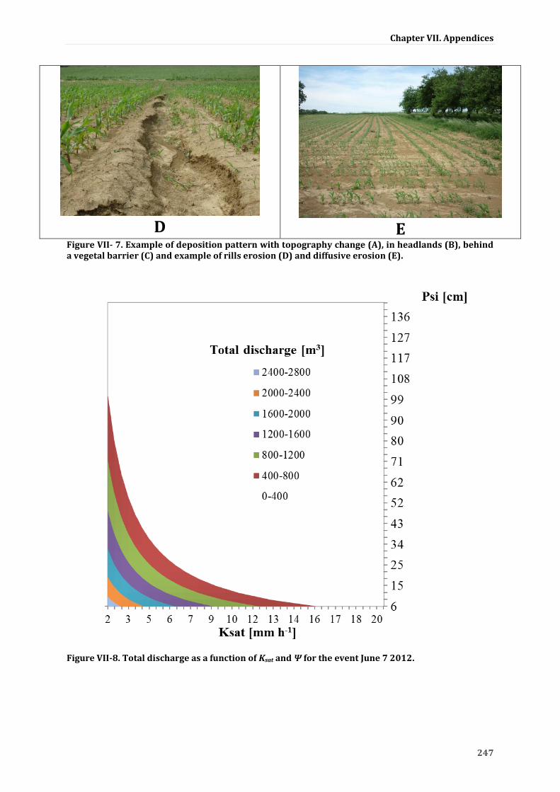
Chapter VII. Appendices

247

D

E

Figure VII- 7. Example of deposition pattern with topography change (A), in headlands (B), behind a vegetal barrier (C) and example of rills erosion (D) and diffusive erosion (E).

Figure VII-8. Total discharge as a function of Ksat and Ψ for the event June 7 2012.

Chapter VII. Appendices

248

Figure VII-9. Accumulated runoff pathways and predicted hydrograph for two different parameters set for the event June 7 2012. For configuration A, Ksat corn and Ksat wheat were set to 18 and 60 mm h-1 respectively and for configuration B, 55 and 7 mm h-1.

Chapter VII. Appendices

249

Chapter VII. Appendices

250

Chapter VII. Appendices

251

Chapter VII. Appendices

252

Chapter VII. Appendices

253

Chapter VII. Appendices

254

Figure VII-10. Rainfall, discharge and drain water height together with predicted discharge according to the both calibration methods for the nine runoff events within the headwater catchment.

Chapter VII. Appendices

255

0

10

20

30

40

50

60

70

80

90

100

0 100 200 300 400 500

Pre

dic

ted

ero

sion

rate

s [t

on

ha

-1]

Observed erosion rates [ton ha-1]

Predicted

1:1

Figure VII-11. Comparison of the predicted runoff pathways for May 21 with the pictures of that day within the headwater catchment. Figure VII-12. Predicted and observed erosion rates for each plot within the agricultural catchment.

Chapter VII. Appendices

256

References

Amoozegar, A., 1989. A Compact Constant-Head Permeameter for Measuring Saturated Hydraulic

Conductivity of the Vadose Zone. Soil Science Society of America Journal. 53, 1356-1361.

Blanchard, B.J., McFarland, M.J., Schmugge, T.J., Rhoades, E., 1981. Estimation of soil moisture with API

algorithms and microwave emission. JAWRA Journal of the American Water Resources

Association. 17, 767-774.

Chabaux, F., Blaes, E., Stille, P., Roupert, R.D., Pelt, E., Dosseto, A., Ma, L., Buss, H.L., Brantley, S.L., 2013.

Regolith formation rate from U-series nuclides: Implications from the study of a spheroidal

weathering profile in the Rio Icacos watershed (Puerto Rico). Geochimica Et Cosmochimica Acta.

100, 73-95.

Cosby, B.J., Hornberger, G.M., Clapp, R.B., Ginn, T.R., 1984. A Statistical Exploration of the Relationships of

Soil-Moisture Characteristics to the Physical-Properties of Soils. Water Resources Research. 20,

682-690.

Ertlen, D., Schwartz, D., Trautmann, M., Webster, R., Brunet, D., 2010. Discriminating between organic

matter in soil from grass and forest by near-infrared spectroscopy. European Journal of Soil

Science. 61, 207-216.

Hunt, R., 1982. Plant growth curves. Edward Arnold, London, 248.

Kohler, M.A., Linsley, R.K., 1951. Predicting the runoff from storm rainfall. US weather Bureau Res.

Madsen, H.B., Jensen, C.R., Boysen, T., 1986. A Comparison of the Thermocouple Psychrometer and the

Pressure Plate Methods for Determination of Soil-Water Characteristic Curves. Journal of Soil

Science. 37, 357-362.

Potter, K.N., 1990. Soil Properties Effect on Random Roughness Decay by Rainfall. Transactions of the

Asae. 33, 1889-1892.

Rémy, J.C., Marin-Laflèche, A., 1974. L’analyse de terre : réalisation d’un programme d’interprétation

automatique. Annales Agronomiques. 25(4), 607-632.

Riley, H., 1996. Estimation of physical properties of cultivated soils in southeast Norway from readily

available soil information. Norwegian Journal of Agricultural Sciences. supplement n°25, 1-51.

USDA, 2003. Revisited Universal Soil Loss Equation. Version 2. RUSLE2.

Van Dijk, P., Bockstaller, C., Villerd, J., Koller, R., In prep. An indicator for overland flow potential of

cropping systems: accounting for farmers’ control on key variables.

Chapter VII. Appendices

257

Annex 1. General solutions of the system for the case 0

For the case 0 , if the polynomial has only one real root 0 with a multiplicity 3, the general

solution form depends on the number of independent associate eigenvectors. If 0 has three

linearly independent eigenvectors1 2,p pv v and

3pv then the general solution is:

0

1 2 31 2 3( ) ( ) ( )t

p p p px t C v C v C v e x t

(1)

If 0 has two linearly independent eigenvectors1pv and

2pv then the general solution is:

0

1 2 2 31 2 3( ) ( ( )) ( )t

p p p p px t C v C v C tv v e x t

(2)

3 3 20where is a solution of ( )p p pv I A v v

If 0 has only one linearly independent eigenvectors1pv then the general solution is:

0

1 1 2 1 2 31 2 3( ) ( ( ) ( ² )) ( )t

p p p p p p px t C v C tv v C t v tv v e x t

(3)

2 2 1 3 3 20 0where is a solution of ( ) and of ( )p p p p p pv I A v v v I A v v

If the polynomial has only two real roots 0 with a multiplicity 2 and 1 then the general

solution is similarly expressed as previously.

Chapter VII. Appendices

258

Annex 2. Analytical expressions for Cs and CM computed with Maple 17©

CS

a = -(Kfilm+qinf+ε*ρb*kr*KD)/(n*ε); b = ρb*kr/n;

c = kr*KD;

d = -kr;

e =(Kfilm+qinf)*Cn/(n*ε);

c1 = (2.0*a*b*d*CS0+2.0*pow(b,2.0)*c*CS0+(d*(a*sqrt(pow(d,2.0)-

2.0*a*d+4.0*b*c+pow(a,2.0))-b*c-pow(a,2.0))+b*c*(a-sqrt(pow(d,2.0)-

2.0*a*d+4.0*b*c+pow(a,2.0)))+a*pow(d,2.0))*CM0+(d*(sqrt(pow(d,2.0)-

2.0*a*d+4.0*b*c+pow(a,2.0))-

a)+pow(d,2.0)+2.0*b*c)*e)/(2.0*a*d*sqrt(pow(d,2.0)-

2.0*a*d+4.0*b*c+pow(a,2.0))-2.0*b*c*sqrt(pow(d,2.0)-

2.0*a*d+4.0*b*c+pow(a,2.0)));

c2 = -(-2.0*a*b*d*CS0+2.0*pow(b,2.0)*c*CS0+(d*(-a*sqrt(pow(d,2.0)-

2.0*a*d+4.0*b*c+pow(a,2.0))-b*c-pow(a,2.0))+b*c*(sqrt(pow(d,2.0)-

2.0*a*d+4.0*b*c+pow(a,2.0))+a)+a*pow(d,2.0))*CM0+(d*(-sqrt(pow(d,2.0)-

2.0*a*d+4.0*b*c+pow(a,2.0))-

a)+pow(d,2.0)+2.0*b*c)*e)/(2.0*a*d*sqrt(pow(d,2.0)-

2.0*a*d+4.0*b*c+pow(a,2.0))-2.0*b*c*sqrt(pow(d,2.0)-

2.0*a*d+4.0*b*c+pow(a,2.0)));

Cs(Kfilm,qinf,ε,ρb,kr,KD,n,Cn)=exp(-(sqrt(pow(d,2.0)-

2.0*a*d+4.0*b*c+pow(a,2.0))*t/2.0))*(sqrt(pow(d,2.0)-

2.0*a*d+4.0*b*c+pow(a,2.0))*((a*c2*d-b*c*c2)*exp(sqrt(pow(d,2.0)-

2.0*a*d+4.0*b*c+pow(a,2.0))*t+d*t/2.0+a*t/2.0)+(b*c*c1-

a*c1*d)*exp(d*t/2.0+a*t/2.0))+(a*c2*pow(d,2.0)+(-b*c-

pow(a,2.0))*c2*d+a*b*c*c2)*exp(sqrt(pow(d,2.0)-

2.0*a*d+4.0*b*c+pow(a,2.0))*t+d*t/2.0+a*t/2.0)+(a*c1*pow(d,2.0)+(-b*c-

pow(a,2.0))*c1*d+a*b*c*c1)*exp(d*t/2.0+a*t/2.0)+2.0*b*c*e*exp(sqrt(pow(d,2.

0)-2.0*a*d+4.0*b*c+pow(a,2.0))*t/2.0))/(2.0*a*b*d-2.0*pow(b,2.0)*c);

CM

a = -(Kfilm+qinf+ε*ρb*kr*KD)/(n*ε); b = ρb*kr/n;

c = kr*KD;

d = -kr;

e =(Kfilm+qinf)*Cn/(n*ε);

c1 = (-2.0*a*b*d*CS0+2.0*pow(b,2.0)*c*CS0+(d*(a*sqrt(pow(d,2.0)-

2.0*a*d+4.0*b*c+pow(a,2.0))-b*c-pow(a,2.0))+b*c*(a-sqrt(pow(d,2.0)-

2.0*a*d+4.0*b*c+pow(a,2.0)))+a*pow(d,2.0))*CM0+(d*(sqrt(pow(d,2.0)-

2.0*a*d+4.0*b*c+pow(a,2.0))-

a)+pow(d,2.0)+2.0*b*c)*e)/(2.0*a*d*sqrt(pow(d,2.0)-

2.0*a*d+4.0*b*c+pow(a,2.0))-2.0*b*c*sqrt(pow(d,2.0)-

2.0*a*d+4.0*b*c+pow(a,2.0)));

c2 = -(-2.0*a*b*d*CS0+2.0*pow(b,2.0)*c*CS0+(d*(-a*sqrt(pow(d,2.0)-

2.0*a*d+4.0*b*c+pow(a,2.0))-b*c-pow(a,2.0))+b*c*(sqrt(pow(d,2.0)-

2.0*a*d+4.0*b*c+pow(a,2.0))+a)+a*pow(d,2.0))*CM0+(d*(-sqrt(pow(d,2.0)-

2.0*a*d+4.0*b*c+pow(a,2.0))-

a)+pow(d,2)+2.0*b*c)*e)/(2.0*a*d*sqrt(pow(d,2.0)-

Chapter VII. Appendices

259

2.0*a*d+4.0*b*c+pow(a,2.0))-2.0*b*c*sqrt(pow(d,2.0)-

2.0*a*d+4.0*b*c+pow(a,2.0)));

Cm(Kfilm,qinf,ε,ρb,kr,KD,n,Cn) = exp(-(sqrt(pow(d,2.0)-

2.0*a*d+4.0*b*c+pow(a,2.0))*t/2.0))*((a*c2*d-b*c*c2)*exp(sqrt(pow(d,2.0)-

2.0*a*d+4.0*b*c+pow(a,2.0))*t+d*t/2.0+a*t/2.0)+(a*c1*d-

b*c*c1)*exp(d*t/2.0+a*t/2.0)-d*e*exp(sqrt(pow(d,2.0)-

2.0*a*d+4.0*b*c+pow(a,2.0))*t/2.0))/(a*d-b*c);

Chapter VII. Appendices

260

Curriculum Vitae

Marie Lefrancq

Born: May 15, 1986 in Périgueux, France

French nationality

marie.lefrancq@etu.unistra.fr

Educational Background

2009-10 Master's degree in Earth and Environmental Sciences in Joseph Fourier's university (Grenoble):

physical and urban hydrology, water quality, river transport, geostatistics.

2006-09 Engineering school of mathematics and mechanical modelling: ENSEIRB-MATMECA

http://www.enseirb-matmeca.fr/ (Bordeaux) specialised in fluids mechanics: numerical simulation of

flow, porous media, complex fluid, diphasic flow, geofluid. Masters degree in applied mathematics.

2004-06 Preparation for the competitive entrance examination to French engineering schools: mathematics

and physics in Faidherbe (Lille).

Research Experience

Dec.10 – Apr. 14

3 years

PhD student on pesticides transport in runoff at headwater catchment scale: from

characterisation to modelling in LHyGeS (Laboratory of hydrology and geochemistry of

Strasbourg): field campaigns, chemical analysis, statistical study and modelling.

Hydrological teaching in ENGEES (engineering school of environmental hydraulics)

Feb.– Jun.10 6 months

Intership in UNAM (National Autonomous University of Mexico) and in LTHE (Laboratory of

transfer in hydrology and environment study) in Grenoble. Study of preferential transport in

Mexican volcanic soil: field, laboratory and modelling.

Feb. – Aug.09 6 months

Internship in Irstea, agricultural and environmental engineering research, in Lyon, France.

Development of a model for dimensioning buffer strip to limit pollution transfer in water.

Jun. – Sept.08 4 months

Internship in INRS-ETE (National Institute of scientific research in Water, Soil and environment)

in Québec, Canada. Hydrological modelling at catchment scale.

Chapter VII. Appendices

261

Scientific contribution

Publication

Lefrancq M, Payraudeau S., García Verdú A. J., Maillard E., Millet M., Imfeld G (2013): Fungicides

transport in runoff from vineyard plot and catchment: contribution of non-target areas. Environ

Sci Pollut Res. Doi: 10.1007/s11356-013-1866-8.

Lefrancq M, Imfeld G, Payraudeau S, Millet M (2013): Kresoxim methyl deposition, drift and

runoff in a vineyard catchment. Science of The Total Environment 442, 503-508. Doi:

10.1016/j.scitotenv.2012.09.082.

Imfeld G, Lefrancq M, Maillard E, Payraudeau S (2012): Transport and attenuation of dissolved

glyphosate and AMPA in a stormwater wetland Chemosphere 90, 1333-1339. Doi :

10.1016/j.chemosphere.2012.04.054.

Oral presentation

Lefrancq M., Imfeld G., Guyot B., Payraudeau S. Transport and attenuation of chloroacetanilides at

the catchment scale. Pesticide behaviour in soils, water and air, York, UK, 2-4/09/2013. Best

platform presentation: Enviresearch Young Scientist Awards

Lefrancq M., García Verdú A. J., Maillard E., Imfeld G., Payraudeau S. Transport of cyazofamid and

kresoxim-methyl in runoff at the plot and catchment scales. European Geoscience Union, Vienna,

Austria, 7-12/04/2013

Lefrancq M., Imfeld G., Payraudeau S., Millet M. Kresoxim methyl deposition, drift and runoff in a

vineyard catchment. 244th American Chemical Society National Meeting & Exposition,

Philadelphia, United States, 19-23/08/12

Lefrancq M., Imfeld G., García Verdú A. J., Maillard E., Payraudeau S. Devenir et transfert de deux

fongicides de la parcelle viticole au bassin versant. 42ème congrès du groupe français des

pesticides (GFP), Poitiers, 30/05- 01/06/12

Chapter VII. Appendices

262

Poster

Lefrancq M., Jetten V., Van Dijk P., Payraudeau S. Adapting Lisem to improve modelling of

pesticide transfer by runoff and erosion. Pesticide behaviour in soils, water and air, York, UK, 2-

4/09/2013

Lefrancq M., Jetten V., Van Dijk P., Payraudeau S. Adapting Lisem to improve modelling of

pesticide transfer by runoff and erosion. European Geoscience Union, Vienna, Austria, 7-

12/04/2013

Lefrancq M., Imfeld G., Millet M., Jetten V., Van Dijk P., Payraudeau S. Hydrological and erosion

processes modelling to improve pesticide loads assessment at the catchment scale. XIV

Symposium in Pesticide Chemistry, Piacenza, Italy, 30/08-1/09/11

Lefrancq M., Payraudeau S., Mc Grath G. S., Grégoire C., Hinz C. Using high resolution rainfall data

to identify critical source areas for runoff-related pesticides: Luxury or necessity? European

Geoscience Union, Vienna, Austria, 3-8/04/2011

Lauvernet C., Lefrancq M., Carluer N., Development of an operational tool to simulate pesticide

transfer through vegetated strips: the 2D runoff part. Pesticide behaviour in soils, water and air,

York, UK, 14-16/09/2009

Gastelum A., Delmas P., Lefrancq M., Duwig C., Marquez J., Prado B., Gimel'farb G., Charrier P.

Visualising 3D porous media fluid interaction using X-ray CT data and Smooth Particles

Hydrodynamics modelling. Image and Vision Computing New Zealand - IVCNZ. , pp. 1-8, 2010

263

Résumé

Comprendre le transport des pesticides est crucial pour évaluer leur impact écologique. Les connaissances sur la variabilité spatiale des dépôts de pesticides, l'impact de l'érosion sur leur export et leur dégradation in situ restent très limitées à l'échelle des bassins versants. La caractérisation expérimentale et la modélisation ont donc été combinées à deux échelles, parcelle et bassin versant, dans deux contextes agricoles. Un formalisme a été développé pour prédire le transport des pesticides par ruissellement et a été intégré dans le modèle LISEM (LImbourg Soil Erosion Model). Les résultats montrent que les surfaces imperméables contribuent significativement à la masse exportée par ruissellement du vignoble. La partition des pesticides entre phase dissoute et particulaire diffère considérablement selon les molécules et le forçage hydrologique, et la présence de produits de dégradation et un enrichissement en R-métolachlore ont été observés ce qui souligne le potentiel des analyses énantiomériques pour évaluer la biodégradation des pesticides. Globalement, cette étude a démontré que la combinaison des échelles et des approches permet une meilleure compréhension du transport des pesticides.

Abstract

Understanding pesticide transport is crucial to evaluate their ecological impact on ecosystems. Current knowledge on the spatial variability of pesticide deposition, the impact of erosion on pesticides export and the in situ pesticide degradation is very limited at the catchment scale. In this thesis, characterisation and modeling at two scales, the plot and catchment, were combined in two agricultural contexts. A formalism was developed to predict pesticide transport in runoff and was integrated in LISEM (LImbourg Soil Erosion Model). The results show that impermeable roads contributed to more than 40% to the overall load of fungicides exported via runoff from the vineyard. Pesticide partitioning between suspended solids and runoff water differed largely according to the molecules and the hydrological dynamics. The occurrence of degradation products and the enrichment of one enantiomer were observed suggesting the potential of chiral analyses for assessing biodegradation of chiral pesticides at such scale. Overall, the investigation demonstrated that combining different approaches enable a better understanding of pesticide transport.

Marie LEFRANCQ

Transport and attenuation of pesticides in runoff from agricultural headwater catchments: from

field characterisation to modelling