Threshold Resummation in Pair

Production

A Dissertation Presented

by

Leandro Giordano Almeida

to

The Graduate School

in Partial Fulfillment of the Requirements

for the Degree of

Doctor of Philosophy

in

Physics

Stony Brook University

May 2010

Stony Brook University

The Graduate School

Leandro Giordano Almeida

We, the dissertation committee for the above candidate for the Doctor ofPhilosophy degree, hereby recommend acceptance of this dissertation.

George Sterman – Dissertation AdvisorDistinguished Professor, C. N. Yang Institute for Theoretical Physics

Abhay Deshpande – Chairperson of DefenseProfessor, Department of Physics and Astronomy

Marivi Fernandez-SerraAssistant Professor, Department of Physics and Astronomy

Amarjit SoniSenior Scientist, Physics Department,Brookhaven National Laboratory

This dissertation is accepted by the Graduate School.

Lawrence MartinDean of the Graduate School

ii

Abstract of the Dissertation

Threshold Resummation in Pair Production

by

Leandro Giordano Almeida

Doctor of Philosophy

in

Physics

Stony Brook University

2010

In performing perturbative calculations in Quantum Chromody-namics, large logarithmic corrections can arise from processes in-volving soft and collinear quanta. These corrections can be re-summed to all orders, allowing us to improve our control overcross section calculations associated with exclusive and inclusiveprocesses. In this thesis, we show how such logarithmic correctionscan appear in perturbative calculations in Quantum Chromody-namics. We then proceed to apply these resummation methodsat next-to-leading logarithmic accuracy to heavy quark pair pro-duction and light hadron pair production. We show how to in-corporate consistently cuts in rapidity and transverse momentumof the observed particles, together with resummation. This allowsus to compare our next-to-leading logarithmic calculations directlyto experiments by placing the precise experimental cuts associatedwith the measurements of these processes. We will also examinethe phenomenological features associated with the logarithmic cor-rections. Specifically, we will look how we can apply this to thestudy jet mass distributions. We will compare jet mass distribu-

iii

tion from jets initiated from light quarks to those initiated by topquarks. This will then allow us to build jet shape observables thatwill let us distinguish between the two.

iv

Contents

List of Figures vii

List of Tables ix

1 Introduction 1

1.1 QCD . . . . . . . . . . . . . . . . . . . . . . . . . . . . . . . . 11.2 Renormalization of Local Field Theories . . . . . . . . . . . . 31.3 Application of Perturbative QCD to DIS . . . . . . . . . . . . 61.4 Factorization . . . . . . . . . . . . . . . . . . . . . . . . . . . 8

1.4.1 The Nature of Infrared Divergences . . . . . . . . . . . 81.4.2 IR Power Counting . . . . . . . . . . . . . . . . . . . . 11

2 Threshold Resummation 14

2.1 Resummation from Factorization . . . . . . . . . . . . . . . . 142.2 Logarithmic Corrections . . . . . . . . . . . . . . . . . . . . . 152.3 Threshold Resummation of Drell Yan . . . . . . . . . . . . . . 162.4 Resummation of QCD Hard Scattering . . . . . . . . . . . . . 21

2.4.1 Outline for Thesis . . . . . . . . . . . . . . . . . . . . . 22

3 Dihadron Production 23

3.1 Introduction . . . . . . . . . . . . . . . . . . . . . . . . . . . . 233.2 Perturbative Cross Section and Partonic Threshold . . . . . . 253.3 Threshold Resummation for Di-hadron Pairs . . . . . . . . . 29

3.3.1 Hard Scales and Transforms . . . . . . . . . . . . . . . 293.3.2 Resummation at Next-to-Leading Logarithm . . . . . 323.3.3 Inverse of the Mellin and Fourier Transform . . . . . . 37

3.4 Phenomenological Results . . . . . . . . . . . . . . . . . . . . 393.5 Conclusions . . . . . . . . . . . . . . . . . . . . . . . . . . . . 51

4 Charge Asymmetry in Top Production 53

4.1 Introduction . . . . . . . . . . . . . . . . . . . . . . . . . . . . 53

v

4.2 Perturbative Cross section, and Charge Asymmetry . . . . . . 554.3 NLL resummation . . . . . . . . . . . . . . . . . . . . . . . . . 574.4 Phenomenological results . . . . . . . . . . . . . . . . . . . . . 624.5 Conclusions and Outlook . . . . . . . . . . . . . . . . . . . . . 67

5 Top Jets at the LHC 69

5.1 Event Simulation . . . . . . . . . . . . . . . . . . . . . . . . . 735.1.1 Monte Carlo Generation . . . . . . . . . . . . . . . . . 735.1.2 Cross Sections . . . . . . . . . . . . . . . . . . . . . . . 745.1.3 Modelling Detector E!ects . . . . . . . . . . . . . . . . 74

5.2 QCD Jet Background . . . . . . . . . . . . . . . . . . . . . . . 765.2.1 Analytic Prediction . . . . . . . . . . . . . . . . . . . . 765.2.2 Jet Function, Theory vs. MC Data . . . . . . . . . . . 79

5.3 High pT Hadronic Top Quarks . . . . . . . . . . . . . . . . . . 855.4 tt Jets vs. QCD Jets at the LHC . . . . . . . . . . . . . . . . 88

5.4.1 Peak Resolution . . . . . . . . . . . . . . . . . . . . . . 885.4.2 Single Top-Tagging . . . . . . . . . . . . . . . . . . . . 925.4.3 Double Top-Tagging . . . . . . . . . . . . . . . . . . . 96

5.5 Jet Substructure . . . . . . . . . . . . . . . . . . . . . . . . . 995.6 Top Quark Polarization Measurement . . . . . . . . . . . . . . 1045.7 Conclusions . . . . . . . . . . . . . . . . . . . . . . . . . . . . 106

6 Jet Event Shapes 109

6.1 Jet Shapes and Jet Substructure . . . . . . . . . . . . . . . . . 1106.2 Top decay and planar flow . . . . . . . . . . . . . . . . . . . . 1116.3 Two-body decay . . . . . . . . . . . . . . . . . . . . . . . . . . 1136.4 Linear three-body decay . . . . . . . . . . . . . . . . . . . . . 117

Bibliography 120

Appendix A: NLO Dihadron cross-section 133

Appendix B: Hard Coe!cients 136

Appendix C: Jets at Fixed Invariant Mass 143

C.0.1 Jet Functions at Next-to-Leading Order . . . . . . . . 144

Appendix D: R-dependence 150

vi

List of Figures

1.1 Scalar Triangle . . . . . . . . . . . . . . . . . . . . . . . . . . 91.2 General pinch surfaces associate with the process of Eq. (1.14). 11

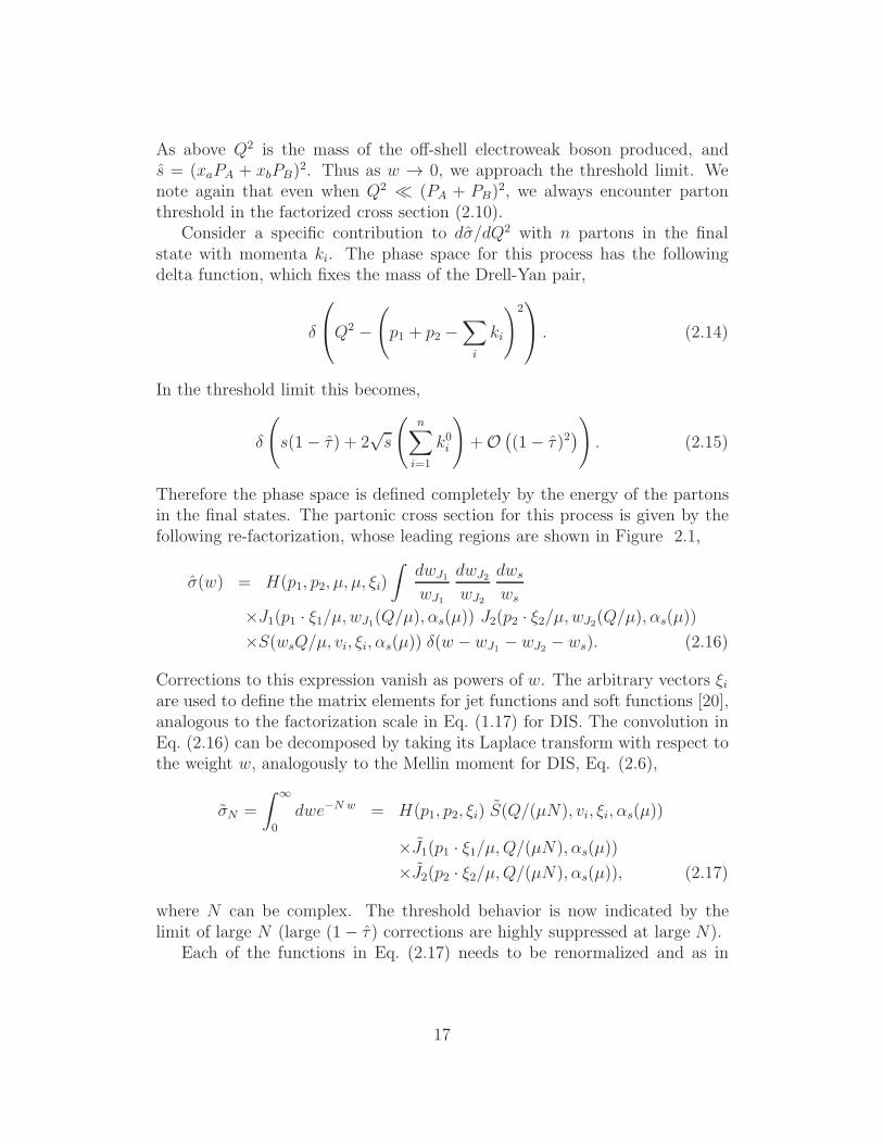
2.1 Factorization for Drell-Yan Scattering . . . . . . . . . . . . . . 18

3.1 Comparison of NLO and Resumed to NA24 data . . . . . . . 413.2 Comparison for charged-hadron production at

!S = 38.8 GeV 41

3.3 Comparison as before, but with E706 cuts . . . . . . . . . . . 443.4 Same as Fig. 3.3, but for proton-Beryllium scattering. . . . . 443.5 Resummed cross section with di!erent pT cuts . . . . . . . . . 453.6 Comparison to E706 with E711 cuts . . . . . . . . . . . . . . . 453.7 Same as Fig. 3.3, but at

!S = 31.6 GeV. . . . . . . . . . . . 46

3.8 Same as Fig. 3.4, but at!S = 31.6 GeV. . . . . . . . . . . . 46

3.9 Comparison to CCOR data at!S = 44.8 GeV . . . . . . . . . 48

3.10 Same as Fig. 3.9, but for!S = 62.4 GeV. . . . . . . . . . . . 48

3.11 Same as Fig. 3.10, but with subleading terms . . . . . . . . . . 493.12 Same as Fig. 3.11, but for the case of NA24. . . . . . . . . . 493.13 E!ects of Hard Coe"cients in CCOR . . . . . . . . . . . . . . 523.14 Normalized distribution in cos !! for charged-hadron production 52

4.1 Charge asymmetric and charge averaged cross sections . . . . 644.2 Scale Dependence of Charge Asymmetry . . . . . . . . . . . . 654.3 Charge asymmetry corresponding to the curves in Fig. 4.1. . 664.4 Asymmetric Distribution for cos ! . . . . . . . . . . . . . . . 67

5.1 We compare the mass distribution of the leading jet . . . . . . 755.2 Various theoretical gluon-jet mass distributions . . . . . . . . 795.3 The jet mass distributions for Sherpa, Pythia and MG/ME . . 805.4 Comparison between the theoretical and MC distributions . . 825.5 The fraction of jets which acquire 140GeV " mJ " 210GeV . 845.6 The di!erential pT crosssectionforQCD(R=0.4)jetproduction 845.7 The R = 0.7 jet mass distribution . . . . . . . . . . . . . . . . 85

vii

5.8 The collimation rate for top quarks as a function of their pT . 865.9 Jet mass distributions for the tt and QCD jet in the sidebands 905.10 Jet mass distributions for the tt and QCD jet samples . . . . . 925.11 A typical example of fitting jet functions . . . . . . . . . . . . 945.12 Fitting jet functions + signal shape to the jet mass distribution 955.13 We compare the pT distribution of the subleading jet for the tt 995.14 The planar flow distribution from Sherpa and MG/ME . . . . 1005.15 The planar flow distribution is plotted for tt and QCD . . . . 1035.16 comparison of the pT distribution of b quark from tL vs. tR . . 1045.17 We compare the #pT $ distribution of the b quark . . . . . . . . 1055.18 We compare the #pT $ distributions of the lepton . . . . . . . . 106

6.1 The planar flow distribution . . . . . . . . . . . . . . . . . . . 1126.2 Normalized jet distributions for gauge bosons . . . . . . . . . 1166.3 The ratio between the signal and background for ""2 . . . . . 1176.4 The angularity distribution for QCD and longitudinal Z . . . 1186.5 Angularity as a function of the azimuthal angle . . . . . . . . 119C.1 Feynman rules associated with the F+! . . . . . . . . . . . . . 145C.2 Feynman rules associated with eikonal lines . . . . . . . . . . 146C.3 Real contributions to the quark jet function . . . . . . . . . . 146C.4 Real non-vanishing contributions to the gluon jet . . . . . . . 147D.1 Contributions to the jet mass from the soft function. . . . . . 151

viii

List of Tables

5.1 Cross sections for producing R = 0.4 cone jets with pT % 1TeV 745.2 Comparison of MC data to pure-quark and -gluon hypothesis . 835.3 Truth-level results for single-tag jet mass method . . . . . . . 935.4 Acceptance of signal and background for the single tag method 945.5 Upper limit on significance of single tag method with 100 fb"1 975.6 Upper limit on significance of peak resolution with 25 fb"1 . . 985.7 Truth-level results for double-tag jet mass . . . . . . . . . . . 995.8 Acceptance of signal and background for the double tag method 1005.9 Upper limit on significance of double tag method with 100 fb"1 1015.10 Upper limit on significance of peak resolution with 25 fb"1 . . 102

ix

Chapter 1

Introduction

1.1 QCD

Quantum Chromodynamics (QCD) provides a cornucopia of ideas on which isbased our knowledge of hadronic physics. It gives a description of all hadronicmatter in a picture of fermionic fields interacting through a SU(3) gauge the-ory.

The idea that hadrons are bound states of localized objects was first intro-duced in an e!ort to explain the regularities associated with spectroscopy anddecays of hadronic states [1]. Eventually, this lead to the concept of quarks asbuilding blocks of hadrons, and it was christened “the quark model”. Laterthis was augmented with the quantum number color [2]. The quark model gavea distinct understanding of the quantum numbers needed to describe hadronicmatter. Hadrons were held together by the strong force, whose fundamentalfield was dubbed the gluon. Quarks are not observed as free particles, however,a property known as confinement.

A series of experiments, which scattered leptons o! hadrons with large mo-mentum transfer, were designed precisely to probe the substructure of nucle-ons. The subsequently observed phenomena were congruent with a descriptionin terms of charged constituents of hadrons that behave as though essentiallyfree at distances below the hadronic scale (see below.) This seemed at oddswith the idea that quarks are confined.

Soon after, however, it was shown that SU(3) gauge theories interactingwith quark fields possess the property of asymptotic freedom, described below,which accounted for this behavior and contained the important features thatdescribe strong interactions [3]. Though precise calculation of hadronic statesare beyond the means of analytic computational methods, simulations basedon lattice extensions of gauge theories have correctly calculated masses of the

1

light hadronic states [4]. They have also shown the correct properties of phasetransition associated with confinement [5]. This theory constitutes what wecall Quantum Chromodynamics.

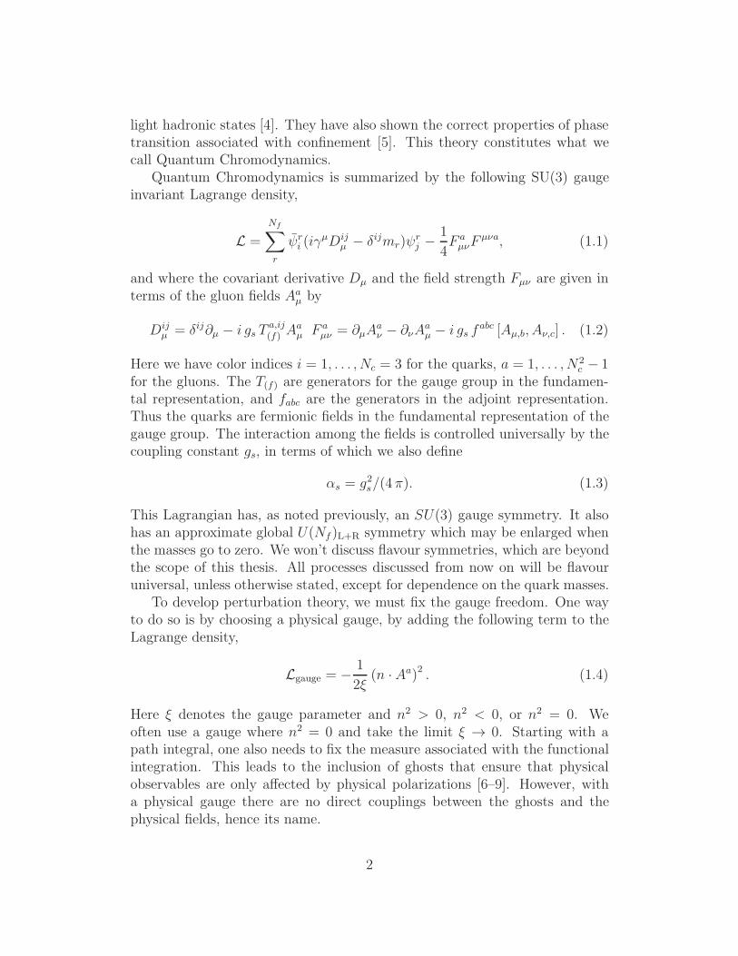
Quantum Chromodynamics is summarized by the following SU(3) gaugeinvariant Lagrange density,

L =

Nf!

r

#ri (i$

µDijµ & %ijmr)#

rj &

1

4F aµ!F

µ!a, (1.1)

and where the covariant derivative Dµ and the field strength Fµ! are given interms of the gluon fields Aa

µ by

Dijµ = %ij&µ & i gs T

a,ij(f) A

aµ F a

µ! = &µAa! & &!A

aµ & i gs f

abc [Aµ,b, A!,c] . (1.2)

Here we have color indices i = 1, . . . , Nc = 3 for the quarks, a = 1, . . . , N2c & 1

for the gluons. The T(f) are generators for the gauge group in the fundamen-tal representation, and fabc are the generators in the adjoint representation.Thus the quarks are fermionic fields in the fundamental representation of thegauge group. The interaction among the fields is controlled universally by thecoupling constant gs, in terms of which we also define

's = g2s/(4 (). (1.3)

This Lagrangian has, as noted previously, an SU(3) gauge symmetry. It alsohas an approximate global U(Nf )L+R symmetry which may be enlarged whenthe masses go to zero. We won’t discuss flavour symmetries, which are beyondthe scope of this thesis. All processes discussed from now on will be flavouruniversal, unless otherwise stated, except for dependence on the quark masses.

To develop perturbation theory, we must fix the gauge freedom. One wayto do so is by choosing a physical gauge, by adding the following term to theLagrange density,

Lgauge = &1

2)(n ·Aa)2 . (1.4)

Here ) denotes the gauge parameter and n2 > 0, n2 < 0, or n2 = 0. Weoften use a gauge where n2 = 0 and take the limit ) ' 0. Starting with apath integral, one also needs to fix the measure associated with the functionalintegration. This leads to the inclusion of ghosts that ensure that physicalobservables are only a!ected by physical polarizations [6–9]. However, witha physical gauge there are no direct couplings between the ghosts and thephysical fields, hence its name.

2

Another class of gauges, which is commonly used, is the covariant gauges.They are defined by the following term added to the Lagrange density:

Lgauge = &1

2)(& · Aa)2 . (1.5)

In this case, one needs to add new fields, which interact with the gluon throughthe density

Lgh = &µba (Dµab) cb, (1.6)

where cb and ba are the ghost and anti-ghost field respectively, and Dµab is the

covariant derivative defined in Eq. (1.2), in the adjoint representation.Once we fix the gauge freedom in Eq. (1.1), with the term (1.4), or (1.5) and

(1.6), we can obtain the diagrammatic rules for the perturbative expansion ofQCD from the gauge fixed Lagrange density. The full list of such rules and howone properly obtains them from the action with the above Lagrange densitycan be found in [7].

1.2 Renormalization of Local Field Theories

The perturbative expansion of interacting quantum fields allows us to computen-point Green functions of the associated fields order-by-order in 's. Onequickly finds, however, that the integrals that define these Green functionsare divergent in 4-dimensional field theories. These divergences come in twovarieties, short distance and long distance. Short distance divergences are fromregions in momentum space where the momenta of virtual modes are large,and thus are called Ultraviolet (UV) divergences. Long distance divergencesare usually associated with the low momentum regions of these virtual modesand therefore are called Infrared (IR) divergences. Their nature and presencewill be discussed in Sec. 1.4. In this section, we will discuss UV divergencesand sketch how to accommodate them.

At the tree level, UV divergences do not occur because of momentum con-servation. At higher orders, however, there is extra freedom in the momentaof virtual modes. This leads individual diagrams to develop divergences thatspoil the calculation of Green functions and physical observables. Remov-ing these divergences from the theory is a process that goes by the name ofrenormalization, and can be summarized as a two step process.

First we make the diagrams finite by modifying the integrals, a procedurecalled regularization. One can, for example, cut o! the momenta at some highscale, or put the theory on a lattice with a fixed spacing. Ideally, this should

3

be done in a manner that preserves the symmetries of the Lagrange densityand that can be systematically applied at higher orders in 's. The mostcommon regularization for perturbation theory is dimensional regularization.In dimensional regularization one defines the Lagrange density in d = 4 &2* dimensions, and the UV divergences of the theory show up as poles in*. Schematically, the results for di!erent loops have the following UV polestructure:

One loop: B(1)

" + A(1),

Two loops: C(2)

"2 + B(2)

" + A(2).(1.7)

For a detailed discussion see References [7–9] and references therein.After regularization, one redefines the parameters and fields of the theory

at a particular mass scale µ, to absorb these divergences. The finite terms ( theA’s in Eq. (1.7), that are absorbed by the renormalization, and the scale, atwhich scale this redefinition is performed are called the renormalization schemeand renormalization mass, respectively. Here we will focus on dimensionalregularization. We will make use of the MS scheme [7, 8]. In this scheme,we absorb the * poles in Eq. (1.7) and a factor of ln (4(/e#E) from the finiteterms, with $E Euler’s constant.

We say a theory is renormalizable if one can continue with this procedureorder by order in 's without introducing new parameters or local operators tothe theory or inducing couplings between physical and unphysical modes, thuspreserving unitarity. QCD and the other components of the Standard Modelare renormalizable in this sense.

The new Lagrange density with the redefined parameters and fields is calledthe renormalized Lagrange density, LR, while the one before renormalizationis called the Bare Lagrange density, L0. For the gauge fixed Lagrange den-sity, we can write the renormalized Lagrange density by introducing a set ofrenormalization constants, Zi, defined by:

Aaµ,0 =

!Z3Aa

µ,R, ca0 =!Z3caR, #0 =

!Z2#R

g0 = ZggR, )0 = Z3)R, m0 = ZmmR.(1.8)

The quantities with the subscript 0 are bare, and those with R are renormal-ized. In the MS scheme, the renormalization constants depend only on gRand *. We will not use mass dependent schemes, a discussion of which can befound in [8]. One can show that with this minimal set of renormalization con-stants one can remove all divergences that appear in the gauge fixed Lagrangedensity, order-by-order in 's (see [7–9] and citations therein for details of theproof.)

4

The renormalized coupling gR in Eq. (1.8) depends on the renormalizationscale, µ. We can determine this dependence or “running,” as follows. First notethat the action is dimensionless, thus the dimension of the Lagrange densityis [L] = massd. By inspection of our Lagrange density in Eq. (1.1), we find[A] = mass, [#] = mass

d!12 and [g] = mass" We replace the dimensionfull

coupling by a dimensionless one, via

gR ' gR(µ)µ". (1.9)

Given our definition of the renormalization constants, we have

gR = µ"" g0Zg(gR)

. (1.10)

We can now define a function that summarizes the running of the coupling,

+(gR; *) (dgRd lnµ

=

"

&*&d lnZg(gR)

d lnµ

#

gR

= &gR *& +0g4R

(4()2& +1

g6R(4()4

+ . . . (1.11)

The coe"cients of +i can be obtained from the perturbative calculations of Zg.The “+ function” is known up to four loops [10] in QCD.

We can solve the di!erential equation in Eq. (1.11) with * = 0 to find thescale dependence of gR(µ), which we give to two loop level in terms of 's(µ),

's(µ) ='s(µ0)

$

1 + $0

2%'s(µ0) log$

µµ0

%%

&

'1 +1

4(

+1

+0

's(µ0)$

1 + $0

(2%)'s(µ0) log$

µµ0

%%

) log

"

1 ++0

2('s(µ0) log

µ

µ0

##

+O(

's(µ0)3)

. (1.12)

The first two coe"cients are given by,

+0 =

"11

3CA &

2

3Nf

#

, +1 =34

3C2

A & 2CFNf &10

3CANf , (1.13)

where CA = Nc = 3, CF = (N2c & 1)/(2Nc), and Nf represents the number of

flavours with masses below the scales µ0 and µ. Since +0 and +1 are positive(In the Standard Model the maximum Nf = 6), we have exactly the behavior

5

we expect from an asymptotically free theory: as we increase the scale thecoupling decreases. We also learn at what scales perturbation theory is notapplicable, because it is clear that if 's(µ) is close to 1, we can not expand init.

1.3 Application of Perturbative QCD to Deep

Inelastic Scattering

The fact that QCD is asymptotically free allows us to make practical use ofperturbative field theory, particularly in scattering experiments where there isa large momentum transfer. Nonetheless, we are stuck with fact that quarkscan only be found in nature within color singlet states, that is, they are con-fined. We believe that confinement comes from the low momentum scales (i. e.long distances), where asymptotic freedom does not help. Therefore any com-putation of scattering that we perform in QCD has to take into account thatthe observed initial and/or final states that participate in any scattering arehadrons, color singlet bound states of quarks and gluons.

Factorization theorems provide us with a framework with which to computesuch cross sections. They allow to us to systematically separate long distancee!ects from short distance physics where perturbative QCD is applicable, i. e.,when there is a large momentum transfer. Long distance e!ects are associatedwith the infrared regime of the theory, and thus are not perturbatively cal-culable. These theorems separate such e!ects into non-perturbative functionsthat describe the distribution of partons in a hadron. Deep-inelastic scatteringof leptons on hadrons is a good example to show how factorization occurs andto allow us to compute cross sections for such processes.

Deep-inelastic scattering is illustrated by the following process,

l(k) +H(P ) ' l(k#) +X(PX), (1.14)

where l is a lepton with incoming and outgoing momenta k and k# respectively,and H is some specific initial hadronic state with momentum P , usually anucleon. X represents any of a multitude of hadronic final states with atotal invariant mass of P 2

X = M2X * MH , where MH is the mass of the

initial hadrons. For charged leptons both electromagnetic (EM) and weakinteractions are possible. In the EM case, Quantum Electrodynamics at thelowest order, O('em), is a good approximation. The di!erential cross section

6

for such process at 'em is proportional to

2,kd-

d3k#=

'2em

s

!

X

* $

"$

d4x

* $

"$

d4y e"i(k"k")·ye"i(P"PX)·x

)| # l±(k), H(P ) | Jem,µlep (y)Aem

µ (y)Aem! (x)Jem,!

had (x) | l±(k#), X(PX) $ |2

= &'2em

s(q2)2

!

X

gµ!

* $

"$

d4x

* $

"$

d4y e"i(k"k")·ye"i(P"PX)·x

)| # l±(k)|Jem,µlep (x)|l±(k#) $ | #H(P ) | Jem,!

had (y) |X(M2X) $ |2

= &'2em

s(q2)2L!µ(k, k#)W!µ(Q,P ), (1.15)

where Aemµ are the photon gauge fields and Jem,µ

lep (x) and Jem,!had (x) are the elec-

tromagnetic currents for the leptons and for the quarks, respectively. We defineLµ$lep to be the leptonic tensor representing the matrix element for two leptonic

currents and similarly W µ& to be the hadronic tensor. The leptonic matrix el-ements can be calculated reliably in QED. We can extract the hadronic tensorfrom the above and sum over the hadronic final states, giving

W µ&(Q,P ) =1

4(

*

d4yeiq·y #H |Jem,µhad (y) Jem,&

had (0) |H $ . (1.16)

The factorization theorem for this process states that for large Q2 = &q2, thehadronic tensor can be written as

W µ! =!

a

* 1

x

d)

)fa/H(), µF )C

µ!a ()/x,Q, µ, µF ,'s(µ)) +O(Q"2), (1.17)

where fa/H is the distribution of parton a in hadron H , with momenta )P , andwhere Ca describes the perturbative short-distance corrections to the electro-magnetic current. The scale µF , represents the scale at which fa/H is defined.

Corrections to the above factorization are suppressed by powers of Q2.Note the sum over partons a, since a hadron is constituted not only of itsvalence quarks but also of quark and anti-quark pairs and of the gauge fieldquanta themselves. Thus the sum includes a = {quarks, anti-quarks, gluons},and if we reach high enough momentum transfers, then even heavy quarks,like the charm, must be included in the initial state [11]. This is exactly thekind of factorization of momentum scales we hope to achieve in general, andindeed such factorization theorems have been proven and tested in a multitudeof processes [12]. We now turn to a discussion of the nature of factorizationproofs.

7

1.4 Factorization

As discussed in the previous section, the statement of factorization reducesto the assertion that we can separate long distance ( non-perturbative) fromshort distance ( perturbative) physics in a manner in which they are incoherent.Specifically one would like to prove that this factorization is possible order-by-order in 's. Though we will not prove such factorization in detail here, wewill try to provide the necessary steps to understand how this is done.

In order to proceed, one would like to understand the role of momentumregions in scattering processes. More specifically, we would like to understandthe nature of IR divergences, since they are closely related with the infraredsector of momentum space, and thus non-perturbative physics. In this sectionwe follow closely [7, 13].

1.4.1 The Nature of Infrared Divergences

In general a Green function for external particles with momenta {pj} can bewritten in the form,

G({pj}) =loops+

r=1

*

dnkr

lines+

i=1

$(

l2i &m2i + i*

)2%"1

N(kr, pj) (1.18)

where N represents the numerator momentum structure. Each line carries amomenta li and mass mi. Applying Feynman parameterization,

N+

i=1

A"aii =

,N+

j=1

1

# [aj ]

-

#

.N!

f=1

af

/N+

i=1

*

d'i 'ai"1i

)%

,

1&N!

r

'r

-,N!

b=1

'bAb

-"!N

c=1 ac

, (1.19)

leads to the following form for the Green function,

G({pj}) =lines+

i

* 1

0

d'i%(!

i

'i & 1)loops+

r

*

dnkrN(kr, pj)

D('i, pj, kr)"lines. (1.20)

8

Here the function D combines the denominator momentum structure. It isgiven by

D('k, kl, pi) =lines!

j

'j

0

l2j (k, p)&m2j

1

+ i*, (1.21)

where lj represents the momemtum of line j.Infrared divergences in a Feynman diagram are possible when its integrand

is singular. We therefore concern ourselves with the zeros of Eq. (1.21).Since the integrand is, however, an analytic function of its parameters, this isnot a su"cient condition. We can simply deform the contours in Eq. (1.20)associated with the loop momentum integration, to bypass such poles if theyare isolated in the complex momentum plane or in 'i.

There are two instances in which contour deformation may not be possible:first, when the pole coincides with the end point of the contour integration,and second, when multiple poles coalesce and pinch the contour. We can easilyfind when the momenta are pinched because Eq. (1.21) is always quadraticin the loop momenta. The following conditions are necessary for a pinch tooccur,

D('i, kµ, pr) = 0,&

&kµD('i, kµ, pr) = 0. (1.22)

These two conditions are summarized by the Landau equations :

either 'j = 0 or l2j = m2j ,

and2

j *jm'jlµj (k, p) = 0,

(1.23)

where j runs over all on-shell lines within each loop, and *jm is either 1 or&1 depending whether the loop momentum m is flowing with or against themomentum of line j. The solutions that satisfy Eqs. (1.23) are characterizedby sets {', k}. These points form surfaces in '&k space referred to as a pinchsurface.

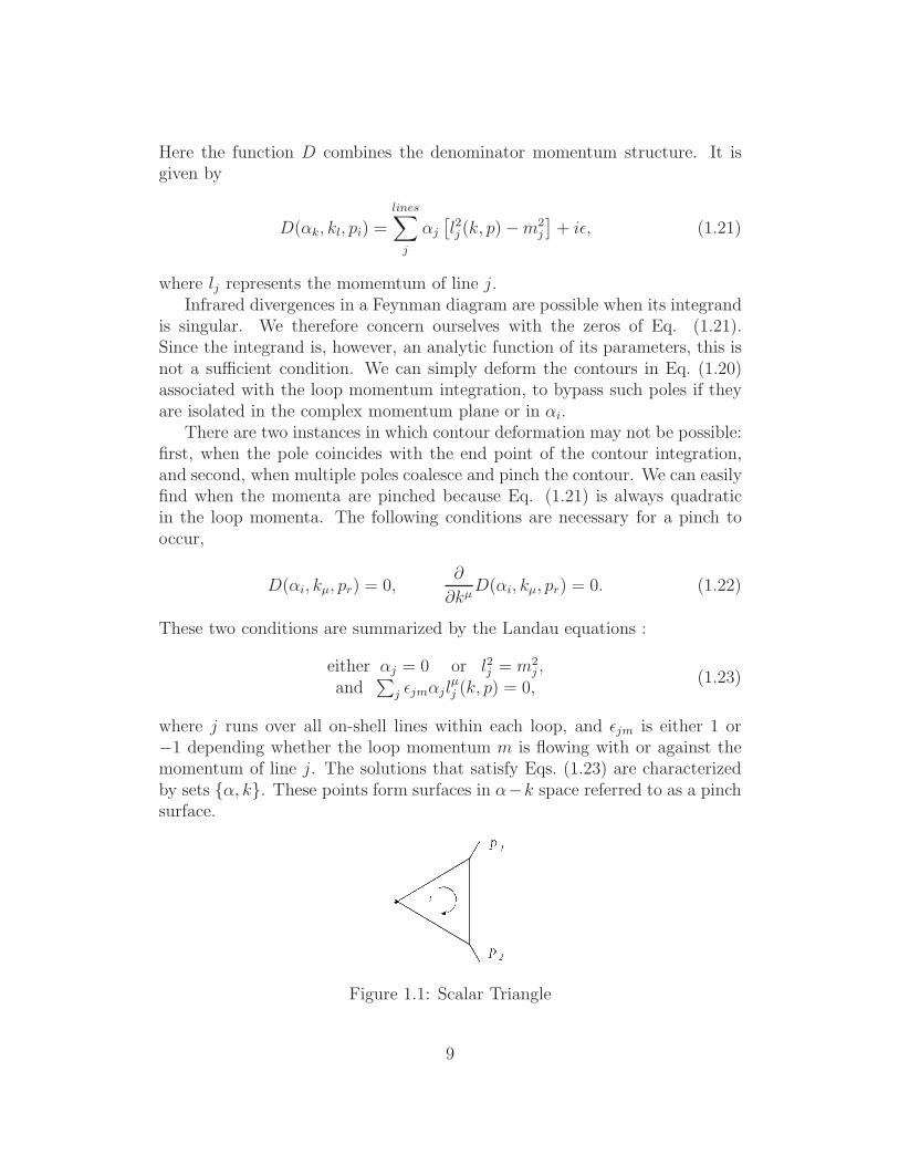
Figure 1.1: Scalar Triangle

9

As an example, we analyze the triangle diagram in a generic scalar theory,Figure 1.1. It is summarized by the following integral,

*ddk

(2()d1

(k2 + i*)((k + p1)2 + i*)((k & p2)2 + i*). (1.24)

The Landau equations corresponding to Eqs (1.23) for this integral are:

'1k2 + '2(k + p1)

2 + '3(k & p2)2 + i* = 0,

'1kµ + '2(k + p1)

µ + '3(k & p2)µ = 0.

These relations have the following non-trivial solutions:

kµ = 0 '2 = '3 = 0,

k = yp2 '2 = 0 and '1 = &'3(1"y)

y ,

k = yp1 '3 = 0 and '1 = '2(1+y)

y .

(1.25)

These solutions separate the pinch surfaces into three distinct regions of mo-mentum space, the soft region, where the all components of the loop momentago to zero, and two collinear regions, where the loop momenta are proportionalto one of the outgoing momenta.

The pinch surfaces corresponding to eqs. (1.25) can be described by a re-duced diagram where o!-shell propagators are shrunk to points. As observedby Coleman and Norton [16], each of these reduced diagrams describes a phys-ical process, where the left over propagators describe the propagation of free,physical particles. With this nice physical picture we can often write the mostgeneral reduced diagrams for a scattering process.

The set of such diagrams is particularly simple for DIS and related processes[14, 15]. We will generally denote a collinear or “jet” subdiagram as J andsoft subdiagrams as S. The possible pinch surfaces associated with the DISprocess are shown in Figure 1.2, where H represents the hard coe"cient whereall momenta is o!-shell by at least Q2. The Ji’s represent the collinear pinchsurfaces associated with final state hadrons in X and are connected to otherJi’s and H by finite-energy on-shell particles. Finally, the region S representsthe soft gluons ,and quark loops, and can connect to the collinear regionsand possibly the hard scattering. The physical picture here presents a initialHadron with momentum P producing a jet collinear to it, J1. We can alsohave an arbitrary number of jets Ji emerging from the scattering. The jetscan be connected by an arbitrary number of soft gluons, S.

Next we would like to bound the integrals near the pinch surfaces to seetheir potency and thus find the regions of momentum that will produce leading

10

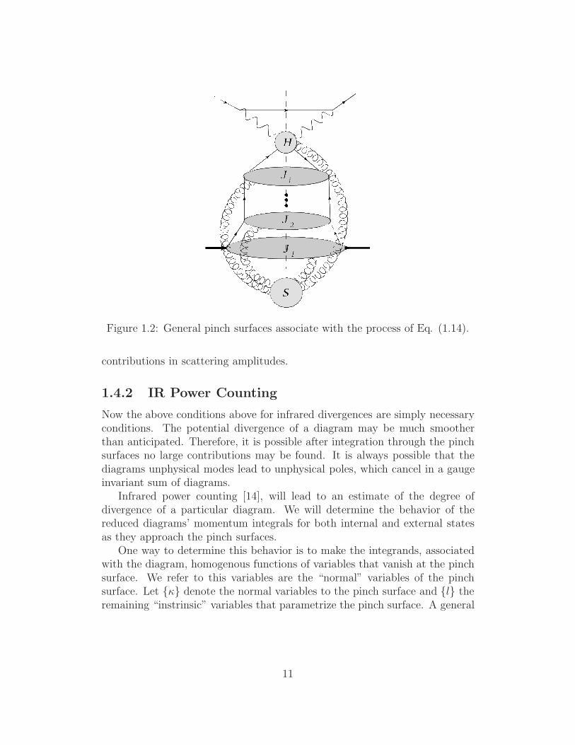
Figure 1.2: General pinch surfaces associate with the process of Eq. (1.14).

contributions in scattering amplitudes.

1.4.2 IR Power Counting

Now the above conditions above for infrared divergences are simply necessaryconditions. The potential divergence of a diagram may be much smootherthan anticipated. Therefore, it is possible after integration through the pinchsurfaces no large contributions may be found. It is always possible that thediagrams unphysical modes lead to unphysical poles, which cancel in a gaugeinvariant sum of diagrams.

Infrared power counting [14], will lead to an estimate of the degree ofdivergence of a particular diagram. We will determine the behavior of thereduced diagrams’ momentum integrals for both internal and external statesas they approach the pinch surfaces.

One way to determine this behavior is to make the integrands, associatedwith the diagram, homogenous functions of variables that vanish at the pinchsurface. We refer to this variables are the “normal” variables of the pinchsurface. Let {.} denote the normal variables to the pinch surface and {l} theremaining “instrinsic” variables that parametrize the pinch surface. A general

11

Green function near a pinch surface $ is then given by

G#(Q) =

*

#

+

b=1

dlb

*

#

D!+

a=1

d.aN(.a, lb, Q)

D(.a, lb, Q), (1.26)

where l represents the intrinsic variables while . represents the normal vari-ables. The numerator polynomials which depend on the intrinsic and normalvariables and on the general physical scale Q, is given N , similarly D is thedenominator associated with propagators of the fields present in the diagram.The parameter D# represents the number of normal variables. By scaling thenormal variables by a parameter /, such that .b = /#.#

b, we insert unity in theGreen function in Eq. (1.26),

* '2max

0

d/2#

/2#

%

,

1&D!!

a=1

."2a

-

= 1. (1.27)

Under this scaling, the numerator and denominators will have some dominantterms in the limit of / ' 0. These terms have the following powers

N(.a, lb, Q) = /n#

0

N(.#a, lb, Q) +O(/#)

1

(1.28)

D(.a, lb, Q) = /d#

0

D(.#a, lb, Q) +O(/#)

1

(1.29)

The power behavior of the integral at the pinch surface is then given by

G# =

* 'max

0

d/#1

/p!#$#(.

#a, lb, Q) (1.30)

where p# ,

p# = d+ 1&D# & n, (1.31)

such that for p# = 1 the integrals J is logarithmic divergent, and $# is therest of the integrand from Eq. (1.26) where the numerator and denominatorpolynomials only have the terms with the leading dependence in /#, i. e., thefirst terms in Eqs. (1.28) and (1.29). Now we could in principle find additionalpinch surfaces in $# , if these are among the original set of pinch surfaces thenwe can bound it eventually on with this basis of pinch surfaces. We can thenbound the entire integral through this method.

Therefore we can build cross-sections that, though are not free of pinchsurfaces, are defined in such a way that the pinch surfaces are not strongenough to produce IR poles.

12

One can then obtain the power of the leading contribution to the physicalprocess, and show that in properly defined observables, the worst divergencesare logarithmic. In the next chapter we will show how these leading regions,can lead to the resummation of logarithmic corrections.

13

Chapter 2

Threshold Resummation

2.1 Resummation from Factorization

In this chapter we will discuss how resummation of many logarithmic correc-tions is possible. We will follow closely to the discussions of Refs. [13, 18, 19].The connection between resummation and factorization is analogous to therenormalization group properties of physical cross sections.

For example, a general unrenormalized Green function of n fields #0, isrelated to the renormalized Green function with n fields #R by

G0(pi, g0) = (Z1/2( (gR(µ).*))

nGren(pi, µ, gR(µ)), (2.1)

where µR is the renormalization scale. Given that L0 does not depend onthe renormalization scale, the unrenormalized Green functions should also beindependent it. This leads to following equation

d lnGren

d lnµR= &n $((gR(µR)), (2.2)

where $( are the anomalous dimensions of the fields #

$( =1

2

d lnZ(

d lnµR. (2.3)

Since in an MS scheme

µd

dµ= µ

&

&µ+ +('s)

&

&'s, (2.4)

14

and Z( depends on µ only through 's(µ), we have

$( =1

2+('s)

& lnZ(

&'s. (2.5)

Combining this reasoning with the observation that a physical cross sectionshould be independent of the factorization scale, we can obtain a similar rela-tion for the deep-inelastic scattering cross section.

Consider the hadronic tensor in Eq. (1.17). For simplicity we suppressLorentz indices and the sum over parton types. Integrating Eq. (1.17) withthe following moment, and choosing µF = µR = µ, gives

W (N,Q2) =

* 1

0

dxxN"1W (x,Q2)

= f(N,'s(µ), µ)C(N, µ,'s(µ), Q2). (2.6)

Since W is a physical observable, it is independent of µ, and we find thefollowing consistency equations for C and f ,

"

µFd

dµ& $N('s)

#

ln C = 0, (2.7)"

µFd

dµ+ $N('s)

#

ln f = 0. (2.8)

The anomalous dimension $N('s) can depend only on N and gR because theseare the only variables on which C and f share in common. We will proceed toshow how such derivations, in more exclusive observables with more physicalscales, lead to the resummation of logarithmic corrections in these exclusivecross sections.

2.2 Logarithmic Corrections

Physical cross section can be factorized into di!erent regions of momentumspace as described in Section 1.4. This allows us to give the leading contri-butions to the cross section by convolutions of functions associated with thecorresponding momentum regions. This factorization is well illustrated forDrell-Yan scattering

HA(PA) +HB(PB) ' $!(Q2) (2.9)

15

where HA and HB are the two hadrons with momenta PA and PB respectively,and $! is an o!-shell singlet gauge boson with an invariant mass Q2. Thefactorization is given by the following convolution

d-H1 H2%##

dQ2=

!

a,b

*

dx1 dx2 fa/H1(x1, µF ,'s(µR))

)fb/H2(x2, µF ,'s(µR))d-a b%##

dQ2(" , Q2/µ, s/µ's(µR)),

=

* 1

)

d"

*

dx1 dx2 fa/H1(x1, µF ,'s(µR)) fb/H2(x2, µF ,'s(µR))

)d-

dQ2(")%(x1x2 & "), (2.10)

where s = x1x2S, " = Q2/S and " = Q2/s. The parton distribution functionsare “universal”, i. e., the same as in Eq. (1.17) for DIS.

The cross section d-/dQ2 in Eq. (2.10) is infrared safe, but for " ' 1 thereis no phase space for gluon radiation into the final state. This mis-cancellationshows up in “plus distributions,” which occur in d-/dQ2 as terms like

'ks

3lnl (1& " )

(1& " )

4

+

, (2.11)

where 0 " l " 2k & 1, and where [f(x)]+ is defined by,

* 1

0

dx[f(x)]+g(x) =

* 1

0

f(x)(g(x)& g(0)). (2.12)

Therefore, the logarithmic plus distribution in Eq. (2.11), though large, arestill finite when integrated with smooth functions, like the parton distributionfunctions. The limit " ' 1 is called partonic threshold. This threshold " = 1is always present even when " + 1. These threshold enhanced logarithmiccontributions are the one we will be resumming.

2.3 Threshold Resummation of Drell Yan

We will proceed to give a view of resummation from the point of view of Drell-Yan Scattering. In this process we can identify a “weight function”, whichmeasures the distance to partonic threshold,

w = 1&Q2

s( 1& " . (2.13)

16

As above Q2 is the mass of the o!-shell electroweak boson produced, ands = (xaPA + xbPB)2. Thus as w ' 0, we approach the threshold limit. Wenote again that even when Q2 + (PA + PB)2, we always encounter partonthreshold in the factorized cross section (2.10).

Consider a specific contribution to d-/dQ2 with n partons in the finalstate with momenta ki. The phase space for this process has the followingdelta function, which fixes the mass of the Drell-Yan pair,

%

&

'Q2 &

,

p1 + p2 &!

i

ki

-25

6 . (2.14)

In the threshold limit this becomes,

%

,

s(1& ") + 2!s

,n!

i=1

k0i

-

+O(

(1& " )2)

-

. (2.15)

Therefore the phase space is defined completely by the energy of the partonsin the final states. The partonic cross section for this process is given by thefollowing re-factorization, whose leading regions are shown in Figure 2.1,

-(w) = H(p1, p2, µ, µ, )i)

*dwJ1

wJ1

dwJ2

wJ2

dws

ws

)J1(p1 · )1/µ, wJ1(Q/µ),'s(µ)) J2(p2 · )2/µ, wJ2(Q/µ),'s(µ))

)S(wsQ/µ, vi, )i,'s(µ)) %(w & wJ1 & wJ2 & ws). (2.16)

Corrections to this expression vanish as powers of w. The arbitrary vectors )iare used to define the matrix elements for jet functions and soft functions [20],analogous to the factorization scale in Eq. (1.17) for DIS. The convolution inEq. (2.16) can be decomposed by taking its Laplace transform with respect tothe weight w, analogously to the Mellin moment for DIS, Eq. (2.6),

-N =

* $

0

dwe"N w = H(p1, p2, )i) S(Q/(µN), vi, )i,'s(µ))

)J1(p1 · )1/µ,Q/(µN),'s(µ))

)J2(p2 · )2/µ,Q/(µN),'s(µ)), (2.17)

where N can be complex. The threshold behavior is now indicated by thelimit of large N (large (1& " ) corrections are highly suppressed at large N).

Each of the functions in Eq. (2.17) needs to be renormalized and as in

17

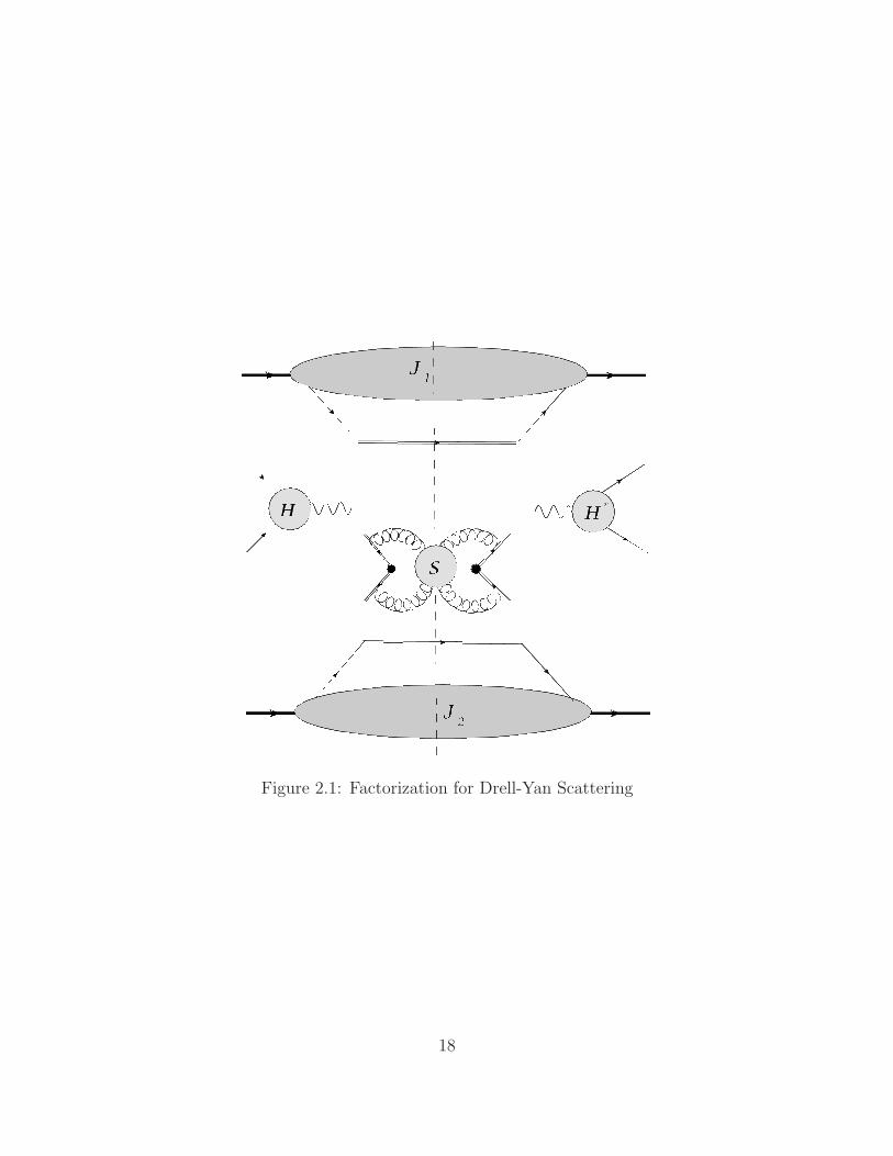
Figure 2.1: Factorization for Drell-Yan Scattering

18

Eq. (2.2), we have

d lnH

d lnµ= &$H('s),

d ln Ji

d lnµ= &$Ji('s), (2.18)

d ln S

d lnµ= &$S('s).

Since the physical cross section is independent of the renormalization scale,these anomalous dimensions are related [17, 18, 20] by

$H + $S +2!

i=1

$Ji = 0. (2.19)

The scheme we use to perform the factorization, and therefore the directionswe pick for the vectors )i, should not a!ect the physical cross section. We canthen impose two extra constraints,

"

p1 · )1&

&p1 · )1H

#

J1J2S + H

"

p1 · )1&

&p1 · )1J1

#

J2S

+HJ1J2

"

p1 · )1&

&p1 · )1S

#

= 0, (2.20)

and similarly for )2. Diving Eq. (2.20) by HJ1J2S, we find

p1 · )1&

&p1 · )1ln J1 = &p1 · )1

&

&p1 · )1lnH

7 89 :

G

&p1 · )1&

&p1 · )1ln S

7 89 :

K

, (2.21)

and similarly for J2. Since the anomalous dimensions of the J ’s depend onlyon 's,

d

d lnµ

(

G(

p1 · )1/µ, µF ,'s(µ2))

+K(

Q#a1/N, µ,'s(µ

2)))

=d

d ln p1 · )1$J1('s) = 0

(2.22)

19

Separation of variables in this equation then leads to

d

d lnµlnK = &$K('s), (2.23)

d

d lnµlnG = $K('s).

Solving these two equation leads to the following relation for K +G:

G(

p1 · )1, µ, µ,'s(µ2))

+K(

Q#a1/N, µ,'s(µ

2))

= &* p1·*1

Qa1/N

dµ#

µ#

"

$K('s(µ#)) + +('s)

&

&'sK(1,'s(µ

#))

#

7 89 :

A(+s)

+K(1,'s(p1 · )1)) +G(1,'s(p1 · )1))7 89 :

A"(+s)

= &* p1·*1

Qa1/N

dµ#

µ#A('s(µ

#2)) + A#('s((p1 · )1)2)). (2.24)

Now using Eq. (2.24) to solve Eq. (2.21) together with (2.18) for the jet func-tions,

J(p1 · )1, Q/(µN),'s(µ2)) = J(1, 1,'s(Q

2/N2/a)) exp

3

&* µ

Q/N

d/

/$J1('s(/

2))

4

.

exp

3

&* p·*

Q/N

d/

/

"* '

Q/N

d)

)A('s()

2))& A#('s(/2))

#4

(2.25)

Putting everything together, and setting p · ) = Q, gives the following re-summed cross section for Drell-Yan in transform space.

-N = lnH(1, 1,'s(Q)) + lnS(1, 1,'s(Q/N))

+!

i=1,2

ln Ji(1, 1,'s(Q/N))&* Q/N

Q

d/

/$S('s(/

2))

&2

* Q

Q/N

d)

)

;

lnQ

)A('s()

2))& A#('s()2)) +

!

j

$Jj('s()2))

<

.

(2.26)

Expanding the above form to one loop in 's, where A('s) = 'sA(1) + . . . , we

20

see that we have exponentiated the following logarithms,

ln -N = · · ·+ 's

=

2B(1) lnN + A(1) ln2N + . . .>

. (2.27)

These correspond precisely to the leading and next-to leading logarithms ofthreshold resummation in the Drell-Yan cross section. The inversion back to" space will be shown in subsequent chapters. Here we only note that theinverses of logarithms of N are “plus distributions” of Eq. (2.11).

2.4 Resummation of QCD Hard Scattering

For processes that involve color exchange, we use a more general factorizationform for the cross section,

- =!

IJ

HIJ SIJ

+

i

Ji (2.28)

where the indices I and J label the color structure in a manner described be-low. The Ji may correspond to initial and/or final collinear radiation. Thus forprocess involving heavy quarks, we will only need two initial-state jet factors,since final state heavy quark propagators do not involve collinear divergences.The functional dependence of the above functions on the kinematics and scalesis the same as for Drell-Yan. As previously, the physical cross section is in-dependent of the renormalization scale, and this leads to the correspondingrenormalization group equations

µd

dµlnHIJ = &(#H('s))IJ ,

µd

dµlnSIJ = &(#S('s))IJ , (2.29)

µd

dµln Ji = &$Ji('s),

where now the anomalous dimensions for the soft and hard functions are de-pendent on the color structure of the process. We can go through the sameanalysis as in the previous section, leading to similar exponentiation of the log-arithms involved, with the additional constraint of keeping the color orderingintact. The details can be found in [20].

21

2.4.1 Outline for Thesis

We will now proceed to study the e!ects of threshold resummation and log-arithmic corrections in di!erent processes and observables. This is based inthe following published work [22–25]. The rest of this thesis is organized asfollows: In Chapter 3 we will discuss the resummation for the exclusive pro-duction of two final state light hadrons. We look at the e!ects of next-leading-logarithm (NLL) resummation in more exclusive observables. This will allowus to compare these results to specific experiments that have measured thesecorrelations. In Chapter 4, we will proceed to the production of heavy quarksat pp collider. Specifically, we will look at the e!ects of threshold resummationat NLL on the Forward Backward asymmetry in tt production. We will thenproceed to a systematic understanding of high invariant jet mass distributionsat the LHC in Chapter 5, whose main contribution comes from logarithmiccorrections. This study will allow us to develop jet observables to distinguishlight quark jets from heavy parton jets, the subject of which is discussed inChapter 6.

22

Chapter 3

Dihadron Production

3.1 Introduction

Cross sections for hadron production in hadronic collisions play an importantrole in QCD. They o!er a variety of insights into strong interaction dynamics.At su"ciently large momentum transfer in the reaction, QCD perturbationtheory can be used to derive predictions. The cross section may be factorizedat leading power in the hard scale into convolutions of long-distance factorsrepresenting the structure of the initial hadrons and the fragmentation of thefinal-state partons into the observed hadrons, and parts that are short-distanceand describe the hard interactions of the partons. If the parton distributionfunctions and fragmentation functions are known from other processes, espe-cially deeply-inelastic scattering and e+e" annihilation, hadron production inhadronic collisions directly tests the factorized perturbative-QCD approachand the relevance of higher orders in the perturbative expansion.

Much emphasis in both theory and experiment has been on single-inclusivehadron production, H1H2 ' hX [26–33]. Here the large momentum transferis provided by the high transverse momentum of the observed hadron. Ofequal importance, albeit explored to a somewhat lesser extent, is di-hadronproduction, H1H2 ' h1h2X , when the pair is produced with large invariantmass M . In many ways, one may think of this process as a generalization ofthe Drell-Yan process to a completely hadronic situation, with the Drell-Yanlepton pair replaced by the hadron pair. The process is therefore particularlyinteresting for studying QCD dynamics, as we shall also see throughout thispaper. Experimental data for di-hadron production as a function of pair massare available from various fixed-target experiments [34–36], as well as from theISR [37]. On the theory side, next-to-leading order (NLO) calculations for thisprocess are available [38–40]. They have been confronted with the available

23

data sets, and it was found that overall agreement could only be achieved whenrather small renormalization and factorizations scales were chosen. The NLOcalculations in fact show very large scale dependence. If more natural scalesare chosen, NLO theory significantly underpredicts the cross section data, aswe shall also confirm below.

In the present chapter, we investigate the all-order resummation of largelogarithmic corrections to the partonic cross sections. This is of consider-able interest for the comparison between data and the NLO calculation justdescribed. A related resummation for the single-inclusive hadron cross sec-tion [30] was found to lead to significant enhancements of the predicted crosssection over NLO, in much better overall agreement with the available data inthat case.

At partonic threshold, when the initial partons have just enough energyto produce two partons with high invariant pair mass (which subsequentlyfragment into the observed hadron pair), the phase space available for gluonbremsstrahlung vanishes, resulting in large logarithmic corrections. To bemore specific, if we consider the cross section as a function of the partonic pairmass m, the partonic threshold is reached when s = m2, that is, " ( m2/s = 1,where

!s is the partonic center-of-mass system (c.m.s.) energy. The leading

large contributions near threshold arise as 'ks

0

ln2k"1(1& ")/(1& ")1

+at the

kth order in perturbation theory, where 's is the strong coupling and the“plus” distribution will be defined below. Su"ciently close to threshold, theperturbative series will be useful only if such terms are taken into accountto all orders in 's, which is what is achieved by threshold resummation [20,41, 42, 80]. Here we extend threshold resummation further, to cross sectionsinvolving cuts on individual hadron pT and the rapidity of the pair.

We note that this behavior near threshold is very familiar from that inthe Drell-Yan process, if one thinks of m as the invariant mass of the leptonpair. Hadron pair production is more complex in that gluon emission willoccur not only from initial-state partons, but also from those in the final state.Furthermore, interference between soft emissions from the various external legsis sensitive to the color exchange in the hard scattering, which gives rise toa special additional contribution to the resummation formula, derived in [20,43, 44].

The larger " , the more dominant the threshold logarithms will be. Becauseof this and the rapid fall-o! of the parton distributions and fragmentationfunctions with momentum fraction, threshold e!ects tend to become more andmore relevant as the hadronic scaling variable " ( M2/S goes to one. Thismeans that the fixed-target regime is the place where threshold resummation isexpected to be particularly relevant and useful. We will indeed confirm this in

24

our study. Nonetheless, because of the convolution form of the partonic crosssections and the parton distributions and fragmentation functions (see below),the threshold regime " ' 1 plays an important role also at higher (collider)energies. Here one may, however, also have to incorporate higher-order termsthat are subleading at partonic threshold.

In Sec. 3.2 we provide the basic formulas for the di-hadron cross section asa function of pair mass at fixed order in perturbation theory, and display therole of the threshold region. Section 3.3 presents details of the threshold re-summation for the cross section. In Sec. 3.4 we give phenomenological results,comparing the threshold resummed calculation to the available experimentaldata. Finally, we summarize our results in Sec. 3.5. The Appendices providedetails of the NLO corrections to the perturbative cross section near threshold.

3.2 Perturbative Cross Section and Partonic

Threshold

We are interested in the hadronic cross section for the production of twohadrons h1,2,

H1(P1) +H2(P2) ' h1(K1) + h2(K2) +X , (3.1)

with pair invariant massM2 ( (K1 +K2)

2 . (3.2)

We will consider the cross section di!erential in the rapidities 01, 02 of the twoproduced hadrons, treated as massless, in the c.m.s. of the initial hadrons, orin their di!erence and average,

$0 =1

2(01 & 02) , (3.3)

0 =1

2(01 + 02) . (3.4)

We will later integrate over regions of rapidity corresponding to the relevantexperimental coverage.

For su"ciently large M2, the cross section for the process can be written

25

in the factorized form

M4d-H1H2%h1h2X

dM2d$0d0=

!

abcd

* 1

0

dxadxbdzcdzd fH1a (xa, µF i)f

H2b (xb, µF i)

) zcDh1c (zc, µFf)zdD

h2d (zd, µFf)

)m4d-ab%cd

dm2d$0d0

$

" ,$0, 0,'s(µR),µR

m,µF i

m,µFf

m

%

, (3.5)

where 0 is the average rapidity in the partonic c.m.s., which is related to 0 by

0 = 0 &1

2ln

"xa

xb

#

. (3.6)

The quantity $0 is a di!erence of rapidities and hence boost invariant. It isimportant to note that the rapidities of the hadrons with light-like momentaK1 and K2 are the same as those of their light-like parent partons. The av-erage and relative rapidities for the hadrons and their parent partons are alsotherefore the same, a feature that we will use below. Furthermore, in Eq. (3.5)the f

H1,2

a,b are the parton distribution functions for partons a, b in hadrons H1,2

and Dh1,2

c,d the fragmentation functions for partons c, d fragmenting into theobserved hadrons h1,2. The distribution functions are evaluated at the initial-state and final-state factorization scales µF i and µFf , respectively. µR denotesthe renormalization scale. The d-ab%cd/d"d0d$0 are the partonic di!erentialcross sections for the contributing partonic processes ab ' cdX #, where X # de-notes some additional unobserved partonic final state. The partonic momentaare given in terms of the hadronic ones by pa = xaP1, pb = xbP2, pc = K1/zc,pd = K2/zd. We introduce a set of variables, some of which have been used inEq. (3.5):

S = (P1 + P2)2 , (3.7)

" (M2

S, (3.8)

s ( (xaP1 + xbP2)2 = xaxbS , (3.9)

m2 ("K1

zc+

K2

zd

#2

=M2

zczd, (3.10)

" (m2

s=

M2

xaxbzczdS=

"

xaxbzczd. (3.11)

At the level of partonic scattering in the factorized cross section, Eq. (3.5), the

26

other relevant variables are the partonic c.m.s. energy!s, and the invariant

mass m of the pair of partons that fragment into the observed di-hadron pair.We have written Eq. (3.5) in such a way that the term in square bracketsis a dimensionless function. Hence, it can be chosen to be a function of thedimensionless ratio m2/s = " and the ratio of m to the factorization andrenormalization scales, as well as the rapidities and the strong coupling. In thefollowing, we will take all factorization scales to be equal to the renormalizationscale for simplicity, that is, µR = µF i = µFf ( µ. We then write

m4d-ab%cd

dm2d$0d0

$

" ,$0, 0,'s(µ),µ

m

%

( ,ab%cd

$

" ,$0, 0,'s(µ),µ

m

%

. (3.12)

The variable " is of special interest for threshold resummation, because it isa measure of the phase space available for radiation at short distances. Thelimit " ' 1 corresponds to the partonic threshold, where the partonic hardscattering uses all available energy to produce the pair. This is kinematicallysimilar to the Drell-Yan process, if one thinks of the hadron pair replaced by alepton pair. The presence of fragmentation of course complicates the analysissomewhat, because only a fraction zczd of m2 is used for the invariant mass ofthe observed hadron pair. In the following it will in fact be convenient to alsouse the variable

" # (m2

S=

M2

zczdS, (3.13)

which is the ratio of the partonic m2 to the overall c.m.s. invariant S andhence may be viewed as the “" -variable” at the level of produced partonswhen fragmentation has not yet been taken into account. This variable isclose in spirit to the variable " = Q2/S in Drell-Yan.

The partonic cross sections can be computed in QCD perturbation theory,where they are expanded as

,ab%cd =$'s

(

%2 ?

,LOab%cd +

's

(,NLOab%cd + . . .

@

. (3.14)

Here we have separated the overall power of O('2s), which arises because the

leading order (LO) partonic hard-scattering processes are the ordinary 2 ' 2QCD scatterings. At LO, one has " = 1, and also the two partons are producedback-to-back in the partonic c.m.s., so that 0 = 0. One can therefore writethe LO term as

,LOab%cd (" ,$0, 0) = % (1& " ) % (0) ,(0)

ab%cd($0) , (3.15)

27

where ,(0)ab%cd is a function of $0 only. The second delta-function implies

that 0 = 12 ln(xa/xb). At next-to-leading order (NLO), or overall O('3

s), onecan have " ,= 1 and 0 ,= 0. Near partonic threshold, " ' 1, however, thekinematics becomes “LO like”. The average rapidity of the final-state partons,c and d (and therefore of the observed di-hadrons) is determined by the ratioxa/xb, up to corrections that vanish when the energy available for soft radiationis squeezed to zero. As noted in Ref. [45], in this limit the delta function thatfixes the partonic pair rapidity 0 becomes independent of soft radiation, andmay be factored out of the phase space integral over the latter. This is trueat all orders in perturbation theory. One has:

,ab%cd (" ,$0, 0,'s(µ), µ/m) = % (0) ,singab%cd (" ,$0,'s(µ), µ/m)

+,regab%cd (" ,$0, 0,'s(µ), µ/m) ,(3.16)

where all singular behavior near threshold is contained in the functions ,singab%cd.

Threshold resummation addresses this singular part to all orders in the strongcoupling. All remaining contributions, which are subleading near threshold,are collected in the “regular” functions ,reg

ab%cd. Specifically, for the NLO cor-rections, one finds the following structure:

,NLOab%cd (" ,$0, 0, µ/m) = % (0)

?

,(1,0)ab%cd($0, µ/m) %(1& ")

+ ,(1,1)ab%cd($0, µ/m)

"1

1& "

#

+

+ ,(1,2)ab%cd($0)

"log(1& ")

1& "

#

+

4

+,reg,NLOab%cd (" ,$0, 0, µ/m) , (3.17)

where the singular part near threshold is represented by the functions ,(1,0)ab%cd,

,(1,1)ab%cd, ,

(1,2)ab%cd, which are again functions of only $0, up to scale dependence.

The “plus”-distributions are defined by

* 1

x0

f(x) (g(x))+ dx (* 1

x0

(f(x)& f(1)) g(x)dx& f(1)

* x0

0

g(x)dx . (3.18)

Appendix A describes the derivation of the coe"cients ,(1,0)ab%cd,,

(1,1)ab%cd,,

(1,2)ab%cd

explicitly from a calculation of the NLO corrections near threshold. This willserve as a useful check on the correctness of the resummed formula, and alsoto determine certain matching coe"cients.

As suggested above, the structure given in Eq. (3.17) is similar to that foundfor the Drell-Yan cross section at NLO. A di!erence is that in the inclusiveDrell-Yan case one can integrate over all $0 to obtain a total cross section.

28

This integration is finite because the LO process in Drell-Yan is the s-channelreaction qq ' 1+1". In the case of di-hadrons, the LO QCD processes alsohave t as well as u-channel contributions, which cause the integral over $0 todiverge when the two hadrons are produced back-to-back with large mass, buteach parallel or anti-parallel to the initial beams. As a result, one will alwaysneed to consider only a finite range in $0. This is, of course, not a problemas this is anyway also done in experiment. It does, however, require a slightlymore elaborate analysis for threshold resummation, which we review below.

3.3 Threshold Resummation for Di-hadron Pairs

3.3.1 Hard Scales and Transforms

The resummation of the logarithmic corrections is organized in Mellin-N mo-ment space [41]. In moment space, the partonic cross sections absorb loga-rithmic corrections associated with the emission of soft and collinear gluonsto all orders. Employing appropriate moments, which we will identify shortly,we will see that the convolutions among the di!erent nonperturbative andperturbative regions in the hadronic cross section decouple.

In terms of the dimensionless hard-scattering function introduced in Eq. (3.12)the hadronic cross section in Eq. (3.5) becomes

M4d-H1H2%h1h2X

dM2d$0d0=

!

abcd

* 1

0

dxadxb dzc dzd fH1a (xa)f

H2b (xb)

) zcDh1c (zc)zdD

h2d (zd),ab%cd

$

" ,$0, 0,'s(µ),µ

m

%

, (3.19)

where for simplicity we have dropped the scale dependence of the partondistributions and fragmentation functions. At lowest order, when the hard-scattering function ,ab%cd is given by Eq. (3.15), the cross section is found tofactorize under “double” moments [46, 47], a Mellin moment with respect to

29

" = M2/S and a Fourier moment in 0 = 0 + 12 ln(xa/xb):

* $

"$

d0 ei!,* 1

0

d" "N"1M4d-H1H2%h1h2X

dM2d$0d0

AAAAALO

=!

abcd

fH1a (N + 1 + i2/2)fH2

b (N + 1& i2/2)Dh1c (N + 2)Dh2

d (N + 2)

)* $

"$

d0 ei!,* 1

0

d" "N"1 % (1& ") % (0)

"'s(µ)

(

#2

,(0)ab%cd($0) ,(3.20)

where the Mellin moments of the parton distributions or fragmentation func-tions are defined in the usual way, for example

fHa (N) (

* 1

0

xN"1fHa (x)dx . (3.21)

We note that instead of a combined Mellin and Fourier transform one mayequivalently use a suitable double-Mellin transform [48]. The last two integralsin Eq. (3.20) give the combined Mellin and Fourier moment of the LO partoniccross section. Because of the two delta-functions, they are trivial and just yieldthe N and 2 independent result ('s/()2,

(0)ab%cd($0). One might expect that

this generalizes to higher orders, so that the double moments

* $

"$

d0 ei!,* 1

0

d" "N"1 ,ab%cd

$

" ,$0, 0,'s(µ),µ

m

%

(3.22)

would appear times moments of fragmentation functions. However, this is im-peded by the presence of the renormalization/factorization scale µ which mustnecessarily enter in a ratio with m = M/

!zczd. As a result of this dependence

on zc and zd, the moments Dh1c (N +2), Dh2

d (N +2) of the fragmentation func-tions will no longer be generated, and the factorized cross section does notseparate into a product under moments. Physically, this is a reflection of themismatch between the observed scale, the di-hadron mass M , and the unob-served threshold scale at the hard scattering, m. Threshold logarithms appearwhen s approaches the latter scale, not the former. This implies that at fixedM there is actually a range of hard-scattering partonic thresholds, extendingall the way from M at the lower end to

!S at the upper. This situation is to

be contrasted to the Drell-Yan process or to di-jet production at fixed masses,where the underlying hard scale is defined directly by the observable.

We will deal with the presence of this range of hard scales m by car-

30

rying out threshold resummation at fixed m as well as at fixed factoriza-tion/renormalization scale. For this purpose, we rewrite the cross section(3.19) in a form that isolates the fragmentation functions:

M4d-H1H2%h1h2X

dM2d$0d0=

!

cd

* 1

0

dzc dzd zcDh1c (zc, µ) zdD

h2d (zd, µ)

%H1H2%cd

$

" #,$0, 0,'s(µ),µ

m

%

, (3.23)

where again " # = m2/S = "xaxb and %H1H2%cd is given by the convolution ofthe parton distribution functions and ,ab%cd:

%H1H2%cd

$

" #,$0, 0,'s(µ),µ

m

%

=!

ab

* 1

0

dxa dxb fH1a (xa, µ) f

H2b (xb, µ)

,ab%cd

$

" ,$0, 0,'s(µ),µ

m

%

, (3.24)

with 0 = 0 & 12 ln(xa/xb) as before. At fixed final-state partonic mass m, the

function %H1H2%cd now has the desired factorization property under Fourierand Mellin transforms:

* $

"$

d0 ei!,* 1

0

d" # (" #)N"1%H1H2%cd

$

" #,$0, 0,'s(µ),µ

m

%

=!

ab

fH1a (N + 1 + i2/2, µ)fH2

b (N + 1& i2/2, µ)

) ,ab%cd

$

N, 2,$0,'s(µ),µ

m

%

, (3.25)

where

,ab%cd

$

N, 2,$0,'s(µ),µ

m

%

(* $

"$

d0 ei!,* 1

0

d" "N"1 ,ab%cd

$

" ,$0, 0,'s(µ),µ

m

%

.(3.26)

Through Eqs. (3.23)–(3.26) we have formulated the hadronic cross section in away that involves moment-space expressions for the partonic hard-scatteringfunctions, which may be resummed. Because the final-state fractions zi equalunity at partonic threshold, the scale m in the short-distance function maybe identified here with the final-state partonic invariant mass, up to correc-tions that are suppressed by powers of N . For the singular, resummed short-distance function we therefore do not encounter the problem with the moments

31

discussed above in connection with Eq. (3.22).

3.3.2 Resummation at Next-to-Leading Logarithm

As we saw in Eq. (3.16), the singular parts of the partonic cross sections nearthreshold enter with %(0). This gives for the corresponding moment-spaceexpression

,resumab%cd

$

N,$0,'s(µ),µ

m

%

=

* 1

0

d" "N"1 ,singab%cd

$

" ,$0,'s(µ),µ

m

%

. (3.27)

which is a function of N only, but not of the Fourier variable 2. Dependenceon the Fourier variable 2 then resides entirely in the parton distributions. Itis this function, ,resum

ab%cd, that threshold resummation addresses, which is thereason for the use of the label “resum” from now on.

The nature of singularities at partonic threshold is determined by the avail-able phase space for radiation as " ' 1. Denoting by kµ the combined mo-mentum of all radiation, whether from the incoming partons a and b or theoutgoing partons c and d, one has

1& " = 1&(pc + pd)2

(pa + pb)2= 1&

(pa + pb & k)2

(pa + pb)2-

2k!0!s, (3.28)

where k!0 is the energy of the soft radiation in the c.m.s of the initial partons.

At partonic threshold, the cross section factorizes into “jet” functions as-sociated with the two incoming and outgoing partons, in addition to an over-all soft matrix, traced against the color matrix describing the hard scatter-ing [20, 43]. Corrections to this factorized structure are suppressed by powersof 1& " . The total cross section is a convolution in energy between these func-tions, which is factorized into a product by moments in "N . exp[&N(1& " )],again with corrections suppressed by powers of (1& " ), or equivalently, pow-ers of N . This result was demonstrated for jet cross sections in [43], and theextension to observed hadrons in the final state was discussed in [49, 50]. Theresummed expression for the partonic hard-scattering function for the processab ' cd then reads [20, 43, 44, 80]:

,resumab%cd

$

N,$0,'s(µ),µ

m

%

= $N+1a

$

's(µ),µ

m

%

$N+1b

$

's(µ),µ

m

%

)TrB

HS†NSSN

C

ab%cd

$

$0,'s(µ),µ

m

%

)$N+2c

$

's(µ),µ

m

%

$N+2d

$

's(µ),µ

m

%

.(3.29)

32

Each of the functions Hab%cd, SN,ab%cd, Sab%cd in Eq. (3.29) is a matrix in aspace of color exchange operators [20, 43], and the trace is taken in this space.Note that this part is the only one in the resummed expression Eq. (3.29)that carries dependence on $0. The Hab%cd are the hard-scattering functions.They are perturbative and have the expansion

Hab%cd

$

$0,'s(µ),µ

m

%

= H(0)ab%cd ($0) +

's(µ)

(H(1)

ab%cd

$

$0,µ

m

%

+O('2s) .

(3.30)

The LO (i.e. O('2s)) parts H

(0)ab%cd are known [20, 43, 44], but the first-order

corrections have not been derived yet. We shall return to this point shortly.The Sab%cd are soft functions. They depend on N only through the argumentof the running coupling, which is set to µ/N [20], and have the expansion

Sab%cd

$

$0,'s,µ

m

%

= S(0)ab%cd +

's

(S(1)ab%cd

$

$0,µ

Nm

%

+O('2s) . (3.31)

The N -dependence of the soft function enters the resummed cross section atthe level of next-to-next-to-leading logarithms. The LO terms S(0)

ab%cd may alsobe found in [20, 43, 44]. They are independent of $0.

The resummation of wide-angle soft gluons is contained in the Sab%cd, whichare exponentials and given in terms of soft anomalous dimensions, #ab%cd:

SN,ab%cd

$

$0,'s(µ),µ

m

%

= P exp

.

1

2

* m2/N2

m2

dq2

q2#ab%cd

(

$0,'s(q2))

/

, (3.32)

where P denotes path ordering and where N ( Ne#E with $E is the Eulerconstant. The soft anomalous dimension matrices start at O('s),

#ab%cd ($0,'s) ='s

(#(1)ab%cd ($0) +O('2

s) . (3.33)

Their first-order terms are presented in [20, 43, 44, 51].The $N

i (i = a, b, c, d) represent the e!ects of soft-gluon radiation collinearto an initial or final parton. Working in the MS scheme, one has [20, 41, 43,44, 80]:

ln$Ni

$

's(µ),µ

m

%

=

* 1

0

zN"1 & 1

1& z

* (1"z)2m2

m2

dq2

q2Ai('s(q

2))

+

* m2

µ2

dq2

q2

3

&Ai('s(q2)) ln N &

1

2Bi('s(q

2))

4

.(3.34)

33

Here the functions Ai and Bi are perturbative series in 's,

Ai('s) ='s

(A(1)

i +$'s

(

%2A(2)

i + . . . , (3.35)

and likewise for Bi. To NLL, one needs the coe"cients [84]:

A(1)i = Ci , A(2)

a =1

2Ci

3

CA

"67

18&

(2

6

#

&5

9Nf

4

,

B(1)q = &

3

2CF , B(1)

g = &2(+0 , (3.36)

where Nf is the number of flavors, and

Cq = CF =N2

c & 1

2Nc=

4

3, Cg = CA = Nc = 3 ,

b0 =11CA & 2Nf

12(. (3.37)

The factors $Ni generate leading threshold enhancements, due to soft-collinear

radiation. We note that our expression for the$Ni di!ers by theN -independent

term proportional to B(1)i from that often used in studies of threshold resum-

mation (see, for example, Refs. [22, 80]). As was shown in [20, 43, 44], thisterm is part of the resummed expression and exponentiates. In fact, the sec-ond term on the right-hand-side of Eq. (3.34) contains the large-N part of themoments of the diagonal quark and gluon splitting functions, matching thefull leading power µF -dependence of the parton distributions and fragmenta-tion functions in Eqs. (3.23) and (3.25). We shall return to this point below.Here, we note that the Born cross sections are recovered by computing thefollowing Tr{H(0)S(0)}ab%cd, which is proportional to the function ,(0)

ab%cd($0)introduced in Eq. (3.15). It is instructive to consider the expansion of thetrace part in Eq. (3.29) to first order in 's. One finds [52]:

TrB

HS†NSSN

C

ab%cd= Tr{H(0)S(0)}ab%cd

+'s

(Tr=

&0

H(0)(#(1))†S(0) +H(0)S(0)#(1)1

ln N

+H(1)S(0) +H(0)S(1)>

ab%cd+O('2

s) . (3.38)

When combined with the first-order expansion of the factors $Ni in Eq. (3.29),

34

one obtains

,resumab%cd

$

N,$0,'s(µ),µ

m

%

= Tr{H(0)S(0)}ab%cd

)

,

1 +'s

(

!

i=a,b,c,d

A(1)i

0

ln2 N + ln N ln(µ2/m2)1

-

+'s

(Tr=

&0

H(0)(#(1))†S(0) +H(0)S(0)#(1)1

ln N

+H(1)S(0) +H(0)S(1)>

ab%cd+O('2

s) . (3.39)

This expression can be compared to the results of the explicit NLO calculationnear threshold given in Appendix A. This provides a cross-check on the termsthat are logarithmic in N , that is, singular at threshold. From comparison tothe part proportional to %(1 & ") in the NLO expression, one will be able toread o! the combination (H(1)S(0)+H(0)S(1)) in Eq. (3.39). This is, of course,not su"cient to determine the full first-order matrices H(1) and S(1), whichwould be needed to fully evaluate the trace part in in Eq. (3.29) to NLL. Toderive H(1) and S(1), one would need to perform the NLO calculation nearthreshold in terms of a color decomposition [53], which is beyond the scopeof this work. Instead, we use here an approximation that has been made inprevious studies (see, for example, Ref. [30]),

TrB

HS†NSSN

C

ab%cd-

$

1 +'s

(C(1)

ab%cd

%

TrB

H(0)S†NS

(0)SN

C

ab%cd(3.40)

where

C(1)ab%cd ($0, µ/m) (

Tr=

H(1)S(0) +H(0)S(1)>

ab%cd

Tr {H(0)S(0)}ab%cd

(3.41)

are referred to as “C-coe"cients”. The coe"cients we obtain for the variouspartonic channels are given in Appendix B. The approximation we have madebecomes exact if only one color configuration contributes or if all eigenvaluesof the soft anomalous dimension matrix are equal. By construction, it is alsocorrect to first order in 's.

We now turn to the explicit NLL expansions of the ingredients in theresummed partonic cross section. For the function $N

i in Eq. (3.34) one finds:

ln$Ni

$

's(µ),µ

m

%

= h(1)i (/) ln N + h(2)

i

$

/,'s(µ),µ

m

%

+ ln Ei$

/,'s(µ),µ

m

%

,

(3.42)

35

where / = b0's(µ) ln N and the functions h(1)i , h(2)

i , ln(Ei) are given by

h(1)i (/) =

A(1)i

2(+0/(2/+ ln(1& 2/)) ,

h(2)i

$

/,'s(µ),µ

m

%

=2/+ ln(1& 2/)

2(b0

,

A(1)i b1b20

&A(2)

i

(+0& A(1)

i lnµ2

m2

-

+A(1)

i b14(+03

ln2(1& 2/) +B(1)

i

2(+0ln(1& 2/) ,

ln Ei$

/,'s(µ),µ

m

%

=1

(+0

"

&A(1)i ln N &

1

2B(1)

i

#

)3

ln(1& 2/)& +0's(µ) lnµ2

m2

4

. (3.43)

We note that we have written Eq. (3.42) in a “non-standard” form that isactually somewhat more complex than necessary. For example, one can im-mediately see that the terms proportional to B(1)

i ln(1 & 2/) cancel between

the functions h(2)i and ln(Ei), as they must because they were not present in

the $Ni in Eq. (3.34) in the first place. The term proportional to ln(µ2/m2)

in ln(Ei) is the expansion of the second term in Eq. (3.34). Its contribution

involving B(1)i does not carry logarithmic dependence on N and would nor-

mally be part of the “C-coe"cients” discussed above. The term proportionalto ln(1& 2/) in ln(Ei) has been separated o! the first term in Eq. (3.34). Ourmotivation to use this form of Eq. (3.42) is that the piece termed ln(Ei) may beviewed as resulting from a large-N leading-order evolution of the correspond-ing parton distribution or fragmentation function between scales m/N and thefactorization scale µF (we remind the reader that we have set the factoriza-tion and renormalization scales equal and denoted them by µ). As mentioned

earlier, the factors (&2A(1)i ln N & B(1)

i ) correspond to the moments of theflavor-diagonal splitting functions, PN

ii , while the term in square brackets is aLO approximation to

+0

* m2/N2

µF

dq2

q2's(q

2) . (3.44)

Therefore, it is natural to identify [54]

Ei$

/,'s(µ),µ

m

%

fHi (N, µ) / fH

i (N, m/N) , (3.45)

that is, the exponential related to Ei evolves the parton distributions from

36

the factorization scale to the scale m/N , and likewise for the fragmentationfunctions. At the level of diagonal evolution, it makes of course no di!erenceif ln(Ei) is used to evolve the parton distributions or if it is just added to the

function h(2)i . However, as was discussed in [54, 55], one can actually promote

the diagonal evolution expressed by Ei to the full singlet case by replacingthe term (&2A(1)

i ln N & B(1)i ) by the full matrix of the moments of the LO

singlet splitting functions, P (1),Nij , so that E itself becomes a matrix. Using

this matrix in Eq. (3.42) instead of the diagonal Ei, one takes into accountterms that are suppressed as 1/N or higher. In particular, one resums termsof the form 'k

s ln2k"1 N/N to all orders in 's [55]. We will mostly stick to

the ordinary resummation based on a diagonal evolution operator Ei in thispaper. However, as we shall show later in one example, the subleading termstaken into account by implementing the non-diagonal evolution in the partondistributions and fragmentation functions can actually be quite relevant inkinematic regimes where one is further away from threshold. Here we willonly take the LO part of evolution into account, extension to NLO is possibleand has been discussed in [54].

For a complete NLL resummation one also needs the expansion of theintegral in Eq. (4.16), which leads to

lnSN,ab%cd

$

$0,'s(µ),µ

m

%

=ln(1& 2/)

2(b0#(1)ab%cd ($0) . (3.46)

As in [22], we perform the exponentiation of the matrix on the right-hand-sidenumerically, by iterating the exponential series to an adequately large order.

3.3.3 Inverse of the Mellin and Fourier Transform

As we have discussed in detail, the resummation is achieved in Mellin momentspace. In order to obtain a resummed cross section in " space, one needs aninverse Mellin transform, accompanied by an inverse Fourier transform thatreconstructs the dependence on 0. The Mellin inverse requires a prescriptionfor dealing with the singularity in the perturbative strong coupling constantin Eqs. (3.34),(4.16) or in the NLL expansions, Eqs. (3.42),(3.43). We willuse the Minimal Prescription developed in Ref. [87], which relies on use of theNLL expanded forms Eqs. (3.42),(3.43), and on choosing a Mellin contour incomplex-N space that lies to the left of the poles at / = 1/2 and / = 1 in the

37

Mellin integrand. From Eqs. (3.25) and (3.26), we find

%resumH1H2%cd

$

" #,$0, 0,'s(µ),µ

m

%

=1

2(

* $

"$

d2 e"i!,

* CMP+i$

CMP"i$

dN

2(i(" #)"N

)!

ab

fH1a (N + 1 + i2/2, µ)fH2

b (N + 1& i2/2, µ)

),resumab%cd

$

N, 2,$0,'s(µ),µ

m

%

, (3.47)

where the Mellin contour is chosen so that b0's(µ2R) lnCMP < 1/2, but all

other poles in the integrand are as usual to the left of the contour. The re-sult defined by the minimal prescription has the property that its perturbativeexpansion is an asymptotic series that has no factorial divergence and there-fore no “built-in” power-like ambiguities [87]. Power corrections may then beadded as phenomenologically required. For most of our discussion below, theresummed short-distance function ,resum

ab%cd is specified directly by Eqs. (3.42)and (3.43). When we refer to “full singlet evolution”, however, we make theidentification in Eq. (3.45), and evolve the parton distributions and fragmen-tation functions to scale m/N . In this case the exponential in ,resum

ab%cd is found

from the h(1)i and h(2)

i terms only in Eq. (3.42).We note that the parton distribution functions in moment space fall o! with

an inverse power of the Mellin moment, typically as 1/N4 or faster. This helpsvery significantly to make the inverse Mellin integral in Eq. (3.47) numericallystable. In particular, the resulting functions %resum

H1H2%cd are very well-behaved athigh " #. This would be very di!erent if one were to invert just the resummedpartonic cross sections ,resum

ab%cd and attempt to convolute the result with theparton distributions. The good behavior of the %resum

H1H2%cd makes it straight-forward numerically to insert them into Eq. (3.23), where they are convolutedwith the fragmentation functions in terms of momentum fractions z at fixedrapidities. At this stage, it is straightforward to impose cuts in the trans-verse momenta and rapidities of the observed particles. This gives the finalhadronic cross section M4d-H1H2%h1h2X/dM2d$0d0. We note that because ofthe presence of the Landau pole and the definition of the Mellin contour in theminimal prescription, the inverted %resum

H1H2%cd has support at " # > 1, where itis however decreasing exponentially with " #. The numerical contribution fromthis region is very small (less than 1%) for all of the kinematics relevant forphenomenology.

When performing the resummation, one of course wants to make full useof the available fixed-order cross section, which in our case is NLO (O('3

s)).Therefore, a matching to this cross section is appropriate, which may be

38

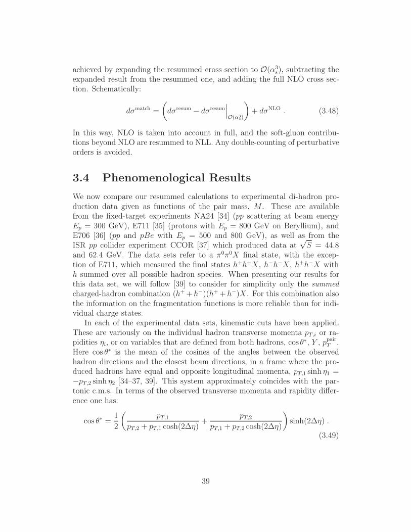
achieved by expanding the resummed cross section to O('3s), subtracting the

expanded result from the resummed one, and adding the full NLO cross sec-tion. Schematically:

d-match =

"

d-resum & d-resumAAAO(+3

s)

#

+ d-NLO . (3.48)

In this way, NLO is taken into account in full, and the soft-gluon contribu-tions beyond NLO are resummed to NLL. Any double-counting of perturbativeorders is avoided.

3.4 Phenomenological Results

We now compare our resummed calculations to experimental di-hadron pro-duction data given as functions of the pair mass, M . These are availablefrom the fixed-target experiments NA24 [34] (pp scattering at beam energyEp = 300 GeV), E711 [35] (protons with Ep = 800 GeV on Beryllium), andE706 [36] (pp and pBe with Ep = 500 and 800 GeV), as well as from theISR pp collider experiment CCOR [37] which produced data at

!S = 44.8

and 62.4 GeV. The data sets refer to a (0(0X final state, with the excep-tion of E711, which measured the final states h+h+X , h"h"X , h+h"X withh summed over all possible hadron species. When presenting our results forthis data set, we will follow [39] to consider for simplicity only the summedcharged-hadron combination (h++h")(h++h")X . For this combination alsothe information on the fragmentation functions is more reliable than for indi-vidual charge states.

In each of the experimental data sets, kinematic cuts have been applied.These are variously on the individual hadron transverse momenta pT,i or ra-pidities 0i, or on variables that are defined from both hadrons, cos !!, Y , ppairT .Here cos !! is the mean of the cosines of the angles between the observedhadron directions and the closest beam directions, in a frame where the pro-duced hadrons have equal and opposite longitudinal momenta, pT,1 sinh 01 =&pT,2 sinh 02 [34–37, 39]. This system approximately coincides with the par-tonic c.m.s. In terms of the observed transverse momenta and rapidity di!er-ence one has:

cos !! =1

2

"

pT,1pT,2 + pT,1 cosh(2$0)

+pT,2

pT,1 + pT,2 cosh(2$0)

#

sinh(2$0) .

(3.49)

39

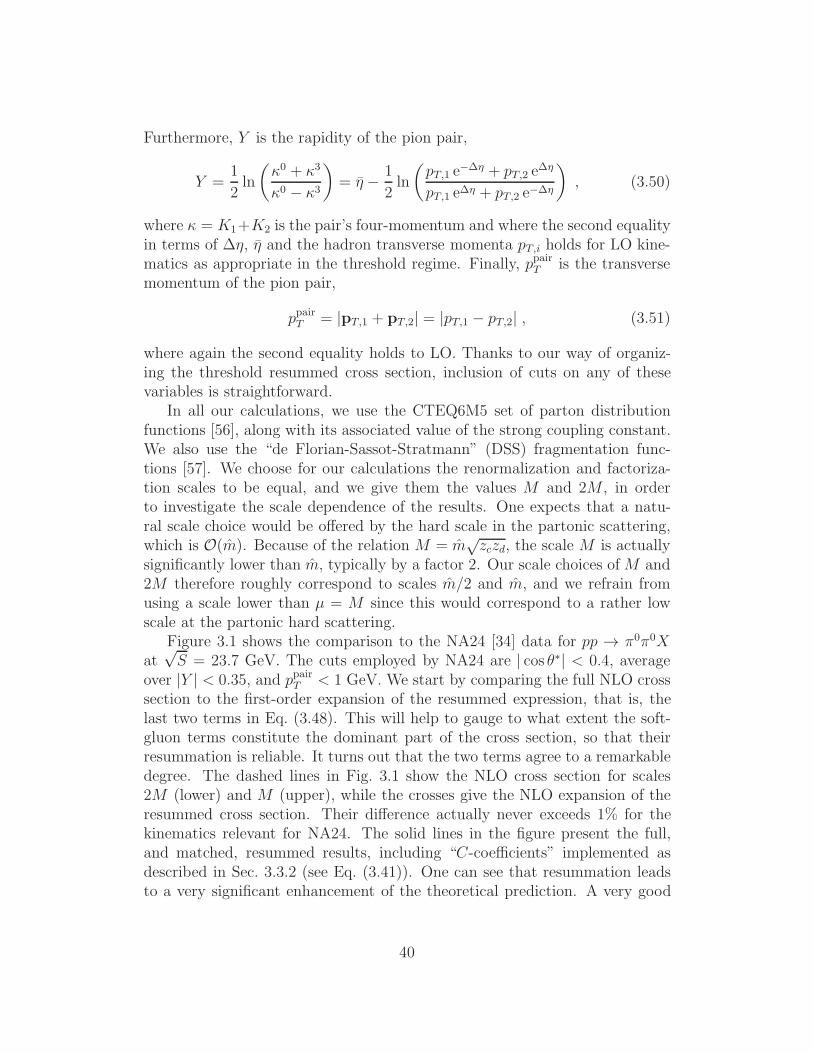
Furthermore, Y is the rapidity of the pion pair,

Y =1

2ln

".0 + .3

.0 & .3

#

= 0 &1

2ln

"pT,1 e"!, + pT,2 e!,

pT,1 e!, + pT,2 e"!,

#

, (3.50)

where . = K1+K2 is the pair’s four-momentum and where the second equalityin terms of $0, 0 and the hadron transverse momenta pT,i holds for LO kine-matics as appropriate in the threshold regime. Finally, ppairT is the transversemomentum of the pion pair,

ppairT = |pT,1 + pT,2| = |pT,1 & pT,2| , (3.51)

where again the second equality holds to LO. Thanks to our way of organiz-ing the threshold resummed cross section, inclusion of cuts on any of thesevariables is straightforward.

In all our calculations, we use the CTEQ6M5 set of parton distributionfunctions [56], along with its associated value of the strong coupling constant.We also use the “de Florian-Sassot-Stratmann” (DSS) fragmentation func-tions [57]. We choose for our calculations the renormalization and factoriza-tion scales to be equal, and we give them the values M and 2M , in orderto investigate the scale dependence of the results. One expects that a natu-ral scale choice would be o!ered by the hard scale in the partonic scattering,which is O(m). Because of the relation M = m

!zczd, the scale M is actually

significantly lower than m, typically by a factor 2. Our scale choices of M and2M therefore roughly correspond to scales m/2 and m, and we refrain fromusing a scale lower than µ = M since this would correspond to a rather lowscale at the partonic hard scattering.

Figure 3.1 shows the comparison to the NA24 [34] data for pp ' (0(0Xat

!S = 23.7 GeV. The cuts employed by NA24 are | cos !!| < 0.4, average

over |Y | < 0.35, and ppairT < 1 GeV. We start by comparing the full NLO crosssection to the first-order expansion of the resummed expression, that is, thelast two terms in Eq. (3.48). This will help to gauge to what extent the soft-gluon terms constitute the dominant part of the cross section, so that theirresummation is reliable. It turns out that the two terms agree to a remarkabledegree. The dashed lines in Fig. 3.1 show the NLO cross section for scales2M (lower) and M (upper), while the crosses give the NLO expansion of theresummed cross section. Their di!erence actually never exceeds 1% for thekinematics relevant for NA24. The solid lines in the figure present the full,and matched, resummed results, including “C-coe"cients” implemented asdescribed in Sec. 3.3.2 (see Eq. (3.41)). One can see that resummation leadsto a very significant enhancement of the theoretical prediction. A very good

40

Figure 3.1: Comparison of the NLO (dashed) and resummed (solid) calcula-tions to the NA24 data [34], for two di!erent choices of the renormalizationand factorization scales, µ = M (upper lines) and µ = 2M (lower lines). Thecrosses display the NLO O('s) expansion of the resummed cross section.

Figure 3.2: Same as Fig. 3.1, but for charged-hadron production for pp scat-tering at

!S = 38.8 GeV and with cuts appropriate for comparison to E711.

The data are from [35].

41

description of the NA24 data [34] is obtained, much better than for the NLOcalculation which falls short of the data unless rather low renormalization andfactorization scales are used. Also the scale dependence of the calculated crosssection is much reduced by resummation.

We next turn to the cross section for charged-hadron production, pBe 'h±h±X , measured by E711 [35] at

!S = 38.8 GeV. We recall that we sum over

the charges of the produced hadrons. The cuts applied by E711 were pT,i >2 GeV, and average over &0.4 < |Y | < 0.2. The cut on the individual hadrontransverse momenta is, in fact, irrelevant for the values of M considered here.Furthermore, as stated in their Fig. 6 [35] for the pair mass distribution weapply ppairT < 2 GeV, and 0.1 < | cos !!| < 0.25. Figure 3.2 shows the data andour results. As before, the agreement between NLO and the NLO expansionof the resummed calculation is excellent. Again, resummation leads to anincrease of the predicted cross section and a reduction of scale dependence.Even though the resummed result agrees with the data much better than theNLO one for the scale we have chosen, it tends to lie somewhat above thedata, in particular at the highest values of M . Keeping in mind the results forNA24, one may wonder if this might be in part related to the fragmentationfunctions for summed charged hadrons, which are probably slightly less wellunderstood than those for pions, due to the contributions from the heavierkaons and, in particular, baryons.

Figures 3.3 and 3.4 show the comparison of our results to the E706 data setsfor neutral pion pair production in pp and pBe scattering at

!S = 38.8 GeV

(800 GeV beam energy), respectively. We do not take into account any nucleare!ects for the Beryllium nucleus, except for the trivial isospin one. This has avery minor e!ect on the cross section, compared to pp. E706 used cuts fairlydi!erent from those applied in the data we have discussed so far. There wereno explicit cuts on cos !!, ppairT or Y , but instead cuts pT,i > pcutT = 2.5 GeV andeither &1.05 < 0i < 0.55 (for the

!S = 38.8 GeV data) or &0.8 < 0i < 0.8

(for the!S = 31.6 GeV data) on the transverse momenta and rapidities of

the individual pions. The cut on transverse momentum, in particular, hasa strong influence at the lower M : in a rough approximation, it leads to akinematic limit M . 2pT,i > 5 GeV, so that the cross section has to decreasevery rapidly once one decreases M toward 5 GeV. This behavior is indeed seenin the figures.

As in the previous cases, the NLO expansion of the resummed and the fullNLO cross section agree extremely well, typically to better than 2%. For thetwo scales we have chosen, the NLO cross sections fall well short of the data. Itwas noted in [39, 40] that in order for NLO to match the data, very low scalesof µ = 0.35M have to be chosen. The resummed cross section, on the other

42

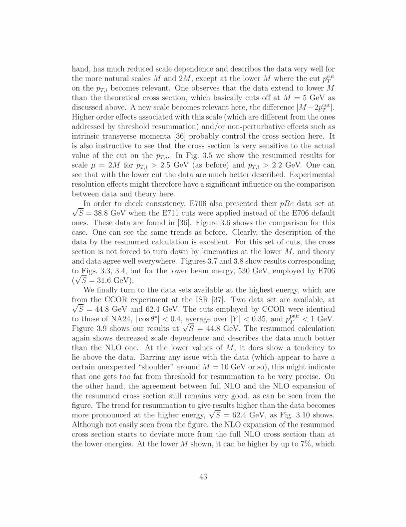
hand, has much reduced scale dependence and describes the data very well forthe more natural scales M and 2M , except at the lower M where the cut pcutT

on the pT,i becomes relevant. One observes that the data extend to lower Mthan the theoretical cross section, which basically cuts o! at M = 5 GeV asdiscussed above. A new scale becomes relevant here, the di!erence |M&2pcutT |.Higher order e!ects associated with this scale (which are di!erent from the onesaddressed by threshold resummation) and/or non-perturbative e!ects such asintrinsic transverse momenta [36] probably control the cross section here. Itis also instructive to see that the cross section is very sensitive to the actualvalue of the cut on the pT,i. In Fig. 3.5 we show the resummed results forscale µ = 2M for pT,i > 2.5 GeV (as before) and pT,i > 2.2 GeV. One cansee that with the lower cut the data are much better described. Experimentalresolution e!ects might therefore have a significant influence on the comparisonbetween data and theory here.

In order to check consistency, E706 also presented their pBe data set at!S = 38.8 GeV when the E711 cuts were applied instead of the E706 default

ones. These data are found in [36]. Figure 3.6 shows the comparison for thiscase. One can see the same trends as before. Clearly, the description of thedata by the resummed calculation is excellent. For this set of cuts, the crosssection is not forced to turn down by kinematics at the lower M , and theoryand data agree well everywhere. Figures 3.7 and 3.8 show results correspondingto Figs. 3.3, 3.4, but for the lower beam energy, 530 GeV, employed by E706(!S = 31.6 GeV).We finally turn to the data sets available at the highest energy, which are

from the CCOR experiment at the ISR [37]. Two data set are available, at!S = 44.8 GeV and 62.4 GeV. The cuts employed by CCOR were identical

to those of NA24, | cos !!| < 0.4, average over |Y | < 0.35, and ppairT < 1 GeV.Figure 3.9 shows our results at

!S = 44.8 GeV. The resummed calculation

again shows decreased scale dependence and describes the data much betterthan the NLO one. At the lower values of M , it does show a tendency tolie above the data. Barring any issue with the data (which appear to have acertain unexpected “shoulder” aroundM = 10 GeV or so), this might indicatethat one gets too far from threshold for resummation to be very precise. Onthe other hand, the agreement between full NLO and the NLO expansion ofthe resummed cross section still remains very good, as can be seen from thefigure. The trend for resummation to give results higher than the data becomesmore pronounced at the higher energy,

!S = 62.4 GeV, as Fig. 3.10 shows.

Although not easily seen from the figure, the NLO expansion of the resummedcross section starts to deviate more from the full NLO cross section than atthe lower energies. At the lowerM shown, it can be higher by up to 7%, which

43

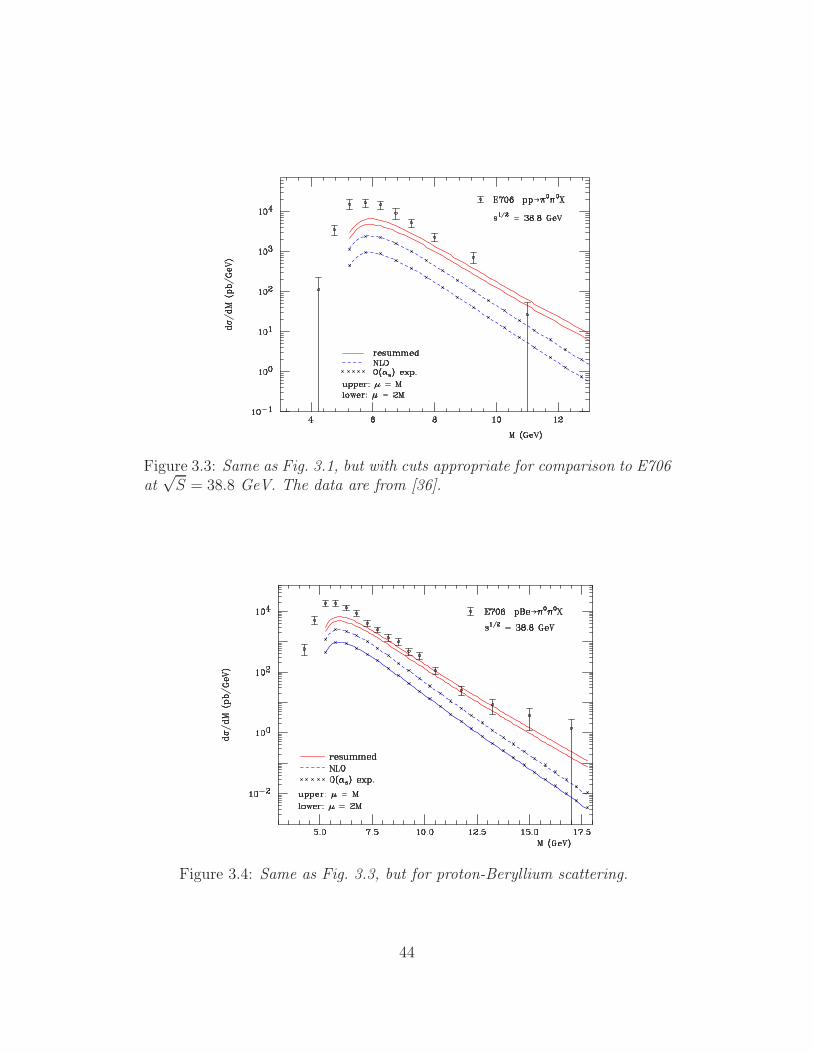
Figure 3.3: Same as Fig. 3.1, but with cuts appropriate for comparison to E706at

!S = 38.8 GeV. The data are from [36].

Figure 3.4: Same as Fig. 3.3, but for proton-Beryllium scattering.

44

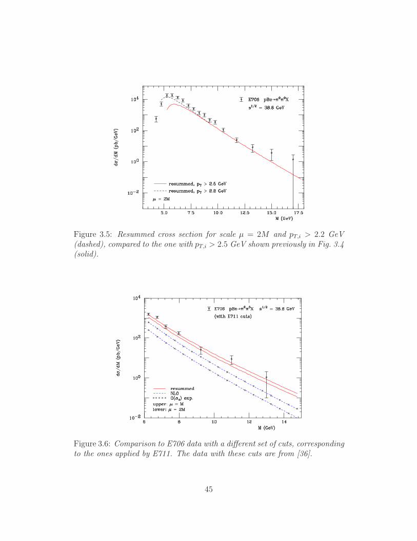
Figure 3.5: Resummed cross section for scale µ = 2M and pT,i > 2.2 GeV(dashed), compared to the one with pT,i > 2.5 GeV shown previously in Fig. 3.4(solid).

Figure 3.6: Comparison to E706 data with a di!erent set of cuts, correspondingto the ones applied by E711. The data with these cuts are from [36].

45

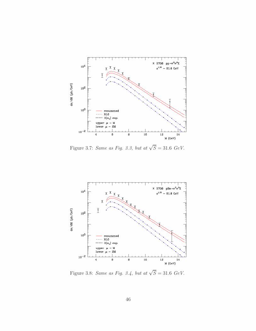
Figure 3.7: Same as Fig. 3.3, but at!S = 31.6 GeV.

Figure 3.8: Same as Fig. 3.4, but at!S = 31.6 GeV.

46

is still a relatively minor deviation, but could be indicative of the reason whythe resummed result is high as well.

Clearly, any deviation between the full NLO cross section and the NLOexpansion of the resummed one is due to terms that are formally suppressedby an inverse power of the Mellin moment N near threshold. It is thereforeinteresting to explore the likely e!ects of such terms. This can be done bypromoting the LO anomalous dimension in the evolution part in Eq. (3.42)from its diagonal form to the full one, as described in Sec. 3.3.2:

& 2A(1)i ln N & B(1)

i ' P (1),Nij , (3.52)

which includes the subleading terms in 1/N and full singlet mixing. For sim-plicity, we perform this modification only for the lowest order part of evolution,as indicated in Eqs. (3.43) and (3.52). The results obtained in this way areshown in Fig. 3.11. One can see that the resummed result obtained in thisway indeed decreases significantly with respect to the one in Fig. 3.10 whichwas based on the diagonal evolution only, and is much closer to the data. Atthe same time, the agreement between the NLO cross section and the O('s)expanded resummed result becomes as good as what we encountered in thefixed-target case. Figure 3.12 presents the corresponding result for the case ofNA24. Comparison with Fig. 3.1 shows that the e!ect of the subleading termsis much smaller here, as expected from the fact that one is closer to thresholdin the case of NA24. Nonetheless, the e!ects lead to a slight further improve-ment between the resummed calculation and the data. In particular, they givethe theoretical result a somewhat flatter behavior, which follows the trend ofthe data more closely overall. While the implementation of subleading termsin this way will require further study, this appears to be a promising approachfor extending the applicability of threshold resummation into regimes whereone is relatively far away from threshold.

That said, we remind the reader that already in the part that is leadingnear threshold we have made the approximation in Eq. (3.41) for our “C-coe"cients”. This, too, will need to be improved in the future, by taking intoaccount the full color structure of the hard scattering function beyond LO, aswe discussed in Sec. 3.3.2. To give a somewhat extreme example of the e!ectsgenerated by the C-coe"cients, we have re-computed the resummed crosssection for the case of CCOR at

!S = 62.4 GeV, but leaving out all e!ects of

the the coe"cients beyond NLO. In other words, we leave out the C-coe"cientsin the first two terms on the right-hand-side of Eq. (3.48), keeping them ofcourse in d-NLO. This is likely not a good approximation of the beyond-NLOhard coe"cients, because the C(1)

ab%cd have (2 terms and logarithms in therenormalization scale µ that are independent of the color channel and truly

47

Figure 3.9: Comparison of the NLO (dashed) and resummed (solid) calcula-tions to the CCOR data [34] at

!S = 44.8 GeV, for two di!erent choices of

the renormalization and factorization scales, µ = M (upper lines) and µ = 2M(lower lines). The crosses display the NLO O('s) expansion of the resummedcross section.

Figure 3.10: Same as Fig. 3.9, but for!S = 62.4 GeV.

48

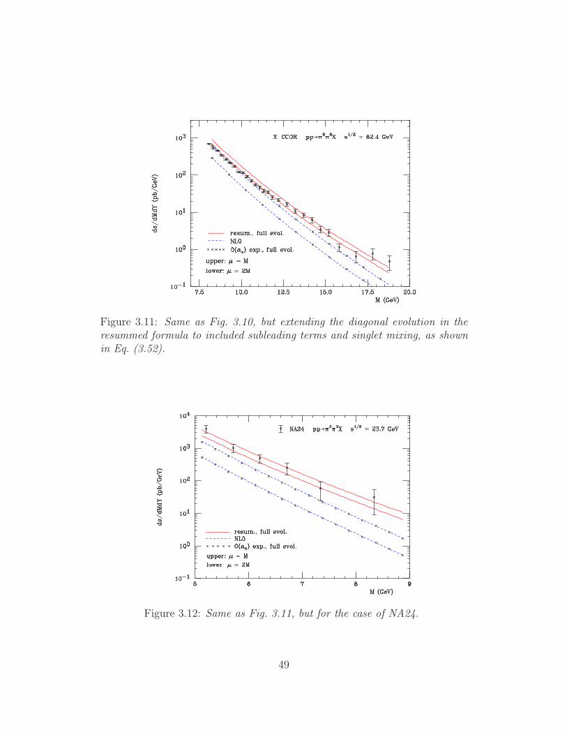
Figure 3.11: Same as Fig. 3.10, but extending the diagonal evolution in theresummed formula to included subleading terms and singlet mixing, as shownin Eq. (3.52).

Figure 3.12: Same as Fig. 3.11, but for the case of NA24.

49

enter in the form given in Eq. (3.41). Some of these are in fact even knownto exponentiate [20, 43, 44, 52, 58]. In any case, the result of this exercise isshown in Fig. 3.13, where it is also compared to our earlier calculation thatincluded the C-coe"cients in the way discussed in Sec. 3.3.2. One can see thatthere is a sizable numerical di!erence, and that the scale dependence of theresummed result without the beyond-NLO C-coe"cients becomes significantlyworse.

We finally turn to the distribution in cos !!, defined in Eq. (3.49), for whichmost of the experiments mentioned above have presented data as well. In fact,the CCOR data [37] for this observable were instrumental in establishing theQCD hard-scattering nature of pp interactions [59]. From the point of viewof threshold resummation, the distribution in cos !! may appear somewhatless interesting than the pair mass one, since the threshold logarithms arise in1& " = 1& m2/s, regardless of cos !!. In addition, the cos !! distributions arepresented as normalized distributions of the form

d-/d cos !!

d-/d cos !!|cos -#=0, (3.53)

so that the main enhancement generated by threshold resummation is expectedto cancel. Nonetheless, as we have seen in Sec. 3.3.2, the resummed expressionsdo contain additional dependence on $0 beyond that present in the Borncross sections, which will a!ect the cos !! distribution at higher orders. Thisis visible from the soft part in Eq. (3.46) and also from the “C-coe"cients”in Eq. (3.41). Rather than going through an exhaustive comparison to allthe available data, we just consider one example that is representative of thee!ects of threshold resummation on the cos !! distribution. Figure 3.14 showsthe normalized distribution for the E711 case, where we have again summedover all charge states of the produced hadrons. The dashed lines show theNLO result calculated again with the code of [39], for scales µ = 2M andµ = M . One can see that for these scales the NLO calculation is lower thanthe data for higher values of cos !!. The dot-dashed lines in Fig. 3.14 showthe resummed results for scales µ = 2M and µ = M . These show a steeperrise with cos !! and describe the data better than NLO for the scales shown.However, they still tend to lie below the data at higher values of cos !!. Aswas suggested in [37, 39, 40], for the cos !! distribution the hard scale in thepartonic process will itself be a function of cos !!, so that it is more naturalto choose a factorization/renormalization scale that reflects this feature. Wetherefore present our resummed results also for scales µ = 2M! and µ = M!,where M!2 = M2(1&cos !!) which is proportional to the Mandelstam variablet in the partonic process. One observes that with these scale choices a very

50

good description of the data is achieved. We note that in the NLO calculationspresented in Refs. [39, 40] the scale was chosen proportional to the (average)transverse momenta of the produced hadrons, which for given M also dependon cos !!. This resulted in a satisfactory description of the data, when scalese!ectively a factor two smaller than our M! were used. Overall, the trendfor the resummed cos !! distribution to lie higher than NLO and be in betteragreement with the data is found to be a generic feature that occurs as wellfor the cases of the other experiments.

3.5 Conclusions

We have investigated the e!ects of next-to-leading logarithmic threshold re-summation on the cross section for di-hadron production in hadronic collisions,H1H2 ' h1h2X , for a range of invariant masses of the produced hadron pair.We have developed techniques to implement the resummation formalism atfixed rapidities for the produced hadrons and for all relevant experimentalcuts. Extensions of these techniques to the level of next-to-next-lo-leadinglogarithms should be relatively straightforward in light of the close relationbetween the one- and two-loop soft anomalous dimension matrices [60].

For the fixed target and collider data studied here, the one-loop expansionsof our resummed expressions approximate the corresponding exact one-loopcross sections excellently, to the level of a few percent and often less. In addi-tion, with scales chosen to match the underlying hard scattering, the matchedresummed cross sections typically explain the available data better than doNLO expressions at similar scales, with significantly reduced scale dependence.

An important extension of these methods will be in the production andfragmentation of heavy quarks and in jet cross sections, where similar resum-mation methods are applicable. Given the reduction in scale dependence, thiscould provide an improved control over Standard Model tests and backgroundsin new physics searches.

In the next chapter we study the e!ects of resummation in top anti-topproduction. We take a special look at a particular observable, the chargeasymmetry in top anti-top production.

51

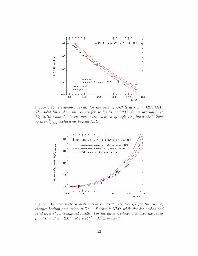
Figure 3.13: Resummed results for the case of CCOR at!S = 62.4 GeV.

The solid lines show the results for scales M and 2M shown previously inFig. 3.10, while the dashed ones were obtained by neglecting the contributionsby the C(1)

ab%cd coe"cients beyond NLO.

Figure 3.14: Normalized distribution in cos !! (see (3.53)) for the case ofcharged-hadron production at E711. Dashed is NLO, while the dot-dashed andsolid lines show resummed results. For the latter we have also used the scalesµ = M! and µ = 2M!, where M!2 = M2(1& cos !!).

52

Chapter 4

Charge Asymmetry in Top

Production

4.1 Introduction

Heavy quark pair production in hadronic collisions is important both for ac-curate tests of the Standard Model and in searches for New Physics. Thanksto the large scale set by the mass of the heavy quark, one can often use QCDperturbation theory in obtaining predictions for heavy-flavor production, em-ploying the factorization of the hadronic cross section into parton distributionfunctions and perturbative short-distance cross sections.

Top quark production may provide an arena for testing possible exten-sions of the Standard Model [62–65]. One particularly interesting observablein tt production that has been considered in this context [66, 67] is the chargeasymmetry (or, forward-backward asymmetry), which is obtained by compar-ing the rate for producing a top quark at a given angle to that for producingan anti-top at the same angle. Electro-weak processes, as well as processes inmany extensions of the Standard Model, may produce a charge asymmetry atBorn level. QCD, on the other hand, being a purely vector theory, does notproduce a charge asymmetry in the lowest-order (LO) processes qq ' tt andgg ' tt. The charge asymmetry thus has the potential of probing or constrain-ing possible tree-level axial couplings of the gluon [66, 67] at the Tevatron orthe LHC.

Starting at order '3s, however, QCD itself contributes to the charge asym-

metry, through qq annihilation qq ' tt(g) and flavor excitation, qg ' q tt [68].This happens through diagrams in which two separate fermion lines (one ofthem the top quark line) are connected by three gluons. This phenomenon,which is also well-known in QED [69], enters with the combination dabcdabc of

53

the symmetric QCD structure constants. The same mechanism for light flavorshas been found to generate a strange quark s & s asymmetry in the nucleonsea [70]. The charge asymmetric part is contained in the full next-to-leadingorder (NLO, O('3

s)) calculations of the di!erential heavy-flavor productioncross section [71–73]. Since this is the order at which the e!ect arises for thefirst time, we will usually refer to the charge asymmetric part arising at O('3

s)as LO. There have been detailed calculations and phenomenological studies ofthe QCD top quark charge asymmetry at the Tevatron (or the LHC), bothfor the inclusive case, pp ' ttX [67, 74], and for associated-jet final states,pp ' tt jetX [75, 76]. In particular, Ref. [76] provides the full NLO (O('4

s))corrections to pp ' tt jetX .

Very recently, first measurements of top quark charge asymmetries havebeen reported by the Tevatron collaborations [77, 78]. In the inclusive case,asymmetries of 12± 8 (stat.)± 1(syst.)% and 23± 12 (stat.)± 6(syst.)% werefound by D0 [77] and CDF [78], respectively. Even though experimental un-certainties are evidently still large, this is a very encouraging first step thatmotivates further theoretical investigations. In the present paper we improvethe theoretical framework for the case of the inclusive charge asymmetry byexamining the e!ects of QCD threshold resummation. This will provide in-sight into the important question of how robust the asymmetry is with respectto higher order QCD corrections. Our study requires us to implement NLLresummation in heavy quark production at fixed angle and rapidity [20, 21].Earlier phenomenological studies of the threshold-resummed tt cross section,which however did not focus on the charge asymmetry, may be found in [79–82].

As is well-known, when the initial partons have just enough energy toproduce a tt pair, the phase space available for gluon bremsstrahlung nearlyvanishes, giving rise to large logarithmic corrections to the partonic cross sec-tion. For example, if we consider the cross section for tt production at fixedpair invariant mass, this partonic threshold is reached when the pair invari-ant mass equals the partonic center of mass (c.m.) energy, M2

tt = s. Atthe nth order of perturbation theory, the large threshold corrections ariseas '2+n

s [logm(1& ")/(1& ")]+ with m " 2n & 1, where " = M2tt/s and the

“+”-distribution will be reviewed below. The maximum value, m = 2n & 1corresponds to the leading logarithms (LL), m = 2n & 2 to next-to-leadinglogarithms (NLL), and so forth. Near threshold, the perturbative calculationproduces potentially large corrections at all orders in the strong coupling, 's.These corrections are addressed by threshold resummation. This is particu-larly relevant for the Tevatron case, where the hadronic c.m. energy is nottoo much larger than twice the top mass, 2mt, so that " is on average rather

54

close to unity. Related considerations also apply at the LHC when the pair isproduced with M2

tt * 4m2t .

For heavy quark production, threshold resummation has been derived toNLL accuracy [20, 80]. The results of [20] have been presented for arbitraryc.m. scattering angle of the produced top quark, which makes it possible toobtain a resummed charge asymmetry from them. Among the processes thatcontribute to the charge asymmetry, only qq annihilation contains thresholdlogarithms, while the flavor excitation qg process is suppressed near threshold.As we shall discuss in some detail, it turns out that the leading logarithms inthe charge asymmetric part of qq annihilation cancel at O('3

s). This is becausethe charge asymmetric part is a di!erence of cross sections with the top orthe anti-top produced at a certain angle, and the leading logarithms enter inassociation with the O('2

s) qq ' tt Born process, which is charge symmetric.We shall return to this point below, and will find that beyond O('2

s) thecharge asymmetric cross section is enhanced by the same threshold logarithmsas the symmetric one. We also note that the gg fusion process is chargesymmetric to all orders; nonetheless its resummation can be relevant also forthe charge asymmetry as it contributes to the denominator of the asymmetryand may thus dilute it somewhat. This e!ect does not lead to significantsuppression, however, because of the higher-order threshold enhancements tothe asymmetric cross section, which we will exhibit below.

The remainder of this chapter is organized as follows. In Sec. 4.2 we givethe basic formulas associated with the charge asymmetry and discuss the near-threshold behavior at O('2

s). In Sec. 3 we present the relevant expressions forthe NLL resummed tt cross section as a function of the tt pair invariant massand the top c.m. scattering angle. Section 4 presents our phenomenologicalresults for Tevatron kinematics, and we summarize our findings in Sec. 5.

4.2 Perturbative Cross section, and Charge

Asymmetry

We consider inclusive tt production in hadronic collisions,

HA(PA) +HB(PB) ' t(pt)t(pt) +X(pX), (4.1)

where we have indicated the momenta. We introduce the invariant masssquared of the tt pair: M2

tt = (pt + pt)2, and the variable " ( M2tt/S with

S = (PA + PB)2. The factorized cross-section for the process is written interms of convolutions of parton distributions fHA

a and fHB

b for partons a,bin hadrons HA, HB, respectively, with perturbative partonic hard-scattering

55

cross-sections -ab:

d2-HAHB%ttX

dM2tt d cos !

=!

ab

* 1

0

dxa

* 1

0

dxb fHAa (xa, µ

2)fHB

b (xb, µ2)

)1

s

d2-ab(" , cos !, µ2/s)

d" d cos !, (4.2)

where the sum runs over all partonic subprocesses that produce top quarkpairs. We have introduced the partonic variable " = M2

tt/s = "/xaxb. Wedefine ! as the production angle of the top quark in the partonic center-of-mass frame. We note from the outset that this is not the definition adoptedin the Tevatron experiments, where the asymmetry is considered as a functionof the rapidity di!erence $yt of the t and t. However, for LO kinematics, thetwo definitions are directly related through [78] tanh($y/2) = + cos !, with+ =

D

1& 4m2t/s the top quark velocity. As the partonic threshold regime

is characterized by LO kinematics, we expect our resummed results below tobe very faithful representations also of the e!ects expected for the Tevatrondefinition (see also [67]). In fact, we have found that for quantities integratedover angle the charge asymmetries for the two definitions agree at the level ofabout 2% or better. The integration limits in Eq. (4.2) are determined by theconditions [81] s % M2

tt % 4m2t/(1&+2 cos2 !). Finally, the scale µ denotes the

factorization and renormalization scales, which we take to be equal throughoutthis study.

We next define the charge-asymmetric and charge-averaged cross sections:

d$-

dM2ttd cos !

(1

2

Ed2-HAHB%ttX

dM2ttd cos !

&d2-HAHB%ttX

dM2ttd cos !

F

,

d-

dM2ttd cos !

(1

2

Ed2-HAHB%ttX

dM2ttd cos !

+d2-HAHB%ttX

dM2ttd cos !

F

,

and the corresponding charge asymmetry

Ac(M2tt, cos !) (

d$-

d-. (4.3)

To lowest order (LO), tt pairs are produced by the processes qq ' tt andgg ' tt. These produce the top and the anti-top evenly at a given productionangle !, so that the charge asymmetry vanishes. Beyond LO, however, qqannihilation as well as the flavor excitation process qg ' ttq have chargeasymmetric contributions [74], while gg scattering remains symmetric. For theqq annihilation process, the asymmetry arises from three gluons connecting the

56

light-quark and the top-quark lines. In the case of inclusive tt production, theasymmetry receives contributions from real diagrams for qq ' ttg and fromvirtual corrections in qq ' tt. The charge asymmetric pieces for the O('3

s)subprocesses have been computed in detail in [74]; they are also included ofcourse in the full next-to-leading order (NLO) calculations of the top quarkcross section [71–73].

As we discussed in the Introduction, large double- and single-logarithmiccorrections arise at higher orders in the partonic cross sections for qq annihila-tion and gg fusion when " becomes large, that is, when M2

tt . s. The structureof the NLO terms in the qq annihilation cross section becomes, for example,

d2-NLOqq (" , cos !)

d" d cos != C1(!)%(1& " ) + C2(!)

"1

1& "

#

+

+C3(!)

"log(1& " )

1& "

#

+

+ . . . , (4.4)

where the ellipses denote terms that are suppressed near threshold. We havesuppressed the dependence on the factorization/renormalization scale, as wewill often do in the following. The “+”-distribution is defined as usual by

* 1

x

dz [g(z)]+ f(z) =

* 1

x

dz g(z) (f(z)& f(1))& f(1)

* x

0

dz g(z) . (4.5)

The coe"cients Ci may be found in Ref. [81]. It turns out that only C1

and C2 possess charge-asymmetric pieces, while the double-logarithmic partassociated with C3 is symmetric and thus cancels in the asymmetry at lowestorder. This is a result of the factorization of collinear logarithms, which donot interfere with color flow in the hard scattering [20]. As a result, the chargeasymmetric contributions in qq ' ttg and qq ' tt each have an infrared (butno collinear) singularity at O('3

s) [74], which cancels in their sum and leavesbehind a single logarithm, represented by the term proportional to 1/(1& ")+in Eq. (4.4). We will see in the next section, however, that, starting with thenext order, leading logarithms contribute to the asymmetric cross section asan overall factor.

4.3 NLL resummation

The resummation of the soft-gluon contributions is organized in Mellin-N mo-ment space. We take a moment of the hadronic cross section with respect to

57

the variable " :d-N

d cos !(* 1

0

d""N"1 d2-

d"d cos !. (4.6)

Under Mellin moments, the convolutions in the factorized cross section nearthreshold become products:

d-N

d cos !=!

ab

fHA,Na (µ2)fHB,N

b (µ2)-ab(N, !) , (4.7)

where the fHA,Na , fHB,N

b are the Mellin moments of the parton distributions,defined by analogy to Eq. (4.6), and where

-ab(N, !) =

* 1

0

d" "N"1d2-ab(" , cos !)

d" d cos !. (4.8)

The threshold limit (" ' 1) now corresponds to N ' 0 in moment space.Threshold resummation results in exponentiation of the soft gluon correc-

tions in moment space. Unlike color singlet cases like the Drell-Yan process,in heavy-flavor production soft gluons emitted at large angles interfere withthe color structure of the underlying Born process. One must then take intoaccount all color structures and sum over them. The details of this procedurewere worked out for scattering at fixed angles in [20, 21, 83]. For a given par-tonic channel (ab = qq, gg), the resumed perturbative cross section is givenby 1

-(res)ab (N, !) = Cab(!)$a(N)$b(N)

)TrB

H(0)ab (!) [Sab(N, !)]† S(0)

ab Sab(N, !)C

, (4.9)

where we have suppressed for simplicity the dependence of the various func-tions on the pair mass Mtt, but have kept dependence on the scattering angle! wherever it occurs. Even before defining the various factors in the resummedcross section, we may note that it naturally gives rise to a charge asymme-try. In Eq. (4.9), all dependence on the c.m. scattering angle ! resides inthe color trace part and in the coe"cients Cab. Therefore, these generate thecharge-asymmetric part of the cross section near threshold:

$-(res)qq (N, !) = ($q(N))2

?

Cqq(!) TrB

H(0)ab (!) [Sab(N, !)]† S(0)

ab Sab(N, !)C

&Cqq(&!) TrB

H(0)ab (!) [Sab(N,&!)]† S(0)

ab Sab(N,&!)C@

.(4.10)

1See, in particular, Eq. (50) of Ref. [21].

58

It is the ratio of Eq. (4.10) and its charge-averaged counterpart that defines theasymmetry. We anticipate that, when expanding the resummed expression tonext-to-leading order, leading logarithms cancel and the C2 term in Eq. (4.4)is reproduced.

Now let us review the elements of the resummed cross sections. The tracein Eq. (4.9) is taken in a space of color exchange operators [20, 21]. At lowest

order, H(0)ab and S(0)

ab are the hard-scattering and the zeroth-order soft functions,respectively. The factors Sab are also matrices in color space and depend onthe basis of color tensors used to describe color exchange. Employing the s-channel singlet-octet basis of [20], one has for the qq subprocess, which we aremostly interested in here,

H(0)qq = '2

s

&

'

0 0

0 2$

t2+u2

s2 + 2m2t

s

%

/C2A

5

6 ,

S(0)qq =

,

C2A 0

0 (C2A & 1)/4

-

, (4.11)

where t ( (pt & pa)2 & m2t = &s(1 & + cos !)/2, u ( (pt & pa)2 & m2

t =&s(1++ cos !)/2, with pa the momentum of initial parton a, + =

D

1& 4m2t/s,

and CA = 3. The corresponding expressions for the soft anomalous dimensionmatrices of the gg-initiated subprocess may be found in [20]. Note that the

Born cross sections are recovered by computing Tr{H(0)ab S

(0)ab } and that H(0)

ab issymmetric under interchange of t and u and hence charge symmetric.

Each of the functions $a,b(N) and Sab(N, !) is an exponential. $a(N)represents the e!ects of soft-gluon radiation collinear to initial parton a andin the MS scheme is given by

ln$a(N) =

* 1

0

zN"1 & 1

1& z

* (1"z)2M2tt

µ2

dq2

q2Aa('s(q

2)) , (4.12)

and similarly for $b(N). The function Aa is a perturbative series in 's,

Aa('s) ='s

(A(1)

a +$'s

(

%2

A(2)a + . . . , (4.13)

with [84]:

A(1)a = Ca , A(2)

a =1

2Ca

3

CA

"67

18&

(2

6

#

&5

9Nf

4

, (4.14)

59

where Nf is the number of flavors, and

Cq = CF = (N2c & 1)/2Nc = 4/3 , Cg = CA = Nc = 3 . (4.15)

The factors $a,b(N) generate leading threshold enhancements, due to soft-collinear radiation, as the same overall factors in both the charge symmetricand antisymmetric cross sections.

The large-angle soft gluon exponentials Sab(N, !) are dependent on theprocess and mix the color structure. One has

Sab (N, !) = P exp

.

1

2

* M2tt/N2

M2tt

dq2

q2#Sab

(

's(q2), !

)

/

, (4.16)

where P denotes path ordering and where #Sab are soft anomalous dimensions,

which are also matrices in a given color basis. They are perturbative; for theresummation at NLL one only needs the first-order term and path orderingbecomes irrelevant. For the qq subprocess, the first-order anomalous dimensionmatrix can be represented as

#S,(1)qq =

's

(

"

#qq11 #qq

12

#qq21 #qq

22

#

, (4.17)

with matrix elements [20]2

#qq11 = &CF [L$ + 1 + i(] ,

#qq21 = 2 ln

"

t

u

#

,

#qq12 =

CF

CAln

"t

u

#

,

#qq22 = CF

3

4 ln

"t

u

#

& L$ & 1& i(

4

+CA

2

3

&3 ln

"t

u

#

& ln

"m2

t s

tu

#

+ L$ + 1 + i(

4

, (4.18)

where

L$ =1& 2m2

t/s

+

"

ln1& +

1 + ++ i(

#

. (4.19)

Finally, the coe"cients Cab(!) contain N -independent hard contributions aris-

2Note that for our definition of the charge asymmetry we need to interchange t and u inthe results of [20].

60

ing from one-loop virtual corrections. They are perturbative as well, and havethe expansion

Cab(!) = 1 +'s

(C(1)

ab (!) +O('2s) . (4.20)

The coe"cients C(1)ab may be obtained by comparison of the resummed formula

to the full NLO calculation. We note that they contain the Coulomb correc-tions which diverge as 1/+ at s . 4m2

t . As indicated, the C(1)ab depend on the

scattering angle !, and in fact for the qq subprocess they also contain a charge-asymmetric part. The full coe"cients have been derived in Ref. [81] and aregiven by very lengthy expressions. Starting from slightly corrected versions 3

of the expressions given in [81], we have been able to verify that the charge-asymmetric part of the resulting coe"cient for the qq process reproduces thecorresponding result given in [74].

We now give explicit formulas for the expansions of the resummed expo-nents to NLL accuracy following the general approach of [87]. The functions$a,b(N) become

ln$aN ('s(µ

2),M2tt/µ

2) = ln N h(1)a (/) + h(2)

a (/,M2tt/µ

2)

+O(

's('s lnN)k)

. (4.21)

Here / = +0's(µ2) ln N with N = Ne#E , where $E is the Euler constant. Thefunctions h(1,2) are given by

h(1)a (/) =

A(1)a

2(+0/[2/+ (1& 2/) ln(1& 2/)] , (4.22)

h(2)a (/,M2

tt/µ2) =&

A(2)a

2(2+20

[2/+ ln(1& 2/)] +A(1)

a

2(+0ln(1& 2/) ln

M2tt

µ2

+A(1)

a +1

2(+30

3

2/+ ln(1& 2/) +1

2ln2(1& 2/)

4

, (4.23)

where +0 = (11CA & 2Nf) /12(, and

+1 =1

24(2

(

17C2A & 5CANf & 3CFNf

)

. (4.24)

The function h(1)a above contains all LL terms in the perturbative series, while

h(2)a is of NLL only. For a complete NLL resummation one also needs the

3Specifically, we use Eq. (A.19) of Ref. [85] in the second and third integral in (A.20) ofRef. [86] and in Eqs. (A.9) and (A.11) of the first paper of Ref. [81].

61

expansion of the integral in Eq. (4.16), given by,

lnSab (N, !) =ln(1& 2/)

2(b0#S,(1)qq (!) . (4.25)

While the full structure of the resummed expressions is rather long andcomplicated, a major simplification occurs when one expands it for small +and ignores the coe"cient Cab. One finds in this case

-(res)qq (N, !) = -(Born)

qq (!) ($q(N))2E

1 ++ cos !(8CF & 3CA) ln(1& 2/)

(b0

F

)e"CA2"b0

ln(1"2') . (4.26)

Here, the factor 8CF &3CA is the typical color factor associated with the QCDcharge asymmetry [74]. One can see how the single threshold logarithm arisesat the first order in 's in the charge-asymmetric part. The charge-asymmetricpiece is suppressed by the factor +, but enhanced by the term ln(1 & 2/).All factors outside the curly brackets are common to the charge-asymmetricand the charge-summed parts and are expected to largely cancel in the chargeasymmetry at hadron level. We note that in the limit + ' 0 our formulasabove reproduce the moment-space expressions for the resummed total heavy-flavor cross section derived in [80].

In our discussion below, we use the full formula (4.10) when calculatingthe charge asymmetry. Since the matrices involved for the qq subprocess aretwo-dimensional, it is straightforward to perform the required exponentiationsand other manipulations, explicitly employing a diagonal color basis for these2 ) 2 matrices [20]. For the (charge-symmetric) gg subprocess, the matricesare three-dimensional, and this procedure becomes more complicated. Wefound it simpler here to do the matrix manipulations numerically, calculatingin particular the matrix exponentials by iterating the exponential series tothe tenth order. We emphasize again that the gg process is charge-symmetric.Thus, it only contributes to the denominator of the charge asymmetry, dilutingthe asymmetry somewhat, because the e!ects of threshold resummation canbe larger for gluons than for quarks.

4.4 Phenomenological results

We will now investigate the numerical size of the QCD charge asymmetry fortop quark production at the Tevatron, making use of the resummation formulaspresented above. In order to do this, we first need to specify the inverse Mellin

62

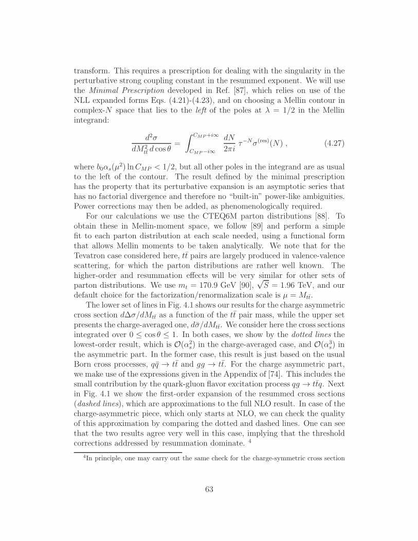
transform. This requires a prescription for dealing with the singularity in theperturbative strong coupling constant in the resummed exponent. We will usethe Minimal Prescription developed in Ref. [87], which relies on use of theNLL expanded forms Eqs. (4.21)-(4.23), and on choosing a Mellin contour incomplex-N space that lies to the left of the poles at / = 1/2 in the Mellinintegrand:

d2-

dM2tt d cos !

=

* CMP+i$

CMP"i$

dN

2(i""N-(res)(N) , (4.27)

where b0's(µ2) lnCMP < 1/2, but all other poles in the integrand are as usualto the left of the contour. The result defined by the minimal prescriptionhas the property that its perturbative expansion is an asymptotic series thathas no factorial divergence and therefore no “built-in” power-like ambiguities.Power corrections may then be added, as phenomenologically required.

For our calculations we use the CTEQ6M parton distributions [88]. Toobtain these in Mellin-moment space, we follow [89] and perform a simplefit to each parton distribution at each scale needed, using a functional formthat allows Mellin moments to be taken analytically. We note that for theTevatron case considered here, tt pairs are largely produced in valence-valencescattering, for which the parton distributions are rather well known. Thehigher-order and resummation e!ects will be very similar for other sets ofparton distributions. We use mt = 170.9 GeV [90],

!S = 1.96 TeV, and our

default choice for the factorization/renormalization scale is µ = Mtt.The lower set of lines in Fig. 4.1 shows our results for the charge asymmetric

cross section d$-/dMtt as a function of the tt pair mass, while the upper setpresents the charge-averaged one, d-/dMtt. We consider here the cross sectionsintegrated over 0 " cos ! " 1. In both cases, we show by the dotted lines thelowest-order result, which is O('2

s) in the charge-averaged case, and O('3s) in

the asymmetric part. In the former case, this result is just based on the usualBorn cross processes, qq ' tt and gg ' tt. For the charge asymmetric part,we make use of the expressions given in the Appendix of [74]. This includes thesmall contribution by the quark-gluon flavor excitation process qg ' ttq. Nextin Fig. 4.1 we show the first-order expansion of the resummed cross sections(dashed lines), which are approximations to the full NLO result. In case of thecharge-asymmetric piece, which only starts at NLO, we can check the qualityof this approximation by comparing the dotted and dashed lines. One can seethat the two results agree very well in this case, implying that the thresholdcorrections addressed by resummation dominate. 4

4In principle, one may carry out the same check for the charge-symmetric cross section

63

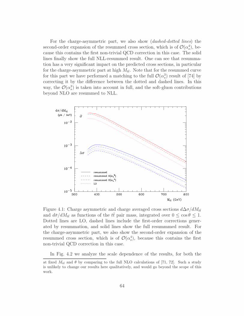
For the charge-asymmetric part, we also show (dashed-dotted lines) thesecond-order expansion of the resummed cross section, which is of O('4

s), be-cause this contains the first non-trivial QCD correction in this case. The solidlines finally show the full NLL-resummed result. One can see that resumma-tion has a very significant impact on the predicted cross sections, in particularfor the charge-asymmetric part at high Mtt. Note that for the resummed curvefor this part we have performed a matching to the full O('3

s) result of [74] bycorrecting it by the di!erence between the dotted and dashed lines. In thisway, the O('3

s) is taken into account in full, and the soft-gluon contributionsbeyond NLO are resummed to NLL.

Figure 4.1: Charge asymmetric and charge averaged cross sections d$-/dMtt

and d-/dMtt as functions of the tt pair mass, integrated over 0 " cos ! " 1.Dotted lines are LO, dashed lines include the first-order corrections gener-ated by resummation, and solid lines show the full resummmed result. Forthe charge-asymmetric part, we also show the second-order expansion of theresummed cross section, which is of O('4

s), because this contains the firstnon-trivial QCD correction in this case.

In Fig. 4.2 we analyze the scale dependence of the results, for both the

at fixed Mtt and ! by comparing to the full NLO calculations of [71, 72]. Such a studyis unlikely to change our results here qualitatively, and would go beyond the scope of thiswork.

64

charge asymmetric and averaged parts. The dash-dotted lines correspond toa variation of Mtt/2 " µ " 2Mtt, with the central lines (dotted) the ones forµ = Mtt already shown in Fig. 4.1. The higher results are obtained for the lowerchoice of scale. The dashed and solid lines display the same for the resummedcross sections. One can see a very significant reduction of scale dependence,in particular for the charge averaged cross section. This improvement in scaledependence due to threshold resummation is in line with similar findings in theliterature for other cross sections [80–82, 91, 92]. We note that the fact thattt production at the Tevatron proceeds primarily through qq valence-valenceannihilation helps here, since only the flavor-diagonal non-singlet evolutionmatters, which is part of the resummation formula [80, 91].

Figure 4.2: Scale dependence of the LO (dotted and dash-dotted) and NLLresummed (solid and dashed) cross sections, for a scale variationMtt/2 " µ "2Mtt.

Figure 4.3 shows the charge asymmetries Ac = d$-/d$- correspondingto the various curves in Fig. 4.1, as functions of the pair mass. As before,the dotted line shows the LO result, the solid represents the full resummedresult, and the dashed one is the expansion of the resummed cross section.For the latter we expand the cross section to O('4

s) in the numerator of theasymmetry, and toO('3

s) in the denominator, thus taking into account the firstnon-trivial QCD correction in both cases. Had we expanded both numeratorand denominator to O('3

s), the numerator would be at LO, and an artificially

65

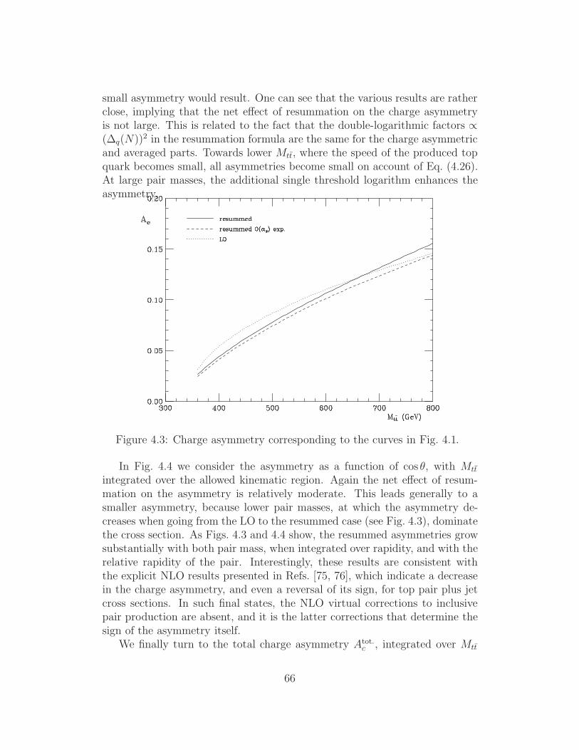
small asymmetry would result. One can see that the various results are ratherclose, implying that the net e!ect of resummation on the charge asymmetryis not large. This is related to the fact that the double-logarithmic factors 1($q(N))2 in the resummation formula are the same for the charge asymmetricand averaged parts. Towards lower Mtt, where the speed of the produced topquark becomes small, all asymmetries become small on account of Eq. (4.26).At large pair masses, the additional single threshold logarithm enhances theasymmetry.

Figure 4.3: Charge asymmetry corresponding to the curves in Fig. 4.1.

In Fig. 4.4 we consider the asymmetry as a function of cos !, with Mtt

integrated over the allowed kinematic region. Again the net e!ect of resum-mation on the asymmetry is relatively moderate. This leads generally to asmaller asymmetry, because lower pair masses, at which the asymmetry de-creases when going from the LO to the resummed case (see Fig. 4.3), dominatethe cross section. As Figs. 4.3 and 4.4 show, the resummed asymmetries growsubstantially with both pair mass, when integrated over rapidity, and with therelative rapidity of the pair. Interestingly, these results are consistent withthe explicit NLO results presented in Refs. [75, 76], which indicate a decreasein the charge asymmetry, and even a reversal of its sign, for top pair plus jetcross sections. In such final states, the NLO virtual corrections to inclusivepair production are absent, and it is the latter corrections that determine thesign of the asymmetry itself.

We finally turn to the total charge asymmetry Atot.c , integrated over Mtt

66

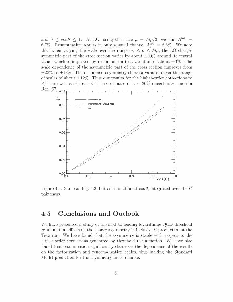
and 0 " cos ! " 1. At LO, using the scale µ = Mtt/2, we find Atot.c =

6.7%. Resummation results in only a small change, Atot.c = 6.6%. We note

that when varying the scale over the range mt " µ " Mtt, the LO charge-symmetric part of the cross section varies by about ±20% around its centralvalue, which is improved by resummation to a variation of about ±3%. Thescale dependence of the asymmetric part of the cross section improves from±28% to ±13%. The resummed asymmetry shows a variation over this rangeof scales of about ±12%. Thus our results for the higher-order corrections toAtot.

c are well consistent with the estimate of a . 30% uncertainty made inRef. [67].

Figure 4.4: Same as Fig. 4.3, but as a function of cos !, integrated over the ttpair mass.

4.5 Conclusions and Outlook

We have presented a study of the next-to-leading logarithmic QCD thresholdresummation e!ects on the charge asymmetry in inclusive tt production at theTevatron. We have found that the asymmetry is stable with respect to thehigher-order corrections generated by threshold resummation. We have alsofound that resummation significantly decreases the dependence of the resultson the factorization and renormalization scales, thus making the StandardModel prediction for the asymmetry more reliable.

67

It will be interesting to extend these studies to the case of tt jet produc-tion, for which sizable negative NLO corrections have been found [76]. Also,there will be interesting applications at the LHC in situations near partonicthreshold, i.e., when the tt pair mass becomes of the order of 1 TeV or larger.Because the initial pp state is symmetric, one needs to apply additional cuts(for example, on the tt pair rapidity) here in order to generate a non-vanishingcharge asymmetry [74].

Now we take a step back from resummation and look how logarithmiccorrections arise in the study jet production and how such jet distributionsare distinct from top jets distributions.

68

Chapter 5

Top Jets at the LHC

The Large Hadron Collider (LHC) is expected to uncover some of the mostinteresting mysteries of nature. We expect to probe the underlying principlesof electroweak symmetry breaking (EWSB) and what stabilizes the weak scaleagainst radiative corrections from unknown microscopic dynamics. Due to itslarge mass, the top quark induces the most severe contributions to the Higgsquadratic divergence. Furthermore, in almost every known natural model ofEWSB, the top sector plays a crucial role in breaking the EW symmetry.Thus, the top sector might hold a key to a new physics (NP) discovery. Manyinteresting models of EWSB predict new particles with mass . TeV scale.In several known examples, the new particles decay into highly boosted topquark pairs (pp ' X ' tt), or other decay chains containing a single top quark(pp ' X ' t Y ). In addition, the Standard Model (SM) predicts that theLHC will produce more than 105 top quarks with pT % 1TeV, significantlyenhancing our ability to study high pT tops and resolving beyond the SMdynamics.

Top quarks decay dominantly into hadronic final states (t ' bW ' bqq)with a branching ratio . 2/3, providing potentially enhanced statistics. In thepresent work, we focus on highly boosted top quarks (decaying through thehadronic channel), and on the dominant QCD jet background. We refer to atop quark that decays hadronically as a hadronic top. For moderately boostedtop quarks (pT . 500 GeV), conventional top quark reconstruction meth-ods, which exploit the decay chain topology, remain adequately e"cient (seee.g. [93]). As the top quark pT approaches 1TeV, the situation significantlychanges [94–97].1 The average separation of the top quark decay productsapproaches the limits of reliable jet reconstruction (cone size R . 0.4), andstarts to encroach upon the detector resolution (R . 0.1). As a result, the

1For earlier works in the case of boosted EW bosons see also [148].

69

e"ciency of conventional reconstruction methods drops quickly. The perfor-mance of b-tagging and light jet rejection is expected to drop substantiallyin this kinematic regime. At present, there is very little published data onb-tagging at pT . 1TeV [99]. We perform our analysis without accounting forthe possible benefits of b-jet identification.2

We turn our focus away from this family of “conventional” reconstructionmethods. We examine the situation where the decay products of at leastone top quark are reconstructed as a single jet, or top-jet. In semileptonictt events, for example, the leptonic top may still be reconstructed via semi-conventional reconstruction methods, giving up on lepton isolation cuts [94],see also [96, 100]. These methods call for further extensive study due toexpected reducible backgrounds and uncertainties related to the ability tomeasure the collimated semi-leptonic top mass (dileptonic tt events are alsoanalyzed in [101]). Hadronic top, on the other hand, will give rise to a top-jet.There will still be some small, but non-negligible, number of tt events whereone of the top quarks reconstructs as a top-jet, but the other top quark can bereconstructed via conventional methods (or semi-conventional methods whereone of the tops is manifested as a two-jet object). In this paper, we focuson the top-jet itself as a means of identifying tt events. The main reasoningbehind that is as follows:

(i) We find that for pT > 1TeV the majority of hadronic-tops are manifestedas top-jets, even for cone size as small as R = 0.4. Thus, it is clear thatour tools will be applicable for a wide range of top momenta.

(ii) The distributions and shapes of both background and signal can be un-derstood via first principle calculations as shown in this study and inRef. [25]. It may allow for a cleaner analysis, in the sense that a moredirect contact between actual data (expected to arrive soon) and themicroscopical theory can be made.

Apart from substructure, to leading order, top jets provide four piecesof information, namely its energy, two angles and mass (just as any QCDjet, ignoring the possibility of b-tagging). Without a mass cut, the QCD jetbackground swamps the hadronic top signal by orders of magnitude. Themost basic tagging method after giving up conventional methods is to use thejet mass as a discriminator between the QCD background and the hadronictop signal; the high-pT top-jet mass distribution should peak around the topmass while the QCD jet mass distribution peaks near zero. However, using a

2The possibility of b-tagging jets, when the top quark reconstructs to 2 (or more) jets,one of which has a mass . mW and the sum of the two jets has a mass . mt, is outside themain focus of this paper.

70

jet mass as a discriminator is more complicated for several reasons. Due toradiation, QCD jets acquire a large tail in the mass distribution. The crosssection for acquiring large jet mass, for example near the top mass, increasessubstantially with pT and cone size. Top-jets also broaden due to radiation,hardening their jet mass distribution.3 Furthermore, a finite jet reconstructioncone size will not always capture all the daughters of the top quark decaychain, thus softening its mass distribution. The net e!ect is a smearing ofthe expected naive, broadened, Breit-Wigner distribution for the top jet massdistribution. Detector e!ects further smear the distribution, making the aboveidealized description unrealistic.

Nevertheless, jet mass cuts should retain some rejection power against theQCD background [103–105]. Our study addresses this issue in both quantita-tive and qualitative manner, by considering the experimental and theoreticalaspects of the analysis. On the theoretical front, based on a factorizationapproach, we derive a simple approximation for the shape of the QCD jetmass spectrum. We demonstrate that there is good agreement between oursimple analytic predictions and Monte Carlo (MC) results. We are able tocompute from first principle various features related to a jet mass cut. Weevaluate its significance in the form of a semi-analytical expression for therejection power and show that it is independent of pseudorapidity. We pro-vide a quantitative study of the distribution of the signal and background, viaMadGraph/MadEvent [106–108](MG/ME) and Sherpa [109]. We consider thedetector resolution by using transfer functions [110], smearing jets accordingto a profile obtained from full Geant4 Atlas simulation. Transfer functionsprovide a versatile mechanism to explore such e!ects as shifts in jet energyscale (JES), etc.

We apply the results of our studies to analyze boosted SM top quark pairproduction, an important discovery channel for NP [94–96, 100, 111–115]. Toput results into perspective, we use both 25 fb"1 and 100 fb"1 of integratedluminosity as reference luminosities. At this time, these correspond to manyyears of data taking. We show that using single- and double-tagging meth-ods with our jet functions (defined below) to analyze jet mass distributions,we can significantly separate the Standard Model tt signal from the QCDbackground. Our theoretical QCD jet mass distributions can e"ciently char-acterize the background via sideband analyses. With 25 fb"1 of data, ourapproach allows us to resolve 1 TeV top-jets from the QCD background, andabout 1.5 TeV top-jets with 100 fb"1, if we exploit the kinematics of the so-called “away” side of the event, without relying on b-tagging. The essence ofthe away side mass cut is that it preferentially keeps the tt signal over the

3For a detailed recent study see [102] and references therein.

71

background. We analyze the mass distribution in more detailed manner, assimple counting methods are inadequate. As described above, the tt signal isexpected to exhibit pronounced structure near the top quark mass. In orderto resolve this “peak” against the QCD background, we need to understandthe shape of both the tt signal and the QCD background. To characterize thebackground we perform a sideband analysis to reduce contamination by thesignal. Our theory-driven ansatz for the QCD background is an admixture ofquark- and gluon-jet functions, the coe"cients of which we analyze by fittingin the sidebands (outside the top mass window). We interpolate the resultsof the fit into the top mass window (140GeV " mJ " 210GeV). Armed withshapes for the signal and background, we fit them into the data to obtain thenormalization constants. These normalization constants are the magnitudeof the signal and background. The errors associated with the normalizationprovides a measure of the significance of the measurement.

To further improve the significance we consider jet shapes [25], which re-solve substructure of energy flow inside cone jets. In a companion paper [25],we explore the possibility that, requiring a large jet mass, perturbative predic-tions for jet shapes di!er between jets that originate from the decay of heavyparticles, and those which result from the showering of light quarks and gluons.With such additional handles, we might have a chance to distinguish boostedtt signal from the QCD background even at a smaller integrated luminosities.4

We discuss jet substructure later in the text.We turn our attention to the use of b-jets as spin analyzers for the top

quarks. For highly boosted top quarks, chirality is approximately equal tohelicity and is conserved to a good approximation. Information about thetop chirality is encoded in the angular distribution of the decay products [94,119, 120]. Naively, one would argue that for hadronic tops this informationis inaccessible due to collimation and the absence of leptons which are knownto be good spin analysers [119, 120]. We explore the possibility of using pT ofthe b-quark for measuring the top quark polarization, which is important forexploring NP. For this, we explore the case when at least one of the boostedtop quark can be resolved into more than two jets. We also consider thepossibility of using pT of the lepton for measuring the top quark polarizationfor semi-leptonically decaying tops.

This work has two main focal points, namely QCD jet mass distributionsand hadronic tt signal, and is structured as follows. In the next section, wediscuss the MC generation and detector simulation. In section 5.2 we focus onhighly boosted QCD jets. The jet mass distribution is examined numerically,

4There are other approaches dealing with a similar situation in a di!erent perspective inrecent literature [97, 116, 153, 154].

72

via MC methods, and analytically, via jet functions. The salient points of thejet functions are introduced, leaving detailed derivations for the Appendix.Section 5.3 discusses the top-jet signal. In section 5.4, we compare high pThadronic tt events with QCD jets. In section 5.5 we discuss jet shapes [25],which can be used as additional discriminants against the background. Sec-tion 5.6 discusses the hadronic top quark polarization by using the transversemomentum of the bottom quark. We conclude in section 5.7.

5.1 Event Simulation

5.1.1 Monte Carlo Generation

The Sherpa [109] and MG/ME (version 4) [106, 108] MC generators were usedto produce tt and QCD jet events, with parameters appropriate to the LHC.To e!ect partonic level cuts during the generation of QCD jets(pT (% 1 parton) % 800 GeV), we used customized code provided by the Sherpaauthors applicable to Sherpa V1.1.0. For technical reasons, tt events were gen-erated using Sherpa version 1.0.9, whereas QCD jet events were generated withSherpa version 1.1.0. MG/ME interfaces to Pythia V6.4 (for parton showerand fragmentation) [121]. For jet reconstruction, we used SISCone V1.3 [122]for both Sherpa and MG/ME. Cross sections are calculated to leading order.Jets are defined via the cone algorithm [123] with R = 0.4 and R = 0.7, re-ferred to as C4 and C7, respectively. Jets have pT > 50GeV and |0| " 2. Atthe hard scatter level, final state partons are required to have pT % 20GeV.For MG/ME events, the final state partons have |0| " 4.5.

We do not account for pile-up e!ects nor characterize the underlying event.E"ciencies for triggering and reconstruction of jets at these energies are veryclose to unity; the corrections are negligible and are not considered. Thestrong coupling constant was allowed to run. Throughout the analysis, weused Sherpa V1.0.9 with CTEQ6M parton distribution functions (PDF) [124].Comparisons to MG/ME were made whenever appropriate, and also occasion-ally to Pythia (version 8.1) [125] for 2 ' 2 process without matching. In suchcases, the distinct curves are marked accordingly. The events used in the anal-ysis were inclusive, i.e. pp ' tt(j) and pp ' jj(j), with matching (see [126]for a detailed discussion): modified MLM [127] for MG/ME and CKKW [128]for Sherpa.

73

5.1.2 Cross Sections

In table 5.1 we present cross sections for producing final state (hadronic level)jets with pT % 1TeV for the di!erent MC simulations. There are large uncer-tainties in the cross sections, due to di!erences between the MLM and CKKWmatching, between MC generators, and between PDFs. It is outside the scopeof this paper to explore the reasons behind these di!erences.5 We estimate a100% systematic uncertainty associated with the tt cross section, and a 20%systematic uncertainty in the QCD jet cross section.

Process Generator PDF Matching Cross Sectionpp ' tt(j) SHERPA 1.0.9 CTEQ6M CKKW 135 fbpp ' tt(j) SHERPA 1.1.2 CTEQ6M CKKW 149 fbpp ' tt(j) MG/ME 4 CTEQ6M MLM 68 fbpp ' tt(j) MG/ME 4 CTEQ6L MLM 56 fbpp ' tt Pythia 6.4 CTEQ6L - 157 fbpp ' tt Pythia 8.1 CTEQ6M - 174 fb

pp ' jj(j) SHERPA 1.1.0 CTEQ6M CKKW 10.2 pbpp ' jj(j) MG/ME 4 CTEQ6L MLM 8.54 pbpp ' jj(j) MG/ME 4 CTEQ6M MLM 9.93 pbpp ' jj Pythia 6.4 CTEQ6L - 13.7 pbpp ' jj Pythia 8.1 CTEQ6M - 13.3 pb

Table 5.1: Cross sections for producing final state R = 0.4 leading cone jetswith pT % 1TeV and |0| " 2. Generation level cuts were imposed as follows.Final state partons from the hard scatter were required to have pT % 20GeV.For MG/ME, final state partons have |0| " 4.5. Processes with a trailing (j)su"x indicate that 2 ' 2 and 2 ' 3 processes are represented.

5.1.3 Modelling Detector E"ects

A transfer function, trained with full ATLAS detector simulation on high pTjet and high pT tt samples, was used to map particle level jets (Atlas truthjet reconstruction) onto a full simulation model [110]. Transfer functions workby feeding back the di!erences between the target collection (Full Simulation)and the source collection (Truth Jets). The di!erences and e"ciencies are

5Sherpa data was generated with an invariant tt mass cut greater than 500 GeV; Mad-Graph was generated with a pT cut > 700 GeV. The initial-state radiation (ISR) contribu-tions to the cross sections do not significantly a!ect our analysis, as such jets populate thelow mass spectrum.

74

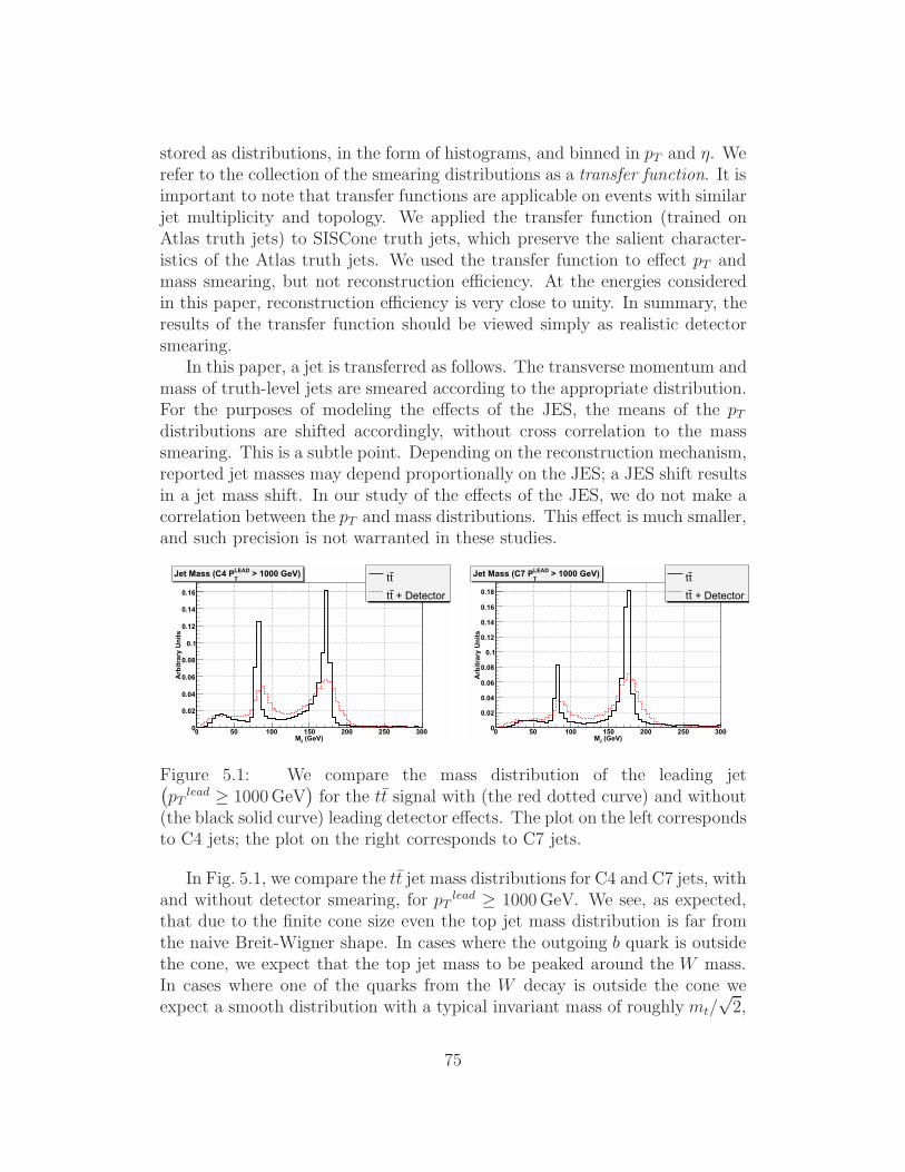
stored as distributions, in the form of histograms, and binned in pT and 0. Werefer to the collection of the smearing distributions as a transfer function. It isimportant to note that transfer functions are applicable on events with similarjet multiplicity and topology. We applied the transfer function (trained onAtlas truth jets) to SISCone truth jets, which preserve the salient character-istics of the Atlas truth jets. We used the transfer function to e!ect pT andmass smearing, but not reconstruction e"ciency. At the energies consideredin this paper, reconstruction e"ciency is very close to unity. In summary, theresults of the transfer function should be viewed simply as realistic detectorsmearing.

In this paper, a jet is transferred as follows. The transverse momentum andmass of truth-level jets are smeared according to the appropriate distribution.For the purposes of modeling the e!ects of the JES, the means of the pTdistributions are shifted accordingly, without cross correlation to the masssmearing. This is a subtle point. Depending on the reconstruction mechanism,reported jet masses may depend proportionally on the JES; a JES shift resultsin a jet mass shift. In our study of the e!ects of the JES, we do not make acorrelation between the pT and mass distributions. This e!ect is much smaller,and such precision is not warranted in these studies.

(GeV)JM0 50 100 150 200 250 300

Arb

itrar

y U

nits

0

0.02

0.04

0.06

0.08

0.1

0.12

0.14

0.16

tt

+ Detector tt

> 1000 GeV)LEADT

Jet Mass (C4 P

(GeV)JM0 50 100 150 200 250 300

Arb

itrar

y U

nits

0

0.02

0.04

0.06

0.08

0.1

0.12

0.14

0.16

0.18

tt

+ Detector tt

> 1000 GeV)LEADT

Jet Mass (C7 P

Figure 5.1: We compare the mass distribution of the leading jet(

pT lead % 1000GeV)

for the tt signal with (the red dotted curve) and without(the black solid curve) leading detector e!ects. The plot on the left correspondsto C4 jets; the plot on the right corresponds to C7 jets.

In Fig. 5.1, we compare the tt jet mass distributions for C4 and C7 jets, withand without detector smearing, for pT lead % 1000GeV. We see, as expected,that due to the finite cone size even the top jet mass distribution is far fromthe naive Breit-Wigner shape. In cases where the outgoing b quark is outsidethe cone, we expect that the top jet mass to be peaked around the W mass.In cases where one of the quarks from the W decay is outside the cone weexpect a smooth distribution with a typical invariant mass of roughly mt/

!2,

75

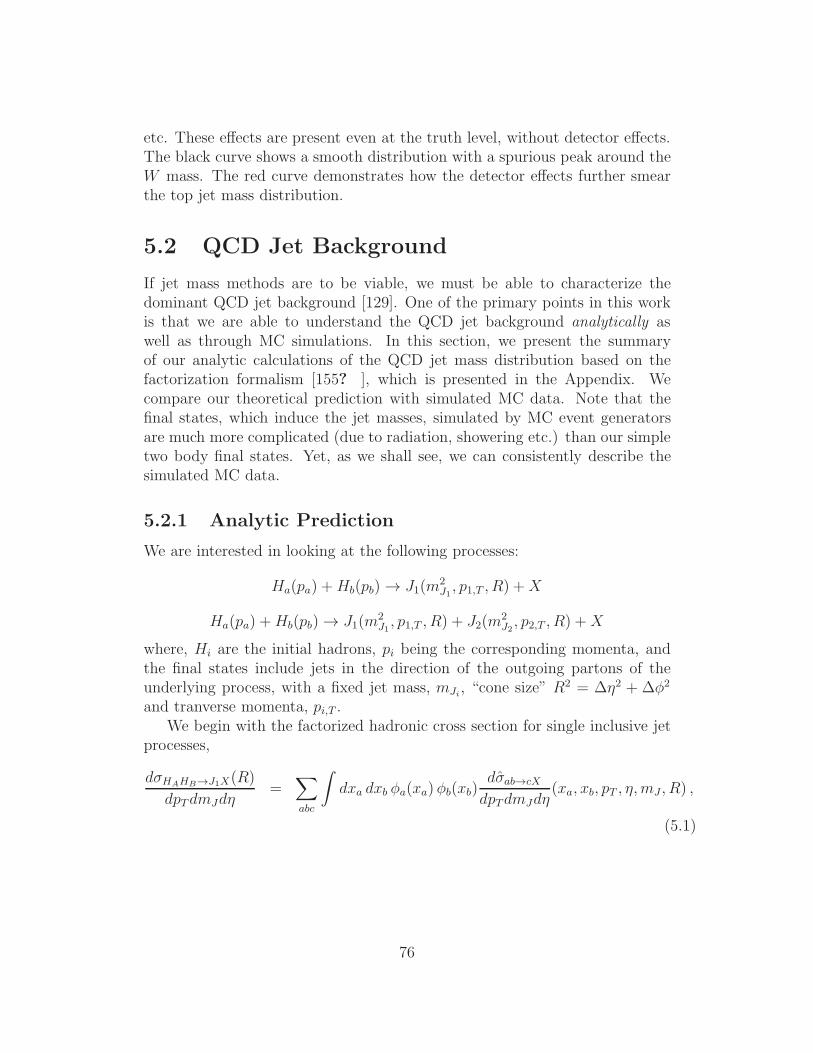
etc. These e!ects are present even at the truth level, without detector e!ects.The black curve shows a smooth distribution with a spurious peak around theW mass. The red curve demonstrates how the detector e!ects further smearthe top jet mass distribution.

5.2 QCD Jet Background

If jet mass methods are to be viable, we must be able to characterize thedominant QCD jet background [129]. One of the primary points in this workis that we are able to understand the QCD jet background analytically aswell as through MC simulations. In this section, we present the summaryof our analytic calculations of the QCD jet mass distribution based on thefactorization formalism [155? ], which is presented in the Appendix. Wecompare our theoretical prediction with simulated MC data. Note that thefinal states, which induce the jet masses, simulated by MC event generatorsare much more complicated (due to radiation, showering etc.) than our simpletwo body final states. Yet, as we shall see, we can consistently describe thesimulated MC data.

5.2.1 Analytic Prediction

We are interested in looking at the following processes:

Ha(pa) +Hb(pb) ' J1(m2J1 , p1,T , R) +X

Ha(pa) +Hb(pb) ' J1(m2J1, p1,T , R) + J2(m

2J2 , p2,T , R) +X

where, Hi are the initial hadrons, pi being the corresponding momenta, andthe final states include jets in the direction of the outgoing partons of theunderlying process, with a fixed jet mass, mJi, “cone size” R2 = $02 + $32

and tranverse momenta, pi,T .We begin with the factorized hadronic cross section for single inclusive jet

processes,

d-HAHB%J1X(R)

dpTdmJd0=

!

abc

*

dxa dxb 3a(xa)3b(xb)d-ab%cX

dpTdmJd0(xa, xb, pT , 0, mJ , R) ,

(5.1)

76

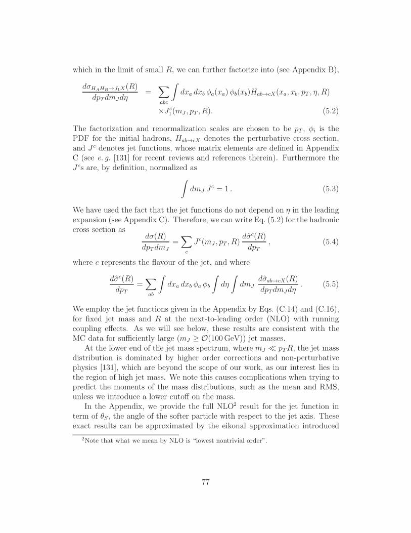
which in the limit of small R, we can further factorize into (see Appendix B),

d-HAHB%J1X(R)

dpTdmJd0=

!

abc

*

dxa dxb 3a(xa)3b(xb)Hab%cX(xa, xb, pT , 0, R)

)Jc1(mJ , pT , R). (5.2)

The factorization and renormalization scales are chosen to be pT , 3i is thePDF for the initial hadrons, Hab%cX denotes the perturbative cross section,and Jc denotes jet functions, whose matrix elements are defined in AppendixC (see e. g. [131] for recent reviews and references therein). Furthermore theJcs are, by definition, normalized as

*

dmJ Jc = 1 . (5.3)

We have used the fact that the jet functions do not depend on 0 in the leadingexpansion (see Appendix C). Therefore, we can write Eq. (5.2) for the hadroniccross section as

d-(R)

dpTdmJ=!

c

Jc(mJ , pT , R)d-c(R)

dpT, (5.4)

where c represents the flavour of the jet, and where

d-c(R)

dpT=!

ab

*

dxa dxb 3a 3b

*

d0

*

dmJd-ab%cX(R)

dpTdmJd0. (5.5)

We employ the jet functions given in the Appendix by Eqs. (C.14) and (C.16),for fixed jet mass and R at the next-to-leading order (NLO) with runningcoupling e!ects. As we will see below, these results are consistent with theMC data for su"ciently large (mJ % O(100GeV)) jet masses.

At the lower end of the jet mass spectrum, where mJ + pTR, the jet massdistribution is dominated by higher order corrections and non-perturbativephysics [131], which are beyond the scope of our work, as our interest lies inthe region of high jet mass. We note this causes complications when trying topredict the moments of the mass distributions, such as the mean and RMS,unless we introduce a lower cuto! on the mass.

In the Appendix, we provide the full NLO2 result for the jet function interm of !S, the angle of the softer particle with respect to the jet axis. Theseexact results can be approximated by the eikonal approximation introduced

2Note that what we mean by NLO is “lowest nontrivial order”.

77

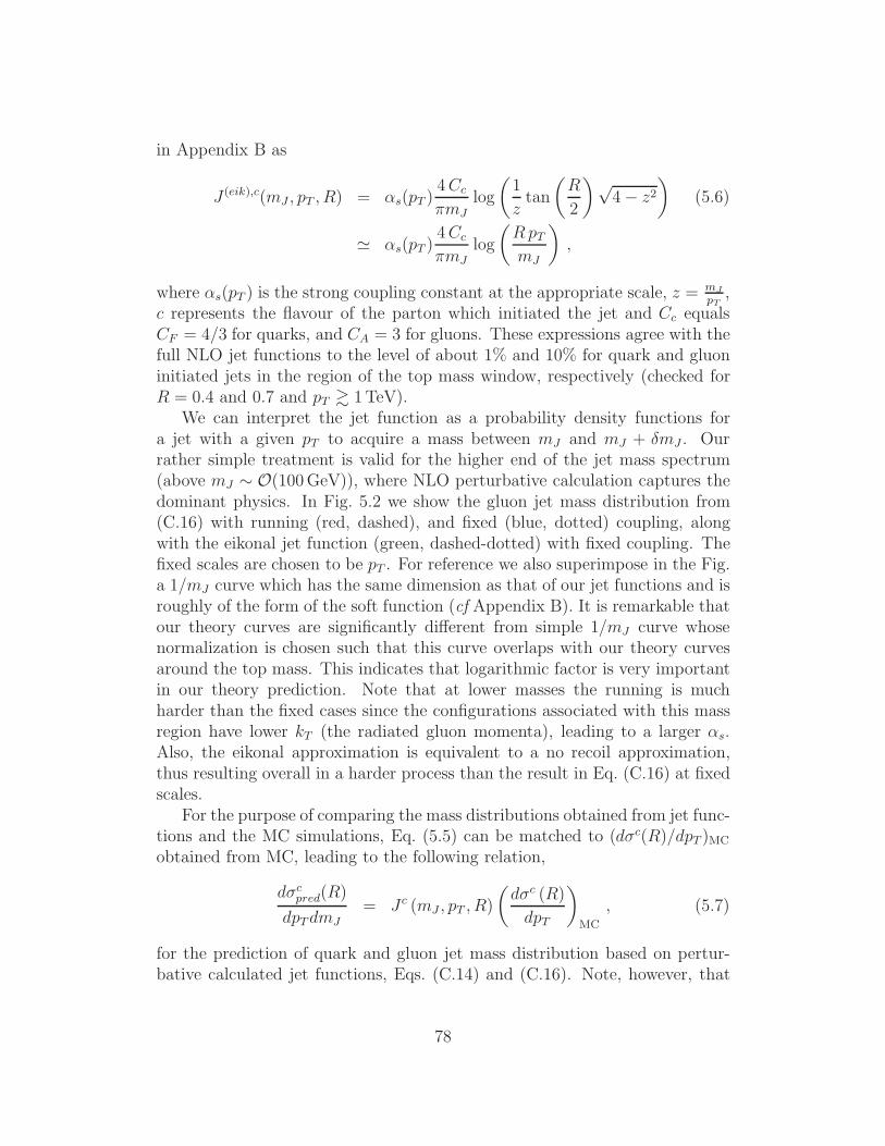
in Appendix B as

J (eik),c(mJ , pT , R) = 's(pT )4Cc

(mJlog

"1

ztan

"R

2

#!4& z2

#

(5.6)

2 's(pT )4Cc

(mJlog

"RpTmJ

#

,

where 's(pT ) is the strong coupling constant at the appropriate scale, z = mJ

pT,

c represents the flavour of the parton which initiated the jet and Cc equalsCF = 4/3 for quarks, and CA = 3 for gluons. These expressions agree with thefull NLO jet functions to the level of about 1% and 10% for quark and gluoninitiated jets in the region of the top mass window, respectively (checked forR = 0.4 and 0.7 and pT ! 1TeV).

We can interpret the jet function as a probability density functions fora jet with a given pT to acquire a mass between mJ and mJ + %mJ . Ourrather simple treatment is valid for the higher end of the jet mass spectrum(above mJ . O(100GeV)), where NLO perturbative calculation captures thedominant physics. In Fig. 5.2 we show the gluon jet mass distribution from(C.16) with running (red, dashed), and fixed (blue, dotted) coupling, alongwith the eikonal jet function (green, dashed-dotted) with fixed coupling. Thefixed scales are chosen to be pT . For reference we also superimpose in the Fig.a 1/mJ curve which has the same dimension as that of our jet functions and isroughly of the form of the soft function (cf Appendix B). It is remarkable thatour theory curves are significantly di!erent from simple 1/mJ curve whosenormalization is chosen such that this curve overlaps with our theory curvesaround the top mass. This indicates that logarithmic factor is very importantin our theory prediction. Note that at lower masses the running is muchharder than the fixed cases since the configurations associated with this massregion have lower kT (the radiated gluon momenta), leading to a larger 's.Also, the eikonal approximation is equivalent to a no recoil approximation,thus resulting overall in a harder process than the result in Eq. (C.16) at fixedscales.

For the purpose of comparing the mass distributions obtained from jet func-tions and the MC simulations, Eq. (5.5) can be matched to (d-c(R)/dpT )MC

obtained from MC, leading to the following relation,

d-cpred(R)

dpTdmJ= Jc (mJ , pT , R)

"d-c (R)

dpT

#

MC

, (5.7)

for the prediction of quark and gluon jet mass distribution based on pertur-bative calculated jet functions, Eqs. (C.14) and (C.16). Note, however, that

78

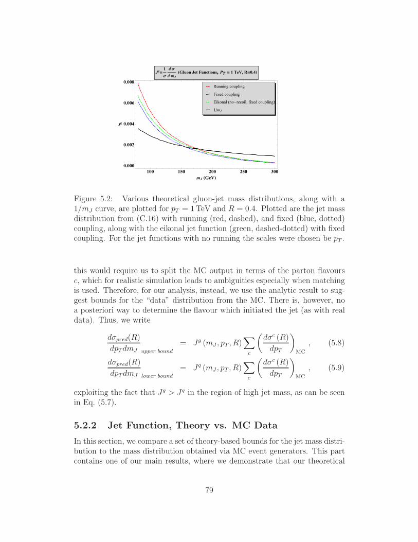
100 150 200 250 3000.000

0.002

0.004

0.006

0.008

mJ !GeV"

Jg

Jg!1

"

d "

d mJ!Gluon Jet Functions, PT ! 1 TeV, R!0.4"

1!mJ

Eikonal "no!recoil, fixed coupling#

Fixed coupling

Running coupling

Figure 5.2: Various theoretical gluon-jet mass distributions, along with a1/mJ curve, are plotted for pT = 1TeV and R = 0.4. Plotted are the jet massdistribution from (C.16) with running (red, dashed), and fixed (blue, dotted)coupling, along with the eikonal jet function (green, dashed-dotted) with fixedcoupling. For the jet functions with no running the scales were chosen be pT .

this would require us to split the MC output in terms of the parton flavoursc, which for realistic simulation leads to ambiguities especially when matchingis used. Therefore, for our analysis, instead, we use the analytic result to sug-gest bounds for the “data” distribution from the MC. There is, however, noa posteriori way to determine the flavour which initiated the jet (as with realdata). Thus, we write

d-pred(R)

dpTdmJ upper bound

= Jg (mJ , pT , R)!

c

"d-c (R)

dpT

#

MC

, (5.8)

d-pred(R)

dpTdmJ lower bound

= Jq (mJ , pT , R)!

c

"d-c (R)

dpT

#

MC

, (5.9)

exploiting the fact that Jg > Jq in the region of high jet mass, as can be seenin Eq. (5.7).

5.2.2 Jet Function, Theory vs. MC Data

In this section, we compare a set of theory-based bounds for the jet mass distri-bution to the mass distribution obtained via MC event generators. This partcontains one of our main results, where we demonstrate that our theoretical

79

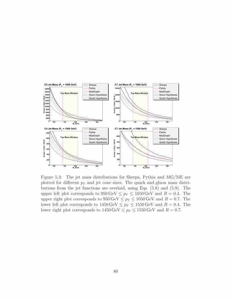
(GeV)JM100 150 200 250 300

-1E

vent

s / 5

GeV

/ 10

0 fb

0

2000

4000

6000

8000

10000

12000

14000

16000

18000

20000

22000

SherpaPythiaMadGraphGluon HypothesisQuark Hypothesis

Top Mass Window

= 1000 GeV)T

C4 Jet Mass (P

(GeV)JM100 150 200 250 300

-1E

vent

s / 5

GeV

/ 10

0 fb

0

5000

10000

15000

20000

25000

SherpaPythiaMadGraphGluon HypothesisQuark Hypothesis

Top Mass Window

= 1000 GeV)T

C7 Jet Mass (P

(GeV)JM100 150 200 250 300

-1E

vent

s / 5

GeV

/ 10

0 fb

0

200

400

600

800

1000

1200

SherpaPythiaMadGraphGluon HypothesisQuark Hypothesis

Top Mass Window

= 1500 GeV)T

C4 Jet Mass (P

(GeV)JM100 150 200 250 300

-1E

vent

s / 5

GeV

/ 10

0 fb

0

200

400

600

800

1000

SherpaPythiaMadGraphGluon HypothesisQuark Hypothesis

Top Mass Window

= 1500 GeV)T

C7 Jet Mass (P

Figure 5.3: The jet mass distributions for Sherpa, Pythia and MG/ME areplotted for di!erent pT and jet cone sizes. The quark and gluon mass distri-butions from the jet functions are overlaid, using Eqs. (5.8) and (5.9). Theupper left plot corresponds to 950GeV " pT " 1050GeV and R = 0.4. Theupper right plot corresponds to 950GeV " pT " 1050GeV and R = 0.7. Thelower left plot corresponds to 1450GeV " pT " 1550GeV and R = 0.4. Thelower right plot corresponds to 1450GeV " pT " 1550GeV and R = 0.7.

80

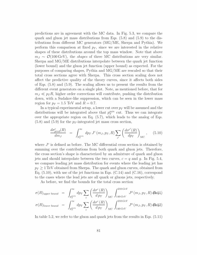
predictions are in agreement with the MC data. In Fig. 5.3, we compare thequark and gluon jet mass distributions from Eqs. (5.8) and (5.9) to the dis-tributions from di!erent MC generators (MG/ME, Sherpa and Pythia). Weperform this comparison at fixed pT , since we are interested in the relativeshapes of these distributions around the top mass window. Note that abovemJ . O(100GeV), the shapes of three MC distributions are very similar.Sherpa and MG/ME distributions interpolate between the quark jet function(lower bound) and the gluon jet function (upper bound) as expected. For thepurposes of comparing shapes, Pythia and MG/ME are rescaled so that theirtotal cross sections agree with Sherpa. This cross section scaling does nota!ect the predictive quality of the theory curves, since it a!ects both sidesof Eqs. (5.8) and (5.9). The scaling allows us to present the results from thedi!erent event generators on a single plot. Note, as mentioned before, that formJ + pTR, higher order corrections will contribute, pushing the distributiondown, with a Sudakov-like suppression, which can be seen in the lower massregion for pT = 1.5 TeV and R = 0.7.

In a typical experimental setup, a lower cut over pT will be assumed and thedistributions will be integrated above that pmin

T cut. Thus we can integrateover the appropriate region on Eq. (5.7), which leads to the analog of Eqs.(5.8) and (5.9) for the pT -integrated jet mass cross section,

d-cpred(R)

dmJ=

* $

pminT

dpT Jc (mJ , pT , R)!

c"

"d-c"(R)

dpT

#

MC

, (5.10)

where Jc is defined as before. The MC di!erential cross section is obtained bysumming over the contributions from both quark and gluon jets. Therefore,the cross section’s shape is characterized by an admixture of quark and gluonjets and should interpolate between the two curves, c = q and g. In Fig. 5.4,we compare leading jet mass distribution for events where the leading jet haspT % 1TeV obtained from Sherpa. The quark and gluon curves, obtained fromEq. (5.10), with use of the jet functions in Eqs. (C.14) and (C.16), correspondto the cases where the lead jets are all quark or gluons jets, respectively.

As before, we find the bounds for the total cross section

-(R)upper bound =

* $

pminT

dpT!

c

"d-c (R)

d pT

#

MC

* 210GeV

140GeV

Jg (mJ , pT , R) dmJ ,(5.11)

-(R)lower bound =

* $

pminT

dpT!

c

"

d-c (R)

d pT

#

MC

* 210GeV

140GeV

Jq (mJ , pT , R) dmJ .(5.12)

In table 5.2, we refer to the gluon and quark jets from the results in Eqs. (5.11)

81

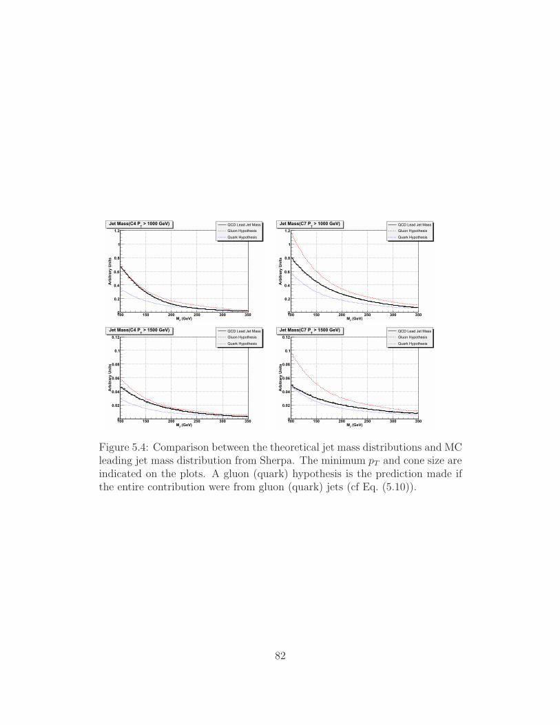
(GeV)JM100 150 200 250 300 350

Arb

itrar

y U

nits

0

0.2

0.4

0.6

0.8

1

1.2

> 1000 GeV)T

Jet Mass(C4 P QCD Lead Jet Mass

Gluon Hypothesis

Quark Hypothesis

(GeV)JM100 150 200 250 300 350

Arb

itrar

y U

nits

0

0.2

0.4

0.6

0.8

1

1.2

> 1000 GeV)T

Jet Mass(C7 P QCD Lead Jet Mass

Gluon Hypothesis

Quark Hypothesis

(GeV)JM100 150 200 250 300 350

Arb

itrar

y U

nits

0

0.02

0.04

0.06

0.08

0.1

0.12

> 1500 GeV)T

Jet Mass(C4 P QCD Lead Jet Mass

Gluon Hypothesis

Quark Hypothesis

(GeV)JM100 150 200 250 300 350

Arb

itrar

y U

nits

0

0.02

0.04

0.06

0.08

0.1

0.12

> 1500 GeV)T

Jet Mass(C7 P QCD Lead Jet Mass

Gluon Hypothesis

Quark Hypothesis

Figure 5.4: Comparison between the theoretical jet mass distributions and MCleading jet mass distribution from Sherpa. The minimum pT and cone size areindicated on the plots. A gluon (quark) hypothesis is the prediction made ifthe entire contribution were from gluon (quark) jets (cf Eq. (5.10)).

82

and (5.12), respectively. The numbers in the table were calculated as follows.From a MC sample corresponding to 100 fb"1 of data, we extracted the num-ber of events with C4 lead jet pT % 1000(1500)GeV and 140GeV < mJ <210GeV, the top mass window. We repeated this exercise for C7 jets. Thedata column contains these results.

pT lead cut Cone Size Data Quark hypothesis Gluon hypothesis1000 GeV C4 113749 70701 1356821000 GeV C7 197981 131955 2600451500 GeV C4 10985 6513 127851500 GeV C7 13993 11164 22469

Table 5.2: Comparison of Sherpa MC data to predictions of pure-quark andpure-gluon hypothesis, for the number of events with leading jet with massbetween 140 GeV and 210 GeV. The data is compared to the bounds given inEqs. (5.11) and (5.12). The statistics reflect 100 fb"1 of integrated luminosity.

Fractional Fake Rate

With the theoretical machinery discussed in the previous section, we are able tomake a prediction of the rate at which QCD jets will fake the mass signatureof top-jets. We define the fractional fake rate as the fraction of jets with140GeV " mJ " 210GeV, for given pT and R. We estimate the upper andlower bounds of the fractional fake rate as* 210 GeV

140 GeV

dmJ Jq(mJ , pT , R) " Fractional fake rate "

* 210 GeV

140 GeV

dmJ Jg(mJ , pT , R) .

(5.13)

In Fig. 5.5, we plot the fractional fake rate as a function of jet transversemomentum. To predict the number of fakes in our sample, we fold the di!er-ential cross section for QCD jet production (Fig. 5.6) with the fractional fakerate (Fig. 5.5). Again we expect a Sudakov-like suppression when mJ + pTR,thus flatting the theoretical fractional fake rate as pT increases. This can beseen more predominately for R = 0.7 in Fig. 5.5.

Pseudorapidity Independence of the Jet Mass Distribution

In general, we expect that NP signals will have a pseudorapidity dependence.Therefore, the study of pseudorapidity dependence may provide a tool for NP

83

(GeV)TP1000 1100 1200 1300 1400 1500 1600

frac

tion

0

0.02

0.04

0.06

0.08

0.1

0.12

0.14

0.16

0.18

0.2

Gluon HypothesisQuark HypothesisSherpa MadGraph

LEADTR = 0.4 Fractional Fake Rate vs P

(GeV)TP1000 1100 1200 1300 1400 1500 1600

frac

tion

0

0.05

0.1

0.15

0.2

0.25

0.3

Gluon HypothesisQuark HypothesisSherpa MadGraph

LEADTR = 0.7 Fractional Fake Rate vs P

Figure 5.5: The fraction of jets which acquire 140GeV " mJ " 210GeV asa function of the transverse momentum of the leading jet. Quark- and gluon-hypothesis curves yield the prediction for the fractional fake rate, if all jetswere either quark- or gluon-jets, respectively. The plot on the left correspondsto C4 jets; the plot on the right corresponds to C7 jets (cf Eq. (5.13)).

(GeV)TP1000 1050 1100 1150 1200 1250 1300 1350 1400 1450 1500

(pb)

/ 20

GeV

!

-110

1

Sherpa

MadGraph

Pythia

(QCD R=0.4 Jets)TP"

!"

Figure 5.6: The di!erential cross section for QCD (R = 0.4) jet productionwith respect to the pT of the leading jet. Sherpa, MG/ME and Pythia arerepresented.

84

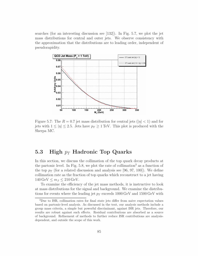
searches (for an interesting discussion see [132]). In Fig. 5.7, we plot the jetmass distributions for central and outer jets. We observe consistency withthe approximation that the distributions are to leading order, independent ofpseudorapidity.

(GeV)JM50 100 150 200 250 300 350

Arb

itrar

y U

nits

0.01

0.02

0.03

0.04

0.05

0.06

0.07

0.08

> 1 TeV)T

QCD Jet Mass (P| < 1) #C7 Lead Jet (|

| < 2.5) #C7 Lead Jet (1.0 < |

Figure 5.7: The R = 0.7 jet mass distribution for central jets (|0| < 1) and forjets with 1 " |0| " 2.5. Jets have pT % 1TeV. This plot is produced with theSherpa MC.

5.3 High pT Hadronic Top Quarks

In this section, we discuss the collimation of the top quark decay products atthe partonic level. In Fig. 5.8, we plot the rate of collimation3 as a function ofthe top pT (for a related discussion and analysis see [96, 97, 100]). We definecollimation rate as the fraction of top quarks which reconstruct to a jet having140GeV " mJ " 210GeV.

To examine the e"ciency of the jet mass methods, it is instructive to lookat mass distributions for the signal and background. We examine the distribu-tions for events where the leading jet pT exceeds 1000GeV and 1500GeV with

3Due to ISR, collimation rates for final state jets di!er from naive expectation valuesbased on partonic-level analysis. As discussed in the text, our analysis methods include agroup mass criteria, a simple but powerful discriminant, against ISR jets. Therefore, ourresults are robust against such e!ects. Residual contributions are absorbed as a sourceof background. Refinement of methods to further reduce ISR contributions are analysis-dependent, and outside the scope of this work.

85

(TOP) (GeV)TP800 900 1000 1100 1200 1300 1400

frac

tion

0

0.1

0.2

0.3

0.4

0.5

0.6

0.7

0.8

0.9

1

C4

C7

Collimation Rate

Figure 5.8: The collimation rate for top quarks as a function of their trans-verse momentum, for C4 (black solid curve) and C7 (red dashed curve) jets.Collimation rate is defined as the fraction of events with top quarks giving riseto a final state jet with 140GeV " mJ " 210GeV.

C4 and C7 jets. In Fig. 5.1, we plot the jet mass distribution for the tt signalfor pT lead % 1000GeV. The e"ciency of C7 jets for capturing the hadronictop is greater than that for C4 jets. For C4 jets, we still observe pronouncedstructure around the W -mass (MW ), which diminishes for C7 jets. We alsonote that the peak for the C7 jets moves closer to the top mass, indicatinga higher e"ciency for capturing the hadronic top. We expect that detectore!ects will further smear the signal. Fig. 5.1 also shows the mass distributionsincluding leading detector e!ects (using transfer functions).

We note that the analysis has an inherent tension with regard to choosingthe cone size for the jet. The reconstruction cone should be su"ciently wide tocapture all the daughter products of the hadronic top. On the other hand, weneed to keep the cone appropriately small to keep out the QCD jet backgroundand other soft contamination [97].

We describe the gross features of the top mass distribution, without pro-viding a detailed analytic expression for the top jet. At lowest order in QCDand before decay, the top jet mass distribution is simply %(mJ & mt). Thisdistribution is modified both by QCD radiation and electroweak decay.

We can describe QCD radiation by a top jet function, J tQCD(mQCD, R, pT ),

similar to the functions for massless QCD jets, where J tQCD is a function of

mQCD ( mt+%mQCD. Gluon radiation from top quarks makes the top jet mass

86

harder, giving the additional mass contribution, %mQCD. Using factorization,this process can be calculated by methods similar to the one discussed inthe Appendix, fixing the mass of the parton to mt and treating it as stable.For our purposes, the resulting broadening is subdominant for a top masswindow of ±35 GeV. 4 The QCD radiation that determines the shape of J t

QCD

at a resolution of . 10 GeV is characterized by a very short time scale ofO(1/(10GeV)) in the top rest frame.

Although long compared to 1/mt, the rest frame time scale on which thedistribution in mQCD is determined is substantially shorter than the elec-troweak time scale, which is set by #t = O(1.5) GeV, the top quark widthin the Standard Model [133, 134]. The di!erence in time scales implies aquantum mechanical incoherence between the QCD radiation, described byJ tQCD(mQCD, R, pT ), and the top quark weak decay. These two physical pro-

cesses are thus expected to factorize up to corrections that are determinedby the ratio of #t to the size of the top quark window, and we shall assumethat this is the case. Using this assumption, we describe the e!ect of elec-troweak decay by an overall factor F t

EW (%mEW , mQCD/(pTR)). This functionis responsible for producing the two peaks corresponding to the top quark andW boson in the signal mass distribution Fig. 5.1, by acting on the underlyingQCD top jet function J t

QCD, which has a single peak at mt.We see from Fig. 5.1 that the e!ect of the decay on the jet mass, %mEW ,

can be sizable. The actual distribution depends on cone size that we use toidentify the jet. The main e!ect here is a softening of the jet mass, becausethe jet cone may not capture all the particles from the top quark decay chain.This kinematic e!ect depends solely onmQCD/(pTR). As we see from Fig. 5.1,it reduces the mass of the top jet and produces a peak near the W mass. Sincethe top jet mass softening is a kinematic process, it should be well describedby generators based on phase space.

In summary, we can schematically express the top jet mass squared as asum of three contributions. 5

mJ . mt + %mQCD + %mEW , (5.14)

where the jet mass function related to Fig. 5.1 can be schematically written

4However, a treatment of the broadening is crucial if one aim to improve the top massmeasurement at the LHC. At the moment this has been studied only for the ILC [102].

5The choice of mass, as opposed to, say, mass squared for the convolution variable is amatter of convention, to keep our notation in J t

QCD consistent with the light quark jet func-tions. Convolutions in jet mass squared, which are familiar from event shape distributions,can be obtained simply by changing variables and as necessary changing the normalizationsof the functions J t

QCD and FEW .

87

as a convolution of three di!erent sources

J t(mJ , R, pT ) .*

d(%mEW )dmQCD %(mJ &mQCD & %mEW )

)J tQCD(mQCD, R, pT )FEW (%mEW , mQCD/(pTR)) .(5.15)

The top mass is large, so we are not concerned about uncertainties in the lowerjet mass spectrum. In fact, the same considerations that lead to this resultallow us to conclude that existing MC tools should well describe this part ofour studies. We will thus rely on event generators rather than Eq. (5.15) inour numerical studies below.

5.4 tt Jets vs. QCD Jets at the LHC

In this section, we combine the results of the previous discussions, and applythem to analyze energetic SM tt events vis-a-vis QCD jet production at theLHC. The main purpose of this section is to understand how well we can dis-criminate our signal from the overwhelming QCD background. We illustratean example analysis using the jet functions, and evaluate their performance onMC data. Unfortunately, it is very di"cult to outline a one-size-fits-all anal-ysis. Therefore, we perform a broad-strokes analysis that contains su"cientdetail to provide general guidance. We do not attempt to invoke advanced,but analysis-specific, procedures that could provide further refinement. It isalso important to bear in mind that the final evaluation of the jet functions,as precision analysis tools, can really only be done on real data. The primaryreason is that we expect the jet functions to describe physics data. The MCdistributions are, at this point, an approximation to what we believe will beLHC data. A precision analysis will show the strains between the jet function-based shape predictions and the e!ective distribution that MC uses to generateits mass distribution.

We examine two cases in detail, both at truth-level (no detector e!ects)and accounting for detector e!ects. The first case, single tagging, consists of“top-tagging” (requiring 140GeV " mJ " 210GeV) the leading jets satisfyinga pT cut. The second case, double tagging, consists of top-tagging the leadingand subleading jets, with a pT cut only on the leading jet.

5.4.1 Peak Resolution

In this analysis, one objective is to resolve the excess of events where the massof the leading jet lies in the top mass window (140GeV " mJ " 210GeV). It

88

is important to note that we are not hunting for a peak; we already know itslocation. The issue is that of resolving its magnitude and estimate the prob-ability that the background would fluctuate to yield the observed data. Toestimate the significance of such a measurement, we perform a rudimentaryanalysis for resolving peaks. We emphasize that it is misleading to estimatethe significance as S/

!B, where the signal and background are separate MC

samples. These numbers represent an unrealizable scenario, and tend to beoptimistic. In real data, there is no way to separate the signal from back-ground with certainty. Furthermore, at the present time, we cannot trust MCto provide the precise shape of QCD jet mass distributions. Therefore, wederive our approximations to the background shape directly from the “data”,via sideband analysis (outside the top mass window). We use our previousknowledge of the shape of the background in the sideband region, to minimizethe number of degree of freedoms involved in the sideband fit. We will discussthis further in the next section.

After approximating the shape of the background in the sideband region,we interpolate the shape of the background into the top mass window. Theprimary challenges are that our background is large and also has large uncer-tainties, which induce large uncertainties in the signal. We discuss this in moredetail at the conclusion of this section. For the shape of the tt signal insidethe top mass window, we use MC. In principle, the shape of the top massdistribution can be also derived semi-analytically, as discussed in section 5.3(see also [102]). However, to leading order we expect the MC data to provideus with a reliable shape (it should capture the radiation at the leading logapproximation, also the, phase space, population of the top decay products ispurely kinematical). For simplicity we use the simulation data for this stepin our analysis. These shapes, after normalization to unit area, are referredto as probability density functions. Unfortunately, the standard acronym forprobability density functions conflicts with existing usage for parton distri-bution functions in this paper. To avoid confusion, we simply refer to themas shapes. We use the approximate shapes for the signal and background toperform an extended maximum likelihood fit to the sample, with jet mass dis-tribution F (mJ), thereby obtaining the background and signal normalizations.We define a jet mass distribution F (mJ) as

F (mJ) = NB ) b (mJ) +NS ) s (mJ ) , (5.16)

whereNB is the predicted background, andNS is the predicted signal in the topmass window. b (mJ) and s (mJ ) are used to denote the background and signalshapes, respectively. Both NB and NS are allowed to float independently.

89

Sideband Background Analysis

We perform a sideband analysis in order to avoid the tt signal-rich region. Thebasic goal is to understand the shape of the background by examining a regionwhere there is no signal. In the sidebands, in particular the low side, the signalcontaminates the background. In Fig. 5.1, we see that the tt signal does notvanish outside the top mass window. Although it is small compared to theQCD background as can be seen in Fig. 5.10, this contamination substantiallyimpacts resolution of the peak. We attempt to purify the background in thisregion, by rejecting energetic jets consistent with originating from a top quarkdecay, i.e. - signal, as follows. For a candidate event where the leading jetpasses preselection criteria, all jets within a cone R = 1 are (vectorially) addedinto a single combined jet. We call this a group jet, although this definitiondi!ers slightly from that in J. Conway, et al., in [97]. If the group mass, mG,of the combined jet falls within the top mass window, the candidate event isrejected. This discriminant tends to reject events where the decay products ofthe top quarks are not fully collimated, i.e. reconstructed as a single jet. Wemust understand any biases introduced by this discriminant. Fig. 5.9 showsthe e!ect of themG cuts on the background and signal. The background shapeis left relatively intact, but the signal is substantially diminished.

(GeV)JM120 140 160 180 200 220 240 260 280

Arb

itrar

y U

nits

0

0.002

0.004

0.006

0.008

0.01

0.012

0.014

0.016

0.018

0.02

Background

Background + cut

QCD Jets - Cut Bias

(GeV)JM120 140 160 180 200 220 240 260 280

Arb

itrar

y U

nits

0

0.2

0.4

0.6

0.8

1Signal

Signal + cut

- Cut Biastt

Figure 5.9: The jet mass distributions for the tt and QCD jet samples in thesidebands. The plot on the left depicts the shape of the QCD jet samplebefore and after making a combined jet mass cut on mG, as described inSec. 5.4.1. Both curves are normalized to unit area, to show the similarity ofthe shapes before and after the cut. The plot on the right depicts the e!ectof the combined jet mass cut on the tt signal. The red (dashed) curve showsthe e!ect of the cut relative to the original jet mass distribution (black solidcurve). Note: Unlike the left plot, these curves are not renormalized.

Advanced use of this mG discriminant is outside the scope of this analysis,possibly leading to more sophisticated analyses (see e. g. J. Conway, et al.,

90

in [97]). We simply use it to e"ciently reject signal events in the sidebands,while keeping the majority of background events.

We analyze the shape of the background in the sidebands using the jetfunctions derived in section 5.2. We expect real QCD jets to be an admixtureof quark and gluon jets. Therefore, our Ansatz posits the admixture of quarksand gluons as a fraction. We expect small corrections (deviations from aconstant admixture) to arise from di!erent sources. For example, we do notconsider events with a leading jet of fixed pT , but rather impose a lower pTcut. Our Ansatz for the jet mass distribution assumes the following form

b(mJ) 1 + (mJ ))JQ(

mJ ; pminT , R

)

+(1& + (mJ)))JG(

mJ ; pminT , R

)

, (5.17)

where + (mJ) is a linear polynomial$

+0 + +1mJ

pminT R

%

. Note that with b(mJ )

defined above, along with Eq. (5.16), the total number of degree of freedominvolved in the sideband fit is four: +0, +1, NB and NS.

Significance

After resolving the magnitude of the signal (tt) peak against that of the QCDjet background, via the methods outlined in the previous sections, we nowdiscuss how to interpret those results. Our analysis is based on log-likelihoodratio method.6 A background+signal hypothesis to describe a data sample isonly meaningful if a background-only hypothesis is unlikely to describe thatsample. We estimate the statistical significance, n., of the peak as

n. =D

2 (logL& logL0), (5.18)

where L0 is the value of the maximized likelihood function obtained fromfitting the data to the background shape alone (equivalent to setting NS tozero in Eq. (5.16)), and L is the value of the maximized likelihood functionobtained from fitting the data to the background shape and signal shape.7

The functional form of the likelihood function is given by

L =NBINS+

k=1

exp (&F (mk))) [F (mk)]Nk

Nk!, (5.19)

where we are fitting for the functional form of F (mJ ) as given by Eq. (5.16).Here,mk andNk refer to the value of the mass at the center, and the occupancy,

6An excellent discussion may be found in the The Review of Particle Physics [135].7Except in pathological cases, the significance is well approximated by S

!S, where S is

the fitted signal, and "S is the error on S.

91

of the k-th bin, respectively.

5.4.2 Single Top-Tagging

For each of the signal (tt) and background (QCD jets) samples, we preselectevents with a pT cut on the leading jet. In Fig. 5.10 we plot the jet massdistribution including detector e!ects for the signal and background, includingthe theoretical upper and lower bound for the background. We show thenumber of events with jet mass in the range 140GeV " mJ " 210GeV. Forreference, the number of events for the signal and background, at the truth-level, are presented in table 5.3. It is clear that the background is roughly twoorders of magnitude larger than the signal. Once we add detector e!ects thesignificance of the signal is further deteriorated. We conclude that a simplecounting method would not be e!ective here.

(GeV)JM100 120 140 160 180 200 220 240 260 280 300

-1N

umbe

r of

Eve

nts

/ 5 G

eV /

100

fb

210

310

410

510

> 1000 GeV)T

(C4 PJdM

!d QCD Lead Jet Mass

Gluon Hypothesis

Quark Hypothesis

Lead Jet Masstt

(GeV)JM100 120 140 160 180 200 220 240 260 280 300

-1N

umbe

r of

Eve

nts

/ 5 G

eV /

100

fb

210

310

410

510

> 1000 GeV)T

(C7 PJdM

!d QCD Lead Jet Mass

Gluon Hypothesis

Quark Hypothesis

Lead Jet Masstt

(GeV)JM100 120 140 160 180 200 220 240 260 280 300

-1N

umbe

r of

Eve

nts

/ 5 G

eV /

100

fb

210

310

> 1500 GeV)T

(C4 PJdM

!d QCD Lead Jet Mass

Gluon Hypothesis

Quark Hypothesis

Lead Jet Masstt

(GeV)JM100 120 140 160 180 200 220 240 260 280 300

-1N

umbe

r of

Eve

nts

/ 5 G

eV /

100

fb

210

310

> 1500 GeV)T

(C7 PJdM

!d QCD Lead Jet Mass

Gluon Hypothesis

Quark Hypothesis

Lead Jet Masstt

Figure 5.10: The jet mass distributions for the tt and QCD jet samples. Theplots on the top row correspond to a pT lead % 1000GeV. The plots on thebottom row correspond to a pT lead % 1500GeV. The plots on the left cor-respond to R = 0.4; the plots on the right correspond to R = 0.7. Thetheoretical bounds, Eq. (5.10), are also plotted. These numbers are tabulatedin table 5.3.

92

Detector E"ects

Here, we repeat the truth-level procedure from above, accounting for the lead-ing e!ects of detector resolution and ±5% jet energy scale. We also tabulatethe relative change in acceptance of the signal and background, due to detectorresolution and energy scale, which we define as

$JES =NJES &NTRUTH

NTRUTH, (5.20)

where NJES is the number of events passing the selection criteria after detectorsmearing and JES e!ects have been applied. These results are tabulated intable 5.4, which shows how the signal and background are a!ected di!erentlyby smearing e!ects. We see that the net e!ects of the detector smearing plusthe uncertainties in the JES lead to substantial uncertainties O (10%& 30%)in the signal and background. As anticipated, this leads to a clear failure ofsimple counting type analyses and calls for a di!erent approach, which will beintroduced in the following in the form of sideband analyses and jet shapes.

pT lead cut Cone Size tt (S) Background (B) S/B1000 GeV C4 6860 113749 0.0601000 GeV C7 8725 197981 0.0441500 GeV C4 630 10985 0.0571500 GeV C7 689 13993 0.049

Table 5.3: Truth-level (no detector e!ects) results for single-tag jet massmethod, reflecting 100 fb"1 of integrated luminosity. S and B reflect the num-ber of jets with 140 GeV < mJ < 210 GeV for the signal and background,respectively.

Results for single tagging

We now apply the analysis described in the previous sections to resolve thepeak related to the top quark in the signal region, the top mass window.First we perform a sideband background analysis, to resolve the shape ofthe background. After applying the cuts described in Sec. 5.4.1, we fit thebackground to our Ansatz. Fig. 5.11 shows an example of such backgroundfit to our Ansatz. The results of this fit described by Eq. (5.16) and beloware shown in Fig. 5.12, which demonstrates how the detector a!ects the signalresolution.

93

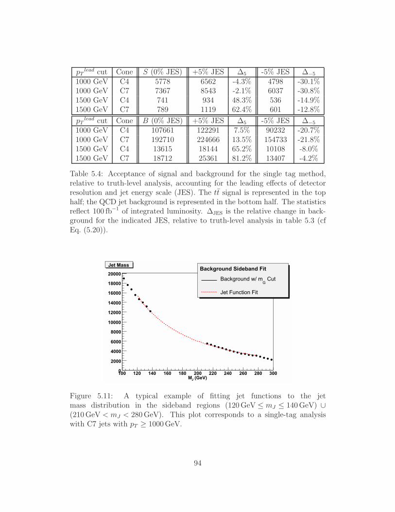
pT lead cut Cone S (0% JES) +5% JES $5 -5% JES $"5

1000 GeV C4 5778 6562 -4.3% 4798 -30.1%1000 GeV C7 7367 8543 -2.1% 6037 -30.8%1500 GeV C4 741 934 48.3% 536 -14.9%1500 GeV C7 789 1119 62.4% 601 -12.8%

pT lead cut Cone B (0% JES) +5% JES $5 -5% JES $"5

1000 GeV C4 107661 122291 7.5% 90232 -20.7%1000 GeV C7 192710 224666 13.5% 154733 -21.8%1500 GeV C4 13615 18144 65.2% 10108 -8.0%1500 GeV C7 18712 25361 81.2% 13407 -4.2%

Table 5.4: Acceptance of signal and background for the single tag method,relative to truth-level analysis, accounting for the leading e!ects of detectorresolution and jet energy scale (JES). The tt signal is represented in the tophalf; the QCD jet background is represented in the bottom half. The statisticsreflect 100 fb"1 of integrated luminosity. $JES is the relative change in back-ground for the indicated JES, relative to truth-level analysis in table 5.3 (cfEq. (5.20)).

(GeV)JM100 120 140 160 180 200 220 240 260 280 3000

2000

4000

6000

8000

10000

12000

14000

16000

18000

20000Background Sideband Fit

CutG

Background w/ m

Jet Function Fit

Jet Mass

Figure 5.11: A typical example of fitting jet functions to the jetmass distribution in the sideband regions (120GeV " mJ " 140GeV) 3(210GeV < mJ < 280GeV). This plot corresponds to a single-tag analysiswith C7 jets with pT % 1000GeV.

94

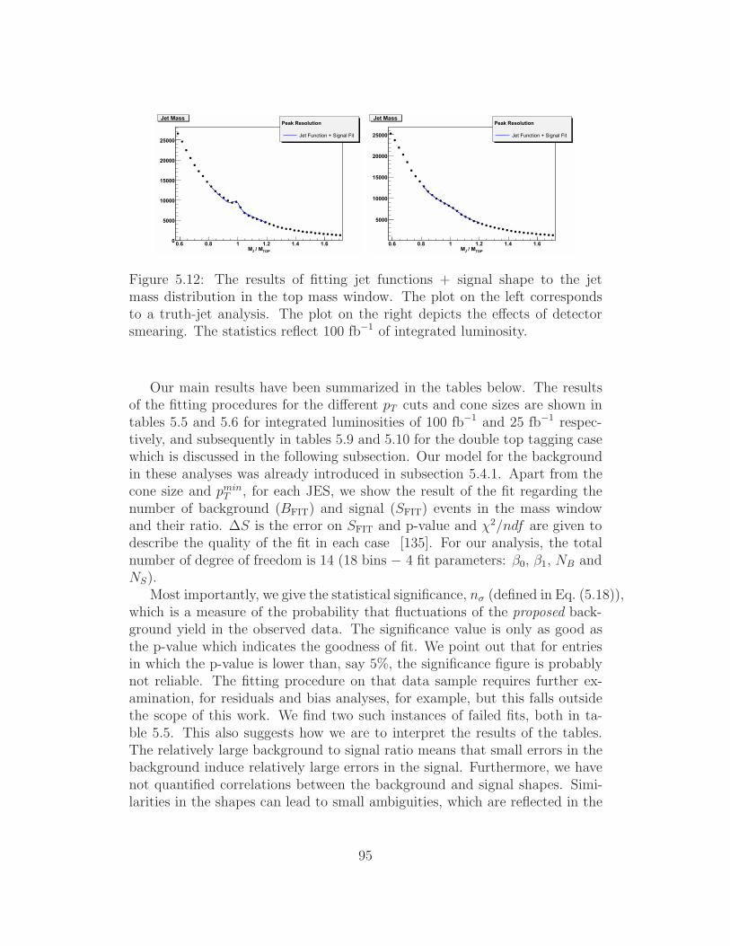
TOP / MJM0.6 0.8 1 1.2 1.4 1.60

5000

10000

15000

20000

25000

Peak Resolution

Jet Function + Signal Fit

Jet Mass

TOP / MJM0.6 0.8 1 1.2 1.4 1.6

5000

10000

15000

20000

25000

Peak Resolution

Jet Function + Signal Fit

Jet Mass

Figure 5.12: The results of fitting jet functions + signal shape to the jetmass distribution in the top mass window. The plot on the left correspondsto a truth-jet analysis. The plot on the right depicts the e!ects of detectorsmearing. The statistics reflect 100 fb"1 of integrated luminosity.

Our main results have been summarized in the tables below. The resultsof the fitting procedures for the di!erent pT cuts and cone sizes are shown intables 5.5 and 5.6 for integrated luminosities of 100 fb"1 and 25 fb"1 respec-tively, and subsequently in tables 5.9 and 5.10 for the double top tagging casewhich is discussed in the following subsection. Our model for the backgroundin these analyses was already introduced in subsection 5.4.1. Apart from thecone size and pmin

T , for each JES, we show the result of the fit regarding thenumber of background (BFIT) and signal (SFIT) events in the mass windowand their ratio. $S is the error on SFIT and p-value and 42/ndf are given todescribe the quality of the fit in each case [135]. For our analysis, the totalnumber of degree of freedom is 14 (18 bins & 4 fit parameters: +0, +1, NB andNS).

Most importantly, we give the statistical significance, n. (defined in Eq. (5.18)),which is a measure of the probability that fluctuations of the proposed back-ground yield in the observed data. The significance value is only as good asthe p-value which indicates the goodness of fit. We point out that for entriesin which the p-value is lower than, say 5%, the significance figure is probablynot reliable. The fitting procedure on that data sample requires further ex-amination, for residuals and bias analyses, for example, but this falls outsidethe scope of this work. We find two such instances of failed fits, both in ta-ble 5.5. This also suggests how we are to interpret the results of the tables.The relatively large background to signal ratio means that small errors in thebackground induce relatively large errors in the signal. Furthermore, we havenot quantified correlations between the background and signal shapes. Simi-larities in the shapes can lead to small ambiguities, which are reflected in the

95

fitting parameter errors. The combination of these two di"culties gives riseto an e!ect, which, strictly speaking, is a defect in the analysis. We remindthe reader that we have a large uncertainty in the tt signal cross section (seetable 5.1), which we have not accounted for in the analysis. We have singledout Sherpa MC data for use in our analyses, and the reader should bear thisin mind when interpreting the results in tables 5.5, 5.6, 5.9, 5.10. Small er-rors in the background shape can yield good fits with high significance figures,and still have relatively large errors in the signal. We are led to interpret theresults in the tables as the significance of the peak, relative to the indicatedbackground shape hypothesis (the jet functions in our case). We find thatour single tagging method allows us to resolve the tt signal from the QCDbackground with pmin

T . 1 TeV and 25 fb"1 of data. This jet mass analysisdoes not include any b-tagging or jet-shapes (to be discussed in the followingsection).

5.4.3 Double Top-Tagging

The above analyses related to single top-tagging are useful not only for ttproduction, but rather for general cases in which we expect to have at leastone very energetic top jet. However, for the cases where there is more thanone heavy high-pT particle, we certainly have more information which canbe used to distinguish signal from the QCD background. Clearly, tt eventscontain more information than what is encoded in a single top jet mass. Weaugment the single-tag analysis for the tt signal, by simply requiring thatthe subleading jet mass be in the top mass window, without imposing a pTcut. This cut preferentially removes more background events than the signalevents, without biasing the distributions. The sideband analysis, applied tothe leading jet, remains the same as for the single top-tagging case. As we shallsee even this simple treatment yields a sizable improvement in the significance.Roughly half of the events have smaller pT than the minimum pT for the leadingjet as shown in Fig. 5.13. Although, by definition, a subleading jet has smallerpT than the leading one, its pT distribution is peaked at the pTmin, and onlysmall portion of events are in the smaller pT tail region. The number of eventsfor the signal and background, at the truth-level, are presented in table 5.7. Toget an idea on how the subleading mass cut a!ects our signal and backgroundsamples, one can compare the numbers given in table 5.3 with the ones in 5.7.For example, we see that at truth level for R = 0.4 and pTmin = 1TeV thesize of the signal sample is decreased by 50% while the background sample byroughly 12%. This is consistent with the results shown in Figs. 5.8 and 5.5 inwhich the analysis is done for a fixed pT .

In principle, one could apply a sideband analysis to the subleading jet.

96

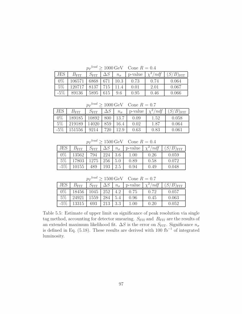
pT lead % 1000GeV Cone R = 0.4

JES BFIT SFIT $S n. p-value 42/ndf (S/B)FIT0% 106571 6868 671 10.3 0.73 0.74 0.0645% 120717 8137 715 11.4 0.01 2.01 0.067-5% 89136 5895 615 9.6 0.95 0.46 0.066

pT lead % 1000GeV Cone R = 0.7JES BFIT SFIT $S n. p-value 42/ndf (S/B)FIT0% 189185 10892 800 13.7 0.09 1.52 0.0585% 219189 14020 859 16.4 0.02 1.87 0.064-5% 151556 9214 720 12.9 0.63 0.83 0.061

pT lead % 1500GeV Cone R = 0.4JES BFIT SFIT $S n. p-value 42/ndf (S/B)FIT0% 13562 794 224 3.6 1.00 0.26 0.0595% 17803 1275 256 5.0 0.89 0.58 0.072-5% 10155 489 193 2.5 0.94 0.49 0.048

pT lead % 1500GeV Cone R = 0.7JES BFIT SFIT $S n. p-value 42/ndf (S/B)FIT0% 18456 1045 252 4.2 0.75 0.72 0.0575% 24921 1559 284 5.4 0.96 0.45 0.063-5% 13315 693 213 3.3 1.00 0.20 0.052

Table 5.5: Estimate of upper limit on significance of peak resolution via singletag method, accounting for detector smearing. SFIT and BFIT are the results ofan extended maximum likelihood fit. $S is the error on SFIT. Significance n.

is defined in Eq. (5.18). These results are derived with 100 fb"1 of integratedluminosity.

97

pT lead % 1000GeV Cone R = 0.4JES BFIT SFIT $S n. p-value 42/ndf (S/B)FIT0% 26642 1712 335 5.1 1.00 0.19 0.0645% 30206 1995 346 5.8 0.96 0.45 0.066-5% 22371 1379 288 4.8 1.00 0.11 0.062

pT lead % 1000GeV Cone R = 0.7JES BFIT SFIT $S n. p-value 42/ndf (S/B)FIT0% 47277 2730 399 6.8 0.98 0.38 0.0585% 54870 3419 424 8.1 0.87 0.60 0.062-5% 37910 2274 354 6.4 1.00 0.21 0.060

pT lead % 1500GeV Cone R = 0.4JES BFIT SFIT $S n. p-value 42/ndf (S/B)FIT0% 3381 201 112 1.8 1.00 0.06 0.0595% 4418 346 130 2.7 1.00 0.07 0.078-5% 2519 136 96 1.4 1.00 0.09 0.054

pT lead % 1500GeV Cone R = 0.7JES BFIT SFIT $S n. p-value 42/ndf (S/B)FIT0% 4609 259 125 2.1 1.00 0.18 0.0565% 6231 382 144 2.6 1.00 0.12 0.061-5% 3320 174 99 1.6 1.00 0.06 0.052

Table 5.6: Estimate of upper limit on significance of peak resolution via singletag method, accounting for detector smearing. SFIT and BFIT are the resultsof an extended maximum likelihood fit. $S is the error on SFIT. Significancen. is defined in Eq. (5.18). These results are derived with 25 fb"1 of integratedluminosity.

98

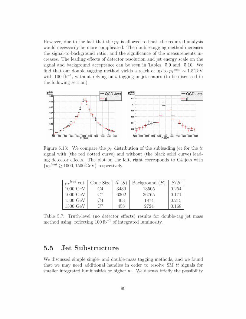
However, due to the fact that the pT is allowed to float, the required analysiswould necessarily be more complicated. The double-tagging method increasesthe signal-to-background ratio, and the significance of the measurements in-creases. The leading e!ects of detector resolution and jet energy scale on thesignal and background acceptance can be seen in Tables 5.9 and 5.10. Wefind that our double tagging method yields a reach of up to pTmin . 1.5TeVwith 100 fb"1, without relying on b-tagging or jet-shapes (to be discussed inthe following section).

(GeV)TP500 600 700 800 900 1000 1100 1200 1300 1400 15000

0.01

0.02

0.03

0.04

0.05

0.06

0.07QCD Jetstt

SUBTP

(GeV)TP1000 1100 1200 1300 1400 1500 1600 1700 1800 1900 20000

0.02

0.04

0.06

0.08

0.1

0.12

QCD Jetstt

SUBTP

Figure 5.13: We compare the pT distribution of the subleading jet for the ttsignal with (the red dotted curve) and without (the black solid curve) lead-ing detector e!ects. The plot on the left, right corresponds to C4 jets with(

pT lead % 1000, 1500GeV)

respectively.

pT lead cut Cone Size tt (S) Background (B) S/B1000 GeV C4 3430 13505 0.2541000 GeV C7 6302 36765 0.1711500 GeV C4 403 1874 0.2151500 GeV C7 458 2724 0.168

Table 5.7: Truth-level (no detector e!ects) results for double-tag jet massmethod using, reflecting 100 fb"1 of integrated luminosity.

5.5 Jet Substructure

We discussed simple single- and double-mass tagging methods, and we foundthat we may need additional handles in order to resolve SM tt signals forsmaller integrated luminosities or higher pT . We discuss briefly the possibility

99

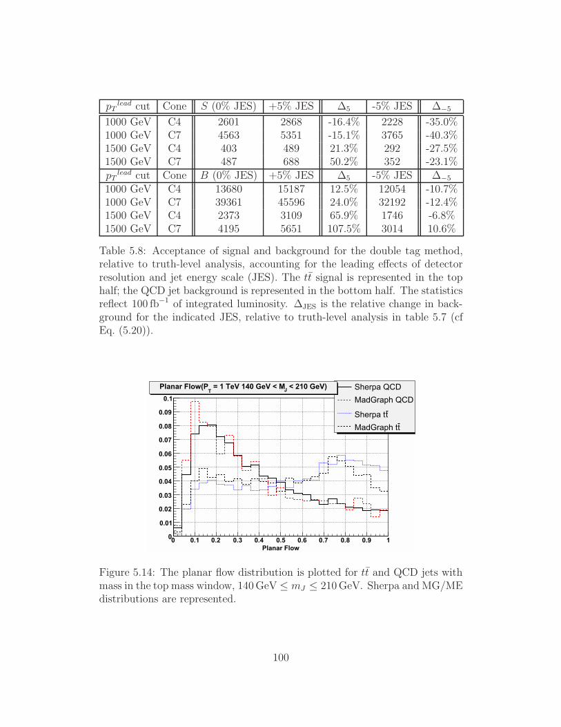
pT lead cut Cone S (0% JES) +5% JES $5 -5% JES $"5

1000 GeV C4 2601 2868 -16.4% 2228 -35.0%1000 GeV C7 4563 5351 -15.1% 3765 -40.3%1500 GeV C4 403 489 21.3% 292 -27.5%1500 GeV C7 487 688 50.2% 352 -23.1%pT lead cut Cone B (0% JES) +5% JES $5 -5% JES $"5

1000 GeV C4 13680 15187 12.5% 12054 -10.7%1000 GeV C7 39361 45596 24.0% 32192 -12.4%1500 GeV C4 2373 3109 65.9% 1746 -6.8%1500 GeV C7 4195 5651 107.5% 3014 10.6%

Table 5.8: Acceptance of signal and background for the double tag method,relative to truth-level analysis, accounting for the leading e!ects of detectorresolution and jet energy scale (JES). The tt signal is represented in the tophalf; the QCD jet background is represented in the bottom half. The statisticsreflect 100 fb"1 of integrated luminosity. $JES is the relative change in back-ground for the indicated JES, relative to truth-level analysis in table 5.7 (cfEq. (5.20)).

Planar Flow0 0.1 0.2 0.3 0.4 0.5 0.6 0.7 0.8 0.9 10

0.01

0.02

0.03

0.04

0.05

0.06

0.07

0.08

0.09

0.1

Sherpa QCD

MadGraph QCD

tSherpa t

tMadGraph t

< 210 GeV)J = 1 TeV 140 GeV < MT

Planar Flow(P

Figure 5.14: The planar flow distribution is plotted for tt and QCD jets withmass in the top mass window, 140GeV " mJ " 210GeV. Sherpa and MG/MEdistributions are represented.

100

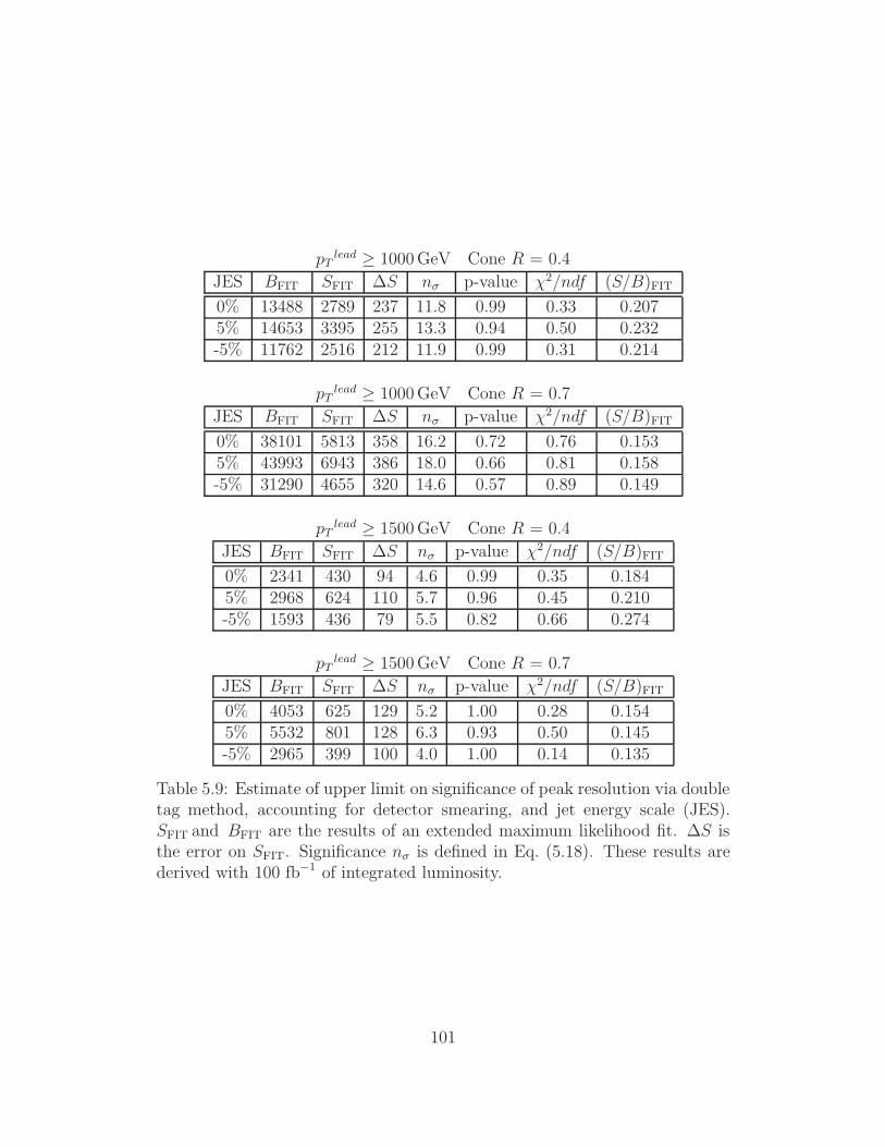
pT lead % 1000GeV Cone R = 0.4JES BFIT SFIT $S n. p-value 42/ndf (S/B)FIT0% 13488 2789 237 11.8 0.99 0.33 0.2075% 14653 3395 255 13.3 0.94 0.50 0.232-5% 11762 2516 212 11.9 0.99 0.31 0.214

pT lead % 1000GeV Cone R = 0.7JES BFIT SFIT $S n. p-value 42/ndf (S/B)FIT0% 38101 5813 358 16.2 0.72 0.76 0.1535% 43993 6943 386 18.0 0.66 0.81 0.158-5% 31290 4655 320 14.6 0.57 0.89 0.149

pT lead % 1500GeV Cone R = 0.4JES BFIT SFIT $S n. p-value 42/ndf (S/B)FIT0% 2341 430 94 4.6 0.99 0.35 0.1845% 2968 624 110 5.7 0.96 0.45 0.210-5% 1593 436 79 5.5 0.82 0.66 0.274

pT lead % 1500GeV Cone R = 0.7JES BFIT SFIT $S n. p-value 42/ndf (S/B)FIT0% 4053 625 129 5.2 1.00 0.28 0.1545% 5532 801 128 6.3 0.93 0.50 0.145-5% 2965 399 100 4.0 1.00 0.14 0.135

Table 5.9: Estimate of upper limit on significance of peak resolution via doubletag method, accounting for detector smearing, and jet energy scale (JES).SFIT and BFIT are the results of an extended maximum likelihood fit. $S isthe error on SFIT. Significance n. is defined in Eq. (5.18). These results arederived with 100 fb"1 of integrated luminosity.

101

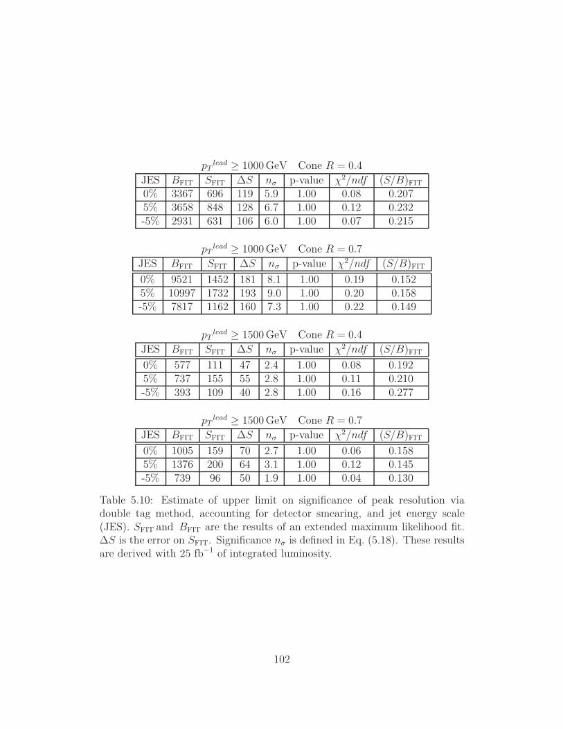
pT lead % 1000GeV Cone R = 0.4JES BFIT SFIT $S n. p-value 42/ndf (S/B)FIT0% 3367 696 119 5.9 1.00 0.08 0.2075% 3658 848 128 6.7 1.00 0.12 0.232-5% 2931 631 106 6.0 1.00 0.07 0.215

pT lead % 1000GeV Cone R = 0.7JES BFIT SFIT $S n. p-value 42/ndf (S/B)FIT0% 9521 1452 181 8.1 1.00 0.19 0.1525% 10997 1732 193 9.0 1.00 0.20 0.158-5% 7817 1162 160 7.3 1.00 0.22 0.149

pT lead % 1500GeV Cone R = 0.4JES BFIT SFIT $S n. p-value 42/ndf (S/B)FIT0% 577 111 47 2.4 1.00 0.08 0.1925% 737 155 55 2.8 1.00 0.11 0.210-5% 393 109 40 2.8 1.00 0.16 0.277

pT lead % 1500GeV Cone R = 0.7JES BFIT SFIT $S n. p-value 42/ndf (S/B)FIT0% 1005 159 70 2.7 1.00 0.06 0.1585% 1376 200 64 3.1 1.00 0.12 0.145-5% 739 96 50 1.9 1.00 0.04 0.130

Table 5.10: Estimate of upper limit on significance of peak resolution viadouble tag method, accounting for detector smearing, and jet energy scale(JES). SFIT and BFIT are the results of an extended maximum likelihood fit.$S is the error on SFIT. Significance n. is defined in Eq. (5.18). These resultsare derived with 25 fb"1 of integrated luminosity.

102

of using substructure to further analyze energetic jets in the top mass window.We defer the details to our recent work in [25] (see also [154]), where we derivesimple analytic expressions to approximate the jet shape variable distributions.For developing additional tools to reslove tt signals, there are approaches whichexploit information outside of hadronic calorimeter [136] such as tracker orelectromagnetic calorimeter. But we limit ourselves to the information encodedonly within the hadronic calorimeter to develop significance for resolving ttsignals. We do not also discuss the possibility of b-tagging for high pT top-jet [99], which is still under speculation for the range of pT relevant for ouranalysis.

Jet shapes are the extensions of well-known event shapes, used at leptoncolliders, applied to the analysis of energy flow inside single jets. The fact thatwe consider only jets with high mass is crucial since it allows us to control theshape of various distributions related to energy flow in a perturbative manner.As an example, we examine the planar flow variable, which measures the extent

Planar flow (Pf)

0 0.1 0.2 0.3 0.4 0.5 0.6 0.7 0.8 0.9 10

0.01

0.02

0.03

0.04

0.05

0.06

0.07= 1 TeV, R = 0.4, "no mass cuts")

TPlanar flow, Pf (P

QCD jetsTop jets

Figure 5.15: The planar flow distribution is plotted for tt and QCD jets withoutfixing jet mass. MG/ME distributions are represented.

to which the energy flow inside the jet is linear or planar. Planar flow (Pf)is defined as follows. We first define an (unnormalized) event shape tensor Iwas8

Iklw =!

i

wipi,kwi

pi,lwi

, (5.21)

8The overall normalization is not important to this discussion.

103

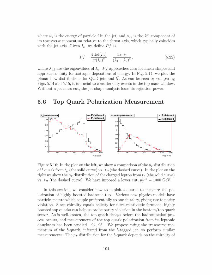
where wi is the energy of particle i in the jet, and pi,k is the kth component ofits transverse momentum relative to the thrust axis, which typically coincideswith the jet axis. Given Iw, we define Pf as

Pf =4det(Iw)

tr(Iw)2=

4/1/2

(/1 + /2)2, (5.22)

where /1,2 are the eigenvalues of Iw. Pf approaches zero for linear shapes andapproaches unity for isotropic depositions of energy. In Fig. 5.14, we plot theplanar flow distributions for QCD jets and tt. As can be seen by comparingFigs. 5.14 and 5.15, it is crucial to consider only events in the top mass window.Without a jet mass cut, the jet shape analysis loses its rejection power.

5.6 Top Quark Polarization Measurement

pt_b_1Entries 10000

Mean 523.3

RMS 266.9

(b) (GeV)TP

0 200 400 600 800 1000 12000

0.01

0.02

0.03

0.04

0.05

0.06pt_b_1

Entries 10000

Mean 523.3

RMS 266.9

(b) distributionTPL

(b) from tTP

R(b) from tTP pt_e_1

Entries 10000

Mean 213.7

RMS 183.1

(l) (GeV)TP

0 200 400 600 800 1000 12000

0.02

0.04

0.06

0.08

0.1

0.12

0.14

pt_e_1Entries 10000

Mean 213.7

RMS 183.1

(lepton) distribution TP L

(l) from tTP

R(l) from tTP

Figure 5.16: In the plot on the left, we show a comparison of the pT distributionof b quark from tL (the solid curve) vs. tR (the dashed curve). In the plot on theright we show the pT distribution of the charged lepton from tL (the solid curve)vs. tR (the dashed curve). We have imposed a lower cut, pmin

T = 1000 GeV.

In this section, we consider how to exploit b-quarks to measure the po-larization of highly boosted hadronic tops. Various new physics models haveparticle spectra which couple preferentially to one chirality, giving rise to parityviolation. Since chirality equals helicity for ultra-relativistic fermions, highlyboosted top quarks can help us probe parity violation in the bottom/top quarksector. As is well-known, the top quark decays before the hadronization pro-cess occurs, and measurement of the top quark polarization from its leptonicdaughters has been studied [94, 95]. We propose using the transverse mo-mentum of the b-quark, inferred from the b-tagged jet, to perform similarmeasurements. The pT distribution for the b-quark depends on the chirality of

104

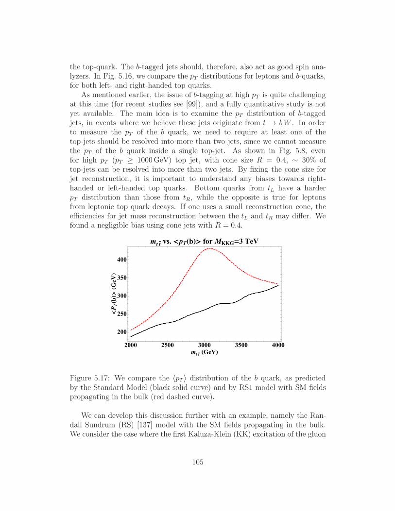
the top-quark. The b-tagged jets should, therefore, also act as good spin ana-lyzers. In Fig. 5.16, we compare the pT distributions for leptons and b-quarks,for both left- and right-handed top quarks.

As mentioned earlier, the issue of b-tagging at high pT is quite challengingat this time (for recent studies see [99]), and a fully quantitative study is notyet available. The main idea is to examine the pT distribution of b-taggedjets, in events where we believe these jets originate from t ' bW . In orderto measure the pT of the b quark, we need to require at least one of thetop-jets should be resolved into more than two jets, since we cannot measurethe pT of the b quark inside a single top-jet. As shown in Fig. 5.8, evenfor high pT (pT % 1000GeV) top jet, with cone size R = 0.4, . 30% oftop-jets can be resolved into more than two jets. By fixing the cone size forjet reconstruction, it is important to understand any biases towards right-handed or left-handed top quarks. Bottom quarks from tL have a harderpT distribution than those from tR, while the opposite is true for leptonsfrom leptonic top quark decays. If one uses a small reconstruction cone, thee"ciencies for jet mass reconstruction between the tL and tR may di!er. Wefound a negligible bias using cone jets with R = 0.4.

2000 2500 3000 3500 4000

200

250

300

350

400

mt#t$ !GeV"

%P

T!b"&!G

eV"

mt#t$ vs. %pT!b"& for MKKG!3 TeV

Figure 5.17: We compare the #pT $ distribution of the b quark, as predictedby the Standard Model (black solid curve) and by RS1 model with SM fieldspropagating in the bulk (red dashed curve).

We can develop this discussion further with an example, namely the Ran-dall Sundrum (RS) [137] model with the SM fields propagating in the bulk.We consider the case where the first Kaluza-Klein (KK) excitation of the gluon

105

has a mass MKKG = 3 TeV. We perform this analysis at partonic level. In themodel we are considering for using b-quark #pT $, KK excitations of the gluoncouple to left-handed top quarks . 5) stronger than to right-handed topquarks. Typical cross sections for KK gluon production are relatively small.The (background) SM top quarks are produced dominantly via parity-invariantQCD processes, and tend to wash out the signal. In order to resolve the signa-ture, we are compelled to correlate deviations in the b-quark #pT $ spectrum toan excess in KK gluon production. In Fig. 5.17, we compare the mean valueof the b-quark pT spectrum, for the Standard Model and RS1 scenarios withSM fields propagating in the bulk. When correlated to the invariant mass ofthe KK gluon, we see a substantial deviation in the distribution of the b-quark#pT $. In Fig. 5.18, we compare the mean value of the lepton pT spectrum,for the Standard Model and RS1 scenarios with SM fields propagating in thebulk, where KK excitations of the gluon couple to right-handed top quarks. 5) stronger than to left-handed top quarks.

Figure 5.18: We compare the #pT $ distributions of the lepton, as predicted bythe Standard Model (blue curve) and by RS1 model with SM fields propagatingin the bulk (red curve).

5.7 Conclusions

In this study we have mainly focused on high pT , hadronically decaying, topsin cases where they are fully collimated. Above pT of 1 TeV the majority of

106

the top daughters particles will be found inside a single cone jet even when thecone size is as small as R = 0.4. Therefore, they are simply denoted as top-jets. The leading background for top-jets comes from high pT QCD jets. Weprovided analytic expressions for the QCD jet functions which approximate thebackground and show consistency with MC data. As an example we considerthe case of SM tt production, and demonstrate how these jet functions, viaside band analysis, allow us to e"ciently resolve 1TeV top-jet from the QCDbackground with 25 fb"1, and . 1.5TeV top-jets with 100 fb"1.

A wide class of new physics models posits tt production mechanisms whichwould significantly contribute to the mass distributions, possibly allowing reso-lution of excess production with less data. To further improve the significancewe consider jet shapes (recently analyzed in [25] and also in [154]), whichresolve substructure of energy flow inside cone jets. Augmentation of theanalysis, such as the use of jet substructure in combination with a jet masscut and b-tagging, may improve the signal resolution, allowing us to discoverNP signal through top quark channel even with lower luminosity or higher pTcut. We provided such an example using the planar flow jet shape variable,and a detailed analysis is presented in our recent work [25]. We also proposedusing the transverse momentum of the bottom quarks to measure top quarkpolarization as a probe of parity violation.

In this paper we mostly focused on fairly extreme (but not uncommon atthe LHC) kinematical configurations where the tops are fully collimated. Thishas several advantages such as having direct contact with theoretical basedcalculation of the jet functions and also the ability to consider arbitrarily hightop momenta (at least in principle). However, it is clear that some fractionof the hadronic tops will be reconstructed in 2-jet (intermediate) or % 3-jet (conventional) topologies. The fraction of events related to the di!erenttopologies is a function of the cone size and pT . Solid reconstruction algorithmsand analyses must be flexible enough to interpolate between these di!erentregions. We note that our approach is complimentary to others that havebeen proposed recently [97, 148, 153, 154]. In most cases, the di!erence isrelated to the fact that the tops considered are not fully collimated and a two-jet topology is exploited to increase the signal to background ratio. It wouldbe very interesting and important to derive theoretically based techniquesto control the corresponding distribution of the background relevant to theintermediate region. It is likely that there are overlaps between the di!erentregions. Such issues are important to examine in detail. Mastering thesecomplimentary methods may help to make potential new physics observationsmore robust, if verified via multiple and independent techniques.

Finally, we want to emphasize that the analysis proposed herein is also

107

applicable to other processes involving, highly boosted, heavy particles suchas electroweak gauge bosons, the Higgs and other new physics particles, towhich QCD is a leading background as well.

108

Chapter 6

Jet Event Shapes

At the Large Hadron Collider (LHC), events with highly-boosted massive par-ticles, tops [144], W , Z and Higgs [145] may be the key ingredient for thediscovery of physics beyond the standard model [146–148]. In many decaychannels, these particles would be identified as high-pT jets, and any suchsignal of definite mass must be disentangled from a large background of light-parton (“QCD”) jets with a continuous distribution. This background farexceeds such signals, and relying solely on jet mass as a way to reject QCDbackground from signal would probably not su"ce in most cases [25], evenusing a narrow window for dijets in the search for massive particles such astops, produced in pairs.

In this chapter, we argue that for massive, high-pT jets, infrared (IR) safeobservables may o!er an additional tool to distinguish heavy particle decaysfrom QCD background, perhaps even on an event-by-event basis. We willrefer to inclusive observables dependent on energy flow within individual jetsas jet shapes. A jet within a cone of radius 0.4, for example, may be identifiedfrom the energy recorded in roughly fifty 0.1)0.1 calorimeter towers. It thuscontains a great deal of information. Perturbatively-calculable, infrared safejet shapes combined, of course, with IR-safe jet finding algorithms [141–143,149], may enable us to access that information systematically, and to form abridge between event generator output and direct theory predictions.

Essentially, any observable that is a smooth functional of the distributionof energy flow among the cells defines an IR-safe jet shape [150]. The jet massis one example, but a single jet may be analyzed according to a variety ofshapes. In particular, the jet mass distribution has large corrections when theratio of the jet mass to jet energy is small [151], but can be computed at fixedorder when the logarithm of that ratio has an absolute value of order unity.Once the jet mass is fixed at a high scale, a large class of other jet shapesbecomes perturbatively calculable with nominally small corrections. Indeed,

109

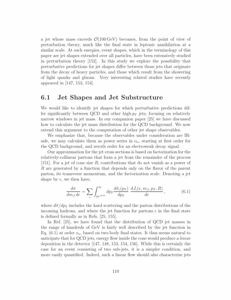
a jet whose mass exceeds O(100GeV) becomes, from the point of view ofperturbation theory, much like the final state in leptonic annihilation at asimilar scale. At such energies, event shapes, which in the terminology of thispaper are jet shapes extended over all particles, have been extensively studiedin perturbation theory [152]. In this study we explore the possibility thatperturbative predictions for jet shapes di!er between those jets that originatefrom the decay of heavy particles, and those which result from the showeringof light quarks and gluons. Very interesting related studies have recentlyappeared in [147, 153, 154].

6.1 Jet Shapes and Jet Substructure

We would like to identify jet shapes for which perturbative predictions dif-fer significantly between QCD and other high-pT jets, focusing on relativelynarrow windows in jet mass. In our companion paper [25] we have discussedhow to calculate the jet mass distribution for the QCD background. We nowextend this argument to the computation of other jet shape observables.

We emphasize that, because the observables under consideration are IR-safe, we may calculate them as power series in 's, starting at first order forthe QCD background, and zeroth order for an electroweak decay signal.

Our approximation for the jet cross sections is based on factorization for therelatively-collinear partons that form a jet from the remainder of the process[151]. For a jet of cone size R, contributions that do not vanish as a power ofR are generated by a function that depends only on the flavor of the parentparton, its transverse momentum, and the factorization scale. Denoting a jetshape by e, we then have,

d-

dmJ de=!

c

* $

pTmin

dpTd-c(pT )

dpT

dJc(e,mJ , pT , R)

de, (6.1)

where d-/dpT includes the hard scattering and the parton distributions of theincoming hadrons, and where the jet function for partons c in the final stateis defined formally as in Refs. [25, 155].

In Ref. [25], we have found that the distribution of QCD jet masses inthe range of hundreds of GeV is fairly well described by the jet function inEq. (6.1) at order 's, based on two-body final states. It thus seems natural toanticipate that for QCD jets, energy flow inside the cone would produce a lineardeposition in the detector [147, 148, 153, 154, 156]. While this is certainly thecase for an event consisting of two sub-jets, it is a simpler condition, andmore easily quantified. Indeed, such a linear flow should also characterize jets

110

from the two-body decay of a highly-boosted, massive particle. We will seebelow that relatively simple jet shapes can help distinguish QCD jets frommany top-decay jets that involve three-body decay. We will also see that jetshapes can help separate samples that contain both QCD jets and jets fromtwo-body decays, such as those of the W , Z or Higgs. We emphasize that asingle event may be analyzed by a variety of jet shapes, so that the resolutionassociated with each one need not be dramatic, so long as they are e!ectivelyindependent.

6.2 Top decay and planar flow

The linear flow of QCD jets at leading order should be compared with a% 3-body decay where the energy deposition tends to be planar , covering atwo-dimensional region of the detector. An IR-safe jet shape, which we denoteas planar flow , a two-dimensional version of the “D parameter” [157–160],distinguishes planar from linear configurations. The utility of a closely-relatedobservable was emphasized in Ref. [154].

Planar flow is defined as follows. We first construct for a given jet a matrixI/ as

Ikl/ =1

mJ

!

i

,ipi,k,i

pi,l,i

, (6.2)

where mJ is the jet mass, ,i is the energy of particle i in the jet, and pi,k isthe kth component of its transverse momentum relative to the axis of the jet’smomentum. Given I/, we define Pf for that jet as

Pf =4det(I/)

tr(I/)2=

4/1/2

(/1 + /2)2, (6.3)

where /1,2 are the eigenvalues of I/. Pf vanishes for linear shapes and ap-proaches unity for isotropic depositions of energy.

Jets with pure two-body kinematics have a di!erential jet function fixedat zero planar flow,

1

J

"

dJ

dPf

#

2body

= %(Pf) . (6.4)

This would apply to leading order for events with highly boosted weak gaugeboson, Higgs and QCD jets. On the other hand, events that are characterizedby % 3-body kinematics have a smooth distribution.

Realistic QCD jets have, of course, nonzero Pf . Because Pf is an IR safeobservable, however, its average value can depend only on the hard momentumscales of the jet, that is, mJ and pT . This suggests an average Pf of order

111

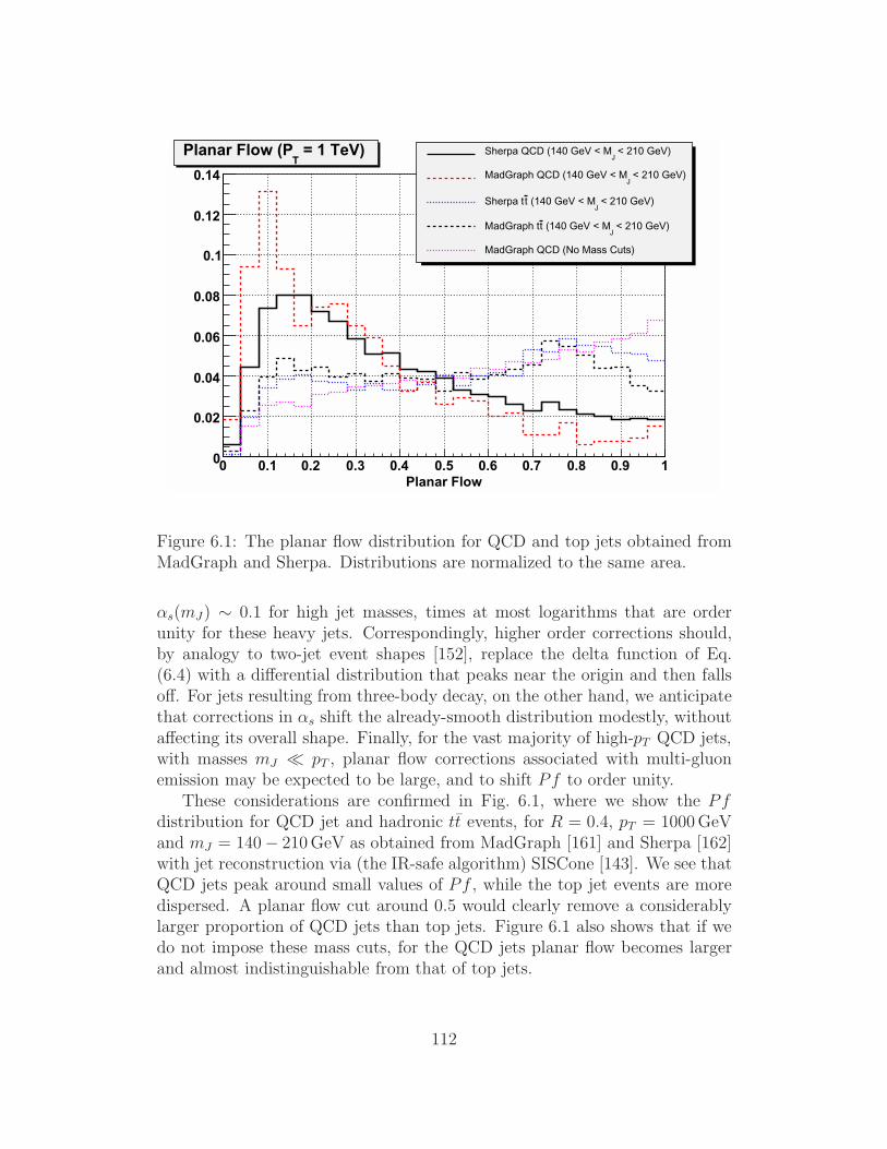
Planar Flow0 0.1 0.2 0.3 0.4 0.5 0.6 0.7 0.8 0.9 10

0.02

0.04

0.06

0.08

0.1

0.12

0.14

< 210 GeV)J

Sherpa QCD (140 GeV < M

< 210 GeV)J

MadGraph QCD (140 GeV < M

< 210 GeV)J

(140 GeV < MtSherpa t

< 210 GeV)J

(140 GeV < MtMadGraph t

MadGraph QCD (No Mass Cuts)

= 1 TeV) T

Planar Flow (P

Figure 6.1: The planar flow distribution for QCD and top jets obtained fromMadGraph and Sherpa. Distributions are normalized to the same area.

's(mJ) . 0.1 for high jet masses, times at most logarithms that are orderunity for these heavy jets. Correspondingly, higher order corrections should,by analogy to two-jet event shapes [152], replace the delta function of Eq.(6.4) with a di!erential distribution that peaks near the origin and then fallso!. For jets resulting from three-body decay, on the other hand, we anticipatethat corrections in 's shift the already-smooth distribution modestly, withouta!ecting its overall shape. Finally, for the vast majority of high-pT QCD jets,with masses mJ + pT , planar flow corrections associated with multi-gluonemission may be expected to be large, and to shift Pf to order unity.

These considerations are confirmed in Fig. 6.1, where we show the Pfdistribution for QCD jet and hadronic tt events, for R = 0.4, pT = 1000GeVand mJ = 140& 210GeV as obtained from MadGraph [161] and Sherpa [162]with jet reconstruction via (the IR-safe algorithm) SISCone [143]. We see thatQCD jets peak around small values of Pf , while the top jet events are moredispersed. A planar flow cut around 0.5 would clearly remove a considerablylarger proportion of QCD jets than top jets. Figure 6.1 also shows that if wedo not impose these mass cuts, for the QCD jets planar flow becomes largerand almost indistinguishable from that of top jets.

112

6.3 Two-body decay

While planar flow can help enrich samples with characteristically three- andhigher-body kinematics, other jet shapes can also provide additional informa-tion on events with relatively low Pf . Here, we will still wish to distinguish theQCD background from highly boosted electroweak gauge bosons or Higgs [156]as well as from top jets whose Pf happens to be relatively low. We begin withjets that are linear at lowest order, and identify a set of jet shapes that havesome power to distinguish between the two. Fixing pT , R and mJ leaves onlyone free parameter to characterize the shape.

The QCD jet function for two-body kinematics is defined as a matrix el-ement in [25] and is readily expressed as an integral over !s, the angle of thesofter particle relative to the jet momentum axis. For a quark jet, for example,the integrand is therefore the di!erential jet function,

dJQCD

d(c!s)=

'sCF+zz2

4(m2J(1& +zc!s)(2(1& +zc!s)& z2)

).

(2(1 + +z)(1& +zc!s)& z2(1 + c!s))2

z2(1 + c!s)(1& +zc!s)+ 3(1 + +z) +

z4(1 + c!s)2

(1& +zc!s)(2(1 + +z)(1& +zc!s)& z2(1 + c!s))

/

, (6.5)

where z ( mJ/pT , +z (!1& z2 and c!s ( cos !s . The jet mass function, for

a jet cone of size R, is found by the integral

J(R, z) =

* R

-m

d!s

"dJ

d!s

#

, (6.6)

where !m = cos"1(!

1& z2)

is the minimum angle the softer particle can makewith the jet axis. At !s = !m, both particles have the same energy and angleto the jet axis.

It is natural to ask how the integrated jet function, Eq. (6.6) depends ofthe jet algorithm used to define the jet, and in particular how results for conejets compare to results when jets are identified by kt or the newer “anti-kt”algorithms [142, 149]. For the low orders and small cones discussed here, thisrelationship is straightforward.

Reference [149] introduces a class of kt algorithms, for which two particles

113

are within the same jet if their distance dij is less than dB, given by

dij = min(k2pT,i, k

2pT,j)

r2ijR2

kt

, (6.7)

dB = min(k2pT,i, k

2pT,j) , (6.8)

where rij =D

$02 +$32 is the distance between particles i and j in therapidity-azimuthal angle plane. The choice p = 1 defines a standard kt algo-rithm, and p = &1 the anti-kt. For small cones, rij - !ij , where !ij is the anglebetween two particles. At lowest order, that is for two particles in the finalstate, for both positive and negative values of p, these algorithms constrainr2ij , and therefore !ij , by

0 <r2ijR2

kt

< 1 . (6.9)

As in Eq. (6.6) the energy and angles of the massless two particles are relatedat fixed jet mass and fixed transverse momentum, through

m2J = 2kT,ikT,j(cosh$0 & cos$3)

- kT,ikT,j(

($0)2 + ($3)2)

, (6.10)

where again we assume small angles. Changing variables from !s to rij, orequivalently !ij , is straightforward, and the basic integral for an inclusive jetfunction in Eq. (6.6) is of the same form for a cone and a kt (or anti-kt) jetat lowest nontrivial order. At this order the di!erence is that in kt algorithmsthe parameter Rkt directly restricts the distance between the two particles, incontrast to a cone size R, which restricts the distance of each particle to thejet axis. The only di!erence is in the upper limit of Eq. (6.6). The integralfound with a cone jet of size R corresponds to a generalized kt algorithm withparameter Rkt(R). Their relation can be easily found from the dependence ofrij in !s,

Rkt(R) = R + sin"1

"z2 sinR

(1 + +2z )& 2+z cosR

#

= R +z2

2

sinR

1& cosR+O(z4) , (6.11)

a result that depends on z, the ratio of the jet energy to its mass. We see thatfor highly boosted heavy jets, or for jets of low mass, with z + 1, Rkt(R) ' R,and the two integrated jet functions are identical. The kt algorithm param-eter, Rkt , approaches the cone jet parameter, R, from above because the kt

114

algorithm is slightly more restrictive at this order. For the remainder of ourdiscussion, we shall assume a cone jet algorithm.

For signal events from highly-boosted massive gauge bosons, we considerseparately the cases when it is longitudinal and when it has helicity (h = ±1),

dJLong

d(c!s)=

C

(1& +zc!s)2, (6.12)

dJh=±1

d(c!s)=

C

(1& +zc!s)2

"

1&(zs!s)2

2(1& +zc!s)2

#

,

where s!s ( sin !s and C is a proportionality coe"cient, totally determinedfrom the two-body decay kinematics. We can interpret the appropriately nor-malized di!erential jet functions, P x(!s) = (dJx/d!s)/Jx as the probability tofind the softer particle at an angle between !s and !s + %!s. As the ratio zdecreases, the decay products become boosted and the cone shrinks. For QCDjets from light partons, however, this shrinkage is much less pronounced. FromFig. 6.2 we can see that the jet functions for the gauge boson distributions ofEq. (6.12) fall o! with !s faster than do QCD jets, Eq. (6.5). This observationsuggests that the signal (vector boson-jet) and background (QCD jets) havedi!erent shapes for fixed pT , R and jet mass. This may be used to obtain animproved rejection power against background events. We now consider a classof jet shapes, angularities, originally introduced in Refs. [155, 163] for two-jetevents in e+e" annihilation. A natural generalization of these jet shapes tosingle-cone jets of large mass mJ is

"a(R, pT ) =1

mJ

!

i&jet

,i sina

"(!i2R

# 3

1& cos

"(!i2R

#41"a

, (6.13)

with mJ the jet mass. The arguments of the trigonometric functions vary fromzero to (/2 as ! increases from zero to R, that is, over the size of the cone.These weights revert to the angularities as defined in for leptonic annihilationin [155, 163] when R = (/2, so that the cone is enlarged to a hemisphere andmJ is replaced by the center-of-mass energy in a two-jet event. For massivejets, the angularities are clearly non-zero at lowest order, in contrast to thelowest order planar flow, Eq. (6.4). Then, precisely because of their IR safety,higher-order corrections to the "a distributions should be moderate.

As the parameter a varies, the angularities give more or less weight toparticles at the edge of the cone compared to those near the center. From thedi!erential jet distribution functions in Eqs. (6.5) and (6.12) and the definitionof "a we can obtain expressions for P x("a) [as before x= sig (signal) or QCD],the probability to find a jet with an angularity value between "a and "a + %"a

115

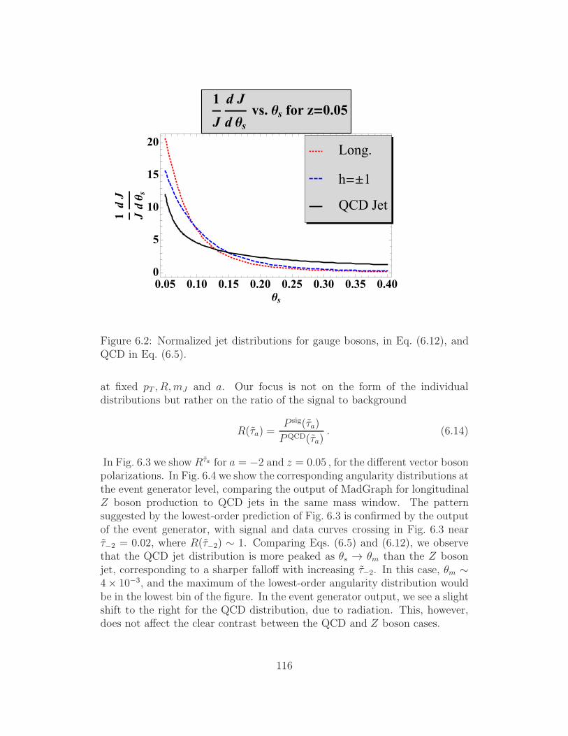
0.05 0.10 0.15 0.20 0.25 0.30 0.35 0.400

5

10

15

20

's

1 J

dJ

d'

s

1

J

d J

d 'svs. 's for z!0.05

QCD Jet

h"#1

Long.

Figure 6.2: Normalized jet distributions for gauge bosons, in Eq. (6.12), andQCD in Eq. (6.5).

at fixed pT , R,mJ and a. Our focus is not on the form of the individualdistributions but rather on the ratio of the signal to background

R("a) =P sig("a)

PQCD("a). (6.14)

In Fig. 6.3 we show R)a for a = &2 and z = 0.05 , for the di!erent vector bosonpolarizations. In Fig. 6.4 we show the corresponding angularity distributions atthe event generator level, comparing the output of MadGraph for longitudinalZ boson production to QCD jets in the same mass window. The patternsuggested by the lowest-order prediction of Fig. 6.3 is confirmed by the outputof the event generator, with signal and data curves crossing in Fig. 6.3 near""2 = 0.02, where R(""2) . 1. Comparing Eqs. (6.5) and (6.12), we observethat the QCD jet distribution is more peaked as !s ' !m than the Z bosonjet, corresponding to a sharper fallo! with increasing ""2. In this case, !m .4) 10"3, and the maximum of the lowest-order angularity distribution wouldbe in the lowest bin of the figure. In the event generator output, we see a slightshift to the right for the QCD distribution, due to radiation. This, however,does not a!ect the clear contrast between the QCD and Z boson cases.

116

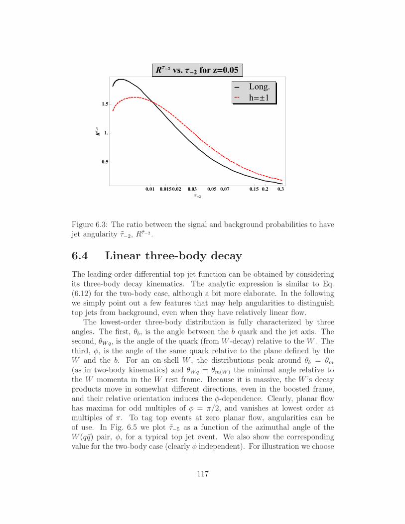
0.01 0.0150.02 0.03 0.05 0.07 0.15 0.2 0.3

0.5

1.

1.5

()2

R()

2

R()2 vs. ()2 for z!0.05

h"#1Long.

Figure 6.3: The ratio between the signal and background probabilities to havejet angularity ""2, R)!2 .

6.4 Linear three-body decay

The leading-order di!erential top jet function can be obtained by consideringits three-body decay kinematics. The analytic expression is similar to Eq.(6.12) for the two-body case, although a bit more elaborate. In the followingwe simply point out a few features that may help angularities to distinguishtop jets from background, even when they have relatively linear flow.

The lowest-order three-body distribution is fully characterized by threeangles. The first, !b, is the angle between the b quark and the jet axis. Thesecond, !Wq, is the angle of the quark (from W -decay) relative to the W . Thethird, 3, is the angle of the same quark relative to the plane defined by theW and the b. For an on-shell W , the distributions peak around !b = !m(as in two-body kinematics) and !Wq = !m(W ) the minimal angle relative tothe W momenta in the W rest frame. Because it is massive, the W ’s decayproducts move in somewhat di!erent directions, even in the boosted frame,and their relative orientation induces the 3-dependence. Clearly, planar flowhas maxima for odd multiples of 3 = (/2, and vanishes at lowest order atmultiples of (. To tag top events at zero planar flow, angularities can beof use. In Fig. 6.5 we plot ""5 as a function of the azimuthal angle of theW (qq) pair, 3, for a typical top jet event. We also show the correspondingvalue for the two-body case (clearly 3 independent). For illustration we choose

117

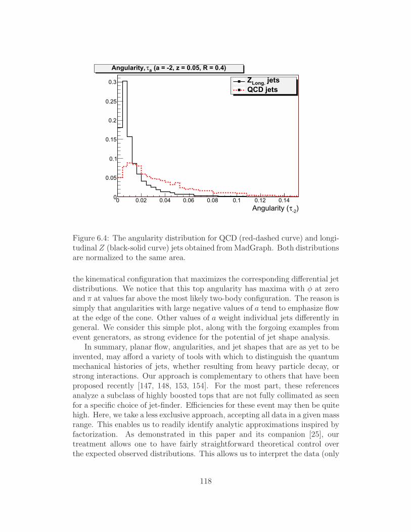
)-2$Angularity (0 0.02 0.04 0.06 0.08 0.1 0.12 0.140

0.05

0.1

0.15

0.2

0.25

0.3 jetsLong.ZQCD jets

(a = -2, z = 0.05, R = 0.4)a$Angularity,

Figure 6.4: The angularity distribution for QCD (red-dashed curve) and longi-tudinal Z (black-solid curve) jets obtained fromMadGraph. Both distributionsare normalized to the same area.

the kinematical configuration that maximizes the corresponding di!erential jetdistributions. We notice that this top angularity has maxima with 3 at zeroand ( at values far above the most likely two-body configuration. The reason issimply that angularities with large negative values of a tend to emphasize flowat the edge of the cone. Other values of a weight individual jets di!erently ingeneral. We consider this simple plot, along with the forgoing examples fromevent generators, as strong evidence for the potential of jet shape analysis.

In summary, planar flow, angularities, and jet shapes that are as yet to beinvented, may a!ord a variety of tools with which to distinguish the quantummechanical histories of jets, whether resulting from heavy particle decay, orstrong interactions. Our approach is complementary to others that have beenproposed recently [147, 148, 153, 154]. For the most part, these referencesanalyze a subclass of highly boosted tops that are not fully collimated as seenfor a specific choice of jet-finder. E"ciencies for these event may then be quitehigh. Here, we take a less exclusive approach, accepting all data in a given massrange. This enables us to readily identify analytic approximations inspired byfactorization. As demonstrated in this paper and its companion [25], ourtreatment allows one to have fairly straightforward theoretical control overthe expected observed distributions. This allows us to interpret the data (only

118

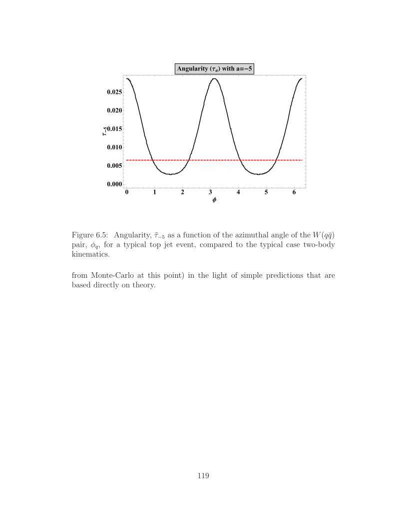
0 1 2 3 4 5 60.000

0.005

0.010

0.015

0.020

0.025

*

()

5

Angularity !(a" with a!)5

Figure 6.5: Angularity, ""5 as a function of the azimuthal angle of the W (qq)pair, 3q, for a typical top jet event, compared to the typical case two-bodykinematics.

from Monte-Carlo at this point) in the light of simple predictions that arebased directly on theory.

119

Bibliography

[1] T. P. Cheng and L. F. Li, “Gauge Theory Of Elementary ParticlePhysics,” Oxford, Uk: Clarendon ( 1984) 536 P. ( Oxford Science Publi-cations)

[2] O. W. Greenberg, Phys. Rev. Lett. 13, 598 (1964) M. Han, Y. Phys.Rev. 139B, 1609 (1965)

[3] D.J. Gross and F. Wilczek, Phys. Rev. Lett. 30, 1343 (1973), H.D.Politzer, Phys. Rev. Lett. 30,1346 (1973), S. Weinberg,Phys. Rev. Lett.31 494, (1973)

[4] C. Aubin et al. (HPQCD Collab.), Phys. Rev. D70, 031504 (2004), C.Aubin et al. (MILC Collab.), Phys. Rev. D70, 114501 (2004), T. Ishikawaet al. (CP-PACS Collab.), Nucl. Phys. (Proc. Supp.) B140, 225 (2005),D.Becirevic et al. (SPQcdR Collab.), Nucl. Phys. (Proc. Supp.) B140, 246(2005), M. Gockeler et al. (QCDSF Collab.), hep-ph/0409312, M. DellaMorte et al. (ALPHA Collab.), hep-lat/0507035, S. Aoki et al. (JLQCDCollab.), Phys. Rev. D68, 054502 (2003), A. Ali Khan et al. (CP-PACSCollab.), Phys. Rev. D65, 054505 (2002); Erratum ibid., D67, 059901(2003).

[5] M. Creutz, “Quarks, Gluons And Lattices,” Cambridge, Uk: Univ. Pr. (1983) 169 P. ( Cambridge Monographs On Mathematical Physics)

[6] L. D. Faddeev and V. N. Popov, Phys. Lett. B 25, 29 (1967).

[7] G. Sterman, “An Introduction to quantum field theory,” Cambridge, UK:Univ. Pr. (1993) 572 p

[8] J. C. Collins, “Renormalization. An Introduction To Renormalization,The Renormalization Cambridge, UK: Univ. Pr. ( 1984) 380p

[9] S. Weinberg, “The quantum theory of fields. Vol. 2: Modern applications,”Cambridge, UK: Univ. Pr. (1996) 489 p

120

[10] T. van Ritbergen, J. A. M. Vermaseren and S. A. Larin, Phys. Lett. B400, 379 (1997) [arXiv:hep-ph/9701390]. M. Czakon, Nucl. Phys. B 710,485 (2005) [arXiv:hep-ph/0411261].

[11] J. Smith, arXiv:hep-ph/0003193.

[12] J. C. Collins, D. E. Soper and G. Sterman, Adv. Ser. Direct. High EnergyPhys. 5, 1 (1988) [arXiv:hep-ph/0409313].

[13] G. Sterman, arXiv:hep-ph/9606312.

[14] G. Sterman, Phys. Rev. D 17, 2773 (1978). Phys. Rev. D 17, 2789 (1978).

[15] S. B. Libby and G. Sterman, Phys. Rev. D 18, 3252 (1978).

[16] S. Coleman and R. E. Norton, Nuovo Cim. 38, 438 (1965).

[17] J. C. Collins and D. E. Soper, Nucl. Phys. B 193, 381 (1981) [Erratum-ibid. B 213, 545 (1983)].

[18] G. Sterman, Nucl. Phys. B 281, 310 (1987).

[19] H. Contopanagos, E. Laenen and G. Sterman, Nucl. Phys. B 484, 303(1997) [arXiv:hep-ph/9604313].

[20] N. Kidonakis and G. Sterman, Nucl. Phys. B 505, 321 (1997) [arXiv:hep-ph/9705234].

[21] N. Kidonakis, G. Oderda and G. Sterman, arXiv:hep-ph/9805279; N. Ki-donakis, G. Oderda and G. Sterman, Nucl. Phys. B 531, 365 (1998)[arXiv:hep-ph/9803241].

[22] L. G. Almeida, G. Sterman and W. Vogelsang, Phys. Rev. D 78, 014008(2008) [arXiv:0805.1885 [hep-ph]].

[23] L. G. Almeida, G. Sterman and W. Vogelsang, Phys. Rev. D 80, 074016(2009) [arXiv:0907.1234 [hep-ph]].

[24] L. G. Almeida, S. J. Lee, G. Perez, G. Sterman, I. Sung and J. Virzi,Phys. Rev. D 79, 074017 (2009) [arXiv:0807.0234 [hep-ph]].

[25] L. G. Almeida, S. J. Lee, G. Perez, I. Sung and J. Virzi, Phys. Rev. D79, 074012 (2009) [arXiv:0810.0934 [hep-ph]]. Dihadron

[26] P. Aurenche, M. Fontannaz, J. P. Guillet, B. A. Kniehl and M. Werlen,Eur. Phys. J. C 13, 347 (2000) [arXiv:hep-ph/9910252].

121

[27] U. Baur et al., arXiv:hep-ph/0005226.

[28] C. Bourrely and J. So!er, Eur. Phys. J. C 36, 371 (2004) [arXiv:hep-ph/0311110].

[29] B. A. Kniehl, G. Kramer and B. Potter, Nucl. Phys. B 597, 337 (2001)[arXiv:hep-ph/0011155].

[30] D. de Florian and W. Vogelsang, Phys. Rev. D 71, 114004 (2005)[arXiv:hep-ph/0501258].

[31] A. Adare et al. [PHENIX Collaboration], Phys. Rev. D 76, 051106(2007) [arXiv:0704.3599 [hep-ex]]; Phys. Rev. D 79, 012003 (2009)[arXiv:0810.0701 [hep-ex]].

[32] J. Adams et al. [STAR Collaboration], Phys. Rev. Lett. 97, 152302 (2006)[arXiv:nucl-ex/0602011].

[33] I. Arsene et al. [BRAHMS Collaboration], Phys. Rev. Lett. 98, 252001(2007) [arXiv:hep-ex/0701041].

[34] C. De Marzo et al. [NA24 Collaboration], Phys. Rev. D 42, 748 (1990).

[35] H. B. White et al. [E711 Collaboration], Phys. Rev. D 48, 3996 (1993);H. B. White, A Study of angular dependence in parton-parton scatteringfrom massive hadron pair production, PhD Thesis, FERMILAB-THESIS-1991-39, FSU-HEP-910722, UMI-92-02321, 1991.

[36] M. Begel [E706 Collaboration], Production of high mass pairs of directphotons and neutral mesons in a Tevatron fixed target experiment, PhDThesis, FERMILAB-THESIS-1999-05, UMI-99-60725, 1999; see also:L. Apanasevich et al. [E706 Collaboration], Phys. Rev. Lett. 81, 2642(1998) [arXiv:hep-ex/9711017].

[37] A. L. S. Angelis et al. [CCOR Collaboration], Nucl. Phys. B 209, 284(1982).

[38] P. Chiappetta, R. Fergani and J. P. Guillet, Z. Phys. C 69, 443 (1996).

[39] J. F. Owens, Phys. Rev. D 65, 034011 (2002) [arXiv:hep-ph/0110036].

[40] T. Binoth, J. P. Guillet, E. Pilon and M. Werlen, Eur. Phys. J. C 24, 245(2002); Eur. Phys. J. direct C 4, 7 (2002) [arXiv:hep-ph/0203064].

[41] G. Sterman, Nucl. Phys. B 281, 310 (1987); S. Catani and L. Trentadue,Nucl. Phys. B 327, 323 (1989); Nucl. Phys. B 353, 183 (1991).

122

[42] A. Idilbi, X. d. Ji and F. Yuan, Nucl. Phys. B 753, 42 (2006) [arXiv:hep-ph/0605068]; T. Becher, M. Neubert and G. Xu, JHEP 0807, 030 (2008)[arXiv:0710.0680 [hep-ph]].

[43] N. Kidonakis, G. Oderda and G. Sterman, Nucl. Phys. B 525, 299(1998) [arXiv:hep-ph/9801268]; Nucl. Phys. B 531, 365 (1998) [arXiv:hep-ph/9803241].

[44] N. Kidonakis and J. F. Owens, Phys. Rev. D 63, 054019 (2001)[arXiv:hep-ph/0007268].

[45] E. Laenen and G. Sterman, in The Fermilab Meeting, DPF 1992 (WorldScientific, Singapore, 1993) Vol. 1, p. 987.

[46] G. Sterman and W. Vogelsang, JHEP 0102, 016 (2001) [arXiv:hep-ph/0011289].

[47] A. Mukherjee and W. Vogelsang, Phys. Rev. D 73, 074005 (2006)[arXiv:hep-ph/0601162].

[48] G. Bozzi, S. Catani, D. de Florian and M. Grazzini, Nucl. Phys. B 791,1 (2008) [arXiv:0705.3887 [hep-ph]].

[49] G. Sterman and W. Vogelsang, Phys. Rev. D 74, 114002 (2006)[arXiv:hep-ph/0606211].

[50] M. Cacciari and S. Catani, Nucl. Phys. B 617, 253 (2001) [arXiv:hep-ph/0107138].

[51] M. Sjodahl, arXiv:0906.1121 [hep-ph].

[52] N. Kidonakis, E. Laenen, S. Moch and R. Vogt, Phys. Rev. D 64, 114001(2001) [arXiv:hep-ph/0105041].

[53] for related studies in heavy flavor production, see: R. Bonciani, S. Catani,M. L. Mangano and P. Nason, Nucl. Phys. B 529, 424 (1998) [Erratum-ibid. B 803, 234 (2008)] [arXiv:hep-ph/9801375]; S. Moch and P. Uwer,Phys. Rev. D 78, 034003 (2008) [arXiv:0804.1476 [hep-ph]]; M. Czakonand A. Mitov, arXiv:0812.0353 [hep-ph].

[54] A. Kulesza, G. Sterman and W. Vogelsang, Phys. Rev. D 66, 014011(2002) [arXiv:hep-ph/0202251].

123

[55] S. Catani, D. de Florian and M. Grazzini, JHEP 0105, 025 (2001)[arXiv:hep-ph/0102227]; see also: M. Kramer, E. Laenen and M. Spira,Nucl. Phys. B 511, 523 (1998) [arXiv:hep-ph/9611272]; R. V. Harlan-der and W. B. Kilgore, Phys. Rev. D 64, 013015 (2001) [arXiv:hep-ph/0102241].

[56] W. K. Tung, H. L. Lai, A. Belyaev, J. Pumplin, D. Stump and C. P. Yuan,JHEP 0702, 053 (2007) [arXiv:hep-ph/0611254].

[57] D. de Florian, R. Sassot and M. Stratmann, Phys. Rev. D 75, 114010(2007) [arXiv:hep-ph/0703242].

[58] T. O. Eynck, E. Laenen and L. Magnea, [arXiv:hep-ph/0305179];E. Laenen and L. Magnea, Phys. Lett. B 632, 270 (2006) [arXiv:hep-ph/0508284]; E. Laenen, G. Stavenga and C. D. White, JHEP 0903, 054(2009) [arXiv:0811.2067 [hep-ph]]; E. Laenen, L. Magnea and G. Stavenga,Phys. Lett. B 669, 173 (2008) [arXiv:0807.4412 [hep-ph]].

[59] M. J. Tannenbaum, Nucl. Phys. A 749, 219 (2005) [arXiv:nucl-ex/0412004].

[60] S. M. Aybat, L. J. Dixon and G. Sterman, Phys. Rev. D 74, 074004(2006) [arXiv:hep-ph/0607309]; Phys. Rev. Lett. 97, 072001 (2006)[arXiv:hep-ph/0606254]; E. Gardi and L. Magnea, JHEP 0903, 079(2009) [arXiv:0901.1091 [hep-ph]]; T. Becher and M. Neubert, JHEP0906, 081 (2009) [arXiv:0903.1126 [hep-ph]].

[61] W. L. van Neerven, Nucl. Phys. B 268, 453 (1986).

[62] K. D. Lane, Phys. Rev. D 52, 1546 (1995) [arXiv:hep-ph/9501260].

[63] For recent work, see contribution of D.G.E. Walker in G. Brooijmans etal., – New Physics Working Group,” arXiv:0802.3715 [hep-ph].

[64] D. Atwood, S. Bar-Shalom, G. Eilam and A. Soni, Phys. Rept. 347, 1(2001) [arXiv:hep-ph/0006032].

[65] For review, see: W. Bernreuther, arXiv:0805.1333 [hep-ph].

[66] L. M. Sehgal and M. Wanninger, Phys. Lett. B 200, 211 (1988); J. Bagger,C. Schmidt and S. King, Phys. Rev. D 37, 1188 (1988).

[67] O. Antunano, J. H. Kuhn and G. V. Rodrigo, Phys. Rev. D 77, 014003(2008) [arXiv:0709.1652 [hep-ph]]; G. Rodrigo, “Axigluon signatures athadron colliders,” arXiv:0803.2992 [hep-ph].

124

[68] F. Halzen, P. Hoyer and C. S. Kim, Phys. Lett. B 195, 74 (1987).

[69] R. W. Brown, K. O. Mikaelian, V. K. Cung and E. A. Paschos, e- 'muon+ muon-,” Phys. Lett. B 43, 403 (1973); F. A. Berends, K. J. F. Gae-mers and R. Gastmans, Nucl. Phys. B 63, 381 (1973); S. J. Brodsky,C. E. Carlson and R. Suaya, Phys. Rev. D 14, 2264 (1976).

[70] S. Catani, D. de Florian, G. Rodrigo and W. Vogelsang, Phys. Rev. Lett.93, 152003 (2004) [arXiv:hep-ph/0404240].

[71] W. Beenakker, H. Kuijf, W. L. van Neerven and J. Smith, Phys. Rev. D40, 54 (1989); W. Beenakker, W. L. van Neerven, R. Meng, G. A. Schulerand J. Smith, Nucl. Phys. B 351, 507 (1991).

[72] P. Nason, S. Dawson and R. K. Ellis, Nucl. Phys. B 327, 49 (1989)[Erratum-ibid. B 335, 260 (1990)].

[73] J. Riedl, A. Schafer and M. Stratmann, Eur. Phys. J. C 52, 987 (2007)[arXiv:0708.3010 [hep-ph]].

[74] J. H. Kuhn and G. Rodrigo, Phys. Rev. Lett. 81, 49 (1998) [arXiv:hep-ph/9802268]; Phys. Rev. D 59, 054017 (1999) [arXiv:hep-ph/9807420].

[75] M. T. Bowen, S. D. Ellis and D. Rainwater, Phys. Rev. D 73, 014008(2006) [arXiv:hep-ph/0509267].

[76] S. Dittmaier, P. Uwer and S. Weinzierl, Phys. Rev. Lett. 98, 262002(2007) [arXiv:hep-ph/0703120].

[77] V. M. Abazov et al. [D0 Collaboration], arXiv:0712.0851 [hep-ex].

[78] J. Weinelt, Masters thesis, Universitat Karlsruhe, FERMILAB-MASTERS-2006-05; IEKP-KA-2006-21; D. Hirschbuehl, Ph.D. Thesis,Universitat Karlsruhe, FERMILAB-THESIS-2005-80.

[79] E. Laenen, J. Smith and W. L. van Neerven, Phys. Lett. B 321, 254(1994) [arXiv:hep-ph/9310233]; S. Catani, M. L. Mangano, P. Nason andL. Trentadue, Phys. Lett. B 378, 329 (1996) [arXiv:hep-ph/9602208];E. L. Berger and H. Contopanagos, Phys. Rev. D 54, 3085 (1996)[arXiv:hep-ph/9603326].

[80] R. Bonciani, S. Catani, M. L. Mangano and P. Nason, Nucl. Phys. B 529,424 (1998) [arXiv:hep-ph/9801375].

125

[81] N. Kidonakis, E. Laenen, S. Moch and R. Vogt, Phys. Rev. D 64, 114001(2001) [arXiv:hep-ph/0105041]; N. Kidonakis and R. Vogt, Phys. Rev. D68, 114014 (2003) [arXiv:hep-ph/0308222].

[82] M. Cacciari, S. Frixione, M. M. Mangano, P. Nason and G. Ridolfi,arXiv:0804.2800 [hep-ph].

[83] R. Bonciani, S. Catani, M. L. Mangano and P. Nason, Phys. Lett. B 575,268 (2003) [arXiv:hep-ph/0307035].

[84] J. Kodaira and L. Trentadue, Phys. Lett. B 112, 66 (1982); Phys. Lett.B 123, 335 (1983);S. Catani, E. D’Emilio and L. Trentadue, Phys. Lett. B 211, 335 (1988).

[85] S. Frixione, M. L. Mangano, P. Nason and G. Ridolfi, Nucl. Phys. B 412,225 (1994) [arXiv:hep-ph/9306337].

[86] M. L. Mangano, P. Nason and G. Ridolfi, Nucl. Phys. B 373, 295 (1992).

[87] S. Catani, M. L. Mangano, P. Nason and L. Trentadue, Nucl. Phys. B478, 273 (1996) [arXiv:hep-ph/9604351].

[88] J. Pumplin, D. R. Stump, J. Huston, H. L. Lai, P. Nadolsky andW. K. Tung, JHEP 0207, 012 (2002) [arXiv:hep-ph/0201195].

[89] G. Bozzi, S. Catani, D. de Florian and M. Grazzini, Phys. Lett. B 564, 65(2003) [arXiv:hep-ph/0302104]; D. de Florian and J. Zurita, Phys. Lett.B 659, 813 (2008) [arXiv:0711.1916 [hep-ph]].

[90] CDF and D0 Collaborations, arXiv:hep-ex/0703034.

[91] G. Sterman and W. Vogelsang, in: High Energy Physics 99, Proceedingsof the “International Europhysics Conference on High-Energy Physics”,ed. K. Huitu et al. (Institute of Physics Publishing, Bristol, UK, 2000),hep-ph/9910371.

[92] see, for example: S. Catani, M. L. Mangano, P. Nason, C. Oleari andW. Vogelsang, JHEP 9903, 025 (1999) [arXiv:hep-ph/9903436]; N. Ki-donakis and J. F. Owens, Phys. Rev. D 61, 094004 (2000) [arXiv:hep-ph/9912388]; G. Sterman and W. Vogelsang, JHEP 0102, 016 (2001)[arXiv:hep-ph/0011289]; S. Catani, D. de Florian, M. Grazzini and P. Na-son, JHEP 0307, 028 (2003) [arXiv:hep-ph/0306211]; D. de Florian andW. Vogelsang, Phys. Rev. D 72, 014014 (2005) [arXiv:hep-ph/0506150];Phys. Rev. D 71, 114004 (2005) [arXiv:hep-ph/0501258].

126

[93] ATLAS Detector and physics performance TDR, CERN-LHCC-99-14;CMS Physics and performance TDR, Volume II: CERN-LHCC-2006-021

[94] K. Agashe, A. Belyaev, T. Krupovnickas, G. Perez and J. Virzi, Phys.Rev. D 77, 015003 (2008) [arXiv:hep-ph/0612015].

[95] A. L. Fitzpatrick, J. Kaplan, L. Randall and L. T. Wang, JHEP 0709,013 (2007) [arXiv:hep-ph/0701150].

[96] U. Baur and L. H. Orr, Phys. Rev. D 76, 094012 (2007) [arXiv:0707.2066[hep-ph]].

[97] G. Brooijmans, ATLAS note, ATL-PHYS-CONF-2008-008; J. Conway, etal., LPC Workshop on Early Physics at CMS, UC Davis (2007); G. Brooi-jmans et al., arXiv:0802.3715 [hep-ph]; M. Vos, talk given in the ATLASFlavour Tagging Meeting, CERN (2008).

[98] D. Benchekroun, C. Driouichi, A. Hoummada, SN-ATLAS-2001-001,ATL-COM-PHYS-2000-020, EPJ Direct 3, 1 (2001); J. M. Butter-worth, B. E. Cox and J. R. Forshaw, Phys. Rev. D 65, 096014 (2002)[arXiv:hep-ph/0201098]; J. M. Butterworth, A. R. Davison, M. Rubinand G. P. Salam, arXiv:0809.2530 [hep-ph].

[99] See, for example, L. March, E. Ros and B. Salvachua, ATL-PHYS-PUB-2006-002, ATL-COM-PHYS-2005-032; L. March, E. Ros andS.G.d.l. Hoz, ATL-COM-PHYS-2006-031, ATL-PHYS-CONF-2006-007;L. March, E. Ros, B. Salvacha, ATL-Phys-PUB-2006-002; M. Vos, ATL-PHYS-PUB-2008-000, ATL-PHYS-CONF-2008-016;

[100] U. Baur and L. H. Orr, arXiv:0803.1160 [hep-ph].

[101] Y. Bai and Z. Han, arXiv:0809.4487 [hep-ph].

[102] S. Fleming, A. H. Hoang, S. Mantry and I. W. Stewart, arXiv:0711.2079[hep-ph]; S. Fleming, A. H. Hoang, S. Mantry and I. W. Stewart,Phys. Rev. D 77, 074010 (2008) [arXiv:hep-ph/0703207]; A. H. Hoangand I. W. Stewart, arXiv:0808.0222 [hep-ph]. A. Jain, I. Scimemi andI. W. Stewart, Phys. Rev. D 77, 094008 (2008) [arXiv:0801.0743 [hep-ph]].

[103] W. Skiba and D. Tucker-Smith, Phys. Rev. D 75, 115010 (2007)[arXiv:hep-ph/0701247].

[104] B. Holdom, JHEP 0708, 069 (2007) [arXiv:0705.1736 [hep-ph]].

127

[105] K. Agashe et al., Phys. Rev. D 76, 115015 (2007) [arXiv:0709.0007 [hep-ph]].

[106] F. Maltoni and T. Stelzer, JHEP 0302, 027 (2003) [arXiv:hep-ph/0208156].

[107] T. Stelzer and W. F. Long, Comput. Phys. Commun. 81, 357 (1994)[arXiv:hep-ph/9401258].

[108] J. Alwall et al., JHEP 0709, 028 (2007) [arXiv:0706.2334 [hep-ph]].

[109] T. Gleisberg et al., JHEP 0402 (2004) 056 [arXiv:hep-ph/0311263].

[110] J. Virzi, “ATLAS Transfer Function,https://twiki.cern.ch/twiki/bin/view/Atlas/TransferFunction.”

[111] R. Frederix and F. Maltoni, arXiv:0712.2355 [hep-ph].

[112] V. Barger, T. Han and D. G. E. Walker, Phys. Rev. Lett. 100, 031801(2008) [arXiv:hep-ph/0612016].

[113] T. Han, R. Mahbubani, D. G. E. Walker and L. T. E. Wang,arXiv:0803.3820 [hep-ph].

[114] K. Agashe, H. Davoudiasl, G. Perez and A. Soni, Phys. Rev. D76, 036006 (2007) [arXiv:hep-ph/0701186]; B. Lillie, L. Randall andL. T. Wang, JHEP 0709, 074 (2007) [arXiv:hep-ph/0701166]; B. Lillie,J. Shu and T. M. P. Tait, Phys. Rev. D 76, 115016 (2007) [arXiv:0706.3960[hep-ph]]; H. Davoudiasl, G. Perez and A. Soni, Phys. Lett. B 665, 67(2008) [arXiv:0802.0203 [hep-ph]].

[115] For a recent review see: T. Han, arXiv:0804.3178 [hep-ph].

[116] S. D. Ellis, Z. Kunszt and D. E. Soper, Phys. Rev. Lett. 69, 3615 (1992)[arXiv:hep-ph/9208249].

[117] D. E. Kaplan, K. Rehermann, M. D. Schwartz and B. Tweedie,arXiv:0806.0848 [hep-ph].

[118] J. Thaler and L. T. Wang, JHEP 0807, 092 (2008) [arXiv:0806.0023[hep-ph]].

[119] F. Hubaut, E. Monnier, P. Pralavorio, K. Smolek and V. Simak, Eur.Phys. J. C 44S2, 13 (2005) [arXiv:hep-ex/0508061].

128

[120] W. Bernreuther, J. P. Ma and T. Schroder, Phys. Lett. B 297, 318(1992); S. Choi, FERMILAB-THESIS-1999-07; K. A. Johns [D0 Col-laboration], Int. J. Mod. Phys. A 16S1A (2001) 366; W. Bern-reuther, A. Brandenburg, Z. G. Si and P. Uwer, Phys. Lett. B 509,53 (2001) [arXiv:hep-ph/0104096]; B. Abbott et al. [D0 Collaboration],Phys. Rev. Lett. 85, 256 (2000) [arXiv:hep-ex/0002058]; T. Torma,JHEP 0111, 055 (2001) [arXiv:hep-ph/9912281]; V. D. Barger, J. Ohne-mus and R. J. N. Phillips, Int. J. Mod. Phys. A 4, 617 (1989);G. L. Kane, G. A. Ladinsky and C. P. Yuan, Phys. Rev. D 45, 124(1992); G. Mahlon and S. J. Parke, Phys. Rev. D 53, 4886 (1996)[arXiv:hep-ph/9512264]; D. Atwood, A. Aeppli and A. Soni, Phys. Rev.Lett. 69, 2754 (1992); D. Atwood, S. Bar-Shalom, G. Eilam and A. Soni,Phys. Rept. 347, 1 (2001) [arXiv:hep-ph/0006032]; M. Arai, N. Okada,K. Smolek and V. Simak, Phys. Rev. D 70, 115015 (2004) [arXiv:hep-ph/0409273]; C. Csaki, J. Heinonen and M. Perelstein, JHEP 0710,107 (2007) [arXiv:0707.0014 [hep-ph]]; M. M. Nojiri and M. Takeuchi,arXiv:0802.4142 [hep-ph].

[121] T. Sjostrand, S. Mrenna and P. Skands, JHEP 0605, 026 (2006)[arXiv:hep-ph/0603175].

[122] G. P. Salam and G. Soyez, JHEP 0705, 086 (2007) [arXiv:0704.0292[hep-ph]].

[123] J.E. Huth et al., Proceedings of Research Directions For The Decade:Snowmass Accord 1990.

[124] J. Pumplin, A. Belyaev, J. Huston, D. Stump and W. K. Tung, JHEP0602, 032 (2006) [arXiv:hep-ph/0512167]; J. Campbell and R. K. Ellis,“MCFM, A Monte Carlo for FeMtobarn processes at Hadron Colliders,http://mcfm.fnal.gov.”

[125] T. Sjostrand, S. Mrenna and P. Skands, Comput. Phys. Commun. 178,852 (2008) [arXiv:0710.3820 [hep-ph]].

[126] J. Alwall et al., Eur. Phys. J. C 53, 473 (2008) [arXiv:0706.2569 [hep-ph]].

[127] M. L. Mangano, M. Moretti, F. Piccinini, R. Pittau and A. D. Polosa,JHEP 0307, 001 (2003) [arXiv:hep-ph/0206293].

[128] S. Catani, F. Krauss, R. Kuhn and B. R. Webber, JHEP 0111, 063(2001) [arXiv:hep-ph/0109231].

129

[129] S. D. Ellis, J. Huston, K. Hatakeyama, P. Loch and M. Tonnes-mann, Prog. Part. Nucl. Phys. 60, 484 (2008) [arXiv:0712.2447 [hep-ph]]; A. Banfi, G. P. Salam and G. Zanderighi, JHEP 0707, 026 (2007)[arXiv:0704.2999 [hep-ph]].

[130] C. F. Berger, T. Kucs and G. Sterman, Phys. Rev. D 68, 014012 (2003)[arXiv:hep-ph/0303051].

[131] G. Sterman, arXiv:hep-ph/0412013; I. M. Dremin, AIP Conf. Proc.828, 30 (2006) [arXiv:hep-ph/0510250]; T. Han, arXiv:hep-ph/0508097;G. Sterman, arXiv:hep-ph/9606312.

[132] P. Meade and L. Randall, arXiv:0708.3017 [hep-ph].

[133] A. Czarnecki and K. Melnikov, Nucl. Phys. B 544, 520 (1999)[arXiv:hep-ph/9806244].

[134] K. G. Chetyrkin, R. Harlander, T. Seidensticker and M. Steinhauser,Phys. Rev. D 60, 114015 (1999) [arXiv:hep-ph/9906273].

[135] C. Amsler et al. [Particle Data Group], Phys. Lett. B 667 (2008) 1,http://www-pdg.lbl.gov/2008/reviews/statrpp.pdf.

[136] M. Strassler, “Unusual Physics Signatures at the LHC,” talk presented atthe 2007 Phenomenology Symposium - Pheno 07, University of Wisconsin,Madison, May 7-9, 2007.

[137] L. Randall and R. Sundrum, Phys. Rev. Lett. 83, 3370 (1999)[arXiv:hep-ph/9905221].

[138] M. Furman, Nucl. Phys. B 197, 413 (1982).

[139] F. Aversa, P. Chiappetta, M. Greco and J. P. Guillet, Nucl. Phys. B327, 105 (1989), Z. Phys. C 46, 253 (1990).

[140] N. Kidonakis and J. F. Owens, Phys. Rev. D 63, 054019 (2001)[arXiv:hep-ph/0007268].

[141] M. H. Seymour, Nucl. Phys. B 513, 269 (1998) [arXiv:hep-ph/9707338];S. D. Ellis, J. Huston, K. Hatakeyama, P. Loch and M. Tonnesmann,Prog. Part. Nucl. Phys. 60, 484 (2008) [arXiv:0712.2447 [hep-ph]].

[142] S. Catani, Y. L. Dokshitzer, M. Olsson, G. Turnock and B. R. Webber,Phys. Lett. B 269, 432 (1991); S. Catani, Y. L. Dokshitzer, M. H. Sey-mour and B. R. Webber, Nucl. Phys. B 406, 187 (1993); S. D. Ellis

130

and D. E. Soper, Phys. Rev. D 48, 3160 (1993) [arXiv:hep-ph/9305266];Y. L. Dokshitzer, G. D. Leder, S. Moretti and B. R. Webber, JHEP 9708,001 (1997) [arXiv:hep-ph/9707323].

[143] G. P. Salam and G. Soyez, JHEP 0705, 086 (2007) [arXiv:0704.0292[hep-ph]].

[144] For recent studies see e.g: K. Agashe et al., Phys. Rev. D 77, 015003(2008) [arXiv:hep-ph/0612015]; B. Lillie, L. Randall and L. T. Wang,JHEP 0709, 074 (2007) [arXiv:hep-ph/0701166].

[145] See e.g: K. Agashe et al., Phys. Rev. D 76, 115015 (2007)[arXiv:0709.0007 [hep-ph]]; K. Agashe, H. Davoudiasl, G. Perez andA. Soni, Phys. Rev. D 76, 036006 (2007) [arXiv:hep-ph/0701186]; J. Hirn,A. Martin and V. Sanz, JHEP 0805, 084 (2008) [arXiv:0712.3783 [hep-ph]].

[146] D. Benchekroun, C. Driouichi, A. Hoummada, SN-ATLAS-2001-001,ATL-COM-PHYS-2000-020, EPJ Direct 3, 1 (2001); J. Conway, et al.,LPC Workshop on Early Physics at CMS, UC Davis (2007); G. Brooij-mans et al., arXiv:0802.3715 [hep-ph]; M. Vos, talk given in the ATLASFlavour Tagging Meeting, CERN (2008).

[147] G. Brooijmans, ATLAS note, ATL-PHYS-CONF-2008-008.

[148] J. M. Butterworth, B. E. Cox and J. R. Forshaw, Phys. Rev. D 65,096014 (2002) [arXiv:hep-ph/0201098].

[149] M. Cacciari, G. P. Salam and G. Soyez, JHEP 0804, 063 (2008)[arXiv:0802.1189 [hep-ph]].

[150] G. Sterman, Phys. Rev. D 19, 3135 (1979).

[151] N. Kidonakis, G. Oderda and G. Sterman, Nucl. Phys. B 525, 299 (1998)[arXiv:hep-ph/9801268]; D. de Florian and W. Vogelsang, Phys. Rev. D76, 074031 (2007) [arXiv:0704.1677 [hep-ph]].

[152] M. Dasgupta and G. P. Salam, J. Phys. G 30, R143 (2004) [arXiv:hep-ph/0312283]; C. F. Berger, Mod. Phys. Lett. A 20, 1187 (2005)[arXiv:hep-ph/0505037]; M. Dasgupta, L. Magnea and G. P. Salam, JHEP0802, 055 (2008) [arXiv:0712.3014 [hep-ph]].

[153] D. E. Kaplan, K. Rehermann, M. D. Schwartz and B. Tweedie,arXiv:0806.0848 [hep-ph].

131

[154] J. Thaler and L. T. Wang, arXiv:0806.0023 [hep-ph].

[155] C. F. Berger, T. Kucs and G. Sterman, Phys. Rev. D 68, 014012 (2003)[arXiv:hep-ph/0303051].

[156] J. M. Butterworth, A. R. Davison, M. Rubin and G. P. Salam,arXiv:0802.2470 [hep-ph].

[157] G. Parisi, Phys. Lett. B 74, 65 (1978).

[158] J. F. Donoghue, F. E. Low and S. Y. Pi, Phys. Rev. D 20, 2759 (1979).

[159] R. K. Ellis, D. A. Ross and A. E. Terrano, Nucl. Phys. B 178, 421(1981).

[160] A. Banfi, Y. L. Dokshitzer, G. Marchesini and G. Zanderighi, JHEP0105, 040 (2001) [arXiv:hep-ph/0104162].

[161] F. Maltoni and T. Stelzer, JHEP 0302, 027 (2003) [arXiv:hep-ph/0208156]; T. Stelzer and W. F. Long, Comput. Phys. Com-mun. 81, 357 (1994) [arXiv:hep-ph/9401258], JHEP 0709, 028 (2007)[arXiv:0706.2334 [hep-ph]].

[162] T. Gleisberg et al., JHEP 0402 (2004) 056 [arXiv:hep-ph/0311263].

[163] C. F. Berger and L. Magnea, Phys. Rev. D 70, 094010 (2004) [arXiv:hep-ph/0407024].

132

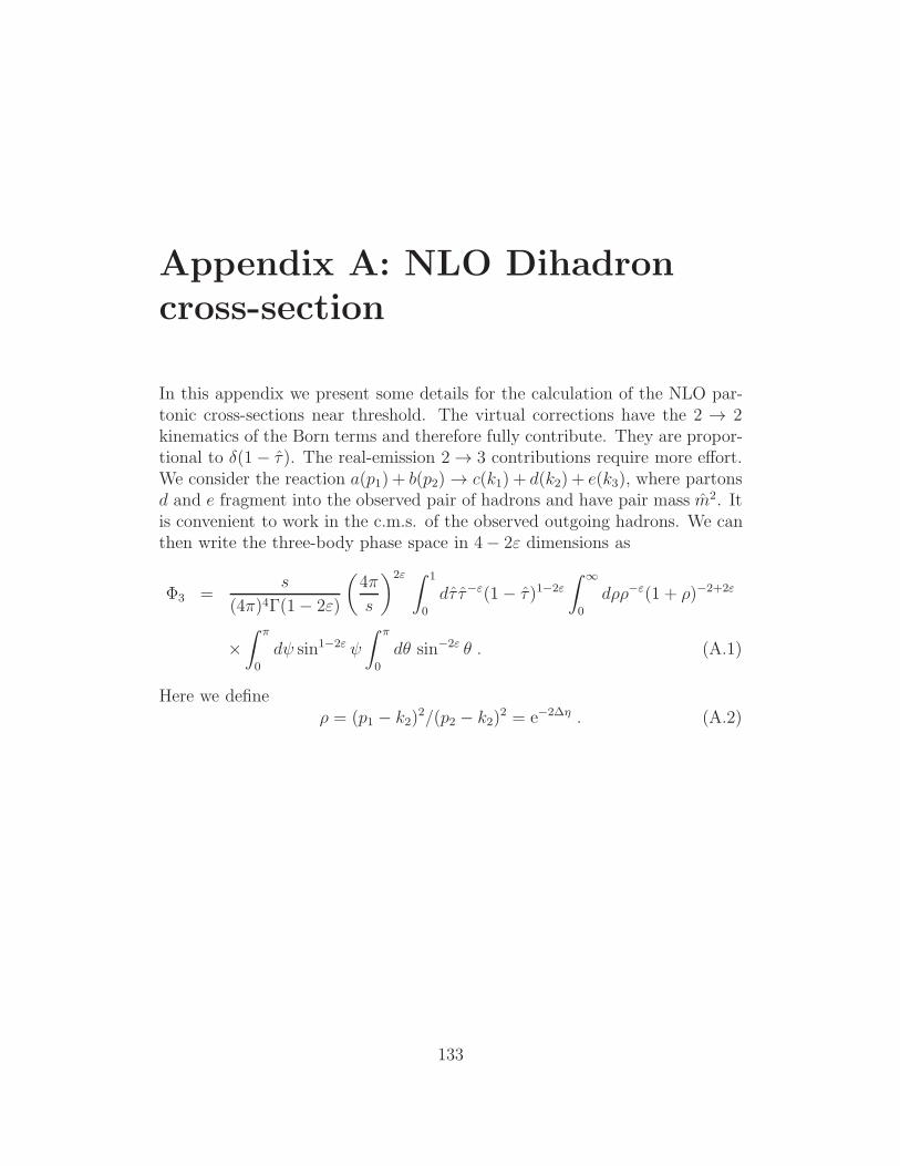
Appendix A: NLO Dihadron

cross-section

In this appendix we present some details for the calculation of the NLO par-tonic cross-sections near threshold. The virtual corrections have the 2 ' 2kinematics of the Born terms and therefore fully contribute. They are propor-tional to %(1& "). The real-emission 2 ' 3 contributions require more e!ort.We consider the reaction a(p1) + b(p2) ' c(k1) + d(k2) + e(k3), where partonsd and e fragment into the observed pair of hadrons and have pair mass m2. Itis convenient to work in the c.m.s. of the observed outgoing hadrons. We canthen write the three-body phase space in 4& 25 dimensions as

&3 =s

(4()4#(1& 25)

"4(

s

#20 * 1

0

d" ""0(1& ")1"20

* $

0

d66"0(1 + 6)"2+20

)* %

0

d# sin1"20 #

* %

0

d! sin"20 ! . (A.1)

Here we define6 = (p1 & k2)

2/(p2 & k2)2 = e"2!, . (A.2)

133

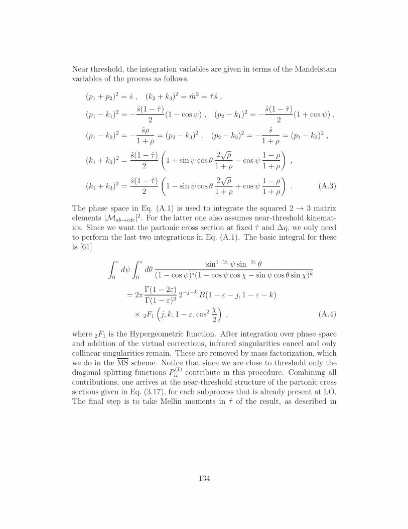
Near threshold, the integration variables are given in terms of the Mandelstamvariables of the process as follows:

(p1 + p2)2 = s , (k2 + k3)

2 = m2 = " s ,

(p1 & k1)2 = &

s(1& ")

2(1& cos#) , (p2 & k1)

2 = &s(1& " )

2(1 + cos#) ,

(p1 & k2)2 = &

s6

1 + 6= (p2 & k3)

2 , (p2 & k2)2 = &

s

1 + 6= (p1 & k3)

2 ,

(k1 + k2)2 =

s(1& ")

2

"

1 + sin# cos !2!6

1 + 6& cos#

1& 6

1 + 6

#

,

(k1 + k3)2 =

s(1& ")

2

"

1& sin# cos !2!6

1 + 6+ cos#

1& 6

1 + 6

#

. (A.3)

The phase space in Eq. (A.1) is used to integrate the squared 2 ' 3 matrixelements |Mab%cde|2. For the latter one also assumes near-threshold kinemat-ics. Since we want the partonic cross section at fixed " and $0, we only needto perform the last two integrations in Eq. (A.1). The basic integral for theseis [61]

* %

0

d#

* %

0

d!sin1"20 # sin"20 !

(1& cos#)j(1& cos# cos4& sin# cos ! sin4)k

= 2(#(1& 25)

#(1& 5)22"j"k B(1& 5& j, 1& 5& k)

) 2F1

$

j, k, 1& 5, cos24

2

%

, (A.4)

where 2F1 is the Hypergeometric function. After integration over phase spaceand addition of the virtual corrections, infrared singularities cancel and onlycollinear singularities remain. These are removed by mass factorization, whichwe do in the MS scheme. Notice that since we are close to threshold only thediagonal splitting functions P (1)

ii contribute in this procedure. Combining allcontributions, one arrives at the near-threshold structure of the partonic crosssections given in Eq. (3.17), for each subprocess that is already present at LO.The final step is to take Mellin moments in " of the result, as described in

134

Eq. (3.26). This gives for the partonic cross sections to NLO:

,thr,LO+NLOab%cd (N,$0,'s(µ), µ/m) = ,(0)

ab%cd($0)

+'s(µ)

(

?

,(1,0)ab%cd($0, µ/m) & ln N ,(1,1)

ab%cd($0, µ/m)

+1

2

(

ln2 N + 7(2))

,(1,2)ab%cd($0)

4

, (A.5)

where terms subleading inN have been neglected. The “C-coe"cients” definedin Eq. (3.41) are obtained from this as

C(1)ab%cd ($0, µ/m) =

,(1,0)ab%cd($0, µ/m) + 1

27(2),(1,2)ab%cd($0)

,(0)ab%cd($0)

. (A.6)

135

Appendix B: Hard Coe!cients

In this section we give the coe"cients C(1)ab%cd for each subprocess contributing

to the production of our di-hadron final state, resulting from the calculationoutlined in Appendix A. In all expressions below, µ is the renormalizationscale. The dependence on the factorization scale is already included in thefunction Ei in Eq. (3.43). As before, we define 6 ( e"2!,.qq# ' qq#:

We define:Qqq" ( 1 + (1 + 6)2 . (B.1)

We then have:

C(1)qq"%qq" ($0, µ/m) = 2(b0 ln

µ2

m2+

"5

6Qqq"+

13

12

#

ln2 6

+

"5

6&

1

3Qqq"

#

ln2(1 + 6) +

"

&8

3+

14 + 96

6Qqq"

#

ln 6

+

"

&4

3+

2

3Qqq"

#

ln(1 + 6) ln 6&6

3Qqq"ln(1 + 6)

+7(2

6Qqq"+

Nf

3ln

6

1 + 6&

5Nf

9+

8

3Li2

"6

1 + 6

#

+3

2ln(1 + 6) +

47(2

36+

7

2. (B.2)

qq# ' qq#:

136

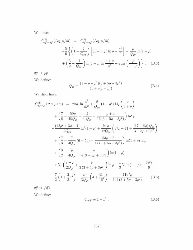
We have:

C(1)qq"%qq" ($0, µ/m) = C(1)

qq"%qq" ($0, µ/m)

+5

6

E"

1&2

Qqq"

#3

(1 + ln 6) ln 6+(2

2

4

&6

Qqq"ln(1 + 6)

+

"3

2&

1

Qqq"

#

ln(1 + 6) ln1 + 6

62& 2Li2

"6

1 + 6

#F

. (B.3)

qq ' qq:

We define:

Qqq ((1& 6+ 62)(3 + 56+ 362)

(1 + 6(1 + 6)). (B.4)

We then have:

C(1)qq%qq ($0, µ/m) = 2(b0 ln

µ2

m2+

8

Qqq

(

1& 62)

Li2

"6

1 + 6

#

+

"7

6&

596

48Qqq+

5

4 Qqq&

6+ 4

16 (3 + 56+ 362)

#

ln2 6

&(1262 + 36& 4)

2Qqqln2(1 + 6) +

ln 6

12Qqq

"

376& 71 +(17& 86)Qqq

3 + 56+ 362

#

+

"7

3&

7

4Qqq(6& 56)&

536& 6

12 (3 + 56+ 362)

#

ln(1 + 6) ln 6

+

"

3

2&

6

4Qqq&

6

4 (3 + 56+ 362)

#

ln(1 + 6)

+Nf

"2& 6

2Qqq+

6

3 (3 + 56+ 362)

#

ln 6&1

3Nf ln(1 + 6)&

5Nf

9

+7

2

"

1 +2

3(2

#

&(2

3Qqq

"

4 +41

166

#

&71(26

144 (3 + 56+ 362). (B.5)

qq ' q#q#:

We define:Qq"q" ( 1 + 62 . (B.6)

137

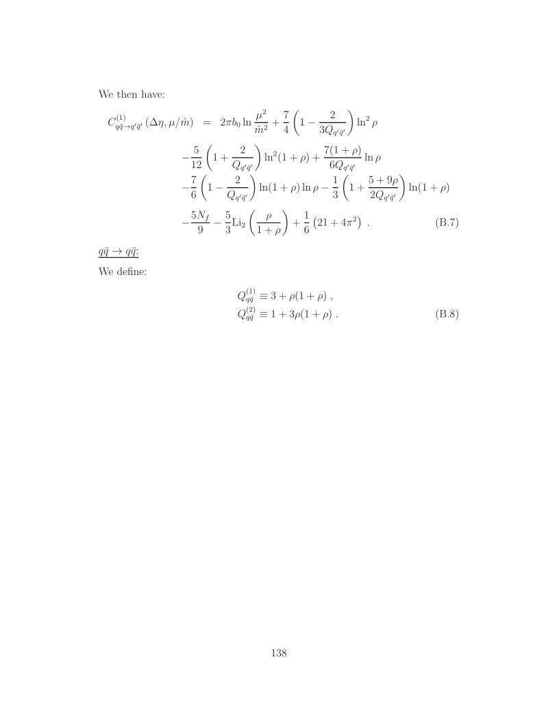
We then have:

C(1)qq%q"q" ($0, µ/m) = 2(b0 ln

µ2

m2+

7

4

"

1&2

3Qq"q"

#

ln2 6

&5

12

"

1 +2

Qq" q"

#

ln2(1 + 6) +7(1 + 6)

6Qq"q"ln 6

&7

6

"

1&2

Qq" q"

#

ln(1 + 6) ln 6&1

3

"

1 +5 + 96

2Qq"q"

#

ln(1 + 6)

&5Nf

9&

5

3Li2

"6

1 + 6

#

+1

6

(

21 + 4(2)

. (B.7)

qq ' qq:

We define:

Q(1)qq ( 3 + 6(1 + 6) ,

Q(2)qq ( 1 + 36(1 + 6) . (B.8)

138

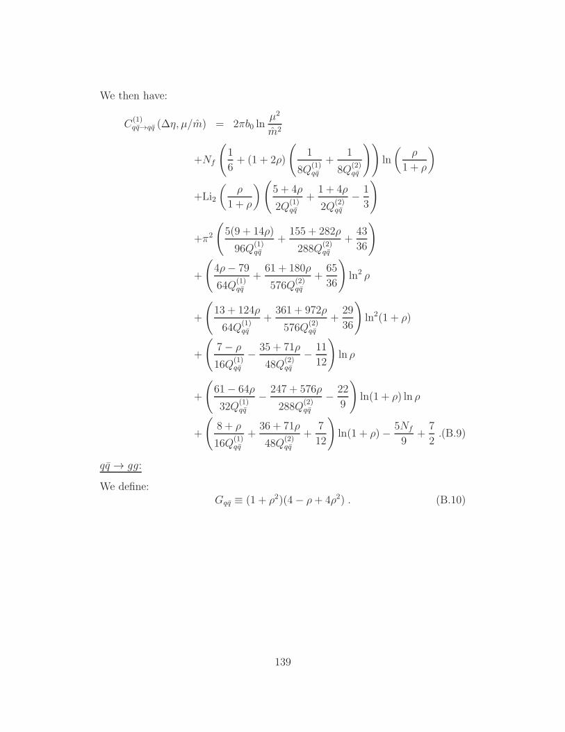
We then have:

C(1)qq%qq ($0, µ/m) = 2(b0 ln

µ2

m2

+Nf

,

1

6+ (1 + 26)

,

1

8Q(1)qq

+1

8Q(2)qq

--

ln

"6

1 + 6

#

+Li2

"6

1 + 6

#,

5 + 46

2Q(1)qq

+1 + 46

2Q(2)qq

&1

3

-

+(2

,

5(9 + 146)

96Q(1)qq

+155 + 2826

288Q(2)qq

+43

36

-

+

,

46& 79

64Q(1)qq

+61 + 1806

576Q(2)qq

+65

36

-

ln2 6

+

,

13 + 1246

64Q(1)qq

+361 + 9726

576Q(2)qq

+29

36

-

ln2(1 + 6)

+

,

7& 6

16Q(1)qq

&35 + 716

48Q(2)qq

&11

12

-

ln 6

+

,

61& 646

32Q(1)qq

&247 + 5766

288Q(2)qq

&22

9

-

ln(1 + 6) ln 6

+

,

8 + 6

16Q(1)qq

+36 + 716

48Q(2)qq

+7

12

-

ln(1 + 6)&5Nf

9+

7

2.(B.9)

qq ' gg:

We define:Gqq ( (1 + 62)(4& 6+ 462) . (B.10)

139

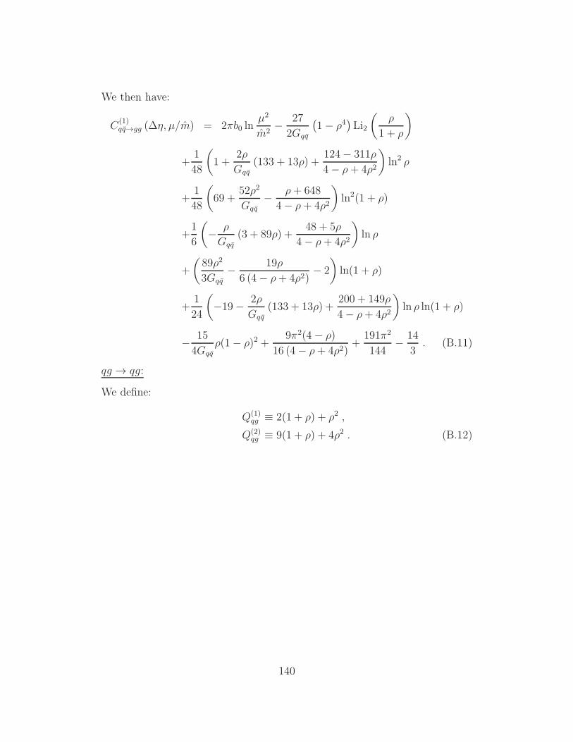
We then have:

C(1)qq%gg ($0, µ/m) = 2(b0 ln

µ2

m2&

27

2Gqq

(

1& 64)

Li2

"

6

1 + 6

#

+1

48

"

1 +26

Gqq(133 + 136) +

124& 3116

4& 6+ 462

#

ln2 6

+1

48

"

69 +5262

Gqq&

6+ 648

4& 6+ 462

#

ln2(1 + 6)

+1

6

"

&6

Gqq(3 + 896) +

48 + 56

4& 6+ 462

#

ln 6

+

"8962

3Gqq&

196

6 (4& 6+ 462)& 2

#

ln(1 + 6)

+1

24

"

&19&26

Gqq(133 + 136) +

200 + 1496

4& 6+ 462

#

ln 6 ln(1 + 6)

&15

4Gqq6(1& 6)2 +

9(2(4& 6)

16 (4& 6+ 462)+

191(2

144&

14

3. (B.11)

qg ' qg:

We define:

Q(1)qg ( 2(1 + 6) + 62 ,

Q(2)qg ( 9(1 + 6) + 462 . (B.12)

140

We then have:

C(1)qg%qg ($0, µ/m) = 2(b0 ln

µ2

m2&

14

3+

15(1 + 6)(2 + 6)2

4Q(1)qg Q

(2)qg

+(2

,

146 + 136

24Q(1)qg

&3(109 + 136)

16Q(2)qg

+241

144

-

+

,

(1 + 6)

,

13

12Q(1)qg

&15

16Q(2)qg

-

+17

16

-

ln2 6

+(1 + 6)

,

89

3Q(1)qg

&231

2Q(2)qg

-

ln 6+

,

31

24+

27(6& 3)

8Q(2)qg

-

Li2

"6

1 + 6

#

+

,

136& 120

24Q(1)qg

+3(173 + 416)

16Q(2)qg

&27

16

-

ln2(1 + 6)

+

,

&86 + 896

6Q(1)qg

+3(43 + 396)

2Q(2)qg

& 2

-

ln(1 + 6)

+

,

120& 136

12Q(1)qg

&3(155 + 236)

8Q(2)qg

+31

24

-

ln 6 ln(1 + 6) . (B.13)

gg ' qq:

We have:

C(1)gg%qq ($0, µ/m) = C(1)

qq%gg ($0, µ/m) . (B.14)

gg ' gg:

We define:Ggg ( 1 + 6(1 + 6) . (B.15)

141

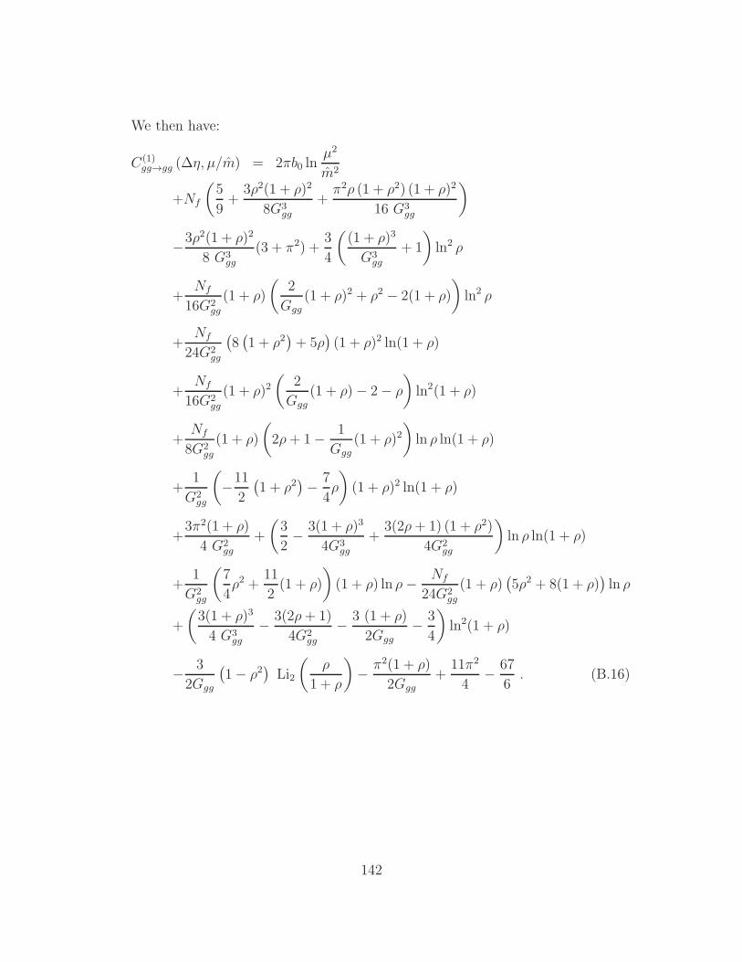
We then have:

C(1)gg%gg ($0, µ/m) = 2(b0 ln

µ2

m2

+Nf

"5

9+

362(1 + 6)2

8G3gg

+(26 (1 + 62) (1 + 6)2

16 G3gg

#

&362(1 + 6)2

8 G3gg

(3 + (2) +3

4

"(1 + 6)3

G3gg

+ 1

#

ln2 6

+Nf

16G2gg

(1 + 6)

"2

Ggg(1 + 6)2 + 62 & 2(1 + 6)

#

ln2 6

+Nf

24G2gg

(

8(

1 + 62)

+ 56)

(1 + 6)2 ln(1 + 6)

+Nf

16G2gg

(1 + 6)2"

2

Ggg(1 + 6)& 2& 6

#

ln2(1 + 6)

+Nf

8G2gg

(1 + 6)

"

26+ 1&1

Ggg(1 + 6)2

#

ln 6 ln(1 + 6)

+1

G2gg

"

&11

2

(

1 + 62)

&7

46

#

(1 + 6)2 ln(1 + 6)

+3(2(1 + 6)

4 G2gg

+

"3

2&

3(1 + 6)3

4G3gg

+3(26+ 1) (1 + 62)

4G2gg

#

ln 6 ln(1 + 6)

+1

G2gg

"

7

462 +

11

2(1 + 6)

#

(1 + 6) ln 6&Nf

24G2gg

(1 + 6)(

562 + 8(1 + 6))

ln 6

+

"3(1 + 6)3

4 G3gg

&3(26+ 1)

4G2gg

&3 (1 + 6)

2Ggg&

3

4

#

ln2(1 + 6)

&3

2Ggg

(

1& 62)

Li2

"6

1 + 6

#

&(2(1 + 6)

2Ggg+

11(2

4&

67

6. (B.16)

142

Appendix C: Jets at Fixed

Invariant Mass

Here we give details of the definitions and calculations for the jet functionsthat we employ in section 3. Single inclusive Jet cross sections have beenstudied intensively [129, 138–140]. Here, we are interested in computing theQCD background to jets of measured mass. The main background to theproduction of tt pairs is from dijet production from hadronic collisions,

Ha(pa) +Hb(pb) ' J1(m2J1, p1,T , 01, R) + J2(m

2J2 , p2,T , 02, R) +X, (C.1)

where the final states are jets in the directions of the outgoing partons, eachwith a fixed jet mass m2

J , a “cone size” R2 = $02 + $32, and transversemomenta, pi,T . For simplicity we choose the cone sizes equal for the two jets,although they can be di!erent. For R < 1, we can isolate the leading (R0)dependence of such cross-sections in factorized “jet” functions,

d-HAHB%J1J2

dpTdm2J1dm2

J2d01d02

=!

abcd

*

dxa dxb 3a(xa)3b(xb)

)Hab%cd (xa, xb, pT , 01, 02,'s(pT ))

)Jc1(m

2J1 , pT cosh 01, R,'s(pT )) J

d2 (m

2J2 , pT cosh 02, R,'s(pT )),(C.2)

with corrections that vanish as powers of R. Here the 3’s are parton distri-bution functions for the initial hadrons, Hab%cd is a perturbative 2 ' 2 QCDhard-scattering function, equal to the dijet Born cross section at lowest or-der, and the Ji are jet functions, which are defined below. Jet function Ji

summarizes the formation of a set of final state particles with fixed invariant

mass and momenta collinear to the ith outgoing parton. Corrections to thecross section of order R0 can only occur through collinear enhancements whichfactorize into these functions [21].

143

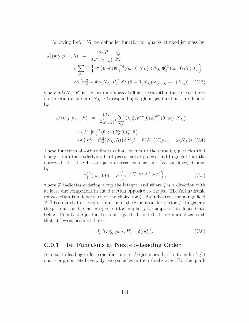
Following Ref. [155] we define jet function for quarks at fixed jet mass by

Jqi (m

2J , p0,Ji, R) =

(2()3

2!2 (p0,Ji)

2

)µNc

)!

NJi

TrB

$µ # 0|q(0)&(q)†* (0, 0)|NJi $ #NJi|&

(q)* (0, 0)q(0)|0 $

C

)%(

m2J & m2

J (NJi, R))

%(2)(n& n(NJi))%(p0,Ji & ,(NJc)), (C.3)

where m2J(NJi , R) is the invariant mass of all particles within the cone centered

on direction n in state NJi . Correspondingly, gluon jet functions are definedby

Jgi (m

2J , p0,Ji, R) =

(2()3

2(p0,Ji)3

!

NJi

# 0|).F .!(0)&(g)†* (0,0) |NJi $

) #NJi|&(g)* (0,0)F &

! (0))&|0 $)%(

m2J & m2

J (NJi, R))

%(2)(n& n(NJi))%(p0,Ji & ,(NJc)). (C.4)

These functions absorb collinear enhancements to the outgoing particles thatemerge from the underlying hard perturbative process and fragment into theobserved jets. The &’s are path ordered exponentials (Wilson lines) definedby

&(f)* (0, 0; 0) = P

B

e"ig"$

0 d, *·A(f)(, *µ)C

, (C.5)

where P indicates ordering along the integral and where ) is a direction withat least one component in the direction opposite to the jet. The full hadroniccross-section is independent of the choice for ). As indicated, the gauge fieldA(f) is a matrix in the representation of the generators for parton f . In generalthe jet function depends on 8) ·n, but for simplicity we suppress this dependencebelow. Finally the jet functions in Eqs. (C.3) and (C.4) are normalized suchthat at lowest order we have

J (0)i (m2

Ji, p0,Ji, R) = %(m2Ji). (C.6)

C.0.1 Jet Functions at Next-to-Leading Order

At next-to-leading order, contributions to the jet mass distributions for lightquark or gluon jets have only two particles in their final states. For the quark

144

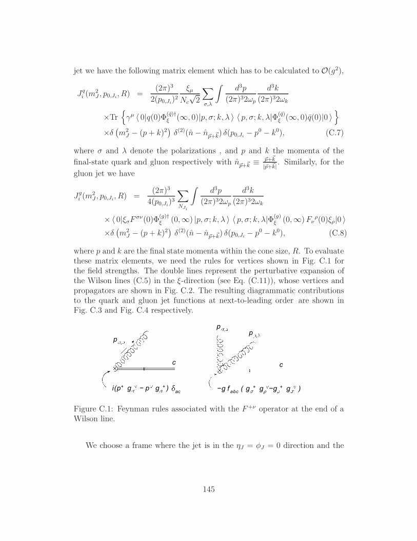
jet we have the following matrix element which has to be calculated to O(g2),

Jqi (m

2J , p0,Ji, R) =

(2()3

2(p0,Ji)2

)µNc

!2

!

.,'

*d3p

(2()32,p

d3k

(2()32,k

)TrB

$µ # 0|q(0)&(q)†* (0, 0)|p, -; k,/ $ # p, -; k,/|&(q)

* (0, 0)q(0)|0 $C

)%(

m2J & (p+ k)2

)

%(2)(n& n1p+1k) %(p0,Ji & p0 & k0), (C.7)

where - and / denote the polarizations , and p and k the momenta of the

final-state quark and gluon respectively with n1p+1k ( 1p+1k

|1p+1k|. Similarly, for the

gluon jet we have

Jgi (m

2J , p0,Ji, R) =

(2()3

4(p0,Ji)3

!

NJi

*d3p

(2()32,p

d3k

(2()32,k

)# 0|).F .!(0)&(g)†* (0,0) |p, -; k,/ $ # p, -; k,/|&(g)

* (0,0)F!&(0))&|0 $

)%(

m2J & (p+ k)2

)

%(2)(n& n1p+1k) %(p0,Ji & p0 & k0), (C.8)

where p and k are the final state momenta within the cone size, R. To evaluatethese matrix elements, we need the rules for vertices shown in Fig. C.1 forthe field strengths. The double lines represent the perturbative expansion ofthe Wilson lines (C.5) in the )-direction (see Eq. (C.11)), whose vertices andpropagators are shown in Fig. C.2. The resulting diagrammatic contributionsto the quark and gluon jet functions at next-to-leading order are shown inFig. C.3 and Fig. C.4 respectively.

pp

!g f abc ( g+ g !g + g )

c

i(p+ g ! p g + ) ac

c

p

Figure C.1: Feynman rules associated with the F+! operator at the end of aWilson line.

We choose a frame where the jet is in the 0J = 3J = 0 direction and the

145

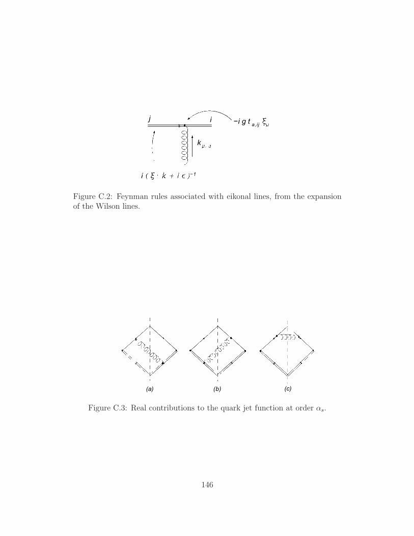
k

ij !i g t a,ij

!1

Figure C.2: Feynman rules associated with eikonal lines, from the expansionof the Wilson lines.

(a) (b) (c)

Figure C.3: Real contributions to the quark jet function at order 's.

146

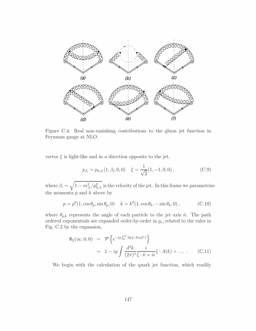
Figure C.4: Real non-vanishing contributions to the gluon jet function inFeynman gauge at NLO.

vector ) is light-like and in a direction opposite to the jet,

pJi = p0,Ji(1, +i, 0, 0) ) =1!2(1,&1, 0, 0) , (C.9)

where +i =G

1&m2Ji/p20,Ji is the velocity of the jet. In this frame we parametrize

the momenta p and k above by

p = p0(1, cos !p, sin !p, 0) k = k0(1, cos !k,& sin !k, 0) , (C.10)

where !p,k represents the angle of each particle to the jet axis n. The pathordered exponentials are expanded order-by-order in gs, related to the rules inFig. C.2 by the expansion,

&*(0, 0; 0) = PB

e"ig"$

0 d, *·A(, *µ)C

= 1& ig

*d4k

(2()4i

) · k + i*) ·A(k) + . . . . (C.11)

We begin with the calculation of the quark jet function, which readily

147

reduces to an integral over the energy and angle of one of the particles,

Jq(1)i (m2

J , p0,Ji, R) =+i

8!2

*d cos !kdk0k0((p0,J & k0)

|M(p, k)|2

)%(m2j & 2k0p0,J (1& +i cos !k))'(R& !k) ,(C.12)

where we choose k to represent the gluon and p the quark. For k the softermomentum, we easily see that !k % !p. Therefore, p0 = k0 fixes the minimumangle for the softest particle, and we find cos(!S,min) = +i. The region ,p < ,k

is found by simply interchanging p and k in |M(p, k)|2 so that

Jq(1)i (m2

J , p0,Ji, R) =+i

16!2

* $i

cos(R)

d cos !S(2()2

m2Ji/p

20,J

"

2(1& +i cos !S)&m2

Ji

p20,J

#

)1

p0,J(1& +i cos !S)

(

|Mqi(p, k)|2 + |Mqi(k, p)|2)

.(C.13)

The evaluation of |Mqi(p, k)|2 is straightforward from the diagrams of Fig. C.3,and we find

Jq(1)i (m2

J , p0,Ji, R) =CF+i

4m2Ji

)* $i

cos(R)

d cos !S(

's(k0) z4

(2(1& +i cos !S)& z2) (1& +i cos !S)

)E

z2(1 + cos !S)2

(1& +i cos !S)

1

(2(1 + +i)(1& +i cos !S)& z2(1 + cos !S))+

3(1 + +i)

z2+

1

z4(2(1 + +i)(1& +i cos !S)& z2(1 + cos !S))

2

(1 + cos !S)(1& +i cos !S)

<

(C.14)

where z =mJi

p0,Ji, p0,Ji =

G

m2Ji+ p2T , and k0 =

p0,Ji2

z2

1"$i cos -S.

The calculation of the gluon jet function proceeds along the same lines, withthe exception that both particles in the final states are now identical, and thepresence of the field strengths, which appear at the end of each Wilson line.The rules for these vertices, as mentioned before, are shown in Fig. C.1. Onceagain, we can write the gluon jet function as an integral over the angle of the

148

softer particle,

Jg(1)i (m2

J , p0,Ji, R) =+i

16m2Ji

* $i

cos(R)

d cos !S(2()2p20,Ji

)z2

(2(1& +i cos !S)& z2) (1& +i cos !S)|Mgi(p, k)|2 ,(C.15)

where |Mgi(p, k)|2 is symmetric under the interchange of p and k. We findfrom the diagrams shown in Fig. C.4, the result

Jg(1)i (m2

J , p0,Ji, R) =CA+i

16m2Ji

* $i

cos(R)

d cos !S(

)'s(k0)

(1& + cos !S)2(1& cos2 !S)(2(1 + +)& z2)

)(

z4(1 + cos !S)2 + z2(1& cos2 !S)(2(1 + +i)& z2)

+(1& cos !S)2(2(1 + +i)& z2)2

)2. (C.16)

These one-loop expressions have been used to generate the comparisons toevent generator output given in Section 3.

149

Appendix D: R-dependence

It is of interest to isolate the leading logarithmic contributions in both gluonand quark jets, which can be found from eikonal graphs in the adjoint andfundamental representations respectively,

J (eik),c(m2J1 , pT , R) =

2Cc!2pT

g2*

d3k

(2()32,k

) · pJ) · k

) · pJ2pJ · k

)%(

m2J1 & (p1 + k)2

)

' (pT & kT ) . (D.1)

Parametrizing k as

k = kT (cosh 0k, cos3k, sin3k, sinh 0k) , (D.2)

this leads to

J (eik),c(m2J1 , pT , R) = g2

Cc

(2()3

*

dkT kT d3kd0k1

k2T (cosh2 0k & cos2 3k)

) %(

2pT kT (cosh 0k & cos3k)&m2J1

)

' (pT & kT ) .

= g2Cc

(2()3

*

d3kd0k1

m2J1

1

k2T (cosh2 0k & cos2 3k)

)%(

2pT kT r &m2J1

)

'

"

cosh 0k & cos3k &m2

J1

p2T

#

.(D.3)

In this expression we can change the variables to

0k = r cos !, 3k = r sin ! . (D.4)

150

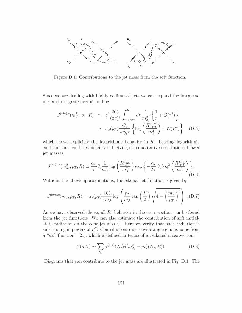
pa

pb

k

k

pa

pb

Figure D.1: Contributions to the jet mass from the soft function.

Since we are dealing with highly collimated jets we can expand the integrandin r and integrate over !, finding

J (eik),c(m2J1, pT , R) 2 g2

2Cc

(2()2

* R

mJ/pT

dr1

m2J1

E1

r+O(r3)

F

2 's(pT )Cc

m2J1(

E

log

"R2 p2Tm2

J

#

+O(R4)

F

, (D.5)

which shows explicitly the logarithmic behavior in R. Leading logarithmiccontributions can be exponentiated, giving us a qualitative description of lowerjet masses,

J (eik),c(m2J1, pT , R) 2

's

(Cc

1

m2J

log

"R2p2Tm2

J

#

exp

E

&'s

2(Cc log

2

"R2p2Tm2

J

#F

.

(D.6)Without the above approximations, the eikonal jet function is given by

J (eik),c(mJ , pT , R) = 's(pT )4Cc

(mJlog

&

'pTmJ

tan

"R

2

#H

4&"mJ

pT

#25

6 . (D.7)

As we have observed above, all R0 behavior in the cross section can be foundfrom the jet functions. We can also estimate the contribution of soft initial-state radiation on the cone-jet masses. Here we verify that such radiation issub-leading in powers ofR2. Contributions due to wide angle gluons come froma “soft function” [21], which is defined in terms of an eikonal cross section,

S(m2Ji) .

!

Ns

-(eik)(Ns)%(m2J1 & m2

J(Ns, R)). (D.8)

Diagrams that can contribute to the jet mass are illustrated in Fig. D.1. The

151

initial state radiation shown behaves as

S .*

d4k%(k2)pa · pb

(pa · k)(pb · k)%(m2

J1 & 2p1 · k)'(R& R(0k,3k)) , (D.9)

with pa and pb the momenta of incoming partons, neither of which is in thedirection of the observed jets. Choosing a frame where the initial momentaare given by

pa =

!s

2(1, 0, 0, 1) , pb =

!s

2(1, 0, 0,&1) , (D.10)

and parametrizing the radiated gluon’s momentum k as in Eq. (D.2) above,we find

S .*

dkTd3kd0k1

kT

1

2pT (cosh 0k & cos3k)%

"

kT &m2

J1

2pT (cosh 0k & cos3k)

#

.2(

m2J1

* R

0

dr r =(R2

m2J1

, (D.11)

which is, as expected, power-suppresed in R compared to the logarithmic de-pendence we get from the jet function.

152