A general method for the resummation of event-shape distributions in e e− annihilation⁺

Article (Published Version)

http://sro.sussex.ac.uk

Banfi, Andrea, McAslan, Heather, Monni, Pier Francesco and Zanderighi, Giulia (2015) A general method for the resummation of event-shape distributions in e e− annihilation. Journal of High ⁺

Energy Physics. p. 102. ISSN 1029-8479

This version is available from Sussex Research Online: http://sro.sussex.ac.uk/58481/

This document is made available in accordance with publisher policies and may differ from the published version or from the version of record. If you wish to cite this item you are advised to consult the publisher’s version. Please see the URL above for details on accessing the published version.

Copyright and reuse: Sussex Research Online is a digital repository of the research output of the University.

Copyright and all moral rights to the version of the paper presented here belong to the individual author(s) and/or other copyright owners. To the extent reasonable and practicable, the material made available in SRO has been checked for eligibility before being made available.

Copies of full text items generally can be reproduced, displayed or performed and given to third parties in any format or medium for personal research or study, educational, or not-for-profit purposes without prior permission or charge, provided that the authors, title and full bibliographic details are credited, a hyperlink and/or URL is given for the original metadata page and the content is not changed in any way.

JHEP05(2015)102

Published for SISSA by Springer

Received: January 8, 2015

Accepted: April 11, 2015

Published: May 20, 2015

A general method for the resummation of event-shape

distributions in e+e− annihilation

Andrea Banfi,a Heather McAslan,a Pier Francesco Monnib and Giulia Zanderighib,c

aDepartment of Physics and Astronomy, University of Sussex,

Sussex House, Brighton, BN1 9RH, U.K.bRudolf Peierls Centre for Theoretical Physics,University of Oxford,

1 Keble Road, Oxford OX1 3NP, U.K.cCERN, Theory Division,

CH-1211 Geneva 23, Switzerland

E-mail: a.banfi@sussex.ac.uk, H.Mcaslan@sussex.ac.uk,

pier.monni@physics.ox.ac.uk, giulia.zanderighi@cern.ch

Abstract: We present a novel method for resummation of event shapes to next-to-next-

to-leading-logarithmic (NNLL) accuracy. We discuss the technique and describe its im-

plementation in a numerical program in the case of e+e− collisions where the resummed

prediction is matched to NNLO. We reproduce all the existing predictions and present new

results for oblateness and thrust major.

Keywords: QCD Phenomenology, Jets

ArXiv ePrint: 1412.2126

Open Access, c© The Authors.

Article funded by SCOAP3.doi:10.1007/JHEP05(2015)102

JHEP05(2015)102

Contents

1 Introduction 2

2 Review of NLL resummation 4

3 NNLL resummation 10

3.1 Logarithmic counting for the resolved real emissions 10

3.2 Structure of the NNLL resummation 12

3.3 NNLL contributions due to resolved emissions 15

3.3.1 Soft-collinear NNLL contributions 16

3.3.2 Recoil and hard-collinear NNLL contributions 17

3.3.3 Soft wide-angle NNLL contributions 20

3.3.4 Soft correlated emission 20

4 Validation and matched results 22

5 Conclusions 27

A Observables definition 28

B Sudakov radiator 29

C Analytic NNLL results for additive observables 32

C.1 Soft-collinear correction 32

C.2 Recoil correction 33

C.3 Hard-collinear correction 34

C.4 Soft wide-angle correction 35

C.5 Soft correlated correction 36

D Monte Carlo determination of real emission corrections 36

D.1 The function FNLL 36

D.2 The function δFsc 37

D.3 The function δFhc 38

D.4 The function δFrec 40

D.5 The function δFwa 41

D.6 The function δFcorrel 41

E Expansion to O(α3

s) 42

– 1 –

JHEP05(2015)102

1 Introduction

Event-shape variables in e+e− annihilation are among the most studied QCD observables.

Since they are very sensitive to the pattern of QCD radiation, they have been widely used in

the past to measure the QCD coupling constant, and to test non-perturbative hadronization

models (see e.g. ref. [1] and references therein). The study of event shapes also led to

important advances in the understanding of all-order properties of QCD radiation, for

instance through the “discovery” of non-global logarithms [2–4]. Fixed order predictions

for observables involving up to three jets in e+e− collisions have been available up to

next-to-next-to-leading order (NNLO) [5–8] for some years. While fixed order calculations

provide a good approximation of hard radiation, which contributes to the region where

event shapes have rather large values, resummed calculations are required where the bulk

of data lies, i.e. in the region dominated by multiple soft-collinear emissions. Next-to-

leading logarithmic (NLL) resummations, that include all terms O(αnsL

n) in the exponent

of integrated distributions are available for specific observables [9–22]. In ref. [23] a semi-

numerical approach was presented to compute the NLL resummation for all event shapes

and jet rates that are recursive infrared and collinear (rIRC) safe and are continuously

global. Most NLL resummations have been performed for observables that satisfy these

minimal requirements. Some recent works address the problem of resumming ratios of

angularities which happen to be not IR safe, but still resummable [24]. Their resummations

rely on factorisation theorems for double differential distributions of angularities [25, 26].

The method of ref. [23] was subsequently extended and implemented in the computer

program CAESAR [27], that also verifies whether a given observable satisfies these properties.

This led to a first systematic study of event shapes in hadronic dijet production at NLL

accuracy matched to next-to-leading order (NLO) results at hadron colliders [28, 29].

More recently, some observables have been resummed beyond NLL accuracy. These

resummations have been so far obtained through observable-dependent factorisation theo-

rems which lead to a full decomposition of the cross section in the infrared limit in terms

of different kinematical subprocesses (i.e. soft, collinear, hard) which are then resummed

individually through evolution equations. Despite being systematically extendable to all

orders, this approach is strictly observable-dependent and requires that the observable can

be factorised in some conjugate space. In particular, full next-to-next-to-leading logarith-

mic (NNLL) predictions are available for a number of event shapes at lepton colliders like

thrust 1−T [30, 31], heavy jet mass ρH [32], jet broadenings BT , BW [33], C-parameter [34]

and energy-energy-correlation [35].1 For 1 − T and ρH all N3LL corrections but the four-

loop cusp anomalous dimension are also known. Similar observables have been resummed

at the same accuracy also in deep inelastic scattering [37–39]. For hadronic collisions,

full NNLL resummations are available for processes where a colour singlet is produced at

Born level, specifically for the boson’s transverse momentum [36, 40] and φ∗ [41], the beam

thrust [42, 43] and the leading jet’s transverse momentum [44–47], and for heavy quark

1Note that the NNLL A(3) coefficient in ref. [35] is incomplete. The correct coefficient has been derived

in ref. [36].

– 2 –

JHEP05(2015)102

pair’s transverse momentum [48, 49]. For an arbitrary number of legs, a NNLL accurate

resummation is available for the N -jettiness variable [50, 51].

Currently most of the phenomenological interest is devoted to hadron-hadron collisions.

However, in view of a possible future e+e− machine (see e.g. [52, 53]), it is desirable to im-

prove our description of generic e+e− event shapes to next-to-next-to-leading logarithmic

(NNLL) level, matched to exact next-to-next-to-leading order (NNLO) results. Further-

more, e+e− observables provide a simpler laboratory in which to develop new methods,

compared to jet production in hadronic collisions. Therefore, in this work we focus on

e+e− collisions, with the aim to extend the method suggested here to hadron colliders in

a future publication.

In this article we derive a general and systematic method to compute NNLL correc-

tions to event shape distributions in e+e− collisions. The method is flexible and can handle

any rIRC safe observable which is continuously global, without any additional requirement

on factorisability of the observable into kinematic subprocesses. The method relies on a

semi-numerical approach in which all real corrections can be expressed in terms of four-

dimensional phase space integrals to all orders, and can be efficiently implemented using

Monte Carlo techniques. The remaining analytic ingredient is a Sudakov form factor, i.e.

the exponential of the so-called “radiator”. In the present paper we do not derive a general

expression for the NNLL radiator, but we show that the only unknown contribution is uni-

versal for classes of observables which scale in the same fashion for a single soft-collinear

emission. The latter property allows us to resum a number of observables by using the

radiator of those for which a NNLL resummation was previously known. We derive the

method and describe its numerical implementation in the program ARES (Automated Re-

summation for Event Shapes). In the present article we limit ourselves to the resummation

of NNLL terms, nevertheless the technique described here can be extended systematically

to higher logarithmic orders.

The paper is structured as follows. In section 2 we recall the NLL method of ref. [23]

in detail, revisiting all the approximations that lead to the derivation of the master re-

summation formula. In section 3 we describe all NNLL corrections, showing how to derive

them systematically. We then apply the resummation method to the following seven event-

shape observables: the thrust 1−T , the C-parameter, the heavy-jet mass ρH , the total and

wide-jet broadenings BT , BW , the thrust-major TM , and the oblateness O, for which data

from LEP are available. In section 4 we test the resummation program by expanding the

resummed cross section to fixed order in the strong coupling. For observables for which an

analytic NNLL resummation was previously available in the literature (i.e. thrust, heavy

jet mass and jet broadenings), we check our results against the analytic ones up to (and

including) O(α3s). For the remaining observables, for which a NNLL analytic result was

not available so far (i.e. C-parameter, thrust-major TM and oblateness O) we check the

expansion of the resummed result against the NLO generator Event2 [54]. In the second

part of section 4 we perform a matching to the NNLO distributions obtained with the

event generator EERAD3 [55]. Our conclusions are reported in section 5. A definition of

the observables studied here can be found in appendix A. All analytic ingredients used in

this article are reported in appendix B. In appendix C we show that for a class of additive

– 3 –

JHEP05(2015)102

observables (e.g. 1 − T , C and ρH), all the necessary NNLL corrections can be computed

analytically, and we give explicit analytic results. The numerical implementation of our

method in a Monte Carlo code is discussed in appendix D.

2 Review of NLL resummation

We consider the resummation of a generic continuously global, recursive infrared and

collinear (rIRC) safe event-shape observable V , a function of all final-state momenta, in

e+e− annihilation. We review here the next-to-leading logarithmic (NLL) resummation for

these observables. This section is largely inspired by section 2 of ref. [27], which contains

a detailed derivation of the NLL resummation for generic event shapes within the CAESAR

approach.

At Born level, the final state consists of a quark p̃1 and an antiquark p̃2, which are

back-to-back. All event shapes we consider vanish in the Born limit, i.e. V ({p̃1, p̃2}) = 0.2

Beyond Born level, further radiation (of gluons or gluons splitting into quarks) is present

and the final state consists in general of n secondary emissions, k1, . . . , kn, and of the

primary quark and antiquark which recoil against these additional emissions. We denote

the value of an event shape by V ({p̃}, k1, . . . , kn), with {p̃} = {p̃1, p̃2}.For any final state event, it is possible to use the thrust axis ~nT to define two like-light

vectors, p1 and p2 as

p1 =Q

2(1, ~nT ) , p2 =

Q

2(1,−~nT ) , (2.1)

where Q denotes the total centre of mass energy of the collision. At Born level clearly p̃1and p̃2 coincide with p1 and p2.

In order to compute the resummed distribution for an observable V , it is useful to

parametrise each emission ki and its phase-space in terms of Sudakov variables:

ki = z(1)i p1 + z

(2)i p2 + κt,i , (2.2)

where κt,i is a space-like four-vector, orthogonal to p1 and p2. In the reference frame in

which p1 and p2 are given by eq. (2.1), each κt,i has no time-like component and can be

written as κt,i = (0, ~kt,i), such that κ2t,i = −k2t,i. Notice that since ki is massless

k2t,i =2(p1ki)2(p2ki)

2(p1p2).

We recall that the thrust axis divides each event in two hemispheres H(1) and H(2). If all

emissions are soft and/or collinear, p̃1 and p̃2 belong to different hemispheres. We denote

by H(i) the hemisphere containing p̃i. Finally, we introduce the emission’s rapidity ηi with

respect to the thrust axis, which is given by

ηi =1

2lnz(1)i

z(2)i

, with |ηi| < lnQ

kt,i, (2.3)

where the boundary for ηi is obtained by imposing z(ℓ)i < 1 for any leg ℓ = 1, 2.

2In the case of the thrust, the resummation is actually performed for τ ≡ 1− T .

– 4 –

JHEP05(2015)102

We consider observables V that obey the following general parametrisation3 for a single

soft emission k collinear to leg ℓ (i.e. parton p̃ℓ):

Vsc({p̃}, k) = dℓ gℓ(φ)

(

ktQ

)a

e−bℓη(ℓ), (2.4)

where η(1) = η and η(2) = −η, and φ is the angle that the transverse momentum ~kt forms

with a fixed reference vector ~n orthogonal to the thrust axis. Collinear and infrared safety

imposes that a > 0 and bℓ > −a.In order to build the NLL resummed cumulative distribution Σ(v)

Σ(v) =1

σ

∫ v

0dv′

dσ(v′)

dv′, (2.5)

it is enough to consider an ensemble of soft-collinear partons, emitted independently off

the hard legs, together with the corresponding virtual corrections, as follows:

Σ(v) = H(Q2)

∞∑

n=0

1

n!

∫

∏

i

[dki]M2(ki)Θ (v − V ({p̃}, k1, . . . , kn)) . (2.6)

Here H(Q2) represents virtual corrections to the Born process, normalised to the total

cross section σ, and [dk]M2(k) is the one-gluon emission probability

[dk]M2(k) = dz(1)dz(2)dφ

2π

dk2tk2t

δ

(

z(1)z(2) − k2tQ2

)

αCMWs (kt)CF

4π

z(1)pgq(z(1))

CF

z(2)pgq(z(2))

CF,

(2.7)

with4

pgq(z) = CF1 + (1− z)2

z. (2.8)

Notice that αCMWs (kt) is the QCD coupling in the CMW scheme [57]. In this scheme the

QCD coupling is defined as the strength of the soft radiation, inclusive in its branchings,

and is related to the coupling in the MS scheme (αs = αMSs ) by

αCMWs (kt) = αs(kt)

(

1 +αs(kt)

2πK

)

+O(

α3s(kt)

)

, K =

(

67

18− π2

6

)

CA − 5

9nf . (2.9)

The constant K is a remainder of the cancellation of infrared and collinear singularities

between unresolved real emissions5 and virtual corrections. This term gives NLL con-

tributions starting at order α2sL

2, which are universal for all rIRC safe observables, and

proportional to the two-loop cusp anomalous dimension [27]. The CMW scheme is an

effective way of incorporating such corrections into a redefinition of the coupling.

3All event shapes for which a NLL resummation is known obey this form.4The azimuthal dependence of the squared amplitude can be ignored in the quark-initiated branching. In

hadron-hadron and hadron-lepton collisions the primary branching g → gg may occur, and the correspond-

ing azimuth-unaveraged splitting functions must be used for a NNLL resummation [56]. However, in special

configurations like colour-singlet production, this azimuthal dependence contributes at most at N3LL.5For a definition of resolved and unresolved emissions see text after eq. (2.11).

– 5 –

JHEP05(2015)102

The soft-collinear limit of eq. (2.7) is obtained by taking the limit z(1), z(2) → 0, giving

[dk]M2sc(k) =

∑

ℓ=1,2

2CℓαCMWs (kt)

π

dktktdη(ℓ)Θ

(

ln

(

Q

kt

)

− η(ℓ))

Θ(η(ℓ))dφ

2π, (2.10)

where Cℓ is the Casimir relative to leg ℓ (CF in the present case) and η(ℓ) is the rapidity

with respect to leg ℓ, as defined after eq. (2.4).

Notice that all integrals in eq. (2.6), as well as the function H(Q2), are to be considered

as suitably regulated, for instance using dimensional regularisation. At NLL the observable

is well approximated by its soft-collinear scaling (2.4). We thus decide to rewrite eq. (2.6) as

Σ(v) = H(Q2)

∞∑

n=0

1

n!

∫

∏

i

[dki]M2(ki) {Θ(v − Vsc({p̃}, k1, . . . , kn))

+ [Θ (v − V ({p̃}, k1, . . . , kn))−Θ(v − Vsc({p̃}, k1, . . . , kn))]} , (2.11)

where Vsc({p̃}, k1, . . . , kn) denotes the observable with all emissions treated as if they were

soft and collinear. We decide to divide the integrals in the real term into a contribution due

to emissions with Vsc({p̃}, k) > ǫv (that we refer to as resolved), and one due to emissions

with Vsc({p̃}, k) < ǫv (that we refer to as unresolved). Here ǫ is a small parameter, that can

be chosen such that ǫ ≪ 1 with ln(1/ǫ) ≪ ln(1/v). Because of rIRC safety, the latter can

be ignored in computing the observable, up to power-suppressed corrections O(v). Due to

the factorised form of the multi-gluon matrix element in eqs. (2.6) and (2.11), at NLL the

contribution of unresolved emissions fully exponentiates, leading to

Σ(v) = H(Q2)e∫ ǫv [dk]M2(k)

∞∑

n=0

1

n!

∫

ǫv

∏

i

[dki]M2(ki) {Θ(v − Vsc({p̃}, k1, . . . , kn))

+ [Θ (v − V ({p̃}, k1, . . . , kn))−Θ(v − Vsc({p̃}, k1, . . . , kn))]} , (2.12)

where we have used the shorthand notations

∫ ǫv

[dk]M2(k) =

∫

[dk]M2(k)Θ (ǫv − Vsc({p̃}, k)) ,∫

ǫv

∏

i

[dki]M2(ki) =

∏

i

∫

[dki]M2(ki)Θ (Vsc({p̃}, ki)− ǫv) .

(2.13)

The combination of the unresolved emissions with the virtual corrections in H(Q2) gives

rise to a Sudakov exponent, representing the probability of having no emissions with

Vsc({p̃}, ki) > ǫv, which at NLL accuracy (i.e. neglecting corrections of relative order αs)

reads

H(Q2)e∫ ǫv [dk]M2(k) ≃ e−R(ǫv) , (2.14)

where

R(ǫv) ≡∫

[dk]M2(k)Θ (Vsc({p̃}, k)− ǫv) = R(v) +

∫ v

ǫv[dk]M2(k) . (2.15)

– 6 –

JHEP05(2015)102

In eqs. (2.12), (2.13), (2.14) and (2.15) any integral over the single-emission’s matrix ele-

ment [dk]M2(k) has to be interpreted as follows

[dk]M2(k)Θ (Vsc({p̃}, k)− v̄) = [dk]M2sc(k)

∑

ℓ=1,2

Θ

(

dℓ gℓ(φ)

(

ktQ

)a

e−bℓη(ℓ) − v̄

)

Θ(η(ℓ))

+∑

ℓ=1,2

dk2tk2t

dz(ℓ)

z(ℓ)

(

z(ℓ)pℓ(z(ℓ))− 2Cℓ

) αs(k2t )

2πΘ

(

dℓ gℓ(φ)

(z(ℓ))bℓ

(

ktQ

)a+bℓ

− v̄

)

, (2.16)

where in the second line we made the replacement e−η(ℓ) = kt/(Qz(ℓ)). Furthermore, the

two step functions in eq. (2.16) have to be expanded in order to avoid power suppressed

contributions and undesired subleading logarithmic terms. At NLL, one can perform the

following approximations in computing the radiator:

Θ

(

dℓ gℓ(φ)

(

ktQ

)a

e−bℓη(ℓ) − v̄

)

≃ Θ

(

ln

(

ktQ

)a

e−bℓη(ℓ) − ln v̄

)

+ δ

(

ln

(

ktQ

)a

e−bℓη(ℓ) − ln v̄

)

ln dℓ gℓ(φ) , (2.17)

Θ

(

dℓ gℓ(φ)

zbℓ

(

ktQ

)a+bℓ

− v̄

)

≃ Θ

(

ln

(

ktQ

)a+bℓ

− ln v̄

)

. (2.18)

This gives

R(v) ≃ RNLL(v) ≡∫

[dk]M2sc(k)

∑

ℓ=1,2

Θ

(

ln

(

ktQ

)a

e−bℓη(ℓ) − ln v

)

Θ(η(ℓ))

+

∫

[dk]M2sc(k)

∑

ℓ=1,2

ln d̄ℓ δ

(

ln

(

ktQ

)a

e−bℓη(ℓ) − ln v

)

Θ(η(ℓ))

+∑

ℓ=1,2

CℓBℓ

∫

dk2tk2t

αs(k2t )

2πΘ

(

(

ktQ

)a+bℓ

− v

)

,

(2.19)

where

ln d̄ℓ =

∫ 2π

0

dφ

2πln (dℓgℓ(φ)) , (2.20)

and

CℓBℓ =

∫ 1

0

dz

z(zpgq(z)− 2Cℓ) . (2.21)

In our case CℓBℓ = −3/2CF . RNLL(v) can be parametrised as

RNLL(v) = −Lg1(λ)− g2(λ) , (2.22)

where L = ln(1/v), λ = αs(Q)β0L and β0 = (11Nc − 4nfTF )/(12π). The functions g1 and

g2 can be written in terms of the constants a, bℓ, dℓ and the functions gℓ(φ) and are given

in appendix B.6 We notice that all integrals over real emissions in eq. (2.12) involve an

6In appendix B we use a modified definition of L = ln(xV /v), and hence of λ, in order to estimate

theoretical uncertainties from higher-order logarithmic corrections by varying xV .

– 7 –

JHEP05(2015)102

upper and a lower bound on each Vsc({p̃}, ki) such that ǫv < Vsc({p̃}, ki) . v. We remind

the reader that ǫ is a small parameter satisfying ǫ ≪ 1 and ln(1/ǫ) ≪ ln(1/v). The upper

bound comes implicitly from the constraint that the observable is smaller than v. Therefore

the real-emission phase space is at most single-logarithmic, unlike the corresponding phase

space region considered in the radiator R(v), which is double logarithmic. As a conse-

quence, for real emissions, at NLL accuracy, one can consider only the soft-collinear matrix

element (i.e. the first line of eq. (2.16)) and replace the observable with its soft-collinear

approximation, i.e. neglect the term in the second line of eq. (2.12). This leads to

Σ(v) = e−RNLL(v)e−∫ vǫv [dk]M

2sc(k)

∞∑

n=0

1

n!

∫

ǫv

∏

i

[dki]M2sc(ki)Θ (v − Vsc({p̃}, k1, . . . , kn)) .

(2.23)

Here the second exponential factor provides the unresolved emissions that cancel the de-

pendence on the cutoff ǫ in the resolved real emissions, so that the result is finite and

independent of ǫ. This gives

Σ(v) ≃ e−RNLL(v)F(v) , (2.24)

where the function F(v) contains NLL corrections due to an ensemble of soft and collinear

gluons, widely separated in rapidity [27],7 and reads

F(v) = e−∫ vǫv [dk]M

2sc(k)

∞∑

n=0

1

n!

∫

ǫv

n∏

i=1

[dki]M2sc(ki)Θ (v − Vsc({p̃}, k1, . . . , kn)) . (2.25)

Although the above expression has all ingredients necessary to achieve NLL accuracy, it

contains also subleading effects. We will first explain how to eliminate them, if one seeks

a pure NLL result, and then discuss how they can be computed at NNLL accuracy in the

next section.

We parametrise the phase space in terms of vi = Vsc({p̃}, ki), i.e. the value that the

event shape has in the presence of each individual emission ki (eq. (2.4)). First, it is

convenient to divide the phase space according to whether an emission is collinear to p1(ηi > 0) or collinear to p2 (ηi < 0). For each emission ki we introduce the rapidity fractions

ξ(ℓ)i = η

(ℓ)i /η

(ℓ)max defined as the emission’s rapidity divided by the largest available rapidity

for a given value of vi. η(ℓ)max is defined as

η(ℓ)max =1

a+ bℓlngℓ(φi)dℓ

vi. (2.26)

We introduce the two functions

R′1

(

v

d1g1(φ̄)

)

=

∫

[dk]M2sc(k) (2π)δ(φ− φ̄) vδ (v − Vsc({p̃}, k)) θ(η) ,

R′2

(

v

d2g2(φ̄)

)

=

∫

[dk]M2sc(k) (2π)δ(φ− φ̄) vδ (v − Vsc({p̃}, k)) θ(−η) .

(2.27)

7The contribution from a phase space region where two gluons are close in rapidity is suppressed by one

power of the logarithm, hence it contributes only to NNLL and will be discussed later.

– 8 –

JHEP05(2015)102

Finally, we introduce R′(v, φ), defined as

R′(v, φ) = R′1

(

v

d1g1(φ)

)

+R′2

(

v

d2g2(φ)

)

. (2.28)

Using this parametrisation, we can recast the matrix element for each emission as follows

[dki]M2sc(ki) =

dvivi

dφi2π

∑

ℓi=1,2

dξ(ℓi)i Θ(1− ξ

(ℓi)i )Θ(ξ

(ℓi)i )R′

ℓi

(

vidℓigℓi(φi)

)

=dζiζi

dφi2π

∑

ℓi=1,2

dξ(ℓi)i Θ(1− ξ

(ℓi)i )Θ(ξ

(ℓi)i )R′

ℓi

(

ζiv

dℓigℓi(φi)

)

,

(2.29)

where ζi = vi/v is defined as the ratio of the observable’s value corresponding to the ith

emission to the actual observable’s value v.

We can now exploit a fundamental property of event shapes. Given a set of emissions

{k1, . . . , kn}, as long as one keeps vi, φi and the leg ℓi to which ki is collinear fixed, the value

of an event shape does not depend on ξ(ℓi)i , which can be then integrated out analytically.

This makes it possible to simplify F(v) as follows

F(v) = e−

∫ dφ2π

∫ 1ǫ

dζζR′(ζv,φ)

∞∑

n=0

1

n!

n∏

i=1

∫ ∞

ǫ

dζiζi

∫ 2π

0

dφi2π

×

×∑

ℓi=1,2

R′ℓi

(

ζiv

dℓigℓi(φi)

)

Θ(v − Vsc({p̃}, k1, . . . , kn)) , (2.30)

where k1, . . . , kn are now soft and collinear emissions with an arbitrary rapidity fraction.

As a last simplification, we can expand each R′ℓ around v

R′ℓ

(

ζv

dℓgℓ(φ)

)

= R′ℓ(v) +O(R′′

ℓ ) R′′ℓ = −vdR

′ℓ(v)

dv, (2.31)

and neglect all contributions of order R′′ℓ . These constitute a NNLL leftover that will be

specifically addressed in section 3.3.1. Notice that

R′ℓ(v) =

∫

[dk]M2sc(k) vδ

(

v − Vsc({p̃}, k)dℓgℓ(φ)

)

θ(η)

does not depend on φ and on dℓ any more. This function can be further split as R′ℓ(v) =

R′NLL,ℓ(v)+ δR

′NNLL,ℓ(v), where R

′NLL,ℓ and δR

′NNLL,ℓ are defined in eqs. (B.10) and (B.11),

respectively. The NNLL term δR′NNLL,ℓ contains running coupling effects as well as the con-

tribution of the cusp anomalous dimension through the CMW scheme. This, as explained

earlier, encodes the contribution of an inclusive soft-gluon splitting. At NNLL one has to

take into account the non-inclusive nature of the observable in the presence of the branching

of a soft gluon. This non-inclusive correction is contained in the full set of NNLL contribu-

tions (see section 3.3.4), therefore the choice of the CMW scheme in the resolved real emis-

sion becomes irrelevant (see section 3.3.4). With this simplification, F(v) ≃ FNLL(λ) where

FNLL(λ) =

∫

dZ[{R′NLL,ℓi

, ki}] Θ(

1− limv→0

Vsc({p̃}, {ki})v

)

, (2.32)

– 9 –

JHEP05(2015)102

and subleading terms have been neglected. In eq. (2.32) we have introduced the average

of a function G({p̃}, {ki}) over the measure dZ:

∫

dZ[{R′NLL,ℓi

, ki}]G({p̃}, {ki})

= ǫR′

NLL

∞∑

n=0

1

n!

n∏

i=1

∫ ∞

ǫ

dζiζi

∫ 2π

0

dφi2π

∑

ℓi=1,2

R′NLL,ℓi

G({p̃}, k1, . . . , kn) ,(2.33)

where R′NLL = R′

NLL,1 + R′NLL,2. Note that the dependence on the regulator ǫ cancels in

eq. (2.33). The limit v → 0 in eq. (2.32) is necessary to remove contributions that are power

suppressed in v. The existence of this limit in the step function of eq. (2.32) is guaranteed by

the rIRC safety property of event shapes here considered, which implies that the quantity

Vsc({p̃}, k1, . . . , kn)/v is independent of v, with corrections that scale as a power of v. To

conclude, neglecting all terms beyond NLL accuracy, we can write Σ(v) in the form

Σ(v) = eLg1(λ)+g2(λ)FNLL(λ) . (2.34)

3 NNLL resummation

In this section we extend the above treatment to NNLL, illustrating how the various cor-

rections arise. We will first discuss the general structure of the NNLL resummation and

then derive the relevant corrections.

3.1 Logarithmic counting for the resolved real emissions

Before extending the above treatment to NNLL, it is worth recalling how, given rIRC safety

of the observable, one can define a logarithmic hierarchy in the resolved real emissions, and

hence give a precise definition of the multiple emissions function F(v) at a given logarithmic

order. We start by considering an ensemble of n soft emissions. The squared matrix element

can be expressed iteratively as a sum of products of matrix elements with a lower number

of emissions (from 1 to n− 1) plus an irreducible remainder M̃2(k1, . . . , kn). The first few

steps of this iterative definition read

M2(k1) = M̃2(k1) ,

M2(k1, k2) =M2(k1)M2(k2) + M̃2(k1, k2) ,

M2(k1, k2, k3) =M2(k1)M2(k2)M

2(k3) + (M̃2(k1, k2)M2(k3) + perm.) + M̃2(k1, k2, k3) ,

M2(k1, . . . , kn) = . . . (3.1)

The product of single-emission matrix elements clearly defines the abelian contribution,

while non-abelian colour factors are associated with the M̃2(k1, . . . , km) squared ampli-

tudes. This makes each single M̃ in the above decomposition invariant under gauge trans-

formations. The M̃2(k1, . . . , km) matrix elements for more than one emission describe the

probability of emitting m colour-connected soft partons, and they are therefore suppressed

if the involved emissions are very far in rapidity from each other. We will refer to M̃2(k1, k2)

as the double-correlated contribution to the squared amplitude for multiple emissions. We

– 10 –

JHEP05(2015)102

will label the correlated squared matrix elements with more than two emissions in an anal-

ogous fashion. We now study the logarithmic structure of each of the terms in eqs. (3.1).

Each resolved real emission (i.e. an emission that contributes to the observable) is defined

by requiring that Vsc({p̃}, ki) > ǫv, where ǫ is independent of v because of rIRC safety.

This condition poses a lower bound on the resolved emission’s phase space which can po-

tentially only give rise to a single logarithm of v (see for instance eq. (2.29)). When several

emissions are considered, the same argument applies, so that each emission can at most

contribute with a single logarithm. This is ensured by rIRC safety since this condition

implies that the observable will have the same scaling independently of the number of

emissions, and therefore the condition Vsc({p̃}, ki) > ǫv will still impose a lower cutoff for

all resolved emissions. The unresolved emissions below this limit (i.e. Vsc({p̃}, ki) < ǫv)

can be ignored in the observable evaluation and their role is simply to cancel the virtual

IRC singularities. They contribute exclusively to the Sudakov radiator and therefore we

do not need to consider them here. With the above property we can immediately see that

a product of n independent emission matrix elements in eq. (3.1) gives rise at most to a

αnsL

n (i.e. a NLL) contribution, where L = ln 1/v.

We now consider the double-correlated M̃2(k1, k2) term. It involves a soft-gluon split-

ting into either a qq̄ or gg pair and it could potentially give rise to a α2sL

3 term (αsL

associated with the emission of the parent gluon, and at most two extra logarithms coming

from its splitting). However, again due to rIRC safety (see for instance section 2.2.4 of

ref. [27] for the relevant properties), one can see that the splitting of the parent gluon

does not give rise to additional logarithms, leaving us with a NNLL term α2sL. The same

argument can be applied to terms with more than two correlated partons, and can be used

to show that they are at most N3LL. Therefore, the sole rIRC safety property of the ob-

servable allows one to define a logarithmic hierarchy in the multiple emissions function and

to define the relevant configurations that contribute to a given logarithmic order. The very

same argument applies to the case of one or more emissions emitted collinearly to the Born

leg with high momentum. Therefore, if we want to limit ourselves to, for instance, NLL (i.e.

αnsL

n terms in the multiple emissions function F(v)) it is sufficient to consider an ensemble

of soft-collinear independent emissions, since any configuration beyond this one would just

be at most NNLL. For a NNLL treatment, in addition, one has to include the contribution

of a single splitting of a soft gluon (following the above argument it is easy to see that

configurations with more than one splitting are subleading), and a single hard collinear

emission. This treatment can be extended to higher orders in a very systematic way.

In addition to the matrix element approximation, we would like to approximate the

resolved emission’s phase space in order to neglect any effects in F(v) which are beyond the

logarithmic accuracy that we want to achieve. We stress that this class of approximations

is not strictly necessary for the resummation, since their only purpose is to ensure that

F(v) is free of any contamination from subleading effects. For instance, at NLL, we can

approximate the rapidities of all soft-collinear emissions with the kinematic limit as done in

section 2, and treat the observable in the pure soft-collinear approximation, all corrections

being at most NNLL. For a NNLL resummation, these approximations are of course not

valid anymore and one has to repeat the calculation without making them. Alternatively,

– 11 –

JHEP05(2015)102

one can simply compute the NNLL corrections associated with these approximations with

respect to the NLL function FNLL(λ), as it will be explained in detail in the next section.

The last ingredient that one needs to go beyond NLL is the Sudakov radiator. This

function has the role of cancelling the infrared and collinear singularities associated with

the unresolved emissions (i.e. Vsc({p̃}, ki) < ǫv) against the virtual corrections. At NLL

its structure is remarkably simple since the unresolved real emissions fully exponentiate in

the observable’s space and the cancellation of singularities is explicit. Beyond this order,

one needs to work out the exact details of real-virtual cancellations (for instance, through

renormalisation group evolution equations). We will not present a general expression for

the radiator in this article, but we will limit ourselves to show that it only depends on the

scaling of the observable in the presence of a single soft and collinear dressed (i.e. inclusive

in its branchings) emission. Therefore, we will show that it is universal for all observables

which have the same soft-collinear parametrisation in the single emission case, i.e. the same

a and bℓ coefficients in eq. (2.4).

3.2 Structure of the NNLL resummation

Using the arguments outlined in the previous section, we now derive the general form of

NNLL corrections. We start by recalling the procedure which lead to the NLL result. On

the one hand, we approximated the matrix element and the phase space in all emissions

appearing in the multiple emissions function of eq. (2.25), neglecting subleading correc-

tions due to the exact rapidity bound for each resolved soft and collinear emission (see

eq. (2.31)), and the correct description of the hard-collinear region (neglecting the second

line of eq. (2.16)). On the other hand, we replaced the observable with its soft-collinear

parametrisation Vsc, neglecting the second line of eq. (2.23). We remark that, at NNLL

accuracy, these approximations have to be relaxed for a single emission at a time, since

relaxing each approximation gives rise a correction of relative order αs. This implies that

configurations in which we correct more than one emission lead to contributions beyond

NNLL, that can be neglected accordingly.

A set of NNLL corrections arises from the first line of eq. (2.12):

e−RNLL(v)e−∫ vǫv [dk]M

2(k)∞∑

n=0

1

n!

∫

ǫv

∏

i

[dki]M2(ki)Θ (v − Vsc({p̃}, k1, . . . , kn)) , (3.2)

where RNLL is defined in eq. (2.22). Besides the NLL multiple emissions function FNLL(λ) of

eq. (2.32) derived in section 2, eq. (3.2) contains corrections due both to the hard-collinear

term of the matrix element (given by the second line of eq. (2.16)), and to the correct

rapidity bounds, which at NLL are the same for all emissions (see eq. (2.31)). Such correc-

tions result in the two NNLL contributions δFhc (section 3.3.2) and δFsc (section 3.3.1),

respectively.

– 12 –

JHEP05(2015)102

Another category of NNLL corrections is contained in the second line of eq. (2.12),

namely

e−RNLL(v)e−∫ vǫv [dk]M

2sc(k)

∞∑

n=0

1

n!

∫

ǫv

∏

i

[dki]M2(ki) [Θ (v − V ({p̃}, k1, . . . , kn))

−Θ(v − Vsc({p̃}, k1, . . . , kn))] ,(3.3)

where we need to relax the soft-collinear approximation made for the observable when an

arbitrary emission becomes hard-collinear or is emitted at small rapidities (large angles).

We stress that, at NNLL accuracy, it is enough to consider an ensemble of soft and collinear

emissions, plus a single extra emission which is free to probe both the hard-collinear and

the soft-wide-angle region of the phase space. Configurations containing more than one

soft-wide-angle or hard-collinear real emission are subleading. We can then expand further

the first step function in eq. (3.3) in order to take into account the correct behaviour of

the observable in these limits for a single emission of the ensemble. The corresponding

NNLL corrections are: a recoil correction δFrec (computed in section 3.3.2) which is due

to the exact kinematics of a hard-collinear emission which recoils against the soft-collinear

ensemble; a soft-wide-angle correction δFwa (computed in section 3.3.3) which is due to a

soft emission that spans the whole rapidity range; a correlated correction δFcorrel (computed

in section 3.3.4) to the inclusive treatment of the soft gluon decay in the matrix element

(encoded in the scheme of the running coupling in the radiator R(v)). An important point

to stress is that the soft-collinear approximation Vsc({p̃}, k1, . . . , kn) guarantees that all

NNLL corrections arising from eq. (3.3) are well defined and finite when the corrected

emission becomes unresolved.

One last NNLL contribution is due to the correction to the NLL Sudakov radiator of

eq. (2.19). At NLL, the radiator encodes the contribution of unresolved real emissions kiwith Vsc({p̃}, ki) < ǫv and corresponding virtual corrections. Moreover, each emission is

considered to be inclusive in its two-parton branchings. Analogously, the NNLL Sudakov

radiator has to include the effect of the inclusive soft three-parton correlation, which can

be absorbed in a redefinition of the running coupling analogously to what is done at NLL,

together with the correct matrix element for an inclusive double collinear emission. Fur-

thermore, it contains exact O(αs) corrections surviving the poles cancellation between real

and virtual corrections. In formulae, we introduce a NNLL radiator RNNLL(v) through the

replacement

H(Q2)e∫ ǫv [dk]M2(k) → e−RNNLL(v)+

∫ vǫv [dk]M

2(k), (3.4)

where

RNNLL(v) =

∫

[dk]M2sc(k)Θ (Vsc({p̃}, k)− v) (3.5)

+∑

ℓ=1,2

∫

dk2tk2t

∫ 1

0

dz

z(zpℓ(z)− 2Cℓ)

αs(k2t )

2πΘ

(

dℓ gℓ(φ)

zbℓ

(

ktQ

)a+bℓ

− v

)

+αs(Q)

πh(λ) .

The function αs(Q)h(λ)/π contains the contribution of the triple-correlated splitting, the

double hard-collinear correction and additional O(αs) constant terms arising from real-

virtual cancellations, and corresponding running coupling effects. Eq. (3.5) contains some

– 13 –

JHEP05(2015)102

power suppressed terms due to the integration limits of the non-singular phase space vari-

ables, i.e. φ in the soft limit and φ, z in the hard-collinear limit. In order to neglect these

terms we have relaxed the lower bound in the z integration relative to the hard-collinear

limit, and set it to zero (the physical bound being z > kt/Q). Moreover, in order to ne-

glect power-suppressed and subleading contributions, we can expand the two Θ-functions

of eq. (3.5) as follows:8

Θ

(

dℓ gℓ(φ)

(

ktQ

)a

e−bℓη(ℓ)

− v

)

≃ Θ

(

ln

(

ktQ

)a

e−bℓη(ℓ)

− ln v

)

+ δ

(

ln

(

ktQ

)a

e−bℓη(ℓ)

− ln v

)

ln dℓ gℓ(φ) +1

2δ′(

ln

(

ktQ

)a

e−bℓη(ℓ)

− ln v)

ln2 dℓ gℓ(φ) , (3.6)

Θ

(

dℓ gℓ(φ)

zbℓ

(

ktQ

)a+bℓ

− v

)

≃ Θ

(

ln

(

ktQ

)a+bℓ

− ln v

)

+ δ

(

ln

(

ktQ

)a+bℓ

− ln v

)

lndℓ gℓ(φ)

zbℓ. (3.7)

We observe that the dependence on the normalisation dℓgℓ(φ) is a local rescaling of the

observable. This induces a local shift of the logarithm ln 1/v and gives rise to subleading

contributions at each logarithmic order. This implies that, at NNLL accuracy, the depen-

dence on dℓgℓ(φ) in the Sudakov radiator is completely encoded in the first two integrals

of eq. (3.5), and it corresponds to a shift in the logarithms of the NLL radiator (before az-

imuthal integration). An important consequence of this is that the function h(λ) depends

exclusively on the scaling in η (or equivalently z) and kt through the a and bℓ coefficients.

By exploiting this property, one can conclude that the resummations of all observables

which have the same soft-collinear scaling in kt and η (i.e. the same a and bℓ coefficients)

will have the same h(λ) function. For example, the function h(λ) will be the same for

thrust 1 − T , C parameter, and heavy jet mass ρH , and it can be taken from [30, 31].

Analogously, the function h(λ) for the jet broadenings BT , BW , thrust major TM and

oblateness O is identical to the one relative to the kt resummation (which we take from

ref. [46] after replacing the constant one-loop virtual corrections with the corresponding

ones in e+e− → hadrons). Practically, the function h(λ) can be obtained by computing the

resummation for the reference observable (e.g. the thrust) leaving h(λ) unspecified, and

fixing it by equating the resummation obtained here to the known result in the literature.

This is similar in spirit to what has been done for the jet-veto in refs. [46, 58].

We parametrise the final NNLL Sudakov radiator as

RNNLL(v) = −Lg1(λ)− g2(λ)−αs(Q)

πg3(λ) . (3.8)

The relevant expressions for the g1, g2, and g3 functions are reported in appendix B. Once

all these corrections have been computed, the NNLL expression for Σ(v) becomes

Σ(v) = eLg1(λ)+g2(λ)+αs(Q)

πg3(λ)

[

FNLL(λ) +αs(Q)

πδFNNLL(λ)

]

. (3.9)

The function

δFNNLL = δFsc + δFhc + δFrec + δFwa + δFcorrel , (3.10)

8For the NLL radiator, it was sufficient to consider the first two terms in the r.h.s. of eq. (3.6), and the

first in the r.h.s. of eq. (3.7), respectively.

– 14 –

JHEP05(2015)102

represents NNLL corrections due to real radiation, and it will be extensively discussed in

the rest of this section.

Before deriving the relevant NNLL corrections to the real radiation it is worth making

an important remark. The whole resummation procedure defined in the present section

depends on a specific choice of the variable on which the cutoff ǫ is applied. This choice

is reflected in the exponentiated part of the resummed cross section. Our default choice is

to define unresolved emissions as those for which Vsc({p̃}, k) < ǫv, where Vsc is defined by

eq. (2.4). This choice is clearly arbitrary and one could equally derive the same resummed

results (that will be anyway independent of the cutoff ǫ) with a different definition for the

unresolved contributions. Different choices will simply lead to different NLL terms (and

beyond) in the Sudakov exponent and in the real corrections described by the multiple

emissions function, but will not affect the final result which does not depend on such a

definition. In the present article we decide to work in the soft-collinear prescription in

which the cutoff ǫ is applied on the soft-collinear approximation of the observable for a

generic emission ki. This prescription has two advantages. On the one hand it allows

one to expand the multiple emissions function around the NLL result, which is simply

determined by the soft-collinear approximation (meaning that the Vsc approximation of

eq. (2.4) is enough to account for all NLL contributions). It also ensures that all NNLL

corrections to the multiple emissions function are finite without further regulators since the

singularities of any unresolved emission are encoded in the soft-collinear approximation.

On the other hand it allows us to define the NNLL function h(λ) in such a way that it is

independent of the observable’s normalisation dℓgℓ(φ) and it only depends on the a and

bℓ coefficients. As stated above, this implies that the function h(λ) is universal for all

observables which have the same a and bℓ scaling in the soft-collinear region.

3.3 NNLL contributions due to resolved emissions

In this section we explicitly derive all corrections to the multiple emission function F(v)

necessary to achieve NNLL accuracy for the cumulative distribution Σ(v) for a generic

event-shape observable v. In order to do this we have to recall the basic assumptions used

to obtain eq. (2.34). They are:

• gluon splitting in R(v) is treated inclusively;

• each real emission ki contributing to F(v) is soft, collinear, and such that ǫv <

Vsc({p̃}, ki) < v;

• the rapidity bound of all emissions contributing to F(v) is the same.

By relaxing any of these approximations valid at NLL accuracy, we obtain a number of

NNLL corrections induced by real radiation, and introduced in the previous section. We

will derive them in the following order:

1. exact rapidity bound and running coupling corrections to the soft and collinear func-

tion F(v) (δFsc);

– 15 –

JHEP05(2015)102

2. one of the emissions ki is collinear but not soft, generating hard-collinear (δFhc) and

recoil (δFrec) corrections;

3. one of the emissions ki is soft but at wide angle (δFwa);

4. gluon decay is treated non-inclusively, giving rise to a correlated-emission correction

(δFcorrel).

The necessary amplitudes to compute δFNNLL are given by the independent emission

probability of eq. (2.7), and the probability of a soft gluon branching into either two

gluons or a quark-antiquark pair (correlated emission). In fact, for the real ensemble the

observable’s value V ({p̃}, {ki}) is bound both from above and from below. This reduces

the phase space of the real emissions to a strip which contributes with one fewer logarithm

at each order of αs with respect to the Sudakov radiator. Therefore, to obtain the whole

set of NNLL real corrections, it is enough to use the same probability amplitudes which

appear in the definition of the Sudakov exponent at NLL, i.e. the independent soft and/or

collinear emission probability, and the correlated soft-gluon splitting.

3.3.1 Soft-collinear NNLL contributions

The first NNLL correction we consider arises from F(v), when we take into account the

exact rapidity bounds for a single emission in the generated soft-collinear ensemble. At

NLL, the correct rapidity limit for the emission ki,

η(ℓi)i <

1

a+ bℓilngℓ(φi)dℓζiv

, (3.11)

was effectively replaced by 1/(a + bℓi) ln(1/v) through the expansion of eq. (2.31). NNLL

corrections to this approximation are obtained by considering the next term in the expan-

sion of R′ℓ, both in real and in virtual corrections, as follows

R′ℓ

(

ζv

dℓgℓ(φ)

)

≃ R′NLL,ℓ(v) + δR′

NNLL,ℓ(v) +R′′ℓ (v) ln

dℓgℓ(φ)

ζ. (3.12)

This gives

F(v) ≃ ǫR′

NLL

(

1−∑

ℓ

(

δR′NNLL,ℓ +R′′

ℓ

∫

dφ

2πln(dℓgℓ(φ))

)

ln1

ǫ− 1

2

∑

ℓ

R′′ℓ ln

2 1

ǫ

)

×

×∞∑

n=0

1

n!

n∏

i=1

∫ ∞

ǫ

dζiζi

∫ 2π

0

dφi2π

∑

ℓi=1,2

(

R′NLL,ℓi

+ δR′NNLL,ℓi

+R′′ℓilndℓigℓi(φi)

ζi

)

×

×Θ

(

1− limv→0

Vsc({p̃}, k1, . . . , kn)v

)

≃ FNLL(λ) +αs(Q)

πδFsc(λ) . (3.13)

We can simplify the above equation by keeping only terms in the sum which are linear in

R′NNLL,ℓ or R

′′ℓi, i.e. by correcting one emission at a time. The latter approximation ensures

that no contributions beyond NNLL are included. Moreover, we can express the virtual

correction in eq. (3.13) as the integral over an extra dummy emission as follows:

ln1

ǫ=

∫ 1

ǫ

dζ

ζ,

1

2ln2

1

ǫ=

∫ 1

ǫ

dζ

ζln

1

ζ. (3.14)

– 16 –

JHEP05(2015)102

The final form of the soft-collinear correction then reads

δFsc(λ) =π

αs(Q)

∫ ∞

0

dζ

ζ

∫ 2π

0

dφ

2π

∑

ℓ=1,2

(

δR′NNLL,ℓ +R′′

ℓilndℓgℓ(φ)

ζ

)∫

dZ[{R′NLL,ℓi

, ki}]×

×[

Θ

(

1− limv→0

Vsc({p̃}, k, {ki})v

)

−Θ(1− ζ)Θ

(

1− limv→0

Vsc({p̃}, {ki})v

)]

, (3.15)

where the average of a function over the measure dZ is defined in eq. (2.33). In the first

term of eq. (3.15), k = k(ζ, φ, ℓ) represents an additional real emission, and the second

term corresponds to virtual corrections. In eq. (3.15) we have set the ζ lower integration

limit to zero, because singular contributions for ζ → 0 exactly cancel between real and

virtual corrections.

3.3.2 Recoil and hard-collinear NNLL contributions

Another source of NNLL contributions arises when one of the emissions is collinear to any

of the legs and hard, i.e. it carries a sizable fraction of emitter’s longitudinal momentum.

The matrix element squaredM2ℓ (k) for the emission of a gluon k collinear to leg ℓ is given by

[dk]M2ℓ (k) =

CℓαCMWs (k̃

(ℓ)t )

4π

dφ

2π

d(k̃(ℓ)t )2

(k̃(ℓ)t )2

dz(ℓ)pℓ(z(ℓ)) , (3.16)

where, in our case, pℓ(z) = pgq(z), given in eq. (2.8) and Cℓ = CF , for ℓ = 1, 2. In the

above equation k̃(ℓ)t is the relative transverse momentum between the emitted gluon and

the final state parton p̃ℓ. The vectors k̃(ℓ)t satisfy

(k̃(1)t )2 =

2(p̃1k)2(p2k)

2(p̃1p2), (k̃

(2)t )2 =

2(p1k)2(p̃2k)

2(p1p̃2). (3.17)

In eq. (3.16), we have identified the energy fraction relative to the splitting with the Su-

dakov variable z(ℓ) defined in eq. (2.2). This is justified by the fact that all remaining

emissions are soft and hence do not change the energy fraction in an appreciable way.

Due to recoil, the generated transverse momentum k̃(ℓ)t is different from the Sudakov

transverse momentum kt of eq. (2.2), which is relative to the thrust axis. In order to

compute reliably V ({p̃}, k, k1, . . . , kn) we need to relate k̃(ℓ)t and kt. For simplicity we

consider the case ℓ = 1 and rename k̃(1)t → k̃t. We start from the Sudakov parametrisation

of k with respect to p1 and p̃1, respectively

k = z(1)p1 + z(2)p2 + κt = z̃(1)p̃1 + z̃(2)p2 + κ̃t , (3.18)

where κt and κ̃t are space-like vectors with κ2t = −k2t and κ̃2t = −k̃2t . They can be related

to the Sudakov parametrisation in the thrust axis reference frame (2.2) by plugging in the

parametrisation of the recoiled momentum p̃1 in terms of the Born momenta p1 and p2

p̃1 = z(1)p p1 + z(2)p p2 + πt,1 , π2t,1 = −p2t,1 , z(2)p =p2t,1

z(1)p Q2

, (3.19)

– 17 –

JHEP05(2015)102

and requiring the resulting decomposition to be equal to the initial parametrisation

eq. (2.2), obtaining~̃kt = ~kt − z(1)

~pt,1

z(1)p

. (3.20)

From energy-momentum conservation and the fundamental property of the thrust axis,

i.e. that transverse momentum is conserved separately in each hemisphere, one has

z(1)p ≃ 1−∑

i∈H(1)

z(1)i − z(1) ≃ 1− z(1) , ~pt,1 = −

∑

i∈H(1)

~kt,i − ~kt . (3.21)

Substituting the expressions of z(1)p and ~pt,1 in eq. (3.20) we obtain

~̃kt ≃ ~kt − z(1)

~pt,1

1− z(1)= ~kt +

z(1)

1− z(1)

∑

i∈H(1)

~kt,i + ~kt

=~kt − z(1)~p

′

t,1

1− z(1), (3.22)

where

~p′

t,1 = −∑

i∈H(1)

~kt,i (3.23)

is the recoil due to all soft and collinear emissions. Defining also ~k′

t ≡ ~kt − z(1)~p′

t,1 we have

that~̃kt = ~k

′

t /(1 − z(1)). Since~̃kt and ~k

′

t are related by a simple rescaling, in the collinear

matrix element squared of eq. (3.16) we can replace dk̃2t /k̃2t with dk′2t /k

′2t . We then obtain

the relation between the transverse momentum with respect to the thrust axis ~kt and the

transverse momentum ~k′

t which enters the collinear emission phase space:

~kt = ~k′

t + z(1)~p′

t,1 . (3.24)

This implies that the input momentum k becomes a function of ~k′

t , ~p′

t,1, z(1). For the sake

of simplicity, we drop the vector superscript from now on.

We have two NNLL contributions coming from hard-collinear radiation. The first

comes from eq. (3.3), in which we have to take into account the exact expression of the

observable when a single emission is hard and collinear:

Frec(v)=e−

∫ vǫv [dk]M

2sc(k)

∞∑

n=0

1

n!

∫

ǫv

n∏

i=1

[dki]M2sc(ki)

∑

ℓ=1,2

∫ 1

0dz pℓ(z)

∫ 2π

0

dφ

2π

∫

dk′2t

k′2t

αs(k′t)

2π×

×[

Θ(

v−V (k)hc ({p̃}, k[k′t, p′t,ℓ, z], k1, . . . , kn)

)

−Θ(

v−Vsc({p̃}, k[k′t, p′t,ℓ, 0], k1, . . . , kn))

]

.(3.25)

In the above expression, V(k)hc ({p̃}, k, k1, . . . , kn) denotes the expression of the observable

V where all emissions but k are treated in the soft-collinear approximation. In the second

term, the one containing Vsc({p̃}, k, k1, . . . , kn), also emission k has been treated as if it

were soft and collinear, so that its transverse momentum with respect to the emitting leg

k′t is equal to kt. Notice that, in eq. (3.25) we can replace k′t with kt in the integration

since this variable is integrated over, and use the short-hand notation

k′ = k[kt, p′t,1, z] , k = k[kt, p

′t,1, 0] .

– 18 –

JHEP05(2015)102

To NNLL accuracy it is possible to further simplify the phase-space for k. Introducing

ζ =1

v

dℓ gℓ(φ)

zbℓ

(

ktQ

)a+bℓ

, (3.26)

we have, at NNLL accuracy

dk2tk2t

αs(kt)

2π=αs((z

bℓζv/(dℓ gℓ(φ)))1/(a+bℓ)Q)

π(a+ bℓ)

dζ

ζ≃ αs(v

1/(a+bℓ)Q)

π(a+ bℓ)

dζ

ζ. (3.27)

In fact, rIRC safety constrains the variable ζ to be of order one, so that further terms

arising from the expansion of the QCD coupling around v1/(a+bℓ)Q are of relative order α2s,

hence at most N3LL.

Following what we did in sections 2 and 3.3.1, we eliminate all subleading contributions

and obtain Frec(v) ≃ (αs(Q)/π)δFrec(λ), where

δFrec(λ) =∑

ℓ=1,2

αs(v1/(a+bℓ)Q)

αs(Q)(a+ bℓ)

∫ ∞

0

dζ

ζ

∫ 2π

0

dφ

2π

∫

dZ[{R′NLL,ℓi

, ki}]× (3.28)

×∫ 1

0dz pℓ(z)

[

Θ

(

1− limv→0

V(k′)hc ({p̃}, k′, {ki})

v

)

−Θ

(

1− limv→0

Vsc({p̃}, k, {ki})v

)

]

.

The second NNLL contribution coming from hard collinear radiation arises from eq. (3.2):

Fcollinear(v)=e−

∫ vǫv [dk]M

2sc(k)

∞∑

n=0

1

n!

∫

ǫv

n∏

i=1

[dki]M2sc(ki)

∑

ℓ=1,2

∫ 1

0dz pℓ(z)

∫ 2π

0

dφ

2π

∫

dk2tk2t

αs(kt)

2π×

× [Θ (v − Vsc({p̃}, k, k1, . . . , kn))−Θ(v − Vsc({p̃}, k1, . . . , kn))Θ (v − Vsc({p̃}, k))] ,(3.29)

where the second term in the square brackets represents virtual corrections. From the

above equation we see that, if k is also soft, i.e. z → 0, the function Fcollinear(v) contains

configurations that have been already taken into account in the function F(v) of eq. (2.25).

We eliminate this double counting by subtracting the NLL contribution

F sub.collinear(v)=e

−∫ vǫv [dk]M

2sc(k)

∑∞n=0

1n!

∫

ǫv

∏ni=1[dki]M

2sc(ki)

∫ 2π0

dφ2π

∫ dk2tk2t

αs(kt)2π

∑

ℓ=1,22Cℓ

∫ 10

dzz

× [Θ (v−Vsc({p̃}, k, k1, . . . , kn))−Θ(v−Vsc({p̃}, k1, . . . , kn))Θ (v−Vsc({p̃}, k))] . (3.30)

Performing the same manipulations as for Frec we arrive at:

Fcollinear(v)−F sub.collinear(v) ≃

αs(Q)

πδFhc(λ) , (3.31)

where

δFhc(λ) =∑

ℓ=1,2

αs(v1/(a+bℓ)Q)

αs(Q)(a+ bℓ)

∫

∞

0

dζ

ζ

∫ 2π

0

dφ

2π

∫

dZ[{R′

NLL,ℓi , ki}]×

×

∫ 1

0

dz

z(zpℓ(z)− 2Cℓ)

[

Θ

(

1− limv→0

Vsc({p̃}, k, {ki})

v

)

−Θ

(

1− limv→0

Vsc({p̃}, {ki})

v

)

Θ(1− ζ)

]

.

(3.32)

– 19 –

JHEP05(2015)102

3.3.3 Soft wide-angle NNLL contributions

This contribution arises when one of the soft gluons is emitted at wide angles. We can

parametrise the observable dependence on the momentum of this extra gluon k as

V (k)wa ({p̃}, k) =

(

ktQ

)a

fwa(η, φ) . (3.33)

In general, when η is close to zero (wide angles), the above expression might differ from

the expression of the observable after a soft and collinear emission k

Vsc({p̃}, k) =(

ktQ

)a

fsc(η, φ) , fsc(η, φ) = d1e−b1ηg1(φ)Θ(η) + d2e

b2ηg2(φ)Θ(−η) .(3.34)

For a fixed value of kt, η, φ for an extra emission k, we denote with

V(k)wa ({p̃}, k, k1, . . . , kn) the observable computed by keeping the full η, φ dependence of

emission k, and using the soft-collinear approximation for all other emissions.

This gives rise to the following correction

Fwa(v) = e−∫ vǫv [dk]M

2sc(k)

∞∑

n=0

1

n!

∫

ǫv

n∏

i=1

[dki]M2sc(ki)2CF

∫ ∞

0

dktkt

αs(kt)

π

∫ ∞

−∞dη

∫ 2π

0

dφ

2π×

×[

Θ

(

1− limv→0

V(k)wa ({p̃}, k, k1, . . . , kn)

v

)

−Θ

(

1− limv→0

Vsc({p̃}, k, k1, . . . , kn)v

)

]

. (3.35)

We can modify the phase space integration for the extra soft gluon as follows:

dktkt

αs(kt)

π=dζ

ζ

αs((ζv)1/aQ)

aπ≃ dζ

ζ

αs(v1/aQ)

aπ, (3.36)

where

ζ =1

v

(

ktQ

)a

(3.37)

is constrained to be of order one for rIRC safe observables. This ensures that the ap-

proximation in eq. (3.36) is valid, up to corrections beyond NNLL accuracy. This gives

Fwa(v) ≃ (αs(Q)/π)δFwa(λ), where

δFwa(λ) =2CF

a

αs(v1/aQ)

αs(Q)

∫ ∞

0

dζ

ζ

∫ ∞

−∞dη

∫ 2π

0

dφ

2π

∫

dZ[{R′NLL,ℓi

, ki}]

×[

Θ

(

1− limv→0

V(k)wa ({p̃}, k, {ki})

v

)

−Θ

(

1− limv→0

Vsc({p̃}, k, {ki})v

)

]

.

(3.38)

3.3.4 Soft correlated emission

Unlike the hard-collinear and soft large-angle emissions, an arbitrary amount of soft and

collinear emissions contribute to Σ(v). Primary gluons emitted off the hard Born legs can

give rise to subsequent branchings which need to be taken into account already at NLL

accuracy [27]. However, at this accuracy any rIRC observable can be treated inclusively

with respect to subsequent branchings of the soft gluons. This results just in a redefinition

– 20 –

JHEP05(2015)102

of the scheme for the QCD running coupling, which is now defined as the strength of the

inclusive soft radiation [57]. Each soft and collinear emission contributing to NLL accuracy

is thus to be interpreted as fully inclusive in its branchings.

A generic event-shape variable is commonly non-inclusive for such splittings. However,

for rIRC observables, non-inclusiveness only matters starting from NNLL accuracy [27].

At NNLL, the observable is sensitive to the details of the secondary soft splitting, so

we need to undo the inclusive branching in order to compute the corresponding NNLL

correction. Once again, in order to achieve NNLL accuracy, only a single non-inclusive

splitting can be considered. The NNLL correlated correction has been already written in

eq. (D.5) of ref. [27], and reads

δFcorrel(v) = e−∫ vǫv [dk]M

2sc(k)

∞∑

n=0

1

n!

∫

ǫv

n∏

i=1

[dki]M2sc(ki)

1

2!

∫

[dka][dkb]M̃2(ka, kb)×

× [Θ (v − Vsc({p̃}, ka, kb, k1, . . . , kn))−Θ(v − Vsc({p̃}, ka + kb, k1, . . . , kn))] ,

(3.39)

where M̃2(ka, kb) is a two-parton correlated matrix element, defined by

M̃2(ka, kb) =M2(ka, kb)−M2(ka)M2(kb) . (3.40)

To show explicitly that this contribution starts from NNLL accuracy, we first express the

two-parton correlated emission matrix element and phase space as

[dka][dkb]M̃2(ka, kb) = [dka][dkb]M

2sc(ka)M

2sc(kb)

M̃2(ka, kb)

M2sc(ka)M

2sc(kb)

. (3.41)

Neglecting terms beyond NNLL accuracy, we rewrite the ka integration as follows:

[dka]M2sc(ka) =

dvava

dφa2π

∫

[dka]M2sc(ka)

∑

ℓa

vaδ

(

va −(

ktaQ

)a

e−bℓaη(ℓa)a

)

Θ(

η(ℓa)a

)

≃ dζaζa

dφa2π

∫

[dka]M2sc(ka)

∑

ℓa

vδ

(

v −(

ktaQ

)a

e−bℓaη(ℓa)a

)

Θ(

η(ℓa)a

)

,

(3.42)

where, in the last line, we have defined ζa = va/v, and neglected terms beyond NNLL

accuracy, using the fact that rIRC safety constrains ζa to be of order one.

We then parametrise the phase space of the emission kb in terms of the variables

κ = kt,b/kt,a, η = ηb − ηa and φ = φb − φa. Notice that this is a convenient choice

since the correlated matrix element M̃2(ka, kb)/(M2sc(ka)M

2sc(kb)) explicitly depends on the

correlated momenta through these variables. This leads to

[dkb]M2sc(kb) =

(

2CFαs(kt,b)

π

)

dκ

κΘ(κ)dη

dφ

2π≃(

2CFαs(kt,a)

π

)

dκ

κΘ(κ)dη

dφ

2π, (3.43)

where in the last step we have set kt,b ≃ kt,a. The latter approximation is valid for rIRC

safe observables only, with corrections beyond NNLL accuracy.

Therefore, eq. (3.41) can be rewritten as

[dka][dkb]M̃2(ka, kb) =

dζaζa

dφa2π

∑

ℓa=1,2

(

2Cℓaλ

aπβ0R

′′

ℓa(v)

)

dκ

κΘ(κ)dη

dφ

2πCab(κ, η, φ) , (3.44)

– 21 –

JHEP05(2015)102

where

Cab(κ, η, φ) =M̃2(ka, kb)

M2sc(ka)M

2sc(kb)

, (3.45)

and∫

[dk]M2sc(k)Θ(η)

(

2CFαs(kt)

π

)

vδ

(

v −(

ktQ

)a

e−b1η(1))

=2CFλ

aπβ0R

′′

1(v) ,

∫

[dk]M2sc(k)Θ(−η)

(

2CFαs(kt)

π

)

vδ

(

v −(

ktQ

)a

e−b2η(2))

=2CFλ

aπβ0R

′′

2(v) .

(3.46)

We are now in a position to write the final expression for the NNLL correlated correction

as δFcorrel(v) ≃ αs(Q)/πδFcorrel(λ), where

δFcorrel(λ) =

∫

∞

0

dζaζa

∫ 2π

0

dφa

2π

∑

ℓa=1,2

(

2Cℓaλ

aβ0

R′′

ℓa(v)

αs(Q)

)

∫

∞

0

dκ

κ

∫

∞

−∞

dη

∫ 2π

0

dφ

2π

1

2!Cab(κ, η, φ)×

×

∫

dZ[{R′

NLL,ℓi , ki}] [Θ (v − Vsc({p̃}, ka, kb, {ki}))−Θ(v − Vsc({p̃}, ka + kb, {ki}))] ,

(3.47)

where, as usual, the observable’s value does not depend on emissions’ rapidities, with the

only exception of kb, given by

kb = κ k(ℓa)t,a (cosh(ηa+η), cos(φa+φ), sin(φa+φ), sinh(ηa+η)) , k

(ℓa)t,a = Qv

1a−

bℓaa+bℓa

ξ(ℓa)a

a .

(3.48)

Furthermore, in order to eliminate subleading effects, in the calculation of the observable we

assume that kb belongs to the same hemisphere as ka, neglecting de facto the contribution

of two emissions falling into two different hemispheres.

It is worth commenting on the connection between eq. (3.47) and the CMW scheme

for the running coupling defined in eq. (2.9). As already explained in section 2, the term K

in eq. (2.9) encodes the contribution of the splitting of a soft gluon into either a qq̄ or a gg

pair. This gives rise to NLL terms in the Sudakov radiator which are universal for all rIRC

safe observables. In the multiple emissions function F(v), the CMW scheme gives rise to

NNLL contributions which are contained in soft-collinear corrections (3.15). In the latter

contribution, the branching of a soft gluon is in fact treated inclusively. This approximation

is subsequently subtracted in the second theta function in the correlated correction (3.47),

which takes into account the correct non-inclusive nature of the observable. Therefore,

the choice of the CMW scheme in the multiple-emission function F(v) is irrelevant at

all logarithmic orders, since the appropriate non-inclusive treatment of the observable is

guaranteed once one adds up all resolved real emission corrections.

4 Validation and matched results

In this section we apply the algorithm described in section 3 to the following set of seven

event-shape variables: thrust 1 − T , heavy jet mass ρH , total and wide broadening BT ,

BW , C-parameter, thrust-major TM , and oblateness O. For the two observables TM , O an

NNLL resummation was not previously available. For C, a numerical result was presented

in [34]. On the other hand, for the remaining four event shapes, analytic results can be

– 22 –

JHEP05(2015)102

found in the literature (1 − T [30], ρH [32], BT , BW [33]). As described in the previous

section, we use the h(λ) function of thrust 1 − T also for the resummation of both the

C-parameter and heavy jet mass ρH . For 1 − T , we compare our resummation formulae

to the analytic result of ref. [31], and extract the corresponding h(λ) function, reported in

eq. (B.14). For ρH we then obtained the same resummed result of [32]. Analogously, for BT

and BW we have compared our numerical expansion to the relative analytic expressions of

ref. [33] and found full agreement up to (and including) terms of order α3sL

2. To check the

resummation for the observables for which we provide new results (i.e. TM , O) and for C,

we subtract the numerical expansion for the differential distributions from the predictions

obtained by generating three-jet NLO distributions with Event2 [54]. In order to get more

stable distributions, we compute differences of observables, and plot the following quantity:

∆(v1, v2) =

(

1

σ0

dσNLO

d ln 1v1

− 1

σ0

dσNNLL|expandedd ln 1

v1

)

− {v1 → v2} . (4.1)

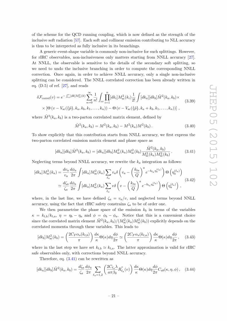
The results are shown in figure 1. There we see that ∆(v1, v2) tends to zero for v → 0,

providing a check of the validity of the NNLL resummation up to O(α2s). In order to

check the expansion to O(α3s) one would have to produce either NNLO 3-jet or NLO 4-jet

distributions which are sufficiently stable in the deep infrared region. This can be achieved

through long runs e.g. with the generators EERAD3 [55], however, we have not been able to

obtain distributions that were stable enough. Alternatively, one could use NLOJET++ [59]

to generate four-jet distributions at NLO and consider differences of observables. On the

other hand, the checks against the analytic results for ρH , BT and BW at O(α3s) provide

us with a proof of the validity of our NNLL resummation at this order.

As a last step, we match the resummed NNLL distributions to NNLO fixed-order

differential cross sections obtained with EERAD3 [55]. The matching is performed according

to the log-R scheme [10, 31]. As it is customary in resummed calculations, to probe the

size of subleading logarithmic terms we introduce a rescaling constant xV as

ln1

v= ln

xVv

− lnxV , (4.2)

and expand the cross section around ln xV /v neglecting subleading terms.9 Eventually we

modify the resummed logarithm ln xV /v in order to impose that the total cross section is

reproduced at the kinematical endpoint vmax

lnxVv

→ 1

pln

(

1 +(xVv

)p−(

xVvmax

)p)

. (4.3)

Here, p denotes a positive number which controls how quickly the logarithms are switched

off close to the endpoint. In the following we use p = 1.

To obtain our central predictions we set µR = Q = MZ , corresponding to αs(µR) =

0.118, and [28, 60]

lnxV =1

2

∑

ℓ=1,2

(

ln dℓ +

∫ 2π

0

dφ

2πln gℓ(φ)

)

. (4.4)

9For details about how the resummed formula and the expansion coefficients change see e.g. ref. [31]

where one has to replace ln xL → − lnxV .

– 23 –

JHEP05(2015)102-30

-20

-10

0

10

20

30

1 2 3 4 5 6 7 8

∆(T

M,B

T)

ln (1/v)

Thrust major - Total Broadening

-30

-20

-10

0

10

20

30

1 2 3 4 5 6 7 8

∆(O

,BT)

ln (1/v)

Oblateness - Total Broadening

-30

-20

-10

0

10

20

30

1 2 3 4 5 6 7 8

∆(O

,BW

)

ln (1/v)

Oblateness - Wide Broadening

-30

-20

-10

0

10

20

30

1 2 3 4 5 6 7 8

∆(T

M,B

W)

ln (1/v)

Thrust Major - Wide Broadening

-30

-20

-10

0

10

20

30

1 2 3 4 5 6 7 8 9 10

∆(C

,ρH

)

ln (1/v)

C parameter - Heavy Jet Mass

-30

-20

-10

0

10

20

30

1 2 3 4 5 6 7 8 9 10

∆(C

,1-T

)

ln (1/v)

C parameter - Thrust

Event2 at O(αs2)

Figure 1. Difference between the NLO differential distributions of pairs of observables after sub-

tracting the expansion of the NNLL resummation formula up to (and including) O(α2sL

0) (see

eq. (4.1)). To obtain these distributions we used about 1011 events.

We then construct the uncertainty bands by varying µR and xV individually by a factor

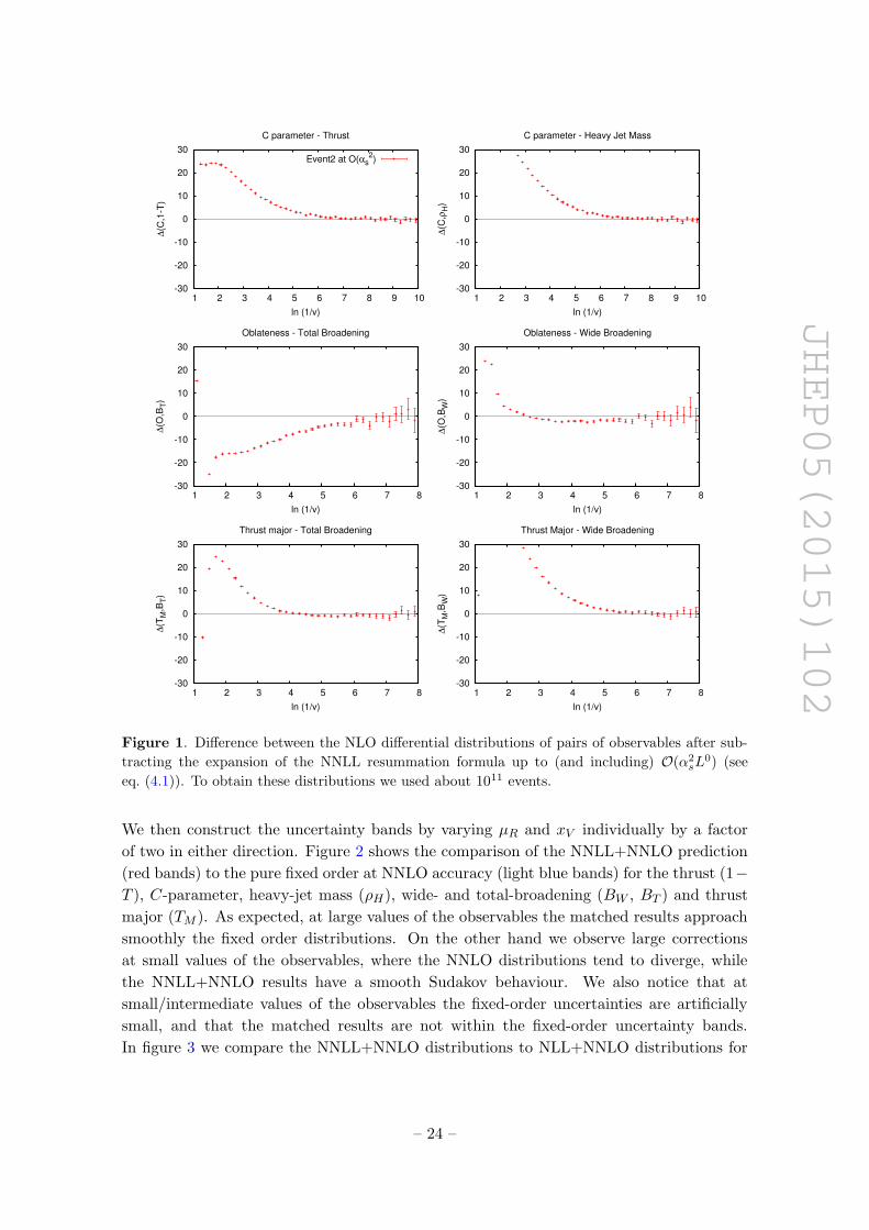
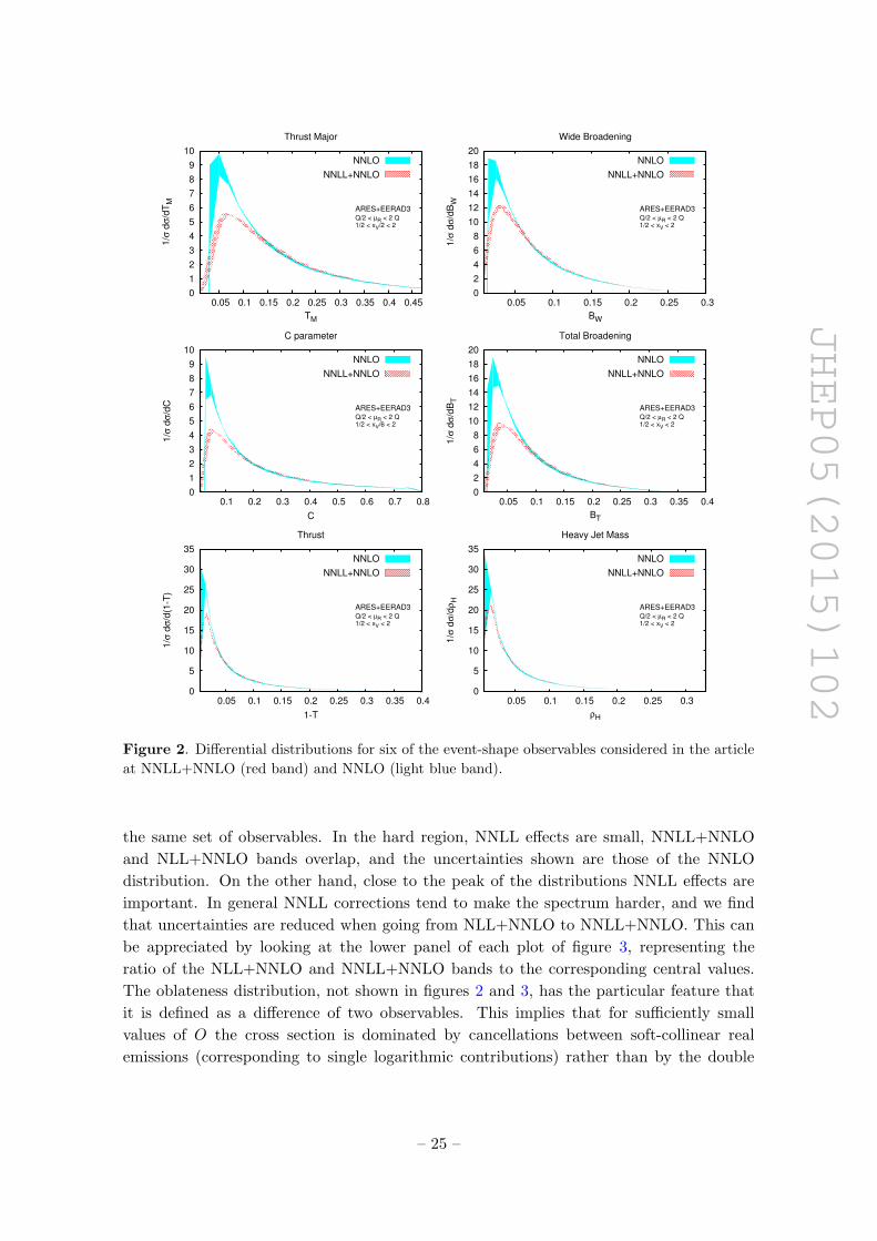
of two in either direction. Figure 2 shows the comparison of the NNLL+NNLO prediction

(red bands) to the pure fixed order at NNLO accuracy (light blue bands) for the thrust (1−T ), C-parameter, heavy-jet mass (ρH), wide- and total-broadening (BW , BT ) and thrust

major (TM ). As expected, at large values of the observables the matched results approach

smoothly the fixed order distributions. On the other hand we observe large corrections

at small values of the observables, where the NNLO distributions tend to diverge, while

the NNLL+NNLO results have a smooth Sudakov behaviour. We also notice that at

small/intermediate values of the observables the fixed-order uncertainties are artificially

small, and that the matched results are not within the fixed-order uncertainty bands.

In figure 3 we compare the NNLL+NNLO distributions to NLL+NNLO distributions for

– 24 –

JHEP05(2015)102

1/σ

dσ

/d(1

-T)

1-T

Thrust

ARES+EERAD3 Q/2 < µR < 2 Q 1/2 < xV < 2

NNLO

NNLL+NNLO

0

5

10

15

20

25

30

35

0.05 0.1 0.15 0.2 0.25 0.3 0.35 0.4

1/σ

dσ

/dC

C

C parameter

ARES+EERAD3 Q/2 < µR < 2 Q 1/2 < xV/6 < 2

NNLO

NNLL+NNLO

0

1

2

3

4

5

6

7

8

9

10

0.1 0.2 0.3 0.4 0.5 0.6 0.7 0.8

1/σ

dσ

/dρ

H

ρH

Heavy Jet Mass

ARES+EERAD3 Q/2 < µR < 2 Q 1/2 < xV < 2

NNLO

NNLL+NNLO

0

5

10

15

20

25

30

35

0.05 0.1 0.15 0.2 0.25 0.3

1/σ

dσ

/dB

T

BT

Total Broadening

ARES+EERAD3 Q/2 < µR < 2 Q 1/2 < xV < 2

NNLO

NNLL+NNLO

0

2

4

6

8

10

12

14

16

18

20

0.05 0.1 0.15 0.2 0.25 0.3 0.35 0.4

1/σ

dσ

/dB

W

BW

Wide Broadening

ARES+EERAD3 Q/2 < µR < 2 Q 1/2 < xV < 2

NNLO

NNLL+NNLO

0

2

4

6

8

10

12

14

16

18

20

0.05 0.1 0.15 0.2 0.25 0.3

1/σ

dσ

/dT

M

TM

Thrust Major

ARES+EERAD3 Q/2 < µR < 2 Q 1/2 < xV/2 < 2

NNLO

NNLL+NNLO

0

1

2

3

4

5

6

7

8

9

10

0.05 0.1 0.15 0.2 0.25 0.3 0.35 0.4 0.45

Figure 2. Differential distributions for six of the event-shape observables considered in the article

at NNLL+NNLO (red band) and NNLO (light blue band).

the same set of observables. In the hard region, NNLL effects are small, NNLL+NNLO

and NLL+NNLO bands overlap, and the uncertainties shown are those of the NNLO

distribution. On the other hand, close to the peak of the distributions NNLL effects are

important. In general NNLL corrections tend to make the spectrum harder, and we find

that uncertainties are reduced when going from NLL+NNLO to NNLL+NNLO. This can

be appreciated by looking at the lower panel of each plot of figure 3, representing the

ratio of the NLL+NNLO and NNLL+NNLO bands to the corresponding central values.

The oblateness distribution, not shown in figures 2 and 3, has the particular feature that

it is defined as a difference of two observables. This implies that for sufficiently small

values of O the cross section is dominated by cancellations between soft-collinear real

emissions (corresponding to single logarithmic contributions) rather than by the double

– 25 –

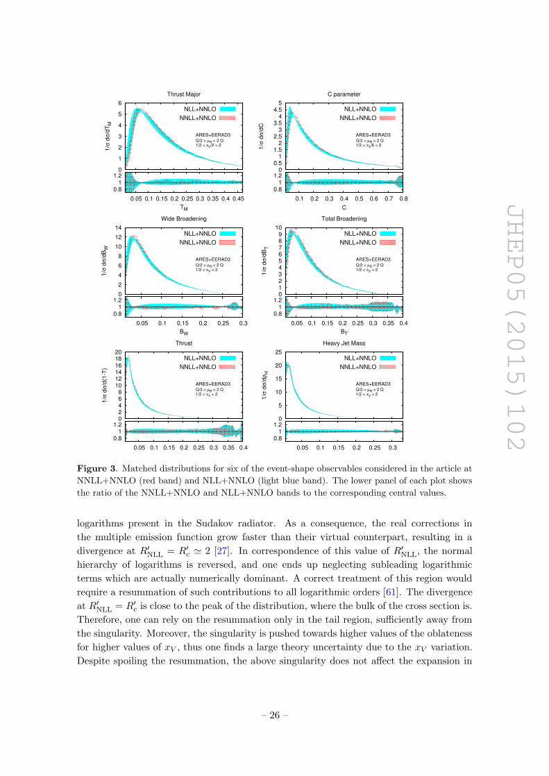
JHEP05(2015)102

1/σ

dσ

/d(1

-T)

Thrust

ARES+EERAD3 Q/2 < µR < 2 Q 1/2 < xV < 2

NLL+NNLO

NNLL+NNLO

0 2 4 6 8

10 12 14 16 18 20

0.8 1

1.2

0.05 0.1 0.15 0.2 0.25 0.3 0.35 0.4

1/σ

dσ

/dC

C parameter

ARES+EERAD3 Q/2 < µR < 2 Q 1/2 < xV/6 < 2

NLL+NNLO

NNLL+NNLO

0 0.5

1 1.5

2 2.5

3 3.5

4 4.5

5

C

0.8 1

1.2

0.1 0.2 0.3 0.4 0.5 0.6 0.7 0.8

1/σ

dσ

/dρ

H

Heavy Jet Mass

ARES+EERAD3 Q/2 < µR < 2 Q 1/2 < xV < 2

NLL+NNLO

NNLL+NNLO

0

5

10

15

20

25

0.8 1

1.2

0.05 0.1 0.15 0.2 0.25 0.3

1/σ

dσ

/dB

T

Total Broadening

ARES+EERAD3 Q/2 < µR < 2 Q 1/2 < xV < 2

NLL+NNLO

NNLL+NNLO

0 1 2 3 4 5 6 7 8 9

10

BT

0.8 1

1.2

0.05 0.1 0.15 0.2 0.25 0.3 0.35 0.4

1/σ

dσ

/dB

W

Wide Broadening

ARES+EERAD3 Q/2 < µR < 2 Q 1/2 < xV < 2

NLL+NNLO

NNLL+NNLO

0

2

4

6

8

10

12

14

BW

0.8 1

1.2

0.05 0.1 0.15 0.2 0.25 0.3

1/σ

dσ

/dT

M

Thrust Major

ARES+EERAD3 Q/2 < µR < 2 Q 1/2 < xV/2 < 2

NLL+NNLO

NNLL+NNLO

0

1

2

3

4

5

6

TM

0.8 1

1.2

0.05 0.1 0.15 0.2 0.25 0.3 0.35 0.4 0.45

Figure 3. Matched distributions for six of the event-shape observables considered in the article at

NNLL+NNLO (red band) and NLL+NNLO (light blue band). The lower panel of each plot shows

the ratio of the NNLL+NNLO and NLL+NNLO bands to the corresponding central values.

logarithms present in the Sudakov radiator. As a consequence, the real corrections in

the multiple emission function grow faster than their virtual counterpart, resulting in a

divergence at R′NLL = R′

c ≃ 2 [27]. In correspondence of this value of R′NLL, the normal

hierarchy of logarithms is reversed, and one ends up neglecting subleading logarithmic

terms which are actually numerically dominant. A correct treatment of this region would

require a resummation of such contributions to all logarithmic orders [61]. The divergence

at R′NLL = R′

c is close to the peak of the distribution, where the bulk of the cross section is.

Therefore, one can rely on the resummation only in the tail region, sufficiently away from

the singularity. Moreover, the singularity is pushed towards higher values of the oblateness

for higher values of xV , thus one finds a large theory uncertainty due to the xV variation.

Despite spoiling the resummation, the above singularity does not affect the expansion in

– 26 –

JHEP05(2015)102

powers of the strong coupling, so that our method can still be used to compute correctly

the coefficients of the expansion to all orders in αs.10

5 Conclusions

We presented a novel method for automated resummation of event-shape distributions

to NNLL accuracy. The method is fully general and it can be applied to any global and

recursive infrared and collinear safe event shape. Neither the factorisation of the observable

into kinematical subprocesses nor an analytic definition is required for the method to be

applied. We implemented the algorithm in the fast and stable numerical code ARES which

will be publicly released soon. For the time being, the method relies on the fact that

the NNLL Sudakov radiator is universal for all observables which have the same scaling

properties for a single soft-collinear emission. Therefore, for the observables analysed in this

article, we could extract the relevant unknown terms of the NNLL radiator from known

resummations. Specifically, using the known result for thrust 1 − T we can reproduce

the known resummation for the heavy jet mass ρH and the C parameter. Analogously,

we extract the missing term from the kt resummations in colour singlet production in

hadronic collisions, re-derive the known results for jet broadenings BT , BW , and obtain

new predictions for both thrust-major TM and oblateness O. The calculation of the NNLL

radiator for a generic observable will be addressed in future work.

We performed checks of our results by expanding known resummed distributions up

to O(α3s) and comparing them to the results in the literature. For observables for which a

NNLL resummation was not previously known, we compare their O(α2s) expansion to the

fixed order generator Event2. We then presented NNLL+NNLOmatched results, where the

NNLO results were obtained using the code EERAD3. We observed that NNLL corrections

are in general sizable and hence play a role in precise determinations of the strong coupling

constant using e+e− data. A simultaneous fit using distributions of several observables will

help disentangle perturbative effects from non-perturbative ones. In fact while perturbative

effects are now well-understood and described at NNLL+NNLO or beyond, some deeper

understanding is still required to model non-perturbative corrections, which are quite siz-

able at LEP energies. These corrections will be much more moderate at future lepton

colliders. In these conditions, the potential of NNLL resummations can be fully exploited

and even data close or at the peak of the distributions can be included in the fit region.

The work presented here represents a first step towards a fully automated resummation

of generic global and rIRC observables. Future work includes the calculation of the NNLL

radiator in the generic case, the treatment of jet resolution parameters, as well as the

extension to observables at hadron colliders. Furthermore, the method could also be applied

to derive corrections beyond NNLL.

Note added. When this work was being finalised ref. [62] appeared, where an analytic

resummation for the C parameter is presented. We compared their formulae to our analytic

result for the C parameter, and found full agreement at NNLL.

10Analogously to what is observed for both TM and C, the oblateness, which has dℓ = 2, receives sizable

NNLL corrections.

– 27 –

JHEP05(2015)102

Acknowledgments

We would like to thank G. Salam for stimulating conversations during the early stage of

this work. We are grateful to T. Gehrmann, A. Gehrmann-De Ridder, and G. Heinrich

for useful advices concerning the use of the generator EERAD3, and for providing us with a

preliminary version of the code. GZ is supported by the ERC grant 614577. PM is sup-

ported by the Research Executive Agency (REA) of the European Union under the Grant

Agreement number PITN-GA-2010-264564 (LHCPhenoNet), and by the Swiss National

Science Foundation (SNF) under the grant PBZHP2-147297. The work of AB is supported

by Science and Technology Facility Council (STFC) under grant number ST/L000504/1.

This research was partly supported by the Munich Institute for Astro- and Particle Physics

(MIAPP) of the DFG cluster of excellence “Origin and Structure of the Universe” (PM and

GZ) and by the Mainz Institute for Theoretical Physics (MITP) of the PRISMA excellence

cluster (GZ). We would like to thank the Galileo Galilei Institute (PM and GZ) and CERN

(AB, PM) for hospitality while part of this work was carried out.

A Observables definition

In this appendix we recall the definition of the event shapes that we considered in this work.

• Thrust:

T ≡ max~n

∑

i |~pi · ~n|Q

, τ ≡ 1− T , (A.1)

where Q is the centre-of-mass energy and the vector ~n that maximizes the sum

defines the direction of the thrust axis, ~nT . The thrust axis divides each event into

two hemispheres, H(1) and H(2).

• Heavy-jet mass:

ρH ≡ maxi=1,2

M2i

Q2, M2

i ≡

∑

j∈H(i)

pj

2

. (A.2)

• C-parameter:

C ≡ 3

1− 1

2

∑

i,j

(pi · pj)2(pi ·Q)(pj ·Q)

, (A.3)

where Qµ is the total four-momentum.

• Total broadening:

BT ≡ BL +BR, (A.4)

where

BL ≡∑

i∈H(1)

|~pi × ~nT |2Q

, BR ≡∑

i∈H(2)

|~pi × ~nT |2Q

. (A.5)

– 28 –

JHEP05(2015)102

• Wide broadening:

BW ≡ max{BL, BR}. (A.6)

• Thrust-major:

TM ≡ max~n· ~nT=0

∑

i |~pi · ~n|Q

, (A.7)

where the vector ~n for which the sum is maximised defines the thrust-major axis.

• Oblateness:

O ≡ TM − Tm, (A.8)

where

Tm ≡∑

i |pi,x|Q

, (A.9)

and where x is the direction perpendicular to both the thrust and the thrust-major

axes.

B Sudakov radiator

The Sudakov radiator can be parametrised as

R(v) = −Lg1(λ)− g2(λ)−αs

πg3(λ) + . . . (B.1)

We introduce the resummation scale xV such that

ln1

v= ln

xVv

− lnxV =λ

αsβ0− lnxV , (B.2)

where λ = αsβ0 lnxV /v. The functions g1, g2 and g3 can be parametrised as

gi(λ) =∑

ℓ=1,2

g(ℓ)i (λ) (B.3)

where g(ℓ)i can be expressed in terms of scaling parameters a and bℓ as follows:

g(ℓ)1 (λ) =

A1

(

(a+ bℓ − 2λ) ln(

1− 2λa+bℓ

)

− (a− 2λ) ln(

1− 2λa

)

)

4πbℓβ0λ, (B.4)

g(ℓ)2 (λ) =

A2

(

a ln(

1− 2λa

)

− (a+ bℓ) ln(

1− 2λa+bℓ

))

8π2bℓβ02 +

B1 ln(

1− 2λa+bℓ

)

4πβ0

+A1

(

β1(a+ bℓ) ln2(

1− 2λa+bℓ

)

+ 2β1(a+ bℓ) ln(

1− 2λa+bℓ

))

8πbℓβ03

−A1

ln(

1− 2λa

) (

aβ1 ln(

1− 2λa

)

+ 2aβ1)

8πbℓβ03

+A1

(

ln(

1− 2λa+bℓ

)

− log(

1− 2λa

)

)

4πbℓβ0lnx2V

−A1

(

ln(

1− 2λa+bℓ

)

− ln(

1− 2λa

)

)

2πbℓβ0ln d̄ℓ ,

(B.5)

– 29 –

JHEP05(2015)102

g(ℓ)3 (λ) =

β1B1

(

(a+ bℓ) ln(

1− 2λa+bℓ

)

+ 2λ)

2β02(a+ bℓ − 2λ)

+A2β1

(

a2(a+ bℓ − 2λ) ln(

1− 2λa

)

− (a+ bℓ)2(a− 2λ) ln

(

1− 2λa+bℓ

)

+ 6bℓλ2)

8πbℓβ03(a− 2λ)(a+ bℓ − 2λ)

+A1

(

β12(a+ bℓ)

2(a− 2λ) ln2(

1− 2λa+bℓ

)

− 4bℓλ2(

β0β2 + β12)

)

8bℓβ04(a− 2λ)(a+ bℓ − 2λ)

− aA1 ln(

1− 2λa

) (

2β0β2(a− 2λ) + aβ12 ln

(

1− 2λa

)

+ 4β12λ)

8bℓβ04(a− 2λ)

+A1(a+ bℓ) ln

(

1− 2λa+bℓ

)

(

β0β2(a+ bℓ − 2λ) + 2β12λ)

4bℓβ04(a+ bℓ − 2λ)

− A1

8(a− 2λ)(a+ bℓ − 2λ)ln2 x2V +

[

πaβ02B1 + λ

(

A2β0 − 2π(

A1β1 + β02B1

))

4πβ02(a− 2λ)(a+ bℓ − 2λ)

+A1β1

(

(a+ bℓ)(a− 2λ) ln(

1− 2λa+bℓ

)

− a(a+ bℓ − 2λ) ln(

1− 2λa

)

)

4bℓβ02(a− 2λ)(a+ bℓ − 2λ)

lnx2V

− A1

2(a− 2λ)(a+ bℓ − 2λ)ln d̄2ℓ +

A1

2(a− 2λ)(a+ bℓ − 2λ)ln d̄ℓ lnx

2V

− πaβ02B1 + λ

(

A2β0 − 2π(

A1β1 + β02B1

))

2πβ02(a− 2λ)(a+ bℓ − 2λ)

ln d̄ℓ

+A1β1

(

a(a+ bℓ − 2λ) ln(

1− 2λa

)

− (a+ bℓ)(a− 2λ) ln(

1− 2λa+bℓ

))

2bℓβ02(a− 2λ)(a+ bℓ − 2λ)

ln d̄ℓ

+A17

16bℓ

1

1− 2a+bℓ

λΘ(bℓ) + h(λ) ,

(B.6)

where ln d̄nℓ =∫ 2π0

dφ2π lnn(dℓgℓ(φ)) and Θ(bℓ) = 1(0) for bℓ > 0 (bℓ = 0). The renormalisation

scale dependence can be restored using the following replacements in eq. (B.1)

g1(λ) → g1(λ) ,

g2(λ) → g2(λ) + λ2g′1(λ) lnµ2RQ2

, (B.7)

g3(λ) → g3(λ) + π

(

β0λg′2(λ) +

β1β0λ2g′1(λ)

)

lnµ2RQ2

+ π

(

β0λ2g′1(λ) +

β02λ3g′′1(λ)

)

ln2µ2RQ2

.

The coefficients of the QCD β function used above are defined as

β0 =11CA − 2nf

12π, β1 =

17C2A − 5CAnf − 3CFnf

24π2, (B.8)

β2 =2857C3

A + (54C2F − 615CFCA − 1415C2

A)nf + (66CF + 79CA)n2f

3456π3. (B.9)

The following functions are also used in the text

R′

NLL,ℓ(v) =A1

(

ln(

1− 2λa+bℓ

)

− ln(

1− 2λa

)

)

2πbℓβ0, (B.10)

– 30 –

JHEP05(2015)102

δR′

NNLL,ℓ(v) =αs(Q)

π

[

−A1β1

(

a(a+ bℓ − 2λ) ln(

1− 2λa

)

− (a+ bℓ)(a− 2λ) ln(

1− 2λa+bℓ

)

+ 2bℓλ)

2bℓβ02(a− 2λ)(a+ bℓ − 2λ)

+A1λ

(a− 2λ)(a+ bℓ − 2λ)ln

µ2R

Q2−

A1

2(a− 2λ)(a+ bℓ − 2λ)lnx2

V

+A2λ

2πβ0(a− 2λ)(a+ bℓ − 2λ)

]

, (B.11)

R′′

ℓ (v) =αs(Q)

π

A1

(a− 2λ)(a+ bℓ − 2λ). (B.12)

The limit bℓ → 0 (relevant for jet broadenings, thrust major and oblateness) is finite and

well defined for all the above expressions. The function h(λ), implicitly defined in eq. (3.5),

is extracted from the resummed expression of

Σ(v) =1

σ

∫ v

0dv′

dσ(v′)

dv′, (B.13)

(where σ is the total cross section for e+e− → hadrons) for the two reference observables

(i.e. kt and thrust 1− T ) leading to

h(1−T )(λ) = −A(1−T )3

λ2

8π2β02(1− 2λ)(2− 2λ)

−B(1−T )2

λ

8πβ0(1− λ)

+ CFπ2

24

1

1− 2λ+ CF

(

1

4− π2

12

)

1

1− λ+ CF

(

−19

8+

7

24π2)

,

(B.14)

and

h(kt)(λ) = −A(kt)3

λ2

8π2β02(1− 2λ)2

−B(kt)2

λ

4πβ0(1− 2λ)

+ CF

(

1

4− π2

24

)

1

1− 2λ+ CF

(

−19

8+

7

24π2)

.

(B.15)

Note that the above expressions imply that g3(0) 6= 0. This means that constant terms

appear in the exponent, which can be expanded to O(αs) neglecting subleading terms.

The anomalous dimensions Ai and Bi used in the above expressions are:

A1 = 2CF , (B.16)

B1 = −3CF , (B.17)

A2 = CF

(

CA

(

67

9− π2

3

)

− 10

9nf

)

, (B.18)

the coefficient A2 defines the running coupling in the CMW scheme used in the definition

of the soft emission probability. The coefficients B2 and A3 are observable dependent in

our study. The expressions for the two reference observables read (with TF = 1/2)

B(1−T )2 = −2

(

C2F

(

−π2

2+

3

8+ 6ζ3

)

+ CFCA

(

11π2

18+

17

24− 3ζ3

)

+ CFTFnf

(

−1

6−

2

9π2

))

,(B.19)

B(kt)2 = B

(1−T )2 + 2πβ0ζ2CF , (B.20)

A(1−T )3 = CFC

2A

(

245

12−

67

27π2 +

11

3ζ3 +

22

5ζ22

)

+ CFTFnf

(

−55

6+ 8ζ3

)

−8

27T 2Fn

2f

– 31 –

JHEP05(2015)102

+CATFnf

(

−209

27+

20

27π2 −

28

3ζ3

)

+ πβ0CF

(

CA

(

808

27− 28ζ3

)

−224

27TFnf

)

, (B.21)

A(kt)3 = A

(1−T )3 − 8π2β2

0ζ2CF . (B.22)

C Analytic NNLL results for additive observables

Some event shapes have the property that they are additive, meaning that for soft emissions

V ({p̃}, k1, . . . , kn) =n∑

i=1

V ({p̃}, ki) +O(V 2) , (C.1)

while for a hard emission k collinear to leg ℓ, the corresponding V ({p̃}, k) has to be replaced

by V (k)({p̃}, k[k′t, p′t,ℓ, z(ℓ)]), as defined in section 3.3.2. This is the case for instance for the

thrust, the C-parameter and the heavy-jet masses. For this simpler class of observables, the

NNLL corrections can be simplified significantly. In this appendix we work out the NNLL

corrections of section 3 for these additive observables analytically. This provides a check

of the numerical implementation of our method. We also show that for these observables

the corresponding NNLL correction δFNNLL factorises in a coefficient that multiplies the

NLL function FNLL(λ), that for an additive observable reads

FNLL(λ) =e−γER′

NLL

Γ(1 +R′NLL)

. (C.2)

C.1 Soft-collinear correction

We consider first the soft-collinear contribution δFsc of eq. (3.15), and use the fact that for

additive observables

Vsc({p̃}, k, {ki}) = ζv + Vsc({p̃}, {ki}) . (C.3)

δFsc(λ) =π

αs(Q)

∫

∞

0

dζ

ζ

∑

ℓ=1,2

(

δR′

NNLL,ℓ +R′′

ℓi ln d̄ℓ +R′′

ℓi ln1

ζ

)∫

dZ[{R′

NLL,ℓi , ki}]×

×

[

Θ

(

1−ζ− limv→0

Vsc({p̃}, {ki})

v

)

−Θ(1− ζ)Θ

(

1− limv→0

Vsc({p̃}, {ki})

v

)]

, (C.4)

where we used the fact that for additive observables the integral over φ can be performed

analytically.

We can define rescaled momenta k̃1, . . . , k̃n in the second theta function such that

Vsc({p̃}, k̃i) = Vsc({p̃}, ki)/(1− ζ). Recursive IRC safety of V guarantees that

Vsc({p̃}, {ki}) = (1− ζ)Vsc({p̃}, {k̃i}) . (C.5)

Using the explicit expression for dZ, and defining ζ̃i = Vsc({p̃}, k̃i)/v, one gets

δFsc(λ) =π

αs(Q)

∫

∞

0

dζ

ζ

∑

ℓ=1,2

(

δR′

NNLL,ℓ +R′′

ℓi ln d̄ℓ +R′′

ℓi ln1

ζ

)

ǫR′

NLL

∞∑

n=0

1

n!

n∏

i=1

∑

ℓi=1,2

R′

NLL,ℓi

×

∫ 2π

0

dφi

2πΘ(1−ζ)

[

∫

∞

ǫ1−ζ

dζ̃i

ζ̃iΘ

(

1− limv→0

Vsc({p̃}, {k̃i})

v

)

−

∫

∞

ǫ

dζiζi

Θ

(

1− limv→0

Vsc({p̃}, {ki})

v

)

]

.

(C.6)

– 32 –

JHEP05(2015)102

We can then rearrange the above equation to reconstruct the function FNLL(λ). This gives

δFsc(λ) = FNLL(λ)π

αs(Q)

∫ 1

0

dζ

ζ

∑

ℓ=1,2

(

δR′NNLL,ℓ+R

′′ℓiln d̄ℓ+R

′′ℓiln

1

ζ

)

(

(1−ζ)R′

NLL−1)

= −FNLL(λ)π

αs(Q)

∑

ℓ=1,2

(

(

δR′NNLL,ℓ +R′′

ℓiln d̄ℓ

)

(

ψ(0)(1 +R′NLL) + γE

)

+R′′

ℓi

2

(

(

ψ(0)(1 +R′NLL) + γE

)2− ψ(1)(1 +R′

NLL) +π2

6

))

. (C.7)

C.2 Recoil correction

Let us now consider the recoil contribution δFrec of eq. (3.28). Considering a hard emission

collinear to leg ℓ, for an additive observable one has

V(k′)hc ({p̃}, k′, {ki}) =

(

k′tQ

)a+bℓ

f (ℓ)(z(ℓ), φ) + Vsc({p̃}, {ki}) , (C.8)

and

Vsc({p̃}, k, {ki}) =(

ktQ

)a+bℓ

f (ℓ)sc (z(ℓ), φ) + Vsc({p̃}, {ki}) , (C.9)

where the presence of k′, rather than k, denotes that the full recoil has been taken into

account in the calculation of the observable.

Using the above equations in eq. (3.28) we get

δFrec(λ) =∑

ℓ=1,2

αs(v1/(a+bℓ)Q)

αs(Q)(a+ bℓ)

∫ ∞

0

dζ

ζ

∫ 2π

0

dφ

2π

∫

dZ[{R′NLL,ℓi

, ki}]∫ 1

0dz pℓ(z)× (C.10)

×[

Θ

(

1−ζf (ℓ)(z, φ)− limv→0

Vsc({p̃}, {ki})v

)

−Θ

(

1−ζf (ℓ)sc (z, φ)− limv→0

Vsc({p̃}, {ki})v

)]

,

where ζ is defined in eq. (3.26). We can define rescaled momenta k̃1, . . . , k̃n in the second

theta function such that Vsc({p̃}, k̃i) = Vsc({p̃}, ki)/(1− ζf(ℓ)sc (z, φ)). Recursive IRC safety

of V guarantees that

Vsc({p̃}, k1, . . . , kn) = (1− ζf (ℓ)sc (z, φ))Vsc({p̃}, k̃1, . . . , k̃n) . (C.11)

Analogously, we define soft and collinear momenta k̃′1, . . . , k̃′n in the theta function contain-

ing f (ℓ)(z, φ)) such that

Vsc({p̃}, k1, . . . , kn) = (1− ζf (ℓ)(z, φ))Vsc({p̃}, k̃′1, . . . , k̃′n) . (C.12)

Using the explicit expression for dZ, one gets

δFrec(λ) =∑

ℓ=1,2

αs(v1/(a+bℓ)Q)

αs(Q)(a+ bℓ)

∫

∞

0

dζ

ζ

∫ 2π

0

dφ

2π

∫ 1

0

dz pℓ(z)ǫR′

NLL

∞∑

n=0

1

n!

n∏

i=1

∑

ℓi=1,2

R′

NLL,ℓi

∫ 2π

0

dφi

2π×

×

[

Θ(1−ζf (ℓ)(z))

∫

∞

0

dζ̃′i

ζ̃′iΘ

(

ζ̃′i −ǫ

1−ζf (ℓ)(z)

)

Θ

(

1− limv→0

Vsc({p̃}, k̃′

1, . . . , k̃′

n)

v

)

−Θ(1−ζf (ℓ)sc (z))

∫

∞

0

dζ̃i

ζ̃iΘ

(

ζ̃i −ǫ

1−ζf(ℓ)sc (z)

)

Θ

(

1− limv→0

Vsc({p̃}, k̃1, . . . , k̃n)

v

)

]

. (C.13)

– 33 –

JHEP05(2015)102

We can then rearrange the above equation to reconstruct the function FNLL(λ). This gives

δFrec(λ) = FNLL(λ)∑

ℓ=1,2

αs(v1/(a+bℓ)Q)

αs(Q)(a+ bℓ)

∫ 2π

0

dφ

2π

∫ 1

0

dz pℓ(z)×

×

∫

∞

0

dζ

ζ

[

(1− ζf (ℓ)(z, φ))R′

NLLΘ(1− ζf (ℓ)(z, φ))− (1− ζf (ℓ)sc (z, φ))R

′

NLLΘ(1− ζf (ℓ)sc (z, φ))

]

= FNLL(λ)∑

ℓ=1,2

αs(v1/(a+bℓ)Q)

αs(Q)(a+ bℓ)

∫ 2π

0

dφ

2π

∫ 1

0

dz pℓ(z) lnf(ℓ)sc (z, φ)

f (ℓ)(z, φ). (C.14)

As an example, we consider the thrust. One can show that its expression in terms of

Sudakov variables is

1− T =

n∑

i=1

ktiQe−|ηi| +

1

Q2

∑

ℓ=1,2

(

∑

i∈H(ℓ)~k(ℓ)ti

)2

1−∑

i∈H(ℓ) z(ℓ)i

. (C.15)

Suppose k is collinear to leg p̃1. Using the Sudakov parametrisation of eq. (3.18) we then

have

1− T ≃n∑

i=1

ktiQe−|ηi| +

k2tz(1)Q2

+k2t

(1− z(1))Q2=

n∑

i=1

ktiQe−|ηi| +

k2tz(1)(1− z(1))Q2

, (C.16)

where we have used the fact that the hard-collinear kt is larger than all soft-collinear kti,

and therefore kt ≃ k′t. A hard collinear emission gives an additive contribution to the

observable, so that we can apply eq. (C.14) with

f (ℓ)(z(ℓ), φ) =1

z(ℓ)(1− z(ℓ)), f (ℓ)sc (z(ℓ), φ) =

1

z(ℓ).

This gives

δFrec(λ) = FNLL(λ)2CFαs(

√τQ)

2αs(Q)

∫ 1

0dz

(1 + (1− z)2)

zln(1− z)

= FNLL(λ)CFαs(

√τQ)

αs(Q)

(

5

4− π2

3

)

.

(C.17)

This result holds also for the C-parameter and the heavy-jet mass, which behave as 1−Tin the collinear region.

C.3 Hard-collinear correction

In a similar way, we compute here the hard-collinear function δFhc(λ) of eq. (3.32). Using

eq. (C.9) we obtain

δFhc(λ) =∑

ℓ=1,2

αs(v1/(a+bℓ)Q)

αs(Q)(a+ bℓ)

∫ ∞

0

dζ

ζ

∫ π

0

dφ

2π

∫ 1

0

dz

z(zpℓ(z)− 2Cℓ)

∫

dZ[{R′NLL,ℓi

, ki}]×

×[

Θ

(

1− ζ − limv→0

Vsc({p̃}, {ki})v

)

−Θ(1− ζ)Θ

(

1− limv→0

Vsc({p̃}, {ki})v

)]

. (C.18)

– 34 –

JHEP05(2015)102

Rescaling the momenta in a similar way as we have done in the previous section we get

δFhc(λ) = FNLL(λ)∑

ℓ=1,2

αs(v1/(a+bℓ)Q)

αs(Q)(a+ bℓ)

∫ ∞

0

dζ

ζ

∫ 2π

0

dφ

2π

∫ 1

0

dz

z(zpℓ(z)− 2Cℓ)×

×[

(1− ζ)R′

NLL Θ(1− ζ)−Θ(1− ζ)]

= FNLL(λ)∑

ℓ=1,2

αs(v1/(a+bℓ)Q)

αs(Q)(a+ bℓ)×

× CℓBℓ

∫ 1

0

dζ

ζ

[

(1− ζ)R′

NLL − 1]

.

(C.19)

For thrust, using the explicit expression for FNLL (C.2) we obtain

δFhc(λ) =αs(

√τQ)

αs(Q)CF

3

2

(

ψ(0)(1 +R′NLL) + γE

)

FNLL. (C.20)

C.4 Soft wide-angle correction

We consider now the case of a NNLL correction induced by a soft large-angle emission,

eq. (3.38) . Then we have

V (k)wa ({p̃}, k, {ki}) =

(

ktQ

)a

fwa(η, φ) + Vsc({p̃}, {ki}) , (C.21)

Vsc({p̃}, k, {ki}) =(

ktQ

)a

fsc(η, φ) + Vsc({p̃}, {ki}) , (C.22)

where fsc(η, φ) and fwa(η, φ) are defined in eqs. (3.33) and (3.34). Performing a similar

rescaling as for the recoil correction one finds

δFwa(λ) = FNLL(λ)2CF

a

αs(v1aQ)

αs(Q)

∫ 2π

0

dφ

2π

∫ ∞

−∞dη ln

fsc(η, φ)

fwa(η, φ). (C.23)

For the thrust and the heavy-jet mass:

fwa(η, φ) = fsc(η, φ) = e−|η| , (C.24)

so that δFwa(λ) = 0. In the case of the C-parameter instead we have

fwa(η, φ) =3

cosh ηand fsc(η, φ) = 6 e−|η| . (C.25)

This gives

δFwa(λ) = FNLL(λ)2CFαs(CQ)

αs(Q)

∫ ∞

−∞dη ln(2 cosh ηe−|η|) = FNLL(λ)CF

αs(CQ)

αs(Q)

π2

6,

(C.26)

where C is the value of the C-parameter.

– 35 –

JHEP05(2015)102

C.5 Soft correlated correction

The correlated correction presented in eq. (3.47) depends on the difference

Θ (v − Vsc({p̃}, ka, kb, k1, . . . , kn))−Θ(v − Vsc({p̃}, ka + kb, k1, . . . , kn)) , (C.27)

which is in general non-zero for additive observables. However, the above correction van-

ishes if the observable Vsc is inclusive, i.e. Vsc(ka, kb) = Vsc(ka + kb). There are observables

which are inclusive in particular regions of the phase space. As an example, the thrust

T happens to be inclusive only for emissions that propagate into the same hemisphere

(defined by the thrust axis itself). In this case, the difference (C.27) is non-zero if the two

correlated soft partons ka, kb move into opposite hemispheres. However, this configuration

requires the parent gluon to be emitted at small rapidities, which in the limit T → 1 gives

rise to a correction which is at most N3LL, and can be neglected accordingly. The other

additive observables treated in this article are also inclusive in the relevant phase space

regions, so we can conclude that for T , C, and ρH , at NNLL

δFcorrel(λ) = 0 . (C.28)

D Monte Carlo determination of real emission corrections

Both the NLL function FNLL(λ) and the NNLL correction δFNNLL(λ) can be computed

efficiently with a Monte Carlo procedure. In this appendix we recall the procedure devised

in ref. [23], simplifying the notation so that it can be easily adapted to the NNLL case. We

then discuss the MC determination of all NNLL corrections.

D.1 The function FNLL

We now recall the procedure of ref. [27] to efficiently compute the function FNLL(λ) via a

Monte Carlo procedure. The first observation is that in the sum in eqs. (2.32) and (2.33)

the term with zero emissions is negligibly small due to the factor ǫR′

NLL . Second, in all other

terms we can pick up the hardest emission k1 (the one for which Vsc({p}, k1) is the largest

of all Vsc({p}, ki)) and neglect all emissions k̄i with vi < ǫv1, with corrections suppressed

by powers of v1 ∼ v. This gives

FNLL(λ) = ǫR′

NLL

∑

ℓ1=1,2

R′NLL,ℓ1

∫ ∞

0

dζ1ζ1ζR′

NLL1

∫ 2π

0

dφ12π

×

×∞∑

n=0

1

n!

n+1∏

i=2

∑

ℓi=1,2

R′NLL,ℓi

∫ ζ1

ǫζ1

dζiζi

∫ 2π

0

dφi2π

Θ

(

1− limv→0

Vsc({p̃}, k1, . . . , kn+1)

v

)

.

(D.1)

We now introduce ζ̃i = ζi/ζ1, with corresponding momenta k̃i such that Vsc({p̃}, k̃i) = vi/ζ1.

Since V is rIRC safe we have

Vsc({p̃}, k1, . . . , kn+1) = ζ1Vsc({p̃}, k̃1, . . . , k̃n+1) . (D.2)

– 36 –

JHEP05(2015)102

Substituting into eq. (D.1) we have

FNLL(λ) = ǫR′

NLL

∞∑

n=0

1

n!

n+1∏

i=2

∑

ℓi=1,2

R′NLL,ℓi

∫ 1

ǫ

dζ̃i

ζ̃i

∫ 2π

0

dφi2π

×

×∑

ℓ1=1,2

R′NLL,ℓ1

∫ ∞

0

dζ1ζ1ζR′

NLL1

∫ 2π

0

dφ12π

Θ

(

1− ζ1 limv→0

Vsc({p̃}, k̃1, . . . , k̃n+1)

v

)

.

(D.3)

The ζ1 integration can be trivially performed to get

FNLL(λ) =∑

ℓ1=1,2

R′

NLL,ℓ1

R′

NLL

∫ 2π

0

dφ1

2π×

× ǫR′

NLL

∞∑

n=0

1

n!

n+1∏

i=2

∑

ℓi=1,2

R′

NLL,ℓi

∫ 1

ǫ

dζ̃i

ζ̃i

∫ 2π

0

dφi

2πexp

(

−R′

NLL ln limv→0

Vsc({p̃}, k̃1, . . . , k̃n+1)

v

)

.

(D.4)

D.2 The function δFsc

We now extend the procedure devised in section D.1 so as to be able to efficiently compute

δFsc with a Monte Carlo procedure. First we observe that without any secondary emission

there is no contribution to δFsc. We isolate the hardest emission k1 among k1, . . . , kn.

We first consider the case in which the special emission is not the hardest of all,

i.e. ζ < ζ1. This gives

δF<sc =

π

αs(Q)

∑

ℓ1=1,2

R′

NLL,ℓ1

∫

∞

0

dζ1ζ1

ζR′

NLL1

∫ 2π

0

dφ1

2π

∫ ζ1

0

dζ

ζ

∫ 2π

0

dφ

2π

∑

ℓ=1,2

(

δR′

NNLL,ℓ+R′′

ℓ ln

(

dℓgℓ(φ)

ζ

))

×

×

ǫR′

NLL

∞∑

n=0

1

n!

n+1∏

i=2

∑

ℓi=1,2

R′

NLL,ℓi

∫ ζ1

ǫζ1

dζiζi

∫ 2π

0

dφi

2π

×

×

[

Θ

(

1− limv→0

Vsc({p̃}, k, k1, . . . , kn+1)

v

)

−Θ(1− ζ)Θ

(

1− limv→0

Vsc({p̃}, k1, . . . , kn+1)

v

)]

. (D.5)

We now rescale all momenta as in section D.1, and obtain

δF<sc =

π

αs(Q)

∑

ℓ1=1,2

R′

NLL,ℓ1

∫

∞

ǫ

dζ1ζ1

ζR′

NLL1

∫ 2π

0

dφ1

2π

∫ 1

0

dζ̃

ζ̃

∫ 2π

0

dφ

2π

∑

ℓ=1,2

(

δR′

NNLL,ℓ+R′′

ℓ ln

(

dℓgℓ(φ)

ζ̃ζ1

))

×

×

ǫR′

NLL

∞∑

n=0

1

n!

n+1∏

i=2

∑

ℓi=1,2

R′

NLL,ℓi

∫ 1

ǫ

dζ̃i

ζ̃i

∫ 2π

0

dφi

2π

× (D.6)

×

[

Θ

(

1− ζ1 limv→0

Vsc({p̃}, k̃, k̃1, . . . , k̃n+1)

v

)

−Θ(1− ζ1ζ̃)Θ

(

1− ζ1 limv→0

Vsc({p̃}, k̃1, . . . , k̃n+1)

v

)]

.

Performing the ζ1 integration we get

δF<sc =

π

αs(Q)

∑

ℓ1=1,2

R′

NLL,ℓ1

R′

NLL

∫ 2π

0

dφ1

2π

∫ 1

0

dζ̃

ζ̃

∫ 2π

0

dφ

2π×

ǫR′

NLL

∞∑

n=0

1

n!

n+1∏

i=2

∑

ℓi=1,2

R′

NLL,ℓi

∫ 1

ǫ

dζ̃i

ζ̃i

∫ 2π

0

dφi

2π

×

×

∑

ℓ=1,2

((

δR′

NNLL,ℓ +R′′

ℓ

(

1

R′

NLL

+ ln

(

dℓgℓ(φ)

ζ̃

)

+ ln limv→0

Vsc({p̃}, k̃, k̃1, . . . , k̃n+1)

v

))

×

× exp

(

−R′

NLL ln limv→0

Vsc({p̃}, k̃, k̃1, . . . , k̃n+1)

v

)

−

(

δR′

NNLL,ℓ +R′′

ℓ

(

1

R′

NLL

+ ln

(

dℓgℓ(φ)

ζ̃

)

+ lnmax

[

ζ̃, limv→0

Vsc({p̃}, k̃1, . . . , k̃n+1)

v

]))

×

– 37 –

JHEP05(2015)102

× exp

(

−R′

NLL lnmax

[

ζ̃, limv→0

Vsc({p̃}, k̃1, . . . , k̃n+1)

v

]))]

. (D.7)

The second contribution arises when the special emission is the hardest of all, i.e.

ζ > ζ1. This gives

δF>sc =

π

αs(Q)

∫

∞

0

dζ

ζζR

′

NLL

∫ 2π

0

dφ

2π

∑

ℓ=1,2

(

δR′

NNLL,ℓ +R′′

ℓ ln

(

dℓgℓ(φ)

ζ

))

×

×

ǫR′

NLL

∞∑

n=0

1

n!

n∏

i=1

∑

ℓi=1,2

R′

NLL,ℓi

∫ ζ

ǫζ

dζiζi

∫ 2π

0

dφi

2π

×

×

[

Θ

(

1− limv→0

Vsc({p̃}, k, k1, . . . , kn)

v

)

−Θ(1− ζ)Θ

(

1− limv→0

Vsc({p̃}, k1, . . . , kn)

v

)]

.

(D.8)

Defining now ζ̃i = ζi/ζ we obtain

δF>sc =

π

αs(Q)

∫

∞

0

dζ

ζζR

′

NLL

∫ 2π

0

dφ

2π

∑

ℓ=1,2

(

δR′

NNLL,ℓ +R′′

ℓ ln

(

dℓgℓ(φ)

ζ

))

×

×

ǫR′

NLL

∞∑

n=0

1

n!

n∏

i=1

∑

ℓi=1,2

R′

NLL,ℓi

∫ 1

ǫ

dζ̃i

ζ̃i

∫ 2π

0

dφi

2π

×

×

[

Θ

(

1− ζ limv→0

Vsc({p̃}, k̃, k̃1, . . . , k̃n)

v

)

−Θ(1− ζ)Θ

(

1− ζ limv→0

Vsc({p̃}, k̃1, . . . , k̃n)

v

)]

.

(D.9)

We can now perform the integration over ζ to obtain

δF>sc =

π

αs(Q)

1

R′NLL

∫ 2π

0

dφ

2π×

ǫR′

NLL

∞∑

n=0

1

n!

n∏

i=1

∑

ℓi=1,2

R′NLL,ℓi

∫ 1

ǫ

dζ̃i

ζ̃i

∫ 2π

0

dφi2π

×

×

∑

ℓ=1,2

((

δR′NNLL,ℓ+R

′′ℓ

(

1

R′NLL

+ln (dℓgℓ(φ))+ln limv→0

Vsc({p̃}, k̃, k̃1, . . . , k̃n+1)

v

))

×

× exp

(

−R′NLL ln lim

v→0

Vsc({p̃}, k̃, k̃1, . . . , k̃n+1)

v

)

−(

δR′NNLL,ℓ+R

′′ℓ

(

1

R′NLL

+ln (dℓgℓ(φ))+lnmax

[

1, limv→0

Vsc({p̃}, k̃1, . . . , k̃n+1)

v

]))

×

× exp

(

−R′NLL lnmax

[

1, limv→0

Vsc({p̃}, k̃1, . . . , k̃n+1)

v

]))]

. (D.10)

Of course, the NNLL correction δFsc = δF<sc + δF>

sc .

D.3 The function δFhc

We start from eq. (3.32), and select k1, the emission with the largest value among the ζi.

We consider first the case ζ < ζ1. This gives

δF<hc =

∑

ℓ1=1,2

R′

NLL,ℓ1

∫

∞

0

dζ1ζ1

ζR′

NLL1

∫ 2π

0

dφ1

2π

∫ ζ1

0

dζ

ζ

∫ 2π

0

dφ

2π

∑

ℓ=1,2

αs(v1

a+bℓ Q)

αs(Q)(a+ bℓ)

∫ 1

0

dz

z(zpℓ(z)− 2Cℓ)×

– 38 –

JHEP05(2015)102

×

ǫR′

NLL

∞∑

n=0

1

n!

n+1∏

i=2

∑

ℓi=1,2

R′

NLL,ℓi

∫ ζ1

ǫζ1

dζiζi

∫ 2π

0

dφi

2π

×

×

[

Θ

(

1− limv→0

Vsc({p̃}, k, k1, . . . , kn+1)

v

)

−Θ(1− ζ)Θ

(

1− limv→0

Vsc({p̃}, k1, . . . , kn+1)

v

)]

. (D.11)

We now define ζ̃ = ζ/ζ1 and ζ̃i = ζi/ζ1. Using the rIRC safety properties of the

observable we get

δF<hc =

∑

ℓ1=1,2

R′

NLL,ℓ1

∫

∞

0

dζ1ζ1

ζR′

NLL1

∫ 2π

0

dφ1

2π

∫ 1

0

dζ̃

ζ̃

∫ 2π

0

dφ

2π

∑

ℓ=1,2

αs(v1

a+bℓ Q)

αs(Q)(a+ bℓ)

∫ 1

0

dz

z(zpℓ(z)− 2Cℓ)×

×

ǫR′

NLL

∞∑

n=0

1

n!

n+1∏

i=2

∑

ℓi=1,2

R′

NLL,ℓi

∫ 1

ǫ

dζ̃i

ζ̃i

∫ 2π

0

dφi

2π

× (D.12)

×

[

Θ

(

1− ζ1 limv→0

Vsc({p̃}, k̃, k̃1, . . . , k̃n+1)

v

)

−Θ(1− ζ1ζ̃)Θ

(

1− ζ1 limv→0

Vsc({p̃}, k̃1, . . . , k̃n+1)

v

)]

.

This allows us to perform the integration with respect to ζ1 and obtain

δF<hc =

∑

ℓ1=1,2

R′NLL,ℓ1

R′NLL

∫ 2π

0

dφ12π

∫ 1

0

dζ̃

ζ̃

∫ 2π

0

dφ

2π

∑

ℓ=1,2

αs(v1

a+bℓQ)

αs(Q)(a+ bℓ)

∫ 1

0

dz

z(zpℓ(z)− 2Cℓ)×

×

ǫR′

NLL

∞∑

n=0

1

n!

n+1∏

i=2

∑

ℓi=1,2

R′NLL,ℓi

∫ 1

ǫ

dζ̃i

ζ̃i

∫ 2π

0

dφi2π

×

×[

exp

(

−R′NLL ln lim

v→0

Vsc({p̃}, k̃, k̃1, . . . , k̃n+1)

v

)

− exp

(

−R′NLL lnmax

[

ζ̃, limv→0

Vsc({p̃}, k̃1, . . . , k̃n+1)

v

])]

. (D.13)

We next consider the case ζ > ζ1. This gives

δF>hc =

∫ ∞

0

dζ

ζζR

′

NLL

∫ 2π

0

dφ

2π

∑

ℓ=1,2

αs(v1

a+bℓQ)

αs(Q)(a+ bℓ)

∫ 1

0

dz

z(zpℓ(z)− 2Cℓ)×

×

ǫR′

NLL

∞∑

n=0

1

n!

n∏

i=1

∑

ℓi=1,2

R′NLL,ℓi

∫ ζ

ǫζ

dζiζi

∫ 2π

0

dφi2π

× (D.14)

×[

Θ

(

1− limv→0

Vsc({p̃}, k, k1, . . . , kn)v

)

−Θ(1−ζ)Θ(

1− limv→0

Vsc({p̃}, k1, . . . , kn)v

)]

.

Defining ζ̃i = ζi/ζ and exploiting the rIRC safety properties of the observable, we find

δF>hc =

∫

∞

0

dζ

ζζR

′

NLL

∫ 2π

0

dφ

2π

∑

ℓ=1,2

αs(v1

a+bℓ Q)

αs(Q)(a+ bℓ)

∫ 1

0

dz

z(zpℓ(z)− 2Cℓ)×

×

ǫR′

NLL

∞∑

n=0

1

n!

n∏

i=1

∑

ℓi=1,2

R′

NLL,ℓi

∫ 1

ǫ

dζ̃i

ζ̃i

∫ 2π

0

dφi

2π

×

×

[

Θ

(

1− ζ limv→0

Vsc({p̃}, k̃, k̃1, . . . , k̃n)

v

)

−Θ(1− ζ)Θ

(

1− ζ limv→0

Vsc({p̃}, k̃1, . . . , k̃n)

v

)]

.

(D.15)

– 39 –

JHEP05(2015)102

This allows us to perform the integration with respect to ζ, to obtain

δF>hc =

1

R′NLL

∫ 2π

0

dφ

2π

∑

ℓ=1,2

αs(v1

a+bℓQ)

αs(Q)(a+ bℓ)

∫ 1

0

dz

z(zpℓ(z)− 2Cℓ)×

×

ǫR′

NLL

∞∑

n=0

1

n!

n∏

i=1

∑

ℓi=1,2

R′NLL,ℓi

∫ 1

ǫ

dζ̃i

ζ̃i

∫ 2π

0

dφi2π

×

×[

exp

(

−R′NLL ln lim

v→0

Vsc({p̃}, k̃, k̃1, . . . , k̃n)v

)

− exp

(

−R′NLL lnmax

[

1, limv→0

Vsc({p̃}, k̃1, . . . , k̃n)v

])]

.

(D.16)

D.4 The function δFrec

We start from eq. (3.28), and again pick up k1, the emission with the largest value among

the ζi. For ζ < ζ1 we have

δF<rec =

∑

ℓ1=1,2

R′

NLL,ℓ1

∫

∞

0

dζ1ζ1

ζR′

NLL1

∫ 2π

0

dφ1

2π

∑

ℓ=1,2

αs(v1/(a+bℓ)Q)

αs(Q)(a+ bℓ)

∫ 1

0

dz pℓ(z)

∫ ζ1

0

dζ

ζ

∫ 2π

0

dφ

2π×

×

ǫR′

NLL

∞∑

n=0

1

n!

n+1∏

i=2

∑

ℓi=1,2

R′

NLL,ℓi

∫ ζ1

ǫζ1

dζiζi

∫ 2π

0

dφi

2π

×

×

[

Θ

(

1− limv→0

V(k′)hc ({p̃′}, k′, k1, . . . , kn+1)

v

)

−Θ

(

1− limv→0

Vsc({p̃}, k, k1, . . . , kn+1)

v

)

]

.

(D.17)

As usual, defining ζ̃i = ζi/ζ1, and integrating over ζ1, we get

δF<rec =

∑

ℓ1=1,2

R′NLL,ℓ1

R′NLL

∫ 2π

0

dφ12π

∑

ℓ=1,2

αs(v1/(a+bℓ)Q)

αs(Q)(a+ bℓ)

∫ 1

0dz pℓ(z)

∫ 1

0

dζ̃

ζ̃

∫ 2π

0

dφ

2π×

×

ǫR′

NLL

∞∑

n=0

1

n!

n+1∏

i=2

∑

ℓi=1,2

R′NLL,ℓi

∫ 1

ǫ

dζ̃i

ζ̃i

∫ 2π

0

dφi2π

×

×[

exp

(

−R′NLL ln lim

v→0

V(k′)hc ({p̃′}, k̃′, k̃1, . . . , k̃n+1)

v

)

− exp

(

−R′NLL ln lim

v→0

Vsc({p̃}, k̃, k̃1, . . . , k̃n+1)

v

)]

.

(D.18)

– 40 –

JHEP05(2015)102

Similarly, for ζ > ζ1 we define ζ̃i = ζi/ζ and integrate over ζ, thus obtaining

δF>rec =

1

R′NLL

∑

ℓ=1,2

αs(v1/(a+bℓ)Q)

αs(Q)(a+ bℓ)

∫ 1

0dz pℓ(z)

∫ 2π

0

dφ

2π×

×

ǫR′

NLL

∞∑

n=0

1

n!

n∏

i=1

∑

ℓi=1,2

R′NLL,ℓi

∫ 1

ǫ

dζ̃i

ζ̃i

∫ 2π

0

dφi2π

×

×[

exp

(

−R′NLL ln lim

v→0

V(k′)hc ({p̃′}, k̃′, k̃1, . . . , k̃n)

v

)

− exp

(

−R′NLL ln lim

v→0

Vsc({p̃}, k̃, k̃1, . . . , k̃n)v

)]

.

(D.19)

D.5 The function δFwa

We start from eq. (3.38), and repeat the above procedure obtaining the two contributions

δF<wa =

∑

ℓ1=1,2

R′NLL,ℓ1

R′NLL

∫ 2π

0

dφ12π

∫ 1

0

dζ̃

ζ̃

∫ 2π

0

dφ

2π

2CF

a

αs(v1/aQ)

αs(Q)

∫ ∞

−∞dη

×

ǫR′

NLL

∞∑

n=0

1

n!

n+1∏

i=2

∑

ℓi=1,2

R′NLL,ℓi

∫ 1

ǫ

dζ̃i

ζ̃i

∫ 2π

0

dφi2π

×[

exp

(

−RNLL ln limv→0

V(k)wa ({p̃}, k̃, k̃1, . . . , k̃n+1)

v

)

− exp

(

−R′NLL ln lim

v→0

Vsc({p̃}, k̃, k̃1, . . . , k̃n+1)

v

)]

,

(D.20)

and

δF>wa =

1

R′NLL

∫ 2π

0

dφ

2π

2CF

a

αs(v1/aQ)

αs(Q)

∫ ∞

−∞dη

×

ǫR′

NLL

∞∑

n=0

1

n!

n∏

i=1

∑

ℓi=1,2

R′NLL,ℓi

∫ 1

ǫ

dζ̃i

ζ̃i

∫ 2π

0

dφi2π

×[

exp

(

−RNLL ln limv→0

V(k)wa ({p̃}, k̃, k̃1, . . . , k̃n)

v

)

− exp

(

−R′NLL ln lim

v→0

Vsc({p̃}, k̃, k̃1, . . . , k̃n)v

)]

.

(D.21)

D.6 The function δFcorrel

We start from eq. (3.47), and pick up k1, the emission with the largest value among the ζi.

We also restrict κ to be less than one, getting rid of the factor 1/2! in front of Cab(κ, η, φ).

We consider first the case ζa < ζ1. This gives

δF<correl =

∫ ∞

0

dζ1ζ1ζR′

NLL1

∫ 2π

0

dφ12π

∑

ℓ1=1,2

R′NLL,ℓ1

∫ ζ1

0

dζaζa

∫ 2π

0

dφa2π

∑

ℓa=1,2

2Cℓaλ

aβ0

R′′ℓa(v)

αs(Q)×

– 41 –

JHEP05(2015)102

×∫ 1

0

dκ

κ

∫ ∞

−∞dη

∫ 2π

0

dφ

2πCab(κ, η, φ)×

×

ǫR′

NLL

∞∑

n=0

1

n!

n+1∏

i=2

∑

ℓi=1,2

R′NLL,ℓi

∫ ζ1

ǫζ1

dζiζi

∫ 2π

0

dφi2π

× (D.22)

× [Θ (v − Vsc({p̃}, ka, kb, k1, . . . , kn+1))− (v − Vsc({p̃}, ka + kb, k1, . . . , kn+1))] .

We now define ζ̃a = ζa/ζ1, and ζ̃i = ζi/ζ, and correspondingly we define the rescaled

momenta k̃a, k̃b and k̃i. Notice that κ, η and φ stay unchanged in the rescaling process.

Integrating over ζ1 we get

δF<correl =

∫ 2π

0

dφ12π

∑

ℓ1=1,2

R′NLL,ℓ1

R′NLL

∫ 1

0

dζ̃a

ζ̃a

∫ 2π

0

dφa2π

∑

ℓa=1,2

2Cℓaλ

aβ0

R′′ℓa(v)

αs(Q)×

×∫ 1

0

dκ

κ

∫ ∞

−∞dη

∫ 2π

0

dφ

2πCab(ζ, η, φ)×

×

ǫR′

NLL

∞∑

n=0

1

n!

n+1∏

i=2

∑

ℓi=1,2

R′ℓi

∫ 1

ǫ

dζ̃i

ζ̃i

∫ 2π

0

dφi2π

×

×[

exp

(

−R′NLL ln lim

v→0

Vsc({p̃}, k̃a, k̃b, k̃1, . . . , k̃n+1)

v

)

− exp

(

−R′NLL ln lim

v→0

Vsc({p̃}, k̃a + k̃b, k̃1, . . . , k̃n+1)

v

)]

.

(D.23)

Similarly, for ζa > ζ1 we define ζ̃i = ζi/ζa, and integrate over ζa to obtain

δF>correl =

1

R′NLL

∑

ℓa=1,2

2Cℓaλ

aβ0

R′′ℓa

αs(Q)

∫ 2π

0

dφa2π

∫ 1

0

dκ

κ

∫ ∞

−∞dη

∫ 2π

0

dφ

2πCab(ζ, η, φ)×

×

ǫR′

∞∑

n=0

1

n!

n∏

i=1

∑

ℓi=1,2

R′NLL,ℓi

∫ 1

ǫ

dζ̃i

ζ̃i

∫ 2π

0

dφi2π

×

×[

exp

(

−R′NLL ln lim

v→0

Vsc({p̃}, k̃a, k̃b, k̃1, . . . , k̃n)v

)

− exp

(

−R′NLL ln lim

v→0

Vsc({p̃}, k̃a + k̃b, k̃1, . . . , k̃n)

v

)]

.

(D.24)

E Expansion to O(α3

s)

To conclude, we give the numerical expansion of the multiple emissions function for the

observables analysed in the article. We recall the form of the resummed cross section

Σ(v) = eLg1(λ)+g2(λ)+αs(Q)

πg3(λ)

[

FNLL(λ) +αs(Q)

πδFNNLL(λ)

]

, (E.1)

– 42 –

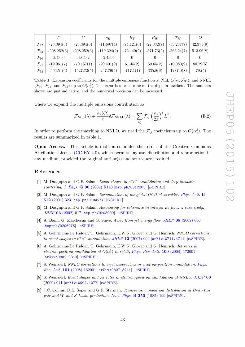
JHEP05(2015)102

T C ρH BT BW TM O

F22 -23.394(6) -23.394(6) -11.697(4) -74.121(6) -27.332(7) -53.287(7) 42.975(9)

F33 -208.252(3) -208.252(3) -119.324(2) -724.49(2) -371.76(2) -563.24(7) 513.96(8)

F10 -5.4396 -1.0532 -5.4396 0 0 0 0

F21 -19.951(7) -70.157(1) -20.401(9) 61.45(2) 59.65(2) -10.080(9) 80.79(5)

F32 -463.51(6) -1427.72(5) -247.79(4) -717.1(1) 335.8(9) -1287.0(8) -79.(5)

Table 1. Expansion coefficients for the multiple emissions function at NLL (F22, F33), and NNLL

(F10, F21, and F32) up to O(α3s). The error is meant to be on the digit in brackets. The numbers

shown are just indicative, and the numerical precision can be increased.

where we expand the multiple emissions contribution as

FNLL(λ) +αs(Q)

πδFNNLL(λ) =

∑

i,j

Fij

(αs

2π

)iLj . (E.2)

In order to perform the matching to NNLO, we need the Fij coefficients up to O(α3s). The

results are summarized in table 1.

Open Access. This article is distributed under the terms of the Creative Commons

Attribution License (CC-BY 4.0), which permits any use, distribution and reproduction in

any medium, provided the original author(s) and source are credited.

References

[1] M. Dasgupta and G.P. Salam, Event shapes in e+e− annihilation and deep inelastic

scattering, J. Phys. G 30 (2004) R143 [hep-ph/0312283] [INSPIRE].

[2] M. Dasgupta and G.P. Salam, Resummation of nonglobal QCD observables, Phys. Lett. B

512 (2001) 323 [hep-ph/0104277] [INSPIRE].

[3] M. Dasgupta and G.P. Salam, Accounting for coherence in interjet Et flow: a case study,

JHEP 03 (2002) 017 [hep-ph/0203009] [INSPIRE].

[4] A. Banfi, G. Marchesini and G. Smye, Away from jet energy flow, JHEP 08 (2002) 006

[hep-ph/0206076] [INSPIRE].

[5] A. Gehrmann-De Ridder, T. Gehrmann, E.W.N. Glover and G. Heinrich, NNLO corrections

to event shapes in e+e− annihilation, JHEP 12 (2007) 094 [arXiv:0711.4711] [INSPIRE].

[6] A. Gehrmann-De Ridder, T. Gehrmann, E.W.N. Glover and G. Heinrich, Jet rates in

electron-positron annihilation at O(α3s) in QCD, Phys. Rev. Lett. 100 (2008) 172001

[arXiv:0802.0813] [INSPIRE].

[7] S. Weinzierl, NNLO corrections to 3-jet observables in electron-positron annihilation, Phys.

Rev. Lett. 101 (2008) 162001 [arXiv:0807.3241] [INSPIRE].

[8] S. Weinzierl, Event shapes and jet rates in electron-positron annihilation at NNLO, JHEP 06

(2009) 041 [arXiv:0904.1077] [INSPIRE].

[9] J.C. Collins, D.E. Soper and G.F. Sterman, Transverse momentum distribution in Drell-Yan

pair and W and Z boson production, Nucl. Phys. B 250 (1985) 199 [INSPIRE].

– 43 –

JHEP05(2015)102

[10] S. Catani, L. Trentadue, G. Turnock and B.R. Webber, Resummation of large logarithms in

e+e− event shape distributions, Nucl. Phys. B 407 (1993) 3 [INSPIRE].

[11] R. Bonciani, S. Catani, M.L. Mangano and P. Nason, Sudakov resummation of multiparton

QCD cross-sections, Phys. Lett. B 575 (2003) 268 [hep-ph/0307035] [INSPIRE].

[12] S. Catani, G. Turnock, B.R. Webber and L. Trentadue, Thrust distribution in e+e−

annihilation, Phys. Lett. B 263 (1991) 491 [INSPIRE].

[13] S. Catani, G. Turnock and B.R. Webber, Heavy jet mass distribution in e+e− annihilation,

Phys. Lett. B 272 (1991) 368 [INSPIRE].

[14] S. Catani and B.R. Webber, Resummed C parameter distribution in e+e− annihilation,

Phys. Lett. B 427 (1998) 377 [hep-ph/9801350] [INSPIRE].

[15] S. Catani, G. Turnock and B.R. Webber, Jet broadening measures in e+e− annihilation,

Phys. Lett. B 295 (1992) 269 [INSPIRE].

[16] Y.L. Dokshitzer, A. Lucenti, G. Marchesini and G.P. Salam, On the QCD analysis of jet

broadening, JHEP 01 (1998) 011 [hep-ph/9801324] [INSPIRE].

[17] S. Catani, Y.L. Dokshitzer, M. Olsson, G. Turnock and B.R. Webber, New clustering

algorithm for multi-jet cross-sections in e+e− annihilation, Phys. Lett. B 269 (1991) 432

[INSPIRE].

[18] S. Catani, Y.L. Dokshitzer and B.R. Webber, Average number of jets in deep inelastic

scattering, Phys. Lett. B 322 (1994) 263 [INSPIRE].

[19] G. Dissertori and M. SchMelling, An improved theoretical prediction for the two jet rate in

e+e− annihilation, Phys. Lett. B 361 (1995) 167 [INSPIRE].

[20] C.F. Berger, T. Kucs and G.F. Sterman, Interjet energy flow/event shape correlations, Int. J.

Mod. Phys. A 18 (2003) 4159 [hep-ph/0212343] [INSPIRE].

[21] C.F. Berger, T. Kucs and G.F. Sterman, Event shape/energy flow correlations, Phys. Rev. D

68 (2003) 014012 [hep-ph/0303051] [INSPIRE].

[22] A.J. Larkoski, D. Neill and J. Thaler, Jet shapes with the broadening axis, JHEP 04 (2014)

017 [arXiv:1401.2158] [INSPIRE].

[23] A. Banfi, G.P. Salam and G. Zanderighi, Semi-numerical resummation of event shapes,

JHEP 01 (2002) 018 [hep-ph/0112156] [INSPIRE].

[24] A.J. Larkoski and J. Thaler, Unsafe but calculable: ratios of angularities in perturbative

QCD, JHEP 09 (2013) 137 [arXiv:1307.1699] [INSPIRE].

[25] A.J. Larkoski, I. Moult and D. Neill, Toward multi-differential cross sections: measuring two

angularities on a single jet, JHEP 09 (2014) 046 [arXiv:1401.4458] [INSPIRE].

[26] M. Procura, W.J. Waalewijn and L. Zeune, Resummation of double-differential cross sections

and fully-unintegrated parton distribution functions, JHEP 02 (2015) 117 [arXiv:1410.6483]

[INSPIRE].

[27] A. Banfi, G.P. Salam and G. Zanderighi, Principles of general final-state resummation and

automated implementation, JHEP 03 (2005) 073 [hep-ph/0407286] [INSPIRE].

[28] A. Banfi, G.P. Salam and G. Zanderighi, Phenomenology of event shapes at hadron colliders,

JHEP 06 (2010) 038 [arXiv:1001.4082] [INSPIRE].

– 44 –

JHEP05(2015)102

[29] A. Banfi, G.P. Salam and G. Zanderighi, Resummed event shapes at hadron-hadron colliders,

JHEP 08 (2004) 062 [hep-ph/0407287] [INSPIRE].

[30] T. Becher and M.D. Schwartz, A precise determination of αs from LEP thrust data using

effective field theory, JHEP 07 (2008) 034 [arXiv:0803.0342] [INSPIRE].

[31] P.F. Monni, T. Gehrmann and G. Luisoni, Two-loop soft corrections and resummation of the

thrust distribution in the dijet region, JHEP 08 (2011) 010 [arXiv:1105.4560] [INSPIRE].

[32] Y.-T. Chien and M.D. Schwartz, Resummation of heavy jet mass and comparison to LEP

data, JHEP 08 (2010) 058 [arXiv:1005.1644] [INSPIRE].

[33] T. Becher and G. Bell, NNLL resummation for jet broadening, JHEP 11 (2012) 126

[arXiv:1210.0580] [INSPIRE].

[34] S. Alioli et al., Combining higher-order resummation with multiple NLO calculations and

parton showers in GENEVA, JHEP 09 (2013) 120 [arXiv:1211.7049] [INSPIRE].

[35] D. de Florian and M. Grazzini, The back-to-back region in e+e− energy-energy correlation,

Nucl. Phys. B 704 (2005) 387 [hep-ph/0407241] [INSPIRE].

[36] T. Becher and M. Neubert, Drell-Yan production at small qT , transverse parton distributions

and the collinear anomaly, Eur. Phys. J. C 71 (2011) 1665 [arXiv:1007.4005] [INSPIRE].

[37] D. Kang, C. Lee and I.W. Stewart, Using 1-jettiness to measure 2 jets in DIS 3 ways, Phys.

Rev. D 88 (2013) 054004 [arXiv:1303.6952] [INSPIRE].

[38] Z.-B. Kang, X. Liu, S. Mantry and J.-W. Qiu, Probing nuclear dynamics in jet production

with a global event shape, Phys. Rev. D 88 (2013) 074020 [arXiv:1303.3063] [INSPIRE].

[39] Z.-B. Kang, X. Liu and S. Mantry, 1-jettiness DIS event shape: NNLL+NLO results, Phys.

Rev. D 90 (2014) 014041 [arXiv:1312.0301] [INSPIRE].

[40] G. Bozzi, S. Catani, D. de Florian and M. Grazzini, Transverse-momentum resummation and

the spectrum of the Higgs boson at the LHC, Nucl. Phys. B 737 (2006) 73 [hep-ph/0508068]

[INSPIRE].

[41] A. Banfi, M. Dasgupta and S. Marzani, QCD predictions for new variables to study dilepton

transverse momenta at hadron colliders, Phys. Lett. B 701 (2011) 75 [arXiv:1102.3594]

[INSPIRE].

[42] I.W. Stewart, F.J. Tackmann and W.J. Waalewijn, The beam thrust cross section for

Drell-Yan at NNLL order, Phys. Rev. Lett. 106 (2011) 032001 [arXiv:1005.4060] [INSPIRE].

[43] C.F. Berger, C. Marcantonini, I.W. Stewart, F.J. Tackmann and W.J. Waalewijn, Higgs

production with a central jet veto at NNLL+NNLO, JHEP 04 (2011) 092 [arXiv:1012.4480]

[INSPIRE].

[44] T. Becher and M. Neubert, Factorization and NNLL resummation for Higgs production with

a jet veto, JHEP 07 (2012) 108 [arXiv:1205.3806] [INSPIRE].

[45] T. Becher, M. Neubert and L. Rothen, Factorization and N3LLp +NNLO predictions for

the Higgs cross section with a jet veto, JHEP 10 (2013) 125 [arXiv:1307.0025] [INSPIRE].

[46] A. Banfi, P.F. Monni, G.P. Salam and G. Zanderighi, Higgs and Z-boson production with a

jet veto, Phys. Rev. Lett. 109 (2012) 202001 [arXiv:1206.4998] [INSPIRE].

[47] I.W. Stewart, F.J. Tackmann, J.R. Walsh and S. Zuberi, Jet pT resummation in Higgs

production at NNLL′ +NNLO, Phys. Rev. D 89 (2014) 054001 [arXiv:1307.1808]

[INSPIRE].

– 45 –

JHEP05(2015)102

[48] H.X. Zhu, C.S. Li, H.T. Li, D.Y. Shao and L.L. Yang, Transverse-momentum resummation

for top-quark pairs at hadron colliders, Phys. Rev. Lett. 110 (2013) 082001

[arXiv:1208.5774] [INSPIRE].

[49] S. Catani, M. Grazzini and A. Torre, Transverse-momentum resummation for heavy-quark

hadroproduction, Nucl. Phys. B 890 (2014) 518 [arXiv:1408.4564] [INSPIRE].

[50] I.W. Stewart, F.J. Tackmann and W.J. Waalewijn, N -jettiness: an inclusive event shape to

veto jets, Phys. Rev. Lett. 105 (2010) 092002 [arXiv:1004.2489] [INSPIRE].

[51] T.T. Jouttenus, I.W. Stewart, F.J. Tackmann and W.J. Waalewijn, The soft function for

exclusive N -jet production at hadron colliders, Phys. Rev. D 83 (2011) 114030

[arXiv:1102.4344] [INSPIRE].

[52] J. Fan, M. Reece and L.-T. Wang, Possible futures of electroweak precision: ILC, FCC-ee

and CEPC, arXiv:1411.1054 [INSPIRE].

[53] R. Brock et al., Planning the future of U.S. particle physics (Snowmass 2013). Section 3:

energy frontier, arXiv:1401.6081 [INSPIRE].

[54] S. Catani and M.H. Seymour, A general algorithm for calculating jet cross-sections in NLO

QCD, Nucl. Phys. B 485 (1997) 291 [Erratum ibid. B 510 (1998) 503] [hep-ph/9605323]

[INSPIRE].

[55] A. Gehrmann-De Ridder, T. Gehrmann, E.W.N. Glover and G. Heinrich, EERAD3: event

shapes and jet rates in electron-positron annihilation at order α3s, Comput. Phys. Commun.

185 (2014) 3331 [arXiv:1402.4140] [INSPIRE].

[56] S. Catani and M. Grazzini, QCD transverse-momentum resummation in gluon fusion

processes, Nucl. Phys. B 845 (2011) 297 [arXiv:1011.3918] [INSPIRE].

[57] S. Catani, B.R. Webber and G. Marchesini, QCD coherent branching and semiinclusive

processes at large x, Nucl. Phys. B 349 (1991) 635 [INSPIRE].

[58] A. Banfi, G.P. Salam and G. Zanderighi, NLL+NNLO predictions for jet-veto efficiencies

in Higgs-boson and Drell-Yan production, JHEP 06 (2012) 159 [arXiv:1203.5773] [INSPIRE].

[59] Z. Nagy, Next-to-leading order calculation of three jet observables in hadron hadron collision,

Phys. Rev. D 68 (2003) 094002 [hep-ph/0307268] [INSPIRE].

[60] M. Dasgupta and G.P. Salam, Resummed event shape variables in DIS, JHEP 08 (2002) 032

[hep-ph/0208073] [INSPIRE].

[61] M. Dasgupta and G.P. Salam, Resummation of the jet broadening in DIS, Eur. Phys. J. C

24 (2002) 213 [hep-ph/0110213] [INSPIRE].

[62] A.H. Hoang, D.W. Kolodrubetz, V. Mateu and I.W. Stewart, C parameter distribution at

N3LL′ including power corrections, arXiv:1411.6633 [INSPIRE].

– 46 –