The Florida LegislatureOffice of Economic and

Demographic Research850.487.1402http://edr.state.fl.us

Presented by:

Florida:Long-Range Financial Outlook

September 15, 2015

Economy RecoveringFlorida growth rates are generally returning to more typical levels and continue to show progress. However, the drags are more persistent than past events, and it will take another year to climb completely out of the hole left by the recession. In the various forecasts, normalcy has been largely achieved by FY 2016-17. Overall...

The recovery in the national economy is well underway. While most areas of commercial and consumer credit have significantly strengthened –residential credit for purchases still remains somewhat difficult for consumers to access with a weighted average credit score of 751 and LTV of 81 percent. Student loan and recently undertaken auto debts appear to be affecting the ability to qualify for residential credit.

By the close of the 2014-15 fiscal year, several key measures of the Florida economy had returned to or surpassed their prior peaks.

Most of the personal income metrics (real per capita income being a notable exception), some employment sectors and all of the tourism counts exceeded their prior peaks. Still other measures were posting solid year-over-year improvements, even if they were not yet back to peak performance levels. In the current forecast, none of the key construction metrics show a return to peak levels until 2021-22.

1

Upside Risks…Construction...

The “shadow inventory” of homes that are in foreclosure or carry delinquent or defaulted mortgages may contain a significant number of “ghost” homes that are distressed beyond realistic use, in that they have not been physically maintained or are located in distressed pockets that will not come back in a reasonable timeframe. This means that the supply has become two-tiered – viable homes and seriously distressed homes. To the extent that the number of viable homes is limited, new construction may come back quicker than expected.

More Buyers... In 2015, the first wave of homeowners affected by foreclosures and short sales are past the seven-year window generally needed to repair credit. While there is no evidence yet, atypical household formation will ultimately unwind—driving up the demand for housing.

2

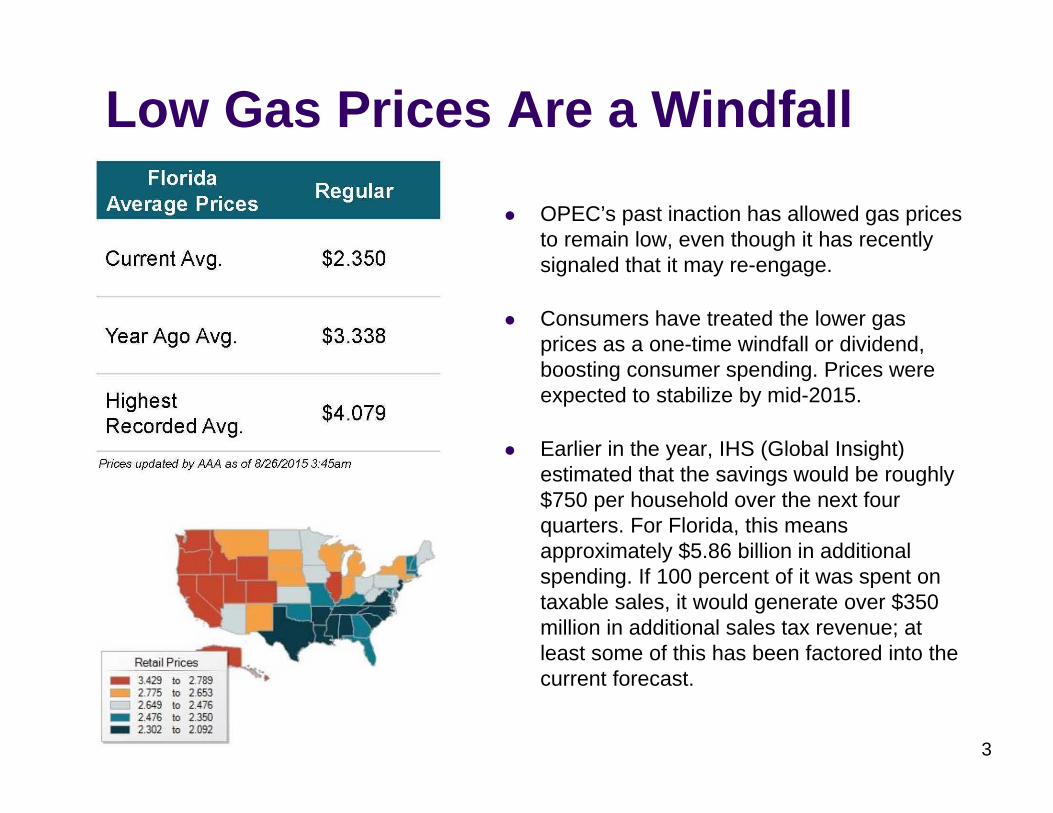
Low Gas Prices Are a Windfall

OPEC’s past inaction has allowed gas prices to remain low, even though it has recently signaled that it may re-engage.

Consumers have treated the lower gas prices as a one-time windfall or dividend, boosting consumer spending. Prices were expected to stabilize by mid-2015.

Earlier in the year, IHS (Global Insight) estimated that the savings would be roughly $750 per household over the next four quarters. For Florida, this means approximately $5.86 billion in additional spending. If 100 percent of it was spent on taxable sales, it would generate over $350 million in additional sales tax revenue; at least some of this has been factored into the current forecast.

3

Downside Risks…International and Financial Market Developments

Recent signs of instability and weakness in the Chinese economy have led to significant financial market concerns and even lower oil price expectations. The risk of a global recession has increased amidst the financial turmoil.

According to New York Federal Reserve President William Dudley, if the recent financial market volatility becomes prolonged, it could influence the U.S. economy through the wealth effect—meaning that stock market losses could lead Americans to cut back their spending. This effect would be further exacerbated by a global slowdown.

The current expansionary period in the United States is now over six years old. The Dow Jones Industrial Average more than doubled in value from June 2009 to June 2015, leading to questions of sustainability and the likelihood of a market correction (at least a 10% downward shift in a stock market index over a short period of time). Many market pundits were highlighting areas of apparent overvaluation well before the China-induced correction began in late August.

At the very least, it has caused the Federal Open Market Committee (FOMC) to question the expected move to raise interest rates in September 2015. The International Monetary Fund and the World Bank have both warned central banks to refrain from raising interest rates since risks to global growth are mounting. At a minimum, a delay would have spillover effects to the adopted economic forecast for Florida.

4

Debt AnalysisIn a Moody’s rating analysis of the state released August 20, 2015, they highlighted the state’s strong fiscal practices saying: “Florida has a history of strong financial management, evidence[d] by frequent revenue forecasts and timely financial reporting, including an annual debt affordability analysis. In addition the state benefits from constitutional protections like the mandate to fund the budget stabilization fund, which allows for a budgetary cushion in the event of revenue volatility.”

Highest Level Credit Ratings: Fitch “AAA” with stable outlook (unchanged); Moody’s “Aa1” with stable outlook (unchanged); Standard and Poor’s “AAA” with stable outlook (unchanged).

Total state debt outstanding at June 30, 2014, was $24.2 billion, approximately $400 million less than the prior fiscal year. Of this, net tax-supported debt totaled $20.0 billion for programs supported by state tax revenues or tax-like revenues. Total state direct debt outstanding at June 30, 2015, will increase due to the execution of the Department of Transportation’s I-4 Ultimate public-private partnership agreement.

During the Outlook period, debt service payments are expected to be approximately $2.1 billion in Fiscal Year 2016-17, $2.3 billion in Fiscal Year 2017-18, and $2.1 billion in Fiscal Year 2018-19 with the increase associated with mandatory payments for DOT contracts.

5

General Revenue Forecast

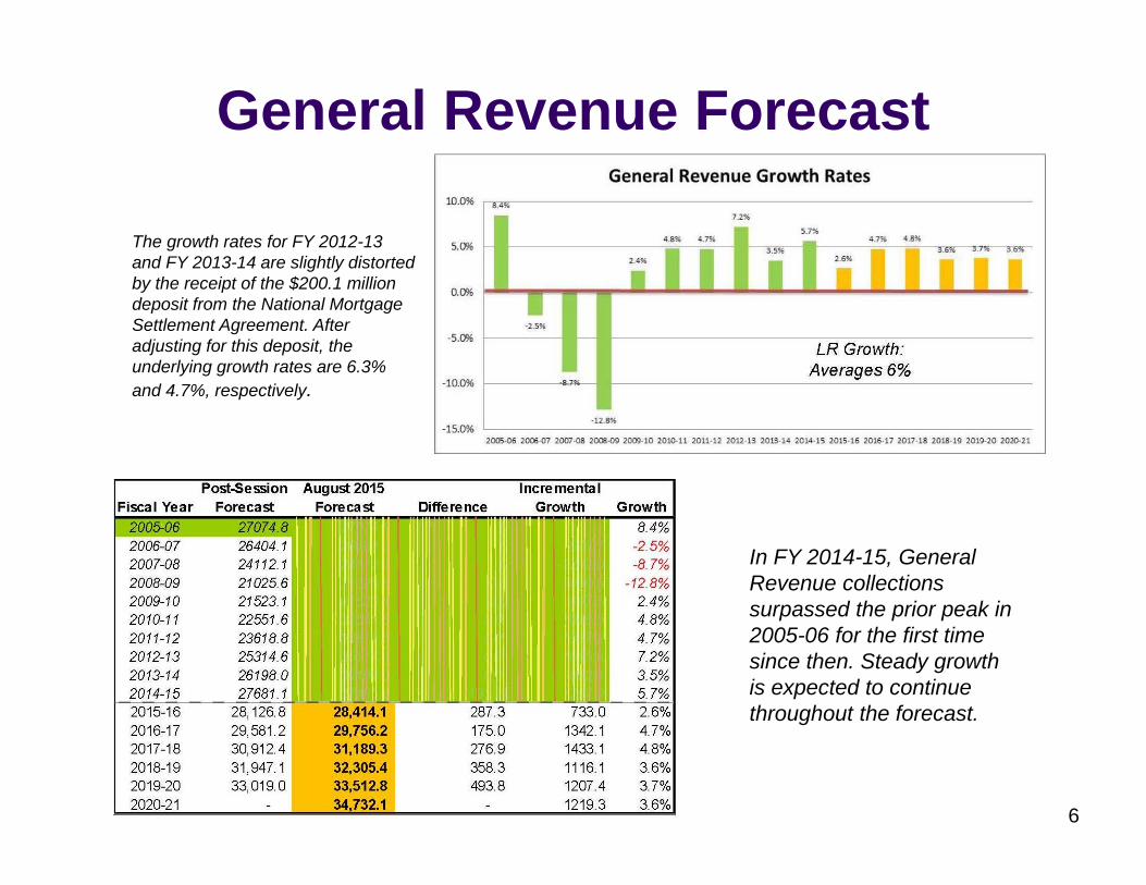
In FY 2014-15, General Revenue collections surpassed the prior peak in 2005-06 for the first time since then. Steady growth is expected to continue throughout the forecast.

The growth rates for FY 2012-13 and FY 2013-14 are slightly distorted by the receipt of the $200.1 million deposit from the National Mortgage Settlement Agreement. After adjusting for this deposit, the underlying growth rates are 6.3% and 4.7%, respectively.

LR Growth: Averages 6%

6

GR Unallocated & Other Reserves

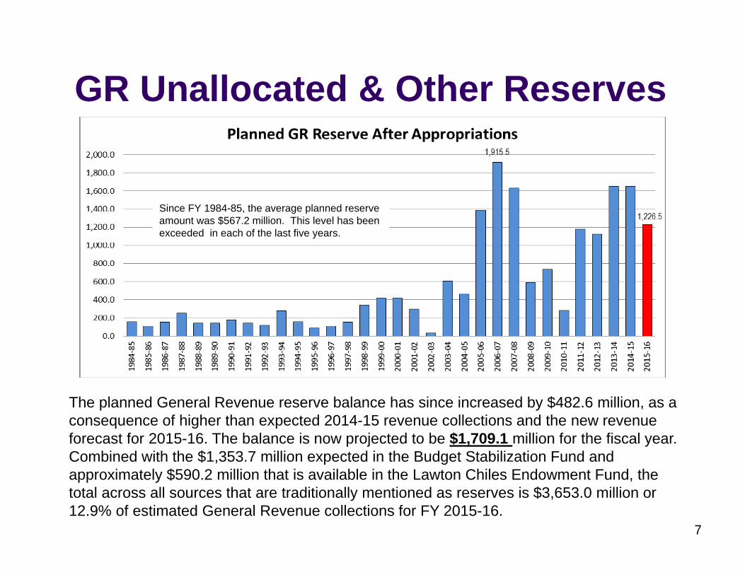
The planned General Revenue reserve balance has since increased by $482.6 million, as a consequence of higher than expected 2014-15 revenue collections and the new revenue forecast for 2015-16. The balance is now projected to be $1,709.1 million for the fiscal year. Combined with the $1,353.7 million expected in the Budget Stabilization Fund and approximately $590.2 million that is available in the Lawton Chiles Endowment Fund, the total across all sources that are traditionally mentioned as reserves is $3,653.0 million or 12.9% of estimated General Revenue collections for FY 2015-16.

7

Since FY 1984-85, the average planned reserve amount was $567.2 million. This level has been exceeded in each of the last five years.

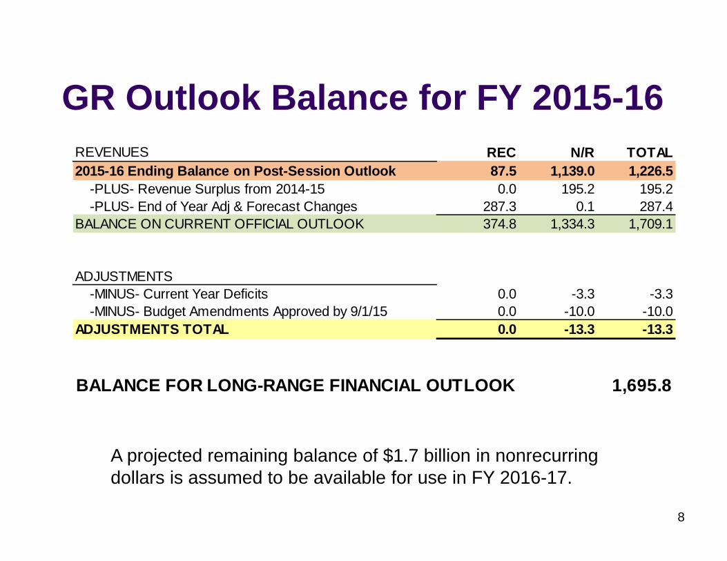
GR Outlook Balance for FY 2015-16

A projected remaining balance of $1.7 billion in nonrecurring dollars is assumed to be available for use in FY 2016-17.

8

REVENUES REC N/R TOTAL2015-16 Ending Balance on Post-Session Outlook 87.5 1,139.0 1,226.5 -PLUS- Revenue Surplus from 2014-15 0.0 195.2 195.2 -PLUS- End of Year Adj & Forecast Changes 287.3 0.1 287.4BALANCE ON CURRENT OFFICIAL OUTLOOK 374.8 1,334.3 1,709.1

ADJUSTMENTS -MINUS- Current Year Deficits 0.0 -3.3 -3.3 -MINUS- Budget Amendments Approved by 9/1/15 0.0 -10.0 -10.0ADJUSTMENTS TOTAL 0.0 -13.3 -13.3

BALANCE FOR LONG-RANGE FINANCIAL OUTLOOK 1,695.8

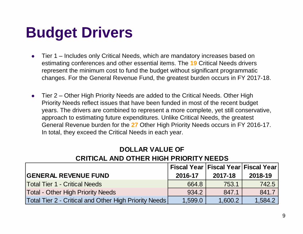
Budget DriversTier 1 – Includes only Critical Needs, which are mandatory increases based on estimating conferences and other essential items. The 19 Critical Needs drivers represent the minimum cost to fund the budget without significant programmatic changes. For the General Revenue Fund, the greatest burden occurs in FY 2017-18.

Tier 2 – Other High Priority Needs are added to the Critical Needs. Other High Priority Needs reflect issues that have been funded in most of the recent budget years. The drivers are combined to represent a more complete, yet still conservative, approach to estimating future expenditures. Unlike Critical Needs, the greatest General Revenue burden for the 27 Other High Priority Needs occurs in FY 2016-17. In total, they exceed the Critical Needs in each year.

9

GENERAL REVENUE FUNDFiscal Year

2016-17Fiscal Year

2017-18Fiscal Year

2018-19Total Tier 1 - Critical Needs 664.8 753.1 742.5 Total - Other High Priority Needs 934.2 847.1 841.7 Total Tier 2 - Critical and Other High Priority Needs 1,599.0 1,600.2 1,584.2

DOLLAR VALUE OFCRITICAL AND OTHER HIGH PRIORITY NEEDS

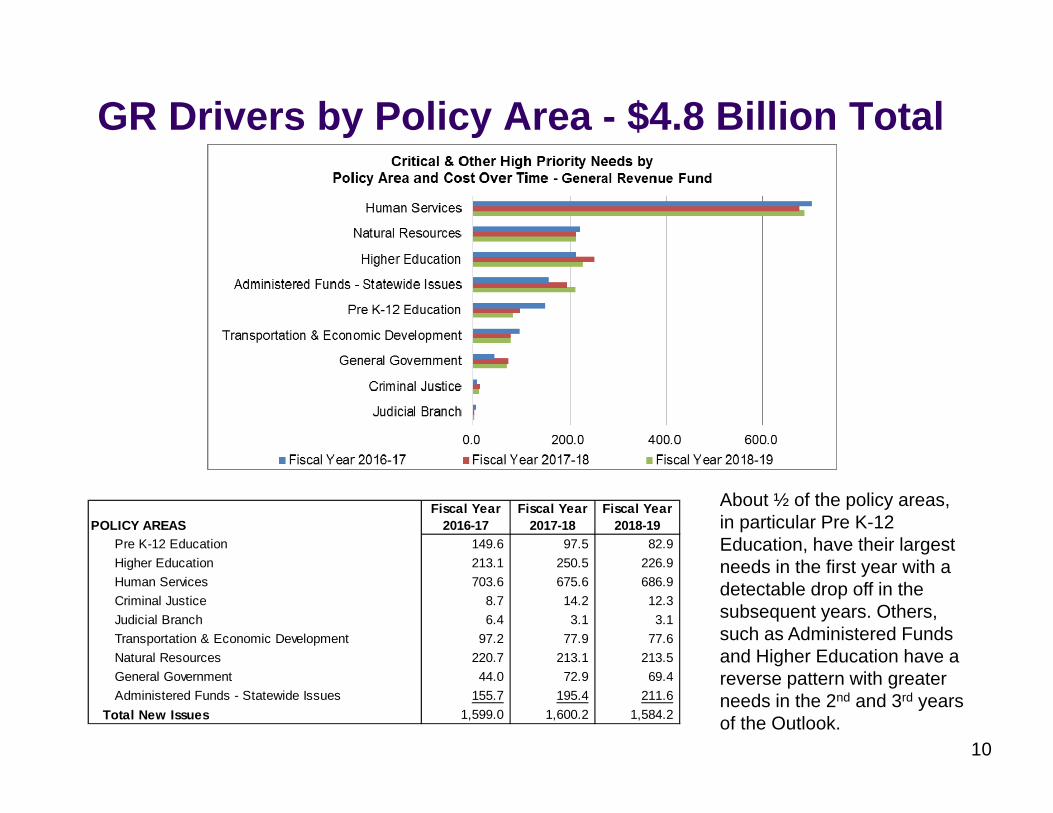
GR Drivers by Policy Area - $4.8 Billion Total

About ½ of the policy areas, in particular Pre K-12 Education, have their largest needs in the first year with a detectable drop off in the subsequent years. Others, such as Administered Funds and Higher Education have a reverse pattern with greater needs in the 2nd and 3rd years of the Outlook.

10

POLICY AREASFiscal Year

2016-17Fiscal Year

2017-18Fiscal Year

2018-19Pre K-12 Education 149.6 97.5 82.9Higher Education 213.1 250.5 226.9Human Services 703.6 675.6 686.9Criminal Justice 8.7 14.2 12.3Judicial Branch 6.4 3.1 3.1Transportation & Economic Development 97.2 77.9 77.6Natural Resources 220.7 213.1 213.5General Government 44.0 72.9 69.4Administered Funds - Statewide Issues 155.7 195.4 211.6

Total New Issues 1,599.0 1,600.2 1,584.2

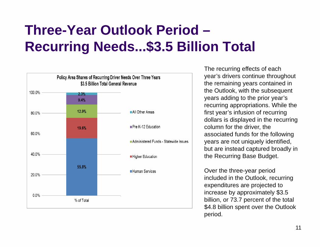
Three-Year Outlook Period –Recurring Needs...$3.5 Billion Total

The recurring effects of each year’s drivers continue throughout the remaining years contained in the Outlook, with the subsequent years adding to the prior year’s recurring appropriations. While the first year’s infusion of recurring dollars is displayed in the recurring column for the driver, the associated funds for the following years are not uniquely identified, but are instead captured broadly in the Recurring Base Budget.

Over the three-year period included in the Outlook, recurring expenditures are projected to increase by approximately $3.5 billion, or 73.7 percent of the total $4.8 billion spent over the Outlook period.

11

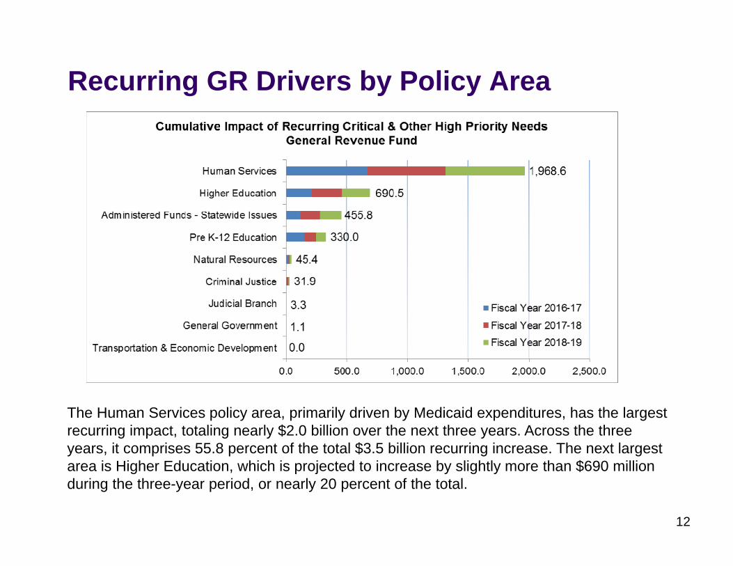
Recurring GR Drivers by Policy Area

The Human Services policy area, primarily driven by Medicaid expenditures, has the largest recurring impact, totaling nearly $2.0 billion over the next three years. Across the three years, it comprises 55.8 percent of the total $3.5 billion recurring increase. The next largest area is Higher Education, which is projected to increase by slightly more than $690 million during the three-year period, or nearly 20 percent of the total.

12

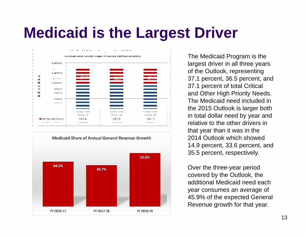
Medicaid is the Largest DriverThe Medicaid Program is the largest driver in all three years of the Outlook, representing37.1 percent, 36.5 percent, and 37.1 percent of total Critical and Other High Priority Needs.The Medicaid need included in the 2015 Outlook is larger both in total dollar need by year and relative to the other drivers in that year than it was in the 2014 Outlook which showed 14.9 percent, 33.6 percent, and 35.5 percent, respectively.

Over the three-year period covered by the Outlook, the additional Medicaid need each year consumes an average of 45.9% of the expected General Revenue growth for that year.

13

37.1%

37.1% 36.5% 37.1%

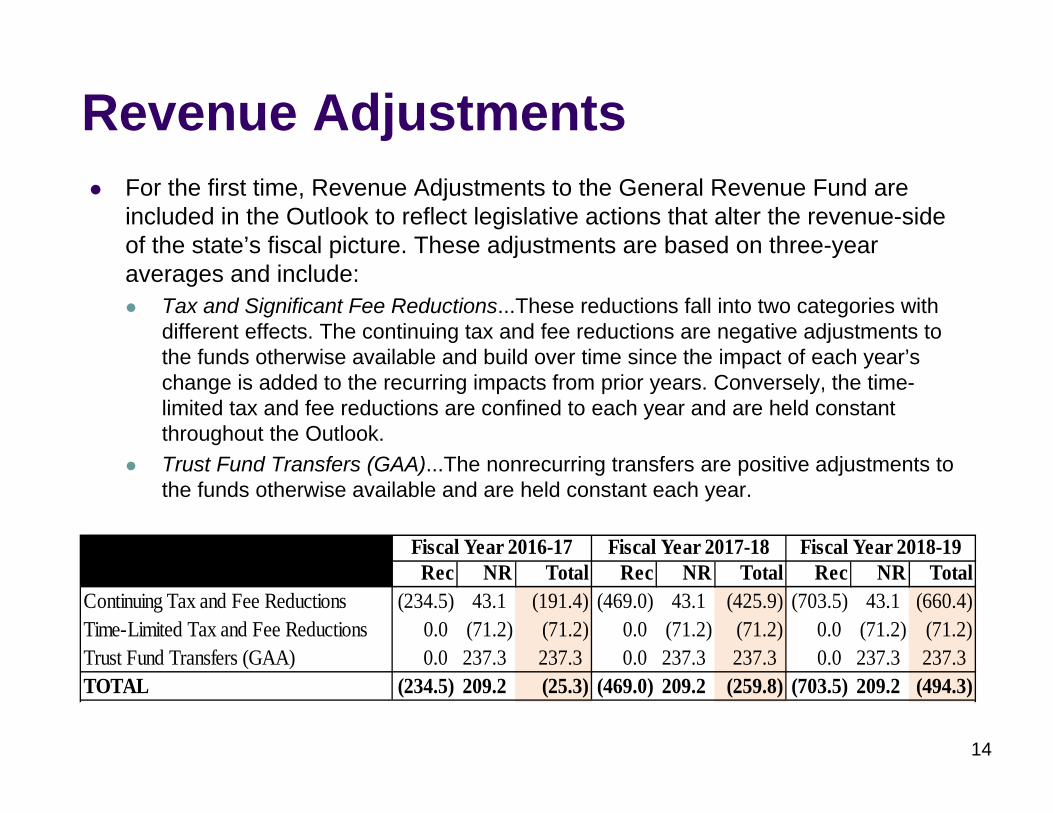
Revenue AdjustmentsFor the first time, Revenue Adjustments to the General Revenue Fund are included in the Outlook to reflect legislative actions that alter the revenue-side of the state’s fiscal picture. These adjustments are based on three-year averages and include:

Tax and Significant Fee Reductions...These reductions fall into two categories with different effects. The continuing tax and fee reductions are negative adjustments to the funds otherwise available and build over time since the impact of each year’s change is added to the recurring impacts from prior years. Conversely, the time-limited tax and fee reductions are confined to each year and are held constant throughout the Outlook. Trust Fund Transfers (GAA)...The nonrecurring transfers are positive adjustments to the funds otherwise available and are held constant each year.

14

Rec NR Total Rec NR Total Rec NR TotalContinuing Tax and Fee Reductions (234.5) 43.1 (191.4) (469.0) 43.1 (425.9) (703.5) 43.1 (660.4)Time-Limited Tax and Fee Reductions 0.0 (71.2) (71.2) 0.0 (71.2) (71.2) 0.0 (71.2) (71.2)Trust Fund Transfers (GAA) 0.0 237.3 237.3 0.0 237.3 237.3 0.0 237.3 237.3TOTAL (234.5) 209.2 (25.3) (469.0) 209.2 (259.8) (703.5) 209.2 (494.3)

Fiscal Year 2016-17 Fiscal Year 2017-18 Fiscal Year 2018-19

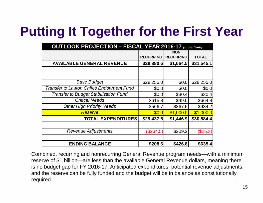
Putting It Together for the First Year

Combined, recurring and nonrecurring General Revenue program needs—with a minimum reserve of $1 billion—are less than the available General Revenue dollars, meaning there is no budget gap for FY 2016-17. Anticipated expenditures, potential revenue adjustments, and the reserve can be fully funded and the budget will be in balance as constitutionally required.

15

RECURRINGNON

RECURRING TOTAL

AVAILABLE GENERAL REVENUE $29,880.6 $1,664.5 $31,545.1

Base Budget $28,255.0 $0.0 $28,255.0 Transfer to Lawton Chiles Endowment Fund $0.0 $0.0 $0.0

Transfer to Budget Stabilization Fund $0.0 $30.4 $30.4 Critical Needs $615.8 $49.0 $664.8

Other High Priority Needs $566.7 $367.5 $934.2 Reserve $0.0 $1,000.0 $1,000.0

TOTAL EXPENDITURES $29,437.5 $1,446.9 $30,884.4

Revenue Adjustments ($234.5) $209.2 ($25.3)

ENDING BALANCE $208.6 $426.8 $635.4

OUTLOOK PROJECTION – FISCAL YEAR 2016-17 (in millions)

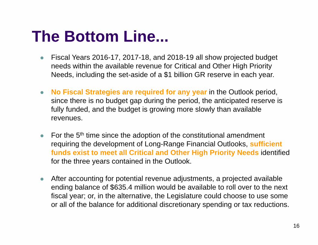
The Bottom Line...Fiscal Years 2016-17, 2017-18, and 2018-19 all show projected budget needs within the available revenue for Critical and Other High Priority Needs, including the set-aside of a $1 billion GR reserve in each year.

No Fiscal Strategies are required for any year in the Outlook period, since there is no budget gap during the period, the anticipated reserve is fully funded, and the budget is growing more slowly than available revenues.

For the 5th time since the adoption of the constitutional amendment requiring the development of Long-Range Financial Outlooks, sufficient funds exist to meet all Critical and Other High Priority Needs identified for the three years contained in the Outlook.

After accounting for potential revenue adjustments, a projected available ending balance of $635.4 million would be available to roll over to the next fiscal year; or, in the alternative, the Legislature could choose to use some or all of the balance for additional discretionary spending or tax reductions.

16

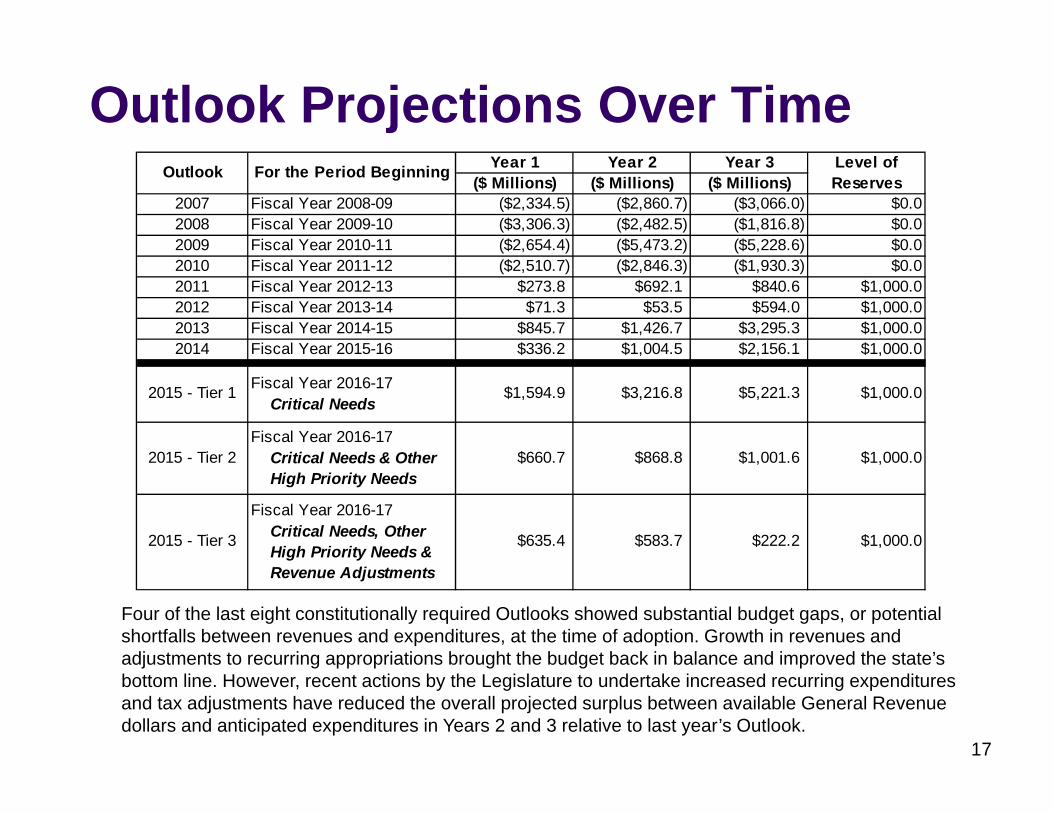
Outlook Projections Over Time

Four of the last eight constitutionally required Outlooks showed substantial budget gaps, or potential shortfalls between revenues and expenditures, at the time of adoption. Growth in revenues and adjustments to recurring appropriations brought the budget back in balance and improved the state’s bottom line. However, recent actions by the Legislature to undertake increased recurring expenditures and tax adjustments have reduced the overall projected surplus between available General Revenue dollars and anticipated expenditures in Years 2 and 3 relative to last year’s Outlook.

17

Year 1 Year 2 Year 3($ Millions) ($ Millions) ($ Millions)

2007 Fiscal Year 2008-09 ($2,334.5) ($2,860.7) ($3,066.0) $0.0 2008 Fiscal Year 2009-10 ($3,306.3) ($2,482.5) ($1,816.8) $0.0 2009 Fiscal Year 2010-11 ($2,654.4) ($5,473.2) ($5,228.6) $0.0 2010 Fiscal Year 2011-12 ($2,510.7) ($2,846.3) ($1,930.3) $0.0 2011 Fiscal Year 2012-13 $273.8 $692.1 $840.6 $1,000.0 2012 Fiscal Year 2013-14 $71.3 $53.5 $594.0 $1,000.0 2013 Fiscal Year 2014-15 $845.7 $1,426.7 $3,295.3 $1,000.0 2014 Fiscal Year 2015-16 $336.2 $1,004.5 $2,156.1 $1,000.0

2015 - Tier 1 Fiscal Year 2016-17 Critical Needs

$1,594.9 $3,216.8 $5,221.3 $1,000.0

2015 - Tier 2Fiscal Year 2016-17 Critical Needs & Other High Priority Needs

$660.7 $868.8 $1,001.6 $1,000.0

2015 - Tier 3

Fiscal Year 2016-17 Critical Needs, Other High Priority Needs & Revenue Adjustments

$635.4 $583.7 $222.2 $1,000.0

Outlook For the Period Beginning Level of Reserves

RiskThe positive budget outlook is heavily reliant on the projected balance forward levels being available, the $1.0 billion reserve not being used, and the growth levels for General Revenue and the major trust funds being achieved. As an example of the Outlook’s sensitivity to risk, it would only take a 3.4% reduction in the General Revenue Estimate for FY 2016-17 to force the use of the $1.0 billion reserve and drive at least two of the scenarios (Tier 2 and Tier 3) negative in the second year. A current-year change of this magnitude last happened in FY 2008-09.

Assuming the $1 billion reserve is strictly adhered to each year, and depending on which scenario is pursued (Tier 1, Tier 2, or Tier 3), all or a portion of the projected ending balance can be invested in additional recurring issues in Fiscal Year 2016-17 without causing a budget gap in Fiscal Years 2017-18 or 2018-19. However, Tier 3 already shows that the recurring expenditures are beginning to outpace available recurring revenues in FY 2018-19.

This is because recurring investments made in Year 1 of the Outlook have a compounding effect over time and reduce future ending balances. Each of the three scenarios has a different growth pattern over time, affecting how large the additional recurring investment—the amount above the level already contemplated—can be in the first year.

18

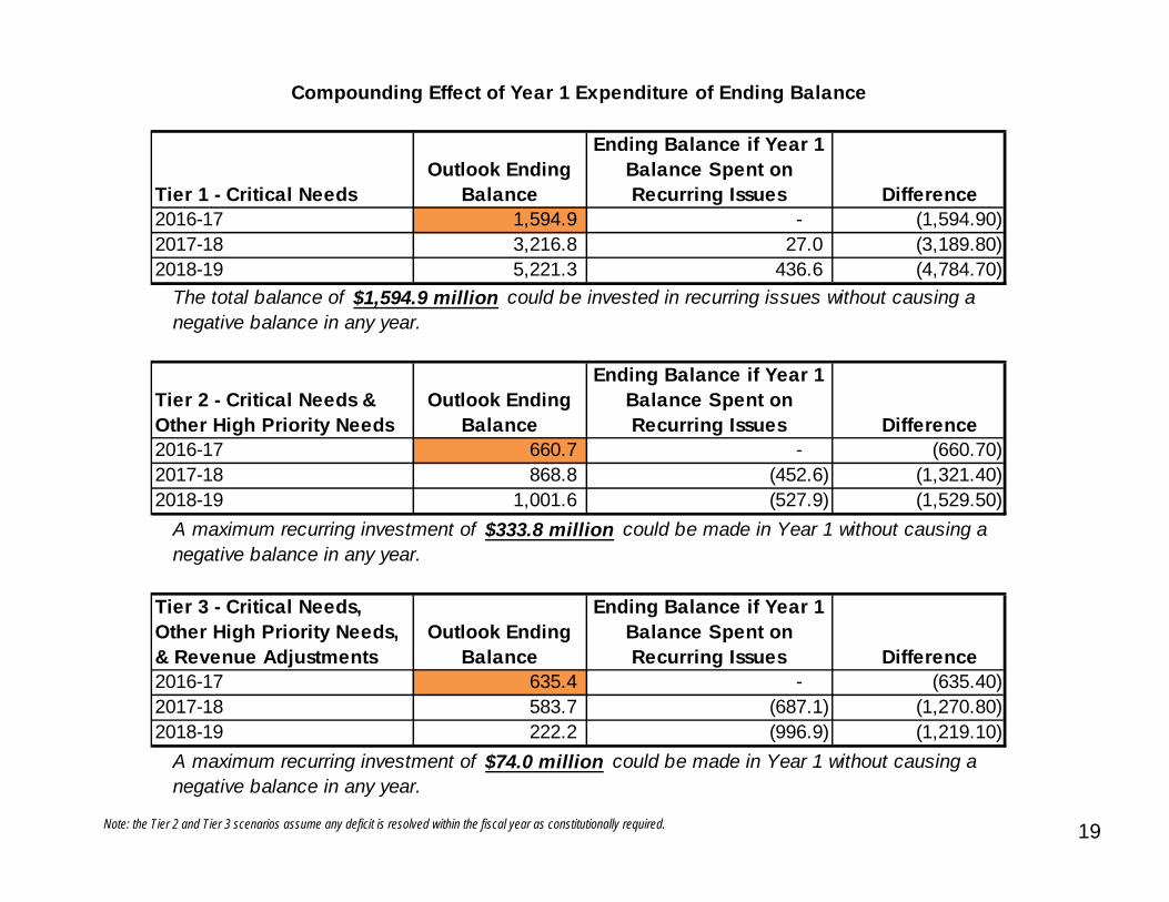
19Note: the Tier 2 and Tier 3 scenarios assume any deficit is resolved within the fiscal year as constitutionally required.

Tier 1 - Critical NeedsOutlook Ending

Balance

Ending Balance if Year 1 Balance Spent on Recurring Issues Difference

2016-17 1,594.9 - (1,594.90) 2017-18 3,216.8 27.0 (3,189.80) 2018-19 5,221.3 436.6 (4,784.70)

Tier 2 - Critical Needs & Other High Priority Needs

Outlook Ending Balance

Ending Balance if Year 1 Balance Spent on Recurring Issues Difference

2016-17 660.7 - (660.70) 2017-18 868.8 (452.6) (1,321.40) 2018-19 1,001.6 (527.9) (1,529.50)

Tier 3 - Critical Needs, Other High Priority Needs, & Revenue Adjustments

Outlook Ending Balance

Ending Balance if Year 1 Balance Spent on Recurring Issues Difference

2016-17 635.4 - (635.40) 2017-18 583.7 (687.1) (1,270.80) 2018-19 222.2 (996.9) (1,219.10)

Compounding Effect of Year 1 Expenditure of Ending Balance

The total balance of $1,594.9 million could be invested in recurring issues without causing a negative balance in any year.

A maximum recurring investment of $333.8 million could be made in Year 1 without causing a negative balance in any year.

A maximum recurring investment of $74.0 million could be made in Year 1 without causing a negative balance in any year.

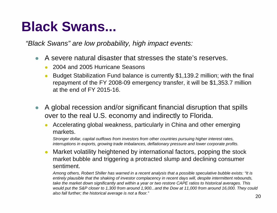
Black Swans...“Black Swans” are low probability, high impact events:

A severe natural disaster that stresses the state’s reserves.2004 and 2005 Hurricane SeasonsBudget Stabilization Fund balance is currently $1,139.2 million; with the final repayment of the FY 2008-09 emergency transfer, it will be $1,353.7 million at the end of FY 2015-16.

A global recession and/or significant financial disruption that spills over to the real U.S. economy and indirectly to Florida.

Accelerating global weakness, particularly in China and other emerging markets.Stronger dollar, capital outflows from investors from other countries pursuing higher interest rates, interruptions in exports, growing trade imbalances, deflationary pressure and lower corporate profits.

Market volatility heightened by international factors, popping the stock market bubble and triggering a protracted slump and declining consumer sentiment.Among others, Robert Shiller has warned in a recent analysis that a possible speculative bubble exists: “It is entirely plausible that the shaking of investor complacency in recent days will, despite intermittent rebounds, take the market down significantly and within a year or two restore CAPE ratios to historical averages. This would put the S&P closer to 1,300 from around 1,900...and the Dow at 11,000 from around 16,000. They could also fall further; the historical average is not a floor.”

20

21

Supporting Economic Material...

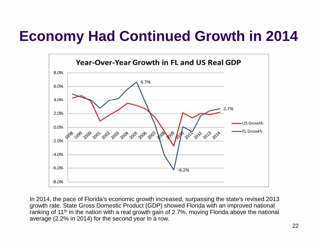
Economy Had Continued Growth in 2014

22

In 2014, the pace of Florida’s economic growth increased, surpassing the state’s revised 2013 growth rate. State Gross Domestic Product (GDP) showed Florida with an improved national ranking of 11th in the nation with a real growth gain of 2.7%, moving Florida above the national average (2.2% in 2014) for the second year in a row.

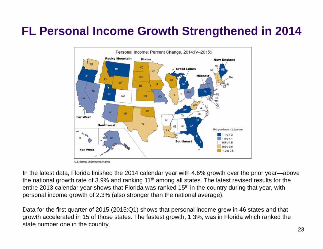
FL Personal Income Growth Strengthened in 2014

23

In the latest data, Florida finished the 2014 calendar year with 4.6% growth over the prior year—above the national growth rate of 3.9% and ranking 11th among all states. The latest revised results for the entire 2013 calendar year shows that Florida was ranked 15th in the country during that year, with personal income growth of 2.3% (also stronger than the national average).

Data for the first quarter of 2015 (2015:Q1) shows that personal income grew in 46 states and that growth accelerated in 15 of those states. The fastest growth, 1.3%, was in Florida which ranked the state number one in the country.

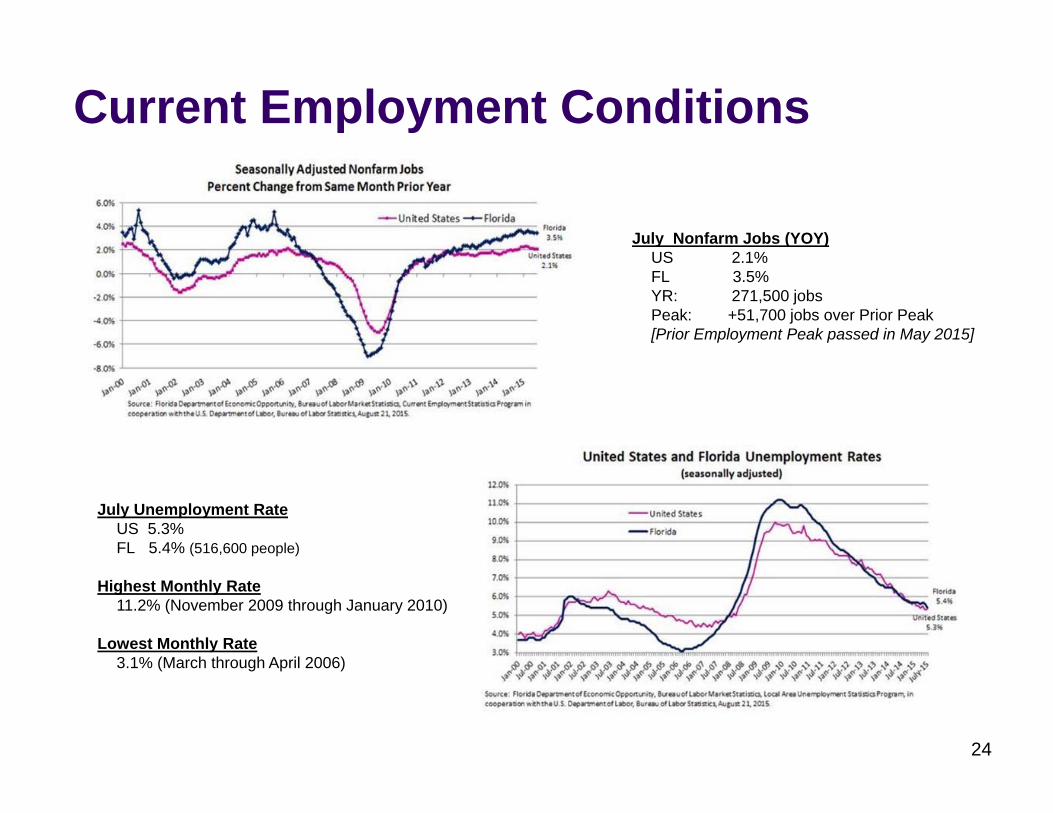
July Nonfarm Jobs (YOY)US 2.1%FL 3.5%YR: 271,500 jobsPeak: +51,700 jobs over Prior Peak[Prior Employment Peak passed in May 2015]

July Unemployment RateUS 5.3%FL 5.4% (516,600 people)

Highest Monthly Rate11.2% (November 2009 through January 2010)

Lowest Monthly Rate3.1% (March through April 2006)

Current Employment Conditions

24

Florida’s Job MarketFlorida’s job market is still recovering. It took 8 years, but the state has finally passed its most recent peak. However, passing the previous peak does not mean the same thing today as it did then.

Florida’s prime working-age population (aged 25-54) has been adding people each month, so even more jobs need to be created to address the population increase since 2007.

It would take the creation of an additional 581,000 jobs for the same percentage of the total population to be working as was the case at the peak, but the unemployment rate at the time was extraordinarily low (3.7%).

A more reasonable benchmark would use an unemployment rate of 5.0%, suggesting that another 460,000 jobs would need to be created over the current level.

25

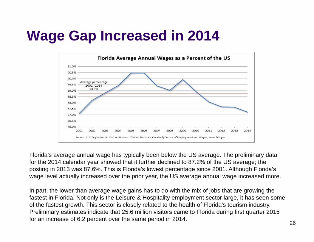
Wage Gap Increased in 2014

26

Florida’s average annual wage has typically been below the US average. The preliminary data for the 2014 calendar year showed that it further declined to 87.2% of the US average; the posting in 2013 was 87.6%. This is Florida’s lowest percentage since 2001. Although Florida’s wage level actually increased over the prior year, the US average annual wage increased more.

In part, the lower than average wage gains has to do with the mix of jobs that are growing the fastest in Florida. Not only is the Leisure & Hospitality employment sector large, it has seen some of the fastest growth. This sector is closely related to the health of Florida’s tourism industry. Preliminary estimates indicate that 25.6 million visitors came to Florida during first quarter 2015 for an increase of 6.2 percent over the same period in 2014.

Population Growth RecoveringPopulation growth is the state’s primary engine of economic growth, fueling both employment and income growth.

Population growth is expected to continue strengthening, showing increasing rates of growth over the next few years. In the near-term, Florida is expected to grow by 1.45% between 2014 and 2015 –then continue its recovery, averaging 1.49% between 2015 and 2020. Most of Florida’s population growth through 2030 will be from net migration (94%). Nationally, average annual growth will be about 0.75% between 2014 and 2030.

The future will be different than the past; Florida’s annual average long-term growth rate between 1970 and 1995 was over 3%.

Florida is on track to break the 20 million mark prior to April 1, 2016, after surpassing New York this year to become the third most populous state.

27

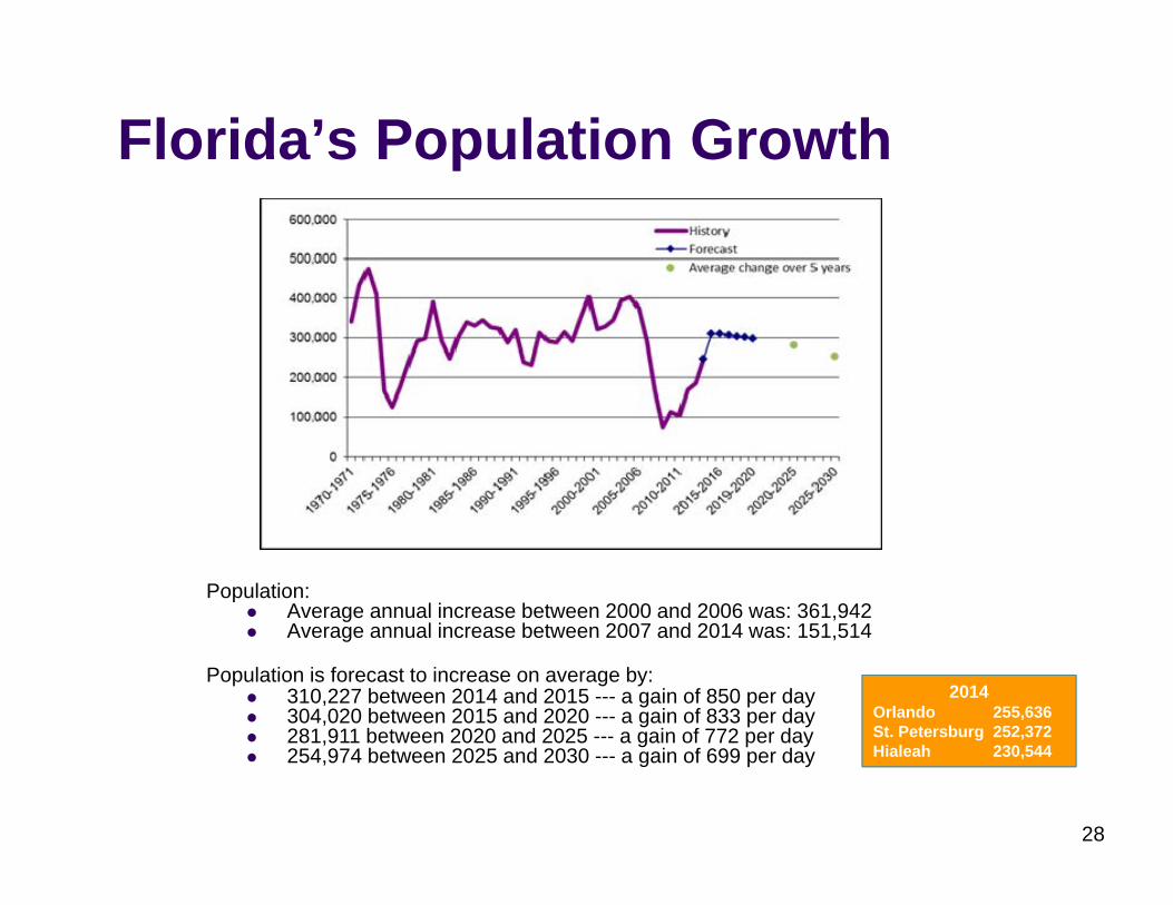
Florida’s Population Growth

Population:Average annual increase between 2000 and 2006 was: 361,942Average annual increase between 2007 and 2014 was: 151,514

Population is forecast to increase on average by:310,227 between 2014 and 2015 --- a gain of 850 per day304,020 between 2015 and 2020 --- a gain of 833 per day281,911 between 2020 and 2025 --- a gain of 772 per day254,974 between 2025 and 2030 --- a gain of 699 per day

2014Orlando 255,636St. Petersburg 252,372Hialeah 230,544

28

Population Growth by Age Group

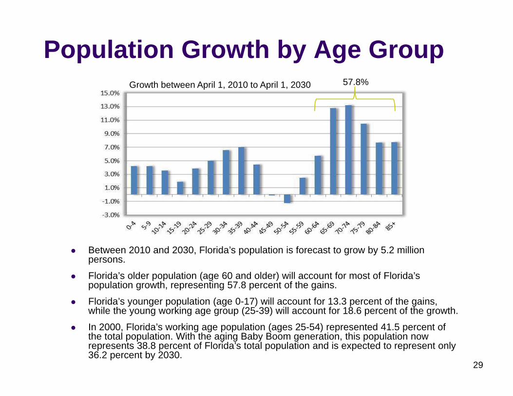
Between 2010 and 2030, Florida’s population is forecast to grow by 5.2 million persons.

Florida’s older population (age 60 and older) will account for most of Florida’s population growth, representing 57.8 percent of the gains.

Florida’s younger population (age 0-17) will account for 13.3 percent of the gains, while the young working age group (25-39) will account for 18.6 percent of the growth.

In 2000, Florida’s working age population (ages 25-54) represented 41.5 percent of the total population. With the aging Baby Boom generation, this population now represents 38.8 percent of Florida’s total population and is expected to represent only 36.2 percent by 2030.

Growth between April 1, 2010 to April 1, 2030 57.8%

29

Florida Housing is Generally Improving

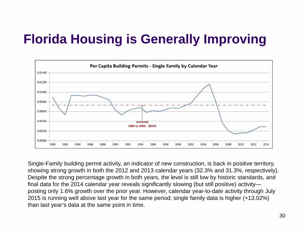
Single-Family building permit activity, an indicator of new construction, is back in positive territory, showing strong growth in both the 2012 and 2013 calendar years (32.3% and 31.3%, respectively). Despite the strong percentage growth in both years, the level is still low by historic standards, and final data for the 2014 calendar year reveals significantly slowing (but still positive) activity—posting only 1.6% growth over the prior year. However, calendar year-to-date activity through July 2015 is running well above last year for the same period; single family data is higher (+13.02%) than last year’s data at the same point in time.

30

Documentary Stamp Collections(Preliminary: Reflecting All Activity)

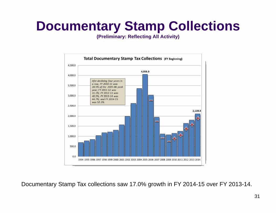
Documentary Stamp Tax collections saw 17.0% growth in FY 2014-15 over FY 2013-14.

31

Sales Mix Still Points to Subdued Pricing…

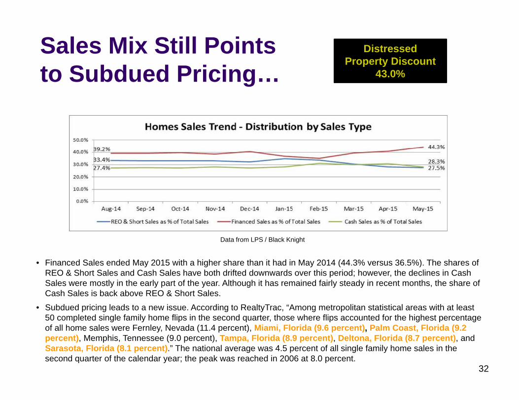
• Financed Sales ended May 2015 with a higher share than it had in May 2014 (44.3% versus 36.5%). The shares of REO & Short Sales and Cash Sales have both drifted downwards over this period; however, the declines in Cash Sales were mostly in the early part of the year. Although it has remained fairly steady in recent months, the share of Cash Sales is back above REO & Short Sales.

• Subdued pricing leads to a new issue. According to RealtyTrac, “Among metropolitan statistical areas with at least 50 completed single family home flips in the second quarter, those where flips accounted for the highest percentage of all home sales were Fernley, Nevada (11.4 percent), Miami, Florida (9.6 percent), Palm Coast, Florida (9.2 percent), Memphis, Tennessee (9.0 percent), Tampa, Florida (8.9 percent), Deltona, Florida (8.7 percent), and Sarasota, Florida (8.1 percent).” The national average was 4.5 percent of all single family home sales in the second quarter of the calendar year; the peak was reached in 2006 at 8.0 percent.

Distressed Property Discount

43.0%

Data from LPS / Black Knight

32

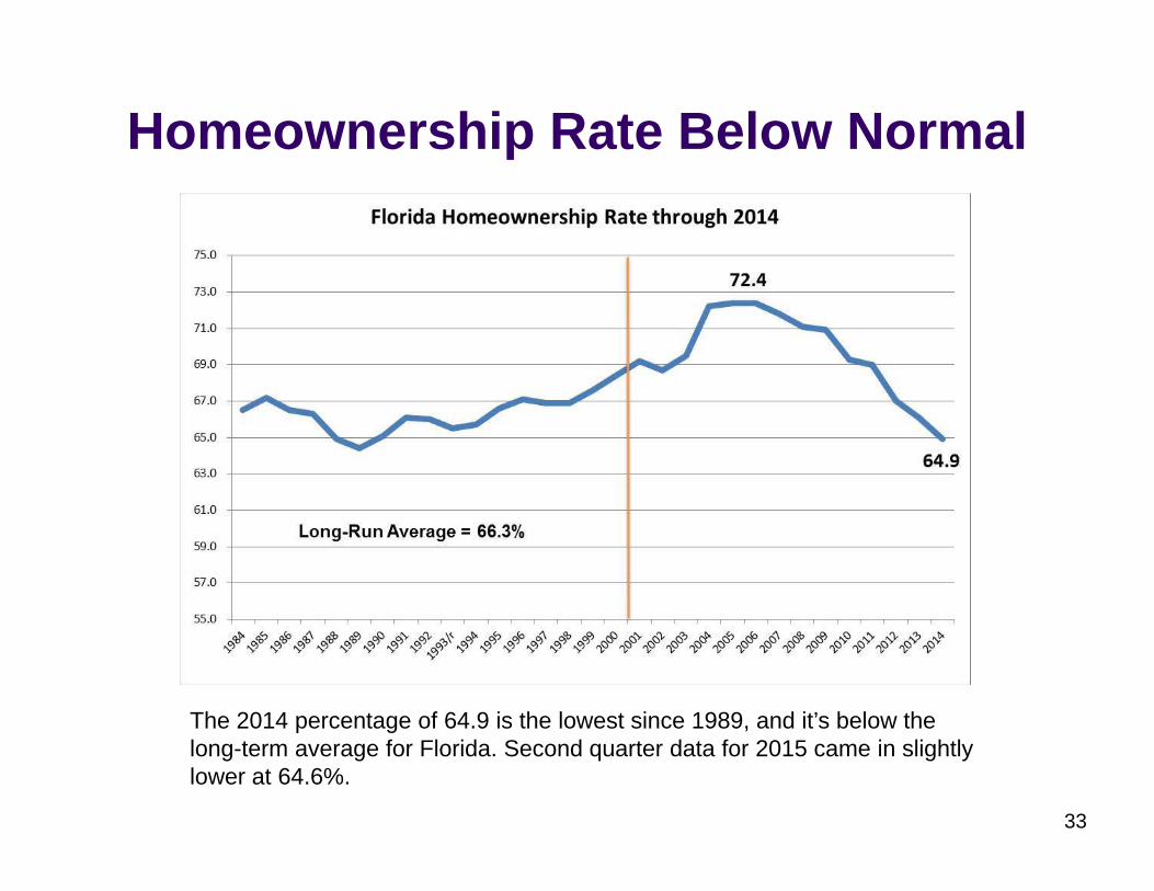
Homeownership Rate Below Normal

The 2014 percentage of 64.9 is the lowest since 1989, and it’s below the long-term average for Florida. Second quarter data for 2015 came in slightly lower at 64.6%.

33

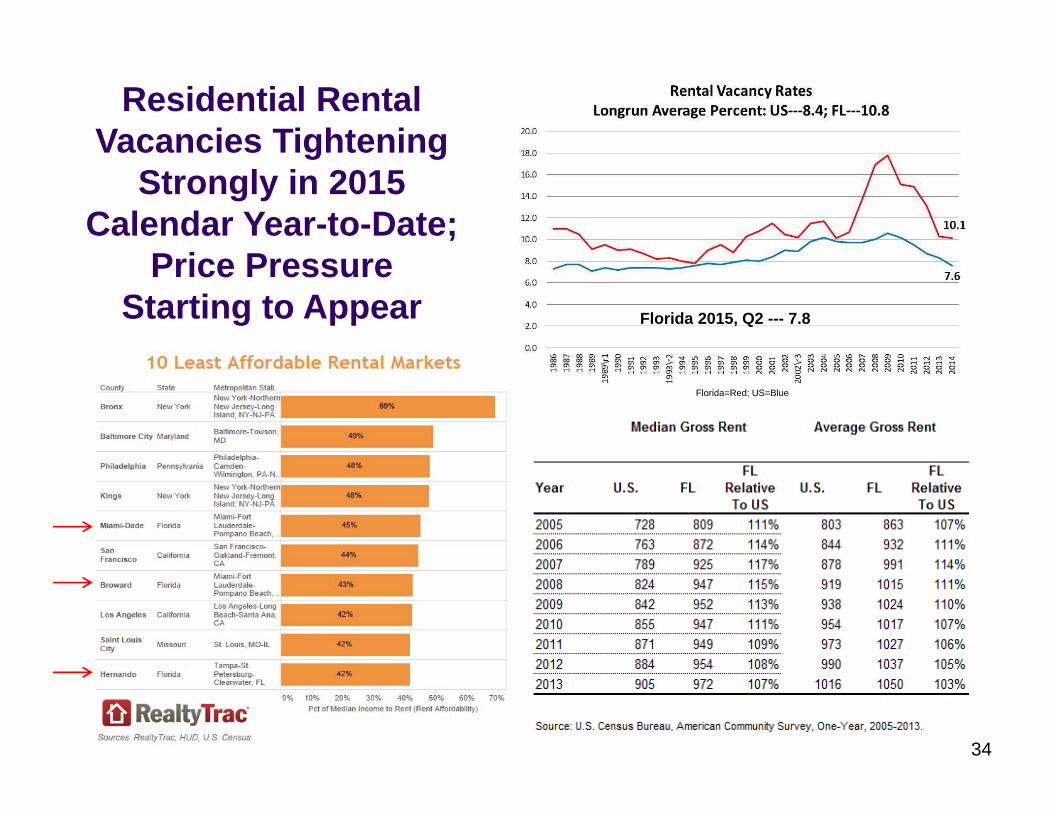
Residential Rental Vacancies Tightening

Strongly in 2015 Calendar Year-to-Date;

Price Pressure Starting to Appear Florida 2015, Q2 --- 7.8

34

Florida=Red; US=Blue