three-phase immiscible displacement in heterogeneous ... · mathematics and computers in simulation...

Mathematics and Computers in Simulation 73 (2006) 2–20

Three-phase immiscible displacement in heterogeneouspetroleum reservoirs

E. Abreua,∗, J. Douglas Jr. b, F. Furtadoc, D. Marchesind, F. Pereiraa

a Departamento de Modelagem Computacional, Instituto Politecnico/UERJ, Caixa Postal 97282, Nova Friburgo 28601-970, RJ, Brazilb Department of Mathematics, Purdue University, West Lafayette, IN 47907-1395, USAc Department of Mathematics, University of Wyoming, Laramie, WY 82071-3036, USA

d Instituto Nacional de Matematica Pura e Aplicada, Estrada D. Castorina 110, Rio de Janeiro 22460-320, RJ, Brazil

Available online 14 August 2006

Abstract

We describe a fractional-step numerical procedure for the simulation of immiscible three-phase flow in heterogeneous porousmedia that takes into account capillary pressure and apply it to indicate the existence of a so-called “transitional" wave in at leastsome multi-dimensional flows, thereby extending theoretical results for one-dimensional flows. The step procedure combines asecond-order, conservative central difference scheme for a pertinent system of conservation laws modeling the convective transportof the fluid phases with locally conservative mixed finite elements for the associated parabolic and elliptic problems.© 2006 IMACS. Published by Elsevier B.V. All rights reserved.

Keywords: Operator splitting; Mixed finite elements; Central difference scheme; Three-phase flow; Heterogeneous reservoirs

1. Introduction

In immiscible, incompressible three-phase flow in porous media for which advection dominates diffusive or capillaryeffects, the leading front caused by injection intended to move one or more of the phases toward a production pointcan split into a classical Buckley–Leverett shock followed by a new type of shock wave related to the existence of anelliptic region or an umbilic point for the system of nonlinear conservation laws describing the convective transport ofthe fluid phases. Unlike classical Buckley–Leverett fronts, this nonclassical “transitional” shock wave is very sensitiveto the form of the parabolic (capillary) terms in the equations; see [31] and references therein. Thus, it is imperativethat capillary pressure effects be modeled accurately in order to calculate physically correct transitional waves.

Transitional waves (also called undercompressive and intermediate waves) have been identified for flows in a lineardomain [26,16,37,22,23] and for a number of other physical problems such as magneto-hydrodynamics, van der Waalsgases and combustion. Recently [8] it was determined that transitional waves arise in lubrication flow.

The purposes of this work are to present an accurate numerical procedure for the simulation of three-phase flowsincluding capillarity and to apply the technique to show the existence of transitional waves in multi-dimensional flowsfor some reasonable capillary pressure functions. The numerical procedure is validated in two ways; first, semi-analyticone-dimensional results [31] are closely reproduced computationally by the numerical method [1,2] and, second, a

∗ Corresponding author. Tel.: +55 22 2528 8545x303; fax: +55 22 2528 8536.E-mail addresses: [email protected] (E. Abreu).

0378-4754/$32.00 © 2006 IMACS. Published by Elsevier B.V. All rights reserved.doi:10.1016/j.matcom.2006.06.018

mailto:[email protected]

dx.doi.org/10.1016/j.matcom.2006.06.018

E. Abreu et al. / Mathematics and Computers in Simulation 73 (2006) 2–20 3

numerical convergence study is presented for a two-dimensional reservoir having moderately inhomogeneous physicalparameters. Then, we focus on two-dimensional problems arising from fractally heterogeneous geology. (We shall usethe terminology of waterflooding in petroleum reservoirs—including calling the three fluids oil, water, and gas.) Ourcalculations verify that transitional waves are present in two-dimensional heterogenous reservoirs for at least somereasonable capillary pressure functions. To the authors’ knowledge such results have not been reported previously inthe literature.

Our new procedure is a two-level operator-splitting procedure with mixed finite element methods being used forthe approximation of the parabolic problem for diffusion (capillarity) and the elliptic problem for the pressure anda Darcy velocity combined with a nonoscillatory, second-order, conservative central difference scheme to handle asystem of nonlinear conservation laws describing advection. As announced above, the technique is designed to treat thenumerical solution of three-phase, immiscible displacement problems in heterogeneous porous media; the numericaltests performed indicate that the two-dimensional simulator produces accurate approximations of the differentialequations making up the model.

Different approaches for solving numerically the three-phase flow equations can be found in [7,9,10].

2. Three-phase flow

We consider two-dimensional, horizontal flow of three immiscible, incompressible fluid phases in a porous medium.For concreteness, the phases will be called gas, oil, and water and indicated by the subscripts g, o, and w, respectively.We assume that there are no internal sources or sinks. Compressibility, mass transfer between phases, and thermal andgravitational effects are neglected.

We assume that the three fluid phases saturate the pores; thus, with Si denoting the saturation (local volume fraction)of phase i,∑

i=g,o,w

Si = 1. (1)

Consequently, any pair of saturations inside the triangle of saturations

� := {(Si, Sj) : Si, Sj ≥ 0, Si + Sj ≤ 1, i �= j} (2)

can be chosen to describe the state of the fluid. In our model we shall work with the saturations Sw and Sg of water andgas. First, let us derive the governing equations for our model.

The equations expressing conservation of mass of oil, water and gas are

∂

∂t(φSiρi) + ∇·(ρivi) = 0, i = o, w, g, (3)

respectively, where φ denotes the porosity of the porous medium. For the phase i, Si denotes its saturation and ρi itsdensity, and vi is its volumetric rate of flow (or, Darcy velocity) and is given by the multiphase Darcy law [34,36,6]

vi = −K(x)λi∇pi, i = o, w, g, (4)

where K(x) denotes absolute permeability of the porous medium; λi ≥ 0 and pi are the mobility and the pressure ofphase i, respectively. The mobility is usually expressed as

λi = ki

μi

, (5)

the ratio of the relative permeability ki and the viscosity μi of the phase i. Each relative permeability ki dependson the saturation vector. Experimentally, ki increases when Si increases, and the relative permeabilities never vanishsimultaneously. The porosity φ and the absolute permeability K(x) are properties of the medium; we take the porosityto be constant and the permeability to be a function of position in the reservoir. If thermal effects and compressibilityare neglected, μi and ρi are constant, and (3) can be rewritten in volumetric form:

∂

∂t(φSi) + ∇·vi = 0, i = o, w, g, (6)

4 E. Abreu et al. / Mathematics and Computers in Simulation 73 (2006) 2–20

Denote the capillary pressure between phase i and phase j, i �= j, by

pij = pi − pj; (7)

clearly, only two of the possible six capillary pressures are independent, since

pij = −pji, and pik = pij + pjk. (8)

An independent pair must be measured experimentally as a function of the saturation vector.Define the total mobility λ and the fractional flow functions fi by

λ =∑

j

λj and fi = λi

λ. (9)

Clearly,∑

j fj = 1. Let the total velocity (total volumetric flow rate) be given by

v =∑

j

vj. (10)

After a bit of algebraic manipulation, we can see that

vfi = −Kλi

∑j

fj∇pj. (11)

If we add and subtract vi in the last equation and note that ∇pi = (∑

j fj)∇pi, we see that

vi = vfi + Kλi

∑j �=i

fj∇pji. (12)

Therefore, by (6) and (12), the equations governing the flow are

∂(φ Sw)

∂t+ ∇·(vfw) = ∇·[Kλw(fg∇pwg + fo∇pwo)],

∂(φ Sg)

∂t+ ∇·(vfg) = ∇·[Kλg(fw∇pgw + fo∇pgo)],

∂(φ So)

∂t+ ∇·(vfo) = ∇·[Kλo(fw∇pow + fg∇pog)].

(13)

Any one of the Eq. (13) is redundant, and the system can be reduced to a two-component system. As a result of theredundancy in (13), one of its characteristic speeds is 0. The two other characteristic speeds are the same for anysubsystem of two equations (see [32]).

As a consequence of the redundancy, the system can be written in the form of a pair of saturation equations and aDarcy pressure–velocity system. The Eq. (15a) results from adding the three equations in (13), and the derivation of(16) is facilitated by applying the relation pwg = pwo + pog. The governing equations then become as follows:

Saturation equations:

∂(φSw)

∂t+ ∇·(vfw(Sw, Sg)) = ∇·ww, (14a)

∂(φSg)

∂t+ ∇·(vfg(Sw, Sg)) = ∇·wg, (14b)

Pressure–velocity equations:

∇·v = 0, (15a)

v = −K(x)λ(Sw, Sg)∇po + vwo + vgo. (15b)

The flux terms ww and wg are given by

[ww, wg]T = K(x) B(Sw, Sg)[∇Sw, ∇Sg

]T. (16)


Here, [a, b] denotes the 2 × 2 matrix with column vectors a and b, and B = QP ′, where

Q(Sw, Sg) =⎡⎣λw(1 − fw) −λwfg

−λgfw λg(1 − fg)

⎤⎦ , P ′(Sw, Sg) =

⎡⎢⎢⎢⎢⎣

∂pwo

∂Sw

∂pwo

∂Sg

∂pgo

∂Sw

∂pgo

∂Sg

⎤⎥⎥⎥⎥⎦ . (17)

In the above, the correction velocities vwo and vgo are defined by

vij = −K(x)λi(Sw, Sg)∇pij. (18)

The diffusive (capillary) term is represented by the right-hand side of the system (14). For our model one can verifythat this term is strictly parabolic in the interior of the saturation triangle � [5].

Boundary and initial conditions for (14)–(18) must be imposed to complete the definition of the mathematicalmodel; in particular, Sw and Sg must be specified at the initial time t = 0. The boundary conditions will be introducedin the description of the operator splitting for the numerical method; the computed fluid flow, in two space dimensionsreported here, are defined in a bounded two-dimensional reservoir Ω = [0, X] × [0, Y ].

3. A fractional-step procedure

We employ a two-level operator-splitting procedure for the numerical solution of the three-phase flow system inwhich we first split the pressure–velocity calculation from the saturation calculation and then split the saturationcalculation into advection and diffusion. The splitting allows time steps for the pressure–velocity calculation that arelonger than those for the diffusive calculation, which are in turn longer than those for advection. Thus, we introducethree time steps: �tt for the solution of the hyperbolic problem for the advection, �td for the diffusive calculation and�tp for the pressure–velocity calculation:

�tp = i1�td = i1 i2�tt, (19)

where i1 and i2 are positive integers, so that �tp ≥ �td ≥ �tt. Let

tm = m�tp, tn = n�td and tn,κ = tn + κ�tt, 0 ≤ κ ≤ i2, (20)

so that tn,i2 = tn+1. Then, given a generic function z, denote its values at times tm, tn, and tn,κ by zm, zn, and zn,κ.In practice, variable time steps are always useful, especially for the advection micro-steps subject dynamically to a

CFL condition. To simplify the description of the operator splitting, assume each time step to have a single value.The oil pressure (and Darcy velocity) will be approximated at times tm, m = 0, 1, 2, . . .. The saturations, Sw and

Sg, will be approximated at times tn, n = 1, 2, . . .; recall that they were specified at t = 0. In addition, there will bevalues for the saturation computed at intermediate times tn,κ for tn < tn,κ ≤ tn+1 that take into account the advectivetransport of the water and gas but not the diffusive effects. The algorithm will be detailed below.

The initial conditions Sw and Sg at t = 0 allow the calculation of {p0o, v0}. The following is the fractional step

algorithm associated with the differential form of three-phase model that should be followed until the final simulationtime is reached. After this, the discretization will be taken up in detail.

3.1. First level

(1) Given Smw (x) and Sm

g (x), m ≥ 0, determine {pmo , vm} by (15)–(18), subject to the boundaries conditions

v · ν = −q, for x = 0, y ∈ [0, Y ],

v · ν = q, for x = X, y ∈ [0, Y ],

v · ν = 0, for y = 0, Y, x ∈ [0, X],(21)

where ν is the unit outer normal vector to ∂Ω.(2) For tm < t ≤ tm+1, solve the advection–diffusion system (14) with the initial conditions Sw(x, tm) = Sm

w (x) andSg(x, tm) = Sm

g (x); Smw (x) and Sm

g (x) are evaluated as the final values of the calculation in [tm−1, tm] for m > 0 orthe initial saturations for m = 0.


3.2. Second level

(1) Let tn1 = tm and assume that {po, v, Sw, Sg} are known for t ≤ tn1 .(2) For n = n1, . . . , n2 = n1 + (i1 − 1):

(a) For κ = 0, . . . , (i2 − 1) and t ∈ [tn,κ, tn,κ+1] solve the advection system given by (for notational convenience,sn,κi is replaced by sκi below)

∂(φ sκi )

∂t+ ∇·(E(tn,κ, v) fi(s

κw, sκg)) = 0, i = w, g, (22)

where

sκi (x, tn,κ) ={

Si(x, tn), κ = 0

sκ−1i (x, tn,κ), κ = 1, . . . , i2 − 1,

, i = w, g (23)

and E(tn,κ, v) indicates a linear extrapolation operator; it extrapolates to time tn,κ the velocity fields vm−1 andvm.

(b) Set Si(x, tn) = si2−1i (x, tn,i2 ), i = w, g.

(c) Compute the diffusive effects on [tn, tn+1] by solving the system

∂(φ Si)

∂t− ∇·wi = 0, i = w, g, (24)

with boundary conditions

wi · ν = 0, i = w, g, x ∈ ∂Ω, (25)

and initial conditions

Si(x, tn) = Si(x, tn), i = w, g. (26)

Remark. The division of the interval [tn, tn+1] into microsteps of length �tt is artificial in the differential casedescribed above, but the division is desirable and often necessary after the full discretization of the advectionequations is introduced.

(3) Set Sm+1i (x) = Si(x, tn2+1), i = w, g.

4. Approximation by mixed finite elements

We shall use a singly-indexed notation for the rectangles in the partition {Ωj} of Ω. Let {Ωj, j = 1, . . . , M}be a uniform partition of Ω into cells of size h × h: Ω = ∪M

j=1Ωj; Ωj ∩ Ωk = ∅, j �= k. Let Γ = ∂Ω, Γj = Γ ∩∂Ωj, Γjk = Γkj = ∂Ωj ∩ ∂Ωk.

4.1. Pressure–velocity equations

We now describe in detail Step (1) of Section 3.1. Assume that the saturations {Sw, Sg} and their fluxes {ww, wg}are known. Then, the phase velocity corrections vwo and vgo can be calculated using {ww, wg} as described below.Their sum defines a source term qB. Then, the auxiliary problem (27) defined below for the pair (po, u) must be solved.Finally, the total velocity can be recovered from (15b).

4.1.1. An auxiliary problemDefine the auxiliary problem for (po, u):

u = −K(x)λ(Sw, Sg)∇po, (27a)

∇·u = −∇·(vwo + vgo) ≡ qB, (27b)

subject to the boundary conditions (21).


Note that, by (16), the diffusive fluxes ww and wg can be expressed in terms of the correction velocities vwoand vgo:

ww = (fw − 1)vwo + fwvgo, wg = fgvwo + (fg − 1)vgo. (28)

Next, express the correction velocities in (28) as functions of the the diffusive fluxes:

vwo = (fg − 1)

foww − fw

fowg, vgo = −fg

foww + (fw − 1)

fowg. (29)

Adding the equations in (29) gives

vwo + vgo = − λ

λo(ww + wg). (30)

Thus,

qB = ∇·(

λ

λo(ww + wg)

), (31)

with boundary conditions specified in (25).Observe that (25), (31), and the divergence theorem imply that∫

Ω

qB dx = 0. (32)

4.1.2. Numerical solution of the auxiliary problemWe shall approximate the solution of (27) - subject to the boundary conditions (21) - by applying the mixed finite

element method based on the space Wh × Vh given by the lowest index Raviart–Thomas space [35] over rectangles.The natural degrees of freedom on the element Ωj are the (constant) value poj of the pressure over Ωj , which

can be interpreted as the value at the center of the element, and the four (constant) values ujβ, β ∈ {L, R, B, T} =

{left, right, bottom, top}, of the outward normal component of u across the edges of the element. Hybridize [3,12,13] themixed method by introducing Lagrange multipliers �ojβ

, β = L, R, B, T, for the oil pressure on Γjk; �ojβis constant on

each edge. We shall assume the porosity and the absolute permeability to be constant on each element and the capillarypressure and relative permeability functions to be independent of position. Thus, the coefficients are constant on eachΩj with respect to the space variable.

Then, the discrete form of (27b) can be written as

ujL + ujR + ujB + ujT = qBj h; (33)

here, qBj should be evaluated using (31) and the divergence theorem. A particularly simple discrete form of (27a) isobtained by applying a trapezoidal rule for the evaluation of the pertinent integrals (see [13]):

ujβ− 2

hKjλjβ

(poj − �ojβ) = 0, β = L, R, B, T, (34)

where the total mobility function λjβis defined through the Lagrange multipliers for the saturations on the interface β

(see Section 4.2).The linear algebra system resulting from the discretized equations can be solved by a preconditioned conjugate

gradient procedure (PCG) or by a multigrid procedure [13].

4.2. Diffusion system

We discuss a numerical procedure that we employ for the solution of the diffusive system (24)–(26) which combinesdomain decomposition with an implicit time discretization in the construction of an efficient iterative method.

We consider an element-by-element domain decomposition; in addition to requiring that the pairs (Swj , wwj ) and(Sgj

, wgj) (where Sij = Si|Ωj , i = w, g, etc.) be a solution of (24)–(26) for x ∈ Ωj , j = 1, . . . , M; it is necessary to


impose the consistency conditions,

Swj = Swk, x ∈ Γjk,

wwjk· νj + wwkj

· νk = 0, x ∈ Γjk,(35)

and

Sgj= Sgk

, x ∈ Γjk,

wgjk· νj + wgkj

· νk = 0, x ∈ Γjk,(36)

where νj is a outward normal unit vector of Ωj .In order to define an iterative method to solve the above problem, it will be convenient to replace (35) and (36) by

equivalent Robin transmission boundary conditions [14]. These consistency conditions are given by

−χwjkwwj · νjj

+ Swj = χwjkwwk

· νjk+ Swk

, x ∈ Γjk ⊂ ∂Ωj, (37)

−χwkjwwk

· νjk+ Swk

= χwkjwwj · νjj

+ Swj , x ∈ Γkj ⊂ ∂Ωk, (38)

−χgjkwgj

· νjj+ Sgj

= χgjkwgk

· νjk+ Sgk

, x ∈ Γjk ⊂ ∂Ωj, (39)

−χgkjwgk

· νjk+ Sgk

= χgkjwgj

· νjj+ Sgj

, x ∈ Γkj ⊂ ∂Ωk, (40)

where χwjkand χgjk

are positive functions on Γjk (see [1,14]).We consider the lowest index Raviart–Thomas space [35] over Ωj to approximate the pairs (Sw, ww) and (Sg, wg).

The degrees of freedom on an element Ωj are the values Swj and Sgjand the two values wwjβ

and wgjβ, β = L, R, B, T,

of the diffusive fluxes across the edge of the elements. We shall also introduce the Lagrange multipliers �wβand �gβ

,β = L, R, B, T, for the water and gas saturations, respectively, on Γjk; these multipliers are constant on each edge.

So, the discrete form of (24) can be written as (see [1,13]):

φ

(Swj − Swj

�td

)− 1

h(wwjU

+ wwjR+ wwjD

+ wwjL) = 0, (41)

wwjβB−1

11β+ wgjβ

B−112β

= 2

h(Swj − �wjβ

), β = L, R, B, T, (42)

φ

(Sgj

− Sgj

�td

)− 1

h(wgjU

+ wgjR+ wgjD

+ wgjL) = 0, (43)

wwjβB−1

21β+ wgjβ

B−122β

= 2

h(Sgj

− �gjβ), β = L, R, B, T, (44)

where B−1ijβ

are the entries of the inverse matrix B−1(�wβ, �gβ

). Here also a trapezoidal rule is used for the evaluationof the pertinent integrals in the derivation of Eqs. (42) and (44).

Define an iterative scheme for the solution of system (24) by applying (37), (38) to (42) and (39), (40) to (44) toexpress all Lagrange multipliers in terms of Lagrange multipliers and fluxes associated with adjacent elements. Thisscheme, developed in [1] (see also [13]), is a natural extension for parabolic systems of the procedure introduced in[14] for scalar elliptic and parabolic problems.

5. Approximation by a central difference scheme

We shall discuss the high-resolution finite difference scheme, introduced by Nessyahu and Tadmor (NT) [33], that weemploy for the solution of the nonlinear advection system (22)–(23). This scheme can be viewed as an extension of thecelebrated first-order Lax–Friedrichs scheme into a second-order scheme. Its two main ingredients are a non-oscillatory,piecewise bilinear reconstruction of the solution point-values from their given cell averages and central differencingbased on the staggered reconstructed averages. The piecewise bilinear reconstruction reduces the excessive dissipationof the Lax–Friedrichs scheme and, like upwind schemes, the scheme uses nonlinear limiters to guarantee the overallnonoscillatory nature of the approximate solution. The central differencing, unlike upwind differencing, bypasses the


need for Riemann solvers, yielding simplicity, avoiding dimensional splitting in multi-dimensional problems. Centraldifferencing also allows for the extension of the scheme to hyperbolic systems by componentwise application of thescalar framework.

5.1. The scalar framework in two space dimensions

Consider the model of hyperbolic conservation law,

∂s

∂t+ ∂(f (s)vx)

∂x+ ∂(f (s)vy)

∂y= 0. (45)

Here vx ≡ vx(x, y, t) and vy ≡ vy(x, y, t) denote the x and y components of the velocity field v.Consider the cell averages,

sj,k(t) ≡ 1

h2

∫ xj+(1/2)

xj−(1/2)

∫ yk+(1/2)

yk−(1/2)

s(x, y, t) dx dy. (46)

To approximate a solution to (45), at each time level, we start with a piecewise bilinear approximation of the cellaverages (46), defined by

Pj,k(x, y, tn,κ) = sj,k(tn,κ) + (x − xj)1

hs′j,k(tn,κ) + (y − yk)

1

hsj,k(tn,κ),

xj−(1/2) ≤ x ≤ xj+(1/2), yk−(1/2) ≤ y ≤ yk+(1/2). (47)

In Eq. (47),

1

hs′j,k(tn,κ) = ∂

∂xs(xj, yk, tn,κ) + O(h)sx (48)

and

1

hsj,k(tn,κ) = ∂

∂ys(xj, yk, tn,κ) + O(h)sy (49)

denote the discrete slopes in the x and y directions. We shall discuss later the form of such discrete slopes.The reconstruction (47) retains conservation, i.e.:

1

h2

∫ xj+(1/2)

xj−(1/2)

∫ yk+(1/2)

yk−(1/2)

P(x, y, t) dx dy = sj,k(t). (50)

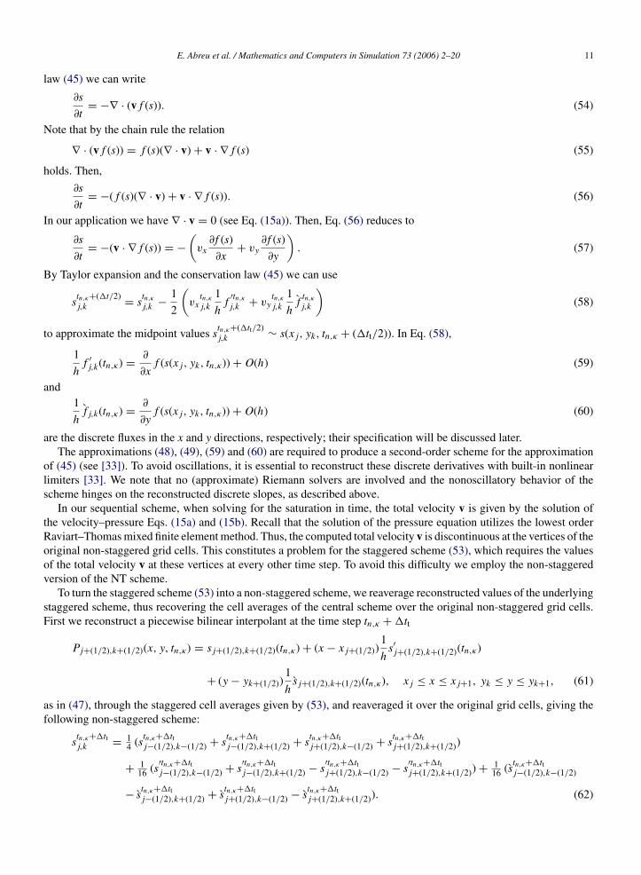
The time evolution of this reconstruction is based on the integration of the conservation law (45) over staggeredvolumes Ij+(1/2),k+(1/2) × [tn,κ, tn,κ + �tt] (dashed grid in Fig. 1). The piecewise bilinear approximation of the cellaverages is evolved in time, and then the result is projected on the staggered cells (dashed grid in Fig. 1) Ij+(1/2),k+(1/2)to yield new cell averages.

The solution in the staggered grid obtained by the time evolution can be expressed as:

sj+(1/2),k+(1/2)(tn,κ + �tt) = s(x, y, tn,κ + �tt) ≡ 1

h2

∫ xj+1

xj

∫ yk+1

yk

s(x, y, tn,κ + �tt) dx dy,

xj ≤ x ≤ xj+1, yk ≤ y ≤ yk+1. (51)

By the conservation law (45), the integral in (51) equals

sj+(1/2),k+(1/2)(tn,κ + �tt)

= 1

h2

∫ xj+(1/2)

xj

∫ yk+(1/2)

yk

Pj,k(x, y, tn,κ) dx dy + 1

h2

∫ xj+(1/2)

xj

∫ yk+1

yk+(1/2)

Pj,k+1(x, y, tn,κ) dx dy

+ 1

h2

∫ xj+1

xj+(1/2)

∫ yk+(1/2)

yk

Pj+1,k(x, y, tn,κ) dx dy + 1

h2

∫ xj+1

xj+(1/2)

∫ yk+1

yk+(1/2)

Pj+1,k+1(x, y, tn,κ) dx dy


Fig. 1. Evolution step for the two-dimensional central scheme.

− 1

h2

[∫ tn,κ+�tt

tn,κ

∫ xj+1

xj

(vx(xj+1, y, t)f (s(xj+1, y, t)) − vx(xj, y, t)f (s(xj, y, t))) dx dt

]

− 1

h2

[∫ tn,κ+�tt

tn,κ

∫ yk+1

yk

(vy(x, yk+1, t)f (s(x, yk+1, t)) − vy(x, yk, t)f (s(x, yk, t))) dx dt

]. (52)

The first four bilinear integrands on the RHS of (52) can be integrated exactly. The remaining integrals on the RHSof (52) involve approximations for the fluxes through the sides of the staggered volume. It is here that the benefit ofstaggering manifests itself: these fluxes are smooth at the vertices of the cell defining the integration volume, sincethese vertices are located at the centers of non-staggered cells, away from the jump discontinuities along the edges(see Fig. 1). This facilitates the construction of second-order approximations. The spatial integrals in both the x and ydirections are approximated by the second-order trapezoid quadrature rule and the temporal integrals are approximatedby the midpoint quadrature rule. Then, the resulting new approximate cell averages for the interior elements take thefollowing form (α ≡ �tt/h and s

tn,κ+�ttj+(1/2),k+(1/2) = sj+(1/2),k+(1/2)(tn,κ + �tt)):

stn,κ+�ttj+(1/2),k+(1/2) = 1

4 (stn,κ

j,k + stn,κ

j,k+1 + stn,κ

j+1,k + stn,κ

j+1,k+1) + 116 (s′tn,κ

j,k + s′tn,κ

j,k+1 − s′tn,κ

j+1,k

− s′tn,κ

j+1,k+1 + s′tn,κ

j,k − s′tn,κ

j,k+1 + s′tn,κ

j+1,k − s′tn,κ

j+1,k+1)

+ 12α[vx

tn,κ+(�tt/2)j,k f (s

tn,κ+(�tt/2)j,k ) + vx

tn,κ+(�tt/2)j,k+1 f (s

tn,κ+(�tt/2)j,k+1 )

− vxtn,κ+(�tt/2)j+1,k f (s

tn,κ+(�tt/2)j+1,k ) − vx

tn,κ+(�tt/2)j+1,k+1 f (s

tn,κ+(�tt/2)j+1,k+1 )

]+ 1

2α[vy

tn,κ+(�tt/2)j,k f (s

tn,κ+(�tt/2)j,k ) + vy

tn,κ+(�tt/2)j+1,k f (s

tn,κ+(�tt/2)j+1,k )

− vytn,κ+(�tt/2)j,k+1 f (s

tn,κ+(�tt/2)j,k+1 ) − vy

tn,κ+(�tt/2)j+1,k+1 f (s

tn,κ+(�tt/2)j+1,k+1 )

]. (53)

The approximation of the fluxes in (53) makes use of the midpoint values in time, stn,κ+(�tt/2)j,k ∼ s(xj, yk, tn,κ + (�tt/2)),

as a predictor step. Since these mid-values are bounded away from the jump discontinuities along the edges, we may usea Taylor expansion and the conservation law (45) to evaluate sj,k(tn,κ + (�tt/2)). In view of the hyperbolic conservation


law (45) we can write

∂s

∂t= −∇ · (vf (s)). (54)

Note that by the chain rule the relation

∇ · (vf (s)) = f (s)(∇ · v) + v · ∇f (s) (55)

holds. Then,

∂s

∂t= −(f (s)(∇ · v) + v · ∇f (s)). (56)

In our application we have ∇ · v = 0 (see Eq. (15a)). Then, Eq. (56) reduces to

∂s

∂t= −(v · ∇f (s)) = −

(vx

∂f (s)

∂x+ vy

∂f (s)

∂y

). (57)

By Taylor expansion and the conservation law (45) we can use

stn,κ+(�t/2)j,k = s

tn,κ

j,k − 1

2

(vx

tn,κ

j,k

1

hf

′tn,κ

j,k + vytn,κ

j,k

1

hf

tn,κ

j,k

)(58)

to approximate the midpoint values stn,κ+(�tt/2)j,k ∼ s(xj, yk, tn,κ + (�tt/2)). In Eq. (58),

1

hf ′

j,k(tn,κ) = ∂

∂xf (s(xj, yk, tn,κ)) + O(h) (59)

and1

hfj,k(tn,κ) = ∂

∂yf (s(xj, yk, tn,κ)) + O(h) (60)

are the discrete fluxes in the x and y directions, respectively; their specification will be discussed later.The approximations (48), (49), (59) and (60) are required to produce a second-order scheme for the approximation

of (45) (see [33]). To avoid oscillations, it is essential to reconstruct these discrete derivatives with built-in nonlinearlimiters [33]. We note that no (approximate) Riemann solvers are involved and the nonoscillatory behavior of thescheme hinges on the reconstructed discrete slopes, as described above.

In our sequential scheme, when solving for the saturation in time, the total velocity v is given by the solution ofthe velocity–pressure Eqs. (15a) and (15b). Recall that the solution of the pressure equation utilizes the lowest orderRaviart–Thomas mixed finite element method. Thus, the computed total velocity v is discontinuous at the vertices of theoriginal non-staggered grid cells. This constitutes a problem for the staggered scheme (53), which requires the valuesof the total velocity v at these vertices at every other time step. To avoid this difficulty we employ the non-staggeredversion of the NT scheme.

To turn the staggered scheme (53) into a non-staggered scheme, we reaverage reconstructed values of the underlyingstaggered scheme, thus recovering the cell averages of the central scheme over the original non-staggered grid cells.First we reconstruct a piecewise bilinear interpolant at the time step tn,κ + �tt

Pj+(1/2),k+(1/2)(x, y, tn,κ) = sj+(1/2),k+(1/2)(tn,κ) + (x − xj+(1/2))1

hs′j+(1/2),k+(1/2)(tn,κ)

+ (y − yk+(1/2))1

hsj+(1/2),k+(1/2)(tn,κ), xj ≤ x ≤ xj+1, yk ≤ y ≤ yk+1, (61)

as in (47), through the staggered cell averages given by (53), and reaveraged it over the original grid cells, giving thefollowing non-staggered scheme:

stn,κ+�ttj,k = 1

4 (stn,κ+�ttj−(1/2),k−(1/2) + s

tn,κ+�ttj−(1/2),k+(1/2) + s

tn,κ+�ttj+(1/2),k−(1/2) + s

tn,κ+�ttj+(1/2),k+(1/2))

+ 116 (s

′tn,κ+�ttj−(1/2),k−(1/2) + s

′tn,κ+�ttj−(1/2),k+(1/2) − s

′tn,κ+�ttj+(1/2),k−(1/2) − s

′tn,κ+�ttj+(1/2),k+(1/2)) + 1

16 (stn,κ+�ttj−(1/2),k−(1/2)

− stn,κ+�ttj−(1/2),k+(1/2) + s

tn,κ+�ttj+(1/2),k−(1/2) − s

tn,κ+�ttj+(1/2),k+(1/2)). (62)


5.1.1. Numerical derivativesWe now discuss our choice for the numerical derivatives (48), (49), (59) and (60). Consider z to be a generic

grid function defined on a grid with nx versus ny cells (nx · ny = M). In the numerical derivatives given below theMinMod{·, ·} is the usual limiter (see [33]),

MM{a, b} ≡ MinMod{a, b} = 12 [sgn(a) + sgn(b)] · Min(|a|, |b|), (63)

where a and b are real numbers.For the cells 3 ≤ j ≤ nx − 2 and 1 ≤ k ≤ ny in the x direction and 1 ≤ j ≤ nx and 3 ≤ k ≤ ny − 2 in the y direction

we employ the UNO limiter [24] given by

z′j,k = MM{�zj−(1/2),k + 1

2 MM{�2zj−1,k, �2zj,k}, �zj+(1/2),k − 1

2 MM{�2zj,k, �2zj+1,k}}, (64)

and

zj,k = MM{�zj,k−(1/2) + 12 MM{�2zj,k−1, �

2zj,k}, �zj,k+(1/2) − 12 MM{�2zj,k, �

2zj,k+1}}, (65)

respectively, where�2zj,k ≡ zj+1,k − 2zj,k + zj−1,k, �2zj,k ≡ zj,k+1 − 2zj,k + zj,k−1, �z

j+ 12 ,k

≡ zj+1,k − zj,k, and �zj,k+ 1

2≡

zj,k+1 − zj,k.For the cells j = 2, nx − 1 and 1 ≤ k ≤ ny in the x direction and 1 ≤ j ≤ nx and k = 2, ny − 1 in the y we use,

z′j,k = MM{θ MM{�zj+(1/2),k, �zj−(1/2),k}, 1

2 (�zj+(1/2),k + �zj−(1/2),k)}, (66)

and

zj,k = MM{θ MM{�zj,k+(1/2), �zj,k−(1/2)}, 12 (�zj,k+(1/2) + �zj,k−(1/2))}. (67)

Here θ ∈ (0.2) is a nonoscillatory limiter (see [28]). For our computations we use θ = 1.0.For the cells j = 1, nx and 1 ≤ k ≤ ny in the x direction and 1 ≤ j ≤ nx and k = 1, ny in the y we use,

z′j,k = zj+1,k − zj,k and zj,k = zj,k+1 − zj,k, (68)

respectively.We refer to [27,30] for information about nonoscillatory boundary treatments.We remark that for the numerical approximation of the system (22)–(23) we employ a componentwise extension

[33] of the scheme described above.

6. Numerical experiments

In our one and two-dimensional experiments we consider two Riemann problems, RP1 and RP2, whose left andright states are given by:

RP1 =⎧⎨⎩

SLw = 0.613, SR

w = 0.05

SLg = 0.387, SR

g = 0.15and RP2 =

⎧⎨⎩

SLw = 0.721, SR

w = 0.05

SLg = 0.279, SR

g = 0.15.(69)

We work with the system of Eqs. (14)–(18) in dimensionless form.We use the Leverett model [29] for capillary pressures given by

pwo = 5ε(2 − Sw)(1 − Sw) and pgo = ε(2 − Sg)(1 − Sg), (70)

where the coefficient ε controls the relative importance of capillary/dispersive and advective forces. We take ε = 1.0 ×10−3 unless a different value is mentioned explicitly. The viscosities of the fluids are μo = 1.0, μw = 0.5, and μg = 0.3.We also adopt the model by Corey–Pope [11,15] which has been used extensively for phase relative permeabilities:kw = S2

w, ko = S2o and kg = S2

g . This model has the peculiarity that for a particular state in the interior of the saturationtriangle the characteristic speeds of the hyperbolic system (22) coincide, or resonate. Such a state, whose location isdetermined by the fluid viscosities, is called an umbilic point [26]. It plays a central role in three-phase flow; in particular,its existence leads to the occurrence on nonclassical transitional shock waves in the solutions of the three-phase flowmodel. Crucial to calculating transitional shock waves is the correct modeling of capillarity (diffusive) effects [25].


For other models of three-phase flow used in petroleum engineering, such as certain models of Stone [39,17], theumbilic point is generally replaced by an elliptic region, in which the characteristic speeds are not real. In general,under reasonable physical assumptions about a model for immiscible three-phase flow, hyperbolic singularities suchas umbilic points and elliptic regions are a necessary consequence of Buckley–Leverett behavior on each two-phaseedge of the saturation triangle [38,32].

We remark that for the choice of parameters described above a transitional (intermediate) shock wave appears inthe one-dimensional solution of RP2. Such a wave is not present in the one-dimensional solution of RP1.

6.1. One-dimensional results

Our one-dimensional solutions computed on a grid with 250 cells show very good agreement with the ones obtainedon finer grids, and we note that our numerical solutions are in agreement with the semi-analytic results reported in [31].

Fig. 2. From top to bottom profiles for oil and gas saturation are shown as a function of dimensionless distance. RP1 on the left and RP2 on theright; a transitional shock wave appears in RP2.


Fig. 3. The source term qB is shown as a function of dimensionless distance for two values of the parameter ε: 1.0 × 10−3 (blue) and 1.0 × 10−4

(red).

Fig. 4. Mesh refinement study for the RP2 data in two spatial dimensions.


Fig. 5. Oil saturation surface plots for three-phase flow problems in 2D heterogeneous reservoirs; RP2 data. From top to bottom are shown oilsaturation surface plots with Cv = 0.5 and Cv = 2.0. Permeability fields with β = ∞ are considered. A transitional shock wave is simulated.


Fig. 2 shows from top to bottom saturation profiles for oil and gas as a function of dimensionless distance and time. Thepictures on the left refer to RP1 and the ones on the right refer to RP2 (note the occurrence of the transitional wave).

Fig. 3 shows the source term (31) for two values of the parameter ε: 1.0 × 10−3 (blue) and 1.0 × 10−4 (red). Weremark that the relation (32) is verified numerically; in fact, we use this identity as one criterion to stop the iterativescheme which solves for diffusive effects (described in Section 4.2).

6.2. Two-dimensional results

A numerical convergence study is performed for the permeability field displayed in the top left picture of Fig. 4;the remaining pictures in this figure show saturation surface plots for the gas phase.

A mixture (72.1% of water and 27.9% of gas) is injected at a constant rate of 0.2 pore volumes every year along theboundary, x = 0 and y ∈ [0, 1], of the computational region. The initial conditions for the system is given by SR

w = 0.05and SR

g = 0.15; these data correspond to RP2. Two values are specified for the permeability field in the computationalregion: 0.01 in a rectangle which touches the top boundary and 1.0 elsewhere. The computational grids used were 64versus 64 (top right picture), 128 versus 128 (bottom left picture) and 256 versus 256 (bottom right picture). Clearlythe 64 versus 64 grid can resolve the low permeability region and captures the transitional (intermediate) wave; as thegrid is refined the jumps in the numerical solution get sharper, indicating numerical convergence of our new procedure.Note that spurious oscillations do not occur in the numerical solutions.

We reiterate that transitional waves have a strong dependency upon the physical diffusion being modeled (see [31]and references therein); note that rock heterogeneity introduces variability in the diffusion term of Eqs. (14a) and (14b).The goal of the numerical experiments reported below is the investigation of the occurrence of transitional waves intwo-dimensional, multiscale heterogeneous problems. As mentioned above such waves have been observed only inone-dimensional problems.

As a model for multi-length scale rock heterogeneity we consider scalar, log-normal permeability fields, so thatξ(x) = log K(x) is Gaussian and its distribution is determined by its mean and covariance function. We assume thedistribution is stationary, isotropic and fractal (self-similar). Thus, the mean is an absolute constant and the covariance

Fig. 6. Gas saturation surface plots for three-phase flow problems in 2D heterogeneous reservoirs; RP2 data. From top to bottom are shown gassaturation surface plots with Cv = 0.5 and Cv = 2.0. Permeability fields with β = ∞ are considered.


Fig. 7. Oil saturation surface plots for three-phase flow problems in 2D heterogeneous reservoirs; RP2 data. From top to bottom are shown oilsaturation surface plots for Cv = 0.5 and Cv = 2.0. Permeability fields with β = 0.5 are considered.


is given by a power law:

Cov(x, y) = |x − y|−β, β > 0. (71)

The scaling exponent β controls the nature of multiscale heterogeneity: as it increases, the heterogeneities concentratedin the larger length scales are emphasized and the field becomes more regular (locally). In our numerical studies wealso consider log-normal, statistically independent random fields. We refer to such fields by β = ∞. See [19] for adiscussion of the numerical construction of fractal fields.

The spatially variable permeability fields are defined on 512 × 128 grids with two values for the coefficiente ofvariation Cv ((standard deviation)/mean): 0.5 and 2.0. Cv is used as a dimensionless measure of the heterogeneity of thepermeability field. The computed fluid flows are defined in a bounded two-dimensional reservoir Ω = [0, X] × [0, Y ]with aspect ratio X/Y = 4, discretized by an uniform grid of 512 × 128 cells. Again, a mixture (72.1% of water and27.9% of gas) is injected at a constant rate of 0.2 pore volumes every year along the boundary, x = 0 and y ∈ [0, Y ],of the computational region. The initial conditions for the system correspond to RP2.

In Figs. 5 and 6 we show saturation surface plots for oil and gas, respectively, displayed as a function of position.Uncorrelated Gaussian field (β = ∞) permeability fields were considered; these figures refer permeability fields withCv = 0.5 and 2.0, from top to bottom. Note in these figures that for both large and small strength heterogeneitiestransitional shock waves were properly simulated.

Correlated Gaussian (β = 0.5) permeability fields were used in the simulations reported in Figs. 7 and 8. In thesefigures the values Cv = 0.5 and 2.0 were considered (from top to bottom) and saturation surface plots are shown foroil (Fig. 7) and gas Fig. 8. Note that for Cv = 0.5 and long-range rock correlations transitional shock waves wereproperly simulated. However, for long-range correlations and stronger heterogeneity (Cv = 2.0) the separate identityof the transitional shock and its precursor Buckley–Leverett shock seems to be lost.

Fig. 8. Gas saturation surface plots for three-phase flow problems in 2D heterogeneous reservoirs; RP2 data. From top to bottom are shown gassaturation surface plots for Cv = 0.5 and Cv = 2.0. Permeability fields with β = 0.5 are considered.


7. Concluding remarks

A new simulator intended for the numerical solution of three-phase, two-dimensional immiscible displacementproblems in heterogeneous reservoirs has been described in detail. The numerical tests performed indicate that thesimulator is accurate. The new simulator was used to extend theoretical results for one-dimensional flows by providingnumerical evidence of the existence of transitional waves in two-dimensional flows.

A two-level fractional-step numerical technique is introduced for the numerical solution of the problem at hand.The nonlinear advection, diffusion and pressure–velocity problems that result from the splitting are approximatedsequentially by a nonoscillatory, second-order, conservative central difference scheme (for advection) and locallyconservative mixed finite elements (for diffusion and pressure–velocity).

The numerical simulation of the full two-dimensional coupled set of pressure–velocity-saturation Eqs. (14)–(17)shows that the heterogeneity has an important effect on the transitional shock front. We recall that this shock is relatedto the loss of strict hyperbolicity inherent in the pure 1D system of conservation laws for the saturations and that thisshock is very sensitive to diffusive effects. Our numerical simulations indicates that, the transitional shock persistsunder the presence of heterogeneities and is accurately captured by our simulator, as shown by comparisons withreliable 1D simulations and calculations for homogeneous media [31]. Moreover, the transitional shock is stable underthe excitations imposed by short-range or weak (small Cv) heterogeneities. On the other hand, for strong, long-rangeexcitations the separate identity of the transitional wave and its precursor Buckley–Leverett shock seems to be lost.

As a first step in the investigation of the scale-up problem for three-phase flow the authors are currently investigatingthe stability (with respect to viscous fingering) of transitional waves in heterogeneous formations; stable transitionalwaves could improve drastically oil production. The upscaled behavior of two-phase flow in heterogeneous media isstrongly dependent on flow regime [20,4,21]. The preliminary results of the current investigation seem to indicate thatscale-up would have to be done wave by wave, perhaps precluding the existence of effective upscaled partial differentialequations for three-phase flow in heterogeneous porous media.

Acknowledgments

E.A. thanks CAPES (IPRJ/UERJ) for a Ph.D. fellowship and the organizers of the 2004 PASI meeting for afellowship which allowed him to attend this event. F.P. was supported in part through grants CNPq/CTPetro 501886/03-6, CNPq/CTPetro 70216/03-4, CNPq/Universal 470216/03-4, CNPq/FAPERJ PRONEX (2003–2006). D.M., F.F. andF.P. wish to acknowledge the support from the CNPq and the NSF for an international collaborative research projecton improved oil recovery through scale up for multiphase flow.

References

[1] E. Abreu, Numerical simulation of three-phase water–oil–gas flows in petroleum reservoirs, M.Sc Thesis, IPRJ/UERJ, Brazil, 2003. (inPortuguese, available at http://www.labtran.iprj.uerj.br/Orientacoes.html).

[2] E. Abreu, F. Furtado, F. Pereira, On the numerical simulation of three-phase reservoir transport problems, Transport Theory Stat. Phys. 33(5–7) (2004) 503–526.

[3] D.N. Arnold, F. Brezzi, Mixed and nonconforming finite element methods: implementation, postprocessing and error estimates, R.A.I.R.O.Modelisation Mathematique et Analyse Numerique 19 (1985) 7–32.

[4] V. Artus, F. Furtado, B. Noetinger, F. Pereira, Stochastic analysis of two-phase immiscible flow in stratified porous media, Computat. Appl.Math. 23 (2–3) (2004) 153–172.

[5] A. Azevedo, D. Marchesin, B.J. Plohr, K. Zumbrun, Capillary instability in models for three-phase flow, Zeit. Angew. Math. Phys. 53 (5)(2002) 713–746.

[6] M. Aziz, A. Settari, Petroleum Reservoir Simulation, Elsevier Applied Science, New York, 1990.[7] I. Berre, H.K. Dahle, K.H. Karlson, H.F. Nordhaug, A streamline front tracking method for two- and three-phase flow including capillary

forces, Proceedings of an AMS-IMS-SIAM, Joint Summer Research Conference on Fluid Flow and Transport in Porous Media: Mathematicaland Numerical Treatment, vol. 295, Mount Holyoke College, South Hadley, Massachusetts, June 17–21, 2002, pp. 49–61.

[8] A. Bertozzi, A. Munch, M. Shearer, Undercompressive shocks in thin flim, Phys. D 134 (1990) 431–464.[9] Z. Chen, Formulations and numerical methods of the black oil model in porous media, SIAM J. Numer. Anal. 38 (2) (2000) 489–514.

[10] Z. Chen, R.E. Ewing, Fully-discrete finite element analysis of multiphase flow in ground-water hydrology, SIAM J. Numer. Anal. 34 (1997)2228–2253.

[11] A. Corey, C. Rathjens, J. Henderson, M. Wyllie, Three-phase relative permeability, Trans. AIME 207 (1956) 349–351.

http://www.labtran.iprj.uerj.br/Orientacoes.html


[12] J. Douglas, R.E. Ewing Jr., M.F. Wheeler, The approximation of the pressure by a mixed method in the simulation of miscible displacement,R.A.I.R.O., Anal. Numer. 17 (1983) 17–33.

[13] J. Douglas Jr., F. Furtado, F. Pereira, On the numerical simulation of waterflooding of heterogeneous petroleum reservoirs, Comput. Geosci. 1(1997) 155–190.

[14] J. Douglas Jr., P.J. Paes Leme, J.E. Roberts, J. Wang, A parallel iterative procedure applicable to the approximate solution of second orderpartial differential equations by mixed finite element methods, Numer. Math. 65 (1993) 95–108.

[15] D.E. Dria, G.A. Pope, K. Sepehrnoori, Three-phase gas/oil/brine relative permeabilities measured under CO2 flooding conditions, Soc. Petr.Engrg. SPE 20184 (1993) 143–150.

[16] A. Falls, W. Schulte, Theory of three-component, three-phase displacement in porous media, SPE Reserv. Eng. 7 (1992) 377–384.[17] F. Fayers, J. Matthews, Evaluation of normalized Stone’s method for estimating three-phase relative permeability, Soc. Petr. Engrg. J. 24 (1984)

225–232.[19] F. Furtado, J. Glimm, B. Lindquist, F. Pereira, Multi-length scale calculations of mixing length growth in tracer floods, F. Kovarik (ed.),

Proceedings of the Emerging Technologies Conference, Houston, TX, 1990.[20] F. Furtado, F. Pereira, Crossover from nonlinearity controlled to heterogeneity controlled mixing in two-phase porous media flows, Comput.

Geosci. 7 (2003) 115–135.[21] J. Glimm, H. Kim, D. Sharp, T. Wallstrom, A stochastic analysis of the scale up problem for flow in porous medium, Comput. Appl. Math. 17

(1998) 67–79.[22] R. Guzman, F. Fayers, Mathematical properties of three-phase flow equations, SPE J., 2 (1997) 291–300 (SPE 35154).[23] R. Guzman, F. Fayers, Solutions to the three-phase flow Buckley-Leverett problem, SPE J., 2 (1997) 301–311 (SPE 35156).[24] A. Harten, S. Osher, Uniformly high order accurate non-oscillatory scheme I, SINUM 24 (1987) 279.[25] E. Isaacson, D. Marchesin, B. Plohr, Transitional waves for conservation laws, SIAM J. Math. Anal. 21 (1990) 837–866.[26] E. Isaacson, D. Marchesin, B. Plohr, J.B. Temple, Multiphase flow models with singular Riemann problems, Comput. Appl. Math. 11 (1992)

147–166.[27] G.S. Jiang, D. Levy, C.T. Lin, S. Osher, E. Tadmor, High-resolution non-oscillatory central schemes with non-staggered grids for hyperbolic

conservation laws, SIAM J. Numer. Anal. 35 (1998) 2147–2168.[28] R. Kupferman, E. Tadmor, A fast high resolution second order central scheme for incompressible flows, Proc. Natl. Acad. Sci. U.S.A. 94 (May

(10)) (1997) 4848–4852.[29] M.C. Leverett, W.B. Lewis, Steady flow of gas-oil-water mixtures through unconsolidated sands, Trans. SPE AIME 142 (1941) 107–16.[30] D. Levy, E. Tadmor, Non-oscillatory boundary treatment for staggered central scheme, UCLACAM, 1998. (Available at http://www.cscamm.

umd.edu/∼tadmor/pub/general.htm).[31] D. Marchesin, B.J. Plohr, Wave structure in WAG recovery, SPEJ 6 (2) (1999/2001) 209–219 (SPE 56480).[32] H. Medeiros, Stable hyperbolic singularities for three phase flow models in oil reservoir simulation, Acta Appl. Math. 28 (1992) 135–159.[33] N. Nessyahu, E. Tadmor, Non-oscillatory central differencing for hyperbolic conservation laws, J. Comput. Phys. (1990) 408–463.[34] D.W. Peaceman, Fundamentals of Numerical Reservoir Simulation, Elsevier, Amsterdam, 1977.[35] P-A. Raviart, J.M. Thomas, A mixed finite element method for second order elliptic problems, in: I. Galligani, E. Magenes (eds.), Mathematical

Aspects of the Finite Element Method, Lecture Notes in Mathematics, vol. 606, Springer-Verlag, Berlin/New York, 1977, pp. 292–315.[36] A.E. Scheidegger, The Physics of Flow Through Porous Media, University of Toronto Press, 1957.[37] W. Schulte, A. Falls, Features of three-component, three-phase displacement in porous media, SPE Reserv. Eng. 7 (1992) 426–432.[38] M. Shearer, Loss of strict hyperbolicity of the Buckley–Leverett equations for three-phase flow in a porous medium, IMA Vol. Math. Appl. 11

(1988) 263–283.[39] H. Stone, Probability model for estimating three-phase relative permeability, J. Petr. Tech. 22 (1970) 214–218.

http://www.cscamm.umd.edu/$~$tadmor/pub/general.htm

http://www.cscamm.umd.edu/$~$tadmor/pub/general.htm

three-phase immiscible displacement in heterogeneous ... · mathematics and computers in simulation...

Documents