three implementation models for scheme -...

Three Implementation Models for Scheme

by

R. Kent Dybvig

A dissertation submitted to the faculty of the University of North Carolina atChapel Hill in partial fulfillment of the requirements for the degree of Doctor ofPhilosophy in the Department of Computer Science.

Chapel Hill

1987

Approved by:

Advisor

Reader

Reader

R. KENT DYBVIG. Three Implementation Models for Scheme (Under the direc-

tion of GYULA A. MAGO.)

Abstract

This dissertation presents three implementation models for the Scheme Program-

ming Language. The first is a heap-based model used in some form in most Scheme

implementations to date; the second is a new stack-based model that is consider-

ably more efficient than the heap-based model at executing most programs; and

the third is a new string-based model intended for use in a multiple-processor im-

plementation of Scheme. The heap-based model allocates several important data

structures in a heap, including actual parameter lists, binding environments, and

call frames. The stack-based model allocates these same structures on a stack

whenever possible. This results in less heap allocation, fewer memory references,

shorter instruction sequences, less garbage collection, and more efficient use of

memory. The string-based model allocates versions of these structures right in

the program text, which is represented as a string of symbols. In the string-based

model, Scheme programs are translated into an FFP language designed specifically

to support Scheme. Programs in this language are directly executed by the FFP

machine, a multiple-processor string-reduction computer. The stack-based model

is of immediate practical benefit; it is the model used by the author’s Chez Scheme

system, a high-performance implementation of Scheme. The string-based model

will be useful for providing Scheme as a high-level alternative to FFP on the FFP

machine once the machine is realized.

Acknowledgements

I would like to thank my advisor, Gyula A. Mago, for his assistance and guidance

throughout my work on this project. His steadiness and patient support were

essential to its completion. I appreciate his help more than he knows.

I would like to thank the other members of my committee as well: Dean

Brock, Dave Plaisted, Rick Snodgrass, and Don Stanat. Each was willing to

spend time discussing various facets of the research, and each offered challenges

and suggestions that helped me along the way.

I would also like to thank Dan Friedman, who introduced me to Scheme and

to many of the concepts of functional programming and parallel computing.

I would like to thank the many other people who have been helpful along the

way, especially Bruce Smith, Dave Middleton, and Bharat Jayaraman.

I would like to thank my parents, Roger S. Dybvig and Elizabeth H. Dybvig,

for their support throughout my education.

Finally, I would like to thank my wife, Susan, who deserves more appreciation

than I can ever show for her support throughout my advanced education and for

her assistance and patience during the writing of this dissertation.

Contents

Chapter 1 Introduction . . . . . . . . . . . . . . . . . . . . . 11.1 Functional Programming Languages . . . . . . . . . . . . . . 41.2 Functional Programming Language Implementations . . . . . . . 61.3 Multiprocessor Systems and Implementations . . . . . . . . . . 9

Chapter 2 The Scheme Language . . . . . . . . . . . . . . . . 132.1 Syntactic Forms and Primitive Functions . . . . . . . . . . . . 15

2.1.1 Core Syntactic Forms . . . . . . . . . . . . . . . . . . 162.1.2 Primitive Functions . . . . . . . . . . . . . . . . . . . 182.1.3 Syntactic Extensions . . . . . . . . . . . . . . . . . . . 23

2.2 Closures . . . . . . . . . . . . . . . . . . . . . . . . . . 292.3 Assignments . . . . . . . . . . . . . . . . . . . . . . . . 33

2.3.1 Maintaining State with Assignments . . . . . . . . . . . . 342.3.2 Lazy Streams . . . . . . . . . . . . . . . . . . . . . . 35

2.4 Continuations . . . . . . . . . . . . . . . . . . . . . . . . 362.5 A Meta-Circular Interpreter . . . . . . . . . . . . . . . . . . 39

Chapter 3 The Heap-Based Model . . . . . . . . . . . . . . . . 433.1 Motivation and Problems . . . . . . . . . . . . . . . . . . . 443.2 Representation of Data Structures . . . . . . . . . . . . . . . 46

3.2.1 Environments . . . . . . . . . . . . . . . . . . . . . . 463.2.2 Frames and the Control Stack . . . . . . . . . . . . . . . 473.2.3 Closures and Continuations . . . . . . . . . . . . . . . . 49

3.3 Implementation Strategy . . . . . . . . . . . . . . . . . . . 503.4 Implementing the Heap-Based Model . . . . . . . . . . . . . . 54

3.4.1 Assembly Code . . . . . . . . . . . . . . . . . . . . . 553.4.2 Translation . . . . . . . . . . . . . . . . . . . . . . . 563.4.3 Evaluation . . . . . . . . . . . . . . . . . . . . . . . 59

3.5 Improving Variable Access . . . . . . . . . . . . . . . . . . 623.5.1 Translation . . . . . . . . . . . . . . . . . . . . . . . 643.5.2 Evaluation . . . . . . . . . . . . . . . . . . . . . . . 65

viii

Chapter 4 The Stack-Based Model . . . . . . . . . . . . . . . . 694.1 Stack-Based Implementation of Block-Structured Languages . . . 71

4.1.1 Call Frames . . . . . . . . . . . . . . . . . . . . . . . 714.1.2 Dynamic and Static Links . . . . . . . . . . . . . . . . 724.1.3 Functionals . . . . . . . . . . . . . . . . . . . . . . . 744.1.4 Stack Operations . . . . . . . . . . . . . . . . . . . . 744.1.5 Translation . . . . . . . . . . . . . . . . . . . . . . . 764.1.6 Evaluation . . . . . . . . . . . . . . . . . . . . . . . 78

4.2 Stack Allocating the Dynamic Chain . . . . . . . . . . . . . . 804.2.1 Snapshot Continuations . . . . . . . . . . . . . . . . . 814.2.2 Evaluation . . . . . . . . . . . . . . . . . . . . . . . 82

4.3 Stack Allocating the Static Chain . . . . . . . . . . . . . . . 844.3.1 Including Variable Values in the Call Frame . . . . . . . . . 854.3.2 Translation and Evaluation . . . . . . . . . . . . . . . . 86

4.4 Display Closures . . . . . . . . . . . . . . . . . . . . . . . 884.4.1 Displays . . . . . . . . . . . . . . . . . . . . . . . . 894.4.2 Creating Display Closures . . . . . . . . . . . . . . . . 904.4.3 Finding Free Variables . . . . . . . . . . . . . . . . . . 914.4.4 Translation . . . . . . . . . . . . . . . . . . . . . . . 934.4.5 Evaluation . . . . . . . . . . . . . . . . . . . . . . . 96

4.5 Supporting Assignments . . . . . . . . . . . . . . . . . . . 984.5.1 Translation . . . . . . . . . . . . . . . . . . . . . . . 1014.5.2 Evaluation . . . . . . . . . . . . . . . . . . . . . . . 105

4.6 Tail Calls . . . . . . . . . . . . . . . . . . . . . . . . . . 1064.6.1 Shifting the Arguments . . . . . . . . . . . . . . . . . . 1074.6.2 Translation . . . . . . . . . . . . . . . . . . . . . . . 1094.6.3 Evaluation . . . . . . . . . . . . . . . . . . . . . . . 111

4.7 Potential Improvements. . . . . . . . . . . . . . . . . . . . 1134.7.1 Global Variables and Primitive Functions . . . . . . . . . . 1134.7.2 Direct Function Invocations . . . . . . . . . . . . . . . . 1144.7.3 Tail Recursion Optimization . . . . . . . . . . . . . . . 1144.7.4 Avoiding Heap Allocation of Closures . . . . . . . . . . . 1154.7.5 Producing Jumps in Place of Continuations . . . . . . . . . 115

Chapter 5 The String-Based Model . . . . . . . . . . . . . . . 1175.1 FFP Languages and the FFP Machine . . . . . . . . . . . . . 118

5.1.1 FFP Syntax . . . . . . . . . . . . . . . . . . . . . . 1195.1.2 FFP Semantics . . . . . . . . . . . . . . . . . . . . . 119

ix

5.1.3 Examples . . . . . . . . . . . . . . . . . . . . . . . . 1235.1.4 The FFP Machine . . . . . . . . . . . . . . . . . . . . 126

5.2 An FFP for Scheme . . . . . . . . . . . . . . . . . . . . . 1295.2.1 Representation . . . . . . . . . . . . . . . . . . . . . 1305.2.2 Compilation . . . . . . . . . . . . . . . . . . . . . . 1325.2.3 Evaluation . . . . . . . . . . . . . . . . . . . . . . . 134

5.3 Environment Trimming . . . . . . . . . . . . . . . . . . . . 1365.3.1 Translation . . . . . . . . . . . . . . . . . . . . . . . 1375.3.2 Evaluation . . . . . . . . . . . . . . . . . . . . . . . 139

5.4 Assignments . . . . . . . . . . . . . . . . . . . . . . . . 1405.4.1 Representation . . . . . . . . . . . . . . . . . . . . . 1405.4.2 Translation . . . . . . . . . . . . . . . . . . . . . . . 1415.4.3 Evaluation . . . . . . . . . . . . . . . . . . . . . . . 143

5.5 Continuations . . . . . . . . . . . . . . . . . . . . . . . . 1445.5.1 Translation . . . . . . . . . . . . . . . . . . . . . . . 1455.5.2 Evaluation . . . . . . . . . . . . . . . . . . . . . . . 146

Chapter 6 Conclusions . . . . . . . . . . . . . . . . . . . . . . 149

Appendix A Heap-Based Vs. Stack-Based . . . . . . . . . . . . 155A.1 Empirical Comparison . . . . . . . . . . . . . . . . . . . . 155A.2 Instruction Sequences . . . . . . . . . . . . . . . . . . . . 159

A.2.1 Variable Reference and Assignment . . . . . . . . . . . . 161A.2.2 Nested (Nontail) Call . . . . . . . . . . . . . . . . . . 163A.2.3 Tail Call . . . . . . . . . . . . . . . . . . . . . . . . 165A.2.4 Return . . . . . . . . . . . . . . . . . . . . . . . . 166A.2.5 Closure Creation . . . . . . . . . . . . . . . . . . . . 167A.2.6 Function Entry . . . . . . . . . . . . . . . . . . . . . 168A.2.7 Continuation Creation . . . . . . . . . . . . . . . . . . 170A.2.8 Continuation Application . . . . . . . . . . . . . . . . 171

Bibliography . . . . . . . . . . . . . . . . . . . . . . . . . . . 173

Chapter 1: Introduction

This dissertation presents three implementation models for Scheme programming

language systems. These three models are referred to as heap-based, stack-based,

and string-based models, because of the primary reliance of the first on heap allo-

cation of important data structures, the reliance of the second on stack allocation,

and of the third on string allocation. The heap-based model is well-known, hav-

ing been employed in most Scheme implementations since Scheme’s introduction

in 1975 [Sus75]. The stack-based and string-based models are new, and are de-

scribed here fully for the first time. The heap-based model requires the use of a

heap to store call frames and variable bindings, while the stack-based and string-

based models allow the use of a stack or string to hold the same information. The

stack-based model avoids most of the heap allocation required by the heap-based

model, reducing the amount of space and time required to execute most Scheme

programs. The string-based model avoids both stack and heap allocation and

facilitates concurrent evaluation of certain parts of a program. The stack-based

model is intended for use on traditional single-processor computers, and the string-

based model is intended for use on small-grain multiple-processor computers that

execute programs by string reduction.

The author’s Chez Scheme system, designed and implemented in 1983 and

1984, was the first to use the stack-based model. Other systems implemented

since have employed some of the same techniques, including PC Scheme [Bar86]

and Orbit [Kra86]. An implementation of ML [Car83, Car84], produced indepen-

dently at about the same time as Chez Scheme, also employed some of the same

techniques. The string-based model has yet to be implemented, though it has been

2

tested by interpretation on a sequential computer. It is expected to be employed

in an implementation of Scheme for the FFP machine of Mago [Mag79, Mag79a,

Mag84], as soon as this machine is realized. The FFP machine is a small-grained

multiprocessor that directly executes programs written in Backus’s FFP languages

[Bac78].

Scheme is a variant of the Lisp programming language [McC60] based on the

λ-calculus [Chu41, Cur58]. It was introduced by Steele and Sussman in 1975 and

has undergone significant changes since [Sus75, Ste78, Ree86, Dyb87]. Unlike most

Lisp dialects, Scheme is lexically-scoped, block-structured, supports functions as

first-class data objects, and supports continuations as first-class data objects1.

The popular Common Lisp dialect of Lisp [Ste84] was somewhat influenced by

Scheme; it supports lexical scoping and first-class functions but not continuations.

The ML programming language [Car83a, Mil84, Gor79] is similar in many respects

to Scheme, supporting lexical scoping and first-class functions, but lacking contin-

uations and variable assignments. Because of the similarities, many of the ideas

presented in this dissertation apply to Common Lisp and ML as well as Scheme.

This dissertation presents several variants of each implementation model.

These variants serve to simplify the presentation and to provide alternative models

that might be useful for other languages similar, but not identical, to Scheme. Each

model or variant addresses the representation of key data structures, the trans-

lation of source-level programs into object-level programs, and the evaluation of

the object-level programs. The translation processes and most of the evaluation

processes are described, in part, with working Scheme code, thus providing an

executable specification of these processes. While it would be possible to base full

implementations of Scheme on this code, most of the details have been suppressed

to simplify and focus the presentation.

1 A first-class object can be passed as an argument to a function, returned asthe value of a function, and stored indefinitely. Most Lisp systems provide manytypes of first-class objects, including lists, symbols, strings, and numbers. Mostother programming languages only provide scalar quantities, e.g., numbers andcharacters, as first-class objects.

3

One contribution of this dissertation is practical and immediately useful. This

is the description of the stack-based model for Scheme, which allows Scheme im-

plementations on sequential computers to use a standard stack in much the same

way as implementations of block-structured languages such Algol 60 [Nau63], Pas-

cal [Jen74] and C [Ker78]. The heap-based model, used by most Scheme systems,

requires call frames and binding environments to be heap-allocated, resulting in

slower and more memory-intensive systems. Heap allocation of stack frames was

thought to be necessary to support closures and continuations.

Another contribution is the description of a string-based model for Scheme

that will allow Scheme to run efficiently on the FFP machine of Mago and on

string-reduction machines in general. This will be useful once the FFP machine

is realized, and may prove useful for other small-grain multiple-processors as well.

A secondary contribution is the description of a new FFP to support Scheme and

the corresponding implication for support of other languages using FFP and the

FFP machine.

A third contribution is the detailed description and comparison of a set of

alternative implementation models from the simplest heap-based systems through

the most complex stack-based and string-based systems. Each may be better than

the others under certain circumstances. Some are ideally suited to Scheme while

others are better suited to languages that differ from Scheme in certain ways.

The stack-based and string-based models support efficient Scheme implemen-

tations partly because Scheme encourages functional rather than imperative pro-

gramming techniques. That is, typical Scheme programs rely principally on func-

tions and recursion rather than statements and loops, and they tend to use few

variable assignments. Assignments are permitted, but they appear infrequently

in Scheme code. The stack-based and string-based models exploit this, improving

the speed of assignment-free code while possibly penalizing code that makes heavy

use of assignments.

The remainder of this chapter gives background information on functional

4

programming languages, implementation techniques for functional languages, and

related multiple-processor systems. Chapter 2 provides detailed information on

Scheme, its syntax, and the features that make it worthy of study. Chapters 3,

4 and 5 present the heap-based, stack-based and string-based techniques. Chap-

ter 6 presents the conclusions and ideas for further research. Finally, Appendix A

completes the dissertation with a comparison of the stack-based model with the

heap-based model. It presents the results of an empirical comparison of the two

models on a set of four simple programs, and compares instruction sequences that

might be generated by compilers for the two models.

1.1 Functional Programming Languages

Most Computer programs can be separated into two categories, imperative and

functional. Imperative programs work by changing state in a statement by state-

ment fashion, using statement-oriented loops and subroutines (procedures that

perform side-effects and that do not necessarily return values) for program control.

Functional programs work without changing state but by computing values in an

expression-oriented fashion, using functions (procedures that simply compute and

return values), recursion, and mapping for program control. A programming lan-

guage can usually be placed into one of these two categories according to the style

of the programs that can be written in the language, which is determined by the

set of features provided by the language. The principal features of an imperative

programming language are statements, including declarations (of procedures and

variables), assignments, loop control statements, conditional statements, subrou-

tine or function calls, and arithmetic expressions. In a functional programming

language, the principal features are expressions, including binding expressions,

conditional expressions, function calls, and arithmetic expressions.

Functional programming languages have several advantages over imperative

programming languages:

5

1. Functional programs are simpler. Functional programs are built from expres-

sions in a natural, recursive fashion. Imperative programs are built from com-

plex statements, or commands, combined with expressions. Certain contexts

require expressions while others require statements. Statements are almost

never allowed within expressions.

2. Functional programs are generally easier to understand. Each piece of the

program can be taken apart from its context and studied separately from the

remainder of the program, because there is little or no state affecting that

piece of the program.

3. Correctness proofs can be applied more easily to functional programs because

of the regularity of structure and lack of state.

4. Local variables are simpler and never uninitialized in functional programs. A

variable is a name for a value rather than a storage location. This value is

established when the variable is bound (declared). In an imperative program,

the initial assignment is typically separated from its binding (declaration).

5. Alternative evaluation orders are possible in functional programming lan-

guages. The order of execution of two independent expressions of a program

is not important, and the absence of state ensures that many expressions are

independent (for example, the arguments to a function application). Such ex-

pressions may even be executed in parallel. Furthermore, an expression whose

value is never required need never be executed at all.

FFP, the related FP [Bac78], KRC [Tur79, Tur82], and Miranda [Tur86] are ex-

amples of functional languages.

In spite of their attractive semantic properties and potential ease of implemen-

tation on parallel computers, there are some programs that are not easily expressed

in functional languages, i.e., programs that require the concept of state. However,

many programs are expressible and stylistically more attractive when written in

a purely functional style. Some languages encourage a functional programming

style but allow the use of imperative variable assignments when necessary. Such

6

languages support the features that make programming in a functional style pos-

sible and omit features that discourage functional programming (such as loops,

gotos, and statement-oriented conditionals). Scheme is one such language, as are

Lisp, ML, APL [Ive62], and ISWIM [Brg81].

Chapter 2 discusses and illustrates the use of a functional subset of Scheme,

but gives some examples of problems that do not easily lend themselves to a

functional style. The Scheme programs used to describe translation and evaluation

in Chapters 3, 4, and 5 are written where possible in a functional style, using

assignments only sparingly. They help to demonstrate that Scheme encourages

programs to be written in a functional style while still allowing assignments when

necessary.

1.2 Functional Programming Language Implementations

Because Scheme is closer in spirit to functional languages than to imperative lan-

guages, it is useful to consider methods commonly used to implement functional

languages. Functional languages may be implemented in several different ways

on a sequential computer. The most common way is the construction of an in-

terpreter. An interpreter requires modeling of the variable environment (if any),

handling of any special syntax, providing for function application, and providing

any run time support (such as storage management) [Wis82]. A related alterna-

tive is to compile the source program into a lower-level language (perhaps machine

code) and to interpret programs in the lower-level language.

For languages without variables, string or graph reduction is possible, either

in a sequential or parallel processor. With string reduction [Ber75], the program

is represented as a string of symbols. Evaluation proceeds by replacing each re-

ducible expression with its value, working within the string itself. Graph reduc-

tion [Wad71, Rev84, Tur79] is similar, except that the program is represented by

a graph with common subexpressions sharing the same node (that is, identical

7

subexpressions are not duplicated as they would be by the flat string representa-

tion). The main difference here is that such expressions are reduced only once.

For functional languages with variables, one alternative is the use of a combi-

nator approach, such as described by Turner [Tur79]. Combinators are (typically)

simple functions with no free variables. Two combinators, called S and K, are

sufficient to describe any function in the λ-calculus [Cur58]. Once a program has

been converted into a composition of S and K combinators, it may be reduced by

a string or graph reduction machine. Hughes describes the use of more complex

“super-combinators,” to gain a more compact and efficient translation of the input

program [Hug82].

When evaluating programs in a functional language, one has the opportunity

to use lazy evaluation [Fri76, Hen76, Tur79]. Lazy evaluation, sometimes referred

to as demand-driven or call-by-need evaluation, promises to evaluate only those

subexpressions necessary to complete the problem. This approach is semantically

valid because an expression whose value is not required, and that does not cause

any side-effects (a requirement of functional languages) cannot affect the computa-

tion. Such an expression may as well be left unevaluated. Both the interpretation

and combinator approaches lend themselves to lazy evaluation strategies.

Languages such as Scheme have somewhat different requirements. In partic-

ular, it is not generally possible to use lazy evaluation. Not only must every

expression that may cause a side-effect be evaluated, but also the ordering of the

evaluation must be preserved. With lazy evaluation, the order of evaluation is un-

predictable, depending upon what is needed when. Because of the requirement for

a binding environment where changes to the values of variables may be recorded,

reduction mechanisms are not easily adapted to languages that allow assignments.

Also, combinators cannot easily be used to remove variables if the variables can

be assigned.

This leaves the direct interpretation and compilation (to traditional machine

code) approaches. Many Scheme systems have been developed [Abe84, Bar86,

8

Cli84, Dyb83, Fri84, Kra86, Sus75, Ste77, Ste78], most of them using some com-

bination of interpretation and compilation. There are also many descriptions of

other Lisp implementations in the literature that use one or both of these ap-

proaches; these implementations are not relevant here since they do not address

support for first-class closures, first-class continuations, or certain other Scheme

features. Because of the need to support first-class functions and continuations,

most implementations allocate call frames and binding environments in a heap.

An optimization of the typical environment structure used in Scheme programs

was given by McDermott [McD80]. McDermott suggested that heap allocation of

environments happen only when necessary, and was able to retain some variables

on the stack. McDermott did not handle full continuations, but suggested that

even in the presence of full continuations, a similar avoidance of heap allocation

might be possible.

The T language developed at Yale was based on Scheme, but its designers

avoided heap allocation of call frames by omitting full continuations from the

early versions of the language. To quote from the 1982 Lisp Conference paper:

“As a concession to efficient implementation on standard architectures, escapeprocedures are not valid outside the dynamic extent of the CATCH-expressionwhich creates them; this ensures that the control stack behaves in a stack-like way, unlike in Scheme, where the control stack must be heap-allocated”[Ree82].

This dissertation shows that this need not be the case, as does a recent paper

describing the latest implementation of T [Kra86].

Similar heap-allocated stack frames have been used in Smalltalk [Gol83, Ing78]

implementations because stack frame objects may be retained indefinitely in a

manner similar to general continuations.

Cardelli independently introduced a closure object nearly identical to the dis-

play closures described later in this dissertation [Car83, Car84]. The main differ-

ence is that Cardelli did not need to support assignment of variables. The use of

ref cells in ML can replace the automatic generation of boxes for assigned vari-

ables described in this dissertation. There is no benefit in stack-allocating variable

9

bindings if the stack itself is implemented in a heap. ML does not support general

continuations, so this was not a problem for Cardelli.

1.3 Multiprocessor Systems and Implementations

Various computer systems have been proposed that provide multiple processor sup-

port for the concurrent execution, or parallel processing of subparts of a computer

program. Parallel processing is often simulated on a single processor by interleav-

ing the execution of subparts; this is often referred to as multi-tasking. Parallel

processing and multi-tasking systems are both considered to be distributed pro-

cessing systems. These have been studied in various forms for almost two decades;

the earliest works on the subject are those of Dijkstra, Brinch Hansen, and Hoare

[Dij68, Bri73, Bri78, Hoa76]. A review of distributed processing languages and

abstractions can be found in Filman and Friedman’s text [Fil84].

General purpose2 multiple-processor systems (termed multiprocessors) can be

partitioned into two categories based on the size of the processor and the com-

plexity of the communication network: small-grain and large-grain. Large-grain

multiprocessors usually contain from several to several hundred processing ele-

ments (PEs), whereas small-grain processors contain anywhere from hundreds to

millions of PE’s. Each PE in a large-grain multiprocessor is typically the size of

a minicomputer or powerful microprocessor. Each PE in a small-grain proces-

sor is typically the size of a small microprocessor or smaller, containing perhaps

an ALU (arithmetic-logical unit), a few words of memory, and communication

circuitry. Large-grain systems often employ a large central memory along with

smaller local memories at each PE; small-grain systems usually do not have any

central memory, relying only upon the local storage at the PEs and the temporary

storage within the communication network.

2 We will not discuss special-purpose multiprocessors, such as systolic arraysor SIMD (single-instruction, multiple-data) machines, since we plan to supportgeneral-purpose programming where parallelism is not obvious in the data struc-tures or operations of the language.

10

One of the most important distinctions between large-grain and small-grain

systems is the type of communication network. Large-grain systems tend to be

well-connected (they can afford to be); that is, access to shared memory and to

each other is typically through a complex communication network that allows

relatively high-speed packet-switched communication between any two processors.

In contrast, small-grain systems provide high-speed, circuit-switched commu-

nication between adjacent or nearly adjacent processors, but slow communication

in general between two distant processors (because the processors are not well-

connected). Also, small amounts of information can be communicated efficiently;

this is not typically the case in large-grain systems.

Large grain systems are most useful for programs where there is high level

parallelism inherent in the structure of the program, that is, when a programmer

or compiler can isolate several large sequential processes. It has yet to be seen

whether there are effective methods for splitting a computation dynamically. Even

with static analysis performed by a compiler, the results have not been impressive.

As a result, most large-grain systems will be programmed by hand, a complex task

that requires precious programmer time.

Small-grain systems should be more appropriate where the parallelism exists

at a lower level, e.g., at the expression level rather than at the procedure level.

Decomposition, or process-splitting, may be performed dynamically, since the cost

of communicating locally is minimal, and the cost of shifting within the network

can be minimized by parallel movement. Although small-grain systems look more

promising than large-grain systems for some purposes, they have not yet been

around long enough for their value to be proven. Mago [Mag85] and Burton

and Sleep [Bur81] provide convincing arguments for the viability of small-grain

systems.

Several large-grain multiprocessors have been proposed for Lisp dialects. Marti

and Fitch [Mar83] perform static analysis with a compiler to decompose Lisp

programs; this seems to be one of the few attempts at executing Lisp programs

11

on a multiprocessor without explicit programmer control over parallelism. Two

recent contributions, one by Halstead [Hal84] (see also [And82]) and the other by

Gabriel and McCarthy [Gab84], propose languages with explicit parallel control

structures of similar natures. Sugimoto, et al. [Sug83] propose to perform some

automatic program decomposition dynamically, while allowing access to lower level

primitives.

Many small-grain multiprocessors have been proposed to support functional

languages. These include string reduction machines such as the FFP machine,

graph reduction machines such as ALICE [Dar81] and AMPS [Kel79], dataflow

machines [Arv77, Den79], and the shared-memory “ultracomputer” [Got83]. Al-

though all of these multiprocessors might be considered to be small-grain systems,

relative to the FFP machine the others are actually large-grain systems.

Chapter 2: The Scheme Language

Scheme is a programming language that is close in spirit to functional program-

ming languages but similar in many ways to more traditional languages such as

Algol 60. The principal similarity between Scheme and Algol 60 is that they

are both lexically-scoped, block-structured languages. Lexical scoping means that

the body of code, or scope, in which a variable is visible depends only upon the

structure of the code and not upon the dynamic nature of the computation (as

with dynamic scoping, which is employed by many Lisp dialects). Block structure

means that scopes may be nested (in blocks); any statement (or expression, in

Scheme) can introduce a new block with its own local variables that are visible

only within that block. Scheme differs from Algol 60 in that it is an applicative

order language, meaning that the subexpressions of a function application, i.e.,

the function and argument expressions, are always evaluated before the applica-

tion is performed. (In contrast, in Algol 60, evaluation of an argument passed by

name does not occur until the argument is used.) Furthermore, Scheme supports

first-class functions, or closures. A closure is an object that combines the function

with the lexical bindings of its free variables at the time it is created. Closures are

first class data objects because they may be passed as arguments to or returned

as values from other functions, or stored in the system indefinitely.

Scheme also supports first-class continuations. A continuation is a Scheme

function that embodies “the rest of the computation.” The continuation of any

Scheme expression (one exists for each, waiting for its value) determines what is

to be done with its value. This continuation is always present, in any language

implementation, since the system is able to continue from each point of the com-

14

putation. Scheme simply provides a mechanism for obtaining this continuation as

a closure. The continuation, once obtained, can be used to continue, or restart,

the computation from the point it was obtained, whether or not the computation

has previously completed, i.e., whether or not the continuation has been used,

explicitly or implicitly. This is useful for nonlocal exits in handling exceptions, or

in the implementation of complex control structures such as coroutines or tasks.

Scheme and Lisp are based on the λ-calculus. The λ-calculus is a mathematical

language for studying functions. In 1982, Rosser summarized the history of the

λ-calculus, which has it roots in the work of Frege in 1893 and Schonfinkel in

1924 [Ros82]. Since then, Church and Curry have worked extensively with the

λ-calculus and related matters [Chu41, Cur58]. Knowledge of the λ-calculus is

not essential for the reading of this dissertation, although it is certainly useful in

understanding the full power and importance of Lisp and Scheme.

McCarthy introduced Lisp around 1960 (making it the second oldest com-

puter programming language in use today, next to Fortran) [McC60]. McCarthy’s

original language has often been referred to as pure Lisp because it was entirely

expression-oriented. Subsequent dialects of Lisp have included many different sorts

of imperative control structures. Early Lisp dialects employed dynamic scoping

and disallowed first-class functions, a definite departure from the λ-calculus.

Sussman and Steele introduced the Scheme dialect of Lisp in 1975 [Sus75].

Scheme more accurately reflects the λ-calculus by supporting lexical scoping and

first-class functions. Because lexical scoping is employed rather than the tradi-

tional dynamic scoping, Scheme is similar in many ways to Algol 60 and other

block-structured languages such as Pascal and C.

Steele describes Common Lisp as a combination of many different Lisp dialects

[Ste84]. Although Common Lisp is a much larger dialect of Lisp, it is based in

part on Scheme. Unlike all popular Lisp dialects except Scheme, Common Lisp

provides lexical scoping and first class functions.

15

Scheme and Lisp are both weakly-typed languages, meaning that the determina-

tion of type correctness is delayed until run time, rather than analyzed at compile

time. In contrast, Algol 60 and Pascal are strongly-typed languages. The ML

language [Car83a, Gor79, Mil84] is a strongly-typed language with lexical scop-

ing and first-class functions. ML’s type system is different from that of Algol 60

and Pascal, in that the type of an expression is determined from context rather

than user declarations. Strong typing results in fewer bugs after compilation and

potentially more efficient generated code. In practice, however, the type system

constrains the programmer in many ways that are unacceptable to Lisp program-

mers: data cannot be interpreted as programs, lists must be homogeneous, and

functions are not easily redefined (as for debugging) without recompiling other

dependent functions.

The Scheme language consists of a set of syntactic forms and primitive func-

tions. Scheme systems vary widely on the particular syntactic forms and primitives

that are provided. This dissertation focuses on a small set of the most important,

or core, syntactic forms. This chapter describes this set as well as the set of syntac-

tic extensions (defined in terms of the core set) and the set of primitive functions

employed by the Scheme-coded programs in the remainder of the dissertation. A

discussion follows of three important Scheme concepts: closures, assignments, and

continuations. The last section of this chapter presents a meta-circular interpreter

for Scheme.

2.1 Syntactic Forms and Primitive Functions

The syntax of Scheme expressions includes a set of core syntactic forms (the core

language) along with a set of syntactic extensions. Syntactic extensions may be

provided by the system or defined by the programmer. Any syntactic extension

must be defined in terms of the core syntactic forms, other syntactic extensions,

and functions, so that the underlying implementation is free to support only the

core forms.

16

Functions can be broken into two categories: primitive (provided by the

Scheme system) and user-defined. Some primitive functions may be supported by

code in the host language, e.g., assembly language, while others may be written

in Scheme. This distinction is not relevant in this dissertation, however; the focus

is on support of the core syntactic forms, not on particular primitive functions

provided by the language.

This section first introduces the core language. Following this are descriptions

of the small sets of primitive functions and syntactic extensions employed in this

dissertation.

2.1.1 Core Syntactic Forms. The core language varies from system to system.

In general, the smaller the core language, the smaller and simpler the interpreter

or compiler. With a small core language, however, the majority of the remaining

syntactic forms must be provided by syntactic extension. This can result in a

loss of efficiency unless sophisticated techniques are used to recover information

that may be obscured in the transformation from syntactic extension into the core

language. Many Scheme systems treat some of the syntactic extensions introduced

later as core forms. Likewise, others treat some of the core forms below as syntactic

extensions. This set is specifically designed to demonstrate the most important

features of the language and their support in a Scheme system.

An important aspect of Scheme is that any Scheme program is itself Scheme

data. Scheme supports lists, e.g., (a b c), symbols, e.g., xyz, integers, e.g.,

12934, strings, e.g., "hi there", and other types of objects. At the same time,

Scheme variables are symbols, e.g., x, Scheme aggregate expressions are lists, e.g.,

(if (eq? x 0) 0 (* x y)), and Scheme constants are numbers, strings and other

types of objects. (Lists and symbols may be treated as data with the quote syntac-

tic form.) This simplifies the writing of interpreters, compilers, and programming

tools for Scheme in Scheme, although the use of the list notation tends to require

a great number of parentheses.

17

A grammar for the core language is given in Figure 2.1. Technically, this

grammar is ambiguous in two ways: Every expression matches the first clause

(since every expression is an object), and every expression that matches the quote,

lambda, if, set! or call/cc clause also matches the last clause. Ambiguities are

resolved by choosing the most specific production.

〈core〉 → 〈object〉

〈core〉 → 〈variable〉

〈core〉 → (quote 〈object〉)

〈core〉 → (lambda (〈variable〉 . . . ) 〈core〉)

〈core〉 → (if 〈core〉〈core〉〈core〉)

〈core〉 → (set! 〈variable〉〈core〉)

〈core〉 → (call/cc 〈core〉)

〈core〉 → (〈core〉〈core〉 . . . )

Figure 2.1 Syntax of the Scheme Core Language

Here is a quick overview of the meaning of each expression:

〈object〉: Any object other than a list or symbol is treated as a constant. A

list or symbol is not treated as a constant because it can always be matched to a

more specific syntactic form.

〈variable〉: Any symbol is treated as a reference to a variable binding, which

should be bound by an enclosing lambda.

(quote 〈object〉): A list or symbol inside a quote expression is treated

as a constant. In other words, its normal syntactic interpretation is dis-

abled. (quote 〈object〉) is often abbreviated with a single quote mark, e.g.,

(quote (a b c)) is abbreviated to ’(a b c).

(lambda (〈variable〉 . . . ) 〈core〉): A lambda expression evaluates to a closure.

A closure is a combination of the function body 〈core〉 with the bindings of the

function’s free variables (those not appearing as formal parameters and hence

18

bound by an enclosing lambda expression). The variables 〈variable〉 . . . are the

formal parameters of the function. When the closure is subsequently applied, each

of the formal parameters will be bound to the corresponding actual parameter.

These bindings, together with the bindings of the free variables saved in the clo-

sure, constitute the environment of the function body; the value of any variable

referenced in the body is found in this environment.

(if 〈core〉〈core〉〈core〉): An if expression causes evaluation of either the

second or third subexpression depending upon the value of the first. If the first

evaluates to true, the second is evaluated and its result returned. If not, the third

is evaluated and its result returned.

(set! 〈variable〉〈core〉): This syntactic form specifies that the variable be

assigned the result of evaluating 〈core〉; this result is also the value of the set!

expression. The ! is present to signal a side-effect.

(call/cc 〈core〉): call/cc (short for call-with-current-continuation) spec-

ifies that 〈core〉 be evaluated and the result (which must be a closure of one

argument) be applied to the current continuation1 (this is explained further in

Section 2.4).

(〈core〉〈core〉 . . . ): This syntactic form specifies that all subexpressions be

evaluated and the value of the leftmost expression (which must be a closure) be

applied to the values of the remaining expressions2.

2.1.2 Primitive Functions. Scheme provides primitives for arithmetic calcu-

lations, list and symbolic processing, and a variety of other applications. This

dissertation is primarily concerned with the list and symbolic processing functions

1 The syntactic form call/cc is often implemented as a function; since it takesits argument evaluated it does not need a special evaluation rule. It is treatedas a syntactic form here because support for it is fundamental to the compiler orinterpreter and the underlying system.

2 This implies, as is true, that all Scheme function applications are written inprefix notation. There are no special cases for the traditional set of binary prefixand unary postfix functions that most languages provide.

19

since it relies on these to demonstrate the parsing and evaluation of Scheme ex-

pressions. However, certain arithmetic functions are needed as well, along with a

few special-purpose functions.

The primitive functions given here operate on pairs, lists, symbols, integers,

and vectors. Integers are the same as for any other language. Symbols are atomic

objects that resemble variable or other names, e.g., ThisIsAnAtom, Hello-Mom, and

cons. Symbols are often used to represent variables in Scheme compilers; they are

also commonly used as ordinary names in natural language programs. One aspect

of symbols that make them particularly suitable for use as variables is that any

two symbols that look alike are the same (see eq? below). In contrast, two lists

may not be the same object even if they look the same.

Pairs are the basic building blocks of lists and other structures in Scheme. A

pair is a structure with two fields, the car and the cdr. A pair is written as two

objects enclosed in parentheses and separated by a dot, e.g., (a . b) is the pair

whose car is the symbol a and whose cdr is the symbol b. This notation is often

referred to as dotted-pair notation.

Pairs may be nested to arbitrary depths, and so are useful for building a variety

of structures. One such structure, the list is so common that it is given a special

syntax. Lists are sequences of pairs linked through the cdr field and print as a

sequence of objects enclosed in parentheses (not separated by dots). The end of

a list (the final cdr field) is signified by a special object, (), called the empty

list. The list (a b c) is a list of three elements, and is really the set of pairs

(a . (b . (c . ()))).

Vectors are more efficient in terms of space and access time than lists because

they are stored in contiguous memory locations rather than in linked cells. A vector

with four elements would typically take up five memory locations, the first of the

five holding the length, whereas a list with four elements would typically take up

eight memory locations (four pairs of memory locations). A vector is written with

a similar syntax to that for lists with a preceding #, e.g., #(a b c d e). Vectors are

20

typically used only when the size of the structure is known in advance and when

the structure is longer than a few elements. Lists are used when the structure is

small, the final size is not known ahead of time, or the structure needs to be built

incrementally. Changing the size of a list only requires the addition or removal of

a pair or set of pairs, while changing the size of a vector requires the creation of

a new vector.

Character strings, characters, rational numbers, floating-point numbers, and

various other data types are found as well in most Scheme systems, but they play

at most a minor role in this dissertation. In particular, strings, which print as a

sequence of characters within double quotes, e.g., "hi there", are used in some of

the programs as error messages but for no other purpose.

Scheme’s notion of boolean values should be explained briefly. In Scheme, all

objects but one are considered to be true for the purposes of conditional expres-

sions, i.e., if. The single false object is the same object as the empty list, ().

This fact is seldom used in well-written Scheme code, but it is important to know.

When a boolean constant appears in the text, the false value appears, naturally,

as (), while the true value appears as t. (More precisely, ’() and ’t or (quote ())

and (quote t).)

Each of the primitive functions described briefly below is shown as an appli-

cation of its name to a set of arguments. The name of the function is the variable

name by which the function is accessed. The number of arguments, and the types

of the arguments are implied by the form of the sample application. For example,

the header for the description of car, (car pair), declares that car is a function of

one argument, which must be a pair.

(+ int1 int2), (- int1 int2), (* int1 int2), and (/ int1 int2) are the standard ad-

dition, subtraction, multiplication, and division operations for integers. Division

is assumed to truncate the result.

(= int1 int2), (< int1 int2), (> int1 int2), (<= int1 int2), and (>= int1 int2) are

the standard relational predicates for integers. Each returns a true value if the

21

relation holds, and () otherwise.

(eq? obj1 obj2) returns a true value if obj1 and obj2 are the same object, otherwise

the false value, (). The ? is often appended to the name of a function that is

used as a predicate. Two symbols that print the same are never different, while

two pairs or two vectors are different if they were created at different times. For

example, (eq? a a) is true but (eq? (cons ’a ’b) (cons ’a ’b)) is not. However,

((lambda (x) (eq? x x)) (cons ’a ’b)) is true, since both arguments to eq? were

created by the same cons operation. This property is really only important when

side-effects to the object are allowed; a change to one object changes another

object if and only if the two objects are the same.

(cons obj1 obj2) creates a new pair, e.g., (cons ’a ’b) returns (a . b). If the

second argument is a list, cons may be viewed as creating a new list whose first

element is obj1 and whose tail is obj2, e.g., (cons ’a ’(b c)) returns (a b c).

(list obj1 obj2 . . . ) takes an arbitrary number of arguments and creates a list

with obj1 as the first element, obj2 as the second element, and so on, e.g.,

(list ’a ’b ’c) returns (a b c). This is more convenient than the corresponding

applications of cons, (cons ’a (cons ’b (cons ’c ’()))).

(car pair) returns the car field of pair, e.g., (car ’(a . b)) returns a. If the

argument is a list, car may be viewed as returning the first element of the list,

e.g., (car ’(a b c)) returns a.

(cdr pair) returns the cdr field of pair, e.g., (cdr ’(a . b)) returns b. If the

argument is a list, cdr may be viewed as returning the tail of the list, e.g.,

(cdr ’(a b c)) returns (b c).

Compositions of car and cdr are frequently replaced by functions with names

of the form c...r, where ... represents 2 or more occurrences of the letters a (for

car) and d (for cdr). For example, cdar is identical to (lambda (x) (cdr (car x)))

and caddr is identical to (lambda (x) (car (cdr (cdr x)))). The use of these

functions helps to shorten and simplify the code.

22

(set-car! pair obj ) changes the car field of pair to obj, effectively discarding the

old car field and destructively changing any structure that the pair is a part of.

The ! is present to signal a side-effect, as with set!. set-car! and set-cdr!

(below) are rarely useful; they are used in this dissertation to record changes to

variable bindings in heap-allocated environments, i.e., to support set!.

(set-cdr! pair obj ) changes the cdr field of pair.

(length list) counts and returns the number of elements in list. For example,

(length ’(a b c)) is 3.

(append list1 list2) creates a new list from the elements of list1 followed by the

elements of list2. For example, (append ’(a b) ’(d e)) is (a b c d).

(make-vector n) creates a new vector of length n.

(vector-ref vector int) returns element int (zero-based) of vector.

(vector-set! vector int obj) changes element int of vector to obj.

(vector-length vector) returns the number of elements in vector; the length of a

vector is always recorded in the vector.

(box obj ) creates a single-cell box containing obj.

(unbox box) returns the contents of box.

(set-box! box obj) stores obj in box.

(integer? obj ), (symbol? obj ), (string? obj ), (pair? obj ), (list? obj ), and

(null? obj ) all return true if the object is of the appropriate type, false otherwise.

The null? predicate returns true for only one object, (). The list? predicate re-

turns true for pairs and for (), i.e., it does not check to see if the final cdr of a

sequence of pairs is ().

(map closure list) applies closure to each element of list, and returns new list of

the resulting values. For example, (map car ’((a b) (c d) (e f))) is (a c e).

(apply closure list) applies closure to the elements of list; each element of list

is passed as a separate argument to closure. For example, (apply + ’(3 4)) has

the same result as (+ 3 4). It is often easier to take apart a list of known size

23

with apply than with the corresponding applications of car and cdr. The record

syntactic extension described later uses apply.

(error string) aborts a running Scheme program with the message given by

string3.

2.1.3 Syntactic Extensions. Syntactic extensions provide a method for defining

new syntactic forms in terms of other syntactic forms and functions. A variety of

different mechanisms exist for specifying syntactic extensions. In this section they

are specified using input pattern, output pattern pairs with italics to set off the

pattern variables4.

Syntactic extension is an important tool in Scheme because it reduces the

number of syntactic forms recognized by the interpreter or compiler, while allow-

ing complete syntactic flexibility. The transformations implied by the syntactic

extensions happen before compilation or interpretation, so that the compiler or

interpreter only need look for the core forms.

Equally important is the conceptual simplicity from the programmer’s stand-

point; once the few core forms are learned, the rest are a matter of understanding

the transformations taking place. One can either look at the syntactic extension

abstractly for what it does without thinking of the underlying implementation or

look at the transformation and try to understand it in terms of the well known

core forms.

It is not within the scope of this dissertation to discuss all of the interesting

possibilities for syntactic extension in Scheme, but a few standard syntactic ex-

tensions are used within the dissertation and require discussion here. Also, a few

other possible extensions not used here are worthy of note because they demon-

strate interesting uses for Scheme, especially for Scheme’s first-class closures.

3 This feature is typically implemented with call/cc.4 This notation is similar to a syntactic extension mechanism proposed by Eu-

gene Kohlbecker [Koh86].

24

Perhaps the most important syntactic extension, and one that is often included

as a core syntactic form because of its importance, is begin. (begin exp1 exp2 . . . )

evaluates exp1 first, then exp2, and so on, returning the value of the last expression.

The values of all but the last expression are ignored, thus, begin is useful only

when these expressions cause side-effects such as assignments or input/output.

The syntactic extension for begin takes advantage of Scheme’s applicative-order

evaluation:

(begin exp1) −→ exp1

(begin exp1 exp2 . . . ) −→((lambda (x) (begin exp2 . . . )) exp1).

This transformation is described recursively. The base case is a begin ex-

pression with exactly one subexpression; this is simply transformed to the subex-

pression itself. In all other cases a lambda expression is introduced to delay the

evaluation of the second and later subexpressions. This lambda is applied to the re-

sult of the first subexpression; because of applicative order this must occur before

evaluation of the function’s body, and hence the second and later subexpressions

of the begin form. One subtle restriction must be made on this transformation:

the variable x introduced into the expansion must not appear free within exp2 . . . .

That is, the new binding for x created by this lambda expression must not capture

a reference to x anywhere within these expressions.

The following function returns (a b) regardless of the value of its argument:

(lambda (x)

(begin

(set! x ’b)

(cons ’a (cons x ’()))))

For convenience, Scheme treats the body of a lambda expression as an implicit

begin, so the expression above could be written as:

(lambda (x)

(set! x b)

(cons ’a (cons x ’())))

This is also true for the bodies of let, recur, and record as well as the clauses of

cond and record-case (to be discussed shortly).

25

The syntactic form let is a syntactic extension that also expands into the

direct application of a lambda expression:

(let ([var val] . . . ) exp . . . ) −→((lambda (var . . . ) exp . . . ) val . . . )

The brackets set off the pairs of variable/value bindings; brackets are interchange-

able with parentheses; they appear in several of the syntactic forms to help read-

ability. let differs from lambda in that it binds the values of its variables and

executes its body immediately, rather than returning a closure that must be ap-

plied to the values. The following expression returns (a b c):

(let ([x ’a] [y ’(b c)])

(cons x y))

The rec syntactic form allows the creation of self-recursive closures. The

definition of rec is somewhat tricky:

(rec var exp) −→(let ([var ’()])

(set! var exp))

The binding of var to () by let encloses the expression exp to which var is

assigned. (The original value () is never referenced.) This means that references

to var within exp refer to this var and not one outside of this scope, due to

lexical scoping. Hence, a new local variable var is created and initially bound to

(). Occurrences of var within exp refer to this new var. var is then bound to

exp, implying that references to var within exp evaluate to the value of exp itself.

The expression exp is usually a recursive lambda expression, so var is not actually

referenced until after the function created by the lambda expression is applied.

The following recursively-defined function counts the number of elements in the

list passed as an argument:

(rec count

(lambda (x)

(if (null? x)

0

(+ (count (cdr x)) 1))))

Within this function, count refers to the function itself, because of rec.

26

Quite often, a rec expression whose body is a lambda is directly applied to

arguments, usually to implement a loop. The syntactic form recur makes the

code more readable. recur is defined in terms of rec and lambda in a manner

similar to let:

(recur f ([var init] . . . ) exp . . . ) −→((rec f (lambda (var . . . ) exp . . . ))init . . . )

The bracketed pairs simultaneously specify the parameters to the recursive func-

tion and their initial values. The following recur expression determines directly

that the list (a b c d e) has 5 elements:

(recur count ([x ’(a b c d e)])

(if (null? x)

0

(+ (count (cdr x)) 1)))

Two similar syntactic expressions provide nonstrict and and or logical opera-

tions. They are nonstrict because they evaluate their subexpressions from left to

right and return as soon as a true value (or) or false value (and) is found. Both

expansions are expressed recursively:

(and exp1) −→ exp1

(and exp1 exp2 . . . ) −→(if exp1 (and exp2 . . . ) ’())

(or exp1) −→ exp1

(or exp1 exp2 . . . ) −→(if exp1 ’t (or exp2 . . . ))

Nonstrict or and and may be used to conditionally avoid unnecessary computa-

tions, undefined computations, or side-effects. For example, the following function

returns the reciprocal of its argument, except when its argument is zero, in which

case it returns ():

(lambda (x)

(and (not (= x 0))

(/ 1 x)))

The syntactic extensions when and unless are useful in place of if when (1)

the value of the expression is not used (in other words, when the expression is

27

used for effect rather than value, as to perform an assignment), and (2) nothing

at all is done if the predicate is false (when) or true (unless). In other words, some

operation is to be performed only if some predicate is true or only if it is false. In

such situations, when and unless convey more information than if.

(when test exp . . . ) −→(if test (begin exp . . . ) ’())

(unless test exp . . . ) −→(if test ’() (begin exp . . . ))

Another syntactic extension, record, binds a set of variables to the elements of

a list (this list, or record, must contain as many elements as there are variables; the

variables name the fields of the record). This syntactic extension uses the apply

function described earlier, which applies a function to a list of arguments:

(record (var . . . ) val exp . . . ) −→(apply (lambda (var . . . ) exp . . . ) val)

The following function uses record to help reverse a list of three elements:

(lambda (x)

(record (a b c) x

(list c b a)))

Two other syntactic extensions of interest provide syntax resembling case

statements found in many other languages. These are cond and record-case.

cond is a generalization of if, allowing multiple tests and consequents. cond may

be defined in terms of if as follows:

(cond [else exp . . . ]) −→(begin exp . . . )

(cond [test exp . . . ] clause . . . ) −→(if test

(begin exp . . . )(cond clause . . . ))

This form is especially useful when one of several actions is to be taken depending

upon the type or value of an expression, as in the following function that returns

one of symbol, integer, list, string, or other, depending upon the type of its

argument:

28

(lambda (x)

(cond

[(symbol? x) ’symbol]

[(integer? x) ’integer]

[(list? x) ’list]

[(string? x) ’string]

[else ’other]))

The record-case syntactic extension is a special purpose combination of cond

and record. It is useful for destructuring a record based on the “key” that appears

as the record’s first element:

(record-case exp1

[key vars exp2 . . . ]...

[else exp3 . . . ]) −→(let ([r exp1])

(cond

[(eq? (car r) ’key)(record vars (cdr r) exp2 . . . )]...

[else exp3 . . . ]))

The variable r is introduced so that exp is only evaluated once. Care must be

taken to prevent r from capturing any free variables as mentioned above in the

description of the begin syntactic extension. record-case is convenient for parsing

an expression, as in the following function that evaluates simple arithmetic ex-

pressions consisting of integers, binary addition, binary multiplication, and unary

minus:

(rec calc

(lambda (x)

(if (integer? x)

x

(record-case x

(+ (x y) (+ (calc x) (calc y)))

(* (x y) (* (calc x) (calc y)))

(- (x) (- 0 (calc x)))

(else (error "invalid expression"))))))

Finally, the define syntactic form is used throughout this dissertation to create

29

global variable bindings, variable bindings that are visible everywhere. A define

expression has the form (define var exp), where var is a variable and exp is

some Scheme expression. The effect of this define expression is to create a global

binding of var to the value of exp. Because the exact mechanism supporting define

is highly implementation-dependent, its expansion is not shown here, although it is

nearly always defined as a syntactic extension (that is, it is rarely a core syntactic

form).

Often, recursive functions are simply made global by using define. Since global

values are visible everywhere, this is an effective method for defining recursive

functions. A recursive function defined with rec does not use a global name, so

rec is used when a global definition is not needed or desired.

2.2 Closures

First-class functions, or closures, serve a variety of purposes in Scheme. Obviously,

they are used as simple functions are used in traditional programming languages,

but they are also used, for example, to implement abstract objects or to specify

complex control flow. Often, closures are used in judicious combination with

assignments to provide abstract objects with state.

A closure retains the lexical bindings, so the x in the closure returned by the

following expression is the x bound to 3 by the surrounding let, no matter where

that closure is used:

(let ([x 3])

(lambda (y)

(+ x y)))

Using define makes the closure visible globally, still with x bound to 3:

(define addx

(let ([x 3])

(lambda (y)

(+ x y))))

If addx is later applied to the argument 4 it will return 7 no matter where the call

to addx occurs. In particular, the binding of x in the following expression has no

30

effect on the value returned by addx; the value is still 7:

(let ([x 17]) (addx 4))

It is the retention of lexical bindings that makes closures interesting.

The following definition of kons demonstrates the use of closures to implement

abstract objects:

(define kons

(lambda (kar kdr)

(lambda (msg)

(if (eq? msg ’kar)

kar

(if (eq? msg ’kdr)

kdr

(error "invalid message"))))))

An invocation of kons binds the two variables kar and kdr to a pair of values and

produces a closure that retains these bindings. Each time kons is invoked it creates

a new closure that retains a new set of bindings. Each of these closures accepts

the messages kar and kdr, returning the value of the variable kar or the variable

kdr. For example, the expression:

(let ([p1 (kons 1 2)] [p2 (kons ’a ’b)])

(list (p1 ’kar) (p2 ’kdr)))

returns (1 b).

Because the lexical bindings (the state) of a computation are stored within a

closure, closures may be used to return to a certain state to finish a computation.

This allows, for instance, the return of multiple values from a given computation.

The following function, split, takes a list and a function and passes the first and

second elements of the list to the function:

(define split

(lambda (pair return)

(return (car pair) (cadr pair))))

(split ’(a b) (lambda (x y) (cons y x))) returns (b a). Another example is

the function integer-divide, which “returns” to its third argument the quotient

and remainder of two numbers:

31

(define integer-divide

(lambda (x y return)

(return (quotient x y) (remainder x y))))

(integer-divide 13 4 cons) returns (3 . 1).

More than one return function may be passed along to provide, for example,

both “success” and “failure” returns. For example, integer-divide might return

the error message "divide by zero" to a failure closure, freeing the caller from

any explicit tests whatsoever:

(define integer-divide

(lambda (x y success failure)

(if (= y 0)

(failure "divide by zero")

(success (quotient x y) (remainder x y)))))

The call:

(integer-divide 13 4 cons (lambda (x) x))

returns (3 . 1), while:

(integer-divide 13 0 cons (lambda (x) x))

returns "divide by zero".

This technique of passing explicit return functions is called continuation-

passing-style (CPS). This is similar to but not the same as the use of continu-

ations discussed in Section 2.4. Here the continuation is explicitly created by the

program, not obtained from the system with call/cc.

Delayed or lazy evaluation is also possible using closures. The body of a closure

does not execute until after the closure is invoked. To delay a computation until

some future time, all that must be done is to create a closure with no arguments

(often called a thunk , a term used to describe Algol 60 by-name parameters) and to

apply this closure at some future time. This is a consequence of applicative order

evaluation; the body of the function cannot be evaluated until (unless) the function

is applied. For example, suppose that the set of core syntactic forms did not

include if. Suppose instead that a primitive function choose of three arguments

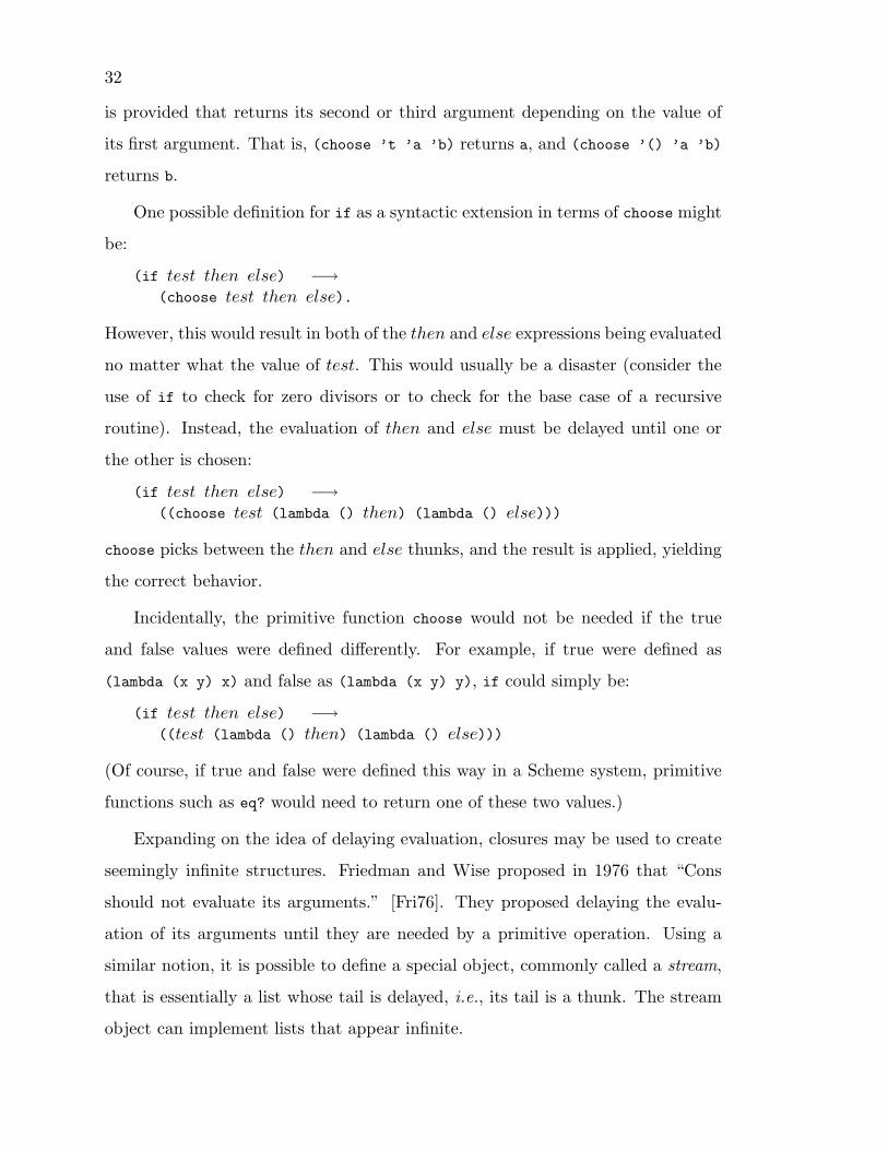
32

is provided that returns its second or third argument depending on the value of

its first argument. That is, (choose ’t ’a ’b) returns a, and (choose ’() ’a ’b)

returns b.

One possible definition for if as a syntactic extension in terms of choose might

be:

(if test then else) −→(choose test then else).

However, this would result in both of the then and else expressions being evaluated

no matter what the value of test. This would usually be a disaster (consider the

use of if to check for zero divisors or to check for the base case of a recursive

routine). Instead, the evaluation of then and else must be delayed until one or

the other is chosen:

(if test then else) −→((choose test (lambda () then) (lambda () else)))

choose picks between the then and else thunks, and the result is applied, yielding

the correct behavior.

Incidentally, the primitive function choose would not be needed if the true

and false values were defined differently. For example, if true were defined as

(lambda (x y) x) and false as (lambda (x y) y), if could simply be:

(if test then else) −→((test (lambda () then) (lambda () else)))

(Of course, if true and false were defined this way in a Scheme system, primitive

functions such as eq? would need to return one of these two values.)

Expanding on the idea of delaying evaluation, closures may be used to create

seemingly infinite structures. Friedman and Wise proposed in 1976 that “Cons

should not evaluate its arguments.” [Fri76]. They proposed delaying the evalu-

ation of its arguments until they are needed by a primitive operation. Using a

similar notion, it is possible to define a special object, commonly called a stream,

that is essentially a list whose tail is delayed, i.e., its tail is a thunk. The stream

object can implement lists that appear infinite.

33

The syntactic extension stream defined below creates a stream object:

(stream exp1 exp2) −→(cons exp1 (lambda () exp2)).

stream-ref returns the nth element of a stream for some stream s and index

n. It traverses the stream by applying its cdr to force evaluation:

(define stream-ref

(lambda (s n)

(if (zero? n)

(car s)

(stream-ref ((cdr s)) (- n 1)))))

It is now straightforward to write a function that generates a stream of integers

that increase in magnitude and alternate between positive and negative:

(define alternate

(lambda (n)

(stream n (alternate (- 0 (+ n 1))))))

Notice that alternate is recursive but has no explicit base case! The implicit base

case is n = 0. stream-ref can now be used to obtain a particular element of an

alternating series, i.e., (stream-ref (alternate 1) 10) returns -10. Of course, we

can generalize the function alternate to create many other kinds of series.

The following section on assignments demonstrates more uses for closures in

combination with assignments. In particular, a modified stream object is given

that “remembers” what has been computed so that the elements need not be

recomputed every time the stream is accessed.

2.3 Assignments

Assignments in Scheme are not usually necessary for the same purposes they serve

in traditional languages. Well-written programs in traditional languages employ

assignments to initialize variables, to update control variables in loops, and to

communicate among procedures through shared variables, often because more than

one value must be returned from a called routine. In Scheme, initialization occurs

at function application (or in let) at the same time as the binding (declaration)

34

occurs, control variables to a loop are the parameters passed to the tail-recursive

function that implements the loop, and return of multiple values is accomplished

by returning a list of values or by using continuation-passing-style.

Without these traditional uses for assignments, well-written Scheme programs

rarely require set!. There are, however, enough interesting uses for set! that the

language would be less powerful without it. This section presents a few of these

uses.

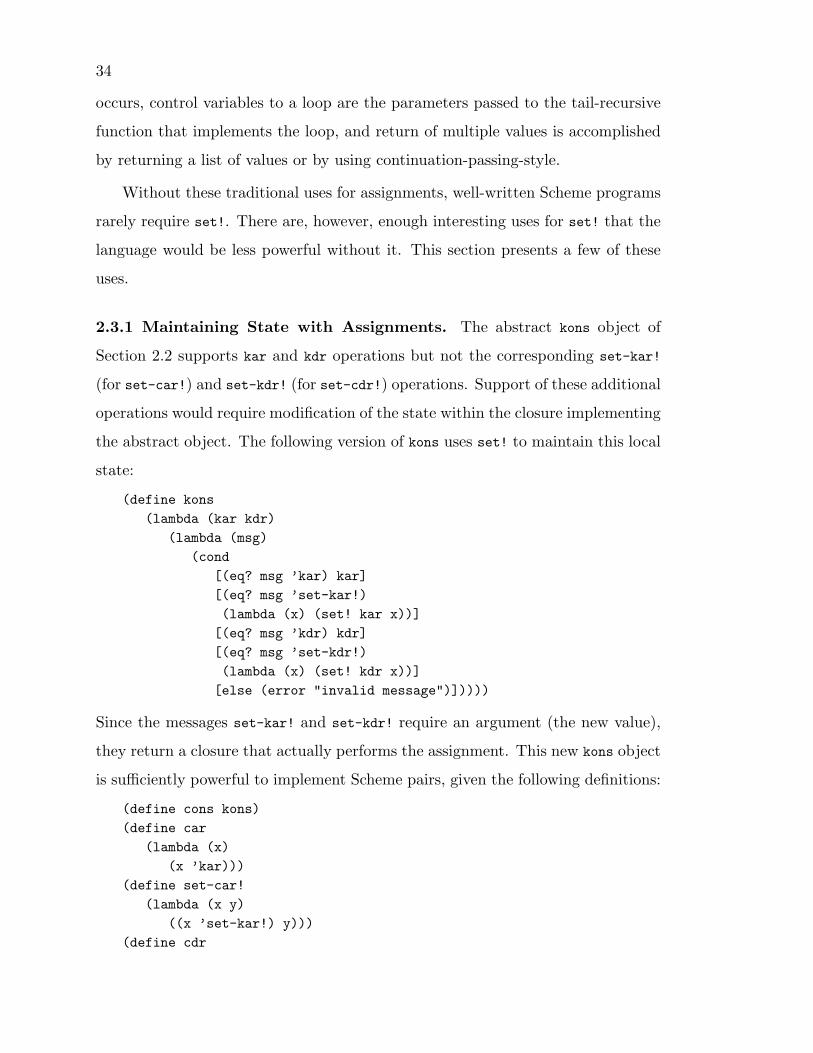
2.3.1 Maintaining State with Assignments. The abstract kons object of

Section 2.2 supports kar and kdr operations but not the corresponding set-kar!

(for set-car!) and set-kdr! (for set-cdr!) operations. Support of these additional

operations would require modification of the state within the closure implementing

the abstract object. The following version of kons uses set! to maintain this local

state:

(define kons

(lambda (kar kdr)

(lambda (msg)

(cond

[(eq? msg ’kar) kar]

[(eq? msg ’set-kar!)

(lambda (x) (set! kar x))]

[(eq? msg ’kdr) kdr]

[(eq? msg ’set-kdr!)

(lambda (x) (set! kdr x))]

[else (error "invalid message")]))))

Since the messages set-kar! and set-kdr! require an argument (the new value),

they return a closure that actually performs the assignment. This new kons object

is sufficiently powerful to implement Scheme pairs, given the following definitions:

(define cons kons)

(define car

(lambda (x)

(x ’kar)))

(define set-car!

(lambda (x y)

((x ’set-kar!) y)))

(define cdr

35

(lambda (x)

(x ’kdr)))

(define set-cdr!

(lambda (x y)

((x ’set-kdr!) y)))

(As with the redefinition of true and false suggested above, redefining cons and

functions related to it would necessitate many changes in the Scheme system,

including modifying the reader to create these structures when it sees list input.)

Local state changes may be implicit rather than explicit as they are with the

set-kar! and set-kdr! operations. The following stack object supports push, pop,

and empty? operations by maintaining a local stack (list). (push x) adds a new

element, x, to the top of the stack, (pop) returns the top element, removing it

from the stack, and (empty?) returns true if and only if the stack is empty.

(define stack

(lambda ()

(let ([s ’()])

(lambda (msg)

(record-case msg

[(empty?) (null? s)]

[(push x) (set! s (cons x s))]

[(pop) (let ([x (car s)]) (set! x (cdr s)) x)]

[else (error "invalid message")])))))

Without the ability to create and modify state, it would be impossible to

accurately model objects such as the kons and stack objects. Closures allow the

creation of objects with state local to the object, and assignments allow this state

to be changed. Many problems do not require this ability, but enough interesting

problems exist where state is required that to omit assignments from the language

would significantly lessen its expressive power. The lazy streams described next

offer a solution to the problem of making streams efficient that would require some

other language support (such as lazy evaluation) if not for assignments.

2.3.2 Lazy Streams. The streams introduced in Section 2.2 have the property

that each time the stream is traversed, the values in the stream are recomputed.

Needless to say, this can be terribly inefficient. A lazy stream does not recompute

36

these values, but saves them for future use. It saves them by altering the list

structure of the stream as it traverses it, using set-cdr!. These alterations are

actually performed by stream-ref, so stream is the same as before:

(stream exp1 exp2) −→(cons exp1 (lambda () exp2))

The new stream-ref checks to see if the cdr is still a closure, i.e., this part of the

stream has not yet been traversed. If so, it computes the new value of the cdr and

changes the cdr to this value, before continuing:

(define stream-ref

(lambda (s n)

(if (zero? n)

(car s)

(if (pair? (cdr s))

(stream-ref (cdr s) (- n 1))

(let ([v ((cdr s))])

(set-cdr! s v)

(stream-ref (cdr s) (- n 1)))))))

The examples given so far use assignments to maintain state local to a sin-

gle function. Assignments are also useful for maintaining state local to a set of

closures or abstract objects, or to allow communication among cooperating tasks

(coroutines). Often, assignments may be avoided and the resulting code may be

clearer without them, but sometimes just the opposite is true.

2.4 Continuations

The continuation-passing-style (CPS) examples of the Section 2.2 demonstrate the

use of closures as continuations to alter the flow of control in a Scheme program.

In CPS, the programmer must explicitly create the continuation closures and ex-

plicitly invoke one to return a result (it would not make sense in the examples

of the previous chapters to simply return without invoking one of the “return”

closures). While CPS is a powerful programming tool with many uses, Scheme

provides an alternative that requires less explicit programming and is sometimes

more appropriate than CPS. Using the syntactic form call/cc, a program can

37

obtain its own continuation. This continuation is a Scheme closure that may be

invoked at any time to continue the computation from the point of the call/cc. It

may be invoked before or after the computation returns; it may be invoked more

than one time.

One of the simplest uses is to allow nonlocal exits, as in the following definition

of reciprocals, which takes a list of numbers and returns a list of their reciprocals.

If it finds one of the numbers to be zero, it returns immediately with an error

message:

(define reciprocals

(lambda (lst)

(call/cc

(lambda (exit)

(recur loop ([lst lst])

(if (null? lst)

’()

(if (= (car lst) 0)

(exit "divide by zero")

(cons (/ 1 (car lst))

(loop (cdr lst))))))))))

With this definition, (reciprocals ’(1 2 3 4)) returns (1 1/2 1/3 1/4), while

(reciprocals ’(0 1 2 3)) returns "divide by zero".

The reciprocals function demonstrates the use of outward continuations to

return control “outward” to an expression before that expression has completed. In

other words, the code that used the call/cc expression is still active and waiting for

an answer. Continuations can also return control “inward”; an inward continuation

returns control to an expression that has already completed; the computation is

restarted from the call/cc expression. In general, the same continuation may be

invoked to return control outward or inward an arbitrary number of times.

Inward continuations can easily produce infinite loops:

(let ([comeback (call/cc (lambda (c) c))])

(comeback comeback))

The call/cc expression creates a continuation and passes it to the closure created

by (lambda (c) c). The closure simply returns this continuation, which then

38

becomes the value of comeback. The application of this continuation to itself

returns control to the call/cc with the continuation as its value (again). This

results in comeback being bound to the continuation (again), and the whole process

repeats forever.

If the code were changed slightly so that the continuation is passed a different

value, say 3:


(comeback 3)),

comeback would be bound to 3 the second time through and the program would

abort with an error message, something like “attempt to apply nonclosure 3”.

The logical next step is to replace 3 with a closure, such as the identity closure

(lambda (x) x):


(comeback (lambda (x) x)))

Now, comeback will be bound to the identity closure the second time. This closure

will be applied to the identity closure, which does not return control to the call/cc

but rather simply returns its argument. So the above expression does terminate,

and returns the identity closure.

Incidentally, this expression may be simplified to:

((call/cc (lambda (c) c)) (lambda (x) x))

and applied to a value of some sort:

(((call/cc (lambda (c) c)) (lambda (x) x)) ’HEY!).

Most people guess this returns HEY! even if they cannot figure out why. This is

probably the most confusing Scheme program of its size!

In addition to providing interesting puzzles for the mind, inward continuations

have practical uses. One example is the creation and use of coroutines [Hay86].

Coroutines are similar to functions, differing in two important ways. First, they

do not usually return a value; rather, they simply stop executing. Second, they

can be restarted from where they left off. Typically, two or more coroutines will

39

cooperate with one another, each executing for a time then stopping and restarting

the next.

Here is a simple coroutine syntactic extension:

(coroutine var exp) −→(define var

(let ([resume

(lambda (next)

(call/cc

(lambda (c)

(set! var (lambda () (c)))

(next))))])

(lambda () exp)))

An expression of the form (coroutine var exp) cause a new coroutine to be cre-

ated and bound to the variable var. Within the body exp of each coroutine, a

different resume function is bound to the variable resume. Whenever the coroutine

wishes to pass control to another coroutine, it invokes its own resume function.

The resume function saves the continuation of the current continuation as the new

value for var (wrapped in a thunk since it takes no arguments). So var is initially

bound to a function that starts the coroutine and is thereafter bound to a function

that continues the execution of the coroutine.

2.5 A Meta-Circular Interpreter

This section presents a meta-circular interpreter for Scheme. A meta-circular in-

terpreter for Scheme is an interpreter written for Scheme, in Scheme. The Scheme

system running the interpreter may be thought of as being at the meta level rel-

ative to the Scheme system implemented by the interpreter. It is possible to run

yet another interpreter within the meta-circular interpreter. The original meta

level would become the meta-meta level. In theory, this process could be carried

out indefinitely, providing an infinite tower of interpreters [Smi82].

The purpose of presenting this interpreter here is twofold. First, it helps to de-

scribe Scheme, providing a sort of operational semantics for the language. Second,

40

it serves as a basis from which the code presented for the implementation models

of Chapters 3, 4, and 5 can grow and with which that code can be compared.

While it does serve as a tool for better understanding the language, the meta-

circular interpreter does not provide a concrete semantics for the language [Rey72],

nor a viable base for an implementation unless you already have a Scheme system.

Because it relies on the underlying Scheme system (at the meta level) for the

support of closures and continuations and the proper treatment of tail calls, it does

not demonstrate any of the techniques for implementing these features directly.

Lexical variable bindings are recorded in an environment structure. The envi-

ronment is a list of pairs of lists, the two lists in each pair being a list of variables

and a corresponding list of values. During the evaluation of any expression, the

list of pairs corresponds to the nesting of the lambda expressions surrounding the

expression; the first pair of lists contains the bindings for the closest enclosing

lambda, the second contains the bindings for the next enclosing lambda, and so on.

This environment representation is often referred to as a rib cage because of its

structure, and the list of variables and list of values are referred to as variable

and value ribs. This structure is used as well in Chapter 3 and is described more

completely there.

Closures in interpreted code are implemented by closures in the interpreter.

The lexical environment and body are present in an interpreted closure because

they are lexically visible in the closure created by the interpreter. Continuations

are also implemented by continuations in the interpreter.

Here is the code. First, meta takes the input expression and passes it on to

exec along with an empty environment:

(define meta

(lambda (exp)

(exec exp ’())))

exec takes an expression exp and an environment env as input, and performs

the evaluation. The cond and record-case syntactic forms within the code parse

the expression. The three cond clauses correspond to variables, list-structured

41

forms, and other objects. Each of the record-case clauses but the last (else)

clause is for for a particular core syntactic form; the else clause is for applications.

(define exec

(lambda (exp env)

(cond

[(symbol? exp) (car (lookup exp env))]

[(pair? exp)

(record-case exp

[quote (obj) obj]

[lambda (vars body)

(lambda (vals)

(exec body (extend env vars vals)))]

[if (test then else)

(if (exec test env)

(exec then env)

(exec else env))]

[set! (var val)

(set-car! (lookup var env) (exec val env))]

[call/cc (exp)

(call/cc

(lambda (k)

((exec exp env)

(list (lambda (args) (k (car args)))))))]

[call/cc (exp) (call/cc (exec exp env))]

[else

((exec (car exp) env)

(map (lambda (x) (exec x env)) (cdr exp)))])]

[else exp])))

When the expression is a variable, the interpreter returns the value of this

variable in the current environment by calling the function lookup. Since lookup

is used for both variable reference and variable assignment, it returns the list con-

taining the value as its first element, so that it may be changed with set-car!. The

function lookup traverses the environment structure to find the variable, returning

the corresponding list tail:

(define lookup

(lambda (var e)

(recur nxtrib ([e e])

(recur nxtelt ([vars (caar e)] [vals (cdar e)])

(cond

[(null? vars) (nxtrib (cdr e))]

42

[(eq? (car vars) var) vals]

[else (nxtelt (cdr vars) (cdr vals))])))))

When the expression is of the form (quote obj), or just obj when obj is not a

symbol or pair, the interpreter simply returns obj.

When the expression is of the form (lambda vars body), the interpreter creates

a closure within the scope of the variables bound to the body, the variables, and the

environment. Later, when this closure is applied, it extends the environment with

the variables and the values it is passed and then recursively evaluates the body

using this new environment. The function extend builds the new environment by

creating a pair from the variable and value ribs and adding this pair to the old

environment:

(define extend

(lambda (env vars vals)

(cons (cons vars vals) env)))

For an if expression, (if test then else), the interpreter recursively evaluates

either test or else depending on the result of recursively evaluating test.

A set! expression, (set! var val), alters the environment structure to change

the binding of var to the result of recursively evaluating val.

For a call/cc expression of the form (call/cc exp), the interpreter recursively

evaluates exp and invokes call/cc to apply the resulting closure (it must be a

closure) to the current continuation.

Finally, for an application of the form (fcn arg1 . . . argn), the interpreter

applies the result of evaluating fcn (which must be a closure) to a list of the results

of evaluating arg1 . . . argn. As explained above, this results in the evaluation of

the body of the closure.

Chapter 3: The Heap-Based Model

This chapter describes a heap-based implementation model for Scheme. Heap-

based models have been used in many Scheme implementations, including Scheme-

84 [Fri84], C-Scheme [Dyb83] and Scheme-311 [Cli84]. These systems are all essen-

tially the same as the ones described in the first report on Scheme [Sus75], though

each uses different strategies for compilation and interpretation.

The first section of this chapter describes the motivation behind and the prob-

lems with the heap-based model. The second section presents the data structures

needed to support the heap-based model, and the third describes the operation

of this model. This is followed in the fourth section by a compiler that gener-

ates code for the heap-based model and a virtual machine that specifies how this

code is executed. Finally, the fifth section presents a common improvement that

substantially cuts the execution overhead of most programs and presents a modi-

fied compiler and virtual machine that serve as a basis for those presented in the

following chapter.

This chapter together with the two that follow describe a sequence of models

along with translators (compilers) and evaluators that implement these models.

Each model builds upon the previous ones, and each translator and evaluator uses

what it can from previous translators and evaluators. Working Scheme code is

given for each of the translators and for the evaluators of this chapter and the

next (Chapter 5 uses a different method for describing the meaning of its low-level

code). Not all of the models support the full Scheme language; the ones that do not

are present because they help focus the reader’s attention on the most important

44

details, they help to highlight problems with supporting particular features, and

they may also be useful for languages differing from Scheme in certain ways.

3.1 Motivation and Problems

In a typical implementation of a lexically-scoped language such as Algol 60, C or

Pascal, a true stack1 is used to record call frames [Aho77, Ran64]. Each call frame

contains a return address, variable bindings, a link to the previous frame, and

sometimes additional information. The variable bindings are the actual parameters

of the called routine and local variables used by the called routine. A call frame

is typically built by the calling routine, or caller. The caller pushes the actual

parameters on the stack, a link to its stack frame, the return address, and jumps

to the called routine, or callee. The callee augments the frame by pushing values

of local variables. If the callee in turn calls another routine, it creates a new stack

frame by pushing the actuals, frame link, and return address, and so on. When

the callee has reached the end of its code, it returns to the caller by resetting the

frame link, removing the frame, and jumping to the saved return address. In this

manner, the state of each active call is recorded on the stack, and this state is

destroyed once the call has been completed.

Because of Scheme’s first-class closures and continuations, this structure is not

sufficient. First-class closures are capable of retaining argument bindings indefi-

nitely. In particular, the closure and the saved bindings may be retained in the

system even after the call that created the bindings has returned and its stack

frame has been removed from the stack. For this reason, it is not possible to

store argument bindings in the stack frame. Instead, a heap-allocated environ-

ment is created to hold the actual parameters, and a pointer to this environment

1 The term “true stack” here refers to the typical stack provided by modernsequential computer architectures. The operations provide (at least) the ability topush items onto the top of the stack, index into the stack to retrieve an item, andremove items from the top of the stack. The ability to maintain multiple pointersinto the stack is also assumed.

45

is placed in the call frame in their place. When a closure is created, a pointer to

this environment is placed in the closure object.

Moving the variable bindings into the heap saves the bindings from being

overwritten as the stack shrinks and grows. With the call frames (minus variable

bindings) still stored on the stack, the only additional overhead in performing a

function call is the allocation of the environment. However, first-class continua-

tions require heap allocation of the call frames as well as the environment. This

is because the natural implementation of a continuation is to retain a pointer into

the call stack. Recall that a continuation is a closure that, when invoked, returns

control to the point where the continuation was obtained. Because the contin-

uation is a first-class object, there is no restriction on when it may be invoked.

In particular, it may be invoked even after control has returned from the point

where it was obtained. If so, the stack may have since grown, overwriting some of

the stack frames in the continuation. The natural solution, then, is to maintain

a linked list of heap-allocated stack frames. As the stack grows, a new frame is

allocated in an unused portion of the heap so that the old stack frames remain

intact.

The major problem with heap allocation of call frames and environments is

the overhead associated with the use of a heap. This overhead includes the direct

cost of finding space in the heap when building the call frames and environments,

and of following links instead of indexing a stack or frame pointer when accessing

pieces of the frame or environment. The overhead also includes the indirect cost

of storage reclamation to deallocate and reuse stack frames and environments and

the indirect cost of using excessive amounts of memory2. Furthermore, use of

2 One might expect this not to be a problem on virtual memory computerswith huge address spaces, but it is indeed a problem. The performance of virtualmemory systems is directly related to locality of reference; the fewer pages ofmemory used over a period of time, the fewer page faults. A stack-based modeluses and reuses the same stack frames as calls and returns are made. A heap-basedmodel, however, allocates a new stack frame each time, so unless these frames arereclaimed frequently (usually implying garbage collection overhead), new pagesare constantly being accessed.

46

the heap rather than a stack prevents the use of commonly available hardware

or microcode-supported stack push, pop and index instructions and the use of

function call and return instructions.

3.2 Representation of Data Structures

In the heap-based system, essentially five different data structures support the core

language. These are environments, call frames, the control stack, closures, and

continuations. The structure of these objects is critical in the design of a Scheme

system, since they are involved in every computation performed by the Scheme

system. These structures are described here along with their representation in

Scheme.

3.2.1 Environments. An environment is built from pairs created with cons.

The structure of an environment resembles a rib cage, since the environment is a

list of pairs of lists. Each element of the top level structure contains the bindings

established by one closure; multiple sets of bindings are needed when the code

consists of nested lambda expressions. Each element contains two lists: a list of

variables (the variable rib) and a corresponding list of values (the value rib). As a

simple example, consider the following code containing nested lambda expressions:

((lambda (a b)

((lambda (c)

((lambda (d e f) body) 3 4 5))

2))

0 1)

Assuming that the environment is empty when the expression is evaluated, the

environment upon evaluation of the body of the outermost lambda expression is a

list containing one pair of the variable rib (a b) and the value rib (0 1). Printed

in Scheme dotted-pair notation, this structure looks like ((a b) . (0 1))3.

3 The Scheme printer avoids using the dotted-pair notation wherever possible, soit would actually print the pairs of ribs without the “.”, as ((a b) 0 1). Regardlessof how the structure prints, the car of this pair is (a b) and the cdr is (0 1). Thisdissertation uses these notations interchangeably.

47

Once inside the next lambda expression, the environment consists of two

pairs, the first containing the variable rib (c) and the value rib (2), and the

second being the environment structure from above. This structure looks like

(((c) . (2)) ((a b) . (0 1))). Finally, inside the innermost lambda expression

(that is, during the evaluation of body), the environment looks like:

(((d e f) . (3 4 5))

((c) . (2))

((a b) . (0 1))).

Figure 3.1 contains a diagram of the typical internal representation of this envi-

ronment.

Note that the innermost bindings are first in the list. This occurs naturally

with the use of cons, which adds an element to the front of a list; here cons takes

the new pair of ribs and adds it to the front of the existing environment. This

structure makes sense anyway in terms of execution efficiency, since it is common

that most references within a particular lambda expression are to the parameters

of that lambda expression, that most other references are to the next level out, and

so on.

The improvement described in Section 3.4 allows the variable ribs to be

dropped from the environment structure; the environment becomes a list of value

ribs.

3.2.2 Frames and the Control Stack. Frames are used to record the state of

a pending computation while performing another. They are most often created

when one function calls another; the first is suspended waiting for the value of

the second. Any information required to continue evaluation of the first function

must be recorded in the frame. Depending upon the implementation, frames may

be needed for other operations as well, although such frames are not used here.

Call frames are used throughout this chapter and the next, and the particular

format varies from model to model. However, a call frame must always contain a

“return address” or expression to be evaluated next, the environment or equivalent

48

3 4 5

fed

2

c

0 1

ba

Figure 3.1 A Nested Environment

49

description of the active variable bindings, a pointer to the previous frame, and

any other state required to continue the computation.

In the heap-based system, call frames are simply lists that contain four fields.

The first field is the expression field. This field determines the next expression

to be evaluated. It corresponds to a return address (saved program counter or

instruction counter) in a standard computer architecture. The second field is the

environment field. This contains the currently active environment. The third field

is the rib field. During the evaluation of an application, this field contains a list

of the arguments that have been evaluated so far. The fourth and final field holds

the next frame.

The control stack in a heap-based system is the linked structure of the current

frame, the previous frame, its previous frame, and so on. It resembles a linked list,

where the fields of each frame are the elements and linking is internal through the

“next frame” pointer. It is reasonable to structure the control stack so that the

links are external to the frames as long as no extra storage overhead or overhead

in following links is introduced.

3.2.3 Closures and Continuations. Closures in a heap-based system are simple

objects that combine the text or executable part of a function with the current

environment. Unless the improvement of Section 3.5 is used, the variables are

needed as well. In the system of Section 3.4, then, a closure object is a list of

three elements: a function body, an environment, and a list of variables. For

example, the closure returned by:

((lambda (x)

(lambda (y) (cons x y)))

’a)

would look something like:

((cons x y) ((x) . (a)) (y))

except that the actual body would be a compiled version of (cons x y). In the

system of Section 3.5 a closure is a list of only two elements, an environment and

50

a function body.

A continuation is a closure that contains enough information to continue a

computation from a given point. Essentially this means that it returns to the point

where call/cc created it. The value it returns is its own argument. To realize

this behavior in a heap-based system, the entire stack, i.e., the top frame, must

be saved somehow. A continuation is simply a special closure object containing a

reference to the current frame (and hence the entire control stack).

It would be possible to tag closures to set the special continuation closures

apart from normal closures, and explicitly check this tag when applying a closure

to its arguments. However, performing this check would be inefficient; continuation

closures are infrequently invoked relative to normal closures. Instead, continuation

closures have the same structure as normal closures, but with a body that, when

executed, restores the saved stack and returns the continuation’s argument to the

routine that created the continuation.

3.3 Implementation Strategy

This section describes one strategy for the implementation of a heap-based system

using the data structures described in the previous section. Many different strate-

gies are possible; the one given here is intended to be simple to understand and

to generalize easily to the systems of the following chapter. It does not exactly

model any used by the implementations mentioned at the start of this chapter.

Computation is performed in an iterative fashion using a set of registers to

hold the state of the computation. An iterative approach is necessary because the

more straightforward recursive approach of the meta-circular interpreter presented

in Chapter 2 cannot properly support continuations or tail calls. The evaluator

must have explicit access to the state of the computation in order to save this state

in a continuation, and recursion makes some of this state implicit; this state is on

the meta level and not available directly to the implementation. Tail calls cannot

51

be properly supported unless the implementation (at the meta level) supports

them properly.

The strategies of this chapter use five registers:

a: the accumulator,

x: the next expression,

e: the current environment,

r: the current value rib, and

s: the current stack.

The paragraphs below describe the use of these registers.

The accumulator holds the last value computed by a value-returning operation

such as loading a constant or referencing a variable. During function application

it holds the value of each of the arguments in turn before they are saved on the

value rib, and the function value before it is applied. During the evaluation of

an if expression it holds the value of the test expression; if uses it to determine

which of the two other subexpressions to evaluate. The value of the accumulator

when a computation finishes is the value of the computation.

The next expression specifies the next expression to evaluate, such as the load-

ing of a constant, the creation of a closure, the assignment of a closure, or the

application of a closure. The expression is almost the same as a Scheme source

expression, except that it has been compiled to make the evaluation more efficient4.

The current environment holds the active lexical bindings. A new environment

is established upon application of a closure from the closure’s saved environment

and the arguments to the closure. Variable references, variable assignments, and

4 It would be reasonable to avoid the compilation step and use a source-levelinterpreter with the same registers given here. This is often done with heap-basedinterpreters because the overhead of interpretation is not that great compared withthe overhead of allocating frames and environments and the reference of variables.A compiler is used here for two reasons: first, the modification given in Section 3.5requires a preprocessing step anyway, and second, compilation is more importantin the stack-based models presented in the following chapter, so for uniformity weuse a compilation strategy throughout.

52

lambda expressions, i.e., creation of closures, use the current environment. Because

the environment is destroyed by function application, the environment is saved in

a call frame before the application takes place and restored upon return from the

application.

During evaluation of an application, the current value rib holds a list of ar-

guments evaluated so far. As with any expression, when the computation of an

argument expression completes, its value is in the accumulator. This value is added

to the current rib using cons. Once all of the argument values and the closure value

have been computed, the current rib combines with the closure’s environment to

produce the new current environment. Because the current rib is destroyed by

the evaluation of an application, it is saved along with the environment in the call

frame before the application takes place.

Finally, the current stack holds the top call frame. Call frames are added to the

stack before the start of an application, and removed upon return from a closure.

As noted earlier, a call frame consists of a saved environment, a saved value rib, a

saved expression that corresponds to a return address, and a link to the previous

call frame. When a call frame is removed from the current stack, these saved

values are restored to the current environment, current rib, and next expression

registers. The current stack itself may be saved at any time in a continuation

object by the evaluation of a call/cc expression.

It may already be apparent how the evaluation of most Scheme expressions

takes place from the description of the registers. However, some aspects of this

evaluation, especially with respect to applications, have not been explained. The

evaluation strategies for constants, variables, applications, and the core syntactic

forms in terms of how they affect the registers is given in the paragraphs below.

A variable reference changes the accumulator to the value of the variable found

in the current environment. (Also, the next expression x is changed to a new

expression determined by the compiler. The other operations change the next

expression x in the same way except as noted below.)

53

Constants and quote expressions are treated in the same manner; both cause

a specific object to be loaded into the accumulator.

A lambda expression results in the creation of a closure. This closure is placed

into the accumulator.

Evaluation of an if expression occurs logically in two steps. First, the com-

piler generates the appropriate code to leave the result of the test expression in the

accumulator before the if operation is evaluated. The if operation tests the accu-

mulator and changes the next expression to one of two expressions corresponding

to the “then” or “else” parts of the if expression.

A set! destructively alters the structure of the current environment to change

the value of the variable it assigns. As with if, the compiler arranges for the value

it needs to be in the accumulator prior to the set! operation.

Evaluation of a call/cc expression results in the creation of a new call frame

to save the current environment, current rib, and the expression to return to. The

new stack is then captured in a continuation object, which is added to the current

rib (which is the empty list, if all is working right). The next expression is updated

to an expression that first evaluates the function expression and then applies the

resulting closure to the current rib. When this continuation is subsequently in-

voked, the saved stack is restored, the top frame is removed, and the argument to

the continuation is placed in the accumulator.

Evaluation of an application occurs in several steps. The first step is the

creation of a new stack frame to save the current environment, the current rib,

and the return expression of the application. Also during this step the current rib

is reinitialized to the empty list. Then each of the arguments is evaluated in turn;

their values are added to the current rib. The function expression is evaluated and

its value left in the accumulator. Finally, the closure in the accumulator is applied

to the argument values in the current rib. Upon application, the new environment

formed by combining the closure’s environment with the current rib is placed in

the current environment register and the closure’s body is placed in the current

54

expression register. When the closure returns, the top stack frame is removed and

the saved values restored (the return value is in the accumulator when the closure

returns; it is left there).

There is one anomaly in the evaluation of call/cc and application expressions

regarding tail calls. In order to optimize tail calls, i.e., in order not to build up

the control stack on a tail call, a new call frame is not added to the stack. The

purpose in adding a call frame is to save the environment, value rib, and return

expression for the code that needs them after the call; in this case the only code

after the call would be a return, which would merely restore the next set of values

immediately.

3.4 Implementing the Heap-Based Model

This chapter and the two that follow demonstrate each model with a complete

compiler and a virtual machine (VM) that executes the compiled code or (in

Chapter 5) a semantic description of the low-level language produced by the com-

piler. In this chapter and in Chapter 4, each compiler transforms input Scheme

expressions into an “assembly code” for the corresponding virtual machine. This

assembly code is not in the linear form that one expects assembly language code to

be in, with labels and jumps for sequencing. Rather, it is in the form of a directed,

acyclic graph that may be processed without the need for labels and jumps. It

would be a simple matter to convert this form into a more traditional assembly

language. Alternatively, the virtual machine assembly code could be assembled

into byte codes for a more compact and faster virtual machine, or perhaps for a

hardware or microcode implementation of the virtual machine.

In this section, the compiler performs a relatively simple transformation, and

the virtual machine is itself relatively simple. The compilers and virtual machines

that follow are somewhat more complex.

55

3.4.1 Assembly Code. The assembly code for the VM described in this section

consists of 12 instructions each with zero or more operands. The instructions are

described below.

(halt) halts the virtual machine. The value in the accumulator is the result of

the computation.

(refer var x) finds the value of the variable var in the current environment, and

places this value into the accumulator and sets the next expression to x.

(constant obj x) places obj into the the accumulator and sets the next expression

to x.

(close vars body x) creates a closure from body, vars and the current environment,

places the closure into the accumulator, and sets the next expression to x.

(test then else) tests the accumulator and if the accumulator is nonnull (that is,

the test returned true), sets the next expression to then. Otherwise test sets the

next expression to else.

(assign var x) changes the current environment binding for the variable var to

the value in the accumulator and sets the next expression to x.

(conti x) creates a continuation from the current stack, places this continuation

in the accumulator, and sets the next expression to x.

(nuate s var) restores s to be the current stack, sets the accumulator to the value

of var in the current environment, and sets the next expression to (return) (see

below).

(frame x ret) creates a new frame from the current environment, the current rib,

and ret as the next expression, adds this frame to the current stack, sets the current

rib to the empty list, and sets the next expression to x.

(argument x) adds the value in the accumulator to the current rib and sets the

next expression to x.

(apply) applies the closure in the accumulator to the list of values in the current

rib. Precisely, this instruction extends the closure’s environment with the closure’s

56

variable list and the current rib, sets the current environment to this new environ-

ment, sets the current rib to the empty list, and sets the next expression to the

closure’s body.

(return) removes the first frame from the stack and resets the current environ-

ment, the current rib, the next expression, and the current stack.

3.4.2 Translation. The compiler transforms Scheme expressions into the assem-

bly language instructions listed above. Some Scheme expressions, such as variables

and constants, are transformed into a single assembly language instruction. Oth-

ers, such as applications, are turned into several instructions.

The compiler looks for each type of expression in turn and converts it into

the corresponding instructions. The inputs to the compiler are the expression to

compile and the next instruction to perform after the expression completes. The

next instruction may be thought of as the continuation of the expression (not to

be confused with continuation objects returned by call/cc).

The code for the compiler appears below. Note the use of cond and record-case

to parse the expression; these are used in all of the compilers in this dissertation.

They are described along with the other Scheme syntactic forms in Chapter 2.

(define compile

(lambda (x next)

(cond

[(symbol? x)

(list ’refer x next)]

[(pair? x)

(record-case x

[quote (obj)

(list ’constant obj next)]

[lambda (vars body)

(list ’close vars (compile body ’(return)) next)]


(let ([thenc (compile then next)]

[elsec (compile else next)])

(compile test (list ’test thenc elsec)))]

[set! (var x)

(compile x (list ’assign var next))]

57

[call/cc (x)

(let ([c (list ’conti

(list ’argument

(compile x ’(apply))))])

(if (tail? next)

c

(list ’frame next c)))]

[else

(recur loop ([args (cdr x)]

[c (compile (car x) ’(apply))])

(if (null? args)

(if (tail? next)

c

(list ’frame next c))

(loop (cdr args)

(compile (car args)

(list ’argument c)))))])]

[else

(list ’constant x next)])))

This compiler performs no error checking, though any compiler intended for actual

use should at least verify the number and structure of the arguments. The com-

pilers and virtual machines presented throughout this dissertation perform little

or no error checking in the interest of shortening the code and simplifying the

presentation.

The transformations for variables (symbols), quote expressions, and constant

expressions (specified in the else clause of the cond expression) are straightforward.

A variable, v, with next instruction, next, is transformed into (refer v next).

Similarly, (quote obj) and simple obj are transformed into (constant obj next).

The transformation of lambda expressions is also straightforward. An ex-

pression of the form (lambda vars body) is mapped into one of the form

(close vars cbody), where cbody is the result of compiling body. The next ar-

gument used when compiling body is a (return) instruction.

Both if and set! need one of their subexpressions to be evaluated before

the real work of the expression can be done. This is where the next argument to

the compiler becomes useful. For an if expression of the form (if test then else),

58

the test subexpression is compiled with a next argument formed from the compiled

then and else subexpressions, (test cthen celse). This result of compiling the test

subexpression with this next argument is returned as the compiled form of the if

expression. Incidentally, by passing on the original next argument when compiling

both of the then and else subexpressions, the compiler is creating a graph structure.

This is how the use of labels and jumps is avoided.

A set! expression is treated in a manner similar to an if expression.

(set! var x) is transformed into the compiled representation of x with a next

instruction of (assign var next), where next is the original argument to compile.

The remaining two expressions, call/cc and application, are treated in a some-

what similar manner. An application of the form (fcn arg1 . . . argn) is transformed

into an instruction “sequence” of the form:

frame

argnargument

...

arg1

argument

fcnapply.

The first instruction to be performed will be a frame instruction of the form

(frame c next), where c refers to the compiled code to perform the application and

next is the next instruction argument to the compiler (this is the return address

of the application). The true next instruction, c, is the compiled code for the last

argument, whose next instruction is the argument instruction. Its next instruction

is the compiled code for the second to last argument, followed by another argument

instruction, and so on, through the first argument and the corresponding argument

instruction. Finally, the next instruction after the last argument instruction is the

apply instruction.

The arguments to an application are evaluated last to first so that they will

be “consed” onto the value rib in the right order. cons adds elements to the front

59

of a list, so the last object pushed is the first object on the list.

A call/cc may be thought of as a special case of an application with a single

argument, an imaginary expression that returns the current continuation. An

expression of the form (call/cc exp) results in an instruction sequence of the

form:

frame

conti

argument

expapply.

This causes the frame to be pushed, followed by creation of the continuation, the

adding of this continuation to the current rib, the computation of exp, and finally

the application of exp to the list of arguments containing the continuation.

Both applications and call/cc expressions are treated slightly differently if

they appear in the tail position. This is determined simply by looking at the next

instruction to see if it is a return instruction as follows:

(define tail?

(lambda (next)

(eq? (car next) ’return)))

An application or call/cc expression in tail position does not push a call frame,

so the frame instruction is omitted.

3.4.3 Evaluation. The virtual machine, VM, interprets the instructions produced

by the compiler given above, using the data structures and registers described

earlier. Its structure is similar to that of a SECD machine [Lan64, Lan65]; the

state changes to a set of registers are modeled by a tail-recursive function. The

arguments to the function are the registers themselves. Each recursive call to the

VM signals the start of a new machine cycle; the new values for the VM registers

are specified by the arguments. This structure avoids the use of assignments,

allowing a cleaner and smaller description of the VM and its state changes.

Here is the code for the VM:

60

(define VM

(lambda (a x e r s)

(record-case x

[halt () a]

[refer (var x)

(VM (car (lookup var e)) x e r s)]

[constant (obj x)

(VM obj x e r s)]

[close (vars body x)

(VM (closure body e vars) x e r s)]

[test (then else)

(VM a (if a then else) e r s)]

[assign (var x)

(set-car! (lookup var e) a)

(VM a x e r s)]

[conti (x)

(VM (continuation s) x e r s)]

[nuate (s var)

(VM (car (lookup var e)) ’(return) e r s)]

[frame (ret x)

(VM a x e ’() (call-frame ret e r s))]

[argument (x)

(VM a x e (cons a r) s)]

[apply ()

(record a (body e vars)

(VM a body (extend e vars r) ’() s))]

[return ()

(record s (x e r s)

(VM a x e r s))])))

The operation of the VM follows the description of the instructions given

earlier. Notice that most of the instructions only alter one or two of the regis-

ters. Only one of the instructions performs a side-effect; this is assign, which

destructively alters the current environment. The help functions lookup, closure,

continuation, call-frame, and extend are shown below.

The function lookup finds the value of the variable var in the environment e. It

does this by searching each variable rib in turn until it finds the variable. As soon

as it finds the variable it returns the list whose car is the corresponding value. It

returns this list rather than the value itself so that it may be used by both refer

61

and assign; assign alters the list structure to perform the assignment.

(define lookup

(lambda (var e)

(recur nxtrib ([e e])

(recur nxtelt ([vars (caar e)] [vals (cdar e)])

(cond

[(null? vars) (nxtrib (cdr e))]

[(eq? (car vars) var) vals]

[else (nxtelt (cdr vars) (cdr vals))])))))

Two loops are needed, one over the ribs of the environment, the other over the

variables in the variable rib. The second loop carries along with it the value rib,

so that the value can be picked out as soon as the right location is found. Notice

that the loops are tail-recursive; the search is iterative.

The function closure creates a new closure object, which is simply a list of a

body, an environment, and a list of variables:

(define closure

(lambda (body e vars)

(list body e vars)))

The function continuation creates a new continuation object. A continuation

is a closure; the body is a nuate instruction, the environment is empty, and the list

of variables contains one element, v. The particular variable name chosen here does

not matter. What does matter is that the variable that appears in the variable

list is the same as the variable enclosed in the nuate instruction. nuate uses this

variable to access the first (and presumably only) argument to the continuation.

(define continuation

(lambda (s)

(closure (list ’nuate s ’v) ’() ’(v))))

The function call-frame merely makes a list of its arguments, a return address,

an environment, a rib, and a stack, i.e., the next frame in the stack:

(define call-frame

(lambda (x e r s)

(list x e r s)))

Finally, the function extend creates a new environment from an environment,

62

a variable rib, and a value rib:

(define extend

(lambda (e vars vals)

(cons (cons vars vals) e)))

One more function is needed to tie the compiler and virtual machine into a

working Scheme evaluator, this is the function evaluate that starts things off:

(define evaluate

(lambda (x)

(VM ’() (compile x ’(halt)) ’() ’() ’())))

The initial value in the accumulator is not really important, but the initial values

of the other registers are. The next expression is the compiled input expression;

its next instruction is halt. The current environment starts out as the empty

environment (an empty list of ribs), the current rib starts out as the empty list,

and the stack starts out empty as well.

3.5 Improving Variable Access

Looking at the code for the virtual machine given in the last section, it is appar-

ent that the five help functions lookup, closure, continuation, call-frame, and

extend do most of the work. No other substantial processing is performed by the

virtual machine. It is to these functions, therefore, that we look to improve the

performance of the Scheme system.

The stack-based models presented in the following chapter address each of

these functions, and greatly improve (or omit altogether) the lookup call-frame,

and extend functions, which are the most frequently used functions in the eval-

uation of almost all Scheme programs. However, before going to a stack-based

model, there is one thing that can be changed to improve performance somewhat.

This change improves the lookup function by performing part of its work in the

compiler.

Scheme variables are statically scoped. This means that the binding of any

variable is apparent in the static structure of the program (see Chapter 2). Because

63

of this, it is possible to determine from looking at the source exactly where a

variable will appear in the run-time environment. One way to do this is to maintain

a similar environment in the compiler.

The goal of this exercise is to compute for each variable its location in the

environment, so that the virtual machine can go straight to this location to find

the variable’s value without searching along the way. To do so, the virtual machine

must know which rib the value is in, i.e., how many ribs to skip over, and which

element it is in the rib. The refer and assign instructions must include these two

numbers.

Consider the following Scheme code:

(lambda (x y)

((lambda (a b c)

(a (lambda (x b) (y x c b))

b

y))

x

x

y)).

To determine the number of ribs and the number of variables within the rib to

pass over, it suffices to (1) find the correct binding, (2) count the number of

intervening lambda expressions, and (3) count the number of intervening variables

in the variable list. For example, the reference to c in the innermost lambda

expression refers to the c not in the current lambda but in the next one out. So the

rib number is 1. Two variables appear before c in the variable list, so the element

number is 2. Replacing all of the references in this piece of code with pairs of the

form (rib . elt), the result is:

(lambda (x y)

((lambda (a b c)

((0 . 0) (lambda (x b) ((2 . 1) (0 . 0) (1 . 2) (0 . 1)))

(0 . 1)

(1 . 1)))

(0 . 0)

(0 . 0)

(0 . 1))).

64

Notice that the rib of the (rib . elt) pair for a particular variable differs depending

on where that variable is referenced. This is because the rib number depends on

how many ribs will be in front of the desired rib at run time.

3.5.1 Translation. The following compiler is similar to the one from the preced-

ing section except that it takes an extra argument e, an environment that holds

only one rib, the variable rib, during compilation. This environment is searched

to produce the rib, element pairs for variable references and assignments.

(define compile

(lambda (x e next)

(cond

[(symbol? x)

(list ’refer (compile-lookup x e) next)]

[(pair? x)

(record-case x

[quote (obj)


[lambda (vars body)

(list ’close

(compile body (extend e vars) ’(return))

next)]


(let ([thenc (compile then e next)]

[elsec (compile else e next)])

(compile test e (list ’test thenc elsec)))]

[set! (var x)

(let ([access (compile-lookup var e)])

(compile x e (list ’assign access next)))]

[call/cc (x)


(list ’argument

(compile x e ’(apply))))])

(if (tail? next)

c


[else


[c (compile (car x) e ’(apply))])

(if (null? args)

(if (tail? next)

c

65


(loop (cdr args)

(compile (car args)

e


[else


Several things have changed with the addition of the environment argument.

First, rather than including the variable in the refer and assign instructions,

the compiler includes the result of calling compile-lookup with the variable and

environment. Also, no longer must the close instruction be given the list of

variables; they are no longer needed in the run-time environment. Notice, however,

that the compiler’s environment is updated with extend just as the virtual machine

updated its environment. This extend is slightly different, however, since it only

adds one rib to the environment:

(define extend

(lambda (e r)

(cons r e)))

This version of extend is used as well by the new virtual machine given later,

except there r refers to the value rib rather than to the variable rib.

The function compile-lookup is similar to the original lookup used by the old

virtual machine. However, instead of returning the value, it returns a pair of the

rib and element indices. It is this pair that the refer and assign instructions

employ.

(define compile-lookup

(lambda (var e)

(recur nxtrib ([e e] [rib 0])

(recur nxtelt ([vars (car e)] [elt 0])

(cond

[(null? vars) (nxtrib (cdr e) (+ rib 1))]

[(eq? (car vars) var) (cons rib elt)]

[else (nxtelt (cdr vars) (+ elt 1))])))))

3.5.2 Evaluation. The new virtual machine must support the slightly different

environment format and slightly different refer, assign and lambda instructions.

66

Most of these changes are to the help functions lookup, closure, continuation,

extend. In fact, the only change to the coding of the VM is to reflect the different

structure of the lambda instruction, and the corresponding change of arguments to

the closure function.

(define VM

(lambda (a x e r s)

(record-case x

[halt () a]

[refer (var x)

(VM (car (lookup var e)) x e r s)]

[constant (obj x)

(VM obj x e r s)]

[close (body x)

(VM (closure body e) x e r s)]

[test (then else)


[assign (var x)

(set-car! (lookup var e) a)

(VM a x e r s)]

[conti (x)


[nuate (s var)

(VM (car (lookup var e)) ’(return) e r s)]

[frame (ret x)

(VM a x e ’() (call-frame ret e r s))]

[argument (x)


[apply ()

(record a (body e)

(VM a body (extend e r) ’() s))]

[return ()

(record s (x e r s)

(VM a x e r s))])))

The change to extend to omit the variable rib was already given above. The

changes to closure and continuation are minor. closure now takes only a body

and an environment:

(define closure

(lambda (body e)

(list body e)))

67

In continuation, the call to closure no longer passes the variable list (v).

Also, instead of including v in the instruction, it now includes an explicit reference

to the first argument of the closest rib, (0 . 0):


(lambda (s)

(closure (list ’nuate s ’(0 . 0)) ’())))

The major change comes in lookup, which was the goal of this section. The

new lookup now simply moves directly to the specified rib and returns the specified

list cell within that rib:

(define lookup

(lambda (access e)

(recur nxtrib ([e e] [rib (car access)])

(if (= rib 0)

(recur nxtelt ([r (car e)] [elt (cdr access)])

(if (= elt 0)

r

(nxtelt (cdr r) (- elt 1))))

(nxtrib (cdr e) (- rib 1))))))

The inner loop is now executed only once for each variable lookup, when the proper

rib is located. Also, the only test on each iteration is for zero, rather than the two

tests of the previous version, one to test for the end of the rib and the other to

compare the two variables.

The improvement given here is substantial and important, but the system still

requires two loops and potentially many memory references to find the binding

of a variable. Also, call frames and environments are still in the heap, although

the latter are now one pair smaller for each environment level. The stack-based

models of the next chapter streamline variable access to as little as one instruction

(actually, to as little as one operand of one instruction) while avoiding most of the

allocation for call frames and environments.

Chapter 4: The Stack-Based Model

An execution profile analysis of a heap-based implementation of Scheme (the au-

thor’s C-Scheme [Dyb83]) showed that more than half of the running time of

the tested programs was spent performing variable lookups and function calls. In

contrast, an insignificant amount of time was spent creating closures, creating con-

tinuations, and invoking continuations. This was due, in part, to the large number

of variable references and function calls performed by most programs, combined

with the overhead of performing these operations. To improve the efficiency of a

Scheme system, then, requires improvement of these basic operations. In a heap-

based system, finding a variable potentially requires following several links, while

performing a function call requires heap allocation of an environment rib and a

call frame.

Perhaps worse than the overall efficiency problem is that the knowledge that

variable references and function calls are slow relative to other operations can

affect programming style. Programmers take for granted that function calls and

variable references are relatively inexpensive; it is unsettling to find out that they

are not, and this can result in a strained programming style (avoidance of the use

of both variables and functions) that adversely affects readability and modularity.

The typical implementation of a block-structured language such as Algol 60,

Pascal, or C does not require the use of a heap to allocate environments or call

frames. However, although all three languages allow nested blocks, and although

Algol 60 and Pascal allow nested function declarations, none of these languages

allows a function to be returned and subsequently called outside of the scope of an

enclosing block or function, as Scheme does. Early Scheme implementors believed

70

that because of the need to support first class functions, the standard techniques

used for block-structured languages were not suitable for Scheme. The need to

optimize tail calls and support continuations further convinced early implementors

that the standard stack techniques were unsuitable. However, as this chapter will

show, these techniques can be made to work for Scheme with a few modifications.

The resulting implementation model allows most function calls to be performed

with little or no allocation, and allows variable references to be performed in one

or two memory references. Heap allocation remains necessary to support closures,

assigned variables, and continuations. Since function calls and variable references

are faster and heap allocation is limited, the running time for most programs is

greatly decreased.

The first section of this chapter describes a typical stack-based implementation

of a block-structured language, including a discussion of the data structures and

concepts involved. A compiler and virtual machine for this standard implemen-

tation is presented. This sets the groundwork for the remaining sections of this

chapter, providing a basis for a stack-based model for the full Scheme language.

The next five sections develop a stack-based model for Scheme through a series

of modifications to the heap-based model of the preceding chapter and to the com-

piler and virtual machine implementing that model. In Section 4.2, the heap-based

model is modified to move the control stack onto a true stack, making function

calls faster but creation and application of continuations slower. Section 4.3 further

modifies this model to move the environment onto the stack, sacrificing support

for first-class functions, tail-call optimization, and assignments. Support for first-

class functions, assignments and optimized tail calls is added is Sections 4.4, 4.5,

and 4.6.

The resulting model supports Scheme and uses a true stack for call frames and

variable bindings. This model has proven itself viable in the author’s Chez Scheme

system that, at the time it was first distributed in early 1985, was considerably

faster than any other Scheme system.

71

Finally, Section 4.7 describes some important techniques that may be employed

by a sophisticated compiler to avoid the (less significant) allocation overhead for

closures, assigned variables, and continuations in certain situations.

4.1 Stack-Based Implementation of Block-Structured Languages

This section describes the typical implementation of Algol 60, C, or Pascal. To

simplify the presentation, the source language considered is a dialect of Scheme

without first-class functions, continuations, and optimized tail-calls, making it

similar to the more standard block-structured languages. Parameters are passed

by value, in contrast to Algol 60, which allows parameters to be passed by name,

and Pascal, which allows parameters to be passed by reference. (The distinctions

among parameter passing styles is not important here.) Functions are allowed as

parameters (functionals), but they are not first class objects since they cannot be

reliably retained and invoked after the defining scope no longer exists.

4.1.1 Call Frames. A call frame is created each time a function is applied to

a set of arguments1. It must hold the parameters to the called function, any

saved pointers and registers (the program counter, expression temporaries, etc.)

to restore upon return, room for local temporaries, the dynamic link, and the static

link (see the following section for a description of the dynamic and static links).

Call frames in the stack model described in this section contain

1. the frame pointer holding the address of the call frame of the suspended call

(the dynamic link),

1 In some instances, a call frame is also created whenever a new block is entered,as with some Algol 60 implementations [Ran64], in which case the new block isconsidered to be a parameterless function. A similar solution is to treat the lo-cal declarations of any block as a function invocation where the parameters arethe locally declared variables. This is most suitable for language constructs likeScheme’s let expression where the initialization always appears with the decla-ration. More often, however, the implementation treats variables declared in thenested block as temporary storage locations local to the current call frame to avoidthe overhead of creating a separate call frame.

72

2. the arguments to the called function,

3. the return address (the next expression after the call), and

4. the frame pointer holding the address of the call frame for the next outer scope

of the called function (the static link).

This information is layed out in the call frame as follows:

static link (pushed last)

first argument...

last argument

next expression

dynamic link (pushed first)

The ordering of the fields in a call frame is somewhat arbitrary; however, support

for optimized tail calls is greatly simplified by the placement of the next expression

(return address) and dynamic link below the arguments and the static link (see

Section 4.6).

4.1.2 Dynamic and Static Links. The dynamic link always points to the

caller’s frame. It is used when returning from a function to determine where the

next frame lies on the stack. The dynamic link is sometimes unnecessary since the

next frame always lies just below the current frame on the stack; assuming the

sizes of the current and previous frames are known to the compiler, it can often

generate efficient code for restoring the previous frame upon return. However, the

dynamic link is nearly always used to simplify the return sequence, to support

debugging, or to facilitate the use of microcoded call and return instructions (such

as the VAX calls/callg and ret instructions [Dig81]).

The static link, on the other hand, always points to the frame of the clos-

est enclosing function definition of the called function, i.e., the frame containing

the closest outer set of variable bindings visible within the called function. The

assumption that the language does not support closures, optimized tail calls, or

73

continuations is important here since it must be guaranteed that this frame is

still on the stack. For instance, if a closure could be returned and used outside

its scope, the frames statically visible to the closure might be gone by the time

the closure is invoked. Similarly, optimizing a tail call may cause the current

stack frame to be deleted; it will not be available when needed by the invocation

of a function within its scope. Continuations pose similar problems discussed in

Section 4.3.

The static link may or may not point to the same frame as the dynamic link.

The dynamic links create a single chain of frames on the stack (the dynamic chain),

each link pointing to the frame below. The static links, however, potentially create

many static chains, where each link points to a frame somewhere below and each

chain ends at the frame of the outermost function in the scope.

In the heap-based model, the static and dynamic chains also exist, but they

exist separate from each other. The linked control stack of call frames is the

dynamic chain, while each environment represents a static chain. The static and

dynamic links are the links that hold the structures together. A dynamic link is

a pointer to the next frame in the control stack; a static link is a pointer to the

next rib of an environment.

Separation of the dynamic and static chains facilitates the support of closures

and tail calls. Closures require the retention of the bindings, so naturally only

the static chain need be kept. To keep the entire dynamic chain (sometimes much

larger) would waste storage space. Optimized tail calls require that part of the

dynamic chain be released even though the static chain may still be required.

Heap allocation protects the static chains (environments) retained in a clo-

sure and the dynamic chain retained in a continuation from being overwritten

by subsequent operations. With a true stack, as control moves into and out of

called routines, the same memory locations record different information at differ-

ent times. Allocation of a fresh block of memory each time a call frame or value rib

is created guarantees that nothing is overwritten (except that the storage manager

74

may determine that the call frame or value rib is no longer needed and reclaim its

storage for later use).

4.1.3 Functionals. It is possible within the framework of this simple stack model

to pass functions as arguments, so long as the function is invoked only while the

call frames in its scope are active. That is, the function must not be returned or

stored and later invoked after the static chain it requires has been overwritten.

Because a functional may be invoked from a block or function with a different

static chain, the functional must retain the static chain just as the closures of the

last chapter retained the environment. This entails saving the address of the frame

when the functional is created along with the body of the functional and restoring

it when the functional is called.

The code for creating a functional in this system appears to be the same as

the code for creating a closure in the heap-based model:

(define functional

(lambda (body e)

(list body e)))

However, there is an important difference; the environment, e, passed to the

functional function is a frame pointer pointing to a frame in the stack, not a

heap-allocated environment.

Since a functional never outlives the code that creates it (that is, it cannot be

used once the scope in which it was created has been exited), it is not necessary to

heap allocate a functional as is implied by the use of the list operation. Instead,

the functional would more appropriately be given space on the stack in the call

frame for the function responsible for creating the functional. In the interest of

keeping the call frames simple, this improvement is not employed here.

4.1.4 Stack Operations. The major difference in the implementation of a stack-

based model and a heap-based model is, naturally, that call frames and variable

bindings are placed on a true stack rather than in a heap-allocated linked structure.

This difference does not affect the implementation as much as might be expected;

75

the compiler and virtual machine presented in this section are quite similar to the

ones presented in the preceding chapter.

The stack is implemented as a Scheme vector:

(define stack (make-vector 1000))

The chosen length (1000) is, of course, arbitrary2. Stack indices grow from zero

as elements are added, and multiple stack pointers (actually, vector indices) are

allowed. The function push takes a stack pointer (which should be the virtual

machine’s notion of the current top-of-stack) and an object and adds the object

to the top of the stack. It returns the updated (incremented) stack pointer:

(define push

(lambda (x s)

(vector-set! stack s x)

(+ s 1)))

The push function corresponds to the auto-increment or auto-decrement operand

addressing mode provided by many contemporary machine architectures.

Two operations are provided for referencing or changing an element of the

stack, index and index-set!. The index function takes a stack pointer (which

should be at or below the virtual machine’s notion of the current top-of-stack)

and an index and returns the object found at the specified offset from the stack

pointer. Similarly, the index-set! function takes a stack pointer, an index, and

an object and places the object at the specified offset from the stack pointer:

(define index

(lambda (s i)

(vector-ref stack (- (- s i) 1))))

(define index-set!

(lambda (s i v)

(vector-set! stack (- (- s i) 1) v)))

2 No checks for stack underflow are necessary if the machine is operating cor-rectly, and checks for stack overflow, while necessary, are never shown. It is as-sumed that the machine architecture for which a high-performance implementa-tion of this system was designed would provide some mechanism for trapping andreporting or recovering from stack overflow.

76

(The expression (- (- s i) 1) allows positive indices to be used for referencing off

of the stack pointer even though the stack grows in the opposite direction.) The

index and index-set! operations correspond to the deferred operand addressing

mode provided by many contemporary machine architectures.

Elements are removed implicitly from the stack by the virtual machine when

it decrements its notion of the current top-of-stack pointer.

4.1.5 Translation. The compiler shown below differs from the compiler of Sec-

tion 3.5 in three relatively minor ways.

First, since the arguments to a function are to be placed directly in the call

frame, the size of a call frame is a function of the number of arguments. The

virtual machine’s return instruction, which is responsible for removing the call

frame, must have this information. Hence, the return instruction is augmented

to accept an argument, n, that tells it how many elements to remove from the

stack in addition to the saved dynamic link and next expression that it removes

and restores explicitly. Since the static link is also stored on the stack but not

explicitly removed it is included in the count.

The second difference is that, since tail calls are not to be supported, the

conditional expression with respect to tail? has been removed from the code for

function application.

The third difference is that support for continuations has been omitted entirely.

Here is the compiler:

(define compile

(lambda (x e next)

(cond

[(symbol? x)

(compile-lookup x e

(lambda (n m)

(list ’refer n m next)))]

[(pair? x)

(record-case x

[quote (obj)


77

[lambda (vars body)

(list ’close

(compile body

(extend e vars)

(list ’return (+ (length vars) 1)))

next)]





[set! (var x)

(compile-lookup var e

(lambda (n m)

(compile x e (list ’assign n m next))))]

[else



(if (null? args)

(list ’frame next c)

(loop (cdr args)

(compile (car args)

e


[else


The functions compile-lookup and extend, which are shown below, are identical to

the functions of the same name used in Section 3.5 for the (improved) heap-based

model. This is because both models require the traversal of a given number of

links to find the right frame or rib and the reference of a given position within

that frame or rib. Note, however, that extend is now only used by the compiler

and not in the virtual machine, since values are stored on the stack rather than in

a rib of an environment.


(lambda (var e return)

(recur nxtrib ([e e] [rib 0])

(recur nxtelt ([vars (car e)] [elt 0])

(cond

[(null? vars) (nxtrib (cdr e) (+ rib 1))]

[(eq? (car vars) var) (return rib elt)]

[else (nxtelt (cdr vars) (+ elt 1))])))))

78

(define extend

(lambda (e r)

(cons r e)))

4.1.6 Evaluation. The virtual machine has a similar structure to that of Sec-

tion 3.5, and supports most of the same instructions. Two of the registers are

used in exactly the same manner, the accumulator (a) and the next expression

(x), while two are used differently, the environment (e) and stack (s). The e reg-

ister still holds an environment of sorts, the static link. However, it is now a stack

pointer pointing at the call frame of the next outer scope. The s register is a stack

pointer pointing at the current top-of-stack. One register, the current rib (r), is

gone entirely. It is no longer needed since arguments are placed directly on the

stack rather than into a heap-allocated rib.

Some of the instructions supported by the virtual machine have changed in be-

havior from the virtual machine of the preceding chapter, as shown in the following

summary:

(halt) behaves the same.

(refer var x) follows static links on the stack instead of links in a heap-allocated

environment. (It also uses an index operation in place of a loop once it finds the

appropriate frame.)

(constant obj x) behaves the same.

(closure vars body x) creates a functional rather than a closure.

(test then else) behaves the same.

(assign var x) follows static links on the stack instead of links in a heap-allocated

environment.

(conti x) not supported.

(nuate s var) not supported.

(frame x ret) starts a new frame by pushing the dynamic link (the current frame

pointer) and next expression ret. The virtual machine of the preceding chapter

79

built a call frame in the heap.

(argument x) pushes the argument on the stack instead of adding an element to

the current rib.

(apply) behaves similarly, but pushes the static link from the functional onto the

stack rather than building onto it by adding a rib.

(return n) takes an additional argument, n, that determines the number of ele-

ments it removes from the stack in addition to the saved dynamic link and next

expression.

Here is the code for the virtual machine:

(define VM

(lambda (a x e s)

(record-case x

[halt () a]

[refer (n m x)

(VM (index (find-link n e) m) x e s)]

[constant (obj x)

(VM obj x e s)]

[close (body x)

(VM (functional body e) x e s)]

[test (then else)

(VM a (if a then else) e s)]

[assign (n m x)

(index-set! (find-link n e) m a)

(VM a x e s)]

[frame (ret x)

(VM a x e (push ret (push e s)))]

[argument (x)

(VM a x e (push a s))]

[apply ()

(record a (body link)

(VM a body s (push link s)))]

[return (n)

(let ([s (- s n)])

(VM a (index s 0) (index s 1) (- s 2)))])))

The only help function not yet described is find-link, which is the analog to

the outer loop of the lookup function in the heap-based model of Section 3.5. It

80

receives two arguments, a number n and a frame pointer e, and locates the nth

frame (zero based) in the static frame starting with e:

(define find-link

(lambda (n e)

(if (= n 0)

e

(find-link (- n 1) (index e -1)))))

The evaluate function shown below invokes the compiler and starts the vir-

tual machine with the empty list as the initial accumulator, the compiled input

expression as the next expression, and zero for both the current frame pointer and

the stack pointer:

(define evaluate

(lambda (x)

(VM ’() (compile x ’() ’(halt)) 0 0)))

4.2 Stack Allocating the Dynamic Chain

This section and the ones that follow transform the heap-based model of Sec-

tion 3.5 step by step into one that can be implemented nearly as efficiently as the

stack-based model shown in the preceding section. Some concessions are made to

support closures, continuations, and tail calls, but most of these concessions need

affect only programs that take advantage of these features. The resulting model

can result in an implementation far more efficient in terms of memory allocation,

memory references, and number of instructions executed than a heap-based model.

The first step in the transformation, shown in this section, is to place the

dynamic chain, or control stack, on a true stack, while leaving the static chain,

or environment, in the heap. The primary difficulty in doing so is the support

of continuations. Continuations must be able to retain and restore the dynamic

chain, even after some or all of the chain has been removed from the stack and

the stack rewritten.

81

4.2.1 Snapshot Continuations. The solution taken here is to make a copy, or

snapshot, of the stack to store in a continuation, and to restore the copy when the

continuation is invoked. The return addresses and environment pointers retained

therein provide sufficient information to continue the computation, just as they

do when the stack is heap-allocated. Furthermore, no changes are made to the

stack itself (frames are added and removed from the top and nothing in a frame

is ever changed), so there are no updating problems involved with the duplicated

structure.

This solution works—but it may seem rather expensive. After all, the stack

could become quite large, and the allocation and copying overhead associated

with creating a continuation and the copying overhead associated with invoking a

continuation can be great. The reason why this is not of great concern is that con-

tinuations are created and invoked infrequently compared with function calls. In

other words, the allocation and execution time savings from function calls nearly

always outweighs the corresponding costs from creation and invocation of contin-

uations.

To see why the savings outweigh the costs, consider first a program that makes

no use of continuations. With the dynamic chain stack-allocated, this program

never requires any call frame to be heap-allocated. On the other hand, consider a

program that makes few calls but creates and perhaps invokes many continuations.

This program would create small continuations; few calls means few call frames.

Perhaps more typical would be a program where the dynamic chain grows and

shrinks, creating or invoking a continuation relatively infrequently compared to

this growing and shrinking. To this program, many of the call frames created on

the stack will never require heap allocation because they will never be needed by

a continuation. A small number will, but the total allocation overhead may still

be no more for these; if each call frame is saved in exactly one continuation, it

takes up no more room in the heap than if it were placed there to begin with (and

potentially less, depending upon the allocation mechanism).

82

In fact, the only situation in which this solution is guaranteed to come out

significantly behind is a fairly contrived one. This is when a program performs

many nested or recursive calls that build up a large dynamic chain on the stack

and while this dynamic chain remains intact creates and perhaps invokes more

than one continuation, then returns through the dynamic chain without making

any further calls. In this situation, the stack is large when the continuations are

created, and all of the call frames created by the program end up in the heap in

more than one place3.

Perhaps the most important reason why this is a reasonable solution is that

any program that does not use continuations does not pay for them, and that even

programs using continuations in a moderate fashion pay less for them than they

save from the now less expensive function calls. This is a simple case of a good

principle, to make common operations as fast as possible while making the less

common operations pay their own way.

4.2.2 Evaluation. The use of stack allocation in place of heap allocation does

not affect the compiler, but does affect a few of the virtual machine instructions.

(Since the compiler is identical to the one shown in Section 3.5, it is not shown

here.) The instructions that change are the instructions that manipulate the stack

register s. These are the conti, nuate, frame, and return instructions.

The frame and return instructions change only in that they now use push,

index, and - to manipulate the stack in place of cons, car and cdr. The push and

index operations used are the ones defined in the preceding section.

The conti instruction still creates a continuation, but it does so with the help

of the function save-stack:

3 It is possible to avoid this duplication in many cases by moving the stack intothe heap and leaving behind a link rather than copying it. This means copyingit back not only when the continuation is called explicitly but also when thefunction passed to call/cc returns normally. This was the solution chosen in theimplementation of Texas Instruments’ PC Scheme [Bar86].

83


(lambda (s)

(closure

(list ’refer 0 0 (list ’nuate (save-stack s) ’(return)))

’())))

The function save-stack creates a Scheme vector to hold the stack, and copies the

current stack from its start (at index 0) to the current stack pointer, passed as the

argument s:

(define save-stack

(lambda (s)

(let ([v (make-vector s)])

(recur copy ([i 0])

(unless (= i s)

(vector-set! v i (vector-ref stack i))

(copy (+ i 1))))

v)))

The nuate instruction, uses the help function restore-stack to restore the stack

saved by saved-stack:

(define restore-stack

(lambda (v)

(let ([s (vector-length v)])

(recur copy ([i 0])

(unless (= i s)

(vector-set! stack i (vector-ref v i))

(copy (+ i 1))))

s)))

Here is the virtual machine:

(define VM

(lambda (a x e r s)

(record-case x

[halt () a]

[refer (n m x)

(VM (car (lookup n m e)) x e r s)]

[constant (obj x)

(VM obj x e r s)]

[close (body x)

(VM (closure body e) x e r s)]

[test (then else)

84


[assign (n m x)

(set-car! (lookup n m e) a)

(VM a x e r s)]

[conti (x)


[nuate (stack x)

(VM a x e r (restore-stack stack))]

[frame (ret x)

(VM a x e ’() (push ret (push e (push r s))))]

[argument (x)


[apply ()

(record a (body e)

(VM a body (extend e r) ’() s))]

[return ()

(VM a (index s 0) (index s 1) (index s 2) (- s 3))])))

The evaluate function initializes the accumulator to the empty list, the next

expression to the compiled input expression, the environment and value ribs to

the empty list, and the stack pointer to zero:

(define evaluate

(lambda (x)

(VM ’() (compile x ’() ’(halt)) ’() ’() 0)))

4.3 Stack Allocating the Static Chain

The preceding section showed how the dynamic chain can be moved from the heap

onto the stack. The other half of the transformation from a heap-based to a stack-

based model is the movement of the static chain to the stack. This problem is

somewhat more difficult, and requires this section and the three following sections

to describe.

This section shows the modifications to move the static chain onto the stack

at the expense of omitting support for first-class functions, assignments, and op-

timized tail calls. The three following sections add these features back into the

model one at a time.

85

4.3.1 Including Variable Values in the Call Frame. Moving the static chain

onto the stack means placing the arguments to a function into the call frame along

with the control information already present there. This can be accomplished by

merging the stack-based model shown in Section 4.1 with the modified heap-based

model shown in Section 4.2. The merger of these two models allows arguments to

be placed in the call frame, as with the Section 4.1 system, while allowing support

for continuations.

However, the Section 4.1 system did not support first-class functions or opti-

mized tail calls. That system did not support first-class functions because that

would require the retention of the static chain that resides on the stack. Of course,

it would be possible to save the entire stack each time a closure is made, just as

the entire stack is saved when a continuation is created. This is likely to be an un-

acceptable solution because the creation of closures is fairly common in Scheme,

much more common than the creation of continuations. A much more efficient

strategy is presented in Section 4.4.

The same system did not support tail calls because it is not always possible

to delete the frame of the caller when it contains variable bindings that may

be required by the called function. The solution to this problem is discussed in

Section 4.6.

Furthermore, with the possibility that a continuation might be created, it

becomes difficult to support assignments as well. Assignments to stack-allocated

variable bindings are difficult to handle in the presence of continuations supported

as they are in the system of Section 4.3, because of a multiple-update problem.

Because each continuation may have its own copy of a segment of the stack, it is

possible that a copy of the same stack frame is in more than one place in memory.

If variable bindings are stored directly in the call frame as they are in the system

of Section 4.1, this means that the value of a variable may be stored in more than

one place. An assignment to such a variable would require that all copies were

updated, not just the one currently on the stack.

86

This is a serious problem because it is not possible for the compiler to detect

when a continuation will be created or invoked, and when one will not be cre-

ated. This means that some run-time bookkeeping would be required to support

assignments, slowing down assignment and causing additional storage overhead

(probably in the heap). A solution to this problem is given in Section 4.5.

4.3.2 Translation and Evaluation. The new compiler and virtual machine

must place argument values in the call frame and support continuations, but they

do not support first-class functions, assignments, or optimized tail calls. Since the

design is a merger of the designs of Sections 4.1 and 4.2, it should not be surprising

that a compiler and virtual machine can be produced by merging the compilers

and virtual machines from these sections.

These compilers and virtual machines already have some features in common:

the essential structure of the stack and the code generated for simple expressions

such as constants and if expressions. The new system retains these similarities,

takes the code for pushing arguments and the static link onto the stack from the

Section 4.1 code, and the code for creating and invoking continuations from the

Section 4.2 code. Support for first-class functions, assignments and tail calls is left

out entirely.

One thing that may not be obvious in the code for the compiler and virtual

machine is that the code for the continuation function has changed slightly from

the previous section to reflect the change in the return instruction:


(lambda (s)

(closure

(list ’refer 0 0 (list ’nuate (save-stack s) ’(return 0)))

’())))

As in Section 4.1, return requires an argument, the number of elements to

remove from the stack in addition to the dynamic link and next expression. Since

the frame pushed by the conti instruction contains neither arguments nor a static

link, the number to remove in this case is always zero.

87

Here is the code for the merged compiler and virtual machine. Help func-

tions are as defined in previous sections (the evaluate function is the same as for

Section 4.1).

(define compile

(lambda (x e next)

(cond

[(symbol? x)

(compile-lookup x e

(lambda (n m)

(list ’refer n m next)))]

[(pair? x)

(record-case x

[quote (obj)


[lambda (vars body)

(list ’close

(compile body

(extend e vars)

(list ’return (+ (length vars) 1)))

next)]





[call/cc (x)

(list ’frame

next

(list ’conti

(list ’argument

(compile x e ’(apply)))))]

[else



(if (null? args)


(loop (cdr args)

(compile (car args)

e


[else


(define VM

88

(lambda (a x e s)

(record-case x

[halt () a]

[refer (n m x)

(VM (index (find-link n e) m) x e s)]

[constant (obj x)

(VM obj x e s)]

[close (body x)

(VM (closure body e) x e s)]

[test (then else)

(VM a (if a then else) e s)]

[conti (x)

(VM (continuation s) x e s)]

[nuate (stack x)

(VM a x e (restore-stack stack))]

[frame (ret x)

(VM a x e (push ret (push e s)))]

[argument (x)

(VM a x e (push a s))]

[apply ()

(record a (body link)

(VM a body s (push link s)))]

[return (n)

(let ([s (- s n)])

(VM a (index s 0) (index s 1) (- s 2)))])))

4.4 Display Closures

First-class functions pose a similar problem to continuations, in that the existence

of a closure may require certain information to be retained that otherwise would

have been unnecessary. For continuations, this information is the entire dynamic

chain from the point of continuation and the static chains containing variable

bindings that may be needed upon continuation. For a closure, the amount of

information retained is much smaller; only one static chain is needed and the

dynamic chain is not needed.

For this reason it would be grossly inefficient to simply copy the entire stack

as is done when creating a continuation. Instead, this section describes a strategy

for retaining only the particular static chain (actually, only the particular values)

89

needed by the function. A new function object, the display closure, is introduced.

The creation and maintenance of this object is similar to the creation and main-

tenance of a display in the implementation of a more traditional block-structured

language.

This section provides background information on the use of displays, then

describes the display closure and how it is created and maintained, and concludes

with a new compiler and virtual machine.

4.4.1 Displays. In a program with deeply nested function definitions and blocks,

it may be inefficient to access the free variables of a particular block through

the traversal of static links. Traversal of static links requires one extra memory

reference per block level. A display is sometimes used to improve free variable

access [Ran64]. A display is an array of display pointers, each holding the address

of one frame in the current static chain. Because the display pointers are typically

held in machine registers or in high-speed memory, a restriction is usually placed

on the maximum nesting level of a program. The compiler enforces this restriction;

it determines both the nesting level and the display pointer to be dedicated to each

block from the structure of the program.

With a pointer to each frame in an index register, access of any variable re-

quires at most one memory reference to bring the display pointer into a register if

it is in memory and one to access the value, indexed off of the display pointer by its

position relative to the frame. The overhead on entry to the block is minimal: at

most one memory reference to store the current frame address in a display pointer.

Static links are no longer needed with the display approach, because the same

linkage information is maintained in the set of display pointers. The cost of initial-

izing the display pointer on entry to a block is thus compensated by the avoided

cost of saving the static link in the frame.

The display approach is not easily supported in the presence of functionals.

The display is ordinarily maintained by an incremental change to the current

display by initializing a new display pointer. But a functional may have been

90

created with an entirely different set of display pointers. The functional must

retain the entire set and restore it before executing.

4.4.2 Creating Display Closures. With the display approach, each display

element is a pointer to a call frame in the static chain. Assume that, instead, each

display element were a pointer to a particular value in some call frame of the static

chain. This may require more or fewer display elements, since the current block

may require zero, one, or more variables in each call frame of the static chain. In

practice, it is rare for a particular block to use more than a few of the free variables

found in outer blocks, just as it is rare for the nesting of blocks to be deep, so the

number of display elements required in either case is usually small.

One advantage of maintaining pointers to particular values is that there is

no indexing required after following the appropriate pointer to find the value.

With the usual display approach, after following the pointer, an index operation

is required to find the value in the call frame, since the pointer is to a call frame

rather than to a value.

Taking this one step further, assume that instead of maintaining a set of point-

ers to values in the display, the system were to maintain a set of the actual values

instead4. This would result in saving the pointer dereference as well as the index

operation. Furthermore, if the values required by a particular block are stored

in the display, there is no need to retain the static chain on the stack! This is

exactly what is needed to support first-class functions, since first-class functions

may outlive the code that creates them.

Using this idea, the system of the previous section may be modified to handle

first-class functions by creating and maintaining display closures in place of simple

functionals. A display closure contains a copy of each of the values of the free

variables of the function, as well as the code of the function itself. That is, the set

4 This presumes that the values do not change unless some arrangement is madeto write the altered values back from the display into the original location on thestack. This is one reason that support for assignments has been put off until laterin the chapter.

91

of values, which may be kept in a vector-like structure, takes the place of the saved

static link in the functional, or the saved environment in the closures of earlier

sections.

To see exactly what a display closure looks like, consider the function defined

by:

(lambda (x) (lambda (f) (f x))).

If this were applied to the symbol a, the result would be a display closure that

looked something like:

code a

where code represents the code for (lambda (f) (f x)). This code would access

x by looking in its own closure for the second element (the value of the first, and

only, free variable).

Similarly, for the function defined by:

(lambda (x y) (lambda (f) (f x y)))

applied to the symbols a and b, the result would be a display closure that looked

something like:

code a b

Here, code would access x by looking at the second element of its closure, and y

by looking at the third element of its closure.

In order to create a display closure, it is necessary for the compiler to compute

the set of free variables of the function, and to generate code that collects the

values of these variables and stores them in the closure. The remainder of this

section presents a simple algorithm for computing the free variables of a function

along with a new compiler and virtual machine to implement the modified model.

4.4.3 Finding Free Variables. Computing the set of free variables of an ex-

pression means finding the set of variables referenced, but not bound, within the

expression. One way to do this is to traverse the expression and its nested subex-

92

pressions, remembering the set of variables bound by enclosing lambda expressions.

Any variable referenced and not in this set is a free variable.

The following function, find-free, uses this simple algorithm to return the

set of free variables of an expression x, given an initial set of bound variables b.

Because it must descend recursively into the input expression, it must recognize

each type of syntactic form: variables, quote expressions, lambda expressions, if

expressions, call/cc expressions, applications, and constants.

(define find-free

(lambda (x b)

(cond

[(symbol? x) (if (set-member? x b) ’() (list x))]

[(pair? x)

(record-case x

[quote (obj) ’()]

[lambda (vars body)

(find-free body (set-union vars b))]


(set-union (find-free test b)

(set-union (find-free then b)

(find-free else b)))]

[call/cc (exp) (find-free exp b)]

[else

(recur next ([x x])

(if (null? x)

’()

(set-union (find-free (car x) b)

(next (cdr x)))))])]

[else ’()])))

When the input expression is a variable, the set of free variables is either the

empty list (set), or a list (set) containing the variable, depending upon whether

the variable appears in the set of bound variables b. In all other cases, the set of

free variables is the union of the free variables found in the subexpressions, if any,

of the input expression. For a lambda expression, this is the set of free variables

found recursively in the body; on recursion, the formal parameters of the lambda

expression are added to the set of bound variables.

find-free employs a pair of help functions, set-member? and set-union, that

93

implement set membership and set union operations on lists. Their definitions

are straightforward but are given below for completeness, along with a few other

definitions needed in the next section.

(define set-member?

(lambda (x s)

(cond

[(null? s) ’()]

[(eq? x (car s)) ’t]

[else (set-member? x (cdr s))])))

(define set-cons

(lambda (x s)

(if (set-member? x s)

s

(cons x s))))

(define set-union

(lambda (s1 s2)

(if (null? s1)

s2

(set-union (cdr s1) (set-cons (car s1) s2)))))

(define set-minus

(lambda (s1 s2)

(if (null? s1)

’()

(if (set-member? (car s1) s2)

(set-minus (cdr s1) s2)

(cons (car s1) (set-minus (cdr s1) s2))))))

(define set-intersect

(lambda (s1 s2)

(if (null? s1)

’()

(if (set-member? (car s1) s2)

(cons (car s1) (set-intersect (cdr s1) s2))

(set-intersect (cdr s1) s2)))))

4.4.4 Translation. A compiler to support display closures must determine the

free variables of each lambda expression, generate the appropriate variable refer-

ences to collect the values of these variables, and store these values in the display

94

closure. In addition, it must handle references to two types of variables: those

local to the current call frame and those stored in the display closure of the active

function.

The code for the compiler is shown below. It employs the function find-free

defined above to locate the free variables of a lambda expression. The compiler

and its remaining help functions are explained after the code.

(define compile

(lambda (x e next)

(cond

[(symbol? x) (compile-refer x e next)]

[(pair? x)

(record-case x

[quote (obj) (list ’constant obj next)]

[lambda (vars body)

(let ([free (find-free body vars)])

(collect-free free e

(list ’close

(length free)

(compile body

(cons vars free)

(list ’return

(length vars)))

next)))]





[call/cc (x)

(list ’frame

next

(list ’conti

(list ’argument

(compile x e ’(apply)))))]

[else



(if (null? args)


(loop (cdr args)

(compile (car args)

e

95


[else (list ’constant x next)])))

The most important change is in the treatment of lambda expressions. After calling

find-free to locate the free variables of the lambda expression, the compiler uses

the function collect-free (shown below) to collect these variables for inclusion in

the closure. collect-free arranges to push the value of each free variable in turn

on the stack (using the argument instruction):

(define collect-free

(lambda (vars e next)

(if (null? vars)

next

(collect-free (cdr vars) e

(compile-refer (car vars) e

(list ’argument next))))))

The help function compile-refer is used by the compiler for variable references

and by collect-free to collect free variable values. Variable reference is slightly

more complex than in previous compilers, since variables may be found on the stack

in the current call frame or in the closure of the current function. compile-refer

employs the function compile-lookup, which is similar to the compile-lookup of

the preceding section. The primary differences are that this version takes two

return arguments, one for when it locates a local variable, one for free variables,

and this version only has to look at two levels; either a variable is in the list of local

variables or it is the list of free variables. A compile-time environment is a pair

whose car is the list of local variables and whose cdr is the list of free variables.

(define compile-refer

(lambda (x e next)

(compile-lookup x e

(lambda (n) (list ’refer-local n next))

(lambda (n) (list ’refer-free n next)))))


(lambda (x e return-local return-free)

(recur nxtlocal ([locals (car e)] [n 0])

(if (null? locals)

(recur nxtfree ([free (cdr e)] [n 0])

(if (eq? (car free) x)

96

(return-free n)

(nxtfree (cdr free) (+ n 1))))

(if (eq? (car locals) x)

(return-local n)

(nxtlocal (cdr locals) (+ n 1)))))))

Several new or modified instructions are generated by this compiler; these

instructions are described next along with the new virtual machine.

4.4.5 Evaluation. Two new instructions, refer-local and refer-free, replace

the refer instruction implemented by the previous virtual machines. These are

the only new instructions. In addition, the close, frame, and return instructions

require modification. To support free variable references out of the active func-

tion’s closure, an additional virtual machine register, c, is required. (Also, since

the environment is now stored partly in the current call frame and partly in the

current closure, the old e register has been renamed f for “frame.”)

Here is a summary of the new or modified instructions:

(refer-local n x) This instruction loads the nth argument value stored in the

current call frame f into the accumulator.

(refer-free n x) This instruction loads the nth free variable value stored in the

current closure c into the accumulator.

(close n body x) Closures are now vectors containing the function body and the

values of the free variables of the function; this instruction builds this vector from

body and the top n items on the stack and places it into the accumulator.

(frame ret x) This instruction now saves the current closure c and the current

frame pointer f, not just the frame pointer.

(return n) This instruction now restores the closure and frame pointer, not just

the frame pointer.

Here is the code for the virtual machine:

97

(define VM

(lambda (a x f c s)

(record-case x

[halt () a]

[refer-local (n x)

(VM (index f n) x f c s)]

[refer-free (n x)

(VM (index-closure c n) x f c s)]

[constant (obj x)

(VM obj x f c s)]

[close (n body x)

(VM (closure body n s) x f c (- s n))]

[test (then else)

(VM a (if a then else) f c s)]

[conti (x)

(VM (continuation s) x f c s)]

[nuate (stack x)

(VM a x f c (restore-stack stack))]

[frame (ret x)

(VM a x f c (push ret (push f (push c s))))]

[argument (x)

(VM a x f c (push a s))]

[apply ()

(VM a (closure-body a) s a s)]

[return (n)

(let ([s (- s n)])

(VM a (index s 0) (index s 1) (index s 2) (- s 3)))])))

The help function closure is responsible for building the vector representing

the display closure. It builds a vector of the appropriate length, places the code

for the body of the function into the first vector slot and the free values found on

the stack into the remaining slots:

(define closure

(lambda (body n s)

(let ([v (make-vector (+ n 1))])

(vector-set! v 0 body)

(recur f ([i 0])

(unless (= i n)

(vector-set! v (+ i 1) (index s i))

(f (+ i 1))))

v)))

98

The functions closure-body and index-closure reference the body or argument

values of a display closure. index-closure is similar to index, which references a

given element of the stack relative to a stack pointer:

(define closure-body

(lambda (c)

(vector-ref c 0)))

(define index-closure

(lambda (c n)

(vector-ref c (+ n 1))))

The remaining help functions have not changed from the previous virtual ma-

chine.

Finally, the evaluate function compiles the input expression and invokes the

virtual machine with the empty list in the accumulator a, the compiled expression

in the next expression register x, the default pointer value 0 for the current frame

f and the stack pointer s, and the empty list for the current closure c (since any

program that compiles correctly will not have any free variables, the initial value

() of the current closure is never referenced):

(define evaluate

(lambda (x)

(VM ’() (compile x ’() ’(halt)) 0 ’() 0)))

4.5 Supporting Assignments

The introduction of a true stack (Section 4.2) required that a copy of the stack be

made for each continuation. With bindings placed on the stack instead of in an

environment (Section 4.3), this means that whenever a continuation is created, the

bindings stored on the copied stack are stored in (at least) two places. Further-

more, with the addition of display closures (Section 4.4), bindings of free variables

are copied whenever a closure is created. As a result, each variable may appear on

the stack, in one or more saved stacks (continuations), and in one or more closures.

Multiple copies of a variable binding do not cause problems as long as the

variable is not assigned. However, if the variable is assigned, each copy of the

99

variable binding must be updated. It is impossible, in general, to determine the set

of closures and continuations containing a particular variable binding at compile

time. Thus, run-time bookkeeping and lookup is required to keep track and to

update the bindings, and it is likely that the overhead of this mechanism would be

more costly than the use of environments. Furthermore, the run-time bookkeeping

would require some heap allocation to hold a set pointers to the closures and

continuations holding a copy of each variable binding. Since one of the objectives

is to reduce heap allocation and variable access (including assignment) time, this

solution may well be worse than heap allocation.

On the other hand, using an environment for all variables seems wasteful, since

most Scheme variables are never assigned. The solution taken here is to introduce

a box, a single-cell object allocated in the heap, for each assigned variable and only

for assigned variables. A pointer to this box is stored in the call frame on the stack

in place of the value; the contents of the box is the value. It is this pointer that

is copied when a continuation or display closure is created. This allows the value

of the variable to be shared by the call frame, any stack copies, and any display

closures with the minimum possible additional allocation overhead of one cell per

value.

Fortunately, because of lexical scoping, it is possible for a compiler to determine

for each variable whether it may be assigned or not, just as it can tell whether it

is free in a particular function or to what variable a particular occurrence in the

code refers. It can determine this by analyzing set! expressions within the scope

of each variable. If this were not true, the system could not be sure that a variable

might be assigned until it actually is assigned, and at that time it may be too late.

In other words, the system would have to be pessimistic and allocate a box for all

variables.

When variable bindings are placed in an environment, the calling routine is

responsible for creating the environment rib containing argument values, rather

than the called function. However, it is not possible, in general, for the caller

100

to know which of the called function’s arguments, if any, may be assigned by

the function, so the caller cannot be responsible for boxing assigned variables.

Instead, the called function itself must create a box for each argument that may

be assigned, and place the argument value in this box. Thus, function call works

as in the previous system; arguments are pushed on the stack after the frame

header and control is passed to the function. Once control reaches the function

but before it begins execution of its body, the function allocates the boxes.

Variable references for unboxed (unassigned) variables do not change. For

boxed (assigned) variables, the only difference is an extra level of indirection,

since the item stored in the call frame or closure is a pointer to the variable’s

value rather than the value itself.

In creating a closure, the collection of free variables does not change, even for

boxed variables. Since the closure must have the box rather than the value, no

indirection is necessary.

The use of boxes is similar in some ways to call-by-reference parameter passing.

With call-by-reference, the calling function passes a pointer to each parameter,

rather than the value of each parameter (as in call-by-value). The similarity is that,

in both cases, the value is obtained through an indirect memory reference, and in

both cases the intent is to allow assignments to the variable to be shared. However,

with call-by-reference, the value is normally kept in a stack location, rather than

in a heap (at least in a traditional block-structured language implementation).

Also, the reference, or pointer, is generated by the calling function rather than by

the called function, as with boxed variables.

Cardelli’s ML implementation [Car83, Car84], which uses objects that are

in essence the same as display closures to support first-class functions, does not

support variable assignments. Assignments are not a part of the ML language.

However, the ML language does have a ref cell data type that can be used explicitly

by the programmer in the same manner that boxes are used here by the system.

In fact, it is possible to use a preprocessor to insert code that performs the boxing

101

and unboxing of assigned variables; this approach is used in the Yale “Orbit”

compiler for T (a dialect of Scheme) [Kra86].

One potential improvement relating to boxes, continuations, and closures is

important enough to mention here, even though it is not readily applicable to

Scheme. If there is no possibility that a continuation will be obtained while a

particular assigned variable is active (that is, while running code within the scope

of the variable), and there is no possibility of a closure being created that refer-

ences or assigns the variable, it is not necessary to create a box for that variable.

Whether or not the first condition is satisfied is not easily determined without sig-

nificant analysis by the compiler; any function call to code outside the scope of the

variable potentially results in the creation of a continuation. On the other hand,

the second condition is easily checked by surveying the list of free variables of each

lambda expression within the scope of the variable. Implementations for languages

that support first-class functions and assignments but not continuations (such as

Common Lisp) can benefit from this optimization; the criteria for creating boxes

is not only that a variable is assigned but also that it occurs free in some function

for which a closure might be created.

4.5.1 Translation. The most interesting changes to the compiler to support

boxed variables involve finding the assigned variables in a lambda expression and

generating boxes for these variables. Finding the assigned variables of a lambda

expression is a similar problem to finding the free variables of an expression. The

following function, find-sets, looks for assignments to any of the set of variables

v. It returns the set of variables in v that are assigned.

(define find-sets

(lambda (x v)

(cond

[(symbol? x) ’()]

[(pair? x)

(record-case x

[quote (obj) ’()]

[lambda (vars body)

(find-sets body (set-minus v vars))]

102


(set-union (find-sets test v)

(set-union (find-sets then v)

(find-sets else v)))]

[set! (var x)

(set-union (if (set-member? var v) (list var) ’())

(find-sets x v))]

[call/cc (exp) (find-sets exp v)]

[else

(recur next ([x x])

(if (null? x)

’()

(set-union (find-sets (car x) v)


[else ’()])))

The implementation of find-sets differs from the implementation of find-free in

two major ways. The first difference is that find-sets searches for assignments,

not for references. The other is that find-sets looks only for variables contained

in its second argument v, whereas find-free looks for variables not in v. (The

definition of find-free given later in this section is only slightly different from

the definition given earlier with the addition of the set! expression to the set of

expressions it must traverse.)

Once the compiler determines what subset of the arguments to a lambda ex-

pression are assigned, it must generate code to create boxes for these arguments.

The following function, make-boxes, generates this code from a list of assigned

variables (sets) and a list of arguments (vars):

(define make-boxes

(lambda (sets vars next)

(recur f ([vars vars] [n 0])

(if (null? vars)

next

(if (set-member? (car vars) sets)

(list ’box n (f (cdr vars) (+ n 1)))

(f (cdr vars) (+ n 1)))))))

The variable n counts the arguments; the argument number is used by the box

instruction to access the correct stack location (see the description of the virtual

103

machine instructions given later).

Here is the code for the compiler. The major changes not yet described are the

addition of the s argument telling the compiler what free variables are assigned

and the use and maintenance of this argument in the compilation of variable

references, variable assignments, and lambda expressions. The slightly modified

help function find-free is shown below, while the help functions compile-refer

and compile-lookup are the same ones given in the preceding section.

(define compile

(lambda (x e s next)

(cond

[(symbol? x)

(compile-refer x e


(list ’indirect next)

next))]

[(pair? x)

(record-case x


[lambda (vars body)

(let ([free (find-free body vars)]

[sets (find-sets body vars)])


(list ’close

(length free)

(make-boxes sets vars

(compile body

(cons vars free)

(set-union

sets

(set-intersect s free))

(list ’return (length vars))))

next)))]


(let ([thenc (compile then e s next)]

[elsec (compile else e s next)])

(compile test e s (list ’test thenc elsec)))]

[set! (var x)


(lambda (n)

(compile x e s (list ’assign-local n next)))

(lambda (n)

104

(compile x e s (list ’assign-free n next))))]

[call/cc (x)

(list ’frame

next

(list ’conti

(list ’argument

(compile x e s ’(apply)))))]

[else


[c (compile (car x) e s ’(apply))])

(if (null? args)


(loop (cdr args)

(compile (car args)

e

s



(define find-free

(lambda (x b)

(cond

[(symbol? x) (if (set-member? x b) ’() (list x))]

[(pair? x)

(record-case x

[quote (obj) ’()]

[lambda (vars body)

(find-free body (set-union vars b))]


(set-union (find-free test b)

(set-union (find-free then b)

(find-free else b)))]

[set! (var exp)

(set-union (if (set-member? var b) ’() (list var))

(find-free exp b))]

[call/cc (exp) (find-free exp b)]

[else

(recur next ([x x])

(if (null? x)

’()

(set-union (find-free (car x) b)


[else ’()])))

105

4.5.2 Evaluation. The virtual machine supports several new instructions, de-

scribed below:

(indirect x) The indirect instruction assumes that the accumulator is a box,

and performs the indirection by placing the contents of the box (obtained with

unbox) into the accumulator5.

(box n x) This instruction allocates a new box, places the nth element (zero-

based) from the top of the stack into the box, and places this box back into the n

slot.

(assign-local n x) The assign-local instruction is similar to the refer-local in-

struction except that it stores the accumulator in a local variable rather than load-

ing the accumulator from a local variable, and it always indirects (using set-box!).

(assign-free n x) The assign-free instruction is identical to assign-local except

that, as with refer-free, it accesses the current closure rather than the stack.

The code for the virtual machine incorporating the new instructions is shown

below:

(define VM

(lambda (a x f c s)

(record-case x

[halt () a]

[refer-local (n x)


[refer-free (n x)


[indirect (x)

(VM (unbox a) x f c s)]

[constant (obj x)

(VM obj x f c s)]

[close (n body x)


[box (n x)

(index-set! s n (box (index s n)))

5 Instead of adding an indirect instruction, it would be possible to add twonew reference instructions, refer-local-indirect and refer-free-indirect, sinceindirect is only used after a variable reference. This would result in a more efficientbut less modular virtual machine.

106

(VM a x f c s)]

[test (then else)


[assign-local (n x)

(set-box! (index f n) a)

(VM a x f c s)]

[assign-free (n x)

(set-box! (index-closure c n) a)

(VM a x f c s)]

[conti (x)


[nuate (stack x)


[frame (ret x)


[argument (x)


[apply ()


[return (n)

(let ([s (- s n)])


Finally, the evaluate function changes slightly to pass the compiler the initial

value of (), representing the empty set, as the set of assigned free variables:

(define evaluate

(lambda (x)

(VM ’() (compile x ’() ’() ’(halt)) 0 ’() 0)))

4.6 Tail Calls

The heap-based model of the preceding chapter optimized tail calls by simply

avoiding the creation of a new frame for the tail call. Essentially this same mech-

anism can be employed here. However, because variable bindings are stored on

the stack in addition to the other frame information, these variable bindings must

be removed. This is not as straightforward as it might seem, since the bindings

cannot be removed as long as they may still be referenced (e.g., by a function

created within the scope of the binding).

107

In an implementation employing static links, thus requiring the bindings of free

variables held in one or more frames above the current frame, it is possible that a

variable must be held on the stack long after its frame is no longer needed. As a

result, some tail calls cannot be optimized. In general, if there is any possibility

that the called routine might return to the scope of the calling routine’s variables,

the calling routine’s call frame must be left on the stack. Functionals passed as

arguments can allow such a return to occur, even if the initial call is to a function

defined outside of the current scope.

However, in a simple block-structured language without nested function decla-

rations (such as C), it is possible to optimize all tail calls, since it is never possible

for a tail call to return to the scope of the calling function’s variables. Nested

blocks present no problem if variables they introduce are placed within the cur-

rent frame, as is typically done. Furthermore, if nested blocks are considered to be

applications of parameter-less functions, these applications are never considered

to be tail calls.

An implementation employing display closures can release the stack locations

holding a functions arguments as soon as control leaves that function on a tail call,

since there is no possibility for reference through the particular stack locations

involved. Even still, the variable bindings cannot in general be released before

the arguments to the tail call have been evaluated and placed on the stack. As a

result, the stack locations to be released end up being lower on the stack than the

arguments; shifting is necessary to fully release the storage.

4.6.1 Shifting the Arguments. The frame header (pushed by the frame in-

struction in the virtual machine) consists of (a) the caller’s display closure, (b) the

caller’s frame pointer, and (c) the next expression to execute after the call. None

of this information is dependent upon the called function. If we think of a tail call

as a jump rather than a call, it is easy to see that none of this information needs

to change when the called function tail calls (jumps to) a new function. Thus, in

108

this system, as in the system of the preceding chapter, tail calls do not rebuild a

frame but instead leave the existing frame on the stack.

However, as mentioned above, just before a tail call is performed, the argu-

ments of the calling function are still on the stack, underneath the arguments of

the function to be called. For example, consider the following Scheme expression:

(let ([g (lambda (x) x)])

(let ([f (lambda (x y) (g y))])

(h (f ’a ’b))))

This expression creates functions named f and g. The function f calls g and returns

the value of this call; this is a tail call. The call to f is used as an argument to h,

which must be defined outside of this expression. Because its value is used directly

by the calling code, the call to f is not a tail call.

When f is called in the body of the innermost let expression, the first few

items on the top of the stack will be the following:

a, the first argument to f

b, the second argument to f

the next expression after call to f

the frame pointer of f’s caller

the display closure of f’s caller

Just before the tail call to g, the argument to g will also have been added:

b, the first argument to g






However, when g receives control, the stack should hold the argument to g and

the frame header but not the arguments to f, which are no longer needed, do to

109

the fact that the call to g is a tail call:





The most straightforward way to accomplish this change is to shift the arguments

of the called function over the arguments of the calling function while subtracting

the number of arguments removed from the stack pointer.

Notice how the seemingly arbitrary decision to push the frame header before

pushing the arguments pays off here. If the header information were pushed after

the arguments, i.e., just before the call, it would end up between the old and new

arguments and the rearrangement would be more complex:







Given this stack layout, it would be necessary to save the frame information while

shifting the arguments, or to perform more than one shift, unless the number of

arguments to the called function is the same as that to the calling function (as in

the case of a recursive tail call, i.e., direct tail-recursion).

4.6.2 Translation. The changes to the compiler required to optimize tail calls

affect only the code for call/cc and applications. In both cases, the generated code

must be sensitive to tail calls in two ways: first, on a tail call, no frame instruction

is generated, and second, on a tail call, a shift instruction is generated to shift

the new arguments over the old. These changes are shown in the new compiler

below:

110

(define compile

(lambda (x e s next)

(cond

[(symbol? x)

(compile-refer x e


(list ’indirect next)

next))]

[(pair? x)

(record-case x


[lambda (vars body)

(let ([free (find-free body vars)]

[sets (find-sets body vars)])


(list ’close

(length free)

(make-boxes sets vars

(compile body

(cons vars free)

(set-union

sets

(set-intersect s free))

(list ’return (length vars))))

next)))]


(let ([thenc (compile then e s next)]

[elsec (compile else e s next)])

(compile test e s (list ’test thenc elsec)))]

[set! (var x)


(lambda (n)

(compile x e s (list ’assign-local n next)))

(lambda (n)

(compile x e s (list ’assign-free n next))))]

[call/cc (x)


(list ’argument

(compile x e s

(if (tail? next)

(list ’shift

1

(cadr next)

111

’(apply))

’(apply)))))])

(if (tail? next)

c


[else


[c (compile (car x) e s

(if (tail? next)

(list ’shift

(length (cdr x))

(cadr next)

’(apply))

’(apply)))])

(if (null? args)

(if (tail? next)

c


(loop (cdr args)

(compile (car args)

e

s



4.6.3 Evaluation. The only new instruction required by the virtual machine is

the shift instruction described below.

(shift n m x) The shift instruction moves the top n stack elements m places

down the stack.

The shifting is performed by the function shift-args that is invoked by the

virtual machine. It moves the given number of values down the stack, and returns

the new stack pointer:

(define shift-args

(lambda (n m s)

(recur nxtarg ([i (- n 1)])

(unless (< i 0)

(index-set! s (+ i m) (index s i))

(nxtarg (- i 1))))

(- s m)))

112

The virtual machine code changes only with the addition of the shift instruc-

tion. The code is shown in its entirety below:

(define VM

(lambda (a x f c s)

(record-case x

[halt () a]

[refer-local (n x)


[refer-free (n x)


[indirect (x)

(VM (unbox a) x f c s)]

[constant (obj x)

(VM obj x f c s)]

[close (n body x)


[box (n x)

(index-set! s n (box (index s n)))

(VM a x f c s)]

[test (then else)


[assign-local (n x)

(set-box! (index f n) a)

(VM a x f c s)]

[assign-free (n x)

(set-box! (index-closure c n) a)

(VM a x f c s)]

[conti (x)


[nuate (stack x)


[frame (ret x)


[argument (x)


[shift (n m x)

(VM a x f c (shift-args n m s))]

[apply ()


[return (n)

(let ([s (- s n)])


113

4.7 Potential Improvements.

The final model of Section 4.6 is essentially the one implemented by the author’s

Chez Scheme system. However, any serious implementation of Scheme, such as

Chez Scheme, must addresses several functionality and efficiency issues not directly

covered by the model. Some of these issues are touched upon in this section; others

were discussed earlier, including the use of a segmented stack (Section 4.5) and

the avoidance of boxed variables (Section 4.7).

4.7.1 Global Variables and Primitive Functions. Most Scheme programs

use several primitive functions supplied by the system for list processing, generic

arithmetic, and a variety of other operations. Since these primitive functions are

shared by all programs in the system, it is useful to bind them to globally-visible

variables; variables that are visible in every program without any explicit binding

on the part of the user.

Global variables are also useful for extending the Scheme system with user-

defined functions. A Scheme system typically allows the programmer to define a

set of functions that may invoke each other, in any order, and to redefine any of

the functions in order to fix an incorrect program.

The most natural way to handle global bindings is to give them the same status

as other variables, and to copy them in the display closure for any function that

references them. This approach would require that all global bindings be given

boxes, since it is cannot be known for certain that a global variable will not be

assigned. However, it would add significantly to the size of most display closures.

Another possibility is to accelerate pointers to the boxes of global variables

into the code generated for the expressions entered by the programmer. That is,

each reference to a global variable in an input expression is replaced by a reference

directly to the box for that variable, rather than through a display closure created

at run time6.

6 It would be possible, in fact, to accelerate all variable references into the code(boxed or not) if we are willing to delay compilation or linking of a function’s code

114

4.7.2 Direct Function Invocations. It is possible to optimize direct function

invocations, which usually result from let expressions, to avoid creating a closure

and performing the function call. The variables of a direct lambda invocation

correspond to the local declared variables of a block in Algol 60 or C. Rather than

forcing the creation of a closure and call frame, the compiler can generate code to

place these local variables into stack locations within the call frame. The compiler

does this either by saving space in the call frame or by extending the call frame

as needed.

In Algol 60 or C this saves the allocation of a call frame on the stack. In

Scheme, this saves collecting the values of the free variables of the directly-applied

lambda expression and the allocation required to create the closure object.

4.7.3 Tail Recursion Optimization. Recursive functions are used to implement

loops in Scheme; there is no other way to perform iteration. It is often the case that

the recursive function calls itself directly, and only in tail position (tail recursion).

Given sufficient analysis to insure this and that the variable used to name the

recursive procedure is never assigned, it is possible to change the recursive calls to

direct jumps, rather than going through the closure to find the function’s value7.

If, in addition, the function is directly invoked (as with recur), it should be

possible to avoid creation of the closure (by analogy with direct lambda invocations)

and to perform optimizations commonly applied to looping constructs in more

traditional languages.

until it is time to create a closure for the code, and avoid the display part of theclosure altogether. This would even allow for better code generation, since theunboxed (unassigned) free variables of the function would have constant values[Amb84]. However, it is unlikely that the cost of this run-time compilation orlinking would be recovered in most situations.

7 Furthermore, if checks are inserted to verify that the function receives thecorrect number and type of arguments, it may be possible to avoid these checkson the direct tail call.

115

4.7.4 Avoiding Heap Allocation of Closures. In some circumstances, it is

possible to stack allocate a closure instead of heap allocating it or to avoid the

creation of a closure altogether. This is only possible if the compiler can prove that

the closure cannot survive the code that creates it, as in the following example,

where the closure bound to f need not be heap allocated:

(let ([f (lambda (x) (+ x x))])

(f 3))

If a closure is passed to another (unknown) function that might save the closure, or

if it is returned from the code that creates it, the closure must be heap allocated.

4.7.5 Producing Jumps in Place of Continuations. Continuations are often

used for simple nonlocal exits, as in the following function that sums a set of

numbers read from an input file until a special end-of-file (eof) object is read. If

any of the objects read from the file is not a number, the function quits with the

value error:

(define sum-input

(lambda (file)

(call/cc

(lambda (quit)

(recur sum ([x (read file)])

(if (eof-object? x)

0

(if (number? x)

(+ (sum (read file)) x)

(quit ’error))))))))

It would be possible to write this particular program more clearly without the

call/cc, but it serves to illustrate the use of call/cc for nonlocal exits. In this

case, the call/cc has the effect of establishing the variable quit as nothing more

than a label for the end of the loop, and the invocation of quit within the loop is

nothing more than a “goto” to this label. A sophisticated compiler can recognize

these situations and generate the appropriate labels and jumps in place of the far

more expensive stack copies and allocation.

116

Some restrictions must be obeyed in order for this to work. The most im-

portant restriction is that the continuation must be able to outlive the code that

creates it, or the stack will need to be restored (and hence, saved when the con-

tinuation is created).

Chapter 5: The String-Based Model

The string-based implementation model proposed in this chapter is intended for

the FFP machine introduced by Mago [Mag79, Mag79a] and refined by Mago

and others [Mag80, Mag84, Mag85, Dan83, Dan83a, Mid87]. The FFP machine

employs string reduction, evaluating expressions in FFP by reducing the text of

the FFP program piece by piece until each evaluable expression has been fully

reduced. It would be possible to employ the techniques described herein to design

a Scheme implementation for any processor capable of string reduction.

One of the most important features of this model is that applicative order

evaluation of function and argument expressions is maintained. That is, the body

of a function is not allowed to begin execution until after each of its argument

expressions has been computed. This has three benefits:

1. The programmer can force sequential evaluation of certain expressions to en-

sure that side-effects are ordered properly.

2. The programmer can force sequential evaluation of certain expressions to in-

hibit parallelism; this may be necessary to avoid overcommitment of comput-

ing resources. (Parallelism may also be inhibited with conditional expressions

[Pag81]).

3. There is no need for the system to detect and halt processes that are no longer

useful [Bak77, Gri81, Hud82].

Of course, the benefits derived from parallel evaluation of the function body and

the argument expressions are lost; these benefits are similar to the benefits derived

from lazy evaluation.

118

The first version of the string-based model described in this chapter supports

a subset of Scheme without assignments and continuations. Since many useful

Scheme programs can be and are written without these features, an implementa-

tion based on this model would be useful. Also, in the absence of assignments and

continuations, Scheme obeys the Church-Rosser property (as long as applicative

order is taken as a feature of the language and not of the implementation), so that

concurrent evaluation of subparts of a program does not affect the meaning of the

program. This subset of Scheme may be particularly valuable to the users of the

FFP machine as a high-level alternative to FFP.

This model requires the design of a new FFP language1 and the implementa-

tion of this language on the FFP machine. In essence, the new FFP is an assembly

language tailored to Scheme, and this assembly language is implemented in the

hardware or microcode of the FFP machine. Although the FFP machine is the

primary target of this effort, this model can be the basis for a Scheme imple-

mentation on any machine capable of evaluating FFP programs (or of employing

string-reduction). Since FFP is significantly simpler than Scheme, it is conceivable

that this model would indeed be valuable elsewhere.

Techniques for supporting assignments and continuations are discussed in later

sections of the chapter. These techniques rely on the addition of an external store

to the FFP machine and on the ability to obtain a snapshot of the program at any

time during its evaluation. These are not expressible within the FFP framework,

and may not be supportable on machines evaluating FFP in a radically different

way from the FFP machine.

5.1 FFP Languages and the FFP Machine

FFP languages were introduced by Backus in his 1977 ACM Turing Award Lecture

[Bac78]. FFP languages are less restricted variants of the FP languages introduced

1 Although this dissertation often refers to FFP as if it were a single, well-definedlanguage, FFP is also used to refer to a class of languages with certain properties[Bac78].

119

by Backus in the same paper. (FP stands for Functional Programming, and FFP

for Formal Functional Programming.) Both classes of languages are characterized

by a simple set of control structures based on functions and applications, and

by the lack of variables as names (or placeholders) for intermediate values. The

FP languages described by Backus are too restrictive to be practical for general-

purpose programming, and both sets of languages lack the amenities of many

higher level languages needed to make them practical end-user programming lan-

guages. However, FFP is particularly well suited for parallel evaluation and is

sufficiently general to support most features found in higher level languages.

5.1.1 FFP Syntax. FFP expressions consist entirely of three syntactic forms:

atoms, sequences, and applications. For our purposes, an atom is a symbol nam-

ing a primitive function, a positive integer representing a selector (for sequence

elements), or the empty sequence, <>.

Symbols are written as strings consisting of a letter possibly followed by one

or more letters and digits, and selectors are written as strings consisting of one

or more digits. Sequences are ordered lists of expressions, i.e., atoms, sequences

or applications, written with the elements in order, separated by commas, and

enclosed in angle brackets ( < , > ). Applications are pairs of expressions, the

first expression of the pair representing the function and the second representing

its arguments. They are written with the two expressions separated by a colon

( : ) and enclosed in parentheses.

A summary of FFP syntax is given in Figure 5.1.

5.1.2 FFP Semantics. Backus described the semantics of FFP by defining a

meaning function, µ, for all FFP expressions. This meaning function is shown in

Figure 5.2.

In the definition of µ, A is the (infinite) set of atoms, and D is a (finite) set of

user definitions. The first line of the definition for µ defines the meaning of any

atom to be the atom itself. The second line defines the meaning of a sequence

120

〈expression〉 → 〈atom〉 | 〈sequence〉 | 〈application〉

〈atom〉 → 〈symbol〉 | 〈selector〉 |<>

〈sequence〉 →<〈exprlist〉>

〈exprlist〉 → 〈expression〉 | 〈expression〉,〈exprlist〉

〈application〉 → (〈expression〉:〈expression〉)

Figure 5.1 FFP Syntax

µx ≡ x ∈ A→ x;

x = <x1, . . . , xn>→ <µx1, . . . , µxn>;

x = (y : z)→

(y ∈ A& (↑y : D) = #→ µ((ρy)(µz));

y ∈ A& (↑y : D) = w → µ(w : z);

y = <y1, . . . , yn>→ µ(y1 : <y, z>);µ(µy : z));⊥

Figure 5.2 Backus’s FFP Meaning Function

of expressions to be a sequence of the meanings of the expressions. The third,

fourth, and fifth lines define the meaning of FFP applications. If the function

expression y is an atom, the meaning depends upon whether the atom represents

a user definition (in D) or a primitive (not in D). In the former case, the result

is simply the meaning of the text of the definition applied to the argument z, i.e.,

µ(w : z). In the latter case, the result is the meaning of the primitive ρy applied

to the meaning of the argument z. If the function expression is neither an atom

nor a sequence, the meaning is the meaning of the function expression applied

to the argument expression. The function ρ applied to an atom is the primitive

denoted by that atom. If the function expression y is a sequence, the meaning

is the meaning of the application of the first element of y to a sequence whose

121

first element is y and whose second is z. This is the metacomposition rule; some

consequences of this rule are discussed below. Finally, if the expression x is not

an atom, sequence, or application, the meaning is undefined. The special symbol,

⊥ (called bottom), is used to represent undefined meaning.

The metacomposition rule allows structured objects, i.e., sequences, to repre-

sent functions. Because metacomposition allows the function to operate on itself,

it is possible to use metacomposition to include constants in the program or to

define self-recursive functions. Metacomposition also allows the construction and

subsequent application of arbitrary new functions.

Bottom ( ⊥ ) represents the meaning of any expression that has no (other)

meaning. That is, whenever evaluation of an FFP expression would result in an

error, its meaning is said to be ⊥. Furthermore, whenever evaluation of an FFP

expression would not terminate, its meaning is ⊥. All FFP primitives are ⊥-

preserving; an FFP primitive applied to ⊥ returns ⊥. The FFP meaning function

µ is also ⊥-preserving in that, if any of the tests performed by µ (such as x ∈ A)

operate on ⊥, µ returns ⊥.

Definitions can be handled using the same mechanism as for primitives, by

including a special type of primitive to handle this situation, as Danforth mentions

in his description of the FFP machine [Dan83a]. This simplifies the meaning

function somewhat, as shown in Figure 5.3.

µx ≡ x ∈ A→ x;

x = <x1, . . . , xn>→ <µx1, . . . , µxn>;

x = (y : z)→

(y ∈ A→ µ((ρy)(µz));

y = <y1, . . . , yn>→ µ(y1 : <y, z>);µ(µy : z));⊥

Figure 5.3 Meaning Function for FFP without Definitions

122

If taken as operational specifications for how FFP programs are to be com-

puted, these definitions for µ suggest a certain order in which expressions are to be

evaluated. In particular, it may appear that when x is an application of the form

(y : z) where y is the sequence <y1, . . . , yn>, z must not be evaluated until after

metacomposition occurs. This is not the case. If the application has a meaning

(not ⊥), it is not important in which order y (or any part of y) and z are evaluated.

Furthermore, if either y (or any part of y) or z produces ⊥, the result will be ⊥.

For this reason, the alternative definition for µ shown in Figure 5.4 is equivalent,

although (if taken as an operational specification) it suggests that both y and z

are evaluated (by µ) before application (by α). It also suggests the possibility that

y and z may be evaluated concurrently. Because the FFP machine evaluates only

the innermost applications of an expression, and evaluates them in parallel, this

definition more accurately reflects its operation.

µx ≡ x ∈ A→ x;

x = <x1, . . . , xn>→ <µx1, . . . , µxn>;

x = (y : z)→ µ(α(µy)(µz));⊥

αyz ≡ y ∈ A→ ((ρy)z);

y = <y1, . . . , yn>→ αy1<y, z>;⊥

Figure 5.4 FFP Meaning Function Employed by the FFP Machine

Incidentally, in his description of the FFP machine, Danforth avoids one reduc-

tion step in meta-composition by expanding out the last case of the above meaning

function. His meaning function could be given by the definition in Figure 5.5.

Of course, this changes the way FFP metacomposition primitives are defined,

since they must now operate on application expressions as well as on atoms and

sequences. Although this is clearly more efficient, in order to avoid this slight

123

µx ≡ x ∈ A→ x;

x = <x1, . . . , xn>→ <µx1, . . . , µxn>;

x = (y : z)→ µ(µ′(µy)(µz));⊥

µ′yz ≡ y ∈ A→ ((ρy)z);

y = <y1, . . . , yn>→

(y1 ∈ A→ ((ρy1)(y : z));

y1 = <y11, . . . , y1m>→ µ′y1<y, z>;⊥);⊥

Figure 5.5 FFP Meaning Function Used by Danforth

complication we will assume that the meaning function of Figure 5.4 is obeyed by

the FFP machine.

5.1.3 Examples. The simplest FFP function given by Backus is the identity

function, ID, which returns its argument:

(ID : <a,b,c>) ⇒ <a,b,c>

Backus also prescribed a set of selector functions for FFP, represented by the

positive integers starting at 1. These return the given element of a sequence:

(2 : <a,b,c>) ⇒ b

If the sequence has fewer elements than required by the selector, the result is ⊥:

(4 : <a,b,c>) ⇒ ⊥

Of course, since FFP functions are ⊥-preserving, the application of a selector to

⊥ is also ⊥.

The metacomposition function CONSTANT returns the same value regardless of

its argument (unless the argument is ⊥):

(<CONSTANT,a> : b) ⇒ a

(<CONSTANT,a> : c) ⇒ a

(<CONSTANT,a> : ⊥) ⇒ ⊥

124

Applying the metacomposition rule, we can see that (<CONSTANT a> : b) reduces

to (CONSTANT : <<CONSTANT a>,b>) before reducing to a. The primitive definition

for CONSTANT, ρCONSTANT, could be given as follows (for all x and y, y not ⊥):

((ρCONSTANT) : <<CONSTANT,x>,y>) ≡ x

Another convenient metacomposition function is COMPOSE, which forms the

composition of two functions:

(<COMPOSE,2,1> : <<a,b>,c>) ⇒ b

In this example, the selector 1 is applied to the argument <<a,b>,c>, and the

selector 2 is applied to the result, <a,b>, yielding b. The primitive definition for

COMPOSE could be given as:

((ρCOMPOSE) : <<COMPOSE,f,g>,x>) ≡ (f : (g : x))

It is interesting to note that CONSTANT need not be a primitive; it may be

defined instead in terms of the selectors 1 and 2 and the COMPOSE metacomposition

function:

Def CONSTANT ≡ <COMPOSE,2,1>

To see that this definition works, consider the expression (<CONSTANT,a> : b).

This reduces to (CONSTANT : <<CONSTANT,a>,b>), which by our definition re-

duces to (<COMPOSE,2,1> : <<CONSTANT,a>,b>). This applies the selector 1 to

<<CONSTANT,a>,b> and the selector 2 to the result, <CONSTANT,a>, yielding a. Of

course, this definition of CONSTANT requires additional reduction steps and would

be less efficient than a primitive definition for CONSTANT that reached directly for

the appropriate piece of the input.

Another useful FFP metacomposition function is CONSTRUCT. CONSTRUCT applies

an arbitrary (but finite) number of functions to its argument, creating a sequence

out of the results:

(<CONSTRUCT,3,2,1> : <a,b,c>) ⇒ <c,b,a>

The primitive definition of CONSTRUCT could be given as:

125

((ρCONSTRUCT) : <<CONSTRUCT,f1,. . . ,fn>,x>) ≡<(f1 : x),. . . ,(fn : x)>

One final metacomposition function, COND is worthy of mention here, because

it involves conditional reduction, and because it requires a “help” function, COND1.

COND applies a test function to the argument, and depending upon the value of

this application, applies one of two other functions to the argument. It is similar

to Scheme’s if expression, except that the “test,” “then,” and “else” parts of the

COND are functions rather than expressions; the functions are embedded within the

COND metacomposition function, as with the subfunctions of CONSTRUCT:

(<COND, 1, 2, 3> : <t, a, b>) ⇒ a

(<COND, 1, 2, 3> : <f, a, b>) ⇒ b

(Here, t represents true, and f represents false.)

COND must apply the test function to the argument first, then choose one of the

two other functions depending upon the value of the first application. It does this

by reducing to an application of a help function, COND1, setting up the application

of the test function to the argument as part of the argument to COND1:

((ρCOND) : <<COND,f1,f2,f3>:x>) ≡((COND1 : <(f1 : x),f2,f3>) : x)

((ρCOND1) : <b,f2,f3>) ≡if b then f2 else f3

We could have defined COND and COND1 a little differently, so that the burden of

creating the second application is on COND1 instead of COND:

((ρCOND) : <<COND,f1,f2,f3>:x>) ≡(COND1 : <(f1 : x),f2,f3,x>)

((ρCOND1) : <b,f2,f3,x>) ≡if b then (f2 : x) else (f3 : x)

The first definition seems preferable, for two reasons. First, COND1 is much simpler

and COND not much more complex than in the second definition, and so the first

definition may yield faster code. Second, the first definition of COND1 may be more

126

useful on its own, as a function that chooses the second or third member of a

sequence depending upon the (boolean) value of the first.

5.1.4 The FFP Machine. The FFP machine is a small-grained multiprocessor,

intended to have thousands or millions of processing elements. These processing

elements are arranged into a tree-structured communication network. The leaf

nodes of the tree are called leaf cells, or L-cells, while the internal nodes are called

tree cells, or T-cells. Figure 5.6 contains a simple diagram of a machine with

eight L-cells; the circles represent T-cells, and the squares represent L-cells. The

program is stored in the L-cells (collectively called the L-array), while the T-cells

are used for communication and some processing. Each L-cell is a microprocessor

with a small control store for microcode, a simple ALU, a few registers, and

connections to the T-cell above it. T-cells are similar to L-cells, with connections

linking it to the two L-cells or T-cells below and one T-cell above.

The FFP machine directly interprets an FFP program via string reduction.

The symbols of the program are placed in consecutive L-cells of the L-array, one

symbol per L-cell. The colon and comma delimiters are omitted to save space; the

FFP machine does not need them to parse FFP expressions (this is a result of the

fact that atoms cannot span cell boundaries). Figure 5.7 shows an FFP program,

(1 : <a,b,c>), stored in the L-array.

The machine scans the program for innermost applications (also called re-

ducible applications or RAs), reduces them in parallel, then scans again. It is

possible that an RA may not be completely reduced before the next scan, in

which case it is again considered to be an RA.

The machine actually operates in cycles, each consisting of three phases:

• Partitioning. During this phase, the RAs are located and parsed, and appro-

priate microcode segments are broadcasted from the root node to the L-cells

containing each RA. RAs are located by matching opening and closing paren-

theses, and RAs are parsed according to opening and closing brackets enclosed

127

Figure 5.6 An FFP Machine with Eight L-cells

( < a b c > )1

Figure 5.7 An FFP Program in the L-array

128

within the RA. After parsing, each L-cell is informed where in the RA it re-

sides, and it uses this information to determine what segment of microcode

broadcasted from the root it should load and execute.

• Execution. During this phase, each L-array segment containing an RA and

the T-cells above it act as a single virtual processor that begins to reduce the

RA. Reduction occurs as each L-cell executes its microcode segment, commu-

nicating with the other L-cells as necessary through the T-cells above them.

If the reduction operation for a particular RA is complex, the reduction may

be only partially completed before the end of this phase.

• Storage management. The reduction of an RA can require more L-cells than it

has available, or it may require fewer L-cells than it has available. That is, the

result of the reduction may be larger or smaller than the original expression.

In order to satisfy the needs of reductions requiring more L-cells, the storage

management phase shifts the programs in the L-array to move empty L-cells

towards these L-cells.

The network of T-cells provides a simple communication network whereby

information can travel from any L-cell to any other in time proportional to the

logarithm of the size of the L-array. In practice, local communication within an

RA during the execution phase can be much faster, since the height of the tree

above the L-array segment is often smaller than the height of the entire tree.

Furthermore, the local communication within an RA does not interfere with local

communication within other RAs, except when T-cells are shared by more than

one RA (any T-cell can be shared by at most two RAs).

The root T-cell is distinguished, in that it contains a link to the external store

that holds the program segments sent in during the partitioning phase. It is also

the node through which programs are input and results are returned. (An actual

implementation of the FFP machine architecture may connect cells at lower levels

to the external store to avoid making the root cell a bottleneck.)

An FFP machine with one million cells total provides a working “memory” of

129

roughly one-half million L-cells. These machine cells are each capable of handling

fairly large pieces of data, including fixed-precision numbers, symbols, and small

strings (perhaps 20 characters or less). So the overall storage capacity may be

several times that of a one-half million byte store on a sequential computer. On the

other hand, there will always be duplicated information and internal fragmentation

in the machine wasting some of this storage area.

Large programming systems today often require several million bytes of mem-

ory to hold system programs, user programs, and data. Since much of the system

code will be stored in the external memory area, a million-cell machine will be large

enough for many computations. However, there will be computations that do not

fit in a million-cell machine. Furthermore, not all machines built are likely to have

a million cells (hardware technology may not allow it for a while, and “economy”

models would probably be available even once hardware advances allow for one

million cells or more).

The logical solution is the same as for sequential machines: supply virtual

memory. Virtual memory systems for the cellular computer are being investigated

[Fra79, Fra84]. The proposed virtual memory systems allow the contents of L-cells

to migrate in and out of the machine through the ends of the L-array. This mi-

gration occurs naturally during storage management, when shifting already takes

place.

5.2 An FFP for Scheme

It is reasonable to view FFP as an assembly language for the FFP machine, im-

plemented in microcode. Taking this view, the most natural approach to imple-

menting a high-level language such as Scheme on the FFP machine is to translate

programs in the high-level languages into FFP. The layers in this implementation

would be similar to typical high-level language implementations for sequential ma-

chines:

• the high-level language (Scheme), supported by

130

• the assembly language, (FFP), supported by

• the firmware (L-cell microcode) supported by

• the physical hardware (the FFP machine).

When we implement a new language for a sequential computer, the most com-

mon practice is to target the existing assembly language, leaving the microcode

and architecture alone. However, because of the special problems with implement-

ing Scheme (and Lisp), microcode support is often contemplated, and there have

actually been entire new assembly languages designed and implemented for Lisp

on microcodable computers [Who84]. Furthermore, completely new computer ar-

chitectures have been built to run Scheme and Lisp efficiently [Ste81, Sym84]. The

approach taken here is to design a new FFP specifically for Scheme and to describe

the meaning of this FFP so that it can be implemented in the microcode of the

FFP machine.

The remainder of this section describes the representation of Scheme expres-

sions in FFP, an FFP designed for Scheme, and a translator for converting Scheme

programs into FFP. Assignments and continuations are not treated initially, since

they require support outside the existing framework of FFP and the FFP machine2.

Modifications to support assignments and continuations are given in Sections 5.4

and 5.5.

5.2.1 Representation. Before designing an FFP for Scheme, we must establish

how Scheme programs are to be represented in FFP. As the first step, we will

consider how to maintain variable bindings.

Because FFP programs must be written without the aid of variables for input

values and intermediate results, input values and intermediate results that may

be required in more than one part of the program must be stored explicitly in

2 It would be possible by using continuation semantics and maintaining an ex-plicit store to implement Scheme within FFP. However, this mechanism wouldresult in sequentializing all Scheme programs and so does not seem worthy ofpursuit.

131

a sequence (with CONSTRUCT) to be retrieved later (with selectors). A significant

amount of sequence manipulation on the part of the programmer is sometimes

required to maintain these values. These sequence manipulations are similar to

the environment manipulation performed (automatically) by the heap-based and

stack-based Scheme systems. It seems natural, then, to use sequences for binding

environments and to generate the appropriate sequence manipulation as part of

the compilation process.

With environments represented by sequences, we can represent Scheme expres-

sions by FFP functions; the argument to an FFP function representing a Scheme

expression is the current environment containing the values of lexical variables

possibly required by that expression. The application of the FFP function to an

environment corresponds to the evaluation of the original Scheme expression in

that environment.

These environments can be maintained in a manner similar to the environ-

ments in the heap-based system. Each function closure can retain a copy of its

lexical environment to be augmented by the list of arguments passed to it, and this

environment may be accessed through a mechanism similar to the two index lookup

described in Section 3.5. However, to avoid unnecessary copying it would be more

desirable to store only those values needed by the function, i.e., to implement the

display closures introduced in the preceding chapter. This can result in significant

savings as environments are copied to give expressions evaluated in parallel their

own environments. The environment trimming technique discussed in Section 5.3

takes this one step further, maintaining the smallest possible environment at all

times, not just within a closure.

In a heap-based system, memory locations are linked together in a graph struc-

ture when new environments are created from old environments. This is not the

case on the FFP machine; structures are copied rather than linked. As a result, it

is no more expensive to append two sequences than to pair two sequences. That

is, for sequences <x1, . . . , xn> and <y1, . . . , ym>, it does not take any more space

132

or time to create

<x1, . . . , xn, y1, . . . , ym>

than to create

<<x1, . . . , xn>,<y1, . . . , ym>>.

In fact, the latter may be more expensive in terms of space, if the machine uses

an L-cell to hold each sequence bracket. It is reasonable, therefore, to represent

environments as flat sequences rather than the more structured representation

used in the heap-based system. This simplifies value access to one index in place

of two.

5.2.2 Compilation. As in the preceding two chapters, description of the model

involves description of translation to a virtual machine language (here, an FFP),

and description of the evaluation of the virtual machine language (the FFP prim-

itives).

Each of the FFP primitives introduced by the compiler corresponds to one

Scheme syntactic form, just as did the virtual machine instructions (for the most

part) in the preceding chapters. Essentially five different primitives are generated

by the compiler: the metacomposition functions CONSTANT (for quote and constant

expressions), CLOSE (for lambda expressions), TEST (for if expressions), and APPLY

(for function applications) and selectors for variable lookups. These primitives are

described after the code for the compiler.

The compiler is a fairly straightforward adaptation of the compilers given in the

preceding chapters. The function compile-lookup is simpler than its earlier coun-

terparts, since it assumes a flat environment structure. Two functions, sequence

and application are used throughout the code but never defined. These functions

are assumed to create FFP sequences or applications in whatever representation

might be expected by the FFP machine or some other FFP evaluator. Also, the

function evaluate shown after the compiler invokes the function ffp-eval, which

is assumed to start up the FFP machine. evaluate is given primarily to show how

the compiler is invoked initially.

133

The code for find-free is not shown here. The version from Section 4.4 is

suitable, although it handles call/cc expressions, which do not appear in the

language at this point.

(define compile

(lambda (x e)

(cond

[(symbol? x) (compile-lookup x e)]

[(pair? x)

(record-case x

[quote (obj) (sequence ’CONSTANT obj)]

[lambda (vars body)

(let ([free (find-free body vars)])

(sequence

’CLOSE

(compile body (append free vars))

(apply sequence

(map (lambda (x) (compile-lookup x e))

free))))]


(sequence

’TEST

(compile then e)

(compile else e)

(compile test e))]

[else

(sequence

’APPLY

(compile (car x) e)

(apply sequence

(map (lambda (x) (compile x e))

(cdr x))))])]

[else (sequence ’CONSTANT x)])))


(lambda (x e)

(recur next ([e e] [n 1])

(if (eq? x (car e))

n

(next (cdr e) (+ n 1))))))

The evaluate function builds an application of the compiled argument to an

empty sequence representing an empty environment, and passes this application

134

to the FFP evaluator. The compiler is called with the expression and an empty

initial environment:

(define evaluate

(lambda (x)

(ffp-eval (application (compile x ’()) (sequence)))))

5.2.3 Evaluation. In order to fully describe the specialized FFP language de-

signed for Scheme evaluation, we must consider the structure and meaning of each

of its primitives. Part of the set of primitives was enumerated earlier, and the

structure of some of these primitives should be apparent from the translation per-

formed by the compiler shown above. Two additional primitives, CLOSURE and

TEST1 are introduced and described below along with the other primitives.

One of the simplest primitives of this new FFP is CONSTANT. CONSTANT is es-

sentially the same as the primitive of the same name given earlier; it returns a

particular object regardless of the argument, which in this case is the current

environment. Its definition is the same:

((µCONSTANT) : <<CONSTANT, x>, e>) ≡ x

An environment can never be ⊥, so there is no need to qualify this or most of the

other definitions by what happens when the argument is undefined.

Another simple primitive is the selector generated for a variable reference:

((µ s) : <x1, ..., xn>) ≡ xs

The selector represents the single index required to access a particular value in

the (flat) environment.

The CLOSE primitive is somewhat more complicated:

((µCLOSE) : <<CLOSE, x, <s1, ..., sn>>, e>) ≡<CLOSURE, x, <(s1 : e), ..., (sn : e)>>

CLOSE creates a closure object that is itself a metacomposition function named

CLOSURE. This new function carries with it the function body, x, and a subse-

quence of the environment. This subsequence contains the values of the free vari-

ables of the function. The subsequence is determined by the sequence of selectors

135

<s1, ..., sn> within the CLOSE function.

When subsequently applied to a sequence of arguments, the CLOSURE function,

the arguments are appended onto the saved values to form a new environment.

The body, x, is applied to this environment:

((µCLOSURE) : <<CLOSURE, x, <x1, ..., xn>>, <y1, ..., ym>>) ≡(x : <x1, ..., xn, y1, ..., ym>)

CLOSURE must be sensitive to ⊥, since its argument is a sequence of argument values

and so may be ⊥.

The CLOSE operation might be made faster by microcode support for the ap-

plication of the sequence of selectors <s1, ..., sn> to the environment e, in such

a way that multiple copies of e would be required. The primitive CLOSE could then

be defined more succinctly as:

((µCLOSE) : <<CLOSE, x, <s1, ..., sn>>, <x1, ..., xm>>) ≡<CLOSURE, x, <xs1, ..., xsn>>

One straightforward way to implement this on the FFP machine would be to

broadcast the selectors s1 through sn to the elements x1 through xm, and the

elements that were not selected would simply erase themselves, thus constructing

the environment in place.

The TEST primitive is similar to the COND primitive shown earlier. The only

difference is the order of subexpressions:

((µTEST) : <<TEST, x1, x2, x3>, e>) ≡((TEST1 : <x1, x2, (x3 : e)>) : e)

The test part of the TEST primitive appears to the right instead of to the left of

the then and else parts; this minimizes the distance e must travel, thus reducing

storage management overhead. The “help” primitive TEST1 is nearly identical to

COND1, which was shown earlier:

((µTEST1) : <x1, x2, b>) ≡if b then x1 else x2

Finally, APPLY arranges for the evaluation of function and argument expres-

sions and subsequent application of the function value to the argument values.

136

APPLY is also the place where concurrency is introduced, since the function and its

arguments are permitted to execute in parallel:

((µAPPLY) : <<APPLY, f, <x1, ..., xn>>, e>) ≡((f : e) : <(x1 : e), ..., (xn : e)>)

The applications of f and xi to e are innermost applications and therefore can

proceed in parallel. Applicative order is preserved, however, because the outer

application (of the function to the sequence of arguments) cannot proceed until

the function and all of its arguments have been completely reduced. Thus, the

programmer may rely upon applicative order to control parallelism.

Incidentally, tail calls are optimized here as they should be, in the sense that

the string does not contain anything that is not necessary to further evaluation

once the application has been made. This is a direct result of the copying of

environments and the reduction mechanism, which allows us to avoid creating

stack frames altogether.

5.3 Environment Trimming

One of the penalties of the string reduction mechanism is that no part of an

environment or its contents can be shared by different subexpressions that use the

environment. That is, each subexpression executing on the machine must have its

own copy of the environment. This is offset by the benefit of parallel evaluation;

having its own copy allows each expression to proceed without interference from

other expressions. Also, on average, environments appear to be relatively small

and do not often contain excessively large elements. Some environments, though,

may be large enough that the overhead of copying them and using up space for

them may outweigh the gains from parallel evaluation. This section addresses this

problem by introducing a technique that allows the least possible copying to occur.

It is worth noting that some copying has already been avoided by the use of

display closures, or closures that contain only the values of free variables. This is

clearly better than retaining with the closure the entire environment as would be

137

done in a heap-based system. However, wherever the reduction rules above create

multiple copies of the environment there is a chance that more is copied than is

necessary.

For example, the reduction rule for APPLY calls for n + 1 copies of e, where n

is the number of argument expressions. Often, each of the function and argument

expressions can only use a subset of the values stored in the environment. It would

be better if each expression could be evaluated in an environment containing only

those values that might be referenced, i.e., the values for free variables of the

expression. The process of removing unneeded elements from the environment

is referred to here as trimming the environment. Trimming occurs before the

FFP function representing a Scheme expression is applied to an environment, so

that expression is evaluated in the smallest possible environment. A new FFP

primitive, TRIM, performs the trimming.

5.3.1 Translation. A TRIM function has the form <TRIM, <s1, ..., sn>>. It

works in a way similar to the CLOSE operation. Of course, it does not create a

closure object, but it does create a subsequence of the current environment passed

to it from the set of selectors s1 through sn stored within it. The selectors represent

in this case the set of free variables of an arbitrary expression, not just of a lambda

expression. However, translation is surprisingly straightforward, since we already

have a mechanism for finding free variables and selecting their values.

Instead of determining the free variables only during compilation of lambda

expressions, this compiler determines the free variables of all expressions. From

the set of free variables it generates a TRIM function for each expression, in addition

to the function generated by the previous compiler. It can still use the same

definition for find-free, which is fortuitously defined for all expressions, not just

for lambda expressions.

The complexity added to the compiler to generate TRIM functions is compen-

sated somewhat by simplified compilation for variables and lambda expressions.

138

For any variable, the set of free variables of that variable contains only the vari-

able itself. That is, free(x) where x is a variable is the set containing only x. This

means that an environment trimmed to contain only free variables contains only

one element, the value of that variable. Therefore, the selector 1 is generated for

all variables, and no compile-time lookup is necessary.

For lambda expressions, the environment is already trimmed by the enclosing

TRIM function, so the trimming formerly performed by the CLOSE function is no

longer necessary.

The code for the compiler appears below3.

(define compile

(lambda (x e)

(let ([free (find-free x ’())])

(sequence

’TRIM

(cond

[(symbol? x) 1]

[(pair? x)

(record-case x


[lambda (vars body)

(sequence

’CLOSE

(compile body (append free vars)))]


(sequence

’TEST

(compile then free)

(compile else free)

(compile test free))]

[else

(sequence

’APPLY

3 Anyone looking carefully at the code given for this compiler, as for the compilerof Section 4.4, will notice that the compilation algorithm is quadratic in the nestinglevel of the program, since find-free is called at each level and find-free itselftraverses the program from that level. It is straightforward to do the compilationin two linear passes: one to determine the free variables, and one to generate code.Use of the two-pass algorithm would complicate the presentation here, since theslower one-pass algorithm is both shorter and simpler.

139

(compile (car x) free)

(apply sequence

(map (lambda (x) (compile x free))

(cdr x))))])]

[else (sequence ’CONSTANT x)])

(apply sequence


free))))))

5.3.2 Evaluation. The only new primitive, TRIM, does part of the work of the

CLOSE operation of the preceding section. And, because TRIM now does this work,

CLOSE does not. The reduction rules for these two primitives are shown below; none

of the other rules change (except that the full selector rule for variable evaluation

is no longer needed, since the only selector generated is the selector 1):

((µTRIM) : <<TRIM, x, <s1, ..., sn>>, e>) ≡(x : <(s1 : e), ..., (sn : e)>)

((µCLOSE) : <<CLOSE, x>, e>) ≡ <CLOSURE, x, e>

As for the CLOSE operation of the preceding section, the FFP machine can

perform the TRIM operation more efficiently with specialized microcode support.

Thus, TRIM could be defined as:

((µTRIM) : <<TRIM, x, <s1, ..., sn>>, <x1, ..., xm>>) ≡(x : <xs1, ..., xsn>)

It should also be noted that more copying still takes place than is strictly

necessary because the TRIM operation is performed separately from the other op-

erations and after some copying has been done. Furthermore, introduction of

one TRIM function for each expression effectively doubles the number of reduction

steps. The trimming could be performed by each operation instead, saving the

extra reduction step and reducing the amount of copying. For example, the APPLY

function could incorporate a sequence of selectors for each subexpression, and use

these sequences to trim the environments it creates for the subexpressions:

((µAPPLY) :

<<APPLY, <f, <sf1, ..., sfm>>,<<x1, <sx1

1 , ..., sx1p1>>,

140

...

<xn, <sxn1 , ..., sxnpn>>>><y1, ..., yq>>) ≡((f : <ysf1

, ..., ysfm>)<(x1 : <ysx1

1, ..., ysx1

p1>),

...

(xn : <ysxn1, ..., ysxnpn >)>)

This might be implemented on the FFP machine by broadcasting the elements of

the environment just as if full copies were to be made. The sequences of selectors

inserted for trimming would select and store only the necessary elements. This

could greatly improve performance, but it would complicate the microcode for

each primitive, though not more than for the APPLY primitive above.

5.4 Assignments

Assignments in the heap-based system result in side-effects to environment struc-

tures stored in the heap. Assignments in the stack-based system result in side-

effects to single-cell boxes stored in the heap. In both cases, the strategy is to

alter a structure that is shared by all code that might reference a particular vari-

able. In FFP, there is no way to perform a side-effect and no way (or need) to

specify that an object must be shared. Since communication is local to an RA

(except during partitioning), the FFP machine cannot directly support structure

sharing or modification of shared structure. Therefore, if structure sharing is to

be supported, modifications to the FFP machine and to FFP are necessary.

The technique proposed here involves the use of an external store attached to

the root T-cell of the FFP machine, and the use of this external store as a heap.

Communication with the store would be through input/output channels that must

be present anyway for loading programs and returning results.

5.4.1 Representation. In the FFP machine, any element of a sequence can

be accessed as quickly as any other, assuming that the sequence is not so large

that it cannot fit within the machine. Many other operations occur in constant

141

time as well, such as removal of any element and concatenation of two sequences.

This makes the sequence an extremely useful and efficient data structure on the

FFP machine [Mag87]. Pairs, lists, and vectors can all be represented easily with

sequences, so long as side-effects to these objects are not permitted. Although

Scheme systems typically do permit side-effects to pairs, lists, and sequences,

side-effects are infrequent. If the system does allow side-effects to these objects, it

would be valuable to include immutable versions if they could be supported more

efficiently, as they can on the FFP machine.

Mutable objects on the FFP machine must reside in the external store, so

that side-effects are shared. Wherever the object would have appeared in the L-

array, it is replaced with a pointer into the external store. Operations for creating,

referencing, and changing locations in the external store must be made available

to the microcode of the machine.

In particular, three operations would be necessary to support assignments,

using the techniques of the previous chapter: create a box (box), dereference a box

(unbox), and change the contents of a box (set-box). These are used to implement

the new FFP primitives BOX, UNBOX, and SETBOX.

5.4.2 Translation. The translation process is a straightforward merger of the

translation processes of Sections 4.5 and 5.3. The most interesting modification is

the sequence of functions generated by make-boxes to be stored in a closure by the

CLOSE primitive. This sequence is applied element by element to the arguments of

the closure, and each element is either the identity function ID or the box creation

function BOX. This is the functional equivalent to the box creation for specific

arguments in the preceding chapter.

The code for a compiler supporting assignments appears below. Code for

find-free and find-sets is not shown here. The versions in Section 4.5 are suit-

able, although as noted for find-free at the beginning of Section 5.3, those versions

handle call/cc expressions, which are not a part of the language at this point.

142

(define compile

(lambda (x e s)

(let* ([free (find-free x ’())]

[sfree (set-intersect s free)])

(sequence

’TRIM

(cond

[(symbol? x)


’UNBOX

1)]

[(pair? x)

(record-case x


[lambda (vars body)

(let ([sets (find-sets body vars)])

(sequence

’CLOSE

(compile body

(append free vars)

(set-union

sets

sfree))

(apply sequence

(make-boxes sets vars))))]


(sequence

’TEST

(compile then free sfree)

(compile else free sfree)

(compile test free sfree))]

[set! (var x)

(let ([n (compile-lookup var free)])

(sequence

’SETBOX

n

(compile x free sfree)))]

[else

(sequence

’APPLY

(compile (car x) free sfree)

(apply sequence

(map (lambda (x) (compile x free sfree))

143

(cdr x))))])]


(apply sequence


free))))))

(define make-boxes

(lambda (sets vars)

(map (lambda (x) (if (set-member? x sets) ’BOX ’ID))

vars)))

The evaluate function is slightly different from the one shown previously, in

that it passes an additional argument to compile, the set of assigned free variables:

(define evaluate

(lambda (x)

(ffp-eval (application (compile x ’() ’()) (sequence)))))

5.4.3 Evaluation. The compiler above generates four primitives not previously

generated: ID, BOX, UNBOX, and SETBOX. These are described below along with the

modified CLOSE and CLOSURE primitives and the “help” primitive SETBOX1.

CLOSE now carries with it a sequence of box creation or identity functions, b.

This sequence is placed directly into the CLOSURE function created by CLOSE:

((µCLOSE) : <<CLOSE, x, b>, e>) ≡ <CLOSURE, x, e, b>

CLOSURE applies this sequence of box creation or identity functions to the argument

sequence before appending it to the end of the sequence of saved bindings:

((µCLOSURE) :

<<CLOSURE, x, <x1, ..., xn> <b1, ..., bm>>,<y1, ..., ym>>) ≡(x : <x1, ..., xn, (b1 : y1), ..., (bm : ym)>)

Since assignments are infrequent, a worthwhile optimization would be to avoid

generating the sequence b of box creation or identity functions whenever each

function is the identity function. That is, whenever none of the formal parameters

of a lambda expression are assigned, the sequence of boxing/identity functions

should be omitted. This would necessitate the addition of new CLOSE and CLOSURE

primitives that did not expect the sequence to be present.

144

The primitive ID is the same one described in Section 5.2:

((µID) : x) ≡ x

BOX, UNBOX, and SETBOX rely on the machine-supported box, unbox, and setbox

operations. SETBOX uses a “help” primitive, SETBOX1, to evaluate its argument

before performing the assignment; the microcode call to setbox actually occurs in

SETBOX1:

((µBOX) : x) ≡ box(x)

((µUNBOX) : <b>) ≡ unbox(b)

((µSETBOX) : <<SETBOX, s, x>, e>) ≡(SETBOX1 : <(s : e), (x : e)>)

((µSETBOX1) : <b,x>) ≡ set-box!(b,x)

5.5 Continuations

A continuation object embodies “the remainder of the computation” at some point

during the execution of a program. In a heap-based system, the remainder of the

computation is fully specified by a link to the heap-allocated control stack. In

a stack-based system, the remainder of the computation is fully specified by a

copy of the control stack. In both cases, the stack contained enough information

to continue the computation with the correct environments or variable bindings

and the correct return addresses specifying what to do next. In happens that in

the string-reduction implementation of FFP on the FFP machine we have a data

structure with this same information: the L-array.

The L-array contains at all times a string representing the current program.

The current program is the same as the original program, except that certain

subexpressions have been evaluated, or reduced, to equivalent expressions. In

other words, the current program contains “the remainder of the program,” which

implicitly specifies exactly what we need: “the remainder of the computation.”

Given this, the implementation of continuations is straightforward, in an abstract

145

sense. A continuation object is simply a copy, or snapshot, of the string represent-

ing the current program. This is entirely analogous to the snapshot continuations

described for stack-based systems in the preceding chapter.

5.5.1 Translation. The modifications to the compiler required by the addition

of call/cc are trivial. Only one new FFP primitive is generated, the metacompo-

sition function CALLCC. CALLCC has the form:

<CALLCC, x>

where x is the compiled argument to the call/cc form.

The functions find-free and find-sets are not shown below since they can

be identical to the ones defined in Section 4.5.

(define compile

(lambda (x e s)

(let* ([free (find-free x ’())]

[sfree (set-intersect s free)])

(sequence

’TRIM

(cond

[(symbol? x)


’UNBOX

1)]

[(pair? x)

(record-case x


[lambda (vars body)

(let ([sets (find-sets body vars)])

(sequence

’CLOSE

(compile body

(append free vars)

(set-union

sets

sfree))

(apply sequence

(make-boxes sets vars))))]


(sequence

’TEST

146

(compile then free sfree)

(compile else free sfree)

(compile test free sfree))]

[set! (var x)

(let ([n (compile-lookup var free)])

(sequence

’SETBOX

n

(compile x free sfree)))]

[call/cc (exp)

(sequence

’CALLCC

(compile exp free sfree))]

[else

(sequence

’APPLY

(compile (car x) free sfree)

(apply sequence

(map (lambda (x) (compile x free sfree))

(cdr x))))])]


(apply sequence


free))))))

5.5.2 Evaluation. The reduction rule for the single new FFP primitive, CALLCC,

is:

((µCALLCC) : <<CALLCC, x>, e>) ≡ (CONTI : (x : e))

CALLCC causes its argument to be evaluated and introduces a new primitive,

CONTI. Unfortunately, CONTI cannot be described as the other primitives have been

described earlier. CONTI requires special treatment from the FFP machine, since

it involves not just the symbols in the reducible application, but the entire string

of symbols representing the current program. This is because CONTI must create

a copy of this string to store in the continuation object. So for CONTI we must

consider the contents of the entire L-array.

After the application of x to e completes, the L-array contains:

147

... s−1 (CONTI : v) s+1 ...,

where ... s−1 are the symbols to the left of the application (CONTI : v), and

s+1 ... are the symbols to the right of the application. These are the symbols re-

quired to continue the computation from the point at which the call/cc expression

was evaluated.

The symbols on both sides of the application must be saved in a continuation

object so that they can be restored when that continuation object is later applied.

One possibility is to collect symbols on the left into a sequence, the symbols on the

right into another sequence, and create a new metacomposition function, NUATE

that includes these sequences. The argument v to CONTI represents the function

argument passed to call/cc, so it is applied to the continuation. After creating

the NUATE function and applying v to it, the L-array contains:

... s−1 (v : <NUATE <... s−1> <s+1 ...>>) s+1 ....

Now, when the NUATE function is recognized in an innermost application, the

reverse process occurs. At this point, the L-array contains:

... s′−1 (NUATE : <<NUATE <... s−1> <s+1 ...>>, <v>>) s′+1 ....

The symbols stored with the NUATE function are restored to the L-array by deleting

the symbols surrounding the NUATE application. In addition, the argument v passed

to NUATE is placed between the two sets of symbols ... s−1 and s+1 ..., where

the original CALLCC application resided. After doing so, the L-array contains:

... s−1 v s+1 ....

This solution has one major flaw. The two sets of symbols ... s−1 and s+1 ...

include atoms, sequence brackets, and application parentheses. Unless the CALLCC

application is the entire program by itself (that is, there are no symbols to the

left or right), some of the opening brackets or parentheses to the left are matched

by closing brackets or parentheses to the right. Simply picking up these symbols

and placing them into separate sequences would leave the sequences improperly

nested.

148

The simplest solution to this problem is to convert the brackets and parentheses

into some other symbol when the continuation is built, and to convert them back

when the continuation is invoked.

Another solution is to store the sequences of symbols in an external store,

perhaps the same store used for mutable objects. This store need not attach any

significance to particular symbols, since it would perform no reduction. Although

it would require a large amount of I/O, it would cut down on storage management

overhead when the continuation is created, and reduce the amount of storage taken

up by continuation objects.

Incidentally, assigned variables whose values are stored in an external store

are treated correctly by this solution. Continuations should contain only control

information, not binding information; assignments to variables made after a con-

tinuation is created but before it is invoked should not be undone by the invocation

of the continuation. In a heap-based system this is assured by the fact that assign-

ments change heap-allocated environments, while in the stack-based system they

change heap-allocated boxes. In this system, they change boxes stored outside of

the machine, and only unassigned (unchangeable) values are stored in the string.

So when the string is restored, it restores unchanged values but not assignable

values.

Chapter 6: Conclusions

The principal contributions of the research documented in this dissertation are (1)

the design and development of a stack-based implementation model for Scheme

that supports efficient evaluation of programs written in Scheme or in similar

languages on sequential computers, and (2) the design and development of a string-

based implementation model for Scheme that shows great promise for parallel

implementations of Scheme or similar languages. These contributions are related

in that the same set of data structures (display closures, snapshot continuations,

and boxes) are used to support first-class functions, continuations, and assigned

variables.

The stack-based implementation model for Scheme is of great practical use

because it allows most Scheme programs to execute with comparable efficiency to

their counterparts in Lisp and in more traditional block-structured languages such

as Algol 60, Pascal, and C. The only heap allocation performed by the stack-based

model results from the use of assignments, first-class closures, and continuations.

Variable references, which require a minimum of two memory references in the

heap-based model (with no upper bound), require one or at most two memory

references in the stack-based model. The stack-based model has been put to use

in the author’s Chez Scheme system, which was designed and implemented in

1983 and 1984. Based on published benchmark figures for existing Lisp systems,

Chez Scheme is among the fastest available Lisp systems for standard computer

architectures.

The string-based implementation model avoids both heap allocation and stack

allocation, instead allocating data structures, where possible, directly in the pro-

150

gram text. Programs are evaluated via string reduction, the program text changing

as reductions are made. Display closures are expanded directly into the program

text, and the call frames employed in the heap-based and stack-based models

do not exist (except implicitly as changes to the program text). The string-

based model facilitates multiple-processor implementations of Scheme, allowing

the subexpressions of an application to be evaluated in parallel. The string-based

model is intended for use on the FFP machine. The FFP machine evaluates FFP

programs via string reduction; the stack-based model calls for transformation of

Scheme programs into a special FFP designed specifically to support Scheme.

While it is too early to judge the efficiency of this model, it seems clear that if

the FFP machine can execute FFP languages efficiently, it will be able to execute

Scheme efficiently as well.

Two aspects of the string-based model and its realization on the FFP ma-

chine simplify both the writing and compilation of Scheme programs. The most

important is that the FFP machine is a small-grain multiprocessor that dynam-

ically partitions the program into expressions that may be evaluated in parallel.

Because of the small granularity, there is no penalty for splitting the program

along very fine lines, e.g., splitting up the function and argument expressions of

an application. The dynamic partitioning allows the splitting to occur at fre-

quent intervals without requiring explicit instructions from the programmer or

compiler. The other aspect that simplifies the writing and compilation of Scheme

programs in the string-based model is the choice to retain applicative order eval-

uation. Applicative order evaluation allows the programmer to exercise control

over parallelism in a way that naturally extends existing sequential control struc-

tures. This control can be used to guarantee correct ordering of side effects and to

control parallelism that might result in over-commitment of computing resources.

Because this control is available to the user, a compiler for Scheme targeted to the

FFP machine need not address these issues.

Development of the stack-based model was guided by a general principle too

often overlooked in the development of language implementations: it is important

151

to support the most commonly-used features with the greatest possible efficiency

even if this means supporting the less common features with less than optimal

efficiency. The traditional heap-based model violates this principle. Indeed, the

features used the least often in typical Scheme code (creation and application of

continuations) are two of the most efficient operations supported by the heap-

based model. In order to make these operations efficient, the heap-based model

causes the most common operations (variable reference and function call) to be

much less efficient than they should be. The stack-based model turns this around,

making variable references and function calls inexpensive, sacrificing efficiency in

the creation and application of continuations.

The development of both of the stack-based and string-based models was also

guided by a related principle: if a language feature is difficult to implement effi-

ciently, and if the choice is between supporting the feature inefficiently and leaving

it out, the choice should be to support it inefficiently (assuming the feature is worth

having at all). Of course, the choice becomes less obvious when support for the

feature seems to affect the more common features, as it does in the heap-based

model. Some ingenuity is required to develop an implementation that supports

the feature in question but that does not severely reduce the efficiency of the re-

maining features. Some Lisp and Scheme system designers choose not to support

continuations or first-class functions because they may cause the entire Lisp sys-

tem to be inefficient; the stack-based model shows that this need not be the case

as long as these features incur all or most of the additional overhead. Some de-

signers of multiple-processor systems, especially of small-grain and medium-grain

systems, choose not to support assignments; the string-based model shows that

this need not be the case. When this principle is applied correctly, programs that

do not use the features in question do not incur significant additional overhead,

but programs that do use these features are still supported.

One counter-intuitive aspect of the stack-based and string-based models is that

both models keep many copies of things that can be shared. In the string-based

152

model, this is what allows a multiple-processor computer to evaluate subexpres-

sions in parallel; the lack of shared structure means the subexpressions can pro-

ceed independently of one another. The stack-based model, though, is intended

for single-processor use, yet it allows multiple copies of a variable binding or stack

frame to exist. The heap-based model never allows multiple copies of a variable

binding or control frame to exist. In spite of this, the heap-based model still

requires a much greater amount of heap allocation. This is not really paradox-

ical; while the stack-based model does not require as much heap allocation, it

does require stack allocation, which is fortunately more efficient in several ways

than heap allocation. One reason that stack allocation is more efficient is that it

takes less work to push values onto a stack than to find space for them in a heap.

Also, because storage allocated on the stack is reclaimed as soon as it is no longer

needed, it does not necessitate the use of a garbage collector. Furthermore, stack

allocation of aggregate structures is more efficient in terms of space and time, since

links that are often required for heap allocation are often implicit in the order of

stack allocation.

Chapter 5 demonstrates that Scheme can be translated into an FFP language

designed for Scheme and suggests that this new FFP language be implemented in

the microcode of the FFP machine. This is potentially of great benefit to those

who will use the FFP machine. Scheme will be an excellent high-level alternative

to FFP on the FFP machine, just as high-level languages on single-processor com-

puters are often excellent alternatives to traditional assembly languages. However,

the technique of translating a high-level language into an FFP designed specifi-

cally to support the high-level language, and implementing this FFP directly in

hardware or microcode may be one of the most important contributions of this re-

search. This technique can be generalized to support languages similar to Scheme

(such as Common Lisp or ML), and it may be possible to generalize it to lan-

guages less similar to Scheme. Furthermore, it may be possible to generalize this

technique to machines other than the FFP machine, perhaps to other small-grain

machines that support string reduction or other forms of reduction.

153

This dissertation does not address many of the problems associated with multi-

processor languages, such as communication among processes, control over mutual

access to shared variables, and indeterminate computations. Limited control over

shared variable access may be exercised with the use of applicative order, but this

often results in a sequential ordering of certain computations and may not allow

the programmer to take full advantage of available parallelism. These are some

of the areas that should be addressed in future research on implementations of

Scheme and similar languages on the FFP machine.

One advantage of the stack-based model for single-processor computers is that

it is similar to the traditional stack-based model used in the implementation of

many block-structured languages. As a result, many of the optimization and

representation techniques employed by existing compilers for these languages are

also useful for Scheme. Research into the use of these techniques could result in

much faster implementations of Scheme than currently exist. Also, although a

great deal of heap allocation is avoided by the stack-based model relative to the

heap-based model, there may still be room for improvement. Avoiding the creation

of closures, boxes, and continuations whenever possible should be one target of

further research and compiler development for Scheme and Scheme-like languages.

Appendix A: Heap-Based Vs. Stack-Based

This appendix presents two comparisons of the heap-based and stack-based imple-

mentation models for Scheme. Section A.1 compares the amount of heap allocation

and the number of memory references required by each model to evaluate four sim-

ple Scheme programs. Section A.2 compares the number of instructions, amount

of heap allocation, and number of memory references required to implement the

most fundamental operations of each model, by first describing instruction se-

quences that might be produced by compilers for each model.

A.1 Empirical Comparison

This section presents an empirical comparison of the stack-based model with the

heap-based model, comparing the amount of heap allocation and the number of

memory references required to evaluate four simple test programs.

In order to determine the amount of allocation and the number of memory

references performed by a program, the virtual machines of Sections 3.5 and 4.6

were modified to record this information. Also, an initial environment containing

a small set of primitive functions was added to each virtual machine. The three

measured programs are variations of a simple program to compute the Fibonacci

numbers, a sequence of numbers beginning with 0 and 1 where each element of

the sequence is the sum of the previous two elements [Knu85]. The first version

of the Fibonacci program (fib) is a doubly-recursive version that implements the

definition literally, using Peano arithmetic [Men84] to define addition in terms of

addition and subtraction by one.

156

(define add

(rec add

(lambda (x y)

(if (zero? y)

x

(add (add1 x) (sub1 y))))))

(define fib

(rec fib

(lambda (x)

(if (zero? x)

1

(if (zero? (sub1 x))

1

(add (fib (sub1 x))

(fib (sub1 (sub1 x)))))))))

This program does not create any closures or continuations, and performs no

assignments. It does perform many function calls and variable references.

The second version, fibk, is the same as the fib, except that it has been

converted into continuation-passing-style:

(define addk

(rec addk

(lambda (x y k)

(if (zero? y)

(k x)

(addk (add1 x) (sub1 y) k)))))

(define fibk

(rec fibk

(lambda (x k)

(if (zero? x)

(k 1)


(k 1)

(fibk (sub1 x)

(lambda (a)

(fibk (sub1 (sub1 x))

(lambda (b)

(addk a b k))))))))))

157

In addition to the function calls and variable references, this version also creates

many closures.

The third version, fibc, is very similar to fibk, except that it uses call/cc to

obtain continuations, instead of explicitly creating them with lambda:

(define addc

(rec addc

(lambda (x y c)

(if (zero? y)

(c x)

(addc (add1 x) (sub1 y) c)))))

(define fibc

(rec fibc

(lambda (x c)

(if (zero? x)

(c 1)


(c 1)

(addc (call/cc

(lambda (c)

(fibc (sub1 x) c)))

(call/cc

(lambda (c)

(fibc (sub1 (sub1 x)) c)))

c))))))

Instead of creating closures, this version creates continuations.

The fourth version, fib!, is similar to the first version, fib, except that it

performs assignments within the definition of add.

(define add!

(lambda (x y)

((rec add!

(lambda ()

(if (zero? y)

x

(begin (set! x (add1 x))

(set! y (sub1 y))

(add!))))))))

(define fib!

(rec fib

158

(lambda (x)

(if (zero? x)

1


1

(add! (fib (sub1 x))

(fib (sub1 (sub1 x)))))))))

This version creates no closures or continuations, but it does perform many

variable assignments.

Each of the functions fib, fibk, fibc, and fib! were used to compute the

10th Fibonacci number in each of the two modified virtual machines. Figures A.1

through A.4 summarize the results for each function. For all of the programs, the

stack-based model requires much less allocation, and for all but fibc (because of

the continuation copying overhead), the stack-based model performs fewer memory

references. While these programs are certainly not typical of all Scheme programs,

they do represent a wide range of characteristics and therefore provide some indi-

cation of the behavior of the two models.

Model Allocation (cells) Memory References

Heap-Based 22302 45806

Stack-Based 0 19145

Figure A.1 Allocation and Reference Counts for fib



Stack-Based 617 23261

Figure A.2 Allocation and Reference Counts for fibk

159




Figure A.3 Allocation and Reference Counts for fibc




Figure A.4 Allocation and Reference Counts for fib!

A.2 Instruction Sequences

This section describes instruction sequences that might be produced by a Scheme

compiler targeting the Digital Equipment Corporation VAX computer architec-

ture [Dig81]. Sequences for both the heap-based model of Section 3.5 and the

stack-based model of Section 4.6 are given, showing assembly code for variable

reference and assignment, function call (including tail call) and return, closure

creation and application, and continuation creation and application. The num-

ber of instructions, number of cells of heap allocation, and number of memory

references (outside the instruction stream) are computed for each sequence, and

comparisons are drawn between corresponding sequences for the two models.

The instruction sequences are representative of what a simple code generator

would produce for each model. A code optimizer could produce much better code

in some cases for both models. Certain features of the VAX architecture, such as

quadword and octaword addressing modes, are not used.

160

To simplify instruction sequences that perform heap allocation, the allocation

operations do not check for heap overflow (that is, the need for garbage collection).

Furthermore, allocation is always performed from the current end of the heap,

i.e., from the end-of-heap pointer (hp). No type information or object descriptor

information that may be required by the system is included. This allows the use

of a rather unrealistic two-instruction sequence to reserve space in the heap. It

is likely (though not necessary) that allocation would actually be performed by

a library routine called from the instruction sequences, making allocation more

expensive than it would appear to be here.

Similarly, instruction sequences that push values onto the stack do not check

for stack overflow. This is not unrealistic, since most modern computer architec-

tures and operating systems provide some mechanism for trapping and recovering

from stack overflow.

A few other simplifications have been made because they are more realistic in

an object-code translation. For the stack-based instruction sequences, the frame

pointer register (fp) is not employed because it is always a known distance from the

stack pointer (sp). Wherever the frame pointer would be used (variable reference

and assignment), the stack pointer is used instead. For the heap-based instruction

sequences, a call frame is stored in four consecutive memory locations, rather than

in four cons-cells. This cuts the amount of allocation for a call frame in half and

simplifies the function entry and function return sequences. Also, the continuation

creation instruction sequences for both models create slightly more space-efficient

structures from those specified by the code for the virtual machines.

The instruction sequences for the heap-based model can become lengthy, es-

pecially with allocation performed in-line (not by a procedure call). This has

lead most implementors to develop specialized virtual machine languages and to

write assembly-code interpreters for these languages. This additional overhead,

a direct result of the complexity of the instruction sequences for the heap-based

model, is an additional reason why heap-based systems are often much slower than

161

stack-based systems.

The heap-based instructions employ the following registers:

ac (accumulator), to hold returned values,

xp (extra pointer), to hold miscellaneous values,

sp (stack pointer), to hold a pointer to the (heap-allocated) stack,

ep (environment pointer), to hold a pointer to the environment, and

rp (rib pointer), to hold a pointer to the value rib currently under construction.

The stack-based instructions employ the following registers:

ac (accumulator), to hold returned values,

xp (extra pointer), to hold miscellaneous values,

sp (stack pointer), to hold a pointer to the current top of stack,

cp (closure pointer), to hold a pointer to the current

A.2.1 Variable Reference and Assignment. For the heap-based model, vari-

able reference takes a minimum of one instruction and one indirection. Additional

instructions or indirections are required for variables further into a rib or further

down the chain of ribs.

The instruction sequences given below are for variable reference. Variable as-

signment requires the same number of instructions and memory references. In fact,

the only difference between the assignment sequences and the reference sequences

is the direction of the last movl instruction in the sequence (from ac to memory

instead of from memory to ac), so the assignment sequences are not shown.

In order to give the best possible instruction sequences, variable references are

considered in six different cases, depending upon the value’s rib m of the current

environment and element n of this rib. When m = n = 0 (the first local variable),

the single instruction is:

movl @(ep),ac

When m = 0 and n>0, two or more instructions are required:

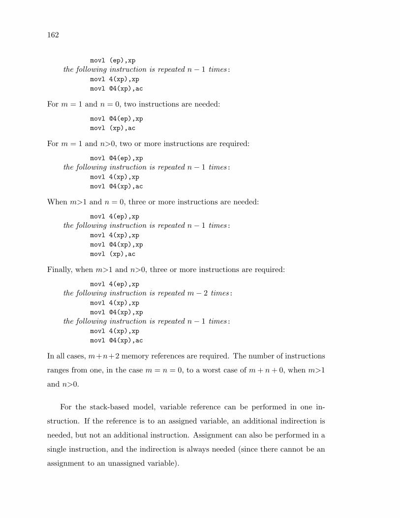
162

movl (ep),xp

the following instruction is repeated n− 1 times:movl 4(xp),xp

movl @4(xp),ac

For m = 1 and n = 0, two instructions are needed:

movl @4(ep),xp

movl (xp),ac

For m = 1 and n>0, two or more instructions are required:

movl @4(ep),xp


movl @4(xp),ac

When m>1 and n = 0, three or more instructions are needed:

movl 4(ep),xp


movl @4(xp),xp

movl (xp),ac

Finally, when m>1 and n>0, three or more instructions are required:

movl 4(ep),xp

the following instruction is repeated m− 2 times:movl 4(xp),xp

movl @4(xp),xp


movl @4(xp),ac

In all cases, m+n+2 memory references are required. The number of instructions

ranges from one, in the case m = n = 0, to a worst case of m+ n+ 0, when m>1

and n>0.

For the stack-based model, variable reference can be performed in one in-

struction. If the reference is to an assigned variable, an additional indirection is

needed, but not an additional instruction. Assignment can also be performed in a

single instruction, and the indirection is always needed (since there cannot be an

assignment to an unassigned variable).

163

One of four instructions may be necessary for variable reference. The first is

for any unassigned local variable n cells from the stack pointer:

movl 4n(sp),ac

(The factor of four appearing here is due to an assumption that each cell is 32

bits, or four bytes long.) The second is for any unassigned nonlocal variable (that

is, not in the current frame but in the current closure):

movl 4n(cp),ac

The third is for any assigned local variable:

movl @4n(sp),ac

The fourth is for any assigned nonlocal variable:

movl @4n(cp),ac

In all cases only one instruction is required, with one or two memory references,

and no heap allocation.

Only two instructions are possible for variable assignment. The first is for any

local variable:

movl ac,@4n(ac)

and the second is for any nonlocal variable:

movl ac,@4n(cp)

In either case, one instruction, two memory references, and no heap allocation is

required.

Although the element number n and the rib number m in the heap-based

model are often small, the average number of instructions and memory references

is probably at least twice or three times the average number for the stack-based

model. In no case does the heap-based model require fewer instructions or memory

references than the stack-based model.

A.2.2 Nested (Nontail) Call. Function call instruction sequences are sepa-

rated into two categories, nested (nontail) calls and tail calls. In addition to the

instructions required to perform a call, instructions are required to apply a closure

164

or continuation. For the stack-based model the application instructions allocate

boxes for any assigned variables, in the case of closure application, or copy the

saved stack elements into the stack, in the case of continuation application. For

the heap-based model the closure application instructions create the environment

from the saved environment (in the closure) and the current rib, while the con-

tinuation application instructions reinstate the stack pointer to the saved stack

pointer. Instruction sequences for closure and continuation application are given

later in this section.

Function calls in the heap-based model require heap allocation of the argument

rib, one element at a time, plus heap allocation of a stack frame. The sequence of

instructions below performs a nontail call with n arguments:

movl hp,xp

addl2 #4*4,hp

moval ret,(xp)

movl ep,4(xp)

movl rp,8(xp)

movl sp,12(xp)

movl xp,sp

movl nil,rp

the next sequence of instructions is repeated n times:ac = evaluate(argument)

movl hp,xp

addl2 #4*2,hp

movl ac,(xp)

movl rp,4(xp)

movl xp,rp

end of repeated sequencecp = evaluate(function)

jmp @(cp)

ret:

This sequence requires 5n+9 instructions, 2n+5 memory references, and 2n+4 cells

of heap allocation. (The instructions for evaluating each argument and placing the

result in the accumulator are not included here or in the other sequences involving

function call.)

The stack-based model nontail call pushes a frame header and arguments on

165

the stack. The sequence of instructions below performs a nontail call with n

arguments:

pushal ret

pushl cp


pushl ac


jmp @(cp)

ret:

This sequence requires n+ 3 instructions, n+ 3 memory references, and no heap

allocation. That the stack-based model uses fewer instructions and performs fewer

memory references is less important than that it performs no heap allocation, since

this avoids garbage collection overhead and other overhead associated with the use

of large amounts of memory.

A.2.3 Tail Call. Tail calls in the heap-based model are simpler in that no frame

is created. The following sequence performs a tail call with n arguments:


movl hp,xp

addl2 #4*2,hp

movl ac,(xp)

movl rp,4(xp)

movl xp,rp


jmp @(cp)

ret:

This sequence requires 5n+ 1 instructions, 2n+ 1 memory references, and 2n cells

of heap allocation.

The stack-based tail call is simpler than the stack-based nontail call in that no

frame header is pushed on the stack, but more complex in that arguments must

be shifted before jumping to the called routine. The following sequence performs

a tail call with n arguments from a function of m arguments:

166


pushl ac


the next instruction is repeated for i = n− 1, i = n− 2, . . . , i = 0:movl 4i(sp),4(i+m)(sp)

addl2 #4m,sp

jmp @(cp)

ret:

The repeated movl instruction that shifts the arguments is not needed when m = 0,

and neither is the instruction that adjusts the stack pointer, since the new argu-

ments are already positioned correctly when m = 0. When n is large (and m>0),

a movc3 (block move) instruction can be used in place of the movl instructions used

to shift the arguments. This decreases the number of instructions but does not

change the number of memory references (outside of the instruction stream). An-

other way to reduce the number of instructions is to employ movq (move quadword)

and movo (move octaword) instructions to move two or four cells per instruction.

When m = 0, the sequence above requires n + 2 instructions, n + 1 memory

references, and no heap allocation. When m>0, it requires 2n+2 instructions, 3n+

1 memory references, and no heap allocation. The number of memory references for

a tail call in the stack-based model is more than the number of memory references

for the heap-based model (except when m = 0), while the number of instructions

is less (except when n = 0). However, as with nontail calls, the fact that the stack-

based model avoids heap allocation is more important than the relative number

of instructions or memory references.

A.2.4 Return. The return sequences for both models restore the machine reg-

isters from the saved frame and jump to the saved return address. The sequence

is executed by any function after it completes its body, unless it avoids a direct

return by performing a tail call. The return sequence is also used to restore the

machine registers after a continuation application (they are saved by the code for

167

call/cc).

Here is the return sequence for the heap-based model:

movl (sp),xp

movl 4(sp),ep

movl 8(sp),rp

movl 12(sp),sp

jmp @(xp)

This sequence requires 5 instructions, 5 memory references, and performs no heap

allocation.

The return sequence in the stack-based model depends upon the number of

arguments of the returning function, and hence the size of frame. The return

sequence for n arguments follows:

addl2 #4n,sp

movl (sp)+,cp

rsb

When n = 0, the first instruction in this sequence can be omitted. The rsb

instruction is equivalent to jmp @(sp)+, but takes one fewer byte in the instruction

stream. This sequence requires 3 instructions, 3 memory references, and performs

no heap allocation. It is only nominally better than the sequence required by the

heap-based model. However, because of code size considerations, the heap-based

sequence might be performed by a library subroutine, whereas the stack-based

sequence is sufficiently smaller that this is probably unnecessary.

A.2.5 Closure Creation. Closure creation in the heap-based model requires

allocating a two-cell closure object and inserting a pointer to the function code

and a pointer to the current environment in this object. The following sequence

performs this operation, where code is the function body:

movl hp,ac

addl2 #4*2,hp

moval code,(ac)movl ep,4(ac)

168

This sequence requires 4 instructions, 2 memory references, and 2 cells of heap

allocation.

Creating a closure in the stack-based model requires allocating a display closure

with enough cells to hold a pointer to the function code and the value (or box

holding the value) of each of the function’s free variables. Values (or boxes) are

moved directly from their location on the stack or in the current closure into the

new closure in a manner similar to unassigned variable reference. The following

sequence creates a display closure containing values or boxes for n free variables:

movl hp,ac

addl2 #4(n+1),hp

moval code,(ac)the following instruction is repeated for i = 1, . . . , i = n:

movl 4oi(ri),4i(ac)

The notation 4oi(ri) is used to represent some offset 4oi from the register ri

(where ri is either sp or cp), i.e., the address of a local or nonlocal variable. This

sequence requires n+ 3 instructions, 2n+ 1 memory references, and n+ 1 cells of

heap allocation. Since it is fairly common for n to be 0 or 1, creation of display

closures is often no more expensive and sometimes less expensive than creation of

heap-based closures. Furthermore, with no more compiler analysis than is already

required by the stack-based model, when n = 0 the closure can easily be created

at compile or load time rather than at run time.

A.2.6 Function Entry. The task performed at entry to a heap-based function is

the creation of an environment containing the current rib (the arguments to the

function) and the environment saved in the function’s closure.

This environment could be created in the calling sequence (both nontail and

tail call). However, there are two benefits to creating the environment after entry

to the function rather than during the call to the function. The first benefit is

that, while there is typically only one entry to a function, there are often many

places that call the function. Placing the code at the front of the function body

means that the code appears once for each function rather than once for each call

169

to a function. This does not save time, but it does save space in the instruction

stream. The other benefit is that environment creation is avoided in the case of

continuation application, which is shown later.

The following code is performed on entry to each heap-based function to create

the environment:

movl hp,ep

addl2 #4*2,hp

movl rp,(ep)

movl 4(cp),4(ep)

This sequence requires 4 instructions, 3 memory references, and 2 cells of heap

allocation.

In the stack-based model, the environment is separated into two parts: the

local variables on the stack and the nonlocal (free) variables in the function’s

closure. The only thing that must be done to complete the environment is to

allocate boxes for assigned variables to contain the values on the stack.

The following sequence allocates space for each value to be placed in a box,

fills each box with the appropriate value and replaces this value on the stack with

its box, for n values:

movl hp,xp

addl2 #4n,hp

the following pair of instructions is repeated n times:movl 4oi(sp),(xp)

moval (xp)+,4oi(sp)

The notation 4oi(sp) represents some offset 4oi from sp, i.e., the address of one of

the argument values. When n = 0 this sequence can be omitted, and so requires no

instructions, memory references, or cells of heap allocation. When n>0 it requires

2n+ 2 instructions, 3n memory references, and n cells of heap allocation.

In well-written Scheme code, assignments are rare, so the case n = 0 is com-

mon. In no case does the amount of allocation here exceed the amount of allocation

saved by not creating argument ribs and environments, although the number of

memory references is greater in the worst case (all variables are assigned variables).

170

A.2.7 Continuation Creation. Continuation creation is significantly simpler

and more efficient in the heap-based model than in the stack-based model. The

heap-based model requires only that a closure be created with a pointer to the

continuation restoration code (nuate) and a pointer to the current stack. (This

is a slightly simplified implementation of the virtual machine conti instruction

from Section 3.5. The virtual machine instruction created a “true” environment

to place in the environment slot of the closure; here the stack pointer is placed

directly in the environment slot.) The following instruction sequence performs this

simple operation:

movl hp,ac

addl2 #4*2,hp

moval nuate,(ac)

movl sp,4(ac)

(Here and in the stack-based sequence below, nuate is the address of the appro-

priate continuation application code.) The instruction sequence above requires 4

instructions, 3 memory references, and 2 cells of heap allocation. Since the con-

tinuation is always passed to an argument closure (as required by call/cc), the

cost of calling a function with one argument should also be added in.

In the stack-based model, the cost of creating a snapshot continuation depends

upon the size of the stack to be copied. Creating the continuation requires the

creation of a display closure of sufficient size to hold the elements of the stack, then

copying the contents of the stack to the closure. In addition to the code pointer (to

nuate) and the stack contents, the closure also contains a field giving the size of the

stack for the continuation application code. (This represents a slight simplification

of the virtual machine conti instruction of Section 4.6. The virtual machine code

creates a display closure that points to a separate vector containing the stack

elements.) The following instruction sequence creates a snapshot continuation

from a stack whose base is given by stackbase:

171

movl hp,ac

subl3 sp,#stackbase,xp

addl2 #4*2,hp

addl2 xp,hp

moval nuate,(ac)

movl xp,4(ac)

movc3 xp,(sp),8(ac)

This instruction sequence requires 7 instructions, 2n + 2 memory references, and

n+ 2 cells of heap allocation, where n is the size of the stack (the number of cells

between stackbase and sp). As with heap-based continuation creation, the actual

cost would include the overhead of passing the continuation as an argument to

another function.

A.2.8 Continuation Application. The instruction sequence to restore a con-

tinuation from its closure representation in the heap-based model requires only

that the argument to the continuation be placed in the accumulator and that the

saved stack pointer be restored. The following instruction sequence performs this

operation:

movl (rp),ac

movl 4(cp),sp

This sequence requires 2 instructions, 2 memory references, and no heap allocation.

The actual cost also includes the cost of the return sequence, which is not shown.

Restoration of a snapshot continuation proceeds in a similar manner, with

the argument removed from the stack and placed in the accumulator, and the

stack copied from the continuation. The instruction sequence below performs this

operation, determining the number of bytes to copy from the saved size field in

the continuation.

movl (sp),ac

movl 4(cp),xp

subl3 xp,#stackbase,sp

movc3 xp,8(cp),(sp)

172

This sequence requires 4 instructions, 2n + 2 memory references, and no heap

allocation. As with the heap-based model, the actual cost would also include the

cost of the return sequence (from a routine with no arguments).

Bibliography

[Abe84] Abelson, H. and Sussman, G. Structure and Interpretation of ComputerPrograms, MIT Press (1984).

[Aho77] Aho, A.V. and Ullman, J.D. Principles of Compiler Design, Addison-Wesley Publishing Company (1979).

[Amb84] Ambler, A., Private communication (March 1984).

[And82] Anderson, T. “The Design of a Multiprocessor Development Sys-tem,” MIT Laboratory for Computer Science Technical Report TR 279(September 1982).

[Arv77] Arvind, Gostelow, K.P. and Plouffe, W. “Indeterminacy, Monitors, andDataflow,” Proceedings of the Sixth ACM Symposium on Operating Sys-tems Principles (November 1977), 159–169.

[Bac72] (uncited) Backus, J. “Reduction Languages and Variable-Free Program-ming” IBM Research Report RJ1010, Yorktown Heights, New York(April 1972).

[Bac73] (uncited) Backus, J. “Programming Language Semantics and Closed Ap-plicative Languages,” IBM Research Report RJ1245, Yorktown Heights,New York (July 1973).

[Bac78] Backus, J. “Can Programming Be Liberated from the von NeumannStyle? A Functional Style and its Algebra of Programs,” CACM 21, 8(August 1978), pp. 613–641.

[Bac81] (uncited) Backus, J. “Is Computer Science Based on the Wrong Fun-damental Concept of Program? An Extended Concept,” in AlgorithmicLanguages, ed. Bakker, Vliet, IFIP, North-Holland Publishing Co. (1981),pp. 133–165.

[Bac82] (uncited) Backus, J. “Function Level Computing,” IEEE Spectrum 19,8 (1982), pp. 22–27.

[Bak77] Baker, H.G. Jr. and Hewitt, C. “The Incremental Garbage Collection ofProcesses,” Proceedings of the Symposium on Artificial Intelligence andProgramming Languages, published as SIGPLAN Notices 12, 8 (August1977), pp. 55–59.

[Bar86] Bartley, D.H. and Jensen, J.C. “The Implementation of PC Scheme,”Proceedings of the 1986 ACM Conference on Lisp and Functional Pro-gramming (1986), pp. 86–93.

174

[Ber75] Berkling, K. “Reduction Languages for Reduction Machines,” SecondAnnual Symposium on Computer Architecture (1975), pp. 133–138.

[Bri73] Brinch Hansen, P. “Concurrent Programming Concepts,” Computer Sur-veys 5, 4 (December 1973), pp. 223–245.

[Bri78] Brinch Hansen, P. “Distributed Processes: A Concurrent ProgrammingConcept,” CACM 21, 11 (November 1978), pp. 934–941.

[Brg81] Burge, W.H. “ISWIM Programming Manual,” IBM Research ReportRA129, Yorktown Heights, New York (November 1981).

[Bur81] Burton, F.W. and Sleep, M.R. “Executing Functional Programs on aVirtual Tree of Processors,” Proceedings of the 1981 ACM Conference onFunctional Programming Languages and Computer Architecture (1981),pp. 187–194.

[Car83] Cardelli, L. “The Functional Abstract Machine,” Bell Labs Techni-cal Memorandum TM-83-11271-1, Bell Labs Technical Report TR-107(1983).

[Car83a] Cardelli, L. “ML under Unix,” User’s manual for Unix ML implementa-tion (1983).

[Car84] Cardelli, L. “Compiling a Functional Language,” Conference Record ofthe 1984 ACM Symposium on Lisp and Functional Programming (1984),pp. 208–217.

[Chu41] Church, A. “The Calculi of Lambda Conversion,” Annals of MathematicsStudies 6, Princeton University Press (1941).

[Cli84] Clinger, W. “The Scheme 311 Compiler: An Exercise in DenotationalSemantics,” Conference Record of the 1984 ACM Symposium on Lispand Functional Programming (1984), pp. 356–364.

[Cur58] Curry, H.B. and Feys, R. “Combinatory Logic,” North-Holland Publish-ing Company, Amsterdam (1958).

[Dan83] Danforth, S.H. DOT, a Distributed Operating System Model of a Tree-structured Multiprocessor, Proceedings of the 1983 International Confer-ence on Parallel Processing (1983), pp. 194–201.

[Dan83a] Danforth, S.H. DOT, a Distributed Operating System Model of a Tree-structured Multiprocessor, Ph.D. dissertation, University of North Car-olina at Chapel Hill (1983).

[Dar81] Darlington, J. and Reeve, M. “ALICE: A Multi-Processor Reduction Ma-chine for the Parallel Evaluation of Applicative Languages,” Proceedingsof the 1981 ACM Conference on Functional Programming Languages andComputer Architecture (1981), pp. 65–76.

[Den79] Dennis, J. “The Varieties of Data Flow Computers,” First InternationalConference on Distributed Computing Systems (October 1979), pp. 430–439.

[Dig81] Digital Equipment Corp. “VAX Architecture Handbook” (1981).

175

[Dij68] Dijkstra, E. W. “Co-operating Sequential Processes,” Programming Lan-guages ed. F. Genuys, Academic Press, New York (1968) pp. 43–112.

[Dyb83] Dybvig, R.K. “C-Scheme,” Indiana University Computer Science De-partment Master’s Thesis, Technical Report 149 (1983).

[Dyb87] Dybvig, R.K. The Schemc Programming Language, Prentice-Hall (1987).

[Fel79] (uncited) Feldman, J.A. “High Level Programming for Distributed Com-puting,” CACM 22, 6, pp. 353–367, (1979).

[Fil84] Filman, R.E. and Friedman, D.P. Coordinated Computing: Tools andTechniques for Distributed Software, McGraw-Hill (1984).

[Fra79] Frank, G.A. Virtual Memory Systems for Closed Applicative LanguageInterpreters, Ph.D. disseratation, Department of Computer Science, Uni-versity of North Carolina at Chapel Hill (1979).

[Fra84] Frank, G.A., Siddall, W.E., and Stanat, D.F. “Virtual Memory Schemesfor an FFP Machine,” International Workshop on High-Level ComputerArchitecture 84 (May 1984), pp. 8.37–8.45.

[Fri76] Friedman, D.P. and Wise, D.S. “Cons Should Not Evaluate its Argu-ments,” in Automata, Languages and Programming, eds. Michaelson, S.,and Milner, R., Edinburgh University Press (1976), pp. 257–284.

[Fri79] (uncited) Friedman, D.P. and Wise, D.S. “An Approach to Fair Applica-tive Multiprogramming,” Proceedings of the International Symposiumon the Semantics of Concurrent Computation, LNCS 70, ed. G. Kahn,Springer-Verlag (1979), pp. 203–225.

[Fri84] Friedman, D.P., Haynes, C.T., Kohlbecker, E. and Wand, M. “Scheme84 Interim Reference Manual,” Indiana University Computer Science De-partment Technical Report 153 (January 1985).

[Gab84] Gabriel, R.P. and McCarthy, J. “Queue-based Multi-processing Lisp,”Conference Record of the 1984 ACM Symposium on Lisp and FunctionalProgramming (1984), pp. 25–44.

[Gol83] Goldberg, A. and Robson, D. Smalltalk-80: The Language and its Im-plementation, Addison-Wesley (1983).

[Gor79] Gordon, M., Milner, R. and Wadsworth, C. “Edinburgh LCF,” LNCS78, Springer-Verlag Publishing Company (1979).

[Gor79a] (uncited) Gordon, M.J.C. The Denotational Description of Program-ming Languages: An Introduction, Springer-Verlag Publishing Company(1979).

[Got83] Gottlieb, A. et al. “The NYU Ultracomputer–Designing an MIMDShared Memory Parallel Computer,” IEEE Transactions on ComputersC-32, 2 (1983), pp. 175–189.

[Gri81] Grit, D.H. and Page, R.L. “Deleting Irrelevant Tasks in an Expression-Oriented Multiprocessor System,” ACM Transactions on ProgrammingLanguages and Systems 3, 1 (January 1981), pp. 49–59.

176

[Hal84] Halstead, R.H. Jr. “Implementation of Multilisp: Lisp on a Multipro-cessor,” Conference Record of the 1984 ACM Symposium on Lisp andFunctional Programming (1984), pp. 9–17.

[Hay86] Haynes, C.T., Friedman, D.P., and Wand, M. “Obtaining Coroutineswith Continuations,” Journal of Computer Languages 11, 3/4 (1986),pp.143–153.

[Hen76] Henderson, P. and Morris, J.H. “A Lazy Evaluator,” Conference Recordof the Third Annual ACM Symposium on Principles of ProgrammingLanguages (1976), pp. 95–103.

[Hew77] (uncited) Hewitt, C.A. and Yonezawa, A. “Modelling Distributed Sys-tems,” Massachusetts Institute of Technology Artificial IntelligenceMemo 428, MIT AI Lab, Cambridge (1977).

[Hoa76] Hoare, C.A.R. “Communicating Sequential Processes,” CACM 21, 8 (Oc-tober 1976), pp. 666–677.

[Hud82] Hudak, P. and Keller, R.M. “Garbage Collection and Task Deletion inDistributed Applicative Processing Systems,” Conference Record of the1982 ACM Symposium on Lisp and Functional Programming (August1982), pp. 168–178.

[Hug82] Hughes, R.J.M. “Super Combinators: A New Implementation Methodfor Applicative Languages,” Conference Record of the 1982 ACM Sym-posium on Lisp and Functional Programming (August 1982), pp. 1–10.

[Ing78] Ingalls, D.H.H. “The Smalltalk-76 Programming System Design and Im-plementation,” Conference Record of the Fifth Annual ACM Symposiumon Principles of Programming Languages (1978), pp. 9–16.

[Ive62] Iverson, K. A Programming Language, John Wiley and Sons (1962).

[Jen74] Jensen, K. and Wirth, N. Pascal User Manual and Report, 2d. ed.,Springer-Verlag (1974).

[Kel79] Keller, R., Lindstrom, G. and Patil, S. “A Loosely-coupled ApplicativeMulti-processing System,” AFIPS Conference Proceedings 48 (1979), pp.613–622.

[Ker78] Kernighan, B.W. and Ritchie, D.M. The C Programming Language,Prentice-Hall, 1978.

[Kie79] (uncited) Kieburtz, R.B. “A Hierarchical Multicomputer for Problem-Solving by Decomposition,” First International Conference on Dis-tributed Computing Systems (October 1979), pp. 63–71.

[Knu85] Knuth, D.E. The Art of Computer Programming, Vol I: FundamentalAlgorithms, 2d. ed., Addison Wesley (1985), pp. 78–79.

[Koh86] Kohlbecker, E. Syntactic Extensions in the Programming Language Lisp,Ph.D. Dissertation, Indiana University (1986).

[Kra86] Kranz, D., Kelsey, R., Rees, J., Hudak, P., Philbin, J., and Adams, N.“Orbit: An optimizing compiler for Scheme,” Proceedings of the SIG-PLAN ’86 Symposium on Compiler Construction, published as SIG-PLAN Notices 21, 7 (July 1986), pp. 219–233.

177

[Lan64] Landin, P.J. “The Mechanical Evaluation of Expressions,” ComputerJournal 6, 4 (1964), pp. 308–320.

[Lan65] Landin, P.J. “An Abstract Machine for Designers of Computing Lan-guages,” IFIP 65 (1965), pp. 438–439.

[Mag79] Mago, G.A. “A Cellular, Language-directed Computer Architecture,”Proceedings of the First Caltech Conference on VLSI (1979), pp. 447–452.

[Mag79a] Mago, G.A. “A Network of Microprocessors to Execute Reduction Lan-guages Parts I and II,” International Journal of Computer and Infor-mation Science 8, 5 and 6 (October, December 1979), pp. 349–385 and435–471.

[Mag80] Mago, G.A. “A Cellular Computer Architecture for Functional Program-ming,” IEEE Computer Society COMPCOM (Spring 1980), pp. 179–187.

[Mag81] (uncited) Mago, G.A. “Copying Operands versus Copying Results: a So-lution to the Problem of Large Operands in FFP’s,” Proceedings of the1981 ACM Conference on Functional Programming Languages and Com-puter Architecture (1981), pp. 93–97.

[Mag82] (uncited) Mago, G.A. “Data Sharing in an FFP machine,” ConferenceRecord of the 1982 ACM Symposium on Lisp and Functional Program-ming (August 1982), pp. 201–207.

[Mag84] Mago, G.A. and Middleton, D. “The FFP Machine—A Progress Report,”International Workshop on High-Level Computer Architecture 84 (May1984), pp. 5.13–5.25.

[Mag85] Mago, G.A. “Making Parallel Computation Simple: The FFP Machine,”IEEE Computer Society COMPCOM (Spring 1985), pp. 179–187.

[Mag87] Mago, G.A. and Partain, W. “Implementing Dynamic Arrays: A Chal-lenge to High-Performance Machines,” to be presented at the 2nd AnnualInternational Supercomputing Conference (May 1987).

[Mar83] Marti, J. and Fitch, J. “The Bath Concurrent Lisp Machine,” ProceedingsEUROCAL ’83, Springer-Verlag LNCS 162 (March 1983), pp. 78–90.

[McC60] McCarthy, J. “Recursive Functions of Symbolic Expressions and TheirComputation by Machine,” CACM 3 (April 1960), pp. 184–195.

[McD80] McDermott, D. “An Efficient Environment Allocation Scheme in an In-terpreter for a Lexically-Scoped Lisp,” Conference Record of the 1980Lisp Conference (August 1980), pp. 154–162.

[Men84] Mendelson, E. Introduction to Mathematical Logic, D. Van NostrandCompany, Inc. (1984), pp. 102–104.

[Mid87] Middleton, D. Alternative Program Representations in the FFP Machine,Ph.D. dissertation, University of North Carolina at Chapel Hill (1987).

[Mil84] Milner, R. “A Proposal for Standard ML,” Conference Record of the 1984ACM Symposium on Lisp and Functional Programming (1984), pp. 184–197.

178

[Nau63] Naur, P. et al., “Revised Report on the Algorithmic Language ALGOL60,” Communications of the ACM 6, 1, January 1963, 1–17.

[Pag81] Page, R., Conant, M.G. and Grit, D.H. “If-then-else as a ConcurrencyInhibitor in Eager Beaver Evaluation,” Proceedings of the 1981 ACMConference on Functional Programming Languages and Computer Ar-chitecture (1981), pp. 179–186.

[Pri80] (uncited) Prini, G. “Explicit Parallelism in Lisp-Like Languages,” Con-ference Record of the 1980 Lisp Conference (August 1980), pp. 13–18.

[Ran64] Randell, B. and Russell, L.J. ALGOL 60 Implementation: The Transla-tion and Use of ALGOL 60 Programs on a Computer, Academic Press(1964).

[Ree82] Rees, J.A. and Adams, N.I. “T: A Dialect of Lisp, or LAMBDA: The Ul-timate Software Tool,” Conference Record of the 1982 ACM Symposiumon Lisp and Functional Programming (August 1982), pp. 114–122.

[Ree86] Rees, J.A. and Clinger, W., eds. “The Revised3 Report on the Algorith-mic Language Scheme,” Sigplan Notices 21, 12, December 1986.

[Rev83] (uncited) Revesz, G. “Axioms for the Theory of Lambda-Conversion,”Tulane University Technical Report 83-111 (October 1983).

[Rev84] Revesz, G. “An Extension of Lambda-Calculus for Functional Program-ming,” Journal of Logic Programming 1984, 1 (1984).

[Rey72] Reynolds, J.C. “Definitional Interpreters for Higher-Order ProgrammingLanguages,” Proceedings of the 25th ACM National Conference (1972),pp. 717–740.

[Ros82] Rosser, J.B. “Highlights of the History of the Lambda-Calculus,” Con-ference Record of the 1982 ACM Symposium on Lisp and FunctionalProgramming (August 1982), pp. 216–225.

[Smi82] Smith, B.C. Reflection and Semantics in a Procedural Language, Mas-sachusetts Institute of Technology LCS-TR 272 (1982).

[Smi84] (uncited) Smith, B.T. “Logic Programming on an FFP machine,” Pro-ceedings of the 1984 International Symposium on Logic Programming(February 1984), pp. 177–186.

[Sta80] (uncited) Staples, J. “Efficient Evaluation of Lambda Expressions: ANew Strategy,” University of Queensland Computer Science TechnicalReport 23 (December 1980).

[Ste77] Steele, G.L. “Rabbit: A Compiler for Scheme (A Study in Compiler Opti-mization),” Massachusetts Institute of Technology Artificial IntelligenceMemo 474, MIT AI Lab, Cambridge (1977).

[Ste78] Steele, G.L. and Sussman, G.J. “The Revised Report on Scheme,”Massachusetts Institute of Technology Artificial Intelligence Memo 452(1978).

[Ste81] Steele, G.L. and Sussman, G.J. “Design of a Lisp-based Microprocessor,”CACM 24, 11 (November 1981), pp. 628–645.

179

[Ste84] Steele, G.L. Common Lisp: The Language, Digital Press (1984).

[Sto77] (uncited) Stoy, J.E. Denotational Semantics: The Scott-Strachey Ap-proach to Programming Language Theory, MIT Press, Cambridge, MA,pp. 38–77 (1977).

[Sug83] Sugimoto, S. et al. “A Multi-Microprocessor System for ConcurrentLisp,” Proceedings of the 1983 International Conference on Parallel Pro-cessing (1983).

[Sus75] Sussman, G.J. and Steele, G.L. “Scheme: an Interpreter for ExtendedLambda Calculus,” Massachusetts Institute of Technology Artificial In-telligence Memo 349 (1975).

[Sym84] Symbolics, Inc. Symbolics 3600 Technical Summary, Cambridge, MA(1984).

[Tre80] (uncited) Treleaven, P. and Mole, G. “A Multi-processor Reduction Sys-tem for User-defined Reduction Languages,” Seventh Annual Symposiumon Computer Architecture (1980), pp. 121–130.

[Tur79] Turner, D.A. “A New Implementation Technique for Applicative Lan-guages,” Software Practice and Experience 19 (1979), pp. 31–34.

[Tur82] Turner, D.A. “Recursion Equations as a Programming Language,” inFunctional Programming and its Applications, eds. Darlington, J., Hen-derson, P., and Turner, D.A., Cambridge University Press (1982), pp.253–280.

[Tur84] (uncited) Turner, D.A. “Functional Programs as Executable Specifica-tions,” Phi. Trans. R. Soc. Lond. A, 312 (1984), pp. 363–388.

[Tur86] Turner, D.A. “An Overview of Miranda,” SIGPLAN Notices 21, 12 (De-cember 1986), pp. 158–166.

[Wad71] Wadsworth, C.P. Semantics and Pragmatics of the λ-Calculus, Ph.D.Dissertation, Oxford University (1971).

[Wag83] (uncited) Wagner, R. A. “The Boolean Vector Machine,” Proceedingsof the 10th International Symposium on Computer Architecture (June1983), pp. 59- 66.

[Wan80] (uncited) Wand, M. “Continuation-Based Multiprocessing,” ConferenceRecord of the 1980 Lisp Conference (August 1980), pp. 19–28.

[Wan82] (uncited) Wand, M. “Semantics-Directed Machine Architecture,” Con-ference Record of the Ninth ACM Symposium on Principles of Program-ming Languages (1982), 234–241.

[Wan82a](uncited) Wand, M. “Deriving Target Code as a Representation of Con-tinuation Semantics,” ACM Transactions on Programming Languagesand Systems 4, 3 (July 1982), pp. 496–517.

[Who84] Wholey, S. and Fahlman, S.E. “The Design of an Instruction Set forCommon Lisp,” Conference Record of the 1984 ACM Symposium on Lispand Functional Programming (1984), pp. 150–166.

180

[Wis82] Wise, D.S. “Interpreters for Functional Programming,” in FunctionalProgramming and its Applications, eds. Darlington, J. and Henderson,P. Turner, D.A., Cambridge University Press (1982), pp. 253–280.

[Wis85] (uncited) Wise, D.S. “The Applicative Style of Programming,” ABACUS2, 2, Springer-Verlag, New York (1985), pp. 20–32.

three implementation models for scheme -...

Documents