three essays on the evaluation of public policy...

THREE ESSAYS ON THE EVALUATION OF

PUBLIC POLICY PROGRAMS

by

Sunita Mondal

M.A. in Economics, Jadavpur University, 2003

B.A. in Economics, Jadavpur University, 2001

Submitted to the Graduate Faculty of

the School of Arts and Sciences in partial ful�llment

of the requirements for the degree of

Doctor of Philosophy

University of Pittsburgh

2009

UNIVERSITY OF PITTSBURGH

SCHOOL OF ARTS AND SCIENCES

This dissertation was presented

by

Sunita Mondal

It was defended on

July 31st, 2009

and approved by

Alexis León, Assistant Professor, Department of Economics, University of Pittsburgh

Daniel Berkowitz, Professor, Department of Economics, University of Pittsburgh

Mark Hoekstra, Assistant Professor, Department of Economics, University of Pittsburgh

Shanti Rabindran, Assistant Professor, Graduate School of Public Policy and International

A¤airs, University of Pittsburgh

Dissertation Director: Alexis León, Assistant Professor, Department of Economics,

University of Pittsburgh

ii

THREE ESSAYS ON THE EVALUATION OF PUBLIC POLICY

PROGRAMS

Sunita Mondal, PhD

University of Pittsburgh, 2009

This dissertation consists of three chapters, each evaluating a di¤erent public policy. The

�rst chapter studies the e¤ect of internet on music sales. Internet usage has increased

dramatically over the past few years. Concurrently, the sales from music CDs have witnessed

a huge decline. I analyze the e¤ect of downloading music on the current downturn in CD sales

by looking at the progressive disappearance of the traditional stores. To identify the causal

impact of downloading and control for endogeneity, I instrument state internet penetration

rates by information on the adoption of Video Franchise Law (VFL). Results indicates that

implementation of VFL increases internet access in states which adopt it, and explains 58.7

percent of total store closings in those states.

The second chapter analyzes whether enactment of the federal Family Medical Leave

Act (FMLA) di¤erentially a¤ected states that previously implemented maternity leave laws

at the state level than those states which did not. Additionally, we study whether FMLA

caused an increase in female employment and labor force participation in those states that

expanded its bene�ts and relaxed the eligibility criteria. Finally, we analyze the Paid Family

Leave program in California, comparing how the change in female employment di¤ers from

those states which have FMLA alone and those which have complemented the bene�ts of

FMLA. Our results con�rm the positive and signi�cant e¤ect of FMLA on female employment

and also a signi�cantly positive impact on female employment for some states when they

complement the bene�ts and eligibility criteria of FMLA.

The third chapter analyses labor market impacts of the implementation of all the state

iii

and local governments�EITC supplement. We examine whether the substantial expansions

in the EITC program created by these supplements are an e¤ective means of providing

work incentives. Exploiting variation in the policy over time both across states and within

states between di¤erent demographic groups, we �nd the EITC supplements have raised

labor supply among single women, but had no e¤ect on the labor supply of married women.

Our results indicate the state and local governments�EITC expansions to be less e¤ective

compared to the federal EITC expansions.

iv

TABLE OF CONTENTS

PREFACE . . . . . . . . . . . . . . . . . . . . . . . . . . . . . . . . . . . . . . . . . xi

1.0 INTRODUCTION . . . . . . . . . . . . . . . . . . . . . . . . . . . . . . . . . 1

2.0 THE EFFECT OF THE INTERNET ON MUSIC SALES . . . . . . . . 5

2.1 Introduction . . . . . . . . . . . . . . . . . . . . . . . . . . . . . . . . . . . 5

2.2 Related literature . . . . . . . . . . . . . . . . . . . . . . . . . . . . . . . . 9

2.3 Research Design and the Identi�cation Strategy . . . . . . . . . . . . . . . 11

2.3.1 Exogeneity of the Video Franchise Laws . . . . . . . . . . . . . . . . 16

2.4 Data and Main Results . . . . . . . . . . . . . . . . . . . . . . . . . . . . . 19

2.4.1 Data Sources and Descriptive Statistics . . . . . . . . . . . . . . . . 19

2.4.2 OLS Estimates . . . . . . . . . . . . . . . . . . . . . . . . . . . . . . 23

2.4.3 Reduced-form Estimation and Main Results . . . . . . . . . . . . . . 26

2.4.4 Falsi�cation . . . . . . . . . . . . . . . . . . . . . . . . . . . . . . . . 35

2.5 Conclusions . . . . . . . . . . . . . . . . . . . . . . . . . . . . . . . . . . . 36

3.0 THE EFFECTOFPARENTAL LEAVEONFEMALE EMPLOYMENT:

EVIDENCE FROM STATE POLICIES . . . . . . . . . . . . . . . . . . . . 38

3.1 Introduction . . . . . . . . . . . . . . . . . . . . . . . . . . . . . . . . . . . 38

3.2 Overview of parental leave laws . . . . . . . . . . . . . . . . . . . . . . . . 43

3.3 Theory . . . . . . . . . . . . . . . . . . . . . . . . . . . . . . . . . . . . . . 45

3.4 Research design . . . . . . . . . . . . . . . . . . . . . . . . . . . . . . . . . 46

3.4.1 Identi�cation Strategy . . . . . . . . . . . . . . . . . . . . . . . . . . 46

3.5 Data . . . . . . . . . . . . . . . . . . . . . . . . . . . . . . . . . . . . . . . 49

3.6 Empirical results for female employment . . . . . . . . . . . . . . . . . . . 51

v

3.7 Analysis of FMLA in states with and without TDI . . . . . . . . . . . . . . 52

3.7.1 Analysis of the results . . . . . . . . . . . . . . . . . . . . . . . . . . 54

3.8 Analysis of extensions of FMLA . . . . . . . . . . . . . . . . . . . . . . . . 57

3.9 Analysis of California�s Paid Family Leave program . . . . . . . . . . . . . 60

3.10 Conclusions . . . . . . . . . . . . . . . . . . . . . . . . . . . . . . . . . . . 64

4.0 THE LABOR MARKET EFFECTS OF STATE AND LOCAL EX-

PANSIONS OF THE EARNED INCOME TAX CREDIT . . . . . . . . 66

4.1 Introduction . . . . . . . . . . . . . . . . . . . . . . . . . . . . . . . . . . . 66

4.2 Structure of Federal and State EITC . . . . . . . . . . . . . . . . . . . . . 68

4.3 Previous Research . . . . . . . . . . . . . . . . . . . . . . . . . . . . . . . . 74

4.4 Data and Main Results . . . . . . . . . . . . . . . . . . . . . . . . . . . . . 77

4.4.1 Data Sources and Summary Statistics . . . . . . . . . . . . . . . . . 77

4.5 Conclusions . . . . . . . . . . . . . . . . . . . . . . . . . . . . . . . . . . . 81

5.0 APPENDIX . . . . . . . . . . . . . . . . . . . . . . . . . . . . . . . . . . . 82

BIBLIOGRAPHY . . . . . . . . . . . . . . . . . . . . . . . . . . . . . . . . . . . . 93

vi

LIST OF TABLES

1 Summary Statistics . . . . . . . . . . . . . . . . . . . . . . . . . . . . . . . . 21

2 Summary Statistics: Store closures . . . . . . . . . . . . . . . . . . . . . . . . 21

3 Summary Statistics: Rural versus Urban States . . . . . . . . . . . . . . . . . 25

4 OLS Estimates of the E¤ect of State Internet Penetration Rates on Store closures 25

5 First Stage Estimates of the E¤ect of VFL Adoption on State Internet Pene-

tration Rates . . . . . . . . . . . . . . . . . . . . . . . . . . . . . . . . . . . . 27

6 First Stage Estimates of the E¤ect of phone measures on State Internet Pene-

tration Rates . . . . . . . . . . . . . . . . . . . . . . . . . . . . . . . . . . . . 29

7 Reduced-form Estimates of the E¤ect of VFL Adoption on Store closures . . 32

8 Reduced-form Estimates of the E¤ect of phone measures on Store closures . . 32

9 2SLS Estimates of the E¤ect of VFL Adoption on Store closures . . . . . . . 33

10 Reduced-form Estimates of the E¤ect of VFL Adoption on Store closures con-

trolling for the presence of megastores . . . . . . . . . . . . . . . . . . . . . . 34


12 Summary Statistics: California . . . . . . . . . . . . . . . . . . . . . . . . . . 51

13 The estimates of Female Employment between states with no law and states

with TDI before FMLA . . . . . . . . . . . . . . . . . . . . . . . . . . . . . . 53

14 The estimates of Female Employment between states with no law and states

with TDI before FMLA, by education groups . . . . . . . . . . . . . . . . . . 54

15 The estimates of FLFP rates between states with no law and states with TDI

before FMLA . . . . . . . . . . . . . . . . . . . . . . . . . . . . . . . . . . . . 56

vii

16 The estimates of FLFP rates between states with no law and states with TDI

before FMLA, by education groups . . . . . . . . . . . . . . . . . . . . . . . . 57

17 The estimates of FLFP rates between Oregon and states with no law before

FMLA . . . . . . . . . . . . . . . . . . . . . . . . . . . . . . . . . . . . . . . 58

18 The estimates of Female Employment between Oregon and states with no law

before FMLA . . . . . . . . . . . . . . . . . . . . . . . . . . . . . . . . . . . . 59

19 The estimates of Female Labor Force Participation rates between Maine and

states with no law before FMLA . . . . . . . . . . . . . . . . . . . . . . . . . 60

20 The estimates of FLFP rates between California and states with no law before

FMLA . . . . . . . . . . . . . . . . . . . . . . . . . . . . . . . . . . . . . . . 61

21 The estimates of FLFP rates between California and states with which ex-

panded FMLA . . . . . . . . . . . . . . . . . . . . . . . . . . . . . . . . . . . 62

22 Federal EITC rate schedule 1975-2007 . . . . . . . . . . . . . . . . . . . . . . 72

23 State EITC supplements (1984-2006, percentages of the federal credit) . . . . 73

24 Labor Force participation rates by demographic groups . . . . . . . . . . . . 79


26 2SLS Estimates of the E¤ect of Phone measures on Store closures . . . . . . . 83

27 Store closures based on the type of store . . . . . . . . . . . . . . . . . . . . . 83

28 Summary Statistics: Store closures based on the type of store between states 84

29 OLS Estimates of E¤ect of State Internet Penetration Rates on Store closures

based on the type of store . . . . . . . . . . . . . . . . . . . . . . . . . . . . . 84

30 Reduced-form Estimates of the E¤ect of VFL Adoption on Store closures based

on the type of store . . . . . . . . . . . . . . . . . . . . . . . . . . . . . . . . 85

31 First Stage Estimates of the E¤ect of VFL Adoption on State Internet Pene-

tration Rates: Falsi�cation test . . . . . . . . . . . . . . . . . . . . . . . . . . 85

32 Reduced Form Estimates of the E¤ect of VFL Adoption on State Internet

Penetration Rates: Falsi�cation test . . . . . . . . . . . . . . . . . . . . . . . 86

33 Estimated Probit Models for the Adoption of Video Franchise Laws . . . . . 86

34 Regression of VFL adoption on state characteristics . . . . . . . . . . . . . . 87

35 Reduced-form regression including additional covariates . . . . . . . . . . . . 87

viii

36 Falsi�cation: The estimates of Female Employment between states with no law

and states with TDI before FMLA assuming FMLA adopted in 1981 . . . . . 88

37 The estimates of Female Labor Force Participation rates between Connecticut

and states with no law before FMLA . . . . . . . . . . . . . . . . . . . . . . . 88

38 The estimates of FLFP rates between Vermont and states with no law before

FMLA . . . . . . . . . . . . . . . . . . . . . . . . . . . . . . . . . . . . . . . 89

39 The estimates of Female Employment between California and states with no

law before FMLA . . . . . . . . . . . . . . . . . . . . . . . . . . . . . . . . . 89

40 The estimates of Female Employment between California and states which

expanded FMLA . . . . . . . . . . . . . . . . . . . . . . . . . . . . . . . . . . 90

41 Weekly Bene�t amount and Duration of Bene�ts in TDI states . . . . . . . . 91

42 Classi�cation of the States . . . . . . . . . . . . . . . . . . . . . . . . . . . . 92

ix

LIST OF FIGURES

1 Trends in home internet access 2000 to 2008 . . . . . . . . . . . . . . . . . . . . 12

2 CD sales revenue �gures 1995 to 2007 . . . . . . . . . . . . . . . . . . . . . . . . 13

3 First-Stage relationship between states that adopted VFL and the Internet

penetration rates in 2007 . . . . . . . . . . . . . . . . . . . . . . . . . . . . . 14

4 Total number of Store closures from 2003 through 2008 . . . . . . . . . . . . . . 22

5 States which adopted VFL in 2005, 2006 and 2007 . . . . . . . . . . . . . . . . . 23

6 Map of the states with store closings in 2007 . . . . . . . . . . . . . . . . . . . . 24

7 First-Stage:VFL states and the Internet penetration rates in 2007 . . . . . . . . . 26

8 Internet Penetration predicted by 1960 phone ownership rates . . . . . . . . . . . 28

9 Total number of Store closures from 2003 through 2007 . . . . . . . . . . . . . . 30

10 Reduced-form:store closings and VFL adoption by states . . . . . . . . . . . . . . 31

11 Parental leave laws: 1942-2004 . . . . . . . . . . . . . . . . . . . . . . . . . . . 43

12 Theoretical predictions of mandated leave policies . . . . . . . . . . . . . . . . . 46

13 Federal EITC schedule, Single Parent Family 2006 . . . . . . . . . . . . . . . . . 70

14 Federal EITC Budget Constraint . . . . . . . . . . . . . . . . . . . . . . . . . . 71

x

PREFACE

I must start by giving sincere thanks to my Ph.D. Advisor and friend Professor Alexis

León for his helpful discussions and encouragement: from the initial conversations of the

di¤erent research ideas included in this Ph.D.thesis from its most initial stage to the writing

and re-writing stages. I am especially grateful to him, as he has strongly encouraged me

to pursuit my research, provided me with valuable guidance and the most insightful com-

ments, and has helped me throughout to improve the quality of my work. I owe a great

debt of gratitude to Professor Mark Hoekstra, who constantly and carefully read even the

most preliminary drafts of new research ideas, and provided very interesting suggestions and

comments about how to enrich the results from my research. I also owe thanks to Professor

Daniel Berkowitz, Professor Shanti Rabindran and Professor Sourav Bhattacharya for all

their helpful suggestions and comments. I would like to thank all participants of the 14th

Annual Meeting of the Society of Labor Economists, at Boston for their insightful comments

and suggestions. I would also like to thank all participants of the 71st Annual Meeting of the

Midwest Economics Association, at Minnesota for their thoughtful comments. I must also

thank my peers and very good friends in the graduate program Ana Espinola, Felix Munoz

Garcia, Sandra Orozco, Heriberto Gonzalez and Jared Lunsford, with whom I shared some

of the most exciting and fruitful years, and with whom I faced many of the usual challenges

of a demanding graduate program. I am extremely blessed of having them as friends. You

have been a big support through the most di¢ cult times of my life and you will always be

a family to me. Thanks are also due to the Department of Economics of the University of

Pittsburgh, all my research would not have been possible without its trust and support.

I must also express my gratitude to all my Professors at the University of Pittsburgh for

becoming my inspiration, not only as researchers, but also as teachers. I want to specially

thank all members of the Department of Economics at the University of Pittsburgh, from

secretaries to classmates, for all their understanding both during good and di¢ cult times,

and the extremely comfortable work environment that they promoted.

Above all, I would like to thank my husband, Sujit Mondal and my daughter Sreyashi

xi

Mondal, without the love, support, trust and utmost understanding of whom, my research

would not have been possible, and my father Samir Kumar Hazra, for his constant advice,

support and encouragement and for being my inspiration as a teacher. They have been my

main support and motivation during all these years. This thesis is dedicated to all three of

you.

xii

1.0 INTRODUCTION

My dissertation focuses on the study of the impact of di¤erent public policy programs. The

broad objective is to empirically investigate how the implementation of policies enacted

at the federal and state governments level have a¤ected the retail industry as well as the

labor market outcomes in various sectors of the economy. Speci�cally, I study how the

implementation of a franchising law varies the availability of internet services across di¤erent

states and hence a¤ects the sale of music. I further study the impact of various state and

federal maternity leave policies on female labor supply and �nally analyze how the state and

local governments� supplements of the Earned Income Tax Credit policy has a¤ected the

female employment.

The �rst chapter, �The E¤ect of the Internet on Music Sales�, examines how the arrival of

the digital technology in the form of increased internet usage is posing a threat to the survival

of the traditional brick and mortar businesses. In order to address this issue, I speci�cally

consider the case study of the music industry, since the music retail has been adversely

a¤ected by an advent of the internet as a major distribution channel of music in digital

form. Over the past few years, with an increase in internet usage there has been a concurrent

decline in the sale from music CDs. Previous literature (Zentner 2006, Oberholzer-Gee and

Strumpf, 2007) have analyzed the e¤ect of �le sharing on record sales but there has not been

a consensus regarding its detrimental e¤ect on music sales. In this chapter, I use two sources

of exogenous variation in the internet access across US states to measure the impact of music

downloads on the progressive disappearance of the traditional music CD stores. Given that

the sale of CDs is the most important source of revenue for the music industry, and the record

stores represent a major share of this revenue, it is crucial to estimate the extent to which a

1

change in the consumer preference in the form of downloading music is causing a decline in

the old format. The goal is to analyze whether an increase in the availability of broadband

internet service, which allows for faster access to music downloads and may thus reduce the

demand for physical CDs, has a¤ected the number of CD store closings in a given region over

a period of time. Establishing a causal e¤ect of an increased internet access on store closings

is di¢ cult due to the presence of unobserved heterogeneity in a taste for music as well as

the potential problem of reverse causality. To address these concerns, I use information on

the passage of Video Franchise Law (VFL) and the di¤erences in the household telephone

adoption rate in the 1960 Census as two sources of exogenous variation in the availability

of the internet access across the states. Employing an instrumental variable (IV) estimation

strategy and using CPS Computer and Internet Use Supplements data for state internet

penetration rates and CD store closings data from the research group Almighty Institute of

Music Retail, I �nd that the implementation of VFL signi�cantly increases the availability

of internet access in the states which adopt it, and explains about 58.7 percent of the total

store closings in those states. As a second set of instruments for state internet penetration

rates, I use the 1960 Census data on the household telephone adoption rates to identify a

variation across states in online access, and �nd that internet has di¤used faster in states

with historically higher rates of telephone adoption which in turn causes a signi�cantly higher

number of music store closures in these states.

The second chapter, �The E¤ect of Parental Leave on Female Employment: Evidence

from State Policies�(joint work with Ana Espinola Arredondo) examines the e¤ect of federal

and state parental leave policies on female labor market outcomes. We study the impact

of three distinct leave policies on female employment, the Family and Medical Leave Act

(FMLA) which is a federal policy, the state expansions of the FMLA, and �nally the Paid

Family Leave program implemented by California. Researches on the e¤ect of such policies

are particularly important given the recent increasing trends in employment of women with

young children. We employ a di¤erence-in-di¤erence-in di¤erences estimation strategy and

data from Integrated Public Use Microdata Series (IPUMS) to conduct our analysis. In

contrary to the previous research (Waldfogel, 1999) which fails to �nd an e¤ect of FMLA on

2

female employment, we show that the introduction of the FMLA has a signi�cantly positive

impact on the employment of women in those states which had no state law providing

parental leave bene�ts compared to the states applying the Temporary Disability Insurance

(TDI) before FMLA was enacted. Further, we �nd that the impact of FMLA expansion on

female employment and labor force participation has been signi�cantly higher in the states

with most generous expansions (in terms of improving the bene�ts and relaxing the eligibility

criteria of FMLA) compared to the states which did not expand FMLA. Finally, in order to

get an intuitive understanding of the e¤ects of further increases in the generosity levels of

parental leave policies, we consider the recent enactment of California�s Paid Family Leave

program. Speci�cally, we �nd no impact of the introduction of this law on the female labor

market outcomes, primarily due to a low-take up rates which results from a lack of worker

awareness of the available bene�ts provided by the Paid Family Leave program.

The third chapter �The Labor Market E¤ects of State and Local Expansions of the

Earned Income Tax Credit�(joint work with Alexis León) analyzes the labor market impacts

of the implementation of all the state and local governments�EITC supplement using March

Current Population Survey data from 1984 to 2008. Previous literature (Eissa and Liebman,

1996; Meyer and Rosenbaum, 2001) have established the signi�cant positive impact of the

federal EITC on the labor force participation rates of single women with children. The

contribution of this chapter to the existing literature is threefold. Firstly, it serves as a further

test for the theory of labor force participation and labor supply, and contributes to answering

the question of whether EITC payments by state and local governments a¤ect participation

in the same way as the federal EITC does. Secondly, it helps to access the e¤ectiveness of

these state programs, that is, whether the EITC programs are indeed an e¤ective means

of boosting labor force participation in a state, or are they expensive programs that do

not achieve these goals. To the extent that state governments can allocate the funds to

alternative means (like child care centers) that may also achieve the same desired impact on

female employment, an estimate of the labor market e¤ects of state EITC programs will help

inform that choice. Finally, while the federal and some of the state EITC programs were

implemented and subsequently expanded at a time of strong female labor force participation

3

growth, many of these state and local government programs implemented in the last decade

coincide with a period of generally �at female participation rates. If these EITC programs are

found to have failed to a¤ect female participation, this would suggest that future increases

in the federal EITC may well fail to lead any more women to the labor force either. Our

results indicate that the EITC expansion increased the labor supply among single women,

but has no substantial impact on the labor market outcomes of married women. Further, we

show that the EITC expansions were most e¤ective in a time period when the bene�t levels

were low, indicating the state and local government EITC expansions to be less e¤ective

compared to the federal EITC expansions.

4

2.0 THE EFFECT OF THE INTERNET ON MUSIC SALES

2.1 INTRODUCTION

Over the last two decades, digital technologies have permeated the recording industry where

music has been encoded in digital form and stored on CDs. Such digital technologies gained

popularity due to their quality and ease of transportation. However, the music industry has

been experiencing rapid changes over the last few years. The Recording Industry Association

of America (RIAA) reports that there has been a decline in CD sales since 1999, with the

highest being a 20.5 percent fall in 2007 compared to the previous year. This huge decrease

in the sale of CDs, which is the most popular format, is a cause of alarm for the music

industry1. This downward trend in the revenue from the sale of CDs is evident from the

increasing number of music CD stores that went out of business in recent years across the

United States2.

Internet piracy and illegal MP3 downloads have often been blamed for the ongoing down-

turn in CD sales (Liebowitz, 2003; Zentner, 2003). Previous studies have analyzed the e¤ect

of �le sharing on record sales with somewhat con�icting results. Zentner (2003), Peitz and

Waelbroeck (2004) and Liebowitz (2005) �nd a negative e¤ect of �le-sharing on music sales.

On the other hand, Oberholzer-Gee and Strumpf (2007) and Boorstin (2004) �nd no evidence

of such detrimental e¤ects of internet piracy on music sales. Liebowitz (2003) also analyzes

alternative reasons which could a¤ect the record sale such as price of CD and change in

taste, but concludes that these reasons cannot explain the observed reduction in sales.

1Sales of CDs account for more than 85 percent of the dollar value of the total music sold (RIAA).2According to the research group Almighty Institute of Music Retail, about 2,700 record stores went out

of business across the country since 2003.

5

The e¤ect of the internet on record sales is not just limited to online piracy and peer-to-

peer �le-sharing, however. According to the International Federation of the Phonographic

Industry (IFPI) and Nielsen SoundScan, consumers are downloading more than ever from

authorized music-download sites in the recent years. The research �rm Ipsos-Insight reports

in their quarterly digital music behavior that in late June 2003, one out of six (roughly

equivalent to ten million people) of U.S. music downloaders aged 12 and older had paid to

download music online.

In the past, bandwidth restrictions have limited the distribution of music in digital form

over the internet. However, these restrictions are disappearing due to advances in networking

(broadband) technologies. Consumers are now able to download and play high-quality music

in digital form directly through the internet at a price considerably less than what they would

otherwise pay for a CD. According to sales �gures from IFPIA, the sales of digital music

has been rising due to legal downloading, for example, in 2005 it nearly tripled over 2004

levels, but were not enough to help the music industry see overall growth. As bandwidth

increases and better compression techniques are being available, the internet is becoming a

major distribution channel of music in the digital form.

The availability of internet services is not the same across the di¤erent states, however.

Prior to 2005, all cable companies and other companies interested in o¤ering cable services to

consumers, were required to negotiate separate agreements with each city before they could

lay cable in the ground or place cable along utility poles. In some states these agreements

were valid for up to as long as 15 years. In order to establish these agreements, the company

needed to enter into negotiations with as many as 2,500 or more cities per state. In recent

years, in order to streamline the video franchising process, some states have passed Video

Franchise Laws (VFL), which permit state issued agreements. Under the law, cable providers

are not required to obtain any other separate franchise agreements. According to the pro-

ponents of this law, these policies should bolster innovation, spur broadband investment,

increase competition and result in lower prices and better quality of service3. The adoption

3TIA Advocates Video Franchise Legislation Reform at September 14th Press Brie�ng, by Alan J Weiss-

6

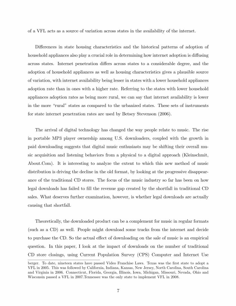
of a VFL acts as a source of variation across states in the availability of the internet.

Di¤erences in state housing characteristics and the historical patterns of adoption of

household appliances also play a crucial role in determining how internet adoption is di¤using

across states. Internet penetration di¤ers across states to a considerable degree, and the

adoption of household appliances as well as housing characteristics gives a plausible source

of variation, with internet availability being lesser in states with a lower household appliances

adoption rate than in ones with a higher rate. Referring to the states with lower household

appliances adoption rates as being more rural, we can say that internet availability is lower

in the more �rural�states as compared to the urbanized states. These sets of instruments

for state internet penetration rates are used by Betsey Stevenson (2006).

The arrival of digital technology has changed the way people relate to music. The rise

in portable MP3 player ownership among U.S. downloaders, coupled with the growth in

paid downloading suggests that digital music enthusiasts may be shifting their overall mu-

sic acquisition and listening behaviors from a physical to a digital approach (Kleinschmit,

About.Com). It is interesting to analyze the extent to which this new method of music

distribution is driving the decline in the old format, by looking at the progressive disappear-

ance of the traditional CD stores. The focus of the music industry so far has been on how

legal downloads has failed to �ll the revenue gap created by the shortfall in traditional CD

sales. What deserves further examination, however, is whether legal downloads are actually

causing that shortfall.

Theoretically, the downloaded product can be a complement for music in regular formats

(such as a CD) as well. People might download some tracks from the internet and decide

to purchase the CD. So the actual e¤ect of downloading on the sale of music is an empirical

question. In this paper, I look at the impact of downloads on the number of traditional

CD store closings, using Current Population Survey (CPS) Computer and Internet Use

berger. To date, nineteen states have passed Video Franchise Laws. Texas was the �rst state to adopt aVFL in 2005. This was followed by California, Indiana, Kansas, New Jersey, North Carolina, South Carolinaand Virginia in 2006. Connecticut, Florida, Georgia, Illinois, Iowa, Michigan, Missouri, Nevada, Ohio andWisconsin passed a VFL in 2007.Tennessee was the only state to implement VFL in 2008.

7

Supplements data for internet availability and CD store closings data from the research

group Almighty Institute of Music Retail. In particular, I analyze whether an increase

in the availability of broadband internet service, which allows for faster access to music

downloads and may thus reduce the demand for physical CDs, has a¤ected the number of

CD store closings in a given region over a period of time4. However, establishing a causal

e¤ect is di¢ cult due to the fact that a positive association between internet penetration and

store closings may just re�ect the fact that people switch to music downloads whenever CD

stores nearby go out of business, thereby raising the demand for faster network connections.

Ordinary least squares (OLS) will not, in general, provide consistent estimates of the causal

e¤ect of downloading on store closings. In order to control for reverse causality and other

potential endogeneity concerns, I use information on the passage of VFLs as a source of

exogenous variation in broadband internet access. This overcomes the potential endogeneity

problem since it directly a¤ects downloading, as people in these states have greater access

to internet connections, but is does not a¤ect the outcome variable of interest. Employing

an instrumental variable (IV) estimation strategy by using the VFLs as an instrument for

state internet penetration rates, I �nd that an increase in internet availability is associated

with 14.5 more music store closings in a state, which explains 58.7 percent of the observed

music store closings in states that adopted VFLs. Examining the CD stores going out of

business gives us an estimate of the impact of the internet on music CD sale, as well as an

idea about its detrimental e¤ect on employment. Each traditional CD store is a source of

employment for many local workers, who might be forced into unemployment due to the

subsequent closing down of these stores5.

As a second set of instruments, I use the variation across states in the household appli-

ances adoption rate to instrument for state internet penetration rates. As a communication

technology, it is not unusual that internet penetration closely mirrors that of the telephone.

4Music CD stores represented over 50.8 percent of total music sales in 1998 and this was reduced to 31.1percent by 2007. This is a signi�cant reduction in the share of sales by the music stores and the e¤ect ofincreased internet access on an increase in the number of music stores closures might explain some of theobserved reduction in sales.

5According to a news article in Rolling Stones, more than 5,000 record-company employees have beenlaid o¤ since 2000.

8

Using the 1960 Census data for the percentage of people in each state having telephone

connection interacted with year e¤ects to instrument for online access (Stevenson 2006), I

�nd that an increase in internet availability by 10 percentage points increase on average, the

number of music stores that go out of business by four, which is lesser compared to that

predicted by using the VFL to instrument for state internet penetration rates.

The rest of the paper is organized as follows. Section 2.2 discusses the related literature.

Section 2.3 develops the estimation framework. Section 2.4 describes the data and reports

the main empirical results. Section 2.5 concludes.

2.2 RELATED LITERATURE

A growing literature analyzes the impact of online �le-sharing on music CD sales. The

leading study to date is Liebowitz (2003), who looks at a 30-year time series of sales in

the US record industry using numbers by the RIAA (Recording Industry Association of

America) until 2002. He explains the annual trend in national record sales using a wide

variety of factors including the macro-economy, demographics, changes in recording format

and listening equipment, prices of albums and other entertainment substitutes, and changes

in music distribution. He concludes that none of these factors can fully explain the decline

in recent sales and hence it is �le sharing that has reduced aggregate sales. Peitz and

Waelbroeck (2003) provides cross-country evidence in support of the claim of losses due to

internet piracy incurred by the music industry. Their results suggest that internet piracy

played a signi�cant role in the decline of CD sales in 2001, but was not substantial to account

for the subsequent drop in 2002.

Using a panel of weekly album sales and information on the weekly number of downloads

by album for the US, Oberholzer and Strumpf (2004) �nd that music downloading has an

e¤ect on sales that is statistically indistinguishable from zero. They use two identi�cation

strategies: across albums variation and within-album variation across weeks. To establish

causality, they employ track length, network congestion and international school holidays

9

as instruments. This approach has some problems, however. The �rst obstacle is that

CDs are durable goods and hence, if substitution or displacement occurs, it need not occur

necessarily within one week. If an individual decides to download instead of purchase, his

decision may very well be re�ected in his future purchasing behavior; hence the absence

of contemporaneous substitution does not rule out substitution more generally. Also, the

variation in a particular album�s popularity over time would tend to induce a spurious

positive relationship between purchases and downloads.

Hui and Png (2003), use international panel data for 1994�98 to estimate that each ad-

ditional download reduces sales by 6.6 percentage points. However, the time period they

study predates the growth of broadband and widespread �le sharing. Zentner (2003) uses

international time-series aggregate data, in conjunction with internet connectedness, to doc-

ument that places with more internet connections have experienced sharper reductions in

album sales. The instrument he uses is a measure of internet sophistication across coun-

tries. A possible problem with this instrument is that, it is a choice variable, hence jointly

endogenous with the interest in downloading music. Zentner mentions in his paper that a

better instrument would be to use variation in internet availability at the regional level6. In

this paper, I use exogenous variation in internet availability at the state level, since internet

adoption across states closely followed that of VFLs and the household appliance adoption

rate in the early years of 1960s.

Another group of researchers use phone surveys or internet panels to determine if indi-

viduals who download also purchase fewer music albums7. A general di¢ culty with these

studies is that they do not consider the appropriate causal relationship. People might turn

to purchasing faster network connections to download music just because there are fewer

albums available for purchase due to local music stores closing down. An additional problem

is the accuracy and the population sample of the data. Those who agree to have their inter-

6Zentner could not use this instrument, since he did not have information on internet availability at thewithin country regional level for the di¤erent countries in his dataset.

7These are mostly industry studies which have reached mixed conclusions about the e¤ect of �le sharing.The studies include Pew Internet Project (2000), Forrester (2002), IFPI (2002), Ipsos-Reid (2002), JupiterMedia Metrix (2002), Edison Media Research (2003), Neilsen//NetRatings (2003).

10

net behavior discussed or monitored are unlikely to be representative of all internet users8.

In the CPS Computer and Internet Use supplements data, I overcome this sample selection

problem by exploiting di¤erences in the internet penetration at the state levels, as opposed

to individual downloading behavior.

A third approach is to see how geographic variability in correlates of downloading, such

as the availability of high-bandwidth internet access, in�uences record sales. The �rst study

in this respect was Fine (2000), which was a legal battle against Napster. The plainti¤ hired

Soundscan, a company that developed an information system to capture point-of-sale data

on music sales in more than 18,000 stores throughout the US. In the report, Fine compared

sales means for the �rst quarter of years 1997, 1998, 1999 (when Napster was not available)

and 2000 (when Napster was available), of all stores, within one mile of any college or

university. He found that from the �rst quarter of 1999 to the �rst quarter of 2000, while

national sales grew 6.6 percent, sales near all universities dropped 2.6 percent, sales near

most wired schools dropped 6.2 percent and sales near schools where Napster was banned

after the �rst quarter of 2000 fell 8.1 percent. However, as pointed out by Fader (2000),

sales near universities were falling since 1998, at a time when Napster was not available and

in which national sales were growing, casting doubts on the conclusion of Fine�s report. In

this paper I use plausible sources of exogenous variation in internet availability across states,

namely the implementation of the VFL, as well as the household appliances adoption rate

from 1960.

2.3 RESEARCH DESIGN AND THE IDENTIFICATION STRATEGY

Internet access became widely available to residential users by the middle of 1990s. For

the �rst few years, a dial-up connection was the primary mechanism to access the internet,

8It is likely that individuals incorrectly self-report their downloading in phone data, especially sincedownloading is considered illegal. Another problem is, these internet surveys depend on individuals whowillingly agree to have all of their internet behavior monitored, and such individuals are not likely to berepresentative of those who engage in illegal behavior.

11

in which, a standard telephone line is used for connecting to the internet. However, the

implementation and availability of the internet has undergone a major change in the last

few years. Adoption of high-speed internet at home grew twice as fast in 2005 than in the

same time frame in 2004 (Joint Center, 2005). A signi�cant part of the increase is tied

to internet newcomers who have bypassed dial-up connections and gone straight to high-

speed connections. Figure 1 shows the trend in internet access at home, with broadband

connection experiencing a steady increase since June 2000. With computers now almost as

common in American homes as cable television service, the internet continues to expand

in importance as a form of communication, information, entertainment, and as the most

important source for downloading music. Home broadband adoption in rural areas, (31

percent), continues to lag high speed adoption in urban centers and suburbs. Many states

realize that the availability of broadband facilities is an important factor for economic growth

and social welfare and there are some common actions taken by state governors to adopt

strategies to facilitate broadband access. Adoption of statewide VFL is one such measure,

which in�uences the deployment of broadband service since companies build infrastructure

to simultaneously provide both video and broadband services (Windhausen, 2008).

Figure 1: Trends in home internet access 2000 to 2008

Concurrently, a trend in the downturn of music sales has been observed globally over the

last few years (Zentner, 2006). Music stores have been shrinking as a source of sales and are

12

mainly being replaced by online retail9. There has been a huge decline in the revenue from

the sale of CDs since the year 2000 (see Figure 2). This downward trend in the sale from

CD continues in spite of its real price falling by 9 percent over the last ten years (RIAA Year

End Report, 2007).

0

2000

4000

6000

8000

10000

12000

14000

1995 1996 1997 1998 1999 2000 2001 2002 2003 2004 2005 2006 2007

Year

Rev

enue

(in

mill

ions

of d

olla

rs)

CD Sales

Figure 2: CD sales revenue �gures 1995 to 2007

One of the most important factors which explains the fall is a huge increase in music

downloading in the recent years. An associated rise in the access to the internet makes

downloading faster and easier. Figure 3 provides visual evidence of the positive relationship

between the VFL adoption and state internet penetration rates. The �tted line slopes

upward, indicating that implementation of VFL by states coincides with higher internet

access in these states.

In order to estimate the e¤ect of state internet penetration on the music store closings,

the following regression equation is used:

Cs;t = �+ �Is;t +X 0s;t + �s + �t + "s;t (1)

9According to the 2007 Consumer Pro�le Report of RIAA, the share of sales in music specialty storesdeclined from 50.8 percent in 1998 to 31.1 percent in 2007. At around the same time, digital downloadsincreased from 6 percent in 2005 to 12 percent in 2007.

13

.50

.51

Fitte

d va

lues

.5 0 .5 1Fitted values

Fitted values Fitted values

Figure 3: First-Stage:VFL states and the Internet penetration rates in 2007

For each state s at year t, the dependent variable Cs;t is the total number of store closings.

X 0s;t is a vector of covariates including demographic characteristics such as mean education,

age and household income of state s in year t. Since high-speed internet adoption has

been concentrated among the young, educated and higher income group, the substitution of

downloads for physical sale of music CDs and hence for store closings might be higher among

the young, educated and higher-income, and thus be correlated with those demographic

characteristics. X 0s;t also includes the proportion of white and female in state s in year t. �s

and �t represent the state-of-residence main e¤ects and the year main e¤ects respectively;

"s;t is a disturbance term and the variable Is;t captures the state internet penetration rates,

which is the key regressor of interest. The parameter of interest in this regression is �, the

sign of which determines the impact of downloading on CD store closings. However, the

potential endogeneity concern between internet penetration rates and store closing makes it

di¢ cult to isolate the causal impact of downloading on CD store closings. One potential

source of exogenous variation in the access to internet comes from the di¤erent rates at

which it has di¤used across states. In order to establish causality, I use the VFLs as a source

of exogenous variation in broadband internet access. The causal relationship of interest is

captured by the following reduced-form regression equation:

Cs;t = �+ �V FLs;t +X 0s;t + �s + �t + "s;t (2)

14

where V FLs;t is a dummy variable taking a value of one for each state s that adopted

the law in year t.

In an alternative speci�cation of equation (2), and following the approach in Stevenson

(2006), I use the rurality of a state as a determinant of state internet penetration rates, as

predicted by the adoption of telephone by households in the 1960 Census to compare with

the results obtained from using VFLs as an instrument.

Cs;t = �+ phones;t=1960 +X 0s;t + �s + �t + "s;t (3)

Here phones;t=1960 is the percentage of people in state s who had a phone connection in

the 1960 Census interacted with the year e¤ects, which acts as an instrument for the state

internet penetration rates. In addition to the set of controls mentioned above, X 0s;t contains

an additional set of covariates, the percentage of people in a state living on plots of land

between one and ten acres in the 1960 Census interacted with the year e¤ects. Since states

with more people on large acres of land have lesser internet access, it is important to control

for this state housing characteristic, otherwise the phone measures might overestimate the

impact of downloading on store closures.

In another alternate speci�cation, I control for the presence of big-box megastores like

Wal-Mart and Best Buy, which are important competitors of CD stores apart from the down-

loading of music. Failing to control for the presence of these megastores might overestimate

the impact of downloading on the CD store closings to the extent there might be correlation

between states having above-average internet penetration and states having above-average

presence of these big box retailers. In this case I estimate the following regression equation:

Cs;t = �+ �V FLs;t +X 0s;t + �Megastoress;t + �s + �t + "s;t (4)

Megastoress;t denoting the number of big-box megastores in state s in year t. The results

from the OLS and reduced-form estimation are reported in the next section.

15

2.3.1 Exogeneity of the Video Franchise Laws

In this section I address some of the potential concerns with my identi�cation strategy.

My estimation strategy is valid as long as we assume that the VFL adoption in�uenced

store closings exclusively through internet penetration and not through some other channel.

However, there could be other sources of bias, for example, a possibility that the states

adopting VFLs might be the ones where the local governments are o¤ering tax breaks or

changing the zoning laws in order to bring big-box retailers or sports arenas which might

serve as live concert venues to their area, which in turn might accelerate the demise of the

independent music stores. On the other hand, there might be the possibility that states

which enacted the VFLs are also passing small business subsidy programs or any other form

of aid which could help music stores survive in the face of �erce competition from high speed

internet access. Hence an important question to address here is, whether the adoption of the

VFL could be endogenous. Of particular concern here is that some state characteristics like

business friendliness or the state unemployment rates could be driving the VFL adoption

and hence potentially biasing the results. In order to probe into the possible factors that

might have driven the adoption of VFL, I estimate a probit model to calculate a predicted

probability of adoption of the law based on the predictors10. In particular, I use the state

business tax climate rankings reported annually by the Tax foundation as an indicator of

the business friendliness of the states11. I also considered the per capita state gross domestic

products, state unemployment rates and mean household income of a state as other possible

factors which might have in�uenced the VFL adoption.

10Table 34 in the appendix con�rms that similar results hold even when we assume a linear model.11The raw correlation coe¢ cient indicates a positive association between VFL adoption and business

friendliness (though the correlation coe¢ cient is only about 0.08). A particular concern is whether VFLadopting states are becoming less business friendly over time. I found that in contrary, these states arebecoming increasingly business friendly over time (this is also true for the years before VFL adoption)

16

The results from the probit estimation are reported in Table 33 in the appendix12. The

results indicate that as the state business ranking increases (a higher rank means the state

is less conducive to businesses), there is no statistically signi�cant change in the likelihood

of VFL adoption. A similar e¤ect is estimated when the role of per capita state gross

domestic product and mean household income are assessed on the adoption of VFL. However,

the state unemployment rates appear to have increased the likelihood of VFL adoption13.

In particular, an increase in state unemployment rate leads to a higher probability that

the state passes a VFL. Since a VFL adoption increases investment in broadband which

encourages economic growth, promotes businesses and results in increased job opportunities,

it is not surprising that states with higher unemployment rates have taken an initiative in

adopting the law. These state characteristics being possible factors driving VFL adoption

could potentially lead to biasing the results if they happen to in�uence the store closures as

well (my outcome variable of interest in the main regression). I discuss about the existence

and any possible directions of these biases in the main results section.

One of the other concerns might be that the increased availability of the internet access

due to the adoption of VFLs are o¤ering some alternate forms of entertainment (other

than downloading music) which people in these states might turn to as a substitute for

downloading music. One such potential alternative could be to download movies. However,

it should be kept in mind that downloading movies takes a much longer time compared to

song tracks over the internet, which might suggest it is not a suitable substitute. The evidence

from recent literature regarding the possible impact of substitutes such as movie viewership

and DVD sales by Leibowitz (2003), suggests that these other forms of entertainment cannot

explain the decrease in the sale of CDs, hence we can not conclude that people have switched

to other sources of entertainment as a result of the faster internet access.

Finally, we need to recognize the possibility of other unobservable state-year speci�c

shocks that might be correlated with the introduction of the VFLs. In particular, if consumer

12Table 35 in the appendix con�rms that similar results hold even when we assume a linear model.13I found no evidence of the age composition or the racial mix of the population being factors driving the

VFL adoption.

17

preference is shifting away from music CDs towards MP3s faster in the states which adopted

VFL compared to the Non-VFL adopting states, this could be a possible explanation for

the increased number of music stores going out of business in the VFL states. Although

it is very di¢ cult to fully account for this kind of a taste-shifter, I include covariates for

the demographic characteristics of the population of the states which might be able to

approximate any changes in underlying consumer tastes. Also, as pointed out by Leibowitz

(2003), a change in the taste for music cannot explain the recent downturn in the sale of

music CDs14. Hence, while it is impossible to fully disprove such unobservable state-year

shocks being correlated with VFL adoption, I am con�dent that, given the inclusion of

demographic controls that might proxy for such state-year shifts (together with the �ndings

in the literature regarding the nature of such changes in internet tastes and how they could

not explain trends in CD sales), such concerns can be largely ruled out in my analysis.

14In particular, he used the �nancial success of concerts as a measure of the market valuation of music andfound that there had been an increase in the real value of the concern revenues, which rules out the concernof a dissatisfaction with the state of music. Recent �gures from RIAA indicate that revenue from concertsales has gone up from 1.6 percent in 2004 to 3 percent in 2008.

18

2.4 DATA AND MAIN RESULTS

2.4.1 Data Sources and Descriptive Statistics

Data on the total number of music store closings for a given state and year are obtained

from Almighty Institute of Music Retail for the years 2003 to 2008. Almighty Institute of

Music Retail is an industry research group that collects data to keep up a comprehensive

retail database, in order to better facilitate communications between record labels and music

retail, mainly for marketing purposes. Almighty Institute maintains detailed records of all

the music stores in each state in the U.S. that went out of business since 2003. They claim

to have assembled a comprehensive directory of every US prerecorded music outlet, based

on the type of store15.

The data on state internet penetration rates are obtained from the Current Population

Survey Computer and Internet Use Supplements. The October 1997, December 1998, August

2000, September 2001, October 2003 and October 2007 CPS Computer and Internet Use

Supplements ask respondents about their households�computer and internet use. This is in

addition to the usual survey questions on employment, demographics, geographic location

and educational attainment of each individual surveyed. The information on the adoption

of VFLs by di¤erent states are obtained from Save Access16 and Miller & Van Eaton17.

Data on variation in household appliances adoption rate across states is obtained from the

Integrated Public Use Microdata Series (IPUMS) from the U.S. Census of Population for

1960, one-percent sample.

Table 1 shows the descriptive statistics for the overall sample, as well as among the states

which adopted VFL and the states which did not implement VFL for the period of 1997-

15The various categories into which each store is divided are: Independent Stores, Chain Stores, Big-boxretailers, Online/Mailorder Retailers, One Stops, Mass Merchants or Lifestyle/Nontraditional retailers withmusic sections.16The primary work of Save Access is to track legislative issues and news articles around PEG and Local

Video Franchising in order to serve the PEG community (http://saveaccess.org).17Miller & Van Eaton is a law �rm o¤ering specialized services in communications law. It covers a wide

range of issues that relate to every communications industry: cable television, broadcasting, telephony, andwireless communications (http://www.millervaneaton.com/).

19

1998, 2000-2001, 2003 and 2007. There are some di¤erences to be noted from these summary

statistics. The average number of CD stores that went out of business (the outcome variable)

were higher in the states that adopted VFL (12 stores) compared to the ones which did not

(4 stores)18. The state internet penetration rates were higher by 0.5 percentage point in

states which passed the VFL compared to the rest of the states. Table 1 also summarizes

other covariates used in the analysis. The proportion of married, fraction of female in

the total population, and other demographics are very similar across the VFL and Non-

VFL states. Also, there is very little di¤erence in the average educational attainment of the

residents between these two types of states. The VFL states have a higher median household

income on average compared to the states which did not adopt the VFL. These descriptive

statistics suggests that the di¤erence in the number of CD store closures between the two

groups of states might be explained by the increase in the internet access associated with the

implementation of VFL. In a later part of this section, I turn to the regression analysis in

order to control for state and year e¤ects in addition to a set of covariates explained above.

The summary statistics for the music store closings for the years 2003 through 2007 are

reported in Table 2. Both the total and average number of store closings were highest in

2006, with the state of California having the largest number (116).

Figure 4 shows the total number of store closings in each of the years 2003 through 2008.

We can see that the number of music stores that went out of business increased sharply

between 2003 and 2004, then declined somewhat in 2005, and there were a substantially

higher number of stores closures between 2005 and 2007.

Figure 5 shows the states which adopted VFL separately for each of the years 2005

through 2007, and Figure 6 depicts the total number of music store closings for each state

in 200719

18Considering only the year 2007 (when all of the 18 states had enforced VFL), the di¤erence in thenumber of storeclosings between the states adopting VFL (19 stores) and states which did not (6 stores) areeven higher.19The �rst, second and third quartiles of the total store closures are the criteria for this division.

20

Table 1: Summary Statistics

Overall VFL States NonVFLStates

Stores Closed 7.29(1.20)

12.37(2.57)

4.27(0.87)

Internet Penetration 43.76(1.06)

43.97(1.67)

43.49(1.35)

Married 55.91(0.28)

56.37(0.22)

55.71(0.42)

Female 0.51(0.0004)

0.51(0.001)

0.51(0.001)

White 0.83(0.006)

0.82(0.006)

0.84(0.01)

Black 0.12(0.07)

0.14(0.006)

0.104(0.009)

Hispanic 0.08(0.005)

0.09(0.009)

0 .07(0.006)

Less than HS 23.21(1.05)

23.75(1.69)

23.05(1.33)

College degree 14.17(0.36)

14.09(0.57)

14.12(0.46)

Income 49577.03(513.04)

51104.82(719.1525)

48426.82(679.022)

State unemployment 4.54(0.07)

4.52(0.09)

4.56(0.09)

Fraction of States 0.38 0.62

Observations 294 114 186

Notes: Standard errors are in parenthesis. The internet penetration data are from CPS Computer Use and Supplementsfor the years 19971998, 20002001, 2003 and 2007. The store closings data are from Almighty Research for the years2003 and 2007. The figures reported for the number of stores closed pertain to the years' 2003 through 2007, since theseare the years for which the store closings data are available.

Table 2: Summary Statistics: Store closures

2003 2004 2005 2006 2007

Average number of Storeclosings

3.22(0.56)

12.10(1.98)

7.41(1.36)

16.35(2.74)

11.37(2.19)

Median number of Storeclosings

2(MO)

7(OR)

3(RI)

12(AZ)

5(WI)

Minimum number of Storeclosings

0(AR, MD,

NH, ID, ME,MT, NV, ND,RI, VT, WY)

0(WY)

0(DC, AL, DE,ID, ME, NH,SD, VT, WY)

0(DE, WV)

0(MT, RI, VT,

WV)

Maximum number of Storeclosings

14(CA, MI)

70(CA)

40(CA)

116(CA)

86(CA)

Total number ofStore closings

160 593 363 801 557

No. of observations 49 49 49 49 49

Notes: Standard errors are in parenthesis. The abbreviations for the states pertain to the State Fips Code classified by theBureau of Labor Statistics. The store closings data are from Almighty Research for the years 2003 through 2007.

21

0

100

200

300

400

500

600

700

800

900

2003 2004 2005 2006 2007 2008

Year

Tota

l num

ber o

f sto

res

clos

ed

Number of stores closed

Figure 4: Total number of Store closures from 2003 through 2008

Table 3 reports the descriptive statistics among the rural and urban states, as de�ned

by the household telephone adoption rate in the 1960 Census. The summary statistics show

that internet penetration rates are 46 percent in the more urbanized states compared to

39 percent in the rural states. These states are classi�ed as urban or rural based on the

percentage of people in each state having a phone connection in the 1960 Census dataset20.

There is very little di¤erence in the demographic characteristics and educational attainment

between the residents of urban and rural states. The median household income is higher for

the urban states, while the state unemployment rate is lower.

As alternative outcome variables, I use the di¤erent categories of stores that went out of

business in my sample, to see whether internet availability a¤ected one type of stores more

than another, or whether there might have been a substitution among the di¤erent types of

stores. Tables 27 and 28 in the appendix report the descriptive statistics for the types of

store closings and those between the VFL and non-VFL states as well as the rural and urban

states respectively. Next we turn to the regression analysis and discussion of the estimates.

20Since around 70 percent of the households on average had a phone connection in the 1960 Census, if thepercentage of people in a particular state having a telephone is less than 70 percent, it is classi�ed as a ruralstate.

22

Adopted VFL in 2005

Adopted VFL in 2007

Adopted VFL in 2006

Figure 5: States which adopted VFL in 2005, 2006 and 2007

2.4.2 OLS Estimates

The relationship of interest is captured by equation (1), where variable Is;t is the regressor

of interest. I estimate various speci�cations of equation (1) for store closures and the results

are shown in Table 4.

Speci�cations 1 and 2 reports results which includes the state of residence main e¤ects as

well as year main e¤ects, whereas speci�cations 3 and 4 shows result without considering the

state-�xed e¤ects. Speci�cation 1 shows results from models where the standard errors are

adjusted to cluster at the state level (reported in parentheis) and when standard errors are

adjusted for unknown forms of heteroskadasticity and serial correlation (reported in brack-

ets). In speci�cation 2, a heteroskedastic error structure with no cross-sectional correlation

is assumed. The coe¢ cient on Is;t has the expected sign in all the speci�cations, although it

is statistically signi�cant only when I assume heteroskadastic error structure with no cross-

sectional correlation, both with and without considering the state-�xed e¤ects, as reported

in columns 2 and 4 of table 4 respectively. The results indicate that if state internet pen-

etration rates increase by ten percentage points on average, ten additional music stores go

out of business in a given state for a given year. The OLS results imply that, for the average

observed increase in internet penetration rates between years 2003 and 2007 in VFL states,

23

0 store closings

(0,3] store closings



>13 store closings

Figure 6: Map of the states with store closings in 2007

we would expect to see an increase in music store closings by ten. The OLS estimation

controls for all of the observed covariates discussed in the section on research design and

identi�cation strategy.

Using the di¤erent categories of store as alternative outcome variables, the results re-

ported in table 29 in the appendix indicate that an increase in internet availability di¤er-

entially a¤ected store closures based on the type of store. The estimates suggest that there

were more independent stores closing down compared to chain stores or the big box retailers.

In fact, there seems to be a substitution across the di¤erent types of store closures, i.e., an

increase in independent store closings and a decrease in big-box and chain store closings

As argued above, the OLS results must be interpreted with some caution because the

internet penetration rate is likely to be endogenous, with the most prominent source of bias

being a simultaneity between a strong taste for music and acquisition of internet connections.

Alternatively, it might be true that people switch to downloading music and thus increasing

the demand for faster internet connections whenever local music stores go out of business.

Given these potential sources of bias, I turn to an IV approach.

24

Table 3: Summary Statistics: Rural versus Urban States

Overall Urban States Rural States

Stores Closed 7.29(1.20)

8.06(1.706)

6.14(1.5)

Internet Penetration 43.76(1.06)

46.16(1.35)

39.67(1.71)

Married 55.91(0.28)

56.50(0.25)

56.36(0.22)

Female 0.51(0.0004)

0.50(0.001)

0.51(0.001)

White 0.83(0.006)

0.87(0.01)

0.79(0.01)

Black 0.12(0.07)

0.07(0.004)

0.16(0.01)

Hispanic 0.08(0.005)

0.07(0.004)

0.09(0.01)

Less than HS 23.21(1.05)

21.11(1.31)

27.09(1.83)

College degree 14.17(0.36)

15.02(0.48)

12.46(0.54)

Income 49577.03(513.04)

52367.39(621.07)

44541.2(692.28)

State unemployment 4.54(0.07)

4.30(0.08)

4.83(0.09)

Fraction of States 0.63 0.36

Observations 294 102 186

Notes: Standard errors are in parenthesis. The states are classified as urban or rural depending on the percentageof people in each state having a telephone connection in the 1960 Census. The internet penetration data are from CPSComputer Use and Supplements for the years 19971998, 20002001, 2003 and 2007. The store closings data are fromAlmighty Research for the years 2003 and 2007.

Table 4: OLS Estimates of the E¤ect of State Internet Penetration Rates on Store closures

Store closures(1)

Store closures(2)

Store closures (3)

Store closures (4)

Internet penetrationrates

1.267[1.166](1.656)

1.025***(0.291)

0.984[0.687](0.741)

1.047***(0.279)

Controls for statefixed effects? Yes Yes No No

Observations 98 98 98 98Notes: Standard errors in brackets are adjusted for unknown forms of heteroskadasticity and serial correlation. Standard errorsin parenthesis are robust. The Internet penetration data are from CPS Computer Use and Supplements and the store closingsdata are from Almighty Research for the years 2003 and 2007. ***denotes significance at the 1% level. All the regressions areweighted by population and include yearfixed effects. Other controls include population, mean education, age, and theproportion of female, white, black and Hispanic for each stateyear. Columns (3) and (4) reports results for regressions withoutincluding the statefixed effects.

25

2.4.3 Reduced-form Estimation and Main Results

In order to estimate the parameter � in equation (1) consistently, we require a variable which

is correlated with Is;t but not with the error term "s;t. As discussed above, I instrument the

endogenous regressor Is;t with V FLs;t, the dummy variable indicating the adoption of a

Video Franchise Law. The �rst-stage regression model is speci�ed as follows:

Is;t = �+ �V FLs;t +X0s;t + �s + �t + "s;t (5)

A positive relationship is depicted in Figure 7, which plots the internet penetration

rates (ipr) against the VFL dummy for the year 2007 (when all of the eighteen states had

implemented the law).

.50

.51

Fitte

d va

lues

.5 0 .5 1Fitted values

Fitted values Fitted values

Figure 7: First-Stage:VFL states and the Internet penetration rates in 2007

A positive relationship is depicted in Figure 5, which plots the internet penetration

rates (ipr) against the VFL dummy for the year 2007 (when all of the eighteen states had

implemented the law). Table 5 reports the estimates from the �rst-stage regression. In all

the speci�cations (depending on the assumptions on the error structure as explained above),

26

Table 5: First Stage Estimates of the E¤ect of VFL Adoption on State Internet Penetration

Rates

Internetpenetration rates

(1)


(2)


(3)


(4)VFL 0.735

[0.650](0.702)

1.013***(0.456)

1.269[0.932](0.969)

1.740***(0.581)


Observations 294 294 294 294Notes: Standard errors in brackets are adjusted for unknown forms of heteroskadasticity and serial correlation. Standard errorsin parenthesis are robust. The Internet penetration data are from CPS Computer Use and Supplements for the years 1997, 1998,2000, 2001, 2003 and 2007. ***denotes significance at the 1% level. All the regressions are weighted by population andinclude yearfixed effects. Other controls include population, mean education, age, and the proportion of female, white, blackand Hispanic for each stateyear. Columns (3) and (4) reports results for regressions without including the statefixed effects.

we �nd a sizeable and positive relationship between Is;t and the corresponding instrumental

variable V FLs;t. For example, the entry in the second column of Table 5 indicates that

adoption of VFL by state s in year t is associated with a 10 percentage point increase in

the internet penetration rate. The t-statistics for the signi�cance of the estimated coe¢ cient

on the instrument is 2.99 when feasible generalized least squares is employed to allow for

heteroskadasticity across states, without including the state-�xed e¤ects (column 4 in Table

5). The reason for a weak �rst-stage might be the lack of su¢ cient data for the period in

which most of the states implemented the VFL21..

Using the phone measures as an instrument for state internet penetration rates, as ex-

plained in section 2.4.3, we obtain positive and statistically signi�cant relationship between

Is;t and the corresponding instrumental variable phones;t. Figure 8 shows the state inter-

net penetration rates in 2003 plotted against the predicted internet penetration using state

ownership rates of telephones in 1960.

21Data for state internet penetration rates are not available for 2005 and 2006, when about 11 statesadopted VFL.

27

AL

AR

AR

CA

CO

CTDE

DC

FL

GA

ID

IL

IN

IAKS

KY LA

MEMD MA

MI

MN

MS

MOMT

NENV

NH

NJ

NM

NY

NCND OH

OK

OR

PA

RI

SC

SD

TN

TX

UTVTVA

WA

WV

WI

WY

4050

6070

80pe

netra

tion/

Fitte

d va

lues

0 20 40 60 80 100phonepercent

penetration Fitted values

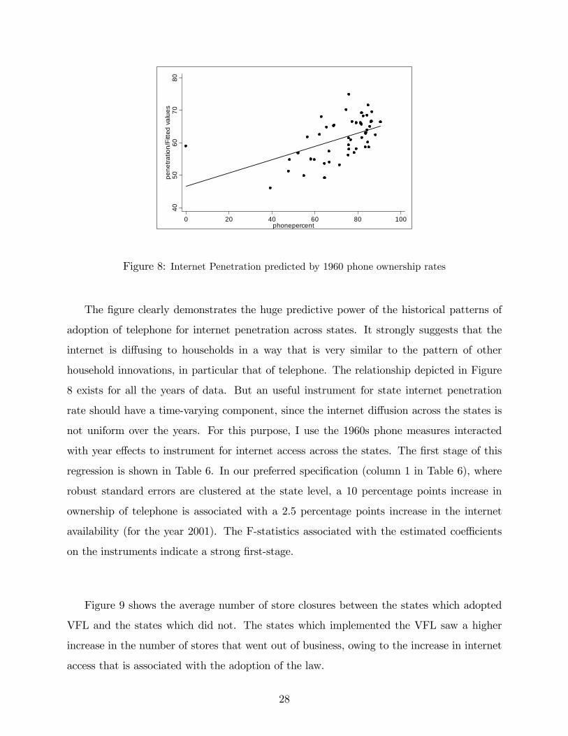
Figure 8: Internet Penetration predicted by 1960 phone ownership rates

The �gure clearly demonstrates the huge predictive power of the historical patterns of

adoption of telephone for internet penetration across states. It strongly suggests that the

internet is di¤using to households in a way that is very similar to the pattern of other

household innovations, in particular that of telephone. The relationship depicted in Figure

8 exists for all the years of data. But an useful instrument for state internet penetration

rate should have a time-varying component, since the internet di¤usion across the states is

not uniform over the years. For this purpose, I use the 1960s phone measures interacted

with year e¤ects to instrument for internet access across the states. The �rst stage of this

regression is shown in Table 6. In our preferred speci�cation (column 1 in Table 6), where

robust standard errors are clustered at the state level, a 10 percentage points increase in

ownership of telephone is associated with a 2.5 percentage points increase in the internet

availability (for the year 2001). The F-statistics associated with the estimated coe¢ cients

on the instruments indicate a strong �rst-stage.

Figure 9 shows the average number of store closures between the states which adopted

VFL and the states which did not. The states which implemented the VFL saw a higher

increase in the number of stores that went out of business, owing to the increase in internet

access that is associated with the adoption of the law.

28

Table 6: First Stage Estimates of the E¤ect of phone measures on State Internet Penetration

Rates


(1)


(2)


(3)Phone*Year=1997 0 .008

(0.069)0 .008(0.08)

0.018(0.058)

Phone*Year=1998 0.167***(0.068)

0.167*** (0.072)

0.126***(0.059)

Phone*Year=2000 0.246***(0.073)

0.246***(0.075)

0.211***(0.056)

Phone*Year=2001 0.251***(0.056)

0.251*(0.071)

0.209***(0.056)

Phone*Year=2003 0.224***(0.065)

0.224*(0.072)

0.172***(0.057)

Phone*Year=2007 0.134**(0.068)

0.134**(0.077)

0.068(0.060)

Controls for statefixed effects?

Yes Yes Yes

Fstatistic 14.97 11.09 Chi2= 120.59

Observations 294 294 294Notes: Standard errors are in parenthesis. The Internet penetration data are from CPS Computer Use and Supplements for theyears 1997, 1998, 2000, 2001, 2003 and 2007. *denotes significance at the 1% level, ** denotes significance at the 5% level.All the regressions are weighted by population and include year fixed effects. Other controls include population, meaneducation, age, and the proportion of female, white, black , Hispanic and percentage of people living on large acres of land foreach stateyear.

29

0

5

10

15

20

25

30

2003 2004 2005 2006 2007

Year

Ave

rage

num

ber o

f sto

recl

osur

es p

er y

ear

Storeclosures in VFL statesStoreclosures in NonVFL states

Figure 9: Total number of Store closures from 2003 through 2007

Figure 10 shows visual evidence of the reduced-form relationship between the store clo-

sures and the instrument. The �tted line has a positive slope, indicating that the adoption

of VFL coincides with a higher number of music stores going out of business.

The reduced-form estimates of equation (2) represents the main results which are shown

in Table 7. The �ndings are consistent with the existence of a positive statistically and

economically signi�cant causal impact of VFL adoption on store closures. When we adjust

the standard errors for unknown forms of heteroskadasticity and serial correlation (Table 7

column 1), the reduced-form estimate implies that adopting VFL causes on an average, 14

more store closures in a state for a given year. This indicates that an increase in internet

availability, through the adoption of VFL by the states, explains 58.7 percent of the total

store closings in those states. The model also explains 15.8 percent of all store closures in

the US22

The estimation results for equation (3) are reported in Table 8. The coe¢ cients on

phones;t have the expected sign in all three speci�cations. However, the �ndings are generally

22Note that the speci�cations do not control for the presence of Megastores. The results including thepresence of Megastores as control are reported in table 10.

30

050

100

150

stor

eclo

sing

s/Fi

tted

valu

es

0 .2 .4 .6 .8 1VFL

storeclosings Fitted values

Figure 10: Reduced-form:store closings and VFL adoption by states

consistent with a positive and statistically signi�cant causal impact only when a feasible

generalized least squares method is employed to allow for heteroskadaticity23. These results

indicate that a 10 percentage points increase in phone ownership is associated with 4 more

store closings in a state for a given year (result for 2006, column 3 in Table 8). Hence the

reduced-form approach yields results that are broadly consistent with the OLS results, thus

providing supporting evidence for their �ndings.

The two-stage least-squares (2SLS) estimates of equation (2) represents the IV results

which are reported in table 9. Here the state internet penetration rates are instrumented

by the VFL dummy. These results indicate an economically signi�cant positive causal re-

lationship between the states adopting the VFL and store closures. However, because of

the sparsity of data, the results are not statistically signi�cant at any common levels of

con�dence. The IV results suggest that state internet penetration rate is mediating the rela-

tionship between VFL and store closings that we �nd in the reduced form estimation. Using

the adoption of telephones in the 1960 Census as an instrument for internet penetration, the

2SLS estimates in table 26 in the appendix indicate a similar relationship between phone

23Homoskadasticity may be a restrictive assumption for panels, where the cross-sectional unit, in this casethe states may be of varying size and as a result may exhibit di¤erent variation.

31

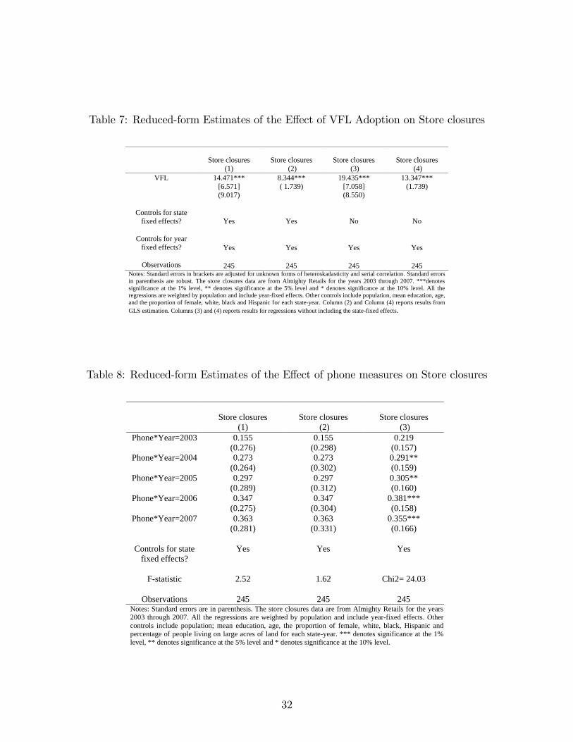
Table 7: Reduced-form Estimates of the E¤ect of VFL Adoption on Store closures

Store closures(1)

Store closures (2)

Store closures (3)

Store closures (4)

VFL 14.471***[6.571](9.017)

8.344***( 1.739)

19.435***[7.058](8.550)

13.347***(1.739)


Controls for yearfixed effects? Yes Yes Yes Yes

Observations 245 245 245 245Notes: Standard errors in brackets are adjusted for unknown forms of heteroskadasticity and serial correlation. Standard errorsin parenthesis are robust. The store closures data are from Almighty Retails for the years 2003 through 2007. ***denotessignificance at the 1% level, ** denotes significance at the 5% level and * denotes significance at the 10% level. All theregressions are weighted by population and include yearfixed effects. Other controls include population, mean education, age,and the proportion of female, white, black and Hispanic for each stateyear. Column (2) and Column (4) reports results fromGLS estimation. Columns (3) and (4) reports results for regressions without including the statefixed effects.

Table 8: Reduced-form Estimates of the E¤ect of phone measures on Store closures

Store closures(1)

Store closures(2)

Store closures(3)

Phone*Year=2003 0.155(0.276)

0.155(0.298)

0.219(0.157)

Phone*Year=2004 0.273(0.264)

0.273(0.302)

0.291**(0.159)

Phone*Year=2005 0.297(0.289)

0.297(0.312)

0.305**(0.160)

Phone*Year=2006 0.347(0.275)

0.347(0.304)

0.381***(0.158)

Phone*Year=2007 0.363(0.281)

0.363(0.331)

0.355***(0.166)

Controls for statefixed effects?

Yes Yes Yes

Fstatistic 2.52 1.62 Chi2= 24.03

Observations 245 245 245Notes: Standard errors are in parenthesis. The store closures data are from Almighty Retails for the years2003 through 2007. All the regressions are weighted by population and include yearfixed effects. Othercontrols include population; mean education, age, the proportion of female, white, black, Hispanic andpercentage of people living on large acres of land for each stateyear. *** denotes significance at the 1%level, ** denotes significance at the 5% level and * denotes significance at the 10% level.

32

Table 9: 2SLS Estimates of the E¤ect of VFL Adoption on Store closures

2SLS(1)

2SLS (2)

VFL 21.823[25.574](36.261)

13.229[10.320](10.764)

Controls for state fixed effects?Yes No

Observations 245 245Notes: Standard errors in brackets are adjusted for unknown forms of heteroskadasticity and serial correlation. Standard errorsin parenthesis are robust. The store closures data are from Almighty Retails for the years 2003 and 2007. All the regressions areweighted by population and include yearfixed effects. Other controls include population, mean education, age, and the proportionof female, white, black and Hispanic for each stateyear. Column (2) reports results for regressions without including thestatefixed effects.

connection and store closings, which supports the reduced-form results.

The reduced form results for the alternate outcome variables depending on the type of

stores is reported in table 30 in the appendix. The estimates imply that there has been

an increase in the number of independent, chain and other category of store closures and

a decrease in big-box retail stores, following the adoption of VFL. These results indicate

that the increase in internet availability through the adoption of VFLs in the states which

implemented it, have not uniformly a¤ected the di¤erent types of music store closures. There

have been more independent and chain store closures compared to the big-box retailers,

suggesting a substitution among the di¤erent categories of music stores.

In an alternate speci�cation of the reduced-form regression equation, I controlled for

the presence of big-box megastores like Wal-Mart and Sam�s Club, which are the main

competitors of the music CD stores. The results from the reduced-form estimation are

reported in table 10. Adjusting the standard errors for unknown forms of heteroskadasticity

and serial correlation (Table 10 column 1), the reduced-form estimate implies that adopting

VFL causes on an average, 9 more store closures in a state for a given year.

Now I turn to a discussion about the existence of any possible sources of bias in the main

estimation regressions. From the above discussion of the exclusion restrictions we identi�ed

state unemployment rates as a factor that might have driven the adoption of VFL. I included

this factor in my main regression. Also I included the state business rankings to see whether

33

Table 10: Reduced-form Estimates of the E¤ect of VFL Adoption on Store closures control-

ling for the presence of megastores

Store closures(1)

Store closures (2)

Store closures (3)

Store closures (4)

VFL 9.276**(6.358)[8.184]

6.161***(1.483)

13.330**(8.261)[9.626]

6.291***(2.165)

Megastores 0.508***(0.193)[0.168]

0.377(0.099)

0.084(0.021)[0.028]

0.109(0.013)


Observations 245 245 245 245Notes: Standard errors in brackets are adjusted for unknown forms of heteroskadasticity and serial correlation. Standard errorsin parenthesis are robust. The store closures data are from Almighty Retails for the years 2003 through 2007. ***denotessignificance at the 1% level, ** denotes significance at the 5% level and * denotes significance at the 10% level. All theregressions are weighted by population. Other controls include population, mean education, age, and the proportion of female,white, black and Hispanic for each stateyear. Columns (3) and (4) reports results for regressions without including the statefixed effects.

this leads to any potential bias. Including this index is important, since it might be that stores

in states which are more business friendly face lower costs, thereby being less likely to incur

losses and thus more liekly to stay in business longer; or perhaps being more business friendly

means that the companies will have a faster turnover and that will accelerate the demise of

the CD stores. So theoretically, the impact of the business friendliness of a state on store

closures (and hence the sign of the possible bias) is not clear a priori. The results reported in

table 35 in the appendix indicate that an increase in business ranking (i.e.: states becoming

less business friendly) leads to more store closures, which might lead to a potential downward

bias of the reduced form estimates. However, since business friendliness is uncorrelated to

VFL adoption, this does not a¤ect the observed relationship between the VFL regressor and

store closures24. The state unemployment rates have no statistically signi�cant impact on

store closures which rules out the possibility of any bias on my reduced form estimates. A

positive coe¢ cient on per capita state gdp might indicate a potential upward bias on the

reduced form estimates, but again, since per capita state GDP is uncorrelated to the VFL

24I also checked whether including these covariates one at a time changes the result; the results are verysimilar to the ones reported in table 35.

34

adoption, this does not a¤ect the observed relationship between the VFL regressor and store

closures25..

2.4.4 Falsi�cation

In order to support the validity of my instrument for state internet penetration rates, in

this section I present a falsi�cation exercise pretending that the adoption of VFL by the

states occurred in 2003 instead of in 2005, 2006 or 2007. The �rst-stage regression model is

speci�ed as before:

Is;t = �+ �V FLs;t +X0s;t + �s + �t + "s;t (6)

with the VFL dummy taking a value of one between the years 2003 and 2004 for the

18 states which adopted the Video Franchise Law. Table 31 in the appendix reports the

estimates from the �rst-stage regression of this falsi�cation exercise. In all of the speci�ca-

tions (depending on the assumptions on the error structure as explained above), I �nd point

estimates which are small and not statistically signi�cant. This exercise con�rms that the

positive impact of adoption of VFL on internet penetration rates in the states which adopt

the law are indeed true e¤ects.

Table 32 in the appendix shows the results for the reduced-form estimates from the fal-

si�cation exercise. In my preferred speci�cation (when the standard errors are adjusted for

unknown forms of heteroskadasticity and serial correlation) as well as other speci�cations

including the state-�xed e¤ects, I �nd no e¤ect of the adoption of VFL on store closures in

those states. However, the estimates without including the state of residence main e¤ects

are statistically di¤erent from zero, indicating that the VFL-adopting states might be hav-

ing more store closures even before the adoption of the law. When I repeated the exercise

25It is somewhat counter intuitive that an increase in per capita state gdp (which is an indication of theeconomic prosperity of a state) is causing more music CD store closings. I further checked whether di¤erenttypes of stores were a¤ected di¤erently and found an increase in per capita state gdp causes an increase inindependent store closings but a reduction in big-box retailers. This is in line with the argument provided inthe discussion of exclusion restrictions that states might be bringing big-box retailers or sports arenas whichin turn might accelerate the demise of the independent music stores.

35

pretending VFL was adopted two years prior to when it actually was, the results are qual-

itatively similar and are reported in panel B of table 32. In spite of not being able to rule

out a concern about an upward trend in store closures in the VFL adopting states before

the adoption, to the extent that the falsi�cation test is satis�ed for my main speci�cation,

this is not a concern here.

2.5 CONCLUSIONS

Internet usage has increased dramatically over the past few years. At about the same time,

the sales from music has witnessed a huge decline. In this paper, I use two sources of

exogenous variation in the internet access across US states to measure the impact of music

downloads on the progressive disappearance of the traditional music CD stores. Speci�cally,

I use information on the passage of Video Franchise Law and the di¤erences in the household

telephone adoption rate in the 1960 Census as the two sources of variation in the availability

of the internet access across the states. The sale of CDs is a very important source of revenue

for the music industry, accounting for more than 85 percent of total music sold in the US.

The share of record stores, which represent a signi�cant portion of the sale from CDs saw a

decline of over 8 percent within the last three years (RIAA Consumer Pro�le, 2007). Hence,

it is crucial to estimate the extent to which a change in the consumer preference in the form

of downloading music is driving out the old format.

Using CPS Computer and Internet Use Supplements data for state internet penetration

rates and CD store closings data from Almighty Institute of Music Retail, I �nd that the

implementation of VFL increases the availability of internet access in the states which adopt

it, and explains 58.7 percent of the total store closings in those states. Also, a 10 percentage

points increase in the phone ownership is associated with 4 more stores going out of business

in a state for a given year. The results suggest that a variability in the access to the internet

can explain the di¤erence in the music store closures across states. These empirical results

support the idea that technological progress in the household in the form of increased internet

access played an important role in the demise of the traditional music CD stores. Although

36

due to data limitations I am using store closings as my outcome variable of interest, in the

event of data availability, looking at the total number of stores in a given region over a period

of time would have been a preferable outcome26.

These results have signi�cant implications for public policy. While the adoption of VFLs

by states have the impetus for economic growth and social welfare, there is some caution

to be exercised by state governors while implementing these policies. In addition to the

detrimental e¤ects of illegal downloading on the music sales that is well documented in the

literature, the increased availability in faster network connections now urge a rise in the legal

downloads as well. This aggravates the situation for an already struggling music industry by

driving the traditional music stores out of business and further reducing revenue from the

sale of CDs.

26To address the concern of whether there were a large number of music store openings in the states whichadopted VFL over the period of time, I did a Lexis-Nexus search of relevant newspaper artilcles. I foundthere were very few store openings over this period. Speci�cally, there were 5 openings in New York, 4 inCalifornia, 3 in Massachussettes and 1 in Ohio.

37

3.0 THE EFFECT OF PARENTAL LEAVE ON FEMALE EMPLOYMENT:

EVIDENCE FROM STATE POLICIES

3.1 INTRODUCTION

Over the past decades, parental leave policies have been an important issue of debate given

their possible impacts on employment, leave taking and earnings. In particular, since 78

percent of labor force is composed of families where both parents work (Grant et. al, 2005),

parental leave policy is a relevant topic both at the federal and state level of the government.

Research on the e¤ect of such leave policies are particularly important given the recent trends

in female employment. For instance, more than half (52 percent) of women with children

under the age of one were employed in 1998 compared to only two-�fths ten years earlier

(Waldfogel, 1999).

In spite of the substantial increase in the percentage of women with young children in the

labor force, the Family and Medical Leave Act (FMLA) is the only law in the United States

at the federal level to directly address family leave issues. In particular, FMLA requires

employers with 50 or more employees to allow twelve weeks of unpaid, job-protected leave

following the birth or adoption of a child. Enacted in 1993, the legislation covers private,

state and local government employees who worked at least 1250 hours in the last 12 months.

Therefore, year 1993 is identi�ed as the beginning of job-protected maternity leave policies

at the federal level. In addition, given that the percentage of employees under maternity

leave coverage increased dramatically after the enforcement of FMLA (86 percent in 1995 as

compared to 39 percent 1991, Waldfogel (1999a)), it is worthwhile analyzing its impact on

female employment.

38

Hence after, some states1 have introduced di¤erent extensions to the FMLA which relax

the employee�s eligibility -such as the minimum number of hours worked and the required

number of workers in the �rm- covering both public and private sector employees. Although

FMLA is the only law at the federal level which provides some assistance to new parents,

there were laws prevalent at the state level long before the federal act came into e¤ect. In

particular, the Temporary Disability Insurance (TDI), which provides wage replacement for

non-work connected sickness or injury, includes disabilities related with pregnancies. The

TDI is implemented by �ve states2, which started to apply this law from 1942 to 1969. The

Paid Family Leave program, implemented by California in 2004, has been the most recent

law enacted with regard to parental leave policy. In particular, it provides partially paid

leave for a period of 6 weeks.

Hence, the above policies basically di¤er in either their medical requirements for eligibility

or the paid/unpaid leave they provide. On the one hand, TDI provides paid leave, but only

if the mother�s maternity is associated with medical conditions which support a doctor�s

decision of considering it a temporary disability3. On the other hand, FMLA provides

unpaid leave but it does not require the consideration of maternity as a temporary disability.

Finally, California�s Paid Family Leave program can be considered as the most generous of

these programs since it provides a paid leave (as TDI) and, in addition, it does not require

the temporary disability consideration (as FMLA).

This paper analyzes the impact of the existing parental leave policies on female employ-

ment. That is, do these di¤erent policies have the same impact on female employment? In

particular, we examine whether the introduction of FMLA di¤erently a¤ected female em-

ployment in those states having some paid parental leave policy before FMLA was enacted

�those which previously implemented the TDI�and those states which did not have any

1Connecticut, Maine, Oregon and Vermont are the states whose FMLA expansion covers both the publicas well as private sector employees. There are seven other states plus District of Columbia which alsoexpanded FMLA but does not cover both public and private sector employees.

2California, Hawaii, New Jersey, New York and Rhode Island. Puerto Rico also has TDI law.3After the Pregnancy Discrimination Act in 1978, every pregnancy is treated as a temporary disability.

39

kind of paid parental leave policy �those which neither passed TDI nor any other form of

state maternity leave policy4. Additionally, we examine if change in the female employment

was higher in those states which expanded the bene�ts (and relaxed the eligibility criteria)

of FMLA than in those which did not. Finally, we analyze whether California�s Paid Family

Leave program has a di¤erential impact on female employment compared to (1) states that

did not expand FMLA, and (2) states which expanded FMLA. The answer to these questions

provides some interesting policy recommendations about parental leave programs.

Previous studies have analyzed the impact of FMLA on female employment, coverage,

leave-taking and earnings. One of the most relevant works in this respect is Waldfogel

(1999a). She used March CPS data for the years 1992-1995 to compare the change in female

employment, coverage, earnings and leave-taking between states which had no job-protected

maternity leave legislations before FMLA (39 states) to the 11 states and DC that had

prior job-protected parental leave laws. Essentially, her analysis grouped together a set of

12 states, each of which had a di¤erent state maternity leave policy and hence are likely to

have di¤erent impacts on female employment. Also, some of the states that she considered as

having no job-protected maternity leave legislations before FMLA (among the 39 states), had

some form of maternity leave policy prevalent before FMLA was passed in 1993. Hence there

was variation within her no protection states in the actual amount of protection that women

in these states were granted before FMLA was passed. Using a di¤erence-in-di¤erence-in-

di¤erences estimation strategy, her results indicate that there has been an increase in coverage

and leave-taking following the enforcement of FMLA, whereas there has been no change in

employment. Given that eligible women in some of the experimental states actually received

treatment, this would have the e¤ect of biasing the estimates towards zero.

The di¤erence between our work and the former paper is twofold. First, we identify

those �ve states that had some form of paid parental leave policy before FMLA was enacted,

i.e. those states which previously implemented TDI. This speci�c classi�cation allows us to4There were eighteen states which had no maternity leave policy before the implementation of FMLA.

They are, Alabama, Arkansas, Delaware, Idaho, Indiana, Kentucky, Michigan, Mississippi, Missouri, Ne-braska, Nevada, New Mexico, North Carolina, South Carolina, South Dakota, Texas, Utah and Wyoming.

40

work with a homogeneous group of states which have been a¤ected by the same law, and

it captures the uniform di¤erential impact of FMLA on female employment between those

states applying TDI and those applying no state parental leave policies5. Second, we go one

step beyond the analysis of FMLA and additionally compare whether the impact of FMLA

on female employment di¤ers between those states which expanded its bene�ts and relaxed

its eligibility criteria and those which did not expand them, which Waldfogel (1999a) did not

analyze. This enables us to study whether the impact on female employment and labor force

participation is di¤erent when certain states make the parental leave policy more generous.

In contrast to the previous results, we �nd a positive and statistically signi�cant impact of

FMLA on female employment in the states which had no law prior to FMLA compared to

the states which had TDI6.

Another important contribution to the literature is Kallaman (1996). She studies the

e¤ect of the FMLA on female employment and wages. Her results show a positive (negative)

and signi�cant e¤ect of FMLA on employment (wages). Kallaman�s work does not make any

distinction between the e¤ects of FMLA and those of other policies. On the contrary, our

paper focuses on comparing the relative performance of the above federal and state policies

on female employment and labor force participation which greatly enriches the analysis.

More recently, Ho¤erth and Curtin (2006) studied how implementation of the FMLA a¤ected

mothers�return to the work place and their changes in wages. However, as mentioned before,

our paper is mainly focused on the e¤ect of maternity leave policies on female employment

across di¤erent states.

We use a di¤erence-in-di¤erences (DD) and di¤erence-in-di¤erence-in-di¤erence (DDD)

estimation strategy, where the �rst di¤erence is between the states which received the treat-

ment (states that had TDI) and the states which did not. The second source of di¤erence

has to do with the time of the treatment, i.e.: before and after 1993, when FMLA was

5Note that California, New Jersey and Rhode Island had some maternity leave legislations before FMLAwas enacted, so the di¤erential e¤ect on female employment cannot be attributed to TDI alone for thesethree states.

6Using the same states as the experimental and non-experimental groups considered by Waldfogel, wereplicate her results, i.e.:obtain no statistically signi�cant impact of FMLA on female employment.

41

passed. The third di¤erence is between the treated group and the control group, which did

not receive the treatment. Some of the results obtained in this paper are the following. First,

the impact of FMLA in those states which did not previously enact TDI is signi�cantly more

positive on female employment than the impact of this law in those states which already

had TDI. The increase in female employment and labor force participation in those states

that most generously expanded the bene�ts and eligibility criteria of FMLA is signi�cantly

higher than in those that did not. Finally, the introduction of California�s Paid Family Leave

program in 2004 has not yet provoked changes in female employment which can be consid-

ered signi�cantly di¤erent from those in states applying either the FMLA or the expanded

FMLA alone.

As mentioned above, the e¤ects of FMLA on employment have been shown to be positive

(but small) by both theoretical and empirical literature; see Klerman and Leibowitz (1994),

Ruhm (1997) and Waldfogel (1996). This paper, then, goes in the line of this literature,

but provides a much richer analysis and comparison about the e¤ects of FMLA on female

employment in states with and without previously enacted TDI, examines the labor market

e¤ects of the FMLA expansions implemented by di¤erent states, and �nally provides a com-

parison about the impact of the most recent and generous parental leave policy in California

with respect to those policies currently applied in the rest of the country.

The paper is organized as follows. In section 3.2 we develop an overview of the parental

leave laws in United States. Section 3.3 explains the theoretical e¤ects of mandated leave

policies on female employment. Section 3.4 lays out the research design and methodology.

Section 3.5 describes the data used in the analysis. In sections 3.6 through 3.9 we present

our results to the main questions analyzed above, and provide some intuition. Section 3.10

concludes and suggests further research in the analysis of parental leave policies at the federal

and state level.

42

3.2 OVERVIEW OF PARENTAL LEAVE LAWS

Parental leave policy has undergone many changes during the last decades. Figure 11 il-

lustrates the evolution of maternity leave laws in US. The �rst state to introduce a paid

maternity leave through TDI was Rhode Island in 1942, followed by California (1946), New

Jersey (1948), New York (1949) and Hawaii (1969). TDI is o¤ered to all workers in these

states by state mandate. The program provides temporary income to workers with non-

work related short-term disabilities, including pregnancy and childbirth. It is funded by

either employee or employer or both, and ranges in coverage from 6 to 52 weeks7

19931942

TDIFirst state:

Rhode IslandFMLA

2004

California’s Paidfamily Leave

Program

1969

TDILast state:

HawaiiStates which have expanded or Complemented FMLA

1978

PDA

Figure 11: Parental leave laws: 1942-2004

In particular, TDI can be understood as a form of paid maternity leave, since disability

insurance policies provide paid leave at state level and bene�ts for disability related to

pregnancy and childbirth to ensure the same treatment as other medical disabilities. The

TDI coverage for the �rst few weeks after a birth is routine, since all mothers are considered

medically disabled for a certain period of time after child-birth. A study by the University

of Rhode Island (2005) suggests that about 62 percent of TDI claimants were women, and

the most explanatory variable to account for such high number of women �ling claims was

TDI coverage for childbirth (Employment Bulletin, RI Department of Labor and Training).

The Family and Medical Leave Act (enacted in 1993) is the only law in terms of parental

leave policy at the federal level. The legislation covers private, state and local government

employees. However, the coverage under the Family and Medical Leave Act is not universal.

7See table 41 in the appendix for a detailed explanation about weekly bene�t amounts and duration ofthe TDI program.

43

FMLA guarantees parents unpaid, job-protected leave of up to 12 weeks following the birth

or adoption of a child, but only if they meet certain qualifying conditions. First, they must

work for a �rm with 50 or more employees, which means only about 60 percent of workers in

the private-sector are covered (Han and Waldfogel, 2003). Second, they must have worked

at least 1,250 hours in the past year for their employers, which reduces the share of workers

covered to 46 percent (Cantor et al, 2001).

Over the years a considerable number of states have relaxed as well as complemented

the requirements of FMLA. This paper considers four states for whose FMLA expansion not

only a¤ected public but also private sector workers8and have made the FMLAmore generous.

In particular, the state of Connecticut expanded FMLA in 1997 applying it to employees

who worked 1000 hours for at least 12 months prior to a request for a leave, and eligible

employees are entitled 16 workweeks of leave (instead of only 12). In 1997, Maine extended

the applicability of its family medical leave laws by lowering the requirements for employee

eligibility to 15 employees. Oregon (1996) made FMLA more generous by applying it to

employers with 25 or more employees, and established that those workers who are employed

for 180 days or more are eligible for 12 weeks of leave within a 12 month period. Finally,

similar to Oregon, Vermont (1998) reduced the number of minimum employees to 10, who

should have worked for one year on an average of 30 hours a week to be eligible for 12

weeks of leave during any 12 month period. In addition, all of these four states allowed the

possibility of substituting accrued paid leave for maternity leave purposes (see table 42 of

appendix for details about the extensions of FMLA).

Finally, one of the most recent parental leave policy to be enacted is California�s Paid

Family Leave (PFL) program, which came into e¤ect in July 2004. California is the �rst state

in the country to create a comprehensive paid family leave program. It provides workers with

paid leave during a period of six weeks, covering approximately 55 percent of their pre-taxed

weekly wage, up to a maximum of $840, while on leave. This insurance program is fully

funded by the employees. The new mothers in California are now eligible for Paid Family8There are eight other states which expanded the FMLA bene�ts, but they did not cover both private and

private sector employees. In addition, the relaxations in eligibility and expansions in bene�ts were minimal.

44

Leave bene�ts in addition to the TDI bene�ts. While FMLA o¤ers 12 weeks of unpaid leave

for those working for employers with 50 or more employees, Paid Family Leave program

guarantees that 6 of those weeks would be paid.

3.3 THEORY

The theory on mandated bene�ts suggest that they preserve the employers�ability to tailor

arrangements to their workers and to o¤er more than minimum packages. In terms of their

allocational e¤ects on employment, mandated bene�ts represent a tax at a rate equal to the

di¤erence between the employers cost of providing the bene�t and the employee�s valuation

of it (Summers, 1989). In other words, it is assumed that workers and �rms will voluntarily

agree to the provision of family leave if the expected bene�ts exceed the associated costs.

Parental leave bene�ts could also increase occupational segregation, by increasing the rel-

ative cost of employing women in certain types of jobs, and lead to higher unemployment

for the groups who are most likely to use it. (Ruhm and Teague, 1997). However, there are

a considerable number of economic arguments that have been made favoring leave entitle-

ments usually focus on retaining �rm-speci�c human capital or decreasing unemployment by

reducing the need for women to change jobs, if they wish to spend time at home with young

children. (Trzcinski, 1991).

According to the theory (Ruhm, 1997), a mandated leave raises labor costs and so shifts

the labor demand curve to the left (from D1 to D2 in Figure 12). Since employees receive

bene�t from the leave entitlement, the supply curve simultaneously shifts to the right (from

S1 to S2). Hence the equilibrium wages fall while employment may either increase or decrease,

depending on the relative size of the shifts. Figure 12 illustrates the case where the expenses

to employers exceed the bene�ts to the employees, and employment decreases (from E1 to

E2). However, there could be additional dynamic e¤ects. For instance, labor productivity

would rise if parental leave increases �rm-speci�c human capital by allowing individuals to

return to their old jobs. This causes the demand curve to shift to the right (from D2 to D3

in Figure 2), increasing employment and decreasing the wage reduction or actually leading

45

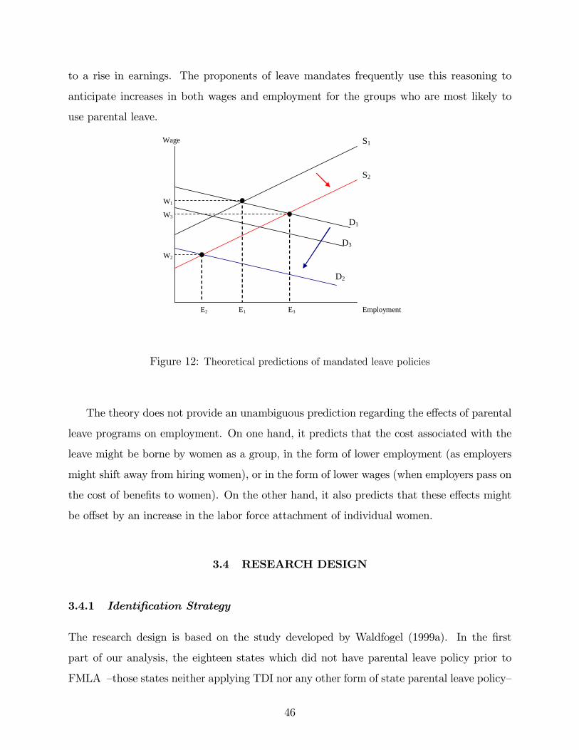
to a rise in earnings. The proponents of leave mandates frequently use this reasoning to

anticipate increases in both wages and employment for the groups who are most likely to

use parental leave.

S1

S2

D1

D3

D2

E2 E1 E3 Employment

W2

W1

W3

Wage

Figure 12: Theoretical predictions of mandated leave policies

The theory does not provide an unambiguous prediction regarding the e¤ects of parental

leave programs on employment. On one hand, it predicts that the cost associated with the

leave might be borne by women as a group, in the form of lower employment (as employers

might shift away from hiring women), or in the form of lower wages (when employers pass on

the cost of bene�ts to women). On the other hand, it also predicts that these e¤ects might

be o¤set by an increase in the labor force attachment of individual women.

3.4 RESEARCH DESIGN

3.4.1 Identi�cation Strategy

The research design is based on the study developed by Waldfogel (1999a). In the �rst

part of our analysis, the eighteen states which did not have parental leave policy prior to

FMLA �those states neither applying TDI nor any other form of state parental leave policy�

46

constitute the experimental states. The �ve states which did have TDI prior to FMLA are the

non-experimental states. For the second part of the study, the four states which expanded

or complemented FMLA are considered as the experimental states for each particular case,

with the non-experimental states being the states applying only FMLA. Finally, the state of

California (experimental state) is compared with those states which only have FMLA or have

expanded it (non-experimental states). We could use DD analysis to compare the change

in outcomes for the experimental states to the change in outcome for the non-experimental

states. However, this approach may produce biased estimate if there were other di¤erences

between these two groups of states that a¤ected both the passage of state laws and the change

in their outcome variables over time (Bertrand and Mullainathan, 2004). To overcome this

problem, we use a DDD methodology.

We study the impact of state parental leave policies on the employment of women. Since

we use a DDD estimation strategy, this requires identifying one or more treatment groups

(the groups who are a¤ected by the passage of a law) and one or more control groups (those

who are not a¤ected by the law but are otherwise a¤ected by the same underlying factors, so

that their behavior can be used to approximate how the treatment group would have acted

in the absence of the policy). The di¤erent parental leave policies that we are analyzing

are expected to primarily bene�t women of childbearing ages, therefore, we use women aged

19 to 45 with children older than one year old, or women in the same age group who are

childless as our treatment group. In addition, we consider an alternative treatment group in

our analysis, which is composed of women aged 19 to 45 with children under the age of one.

These groups of women are included in the treatment group because they are eligible and

more likely to obtain the bene�ts of parental leave policies. Also, we focus on these women

because they are the potential bene�ciaries of the law and might bear some of the costs of

the law (in terms of employers passing along the costs of these bene�ts to those potentially

bene�tting from it). In order to isolate the impact of the parental leave policies from other

factors (like economic shocks or other policy changes) that a¤ect labor market outcomes,

we use control groups. Ideally, a control group should be similar in characteristics to the

treatment group, and hence likely to respond in the same way to a given policy change,except

47

for the fact that it does not receive the treatment. For this purpose, we use women aged

46 to 60 as the control group, since they may plausibly substitute for women under 45 in

employment but are more likely to have reached the end of their reproductive lives and

hence less likely to take advantage of parental leave laws. However, comparison between

younger females and older females might not be su¢ cient to identify the e¤ect of parental

leave policies. These older women have their own labor market trends which di¤er from that

of the younger women, and there could be some age-speci�c factors that might make their

preferences towards work di¤erent from that of younger females. For this purpose (and as

is customary in the literature)9, we use men between the age of 19 and 45 as an alternative

control group. Men of the same age as women in the treatment group, while also potential

substitutes in employment, are less likely to have been a¤ected by changes in tastes for work

as older women. However, men have their own work preferences and might face di¤erent

labor market prospects compared to women (mainly due to gender discrimination in the

workplace). Since each of the control groups we use are plausible but imperfect comparisons

for the treatment group, we use both types of workers alternatively as control groups in order

to better identify the e¤ects of parental leave policies on female employment10.

Our estimates of the e¤ects of the federal parental leave policy on female employment is

the di¤erence between the change in female employment after the introduction of the FMLA

in those states which previously applied TDI and those which did not. Another estimate of

this e¤ect is obtained from the di¤erence in the change of the female employment between

those states which expanded FMLA and those which did not. Finally, the estimate of the

e¤ect of the state parental leave policies on female employment measures the di¤erence

between the change in the female employment in California �after the enactment of the Paid

Family Leave program�and that in the states which expanded FMLA and those which did

not.

9See Baker and Milligan (2008), Rodgers and Zveglich (2003)10Also, since our analysis closely follows that of Waldfogel (1999a) who used men as alternate control

group, in order to replicate as well as compare our results to this study, we include this group.

48


Variable Treatment AlternativeTreatment

Control AlternativeControl

Age 32.28 (0.00) 28.16 (0.01) 51.96 (0.01) 31.80 (0.01)

CollegeGraduate

0.44 (0.00) 0.42 (0.00) 0.35 (0.001) 0.46 (0.00)

High SchoolDrop Out

0.17 (0.00) 0.18 (0.00) 0.26 (0.00) 0.17 (0.00)

Employed 0.74 (0.00) 0.58 (0.00) 0.66 (0.00) 0.91 (0.00)

Fraction inStates with no

Law

0.56 (0.00) 0.57 (0.00) 0.55 (0.00) 0.56 (0.00)

Observations 1,210,503 164,265 618,343 1,269,131Notes: Treatment refers to the women aged 19 to 45 with children older than one year old or childlesswomen; Alternative Treatment refers to women aged 19 to 45 with children under the age of one. Controlrefers to women aged 46 to 60 and Alternative Control refers to men aged 19 to 45. Data are from IPUMSCPS for the years 19792007.

3.5 DATA

We use IPUMS-CPS data from 1979-2007, which is an integrated set of data from the March

Current Population Survey (CPS). In the second part of our study, which analyzes the

e¤ects of the FMLA expansions, we also use data from CPS where time period depends on

the particular year in which the state expanded FMLA. Finally, the analysis of California

uses data from the 2001-2007 CPS.

Table 11 presents the summary statistics for the period 1979-2007 (mean and standard

error) of the characteristics of the treatment and control groups. Column 1 shows the

characteristics of women in their childbearing age with their youngest child above the age of

one or women without children. Column 2 contains women between 19-45 whose youngest

child is less than one year. Column 3 shows women aged between 46-60 and column 4 shows

the summary statistics of men aged between 19-45.

There are some di¤erences to be noted from the summary statistics. Women with children

49

above the age of one or without children (column 1) have, on average, the same age as

men (32 years), whereas women in alternative treatment group are on average younger

than men (the alternative control group). The percentage of employed in the treatment

group is lower (74 versus 91 percent) than the alternative control group, and the percentage

employed for the alternative treatment group is even lesser. Both treatment and alternative

treatment group women on average are more educated than women aged between 46-60

(control group). Notice that, the percentage of women and men in the eighteen states

which had no law prior to FMLA is fairly constant, so we can be certain that any of the

results are not driven by compositional changes. The summary statistics indicate that any

di¤erences in the labor force participation among the groups are not driven by di¤erences in

the demographic characteristics of those groups. The only di¤erence between the treatment

(and alternative treatment) and control (and alternative control) groups are that the former

have been a¤ected by changes in parental leave laws whereas the latter have not been a¤ected

by such changes.

Table 12 presents the summary statistics for the case of California (2001-2007). Column

1 shows the treatment group, column 2 the alternative treatment group, while columns 3

and 4 show the control and the alternative control group, respectively.

Some di¤erences can also be pointed out from the above table. Women with children

above the age of one or without children (column 1) have, on average, the same age as

men (33 years), whereas women in alternative treatment group are younger (30 years);

treatment group works less than the alternative control group (73 versus 89 percent), whereas

alternative treatment group are less likely to be employed compared to both control groups.

Both the treatment and alternative treatment group women are similarly educated compared

to women and men in the control groups.

50

Table 12: Summary Statistics: California

Variable Treatment Alternativetreatment

Control Alt. Control

Age 32.95 (0.05) 30.45 (0.11) 51.49 (0.04) 32.51 (0.05)

CollegeGraduate

0.56 (0.00) 0.53 (0.01) 0.57 (0.00) 0.51 (0.00)

High SchoolDrop Out

0.18 (0.00) 0.22 (0.01) 0.19 (0.00) 0.20 (0.00)

Employed 0.73 (0.00) 0.55 (0.01) 0.71 (0.00) 0.89 (0.00)

Fraction inStates with noLaw

0.61 (0.00) 0.65 (0.00) 0.61 (0.00) 0.61 (0.00)

Observations 21,733 2,880 112,45 23,236Notes: Treatment refers to the women aged 19 to 45 with children older than one year old or childlesswomen; Alternative Treatment refers to women aged 19 to 45 with children under the age of one. Controlrefers to women aged 46 to 60 and Alternative Control refers to men aged 19 to 45. Data are from IPUMSCPS for the years 20012007.

3.6 EMPIRICAL RESULTS FOR FEMALE EMPLOYMENT

The likely direction of the e¤ects of maternity leave policies on female employment is not

clear apriori. On the one hand, if women are more inclined to take leave and return to their

previous jobs, then we expect to �nd a positive e¤ect on employment. On the other hand,

if employers pass on the costs of mandated bene�ts to those potentially bene�tting from it

(women of childbearing age), then we might observe a decrease in employment. Further, if

these two e¤ects o¤set each other, we might �nd no impact on employment at all. Therefore,

the direction of the e¤ect of maternity leave policies on female employment is an empirical

question. This section, given the above research design, estimates the following equation

Yilt = �0+�1t+ �2NSl+�3TGi+�4NSl�TGi+�0POST t+�1NSl�POST t

+�2TGi�POST t+�3NSl�TGi�POST t (7)

where i indexes the individual, l the state and t the year. The outcome variable of interest,

Yilt; is a dummy equal to one if a woman worked for at least one week during the previous

year, and zero otherwise. NSl is a dummy equal to one if the lth state has no state parental

51

leave policy before 1993, and zero if the state had TDI. TGi is a dummy taking a value

one if individual i belongs to the treatment group and zero otherwise. Finally, POSTt is a

year dummy taking value one after FMLA was enacted (i.e. after 1993) and zero otherwise.

Since FMLA was enacted in 1993, we conduct our analysis pre and post 1993, in order to

capture the impact of the law on female employment. We de�ne employment as working for

a positive number of weeks during the year. In alternate speci�cations, we use labor force

participation rate as the outcome variable, where it is de�ned as participation in the labor

force during the preceding week.

3.7 ANALYSIS OF FMLA IN STATES WITH AND WITHOUT TDI

Table 13 reports the di¤erential impact of FMLA on female employment between states that

had no law prior to FMLA and states which had TDI before FMLA. Column (3) shows the

di¤erence between the change in female employment for experimental states �those with no

previous laws�and non-experimental states �those with TDI, before and after 1993. Column

(4) represents the change of female employment between the treatment and control group,

i.e. DDD. Finally, DDD adjusted 1 controls for marital status �i.e. dummy variable married

takes a value of one if the individual is married and zero otherwise�, DDD adjusted 2 includes

a time trend since the data contains more pre than post years, and DDD adjusted 3 controls

for both marital status and time trend. Notice that the Treatment group represents women

aged 19-45 with their youngest child above age one or childless women, while control group

are women aged 46-60 years and alternative control group are men aged 19-45 years.

In order to analyze the possibility of a di¤erent impact of FMLA depending on the

woman�s educational attainment, we di¤erentiate our sample by education levels. In partic-

ular, the dummy variable Educi is one when individual i has less than 12 years of schooling,

and zero otherwise. We divide our sample into two groups, one represents high school

dropouts and the second group contains the individuals who have a high school degree, a

52

Table 13: The estimates of Female Employment between states with no law and states with

TDI before FMLA

NoLaw(1) TDI(2) DD(3) DDD(4) DDD.adj1

DDD.adj2

DDD.adj3

Treat Pre'93 0.790 0.740Pos'93 0.720 0.660 0.016

Control Pre'93 0.630 0.630Obs.675,816 Pos'93 0.740 0.720 0.020 0.004 0.001 0.004 0.004

standarderrors

(0.004) (0.004) (0.004) (0.004)

Alt. Control Pre'93 0.920 0.900Obs.963,726 Pos'93 0.920 0.890 0.012 0.006*** 0.007*** 0.006*** 0.007***

standarderrors

(0.003) (0.003) (0.003) (0.003)

maritalstatus?

no yes no yes

linear timetrend?

no no yes yes

Notes: The Pre '93 period consists of the years 1978 1992. Robust Standard errors are reported. ***denotes statistically significant at onepercent level.

college degree or are college dropouts. In this case, equation 7 can be rewritten as,

Yilt = �0+�1tl + �2NSl+�3TGi+�4NSl�TGi+�0POST t+�1NSl�POST t+�2TGi�POST t

+�3NSl�TGi�POST t + �5Educ+ �6NSl�Educi+�7TGi�Educi+�8NSl�TGi�Educi

+�4POST t�Educi+�5NSl�POST t�Educi+�6TGi�POST t�Educi

+�7NSl�TGi�POST t�Educi (8)

The results obtained from both equations (with and without the dummy variable Educ)

are shown in tables 13 and 14. In addition, the same analysis is conducted for labor force

participation, where Yilt is a dummy equal to one if a woman participated in the labor force

during the preceding week and zero otherwise (tables 15 and 16 contain the results obtained

for labor force participation)

According to the PDA in 1978, the TDI should treat every pregnancy as a temporary

disability. Hence the coverage of the TDI extended to cover pregnancy as mandatory after

the passage of the PDA. In order to analyze the possibility of a di¤erential impact of FMLA

on female employment and labor force participation rates, we restrict the sample for the

pre-FMLA period from 1978 through 1992.

53

Table 14: The estimates of Female Employment between states with no law and states with

TDI before FMLA, by education groups

NoLaw(1) TDI(2) DD(3) DDD(4) DDD.adj1

DDD.adj2

DDD.adj3

Treat Pre'93 0.910 0.860Pos'93 0.880 0.810 0.017

Control Pre'93 0.770 0.780Obs.675,816 Pos'93 0.840 0.810 0.031 0.013 0.015 0.013 0.015Fstatistic (3.76) (4.92) (3.96) (5.12)

Alt. Control Pre'93 0.810 0.800Obs.963,726 Pos'93 0.790 0.780 0.001 0.016*** 0.017*** 0.016*** 0.007***Fstatistic (12.11) (12.66) (12.08) (12.65)

maritalstatus?

no yes no yes

linear timetrend?

no no yes yes

Notes: The Pre '93 period consists of the years 1978 1992. Robust Standard errors are reported. ***denotes statistically significant at onepercent level.

3.7.1 Analysis of the results

Table 13 suggests that when the treatment group is compared to the control group as ob-

served in column 4, the introduction of FMLA has an e¤ect on female employment which is

indistinguishable from zero. However, when the treatment group is compared to the alterna-

tive control group, i.e. men, the DDD estimates are positive and signi�cant. This suggests

female employment increased in states which had no law compared to the TDI states after

the implementation of FMLA, when women in their childbearing ages are compared to men.

When we further analyze by the educational attainment, table 14 shows signi�cant DDD

estimates for high-school dropout women, when the employment of female are compared to

men.

We further check whether the high educated women (having more than a high school

degree) are di¤erentially a¤ected by the implementation of FMLA. The results indicate

(tables not reported) that there is a no impact of FMLA on the employment of higher

educated women in the states which had no law compared to the TDI states, when women in

childbearing ages are compared to men. Also, the estimates are statistically indistinguishable

from zero when these women are compared to the control group, i.e. older women.

54

One reason for the insigni�cant results for the comparison between treatment group and

control group that is older women could be explained by the fact that the paper considers a

long period of time and hence on average the e¤ects are obscured although there might be a

di¤erent impact for some of the years compared to others. However, repeating the analysis

by separately taking each of the years after 1993 did not change the results.

A possible explanation for the results can be obtained from the literature analyzing

the theoretical predictions of mandated leave policies (Ruhm, 1997). In particular, this

literature suggests that, after the introduction of maternity leave policies, labor demand

shifts downwards, decreasing employment level. However, as women�s awareness of the policy

increases, we should expect a downward shift in the labor supply curve, raising employment

level as a consequence. Nonetheless, in the long run, women are more likely to return to

their original jobs (reducing the employer adjustment costs) and work more hours to be

eligible for the bene�ts. The former e¤ects may increase the employer�s labor demand �due

to the higher productivity levels of female employees� shifting it upwards, what is referred

by the literature as the dynamic e¤ect of mandated leave policies. In this context, our results

re�ect that the dynamic e¤ect of FMLA is slightly positive and signi�cant for women in their

childbearing ages (when compared to men).

Regarding our results with respect to labor force participation, table 15 shows that

the DDD estimates are positive and signi�cant when we compare treatment group to the

alternative control group. Hence, the change in female labor force participation after the

FMLA was enacted (between experimental and non-experimental states) was signi�cantly

higher for those women potentially bene�ting from the law (in the treatment group) than for

men (in the alternative group). Therefore, the change in female labor force participation after

the implementation of the FMLA was higher for women in states which had no maternity

leave laws prior to FMLA compared to women in states which have TDI

Table 16 analyzes the possibility of a di¤erent impact of FMLA, depending on the

woman�s educational attainment. Indeed, we also observe a positive and signi�cant DDD

estimates for high-school dropout women, when the employment of female are compared to

55

Table 15: The estimates of FLFP rates between states with no law and states with TDI

before FMLA

NoLaw(1) TDI(2) DD(3) DDD(4) DDD.adj1 DDD.adj2 DDD.adj3

Treat Pre'93 0.745 0.706Pos'93 0.686 0.623 0.024

Control Pre'93 0.581 0.595Obs.675,816 Pos'93 0.712 0.699 0.026 0.002 0.003 0.003 0.004standarderrors

(0.005) (0.005) (0.005) (0.005)

Alt. Control Pre'93 0.919 0.907Obs.963,726 Pos'93 0.9081 0.886 0.010 0.014*** 0.014*** 0.014*** 0.014***standarderrors

(0.003) (0.003) (0.003) (0.003)

maritalstatus?

no yes no yes

linear timetrend?

no no yes yes

Notes: The Pre '93 period consists of the years 1978 through 1992. Robust Standard errors are reported.DDDadj 1 reports estimates controlling for marital status, DDDadj2 reports estimates controlling for alinear time trend and DDDadj3 reports estimates controlling for both. *** denotes statistically significant atonepercent level.

men. There is a positive e¤ect on the female labor force participation when we analyze by

the high educated group of women. Hence, the aforementioned shift in female labor supply

can be mainly explained by a change in willingness to work for low-educated women, and

also changed incentives for higher educated women.

Table 36 in the appendix analyzes the results from a falsi�cation exercise pretending that

FMLA was adopted in 1981 instead of the actual year 1993 of its implementation. Hence

pretending that treatment occurred several years before it actually did, I �nd that none of

the estimates are statistically signi�cant. As reported in table 36, the DDD estimates are

positive but insigni�cant when we compare the treatment group both to the control group

(older women) and to the alternative control group (men). Therefore, the change in female

labor force participation after the implementation of the FMLA (pretending it was adopted

in 1981) was not statistically di¤erent for women in states which had no maternity leave

laws prior to FMLA compared to women in states which have TDI.

56

Table 16: The estimates of FLFP rates between states with no law and states with TDI

before FMLA, by education groups

NoLaw(1) TDI(2) DD(3) DDD(4) DDDadj1

DDDadj2

DDDadj3

Treat Pre'93 0.860 0.808Pos'93 0.836 0.763 0.021

Control Pre'93 0.732 0.753Obs.675,816 Pos'93 0.821 0.807 0.035 0.014 0.017 0.015 0.042Fstatistic (4.22) (5.64) (4.63) (4.22)

Alt. Control Pre'93 0.774 0.769Obs.963,726 Pos'93 0.746 0.740 0.001 0.020*** 0.020*** 0.019*** 0.021***Fstatistic (17.92) (19.09) (18.09) (17.92)

maritalstatus?

no yes no yes

linear timetrend?

no no yes yes

Notes: The Pre '93 period consists of the years 1978 through 1992. Robust Standard errors are reported.DDDadj 1 reports estimates controlling for marital status, DDDadj2 reports estimates controlling for alinear time trend and DDDadj3 reports estimates controlling for both. *** denotes statistically significant atonepercent level.

3.8 ANALYSIS OF EXTENSIONS OF FMLA

Using equation (7) we study the e¤ects of the expansions of FMLA that the aforementioned

four states introduces in their jurisdiction. The results obtained for Connecticut and Vermont

are presented in tables 37 and 38 in the appendix respectively. Speci�cally, in this section we

report the estimates of the alternative treatment group, which is composed of women aged

19 to 45 with children under the age of one, comparing with both the control group and the

alternative control group. The results using the treatment group are very similar that of

the alternative treatment group, with the only di¤erence being that none of the results are

statistically indistinguishable from zero when we use the treatment group.

The DDD estimates are positive and statistically signi�cant for Oregon, (table 17). In

particular, the labor force participation rates are higher by 18.84 percentage points in Oregon

compared to states which did not expand FMLA, when we compare women with young

children to older women in the control group. The labor force participation rates for women

with young children in Oregon are higher by 11.04 percentage points when compared with

men in the same age group. This result indicates that making the FMLA more generous in

57

Table 17: The estimates of FLFP rates between Oregon and states with no law before FMLA

Oregon OnlyFMLA

DD DDD DDDadj. 1

Alt. Treat Pre 96 0.417 0.592Pos 96 0.527 0.570 0.131

Control Pre 96 0.747 0.668Obs. 28,463 Pos 96 0.720 0.699 0.056 0.189*** 0.188***standard errors (0.075) (0.075)

Alt. Control Pre 96 0.909 0.913Obs. 58,817 Pos 96 0.929 0.913 0.021 0.111* 0.105*standard errors (0.069) (0.069)

marital status? no yes

linear time trend? no noNotes: Robust Standard errors are reported. *** denote statistically significant at the onepercent level. *denotes statistically significant at tenpercent level. DDDadj 1 reports estimates controlling for maritalstatus. Pre 96 years are '93'95. Pos 96 years are '96'98.

terms of eligibility and leave options are encouraging more women in the childbearing age

with young infants to participate in the labor force, compared to similar women in states

which o¤er no such generosity. The results are very similar if we control for the marital

status of the individual and include a linear time trend. However, when we further divide

the sample into two groups based on their educational attainment, the di¤erence in the

employment growth of women with infants between Oregon and states that had no law

before FMLA is not signi�cant

The women in the childbearing age with young infants are also 17.15 percentage points

more likely to be employed in Oregon compared to similar women in states which do not

complement the FMLA (table 18) and 10.01 percentage points more likely to be employed

when compared to men. Similar to the result for labor force participation, exploring the

possibility of a di¤erential impact depending on the educational attainment, we do not �nd

anything statistically indistinguishable from zero. Note that Oregon is the state o¤ering

the most generous bene�ts and eligibility criteria in its expansion of FMLA. In particular,

this state reduced the minimum number of �rm employees from 50 to 25, and the number

of days worked for the same �rm to 180. Intuitively, the positive e¤ect of such generous

expansion may come from two sources. First, women may increase their willingness to work,

58

Table 18: The estimates of Female Employment between Oregon and states with no law

before FMLA

Oregon Only FMLA DD DDD DDD adj. 1Alt. Treat Pre 96 0.554 0.661

Pos 96 0.686 0.661 0.131

Control Pre 96 0.785 0.706Obs. 28,463 Pos 96 0.768 0.729 0.040 0.172*** 0.171***standard errors (0.069) (0.069)

Alt. Control Pre 96 0.916 0.931Obs. 58,817 Pos 96 0.949 0.931 0.031 0.100* 0.096*standard errors (0.063) (0.063)


linear time trend? no noNotes: Robust Standard errors are reported. *** denotes statistically significant at the onepercent level. *denotes statistically significant at the tenpercent level. DDDadj 1 reports estimates controlling for maritalstatus. Pre_96 years are '93'95. Post_96 years are '96'98.

which shifts the female labor supply downwards. Second, a generous FMLA expansion raises

the opportunity cost from losing the job, which increases worker�s e¤ort and productivity,

ultimately leading to a greater employer�s demand for female workers.

The DDD estimates are positive and statistically signi�cant at the 5-percent level for

female labor force participation rates, for Maine (table 19). The female labor force partici-

pation rates are higher by 14.57 percentage points in Maine compared to states which did not

expand FMLA, when we compare women with young children to older women in the control

group. The labor force participation rates for women with young children in Maine are higher

by 13.38 percentage points when compared with men in the same age group. The results are

very similar if we control for the marital status of the individual and include a linear time

trend. However, the estimates are not statistically signi�cant for female employment, and

when we divide the sample into groups based on their educational attainment11

One of the reasons of not observing any signi�cant impact on female employment and

female labor force participation in the other two studied states might be that the expansions

are not e¤ective enough to invoke any change in the employment behavior of women in these

states. With a more relaxed eligibility criteria and greater complementarity to the FMLA,

11The results for female employment and two di¤erent educational groups are not reported.

59

Table 19: The estimates of Female Labor Force Participation rates between Maine and states

with no law before FMLA

Maine Only FMLA DD DDD DDDadj.1

Alt. Treat Pre 97 0.619 0.595Pos 97 0.748 0.588 0.136

Control Pre 97 0.716 0.685Obs. 27,886 Pos 97 0.724 0.703 0.009 0.146** 0.142**Standard errors (0.079) (0.079)

Alt. Control Pre 97 0.897 0.912Obs. 56,213 Pos 97 0.901 0.913 0.003 0.134** 0.137**Standard errors (0.074) (0.074)


linear time trend? no noNotes: Robust Standard errors are reported. ** denotes statistically significant at the fivepercent level.DDDadj 1 reports estimates controlling for marital status. Pre 97 years are '94'96. Pos 97 years are '97'99.

the states might be able to initiate an increase in female labor force participation rate as

well as in female employment. Also, the small size of the state of Vermont which leads to

very small sample sizes of all groups in this state, it is not surprising that none of the results

are signi�cant.

3.9 ANALYSIS OF CALIFORNIA�S PAID FAMILY LEAVE PROGRAM

In this subsection, we use equation (1) to examine how California�s Paid Family Leave pro-

gram has a¤ected the change in female employment and labor force participation rates.

We compare California�s Paid Family Leave program with those states applying the ex-

panded and non-expanded FMLA. Table 20 analyzes how the female labor force participa-

tion changed in California before and after the enactment of the Paid Family Leave program

in 2004. In particular, Column 3 (DD estimates) in table 20 compares the change in the

female labor force participation with respect to that in states which only had FMLA (non-

expanded), and the four states which have expanded FMLA programs. Finally, Column

4 (DDD estimates) compares the change in female labor force participation between the

60

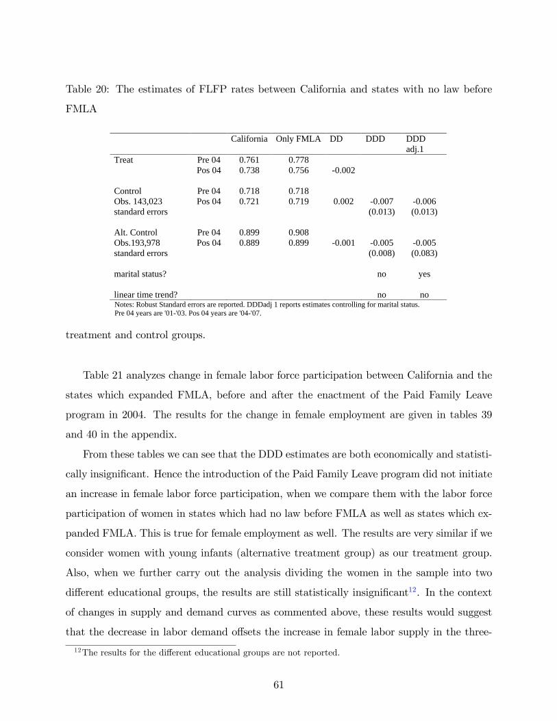
Table 20: The estimates of FLFP rates between California and states with no law before

FMLA

California Only FMLA DD DDD DDDadj.1

Treat Pre 04 0.761 0.778Pos 04 0.738 0.756 0.002

Control Pre 04 0.718 0.718Obs. 143,023 Pos 04 0.721 0.719 0.002 0.007 0.006standard errors (0.013) (0.013)

Alt. Control Pre 04 0.899 0.908Obs.193,978 Pos 04 0.889 0.899 0.001 0.005 0.005standard errors (0.008) (0.083)


linear time trend? no noNotes: Robust Standard errors are reported. DDDadj 1 reports estimates controlling for marital status.Pre 04 years are '01'03. Pos 04 years are '04'07.

treatment and control groups.

Table 21 analyzes change in female labor force participation between California and the

states which expanded FMLA, before and after the enactment of the Paid Family Leave

program in 2004. The results for the change in female employment are given in tables 39

and 40 in the appendix.

From these tables we can see that the DDD estimates are both economically and statisti-

cally insigni�cant. Hence the introduction of the Paid Family Leave program did not initiate

an increase in female labor force participation, when we compare them with the labor force

participation of women in states which had no law before FMLA as well as states which ex-

panded FMLA. This is true for female employment as well. The results are very similar if we

consider women with young infants (alternative treatment group) as our treatment group.

Also, when we further carry out the analysis dividing the women in the sample into two

di¤erent educational groups, the results are still statistically insigni�cant12. In the context

of changes in supply and demand curves as commented above, these results would suggest

that the decrease in labor demand o¤sets the increase in female labor supply in the three-

12The results for the di¤erent educational groups are not reported.

61

Table 21: The estimates of FLFP rates between California and states with which expanded

FMLA

California Exp. FMLA DD DDD DDDadj.1

Treat Pre 04 0.816 0.795Pos 04 0.790 0.769 0.001


Alt. Control Pre 04 0.899 0.899Obs. 74,235 Pos 04 0.889 0.885 0.004 0.008 0.008standard errors (0.115) (0.115)



year period following the implementation of the law, and future years of data are needed

to observe whether the dynamic e¤ect on labor demand �nally raises female employment.

Whenever a new policy is implemented at the state level, people are not immediately aware

of that and hence a certain period of time is required before we can observe the full e¤ects

of such a policy. It should also be noted that California is a state where women having

children can utilize the bene�ts of TDI and FMLA. Hence it might not be possible for Paid

Family Leave program to initiate any further changes to the employment behavior of women,

especially when such a parental leave policy is fully funded by the employees themselves. A

relevant policy recommendation would be to implement such a policy where there could be

equal contributions on part of the employer in addition to that of an employee.

Another possible explanation for the insigni�cant results of the Paid Family Leave pro-

gram in California could be the low take-up rates. According to the statistics reported by

the Employment Development Department of California, the percentage claim of PFL ben-

e�ts was only 1.01% in 2005 and 1.07% in 2006. A study by Rothschild (2007) suggests

the possible reasons for the low take-up rates13. The most important of them is that a

13Jesse Rothschild and Rothschild-Landry Holding Inc.(November 2007)

62

signi�cant portion of California�s workforce is undocumented, due to the high percentage of

immigrant population in California. Also, workers use available sick leave, vacation leave

instead of parental leave and hence no claims are �led. The surveys conducted support

the lack of worker awareness of the available bene�ts provided by the Paid Family Leave

program, which further adds to the ine¤ectiveness of such parental leave policies.

63

3.10 CONCLUSIONS

This paper examines the e¤ect of federal and state parental leave policies on female employ-

ment and labor force participation, analyzing the interaction of these laws when more than

one coexists in the same labor market. First, this study shows that the introduction of the

Family and Medical Leave Act (FMLA) has a signi�cantly positive impact on the employ-

ment of women in those states which had no state law providing parental leave bene�ts than

in those applying the Temporary Disability Insurance (TDI). However, the estimated e¤ects

are quire small. Since the FMLA is granting unpaid leave, one implication of this result is

that the FMLA is not really a¤ecting the employment decisions of women in childbearing

ages since most of them cannot a¤ord to take leave which provides no payment. In general,

the results suggest that the bene�ts associated with the FMLA are not enough to alter the

labor force participation decisions of women who are the potential bene�ciaries of the law

by a substantial amount.

Second, we �nd that the impact of FMLA expansion on female employment and labor

force participation in those states with the most generous expansions (in terms of improving

the bene�ts and relaxing the eligibility criteria of FMLA) is signi�cantly higher than in those

states which did not expand FMLA. In particular, the higher opportunity cost from losing

the job and its consequences on productivity may explain these interesting results.

Finally, in order to get an intuitive understanding of the e¤ects of further increases in the

generosity levels of parental leave policies, we consider the recent enactment of California�s

Paid Family Leave program. Speci�cally, we obtain that there is no impact of the introduc-

tion of this law, which may be due to the short time period of its application. Additionally,

another explanation for the limitation of this policy (neither positive nor negative e¤ect) on

female employment and labor force participation is based on the previous adjustments in

California�s female labor market prior to the passage of this leave program, which reduces

the possibility of further changes in the labor market behavior of both female workers and

their employers. Also, the low take-up rates of the policy plays a crucial role in explaining

its lack of e¤ectiveness.

64

More extensive analysis should be conducted specially in the case of California, in order

to test the hypothesis. In addition, further research can be carried out to examine the impact

of additional increases in the generosity levels of federal and state parental leave policies on

female employment and labor force participation, as well as the interaction of these policies

in the same labor market, as is suggested in this paper.

65

4.0 THE LABOR MARKET EFFECTS OF STATE AND LOCAL

EXPANSIONS OF THE EARNED INCOME TAX CREDIT

4.1 INTRODUCTION

EITC is one of the major federal programs providing assistance to the working poor. It

encourages low-income workers with children to enter and remain in the labor market by

supplementing the earnings of those working for low wages, hence "making work pay". It

is a subsidy on labor earnings which raises the income of recipients without providing a

disincentive to work. The EITC operates as a tax credit that serves to o¤set the payroll

taxes and supplement the wages of low-income workers. The EITC�s popularity relative to

means-tested cash transfers like the Aid to Families with Dependent Children (AFDC) and

TANF programs is due, at least in part, to the perception that the EITC rewards work.

Unique among income-transfer programs for the poor, the EITC conditioned its bene�ts on

earnings. Bene�ts actually increased with family earnings through a portion of the income

distribution, before eventually phasing out at higher incomes. This was just the opposite

of the traditional welfare programs like AFDC and Food Stamps, which provided maximum

bene�ts to families without earnings and then reduced bene�ts at a very high rate as family

earnings increased. As a result, EITC was viewed not as a replacement for traditional

welfare, but as a supplement and as a potential source of cash assistance for the working

poor, a group often overlooked by most poverty programs. The growing popularity of the

federal EITC has led several states and some local governments to implement their own

programs in recent years. The individuals who qualify for the federal EITC are entitled to

receive the state supplement, which is typically a �xed percentage of the federal credit. The

labor market e¤ects of the federal EITC are well known; Eissa and Leibman (1996) found

66

a positive, signi�cant e¤ect and Meyer and Rosenbaum found that as much as 40 percent

of the increase in labor force participation of single women with children between 1980 and

2000 can be attributed to the EITC expansions. The recent literature has also studied some

of the state programs, most of which have focussed on one of the state supplements to the

federal EITC (Ho¤man, 2007;Cancian and Levinson, 2006), with somewhat contradictory

results.

In this paper, we analyze the labor market impacts of the implementation of all the state

and local governments�EITC supplement1 using Current Population Survey data from 1984

to 2006. This is important for three reasons: it serves as a further test for the theory of labor

force participation and labor supply, and contributes to answering the question of whether

EITC payments by state governments a¤ect participation in the same way as the federal

EITC does. Given that at least one study found no signi�cant e¤ects of state EITCs (Cancian

and Levinson, 2006), this question seems to be unresolved at this point. Moreover, since

Cancian and Levinson looked at only one particular state EITC supplement (Wisconsin),

it is worth checking the e¤ect on labor force participation of all the states together, thus

creating additional variation. A second reason is to help access the e¤ectiveness of these state

programs, that is, whether the EITC programs are indeed an e¤ective means of boosting

labor force participation in a state, or are they expensive programs that do not achieve

these goals. To the extent that state governments can allocate the funds to alternative

means (like child care centers) that may also achieve the same desired impact, an estimate

of the labor market e¤ects of state EITC programs will help inform that choice. Hence, the

magnitudes of these e¤ects are key determinants of the gains or losses from the changes in

income redistribution. Finally, while the federal and some of the state EITC programs were

implemented and subsequently expanded at a time of strong female labor force participation

growth, many of these state programs implemented in the last decade coincide with a period

of generally �at female participation rates. If these EITC programs are found to have failed

to a¤ect female participation, this would suggest that future increases in the federal EITC

may well fail to lead any more women to the labor force either. No other study has analyzed1Till date, there are twenty-three states and the District of Columbia, and four local governments which

have implemented the EITC supplement.

67

the labor market impact of all of the state EITC programs that have been implemented till

date. Our focus here will be on married women because they are the demographic group of

workers whose behavior is most susceptible to policy changes.

The remainder of the paper is organized as follows. Section 4.2 explains the eligibil-

ity criteria and the general structure of the EITC and outlines its theoretical impact on

participation and hours worked. Section 4.3 discusses the pervious literature. Section 4.4

describes the data and the identi�cation strategy and presents the empirical results. Section

4.5 concludes.

4.2 STRUCTURE OF FEDERAL AND STATE EITC

The EITC was established in 1975 for low-income working families with children. It is the

largest cash transfer program for lower income families at the federal level. An unusual

feature of the credit is its explicit goal to use the tax system to encourage and support those

who choose to work. It is a tax credit for working families and individuals who earn less than

a speci�ed yearly wage. The EITC provides a wage supplement that is equal to a percentage

of the earnings of the low-income individuals. The credit o¤sets the taxpayer�s income

tax liability or provides a refund in a situation where the family does not owe any taxes.

Since its inception, the EITC has undergone three substantial expansions, the 1986 Tax

Reform Act, the 1990 Omnibus Budget Reconciliation Act (OBRA) and the 1993 OBRA. It

represents the largest single source of funding for low-income working families ($41.5 billion

in 2005, National Center for Children in Poverty) and has been found to produce discernible

increases in employment and reductions in welfare receipt among single parents, as well as

large decreases in poverty (Neumark and Wascher, 2000).

The EITC is refundable, meaning that the Treasury Department pays it out regardless

of whether the taxpayer has any federal income tax liability. A taxpayer�s eligibility for

the earned income tax credit depends on his earned income (or in some cases adjusted

gross income), and the number of qualifying children who meet certain age, relationship and

68

residency tests2. First, the taxpayer must have positive earned income, de�ned as wage and

salary income, business self-employment income, and farm self-employment income. Also,

the taxpayer must have adjusted gross income and earned income below a speci�ed amount

(in 2006, the maximum allowable income for a taxpayer with two or more children was

$36,348; Tax Policy Center). Second, a taxpayer must have a qualifying child, who must

be under age 19 (or 24 if a full-time student) or permanently disabled and residing with

the taxpayer for more than half the year. Prior to 1993, the EITC was only available to

families with children, and even now, the maximum credit available to families with children

is much larger than that available to childless taxpayers. In addition, households with two

or more children are able to claim a higher EITC than households with only one child,

starting in 1991. The amount of the credit to which a taxpayer is entitled depends on the

taxpayer�s earned income, adjusted gross income, and the number of EITC-eligible children

in the household.

There are three regions in the EITC credit schedule. The initial phase-in region trans-

fers an amount which is equal to the subsidy rate times their earnings. In tax year 2006,

the subsidy rate of the EITC was 7.66 percent for taxpayers with no child, 34 percent for

taxpayers with one child and 40 percent for those with two or more children. In the �at

region, the family receives the maximum credit ($412, $2747 and $4536, respectively in tax

year 2006), while in the phase-out region, the credit is phased out at the phase-out rate

7.66 percent for taxpayers with no child, 15.98 percent for those with one child and 21.06

percent for taxpayers with two or more children (2006). Figure 13 shows the EITC (2006)

parameters for single parent families with one child, and two or more children.

Figure 14 shows how the introduction of the EITC shifts the budget constraint of an

otherwise untaxed individual from ADE to ABCDE. With the EITC, an individual faces a

new budget constraint, where each hour chosen produces at least as much after-tax earnings

as it did before the earned income tax credit was introduced. Since the credit is not available

to a taxpayer who does not work, that is, one who has zero earnings, his well-being has not

changed. Hence any taxpayer who preferred to work before will still prefer working and some

2Since 1993, a small amount of the credit is available to taxpayers without children.

69

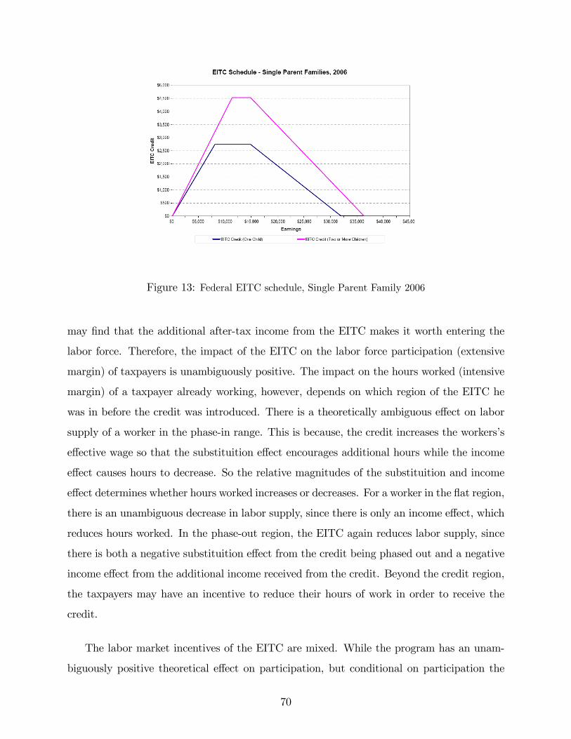
Figure 13: Federal EITC schedule, Single Parent Family 2006

may �nd that the additional after-tax income from the EITC makes it worth entering the

labor force. Therefore, the impact of the EITC on the labor force participation (extensive

margin) of taxpayers is unambiguously positive. The impact on the hours worked (intensive

margin) of a taxpayer already working, however, depends on which region of the EITC he

was in before the credit was introduced. There is a theoretically ambiguous e¤ect on labor

supply of a worker in the phase-in range. This is because, the credit increases the workers�s

e¤ective wage so that the substituition e¤ect encourages additional hours while the income

e¤ect causes hours to decrease. So the relative magnitudes of the substituition and income

e¤ect determines whether hours worked increases or decreases. For a worker in the �at region,

there is an unambiguous decrease in labor supply, since there is only an income e¤ect, which

reduces hours worked. In the phase-out region, the EITC again reduces labor supply, since

there is both a negative substituition e¤ect from the credit being phased out and a negative

income e¤ect from the additional income received from the credit. Beyond the credit region,

the taxpayers may have an incentive to reduce their hours of work in order to receive the

credit.

The labor market incentives of the EITC are mixed. While the program has an unam-

biguously positive theoretical e¤ect on participation, but conditional on participation the

70

E

D

C

B

AfterTaxIncome

Hours workedA

Figure 14: Federal EITC Budget Constraint

program has largely ambiguous e¤ects on the labor supply decisions. There are also reasons

to believe that all of these e¤ects will be a¤ected by complexities and lags in the tax code.

The tax credits for income earned in one year are not received until taxpayers��le their EITC

forms the following year. Also, workers�limited understanding of the EITC may reduce their

responsiveness. For these reasons, the magnitude of the actual e¤ect of the EITC on hours

worked is an empirical question. Table 22 shows the complete federal EITC rate schedule

since 1975.

Over the years, twenty four states and a few cities and counties have adopted their

own EITC programs: Colorado, Delaware, Illinois, Indiana, Iowa, Kansas, Lousiana, Maine,

Maryland, Massachussettes, Michigan, Minnesota, Nebraska, New Jersey, New Mexico, New

York, North Carolina, Oklahoma, Oregon, Rhode Island, Vermont, Virginia, Washington,

Wisconsin and the District of Columbia. These are set as a supplement to the federal

EITC by o¤ering bene�ts equal to some designated proportion of the federal payments3,

typical percentages ranging from 5 percent to 43 percent. Most of these states provide EITC

supplements which are refundable for taxpayers with zero liability4. Wisconsin is the only

state that di¤erentially a¤ects families with three or more children, by providing a more

3Minnesota�s credit for families with children is not structured as a percentage of the federal credit.Depending on income level, the credit for families with children may range from 25 percent to 45 percent ofthe federal credit. Also, Indiana has an EITC that is not based on the federal credit, but applies to familieswith children, where earned income exceeded 80% of total income and total income is below $12,000.

4Delaware,Iowa,Maine and Virginia provide non-refundable EITC supplements.

71

Table 22: Federal EITC rate schedule 1975-2007

72

Table 23: State EITC supplements (1984-2006, percentages of the federal credit)

State CO DC DE IL IN IA KS ME MD MA MN MN MI NE NJ NY OK OR RI VT VA WI WI WIchildren 1+ 0 1+ 1+ 1 2 3+198419851986 22.211987 23.461988 22.96 231989 22.96 25 5 25 751990 5 22.96 28 5 25 751991 6.5 10 10 27.5 28 5 25 751992 6.5 10 10 27.5 28 5 25 751993 6.5 10 10 27.5 28 5 25 751994 6.5 15 15 7.5 27.5 25 4.4 20.8 62.51995 6.5 15 15 10 27.5 25 4 16 501996 6.5 15 15 20 27.5 25 4 14 431997 6.5 10 15 15 20 5 27.5 25 4 14 431998 6.5 10 10 10 25 25 20 5 27 25 4 14 431999 8.5 6.5 10 10 10 25 33 20 5 26.5 25 4 14 432000 10 10 5 6.5 10 5 15 10 25 33 10 22.5 5 26 32 4 14 432001 10 25 5 6.5 10 5 16 15 25 33 15 25 5 25.5 32 4 14 432002 10 25 5 6.5 15 5 16 15 25 33 17.5 27.5 5 5 25 32 4 14 432003 10 25 5 6 6.5 15 4.92 20 15 25 33 20 30 5 5 25 32 4 14 432004 10 25 5 6 6.5 15 4.92 20 15 25 33 20 30 5 5 25 32 20 4 14 432005 10 25 20 5 6 6.5 15 4.92 20 15 25 33 20 30 5 5 25 32 20 4 14 432006 10 35 20 5 6 6.5 15 5 20 15 25 33 10 8 20 30 5 5 25 32 20 4 14 43Refundable? Y Y N Y Y N Y N Y Y Y Y Y Y Y Y Y Y Y Y N Y Y Y

Notes: children is left blank if the state supplement applies irrespective of the taxpayer's number of children. Maryland also had a nonrefundable EITC of 50 percent for families with children from 19872006.

generous state EITC supplement for these families. State EITCs are set as a supplement to

those who already qualify for the federal EITC, and the level is assigned to equal a given

percentage of the federal payment. So the e¤ective EITC rate � in a given state is such

that, � =(federal EITC rate) * (1+state EITC supplement). For example, a single parent

with one child who earned $7500 in 2007 would be in the phase-in range of income, and is

eligible for a federal EITC payment of $2550. If he lives in Rhode Island, which provides a

25 percent state EITC supplement, his e¤ective phase-in rate would be (34*1.25) and hence

would receive an additional $637.50 from the state government. Therefore, a 25 percent

EITC supplement is equivalent to a 25 percent expansion of the federal EITC for residents

of that particular state.

The details on state supplements are provided in table 23. While most of the states

introduced EITC supplements in the mid to late 1990s, a considerable number of them

implemented their state EITCs in the last few years.

The �rst state to enact an EITC supplement was Rhode Island in 1986. Initially, it

o¤ered a non-refundable EITC until 2002, and henceafter a small portion is made refundable.

73

There are four other states, Delaware, Iowa, Maine, and Virginia which o¤er credits that are

nonrefundable. Such a credit is available only to the extent that it o¤sets a family�s income

tax. A nonrefundable EITC can provide substantial tax relief to families with state income

tax liability, but it provides no bene�ts to working families that have income too low to owe

any income taxes. Over the years, many states have increased their credits several times

since �rst passing them and some states which had non-refundable state EITC supplements

have made them refundable.

State EITCs are �nanced in whole or in part from funds available in a state�s general fund

that is, the same funding sources that are typically used for other types of tax cuts. When

an EITC is used to o¤set the e¤ects of a regressive tax increase such as a sales tax increase,

a part of the proceeds of the revenue increase may be set aside for the EITC. Current federal

regulations also o¤er the opportunity to �nance a portion of the cost of a refundable credit

from a state�s share of the federal Temporary Assistance to Needy Families (TANF) block

grant, but most states have very limited availability of such funds because the value of the

TANF block grant has eroded over time and also states face costly new work requirements

under the federal budget law5. There are four local governments who have also implemented

their EITC programs in recent years. The �rst was Montgomery county in Maryland, which

enacted the local EITC in 1999, set at 20 percent of the federal payment. The second local

government and �rst city to pass its own EITC was Denver in 2002, a program which was

discontinued in 2004 due to insu¢ cient TANF funds. This was followed by New York City

in 2004, which enacted a refundable EITC with the tax credit set at 5 percent of the federal

credit. Finally, San Francisco launched a city-level, refundable EITC in 2005, which was

initially set at 10 percent and increased to 16 percent in 2006.

4.3 PREVIOUS RESEARCH

Most of the previous studies of the labor supply e¤ects of the EITC have focussed on the

three major discrete policy changes in the federal EITC as the main source of variation. Eissa

5Colorado�s EITC was funded by a state surplus under the Taxpayer Bill of Rights (TABOR). It wassuspended in 2002 when surplus funds ran out.

74

and Liebman (1996) use a di¤erence-in-di¤erences approach to analyze the 1986 expansion

of the EITC and found that the labor force participation rates of single women with children

increased signi�cantly compared to childless single women, whereas they found no change

in the relative hours worked by single women with children who were already in the labor

force. Meyer and Rosenbaum (2001) also determines the e¤ect of EITC on the labor force

participation of single women, by considering the impact of other tax and welfare changes

like AFDC, Medicaid, Food Stamps and their implicit tax rates and earnings disregards, as

well as AFDC waivers instituting time limits or work requirements, with their major source

of variation being di¤erences in incentives faced by single women with and without children.

They found that the EITC played a dominant role in increasing the labor force participation

rates of single mothers. Grogger (2003) looks at the e¤ect of the federal EITC expansions

and �nds it to be the single most important policy measure for explaining the decrease in

welfare and the rise in work and earnings among female-headed families.

Eissa and Hoynes (2004) look at the e¤ect of federal EITC expansions from 1984-1996

on the labor supply of married couples, to �nd that increasing the EITC credit had a small

positive impact on the labor supply of the husband, but a larger negative e¤ect on the wives�

labor supply, due to the marginal rate in the phase-out range. Hence, their �nding suggests

that EITC expansions reduced total family labor supply, and that the EITC is e¤ectively

subsidizing married mothers to stay at home. This is consistent with the earlier �ndings by

Dickert et al (1995) and Ellwood (2000), who, using structural and quasi-experimental meth-

ods respectively, conclude that EITC does reduce the labor force participation of married

women with children.

Neumark and Wascher (2001) exploit state level variation in EITC to see its e¤ect on

poor families. In order to get around the problem of endogeneity, they control for the

state unemployment rate and welfare generosity. Analyzing a period from 1985-1994, when

seven states implemented EITC supplements, they conclude that an increase in a state�s

EITC supplement helps families rise above poverty-level earnings by inducing labor market

entry in families that initially did not have an adult in the workforce. Leigh (2005) also

75

uses variation in the state EITC supplements to examine the e¤ect of the EITC on pretax

wages. Using data from the Current Population Survey Merged Outgoing Rotation Group

for the period 1984-2002, he uses variation across states in the presence and generosity of

state EITC add-ons to create cross-sectional variation in the average tax rate faced by women

with children. He �nds a very strong negative e¤ect of the credit on wages especially for low-

skilled workers, implying very little bene�t of the credit for its nominal recipients. However,

he �nds no e¤ect of the credit on the wages of college graduates, and although workers

with children receive a more generous tax credit than childless workers, the hourly wages of

both groups are similarly a¤ected by an increase in the generosity of the EITC. Leigh also

uses an instrumental variable startegy by constructing a simulated instrument for the EITC

parameters in an employee�s labor market, to �nd that wages respond to variation in the

fraction of eligible employees and the average EITC rate, but do not respond to changes in

the marginal EITC rate.

Our work goes along the lines of Leigh, but using additional variation with more states

o¤ering their own EITC programs in the recent years6, and focussing on the labor force

participation rates and week worked as outcomes, which he did not analyze speci�cally.

Also, we use a richer set of regressors in di¤erent speci�cations to measure the presence and

magnitude of the EITC o¤ered by both the state and the local governments. This includes

using the maximum credit received in some speci�cations, the phase-in rate in others, or

whether the state is o¤ering a sizeable enough credit in some other speci�cations. We focus

here on married women in order to investigate whether added EITC payments from the

state and local governments contribute to increasing the female labor force participation,

above and beyond the positive impact that the federal EITC expansions have been shown to

have on the national female participation trends. We do the analysis separately for married

women with one child, married women with 2 children, and married women with 3 or more

children so that we can control for the compositional e¤ects that could arise because the

fertility rates have not been constant over time.

6Eight more states enacted the state EITC supplement since Leigh�s analysis in 2002.

76

More recently, Cancian and Levinson (2006) have examined the e¤ect of the EITC on

labor supply comparing outcomes in Wisconsin, which supplements the federal EITC for

families with three children di¤erently, to outcomes in the states which do not supplement

the federal EITC. They �nd no e¤ect of the EITC on labor force participation, which is

somewhat surprising given the �ndings of previous research. Ho¤man (2007) looks at the

e¤ects of a non-refundable state EITC supplement considering the example of Delaware

and �nds atypical distributional impacts of this policy. Speci�cally, he �nds that the lower

income half of the EITC recipient population is ineligible for the Delaware non-refundable

EITC. Married couples and both single-parent and two-parent families with less than two

children often lose eligibility and substantial portions of the bene�ts. Thus treating EITC as

a tax relief, as in a non-refundable EITC, rather than income support operating through the

tax system, eliminates the advantages of an EITC program. This �nding encourages us to

use additional variation by grouping together states with and without non-refundable EITC

programs and see how female labor force participation rates vary between them.

4.4 DATA AND MAIN RESULTS

4.4.1 Data Sources and Summary Statistics

The data we use come from the Current Population Survey Merged Outgoing Rotation

Group, and the March CPS for the period 1984-2006. The CPS is the monthly household

survey conducted by the Bureau of Labor Statistics to measure labor force participation

and employment of about 60,000 households per month. In the Outgoing Rotation Group

surveys, every household that enters the CPS is interviewed each month for 4 months, then

ignored for 8 months, then interviewed again for 4 more months. The usual weekly earning

questions are asked only to households in their 4th and 8th interview. New households enter

each month, so one fourth of the households are in an outgoing rotation each month. The

March CPS is an annual demographic �le of between 50,000 and 60,000 households per year,

and includes detailed labor market and income information.

77

Our primary sample includes women of prime working age (between 18 and 55 years).

In order to determine the EITC eligibility, we consider any member of the household who is

under the age of 19 years (or under 24 years if a full-time student) to be a dependent child

for tax purposes7. There are potential limitations with the MORG data. From January 1994

until October 1999, the basic monthly CPS (from which the MORG sample is drawn) did

not ask respondents for their number of children. For this period, therefore, The MORG

records for January 1994 to October 1999 were merged with the March CPS records for the

same years, resulting in a successful merge rate of around 75 percent. We exclude women

who are self-employed, ill or disabled, or in school full time during the previous year. We

also exclude women with positive earned income but zero hours of work. The resulting size

of the primary sample, after pooling all 22 years is 2,117,003 observations.

Table 24 presents summary statistics for the primary sample separately by family size

and marital status. The demographic variables used in the analysis include age, race, mar-

tital status, education, number of children, labor force participation rates and the state

unemployment rate. Summary statistics show that married women are older and have about

the same education levels as the single women, and this is true for women both with and

without children. Of interest is the pattern of labor force participation. The participation

rate is lower for married women compared to single women, but declines more sharply with

the �rst child in case of married women.

Table 25 presents the labor force participation rates of women separately by marital

status and the number of children, between states with and without state EITC supplements,

as well as for all of the states together. As mentioned above, the labor force participation

rates are lower for married women with children, compared to single women both with and

without children. However, the labor force participation rates for married women (both with

and without children) are higher in the states which supplement the federal EITC, compared

to those states which do no o¤er any such state program. This is further evidenced in Figure

7Due to data limitations, we omit some criteria for determination of eligible children- we assume that theresidency requirement is met.

78

Table 24: Labor Force participation rates by demographic groups

Single Married

No child 1 child 2+ children No child 1 child 2+ children

Labor Force(all states)

0.89(0.30)

0.86(0.34)

0.86(0.34)

0.88(0.31)

0.83(0.37)

0.82(0.38)

Labor Force(EITC states)

0.89(0.30)

0.86(0.34)

0 .86(0.33)

0.89(0.30)

0.84(0.36)

0.83(0.37)

Labor Force(nonEITCstates)

0 .89(0.31)

0.86(0.34)

0.86(0.34)

0.87(0.32)

0.83(0.37)

0.81(0.38)

Observations(all states)

211048 131704 555046 420248 253610 544831

Notes: Standard deviations are in parentheses.The data are from survey years 19842006 of the Merged Ongoing Rotation Groups and March CPS. Thesample contains women between the ages of 18 and 55 years. We exclude women who are selfemployed.LFP: Labor force participation, which equals 1 if employed or unemployed, and zero if the individual is notin the labor force. Education: 1 refers to less than high school, 2 refer to high school degree, 3 refer to somecollege, 4 refer to college degree and 5 refer to advanced degree.

3, which shows the labor force participation rates of single and married women between

1986-2006, in a four-year period interval.

79


Single MarriedNo child 1 child 2+ children No child 1 child 2+ children

LFP 0.89(0.31)

0.86(0.34)

0.86(0.34)

0.88(0.31)

0.83(0.37)

0.82(0.38)

Age 32.56(11.73)

31.54(10.26)

32.07(10.67)

41.04(10.49)

36.64(8.86)

36.62(7.67)

Education 2.72(1.00)

2.53(0.95)

2.75(1.06)

2.80(1.08)

2.77(1.08)

2.79(1.08)

Children 0(0)

1(0)

2.86(0.34)

0(0)

1(0)

2.86(0.34)

Black 0.16(0.37)

0.21(0.40)

0.15(0.36)

0.06(0.24)

0.07(0.26)

0.07(0.26)

Hispanic 0.06(0.25)

0.09(0.28)

0.08(0.28)

0.05(0.22)

0.07(0.26)

0.09(0.29)

Other 0.04(0.20)

0.04(0.19)

0.05(0.21)

0.04(0.20)

0.05(0.21)

0.05(0.22)

Observations 211048 131704 555046 420248 253610 544831

Notes: Standard deviations are in parentheses.The data are from survey years 19842006 of the Merged Ongoing Rotation Groups and March CPS. Thesample contains women between the ages of 18 and 55 years. We exclude women who are selfemployed.LFP: Labor force participation, which equals 1 if employed or unemployed, and zero if the individual is notin the labor force. Education: 1 refers to less than high school, 2 refer to high school degree, 3 refer to somecollege, 4 refer to college degree and 5 refer to advanced degree.

80

4.5 CONCLUSIONS

A key goal of the EITC is to redistribute income to working poor families. In practice, the

EITC is an important income source for many vulnerable families, including many single-

mother families making the transition from welfare to work under recent welfare reforms. To

many analysts, the EITC is preferable to other programs aimed at low-income families be-

cause it is tied to work. For families with a single worker earning low wages, the more hours

worked, the greater their EITC. Thus, given its basic structure, the EITC unambiguously

targets resources to low-income working families.

A less certain advantage of the EITC is its ability to increase labor supply. We analyze

the labor market impacts of the implementation of all the state and local governments�

EITC supplement using Current Population Survey data from 1984 to 2006.to examine the

labor market consequences of the EITC. We �nd that the labor force participation rates

for married women with children are higher in states which supplement the federal EITC

program, compared to single women both with and without children in the states which do

not provide any such supplement.

81

5.0 APPENDIX

82

Table 26: 2SLS Estimates of the E¤ect of Phone measures on Store closures

2SLS(1)

2SLS (2)

Phone 15.073[26.357](37.467)

3.105[2.269](2.140)

Controls for state fixed effects?Yes No

Observations 245 245Notes: Standard errors in brackets are adjusted for unknown forms of heteroskadasticity and serial correlation. Standard errorsin parenthesis are robust. The store closures data are from Almighty Retails for the years 2003 and 2007. All the regressionsare weighted by population and include yearfixed effects. Other controls include population, mean education, age, and theproportion of female, white, black and Hispanic for each stateyear. Column (2) reports results for regressions withoutincluding the statefixed effects.

Table 27: Store closures based on the type of store

2003 2004 2005 2006 2007

Average number of IndieStore closings

1.755(0.31)

6.89(1.18)

3.26(0.72)

5.69(0.91)

6.81(1.53)

Average number of OthersStore closings

1.53(0.29)

5(0.85)

4.06(0.70)

10.45(1.86)

4.51(0.77)

Average number of ChainStore closings

2.14(0.33)

4.23(0.64)

4.25(0.65)

10.19(1.75)

3.89(0.55)

Average number of Big BoxStore closings

1(0.72)

1.84(0.32)

2.07(0.42)

1(0.32)

2.35(0.51)

Average number of OtherStore closings

0.22(0.08)

1(0.19)

0.43(0.12)

0.78(0.23)

0.78(0.21)

Total number ofStore closings

160 593 363 801 557

Notes: Standard errors are in parenthesis. The abbreviations for the states pertain to the State Fips Code classified by theBureau of Labor Statistics. The store closings data are from Almighty Research for the years 2003 through 2007.

83

Table 28: Summary Statistics: Store closures based on the type of store between states

Notes: Standard errors are in parenthesis. The states are classified as urban or rural depending on the percentage of people in eachstate having a telephone connection in the 1960 Census. The internet penetration data are from CPS Computer Use andSupplements for the years 19971998, 20002001, 2003 and 2007. The store closings data are from Almighty Research for theyears 2003 and 2007.

Overall VFL States NonVFLStates

UrbanStates

RuralStates

Indie StoreClosures

4.89(0.47)

8.08(0.97)

2.94(0.37)

5.31(0.68)

4.33(0.54)

Others StoreClosures

5.11(0.49)

8.62(1.06)

2.97(0.35)

5.59(0.69)

4.52(0.63)

Chain StoreClosures

3.98(0.42)

6.6(0.91)

2.38(0.31)

4.39(0.61)

3.46(0.51)

Big box StoreClosures

0.49(0.07)

0.94(0.18)

0.23(0.05)

0.47(0.08)

0.55(0.17)

Other StoreClosures

0.64(0.08)

0.82(0.006)

0.84(0.01)

0.73(0.12)

0.51(0.09)

Number ofobservations

245 95 155 155 85

Table 29: OLS Estimates of E¤ect of State Internet Penetration Rates on Store closures

based on the type of store

Indie

(1)

ChainStores

(2)

Big box

(3)

Other

(4)

Indie

(5)

ChainStores

(6)

Bigbox

(7)

Other

(8)

Internetpenetration

rates

1.389***[0.89]

(1.258)

0.104[0.256](0.364)

0.261[0.214](0 .304)

0.245[0.175](0.25)

1.041*(0.209)

0.139*(0.052)

0.228*(0.037)

0.238*(0.028)

Controls forstate fixed

effects?Yes Yes Yes Yes Yes Yes Yes Yes

Observations 98 98 98 98 98 98 98 98Notes: Standard errors in brackets are adjusted for unknown forms of heteroskadasticity and serial correlation.Standard errors in parenthesis are robust. The store closures data are from Almighty Retails for the years 2003 and2007. All the regressions are weighted by population and include yearfixed effects. ***denotes significance at the1% level. *denotes significance at the 10% level. In columns (5) through (8) a heteroskedastic error structure with nocrosssectional correlation is assumed. Other controls include population, mean education, age, and the proportion offemale, white, black and Hispanic for each stateyear.

84

Table 30: Reduced-form Estimates of the E¤ect of VFL Adoption on Store closures based

on the type of store

Indie

(1)

ChainStores

(2)

Big box

(3)

Other

(4)

Indie

(5)

ChainStores

(6)

Big box

(7)

Other

(8)

VFL 4.516**[2.26]

(2.522)

9.044[5.74](6.61)

0.106[0.447](0.426)

0.941[0.769](0.977)

2.797*(0.89)

4.241*(1.21)

0.192(0.24)

0.372*(0.18)

Controls forstate fixed

effects?Yes Yes Yes Yes Yes Yes Yes Yes

Observation 98 98 98 98 98 98 98 98Notes: Standard errors in brackets are adjusted for unknown forms of heteroskadasticity and serial correlation. Standarderrors in parenthesis are robust. The store closures data are from Almighty Retails for the years 2003 through 2007. Allthe regressions are weighted by population and include yearfixed effects. Columns (1) through (4) reports results forregressions where standard errors are adjusted to cluster at the state level. In columns (5) through (8) a heteroskedasticerror structure with no crosssectional correlation is assumed. Other controls include population, mean education, age,and the proportion of female, white, black and Hispanic for each stateyear.

Table 31: First Stage Estimates of the E¤ect of VFL Adoption on State Internet Penetration

Rates: Falsi�cation test

Internet penetrationrates(1)

Internet penetrationrates (2)



VFL 0.398(0.928)[0.634]

0.337(1.447)

0.316(0.721)[0.854]

0.306(1.893)

Controls for state fixedeffects? Yes Yes No No

Observations 276 276 276 276Notes: The Internet penetration data are from CPS Computer Use and Supplements for the years 1997, 1998, 2000, 2001, 2003 and 2007. All the regressions areweighted by population and include year fixed effects. Other controls include population, mean education, age, and the proportion of female, white, black andHispanic for each stateyear. Column (1) shows results when the standard errors are clustered at the state level, in brackets and when standard errors are adjustedfor unknown forms of heteroskadasticity and serial correlation, in parenthesis. Column (2) reports results from GLS estimation. Columns (3) and (4) reportsresults for regressions without including the statefixed effects.

85

Table 32: Reduced Form Estimates of the E¤ect of VFL Adoption on State Internet Pene-

tration Rates: Falsi�cation test

Store closures(1)

Store closures (2)

Store closures (3)

Store closures (4)

Panel A VFL 13.469(11.842)[9.977]

7.245(6.268)

5.623***

(1.995)[2.938]

8.384***

(1.266)

Panel B VFL 6.572(4.712)[6.436]

2.202(1.620)

8.628***

(3.029)[3.728]

8.876***

(1.436)

Controls for state fixedeffects? Yes Yes No No

Observations 218 218 218 218Notes: Standard errors are in parenthesis. The store closures data are from Almighty Retails for the years 2003 through 2007. Panel A denotes results pretendingVFL was adopted in 2003. Panel B reports results pretending VFL was adopted two years prior to the actual period when it was adopted. ***denotes significanceat the 1% level. All the regressions are weighted by population and include year fixed effects. Other controls include population, mean education, age, and theproportion of female, white, black and Hispanic for each stateyear. Column (1) shows results when the standard errors are clustered at the state level, in bracketsand when standard errors are adjusted for unknown forms of heteroskadasticity and serial correlation, in parenthesis. Column (2) reports results from GLSestimation. Columns (3) and (4) reports results for regressions without including the statefixed effects.

Table 33: Estimated Probit Models for the Adoption of Video Franchise Laws

Notes: Robust standard errors are in parenthesis. Per capita state GDP and household income are scaled bythousand. The state business ranking data are from Tax Foundation's State Business Tax Climate Index;State GDP, Household income and unemployment rates data are from Bureau of Economic Analysis.***denotes significance at the 1% level. Other controls include population, mean education, age, and theproportion of female, white, black and Hispanic for each stateyear.

Pr(VFL)(1)

Pr(VFL)(2)

Pr(VFL)(3)

Pr(VFL)(4)

Pr(VFL)(5)

Business ranking 0.0006(0.0009)

0.001(0.001)

Per Capita State GDP 0.001(0.002)

0.0007(0.002)

State unemploymentrates

0.046***(0.015)

0.043***(0.014)

Household income 0.001(0.005)

0.002(0.004)

Observations 245 245 245 245 245

86

Table 34: Regression of VFL adoption on state characteristics

Notes: Robust standard errors are in parenthesis. Per capita state GDP and household income are scaled bythousand. The state business ranking data are from Tax Foundation's State Business Tax Climate Index;State GDP, Household income and unemployment rates data are from Bureau of Economic Analysis.***denotes significance at the 1% level. Other controls include population, mean education, age, and theproportion of female, white, black and Hispanic for each stateyear. All regressions include the statefixedeffects and yearfixed effects.

VFL(1)

VFL(2)

VFL(3)

VFL(4)

VFL(5)

Business ranking 0.002(0.002)

0.001(0.002)

Per Capita StateGDP

0.010(0.014)

0.012(0.013)

Stateunemployment rates

0.062***(0.031)

0.063***(0.030)

Household income 0.011(0.014)

0.012(0.015)

Observations 245 245 245 245 245

Table 35: Reduced-form regression including additional covariates

Store closures (1)

Store closures (2)

VFL 8.344***(1.739)

7.490***(1.735)

Business ranking 0.102***(0.041)

Per Capita State GDP 0.512**(0.293)

State unemployment0.384

(0.915)

Controls for state fixed effects? Yes Yes

Observations 245 245Notes: Results are from FGLS estimation. The store closures data are from Almighty Retails for the years2003 through 2007. ***denotes significance at the 1% level. Per capita state GDP and household income are scaledby thousand. All the regressions are weighted by population. Other controls include population, mean education, age,and the proportion of female, white, black and Hispanic for each stateyear. Column (1) shows results without includingany additional controls. Column (2) shows results including state GDP, business ranking and megastores. All regressionsinclude yearfixed and statefixed effects.

87

Table 36: Falsi�cation: The estimates of Female Employment between states with no law

and states with TDI before FMLA assuming FMLA adopted in 1981

NoLaw(1) TDI(2) DD(3) DDD(4) DDD.adj1 DDD.adj2 DDD.adj3

Treat Pre'81 0.686 0.680Pos'81 0.684 0.674 0.005

Control Pre'81 0.539 0.543Obs.675,816 Pos'81 0.552 0.568 0.012 0.015 0.017 0.016 0.017standarderrors

(0.012) (0.011) (0.012) (0.012)

Alt. Control Pre'81 0.924 0.912Obs.963,726 Pos'81 0.919 0.908 0.001 0.005 0.006 0.005 0.006standarderrors

(0.007) (0.007) (0.007) (0.007)

maritalstatus?

no yes no yes

linear timetrend?

no no yes yes

Notes: The Pre '81 period consists of the years 1978 1980. Pos’ 81 period consists of 19811984. RobustStandard errors are reported.

Table 37: The estimates of Female Labor Force Participation rates between Connecticut and

states with no law before FMLA

Connecticut OnlyFMLA

DD DDD DDDadj.1

Alt. Treat Pre 97 0.582 0.595Pos 97 0.684 0.588 0.108





88

Table 38: The estimates of FLFP rates between Vermont and states with no law before

FMLA

Vermont OnlyFMLA

DD DDD DDDadj.1

Alt. Treat Pre 98 0.575 0.599Pos 98 0.666 0.587 0.104


Alt. Control Pre 98 0.899 0.912Obs.54,698 Pos 98 0.915 0.915 0.013 0.091 0.088standard errors (0.076) (0.076)



Table 39: The estimates of Female Employment between California and states with no law

before FMLA

California Only FMLA DD DDD DDDadj.1

Treat Pre04 0.787 0.807Pos 04 0.764 0.783 0.001





89

Table 40: The estimates of Female Employment between California and states which ex-

panded FMLA

California Exp. FMLA DD DDD DDDadj.1

Treat Pre 04 0.843 0.831Pos 04 0.819 0.814 0.006





90

Table 41: Weekly Bene�t amount and Duration of Bene�ts in TDI states

State Status Weekly Benefit Amount DurationCA All

workers$50$336 based on schedule of highquarter wage

6 – 52 weeks, $300 $14,472, computed aslesser of 52 x weekly benefit amount or thetotal of base period wages.

Duration separate from UIHI Employed

workers$14$357. For an average weeklywage of less than $26, weekly benefitamount is the average weekly wageup to a maximum of $14. If averageweekly wage is $26 or more, weeklybenefit amount is 58% of averageweekly wage with a maximum of 662/3 percent of average weekly wage.

Uniform 26 weeks in benefit year

Unemployed worker

Same as UI Balance of weeks claimant would have beeneligible for benefits in his UI benefit yearbut not more than 26 weeks.

NJ Employedworkers

$68$470 (based on schedule ofaverage weekly wage). Averageweekly wage determined by dividingwage from 1 employer during baseweeks in weeks. If less than averageusing all employment during last 8weeks, use earnings from allemployers.

Computed as lesser of 26 x weekly benefitamount or 1/3 base period wages. Limitapplies to benefits in any 12 consecutivemonth periods. Duration separate from UIand from benefits as an unemployed disableworker.

Unemployed worker

$61$475 (based on schedule ofaverage weekly wage). Averageweekly wage determined by dividingwage from 1 employer in all baseweeks by numbers of base weeks. Ifnot 20 base weeks with any 1employer, average base weeks withall employers.

1526 weeks, $1,095$9,464 computed as ¾weeks, but not more than 26 x weeklybenefit amount. Duration under UI anddisability during employment limited to150% of duration for either programseparately.

NY Allworkers

$20 $170 on basis of onehalf averageweekly wage in last 8 weeks, or portionthereof, in covered employment prior tocommencement of disability.If average is less than $20, weeklybenefit is average wage.

Uniform potential 26 weeks in any 52consecutive weeks or for any single period ofdisability, $520 (or less if weekly benefit amountis less than $20 $4,420). Duration separatefrom UI.

RI Allworkers

$53 $588 (4.62% of high quarter wagesup to 85% of state’s average weeklywage in preceding calendar year, plus thegreater of $10 or 7% of the individual’sbenefit rate for each dependent up to 5dependents).

12 30 weeks $636 $17,640 computed as 36%of total base period wages plus dependentallowance if any.

91

Table 42: Classi�cation of the States

States TDI FMLAonly

Expa.FMLA

No

weeksNo

HoursNo Workers Others

AlabamaAlaskaArizonaArkansasCaliforniaColoradoConnecticutDelawareFloridaGeorgiaHawaiiIdahoIllinoisIndianaIowaKansasKentuckyLouisianaMaineMarylandMassachusettsMichiganMinnesotaMississippiMissouriMontanaNebraskaNevadaNew HampshireNew JerseyNew MexicoNew YorkNorth CarolinaNorth DakotaOhioOklahomaOregonPennsylvaniaRhode IslandSouth CarolinaSouth DakotaTennesseeTexasUtahVermontVirginiaWashingtonWest VirginiaWisconsinWyomingDistrict ofColumbia

X

X

X

X

X

ü

ü

ü

ü

ü

ü

ü

üü

üü

ü

ü

üü

üü

ü

§

§

§

§

§

§

§

§

§

§

§

§

16

12

12

12

1000

1250

1250

75 or more

15 or more

21 or more

25 or more

10 or more

accrued sick leave

accrued sick leave

accrued sick leave

accrued sick leave

92

BIBLIOGRAPHY

[1] A Workable Balance: Report to Congress on Family and Medical Leave Policies. (1996).U.S. Commission on Family and Medical Leave. Cornell University.

[2] Acemoglu,D. and Angrist,J. (2001). "Consequences of Employment Protection:TheCase of the Americans with Disabilities Act". Journal of Political Economy. 109(5), 915-957.

[3] An RIAA Report Prepared By the Communications and Strategic Analysis DepartmentOf the Recording Industry Association of America, The CD: A Better Value Than Ever,August 2007.

[4] Baker, M, and Milligan, K. (2008). How Does Job-Protected Maternity LeaveA¤ect Mothers�Employment?, Journal of Labor Economics, 26(4), 655-691

[5] Baughman,R. and Dickert-Colin,S. (2006)."The Earned Income Tax Credit andFertility". Working Paper.

[6] Basker, E. (2006), "When Good Instruments Go Bad:A Reply to Neumark, Zhangand Ciccarella". Working Paper, University of Missouri.

[7] Bertrand, M., Duflo, E. and Mullainathan, S. (2004), "How Much ShouldWe Trust Di¤erence-in-Di¤erences Estimates". Quarterly Journal of Economics, 119(1),249-275.

[8] Betsey, S. (2006), "The Impact of the Internet on Worker Flows". Working Paper.

[9] Breslow, S., Earle, A., Heymann, J. , Kuehnhoff, A. and Simmons, S. (2004)."The Work, Family, and Equity Index: Where Does the United States Stand Globally?"Boston, MA: Harvard University, The Project on Global Working Families.

[10] Bureau of Economic Analysis. Regional Economic Accounts.

[11] Burgess, S., Gregg, P., Propper, C., Washbrook, E. and the ALSPACStudy Team. (2002). "Maternity Rights and Mothers�Return to Work". CMPOWork-ing paper series No 02/055.

93

[12] Cancian,M. and Levinson,A. (2006). "Labor Supply E¤ects Of The Earned IncomeTax Credit: Evidence From Wisconsin�s Supplemental Bene�t For Families With ThreeChildren". Working Paper 11454. NBER

[13] Cantor, D., Kerwin, J., Levin, K., Heltmes, S,. and Becher, D. (1995). "TheImpact of the Family and Medical Leave Act: A survey of employer". Rockville, MD:Westat.

[14] Cantor, D., Waldfogel, J ,Kerwin J ,McKinley, M , Levin, K.,Rauch.J ,Hagerty T and Kadula M.S. (2001). "Balancing the Needs of Families and Em-ployers:Family and Medical Leave Surveys, 2000 Update".

[15] Card, D. (1990). "The Impact of the Mariel Boatlift on the Miami Labor Market".Industrial and Labor Relations Review, 43( 2), 245-257.

[16] Center on Budget and Policy Priorities, The 2007 Earned Income Tax Credit OutreachKit

[17] Commission on Family and Medical Leave (1996). Workable Balance: Report toCongress on Family and Medical Leave Policies. Washington, D.C: U.S. Departmentof Labor.

[18] Curtin, S. and Hofferth, S. (2006). "Parental Leave Statues and Maternal Returnto Work After Childbirth in the United States". Work and Occupations, 33(1), 73-105.

[19] Dickert,S,.Houser,S. and Scholtz,J. (1995). "The Earned Income Tax Credit andTransfer program: A Study of Labor market and Program Participation". Tax Policyand the Economy,.Vol 9 James Poterba, editor. Cambridge: MIT press, 1-50.

[20] Edison Media Research (2003). The National Record Buyers Study III. Sponsored byRadio & Records. <http://www.edisonresearch.com>

[21] Eissa, N. and Leibman, J. (1996). "Labor Supply Response to the Earned IncomeTax Credit". The Quarterly Journal of Economics, 111(2), 605-637.

[22] Eissa,N. and Hoynes,H.W. (2004). "Taxes and the labor market participation ofmarried:couples: the earned income tax credit". Journal of Public Economics, 88, 1931-1958.

[23] Ellwood,D. (2000). "The Impact of the Earned Income Tax Credit and Social PolicyReforms on Work, Marriage, and Living Arrangements". National Tax Journal, LIII(4,Part2), 1063-1105.

[24] Employment Bulletin. (2005). Rhode Island Department of Labor and Training, October2005.

[25] Employment Development Department, California Government. Quick Statistics.

94

[26] Fact Sheet, Institute For Women�s Policy Research, August 2007 (IWPR#A131)

[27] Fader, Peter. Expert Report, A&M Records, Inc v. Napster, Inc. 114 F Supp. 2d896, 2000.

[28] Family Caregiver Alliance. The Labor Project forWorking Families and California LaborFederation. National Center on Caregiving.

[29] Fisher, K. Accounting for the big plunge in "music sales": the digital singles e¤ectArticle:Ars Technica, 2007.

[30] Forrester (2002). �Downloads Save the Music Business.�<http://www.forrester.com>

[31] GAO. Report to Congressional Committees (2006). Broadband Deployment is Extensivethroughout the United States, but it is di¢ cult to Access the Extent of Deployment Gapsin Rural Areas.

[32] Grant, J., Hatcher, T. and Patel, N. (2005) "Expecting Better: A State-by-StateAnalysis of Parental Leave Programs". National Partnership for Women and Families.

[33] Grogger,J. (2003). "The E¤ects of Time Limits, the EITC and Other Policy Changeson Welfare use, Work, and Income among Female-headed Families". The Review ofEconomics and Statistic, 85(2), 394-408.

[34] Han, W and Waldfogel, J. (2003). "Parental Leave: The Impact of Recent Legis-lation on Parent�s Leave Taking". Demography, 40(1), 191-200.

[35] Hiatt, B and Serpick, E. The Record Industry�s Decline (June, 2007).<http://www.rollingstone.com/news/story/15137581/the_record_industrys_decline>

[36] Hofferth, S. and Curtin, S. (2006). "Parental Leave Statutes and Maternal Returnto Work After Childbirth in the United States". Work and Occupations, 33(1), 73-105

[37] Hoffman,S. (2007). "A Good Policy Gone Bad:The Strange Case of the Non Refund-able State EITC," Working Paper Series, University of Delaware.

[38] Horrigan, J. (2007), Home Broadband Adoption 2007. Pew Internet and AmericanLife Project.

[39] Hui, K and Png, I. (2003), "Piracy and the Legitimate Demand for Recorded Music".Contributions to Economic Analysis and Policy, 2(1), 1-22.

[40] IFPI (2002). Recording Industry in Numbers 2001. International Federation of Phono-graphic Industry.

[41] Institute for Women�s Policy Research (1993). Research in Brief: What is TemporaryDisability Insurance? Washington, DC: Institute for Women�s Policy Research.

95

[42] Ipsos-Reid (2002). �File Sharing and CD Burners Proliferate (12 June 2002).�Tempo:Researching the Digital Landscape. <http://www.ipsosna.com/dsp_tempo.cfm>

[43] Jupiter Media Metrix (2002). �File Sharing: To Preserve Market Value Look BeyondEasy Scapegoats.�<http://www.jupiterresearch.com>

[44] Kallaman, C. (1998). "State Mandates For Maternity Leave: Impact on Wages, Em-ployment and Access to Leave, Boston College".

[45] Klerman, J. A., and A. Leibowitz. (1997). "Labor Supply E¤ects of State Mater-nity Leave Legislation. Gender and Family Issues in the Workplace," edited by F. Blauand R. Ehrenberg. New York: Russell Sage, 65�85.

[46] Leigh,A. (2005). "Who Bene�ts from the Earned Income Tax Credit?Incidence AmongRecipients,Coworkers and Firms". Center for Economic Policy Research, Discussion Pa-per No.494.

[47] Liebowitz, S. (2002), "Policing Pirates in the Networked Age". Policy Analysis, 438.

[48] Liebowitz, S. (2003), "Will MP3 downloads Annihilate the Record Industry?The Ev-idence so Far. In Advances in the Study of Entrepreneurship,Innovation, and EconomicGrowth," edited by ary Libecap,JAI Press.

[49] Lohman, J. (2007). "State Earned Income Tax Credit". OLR Research Report.

[50] Love, J., Raikes, H., Paulsell, D.and Kisker E. (2000). "New Directions forStudying Quality in Programs for Infants and Toodlers". Princeton NJ: MathematicaPolicy Research Inc.

[51] Meyer, C., Mukerjee, S. and Sestero A. (2001). "Work-Family Bene�ts: WhichOnes Maximize Pro�ts?". Journal of Managerial Issues, 13(1), 28 - 44.

[52] Meyer,D. and Rosenbaum,D. (2000). "Making Single Mothers Work:Recent Taxand Welfare Policy and Its E¤ects". National Tax Journal,.53(4, part 2), 1027-1062.

[53] Nagle, A. and Johnson, N. (2006). "A Hand Up:How State Earned Income TaxCredits Help Working Families Escape Poverty in 2006". Center on Budget and PolicyPriorities.

[54] Neilsen//NetRatings (2003). �More Than One in Five Surfers Download Music (8 May2003).�<http://www.nielsen-netratings.com/>

[55] Neumark,D. (2000). "Using The EITC To Help Poor Families:New evidence And AComparison With The Minimum Wage," Working Series, NBER.

[56] Oberholzer-Gee, F and Strumpf, K. (2007), "E¤ect of File Sharing on RecordSales:An Empirical Analysis". Journal of Political Economy, 115(1), 1-42.

96

[57] Peitz, M and Waelbroeck, P. (2004), "The E¤ect of Internet Piracy on MusicSales:Cross-Section Evidence". Review of Economics Research on Copyright Issues, 1(2),71-79.

[58] Pew Internet Project (2000). �Downloading Free Music: Internet Music Lovers Don�tThink It�s Stealing.�<http://www.pewtrusts.com/pubs/>

[59] RIAA Report. The CD: A Better Value Than Ever, August 2007.

[60] RIAA Report. 2007 Consumer Pro�le.

[61] Rob, R and Waldfogel, J. (2006), "Piracy on the High C�s:Music Downloading,Sales Displacement, and Social Welfare in a Sample of College Students". Journal ofLaw and Economics, 49(1), 29-62.

[62] Rodgers, Y , and Zveglich. (2003). The Impact of Protective Measures for FemaleWorkers, Journal of Labor Economics, 21(3), 533-555

[63] Rothschild J. (2007). "Calculating The Take-Up Rate and Length of Leavesfor Wash-ington�s Paid Family Leave Program". (Washington Government documents, November2007).

[64] Ruhm, C. (1997). "Policy Watch: The Family and Medical Leave Act". Journal ofEconomic Perspectives, 11(3), 175-186.

[65] Ruhm, C., and Teague, J. (1997). "Parental Leave Policies in Europe and NorthAmerica. Gender and Family Issues in the Workplace," edited by F. Blau and R. Ehren-berg. New York: Russell Sage, 133�156.

[66] Smith, E. "Sales of Music, Long in Decline, Plunge Sharply," Wall Street Journal,March 2007.

[67] Summers, L. (1989). "Some Simple Economics of Mandated Bene�ts," The AmericanEconomic Review, 79(2), 177-183.

[68] Tax Foundation. <http://www.taxfoundation.org/>

[69] Tax Policy center, Joint Committee on Taxation, Ways and Means Committee, 2004Greenbook.

[70] The Phoenix Center. The Impact of Video Service Regulation on the Construction ofBroadband Networks To Low Income Households.

[71] Trzcinski, E. (1991). "Employers� Parental Leave Policies:Does the Labor MarketProvide Parental Leave?". Parental Leave and Child Care, Janet Hyde and MarilynEssex, eds. (Philadelphia, PA:Temple University Press, 1991).

[72] U.S. Department of Labor: Employment Standards Administration.

97

[73] Waldfogel, J. (1998). "The Family Gap for Young Women in the United States andBritain:Can Maternity Leave Make a Di¤erence?", Journal of Labor Economics, 16(3),505-545.

[74] Waldfogel, J. (1999a). "The Impact of the Family and Medical Leave Act". Journalof Policy Analysis and Management, 18(2), 281-302.

[75] Waldfogel, J. (1999b). "Family leave coverage in the 1990s". Monthly Labor Review,122(10), 1-9.

[76] Wal-Mart Annual Report, 1997-2007.

[77] Wallsten, S. (2005), "Broadband Penetration:An Empirical Analysis of State andFederal Policies". Working Paper. Joint Center For Regulatory Studies.

[78] Washington State Legislature. (2007).An Overview on Statewide Video Franchising.

[79] Windhausen, J. "A Blueprint for Big Broadband". January 2008.

[80] Zentner, A. (2006), "Measuring the E¤ect of File Sharing on Music Purchases". Jour-nal of Law and Economics, 49(1), 63-90.

98

three essays on the evaluation of public policy...

Documents