three essays in quantitative marketing models
TRANSCRIPT


HEC MONTREALEcole affiliee a l’Universite de Montreal
Three Essays in QuantitativeMarketing Models
parTarek Ben Rhouma
These presentee en vue de l’obtention du grade de Ph.D. en administration
Option Methodes quantitatives de gestion
Septembre 2013
c©Tarek Ben Rhouma, 2013

HEC MONTREALEcole affiliee a l’Universite de Montreal
Cette these intitulee :
Three Essays in Quantitative Marketing Models
Presentee par :
Tarek Ben Rhouma
a ete evaluee par un jury compose des personnes suivantes :
Francois BellavanceHEC Montreal
President-rapporteur
Georges ZaccourHEC Montreal
Directeur de recherche
Marc FredetteHEC Montreal
Membre du jury
Emine SarigolluMcGill
Membre du jury
Kamel JedidiColumbia UniversityExaminateur externe
James LovelandHEC Montreal
Representant du directeur de HEC Montreal

RESUME
L’application de la modelisation quantitative a revolutionne la recherche en marketing.
En effet, l’alliance entre les donnees et la theorie a permis de produire une panoplie d’outils
polyvalents pour assister les gestionnaires dans leur prise de decision. Cette these se compose
de trois essais mettant en evidence l’application de la modelisation quantitative dans la
resolution de differentes problematiques d’actualite en marketing.
Le premier essai porte sur l’analyse du comportement des encherisseurs tardifs dans les
encheres en ligne. Nous revisitons la question portant sur les raisons qui motivent les par-
ticipants a des encheres en ligne a placer leur premiere enchere juste avant la cloture de la
vente. En utilisant des donnees d’eBay relatives a deux categories de produits, a savoir les
antiquites et les iPods, nous developpons deux modeles de comptage afin de modeliser a la
fois la presence et l’intensite du phenomene etudie.
Le deuxieme essai s’interesse a la diffusion des services d’abonnement dans une perspective
de gestion de la relation client. Nous proposons un nouveau modele qui incorpore les depenses
en acquisition et en retention dans le processus de diffusion du service. La croissance du nom-
bre d’abonnes est le resultat de deux dynamiques distinctes : une dynamique d’acquisition et
une autre dynamique de retention. En utilisant la programmation dynamique, nous etablis-
sons une nouvelle approche de modelisation dans le but de determiner les politiques optimales
en acquisition et en retention maximisant le capital client.
Finalement, nous presentons dans le troisieme essai une analyse de l’interaction des canaux
de distribution en presence de la marque privee. Nous examinons les consequences d’adoption
d’une strategie parapluie par le detaillant sur sa performance. Cette strategie consiste a
utiliser un meme nom pour la commercialisation de differents produits, pouvant etre lies

ou dependants. Cette politique offre au detaillant une opportunite de renforcer une position
deja confortable, induite par le lancement prealable de sa marque privee. Notre analyse
considere les interactions strategiques entre manufacturiers et detaillants, ainsi que les effets
d’entrainement positifs generes par les ventes de la marque privee dans differentes categories.
Nous adoptons une methodologie basee sur la theorie des jeux afin de determiner les strategies
optimales de fixation de prix dans plusieurs cas de figures.
Mots cles : modelisation quantitative, recherche marketing, encheres en ligne, encherisse-
ment tardif, modeles de diffusion, services d’abonnement, relation client, retention des clients,
acquisition des clients, marque privee, strategie parapluie, canaux de distribution, modeles
de comptage, programmation dynamique, theorie des jeux.
iv

ABSTRACT
Quantitative methods and models have produced major practical and scientific value in
marketing. By combining data and theory, quantitative modeling marketing provides a ver-
satile set of tools to aid decision makers in a variety setting. This thesis is composed of three
articles which apply quantitative modeling to address some topical marketing issues. The
first essay focuses on bidder’s behavior in online auctions. We revisit the question of why
some participants in online auctions place their bids right before the time of closing. Using
e-Bay data for two product categories, antiques and iPods, we propose count-data models to
look at both the presence of the late-bidding phenomenon and its intensity.
The second essay focuses on proposing the diffusion of subscription services under a cus-
tomer relationship management perspective. We propose a new diffusion model that in-
corporates acquisition and retention expenditures. The service growth is characterized by
two processes: customer acquisition process and customer attrition process. By using dy-
namic programming, we introduce an innovative approach to calculate optimal acquisition
and retention spending in order to maximize the customer equity.
Finally, the third essay concentrates on marketing channels interactions in the presence
of private label. We look into the impact of adopting an umbrella branding strategy on the
retailer’s performance. This strategy consists in using the same name to market different
products which may, or may not, be related. The latter is a way of reinforcing their position
through an already established private label in order to benefit from its position. The analysis
takes into account the strategic interactions between the manufacturers and the retailer, as
well as the positive spillover between sales of the private label in different categories. We
adopt a game theoretic methodology to determine optimal pricing strategies under different
settings.
v

Keywords: quantitative modeling, marketing research, online auctions, late-bidding, dif-
fusion models, subscription services, customer relationship, customer retention, customer ac-
quisition, private label, umbrella branding, marketing channel, count data models, dynamic
programming, game theory.
vi

TABLE OF CONTENTS
RESUME . . . . . . . . . . . . . . . . . . . . . . . . . . . . . . . . . . . . . . . . . . . iii
ABSTRACT . . . . . . . . . . . . . . . . . . . . . . . . . . . . . . . . . . . . . . . . . v
TABLE OF CONTENTS . . . . . . . . . . . . . . . . . . . . . . . . . . . . . . . . . . vii
LIST OF TABLES . . . . . . . . . . . . . . . . . . . . . . . . . . . . . . . . . . . . . . x
LIST OF FIGURES . . . . . . . . . . . . . . . . . . . . . . . . . . . . . . . . . . . . . xi
REMERCIEMENTS . . . . . . . . . . . . . . . . . . . . . . . . . . . . . . . . . . . . . xii
AUTHOR CONTRIBUTIONS . . . . . . . . . . . . . . . . . . . . . . . . . . . . . . . xiv
GENERAL INTRODUCTION . . . . . . . . . . . . . . . . . . . . . . . . . . . . . . . 1
CHAPTER 1 An Empirical Investigation of Late Bidding in Online Auctions . . . . . 5
1.1 Abstract . . . . . . . . . . . . . . . . . . . . . . . . . . . . . . . . . . . . . . . 5
1.2 Introduction . . . . . . . . . . . . . . . . . . . . . . . . . . . . . . . . . . . . . 5
1.3 Model . . . . . . . . . . . . . . . . . . . . . . . . . . . . . . . . . . . . . . . . 6
1.3.1 Hypothesis and Variables . . . . . . . . . . . . . . . . . . . . . . . . . . 7
1.4 Results . . . . . . . . . . . . . . . . . . . . . . . . . . . . . . . . . . . . . . . . 8
1.5 Bibliography . . . . . . . . . . . . . . . . . . . . . . . . . . . . . . . . . . . . . 11
CHAPTER 2 Optimal CRM Expenditures for the Diffusion of Subscription Services . 13
2.1 Abstract . . . . . . . . . . . . . . . . . . . . . . . . . . . . . . . . . . . . . . . 13
2.2 Introduction . . . . . . . . . . . . . . . . . . . . . . . . . . . . . . . . . . . . . 13
vii

2.3 Literature Background . . . . . . . . . . . . . . . . . . . . . . . . . . . . . . . 15
2.3.1 Diffusion of Services . . . . . . . . . . . . . . . . . . . . . . . . . . . . 15
2.3.2 Optimal CRM Spending . . . . . . . . . . . . . . . . . . . . . . . . . . 17
2.4 The Model . . . . . . . . . . . . . . . . . . . . . . . . . . . . . . . . . . . . . . 18
2.5 Optimal Customer Acquisition and Retention Policies . . . . . . . . . . . . . . 21
2.5.1 Sensitivity Analysis . . . . . . . . . . . . . . . . . . . . . . . . . . . . . 26
2.6 Empirical Study . . . . . . . . . . . . . . . . . . . . . . . . . . . . . . . . . . . 27
2.6.1 Estimation and Results . . . . . . . . . . . . . . . . . . . . . . . . . . . 29
2.6.2 Impact of CRM Expenditures on Service Growth . . . . . . . . . . . . 31
2.6.3 Optimal Spendings . . . . . . . . . . . . . . . . . . . . . . . . . . . . . 34
2.6.4 Which Is More Critical: Underspending or Overspending? . . . . . . . 35
2.7 Concluding Remarks . . . . . . . . . . . . . . . . . . . . . . . . . . . . . . . . 37
2.8 Bibliography . . . . . . . . . . . . . . . . . . . . . . . . . . . . . . . . . . . . . 38
2.9 Appendix: . . . . . . . . . . . . . . . . . . . . . . . . . . . . . . . . . . . . . . 42
2.9.1 Proof of Proposition 1 . . . . . . . . . . . . . . . . . . . . . . . . . . . 42
2.9.2 Sensitivity Analysis . . . . . . . . . . . . . . . . . . . . . . . . . . . . . 44
CHAPTER 3 Branding Decisions for Retailer’s Private Labels . . . . . . . . . . . . . 48
3.1 Abstract . . . . . . . . . . . . . . . . . . . . . . . . . . . . . . . . . . . . . . . 48
3.2 Introduction . . . . . . . . . . . . . . . . . . . . . . . . . . . . . . . . . . . . . 48
3.3 The Model . . . . . . . . . . . . . . . . . . . . . . . . . . . . . . . . . . . . . . 52
3.3.1 Demand Structure Prior to New PL Introduction . . . . . . . . . . . . 53
3.3.2 Demand Structure After New PL Introduction . . . . . . . . . . . . . . 55
3.3.3 Profit-Maximization Problems . . . . . . . . . . . . . . . . . . . . . . . 57
3.3.4 Private-Label and National-Brand Types . . . . . . . . . . . . . . . . . 58
3.4 Equilibrium Pricing Strategies . . . . . . . . . . . . . . . . . . . . . . . . . . . 60
3.4.1 Benchmark Equilibrium . . . . . . . . . . . . . . . . . . . . . . . . . . 60
3.4.2 Equilibria with a Private Label in Both Categories . . . . . . . . . . . 61
3.4.3 Comparison of the Two Branding Strategies . . . . . . . . . . . . . . . 64
3.5 Profitability of Umbrella Branding . . . . . . . . . . . . . . . . . . . . . . . . 67
3.6 Conclusion . . . . . . . . . . . . . . . . . . . . . . . . . . . . . . . . . . . . . . 74
3.7 Bibliography . . . . . . . . . . . . . . . . . . . . . . . . . . . . . . . . . . . . . 75
viii

3.8 Appendix: Proofs of Propositions . . . . . . . . . . . . . . . . . . . . . . . . . 79
3.8.1 Proof of Proposition 1 . . . . . . . . . . . . . . . . . . . . . . . . . . . 79
3.8.2 Proof of Proposition 2 . . . . . . . . . . . . . . . . . . . . . . . . . . . 80
3.8.3 Proof of Proposition 3 . . . . . . . . . . . . . . . . . . . . . . . . . . . 80
3.8.4 Proof of Proposition 4 . . . . . . . . . . . . . . . . . . . . . . . . . . . 80
GENERAL CONCLUSION . . . . . . . . . . . . . . . . . . . . . . . . . . . . . . . . . 81
ix

LIST OF TABLES
1.1 Descriptive statistics . . . . . . . . . . . . . . . . . . . . . . . . . . . . 9
1.2 Poisson estimates for different T . . . . . . . . . . . . . . . . . . . . . . 9
2.1 Optimal strategies sensitivity toward models parameters . . . . . . . . 26
2.2 Descriptive Statistics . . . . . . . . . . . . . . . . . . . . . . . . . . . . 29
2.3 Parameter estimates . . . . . . . . . . . . . . . . . . . . . . . . . . . . 31
2.4 Optimal spending strategies . . . . . . . . . . . . . . . . . . . . . . . . 35
2.5 Percentage Change in CE from Optimal CE for Sky and DIRECTV . 36
2.6 Percentage Change in CE from Optimal CE for Netflix . . . . . . . . . 37
x

LIST OF FIGURES
2.1 Impact of CRM spending on DIRECTV service growth . . . . . . . . 33
2.2 Impact of CRM spending on Sky service growth . . . . . . . . . . . . 33
3.1 Definition of regions . . . . . . . . . . . . . . . . . . . . . . . . . . . . 70
3.2 Varying the spillover parameter in a symmetric competitive structure . 72
3.3 Varying the competitive structure (δ = 0.1) . . . . . . . . . . . . . . . 73
xi

REMERCIEMENTS
Je tiens a exprimer ma vive gratitude et ma sincere reconnaissance a l’egard de mon
professeur et directeur de these Georges Zaccour pour son encadrement, son soutien constant,
son aide precieuse et sa grande disponibilite tout au long de ces annees de recherche et depuis
mes debuts a HEC Montreal. Je remercie aussi les membres de mon comite Marc Fredette
et Emine Sarigollu d’avoir contribue a l’amelioration de ce travail.
Ma profonde gratitude a mon pere Mahmoud pour ses grands sacrifices m’ayant permis
d’atteindre ce moment de gloire!
Je remercie grandement ma conjointe Haıfa pour son soutien inconditionnel, son encour-
agement, sa patience et l’effort supplementaire fourni aupres de mes trois perles; Aya, Ayoub
et Rahma, afin d’attenuer l’effet de mon absence. Je remercie aussi mes sœurs et mes freres
et en particulier Ouahid.
Je remercie egalement tous mes professeurs, mes amis et mes collegues du travail qui m’ont
aide et encourage a me rendre jusqu’au bouT. Merci Mouna de m’avoir toujours encourage
et d’avoir tout partage. Merci Aıda pour l’aide que tu m’as fournie au moment du depot de
la these.
Je ne peux passer sous silence les differents organismes qui m’ont appuye financierement
tout au long du parcours doctoral : le fonds de recherche du Quebec sur la societe et la culture,
la fondation J. A. DeSeve, la fondation Edouard-Montpetit, Standard Life, la Fondation HEC
Montreal et HEC Montreal.
Je dedie finalement ce travail a la personne la plus chere dans ma vie, ma mere Saida a qui
je presente mes profondes excuses pour toutes les annees que j’ai passees loin d’elle. Merci
xii

maman pour ton amour, ton affection, ta presence infaillible, ton ecoute et ton reconfort.
Les mots peuvent a peine exprimer ce que tu representes pour moi. Tu es merveilleuse!
xiii

AUTHOR CONTRIBUTIONS
The first essay entitled «An Empirical Investigation of Late Bidding in Online Auctions»is co-authored with Professor Georges Zaccour and published in «Economics Letters». The
second essay «Optimal CRM Expenditures for the Diffusion of Subscription Services» is also
co-authored with Professor Georges Zaccour and being prepared for submission. Finally, the
third essay «Branding Decisions for Retailer’s Private Labels» is co-authored with Professor
Georges Zaccour and Professor Nawel Amrouche and published in «Journal of Marketing
Channels». Authors have equal contributions.
xiv

General Introduction
Quantitative methods and models have produced major practical and scientific value in
marketing. By combining data and theory, quantitative marketing provides a versatile set of
tools to aid decision makers in a variety setting. In fact, managers seek first to understand
customer behavior in order to influence it through different marketing strategies. Some
strategies could be product-oriented (quality, price, channels, etc.) and others could be
customer-centric oriented (customer satisfaction, customer experience, customer relationship
management, etc.). In this process, optimization theory plays a crucial role to aid managers
determining optimal marketing strategies. The scope of quantitative marketing methods is
very wide. Applications go beyond traditional marketing topics to address several new issues
related to technological advances such online auctions, social networks, and others. From
market structure perspective, some applications have focused on situations restricting to one
decision maker, while others have incorporated the interaction between several players. This
research work presents new applications of quantitative models in three topical marketing
issues, namely, bidders’ behavior in online auctions, customer relationship management in
the diffusion of subscription services and marketing channel in the presence of private labels.
The first essay focuses on bidders’ behavior in online auctions. The easy access and low
transaction costs have allowed online auctions to become an increasingly popular and efficient
market form, giving everyone the opportunity to sell or buy variety of products. Presently,
there are hundreds of websites dedicated to online auctions. In addition, Pew Internet and
American Life Project reported that 22% of Internet users have participated in online auctions
as of December 2002 1. This reflected an 85% growth from 13 million users who participated
in online auctions as of March 2000, to 24 million users as of December 2002. This huge
1. http://www.pewinternet.org/Reports/2003/Americas-Online-Pursuits

quantity of transactions provides a new source of data to analyse the impact of the game
rules (market design) on the behavior of the participants. For this reason, several studies
have been carried out to understand different bidders’ behaviors in online auctions. The late-
bidding or sniping is the most popular behavior observed in eBay auctions. It describes the
bidder that places a high bid in the closing seconds of an auction. Some authors argue that
late-bidding affects the expected revenue of the seller and suggest eBay managers to change
the ending rules of the auction. In this sense, a better understanding of this phenomenon
is needed to assess whether late-bidders really represent a threat for sellers and auctioneers
revenue.
The first essay revisits the question of why some participants in online auctions place their
bids right before the time of closing. The proposed concept differs with respect to published
studies in the definition of a late bidder. Whereas the literature considers all bids placed
within the late-bidding time window as late bids, we only retain here those bids made by
participants who did not before reaching this time window. We believe that our approach is
more in line with the provided rationale for late bidding. Using e-Bay data for two product
categories, antiques and iPods, we propose count-data models to look at both the presence
of the late-bidding phenomenon and its intensity. Our results reveal a notable difference
when we compare extremely late bidders or snipers to moderately late bidders. Snipers are
the most experienced and object-value enlightened members. They are less-sensitive toward
entry-deterrence factors and are motivated by their desire to win the auction.
The modeling framework of the second essay combines two research streams in market-
ing: diffusion models and customer relationship management. Since the 1980s, the concept
of relationship marketing has gained an increased interest in the field of general marketing,
and particularly that of direct marketing. The core of relationship marketing is the devel-
opment and maintenance of long-term relationship with customers. This task requires an
efficient allocation of marketing resources that takes into account the benefits and the costs
of marketing, sales and customer interactions. In a recent survey of Forbes (2011), more than
half of marketing executives surveyed consider customer retention as their top current pri-
ority (52%), followed by customer acquisition (38%), and customer profitability (29%). For
this, about four in ten executives (39%) allocate the largest part of their marketing budget
to customer retention; customer acquisition occupies the second position (36%). Here, the
fundamental marketing question is how effectively manage marketing expenditures related
2

to customer acquisition and customer retention. Prior research has examined parts of this
issue, but to date, there has not been a comprehensive examination of optimal CRM strate-
gies, and particularly in services sector. It is well known that services sector has experienced
strong growth during the last century. In 2013, the International Telecommunications Union
estimates the number of mobile-cellular subscriptions worldwide to 6.8 billion, corresponding
to a global penetration of 96%. Beyond their traditional use (home phones, cellular phones),
subscription services have revolutionized the film, TV, and digital media sector by intro-
ducing many new services such as YouView, iTunes, Apple TV, Netflix and other Internet
streaming media services. Despite the growing role of subscription services in the modern
economy, published research related to the diffusion of these services remains modest com-
pared to the marketing literature on new product diffusion. Moreover, the need for a deeper
understanding of the role CRM tools in the diffusion of subscription services represents a
major concern for academics and practitioners.
In this essay, we seek to fill this important gap by developing a new framework for modeling
subscription services diffusion. The evolution over time of number of subscribers is governed
by a differential equation combining two processes, namely, a customer acquisition process
and a customer attrition process. Each of these processes is influenced by internal incentives
provided by the firm and external incentives related to all other factors not related to mar-
keting expenditures. We seek to determine the optimal investment level a provider should
make to attract new customers and retain existing ones throughout the lifecycle of the ser-
vice. A model relying on dynamic programming solution techniques has been developed to
determine optimal strategies of customer acquisition and retention. Results show that the
optimal customer equity represents the sum of the value of existing customers and the value
of the remaining market. Moreover, we find that optimal acquisition and retention policies
are constant throughout the service growth and does not depend on the penetration rate. A
sensitivity analysis is performed to assess the impact of model parameters on the results. Fi-
nally, we illustrate our findings in two cases concerning companies in the telecommunications
sector.
The last essay focuses on marketing channel interactions in the presence of a private label.
This product category reports annually about 370 US billion dollars on the international gro-
cery market and witnessed a sustained growth over 11% for the period 2002-2009, providing
the retailers’ brand a very comfortable position on their chain shelves. Compared to 2004,
3

global private label sales grew by 5% in 2005, outpacing manufacturer brands (growing by
only 2%) in every region except for Latin America. During the economic downturn of 2008-
2009, 61% consumers surveyed by Nielsen Company declared purchasing more private label
brands, fully 91% said they will continue to do so when the economy improves. Therefore,
retailers should have more interest toward private label for the next years. This keen interest
is motivated by various reasons. When introducing their own labels, retailers aim to benefit
from higher retail margins on private labels than on national brands, to improve their bar-
gaining position, to increase store traffic, to build store loyalty, and thus to enhances their
chain profitability. In our work, we look into the impact of adopting an umbrella branding
strategy on the retailer’s performance. This strategy consists in using the same name to
market different products which may, or may not, be related. The latter is a way of rein-
forcing their position through an already established private label in order to benefit from
its position. The analysis takes into account the strategic interactions between the manu-
facturers and the retailer, as well as the positive spillover between sales of the private label
in different categories. Surprisingly, our results show that umbrella branding strategy may
lead to lower profits for the retailer. Actually, the results depend ultimately on the power of
the core PL compared to the NB, the cross-price competition between the PLs and the NBs
and the level of spillover. From manufacturers’ perspective, we find that the retailer succeeds
in lowering the wholesale price of the NBs and consequently it is never interesting for NBs’
manufacturers to see their retailer implementing an umbrella strategy.
4

Chapter 1
An Empirical Investigation of Late
Bidding in Online Auctions
1.1 Abstract
Why some participants in online auctions place their bids right before the time of closing?
Using e-Bay data, we propose count-data models to look at both the presence of the late-
bidding phenomenon and its intensity. Our results reveal significant differences between
extremely late-bidders (snipers) and moderately late-bidders.
Key Words: Late Bidding, Internet Auctions, eBay, Count Models.
1.2 Introduction
The literature has offered three explanations for late-bidding in online auctions, namely: (i)
to delay the release of private information in common value auctions; (ii) to avoid price wars
with like-minded bidders and with naıve bidders; and (iii) to attempt to generate collusive
gains (Roth and Ockenfels, 2002a,b, 2006; Bajari and Hortascu, 2003; Ariely et al., 2005;
Nekipelov, 2007; Wintr, 2008; Ely and Hossain, 2009).
We use count-data models to look at both the presence and intensity of the late-bidding
phenomenon. We include variables that have not yet been considered (initial price, auc-
tion duration, and seniority of bidders) and conduct a sensitivity analysis to highlight the

difference between moderately and extremely late-bidders. We obtain that the significance,
sign and magnitude of the determinants of late-bidding depend on time remaining before the
auction deadline. We consider two product categories, namely, antiques and iPods. We chose
iPods because iPod auctions usually end up with a lower price than the threshold at which
eBay must hide the bidders’ identity, including the creation date of their account. We believe
that this data provide interesting information on bidder seniority.
Our database includes 3,527 closed auctions that took place on eBay between January 3
and February 2, 2008. They involved 13,085 distinct bidders who submitted 43,798 bids.
1.3 Model
Late-bidding is measured by the number of bidders during a remaining time T before the
closing of the auction. We let T have different
The dependent variable is the number of late-bidders in an auction. This is a count
variable, i.e., it only takes nonnegative integer values. It is well known that linear and
multinomial models are ill-suited to deal with such variables. Count-data models are a
natural choice here because they capture more thoroughly both the presence and intensity
of the phenomenon. Within this family, we retained the Poisson and the negative-binomial
models.
Poisson model Negative – binomial model
P (NLB(T )i = ki/Xi) =λkii e−λi
ki!P (NLB(T )i = ki/Xi, εi) =
λkii e−λi
ki!
where where
ln(λi) = Xiβ ln(λi) = Xiβ + εi, and
exp(εi) ∼ Gamma(α2, 1/α2)
where
6

NLB(T )i: number of late-bidders during T
λi: conditional mean of this number given the vector of exogenous variables Xi
εi: specification error
α: parameter of gamma distribution
β: vector of coefficients to estimate.
1.3.1 Hypothesis and Variables
Implicit collusion: Roth and Ockenfels (2002a) argue that late-bidding strategy is an
implicit collusion among bidders to capture the seller’s surplus. As a counter-strategy, many
sellers use a secret-reserve price to protect themselves from selling at an unsatisfactory price.
If the late-bidders’ goal is to win the item at the lowest possible price, then their number
should decrease for reserve-met auctions.
H1: Late-bidders entry is less prevalent in reserve-met auctions.
Entry deterrence: The bidder’s decision to participate in an auction may depend on
several factors. Bajari and Hortacsu (2003) showed that a higher starting price affects the
attractiveness of entering the auction.
H2: There is a negative relationship between the starting price and the number of late-
bidders.
The level of competition, reflected in the pre-T bidding activity, may also deter a bidder
from joining the auction. To account for the previous bidding activity, we retain two variables,
namely, the number of early 1 bidders and the number of early multiple bidders. Indeed, a
high number of early bidders signals an aggressive competition, and this may discourage
potential bidders from participating. Now, many bidders submit multiple bids in the early
period of an auction. While Roth and Ockenfels (2006) consider multiple bidding as a naıve
behavior, Nekipelov (2007) argue that some bidders start submitting early multiple bids in
order to deter the entry of other rivals.
H3: The number of late-bidders decreases with the number of early bidders.
1. Early-bidding period corresponds to the first 80% of auction’s duration (Nekipelov, 2007).
7

H4: The number of late-bidders decreases with the number of early multiple bidders.
Protection of private information: Roth and Ockenfels (2002a, 2006) found that late
bids are more numerous in the antiques category, where personal information plays a more
crucial role in the item’s assessment, than in the computers category. Late-bidding prevents
learning by less-informed rivals.
H5: Late-bidders are more numerous in antiques than in iPods auctions.
Bidder’s experience: Bidding late is the best strategy to avoid bidding wars with naive
participants (Roth and Ockenfels, 2002b; Ely and Hossain, 2009), in the sense that they will
not have enough time to resubmit a bid in the auction.
H6: Late-bidders are the most experienced members of eBay.
Bidder expertise has been measured by eBay’s feedback score . We adopt this variable
as an indicator of the bidder’s activity level, and complement the experience description
with the seniority of bidder . This variable, considered for the first time, is measured
by the bidder’s eBay age (difference between auction and subscription dates). This variable
is no longer provided by eBay, and therefore, we have a unique opportunity to assess its
importance.
1.4 Results
Table 1.1 provides some descriptive statistics. The specification (likelihood-ratio 2) tests
showed that the Poisson model is the most parsimonious and fits best the data. Table 1.2
reports the maximum-likelihood Poisson-coefficient estimates. The regression of the total
number of bidders shows that iPods auctions attract more participants than antiques, and
this number is negatively affected by the starting price and the reserve-price-met variable.
Our results reveal that the sign, the value and/or the significance of the coefficients vary
considerably with T . In particular, we observe a notable difference between extremely late-
bidders (1m, 30s and 15s) and moderately late-bidders (15m, 10m and 5m). This holds true
for the bidders’ average seniority, the product category, entry deterrence variables, and the
reserve price.
2. The two models are nested for α = 0.
8

Table 1.1 Descriptive statistics
Antiques (1,696 auctions) iPods (1,831 auctions)
T Mean Std Min Max Mean Std Min Max
15s 0.42 0.62 0 4 0.23 0.49 0 4
30s 0.52 0.67 0 4 0.38 0.62 0 5
Number of late-bidders 1m 0.60 0.72 0 4 0.58 0.78 0 5
5m 0.72 0.80 0 4 1.15 1.14 0 6
10m 0.78 0.84 0 4 1.50 1.30 0 8
15m 0.83 0.86 0 5 1.76 1.45 0 8
Reserve price met 6% 3%
Total number of bidders 4.18 2.12 1 16 8.23 3.37 1 21
Starting price 18.75 21.97 0.01 166.00 16.77 31.23 0.01 165.00
Number of early bidders 1.82 1.56 0 10 2.35 2.04 0 11
Number of early multiple 0.37 0.70 0 4 0.85 1.16 0 6
bidders
Average-bidder seniority 5.10 1.65 0.36 9.91 3.31 1.16 0 8.74
(in years)
Average-bidder-feedback 5.03 5.11 0.03 64.72 0.88 0.94 0.01 14.25
score (divided by 100)
Table 1.2 Poisson estimates for different T
Total
Time window T number
Variables 15s 30s 1m 5m 10m 15m of bidders
Constant -1.210*** -0.923*** -0.594*** -0.222** -0.001 0.094 1.830***
(0.000) (0.000) (0.000) (0.014) (0.994) (0.229) (0.000)
Reserve price met -0.125 -0.201 -0.277** -0.283*** -0.329*** -0.308*** -0.073**
(0.39) (0.123) (0.022) (0.004) (0.000) (0.000) (0.037)
Log (Starting price) -0.007 -0.009 -0.029 -0.041*** -0.057*** -0.069*** -0.158
(0.801) (0.689) (0.12) (0.005) (0.000) (0.000) (0.000)
Log (Number of early) -0.063 -0.046 -0.063 -0.091** -0.105*** -0.112***
bidders + 1) (0.361) (0.433) (0.217) (0.026) (0.004) (0.001)
Log (Number of early) -0.058 -0.105 -0.109* -0.097* -0.095** -0.116***
multiple bidders + 1) (0.515) (0.159) (0.087) (0.052) (0.035) (0.006)
iPods -0.369*** -0.121* 0.118** 0.532*** 0.672*** 0.776*** 0.523***
(0.000) (0.064) (0.039) (0.000) (0.000) (0.000) (0.000)
Average-bidder seniority 0.052*** 0.048*** 0.025 0.004 -0.011 -0.012 -0.006
(in years) (0.01) (0.008) (0.12) (0.758) (0.376) (0.308) (0.283)
Average-bidder-feedback 0.029*** 0.023*** 0.021*** 0.018*** 0.016*** 0.016*** 0.004
score (divided by 100) (0.000) (0.000) (0.000) (0.000) (0.000) (0.000) (0.112)
Log-likelihood -2336.6 -2806.2 -3156.4 -3410.6 -3252.1 -3020.0 20221.2
R-squared (Deviance 15.90% 21.80% 27.40% 33.10% 38.00% 42.30% 41.7%
residuals)
*/**/*** indicate significance at the 10/5/1/ percent level, respectively.
Implicit collusion: Exceeding the reserve price significantly affects the number of mod-
erately late-bidders, but not the number of extremely late-bidders. This means that, while
moderately late-bidders do indeed attempt to win the item at the lowest price, extremely
9

late-bidders are not that price-sensitive and are motivated by their desire to win the auction.
This is conveyed by the fact that the reserve-price elasticity 3 of the number of late-bidders is
decreasing with the remaining time. Therefore, accepting or rejecting the implicit collusion
hypothesis depends on the choice of T .
Entry deterrence: Expectedly, we obtain a negative relationship between the opening-
price and the number of late-bidders. However, the opening-price elasticity value for the
last-15-minutes (−0.07) is ten times that of its last-15-seconds counterpart (−0.007). Fur-
thermore, the effect of this variable is not significant for extremely late-bidders. A higher
opening price discourages moderately late-bidders from entering in the auction but not ex-
tremely late-bidders. We found the same results for variables describing the previous bidding
activity. A higher number of early bidders decreases significantly only the number of mod-
erately late-bidders. In the final seconds of the auction, the prevalence of late-bidders seems
not affected by the early bidding activity and even by the presence of multiple bidders.
Bidder’s experience: The feedback-score coefficient is positive and significant for all T .
Further, the lower the remaining time, the higher the impact of the feedback scores. This
suggests that late-bidders are the most active members on eBay. For bidder seniority, we
obtain a significantly positive correlation with the number of extremely late-bidders and we
find that the impact of seniority is strictly increasing when the auction is coming to an end.
These results state that extremely late-bidders are the oldest eBay members. As postulated,
more-experienced bidders bid later than less-experienced ones.
Protection of private information: Contrary to expectations, iPods attract more late-
bidders for the four highest values of T than do antiques (Wintr, 2008). In the final 15
minutes, the average number of late-bidders for iPods is double (e0.776) that for antiques. As
iPod prices are highly visible on the Internet, one assumes that it does not require much
expertise to evaluate them, and that all participants have similar valuations. This gives all
bidders incentive to bid late, to avoid bidding wars with like-minded bidders. However, when
we consider the results for T less-or-equal-to-30-seconds, the story changes, and late-bidders
3. The elasticity of E(NLB(T )) with respect to xj is equal to βj when xj is discrete or xj is continuousand is in logarithmic form (Winkelmann, 2008).
10

are more numerous in the antiques auctions. In the last 15 seconds, the average number of
late-bidders is 1.5 times higher for antiques than for iPods. Therefore, the hypothesis on the
protection of private information is only confirmed for extremely late-bidders. This would
make sense because, unlike extreme late bidders, moderately late ones act when there is still
time for their opponents to use their private information to formulate a counter-bid.
To conclude, our results clearly show that the effects of some variables are different for
moderately late-bidders compared to extremely late-bidders. Extremely late-bidders are : (i)
the oldest and most experienced members, (ii) more present in antiques auctions in which
personal information plays a crucial role; and (iii) less-sensitive toward entry-deterrence
factors.
1.5 Bibliography
Ariely, D., A. Ockenfels and A.E Roth (2005). An Experimental Analysis of ending Rules
in Internet Auctions. RAND Journal of Economics, 36, 890–907.
Bajari, P. and A. Hortacsu (2003). The Winner’s Curse, Reserve Prices, and Endogenous
Entry: Empirical Insights from eBay Auctions. RAND Journal of Economics, 24, 329–355.
Elfenbein, D.W., B. McManus (2010). Last-minute Bidding in eBay Charity Auctions. Eco-
nomics Letters, 107, 42–45.
Ely, J.C. and T. Hossain (2009). Sniping and Squatting in Auction Markets. American
Economic Journal: Microeconomics, 1:2, 68–94.
Nekipelov, D. (2007). Entry deterrence and learning prevention on eBay. Working paper,
Duke University, Durham, NC.
Roth, A.E. and A. Ockenfels (2002a). The Timing of Bids in Internet Auctions: Market
Design, Bidder Behavior, and Artificial Agents. Artificial Intelligence Magazine, 23, 79–87.
Roth, A.E. and A. Ockenfels (2002b). Last-minute bidding and the rules for ending second-
price auctions: Evidence from eBay and Amazon auctions on the Internet. American Eco-
nomic Review, 92, 1093–1103.
Roth, A.E. and A. Ockenfels (2006). Late and Multiple Bidding in Second Price Internet
Auctions: Theory and Evidence Concerning Different Rules for Ending an Auction. Games
and Economic Behavior, 55, 297–320.
11

Winkelmann, R. (2008). Econometric Analysis of Count Data. Fifth edition, Springer.
Wintr, L. (2008). Some Evidence on Late Bidding in eBay Auctions. Economic Inquiry, 46,
369–379.
12

Chapter 2
Optimal CRM Expenditures for the
Diffusion of Subscription Services
2.1 Abstract
In this paper, we propose a new model to deal with the diffusion of subscription ser-
vices. The evolution over time of number of subscribers is governed by a differential equation
combining two processes, namely, a customer acquisition process and a customer attrition
process. Assuming profit-maximization behavior of the firm, we use dynamic programming
to maximize the customer equity and determine optimal customer relationship marketing
expenditures, taking into account the presence of some external incentives to join and leave
the service. A sensitivity analysis is performed to assess the impact of model’s parameters
on the results. Finally, we illustrate our findings in two cases concerning companies in the
telecommunications sector.
Key Words: Diffusion Models, Subscription Service, Customer Retention, Customer Ac-
quisition, Optimal Spending, Dynamic programming
2.2 Introduction
With the sustained improvement in the Information and Communication Technologies,
subscription-based services have witnessed a rapid growth in recent years. In 2013, the In-
ternational Telecommunications Union estimates the number of mobile-cellular subscriptions

worldwide to 6.8 billion, corresponding to a global penetration of 96%. Beyond their tradi-
tional use (home phones, cellular phones), subscription services have revolutionized the film,
TV, and digital media sector by introducing many new services such as YouView, iTunes,
Apple TV, Netflix and other Internet streaming media services. Despite the growing role of
subscription services in the modern economy, published research related to the diffusion of
these services remains modest compared to the marketing literature on new product diffusion.
The few studies that focused on this issue have omitted a fundamental aspect: the relation-
ship between customers and service providers. Indeed, the service growth is not restricted to
the number of adopters at each period but depends also on the number of subscribers who
stayed with the service. The development and maintenance of long-term relationship with
customers represent the core of customer relationship management (CRM). This task requires
an efficient management of marketing expenditures that takes into account the benefits and
the costs of marketing, sales and customer interactions. In a recent review, Peres, Muller,
and Mahajan (2010) highlighted the need to incorporate CRM concepts into the diffusion
framework in the service sector. They consider that modeling should be directed more toward
tying diffusion and CRM concepts to describe the influence of relationship measures on the
growth and profitability of customers and firms.
This paper attempts to fill the gap by developping a new framework for modeling sub-
scription services diffusion. We propose a model where the service growth is described by
two processes: customer acquisition process and customer retention process. Each of these
processes is influenced by internal incentives provided by the firm and external incentives
related to all other factors not related to marketing expenditures. Using a dynamic program-
ming approach, we determine the optimal acquisition and retention spendings to maximize
the customer equity. The results provide a better understanding of the relationship between
customer lifetime value and prospect lifetime value to identify optimal CRM strategies. We
conduct a sensitivity analysis to assess how marketing effectiveness, external incentives, mar-
gin and discount rate influence the optimal acquisition and retention strategies. We also
report the empirical results obtained for two companies operating in the TV sector. Our
results reveal a significant impact of internal and external incentives on the acquisition and
retention processes. A recurrent question of interest to CRM managers is the allocation
of spendings between acquisition and retention. Our results show that each firm has its
14

own reality, that is, there is no clear cut answer to whether acquisition is more critical than
retention or the other way around.
The paper is organized as follows: In Section 2, we give an overview of the literature
on diffusion of services and optimal CRM spending. In Section 3, we develop a diffusion
model that links CRM expenditures to customer acquisition and retention. In Section 4, we
determine the optimal acquisition and retention spendings, and in Section 5 we proceed with
an empirical illustration. Section 6 briefly concludes.
2.3 Literature Background
Our approach draws on two literatures, namely, the diffusion of new products (or services)
in marketing and on customer-relationship marketing. In the next two subsections, we briefly
report on most relevant papers to ours.
2.3.1 Diffusion of Services
The new product diffusion literature is undoubtly one of the most active one in marketing
science. Since the seminal paper by Bass (1969), hundreds of papers have been published and
addressed a large variety of issues and contexts pertaining the diffusion of durable products
(see the surveys in Mahajan et al., 1990 and Peres et al. 2010). Surprisingly, little effort has
been dedicated to model and forecast the growth of service markets despite its considerable
evolution during the past few decades.
The sparse literature in services that used the Bass-type (or S-shaped) model includes
empirical papers that aimed at forecasting the sevice growth in some sectors such as telecom-
munications (see, e.g., Botelho and Pinto,2004; Jongsu and Minkyu, 2009; Michalakelis et
al, 2008). Other papers added some features to basic Bass model. For instance, Krishnan
et al (2000) studied brand-level diffusion model in the cellular telephone industry, and anal-
ysed the impact of new entrant on the diffusion dynamics of the category and on existing
brands. Jain et al. (1991) and Islam and Fiebig (2001) extended the modeling framework
to incorporate supply restrictions, and evaluate their impact on the growth of a new service
in telecommunications markets.
15

In the above references, the models did not account for the role marketing variables in
the diffusion process. Mesak and Darrat (2002) examined the impact of interdependence
between the adoption processes of consumers and retailers on the optimal pricing policy
of new subscriber services. Fruchter and Rao (2001) studied the pricing decision in the
presence of two components: service access pricing and usage pricing. They show that the
adoption rate could be boosted by keeping the membership fee low. These studies have a
common shortcoming, namely, they modeled the diffusion of services as if they were durable
goods. However, services diffusion differ from durable goods diffusion by the presence of
two processes, that is, the adoption process, and the retention process. The influence of
customer retention on the service growth has generally been neglected. Indeed, ignoring
customer attrition will likely distort forecasts and leads to underestimate the price sensitivity
(Danaher, 2002). Libai et al. (2009) were probably the first to incorporate customer attrition
into the Bass diffusion model. They showed that customer attrition affects considerably
the market growth of a new service as well as the stock market value of firms. However,
their modeling framework did not incorporate marketing variables neither in the acquisition
process nor in the retention process. Therefore, the adoption and attrition rates were assumed
to be constant over time. All these papers have used the aggregate approach to model
the services diffusion. In many marketing applications, especially for subscription services,
it is important to anticipate adoption timing and defection timing at the individual level.
Therefore, alternative models have been proposed that disaggregate the diffusion process
to customer’s level. These models allow to introduce heterogeneity of customers into the
diffusion process by incorporating explanatory variables. Numerous studies have attempted
to examine services adoption drivers (Wareham et al. ,2004; Prins and Verhoef , 2007; Nam et
al, 2010; Landsman and Givon, 2010; Katona et al, 2011; Nitzan and Libai, 2011) and services
defection drivers (Li, 1995; Bolton, 1998; Bolton and Lemon, 1999; Reinartz and Kumar,
2003; Verhoef, 2003). The two main influences leading to adoption and retention decisions
include those under firm’s control (price, advertising, direct mailing, service’s quality, loyalty
program, etc.) and influences related to the individual (demographic profile,economic profile,
satisfaction, usage patterns, personnal social network/word-of-mouth, etc.).
16
2.3.2 Optimal CRM Spending
It is well established that the duration of the relationship with their customers has an
important financial implications for firms (Bolton, 1998; Reinartz and Kumar, 2003, Nagar
and Rajan, 2005; Rust and Chung, 2006). Consequently, the optimal management of cus-
tomer relationship marketing expenditures has been the subject of considerable interest by
both practitioners and researchers in recent years. Blattberg and Deighton (1996), along
with others, used a decision calculus approach to determine separately the optimal acquisi-
tion spending and the optimal retention spending maximizing the individual customer equity.
Several extensions have been proposed for their model. For instance, Berger and Bechwati
(2001) dealt with budget allocation between acquisition and retention, under several different
market situations. Pfeifer (2005) examined the context in which the cost to acquire a new
customer is five times the cost of retaining an existing one. He demonstrated that the optimal
allocation depends on the concept of costs ( average costs vs marginal costs). Calciu (2008)
focused on the comparison of the Blattberg and Deighton’s model and its extensions. He
also proposed an alternative to the ‘lost-for-good’ assumption, stating that a lost customer
leaves the service for a limited time and then may return.
Reinartz et al. (2005) propose a conceptual framework that established the link between
customer acquisition, relationship duration and customer profitability. They studied the case
in which the firm can invest on customer acquisition and retention through several commu-
nication channels (telephone, face-to-face, and E-mail). Using the parameter estimates, the
authors simulate the allocation of resources between customer acquisition and customer re-
tention, under several scenarios. Reinartz et al. (2005) find that a suboptimal allocation to
retention spending generates greater impact on long-term customer profitability than subopti-
mal acquisition spending. Furthermore, they show that the optimal choice of communication
channels depends on the maximizing-criteria.
In a competitive context, Musalem and Joshi (2009) consider two firms competing for
customer relationship in two periods by investing in acquisition and retention efforts. Their
model is based on utility functions that depend on the intrinsic customer preference and
the effectiveness of CRM efforts. They suggest that retention efforts should be focused on
17

the moderately responsive customers, while acquisition efforts should be most aggressively
targeted towards moderately profitable competitor’s customers.
Surprisingly, all these papers did not address the question of optimal CRM spending in a
dynamic diffusion context. This omission is particularly striking for subscription services.
2.4 The Model
Denote by m the market potential for a service, and by N(t) the number of subscribers at
time t ∈ [0,∞). Therefore, the remaining market potential at time t is given by m−N(t).
Let a(t) be the conditional probability that a new customer subscribes to this service at time
t, given that he is not an actual user. This conditional probability represents the customer
acquisition rate at time t. Denote by r (t) the retention rate of customers, which measures
the conditional probability that a current client will not unsubscribe at time t. The evolution
of subscribers’ number is then governed by the following differential equation:
N(t) =dN(t)
dt= a(t)[m−N(t)]− [1− r(t)]N(t), N (0) = N0. (2.1)
Equation (2.1) presents the balance between new and lost customers at each time t. It is
useful, from the outset, to make the following three comments:
1. Our market dynamics assume that a customer who stops his subscription is not neces-
sary lost forever, but joins the untapped market m−N(t). Put differently, we consider
that the alternative“lost-for-good”customer assumption made in, e.g., Berger and Nasr
(1998), may not be empirically supported in some sectors, where the switching cost to
another sevice provider is relatively low. In particular, in the telecommunications sec-
tor, a customer could leave a company for a while and comes back later on because of
a special offer or an improvement in service quality (Libai et al., 2009).
2. Our dynamics do not distinguish between new (never-have-been) customers and won-
back ones in terms of their reaction to marketing effort. This simplifying assumption is
common in the relationship-marketing literature (see, e.g., Libai et al., 2009 and Calciu,
2008).
18

3. Contrary to the case of durable products, which have been heavily studied in the
literature, the number of “adopters ”N (t) is not necessarily monotonically increasing
overtime.
Denote by A(t) the expenditure to acquire a new subscriber and by R(t) the expenditure
to retain an existing one. The acquisition spending includes the cost of different marketing
actions to attract new subscribers, e.g., incentives (premiums, special saving), advertising.
The retention spending refers to marketing expenditures in terms of, e.g., loyalty programs,
direct-mail campaigns. Following Berger and Nasr-Bechwati (2001), Pfeifer (2005) and Calciu
(2008), we assume that acquisition and retention rates are related to marketing expenditures
through the following exponential functions:
a(t) = γa(1− e−f1A(t)−f0
), (2.2)
r(t) = γr(1− e−h1R(t)−h0
), (2.3)
where γa and γr are ceiling parameters belonging to (0, 1] .
The acquisition ceiling rate γa is the maximum proportion of targeted prospects who would
be acquired if there were no limit to spending. The positive parameters f1 and h1 measure the
effectiveness of marketing efforts. They could also be interpreted as the customer’s sensitivity
toward CRM spending. Floor rates are determined by the positive constants f0 and h0, and
are equal to γa(1− e−f0
)and γr
(1− e−h0
)for acquisition and retention, respectively. Here,
the novelty of our model lies in the introduction of two different dimensions influencing
the customer’s decision, namely, the internal incentives (f1, h1) and the external incentives
(f0, h0). The external part represents incentives that are not provided by the firm. In this
sense, switching costs have a significant role in customer retention (Jones et al., 2000). They
make it more costly for consumers to churn. Switching costs include learning cost, transaction
cost, and all efforts resulting from changing service provider. Other social barriers may
also reduce the customer defection (Woisetschlager et al., 2011). On the acquisition side,
some customers join the firm as a result of their own initiative and based on their intrinsic
motivation, that is, not as a result of marketing efforts. These self-determined customers
perceive their act of adoption service as self-instigated (Dholakia, 2006). In contrast, firm-
determined customers adopt a new product/service in response to firm’s incentives.
19

The specifications in (2.2) and (2.3) have two important properties. First, for all non-
negative A(t) and R(t), the resulting values of a(t) and r(t) are in the interval [0, 1]. This is
consistent with our definition of a(t) and r(t) as conditional probabilities.
In the new-product diffusion literature, this property has been often neglected. Second,
they exhibit strictly diminishing returns to acquisition (retention) spending. Indeed, we
clearly have
da(t)
dA(t)= γaf1e
−f1A(t)−f0 > 0,d2a(t)
d (A(t))2= −γaf 2
1 e−f1A(t)−f0 < 0,
dr(t)
dR(t)= γrh1e
−h(t)R(t)−h0 > 0,d2r(t)
d (R(t))2= −γrh21e−h1R(t)−h0 < 0.
Following the literature, see, e.g., Gupta et al.,2004; Libai et al., 2009, we assume that
the service provider selects the acquisition and retention strategies that maximize the cus-
tomer equity (CE). According to Wiesel et al (2008), the calculation of this value combines
three customer metrics, namely, the net present value of customer revenue, the net present
value of customer acquisition expenditures, and the net present value of customer retention
expenditures. Formally, the optimization problem is stated as follows:
J = maxR,A
CE = maxR,A
∞∫0
[N (t) g −N (t)R(t)− (m−N (t))A(t)] e−ρtdt, (2.4)
subject to : (2.5)
N(t) = a(t)[m−N(t)]− [1− r(t)]N(t), N (0) = N0, (2.6)
a(t) = γa(1− e−f1A(t)−f0
), (2.7)
r(t) = γr(1− e−h1R(t)−h0
)(2.8)
where constant g is the net revenue per subscriber and ρ is the discount rate. A (t) and
R (t) are the control variables and N (t) is the state variable. We shall from now on omit the
time argument when no confusion may arise. The last two equations in the above problem
can be written equivalently as follows:
20

A(a) = − 1
f1
[ln(1− a
γa) + f0
], (2.9)
R(r) = − 1
h1
[ln(1− r
γr) + h0
], (2.10)
Substituting for A(a) and R(r) in the objective function (2.4), the optimal-control problem
of the service provider becomes
J = maxa,r∈[0,1]
CE = maxa,r∈[0,1]
∞∫0
(Ng +
N
h1
[ln(1− r
γr) + h0
]
+(m−N)
f1
[ln(1− a
γa) + f0
])e−ρtdt, (2.11)
N = a [m−N ]− [1− r]N, N (0) = N0, (2.12)
where the acquisition rate a(t) and the retention rate r(t) are the new control variables and
N (t) is the state variable. Optimal CRM expenditures A (t) and R (t) are easily calculated
based on equations (2.9) and (2.10).
2.5 Optimal Customer Acquisition and Retention Policies
To determine the optimal acquisition and retention policies, we need to solve the standard
dynamic programming problem in (2.11)-(2.28). Denote by V (N) the value function, that
is, the maximal customer equity value that can be achieved when the number of subscribers
is equal to N, assuming that the service provider implements the optimal acquisition and
retention policies. The following proposition characterizes these policies.
Proposition 1 The optimal value of CE at N subscribers is equal to
V (N) = η1 ×N + η0,
where η0 and η1 are constant, with η1 being the solution of the equation
H (η) = Bη + C ln (η) +D = 0,
21

where
B = ρ+ 1 + γa − γr, C =1
h1− 1
f1,
D =1
f1[f0 − ln (γa)− ln (f1)− 1]− 1
h1[h0 − ln (γr)− ln (h1)− 1]− g.
Proof. See Appendix.
Proposition 1 indicates that the optimal customer equity value (value function or payoff-
to-go in the language of dynamic optimization) is a linear function of the total number of
subscribers. In particular, if the service provider chooses optimally the expenditure rates
in acquisition and retention at initial date throughout the planning horizon, then its total
payoff would be given by
J∗ = V (N0) = η1 ×N0 + η0.
From the proof of Proposition 1, it can be easily seen that the value function can be
rewritten as
V (N) = η1 ×N + η2m,
or equivalently as
V (N) = (η1 + η2)×N + η2 × (m−N) , (2.13)
where
η2 =1
ρ (f1 − h1)
[η1 (γaf1 + (ρ+ 1− γr)h1) + f0 − h0 + ln
(h1γrf1γa
)− h1g
].
Equation (2.13) has an interesting marketing interpretation: it states that the optimal
customer equity is composed of two parts, namely, the value of actual customers given by
(η1 + η2)N , and the value of untapped market potential given by η2 (m−N). In this sense,
the sum of coefficients (η1 + η2) can be interpreted as the customer life-time value (CLV),
that is, the present value of all future profits generated by an existing customer (Kamakura
22

et al., 2005). Similarly, we interpret η2 as the prospect lifetime value (PLV), that is, the
value of a potential customer. This last measure provides a valuable information to current
and potential investors, creditors, managers and other possible stakeholders, in terms of
assessement of the financial performance of future prospects or potential customers. The few
papers (Pfeifer and Farris, 2004; Calciu, 2008) that focused on PLV concept argue that the
firm should invest to convince prospects with high PLV to become customers. Other studies
(Gupta and Lehmann, 2003 ; Gupta and Zeithaml, 2006) claim that customer acquisition
decisions should be based on CLV. Through our model, we show that the CRM policy of
the service provider is based, among others, on the difference between CLV and PLV. This
difference is given by the coefficient η1 and represents the marginal customer equity V ′ (N) .
We will get back to this interesting finding. To obtain the optimal acquisition and retention
policies, it suffices to substitute for V ′ (N) in (2.29) and (2.30) (see Appendix 2.9.1) to get
a∗ = γa −1
f1η1, (2.14)
r∗ = γr −1
h1η1. (2.15)
Unfortunately, the coefficient η1, which is the solution of the following equation
H (η) = Bη + C ln(η) +D = 0, (2.16)
cannot be determined analytically. In that follows, we discuss the existence of η1.
Deriving (2.16), we obtain
H′(η) = B +
C
η, H
′′(η) = −C
η2.
Therefore, H (η) can be characterized as follows:
1. if C > 0, that is, the acquisition effectiveness is greater than the retention effectiveness
(f1 > h1), then H (η) is strictly concave and increasing from −∞. There exists one η1
satisfying (2.16).
23

2. if C = 0, that is, f1 = h1, then we would have η1 = −DB
. As B is strictly positive for
all parameter values, we must have D < 0 for η1 to be positive, which is intuitively and
conceptually appealing; otherwise the acquisition and retention rates (2.14 and 2.18)
become greater than the ceiling rates.
3. if C < 0, that is, f1 < h1, then H (η) is strictly convex and reachs its minumum at
−BC
> 0. To obtain at least one solution for (2.16), we have then to assume that
H
(−BC
)≤ 0.
Inserting (2.14)-(2.15) in (2.17)- (2.18) yields the following optimal CRM expenditures:
A∗ =1
f1(ln(γaf1η1)− f0) , (2.17)
R∗ =1
h1(ln(γrh1η1)− h0) . (2.18)
The above equations show that the optimal acquisition and retention rates and expen-
ditures are independent of the number of subscribers, which is consistent with our model
assumptions, namely, the revenue per subscriber, as well as the individual acquisition and
retention costs do not vary with the number of subscribers. We will get back to this point
later on. Equations (2.17)-(2.18) also show that the optimal acquisition and retention expen-
ditures depend through η1 on all model’s parameters. Furthermore, the optimal expenditures
are increasing with η1. Similarly, optimal rates, given by (2.14) and (2.15), become closer to
ceiling rates for high values of η1 and closer to floor rates for low values of η1. This means,
when the marginal customer equity is high, the provider should invest more on customers’
acquisition and retention.
For the above expenditures to be non negative, η1 must satisfy the following inequality:
η1 ≥ ηm = min
(ef0
γaf1,eh0
γrh1
), (2.19)
24

otherwise, the firm will not invest in CRM and the acquisition and retention rates would
only depend on ceiling and external parameters, that is,
a = γa(1− e−f0
), r = γr
(1− e−h0
).
Note that in the absence of external factors leading to subscription and retention (f0 =
h0 = 0), the service provider will be then out of business. Interestingly, as we will see in the
next section, we observe that empirically the parameters f0 and h0 are significantly different
from zero. If η1 <ef0γaf1
, then the service provider should not invest in acquisition. Similarly,
if η1 <eh0
γrh1, then it is optimal not to invest in retention.
A recurrent question in CRM is whether the firm should invest more in acquisition or
retention. In our case, the answer depends on the value of η1, that is, on all model’s
parameters. Indeed, from (2.16), we have
A∗ −R∗ = (ρ+ 1 + γa − γr) η1 − g +1
h1− 1
f1,
Let
η∗ =
g +1
f1− 1
h1(ρ+ 1 + γa − γr)
When ηm ≤ η1 ≤ η∗, the service provider should invest more in acquisition. When the
marginal customer equity η1 exceeds η∗, retention expenditures should be higher. We will
provide deeper insights in the empirical part. Finally, the steady state of the dynamics is
given by
Nss =a∗m
1 + a∗ − r∗, (2.20)
a level at which the number of new subscribers is equal to the number of lost subscribers.
As a (t) and r (t) are constant over time, it is easy to verify that the number of subscribers
at time t is given by
N (t) = (N0 −Nss) e−(1+a∗−r∗)t +Nss, (2.21)
where a∗ and r∗ are given by (2.14)-(2.15).
25

2.5.1 Sensitivity Analysis
Table 2.1 summarizes the effect of varying the model parameters on acquisition and reten-
tion policies (+ positive, − negative, ? depends on parameter values). The computations of
derivatives are provided in the Appendix.
Table 2.1 Optimal strategies sensitivity toward models parameters
a∗ A∗ r∗ R∗
g + + + +ρ − − − −γa ? ? − −γr + + + +h0 + + + ?f0 − − − −h1 + + + ?f1 ? ? − −
Impact of f1: A higher acquisition effectiveness leads to lower retention expenditures, and
consequently to lower retention rate. The intuition behind this result is that when acquisition
effectiveness increases, retention becomes less an issue and retention expenditures could be
safely reduced. Put differently, for a firm that is highly effective in attracting customers, it
would be less costly to acquire (possibly lost) customers than to invest in retaining them.
We note that this result is a by-product of our “not-lost-for-good” assumption, meaning that
lost customers join the pool of untapped market potential, and therefore remain candidates
for a come back.
Impact of h1: When retention effectiveness increases, acquisition expenditures (and con-
sequently acquisition rate) and retention rate increase. A firm that is efficient in having a
long-term relationship with its customers, this is indeed what retaining a customer is about,
then it is worth to heavily invest to acquire these customers. Taking into account the above
result, we see that increasing retention effectiveness and acquisition effectiveness do not yield
the same impacts.
Impact of g and ρ : A higher margin per subscriber leads to an increase in customer
relationship marketing expenditures and rates. This result is intuitive as an increase in the
margin means a more profitable customer relationship, and therefore the service provider has
26

an incentive to increase its investment in acquisition and retention. A higher discount rate
leads to the opposite effect because future cash flows are less valued, and consequently the
firm is better off reducing its current investment in acquisition and retention.
Impact of f0 and h0 : When the external incentives f0 to subscribe to the service go
up, then the optimal acquisition and retention expenditures decline, and consequently the
corresponding rates. This result is intuitive: if the service provider benefits from freely
positive marketing circumstances, e.g., higher switching cost, customer intrinsic motivation,
then there is less need to invest in marketing effort to reach the same outcome. The impact
of the external incentives to keep the service h0 is simply the opposite of f0.
2.6 Empirical Study
To illustrate the role of CRM in the diffusion process in a real business context, we apply
our model to two well known service providers, namely, Sky Deutschland AG and DI-
RECTV. Sky Deutschland AG is a leading pay-TV company that operates in Germany and
Austria, and offers a collection of basic and premium digital subscription television channels
of different categories via satellite and cable television. DIRECTV is also a leading provider
of digital television entertainment services.
This company operates in the United States, Brazil, Mexico and other countries in Latin
America. To avoid problems of data comparability and the use of different monetary units,
we only retain the U.S. market. We use quarterly customer and financial data that are
available in annual reports, namely, the number of subscribers, the number of new subscribers,
the number of lost subscribers, revenues and operating expenses, and total acquisition and
retention spendings. The following transformations were performed to fit our needs in terms
of estimation of the model’s parameters (see Table 2.2 for some descriptive statistics):
Margin: The margin per subscriber is given by the difference between total revenues and
operating costs (excluding acquisition and retention expenditures) during a quarter divided
by the total number of subscribers. To smooth the computation, we follow Gupta et al.
(2004) and Libai (2009) and take the average over the preceding four quarters.
Acquisition spending per prospect: The acquisition cost is the ratio of total acquisi-
tion expenditures to the number of newly acquired customers during a given period. As we
27

need the acquisition spending per prospect, we divide the total acquisition expenditures by
the size of the remaining (untapped) market at the beginning of a quarter.
Retention spending per customer: It is obtained by dividing total retention expen-
ditures by the current number of subscribers at the beginning of each quarter.
Acquisition rate: It is the number of newly acquired customers during a given quarter
divided by the size of the remaining market.
Retention rate: It is given by the ratio of the number of retained subscribers to the
total number of subscribers at the beginning of each time period.
Finally, we proceeded as follows to estimate the market size and the discount rate:
Market size: As subscription to TV services is household based, we set the market size
equal to the total number of households (Sudhir, 2001).
Discount rate: Researchers and practioners suggest a range of 8% to 16% for the annual
discount rate (Gupta et al., 2004). Following Gupta et al. (2004), we estimated the annual
discount rate using the weighted average of cost of capital. For both Sky and DIRECTV,
this rate is equal to 9%, 1 which translates into a quarter discount rate of 2.2%.
1. http://www.wikiwealth.com/
28

Table 2.2 Descriptive Statistics
DIRECTV
Data period: From March 2007 To September 2012Quarterly Statistics Mean St. deviation Min Max
Number of new subscribers (’000) 1, 020.27 101.62 863 1280
Acquisition rate (a) 1.06% 0.11% 0.91% 1.34%
Acquisition spending per prospect (CA $) 6.39 0.96 4.52 8.3
Number of lost subscribers (’000) 844.64 91.57 689 1, 040
Retention rate (r) 95.39% 0.33% 94.78% 95.94%
Retention spending per subscriber (CR $) 15.02 1.5 12.17 17.49
Revenue per subscriber (g $) 101.15
Total number of subscribers at beginning of quarter (’000) 16, 188
Total number of subscribers at end of quarter (’000) 19, 981
Number of Households (Millions) 115
Sky Deutschland AG
Data period: From June 2007 To September 2012Quarterly Statistics Mean St. deviation Min Max
Number of new subscribers (’000) 145.14 44.72 58 246
Acquisition rate (a) 0.32% 0.10% 0.13% 0.54%
Acquisition spending per prospect (CA e) 0.98 0.32 0.42 1.57
Number of lost subscribers (’000) 110.90 29.53 65 171
Retention rate (r) 95.64% 1.38% 93.16% 97.62%
Retention spending per subscriber (CR e) 6.17 0.82 4.48 7.54
Revenue per subscriber (g e) 30.67
Total number of subscribers at beginning of quarter (’000) 2, 495
Total number of subscribers at end of quarter (’000) 3, 212
Number of Households (Millions)2 48
2. Germany and Austria.
2.6.1 Estimation and Results
Our diffusion model has two equations, namely, acquisition and retention equations (see
(2.2)-(2.3)). Three parameters have to be estimated for each equation, that is, the ceiling
rate (γa or γr) , the spending effectiveness (f1 or h1) and the external icentives (f0 or h0). As
these equations are nonlinear in their parameters, we started by using two nonlinear methods
implemented in SAS: least-squares estimation (proc nlin) and seemingly unrelated regression
29

(proc model). However, as the results turned out to be unreliable due to very high parameter
estimate correlations, we adopted the linearization approach proposed by Horsky and Simon
(1983) in also a context of new-product diffusion model, i.e.,
ln
(1− a(t)
γka
)= −f1A(t)− f0,
ln
(1− r(t)
γkr
)= −h1R(t)− h0,
where γka and γkr are the values at iteration k, with γka ∈ [γmaxa , 1] and γkr ∈ [γmax
r , 1]. This
procedure deserves some explanations. The lower bound in each of the interval, that is, γmaxa
and γmaxr , is the highest value observed in the data set. The reason for this choice is twofold.
First, the ceiling rate is the maximun rate can be reached when there is no limit to spending.
Therefore, this rate cannot logically be less than an already empirically observed one. Second,
a ceiling rate below this maximum leads to a technical problem, namely, a logarithm of a
negative number for all values exceeding this rate. Adopting a mesh size of 0.01%, we run
regressions for all admissible values of γka and γkr , and select the result exhibiting the highest
goodness of fit (R2) for each equation. Finally, we note that although the linearization
does not allow to test for the null hypothesis of γa and γr, our estimation approach is still
attractive because obviously the ceiling acquisition and retention rates are larger than zero
for an existing service. Actually, what is important here is the assessment of the significance
of marketing expenditures and external incentives.
Parameter estimates and fit statistic for each of the two companies are provided in Table
2.3. These results call for the following comments:
1. The R2 for the acquisition equations is much higher than for the retention equations,
that is, 73% versus 45% for Sky and 56% versus 24% for DIRECTV. One possible
explanation is that the variable we used to measure retention does not fully capture all
expenditures made by the companies.
2. The marketing efficiency parameters (f0, f1, h0, h1) have all the expected (positive) sign,
which confirms the positive impact of CRM expenditures on the service growth.
3. Without any acquisition spending, DIRECTV can acquire 0.44% of potential customers
in each period. This percentage represents 13.2% of the maximum rate that DIRECTV
30

can reach (0.44/3.34). For Sky, only 0.05% of prospects can be acquired without ac-
quisition effort, which represents only 1.25% of the ceiling rate. This implies that the
external acquistion incentives is more than ten times higher in DIRECTV market than
in Sky market.
4. The external factors influencing a subscriber to stay with the service are (again) stronger
in the case DIRECTV than for Sky. Indeed, whereas 94.41% of DIRECTV subscribers
keep the service for the next period without retention spending, Sky would lose almost
a quarter of its subscribers if it makes no retention effort.
A first general conclusion is that our model performs well empirically, and that the external
factors are market specific.
Table 2.3 Parameter estimates
Sky Deutschland AG DIRECTV
Parameters s.e Parameters s.e
Acquisition EquationCeiling acquisition rate (γa) 3.99% 3.34%Floor acquisition rate 0.05% 0.44%Acquisition spending effectiveness (f1) 0.0719∗∗∗ 0.0100 0.0385∗∗∗ 0.0077External acquisition incentives (f0) 0.0135 0.0103 0.1404∗∗∗ 0.0495Goodness of fit (R2) 73.00% 55.87%
Retention EquationCeiling retention rate (γr) 100.00% 99.90%Floor retention rate 77.38% 94.41%Retention spending effectiveness (h1) 0.2753∗∗∗ 0.0694 0.0159∗∗ 0.0076External retention incentives (h0) 1.4865∗∗∗ 0.4315 2.9012∗∗∗ 0.1110Goodness of fit (R2) 45.32% 24.05%
(∗∗∗) Significant at 1%
(∗∗) Significant at 5%
2.6.2 Impact of CRM Expenditures on Service Growth
We can use the estimated coefficients to assess the impact of CRM spendings on the growth
of the service, that is, the evolution overtime of the percentage of subscribers for each of the
31

two companies. To do so, we use the general form of the equation (2.21)
N (t) =am
1 + a− r(1− e−(1+a−r)t
), N0 = 0
with
a = γa
(1− e−f1A(t)−f0
), (2.22)
r = γr
(1− e−h1R(t)−h0
), (2.23)
where a hat refers to the estimated value of the coefficient in Table 2.3. Four scenarios are
compared, namely: (1) the firm does not invest in marketing efforts, i.e., A(t) = R (t) = 0
and acquisition and retention rates are at their floor values); (2) the firm only invests one
unit in acquisition efforts, and retention level is at its floor rate; (3) the firm only invests
one unit in retention efforts, and acquisition level is at its floor rate; and (4) the firm invests
in acquisition and retention efforts. Figure 3.1 (resp. Figure 3.2) shows the penetration
rate growth (the number of subscribers divided by the market potential) over time for the
four scenarios for DIRECTV (resp. for Sky). The main takeaways are the following: (i)
As theory predicts, the penetration rate exhibits marginal decreasing returns to scale for
both companies, with the steady state being reached more rapidly in the case of Sky than
for DIRECTV; (ii) The importance of the external incentives varies considerably between
Sky and DIRECTV. Indeed, roughly speaking, in the no-marketing-spending scenario, the
steady state represents 0.2% of the market potential for Sky and 7.3% for DIRECTV; (iii)
Acquisition spendings have a higher impact, in terms of upward shift with respect to the no-
marketing-spendings benchmark than retention efforts for both companies; and finally (iv)
Retention spendings are more crucial for Sky. Indeed, compared to scenario 2, investing the
same amount in customer retention allows to reach 212, 414 more subscribers for Sky (0.4%
of the market potential) and 191, 607 more subscribers for DIRECTV (0.1% of the market
potential).
32

Figure 2.1 Impact of CRM spending on DIRECTV service growth
Figure 2.2 Impact of CRM spending on Sky service growth
33

2.6.3 Optimal Spendings
We used the estimation results to determine optimal acquisition and retention expenditures
based on (2.17) and (2.18). Table 2.4 reports the optimal spending strategies and customer
metrics for each company.
A∗ =1
f1
(ln(γaf1η1)− f0
), (2.24)
R∗ =1
h1
(ln(γrh1η1)− h0
). (2.25)
a∗ = γa
(1− e−f1A∗−f0
), (2.26)
r∗ = γr
(1− e−h1R∗−h0
), (2.27)
Our results show that the arbitration between acquisition spending and retention spending
is not obvious. While Sky should invest on retention twice the amount spent on acquisition,
DIRECTV have to manage its CRM expenditures oppositely. We can therefore conclude
that the optimal strategies is closely determined by the market structure shown through the
model parameters. In accordance, we make the following comments:
1. As the customer retention due to external incentives is considerably closer to the ceiling
rate, DIRECTV has no interest to invest on retention, contrary to the acquisition
dimension for which marketing efforts could improve the performance.
2. For Sky, the external incentives are low for both acquisition and retention leading to a
higher ratio of the CLV to the PLV (7 for Sky versus 5 for DIRECTV). In this case,
marketing expenditures play a crucial role to acquire new customers and retain existing
ones. Sky should invest 42% of the margin generated by a subscriber to retain him. In
contrast, this percentage is equal to 4% for DIRECTV.
34

Table 2.4 Optimal spending strategies
Sky Deutschland AG DIRECTV
Optimal CE at September 2012 (Billion) 6.05 e 59.07 $Optimal CLV 644.10 e 1517.07 $Optimal PLV 88.93 e 302.64 $Optimal acquisition spending 6.28 e 7.94 $Optimal acquisition rate 1.48% 1.20% $Optimal retention spending 12.87 e 3.75 $Optimal retention rate 99.35% 94.78%
2.6.4 Which Is More Critical: Underspending or Overspending?
We follow the same approach applied by Reinartz et al. (2005), which focuses on the impact
of not optimizing acquisition expenditures versus not optimizing retention expenditures. We
analyze the effect of expenditure change on customer equity. In Table 2.5, we report how the
customer equity deviates from the optimal state at different levels. The results for Sky and
DIRECTV confirmed the findings in Reinartz et al. (2005), namely:
1. Under the assumption that retention spending is optimal, underspending on acquisition
is worse than overspending by the same amount.
2. Under the assumption that acquisition spending is optimal, overspending on retention
is better than underspending by the same amount. 2
An interesting result appears when we analyse situations in which the expenditures are
not optimal. When the acquisition spending is not at its optimum value, overspending on
retention remains the best strategy for both Sky and DIRECTV. On the other hand, when
the retention spending is not at its optimum value, the best acquisition strategy is not the
same for the two compagnies. While overspending on acquisition is better for DIRECTV,
underspending generates a higher customer equity for Sky. This result suggests that even the
conclusions mentioned above (Reinartz et al., 2005) could not be generalizable to all markets,
2. For DIRECTV, as a result of rounding, increasing and decreasing the retention expenditure appears togive the same result. However, we find that decreasing the retention spending results a slightly lower change.
35

Table 2.5 Percentage Change in CE from Optimal CE for Sky and DIRECTV
DIRECTV Retention ExpendituresAcquisiation Expenditures 0.75×Optimal 0.9×Optimal Optimal 1.1×Optimal 1.25×Optimal
0.75×Optimal −1.040% −1.029% −1.026% −1.028% −1.037%
0.9×Optimal −0.174% −0.162% −0.160% −0.162% −0.173%
Optimal −0.014% −0.002% − −0.002% −0.014%
1.1×Optimal −0.170% −0.157% −0.154% −0.157% −0.169%
1.25×Optimal −0.957% −0.942% −0.939% −0.941% −0.954%
Sky Deutschland AG Retention ExpendituresAcquisiation Expenditures 0.75×Optimal 0.9×Optimal Optimal 1.1×Optimal 1.25×Optimal
0.75×Optimal −27.44% −7.03% −3.33% −6.46% −21.13%
0.9×Optimal −27.11% −4.51% −0.50% −4.02% −20.21%
Optimal −28.18% −4.23% − −3.72% −20.78%
1.1×Optimal −30.17% −4.91% −0.46% −4.34% −22.16%
1.25×Optimal −34.64% −7.52% −2.71% −6.76% −25.53%
all companies and all services. In what follows, we present an example that confirms our latter
statement.
The parameters of this example were partially compiled data from Netflix data, an Ameri-
can provider of on-demand Internet streaming media. As Netflix does not publish its retention
expenditures, we have chosen parameter values of the retention equation (γr, h0, h1) . The rest
of the parameters were estimated from data. Of course, the purpose of this example is not
to estimate the model parameters, thing already done with DIRECTV and Sky data, but
rather to give a context in which overspending can be riskier.
Table 2.6 provides the percentage change in customer equity from its Optima. Unlike
the previous two cases (DIRECTV and Sky), and under the assumption that acquisition
spending is optimal, overspending on retention is worse than underspending by the same
amount. Thus, overspending can be more critical in some economic contexts and less critical
in some others.
36

Table 2.6 Percentage Change in CE from Optimal CE for Netflix
Netflix Retention ExpendituresAcquisiation Expenditures 0.75×Optimal 0.9×Optimal Optimal 1.1×Optimal 1.25×Optimal
0.75×Optimal −14.16% −6.01% −4.24% −6.12% −17.06%
0.9×Optimal −11.73% −2.58% −0.65% −2.80% −15.14%
Optimal −11.82% −2.06% − −2.30% −15.44%
1.1×Optimal −13.15% −2.80% −0.61% −3.03% −16.88%
1.25×Optimal −17.26% −6.05% −3.65% −6.20% −20.93%
m = 115 millions, g = 18.18$, ρ = 2.2%, γa = 3.4%, f0 = 0.015, f1 = 0.844, γr = 100%, h0 = 0.925, h1 = 0.147
2.7 Concluding Remarks
Our research aimed to directly tie the concepts and processes of customer relationship
marketing to the diffusion literature. Indeed, customer relationship management has become
a central consideration for most firms. Though research in this area is burgeoning, little
work has addressed the issue of customer acquisition and retention efforts in the context of
diffusion of subscription services. For these services, customer relationship duration affects
hugely the service growth and the customer profitability. We proposed a new diffusion model
that incorporates acquisition and retention expenditures. The service growth is character-
ized by two processes: customer acquisition process and customer attrition process. By using
dynamic programming, we introduced an innovative approach to calculate optimal acquisi-
tion and retention spending in order to maximize the customer equity. We showed that the
optimal customer equity represents the sum of the value of existing customers and the value
of the remaining market. Moreover, we found that optimal acquisition and retention policies
are constant throughout the service growth and does not depend on the penetration rate.
Through our results, the marginal customer equity, given by the difference between the cus-
tomer lifetime-value and the prospect lifetime-value, plays a crucial role in the determination
of the optimal CRM expenditures. The sensitivity analysis provided the consequences of
varying the effectiveness of internal incentives as well as the magnitude of external incentives
on optimal policies.
For empirical evidence regarding the impact of acquisition and retention efforts on the
services growth, we estimated the model parameters by using real data of two pay-TV com-
panies. The results confirmed the positive impact of CRM expenditures on the service growth
37

and the significant presence of external factors that influenced acquisition and retention pro-
cesses. The external factors are market specific. We showed that underspending on CRM
may be less critical than overspending in some market context.
Finally, we mention two possible extensions to our work. First, we assumed that individual
acquisition and retention costs do not vary with the penetration rate. This could explain why
optimal spending policies were constant. Several researchers have shown that the innovators
are less price sensitive than other consumers (Goldsmith, 1996; Goldsmith and Newell, 1997;
Goldsmith et al., 2005; Park et al., 2010). The acquisition cost of early adaptors should
be low compared to laggards who are more resistant to change. Likewise, the retention be-
haviour could change with the penetration rate (Fader and Schmittlein, 1992). Based on
these remarks, an interesting extention to this work would to be to assume that marketing
effectiveness varies with the penetration rate. Second, our model does not distinguish be-
tween new customers and won-back ones in terms of their acquisition cost. In reality, it is
less expensive to acquire a new subscriber than a lost one who has probably a negative per-
ception toward the service. In this sense, the model might be extended by treating won-back
customers differently. Finally, our study is developed in a non-competitive market. Though
the external incentives parameters could capture the effect of marketing efforts of other firms,
competitive framework with strategic interactions might yield additional insights on the role
of CRM expenditures in the diffusion of subscription services.
2.8 Bibliography
Bass, F. M., 1969. A new product growth for model consumer durables. Management Sci-
ence, 15 (5), 215-227.
Berger, P.D. and Nasr-Bechwati , N. I., 2001. The allocation of promotion budget to maxi-
mize customer equity. OMEGA , 29 (1), 49 – 61.
Berger, P. D. and N. I. Nasr (1998). Customer Lifetime Value: Marketing Models and
Applications. Journal of Interactive Marketing 12(1), 17-29.
Bolton, R. N. (1998). A dynamic model of the duration of the customer’s relationship with
a continuous service provider: the role of satisfaction. Marketing Science 17(1), 45–65.
38

Bolton, R. N. and K. N. Lemon (1999). A Dynamic Model of Customers’ Usage of Services:
Usage as an Antecedent and Consequence of Satisfaction. Journal of Marketing Research
36(2), 171-186
Botelho, A. and L.C. Pinto,(2004). The diffusion of cellular phones in Portugal. Telecom-
munications Policy 28(5–6), 427–437.
Blattberg, R. C. and J. Deighton (1996). Manage marketing by the customer equity test.
Harvard Business Review 74(4), 136–144.
Calciu, M., 2008. Numeric decision support to find optimal balance between customer ac-
quisition and retention spending. Journal of Targeting, Measurement and Analysis for Mar-
keting 16 (3), 214-227.
Danaher, P. J., 2002. Optimal Pricing of New Subscription Services: Analysis of a Market
Experiment. Marketing Science, 21(2), 119-138
Dholakia, U. M. (2006). How Customer Self-Determination Influences Relational Marketing
Outcomes: Evidence from Longitudinal Field Studies. Journal of Marketing Research 43(1),
109-120.
Fader, P.S. and D.C Schmittlein,1993. Excess Behavioral Loyalty for High-Share Brands:
Deviation from the Dirichlet Model for Repeat Purchasing: Deviations from the Dirichlet
Model for Repeat Purchase. Journal of Marketing Research, 30 (4), 478-493.
Fruchter, G. E. and Rao, R.C., 2001. Optimal membership fee and usage price over time for
a network service. Journal of Service Research, 4(1), 3-14.
Goldsmith, R.E., 1996. Service innovativeness and price sensitivity: an exploratory study.
Association of Marketing Theory and Practice Proceedings, 5, 85-91.
Goldsmith, R.E. and S. J. Newell, 1997. Innovativeness and price sensitivity: managerial,
theoretical, and methodological issues. Journal of Product & Brand Management, 6 (3),
163-74.
Goldsmith, R.E., D. Kim , L. R. Flynn , and W.M. Kim, 2005. Price Sensitivity and
Innovativeness for Fashion Among Korean Consumers. The Journal of Social Psychology,
145(5), 501-508.
Gupta, S. and D. R. Lehmann (2003). Customers as Assets. Journal of Interactive Marketing
17(1), 9-24.
39

Gupta, S., D. R. Lehmann, and J. A. Stuart (2004). Valuing Customers. Journal of Mar-
keting Research 41(1), 7-18.
Gupta, S. and V. Zeithaml (2006). Customer Metrics and Their Impact on Financial Per-
formance. Marketing Science, 25(6), 718–739.
Horsky, D. and L. S. Simon (1983).Advertising and the Diffusion of New Products.Marketing
Science 2(1), 1-17.
Islam, T. and D. Fiebig (2001). Modelling the development of supply-restricted telecommu-
nications markets. Journal of Forecasting, 20(4), 249–264
Jain, D., V. Mahajan, E. Muller, 1991. Innovation Diffusion in the Presence of Supply
Restrictions. Marketing Science, 10 (1), 83-90.
Jones, M. A., D. L. Mothersbaugh, and S. E. Beatty (2000). Switching barriers and repur-
chase intentions in services.Journal of Retailing 76(2), 259–274
Jongsu, L. and Minkyu, L., 2009. Analysis on the growth of telecommunication services: a
global comparison of diffusion patterns. Applied Economics, 41 (24), 3143- 3150.
Katona, Z., P. P. Zubcsek, and M. Sarvary (2011). Network effects and personal influences:
The diffusion of an online social network. Journal of Marketing Research 48(3), 425-443.
Krishnan, T. V., F.M. Bass, V. Kumar, 2000. Impact of a Late Entrant on the Diffusion of
a New Product/Service. Journal of Marketing Research, 37 (2), 269-278.
Landsman, V. and M. Givon (2010). The diffusion of a new service: Combining service
consideration and brand choice. Quantitative Marketing and Economics 8(1),91-121.
Libai, B., E. Muller, and R. Peres, 2009. The Diffusion of Services. Journal of Marketing
Research, 46 (2), 163-175.
Li, S. (1995). Survival Analysis. Marketing Research, 7(Fall), 17-23.
Mahajan, V., E. Muller, F. M. Bass, 1990. New Product Diffusion Models in Marketing: A
Review and Directions for Research. The Journal of Marketing, 54 (1), 1-26
Mesak, H. and Darrat, A. F., 2002. Optimal pricing of new subscriber services under inter-
dependent adoption processes. Journal of Service Research, 6, 180-192.
Michalakelis, C. , D. Varoutas , and T. Sphicopoulos (2008). Diffusion models of mobile
telephony in Greece. Telecommunications Policy 32(3–4), 234–245.
40

Musalem, A. and Y. V. Joshi, 2009. How Much Should You Invest in Each Customer
Relationship? A Competitive Strategic Approach. Management Science, 28 (3), 555–565.
Nagar, V. and Rajan M. V., 2005. Measuring Customer Relationships: The Case of the
Retail Banking Industry.Management Science, 51 (6), 904-919.
Nam, S., P. Manchanda, and P. K. Chintagunta (2010).The Effect of Signal Quality and
Contiguous Word of Mouth on Customer Acquisition for a Video-on-Demand Service. Mar-
keting Science 29(4), 690-700.
Nitzan, I. and B. Libai (2011). Social Effects on Customer Retention. Journal of Marketing
75(6), 24-38.
Sudhir, K. (2001). Competitive Pricing Behavior in the Auto Market: A Structural Analysis.
Marketing Science 20(1), 42–60
Park, J. E., J. Yu, and J. X. Zhou, 2010. Consumer innovativeness and shopping styles.
Journal of Consumer Marketing, 27 (5), 437 – 446.
Peres, R., E. Muller, and V. Mahajan (2010). Innovation diffusion and new product growth
models: A critical review and research directions. International Journal of Research in
Marketing 27(2), 91–106.
Pfeifer, P. E., 2005. The optimal ratio of acquisition and retention costs. Journal of Target-
ing, Measurement and Analysis for Marketing, 13 (2), 179-188.
Pfeifer, P. E. and P.W. Farris (2004).The elasticity of customer value to retention: The
duration of a customer relationship. Journal of Interactive Marketing 18(2), 20–31.
Prins, R. and P. C. Verhoef (2007). Marketing Communication Drivers of Adoption Timing
of a New E-Service among Existing Customers. Journal of Marketing, 71 (2), 169-183
Reinartz, W. J. and V. Kumar (2003). The Impact of Customer Relationship Characteristics
on Profitable Lifetime Duration. Journal of Marketing 67(1), 77-99.
Reinartz, W., J. C. Tomas, and V. Kumar , 2005. Balancing acquisition and retention
resources to maximize customer profitability. Journal of marketing, 69, 63-79.
Rust, R. T. and Chung, T. S., 2006. Marketing Models of Service and Relationships. Mar-
keting Science, 26 (6) , 560-580.
Verhoef, P. C. (2003). Understanding the Effect of Customer Relationship Management
Efforts on Customer Retention and Customer Share Development. Journal of Marketing
67(4), 30-45.
41

Wareham, J., A. Levy, and W. Shi (2004). Wireless diffusion and mobile computing: impli-
cations for the digital divide. Telecommunications Policy 28 (5–6), 439–457.
Wiesel, T., B. Skiera, and J. Villanueva (2008). Customer Equity: An Integral Part of
Financial Reporting. Journal of Marketing 72(2), 1-14.
Woisetschlager, D. M., P. Lentz, and H. Evanschitzky (2011). How habits, social ties, and
economic switching barriers affect customer loyalty in contractual service settings. Journal
of Business Research 64(8), 800–808.
Gonul, F. and M. Z. Shi, 1998. Optimal Mailing of Catalogs: A New Methodology Using
Estimable Structural Dynamic Programming Models. Management Science, 44 (9), 1249-
1262.
Piersma, N. and J.J. Jonker, 2004. Determining the optimal direct mailing frequency. Eu-
ropean Journal of Operational Research, 158, 173-182.
Jonker, J.J., N. Piersma and R. Pothars , 2006. A decision support system for direct mailing
decisions. Decision Support Systems, 42 (2), 915-925.
2.9 Appendix:
2.9.1 Proof of Proposition 1
The value function must satisfy the following Hamilton-Jacobi-Bellman (HJB):
ρV (N) = maxa, r∈[0,1]
Ng +
N
h1
[ln(1− r
γr) + h0
]+
(m−N)
f1
[ln(1− a
γa) + f0
]+∂V
∂N[a(m−N)− (1− r)N ]
. (2.28)
Assuming an interior solution, the maximizatioin of the right-hand side of (2.28) yields
the following first-order optimiality conditions:
a = γa −1
f1V ′ (N), (2.29)
r = γr −1
h1V ′ (N). (2.30)
42

Substituting in (2.28), leads to
ρV =m (f0 − ln (γa))
f1+N
(g +
h0− ln (γr)
h1− f0− ln (γa)
f1
)−Nh1
ln (h1V′ (N))− (m−N)
f1ln (f1V
′ (N)) (2.31)
+VN
[(γa −
1
f1V ′ (N)
)(m−N)−
(1−
(γr −
1
h1V ′ (N)
))N
]
We conjecture that V (N) is linear in N , i.e.,
V (N) = η1N + η0.
Substituting for V (N) and V ′ (N) in (2.32) yields
ρ (η1N + η2) =m (f0 − ln (γa))
f1+N
(g +
h0− ln (γr)
h1− f0− ln (γa)
f1
)− N
h1ln (h1η1)
−(m−N)
f1ln (f1η1) + η1
[(γa −
1
f1η1
)(m−N)−
(1−
(γr −
1
h1η1
))N
].
By Identification of coefficients in order of N , we obtain
ρη1 = −(
1
h1− 1
f1
)ln (η1)− η1 (1 + γa − γr) +
1
h1[h0 − ln (γr)− ln (h1)− 1]
− 1
f1[f0 − ln (γa)− ln (f1)− 1] + g (2.32)
ρη0 = m
(γaη1 −
1
f1ln (η1) +
f0 − ln (γa)− ln (f1)− 1
f1
). (2.33)
The coefficient η1 is therefore the solution of the following equation:
H (η) = Bη + C ln(η) +D = 0, (2.34)
43

where
B = ρ+ 1 + γa − γr, C =1
h1− 1
f1,
D =1
f1[f0 − ln (γa)− ln (f1)− 1]− 1
h1[h0 − ln (γr)− ln (h1)− 1]− g.
From (2.34), we get
ln(η1) =−Bη1 −D
C.
Substituting in (2.33), gives
ρη0 =
[η1
(γa +
B
f1C
)+f0 − ln (γa)− ln (f1)− 1
f1+
D
Cf1
]m,
or equivalently
η0 =
[η1ρ
(γa +
(ρ+ 1 + γa − γr)h1(f1 − h1)
)+
1
ρ (f1 − h1)
(f0 − h0 + ln
(h1γrf1γa
)− h1g
)]m.
2.9.2 Sensitivity Analysis
Let
H (ρ, γa, γr, g, h0, f0, h1, f1, η1) = (ρ+ 1 + γa − γr) η1 +
(1
h1− 1
f1
)ln(η1)
+1
f1[f0 − ln (γa)− ln (f1)− 1]− 1
h1[h0 − ln (γr)− ln (h1)− 1]− g = 0,
44

We use the implicit function theorem to determine the effect of a model parameter on η1.
Let xi be a parameter, then we have
∂η1∂xi
= −∂H∂xi∂H∂η1
, xi
We first determine the value of ∂H∂η1
and its sign, that is,
∂H
∂η1= (ρ+ 1 + γa − γr) +
(1
h1− 1
f1
)1
η1= ρ+ 1 + a∗ − r∗ > 0
The derivatives of H with respect to the different parameters are given by
∂H
∂f0=
1
f1,∂H
∂h0= − 1
h1,∂H
∂γa= η1,
∂H
∂γr= −η1
∂H
∂g= −1
∂H
∂ρ= η1,
∂H
∂f1=
(1
f1
)2
[ln(η1γaf1)− f0]∂H
∂h1= −
(1
h1
)2
[ln(η1γrh1)− h0] .
The derivatives of η1 with respect to the different parameters are given by
∂η1∂f0
= − 1
f1∂H∂η1
< 0,∂η1∂h0
=1
h1∂H∂η1
> 0,∂η1∂γa
= − η1∂H∂η1
< 0,
∂η1∂γr
=η1∂H∂η1
> 0,∂η1∂g
=1∂H∂η1
> 0,∂η1∂ρ
= − η1∂H∂η1
< 0
∂η1∂f1
= − 1∂H∂η1
(1
f1
)2
[ln(η1γaf1)− f0] < 0,
∂η1∂h1
=1∂H∂η1
(1
h1
)2
[ln(η1γrh1)− h0] > 0
Si nce, ln(η1γaf1)− f0 ≥ 0 and ln(η1γrh1)− h0 ≥ 0 (floor rates constraints)
The derivatives of CA are given by
45

∂CA
∂f0= − 1
f1
(1 +
1
f1η1∂H∂η1
)< 0,
∂CA
∂h0=
1
h1f1η1∂H∂η1
> 0
∂CA
∂f1= −
(1
f1
)2
[ln(γaf1η1)− f0]
[1 +
1
f1η1∂H∂η1
]+
(1
f1
)2
could be + or −
∂CA
∂h1=
1
f1η1∂H∂η1
(1
h1
)2
[ln(η1γrh1)− h0] ≥ 0
∂CA
∂γa=
1
f1
(1
γa− 1
∂H∂η1
)could be + or −, ∂CA
∂γr=
1
f1∂H∂η1
> 0
∂CA
∂g=
1
f1η1∂H∂η1
> 0,∂CA
∂ρ= − 1
f1∂H∂η1
< 0
The derivatives of CR are given by
∂CR
∂f0= − 1
f1h1η1∂H∂η1
< 0,∂CR
∂h0=
1
h1
(1
h1η1∂H∂η1
− 1
)could be + or −
∂CR
∂f1= − 1
h1η1∂H∂η1
(1
f1
)2
[ln(γrh1η1)− f0] ≤ 0;
∂CR
∂h1=
(1
h1
)2
[ln(η1γrh1)− h0]
(1
h1η1∂H∂η1
− 1
)+
(1
h1
)2
could be + or −
∂CR
∂γr=
1
h1
(1
γr+
1∂H∂η1
)> 0,
∂CR
∂γa= − 1
h1∂H∂η1
< 0
∂CR
∂g=
1
h1η1∂H∂η1
> 0,∂CR
∂ρ= − 1
h1∂H∂η1
< 0
The derivatives of a are given by
46

∂a
∂f0= − 1
(f1η1)2 ∂H∂η1
< 0,∂a
∂h0=
1
f1h1 (η1)2 ∂H∂η1
> 0
∂a
∂f1=
1
(f1η1)2
(η1 −
1
f1∂H∂η1
[ln(η1γaf1)− f0]
)could be + or −
∂a
∂h1=
1
f1 (η1)2
1∂H∂η1
(1
h1
)2
[ln(η1γrh1)− h0] > 0
∂a
∂γa= 1− 1
f1η1∂H∂η1
could be + or −, ∂a
∂γr=
1
f1η1∂H∂η1
> 0
∂a
∂g=
1
f1 (η1)2
1∂H∂η1
> 0,∂a
∂ρ= − 1
f1η1∂H∂η1
< 0
The derivatives of r are given by
∂r
∂f0= − 1
f1h1 (η1)2 ∂H∂η1
< 0,∂r
∂h0=
1
(h1η1)2 ∂H∂η1
> 0
∂r
∂f1= − 1
h1 (η1)2
1∂H∂η1
(1
f1
)2
[ln(η1γaf1)− f0] < 0
∂r
∂h1=
1
(h1η1)2
(η1 +
1
h1∂H∂η1
[ln(η1γrh1)− h0]
)> 0
∂r
∂γa= − 1
h1η1∂H∂η1
< 0,∂r
∂γr= 1 +
1
h1η1∂H∂η1
> 0
∂r
∂g=
1
h1 (η1)2
1∂H∂η1
> 0,∂r
∂ρ= − 1
h1η1∂H∂η1
< 0
47

Chapter 3
Branding Decisions for Retailer’s
Private Labels
3.1 Abstract
Umbrella branding strategies for manufacturers’ products have received considerable at-
tention in the literature. Not much is known about the use of this strategy for private labels.
Using a game-theoretic approach, this paper intends to reassess the benefits of introducing a
private label in a distinct category, and provide favorable conditions for the retailer to imple-
ment umbrella or individual branding for his private labels. We find that (i) by implementing
umbrella branding, the retailer succeeds in lowering the wholesale price and the retail prices
of both national brands; (ii) the national brands’ manufacturers prefer individual branding
over umbrella branding for private labels (iii) the profitability of umbrella branding is not
always guaranteed for the retailer though it produces a positive spillover effect between both
private labels.
Keywords: Umbrella branding, Private labels, Game theory, Pricing strategies.
3.2 Introduction
Consider a retailer who offers his own private label in a given product category and who
is considering launching a new private label in another category. Should he use umbrella-
branding strategy, that is, adopt the same name, or should he use a different name for his

new product? This is essentially the research question we wish to answer in this paper. We
shall characterize the profitability of both possible strategies, and assess their impact on the
manufacturers whose brands are already on retailer’s shelves.
The competition between a manufacturer’s brand (also know as a national brand) and a
retailer’s brand (also called a private label or store brand) has long been a prominent topic
in the literature. When private labels (PLs) were first launched, over fifty years ago, retailers
were smaller than manufacturers and consumers had greater trust for national brands (NBs),
which were seen as a symbol of quality and innovation. During the 1970s, retailers such
as Wal-Mart, Ikea and Carrefour started to consolidate, expand globally, and improve the
quality of their PLs (Kumar and Steenkamp 2007). This created a power shift benefiting
retailers who became the manufacturers’ competitors rather than simply distributors of their
products. Apart from their increasing bargaining power (Ailawadi and Harlam 2004), retailers
have also total control over the assortment and positioning of brands on their shelves, and
these are key drivers of their PLs’ success (Morton and Zettelmeyer 2004). Also, PLs help
increase store traffic and loyalty to the store (Ailawadi et al. 2008).
Over the last decade, annual sales of PL products increased by 40% in supermarkets and
96% in drug chains according to the Private Label Manufacturers Association (PLMA 2011). 1
A GFK Roper study (2011) reports that 8 out of 10 consumers in the US say that PLs are as
good as or better than NBs; more than 50% frequently purchase PLs; and, more than 50% are
aware of PLs. 2 Their popularity and success are not only due to their competitive prices but
also to their constantly improving quality (see, e.g., Hock and Banerji 1993; Wilensky 1994),
lack of perceived difference due to premium PLs (e.g., President’s Choice from Loblaws),
the good value they offer, their packaging design and shelf placement (Mintel study 2011). 3
Retailers are introducing a variety of innovative tools to boost PL sales and power such as
new flavors, creative packaging design and super-premium PLs.
The literature has studied a variety of topics related to PLs including: (i) determining
factors in PL success (e.g., Dhar and Hock 1997); (ii) purchasing behavior of consumers and
positioning of PLs (e.g., Erdem et al. 2004); (iii) price competition between PLs and NBs
(e.g., Sethuraman et al. 1999); (iv) advertising strategies for NBs confronting PLs (e.g.,
1. ”2011 private label yearbook”. Retrieved from www.plma.com.2. ”Store brand perception and shopping behavior”. Retrieved from www.plma.com3. ”Store brands: As good as or better than national brands”. Retrieved from www.plma.com.
49

Abe 1995); (v) effectiveness of promotion and brand switching (Putsis and Dhar 2001); and
(vi) impact of introducing a PL on the pricing strategies and performance of supply-chain
members (e.g., Mills 1995, 1999; Narasimhan and Wilcox 1998; Raju et al. 1995; Morton
and Zettelmeyer 2004; Chintagunta et al. 2002; Ailawadi and Keller 2004). In this paper,
we reassess the issue of PL introduction and extend the analysis to a new topic, namely, the
effectiveness of using umbrella branding for PLs.
Previous articles dealing with umbrella branding (UB) focused on different issues. Mont-
gomery and Wernerfelt (1992) investigated the risk-reducing effect of this strategy and showed
that this effect is stronger for expensive products. Wernerfelt (1988) studied the quality-
guarantee function of UB and its signaling effect. The author showed that a firm should
not use umbrella branding when the old product (already available on the market) or the
new product are of poor quality. In the first case, customers will perceive the new product
as being as low-quality as the old one and in the second case, the new product will benefit
from the good quality of the old one but will then hurt sales of the old one. Sullivan (1990)
and Balachander and Ghose (2003) proposed empirical models to measure spillover effects.
Sullivan (1990) showed that umbrella branding should be used in markets characterized by
low uncertainty and little perceived substitutability between the established product and the
new one. The author proposed a decomposition of the spillover effect into brand-image and
intrabrand substitution effects. Both occur and can be measured. Balachander and Ghose
(2003) found that advertising a brand extension has a significant reciprocal spillover effect on
the choice of the parent brand. Hakenes and Peitz (2008) and Erdem (1998) examined the
conditions of using and the incentives to use umbrella branding. Hakenes and Peitz (2008)
gave insight into the role of asymmetric costs, consumer valuations and quality-detection
probabilities 4 on UB profitability. Erdem (1998) explored the influence of marketing mix
strategies (e.g., free samples) in one product category on learning, quality perceptions and
consumer-risk reduction, which ultimately affect the consumer-choice process in a different
category. Contrary to some previous studies insisting on ensuring the strength of the parent
brand and its good fit with the new same-name product, the author highlights that those
conditions do not ensure UB success if the quality of the extension does not match consumer
expectations.
4. The quality-detection probability varies between 0 and 1. If it is equal to 0, a product is a pure credencegood. If it is equal to 1, a product is a pure experience good.
50

Several studies (e.g., Aaker and Keller 1990, 1992; Moorthy 2012) have investigated the
sources of failure and success of UB, while others analyzed the case of line extensions under
the same name (e.g., Nijssen and Agustin 2005; Alexander and Colgate 2005; Martinez and
Pina 2003; Laforet 2008). However, few papers considered umbrella branding in the context
of PLs. Wang et al. (2007) proposes a Bayesian multivariate Poisson-regression model to
highlight the benefits of using that strategy across categories and to uncover the factors that
increase the likelihood of buying PLs. The analysis is conducted at the retailer level and
does not include possible interactions with manufacturers. In a descriptive paper, Thompson
(1999) highlights the perceptions of different managers concerning the challenges facing PLs.
Erdem and Chang (2012) extended the previous work by Erdem (1998) to study the learning
spillover effects of umbrella brands across five categories in three countries (United States,
United Kingdom, and Spain) for NBs and PLs. Their results revealed the presence of cross-
category learning effects for both PLs and umbrella NBs. They also found that PLs in the
United States provide less consistent consumer experiences compared to NBs, which is not
the case in the UK and Spain. On the other hand, the literature dealing with UB for NBs
(e.g., Wernerfelt 1988; Erdem 1998; Hakenes and Peitz 2008) skips over the retailer’s role
and focuses on the manufacturer’s or the consumer’s role in the decision process. Previous
research about UB has also used different approaches such as experiments (Martinez and Pina
2003); conjoint analysis (Nijssen and Agustin 2005); surveys (Laforet 2008); Mutivariate
Multinominal Probit model (Erdem and Chang 2012); and regression analysis (Wang et
al. 2007). It seems, however, that no paper has yet studied the profitability of UB for
PLs competing against NBs, by taking into account the interaction between supply-chain
members in shaping their respective decisions. This paper aims at filling this gap by using
a game-theoretic approach and evaluates how and to which level such interaction impacts
optimal decisions.
To summarize, we reassess the favorable circumstances for introducing a new PL in a
second product category. Further, we investigate whether the new PL should be under the
same name as the core PL (already available on the market) or whether the new PL should
be under a different name. More specifically, we wish to address the following questions:
1. What are the conditions for introducing a profitable new PL in a second product cate-
gory?
51

2. What are the equilibrium wholesale and retail-pricing strategies when the retailer im-
plements an umbrella-branding strategy (UB scenario) versus when he does not (NO
UB scenario)?
3. Under which conditions is UB detrimental to NB manufacturers, profit-wise?
4. Assuming that UB creates positive spillovers between PL sales in different product
categories, are there still conditions under which UB is a bad strategy for the retailer?
To answer these questions, we propose a parsimonious model where the retailer carries
two NBs, in two independent product categories. The retailer also offers a PL in the first
category, which enjoys a level of power relative to the NB in this first category. The retailer
is, then, interested in introducing a new PL in the second category, where a NB is already
available on the market. We determine the favorable conditions for the retailer to launch the
new PL, and whether or not he should use UB. We characterize and contrast the equilibrium
outcomes of two Stackelberg games, with and without UB, in which the manufacturers move
first by announcing their wholesale prices, and then the retailer determines the retail prices.
The main results are the following: (i) by implementing UB, the retailer succeeds in lowering
the wholesale price of the NBs and consequently their retail prices; (ii) it is never interesting
for NBs’ manufacturers to see their retailer implementing an umbrella strategy; and lastly
(iii) there are indeed instances where the retailer is better off not implementing UB (though it
has a positive spillover effect) and should rather use a distinct name for his new PL. Different
parameters must be examined to make the optimal decision, namely, the relative power of
the core PL compared to the NB, the expected relative power of the new PL in the second
category, the cross-price competition between the PLs and the NBs and the level of spillover
expected to occur if a new PL is introduced.
The remainder of the paper is organized as follows. In Section 2, we introduce the model.
In Section 3, we characterize the equilibrium strategies for the two scenarios and compare
them. In Section 4, we deal with the profitability of UB. We briefly conclude in Section 5.
3.3 The Model
We consider a retailer carrying two product categories and offering one NB in each. In
the first category, the retailer also markets a PL, which has a certain level of power relative
to the NB, e.g., low, medium or high. The retailer is, then, interested in introducing a new
52

PL in the second category where a NB is already available on the market. The key question
is then should the retailer use the same name as the core PL or a different name?
To isolate the effect of umbrella branding on strategies and payoffs, we assume that the
two categories are independent. In other words, there is no apparent complementarity or
substitutability in the demand for the two products (e.g., detergent and frozen juice). We
say that the retailer is using UB if the PL products in both categories bear the same name.
We would then expect the consumer to make an association between the retailer’s two items
in terms of factors such as quality, value for the money, environmentally friendly packaging,
etc. We shall capture this spillover impact by linking the baseline demand for the retailer’s
two items. In the NO UB scenario, the retailer is using different names for his two products
and the consumer treats them as two different brands. For instance, Sears sells appliances
and hardware under two different names, i.e., Kenmore and Craftsman. Nabisco went with a
whole new brand with Snackwells instead of linking it to Oreo cookies or Ritz crackers (The
Gale Group Inc. 2013). 5
Let c = 1, 2 refer to the product category and b = n, s to the brand (n for NB and s for PL).
Denote by pbc the retail price of brand b in category c, and by wbc the wholesale price paid
by the retailer to the manufacturer. We follow the literature on PLs (e.g., Raju et al. 1995)
and assume that the retailer buys the store-brand items from non-strategic manufacturers at
given wholesale prices denoted wsc. Put differently, we assume that the retailer already has
a long-term contract with PL manufacturers, which allows him to get the PL at a price close
to the marginal cost of production. This is consistent with the industry practice (McMaster
1987). As in Raju et al. (1995), we assume that the production costs of the NB and the PL
are equal and set them equal to 0 for simplicity. These assumptions, made for tractability,
will allow us to focus on the strategic issues of pricing and branding rather than on costs.
That being said, in principle, there would be no conceptual difficulty in adding these costs.
3.3.1 Demand Structure Prior to New PL Introduction
We assume that the demand for a brand in the first category depends on the retail price
of both brands. In the second category, the demand for the NB depends only on its retail
5. The Gale Group Inc. (2013). Cookies and crakers. Retrieved fromhttp://business.highbeam.com/industry-reports/food/cookies-crackers.
53

price, i.e.,
Db1 = f (pn1, ps1) , b = n, s,
Dn2 = g (pn2)
with∂Dkc
∂pkc< 0,
∂Dkc
∂plc≥ 0, k, l = n, s, k 6= l.
That is, each brand’s demand is decreasing in its own price and, when relevant, increasing
in the competing brand’s price. These are standard assumptions in economics (e.g., Cotterill
et al. 2000). We specify the demand functions in the two categories as follows:
Dn1 = Sn1 − pn1 + θ1 (ps1 − pn1) ,
Ds1 = Ss1 − ps1 + θ1 (pn1 − ps1) ,
Dn2 = 1− ps2,
where θ1, 0 ≤ θ1 ≤ 1, represents the consumer’s sensitivity to the difference in price between
the NB and the PL in category 1. In particular, θ1 = 0 means that the two products in a
category are independent. We adopt the same assumption as in Raju et al. (1995) using
equal cross-price sensitivity in the NB and PL’s demand. Sb1, 0 < Sb1 < 1, is a parameter
representing the baseline demand of the NB (b = n) and the PL (b = s) in the first category.
Our specification assumes that the demand for each brand is linear in both prices and that the
market potential (i.e., the total category demand when prices tend toward zero) is equal to 1
independently of the retailer’s branding strategy (Sn1 + Ss1 = 1). The linearity assumption
is very common in the economics and marketing literature (see the same demand structure
in Raju et al. (1995)) and can be easily justified on the grounds that a linear demand is
derivable from the maximization of the consumer’s utility function. Further, a linear demand
is tractable and is often a very good local approximation (i.e., in a certain price range) of
possible non linearities. The normalization of the market potential to 1 in each category
ensures that the difference in results between the different scenarios (UB versus NO UB) can
be safely attributed to, and only to, the different branding strategies used by the retailer and
not to market expansion or shrinking.
54

Denote by ηs1 the power of the NB and by ηn1 the power of the PL in category 1. Raju
et al. (1995) found that the PLs’ share is higher when their baseline demand (a measure
of their strength compared to NBs) is higher. Following these authors, we link the baseline
demand of each brand to their relative power. More specifically, we assume that
Sn1 =ηn1
ηs1 + ηn1=
1
1 + α1
Ss1 =ηs1
ηs1 + ηn1=
α1
1 + α1
where α1 = ηs1ηn1
is the power ratio of the PL with respect to the NB. Hence, the higher
the power of PL1 compared to NB1 (high α1), the lower is NB1’s baseline demand and the
higher is PL1’s baseline demand. Further, Reisenbeck and Perrey (2009) argue that a brand’s
sales potential is not only due to the strength of the brand but is also related to marketing
mix strategies. They illustrate this with the example of the Volkswagen Passat’s high rate
of conversion from the stage of awareness to that of familiarity, compared to the Mercedes
C-Class (52% versus 39% according to a McKinsey survey (2002)). They assert that this
result is due to the price differential and to the Passat’s greater presence on the road, rather
than simply to brand power. Our model accounts for both the brand’s power and the price
differential between the two brands.
3.3.2 Demand Structure After New PL Introduction
The retailer now introduces the PL in category 2. Two options are available to him,
namely, adopting an umbrella-branding strategy or adopting a distinct branding strategy.
From now on, we use the superscript N in the NO UB scenario and U in the UB scenario.
The demand for each brand in the NO UB scenario is giving by
DNnc =
1
1 + αc− pNnc + θc
(pNsc − pNnc
), c = 1, 2,
DNsc =
αc1 + αc
− pNsc + θc(pNnc − pNsc
), c = 1, 2.
When the retailer offers both PLs under the same name (UB), then, as mentioned before,
we expect some spillover effects between the two categories. This spillover is assumed to
be proportional to the power ratio in the other category. More specifically, under the UB
55

scenario, the demands are assumed to be as follows:
DUnc =
1
1 + (αc + δα3−c)− pUnc + θc
(pUsc − pUnc
), c = 1, 2,
DUsc =
(αc + δα3−c)
1 + (αc + δα3−c)− pUsc + θc
(pUnc − pUsc
), c = 1, 2,
where δ is the spillover parameter satisfying 0 ≤ δ ≤ 1. Clearly, the higher the power of
the PL in category 3− c (c = 1, 2), the higher the spillover and the higher the PL’s baseline
demand in category c. Therefore, when implementing an umbrella-branding strategy, the
PL’s baseline demand in category 1 increases by
∆Ss1 =δα2
(1 + α1 + δα2) (1 + α1).
Using our example of the two independent categories of detergent and frozen juice, our
spillover assumption is simply stating that the higher the PL’s baseline demand (a proxy
measure of the brand’s attractiveness, quality, popularity, etc.) in the detergent category, the
higher is its attractiveness in the orange-juice category. The rationale for this relationship
is that consumers use the information acquired about the brand in one category in their
perceptual assessment of the same brand in the other category. Hence, umbrella branding
confers onto new products using the same name a certain awareness, goodwill and association
that are already established in the market. More specifically, the higher is the PL1 power
with respect to NB1, the lower is the variation of the PL1 baseline due to UB. However, a
higher PL2 power with respect to NB2 boosts the impact of UB on the PL1 baseline. Indeed,
we have the following derivatives:
∂∆Ss1∂α1
= − δα2 (2α1 + δα2 + 2)
(α1 + 1)2 (α1 + δα2 + 1)2< 0
∂∆Ss1∂α2
=δ
(α1 + δα2 + 1)2> 0.
We notice that the two demand functions are nested. Indeed, setting δ = 0 in the UB
demand functions leads us to the demands in the NO UB scenario. Although our model could
also easily allow for negative spillover, we only consider the situation where the spillover effect
is non negative. The situation where there is a negative effect is excluded because the retailer
56

would obviously not implement UB or would stop using it after realizing that it is harmful.
Actually, an empirical observation of positive spillover is provided in Wang et al. (2007),
where they find all spillover effects to be positive across the five retained categories.
3.3.3 Profit-Maximization Problems
Assuming profit-maximization behavior by channel members, the optimization problems
of the retailer and two manufacturers before the PL’s introduction into category 2 read as
follows:
maxpn1,pn2,ps1
πR = [(pn1 − wn1)Dn1 + ps1Ds1] + (pn2 − wn2)Dn2 − FN
maxwn1
πM1 = wn1Dn1,
maxwn2
πM2 = wn2Dn2,
whereFN represents the retailer’s merchandising cost, which is assumed to be fixed. In the
UB scenario, this cost is denoted FU , with FU ≤ FN . DeGraba and Sullivan (1995) explained
that extending a brand name to other categories provides a stock of information about the
product’s quality and reduces the need for advertising. Also, using the same brand name
lowers the promotional costs and facilitates the brand trade.
After the PL’s introduction into category 2, the optimization problems of the retailer and
the two manufacturers in the NO UB scenario are given by
maxpNn1,p
Nn2,p
Ns1,p
Ns2
πNR =[(pNn1 − wNn1
)DNn1 + pNs1D
Ns1
]+[(pNn2 − wNn2
)DNn2 + pNs2D
Ns2
]− FN
maxwNn1
πNM1= wNn1D
Nn1,
maxwNn2
πNM2= wNn2D
Nn2.
57

After the PL’s introduction into category 2, the optimization problems of the retailer and
the two manufacturers in the UB scenario are given by
maxpUn1,p
Un2,p
Us1,p
Us2
πUR =(pUn1 − wUn1
)DUn1 + pUs1D
Us1 +
(pUn2 − wUn2
)DUn2 + pUs2D
Us2 − FU ,
maxwUn1
πUM1= wUn1D
Un1,
maxwUn2
πUM2= wUn2D
Un2.
3.3.4 Private-Label and National-Brand Types
The parameters α and θ allow us to consider different types of PLs and NBs. Before
precisely specifying these links, let us recall the possible positioning of PLs (see, e.g., Burt
2000; Kumar and Steenkamp 2007).
Generic PL: Low-quality PLs for which retailers cannot establish loyalties (Parker and
Kim 1997). Examples are the A&P Saving Plus line and Great Value from Wal-Mart. An-
other group of PLs related to generics are second-tier store brands whose image could be
improved but which are aimed at consumers who are highly price-sensitive and do not care
much about brand, e.g., Carrefour Group’s One brand (Fernandez and Gomez 2005). These
PLs are the cheapest among all types of PLs, their objective being to expand the store’s
customer base, and they offer large discounts of 20% to 50% below leading NBs. They have
poor quality and are less visible on the shelves (Kumar and Steenkamp 2007).
Copycats: Also called me-too PLs. They compete with NBs by targeting the same seg-
ments and offer similar attributes to mimic leading NBs. Examples are ChipMates from
Kroger, which imitate Chips Ahoy! in the cookies category. Their objective is to increase
retailer’s negotiating power and the PL’s share in the category profits. The discount on these
brands is moderate (up to 25%) and they are positioned very close to NBs on the shelves
(Kumar and Steenkamp 2007).
58

Premiums: These brands are differentiated from NBs by offering high quality PLs and
targeting separate segments from those targeted by leading NBs. Examples include Presi-
dent’s Choice from Loblaws or Sam’s Choice from Wal-Mart. Regular premiums are called
“premium lite” brands and super-premiums, which may have a higher quality and even a
higher price than NBs are called “premium price” brands (Kumar and Steenkamp 2007). Ex-
amples of super-premiums are the Eating Right and O Organics brands offered by Safeway
(Amrouche and Yan 2012).
Recalling that α is a measure of the PL’s strength compared to the NB and that θ is the
differential-price sensitivity parameter, our model represents all the above concepts except
super-premiums, as we assume that the baseline NB demand in category 1 is higher than the
PL demand in the same category ( 11+α1
> α1
1+α1). Indeed, we have the following (qualitative)
configuration:
α θ
Generics low low
Nonsense low high
Premiums high low
Copycats high high
Kumar and Steenkamp (2007) and Mullik-Kanwar (2004) 6 explain the evolution of each
PL concept and help categorize the level of (α, θ) as low or high. For instance, though
generics were more successful to compete against NBs during the 80’s and early 90’s, by of-
fering a cheaper choice and forcing NBs to lower their prices (Mullik-Kanwar 2004), they have
lost nowadays shelf space and importance to copycats and premiums (Kumar and Steenkamp
2007). Unfortunately, the old strategy led to missed opportunities since they were not consid-
ering untapped needs (Mullik-Kanwar 2004). Nowadays, however, retailers are offering more
diversification and a clear positioning of each concept. This classification will be helpful in
interpreting the results in the next section.
6. Mullik-Kanwar, M. (2004). The evolution of private label branding. Retrieved fromwww.brandchannel.com.
59
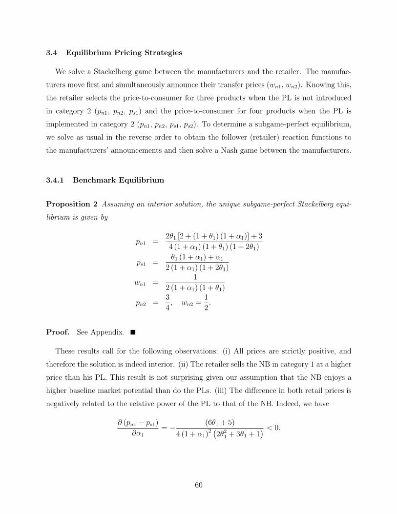
3.4 Equilibrium Pricing Strategies
We solve a Stackelberg game between the manufacturers and the retailer. The manufac-
turers move first and simultaneously announce their transfer prices (wn1, wn2). Knowing this,
the retailer selects the price-to-consumer for three products when the PL is not introduced
in category 2 (pn1, pn2, ps1) and the price-to-consumer for four products when the PL is
implemented in category 2 (pn1, pn2, ps1, ps2). To determine a subgame-perfect equilibrium,
we solve as usual in the reverse order to obtain the follower (retailer) reaction functions to
the manufacturers’ announcements and then solve a Nash game between the manufacturers.
3.4.1 Benchmark Equilibrium
Proposition 2 Assuming an interior solution, the unique subgame-perfect Stackelberg equi-
librium is given by
pn1 =2θ1 [2 + (1 + θ1) (1 + α1)] + 3
4 (1 + α1) (1 + θ1) (1 + 2θ1)
ps1 =θ1 (1 + α1) + α1
2 (1 + α1) (1 + 2θ1)
wn1 =1
2 (1 + α1) (1 + θ1)
pn2 =3
4, wn2 =
1
2.
Proof. See Appendix.
These results call for the following observations: (i) All prices are strictly positive, and
therefore the solution is indeed interior. (ii) The retailer sells the NB in category 1 at a higher
price than his PL. This result is not surprising given our assumption that the NB enjoys a
higher baseline market potential than do the PLs. (iii) The difference in both retail prices is
negatively related to the relative power of the PL to that of the NB. Indeed, we have
∂ (pn1 − ps1)∂α1
= − (6θ1 + 5)
4 (1 + α1)2 (2θ21 + 3θ1 + 1
) < 0.
60

The result implies that the higher the PL’s power, the lower is the price differential. Hence,
the closer the positioning of the PL to the NB in terms of popularity, attractiveness or
image, then the closer is the PL’s price to the NB’s. In the terminology of PL, this means
that offering a me-too PL justifies asking for a price that’s close to the NB, compared to
offering a generic PL, where the price would be expected to be much lower than the NB
price. (iv) The derivative of the price differential with respect to θ1 is given by
∂ (pn1 − ps1)∂θ1
=4α1 (1 + θ1)
2 − 12θ1 − 8θ21 − 5
4 (1 + α1)(2θ21 + 3θ1 + 1
)2 < 0.
This result states that the higher the θ1, i.e., the higher the degree of consumer sensitivity to
the difference in price between the NB and PL, then the closer are these prices. To reinterpret
the result in the context of competition between NBs and PLs, we recall that Pauwels and
Srinivasan (2004) showed that second-tier NBs experience a higher long-term sensitivity to
PLs and that the reverse occurs for leading NBs. Combining our result with theirs, we can
conclude that it is more likely that the retailer will position a generic PL (e.g., Great Value
cereals from Wal-Mart) closer to a NB having the characteristics of a second-tier NB (e.g.,
Quaker cereals) rather than a leading NB (e.g., Kellogg’s cereals) when price sensitivity is
expected to be very high for a long time. However, Sayman et al. (2002) found empirically
that, only for categories with high-quality PLs, the PL competes more aggressively (in terms
of price) against leading NBs rather than secondary (or second-tier) NBs. Combining our
result with theirs, we can conjecture that if the retailer proposes a high-quality PL, then the
PL should be a me-too brand (e.g., ChipMates cookies) competing strongly in terms of price
with a leading NB (e.g., Chips Ahoy! cookies) rather than with a premium PL. The rationale
is that a premium PL is positioned in a distinct region of the perceptual map from a leading
NB, as they target separate segments of the market.
To conclude, the results are rather intuitive and the main value of this scenario is derived
from its role as a benchmark for the two others.
3.4.2 Equilibria with a Private Label in Both Categories
As we are considering a new-product launch, our results should be interpreted while keep-
ing in mind that α1 is the observed power ratio in category 1, while α2 is the expected
61

power ratio in category 2. Similarly, the cross-price parameter θ1 can be estimated using
historical data, whereas θ2 is hypothetical. Alternatively, we could assume that the results
were generated by two experiments, which consist of launching a new PL under the same
name and another one under UB in two identical retail stores located in two areas with the
same characteristics.
The next proposition characterizes the equilibrium prices when the retailer introduces his
new product in category 2 under a different name than the one used in category 1.
Proposition 3 Assuming an interior solution, the unique subgame-perfect Stackelberg equi-
librium in the NO UB scenario is given by
pNnc =2θc [2 + (1 + θc) (1 + αc)] + 3
4 (1 + αc) (1 + θc) (2θc + 1), c = 1, 2,
pNsc =θc (1 + αc) + αc
2 (1 + αc) (1 + 2θc), c = 1, 2,
wNnc =1
2 (1 + αc) (1 + θc), c = 1, 2.
Proof. See Appendix.
The equilibrium prices are positive and vary as follows with respect to the PL’s relative
power and the cross-price parameter:
∂pNnc∂αc
< 0,∂pNsc∂αc
> 0,∂wNnc∂αc
< 0, c = 1, 2,
∂pNnc∂θc
< 0,∂pNsc∂θc
> 0,∂wNnc∂θc
< 0, c = 1, 2.
The manufacturers’ wholesale prices are decreasing in both the PLs’ relative power and cross-
price competition. In other words, offering a premium PL that enjoys a high reputation will
be used as a negotiating tool against the NB’s manufacturer. Further, the PL’s relative power
and cross-price competition have a positive effect on the PLs’ retail prices and a negative
effect on the NBs’ retail prices. This means that both assets give the retailer an opportunity
to ask a premium price for his PL and a closer price positioning to the NB.
62

Proposition 4 Assuming an interior solution, the unique subgame-perfect Stackelberg equi-
librium in the UB scenario is given by
pUnc =2θc [2 + (1 + θc) (1 + αc + δα3−c)] + 3
4 (1 + αc + δα3−c) (1 + θc) (1 + 2θc), c = 1, 2,
pUsc =θc (1 + αc + δα3−c) + (αc + δα3−c)
2 (1 + αc + δα3−c) (1 + 2θc), c = 1, 2,
wUnc =1
2 (1 + αc + δα3−c) (1 + θc), c = 1, 2.
Proof. See Appendix.
The main interesting message from the above proposition is that the prices in each category
now also depend on the brands’ strength in the other category. Umbrella branding induces
strategic interactions between the two categories, which are a priori fully independent. The
derivatives with respect to the PL’s relative power and to the cross-price parameter are given
by
∂pUnc∂αc
< 0; sign
(∂pUnc∂θc
)= sign
(2 (1 + θc)
2 (αc + δα3−c)− 2θc (3θc + 4)− 3),
∂pUsc∂αc
> 0; sign
(∂pUsc∂θc
)= sign (1− αc − δα3−c) ,
∂wUnc∂αc
< 0;∂wUnc∂θc
< 0.
The difference with the results obtained in the NO UB case is that the direction of the
variation in retail price, with respect to substitution parameter θc, is no longer clear-cut.
Qualitatively speaking, ∂pUnc∂θc
would be negative, as it is in the NO UB scenario, if the spillover
parameter δ is small enough, i.e.,
δ <2θc (3θc + 4) + 3− 2αc (1 + θc)
2
2 (1 + θc)2 α3−c
.
The relationships between the prices and δ are as follows:
∂pUnc∂δ
< 0,∂pUsc∂δ
> 0,∂wUnc∂δ
< 0, c = 1, 2,
63

that is, a higher spillover allows the retailer to negotiate lower wholesale prices in both
categories and to price his PLs higher.
An important question in supply chain is how the pricing strategies of the manufacturers
and retailers interact. Their decisions are said to be strategic complements (substitutes)
if, when one increases, the other increases (decreases). The interest in this question lies in
the fact that the actual pricing decisions and the payoffs depend on the type of strategic
interactions between the players (see, e.g., Bulow et al. 1985; Moorthy 1988). In our case,
these relationships are given by the following derivatives:
∂pn1 (wn1, wn2)
∂wn1=
∂pn2 (wn1, wn2)
dwn2=
1
2> 0;
∂pn1 (wn1, wn2)
∂wn2=∂pn2 (wn1, wn2)
∂wn1= 0,
∂ps1 (wn1, wn2)
∂wn1=
∂ps1 (wn1, wn2)
∂wn2=∂ps2 (wn1, wn2)
∂wn1=∂ps2 (wn1, wn2)
∂wn2= 0.
These results show that the retail price of the NB in category c is increasing in the wholesale
price of that brand and is independent of all other wholesale prices. This result is not
surprising given our assumption of independent categories. Also note that the PLs’ retail
prices are independent of the NBs’ wholesale prices.
3.4.3 Comparison of the Two Branding Strategies
Comparing the results in Propositions 2 and 3 leads to the following interesting observa-
tions. In the NO UB scenario, the wholesale and retail prices in category c are independent
of the brands’ relative power in category 3 − c, that is, the two categories can be managed
separately. As seen from Proposition 3, the equilibrium UB wholesale and retail prices in
category c include the term α3−c, c = 1, 2. By using the same name for his two products, the
retailer is altering the competitive map by strategically relating the pricing of the two NBs
(versus PLs), which are a priori independent.
The next proposition compares the equilibrium prices in the different scenarios.
64
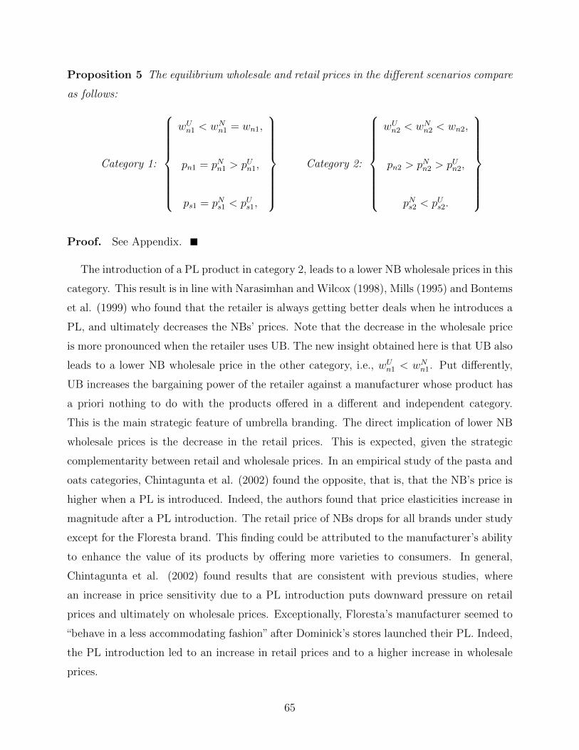
Proposition 5 The equilibrium wholesale and retail prices in the different scenarios compare
as follows:
Category 1:
wUn1 < wNn1 = wn1,
pn1 = pNn1 > pUn1,
ps1 = pNs1 < pUs1,
Category 2:
wUn2 < wNn2 < wn2,
pn2 > pNn2 > pUn2,
pNs2 < pUs2.
Proof. See Appendix.
The introduction of a PL product in category 2, leads to a lower NB wholesale prices in this
category. This result is in line with Narasimhan and Wilcox (1998), Mills (1995) and Bontems
et al. (1999) who found that the retailer is always getting better deals when he introduces a
PL, and ultimately decreases the NBs’ prices. Note that the decrease in the wholesale price
is more pronounced when the retailer uses UB. The new insight obtained here is that UB also
leads to a lower NB wholesale price in the other category, i.e., wUn1 < wNn1. Put differently,
UB increases the bargaining power of the retailer against a manufacturer whose product has
a priori nothing to do with the products offered in a different and independent category.
This is the main strategic feature of umbrella branding. The direct implication of lower NB
wholesale prices is the decrease in the retail prices. This is expected, given the strategic
complementarity between retail and wholesale prices. In an empirical study of the pasta and
oats categories, Chintagunta et al. (2002) found the opposite, that is, that the NB’s price is
higher when a PL is introduced. Indeed, the authors found that price elasticities increase in
magnitude after a PL introduction. The retail price of NBs drops for all brands under study
except for the Floresta brand. This finding could be attributed to the manufacturer’s ability
to enhance the value of its products by offering more varieties to consumers. In general,
Chintagunta et al. (2002) found results that are consistent with previous studies, where
an increase in price sensitivity due to a PL introduction puts downward pressure on retail
prices and ultimately on wholesale prices. Exceptionally, Floresta’s manufacturer seemed to
“behave in a less accommodating fashion” after Dominick’s stores launched their PL. Indeed,
the PL introduction led to an increase in retail prices and to a higher increase in wholesale
prices.
65

Regarding the PLs’ prices, we obtain that the retailer charges a higher price under UB
in both categories. One would then expect the demand for the PLs to be lower in the
umbrella-branding scenario than in the NO UB one. However, we obtain
DUsc −DN
sc =δα3−c (2 + θc)
4 (1 + αc + δα3−c) (1 + αc) (1 + θc)≥ 0, c = 1, 2.
This means that the potential loss in demand due to a higher price more than compensated
for the increase in the market potential baseline of the PLs due to UB. This result is consistent
with Raju et al. (1995), who found that the PLs can gain greater sales without lowering their
prices. This increase in the demand for PLs is borrowed from the NBs, whose demands in
the different scenarios are related as follows:
DUn2 =
θ2 + 2 (α2 + δα1) (1 + θ2)
4 (1 + α2 + δα1) (1 + θ2)≤ DN
n2 =1
4 (1 + α2)≤ Dn2 =
1
4,
DUn1 =
θ1 + 2 (α1 + δα2) (1 + θ1)
4 (1 + α1 + δα2) (1 + θ1)≤ DN
n1 = Dn1 =1
4 (1 + α1).
Recalling that we assumed the purchasing cost of the PLs to be zero, the margins in the
different scenarios compare as follows: 7
ps1 = pNs1 < pUs1, pNs2 < pUs2,(pUnc − wUnc
)≤
(pNnc − wNnc
)≤ (pn2 − wn2) .
A first conclusion is that choosing to market both PLs under the same name is a double-
facet strategy and the retailer needs to carefully trade-off between the two opposite effects
demonstrated above. More specifically, the UB increases the appeal (the baseline demand)
for the PL in both categories, which allows the retailer to enjoy higher demands for his brands
with higher margins, at the expense of the demands and margins for NBs. However, what
remains to be seen is how the profits compare under the two strategies.
7. Indeed, we have
(pNn2 − wN
n2
)− (pn2 − wn2) = − (θ2 + α2 (1 + θ2))
4 (1 + α2) (1 + θ2) (2θ2 + 1)≤ 0
(pUnc − wU
nc
)−(pNnc − wN
nc
)= − α1δ
4 (1 + α2) (1 + α2 + δα1) (1 + θ2) (1 + 2θ2)≤ 0
66

3.5 Profitability of Umbrella Branding
The NB manufacturers’ profits in the different scenarios are given by
PL in only category 1 : πM1 =1
8 (1 + θ1) (1 + α1)2 , πM2 =
1
8,
PL in both categories (NO UB) : πNMc=
1
8 (1 + θ1) (1 + α1)2 , c = 1, 2,
PL in both categories (UB) : πUMc =1
8 (1 + θc) (1 + αc + δα3−c)2 , c = 1, 2.
For the manufacturers of NBs, the introduction of a PL under a different name is detrimental
to their profits, and it is even worse when the retailer adopts an umbrella-branding strategy.
Indeed, straightforward computations lead to the following ranking of profits: 8
πUMc≤ πNMc
≤ πMc , c = 1, 2.
The above result is a direct consequence of the previous ones, namely, that UB implies lower
retail prices and a lower demand for NBs. Faced with such outcome, the manufacturers should
then find suitable counterstrategies to the introduction of store brands, and particularly, to
UB strategies.
We now turn to the crucial issue of the retailer’s performance. Recall that the retailer is
the player who actually has the option of implementing an umbrella strategy or not. The
8. Indeed, the difference in profits is given by
πM1= πN
M1,
πNM2− πM2
= −α2 (2 + α2) (1 + θ2) + θ2
8 (1 + θ2) (1 + α2)2 ≤ 0,
πUMc− πN
Mc= − δα3−c (2 (1 + αc) + δα3−c)
8 (1 + θc) (1 + αc)2
(1 + αc + δα3−c)2 ≤ 0, c = 1, 2.
67

differences in profit with respect to the benchmark scenario are given by
πR − πNR =θ2 + 2α2 (1− θ2)− 2θ22 (1 + 2α2)− α2
2
(3 + 2θ22 + 5θ2
)16 (1 + α2)
2 (1 + θ2) (1 + 2θ2),
πR − πUR =4 (θ1 + α1)
2 + 2θ1 + 4θ1α1 (θ1α1 + 2α1 + 2θ1) + 1
16 (1 + α1)2 (1 + θ1) (1 + 2θ1)
+1
16
−2θ1 (1 + 2θ1) + 4 (α1 + δα2)2 (1 + θ1)
2 + 8θ1 (α1 + δα2) (1 + θ1) + 1
16 (1 + α1 + δα2)2 (1 + θ1) (1 + 2θ1)
−2θ2 (1 + 2θ2) + 4 (α2 + δα1)2 (1 + θ2)
2 + 8θ2 (α2 + δα1) (1 + θ2) + 1
16 (1 + α2 + δα1)2 (1 + θ2) (1 + 2θ2)
.
These highly nonlinear expressions involve all the model’s parameters, namely, the cross-
price coefficients (θ1, θ2), the relative power of PLs (α1, α2) and the spillover parameter
δ. Unfortunately, the signs of the above expressions cannot be analytically determined.
Therefore, we resort to numerical analysis to get some insight into our only pending research
question, namely, when UB is in the best interest of the retailer. Schematically, the differences
in profit are the result of the trade-offs between three items, namely: (i) the incremental
profits realized on PL sales; (ii) the savings on the fixed cost; and (iii) the losses on the
NBs. Let us disregard the fixed-cost differential term, i.e., FN − FU , and focus on the other
elements that are more strategic in nature. Actually, if we find that the umbrella-branding
strategy is profit-improving without accounting for this cost term, then there is no need to
consider it. Otherwise, it will provide a lower bound for the profitability of UB.
Recall that, by construction of the model, the bounds on the parameters are given by
0 ≤ αc ≤ 1, 0 ≤ θc ≤ 1, 0 ≤ δ ≤ 1, c = 1, 2.
Our numerical simulations are conducted as follows: We fix the values of δ and θc, c = 1, 2,
and discretize the interval of admissible values of the parameters αc, c = 1, 2, using a mesh
size of 0.001. Therefore, for each vector (δ, θ1, θ2, α1, α2), we have a grid of one million points.
For each point, we compute πR−πNR and πR−πUR. The result of the comparison of these two
68

differences lies in one of the following regions in the (α1, α2)-space:
No PL introduction (Region 1) : πR ≥ πNR and πR ≥ πUR,
PL introduction under NO UB (Region 2) : πNR ≥ πR and πNR ≥ πUR,
PL introduction under UB (Region 3) : πUR ≥ πR and πUR ≥ πNR .
We conducted a high number of runs, and in all cases, we obtained a pattern that can
generically be represented by Figure 3.1, which is drawn in the (α1, α2)-space for fixed values
δ = 0.1 and θ1 = θ2 = 0.1, that is, the upper-right side is region 3, the lower-right side is
region 2 and the left side is region 1. Figures 3.2 and 3.3 illustrate how the three regions
shown in Figure 3.1 vary when the values of the spillover parameter and the cross-price
coefficients are changed. 9 More specifically, the panels in the first row of Figure 2 correspond
to a low spillover value (δ = 0.1), whereas the second row’s panels are drawn for a high
spillover value (δ = 0.3). The panels in Figure 3 show the changes in the three regions for
different competitive-structure configurations in the two categories. For illustration purpose,
we retain three values for θ1 and θ2, namely, 0.1, 0.3 and 0.6. A high value of θc corresponds
to the case where the PL is of the copycat variety. A low value can designate either a generic,
if α is low, or a premium, if α is high. Note that the panels on the diagonal in Figure 3.3
correspond to a situation where the competitive intensity between the NB and the PL is the
same in both categories.
Our numerical results allow for the following general observations:
1. In all simulations, the (α1, α2)-space is divided into continuous parts, with the right-
hand-side part corresponding to the union of regions 2 and 3 (i.e., launching a PL is
profitable), and the left-hand side corresponding to the region where it is not profitable
to add a PL in category 2. This result tends to imply that there is a minimal value for
α2, say α2, below which launching a new PL is not profitable. Clearly, this threshold
depends on the other parameters, namely, the spillover δ and the cross-price coefficient
θ2 in category 2. Interestingly, the competition intensity in category 1, measured by
θ1, does not seem to play an important role in determining α2. This can be seen
by inspecting the three panels in each column in Figure 3, where θ1 is varied, while
9. Results for any parameter values can be provided by the authors upon request.
69

Figure 3.1 Definition of regions
70

θ2 and δ are kept constant. The same variation in cross-price parameters leads to a
completely different impact on the location of the three regions. A higher θ1 promotes
the implementation of the UB strategy without significantly expanding the regions
where it is beneficial for the retailer to introduce the PL. In contrast, a higher θ2 leads
to a significant reduction in the region where the PL’s introduction is not profitable.
To wrap up, our first conclusion is that it takes a minimum market potential for a new
PL launch to be successful and profit-improving, and that this minimum is lower for a
higher spillover δ and when the retailer launches a copycat. Note that the lowest value
for α2 that we obtained in our simulations is slightly larger than 0.20. Such a minimal
level may still be quite demanding if the NB has an excellent reputation and is fairly
priced.
2. Even when the UB strategy induces only positive spillovers between the categories,
there is still a region in the (α1, α2)-space, albeit a small one, where distinct branding
is preferred to umbrella branding. Recall that our assessment was carried out under
the assumption that UB does not involve a cost saving for the retailer. If UB involves a
cost reduction (e.g., in merchandising or advertising), then we would expect the regions
where UB is optimal to expand accordingly.
In the following claims based on Figures 3.2–3.3, 10 we refine our interpretations regarding
UB versus NO UB strategies.
Claim 6 Implementing a distinct-branding strategy can be optimal only if the existing PL is
generic.
To “prove” this claim, we first mention that in none of our simulations did we observe
an instance where (i) distinct-branding strategy dominates the two other strategies (no PL
launch and UB), and (ii) α1 is relatively high (say above 0.15). Second, the only cases where
we observed a small zone where NO UB is optimal are when θ1 is low (0.1) or medium (0.3).
In this last case, the region in question is very small. As a generic PL is characterized by both
a low α and a low θ, we arrive at the conclusion stated in the claim. The main contribution
of this result is in providing the necessary conditions for a NO UB strategy to be potentially
optimal.
10. We call these results claims instead of propositions, because they are based on numerical simulationsand not formal proofs.
71
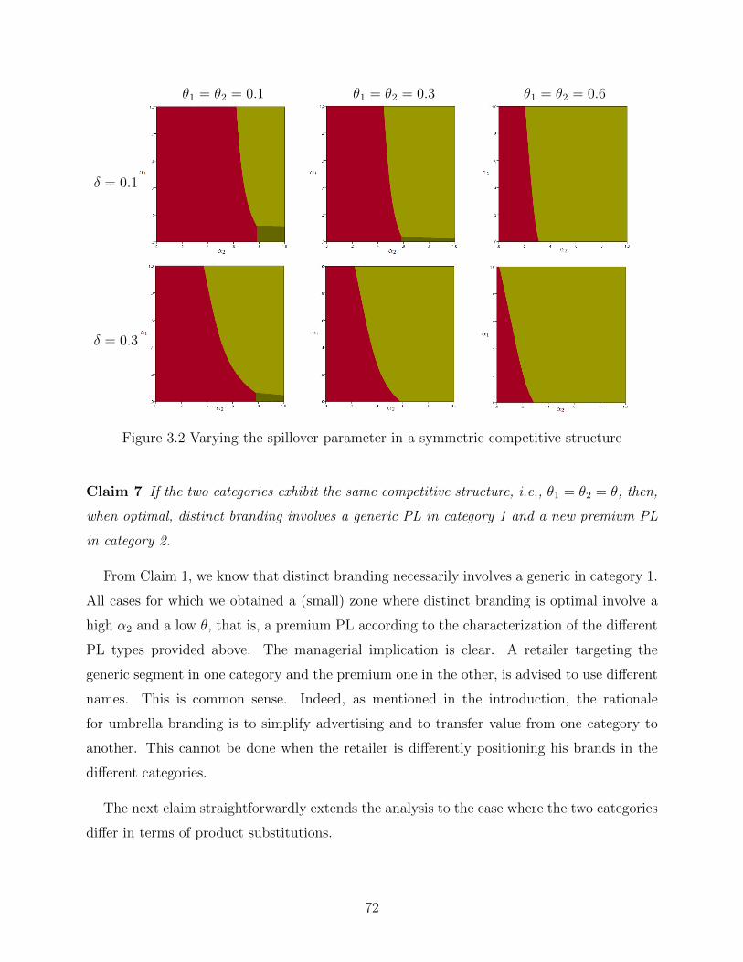
θ1 = θ2 = 0.1 θ1 = θ2 = 0.3 θ1 = θ2 = 0.6
δ = 0.1
δ = 0.3
Figure 3.2 Varying the spillover parameter in a symmetric competitive structure
Claim 7 If the two categories exhibit the same competitive structure, i.e., θ1 = θ2 = θ, then,
when optimal, distinct branding involves a generic PL in category 1 and a new premium PL
in category 2.
From Claim 1, we know that distinct branding necessarily involves a generic in category 1.
All cases for which we obtained a (small) zone where distinct branding is optimal involve a
high α2 and a low θ, that is, a premium PL according to the characterization of the different
PL types provided above. The managerial implication is clear. A retailer targeting the
generic segment in one category and the premium one in the other, is advised to use different
names. This is common sense. Indeed, as mentioned in the introduction, the rationale
for umbrella branding is to simplify advertising and to transfer value from one category to
another. This cannot be done when the retailer is differently positioning his brands in the
different categories.
The next claim straightforwardly extends the analysis to the case where the two categories
differ in terms of product substitutions.
72

θ2 = 0.1 θ2 = 0.3 θ2 = 0.6
θ1 = 0.1
θ1 = 0.3
θ1 = 0.6
Figure 3.3 Varying the competitive structure (δ = 0.1)
Claim 8 When the competitive structure is different in the two categories, Region 2 increases
in size with θ2 and shrinks when θ1 is higher. See Figure 3.3.
Analyzing Figure 3.3, it seems that a high cross-price competition in category 1 and low
cross-price competition in category 2 lead to no chances of introducing PL2 under a different
name and the smallest region to implement UB. However, under opposite circumstances, the
retailer has room for more situations to introduce a PL in category 2 under a distinct name.
This result is in line with Claim 1, stating that a necessary condition to use NO UB is first
offer a generic PL that requires a low θ1.
73

Claim 9 Increasing the value of the spillover parameter δ:
(i) significantly enlarges the region where launching a new PL is profitable;
(ii) significantly shrinks the region where NO UB is optimal.
The impact of the spillover parameter can easily be seen in Figure 3.2 for symmetric
categories. 11 These results are related to those obtained earlier. Indeed, we found that UB
allows the retailer to extract lower wholesale prices from NB manufacturers in both categories
and to increase the price of his PLs without decreasing the PLs’ demands. As the benefits
of UB increase with δ, the reverse is expected to hold for a NO UB strategy. Given that
an increase of the spillover has a strategic impact on the retailer’s decision, research should
investigate the determining factors that could boost such a spillover (e.g., PL positioning,
product characteristics, retailer format, etc.).
Claim 10 Very high θ1 in the symmetric and asymmetric competitive structure gives exclu-
sive use of the UB strategy.
In particular (see Figure 3.3) for me-too PLs (high level of cross-price effects combined
with high level of power ratios-observed in category 1 and expected in category 2), UB is
always a winning strategy for the retailer. Indeed, me-too PLs have dual benefits: (i) the
close positioning to the NB in terms of quality helps them take advantage of the positive
image association to the NB and ultimately results in more sales for PLs (Lassar et al. 1995);
and (ii) at the same time, they enjoy a positive spillover between PLs from different categories
under the same name.
3.6 Conclusion
Previous research has focused on the umbrella strategy, using the following: experiments
(see e.g., Martinez and Pina 2003; Aaker and Keller 1992); conjoint analysis (see e.g., Nijssen
and Agustin 2005); surveys (see e.g., Laforet 2008); modeling at the firm level (see e.g.,
Hakenes and Peitz 2008; Montgomery and Wernerfelt 1992; Degraba and Sullivan 1995);
regression analysis (see e.g., Wang et al. 2007). But, to our knowledge, no study has used a
game-theory setting involving the retailer and the manufacturers. Additionally, few papers
have studied this strategy when the retailer offers NBs along with PLs. This paper therefore
11. The results are very similar in the asymmetric case and are omitted to save on space.
74

makes a number of contributions. We investigate the use of an umbrella strategy in the
context of NBs competing against PLs. We also take into account the interaction of the NB
manufacturers with the retailer to shape their decisions in terms of: (1) introducing or not
a PL in a new category; (2) implementing an umbrella strategy or using a separate name
for the new PL; and, (3) choosing the optimal pricing strategies under different settings.
More specifically, the paper explores whether choosing the same brand name for PLs could
be detrimental for the retailer even if there is a positive-spillover effect between the products
in the two different categories. As pointed out above, the answer is yes in some instances.
The findings of this paper can therefore be used as a strategic dashboard for the retailers, to
make more effective branding decisions.
This research could be extended in different directions. One could study the effectiveness
of joint promotions along with the choice of umbrella strategy for PLs. Indeed, Wang et
al. (2007) explained that retailers should take advantage of the positive correlation between
products under the same name and maximize their profits by capitalizing on joint promo-
tions. Also, one could consider a dynamic model where the PL’s reputation evolves over
time due to an investment in quality, for instance. Further, it may be of interest for NB
manufacturers to look at potential channel-coordination solutions to avoid the losses when
the umbrella strategy is used by the retailer. Finally, it is of interest to NB manufacturers to
investigate what type of counterstrategy they can implement to minimize the damage done
by an umbrella strategy.
3.7 Bibliography
Aaker, D.A., & Keller, K.L. (1990). Consumer evaluations of brand extensions. Journal of
Marketing, 54 (1), 27–41.
Aaker, D.A., & Keller, K.L. (1992). The effect of sequential introduction of brand extensions.
Journal of Marketing Research, 29 (1), 35–50.
Abe, M. (1995). Price and advertising strategy of a national brand against its private-label
clone: A signaling game approach. Journal of Business Research, 33 (3), 241–250.
Ailawadi, K.L., & Harlam, B. (2004). An empirical analysis of the determinants of retail
margins: the role of store brand share. Journal of Marketing, 68, 147–165.
75

Ailawadi, K.L., & Keller, K.L. (2004). Understanding retail branding: Conceptual insights
and research priorities. Journal of Retailing, 80, 331–342.
Ailawadi, K.L., Pauwels, K., & Steenkamp, J-B. (2008). Private label use and store loyalty.
Journal of Marketing, 72 (6), 19–30.
Alexander, N., & Colgate, M. (2005). Customers’ responses to retail brand extensions.
Journal of Marketing Management, 21 (3/4), 393–419.
Amrouche, N., & Yan, R. (2012). Implementing online store for national brand competing
against private label. Journal of Business Research, 65 (3), 325–332.
Balachander, S., & Ghose, S. (2003). Reciprocal spillover effects: A strategic benefit of
brand extensions. Journal of Marketing, 67 (1), 4–13.
Bontems, P., Monier, S. & Requillart, V. (1999). Strategic effects of private labels. European
Review of Agricultural Economics, 26, 147–165.
Bulow, J. I., Geanakoplos J.D., & Klemperer, P.D. (1985). Multimarket oligopoly: Strategic
substitutes and complements. Journal of Political Economy, 93 (3), 488–511.
Burt, S. (2000). The strategic role of retail brands in British grocery retailing. European
Journal of Marketing, 34 (8), 875–890.
Chintagunta, P.K., Bonfrer, A., & Song, I. (2002). Investigating the effects of store-brand
introduction on retailer demand and pricing behavior. Management Science, 40 (10), 1242–
1267.
Cotterill, R.W., Putsis, Jr W.P. & Dhar, R. (2000). Assessing the competitive interaction
between private labels and national brands. Journal of Business, 73 (1), 109–137.
Degraba, P. & Sullivan, M.W. (1995). Spillover effects, cost savings, R&D and the use of
brand extensions. International Journal of Industrial Organization, 13 (2), 229–248.
Dhar, S., & Hoch, J. (1997). Why store brand penetration varies by retailer. Marketing
Science, 16 (3), 208–227.
Erdem, T. (1998). An empirical analysis of umbrella branding. Journal of Marketing Re-
search, 35 (3), 339–351.
Erdem, T. & Chang S.R. (2012). A cross-category and cross-country analysis of umbrella
branding for national and store brands. Journal of the Academy of Marketing Science, 40
(1), 86–101
76

Erdem, T., Zhao, Y., & Valenzuela, A. (2004). Performance of store brands: a cross-country
analysis of consumer store brand preferences, perceptions, and risk. Journal of Marketing
Research, 41 (1), 86–100.
Fernandez, AN., & Gomez, M.S. (2005). Shelf space management of private labels: A case
study in Spanish retailing. Journal of Retailing and Consumer Services, 12, 205–216.
Hakenes, H., & Peitz, M. (2008). Umbrella branding and the provision of quality. Interna-
tional Journal of Industrial Organization, 26 (2), 546–556.
Hoch, S.J., & Banerji, S. (1993). When do private labels succeed? Sloan Management
Review, 34 (4), 57–67.
Kapferer, J-N. (2008). The new strategic brand management: Creating and sustaining brand
equity long term. Kogan Publisher (4th Edition), 512 pages.
Karger, T. (1981). Analyze existing product’s values when researching brand extensions.
Marketing News, January 23, 1–4.
Kumar, N., & Steenkamp, J-B. (2007). Private label strategy: How to meet the store brand
challenge. Harvard Business School Press, 270 pages.
Laforet, S. (2008). Retail brand extension - perceived fit, risks and trust. Journal of Con-
sumer Behaviour, 7 (3), 189–209.
Lassar, W., Mittal, B., & Sharma, A. (1995). Measuring customer-based brand equity.
Journal of Consumer Marketing, 12 (4), 11–19.
Martinez, E., & Pina, J.M. (2003). The negative impact of brand extensions on parent
brand image / Executive summary. The Journal of Product and Brand Management, 12
(6/7), 432–449.
McMaster, D. (1987). Own brands and the cookware market. European Journal of Market-
ing, 21 (1), 83–94.
Mills, D. E. (1995). Why retailers sell private labels. Journal of Economics and Management
Strategy, 4, 509–528.
Mills, D.E. (1999). Private labels and manufacturer counterstrategies. European Revenue
Agricultural Economic, 26 (2), 125–145.
Montgomery, C.A., & Wernerfelt, B. (1992). Risk reduction and umbrella branding. Journal
of Business, 65 (1), 31–50.
77

Moorthy, K.S. (1988). Strategic decentralization in channels. Marketing Science, 7 (4), 335–
356.
Moorthy, K.S. (2012). Can brand extension signal product quality? Marketing Science, 31
(5), 756-770.
Morton, F.S., & Zettelmeyer, F. (2004). The strategic positioning of store brands in retailer–
manufacturer negotiations. Review of Industrial Organization, 24, 161–194.
Narasimhan, C., & Wilcox, R.T. (1998). Private labels and the channel relationship: A
cross-category analysis. The Journal of Business, 71 (4), 573–600.
Nijssen, E. J., & Agustin, C. (2005). Brand extensions: A manager’s perspective. Journal
of Brand Management, 13 (1), 33–50.
Parker P., & Kim, N. (1997). National brands versus private labels: An empirical study of
competition, advertising and collusion. European Management Journal, 15 (3), 220–235.
Pauwels, K., & Srinivasan, S. (2004). Who benefits from store brand entry? Marketing
Science, (23) 3, 364–390.
Putsis, Jr., W.P., & Dhar, R. (2001). An empirical analysis of the determinants of category
expenditure. Journal of Business Research, 52 (3), 277–291.
Raju, J.S., Sethuraman, R., & Dhar, S.K. (1995). The introduction and performance of
store brands. Management Science, 41 (6), 957–978.
Reisenbeck, H., & Perrey, J. (2009). Power brands: Measuring, making and managing brand
success. Wiley-VCH, Weinheim, 350 pages.
Ries, A.L., & Trout, J. (1986). Positioning: The battle for your mind. New York, McGraw-
Hill.
Sayman, S., Hoch, S.J., & Raju, J.S. (2002). Positioning of store brands. Management
Science, 21 (4), 378–397.
Sethuraman, R., Srinivasan, R., & Kim, D. (1999). Asymmetric and neighborhood cross-
price effects: some empirical generalizations. Marketing Science, 18 (1), 23–41.
Sullivan, M.W. (1990). Measuring image spillovers in umbrella branded products. Journal
of Business, 63 (1), 309–330.
Thompson, S. (1999). The new private enterprise. Brandweek, 40 (18), 36–40.
78

Wang, H., Kalwani, M.U., & Tolga, A. (2007). A Bayesian multivariate Poisson regression
model of cross-category store brand purchasing behavior. Journal of Retailing and Consumer
Services, 14 (6), 369–382.
Wernerfelt, B. (1988). Umbrella branding as a signal of new product quality: An example
of signalling by posting a bond. Rand Journal of Economics, 19 (3), 458–466.
Wilensky, D. (1994). Private label success no secret as discount. Discount Store News, 33
(5), 23–44.
3.8 Appendix: Proofs of Propositions
3.8.1 Proof of Proposition 1
Assuming an interior solution, we first determine the retailer’s reaction functions from the
first-order-optimality, that is,
pn1 (wn1, wn2) =w1 (2θ1 + 1) (1 + α1) + θ1 (1 + α1) + 1
2 (1 + α1) (2θ1 + 1),
ps1 (wn1, wn2) =θ1 (1 + α1) + α1
2 (1 + α1) (2θ1 + 1),
pn2 (wn1, wn2) =1
2w3 +
1
2.
Substituting in the manufacturers’ problems and optimizing leads to, after some straight-
forward calculations to,
w1 =1
2 (1 + α1) (1 + θ1),
w3 =1
2.
Substituting for the transfer prices in the retailer’s reaction functions gives the retail prices
in the Proposition. Note that all prices are strictly positive, and therefore, the solution is
indeed interior.
79

3.8.2 Proof of Proposition 2
The retailer’s reaction functions from the first-order-optimality are:
pNnc(wNnc, w
Nnc
)=
wc (1 + 2θc) (1 + αc) + θc (1 + αc) + 1
2 (1 + αc) (1 + 2θc), c = 1, 2,
pNs1(wNn1, w
Nn2
)=
θc (1 + αc) + αc2 (1 + αc) (1 + 2θc)
, c = 1, 2.
Substituting in the manufacturers’ problems and optimizing leads to, after some straightfor-
ward calculations to,
wN∗nc =1
2 (1 + αc) (1 + θc), c = 1, 2.
Substituting for the transfer prices in the retailer’s reaction functions gives the retail prices
in the Proposition.
3.8.3 Proof of Proposition 3
Follows the same steps as Proposition 4, while replacing αc by αc + δα3−c.
3.8.4 Proof of Proposition 4
Straightforward computations lead to the following differences:
wNn1 = wn1, wNn2 − wn2 = − α2 + θ2 (1 + α2)
2 (1 + α2) (1 + θ2)≤ 0,
wUnc − wNnc = − δα3−c
2 (αc + δα3−c + 1) (1 + αc) (1 + θc)≤ 0, c = 1, 2,
pNn2 − pn2 = − [α2 + θ2 (1 + α2)] (4θ2 + 3)
4 (1 + α2) (1 + θ2) (2θ2 + 1)≤ 0,
pU∗nc − pN∗nc = − δα3−c (4θc + 3)
4 (αc + δα3−c + 1) (1 + αc) (1 + θc) (1 + 2θc)≤ 0, c = 1, 2,
pU∗sc − pN∗sc =δα3−c
2 (αc + δα3−c + 1) (1 + αc) (1 + 2θc)≥ 0, c = 1, 2.
80

General Conclusion
The progress achieved in statistical software, data collection and storage techniques has
increased the importance of quantitative modeling in marketing research. The wide variety
of techniques and modeling approaches has provided practitioners and researchers with the
opportunity to a deeper understanding of various phenomena and to overcome renewable
marketing challenges. This thesis contributes to extend quantitative marketing literature by
developing new models applied to three topical issues, namely, bidders’ behavior in online
auctions, customer relationship management in the diffusion of subscription services, and
marketing channel in presence of private labels. The modeling framework of this research
incorporates three modeling approaches: response modeling, dynamic programming and game
theory.
In the first paper, we investigated the late-bidding behavior in online auctions. The results
showed a notable difference between extremely late-bidders or snipers and moderately late-
bidders. Snipers are the oldest and the most active members. The prevalence of these
bidders is not affected by entry-deterrence factors (reserve price, opening price and level of
competition). These results provide some interesting managerial implications for sellers and
auctioneers. Since snipers do not aim essentially to cut selling price, eBay managers do
not have interest to change the ending rules of the auction. Indeed, switching from fixed
end-time to automatically extended end-time (such in iGavel and TradeMe) could eliminate
late-bidding but will increase operation costs 12 without guaranteeing better revenue. Likely,
sellers can use a secret-reserve price to impose a minimum price for their objects. However,
we show that this strategy do not allow to deter snipers. On the contrary, a secret reserve-
price reduces significantly the number of other bidders and therefore the auction income.
12. An automatic extension leads a high increase on the number of ongoing auctions.
To conclude, it is clear that late-bidding became a common practice in online auctions,
but this does not represent any serious threat for sellers and auctioneers. The success and
sustainability of eBay confirm our statement.
This study can be extended in several directions. First, it would be interesting to use
panel data to investigate whether some bidders are late for all the auctions in which they
participate, or if they are only occasional late-bidders, i.e., whether their strategy is auction
specific. By using panel data, we would be also able to model the interdependence between
bidders’ behavior. In other words, the first bid timing of a specific bidder could depend on the
first bid timing of the other bidders. Second, studying more product categories and different
auction ending rules would surely be a welcome move to check the generalizability of our
findings. Finally, form a technical perspective, models used (Poisson and negative-binomial
models) dismiss the underdispersion hypothesis of data. It would be interesting to consider
other count-data models such zero-inflated models, hurdle models, etc.
The second paper focused on the role of CRM expenditures in the diffusion of subscription
services. In this sector, customer relationship duration affects hugely the service growth and
the customer profitability. We proposed a new diffusion model that incorporates acquisition
and retention expenditures. By using dynamic programming, we introduced an innovative
approach to calculate optimal acquisition and retention spending in order to maximize the
customer equity. Our results reveal that the optimal customer equity represents the sum of
the value of existing customers and the value of the remaining market. Further, we show that
the marginal customer equity, given by the difference between the customer lifetime-value
and the prospect lifetime-value, plays a crucial role in the determination of the optimal CRM
expenditures.
Through our empirical results, we confirm the positive impact of CRM expenditures on the
service growth and the significant presence of external factors influencing acquisition and
retention processes. These external factors are market specific. Moreover, we show that
underspending on CRM may be less critical than overspending in some market context.
The main contribution of this paper is fourfold: (i) incorporating CRM considerations in
the growth of subscription services, (ii) considering the impact of external incentives in the
determination of optimal CRM spending, (iii) illustrating optimal expenditures sensitivity
toward marketing effectiveness, margin, discount rate, and depth of external factors, (iiii)
82

analysing situations in which customer retention spending is more critical than customer
acquisition spending and vice versa.
We mention three possible extensions for our work. First, the present research assumed
that individual acquisition and retention costs do not vary with the penetration rate. As
several researchers have shown that innovators are less price sensitive than other consumers,
the acquisition cost of early adaptors should be low compared to laggards who are more
resistant to change. Likewise, the retention behavior could change with the penetration
rate. Based on these remarks, an interesting extension to this work would be to assume
that marketing effectiveness varies with the penetration rate. Second, our model does not
distinguish between new customers and won-back ones in terms of their acquisition cost. In
reality, it comes less expensive to acquire a new subscriber than a lost one having probably a
negative perception toward the service. In this sense, the model might be extended by treating
won-back customers differently. Finally, our study is developed in a non-competitive market.
Though the external incentives parameters could capture the effect of marketing efforts of
other firms, competitive framework with strategic interactions might yield additional insights
on the role of CRM expenditures in the diffusion of subscription services.
Finally, in the third essay, we focused on marketing channel interactions in the presence
of private labels. We looked into the impact of adopting an umbrella branding strategy on
the retailer’s performance. This strategy consists in using the same name to market different
products which may, or may not, be related. We take into account the interaction of the NB
manufacturers with the retailer to shape their decisions in terms of: (1) introducing or not a
PL in a new category; (2) implementing an umbrella strategy or using a separate name for
the new PL; and, (3) choosing the optimal pricing strategies under different settings. The
main finding are the following: (i) by implementing UBS, the retailer succeeds in lowering
the wholesale price of the NBs and consequently their retail prices; (ii) there is no interesting
for NBs’ manufacturers to see their retailer implementing an umbrella strategy; and lastly
(iii) there are indeed instances where the retailer is better off not implementing UBS and
should rather use a distinct name for his new PL.
This research could be extended in different directions. One attempt is to study the
effectiveness of joint promotions along with the choice of umbrella strategy for PLs. Indeed,
retailers should take advantage of the positive correlation between products under the same
83

name and maximize their profits by capitalizing on joint promotions. Also, we could consider
a dynamic model where the PL’s reputation evolves over time due to an investment in quality,
for instance. Further, it may be of interest for NB manufacturers to look at potential channel-
coordination solutions to avoid the losses when the umbrella strategy is used by the retailer.
Finally, it is of interest to NB manufacturers to investigate what type of counterstrategy they
might implement to minimize the damage done by an umbrella strategy.
84
