three essays on land rights, labor mobility and human
TRANSCRIPT

Three Essays on Land Rights, Labor Mobility and Human Capital Investment in
China
Dan Wang
A Dissertation
submitted in partial fulfillment of the
requirements for the degree of
Doctor of Philosophy
University of Washington
2013
Reading Committee:
Judith Thornton, Chair
Seik Kim
Hendrik Wolff
Program Authorized to Offer Degree:
Economics

©Copyright 2013
Dan Wang

University of Washington
Abstract
Three Essays on Land Rights, Labor Mobility and Human Capital Investment in
China
Dan Wang
Chair of the Supervisory Committee:
Professor Judith Thornton
Department of Economics
This dissertation explores how institutional features of the Chinese economy
impact the welfare and behavior of Chinese households. The first two
chapters investigate the economic implications of varying land security in
rural China. The third chapter provides an empirical test of household
responses to China’s One-Child Policy, looking at children’s education
attainments and subsequent earnings.
Chapter one first develops a theoretical model to understand how land rights
security may affect farmers’ employment choices. The model suggests that with
secured land rights, households with high farming ability are likely to
invest in land while households with low farming ability tend to invest in
human capital and migrate to the city. This result is important because it
suggests that land security promotes labor specialization based on ability,
which results in higher efficiency in the labor market. This chapter also
contributes to the debate of land tenure in rural China by using the regime
of land adjustments to identify land security. Land security is identified
based on whether the village has adopted small-scale land adjustment as its
main land reallocation regime. The empirical results suggest that land
security has a sorting function in employment decisions. Secured land rights
increase participation in non-farm jobs such as migration and local wage

employments while decreasing the probability of full-time farm employment.
The results imply that governmental policies promoting land security may
facilitate both migration and investment in land.
Chapter two examines the role of rural land reallocation on household welfare
and risk coping. The theoretical model suggests that in a self-sufficient
agricultural economy, large-scale land reallocation help households to cope
with labor supply shocks. However, when non-farm labor market and land rental
market exist as well, the proportion of households that benefit from large-
scale land adjustments will decrease. The empirical results suggest that
illnesses tend to increase the probability of both local employment and
migration by other family members; however, death of a family member has no
significant effect on non-farm employment. Large-scale land reallocation has
some mitigating effects on migration. In villages making use of large-scale
reallocation, households are more likely to rent out land when they
experience negative supply shocks compared with villages that use only small-
scale land reallocation. Both migration and large-scale reallocation appear
to serve as effective strategies to smooth out consumption. On the other hand,
access to land rental markets, does not appear to improve household ability
to smooth consumption. In this data, large-scale land reallocation appears
to play a bigger role in smoothing consumption than in smoothing income.
Chapter three provides an empirical test to evaluate the impacts of the One-
Child Policy (OCP) on children’s education attainments and subsequent
earnings. The introduction of OCP is used as a natural experiment to analyze
how the exogenous restrictions on fertility affect labor market decisions.
The baseline identification strategy uses a difference-in-difference approach
to compare outcome for children born before and after OCP; it also compares
outcomes between a treatment and a control group facing different
institutional constraints at the same period of time. The study also
estimates the Local Average Treatment Effect (LATE) for returns to education.
Empirical results suggest that OCP has bigger impacts on years of education
of urban men compared with urban women. Regarding the highest degree obtained,
OCP increases the likelihood of obtaining a college degree and high school
degree for men and women. Wage estimations show that one more year of
education increases women's hourly wage earnings by 5.6 to 8.1 percentage
points but an additional year has no significant impact on the wage of men.
Thus, returns to education for women appear to be higher than for men.

Acknowledgements
I am extremely grateful to my dissertation committee, Judith Thornton, Seik
Kim, Hendrik Wolff and Susan Whiting for their advice and encouragement. I am
also grateful to James Kung for his inspiration, to Scott Rozelle for
introducing me to Jikun Huang, who gives me my first job. In addition, I
would like to thank Edward Rice for being my reference.
I am thankful to participants in the labor brownbag and CSDE seminars. I have
benefitted from the help of faculty and staff of the economics department, my
fellow graduate students, and my students. I appreciate conversations with
Scott Tennican and Greg Teplow, which have contributed much to the
dissertation.
I would also like to acknowledge the faculty at Tulane University and Harvard
University. They motivate me tremendously in my pursuit of a doctorate in
economics. I am truly grateful to classes of Gregory Mankiw and Edward
Glaeser who have been tremendous models for me as teachers and researchers.
I benefited from the Positive Psychology class taught by Tal Ben-Shahar who
has transformed my view of teaching and attitudes towards life in general. I
am grateful for having Lan Yang as my first math teacher. She is devoted,
insightful and loving and I have learned so much from her.
I am indebted to Sally, Brick and Zhengji Qian for their tremendous help in
my most difficult times. I thank Yaw Agyeman and Connie O’Connor for helping
me after Hurricane Katrina. I also want to extend my thanks to everybody else
who has helped me along the way.
Finally, I would like to dedicate the dissertation to my parents for their
unconditional support and education.

1
Contents
1 Land Security and Labor Specialization in Rural China ....................4
1.1 Introduction .........................................................4
1.2 Theoretical Framework ................................................8
1.2.1 Basic Model: A Self-sufficient Agricultural Economy .............9
1.2.2 Extend the Model: Including Non-farm Sector ....................13
1.2.3 Tenure Security and Labor Mobility .............................15
1.3 Data ................................................................19
1.3.1 China Living Standards Survey (CLSS) ...........................19
1.3.2 Migration ......................................................19
1.3.3 Land Reallocation ..............................................21
1.4 Empirical Results ...................................................22
1.4.1 Land Security: Measurement and Endogeneity .....................22
1.4.2 Land Security on Human Capital Investment ......................25
1.4.3 Land Security on Land Investment ...............................27
1.4.4 Land Security on Migration and Other Employments ...............29
1.4.5 Robustness Check ...............................................31
1.5 Conclusion ..........................................................33
Appendix: Including a Financial Constraint in the Model ..................36
References ................................................................38
Figures and Tables ........................................................41

2
2 Risk Coping: Land Tenure, Land Rental Market and Migration ..............49
2.1 Introduction ........................................................49
2.2 Theoretical Framework ...............................................51
2.2.1 Welfare Effect of Land Reallocation in an Agricultural Economy .51
2.2.2 Including Land Rental Market and Non-farm Sector ...............54
2.2.3 Including Labor Supply Shocks ..................................56
2.3 Data ................................................................58
2.3.1 Rural Household Survey by Development Research Center ..........58
2.3.2 Key Variables ..................................................60
2.4 Empirical Strategy and Main Results .................................62
2.4.1 Risk-Coping Strategies and the Role of Land Reallocation .......62
2.4.2 Labor Shocks, Household Welfare and Risk-Coping Strategies .....65
2.4.3 Alternative Specifications .....................................67
2.5 Conclusion ..........................................................68
References ................................................................70
Figures and Tables ........................................................71
3 Unintended Consequences: One-child Policy in China ......................81
3.1 Introduction ........................................................81
3.2 Institutional Background ............................................84
3.3 Data ................................................................86
3.3.1 China Health and Nutrition Survey (CHNS) .......................86
3.3.2 Descriptive Evidence: Education and Wage .......................87

3
3.3.3 Key Variables ..................................................89
3.4 Identification Strategy: Difference-in-difference ...................91
3.4.1 Treatment Group ................................................91
3.4.2 Rural Control Groups: Rural Households with OCP-Cohort .........91
3.4.3 Urban Control Groups: Urban Households with Before-Cohort ......93
3.4.4 Differences between Treatment Group and Control Groups .........94
3.5 Main Results ........................................................95
3.5.1 OCP on Years of Education ......................................95
3.5.2 OCP on Highest Level of Education ..............................98
3.5.3 OCP on Wage Earnings ..........................................100
3.5.4 Parallel-trend Assumption .....................................102
3.6 Conclusion .........................................................104
References ...............................................................105
Figures and Tables .......................................................107

4
1 Land Security and Labor Specialization in Rural China
1.1 Introduction
An unresolved debate about land rights in China concerns whether the economic
growth is trapped by its seemingly inefficient institutions. The agricultural
de-collectivization in early 1980s has individualized the production of farms,
but land remains collectively owned. Every village resident is entitled to an
equal share of the arable land, which has resulted in the periodic land
reallocation.1 In rural China, there is no effective social insurance program
and land remains the most important productive assets for households. For the
poor, equal distribution of land could be a substitute for social insurance.
To a certain extent, it means loss in farm productivity (Wen, 1995; Li et al.,
1998; Jacoby et al., 2002), but it could also be a response to the missing
markets. Burgess (1998) suggests equal land redistribution contribute greatly
to nutrition intakes for Chinese farmers. Kung (1997) suggests that current
land tenure helps farmers to diversify income risks.
While it is widely accepted that land insecurity discourage farm productivity,
there is a lack of evidence on its labor market consequences. Researchers
have documented the relationship between migration and land rights security,
but the mechanisms through which the effects work are not clearly explored.
This paper identifies land security as whether the village has adopted small-
scale land adjustments as its main reallocation regime. Past studies have
tried several measures as proxies, such as the frequency of land
reallocations, or the percentage of land adjusted, or percentage of
households who have received land in the previous round of land adjustment.
1 Land reform in 1984 allocated land to villagers based on household size, labor supply or both.
The length of the land contract was 15 years in 1984 and then extended to 30 years in 1993.
Despite the contract by law, most villages have reallocated land among households periodically in
response to demographic and other structural changes.

5
It’s problematic because there is no evidence that land security perceived by
farmers is captured in these measures. Farmers understand that if they have
more family members, they will have inadequate land to farm should land
ownership be frozen for 30 years. Their perception of land security is
unlikely to be simply determined by the frequency or magnitude of land
relocations in the past.
This paper contributes to the debate of land tenure in rural China by using
the regime of land adjustments to identify land security. Kung (2011)
analyzed two types of land reallocation regimes and their determinants. Some
villages adjust land on a large-scale basis in which all households are
affected until every household has the same amount of land per person. Other
villages adjust land in small-scale, in which only households with
demographic changes are affected. Farmers have higher perception of land
security with small-scale land adjustments.
In addition to the new measure of land security, this paper also contributes
to the land security literature by using a new list of exogenous variables as
instruments for land security. Researchers have found several factors that
determine the choice of land tenure, such as off-farm activities and land
rental markets (Kung, 2000; Brandt et al., 2004; Yao, 2004). Built upon the
transaction cost story of Kung (2011), I treat land rights as the result of
three sets of exogenous variables: factor endowment (land and labor), village
topographies, and pressure from the higher authority. Pressures from higher
authorities are important because villages under higher quota requirements
are likely to be more concerned about efficiency.
I develop a two-period household model to show that secured land rights
encourage rural-urban migration. Rural households, constrained by their
wealth, have to choose between land investment and human capital investment.

6
Secured land rights increase the expected land holdings in the second period.
High-ability farmers in agriculture have high marginal return to labor and
are likely to invest more in land with more secured land rights. Low-ability
farmers do not have a comparative advantage in farming and the optimal
strategy would be to invest more in human capital and be prepared to take
non-farm jobs in the second period. Labor specialization thus emerges.
Using data from China Living Standard Survey (CLSS), my estimates is largely
consistent with the theoretical prediction. I estimate impacts of land
security on human capital investment, land investment and employments, using
instrumented probit model, two-part Tobit model and Biprobit model separately.
The theory is based on the assumption that households are credit constrained
and have to choose between investment in human capital and in land. CLSS does
not include expenditures in the two items, so I estimate the two types of
investments separately.
Education attainments of age group 15-25 are used to represent human capital
investment of the household. This age group is chosen because the period
1984-1994 is when they received and finished education, which coincides with
the land reform era and fit the identification of land security used in this
paper. Empirical results indicate that land security promotes the overall
education attainments and have stronger impact on households with lower
farming ability.
In terms of land investment, I choose the usage of organic fertilizer as
dependent variable. Since not every household uses organic fertilizer in land,
a Tobit model is used in the estimation. Results indicate a positive impact
of land security on the probability of using organic fertilizer, especially
for households with high farming ability.

7
When it comes to the migration decisions, I divide migrants into two groups
by migration duration: temporary migrants (away for less than one year) and
permanent migrants (away for more than one year). Since permanent migration
requires higher initial cost and involves more risk, it is likely to be
affected differently by land security comparing to temporary migration.
Empirical results suggest that land security actually has opposite effects on
the two types of migration. For temporary migration, it is consistent with
the theory: land security increases the probability of migration more for
low-ability households. However, for permanent migrants, land security have
stronger impacts for high-ability households, but other factors such as
wealth and whether possessing an urban hukou are more important determinant
for permanent migration.
Additional regressions on participations in farming and local wage jobs
suggest that land security has a sorting function in employment decisions: it
increases the probability of non-farm jobs and decrease participation in
farming. Households with low farming ability benefit more from land security
in their participation in temporary migration and local wage jobs, and
households with high farming ability benefit more in their participation in
farming. This result is also consistent with the labor specialization story
in the theoretical model.
Furthermore, this paper is in line with the existing property rights
literature by offering a theoretical model and empirical tests of the impact
of property rights on farmers' employment decisions. To my knowledge, there
hasn’t been other similar research. Economic research supports the importance
of secured property rights for household decisions regarding labor (Field,
2007) and agriculture (Besley, 1995). Wang (2012) argued that urban housing
has potential wealth that could be transformed into entrepreneurship through
the formation of property rights. In rural China, with more secured land

8
rights, wealth embedded in land can also be transformed into farmers’
productivity by improving human capital investments and labor mobility.
The rest of the paper is organized as follows. Section 1.2 develops a
theoretical model to explore the mechanisms through which land rights have
impacts on non-farm employments, especially on migration decisions. Section
1.3 presents data, variable definitions and descriptive statistics. Section
1.4 presents empirical strategy and results. Section 1.5 is conclusion.
1.2 Theoretical Framework
I develop a two-period household model that investigates the mechanisms
through which land rights security affects land investment, human capital
investment, and employment choices. Depending on their farming abilities,
households in the first period make investment decisions, taking into account
the expected effects of these decisions on their future wellbeing. Prior to
the second period, two village-level shocks are realized, a land reallocation
shock and a labor supply shock. Households then allocate variable factors of
production for the second period production. The model assumes that farming
doesn’t require much human capital investment but non-farm jobs do.
The model proceeds in two steps. The first step is to set up a basic model of
a self-sufficient agricultural economy without non-farm sector or labor
supply shocks. When the village adopts big-scale land adjustments, in which
all land are pooled together and equally distributed to households, every
household in the village is affected. Land is taken from households with high
abilities to those with low abilities. Anticipating losing part of the
investment in land, high-ability households will reduce their land investment
in the first period.

9
The second step is to include a non-farm sector. Constrained by wealth,
households face the tradeoff between land investment and human capital
investment. Non-farm jobs, especially migration, yield higher return than
farming but also have higher costs. Two types of costs are associated with
non-farm jobs. One is the investments in education and training, which are
crucial in non-farm employments but not so important in agriculture. The
other one is transaction costs mainly associated with migration, such as the
cost of living permit in the city and expense in searching for jobs. The
model suggests that with secured land rights, labor tend to specialize. High-
ability households tend to stay on farm, because more secured land rights
increase the expected holdings of land in the second period, thus encouraging
land-related investment in the first period. Low-ability households tend to
invest in human capital and take non-farm jobs because it is a better
portfolio choice for them.
1.2.1 Basic Model: A Self-sufficient Agricultural Economy
Consider a self-sufficient agricultural village with households ( is
large). Each household is endowed with labor and land . Land-labor ratio
is . Households differ in their farm ability (or agricultural comparative
advantage), and their initial wealth .
Every household lives for two periods. In the first period, there is no
agricultural production. 2 Households make land-related investment, , at a
2 The model could also introduce farm production in the first period. However, since this
complicates the model by a great deal while the only difference is in households’ wealth level
when they enter the second period, production is thus assumed away. Instead, I assume that
households in the first period start with different level of wealth, which has the same impact as
introducing farm production.

10
unit cost . 3 I define effective land as the production of land area and
the capital invested in it, which can be seen as quality adjusted land:
(1)
Effective land captures that if households lose land, they also lose the
irreversible capital investment in it. Land investment follows the
distribution of farm ability . 4 Household wealth is divided into investment
and consumption. Consumption per capita can be written as:
(2)
Before the second period, land reallocations happen with probability . The
result is that every individual enjoys the same level of effective land :
∑
∑
(3)
where is large enough so that changes in an individual’s investment will
not affect the village average level .
Without land reallocation, each family holds the same amount of land as in
the first period:
(4)
3 Land-related investments refer to spending that will improve the quality of land, such as
irrigation equipment, organic fertilizers and etc. 4 Land investment captures the kind of input in land that is non-removable and cannot be recovered once the land is taken away. An example of it is organic fertilizer. Farm ability refers to other factors that will increase farm output but can be recovered once the land is
taken away, such as farm experience, tractors, and other agricultural tools. If land is taken by
the village, households will lose but still possess . Algebra later will show that high-ability households tend to have higher

11
Assume a constant return to scale (CES) production function: ( ) ,
where the two inputs are effective land and labor supply. 5 Normalize output
price to one, household consumption per capita is:
( )
( )
(5)
If land reallocation happens, the consumption level is:
( )
(6)
Without land reallocation, the consumption level is:
( )
(7)
Assume an additively separable utility function, households choose land-
related investment to maximize total expected utility over the two periods:
( ) ( ) ( ) (8)
where ( ) ( ) ( ) ( ) ; is a discounting factor; and are
risk premiums corresponding to two possible outcomes (with and without land
reallocation).
The first order condition with respect to is:
( ) ( ) [ ( ) ( )] (9)
The optimal investment level is when marginal cost of investment equals to
the discounted marginal expected return.
The relationship between land security and land investment is shown as below:
5 Unlike the concept of “effective land”, I do not use “effective labor” in this equation.
Instead, I use the technological parameter to capture the labor ability. It will simplify the algebra by a great deal in later analysis.

12
( ) ( )
(10)
where is a positive constant. 6 This relationship can be illustrated by
dividing households into the high-ability ( ), and the low-ability ones
( ). From equation (10), households with high farming ability also tend to
invest more in land. Assume that the initial wealth is the same for all
households, the intertemporal consumption choices for high-ability and low-
ability households can be illustrated as in Figure 1.
In Figure 1, curve i (blue) represents consumption level when capital
investment is equal to the village average. In graph (a), curve ii shows that
high-ability households invest more than the average level in the first
period. If land reallocation does not happen, their second period consumption
will be higher than the village average. If land reallocation does happen,
their consumption would drop to the village average. The distance between
curve ii and curve iii (red interval) represents the expected loss in
consumption. Similarly, low-ability households also want to decrease
investment when expecting land reallocation. The reason is that, the lower
they invest, the higher the expected gain from land reallocation would be
(red interval in (b)). Land reallocation acts like a subsidy to low-skill
families. 7
In a self-sufficient agricultural economy, the first best strategy for all
households is to lower land investment if land rights are not secure.
6 More details see Silberberg Structure of Economics page 158: Samuelson’s “conjugate pairs”
result. 7 Figure 1 shows the cases when land reallocation happen and when it doesn’t happen. If it
happens with probability , then it’s easier to show the effect with algebra instead of graphs. For example, if high-ability households increase their investment by , then the expected change
in income will be
- [ ( ) ( )]. The second term is the expected loss in income. We can
see that the higher is, the higher the expected loss. For low-ability households, the story is
the opposite. Their expected lost in subsidy by increasing investment is be
- [ ( ) ( )].
The more they invest, the less they receive.

13
Therefore, the average investment in the village decreases i.e.
and
land investment for the whole village will also decrease. In addition,
equation (11) suggests that investment will decrease even faster high-ability
farmers.
1.2.2 Extend the Model: Including Non-farm Sector
I extend the model by adding in a non-farm sector which includes local non-
farm employment and migration. As previously discussed, migration requires
higher education and additional transaction cost. 8 Assume that households need
to invest in human capital at price in the first period to gain the
skills necessary for non-farm jobs. Other transaction costs are assumed to be
fixed as . In the second period, those who invested in human capital could
work in non-farm sector and earn income ( ). To simplify, I assume that if
the household doesn’t invest in human capital, it cannot participate in non-
farm employment.
In period one, consumption per capita is:
(11)
In period two, household income could come from both farm and non-farm
employments. If land reallocation happens, consumption per capita is:
( ) ( )
(12)
If land reallocation doesn’t happen, the consumption level is:
8 If the household is self-employed, the initial cost could be the cost of borrowing or capital
purchase. However, in rural China, it is usually difficult to borrow from official institutions
and households usually use their accumulated wealth to pay for the starting up capital.

14
( ) ( )
(13)
Migration in the second period is contingent on human capital investment of
the household in the first period. If , then non-farm income ( ) is
also zero.
Labor supply in the second period is the sum of farm labor and non-farm labor:
(14)
Households want to diversify the income sources. Define as the share of
labor working on the farm, thus farm labor and non-farm labor (
) . Solve for FOCs with respect to , and :
( ) ( ) [ ( ) ( )] (15)
( ) ( ) { [ ( ) ] ( ) [ ( ) ]} (16)
( ) ( ) (17)
For each household, each dollar spent on will yield an increase in farm
income by while a dollar spent on will yield . Which investment is
more beneficial depends on the relative marginal return of the two
investments.
The optimal investment in land and human capital are determined
simultaneously by probability of reallocation, and farm ability, . The
most interesting result is the relationship between land rights security and
capital investment.
[ ( ) ( )]{ ( ) [ ( )]}
(18)

15
where ( ){ ( ) [ ( ) ( ) ( )]}; is a positive constant;
( ) is the first derivative with respect to . Function is the same for
every household no matter what level of land investment it has.
The first term captures the portfolio effect of investment between land
investment and human capital investment. The expression in the big bracket is
always negative due to diminishing marginal utility in consumption. The
difference between the two first derivatives, [ ( ) ( )], is determined
by the distribution of . If , then [ ( ) ( )] due to the
concave nature of the utility function and will increase as land rights
become more secure.
What’s substantial about this result is that by introducing a non-farm sector,
land security can result in labor specialization. For a household with a
large amount of initial investment, it runs the risk of losing much of the
investment if land reallocation happens in the second period. If land rights
security improves, the expected return in land investment will increase. On
the other hand, if a household has little or no land investment to start with,
then the optimal strategy is to specialize in non-farm jobs. 9
1.2.3 Tenure Security and Labor Mobility
Assume that households are not credit constrained, i.e. 10 .
To decide whether to participate in the non-farm sector, households compare
the expected utility under each employment choice. If not participating in
9 A closer look at the determination of land investment suggests that not all households increase
land investment when land rights are more secured. Given that farm skill and farm investment are
positively related, high-ability households will invest more when land rights are more secure.
However, for low-ability households, this may not be the case. As shown in equation (19), when
, the sign of the relative distribution effect is positive. As a result, the sign of
depends on the relative magnitude of . We can find a threshold level of farm ability, , above
which
, and below which
. The result indicates that the most productive farmers will
increase land related investment when land rights are more secure. For less productive farmers,
the optimal strategy is to reduce land investment and switch to non-farm jobs. 10 See the Appendix for discussion of the case when households are credit constrained.

16
non-farm sector, human capital investment is zero, the expected utility is
thus:
( ) [ (
) ( ) ( )] (19)
where
,
(
),
(
) .
If households invest in human capital, then they could take non-farm jobs in
the second period. The total expected utility is:
( ) [ (
) ( ) ( )] (20)
where
,
( ) ( )
,
( ) ( )
.
Define as the difference between expected utility:
(21)
If , households choose take non-farm jobs; if , they stay on farms.
If a household is indifferent, then . Plug equation (20) and (21) into
(22):
( ) (
) [ ( ) ( ) (
)] (22)
where ( ) (
) if , and ( ) (
) if . Functions and
can be seen as the absolute benefit from land reallocation.
The first derivative of with respect to is:
{( )
[ (
) ( ) (
) ( )]}
(23)

17
where is the land labor ratio
. The sign of the terms in the big bracket
is determined by two parts. Before proceeding any further, we need to discuss
the sign for the first term ( ). It can be solved from equation (13):
{ (
) ( )
[ (
) ( )]}
(24)
Households that have invested in human capital will have a lower consumption
level in the first period, and thus
. The marginal return of non-farm
jobs is higher than farm labor, so that
. The intuition is that if
households have invested in human capital in the first period, they must have
anticipated a higher return in the second period from non-farm jobs.
Therefore, the value of ( ) is always positive.
The second term in the big bracket in equation (14), [ ( ) (
) ( ) (
)],
is always negative. The reason is that with human capital investment in the
first period, the income in the second period will be higher and thus the
expected marginal value of consumption is lower due to the concavity of the
utility function.
We can find a pair of threshold values of farm technology and wealth
that make
. If a household has farm technology lower than or wealth
higher than , as goes down, will go up, then the household will enter
non-farm sector. On the other hand, if is higher or lower than the
threshold, then will go down as goes down, and the household will choose
farming. The result can be illustrated in figure 2.
A combination of and can be traced out that makes a household
indifferent between farming and migration. Farm ability and wealth are
positively correlated when households are indifferent between farming and

18
migration. The indifference curve, ( ) , is convex in . 11 It
divides the space into two parts. Households above the indifference curve
will enter migration and those below the curve stay in agriculture. Some of
the farmers previously with higher initial wealth and lower farm ability will
switch to non-farm jobs, as shown by area , and some of the non-farm
participants will switch back to agriculture, as shown by area , if their
farm ability is higher. The initial household wealth has to be greater
than a minimum amount to finance the transaction cost and or startup
capital for entering the non-farm sector. This change in the distribution of
households can be illustrated by a steeper indifference curve in the figure.
A household is not able to switch to non-farm jobs if it is financially
constrained.
The model suggests that for households with high farm ability, secured land
rights increases their expected holdings of effective land in the second
period, thus the expected marginal return in farming ability will increase.
Therefore, these households will have a higher incentive to invest in land
instead of in human capital in the first period. The story is the opposite
for households with low farming ability. They will have a high incentive to
invest in human capital because given their expected return in land and human
capital, their optimal portfolio choice would be to invest in human capital
and participate in non-farm employments.
11 From equation (22) and (23),
and
. Rewrite as a implicit function of key
parameters and and we can derive the relationship between and when . We have
.

19
1.3 Data
1.3.1 China Living Standards Survey (CLSS)
Data used in this study is from China Living Standards Survey (CLSS), which
was carried out in 31 villages in Hebei and Liaoning Provinces in the summer
of 1995. 12
The survey collected detailed information on individual and
household wealth, investments, labor supply in both farm and nonfarm
activities. It also contains details in village-level characteristics as well
as the political organization. In the 1995 survey, there are in total 880
households, in which 50 households were selected from the village surveyed in
the 1930s and 20 from every other village. Households in each village were
picked by random sampling using the most recent village registration.
The CLSS data is relatively old but has several advantages. First, it
contains detailed information on past land redistribution practice and
property rights policies, which is normally not recorded by other surveys
available. Second, it eliminates the land rental markets and financial
markets as determining factors on farmers’ employments choice because before
1997 those markets were virtually non-existent in rural China. The survey
facilitates the empirical tests by eliminating those two endogenous variables.
1.3.2 Migration
Migrants are defined as villagers that are away for more than one month,
currently working or looking for a job in the city. About 38% of the
households (15% of the individuals) participated in 1994 and they on average
send out more than one migrant. Migrants on average have two more years of
education than non-migrants. Most temporary migrants (away for work, for more
12 The survey was a collaborative effort of Loren Brandt (University of Toronto), Paul Glewwe
(University of Minnesota), Scott Rozelle (Stanford University) and Bai Nansheng (Renmin
University of China). The sample selection was not entirely random. It was a follow up of a
household investigation carried out by Japanese researchers in 1936 and 1937.

20
than 1 month but less than 1 year) are men while most permanent migrants
(away for more than 1 year) women. Possessing an urban hukou (the city
residential permit that allow rural workers to legally live in the city), is
the most important determinant for permanent migration. Non-migrant
households have more females and more children. Migrant households have more
land, less farm-capital, lower savings and lower farm income.
Temporary migration presents a short-term, circular nature: migrants come
back to the village and work on farm during busy harvest seasons. About 70%
of the temporary migrants also work on farm. About 33% were away in 1994 for
less than 3 months and only 16% for more than 9 months. The average time
migrants working on farm are 23 days with 9 hours per day in busy season,
quite close to local farmers. Among temporary migrants, 56% work as low-
ability labor and their monthly salary is much higher than other local
employments.
Agriculture remains the most important employment, with more than 87%
households’ participation. Agricultural income accounts for about half of the
household net income. Land owned by the household ranges from 0.2 mu (0.03
acre) to 184 mu (29.4 acre), with farms in Liaoning larger than in Hebei.
Family owned business and local nonfarm wage job are also major sources of
income. About 40% of households reported to have family owned business and
20% with local wage employments. In farm labor supply, farmers in Hebei work
for more days than those in Liaoning. No significant difference is found
between male and female farmers.

21
1.3.3 Land Reallocation
Since 1984, most villages have redistributed land at least once and land
holdings for most households have increased. 13 The most recent large-scale
land reallocation for each village happens around 1993 and 1994, during which
the state extended the land contract from 15 years to 30 years. During this
reallocation, Liaoning had much bigger adjustments than Hebei. About 46% of
the households on average were affected in Liaoning while in Hebei this
number is only 25%. Farmers in Liaoning also had a more drastic change in
their land holding with an average of 9.5 mu of increase or 4.7 mu of
decrease, while in Hebei the two statistics are 2.3 mu and 2 mu.
The sample villages present a “bi-modal” structure of land adjustment:
whereas some villages have only reallocated land on a large-scale basis,
others mainly readjusted a tiny fraction of the village landholdings each
time for households with demographic change. 14 There are 9 villages with only
large-scale land reallocation, 8 of which are from Liaoning; 2 villages in
Hebei only adjust land in small-scale; 17 villages mainly adjust land in
small scale but with occasional village-wide land adjustment (most of those
villages adjust land only in 1993 following the extension of land contract);
2 villages in Hebei have never adjusted land in any fashion. In terms of
land rights policies, villages in Hebei are more lenient than in Liaoning.
Farmers in Hebei are able to keep the farm land after they migrate, whereas
those in Liaoning have to return the land.
Table 4 displays major differences in village characteristics by land
reallocation regime. In villages where land is only reallocated in large
13 In some villages, this is done through “reserved land”. By law, about 5% of farm land can be
reserved beforehand to meet the population change in households without carrying out the village -
wide large scale reallocation. This method ensures the land rights security of farmers for a
longer period of time. 14 Many Chinese scholars suggest villages tend to adjust land in small-scale every three years and
on a large scale every five years (sannian yi xiaotiao wunian yi datiao). This statement doesn’t
hold for all villages in the sample.

22
scale, there is higher participation in local employments and migration. They
have higher percentage of land adjusted since 1984 and much smaller portion
of paddy land. 15 Change in party secretaries is more frequent in villages
with large-scale land adjustments only.
1.4 Empirical Results
The most important result of the theoretical model is the labor
specialization effects of land security, i.e. land rights security will
affect households with different farming ability differently. In empirical
tests, I will first discuss the measurement of land security and the
endogeneity issue, and then estimate the impacts of land security on human
capital investment, land investment, and migration respectively.
1.4.1 Land Security: Measurement and Endogeneity
Land rights security is endogenous because land tenure is determined
intrinsically within the village. Past studies have used different proxies,
such as the frequency of past land reallocations, the percentage of land that
have been adjusts, the percentage of households that were affected in the
last land adjustments. Carter and Yao (1999) constructed a land security
index and suggested that frequent land reallocations in the past mean
unsecured land rights. It is problematic because with frequent land
reallocation, land is more equally allocated among households. It may instead
indicate a more secured land rights in the future.
Kung and Liu (1997) employed a survey conducted in 8 counties within Zhejiang
and Jilin province in 1994 and found that households prefer the egalitarian
land arrangement because they consider it “fair”. The result is somewhat
surprising. It’s hard to imagine that the households with more land per
15 The percentage of land adjustments is not 100% because new arable land is developed over the
years and some land has been set aside as reserved land without being allocated)

23
person are willing to give up land and give it to others without proper
compensation. If a household receives land in some year when a new member
joins the family, it must also anticipate giving up some of its land some
other year if some family member leaves. Therefore, households’ preference
for egalitarian land reallocation cannot reflect their true wills but a
reflection of the imposed moral requirement of the collective.
Turner, Brandt and Rozelle (2002) assume that village cadres make land
reallocation decisions to maximize the total producer surplus in the village.
The administrative reallocation plays the role of the land market and shift
land between households until the marginal product of land equalize. The
theory predicts that land will be redistributed more if village population
grows faster and when non-farm employments proliferate. Population growth
turns out to have a significant effect on the probability of land
reallocation but non-farm employment opportunities are not in accord with the
experience and their empirical result was contradicting to this hypothesis
too. Their assumption on village cadres maximizing village welfare is not
realistic and is against reality.
While non-farm market and land rental market may play important roles in
village land tenure, they are highly endogenous. We need exogenous variables
that explain land tenure while uncorrelated with the employment choices. Kung
(2011) suggests that village topography is an important factor determining
the fashion of land reallocation because it determines the transaction cost
of doing so. Villages that tend to adjust land in small-scale usually have
more complex topographies as well as large numbers of plots. Small-scale land
adjustments have to consider transaction costs of mapping and matching land
among households. Village cadres and production teams have to resurvey and
recombine plots of different qualities, locations, and facilities before
plots are reassigned to households with demographic changes. These costs only

24
happen when the village adjusts land in small-scale. On the other hand,
large-scale land reallocations cause more efficiency loss but without those
additional transaction costs.
I define land security following the suggestion by Kung (2011). He claims
that large-scale land reallocation results in much higher land insecurity
than small scale adjustments. In a village with large-scale adjustments,
changes in land ownership will only happen in the next village-wide land
adjustments. Villages with small-scale land adjustments only reallocate land
when a household has demographic changes. Small-scale land adjustments have
low uncertainty because farmers know exactly when the land change will be.
I choose three categories of exogenous variables as instrument for land
security 16: (1) village land endowment; (2) variables related to transaction
costs of land reallocation, such as the number of households, number of plots
and village topography variables including the percentage of paddy land and
the percentage of plain land; (3) the number of party secretaries since HRS
is used as a proxy for pressure from the state. Village heads in the sample
elected by villagers and are changed less frequently. Village party
secretaries are assigned from the higher authority (county or city), which is
much more frequent.
The first stage results are shown in Table 5. Besides the explanatory
variables discussed before, a province dummy is also included for column [3],
[4] and [5] to capture the macroeconomic policy on the provincial level. As
expected, villages with more households and smaller number of plots are more
likely to adopt the large scale land reallocation in practice. Number of
party secretaries and village topography variables do not have significant
16 Although data used in this paper are from households who have no right to determine land tenure,
we cannot rule out the unobserved variables in the error term in estimating equations, such as
the innate abilities and other characteristics of the village.

25
impacts. Land-labor ratio has a negative impact on the likelihood of
adopting large-scale land reallocation for the sample villages.17
I use “whether the village mainly adopts small-scale land reallocation” as
the proxy for land rights security. Four instrumental variables are chosen
from column [3]: number of households, number of land plots, land cultivated
per person and number of party secretaries since HRS. I also experimented
with different subsets of explanatory variables from Table 5 as instruments
for land security, and the results are robust.
1.4.2 Land Security on Human Capital Investment
I divide land rights in rural China into two periods: before 1984 and after
1984. As discussed in the introduction, before 1984, land rights were
determined by the State. After 1984, villages gained the authority to make
land reallocation decisions, and thus we observed vast differences in land
tenure between villages. Since the paper focuses on impacts of different land
tenure on labor market outcomes, individuals selected should receive their
education between 1984 and 1994. If children go to elementary school at the
age of 6, they will finish middle school at 15 and finish high school at 18. 18
If children have received their education between 1984 and 1994, they will be
between 15 and 25 in 1994.
In CLSS, the age group 15-25 has on average 8 years of education, with nearly
90% of middle school graduates. About 52% of children finished middle school
and 7.8% finished high school. More than 43% of children have dropped out
17 In studies by Kung (2011) , he did not find significant impact of land endowment per capita on
land tenure choice. 18 Less than 3% of the sample have received education beyond high school and thus were excluded
from the analyses.

26
before high school.19 It is common practice in rural China for children of age
13-16 to work on the farm or other employments, part-time or full-time.
I estimate the following specification:
( ) (25)
where is the education attainment. Three indicators are used: years of
education, whether the individual has finished middle school (1=finished
middle school), and whether the individual dropped out before high school
(1=dropped out before high school). Children who didn’t finish school in 1994
are excluded from the sample. is the measure for land security. When ,
the village adopts small-scale land reallocation regime and we consider land
rights secured. is farming ability of the household, proxied by the log
value of farm capital owned per person.
captures individual characteristics such as age, gender, parents’
education and type of hukou (urban or rural resident registration). is
household characteristics such as household size and land cultivated per
capita in 1984. is village level characteristics such as distance to the
closest county, if the village could access credit in 1988, and whether the
village had migrants in 1988 (a proxy for migration network effect). 20
I am interested in signs of and , which capture the effect of the land
security on education at different farming ability. If is negative,
households with low farming ability will have higher education outcome and
vice versa. It is noteworthy that unlike in linear models, the coefficients
on interaction variables in probit models are not the usual parameters of
19 Due to limited number in the sample, dropouts here refer to either dropping out of elementary
school or middle school. 20 I use variables from 1984 and 1988 as estimates for average household condition between 1984
and 1994 because education attainments are affected by the continuous changes in the household.

27
interest. Table 6 and later tables, I also focus on the coefficients of the
interaction terms.
Dependent variables include a continuous variable (years of education) and
binary variables (whether graduate from middle school; whether quit before
high school), so two types of regressions are used. For the continuous
variable, I use OLS and 2SLS estimates. For binary outcomes, probit models
are used. Since land security is a binary endogenous variable, I use the two-
stage correction. 21 This procedure uses a probit model to estimate the
endogenous variable in the first step and then use the predicted value as the
instrument in the second step. The main results are shown in Table 6.
Columns [1], [3] and [5] are baseline regressions, and other columns
instrument land security with the list of variables chosen from Table 5.
Results show that secured land rights increase the probability of graduating
from middle school and decrease the probability of dropping out before high
school. The coefficient is not significant for years of education at 10%
level, but it is significant at 15% level. The sign of the interactive term
is as expected--secured land rights on average have stronger effects for
households with less farm capital in their education attainments. Overall,
the empirical results confirm the theoretical prediction that land rights
security promotes education attainments, and have stronger effects on
households with low farming abilities.
1.4.3 Land Security on Land Investment
I choose the usage of organic fertilizer as the measurement for land
investment. The effect of organic fertilizer could last for a few years, and
thus their usage is subject to the risk of land reallocation. CLSS reveals a
significant proportion of households with zero organic fertilizer usage and
21 The two-step correction is suggested by Wooldridge (2002, section 15.7.3).

28
the rest with a positive level. OLS regression will not yield consistent
estimates, so Tobit model is a better choice. It is more flexible to use the
two-part model because the standard Tobit regression makes a strong
assumption that the same probability mechanism generates both the zeros and
the positive values. The first part of the two-part model is a binary outcome
equation and the second part uses linear regression. The two parts are
estimated separately.
I use the following specification. Let denote land investment (the amount of
organic fertilizer). Let be a binary indicator such that if and
if . When , we only observe ( ). When , define ( | )
be the conditional density of . The two-part model for is:
( | ) { ( | )
( | ) ( | )
(26)
For the first part, I use probit model, then ( | ) ( ), where is the
vector of all explanatory variables. For the second part, I first use an OLS
regression and then use IV-GMM model to instrument for land security. The
weighting matrix used in the GMM estimator accounts for heteroscedasticity
and is asymptotically efficient. 22
Main results are reported in Table 7. The unreported variables include
quality and type of the plot, other plot characteristics, village control
variables, and a province dummy. Columns [1] and [2] present estimates of
equation (28) where the dependent variable is an indicator for using organic
fertilizer. Columns [3] and [4] instrument land security with the list of
variables chosen from Table 5.
22 See Wooldridge, 2002; Baum, Schaffer, and Stillman, 2003.

29
Columns [2] and [4] show that land security (small-scale land adjustments)
decrease the use of organic fertilizers if farm capital is low. As predicted
by the theoretical model, when land rights are secure, households with more
farm capital have a higher probability to use organic fertilizers. The impact
of land security on the amount of fertilizer used in land is not as
significant.
1.4.4 Land Security on Migration and Other Employments
I examine the employment decisions for age group 15-25. The theoretical model
suggests that households invest in human capital to prepare for non-farm jobs,
especially for migration. Migration decision is more complicated than other
forms of employments because it could either be temporary or permanent
depending on the duration. In empirical tests, the two outcomes in migration
do not directly depend on each other, but the error terms may be correlated.
Therefore, I choose an ordered multinomial model and assume two latent
variables and
as below:
(27)
where and are jointly normally distributed with means of 0, variances of 1,
and correlations of . We observe the two binary outcomes
{
(28)
The model collapses to two separate probit models if correlation . I use
the same regressors in both estimates. Vector includes individual,
household, village controls as in the previous regressions.
One specification issue arises investigating the relationship between
migration and household wealth. I use farm capital as a proxy for the
household farming ability. It could also be a proxy for household wealth.

30
Past studies in migration has found numerous evidence on the inverted-U
relationship between household wealth and migration. Du, Park and Wang (2005)
found that the probability of migration first increases with household income,
and then decrease in rural China. If the inverted-U relationship exists, by
including the square of farm capital interacted with land security, we
expected to have different coefficient for the interaction term. Main results
are reported in Table 8.
Table 8 (a) presents basic results and table 8 (b) also includes the squared
term of farm capital interacted with land security. Column [1] and [2] report
results of the basic biprobit model. Column [3] and [4] instrument land
security and education with lists of variables from Table 5 (for land
security) and Table 6 (for education). Using instrumental variables yield
significant different results. Therefore, I focus on results in column [3]
and [4].
In 8 (a), the interactive term has a negative sign for temporary migration,
but for permanent migration, the coefficient of the interactive term is not
significant. In 8(b), by controlling for squared farm capital, the
interactive term for temporary migration has a much bigger coefficient. Also,
coefficient for permanent migration is positive and significant at 10% level.
The results suggest that at lower level of household farm capital, land
security increase the probability of temporary migration but decrease the
probability of permanent migration. One possible explanation is that
permanent migration is associated with much higher initial cost comparing to
temporary migration. When households have less farm capital, they are likely
to be credit constrained to participate in permanent migration. The
coefficient for is negative, suggesting that the impact of secured land
rights on households with little farm capital will be the smallest. Temporary

31
migration, on the other hand, is associated with less initial cost and thus
households are less likely to be credit constrained to participate.
Other important employments include farming and local wage employment. Land
security decreases the probability to be a full-time farmer but this effect
is weaker for those with high farming ability. Local wage employments
increase with land security and the participation increases faster for low-
ability households. Overall, land security increases non-farm employment
participation for low-ability households, in terms of both migration and
local wage employments.
1.4.5 Robustness Check
1.4.5.1 Nonlinearity in Farm Capital
The main results show that higher land security has larger impacts on
households with low farm abilities in their investment in human capital and
participation in migration. In all my estimates, farm ability is proxied by
the amount of productive farm capital that the household owns. It is possible
that the interactive term which yields the results is a proxy for
nonlinearities in the effect of the farm capital. If this is true, then
controlling for the nonlinearity will not yield significant results for the
interactive term.
To examine whether the results are robust to nonlinearities, I estimate each
equations by including a square term of farm capital. Results are presented
in Table 9. It is clear that in both the basic models (without instruments)
and the full models (with instruments), there is little change in the
coefficients of interest. Therefore, the possibility of nonlinearities that
may be driving the negative results can be ruled out.

32
1.4.5.2 Farm Output as Proxy for Household Farming Ability
The previous tests use farm capital owned by the household as the proxy for
household farming ability. Another possible proxy is farm productivity, i.e.
farm output per person. Farm capital owned indicates the household’s
potential in farm production, and farm output is a direct indicator on
farming ability. I use farm output per person in 1993 as a proxy for farming
ability for fertilizer usage and employment choices. For education attainment,
we have to make the assumption that farm productivity for the household has
been relatively stable between 1984 and 1994.
The results are shown in Table 10. The coefficients for the interactive term
in 10 (a) and 10 (b) are consistent with previous tests. Table 10 (c)
presents impacts of land security on migration and other employment choices.
I did not include the square term of farm output because past studies have
not shown evidence on the nonlinear relationship between farm output and
employment decisions. 23 The results are similar to previous findings.
However, the impact of land security on permanent migration is no longer
significant. It could be because that the quality of the data on output is
not as good as the farm capital in the survey. Also, permanent migration is
defined as being away from village for more than one year, so it happens
before farm output is realized. The causality could be reversed. In general,
farm output is not as good an indicator as the farm capital because the
amount of farm capital is relatively stable for a long time but farm output
is affected by many factors such as weather, government policy or natural
disasters.
23 I estimated separate regressions to include the square term of farm output per person and
interact the term with land security, and did not find evidence for any nonlinear effect. The
coefficient for the square term is small and not significant. The coefficients for LS*A had
little change.

33
1.5 Conclusion
The paper provides new evidence on labor market implications of land tenure
in rural China. Large-scale land reallocations within a village affect all
households and generate land rights insecurity, while small-scale land
reallocations only affect those with demographic changes and thus have higher
land security. For households with high farming ability, land security
increases the expected land holding in the second period and in turn
increases the marginal return to farming ability. Consequently, the incentive
of those households to invest in human capital and participate in non-farm
sector will be weaker. For households with low farming ability, the story is
the opposite. They anticipate receiving more land from future land
redistribution and the return to farming ability is lower. Their optimal
investment strategy would be to invest in human capital and prepare for non-
farm jobs. The theoretical results suggest that land security (small-scale
land adjustments) facilitate labor specialization in rural area in that high-
ability households focus on farming and low-ability households focus switch
to the non-farm sector.
Different from past studies, I identify land rights security as whether the
village has adopted small-scale land reallocation as its main regime. The
advantage of this identification is that it reflects the perceived land
security of farmers. Identifications used in past studies, such as the number
of land reallocations since the land reform or the percentage of households
affected in the last round of land reallocation, were somewhat arbitrary
because there is no empirical evidence indicating that these measures reflect
how farmers perceive land security. In empirical tests, following the
transaction cost story, land security is instrumented with three sets of
exogenous variables: village resource endowments, topography and the pressure
from the higher authority.

34
The empirical results drawn from a 1995 CLSS survey data support the
theoretical implications. I test the impact of land security on human capital
investment, land investment and employment choices separately. It appears
that education attainments for age group 15-25 is positively affected by land
security and this effect is stronger for low-ability (in farming) households.
Results from IV-probit models suggests that individuals are more likely to
graduate from middle school and less likely to quite before high school with
secured land rights, especially for low-ability households.
In terms of land investment, I use the probability of using organic
fertilizer and its quantity used per mu as dependent variables. Organic
fertilizers usage will have effects in land for several years and thus are
subject to the risk of land reallocations. The IV-probit and GMM results
suggest that at low levels of farm ability, land security decreases the
probability of using organic fertilizer significantly, while at high levels
of farm ability, land security increases the probability of using it.
Migration decision is complicated for two reasons. First, migration with
different duration will be affected differently by land security. Long-term
migration is subject to high initial costs (e.g. purchasing a city
residential permit) and high risks in job search, while short-term migration
has a circular nature that individuals travel between the city and the
village with more flexibility. Temporary migrants are able to work on the
farm during the busy season and go back to the city during the slack season.
Second, farm capital is used as a proxy for farming ability of the household
but it could also be a proxy for household wealth. Past studies have shown
that there is an inverted-U relationship between household wealth and
migration. Taking both factors into consideration, I estimate a biprobit
model to test temporary and permanent migration decisions simultaneously. The
result for temporary migration is as expected: land security facilitates

35
temporary migration overall and have stronger impacts for households with low
farm capitals. For permanent migration, although the overall effect of land
security is positive, the interactive term is also positive and significant
at 10% level, which means land security increases permanent migration for
households with more farm capitals. This result could be explained by the
credit constraint story. Households with less farm capital to start with are
more likely to be constrained to meet the initial costs of permanent
migration. In the robustness check, when I use farm output as a proxy for
farming ability, the coefficient for both land security and the interactive
term becomes small and not significant. It indicates that land security is
only important for temporary migration, and permanent migration is determined
by other factors such as wealth.
The main result from secured land rights is the labor market specialization
based on education and farming skills. It's important for policy makers to
understand its implication. Large scale adjustment causes more distortions in
land investment and employments than small-scale land adjustments. If rural
credit market and non-farm labor market do not exist, large-scale land
reallocation will benefit households with low farming ability and less farm
capital. However, if other markets exist, the benefit of large-scale land
distribution for low-ability households will decrease, and its distortion
effect in land investment and non-farm employments will be more apparent.
Land reform that aims at higher land security will increase the welfare of
low-ability households in this case.

36
Appendix: Including a Financial Constraint in the Model
Without constraints on investments, the first order conditions of and
show that the optimal capital investments are simultaneously determined by
farm ability and household wealth. However, households are likely to be
constrained on how much they can borrow and invest. Wealthier households are
more likely to have a higher level of capital input and also easier access to
the credit market.
To simplify algebra, I consider the case when the household is constrained
only in the human capital investment but not in farm capital . The value
of depends on wealth and the amount that the household can borrow. It is
possible that a constrained household chooses not to enter non-farm sector
even though it would have if it were able to borrow. Credit constraints

37
therefore produce a correlation between household wealth and their likelihood
to take local non-farm jobs and to migrate.
Assume that investment is financed by household wealth , land rental income
and borrowing . Households can use illiquid assets, such as housing or
farm equipment, as collateral to borrow at rental rate . Here I use to
denote the value of all household assets that can be used as collaterals.
Land cannot be used as collateral for loans because it’s not owned by farmers.
The model now has two additional constraints on investment and borrowing:
(1)
( ) (2)
where is the amount of land rented out. If the household rents in land,
this term will be negative. The amount that a household can borrow, , cannot
exceed a fraction of its total wealth which includes the value of collaterals
and the total wealth. And the household can also lend out the wealth .
Assuming that the shadow value of human capital is and the first order
condition with respect to becomes:
( ) ( ) (3)
The marginal product of human capital is equal to the sum of its marginal
return and shadow value. If the borrowing constraint is not binding, i.e. ,
then solves ( ) ( ). If the constraint is binding, then
( ) . Therefore the human capital investment is:
{ } (4)

38
For binding households, If , then [ ( )] [ (
)]. Here the level of
constrained utility is lower than the non-binding case because utility is an
increasing function of capital.
With more secured land rights, both credit constrained and non-constrained
households will increase their labor participation in migration. For credit
constrained households who have already participated in migration, with more
secured land rights, their land rental value will go up and we shall see
higher participation in local employments and migration.
If the land rental market is complete, households may mitigate risk and
smooth out consumption by renting in or out effective land. In our equations,
will again be replaced by the land rental price . The sign of
no
longer depends on the farm ability directly. The wealth determines the
household’s decision of participating in migration. As long as , the
household may choose to enter migration regardless of its farm ability.
Introducing a land rental market will increase households’ ability to cope
with risk ex post. For example, if there is a positive labor supply shock,
households could mitigate its impact by either participating in migration or
renting out land or both.
References
[1] Acemoglu, Daron and Simon Johnson. (2005): Unbundling Institutions,
Journal of Political Economy, 113(5): 949-995.
[2] Benjamin, Dwayne and Loren Brandt. (2002): Property Rights, Labor
Markets, and Efficiency in A Transition Economy: The Case of China,
Canadian Journal of Economics, 35(4): 689-716.
[3] Besley, Timothy. (1995): Property rights and investment
incentives: Theory and evidence from Ghana. Journal of Political
Economy, 103: 903-937

39
[4] Brandt, Loren, Scott Rozelle, and Matthew A. Turner. (2004): Local
Government Behavior and Property Right Formation in Rural China,
Journal of Institutional and Theoretical Economics, 160: 627-662.
[5] Brandt, Loren, Jikun Huang, Guo Li, and Scott Rozelle. (2002): Land
Rights in Rural China: Facts, Fictions and Issues, China Journal,
47: 67-97.
[6] Carter, Michael and Yang Yao. (1999): Specialization Without
Regret: Transfer Rights and Agricultural Investment in an
Industrializing Economy. World Bank Policy Research Working Paper
[7] De Brauw, Alan, John Giles. (2008): Migrant Labor Markets and the
Welfare of Rural Households in the Developing World: Evidence from
China, Policy Research Working Paper Series 4585, The World Bank.
[8] De Soto, Hernando. (2000): The Mystery of Capital: Why Capitalism
Triumphs in the West and Fails Everywhere Else, New York: Basic
Books.
[9] Deiniger, Klaus and Gershon Feder. (2001): Land Institutions and
Land Markets, in Bruce L. Gardner and Gordon C. Rausser, Handbook
of Agricultural Economics, 1: 288-331.
[10] Du, Yang, Albert Park, and Sangui Wang. (2005): “Migration and
Rural Poverty in China.” Journal of Comparative Economics, 33,
688-709.
[11] Jin, Songqing and Klaus Deininger. (2009): Land Rental markets in
the Process of Rural Structural Transformation, Journal of
Comparative Economics, 37(4): 629-646.
[12] Kung, James Kai-sing, Nansheng Bai, and Yiu-Fai Lee. (2011): Human
Capital, Migration, and ‘vent’ for Surplus Rural Labor in 1930s'
China: the Case of the Lower Yangzi. Economic History Review, 64
(1): 117–141. Lattimore, O., 1962. I
[13] Kung, James Kai-sing and Ying Bai. (2011): Induced Institutional
Change or Transaction Costs? The Economic Logic of Land
Reallocations in Chinese Agriculture, Journal of Development
Studies, 47(10): 1510-1528.
[14] Kung, James Kai-sing. (2002): Off-farm Labor Markets and the
Emergence of Land Rental Markets in Rural China, Journal of
Comparative Economics, 30 (2): 395-414.
[15] Kung, James Kai-sing and Shouying Liu. (1997): “Farmers'
Preferences regarding Ownership and Land Tenure in Post‐Mao China: Unexpected Evidence from Eight Counties,” China Journal, 38 (1997):
33–63
[16] Li, Guo, Scott Rozelle, Loren Brandt. (1998): Tenure, Land Rights,
and Farmer Investment Incentives in China. Agricultural Economics,
19 (1-2), 63–71.
[17] Liu, Shouying, Michael Carter and Yang Yao. (1996): Dimensions and
diversity of property rights in rural China: Dilemmas on the road
to further reform. Agricultural and applied economics (Staff Paper
Series No. 395, revised). Madison, Wisconsin: University of
Wisconsin—Madison
[18] Taylor, John. Edward, Scott Rozelle, and Alan de Brauw. (2003):
Migration and Incomes in Source Communities: A New Economics of
Migration Perspective from China,’ Economic Development and

40
Cultural Change, 52: 75-101.
[19] Turner, Matthew, Loren Brandt, and Scott Rozelle. (1998): “Local
Government Behavior and Property Right Formation in Rural China,”
Manuscript, University of Toronto
[20] Wang, Shing-Yi. (2012), “Credit Constraints, Job Mobility and
Entrepreneurship: Evidence from a Property Reform in China,” Review
of Economics and Statistics, 94(2): 523-551.
[21] Wen, Guanzhong James. (1995): The Land Tenure System and its Saving
and Investment Mechanism: The Case of Modern China. Asian
Economics, 9(31): 233-259.
[22] Yang, Dennis Tao. (1997): China’s land Arrangement and Rural Labor
Mobility, China Economic Review, 8(2): 101-115.
[23] Yao, Yang. (2000): The Development of the Land Lease Market in
Rural China, Land Economics, 76: 252-266.
[24] Yao, Yang. (2004): Land Tenure Choice in Chinese Villages: The
Rational Versus the Political Model, Land Economics, 80: 477-489.
[25] Zhao, Yaohui. (1999): Leaving the Countryside: Rural-to-Urban
Migration Decisions in China. American Economic Review, 89(2): 281–
286.

41
Figures and Tables
𝐶 𝐶
𝐶 (𝐾)
𝐶 (𝐾)
𝐶 𝑟
𝐶 𝑛 𝐶
𝐶 𝑟
𝐶 𝑛 𝐶
(a) High-ability households
(b) Low-ability households
Figure 1: INTERTEMPORAL CONSUMPTIONS
i
ii iii
i
ii
iii
Δ𝑉(Φ 𝐴 𝜌 )
Δ𝑉(Φ 𝐴 𝜌 ) Migration
Farming
Figure 2: LAND REALLOCATION AND MIGRATION
Φ
𝐴
Φ
��
NOTE: 𝜌 is the probability of land reallocation in period two and ρ ρ
Ι
ΙΙ
Φ

42
Table 1 BASIC HOUSEHOLD STATISTICS BY MIGRATION STATUS
Variable mean Non-migrants
Permanent migrants
(away>1 year)
Temporary migrants
(away>1 month)
Age 31.78 [18.51] 30.05 [7.20] 32.99 [11.54]
Education 5.34 [3.31] 7.42 [3.13] 7.36 [2.45]
Male, percentage 0.52 [0.50] 0.32 [0.47] 0.8 [0.40]
Urban hukou, percentage 0.05 [0.21] 0.26 [0.44] 0.09 [0.28]
N 3,272 434 136
NOTE:
(1) Means are calculated at individual level. Standard deviations are in parentheses.
(2) Education is the number of years of school completed.
(3) Having urban registration means the ability to access urban welfare programs.
Table 2 DESCRIPTIVE STATISTICS FOR HOUSEHOLDS BY MIGRATION STATUS
Variable mean Non-migrant households
(n=454)
Migrant households
(n=333)
Migration and demographic variables
Number of migrants .. .. 1.91 [1.20]
Household size 3.83 [1.00] 3.54 [1.35]
Age of household head 39.07 [9.60] 51.8 [11.64]
Number of female 1.91 [0.87] 1.76 [0.89]
Number of children, age 0-7 0.35 [0.52] 0.24 [0.47]
Number of seniors, age>55 0.3 [0.64] 0.84 [0.90]
Household Wealth
Land owned, mu 18.07 [13.54] 21.27 [13.54]
Present value of farm capital owned, yuan 2738.5 [3371.88] 2535.94 [2991.02]
Use value of nonproductive durable goods 437.96 [555.70] 289.98 [409.07]
Household saving, yuan 8076.98 [18645.97] 3734.24 [6910.85]
Income sources
Farm income (87.4%) 3970.92 [5949.81] 2804.3 [3363.05]
Nonfarm wage income (19.1%) 5285.41 [3228.02] 6052.02 [3412.26]
Remittances (28.8%) 795.24 [1147.84] 1244.57 [1994.85]
Family owned business (39.6%) 39673.31 [127579.23] 31745.4 [96180.60]
Other income (52%) 1219.07 [2430.12] 1151.2 [2438.70]
NOTE:
(1) Means are calculated at household level. Standard deviations are in parentheses.
(2) Percentage in the bracket in income sources is the participation rate.
(3) Household size refers to numbers of family members living at home. Non-productive durable
goods refer to furniture, TV and etc. Farm capital refers to all productive capital such as
irrigation equipment and tractors and their total present value are reported. Other income
includes pension, health care, rent and etc.
(4) 1 yuan=0.12 dollar in 1995. 1 mu=0.17 acre.

43
Table 3 FARM LABOR, LAND AND OUTPUT BY PROVINCE
Variable mean
Hebei
(n=393)
Liaoning
(n=394)
Farm labor supply, days
Family male 68.09 [53.61] 49.04 [39.93]
Family female 69.99 [47.64] 50.21 [34.86]
Hired labor 38.8 [78.97] 7.65 [12.78]
Exchange labor 7.87 [6.77] 8.71 [7.41]
Total farm labor supply 169.92 [118.48] 111.71 [98.06]
Farm output and capital, yuan
Farm output 4356.1 [3072.80] 8285.89 [9080.44]
Land, mu 7.32 [4.6] 15.52 [15.84]
Farm capital 3038.22 [2978.18] 2194.74 [3474.00]
Households with land change, percentage
Received land(past 2 years) 8% [0.27] 26% [0.44]
Lost land (past 2 years) 18% [0.38] 22% [0.41]
Received land (since 1984) 38% [0.49] 63% [0.48]
Lost land(since 1984) 10% [0.30] 3% [0.16]
NOTE:
(1) Means are calculated at household level. Standard deviations are in parentheses.
(2) Farm capital refers to all productive capital like irrigation equipment and tractors. Their
present values are reported.
(3) Much of the farm output was sold in 1994 at fixed or negotiated price to the state. In
calculating farm output, this portion of sold output is corrected by 1994 market price.
(4) 1 yuan=0.12 dollar in 1995. 1 mu=0.17 acre.
Table 4 VILLAGE CHARACTERISTICS BY LAND REALLOCATION REGIME
Large-scale Small-scale
Number of households 312.38 [110.08] 500.33 [262.71]
Number of party secretaries since HRS 3.29 [2.05] 2.78 [1.79]
If the last election was competitive 1.2 [0.41] 1.22 [0.44]
Percentage local wage employment 0.13 [0.10] 0.11 [0.08]
Percentage temporary migrants 0.03 [0.06] 0.01 [0.03]
Percentage permanent migrants 0.04 [0.06] 0.03 [0.03]
Number of land reallocations since HRS 2.29 [2.61] 3 [3.54]
Percentage of land adjusted since HRS 0.85 [0.32] 0.76 [0.36]
Percentage of paddy land 0.09 [0.22] 0.44 [0.39]
Percentage villages with plain land only 0.33 [0.48] 0.56 [0.53]
NOTE: Standard deviations are in brackets.

44
Table 5 DETERMINANTS OF LAND TENURE CHOICE: PROBIT MODEL
Dependent variable: land security (small-scale land
adjustment=1)
[1] [2] [3] [4] [5]
Number of households, log -1.782* -1.842
* -2.833
* -2.419
* -1.875
**
[0.858] [0.889] [1.197] [1.080] [0.720]
Number of plots per household,
log 1.289
* 1.344
* 1.139
*
[0.571] [0.601] [0.489]
Land cultivated per person,
log -0.683 -0.693 0.966
** 1.605
*** 1.025
**
[0.510] [0.510] [0.303] [0.315] [0.358]
Number of party secretary since HRS -0.053 0.213 0.302 0.234
[0.157] [0.212] [0.189] [0.204]
Percentage of paddy land -1.549
[1.200]
If village has only plain land -0.587
[0.741]
Liaoning -3.176
*** -3.090
*** -3.123
***
[0.426] [0.387] [0.581]
Constant 10.973* 11.462
* 14.889
* 12.285
* 10.546
*
[5.137] [5.411] [7.076] [6.190] [4.891]
Clustered SE No No Yes Yes Yes
Pseudo R2 0.346 0.349 0.512 0.494 0.465
Table 6: EDUCATION ATTAINMENT OF AGE GROUP 15-25
Years of education
If graduate
from middle school
If quit
before high school
OLS 2SLS PROBIT IVPROBIT PROBIT IVPROBIT
[1] [2] [3] [4] [5] [6]
LS 0.339 0.767 0.428 1.330* -0.694 -1.786
*
[0.447] [0.575] [0.420] [0.608] [0.445] [0.752]
LS*A -0.032 -0.089 -0.049 -0.170* 0.06 0.206
*
[0.070] [0.088] [0.052] [0.079] [0.056] [0.097]
A 0.055 0.093 0.014 0.098 -0.049 -0.147+
[0.051] [0.062] [0.042] [0.070] [0.047] [0.086]
EDU_father 0.167* 0.164
** 0.090
** 0.082
** -0.050
* -0.044
+
[0.061] [0.059] [0.029] [0.028] [0.024] [0.025]
Observations 639 639 676 676 676 676
NOTES:
(1) Clustered robust standard errors are in brackets. *** denotes significance at the 0.1%
level, ** at the 1% level, * at the 5% level, + at the 10% level.
(2) LS is whether the village adopts small-scale land adjustments as its main reallocation
regime. Small-scale adjustments represent land security. A is household farming ability,
proxied by log farm capital per person. EDU_father is the years of education of the father.
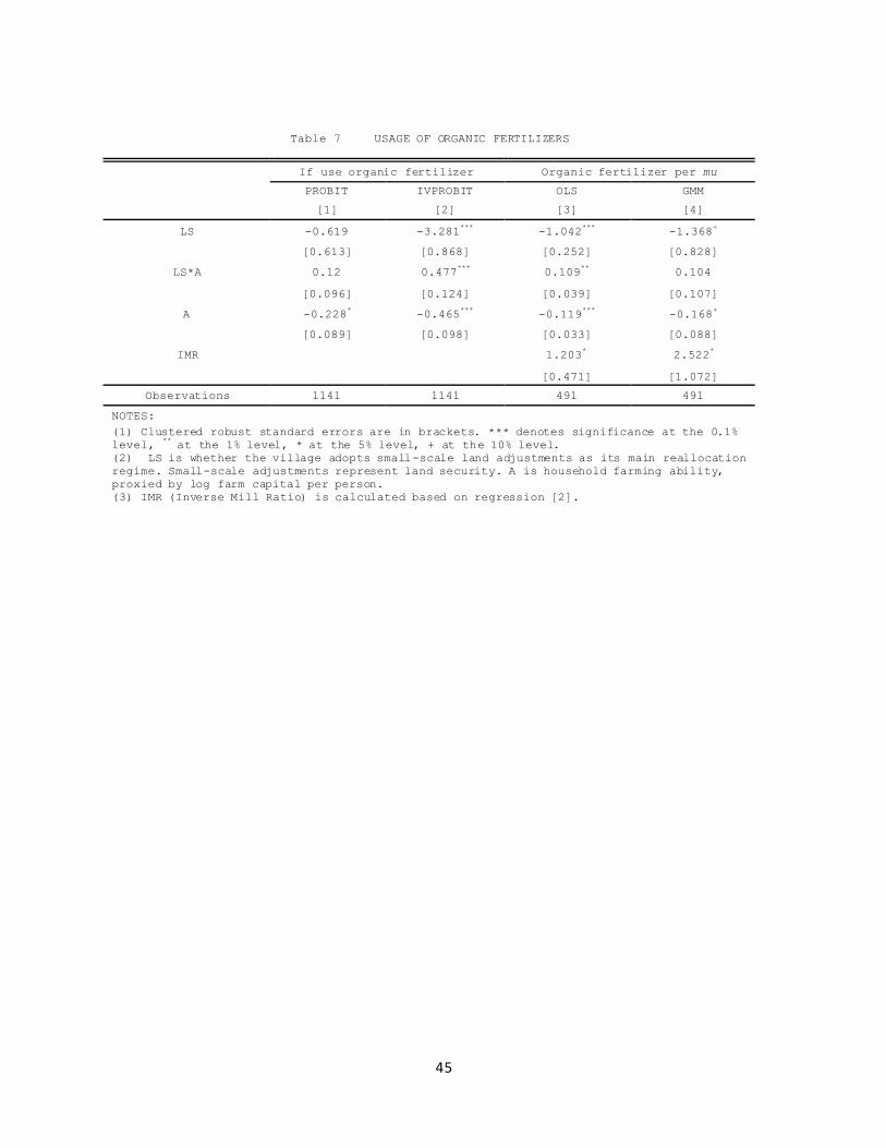
45
Table 7 USAGE OF ORGANIC FERTILIZERS
If use organic fertilizer Organic fertilizer per mu
PROBIT IVPROBIT OLS GMM
[1] [2] [3] [4]
LS -0.619 -3.281*** -1.042
*** -1.368
+
[0.613] [0.868] [0.252] [0.828]
LS*A 0.12 0.477*** 0.109
** 0.104
[0.096] [0.124] [0.039] [0.107]
A -0.228* -0.465
*** -0.119
*** -0.168
+
[0.089] [0.098] [0.033] [0.088]
IMR
1.203* 2.522
*
[0.471] [1.072]
Observations 1141 1141 491 491
NOTES:
(1) Clustered robust standard errors are in brackets. *** denotes significance at the 0.1%
level, ** at the 1% level, * at the 5% level, + at the 10% level.
(2) LS is whether the village adopts small-scale land adjustments as its main reallocation
regime. Small-scale adjustments represent land security. A is household farming ability,
proxied by log farm capital per person.
(3) IMR (Inverse Mill Ratio) is calculated based on regression [2].

46
Table 8 LAND SECURITY ON MIGRATION
Migration
temporary
Migration
permanent
Migration
temporary
Migration
permanent
BIPROBIT IV-BIPROBIT
[1] [2] [3] [4]
a. BASIC REGRESSION
LS -0.189 0.109 0.553 0.525+
[0.384] [0.259] [0.598] [0.303]
LS*A -0.075 0.01 -0.140*** 0.011
[0.061] [0.069] [0.026] [0.063]
A 0.082* -0.01 0.110
** -0.02
[0.040] [0.075] [0.036] [0.075]
EDU -0.011 -0.026 -0.146 0.223**
[0.055] [0.039] [0.137] [0.081]
b. CONTROLLING FOR NONLIEANRITY OF FARM CAPITAL
LS 0.017 0.231 1.705*** 0.543
[0.302] [0.175] [0.517] [0.338]
LS*A -0.253+ 0.377
+ -0.433
** 0.475
+
[0.149] [0.207] [0.159] [0.262]
LS*A2 0.03 -0.060
* 0.04 -0.074
*
[0.027] [0.024] [0.028] [0.032]
A 0.151 -0.364+ 0.258
* -0.448
+
[0.132] [0.204] [0.123] [0.249]
A2 -0.014 0.061
* -0.021 0.072
*
[0.024] [0.025] [0.020] [0.030]
EDU -0.018 -0.019 -0.16 0.214+
[0.054] [0.033] [0.156] [0.110]
Observations 744 744 676 676
NOTES:
(1) Clustered robust standard errors are in brackets. *** denotes significance at the
0.1% level, ** at the 1% level, * at the 5% level, + at the 10% level.
(2) LS is whether the village adopts small-scale land adjustments as its main
reallocation regime. Small-scale adjustments represent land security. A is household
farming ability, proxied by log farm capital per person. EDU is years of education.

47
Table 9 LAND SECURITY ON OTHER EMPLOYMENTS
Only Farming Only Local
PROBIT IVPROBIT PROBIT IVPROBIT
[1] [2] [3] [4]
LS -0.309+ -1.768
*** 0.23 1.553
***
[0.182] [0.456] [0.323] [0.384]
LS*A 0.045 0.265** 0.075 -0.132
[0.048] [0.082] [0.082] [0.107]
A -0.052 -0.227** -0.147
** 0.021
[0.045] [0.075] [0.056] [0.090]
EDU -0.014 -0.099 -0.021 0.333***
[0.033] [0.158] [0.063] [0.033]
Observations 521 482 521 482
Table 10: ROBUSTNESS CHECK
a. EDUCATION ATTAINMENT
Years of education
If graduate from middle
school
If quit before high
school
OLS 2SLS PROBIT IVPROBIT PROBIT IVPROBIT
[1] [2] [3] [4] [5] [6]
LS 0.362 0.789 0.445 1.353* -0.708 -1.814
*
[0.436] [0.557] [0.412] [0.597] [0.436] [0.737]
LS*A -0.036 -0.094 -0.052 -0.175* 0.063 0.211
*
[0.068] [0.085] [0.052] [0.078] [0.054] [0.095]
A 0.026 0.051 -0.005 0.051 -0.032 -0.094
[0.113] [0.112] [0.073] [0.082] [0.066] [0.092]
A2 0.005 0.007 0.003 0.008 -0.003 -0.009
[0.019] [0.019] [0.013] [0.014] [0.008] [0.009]
b. FERTILIZER USAGE
If use organic
fertilizer Organic fertilizer per mu
PROBIT IVPROBIT OLS GMM
[1] [2] [3] [4]
LS -0.322 -2.985
*** -1.120
*** -1.181
[0.427] [0.816] [0.239] [0.738]
LS*A 0.071 0.431*** 0.125
** 0.098
[0.067] [0.113] [0.038] [0.099]
A -0.012 -0.269* -0.061 0.105
[0.091] [0.111] [0.055] [0.087]
A2 -0.022
* -0.021
* -0.01 -0.039
**
[0.009] [0.009] [0.008] [0.013]

48
Table 11 ROBUSTNESS CHECK: FARM OUTPUT AS PROXY FOR ABILITY
a. EDUCATION ATTAINMENT
Years of education
If graduate from
middle school
If quit before high
school
OLS 2SLS PROBIT IVPROBIT PROBIT IVPROBIT
[1] [2] [3] [4] [5] [6]
LS 0.001 1.702 0.208 3.094
* -0.26 -3.844
**
[0.704] [2.089] [0.594] [1.462] [0.596] [1.391]
LS*A 0.033 -0.194 0.003 -0.384
+ -0.028 0.454
*
[0.105] [0.297] [0.080] [0.208] [0.062] [0.188]
A -0.017 0.103 -0.039 0.159 0.021 -0.221
[0.089] [0.186] [0.062] [0.134] [0.036] [0.141]
b. FERTILIZER USAGE
If use organic
fertilizer
Organic fertilizer
(cubic meters per
mu)
PROBIT IVPROBIT OLS GMM
[1] [2] [3] [4]
LS 2.314 -20.108
*** -4.648
* -16.191
[2.032] [2.472] [2.043] [11.009]
LS*A -0.304 2.647*** 0.565
* 2.066
[0.280] [0.328] [0.275] [1.473]
A 0.467
+ -1.831
*** -0.675
*** -1.819
+
[0.266] [0.308] [0.192] [1.036]
C. EMPLOYMENT CHOICES
Migration
temporary
Migration
permanent
Migration
temporary
Migration
permanent Only Farming Only Local
BIPROBIT IV-BIPROBIT PROBIT IVPROBIT PROBIT IVPROBIT
[1] [2] [3] [4] [5] [6] [7] [8]
LS 0.675 -1.089* 1.947
*** 0.489 -0.347 0.292 -1.812
** -5.352
*
[0.658] [0.534] [0.465] [0.378] [0.487] [0.601] [0.637] [2.307]
LS*A -0.142 0.178+ -0.164
*** 0.009 0.078 0.007 0.273
*** 0.732
*
[0.088] [0.104] [0.030] [0.051] [0.083] [0.057] [0.074] [0.322]
A 0.006 -0.099 0.015 0.039 0.201** 0.238
*** -0.236
** -0.338
[0.054] [0.088] [0.042] [0.124] [0.064] [0.066] [0.080] [0.254]
EDU -0.013 -0.029 -0.183 0.212+ -0.008 -0.08 -0.029 0.446
***
[0.053] [0.040] [0.182] [0.110] [0.037] [0.148] [0.073] [0.092]
NOTES:
(1) Clustered robust standard errors are in brackets. *** denotes significance at the 0.1%
level, ** at the 1% level, * at the 5% level, + at the 10% level.
(2) LS is whether the village adopts small-scale land adjustments as its main reallocation
regime. Small-scale adjustments represent land security. A is household farming ability,
proxied by log farm output per person from the previous year.

49
2 Risk Coping: Land Tenure, Land Rental Market and Migration
2.1 Introduction
Despite the rapid growth in the economy, rural China doesn’t have an
effective social security system. For most villages, households get access to
only the basic social and medical welfare programs. Farm land remains to be
the most important form of insurance for living. During a large-scale land
adjustment where everyone in the village is affected, land will be taken from
households with high land-labor ratio to those with low land-labor ratio
until every individual enjoys the same amount of land. Periodic land
reallocations on the village level help households to counter labor supply
shocks and maintain the same level of living standard as before.
Large-scale land reallocation was crucial in supporting the poor in rural
villages when farming was the only employment option for villagers. In the
commune period (1958-1984), farmers had no other employment choices besides
farming, and rural-urban migration was strictly prohibited. For households,
there were no other ways to cope with labor supply risks other than relying
on land reallocations. Imagine a household started with only two adults. For
some reason, two new family members joined the household (marriage, birth,
and etc.). Without land adjustment, each member in the household will enjoy
only half of the land as before, and income per person will drop. Kung (1994)
suggested that equal land reallocation diversifies income risk for rural
households. However, gains from land reallocation will be less significant
when other employment options are available. For instance, the household in
the example could send two members (surplus labor) to take non-farm jobs. Or,
if land rental market exists, they could rent in additional land to support
the additional household members. On the other hand, if the household has
50
lost some family members due to death or migration, it may rent out the extra
land to others to cope with the negative labor supply shock.
Rural households can cope with risk either ex ante or ex post (Morduch, 1995).
Ex ante, households can smooth income by diversifying income sources through
both farm and non-farm employments. Ex post, households could smooth
consumption through borrowing or saving (Meng, 2003), accumulation or
depletion of productive assets (Rosenzweig and Wolpin, 1993) or risk-sharing
arrangements such as land reallocation. If credit and insurance markets are
missing, income and consumption of the household may be closed related. This
paper will discuss risk coping strategies in rural China and the role of land
reallocation in coping with labor supply shocks to households.
In rural China, ownership of the land belongs to the collective, which
generates complications in both risk coping strategies and land investments.
Households have land use rights to the land, which provides a form of social
insurance (Naughton, 2007). However, since land is not privately owned,
households are not able to exploit the value of land to smooth consumption
easily. Villages step in to adjust land for the households, but this practice
not only affects the household with labor supply shocks but also others who
do not experience any labor shocks. This inevitably causes inefficiency in
long-term land related investments. In addition, because of the poorly-
defined property rights in land, the development of land rental markets in
China has also been slow even though land rentals are widely encouraged in
many places. In villages with only small-scale land reallocations, given that
land rights are relatively more secured, we anticipate to see higher level of
land rental activities.
This paper utilizes a unique data set that was specifically designed for
exploring land reallocation regimes. The survey was carried out in 2003 by

51
the Development Research Center (DRC). It includes information in how land
was reallocated each time since the land reform in 1984, for both large-scale
and small-scale land adjustments. No data sets in the past have recoded
small-scale land reallocated in such details.
Chapter one presented the labor market distortions associated with large-
scale land reallocation (land rights insecurity). This chapter will examine
the role of land security on household welfare and its impact on household
ability to cope with labor market shocks. In section 2, I set up a
theoretical model, first including only a closed agricultural economy, then
adding in land rental market and non-farm labor market, and lastly discussing
the welfare implications of land reallocation when a labor supply shock
happens. Section 3 describes data and descriptive statistics. Section 4
presents the main results and robustness checks. Section 5 is conclusion.
2.2 Theoretical Framework
2.2.1 Welfare Effect of Land Reallocation in an Agricultural Economy
As discussed in Chapter one, higher land security will increase land
investment. Higher investment in the first period means lower consumption
assuming that credit market does not exist. The model setup is the same as in
Chapter one from equation (1) to (10). Let be the indirect utility function
and it can be written as:
( ) [ ( )] [
( )] (1)
By Envelope theorem, the impact of land security on the household expected
utility is:
{[ (
) ( )] (
) ( )
}
(2)

52
The sign of the first term, [ ( ) (
)], depends on the distribution
of land investment . This term is negative for households with capital
investment that is greater than the village average, i.e. , and positive
for those with . It captures the relative effect of land reallocation on
household welfare: households with less investment will benefit more from
land reallocation when farming is the only employment option.
The second term ( ) ( )
is always negative regardless of investment
distribution. The farm ability of the household determines the magnitude of
this effect. The higher the farm ability, the lower gains households will
receive from land reallocation (insecurity). This term captures the absolute
effect of land rights insecurity because it is not affected by household
investment.
We can solve for the threshold level of farm ability, , at which household
welfare is indifferent about land reallocation by setting
. From equation
(2), if , household welfare will be negatively affected by land
reallocation (
) . For households with , their welfare could be
improved by land reallocation if the farm ability is less than the
threshold level .
The relationship between expected utility and farm ability is illustrated
in Figure 1. Curve ( ) represents the expected utility without land
reallocation. Curve ( ) represents the expected utility after land
reallocation, where all households have the same land investment (the
village average). Household welfare captured by area is transferred from
high-ability households in area II to low-ability ones in area I. By and

53
large, land reallocation will benefit those with lower and lower , but not
those with higher and higher .
The relationship between the optimal capital investment and the technology
parameter is more complicated because it’s determined by the portfolio
choice of the household. The response of capital with a change in technology
is:
{ ( )[
]}
(3)
where is a positive constant; is the relative risk aversion coefficient
and is the absolute risk aversion coefficient. When the rural household has
a higher technology level, it has two effects on the capital investment.
Firstly, higher will increase the return from farming directly, promoting
the incentive to invest in the first period. Secondly, the effect of on
is also affected by the risk preference. Empirical evidence in the literature
has shown that most people exhibit decreasing absolute risk aversion (DARA),
implying that
.24 If (weak relative risk aversion), then with
higher , the household will increase investment, i.e.
. On the other
hand, if the household has , (strong relative risk aversion), then an
improvement in technology may weaken the household’s incentive to invest if
is below certain threshold level. In other words, for low-skilled households,
if they are strongly risk averse we may have
. If the household is risk
neutral and the relative risk aversion coefficient is equal to one, then
. Throughout the rest of the paper, we assume that farmers are risk
averse and their land investment increases with farming ability.
24 See Chavas and Holt, 1996.

54
To sum up, in an economy with only the agricultural sector, secured land
rights will benefit households with high farming ability because they employ
the highest level of investments. Yet for low-ability households, they
benefit from land reallocation. The current land reallocation regime is out
of egalitarian consideration rather than efficiency. Although the less
skilled households prefer the periodic land reallocation in an agricultural
economy, we will show in the following sections that by adding in land rental
market and non-farm market, low-ability household will gain less from land
reallocation, and distortions of land reallocation on land investment will go
up.
2.2.2 Including Land Rental Market and Non-farm Sector
Without an effective land rental market, the household has to absorb the
additional workers into the existing land, causing an inverse relationship
between farm size and input intensity (Brandt, 2002). This relationship is
usually used as an evidence for farm inefficiency in rural China. However,
when land rental market exists, households could equalize their marginal
return to labor through renting in or out land, and thus the inverse
relationship could break down. To avoid duplication, the following model only
includes equations that are different from Chapter one. If land rental market
exists, consumption per capita in the first period is:
( ) (
) (4)
where denotes land cultivated per person and land owned per person. When
land is redistributed, we have equal to the village average landholdings,
; is the land rental fee per mu. 25 For simplicity, I assume away the
transaction cost in land rental activities, which does not change the main
25 Land rental fees are assumed to be the same regardless of renting in or renting out.

55
results of the theoretical model. Households live for two periods and
maximize total expected utility. First order condition with respect to is:
( ) ( ) ( ) (5)
Comparing to equation (9) in the previous chapter, this new FOC replaces
( ) with market rental rate . In this case, the optimal capital investment
level is not directly constrained by farming ability anymore. The marginal
return to land is equal to the market rental price . Land cultivated by a
household, , therefore, should be the same with or without land reallocation.
High-ability households will rent in land and low-ability households rent out
until their marginal return to land is equal to the market rental rate. The
expected consumption for the household will also be the same with or without
land reallocation, i.e.
.
The impact of probability of land reallocation on the household’s welfare is
thus:
{[ (
) ( )] (
)
}
(6)
The impact of the probability of land reallocation on the indirect utility
also depends on the relative level of land investment with respect to the
village average capital. Farm ability doesn’t play an important role here
comparing to the case of the self-sufficient agricultural economy. When land
rental market is present, farm ability has only an impact on marginal utility
through increased income, but not a direct effect on household utility. Farm
ability still plays a role in determining land investment, but the difference
in land investment will be much smaller than in the agriculture economy. If
households are risk averse, some low-ability households still benefit from
land reallocation. However, if households are risk neutral, then this benefit

56
will disappear. In this case,
, and the first term in the big bracket in
equation (5) will drop out. We have:
(
)
(7)
Higher probability of land reallocation (land insecurity) will decrease the
indirect utility. In other words, secured land rights will increase expected
utility for every household, i.e. it’s a Pareto improvement for all.
If we add in non-farm labor market, the functional form for the second period
consumption becomes:
[ (
) ( )] ( )
(8)
where if land reallocation happens. is the village average level of
land. Despite the complicated functional form of consumption, the expression
for
is the same as in equation (20) in Chapter one. The difference is that
consumption level here is higher because non-farm employments are assumed to
have higher rate of return than farming. A non-farm labor market will further
reduce the proportion of households that benefit from land reallocation. In
conclusion, when land rental market and non-farm employment opportunities
both exist, households are able to cope with labor supply shocks through
those two markets instead of solely relying on land reallocation.
2.2.3 Including Labor Supply Shocks
This section will show that when labor shocks exist, gains from land
reallocation will be smaller than when labor shocks don’t exist. I follow the
approach of mean-preserving spreads by introducing an exogenous labor shock

57
to labor endowment . 26 A labor supply shock could be any demographic changes
that affect household productivity, such as death, birth, diseases, marriage
and so on. Assuming that a labor shock happens right before the second period,
then labor supply in the second period is:
(9)
where labor shock follows a known distribution with mean 0 and variance .
Assume that the village is big enough so that shock to one household will not
affect the average labor supply in the village.
Solve FOC with respect to in a closed agricultural economy
( ) ( ) [ ( ) ( )
] (10)
The marginal utility function ( ) is convex in labor supply. 27 Thus, if the
income prospect becomes more risky (i.e. its probability distribution
undergoes a mean-preserving spread), the expected utility of a risk-averse
household will fall. The right hand side of the equation, i.e. the expected
marginal return, is higher with labor supply shock than without the shock. A
household will increase the land investment in the first period to insure
itself against the possible risk in the second period.
The relationship between household utility and land rights security with a
labor supply shock is:
{[ (
) ( )] [ (
) ( )
]
}
(11)
26 See Silberberg Structure of Economics (2001) for more details of this approach.
27 On the right hand side of the FOC, [ ( ) ( )
] [
( )
]=E( ). Given
, which
indicates the convexity of the marginal utility function in labor.

58
where . Since ( ) is convex in , then ( ) . The proportion of
households that benefit from land reallocation shrinks with labor supply
shock. In turn, the benefits that poor households could obtain from land
reallocation will also shrink when we include the land rental and non-farm
markets.
The relationship between household welfare, land reallocation, land rental
market and non-farm market can be illustrated in Figure 2.
Curve ( | ) represents household utility in a pure agricultural economy;
Curve ( | ) introduces the labor market risk; Curve ( | ) represents
utility with labor market risk as well as all other markets. represents the
threshold of farm ability below which households will benefit from land
reallocation. It’s clear from Figure 2 that without the labor supply risk,
households between and would have gained from land reallocation. However,
to cope with possible labor market risks, households have to take
precautionary investment in the first period by reducing consumption. Their
capital level is then above the village average level and they no longer
benefit from land reallocation (land insecurity). In a word, when facing
labor supply shock, a higher proportion of households would prefer a more
secured land rights.
2.3 Data
2.3.1 Rural Household Survey by Development Research Center
The survey was carried out in 2003 by the Development Research Center (DRC).
It includes six provinces: Zhejiang, Fujian, Hunan, Anhui, Sichuan and
Heilongjiang. 28 The first two provinces were chosen to represent the richer
rural areas along the south-eastern coast. The following two represent areas
28 Thank Professor James Kung for providing the data.

59
with dense populations in agriculture and with active rural-urban migration
activities. The last two provinces were chosen to represent the southwest and
northeast. Two counties were selected from each province. Four townships were
chosen from each county: one each from higher- and lower-income categories
and two from the middle. Two villages were selected from each county
following the same selection criteria as the county. Finally, 22 households
in each village were selected randomly. In total, the survey includes 2112
households, 96 villages, 48 townships and 12 counties.
The survey was designed to unveil the history of land reallocation so it
collected rich variables on agricultural de-collectivization such as the time
of land de-collectivization, the frequency of land allocations and what
criteria did each land adjustment follow. Distinctions between large-scale
and small-scale land adjustments were drawn clearly. No survey in the past
has collected such rich information on land reallocation practice, especially
concerning the small-scale land adjustments.
Kung (2011) has pointed out that villages alternate between large- and small-
scale land adjustments are without basis. Because according to the survey,
less than 30 percent of the villages have adopted both practices; the rest
have reallocated land either in small-scale (41%) or in large-scale (30%),
but not both.
Table 1 reports summary stats on the household level. There is little
difference in the basic demographic variables. In terms of land, LS-villages
have smaller number of plots, bigger areas of each plot, higher amount of
arable land per labor and higher frequency of land reallocation. In addition,
LS-villages enjoy higher income in almost every source except for
agricultural income. Variables on the village level tell a similar story. In
general, when not controlling for other variables, villages with large-scale

60
land reallocation are richer, enjoy higher level of land per person and have
more active off-farm employments participation.
2.3.2 Key Variables
2.3.2.1 Choice of Land Tenure
Land tenure is by nature endogenous because it’s the choice of local
villagers. Villages choose land tenure based on village topography, land
endowment and pressures from higher authorities. The advantage of using this
identification is that all explanatory variables are exogenous. Kung and Bai
(2010) use the same data sets and test the determinants of land tenure. Their
dependent variable is constructed as the share of the overall land
reallocations in the village. I adopt a slightly different identification and
define LS-villages as those who adopted large-scale land reallocation as
their main land adjustment regime. Survey statistics show that less than 30%
of the villages have adopted both land regimes.
In the sample, villagers with different land regimes have distinctive
characteristics. LS-villages have on average larger households, higher labor
ratio and more party members living in the villages. More than 96% of LS-
villages have land transfer, in contrast to 78% of SS-villages. In terms of
land conditions, SS-villages have much more scattered plots and smaller size
of arable land. Farming activities in SS-villages are more labor intensive,
uses more cattle and fewer machines. There is higher percentage of households
engaging in agriculture in SS-villages than in LS-villages.
I choose three categories of exogenous variables as instrument for land
tenure: (1) village land endowment; (2) variables related to transaction
costs of land reallocation, such as the number of households, number of plots
and percentage of paddy land; (3) the number of party secretaries in the

61
village, which represents the pressure from higher authorities. Party
secretaries are assigned from the higher level of government. It is different
from village heads who are elected within the village.
My results are consistent to Kung and Bai’s findings. Table 3 reports the
main results. Besides the explanatory variables discussed before, a province
dummy is also included for column [4], [5] and [6] to capture the
macroeconomic policy on the provincial level. As expected, villages with
smaller number of plots are more likely to adopt LS land reallocation in
practice. Villages with higher numbers of party secretaries are more likely
to adopt LS reallocation. Land-labor ratio has no significant impacts on the
likelihood of adopting LS land reallocation for the sample villages. The
coefficient of number of households is not statistically significant either
but remains negative.
2.3.2.2 Household Welfare, Non-farm Employments and Rental Market
Household welfare is measured by both income and consumption per person.
Income is constructed by adding up money income from agriculture, non-farm
local employments and migration. Due to data limitations, consumption is
defined as the total spending on food and clothing in the previous year.
Local non-farm wage employment and migration are defined on the household
level and thus is endogenous. I use village level labor market conditions to
instrument household participation in non-farm jobs. 29 Migrants are defined
as those who work outside the county in the previous year for more than three
months. It is further divided into short-term migrants who were away less
than nine months out of one year, and long-term migrants who were away for
more than nine months. Out of 2083 households, about 35% of them have at
29 More discussions regarding this method refer to Ham (1986), Reilly (2002), Benjamin and Brandt
(2002), Taylor and Rozelle (2003). They all use the local measures to instrument for the
household or individual variables.

62
least one migrant. SS-villages have higher ratios of migration participation
than LS-villages.
Land rental activities are quite active in the sample. As shown in Table 1,
LS-villages have more active land rental markets than the SS-villages. It is
mainly because LS-villages have larger areas of land and higher degree of
machine utilization in their farm productions.
2.3.2.3 Other Control Variables
Control variables for empirical estimations include: (1) household
demographics: cube of average age of the household, average education,
dependent ratio (ratio of children < 7 years old plus ratio of seniors > 65
years old), whether the household has village cadre, tax burden as a
percentage of net income, arable land per person, and the ratio of income
from economic crops; (2) village characteristics: log village population; log
distance to the closest county; total size of arable land (taking into
account rent-in and rent-out land), and log village income per person.
2.4 Empirical Strategy and Main Results
2.4.1 Risk-Coping Strategies and the Role of Land Reallocation
Giving the missing credit market, there are mainly three methods of risk-
coping strategies in rural areas to smooth out income or consumption: land
reallocation on the village level, sending out local wage workers or migrants,
and participation in the land rental market. When a household is subject to a
negative labor supply shock—either serious disease or death—it could resort
to the three methods. Since the dependent variables here are binary, I choose
a probit model as follows:
( ) (12)

63
where refers to the three risk-coping methods. Variable represents
whether the village adopts large-scale land reallocation as its main land
regime. Probit models are used to test equation (12). I also test the impact
of labor shocks on the amount of land rental. Since a significant proportion
of households have zero land rental and the rest have positive level of land
rental, I use Tobit models in my estimation. Let denote the size of land
rental, and as an unobserved latent variable. Then we have:
(13)
where ( ). The observed variable is related to the latent variable
through the observation rule:
{
(14)
Two-stage correction procedure is also used in all estimations because the
endogenous variable is binary. This procedure uses a probit model to
estimate the endogenous variable in the first step and then uses the
predicted value as the instrument in the second step and then correct for the
standard errors. 30 Three measures are chosen to represent labor supply
shocks: whether the household had illness in the last two years, whether the
household had illness in the last 5 years, and whether the household had
death in the previous year. Main results are presents in Table 4 and Table 5.
Table 4 presents results with four different dependent variables: whether the
household has participated local wage employment, whether sent out migrants,
whether sent out short-term migrants (away for less than 9 month) and whether
sent out long-term migrants (away for more than 9 month but less than a year).
Column [1], [3], [5] and [7] presents the average effects of having a labor
30 The two-step correction is suggested by Wooldridge (2002, section 15.7.3).

64
supply shock on the probability of non-farm employments. The results suggest
illness in the past 5 years will significantly increase the probability of
both local employments and migration. Furthermore, the impact is stronger for
short-term migration than long-term migration. In contrast to the 5-year
illness, illness in the last 2 years has only moderate effects on migration,
and death in the last year has no significant effects on non-farm employments.
The results suggest that households tend to resort to non-farm employments
for labor shocks that have happened a while back. In other words, there is
some delay in households’ participation in non-farm jobs when facing labor
supply shocks.
Columns [2], [4], [6] and [8] present results with the interaction of labor
shocks and LS. There are no significant differences in LS- and SS-villages in
their risk coping strategies in the case of non-farm employments with the
exception of short-term migration. When there is illness in the last 5 years,
the probability of short-term migration will still go up but LS-villages will
have smaller increase than SS-villages. In addition, when death happened in
the household, the probability of short-term migration will go down and it
decreases more in LS-villages. In a word, migration, especially short-term
migration is an effective risk-coping strategy to reduce the negative impact
of labor supply shocks.
Table 5 presents results of labor shocks on land rental activities. Column [1]
and [5] suggest that illnesses will decrease the probability of renting out
land significantly but not much on the size of land rent out. On the other
hand, column [3] and [7] suggest that illnesses have no significant impacts
on land rent in. Death in the previous year has negative impacts on the size
of land rent in but not on other dependent variables (Table 5c).

65
One interesting finding in Table 5 is that LS land reallocation plays an
important role in participating in land rental market. After adding in LS and
an interactive term of labor supply shock and LS, Column [2] and [6] show
that if labor supply shocks happen, LS land reallocation will increase the
probability of renting out as well as the area rent out significantly. For
land rent in, LS will decrease the area or land rental when there is an
illness but not death. The results indicate that in LS-villages, households
are more likely to rent out land when they experience negative supply shocks
than in SS-villages. In other words, households in LS-villages are more
likely to resort to land rental market as a risk-coping strategy than in SS-
villages.
2.4.2 Labor Shocks, Household Welfare and Risk-Coping Strategies
The theoretical model suggests that land distribution help households to
counter negative labor supply shocks and thus to smooth out income and
consumption. However, when non-farm employments exist, this effect will be
smaller.
I estimate the following specification:
(15)
where is log consumption per person of a household. Variable is
labor supply shock. I use three measures to proxy labor shock: whether some
household member had experienced serious disease in the past two years, in
the past five years, or death of a family member in the previous year.
Variable refers to the three risk-coping strategies. It could be
land reallocation on the village level, participating in non-farm employments,
and land rental. Variables and are control variables on household and
village level respectively.

66
Coefficient is expected to be negative. Coefficient shall be positive
following the theoretical model: non-farm employments and land rental market
will counteract the impact of negative labor supply shock.
The dependent variables are log values of consumption and income per person.
I use OLS and 2SLS estimates. Since land security is a binary endogenous
variable, I use the two-stage correction as well. The main results are
presented in Table 6 and Table 7.
Impacts of labor shocks on consumption per person are as expected. Columns 6a
[1], 6b [1] and 6c [1] show that illness do not affect log consumption much
without controlling for risk coping strategies. Also, if family members die,
consumption per person will slightly go up. Since the data did not give more
information on the reasons people die, it is likely that most death happen to
elderly rather than to working age labors.
Then in column 6a [2], 6b [2] and 6c [2], I add in LS and the interaction of
LS and labor supply shock. Without controlling for non-farm local jobs,
migration or land rental market, we can see that LS land reallocation
positively counteract the effect of illness in last 5 years, but not to
illness in the last 2 years or death.
When we add in the local employment variable and its interaction with labor
shocks, the significance of LS on labor shock is smaller than without the
local employment if the shock is illness in the last 5 years. Column 6c [3]
now also shows some counteracting effect of LS land distribution, but the
coefficient is small.
The next step is to add in migration and its interaction with labor shocks. I
did not include both migration and local employments in the same regression
because they are highly correlated and tend to be affected by the same

67
unobserved characteristics on both household and village levels. Table 6a and
6c suggest that when including migration, LS has no significant impacts on
labor shocks. However, table 6b has bigger coefficient for the interaction
term and LS. When there is illness in the last 5 years, both migration and LS
seem to be effective consumption smoothing strategies.
The last step is to add in land rental market. The coefficients on ( )
are not significant in any tables. The magnitude of these coefficients is
quite close to without the land rental market. Therefore, we can conclude
that land rental market actually is not an important consumption smoothing
strategy for the household.
Impacts of labor shocks on log income person are presents in Table 7. In
Table 4, without including other risk coping variables, having LS land
reallocation will increase household income when there is death but has no
significant impacts with the other two labor shocks. After we add in the
local employments, all coefficients on ( ) become significant. After
adding in migration, LS has some moderate effects on death. Land rental
market again does not change how LS interact with illness. However, the
impact of LS on death is no longer significant. Among all households who rent
out land, those with death have lower income than those without death.
2.4.3 Alternative Specifications
Previous tests focus on the impacts of labor supply shocks on employment
decisions and household welfare. However, they do not shed light on the
mechanisms by which labor supply shocks affects consumption or income. For
example, migrants may relax the credit constraints locally through
remittances, resulting in higher productive investment in farming or non-farm
activities. In this case, we will see a higher land investment. At the same
time, LS land reallocation will appear to be less important as well.

68
The theoretical model suggests that LS-villages will discourage land
investment more than the SS-villages if credit market is missing. 31 I use a
Tobit model to test the impact of labor supply shocks on land investment. To
capture the nature of the long-term investment, I use whether the household
has used organic fertilizer in the previous year as the dependent variable.
The key explanatory variables are whether the village adopts LS as its main
land reallocation regime and the interaction terms of labor supply shocks and
LS. Other explanatory variables include the same sets of households and
village level characteristics. Main results are reported in Table 8.
It is clear that LS will discourage the probability of using organic
fertilizers in all specifications. Columns [2], [4] and [6] show that when
households have negative labor shocks, LS will increase the probability of
land investment on average. The results suggest that LS indeed contributes to
counter the effects of illness in the past 2 or 5 years. For death, the
counteracting effect is significant at 10% level and is smaller in magnitude.
By and large, although LS land reallocation discourages the use of organic
fertilizers, it mitigates some of the negative impacts of labor supply shocks
that happen to the household.
2.5 Conclusion
The paper focuses on three risk coping strategies in rural China: land
reallocation on the village level, participating in non-farm employments, and
land rental. The theoretical model suggests that land reallocation helps to
counteract the negative labor supply shocks, but this effect will be smaller
when non-farm labor market or land rental market exist. Using Rural
Household Survey by Development Research Center (2002), I test impacts of LS
and labor supply shocks on migration, land rental activities, and household
31 More details see chapter 1.

69
welfare. Three measures are chosen to proxy the labor supply shock: whether
the household had illness in the past 2 years, in the past 5 years or death
in the last year.
The empirical results suggest that illness in the past 5 years will
significantly increase the probability of both local employments and
migration. In contrast to the 5-year illness, illness in the last 2 years has
only moderate effects on migration, and death in the last year has no
significant effects on non-farm employments.LS has some mitigation effects on
migration. LS-villages tend to have less migration than SS-villages.
Illness will decrease the probability of land rent out but have no
significant impacts on land rent in. In LS-villages, households are more
likely to rent out land when they experience negative supply shocks than in
SS-villages. In other words, households in LS-villages are more likely to
resort to land rental market as a risk-coping strategy than in SS-villages.
In terms of consumption and income smoothing, we have mixed results. Firstly,
we find that when there is illness in the last 5 years, both migration and LS
are effective consumption smoothing strategies. Land rental market, on the
other hand, is not important. The impact of LS land reallocation on income is
not as significant as that on consumption. When adding in only local
employments, LS has significant effects on income. However, if including
migration or land rental market, LS is no longer significant. The results are
largely consistent with the theoretical prediction that LS plays an important
role in income and consumption smoothing, but when migration and land rental
market exist, the importance of LS will go down.
The policy implication is that for the purpose of poverty reduction, large-
scale land adjustments become less necessary. Local government should
encourage the development of non-farm labor markets to help the poor to cope

70
with negative labor supply shock rather than relying on large scale land
allocations.
References
[1] Alderman, Harold. "Saving and economic shocks in rural Pakistan."
Journal of Development Economics 51.2 (1996): 343-365.
[2] Benjamin, Dwayne, and Loren Brandt. "Property rights, labor
markets, and efficiency in a transition economy: the case of rural
China." Canadian Journal of Economics/Revue canadienne d'économique
35.4 (2002): 689-716.
[3] Dercon, Stefan. "Income risk, coping strategies, and safety nets."
The World Bank Research Observer 17.2 (2002): 141-166.
[4] Ham, John C. "Testing whether unemployment represents intertemporal
labor supply behaviour." The Review of Economic Studies 53.4
(1986): 559-578.
[5] Ham, John C., and Kevin T. Reilly. "Testing intertemporal
substitution, implicit contracts, and hours restriction models of
the labor market using micro data." The American Economic Review
92.4 (2002): 905-927.
[6] Kung, James Kai-sing, and Ying Bai. "Induced Institutional Change
or Transaction Costs? The Economic Logic of Land Reallocations in
Chinese Agriculture." Journal of Development Studies 47.10 (2011):
1510-1528.
[7] Morduch, Jonathan. "Income smoothing and consumption smoothing."
The journal of economic perspectives 9.3 (1995): 103-114.
[8] Meng, Xin. "Unemployment, consumption smoothing, and precautionary
saving in urban China." Journal of Comparative Economics 31.3
(2003): 465-485.
[9] Naughton, Barry. "The Chinese economy: Transitions and growth." MIT
Press Books 1 (2007).
[10] Rosenzweig, Mark R., and Kenneth I. Wolpin. "Credit market
constraints, consumption smoothing, and the accumulation of durable
production assets in low-income countries: Investments in bullocks
in India." Journal of political economy (1993): 223-244.
[11] Taylor, J. Edward, Scott Rozelle, and Alan De Brauw. "Migration and
incomes in source communities: A new economics of migration
perspective from China*." Economic Development and Cultural Change
52.1 (2003): 75-101.

71
Figures and Tables
𝑉(𝑐𝑛)
Figure 1: FARM ABILITY AND HOUSEHOLD WELFARE IN A
CLOSED AGRICULTURAL ECONOMY
𝑉
𝐴 ��
𝑉(𝑐𝑟|𝐾 ��)
Ι
ΙΙ
𝑉(𝑐𝑛| 𝑓𝑎𝑟𝑚)
Figure 2:
FARM ABILITY AND HOUSEHOLD WELFARE WITH LABOR SUPPLY
SHOCK AND OTHER MARKETS
𝑉
𝐴 ��
𝑉(𝑐𝑟|𝐾 ��)
�� ��
𝑉(𝑐𝑛| 𝑚𝑎𝑟𝑘𝑒𝑡𝑠)
𝑉(𝑐𝑛| 𝑟𝑖𝑠𝑘)

72
Table 1 DESCRIPTIVE STATISTICS FOR HOUSEHOLDS BY LAND TENURE
Variable mean Small-scale (n=898) Large-scale (n=1185)
Demographic variables
Age of household head 47.28 [11.59] 46.38 [11.00]
Education of household head 2.59 [0.83] 2.62 [0.84]
Household size 4 [1.38] 4.02 [1.32]
Dependent ratio 0.31 [0.25] 0.31 [0.27]
Land-related variable
Average plot size, mu 2.08 [3.72] 2.74 [4.87]
Number of plots 1.97 [1.64] 1.2 [1.23]
Arable land per labor, mu 10.94 [12.87] 11.32 [17.30]
Frequency of land reallocations 2.1 [1.33] 2.5 [1.62]
Income sources (yuan)
Net income per person 2837.47 [4652.53] 3608.84 [8986.20]
Agricultural income 6683.47 [18633.66] 6029.78 [19488.55]
Non-farm income 7834.69 [6997.13] 12200.43 [26545.95]
Migration income 15408.98 [15018.35] 18251.32 [39874.11]
Percentage of households
Only farming 33.90%
36%
Non-farm local employments 33%
39%
Migration 39%
33%
Rent out land 8.80%
10.11%
Rent in land 12.23% 16.69%
NOTE:
(1) Means are calculated at household level. Standard deviations are in parentheses.
(2) Frequency of land reallocations include both small- and large-scale adjustment. It
is truncated at 7 if the village has reallocated the land more than 6 times.
(3) 1 yuan=0.12 dollar in 2002. 1 mu=0.17 acre.
Table 2 DESCRIPTIVE STATISTICS OF VILLAGE VARIABLES
Variable mean Small-scale (n=41) Large-scale (n=54)
Village demographic variables
Average size of households 3.69 [0.62] 4.5 [5.01]
Male labor ratio 0.56 [0.08] 0.59 [0.16]
Number of party members 34.65 [14.18] 44.02 [16.55]
Percentage of households in agriculture 0.33 [0.21] 0.31 [0.15]
Percentage of households in industry 0.11 [0.10] 0.13 [0.12]
Land related variables
Percentage of villages with land transfer 0.78 [0.42] 0.96 [0.19]
Land, mu 3660.16 [7202.25] 6582.02 [8838.58]
Arable land, mu 3659.05 [5541.66] 4082.71 [5731.97]
Average number of plots per household 7.95 [9.56] 4.57 [2.63]
Percentage of land using machines for
farming 0.4 [0.43] 0.67 [0.35]
Percentage of land using cattle for farming 0.42 [0.43] 0.24 [0.30]
Percentage of land using labors for farming 0.18 [0.35] 0.09 [0.19]
NOTE:
(1) Means are calculated at household level. Standard deviations are in
parentheses.
(2) 1 yuan=0.12 dollar in 2002. 1 mu=0.17 acre.

73
Table 3 DETERMINANTS OF LAND TENURE CHOICE: PROBIT MODEL
Dependent variable: if village adjust land in large-scale
[1] [2] [3] [4] [5] [6]
Number of households, log 0.236 -0.099 -0.753
* -0.357 -0.456 -0.35
[0.201] [0.244] [0.367] [0.397] [0.424] [0.397]
Land cultivated per person, log -0.152 -0.433
** -0.435
** -0.182 -0.182 -0.171
[0.135] [0.164] [0.168] [0.252] [0.250] [0.252]
Number of plots per household, log -1.234
*** -1.198
*** -1.079
*** -1.033
** -1.091
***
[0.299] [0.298] [0.320] [0.333] [0.319]
Number of party members since HRS 1.454
** 1.215
* 1.372
* 1.175
*
[0.561] [0.563] [0.558] [0.552]
Percentage of paddy land -1.112
+
[0.608]
If village has only flat land -0.148
[0.322]
Province dummies No No No Yes Yes Yes
Clustered SE No No Yes Yes Yes Yes
Observations 95 95 94 94 94 94
Pseudo R2 0.018 0.176 0.24 0.28 0.299 0.281
NOTE:
(1) Robust standard errors are in brackets. *** denotes significance at the 0.1% level,
** at the 1% level, * at the 5% level, + at the 10% level.
(2) Unreported variables include province dummies and a constant.

74
Table 4 IMPACT OF LABOR SUPPLY SHOCK ON LOCAL EMPLOYMENTS AND MIGRATION
[1] [2] [3] [4] [5] [6] [7] [8]
Local Local Migration Migration Migration
< 9 month
Migration
< 9 month
Migration
> 9 month
Migration
> 9 month
4a. SHOCK: illness in last 2 years
SHOCK 0.221 0.307 0.282+ 0.507
* 0.339 0.742
* 0.253 0.460
*
[0.149] [0.234] [0.150] [0.208] [0.225] [0.349] [0.161] [0.216]
LS
-0.008
-0.281
-0.164
-0.28
[0.249]
[0.242]
[0.273]
[0.283]
SHOCK*LS -0.05
-0.416
-0.558
-0.402
[0.303] [0.304] [0.476] [0.322]
4b. SHOCK: illness in last 5 years
SHOCK 0.372*** 0.392
* 0.291
* 0.428
* 0.306
+ 0.674
* 0.286
* 0.383
+
[0.112] [0.198] [0.115] [0.192] [0.165] [0.264] [0.121] [0.208]
LS
-0.02
-0.276
-0.109
-0.285
[0.255]
[0.249]
[0.278]
[0.294]
SHOCK*LS 0.032
-0.279
-0.649+
-0.211
[0.264] [0.270] [0.367] [0.291]
4c. SHOCK: death in the last year
SHOCK 0.071 0.123 0.073 0.149 0.149 0.486+ 0.052 0.064
[0.096] [0.179] [0.104] [0.186] [0.149] [0.257] [0.116] [0.205]
LS
-0.003
-0.277
-0.095
-0.292
[0.266]
[0.265]
[0.292]
[0.310]
SHOCK*LS -0.006
-0.208
-0.703*
-0.081
[0.276] [0.273] [0.347] [0.306]
Observations 1060 1042 1121 1103 708 697 980 967
NOTE:
(1) Robust standard errors are in brackets. *** denotes significance at the 0.1% level, ** at
the 1% level, * at the 5% level, + at the 10% level.
(2) Unreported variables include province dummies, a polynomial of household average age,
household and village level control variables and a constant.
(3) LS is whether the village mainly adopts large-scale land reallocation regime, instrumented
by variables in Table 3.
(4) Local is whether a household member is working in local wage employment. Migration is
whether the household has migrants outside the county. Rent_out is whether the household has
rented out land in the previous year. All three variables are instrumented by the village level
of corresponding variables as a percentage of village population.
(5) All the first stage F-statistics are greater than the rule of thumb
value of 10.

75
Table 5 IMPACTs OF LABOR SUPPLY SHOCK ON LAND RENTAL AVTIVITIES
[1] [2] [3] [4] [5] [6] [7] [8]
Rent-
out
Rent-
out
Rent-
in
Rent-
in
log rent-
out
log rent-
out
log rent-
in
log rent-
in
5a. SHOCK: illness in last 2 years
SHOCK -0.727+ -5.521
*** 0.033 0.415 -0.354 -3.801
*** -0.085 0.362
+
[0.419] [0.166] [0.136] [0.262] [0.394] [0.550] [0.154] [0.210]
LS
-1.071
0.265
-0.405
0.112
[0.653]
[0.313]
[0.487]
[0.248]
SHOCK*LS 5.496***
-0.563
3.973
***
-0.620
+
[0.511] [0.410] [0.678] [0.345]
5b. SHOCK: illness in last 5 years
SHOCK -0.770** -1.833
*** 0.084 0.384
+ -0.600
+ -5.939
* 0.143 0.425
**
[0.260] [0.417] [0.117] [0.218] [0.323] [2.498] [0.134] [0.162]
LS
-1.117
0.276
-0.335
0.128
[0.692]
[0.323]
[0.470]
[0.255]
SHOCK*LS 1.714**
-0.404
5.811
*
-0.453
+
[0.548]
[0.324]
[2.579]
[0.264]
5c. SHOCK: death in the last year
SHOCK 0.265 -0.704
+ -0.152 -0.101 0.386 -0.44 -0.258
+ -0.2
[0.246] [0.417] [0.104] [0.193] [0.237] [0.302] [0.151] [0.167]
LS
-1.277+
0.243
-0.464
0.063
[0.677]
[0.312]
[0.476]
[0.250]
SHOCK*LS 1.579**
-0.287
1.090
*
-0.177
[0.562]
[0.293]
[0.490]
[0.267]
Observations 1254 947 1477 1450 1254 1236 1477 1450
NOTE:
(1) Robust standard errors are in brackets. *** denotes significance at the 0.1% level, ** at
the 1% level, * at the 5% level, + at the 10% level.
(2) Unreported variables include province dummies, a polynomial of household average age,
household and village level control variables and a constant.
(3) LS is whether the village mainly adopts large-scale land reallocation regime, instrumented
by variables in Table 3.
(4) Local is whether a household member is working in local wage employment. Migration is
whether the household has migrants outside the county. Rent_out is whether the household has
rented out land in the previous year. All three variables are instrumented by the village level
of corresponding variables as a percentage of village population.
(5) All the first stage F-statistics are greater than the rule of thumb value of
10.

76
Table 6 IMPACT OF LABOR SHOCKS ON LOG CONSUMPTION PER PERSON: KEY VARIABLES
6a. SHOCK: illness in last 2 years
6b. SHOCK: illness in last 5 years
6c. SHOCK: death in the last year
[1] [2] [3] [4] [5]
[1] [2] [3] [4] [5]
[1] [2] [3] [4] [5]
SHOCK -0.073 -0.095***
0.029 -0.177***
-0.101***
-0.04 -0.099***
0.033 -0.161** -0.110
** 0.061
+ 0.073
*** 0.191
*** -0.053 0.083
**
[0.043] [0.020] [0.043] [0.041] [0.030]
[0.028] [0.017] [0.046] [0.052] [0.036]
[0.028] [0.019] [0.050] [0.049] [0.029]
SHOCK*LS 0.049 -0.027 0.06 0.042
0.116* 0.105
* 0.127
* 0.09
-0.03 -0.065
+ 0.001 -0.035
[0.060] [0.050] [0.058] [0.112]
[0.051] [0.047] [0.064] [0.084]
[0.051] [0.035] [0.049] [0.096]
SHOCK*Local
-0.237**
-0.296
***
-0.212
*
[0.075]
[0.083]
[0.092]
SHOCK*Migration
0.200**
0.164
+
0.225
***
[0.071]
[0.093]
[0.059]
SHOCK*Rent_out
-0.355***
0.122
-0.013
[0.079] [0.310] [0.105]
LS -0.004 0.016 -0.033 -0.037
-0.013 0.005 -0.046 -0.054
0.011 0.02 -0.024 -0.021
[0.048] [0.062] [0.059] [0.062]
[0.048] [0.063] [0.059] [0.068]
[0.047] [0.070] [0.054] [0.069]
Local 0.226
**
0.264
**
0.242
**
[0.080]
[0.093]
[0.093]
Migration
-0.337***
-0.352***
-0.415***
[0.063]
[0.073]
[0.065]
Rent_out
0.055
0.019
0.06
[0.070]
[0.103]
[0.083]
Observations 1521 1494 1042 1103 947 1521 1494 1042 1103 947 1521 1494 1042 1103 947
NOTE:
(1) Robust standard errors are in brackets. *** denotes significance at the 0.1% level, ** at the 1% level, * at the 5% level , + at the 10%
level.
(2) Household and village level controls are reported in the next page. Unreported variables inclu de province dummies, a polynomial of household
average age and a constant.
(3) LS is whether the village mainly adopts large-scale land reallocation regime, instrumented by variables in Table 3.
(4) Local is whether a household member is working in local wage employment. Migration is whether the household has migrants outside the county.
Rent_out is whether the household has rented out land in the previous year. All three variables are instrumented by the villa ge level of
corresponding variables as a percentage of village population.
(5) All the first stage F-statistics are greater than the rule of thumb value of 10.

77
Table 6 CONTINUE: OTHER VARIABLES
4a. SHOCK: illness in last 2 years
4b. SHOCK: illness in last 5 years
4c. SHOCK: death in last 10 years
[1] [2] [3] [4] [5]
[1] [2] [3] [4] [5]
[1] [2] [3] [4] [5]
average education, years 0.032+ 0.032
** 0.019 0.085
*** 0.025
**
0.033+ 0.034
** 0.018 0.086
*** 0.027
***
0.034+ 0.035
** 0.03 0.089
*** 0.028
**
[0.013] [0.012] [0.024] [0.018] [0.009]
[0.013] [0.012] [0.023] [0.020] [0.008]
[0.014] [0.013] [0.023] [0.017] [0.009]
dependent ratio -0.415** -0.418
*** -0.407
*** -0.466
*** -0.531
***
-0.415** -0.413
*** -0.405
*** -0.468
*** -0.535
***
-0.421** -0.424
*** -0.418
*** -0.491
*** -0.535
***
[0.086] [0.078] [0.081] [0.089] [0.123]
[0.084] [0.073] [0.084] [0.087] [0.112]
[0.084] [0.076] [0.081] [0.085] [0.114]
if have cadre 0.013 0.008 0.021 -0.004 0.007
0.012 0.007 0.018 -0.005 0.005
0.012 0.006 0.019 -0.009 0.004
[0.013] [0.012] [0.022] [0.022] [0.015]
[0.012] [0.012] [0.021] [0.023] [0.014]
[0.011] [0.012] [0.020] [0.020] [0.016]
ratio of tax burden -0.018* -0.018
*** -0.014 -0.032
*** -0.027
***
-0.018* -0.018
** -0.013
+ -0.032
*** -0.030
***
-0.019** -0.020
*** -0.022
** -0.032
*** -0.029
***
[0.005] [0.005] [0.010] [0.007] [0.007]
[0.005] [0.006] [0.007] [0.007] [0.007]
[0.005] [0.005] [0.007] [0.006] [0.006]
arable land per person -0.005** -0.006
*** -0.006
*** -0.005
*** 0.001
-0.005
** -0.005
*** -0.006
*** -0.005
*** 0.002
-0.005
** -0.006
*** -0.006
*** -0.005
*** 0.001
[0.001] [0.001] [0.001] [0.001] [0.005]
[0.001] [0.001] [0.001] [0.001] [0.005]
[0.001] [0.001] [0.001] [0.001] [0.004]
income ratio of economic crops 0.093* 0.097
*** 0.091
** 0.139
*** 0.082
*
0.094* 0.098
*** 0.091
* 0.139
*** 0.085
*
0.084* 0.088
*** 0.092
** 0.130
*** 0.073
+
[0.027] [0.025] [0.035] [0.025] [0.041]
[0.027] [0.024] [0.036] [0.027] [0.040]
[0.026] [0.023] [0.035] [0.024] [0.039]
village population, log -0.031 -0.03 -0.01 -0.048+ -0.039
-0.031 -0.031 -0.007 -0.048
+ -0.036
-0.029 -0.029 -0.003 -0.048
+ -0.034
[0.028] [0.029] [0.027] [0.025] [0.040]
[0.028] [0.028] [0.027] [0.026] [0.038]
[0.027] [0.028] [0.027] [0.026] [0.041]
distance to town, log -0.039***
-0.042***
-0.015+ -0.041
*** -0.044
*** -0.039
*** -0.042
*** -0.017
+ -0.040
*** -0.044
*** -0.040
*** -0.042
*** -0.016 -0.039
*** -0.044
***
[0.006] [0.007] [0.008] [0.006] [0.006]
[0.006] [0.008] [0.009] [0.007] [0.007]
[0.005] [0.007] [0.010] [0.008] [0.006]
village arable land, log 0.005***
0.005***
0.006***
0.005***
-0.02
0.005***
0.005***
0.006***
0.005***
-0.021
0.005***
0.005***
0.006***
0.005***
-0.020+
[0.001] [0.000] [0.001] [0.001] [0.012]
[0.001] [0.001] [0.001] [0.001] [0.013]
[0.001] [0.000] [0.001] [0.001] [0.012]
village income per person, log 0 -0.000+ 0 0 0
0 -0.000
+ 0 0 0
-0.000
+ -0.000
* 0 0 0
[0.000] [0.000] [0.000] [0.000] [0.000] [0.000] [0.000] [0.000] [0.000] [0.000] [0.000] [0.000] [0.000] [0.000] [0.000]
Observations 1521 1494 1042 1103 947 1521 1494 1042 1103 947 1521 1494 1042 1103 947

78
Table 7 IMPACT OF LABOR SHOCKS ON LOG INCOME PER PERSON: KEY VARIABLES
4a. SHOCK: illness in last 2 years
4b. SHOCK: illness in last 5 years
4c. SHOCK: death in the last year
[1] [2] [3] [4] [5]
[1] [2] [3] [4] [5]
[1] [2] [3] [4] [5]
SHOCK 0.12 -0.098 0.181 0.105 0.279
0.088 -0.234 0.089 -0.055 0.223***
0.039 -0.273 -0.232 -0.294 0.072
[0.119] [0.235] [0.512] [0.333] [0.233]
[0.077] [0.243] [0.638] [0.575] [0.062]
[0.089] [0.213] [0.507] [0.499] [0.211]
SHOCK*LS 0.406 0.796* 0.327 -0.402
0.579 0.801* 0.424 -0.167
0.580* 0.991
*** 0.540
+ 0.156
[0.451] [0.397] [0.456] [0.289]
[0.417] [0.385] [0.317] [0.185]
[0.284] [0.164] [0.288] [0.268]
SHOCK*Local
-1.405+
-1.314
-0.91
[0.767]
[0.933]
[0.808]
SHOCK*Migration
-0.445
-0.436
-0.011
[0.698]
[0.825]
[0.870]
SHOCK*Rent_out
0.689**
-0.398
-1.897**
[0.225]
[0.397]
[0.734]
LS -1.144 -1.498* -1.18 0.103
-1.189 -1.520
* -1.198 0.11
-1.198 -1.585
** -1.232 -0.034
[0.843] [0.657] [0.953] [0.407]
[0.854] [0.668] [0.947] [0.420]
[0.841] [0.602] [0.957] [0.403]
Local
2.739**
2.893
**
2.714
**
[0.864]
[0.978]
[0.992]
Migration
1.638+
1.760
+
1.625
[0.851]
[0.986]
[1.010]
Rent_out
0.759
0.854+
1.084**
[0.494] [0.463] [0.406]
Observations 1521 1494 1042 1103 947 1521 1494 1042 1103 947 1521 1494 1042 1103 947
NOTE:
(1) Robust standard errors are in brackets. *** denotes significance at the 0.1% level, ** at the 1% level, * at the 5% level , + at the 10% level.
(2) Household and village level controls are reported in the next page. Unreported variables include province dummies, a polynomial of household
average age and a constant.
(3) LS is whether the village mainly adopts large-scale land reallocation regime, instrumented by variables in Table 3.
(4) Local is whether a household member is working in local wage employment. Migration is whether the household has migrants outside the county.
Rent_out is whether the household has rented out land in the previous year. All three variables are instrumented by the village level of
corresponding variables as a percentage of village population.
(5) All the first stage F-statistics are greater than the rule of thumb value of 10.

79
Table 7 CONTINUE: OTHER VARIABLES
4a. SHOCK: illness in last 2 years
4b. SHOCK: illness in last 5 years
4c. SHOCK: death in last 10 years
[1] [2] [3] [4] [5]
[1] [2] [3] [4] [5]
[1] [2] [3] [4] [5]
average education, years 0.246+ 0.250
* -0.125 0.057 0.349
***
0.245+ 0.252
* -0.126 0.041 0.342
***
0.243+ 0.257
* -0.064 0.069 0.343
***
[0.115] [0.116] [0.123] [0.198] [0.042]
[0.116] [0.114] [0.128] [0.200] [0.043]
[0.116] [0.116] [0.124] [0.181] [0.047]
dependent ratio -1.267* -1.380
*** -1.297
*** -0.989
* -0.409
-1.269* -1.354
*** -1.245
*** -0.930
+ -0.401
-1.262* -1.380
*** -1.268
*** -0.978
+ -0.534
*
[0.360] [0.370] [0.382] [0.501] [0.249]
[0.352] [0.348] [0.373] [0.507] [0.266]
[0.355] [0.372] [0.371] [0.515] [0.260]
if have cadre 0.153 0.173 0.305* 0.234 0.112
0.155 0.174 0.299* 0.247 0.115
0.153 0.167 0.301* 0.228 0.114
[0.086] [0.109] [0.146] [0.166] [0.086]
[0.085] [0.107] [0.151] [0.166] [0.085]
[0.086] [0.115] [0.131] [0.162] [0.085]
ratio of tax burden -0.214* -0.234
*** -0.104 -0.175
* -0.218
***
-0.214* -0.234
*** -0.1 -0.172
+ -0.211
***
-0.217* -0.222
*** -0.095 -0.159
+ -0.229
***
[0.055] [0.056] [0.080] [0.084] [0.057]
[0.057] [0.059] [0.070] [0.090] [0.062]
[0.056] [0.057] [0.065] [0.084] [0.067]
arable land per person 0.018 0.018* 0.020
* 0.017
* -0.032
*
0.018 0.018* 0.020
* 0.017
* -0.034
*
0.018 0.017+ 0.018
* 0.016
+ -0.024
[0.010] [0.009] [0.008] [0.008] [0.014]
[0.010] [0.009] [0.008] [0.008] [0.016]
[0.010] [0.009] [0.008] [0.009] [0.015]
income ratio of economic crops 0.586** 0.601
*** 0.558
* 0.602
*** 0.401
***
0.584** 0.598
*** 0.557
* 0.607
*** 0.399
***
0.580** 0.583
*** 0.629
* 0.597
*** 0.381
***
[0.123] [0.101] [0.247] [0.142] [0.102]
[0.124] [0.099] [0.266] [0.148] [0.109]
[0.133] [0.113] [0.247] [0.157] [0.099]
village population, log -0.125 0.08 0.368** 0.186 -0.128
-0.124 0.077 0.375** 0.191 -0.131
-0.127 0.062 0.346* 0.17 -0.104
[0.086] [0.263] [0.141] [0.208] [0.232]
[0.089] [0.258] [0.130] [0.207] [0.240]
[0.086] [0.249] [0.136] [0.205] [0.224]
distance to town, log -0.014 -0.079** 0.054 0.036 -0.098
+
-0.013 -0.078** 0.052 0.033 -0.098
+
-0.014 -0.077** 0.056 0.036 -0.096
[0.056] [0.025] [0.098] [0.022] [0.056]
[0.056] [0.025] [0.088] [0.020] [0.058]
[0.056] [0.028] [0.115] [0.023] [0.059]
village arable land, log -0.024+ -0.019
+ -0.016
* -0.019
* 0.079
-0.025+ -0.019
* -0.017
* -0.019
* 0.083
+
-0.024+ -0.019
+ -0.015
+ -0.019
* 0.066
[0.010] [0.010] [0.008] [0.008] [0.049]
[0.010] [0.010] [0.008] [0.008] [0.050]
[0.010] [0.010] [0.008] [0.008] [0.050]
village income per person, log 0 0 0.000* 0.000
+ -0.000
+
0 0 0.000* 0 -0.000
*
0 0 0.000+ 0 0
[0.000] [0.000] [0.000] [0.000] [0.000]
[0.000] [0.000] [0.000] [0.000] [0.000]
[0.000] [0.000] [0.000] [0.000] [0.000]
Observations 1521 1494 1042 1103 947 1521 1494 1042 1103 947 1521 1494 1042 1103 947

80
Table 8 LABOR SHOCKS ON LAND INVESTMENT
Dependent Variable: If used organic fertilizer last year
[1] [2] [3] [4] [5] [6]
LS
-0.249*
-0.234
*
-0.241
*
[0.118]
[0.116]
[0.122]
ill5 0.066* -0.031
[0.025] [0.033]
ill5*LS
0.183**
[0.061]
ill2
0.061* -0.004
[0.021] [0.021]
ill2*LS
0.123**
[0.038]
death
0.031 -0.044
[0.036] [0.041]
death*LS
0.130+
[0.078]
average education, years 0.029 0.036 0.028 0.035+ 0.027 0.036
+
[0.021] [0.022] [0.020] [0.020] [0.020] [0.021]
dependent ratio -0.034 -0.043 -0.032 -0.049 -0.029 -0.047
[0.028] [0.027] [0.029] [0.032] [0.029] [0.031]
if have cadre 0.006 0.003 0.005 0.002 0.005 0
[0.047] [0.034] [0.047] [0.035] [0.047] [0.035]
ratio of tax burden -0.052*** -0.058
*** -0.053
*** -0.058
*** -0.055
*** -0.057
***
[0.007] [0.007] [0.007] [0.007] [0.007] [0.007]
arable land per person 0.002 0.003** 0.002 0.002
** 0.002 0.002
**
[0.001] [0.001] [0.001] [0.001] [0.001] [0.001]
income ratio of economic crops 0.027 0.03 0.029 0.032 0.024 0.025
[0.097] [0.089] [0.096] [0.086] [0.101] [0.093]
village population, log 0.007 0.031 0.006 0.031 0.005 0.026
[0.037] [0.031] [0.037] [0.033] [0.038] [0.031]
distance to town, log 0.015 0.007 0.015 0.007 0.015 0.007
[0.013] [0.016] [0.013] [0.016] [0.013] [0.017]
village arable land, log -0.003 -0.002* -0.003 -0.002
* -0.003 -0.002
*
[0.002] [0.001] [0.002] [0.001] [0.002] [0.001]
village income per person, log -0.000* -0.000
*** -0.000
* -0.000
*** -0.000
* -0.000
***
[0.000] [0.000] [0.000] [0.000] [0.000] [0.000]
Observations 1515 1488 1515 1488 1515 1488
NOTE:
(1) Robust standard errors are in brackets. *** denotes significance at the 0.1% level, ** at
the 1% level, * at the 5% level, + at the 10% level.
(2) LS is whether the village adopts large-scale land reallocation regime, instrumented by
variables in Table 3.
(3) ill2 is whether having illness in the last two years; ill5 is whether having illness in the
last five years; death is whether having death last year.
(4) All the first stage F-statistics are greater than the rule of thumb value of 10.

81
3 Unintended Consequences: One-child Policy in China
3.1 Introduction
From an international perspective, an interesting observation regarding wage
situations in China is that the gender wage gap in urban areas appears to be
relatively small compared to other developing countries (Gustafsson and Li,
2000; Meng and Kidd, 1996). By and large, gender wage gap tend to be larger
in countries with market oriented wage setting and smaller in former central-
planned economies. However, the causes of the gender wage difference in China
are not well documented. Some researchers suggest that one important factor
in explaining the gender wage gap is a reduction in wage discrimination. Liu
et al. (2000) found that even though gender wage gap increases in absolute
terms over the years, marketization actually reduces gender wage
discrimination. Other studies have explored the improved situation in
education and its impact on wage earnings. In general, however, the existing
literature on gender aspects of earnings in China is rather limited.
This paper contributes to the gender wage literature by examining the role of
the One-Child Policy (OCP) in altering women’s education attainments and its
implications in changing the gender wage gap in urban China. To my knowledge,
this paper is the first analysis of the gender wage consequences of OCP. A
related literature was Becker-Lewis quantity-quality (Q-Q) trade-off model
(1976), which suggests that there is an inverse relationship between parental
investment per child and family size.
The challenge in testing the idea is that it is difficult to find exogenous
variation in family size to establish the causal relation between family size
and human capital investment. Numerous studies in the past attempted to test
the Q-Q model and yield different results (Hanushek, 1992). People from
smaller families tend to have more schooling than those from bigger families.

82
However, this difference may not be due to the size of the family, but due to
the differences in unobserved family characteristics such as parental
education, entrepreneurship or other factors that also affect fertility and
education. To address this omitted variable problem, numerous studies have
used instrumental variables (IV). Angrist and Evans (2005) used multiple
births and preferences for a mixed sibling-sex composition as IV to estimate
the effect of family size on labor supply of mothers. Qian (2006) used
twinning to evaluate the impact of an exogenous increase in the number of
children on school enrollment.
This paper provides new evidence on the Q-Q tradeoff. The One-child policy
(OCP) was introduced in 1979, which has been strictly enforced in urban areas
but not so stringent in rural areas. The introduction of OCP is used as a
natural experiment to analyze how the exogenous restrictions on fertility
affect labor market decisions. I focus on the impact of OCP on children’s
education attainments and their subsequent wage earnings.
My baseline identification strategy uses a difference-in-difference (DID)
approach to compare outcome for children born before and after 1979, and also
between the treatment and the control group. I define the treatment group as
urban households with only one child born between 1980 and 1989. Four control
groups are defined. I firstly define two possible rural control groups using
households with children born between 1980 and 1989. The first control group
includes rural households with two children, and the second control group
includes those with only one child. OCP affects the whole country in general,
but the enforcement of the policy in rural areas has been looser. As a
comparison, I then define two additional control groups using urban
households which had children between 1970 and 1979. The first urban control
group includes households who had two children, and the second urban control
group includes households with one child.

83
Both rural and urban control groups have their own strength and weakness. The
advantage of using rural OCP-cohort as the control group is that they were
born at the same time period as the treatment group. However, they are
subject to different social and economic environment from the urban cohort.
If we use the urban before-cohort as the control group, the main disadvantage
is that they were born at different time from the treatment group. Thus, we
need to control for the time-specific factors that may contribute to the
difference in education performance.
It is likely that the return to education is different for the treatment and
control groups, and between treated individuals who responded to the
treatment (compliers) and those who did not (non-compliers). In this case, it
is inappropriate to use the simple linear regression models since they ignore
the heterogeneity within the group. To explore this issue, I estimate the
Local Average Treatment Effect (LATE).
Using data from the China Health and Nutrition Survey, I find significant
treatment effects relative to both control groups. Using urban before-cohort
as the control group, The OCP increases years of education for women by 1 to
1.5 years, and for men by 1.8 to 2.4 years. In terms of highest degree
obtained, OCP significantly increases the probability of obtaining a
university degree. The treatment effects are smaller for high school and
junior technical school degrees. In LATE estimates for returns to education,
female compliers who have received one more year of education due to OCP can
experience 5.6 to 8.1 percentage points increase in wage earnings for an
additional year of education and for male compliers this effect is not
significant.
The following section describes the institutional background of OCP. Then I
provide descriptive evidence in Section 3 on the correlations between OCP,

84
education attainments and wage income for urban workers. Section 4 presents
the empirical strategy. Section 5 reports empirical results. Section 6 is
conclusion.
3.2 Institutional Background
When the Communist Party came into power in 1949, they encouraged high
fertility to rebuild the nation that had just emerged from WWII and the Civil
War. The growth rate had been about 6% between 1949 and 1959 until the Great
Famine, but it bounced back soon after. Banister (1987) showed that Chinese
fertility rate exceeded six births per mother throughout the 1960s. No birth
control measures were publicly encouraged during that time. In the 1970s,
policy makers started to concern about the nation's ability to feed its
people. The debate on whether the country could fall into a Malthusian
population trap was widely popular among academics and the common public. The
government initiated series of policies to slow down the population growth by
encouraging households to have children later, with longer gaps between each
birth, and have fewer children. The total fertility rate declined to as low
as 2% at the end of 1970 ((Cai, 2010). In June 1979, One-Child Policy (OCP)
was officially introduced at the second meeting of the fifth People's
congress (Center for Population Studies, CASS, 1986). However, it is
noteworthy that birth rate didn’t suddenly slow down only due to OCP. Even
before OCP was introduced, the growth rate of population had a clear trend of
slowing down (Qian, 2009).
Evidence from CHNS indicates that OCP has been strictly enforced in China.
Since 1989, over 98% of the communities applied the OCP responsibility system
and over 70% communities report that the success of the family planning
policy is connected with economic rewards to the local cadres. However, the
requirement of OCP was looser in rural area. In 2009, if the first child was

85
a girl, 82 rural communities (63% of all rural communities) allowed a second
child while only 15 urban communities (22%) allowed a second child. The
percentages were even higher in earlier rounds of the survey.
The costs of having a second child are prohibitive, for both urban and rural
residents. Surveys in 1989, 1991 and 1993 recorded four forms of punishments
for an additional child: fines, denied rations in food and other life
necessities, denied social health welfare for the additional child, as well
as losing work related benefits. If the couple has more children than what
the policy allows, over 98% of communities say that they have to pay a fine.
On average, one extra child will cost a rural family 1608 yuan in 1989 and
3216 yuan in 1993. In urban areas, these numbers are 2115 yuan in 1989 and
4459 yuan in 1993. The amount of the fines was sizable, accounting for over
50% of the household annual income.
About 20-30% of communities say that households will lose their grain, oil or
other types of rations. This loss was small comparing to the possible loss
related to work benefits. In 1993, over 70% of rural communities, and over
90% of urban communities report that individuals will lose work promotions
and bonus. In addition, over 60% of rural communities and over 90% of urban
ones punish non-compliers by denying their access to work-provided housing.
There are a few exceptions in the implementation of OCP. If the first child
is handicapped, families could have a second child in almost all survey
communities. Minority groups enjoy looser requirements as well. Nearly 70%
of communities say that minority couples could have a second child if one or
both parents are minority.
OCP has been criticized to have increased female infanticide, forced abortion
and sterilization. One apparent consequence is that China’s gender balance
has become increasingly skewed (Hull, 1990). Realizing the negative impact

86
of OCP, some cities in recent years have adopted policies to loosen the
impact of OCP. For example, if both couples are single child, they are
allowed to have a second child upon approval. In 2009, over 60% of the rural
communities and over 70% of urban communities allow couples who are both
single child to have a second child.
3.3 Data
3.3.1 China Health and Nutrition Survey (CHNS)
The data for this analysis comes from the China Health and Nutrition Survey
(CHNS), a longitudinal household survey conducted by the Carolina Population
Center at the University of North Carolina, Chapel Hill and the National
Institute of Food Safety at the Chinese Center for Disease Control and
Prevention.32 The survey was designed to present the economic and social
transformations of China and how these changes are reflected in the health
and nutritional status of the population. It follows a stratified, multistage,
random cluster design. The first round of the survey was collected in 1989,
with additional waves finished in 1991, 1993, 1997, 2000, 2004, 2006 and 2009.
The CHNS data covers nine provinces: Liaoning, Shandong, Jiangsu,
Heilongjiang, Henan, Hubei, Hunan, Guizhou, and Guangxi. 33 The first three
provinces are from the eastern China, the following four from the middle and
the last two from the west.34
32 This research uses data from the China Health and Nutrition Survey (CHNS). We thank the
National Institute of Nutrition and Food Safety, China Center for Disease Control and Prevention;
the Carolina Population Center, University of North Carolina at Chapel Hill; the National
Institutes of Health (NIH; R01-HD30880, DK056350, and R01-HD38700); and the Fogarty International
Center, NIH, for financial support for the CHNS data collection and analysis files since 1989. We
thank those parties, the China-Japan Friendship Hospital, and the Ministry of Health for support
for CHNS 2009 and future surveys.
33 Liaoning could not participate in 1997 so Heilongjiang was included in the survey to replace
Liaoning. In the following waves, Liaoning came back and Heilongjiang stayed in the survey too.
34 There have been some concerns on whether the survey is nationally-representative, but generally
the selected communities demonstrate great variations over important demographic characteristics
and can be confirmed by many studies. I want to thank Lauren Brandt for pointing out that the

87
To estimate the impacts of OCP on education attainments, I restrict the
sample to individuals who have finished school at the time of the survey and
started working. To estimate the OCP impact on wage earnings, I further
restrict the sample to those who are full-time employed at the time of the
survey and with wage income. The OCP-cohort (born between 1980 and 1989)
includes 609 urban individuals and 1514 rural individuals, and the before-
cohort (born between 1970 and 1979) includes 1436 and 3563 from urban and
rural areas respectively.
The advantage of using CHNS is that it contains both urban and rural samples,
and has detailed information of household income and parents’ education. In
the last round of survey in 2009, individuals in OCP-cohort were between 19
and 29 years and most of them have finished school and started working, which
made the analysis of wage determination possible. In addition, the survey has
a twenty-year time span from 1989 to 2009, which allows us to identify a
relatively large before-cohort and OCP-cohort (discussed in the next section).
3.3.2 Descriptive Evidence: Education and Wage
Education attainments are measured with two outcome variables: years of
education and the highest level of education obtained. Summary statistics for
key outcome variables are reported in Table 1. Urban OCP-cohort has much
higher education attainments than other groups: people have one to three more
years of education on average and the percentage of people holding university
and technical school degrees are 18 to 35 percentage points higher. One
noticeable difference between the treatment group and the urban before-cohort
is in terms of high school degree. There is much lower percentage of people
with only a high-school degree in urban OCP-cohort than the before-group.
distribution of income shifts down for every age group after 2000 due to unconfirmed changes in
the survey. More discussions see Ward and Shively (2011).

88
Although not officially documented, one explanation is that students actually
do not gain practical skills through high school education. The purpose of
high school education is to prepare for universities or higher level of
technical schools.35 Changes in the of university degree attainments are also
consistent with this point. More than 25% of urban OCP-cohort has obtained
the university degree, much higher than the 14% urban before-cohort and the
11% in rural OCP-cohort. Regarding monthly wage income, the OCP-cohort earns
significantly higher wage than the before-cohort.
Figure 1 compares mean years of education by birth cohort for both urban and
rural workers. The gender difference in education was narrowed after 1980. In
fact, for urban cohort born between 1980 and 1985, the average education of
women was higher than men, a reverse trend from before. The gender education
gap in rural area was also narrowed but at a much small scale than the urban
counterpart. As for the highest level of education obtained, Figure 2 and 3
present comparison for both urban and rural cohorts. In general, urban
workers who were born after 1979 have higher education achievements than
those who were born before 1979. The impact of OCP on rural area is small,
especially for university degrees.
What’s interesting is the trend in wage income for urban workers. Figure 4
reports log monthly wage using both raw data and residuals (detrending wage
by the age factor). There is a clear convergence in gender wage after 1980.
The rest of the paper attempts to explore whether OCP has contributed to the
shrink of the gender wage gap and through which mechanism the impacts work.
35 I would like to thank Professor Yao Yang for pointing this out.

89
3.3.3 Key Variables
3.3.3.1 Dependent Variables
Regarding education attainments, two measurements are used. One is the years
of education that an individual has received. The other one is the highest
degree one has obtained. Three qualifications are chosen for the empirical
tests: college or university degree, 36 high school diploma and junior
technical school degree. Junior technical school (zhong zhuan) is equivalent
to a high school degree and usually requires three years of study, the same
as high school. The number of observations of other qualifications such as
senior technical school (da zhuan) or degrees beyond college is too limited
for the estimation.
In wage equations, I use the log monthly wage as the dependent variable. A
high percentage of rural workers are self-employed so they don’t report a
wage income. I only include rural individuals who work for local enterprises
or as migrants and have wage income.
3.3.3.2 Explanatory Variables
Explanatory variables include characteristics on individual, household and
community levels. Individual characteristics include a cubic polynomial in
age as a way of detrending to separate age and cohort effects. 37 A gender
dummy variable is also included.
The hukuo system in China has created large differences between urban and
rural areas in terms of education and wage. There are differences in the
36 CHNS did not distinguish the university degree from senior technical school degree, so in the
rest of the analyses, university degree refers to both college graduates and senior technical
school graduates.
37 See Ichino and Winter-Ebmer (2004) for the importance of detrending to separate age and cohort
effects.

90
costs of education—paid by households in the rural sector, public and
subsidized in the case of households with urban hukuo. Controlling for
presence of a high school and/or tertiary school in the community would
control for one difference in costs or access to education.
Past studies have shown that intergeneration transfer may be particularly
important for children’s education and subsequent earnings (Chevalier, 2004).
Years of education of parents are proxies for household wealth that may
facilitate education and job search for children. The parental education also
captures the urban-rural difference in access to education.
Returns to education might be a factor in accounting for educational demand.
The difference in gender wage may explain the difference in gender return to
education. I therefore include male-female wage ratio on the community level
to account for the gender wage differential.
Social status may be of particular importance in accessing education and job
search in China, especially in rural areas. Communist Party membership helps
to identify households that have easier access to social resources. I
therefore estimate main equations by adding a dummy variable indicating
whether the household has a communist cadre. Cadres here refer to those who
hold administrative positions in state-owned enterprises, government, the
communist party, or the village.
In addition, three labor market measures on the community level are included:
the percentage of farm labor, the percentage of migrants and the population
growth rate of the community from 1989 to 2009. A higher percentage of farm
labor may indicate lower education attainments due to the low and volatile
income in agriculture. More migrants in the community may have mixed impacts
on children. On the one hand, migrants may earn higher wage than local wage
earners and thus can afford better quality of education for their children.

91
On the other hand, migrants are usually absent from home for a long time
period in one year and a lack of parental company may decrease the education
attainments for children. Population growth in a village may indicate job
opportunities and access to health and education resources. Communities with
population growth may be associated with higher wealth and therefore higher
education and wage income.
3.4 Identification Strategy: Difference-in-difference
The paper has two goals. First, I will evaluate the impact of OCP on
education attainments. Second, I will estimate the impact of changes in
education due to OCP on individual’s subsequent wage earnings. I use a
differences-in-differences framework to compare the outcome before and after
OCP was introduced, and also between the treatment group and the control
group.
3.4.1 Treatment Group
I define the treatment group as urban households with only one child born
between 1980 and 1989. CHNS has a relatively small sample size for the
purpose of the study, so choosing a ten-year period after the introduction of
OCP will cover a larger amount of observations. During the last round of
survey in 2009, the youngest OCP-cohort members will be 20 years old and
oldest ones 29 years old. The selection into treatment is based on birth
cohort and thus is exogenous.
3.4.2 Rural Control Groups: Rural Households with OCP-Cohort
As discussed in the data section, OCP affects the whole country in general,
but the enforcement of the policy in rural areas has been looser. In 1989, 69
out of 121 of rural communities allowed a second child if the first child was
a girl, and only 13 urban communities allowed so. For households which had

92
children between 1980 and 1989, 68% of rural and 85% of urban households had
only one child. Among all households with single child, 60% of rural children
and 52% urban children were boys. Thus there is clearly a gender bias towards
boys for rural households with single child.
One concern of using rural sample as the control group is that we do not know
if OCP affects education in the rural area. So far, no official documents
have identified OCP as an important factor on education attainments in rural
China. As will be discussed later, CHNS data suggest that comparing to their
urban counterparts, the education attainments of the rural OCP-cohort were
affected to a much smaller extent due to OCP.
I define two possible rural control groups using households with children
born between 1980 and 1989. The first control group includes rural households
with two children, and the second control group includes those with only one
child.
The advantage of using a rural control group is that it matches age groups of
the treatment group. The rural OCP-cohort was born at the same period but not
“treated”, i.e. OCP was not enforced (no restriction on fertility), or was
treated at a much lower level (allowing two or more children under certain
circumstances).
One problem with using the rural sample as control group is that most rural
residents are self-employed and only a small percentage is employed in the
industrial sector and earns a positive wage. This may be a source of sample
selection bias. Besides, rural and urban residents may have systematic
differences in terms of education system, economic conditions, household
characteristics and financial constraints. The difference-in-difference
estimator will remove the time-invariant factors. In addition, I will include

93
important control variables as much as possible to control for the time-
varying factors such as the cost of education or household income.
Mathematically, the outcomes for the urban and rural sample can be defined as:
(16)
(17)
where is the OCP effect for rural population. Variables, and
, are
outcomes for rural population after and before the OCP policy, and and
are outcomes for urban population. Variables, and , capture time
specific effects that affects OCP-cohort and the before-cohort differently.
Vector includes all variables that affect everyone the same way.
On the assumption that the same in urban and rural areas, the difference-
in-difference estimator is:
(
) (
) (18)
The variable is the OCP effect of interest. However, the result could be
biased if is big, i.e. OCP also has significantly large impact on rural
groups. In that case, the empirical results will underestimate the OCP effect
in urban areas.
3.4.3 Urban Control Groups: Urban Households with Before-Cohort
As a comparison, I define two additional control groups using urban
households which had children between 1970 and 1979. The first urban control
group includes households who had two children, and the second urban control
group includes households with one child.

94
The advantage of using urban control groups is that both treatment and
control groups live in the urban areas and are subject to similar economic
changes and education systems. The difference-in-difference estimator will
remove any systematic difference that may occur. According to equation (1),
we obtain the difference between the two urban groups:
(19)
where is the policy effect on the treatment group. Variable, , is the
difference between and , the time specific effects that affects
OCP-cohort and the before-cohort differently. The value of has to be zero
or small to ensure the validity of the difference-in-difference estimator.
Otherwise, the empirical estimate may measure both the effect due to OCP and
time specific factors.
3.4.4 Differences between Treatment Group and Control Groups
Children born between 1970 and 1979 are referred to as the "before-cohort",
and those born between 1980 and 1989 as the "OCP-cohort". Assuming that one
economy contains only one-child and two-child families, Figure 5 illustrates
the treatment effect of OCP. After 1979, controlling for other variables, the
trend of education for 2-child families should stay the same but the
treatment effect for one-child families will be positive if the quality-
quantity story holds.
To estimate the number of children born in each cohort, I mainly use the 1989
survey and use later surveys to correct for missing records. The 1989 survey
picks up most of the 1970-79 cohort (10-19 years old) and some of the 1980-89
cohort (0-9 years old). Some households have missing records of children who
were not home when the 1989 survey took place but those children came home in
later rounds and entered the survey.

95
Table 1 presents comparisons of the treatment group and control groups in
2009 in which all members in the OCP-cohort have completed their education.
Comparing to the rural control groups, the treatment group is largely
statistically similar in the dimension of gender, age, and ethnicity. As
expected, the treatment group is different from the rural control groups in
several labor market characteristics. Education attainments of head and
spouse as well as their children in the treatment group are significantly
higher than their rural cohort. Higher percentage of the treatment group
households has family members as cadres. The income levels of households in
the treatment groups are significantly higher than the two-child rural
households, but not significantly different from the one-child households. In
addition, the value of productive assets (such as cars, computers or farming
tools) and the non-productive assets (such as furniture, electronics and etc.)
of the treatment group are much higher than the rural control groups.
The comparison between the treatment group and the urban control groups shows
a different picture. All groups are similar in gender and ethnicity. Levels
of incomes and assets of urban control groups are similar to the treatment
group. The urban before-cohort on average have older heads and bigger
families. Education attainments of parents in the treatment groups are much
higher than the two-child urban before-group, but less different from the
one-child urban before-group.
3.5 Main Results
3.5.1 OCP on Years of Education
When the dependent variable is years of education, I estimate the following
equation:

96
( ) (20)
where OCP is a dummy variable for OCP-cohort who was born between 1980 and
1989. Dummy variable equals to one if living in urban area. The vector
of covariates, , includes a cubic polynomial in age, province dummies and
other explanatory variables discussed in the previous section. The
coefficient, , on the interaction term, , is the estimated effect
of OCP when we use rural control groups.
If we only use the urban before-cohort as the control group, rural sample is
dropped and equation (5) is reduced to:
(21)
where coefficient is represents the policy effect.
Table 3a presents the results using total sample. Column [1], [2] use the
total sample. Column [3] and [4] use only urban sample and column [5] and [6]
use only rural sample as a comparison.
The results indicate significant treatment effects of OCP. The effect is
bigger when we use urban before-cohort as control groups comparing to the
rural OCP control group. I focus on the results in column [1] and [2] when we
use the rural OCP-cohort as the control group. The coefficient on the
interaction term (OCP-cohort*Urban) is the treatment effect. The result
suggests that OCP, by reducing the number of children, has increased the
years of education. Comparing to the two-child rural household, OCP increases
children’s education in the treatment group by 1.65 years on average. If we
use one-child rural household as the control group, this number is smaller,
1.18 years. This result is as expected because quantity-quality tradeoff
states that higher number of children will reduce the average education
attainment.

97
Columns [3] and [4] show significant impact of OCP using urban before-cohort
as control groups. The treat effects are also significant. If we use the one-
child household as the control group, the OCP effect is bigger than the case
when we use two-child household as the control group. It’s counter intuitive
because more children should indicate lower average education level according
to the quality-quantity tradeoff theory. There may be other factors that we
fail to take into account such as the huge institutional change before and
after 1979 when OCP was introduced (I will discuss this in the next section).
Column [5] and [6] use rural sample as a comparison and show that that OCP
also had positive impact on rural OCP-cohort though to a much smaller extent.
Column [6] shows that if we use one-child rural before-cohort as the control
group, then OCP has no significant treatment effect for the rural OCP-cohort.
This result suggests that in rural area there is a tradeoff between
children’s quality and quantity. The education attainments between OCP-
cohort and before-cohort are not statistically different for one-child
households. However, if we compare rural OCP-cohort with the before-cohort
that comes from two-child household, OCP does have a treatment effect for the
rural sample.
Coefficients on other control variables are largely as expected. Parental
years of education have significant positive impacts on children’s years of
education received, especially father’s education. Having a cadre in the
household will increase children’s education from 0.65 to about one year.
Having high school or tertiary school in the community do not seem to have
significant impacts on urban children but will increase years of education by
about 0.4 year on rural children.
In addition, among the unreported variables, higher amount of non-productive
assets of the household, locating close to an open trade area, having a

98
higher population grow in the community will increase years of education. A
higher percentage of farm labor decreases the education performance. A higher
percentage of migrants in the community does not have significant impact for
urban OCP-cohort but has a positive significant impact on the rural OCP-
cohort.
Table 3b presents results using male and female sample separately. The
results are largely consistent with the whole sample. We notice that OCP has
bigger impact on males than females. Using two-child rural cohort as the
control group, column [1] shows that OCP increases education by about 2.4
years for males and 1.5 years for females.
An interesting observation is that for boys father’s education is more
important, while for girls mother’s education is more important. Having a
cadre in the household will significantly increase a boy’s years of education
but this effect is not significant for girls. In addition, having high school
or tertiary school in the community will increase education only for girls in
rural areas, but have no significant impacts for either urban girls or boys
anywhere.
3.5.2 OCP on Highest Level of Education
The dependent variables in this section are whether the individual has a
college degree, a higher diploma or a junior technical school degree. The
regressions with binary outcomes are estimated with a logistic regression.
Descriptive analysis suggests that the mean rate of outcome variable is low,
thus the logistic model will perform better than a linear probability model.
I use the following estimating equation:
( ) ( ( ) ) (22)

99
where is a dummy variable for the holding of the highest degree. The
definition of other variables follows equation (5). The treatment effect is
captured by .38 Similar to equation (6), when using the urban before-cohort
as a control group, equation (7) will be reduced to
( ) ( ) (23)
For the logistic models, I report the results in log odds ratios, which are
interpreted as the log of relative odds of the outcome occurring for the
treatment group relative to the control group.
Table 4 first presents results of equation (7) and (8) when the dependent
variable is whether the individual holds a university degree. Observations
with degrees higher than university qualification are excluded. Similarly, in
estimations with high school and junior technical school, individuals with
degree higher than high school and higher than junior technical school are
excluded from the estimation respectively.
The sample size is too small to yield accurate estimates for males and
females separately. The coefficients of interest remain significant but the
R-squares are too low. Therefore, I only report results for the total sample.
Column [1] and [2] show that there is a clear OCP impact on the acquisition
of university degree and high school diploma, but not on junior technical
school degree. For the rural sample, OCP only has impact on the probability
of getting a junior technical school degree. Past studies on human capital
investment in rural China suggest that rural households are much more credit-
constrained than urban residents in investing in education. It is more
practical and financially affordable to get a technical degree and start to
work early than to invest in a college degree (Yao, 2000).
38 It is noteworthy that unlike in linear models, the coefficients on interaction variables in
probit models are not the usual parameters of interest.

100
3.5.3 OCP on Wage Earnings
It is likely that the return to education is different for the treatment and
control groups, and different between treated individuals who responded to
the treatment (compliers) and those who did not (non-compliers). In this case,
it is inappropriate to use the simple linear regression models since they
ignore the heterogeneity within the group. To explore this issue, I estimate
the Local Average Treatment Effect (LATE) proposed by Imbens and Angrist
(1995, 1996). As the outcome of interest, I use log monthly wage in a Mincer
type equation:
( ) (24)
where is the log value of monthly wage. Variable is the education
attainments either in term of years of education or highest level of degrees
obtained. Vector includes all other exogenous variables defined in previous
estimations.
Education is by nature endogenous because individuals with higher ability
would have had higher wage earnings given any level of education, as well as
be more likely to have high levels of education. Simple least squares
estimates would overestimate the returns to education. I use whether an
individual belongs to the OCP-cohort as instrument. In the context of
heterogeneous returns to education, this estimate by using OCP as instrument
for education is an average of returns to education consisting of two types
of averaging. It is firstly a weighted average of the return from gaining one
more year of schooling. In addition, for any level of schooling, e.g. to
moving from six to seven years of education, it is averaging over those
people whose education would have been at least seven of schooling with OCP,
and who would had less than seven years of education had OCP not been
introduced.

101
Before presenting empirical results, we need to discuss assumptions required
to interpreting the IV estimates as LATE estimator. Firstly, the instrument
has to be as good as randomly assigned and does not directly affect the
outcome. Whether an individual belongs to OCP-cohort is tied to an
individual’s day of birth, so more or less random. However, that alone does
not make it valid as an LATE instrument. The exclusion restriction is the key
assumption that has to be met. The restriction implies that for those whose
education was not affected by OCP, there should be no change in subsequent
wage earnings. For those whose education was affected by OCP, the only
channel of increasing earnings should be the increase in education. There are
a number of reasons why this could be violated. For example, with only one
child, the household may decide to have the child work earlier if it is
credit constrained. Entering the job market earlier will gain experience for
the workers. Thus the early wage earning for them may be lower due to shorter
years of schooling but their wage may increase faster in later years due to
additional working experience. In that case, the empirical results may
underestimate the OCP effect on wage.
There were huge institutional changes between the 1970s environment and the
1980s. In the 1970s, rural households were in collective farms and rural
Township and Village Enterprises (TVE) or private enterprises were not
allowed. In the 1980s, we have the household responsibility system, family
specialization and trade in food, and the emergence of TVE enterprises
employing underemployed agricultural workers. In the cities in 1970s, urban
households are in state-owned enterprises with the danwei system, in which
case there was little or no wage differentiation for education. Starting in
the 1980s, we see the rise of non-state employers. Workers with more
education are able to access higher wages in urban areas.

102
CHNS does not provide information on length of employments. Thus directly
estimating the impact of OCP on individual decision of entering the job
market is not possible. However, we could provide some evidence by estimating
wage equations including an OCP-cohort dummy. Table 5 presents results of the
reduced form estimation with and without years of education. When not
including education in the estimation, the OCP effect is significant. After
adding in the education, OCP effects become much smaller when we use rural
OCP-cohort as control group in column [1] and [2]. For column [3] to [6], the
coefficients on OCP-cohort became smaller. This estimation provides some
evidence that OCP affects wage through education. However, this test should
be treated with caution because it’s possible that OCP variable also picks up
other factors that are occurred at the same time such as changes in social
institutions.
Table 6 reports the LATE estimates. To test the strength of the instruments,
the first stage restricted F-statistics are presented in Table 6b. I focus on
estimations with rural control groups. Female compliers, i.e. people who
obtain one more year of schooling because of OCP, experienced 5.6 to 8.1
percent increase in wage earnings. For male compliers, this effect is not
significant.
3.5.4 Parallel-trend Assumption
Identification of a DID estimator requires a parallel-trend assumption, which
assumes the difference in the outcome between the treatment and the control
group would be the same without the policy change. When many years of data
are available, we can usually plot the series of average outcomes for
treatment and control groups and see whether trends are parallel and whether
there is a sudden change right after the reform for the treatment group. The
CHNS data has a panel structure but the sample used in the paper is not a

103
panel. Therefore, to examine the parallel-trend assumption, I utilize the
following two strategies. Firstly, I will check the assumption with the
“placebo events” test (Duflo, 2001). Secondly, I will discuss the differences
using alternative control groups (Gruber, 1996).
3.5.4.1 Comparing Different Control Groups
If DID estimates with the alternative controls is different from those with
the original control, the original results are likely to be biased. In the
paper, I used two sets of control groups: rural groups and urban groups. The
empirical results differ in magnitudes but are consistent in significance.
3.5.4.2 Placebo Events
I use data for the prior period, 1960-69, and redo the DID comparing to
period 1970-79. If this placebo DID is non-zero, then it is likely that my
estimates comparing period 1970-79 and 1980-89 is biased as well.
The 1960-69 cohorts have some different characteristics comparing to later
cohorts. Few people went to college or university and the enrollment in
senior technical schools were rather limited as well. Most families had more
than one child, in both urban and rural area. Having three or even more
children were common. To be consistent with the previous tests, I use one-
child and two-child families in control groups but this way limits the sample
size. In addition, the calculation of the number of kids is a rough
estimation. The reason is that the first round of CHNS was collected in 1989
and by then the 1960-69 cohorts were between 20 and 29 years old so many
would have moved out of the household. Once moving out, their information was
no longer tracked. Therefore, in the Placebo test, the sample size is much
smaller than later tests.

104
Empirical results are reported in Table 7. Coefficients of interest are not
significant, indicating no significant difference between control and
treatment groups. 39
3.6 Conclusion
The One-child Policy (OCP) reduced child births in urban areas tremendously
for the following thirty years which has increased education attainments,
especially for women. The policy provides a unique natural experiment to
evaluate the impact of reducing family size on subsequent labor market
consequences.
This paper uses a difference-in-difference framework to test the impacts of
OCP on children’s education and their subsequent earnings. The empirical
results are by and large consistent with the Quality-Quantity tradeoff theory.
Depending on the choice of control group, OCP contributes to between 1 to 1.5
more years of education for urban women, and 1.8 to 2.4 years for urban men.
In terms of obtaining university degrees, OCP increased the likelihood to
obtain university and high school degrees when using rural OCP-cohorts as
control groups. When using urban before-cohorts as control groups, the
likelihood of obtaining all three degrees are higher due to OCP. One
interesting observation is that OCP has much bigger effects on obtaining high
school degree than junior technical school degree. Although not officially
documented, one possible explanation is that high school degree does not
indicate any practice skill. It is only meaningful to finish high school if
one intends to go to college.
In wage estimation equations, return to education is higher for urban women
than men, which is consistent with findings in previous studies. One more
39 Table 7 uses the whole sample with completed education, regardless of their wage income. If we
restrict the sample to those with positive wage income, coefficients of interest are not
significant either but the sample size is too small to give meaningful implications. Results are
available upon request.

105
year of education will increase women's hourly wage earnings by 5.6 to 8.1
percentage points and have no significant impacts for men. The results
suggest a higher return to education for women.
To my knowledge, this is the first paper to relate the impact of OCP on
education and gender wage gap. We find positive effects of reduced family
size on children’s education and their subsequent wage earnings. In terms of
policy implications, however, the contribution of OCP to social welfare is
unclear. Reducing the number of children also indicates higher burdens of
supporting parents per child. Given the imperfect capital and insurance
markets, the expected benefits that a household could obtain may not be
improved. The underlying mechanisms that relate family size to subsequent
economic consequences need to be further explored.
References
[1] Angrist, Joshua D., Victor Lavy, and Analia Schlosser. New evidence
on the causal link between the quantity and quality of children.
No. w11835. National Bureau of Economic Research, 2005.
[2] Angrist, Joshua D., and Guido W. Imbens, and Donald B. Rubin.
"Identification of causal effects using instrumental variables."
Journal of the American statistical Association 91.434 (1996): 444-
455.
[3] Angrist, Joshua D., and Guido W. Imbens. "Two-stage least squares
estimation of average causal effects in models with variable
treatment intensity." Journal of the American statistical
Association 90.430 (1995): 431-442.
[4] Bailey, Martha J., Brad Hershbein, and Amalia R. Miller. The opt-in
revolution? Contraception and the gender gap in wages. No. w17922.
National Bureau of Economic Research, 2012.
[5] Banister, Judith. "Implications of the aging of China's
population." Changing family structure and population aging in
China: A comparative approach (1990): 268-308.
[6] Becker, Gary S., and H. Gregg Lewis. "Interaction between quantity
and quality of children." Economics of the family: Marriage,
children, and human capital. UMI, 1974. 81-90.
[7] Bound, John, David A. Jaeger, and Regina M. Baker. "Problems with
instrumental variables estimation when the correlation between the
instruments and the endogenous explanatory variable is weak."

106
Journal of the American statistical association 90.430 (1995): 443-
450.
[8] Cai, Fang. "Demographic transition, demographic dividend, and Lewis
turning point in China." China Economic Journal 3.2 (2010): 107-
119.
[9] Gustafsson, Björn, and Shi Li. "Economic transformation and the
gender earnings gap in urban China." Journal of Population
Economics 13.2 (2000): 305-329.
[10] Hull, Terence H. "Recent trends in sex ratios at birth in China."
Population and Development Review (1990): 63-83.
[11] Kaufman, Joan, et al. "Family planning policy and practice in
China: A study of four rural counties." Population and Development
Review (1989): 707-729.
[12] Liu, Pak-Wai, Xin Meng, and Junsen Zhang. "Sectoral gender wage
differentials and discrimination in the transitional Chinese
economy." Journal of Population Economics 13.2 (2000): 331-352.
[13] Mengtao, Gao, and Yao Yang. "Which Is the Main Reason for Income
Inequality in Rural China: Physical Assets or Human Capital?[J]."
Economic Research Journal 12 (2006): 71-80.
[14] Meng, Xin, and Michael P. Kidd. "Labor market reform and the
changing structure of wage determination in China's state sector
during the 1980s." Journal of Comparative Economics 25.3 (1997):
403-421.
[15] Meng, Xin, and Paul Miller. "Occupational segregation and its
impact on gender wage discrimination in China's rural industrial
sector." Oxford Economic Papers (1995): 136-155.
[16] Meng, Xin, and Robert G. Gregory. "The Impact of Interrupted
Education on Subsequent Educational Attainment: A Cost of the
Chinese Cultural Revolution*." Economic Development and Cultural
Change 50.4 (2002): 935-959.
[17] Peng, Xizhe. Demographic transition in China: Fertility Trends
since the 1950s. Oxford: Clarendon Press, 1991.
[18] Qian, Nancy. "Quantity-quality and the one child policy: The
positive effect of family size on school enrollment in China."
Chapter in PhD thesis, Department of Economics, Massachusetts
Institute of Technology (2004).
[19] Qian, Nancy. Quantity-quality and the one child policy: The only-
child disadvantage in school enrollment in rural China. No. w14973.
National Bureau of Economic Research, 2009.
[20] Wang, Shing-Yi. "Credit Constraints, Job Mobility, and
Entrepreneurship: Evidence from a Property Reform in China." Review
of Economics and Statistics 94.2 (2012): 532-551.

107
Figures and Tables
10.5
11
11.5
12
12.5
1960 1965 1970 1975 1980 1985
Total Male Female
Urban
8.5
99.5
10
10.5
1960 1965 1970 1975 1980 1985
Total Male Female
Rural
Figure 1: Mean Years of Education by Birth Cohort
0
.05
.1.1
5.2
1960 1965 1970 1975 1980 1985
Total Male Female
Urban
0
.05
.1.1
5.2
1960 1965 1970 1975 1980 1985
Total Male Female
Rural
Figure 2: University Degree by Birth Cohort

108
0
.05
.1.1
5.2
.25
1960 1965 1970 1975 1980 1985
Total Male Female
Urban
0
.05
.1.1
5.2
.25
1960 1965 1970 1975 1980 1985
Total Male Female
Rural
Figure 3: Junior Technical School Degree by Birth Cohort
66.5
7
1960 1965 1970 1975 1980 1985
Total Male Female
4a: urban workers, raw data
-.5
0.5
11.5
1960 1965 1970 1975 1980 1985
Total Male Female
4b: urban workers, residuals
Figure 4: Log Monthly Wage for Urban Workers
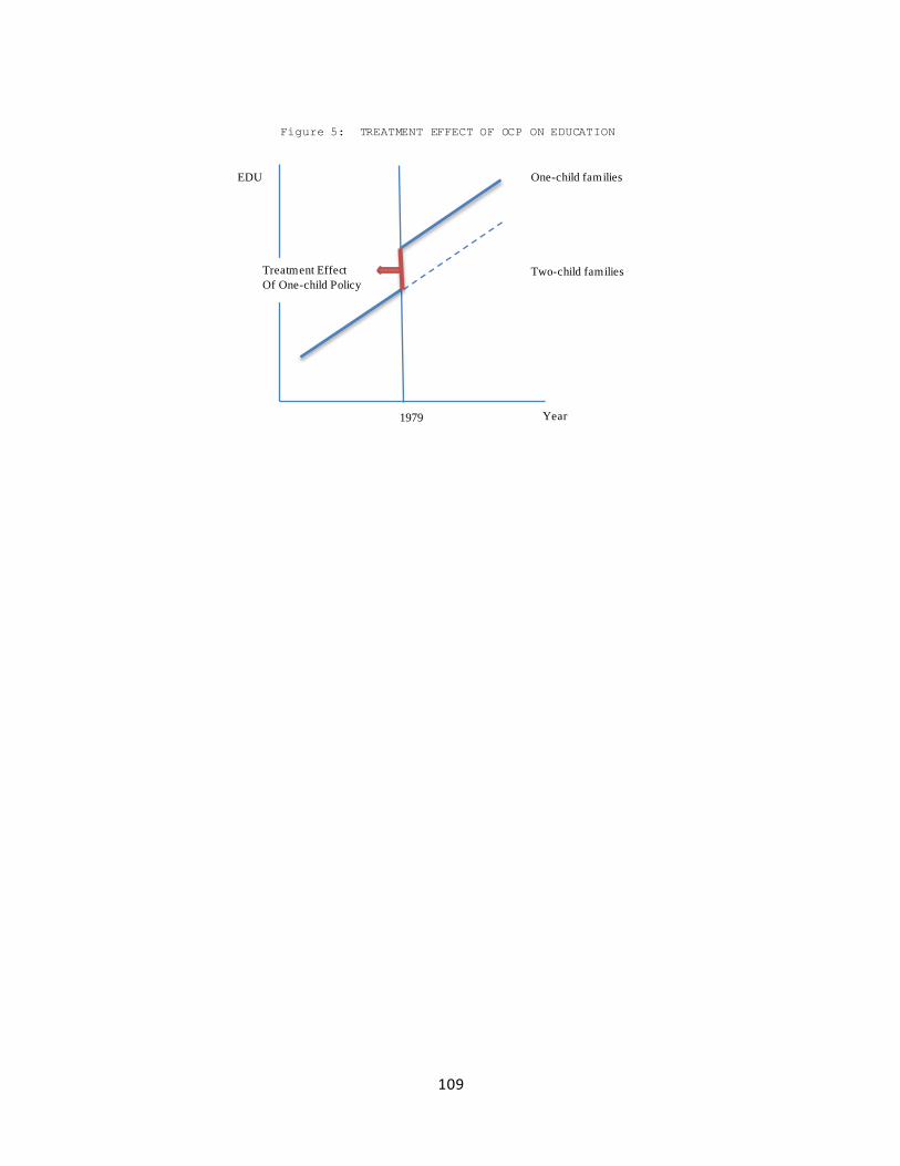
109
Figure 5: TREATMENT EFFECT OF OCP ON EDUCATION
EDU
Year
One-child families
Two-child families
1979
Treatment Effect
Of One-child Policy

110
Table 1 SUMMARY STATISTICS OF HOUSEHOLDS IN 2009
Treatment
Rural controls (OCP-cohort) Urban control (Before-cohort)
Control 1: Control 2: Control 3: Control 4:
2-child household 1-child household 2-child household 1-child household
Demographic Variables
Household size 3.51 [0.88] 5.02*** [1.27] 4.00
*** [1.24] 5.73
*** [1.86] 3.89
*** [1.42]
Average age of household 45.29 [7.64] 43.92** [8.71] 44.91 [8.62] 49.82
*** [9.79] 51.06
*** [10.48]
Percentage of males 0.48 [0.50] 0.46 [0.50] 0.49 [0.50] 0.48 [0.50] 0.48 [0.50]
If cadre in the household 0.13 [0.33] 0.06*** [0.24] 0.10
* [0.30] 0.18 [0.38] 0.20
*** [0.40]
Age of head 51.55 [5.59] 51.14 [4.19] 49.92*** [6.44] 60.12
*** [8.16] 57.97
*** [11.79]
Head is minority 0.1 [0.31] 0.17*** [0.38] 0.1 [0.30] 0.20
*** [0.40] 0.12 [0.33]
Education of head 10.27 [3.92] 7.94*** [3.58] 8.99
*** [4.06] 7.13
*** [5.38] 9.28
*** [5.33]
Education of head's spouse 9.62 [4.15] 5.85*** [4.36] 7.21
*** [4.22] 5.04
*** [5.78] 8.44
*** [5.32]
Education of children 14.74 [4.04] 10.84*** [3.51] 11.77
*** [3.81] 11.53
*** [4.50] 11.71
*** [4.03]
Percentage of male children 0.55 [0.50] 0.67*** [0.41] 0.77
*** [0.42] 0.87
*** [0.30] 0.77
*** [0.42]
Household's income and assets
Net household income 42944.84 [43883.28] 33567.96***
[36089.67] 38717.19 [85824.63] 47407.34 [40611.69] 40983.42 [31435.59]
Household wage income 33514.89 [32800.54] 19783.24***
[17349.10] 26637.27***
[43355.59] 42594.54***
[36668.38] 27116.01***
[24352.86]
Value of productive assets 18846.79 [64832.88] 7089.57***
[27230.53] 10066.59***
[31475.79] 15653.66 [52636.32] 11431.15** [30640.82]
Value of non-productive assets 11245.42 [10766.64] 6040.34***
[6265.93] 6550.73***
[6823.48] 12932.90* [14922.40] 10190.97 [8201.68]
Observations 342 182 453 115 257
Note:
(1) Standard deviations are reported in brackets. * denotes the level of significance on the equality of means between treatment and
control group using t-tests; * denotes significance level at 10%, ** at 5% level, and *** at 1% level.
(2) Productive assets include farm tools, transportation vehicles, computers and etc. Non-productive assets include furniture,
electronics and other consumptive investment.

111
Table 2 STATISTICS OF TREATMENT AND CONTROL GROUPS
Treatment Control 1 Control 2 Control 3 Control 4
Year of birth 1980-89 1980-89 1980-89 1970-79 1970-79
Hukou Status Urban Rural Rural Urban Urban
Number of children in the household 1 2 1 2 1
Total number of boys in the group 179 194 279 136 164
Total number of girls in the group 163 170 174 94 93
Total number of households 342 182 453 115 257
Table 3a IMPACTS OF OCP ON YEARS OF EDUCATION: OLS
Sample Urban and Rural Urban Rural
Control group Rural OCP-cohort Urban Before-cohort Rural Before-cohort
2-child
HH
1-child
HH
2-child
HH
1-child
HH
2-child
HH
1-child
HH
[1] [2] [3] [4] [5] [6]
OCP-cohort 1.018** 1.178
** 2.780
*** 3.127
*** 0.948
** 0.607
[0.327] [0.451] [0.628] [0.756] [0.343] [0.493]
OCP-cohort*Urban 1.645*** 1.178
*
[0.457] [0.465]
Urban 0.124 0.416+
[0.271] [0.252]
Male 1.263*** 1.423
*** 1.203
*** 0.936
** 1.566
*** 1.662
***
[0.191] [0.171] [0.324] [0.329] [0.208] [0.198]
Father's education 0.203*** 0.232
*** 0.244
*** 0.270
*** 0.190
*** 0.211
***
[0.033] [0.030] [0.065] [0.064] [0.033] [0.034]
Mother's education 0.107*** 0.210
*** 0.043 0.213
*** 0.161
*** 0.204
***
[0.031] [0.029] [0.052] [0.057] [0.033] [0.033]
Have cadre in
household 0.959
* 0.658
* 0.858 0.647 1.092
* 0.537
[0.386] [0.303] [0.549] [0.531] [0.434] [0.400]
Have school in
community 0.046 0.332 -0.178 0.756 0.408
+ 0.365
[0.231] [0.215] [0.704] [0.640] [0.240] [0.261]
Observations 1212 1428 453 456 927 972
NOTE:
(1) Robust standard errors are reported in brackets. *** denotes significance at the 0.1%
level, ** at the 1% level, * at the 5% level,
+ at the 10% level.
(2) Unreported explanatory variables include a cubic polynomial in age, the value of
household non-productive assets (furniture, electronics and other consumptive
investment), community characteristics such as whether the community is close to an open
trade area, the percentage of farm labor among all working age labor, the percentage of
migrants, the population growth rate of the community from 1989 to 2009, province
dummies, and a constant term.
(3) The variable "Have school in community" refers to either high school or tertiary
school locating within the community.

112
Table 3b IMPACTS OF OCP ON YEARS OF EDUCATION: MALE VS FEMALE
Sample Urban and Rural Urban Rural
Control group Rural OCP-cohort Urban Before-cohort Rural Before-cohort
2-child
HH
1-child
HH
2-child
HH
1-child
HH
2-child
HH
1-child
HH
[1] [2] [3] [4] [5] [6]
Male
OCP-cohort 1.381** 2.337
*** 4.416
*** 4.560
*** 1.697
** 1.458
+
[0.498] [0.638] [1.025] [1.062] [0.539] [0.766]
OCP-cohort*Urban 2.440*** 1.750
**
[0.643] [0.655]
Urban 0.161 0.229
[0.373] [0.351]
Father's education 0.324*** 0.421
*** 0.391
*** 0.448
*** 0.338
*** 0.389
***
[0.049] [0.044] [0.104] [0.108] [0.052] [0.049]
Mother's education -0.021 0.014 -0.082 0.011 0.022 0.015
[0.041] [0.036] [0.060] [0.085] [0.045] [0.040]
Have cadre 1.404* 1.155
** 1.532
* 0.721 1.404
* 1.064
*
[0.544] [0.415] [0.713] [0.634] [0.612] [0.532]
Have school in
community -0.264 0.401 -0.331 0.555 0.111 0.365
[0.310] [0.286] [0.975] [0.918] [0.329] [0.356]
Observations 532 647 197 192 427 455
Female
OCP-cohort 0.599 0.396 1.640+ 1.845 0.334 0.189
[0.468] [0.631] [0.893] [1.332] [0.483] [0.685]
OCP-cohort*Urban 1.506* 0.983
[0.684] [0.721]
Urban 0.156 0.833*
[0.412] [0.367]
Father's education 0.090* 0.044 0.008 0.045 0.051 0.029
[0.043] [0.038] [0.078] [0.095] [0.044] [0.043]
Mother's education 0.215*** 0.370
*** 0.155
* 0.372
*** 0.301
*** 0.367
***
[0.044] [0.043] [0.069] [0.086] [0.047] [0.049]
Have cadre 0.644 0.499 -0.131 0.423 1.285* 0.521
[0.509] [0.484] [0.698] [0.824] [0.654] [0.644]
Have school in
community 0.373 0.448 1.107 2.110
+ 0.717
* 0.647
+
[0.353] [0.326] [1.170] [1.158] [0.354] [0.377]
Observations 605 682 226 212 457 470
Note:
(1) Robust standard errors are reported in brackets. *** denotes significance at the 0.1%
level, ** at the 1% level, * at the 5% level,
+ at the 10% level.
(2) Unreported explanatory variables include all explanatory variables in Table 3a and
the gender wage ratio in the community.

113
Table 4 IMPACTS OF OCP ON HIGHEST DEGREE RECEIVED: LOGIT
Sample Urban and Rural Urban Rural
Control group Rural OCP-cohort Urban Before-cohort Rural Before-cohort
2-child
HH
1-child
HH
2-child
HH
1-child
HH
2-child
HH
1-child
HH
[1] [2] [3] [4] [5] [6]
University
OCP-cohort 1.076 2.091** 2.966
*** 2.513
*** 1.436 2.905
+
[0.701] [0.711] [0.735] [0.694] [1.016] [1.589]
OCP-cohort*Urban 1.249+ 0.603
[0.670] [0.563]
Urban 0.192 0.756
[0.609] [0.475]
Male 0.2 0.694* 0.486 0.453 0.796 1.426
**
[0.308] [0.286] [0.412] [0.340] [0.499] [0.552]
Observations 1212 1427 453 455 847 972
High school
OCP-cohort 0.711+ 0.422 1.514
** 0.902 0.557 0.453
[0.380] [0.434] [0.565] [0.718] [0.429] [0.585]
OCP-cohort*Urban 0.821+ 0.724
[0.462] [0.448]
Urban 0.271 0.034
[0.293] [0.238]
Male 0.138 0.670*** 0.241 0.223 0.639
** 1.014
***
[0.187] [0.162] [0.298] [0.266] [0.209] [0.219]
Observations 1041 1225 339 338 851 887
Junior technical school
OCP-cohort 0.946* 1.034 1.663
* 2.417
+ 1.151
* 0.303
[0.457] [0.674] [0.830] [1.418] [0.584] [0.636]
OCP-cohort*Urban 0.389 0.808
[0.595] [0.576]
Urban 1.108* 0.740
+
[0.471] [0.439]
Male 0.33 0.39 0.575 -0.012 0.49 0.536+
[0.268] [0.259] [0.466] [0.485] [0.362] [0.326]
Observations 960 1061 302 270 748 711
NOTE:
(1) Robust standard errors are reported in brackets. *** denotes significance at the
0.1% level, ** at the 1% level, * at the 5% level, + at the 10% level.
(2) Unreported explanatory variables are the same as in Table 3a.

114
Table 5 TEST FOR EXCLUSION CRITERIA OF LATE ESTIMATION
Sample Urban and Rural Urban Rural
Control group Rural OCP-cohort Urban Before-cohort Rural Before-cohort
2-child
HH
1-child
HH
2-child
HH
1-child
HH
2-child
HH
1-child
HH
[1] [2] [3] [4] [5] [6]
Without education
OCP-cohort 0.867*** 0.554
*** 1.036
*** 0.775
** 0.833
*** 0.568
***
[0.133] [0.140] [0.198] [0.243] [0.147] [0.164]
OCP-cohort*Urban 0.031 0.294*
[0.165] [0.147]
Urban 0.229+ 0.104
[0.128] [0.112]
With education
OCP-cohort 0.863*** 0.550
*** 0.851
*** 0.561
* 0.803
*** 0.575
***
[0.133] [0.139] [0.198] [0.238] [0.148] [0.165]
OCP-cohort*Urban -0.106 0.184
[0.173] [0.153]
Urban 0.2 0.105
[0.128] [0.110]
Education, years 0.047*** 0.043
*** 0.063
*** 0.063
*** 0.036
* 0.033
*
[0.012] [0.011] [0.017] [0.018] [0.016] [0.015]
Observations 512 651 252 265 363 386
NOTE:
(1) Robust standard errors are reported in brackets. *** denotes significance at the
0.1% level, ** at the 1% level, * at the 5% level, + at the 10% level.
(2) Unreported explanatory variables are the same as in Table
3a.

115
Table 6a WAGE EQUATION FIRSTSTAGE
Sample Urban and Rural Urban Rural
Control group Rural OCP-cohort Urban Before-cohort Rural Before-cohort
2-child HH 1-child HH 2-child HH 1-child HH 2-child HH 1-child HH
[1] [2] [3] [4] [5] [6]
All sample
OCP-cohort 0.084 0.097 2.921*** 3.403
*** 0.833 -0.213
[0.572] [0.798] [0.867] [0.978] [0.618] [0.843]
OCP-cohort*Urban 2.925*** 2.554
***
[0.725] [0.724]
Father's education 0.333*** 0.403
*** 0.340
*** 0.497
*** 0.356
*** 0.350
***
[0.051] [0.043] [0.081] [0.070] [0.053] [0.053]
Mother's education 0.110* 0.154
*** 0.067 0.185
** 0.126
* 0.135
**
[0.046] [0.037] [0.059] [0.067] [0.051] [0.042]
Male
OCP-cohort 0.151 0.847 4.445*** 4.091
** 0.885 0.581
[0.884] [1.037] [1.111] [1.389] [0.910] [1.150]
OCP-cohort*Urban 3.459** 2.604
*
[1.100] [1.085]
Father's education 0.479*** 0.564
*** 0.476
*** 0.620
*** 0.540
*** 0.532
***
[0.068] [0.047] [0.104] [0.094] [0.070] [0.054]
Mother's education -0.018 -0.004 -0.051 -0.01 0.01 0.002
[0.057] [0.035] [0.059] [0.077] [0.063] [0.037]
Female
OCP-cohort -0.032 0.026 1.608 2.343
+ 0.418 -0.666
[0.731] [1.094] [1.300] [1.222] [0.781] [1.185]
OCP-cohort*Urban 1.995* 1.002
[0.959] [0.971]
Father's education 0.164* 0.182
** 0.12 0.332
** 0.146
+ 0.087
[0.068] [0.065] [0.122] [0.100] [0.080] [0.087]
Mother's education 0.243*** 0.372
*** 0.195
+ 0.395
*** 0.305
*** 0.351
***
[0.069] [0.061] [0.102] [0.097] [0.077] [0.075]

116
Table 6b IMPACTS OF OCP ON WAGE: 2SLS
Sample Urban and Rural Urban Rural
Control group Rural OCP-cohort Urban Before-cohort Rural Before-cohort
2-child HH 1-child HH 2-child HH 1-child HH 2-child HH 1-child HH
[1] [2] [3] [4] [5] [6]
Total
Years of education 0.065** 0.049
* 0.114
*** 0.061
* 0.062
+ 0.026
[0.022] [0.019] [0.034] [0.026] [0.033] [0.030]
Male 0.483*** 0.421
*** 0.514
*** 0.506
*** 0.494
*** 0.379
***
[0.081] [0.072] [0.110] [0.102] [0.118] [0.100]
1st stage F-test 89.2 173.05 34.57 80.48 69.71 79.66
Observations 512 651 252 265 363 386
Male
Years of education 0.029 0.033 0.077* 0.038 0.019 0.035
[0.026] [0.022] [0.037] [0.034] [0.035] [0.031]
1st stage F-test 62.54 161.37 28.65 61.3 72.86 101.03
Observations 269 382 133 142 210 240
Female
Years of education 0.081
* 0.056
* 0.107
+ 0.076
* 0.140
** -0.003
[0.036] [0.025] [0.057] [0.031] [0.049] [0.038]
1st stage F-test 34.54 73.64 10.09 35.44 24.72 35.17
Observations 243 269 119 123 153 146
NOTE:
(1) Robust standard errors are reported in brackets. Restricted F-tests are reposted. ***
denotes significance at the 0.1% level, ** at the 1% level, * at the 5% level, + at the 10%
level.
(2) Unreported explanatory variables are the same as in Table 3a.

117
Table 7 PARALLEL TREND TESTS IN EDUCATION: : DID 1960-69 VS 1970-79
Sample Urban and Rural Urban Rural
Control group Rural OCP-cohort Urban Before-cohort Rural Before-cohort
2-child HH 1-child HH 2-child HH 1-child HH 2-child HH 1-child HH
[1] [2] [3] [4] [5] [6]
All sample
OCP-cohort 0.788+ -0.214 0.381 -0.023 0.18 -0.427
[0.404] [0.435] [0.842] [0.782] [0.550] [0.480]
OCP-cohort*Urban -0.262 0.362
[0.644] [0.635]
Observations 853 821 238 286 417 535
Male
OCP-cohort 0.875 -0.563 0.01 -0.548 0.499 -0.381
[0.571] [0.660] [1.217] [1.367] [0.839] [0.774]
OCP-cohort*Urban -0.496 0.396
[0.975] [1.063]
Observations 356 368 99 124 189 244
Female
OCP-cohort 0.383 -0.433 1.283 -0.178 -0.303 -0.738
[0.538] [0.599] [1.248] [0.898] [0.708] [0.661]
OCP-cohort*Urban 0.267 0.165
[0.905] [0.847]
Observations 446 403 111 135 216 268