essays in local labor economics - harvard university

Essays in Local Labor EconomicsThe Harvard community has made this

article openly available. Please share howthis access benefits you. Your story matters

Citation Diamond, Rebecca. 2013. Essays in Local Labor Economics.Doctoral dissertation, Harvard University.

Citable link http://nrs.harvard.edu/urn-3:HUL.InstRepos:12362593

Terms of Use This article was downloaded from Harvard University’s DASHrepository, and is made available under the terms and conditionsapplicable to Other Posted Material, as set forth at http://nrs.harvard.edu/urn-3:HUL.InstRepos:dash.current.terms-of-use#LAA

http://osc.hul.harvard.edu/dash/open-access-feedback?handle=&title=Essays%20in%20Local%20Labor%20Economics&community=1/1&collection=1/4927603&owningCollection1/4927603&harvardAuthors=929586e81192fd14afc415844e0ee7cc&departmentEconomics

http://nrs.harvard.edu/urn-3:HUL.InstRepos:12362593

http://nrs.harvard.edu/urn-3:HUL.InstRepos:dash.current.terms-of-use#LAA



Essays in Local Labor Economics

A dissertation presented

by

Rebecca Randolph Diamond

to

The Department of Economics

in partial ful�llment of the requirements

for the degree of

Doctor of Philosophy

in the subject of

Economics

Harvard University

Cambridge, Massachusetts

April 2013

c 2013 Rebecca Randolph Diamond

All rights reserved.

Disseration Advisor: Lawrence Katz Rebecca Randolph Diamond

Essays in Local Labor Economics

Abstract

This dissertation consists of three independent chapters. Chapter 1 examines the

determinants and welfare implications of the increased geographic of workers by skill

from 1980 to 2000. I estimate a structural spatial equilibrium model of local labor

demand, housing supply, labor supply, and amenity levels. The estimates indicate that

cross-city changes in �rms�demands for high and low skill labor were the underlying

forces driving the increase in geographic skill sorting. I �nd that the combined e¤ects

of changes in cities�wages, rents, and endogenous amenities increased well-being in-

equality between high school and college graduates by a signi�cantly larger amount

than would be suggested by the increase in the college wage gap alone.

Chapter 2 examines the abilities of state and local governments to extract rent

from private sector workers by charging high tax rates and paying government workers

high wages. Using a spatial equilibrium model where private sector workers are free

to migrate across government jurisdictions, I show that variation in areas� housing

supply elasticities di¤erentially restrains governments� abilities to extract rent from

private sector workers. Governments in less housing elastic areas can charge higher

taxes without worry of shrinking their tax bases. I test the model�s predictions by

using worker wage data from the CPS-MORG. I �nd the public-private sector wage

gap is higher in areas with less elastic housing supplies.

Chapter 3 studies the standard practice in regression analyses to allow for clustering

in the error covariance matrix when an explanatory variable varies at a more aggregate

level than the units of observation. However, the structure of the error covariance

matrix may be more complex, with correlations not vanishing for units in di¤erent

clusters. I show that with equal-sized clusters, if the covariate of interest is randomly

assigned at the cluster level, only accounting for non-zero covariances at the cluster

iii

level, and ignoring correlations between clusters as well as di¤erences in within-cluster

correlations, leads to valid con�dence intervals. However, in the absence of random

assignment of the covariates, ignoring general correlation structures may lead to biases

in standard errors.

iv

Acknowledgements

I would like to thank my advisors, professors Lawrence Katz, Ariel Pakes, and Edward

Glaeser for their advice, help, and support throughout my graduate studies. Their guidance

has been crucial to the completion of this dissertation and shaping my abilities to produce

economic research.

In the past �ve years I have bene�tted from many interactions with other economics

graduate students and professors at Harvard University. In particular, I would like to ac-

knowledge my peers Nikhil Agarwal and Adam Guren. Their thoughts and advice from many

long discussions have helped me through every step of the research process. I would also

like to thank my co-authors Guido Imbens, Michal Kolesar, and Thomas Barrios. The third

chapter of this disseration is our joint work which my co-authors heavily helped produce.

This chapter has been published in the Journal of the American Statistical Association,

volume 107, 2012.

v

Contents

Introduction . . . . . . . . . . . . . . . . . . . . . . . . . . . . . . . . . . . . . . . 1

1 The Determinants and Welfare Implications of US Workers�Diverging

Location Choices by Skill: 1980-2000 . . . . . . . . . . . . . . . . . . . . . . 4

1.1 Introduction . . . . . . . . . . . . . . . . . . . . . . . . . . . . . . . . . . . . 4

1.2 Data . . . . . . . . . . . . . . . . . . . . . . . . . . . . . . . . . . . . . . . . 11

1.3 Reduced Form Facts . . . . . . . . . . . . . . . . . . . . . . . . . . . . . . . 15

1.4 An Empirical Spatial Equilibrium Model of Cities . . . . . . . . . . . . . . . 24

1.4.1 Labor Demand . . . . . . . . . . . . . . . . . . . . . . . . . . . . . . 25

1.4.2 Housing Supply . . . . . . . . . . . . . . . . . . . . . . . . . . . . . . 28

1.4.3 Amenity Supply . . . . . . . . . . . . . . . . . . . . . . . . . . . . . . 30

1.4.4 Labor Supply to Cities . . . . . . . . . . . . . . . . . . . . . . . . . . 31

1.4.5 Equilibrium . . . . . . . . . . . . . . . . . . . . . . . . . . . . . . . . 37

1.5 Estimation . . . . . . . . . . . . . . . . . . . . . . . . . . . . . . . . . . . . . 38

1.5.1 Labor Demand . . . . . . . . . . . . . . . . . . . . . . . . . . . . . . 38

1.5.2 Housing Supply . . . . . . . . . . . . . . . . . . . . . . . . . . . . . . 43

1.5.3 Labor Supply . . . . . . . . . . . . . . . . . . . . . . . . . . . . . . . 43

1.5.4 Summary of Estimating Equations . . . . . . . . . . . . . . . . . . . 46

1.6 Parameter Estimates . . . . . . . . . . . . . . . . . . . . . . . . . . . . . . . 48

1.6.1 Worker Labor Supply . . . . . . . . . . . . . . . . . . . . . . . . . . . 48

1.6.2 Housing Supply . . . . . . . . . . . . . . . . . . . . . . . . . . . . . . 56

1.6.3 Labor Demand . . . . . . . . . . . . . . . . . . . . . . . . . . . . . . 56

1.6.4 Estimation Robustness . . . . . . . . . . . . . . . . . . . . . . . . . . 58

1.7 Amenities & Productivity Across Cities . . . . . . . . . . . . . . . . . . . . . 64

1.7.1 The Determinants of Cities�College Employment Ratio Changes . . . 69

1.7.2 College Employment Ratio Changes and Productivity . . . . . . . . . 69

vi

1.7.3 Corroborating Reduced Form Evidence . . . . . . . . . . . . . . . . . 73

1.7.4 Summary of Skill Sorting Mechanisms . . . . . . . . . . . . . . . . . 80

1.8 Welfare Implications & Well-Being Inequality . . . . . . . . . . . . . . . . . 80

1.9 Conclusion . . . . . . . . . . . . . . . . . . . . . . . . . . . . . . . . . . . . . 87

2 Housing Supply Elasticity and Rent Extraction by State and Local Gov-

ernments . . . . . . . . . . . . . . . . . . . . . . . . . . . . . . . . . . . . . . . . 88

2.1 Introduction . . . . . . . . . . . . . . . . . . . . . . . . . . . . . . . . . . . . 88

2.2 Model . . . . . . . . . . . . . . . . . . . . . . . . . . . . . . . . . . . . . . . 93

2.2.1 Government . . . . . . . . . . . . . . . . . . . . . . . . . . . . . . . . 93

2.2.2 Workers . . . . . . . . . . . . . . . . . . . . . . . . . . . . . . . . . . 94

2.2.3 Firms . . . . . . . . . . . . . . . . . . . . . . . . . . . . . . . . . . . 94

2.2.4 Housing . . . . . . . . . . . . . . . . . . . . . . . . . . . . . . . . . . 95

2.2.5 Equilibrium in Labor and Housing . . . . . . . . . . . . . . . . . . . 95

2.2.6 Government Tax Competition . . . . . . . . . . . . . . . . . . . . . . 96

2.3 Empirical Evidence . . . . . . . . . . . . . . . . . . . . . . . . . . . . . . . . 100

2.3.1 Wage Gap Regressions . . . . . . . . . . . . . . . . . . . . . . . . . . 103

2.3.2 Falsi�cation Tests . . . . . . . . . . . . . . . . . . . . . . . . . . . . . 113

2.3.3 Bene�ts . . . . . . . . . . . . . . . . . . . . . . . . . . . . . . . . . . 119

2.4 Conclusion . . . . . . . . . . . . . . . . . . . . . . . . . . . . . . . . . . . . . 121

3 Clustering, Spatial Correlations and Randomization Inference . . . . . . . 123

3.1 Introduction . . . . . . . . . . . . . . . . . . . . . . . . . . . . . . . . . . . . 123

3.2 Framework . . . . . . . . . . . . . . . . . . . . . . . . . . . . . . . . . . . . . 125

3.3 Spatial Correlation Patterns in Earnings . . . . . . . . . . . . . . . . . . . . 128

3.4 Randomization Inference . . . . . . . . . . . . . . . . . . . . . . . . . . . . . 139

3.5 Randomization Inference with Cluster-level Randomization . . . . . . . . . . 142

3.6 Variance Estimation Under Misspeci�cation . . . . . . . . . . . . . . . . . . 144

vii

3.7 Spatial Correlation in State Averages . . . . . . . . . . . . . . . . . . . . . . 146

3.8 A Small Simulation Study . . . . . . . . . . . . . . . . . . . . . . . . . . . . 151

3.9 Conclusion . . . . . . . . . . . . . . . . . . . . . . . . . . . . . . . . . . . . . 155

A Chapter 1 Appendix . . . . . . . . . . . . . . . . . . . . . . . . . . . . . . . . 164

A.1 Data Appendix . . . . . . . . . . . . . . . . . . . . . . . . . . . . . . . . . . . 164

A.2 Estimation Appendix . . . . . . . . . . . . . . . . . . . . . . . . . . . . . . . 166

A.2.1 Labor Demand . . . . . . . . . . . . . . . . . . . . . . . . . . . . . . 166

A.2.2 Housing Supply . . . . . . . . . . . . . . . . . . . . . . . . . . . . . . 170

A.2.3 Labor Supply . . . . . . . . . . . . . . . . . . . . . . . . . . . . . . . 171

A.2.4 Estimation of wage, local price, and amenity preferences . . . . . . . 172

A.3 Dynamic Adjustment & Equilibrium Stability . . . . . . . . . . . . . . . . . 175

A.4 Comparison of Productivity Estimates to Outside Research . . . . . . . . . . 181

A.5 College Share Changes and Housing Supply Elasticity . . . . . . . . . . . . . 184

A.6 Microfounding Endogenous Amenities . . . . . . . . . . . . . . . . . . . . . . 186

A.6.1 Workers�demand for local goods . . . . . . . . . . . . . . . . . . . . 187

A.6.2 Firms�supply of local goods . . . . . . . . . . . . . . . . . . . . . . . 188

A.6.3 Comparative Statics . . . . . . . . . . . . . . . . . . . . . . . . . . . 190

A.7 Supplementary Tables and Figures . . . . . . . . . . . . . . . . . . . . . . . 192

B Chapter 2 Appendix . . . . . . . . . . . . . . . . . . . . . . . . . . . . . . . . 202

B.1 Income Tax . . . . . . . . . . . . . . . . . . . . . . . . . . . . . . . . . . . . 202

B.1.1 Government . . . . . . . . . . . . . . . . . . . . . . . . . . . . . . . . 202

B.1.2 Workers . . . . . . . . . . . . . . . . . . . . . . . . . . . . . . . . . . 202

B.1.3 Firms . . . . . . . . . . . . . . . . . . . . . . . . . . . . . . . . . . . 202

B.1.4 Housing . . . . . . . . . . . . . . . . . . . . . . . . . . . . . . . . . . 203

B.1.5 Equilibrium in Labor and Housing . . . . . . . . . . . . . . . . . . . 203

B.1.6 Government Tax Competition . . . . . . . . . . . . . . . . . . . . . . 204

viii

B.2 Property Tax . . . . . . . . . . . . . . . . . . . . . . . . . . . . . . . . . . . 205

B.2.1 Government . . . . . . . . . . . . . . . . . . . . . . . . . . . . . . . . 205

B.2.2 Workers . . . . . . . . . . . . . . . . . . . . . . . . . . . . . . . . . . 205

B.2.3 Firms . . . . . . . . . . . . . . . . . . . . . . . . . . . . . . . . . . . 205

B.2.4 Housing . . . . . . . . . . . . . . . . . . . . . . . . . . . . . . . . . . 206

B.2.5 Equilibrium in Labor and Housing . . . . . . . . . . . . . . . . . . . 206

B.2.6 Government Tax Competition . . . . . . . . . . . . . . . . . . . . . . 206

C Chapter 3 Appendix . . . . . . . . . . . . . . . . . . . . . . . . . . . . . . . . 209

ix

Introduction

This dissertation consists of three independent chapters all related to local labor mar-

ket economics. Chapter 1 studies the causes and welfare consequences of the increase in

geographic sorting of workers by skill from 1980 to 2000. During this time period, the sub-

stantial rise in the U.S. college-high school graduate wage gap coincided with an increase

in geographic sorting as college graduates increasingly concentrated in high wage, high rent

metropolitan areas, relative to lower skill workers. The increase in wage inequality may

not re�ect a similar increase in well-being inequality because high and low skill workers

increasingly paid di¤erent housing costs and consumed di¤erent local amenities.

This chapter examines the determinants and welfare implications of the increased geo-

graphic skill sorting. I estimate a structural spatial equilibrium model of local labor de-

mand, housing supply, labor supply, and amenity levels. The model allows local amenity

and productivity levels to endogenously respond to a city�s skill-mix. I identify the model

parameters using local labor demand changes driven by variation in cities�industry mixes

and interactions of these labor demand shocks with determinants of housing supply (land

use regulations and land availability). The GMM estimates indicate that cross-city changes

in �rms�demands for high and low skill labor were the underlying forces of the increase

in geographic skill sorting. An increase in labor demand for college relative to non-college

workers increases a city�s college employment share, which then endogenously raises the local

productivity of all workers and improves local amenities. Local wage and amenity growth

generates in-migration, driving up rents. My estimates show that low skill workers are less

willing to pay high housing costs to live in high-amenity cities, leading them to elect more

a¤ordable, low-amenity cities. I �nd that the combined e¤ects of changes in cities�wages,

rents, and endogenous amenities increased well-being inequality between high school and

college graduates by a signi�cantly larger amount than would be suggested by the increase

in the college wage gap alone.

1

Chapter 2 examines the abilities of state and local governments to extract rent from

private sector workers by charging high tax rates and spending the revenue on non-social

desirable projects, such as excessive government worker wages. Using a spatial equilibrium

model where private sector workers are free to migrate across government jurisdictions, I

show that private sector workers�migration elasticity with respect to local taxes determines

the magnitude of rent extraction by rent seeking state and local governments. Since private

sector workers �vote with their feet�by migrating out of rent extractive areas, governments

trade o¤ the bene�ts a higher tax rate with the cost of a smaller population to tax.

Variation in areas�housing supply elasticities di¤erentially restrains governments�abilities

to extract rent from private sector workers. The incidence of a tax increase falls more on

local housing prices in a less housing elastic area, leading to less out-migration. Thus,

governments in less housing elastic areas can charge higher taxes without worry of shrinking

their tax bases. I test the model�s predictions by using worker wage data from the CPS-

MORG. I �nd the public-private sector wage gap is higher in areas with less elastic housing

supplies. This fact holds both within state across metropolitan areas for local government

workers and between states for state government workers.

In Chapter 3, which is joint work with Guido Imbens, Michal Kolesar, and Thomas

Barrios, we examine the standard practice in regression analyses of allowing for clustering

in the error covariance matrix when the explanatory variable of interest varies at a more

aggregate level (e.g., the state level) than the units of observation (e.g., individuals). Often,

however, the structure of the error covariance matrix is more complex, with correlations not

vanishing for units in di¤erent clusters. Here we explore the implications of such correlations

for the actual and estimated precision of least squares estimators. Our main theoretical result

is that with equal-sized clusters, if the covariate of interest is randomly assigned at the cluster

level, only accounting for non-zero covariances at the cluster level, and ignoring correlations

between clusters as well as di¤erences in within-cluster correlations, leads to valid con�dence

intervals. However, in the absence of random assignment of the covariates, ignoring general

2

correlation structures may lead to biases in standard errors. We illustrate our �ndings using

the 5% public use census data. Based on these results we recommend that researchers as a

matter of routine explore the extent of spatial correlations in explanatory variables beyond

state level clustering.

3

Chapter 1The Determinants and Welfare Implications of USWorkers�Diverging Location Choices by Skill:

1980-2000

1.1 Introduction

The dramatic increase in the wage gap between high school and college graduates over the

past three decades has been accompanied by a substantial increase in geographic sorting of

workers by skill.1 Metropolitan areas which had a disproportionately high share of college

graduates in 1980 further increased their share of college graduates from 1980 to 2000.

Increasingly high skill cities also experienced higher wage and housing price growth than less

skilled cities (Moretti (2004b), Shapiro (2006)). Moretti (2012) coins this phenomenon "The

Great Divergence."

These facts call into question whether the increase in the college wage gap re�ects a sim-

ilar increase in the college well-being gap. Since college graduates increasingly live in areas

with high housing costs, local price levels might o¤set some of the consumption bene�ts of

their high wages, making the increase in wage inequality overstate the increase in consump-

tion or well-being inequality (Moretti (2011b)). Alternatively, high housing cost cities may

o¤er workers desirable amenities, compensating them for high house prices, and possibly

increasing the well-being of workers in these cities. The welfare implications of the increased

geographic skill sorting depend on why high and low skill workers increasingly chose to live

in di¤erent cities.

This paper examines the determinants of high and low skill workers�choices to increas-

ingly segregate themselves into di¤erent cities and the welfare implications of these choices.

By estimating a structural spatial equilibrium model of local labor demand, housing supply,

1This large increase in wage inequality has led to an active area of research into the drivers of changes inthe wage distribution nationwide. See Goldin and Katz (2007) for a recent survey.

4

labor supply, and amenity levels in cities, I show that changes in �rms�relative demands for

high and low skill labor across cities, due to local productivity changes, were the underlying

drivers of the di¤erential migration patterns of high and low skill workers.2 Despite local

wage changes being the initial cause of workers�migration, I �nd that cities which attracted

a higher share of college graduates endogenously became more desirable places to live and

more productive for both high and low skill labor. The combination of desirable wages

and amenities made college workers willing to pay high housing costs to live in these cities.

While lower skill workers also found these areas�wages and amenities desirable, they were

less willing to pay high housing costs, leading them to choose more a¤ordable cities. Overall,

I �nd that the welfare e¤ects of changes in local wages, rents, and endogenous amenities led

to an increase in well-being inequality between college and high school graduates which was

signi�cantly larger than would be suggested by the increase in the college wage gap alone.

To build intuition for this e¤ect, consider the metropolitan areas of Detroit and Boston.

The economic downturn in Detroit has been largely attributed to decline of auto manu-

facturing (Martelle (2012)), but the decline goes beyond the loss of high paying jobs. In

2009, Detroit public schools had the lowest scores ever recorded in the 21-year history of

the national math pro�ciency test (Winerip (2011)). Historically, the Detroit school district

had not always been in such a poor state. In the early 20th century, when manufacturing

was booming, Detroit�s public school system was lauded as a model for the nation in urban

education (Mirel (1999)).

By comparison, Boston has increasingly attracted high skill workers with its cluster of

biotech, medical device, and technology �rms. In the mid 1970s, Boston public schools were

declining in quality, driven by racial tensions from integrating the schools (Cronin (2011)).

In 2006, however, the Boston public school district won the Broad Prize, which honors the

urban school district that demonstrates the greatest overall performance and improvement

2Work by Berry and Glaeser (2005) and Moretti (2011b) come to similar conclusions. Berry and Glaeser(2005) consider the role of entrepreneurship in cities. Moretti (2011b) analyzes the di¤erential labor demandsfor high and low skill workers across industries.

5

in student achievement while reducing achievement gaps among low-income and minority

students. Similar patterns can be seen in the histories of the Detroit and Boston Symphony

Orchestras.3 The prosperity of Boston and decline of Detroit go beyond jobs and wages,

directly impacting the amenities and quality-of-life in these areas.

I illustrate these mechanisms more generally using U.S. Census data by estimating a

structural spatial equilibrium model of cities. The setup shares features of the Rosen (1979)

and Roback (1982) frameworks, but I extend the model to allow workers to have heterogenous

preferences for cities. The fully estimated model allows me to assess the importance of

changes in cities�wages, rents, and amenities in di¤erentially driving high and low skill

workers to di¤erent cities.

I use a static discrete choice setup to model workers�city choices.4 The model allows

workers with di¤erent demographics to di¤erentially trade o¤ the relative values of cities�

characteristics, leading them to make di¤erent location decisions.5 Workers maximize their

utility by living in the city which o¤ers them the most desirable bundle of wages, housing

rent, and amenities.

Firms in each city use capital, high skill labor, and low skill labor as inputs into produc-

tion. High and low skill labor have a constant elasticity of substitution in �rms�production

functions. I assume capital is sold in a national market, while labor is hired locally in a per-

fectly competitive labor market. Housing markets di¤er across cities due to heterogeneity in

their elasticity of housing supply.

The key distinguishing worker characteristic is skill, as measured by graduation from a

4-year college. Cities�local productivity levels di¤er across high and low skill workers, and

3The Detroit Symphony Orchestra was one of the top in the nation during the 1950s. More recently, ithas defaulted on loans, and is facing a labor dispute over wage cuts driven by decreased ticket sales andcorporate donations. (Bennett (2010)) The Boston Symphony Orchestra, however, continues to be one ofthe best in the world.

4The model could be extended to allow for dynamics, as done by Kennan and Walker (2011) and Bishop(2010). However, panel data is needed to estimate a model of this nature. I focus on the role of preferenceheterogeneity in determining long run migration patterns, while Kennan and Walker (2011) and Bishop(2010) focus exclusively on high-school graduates and life-cycle migration patterns.

5Estimation of spatial equilibrium models when households have heterogeneous preferences using hedonicshave been analyzed by Epple and Sieg (1999).

6

the productivity levels of both high and low skill workers within a city are endogenously

impacted by the skill-mix in the city. Thus, changes in the skill-mix of a city will impact

local wages both by moving along �rms� labor demand curves and by directly impacting

worker productivity.

A city�s skill-mix is also allowed to in�uence local amenity levels, both directly, as more

educated neighbors may be desirable, and indirectly by improving a variety of city amenities

(Chapter 5 in Becker and Murphy (2000)). Indeed, observable amenities such as bars and

restaurants per capita, crime rates, and pollution levels improve in areas with larger college

populations and decline in areas with larger non-college populations. I use the ratio of

college to non-college employees in each city as a unidimensional index for all amenities that

endogenously respond to the demographics of cities�residents.

Workers�preferences for cities are estimated using a two-step estimator, similar to the

methods used by Berry, Levinsohn, and Pakes (2004) and the setup proposed by McFadden

(1973). In the �rst step, a maximum likelihood estimator is used to identify how desirable

each city is to each type of worker, on average, in each decade, controlling for workers�pref-

erences to live close to their state of birth. The utility levels for each city estimated in the

�rst step are used in the second step to estimate how workers trade o¤ wages, rents, and

amenities when selecting a location to live. The second step of estimation uses a simultane-

ous equation non-linear GMM estimator. Moment restrictions on workers�preferences are

combined with moments identifying cities�labor demand and housing supply curves. These

moments are used to simultaneously estimate local labor demand, housing supply, and labor

supply to cities.

The model is identi�ed using local labor demand shocks driven by the industry mix in each

city and their interactions with local housing supply elasticities. Variation in productivity

changes across industries di¤erentially impact cities� local labor demand for high and low

skill workers based on the industrial composition of the city�s workforce (Bartik (1991)). I

measure exogenous local productivity changes by interacting cross-sectional di¤erences in

7

industrial employment composition with national changes in industry wage levels separately

for high and low skill workers.

I allow cities� housing supply elasticities to vary based on geographic constraints on

developable land around a city�s center and land-use regulations (Saiz (2010), Gyourko,

Saiz, and Summers (2008)). A city�s housing supply elasticity will in�uence the equilibrium

wage, rent, and population response to the labor demand shocks driven by industrial labor

demand changes.

Workers�migration responses to changes in cities�wages, rents, and endogenous ameni-

ties driven by the Bartik labor demand shocks and the interactions of these labor demand

shocks with housing supply elasticity determinants identify workers�preferences for cities�

characteristics. Housing supply elasticities are identi�ed by the response of housing rents to

the Bartik shocks across cities.

The interaction of the Bartik productivity shocks with cities�housing markets identi�es

the labor demand elasticities. The wage di¤erences, driven by the productivity shocks, induce

workers to migrate to cities which o¤er more desirable wages. The migration drives demand

in the local housing markets, which impacts house prices, as determined by the elasticity of

housing supply. Heterogeneity in housing supply elasticity leads to di¤erences in population

changes, in response to a given Bartik shock. For a given size labor demand shock, fewer

workers will migrate to a city with a less elastic housing supply because rents increase more

than in a more elastic city. Thus, the interaction of Bartik shocks with measures of housing

supply elasticity creates variation in high and low skill local populations which is independent

of unobserved local productivity changes, which can identify labor demand elasticities.

The parameter estimates of workers�preferences show that while both college and non-

college workers �nd higher wages, lower rents, and higher amenity levels desirable, high skill

workers�demand is relatively more sensitive to amenity levels and low skill workers�demand

is more sensitive to wages and rents.6 The labor demand estimates show that increases

6These results are consistent with a large body of work in empirical industrial organization which �ndssubstantial heterogeneity in consumers�price sensitivites. A Consumer�s price sensitivity is also found to be

8

in the college employment ratio leads to productivity spillovers on both college and non-

college workers. Combining the estimates of �rms�elasticity of labor substitution with the

productivity spillovers, I �nd that an increase in a city�s college worker population raises

both local college and non-college wages. Similarly, an increase in a city�s non-college worker

population decreases college and non-college wages.

Using the estimated model, I decompose the changes in cities�college employment ratios

into the underlying changes in labor demand, housing supply, and labor supply to cities. I

show that when a city�s productivity gap between high and low skill workers exogenously

increases, the local wage gap between these workers increases. If the migration responses to

these wage changes lead to an increase in the local share of college workers, the wages of

all workers will further increase beyond the initial e¤ect of the productivity change due to

the combination of endogenous productivity changes and shifts along �rms�labor demand

curves.

In addition to raising wages, an increase in a city�s college employment ratio leads to

local amenity improvements. The combination of desirable wage and amenity growth for all

workers causes large amounts of in-migration, as college workers are particularly attracted

by desirable amenities, while low skill workers are particularly attracted by desirable wages.

The increased housing demand in high college share cities leads to large rent increases. Since

low skill workers are more price sensitive, the increases in rent disproportionately discourage

low skill workers from living in these high wage, high amenity cities. Lower skill workers are

not willing to pay the �price�of a lower real wage to live in high amenity cities. Thus, in

equilibrium, college workers sort into high wage, high rent, high amenity cities.

I use the model estimates to quantify the change in well-being inequality. I �nd the

welfare impacts due to wage, rent, and endogenous amenity changes from 1980 to 2000 led

to an increase in well-being inequality equivalent to at least a 24 percentage point increase

in the college wage gap, which is 20% more than the actual increase in the college wage gap.

closely linked to his income. See Nevo (2010) for a review of this literature.

9

In other words, the additional utility college workers gained from of being able to consume

more desirable amenities made them better o¤ relative to high school graduates, despite the

high local housing prices.

This paper is related to several literatures. Most closely related to this paper is work

studying how local wages, rents, and employment respond to local labor demand shocks

(Topel (1986), Bartik (1991), Blanchard and Katz (1992), Saks (2008), Notowidigdo (2011).

See Moretti (2011a) for a review.) Traditionally, this literature has only allowed local labor

demand shocks to in�uence worker migration through wage and rents changes.7 My results

suggest that endogenous local amenity changes are an important mechanism driving workers�

migration responses to local labor demand shocks.

A small and growing literature has considered how amenities change in response the

composition of an area�s local residents (Chapter 5 in Becker and Murphy (2000), Bayer,

Ferreira, and McMillan (2007), Card, Mas, and Rothstein (2008), Guerrieri, Hartley, and

Hurst (2011), Handbury (2012)). Work by Handbury (2012) studies the desirability and

prices of grocery products for sale across cities. Her work �nds that higher quality products

(an amenity) are more available in cities with higher incomes per-capita, but these areas

also have higher prices for groceries. The paper �nds higher income households are more

willing to pay for grocery quality, leading them to prefer the high price, high quality grocery

markets, relative to lower income households. I �nd a similar relationship for amenities and

local real wages.

My �ndings also relate to the literature studying changes in the wage structure and

inequality within and between local labor markets (Berry and Glaeser (2005), Beaudry,

Doms, and Lewis (2010), Moretti (2011b), Autor and Dorn (2012), Autor, Dorn, and Hanson

(2012)). Most related to this paper is Moretti (2011b), who is the �rst to show the importance

of accounting for the diverging location choices of high and low skill workers when measuring

both real wage and well-being inequality changes. Another strand of this literature, most

7Notowidigdo (2011) allows government social insurance programs in a city to endogenously respond tolocal wages, which is one of many endogenous amenity changes.

10

speci�cally related to my labor demand estimates, studies the impact of the relative supplies

of high and low skill labor on high and low skill wages (Katz and Murphy (1992), Card and

Lemieux (2001), Card (2009)). Card (2009) estimates the impact of local labor supply on

local wages in cities. My paper presents a new identi�cation strategy to estimate city-level

labor demand and allows for endogenous productivity changes.

This paper is also related to the literature on the social returns to education (Acemoglu

and Angrist (2001), Moretti (2004c), Moretti (2004a)) and work studying the determinants

of economic growth in cities (Glaeser et al. (1992), Glaeser, Scheinkman, and Shleifer (1995),

Shapiro (2006)). By using the interaction of local labor productivity shocks with housing

supply elasticities as instruments for education di¤erences across cities, I provide a new

identi�cation strategy for measuring the impact of an increase in a city�s education level on

the wages for all workers. Further, my �ndings show that an increase in a city�s education

level also spills over onto all workers�well-being through endogenous amenity changes.

The labor supply model and estimation draws on the discrete choice methods developed

in empirical industrial organization to estimate consumers demand for products (McFadden

(1973), Berry, Levinsohn, and Pakes (1995), Berry, Levinsohn, and Pakes (2004)). These

methods have been applied to estimate households�preferences for neighborhoods by Bayer,

Ferreira, and McMillan (2007). My paper adapts these methods to estimate the determinants

of workers�labor supply to cities.8

The rest of the paper proceeds as follows. Section 2 discusses the data. Section 3 presents

reduced form facts. Section 4 lays out the model. Section 5 discusses the estimation tech-

niques. Section 6 presents parameter estimates. Section 7 discusses the estimates. Section

8 analyzes the determinants of cities�college employment ratio changes. Section 9 presents

welfare implications. Section 10 concludes.

8Similar methods have been used by Bayer, Keohane, and Timmins (2009), Bishop (2010), and Kennanand Walker (2011) to estimate workers�preferences for cities. However, these papers do not allow local wagesand rents to be freely correlated with local amenities. Bayer, Keohane, and Timmins (2009) focuses on thedemand for air quality, while Bishop (2010) and Kennan and Walker (2011) study the dynamics of migrationover the life-cycle exclusively for high school graduates.

11

1.2 Data

The paper uses the 5 percent samples of the U.S. Censuses from the 1980, 1990, and 2000

Integrated Public Use Microdata Series (IPUMS) (Ruggles et al. (2010)). These data provide

individual level observations on a wide range of economic and demographic information,

including wages, housing costs, and geographic location of residence. All analysis is restricted

to 25-55 year-olds who report positive wage earnings. The geographical unit of analysis is the

metropolitan statistical area (MSA) of residence, however I interchangeably refer to MSAs

as cities. The Census includes 218 MSAs consistently across all three decades of data. Rural

households are not assigned to an MSA in the Census. To incorporate the choice to live in

rural areas, all areas outside of MSAs within each state are grouped together and treated as

additional geographical units.9

The IPUMS data are also used to construct estimates of local area wages, population,

and housing rents in each metropolitan and rural area. The advantage of the Census data

is the ability to construct MSA-level measures disaggregated by education level and other

demographics. A key city characteristic I focus on is the local skill mix of workers. I de�ne

high skill or college workers as workers with positive wage earnings and who have completed

at least 4 years of college, while all other workers with positive wage earnings are classi�ed

as low skill or non-college. Throughout the paper, the local college employment ratio is

measured by the ratio of college employees to non-college employees working within a given

MSA. I use a two skill group model since the college/non-college division is where the largest

divide in wages across education is seen, as found by Katz and Murphy (1992) and Goldin

and Katz (2008).

Cities�high and low skill wages are measured by the average local hourly wage for each

skill level in each city. The sample used to measure local wages is restricted to workers

employed at least 35 hours a week and 48 weeks per year to get a standardized wage mea-

9Households living in MSAs which the census does not identify in all 3 decades are included as residentsof states�rural areas.

12

sure. Local rents are measured by the average household rent in the city, where rent is

measured using both reported rents, as well as imputed from reported house price values.10

For additional city characteristics, I supplement these data with Saiz (2010)�s measures of

geographic constraints and land use regulations to measure di¤erences in housing supply

elasticities. Table 1.1 reports summary statistics for these variables.

When estimating workers�city choices, I assume heads of household make city decisions

for the entire household. If a household has multiple working adults between ages 25 and

55, I assume all household members migrate with the household head and supply labor

to the labor market of the household�s residence.11 Thus, local labor supply and a city�s

college employment ratio are calculated using all household members who have positive

wage earnings and are between ages 25 and 55, while the sample used to estimate workers�

preferences for cities is restricted only to the household heads. See Appendix Table 1.1 for

summary statistics of this head-of-household sample. Appendix A contains remaining data

and measurement details.10In Section 6 I consider de�ning the local wage and rents measures in a number of ways such as using

hedonic adjustments to wages and rents, dropping imputed housing rents, and allowing high and low skillworkers to face di¤erent local rents within a city. I re-estimate the model using these alternative de�nitions.11While I abstract away from the role joint location decisions of dual earner households, work by Costa and

Kahn (2000) shows that couples where both partners have high powered careers are particularly attracted tolarge, high skill cities. The labor markets of these cities are more likely to o¤er good jobs for both householdmembers�careers. Costa and Kahn (2000) �nd that the increase in women�s labor supply over this periodhas also contributed to increase in geographic skill sorting as large, high skill cities are increasingly attractiveto high skill couples as the number of dual career couples increases.

13

Obs Mean Std. Dev. Min Max1980

Ln College Wage 268 6.657 0.102 6.433 7.066Ln NonCollege Wage 268 6.326 0.127 5.919 6.703

Ln Rent 268 6.544 0.163 6.109 7.104Ln College Employment Ratio 268 1.247 0.364 2.092 0.236

1990Ln College Wage 268 6.792 0.119 6.470 7.287

Ln NonCollege Wage 268 6.369 0.126 5.927 6.697Ln Rent 268 6.535 0.286 6.033 7.569

Ln College Employment Ratio 268 1.113 0.403 2.061 0.0662000

Ln College Wage 268 6.847 0.131 6.536 7.585Ln NonCollege Wage 268 6.390 0.113 5.939 6.699

Ln Rent 268 6.609 0.247 6.142 7.721Ln College Employment Ratio 268 1.006 0.431 1.903 0.500

Obs Mean Std. Dev. Min MaxΔ Ln College Wage 536 0.095 0.077 0.127 0.339

Δ Ln NonCollege Wage 536 0.032 0.070 0.215 0.305Δ Ln Rent 536 0.032 0.170 0.417 0.660

Δ Ln College Emp Ratio 536 0.142 0.133 0.304 0.624Δ Ln College Population 536 0.314 0.277 0.820 1.478

Δ Ln NonCollege Population 536 0.172 0.273 1.052 1.249College Bartik 386 0.003 0.007 0.027 0.013

NonCollege Bartik 386 0.018 0.008 0.001 0.058Total Bartik 386 0.013 0.007 0.003 0.052

Land Unavailability 193 0.254 0.215 0.005 0.860Land Use Regulation 193 0.032 0.733 1.677 2.229

Table 1.1: Summary Statistics

Notes: Summary statistics for changes pool decadal changes in wages, rents, population from 19801990 and 19902000. The Bartik shocks are also measured across decades. The sample reported forMSAs' wages, rents, and population include a balanced panel of MSAs and rural areas which the1980, 1990, and 2000 Censuses cover. The sample used for statistics on the Bartik shocks andhousing supply elasticity characteristics are the balanced panel of MSAs which also contain data onhousing supply elasticity characteristics. Wages, rents, and population are measured in logs. Bartikshocks use national changes in industry wages weighted by the share of a cities work force employedin that industry. College Bartik uses only wages and employment shares from college workers. NonCollege Bartik uses noncollege workers. Aggregate Bartik combines these. Land Unavailabilitymeasures the share of land within a 50Km radius of a city's center which cannot be developed due togeographical land constraints. Land use regulation is an index of LandUse regulation policies withinan MSA. College employment ratio is defined as the ratio of number of employed workers in the citywith a 4 year college degree to the number of employed lower skill workers living in the city. Seedata appendix for further details.

A. Levels

B. Changes

C. Housing Supply Elasticity Measures

14

1.3 Reduced Form Facts

From 1980 to 2000, the distribution of college and non-college workers across metropolitan

areas was diverging. Speci�cally, a MSA�s share of college graduates in 1980 is positively

associated with larger growth in its share of college workers from 1980 to 2000. Figure 1.1

shows a 1% increase in a city�s college employment ratio in 1980 is associated with a .22%

larger increase in the city�s college employment ratio from 1980 to 2000. The diverging college

employment ratios across cities can also be seen in Figure 1.2, which shows the distribution

of college employment ratios across cities. The standard deviation was 0.116 in 1980 and

increased to 0.192 in 2000. These facts have also been documented by Moretti (2004b),

Berry and Glaeser (2005), and Moretti (2011b).

The distribution and divergence of worker skill across cities are strongly linked to cities�

wages and rents. Figure 1.3 shows that a higher college employment ratio is positively asso-

ciated with higher rents across cities in both 1980 and 2000. Additionally, as the distribution

of skill-mix across cities has spread out from 1980 to 2000, Figure 1.3 shows that there has

been a similar spreading out of the distribution of rents. The third panel of Figure 1.3 plots

changes in local rents against changes in college employment ratios from 1980 to 2000. A 1%

increase in local college employment ratio is associated with a .63% increase in local rents.

Further, the relationship between rent and college employment ratio is extremely tight. In

2000, variation in cities�college employment ratios can explain 74% of the variation of rent

across cities. Overall, these �gures show that college graduates are increasingly paying higher

housing costs than lower skill workers and that local housing costs are strongly related to a

city�s skill-mix.

15

Figure 1.1: �College Employment Ratio: 1980-2000 vs. College Employment Ratio: 1980

16

Figure 1.2: Distribution of Cities�College Employment Ratios: 1980-2000

17

Figure 1.3:Rents vs. College Employment Ratios: Levels & Changes

18

Cities� local wages have a similar, but less strong relationship with the local college

employment ratio. Figure 1.4 shows that local non-college wages are positively associated

with local college employment ratios in both 1980 and 2000. The third panel of Figure 1.4

plots changes in local college employment ratios against changes in local non-college wages

from 1980 to 2000. A 1% increase in college employment ratio is associated with a 0.18%

increase in non-college wages. In 2000, the variation in college employment ratios across

cities can explain 56% of the variation in local non-college wages. These �gures show that

low skill workers were both initially and increasingly concentrating in low wage cities.

Similarly, Figure 1.5 shows that college wages are higher in high college employment

ratio cities in both 1980 and 2000. Looking at this relationship in changes, panel three of

Figure 1.5 shows that a 1% increase in a city�s college employment ration is associated with

a 0.29% increase in college wages. Additionally, college employment ratio can explain 68% of

the variation in local college wages in 2000. College workers are increasingly concentrating

in high wage cities and high skill wages are closely linked to a city�s skill-mix. Moretti

(2011b) has also documented this set of facts and refers to them as �The Great Divergence�

in Moretti (2012).

The polarization of skill across cities coincided with a large, nationwide increase in wage

inequality. Table 1.9, along with a large body of literature, documents that the nationwide

average college-high school graduate wage gap has increased from 42% in 1980 to 62% in

2000.12 Moretti (2011b) points out that the increase in geographic skill sorting calls into

question whether the rise in wage inequality represents a similar increase in well-being or

�utility� inequality between college and high school graduates. Since college workers are

increasingly living in high cost cities, the high local prices may diminish the consumption

value of their wages relative to local prices faced by lower skilled workers. Looking only at

changes in workers�wages and rents, it appears the di¤erential increases in housing costs

across cities disproportionately bene�ted low skill workers.

12This is estimated by a standard Mincer regression using individual 25-55 year old full time full yearworkers�hourly wages and controls for sex, race dummies, and a cubic in potential experience.

19

Figure 1.4: Non-College Wages vs. College Employment Ratios: Levels & Changes20

Figure 1.5: College Wages vs. College Employment Ratios: Levels & Changes21

However, high skill workers were free to live in more a¤ordable cities, but they chose

not too. As Moretti (2011b) notes, the welfare impacts of the changes in rents across cities

depends crucially on why high and low skill workers elected to live in high and low housing

price cities.

While wage di¤erences across cities are a possible candidate for driving high and low

skill workers to di¤erent cities, it is possible that the desirability of cities�local amenities

di¤erentially in�uenced high and low skill workers�city choices. If college workers elected to

live in high wage, high housing cost cities because they found the local amenities desirable,

then the negative welfare impact of high housing costs would be o¤set by the positive welfare

impact of being able to consume amenities.

Table 1.2 presents the relationships between changes in cities�college employment ratios

from 1980 to 2000 and changes in a large set of local amenities.13 These results show that

increases in cities�college employment ratios are associated with larger increases in apparel

stores per capita, eating and drinking places per capita, dry cleaners per capita, and movie

theaters per capita, as well as larger decreases in pollution levels. There are similar point

estimates for book stores per capita, museum and art galleries per capita, and property

crime rates, but the estimates are not statistically signi�cant. Changes in grocery stores

per capita are negatively associated with change in a city�s college employment ratio and

property crime rates are positively associated, however these estimates are not statistically

signi�cant. While this is not an exhaustive set of amenities, it appears that the cities which

increased their skill-mix not only experienced larger increases in wages and rents, but also

had larger increases in amenities. Additionally, stores per capita, crime, and air quality

could be endogenous outcomes. Just as wages and rents, are endogenously determined in

the labor and housing markets, amenity levels could also respond to characteristics of a city.

13Appendix Table 2 presents similar regressions of observable amenity changes on changes in cities�collegeand non-college populations. These regressions show that when high and low skill population changes areseperatedly measured, amenities tend to improve with high skill population growth and decline with lowskill population growth.

22

(1)

(2)

(3)

(4)

(5)

Gro

cery

Sto

res p

er10

00 R

esid

ents

App

arel

Sto

res p

er10

00 R

esid

ents

Eatin

g an

d D

rinki

ngPl

aces

per

100

0R

esid

ents

Boo

k St

ores

per

1000

Res

iden

tsD

ry C

lean

ers p

er10

00 R

esid

ents

Δ C

olle

ge E

mp

Rat

io0

.083

50.

430*

**0.

199*

**0.

122

0.40

2***

[0.0

866]

[0.0

898]

[0.0

524]

[0.1

59]

[0.1

38]

Con

stan

t0.

236*

**0

.432

***

0.21

2***

0.15

3***

0.0

116

[0.0

300]

[0.0

311]

[0.0

182]

[0.0

552]

[0.0

479]

Obs

erva

tions

218

218

218

218

218

RS

quar

ed0.

004

0.09

50.

062

0.00

30.

037

(6)

(7)

(8)

(9)

(10)

Mov

ie T

hear

ters

per

1000

Res

iden

ts

Mus

eum

s and

Art

Gal

lerie

s per

100

0R

esid

ents

Prop

ery

Crim

es p

er10

00 R

esid

ents

Vio

lent

Crim

es P

er10

00 R

esid

ents

EPA

Air

Qua

lity

Inde

x

Δ C

olle

ge E

mp

Rat

io0.

331*

0.39

10

.177

0.13

90

.300

*[0

.172

][0

.240

][0

.122

][0

.161

][0

.169

]C

onst

ant

0.8

65**

*0.

679*

**0.

200*

**0

.042

50

.054

0[0

.059

6][0

.086

4][0

.042

6][0

.056

2][0

.061

4]

Obs

erva

tions

218

174

215

215

177

RS

quar

ed0.

017

0.01

50.

010

0.00

30.

018

Tabl

e 1.

2: M

SA C

olle

ge R

atio

Cha

nges

on

Am

enity

Cha

nges

: 198

020

00

Not

es:S

tand

ard

eror

rsin

brac

kets

.Cha

nges

mea

sure

dbe

twee

n19

802

000.

All

varia

bles

are

mea

sure

din

logs

.Col

lege

empl

oym

entr

atio

isde

fined

asth

era

tioof

num

ber

ofem

ploy

edco

llege

wor

kers

toth

enu

mbe

rof

empl

oyed

low

ersk

illw

orke

rsliv

ing

inth

eci

ty.R

etai

land

loca

lse

rvic

ees

tabl

ishm

ents

per

capi

tada

taco

me

from

Cou

nty

Bus

ines

sPa

tters

1980

,200

0.C

rime

data

isfr

omth

eFB

I.A

irQ

ualit

yIn

dex

infr

omth

eEP

A.

Hig

her v

alue

s of o

f the

air

qual

ity in

dex

indi

cate

mor

e po

llutio

n. *

** p

<0.0

1, *

* p<

0.05

, * p

<0.1

23

The amenity regressions in Table 1.2 do not tell us whether the link between amenities

and skill-mix is driven by high skill workers disproportionately migrating to high amenity

cities or amenities endogenously improving when a city�s college employment ratio increases.

To understand why college workers elected to live in high wage, high rent, high amenity

cities, one needs causal estimates of workers�migration elasticities with respect to each

one of these city characteristics. Further, the impact of changes in high and low skill worker

populations on wages, rents, and amenities depends on the elasticities of local housing supply,

local labor demand, and amenity supply. To understand how this set of supply and demand

elasticities interact and lead to equilibrium outcomes, it useful to view these elasticities

through the lens of a structural model. Further, using a utility microfoundation of workers�

city choices allows migration elasticities to be mapped to utility functions. The estimated

parameters can then be used to quantify the welfare impacts of changes in wage, rents, and

amenities.

1.4 An Empirical Spatial Equilibrium Model of Cities

This section presents a spatial equilibrium model of local labor markets that captures how

wages, housing rents, amenities, and population are determined in equilibrium. The setup

shares many features of the Rosen (1979) and Roback (1982) frameworks, but I enrich the

model to more �exibly allow for heterogeneity in workers�preferences, cities�productivity

levels, and cities�housing supplies. I also allow city productivity and amenities to be en-

dogenously determined by the types of workers that choose to live in the city.

The model admits workers of di¤erent types based on their education level, race, immi-

grant status, and state of birth. Workers of di¤erent types di¤erentially trade o¤ the relative

value of city characteristics, leading them to make di¤erent location decisions. Workers max-

imize their utility by living in the city which o¤ers them the most desirable bundle of wages,

housing rent, and amenities.

The key distinguishing worker characteristic is skill. Cities�local productivity levels di¤er

24

across high and low skill workers, and workers of di¤erent skill are imperfect substitutes into

production. Further, the productivity levels of both high and low skill workers within a city

are endogenously in�uenced by the skill-mix in the city.

The skill mix of cities also partially determines cities�amenity levels. Many amenities

likely respond to the college employment ratio in the city, such as education quality, the

quality of the local goods and services markets, as well as crime. I use the college employment

ratio as an index to represent the overall level of all of these amenities.

Housing markets di¤er across cities due to heterogeneity in their elasticity of housing sup-

ply. MSAs�housing supply elasticities di¤er based on geographic constraints on developable

land around a city center, such as bodies of water or wetlands (Saiz (2010)). Additionally,

land-use regulations also play an important role in housing supply elasticities by restrict-

ing new construction, leading to less new construction in response to population increases

(Gyourko, Saiz, and Summers (2008), Saks (2008)).

The sections below describe the setup for labor demand, housing supply, worker labor

supply to cities, and how they jointly determine the spatial equilibrium across cities.

1.4.1 Labor Demand

Each city, indexed j; has many homogeneous �rms, indexed by d; in year t:14 15 They produce

a homogenous tradeable good using high skill labor (Hdjt), low skill labor (Ldjt), and capital

14Autor and Dorn (2012) model local labor demand using a two sector model, where one sector producesnationally traded goods, and the other produces local goods. My use of a single tradable sector allows meto derive simple expressions for city-wide labor demand. I do not mean to rule out the importance of localgoods production, which is surely an signi�cant driver of low skill worker labor demand.15I model �rms as homogenous to derive a simple expression for the city-wide aggregate labor demand

curves. Alternatively, one could explicitly model �rms�productivities di¤erences across industries to derivean aggregate labor demand curve.

25

(Kdjt) according to the production function:

Ydjt = N�djtK

1��djt ; (1.1)

Ndjt =��LjtL

�djt + �

HjtH

�djt

� 1�

�Ljt =

�HjtLjt

� Lexp

�"Ljt�

(1.2)

�Hjt =

�HjtLjt

� Hexp

�"Hjt�

(1.3)

The production function is Cobb-Douglas in the labor aggregate Ndjt and capital, Kdjt:16

This setup implies that the share of income going to labor is constant and governed by �.17

The labor aggregate hired by each �rm, Ndjt; combines high skill labor, Hdjt; and low skill

labor, Ldjt; as imperfect substitutes into production with a constant elasticity of substitu-

tion, where the elasticity of labor substitution is 11�� : The large literature on understanding

changes in wage inequality due to the relative supply of high and low skill labor uses this

functional form for labor demand, as exempli�ed by Katz and Murphy (1992).

Cities�production functions di¤er based on productivity. Each city�s productivity of high

skill workers is measured by �Hjt and low skill productivity is measured by �Ljt. Equations (1:2)

and (1:3) show that local productivity is determined by exogenous and endogenous factors.

Exogenous productivity di¤erences across cities and worker skill are measured by exp�"Ljt�

and exp�"Hjt�. Exogenous di¤erences in productivity across cities could be proximity to a

port or coal mine, as well as di¤erences in industry mix of �rms in the area.

Additionally, productivity is endogenously determined by the skill mix in the city. Equa-

16The model could be extended to allow local housing (o¢ ce space) to be an additional input into �rmproduction. I leave this to future work, as it would require a more sophisticated model of how workers and�rms compete in the housing market. Under the current setup, if o¢ ce space is additively separable in the�rm production function, then the labor demand curves are unchanged.17Ottaviano and Peri (2012) explicitly consider whether Cobb-Douglas is a good approximation to use

when estimating labor demand curves. They show that the relative cost-share of labor to income is constantover the long run in the US. This functional form is also often used by the macro growth literature since thelabor income share is found to be constant across many countries and time. See Ottaviano and Peri (2012)for further analysis.

26

tions (1:2) and (1:3) show that the ratio of high to low skill labor working in the city, HjtLjt

di¤erentially impacts high skill and low skill productivity, as measured by H and L; respec-

tively. The literature on the social returns to education has shown that areas with a higher

concentration of college workers could increase all workers�productivity through knowledge

spillovers. For example, increased physical proximity with educated workers may lead to

better sharing of ideas, faster innovation, or faster technology adoption.18 Productivity may

also be in�uenced by endogenous technological changes or technology adoption, where the

development or adoption of new technologies is targeted at new technologies which o¤er the

most pro�t (Acemoglu (2002), Beaudry, Doms, and Lewis (2010)).

Since there are a large number of �rms and no barriers to entry, the labor market is

perfectly competitive and �rms hire such that wages equal the marginal product of labor. A

frictionless capital market supplies capital perfectly elastically at price �t; which is constant

across all cities. Thus, each �rm�s demand for labor and capital is:

WHjt = �N��

djt K1��djt H

��1djt

�HjtLjt

� Hexp

�"Hjt�;

WLjt = �N��

djt K1��djt L

��1djt

�HjtLjt

� Lexp

�"Ljt�;

�t = N�djtK

��djt (1� �) :

Note that the productivity spillovers are governed by the city-level college employment ratio,

so the hiring decision of each individual �rm takes the city-level college ratio as given when

making their hiring decisions.

Since capital is in equilibrium, it can freely adjust to changes in the labor quantities within

cities, over time.19 Firm-level labor demand translates directly to city-level aggregate labor

18See Moretti (2011a) for a literature review of these ideas.19An alternative assumption would be to assume that capital is �xed across areas, leading to downward

slopping aggregate labor demand within each city. Ottaviano and Peri (2012) explicitly consider the speedof capital adjustment to in response to labor stock adjustment across space. They �nd the annual rate ofcapital adjustment to be 10%. Since my analysis of local labor markets is across decades, I assume capitalis in equilibrium.

27

demand since �rms face constant returns to scale production functions and share identical

production technology. Substituting for equilibrium levels of capital, the city-level log labor

demand curves are:

wHjt = lnWHjt = ct + (1� �) lnNjt + (�� 1) lnHjt + H ln

�HjtLjt

�+ "Hjt (1.4)

wLjt = lnWLjt = ct + (1� �) lnNjt + (�� 1) lnLjt + L ln

�HjtLjt

�+ "Ljt (1.5)

Njt =

�exp

�"Ljt��Hjt

Ljt

� LL�jt + exp

�"Hjt��Hjt

Ljt

� HH�jt

� 1�

(1.6)

ct = ln

�

�(1� �)�t

� 1��

!:

1.4.2 Housing Supply

Local prices, Rjt; are set through equilibrium in the housing market. The local price level

represents both local housing costs and the price of a composite local good, which includes

goods such as groceries and local services which have their prices in�uenced by local housing

prices. See Appendix A.6 for a full micro-foundation of the local goods market. Inputs

into the production of housing include construction materials and land. Developers are

price-takers and sell homogenous houses at the marginal cost of production.

P housejt =MC (CCjt; LCjt) :

The function MC (CCjt; LCjt) maps local construction costs, CCjt; and local land costs,

LCjt; to the marginal cost of constructing a home. In the asset market steady state equi-

librium, there is no uncertainty and prices equal the discounted value of rents. Local rents

are:

Rjt = �t �MC (CCjt; LCjt) ;

28

where �t is the interest rate. Housing is owned by absentee landlords who rent the housing

to local residents.

The cost of land LCjt is a function of the population size of the city. As more people

move into the city, the developable land in the city becomes more scarce, driving up the

price of land.20

I parameterize the log housing supply equation as:

rjt = ln (Rjt) = ln (�t) + ln (CCjt) + j ln (Hjt + Ljt) ; (1.7)

j = + geo exp�xgeoj

�+ reg exp

�xregj

�: (1.8)

The elasticity of rent with respect to population (Hjt+Ljt), varies across cities, as measured

by j: House price elasticities are in�uenced by characteristics of the city which impact

the availability of land suitable for development. Geographic characteristics, which make

land in the city undevelopable, lead to a less elastic housing supply. With less available

land around to build on, the city must expand farther away from the central business area to

accommodate a given amount of population. xgeoj measures the share of land within 50 km of

each city�s center which is unavailable for development due to the presence of wetlands, lakes,

rivers, oceans, and other internal water bodies as well as share of the area corresponding to

land with slopes above 15 percent grade. This measure was developed by Saiz (2010). In

equation (1:8) ; geo measures how variation in exp�xgeoj

�in�uences the inverse elasticity of

housing supply, j:

Local land use regulation has a similar e¤ect by further restricting housing development.

Data on municipalities�local land use regulation was collected in the 2005 Wharton Regu-

20A full micro-foundation of this assumption can be derived from the Alonso-Muth-Mills model (Brueckner(1987)) where housing expands around a city�s central business district and workers must commute fromtheir house to the city center to work. Within-city house prices are set such that workers are indi¤erentbetween having a shorter versus longer commute to work. Average housing prices rise as the populationgrows since the houses on the edge of the city must o¤er the same utility as the houses closer in. As thecity population expands, the edge of the city becomes farther away from the center, making the commutingcosts of workers living on the edge higher than those in a smaller city. Since the edge of the city must o¤erthe same utility value as the center of the city, housing prices rise in the interior parts of the city.

29

lation Survey. Gyourko, Saiz, and Summers (2008) use the survey to produce a number of

indices that capture the intensity of local growth control policies in a number of dimensions.

Lower values in the Wharton Regulation Index, can be thought of as signifying the adoption

of more laissez-faire policies toward real estate development. Metropolitan areas with high

values of the Wharton Regulation Index have zoning regulations or project approval prac-

tices that constrain new residential real estate development. I use Saiz (2010)�s metropolitan

area level aggregates these data as my measure of land use regulation xregj : See Table 1.1

for summary statistics of these measures. In equation (1:8) ; reg measures how variation

in exp�xregj

�in�uences the inverse elasticity of housing supply j: measures the �base�

housing supply elasticity for a city which has no land use regulations and no geographic

constraints limiting housing development.

1.4.3 Amenity Supply

Cities di¤er in the amenities they o¤er to their residents. I de�ne amenities broadly as all

characteristics of a city which could in�uence the desirability of a city beyond local wages

and prices. This includes the generosity of the local social insurance programs as well as

more traditional amenities like annual rainfall. All residents within the city have access

to these amenities simply by choosing to live there.21 Some amenity di¤erences are due to

exogenous factors such as climate or proximity to the coast. I refer to exogenous amenities

in city j in year t by the vector xAjt:

I also consider the utility value one gets from living in a city in or near one�s state of

birth to be an amenity of the city. De�ne xstj as a 50x1 binary vector where each element

k is equal to 1 if part of city j is contained in state k: Similarly, de�ne xdivj as a 9x1 binary

vector where each element k is equal to 1 if part of city j is contained within Census division

k:

21See appendix A.6 in which amenities are partially determined by the quality of the local retail market."Access" to the city�s amenities then depends on the purchase choices of the household in the local retailmarket. In this case, the amenity value represents the indirect utility function which measures the qualityof the products purchased by the worker in the local retail market.

30

Additionally, city amenities endogenously respond to the types of residents who choose

to live in the city. I model the level of endogenous amenities to be determined by cities�

college employment ratio, HjtLjt: Using the college employment ratio as an index for the level

of endogenous amenities is a reduced form for the impact of the distribution of residents�

education levels, as well as the impact of residents�incomes on local amenities. The vector

of all amenities in the city, Ajt; is:

Ajt =

�xAjt; x

stj ; x

divj ;

HjtLjt

�:

This setup is motivated by work by Guerrieri, Hartley, and Hurst (2011), Handbury

(2012), and Bayer, Ferreira, and McMillan (2007). Guerrieri, Hartley, and Hurst (2011)

shows that local housing price dynamics suggest local amenities respond to the income levels

of residents. Bayer, Ferreira, and McMillan (2007) show that at the very local neighborhood

level, households have direct preferences for the race and education of neighboring house-

holds. Handbury (2012) shows that cities with higher income per capita o¤er wider varieties

of high quality groceries. The quality of the products available within a city are an amenity.

I approximate these forces by cities�college employment ratios as an index for local en-

dogenous amenity levels. Regressions of changes in observable amenities over time discussed

earlier in section 1.3 suggest that amenities are positively associated with a city�s college

employment, which motivates this setup. For a full microfoundation of how amenities en-

dogenously respond to the skill mix of the city through changes in the desirability of the

local retail market, see Appendix A.6.

1.4.4 Labor Supply to Cities

Each head-of-household worker, indexed by i; chooses to live in the city which o¤ers him the

most desirable bundle of wages, local good prices, and amenities. Wages in each city di¤er

between college graduates and lower educated workers. A worker of skill level edu living in

31

city j in year t inelastically supplies one unit of labor and earns a wage of W edujt :

The worker consumes a local good M; which has a local price of Rjt and a national good

O; which has a national price of Pt; and gains utility from the amenities Ajt in the city: The

worker has Cobb-Douglas preferences for the local and national good, which he maximizes

subject to his budget constraint:

maxM;O

ln�M �i

�+ ln

�O1��i

�+ si (Ajt) (1.9)

s:t: PtO +RjtM � W edujt :

Workers di¤er in the relative taste for national versus local goods, which is governed by � i,

where 0 � � i � 1: Workers�relative value of the local versus national good is a function of

their demographics, zi:22

� i = �rzi:

zi is a vector of the workers�s demographics, which includes his skill level, as well as his

skill level interacted with his race and whether the worker immigrated to the US.23 Thus,

preferences for the local and national good are heterogenous between workers with di¤erent

demographics, but homogenous within demographic group.

Workers are also heterogenous in how much they desire the local non-market amenities.

The function si (Ajt) maps the vector of city amenities, Ajt; to the worker�s utility value for

them.

The worker�s optimized utility function can be expressed as an indirect utility function

22The demographics which determine a household�s city preferences are those of the household head. Iabstract away from the impact of preferences of non-head-of-household workers on a household�s city choice.23Since I focus on the location choices of head-of-households, I do not include gender as characteristic

in�uencing preferences for city. My sample of household heads is mechanically strongly male dominated.

32

for living in city j: If the worker were to live in city j in year t; his utility Vijt would be:

Vijt = ln

W edujt

Pt

!� �rzi ln

�RjtPt

�+ si (Ajt) ;

= wedujt � ��zirjt + si (Ajt) ;

where wedujt = ln�W edujt

Pt

�and rjt = ln

�RjtPt

�: Since the worker�s preferences are Cobb-Douglas,

he spends �rzi share of his income on the local good, and (1� �rzi) share of his income on

the national good. The price of the national good is measured by the CPI-U index for all

goods excluding shelter and measured in real 2000 dollars.

Consumption of amenities is only determined by the city a worker chooses to live in

because all workers living in city j have full access to the amenities Ajt. Worker i�s value of

amenities Ajt is:

si (Ajt) = �Ai xAjt + �

coli

HjtLjt

+ �sti xstj + �

divi x

divj + �i"ijt (1.10)

�Ai = �Azi

�coli = �colzi (1.11)

�sti = �stzisti

�divi = �divzi divi (1.12)

�i = ��zi (1.13)

"ijt � Type I Extreme Value:

Worker i0s marginal utility of the exogenous amenities �Ai , endogenous amenities �coli , and

birthplace amenities �bi , are each a function of his demographics zi: sti and divi are a 50x1

and 9x1 binary vectors, respectively where each element is equal to 1 if the worker was born

in the state or Census division.

The endogenous amenities are a function of the college employment ratio of the overall

city, which workers take as �xed when evaluating the desirability of the amenities. Each

33

worker is small and cannot individually impact amenity levels.

Each worker also has an individual, idiosyncratic taste for cities� amenities, which is

measured by "ijt: "ijt is drawn from a Type I Extreme Value distribution.24 The variance

of workers�idiosyncratic tastes for each city di¤ers across demographic groups, as shown in

equation (1:12) : Explicitly incorporating iid error terms in the utility function is important

because households surely have idiosyncratic preferences beyond those based on their demo-

graphics, and iid errors allow a demographic group�s aggregate demand elasticities for each

city with respect to cities�characteristics to be smooth and �nite.

To simplify future notation and discussion of estimation, I re-normalize the utility func-

tion by dividing each workers�utility by ��zi: Using these units, the standard deviation

of worker idiosyncratic preferences for cities is normalized to one. The magnitudes of the

coe¢ cient on wages, rents, and amenities now represent the elasticity of workers�demand for

a small city with respect to its local wages, rents, or amenities, respectively:25 With a slight

abuse of notation, I rede�ne the parameters of the re-normalized utility function using the

same notation of the utility function measured in wage units. The indirect utility for worker

i of city j is now represented as:

Vijt = �wziw

edujt � �rzirjt + �AzixAjt + �colzi

HjtLjt

+ �stzistixstj + �

divzi divi xdivj + "ijt:

To show how the utility function determines the population distribution of workers across

cities, I introduce some additional notation. The preferences of di¤erent workers with iden-

tical demographics z for a given city di¤er only due to workers�birth states and divisions

(sti; divi) and their idiosyncratic taste for the city, "ijt: I de�ne �zjt as utility value of the

24I also normalize "ijt such that is has a mean of zero. The standard Type I extreme value distributionhas a mean of 0.57. Thus, I make "ijt distributed by a Type I value distribution, minus .57. This simplyamounts to subtracting 0.57 from all workers�utility functions.25Due to the functional form assumption for the distribution of workers�idiosyncratic tastes for cities, the

elasticity of demand of workers with demographics z for a city j with respect to local rents, for example,is:(1� sjz)�rz: sjz is the share of all workers of type z in the nation, living in city j: For a small city, wherethe share of all type z workers living in city j is close to zero, the demand elasticity for rent is simply �rz:

34

components of city j which all workers�of type z value identically:

�zjt = �wzwedujt � �rzrjt + �AzxAjt + �colz

HjtLjt:

Economically, �zjt measures workers of type z who are not born in city j0s state or census

division�s average utility for a city. I will refer to �zjt as the mean utility of city j for workers

of type z: Rewriting the utility function in terms of �zjt gives:

Vijt = �zjt + �

stzistixstj + �

divzi divi xdivj + "ijt:

Since each worker elects to live in the city which gives him the highest utility level, di¤erent

city choices made by workers with identical demographics and birth states must be due to

di¤erences in their idiosyncratic tastes, "ijt:

Aggregate population di¤erences of workers of a given type z across cities represent

di¤erences in these workers�mean utility values for these cities. To illustrate this, I use

a simple example of 2 cities and no demographic di¤erences in the population. Workers�

utilities for cities 1 and 2 are:

Ui1 = u1 + "i1

Ui2 = u2 + "i2:

Each worker chooses which city he prefers to live in. Without loss of generality, assume city

2 is on average nicer that city 1, u2 > u1: The share of the population that live in city 1 is

the percent of people whose idiosyncratic preference for city 1 relative to city 2 ("i1 � "i2) is

larger than the di¤erence in average utility of city 2 versus city 1:

("i1 � "i2) > u2 � u1:

35

While this relationship holds for any distributional assumption on "ij; the expected popula-

tion in each city is analytic when "ij is assumed to be drawn from a Type I Extreme Value

distribution. Under this assumption, the expected population shares for each city are:

Pop1Pop1 + Pop2

=exp (u1)

exp (u1) + exp (u2)

Pop2Pop1 + Pop2

=exp (u2)

exp (u1) + exp (u2):

Pop1 and Pop2 are the population sizes in cities 1 and 2, respectively. Dividing these and

taking logs gives:

ln (Pop1)� ln (Pop2) = u1 � u2:

The di¤erence in the cities�mean utilities equals the di¤erence in log population of the cities.

In the general case, there are many cities, and workers have heterogeneous preferences

based on demographics. The probability worker i chooses to live in city j is:

Pr(Vijt > Vi�jt) =exp(�zijt + �

stzistixstj + �

divzi divi xdivj )PJ

k exp(�zikt + �

stzistixstk + �divzi divi xdivk )

:

This setup is the conditional logit model, �rst formulated in this utility maximization context

by McFadden (1973). The total expected population of city j is simply the probability

each worker lives in the city, summed over all workers. Thus, the total high and low skill

populations of city j are:

Hjt =Xi2Ht

exp(�zijt + �stzistix

stj + �


k exp(�zikt + �


Ljt =Xi2Lt


stj + �


k exp(�zikt + �


:

Ht and Lt are the set of high and low skill workers in the nation, respectively.

While population re�ects a city�s desirability, this relationship can be attenuated in the

presence of moving costs, since households will be less willing to move to nicer cities and away

36

from worse cities in the presence of moving costs. I have implicitly incorporated moving

costs by allowing workers to prefer to live in or near their state of birth. This setup can be

thought of as there being a childhood period of life before one�s career. During childhood,

workers are born into their birth locations, and as adults, they are allowed to move to a

new city for their career. The utility value of living in or near one�s birth state represents

both the value of being near one�s family and friends, as well as the psychic and �nancial

costs of moving away. In a fully dynamic model, workers can elect to move every period,

and they are no longer always moving away from their birth state. Panel data is needed

to estimate a model of this nature, such as the NLSY used by Kennan and Walker (2011)

and Bishop (2010). However, this dataset is signi�cantly smaller and is not large enough

to consistently estimate my model.26 Further, recent work by Notowidigdo (2011) argues

that mobility costs are reasonably modest (around 17% of annual income for the marginal

migrant). He concludes that changes over 10 year horizons, as I analyze here, can be well

approximated with a model of no mobility costs.

1.4.5 Equilibrium

Equilibrium in this model is de�ned by a menu of wages, rents and amenity levels,�wL�t ; w

H�t ; r

�t ;H�jt

L�jt

�with populations

�H�jt; L

�jt

�such that:

� The high skill labor demand equals high skill labor supply:

H�jt =

Xi2Ht


stj + �


k exp(�zikt + �


(1.14)

wH�jt = ct + (1� �) lnN�jt + (�� 1) lnH�

jt + H ln

�H�jt

L�jt

�+ "Hjt

26I have considered more explicitly incorporating moving costs using the census�migration data in whichMSA workers lived 5 years ago. Unfortunately, the con�dentially screening makes this data o¤er little usefulinformation. In all decades of the public use census data, signi�cantly more MSAs (and a larger proportionof each MSA) are reported in the data covering MSA of current residence than the data reporting MSAresidence 5 years earlier. As a result, implied 5 year population changes do not strongly track other o¢ cialdata on measured population changes across the 5 year periods. Further, only half of the 1980 dataset hasmigration data reported. Overall, this data is not helpful in estimating moving costs.

37

� The low skill labor demand equals low skill labor supply:

L�jt =Xi2Lt


stj + �


k exp(�zikt + �


(1.15)

wL�jt = ct + (1� �) lnN�jt + (�� 1) lnL�jt + L ln

�H�jt

L�jt

�+ "Ljt

� Total labor supply equals housing supply:

r�jt = ln (it) + ln (CCjt) +� + geo exp

�xgeoj

�+ reg exp

�xregj

��ln�L�jt +H

�jt

�:

� Endogenous amenities supplied equal college employment ratio:

�zi2Htjt = �wziw

H�jt � �rzir�jt + �AzixAjt + �colzi

H�jt

L�jt

�zi2Ltjt = �wziw

L�jt � �rzir�jt + �AzixAjt + �colzi

H�jt

L�jt:

The model does not allow me to solve for equilibrium wages and local prices analytically,

but this setup is useful in estimation.

1.5 Estimation

1.5.1 Labor Demand

As discussed in the Section 1.4.1, a city�s high and low skill labor demand curves determine

the quantity of labor demanded by local �rms as a function of local productivity and wages.

In �rst di¤erences over decades, these are:

�wHjt = �ct + (1� �)� lnNjt + (�� 1)� lnHjt + H� ln�HjtLjt

�+�"Hjt (1.16)

�wLjt = �ct + (1� �)� lnNjt + (�� 1)� lnLjt + L� ln�HjtLjt

�+�"Ljt (1.17)

38

Changes over a decade in cities�high and low skill exogenous productivity levels, �"Ljt

and �"Hjt ; shift the local labor demand curves, directly impacting wages. Changes in the pro-

ductivity levels of the industries located within each city contribute to the city�s productivity

change. Variation in productivity changes across industries will di¤erentially impact cities�

local high and low skill productivity levels based on the industrial composition of the city�s

workforce (Bartik (1991)). I measure exogenous local productivity changes by interacting

cross-sectional di¤erences in industrial employment composition with national changes in

industry wage levels, separately for high and low skill workers.27 I refer to these as Bartik

shocks. Formally, I de�ne the Bartik shock for high and low skill workers; as:

�BHjt =Xind

�wHind;�j;t � wHind;�j;t�10

� Hind;jt�10Hjt�10

(1.18)

�BLjt =Xind

�wLind;�j;t � wLind;�j;t�10

� Lind;jt�10Ljt�10

;

where wHind;�j;t and wLind;�j;t represent the average log wage of high and low skill workers,

respectively, in industry ind in year t, excluding workers in city j: Hind;jt�10 and Lind;jt�10

measure the number of high and low skill workers, respectively, employed in industry ind in

city j; in year t-10:

Since I do not observe all contributors to local productivity changes, I rewrite the labor

demand equations (1:16) and (1:17) by explicitly de�ning �~"Hjt and �~"Ljt; as all high and low

27Other work has measured industry productivity changes by using national changes in employment sharesof workers across industries, instead of changes in industry wages. (See Notowidigdo (2011), and Blanchardand Katz (1992).) They use the productivity shocks as an instrument for worker migration to cities. Thus, itmakes sense to measure the shock in units of workers, instead of wages units. I focus on how these industryproductivity shocks impact wages, which is why I measure the shock in wages units. Guerrieri, Hartley, andHurst (2011) also constructs the instrument using industry wage changes.

39

skill local productivity changes uncorrelated with the Bartik shocks �BHjt ;�BLjt:28

�wHjt = �ct + (1� �)� lnNjt + (�� 1)� lnHjt (1.19)

+ H� ln

�HjtLjt

�+ �HB�B

Hjt +�~"

Hjt

�wLjt = �ct + (1� �)� lnNjt + (�� 1)� lnLjt (1.20)

+ L� ln

�HjtLjt

�+ �LB�B

Ljt +�~"

Ljt:

The direct e¤ect of the Bartik shocks shift the local labor demand curves, directly in-

�uencing local wages. To identify the labor demand curve parameters, one needs variation

in the quantities of high and low skill labor supplied to each city which is independent of

unobserved changes in local productivity levels.

The interaction of the Bartik productivity shocks with cities�housing supply elasticities

leads to variation in the migration response to the Bartik shocks, which can identify the

labor demand parameters. To see this, consider an example of 2 cities which receive the

same positive local productivity shocks. One city has a very elastic housing supply, while

the housing supply of the other is very inelastic. As workers migrate into these cities to

take advantage of the increased wages, they drive up the housing prices by increasing the

local demand for housing. The housing inelastic city exhibits much larger rent increases in

response to a given amount of migration than the elastic city. These rent increases lead to

relatively less in-migration to the housing inelastic city because the sharp rent increase driven

by a relatively small amount of in-migration o¤sets the desirability of high local wages.29

While the direct e¤ect of the Bartik shocks shifts local labor demand curves, the interaction

of the labor demand shocks with city�s housing supply elasticities causes variation in labor

28The parameters��HB ; �

LB

�on the Bartik shocks in the high and low skill labor demand equations

represent the projection of exogenous changes in local productivity on the Bartik shocks: �"Hjt = �HB�B

Hjt +

�~"Hjt : Thus, �HB and �LB are not structural parameters. Since this is a projection, �~"Hjt is mechanically

uncorrelated with the Bartik shock �BHjt :29Saks (2008) has also analyzed how labor demand shocks interact is local housing supply elasticities to

in�uence equilbrium local wages, rents, and populations.

40

supply, which can be used as instruments for high and low skill population changes to identify

the labor demand curve parameters.

As discussed in Section 1.4.2, land unavailable for housing development due to geographic

features xgeoj and land-use regulation xregj impact local housing supply elasticity. The in-

teraction of these housing supply elasticity measures with local Bartik shocks are used as

instruments for quantities of labor within the city. The exclusion restriction assumes that

land-unavailability and land-use regulation do not directly impact unobserved changes in

local productivity.

An additional measure of how Bartik shocks in�uence housing price changes is the size

of the aggregate Bartik shock. I measure the aggregate Bartik shock by:

�Balljt =Xind

0B@ �wHind;�j;t � wHind;�j;t�10

� Hind;jt�10Ljt�10+Hjt�10

+�wLind;�j;t � wLind;�j;t�10

� Lind;jt�10Ljt�10+Hjt�10

1CA= �BHjt

Hjt�10Ljt�10 +Hjt�10

+�BLjtLjt�10

Ljt�10 +Hjt�10: (1.21)

The aggregate Bartik shock adds additional information by weighting the high and low skill

Bartik shocks by the share of each cities total population made up of high and low skill

workers. Cities which have a disproportionate amount of high skill workers will have local

house prices respond relatively more to high skill Bartik shocks than cities with smaller

college population shares.

The shape of cities� labor demand curves are functions of �rms�labor demand curves;

which are governed by �; and the spillovers of the city�s college employment ratio on the

productivity of high and low skill workers, governed by H and L: Since I only observe

changes in city-level aggregate amounts of labor, I cannot disentangle the shape of �rms�labor

demand curves from changes in city productivity spillovers without parametric assumptions.

However, the combined e¤ect of productivity spillovers and �rms�labor demands on local

wages can be identi�ed. Exogenous changes in the supply of labor to a city can be used to

41

measure the impact of labor supply to a city on local wages, but not how much of this e¤ect

is driven by productivity spillovers versus movement along �rms�labor demand curves.

Under the assumption that �rms�labor demand curves have a CES functional form, one

can disentangle the productivity spillovers from shifts along �rm�s labor demand curves by

the asymmetric response of high and low skill labor changes on high and low skill wages.

Equations (1:16) and (1:17) show that if there were no productivity spillovers, the inverse

elasticity of high skill labor demand with respect to high skill wages should be the same

as the inverse elasticity of low skill labor demand with respect to low skill wages. Further,

the cross price inverse elasticities should also be the same for high and low skill labor. By

adding productivity spillovers, I allow the labor demand elasticities to be more �exible than

the structure imposed by the CES functional form. However, separately identifying � from

H and L is due to parametric assumptions.

A technical issue with estimating the labor demand equations (1:19) and (1:20) is that

lnNjt is a non-linear, non-seperable function of local productivity "Ljt and "Hjt ; which is not

directly observed by the econometrician, as seen in equation (1:5) : Due to the CES functional

form, I show in Appendix A.2 that Njt can be rewritten as non-linear function of data

(wHjt ; wLjt; Ljt; Hjt) and parameters (�; L; H) :

Njt (�; L; H) =

wLjtH

��1+ Hjt L

�� Ljt + wHjtL

��1� Ljt H

�+ Hjt

wHjtL��1+ H� Ljt + wLjtH

��1+ H� Ljt

!1=�: (1.22)

Equation (1:22) can be substituted in for Njt in the labor demand equations:

�wHjt = �ct + (1� �)� ln Njt (�; L; H) + (�� 1)� lnHjt

+ H� ln

�HjtLjt

�+ �HB�B

Hjt +�~"

Hjt

�wLjt = �ct + (1� �)� ln Njt (�; L; H) + (�� 1)� lnLjt

+ L� ln

�HjtLjt

�+ �LB�B

Ljt +�~"

Ljt:

42

Thus, for a given guess of the parameter estimates (�; L; H), Njt is known and does not

depend on�"Ljt; "

Hjt

�: The local productivity terms

�"Ljt; "

Hjt

�are additively separable in the

labor demand equation, given Njt: See Appendix A.2 for further details on constructing the

moment functions used in estimation.

These moment restrictions will be combined with the moments identifying cities�housing

supply curves and workers�labor supply to cities. All parts of the model will be estimated

jointly using two-step GMM estimation.


I rewrite the housing supply curve in �rst di¤erences over decades:

�rjt = � ln (it) +� + geo exp

�xgeoj

�+ reg exp

�xregj

�� ln (Hjt + Ljt) + �"

CCjt :

�"CCjt measures local changes in construction costs and other factors impacting housing prices

not driven by population change. To identify the elasticity of housing supply, one needs

variation in a city�s total population which is unrelated to changes in unobserved factors

driving housing prices. I use the Bartik shocks discussed above, which shift local wages

leading to a migration response of workers, as instruments for housing demand. I combine

these moments with the labor demand and labor supply moments to jointly estimate all the

parameters of the model.

1.5.3 Labor Supply

Recall that the indirect utility of city j for worker i with demographics zi is:

Vijt = �zjt + �stzistix

stj + �

divzi divi xdivj + "ijt

�zijt = �wziwedujt � ��zirjt + �AzixAjt + �colzi

HjtLjt:

43

To estimate workers� preferences for cities, I use a two-step estimator similar to Berry,

Levinsohn, and Pakes (2004).

In the �rst step, I use a maximum likelihood estimator, in which I treat the mean utility

value of each city for each demographic group in each decade �zjt as a parameter to be

estimated. Recall the discussion from Section (1:4:4) that shows how di¤erences in the

mean utility value of cities leads to population di¤erences across cities for a given type of

worker. Observed population di¤erences in the data for a given type of worker are what

identify the mean utility estimates for each city. In the simple case where workers do not

gain utility from living close to their birth state, the estimated mean utility levels for each

city would exactly equal the log population of each demographic group observed living in

that city. When workers�care about living close to their state of birth, the mean utility

estimates represent what the population distribution would be across cities in the absence of

birth state preferences. The maximum likelihood estimation measures the mean utility level

for each city, for each demographic group, for each decade of data.30

The second step of estimation decomposes the mean utility estimates into how workers

value wages, rents, and amenities. First di¤erencing cities�mean utility estimates for workers

with demographics z across decades:

��zjt = �wz�wedujt � �rz�rjt + �Az�xAjt + �colz�

�HjtLjt

�: (1.23)

I observe changes in cities�wages, rents, and college employment ratios in the data. However,

I do not observe the other amenity changes. De�ne ��zjt as the change in utility value of city

j0s amenities unobserved to the econometrician across decades for workers with demographics

z:

��zjt = �Az�xAjt:

30While one often worries about bias in estimating �xed e¤ects using a non-linear objective function, suchas maximum likelihood, I have a very large sample of individual level data (over 2 million observationsfor each decade), relative to about 1000 estimated �xed e¤ects per decade. The asymptotics assume thenumber of individuals goes to in�nity at a faster rate than the number of cities goes to in�nity.

44

Plugging this into equation (1:23) gives:

��zjt = �wz�wedujt � ��z�rjt + �colz�

�HjtLjt

�+��zjt: (1.24)

To identify workers� preferences for cities� wages, rents, and endogenous amenities, I

instrument for these outcomes using the Bartik productivity shocks and their interaction

with housing supply elasticity characteristics (land-use regulation and land availability). The

Bartik shocks measure nationwide changes in industry wages and provide variation in local

labor demand unrelated to unobserved changes in local amenities. Since workers will migrate

to take advantage of desirable wages driven by the labor demand shocks, they will bid up rents

in the housing market. Heterogeneity in cities�housing supply elasticities provides variation

in the rental rate response to the induced migration. Thus, the interactions of housing

supply elasticity characteristics with the Bartik shocks impact changes in rents (and wages)

unrelated to unobserved changes in local amenities. To identify the migration elasticity

of workers within a given skill group with respect to endogenous amenities (as measured

by the college employment ratio), the Bartik shock to the other skill group is useful. For

example, the low skill Bartik shock impacts the quantity of low skill workers living in a city,

which leads to endogenous amenity changes by shifting the local college employment ratio.

This shift in endogenous amenities will impact high skill workers�migration, identifying

high skill workers�preference for endogenous amenities. While the low skill Bartik shocks

also in�uence local prices and high skill workers�wages, jointly instrumenting for all three

endogenous parameters simultaneously (wages, local prices, college employment ratio) allows

all instruments to impact all endogenous outcomes and simultaneously identi�es all three

parameters. The exclusion restrictions assume that these instruments are uncorrelated with

unobserved exogenous changes in the city�s local amenities.

45

1.5.4 Summary of Estimating Equations

The key structural parameters to be estimated are workers�migration elasticities with respect

to wages, local prices, and the endogenous amenity index (college employment ratio); city-

wide labor demand elasticities, including �rm�s labor demand elasticities and endogenous

productivity spillovers; and housing supply elasticities. All moment restrictions from the

models of labor demand, housing supply, and labor supply to cities are stacked and all

parameters are jointly estimated using a 2-step simultaneous equations GMM estimator. I

summarize the estimating equations, moment restrictions, and instruments below.

Labor Demand

� Estimating Equations:

�wHjt = �ct + (1� �)� ln Njt (�; L; H) + (�� 1)� lnHjt

+ H� ln

�HjtLjt

�+ �HB�B

Hjt +�~"

Hjt

�wLjt = �ct + (1� �)� ln Njt (�; L; H) + (�� 1)� lnLjt

+ L� ln

�HjtLjt

�+ �LB�B

Ljt +�~"

Ljt:

� Moment Restrictions:

E��~"Hjt�Zjt

�= 0

E��~"Ljt�Zjt

�= 0

Instruments:�Zjt 2

8>>>><>>>>:�Balljt ;�B

Hjt ;�B

Ljt

�Balljt xregj ;�BHjtx

regj ;�BLjtx

regj

�Balljt xgeoj ;�BHjtx

geoj ;�BLjtx

geoj

9>>>>=>>>>;Firm�s labor demand elasticities and productivity spillovers due to a city�s college employ-

ment ratio are identi�ed by using the interaction of the Bartik labor demand shocks with

46

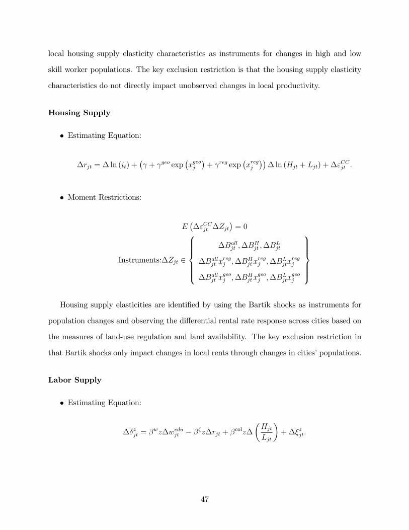
local housing supply elasticity characteristics as instruments for changes in high and low

skill worker populations. The key exclusion restriction is that the housing supply elasticity

characteristics do not directly impact unobserved changes in local productivity.

Housing Supply

� Estimating Equation:

�rjt = � ln (it) +� + geo exp

�xgeoj

�+ reg exp

�xregj

�� ln (Hjt + Ljt) + �"

CCjt :


E��"CCjt �Zjt

�= 0


8>>>><>>>>:�Balljt ;�B

Hjt ;�B

Ljt


regj ;�BLjtx

regj


geoj ;�BLjtx

geoj

9>>>>=>>>>;Housing supply elasticities are identi�ed by using the Bartik shocks as instruments for

population changes and observing the di¤erential rental rate response across cities based on

the measures of land-use regulation and land availability. The key exclusion restriction in

that Bartik shocks only impact changes in local rents through changes in cities�populations.

Labor Supply

� Estimating Equation:

��zjt = �wz�wedujt � ��z�rjt + �colz�

�HjtLjt

�+��zjt:

47


E��zjt�Zjt

�= 0


8>>>><>>>>:�Balljt ;�B

Hjt ;�B

Ljt


regj ;�BLjtx

regj


geoj ;�BLjtx

geoj

9>>>>=>>>>;Changes in local wages, local prices, and college employment ratios are jointly instru-

mented for using Bartik shocks to local labor demand and their interactions with local hous-

ing supply elasticity characteristics. The key exclusion restriction assumes the Bartik shocks

and housing supply elasticity characteristics do not directly impact changes in unobserved

amenities.

See Appendix A.2 for further details on all steps of the estimation procedures.

1.6 Parameter Estimates

1.6.1 Worker Labor Supply

I estimate two speci�cations of the model. The main speci�cation, which I refer to as

the �full model,�is the model exactly described in the previous sections. As an alternative

speci�cation, I estimate the model without endogenous amenities or endogenous productivity

changes. I refer to this speci�cation as the �no spillover�model. Parameter estimates for

both models are reported in Table 1.3.

Panel A of Table 1.3 reports the estimates of workers�demand elasticities for cities with

respect to wages, rents,and endogenous amenities. Focusing on the estimates of the full

model, I �nd that both college and non-college workers prefer cities with higher wages, lower

rent, and a higher college employment ratio. While both college and non-college workers

�nd higher wages net of local prices and amenity levels desirable, the elasticity of college

workers�demand for a city with respect to amenities is much higher than non-college workers�

48

amenity demand elasticity. The improvement in amenities driven by a 1% increase in a cities�

college employment ratio raises the college population within the city by 3.3%, while it only

increases the non-college population by 1.3%.

Similarly, non-college workers�demand is much more elastic with respect to wages and

rent than college workers. A 1% increases in local college wages increases the local college

population by 1.4%, while a similar increase in low-skill worker wages leads to a 4.2% increase

in the low-skill worker population. Similarly for rents, a 1% increase in local rent, leads to

a 2.8% decrease in low skill worker population, while it only leads to a .95% decrease in the

high skill population.

49

Full

Mod

elN

o Sp

illO

vers

Full

Mod

elN

o Sp

illO

vers

Wag

e1.

438*

**2.

326*

**W

age

4.18

1***

4.67

3***

[0.2

66]

[0.3

30]

[0.5

77]

[0.5

19]

Ren

t0

.953

***

0.1

56R

ent

2.8

32**

*2

.464

***

[0.2

52]

[0.2

48]

[0.3

33]

[0.3

06]

Impl

ied

Loca

l Exp

endi

ture

Shar

e0.

663*

**0.

067

Impl

ied

Loca

l Exp

endi

ture

Shar

e0.

677*

**0.

527

[0.1

80]

[0.0

10]

[0.0

71]

[0.0

45]

Col

lege

Em

p R

atio

Am

enity

3.26

8***

Col

lege

Em

p R

atio

Am

enity

1.30

1***

[0

.531

]

[0.4

82]

D

iffer

entia

l Eff

ects

: Bla

cks

Diff

eren

tial E

ffec

ts: B

lack

sW

age

3.18

2***

4.59

7***

Wag

e3.

351*

**3.

539*

**[1

.202

][0

.870

][0

.761

][0

.687

]R

ent

1.9

56**

*1

.152

***

Ren

t0

.994

***

0.8

87**

*[0

.542

][0

.446

][0

.398

][0

.357

]

Col

lege

Em

p R

atio

Am

enity

3.50

5***

Col

lege

Em

p R

atio

Am

enity

0.20

1

[0.7

86]

[0

.414

]

Diff

eren

tial E

ffec

ts:

Imm

igra

nts

Diff

eren

tial E

ffec

ts:

Imm

igra

nts

Wag

e3.

709*

**3.

424*

**W

age

2.94

9***

2.87

2***

[1.0

22]

[0.8

39]

[0.9

4][0

.908

]R

ent

0.86

60.

080

Ren

t0

.069

0.43

2[0

.523

][0

.469

][0

.488

][0

.477

]C

olle

ge R

atio

Am

enity

2.1

6***

Col

lege

Rat

io A

men

ity0.

802

[0

.499

]

[0.5

15]

Col

lege

Wor

kers

:

Tabl

e 1.

3: G

MM

Est

imat

es o

f Ful

l Mod

el &

Mod

el w

ith N

o Sp

illov

ers

Non

Col

lege

Wor

kers

:A

. Wor

ker P

refe

renc

es fo

r Citi

es

50

Full

Mod

elN

o Sp

illO

vers

Exp(

Land

Use

Reg

ulat

ion)

0.06

2***

0.06

3***

[0.0

1][0

.009

]Ex

p(La

nd U

nava

ilabi

lity)

0.02

4***

0.01

9***

[0.0

08]

[0.0

07]

Bas

e H

ouse

Sup

ply

Elas

ticity

0.02

10.

003

Min

imum

:0.

04[0

.082

][0

.074

]M

axim

um:

1.3

Full

Mod

elN

o Sp

illO

vers

Full

Mod

elN

o Sp

illO

vers

Rho

0.55

8***

0.49

9***

[0.0

43]

[0.0

48]

Prod

uctiv

ity S

pillo

ver o

nC

olle

ge W

orke

rs0.

553*

**

Prod

uctiv

ity S

pillo

ver o

nN

onC

olle

ge W

orke

rs0.

182*

**

[0.0

45]

[0

.059

]

Col

lege

Wag

e w

rt Co

llege

Labo

r0.

517

Non

Col

lege

Wag

es w

rtC

olle

ge L

abor

0.58

95C

olle

ge W

age

wrt

Non

C

olle

ge L

abor

0.5

17N

onC

olle

ge W

age

wrt

Non

C

olle

ge L

abor

0.5

895

Impl

ied

Ave

rage

Wag

e El

astic

ity w

ith re

spec

t to

Labo

r, Fu

ll M

odel

:

Not

es:S

tand

ard

erro

rsin

brac

kets

.Cha

nges

mea

sure

dbe

twee

n19

801

990

and

1990

200

0.B

lack

and

imm

igra

ntes

timat

esth

edi

ffer

entia

lpr

efer

ence

sof

thes

egr

oups

for

each

city

char

acte

ristic

,rel

ativ

eto

base

estim

ates

for

colle

gean

dno

nco

llege

wor

kers

.M

agni

tude

ofpa

ram

eter

estim

ates

repr

esen

twor

ker's

dem

and

elas

ticity

with

resp

ectt

oth

egi

ven

city

char

acte

ristic

,in

asm

allc

ity.S

ampl

eis

allh

eads

ofho

useh

old

with

pos

itive

labo

r inc

ome.

See

text

for m

odel

det

ails

. Sta

ndar

d er

rors

clu

ster

ed b

y M

SA. *

** p

<0.0

1, *

* p<

0.05

, * p

<0.1

B. H

ousi

ng S

uppl

y

C. L

abor

Dem

and

Mea

n:0.

17

Stan

dard

Dev

iatio

n:0.

16

Pred

icte

d In

vers

e H

ousi

ng S

uppl

y El

astic

ities

(Ful

l Mod

el):

Tabl

e 1.

3 (C

ontin

ued)

51

These results are consistent with a large body of work in empirical industrial organization

which �nds large amounts of heterogeneity in how sensitive consumers are to products�

prices.31

The ratio of workers�demand elasticities for rents to wages measures their expenditure

share on local goods. As derived in Section 1.4, since workers�preferences are Cobb-Douglas

in the national and local good, the indirect utility value of rent measured in wage units

represents the share of expenditure spent on locally priced goods. For both college and

non-college workers, I estimate this to be 66%-68% (0.95/1.4=0.66 for college, 2.8/4.2=0.68

for non-college). Note that the estimation methods in no way mechanically restricted this to

be less than one or similar across workers�skill groups. The expenditure share is inferred by

workers�revealed preference on the trade o¤ between wages and rents across cities. Albouy

(2008) measures the relative utility impact of housing rents versus local wages to equal 65%.32

While Albouy (2008) takes a very di¤erent estimation approach, it is reassuring we �nd very

similar estimates.

The estimates of the �no spillover�model strongly di¤er from the full model. The no

spillover model assumes that Bartik shocks and housing supply elasticity can only impact

worker migration by in�uencing local wages and rent. Under this assumption, I �nd that

college workers would have to spend only 7% of their expenditure on local goods, while non-

college workers would spend 53%. To be able to rationalize the migration responses to the

Bartik shocks through only wage and rent changes, college workers would have to be almost

indi¤erent to local price levels in order to be willing to live in cities with such high housing

prices. Data from the Consumer Expenditure Survey shows that housing expenditure makes

31For an example, see Berry, Levinsohn, and Pakes (1995) on consumer demand for cars. See Nevo (2010)for a review of this literature.32He takes a di¤erent approach to estimating the relative utility value of wage earnings versus housing rent

by explicitly accounting for a variety of mechanisms which in�uence how local wage earnings and housingprices impact workers�utility, such as non-labor income and tax rates. Since my methods use workers�revealed preferences on the relative utility value of local wages versus rents based on their city choices, Ido not need to explicitly model all the possible mechanisms which wages and rent in�uence workers�utilitylevels. Workers will take into account all the ways which wages and rent impact their utility when selectingwhich city to live in. Moretti (2011b) uses a similar approach to Albouy, but does not explicitly considertaxes and non-labor income. He estimates local good expenditure to be 58%.

52

up 33% of the average college household�s consumption and 32% of the average non-college

household�s consumption. These data make it clear that college workers�expenditure shares

on local goods cannot be close to 7% and do not appear to be strongly non-homothetic.33

This result is consistent with the reduced form evidence presented earlier in Section 1.3,

which shows that in addition to local wage and rent changes, local amenity changes were

related to changes in cities�college employment ratios.

Panel A of Table 1.3 shows that black college and non-college workers are more sensitive

to wages, rents, and amenities. As explicitly derived in the model section, higher aggregate

demand elasticities with respect to all city characteristics signi�es a relatively low variance of

idiosyncratic tastes across workers for each city. Since the black population is likely a more

homogenous group than the combination of all other non-immigrant races and ethnicities

lumped together in the non-black group, the variance of black worker�s idiosyncratic tastes

for each city is likely to be lower. Intuitively, if most workers agree on the utility value of

each city, changes in local wages, rents, or amenities that make a given worker migrate to

that city will also make many other similar workers migrate, since they all agree it o¤ers the

higher utility value.

Immigrant preferences di¤er strongly from the US non-immigrant population. I �nd that

immigrants are much more sensitive to city wages. A 1% increase in local wages increases

the low skill immigrant population by 7.1% and the high skill immigrant population by

5.2%. However, immigrants are much less sensitive to local good prices. A 1% increase in

local rents lead to out migration of 0.09% of the high skill immigrant population, and 2.9%

decrease in the low skill immigrant population. This relative wage-rent trade o¤ implies that

33When looking at housing expenditure shares across households of di¤erent incomes in the CEX, onesees that households with higher incomes have a lower expenditure share on housing. However, Chetty andSzeidl (2007) show that housing consumption expenditure is relatively hard for a household to adjust yearto year. Household income, on the other hand, has much more year to year �uctuation. High variance inincome coupled with a low variance in housing consumption over time, within a household, will lead to thespurious cross-sectional correlation that the households with higher annual income spend a small fraction onhousing. If this were evidence of non-homotheticity in housing consumption, then we should see a similargradient across proxies for households�permanent income, such as education. Given that the consumptionexpenditure on housing is strikingly �at across education levels, one can conclude that housing consumptionis close to homothetic.

53

immigrants must spend a smaller share of their expenditure on local goods. Additionally,

high skill immigrants are less elastic to the college employment ratio driven endogenous

amenities than non-immigrant college workers. Overall, these results show that immigrants

elect their city to live in based almost exclusively on local wages. They spend much less on

housing and local goods, which makes them able to a¤ord to live in cities with high housing

prices.

Table 1.4 reports estimates for workers�preferences to live in their own state of birth or

Census Division of birth.34 Non-college workers are 4.4 times more likely to live in a given

MSA if it is located is his state of birth than if it is not, while college workers are only 3.5

times more likely. Both college and non-college workers are 2.2 times more likely to live in

an MSA located in his Census Division of birth than an MSA farther away. These estimates

are similar for blacks. Unlike the amenities in�uenced by a city�s college employment ratio,

the amenity of living near one�s place of birth in�uences the city choices of low skill workers

more than high skill. This is consistent with the migration literature that �nds high skilled

workers are more likely to move away from their place of birth.35

34I estimate decade-speci�c parameters for workers�preferences to live close to their state of birth. Thisis purely for computational convenience. Since these parameters are jointly estimated along with the meanutility levels for each city for each demographic group for each decade, estimating each decade�s parameters ina separate optimization allowed for a sign�cant decrease in the computational memory requirements neededfor estimation.35See Greenwood (1997) for a review of this literature.

54

Base Black Base Black Base Black

NonCollege 3.413 0.119 3.412 0.054 3.423 0.157[0.0022] [0.0069] [0.004] [0.018] [0.005] [0.018]

College 2.537 0.225 2.525 0.252 2.629 0.206[0.0047] [0.018] [0.003] [0.0105] [0.0032] [0.0105]

Base Black Base Black Base Black

NonCollege 1.286 0.325 1.268 0.529 1.216 0.540[0.0034] [0.0059] [0.006] [0.028] [0.005] [0.014]

College 1.199 0.484 1.192 0.510 1.140 0.382[0.0047] [0.018] [0.002] [0.0101] [0.0042] [0.0105]

1980 1990 2000

Notes: Standard erorrs in brackets. Estimates from maximum likelihood of conditional logit model of citychoice. Magnitudes represent the semielasticity of demand for an average sized city with respect towhether the city is located within one's birth state or division. Black estimates are relative to baseestimates. Sample is all heads of household with positive labor income.

Table 1.4: Value of Living in Own Birth State & Division

A. Birth State1980 1990 2000

B. Birth Division

55


Panel B of Table 1.3 presents the inverse housing supply elasticity estimates. Consistent

with the work of Saiz (2010) and Saks (2008), I �nd housing supply is less elastic in areas

with higher levels of land-use regulation and less land near a city�s center available for real

estate development. The inverse housing supply elasticity estimates do not di¤er much

between the full model and the no spillover model. This is expected, since these two models

have identical housing supply models. I use the parameter estimates to predict the inverse

elasticity of housing supply in each city. Panel B of Table 1.3 shows that the average inverse

housing supply elasticity is 0.17, with a standard deviation of 0.16. A regression of my

inverse housing supply elasticity estimates on Saiz (2010)�s estimates yields a coe¢ cient of

1.04 (0.12), suggesting we �nd similar amounts of variation in housing supply elasticities

across cities. However, Saiz (2010)�s inverse housing supply estimates are higher than mine

by 0.39, on average. The overall level of my estimates is governed by the "base" inverse

housing supply term, :This parameter is the least precisely estimated of the housing supply

elasticity parameters, with a point estimate of 0.021 (0.082), which could explain why I �nd

lower inverse housing supply estimates overall. Further, Saiz�s estimates are identi�ed using

a single, long run change in housing prices from 1970-2000, while I am looking at decadal

changes from 1980 to 1990 and 1990 to 2000. Di¤erences in time frame could impact these

parameter estimates as well.

1.6.3 Labor Demand

Panel C of Table 1.3 presents parameter estimates for the local labor demand curves. In the

no spillovers model, I estimate � to be 0.499, which implies a elasticity of labor substitution

of 1.99. This estimate is very close to others in the literature, which tend to be between 1

and 3.36 Work by Card (2009) estimates the elasticity of labor substitution at the MSA level

and �nds an elasticity of 2.5, which is not statistically distinguishable from my results.

36See Katz and Autor (1999) for a literature review of this work.

56

In the full model speci�cation, I allow for a more �exible labor demand curve. The

parametric assumptions allow me to disentangle the slopes of �rms� labor demand curves

from productivity spillovers due to changes in cities�college employment ratios. With this

more general model, I estimate � to be 0.558, which implies an elasticity of labor substitution

within �rms of 2.26, slightly higher than the more restrictive model. Additionally, a 1%

increase in the a city�s college employment ratio increases the productivity of college workers

by 0.55% and non-college workers by 0.18%.

These estimates suggest that the social returns to education are high. Combining the

estimates of the elasticity of labor substitution with the productivity spillovers, I �nd that

a 1% increase in a city�s college worker population raises the local college wage by 0.52%

and the local non-college wage by 0.59%. Similarly, a 1% increase in a city�non-college

worker population decreases college wages by 0.52% and non-college wages by 0.59%. The

wage increases due to local productivity spillovers, such as endogenous technology adoption

or knowledge and ideas spillovers, overwhelm the wage decreases driven by movement along

�rms�labor demand curves from the increase supply of college graduate labor.

Moretti (2004a) also analyzes the impact of high and low skill worker labor supply on

workers�wages within a city. He estimates a 1% increase in a city�s college employment ratio

leads to a .16% increase in the wages of high school graduates and a .10% increase in the wages

of college graduates, both of which are smaller than my �ndings.37 His estimates are identi�ed

o¤ of cross-sectional variation in city�s college shares, driven by the presence of a land

grant college, while my estimates are estimated o¤ of changes in skill-mix driven by housing

supply elasticity heterogeneity. Additionally, my estimates explicitly combine the impact of

37Moretti (2004a)�s setup looks at the impact of a city�s share of college graduates�

Hjt

Hjt+Ljt

�on workers�

wages by education level, while my setup measures the local education mix using the log ratio of college

to non-college workers�ln

Hjt

Ljt

�: To transform Moretti�s estimates into the same units of my own, note

that Hjt

Hjt+Ljt=

HjtLjt

1+HjtLjt

: Moretti estimates: wjt = �Hjt

Hjt+Ljt: Thus, @wjt

@ ln�HjtLjt

� =@wjt

@Hjt

Hjt+Ljt

@Hjt

Hjt+Ljt

@ ln�HjtLjt

� = � ��Hjt

Hjt+Ljt

��1� Hjt

Hjt+Ljt

��: Plugging in the average college share in 1990, 0.25 gives: @wjt

ln�HjtLjt

� = ��(0:1875) :Thus, I scale Moretti�s estimates by 0:1875 to make them in the same units as my own.

57

movement along �rm�s labor demand curves with endogenous productivity spillovers, while

Moretti controls for labor demand variation (he includes the local unemployment rate as well

as other city controls). He also uses the lagged age structure of the city as a instrument for

changes in cities�skill mix. Using this identi�cation strategy, he �nds slightly larger e¤ects

(point estimates become 0.39 for high school graduate wages and 0.16 for college wages.)

While my estimates of the social returns to education are slightly above Moretti�s, we both

conclude that they are large and substantial.38

In Appendix A.3, I consider whether the observed population distribution across cities

in each decade is a stable equilibrium assuming a simple dynamic adjustment process, given

the parameter estimates of the model. Using a simple dynamic adjustment process where

5% of the population can choose to migrate to a new city each period, and cities�wages,

rents, and amenities instantaneously respond to population changes each period, I �nd that

the equilibria observed in the data in 1980, 1990, and 2000 are stable under this assumed

adjustment dynamic. See Appendix A.3 for further details.

1.6.4 Estimation Robustness

To assess whether the parameter estimates of the model are sensitive to ways that I have

measured wages, rents, and Bartik shocks, I re-estimate the model using a variety of di¤erent

variable de�nitions. These results are in Table 1.5. A particularly important reason to assess

whether the parameter estimates are stable across di¤erent speci�cations is to indirectly test

for whether my instruments are weak. I am not aware of a standard econometric test for

weak instruments when estimating a multiple equation, non-linear GMM model where there

are multiple endogenous variables.

38Ciccone and Peri (2006) also estimate the productivity spillovers of education. However, they focuson the social return to an additional year of average education, without di¤entiating between college andnon-college years of education. They also use lagged age structure of a city as an instrument for the localskill mix, but do not �nd any evidence of spillovers. Since they do not explicitly analyze spillovers due tocollege versus. non-college skill mix, it is hard to compare exactly why these estimates di¤er. Their analysisalso does not include the 2000 census.

58

(1)

(2)

(3)

(4)

(5)

(6)

(7)

(8)

Dro

p To

tal

Bar

tikSh

ock

Hed

onic

Adj

uste

dW

age

&R

ent

Onl

yA

ctua

lR

ents

Onl

yIm

pute

dR

ents

Ren

tsfr

omC

olle

geW

orke

rs

Ren

tsfr

om N

on

Col

lege

Wor

kers

Use

Endo

gA

men

ityIn

dex

Red

uced

Form

Labo

rD

eman

d

Col

lege

Wor

kers

:

Wag

e1.

883

3.33

71.

382

1.13

11.

499

1.33

75.

294

1.72

3[0

.437

][0

.345

][0

.288

][0

.276

][0

.289

][0

.259

][0

.622

][0

.339

]R

ent

1.2

292

.597

0.6

460

.857

0.9

011

.020

0.4

390

.563

[0.4

59]

[0.3

73]

[0.2

85]

[0.2

16]

[0.2

54]

[0.2

64]

[0.3

77]

[0.2

67]

Endo

g A

men

ity4.

275

3.16

72.

838

3.22

32.

982

3.36

22.

292

3.35

2[1

.189

][0

.601

][0

.417

][0

.521

][0

.502

][0

.551

][0

.852

][0

.613

]D

iffer

entia

l Eff

ects

, Bla

cks:

W

age

4.36

67.

825

3.84

72.

302

3.22

02.

815

7.46

02.

993

[1.6

54]

[1.3

85]

[1.3

26]

[1.1

51]

[1.2

24]

[1.1

86]

[1.3

65]

[1.1

85]

Ren

t2

.336

6.3

392

.136

1.5

451

.866

2.0

211

.533

1.3

31[0

.846

][0

.932

][0

.771

][0

.448

][0

.488

][0

.575

][0

.595

][0

.544

]En

dog

Am

enity

3.39

74.

091

3.40

63.

116

2.75

33.

633

2.72

23.

497

[1.4

28]

[0.9

76]

[0.8

54]

[0.7

15]

[0.7

18]

[0.7

79]

[1.3

25]

[0.8

35]

Diff

eren

tial E

ffec

ts, I

mm

igra

nts:

W

age

5.49

78.

424

2.59

15.

535

5.58

35.

231

2.95

93.

882

[0.9

18]

[0.9

9][1

.143

][0

.642

][0

.683

][0

.691

][1

.189

][1

.049

]R

ent

0.57

82

.130

2.46

40.

028

0.02

70.

331

0.26

50.

573

[0.7

09]

[0.5

23]

[0.7

14]

[0.3

38]

[0.3

84]

[0.4

31]

[0.5

63]

[0.5

21]

Endo

g A

men

ity4

.609

1.9

133

.835

2.0

452

.189

2.1

960.

017

1.9

57[1

.899

][0

.653

][0

.646

][0

.514

][0

.5]

[0.5

][0

.792

][0

.515

]N

onC

olle

ge W

orke

rs:

W

age

4.36

16.

757

6.67

62.

678

3.84

73.

888

4.34

44.

327

[0.8

21]

[0.5

54]

[0.7

65]

[0.4

66]

[0.5

47]

[0.5

86]

[0.6

12]

[0.5

64]

Ren

t3

.379

5.9

404

.223

2.0

902

.614

2.8

552

.247

2.5

87[0

.65]

[0.5

08]

[0.5

6][0

.241

][0

.279

][0

.365

][0

.348

][0

.312

]En

dog

Am

enity

2.82

92.

267

1.04

31.

114

0.65

91.

243

0.41

31.

105

[1.1

95]

[0.5

91]

[0.4

59]

[0.4

05]

[0.4

47]

[0.4

73]

[0.6

09]

[0.5

46]

Diff

eren

tial E

ffec

ts, B

lack

s:

Wag

e2.

672

4.28

93.

492

3.03

73.

392

3.37

13.

055

3.35

4[0

.982

][0

.74]

[0.8

97]

[0.6

51]

[0.6

86]

[0.7

67]

[0.6

98]

[0.8

61]

Tabl

e 1.

5: R

obus

tnes

s Tes

ts o

f Alte

rnat

ive

Mod

el S

peci

ficat

ions

Hou

seho

ld P

refe

renc

es fo

r Citi

es

59

Ren

t0

.754

2.2

440

.565

0.7

750

.938

0.9

260

.816

0.8

22[0

.614

][0

.516

][0

.615

][0

.307

][0

.347

][0

.417

][0

.379

][0

.431

]C

olle

ge E

mp

Rat

io A

men

ity0.

222

0.49

80

.496

0.18

60

.106

0.08

20

.123

0.28

8[0

.932

][0

.468

][0

.437

][0

.404

][0

.392

][0

.412

][0

.609

][0

.416

]D

iffer

entia

l Eff

ects

, Im

mig

rant

s:

Wag

e1.

944

2.92

91.

679

2.83

92.

704

2.55

13.

620

2.54

7[1

.286

][0

.828

][0

.953

][0

.794

][0

.844

][0

.932

][1

.112

][1

.075

]R

ent

0.46

50.

379

0.61

00

.063

0.05

00.

134

1.0

180.

246

[0.7

2][0

.559

][0

.53]

[0.3

71]

[0.4

27]

[0.5

11]

[0.6

21]

[0.5

53]

Col

lege

Em

p R

atio

Am

enity

0.10

80

.687

1.16

50.

780

0.71

20.

676

3.1

931.

487

[0.9

7][0

.469

][0

.57]

[0.5

41]

[0.5

37]

[0.5

04]

[0.7

5][0

.677

]

Land

Use

Reg

ulat

ion

0.06

60.

044

0.03

60.

080

0.06

20.

059

0.06

60.

044

[0.0

13]

[0.0

08]

[0.0

07]

[0.0

12]

[0.0

1][0

.01]

[0.0

1][0

.01]

Land

Una

vaila

bilit

y0.

021

0.01

60.

020

0.03

60.

025

0.02

80.

017

0.02

0[0

.01]

[0.0

07]

[0.0

06]

[0.0

1][0

.009

][0

.008

][0

.008

][0

.007

]B

ase

Hou

se S

uppl

y El

astic

ity0.

029

0.19

70.

170

0.2

110

.028

0.0

320.

033

0.08

2[0

.119

][0

.063

][0

.056

][0

.104

][0

.081

][0

.081

][0

.08]

[0.0

83]

Rho

0.46

60.

405

0.56

80.

569

0.55

20.

570

0.56

4[0

.073

][0

.038

][0

.044

][0

.045

][0

.044

][0

.042

][0

.066

]Pr

oduc

tivity

Spi

llove

r on

Col

lege

Wor

kers

0.57

30.

616

0.55

60.

560

0.55

70.

557

0.70

4[0

.096

][0

.037

][0

.047

][0

.045

][0

.045

][0

.046

][0

.047

]Pr

oduc

tivity

Spi

llove

r on

Non

Col

lege

0.13

10

.001

0.22

10.

195

0.17

30.

207

0.28

9[0

.129

][0

.053

][0

.059

][0

.06]

[0.0

6][0

.061

][0

.094

]

Col

lege

Wag

e w

rt Co

llege

Lab

or0.

389

[0.0

82]

Col

lege

wag

e w

rt N

onC

olle

ge L

abor

0.1

16[0

.094

]N

onC

olle

ge w

age

wrt

Col

lege

Lab

or0.

587

[0.0

96]

Non

Col

lege

wag

e w

rt N

onC

olle

ge L

abor

0.4

22[0

.104

]N

otes

: Sta

ndar

d er

rors

in b

rack

ets.

Stan

dard

err

ors c

luste

red

by M

SA.

See

text

for d

etai

ls o

n al

l the

alte

rnat

ive

mod

el sp

ecifi

catio

ns.

Tabl

e 1.

5 (C

ontin

ued)

Hou

sing

Sup

ply

Labo

r Dem

and

Labo

r Dem

and

Elas

ticity

Est

imat

es fo

r Red

uced

for L

abor

Dem

and

Mod

el

60

Stock, Wright, and Yogo (2002) say �If identi�cation is weak, then GMM estimates can

be sensitive to the addition of instruments or to changes in the sample. If these features are

present in an empirical application, then they can be symptomatic of weak identi�cation.�

I try to do the best I can to �test�for weak identi�cation by changing which instruments I

include and how I de�ne the sample�s variables.

I �rst assess the sensitivity of including the �aggregate�Bartik shock as an additional

instrument: The model can be identi�ed using only the high skill and low skill Bartik shocks,

along with their interactions with housing supply elasticities. I included the aggregate Bartik

shock because it likely contains information about how each individual low and high skill

Bartik shock in�uences local housing prices. Column 1 of Table 1.5 reports the parameter

estimates when all of the moments using the aggregate Bartik shocks are dropped. The para-

meter estimates are extremely similar between this speci�cation and the main speci�cation.

The standard errors increase slightly, which is expected when there are fewer identifying

restrictions used to estimate the model. No parameters change sign and all of the changes

in the parameter estimates are within the con�dence bands of my preferred speci�cation.

As additional robustness tests, I try a variety of methods for measuring local wages and

rent. I re-estimate the model where I hedonically adjust local wage and rent changes. Wages

are adjusted for a more �ne measure of education, a quadratic in experience, gender, and

race. I adjust rents by number of rooms, number of bedrooms, and apartment units in the

structure. The model estimates using these wage and rent measures are qualitatively the

same. High and low skill workers are slightly more elastic to cities�wages and rents, but

high skill workers remain signi�cantly less price sensitive than low skill workers.

I also measure local rent changes in a variety of ways. I try using only rent data from

housing units actually rented, dropping the imputed rents. I also try using only the imputed

rents. Further, I estimate the model using only rents from college workers, as well as rents

only from non-college workers. The results are very similar across all of these speci�cations.

This shows that the variation of housing costs between cities does not strongly di¤er across

61

home owners versus home rents or between the neighborhoods of the high skill workers or low

skill workers. Overall, the parameter estimates are stable across a variety of speci�cations,

which alleviates some concern about whether the model is weakly identi�ed.

I also consider an alternative measure of cities�endogenous amenities using the observable

amenity data. The main model speci�cation uses the college employment ratio as the index

of endogenous amenities within a city. This index captures both the direct bene�ts of

having more educated neighbors, as well as the indirect bene�ts through amenities such as

more restaurants, lower crime, or better air quality. To assess whether these observable

amenities can capture the full extent of the increased desirability of high skill cities, I create

an alternative endogeneous amenity index. I compute changes in the observable amenity

index by measuring the average change in logs of each amenity measure in each decade.39

Speci�cally, the amenity index is de�ned as:

�amen_indexjt =1

K

Xk

� ln (amenkjt) :

Column 7 of Table 1.5 shows the re-estimated model where this observable amenity index

is used in place of the college employment ratio for workers�preferences for cities. Similar

to the main model estimates, I �nd that elasticity of college workers� demand for a city

with a high amenity index is substantially larger than lower skill workers�demand elastcity

(2.29 (0.85) for college versus 0.413 (0.61) for non-college). However, the model estimates

using this amenity index still show that college workers appear to allocate a very small

share of their expenditure to housing and local goods, relative to non-college workers. These

estimates would imply that college workers only spend 8% of their expenditure housing and

local goods, while non-college workers spend 52%. This suggests that the college employment

39The amenity measures included are grocery stores per 1000 residents, apparel stores per 1000 residents,eating and drinking places per 1000 residents, book stores per 1000 residents, dry cleaners per 1000 residents,movie thearters per 1000 residents, property crimes per 1000 residents, violent crimes per 1000 residents,and the EPA air quality index. I do not include museums and art galleries because data is missing for asubstantial number of MSAs. Since the air quality data is missing for a number of MSAs, espcially in 1980,I impute air quality by regressing non-missing air quality on the other amenities, as well as future period�sairquality measures. I then impute the missing airquality data from this regression.

62

ratio is capturing desirable amenities of the city, over and beyond these observable measures.

This is not surprising, since Table 1.2 showed that while the college employment ratio was

positively correlated with many of these desirable amenities, the college employment ratio

could explain only a very small fraction of the varition in any of these obsevable amenity

measures. A high college share city appears to be desirable for reasons over and beyond

these measures of observable amenities.

As a �nal robustness test, I consider an alternative functional form for the local labor

demand curves. Using the standard constant elasticity of substitution production function

restricts wages to only depend on the the relative supply of college and non-college workers,

and not aggregate amount of labor in the city. To assess whether the model�s labor demand

elasticity estimates are being restricted due to the functional form assumptions, I estimate

reduced form local labor demand curves. I replace the CES labor demand curves with the

following log-linear labor demand curves:

�wHjt = �Ht + �HH� log (Hjt) + �

HL� log (Ljt) + �"Hjt

�wLjt = �Lt + �LH� log (Hjt) + �

LL� log (Ljt) + �"Ljt:

Column 8 of Table 1.5 reports the model estimates using these reduced-form labor demand

curves. None of the labor demand elasticity estimates change sign from the main model

estimates. The reduced form estimates show that a 1% increase in non-college labor leads

only to a 0.12% decline in college worker wages. The magnitude of this estimate is smaller

than the main model estimate of a 0.59% decline in college worker wages. The other reduced

form labor demand estimates are of similar magnitudes to those in the main model estimates.

Overall it seems the functional form restrictions of the CES production function are not

restraining the labor demand elasticities to be extremely di¤erent from those found in the

reduced form estimates.

63

1.7 Amenities & Productivity Across Cities

Using the estimated parameters, one can infer the productivity of local �rms and the desir-

ability local amenities in each city. Comparing the model�s predicted amenity and produc-

tivity levels to outside research and data on these city characteristics will assess model �t

and provide a sanity check of whether these estimates appear plausible.

There is a large literature which attempts to estimate which cities o¤er the most desirable

amenities using hedonic techniques.40 The methodology used in this paper to infer which

cities o¤er the most desirable amenities di¤ers from the previous hedonic literature. Recalling

equation (1:24) ; the utility value of the amenities in a city to workers of a given demographic

group (�colzHjtLjt+ �zjt) is measured by the component of the workers�common utility level for

each city, �zjt; which is not driven by the local wage and rent level, �wzwedujt + �rzrjt. The

utility workers of type z receive from the amenities in city j in year t; U zA; is thus:

U zA = �colz

HjtLjt

+ �zjt = �zjt � �wzwedujt � �rzrjt:

Intuitively, amenities are inferred to be highest in cities which have higher population levels

of a given demographic group than would be expected, given the city�s wage and rent levels

and workers�preferences for wages and rent. If many workers choose to live in a city that

appears relatively undesirable based on its wages and rent, as compared to other cities, it

must o¤er desirable amenities. Unlike the literature using hedonics to rank city amenities,

these methods are able to rank the desirability of cities amenities separately for di¤erent

types of workers.

A test of whether the model �ts the data well is to asses whether the amenity rankings ap-

pear �intuitive.�Of the largest 75 cities, as measured by their population in 1980, Appendix

40The hedonic methods infer a city�s amenities by directly comparing local real wages across cities. In amodel where workers have homogeneous preferences for cities, the equilibrium local real wages across citiesmust be set to equate all workers utility values in all cities. In equilibrium, the di¤erence in real wages acrosscities is a direct measure of the amenity value of the city. A low amenity city must o¤er a high real wage inorder to o¤er the same utility as a high amenity city. See Albouy (2008) for recent amenity estimates usingthese techniques.

64

Table 1.3 reports the top 10 cities with the most desirable and undesirable amenities for col-

lege and non-college workers in 1980 and 2000, as well as the cities with the largest improve-

ments and declines in amenities during this time period. In 2000, Los Angeles-Long Beach,

CA had the most desirable amenities for non-college workers, followed by Phoenix, AZ,

Denver-Boulder, CO, Seattle-Everett, WA, and Boston, MA-NH. The cities with the most

desirable amenities for college workers in 2000 were: Los Angeles-Long Beach CA, Wash-

ington, DC/MD/VA, Boston, MA-NH, Atlanta, GA, and San Francisco-Oakland-Vallejo,

CA. These cities are known to have vibrant cultural scenes, desirable weather, and often

considered to have high quality-of-life.

The least desirable city amenities for college workers in 2000 are located in Youngstown-

Warren, OH-PA, which is followed by Allentown-Bethlehem-Easton, PA/NJ, Syracuse, NY,

Harrisburg-Lebanon�Carlisle, PA, and Scranton-Wilkes-Barre, PA. Similarly, non-college

workers �nd the least desirable amenities in Youngstown-Warren, OH-PA, followed by Toledo,

OH/MI, Syracuse, NY, Bu¤alo-Niagara Falls, NY, and Allentown-Bethlehem-Easton, PA/NJ.

All of these cities are located in America�s Rust Belt, where the cities have historically had

high levels of pollution due the concentration of manufacturing jobs. They have recently

faced large declines in manufacturing jobs, population declines, and growing crime rates

since the 1980s. It is not surprising these cities o¤er the least desirable amenities. Overall,

the model seems to do well at capturing which cities are the most and least desirable.

A similar validation test can be done by analyzing which cities have the highest and

lowest productivity levels. The productivity level in each city for each skill level of worker

can be inferred from the residual of the labor demand equation:

ProdHjt = lnwHjt � ((1� �) lnNjt + (�� 1) lnHjt) (1.25)

ProdLjt = lnwLjt � ((1� �) lnNjt + (�� 1) lnLjt) : (1.26)

Intuitively, productivity is inferred to be the highest in areas where wages are much higher

65

than what would be predicted by the amount of labor supplied to an area. Appendix

Table 1.4 reports the most and least productive cities in 1980 and 2000 for college and non-

college workers. In 2000, the most productive city for college graduates was San Jose, CA,

followed by San Francisco-Oakland-Vallejo, CA, New York-Northeastern NJ, Washington,

DC/MD/VA, and Boston, MA-NH. These cities are the hubs of many of the most productive

industries such as high tech in Silicon Valley, �nance in New York, and biotech in Boston

and San Francisco.

The most productive cities for lower skill workers are very di¤erent. In 2000, the city

most productive for low skill workers was Riverside-San Bernardino,CA, followed by Detroit,

MI, Las Vegas, NV, Tacoma, WA, and Ventura-Oxnard-Simi Valley, CA. Riverside-San

Bernardino, CA is where many of the largest manufacturing companies have chosen to place

their distribution centers. These centers transport �nished goods and materials from the

ports surrounding Los Angeles to destinations around the US. Shipping and distribution

provide many relatively high paying jobs for low skill workers here. While Detroit, MI ranks

as the second most productive area in 2000, it is also in the top 10 for cities which have

experienced the largest productivity declines for low skill workers from 1980 to 2000. In

1980, Detroit, MI was the most productive city for low skill workers, but as American auto

manufacturing has lost market share, wages and jobs have fallen here. However, Detroit still

provides some of the most productive uses of low skill labor in 2000.

In Appendix A.4, I compare my productivity estimates with other work studying the

determinants of productivity changes across cities. My estimates are consistent with work

by Autor and Dorn (2012) who study the di¤erences in skill biased technology change across

cities driven by historical occupation di¤erences. Work by Beaudry, Doms, and Lewis (2010)

studying di¤erences in technology adoption of �rms across cities also lines up with my esti-

mated productivity changes. Additionally, the cities which I �nd to have the largest declines

in low skill productivity closely overlap with the cities�which had larger amounts of their

labor force employed in industries that faced the most competition from the increased pen-

66

etration of Chinese exports (Autor, Dorn, and Hanson (2012)).

There are striking di¤erence in which cities have had the largest changes in their local

high and low skill productivity from 1980 to 2000. Appendix Table 1.4 shows that three cities

(San Jose, CA, Boston, MA-NH, and Chicago, IL) rank in the top 10 largest productivity

increases for high skill workers and the top 10 largest productivity decreases for low skill

workers. Table 1.6 presents a regression of the model�s predicted change in a city�s high

skill productivity on its predicted change in low skill productivity. I �nd a slight negative

relationship between local high skill productivity change, and local low skill productivity.

Note that this negative relationship between changes in local high skill productivity and low

skill productivity cannot be seen by simply comparing changes in local high skill wages with

changes in local low skill wages. Table 1.6 shows that changes in high and low skill wages

are strongly positively correlated, with an R squared of 0.50. Movement along local labor

demand curves driven by migration masks the large di¤erences local productivity changes

by skill.

The di¤erences in high and low skill workers�preferences for a city�s amenities is unlikely

to di¤er by the same magnitude. The preference estimates of the model showed that both

high and low skill workers agreed that the amenity changes caused by an increase in a

city�s college employment ratio were desirable. Thus, one would expect that college workers�

overall utility value for a city�s amenities to be positively associated with non-college workers�

utility value for the same city�s amenities. Table 1.6 shows that the utility value of college

and non-college amenity changes across cities are strongly positively correlated. Changes in

non-college workers�utility due to changes in cities�amenities explains 58% of the variation

in changes in college workers�utility for the same cities�amenities.

67

(1)

(2)

(3)

(4)

(5)

(6)

(7)

Δ C

olle

geA

men

tity

Δ N

onC

olle

geA

men

ityΔ

Col

lege

Am

entit

y

Δ N

on

Col

lege

Am

enity

Δ C

olle

geA

men

tity

Δ C

olle

gePr

oduc

tivity

Δ C

olle

geW

age

Δ N

onC

olle

geA

men

ity0.

595*

**[0

.031

0]Δ

Col

lege

Prod

uctiv

ity1.

039*

**0

.037

[0.2

74]

[0.3

60]

Δ N

onC

olle

gePr

oduc

tivity

0.61

51

.289

**0

.062

[0.4

02]

[0.5

12]

[0.0

883]

Δ N

onC

olle

geW

age

0.68

79**

*[0

.042

6]C

onst

ant

0.3

42**

*0

.394

***

0.0

898*

**0

.429

***

0.13

7***

0.22

9***

0.14

6***

[0.0

669]

[0.0

880]

[0.0

242]

[0.0

307]

[0.0

194]

[0.0

0529

][0

.004

6]

Obs

erva

tions

267

267

267

267

267

268

268

Rs

quar

ed0.

052

0.00

0.00

90.

023

0.58

10.

002

0.50

0

Tabl

e 1.

6: R

elat

ions

bet

wee

n A

men

ity a

nd P

rodu

ctiv

ity C

hang

es

Stan

dard

erro

rsin

brac

kets

.Cha

nges

inam

eniti

esan

dpr

oduc

tiviti

esar

em

easu

red

betw

een

1980

and

2000

.Citi

es'a

men

ities

and

prod

uctiv

ityle

vels

are

infe

rred

from

mod

el e

stim

ates

. See

text

for f

urth

er d

etai

ls. *

** p

<0.0

1, *

* p<

0.05

, * p

<0.1

68

Table 1.6 shows that changes in college productivity are positively associated with changes

in college amenities. However, changes in non-college productivity are negatively associated

with non-college amenity changes. Industries which are the most productive for low skill

workers may negatively impact the amenities of the city. For example, Kahn (1999) �nds

the decline of manufacturing in Rust Belt cities led to increases in local air-quality. The

model allows for this e¤ect through the college employment ratio. However, the industries

most productive for college workers tend to be driven by research, ideas and innovation.

Even though high skill production might not directly spillover onto a city�s amenities, cities

which attract high skill workers by o¤ering high wages bene�t from the endogenous amenity

increases, driven by the presence of high skill workers living in the city.

The inferred local productivity and amenity changes across cities appear consistent with

outside knowledge on these measures, and the relationships between productivity and ameni-

ties changes also appear intuitive. These tests of the model provide evidence that the model

setup and parameter estimates capture the key underlying drivers of the determinants of

local wages, rents, and amenities across cities.

1.7.1 The Determinants of Cities�College Employment Ratio Changes

To understand what drove the changes in cities� college employment ratios from 1980 to

2000, I use the estimated model to assess the contributions of productivity, amenities, and

housing supply elasticities to the changes in cities�college employment ratios.

1.7.2 College Employment Ratio Changes and Productivity

I �rst consider how much of the observed changes in cities�college employment ratios can be

explained by changes in cities�exogenous productivity levels. Changes in local productivity

directly impact wages, but also in�uence local prices and endogenous amenities through

migration. Before considering how local productivity changes are capitalized into equilibrium

wages, rents, and endogenous amenities, I consider the direct e¤ect of productivity changes

69

on local wages. Using the exogenous productivity changes predicted by the model, I compute

the direct e¤ect of exogenous changes in productivity from 1980 to 2000 in each city on local

high and low skill wages. These counterfactual college and non-college wages in 2000, wHj2000

wLj2000 are de�ned as:

wHj2000 = c1980 + (1� �) ln Nj2000 + (�� 1) lnHj1980 + H ln�Hj1980Lj1980

�| {z }

Labor Supply in 1980

+ "Hj2000| {z }Exog. Productivity in 2000

wLj2000 = c1980 + (1� �) ln Nj2000 + (�� 1) lnLj1980 + L ln�Hj1980Lj1980

�| {z }

Labor Supply in 1980

+ "Lj2000| {z }Exog. Productivity in 2000

Nj2000 =

�exp

�"Lj2000

��Hj1980Lj1980

� LL�j1980 + exp

�"Hj2000

��Hj1980Lj1980

� HH�j1980

� 1�

:

The counterfactual wages only re�ect the shifts in local labor demand curves driven by the

exogenous changes in local productivity from 1980 to 2000, but not the movement along

cities�labor demand curves or endogenous productivity changes due to migration.

Using these counterfactual year 2000 wages, while holding rents and amenity levels �xed

at their 1980 levels, I use the model to predict where workers would have chosen to live if

they had to choose among this set of hypothetical cities. Speci�cally, worker i�s utility for

hypothetical city j is:

Vijt = �wziw

eduj2000 � �rzirj1980 + �zj1980 + �colzi

Hj1980Lj1980


divzi divi xdivj + "ij80:

The predicted cities�college employment ratios from this hypothetical world are then com-

pared to those observed in the data. This counterfactual scenario assesses whether the cities

which became disproportionately productive for college, relative to non-college workers, were

also the cities which experienced disproportionate growth in their college versus non-college

populations. Figure 1.6 panel A plots the observed college employment ratio changes against

these predicted counterfactual changes.

70

Figure 6.A Predicted change in college ratio

due to local wage changes from productivity

changes

Figure 6.B Predicted change in ln college

ratio due to observed changes in local wages

& rent

Figure 6.C Predicted change in ln college

ratio due to changes in observed changes in

wages, rent, and endogenous amenities

Figure 1.6: Predicted Changes in Ln College Employment Ratio: 1980-2000

71

The predicted and actual changes are strongly correlated with a correlation coe¢ cient of

0.70. This shows local productivity changes explain a large share of the changes in cities�

local college employment ratios from 1980 to 2000.

While simple shifts in cities�wages due to productivity changes explain a large amount

of the variation in college employment ratio changes, workers� actual migration decisions

depended on how local productivity changes in�uenced the overall desirability of cities�s

wages, rents, and amenities. For example, productivity growth in a city with very inelastic

housing supply would attract many fewer workers than a similar city with elastic housing

supply. Additionally, the amenities of the city will respond to the mix of college and non-

college workers living in the city.

In a model where amenities are assumed to be exogenous, the only ways which productiv-

ity changes can in�uence workers�location decisions is by in�uencing local wages and rents.

To measures the importance of endogenous amenity changes in in�uencing cities� college

employment ratio changes, I use the model to predict workers�city choices in 2000, using

only the observed changes in wages and rent. Holding amenities �xed at the 1980 levels, I

set local wages and rents to the levels observed in 2000. Speci�cally, worker i�s utility for

hypothetical city j is:

Vijt = �wziw


Hj1980Lj1980



I predict where workers would have chosen to live if they had to choose from this set of

counterfactual cities. If endogenous amenity changes were not an important factor in how

productivity changes in�uenced cities�college employment ratio changes, then local wage and

rent changes should be at least as strong of a predictor of college employment ratio changes as

simply shifting wages by productivity changes. Figure 1.6 panel B plots the observed college

employment ratio changes against these counterfactual predicted college employment ratio

changes. The correlation of the predicted versus actual college employment ratio changes

72

falls by 14% to 0.60. Local wage and rent changes have less predictive power in explaining

cities�college employment ratio changes than the direct impact of productivity changes. This

suggests endogenous amenity changes are an important component in changing cities�college

employment ratios.

To test how much predictive power the endogenous amenity changes have in explaining

college employment ratio changes, beyond wages and rent, I create a third set of counter-

factual cities. These cities hold the exogenous amenities �xed at their 1980 levels, but allow

wages, rents, and endogenous amenities to shift to the level observed in 2000. Speci�cally,

worker i�s utility for hypothetical city j is:

Vijt = �wziw


Hj2000Lj2000



I use the model to predict where workers would have chosen to live within this set of counter-

factual cities. Figure 1.6 panel C plots actual college employment ratio changes against these

predicted changes due to wages, rents, and endogenous amenities. The correlation coe¢ cient

is now 0.80, a 30% increase relative to the predictive power of wage and rent changes alone.

The combination of wage, rent, and endogenous amenity changes have more predictive power

than the productivity shifts alone, which shows that the endogenous amenity response was

a key mechanism in how local productivity changes led to migration changes.

1.7.3 Corroborating Reduced Form Evidence

As an alternative method to assess the role of local productivity changes in driving local

migration patterns, I analyze the reduced form relationship between the observable Bartik

local labor demand shocks and changes in cities college employment ratios. To measure

the labor demand impacts of the Bartik shocks directly on migration, I measure the Bartik

shocks using changes in nationwide industry employment.41 I regress changes in cities�college

41Since the Bartik shocks were used as instruments for wages in estimation, they o¤er the most powerwhen measured in wage units. However, when measuring the reduced form impact of Bartik labor demandshocks on migration, it is useful to measure the industry shock in the same units as migration: counts of

73

employment ratios on the college and non-college Bartik local labor demand shocks. The

results are in Table 1.7. Consistent with the �ndings of Moretti (2011b), I �nd that high

skill labor demand shocks strongly predict increases in cities� college employment ratios,

while low skill labor demand shocks are negatively predictive. Further, the R-squared of this

regression shows that over 40% of the variation in changes in cities�college employment ratios

can be explained by changes in industrial labor demand for high and low skill workers. Both

these observable local productivity changes, as well as the model estimated local productivity

changes, show that the local productivity changes were the underlying drivers of changes in

cities�college employment ratios.

As an additional test for the importance of endogenous amenity changes, I analyze the

relationship between the observed Bartik labor demand shocks and changes in local real

wages. The model estimates showed that both college and non-college workers spent 67% of

their expenditure on locally priced goods. Thus, I measure local real wages as:

local real wageedujt = wedujt � 0:67 � rjt:

A regression of changes in college workers�local real wages on Bartik labor demand shocks in

Table 1.7 show that an increase in the college Bartik labor demand decreases college work-

ers�local real wages. As previously discussed, the college Bartik shocks strongly predicted

increases in the local college employment ratio. It is hard to rationalize why college workers

would disproportionately migrate to areas with decreases in local real wages, unless the Bar-

tik shocks caused increases in local amenities. In contrast, Table 1.7 shows that increases in

non-college Bartik shocks lead to increases in non-college workers�local real wages, which

workers. Additionally, Bartik measured in wage changes for each skill group should impact wages, and thusmigration of both skill groups, due to imperfect labor substitution within �rms. Bartik measured in quanti-ties, thus, should give a more precise measure of the increase in quantities of labor demanded for high andlow skill workers. Bartik shocks measured in quantities are de�ned as: �BH;quantjt =

Pind s

H;indjt�1 � lnH

ind(�j)t;

�BL;quantjt =P

ind sL;indjt�1 � lnL

ind(�j)t; where s

H;indjt�1 and sL;indjt�1 are the share of college and non-college workers

employed in industry ind in city j in 1980, respectively. � lnHind(�j)t measures the change between 1980 and

2000 in the log of number of jobs for college graduates in industry ind nationwide, excluding city j: � lnLind(�j)tis a similar measure for non-college workers.

74

shows the in-migration of low skill workers did not endogenously increase local amenities.

Additionally, Table 1.7 shows the OLS relationship between changes in local college employ-

ment ratios and cities� local real wages for high and low skill workers. Increases in local

college employment ratios are associated with decreases in local real wages for both college

and non-college workers. Earlier reduced form facts presented in Section 3 showed changes

in cities�college employment ratios are positively associated with increases in both wages

and rents. However, the rent increases are so large, that they overwhelm the wage increases,

leading to local real wage decreases. This further shows that local amenities changes played

an important role in the observed migration patterns.

As a direct test of the impact of local Bartik labor demand shocks on endogenous amenity

changes, Table 1.8 reports regressions of a set of observable amenity changes on high and low

skill Bartik labor demand shocks. I �nd apparel stores per capita and eating and drinking

places per capita positively respond to increases in labor demand for college workers. I also

�nd property crime rates and pollution levels fall in response to increase in labor demand

for college workers. Similarly, increase in non-college labor demand causes decreases in

grocery stores per capita, apparel stores per capita, eating and drinking places per capita,

and movie theaters per capita. These results show that in-migration of college workers leads

to increases in a large set of amenities, while in-migration of low skill workers, leads to

decreases of amenities. This further con�rms the structural model estimates which showed

workers�migration responses to Bartik shocks could not be rationalized without the college

employment ratio directly in�uencing local amenities.

75

(1) (2) (3) (4)

Δ CollegeEmployment

Ratio

Δ CollegeEmployment

Ratio

Δ CollegeLocal Real

Wage

Δ NonCollege Local

Real Wage

Δ College Local RealWage 0.500***

[0.183]Δ NonCollege Local

Real Wage 0.783***[0.147]

College BartikEmployment Shock 2.375*** 0.651*** 0.780***

[0.176] [0.0745] [0.0912]NonCollege BartikEmployment Shock 1.588*** 0.283*** 0.240**

[0.179] [0.0757] [0.0927]Constant 0.405*** 0.632*** 0.442*** 0.398***

[0.0259] [0.0766] [0.0324] [0.0397]Observations 268 268 268 268

Rsquared 0.257 0.409 0.256 0.276

Table 1.7: Reduced Form Relationships between College Employment Ratios,Local Real Wages & Local Employment Shocks

Notes: Standard errors in brackets. Changes measured between 19802000. Weighted byMSA population in 1980. College employment ratio is defined as the ratio of number ofemployed college workers to the number of employed lower skill workers living in the city.Δ Real Wage = Δ ln(Wage).67*ΔLn(Rent). Bartik employment shock measure usesnational industry changes in log employment quantities, weighted by the share of a city'semployees employed in the industry. See text for futher details. *** p<0.01, ** p<0.05, *p<0.1

76

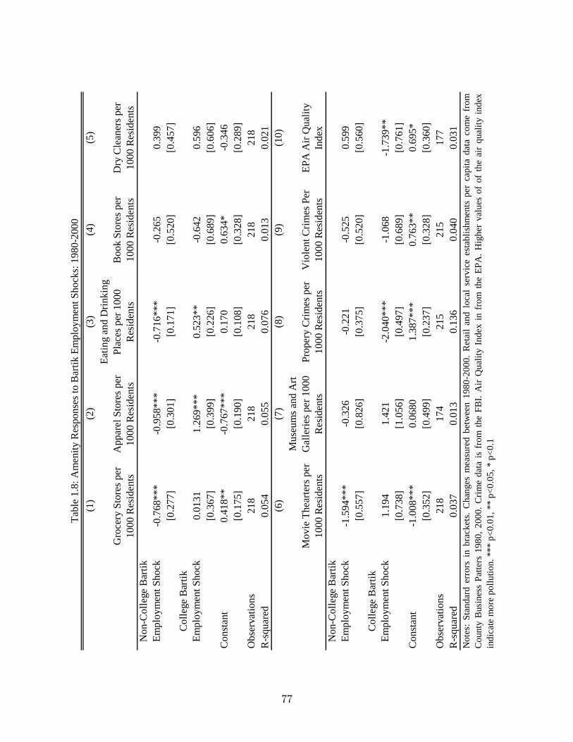
(1)

(2)

(3)

(4)

(5)

Gro

cery

Sto

res p

er10

00 R

esid

ents

App

arel

Sto

res p

er10

00 R

esid

ents

Eatin

g an

d D

rinki

ngPl

aces

per

100

0R

esid

ents

Boo

k St

ores

per

1000

Res

iden

tsD

ry C

lean

ers p

er10

00 R

esid

ents

Non

Col

lege

Bar

tikEm

ploy

men

t Sho

ck0

.768

***

0.9

58**

*0

.716

***

0.2

650.

399

[0.2

77]

[0.3

01]

[0.1

71]

[0.5

20]

[0.4

57]

Col

lege

Bar

tikEm

ploy

men

t Sho

ck0.

0131

1.26

9***

0.52

3**

0.6

420.

596

[0.3

67]

[0.3

99]

[0.2

26]

[0.6

89]

[0.6

06]

Con

stan

t0.

418*

*0

.767

***

0.17

00.

634*

0.3

46[0

.175

][0

.190

][0

.108

][0

.328

][0

.289

]O

bser

vatio

ns21

821

821

821

821

8R

squ

ared

0.05

40.

055

0.07

60.

013

0.02

1(6

)(7

)(8

)(9

)(1

0)

Mov

ie T

hear

ters

per

1000

Res

iden

ts

Mus

eum

s and

Art

Gal

lerie

s per

100

0R

esid

ents

Prop

ery

Crim

es p

er10

00 R

esid

ents

Vio

lent

Crim

es P

er10

00 R

esid

ents

EPA

Air

Qua

lity

Inde

xN

onC

olle

ge B

artik

Empl

oym

ent S

hock

1.5

94**

*0

.326

0.2

210

.525

0.59

9[0

.557

][0

.826

][0

.375

][0

.520

][0

.560

]C

olle

ge B

artik

Empl

oym

ent S

hock

1.19

41.

421

2.0

40**

*1

.068

1.7

39**

[0.7

38]

[1.0

56]

[0.4

97]

[0.6

89]

[0.7

61]

Con

stan

t1

.008

***

0.06

801.

387*

**0.

763*

*0.

695*

[0.3

52]

[0.4

99]

[0.2

37]

[0.3

28]

[0.3

60]

Obs

erva

tions

218

174

215

215

177

Rs

quar

ed0.

037

0.01

30.

136

0.04

00.

031

Tabl

e 1.

8: A

men

ity R

espo

nses

to B

artik

Em

ploy

men

t Sho

cks:

198

020

00

Not

es:

Stan

dard

erro

rsin

brac

kets

.C

hang

esm

easu

red

betw

een

1980

200

0.R

etai

lan

dlo

cal

serv

ice

esta

blish

men

tspe

rca

pita

data

com

efr

omC

ount

yB

usin

ess

Patte

rs19

80,2

000.

Crim

eda

tais

from

the

FBI.

Air

Qua

lity

Inde

xin

from

the

EPA

.Hig

her

valu

esof

ofth

eai

rqu

ality

inde

xin

dica

te m

ore

pollu

tion.

***

p<0

.01,

**

p<0.

05, *

p<0

.1

77

Overall, the underlying cause of the increase in sorting of workers by skill levels across

cities was due to an increases in sorting of productivity by skill across cities. As presented

earlier, Figure 1.2 shows the widening of the distribution of college employment ratios across

cities from 1980 to 2000. Figure 1.7 provides a similar histogram of the ratio of college

productivity to non-college productivity across cities for each decade. The productivity

ratio in each city is de�ned as:

Productivity Ratio=exp

�ProdHjt

�exp

�ProdLjt

� ;where ProdHjt ; Prod

Ljt are the local productivities of high and low skill workers, as de�ned in

equations (1:25) ; (1:26).42 As seen in Figure 1.7, the productivity ratio distribution across

cities exhibits the same widening over decades as seen in the college share distribution across

cities in Figure 1.2.

In Appendix A.5, I analyze the role of housing supply elasticity heterogeneity in explain-

ing the increase in geographic skill sorting. As the nation�s population grows, the cities with

less elastic housing supply experience relatively higher increases in housing rents. Since low

skill workers are more price sensitive, the rent increases in inelastic cities lead to more out

migration of low skill than high skill workers. This, in turn, leads to larger increases in the

college employment ratios of housing inelastic cities. Increases in a city�s college employment

ratio raise all workers�wages, as well as increase the city�s amenities. These e¤ects will mit-

igate the out-migration driven by the initial increase in the city�s rent, keeping the rent high

in these housing inelastic cities. Thus, nationwide population growth over time should lead

to larger increases in wages, rents, and college employment ratios in housing inelastic cities.

While I �nd evidence for these e¤ects, they only explain a small amount of the changes in

cities�college employment ratios. The dominant cause is local productivity change.

42The productivities are exponentiated since they are measured in log wage units. This makes the ratio ofhigh and low skill productivity comparable to the college employment ratio because both now are measuredin levels, not logs.

78

Figure 1.7: Distribution of College Productivity Gap Across MSAs: 1980-2000

79

1.7.4 Summary of Skill Sorting Mechanisms

To summarize, I �nd the underlying cause of the relative migration choices of high and low

skill workers to be changes in high and low skill workers�relative productivity across cities.

The structural model estimates show that a migration response to local productivity changes

which increases a city�s college employment ratio further increases the wages of all workers in

the city and increases the local amenities. Wages rise due the combined e¤ect of endogenous

productivity changes and movement along �rm�s labor demand curves. Amenities such as

pollutions levels, crime rates, and the quality of the local goods market improve in response

to increases in the college employment ratio.

The combination of desirable wage and amenity growth for all workers led to large

amounts of in-migration of both high and low skill workers. College workers were par-

ticularly attracted by desirable amenities, while low skill workers were particularly attracted

by desirable wages. The increase in population in high college share cities led to large rent

increases. Since low skill workers are more price sensitive, the increases in rent dispropor-

tionately discouraged low skill workers from living in these high wage, high amenity cities.

Thus, in equilibrium, college workers sort into high wage, high rent, high amenity cities.

Lower skill workers are not willing to pay the �price�of a lower local real wage to live in

high amenity cities, leading them to chose more a¤ordable, low amenity cities.

1.8 Welfare Implications & Well-Being Inequality

It is well documented that the nationwide wage gap between college workers and high school

graduates has increased signi�cantly from 1980 to 2000. Table 1.9 shows that the nationwide

college wage gap has increased by 0.20 log points.43 However, increases in wage inequality do

not necessarily re�ect increases in well-being inequality. College workers increasingly chose

43I focus on the college graduate-high school graduate wage gap because most of the literature has used thisas a key wage inequality statistic. My model assumes all non-college workers face the same wage di¤entialsacross cities. To make the welfare analysis comparable to the college-high school wage gap, I adjust the non-college workers�wages nationwide to represent the wages of a high school graduate, instead of the typicalnon-college worker. This does not impact the relative wages across cities.

80

to live in cities with higher wages, high rents, and more desirable amenities than non-college

workers. The additional welfare e¤ects of local rents and amenities could either add to or

o¤set the welfare e¤ects of wage changes.

First, I look only at wage and rent changes. I measure changes in the college �local

real wage gap�, where I de�ne a worker�s local real wage as his utility from wages and rent,

measured in log wage units:

Local Real Wageijt = wedujt � �rzi

�wzirjt:

�rzi�wzi

measure worker i0s expenditure share on locally priced goods. Table 1.9 reports changes

in the college local real wage gap from 1980-2000. Similar to the �ndings of Moretti (2011b),

I �nd the local real wage gap has increased 0.15 log points, 24% less than the increase in the

college wage gap. However, this is not a full welfare metric.

Part of the reason college workers chose to pay such high housing rents was because they

gained utility from the areas�amenities. To measure how changes in cities�wages, rents,

and amenities each contributed to well-being inequality, I conduct a welfare decomposition.

First, I measure each worker�s expected utility change from 1980 to 2000 if the only cities�

wages had changed, but local rents and amenities had stayed �xed. A worker �{0s expected

utility in 1980 is measured by the expected utility he would receive from living in his �rst

choice city:

E (Ui1980) = E

�maxjVij1980

�Vij1980 = �wziw


Hj1980Lj1980

+�stzistixstj + �


81

(1)

(2)

(3)

Yea

rC

olle

geH

igh

Scho

ol G

rad

Wag

e G

apC

olle

geH

igh

Scho

ol G

rad

Ren

t Gap

Loca

l Rea

l Wag

e G

ap19

800.

417

0.04

50.

386

[0.0

011]

[0.0

003]

[0.0

011]

1990

0.56

10.

130

0.47

4[0

.000

8][0

.000

6][0

.000

9]20

000.

616

0.11

60.

538

[0.0

007]

[0.0

003]

[0.0

008]

Cha

nge:

'80

'00

0.19

90.

071

0.15

2

(1)

(2)

(3)

(4)

Yea

rW

ellb

eing

Gap

Due

toW

ages

Wel

lbei

ng G

ap D

ue to

Wag

es &

Ren

t

Wel

lbei

ng G

ap D

ue to

Wag

e, R

ent,

+ En

dog.

Am

eniti

es fr

om R

eSo

rting

Acr

oss C

ities

Wel

lbei

ng G

ap D

ue to

Wag

e, R

ent,

Endo

g.A

men

ites f

rom

Nat

iona

lG

row

th in

Col

lege

Rat

io +

Re

Sorti

ng19

800.

417

0.41

70.

417

0.41

7

19

900.

529

0.51

00.

543

0.64

3[0

.001

1][0

.012

5][0

.014

7][0

.021

8]20

000.

609

0.59

20.

655

0.87

7[0

.001

5][0

.018

9][0

.021

6][0

.039

6]C

hang

e: '8

0'0

00.

193

0.17

50.

239

0.46

1[0

.001

5][0

.018

9][0

.021

6][0

.039

6]W

ald

Test

: Wel

lbei

ngIm

pact

vs.

Wel

lbei

ngIm

pact

of W

ages

1

.018

2.27

7**

6.55

5***

Dec

ompo

sitio

n of

Wel

lBei

ng In

equa

lity:

Wag

es, R

ents

, & E

ndog

enou

s Am

eniti

es: 1

980

2000

Obs

erve

d Ch

ange

s in

Wag

es &

Loc

al R

eal W

ages

: 198

020

00Ta

ble

1.9:

Cha

nges

in In

equa

lity

due

to W

ages

, Ren

ts, &

End

ogen

ous A

men

ities

Not

es:W

age

gap

mea

sure

dth

elo

gw

age

diff

eren

cebe

twee

nco

llege

and

high

scho

olgr

adua

tes.

Loca

lrea

lwag

ega

pm

easu

res

the

wag

esne

tofl

ocal

rent

sga

p.W

ellb

eing

gap

ism

easu

red

byth

edi

ffer

ence

ina

colle

gean

dhi

ghsc

hool

grad

uate

'sw

illin

gnes

sto

pay

toliv

ein

hisf

irstc

hoic

eci

tyfr

omth

ech

oice

sava

ilble

in20

00ve

rsus

his

first

choi

cein

1980

.For

exam

ple,

the

wel

lbei

ngga

pdu

eto

wag

ech

ange

son

lyac

coun

tsfo

rthe

wel

fare

impa

ctof

wag

ech

ange

sfr

om19

80to

2000

,whi

leth

ew

ellb

eing

due

tow

ages

and

rent

sacc

ount

sfor

both

the

impa

ctso

fwag

esan

dre

nts.

The

wel

lbei

ngga

pis

norm

aliz

edto

the

colle

gew

age

gap

in19

80. S

tand

ard

erro

rs fo

r wel

fare

esti

mat

es u

se th

e de

lta m

etho

d.

82

Since I do not observe each worker�s idiosyncratic taste for each city, I must integrate out

over the error distribution to calculate his expected utility from the city he chooses to live

in. Since the error terms are distributed Type I extreme value, a worker�s expected utility

from his top choice city is:

E (Ui1980) = ln

0B@Xj

exp

0B@ �wziweduj1980 � �rzirj1980 + �zj1980 + �colzi

Hj1980Lj1980


divzi divi xdivj

1CA1CA :

Similarly, worker i0s expected utility if wages adjust to the levels observed in 2000,E�Uwi2000

�;

is measured by:

E�Uwi2000

�= ln

0B@Xj

exp


Hj1980Lj1980


divzi divi xdivj

1CA1CA :

E�Uwi2000

�measures the utility worker i receives from living in the city he �nds most desir-

able. Combining these, the expected utility impact due to cities�wage changes from 1980 to

2000 is:E�Uwi2000

�� E

�Uwi1980

��wzi

:

The change in utility is divided by worker i�s marginal utility of wages, so that utility is

measured in log wage units. Intuitively, the expected utility change measures each workers

willingness to pay (in log wages) to live in his �rst choice counterfactual city instead of his

�rst choice city from the set available in 1980. I compute this for each worker in 2000 and

compare the average utility impact for college workers to the that of non-college workers.

Table 1.9 reports these estimates. From 1980-2000 changes in cities�wages led to an

increase in the college well-being gap equivalent to a nationwide increase of 0.193 log points

in the college wage gap, which is very close to observed increase of 0.199 in the college

wage gap. Even if local amenities and rents had not changed, there still would have been a

83

substantial increase in well-being inequality between college and non-college workers due to

local wage changes.

To account for the additional e¤ect of local rent changes, I perform a similar calculation

that allows local wages and rents to adjust to the level observed in 2000. The expected

utility of worker i if wages and rent adjust to the level observed in 2000 E�Uwri2000

�is:

E�Uwri2000

�= ln

0B@Xj

exp


Hj1980Lj1980


divzi divi xdivj

1CA1CA :

The change in well-being inequality between college and and high school graduates due to

wage and rent changes from 1980 to 2000 is equivalent to a nationwide increase of 0.175 log

points in the college wage gap. The welfare impacts of wages and rents lead to a smaller

increase in well-being inequality because the cities which o¤ered the most desirable wages

for college workers also had the highest rents, o¤setting some of the wage bene�ts.

To measure the additional contribution of amenity changes to well-being inequality, I can

only quantify the welfare impacts of endogenous amenity changes due to changes in cities�

college employment ratios. Since the model infers unobserved exogenous amenity changes by

measuring which cities have larger population growth than would be expected from the local

wage and rent changes, the model only identi�es relative amenity changes between cities

across years.

The model cannot identify the overall magnitude of amenity changes across decades. To

see this consider a simple example of 2 cities: New York and Chicago. Assume New York

and Chicago are equally appealing in year 1, and have equal populations. In year 2, there

is large migration from New York to Chicago, which cannot be explained by wage and rent

changes. One can conclude that the amenities of Chicago must have improved, relative to

the amenities of New York. If the amenities of New York stayed �xed, while the amenities

of Chicago improved, workers were able increase their utility, since New York is equally

84

desirable in years 1 and 2, but Chicago improved. In contrast, if the amenities of New York

declined, but Chicago�s amenities stayed �xed, workers would be worse o¤ in year 2 than

year 1, because both cities are weakly less desirable in year 2 than year 1. Yet these two

scenarios produced identical migration patterns, which makes inferring the welfare e¤ects of

unobserved amenity changes over time impossible.

The welfare e¤ects of endogenous amenity changes over time, however, can be measured.

Since a city�s college employment ratio represents an index of the city�s endogenous amenity

level, an increase in a city�s college employment ratio over time means that the endogenous

amenities must have improved from one year to the next. This welfare e¤ect can be measured

directly.

There are two main reasons the endogenous amenities of cities have changed over time.

First, there has been a nationwide increase in the share of the population with a college

degree. This led to increases in the college shares of almost all cities from 1980 to 2000.

Second, there has been a re-sorting of college and non-college workers across cities, which,

coupled with the nationwide college share increase, led to increases in some cities�college

shares more than others.

First, I measure the impact of amenity changes on well-being inequality driven only by

the re-sorting of college and non-college workers across cities. I hold the nationwide college

share �xed at the 1980 level. The expected utility of worker i if wages, rents, and endogenous

amenities due to resorting adjust to the level observed in 2000 E�Uwri2000

�; is measured by:

E�Uwri2000

�= ln

0B@Xj

exp


Hj2000

Lj2000


divzi divi xdivj

1CA1CA

Hj2000 =Hj2000H2000

H1980; Lj2000 =Lj2000L2000

L1980:

Hj2000 measures the share of all high skill workers living in city j in year 2000, scaled by the

85

national population size of high skill workers in 1980:H1980: Lj2000 is similarly de�ned, for

low skill workers.

The change in well-being inequality between college and high school graduates due to

wage, rent, and endogenous amenity changes due to workers re-sorting across cities from

1980 to 2000 is equivalent to a nationwide increase of 0.238 log points in the college wage

gap. This change in well-being inequality is 20% larger than the observed increase in the

actual college wage gap from 1980 to 2000. AWald test of whether this increase in well-being

inequality is statistically indistinguishable from the well-being increases due only to wage

changes is rejected.

The additional nationwide growth in the country�s college share led to large amenity

changes across almost all US cities. Adding on the additional e¤ect of the change in en-

dogenous amenities due to the nationwide increase in all cities�college shares leads to an

overall increase in well-being inequality equivalent to 0.461 log point increase in the college

wage gap. This �gure, however, should be interpreted with caution. There are surely many

other nationwide changes in the US which di¤erentially e¤ected the well-being of college and

non-college workers. For example, nationwide improvements in health care, life expectancy,

air-conditioning, television, and the internet likely in�uenced the well-being of all workers

nationwide. Since the model can only capture the welfare e¤ects of college share changes

and not the many other nationwide change, one should not interpret the welfare e¤ects of

the nationwide increase in college graduates as an accurate measure of changes in overall

well-being inequality. It is di¢ cult to gauge what aspects of well-being inequality changes

are measured in the nationwide increase in cities�endogenous amenities.

For these reasons, I place more con�dence in the estimated changes in well-being inequal-

ity due to wage, rent, and endogenous amenity changes driven by workers re-sorting across

cities. The combined welfare e¤ects of changes in wages, rents, and endogenous amenities

driven only by the re-sorting of workers across locations have led to at least a 20% larger

increase in well-being inequality than is apparent in the changes in the college wage gap

86

alone.

1.9 Conclusion

The divergence in the location choices of high and low skill workers from 1980 to 2000 was

fundamentally caused by a divergence in high and low skill productivity across space. By

estimating a structural spatial equilibrium model of local labor demand, housing supply,

and labor supply to cities, I quantify the ways through which local productivity changes

led to a re-sorting of workers across cities. The estimates show that cities which became

disproportionately productive for high skill workers attracted a larger share of skilled workers.

The rise in these cities� college shares caused increases in local productivity, boosting all

workers�wages, and improved the local amenities. The combination of desirable wage and

amenity growth caused large amounts of in-migration, driving up local rents. However, low

skill workers were less willing to pay the �price�of a lower real wage to live in high amenity

cities, leading them to prefer more a¤ordable, low amenity locations.

The net welfare impacts of the changes in cities�wages, rents, and endogenous amenities

led to an increase in well-being inequality between college and high school graduates of at

least 20% more than the increase in the college wage gap alone. The additional utility college

workers gained from of being able to enjoy more desirable amenities, despite the high housing

local prices, increased college workers�well-being, relative to high school graduates.

While the model quanti�es high and low skill productivity levels across cities, it does not

fully analyze the underlying determinants of these productivity di¤erences across locations.

A point of future work is to study the causes of the geographic decoupling of high skill

productivity from low skill productivity and the resulting re-sorting of �rms across US cities.

87

Chapter 2:Housing Supply Elasticity and Rent Extraction by

State and Local Governments

2.1 Introduction

Can government workers extract rent from private sector workers by charging high tax rates

and paying themselves high wages? The determinants and justi�cation of government work-

ers�compensation levels has taken on considerable heat in the past few years, as many states

and localities face budgetary stress. Since state and local governments set taxes and govern-

ment employee wages, government employees could earn rents by charging high taxes and

receiving high wages. There has long been debate over whether the government acts as a

benevolent social planner for its citizens or uses its market power to bene�t its workers and

political interest groups. (See Gregory and Borland (1999) for a review of this literature.)

In particular, the high unionization rate in the public sector may allow union bargaining

to in�uence the political process and the decisions of elected o¢ cials (Freeman (1986)). In

this paper, I analyze whether government workers receive higher wages than similar private

sector workers in areas where state and local governments have stronger abilities to exercise

market power.

This paper develops a model where state and local governments set taxes and the level of

government services to maximize government "pro�ts", which can then be paid to employees

as excessive wages. I use a Rosen (1979) Roback (1982) spatial equilibrium model where

workers maximize their utility by living in the city which o¤ers them the most utility based

on the city�s wage, rental rate of housing, tax rate, government services, and other amenities.

Thus, governments must compete for residents to tax, and workers can "vote with their feet"

by migrating away from excessively rent extractive governments.

I show that if state and local governments are using their market power to over pay their

employees, their abilities to extract rents from their citizens is determined by the equilibrium

88

migration elasticity of private sector residents with respect to local tax rates. Governments

must trade o¤ the bene�ts of a higher tax with the cost that a higher tax will cause workers

to migrate away, leaving the government with a smaller population to tax. This is analogous

to the standard result found in analysis of imperfect competition between product producers

where a �rm�s optimal price markup over cost is equal to the inverse elasticity of consumer

demand with respect to price for the �rm�s product.

Unlike �rm competition for consumer demand, I show that a government�s market power

to charge wasteful taxes remains even when there are a large number of governments com-

peting for residents and every government is small.44 The spatial equilibrium model shows

that when a government raises taxes, workers will migrate away to other jurisdictions. How-

ever, this out-migration decreases the level of labor supply and housing demand in the area.

Assuming labor demand curves slope down and housing supply curves slope up, this decrease

in population raises wages and decreases housing rents. Thus, some of the disutility of a tax

increase will be o¤set by an increase in the desirability of local wages and rents, which limits

the amount of out-migration caused by the tax increase. Since the local housing and labor

markets will respond to government imposed taxes through migration, the government will

always have market power.

An area�s elasticity of housing supply will determine how local housing rents respond

to population changes in an area. Governments presiding over areas with inelastic housing

supplies will have more market power than governments in housing elastic areas. A tax

hike by a government in an area with inelastic housing supply leads to a small amount of

out-migration because housing prices sharply fall due to the decrease in housing demand

driven by the tax hike. The housing cost decline o¤sets the negative utility impact of a

tax increase with a only small amount of out-migration in the housing inelastic area. Thus,

governments in housing inelastic areas can charge higher taxes without shrinking their tax

base since housing price changes limit the migration response.

44This result is closely related to Epple and Zelenitz (1981), which shows that worker migration betweengovernment juristidictions is not enough to entirely compete away a government�s market power.

89

If state and local governments exercise more market power in areas with inelastic housing

supplies, the wage gap between public and private sectors workers should be larger in these

areas. I test the model�s prediction by measuring variation in public-private sector wage

gaps across areas with di¤erent housing supply elasticities. I measure workers�wages using

data from the 1995-2011 Current Population Survey Merged Outgoing Rotation Groups

(CPS-MORG). I proxy for a metropolitan areas�s housing supply elasticity using data from

Saiz (2010) on the share of land within 50km of a city�s center unavailable for real-estate

development due to geographic constraints, such as the presence of swamps, steep grades,

or bodies of water. With less available land around to build on, the city must expand

farther away from the central business area to accommodate a given amount of population,

driving up average housing costs.45 I also use the Wharton Land Use Regulation Index

from Gyourko, Saiz, and Summers (2008) as component of housing supply elasticity. Since

the decision to regulate real-estate development is endogenous and possibly correlated with

unobserved characteristics which could impact government workers wages, I focus on the

Saiz (2010) measure of geographic constraints on real-estate development as an exogenous

source of variation in housing supply elasticity. These data are the metropolitan area level.

To measure states�housing supply elasticities I use an average of these measures across each

state�s MSAs, weighted by the MSAs�populations.

I �nd that the public-private sector wage gap is higher in states and metropolitan ar-

eas with less elastic housing supplies. This result holds when analyzing variation in state

government-private sector wage gaps across states and in local government-private sector

wage gaps across MSAs. This �nding is robust to including a host of controls for workers�

demographics and characteristics, including dummies for three digit occupation codes. Ad-

45A full micro-foundation of this mechanism can be derived from the Alonso-Muth-Mills model (Brueckner(1987)) where housing expands around a city�s central business district and workers must commute fromtheir house to the city center to work. Within-city house prices are set such that workers are indi¤erentbetween having a shorter versus longer commute to work. Average housing prices rise as the populationgrows since the houses on the edge of the city must o¤er the same utility as the houses closer in. As thecity population expands, the edge of the city becomes farther away from the center, making the commutingcosts of workers living on the edge higher than those in a smaller city. Since the edge of the city must o¤erthe same utility value as the center of the city, housing prices rise in the interior parts of the city.

90

ditionally, the local government-private sector wage gap is found to be higher in housing

inelastic MSAs, even when only comparing MSAs within the same state.

As falsi�cation tests, I show that housing supply elasticity has no impact on the federal

government worker-private sector wage gap. Since federal workers� compensation is not

derived from government revenues of their place of residence, the market power of the state

and local government should have no impact on their wages. Additionally, I show that

variation in the state government worker-private sector wage gap does not vary across MSAs,

within a state. The public-private wage gaps only vary with housing supply elasticities when

the housing supply elasticity variation impacts the government�s market power. I also show

that the e¤ect is larger for government workers who are union members, suggesting unions

allow government workers to bargain for a larger share of government rents.

The CPS-MORG only reports data on workers�earnings, and does not include data on

the value of workers�benefts. Gittleman and Pierce (2012) show that goverment employees

receive more generous bene�ts than similar private sector workers, on average. I use data

from on average government pension payouts per bene�ciary across states from the Census�

2007-2010 Annual Surveys of Public Employee Retirement Systems as a measure of state

government workers�bene�ts. While I do not have a data source for similar private sector

workers�retirement bene�ts, I show that average annual state government pension payouts

per bene�ciary are higher in states with less elastic housing supplies. This suggests that the

wage gap estimates from the CPS understate the full impact of housing supply elasticity on

government worker compensation.

Previous work has also found evidence suggesting government jobs are more desirable

than similar private sector jobs. Gittleman and Pierce (2012) show that public sector em-

ployees are more generously compensated than similarly quali�ed private sector employees.

In particular, they �nd that government worker wages tend to be slightly lower than similar

private sector workers. However, the value of government workers�bene�ts strongly outweigh

those of the private sector, leading to public sector employees to be better compensated over-

91

all. Krueger (1988) �nds that there are more job applications for each government job than

for each private sector job, suggesting that government jobs are more desirable to workers,

on average. Additionally, average job quit rates reported from the 2002-2006 Job Openings

and Labor Turnover Surveys show that average annual quit rate is 28% for private sector

workers, but only 8% for public sector employees. These fact taken together suggest that

government jobs are better compensated than private sector jobs, and that there appears to

be excess labor supply for these jobs, which is consistent with government workers receiving

rents. While this evidence shows that government jobs appear desirable to workers, it is not

clear that this desirability is due to rent-seeking behavior of governments exercising market

power. My paper shows that an increase in governments�abilities to extract rent directly

leads to better paid government employees.

The public sector workforce is also highly unionized, enabling government employees to

bargain for government rents. Gyourko and Tracy (1991) use a spatial equilibrium model to

show that if the cost of government taxes to citizens are not completely o¤set by bene�ts

of government services, they will be capitalized into housing prices. Similarly, if high levels

of public sector unionization lead to more government rent extraction, the public sector

unionization rate will proxy for government waste and also be capitalized into housing prices.

While Gyourko and Tracy (1991) �nd evidence for both of these e¤ects, it is unclear what

drives the variation in taxes and unionization rates across localities. This paper uses housing

supply elasticity as a source of exogenous variation in government market power to assess

whether government take advantage of their power to over pay employees.

Brueckner and Neumark (2011) considers whether government can extract more rent from

local residents if the government presides over an area with more desirable amenities. They

use a similar setup to this paper where pro�t maximizing governments compete for residents

by setting local tax rates. They allow local governments to play a game in tax-competition

where the number of competing governments is small. My model di¤ers from theirs by

allowing each government to be small when deriving tax rates chosen by governments. They

92

�nd evidence that amenity di¤erences are positively associated with public-private wage

gaps. However, it is possible that some of the amenity measures, such as coastal proximity

and population density, are correlated with housing supply elasticity di¤erences.

The paper proceeds as follows. Section 2 layouts of the model. Section 3 presents

empirical evidence, and Section 4 concludes.

2.2 Model

The model detailed below uses a Rosen (1979) Roback (1982) spatial equilibrium to analyzes

how local governments set taxes and compete for residents. In the model, I assume that

governments use a head tax to collect revenue, however in reality, most state and local

governments use property and income tax instruments. In Appendix B I derive results for

the case of a government income or property tax and show the same results. I also abstract

away from the political election process in each area. While politics could surely in�uence

the extent of government rent seeking, my goal is to analyze contributors to governments�

abilities to excercise market power if they had a rent seeking motivation.

The nationwide economy is made up of many cities. There are N cities, where N is large.

Cities are di¤erentiated by their endowed amenity levels Aj;which impact how desirable

workers �nd the city, and their endowed productivity levels �j; which impact how productive

�rms are in the city. Workers are free to migrate to any city within the country. Each city

has a local labor and housing market, which determine local wages and rents. The local

government provides government services and collects taxes.

2.2.1 Government

The local government of city j charges a head tax � j to workers who choose to reside within

the city. The local government also produces government services, which cost sj for each

93

worker in the city. The government revenue and cost are

Revenuej = � jNj

Costj = sjNj:

Nj measure the population of city j: The local government is not benevolent and maximizes

pro�ts. These pro�ts could be spent on ine¢ cient production of sj (thus, making the

government benevolent, but naive). They could also be directly pocketed by government

workers, such as through union negotiations. The local government maximizes:

max�j ;sj

� jNj � sjNj

2.2.2 Workers

All workers are homogeneous. Workers living in city j inelastically supply one unit of labor,

and earn wage wj: Each worker must rent a house to live in the city at rental rate rj and

pay the local tax � j:Workers value the local amenities as measure by Aj:The desirability of

government services sj is represented by g (sj) : Thus, workers�utility from living in city j

is:

Uj = wj � rj + Aj + g (sj)� � j:

Workers maximize their utility by living in the city which they �nd the most desirable.

2.2.3 Firms

All �rms are homogenous and produce a tradeable output Y:Cities exogenously di¤er in

their productivity as measured by �j. Local government services impact �rms productivity,

as measured by b(sj): The production function is:

Yj = �jNj + b(sj)Nj + F (Nj) ;

94

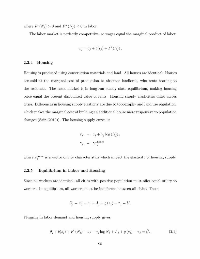
where F 0 (Nj) > 0 and F 00 (Nj) < 0 in labor:

The labor market is perfectly competitive, so wages equal the marginal product of labor:

wj = �j + b(sj) + F0 (Nj) :

2.2.4 Housing

Housing is produced using construction materials and land. All houses are identical. Houses

are sold at the marginal cost of production to absentee landlords, who rents housing to

the residents. The asset market is in long-run steady state equilibrium, making housing

price equal the present discounted value of rents. Housing supply elasticities di¤er across

cities. Di¤erences in housing supply elasticity are due to topography and land use regulation,

which makes the marginal cost of building an additional house more responsive to population

changes (Saiz (2010)). The housing supply curve is:

rj = aj + j log (Nj) ;

j = xhousej

where xhousej is a vector of city characteristics which impact the elasticity of housing supply.

2.2.5 Equilibrium in Labor and Housing

Since all workers are identical, all cities with positive population must o¤er equal utility to

workers. In equilibrium, all workers must be indi¤erent between all cities. Thus:

Uj = wj � rj + Aj + g (sj)� � j = �U:

Plugging in labor demand and housing supply gives:

�j + b(sj) + F0 (Nj)� aj � j logNj + Aj + g (sj)� � j = �U: (2.1)

95

Equation (2:1) determines the equilibrium distribution of workers across cities.

2.2.6 Government Tax Competition

Local governments set city tax rates and the level of government services to maximize pro�ts,

taking into account the endogenous response of workers and �rms in equilibrium, equation

(2:1). Each city is assumed to be small, meaning out-migration of workers to other cities does

not impact other cities�equilibrium wages and rents. If there were a small number of cities,

each city would have even more market power than in this limiting case. The results below

can be thought of as a lower bound on the market power of local governments competing for

residents. They maximize:

maxsj ;�j

� jNj � sjNj:

The �rst order conditions are:

0 = � j@Nj@sj

�Nj � sj@Nj@sj

(2.2)

0 = � j@Nj@� j

+Nj � sj@Nj@� j

:

Di¤erentiating equation (2:1) to solve for @Nj@sj

and @Nj@�jgives:

@Nj@sj

=b0 (sj) + g

0 (sj)� jNj� F 00 (Nj)

� > 0@Nj@� j

=�1�

jNj� F 00 (Nj)

� < 0: (2.3)

96

Population increases with government services and decreases in taxes. Plugging these into

(2:2) gives:

0 = (� j � sj)

0@ b0 (sj) + g0 (sj)�

jNj� F 00 (Nj)

�1A�Nj

� j = Nj

� jNj� F 00 (Nj)

�+ sj:

Combining the �rst order conditions shows that government services are provided such that

the marginal bene�t (b0 (sj) + g0 (sj)) equals marginal cost (1) :

b0�s�j�+ g0

�s�j�= 1:

This is the socially optimal level of government service.

The equilibrium tax rate is:

� �j = j �NjF 00 (Nj) + s�j : (2.4)

The elasticity of city population with respect to the tax rate�"migratej

�can be written as:

"migratej =@Nj@� j

� jNj:

Plugging in equation (2:3) for @Nj@�j

and rearranging gives:

� jNj� F 0 (Nj)

�Nj =

�� j"migratej

:

Substituting this expression into the equation (2:4) shows that the tax markup can be written

as:� �j � s�j� �j

=�1

"migratej

:

97

The tax markup above cost is equal to the inverse elasticity of city population with respect

to the tax rate: While workers are perfectly mobile between cities, worker migration causes

shifts along the local labor demand and housing supply curves. An increase in local taxes

would cause workers to migrate to other cities. A decrease in population will increase local

wages, since I have assumed a downward sloping labor demand curve. The decrease in

population will also cause rents to fall, by moving along the housing supply curve. This

increase in wages and decrease in rents will increase the desirability of the city to workers,

limiting the migration response to the tax increase. The government takes into account the

equilibrium wage and rent response to a tax hike when setting taxes to pro�t maximize.

Thus, if migration leads to large changes in local wages and rent, a tax increase will not lead

to large amounts of out-migration, since workers will be compensated for the tax with more

desirable wages and rents.

To analyze the e¤ect of housing supply elasticity on governments�ability to extract rent

from taxes, I di¤erentiate the tax markup with respect to the slope of the inverse housing

supply curve, j:@

@ j

�� j � s�j

�= 1� @

@Nj(NjF

00 (Nj))@Nj@ j

: (2.5)

The �rst term (1) in equation (2:5) represents the increased rent response to migration

induced by a tax hike in a city with an inelastic housing supply. The equilibrium condition,

equation (2:1) ; shows that out-migration will continue until the negative utility impact of

the tak hike has been completely o¤set by changes in the city�s wage and rent. In a city

with a less elastic housing supply, a smaller amount of migration is needed to push housing

rents down to o¤set the negative utility impact of the tax hike. The second term in equation

(2:5) represents the change in the elasticity of labor demand due to being at a di¤erent

point on the labor demand curve�

@@Nj

(NjF00 (Nj))

�. Since a city with a less elastic housing

supply has a smaller equilibrium population, the slope of the labor demand curve in a smaller

city could di¤er from the slope of the labor demand curve in a larger city. I will assume

98

@@Nj

(NjF00 (Nj)) = 0; which is equivalent to assuming exp (F 0 (Nj)) has a constant elasticity

with respect to Nj. Under this assumption, the derivative of the tax markup with respect

to the slope of the inverse housing curve is:

@

@ j

�� j � s�j

�= 1 > 0:

The government can extract more rent through higher taxes in a city with a less elastic

housing supply.

Note that this result assumes there are a large number of cities. When there are a small

number of cities, the incentives for rent extraction will be even higher. Outward migration

from a city in response to a tax increase will lead to increases in other cities� rents and

decreases in their wages, leading to less outward migration in response to tax increases. I

have assumed this e¤ect away by not allowing the equilibrium utility level across all cities to

fall in response to a given city�s tax increase. Cities can extract rent even in an environment

where there are a large number of competitors because household demand for city residence

can never be in�nite in equilibrium.

Additionally, this model assumes cities charge a head tax, while in reality most cities and

states tax their population through income taxes and property taxes. The amount of rent

extraction depends on the elasticity of tax revenue with respect to the tax rate. Thus, an

income tax will depend both on the wage response to the tax rate, as well as the migration

response. Appendix B shows that when using an income tax, governments can still excercise

more market power in housing inelastic areas.

In the case of a property tax, government revenue will depend on local the rental rate

and the size of the tax base. An increase in the property tax rate can decrease government

revenue both by incentivizing workers to migrate away, shrinking the tax base, and decreasing

housing rents, lowering tax revenue from each household. However, I show in appendix B

that if local labor demand is perfectly elastic, the housing supply elasticity will not impact

99

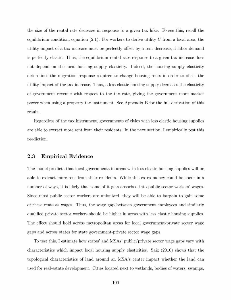
the size of the rental rate decrease in response to a given tax hike. To see this, recall the

equilibrium condition, equation (2:1) : For workers to derive utility �U from a local area, the

utility impact of a tax increase must be perfectly o¤set by a rent decrease, if labor demand

is perfectly elastic. Thus, the equilibrium rental rate response to a given tax increase does

not depend on the local housing supply elasticity. Indeed, the housing supply elasticity

determines the migration response required to change housing rents in order to o¤set the

utility impact of the tax increase. Thus, a less elastic housing supply decreases the elasticity

of government revenue with respect to the tax rate, giving the government more market

power when using a property tax instrument. See Appendix B for the full derivation of this

result.

Regardless of the tax instrument, governments of cities with less elastic housing supplies

are able to extract more rent from their residents. In the next section, I empirically test this

prediction.

2.3 Empirical Evidence

The model predicts that local governments in areas with less elastic housing supplies will be

able to extract more rent from their residents. While this extra money could be spent in a

number of ways, it is likely that some of it gets absorbed into public sector workers�wages.

Since most public sector workers are unionized, they will be able to bargain to gain some

of these rents as wages. Thus, the wage gap between government employees and similarly

quali�ed private sector workers should be higher in areas with less elastic housing supplies.

The e¤ect should hold across metropolitan areas for local government-private sector wage

gaps and across states for state government-private sector wage gaps.

To test this, I estimate how states�and MSAs�public/private sector wage gaps vary with

characteristics which impact local housing supply elasticities. Saiz (2010) shows that the

topological characteristics of land around an MSA�s center impact whether the land can

used for real-estate development. Cities located next to wetlands, bodies of waters, swamps,

100

or extreme hilliness have limits on how many building can be built close to the city center,

which impacts the elasticity of housing supply to the area. Saiz (2010) uses satellite data to

measure the share of land within 50km of an MSA�s center which cannot be developed due

to these topological constraints. A rent-seeking government is able to charge higher taxes

in areas with less land available for development. Thus, the public-private sector wage gap

should be higher in these areas.

A city�s housing supply elasticity is also in�uenced by the amount of land-use regulation

in the area. The 2005 Wharton Land Use Regulation Survey Gyourko, Saiz, and Summers

(2008) collected survey data on a number of land-use regulations and practices, which were

aggregated into the Wharton Land Use Regulation Index (WLURI). Saiz (2010) aggregates

this municipality measure into a MSA-level index.

I z-score the MSA level data from the WLURI and the land unavailability measure and

will use both as measures of cities�housing supply elasticities. I also aggregate these measures

to a state-level index, where I weight each MSA measure by the state population in each

MSA. The state-level housing supply elasticity measure is a noisy measure of the overall

housing supply elasticity for the state, since the data is only based o¤ of the MSAs covered

by Saiz�s sample. Table 2.1 reports summary statistics on these measures. The data covers

48 states (there is no data for Hawaii or Alaska) and 228 MSAs.

101

MeanStandard

Dev. Min Max NLocal Government Worker Ln WeeklyEarnings 6.723 0.519 4.854 8.695 112639State Government Worker Ln WeeklyEarnings 6.725 0.509 4.857 8.695 62994Federal Government Worker LnWeekly Earnings 6.964 0.496 4.855 8.695 37008Private Sector Worker Ln WeeklyEarnings 6.686 0.613 4.852 8.695 968349

MeanStandard

Dev. Min Max NState Aggregated Land Unavailability: ZScore 0.000 1.000 1.427 2.982 48State Aggregated Wharton Land UseRegulation Index: ZScore 0.000 1.000 1.640 2.348 48MSA Land Unavailability: ZScore 0.000 1.000 1.205 2.824 228MSA Wharton Land Use RegulationIndex: ZScore 0.000 1.000 1.746 3.938 228

MeanStandard

Dev. Min Max N

Log Thousand Dollars of Annual Payoutper beneficiary from State Pension 2.9897 0.24996 2.5289 3.629 192

Table 2.1: Summary StatisticsA. CPS Data 19952011

B. Housing Supply Elasticity Measures

C. State Government Pension Payouts: 20072010

Notes: Wages are measured as weekly wages deflated by the CPIU and reported in constant 2011 dollarsfor 2555 year old workers working at least 35 hours per week. Workers with imputed weekly earningsare dropped from the analysis. Top coded weekly earnings as set to 1.5 times the top coded value andweekly earnings below $128 (in real 2011 dollars) are dropped from the analysis. Sector of worker(local/state/federal/private) is measured by reported class of worker. MSA land unavailability measuresthe share of land within 50km of an MSA's center which cannot be developed due to these topologicalconstraints from Saiz (2010). This measure is then Zscored. The Wharton Land Use Regulation indexaggregates survey data on a large set of local land use practices by local municipalities. This is aggregatedto the MSA level and then Zscored. State aggregated housing supply elasticity meaures use a populationweighted average of MSA level data. State and MSA level housing supply elasticity measures are zscored.Government pension data come from 20072010 Annual Surveys of PublicEmployee RetirementSystems.

102

2.3.1 Wage Gap Regressions

To measure public-private sector wage gaps across MSAs and states, I use data from the

Current Population Survey Merged Outing Rotation groups from 1995-2011.46 The CPS-

MORG is a household survey which collects data on a large number of outcomes including

workers�weekly earnings, hours worked, public/private sector of employment, union status,

and a host of demographics. I restrict the sample to 25 to 55 year old workers with positive

labor income, working at least 35 hours per week, to have a standardized measure of weekly

earnings. The CPS�s usual weekly earnings question does not include the self-employment

income so all analysis excludes the self-employed. I also restrict analysis to workers whose

wages are not imputed to avoid any bias due to the CPS�s wage imputation algorithm

(Bollinger and Hirsch (2006)). I measure earnings using workers�log usual weekly earnings,

de�ated by the CPI-U and measured in real 2011 dollars. Top coded weekly earnings are

multiplied by 1.5 and weekly earnings below $128 are dropped from the analysis.47 All

analysis is weighted by the CPS earnings weights.

Table 2.1 reports summary statistics of workers�log weekly earnings each for workers em-

ployed in the private sector, local government, state government, and federal government.48

Consistent with previous works, such as Gittleman and Pierce (2012), the raw earnings are

higher for all three classes of government workers than for private sector workers. However,

these raw earnings di¤erences do not account for di¤erences in the characteristics of work-

ers between the public and private sector. To test the model�s predictions, I will control

for worker characteristics when evaluating di¤erences in the public private sector wage gap.

46Since there was a signi�cant change in the CPS�s earnings questions in 1994, I restrict analysis to 1994-2011. I also focus my analysis on workers whose wages are not imputed in the CPS. Since sector, occupation,and union status and not used in the CPS�s imputation algorithm, analyzing government wage gaps andunion wage gaps using imputed wages can be problematic (Bollinger and Hirsch (2006)). Thus, I focus onlyon the non-imputed wage sample. The data �agging which wages were imputed are missing in the 1994 data,so I drop this year, leaving me with a 1995-2011 sample.47I follow Autor, Katz, and Kearney (2008)�s top and bottom coding procedures. Autor, Katz, and

Kearney (2008) drops all reported hourly wages below $2.80 in real 2000 dollars. This translates to $128 perweek in real 2011 dollars, assuming a 35 hour work week. They also scale top coded wages by 1.5.48A worker�s sector is measured by the CPS variable reporting a worker�s class.

103

Additionally, the CPS only collects data on workers�earnings, but not compensation paid to

workers in the form of bene�ts. Gittleman and Pierce (2012) show using the BLS�restricted-

use Employer Cost of Employee Compensation microdata that government employees receive

signi�cantly more generous bene�ts than similar workers in the private sector. I will return

to the question of bene�ts compensation, but �rst focus on public-private sector wage gaps.

To test the model�s predictions, I estimate the following regression:

lnwijt = �j + �t + �govgovit + �

elastzelastj � govit + �Xit + "ijt: (2.6)

As controls, I include location �xed-e¤ects �j; year �xed e¤ects, �t; and a set of worker

demographics which include 15 dummies for education categories, gender, race, Hispanic

origin, a quartic in age, and a rural dummy. govi is a dummy for whether the worker is

government worker, zelastj measures land use regulation and topography. Standard errors are

clustered by state when using state-level measures of housing supply elasticity and clustered

by MSA when using MSA variation in housing supply elasticity.

The nationwide average public-private wage gap is measured by �gov:The model predicts

that public-private wage gap should be higher in areas with less elastic housing supplies:

�elast > 0:

The prediction should hold both for areas with less land available for development and for

areas with stricter land-use regulations. Since land-use regulations are chosen by local mu-

nicipalities, it is possible that the decision to regulate land-use could be correlated with other

characteristics of the area which could impact workers�wages. Since the topological con-

straints around a city are pre-determined, they are likely a measure of exogenous di¤erences

in housing supply elasticities across areas. I perform all analysis using both measures, but I

also drop the regulation index to focus directly on the impact of land availability, which is

likely a cleaner estimate of the impact of housing supply elasticity on public-private sector

104

wage gaps.

I test this prediction �rst using a sample including private sector workers and state

government workers. Column 1 of Table 2.2 shows that the nationwide average wage gap be-

tween state government employees and private sector workers is -0.112 log points. Consistent

with Gittleman and Pierce (2012), after controlling for worker demographics, government

workers�earnings are lower than similar private sector workers, on average. However, the

state worker-private sector wage gap increases by 0.017 log points in states with a 1 stan-

dard deviation increase in land unavailability. This e¤ect is signi�cant at the 10% level. The

wage gap is 0.026 log points higher in states with a 1 standard deviation increase land-use

regulation. This e¤ect is signi�cant at the 5% level. In a regression which drops the land-use

index, a 1 standard deviation increase in a state�s land availability increases the wage gap

by 0.026 log points. This e¤ect is signi�cant at the 1% level. Figure 2.1 plots states�land

unavailability against states�state government worker-private sector wage gaps, after wages

have been residualized against the set of controls included in equation (2:6) : Figure 1 shows

the state government-private sector wage gaps are higher in states including California, Ver-

mont, Florida, and Connecticut, but must lower in states such as Iowa, Texas, Montana,

and Kentucky which lines up with these states�land unavailability. Note that states such as

Utah are signi�cant outliers. However, Utah�s land availability was measured only based on

Salt Lake City, which has a large share of land unavailable for development due proximity

to the Great Salt Lake. This is likely a poor measure of the overall state housing supply

elasticity. Despite the short comings of the state-level data, I �nd that states with less elastic

housing supplies have signi�cantly better paid state government employees, as compared to

the private sector employees residing in the state.

105

1 2 3 4 5 6

Government Worker 0.112*** 0.113*** 0.0798***0.0707***[0.00909] [0.00931] [0.00721] [0.00758]

Gov* Land Unavailability 0.0170* 0.0262*** 0.0287*** 0.0366*** 0.00856 0.0108*[0.0101] [0.00976] [0.00781] [0.00855] [0.00637] [0.00657]

Gov* Land Use Regulation 0.0263** 0.0348*** 0.0220**[0.0125] [0.00803] [0.00920]

Constant 2.493*** 2.487*** 2.382*** 2.378*** 2.396*** 2.399***[0.289] [0.290] [0.397] [0.396] [0.397] [0.397]

State x Gov Worker FE: X XState Elasticity Measures: X XMSA Elasticity Measures: X X X XState Gov Workers Sample: X XLocal Gov Workers Sample: X X X XObservations 973,792 973,792 586,696 586,696 586,696 586,696Rsquared 0.384 0.384 0.389 0.389 0.39 0.39

Table 2.2: Ln Wage vs. State & Local Public SectorHousing Supply Elasticity Interactions

Note: Standard errors clustered by state for state worker regressions. Standard errors clustered by MSA for localgovernment worker regressions. Weekly wage data from 19952011 CPS MORG. Wage data is restricted to 2555year old workers working at least 35 hours per week. State government worker sample includes private sectorand state government workers. Local government worker sample includes private sector and local governmentworkers living in MSAs. Land unavailability measures a zscore of the share of land within 50km of an MSA'scenter which cannot be developed due to topological constraints. Land use regulation is an index of aggregatedsurvey data on a large set of local land use practices by local municipalities. This is aggregated to the MSA leveland then Zscored. State level measures are zscores of average MSAlevel measures within the state, weightedby MSA population. Controls include 15 dummies for education categories, gender, race and hispanic origin, aquartic in age, a rural dummy, and year dummies. All regressions weighted using CPS MORG earnings weights.

State GovPrivateSector Wage Gaps Local GovPrivate Sector Wage Gaps

106

AL

AZ

AR

CA

CO

CT

DEFL

GA

ID

IL

IN

IA

KS

KY LA

ME

MDMA

MI

MN

MS

MO

MT

NE

NV

NH

NJ

NM

NY

NCND

OH

OK

OR

PA RI

SC

SD

TN

TX

UT

VT

VA

WA

WV

WI

WY

.2.1

5.1

.05

0Pu

blic

Priv

ate

Wag

e G

ap

1 0 1 2 3State Average Land Unavai labil i ty in MSAs: ZScore

Figure 2.1: State Goverment-Private Sector Wages Gaps vs. State Land

Unavailability Z-Score. State wage gaps calculated after residualizing wages

against 15 dummies for education categories, gender, race, hispanic origin, a

quartic in age, a rural dummy, and year dummies. Regression weighted using

CPS earnings weights.

107

Performing the same analysis on local government employees, I compare the wage gaps

between local government workers and private sector workers across 229 MSAs. The controls

in this setup now include MSA �xed e¤ects and the housing supply measures are now at the

MSA level. Column 3 of Table 2.2 shows that the nationwide local government worker-private

sector wage gap is -0.080 log points. A 1 standard deviation increase in land unavailability

increases the wage gap by 0.029 log points and a 1 standard deviation increase in land-use

regulation increases the wage gap by 0.0348 log points. Both of these e¤ects are signi�cant at

the 1% level. Dropping the land-use regulation, I �nd the coe¢ cient on land unavailability

increases to 0.037 log points, and is signi�cant at the 1% level. Figure 2.2 plots MSAs�land

unavailability against MSAs�local government worker-private sector wage gaps, after wages

have been residualized against the set of controls included in equation (2:6) : The plot shows

high local government wages gaps in land unavailable cities including Los Angeles, New York,

Cleveland, Chicago, and Portland and low government wage gaps in cities with lots of land

to develop including Atlanta, Houston, Minneapolis, and Phoenix. Housing supply elasticity

explains a signi�cant amount of the cross-section variation in public-private wage gaps.

To test whether the local housing supply elasticity measures impact local government

worker-private sector wage gaps within states, across MSAs, I add controls for state di¤er-

ences in the local government worker-private sector wage gaps. I now estimate:

lnwijkt = �j + �t + �govgovit + �

govk govit + �

elastzelastj � govit + �Xit + "ijt;

where j represents an MSA and k represents a state. Columns 5 and 6 of Table 2.2 show

that the impact of land unavailability on the local government-private sector wage gap falls

slightly, but remains statistically sigin�cant when land-use regulations are not included in

the regression. Land unavailability consistently has a positive impact the public-private

sector wage gap both for local and state government workers, as predicted by the model.

108

Atlanta

Baltimore

Boston

ChicagoClevelandDetroit

HoustonKansasCity

LasVegas

LA

Minneapolis

NYC

PhiladelphiaPhoeniz

Pittsburgh

PortlandStLouis

SaltLake

Washington

.6.4

.20

.2Pu

blic

Priv

ate

Wag

e G

ap

1 0 1 2 3MSA Land Unavai labil i ty: ZScore

Figure 2.2: Local Goverment-Private Sector Wages Gaps vs. MSA Land

Unavailability Z-Score. MSA wage gaps calculated after residualizing wages

against 15 dummies for education categories, gender, race, Hispanic origin, a

quartic in age, a rural dummy, and year dummies. Regression weighted using

CPS earnings weights.

109

Table 2.3 repeats the analysis adding in dummies for each three-digit occupation code to

attempt to further control for di¤erences in workers�skills in the public and private sectors.

The point estimate measuring the impact of land unavailability of the state government-

private sector wage gap remains positive, but the standard errors increase, making the e¤ect

only statistically signi�cant when land-use regulations are dropped from the regression. How-

ever, the large standard errors shows that one cannot rule out a point estimate equal to the

magnitude found when 3-digit occupation code dummies were not included in the regression.

The estimates for local-government worker wage gaps are positive and statistically sig-

ni�cant at the 1% level. Column 4 of Table 2.3 shows that even when including the full

set of 3 digit occupation dummies, a 1 standard deviation increase in land unavailability

increases the local public-private wage gap by 0.028 log points. Note that with the inclusion

of occupation dummies, the nationwide local government worker-private sector wage gap is

now positive at 0.028 log points.

One possible way government workers can raise their wages is through union wage bar-

gaining. I repeat the analysis adding in additional housing supply elasticity interactions

terms for whether the government worker is part of a labor union. I control for the direct ef-

fect of being in a union, and its interaction with the housing supply elasticity characteristics.

This controls for di¤erences in union bargaining power across states and MSAs for all unions,

public and private. Table 2.4 shows that a standard deviation increase in land unavailability

raises state government-private sector wage gaps by 0.0127 log points for non-union mem-

bers and an addition 0.0214 log points for unionized government workers. State government

worker unions appear to be able to bargain for better wages in inelastic areas, relative to

non-unionized government workers. The point estimates in Columns 3 and 4 of Table 2.4

are similar for local government-private sector wage gaps. However, the additional impact

of goverment labor unions is positive, but not statistically signi�cant. These point estimates

suggest government workers part of a labor union might be able to use their market power

to negotiate for larger rents beyond the o¤erings of the private sector.

110

1 2 3 4

Government Worker 0.0320***0.0331*** 0.0181*** 0.0275***[0.00830] [0.00837] [0.00538] [0.00545]

Gov* Land Unavailability 0.0107 0.0188* 0.0197*** 0.0275***[0.0111] [0.0109] [0.00675] [0.00743]

Gov* Land Use Regulation 0.0234** 0.0350***[0.0112] [0.00716]

Constant 4.263*** 4.258*** 4.211*** 4.208***[0.274] [0.274] [0.386] [0.386]

State Elasticity Measures: X XMSA Elasticity Measures: X XState Gov Workers Sample: X XLocal Gov Workers Sample: X XObservations 973,792 973,792 586,696 586,696Rsquared 0.524 0.524 0.526 0.526

Table 2.3: Ln Wage vs. State & Local Public SectorHousing Supply ElasticityInteractions with 3 Digit Occupation Dummy controls

Note: Standard errors clustered by state for state worker regressions. Standard errorsclustered by MSA for local government worker regressions. Weekly wage data from19952011 CPS MORG. Wage data is restricted to 2555 year old workers working atleast 35 hours per week. State government worker sample includes private sector andstate government workers. Local government work sampe includes private sector andlocal government workers living in MSAs. Land unavailability measures a zscore of theshare of land within 50km of an MSA's center which cannot be developed due totopological constraints. Land use regulation is an index of aggregated survey data on alarge set of local land use practices by local municipalities. This is aggregated to theMSA level and then Zscored. State level measures are zscores of average MSAlevelmeasures within the state, weighted by MSA population. Controls include 1057occupation dummies, 15 dummies for education categories, gender, race, hispanicorigin, a quartic in age, a rural dummy, and year dummies. Three digit occupation codedefinitions change in 2000, so I include the full set of combined 3 digit occupationdummies. I treat occupation codes used in years 20002011 as distinct occupationsfrom those in previous years, giving a total of 1057 occupation codes. All regressionsweighted using CPS earnings weights. *** p<0.01, ** p<0.05, * p<0.1

State GovPrivateSector Wage Gaps

Local GovPrivateSector Wage Gaps

111

1 2 3 4

Government Worker 0.140*** 0.142*** 0.123*** 0.119***[0.00613] [0.00575] [0.00695] [0.00718]

Gov* Land Unavailability 0.0101 0.0127** 0.0269*** 0.0316***[0.00705] [0.00624] [0.00739] [0.00801]

Gov* Land Use Regulation 0.00782 0.0238***[0.00889] [0.00801]

Gov* Land Unavailability*Union 0.00372 0.0214* 0.00373 0.00753[0.0120] [0.0128] [0.00845] [0.00934]

Gov* Land Use Regulation*Union 0.0492** 0.0356***[0.0191] [0.0106]

Constant 2.532*** 2.540*** 2.456*** 2.442***[0.289] [0.288] [0.395] [0.396]

State Elasticity Measures: X XMSA Elasticity Measures: X XState Gov Workers Sample: X XLocal Gov Workers Sample: X X

973,792 973,792 586,696 586,6960.39 0.389 0.395 0.394

Table 2.4: Ln Wage vs. State & Local Public SectorHousing Supply ElasticityInteractions: Union Government Workers

Note:Standard errors clustered by state for state worker regressions. Standard errorsclustered by MSA for local government worker regressions. Weekly wage data from 19952011 CPS MORG. Wage data is restricted to 2555 year old workers working at least 35 hoursper week. State government worker sample includes private sector and state governmentworkers. Local government work sampe includes private sector and local governmentworkers living in MSAs. Land unavailability measures a zscore of the share of land within50km of an MSA's center which cannot be developed due to topological constraints. Landuse regulation is an index of aggregated survey data on a large set of local land use practicesby local municipalities. This is aggregated to the MSA level and then Zscored. State levelmeasures are zscores of average MSAlevel measures within the state, weighted by MSApopulation. Controls include 15 dummies for education categories, gender, race andhispanic origin, a quartic in age, a rural dummy, and year dummies. Controls also include alabor union dummy, labor union dummy interacted with government dummy, and the laborunion dummy interacted with the housing supply elasticity measures. Union is defined as amember of a labor union. All regressions weighted using CPS earnings weights. *** p<0.01,** p<0.05, * p<0.1

State GovPrivateSector Wage Gaps

Local GovPrivateSector Wage Gaps

112

Table 2.5 repeats the analysis separately for workers with and without a 4 year college

education. I �nd a positive and statistically signi�cant e¤ect both for college and non-college

educated workers. The impact of land unavailability is stronger for low skill workers than

for those with a college education. Overall, housing supply elasticity appears to impact the

public-private wage gap.

2.3.2 Falsi�cation Tests

The evidence presented thus far suggests that governments are exercising their market power

by extracting rents and paying government employees higher wages than are paid by local

private sector employers. Variation in housing supply elasticities across areas impacts the

extent to which governments can exercise market power. A falsi�cation test of these pre-

dictions is to analyze whether the federal government-private sector wage gaps across cities

and states exhibit similar properties. Since federal workers are not paid by the state or local

government which presides over their location of residence, housing supply elasticity should

have no impact on federal workers�wages.

Columns 1 through 4 of Table 2.6 estimate the same state and local wage gap regressions,

but use federal workers instead of state and local workers. The point estimate of the impact

of land unavailability of the federal worker-private sector wage gap is consistently negative.

As predicted by the model, the federal worker-private sector wage gaps are not in�ated by

the housing supply elasticity of these workers�cities or states of residence.

113

12

34

56

78

Gove

rnm

ent W

orke

r0

.182

***

0.1

82**

*0

.123

***

0.1

19**

*0

.018

30

.020

10

.036

1***

0.0

221*

*[0

.008

37]

[0.0

0832

][0

.008

52]

[0.0

0866

][0

.013

0][0

.014

3][0

.008

45]

[0.0

0949

]Go

v* L

and

Una

vaila

bilit

y0.

0113

*0.

0088

9*0.

0231

***

0.02

71**

*0.

0243

*0.

0424

***

0.03

59**

*0.

0481

***

[0.0

0644

][0

.005

18]

[0.0

0880

][0

.008

94]

[0.0

142]

[0.0

148]

[0.0

0881

][0

.010

2]Go

v* L

and

Use

Reg

ulat

ion

0.0

0686

0.01

69*

0.05

20**

*0.

0563

***

[0.0

0981

][0

.009

94]

[0.0

156]

[0.0

0959

]

Cons

tant

2.76

7***

2.77

3***

2.78

8***

2.79

1***

2.47

2***

2.47

1***

2.39

3***

2.37

9***

[0.7

68]

[0.7

69]

[0.8

40]

[0.8

40]

[0.3

25]

[0.3

25]

[0.4

34]

[0.4

34]

Stat

e El

astic

ity M

easu

res:

XX

XX

MSA

Ela

stic

ity M

easu

res:

XX

XX

Stat

e Go

v W

orke

rs S

ampl

e:X

XX

XLo

cal G

ov W

orke

rs S

ampl

e:X

XX

XO

bser

vatio

ns30

7,95

130

7,95

120

1,69

120

1,69

166

5,84

166

5,84

138

5,00

538

5,00

5R

squa

red

0.22

70.

227

0.22

90.

229

0.26

0.26

0.27

80.

277

Colle

ge S

ampl

eN

onC

olle

ge S

ampl

e

Tabl

e 2.

5: L

n W

age

vs. S

tate

& L

ocal

Pub

lic S

ecto

rHo

usin

g Su

pply

Ela

stic

ity In

tera

ctio

ns: S

ubsa

mpl

es b

y Co

llege

Edu

catio

n of

Wor

kers

Not

e:St

anda

rder

rors

clus

tere

dby

stat

efo

rst

ate

wor

ker

regr

essio

ns.S

tand

ard

erro

rscl

uste

red

byM

SAfo

rlo

calg

over

nmen

tw

orke

rre

gres

sions

.Wee

kly

wag

eda

tafr

om19

952

011

CPS

MO

RG.W

age

data

isre

stric

ted

to25

55

year

old

wor

kers

wor

king

atle

ast

35ho

urs

per

wee

k.St

ate

gove

rnm

ent

wor

ker

sam

ple

incl

udes

priv

ate

sect

oran

dst

ate

gove

rnm

ent

wor

kers

.Loc

algo

vern

men

tw

orke

rsa

mpl

ein

clud

espr

ivat

ese

ctor

and

loca

lgov

ernm

entw

orke

rsliv

ing

inM

SAs.

Land

unav

aila

bilit

ym

easu

res

az

scor

eof

the

shar

eof

land

with

in50

kmof

anM

SA's

cent

erw

hich

cann

otbe

deve

lope

ddu

eto

topo

logi

calc

onst

rain

ts.L

and

use

regu

latio

nis

anin

dex

ofag

greg

ated

surv

eyda

taon

ala

rge

set

oflo

call

and

use

prac

tices

bylo

calm

unic

ipal

ities

.Thi

sis

aggr

egat

edto

the

MSA

leve

land

then

Zsc

ored

.Sta

tele

vel

mea

sure

sar

ez

scor

esof

aver

age

MSA

leve

lmea

sure

sw

ithin

the

stat

e,w

eigh

ted

byM

SApo

pula

tion.

Cont

rols

incl

ude

15du

mm

ies

for

educ

atio

nca

tego

ries,

gend

er,r

ace

and

hisp

anic

orig

in,a

quar

ticin

age,

aru

rald

umm

y,an

dye

ardu

mm

ies.

Allr

egre

ssio

nsw

eigh

ted

usin

gCP

S M

ORG

ear

ning

s wei

ghts

. ***

p<0

.01,

**

p<0.

05, *

p<0

.1

Stat

e Go

vPr

ivat

eSe

ctor

Wag

e Ga

psLo

cal G

ovP

rivat

eSe

ctor

Wag

e Ga

psSt

ate

Gov

Priv

ate

Sect

or W

age

Gaps

Loca

l Gov

Priv

ate

Sect

or W

age

Gaps

114

1 2 3 4 5 6

Government Worker 0.162*** 0.161*** 0.158*** 0.154***[0.0130] [0.0130] [0.00701] [0.00748]

Gov* Land Unavailability 0.0172 0.0216** 0.00698 0.00972 0.0122 0.0117[0.0112] [0.0103] [0.00805] [0.00776] [0.00786] [0.00793]

Gov* Land Use Regulation 0.0151 0.0158 0.00625[0.0122] [0.0114] [0.0100]

Constant 2.338*** 2.337*** 2.422*** 2.418*** 2.701*** 2.701***[0.291] [0.291] [0.413] [0.412] [0.413] [0.413]

State FE X XMSA FE X X X XState x Gov Worker FE: X XState Elasticity Measures: X XMSA Elasticity Measures: X X X XFederal Gov Worker Sample: X X X XState Gov Workers Sample: X X

948,785 948,785 549,857 549,857 560,367 560,3670.383 0.383 0.394 0.394 0.39 0.39

Table 2.6: State & Federal Government Workers Falsification Tests

Note:Standard errors clustered by state for state worker regressions. Standard errors clustered by MSA for localgovernment worker regressions. Weekly wage data from 19952011 CPS MORG. Wage data is restricted to 2555year old workers working at least 35 hours per week. State government worker sample includes private sectorand state government workers. Federal government work sampe includes private sector and federal governmentworkers. Land unavailability measures a zscore of the share of land within 50km of an MSA's center whichcannot be developed due to topological constraints. Land use regulation is an index of aggregated survey dataon a large set of local land use practices by local municipalities. This is aggregated to the MSA level and then Zscored. State level measures are zscores of average MSAlevel measures within the state, weighted by MSApopulation. Controls include 15 dummies for education categories, gender, race, hispanic origin, a quartic inage, a rural dummy, and year dummies. All regressions weighted using CPS earnings weights. *** p<0.01, **p<0.05, * p<0.1

State GovPrivateSector Wage GapsFederal GovPrivate Sector Wage Gaps

115

As an additional falsi�cation test, I compare the wage gaps between state government

and private sector workers across MSAs within states. Since the revenues used to pay state

government workers are collected from all areas within a state, the MSA of residence of a

state governments should not impact their pay, relative to private sector workers living in

the same MSA. I add state �xed e¤ects interacted with whether the worker is employed by

the state government as controls:

lnwijkt = �j + �t + �govgovit + �

govk govit + �

elastzelastj � govit + �Xit + "ijt:

This setup estimates the relation between state government-private sector wage gaps and

local housing supply elasticities within states, across MSAs. Columns 5 and 6 of Table 2.6

show that the impact of land unavailability on state government-private sector wages gaps

is not statically signi�cant and that the point estimates are negative.

While state level variation in housing supply elasticity impacts state worker-private sector

wage gaps, variation across MSAs within a state have no impact on the state worker-private

sector wage gap, exactly as predicted by the model. Further, federal worker-private sector

wages gaps are una¤ected by state level or MSA level variation in housing supply elasticities,

as also predicted by the model. However, local government worker-private sector wage gaps

vary across MSAs both within and across states. Additionally, the impact of housing supply

elasticities of these the public-private sector wage gaps is larger for unionized government

workers. This evidence suggests that governments are exercising market power and over

paying their employees, relative to the private sector.

The empirical evidence shows that housing supply elasticity impacts the average wage gap

between public and private sector workers. A possible alternative explanation for this result

other than rent-seeking and market power is that housing supply elasticity in�uences the type

of workers state and local governments choose to employ. The wage gap between public and

private sector workers could represent unobserved skill di¤erences between workers employed

116

in the public and private sectors. If this were true, the regressions previously presented which

controlled for 3-digit occupation codes should have had much smaller point estimates than

those which did not control for occupation, since there is likely less variation in worker skill

within occupation than between.

As an additional test of this alternative hypothesis, I assess whether public-private sector

workers years of education gaps vary with state and local housing supply elasticities. Table

2.7 preforms the standard analysis used to analyze state and local wage gaps, but replaces

the left hand side variable with a worker�s years of education. If government workers are

higher skilled that private sector workers in housing inelastic areas, then this should hold

both for observed skills (education) and unobserved skills (which cannot be tested). Ta-

ble 2.7 shows that impact of land unavailability on public-private sector education gaps is

not statistically signi�cant. This holds in the state government workers sample and local

government workers sample. This result is also robust to dropping worker demographics as

controls in the regressions. Overall, di¤erences in public and private sector workers�years

of schooling to not appear to relate to state and local housing supply elasticities. Columns

5 through 8 of Table 2.7 reports additional robustness by re-doing the same analysis with

the left-hand side variable equal to a dummy of whether the worker has a four year col-

lege degree. These results further show housing supply elasticity does not positively impact

public-private sector worker skill di¤erences. Government workers�wages appear to re�ect

the market power of state and local governments.

117

12

34

56

78

Gove

rnm

ent W

orke

r1.

719*

**1.

836*

**1.

390*

**1.

463*

**0.

266*

**0.

264*

**0.

238*

**0.

230*

**[0

.063

4][0

.078

0][0

.035

6][0

.065

5][0

.011

9][0

.012

1][0

.006

79]

[0.0

0732

]Go

v* L

and

Una

vaila

bilit

y0.

0383

0.12

40.

0075

10.

0794

0.0

0263

0.00

480

.009

50

.001

27[0

.057

7][0

.087

5][0

.042

1][0

.082

3][0

.008

27]

[0.0

0839

][0

.006

66]

[0.0

0732

]Go

v* L

and

Use

Reg

ulat

ion

0.2

35**

*0

.249

***

0.0

299

0.02

590

.053

5***

0.0

530*

**0

.019

1**

0.0

0755

[0.0

641]

[0.0

714]

[0.0

425]

[0.0

538]

[0.0

100]

[0.0

101]

[0.0

0758

][0

.006

53]

Cons

tant

13.5

2***

12.9

4***

13.9

1***

13.4

4***

0.35

4***

0.17

8***

0.42

4***

0.26

9***

[0.1

85]

[0.0

174]

[0.1

72]

[0.0

203]

[0.0

327]

[0.0

0288

][0

.038

5][0

.005

85]

Dem

ogra

phic

Con

trol

s:X

XX

XM

SA F

EX

XX

XSt

ate

FEX

XX

XSt

ate

Gov

Wor

kers

Sam

ple:

XX

XX

Loca

l Gov

Wor

kers

Sam

ple:

XX

XX

Obs

erva

tions

973,

792

1,27

2,25

858

6,69

658

6,69

697

3,79

21,

272,

258

586,

696

586,

696

RSq

uare

d0.

181

0.03

90.

186

0.04

20.

091

0.03

0.09

40.

029

Loca

l Gov

Priv

ate

Sect

or W

age

Gaps

Tabl

e 2.

7: W

orke

rs'

Educ

atio

n vs

. Sta

te P

ublic

Sec

tor

Hous

ing

Supp

ly E

last

icity

Inte

ract

ions

Educ

atio

n M

easu

re:

Year

s of S

choo

ling

Educ

atio

n M

easu

re: 4

yea

r Col

lege

Deg

ree

(0/1

)

Not

e: S

tand

ard

erro

rs c

lust

ered

by

stat

e fo

r sta

te w

orke

r reg

ress

ions

. Sta

ndar

d er

rors

clu

ster

ed b

y M

SA fo

r loc

al g

over

nmen

t wor

ker

regr

essio

ns. S

ampl

e is

from

199

520

11 C

PS M

ORG

. Sam

ple

is re

stric

ted

to 2

555

yea

r old

wor

kers

wor

king

at l

east

35

hour

s per

wee

k.St

ate

gove

rnm

ent w

orke

r sam

ple

incl

udes

priv

ate

sect

or a

nd st

ate

gove

rnm

ent w

orke

rs. L

ocal

gov

ernm

ent w

orke

r sam

ple

incl

udes

priv

ate

sect

or a

nd lo

cal g

over

nmen

t wor

kers

livi

ng in

MSA

s. L

and

unav

aila

bilit

y m

easu

res a

zsc

ore

of th

e sh

are

of la

nd w

ithin

50k

m o

f an

MSA

's ce

nter

whi

ch c

anno

t be

deve

lope

d du

e to

topo

logi

cal c

onst

rain

ts. L

and

use

regu

latio

n is

an in

dex

of a

ggre

gate

d su

rvey

dat

a on

ala

rge

set o

f loc

al la

nd u

se p

ract

ices

by

loca

l mun

icip

aliti

es. T

his i

s agg

rega

ted

to th

e M

SA le

vel a

nd th

en Z

sco

red.

Sta

te le

vel m

easu

res a

rez

scor

es o

f ave

rage

MSA

leve

l mea

sure

s with

in th

e st

ate,

wei

ghte

d by

MSA

pop

ulat

ion.

Con

trol

s in

clud

e ge

nder

, rac

e an

d hi

span

ic o

rigin

,a

quar

tic in

age

, a ru

ral d

umm

y, a

nd y

ear d

umm

ies.

All r

egre

ssio

ns w

eigh

ted

usin

g CP

S M

ORG

ear

ning

s wei

ghts

. ***

p<0

.01,

**

p<0.

05, *

p<0.

1

Stat

e Go

vPr

ivat

eSe

ctor

Wag

e Ga

psLo

cal G

ovP

rivat

eSe

ctor

Wag

e Ga

psSt

ate

Gov

Priv

ate

Sect

or W

age

Gaps

118

2.3.3 Bene�ts

Gittleman and Pierce (2012) show that government workers�bene�ts are more generous than

private sector workers�bene�ts. If the market power of state and local governments allows

government workers to earn more desirable wages than similar private sector workers, this

should also be true for public-private di¤erences in the generosity of bene�ts.

As a measure of government workers�pension bene�ts, I use data from the Census�2007-

2010 Annual Surveys of Public Employee Retirement Systems. This data is collected annually

from states governments�pension plans on the aggregate amount of retirement bene�ts paid

out during the year, as well as the total number of bene�ciaries who received a transfer that

year. Taking the ratio of these, gives the average pension payout per bene�ciary. Table 2.1

reports summary statistics on this data. Unfortunately, there is not a similar data set for

retirement payouts to private sector workers.

An indirect test of whether bene�ts augment or o¤set wage gap di¤erences is to assess

whether the state worker-private sector wage gap negatively varies with pension payouts

per retiree. If the public-private wage gap is high when public pension bene�ts are low,

than changes in wage gaps across states might be o¤set by changes in bene�ts across states.

However, Table 2.8 shows a regression of state government pensions payouts per retiree

is strongly positively correlated with the public-private sector wage gap. This suggests

that increases in the public-private wage gap are positively associated with increases in the

public-private bene�ts gap. The wage gap estimates are likely a lower bound of impact of

government market power of government employees compensation since they do not account

for the impacts on bene�ts.

119

1 2 3

Land Unavailability 0.0317 0.0674**[0.0311] [0.0329]

Land Use Regulation 0.0925**[0.0366]

PublicPrivate State Wage Gap 2.830***[0.651]

Constant 2.932*** 2.931*** 3.130***[0.0318] [0.0342] [0.0534]

Observations 192 192 192Rsquared 0.219 0.099 0.287Standard errors clustered by state. Data from 20072010 Annual Surveys of PublicEmployee Retirement Systems. Annual payout per beneficiary is measured in logthousands of dollars.

Table 2.8: State Housing Supply Elasticity, State Pension Payout per Statebeneficiary & State PublicPrivate Government Wage Gaps

120

If private sector bene�ts do not vary with states� housing supply elasticities, than a

regression of state pension payouts per bene�ciary on states� housing supply elasticities

measures the impact of housing supply elasticity on government retirement bene�ts. Table

2.9 reports these regressions. I �nd a 1 standard deviation increases in a states�land unavail-

ability increases annual retirement payouts per retired state government employee by 0.0674

log points. Government workers appear to receive better compensation in both wages and

retirement bene�ts in areas where the government can exercise more market power.

2.4 Conclusion

By using housing supply elasticity as exogenous variation in governments�abilities to exercise

market power, I show that the public-private sector wage gap is higher in areas where the

government can extract more rent from residents. Further, this e¤ect is stronger for unionized

government workers, suggesting that public sector unions might in�uence governments to

engage in rent seeking behavior. While I cannot gauge to what extent government workers

are overcompensated overall, government market power appears to play a role in government

worker compensation.

The spatial equilibrium model shows that the scope of governments�market power does

not disappear when there is competition between a large number of governments or when

each government is small. The local labor and housing market will respond to the tax policy

choices of the state and local government, mitigating the disciplining e¤ects of workers�

voting with their feet through migration.

It is possible that the unmodeled political system where multiple candidates run for

election and campaign for less wasteful government policies could compete away some of this

government market power. However, the empirical evidence of this paper suggests that these

rents have not been fully competed away.

These results also speak to the welfare e¤ects of land-use regulation policy. While the

decision to regulate real-estate development and population expansion has many costs and

121

bene�ts not studied in this paper, my results show that decreasing a city�s housing supply

elasticity through regulation gives the local government more market power. Thus, the rise in

land-use regulations since the 1970s may have had an unintended consequence of increasing

rent seeking by governments and leading to overpaid government workers. State and local

governments appear to take advantage of their market power and some of these rents are

shared with government employees.

122

Chapter 3Clustering, Spatial Correlations and Randomization

Inference

3.1 Introduction

Many economic studies that analyze the causal e¤ects of interventions on economic behavior

study interventions or treatments that are constant within clusters whereas the outcomes

vary at a more disaggregate level. In a typical example, and the one we focus on in this paper,

outcomes are measured at the individual level, whereas interventions vary only at the state

(cluster) level. Often, the e¤ect of interventions is estimated using least squares regression.

Since the mid-eighties Liang and Zeger (1986), Moulton (1986) empirical researchers in

social sciences have generally been aware of the implications of within-cluster correlations in

outcomes for the precision of such estimates. The typical approach is to allow for correlation

between outcomes in the same state in the speci�cation of the error covariance matrix.

However, there may well be more complex correlation patterns in the data. Correlation in

outcomes between individuals may extend beyond state boundaries, it may vary in magnitude

between states, and it may be stronger in more narrowly de�ned geographical areas.

In this paper we investigate the implications, for the repeated sampling variation of least

squares estimators based on individual-level data, of the presence of correlation structures

beyond those that are constant within and identical across states, and vanish between states.

First, we address the empirical question whether in census data on earnings with states as

clusters such correlation patterns are present. We estimate general spatial correlations for

the logarithm of earnings, and �nd that, indeed, such correlations are present, with substan-

tial correlations within groups of nearby states, and correlations within smaller geographic

units (speci�cally pumas, public use microdata areas) considerably larger than within states.

Second, we address whether accounting for such correlations is important for the properties

of con�dence intervals for the e¤ects of state-level regulations or interventions. We report

123

theoretical results, and demonstrate their relevance using illustrations based on earnings

data and state regulations, as well as Monte Carlo evidence. The theoretical results show

that if covariate values are as good as randomly assigned to clusters, implying there is no

spatial correlation in the covariates beyond the clusters, variance estimators that incorpo-

rate only cluster-level outcome correlations remain valid despite the misspeci�cation of the

error-covariance matrix. Whether this theoretical result is useful in practice depends on the

magnitude of the spatial correlations in the covariates. We provide some illustrations that

show that, given the spatial correlation patterns we �nd in the individual-level variables,

spatial correlations in state level regulations can have a substantial impact on the precision

of estimates of the e¤ects of interventions.

The paper draws on three strands of literature that have largely evolved separately. First,

it is related to the literature on clustering, where a primary focus is on adjustments to stan-

dard errors to take into account clustering of explanatory variables. See, e.g., Liang and

Zeger (1986), Moulton (1986), Bertrand, Du�o, and Mullainathan (2004), Hansen (2007)

and the textbook discussions in Angrist and Pischke (2009), Diggle, Heagerty, Liang, and

Zeger (2002), and Wooldridge (2002). Second, the current paper draws on the literature on

spatial statistics. Here a major focus is on the speci�cation and estimation of the covariance

structure of spatially linked data. For textbook discussions see Schabenberger and Gotway

(2004) and and Gelfand, Diggle, Guttorp, and Fuentes (2010). In interesting recent work

Bester, Conley, and Hansen (2011) and Ibragimov and Muller (2010) link some of the inferen-

tial issues in the spatial and clustering literatures. Finally, we use results from the literature

on randomization inference going back to Fisher (1925) and Neyman (1990). For a recent

textbook discussion see Rosenbaum (2002). Although the calculation of Fisher exact p-values

based on randomization inference is frequently used in the spatial statistics literature Sch-

abenberger and Gotway (2004), and sometimes in the clustering literature Bertrand, Du�o,

and Mullainathan (2004), Abadie, Diamond, and Hainmueller (2010), Neyman�s approach to

constructing con�dence intervals using the randomization distribution is rarely used in these

124

settings. We will argue that the randomization perspective provides useful insights into the

interpretation and properties of con�dence intervals in the context of spatially linked data.

The paper is organized as follows. In Section 3.2 we introduce the basic set-up. Next,

in Section 3.3, using census data on earnings, we establish the presence of spatial correla-

tion patterns beyond the constant-within-state correlations typically allowed for in empirical

work. In Section 3.4 we discuss randomization-based methods for inference, �rst focusing

on the case with randomization at the individual level. Section 3.5 extends the results to

cluster-level randomization. In Section 3.6, we present the main theoretical results. We show

that if cluster-level covariates are randomly assigned to the clusters, the standard variance

estimator based on within-cluster correlations can be robust to misspeci�cation of the error-

covariance matrix. Next, in Section 3.7 we show, using Mantel-type tests, that a number

of regulations exhibit substantial regional correlations, suggesting that ignoring the error

correlation structure may lead to invalid con�dence intervals. Section 3.8 reports the results

of a small simulation study. Section 3.9 concludes. Proofs are collected in the Appendix.

3.2 Framework

Consider a setting where we have information on N units, say individuals in the United

States, indexed by i = 1; : : : ; N . Associated with each unit is a location Zi, measuring

latitude and longitude for individual i. Associated with a location z are a unique puma P (z)

(public use microdata area, a census bureau de�ned area with at least 100,000 individuals),

a state S(z), and a division D(z) (also a census bureau de�ned concept, with nine divisions

in the United States). In our application the sample is divided into 9 divisions, which are

then divided into a total of 49 states (we leave out individuals from Hawaii and Alaska,

and include the District of Columbia as a separate state), which are then divided into 2,057

pumas. For individual i, with location Zi, let Pi, Si, and Di, denote the puma, state, and

division associated with the location Zi. The distance d(z; z0) between two locations z and

z0 is de�ned as the shortest distance, in miles, on the earth�s surface connecting the two

125

points. To be precise, let z = (zlat; zlong) be the latitude and longitude of a location. Then

the formula for the distance in miles between two locations z and z0 we use is

d(z; z0) = 3; 959� arccos(cos(zlong � z0long) � cos(zlat) � cos(z0lat) + sin(zlat) � sin(z0lat)):

In this paper, we focus primarily on estimating the slope coe¢ cient � in a linear regression

of some outcome Yi (e.g., the logarithm of individual level earnings for working men) on a

binary intervention or treatment Wi (e.g., a state-level regulation), of the form

Yi = �+ � �Wi + "i: (3.1)

A key issue is that the explanatory variable Wi may be constant withing clusters of individ-

uals. In our application Wi varies at the state level.

Let " denote the N -vector with typical element "i, and let Y,W, P, S, and D, denote

the N -vectors with typical elements Yi, Wi, Pi, Si, and Di. Let �N denote the N -vector of

ones, let Xi = (1;Wi), and let X and Z denote the N � 2 matrices with ith rows equal to

Xi and Zi, respectively, so that we can write in matrix notation

Y = �N � �+W � � + " = X��

�0+ ": (3.2)

Let N1 =PN

i=1Wi, N0 = N � N1, W = N1=N , and Y =PN

i=1 Yi=N . We are interested in

the distribution of the ordinary least squares estimators:

�ols =

PNi=1(Yi � Y ) � (Wi �W )PN

i=1(Wi �W )2; and �ols = Y � �ols �W:

The starting point is the following model for the conditional distribution of Y given the

location Z and the covariateW:

126

Assumption 1. (Model)

Y��W = w;Z = z � N (�N � �+ w � �;(z)):

Under this assumption we can infer the exact (�nite sample) distribution of the least

squares estimator, conditional on the covariates X, and the locations Z.

Lemma 2. (Distribution of Least Squares Estimator) Suppose Assumption 1 holds.

Then �ols is unbiased and Normally distributed,

Eh�ols jW;Z

i= �; and �ols

��W;Z � N (�;VM(W;Z)) ; (3.3)

where

VM(W;Z) =1

N2 �W 2 � (1�W )2

�W �1

��N W

�0(Z)

��N W

�0B@W�1

1CA : (3.4)

We write the model-based variance VM(W;Z) as a function of W and Z to make ex-

plicit that this variance is conditional on both the treatment indicators W and the loca-

tions Z. This lemma follows directly from the standard results on least squares estima-

tion and is given without proof. Given Assumption 1, the exact distribution for the least

squares coe¢ cients (�ols; �ols)0 is Normal, centered at (�; �)0 and with covariance matrix

(X0X)�1 (X0(Z)X) (X0X)�1. We then obtain the variance for �ols in (3.4) by writing out

the component matrices of the joint variance of (�ols; �ols)0.

It is also useful for the subsequent discussion to consider the variance of �ols, conditional

on the locations Z, and conditional on N1 =PN

i=1Wi, without conditioning on the entire

vectorW. With some abuse of language, we refer to this as the unconditional variance VU(Z)

(although it is still conditional on Z and N1). Because the conditional and unconditional

expectation of �ols are both equal to �, it follows that the unconditional variance is simply

127

the expected value of the model-based variance:

VU(Z) = E[VM(W;Z) j Z]

=N2

N20 �N2

1

� E [(W �N1=N � �N)0(Z)(W �N1=N � �N) j Z] :(3.5)

3.3 Spatial Correlation Patterns in Earnings

In this section we provide some evidence for the presence and structure of spatial correlations,

that is, how varies with Z. Speci�cally we show in our application, �rst, that the structure

is more general than the state-level correlations that are typically allowed for, and second,

that this matters for inference.

We use data from the 5% public use sample from the 2000 census. Our sample consists

of 2,590,190 men at least 20 and at most 50 years old, with positive earnings. We exclude

individuals from Alaska, Hawaii, and Puerto Rico (these states share no boundaries with

other states, and as a result spatial correlations may be very di¤erent than those for other

states), and treat DC as a separate state, for a total of 49 �states�. Table 3.1 presents

some summary statistics for the sample. Our primary outcome variable is the logarithm of

yearly earnings, in deviations from the overall mean, denoted by Yi. The overall mean of

log earnings is 10.17, the overall standard deviation is 0.97. We do not have individual level

locations. Instead we know for each individual only the puma (public use microdata area)

of residence, and so we take Zi to be the latitude and longitude of the center of the puma of

residence.

128

Let Y be the variable of interest, in our case log earnings in deviations from the overall

mean. Suppose we model the vector Y as

Y j Z � N (0;(Z; )):

If researchers have covariates that vary at the state level, the conventional strategy is to

allow for correlation at the same level of aggregation (�clustering by state�), and model the

covariance matrix as

ij(Z; ) = �2" � 1i=j + �2S � 1Si=Sj =

8>>>><>>>>:�2S + �

2" if i = j

�2S if i 6= j; Si = Sj

0 otherwise;

(3.6)

where ij(Z; ) is the (i; j)th element of (Z; ). The �rst variance component, �2", captures

the variance of idiosyncratic errors, uncorrelated across di¤erent individuals. The second

variance component, �2S, captures correlations between individuals in the same state. Esti-

mating �2" and �2S on our sample of 2,590,190 individuals by maximum likelihood leads to

�2" = 0:929 and �2S = 0:016. The question addressed in this section is whether the covariance

structure in (3.6) provides an accurate approximation to the true covariance matrix (Z).

We provide two pieces of evidence that it is not.

The �rst piece of evidence against the simple covariance matrix structure is based on

simple descriptive measures of the correlation patterns as a function of distance between

individuals. For a distance d (in miles), de�ne the overall, within-state, and out-of-state

covariances as

C(d) = E [Yi � Yjj d(Zi; Zj) = d] ;

CS(d) = E [Yi � YjjSi = Sj; d(Zi; Zj) = d] ;

130

and

CS(d) = E [Yi � YjjSi 6= Sj; d(Zi; Zj) = d] :

If the model in (3.6) was correct, then CS(d) should be constant (but possibly non-zero) as

a function of the distance d, and CS(d) should be equal to zero for all d.

We estimate these covariances using averages of the products of individual level outcomes

for pairs of individuals whose distance is within some bandwidth h of the distance d:

[C(d) =Xi<j

1jd(Zi;Zj)�dj�h � Yi � Yj�X

i<j

1jd(Zi;Zj)�dj�h;

\CS(d) =X

i<j;Si=Sj

1jd(Zi;Zj)�dj�h � Yi � Yj� X

i<j;Si=Sj

1jd(Zi;Zj)�dj�h;

and

\CS(d) =Xi<j

1Si 6=Sj � 1jd(Zi;Zj)�dj�h � Yi � Yj� X

i<j;Si 6=Sj

1jd(Zi;Zj)�dj�h:

Figure 3.1 shows the covariance functions for \CS(d) and \CS(d) for the bandwidth h = 50

miles for the within-state and out-of-state covariances. (Results based on a bandwidth

h = 20 are similar.) The main conclusion from Figure 3.1a is that within-state correlations

decrease with distance. Figure 3.1b suggests that correlations for individuals in di¤erent

states are non-zero, also decrease with distance, and are of a magnitude similar to within-

state correlations. Thus, these �gures suggest that the simple covariance model in (3.6) is

not an accurate representation of the true covariance structure.

131

As a second piece of evidence we consider various parametric structures for the covariance

matrix (Z) that generalize (3.6). At the most general level, we specify the following form

for ij(Z; ):

ij(Z; ) =

8>>>>>>>>>>>>>>>>>><>>>>>>>>>>>>>>>>>>:

�2dist � exp(�� d(Zi; Zj)) + �2D + �2S + �2P + �2" if i = j,

�2dist � exp(�� d(Zi; Zj)) + �2D + �2S + �2P if i 6= j; Pi = Pj,

�2dist � exp(�� d(Zi; Zj)) + �2D + �2S if Pi 6= Pj; Si = Sj,

�2dist � exp(�� d(Zi; Zj)) + �2D if Si 6= Sj; Di = Dj,

�2dist � exp(�� d(Zi; Zj)) if Di 6= Dj.

(3.7)

Beyond state level correlations the most general speci�cation allows for correlations at the

puma level (captured by �2P ) and at the division level (captured by �2D). In addition we

allow for spatial correlation as a smooth function geographical distance, declining at an

exponential rate, captured by �2dist �exp(��d(z; z0)). Although more general than the typical

covariance structure allowed for, this model still embodies important restrictions, notably

that correlations do not vary by location. A more general model might allow variances or

covariances to vary directly by the location z, e.g., with correlations stronger or weaker in

the Western versus the Eastern United States, or in more densely or sparsely populated parts

of the country.

Table 3.2 gives maximum likelihood estimates for the covariance parameters given

various restrictions, based on the log earnings data, with standard errors based on the

second derivatives of the log likelihood function. To put these numbers in perspective,

the estimated value for � in the most general model, � = 0:0293, implies that the pure

spatial component, �2dist � exp(�� d(z; z0)), dies out fairly quickly: at a distance of about

twenty-�ve miles the spatial covariance due to the �2dist � exp(�� d(z; z0)) component is half

what it is at zero miles. The covariance of log earnings for two individuals in the same puma

133

is 0:080=0:948 = 0:084. For these data, the covariance between log earnings and years of

education is approximately 0.3, so the within-puma covariance is substantively important,

equal to about 30% of the log earnings and education covariance. For two individuals in the

same state, but in di¤erent pumas and ignoring the spatial component, the total covariance

is 0.013. The estimates suggest that much of what shows up as within-state correlations in

a model such as (3.6) that incorporates only within-state correlations, in fact captures much

more local, within-puma, correlations.

To show that these results are typical for the type of correlations found in individual

level economic data, we calculated results for the same models as in Table 3.2 for two other

variables collected in the census, years of education and hours worked. Results for those

variables are reported in an earlier version of the paper Barrios, Imbens, Diamond, and

Kolesár (2010). In all cases puma-level correlations are an order of magnitude larger than

within-state out-of-puma level correlations, and within-division correlations are of the same

order of magnitude as within-state correlations.

The two sets of results, the covariances by distance and the model-based estimates of clus-

ter contributions to the variance, both suggest that the simple model in (3.6) that assumes

zero covariances for individuals in di¤erent states, and constant covariances for individu-

als in the same state irrespective of distance, is at odds with the data. Covariances vary

substantially within states, and do not vanish at state boundaries.

134

Now we turn to the second question of this section, whether the magnitude of the corre-

lations we reported matters for inference. In order to assess this, we look at the implications

of the models for the correlation structure for the precision of least squares estimates. To

make this speci�c, we focus on the model in (3.1), with log earnings as the outcome Yi,

and Wi equal to an indicator that individual i lives in a state with a minimum wage that is

higher than the federal minimum wage in the year 2000. This indicator takes on the value

one for individuals living in nine states in our sample, California, Connecticut, Delaware,

Massachusetts, Oregon, Rhode Island, Vermont, Washington, and DC, and zero for all other

states in our sample (see Figure 3.2 for a visual impression).49 In the second to last column

in Table 3.2, under the label �MW,�we report in each row the standard error for �ols based

on the speci�cation for (Z; ) in that row. To be precise, if = (Z; ) is the estimate for

(Z; ) in a particular speci�cation, the standard error is

s:e:(�ols) =

0B@ 1

N2W2(1�W )2

0B@ W

�1

1CA0�

�N W

�0(Z; )

��N W

�0B@ W

�1

1CA1CA1=2

:

With no correlation between units at all, the estimated standard error is 0.002. If we allow

only for state level correlations, Model (3.6), the estimated standard error goes up to 0.080,

demonstrating the well known importance of allowing for correlation at the level that the

covariate varies. There are two general points to take away from the column with standard

errors. First, the biggest impact on the standard errors comes from incorporating state-

level correlations (allowing �2S to di¤er from zero), even though according to the variance

component estimates other variance components are substantially more important. Second,

among the speci�cations that allow for �2S 6= 0, however, there is still a substantial amount

of variation in the implied standard errors. Incorporating only �2S leads to a standard

error around 0.080, whereas also including division-level correlations (�2D 6= 0) increase that49The data come from the website http://www.dol.gov/whd/state/stateMinWageHis.htm. To be con-

sistent with the 2000 census, we use the information from 2000, not the current state of the law.

136

to approximately 0.091, an increase of 15%. We repeat this exercise for a second binary

covariate, with the results reported in the last column of Table 3.2. In this case the covariate

takes on the value one only for the New England (Connecticut, Maine, Massachusetts, New

Hampshire, Rhode Island, and Vermont) and East-North-Central states (Illinois, Indiana,

Michigan, Ohio, and Wisconsin), collectively referred to as the NE/ENC states from here on.

This set of states corresponds to more geographical concentration than the set of minimum

wage states (see Figure 3.2). In this case, the impact on the standard errors of mis-specifying

the covariance structure (Z) is even larger, with the most general speci�cation leading to

standard errors that are almost 50% larger than those based on the state-level correlations

speci�cation (3.6). In the next three sections we explore theoretical results that provide

some insight into these empirical �ndings.

137

3.4 Randomization Inference

In this section we consider a di¤erent approach to analyzing the distribution of the least

squares estimator, based on randomization inference Rosenbaum (2002). Recall the linear

model (3.1),

Yi = �+ � �Wi + "i; with "jW;Z � N (0;(Z)):

In Section 3.2 we analyzed the properties of the least squares estimator �ols under repeated

sampling. To be precise, the sampling distribution for �ols was de�ned by repeated sampling

in which we keep both the vector of treatments W and the location Z �xed on all draws,

and redraw only the vector of residuals " for each sample. Under this repeated sampling

thought-experiment, the exact variance of �ols is VM(W;Z) as given in Lemma 2.

It is possible to construct con�dence intervals in a di¤erent way, based on a di¤erent

repeated sampling thought-experiment. Instead of conditioning on the vectorW and Z, and

resampling the ", we can condition on " and Z, and resample the vectorW. To be precise,

let Yi(0) and Yi(1) denote the potential outcomes under the two levels of the treatment Wi,

and let Y(0) and Y(1) denote the corresponding N -vectors. Then let Yi = Yi(Wi) be the

realized outcome. We assume that the e¤ect of the treatment is constant, Yi(1)� Yi(0) = �.

De�ning � = E[Yi(0)], the residual is "i = Yi � � � � �Wi. In this section we focus on the

simplest case, where the covariate of interestWi is completely randomly assigned, conditional

onPN

i=1Wi = N1.

Assumption 3. Randomization

pr(W = w j Y(0);Y(1);Z) = 1�0B@ N

N1

1CA ; for all w s.t.NXi=1

wi = N1:

Under this assumption we can infer the exact (�nite sample) variance for the least squares

estimator for �ols conditional on Z and (Y(0);Y(1)):

139

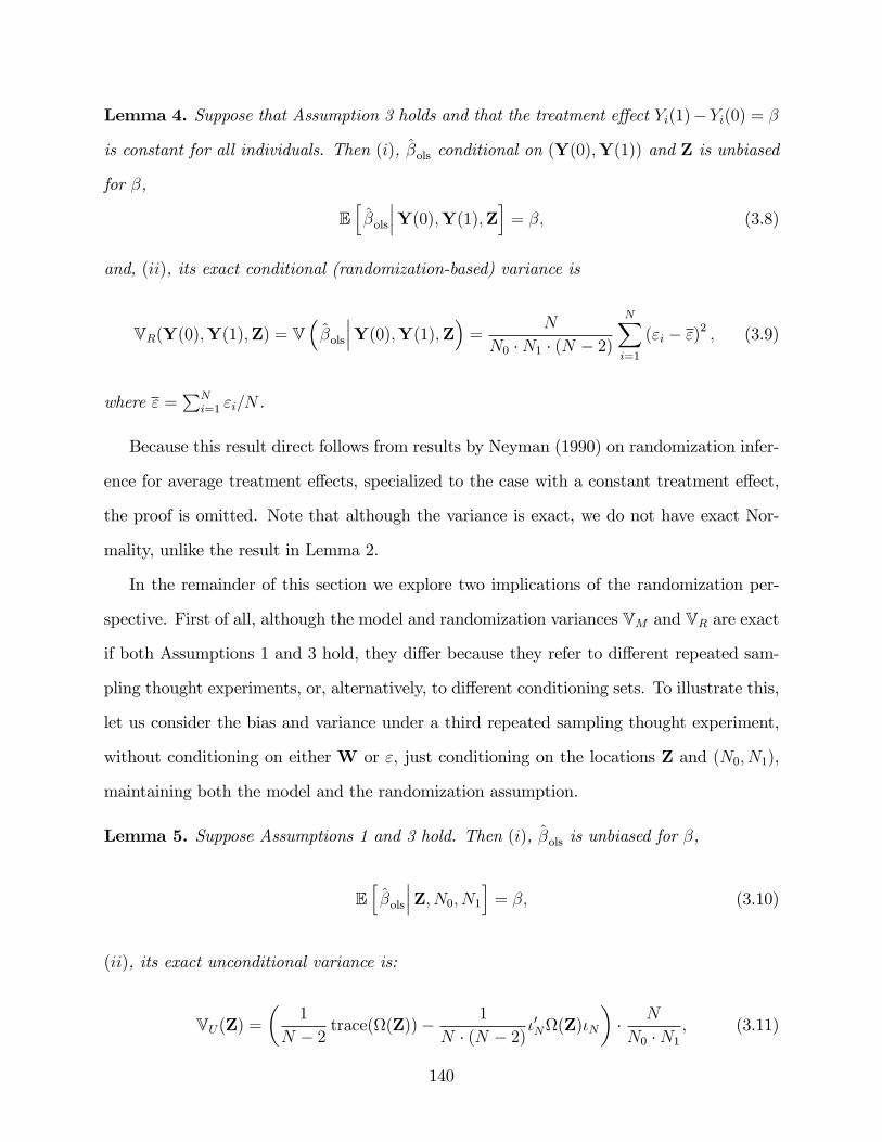
Lemma 4. Suppose that Assumption 3 holds and that the treatment e¤ect Yi(1)�Yi(0) = �

is constant for all individuals. Then (i), �ols conditional on (Y(0);Y(1)) and Z is unbiased

for �,

Eh�ols

��Y(0);Y(1);Zi = �; (3.8)

and, (ii), its exact conditional (randomization-based) variance is

VR(Y(0);Y(1);Z) = V��ols

��Y(0);Y(1);Z� = N

N0 �N1 � (N � 2)

NXi=1

("i � ")2 ; (3.9)

where " =PN

i=1 "i=N .

Because this result direct follows from results by Neyman (1990) on randomization infer-

ence for average treatment e¤ects, specialized to the case with a constant treatment e¤ect,

the proof is omitted. Note that although the variance is exact, we do not have exact Nor-

mality, unlike the result in Lemma 2.

In the remainder of this section we explore two implications of the randomization per-

spective. First of all, although the model and randomization variances VM and VR are exact

if both Assumptions 1 and 3 hold, they di¤er because they refer to di¤erent repeated sam-

pling thought experiments, or, alternatively, to di¤erent conditioning sets. To illustrate this,

let us consider the bias and variance under a third repeated sampling thought experiment,

without conditioning on either W or ", just conditioning on the locations Z and (N0; N1),

maintaining both the model and the randomization assumption.

Lemma 5. Suppose Assumptions 1 and 3 hold. Then (i), �ols is unbiased for �,

Eh�ols

��Z; N0; N1i = �; (3.10)

(ii), its exact unconditional variance is:

VU(Z) =�

1

N � 2 trace((Z))�1

N � (N � 2)�0N(Z)�N

�� N

N0 �N1; (3.11)

140

and (iii),

VU(Z) = E [VR(Y(0);Y(1);Z)jZ; N0; N1] = E [VM(W;Z)jZ; N0; N1] :

Thus, in expectation, VR(Y(0);Y(1);Z), is equal to the expectation of VM(W;Z).

For the second point, suppose we had focused on the repeated sampling variance for

�ols conditional on W and Z, but possibly erroneously modeled the covariance matrix as

constant times the identify matrix, (Z) = �2 � IN . Using such a (possibly incorrect) model

a researcher would have concluded that the exact sampling distribution for �ols conditional

on the covariates would be

�ols

��W;Z � N (�;VINC) ; where VINC = �2 �N

N0 �N1: (3.12)

If (Z) di¤ers from �2 � IN , then VINC is not in general the correct (conditional) distribution

for �ols. However, in some cases the misspeci�cation need not lead to invalid inferences

in large samples. To make that precise, we �rst need to de�ne precisely how inference is

performed. Implicitly the maximum likelihood estimator for the misspeci�ed variance de�nes

�2 as the probability limit of the estimator:

�2 = argmax

(N

2ln(�2)� 1

2�2

NXi=1

�Yi � �ols � �olsWi

�2)

=1

N

NXi=1

�Yi � �ols � �olsWi

�2:

The probability limit for this estimator �2, under Assumptions given in the Lemma below, is

plim( trace((Z))=N). Then the probability limit of the normalized variance based on the

possibly incorrect model is

N � VINC = plim(trace((Z))=N) plim�

N2

N0 �N1

�:

141

The following result clari�es the properties of this probability limit.

Lemma 6. Suppose Assumption 1 holds with (Z) satisfying trace((Z))=N ! c for some

0 < c < 1, and �0N(Z)�N=N2 ! 0, and Assumption 3 holds with N1=N ! p for some

0 < p < 1. Then

N � (VINC � VU(Z))p�! 0; and N � VINC

p�! c

p � (1� p) :

Hence, and this is a key insight of this section, if the assignmentW is completely random,

and the treatment e¤ect is constant, one can, at least in large samples, ignore the o¤-diagonal

elements of (Z), and (mis-)specify (Z) as �2�IN . Although the resulting variance estimator

will not be estimating the variance under the repeated sampling thought experiment that

one may have in mind, (namely VM(W;Z)), it leads to valid con�dence intervals under the

randomization distribution. The result that the mis-speci�cation of the covariance matrix

need not lead to inconsistent standard errors if the covariate of interest is randomly assigned

has been noted previously. Greenwald (1983) writes: �when the correlation patterns of the

independent variables are unrelated to those across the errors, then the least squares variance

estimates are consistent.�Angrist and Pischke (2009) write, in the context of clustering, that:

�if the [covariate] values are uncorrelated within the groups, the grouped error structure does

not matter for standard errors.�The preceding discussion interprets this result formally from

a randomization perspective.

3.5 Randomization Inference with Cluster-level Randomization

Now let us return to the setting that is the main focus of the paper. The covariate of

interest, Wi, varies only between clusters (states), and is constant within clusters. Instead

of assuming that Wi is randomly assigned at the individual level, we now assume that it is

randomly assigned at the cluster level. Let M be the number of clusters, M1 the number

of clusters with all individuals assigned Wi = 1, and M0 the number of clusters with all

142

individuals assigned to Wi = 0. The cluster indicator is

Cim = 1Si=m =

8><>: 1 if individual i is in cluster=state m;

0 otherwise;

withC theN�M matrix with typical element Cim. For randomization inference we condition

on Z, ", and M1. Let Nm be the number of individuals in cluster m. We now look at the

properties of �ols over the randomization distribution induced by this assignment mechanism.

To keep the notation precise, let ~W be the M -vector of assignments at the cluster level,

with typical element ~Wm. Let ~Y(0) and ~Y(1) be M -vectors, with m-th element equal to

~Ym(0) =P

i:Cim=1Yi(0)=Nm, and ~Ym(1) =

Pi:Cim=1

Yi(1)=Nm respectively. Similarly, let ~"

be an M -vector with m-th element equal to ~"m =P

i:Cim=1"i=Nm, and let ~" =

PMm=1 ~"m=M .

Formally the assumption on the assignment mechanism is now:

Assumption 7. (Cluster Randomization)

pr( ~W = ~w j Z = z) = 1�0B@ M

M1

1CA ; for all w s.t.MXm=1

~wm =M1, and 0 otherwise.

We also make the assumption that all clusters are the same size:

Assumption 8. (Equal Cluster Size) Nm = N=M for all m = 1; : : : ;M .

Lemma 9. Suppose Assumptions 7 and 8 hold, and the treatment e¤ect Yi(1)�Yi(0) = � is

constant. Then (i), the exact sampling variance of �ols, conditional on Z and ", under the

cluster randomization distribution is

VCR(Y(0);Y(1);Z) =M

M0 �M1 � (M � 2)

MXm=1

�~"m � ~"

�2; (3.13)

143

(ii) if also Assumption 1 holds, then the unconditional variance is

VU(Z) = E [VCR(Y(0);Y(1);Z)jZ;M1] =

M2

M0 �M1 � (M � 2) �N2� (M � trace (C0(Z)C)� �0(Z)�) : (3.14)

The unconditional variance is a special case of the expected value of the unconditional

variance in (3.5), with the expectation taken overW given the cluster-level randomization.

3.6 Variance Estimation Under Misspeci�cation

In this section we present the main theoretical result in the paper. It extends the result in

Section 3.4 on the robustness of model-based variance estimators under complete random-

ization to the case where the model-based variance estimator accounts for clustering, but

not necessarily for all spatial correlations, and that treatment is randomized at cluster level.

Suppose the model generating the data is the linear model in (3.1), with a general covari-

ance matrix (Z), and Assumption 1 holds. The researcher estimates a parametric model

that imposes a potentially incorrect structure on the covariance matrix. Let (Z; ) be the

parametric model for the error covariance matrix. The model is misspeci�ed in the sense

that there need not be a value such that (Z) = (Z; ). The researcher then proceeds to

calculate the variance of �ols as if the postulated model is correct. The question is whether

this implied variance based on a misspeci�ed covariance structure leads to correct inference.

The example we are most interested in is characterized by a clustering structure by state.

In that case (Z; ) is the N �N matrix with = (�2"; �2S)0, where

ij(Z; �2"; �

2S) =

8>>>><>>>>:�2" + �

2S if i = j

�2S if i 6= j; Si = Sj;

0 otherwise:

(3.15)

Initially, however, we allow for any parametric structure (Z; ). The true covariance matrix

144

(Z) may include correlations that extend beyond state boundaries, and that may involve

division-level correlations or spatial correlations that decline smoothly with distance as in

the speci�cation (3.7).

Under the (misspeci�ed) parametric model (Z; ), let ~ be the pseudo true value, de�ned

as the value of that maximizes the expectation of the logarithm of the likelihood function,

~ = argmax E��12� ln (det ((Z; )))� 1

2� "0(Z; )�1"

��Z� :Given the pseudo true error covariance matrix (~ ), the corresponding pseudo-true

model-based variance of the least squares estimator, conditional onW and Z, is

VINC;CR =1

N2W2(1�W )2

0B@W�1

1CA0��N W

�0(Z; ~ )

��N W

�0B@W�1

1CA :Because for some Z the true covariance matrix (Z) di¤ers from the misspeci�ed one,

(Z; ~ ), it follows that in general this pseudo-true conditional variance VM((Z; ~ );W;Z)

will di¤er from the true variance VM((Z);W;Z). Here we focus on the expected value

of VM((Z; ~ );W;Z), conditional on Z, under assumptions on the distribution of W. Let

us denote this expectation by VU((Z; ~ );Z) = E[VM((Z; ~ );W;Z)jZ]. The question is

under what conditions on the speci�cation of the error-covariance matrix (Z; ), in combi-

nation with assumptions on the assignment process, this unconditional variance is equal to

the expected variance with the expectation of the variance under the correct error-covariance

matrix, VU((Z);Z) = E[VM((Z);W;Z)jZ].

The following theorem shows that if the randomization ofW is at the cluster level, then

solely accounting for cluster level correlations is su¢ cient to get valid con�dence intervals.

Theorem 10. (Clustering with Misspecified Error-Covariance Matrix)

Suppose Assumption 1 holds with (Z) satisfying trace(C0(Z)C)=N ! c for some 0 < c <

1, and �0N(Z)�N=N2 ! 0, Assumption 7 holds with M1=M ! p for some 0 < p < 1, and

145

Assumption 8 holds. Suppose also that that (Z; ) is speci�ed as in (3.15). Then

N � (VINC;CR � VU(Z))p�! 0; and N � VINC;CR

p�! c

N2m � p � (1� p)

:

This is the main theoretical result in the paper. It implies that if cluster level explanatory

variables are randomly allocated to clusters, there is no need to consider covariance structures

beyond those that allow for cluster level correlations. In our application, if the covariate

(state minimum wage exceeding federal minimum wage) were as good as randomly allocated

to states, then there is no need to incorporate division or puma level correlations in the

speci�cation of the covariance matrix. It is in that case su¢ cient to allow for correlations

between outcomes for individuals in the same state. Formally the result is limited to the case

with equal sized clusters. There are few exact results for the case with variation in cluster

size, although if the variation is modest, one might expect the current results to provide

useful guidance.

In many econometric analyses researchers specify the conditional distribution of the out-

come given some explanatory variables, and ignore the joint distribution of the explanatory

variables. The result in Theorem 10 shows that it may be useful to pay attention to this

distribution. Depending on the joint distribution of the explanatory variables, the analyses

may be robust to mis-speci�cation of particular aspects of the conditional distribution. In

the next section we discuss some methods for assessing the relevance of this result.

3.7 Spatial Correlation in State Averages

The results in the previous sections imply that inference is substantially simpler if the ex-

planatory variable of interest is randomly assigned, either at the unit or cluster level. Here

we discuss tests originally introduced by Mantel (1967) Schabenberger and Gotway (2004)

to analyze whether random assignment is consistent with the data, against the alternative

146

hypothesis of some spatial correlation. These tests allow for the calculation of exact, �nite

sample, p-values. To implement these tests we use the location of the units. To make the

discussion more speci�c, we test the random assignment of state-level variables against the

alternative of spatial correlation.

Let Ys be the variable of interest for state s, for s = 1; : : : ; S, where state s has location

Zs (the centroid of the state). In the illustrations of the tests we use an indicator for a state-

level regulation, and the state-average of an individual-level outcome. The null hypothesis of

no spatial correlation in the Ys can be formalized as stating that conditional on the locations

Z, each permutation of the values (Y1; : : : ; YS) is equally likely. With S states, there are S!

permutations. We assess the null hypothesis by comparing, for a given statistic M(Y;Z),

the value of the statistic given the actual Y and Z, with the distribution of the statistic

generated by randomly permuting the Y vector.

The tests we focus on in the current paper are based on Mantel statistics Mantel (1967),

Schabenberger and Gotway (2004). These general form of the statistics we use is Geary�s c

(also known as a Black-White or BW statistic in the case of binary outcomes), a proximity-

weighted average of squared pairwise di¤erences:

G(Y;Z) =S�1Xs=1

SXt=s+1

(Ys � Yt)2 � dst; (3.16)

where dst = d(Zs; Zt) is a non-negative weight monotonically related to the proximity of the

states s and t. Given a statistic, we test the null hypothesis of no spatial correlation by

comparing the value of the statistic in the actual data set, Gobs, to the distribution of the

statistic under random permutations of the Ys. The latter distribution is de�ned as follows.

Taking the S units, with values for the variable Y1; : : : ; YS, we randomly permute the values

Y1; : : : ; YS over the S units. For each of the S! permutations g we re-calculate the Mantel

statistic, say Gg. This de�nes a discrete distribution with S! di¤erent values, one for each

allocation. The one-sided exact p-value is de�ned as the fraction of allocations g (out of the

147

set of S! allocations) such that the associated Mantel statistic Gg is less than or equal to the

observed Mantel statistic Gobs:

p =1

S!

S!Xg=1

1Gobs�Gg : (3.17)

A low value of the p-value suggests rejecting the null hypothesis of no spatial correlation in

the variable of interest. In practice the number of allocations is often too large to calculate the

exact p-value and so we approximate the p-value by drawing a large number of allocations,

and calculating the proportion of statistics less than or equal to the observed Mantel statistic.

In the calculations below we use 10; 000; 000 draws from the randomization distribution.

We use six di¤erent measures of proximity. First, we de�ne the proximity dst as states s

and t sharing a border:

dBst =

8><>: 1 if s; t share a border;

0 otherwise:(3.18)

Second, we de�ne dst as an indicator for states s and t belonging to the same census division

of states (recall that the US is divided into 9 divisions):

dDst =

8><>: 1 if Ds = Dt;

0 otherwise:(3.19)

The last four proximity measures are functions of the geographical distance between states

s and t:

dGDst = �d (Zs; Zt) ; and d�st = exp (�� d (Zs; Zt)) (3.20)

where d(z; z0) is the distance in miles between two locations z and z0, and Zs is the latitude

and longitude of state s, measured as the latitude and longitude of the centroid for each

state. We use � = 0:00138, � = 0:00276, and � = 0:00693. For these values the proximity

index declines by 50% at distances of 500, 250, and 100 miles.

We calculate the p-values for the Mantel test statistic based on three variables. First,

148

an indicator for having a state minimum wage higher than the federal minimum wage. This

indicator takes on the value 1 in nine out of the forty nine states in our sample, with

these nine states mainly concentrated in the North East and the West Coast. Second, we

calculate the p-values for the average of the logarithm of yearly earnings. Third, we calculate

the p-values for the indicator for NE/ENC states. The results for the three variables and

six statistics are presented in Table 3.3. All three variables exhibit considerable spatial

correlation. Interestingly the results are fairly sensitive to the measure of proximity. From

these limited calculations, it appears that sharing a border is a measure of proximity that is

sensitive to the type of spatial correlations in the data.

149

3.8 A Small Simulation Study

We carried out a small simulation study to investigate the relevance of the theoretical results

from Section 3.6. In all cases the model was

Yi = �+ � �Wi + "i;

with N = 2; 590; 190 observations to mimic our actual data. In our simulations every state

has the same number of individuals, and every puma within a given state has the same

number of individuals. We considered three distributions for Wi. In all cases Wi varies only

at the state level. In the �rst case Wi = 1 for individuals in nine randomly chosen states.

In the second case Wi = 1 for the the nine minimum wage states. In the third case Wi = 1

for the eleven NE/ENC states. The distribution for " is in all cases Normal with mean zero

and covariance matrix . The general speci�cation we consider for is

ij(Z; ) =

8>>>>>>>>>><>>>>>>>>>>:

�2D + �2S + �

2P + �

2" if i = j,

�2D + �2S + �

2P if i 6= j; Pi = Pj,

�2D + �2S if Pi 6= Pj; Si = Sj,

�2D if Si 6= Sj; Di = Dj,

We look at two di¤erent sets of values for (�2"; �2P ; �

2S; �

2D), (0:929; 0; 0:016; 0) (only state level

correlations, corresponding to the second pair of rows in Table 3.4) and (0:868; 0:005; 0:005; 0:066)

(puma, state and division level correlations, corresponding to the �fth pair of rows in Table

3.4).

Given the data, we consider �ve methods for estimating the variance of the least squares

estimator �ols, and thus for constructing con�dence intervals. The �rst is based on the

151

randomization distribution:

VCR(Y(0);Y(1);Z) =M

M0 �M1 � (M � 2)

MXm=1

~"2m;

where ~"m is the average value of the residual "i = Yi � �ols � �ols �Wi over cluster m. The

second, third and fourth variances are model-based:

VM((Z);W;Z) =1

N2 �W 2 � (1�W )2(W � 1)

��N W

�0(Z)

��N W

�0B@ W

�1

1CA ;using di¤erent estimates for (Z). First we use an infeasible estimator, namely the true

value for (Z). Second, we specify

ij(Z; ) =

8>><>>:�2S + �

2" if i = j,

�2S if i 6= j; Si = Sj.

We estimate �2P and �2S using moment-based estimators, and plug that into the expression

for the covariance matrix. For the third variance estimator in this set of three variance

estimators we specify

ij(Z; ) =

8>>>>>>>>>><>>>>>>>>>>:

�2D + �2S + �

2P + �

2" if i = j,

�2D + �2S + �

2P if i 6= j; Pi = Pj,

�2D + �2S if Pi 6= Pj; Si = Sj,

�2D if Si 6= Sj; Di = Dj,

and again use moment-based estimators.

The �fth and last variance estimator allows for more general variance structures within

states, but restricts the correlations between individuals in di¤erent states to zero. This

152

estimator assumes is block diagonal, with the blocks de�ned by states, but does not

impose constant correlations within the blocks. The estimator for takes the form

STATA;ij(Z) =

8>>>>>><>>>>>>:"2i if i = j,

"i � "j if i 6= j; Si = Sj,

0 otherwise,

leading to

VSTATA =1

N2 �W 2(1�W )2

� (W � 1)��N W

�0STATA(Z)

��N W

�0B@ W

�1

1CA :This is the variance estimator implemented in STATA and widely used in empirical work.

In Table 3.4 we report the actual level of tests of the null hypothesis that � = �0 with a

nominal level of 5%. First consider the two columns with random assignment of states to the

treatment. In that case all variance estimators lead to tests that perform well, with actual

levels between 5.0 and 7.6%. Excluding the STATA variance estimator the actual levels are

below 6.5%. The key �nding is that even if the correlation pattern involves pumas as well

as divisions, variance estimators that ignore the division level correlations do very well.

153

When we do use the minimum wage states as the treatment group the assignment is

no longer completely random. If the correlations are within state, all variance estimators

still perform well. However, if there are correlations at the division level, now only the

variance estimator using the true variance matrix does well. The estimator that estimates

the division level correlations does best among the feasible estimators, but, because the

data are not informative enough about these correlations to precisely estimate the variance

components, even this estimator exhibits substantial size distortions. The same pattern, but

even stronger, emerges with the NE/ENC states as the treatment group.

3.9 Conclusion

In empirical studies with individual level outcomes and state level explanatory variables,

researchers often calculate standard errors allowing for within-state correlations between

individual-level outcomes. In many cases, however, the correlations may extend beyond

state boundaries. Here we explore the presence of such correlations, and investigate the im-

plications of their presence for the calculation of standard errors. In theoretical calculations

we show that under some conditions, in particular random assignment of regulations, corre-

lations in outcomes between individuals in di¤erent states can be ignored. However, state

level variables often exhibit considerable spatial correlation, and ignoring out-of-state corre-

lations of the magnitude found in our application may lead to substantial underestimation

of standard errors.

In practice we recommend that researchers explicitly explore the spatial correlation struc-

ture of both the outcomes as well as the explanatory variables. Statistical tests based on

Mantel statistics, with the proximity based on shared borders, or belonging to a common

division, are straightforward to calculate and lead to exact p-values. If these test suggest

that both outcomes and explanatory variables exhibit substantial spatial correlation, we rec-

ommend that one should explicitly account for the spatial correlation by allowing for a more

�exible speci�cation than one that only accounts for state level clustering.

155

References

Abadie, A., A. Diamond, and J. Hainmueller (2010, June). Synthetic Control Methods

for Comparative Case Studies: Estimating the E¤ect of California�s Tobacco Control

Program. Journal of the American Statistical Association 105 (490), 493�505.

Acemoglu, D. (2002). Directed technical change. The Review of Economic Studies 69 (4),

781�809.

Acemoglu, D. and J. Angrist (2001). How large are human-capital externalities? evidence

from compulsory-schooling laws. In NBER Macroeconomics Annual 2000, Volume 15,

NBER Chapters, pp. 9�74. National Bureau of Economic Research, Inc.

Acemoglu, D. and D. Autor (2011). Skills, tasks and technologies: Implications for em-

ployment and earnings. Volume 4 of Handbook of Labor Economics, Chapter 12, pp.

1043�1171. Elsevier.

Albouy, D. (2008). Are big cities bad places to live? estimating quality of life across

metropolitan areas. Working Paper 14472, National Bureau of Economic Research.

Angrist, J. D. and J.-S. Pischke (2009). Mostly Harmless Econometrics: An Empiricist�s

Companion. Princeton: Princeton University Press.

Autor, D., L. Katz, and M. Kearney (2008). Trends in us wage inequality: Revising the

revisionists. Review of Economics and Statistics.

Autor, D. H. and D. Dorn (2012). The growth of low skill service jobs and the polarization

of the u.s. labor market. Massuchusetts Institute of Technology Mimeo.

Autor, D. H., D. Dorn, and G. H. Hanson (2012). The china syndrome: Local labor

market e¤ects of import competition in the united states. NBER Working Papers

18054, National Bureau of Economic Research, Inc.

Barrios, T., G. W. Imbens, R. Diamond, and M. Kolesár (2010). Clustering, Spatial

Correlations and Randomization Inference. NBER Working Paper, 15760.

156

Bartik, T. J. (1991).Who Bene�ts from State and Local Economic Development Policies?

Books from Upjohn Press. W.E. Upjohn Institute for Employment Research.

Bayer, P., F. Ferreira, and R. McMillan (2007). A uni�ed framework for measuring pref-

erences for schools and neighborhoods. Journal of Political Economy 115 (4), 588�638.

Bayer, P., N. Keohane, and C. Timmins (2009). Migration and hedonic valuation: The

case of air quality. Journal of Environmental Economics and Management 58 (1), 1 �

14.

Beaudry, P., M. Doms, and E. Lewis (2010). Should the personal computer be considered

a technological revolution? evidence from u.s. metropolitan areas. Journal of Political

Economy 118 (5), 988 �1036.

Becker, G. and K. Murphy (2000). Social Economics: Market Behavior in a Social Envi-

ronment. Belknap Series. Belknap Press of Harvard University Press.

Bennett, J. (2010). As detroit faces cutbacks, this one hits a sour note. The Wall Street

Journal .

Berry, C. R. and E. L. Glaeser (2005). The divergence of human capital levels across

cities*. Papers in Regional Science 84 (3), 407�444.

Berry, S., J. Levinsohn, and A. Pakes (1995). Automobile prices in market equilibrium.

Econometrica 63 (4), 841�90.

Berry, S., J. Levinsohn, and A. Pakes (2004). Di¤erentiated products demand systems

from a combination of micro and macro data: The new car market. Journal of Political

Economy 112 (1), pp. 68�105.

Bertrand, M., E. Du�o, and S. Mullainathan (2004). How Much Should We Trust

Di¤erences-in-Di¤erences Estimates? Quarterly Journal of Economics 119 (1), 249�

275.

Bester, C. A., T. G. Conley, and C. B. Hansen (2011). Inference with dependent data

157

using cluster covariance estimators. Journal of Econometrics 165 (2), 137�151.

Bishop, K. (2010). A dynamic model of location choice and hedonic valuation.Washington

University Mimeo.

Blanchard, O. J. and L. F. Katz (1992). Regional evolutions. Brookings Papers on Eco-

nomic Activity 23 (1), 1�76.

Bollinger, C. and B. Hirsch (2006). Match bias from earnings imputation in the current

population survey: The case of imperfect matching. Journal of Labor Economics 24 (3),

483�519.

Brueckner, J. and D. Neumark (2011). Beaches, sunshine, and public-sector pay: the-

ory and evidence on amenities and rent extraction by government workers. Technical

report, National Bureau of Economic Research.

Brueckner, J. K. (1987). The structure of urban equilibria: A uni�ed treatment of the

muth-mills model. In E. S. Mills (Ed.), Handbook of Regional and Urban Economics,

Volume 2 of Handbook of Regional and Urban Economics, Chapter 20, pp. 821�845.

Elsevier.

Card, D. (2009). Immigration and inequality. American Economic Review 99 (2), 1�21.

Card, D. and T. Lemieux (2001). Can falling supply explain the rising return to college for

younger men? a cohort-based analysis. The Quarterly Journal of Economics 116 (2),

pp. 705�746.

Card, D., A. Mas, and J. Rothstein (2008). Tipping and the dynamics of segregation. The

Quarterly Journal of Economics 123 (1), 177�218.

Chetty, R. and A. Szeidl (2007). Consumption commitments and risk preferences. The

Quarterly Journal of Economics 122 (2), 831�877.

Ciccone, A. and G. Peri (2006). Identifying human-capital externalities: Theory with

applications. The Review of Economic Studies 73 (2), 381�412.

158

Costa, D. and M. Kahn (2000). Power couples: changes in the locational choice of the

college educated, 1940�1990. The Quarterly Journal of Economics 115 (4), 1287�1315.

Cronin, J. (2011). Reforming Boston Schools, 1930 to the Present: Overcoming Corruption

and Racial Segregation. Palgrave Studies in Urban Education. Palgrave Macmillan.

Diggle, P., P. Heagerty, K.-Y. Liang, and S. L. Zeger (2002). Analysis of longitudinal data.

Oxford University Press.

Epple, D. and H. Sieg (1999). Estimating equilibrium models of local jurisdictions. The

Journal of Political Economy 107 (4), 645�681.

Epple, D. and A. Zelenitz (1981). The implications of competition among jurisdictions:

does tiebout need politics? The Journal of Political Economy, 1197�1217.

Fisher, R. A. (1925). The Design of Experiments (�rst ed.). London: Oliver and Boyd.

Freeman, R. (1986). Unionism comes to the public sector. Journal of Economic Literature,

41�86.

Gelfand, A. E., P. Diggle, P. Guttorp, and M. Fuentes (2010). Handbook of Spatial Statis-

tics. Chapman & Hall.

Gittleman, M. and B. Pierce (2012). Compensation for state and local government workers.

The Journal of Economic Perspectives, 217�242.

Glaeser, E., J. Scheinkman, and A. Shleifer (1995). Economic growth in a cross-section of

cities. Journal of Monetary Economics 36 (1), 117�143.

Glaeser, E. L., H. D. Kallal, J. A. Scheinkman, and A. Shleifer (1992). Growth in cities.

Journal of Political Economy 100 (6), 1126�52.

Goldin, C. and L. Katz (2008). The Race Between Education and Technology. Belknap

Press for Harvard University Press.

Goldin, C. and L. F. Katz (2007). Long-run changes in the wage stucture: Narrowing,

widening, polarizing. Brookings Papers on Economic Activity, 135�65.

159

Greenwald, B. C. (1983). A general analysis of bias in the estimated standard errors of

least squares coe¢ cients. Journal of Econometrics 22 (3), 323�338.

Greenwood, M. J. (1997). Chapter 12 internal migration in developed countries. Volume

1, Part B of Handbook of Population and Family Economics, pp. 647 �720. Elsevier.

Gregory, R. G. and J. Borland (1999). Chapter 53 recent developments in public sector

labor markets. Volume 3, Part C of Handbook of Labor Economics, pp. 3573 �3630.

Elsevier.

Guerrieri, V., D. Hartley, and E. Hurst (2011). Endogenous gentri�cation and housing

price dynamics. Booth School of Business Mimeo.

Gyourko, J., A. Saiz, and A. Summers (2008). A new measure of the local regulatory

environment for housing markets: The wharton residential land use regulatory index.

Urban Studies 45 (3), 693�729.

Gyourko, J. and J. Tracy (1991). The structure of local public �nance and the quality of

life. Journal of Political Economy, 774�806.

Handbury, J. (2012). Are poor cities cheap for everyone? non-homotheticity and the cost

of living across u.s. cities. Columbia University Mimeo.

Hansen, C. B. (2007). Generalized least squares inference in panel and multilevel models

with serial correlation and �xed e¤ects. Journal of Econometrics 140 (2), 670�694.

Ibragimov, R. and U. Muller (2010). t-statistic based correlation and heterogeneity robust

inference. Journal of Business & Economic Statistics 28 (4), 453�468.

Kahn, M. E. (1999). The silver lining of rust belt manufacturing decline. Journal of Urban

Economics 46 (3), 360�376.

Katz, L. F. and D. H. Autor (1999). Chapter 26 changes in the wage structure and

earnings inequality. Volume 3, Part A of Handbook of Labor Economics, pp. 1463 �

1555. Elsevier.

160

Katz, L. F. and K. M. Murphy (1992). Changes in relative wages, 1963-1987: Supply and

demand factors. The Quarterly Journal of Economics 107 (1), 35�78.

Kennan, J. and J. R. Walker (2011). The e¤ect of expected income on individual migration

decisions. Econometrica 79 (1), 211�251.

Krueger, A. (1988). Are public sector workers paid more than their alternative wage? evi-

dence from longitudinal data and job queues. InWhen public sector workers unionize,

pp. 217�242. University of Chicago Press.

Liang, K.-Y. and S. L. Zeger (1986, January). Longitudinal data analysis for generalized

linear models. Biometrika 73 (1), 13�22.

Mantel, N. (1967, February). The Detection of Disease Clustering and a Generalized Re-

gression Approach. Cancer research 27 (2), 209�20.

Martelle, S. (2012). Detroit: A Biography. Chicago Review Press.

McFadden, D. (1973). Conditional logit analyisis of qualitative choice behavior. In

P. Zarembka (Ed.), Frontiers in Econometrics, pp. pp. 105�142. Academic Press.

Mirel, J. (1999). The rise and fall of an urban school system : Detroit, 1907-81. Ann

Arbor : University of Michigan Press.

Moretti, E. (2004a). Estimating the social return to higher education: evidence from

longitudinal and repeated cross-sectional data. Journal of Econometrics 121 (1-2), 175�

212.

Moretti, E. (2004b). Human capital externalities in cities. Handbook of regional and urban

economics 4, 2243�2291.

Moretti, E. (2004c). Workers�education, spillovers, and productivity: Evidence from plant-

level production functions. American Economic Review 94 (3), 656�690.

Moretti, E. (2011a). Local labor markets. Volume 4 of Handbook of Labor Economics,

Chapter 14, pp. 1237�1313. Elsevier.

161

Moretti, E. (2011b). Real wage inequality. University of California Berkeley Mimeo.

Moretti, E. (2012). The New Geography of Jobs. Houghton Mi in Harcourt.

Moulton, B. R. (1986). Random group e¤ects and the precision of regression estimates.

Journal of Econometrics 32 (3), 385�397.

Nevo, A. (2010). Empirical models of consumer behavior. NBER Working Papers 16511,

National Bureau of Economic Research, Inc.

Neyman, J. (1990). On the Application of Probability Theory to Agricultural Experiments.

Essay on principles. Section 9. Statistical Science 5 (4), 465�480.

Notowidigdo, M. J. (2011). The incidence of local labor demand shocks. Booth School of

Business Mimeo.

Ottaviano, G. I. P. and G. Peri (2012). Rethinking the e¤ect of immigration on wages.

Journal of the European Economic Association 10 (1), 152�197.

Pakes, A. and P. McGuire (2001). Stochastic algorithms, symmetric markov perfect equi-

librium, and the �curse�of dimensionality. Econometrica 69 (5), 1261�81.

Roback, J. (1982). Wages, rents, and the quality of life. Journal of Political Econ-

omy 90 (6), pp. 1257�1278.

Rosen, S. (1979). Wages-based indexes of urban quality of life. In P. Mieszkowski and

M. Straszheim (Eds.), Current Issues in Urban Economics. John Hopkins Univ. Press.

Rosenbaum, P. R. (2002). Observational Studies. New York: Springer-Verlag.

Ruggles, S., J. T. Alexander, K. Genadek, R. Goeken, M. B. Schroeder, and M. Sobek.

(2010). Integrated Public Use Microdata Series: Version 5.0 [Machine-readable data-

base]..

Saiz, A. (2010). The geographic determinants of housing supply. The Quarterly Journal

of Economics 125 (3), pp. 1253�1296.

162

Saks, R. E. (2008). Job creation and housing construction: Constraints on metropolitan

area employment growth. Journal of Urban Economics 64 (1), 178�195.

Schabenberger, O. and C. A. Gotway (2004). Statistical Methods for Spatial Data Analysis

(�rst ed.). Chapman and Hall/CRC.

Shapiro, J. (2006). Smart cities: Quality of life, productivity, and the growth e¤ects of

human capital. The Review of Economics and Statistics 88 (2), 324�335.

Stock, J. H., J. H. Wright, and M. Yogo (2002). A survey of weak instruments and weak

identi�cation in generalized method of moments. Journal of Business & Economic

Statistics 20 (4), 518�29.

Topel, R. H. (1986). Local labor markets. Journal of Political Economy 94 (3), pp. S111�

S143.

Winerip, M. (2011). For detroit schools, mixed picture on reforms. The New York Times.

Wooldridge, J. M. (2002). Econometric Analysis of Cross Section and Panel Data. Cam-

bridge, MA: MIT Press.

163

A Chapter 1 Appendix

A.1 Data Appendix

Variable Source Sample Notes

MetropolitainStatisticalArea

US Census1980, 1990,2000

All MSAs identified across all 3censuses. Rural areas of eachstate are included as additionalgeopgraphic units.

MSAs identified in some, but notall of the censuses are included inrural areas of each state.

Local HighSkill and LowSkill Wages

US Census1980, 1990,2000

All individuals ages 2555working at least 35 hours perweek and 48 weeks per year.

Local wages in each MSA areaverages of workers for each skilllevel living in each city. High skillworker is defined as a worker withat least a 4 year college degree.All other workers are consideredlow skill.

Local HousingRent

US Census1980, 1990,2000

All households where the headofhousehold is between the ages of25 and 55 and works at least 35hours per week and 48 weeks peryear.

Rental rates are measured as thegross rent, which includes both thehousing rent and the cost ofutilities. Rents are imputed forhouseholds which own their home.Imputed rents are converted fromhousing values using a discountrate of 7.85 percent (Peiser andSmith 1985), to which electricityand gas utility costs are added.

Local CollegeEmploymentRatio

US Census1980, 1990,2000

All employed workers betweenthe ages of 25 and 55.

College employment ratio isdefined as the ratio of number ofemployed workers in the city witha 4 year college degree to thenumber of employed lower skillworkers living in the city.

Worker's Race

US Census1980, 1990,2000

All households where the headofhousehold is between the ages of25 and 55 with positive wageearnings.

A household is classifed as blackif the head of household reportshis race as black.

Worker'sImmigrantStatus

US Census1980, 1990,2000

All households where the headofhousehold is between the ages of25 and 55 with positive wageearnings.

A household is classifed as animmigrant if the headofhousehold was born outside of theUnited States.

164

Variable Source Sample NotesPropertyCrimes andViolentCrimes per1000Residents

FBIUniformCrimeReports1980, 2000

All nonrural MSAs which theFBI data covers.

EPA AirQuality Index

Envionmental

ProtectionAgency

All nonrural MSAs which theEPA reports data on.

165

A.2 Estimation Appendix

A.2.1 Labor Demand

The parameters to be estimated in cities� labor demand curves are (�; H ; L) : � governs

the slope of �rms�labor demand curves and H and L measure endogenous productivity

spillovers driven by cities�college employment ratios.

Throughout the appendix, I use a change of variables de�ning the high and low skill

exogenous productivities:

ln��1=�jt (1� �jt)

�= "Hjt

ln��1=�jt �jt

�= "Ljt:

These variable de�nitions are useful for showing how Njt is computed for estimation, but

have no economic impact on the model. City j0s inverse labor demand is:

�wHjt = �ct +� ln��1=�jt (1� �jt)

�+ (1� �)� lnNjt + (�� 1)� lnHjt + H� ln

�HjtLjt

��wLjt = �ct +� ln

��1=�jt �jt

�+ (1� �)� lnNjt + (�� 1)� lnLjt + L� ln

�HjtLjt

�Njt =

��jt

�HjtLjt

� LL�jt + (1� �jt)

�HjtLjt

� HH�jt

� 1�

: (A.1)

A contributor to local productivity change is changes in the productivity levels of the

industries located within each city. I measure these observable local productivity shocks by

interacting cross-sectional di¤erences in industrial employment composition with national

changes in industry wage levels, separately for high and low skill workers. I refer to these as

Bartik shocks, as represented by�BHjt and �BLjt. The aggregate Bartik shock, which weights

the two skill group speci�c Bartik shock by the share of a city�s employment made up of

each skill group is represented by �Balljt : Industry classi�cations are those used in the 1980,

166

1990 and 2000 Census, which is very close to 3 digit SIC code classi�cations. See equations

(1:18) and (1:21) in the main text for the exact de�nition.

Since I do not observe all other contributors to local productivity changes, I rewrite the

labor demand equations by explicitly de�ning�~"Hjt and�~"Ljt; which represent all productivity

changes of high and low skill workers, respectively, unaccounted for by the Bartik shocks

�BHjt ;�BLjt:

�~"Hjt = �wHjt �

0B@ �ct + �HB�B

Hjt + (1� �)� lnNjt

+(�� 1)� lnHjt + H� ln�HjtLjt

�1CA (A.2)

�~"Ljt = �wLjt �

0B@ �ct + �LB�B

Ljt + (1� �)� lnNjt

+(�� 1)� lnLjt + L� ln�HjtLjt

�1CA : (A.3)

While the direct impact of Bartik shocks lead to shifts in local labor demand curves,

the interaction of the Bartik shocks with cities�housing markets creates variation that can

identify the labor demand parameters. Heterogeneity in housing supply elasticity will lead to

di¤erences in population changes in response to a given Bartik shock. Land unavailable for

housing development due to geographic features, xgeoj ; as well as land-use regulation, xregj ;

impact local housing supply elasticity. The interaction of these housing supply elasticity

measures with local Bartik shocks can be used as instruments for quantities of labor within

the city.

This leads to the following moments:

� Bartik Shocks uncorrelated with unobserved productivity changes:50

50These moments only identify the coe¢ cients which measure the Bartik shocks direct impact on wages.They do not directly identify any of the structural labor demand parameters.

167

E��~"Hjt�B

Hjt

�= 0

E��~"Ljt�B

Ljt

�= 0

� Bartik shocks interacted with housing supply elasticity measures are uncorrelated with

unobserved productivity changes:

E��~"Hjt�B

Hjtx

geoj

�= 0

E��~"Hjt�B

Hjtx

regj

�= 0

E��~"Ljt�B

Ljtx

geoj

�= 0

E��~"Ljt�B

Ljtx

regj

�= 0

� The aggregate Bartik shock and interactions with housing supply elasticity are uncor-

related with high and low skill unobserved productivity changes:

E��~"Ljt�B

alljt

�= 0

E��~"Hjt�B

alljt

�= 0

E��~"Ljt�B

alljt x

geoj

�= 0

E��~"Ljt�B

alljt x

regj

�= 0

E��~"Hjt�B

alljt x

geoj

�= 0

E��~"Hjt�B

alljt x

regj

�= 0:

� High skill Bartik shock and interactions with housing supply elasticity are uncorrelated

with low skill unobserved productivity changes, and vice versa:

168

E��~"Ljt�B

Hjt

�= 0

E��~"Hjt�B

Ljt

�= 0

E��~"Ljt�B

Hjtx

geoj

�= 0

E��~"Ljt�B

Hjtx

regj

�= 0

E��~"Hjt�B

Ljtx

geoj

�= 0

E��~"Hjt�B

Ljtx

regj

�= 0:

I also include decade �xed e¤ects.

To compute the moments, I need to be able to compute the unobserved changes in cities�

productivities��~"Hjt ;�~"

Ljt

�, given a guess of the labor demand parameters (�; H ; L), and

the data�wcoljt ; w

hsjt ; Hjt; Ljt

�, as seen in equations (1:19) and (1:20) :�~"Hjt and �~"

Ljt depend

on the CES aggregate labor quantity in the city, Njt: Njt is a function of �jt; which measures

the relative productivity of high and low skill workers, and it is not directly observable.

However, the CES functional form allows one to solve for �jt in terms of observable data.

Taking the ratio of high skill wages to low skill wages in city j gives:

wHjtwLjt

=�jt�N

1��jt

��jt(1��)

r

� 1��(1� �jt)H��1

jt

�HjtLjt

� H�jt�N

1��jt

��jt(1��)

r

� 1��jtL

��1jt

�HjtLjt

� L :

Solving for �jt :

�jt =wLjtH

��1+ H� Ljt


��1+ H� Ljt

:

Plugging in this expression for �jt into equation (A:1) ;the CES aggregate labor quantity in

the city, and rearranging gives:

Njt =

wLjtH

��1+ Hjt L

�� Ljt + wHjtL

��1� Ljt H

�+ Hjt


��1+ H� Ljt

!1=�: (A.4)

169

Thus, given a guess of the parameter values (�; H ; L) and data�wHjt ; w

Ljt; Hjt; Ljt

�from

each decade 1980, 1990, and 2000, one can compute �~"Hjt and �~"Ljt using equations (A:2),

(A:3) ; and (A:4) : These residuals can the be used to form the labor demand moments:

mH_labor (�; H ; L) =1

JT

Xjt

��~"Hjt�Zjt

�mL_labor (�; H ; L) =

1

JT

Xjt

��~"Ljt�Zjt

�

�Zjt 2

8>>>><>>>>:�Balljt ;�B

Hjt ;�B

Ljt


regj ;�BLjtx

regj


geoj ;�BLjtx

geoj

9>>>>=>>>>; :

A.2.2 Housing Supply

To identify the elasticity of housing supply, one needs variation in a city�s total popula-

tion which is unrelated to changes in unobserved construction costs. De�ning changes in

unobserved construction costs as �"CCjt ; I rewrite the housing supply curve as:

�"CCjt = � ln (CCjt)

= �rjt �� ln (�t) +

� + geo exp

�xgeoj

�+ reg exp

�xregj

�� ln (Hjt + Ljt)

�:

I instrument for housing demand changes using the Bartik shocks discussed above. This

leads to moments:

E��"CCjt �Zjt

�= 0

�Zjt 2

8>>>><>>>>:�Balljt ;�B

Hjt ;�B

Ljt


regj ;�BLjtx

regj


geoj ;�BLjtx

geoj

9>>>>=>>>>; :

170

The sample analog for each of these moments is measured by:

mhousing ( ; geo; reg) =1

JT

Xjt

��"CCjt �Zjt

�:

A.2.3 Labor Supply

Recall that the utility of worker i in city j at time t is a function of the city�s wage, rent,

amenities o¤ered, the worker�s demographic characteristics, zi; and his state and Census

division of birth, sti; divi:

Vijt = �zijt + �stzistix

stj + �

divzi divi xdivj + "ijt

�zijt = �wziwedujt � �rzirjt + �AzixAjt + �colzi

HjtLjt:

The utility a worker with demographics z gains from any city can be written as the sum of the

common utility value of that city for all workers with demographics z,�zjt; the utility value

of whether the city is located close to the workers�state of birth, �stzistixstj +�divzi divi x

divj ;

and a worker speci�c idiosyncratic taste for the city "ijt:

To estimate workers� preferences for cities, I use a two-step estimator similar to the

methods used by Berry, Levinsohn, and Pakes (2004) to estimate households�demand for

automobiles. In the �rst step, I use a maximum likelihood estimator, where I treat the

common utility value of each city for each demographic group, �zjt; as a parameter to be

estimated. The distributional assumption on the iid taste preferences for cities ("ijt) allow

me to form a likelihood function to maximize.51 Since "ijt is distributed Type I extreme

51While one often worries about bias in estimating �xed e¤ects using a non-linear objective function, suchas maximum likelihood, I have a very large sample of individual level data (over 2 million observations foreach decade), relative to about 1000 estimated �xed e¤ects per decade. The asymptotics assumes thenumber of individuals goes to in�nity, either holding the number of cities �xed or at a faster rate than thenumber of cities goes to in�nity.

171

value, the likelihood function is:

LLH(�zjt; �st; �div) =

nXi=1

log(exp(�zijt + �

stzistixstj + �

divzi divi xdivj ) � 1(ji = j)PJ

k exp(�zikt + �


);

where 1(ji = j) is an indicator function of whether worker i did, in fact, choose to live in city

j and n is the total number of workers in the data. This setup allows the econometrician

to only need to observe the location choices of workers and the workers�demographics, but

not cities�characteristics, to estimate how di¤erent types of workers value di¤erent cities.52

The maximum likelihood estimation identi�es a mean utility level for each city, for each

demographic group, for each decade of data. This amounts to estimating 1608 mean utility

parameters (268 cities x 6 demographic groups) in each decade. A desirable property of the

conditional logit model is that the likelihood function is globally concave. Optimizing the

likelihood function to �nd the global maximum is relatively simple, since there are no local

minima.

A.2.4 Estimation of wage, local price, and amenity preferences

The second step of estimation decomposes the mean utility estimates into how workers value

wages, rents and amenities. For each demographic group, the maximum likelihood estimation

produced mean utility estimates in 1980, 1990, and 2000 for each city. I �rst di¤erence the

mean utility estimates for a given city, for each demographic group across decades. The

change in a city�s mean utility across a decade for workers with demographics z is driven by

changes in wages, rents, and amenities:

52An issue I do not explicitly consider is the presence of unobserved household characteristics which impactpreferences over cities. Many discrete choice models incorporate this by adding random coe¢ cients on someproduct characteristics in the utility function. These can be useful for estimating realistic substitutionelasticities across products. The random coe¢ cients would allow the characteristics of the city a workerchose to live in to inform what types of city characteristics that worker is likely to prefer. This break theundesirable independence of irrelevent alternatives (IIA) property of conditional logit models. However,since I do not observe any information about workers�preferences over cities beyond their �rst choice cities,any identi�cation of the variance of random coe¢ cient parameters would be solely due to functional formrestrictions.

172

��zjt = �wz�wedujt � �rz�rjt + �Az�xAjt + �colz�

�HjtLjt

�: (A.5)

Changes in cities�wages, rents, and college employment ratios are observed in the data.

However, other amenity changes are unobserved by the econometrician. De�ne ��zjt as the

change in utility value of city j0s amenities unobserved to the econometrician across decades

for workers with demographics z:Formally, ��zjt is de�ned by:

��zjt = �Az�xAjt:

Plugging this into equation (A:5) :

��zjt = �wz�wedujt � �rz�rjt + �colz�

�HjtLjt

�+��zjt:

If the changes in unobserved amenities across decades were uncorrelated with the changes in

local wages, rents, and endogenous amenities, then the equation above could be estimated

by regressing the changes in mean utilities on the changes in local wages, rents, and college

concentration. However, since wages, rents, and the college employment ratios are simulta-

neously determined with workers�city choices, exogenous changes in local amenities will be

correlated wages, rent, and college employment ratio changes.

To identify workers�preferences for cities�wages, rents, and endogenous amenities, Bartik

productivity shocks and their interaction with housing supply characteristics are used as

instruments for these endogenous outcomes. Since Bartik productivity shocks are driven by

national changes in industrial productivity, they are unrelated to local exogenous amenity

changes. While local housing supply elasticity characteristics, such as coastal proximity and

mountains, likely are amenities of a city, they do not change over time. The identifying

assumption is that housing supply elasticity characteristics are independent of changes in

173

local exogenous amenities.

Identifying workers� preferences for endogenous amenities is equivalent to identifying

workers�preferences for a city�s college employment ratio. The lefthand side of the estimating

equation is equal to a demographic group�s mean utility level for each city, which is identi�ed

o¤ of population di¤erences across cities. A city has a high mean utility if a large share of all

workers nationwide, within a demographic group, choose to live there. The populations of all

demographic groups within a city also determine a city�s college employment ratio. While

population is both on the left and right hand side of the estimating equation, variation

in cities�college employment ratios is not solely driven by any given demographic group.

For example, variation in cities�low skill populations impacts the college employment ratio,

holding the high skill local population �xed. Variation in cities�college employment ratios

driven by Bartik shocks and their interactions to housing supply elasticity is driven by how

these local shocks di¤erentially impact high and low skill workers. Thus, the migration

response of a given demographic group to the set of Bartik productivity shocks and their

interactions with housing supply elasticity depends on how these shocks jointly in�uence

local wages, rents, and college employment ratios. Intuitively, workers� preferences for a

city�s college employment ratio is identi�ed o¤ how other demographic groups respond to

the local Bartik shocks.

This leads to the following moment restrictions:

E��zjt�Zjt

�= 0

�Zjt 2

8>>>><>>>>:�Balljt ;�B

Hjt ;�B

Ljt


regj ;�BLjtx

regj


geoj ;�BLjtx

geoj

9>>>>=>>>>; :

Decade �xed e¤ects are also included.

174

The sample analog for each of these moments is measured by:

mutilz

��w; �r; �col

�=

1

JT

Xjt

��zjt�Zjt

�:

The labor demand, housing supply, and labor supply moments are all used together to jointly

estimate all parameters using a 2-step GMM estimator. Standard errors are clustered by

MSA in all estimating equations. Standard errors for the worker preference estimates account

for the fact that the mean utilities are estimated. However, since the �rst step is estimated

o¤ such a large dataset, this additional source of error does not have a meaningful e¤ect on

the standard errors of worker preference estimates.

A.3 Dynamic Adjustment & Equilibrium Stability

Since a city�s college share endogenously determines a city�s productivity and amenity level,

there could be many possible equilibrium outcomes. The equilibrium selected will depend

on initial conditions and the dynamic adjustment mechanism of wages, rents, amenities,

and population. Under the true dynamic adjustment process, the equilibrium selected in

the data is likely to be stable. While I have not modeled or estimated the determinants

of the dynamic adjustment process, I will assume a simple dynamic adjustment process to

assess whether the observed equilibrium outcomes in the data are stable, given the model�s

parameter estimates.

Consider a dynamic adjustment mechanism where in each year t �% of the US population

considers moving to a new city, while (1� �)% remain �xed in their current location. Let

g

0B@ Ht�1

Lt�1

1CA be a function that maps the population distribution of migrants across cities

in year t � 1,

0B@ Ht�1

Lt�1

1CA ; to the city choices of the migrate population in year t: Totalpopulation in each city in year t is then the combination of the migrant�s city choices and

175

the population distribution of non-migrants from the previous year, as represented by the

function f :

0B@ Ht

Lt

1CA = f

0B@ Ht�1

Lt�1

1CA ; (A.6)

f

0B@ Ht�1

Lt�1

1CA = �g

0B@ Ht�1

Lt�1

1CA+ (1� �) �0B@ Ht�1

Lt�1

1CA : (A.7)

Ht = (H1t; H2t; :::HJt) ;

Lt = (L1t; L2t; :::LJt) :

The migrants choose where to live in year t based o¤ of the wages, rents, and amenities

observed in year t�1:Workers do not take into account the impact of their migration or the

expected migration of others on cities�wages, rents, and amenities in the following period.

The wages, rents, and amenities in each city in year t�1 are the city�s labor demand, housing

supply, and amenity levels given the population in year t � 1: Thus, I am assuming labor

demand, housing supply, and amenity supply fully respond to population changes from the

previous period. An alternative approach would be to allow wages, rents, and amenities to

sluggishly adjust to population changes each period. Each migrant moves to the city which

176

o¤ers him the highest utility. Formally, g is parameterized as:

g

0B@ Ht�1

Lt�1

1CA =

0B@g10B@ Ht�1

Lt�1

1CA ; g20B@ Ht�1

Lt�1

1CA ; :::gJ0B@ Ht�1

Lt�1

1CA1CA

gj

0B@ Ht�1

Lt�1

1CA =

0BBBBBBBBBBBBBBBBBBBBB@

Pi2H

exp

0BBBB@uij0BBBB@Ht�1

Lt�1

1CCCCA1CCCCA

Pk exp(uik

0BBBB@Ht�1

Lt�1

1CCCCA)

Pi2L

exp

0BBBB@uij0BBBB@Ht�1

Lt�1

1CCCCA1CCCCA

Pk exp(uik

0BBBB@Ht�1

Lt�1

1CCCCA)

1CCCCCCCCCCCCCCCCCCCCCAH and L are the sets of high and low skill workers nationwide, respectively. The utility each

migrant worker would receive from each city in period t� 1 is:

Vijt = uijt + "ijt;

uij

0B@ Ht�1

Lt�1

1CA = �wi weduj (Hjt�1; Ljt�1) + �

ri rj (Hjt�1; Ljt�1) + �

coli

Hjt�1Ljt�1

+ �ij

+�sti stixstj + �

divi divi x

divj ;

where��wi ; �

ri ; �

coli ; �ij; �

sti ; �

divi

�are the migrant�s preferences as determined by his demo-

graphics.

The wages and rents workers expect to receive in each city are de�ned as:

177

wHj (Hjt�1; Ljt�1) = c+ (1� �) lnNj (Hjt�1; Ljt�1) + (�� 1) lnHjt�1 + H ln�Hjt�1Ljt�1

�+ "Hj ;

wLj (Hjt�1; Ljt�1) = c+ (1� �) lnNj (Hjt�1; Ljt�1) + (�� 1) lnLjt�1 + L ln�Hjt�1Ljt�1

�+ "Lj ;

rj (Hjt�1; Ljt�1) = a+� + geo exp

�xgeoj

�+ reg exp

�xregj

��ln (Hjt�1 + Ljt�1) + "

CCj :

These represent labor demands and housing supplies which fully adjust to the population

levels in year t� 1:

Migrant workers gain utility in period t� 1 based on the city they choose to migrate to.

Worker are myopic under this dynamic because they do not take into account that they will

only have a �% chance of being able to migrate again the following period. They migrate

based on the current period�s wages, rents, and amenities. However, other workers may

also �nd the same city appealing, and the aggregate migration responses of all workers will

impact the wages, rents, and amenities in the following period. I do not argue that this

dynamic adjustment process mimics the actual migration dynamics of workers in reality, but

it is a simple dynamic and useful for considering the stability of equilibria. Blanchard &

Katz (1992) and other work �nds that migration only partially responds to utility di¤erences

across states each year. This fact could motivate using this dampened migration dynamic.

Fixed points of this dynamic adjustment mechanism are equilibria of the model:

0B@ Ht

Lt

1CA = f

0B@ Ht

Lt

1CA :To calculate f; I plug in the model�s parameter estimates of labor demand, labor supply,

housing supply, and the inferred levels of exogenous productivity, amenities, and construction

costs. By construction, the population distribution of workers observed in the data is in

equilibrium. To test for stability, I hold the population distribution �xed at that observed

in the data and test whether the magnitude of all eigenvalues of the Jacobian of f are less

178

than 1. When 0 � � � 0:07; the equilibrium observed in the data in 1980, 1990, and 2000

are all stable. However, for � > 0:07; the Jacobian of f has eigenvalues below -1 in some

years. While this model can potentially have a large set of possible equilibria, the equilibria

observed in the data are stable under this assumed migration dynamic.

If a large fraction of the population can migrate each period (� > 0:07) and workers do

not take into account the expected migration of others, the dynamic adjustment process can

cycle, where cities oscillate between being high college share, desirable cities, to low college

share, undesirable cities.

To build intuition for why the dynamic can oscillate, I simulate this dynamic adjustment

process for a simple two city case. I simplify the model to a two skill group model, ignoring

preference heterogeneity of immigrants and Blacks. I also ignore workers�preferences to live

their state of birth.

I create two cities with identical housing supply curves and exogenous amenity levels.

I allow city 1 to exogenously be more productive than city 2 for college workers, but both

cities are equally productive for non-college workers. The cities�exogenous productivities

are set to:

"H1 = 1:5

"L2 = 1

"L1 = "L2 = :5

Housing supply elasticities are set to the estimated average city�s housing supply elasticity:

1 = 2 = 0:16:

179

The cities�labor demand and housing supply curves are:

wHj (Hjt�1; Ljt�1) = (1� �) lnNj (Hjt�1; Ljt�1) + (�� 1) lnHjt�1 + H ln�Hjt�1Ljt�1

�+ "Hj ;

wLj (Hjt�1; Ljt�1) = (1� �) lnNj (Hjt�1; Ljt�1) + (�� 1) lnLjt�1 + L ln�Hjt�1Ljt�1

�+ "Lj ;

rj (Hjt�1; Ljt�1) = j ln (Hjt�1 + Ljt�1) :

(�; H ; L) ; are set the estimated values (0:563; 0:555; 0:020) ;as reported in Table 1.3. I

set exogenous amenities equal in both cities, and I normalize them to 0. Workers� (non-

random) utility value for each city is then:

uij

0B@ Ht�1

Lt�1

1CA = �wi weduj (Hjt�1; Ljt�1) + �

ri rj (Hjt�1; Ljt�1) + �

coli

Hjt�1Ljt�1

:

Plugging in the model estimated worker preferences from Table 1.3 gives:

uHj

0B@ Ht�1

Lt�1

1CA = 1:41wHj (Hjt�1; Ljt�1)� :95rj (Hjt�1; Ljt�1) + 3:38Hjt�1Ljt�1

;

uLj

0B@ Ht�1

Lt�1

1CA = 4:12wLj (Hjt�1; Ljt�1)� 2:80rj (Hjt�1; Ljt�1) + 1:36Hjt�1Ljt�1

:

I set the mass of college workers in the nation equal to one and the mass of non-college

workers equal to 3. This gives a nationwide college share of 0.25, which is the share of

college workers observed in the data from 1990.

I simulate this dynamic starting the population distribution equal across both cities:

H1t=0 = H2t=0 = :5

L1t=0 = L2t=0 = 1:5:

180

I simulate the dynamic adjustment varying the share of workers which can migrate period,

as measured by � in equation (A:7) : I plot the dynamic adjustments in Figure A.1. The

�gure shows that for � 2 f0:05; 0:25; 0:5g ; the dynamic adjustment process converges to an

equilibrium. However, for � = 0:75; the dynamic oscillates between each city being high

wage, high rent, high skill to low wage, low rent, low skill. Intuitively, a city that has a high

college share appears desirable to high and low skill workers. Both groups migrate in to the

desirable city, but the in-migration of the low skill overwhelms the migration of the high skill.

This sharply lowers the college share in the following period, making the city undesirable,

leading to large out-migration. By dampening the migration process, the migration response

each period to desirable cities does not drive down the utility of that city as much in the

following period. This allows the dynamic to converge to an equilibrium.

While I have only evaluated dynamic adjustment and stability under a simple assumed

dynamic, future work could attempt to estimate the dynamics of this system. Under a

known dynamic adjustment process, counterfactual policy experiments, such as place-based

policies, could be run to assess the possible equilibrium outcomes for di¤erent cities.

A.4 Comparison of Productivity Estimates to Outside Research

The large literature studying the nationwide increases in the college wage gap �nds that

the advent of computers and the internet has led to increases in high skill productivity and

decreases in low skill productivity.53 Computers substitute for routine tasks often performed

by low skill workers such as the tasks performed by bookkeepers, bank tellers, and secretaries.

Computers complement non-routine abstract tasks often performed by high skill workers

such as computer scientists, engineers, and physicians. Recent work by Autor and Dorn

(2012) shows that the commuting zones (a geographic unit similar to MSAs) that historically

employed workers in routine tasks experienced more wage growth for high skill workers, along

53See Acemoglu and Autor (2011) for a review of this literature.

181

with larger wage declines for low skill workers employed in routine tasks from 1980-2005.54

Additionally, work by Beaudry, Doms, and Lewis (2010) shows how cities most likely to

adopt new computer technology are those with higher skill workforces, since the returns to

the technology adoption in high skill areas are higher. Thus, a validation check of my model

is whether the locations which Autor and Dorn (2012) measure to have a historically high

share of employment in occupations requiring routine tasks and the locations which Beaudry,

Doms, and Lewis (2010) measure to have the highest rates of computer technology adoption

coincide with my model�s predictions of which cities experienced the largest amounts of skill

biased technological change.

Appendix Table A.5 reports the MSA which had the largest increases in the gap between

high skill productivity and low skill productivity, which measures how skill biased local

productivity change was. While Autor and Dorn (2012) and Beaudry, Doms, and Lewis

(2010) do not directly report a city ranking based on their metrics, from looking at cities

labeled on their graphs, the cities ranking highest on routine tasks share include New York,

NY, Chicago, IL, San Francisco, CA, Detroit, MI, Milwaukee, WI, and Providence, RI.

My model ranks New York, Chicago, San Francisco, and Milwaukee in the top ten largest

increases in the skill biased productivity change. Cities ranking lowest for routine task share

include: Fresno, CA, West Palm Beach, FL, New Orleans, LA, Virginia Beach, VA, Orlando,

FL, and Scranton, PA. The model predicts Fresno, CA and New Orleans LA to be in the

top ten cities with the least amount of skill bias productivity change.

The cities ranking highest on computer adoption, as measured by Beaudry, Doms, and

Lewis (2010) are: San Francisco Bay Area, CA, Seattle, WA, Washington DC, Houston,

TX, Boston, MA and Dallas, TX. The model ranks San Francisco-Oakland-Vallejo, CA, San

Jose, CA, Seattle-Everett, WA, Houston-Brazoria, TX, Dallas-Fort Worth, TX and Boston,

54Autor and Dorn (2012) also focus on the polarization of the labor market by comparing wage changes ofnon-routine, low skill jobs, mainly comprised of local service occupations, with the wages of routine, low-skilljobs. Modeling local wage changes for di¤erent types of low skill workers within an MSA is beyond the scopeof this paper and a point of future research.

182

MA-NH in the top ten largest increases in the local productivity gap.55

The cities with the largest increases in low skill productivity are very di¤erent loca-

tions. The city with the largest increase in low skill productivity, a mere 5.3% increase,

was Greensboro-Winston Salem-High Point, NC, followed by Austin, TX, Riverside-San

Bernardino,CA, Fresno, CA, and Providence-Fall River-Pawtucket, MA/RI. Greensboro-

Winston Salem-High Point, NC is known for large textile, tobacco, and furniture corpora-

tions. While some manufacturing jobs in these industries have left, the area remains the

national center for textile manufacturing. The area has more recently focused on attracting

technology industries to the area. For example the computer manufacturer Dell Inc opened a

computer assembly plant in the area during the early 2000s. This area is still highly focused

on manufacturing and has fared better than other manufacturing towns during the 80s and

90s. The cities with the largest decreases in low skill productivity represent the areas hit

hardest by the manufacturing decline. The largest low skill productivity declines were in

Pittsburgh, PA, followed by Youngstown-Warren, OH-PA, San Jose, CA, Milwaukee, WI,

and Seattle-Everett, WA.

One reason some manufacturing towns fared better than others during the 80s and 90s

is based on their exposure to Chinese exports. Work by Autor, Dorn, and Hanson (2012)

analyzes which cities�had large amounts of their labor force employed in industries that

faced the most competition from the increased penetration of Chinese exports. They �nd

the cities which were most exposed to Chinese export competition experienced wage and

employment declines, particularly for low skill workers. Autor, Dorn, and Hanson (2012)

reports the top 10 Commuting Zones of the 40 largest commuting zones which experienced

the largest exposure to Chinese export competition from 1990 to 2007. I compare this to my

list of locations with top 10 largest productivity declines for low skill workers. My ranking

is taken from the sample of the 75 largest MSAs, unlike Autor, Dorn, and Hanson (2012)�s

sample, which contains only the largest 40 commuting zones. Three cities in my top 10 list

55Beaudry, Doms, and Lewis (2010) does not explicitly report which cities had the least computer adoption,which prevents doing a comparison.

183

are too small to be included in Autor, Dorn, and Hanson (2012)�s list. Of the remaining seven

cities, four cities appear in both lists: San Jose, CA, Milwaukee, WI, Boston, MA-NH, and

Chicago, IL. This provides further evidence that the model predictions about productivity

di¤erences across space �ts well with outside knowledge on which cities are thought to have

higher or lower productivity levels.

A.5 College Share Changes and Housing Supply Elasticity

While local productivity changes appear to be the predominant driver of changes in cities�

employment, cities with less elastic housing supplies have also experienced larger increases

in their college shares. Appendix Table A.6 shows that cities with less elastic housing supply

have had larger increases in wages, rents, and college employment ratios. This phenomenon

can be explained by the national increase in population over time. As the nation�s population

grows larger, the cities with less elastic housing supply will experience relatively higher

increases in housing rents. Since low skill workers have a higher demand elasticity with

respect to rent than higher skill workers, the rent increases in inelastic cities will lead to more

out migration of low skill than high skill workers. This, in turn, leads to larger increases in the

college employment ratios of housing inelastic cities. Increases in a city�s college employment

ratio raises all workers�wages, as shown by the estimates for cities�labor demand curve, as

well as increase the city�s amenities. These e¤ects will mitigate the out-migration driven by

the initial increase in the city�s rent, keeping the rent high in these housing inelastic cities.

Thus, nationwide population growth over time should lead to larger increases in wages, rents,

and college employment ratios in housing inelastic cities.

To test whether the observed relationship between college share growth and housing

supply elasticity is consistent with the model�s predicted equilibrium response to nationwide

population growth, I simulate this counterfactual scenario. I hold �xed the exogenous

productivity and amenities levels of cities in 1980, but I allow the nationwide population to

shift from its 1980 level to the level observed in 2000. This population change includes both

184

the overall increase in the number of people, as well as the changes in characteristics of the

population, such as the increase in the average education level of the population.

Using the 2000 population but the 1980 exogenous amenity and productivity levels, I

solve for the equilibrium wages, rents, and population distribution. Since this model can

have multiple equilibria, I must select between equilibria. The equilibrium is selected by

assuming a process of how workers adjust to local wages, rents, and amenities. I assume

an adjustment process which is a simpli�ed version of the iterated best response learning

dynamic often used to solve dynamic games in industrial organization. (See Pakes and

McGuire (2001).) To solve for the equilibrium, I take the worker population of 2000 and

assume these workers start out living in the cities based on the population distribution

observed in 1980. I then compute what local wages, rents, and amenities would be based

on this population distribution across cities. I then allow 5% of workers to migrate between

cities based on this new set of wages, rents, and amenities.56 I don�t allow 100% of workers

to adjust to cities� wages, rents, and amenities instantaneously to allow for a �sluggish

adjustment process.� There is a large amount of evidence that workers slowly adjust to

wages across space.57 After these 5% of workers have migrated, I recompute new local

wages, rents, and amenities and iterate on this process until it converges. I have tried a

variety of alternative starting population distributions and population adjustments rates.

While the �nal equilibrium can di¤er slightly based on these choices, all equilibria which I

have been able to compute exhibit very similar patterns of how workers sort into cities with

di¤erent housing supply elasticities.

Using the counterfactual equilibrium college employment ratios across cities, I measure

the change in each city�s college employment ratio from the observed level in 1980 to the

counterfactual level in 2000. Appendix Table A.7 shows regressions of these counterfactual

college employment ratio changes on each city�s inverse housing supply elasticity. I �nd

56The 1980-2000 census show that 12% of workers move between MSAs within a 5 year period. I havetried a variety of migration adjustment rates between 1% and 10% and all yield similar results.57See Blanchard and Katz (1992) for a study on the properties of worker migration dynamics.

185

that cities with less elastic housing supplies would have had larger increases their college

employment ratios.

To gauge whether the magnitude of sorting across areas with di¤ering housing supply

elasticities in this counterfactual is similar to that observed in the real data, I run the same

regression using the actual changes in cities� college employment ratios on cities� inverse

housing supply elasticities. Appendix Table A.7 shows that the coe¢ cient on this regression

is almost identical to the regression using the counterfactual college shares. A test of whether

these coe¢ cients are the same cannot be rejected. As further evidence, I regress the coun-

terfactual college employment ratio changes on the actual college employment ratio changes

across cities. Appendix Table A.7 shows that a coe¢ cient of 1 cannot be rejected, meaning

that the magnitude of sorting across cities with di¤ering housing supplies can be explained

by the nationwide population change from 1980 to 2000. However, the R squared of this re-

gression is only 0.084. The interaction of nationwide population growth with housing supply

elasticity heterogeneity mechanism does not explain very much of the observed changes in

city�college employment ratios, the overwhelming driver is local productivity change.

A.6 Microfounding Endogenous Amenities

I microfound the endogenous amenities in a city by modeling them as local goods, such as

bars, restaurants, and dry cleaners. While this setup provides a possible mechanism of how

increases in a city�s college share could lead to more desirable amenities, I do not intend to

argue that this mechanism is the main driver behind my estimated results. Other important

possible mechanisms include direct preferences for more educated neighbors, peer e¤ects

within the local school system leading to better schools, or changes in crime or air quality.

Since many of my observable amenities involve the amount of local goods per-capita, I focus

on that mechanism here.

I assume that all workers have a taste for variety in the local goods available. By modeling

the �rms which produce local goods as monopolistically competitive, increases in a city�s total

186

income across all residents leads to a larger variety of local goods and services available.

However, for a given number of local goods available in the city, I assume that increases in

population leads to congestion within the city, which lowers workers�utility. For a given

number of stores, increases in population will lead to longer lines within each store, as well

as more tra¢ c congestion on city streets. Since college educated workers earn more income

than lower educated workers, an increase in a city�s college population will increase the

variety of goods available in the city by a larger amount than an increase in the population

of lower skill workers. However, increases in the population of each education group lead

to the same amount of congestion in the city. If the increase in the variety of local goods

outweighs the congestion costs for high skill workers, but not for low skill workers, then the

overall desirability of the cities�local goods is increasing is college workers and decreasing in

non-college workers.

A.6.1 Workers�demand for local goods

Let worker a of type edu; earn a wage W edujt in city j. He consumes a national good O,

housing M , and local goods k where the total number of local goods is Kjt:58 The price of

the national good is Pt; the price of housing is Rjt; and the price of each local good is Pkjt:

The worker also consumes the exogenous amenities in city. The consumption value of local

amenities, such as parks and climate, are freely consumed by all city residents He maximizes

his utility function subject to his budget constraint:

maxO;H;q1;::qK

ln�O1��

�+ ln (M�) + ln

Xk

q�k

!��

� c(Hjt + Ljt)

Kjt

+ Ajt

s:t: PtO +RjtM +Xk

Pkjtqk � W edujt :

58I only allow workers to be heterogeneous based in their wage in this setup. Allowing richer preferenenceheterogeneity does not change the results, but complicates exposition.

187

Utility from the consumption of local goods is measured by ln (P

k q�k)

�� : Workers have a

love of variety for local goods k; as represented by the CES functional form:The amount of

consumption of good k is represented by qk: Higher levels of qk measures both consumption

of higher qualities of k as well as higher quantities. For example, consider the consumption

of co¤ee at a co¤ee shop. Higher values of q could represent buying a large size instead of

a small, or it could represent buying a higher quality co¤ee such as a latte, instead of drip

co¤ee.

To consume the local goods, the worker must �pay�a congestion cost, c (Hjt+Ljt)Kjt

; propor-

tional to the number of shoppers per store in the city. For a given number of local goods,

Kjt; increases in the city population creates crowding at local stores, as well as more tra¢ c

congestion in the city streets. If there are a fewer number of stores per-capita, each consumer

must drive further, on average, within the city to get to each store, causing more congestion.

The congestion cost is proportional to the number of consumers, but does not depend on

the amount each consumer spends on each good. For example, driving a given distance to

either Walmart or Whole Foods leads to similar amounts of tra¢ c, even if the Whole Foods

consumer will spend more money on their journey.

Demand for each local product k; as a function of its price pkjt; is equal to the sum of

each individual�s demand. Since workers are identical, except that workers with di¤erent

education earn di¤erent wages, the product demand function is:

q (pkjt) =� (pkjt)

� 11��WHjtHjt +W

LjtLjt

��Pk p

� �1��

kjt

�� :

A.6.2 Firms�supply of local goods

There are a large number of potential entrants into the local goods market in city j: Each

�rm has identical production costs equal to:

c (qkjt) = Ft + �Rjtqkjt:

188

There is a �xed cost of operation, Ft. The marginal cost of production depends on the

housing rental rate Rjt and � measures the amount of store space needed to stock amount

qjkt. Local good producers must rent a storefront to sell their products and they must rent

a larger space to sell a larger quantity. Since qjkt measures both quality and quantity, this

can be thought of both the need for space to store larger quantities of goods, as well as

the extra needs for space to store higher quality goods. For example, fresh juice requires a

refrigerator, while juice from concentrate only requires shelf space.

Firms maximize pro�ts by pricing such that marginal cost equals marginal revenue:

maxPkjt

�kjt = maxpkjt

pq (Pkjt)� Ft � �Rjtq (Pkjt) :

Each �rm�s pricing equation is:

Pjkt = Pjt =�Rjt�:

Since �rms�all have identical marginal costs, and workers have CES preferences, all goods

within the same city have the same price, which I will refer to as Pjt.

The number of local good produced in the city is pinned down from a free entry condition.

Since �rms can freely enter, equilibrium pro�ts must equal zero.

�kjt =�Rjt�q

��Rjt�

�� Ft � �Rjtq

��Rjt�

�= 0:

Since all products have identical prices and workers�preferences are symmetric across prod-

ucts, each �rm�s total revenue is equal to the total amount of expenditure on local goods

within the city, ��WHjtHjt +W

LjtLjt

�; divided by the total number of products for sale in

the local goods market, K.

��WHjtHjt +W

LjtLjt

�K

� Ft � �Rjt��WHjtHjt +W

LjtLjt

��Rjt�K

= 0:

189

Solving for K :

K =(1� �) �

�WHjtHjt +W

LjtLjt

�Ft

: (A.8)

The number of local goods for sale within a city is increasing in population and wages.

A.6.3 Comparative Statics

Returning to workers�utility functions of each city, I solve for the worker�s indirect utility

function. Since the utility function is Cobb-Douglas, the worker�s expenditure share on

housing is equal to �; the total expenditure share on local goods is �, which makes the

expenditure share on national goods equal to (1� �� ) : The indirect utility function is:

Vijt = (1� �� ) ln (1� �� )W edu

jt

Pt

!+ � ln

�W edu

jt

Rjt

!

+� ln

Xk

�W edu

jt �

K�Rjt

!�! 1�

� c(Hjt + Ljt)Kjt

+ Ajt:

Since all local products have the same price and worker preferences are symmetric across

products, each worker divides his local goods expenditure equally across all local goods.

Dropping terms which do not vary across cities and grouping like terms gives:

Vijt = ln�W edujt

�� (�+ �) ln (Rjt) + �

�1� ��

�ln (Kjt)� c

(Hjt + Ljt)

Kjt

+ Ajt: (A.9)

Since both housing and local goods�prices re�ect housing costs, the coe¢ cient on the

housing rental rate re�ects consumption both on housing and local goods. Equation (A:9)

also explicitly shows the trade o¤ between increases in the number of local good providers,

Kjt; and increases in congestion costs c(Hjt+Ljt)

Kjt:

I now plug in the equilibrium number of local good providers in the city, equation (A:8) ;

and drop terms which do not vary across cities. This leads to the indirect utility function

190

rewritten as:

Vjt = ln�W edujt

�� (�+ �) ln (Rjt) + �

�1� ��

�ln�WHjtHjt +W

LjtLjt

��c Ft (Hjt + Ljt)

(1� �) ��WHjtHjt +W

LjtLjt

� + Ajt:Taking comparative statics of utility with respect to high skill population gives:

@Vijt@Hjt

= �

�1� ��

�WHjt

WHjtHjt +W

LjtLjt| {z }

Utility gain from increase in variety

� cFt(1� �) �

�WLjt �WH

jt

�Ljt�

WHjtHjt +W

LjtLjt

�2 > 0| {z }Utility gain from decreased congestion

: (A.10)

Equation (A:10) show that increases in a city�s high skill population leads to a net utility

gain from the expansion of local product variety and changes in the congestion costs. Since

high skill workers�incomes allows them to expand the product market more than lower skill

workers, population per local good provider falls. This lowers congestions costs by decreasing

the number of shoppers per store.

Similarly, the utility impact from increases in non-college population is:

@Vijt@Ljt

= �

�1� ��

�WLjt

WHjtHjt +W

LjtLjt| {z }

Utility gain from increase in variety

� cFt(1� �) �

�WHjt �WL

jt

�Hjt�

WHjtHjt +W

LjtLjt

�2| {z }Utility loss from increased congestion

:

An increase in low skill workers in the city will expand the local good market. However,

since the low skill population cannot support as many stores per worker as the high skill

population, increases in the low skill population lead to more crowding in each store. The

overall utility impact of low skill population increases is ambiguous, and depends on whether

the utility gain from the love of variety outweighs the utility cost of additional congestion.

If the overall utility impact of low skill population changes is negative, then �amenities,�as

measured by the desirability of the local goods market, is increasing in high skill population

and decreasing in low skill population.

191

Appendix Table 1.8 shows the reduced form causal e¤ect of a city�s college employment

ratio on many local amenities. Using high and low skill industrial labor demand shocks as

instruments for cities�college employment ratios, I �nd high college employment ratios leads

to more apparel stores per capita, eating and drinking places per capita, and movie theaters

per capita. The college employment ratio also decreases property crime rates and improves

local air quality. This motivates using the ratio of college to non-college residents of a city

as an index for the desirability of local endogenous amenities.

A.7 Supplementary Tables and Figures

192

Obs

Mea

nSt

d. D

ev.

Min

Max

Obs

Mea

nSt

d. D

ev.

Min

Max

Bla

ck14

9180

30.

121

0.32

70

149

0596

0.05

10.

219

01

Imm

igra

nt14

9180

30.

075

0.26

30

149

0596

0.07

90.

269

01

Live

in S

tate

of B

irth

1380

427

0.64

40.

479

01

4519

540.

488

0.50

00

1

Obs

Mea

nSt

d. D

ev.

Min

Max

Obs

Mea

nSt

d. D

ev.

Min

Max

Bla

ck16

9702

90.

107

0.30

80

165

1938

0.05

30.

225

01

Imm

igra

nt16

9702

90.

090

0.28

60

165

1938

0.09

70.

296

01

Live

in S

tate

of B

irth

1544

252

0.66

10.

473

01

5888

760.

485

0.50

00

1

Obs

Mea

nSt

d. D

ev.

Min

Max

Obs

Mea

nSt

d. D

ev.

Min

Max

Bla

ck19

0047

00.

124

0.32

90

182

3856

0.06

70.

250

01

Imm

igra

nt19

0047

00.

132

0.33

80

182

3856

0.13

50.

341

01

Live

in S

tate

of B

irth

1650

555

0.66

90.

470

01

7129

290.

499

0.50

00

1

Non

Col

lege

Sam

ple

Col

lege

Sam

ple

Not

es:S

ampl

eis

allh

eads

ofho

useh

old

betw

een

ages

25an

d55

with

posi

tive

wag

eea

rnin

gs.T

his

sam

ple

isus

edto

estim

ate

wor

kers

'pre

fere

nces

forc

ities

.Sum

mar

yst

atis

tics

forw

heth

era

wor

kerl

ives

inhi

ssta

teof

birth

isre

stric

ted

tono

nim

mig

rant

wor

kers

.Col

lege

isde

fined

asha

ving

a4

year

col

lege

deg

ree.

A. 1

980

Tabl

e A

.1: S

umm

ary

Stat

istic

s of H

ouse

hold

Hea

d C

ity C

hoic

e Sa

mpl

es

B. 1

990

Non

Col

lege

Sam

ple

Col

lege

Sam

ple

C.2

000

Non

Col

lege

Sam

ple

Col

lege

Sam

ple

193

(1)

(2)

(3)

(4)

(5)

Gro

cery

Sto

res p

er10

00 R

esid

ents

App

arel

Sto

res p

er10

00 R

esid

ents

Eatin

g an

d D

rinki

ngPl

aces

per

100

0R

esid

ents

Boo

k St

ores

per

1000

Res

iden

tsD

ry C

lean

ers p

er10

00 R

esid

ents

Δ Lo

g N

onC

olle

gePo

pula

tion

0.01

950

.441

***

0.2

12**

*0

.118

0.3

94**

*[0

.084

7][0

.091

3][0

.053

2][0

.162

][0

.141

]Δ

Log

Col

lege

Popu

latio

n0

.225

**0.

405*

**0.

170*

**0.

131

0.41

9***

[0.0

896]

[0.0

967]

[0.0

563]

[0.1

72]

[0.1

49]

Con

stan

t0.

344*

**0

.413

***

0.23

4***

0.14

6**

0.0

251

[0.0

383]

[0.0

413]

[0.0

240]

[0.0

733]

[0.0

636]

Obs

erva

tions

218

218

218

218

218

Rs

quar

ed0.

083

0.09

70.

071

0.00

30.

038

(6)

(7)

(8)

(9)

(10)

Mov

ie T

hear

ters

per

1000

Res

iden

ts

Mus

eum

s and

Art

Gal

lerie

s per

100

0R

esid

ents

Prop

ery

Crim

es p

er10

00 R

esid

ents

Vio

lent

Crim

es P

er10

00 R

esid

ents

EPA

Air

Qua

lity

Inde

xΔ

Log

Non

Col

lege

Popu

latio

n0

.340

*0

.366

0.14

70

.145

0.31

1*[0

.175

][0

.246

][0

.124

][0

.164

][0

.175

]Δ

Log

Col

lege

Popu

latio

n0.

310*

0.42

8*0

.245

*0.

123

0.2

87[0

.185

][0

.253

][0

.131

][0

.174

][0

.177

]C

onst

ant

0.8

49**

*0.

649*

**0.

252*

**0

.030

40

.064

9[0

.079

3][0

.108

][0

.056

3][0

.074

6][0

.075

9]O

bser

vatio

ns21

817

421

521

517

7R

squ

ared

0.01

70.

016

0.01

90.

004

0.01

8

Tabl

e A

.2: A

men

ity C

hang

es A

ssoc

iate

d w

ith C

olle

ge a

nd N

onC

olle

ge P

opul

atio

n C

hang

es: 1

980

2000

Not

es:

Stan

dard

erro

rsin

brac

kets

.C

hang

esm

easu

red

betw

een

1980

200

0.R

etai

lan

dlo

cal

serv

ice

esta

blish

men

tspe

rca

pita

data

com

efr

omC

ount

yB

usin

ess

Patte

rs19

80,2

000.

Crim

eda

tais

from

the

FBI.

Air

Qua

lity

Inde

xin

from

the

EPA

.Hig

her

valu

esof

ofth

eai

rqu

ality

inde

xin

dica

te m

ore

pollu

tion.

***

p<0

.01,

**

p<0.

05, *

p<0

.1

194

Largest Increases in College AmenitiesΔ

AmenityLargest Increases in NonCollege

AmenitiesΔ

AmenityRaleighDurham, NC 0.904 RaleighDurham, NC 0.439Las Vegas, NV 0.827 Boston, MANH 0.410CharlotteGastoniaRock Hill, NCSC 0.804 ScrantonWilkesBarre, PA 0.389Boston, MANH 0.742 Rochester, NY 0.382ProvidenceFall River, MA/RI 0.738 HarrisburgLebanonCarlisle, PA 0.352Orlando, FL 0.722 Atlanta, GA 0.346Tacoma, WA 0.682 Syracuse, NY 0.336West Palm BeachBoca Raton, FL 0.679 AllentownBethlehemEaston, PA/NJ 0.335Atlanta, GA 0.670 CharlotteGastoniaRock Hill, NCSC 0.333ScrantonWilkesBarre, PA 0.665 Pittsburgh, PA 0.328

Largest Decreases in CollegeAmenities

ΔAmenity

Largest Decreases in NonCollegeAmenities

ΔAmenity

Fresno, CA Los AngelesLong Beach, CA Baton Rouge, LA 0.006 VenturaOxnardSimi Valley, CA 0.027Los AngelesLong Beach, CA 0.011 San Diego, CA 0.031Tulsa, OK 0.038 Fresno, CA 0.040San Jose, CA 0.052 San Jose, CA 0.057Oklahoma City, OK 0.054 San FranciscoOaklandVallejo, CA 0.061HoustonBrazoria, TX 0.114 Sacramento, CA 0.093New Orleans, LA 0.127 Honolulu, HI 0.106MiamiHialeah, FL 0.140 MiamiHialeah, FL 0.121HartfordBristolMiddleton, CT 0.158 Fort LauderdaleHollywood, FL 0.122

Best Amenities, College Workers,1980 Amenity

Best Amenities, NonCollege Workers,1980 Amenity

Los AngelesLong Beach, CA 2.889 Los AngelesLong Beach, CA 1.213San FranciscoOaklandVallejo, CA 2.530 San FranciscoOaklandVallejo, CA 0.956Washington, DC/MD/VA 2.492 San Diego, CA 0.910DenverBoulder, CO 2.285 Phoenix, AZ 0.855New YorkNortheastern NJ 2.167 Honolulu, HI 0.829SeattleEverett, WA 2.143 DenverBoulder, CO 0.818Chicago, IL 2.126 San Jose, CA 0.816DallasFort Worth, TX 2.117 TampaSt. PeteClearwater, FL 0.773Atlanta, GA 2.039 New YorkNortheastern NJ 0.728HoustonBrazoria, TX 2.021 Fort LauderdaleHollywood, FL 0.728

Table A.3: Largest and Smallest Amenity Changes across 75 Largest Cities

195

Worst Amenities, College Workers,1980 Amenity

Worst Amenities, NonCollegeWorkers, 1980 Amenity

ScrantonWilkesBarre, PA Syracuse, NY YoungstownWarren, OHPA 0.075 Rochester, NY 0.013AllentownBethlehemEaston, PA/NJ 0.112 AllentownBethlehemEaston, PA/NJ 0.042Syracuse, NY 0.117 Toledo, OH/MI 0.044HarrisburgLebanonCarlisle, PA 0.183 HarrisburgLebanonCarlisle, PA 0.045Toledo, OH/MI 0.210 ScrantonWilkesBarre, PA 0.050Rochester, NY 0.457 YoungstownWarren, OHPA 0.051AlbanySchenectadyTroy, NY 0.464 AlbanySchenectadyTroy, NY 0.120BuffaloNiagara Falls, NY 0.507 BuffaloNiagara Falls, NY 0.126ProvidenceFall RiverPawtucket, MA/RI 0.583 Grand Rapids, MI 0.148

Best Amenities, College Workers,2000 Amenity

Best Amenities, NonCollege Workers,2000 Amenity

Los AngelesLong Beach, CA 2.473 Los AngelesLong Beach, CA 0.892Washington, DC/MD/VA 2.414 Phoenix, AZ 0.820Boston, MANH 2.290 DenverBoulder, CO 0.737Atlanta, GA 2.282 SeattleEverett, WA 0.714San FranciscoOaklandVallejo, CA 2.279 Boston, MANH 0.710DenverBoulder, CO 2.277 San FranciscoOaklandVallejo, CA 0.695SeattleEverett, WA 2.259 TampaSt. PeteClearwater, FL 0.695Phoenix, AZ 2.202 Atlanta, GA 0.691New YorkNortheastern NJ 2.102 Las Vegas, NV 0.689DallasFort Worth, TX 2.096 New YorkNortheastern NJ 0.658

Worst Amenities, College Workers,2000 Amenity

Worst Amenities, NonCollegeWorkers, 2000 Amenity

YoungstownWarren, OHPA YoungstownWarren, OHPA AllentownBethlehemEaston, PA/NJ 0.121 Toledo, OH/MI 0.008Syracuse, NY 0.200 Syracuse, NY 0.015HarrisburgLebanonCarlisle, PA 0.221 BuffaloNiagara Falls, NY 0.042ScrantonWilkesBarre, PA 0.238 AllentownBethlehemEaston, PA/NJ 0.056Toledo, OH/MI 0.288 AlbanySchenectadyTroy, NY 0.062BuffaloNiagara Falls, NY 0.431 Rochester, NY 0.073Akron, OH 0.436 HarrisburgLebanonCarlisle, PA 0.075AlbanySchenectadyTroy, NY 0.440 Grand Rapids, MI 0.096Fresno, CA 0.485 Akron, OH 0.117Notes: Sample reports top and bottom 10 from the 75 biggest cities by 1980 population. Local amenities areinferred from model estimates. Local high and low skill amenities are normalized to 0 in city least with the leastdesirable amenities in 1980 and 2000. Units measure the log wage value equilvalent to the utility differencebetween the amenities in the given city and the city normalized to 0. See text for further details.

Table A.3 (Continued)

196

Δ Prod. Δ Prod.San Jose, CA 0.442 GreensboroWinston Salem, NC 0.053Boston, MANH 0.423 Austin, TX 0.050San FranciscoOaklandVallejo, CA 0.402 RiversideSan Bernardino,CA 0.029TampaSt. PetersburgClearwater, FL 0.356 Fresno, CA 0.021ProvidenceFall River, MA/RI 0.344 ProvidenceFall Rivert, MA/RI 0.017Austin, TX 0.341 San Antonio, TX 0.017GreenvilleSpartanburgAnderson SC 0.340 Tacoma, WA 0.016New YorkNortheastern NJ 0.337 Memphis, TN/AR/MS 0.012VenturaOxnardSimi Valley, CA 0.334 Las Vegas, NV 0.008Chicago, IL 0.332 Salt Lake CityOgden, UT 0.002

Δ Prod. Δ Prod.Rochester, NY 0.089 Pittsburgh, PA 0.176Baton Rouge, LA 0.125 YoungstownWarren, OHPA 0.133New Orleans, LA 0.138 San Jose, CA 0.131Fresno, CA 0.160 Milwaukee, WI 0.114Syracuse, NY 0.173 SeattleEverett, WA 0.112Toledo, OH/MI 0.176 Boston, MANH 0.111Oklahoma City, OK 0.187 Chicago, IL 0.106Knoxville, TN 0.189 Akron, OH 0.104AlbanySchenectadyTroy, NY 0.202 Louisville, KY/IN 0.101Honolulu, HI 0.202 Detroit, MI 0.098

Prod. Prod.Washington, DC/MD/VA 0.518 Detroit, MI 0.463San Jose, CA 0.439 YoungstownWarren, OHPA 0.444HoustonBrazoria, TX 0.394 Toledo, OH/MI 0.394New YorkNortheastern NJ 0.386 AllentownBethlehemEaston, PA/NJ 0.357Rochester, NY 0.379 RiversideSan Bernardino,CA 0.354HartfordBristolMiddleton, CT 0.359 Cleveland, OH 0.346San FranciscoOaklandVallejo, CA 0.345 Milwaukee, WI 0.345VenturaOxnardSimi Valley, CA 0.330 Las Vegas, NV 0.345DenverBoulder, CO 0.328 Akron, OH 0.342Los AngelesLong Beach, CA 0.327 Pittsburgh, PA 0.339

Most Productive, NonCollege Workers, 1980

Table A.4: Largest and Smallest Productivity Changes across 75 Largest MSAs

Largest Decreases in NonCollege Productivity

Largest Increases in NonCollege ProductivityLargest Increases in College Productivity

Largest Decreases in College Productivity

Most Productive, College Workers, 1980

197

Prod. Prod.ScrantonWilkesBarre, PA 0.000 Austin, TX 0.000YoungstownWarren, OHPA 0.058 RaleighDurham, NC 0.048Las Vegas, NV 0.080 Washington, DC/MD/VA 0.064ProvidenceFall River, MA/RI 0.084 San Antonio, TX 0.121TampaSt. PetersburgClearwater, FL 0.099 Knoxville, TN 0.148GreenvilleSpartanburgAnderson SC 0.101 GreensboroWinston Salem, NC 0.151RiversideSan Bernardino,CA 0.108 Boston, MANH 0.161SpringfieldHolyokeChicopee, MA 0.108 MiamiHialeah, FL 0.163Tacoma, WA 0.124 Atlanta, GA 0.163BuffaloNiagara Falls, NY 0.132 Memphis, TN/AR/MS 0.168

Prod. Prod.San Jose, CA 0.611 RiversideSan Bernardino,CA 0.361San FranciscoOaklandVallejo, CA 0.477 Detroit, MI 0.343New YorkNortheastern NJ 0.453 Las Vegas, NV 0.331Washington, DC/MD/VA 0.451 Tacoma, WA 0.324Boston, MANH 0.448 VenturaOxnardSimi Valley, CA 0.293HartfordBristolMiddleton, CT 0.398 YoungstownWarren, OHPA 0.290VenturaOxnardSimi Valley, CA 0.395 Toledo, OH/MI 0.288Chicago, IL 0.375 Grand Rapids, MI 0.273HoustonBrazoria, TX 0.356 AllentownBethlehemEaston, PA/NJ 0.251Philadelphia, PA/NJ 0.354 Salt Lake CityOgden, UT 0.243

Prod. Prod.YoungstownWarren, OHPA 0.000 RaleighDurham, NC 0.000Las Vegas, NV 0.024 Washington, DC/MD/VA 0.015Fresno, CA 0.039 Austin, TX 0.028ScrantonWilkesBarre, PA 0.056 Boston, MANH 0.029Tacoma, WA 0.058 Knoxville, TN 0.097RiversideSan Bernardino,CA 0.073 San Jose, CA 0.097Toledo, OH/MI 0.076 MiamiHialeah, FL 0.100Oklahoma City, OK 0.106 Tucson, AZ 0.103Tucson, AZ 0.118 RichmondPetersburg, VA 0.111Baton Rouge, LA 0.119 Birmingham, AL 0.112

Table A.4 (Continued)

Notes: Sample reports top and bottom 10 from the 75 biggest cities by 1980 population. Local productivity isinferred from model estimates. Local high and low skill productivities are normalized to 0 in city leastproductive in 1980 and 2000. Unit measure differnece in log wages between cities directly due to productivitydifferences. Some MSA names shortened to fit in table column. See text for further details.

Least Productive, NonCollege Workers, 2000Least Productive, College Workers, 2000

Most Productive, College Workers, 2000

Least Productive, College Workers, 1980 Least Productive, NonCollege Workers, 1980

Most Productive, NonCollege Workers, 2000

198

MSA

Δ LogProd.Gap MSA

Δ LogProd.Gap

San Jose, CA 0.320 San Jose, CA 0.580San FranciscoOaklandVallejo, CA 0.272 Boston, MANH 0.520Boston, MANH 0.270 San FranciscoOaklandVallejo, CA 0.468HoustonBrazoria, TX 0.246 Chicago, IL 0.437Los AngelesLong Beach, CA 0.237 Louisville, KY/IN 0.398Chicago, IL 0.235 SeattleEverett, WA 0.395Pittsburgh, PA 0.232 Milwaukee, WI 0.388Phoenix, AZ 0.225 Pittsburgh, PA 0.387SeattleEverett, WA 0.222 BuffaloNiagara Falls, NY 0.376DallasFort Worth, TX 0.219 New YorkNortheastern NJ 0.366

MSA

Δ LogProd.Gap MSA

Δ LogProd.Gap

Fort Wayne, IN 0.052 Fort Wayne, IN 0.055Columbia, SC 0.062 Rochester, NY 0.123GreensboroWinston Salem, NC 0.063 GreensboroWinston Salem, NC 0.127Colorado Springs, CO 0.084 Fresno, CA 0.138Tacoma, WA 0.088 New Orleans, LA 0.160AlbanySchenectadyTroy, NY 0.094 Syracuse, NY 0.171San Antonio, TX 0.094 Tacoma, WA 0.178Las Vegas, NV 0.099 AlbanySchenectadyTroy, NY 0.194Rochester, NY 0.099 Columbia, SC 0.207CharlotteGastoniaRock Hill, NCSC 0.100 Las Vegas, NV 0.208

Table A.5: Largest and Smallest Productivity Gap Changes across 75 Largest Cities

Notes: Sample reports top and bottom 10 from the 75 biggest cities by 1980 population. Local productivity isinferred from model estimates. Change in local productivity gap is defined as the difference between the changein local high skill productivity and low skill productive from 1980 to 2000. Unit measure differneces in theincrease in local college wages gaps between cities directly due to productivity differences. Exogenousproductivity changes are inferred from the residual of labor demand equations, while total productivity changesinclude by the exogenous change and the endogenous response due to changes in the local college employmentratio. See text for further details.

Largest Exogenous Changes in Log College/NonCollege Productivity Gap

Smallest Exogenous Changes in LogCollege/NonCollege Productivity Gap

Largest Total Changes in Log College/NonCollege Productivity Gap

Smallest Total Changes in Log College/NonCollege Productivity Gap

199

(1)

(2)

(3)

(4)

(5)

Gro

cery

Sto

res p

er10

00 R

esid

ents

App

arel

Sto

res p

er10

00 R

esid

ents

Eatin

g an

d D

rinki

ngPl

aces

per

100

0R

esid

ents

Boo

k St

ores

per

1000

Res

iden

tsD

ry C

lean

ers p

er10

00 R

esid

ents

Δ C

olle

ge E

mp

Rat

io0.

176

0.60

7***

0.32

2***

0.1

390.

0951

[0.1

66]

[0.1

70]

[0.0

998]

[0.3

01]

[0.2

63]

Con

stan

t0.

158*

**0

.485

***

0.17

5***

0.23

1**

0.08

07[0

.052

3][0

.053

6][0

.031

4][0

.094

8][0

.082

6]

Obs

erva

tions

218

218

218

218

218

(6)

(7)

(8)

(9)

(10)

Mov

ie T

hear

ters

per

1000

Res

iden

ts

Mus

eum

s and

Art

Gal

lerie

s per

100

0R

esid

ents

Prop

ery

Crim

es p

er10

00 R

esid

ents

Vio

lent

Crim

es P

er10

00 R

esid

ents

EPA

Air

Qua

lity

Inde

x

Δ C

olle

ge E

mp

Rat

io0.

732*

*0.

568

0.5

82**

0.2

110

.583

*[0

.326

][0

.493

][0

.238

][0

.309

][0

.301

]C

onst

ant

0.9

86**

*0.

624*

**0.

323*

**0.

0636

0.03

73[0

.103

][0

.162

][0

.075

2][0

.097

8][0

.101

]

Obs

erva

tions

218

174

215

215

177

Tabl

e A

.6: T

reat

men

t Eff

ect o

f Col

lege

Rat

io C

hang

es o

n A

men

ity C

hang

es: 1

980

2000

Not

es:

Stan

dard

eror

rsin

brac

kets

.C

hang

esm

easu

red

betw

een

1980

200

0.C

olle

geem

ploy

men

tra

tiois

defin

edas

the

ratio

ofnu

mbe

rof

empl

oyed

colle

gew

orke

rsto

the

num

bero

fem

ploy

edlo

wer

skill

wor

kers

livin

gin

the

city

.Ins

tum

ents

are

high

skill

Bar

tikla

bord

eman

dsh

ock

and

low

skill

Bar

tikla

bor

dem

and

shoc

km

easu

red

from

1980

to20

00.F

irst

stag

eF

stat

istic

ofin

stru

men

tsst

reng

this

42.R

etai

lan

dlo

cals

ervi

cees

tabl

ishm

ents

per

capi

tada

taco

me

from

Cou

nty

Bus

ines

sPa

tters

1980

,200

0.C

rime

data

isfr

omth

eFB

I.A

irQ

ualit

yIn

dex

infr

omth

eEP

A.

Hig

her v

alue

s of o

f the

air

qual

ity in

dex

indi

cate

mor

e po

llutio

n. *

** p

<0.0

1, *

* p<

0.05

, * p

<0.1

200

Figure A.1: Equilibrium convergence across various migration dampening parameters, �

Notes: All �gures plot di¤erence in outcome variable between city 1 and city 2. Cities 1 and 2 have identical

exogenous characteristics other than city 1 is more productive for high skill than city 2. See text for details on

dynamic adjust process.

201

B Chapter 2 Appendix

B.1 Income Tax

B.1.1 Government

The local government of city j charges an income tax � j to workers who choose to reside

within the city. The local government also produces government services, which cost sj

for each worker in the city. Nj measure the population of city j: The local rent seeking

government maximizes:

max�j ;sj

� jwjNj � sjNj

B.1.2 Workers

All workers are homogeneous. Workers living in city j inelastically supply one unit of labor,

and earn wage wj: Each worker must rent a house to live in the city at rental rate rj and pay

the local income tax � j:Workers value the local amenities as measure by Aj:The desirability

of government services sj is represented by g (sj) : Thus, workers�utility from living in city

j is:

Uj = wj (1� � j)� rj + Aj + g (sj) :

Workers maximize their utility by living in the city which they �nd the most desirable.

B.1.3 Firms

All �rms are homogenous and produce a tradeable output Y:Cities exogenously di¤er in

their productivity as measured by �j. Local government services impact �rms productivity,

as measured by b(sj): The production function is:


202

where F 0 (Nj) > 0 and F 00 (Nj) = 0 in labor: I assume a completely elastic labor demand

curve to focus on the role of housing supply elasticity in setting tax rates.


wj = �j + b(sj) + F0 (Nj) :

B.1.4 Housing

The housing market is identical to the setting described in the main text in Section 2.2.4.

The housing supply curve is:


j = xhousej


B.1.5 Equilibrium in Labor and Housing



Uj = wj (1� � j)� rj + Aj + g (sj) = �U:


(�j + b(sj) + F0 (Nj)) (1� � j)� aj � j logNj + Aj + g (sj) = �U: (B.1)

Equation (B:1) determines the equilibrium distribution of workers across cities.

203

B.1.6 Government Tax Competition

The government maximizes:

maxsj ;�j

� jwjNj � sjNj:


0 = wj� j@Nj@sj

+ � jNj@wj@Nj

@Nj@sj

�Nj � sj@Nj@sj

(B.2)

0 = � j

�@wj@Nj

@Nj@� j

Nj + wj@Nj@� j

�+ wjNj � sj

@Nj@� j

:

Di¤erentiating equation (B:1) to solve for @Nj@sj

and @Nj@�jgives:

@Nj@sj

= Nj(1� � j) b0 (sj) + g0 (sj)

j> 0

@Nj@� j

= �Nj(�j + b(sj) + F

0 (Nj))

j< 0: (B.3)

Population increases with government services and decreases in taxes. Plugging these into

(B:2) and combining the �rst order conditions shows that government services are provided

such that the marginal bene�t��1� � �j

�b0 (sj) + g

0 (sj)�equals marginal cost (1) :

�1� � �j

�b0�s�j�+ g0

�s�j�= 1:

This is the socially optimal level of government service, given the tax rate.

The equilibrium tax revenue per capita is:

wj��j = j + s

�j : (B.4)

To analyze the e¤ect of housing supply elasticity on governments�ability to extract rent

from taxes, I di¤erentiate the tax markup with respect to the slope of the inverse housing

204

supply curve, j:@

@ j

�wj�

�j � s�j

�= 1 > 0: (B.5)


housing supply with a income tax instrument.

B.2 Property Tax

B.2.1 Government

The local government of city j charges a property tax � j to workers who choose to reside

within the city. The local rent seeking government maximizes:

max�j ;sj

� jrjNj � sjNj

B.2.2 Workers

Workers�utility from living in city j facing a property tax � j is:

Uj = wj � rj (1 + � j) + Aj + g (sj) :

B.2.3 Firms

The production function is:


where F 0 (Nj) > 0 and F 00 (Nj) = 0 in labor: I assume a completely elastic labor demand

curve to focus on the role of housing supply elasticity in setting tax rates.

205


wj = �j + b(sj) + F0 (Nj) :

B.2.4 Housing

The housing market is identical to the setting described in the main text in Section 2.2.4.

The housing supply curve is:


j = xhousej


B.2.5 Equilibrium in Labor and Housing



Uj = wj � rj (1 + � j) + Aj + g (sj) = �U:


(�j + b(sj) + F0 (Nj))�

�aj + j logNj

�(1 + � j) + Aj + g (sj) = �U: (B.6a)

Equation (2:1) determines the equilibrium distribution of workers across cities.

B.2.6 Government Tax Competition

The government maximizes:

maxsj ;�j

� jrjNj � sjNj:

206


0 = rj� j@Nj@sj

+ � jNj@rj@Nj

@Nj@sj

�Nj � sj@Nj@sj

(B.7)

0 = � j

�@rj@Nj

@Nj@� j

Nj + rj@Nj@� j

�+ rjNj � sj

@Nj@� j

: (B.8)

Di¤erentiating equation (2:1) to solve for @Nj@sj

and @Nj@�jgives:

@Nj@sj

= Njb0 (sj) + g

0 (sj)

j (1 + � j)> 0

@Nj@� j

= �Njrj

j (1 + � j)< 0: (B.9)

Combining the �rst order conditions shows that government services are provided such that

the marginal bene�t (b0 (sj) + g0 (sj)) equals marginal cost (1) ; which is the same �nding for

an income tax and head tax:

b0�s�j�+ g0

�s�j�= 1:

Plugging (B:9) into (B:8) and rearranging shows the equilibrium tax revenue per capita

is:

rj��j = j + s

�j : (B.10)

Di¤erentiating the tax markup with respect to the slope of the inverse housing supply curve,

j:

@

@ j

�wj�

�j � s�j

�= 1 > 0: (B.11)


housing supply using a property tax instrument. In the case of a property tax, as opposed to

a head tax, there are four mechanisms through which a tax rate change impacts government

207

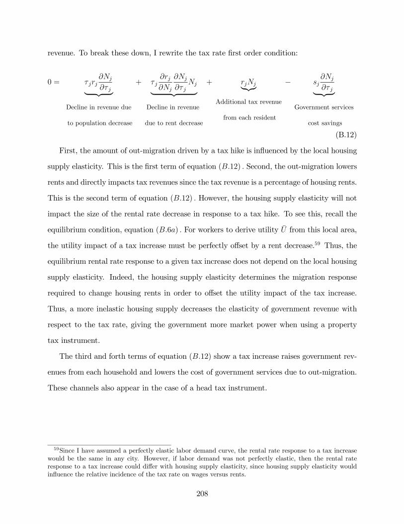
revenue. To break these down, I rewrite the tax rate �rst order condition:

0 = � jrj@Nj@� j| {z }

Decline in revenue due

to population decrease

+ � j@rj@Nj

@Nj@� j

Nj| {z }Decline in revenue

due to rent decrease

+ rjNj|{z}Additional tax revenue

from each resident

� sj@Nj@� j| {z }

Government services

cost savings

(B.12)

First, the amount of out-migration driven by a tax hike is in�uenced by the local housing

supply elasticity. This is the �rst term of equation (B:12) : Second, the out-migration lowers

rents and directly impacts tax revenues since the tax revenue is a percentage of housing rents.

This is the second term of equation (B:12) : However, the housing supply elasticity will not

impact the size of the rental rate decrease in response to a tax hike. To see this, recall the

equilibrium condition, equation (B:6a) : For workers to derive utility �U from this local area,

the utility impact of a tax increase must be perfectly o¤set by a rent decrease.59 Thus, the

equilibrium rental rate response to a given tax increase does not depend on the local housing

supply elasticity. Indeed, the housing supply elasticity determines the migration response

required to change housing rents in order to o¤set the utility impact of the tax increase.

Thus, a more inelastic housing supply decreases the elasticity of government revenue with

respect to the tax rate, giving the government more market power when using a property

tax instrument.

The third and forth terms of equation (B:12) show a tax increase raises government rev-

enues from each household and lowers the cost of government services due to out-migration.

These channels also appear in the case of a head tax instrument.

59Since I have assumed a perfectly elastic labor demand curve, the rental rate response to a tax increasewould be the same in any city. However, if labor demand was not perfectly elastic, then the rental rateresponse to a tax increase could di¤er with housing supply elasticity, since housing supply elasticity wouldin�uence the relative incidence of the tax rate on wages versus rents.

208

C Chapter 3 Appendix

For the general model, leaving aside terms that do not involve unknown parameters, the log

likelihood function is

L( jY) = �12ln (det((Z; )))� "0�1(Z; )"=2:

The matrix (Z; ) is large in our illustrations, with dimension 2,590,190 by 2,590,190.

Direct maximization of the log likelihood function is therefore not feasible. However, because

locations are measured by puma locations, (Z; ) has a block structure, and calculations

of the log likelihood simplify and can be written in terms of �rst and second moments by

puma. We �rst give a couple of preliminary results.

Theorem 11. (Sylvester�s Determinant Theorem) Let A and B be arbitrary M �N

matrices. Then:

det(IN + A0B) = det(IM +BA

0):

Proof of Theorem 11: Consider a block matrix�M1 M2M3 M4

�. Then:

det�M1 M2M3 M4

�= det

�M1 0M3 I

�det�I M�1

1 M2

0 M4�M3M�11 M2

�= detM1 det(M4 �M3M

�11 M2)

similarly

det�M1 M2M3 M4

�= det

�I M20 M4

�det�M1�M2M

�14 M3 0

M�14 M3 I

�= detM4 det(M1 �M2M

�14 M3)

Letting M1 = IM ;M2 = �B;M3 = A0;M4 = IN yields the result.

Lemma 12. (Determinant of Cluster Covariance Matrix) Suppose C is an N�M

matrix of binary cluster indicators, with C0C equal to a M �M diagonal matrix, � is an

arbitrary M �M matrix, and IN is the N-dimensional identity matrix. Then, for scalar �2",

209

and

= �2�IN +C�C0 C = �+ �

2�(C

0C)�1;

we have

det() = (�2�)N�M det(C0C) det(C):

Proof of Lemma 12: By Sylvester�s theorem:

det() = (�2�)N det(IN +C�=�

2�C

0) = (�2�)N det(IM +C

0C�=�2�)

= (�2�)N det(IM +C

0CC=�2� � IM) = (�2�)N det(C0C) det(C=�2�)

= (�2�)N�M

�YNp

�det(C):

Lemma 13. Suppose Assumptions 7 and 8 hold. Then for any N �N matrix ,

E [W0W] =M1 � (M1 � 1)M � (M � 1) � �

0N�N +

M1 �M0

M � (M � 1) � trace (C0C) :

Proof of Lemma 13: We have

E[Wi �Wj] =

8><>: M1=M if 8m;Cim = Cjm;

(M1 � (M1 � 1))=(M � (M � 1)) otherwise:

it follows that

E[WW0] =M1 � (M1 � 1)M � (M � 1) � �N �

0N +

�M1

M� M1 � (M1 � 1)M � (M � 1)

��CC0

=M1 � (M1 � 1)M � (M � 1) � �N �

0N +

M1 �M0

M � (M � 1) �CC0:

Thus

E[W0W] = trace (E[WW0])

210

= trace

� ��M1 � (M1 � 1)M � (M � 1) � �N �

0N +

M1 �M0

M � (M � 1) �CC0��

=M1 � (M1 � 1)M � (M � 1) � �

0N�N +

M1 �M0

M � (M � 1) � trace (C0C) :

Lemma 14. Suppose the N �N matrix satis�es

= �2" � IN + �2C �CC0;

where IN is the N �N identity matrix, and C is an N �M matrix of zeros and ones, with

C�M = �N and C0�N = (N=M)�M , so that,

ij =

8>>>><>>>>:�2" + �

2C if i = j

�2C if i 6= j;8m;Cim = Cjm;

0 otherwise;

(C.1)

Then, (i)

ln (det ()) = N � ln��2"�+M � ln

�1 +

N

M� �

2C

�2"

�;

and, (ii)

�1 = ��2" � IN ��2C

�2" � (�2" + �2C �N=M)�CC0

Proof of Lemma 14: First, consider the �rst part. Apply Lemma 12 with

� = �2C � IM ; and C0C =N

M� IM ; so that C =

��2C + �

2" �M

N

�� IM :

Then, by Lemma 12, we have

ln det() = (N �M) � ln(�2") +M � ln(N=M) + ln det(C)

= (N �M) � ln(�2") +M � ln(N=M) +M � ln��2C + �

2" �M

N

�

211

= (N �M) � ln(�2") +M � ln�N

M�2C + �

2"

�

= N � ln(�2") +M � ln�1 +

N

M� �

2C

�2"

�:

Next, consider part (ii). We need to show that

��2" � IN + �2C �CC0��2" � IN �

�2C�2" � (�2" + �2C �N=M)

�CC0�= IN ;

which amounts to showing that

� �2" � �2C�2" � (�2" + �2C �N=M)

�CC0 + �2C �CC0��2" �CC0 � �4C�2" � (�2" + �2C �N=M)

�CC0 = 0:

This follows directly from the fact that C0C = (N=M) � IM and collecting the terms.

Proof of Lemma 5: The unbiasedness result directly follows from the conditional unbi-

asedness established in Lemma 4. Next we establish the second part of the Lemma. By the

Law of Iterated Expectations,

VU(Z) = V�Eh� j Y(0);Y(1);Z

ij Z; N1

�+ E

hV��Y(0);Y(1);Z� j Z; N1i (C.2)

= EhV��Y(0);Y(1);Z� j Z; N1i

where the second line follows since �ols is unbiased. By Lemma 4, we have:

EhV��Y(0);Y(1);Z� j Z; N1i = E" N

N0 �N1 � (N � 2)

NXi=1

("i � ")2 j Z; N1

#

212

Observe that we can write:

NXi=1

("i � ")2 = ("� �N �0N"=N)0("� �N �0N"=N)

= "0"� 2"0�N �0N"=N + "0�N �N �N �0N"=N2

= "0"� "0�N �0N"=N:

Hence:

VU(Z) =N

N0 �N1 � (N � 2)E ["0"� "0�N �0N"=N jZ; N0; N1]

=N

N0 �N1 � (N � 2)trace (E [""0 � �0N""0�N=N jZ; N0; N1])

=N

N0 �N1 � (N � 2)(trace ((Z))� �0N(Z)�N=N)

which establishes (3.11). Finally, we prove the third part of the Lemma. By Lemma 2, �ols

is unbiased conditional on Z;W, so that by argument like in Equation (C.2) above, we can

also write:

VU(Z) = V�Eh� j Z;W

ij Z; N1

�+ E

hV��Z;W�

j Z; N1i

= EhV��Y(0);Y(1);Z� j Z; N1i

which equals E [VR (Y(0);Y(1);Z) j Z; N1] by (C.2).

Suppose Assumptions 1 holds with (Z) satisfying trace((Z))=N ! c for some 0 < c <

1, and �0N(Z)�N=N2 ! 0, and Assumption 3 holds with N1=N ! p for some 0 < p < 1.

Then

N � (VINC � VU(Z))p�! 0; and N � VINC

p�! c

p � (1� p) :

Proof of Lemma 6: We will �rst show that the second claim in the Lemma holds,

N � VINCp�! c

p � (1� p) ; (C.3)

213

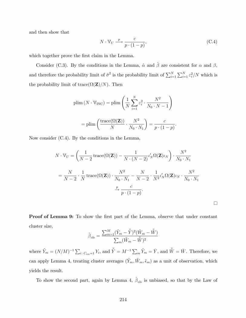
and then show that

N � VUp�! c

p � (1� p) ; (C.4)

which together prove the �rst claim in the Lemma.

Consider (C.3). By the conditions in the Lemma, � and � are consistent for � and �,

and therefore the probability limit of �2 is the probability limit ofPN

i=1

PNi=1 "

2i =N which is

the probability limit of trace((Z)=N). Then

plim (N � VINC) = plim 1

N

NXi=1

"2i �N2

N0 �N � 1

!

= plim

�trace((Z))

N� N2

N0 �N1

�=

c

p � (1� p) :

Now consider (C.4). By the conditions in the Lemma,

N � VU =�

1

N � 2 trace((Z))�1

N � (N � 2)�0N(Z)�N

�� N2

N0 �N1

=N

N � 2 �1

Ntrace((Z)) � N2

N0 �N1� N

N � 2 �1

N2�0N(Z)�N �

N2

N0 �N1p! c

p � (1� p) :

Proof of Lemma 9: To show the �rst part of the Lemma, observe that under constant

cluster size,

�ols =

PMm=1(

~Ym � �~Y )2( ~Wm � �~W )Pm(~Wm � �~W )2

where ~Ym = (N=M)�1P

i : Cim=1Yi, and

�~Y =M�1Pm~Ym = �Y , and �~W = �W . Therefore, we

can apply Lemma 4, treating cluster averages ( ~Ym; ~Wm;~�m) as a unit of observation, which

yields the result.

To show the second part, again by Lemma 4, �ols is unbiased, so that by the Law of

214

Iterated Expectations, and the �rst part of the Lemma,

VU(Z) = V�Eh� j Y(0);Y(1);Z

ij Z;M1

�+ E

hV��Y(0);Y(1);Z� j Z;M1

i

= EhV��Y(0);Y(1);Z� j Z;M1

i= E

"M

(M � 2) �M0 �M1

MXm=1

�~"m � ~"

�2 j Z;M1

#Hence, it su¢ ces to show that

E

"MXs=1

�~"s � ~"

�2��Z;M1

#=

�M2

N2� trace (C0(Z)C)� M

N2�0(Z)�

�:

Note that in general C�M = �N ; and under Assumption 8, it follows that C0C = (N=M) � IM :

We can write

~"m = (C0C)

�1C0" =

M

NC0"; and ~" =

1

M�0M (C

0C)�1C0" =

1

N�0N";

so thatMXm=1

�~"m � ~"

�2=

�M

NC0"� 1

M�M �

0N"

�0�M

NC0"� 1

M�M �

0N"

�

=

��M

NC0 � 1

N�M �

0N

�"

�0��M

NC0 � 1

N�M �

0N

�"

�:

= "0�M

NC� 1

N�N �

0M

�0�M

NC0 � 1

N�M �

0N

�":

Thus

E

"MXm=1

�~"s � ~"

�2��Z;M1

#= E

�"0�M

NC� 1

N�N �

0M

�0�M

NC0 � 1

N�M �

0N

�"

��Z;M1

�

= trace

�E��M

NC� 1

N�N �

0M

�0�M

NC0 � 1

N�M �

0N

�""0��Z;M1

��

215

= trace

��M

NC� 1

N�N �

0M

�0�M

NC0 � 1

N�M �

0N

�(Z)

�

= trace

��M

NC0 � 1

N�M �

0N

�(Z)

�M

NC� 1

N�N �

0M

�0�

=M2

N2� trace (C0(Z)C)� M

N2� �0N(Z)�N :

Proof of Theorem 10: We show

N � VUp�! c

N2m � p � (1� p)

;

and

N � VINC;CRp�! c

N2m � p � (1� p)

;

which together imply the two claims in the Theorem. First consider the �rst claim. The

normalized variance is

N � VU(Z) =M2 �N

M0 �M1 � (M � 2) �N2� (M � trace (C0(Z)C)� �0(Z)�)

=M2 �N

M0 �M1 � (M � 2) ��M

N� trace (C

0(Z)C)

N� �

0(Z)�

N2

�:

By the conditions in the Theorem the probability limit of this expression is

plim

�M2 �N

M0 �M1 � (M � 2) ��M

N� trace (C

0(Z)C)

N� �

0(Z)�

N2

��

= plim

�M2 �N

M0 �M1 � (M � 2)

��plim

�M

N� trace (C

0(Z)C)

N

�� plim

��0(Z)�

N2

��=

c

N2m � p � (1� p)

:

Next, consider the second claim. Now the probability limit of the model-based variance is

plim (N � VINC;CR(Z)) =

216

plim

�M2 �N

M0 �M1 � (M � 2) �N2��M � trace

�C0(Z; ~�"; ~�

2S)C

�� 0(Z; ~�"; ~�2S)�

��

= plim

M2 �N

M0 �M1 � (M � 2) � M

N�trace

�C0(Z; ~�"; ~�

2S)C

�N

� �0(Z; ~�"; ~�

2S)�

N2

!!

=1

Nm � p � (1� p)� plim

M

N�trace

�C0(Z; ~�"; ~�

2S)C

�N

!� plim

��0(Z; ~�"; ~�

2S)�

N2

�!

=1

N2m � p � (1� p)

� plim trace

�C0(Z; ~�"; ~�

2S)C

�N

!

Hence, in order to prove the second claim it su¢ ces to show that trace(C0(Z)C) =

trace(C0(Z; (~�"; ~�2S))C). The log likelihood function based on the speci�cation (C.1) is

L(�2"; �2SjY;Z) = �

1

2� ln��Z; �2"; �

2S

�� 12�Y0(�2"; �

2S)�1Y:

The expected value of the log likelihood function is

E�L(�2"; �

2SjY;Z)

��Z� = �12ln��Z; �2"; �

2S

�� 12� E�Y0(Z; �2"; �

2C)�1Y

�= �1

2� ln��Z; �2"; �

2S

�� 12� trace

�Eh�Z; �2"; �

2S

��1YY0

�i= �1

2� ln��Z; �2"; �

2S

�� 12� trace

��Z; �2"; �

2S

��1(Z)

�:

Using Lemma 14, this is equal to

E�L(�2"; �

2SjY;Z)

��Z� = �N2� ln(�2")�

M

2� ln�1 +N=M � �2S=�2"

�

� 1

2 � �2"� trace((Z)) + �2S

2 � �2" � (�2" + �2S �N=M)� trace (C0(Z)C) :

The �rst derivative of the expected log likelihood function with respect to �2S is

@

@�2SE�L(�2"; �

2SjY;Z)

��Z� = � N

2 � (�2" +N=M � �2S)+

trace (C0(Z)C)

(�2" + �2S � (N=M))2

217

Hence the �rst order condition for ~�2S implies that

trace (C0(Z)C) = N � (~�2" + ~�2S � (N=M)):

For the misspeci�ed error-covariance matrix (Z; ~ ) we have

trace (C0(Z; ~ )C) =

MXm=1

�N2m � ~�2S +Nm � ~�2"

�:

By equality of the cluster sizes this simpli�es to

trace (C0(Z; ~ )C) = N ��~�2" + ~�

2S � (N=M)

�= trace (C0(Z)C) :

218

essays in local labor economics - harvard university

Documents