Three-Dimensional Route Planner Using A* Algorithm; Application to Autonomous Underwater Vehicles

Nathan E. Brener*, Member, IEEE, Hua C. Looney, S. Sitharama Iyengar, Fellow, IEEE,

and Narayanadas Vakamudi Robotics Research Laboratory, Department of Computer Science,

Louisiana State University, Baton Rouge, LA 70803 USA Email: brener@bit.csc.lsu.edu, iyengar@bit.csc.lsu.edu

* Corresponding author

Jacob Barhen, Member, IEEE

CESAR Laboratory, Oak Ridge National Laboratory, Oak Ridge, TN 37831, USA

Abstract – We have developed a 3D route planner, called 3DPLAN, which employs the A* Algorithm to find optimum paths. The A* Algorithm has a major advantage compared to other search methods because it is guaranteed to give the optimum path. We have shown that it is quite feasible to use A* for 3D route planning if one employs the new mobility and threat heuristics that we have developed. We have adapted 3DPLAN to autonomous underwater vehicles (AUVs) by developing a map of realistic travel times that depend on ocean currents and the still water speed of the AUV. This version of 3DPLAN, called AUVPLAN, was used to calculate optimum paths in a region of the East China Sea. These optimum path calculations employed a travel time map with more than a million grid points and required less than 15 seconds of CPU time for each path. To our knowledge, this is the first time that actual travel times based on realistic ocean currents have been used in AUV route planning. We also used AUVPLAN to calculate optimum paths in the Persian Gulf, demonstrating that it successfully avoids underwater mines. Index Terms – Artificial intelligence, graph search strategies, heuristic methods, autonomous

vehicles. 1 Introduction Route planning has been widely used for civilian and military purposes. Three-dimensional (3D) route planning is especially useful for the navigation of autonomous underwater vehicles (AUVs) and combat helicopters. 3D route planning is a very challenging problem because the large grids that are typically required can cause a prohibitive computational burden if one does not use an efficient search algorithm. Several search algorithms have been proposed to perform 3D route planning, including case-based reasoning [6], [10] and the genetic algorithm [5], [7], [8], [9].

2

Case–based reasoning relies on specific instances of past experience to solve new

problems. A new path is obtained by searching previous routes to see if there is one that matches the current situation in the features, goals and constraints. The new path is generated by modifying an old path in the previous path database using a set of repair rules. However, since the number of possible threat distributions is very large for most battle areas, it would not be feasible to store old routes for all or most of the possible threat arrangements. Thus the case-based method is not suitable for handling threats in route planning. In addition, when it has to synthesize complete new routes (in an area where no old paths are available) or modify old routes by synthesizing new segments, it doesn’t use a guaranteed best-first search algorithm such as A*, but instead uses straight-line segments that go around obstacles. Thus the routes that it generates are neither locally nor globally optimal.

The genetic algorithm (GA) method is a stochastic search technique based on the

principles of biological evolution, natural selection and genetic recombination. Genetic algorithms generate a population of solutions. Then such solutions mate and bear offspring solutions in the next generation. In this way, the solutions in the population improve over many generations until the best solution is obtained. However, genetic algorithms have been accepted slowly for research problems because crossing two feasible solutions does not, in many cases, result in a feasible solution as an offspring. Another disadvantage of GA is that although it can generate solutions to a route planning problem, it cannot guarantee that the solution is optimal (i.e., it can converge to a local, rather than a global, minimum).

The A* Algorithm [4] is a guaranteed best-first search algorithm that has been used

previously in 2D route planning by several researchers including some of the authors of this paper [1], [2]. A major advantage of the A* Algorithm compared to the other methods mentioned above is that A* is guaranteed to give the optimum path. In spite of this significant advantage, no one has previously used the A* Algorithm for 3D route planning as far as we are aware. The probable reason for this is the belief that the computational cost of using A* for 3D route planning would be prohibitive. We have developed a 3D A* route planner [3], called 3DPLAN, and have used it to demonstrate that, on the contrary, it is quite feasible to use A* for 3D searches if one employs the new mobility and threat heuristics that we have developed. These new heuristics substantially speed up the A* Algorithm so that the run times are quite reasonable for the large grids that are typical of 3D searches. In particular, we tested 3DPLAN on a grid with almost 8 million points, which is the largest number of grid points that has ever been used in an A* search as far as we aware, and found that all of the optimum path calculations required less than a minute of CPU time on a Dell PC with a 4.3 GHZ Pentium IV processor [3]. We also compared our new mobility and threat heuristics to a straight line mobility heuristic and no threat heuristic, which is what other researchers have used in A* searches, and found that our new heuristics cause the A* algorithm to run up to 4.3 times faster. In this paper, we apply 3DPLAN to autonomous underwater vehicles (AUVs).

3

2 Application to Autonomous Underwater Vehicles 2.1 Travel Time Map We now apply our 3D A* route planner, 3DPLAN, to Autonomous Underwater Vehicles (AUVs) by replacing the test mobility map described in [3] with a map of realistic travel times which depend on ocean currents and the still water speed of the AUV. This application of 3DPLAN will be called AUVPLAN. In the test calculations described in [3], the path cost depends on mobility penalties (to which the travel time is roughly proportional), but in the AUV application in this paper, the path cost is equal to the actual travel time rather than just being approximately proportional to it. As far as we are aware, this is the first time that actual travel times based on realistic ocean currents have been used in AUV route planning.

In order to construct the map of travel times, we first created an ocean current map using the current velocity data from the Navy Coastal Ocean Model (NCOM) – East Asian Seas version, which was provided by the Naval Research Lab (NRL) at the Stennis Space Center in Mississippi. In this 3D ocean current map, there are 229×128×35 grid points in the x, y and z directions for a total of more than one million grid points. The x coordinate goes from longitude 115° E to 135° E in steps of 11.4 minutes of arc, the y coordinate goes from latitude 20° N to 30° N in steps of 11.4 minutes, and the z coordinate goes from 0 (the ocean surface) to a maximum depth of 4,655 m. This area includes a region of the East China Sea which contains Taiwan and neighboring islands.

At each grid point, the map gives the two components of the current velocity: the “U”

velocity, which is in the x (East/West) direction, and the “V” velocity, which is in the y (North/South) direction, where East and North are positive and West and South are negative, and the velocities are in m/s. There is no current velocity in the z direction.

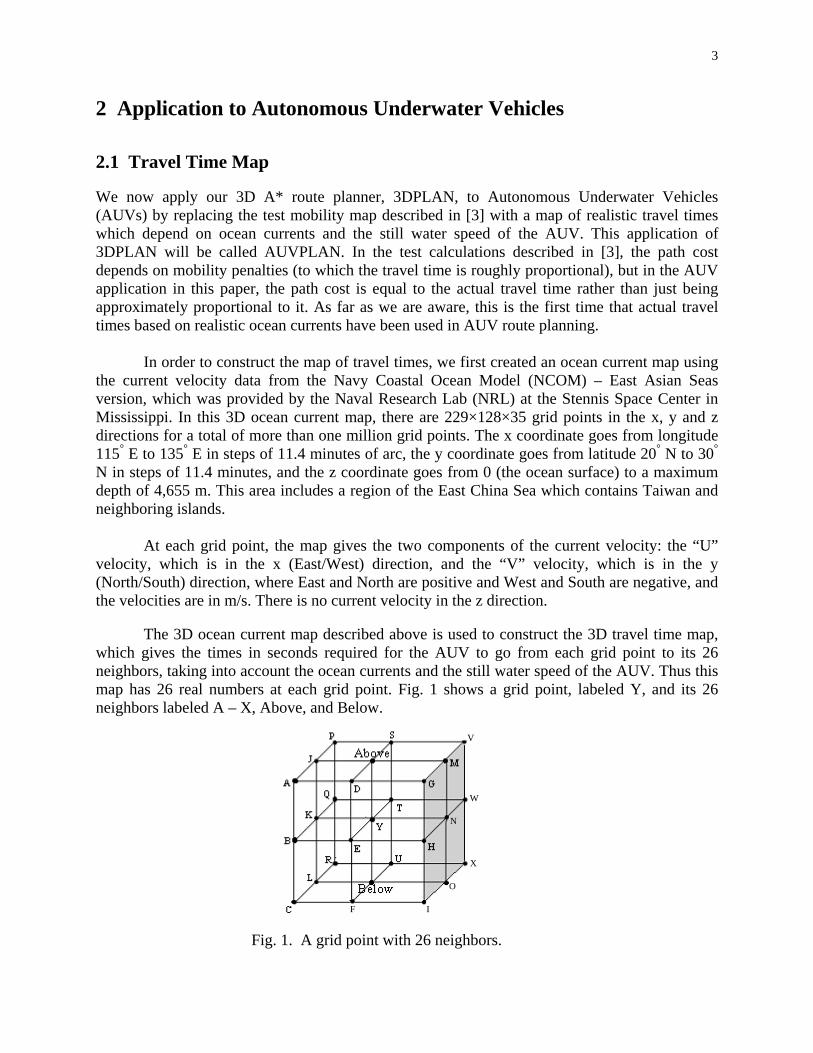
The 3D ocean current map described above is used to construct the 3D travel time map, which gives the times in seconds required for the AUV to go from each grid point to its 26 neighbors, taking into account the ocean currents and the still water speed of the AUV. Thus this map has 26 real numbers at each grid point. Fig. 1 shows a grid point, labeled Y, and its 26 neighbors labeled A – X, Above, and Below.

V

X

W

N

O F I Fig. 1. A grid point with 26 neighbors.

4

The grid point Y will be called the central grid point and the points A – X will be referred to as follows: A – southwest above, B – southwest same level, C – southwest below, D – south above, E – south same level, F – south below, G – southeast above, H – southeast same level, I – southeast below, J – west above, K – west same level, L – west below, M – east above, N – east same level, O – east below, P – northwest above, Q – northwest same level, R – northwest below, S – north above, T – north same level, U – north below, V – northeast above, W – northeast same level, X – northeast below. In this figure, the scale in the z direction is different from the scale in the x and y directions so that the grid can conveniently be displayed. In calculating the travel times to the N, S, E, W, NE, NW, SE, and SW neighbors in the planes above and below, we use only the component of the distance in the xy plane, since the AUV can move up or down by simply changing its ballast and thus vertical motion that occurs at the same time as horizontal motion does not require any additional travel time. This assumption is valid as long as the vertical spacing between the grid points is substantially smaller than the horizontal spacing, which is the case here. Hence the difference in travel time to a neighbor in the plane above and the corresponding neighbor in the same plane (e.g., NE above and NE same level) is due only to the difference between the U and V velocities at the two neighbors and not to their distances from the central point.

In order to illustrate the calculation of the travel time map, we now give the formulas for the travel times from the central point to the three NE neighbors (NE same level, NE above, NE below), the three E neighbors (E same level, E above, E below), and the neighbors directly above and below. 2.1.1 NE Neighbors

α

φ θ

d

P2

P1

d2

d1

d1d1

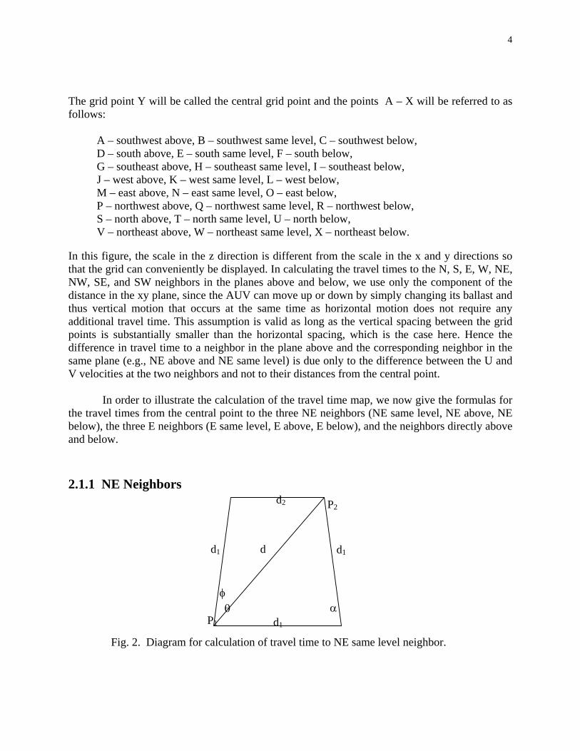
Fig. 2. Diagram for calculation of travel time to NE same level neighbor.

5

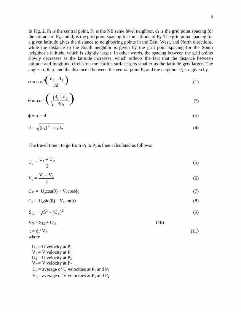
In Fig. 2, P1 is the central point, P2 is the NE same level neighbor, d1 is the grid point spacing for the latitude of P1, and d2 is the grid point spacing for the latitude of P2. The grid point spacing for a given latitude gives the distance to neighboring points in the East, West, and North directions, while the distance to the South neighbor is given by the grid point spacing for the South neighbor’s latitude, which is slightly larger. In other words, the spacing between the grid points slowly decreases as the latitude increases, which reflects the fact that the distance between latitude and longitude circles on the earth’s surface gets smaller as the latitude gets larger. The angles α, θ, φ, and the distance d between the central point P1 and the neighbor P2 are given by

α = cos-1(1

21

2ddd − ) (1)

θ = cos-1(1

21

4ddd + ) (2)

φ = α − θ (3)

d = 212

1 dd)(d + (4)

The travel time t to go from P1 to P2 is then calculated as follows:

Ua = 2

UU 21 + (5)

Va = 2

VV 21 + (6)

C12 = Uacos(θ) + Vacos(φ) (7)

Cp = Uasin(θ) − Vasin(φ) (8)

2p

212 )C(SS −= (9)

VN = S12 + C12 (10) t = d / V (11) N where

U1 = U velocity at P1 V1 = V velocity at P1 U2 = U velocity at P2 V2 = V velocity at P2

Ua = average of U velocities at P1 and P2

Va = average of V velocities at P1 and P2

6

C12 = component of current velocity along the line joining P1 and P2 Cp = component of current velocity perpendicular to the line joining P1 and P2 S = AUV’s still water horizontal velocity S12 = component of AUV’s still water horizontal velocity along the line joining P1 and P2 VN = net velocity of AUV (the net velocity is along the line joining P1 and P2) .

The travel times to the NE above and NE below neighbors are calculated with the same formulas, where U2 and V2 are the U and V velocities at the NE above or NE below neighbor, and the distance d and angles α, θ and φ are the same as for the NE same level neighbor. As mentioned previously, we use only horizontal distances and velocities to calculate the travel times to neighbors in the above and below levels (except the ones directly above and below) because the travel time is determined by the horizontal motion. Vertical motion that occurs concurrently with horizontal motion does not add to the travel time. The travel times to the NW, SE and SW neighbors are calculated in a similar manner. 2.1.2 E Neighbors

P1d1 P2

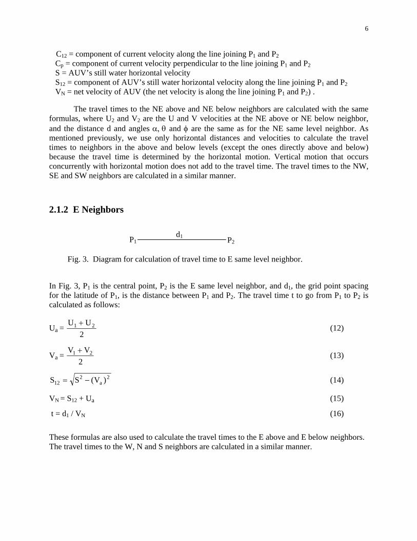
Fig. 3. Diagram for calculation of travel time to E same level neighbor. In Fig. 3, P1 is the central point, P2 is the E same level neighbor, and d1, the grid point spacing for the latitude of P1, is the distance between P1 and P2. The travel time t to go from P1 to P2 is calculated as follows:

Ua = 2

UU 21 + (12)

Va = 2

VV 21 + (13)

2a

212 )V(SS −= (14)

VN = S12 + Ua (15)

t = d1 / VN (16)

These formulas are also used to calculate the travel times to the E above and E below neighbors. The travel times to the W, N and S neighbors are calculated in a similar manner.

7

2.1.3 Above and Below Neighbors The travel time to go from the central point to the neighbor directly above or below is given by t = d / S (17) v where d is the distance to the neighbor and Sv is the velocity of the AUV in the vertical direction (due to changing the ballast). 2.2 Threat Map Threats are handled the same way as described in [3], where each threat is modeled by an inner sphere called the no-go sphere where the AUV is not allowed to go, and an outer sphere called the penalty sphere where the AUV is within range of the threat and hence incurs a threat penalty. Thus if the line between a central point and a neighbor passes through the no-go sphere of a threat, the AUV is not allowed to travel from the central point to that neighbor. If the threat is an underwater mine, it has a no-go sphere but no penalty sphere. 2.3 A* Algorithm AUVPLAN employs the A* Algorithm, in which the total cost, f, of the path that goes through a particular grid point on the digital map (this grid point will be referred to as the current point) is given by

f = g + h (18) where g is the actual cost that was accumulated in going from the starting point to the current point and h is an underestimate of the remaining cost required to go from the current point to the target. The heuristic h is the key quantity that determines how efficiently the algorithm works. h must not only be a guaranteed underestimate of the remaining cost, which ensures that no potential optimum paths will be discarded due to overestimating their total cost, but must also provide as close an estimate as possible of the remaining cost. The closer h is to the actual remaining cost, the faster the algorithm will find the optimum path. Thus the success of the algorithm depends on the choice of the heuristic h. With a proper choice of h, the algorithm can be highly efficient and can find the optimum path in a matter of seconds.

The actual accumulated cost, g, is given by

g = αtt TT + αt T (19) where

TT = accumulated travel time T = accumulated threat penalty

8

αtt = travel time weight αt = threat weight.

The weights αtt and αt are entered by the user and enable the military planner to put any desired degree of emphasis on each of the cost factors. For example, a large weight for travel time and a small weight for threats would produce a fast path that may go close to enemy threats, while a large weight for threats and a small weight for travel time would produce a path that stays as far away from threats as possible and consequently may require a considerably longer travel time.

The accumulated travel time and threat penalty are given by

TT = Σ TTi (20) T = Σ Ri(Ti-1 + Ti)/2 (21)

where the sum is over the grid points traversed in going from the starting point to the current point , TTi is the travel time to go from grid point i-1 to grid point i, Ti is the threat penalty at grid point i, and Ri is the stepsize to go from grid point i-1 to grid point i.

The heuristic, which is an underestimate of the remaining cost required to go from the current point to the target, is given by:

h = αtthtt + αtht (22)

where

htt = underestimate of remaining travel time (travel time heuristic)

ht = underestimate of remaining threat penalty (threat heuristic) We now describe the travel time heuristic and threat heuristic in detail. 2.3.1 Travel Time Heuristic We first describe our mobility heuristic and then modify it to obtain the travel time heuristic. Our mobility heuristic is different and better than the straight line heuristic used in previous A* approaches, since it is larger than the straight line heuristic and still is an underestimate of the remaining cost. We start by describing the 2D version of our mobility heuristic.

9

P3

P2

P1 Fig. 4. Mobility heuristic from P2 to P3 (solid line).

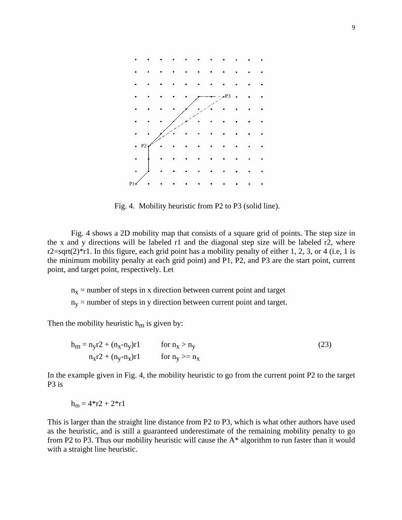
Fig. 4 shows a 2D mobility map that consists of a square grid of points. The step size in the x and y directions will be labeled r1 and the diagonal step size will be labeled r2, where r2=sqrt(2)*r1. In this figure, each grid point has a mobility penalty of either 1, 2, 3, or 4 (i.e, 1 is the minimum mobility penalty at each grid point) and P1, P2, and P3 are the start point, current point, and target point, respectively. Let

nx = number of steps in x direction between current point and target

ny = number of steps in y direction between current point and target. Then the mobility heuristic hm is given by:

hm = nyr2 + (nx-ny)r1 for nx > ny (23) nxr2 + (ny-nx)r1 for ny >= nx

In the example given in Fig. 4, the mobility heuristic to go from the current point P2 to the target P3 is

hm = 4*r2 + 2*r1 This is larger than the straight line distance from P2 to P3, which is what other authors have used as the heuristic, and is still a guaranteed underestimate of the remaining mobility penalty to go from P2 to P3. Thus our mobility heuristic will cause the A* algorithm to run faster than it would with a straight line heuristic.

10

It is straightforward to extend this 2D mobility heuristic to the 3D travel time heuristic htt. Let

nx = number of steps in x direction between current point and target ny = number of steps in y direction between current point and target nz = number of steps in z direction between current point and target.

The 3D travel time heuristic is then given by

htt = nx*t5 + (ny-nx)*t4 + (nz-ny)*t3 for nx <= ny <= nz (24)

nx*t5 + (nz-nx)*t4 + (ny-nz)*t1 for nx <= nz <= ny

ny*t5 + (nx-ny)*t4 + (nz-nx)*t3 for ny <= nx <= nz

ny*t5 + (nz-ny)*t4 + (nx-nz)*t1 for ny <= nz <= nx

nz*t5 + (nx-nz)*t2 + (ny-nx)*t1 for nz <= nx <= ny

nz*t5 + (ny-nz)*t2 + (nx-ny)*t1 for nz <= ny <= nx where t1 = smallest travel time to go from a central point to an E, W, N, or S neighbor in the same plane t2 = smallest travel time to go from a central point to a NE, NW, SE, or SW neighbor in the same plane t3 = smallest travel time to go from a central point to a neighbor directly above or below t4 = smallest travel time to go from a central point to an E, W, N, or S neighbor in the plane above or below t5 = smallest travel time to go from a central point to a NE, NW, SE, or SW neighbor in the plane above or below. These minimum travel times are obtained by scanning the entire travel time map. 2.3.2 Threat Heuristic We now describe our threat heuristic. As far as we know, no other authors have ever used a threat heuristic in the A* Algorithm. The probable reason for this is that the minimum threat penalty is 0 rather than 1 (the minimum mobility penalty is 1 in our test map). Thus if one tried to use the same technique for the threat heuristic as was used for the mobility heuristic, the threat heuristic would be 0. We have developed a threat heuristic that is different from the mobility heuristic and is, in general, nonzero. Thus our new threat heuristic will speed up the A* Algorithm compared to not having a threat heuristic at all.

We will first describe our threat heuristic in 2D and then extend it to 3D. Fig. 5 shows the same square grid of points that was shown in Fig. 4, where P1, P2, and P3 are the start point, current point and target point, respectively. The threat heuristic ht will be an underestimate of the

11

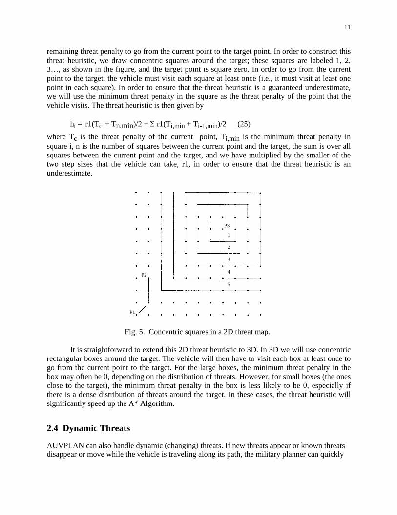
remaining threat penalty to go from the current point to the target point. In order to construct this threat heuristic, we draw concentric squares around the target; these squares are labeled 1, 2, 3…, as shown in the figure, and the target point is square zero. In order to go from the current point to the target, the vehicle must visit each square at least once (i.e., it must visit at least one point in each square). In order to ensure that the threat heuristic is a guaranteed underestimate, we will use the minimum threat penalty in the square as the threat penalty of the point that the vehicle visits. The threat heuristic is then given by

ht = r1(Tc + Tn,min)/2 + Σ r1(Ti,min + Ti-1,min)/2 (25)

where Tc is the threat penalty of the current point, Ti,min is the minimum threat penalty in square i, n is the number of squares between the current point and the target, the sum is over all squares between the current point and the target, and we have multiplied by the smaller of the two step sizes that the vehicle can take, r1, in order to ensure that the threat heuristic is an underestimate. P3 1

2 3

4 P2 5

P1

Fig. 5. Concentric squares in a 2D threat map.

It is straightforward to extend this 2D threat heuristic to 3D. In 3D we will use concentric rectangular boxes around the target. The vehicle will then have to visit each box at least once to go from the current point to the target. For the large boxes, the minimum threat penalty in the box may often be 0, depending on the distribution of threats. However, for small boxes (the ones close to the target), the minimum threat penalty in the box is less likely to be 0, especially if there is a dense distribution of threats around the target. In these cases, the threat heuristic will significantly speed up the A* Algorithm. 2.4 Dynamic Threats AUVPLAN can also handle dynamic (changing) threats. If new threats appear or known threats disappear or move while the vehicle is traveling along its path, the military planner can quickly

12

update the threat map. AUVPLAN will then rapidly generate a new optimum path from the current position to the target.

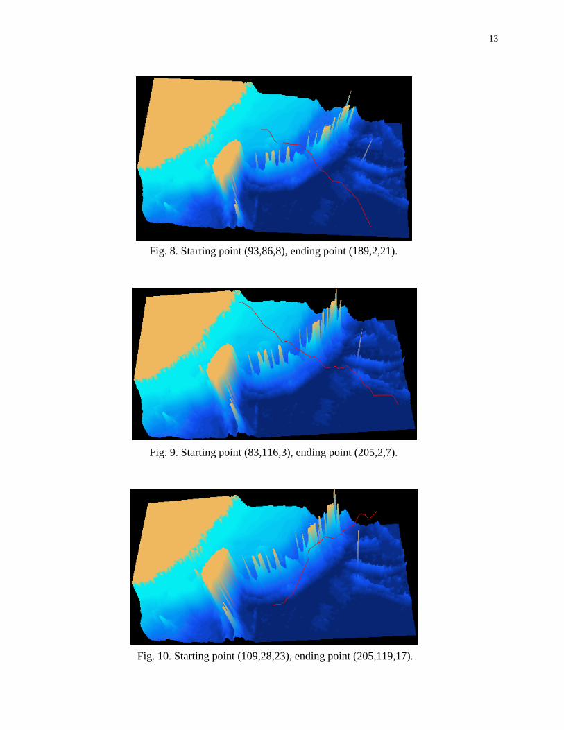
3 Sample Path Calculations We used Microsoft Visual C++ 6.0 to develop 3DPLAN, the travel time map, and AUVPLAN. We then used AUVPLAN and the travel time map to perform optimum path calculations in a region of the East China Sea that contains Taiwan and neighboring islands. Figs 6-12 show the results of these optimum path calculations, which were done on a Dell PC with a 1.7 GHZ Pentium IV processor. All of the path calculations required less than 15 seconds of CPU time. Note that the optimum paths move up and down in order to find the most favorable currents. As discussed above, the use of the A* algorithm guarantees that the calculated paths have the shortest possible travel times. This cannot be guaranteed when other route planning algorithms, such as the genetic algorithm (GA), are used. Fig. 6: Starting point (33,40,4), ending point (208,8,13).

Fig. 7: Starting point (9,28,3), ending point (201,83,6).

13

Fig. 8. Starting point (93,86,8), ending point (189,2,21).

Fig. 9. Starting point (83,116,3), ending point (205,2,7).

Fig. 10. Starting point (109,28,23), ending point (205,119,17).

14

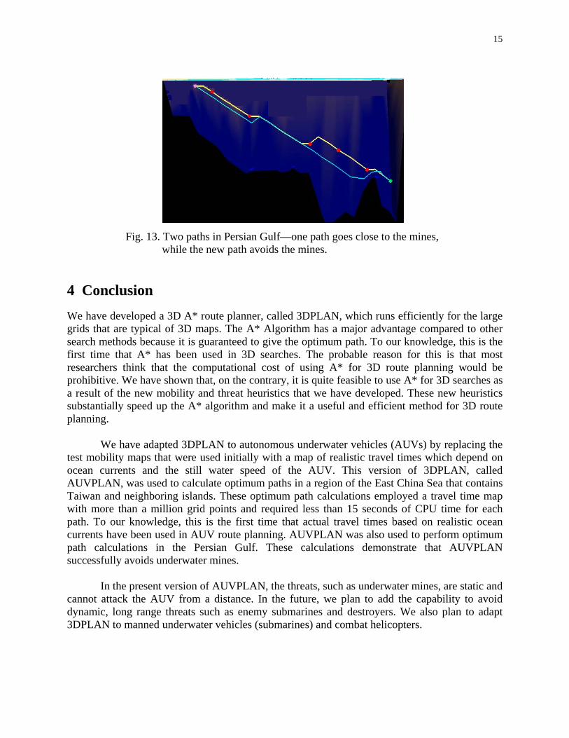
Fig. 11. Starting point (9,8,13), ending point (108,119,7). Fig. 12. Starting point (9,8,6), ending point (108,88,9). 3.1 Avoidance of Underwater Mines If there are underwater mines in the region between the start point and the target, AUVPLAN will calculate the fastest path that avoids the no-go spheres around the mines. Also, if previously undetected mines are discovered near an optimum path that has already been determined, AUVPLAN will quickly calculate a new path that safely bypasses the mines. As an example, Fig. 13 shows an initial optimum path that was calculated in the Persian Gulf, previously unknown mines that lie close to this path, and the new path that maintains a safe distance from these mines. This new path is optimal subject to the constraint of avoiding the mines.

15

Fig. 13. Two paths in Persian Gulf—one path goes close to the mines, while the new path avoids the mines. 4 Conclusion We have developed a 3D A* route planner, called 3DPLAN, which runs efficiently for the large grids that are typical of 3D maps. The A* Algorithm has a major advantage compared to other search methods because it is guaranteed to give the optimum path. To our knowledge, this is the first time that A* has been used in 3D searches. The probable reason for this is that most researchers think that the computational cost of using A* for 3D route planning would be prohibitive. We have shown that, on the contrary, it is quite feasible to use A* for 3D searches as a result of the new mobility and threat heuristics that we have developed. These new heuristics substantially speed up the A* algorithm and make it a useful and efficient method for 3D route planning.

We have adapted 3DPLAN to autonomous underwater vehicles (AUVs) by replacing the test mobility maps that were used initially with a map of realistic travel times which depend on ocean currents and the still water speed of the AUV. This version of 3DPLAN, called AUVPLAN, was used to calculate optimum paths in a region of the East China Sea that contains Taiwan and neighboring islands. These optimum path calculations employed a travel time map with more than a million grid points and required less than 15 seconds of CPU time for each path. To our knowledge, this is the first time that actual travel times based on realistic ocean currents have been used in AUV route planning. AUVPLAN was also used to perform optimum path calculations in the Persian Gulf. These calculations demonstrate that AUVPLAN successfully avoids underwater mines.

In the present version of AUVPLAN, the threats, such as underwater mines, are static and

cannot attack the AUV from a distance. In the future, we plan to add the capability to avoid dynamic, long range threats such as enemy submarines and destroyers. We also plan to adapt 3DPLAN to manned underwater vehicles (submarines) and combat helicopters.

16

Acknowledgments This work was supported in part by DOE-ORNL grant no. 4000008407 and by an NSF grant. References [1] J.R. Benton, S.S. Iyengar, W. Deng, N.E. Brener, and V.S. Subrahmanian, “Tactical Route

Planning: New Algorithms for Decomposing the Map,” Int’l J. Artificial Intelligence Tools, vol. 5, nos. 1 & 2, pp. 199-218, 1996.

[2] N.E. Brener, S.S. Iyengar, and J.R. Benton, “Predictive Intelligence Military Tactical

Analysis System (PIMTAS),” a software system developed at Louisiana State University and the U. S. Army Topographic Engineering Center, 1999. For additional information, contact brener@bit.csc.lsu.edu.

[3] N.E. Brener, S.S. Iyengar, H.C.Looney, N. Vakamudi, D. Yu, Q. Huang, and J. Barhen,

“Three Dimensional Route Planning for Large Grids,” J. Indian Inst. Science, vol. 84, pp. 67-76, May-Aug. 2004.

[4] P. Hart, N. Nilsson, and B. Raphael, “A Formal Basis for the Heuristic Determination of

Minimum Cost Paths,” IEEE Trans. Systems Science and Cybernetics, vol. 4, pp. 100-107, July 1968.

[5] D. Kang, H. Hashimoto, and F. Harashima, “Path Generation for Mobile Robot Using

Genetic Algorithm,” Trans. Inst. Electrical Eng. Japan, vol. 117-C, pp. 102-109, 1997. [6] M. Kruusmaa and B. Svensson, “Combined Map-Based and Case-Based Path Planning for

Mobile Robot Navigation,” Proc. Int’l Symp. Intelligent Robotic Systems, Jan. 10-12, 1998. [7] F. Jensen and U. Kiarulff, “DATS Project Proposal – Self-Adaptive Genetic Algorithm,”

research unit of decision support systems, Aalborg University, Denmark, www.cs.auc.dk/research/DDS/dat5_projekter/genalg.html.

[8] J. Smith and K. Sugihara, “GA Toolkit on the Web,” Proc. First Online Workshop Soft

Computing, pp. 93-98, August 1996. [9] K. Sugihara and J. Yuh, “GA-Based Motion Planning for Underwater Robotic Vehicles,”

Proc. Tenth Int’l Symp. Unmanned Untethered Submersible Technology, Autonomous Undersea Systems Institute, Durham, NH, pp. 406-415, 1997.

[10] C. Vasudevan and K. Ganesan, “Cased-Based Path Planning for Autonomous Underwater

Vehicles,” Autonomous Robots, vol. 3, pp. 79-89, 1996.