econstorMake Your Publications Visible.

A Service of

zbwLeibniz-InformationszentrumWirtschaftLeibniz Information Centrefor Economics

Eibich, Peter

Article — Manuscript Version (Preprint)

Understanding the Effect of Retirement on Health:Mechanisms and Heterogeneity

Journal of Health Economics

Provided in Cooperation with:German Institute for Economic Research (DIW Berlin)

Suggested Citation: Eibich, Peter (2015) : Understanding the Effect of Retirement on Health:Mechanisms and Heterogeneity, Journal of Health Economics, ISSN 0167-6296, Elsevier,Amsterdam, Vol. 43, pp. 1-12,http://dx.doi.org/10.1016/j.jhealeco.2015.05.001

This Version is available at:http://hdl.handle.net/10419/125928

Standard-Nutzungsbedingungen:

Die Dokumente auf EconStor dürfen zu eigenen wissenschaftlichenZwecken und zum Privatgebrauch gespeichert und kopiert werden.

Sie dürfen die Dokumente nicht für öffentliche oder kommerzielleZwecke vervielfältigen, öffentlich ausstellen, öffentlich zugänglichmachen, vertreiben oder anderweitig nutzen.

Sofern die Verfasser die Dokumente unter Open-Content-Lizenzen(insbesondere CC-Lizenzen) zur Verfügung gestellt haben sollten,gelten abweichend von diesen Nutzungsbedingungen die in der dortgenannten Lizenz gewährten Nutzungsrechte.

Terms of use:

Documents in EconStor may be saved and copied for yourpersonal and scholarly purposes.

You are not to copy documents for public or commercialpurposes, to exhibit the documents publicly, to make thempublicly available on the internet, or to distribute or otherwiseuse the documents in public.

If the documents have been made available under an OpenContent Licence (especially Creative Commons Licences), youmay exercise further usage rights as specified in the indicatedlicence.

http://creativecommons.org/licenses/by-nc-nd/4.0/

www.econstor.eu

This is the preprint of an article published in Journal of Health Economics 43 (2015), pp. 1-12, available online at: http://dx.doi.org/10.1016/j.jhealeco.2015.05.001

Understanding the effect of retirement on health using

Regression Discontinuity Design

Peter Eibich∗

July 29, 2014

Abstract

This paper estimates the causal effect of retirement on health, health behavior, and healthcare

utilization. Using Regression Discontinuity Design to exploit financial incentives in the German

pension system for identification, I investigate a wide range of health behaviors (e.g. alcohol and

tobacco consumption, physical activity, diet and sleep) as potential mechanisms. The results

show a long-run improvement in health upon retirement. Relief from work-related stress and

strain, increased sleep duration and more frequent physical exercise seem to be key mechanisms

through which retirement affects health. Moreover, the improvement in health caused by retire-

ment leads to a reduction in healthcare utilization.

Keywords: retirement, health, regression discontinuity design, health behavior, healthcare

JEL codes: I12, J14, J26

∗ DIW Berlin, Mohrenstrasse 58, 10117 Berlin and University of Hamburg, Germany, e-mail: peibich@diw.de, Phone: +49-(30) 897 89-464, Fax: +49-(30) 897 89-200.

I gratefully acknowledge generous support under “BASEII” by the Bundesministerium für Bildung und Forschung (BMBF; “Federal Ministry of Education and Research”, 16SV5537). I would like to thank Adam Lederer for excel-lence in editing this paper. Moreover, I thank Yu Aoki, Alexandra Avdeenko, Arnab Bhattacharjee, Mark Duggan, Mathilde Godard, Nabanita Datta Gupta, Martin Kroh, Peter Kuhn, Paul Lambert, Maarten Lindeboom, Taps Maiti, Raymond Montizaan, Erik Plug, Mark Schaffer, Mathias Schumann, Thomas Siedler, Ola Vestad, Nicolas R. Ziebarth and participants of the 10th TEPP Conference in Le Mans, the annual meeting of the German Association of Health Economists (dggö), the 10th International Young Scholar German Socio-Economic Panel Symposium as well as seminar participants at the German Institute for Economic Research (DIW Berlin), the BeNA seminar for labor market research, the University of Hamburg and the Heriot-Watt University Edinburgh for their helpful com-ments and discussions. The research reported in this paper is not the result of a for-pay consulting relationship. My employer does not have a financial interest in the topic of the paper that might constitute a conflict of interest.

©2015. This manuscript version is made available under the CC-BY-NC-ND 4.0 license http://creativecommons.org/licenses/by-nc-nd/4.0/

2

1 Introduction

Since 2000, policymakers in several European countries have agreed upon reforms that in-

crease the statutory retirement age. On the one hand, the demographic change in developed coun-

tries is expected to result in a larger share of elderly people. This has led to public concerns

about the sustainability of pay-as-you-go pension systems. On the other hand, health and vitality

of the elderly have greatly increased during the last decades of the 20th century. For example, the

remaining life expectancy for a 60-year old male (female) in Germany has increased by 3.68

(2.87) years between 1989 and 2009 (FEDERAL STATISTICAL OFFICE, 2014). Although critics of

these reforms expressed concerns that workers in strenuous occupation might not be able to work

until the (raised) official retirement age, the overall health effects of retirement are neglected in

the political debate. This disregard can lead to the introduction of policies with adverse health

effects (see e.g. De Grip et al., 2012). This paper estimates the causal effect of retirement on

health and considers its implications for the healthcare system.

There are several conflicting ways that retirement might affect health. Retirement increases the

amount of leisure time that an individual can invest in their health (e.g. physical exercise, sleep).

Retirement might also reduce the amount of work-related stress and strain. Following these ar-

guments, retirement positively affects health. On the other hand, retirees no longer have an in-

centive to invest in their health in order to maintain their income. As a consequence their health

investment could decrease in retirement. In addition, work-related physical activity and social

contacts on the job decrease as a result of the transition from work to retirement. Individuals who

are very satisfied with their work might experience stress as a result of ‘being forced’ to retire.

Finally, health might deteriorate due to the negative income effects of retirement.1

The direction of the overall health effect has implications for policies affecting the official re-

tirement age and, as a consequence, the labor supply of elderly people. If retiring decreases

health, an increase of the retirement age preserves the health of elderly employees. In contrast, if

retirement has a positive effect on health, then an increase in the retirement age would lead to

poorer health for individuals who have to keep on working instead of retiring. This could lead to

increased healthcare spending, which might partially offset the savings of the pension funds.

1 The average compensation level in Germany is around 50 percent net, i.e. the state pension benefits only amount to 50 percent of the last net wage income.

3

Previous studies on the causal effect of retirement on health are inconclusive. The strand of lit-

erature most relevant to this paper has focused on subjective (e.g. self-assessed health, well-

being) and objective (e.g. limitations in Activities of Daily Living, diagnoses of specific diseas-

es) measures of general health. Several studies report a significant increase in health after retire-

ment (e.g. Charles, 2002, Johnston and Lee, 2009, Neuman, 2008, Coe and Lindeboom, 2008,

Coe and Zamarro, 2011, Blake and Garrouste, 2012, De Grip et al., 2012, Latif, 2013, Insler,

2014), whereas other researchers (e.g. Dave et al., 2008, Behncke, 2012, Sahlgren, 2012) report

significant negative effects on both objective and subjective health measures. Interestingly, these

studies focus on the same countries, and therefore the contradictory findings cannot be explained

by differences in the institutional setting or culture.2

Similarly, studies focusing on health-related outcomes come to conflicting conclusions.

Rohwedder and Willis (2010), Mazzonna and Peracchi (2012), Bonsang et al. (2013) and

Bingley and Martinello (2013) all find that retirement leads to a decrease in cognitive functions.

Kuhn et al. (2010) report increased mortality upon retirement. Snyder and Evans (2006) con-

clude that employment past retirement age decreases mortality. However, Hernaes et al. (2013)

find no significant effect of retirement on mortality, while Blake and Garrouste (2013), Bloemen

et al. (2013) and Hallberg et al. (2014) even find that retirement leads to a decrease in mortality.

The inconclusive and conflicting evidence might stem from two different sources: endogeneity

and effect heterogeneity. Workers experiencing a decline in health are more likely to retire

(McGarry, 2004). If this reverse-causality is not resolved, the results can be negatively biased.

Another possible explanation is effect heterogeneity. Due to different job characteristics and so-

cio-demographic background, some individuals might experience a health-preserving effect upon

retirement, whereas others experience no effect or a health-limiting effect. There is little research

on heterogenous effects or potential mechanisms in this area.3

2 Behncke (2012) and Johnston and Lee (2009) use different datasets from the UK, whereas Charles (2002), Dave et al. (2008), Coe and Lindeboom (2008), Neuman (2008) and Insler (2014) use U.S. data from the Health and Retire-ment study. Coe and Zamarro (2011) and Sahlgren (2012) use European cross-country data from the Study of Health, Aging and Retirement in Europe (SHARE). Blake and Garrouste (2012) use French data. De Grip et al. (2012) use a sample of public sector workers from the Netherlands. Latif (2013) uses data from Canada. 3 Several studies in the public health literature investigate changes in lifestyle upon retirement (for a literature re-view see Zantinge et al., 2014). However, these studies do not account for endogeneity of retirement. Among the few studies addressing reverse causality, Goldman et al. (2008), Chung et al. (2009) and Godard (2014) investigate body mass as a potential mechanism. Insler (2014) finds a decrease in smoking and an increase in physical activity

4

This paper uses Regression Discontinuity Design (RDD) to address the endogeneity of retire-

ment. The RDD approach exploits that the probability of retiring increases discontinuously at the

ages of 60 and 65. These thresholds are induced by financial incentives in the German pension

system. The first contribution of this paper is to provide further evidence on the effect of retire-

ment on general health. In addition, focusing on several discontinuities increases the external

validity of the findings.

The German institutional setting offers another important advantage over studies focusing on

the US. In the US individuals become eligible for the Medicare insurance program once they

pass the age threshold of 65. Previous studies suggested that Medicare eligibility affects the re-

tirement probability as well as healthcare utilization (e.g. Rust and Phelan, 1997; Card et al.,

2008). Both findings taken together imply that US studies need to disentangle the effects of re-

tirement from Medicare insurance effects. Studies using (among else) the threshold of age 65 as

an instrument for retirement (e.g. Neuman, 2008, Insler 2014) run the risk of confounding their

results with the effects of Medicare eligibility. This problem is sidestepped in this paper by fo-

cusing on the German setting. Germany has a universal healthcare system, in which almost all

individuals are either insured via Statutory Health Insurance or Private Health Insurance.4 Retir-

ees continue to be enrolled in their healthcare plan; therefore the estimated effect of retirement is

not confounded by changes in health insurance.

The most important contribution of this paper is to estimate the effect of retirement on health,

health behavior, time use and healthcare utilization to present suggestive evidence for the poten-

tial mechanisms through which retirement affects health. Investigating all four aspects using the

same data and the same methodology provides comprehensive evidence for the health effects of

retirement, the important mechanisms and their consequences for policy design. The only previ-

ous study that investigates health effects as well as potential mechanisms is by Insler (2014). He

proposes behavioral adjustments of retirees as one of the main mechanisms. Analyzing the effect upon retirement. Lemola and Richter (2013) study age profiles in sleep satisfaction and report an increase around the statutory retirement age in Germany. 4 The Statutory Health Insurance covers 85.1% of the population, most importantly employees with an income be-tween 450 and 4,350 Euro per month, spouses and children without individual insurance, students up to the age of 30 and unemployed individuals. Private Health Insurance covers 11.1% of the population, mostly employees above the earnings threshold and self-employed individuals. 3.8% of the population have other sources of coverage (mostly soldiers, judges and civil servants covered by the state) and 0.2% are uninsured (FEDERAL STATISTICAL OFFICE, 2012).

5

of retirement on smoking and physical exercise, he finds that individuals invest more in their

health upon retirement (e.g. quit smoking and exercise more frequently). This paper extends the

investigation of health behavior as a mechanism by analyzing dietary habit, alcohol consump-

tion, body weight, sleep and social activity in addition to smoking and physical exercise, and

goes beyond by considering heterogeneous effects and changes in time use as further explana-

tions for the health effects of retirement. Finally, I consider the implications for the healthcare

system, which is highly relevant for policy design.5

The results show that retirement has a significant and positive effect on self-reported health

and mental health. These effects are not transitory and can be confirmed even three years after

retirement. The investigation of effect heterogeneity, health behavior and time use data suggests

three important mechanisms through which retirement affects health: (i) relief from work-related

stress and strain; (ii) an increase in sleep duration; and (iii) an increase in physical activity. Re-

tirees exercise more frequently and spend more time on physical activities in the household (e.g.

repairs and gardening). In addition, retirement leads to an increase in the frequency of alcohol

consumption, and decreases the probability to smoke. Most importantly, retirement also reduces

utilization of both inpatient and outpatient care.

The rest of the paper is structured as follows: Section 2 describes the institutional setting in

Germany and provides an overview over the data. The identification strategy and the correspond-

ing econometric models are explained in section 3. Section 4 gives the results and provides sev-

eral robustness checks. Section 5 concludes.

2 Institutional setting and data

2.1 The state pension system in Germany

Old-age provisions in Germany consist of three elements – state pensions, employer-based

pensions, and private pension insurance schemes. Although policymakers have introduced sever-

5 Hallberg et al. (2014) investigate the effect of retirement on both mortality and the number of inpatient days. How-ever, their study focuses on a very specific subpopulation, i.e. Swedish military personnel.

6

al reforms since 20016 that are aimed at increasing the share of private pension schemes, the

state pension scheme is still the single most important source of old-age provisions. According to

the FEDERAL MINISTRY OF LABOR AND SOCIAL AFFAIRS (2012), 64 percent of the gross house-

hold income of retirees comes on average from state pensions paid by the GERMAN STATUTORY

PENSION INSURANCE SCHEME (DEUTSCHE RENTENVERSICHERUNG, DRV). Employer-based pen-

sions and private pension schemes amount to less than 20 percent of the household income.

Moreover, 63 percent of all retirees rely on state pensions as their only source of income.

Eligibility for state pensions depends on the number of contribution years. Contribution times

are accumulated either by paying an insurance premium, or through recognition of non-income

periods, e.g. periods of unemployment, maternity leave or education. The insurance premium is

relative to the monthly gross wage up to a contribution cap (18.9% up to an income of 5,800 Eu-

ros per month). The premium is equally split between employers and employees, i.e. the maxi-

mum premium for an employee in 2013 was 548 Euros per month. Soldiers, judges, civil serv-

ants, employees with an income less than 400 Euros per month, and the self-employed in certain

occupations are not insured by the state pension system.7 The amount of the pension paid is cal-

culated according to the pension formula: pension EP AF cPV= × × , where EP are the amassed

earnings points8, AF is the age factor and cPV the current pension value (DRV, 2014a). The age

factor depends on the age at which the pension is claimed. The base factor is 1.0 for the official

retirement age, and it is decreased by 0.003 (0.3%) for each month of early retirement and in-

creased by 0.005 (0.5%) for each month of delayed retirement. The current pension value speci-

fies the monetary value of one earnings point. It is adjusted yearly according to the development

of wages in the previous year, the current premium rate and a sustainability factor.9 Since July 1,

2013, the current pension value is 28.14 Euros for West Germany and 25.74 Euros for East Ger-

many. The nominal pension level states the ratio of the benchmark pension to average income.10

6 The “Riester- Rente” (Riester pension) was introduced in 2001 and the “Rürup-Rente” (Rürup pension) was intro-duced in 2005. 7 Self-employed craftsmen, artists, publicists, and self-employed in educational, nursing or naval professions are mandatory insured in the DRV. 8 These are calculated as the gross income relative to the mean income, i.e. an employee earning exactly the mean income gains 1 earnings point. 9 The sustainability factor depends on the ratio between retirees receiving a pension and employees paying contribu-tions. 10 The benchmark pension is the amount a retiree would receive if she had 45 contribution years and earned average income in all years.

7

It can be interpreted as the share of the last income that an (average) employee would receive

upon retirement. In 2012 it is reported as 46 percent gross and 50 percent net (DRV, 2013b) The

average monthly pension paid by the DRV in 2013 was 855 Euros (DRV, 2014b).

The DRV offers 6 different pension plans (DRV, 2013c). These pension plans are targeted to-

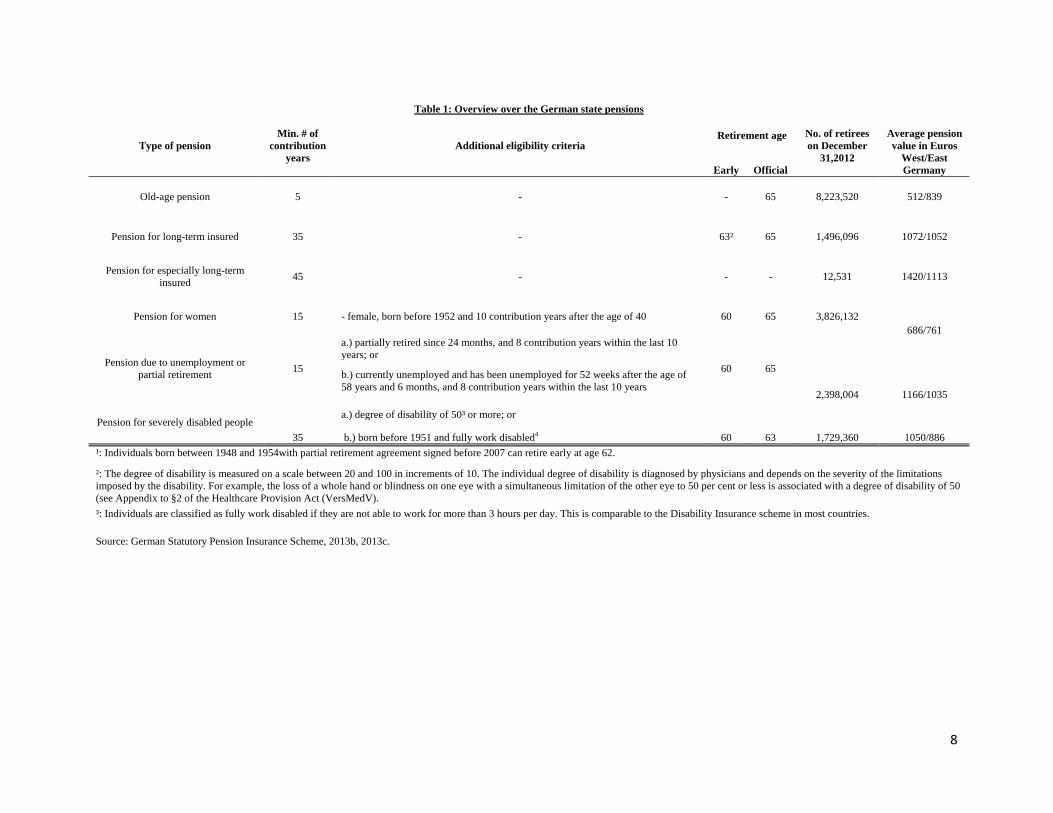
wards different segments of the population, hence the eligibility criteria vary. Table 1 below lists

the eligibility criteria, early and official retirement ages. In addition, the number of retirees on

this plan in 2012 and the average pension value in 2012 for each pension plan are given to indi-

cate the relative importance of the schemes (DRV, 2013b). Since the early 2000s most schemes

underwent major reforms. However, these reforms were implemented with a lag of several years,

and the retirement ages are only increased in small steps (e.g. the official retirement age for the

standard old-age pension is increased by one month per birth year for individuals born after

1947). These reforms introduce only little exogenous variation and affect retirees from 2012 on-

wards. Therefore it is not possible to exploit these reforms for identification, and the analyses

presented in this paper focuses on pre-reform retirement ages.

As can be inferred from Table 1, there are three major age thresholds in the German pension

system – age 60 for the pension for women, the pension due to unemployment and partial retire-

ment and the pension for severely disabled people11, age 63 for the pension for long-term insured

and age 65 for the standard old-age pension and the pension for especially long-term insured.

Table 1 also demonstrates that the thresholds at age 60 and 65 are relatively more important than

the threshold at age 63, since most retirees receive their pension under a plan with retirement age

60 or 65, respectively. For the empirical analysis I will exploit these thresholds in a Regression

Discontinuity Design. However, I exclude the pension for severely disabled people from the

analysis since the behavioral response of disabled people might differ from non-disabled retirees.

11 This should not be confused with Disability Insurance. The pension for severely disabled people is considered as a regular old-age pension, which offers disabled individuals the possibility of early retirement.

8

Table 1: Overview over the German state pensions

Type of pension Min. # of

contribution years

Additional eligibility criteria Retirement age No. of retirees

on December 31,2012

Average pension value in Euros

West/East Germany Early Official

Old-age pension 5 - - 65 8,223,520 512/839

Pension for long-term insured 35 - 63² 65 1,496,096 1072/1052

Pension for especially long-term insured 45 - - - 12,531 1420/1113

Pension for women 15 - female, born before 1952 and 10 contribution years after the age of 40 60 65 3,826,132 686/761

Pension due to unemployment or partial retirement 15

a.) partially retired since 24 months, and 8 contribution years within the last 10 years; or

60 65

2,398,004 1166/1035

b.) currently unemployed and has been unemployed for 52 weeks after the age of 58 years and 6 months, and 8 contribution years within the last 10 years

Pension for severely disabled people 35

a.) degree of disability of 50³ or more; or

60 63 1,729,360 1050/886 b.) born before 1951 and fully work disabled4 ¹: Individuals born between 1948 and 1954with partial retirement agreement signed before 2007 can retire early at age 62.

²: The degree of disability is measured on a scale between 20 and 100 in increments of 10. The individual degree of disability is diagnosed by physicians and depends on the severity of the limitations imposed by the disability. For example, the loss of a whole hand or blindness on one eye with a simultaneous limitation of the other eye to 50 per cent or less is associated with a degree of disability of 50 (see Appendix to §2 of the Healthcare Provision Act (VersMedV). ³: Individuals are classified as fully work disabled if they are not able to work for more than 3 hours per day. This is comparable to the Disability Insurance scheme in most countries.

Source: German Statutory Pension Insurance Scheme, 2013b, 2013c.

9

2.2 Data

The data in this analysis is from the German Socio-Economic Panel Study (SOEP). SOEP is a

representative panel study of private households in Germany. Starting in 1984, individuals are

surveyed annually. The study expanded to include residents of former East Germany in 1990. All

respondents answer about 150 questions per year on a range of topics, e.g. on labor market par-

ticipation, education, family status, attitudes and perceptions, as well as health and health behav-

ior. Moreover, the head of the household fills in a household questionnaire. Since 2000 the study

interviews more than 20,000 individuals across more than 10,000 households. For further details,

see Wagner, Frick and Schupp (2007).

The SOEP includes several measures of individual health. The standard 5-categorical Self-

Assessed Health (SAH) and the 11-categorical health satisfaction measure are surveyed annually

since 1994. In addition, since 2002, the continuous quasi-objective SF12 measure and the objec-

tive grip strength measure are included in every second year. Information on several dimensions

of health behavior is available for different years.

2.2.1 Dependent variables

Health measures

For the empirical analysis I use both the SAH measure as well as the SF12 measure. For the

SAH, respondents are asked how they would describe their current health status on a 5-point

scale. The answers range from “bad” and “poor” to “satisfactory”, “good” and “very good”. For

the analysis, I dichotomize the variable. The outcome “satisfactory health” is defined as “1” for

the best three categories (i.e. the subjective health status is at least satisfactory) and “0” for the

worst two categories.12 As shown in Table 2 below, 81 percent of individuals in the sample re-

port their health to be at least satisfactory (Column 2). The difference between retirees and non-

retirees (Column 7 and 8) is about 6 percentage points and highly significant.

The SF12 consists of two measures for physical health (pcs) and mental health (mcs). For these

measures, respondents answer 12 questions that relate to different dimensions of health, e.g. vi-

12 The dichotomization of the ordinal SAH measure offers an easier interpretation of the marginal effects. However, to ensure that the conclusions are robust to the choice of the cut-off, I estimate all models using the full 5-point scale. Neither direction nor significance of the effect change.

10

tality, bodily pain, or emotional functioning. These questions are then aggregated into 8 sub-

scales, and a specific algorithm13 generates the two dimensions physical and mental health. In

the standard SOEP version, both measures take on continuous values between 0 and 100, with a

mean of 50 and a standard deviation of 10. The advantages of these two measures are, first, that

they are less subjective than the SAH measure, i.e. they eliminate reporting bias (Ziebarth, 2010,

Frick and Ziebarth, 2013). Second, they are based on a broad definition of health. Typical objec-

tive measures (such as grip strength or diagnoses of specific diseases) are based on very narrow

definitions of health, for example they lack a mental health dimension. In contrast, the SF12

combines different dimensions of health (e.g. pain, vitality, functioning) into two comprehensive

indices. As can be inferred from Table 2, retirees have on average worse physical health, but a

higher mental health score.

Health behavior, time use and healthcare utilization

The SOEP offers various measures of health behavior in different years. In this analysis, I use

data on smoking, alcohol consumption, diet and exercise, body weight, sleep and social sup-

port.14 Smoking status is captured by a dummy variable, which takes on the value “1” if an indi-

vidual smokes.15 Alcohol consumption is captured by two dummy variables. In the SOEP, indi-

viduals are asked how often they drink beer, wine and sparkling wine, spirits and mixed drinks.

If a respondent states that s/he never drinks any kind of alcohol, no alcohol consumption takes on

the value “1”. In contrast, if a respondent drinks any kind of alcohol on a regular basis, regular

alcohol consumption is assigned the value “1” (Ziebarth and Grabka, 2009). Data on alcohol

consumption is available for three years.

Concerning their diet, respondents are asked whether they follow a health-conscious diet. The

variable health-conscious diet takes on the value “1” if respondents answer “very much” or

“much” and “0” if they answer “a little” or “not at all”. Individuals are also asked how often they

participate in sports or exercise. If they exercise at least once a week, the variable regular physi-

13 A detailed description of the algorithm is given by Andersen et al. (2007). 14 Strictly speaking, social support is not health behavior. However, since it is potentially an important mechanism and a result of individual choices, I include it in this section of the analysis. 15 While more detailed information on the quantity of tobacco is available, it also involves a larger measurement error. In earlier waves the question conflated cigarettes, cigars and pipes, although the health consequences are like-ly to differ. Moreover, I would expect that changes on the extensive margin have a larger impact on health than changes on the intensive margin.

11

cal activity is assigned a “1”, otherwise the value is “0”. This measure does not take into account

physical activity on the job. The body mass index is calculated from self-reported height and

weight. Respondents also answer how long they typically sleep on a regular week day. Lastly, I

use the reported number of close friends as a proxy for social contacts. If a person experiences a

negative health shock, a high number of close friends implies that there are more people to draw

support from. The sample sizes for each outcome are shown in Table 2.

For the data on time use respondents state how many hours on a typical weekday they spend

on the respective activities. For this paper I focus on repairs and gardening, leisure time activi-

ties, running errands, household chores, education and childcare. Repairs and gardening in-

clude “repairs in and around the house, car, garden work etc.”, i.e. activities that require a physi-

cal effort and concentration and could potentially enhance an individuals’ health. Similarly, run-

ning errands and household chores require an effort and can be regarded as evidence of an active

lifestyle. Leisure time activities are more ambiguous, as they include both physical activities (e.g.

sports) and sedentary activities (e.g. reading). While time spend on education and learning can

have a positive effect on health, retirees have less incentives to invest into their education and

skills. Finally, time spend on childcare can be regarded as an intergenerational time transfer from

grandparents to their middle-aged children. This can enhance (mental) health of the grandpar-

ents.

I also investigate the effects of retirement on healthcare utilization to provide further evidence

for policy makers.16 For this analysis I use two measures of healthcare utilization – (i) whether

an individual was hospitalized in the past year or not, and (ii) the number of doctor visits within

the past three months. Only 11 percent of the sample was admitted to a hospital within the past

year, whereas the mean number of doctor visits is 3.5, albeit with variation between 0 and 99.

16 While, a priori, the causal direction between health and healthcare utilization is not clear, a positive effect on health and a negative effect on healthcare utilization would indicate that individuals need less healthcare due to the positive health shock, since it is highly unlikely that less healthcare leads to better health. The same argument holds for a negative health shock and a positive effect on healthcare. On the other hand, if the effects on health and healthcare have the same sign, the causation is likely to run from healthcare to health, since it is unlikely that worse health leads to lower healthcare utilization and vice versa.

12

2.2.2 Definition of retirement and covariates

Before analyzing the effect of retirement, it is necessary to define the treatment. There are sev-

eral definitions used in the literature (see for example Coe and Zamarro, 2011 and Insler, 2014).

In general, retirement implies that an individual exits the labor market.17 This encompasses also

individuals who are technically unemployed, but are not actively searching for a job. On the oth-

er hand, some retirees might exit their main occupation, but continue to work in another occupa-

tion, e.g. to generate additional income, meet other people or engage in meaningful work. In this

paper I use self-reported retirement status as the treatment variable. I assume that retirement af-

fects health mainly through behavioral adjustments, and that the behavioral adjustment occurs if

an individual regards herself as retired.18

Control variables

I also include additional control variables as a robustness check and to investigate heterogene-

ous effects, e.g. gender, marital status, log of household income, education, retirement status of

the partner and the existence of grandchildren. Education is measured by two dummy variables

for individuals who completed vocational training, and individuals who obtained a university

degree, respectively. The dummy variable for marital status is “1” if the individual is married

and cohabiting and “0” otherwise. Monthly household income is adjusted to the price level of the

year 2000 and equivalized according to the OECD formula.19 The retirement status of the partner

is obtained by matching the self-reported retirement status of spouses to each other.

17 Several studies distinguish between voluntary and involuntary retirement. While there is potentially important heterogeneity, unfortunately there is no information available to differentiate between these two groups. 18 Since the questions on retirement status, pension income and employment status are asked independently, it is possible to check the concurrence of these indicators. For example, the definition of retirement could be based on the receipt of pension benefits. This definition would exclude individuals living off unemployment benefits or sav-ings and not actively looking for work. On the other hand, some pension plans allow recipients to continue working while claiming benefits (e.g. the standard old-age pension). In the sample 92.7% of the self-reported retirees stated to receive an old-age pension. Only 1.5% of the individuals receiving pension benefits do not report themselves to be retired. This indicates that using a definition of retirement based on pensions is not likely to alter the results, since both definitions coincide for most observations. Similarly, only 2.8% of the self-reported retirees stated to work either full- or part-time, while 94.7% report their employment status as “Not working”. 19 The household income is weighted by the number of persons in the household. Children under the age of 14 are assigned a weight of 0.3, and each additional adult receives a weight of 0.5.

13

Occupational strain

I also check for effect heterogeneity with respect to occupational strain. The data on occupa-

tional strain is provided by Kroll (2011). Using data from the Employment Survey of the

FEDERAL INSTITUTE FOR VOCATIONAL EDUCATION AND TRAINING (BIBB/BAuA-

Erwerbstätigenbefragung), separate scales for physical and mental strain are constructed for the

International Standard Classification of Occupations (ISCO88). The scales range from “1” (low

strain) to “10” (high strain). Occupations with maximum physical strain (10) include (e.g.) min-

ers, construction workers and firemen, whereas statisticians and accountants experience only

minimum physical strain (1). Similarly, nurses and stewards are classified as having maximum

mental strain, whereas construction workers have very low mental strain. These scales are

matched to the SOEP data via the 4 digit ISCO88 codes. Using the original scales I generate

three dummy variables: High physical strain is “1” if the average physical occupational strain of

an individual (prior to retirement) is above the 75th percentile of the distribution of physical

strain. Similarly, high mental strain is defined as “1” if the mental occupational strain of an indi-

vidual is above the 75th percentile of the distribution of mental strain. High overall strain is de-

fined as “1” if the combined average strain exceeds the 75th percentile.

2.2.3 Sample selection

For the main analysis (“working sample”) I keep all observations within the 50 to 75 age

range. Respondents who report a disability are dropped from the sample, since their behavioral

response to retirement is likely to differ from non-disabled retirees. Individuals who return to the

labor market (i.e. for which a switch from “retired” to “not retired” is observed) are excluded

from the analysis. This sample includes civil servants and self-employed. While the pension sys-

tem for civil servants is markedly different, the age thresholds are similar to those for employees.

For some self-employed occupations pension insurance in the DRV is mandatory, while all other

self-employed can opt-in. Therefore, it is likely that the age thresholds are also (partly) relevant

for self-employed individuals. Finally, the sample also includes individuals who were not em-

ployed prior to retirement. Retirement still marks a transition for these individuals, since they

finally exit the labor market. Moreover, this group is relatively large and excluding it would re-

sult in a large loss of statistical power.

14

For a robustness check based on eligibility for a state pension, I construct a second sample

(“eligibility sample”). Linked register data on pension eligibility is not available, therefore I cal-

culate a proxy for the individual eligibility age using self-reported information on employment

history, gender, birth cohort, number and year of birth of children, and education. In this sample,

I exclude individuals with a disability, civil servants and individuals, who were not part- or full-

time employed prior to retirement.

Table 2 shows summary statistics for the working sample. Columns 2 to 6 provide the mean,

standard deviation, minimum, maximum and number of observations for the whole sample. Col-

umns 7 and 8 show the means for the treatment and control group (i.e. retirees and non-retirees),

respectively. Column 9 provides the t-statistic for a test for the equality of means between treat-

ment and control group.

15

Table 2: Summary Statistics

Variable Mean SD Min Max N Mean non-retirees Mean retirees t-statistic

A. Health measures

Satisfactory health (3/5 of SAH categories) 0.817 0.387 0 1 99,409 0.842 0.785 22.694

Physical health (SF12) 47.330 9.152 10.526 76.421 38,545 49.294 44.878 48.083

Mental health (SF12) 51.795 9.531 3.533 78.264 38,545 51.122 52.635 -15.485

B. Covariates

Age 60.659 7.036 50 75 99,409 55.805 66.696 -376.017

Male 0.472 0.499 0 1 99,409 0.473 0.472 0.387

Married and cohabiting 0.773 0.419 0 1 99,409 0.808 0.729 29.377

Log of household income (equivalized) 7.382 0.537 3.912 11.125 64,231 7.454 7.292 39.193

University degree 0.238 0.426 0 1 99,409 0.271 0.197 27.608

No formal degree 0.182 0.386 0 1 99,409 0.154 0.217 -25.108

Social activites with friends once a week 0.131 0.337 0 1 99,409 0.121 0.142 -9.665

Participation in communities once a week 0.071 0.257 0 1 99,409 0.065 0.079 -8.729

Partner is retired 0.449 0.497 0 1 76,434 0.226 0.755 -170.227

Existence of grandchildren 0.399 0.490 0 1 99,409 0.281 0.545 -86.730

Average overall strain 5.199 2.685 1 10 63,001 5.193 5.218 -0.980

Average physical strain 5.186 2.689 1 10 63,001 5.163 5.258 -3.803

Average mental strain 5.325 2.683 1 10 63,001 5.355 5.234 4.812

C. Health behavior

Smoking 0.256 0.437 0 1 37,953 0.316 0.181 30.854

Regular alcohol consumption 0.213 0.409 0 1 18,869 0.208 0.218 -1.580

No alcohol consumption 0.115 0.319 0 1 18,869 0.100 0.135 -7.436

Health-conscious diet 0.562 0.496 0 1 32,955 0.524 0.607 -15.182

Regular leisure-time physical activiy 0.337 0.473 0 1 45,408 0.353 0.317 8.109

Sleep duration on week days 7.028 1.194 1 16 35,862 6.862 7.221 -28.334

Body Mass Index (BMI) 26.803 4.285 13.281 75.276 39,587 26.592 27.066 -11.001

Number of close friends 4.461 4.235 0 99 20,741 4.444 4.482 -0.642

D. Time use

Time use: Repairs and gardening 1.177 1.295 0 13 95,122 0.927 1.485 -65.400

Time use: Leisure time activities 2.549 2.146 0 20 96,729 1.988 3.242 -91.449

Time use: Running errands 1.186 0.820 0 12 96,968 1.048 1.358 -59.213

Time use: Household chores 2.039 1.693 0 20 96,741 1.816 2.313 -45.902

Time use: Education 0.144 0.533 0 12 90,930 0.184 0.095 25.953

Time use: Childcare 0.252 1.018 0 24 90,756 0.264 0.238 3.959

E. Healthcare utilization

Hospital stay in the past year 0.119 0.324 0 1 99,163 0.097 0.147 -23.719

Doctor visits in the past three months 3.508 4.007 0 99 72,819 3.338 3.687 -11.738 Source: SOEP v29, own calculations. Notes: Column 1 and 2 give the overall mean and standard deviation of the variable. Column 3 to 5 provide the overall minimum, maximum and the number of observations. Column 6 gives the mean for retirees (treatment group). The means for non-retirees (control group) are given in column 7. Column 8 gives the t-statistic for the equality of means of both groups. Household income is measured in Euros per month and adjusted to the price level of the year 2000. The equivalence income is then calculated using the standard OECD formula. Social activities with friends include time spent helping friends. Participation in communities includes voluntary work, local politics and religious communities. Average strain is derived from the occupational demand scales provided by Kroll (2011) by taking the average of the strain values associated with the jobs held prior to retirement.

16

3 Econometric models

3.1 Endogeneity

Apart from the need to distinguish the effect of retirement on health from the effect of aging, it

is also necessary to resolve the endogeneity problem of retirement status. The literature identifies

three sources of endogeneity – omitted variable bias (OVB), justification bias, and reverse cau-

sality. Omitted variable bias might be induced through differences in unobserved individual

characteristics, which influence both health and the retirement decision, e.g. the genetic makeup

or subjective life expectancy. In order to control for unobserved, time-invariant individual heter-

ogeneity, all models are estimated as individual fixed-effects panel data models.

If non-working (i.e. retired or unemployed) respondents perceive continued employment as the

norm for healthy persons of their age, they might underreport their health status in order to justi-

fy their deviation from the norm. This “justification bias” would downward-bias the results. It is

difficult to address this issue in the absence of objective health measures. However, with regard

to the average retirement age in Germany (63.5 in 2011) it seems questionable whether individu-

als at age 60 would feel the need to justify their retirement status. In addition, the direction of the

bias also implies that the results can be interpreted as a lower bound.

Reverse causality poses a more severe problem. As noted earlier, several studies show that

health affects the retirement decision. Moreover, unexpected health shocks have a larger impact

than a steady decline in health. This means that comparisons of pre-retirement health to post-

retirement health cannot claim a causal interpretation. In order to allow for a causal interpretation

of the analysis, I use Regression Discontinuity Design.

3.2 Regression Discontinuity Design

General idea

The RDD approach exploits institutional rules by which the treatment is assigned. It requires

an assignment variable that (partly) determines whether individuals are treated or not. Individu-

als above a certain threshold receive the treatment, whereas individuals just below the threshold

are not treated. Then, a discontinuity in the outcome variable at the value of the threshold of the

17

assignment variable can be interpreted as a causal effect of the treatment under some mild as-

sumptions (Lee and Lemieux, 2010).

This paper uses age as an assignment for retirement. While in Germany individuals are not

forced into retirement,20 the statutory pension schemes provide strong incentives to retire at cer-

tain ages, i.e. there are thresholds for early and full retirement, and individuals are not eligible for

any pension before the early retirement age.21 However, this implies that treatment is not com-

pletely determined by age; instead, the probability to retire increases rapidly at the thresholds for

early and full retirement. This implies that the analysis is based on a fuzzy regression discontinu-

ity design. The estimated treatment effect is a Local Average Treatment Effect (LATE), i.e. the

effect on the compliers affected by the instrument. In this case, the estimated effect should be

interpreted as the effect on individuals retiring once they exceed the specified age threshold,

which is used as a discontinuity.

Setup

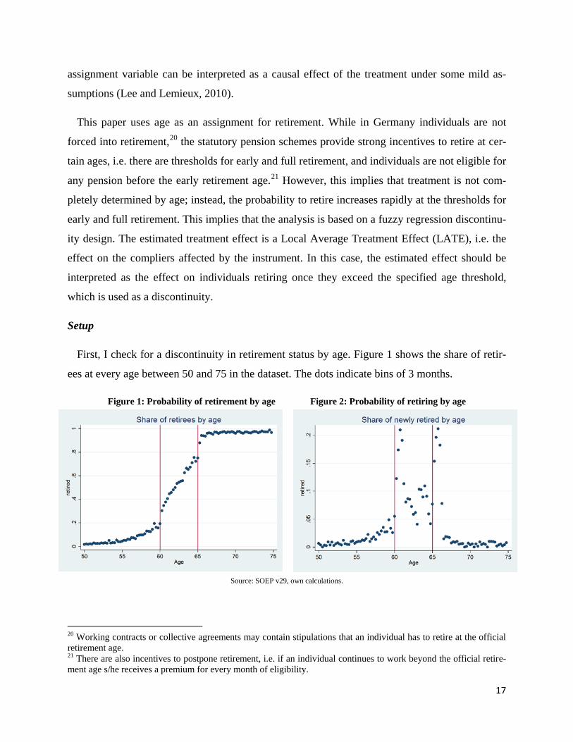
First, I check for a discontinuity in retirement status by age. Figure 1 shows the share of retir-

ees at every age between 50 and 75 in the dataset. The dots indicate bins of 3 months.

Figure 1: Probability of retirement by age Figure 2: Probability of retiring by age

Source: SOEP v29, own calculations.

20 Working contracts or collective agreements may contain stipulations that an individual has to retire at the official retirement age. 21 There are also incentives to postpone retirement, i.e. if an individual continues to work beyond the official retire-ment age s/he receives a premium for every month of eligibility.

18

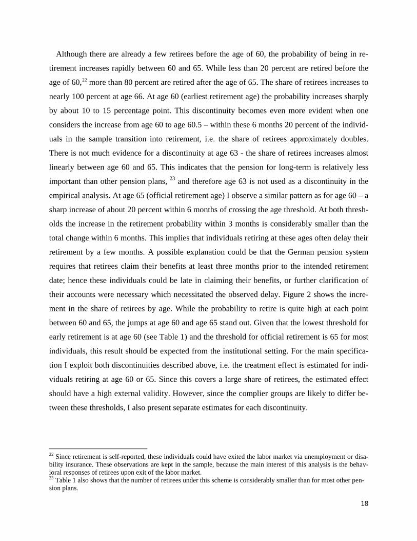
Although there are already a few retirees before the age of 60, the probability of being in re-

tirement increases rapidly between 60 and 65. While less than 20 percent are retired before the

age of 60,22 more than 80 percent are retired after the age of 65. The share of retirees increases to

nearly 100 percent at age 66. At age 60 (earliest retirement age) the probability increases sharply

by about 10 to 15 percentage point. This discontinuity becomes even more evident when one

considers the increase from age 60 to age 60.5 – within these 6 months 20 percent of the individ-

uals in the sample transition into retirement, i.e. the share of retirees approximately doubles.

There is not much evidence for a discontinuity at age 63 - the share of retirees increases almost

linearly between age 60 and 65. This indicates that the pension for long-term is relatively less

important than other pension plans, 23 and therefore age 63 is not used as a discontinuity in the

empirical analysis. At age 65 (official retirement age) I observe a similar pattern as for age 60 – a

sharp increase of about 20 percent within 6 months of crossing the age threshold. At both thresh-

olds the increase in the retirement probability within 3 months is considerably smaller than the

total change within 6 months. This implies that individuals retiring at these ages often delay their

retirement by a few months. A possible explanation could be that the German pension system

requires that retirees claim their benefits at least three months prior to the intended retirement

date; hence these individuals could be late in claiming their benefits, or further clarification of

their accounts were necessary which necessitated the observed delay. Figure 2 shows the incre-

ment in the share of retirees by age. While the probability to retire is quite high at each point

between 60 and 65, the jumps at age 60 and age 65 stand out. Given that the lowest threshold for

early retirement is at age 60 (see Table 1) and the threshold for official retirement is 65 for most

individuals, this result should be expected from the institutional setting. For the main specifica-

tion I exploit both discontinuities described above, i.e. the treatment effect is estimated for indi-

viduals retiring at age 60 or 65. Since this covers a large share of retirees, the estimated effect

should have a high external validity. However, since the complier groups are likely to differ be-

tween these thresholds, I also present separate estimates for each discontinuity.

22 Since retirement is self-reported, these individuals could have exited the labor market via unemployment or disa-bility insurance. These observations are kept in the sample, because the main interest of this analysis is the behav-ioral responses of retirees upon exit of the labor market. 23 Table 1 also shows that the number of retirees under this scheme is considerably smaller than for most other pen-sion plans.

19

Assumptions

There are two main assumptions needed for the validity of RDD. First, I have to assume that

the outcome is a smooth function of the assignment variable. Since aging is a gradual process, it

appears reasonable to assume that the health-age profile of an individual is smooth. Of course,

this further requires that this smooth function is appropriately modeled. Otherwise nonlinearities

in the health-age profile could be mistaken as discontinuities, as demonstrated by Angrist and

Pischke (2009). Second, I need to assume that the assignment variable cannot be precisely con-

trolled near the threshold, i.e. individuals cannot manipulate their age. This assumption holds by

construction, since individuals cannot manipulate their age.24 A common check for this assump-

tion is to investigate the density of the forcing variable (i.e. age). The histogram and the kernel

density estimate of age are shown in Figure 3 below. The binwidth corresponds to three months.

Apart from a seasonal pattern, the density of age appears to be very smooth.

Figure 3: Density of age

Source: SOEP v29, own calculation

I also check for discontinuities in predetermined variables. If there would be discontinuities in

another, predetermined variable, this would cast doubt on the identification strategy since the

results could be driven by an unobserved confounder. Figure 4 below shows the log of household

income, the probability of being married and cohabiting, years of education and the share of

24 The age of an individual is not self-reported but rather calculated from their date of birth. Given that the SOEP is a long-term panel study and that inconsistencies in the data are cleared every year, it appears highly unlikely that individuals would systematically lie about their age. Still, this cannot be excluded in principle.

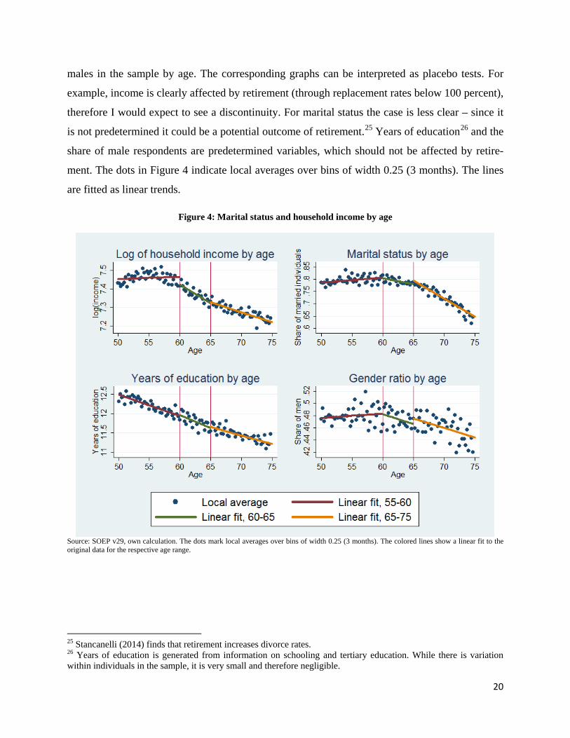
20

males in the sample by age. The corresponding graphs can be interpreted as placebo tests. For

example, income is clearly affected by retirement (through replacement rates below 100 percent),

therefore I would expect to see a discontinuity. For marital status the case is less clear – since it

is not predetermined it could be a potential outcome of retirement.25 Years of education26 and the

share of male respondents are predetermined variables, which should not be affected by retire-

ment. The dots in Figure 4 indicate local averages over bins of width 0.25 (3 months). The lines

are fitted as linear trends.

Figure 4: Marital status and household income by age

Source: SOEP v29, own calculation. The dots mark local averages over bins of width 0.25 (3 months). The colored lines show a linear fit to the original data for the respective age range.

25 Stancanelli (2014) finds that retirement increases divorce rates. 26 Years of education is generated from information on schooling and tertiary education. While there is variation within individuals in the sample, it is very small and therefore negligible.

21

There appears to be a small discontinuity in income at age 60. There are no visible discontinui-

ties for marital status. Years of education decreases linearly with age, i.e. there are no visible

discontinuities. There is strong variation in the gender ratio across bins without an indication of a

discontinuity at the given age thresholds. All in all, the validity of RDD is not threatened by the

covariates. Nevertheless I provide estimates with and without covariates as a robustness check in

section 4.

Choice of the bandwidth

A crucial decision in RDD is the choice of the bandwidth. The bandwidth determines which

observations should be used in the estimation by setting a maximum distance from the disconti-

nuity. Observations outside this range are simply discarded. Adopting a small bandwidth will

minimize the bias, however the variance might be very large due to the small number of observa-

tions (Lee and Lemieux, 2010). In contrast, a larger bandwidth will lead to a smaller variance,

but the bias is potentially large. In line with Moreau and Stancanelli (2013) and Stancanelli and

van Soest (2012) I use a bandwidth of 10 years for the main specification, which leads to an es-

timation sample of age 50 to 75 (10 years before the first discontinuity at age 60 and 10 years

after the last discontinuity at age 65). As a robustness check I provide estimates using a band-

width of 5 years, i.e. an estimation sample of age 55 to 70.27

Graphical evidence

Before I estimate the treatment effect, I investigate the outcome variables graphically in order

to detect possible discontinuities. Figure 5 below shows the health-age profile for all three out-

comes. As before, the dots mark local averages over intervals of width 0.25 (or three months),

while the colored lines are fitted to the original data. According to the graph, physical health de-

creases almost linearly with age. Satisfactory health also decreases with age, however there

seems to be a small increase between age 60 and 65, after which it decreases again. The relation-

ship between mental health and age is highly nonlinear. The mental health summary score in-

creases with age until approximately 70, and then decreases slightly. From the graphical inspec-

tion it appears that there are positive discontinuities in satisfactory and mental health at age 60,

and a positive discontinuity at age 65 for mental health. This could indicate (i) that the effect of

27 This bandwidth is close to the optimal bandwidth following Imbens and Kalyamaran (2009).

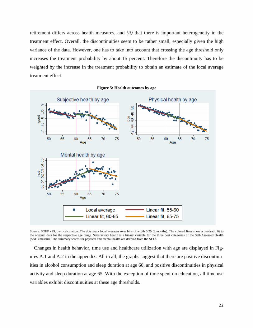
22

retirement differs across health measures, and (ii) that there is important heterogeneity in the

treatment effect. Overall, the discontinuities seem to be rather small, especially given the high

variance of the data. However, one has to take into account that crossing the age threshold only

increases the treatment probability by about 15 percent. Therefore the discontinuity has to be

weighted by the increase in the treatment probability to obtain an estimate of the local average

treatment effect.

Figure 5: Health outcomes by age

Source: SOEP v29, own calculation. The dots mark local averages over bins of width 0.25 (3 months). The colored lines show a quadratic fit to the original data for the respective age range. Satisfactory health is a binary variable for the three best categories of the Self-Assessed Health (SAH) measure. The summary scores for physical and mental health are derived from the SF12.

Changes in health behavior, time use and healthcare utilization with age are displayed in Fig-

ures A.1 and A.2 in the appendix. All in all, the graphs suggest that there are positive discontinu-

ities in alcohol consumption and sleep duration at age 60, and positive discontinuities in physical

activity and sleep duration at age 65. With the exception of time spent on education, all time use

variables exhibit discontinuities at these age thresholds.

23

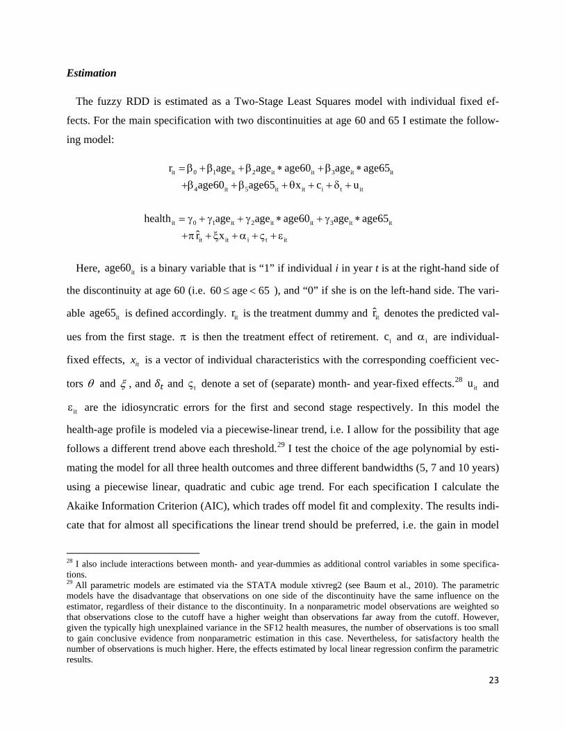
Estimation

The fuzzy RDD is estimated as a Two-Stage Least Squares model with individual fixed ef-

fects. For the main specification with two discontinuities at age 60 and 65 I estimate the follow-

ing model:

it 0 1 it 2 it it 3 it it

4 it 5 it it i t it

it 0 1 it 2 it it 3 it it

it it i t it

r age age age60 age age65age60 age65 x c u

health age age age60 age age65r̂ x

= β +β +β ∗ +β ∗+β +β + θ + + δ +

= g + g + g ∗ + g ∗+π + x +a + ς + e

Here, itage60 is a binary variable that is “1” if individual i in year t is at the right-hand side of

the discontinuity at age 60 (i.e. 60 age 65≤ < ), and “0” if she is on the left-hand side. The vari-

able itage65 is defined accordingly. itr is the treatment dummy and itr̂ denotes the predicted val-

ues from the first stage. π is then the treatment effect of retirement. ic and ia are individual-

fixed effects, itx is a vector of individual characteristics with the corresponding coefficient vec-

tors θ and x , and 𝛿𝑡 and tς denote a set of (separate) month- and year-fixed effects.28 itu and

ite are the idiosyncratic errors for the first and second stage respectively. In this model the

health-age profile is modeled via a piecewise-linear trend, i.e. I allow for the possibility that age

follows a different trend above each threshold.29 I test the choice of the age polynomial by esti-

mating the model for all three health outcomes and three different bandwidths (5, 7 and 10 years)

using a piecewise linear, quadratic and cubic age trend. For each specification I calculate the

Akaike Information Criterion (AIC), which trades off model fit and complexity. The results indi-

cate that for almost all specifications the linear trend should be preferred, i.e. the gain in model

28 I also include interactions between month- and year-dummies as additional control variables in some specifica-tions. 29 All parametric models are estimated via the STATA module xtivreg2 (see Baum et al., 2010). The parametric models have the disadvantage that observations on one side of the discontinuity have the same influence on the estimator, regardless of their distance to the discontinuity. In a nonparametric model observations are weighted so that observations close to the cutoff have a higher weight than observations far away from the cutoff. However, given the typically high unexplained variance in the SF12 health measures, the number of observations is too small to gain conclusive evidence from nonparametric estimation in this case. Nevertheless, for satisfactory health the number of observations is much higher. Here, the effects estimated by local linear regression confirm the parametric results.

24

fit does not compensate for the higher complexity of the model. Nevertheless, in a robustness

check I estimate the model using a piecewise quadratic age trend.

4 Results

4.1 Results from OLS

In a first step I estimate the correlation between retirement and health using simple Ordinary

Least Squares and Fixed-effects models. The results from these models cannot be interpreted as

causal effects, since they do not address reverse causality. However, since I would suspect a neg-

ative bias from reverse causality (negative health shocks force an individual to retire), the results

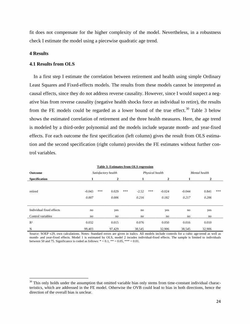
from the FE models could be regarded as a lower bound of the true effect.30 Table 3 below

shows the estimated correlation of retirement and the three health measures. Here, the age trend

is modeled by a third-order polynomial and the models include separate month- and year-fixed

effects. For each outcome the first specification (left column) gives the result from OLS estima-

tion and the second specification (right column) provides the FE estimates without further con-

trol variables.

Table 3: Estimates from OLS regression

Outcome Satisfactory health Physical health Mental health

Specification 1 2 1 2 1 2

retired -0.043 *** 0.029 *** -2.52 *** -0.024

-0.044

0.841 ***

0.007

0.006

0.216

0.182

0.217

0.206

Individual fixed effects no yes no yes no yes

Control variables no

no

no

no

no

no

R² 0.032 0.015 0.076 0.050 0.016 0.010

N 99,403 97,429 38,545 32,906 38,545 32,906 Source: SOEP v29, own calculations. Notes: Standard errors are given in italics. All models include controls for a cubic age-trend as well as month- and year-fixed effects. Model 1 is estimated by OLS, model 2 incudes individual-fixed effects. The sample is limited to individuals between 50 and 75. Significance is coded as follows: * = 0.1, ** = 0.05, *** = 0.01.

30 This only holds under the assumption that omitted variable bias only stems from time-constant individual charac-teristics, which are addressed in the FE model. Otherwise the OVB could lead to bias in both directions, hence the direction of the overall bias is unclear.

25

The results show that the correlations estimated via OLS are large and negative for satisfactory

and physical health, i.e. retirees have on average worse physical health and a lower probability

to rate their current health as at least satisfactory than non-retirees of the same age. The correla-

tion of retirement and mental health is insignificant in the OLS specification. However, once I

account for time-invariant unobserved heterogeneity (e.g. genetic makeup) in the Fixed-Effects

specifications, the correlations are insignificant (physical health) or even positive (subjective and

mental health).

4.2 Results from Regression Discontinuity design

Table 4 shows the estimated effects for all three outcomes and discontinuities. All specifica-

tions include a piecewise linear age trend, individual- and separate month- and year-fixed effects.

The first specification (Columns 1, 3 and 5) gives the effect for pure RDD, i.e. without further

control variables. The second specification (Columns 2, 4 and 6) includes additional controls for

marital status, education as well as month-year interaction effects. First, the Kleibergen-Paap

Wald F-statistics for weak instruments are well above the rule-of-thumb value of 10 and suggest

that the discontinuities are jointly significant as predictors of retirement status. The point esti-

mates (omitted for space limitations) indicate that conditional on age the retirement probability

increases by about 14 percentage points if an individual is slightly above the threshold at age 60.

Similarly, crossing the threshold at age 65 increases the retirement probability by about 14 per-

centage points.

Table 4: Multiple Regression Discontinuity estimates at age 60 and 65

Satisfactory health Physical health Mental health

Specification 1 2 1 2 1 2

retired 0.128 *** 0.128 *** 1.033

1.057 * 2.949 *** 2.906 ***

0.023

0.023

0.630

0.628

0.716

0.714

Change in standard devia-tions 0.331 0.331 0.113 0.115 0.309 0.305

N 97,429

97,429

32,906

32,906

32,906

32,906

Kleibergen-Paap Wald F 823.173

836.463

442.245

445.841

442.245

445.841

Additional controls no yes no yes no yes Source: SOEP v29, own calculations. Notes: Standard errors are given in italics. All standard errors are clustered on the individual-level. All models include a piecewise linear age trend, individual-fixed effects and separate dummy variables for month and year of the interview. Specifi-cation 2 includes control variables for marital status, education and month-year interaction effects. The sample includes all observations from age 50 to 75. Significance is coded as follows: * = 0.1, ** = 0.05, *** = 0.01.

26

The estimated treatment effects in Table 4 show that retirement has a strong positive impact on

satisfactory and mental health. The effect on mental health is especially large, resulting in a

change of about half a standard deviation. The effect on satisfactory health is smaller (about 0.3

standard deviations), but highly significant. The estimated coefficient for physical health is posi-

tive (about 0.1 standard deviations), but only marginally significant once control variables are

included. All in all, the results indicate that there is a positive causal effect of retirement on

health. Moreover, the results suggest that the effect on mental health is more profound than on

physical health. These findings are in line with, for example, the findings of Blake and Garrouste

(2012) for French retirees and Johnston and Lee (2009) for the UK.

The estimated effects cover individuals retiring either at the early and official retirement age

for both men and women. Hence, the findings presented above should be valid for the majority

of retirees in Germany. However, this joint estimation might also conceal important heterogenei-

ty across complier groups. Therefore I estimate the model using only one discontinuity and the

corresponding sub-sample. In particular, I estimate the effect (a) for women retiring at age 60

(with the sample including all women aged 50 to 70); and (b) for men at age 65 (sample aged 55

to 75). The results are given in Table 5. Panel A shows the effects for all three health outcomes

on women at age 60. The effects on satisfactory and mental health are small and insignificant,

whereas the effect on physical health is smaller than in table 4, but marginally significant. This

indicates that the estimated effects in Table 4 are not identified by women retiring at age 60, with

the exception of physical health. Panel B gives the result for men retiring at age 65. Here, the

results show an improvement in satisfactory health that is slightly larger than the joint effect in

Table 4. Similarly, the effect on mental health is positive and highly significant, whereas the ef-

fect on physical health is small and insignificant. All in all, this suggests that the overall effects

reported in Table 4 are mostly identified by men, which might be due to the higher labor market

participation compared to women.

27

Table 5: Single Regression Discontinuity estimates

Satisfactory health Physical health Mental health

Specification 1 2 1 2 1 2

A. Women at age 60

retired 0.015 0.020 1.507 ** 1.449 * -0.630

-0.657

0.029

0.029

0.758

0.767

0.868

0.872

N 43,951

43,951

14,516

14,516

14,516

14,516

Kleibergen-Paap Wald F 793.422

781.695

792.328

779.910

792.328

779.910

B. Men at age 65

retired 0.150 *** 0.147 *** 0.043

0.140

7.487 *** 7.374 ***

0.027

0.027

0.881

0.876

0.991

0.986

N 34,242

34,242

11,650

11,650

11,650

11,650

Kleibergen-Paap Wald F 1,542.393

1,539.053

0.296

0.295

705.782

697.969

Additional controls no yes no yes no yes

Source: SOEP v29, own calculations. Notes: Standard errors are given in italics. All standard errors are clustered on the individual-level. All models include a piecewise linear age trend, individual-fixed effects and separate dummy variables for month and year of the interview. Specifi-cation 2 includes control variables for marital status, education and month-year interaction effects. The bandwidth for each sample is 10 years. Significance is coded as follows: * = 0.1, ** = 0.05, *** = 0.01.

I also estimate the models using two-year leads of health as outcomes in order to investigate

the long-run effects of retirement. The results in Table 6 suggest that after two years the effects

on self-reported health and mental health are still large and significant. Therefore, I conclude that

retirement has positive long-run effect on self-rated and mental health. Before I explore hetero-

geneity and potential mechanisms of the treatment effects, I present some additional robustness

checks for the main results.

28

Table 6: Long-term effects - Multiple Regression Discontinuity estimates

Satisfactory health in two years Physical health in two years Mental health in two years

Specification 1 2 1 2 1 2

retired 0.090 *** 0.089 *** 0.659

0.614

2.629 *** 2.661 ***

0.028

0.028

0.675

0.674

0.780

0.780

Change in standard devia-tions 0.233 0.230 0.072 0.067 0.276 0.279

N 65,709

65,709

26,290

26,290

26,290

26,290

Kleibergen-Paap Wald F 503.295

510.450

356.594

359.000

356.594

359.000

Additional controls no yes no yes no yes Source: SOEP v29, own calculations. Notes: Standard errors are given in italics. All standard errors are clustered on the individual-level. All models include a piecewise linear age trend, individual-fixed effects and separate dummy variables for month and year of the interview. Specifi-cation 2 includes control variables for marital status and education. The sample includes all observations from age 50 to 75. Significance is coded as follows: * = 0.1, ** = 0.05, *** = 0.01.

4.3 Robustness

The robustness of the estimated effects with respect to the inclusion of covariates is shown in

Table 4 above. Furthermore, I investigate the robustness to the choice of the bandwidth, the spec-

ification of the age trend and the specification of the assignment variable.31

Bandwidth choice

The bandwidth choice is crucial in RDD, since there is a trade-off between bias and variance.

Therefore, I estimate the model described in section 3.2 using a bandwidth of five years, i.e. the

sample is restricted to observations between age 55 and age 70. The results are provided in Table

A.3 in the appendix. The estimated effect on satisfactory health is only slightly smaller. The ef-

fects on physical and mental health are considerably smaller (about 0.05 and 0.15 standard devia-

tions, respectively) and insignificant. This suggests the presence of an upward-bias in the origi-

nal results, which could be due to the nonlinear relationship between mental health and age.

31 As noted before, I also investigate the robustness of the results for satisfactory health to a different variable speci-fication. I estimate all models using the full five-point SAH measure. While the magnitude of the effects is not com-parable, the direction and significance remain the same.

29

Quadratic age trends

Similarly, in parametric models the validity of RDD depends on the correct specification of the

trend in the assignment variable. If the chosen polynomial is too restrictive, nonlinearities in the

assignment variable can be mistaken for discontinuities. On the other hand, a flexible higher-

order polynomial reduces the statistical power of the model. Therefore, I estimate models using a

piecewise quadratic age trend (i.e. a quadratic age trend interacted with all discontinuities). Table

A.4 in the appendix presents the results. The estimated coefficient for satisfactory health is

slightly smaller than the original estimate (0.27 standard deviations), but highly significant. The

effect on physical health is about the same magnitude as in Table 4 (0.1 standard deviations) and

marginally significant in both specifications. The effect on mental health decreases to 0.24

standard deviations, but remains significant.

Specification of the assignment variable

One might argue that age is not the correct assignment variable, since the probability to retire

depends on the individual eligibility age, and not on age itself. For example, for an employed

man it should not matter whether he is above or below the age threshold of 60, since he is eligi-

ble neither for a pension for women, nor for a pension due to unemployment. In this framework,

the assignment variable would be calculated as the difference between an individual’s age and

the earliest age at which s/he is eligible for a state pension. I also run a RDD based on the time to

eligibility as a robustness check using the “eligibility sample” described in section 2. All in all,

the results (shown in Table A.5 in the appendix) confirm the finding of a positive effect of re-

tirement on health. The effect on satisfactory health is positive and significant. The effect on

physical health is large and negative, but very imprecisely estimated. In contrast, the effect on

mental health is large (about 1.5 standard deviations) and highly significant.

In the next two sections I investigate heterogeneity and potential mechanisms of the treatment

effect using RDD with age as the assignment variable and a bandwidth of 10 years.

30

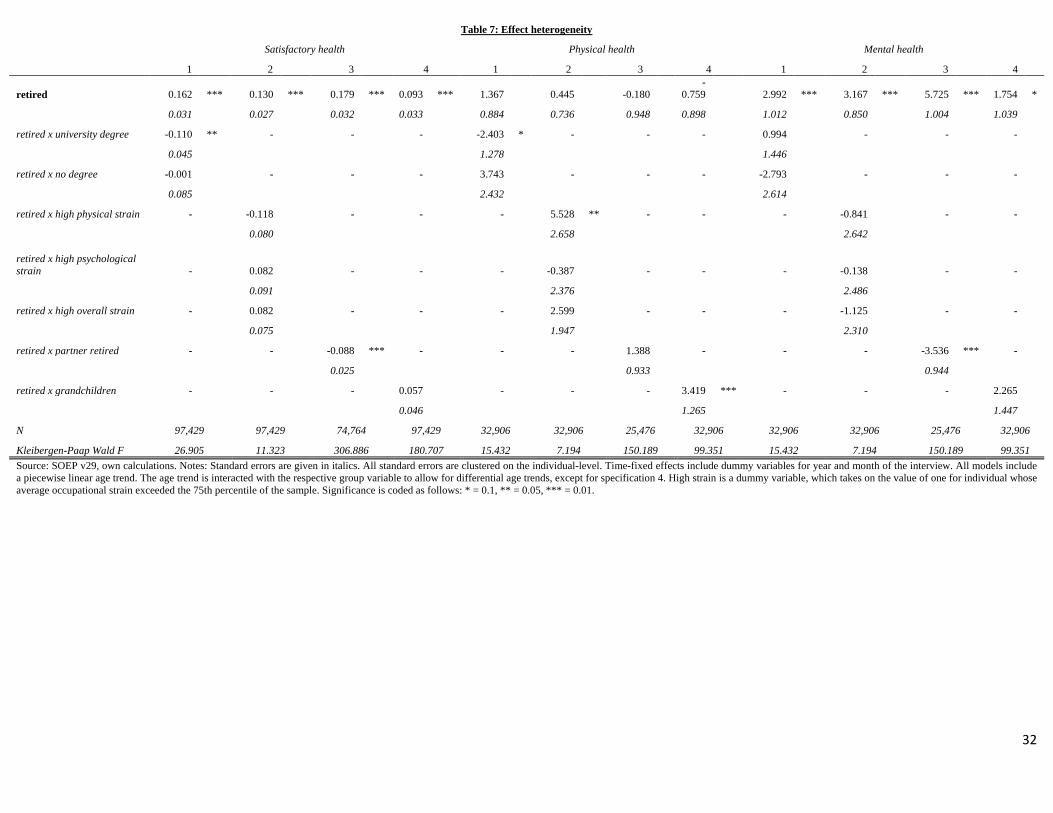
4.4 Effect heterogeneity

I investigate whether the estimated effects differ according to education, occupational demands

or family characteristics. On the one hand, individuals retiring from strenuous jobs might experi-

ence different effects than individuals retiring from sedentary jobs, since retirement relieves

them from work-related strain. Education is an important determinant of occupational choice,

hence occupational heterogeneity might also be reflected in heterogeneity with respect to educa-

tion. On the other hand, the above mentioned characteristics might influence the behavioral re-

sponse of retiring individuals. For example, individuals in physically straining occupations might

experience a reduction in overall physical activity upon retirement due to the loss of work-related

activity. Higher educated individuals might invest more in their health due to the lower oppor-

tunity costs. Hence, heterogeneous treatment effect might also reflect the underlying mecha-

nisms. I estimate the models separately for each subgroup by interacting all independent varia-

bles with the group dummies.32 The results for all health outcomes are shown in Table 7.

The first row shows the treatment effect for the reference group (individuals with vocational

training, from sedentary occupations, without a retired partner and without grandchildren, re-

spectively). Each column gives the result for a separate regression. There is effect heterogeneity

with respect to education, i.e. individuals with a university degree experience a significantly

smaller effect on satisfactory health. This is likely due to different occupations, e.g. academics

have a higher job satisfaction and might therefore dislike retirement. There is little evidence for

heterogeneity with respect to occupational demands. Individuals retiring from physically de-

manding jobs experience a large and positive effect on physical health, which suggests that their

health improves as a consequence of relief from work-related strain. On the other hand, individu- 32 This allows for the possibility of differential age-trends, while at the same time delivering standard errors for the group differences. However, I restrict the time-shocks to be the same across groups. The instruments (i.e. the dum-mies for the discontinuities) were also interacted with the group dummies to derive additional instruments. This is only valid if the group variables are assumed to be exogenous with respect to health for the according age range. In the case of gender and education, this assumption appears reasonable. In the case of occupational demand, it might be the case that individuals with a declining health status switch to less demanding occupations prior to retirement. However, given that employment perspectives are declining with age, this might not happen very often. Moreover, by calculating the average occupational strain for all years prior to retirement, the bias should be minimized. Lastly, retirement status of the partner cannot be expected to be exogenous. If an individual suffers a negative health shock and is forced to retire, it can be expected that the partner is also more likely to retire (e.g. in order to provide care and assistance (Marcus, 2013)). Therefore I additionally instrument the retirement status of the partner by a dummy variable indicating whether the partner is above the early retirement threshold at age 60 or not. This additional in-strument is then interacted with the dummy variables for the three discontinuities. Furthermore, in this case I restrict the age-trend to be the same across groups, since the group variable is not exogenous.

31

als retiring from physically or mentally straining occupations experience no significant mental

health improvements. It should be noted that the Wald F-statistic is very small in this case, i.e.

the instruments are weak (due to the small group size in the fully interacted model) and the ef-

fects are imprecisely estimated. Individuals whose partner is also retired benefit less with respect

to their self-reported health status and their mental health. This could suggest that the increase in

the time spent together leads to more conflicts, which deteriorate their mental health. Lastly, re-

tirees with grandchildren experience an improvement in physical health. This could indicate that

providing childcare for their grandchildren leads to an increase in physical activity.

32

Table 7: Effect heterogeneity

Satisfactory health Physical health Mental health

1 2 3 4 1 2 3 4 1 2 3 4

retired 0.162 *** 0.130 *** 0.179 *** 0.093 *** 1.367 0.445 -0.180 -

0.759 2.992 *** 3.167 *** 5.725 *** 1.754 *

0.031

0.027

0.032

0.033

0.884

0.736

0.948

0.898

1.012

0.850

1.004

1.039

retired x university degree -0.110 ** -

-

-

-2.403 * -

-

-

0.994

-

-

-

0.045

1.278

1.446

retired x no degree -0.001

-

-

-

3.743

-

-

-

-2.793

-

-

-

0.085

2.432

2.614

retired x high physical strain -

-0.118

-

-

-

5.528 ** -

-

-

-0.841

-

-

0.080

2.658

2.642

retired x high psychological strain -

0.082

-

-

-

-0.387

-

-

-

-0.138

-

-

0.091

2.376

2.486

retired x high overall strain -

0.082

-

-

-

2.599

-

-

-

-1.125

-

-

0.075

1.947

2.310

retired x partner retired -

-

-0.088 *** -

-

-

1.388

-

-

-

-3.536 *** -

0.025

0.933

0.944

retired x grandchildren -

-

-

0.057

-

-

-

3.419 *** -

-

-

2.265

0.046

1.265

1.447

N 97,429 97,429 74,764 97,429 32,906 32,906 25,476 32,906 32,906 32,906 25,476 32,906

Kleibergen-Paap Wald F 26.905 11.323 306.886 180.707 15.432 7.194 150.189 99.351 15.432 7.194 150.189 99.351 Source: SOEP v29, own calculations. Notes: Standard errors are given in italics. All standard errors are clustered on the individual-level. Time-fixed effects include dummy variables for year and month of the interview. All models include a piecewise linear age trend. The age trend is interacted with the respective group variable to allow for differential age trends, except for specification 4. High strain is a dummy variable, which takes on the value of one for individual whose average occupational strain exceeded the 75th percentile of the sample. Significance is coded as follows: * = 0.1, ** = 0.05, *** = 0.01.

33

4.5 Mechanisms

Health behavior

The investigation of effect heterogeneity suggests that one mechanism of the effect of retire-

ment is indeed the relief from occupational strain. However, behavioral adjustment might also

contribute to the increase in health. Therefore I estimate the model using various measures of

health behavior as outcome variables. In particular, I look at alcohol and tobacco consumption,

diet and exercise, sleep and social contacts. The results are shown in Table 8 below.

The effect on smoking is negative and significant, which is in line with the results reported by

Insler (2014). There is some evidence for a change in alcohol consumption – retirement seems to

decrease the probability to abstain from alcohol by about 12 percentage points. While alcohol is

usually associated with negative health effects, the variable does not measure the quantity of

alcohol consumed. Hence, if retirees consume small or moderate quantities of alcohol, this

should not affect their health negatively. In addition, Ziebarth and Grabka (2009) document that

(moderate) alcohol consumption is positively correlated with health. The results also suggest that

there is a sizable increase in the probability to regularly participate in leisure-time physical activ-

ity. Since many forms of physical activity require a time investment, this is in line with the ex-

pectations derived from economic theory. There seems to be no effect on body mass. The results

also show that the sleep duration on a week day increases upon retirement. The effect of about

0.8 hours (0.6 standard deviations) is very large, and seems to explain the increase in self-

reported and mental health. Retirement also seems to increase social support – the number of

close friends increases by about 1.3, which suggests that retirees spend part of their time socializ-

ing.

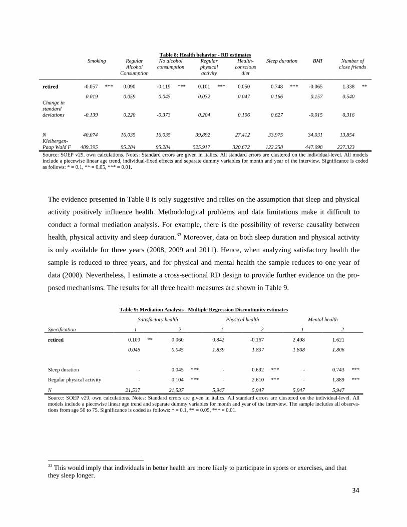
34

Table 8: Health behavior - RD estimates

Smoking Regular Alcohol

Consumption

No alcohol consumption

Regular physical activity

Health-conscious

diet

Sleep duration BMI Number of close friends

retired -0.057 *** 0.090 -0.119 *** 0.101 *** 0.050 0.748 *** -0.065

1.338 **

0.019

0.059

0.045

0.032

0.047

0.166

0.157

0.540

Change in standard deviations -0.139

0.220

-0.373

0.204

0.106

0.627

-0.015

0.316

N 40,074

16,035

16,035

39,892

27,412

33,975

34,031

13,854

Kleibergen-Paap Wald F 489.395

95.284

95.284

525.917

320.672

122.258

447.098

227.323

Source: SOEP v29, own calculations. Notes: Standard errors are given in italics. All standard errors are clustered on the individual-level. All models include a piecewise linear age trend, individual-fixed effects and separate dummy variables for month and year of the interview. Significance is coded as follows: * = 0.1, ** = 0.05, *** = 0.01.

The evidence presented in Table 8 is only suggestive and relies on the assumption that sleep and physical

activity positively influence health. Methodological problems and data limitations make it difficult to

conduct a formal mediation analysis. For example, there is the possibility of reverse causality between

health, physical activity and sleep duration.33 Moreover, data on both sleep duration and physical activity

is only available for three years (2008, 2009 and 2011). Hence, when analyzing satisfactory health the

sample is reduced to three years, and for physical and mental health the sample reduces to one year of

data (2008). Nevertheless, I estimate a cross-sectional RD design to provide further evidence on the pro-

posed mechanisms. The results for all three health measures are shown in Table 9.

Table 9: Mediation Analysis - Multiple Regression Discontinuity estimates

Satisfactory health Physical health Mental health

Specification 1 2 1 2 1 2

retired 0.109 ** 0.060 0.842

-0.167

2.498

1.621

0.046

0.045

1.839

1.837

1.808

1.806

Sleep duration -

0.045 *** -

0.692 *** -

0.743 ***

Regular physical activity -

0.104 *** -

2.610 *** -

1.889 ***

N 21,537

21,537

5,947

5,947

5,947

5,947 Source: SOEP v29, own calculations. Notes: Standard errors are given in italics. All standard errors are clustered on the individual-level. All

models include a piecewise linear age trend and separate dummy variables for month and year of the interview. The sample includes all observa-tions from age 50 to 75. Significance is coded as follows: * = 0.1, ** = 0.05, *** = 0.01.

33 This would imply that individuals in better health are more likely to participate in sports or exercises, and that they sleep longer.

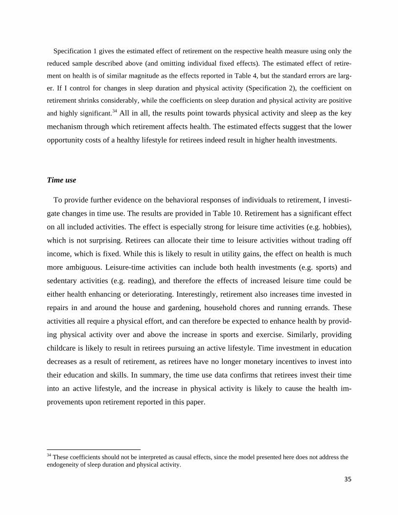
35

Specification 1 gives the estimated effect of retirement on the respective health measure using only the

reduced sample described above (and omitting individual fixed effects). The estimated effect of retire-

ment on health is of similar magnitude as the effects reported in Table 4, but the standard errors are larg-

er. If I control for changes in sleep duration and physical activity (Specification 2), the coefficient on

retirement shrinks considerably, while the coefficients on sleep duration and physical activity are positive

and highly significant.34 All in all, the results point towards physical activity and sleep as the key

mechanism through which retirement affects health. The estimated effects suggest that the lower

opportunity costs of a healthy lifestyle for retirees indeed result in higher health investments.

Time use

To provide further evidence on the behavioral responses of individuals to retirement, I investi-

gate changes in time use. The results are provided in Table 10. Retirement has a significant effect

on all included activities. The effect is especially strong for leisure time activities (e.g. hobbies),

which is not surprising. Retirees can allocate their time to leisure activities without trading off

income, which is fixed. While this is likely to result in utility gains, the effect on health is much

more ambiguous. Leisure-time activities can include both health investments (e.g. sports) and

sedentary activities (e.g. reading), and therefore the effects of increased leisure time could be

either health enhancing or deteriorating. Interestingly, retirement also increases time invested in

repairs in and around the house and gardening, household chores and running errands. These

activities all require a physical effort, and can therefore be expected to enhance health by provid-

ing physical activity over and above the increase in sports and exercise. Similarly, providing

childcare is likely to result in retirees pursuing an active lifestyle. Time investment in education

decreases as a result of retirement, as retirees have no longer monetary incentives to invest into

their education and skills. In summary, the time use data confirms that retirees invest their time

into an active lifestyle, and the increase in physical activity is likely to cause the health im-

provements upon retirement reported in this paper.

34 These coefficients should not be interpreted as causal effects, since the model presented here does not address the endogeneity of sleep duration and physical activity.

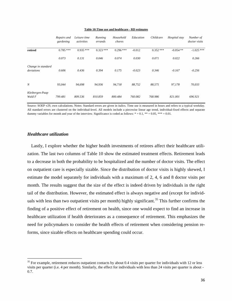
36

Table 10:Time use and healthcare - RD estimates

Repairs and gardening

Leisure time activities

Running errands

Household chores

Education Childcare Hospital stay Number of doctor visits

retired 0.785 *** 0.935 *** 0.323 *** 0.296 *** -0.012 0.352 *** -0.054 ** -1.025 ***

0.073

0.131

0.046

0.074

0.030

0.071

0.022

0.266

Change in standard deviations 0.606

0.436

0.394

0.175

-0.023

0.346

-0.167

-0.256

N 93,044

94,698

94,936

94,718

88,752

88,575

97,178

70,033

Kleibergen-Paap Wald F 799.481

809.536

810.859

800.484

760.082

768.986

821.001

696.921

Source: SOEP v29, own calculations. Notes: Standard errors are given in italics. Time use is measured in hours and refers to a typical weekday. All standard errors are clustered on the individual-level. All models include a piecewise linear age trend, individual-fixed effects and separate dummy variables for month and year of the interview. Significance is coded as follows: * = 0.1, ** = 0.05, *** = 0.01.

Healthcare utilization

Lastly, I explore whether the higher health investments of retirees affect their healthcare utili-

zation. The last two columns of Table 10 show the estimated treatment effects. Retirement leads

to a decrease in both the probability to be hospitalized and the number of doctor visits. The effect

on outpatient care is especially sizable. Since the distribution of doctor visits is highly skewed, I

estimate the model separately for individuals with a maximum of 2, 4, 6 and 8 doctor visits per

month. The results suggest that the size of the effect is indeed driven by individuals in the right

tail of the distribution. However, the estimated effect is always negative and (except for individ-

uals with less than two outpatient visits per month) highly significant.35 This further confirms the

finding of a positive effect of retirement on health, since one would expect to find an increase in

healthcare utilization if health deteriorates as a consequence of retirement. This emphasizes the

need for policymakers to consider the health effects of retirement when considering pension re-

forms, since sizable effects on healthcare spending could occur.

35 For example, retirement reduces outpatient contacts by about 0.4 visits per quarter for individuals with 12 or less visits per quarter (i.e. 4 per month). Similarly, the effect for individuals with less than 24 visits per quarter is about -0.7.

37

5 Conclusion

This paper estimates the causal effect of retirement on health, health behavior and healthcare

utilization using a Regression Discontinuity Design with multiple discontinuities that are caused

by incentives in the German pension systems. The results indicate that retirement has a positive

effect on health. The probability to report a health status of satisfactory or better increases by

about 12 percentage points, while mental health improves by 0.3 standard deviations. These

RDD results are robust to the inclusion of control variables, the choice of the bandwidth, the age

trend and an alternative specification. Most importantly, these effects are not transitory. Even 3

years after retirement significant health improvements can be confirmed.

Furthermore, there is significant heterogeneity across socio-economic groups. Highly educated

individuals benefit less from an improvement of their self-reported health, and individuals retir-

ing from physically strenuous occupations report a significant improvement in their physical

health. The investigation of health behavior shows that retirement leads to an increase in alcohol

consumption, physical activity and sleep duration, as well as a reduction in smoking.

Overall, the findings of this paper suggest three important mechanisms through which retire-

ment affects health. First, retirement relieves employees from work-related stress and strain.

Employees from physically straining occupations benefit especially from a recovery of their

physical health, whereas the majority of workers experience an improvement in self-rated and

mental health. Second, retirees increase their sleep duration on weekdays. Given that non-retirees

sleep on average less than 7 hours per workday, an increase by 45 minutes per day is likely to

enhance their self-reported and mental health. Third, and finally, retirees use their additional

leisure-time to pursue a more active lifestyle by investing more time into daily activities requir-

ing a physical effort, and by exercising more frequently.

Most importantly, the findings of this paper imply that the positive health effect of retirement

leads to reductions in healthcare costs. Therefore, increasing the official retirement age as a cost

containment measure in the pension system is likely to increase costs in the healthcare systems,

since older employees face higher opportunity costs to maintain their health status through health

investments. This underlines the importance for policymakers to consider the externalities of

retirement policies for population health.

38

References

Andersen, H. H., Mühlbacher, A., Nübling, M., Schupp, J., and Wagner, G. G., 2007. Computa-tion of standard values for physical and mental health scale scores using the SOEP ver-sion of SF12v2. Journal of Applied Social Science Studies (Schmollers Jahrbuch), 127(1), 171-182.

Angrist, J. and Pischke, S., 2009. Mostly Harmless Econometrics, Princeton University Press, Princeton and Oxford.

Baum, C.F., Schaffer, M.E. and Stillman, S., 2010. ivreg2: Stata module for extended instrumen-tal variables/2SLS, GMM and AC/HAC, LIML and k-class regression. Available online via http://ideas.repec.org/c/boc/bocode/s425401.html, last accessed December 30, 2013.

Behncke, S., 2012. Does retirement trigger ill health?, Health Economics, 21, 282-300.

Bingley, P. and Martinello, A., 2013. Mental retirement and schooling, European Economic Re-view, 63, 292-298.

Blake, H. and Garrouste, C., 2012. Collateral effects of a pension reform in France, Health, Econometrics and Data Group (HEDG) Working Papers 12/16, University of York.

Blake, H. and Garrouste, C., 2013. Killing me softly: Work and mortality among French seniors, Health, Econometrics and Data Group (HEDG) Working Papers 13/25, University of York.

Bloemen, H., Hochguertel, S. and Zweerink, J., 2013. The causal effect of retirement and mortal-ity: Evidence from targeted incentives to retire early, IZA DP No. 7570.

Bonsang, E., Adam, S. and Perelman, S., 2013. Does retirement affect cognitive functioning? Journal of Health Economics, 31, 490-501.

Card, D., Dobkin, C. and Maestas, N., 2008. The Impact of Nearly Universal Insurance Cover-age on Health Care Utilization: Evidence from Medicare, American Economic Review, 98(5), 2242-2258.

Charles, K., 2002. Is retirement depressing?: Labor force inactivity and psychological well-being in later life. NBER Working Paper 9033.

Chung, S., Domino, M.E. and Stearns, S.C., 2009. The effect of retirement on weight, Journals of Gerontology, Series B, Psychological Sciences and Social Sciences, 64(5), 656-665.

Coe, N.B. and Lindeboom, M., 2008. Does Retirement Kill You? Evidence from Early Retire-ment Windows, IZA Discussion Paper 3817.

39

Coe, N.B. and Zamarro, G., 2011. Retirement effects on health in Europe, Journal of Health Economics, 30, 77-86.

Dave, D., Rashad, I. and Spasojevic, J., 2006. The effects of retirement on physical and mental health outcomes, NBER Working Paper 12123.

De Grip, A., Lindeboom, M. and Montizaan, R., 2011. Shattered Dreams: The Effects of Chang-ing the Pension System Late in the Game, Economic Journal, 122(559) , 1-25.

FEDERAL STATISTICAL OFFICE, 2012. Less individuals without health insurance. Available online via https://www.destatis.de/DE/PresseService/Presse/Pressemitteilungen/2012/08/PD12_285_122.html, last accessed on May 1, 2014.

FEDERAL STATISTICAL OFFICE, 2014. Remaining life expectancy by age groups from 1871-88 to 2009-11. Available online via https://www.destatis.de/DE/ZahlenFakten/GesellschaftStaat/Bevoelkerung/Sterbefaelle/Tabellen/Lebenserwartung.pdf?__blob=publicationFile, last accessed on February 12, 2014.

FEDERAL MINISTRY OF LABOR AND SOCIAL AFFAIRS, 2012. Report on old-age assurance 2012. Available online via http://www.bmas.de/SharedDocs/Downloads/DE/PDF-Gesetze/alterssicherungsbericht_2012.pdf?__blob=publicationFile, last accessed on De-cember 31, 2013.

Frick, J.R. and Ziebarth, N.R., 2013. Welfare-Related Health Inequalities: Does the Choice of Measure Matter?, European Journal of Health Economics, 14(3), 431-442.

DRV, 2013a. Pension insurance in time series. Available online via http://www.deutsche-rentenversicherung.de/cae/servlet/contentblob/238700/publicationFile/62907/03_rv_in_zeitreihen.pdf;jsessionid=6387A8BA7BB6910C18F38BE21C9C1791.cae04, last accessed February 12, 2014.

DRV, 2013b. Pension insurance in numbers. Available online via http://www.deutsche-rentenversicherung.de/cae/servlet/contentblob/238692/publicationFile/57922/rv_in_zahlen_2013.pdf, last accessed on December 31, 2013.

DRV, 2013c. The right pension for you. Available online via http://www.deutsche-rentenversicherung.de/Allgemein/de/Inhalt/5_Services/03_broschueren_und_mehr/01_broschueren/01_national/die_richtige_altersrente_fuer_sie.html, last accessed on December 31, 2013.

DRV, 2014a. How the pension is calculated. Available online via http://www.deutsche-rentenversicherung.de/Allgemein/de/Navigation/1_Lebenslagen/05_

40

Kurz_vor_und_in_der_Rente/01_Kurz_vor_der_Rente/04_wie_sich_die_rente_berechnet/wie_sich_die_rente_berechnet_node.html, last accessed February 25, 2014.

DRV, 2014b. Effective information 2014. Available online via http://www.deutsche-rentenversicherung.de/cae/servlet/contentblob/238644/publicationFile/63798/07_aktuelle_daten_2014.pdf, last accessed February 25, 2014.

Godard, M., 2014. Gaining weight through retirement? Results from the SHARE survey, La-boratoire d’Economie de Dauphine WP n°7/2014.

Goldman, D., Lakdawalla, D. and Zheng, Y., 2008. Retirement and weight, mimeo, available online via http://www.aeaweb.org/assa/2009/retrieve.php?pdfid=219, last accessed De-cember 29, 2013.

Hallberg, D., Johansson, P. and Josephson, M., 2014. Early Retirement and Post Retirement Health, IZA Discussion Paper 8260.

Hernaes, E., Markussen, S., Pigott, J. and Vestad, O.L., 2013. Does retirement age impact mor-tality? Journal of Health Economics, 32, 586-598.

Imbens, G.W. and Kalyanaraman, K., 2009. Optimal Bandwidth Choice for the Regression Dis-con-tinuity Estimator, NBER Working Paper 14726.

Insler, M., 2014. The Health Consequences of Retirement, Journal of Human Resources, 49(1), 195-233.

Johnston, D. and Lee, W.-S. ,2009. Retiring to the good life? The short-term effects of retirement on health, Economic Letters, 103, 8-11.

Kroll, L., 2011. Construction and Validation of a General Index for Job Demands in Occupations Based on ISCO-88 and KldB-92, Methoden – Daten – Analysen, 5(1), 63-90.

Kuhn, A., Wuellrich, J.P. and Zweimuller, J., 2010. Fatal attraction? Access to early retirement and mortality. IZA Discussion Paper 5160.

Latif, E., 2013. The impact of retirement on mental health in Canada, Journal of Mental Health Policy and Economics, 16(1), 35-46.

Lee, D.S. and Lemieux, T., 2010. Regression Discontinuity Design in Economics. Journal of Economic Literature, 48, 281-355.

Lemola, S. and Richter, D., 2013. The course of subjective sleep quality in middle and old adult-hood and its relation to physical health, Journals of Gerontology, Series B, Psychological Sciences and Social Sciences, 68(5), 721-729.

41

Marcus, J., 2013. The effect of unemployment on the mental health of spouses – Evidence from plant closures in Germany, Journal of Health Economics, 32(3), 546-558.

Mazzonna, F. and Peracchi, F., 2012. Ageing, cognitive abilities and retirement. European Eco-nomic Review, 56, 691-710.

McGarry, K., 2004. Do Changes in Health Affect Retirement Expectations?, Journal of Human Resources, 39(3), 624-648.

Moreau, N. and Stancanelli, E., 2013. Household Consumption at Retirement: A Regression Dis-continuity Study on French Data, IZA DP No. 7709.

Neuman, K., 2008. Quit Your Job and Get Healthier? The Effect of Retirement on Health, Jour-nal of Labor Research, 29, 177-201.

Rohwedder, S. and Willis, R.J., 2010. Mental Retirement. Journal of Economic Perspectives,

24(1), 119-138.

Rust, J. and Phelan, C., 1997. How Social Security and Medicare Affect Retirement Behavior in

a World of Incomplete Markets, Econometrica, 65(4), 781-831.

Sahlgren, G., 2012. Work ‘til you drop: Short- and longer-term health effects of retirement in Europe, IFN Working Paper No. 928.

Snyder, S. E. and Evans, W. N., 2006. The Effect of Income on Mortality: Evidence from the Social Security Notch, The Review of Economics and Statistics, 88(3), 482-495.

Stancanelli, E. and van Soest, A., 2012. Joint Leisure Before and After Retirement: A Double Regression Discontinuity Approach, IZA DP No. 6698.

Stancanelli, E., 2014. Divorcing Upon Retirement: A Regression Discontinuity Study, IZA DP No. 8117.

Wagner, G. G., Frick, J. R., and Schupp, J., 2007. The German Socio-Economic Panel study (SOEP) - evolution, scope and enhancements, Schmollers Jahrbuch, 127(1), 139-169.

Zantinge, E.M., van den Berg, M., Smit, H.A. and Picavet, H.S.J., 2014. Retirement and a healthy lifestyle: opportunity or pitfall? A narrative review of the literature, European Journal of Public Health, 24(3), 433-439.

Ziebarth, N.R. and Grabka, M. M., 2009. In Vino Pecunia? The Association Between Beverage-Specific Drinking Behavior and Wages, Journal of Labor Research, 30(3), 219-244.

Ziebarth, N.R., 2010. Measurement of Health, Health Inequality and Reporting Heterogeneity, Social Science & Medicine, 71(1), 116-124.

42

Appendix

Figure A.1: Health behavior by age

Panel A: Smoking, Alcohol and Diet Panel B: Physical activity, BMI, Sleep and Friends

Source: SOEP v29, own calculation. The dots mark local averages over bins of width 0.25 (3 months). The colored lines show a linear fit to the original data for the respective age range. The age thresholds are indicated by the vertical red lines.

43

Figure A.2: Time use and healthcare utilization by age

Panel A: Repairs, Leisure, Errands and Chores Panel B: Education, Childcare, Hospitalization and Outpatient visits

Source: SOEP v29, own calculation. The dots mark local averages over bins of width 0.25 (3 months). The colored lines show a linear fit to the original data for the respective age range. The age thresholds are indicated by the vertical red lines.

44

Table A.3: Robustness check I: Bandwidth of five years

Satisfactory health Physical health Mental health

Specification 1 2 1 2 1 2

retired 0.088 *** 0.087 *** 0.533

0.548

1.481

1.452

0.031

0.031

0.795

0.795

0.909

0.909

Change in standard deviations 0.227 0.225 0.058 0.060 0.155 0.152

N 59,079

59,079

19,267

19,267

19,267

19,267

Kleibergen-Paap Wald F 417.744

420.925

295.781

296.128

295.781

296.128

Additional controls no yes no yes no yes Source: SOEP v29, own calculations. Notes: Standard errors are given in italics. All standard errors are clustered on the individual-level. All models include a piece-wise linear age trend, individual-fixed effects and separate dummy variables for month and year of the interview. Specification 2 includes control variables for marital status, education and month-year interaction effects. The sample includes all observations from age 55 to 70. Significance is coded as follows: * = 0.1, ** = 0.05, *** = 0.01.

Table A.4: Robustness check II: Quadratic age trends

Satisfactory health Physical health Mental health

Specification 1 2 1 2 1 2

retired 0.108 *** 0.107 *** 1.057 * 1.064 * 2.296 *** 2.242 ***

0.023

0.022

0.631

0.630

0.714

0.712

Change in standard deviations 0.279 0.276 0.115 0.116 0.241 0.235

N 97,429

97,429

32,906

32,906

32,906

32,906

Kleibergen-Paap Wald F 682.075

687.848

408.957

410.377

408.957

410.377

Additional controls no yes no yes no yes Source: SOEP v29, own calculations. Notes: Standard errors are given in italics. All standard errors are clustered on the individual-level. All models include a piece-wise quadratic age trend, individual-fixed effects and separate dummy variables for month and year of the interview. Specification 2 includes control variables for marital status, education and month-year interaction effects.The sample includes all observations from age 50 to 75. Significance is coded as follows: * = 0.1, ** = 0.05, *** = 0.01.

Table A.5: Robustness check III: RD design on eligibility

Satisfactory health Physical health Mental health

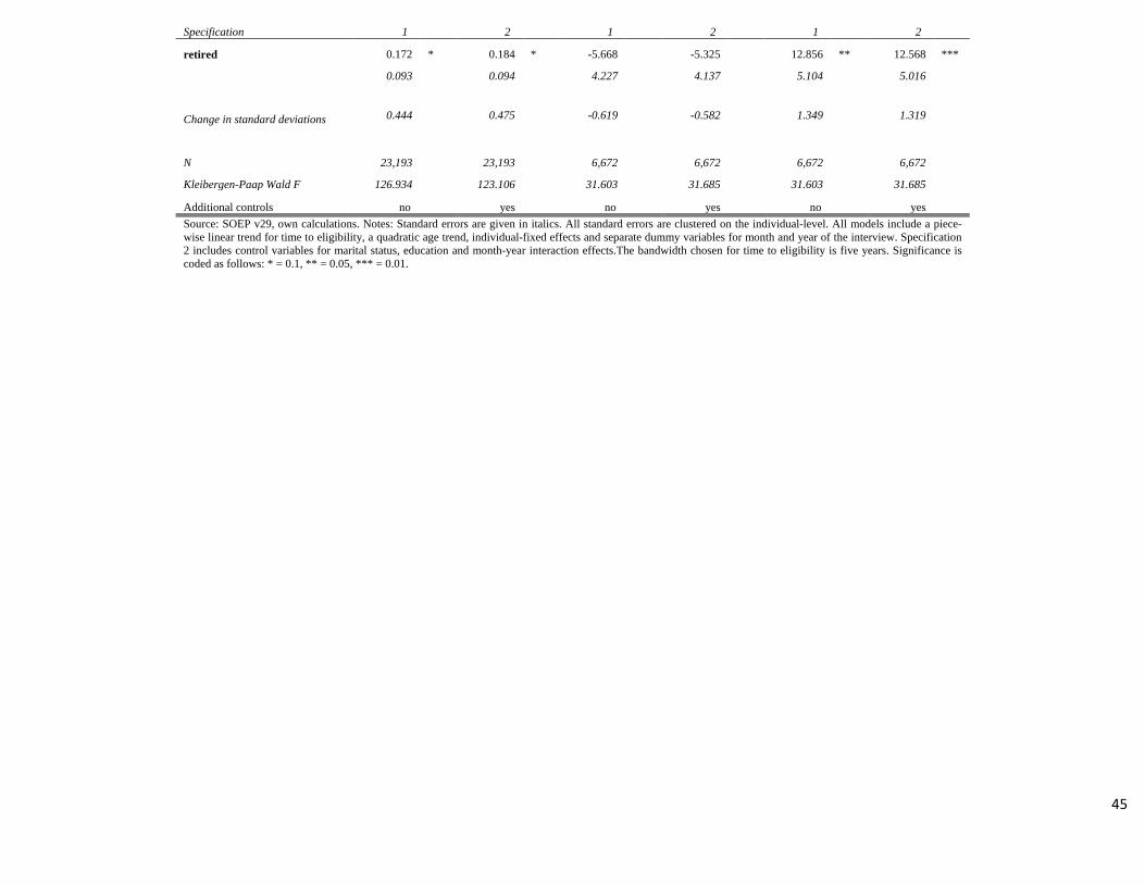
45

Specification 1 2 1 2 1 2

retired 0.172 * 0.184 * -5.668

-5.325

12.856 ** 12.568 ***

0.093

0.094

4.227

4.137

5.104

5.016

Change in standard deviations 0.444 0.475 -0.619 -0.582 1.349 1.319

N 23,193

23,193

6,672

6,672

6,672

6,672

Kleibergen-Paap Wald F 126.934

123.106

31.603

31.685

31.603

31.685

Additional controls no yes no yes no yes Source: SOEP v29, own calculations. Notes: Standard errors are given in italics. All standard errors are clustered on the individual-level. All models include a piece-wise linear trend for time to eligibility, a quadratic age trend, individual-fixed effects and separate dummy variables for month and year of the interview. Specification 2 includes control variables for marital status, education and month-year interaction effects.The bandwidth chosen for time to eligibility is five years. Significance is coded as follows: * = 0.1, ** = 0.05, *** = 0.01.