this page intentionally left blank -...
TRANSCRIPT


This page intentionally left blank

P E A R L S O F F U N C T I O NA L A L G O R I T H M D E S I G N
In Pearls of Functional Algorithm Design Richard Bird takes a radically newapproach to algorithm design, namely design by calculation. The body of the textis divided into 30 short chapters, called pearls, each of which deals with a partic-ular programming problem. These problems, some of which are completely new,are drawn from sources as diverse as games and puzzles, intriguing combinatorialtasks and more familiar algorithms in areas such as data compression and stringmatching.
Each pearl starts with the statement of the problem expressed using thefunctional programming language Haskell, a powerful yet succinct language forcapturing algorithmic ideas clearly and simply. The novel aspect of the book is thateach solution is calculated from the problem statement by appealing to the laws offunctional programming.
Pearls of Functional Algorithm Design will appeal to the aspiring functionalprogrammer, students and teachers interested in the principles of algorithm design,and anyone seeking to master the techniques of reasoning about programs in anequational style.
RICHARD BIRD is Professor of Computer Science at Oxford University and Fellowof Lincoln College, Oxford.

PEARLS OF FUNCTIONALALGORITHM DESIGN
R I C H A R D B I R DUniversity of Oxford

CAMBRIDGE UNIVERSITY PRESSCambridge, New York, Melbourne, Madrid, Cape Town, Singapore,São Paulo, Delhi, Dubai, Tokyo
Cambridge University PressThe Edinburgh Building, Cambridge CB2 8RU, UK
First published in print format
ISBN-13 978-0-521-51338-8
ISBN-13 978-0-511-79588-6
© Cambridge University Press 2010
2010
Information on this title: www.cambridge.org/9780521513388
This publication is in copyright. Subject to statutory exception and to the provision of relevant collective licensing agreements, no reproduction of any partmay take place without the written permission of Cambridge University Press.
Cambridge University Press has no responsibility for the persistence or accuracy of urls for external or third-party internet websites referred to in this publication, and does not guarantee that any content on such websites is, or will remain, accurate or appropriate.
Published in the United States of America by Cambridge University Press, New York
www.cambridge.org
eBook (Adobe Reader)
Hardback

Dedicated to my wife, Norma.


Contents
Preface page ix
1 The smallest free number 1
2 A surpassing problem 7
3 Improving on saddleback search 12
4 A selection problem 21
5 Sorting pairwise sums 27
6 Making a century 33
7 Building a tree with minimum height 41
8 Unravelling greedy algorithms 50
9 Finding celebrities 56
10 Removing duplicates 64
11 Not the maximum segment sum 73
12 Ranking suffixes 79
13 The Burrows–Wheeler transform 91
14 The last tail 102
15 All the common prefixes 112
16 The Boyer–Moore algorithm 117
17 The Knuth–Morris–Pratt algorithm 127
18 Planning solves the Rush Hour problem 136
19 A simple Sudoku solver 147
20 The Countdown problem 156
21 Hylomorphisms and nexuses 168
22 Three ways of computing determinants 180
23 Inside the convex hull 188
vii

viii Contents
24 Rational arithmetic coding 198
25 Integer arithmetic coding 208
26 The Schorr–Waite algorithm 221
27 Orderly insertion 231
28 Loopless functional algorithms 242
29 The Johnson–Trotter algorithm 251
30 Spider spinning for dummies 258Index 275
Preface
In 1990, when the Journal of Functional Programming (JFP) was in thestages of being planned, I was asked by the then editors, Simon PeytonJones and Philip Wadler, to contribute a regular column to be called Func-tional Pearls. The idea they had in mind was to emulate the very successfulseries of essays that Jon Bentley had written in the 1980s under the title“Programming Pearls” in the Communications of the ACM. Bentley wroteabout his pearls:
Just as natural pearls grow from grains of sand that have irritated oysters, theseprogramming pearls have grown from real problems that have irritated program-mers. The programs are fun, and they teach important programming techniquesand fundamental design principles.
I think the editors had asked me because I was interested in the specific taskof taking a clear but inefficient functional program, a program that actedas a specification of the problem in hand, and using equational reasoning tocalculate a more efficient one. One factor that stimulated growing interestin functional languages in the 1990s was that such languages were good forequational reasoning. Indeed, the functional language GOFER, invented byMark Jones, captured this thought as an acronym. GOFER was one of thelanguages that contributed to the development of Haskell, the language onwhich this book is based. Equational reasoning dominates everything in thisbook.
In the past 20 years, some 80 pearls have appeared in the JFP, togetherwith a sprinkling of pearls at conferences such as the International Confer-ence of Functional Programming (ICFP) and the Mathematics of ProgramConstruction Conference (MPC). I have written about a quarter of them,but most have been written by others. The topics of these pearls includeinteresting program calculations, novel data structures and small but elegantdomain-specific languages embedded in Haskell and ML for particularapplications.
ix
x Preface
My interest has always been in algorithms and their design. Hence thetitle of this book is Pearls of Functional Algorithm Design rather than themore general Functional Pearls. Many, though by no means all, of the pearlsstart with a specification in Haskell and then go on to calculate a moreefficient version. My aim in writing these particular pearls is to see to whatextent algorithm design can be cast in a familiar mathematical tradition ofcalculating a result by using well-established mathematical principles, the-orems and laws. While it is generally true in mathematics that calculationsare designed to simplify complicated things, in algorithm design it is usuallythe other way around: simple but inefficient programs are transformed intomore efficient versions that can be completely opaque. It is not the finalprogram that is the pearl; rather it is the calculation that yields it. Otherpearls, some of which contain very few calculations, are devoted to trying togive simple explanations of some interesting and subtle algorithms. Explain-ing the ideas behind an algorithm is so much easier in a functional style thanin a procedural one: the constituent functions can be more easily separated,they are brief and they capture powerful patterns of computation.
The pearls in this book that have appeared before in the JFP and otherplaces have been polished and repolished. In fact, many do not bear muchresemblance to the original. Even so, they could easily be polished more.The gold standard for beauty in mathematics is Proofs from The Book byAigner and Ziegler (third edition, Springer, 2003), which contains some per-fect proofs for mathematical theorems. I have always had this book in mindas an ideal towards which to strive.
About a third of the pearls are new. With some exceptions, clearly indi-cated, the pearls can be read in any order, though the chapters have beenarranged to some extent in themes, such as divide and conquer, greedy algor-ithms, exhaustive search and so on. There is some repetition of material inthe pearls, mostly concerning the properties of the library functions that weuse, as well as more general laws, such as the fusion laws of various folds.A brief index has been included to guide the reader when necessary.
Finally, many people have contributed to the material. Indeed, severalpearls were originally composed in collaboration with other authors. I wouldlike to thank Sharon Curtis, Jeremy Gibbons, Ralf Hinze, Geraint Jones andShin-Cheng Mu, my co-authors on these pearls, for their kind generosity inallowing me to rework the material. Jeremy Gibbons read the final draftand made numerous useful suggestions for improving the presentation. Somepearls have also been subject to close scrutiny at meetings of the Algebra ofProgramming research group at Oxford. While a number of flaws and errorshave been removed, no doubt additional ones have been introduced. Apart
Preface xi
from those mentioned above, I would like to thank Stephen Drape, TomHarper, Daniel James, Jeffrey Lake, Meng Wang and Nicholas Wu for manypositive suggestions for improving presentation. I would also like to thankLambert Meertens and Oege de Moor for much fruitful collaboration overthe years. Finally, I am indebted to David Tranah, my editor at CambridgeUniversity Press, for encouragement and support, including much neededtechnical advice in the preparation of the final copy.
Richard Bird


1
The smallest free number
Introduction
Consider the problem of computing the smallest natural number not in agiven finite set X of natural numbers. The problem is a simplification of acommon programming task in which the numbers name objects and X isthe set of objects currently in use. The task is to find some object not inuse, say the one with the smallest name.
The solution to the problem depends, of course, on how X is represented.If X is given as a list without duplicates and in increasing order, then thesolution is straightforward: simply look for the first gap. But suppose X isgiven as a list of distinct numbers in no particular order. For example,
[08, 23, 09, 00, 12, 11, 01, 10, 13, 07, 41, 04, 14, 21, 05, 17, 03, 19, 02, 06]
How would you find the smallest number not in this list?It is not immediately clear that there is a linear-time solution to the
problem; after all, sorting an arbitrary list of numbers cannot be done inlinear time. Nevertheless, linear-time solutions do exist and the aim of thispearl is to describe two of them: one is based on Haskell arrays and the otheron divide and conquer.
An array-based solution
The problem can be specified as a function minfree, defined by
minfree :: [Nat ]→ Natminfree xs = head ([0 .. ] \\ xs)
The expression us \\ vs denotes the list of those elements of us that remainafter removing any elements in vs:
(\\) :: Eq a ⇒ [a]→ [a]→ [a]us \\ vs = filter (�∈ vs) us
1
2 Pearls of Functional Algorithm Design
The function minfree is executable but requires Θ(n2) steps on a list oflength n in the worst case. For example, evaluating minfree [n−1,n−2 .. 0]requires evaluating i /∈ [n−1,n−2 .. 0] for 0 ≤ i ≤ n, and thus n(n + 1)/2equality tests.
The key fact for both the array-based and divide and conquer solutionsis that not every number in the range [0 .. length xs] can be in xs. Thus thesmallest number not in xs is the smallest number not in filter (≤ n)xs, wheren = length xs. The array-based program uses this fact to build a checklistof those numbers present in filter (≤ n) xs. The checklist is a Boolean arraywith n +1 slots, numbered from 0 to n, whose initial entries are everywhereFalse. For each element x in xs and provided x ≤ n we set the array elementat position x to True. The smallest free number is then found as the positionof the first False entry. Thus, minfree = search · checklist , where
search :: Array Int Bool → Intsearch = length · takeWhile id · elems
The function search takes an array of Booleans, converts the array into a listof Booleans and returns the length of the longest initial segment consistingof True entries. This number will be the position of the first False entry.
One way to implement checklist in linear time is to use the functionaccumArray in the Haskell library Data.Array . This function has the ratherdaunting type
Ix i ⇒ (e → v → e) → e → (i , i)→ [(i , v)] → Array i e
The type constraint Ix i restricts i to be an Index type, such as Int orChar , for naming the indices or positions of the array. The first argument isan “accumulating” function for transforming array entries and values intonew entries, the second argument is an initial entry for each index, the thirdargument is a pair naming the lower and upper indices and the fourth isan association list of index–value pairs. The function accumArray buildsan array by processing the association list from left to right, combiningentries and values into new entries using the accumulating function. Thisprocess takes linear time in the length of the association list, assuming theaccumulating function takes constant time.
The function checklist is defined as an instance of accumArray :
checklist :: [Int ] → Array Int Boolchecklist xs = accumArray (∨) False (0,n)
(zip (filter (≤ n) xs) (repeat True))where n = length xs

The smallest free number 3
This implementation does not require the elements of xs to be distinct, butdoes require them to be natural numbers.
It is worth mentioning that accumArray can be used to sort a list ofnumbers in linear time, provided the elements of the list all lie in someknown range (0,n). We replace checklist by countlist , where
countlist :: [Int ] → Array Int Intcountlist xs = accumArray (+) 0 (0,n) (zip xs (repeat 1))
Then sort xs = concat [replicate k x | (x , k)← countlist xs]. In fact, if we usecountlist instead of checklist , then we can implement minfree as the positionof the first 0 entry.
The above implementation builds the array in one go using a clever libraryfunction. A more prosaic way to implement checklist is to tick off entries stepby step using a constant-time update operation. This is possible in Haskellonly if the necessary array operations are executed in a suitable monad, suchas the state monad. The following program for checklist makes use of thelibrary Data.Array .ST :
checklist xs = runSTArray (do{a ← newArray (0,n) False;sequence [writeArray a x True | x ← xs, x ≤ n];return a})
where n = length xs
This solution would not satisfy the pure functional programmer because itis essentially a procedural program in functional clothing.
A divide and conquer solution
Now we turn to a divide and conquer solution to the problem. The idea isto express minfree (xs ++ys) in terms of minfree xs and minfree ys. We beginby recording the following properties of \\:
(as ++ bs) \\ cs = (as \\ cs) ++ (bs \\ cs)as \\ (bs ++ cs) = (as \\ bs) \\ cs(as \\ bs) \\ cs = (as \\ cs) \\ bs
These properties reflect similar laws about sets in which set union ∪ replaces++ and set difference \ replaces \\. Suppose now that as and vs are disjoint,meaning as \\ vs = as, and that bs and us are also disjoint, so bs \\ us = bs.It follows from these properties of ++ and \\ that
(as ++ bs) \\ (us ++ vs) = (as \\ us) ++ (bs \\ vs)
4 Pearls of Functional Algorithm Design
Now, choose any natural number b and let as = [0 .. b−1] and bs = [b..].Furthermore, let us = filter (< b) xs and vs = filter (≥ b) xs. Then as andvs are disjoint, and so are bs and us. Hence
[0 .. ] \\ xs = ([0 .. b−1] \\ us) ++ ([b .. ] \\ vs)where (us, vs) = partition (< b) xs
Haskell provides an efficient implementation of a function partition p thatpartitions a list into those elements that satisfy p and those that do not.Since
head (xs ++ ys) = if null xs then head ys else head xs
we obtain, still for any natural number b, that
minfree xs = if null ([0 .. b−1] \\ us)then head ([b .. ] \\ vs)else head ([0 .. ] \\ us)where (us, vs) = partition (< b) xs
The next question is: can we implement the test null ([0 .. b−1] \\ us) moreefficiently than by direct computation, which takes quadratic time in thelength of us? Yes, the input is a list of distinct natural numbers, so is us.And every element of us is less than b. Hence
null ([0 .. b−1] \\ us ≡ length us b
Note that the array-based solution did not depend on the assumption thatthe given list did not contain duplicates, but it is a crucial one for an efficientdivide and conquer solution.
Further inspection of the above code for minfree suggests that we shouldgeneralise minfree to a function, minfrom say, defined by
minfrom :: Nat → [Nat ]→ Natminfrom a xs = head ([a .. ] \\ xs)
where every element of xs is assumed to be greater than or equal to a.Then, provided b is chosen so that both length us and length vs are less thanlength xs, the following recursive definition of minfree is well-founded:
minfree xs = minfrom 0 xsminfrom a xs | null xs = a
| length us b − a = minfrom b vs| otherwise = minfrom a us
where (us, vs) = partition (< b) xs

The smallest free number 5
It remains to choose b. Clearly, we want b > a. And we would also like tochoose b so that the maximum of the lengths of us and vs is as small aspossible. The right choice of b to satisfy these requirements is
b = a + 1 + n div 2
where n = length xs. If n �= 0 and length us < b − a, then
length us ≤ n div 2 < n
And, if length us = b − a, then
length vs = n − n div 2− 1 ≤ n div 2
With this choice the number of steps T (n) for evaluating minfrom 0 xswhen n = length xs satisfies T (n) = T (n div 2) + Θ(n), with the solutionT (n) = Θ(n).
As a final optimisation we can avoid repeatedly computing length with asimple data refinement, representing xs by a pair (length xs, xs). That leadsto the final program
minfree xs = minfrom 0 (length xs, xs)minfrom a (n, xs) | n 0 = a
| m b − a = minfrom b (n −m, vs)| otherwise = minfrom a (m, us)
where (us, vs) = partition (< b) xsb = a + 1 + n div 2m = length us
It turns out that the above program is about twice as fast as the incrementalarray-based program, and about 20% faster than the one using accumArray .
Final remarks
This was a simple problem with at least two simple solutions. The secondsolution was based on a common technique of algorithm design, namelydivide and conquer. The idea of partitioning a list into those elements lessthan a given value, and the rest, arises in a number of algorithms, mostnotably Quicksort. When seeking a Θ(n) algorithm involving a list of nelements, it is tempting to head at once for a method that processes eachelement of the list in constant time, or at least in amortized constant time.But a recursive process that performs Θ(n) processing steps in order toreduce the problem to another instance of at most half the size is also goodenough.
6 Pearls of Functional Algorithm Design
One of the differences between a pure functional algorithm designer anda procedural one is that the former does not assume the existence of arrayswith a constant-time update operation, at least not without a certain amountof plumbing. For a pure functional programmer, an update operation takeslogarithmic time in the size of the array.1 That explains why there sometimesseems to be a logarithmic gap between the best functional and proceduralsolutions to a problem. But sometimes, as here, the gap vanishes on a closerinspection.
1 To be fair, procedural programmers also appreciate that constant-time indexing and updatingare only possible when the arrays are small.
2
A surpassing problem
Introduction
In this pearl we solve a small programming exercise of Martin Rem (1988a).While Rem’s solution uses binary search, our solution is another applicationof divide and conquer. By definition, a surpasser of an element of an arrayis a greater element to the right, so x [j ] is a surpasser of x [i ] if i < jand x [i ] < x [j ]. The surpasser count of an element is the number of itssurpassers. For example, the surpasser counts of the letters of the stringGENERATING are given by
G E N E R A T I N G5 6 2 5 1 4 0 1 0 0
The maximum surpasser count is six. The first occurrence of letter E has sixsurpassers, namely N, R, T, I, N and G. Rem’s problem is to compute themaximum surpasser count of an array of length n > 1 and to do so with anO(n log n) algorithm.
Specification
We will suppose that the input is given as a list rather than an array. Thefunction msc (short for maximum surpasser count) is specified by
msc :: Ord a ⇒ [a]→ Intmsc xs = maximum [scount z zs | z : zs ← tails xs]scount x xs = length (filter (x <) xs)
The value of scount x xs is the surpasser count of x in the list xs and tailsreturns the nonempty tails of a nonempty list in decreasing order of length:1
tails [ ] = [ ]tails (x : xs) = (x : xs) : tails xs
The definition of msc is executable but takes quadratic time.1 Unlike the standard Haskell function of the same name, which returns the possibly empty tails
of a possibly empty list.
7

8 Pearls of Functional Algorithm Design
Divide and conquer
Given the target complexity of O(n log n) steps, it seems reasonable to headfor a divide and conquer algorithm. If we can find a function join so that
msc (xs ++ ys) = join (msc xs) (msc ys)
and join can be computed in linear time, then the time complexity T (n) ofthe divide and conquer algorithm for computing msc on a list of length nsatisfies T (n) = 2T (n/2)+O(n), with solution T (n) = O(n log n). But it isfairly obvious that no such join can exist: too little information is providedby the single number msc xs for any such decomposition.
The minimal generalisation is to start out with the table of all surpassercounts:
table xs = [(z , scount z zs) | z : zs ← tails xs]
Then msc = maximum ·map snd · table. Can we find a linear-time join tosatisfy
table (xs ++ ys) = join (table xs) (table ys)
Well, let us see. We will need the following divide and conquer property oftails:
tails (xs ++ ys) = map (++ys) (tails xs) ++ tails ys
The calculation goes as follows:
table (xs ++ ys)
= {definition}[(z , scount z zs) | z : zs ← tails (xs ++ ys)]
= {divide and conquer property of tails}[(z , scount z zs) | z : zs ←map (++ys) (tails xs) ++ tails ys]
= {distributing ← over ++}[(z , scount z (zs ++ ys)) | z : zs ← tails xs] ++[(z , scount z zs) | z : zs ← tails ys])
= {since scount z (zs ++ ys) = scount z zs + scount z ys}[(z , scount z zs + scount z ys) | z : zs ← tails xs] ++[(z , scount z zs) | z : zs ← tails ys])
= {definition of table and ys = map fst (table ys)}[(z , c + scount z (map fst (table ys))) | (z , c)← table xs] ++ table ys

A surpassing problem 9
Hence join can be defined by
join txs tys = [(z , c + tcount z tys) | (z , c)← txs] ++ tystcount z tys = scount z (map fst tys)
The problem with this definition, however, is that join txs tys does not takelinear time in the length of txs and tys.
We could improve the computation of tcount if tys were sorted inascending order of first component. Then we can reason:
tcount z tys
= {definition of tcount and scount}length (filter (z <) (map fst tys))
= {since filter p ·map f = map f · filter (p · f )}length (map fst (filter ((z <) · fst) tys))
= {since length ·map f = length}length (filter ((z <) · fst) tys)
= {since tys is sorted on first argument}length (dropWhile ((z ≥) · fst) tys)
Hence
tcount z tys = length (dropWhile((z ≥) · fst) tys) (2.1)
This calculation suggests it would be sensible to maintain table in ascendingorder of first component:
table xs = sort [(z , scount z zs) | z : zs ← tails xs]
Repeating the calculation above, but for the sorted version of table, we findthat
join txs tys = [(x , c + tcount x tys) | (x , c)← txs] ∧∧ tys (2.2)
where ∧∧ merges two sorted lists. Using this identity we can now calculatea more efficient recursive definition of join. One of the base cases, namelyjoin [ ] tys = tys, is immediate. The other base case, join txs [ ] = txs, followsbecause tcount x [ ] = 0. For the recursive case we simplify
join txs@((x , c) : txs ′) tys@((y , d) : tys ′) (2.3)
by comparing x and y . (In Haskell, the @ sign introduces a synonym, so txsis a synonym for (x , c) : txs ′; similarly for tys.) Using (2.2), (2.3) reduces to
((x , c + tcount x tys) : [(x , c + tcount x tys) | (x , c)← txs ′]) ∧∧ tys
10 Pearls of Functional Algorithm Design
To see which element is produced first by ∧∧ we need to compare x and y . Ifx < y , then it is the element on the left and, since tcount x tys = length tysby (2.1), expression (2.3) reduces to
(x , c + length tys) : join txs ′ tys
If x = y , we need to compare c + tcount x tys and d . But d = tcount x tys ′
by the definition of table and tcount x tys = tcount x tys ′ by (2.1), so (2.3)reduces to (y , d) : join txs tys ′. This is also the result in the final case x > y .
Putting these results together, and introducing length tys as an additionalargument to join in order to avoid repeating length calculations, we arriveat the following divide and conquer algorithm for table:
table [x ] = [(x , 0)]table xs = join (m − n) (table ys) (table zs)
where m = length xsn = m div 2(ys, zs) = splitAt n xs
join 0 txs [ ] = txsjoin n [ ] tys = tysjoin n txs@((x , c) : txs ′) tys@((y , d) : tys ′)
| x < y = (x , c + n) : join n txs ′ tys| x ≥ y = (y , d) : join (n−1) txs tys ′
Since join takes linear time, table is computed in O(n log n) steps, and sois msc.
Final remarks
It is not possible to do better than an O(n log n) algorithm for computingtable. The reason is that if xs is a list of distinct elements, then table xs pro-vides enough information to determine the permutation of xs that sorts xs.Moreover, no further comparisons between list elements are required. In fact,table xs is related to the inversion table of a permutation of n elements;see Knuth (1998): table xs is just the inversion table of reverse xs. Sincecomparison-based sorting of n elements requires Ω(n log n) steps, so doesthe computation of table.
As we said in the Introduction for this pearl, the solution in Rem (1998b)is different, in that it is based on an iterative algorithm and uses binarysearch. A procedural programmer could also head for a divide and conqueralgorithm, but would probably prefer an in-place array-based algorithmsimply because it consumes less space.
A surpassing problem 11
ReferencesKnuth, D. E. (1998). The Art of Computer Programming, Volume 3: Sorting and
Searching, second edition. Reading, MA: Addison-Wesley.Rem, M. (1988a). Small programming exercises 20. Science of Computer Program-
ming 10 (1), 99–105.Rem, M. (1998b). Small programming exercises 21. Science of Computer Program-
ming 10 (3), 319–25.
3
Improving on saddleback search
The setting is a tutorial on functional algorithm design. There are fourstudents: Anne, Jack, Mary and Theo.
Teacher: Good morning class. Today I would like you design a functioninvert that takes two arguments: a function f from pairs of natural numbersto natural numbers, and a natural number z . The value invert f z is a listof all pairs (x , y) satisfying f (x , y) = z . You can assume that f is strictlyincreasing in each argument, but nothing else.
Jack: That seems an easy problem. Since f is a function on naturals andis increasing in each argument, we know that f (x , y) = z implies x ≤ z andy ≤ z . Hence we can define invert by a simple search of all possible pairs ofvalues:
invert f z = [(x , y) | x ← [0 .. z ], y ← [0 .. z ], f (x , y) z ]
Doesn’t this solve the problem?
Teacher: Yes it does, but your solution involves (z + 1)2 evaluations of f .Since f may be very expensive to compute, I would like a solution with asfew evaluations of f as possible.
Theo: Well, it is easy to halve the evaluations. Since f (x , y) ≥ x + y if f isincreasing, the search can be confined to values on or below the diagonal ofthe square:
invert f z = [(x , y) | x ← [0 .. z ], y ← [0 .. z − x ], f (x , y) z ]
Come to think of it, you can replace the two upper bounds by z − f (0, 0)and z − x − f (0, 0). Then if z < f (0, 0) the search terminates at once.
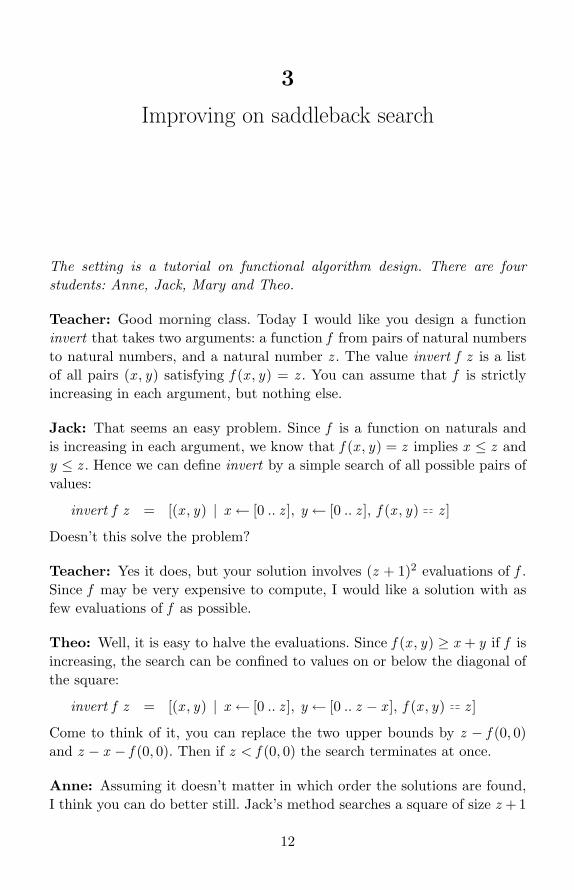
Anne: Assuming it doesn’t matter in which order the solutions are found,I think you can do better still. Jack’s method searches a square of size z +1
12

Improving on saddleback search 13
from the origin at the bottom left, and proceeds upwards column by column.We can do better if we start at the top-left corner (0, z ) of the square. At anystage the search space is constrained to be a rectangle with top-left corner(u, v) and bottom-right corner (z , 0). Here is the picture:
(0, 0)
(0, z ) (z , z )
(z , 0)
(u, v)
Let me define
find (u, v) f z = [(x , y) | x ← [u .. z ], y ← [v , v − 1 .. 0], f (x , y) z ]
so that invert f z = find (0, z ) f z . It is now easy enough to calculate a moreefficient implementation of find .
First of all, if u > z or v < 0, then, clearly, find (u, v) f z = [ ]. Otherwise,we carry out a case analysis on the value f (u, v). If f (u, v) < z , thenthe rest of column u can be eliminated, since f (u, v ′) < f (u, v) < z forv ′ < v . If f (u, v) > z , we can similarly eliminate, the rest of row v . Finally,if f (u, v) = z , then we can record (u, v) and eliminate the rest of bothcolumn u and row v .
Here is my improved version of invert :
invert f z = find (0, z ) f zfind (u, v) f z
| u > z ∨ v < 0 = [ ]| z ′ < z = find (u+1, v) f z| z ′ z = (u, v) : find (u+1, v−1) f z| z ′ > z = find (u, v−1) f z
where z ′ = f (u, v)
In the worst case, when find traverses the perimeter of the square from thetop-left corner to the bottom-right corner, it performs 2z + 1 evaluationsof f . In the best case, when find proceeds directly to either the bottom orrightmost boundary, it requires only z + 1 evaluations.
Theo: You can reduce the search space still further because the initialsquare with top-left corner (0, z ) and bottom-right corner (z , 0) is an overly

14 Pearls of Functional Algorithm Design
generous estimate of where the required values lie. Suppose we first computem and n, where
m = maximum (filter (λy → f (0, y) ≤ z ) [0 .. z ])n = maximum (filter (λx → f (x , 0) ≤ z ) [0 .. z ])
Then we can define invert f z = find (0,m) f z , where find has exactly thesame form that Anne gave, except that the first guard becomes u > n∨v < 0.In other words, rather than search a (z+1)× (z+1) square we can get awaywith searching an (m+1)× (n+1) rectangle.
The crucial point is that we can compute m and n by binary search.Let g be an increasing function on the natural numbers and suppose x ,y and z satisfy g x ≤ z < g y . To determine the unique value m, wherem = bsearch g (x , y)z , in the range x ≤ m < y such that gm ≤ z < g (m+1)we can maintain the invariants g a ≤ z < g b and x ≤ a < b ≤ y . This leadsto the program
bsearch g (a, b) z| a+1 b = a| g m ≤ z = bsearch g (m, b) z| otherwise = bsearch g (a,m) z
where m = (a + b) div 2
Since a+1 < b ⇒ a < m < y it follows that neither g x nor g y are evaluatedby the algorithm, so they can be fictitious values. In particular, we have
m = bsearch (λy → f (0, y)) (−1, z + 1) zn = bsearch (λx → f (x , 0)) (−1, z + 1) z
where we extend f with fictitious values f (0,−1) = 0 and f (−1, 0) = 0.This version of invert takes about 2 log z + m + n evaluations of f in the
worst case and 2 log z + m minn in the best case. Since m or n may besubstantially less than z , for example when f (x , y) = 2x + 3y , we can endup with an algorithm that takes only O(log z ) steps in the worst case.
Teacher: Congratulations, Anne and Theo, you have rediscovered animportant search strategy, dubbed saddleback search by David Gries; seeBackhouse (1986), Dijkstra (1985) and Gries (1981). I imagine Gries calledit that because the shape of the three-dimensional plot of f , with the small-est element at the bottom left, the largest at the top right and two wings,is a bit like a saddle. The crucial idea, as Anne has spotted, is to start thesearch at the tip of one of the wings rather than at the smallest or high-est value. In his treatment of the problem, Dijkstra (1985) also mentionedthe advantage of using a logarithmic search to find the appropriate startingrectangle.
Improving on saddleback search 15
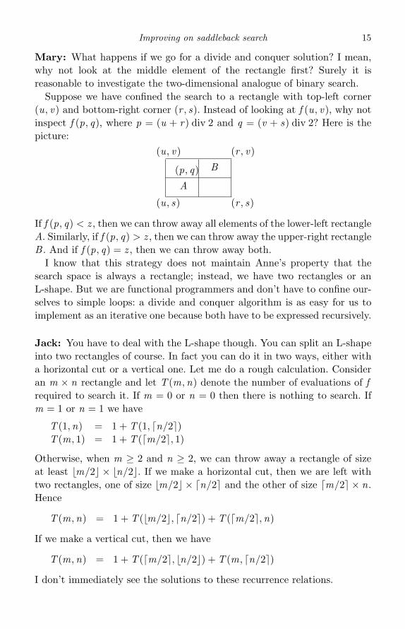
Mary: What happens if we go for a divide and conquer solution? I mean,why not look at the middle element of the rectangle first? Surely it isreasonable to investigate the two-dimensional analogue of binary search.
Suppose we have confined the search to a rectangle with top-left corner(u, v) and bottom-right corner (r , s). Instead of looking at f (u, v), why notinspect f (p, q), where p = (u + r) div 2 and q = (v + s) div 2? Here is thepicture:
(u, s)
(u, v) (r , v)
(r , s)
(p, q)
A
B
If f (p, q) < z , then we can throw away all elements of the lower-left rectangleA. Similarly, if f (p, q) > z , then we can throw away the upper-right rectangleB . And if f (p, q) = z , then we can throw away both.
I know that this strategy does not maintain Anne’s property that thesearch space is always a rectangle; instead, we have two rectangles or anL-shape. But we are functional programmers and don’t have to confine our-selves to simple loops: a divide and conquer algorithm is as easy for us toimplement as an iterative one because both have to be expressed recursively.
Jack: You have to deal with the L-shape though. You can split an L-shapeinto two rectangles of course. In fact you can do it in two ways, either witha horizontal cut or a vertical one. Let me do a rough calculation. Consideran m × n rectangle and let T (m,n) denote the number of evaluations of frequired to search it. If m = 0 or n = 0 then there is nothing to search. Ifm = 1 or n = 1 we have
T (1,n) = 1 + T (1, n/2�)T (m, 1) = 1 + T ( m/2�, 1)
Otherwise, when m ≥ 2 and n ≥ 2, we can throw away a rectangle of sizeat least �m/2� × �n/2�. If we make a horizontal cut, then we are left withtwo rectangles, one of size �m/2� × n/2� and the other of size m/2� × n.Hence
T (m,n) = 1 + T (�m/2�, n/2�) + T ( m/2�,n)
If we make a vertical cut, then we have
T (m,n) = 1 + T ( m/2�, �n/2�) + T (m, n/2�)
I don’t immediately see the solutions to these recurrence relations.

16 Pearls of Functional Algorithm Design
Theo: If you make both a horizontal and a vertical cut, you are left withthree rectangles, so when m ≥ 2 and n ≥ 2 we have
T (m,n) = 1 + T ( m/2�, �n/2�) + T ( m/2�, n/2�) + T (�m/2�, n/2�)
I can solve this recurrence. Set U (i , j ) = T (2i , 2j ), so
U (i , 0) = iU (0, j ) = jU (i + 1, j + 1) = 1 + 3U (i , j )
The solution is U (i , j ) = 3k (|j − i |+ 1/2)− 1/2, where k = i min j , as onecan check by induction. Hence, if m ≤ n we have
T (m,n) ≤ 3log m log(2n/m) = m1·59 log(2n/m)
That’s better than m + n when m is much smaller than n.
Jack: I don’t think the three-rectangle solution is as good as the two-rectangle one. Following your approach, Theo, let me set U (i , j ) = T (2i , 2j ).Supposing i ≤ j and making a horizontal cut, we have
U (0, j ) = jU (i + 1, j + 1) = 1 + U (i , j ) + U (i , j + 1)
The solution is U (i , j ) = 2i(j − i/2 + 1)− 1, as one can check by induction.Hence
T (m,n) ≤ m log(2n/√
m)
If i ≥ j we should make a vertical cut rather than a horizontal one; then weget an algorithm with at most n log(2m/
√n) evaluations of f . In either case,
if one of m or n is much smaller than the other we get a better algorithmthan saddleback search.
Anne: While you two have been solving recurrences I have been thinkingof a lower bound on the complexity of invert . Consider the different possibleoutputs when we have an m × n rectangle to search. Suppose there areA(m,n) different possible answers. Each test of f (x , y) against z has threepossible outcomes, so the height h of the ternary tree of tests has to satisfyh ≥ log3 A(m,n). Provided we can estimate A(m,n) this gives us a lowerbound on the number of tests that have to be performed. The situation isthe same with sorting n items by binary comparisons; there are n! possibleoutcomes, so any sorting algorithm has to make at least log2 n! comparisonsin the worst case.
Improving on saddleback search 17
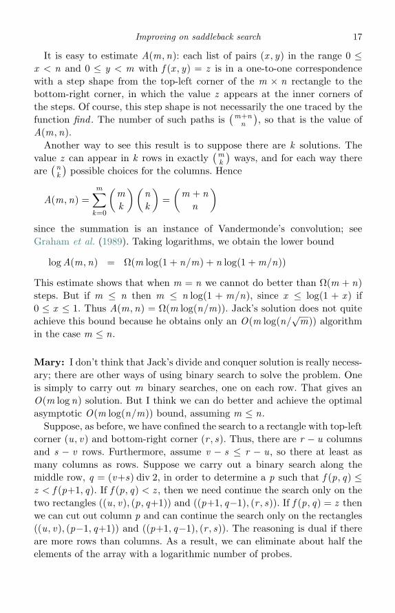
It is easy to estimate A(m,n): each list of pairs (x , y) in the range 0 ≤x < n and 0 ≤ y < m with f (x , y) = z is in a one-to-one correspondencewith a step shape from the top-left corner of the m × n rectangle to thebottom-right corner, in which the value z appears at the inner corners ofthe steps. Of course, this step shape is not necessarily the one traced by thefunction find . The number of such paths is
(m+nn
), so that is the value of
A(m,n).Another way to see this result is to suppose there are k solutions. The
value z can appear in k rows in exactly(
mk
)ways, and for each way there
are(
nk
)possible choices for the columns. Hence
A(m,n) =m∑
k=0
(mk
) (nk
)=
(m + n
n
)
since the summation is an instance of Vandermonde’s convolution; seeGraham et al. (1989). Taking logarithms, we obtain the lower bound
log A(m,n) = Ω(m log(1 + n/m) + n log(1 + m/n))
This estimate shows that when m = n we cannot do better than Ω(m + n)steps. But if m ≤ n then m ≤ n log(1 + m/n), since x ≤ log(1 + x ) if0 ≤ x ≤ 1. Thus A(m,n) = Ω(m log(n/m)). Jack’s solution does not quiteachieve this bound because he obtains only an O(m log(n/
√m)) algorithm
in the case m ≤ n.
Mary: I don’t think that Jack’s divide and conquer solution is really necess-ary; there are other ways of using binary search to solve the problem. Oneis simply to carry out m binary searches, one on each row. That gives anO(m log n) solution. But I think we can do better and achieve the optimalasymptotic O(m log(n/m)) bound, assuming m ≤ n.
Suppose, as before, we have confined the search to a rectangle with top-leftcorner (u, v) and bottom-right corner (r , s). Thus, there are r − u columnsand s − v rows. Furthermore, assume v − s ≤ r − u, so there at least asmany columns as rows. Suppose we carry out a binary search along themiddle row, q = (v+s) div 2, in order to determine a p such that f (p, q) ≤z < f (p+1, q). If f (p, q) < z , then we need continue the search only on thetwo rectangles ((u, v), (p, q+1)) and ((p+1, q−1), (r , s)). If f (p, q) = z thenwe can cut out column p and can continue the search only on the rectangles((u, v), (p−1, q+1)) and ((p+1, q−1), (r , s)). The reasoning is dual if thereare more rows than columns. As a result, we can eliminate about half theelements of the array with a logarithmic number of probes.
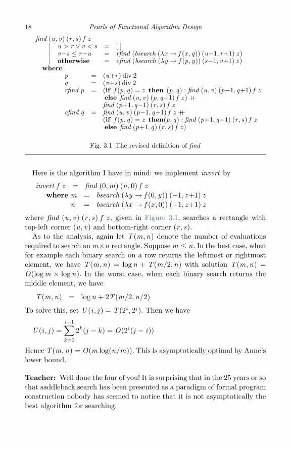
18 Pearls of Functional Algorithm Design
find (u, v) (r , s) f z| u > r ∨ v < s = [ ]| v−s ≤ r−u = rfind (bsearch (λx → f (x , q)) (u−1, r+1) z )| otherwise = cfind (bsearch (λy → f (p, y)) (s−1, v+1) z )
wherep = (u+r) div 2q = (v+s) div 2rfind p = (if f (p, q) = z then (p, q) : find (u, v) (p−1, q+1) f z
else find (u, v) (p, q+1) f z ) ++find (p+1, q−1) (r , s) f z
cfind q = find (u, v) (p−1, q+1) f z ++(if f (p, q) = z then(p, q) : find (p+1, q−1) (r , s) f zelse find (p+1, q) (r , s) f z )
Fig. 3.1 The revised definition of find
Here is the algorithm I have in mind: we implement invert by
invert f z = find (0,m) (n, 0) f zwhere m = bsearch (λy → f (0, y)) (−1, z+1) z
n = bsearch (λx → f (x , 0)) (−1, z+1) z
where find (u, v) (r , s) f z , given in Figure 3.1, searches a rectangle withtop-left corner (u, v) and bottom-right corner (r , s).
As to the analysis, again let T (m,n) denote the number of evaluationsrequired to search an m×n rectangle. Suppose m ≤ n. In the best case, whenfor example each binary search on a row returns the leftmost or rightmostelement, we have T (m,n) = log n + T (m/2,n) with solution T (m,n) =O(log m × log n). In the worst case, when each binary search returns themiddle element, we have
T (m,n) = log n + 2T (m/2,n/2)
To solve this, set U (i , j ) = T (2i , 2j ). Then we have
U (i , j ) =i−1∑k=0
2k (j − k) = O(2i(j − i))
Hence T (m,n) = O(m log(n/m)). This is asymptotically optimal by Anne’slower bound.
Teacher: Well done the four of you! It is surprising that in the 25 years or sothat saddleback search has been presented as a paradigm of formal programconstruction nobody has seemed to notice that it is not asymptotically thebest algorithm for searching.
Improving on saddleback search 19
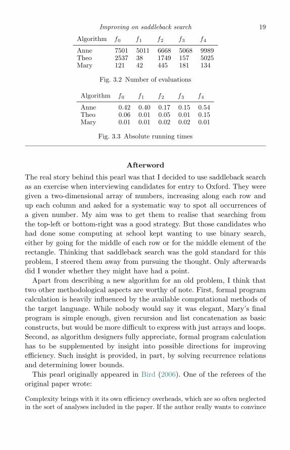
Algorithm f 0 f 1 f 2 f 3 f 4
Anne 7501 5011 6668 5068 9989Theo 2537 38 1749 157 5025Mary 121 42 445 181 134
Fig. 3.2 Number of evaluations
Algorithm f 0 f 1 f 2 f 3 f 4
Anne 0.42 0.40 0.17 0.15 0.54Theo 0.06 0.01 0.05 0.01 0.15Mary 0.01 0.01 0.02 0.02 0.01
Fig. 3.3 Absolute running times
Afterword
The real story behind this pearl was that I decided to use saddleback searchas an exercise when interviewing candidates for entry to Oxford. They weregiven a two-dimensional array of numbers, increasing along each row andup each column and asked for a systematic way to spot all occurrences ofa given number. My aim was to get them to realise that searching fromthe top-left or bottom-right was a good strategy. But those candidates whohad done some computing at school kept wanting to use binary search,either by going for the middle of each row or for the middle element of therectangle. Thinking that saddleback search was the gold standard for thisproblem, I steered them away from pursuing the thought. Only afterwardsdid I wonder whether they might have had a point.
Apart from describing a new algorithm for an old problem, I think thattwo other methodological aspects are worthy of note. First, formal programcalculation is heavily influenced by the available computational methods ofthe target language. While nobody would say it was elegant, Mary’s finalprogram is simple enough, given recursion and list concatenation as basicconstructs, but would be more difficult to express with just arrays and loops.Second, as algorithm designers fully appreciate, formal program calculationhas to be supplemented by insight into possible directions for improvingefficiency. Such insight is provided, in part, by solving recurrence relationsand determining lower bounds.
This pearl originally appeared in Bird (2006). One of the referees of theoriginal paper wrote:
Complexity brings with it its own efficiency overheads, which are so often neglectedin the sort of analyses included in the paper. If the author really wants to convince

20 Pearls of Functional Algorithm Design
us that his algorithms are better than Gries’s, then he should show some concreteevidence. Run the algorithm for specific functions on specific data, and comparethe results.
Figures 3.2 and 3.3 provide such evidence. Five functions were chosenalmost at random:
f0 (x , y) = 2y(2x + 1)− 1f1 (x , y) = x2x + y2y + 2x + yf2 (x , y) = 3x + 27y + y2
f3 (x , y) = x 2 + y2 + x + yf4 (x , y) = x + 2y + y − 1
Figure 3.2 lists the exact number of evaluations of fi required in thecomputation of invert fi 5000 using Anne’s initial version of saddlebacksearch, Theo’s version (with binary search to compute the boundaries) andMary’s final version. Figure 3.3 lists absolute running times in secondsunder GHCi. The close correspondence with the first table shows that thenumber of evaluations is a reasonable guide to absolute running time.
ReferencesBackhouse, R. (1986). Program Construction and Verification. International Series
in Computer Science. Prentice Hall.Bird, R. (2006). Improving saddleback search: a lesson in algorithm design.
Mathematics of Program Construction, LNCS 4014, pp. 82–9.Dijkstra, E. W. (1985). The saddleback search. EWD-934.
http://www.cs.utexas.edu/users/EWD/index09xx.html.Gries, D. (1981). The Science of Programming. Springer-Verlag.Graham, R. L., Knuth, D. E. and Patashnik, O. (1989). Concrete Mathematics.
Reading, MA: Addison-Wesley.
4
A selection problem
Introduction
Let X and Y be two finite disjoint sets of elements over some ordered typeand of combined size greater than k . Consider the problem of computingthe kth smallest element of X ∪ Y . By definition, the kth smallest ele-ment of a set is one for which there are exactly k elements smaller than it,so the zeroth smallest is the smallest. How long does such a computationtake?
The answer depends, of course, on how the sets X and Y are represented.If they are both given as sorted lists, then O(|X |+ |Y |) steps are sufficient.The two lists can be merged in linear time and the kth smallest can befound at position k in the merged list in a further O(k) steps. In fact, thetotal time is O(k) steps, since only the first k + 1 elements of the mergedlist need be computed. But if the two sets are given as sorted arrays, then –as we show below – the time can further be reduced to O(log |X |+ log |Y |)steps. This bound depends on arrays having a constant-time access function.The same bound is attainable if both X and Y are represented by balancedbinary search trees, despite the fact that two such trees cannot be mergedin less than linear time.
The fast algorithm is another example of divide and conquer, and theproof that it works hinges on a particular relationship between merging andselection. Our aim in this pearl is to spell out the relationship, calculate thelist-based divide and conquer algorithm and then implement it for the arrayrepresentation of lists.
Formalisation and first steps
In terms of two sorted disjoint lists xs and ys, the problem is to compute
smallest :: Ord a ⇒ Int → ([a], [a])→ asmallest k (xs, ys) = union (xs, ys) !! k
21

22 Pearls of Functional Algorithm Design
The value of xs !! k is the element of xs at position k , counting from zero.The function union :: Ord a ⇒ ([a], [a])→ [a] for merging two disjoint lists,each in increasing order, is defined by
union (xs, [ ]) = xsunion ([ ], ys) = ysunion (x : xs, y : ys) | x < y = x : union (xs, y : ys)
| x > y = y : union (x : xs, ys)
Our aim is to derive a divide and conquer algorithm for smallest , so we needsome decomposition rules for !! and union. For the former, abbreviatinglength xs to |xs|, we have
(xs ++ ys) !! k = if k < |xs| then xs !! k else ys !! (k−|xs|) (4.1)
The straightforward proof is omitted. For union we have the followingproperty. Suppose xs ++ ys and us ++ vs are two sorted disjoint lists suchthat
union (xs, vs) = xs ++ vs and union (us, ys) = us ++ ys
In other words, no element of xs is greater than or equal to any element ofvs; similarly for us and ys. Then
union (xs ++ ys, us ++ vs) = union (xs, us) ++ union (ys, vs) (4.2)
It is instructive to rewrite (4.2) using an infix symbol ∪ for union:
(xs ++ ys) ∪ (us ++ vs) = (xs ∪ us) ++ (ys ∪ vs)
Compare this with the similar identity1 involving list difference \\:
(xs ++ ys) \\ (us ++ vs) = (xs \\ us) ++ (ys \\ vs)
which holds when xs \\ vs = xs and ys \\ us = ys. When two operators,++ and ∪, or ++ and \\, interact in this way, they are said to abide2 withone another. The abides property (4.2) of ++ and ∪ is, we hope, sufficientlyclear that we can omit a formal proof.
In what follows, the condition union (xs, ys) = xs ++ ys is abbreviated toxs � ys. Thus, xs � ys if x < y for all elements x of xs and y of ys. Notethat, restricted to nonempty lists, � is a transitive relation.
1 Used in Pearl 1: “The smallest free number”.2 “Abide” is a contraction of above-beside, in analogy with two operations on picture objects, one
placing two equal-height pictures beside one another, and the other placing two equal-widthpictures one above the other.
A selection problem 23
Divide and conquer
The aim of this section is to decompose the expression
smallest k (xs ++ [a] ++ ys, us ++ [b] ++ vs)
We deal only with the case a < b, since the case a > b, is entirely dual.The key point is that (xs ++ [a]) � ([b] ++ vs) if a < b because all lists are inincreasing order.
Assume first that k < |xs++[a]++us|, which is equivalent to k ≤ |xs ++us].We calculate:
smallest k (xs ++ [a] ++ ys, us ++ [b] ++ vs)
= {definition}union (xs ++ [a] ++ ys, us ++ [b] ++ vs) !! k
= {choose ys1 and ys2 so that ys = ys1 ++ ys2 and(xs ++ [a] ++ ys1) � ([b] ++ vs) and us � ys2}
union (xs ++ [a] ++ ys1 ++ ys2, us ++ [b] ++ vs) !! k
= {abides property of ++ and ∪ and choice of ys1 and ys2}(union (xs ++ [a] ++ ys1, us) ++ union (ys2, [b] ++ vs)) !! k
= {using (4.1) and assumption that k < |xs ++ [a] ++ us|}union (xs ++ [a] ++ ys1, us) !! k
= {using (4.1) again}(union (xs ++ [a] ++ ys1, us) ++ union (ys2, [ ]) !! k
= {abides property again, since xs ++ [a] ++ ys1 � [ ]}union (xs ++ [a] ++ ys1 ++ ys2, us ++ [ ]) !! k
= {definition of ys and smallest}smallest k (xs ++ [a] ++ ys, us)
Next, assume that k ≥ |xs ++ [a] ++ us|. A symmetric argument gives
smallest k (xs ++ [a] ++ ys, us ++ [b] ++ vs)
= {definition}union (xs ++ [a] ++ ys, us ++ [b] ++ vs) !! k
= {choose us1 and us2 so that us = us1 ++ us2 andus1 � ys and (xs ++ [a]) � (us2 ++ [b] ++ vs)}
union (xs ++ [a] ++ ys, us1 ++ us2 ++ [b] ++ vs) !! k
= {abides property of ++ and ∪ and choice of us1 and us2}(union (xs ++ [a], us1) ++ union (ys, us2 ++ [b] ++ vs)) !! k
24 Pearls of Functional Algorithm Design
= {using (4.1) and assumption that k ≥ |xs ++ [a] ++ us|}union (ys, us2 ++ [b] ++ vs) !! (k − |xs ++ [a] ++ us1|)
= {using (4.1) again}(union ([ ], us1) ++ union (ys, us2 ++ [b] ++ vs)) !! (k − |xs ++ [a]|)
= {as before}smallest (k − |xs ++ [a]|) (ys, us ++ [b] ++ vs)
Summarising, we have that if a < b, then
smallest k (xs ++ [a] ++ ys, us ++ [b] ++ vs)| k ≤ p+q = smallest k (xs ++ [a] ++ ys, us)| k > p+q = smallest (k−p−1) (ys, us ++ [b] ++ vs)
where (p, q) = (length xs, length us)
Entirely dual reasoning in the case a > b yields
smallest k (xs ++ [a] ++ ys, us ++ [b] ++ vs)| k ≤ p+q = smallest k (xs, us ++ [b] ++ vs)| k > p+q = smallest (k−q−1) (xs ++ [a] ++ ys, vs)
where (p, q) = (length xs, length us)
To complete the divide and conquer algorithm for smallest we have toconsider the base cases when one or other of the argument lists is empty.This is easy, and we arrive at the following program:
smallest k ([ ],ws) = ws !! ksmallest k (zs, [ ]) = zs !! ksmallest k (zs,ws) =
case (a < b, k ≤ p+q) of(True,True) → smallest k (zs, us)(True,False) → smallest (k−p−1) (ys,ws)(False,True) → smallest k (xs,ws)(False,False) → smallest (k−q−1) (zs, vs)
where p = (length zs) div 2q = (length ws) div 2(xs, a : ys) = splitAt p zs(us, b : vs) = splitAt q ws
The running time of smallest k (xs, ys) is linear in the lengths of the lists xsand ys, so the divide and conquer algorithm is no faster than the specification.The payoff comes when xs and ys are given as sorted arrays rather than lists.Then the program can be modified to run in logarithmic time in the sizes of

A selection problem 25
search k (lx , rx ) (ly ry)| lx rx = ya ! k| ly ry = xa ! k| otherwise = case (xa ! mx < ya ! my , k ≤ mx+my) of
(True,True) → search k (lx , rx ) (ly ,my)(True,False) → search (k−mx−1) (mx , rx ) (ly , ry)(False,True) → search k (lx ,mx ) (ly , ry)(False,False) → search (k−my−1) (lx , rx ) (my , ry)where mx = (lx+rx ) div 2; my = (ly+ry) div 2
Fig. 4.1 Definition of search
the arrays. Instead of repeatedly splitting the two lists, everything can bedone with array indices. More precisely, a list xs is represented by an arrayxa and two indices (lx , rx ) under the abstraction xs = map (xa!) [lx .. rx−1],where (!) is the array indexing operator in the Haskell library Data.Array .This library provides efficient operations on immutable arrays, arrays thatare constructed in one go. In particular, (!) takes constant time. A list xscan be converted into an array xa indexed from zero by
xa = listArray (0, length xs − 1) xs
We can now define
smallest :: Int → (Array Int a,Array Int a)→ asmallest k (xa, ya) = search k (0,m+1) (0,n+1)
where (0,m) = bounds xa(0,n) = bounds ya
The function bounds returns the lower and upper bounds on an array, hereindexed from zero. Finally, the function search, which is local to smallestbecause it refers to the arrays xa and ya, is given in Figure 4.1.
There is a constant amount of work at each recursive call, and each callhalves one or other of the two intervals, so the running time of search islogarithmic.
Final remarks
Although we have phrased the problem in terms of disjoint sets representedby lists in increasing order, there is a variation on the problem in whichthe lists are not necessarily disjoint and are only in weakly increasingorder. Such lists represents multisets or bags. Consider the computation
26 Pearls of Functional Algorithm Design
of merge (xs, ys) !! k , where merge merges two lists in ascending order, somerge = uncurry (∧∧):
merge ([ ], ys) = ysmerge (xs, [ ]) = xsmerge (x : xs, y : ys) | x ≤ y = x : merge (xs, y : ys)
| x ≥ y = y : merge (x : xs, ys)
Thus, merge has the same definition as union except that < and > arereplaced by ≤ and ≥. Of course, the result is no longer necessarily the kthsmallest element of the combined lists. Furthermore, provided we replace �by �, where xs � ys if merge (xs, ys) = xs ++ ys, and equivalently if x ≤ yfor all x in xs and y in ys, then the calculation recorded above remains validprovided the cases a < b and a > b are weakened to a ≤ b and a ≥ b.
As a final remark, this pearl originally appeared, under a different title,in Bird (1997). But do not look at it, because it made heavy weather of thecrucial relationship between merging and selection. Subsequently, JeremyGibbons (1997) spotted a much simpler way to proceed, and it is really hiscalculation that has been recorded above.
ReferencesBird, R. S. (1997). On merging and selection. Journal of Functional Programming
7 (3), 349–54.Gibbons, J. (1997). More on merging and selection. Technical Report CMS-TR-
97-08, Oxford Brookes University, UK.
5
Sorting pairwise sums
Introduction
Let A be some linearly ordered set and (⊕) :: A→ A→ A some monotonicbinary operation on A, so x ≤ x ′ ∧ y ≤ y ′ ⇒ x ⊕ y ≤ x ′ ⊕ y ′. Consider theproblem of computing
sortsums :: [A]→ [A]→ [A]sortsums xs ys = sort [x ⊕ y | x ← xs, y ← ys]
Counting just comparisons, and supposing xs and ys have the same lengthn, how long does sortsums xs ys take?
Certainly O(n2 log n) comparisons are sufficient. There are n2 sums andsorting a list of length n2 can be done with O(n2 log n) comparisons. Thisupper bound does not depend on⊕ being monotonic. In fact, without furtherinformation about⊕ and A this bound is also a lower bound. The assumptionthat ⊕ is monotonic does not reduce the asymptotic complexity, only theconstant factor.
But now suppose we know more about ⊕ and A: specifically that (⊕,A)is an Abelian group. Thus, ⊕ is associative and commutative, with identityelement e and an operation negate :: A → A such that x ⊕ negate x = e.Given this extra information, Jean-Luc Lambert (1992) proved that sortsumscan be computed with O(n2) comparisons. However, his algorithm alsorequires Cn2 log n additional operations, where C is quite large. It remainsan open problem, some 35 years after it was first posed by Harper et al.(1975), as to whether the total cost of computing sortsums can be reducedto O(n2) comparisons and O(n2) other steps.
Lambert’s algorithm is another nifty example of divide and conquer.Our aim in this pearl is just to present the essential ideas and give animplementation in Haskell.
27

28 Pearls of Functional Algorithm Design
Lambert’s algorithm
Let’s first prove the Ω(n2 log n) lower bound on sortsums when the onlyassumption is that (⊕) is monotonic. Suppose xs and ys are both sortedinto increasing order and consider the n × n matrix
[[x ⊕ y | y ← ys] | x ← xs]
Each row and column of the matrix is therefore in increasing order. Thematrix is an example of a standard Young tableau, and it follows fromTheorem H of Section 5.1.4 of Knuth (1998) that there are precisely
E (n) = (n2)!/(
(2n−1)!(n−1)!
(2n−2)!(n−2)!
· · · n!0!
)
ways of assigning the values 1 to n2 to the elements of the matrix, and soexactly E (n) potential permutations that sort the input. Using the fact thatlog E (n) = Ω(n2 log n), we conclude that at least this number of comparisonsis required.
Now for the meat of the exercise. Lambert’s algorithm depends on twosimple facts. Define the subtraction operation (�) :: A → A → A byx � y = x ⊕ negate y . Then:
x ⊕ y = x � negate y (5.1)
x � y ≤ x ′ � y ′ ≡ x � x ′ ≤ y � y ′ (5.2)
Verification of (5.1) is easy, but (5.2), which we leave as an exercise, requiresall the properties of an Abelian group. In effect, (5.1) says that the problemof sorting sums can be reduced to the problem of sorting subtractions and(5.2) says that the latter problem is, in turn, reducible to the problem ofsorting subtractions over a single list.
Here is how (5.1) and (5.2) are used. Consider the list subs xs ys of labelled
subtractions defined by
subs :: [A] → [A]→ [Label A]subs xs ys = [(x � y , (i , j )) | (x , i)← zip xs [1..], (y , j )← zip ys [1..]]
where Label a is a synonym for (a, (Int , Int)). Thus, each term x � y islabelled with the position of x in xs and y in ys. Labelling information willbe needed later on. The first fact (5.1) gives
sortsums xs ys = map fst (sortsubs xs (map negate ys))sortsubs xs ys = sort (subs xs ys)
The sums are sorted by sorting the associated labelled subtractions andthrowing away the labels.
Sorting pairwise sums 29
The next step is to exploit (5.2) to show how to compute sortsubs xs yswith a quadratic number of comparisons. Construct the list table by
table :: [A]→ [A]→ [(Int , Int , Int)]table xs ys = map snd (map (tag 1) xxs ∧∧map (tag 2) yys)
where xxs = sortsubs xs xsyys = sortsubs ys ys
tag i (x , (j , k)) = (x , (i , j , k))
Here, ∧∧ merges two sorted lists. In words, table is constructed by mergingthe two sorted lists xxs and yys after first tagging each list in order to beable to determine the origin of each element in the merged list. Accordingto (5.2), table contains sufficient information to enable sortsubs xs ys to becomputed with no comparisons over A. For suppose that x�y has label (i , j )and x ′�y ′ has label (k , �). Then x�y ≤ x ′�y ′ if and only if (1, i , k) precedes(2, j , �) in table. No comparisons of elements of A are needed beyond thoserequired to construct table.
To implement the idea we need to be able to compute precedenceinformation quickly. This is most simply achieved by converting table into aHaskell array:
mkArray xs ys = array b (zip (table xs ys) [1..])where b = ((1, 1, 1), (2, p, p))
p = max (length xs) (length ys)
The definition of mkArray makes use of the library Data.Array of Haskellarrays. The first argument b of array is a pair of bounds, the lowest and high-est indices in the array. The second argument of array is an association listof index–value pairs. With this representation, (1, i , k) precedes (2, j , �) intable if a !(1, i , k) < a !(2, j , �), where a = mkArray xs ys. The array indexingoperation (!) takes constant time, so a precedence test takes constant time.We can now compute sortsubs xs ys using the Haskell utility function sortBy :
sortsubs xs ys = sortBy (cmp (mkArray xs ys)) (subs xs ys)cmp a (x , (i , j )) (y , (k , �))
= compare (a ! (1, i , k)) (a ! (2, j , �))
The function compare is a method in the type class Ord . In particular,sort = sortBy compare and (∧∧) = mergeBy compare. We omit the divideand conquer definition of sortBy in terms of mergeBy .
The program so far is summarised in Figure 5.1. It is complete apart fromthe definition of sortsubs ′, where sortsubs ′ xs = sortsubs xs xs. However, thisdefinition cannot be used in sortsums because the recursion would not be

30 Pearls of Functional Algorithm Design
sortsums xs ys = map fst (sortsubs xs (map negate ys))sortsubs xs ys = sortBy (cmp (mkArray xs ys)) (subs xs ys)
subs xs ys = [(x � y , (i , j )) | (x , i)← zip xs [1..], (y , j )← zip ys [1..]]
cmp a (x , (i , j )) (y , (k , �) = compare (a ! (1, i , k)) (a ! (2, j , �))
mkArray xs ys = array b (zip (table xs ys) [1..])where b = ((1, 1, 1), (2, p, p))
p = max (length xs) (length ys)table xs ys = map snd (map (tag 1) xxs ∧∧map (tag 2) yys)
where xxs = sortsubs ′ xsyys = sortsubs ′ ys
tag i (x , (j , k)) = (x , (i , j , k))
Fig. 5.1 The complete code for sortsums, except for sortsubs ′
well founded. Although computing sortsubs xs ys takes O(mn log mn) steps,it uses no comparisons on A beyond those needed to construct table. Andtable needs only O(m2 + n2) comparisons plus those comparisons neededto construct sortsubs ′ xs and sortsubs ′ ys. What remains is to show how tocompute sortsubs ′ with a quadratic number of comparisons.
Divide and conquer
Ignoring labels for the moment and writing xs�ys for [x�y |x←xs, y←ys],the key to a divide and conquer algorithm is the identity
(xs ++ ys)� (xs ++ ys)= (xs � xs) ++ (xs � ys) ++ (ys � xs) ++ (ys � ys)
Hence, to sort the list on the left, we can sort the four lists on the rightand merge them together. The presence of labels complicates the divide andconquer algorithm slightly because the labels have to be adjusted correctly.The labelled version reads
subs (xs ++ ys) (xs ++ ys)= subs xs xs ++ map (incr m) (subs xs ys) ++
map (incl m) (subs ys xs) ++ map (incb m) (subs ys ys)
where m = length xs and
incl m (x , (i , j )) = (x , (m+i , j ))incr m (x , (i , j )) = (x , (i ,m+j ))incb m (x , (i , j )) = (x , (m+i ,m+j ))
Sorting pairwise sums 31
sortsubs ′ [ ] = [ ]sortsubs ′ [w ] = [(w � w , (1, 1))]sortsubs ′ ws = foldr1 (∧∧) [xxs,map (incr m) xys,
map (incl m) yxs,map (incb m) yys]where xxs = sortsubs ′ xs
xys = sortBy (cmp (mkArray xs ys)) (subs xs ys)yxs = map switch (reverse xys)yys = sortsubs ′ ys(xs, ys) = splitAt m wsm = length ws div 2
incl m (x , (i , j )) = (x , (m + i , j ))incr m (x , (i , j )) = (x , (i ,m + j ))incb m (x , (i , j )) = (x , (m + i ,m + j ))
switch (x , (i , j )) = (negate x , (j , i))
Fig. 5.2 The code for sortsubs ′
To compute sortsubs ′ws we split ws into two equal halves xs and ys. The listssortsubs ′ xs and sortsubs ′ ys are computed recursively. The list sortsubs xs ysis computed by applying the algorithm of the previous section. We can alsocompute sortsubs ys xs in the same way, but an alternative is simply toreverse sortsubs xs ys and negate its elements:
sortsubs ys xs = map switch (reverse (sortsubs xs ys)switch (x , (i , j )) = (negate x , (j , i))
The program for sortsubs ′ is given in Figure 5.2. The number C (n) ofcomparisons required to compute sortsubs ′ on a list of length n satisfiesthe recurrence C (n) = 2C (n/2) + O(n2) with solution C (n) = O(n2).That means sortsums can be computed with O(n2) comparisons. However,the total time T (n) satisfies T (n) = 2T (n/2) + O(n2 log n) with solutionT (n) = O(n2 log n). The logarithmic factor can be removed from T (n) ifsortBy cmp can be computed in quadratic time, but this result remainselusive. In any case, the additional complexity arising from replacing com-parisons by other operations makes the algorithm very inefficient in practice.
Final remarks
The problem of sorting pairwise sums is given as Problem 41 in the OpenProblems Project (Demaine et al., 2009), a web resource devoted to record-ing open problems of interest to researchers in computational geometry andrelated fields. The earliest known reference to the problem is Fedman (1976),
32 Pearls of Functional Algorithm Design
who attributes the problem to Elwyn Berlekamp. All these referencesconsider the problem in terms of numbers rather than Abelian groups, butthe idea is the same.
ReferencesDemaine, E. D., Mitchell, J. S. B. and O’Rourke, J. (2009). The Open Problems
Project. http://mave,smith.edu/∼orourke/TOPP/.Fedman, M. L. (1976). How good is the information theory lower bound in sorting?
Theoretical Computer Science 1, 355–61.Harper, L. H., Payne, T. H., Savage, J. E. and Straus, E. (1975). Sorting X + Y .
Communications of the ACM 18 (6), 347–9.Knuth, D. E. (1998). The Art of Computer Programming: Volume 3, Sorting and
Searching, second edition. Reading, MA: Addison-Wesley.Lambert, J.-L. (1992). Sorting the sums (xi +yj ) in O(n2) comparisons. Theoretical
Computer Science 103, 137–41.
6
Making a century
Introduction
The problem of making a century is to list all the ways the operations +and × can be inserted into the list of digits [1 .. 9] so as to make a total of100. Two such ways are:
100 = 12 + 34 + 5×6 + 7 + 8 + 9100 = 1 + 2×3 + 4 + 5 + 67 + 8 + 9
Note that no parentheses are allowed in expressions and× binds more tightlythan +. The only way to solve the problem seems to be by searching throughall possible expressions, in other words to carry out an exhaustive search.The primary aim of this pearl is to examine a little of the theory of exhaustivesearch in order to identify any features that can improve its performance.The theory is then applied to the problem of making a century.
A little theory
We begin with the three types Data, Candidate and Value and threefunctions:
candidates :: Data → [Candidate]value :: Candidate → Valuegood :: Value → Bool
These three functions are be used to construct a function solutions:
solutions :: Data → [Candidate]solutions = filter (good · value) · candidates
The function solutions carries out an exhaustive search through the list ofcandidates to find all those having good value. No special steps have to betaken if only one answer is required because lazy evaluation will ensure thatonly the work needed to evaluate the first solution will be performed. Apart
33
34 Pearls of Functional Algorithm Design
from this general remark about the benefits of lazy evaluation, nothing muchmore can be said about solutions unless we make some assumptions aboutthe ingredients.
The first assumption is that Data is a list of values, say [Datum], and thatcandidates :: [Datum]→ [Candidate] takes the form
candidates = foldr extend [ ] (6.1)
where extend :: Datum → [Candidate] → [Candidate] is some functionthat builds a list of extended candidates from a given datum and a list ofcandidates.
The second assumption is in two parts. First, there is a predicate ok suchthat every good value is necessarily an ok value, so good v ⇒ ok v for all v .Hence
filter (good · value) = filter (good · value) · filter (ok · value) (6.2)
The second part is that candidates with ok values are the extensions ofcandidates with ok values:
filter (ok · value) · extend x
= filter (ok · value) · extend x · filter (ok · value) (6.3)
Using these assumptions, we calculate:
solutions
= {definition of solutions}filter (good · value) · candidates
= {equation (6.1)}filter (good · value) · foldr extend [ ]
= {equation (6.2)}filter (good · value) · filter (ok · value) · foldr extend [ ]
= {with extend ′ x = filter (ok · value) · extend x ; see below}filter (good · value) · foldr extend ′ [ ]
The last step in this calculation is an appeal to the fusion law of foldr . Recallthat this laws states that f · foldr g a = foldr h b provided three conditionsare satisfied: (i) f is a strict function; (ii) f a = b; (iii) f (g x y) = h x (f y)for all x and y . In particular, taking f = filter (ok · value) and g = extend ,we have that (i) is satisfied, (ii) holds for a = b = [ ] and (iii) is just (6.3)with h = extend ′.

Making a century 35
We have shown that
solutions = filter (good · value) · foldr extend ′ [ ]
The new version of solutions is better than the previous one, as a potentiallymuch smaller list of candidates is constructed at each stage, namely onlythose with an ok value. On the other hand, the function value is recomputedat each evaluation of extend ′.
We can avoid recomputing value with the help of yet a third assumption:
map value · extend x = modify x ·map value (6.4)
Assumption (6.4) states that the values of an extended set of candidatescan be obtained by modifying the values of the candidates out of which theextensions are built.
Suppose we redefine candidates to read
candidates = map (fork (id , value)) · foldr extend ′ [ ]
where fork (f , g)x = (f x , g x ). The new version of candidates returns a list ofpairs of candidates and their values. The form of the new definition suggestsanother appeal to the fusion law of foldr . For the main fusion condition wehave to find a function, expand say, satisfying
map (fork (id , value)) · extend ′ x = expand x ·map (fork (id , value))
Then we obtain candidates = foldr expand [ ].We are going to use simple equational reasoning to discover expand . In
order to do so, we need a number of combinatorial laws about fork , lawsthat are used in many program calculations. The first law is that
fst · fork (f , g) = f and snd · fork (f , g) = g (6.5)
The second law is a simple fusion law:
fork (f , g) · h = fork (f · h, g · h) (6.6)
For the third law, define cross by cross (f , g) (x , y) = (f x , g y). Then wehave
fork (f · h, g · k) = cross (f , g) · fork (h, k) (6.7)
The next two laws relate fork to two functions, zip and unzip. The functionunzip is defined by
unzip :: [(a, b)]→ ([a], [b])unzip = fork (map fst ,map snd)
36 Pearls of Functional Algorithm Design
and zip :: ([a], [b]) → [(a, b)] is specified by the condition zip · unzip = id .1
In particular, we can reason:
unzip ·map (fork (f , g))
= {definition of unzip}fork (map fst ,map snd) ·map (fork (f , g))
= {(6.6) and map (f · g) = map f ·map g}fork (map (fst · fork (f , g)),map (snd · fork (f , g)))
= {(6.5)}fork (map f ,map g)
Hence
fork (map f ,map g) = unzip ·map (fork (f , g)) (6.8)
Using zip · unzip = id we have from (6.8) that
map (fork (f , g)) = zip · fork (map f ,map g) (6.9)
The final law relates fork to filter :
map (fork (f , g)) · filter (p · g)
= filter (p · snd) ·map (fork (f , g)) (6.10)
Evaluating the expression on the right is more efficient than evaluating theexpression on the left because g is evaluated just once for each element ofthe argument list.
Having identified the various plumbing combinators and the rules thatrelate them, we are ready for the final calculation:
map (fork (id , value)) · extend ′ x
= {definition of extend ′}map (fork (id , value)) · filter (ok · value) · extend x
= {(6.10)}filter (ok · snd) ·map (fork (id , value)) · extend x
We now focus on the second two terms, and continue:
map (fork (id , value)) · extend x
= {(6.9) and map id = id}zip · fork (id ,map value) · extend x
1 The Haskell function zip :: [a] → [b] → [(a, b)] is defined as a curried function.
Making a century 37
= {(6.6)}zip · fork (extend x ,map value · extend x )
= {(6.4)}zip · fork (extend x ,modify x ·map value)
= {(6.7)}zip · cross (extend x ,modify x ) · fork (id ,map value)
= {(6.8)}zip · cross (extend x ,modify x ) · unzip ·map (fork (id , value))
Putting the two calculations together, we arrive at
solutions = map fst · filter (good · snd) · foldr expand [ ]expand x = filter (ok · snd) · zip · cross (extend x ,modify x ) · unzip
This is our final version of solutions. It depends only on the definitionsof good , ok , extend and modify . The term foldr expand [ ] builds a list ofcandidates along with their values, and solutions picks those candidateswhose values satisfy good . The function expand x builds an extended listof candidates, maintaining the property that all extended candidates havevalues that satisfy ok .
Making a century
Let us now return to the problem in hand, which was to list all the waysthe operations + and × can be inserted into the list of digits [1 .. 9] so as tomake a total of 100.
Candidate solutions are expressions built from + and ×. Each expressionis the sum of a list of terms, each term is the product of a list of factors andeach factor is a list of digits. That means we can define expressions, termsand factors just with the help of suitable type synonyms:
type Expression = [Term]type Term = [Factor ]type Factor = [Digit ]type Digit = Int
Thus, Expression is synonymous with [[[Int ]]].The value of an expression is given by a function valExpr , defined by
valExpr :: Expression → IntvalExpr = sum ·map valTerm
38 Pearls of Functional Algorithm Design
valTerm :: Term → IntvalTerm = product ·map valFact
valFact :: Factor → IntvalFact = foldl1 (λn d → 10 ∗ n + d)
A good expression is one whose value is 100:
good :: Int → Boolgood v = (v 100)
To complete the formulation we need to define a function expressions thatgenerates a list of all possible expressions that can be built out of a given listof digits. We can do this in two ways. One is to invoke the standard functionpartitions of type [a]→ [[[a]]] that partitions a list into one or more sublistsin all possible ways. If we apply partitions to a list of digits xs we get a listof all possible ways of splitting xs into a list of factors. Then, by applyingpartitions again to each list of factors, we obtain a list of all possible waysa list of factors can be split into lists of terms. Hence
expressions :: [Digit ]→ [Expression]expressions = concatMap partitions · partitions
Alternatively, we can define expressions by expressions = foldr extend [ ],where
extend :: Digit → [Expression]→ [Expression]extend x [ ] = [[[[x ]]]]extend x es = concatMap (glue x ) es
glue :: Digit → Expression → [Expression]glue x ((xs : xss) : xsss) = [((x : xs) : xss) : xsss,
([x ] : xs : xss) : xsss,[[x ]] : (xs : xss) : xsss]
To explain these definitions, observe that only one expression can be builtfrom a single digit x , namely [[[x ]]]. This justifies the first clause of extend .An expression built from more than one digit can be decomposed into aleading factor (a list of digits, xs say), a leading term (a list of factors, xsssay) and a remaining expression (a list of terms, xsss say). A new digit x canbe inserted into an expression in exactly three different ways: by extendingthe current factor on the left with the new digit, by starting a new factoror by starting a new term. This justifies the second clause of extend andthe definition of glue. One advantage of the second definition is that it isimmediate that there are 6561 = 38 expressions one can build using thedigits [1 .. 9]; indeed, 3n−1 expressions for a list of n digits.
Making a century 39
Evaluating filter (good · valExpr) · expressions and displaying the resultsin a suitable fashion, yields the seven possible answers:
100 = 1×2×3 + 4 + 5 + 6 + 7 + 8×9100 = 1 + 2 + 3 + 4 + 5 + 6 + 7 + 8×9100 = 1×2×3×4 + 5 + 6 + 7×8 + 9100 = 12 + 3×4 + 5 + 6 + 7×8 + 9100 = 1 + 2×3 + 4 + 5 + 67 + 8 + 9100 = 1×2 + 34 + 5 + 6×7 + 8 + 9100 = 12 + 34 + 5×6 + 7 + 8 + 9
The computation does not take too long because there are only 6561possibilities to check. But on another day the input might consist of a differ-ent target value and many more digits, so it is worth spending a little timeseeing whether the search can be improved.
According to the little theory of exhaustive search given above, we have tofind some definition of ok such that all good expressions are ok expressions,and such that ok expressions are necessarily constructed out of ok sub-expressions. Given that good v = (v c), where c is the target value, theonly sensible definition of ok is ok v = (v ≤ c). Since the only operationsare + and ×, every expression with a target value c has to be built out ofsubexpressions with target values at most c.
We also have to find a definition of modify so that
map valExpr · extend x = modify x ·map valExpr
Here we run into a small difficulty, because not all the values of expressionsin glue x e can be determined simply from the value of e: we need the valuesof the leading factor and leading term as well. So we define value not to bevalExpr but
value ((xs : xss) : xsss) = (10n , valFact xs, valTerm xss, valExpr xsss)
where n = length xs
The extra first component 10n is included simply to make the evaluation ofvalFact (x : xs) more efficient. Now we obtain
modify x (k , f , t , e)= [(10∗k , k∗x+f , t , e), (10, x , f ∗t , e), (10, x , 1, f ∗t+e)]
Accordingly, the definitions of good and ok are revised to read:
good c (k , f , t , e) = (f ∗t + e c)ok c (k , f , t , e) = (f ∗t + e ≤ c)
40 Pearls of Functional Algorithm Design
Installing these definitions in the definition of expand gives a faster exhaust-ive search:
solutions c = map fst · filter (good c · snd) · foldr (expand c) [ ]expand c x = filter (ok c · snd) · zip · cross (extend x ,modify x ) · unzip
The definition of expand can be simplified to read:
expand c x [ ] = [([[[x ]]], (10, x , 1, 0))]expand c x evs = concat (map (filter (ok c · snd) · glue x ) evs)
glue x ((xs : xss) : xsss, (k , f , t , e)) =[(((x : xs) : xss) : xsss, (10∗k , k∗x + f , t , e)),(([x ] : xs : xss) : xsss, (10, x , f ∗t , e)),([[x ]] : (xs : xss) : xsss, (10, x , 1, f ∗t + e))]
The result is a program for solutions c that is many times faster than thefirst version. As just one experimental test, taking c = 1000 and the first14 digits of π as input, the second version was over 200 times faster.
Final remarks
The problem of making a century is discussed in Exercise 122 of Knuth(2006), which also considers other variants of the problem, such as allowingparentheses and other arithmetical operators; see also the Countdown pearllater in the book (Pearl 20). One moral of the exercise is that, when seekingcandidates whose value satisfies some criterion, it is a good idea to combinethe generation of the candidates with the generation of their values. Thatway, we can avoid recomputing values. Usually, it is clear enough how todo this directly without formally instantiating the recipe described above,but it is nice to know that a recipe does exist. The other moral is that itis useful to see whether or not a good value can be weakened to some kindof ok value that can be maintained for all candidates. That way, the set ofcandidates that have to be considered is reduced in size.
ReferencesKnuth, D. E. (2006). The Art of Computer Programming, Volume 4, Fascicle 4:
Generating All Trees. Reading, MA: Addison-Wesley.

7
Building a tree with minimum height
Introduction
Consider the problem of building a leaf-labelled tree of minimum height witha given list of integers as fringe. Leaf-labelled trees are defined by
data Tree = Leaf Int | Fork Tree Tree
and the fringe of a tree is the list of labels at the leaves in left-to-right order.There are two well-known algorithms for this problem, both of which canbe implemented in linear time. One is recursive, or top-down, and works bysplitting the list into two equal halves, recursively building a tree for eachhalf, and then combining the two results with a Fork . The other method isiterative, or bottom-up, and works by first turning the fringe into a list ofleaves and then repeatedly combining all adjacent pairs until just one treeremains. The two methods will lead to different trees, but in each case theresult is a tree with minimum height.
The form of the bottom-up algorithm suggests an intriguing generalisa-tion: given an arbitrary list of trees together with their heights, is there alinear-time algorithm to combine them into a single tree of minimum height?The restriction, of course, is that the trees should appear as subtrees of thefinal tree in the same order as they appear in the list. In the special case thatthe input is a list of leaves, the problem reduces to the one above, but thereis no immediate reason why the more general problem should be solvable inlinear time. Nevertheless, our aim in this pearl is to derive precisely such analgorithm.
First steps
An alternative, but equivalent, version of the problem is to ask: given asequence xs = [x1, x2, . . . , xn ] of natural numbers (representing the heightsof the given trees), can one find a linear-time algorithm to build a tree withfringe xs that minimises cost , where
41
42 Pearls of Functional Algorithm Design
cost (Leaf x ) = xcost (Fork u v) = 1 + (cost u max cost v)
Thus, cost has the same definition as height except that the “height” ofLeaf x is x rather than zero.
Formulated in this way, the problem is to compute
mincostTree = minBy cost · trees
where trees builds all possible trees with a given fringe and minBy costselects one with minimum cost. A constructive definition of trees can beformulated in a number of ways, following either a top-down or bottom-up scheme. However, we are going for a third option, namely an inductivealgorithm:
trees :: [Int ]→ [Tree]trees [x ] = [Leaf x ]trees (x : xs) = concatMap (prefixes x ) (trees xs)
The Haskell function concatMap f abbreviates concat · map f . The valueprefixes x t is a list of all the ways x can be inserted as a leftmost leaf in thetree t :
prefixes :: Int → Tree → [Tree]prefixes x t@(Leaf y) = [Fork (Leaf x ) t ]prefixes x t@(Fork u v) = [Fork (Leaf x ) t ] ++
[Fork u ′ v | u ′← prefixes x u]
We could have taken trees [ ] = [ ], and so defined trees as an instance offoldr . But minBy cost is not defined on an empty set of trees and it is best torestrict the input to nonempty lists. Haskell does not provide a general foldfunction on nonempty lists (the function foldr1 is not quite general enough),but if we define foldrn by
foldrn :: (a → b → b)→ (a → b) → [a]→ bfoldrn f g [x ] = g xfoldrn f g (x : xs) = f x (foldrn f g xs)
then trees can be expressed as an instance of foldrn:
trees = foldrn (concatMap · prefixes) (wrap · Leaf )wrap x = [x ]
Wherever there are trees there are also forests, and many definitionsinvolving the former can be phrased, often more cleanly, in terms of thelatter. So it is with trees. A cleaner definition is obtained by first building alist of forests (where a forest is itself a list of trees) and then rolling up eachforest into a tree:
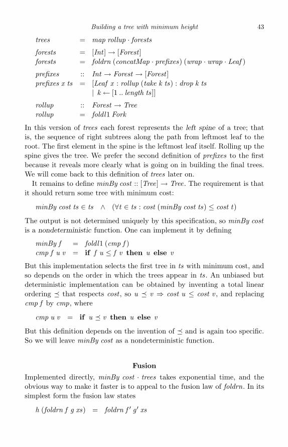
Building a tree with minimum height 43
trees = map rollup · forestsforests = [Int ] → [Forest ]forests = foldrn (concatMap · prefixes) (wrap · wrap · Leaf )
prefixes :: Int → Forest → [Forest ]prefixes x ts = [Leaf x : rollup (take k ts) : drop k ts
| k ← [1 .. length ts]]
rollup :: Forest → Treerollup = foldl1 Fork
In this version of trees each forest represents the left spine of a tree; thatis, the sequence of right subtrees along the path from leftmost leaf to theroot. The first element in the spine is the leftmost leaf itself. Rolling up thespine gives the tree. We prefer the second definition of prefixes to the firstbecause it reveals more clearly what is going on in building the final trees.We will come back to this definition of trees later on.
It remains to define minBy cost :: [Tree]→ Tree. The requirement is thatit should return some tree with minimum cost:
minBy cost ts ∈ ts ∧ (∀t ∈ ts : cost (minBy cost ts) ≤ cost t)
The output is not determined uniquely by this specification, so minBy costis a nondeterministic function. One can implement it by defining
minBy f = foldl1 (cmp f )cmp f u v = if f u ≤ f v then u else v
But this implementation selects the first tree in ts with minimum cost, andso depends on the order in which the trees appear in ts. An unbiased butdeterministic implementation can be obtained by inventing a total linearordering � that respects cost , so u � v ⇒ cost u ≤ cost v , and replacingcmp f by cmp, where
cmp u v = if u � v then u else v
But this definition depends on the invention of � and is again too specific.So we will leave minBy cost as a nondeterministic function.
Fusion
Implemented directly, minBy cost · trees takes exponential time, and theobvious way to make it faster is to appeal to the fusion law of foldrn. In itssimplest form the fusion law states
h (foldrn f g xs) = foldrn f ′ g ′ xs
44 Pearls of Functional Algorithm Design
for all finite nonempty lists xs provided h (g x ) = g ′x and h (f x y) = f ′x (h y)for all x and y . However, asking for equality of both terms when h is anondeterministic function is unreasonable: we need only that the right-handterm is a refinement of the left-hand one. Suppose we define f x � g x tomean that the set of possible outputs of f x includes the (nonempty) set ofpossible outputs of g x . In particular, if g is a normal deterministic function,then f x � g x means that g x is a possible output of f x . A weaker statementof fusion is that
h (foldrn f g xs) � foldrn f ′ g ′ xs
for all finite nonempty lists xs provided h (g x ) � g ′ x for all x , and h y � y ′
implies h (f x y) � f ′ x y ′ for all x , y and y ′.Since minBy cost · wrap = id , we obtain on appeal to fusion that
minBy cost (foldrn (concatMap · prefixes) (wrap · Leaf ) xs)� foldrn insert Leaf xs
provided a function insert can be defined to satisfy the fusion condition
minBy cost ts � t
⇒ minBy cost (concatMap (prefixes x ) ts) � insert x t (7.1)
Suppose we specify insert by the condition
minBy cost · prefixes x � insert x
In words, insert x t returns some minimum cost tree in prefixes x t . Thenwe claim that (7.1) holds if the following does:
minBy cost ts � t
⇒ minBy cost (map (insert x ) ts) � insert x t (7.2)
For the proof we need the fact that
minBy cost · concat = minBy cost ·map minBy cost
over nonempty lists of nonempty lists. In words, every possible result ofthe left-hand side is a possible result of the right-hand side and vice versa.Now we argue
minBy cost (concatMap (prefixes x ) ts)
= {expanding concatMap}minBy cost (concat (map (prefixes x ) ts))

Building a tree with minimum height 45
= {above fact}minBy cost (map (minBy cost · prefixes x ) ts)
� {since f � f ′ implies map f � map f ′ and g · f � g · f ′}minBy cost (map (insert x ) ts)
The fusion condition (7.2) holds provided that
cost u ≤ cost v ⇒ cost (insert x u) ≤ cost (insert x v) (7.3)
for all trees u and v with the same fringe. However (7.3) does not hold.Consider the trees u and v given by
10
9
5
6 7
9
10
8
7
5 6
7
9
In each tree the left spines have been labelled with cost information, so thecost of both trees is 10. Inserting 8 into the left tree u gives a tree withminimum cost 11, but inserting 8 into the right tree v gives a tree with cost10. So (7.3) fails.
But notice that the costs [10, 8, 7, 5] reading downwards along the leftspine of v are lexicographically less than the costs [10, 9, 5] along the leftspine of u. What we can establish is the monotonicity condition
cost ′ u ≤ cost ′ v ⇒ cost ′ (insert x u) ≤ cost ′ (insert x v) (7.4)
where
cost ′ = map cost · reverse · spine
The function spine is the inverse of rollup, so spine · rollup = id . Minimisingcost ′ also minimises cost , since xs ≤ ys ⇒ head xs ≤ head ys. As we willshow in a moment, (7.4) implies that
minBy cost ′ ·map(insert x ) � insert x ·minBy cost ′
Since spines have appeared on the scene it is sensible to make use of thedefinition of trees in terms of spines and summarise the calculation so far inthe following way:
minBy cost · trees� {refinement}
46 Pearls of Functional Algorithm Design
minBy cost ′ · trees= {definition of trees in terms of forests}
minBy cost ′ ·map rollup ·foldrn (concatMap · prefixes) (wrap · wrap · Leaf )
= {defining costs = map cost · reverse}minBy (costs · spine) ·map rollup ·foldrn (concatMap · prefixes) (wrap · wrap · Leaf )
= {claim: see below}rollup ·minBy costs ·foldrn (concatMap · prefixes) (wrap · wrap · Leaf )
� {fusion, with minBy costs · prefixes x � insert x}rollup · foldrn insert (wrap · Leaf )
The claim is that
minBy (costs · spine) ·map rollup = rollup ·minBy costs
This follows from the definition of minBy and the fact that spine and rollupare each other’s inverse.
It remains to implement insert , to show that (7.4) holds and to prove thatit leads to a linear-time program.
Optimal insertion
Consider the two trees of Figure 7.1. The tree on the left has spine ts, wherets = [t1, t2, . . . , tn ]. The one on the right has spine Leaf x : rollup (take j ts) :drop j ts. Each spine is also labelled with cost information: ck is defined for2 ≤ k ≤ n by
ck = 1 + (ck−1 max cost tk )
and c1 is the value at the leaf t1. A similar equation defines c′k for k in therange j+1 ≤ k ≤ n. Note that c′j > cj and c′k ≥ ck for j+1 ≤ k ≤ n.Bearing (7.4) in mind, we want to choose some j in the range 1 ≤ j ≤ nthat minimises
[c′n , c′n−1, . . . , c′j+1, c
′j , x ]
We claim that the minimum is obtained by choosing j to be the smallestvalue in the range 1 ≤ j < n, if it exists, such that
1 + (x max cj ) < cj+1 (7.5)
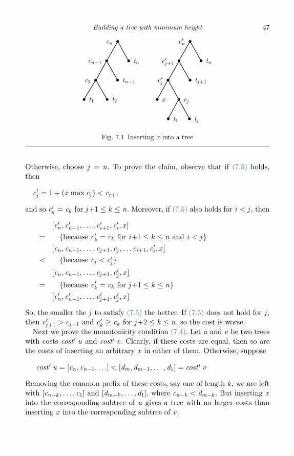
Building a tree with minimum height 47
cn
cn−1
c2
t1 t2
tn−1
tn
c′n
c′j+1
c′j
x cj
t1 tj
tj+1
tn
Fig. 7.1 Inserting x into a tree
Otherwise, choose j = n. To prove the claim, observe that if (7.5) holds,then
c′j = 1 + (x max cj ) < cj+1
and so c′k = ck for j+1 ≤ k ≤ n. Moreover, if (7.5) also holds for i < j , then
[c′n , c′n−1, . . . , c′i+1, c
′i , x ]
= {because c′k = ck for i+1 ≤ k ≤ n and i < j}[cn , cn−1, . . . , cj+1, cj , . . . ci+1, c′i , x ]
< {because cj < c′j }[cn , cn−1, . . . , cj+1, c′j , x ]
= {because c′k = ck for j+1 ≤ k ≤ n}[c′n , c′n−1, . . . , c
′j+1, c
′j , x ]
So, the smaller the j to satisfy (7.5) the better. If (7.5) does not hold for j ,then c′j+1 > cj+1 and c′k ≥ ck for j+2 ≤ k ≤ n, so the cost is worse.
Next we prove the monotonicity condition (7.4). Let u and v be two treeswith costs cost ′ u and cost ′ v . Clearly, if these costs are equal, then so arethe costs of inserting an arbitrary x in either of them. Otherwise, suppose
cost ′ u = [cn , cn−1, . . .] < [dm , dm−1, . . . , d1] = cost ′ v
Removing the common prefix of these costs, say one of length k , we are leftwith [cn−k , . . . , c1] and [dm−k , . . . , d1], where cn−k < dm−k . But inserting xinto the corresponding subtree of u gives a tree with no larger costs thaninserting x into the corresponding subtree of v .

48 Pearls of Functional Algorithm Design
Finally, since (7.5) is equivalent to x maxcj < cost tj+1, we can implementinsert by
insert x ts = Leaf x : split x tssplit x [u] = [u]split x (u : v : ts) = if x max cost u < cost v then u : v : ts
else split x (Fork u v : ts)
Cost computations can be eliminated by a simple data refinement in whicheach tree t is represented by a pair (cost t , t), leading to the final algorithm
mincostTree = foldl1 Fork ·map snd · foldrn insert (wrap · leaf )insert x ts = leaf x : split x tssplit x [u] = [u]split x (u : v : ts) = if x max fst u < fst v then u : v : ts
else split x (fork u v : ts)leaf x = (x ,Leaf x )fork (a, u) (b, v) = (1 + a max b,Fork u v)
The smart constructors leaf and fork each construct a pair consisting of acost and a tree.
It remains to time the program, which we can do by counting the calls tosplit . By induction we prove that foldrn insert (wrap · leaf ) applied to a listof length n and returning a forest of length m involves at most 2n −m callsto split . The base case, n = 1 and m = 1, is obvious. For the induction step,note that split applied to a list of length m ′ and returning a list of lengthm is called m ′ −m times. And since 2(n − 1)−m ′ + m ′ −m + 1 ≤ 2n −m,the induction is established. Hence the algorithm takes linear time.
Final remarks
The minimum-cost tree problem and its derivation is an exercise inconstructing a greedy algorithm. Greedy algorithms are tricky, not so muchbecause the final algorithm is opaque, but because of the delicate reasoningrequired to prove that they work. First, one usually has to invent astrengthening of the cost function and to minimise that at each step. Here,the monotonicity condition (7.4) is crucial to the success of the enterprise.Second, in dealing with most optimisation problems there is a need to bringrelations, or nondeterministic functions, into the derivation. The outcomeof the derivation is not equivalent to the initial specification, but a refine-ment of it. Our treatment of relations has been “light touch”, and reliedon Haskell-like notation for carrying the derivation forward. In Bird and

Building a tree with minimum height 49
de Moor (1997), the treatment of relations and their use in program deriva-tion is made much more systematic.
Finally, it is worth mentioning that another way to solve the minimum-cost tree problem is by using, the Hu–Tucker (or the more modern version,the Garsia–Wachs) algorithm; see Hu (1982) or Knuth (1998). The Hu–Tucker algorithm applies because cost is a regular cost function in the senseof Hu (1982). But the best implementation of that algorithm has a runningtime of Θ(n log n).
ReferencesBird, R. S. and de Moor, O. (1997). Algebra of Programming. Hemel Hempstead:
Prentice Hall.Hu, T. C. (1982). Combinatorial Algorithms. Reading, MA: Addison-Wesley.Knuth, D. E. (1998). The Art of Computer Programming, Volume 3: Searching
and Sorting, second edition. Reading, MA: Addison-Wesley.

8
Unravelling greedy algorithms
Make you to ravel all this matter out.Hamlet, Act 3, Scene 4
Introduction
As we said in the previous pearl, greedy algorithms are tricky things. Sothe subject deserves a second example. Here is another problem that canbe solved by a greedy algorithm, and the path to the solution has much incommon with the previous one.
An unravel1 of a sequence xs is a bag of nonempty subsequences of xsthat when shuffled together can give back xs. For example, the letters of“accompany” can be unravelled into three lists: “acm”, “an” and “copy”.The order of these lists is not important, but duplications do matter; forexample, “peptet” can be unravelled into two copies of “pet”. Thus, anunravel is essentially a bag of sequences, not a set or a list.
An unravel is called an upravel if all its component sequences are weaklyincreasing. Since each of “acm”, “an” and “copy” is increasing, they give anupravel of “accompany”, and so do “aany”, “ccmp” and “o”. Each nonemptysequence has at least one upravel, namely the upravel consisting of justsingleton sequences. However, of all possible upravels, we want to determineone with shortest size.
Specification
Here is the specification of the function supravel (short for shortest upravel):
supravel :: Ord a ⇒ [a]→ [[a]]supravel = minBy length · filter (all up) · unravels
1 By the way, “to unravel” and “to ravel” mean the same thing, just as “to unloose” and “toloose”. The prefix “un-” serves both to negate an action and to emphasize it.
50

Unravelling greedy algorithms 51
We represent the bag of sequences in a shortest upravel by a list. The func-tion minBy f is the non-deterministic function introduced in the previouspearl and specified by
minBy f xs ∈ xs ∧ (∀x ∈ xs : f (minBy f xs) ≤ f x )
The predicate up, whose definition is omitted, determines whether itsargument is in ascending order. The function unravels returns all unravelsof a sequence and can be defined inductively by
unravels :: [a]→ [[[a]]]unravels = foldr (concatMap · prefixes) [[ ]]prefixes x [ ] = [[[x ]]]prefixes x (xs : xss) = [(x : xs) : xss] ++ map (xs :) (prefixes x xss)
The function prefixes x adds x as a new first element to an unravel byprefixing it in all possible ways to each sequence in the unravel.
Derivation
The first step is to employ the fusion law of foldr to fuse filter (all up) andunravels. Define upravels by
upravels = filter (all up) · unravels
An easy application of the fusion law of foldr gives the following definitionof upravels:
upravels :: Ord a ⇒ [a]→ [[[a]]]upravels = foldr (concatMap · uprefixes) [[ ]]uprefixes x [ ] = [[[x ]]]uprefixes x (xs : xss) = if x ≤ head xs then
[(x : xs) : xss] ++ map (xs :) (uprefixes x xss)else map (xs :) (uprefixes x xss)
Here, uprefixes x adds x as a new first element to an unravel by prefixing itin all possible ways to each sequence in the unravel whose first element is atleast x .
Now we have arrived at the nub of the problem, which is how to fuseminBy length with upravels. Recall from the previous pearl the meaningof the refinement relation �: for non-deterministic function f and normaldeterministic function g we have that f � g if for all x the result of g x isa possible result of f x . Suppose the function insert is specified by
minBy length · uprefixes x � insert x
52 Pearls of Functional Algorithm Design
Thus, insert x ur returns some shortest possible way of inserting x intothe upravel ur . By appealing to the weaker fusion law of foldr in terms ofrefinement rather than equality, we then obtain
minBy length (upravels xs) � foldr insert [ ] xs
for all finite lists xs, provided the fusion condition
minBy length urs � ur⇒ minBy length (map (insert x ) urs) � insert x ur
holds for all upravels urs of a list. And, in turn, the fusion condition holds if
length ur ≤ length vr
⇒ length (insert x ur) ≤ length (insert x vr) (8.1)
for any two upravels ur and vr of the same list.Unfortunately, (8.1) does not hold. Take the two equal-length upravels
[“ad”, “a”] and [“aa”, “d”] of “ada”. Inserting “c” in the first upravel givesthe best possible upravel [“ad”, “a”, “c”], but [“aa”, “cd”] is a better upravelof the second.
The conclusion is that, just as in the problem of finding a minimum costtree, we have to strengthen the cost function being minimised. It is fairlyclear that the length of insert x ur depends only on x and the first elementof each sequence in ur . Suppose we define heads by
heads :: Ord a ⇒ [[a]]→ [a]heads = sort ·map head
Informally, the larger (lexicographically speaking) that heads ur is, the morelikely it is that x can be prefixed to some sequence in ur , thereby ensuringinsert x ur is no longer than ur . The problem with replacing minBy lengthby maxBy heads is that
heads ur ≥ heads vr �⇒ length ur ≤ length vr
even for upravels ur and vr of the same sequence. So, we need somethingelse.
One way out is to abandon the lexicographic ordering and consider insteadthe partial preorder �, defined by
ur � vr = heads ur � heads yr
where [x1, x2, . . . , xm ] � [y1, y2, . . . , yn ] if m ≤ n and xj ≥ yj for all j in therange 1 ≤ j ≤ n. Thus, ur � vr if length ur ≤ length vr and the elements

Unravelling greedy algorithms 53
of heads ur are pointwise no smaller than those of heads vr . Since � clearlyrespects length, we can replace minBy length by minWith (�), where
minWith (�) urs ∈ urs and (∀ur ∈ urs : minWith (�) urs � ur)
and establish the monotonicity condition
ur � vr ⇒ insert x ur � insert x vr (8.2)
where insert x is some refinement of minWith (�) · uprefixes x . Condition(8.2) then gives
minWith (�) · upravels � foldr insert [ ]
However, there is a slight technical difficulty with partial orderings: ingeneral there is no guarantee that minimum, as distinct from minimal, ele-ments exist. An element is minimum if it is smaller than all other candidates,but minimal only if there is no candidate smaller than it. For example,the set {{a, b}, {a, c}, {a, b, c}} has no minimum elements under ⊆, buttwo minimal elements, namely {a, b} and {a, c}. So we have to check thatminWith (�)(upravels xs) is inhabited. But this is easily proved by inductionon xs, given that minWith (�) · uprefixes x � insert x and (8.2).
Let us next show how to construct insert x . Suppose
heads ur = [x1, x2, . . . , xm ]
so xi ≤ xj for 1 ≤ i ≤ j ≤ m. Define k by the condition xk < x ≤ xk+1,where we can set xm+1 =∞. Then
heads (uprefixes x ur) = map ([x1, x2, . . . , xk , x ]++) xss
where xss are the lists
[xk+2, xk+3, . . . , xm ][xk+1, xk+3, . . . , xm ]· · ·[xk+1, xk+2, . . . , xm−1][xk+1, xk+2, . . . , xm−1, xm ]
Of these, the first list is pointwise largest (though not necessarily the onlyone that is) and hence a minimum under �. In words, we can minimise �by prefixing x to a sequence whose first element is the shortest one greaterthan or equal to x . In fact we can define insert by
insert x [ ] = [[x ]]insert x (xs : xss) = if x ≤ head xs then (x : xs) : xss
else xs : insert x xss

54 Pearls of Functional Algorithm Design
It is an invariant on insert x ur that map head ur is in strictly increasingorder. Hence the best way to insert x is by prefixing x to the first sequencein ur whose head is at least x . The definition of insert x ur takes lineartime in the length of ur , but the complexity can be reduced to logarithmictime either by representing upravels as arrays of lists and employing binarysearch, or by making use of balanced trees. We omit further details and justclaim that foldr insert [ ] can be implemented to run in O(n log n) steps.
Let us now turn to the proof of (8.2). Let heads ur = [x1, x2, . . . , xm ] andheads vr = [y1, y2, . . . , yn ], so m ≤ n and yi ≤ xi for 1 ≤ i ≤ m. As we sawabove:
heads (insert x ur) = [x1, x2, . . . , xk , x , xk+2, xk+3, . . . , xm ]heads (insert x vr) = [y1, y2, . . . , y�, x , x�+2, x�+3, . . . , yn ]
where xk < x ≤ xk+1 and y� < x ≤ y�+1. But yk ≤ xk , so k ≤ �. Lining upthe two lists, as in
[x1, x2, . . . , xk , x , xk+2, . . . , x�, x�+1, x�+2, . . . , xm ][y1, y2, . . . , yk , yk+1, yk+2, . . . , y�, x , y�+2, . . . , ym ]
we see that the first is pointwise larger than the second because yk+1 ≤ xand x ≤ xl+1.
In summary, the problem of computing the shortest upravel of a givenlist can be solved by a greedy algorithm that takes O(n log n) steps in thelength of the list.
Final remarks
The problem of the shortest upravel was first posed and solved by LambertMeertens in September 1984, at a meeting of IFIP Working Group 2.1 inPont-a-Mousson, France (Meertens, 1984). Subsequently, Kaldewaij (1985)published a quite different solution. Kaldewaij’s (one-page!) solution wasbased on a constructive proof of a specialisation of Dilworth’s theorem: thesize of a shortest upravel of xs is equal to the length of the longest decreasingsubsequence of xs. This fact can be combined with a well-known algorithmfor finding the length of a longest decreasing subsequence in O(n log n)steps to produce an algorithm for the shortest upravel with the same timecomplexity. The present pearl is based on Bird (1992), which also considersanother greedy algorithm that starts off with the following definition ofunravels:
unravels [ ] = [[ ]]unravels xs = [ys : yss | ys ← subseqs xs, not (null ys),
yss ← unravels (xs \\ ys)]
Unravelling greedy algorithms 55
A shortest upravel can then obtained by extracting the rightmost maximal
upsequence at each stage, computed by rmu = foldr op [ ], where
op x [ ] = [x ]op x (y : ys) = if x ≤ y then x : y : ys else y : ys
The derivation of the alternative algorithm is left as an exercise.
ReferencesBird, R. S. (1992). The smallest upravel. Science of Computer Programming 18,
281–92.Kaldewaij, A. (1985). On the decomposition of sequences into ascending sub-
sequences. Information Processing Letters 21, 69.Meertens, L. G. L. T. (1984). Some more examples of algorithmic developments.
IFIP WG2.1 Working Paper, Pont-a-Mousson, France. See also An AbstractoReader prepared for IFIP WG 2.1. Technical Report CWI Note CS-N8702,Centrum voor Wiskunde en Informatica, April 1987.

9
Finding celebrities
The setting is a tutorial on functional algorithm design. There are fourstudents: Anne, Jack, Mary and Theo.
Teacher: Good morning class. Today I would like you to solve the followingproblem. Imagine a set P of people at a party. Say a subset C of P formsa celebrity clique if C is nonempty, everybody at the party knows everymember of C , but members of C know only each other. Assuming there issuch a clique at the party, your problem is to write a functional program forfinding it. As data for the problem you are given a binary predicate knowsand the set P as a list ps not containing duplicates.
Jack: Just to be clear, does every member of a celebrity clique actuallyknow everyone else in the clique? And does everyone know themselves?
Teacher: As to the first question, yes, it follows from the definition:everyone in the clique is known by everyone at the party. As to the secondquestion, the answer is not really relevant to the problem, so ask a philo-sopher. If it simplifies things to assume that x knows x for all x , then goahead and do so.
Theo: This is going to be a hard problem, isn’t it? I mean, the problem ofdetermining whether there is a clique of size k in a party of n people willtake Ω(nk ) steps, so we are looking at an exponential time algorithm.
Anne: That doesn’t follow, since being a celebrity clique is a much strongerproperty than being a clique. In a directed graph, a clique is a set of nodesin which each pair of nodes has an arc in both directions between them,but a celebrity clique also requires an arc from every node in the graph toevery node in the clique, and no arcs from the clique to nodes outside theclique.
56
Finding celebrities 57
Mary: Yes, while there can be many cliques in a graph, there is at mostone celebrity clique. Suppose that C1 and C2 are two celebrity cliques.Pick any c1 in C1 and c2 in C2. We have that c1 knows c2 from the factthat everybody in the clique C2 is known by everybody at the party. Butsince clique members know only other members of the clique, it followsthat c2 ∈ C1. Since c2 was arbitrary, we have C2 ⊆ C1 and, by symmetry,C1 ⊆ C2.
Theo: Agreed, they are different problems. Let me formalise the problem.To simplify matters I am going to suppose that x knows x is true for all x .By definition C is a celebrity clique of P if ∅ ⊂ C ⊆ P and
(∀x ∈ P , y ∈ C :: x knows y ∧ (y knows x ⇒ x ∈ C ))
Let me abbreviate this last condition to C � P . Given lists ps and cs rep-resenting P and C respectively, we can translate the condition into a listcomprehension:
cs � ps = and [x knows y ∧ (y knows x ⇒ x ∈ cs) | x ← ps, y ← cs]
Now define cclique ps = head (filter (�ps) (subseqs ps)), where subseqs ps isa list of all subsequences of ps:
subseqs [ ] = [[ ]]subseqs (x : xs) = map (x :) (subseqs xs) ++ subseqs xs
Since subseqs ps generates subsequences in descending order of length, thevalue of cclique ps is either the empty list if there is no celebrity clique, orthe unique celebrity clique.
Jack: Theo’s exhaustive search program seems a reasonable place to startI would say. Clearly, the way to achieve greater efficiency is to fuse thefiltering with the generation of subsequences. For the base case when thereare no people at the party we have filter (� [ ]) (subseqs [ ]) = [[ ]] sincecs � [ ] = True. For the inductive case we can reason
filter (�(p : ps)) (subseqs (p : ps))
= {definition of subseqs}filter (� (p : ps)) (map (p:) (subseqs ps) ++ subseqs ps)
= {since filter distributes over ++}filter (� (p : ps)) (map (p:) (subseqs ps)) ++filter (� (p : ps)) (subseqs ps)
What next?

58 Pearls of Functional Algorithm Design
Anne: We have to simplify (p : cs) � (p : ps) and cs � (p : ps) when cs is asubsequence of ps and p is not in cs. Let us deal with the second case first.The definition of � gives that cs�(p :ps) just in the case that cs�ps, that nocelebrity in cs knows p and that p knows every celebrity in cs. In symbols:
cs � (p : ps) = cs � ps ∧ nonmember p cs
where
nonmember p cs = and [p knows c ∧ not (c knows p) | c← cs]
Now we can reason
filter (� (p : ps)) (subseqs ps)
= {above simplification of cs � (p : ps)}filter (λcs → cs � ps ∧ nonmember p cs) (subseqs ps)
= {since filter (λx → p x ∧ q x ) = filter q · filter p}filter (nonmember p) (filter (�ps) (subseqs ps))
Now for the other case. We have that (p : cs)� (p : ps) holds just in the casethat cs � ps, and p is a new celebrity, meaning that everyone knows p andp knows all and only members of cs. In symbols:
(p : cs) � (p : ps) = cs � ps ∧member p ps cs
where
member p ps cs = and [x knows p ∧ (p knows x ⇔ x ∈ cs) | x ← ps]
A similar calculation to the one above now gives
filter (� (p : ps)) (map (p:) (subseqs ps))= map (p:) (filter (member p ps) (filter (�ps) (subseqs ps)))
Putting the two pieces together, we have cclique = head · ccliques, where
ccliques [ ] = [[ ]]ccliques (p : ps) = map (p:) (filter (member p ps) css) ++
filter (nonmember p) csswhere css = ccliques ps
The predicates member and nonmember can be evaluated in linear time and,as ccliques returns at most two lists, a proper celebrity clique and an emptylist, we have reduced an exponential algorithm to a quadratic one.
Finding celebrities 59
Theo: Well, you can’t do better than a quadratic algorithm, at least in theworst case. Suppose there was a sub-quadratic one, so at least one entry inthe knows matrix is not inspected. Suppose, furthermore, that all entries aretrue, so everyone knows everyone else and the celebrity clique is the wholeparty. Now change the non-inspected entry, knows x y say, to false. Then yis no longer a celebrity. But everyone apart from x still knows y , so theycannot be celebrities. That leaves x as the only possible celebrity; but unlessx and y are the only people at the party, there is some non-celebrity that xknows, so x is not a celebrity either. That means there is no celebrity cliqueat the modified party, and the sub-quadratic algorithm returns the wronganswer. So, in the worst case, every element of the knows matrix has to beinspected to arrive at the correct answer.
Teacher: Very good, Theo, and quite correct, but the problem was not todetermine whether or not there was a celebrity clique. All I asked for was toidentify a celebrity clique assuming one exists. In your scenario the answerps will suffice for both cases: in the first case it is the correct answer and inthe second case there is no celebrity clique, so any answer will do.
There is a pause while the class digests this information.
Mary: I have an idea. Anne’s reasoning shows that for all xs
xs � (p : ps) ⇒ (xs \\ [p]) � ps
where \\ denotes list difference. In other words, if cs � ps and p is someonenew who joins the party ps, then the only possible values of xs satisfyingxs � (p : ps) are [ ], [p], cs, or p : cs. I think this gives us another way ofsolving the problem. Suppose first that cs is empty, so the only possiblecelebrity clique of p : ps is [p]. In symbols:
null (cclique ps) ⇒ cclique (p : ps) ∈ {[ ], [p]}
On the other hand, suppose cs is not empty and contains some celebrityc. What are the possible outcomes when a new person p joins the party?Well, assume first that p does not know c. Then c is no longer a celebrityin the extended party, and neither is any other member of cs because theyall know c. Hence
c ∈ cclique ps ∧ not (p knows c) ⇒ cclique (p : ps)) ∈ {[ ], [p]}

60 Pearls of Functional Algorithm Design
Assume next that p does know c but c does not know p. In this case cs isalso the celebrity clique of the extended party:
c ∈ cclique ps ∧ p knows c ∧ not (c knows p)⇒ cclique (p : ps) = cclique ps
Finally, if p and c know each other, then the only celebrity clique of p : psis p : cs; in symbols:
c ∈ cclique ps ∧ p knows c ∧ c knows p⇒ cclique (p : ps) ∈ {[ ], p : cs}
Theo: While I agree that your reasoning is correct, Mary, I do not see howit leads to a solution. All you have shown is that if we know the value ofcclique ps and if the party p : ps contains a celebrity clique, then we canquickly determine it. But how do we know the value of cclique ps in the firstplace? You seem to be suggesting that if we define cclique ′ by
cclique ′ = foldr op [ ]op p cs | null cs = [p]
| not (p knows c) = [p]| not (c knows p) = cs| otherwise = p : cs
where c = head cs
then
not (null (cclique ps)) ⇒ cclique ps = cclique ′ ps (9.1)
But I don’t see how your reasoning proves (9.1).
Mary: Let me try again then. I will prove (9.1) by induction on ps. Thereare two cases:Case [ ]. We have cclique [ ] = [ ], so (9.1) is true by default.Case p : ps. Assume cclique (p : ps) is not empty. There are two subcases,depending on whether cclique ps is empty or not. If not, then cclique ps =cclique ′ ps by induction. We then have
cclique (p : ps)
= {my previous reasoning and definition of op}op p (cclique ps)
= {since cclique ps = cclique ′ ps}op p (cclique ′ ps)
= {definition of cclique ′}cclique ′ (p : ps)
Finding celebrities 61
If, on the other hand, cclique ps is empty, then
cclique (p : ps)
= {assumption that cclique (p : ps) is not empty,and first case of my previous reasoning}
[p]
= {p is the unique celebrity,so not (p knows c) for any c ∈ cclique ′ ps}
op p (cclique ′ ps)
= {as before}cclique ′ (p : ps)
This establishes the case and the induction.
Anne: That’s amazing, a simple linear-time algorithm! But we have onlyarrived at the solution because of Mary’s cleverness. I still want a formalderivation of cclique ′ from some suitable fusion law.
Teacher: Thank you, Anne, it’s good to have you in the class.
Anne: We can write subseqs using foldr :
subseqs = foldr add [[ ]]add x xss = map (x :) xss ++ xss
So it appears that we are appealing to some fusion law of foldr . The textbookstatement of the fusion law for foldr states that f · foldr g a = foldr h b pro-vided f is strict, f a = b, and f (gx y) = hx (f y) for all x and y . The strictnesscondition is not needed if we want only to assert that f (foldr g a xs) =foldr h b xs for all finite lists xs. This fusion rule does not apply directly tothe celebrity clique problem, namely filter (�ps) (subseqs ps), first becausefilter (�ps) has ps as a parameter and second because we want somethingmore general than the equality of both sides.
Theo: The first restriction is not really a problem. We can always define aversion of subseqs that returns both the subsequences of a list and the listitself. Suppose we define
subseqs ′ = foldr step ([ ], [[ ]])step x (xs, xss) = (x : xs,map (x :) xss ++ xss)
Then cclique = f ·subseqs ′, where f (ps, css) = head (filter (�ps)css). In thisway the additional parameter is eliminated.
62 Pearls of Functional Algorithm Design
Mary: The textbook statement of the fusion rule is not general enough forthe problem. Let � be some relation on values; I don’t care what. Then itis easy to show by induction that
f (foldr g a xs) � foldr h b xs
for all finite lists xs provided f a � b and f y � z ⇒ f (g x y) � h x z forall x , y and z .
Jack: Yes, that’s it. We want to define xs � ys by
xs � ys = not (null xs) ⇒ xs = ys
Then the conditions we have to establish are first that
head (filter (� [ ]) [[ ]]) � [ ]
and second that
head (filter (� ps) css) � cs⇒ head (filter (�(p : ps))(map (p:) css ++ css)) � op p cs
Mary’s reasoning establishes exactly these conditions.
Teacher: Yes. The more general statement of fusion is the one provided byparametricity in Wadler’s (1989) “Theorems for free!” paper. It is nice to seean example where the more general statement is needed. What is interestingabout the problem is that it is the first example I have seen in which it isasymptotically more efficient to find a solution assuming one exists thanto check that it actually is a solution. A similar problem is the majority
voting problem – see, for example, Morgan (1994), Chapter 18 – in whichone is given a list xs and it is required to determine whether there is a valuein xs that occurs strictly greater than �length xs/2� times. It is easier tofirst compute a putative majority and then check whether it is actually amajority afterwards. But checking for a majority takes linear time ratherthan quadratic time, so there is no asymptotic gap.
Afterword
The true story of the celebrity clique problem was as follows. I was givinga course of lectures on Formal Program Design, in an imperative ratherthan functional framework, and thought of the problem as a generalisationof the one in Kaldewaij’s (1990) book. But despite a day of struggling withloop invariants, I could not produce a sufficiently simple solution to presentto the class, so I set it as a challenge. I also talked about it at a research
Finding celebrities 63
meeting the following Friday. Over the weekend, Sharon Curtis produced asimple linear-time algorithm and Julian Tibble, a second-year undergradu-ate, provided a good way to reason about the problem.
In the belief that whatever can be done with loops and invariants can alsobe done at least as easily using the laws of functional program derivation, theproblem was translated into a functional setting and the dialogue above wascomposed. Afterwards, the problem was tried out at a WG2.1 meeting inNottingham in September, 2004. Gratifyingly, the actual discussion followedthe early part of the dialogue quite closely. On repeatedly being urged totry harder, Andres Loh and Johan Jeuring came up a day later with thelinear-time solution.
ReferencesKaldewaij, A. (1990). Programming the Derivation of Algorithms. Hemel
Hempstead: Prentice Hall.Morgan, C. (1994). Programming from Specifications, 2nd edition. Hemel
Hempstead: Prentice Hall.Wadler, P. (1989). Theorems for free! Fourth International Symposium on
Functional Programming Languages and Computer Architecture. ACMPress, pp. 347–59.

10
Removing duplicates
Introduction
The Haskell library function nub removes duplicates from a list:
nub :: Eq a ⇒ [a]→ [a]nub [ ] = [ ]nub (x : xs) = x : nub (xs \\ [x ])
The value xs \\ys is what remains of xs after all the elements in ys have beendeleted. For example, nub “calculus” = “calus”. Evaluation of nub on a listof length n takes Θ(n2) steps. This is the best one can hope for, since anyalgorithm for the problem requires Ω(n2) equality tests in the worst case.With the definition above, nub xs returns a list of the distinct elements inxs in the order in which they first appear in xs. In other words, the positionof nub xs as a subsequence of xs is lexicographically the least among thepositions of all possible solutions.
Let us now change the problem and ask that nub :: Ord a ⇒ [a] → [a]simply returns the lexicographically least solution. Note the subtle differ-ence: before it was the position of the subsequence that was lexicographi-cally the least; now it is the subsequence itself. For example, nub“calculus” =“aclus” under the second definition. The change of type of nub is necessaryto make the new problem meaningful. Changing the type of nub changesthe lower bound complexity: only Ω(n log n) comparison tests are needed inthe worst case. A pretty proof of this claim is given by Bloom and Wright(2003). Can we find an Θ(n log n) program for the new version of nub? Theanswer turns out to be yes, but the algorithm is not obvious and calculatingit requires some work. So, be prepared.
A first version
We begin with the specification
nub = minimum · longest · filter nodups · subseqs
64
Removing duplicates 65
In words, compute all possible subsequences of the given list (subseqs),filter this list of subsequences for just those that do not contain duplicates(filter nodups), compute all the longest ones (longest) and finally select thesmallest one (minimum).
It is not too difficult to calculate the following recursive definition of nubfrom the specification:
nub [ ] = [ ]nub (x : xs) = if x /∈ xs then x : nub xs else
(x : nub (xs \\ [x ])) min (nub xs)
We omit the details, leaving them as an exercise for the interested reader.Anyway, the recursive version is reasonably intuitive: in the case x :xs, eitherx does not appear in xs, so there is no choice, or it does, in which case theresult is the smaller of two alternatives, choosing x now or later on.
The problem with the recursive definition of nub is that it can take expo-nential time because the number of recursive calls can double at each step.We therefore have some work to do in reaching an Θ(n log n) algorithm.
A generalisation
The first thought, given the target time complexity, is a divide and conqueralgorithm, seeking a function join for which
nub (xs ++ ys) = join (nub xs) (nub ys) (10.1)
But no such function can exist. For instance, (10.1) requires
join “bca” “c” = join (nub “bca”) (nub “c”) = nub “bcac” = “bac”
But also (10.1) requires
join “bca” “c” = join (nub “bcab”) (nub “c”) = nub “bcabc” = “abc”
This example also shows that nub cannot be expressed as an instance offoldl . It is also easy to construct an example to show that nub cannot beexpressed as an instance of foldr .
We therefore need some generalisation of nub. To see what it might be,consider a list of the form x : y : xs with x ∈ xs and y ∈ xs and x �= y .Unfolding the definition of nub(x :y :xs), and exploiting both the associativityof min and the fact that (x :) distributes through min, we find

66 Pearls of Functional Algorithm Design
nub (x : y : xs) = x : y : nub (xs \\ [x , y ]) minx : nub (xs \\ [x ])) miny : nub (xs \\ [y ]) minnub xs
Now suppose that x < y , so the second term is lexicographically smallerthan the third. That means the third term can be dropped:
nub (x : y : xs) = x : y : nub (xs \\ [x , y ]) minx : nub (xs \\ [x ])) minnub xs
If, on the other hand, x > y , then the first two terms can be dropped:
nub (x : y : xs) = y : nub (xs \\ [y ]) minnub xs
The forms of these two expressions suggest our generalisation, which we willcall hub. To help keep expressions reasonably short, abbreviate minimum tomin in all that follows. The definition of hub is
hub ws xs = min [is ++ nub (xs \\ is) | is ← inits ws] (10.2)
where ws is a list in strictly increasing order. The standard function initsreturns a list of all the initial segments, or prefixes, of a list. The exampleabove now reads
nub (x : y : xs) = if x < y then hub [x , y ] xs else hub [y ] xs
The function hub generalises nub, for inits [ ] = [[ ]] and xs \\ [ ] = xs, sonub xs = hub [ ] xs. Two other immediate facts about hub are that hub ws xsbegins with a prefix of ws, and that hub ws xs ≤ nub xs since the empty listis a prefix of every list.
The aim now is to derive an inductive definition of hub. For the base casewe reason
hub ws [ ]
= {definition}min [is ++ nub ([ ] \\ is) | is ← inits ws]
= {since [ ] \\ is = [ ] and nub [ ] = [ ]}min [is | is ← inits ws]
= {since [ ] is the lexicographically least list in inits ws}[ ]
Removing duplicates 67
Hence hub ws [ ] = [ ]. For the inductive case, (10.2) gives
hub ws (x : xs) = min [is ++ nub ((x : xs) \\ is) | is ← inits ws] (10.3)
To simplify the right-hand side we need to know whether or not x ∈ ws, sowe start by splitting ws into two lists, us and vs, defined by
(us, vs) = (takeWhile (< x ) ws, dropWhile (< x ) ws)
More briefly, (us, vs) = span (< x ) ws, where span is a standard Haskelllibrary function. Since ws = us ++ vs and ws is in increasing order, both usand vs are also in increasing order. Moreover, if x ∈ ws, then x = head vs;if not, then either vs is empty or x < head vs.
The following property of inits is key to the simplification of (10.3):
inits (us ++ vs) = inits us ++ map (us++) (inits+ vs) (10.4)
where inits+ vs returns the list of nonempty prefixes of vs. Using thisexpression for inits in (10.3) and splitting the comprehension into two parts,we obtain that hub ws (x : xs) = A min B , where
A = min [is++nub ((x : xs) \\ is) | is ← inits us] (10.5)
B = min [us++is++nub ((x : xs) \\ (us++is)) | is ← inits+ vs] (10.6)
To discover A min B we deal with A first, distinguishing the two cases x /∈ xsand x ∈ xs. In the first case, x /∈ xs, we argue:
A
= {definition (10.5)}min [is ++ nub ((x : xs) \\ is) | is ← inits us]
= {recursive definition of nub since x /∈ xs and x /∈ us}min [is ++ [x ] ++ nub (xs \\ is) | is ← inits us]
= {since us < is ++ [x ] for is ∈ inits us}us ++ [x ] ++ nub (xs \\ us)
= {since nub xs = hub [ ] xs}us ++ [x ] ++ hub [ ] (xs \\ us)
In the second case, x ∈ xs, we argue:
A
= {recursive definition of nub since x ∈ xs and x /∈ us}min [is ++ ([x ] ++ nub (xs \\ (is ++ [x ])) min nub (xs \\ is))
| is ← inits us]

68 Pearls of Functional Algorithm Design
= {taking min outside the comprehension}min [is ++ [x ] ++ nub (xs \\ (is ++ [x ])) | is ← inits us] minmin [is ++ nub (xs \\ is) | is ← inits us]
= {since us < is ++ [x ] for is ∈ inits us}(us ++ [x ] ++ nub (xs \\ (us ++ [x ]))) minmin [is ++ nub (xs \\ is) | is ← inits us]
= {since inits (us ++ [x ]) = inits us ++ [us ++ [x ]]}min [is ++ nub (xs \\ is) | is ← inits (us ++ [x ])]
= {definition (10.2)}hub (us ++ [x ]) xs
Summarising, A equals
if x ∈ xs then hub (us++[x ]) xs else us++[x ]++hub [ ] (xs \\ us)
Now we turn to B . According to (10.6), if vs is empty (so inits+vs is empty),then B is the fictitious value min [ ]. Otherwise, we reason:
B
= {definition (10.6)}min [us++is++nub ((x : xs) \\ (us++is)) | is ← inits+ (v : vs ′)]
= {since inits+ (v : vs ′) = map (v :) (inits vs ′)}min [us++[v ]++is++nub ((x : xs) \\ (us++[v ]++is)) | is ← inits vs ′]
= {since min ·map (ys++) = (ys++) ·min}us++[v ]++min [is++nub ((x : xs) \\ (us++[v ]++is)) | is ← inits vs ′]
In particular, B begins with us ++ [v ]. Without going further we now haveenough information to determine hub ws (x : xs) in the case x /∈ ws. In thiscase, either vs is empty, so A < B , or vs is not empty and begins with vwhere x < v . In the latter situation we again have A < B because A beginswith a prefix of us ++ [x ] and us ++ [x ] < us ++ [v ]. Hence
x /∈ ws ⇒ hub ws (x : xs) = A
It remains to deal with the case x ∈ ws, so x = v . In this case B simplifies to
us++[x ]++min [is++nub (xs \\ (us++[x ]++is)) | is ← inits vs ′]
Now we need a final case analysis. Assume first that x /∈ xs. We calculate:
B
= {above}us++[x ]++min [is++nub (xs \\ (us++[x ]++is)) | is ← inits vs ′]
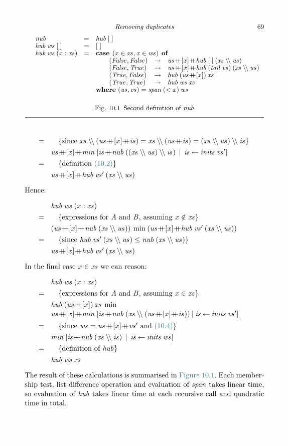
Removing duplicates 69
nub = hub [ ]hub ws [ ] = [ ]hub ws (x : xs) = case (x ∈ xs, x ∈ ws) of
(False,False) → us++[x ]++hub [ ] (xs \\ us)(False,True) → us++[x ]++hub (tail vs) (xs \\ us)(True,False) → hub (us++[x ]) xs(True,True) → hub ws xs
where (us, vs) = span (< x ) ws
Fig. 10.1 Second definition of nub
= {since xs \\ (us++[x ]++is) = xs \\ (us++is) = (xs \\ us) \\ is}us++[x ]++min [is++nub ((xs \\ us) \\ is) | is ← inits vs ′]
= {definition (10.2)}us++[x ]++hub vs ′ (xs \\ us)
Hence:
hub ws (x : xs)
= {expressions for A and B , assuming x /∈ xs}(us++[x ]++nub (xs \\ us)) min (us++[x ]++hub vs ′ (xs \\ us))
= {since hub vs ′ (xs \\ us) ≤ nub (xs \\ us)}us++[x ]++hub vs ′ (xs \\ us)
In the final case x ∈ xs we can reason:
hub ws (x : xs)
= {expressions for A and B , assuming x ∈ xs}hub (us++[x ]) xs minus++[x ]++min [is++nub (xs \\ (us++[x ]++is)) | is ← inits vs ′]
= {since ws = us++[x ]++vs ′ and (10.4)}min [is++nub (xs \\ is) | is ← inits ws]
= {definition of hub}hub ws xs
The result of these calculations is summarised in Figure 10.1. Each member-ship test, list difference operation and evaluation of span takes linear time,so evaluation of hub takes linear time at each recursive call and quadratictime in total.

70 Pearls of Functional Algorithm Design
Introducing sets
The final step is to introduce an efficient representation of sets to reduce thecomplexity of the subsidiary operations from linear to logarithmic. Ratherthan program the set operations ourselves, we can invoke the Haskelllibrary Data.Set . This library provides a data type Set a and the followingoperations (among others):
empty :: Set amember :: Ord a ⇒ a → Set a → Boolinsert :: Ord a ⇒ a → Set a → Set asplit :: Ord a ⇒ a → Set a → (Set a,Set a)elems :: Ord a ⇒ Set a → [a]
The value empty denotes the empty set, member is the membership test,insert x xs inserts a new element x into the set xs, while split x splits a setinto those elements less than x and those greater than x , and elems returnsthe elements of a set in increasing order. As to the costs, empty takes con-stant time, member , insert and split take O(log n) steps on a set of size n,while elems takes O(n) steps.
In order to introduce sets into the definition of nub we need a preprocessingphase that associates with each element x of xs the set of elements that comeafter it. That is, we need to compute
(x1, {x2, x3, . . . xn}), (x2, {x3, . . . , xn}), . . . (xn , {})
This list can be computed using the Haskell function scanr :
preprocess :: Ord a ⇒ [a]→ [(a,Set a)]preprocess xs = zip xs (tail (scanr insert empty xs))
The expression scanr insert empty [x1, x2, . . . xn ] returns the list
[{x1, x2, . . . , xn}, {x2, . . . , xn}, . . . , {xn}, {}]
and takes O(n log n) steps to do so.The result of installing sets in Figure 10.1 is given in Figure 10.2. Unfor-
tunately, its running time is not O(n log n). To see why, let us estimate thecosts of the various operations. Each membership test contributes O(log n)steps to the cost at each recursive call. So does split . Let m be the size ofus. Since elems takes O(m) steps, as does concatenating the result with therest of the list, and there are at most n elements in the final list, the totalcontribution of elems and ++ to the final cost is O(n) steps. However, the

Removing duplicates 71
nub = hub empty · preprocesspreprocess xs = zip xs (tail (scanr insert empty xs))hub ws [ ] = [ ]hub ws ((x , xs) : xss) =
case (member x xs,member x ws) of(False,False) → eus++[x ]++hub empty yss(False,True) → eus++[x ]++hub vs yss(True,False) → hub (insert x us) xss(True,True) → hub ws xss
where (us, vs) = split x wseus = elems usyss = [(x , xs) | (x , xs)← xss,not (member x us)]
Fig. 10.2 Introducing sets
cost of computing yss is Ω(n log m) steps at each call, and summing thiscost gives Ω(n2) steps. As a specific example, consider the input
[1 .. n] ++ [j | j ← [1 .. n], j mod 3 �= 0]
The output is [1 .. n]. Each multiple of 3 causes the program to flush twoelements from the set ws, namely [1, 2], [4, 5], [7, 8] and so on, and the totalcost of computing yss is quadratic in n.
One way to solve this problem is to introduce an additional argument psinto hub, defining hub ′ by
hub ′ :: Set a → Set a → [(a,Set a)] → [a]hub′ ps ws xss = hub ws [(x , xs) | (x , xs)← xss, x /∈ ps]
Then we obtain the program of Figure 10.3. The cost of computing qs isO(m log n), where m is the size of us, rather than the O(n log m) cost ofcomputing yss in the previous version. Since the combined size of the setsus for which this operation is performed is at most n, the total running timeis O(n log n) steps.
Final remarks
It was quite a lot of work to achieve the result, and the final algorithm isneither pretty nor intuitive. A nagging doubt remains that there might bea much simpler solution to such a simply stated problem. But so far I havenot been able to find one. The main calculation turned out to be quiteintricate and bedevilled by case analysis. Nevertheless, the battle plan iscommon enough: obtain a recursive formulation of the problem and then
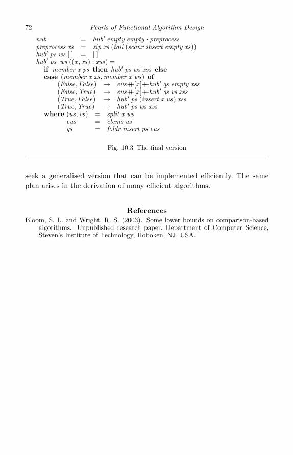
72 Pearls of Functional Algorithm Design
nub = hub′ empty empty · preprocesspreprocess xs = zip xs (tail (scanr insert empty xs))hub′ ps ws [ ] = [ ]hub′ ps ws ((x , xs) : xss) =
if member x ps then hub′ ps ws xss elsecase (member x xs,member x ws) of
(False,False) → eus++[x ]++hub′ qs empty xss(False,True) → eus++[x ]++hub′ qs vs xss(True,False) → hub′ ps (insert x us) xss(True,True) → hub′ ps ws xss
where (us, vs) = split x wseus = elems usqs = foldr insert ps eus
Fig. 10.3 The final version
seek a generalised version that can be implemented efficiently. The sameplan arises in the derivation of many efficient algorithms.
ReferencesBloom, S. L. and Wright, R. S. (2003). Some lower bounds on comparison-based
algorithms. Unpublished research paper. Department of Computer Science,Steven’s Institute of Technology, Hoboken, NJ, USA.
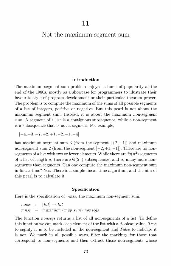
11
Not the maximum segment sum
Introduction
The maximum segment sum problem enjoyed a burst of popularity at theend of the 1980s, mostly as a showcase for programmers to illustrate theirfavourite style of program development or their particular theorem prover.The problem is to compute the maximum of the sums of all possible segmentsof a list of integers, positive or negative. But this pearl is not about themaximum segment sum. Instead, it is about the maximum non-segment
sum. A segment of a list is a contiguous subsequence, while a non-segmentis a subsequence that is not a segment. For example,
[−4,−3,−7, +2, +1,−2,−1,−4]
has maximum segment sum 3 (from the segment [+2, +1]) and maximumnon-segment sum 2 (from the non-segment [+2, +1,−1]). There are no non-segments of a list with two or fewer elements. While there are Θ(n2) segmentsof a list of length n, there are Θ(2n) subsequences, and so many more non-segments than segments. Can one compute the maximum non-segment sumin linear time? Yes. There is a simple linear-time algorithm, and the aim ofthis pearl is to calculate it.
Specification
Here is the specification of mnss, the maximum non-segment sum:
mnss :: [Int ] → Intmnss = maximum ·map sum · nonsegs
The function nonsegs returns a list of all non-segments of a list. To definethis function we can mark each element of the list with a Boolean value: Trueto signify it is to be included in the non-segment and False to indicate itis not. We mark in all possible ways, filter the markings for those thatcorrespond to non-segments and then extract those non-segments whose
73
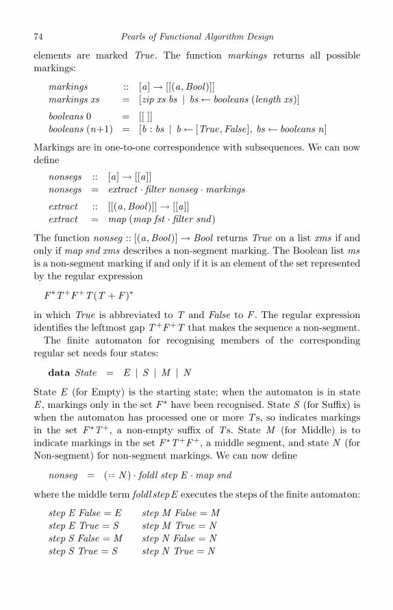
74 Pearls of Functional Algorithm Design
elements are marked True. The function markings returns all possiblemarkings:
markings :: [a]→ [[(a,Bool)]]markings xs = [zip xs bs | bs ← booleans (length xs)]
booleans 0 = [[ ]]booleans (n+1) = [b : bs | b ← [True,False], bs ← booleans n]
Markings are in one-to-one correspondence with subsequences. We can nowdefine
nonsegs :: [a]→ [[a]]nonsegs = extract · filter nonseg ·markings
extract :: [[(a,Bool)]]→ [[a]]extract = map (map fst · filter snd)
The function nonseg :: [(a,Bool)] → Bool returns True on a list xms if andonly if map snd xms describes a non-segment marking. The Boolean list msis a non-segment marking if and only if it is an element of the set representedby the regular expression
F ∗T+F+T (T + F )∗
in which True is abbreviated to T and False to F . The regular expressionidentifies the leftmost gap T+F+T that makes the sequence a non-segment.
The finite automaton for recognising members of the correspondingregular set needs four states:
data State = E | S | M | N
State E (for Empty) is the starting state; when the automaton is in stateE , markings only in the set F ∗ have been recognised. State S (for Suffix) iswhen the automaton has processed one or more T s, so indicates markingsin the set F ∗T+, a non-empty suffix of T s. State M (for Middle) is toindicate markings in the set F ∗T+F+, a middle segment, and state N (forNon-segment) for non-segment markings. We can now define
nonseg = ( N ) · foldl step E ·map snd
where the middle term foldl stepE executes the steps of the finite automaton:
step E False = E step M False = Mstep E True = S step M True = Nstep S False = M step N False = Nstep S True = S step N True = N
Not the maximum segment sum 75
Finite automata process their input from left to right, which explains the useof foldl . We could equally as well have processed lists from right to left, andlooked for the rightmost gap, but why break with convention unnecessarily?Notice also that there is nothing special here about the nonseg property:any property of markings that can be recognised by a finite-state automatonyields to exactly the same treatment.
Derivation
Here is the definition of mnss again:
mnss = maximum ·map sum · extract · filter nonseg ·markingsextract = map (map fst · filter snd)nonseg = ( N ) · foldl step E ·map snd
Our plan of attack is to express extract · filter nonseg ·markings as an inst-ance of foldl and then to apply the fusion law of foldl to complete the passageto a better algorithm. To this end, define pick by
pick :: State → [a]→ [[a]]pick q = extract · filter (( q) · foldl step E ·map snd) ·markings
In particular, nonsegs = pickN . We claim that the following seven equationshold:
pick E xs = [[ ]]pick S [ ] = [ ]pick S (xs ++ [x ]) = map (++[x ]) (pick S xs ++ pick E xs)pick M [ ] = [ ]pick M (xs ++ [x ]) = pick M xs ++ pick S xspick N [ ] = [ ]pick N (xs ++ [x ]) = pick N xs ++
map (++[x ]) (pick N xs ++ pick M xs)
The pukka way to derive these equations is through due process of calcu-lation from the definition of pick q , but the steps are tedious and we willnot bother. Instead, each equation can be justified by appeal to step. Forexample, the equation for pick E is justified because step returns E only onempty subsequences. Similarly for pick S , because step returns S only whenx is marked True and preceded either by an element of pick E or pick S . Theother definitions can be justified in a similar way. Again, there is nothingspecific to non-segments: any finite automaton with k states that recog-nises correct markings can be systematically transformed into essentially kfunctions that operate directly on the given input.
76 Pearls of Functional Algorithm Design
The next step is to recast the definition of pick as an instance of foldl .Consider the function pickall , specified by
pickall xs = (pick E xs, pick S xs, pick M xs, pick N xs)
The following definition of pickall as an instance of foldl follows from thedefinitions above:
pickall = foldl step ([[ ]], [ ], [ ], [ ])step (ess,nss,mss, sss) x = (ess,
map (++[x ]) (sss ++ ess),mss ++ sss,nss ++ map (++[x ]) (nss ++ mss))
Our problem now takes the form
mnss = maximum ·map sum · fourth · pickall
where fourth returns the fourth element of a quadruple. We can move thefourth to the front of the expression on the right by introducing
tuple f (w , x , y , z ) = (f w , f x , f y , f z )
Then we have
maximum ·map sum · fourth = fourth · tuple (maximum ·map sum)
so mnss = fourth · tuple (maximum ·map sum) · pickall .As hoped for, we are now in a position to apply the fusion law of foldl .
This law states that f (foldl g a xs) = foldl h b xs for all finite lists xs providedthat f a = b and f (g x y) = h (f x ) y for all x and y . In our problem wehave the instantiations
f = tuple (maximum ·map sum)g = stepa = ([[ ]], [ ], [ ], [ ])
It remains to find h and b to satisfy the fusion conditions. First:
tuple (maximum ·map sum) ([[ ]], [ ], [ ], [ ]) = (0,−∞,−∞,−∞)
because the maximum of an empty set of numbers is −∞. This gives thedefinition of b. For h we need to satisfy the equation
tuple (maximum ·map sum) (step (ess, sss,mss,nss) x )= h (tuple (maximum ·map sum) (ess, sss,mss,nss)) x
Not the maximum segment sum 77
To derive h we look at each component in turn. To keep expressions short,abbreviate maximum to max . For the fourth component we reason:
max (map sum (nss ++ map (++[x ]) (nss ++ mss)))
= {definition of map}max (map sum nss ++ map (sum · (++[x ])) (nss ++ mss))
= {since sum · (++[x ]) = (+x ) · sum}max (map sum nss ++ map ((+x ) · sum) (nss ++ mss))
= {since max (xs ++ ys) = (max xs) max (max ys)}max (map sum nss) max max (map ((+x ) · sum) (nss ++ mss))
= {since max ·map (+x ) = (+x ) ·max}max (map sum nss) max (max (map sum (nss ++ mss)) + x )
= {introducing n = max (map sum nss) andm = max (map sum mss)}
n max ((n max m) + x )
The other three components are treated similarly, and we arrive at
h (e, s,m,n) x= (e, (s max e) + x ,m max s,n max ((n max m) + x ))
and mnss = fourth · foldl h (0,−∞,−∞,−∞).That, basically, is it. Well, we still have to deal with the fictitious −∞
values. Perhaps the best method is to eliminate them entirely by consideringthe first three elements of the list separately:
mnss xs = fourth (foldl h (start (take 3 xs)) (drop 3 xs))start [x , y , z ] = (0,max [x+y+z , y+z , z ],max [x , x+y , y ], x+z )
Not quite as pretty, but more effective.
Final remarks
The origins of the maximum segment sum problem go back to about 1975,and its history is described in one of Bentley’s (1987) programming pearls.For a derivation using invariant assertions, see Gries (1990); for an algebraicapproach, see Bird (1989). The problem refuses to go away, and variations arestill an active topic for algorithm designers because of potential applicationsin data-mining and bioinformatics; see Mu (2008) for recent results.
The interest in the non-segment problem is what it tells us about anymaximum marking problem in which the marking criterion can be formulated
78 Pearls of Functional Algorithm Design
as a regular expression. For instance, it is immediate that there is an O(nk)algorithm for computing the maximum at-least-length-k segment problembecause F ∗TnF ∗ (n ≥ k) can be recognised by a k -state automaton.And even non-regular conditions such as F ∗TnF ∗TnF ∗ (n ≥ 0), whoserecogniser requires an unbounded number of states, is susceptible to thesame method. What is more, the restriction to lists is not necessary either;one can solve maximum marking problems about a whole variety of datatypes in a similar way.
ReferencesBentley, J. R. (1987). Programming Pearls. Reading, MA: Addison-Wesley.Bird, R. S. (1989). Algebraic identities for program calculation. Computer Journal
32 (2), 122–6.Gries, D. (1990). The maximum segment sum problem. In Formal Development of
Programs and Proofs, ed. E. W. Dijkstra et al. University of Texas at AustinYear of Programming Series. Menlo Park. Addison-Wesley, pp. 43–5.
Mu, S.-C. (2008). The maximum segment sum is back. Partial Evaluation andProgram Manipulation (PEPM ’08), pp. 31–9.
12
Ranking suffixes
Introduction
The idea of ranking the elements of a list crops up frequently. An elementx is assigned rank r if there are exactly r elements of the list less thanx . For example, rank [51, 38, 29, 51, 63, 38] = [3, 1, 0, 3, 5, 1]. This schemeranks from 0 and from lowest to highest, but one can also rank from 1and from highest to lowest, as when ranking candidates by their marks inan examination. Rankings are distinct if and only if the list does not containduplicates, in which case rank xs is a permutation of [0 .. length xs − 1].
In this pearl we consider the problem of ranking the suffixes of a listrather than the list itself. It takes Θ(n log n) steps to rank a list of lengthn, assuming a test x < y takes constant time. Since in the worst case ittakes Θ(n) such tests to make one lexicographic comparison between twosuffixes of a list of length n, it seems that ranking the suffixes of a listshould require Θ(n2 log n) basic comparisons. The point of this pearl is toshow that only Θ(n log n) steps are necessary. Asymptotically speaking, ittakes no more time to rank the suffixes of a list than it does to rank the listitself. Surprising but true.
Specification
In Haskell the suffixes of a list are called its tails, and henceforth we willrefer to tails rather than suffixes. The function tails returns the nonempty
tails of a list in decreasing order of length:
tails :: [a]→ [[a]]tails [ ] = [ ]tails xs = xs : tails (tail xs)
This definition of tails differs from the standard Haskell function of the samename, which returns all the tails, including the empty tail. The function rankcan be specified by
79
80 Pearls of Functional Algorithm Design
rank :: Ord a ⇒ [a]→ [Int ]rank xs = map (λx → length (filter (< x ) xs)) xs
This definition takes Θ(n2) steps on a list of length n, but rank can beimproved to take Θ(n log n) steps, something we will take up later on.
The required function, ranktails say, can now be defined by
ranktails :: Ord a ⇒ [a]→ [Int ]ranktails = rank · tails
Our task is to implement ranktails to take Θ(n log n) steps.
Properties of rank
We will need various properties of rank , the most important of which is thatrank maintains order: if we know only rank xs, then we know everythingabout the relative order of the elements of xs, though nothing about thenature of the elements themselves. Suppose we define xs ≈ ys to meanrank xs = rank ys. Then xs ≈ ys if the elements in xs have the same relativeorder as the elements in ys. As two examples among many:
xs ≈ zip xs xs and zip (zip xs ys) zs ≈ zip xs (zip ys zs)
We will also need the following property of rank . Let select :: [a] → [a]be any function such that:
(i) every element in select xs is in xs;(ii) select ·map f = map f · select for any f .
Then
rank · select · rank = rank · select (12.1)
In particular, taking select = id we have rank · rank = rank , and takingselect = tail , we have rank · tail · rank = rank · tail . The proof of (12.1) isleft as an instructive exercise to the interested reader.
Finally, a useful idea associated with ranking is that of refining oneranking by another one. Suppose we define the operation �, pronounced“refined by”, by
xs � ys = rank (zip xs ys) (12.2)
For example, [3, 1, 3, 0, 1] � [2, 0, 3, 4, 0] = [2, 1, 3, 0, 1]. Thus, equal ranksin xs may be refined to distinct ranks in xs � ys. The operation � is
Ranking suffixes 81
associative. Here is the proof:
(xs � ys)� zs
= {(12.2)}rank (zip (rank (zip xs ys)) zs)
= {since zip us vs ≈ zip (rank us) vs}rank (zip (zip xs ys) zs)
= {since zip (zip xs ys) zs ≈ zip xs (zip ys zs)}rank (zip xs (zip ys zs))
= {as before}xs � (ys � zs)
Observe also that if a ranking xs consists of distinct elements, and thereforeis a permutation of [0 .. n−1], where n = length xs, then xs � ys = xs forany ys of the same length as xs. In words, once a ranking is a permutationit cannot be further refined.
A better algorithm
One obvious approach to improving the performance of ranktails, given itstarget complexity, is to look for a divide and conquer solution based on thedecomposition
tails (xs ++ ys) = map (++ys) (tails xs) ++ tails ys
But this does not seem to lead anywhere. Instead, we take another approachand first generalise ranktails to a function rats by replacing the lexicographiccomparison test (<) with (<k ), where xs <k ys = take k xs < take k ys.In other words, we rank the tails of a list by looking only at the first kelements of each tail. Define rats by
rats k = rank ·map (take k) · tails (12.3)
We have ranktails xs = rats (length xs) xs, so rats is a generalisation ofranktails. The main reason for the name rats, apart from being a compressionof both rank and tails, is that it is pronounceable and short enough to avoidlengthy expressions in calculations.
The key to the derivation of a faster algorithm for ranktails is the followingproperty of rats:
rats (2∗k) xs = rats k xs � shiftBy k (rats k xs) (12.4)

82 Pearls of Functional Algorithm Design
We will prove this, and also give the definition of shiftBy , later on. Sincexs ≈ map (take 1) (tails xs) we have rats 1 = rank . The idea is to use (12.4)to successively rank map (take 2) (tails xs), map (take 4) (tails xs) and so onuntil we reach a permutation. Thus, we propose the following algorithm forranktails:
ranktails = applyUntil isperm rerankings · rankrerankings = map rerank (iterate (∗2) 1)rerank k rs = rs � shiftBy k rs
The function applyUntil is a variant of the standard function until and isdefined by
applyUntil :: (a → Bool)→ [a → a]→ a → aapplyUntil p (f : fs) x = if p x then x else applyUntil p fs (f x )
The function isperm tests whether a ranking is a permutation and can bedefined using a Haskell array:1
isperm :: [Int ]→ Boolisperm is = and (elems
(accumArray (∨) False (0,n−1) (zip is (repeat True))))where n = length is
This definition of isperm takes linear time.In words, ranktails first ranks the elements of the input and then succes-
sively applies rerank 1, rerank 2, rerank 4 and so on until the result is apermutation. Note that it is only the very first ranking that inspects theinput; the remaining rerankings deal exclusively with ranks; that is, lists ofintegers. At worst, ranktails xs requires log n rerankings where n = length xs.Assuming rank takes Θ(n log n) steps and shiftBy takes Θ(n) steps, the newversion of ranktails takes Θ(n log2 n) steps. Better than Θ(n2 log n), but notyet at our target complexity of Θ(n log n).
Proof
Now we prove (12.4), and at the same time discover a definition of shiftBy .We are going to need a number of additional properties involving lists, tailsand rankings, the first of which is that
all (not · null) xss ⇒ xss = zipWith (:) (map head xss) (map tail xss)
1 An almost identical program was used in the pearl “The smallest free number”; see pearl 1.
Ranking suffixes 83
To reduce the parenthesis count in expressions we rewrite the consequent inthe form
id = zipWith (:) · fork (map head ,map tail) (12.5)
where fork (f , g) x = (f x , g x ) and zipWith (:) is quietly assumed to benon-curried. Proofs of this and other properties are omitted.
We start by calculating
rats (k+1)
= {(12.3)}rank ·map (take (k+1)) · tails
= {(12.5) since all (not · null) ·map (take (k+1)) · tails}rank · zipWith (:) · fork (map head ,map tail) ·map (take (k+1)) · tails
Now, fork (f , g) · h = fork (f · h, g · h) and
map head ·map (take (k+1)) · tails = idmap tail ·map (take (k+1)) · tails = snoc [ ] · tail ·map (take k) · tails
where snoc x xs = xs ++ [x ]. Hence we can continue:
rank · zipWith (:) · fork (map head ,map tail) ·map (take (k+1)) · tails
= {above}rank · zipWith (:) · fork (id , snoc [ ] · tail ·map (take k) · tails)
The next step is to see that zipWith (:) xs xss ≈ zip xs xss, or, more briefly,zipWith (:) ≈ zip, where zip is also quietly assumed to be non-curried. Hencewe obtain
rats (k+1) = rank · zip · fork (id , snoc [ ] · tail ·map (take k) · tails)
Now rank · zip = (�) by (12.2). And since xs � ys = xs � rank ys, thatgets us to
rats (k+1) = (�) · fork (id , rank · snoc [ ] · tail ·map (take k) · tails)
Now rank · snoc [ ] = lift · rank , where lift = snoc 0 ·map (+1), so
rats (k+1) = (�) · fork (id , lift · rank · tail ·map (take k) · tails)
Next we claim that lift · rank · tail ≈ lift · tail · rank . Here is the proof:
lift (rank (tail xs)) ≈ lift (tail (rank xs))
84 Pearls of Functional Algorithm Design
⇐ {since xs ≈ ys implies lift xs ≈ lift ys}rank (tail xs) ≈ tail (rank xs)
≡ {definition of ≈}rank (rank (tail xs)) = rank (tail (rank xs))
⇐ {using (12.1) twice, once for subseq = idand once for subseq = tail}
true
Hence rats (k+1) = (�) · fork (id , lift · tail · rats k). Equivalently:
rats (k+1) xs = rank xs � shift (rats k xs) (12.6)
where shift = lift · tail and lift is = map (+1) is ++ [0].The next step is to exploit the fact that
shift (is � js) = shift is � shift js
and the associativity of �. Then we obtain from (12.6) that
rats k xs = rs � shift rs � shift2 rs � · · · � shiftk−1 rs
where rs = rank xs and shiftk is the k -fold composition of shift with itself.It is now easy to group terms in this series expansion for rats to obtain
rats (2∗k) xs = rats k xs � shiftk (rats k xs)
Finally, we can set shiftBy k = shiftk to establish (12.4). In fact, we have
shiftBy k rs = map (+k) (drop k rs) ++ [k−1, k−2 .. 0]
Evaluation of shiftBy k rs takes Θ(n) steps where n = length rs.
A better rank
We turn next to a better method for computing rank . As every examinerknows, the way to rank a list of candidate–mark pairs, given in candidateorder, is first to partition the candidates by sorting them according to theirmarks, and placing candidates with equal marks into groups. Then eachcandidate in the first group receives rank 0, each candidate in the secondgroup receives rank g0, where g0 is the size of the first group, each candidatein the third group receives rank g0 + g1, where g1 is the size of the secondgroup, and so on. The result is then resorted in the original candidate order.This method is formalised by
rank = resort · concat · label · psort · zip [0..]
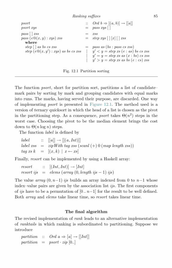
Ranking suffixes 85
psort :: Ord b ⇒ [(a, b)] → [[a]]psort xys = pass xys [ ]
pass [ ] xss = xsspass (e@(x , y) : xys) xss = step xys [ ] [x ] [ ] xss
wherestep [ ] as bs cs xss = pass as (bs : pass cs xss)step (e@(x , y ′) : xys) as bs cs xss | y ′ < y = step xs (e : as) bs cs xss
| y ′ = y = step xs as (x : bs) cs xss| y ′ > y = step xs as bs (e : cs) xss
Fig. 12.1 Partition sorting
The function psort , short for partition sort, partitions a list of candidate–mark pairs by sorting by mark and grouping candidates with equal marksinto runs. The marks, having served their purpose, are discarded. One wayof implementing psort is presented in Figure 12.1. The method used is aversion of ternary quicksort in which the head of a list is chosen as the pivotin the partitioning step. As a consequence, psort takes Θ(n2) steps in theworst case. Choosing the pivot to be the median element brings the costdown to Θ(n log n) steps.
The function label is defined by
label :: [[a]]→ [[(a, Int)]]label xss = zipWith tag xss (scanl (+) 0 (map length xss))tag xs k = [(x , k) | x ← xs]
Finally, resort can be implemented by using a Haskell array:
resort :: [(Int , Int)] → [Int ]resort ijs = elems (array (0, length ijs − 1) ijs)
The value array (0,n−1) ijs builds an array indexed from 0 to n−1 whoseindex–value pairs are given by the association list ijs. The first componentsof ijs have to be a permutation of [0 ..n−1] for the result to be well defined.Both array and elems take linear time, so resort takes linear time.
The final algorithm
The revised implementation of rank leads to an alternative implementationof ranktails in which ranking is subordinated to partitioning. Suppose weintroduce
partition :: Ord a ⇒ [a]→ [[Int ]]partition = psort · zip [0..]
86 Pearls of Functional Algorithm Design
Then rank = resort · concat · label · partition. Furthermore, � can beexpressed in terms of partition because it is expressed in terms of rank .That means we can regroup terms and express ranktails in terms of partitionrather than rank . One advantage of doing so is that rank returns a permuta-tion if and only if partition returns a list all of whose elements are singletons,so isperm can be replaced by all single, where single determines whether itsargument is a singleton list. Installing these changes leads to
ranktails = resort · concat · label ·applyUntil (all single) repartitions · partition
repartitions = map repartition (iterate (∗2) 1)repartition k iss = partition(zip rs (shiftBy k rs))
where rs = resort (concat (label iss))
This version has the same time complexity as the previous one, but it opensup the route for further optimisation. In fact, we are now just two stepsaway from our goal of a Θ(n log n) algorithm for ranktails.
The first of these is to make use of the identity
partition (zip xs ys)
= concatMap (psort ·map (install ys)) (partition xs) (12.7)
where
install ys i = (i , ys !! i) (12.8)
In words, one can partition a list of pairs by first partitioning with respectto first components and refining the result using the second components.The correct second components can be installed in each run because eachrun is a list of positions. After installation, each run is partition sorted andthe results concatenated.
To be accurate, (12.7) holds only if psort is a stable sorting algorithmand the implementation in Figure 12.1 is not stable. If psort is not stablethen the elements in each run will appear in a different order in the left-and right-hand sides. But (12.7) does hold if we interpret equality of twopartitions to mean equal up to some permutation of the elements in eachrun. Since the computation of ranktails does not depend on the precise orderof the elements in a run, that is all that is required.
We are now ready to rewrite repartition:
repartition k iss
= {definition, setting rs = resort (concat (label iss))}partition(zip rs (shiftBy k rs))

Ranking suffixes 87
= {(12.7)}concatMap (psort ·map (install (shiftBy k rs))) (partition rs)
= {since iss = partition xs implies rs = rank xsand partition · rank = partition}
concatMap (psort ·map (install (shiftBy k rs))) iss
Hence
repartition k iss = concatMap (psort ·map (install rs)) isswhere rs = shiftBy k (resort (concat (label iss)))
We are nearly there, but (12.8) gives an inefficient way of computing installbecause it uses list-indexing (!!) which is not constant time. Better is touse array-indexing (!) which does take constant time. The final step is torewrite install :
(shiftBy k (resort (concat (label iss)))) !! i
= {definition of shiftBy}(map (+k) (drop k (resort (concat (label iss)))) ++[k−1, k−2 .. 0]) !! i
= {arithmetic, with n = length(concat (label iss)) and j = i+k}if j < n then k + (resort (concat (label iss))) !! j else n−i−1
= {definition of resort and elems a !! i = a ! i}if j < n then k + array (0,n−1) (concat (label iss)))) ! jelse n−i−1
The final program for ranktails is recorded in Figure 12.2. The length of theinput is computed once and passed to the various subsidiary functions thatneed it.
Analysis
It remains to time ranktails. We will do this by estimating the total numberof comparisons T (n, k) required to carry out k repartitions on a list oflength n. The key to the analysis is to appreciate that the computation ofranktails is essentially the same as partition sorting a list of n vectors, eachof dimension k , by sorting on each dimension in turn. The first componentsof these vectors consist of the elements of the input, but each subsequentcomponent is an integer which is determined dynamically from the result ofsorting with respect to previous components. Unlike the implementation ofpsort given in Figure 12.1 we will suppose that each partition step chooses
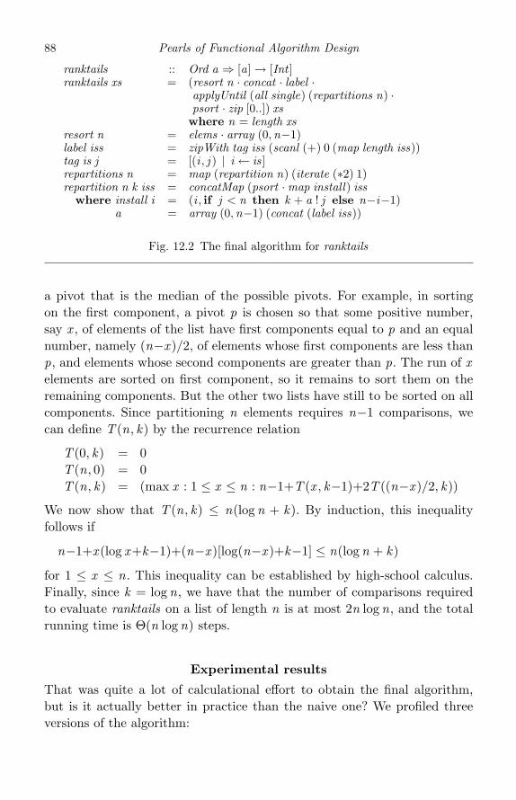
88 Pearls of Functional Algorithm Design
ranktails :: Ord a ⇒ [a] → [Int ]ranktails xs = (resort n · concat · label ·
applyUntil (all single) (repartitions n) ·psort · zip [0..]) xswhere n = length xs
resort n = elems · array (0,n−1)label iss = zipWith tag iss (scanl (+) 0 (map length iss))tag is j = [(i , j ) | i ← is]repartitions n = map (repartition n) (iterate (∗2) 1)repartition n k iss = concatMap (psort ·map install) iss
where install i = (i , if j < n then k + a ! j else n−i−1)a = array (0,n−1) (concat (label iss))
Fig. 12.2 The final algorithm for ranktails
a pivot that is the median of the possible pivots. For example, in sortingon the first component, a pivot p is chosen so that some positive number,say x , of elements of the list have first components equal to p and an equalnumber, namely (n−x )/2, of elements whose first components are less thanp, and elements whose second components are greater than p. The run of xelements are sorted on first component, so it remains to sort them on theremaining components. But the other two lists have still to be sorted on allcomponents. Since partitioning n elements requires n−1 comparisons, wecan define T (n, k) by the recurrence relation
T (0, k) = 0T (n, 0) = 0T (n, k) = (max x : 1 ≤ x ≤ n : n−1+T (x , k−1)+2T ((n−x )/2, k))
We now show that T (n, k) ≤ n(log n + k). By induction, this inequalityfollows if
n−1+x (log x+k−1)+(n−x )[log(n−x )+k−1] ≤ n(log n + k)
for 1 ≤ x ≤ n. This inequality can be established by high-school calculus.Finally, since k = log n, we have that the number of comparisons requiredto evaluate ranktails on a list of length n is at most 2n log n, and the totalrunning time is Θ(n log n) steps.
Experimental results
That was quite a lot of calculational effort to obtain the final algorithm,but is it actually better in practice than the naive one? We profiled threeversions of the algorithm:
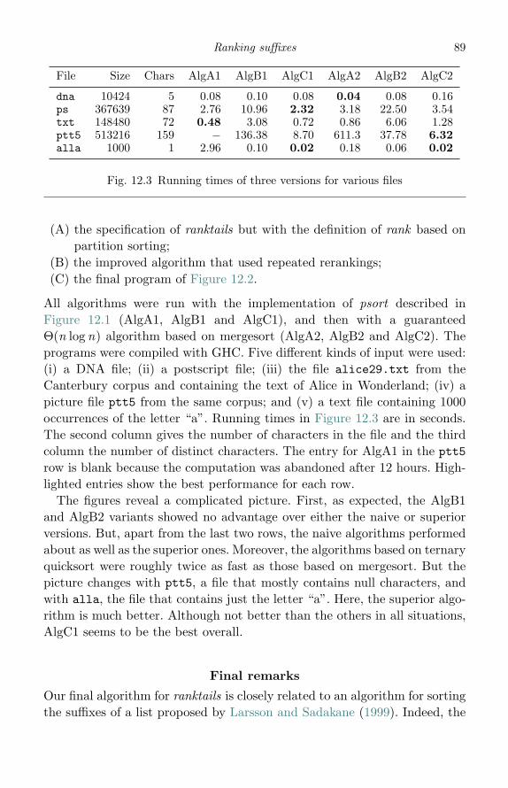
Ranking suffixes 89
File Size Chars AlgA1 AlgB1 AlgC1 AlgA2 AlgB2 AlgC2
dna 10424 5 0.08 0.10 0.08 0.04 0.08 0.16ps 367639 87 2.76 10.96 2.32 3.18 22.50 3.54txt 148480 72 0.48 3.08 0.72 0.86 6.06 1.28ptt5 513216 159 − 136.38 8.70 611.3 37.78 6.32alla 1000 1 2.96 0.10 0.02 0.18 0.06 0.02
Fig. 12.3 Running times of three versions for various files
(A) the specification of ranktails but with the definition of rank based onpartition sorting;
(B) the improved algorithm that used repeated rerankings;(C) the final program of Figure 12.2.
All algorithms were run with the implementation of psort described inFigure 12.1 (AlgA1, AlgB1 and AlgC1), and then with a guaranteedΘ(n log n) algorithm based on mergesort (AlgA2, AlgB2 and AlgC2). Theprograms were compiled with GHC. Five different kinds of input were used:(i) a DNA file; (ii) a postscript file; (iii) the file alice29.txt from theCanterbury corpus and containing the text of Alice in Wonderland; (iv) apicture file ptt5 from the same corpus; and (v) a text file containing 1000occurrences of the letter “a”. Running times in Figure 12.3 are in seconds.The second column gives the number of characters in the file and the thirdcolumn the number of distinct characters. The entry for AlgA1 in the ptt5row is blank because the computation was abandoned after 12 hours. High-lighted entries show the best performance for each row.
The figures reveal a complicated picture. First, as expected, the AlgB1and AlgB2 variants showed no advantage over either the naive or superiorversions. But, apart from the last two rows, the naive algorithms performedabout as well as the superior ones. Moreover, the algorithms based on ternaryquicksort were roughly twice as fast as those based on mergesort. But thepicture changes with ptt5, a file that mostly contains null characters, andwith alla, the file that contains just the letter “a”. Here, the superior algo-rithm is much better. Although not better than the others in all situations,AlgC1 seems to be the best overall.
Final remarks
Our final algorithm for ranktails is closely related to an algorithm for sortingthe suffixes of a list proposed by Larsson and Sadakane (1999). Indeed, the
90 Pearls of Functional Algorithm Design
whole pearl was inspired by their work. Ranking a list and sorting a list areclosely related operations and each can be computed quickly from the other.In particular, the function sorttails that returns the unique permutationthat sorts the tails of a list can be obtained from the final program forranktails simply by replacing resort ·concat · label in the first line of ranktailsby concat . The function sorttails is needed as a preliminary step in theBurrows–Wheeler algorithm for data compression, a problem we will takeup in the following pearl. The problem of sorting the suffixes of a string hasbeen treated extensively in the literature because it has other applicationsin string matching and bioinformatics; a good source is Gusfield (1997).
This pearl was rewritten a number of times. Initially we started out withthe idea of computing perm, a permutation that sorts a list. But perm is toospecific in the way it treats duplicates: there is more than one permutationthat sorts a list containing duplicate elements. One cannot get very far withperm unless one generalises to either rank or partition. We reformulated theproblem in terms of rank , but ended up with the idea of partitioning a listrather than ranking it. Nevertheless, rank entered the picture again for thefinal optimisation step.
ReferencesLarsson, N. J. and Sadakane, K. (1999). Faster suffix sorting. Research Report
LU-CS-TR-99-214, Department of Computer Science, Lund University,Sweden.
Gusfield, D. (1997). Algorithms on Strings, Trees and Sequences. Cambridge, UK:Cambridge University Press.
13
The Burrows–Wheeler transform
Introduction
The Burrows–Wheeler transform (BWT) is a method for permuting a listwith the aim of bringing repeated elements together. Its main use is as apreprocessing step in data compression. Lists with many repeated adjacentelements can be encoded compactly using simple schemes such as run lengthor move-to-front encoding. The result can then be fed into more advancedcompressors, such as Huffman or arithmetic coding,1 to compress the inputeven more.
Clearly, the best way of bringing repeated elements together is just to sortthe list. But the idea has a major flaw as a preliminary to compression: thereis no way to recover the original list unless the complete sorting permutationis also produced as part of the output. Without the ability to recover theoriginal input, data compression is pointless; and if a permutation has to beproduced as well, then compression is ineffective. Instead, the BWT achievesa more modest permutation, one that brings some but not all repeatedelements into adjacent positions. The main advantage of the BWT is thatthe transform can be inverted using a single additional piece of information,namely an integer k in the range 0 ≤ k < n, where n is the length ofthe (nonempty) input list. In this pearl we describe the BWT, identify thefundamental reason why inversion is possible, and use it to derive the inversetransform from its specification.
Defining the BWT
Applied to a list xs the BWT sorts the rotations of xs, producing a matrixof rotated lists, and then returns the last column of the sorted matrixtogether with the position of xs in the matrix. As an illustration, considerthe string yokohama. The rotations and the sorted rotations are pictured in
1 Arithmetic coding is considered in two subsequent pearls; see Pearls 24 and 25.
91
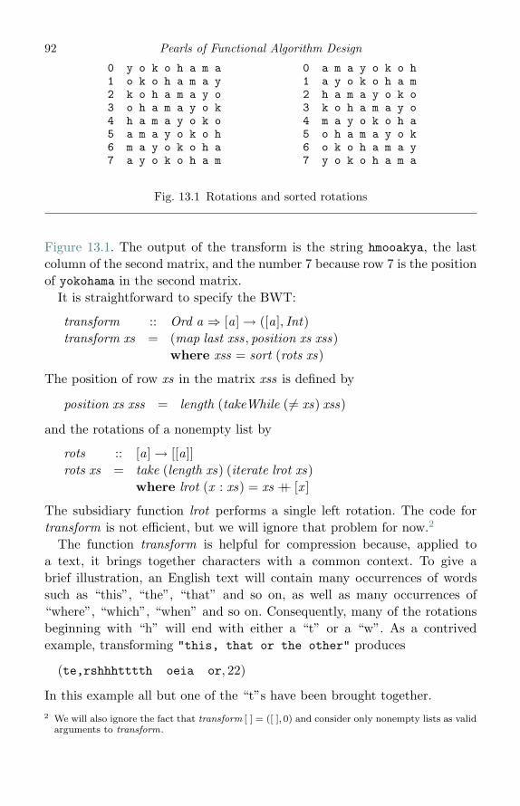
92 Pearls of Functional Algorithm Design
0 y o k o h a m a 0 a m a y o k o h1 o k o h a m a y 1 a y o k o h a m2 k o h a m a y o 2 h a m a y o k o3 o h a m a y o k 3 k o h a m a y o4 h a m a y o k o 4 m a y o k o h a5 a m a y o k o h 5 o h a m a y o k6 m a y o k o h a 6 o k o h a m a y7 a y o k o h a m 7 y o k o h a m a
Fig. 13.1 Rotations and sorted rotations
Figure 13.1. The output of the transform is the string hmooakya, the lastcolumn of the second matrix, and the number 7 because row 7 is the positionof yokohama in the second matrix.
It is straightforward to specify the BWT:
transform :: Ord a ⇒ [a]→ ([a], Int)transform xs = (map last xss, position xs xss)
where xss = sort (rots xs)
The position of row xs in the matrix xss is defined by
position xs xss = length (takeWhile (�= xs) xss)
and the rotations of a nonempty list by
rots :: [a]→ [[a]]rots xs = take (length xs) (iterate lrot xs)
where lrot (x : xs) = xs ++ [x ]
The subsidiary function lrot performs a single left rotation. The code fortransform is not efficient, but we will ignore that problem for now.2
The function transform is helpful for compression because, applied toa text, it brings together characters with a common context. To give abrief illustration, an English text will contain many occurrences of wordssuch as “this”, “the”, “that” and so on, as well as many occurrences of“where”, “which”, “when” and so on. Consequently, many of the rotationsbeginning with “h” will end with either a “t” or a “w”. As a contrivedexample, transforming "this, that or the other" produces
(te,rshhhtttth oeia or, 22)
In this example all but one of the “t”s have been brought together.2 We will also ignore the fact that transform [ ] = ([ ], 0) and consider only nonempty lists as valid
arguments to transform.
The Burrows–Wheeler transform 93
The inverse untransform :: Ord a ⇒ ([a], Int) → [a] is, naturally enough,specified (over nonempty lists) by
untransform · transform = id
The problem is how to compute untransform. The obvious method, if it canbe made to work, is to use the first component of the result of transformto recreate the sorted matrix of rotations and then to use the secondcomponent to select the appropriate row. Fleshing out the idea, supposerecreate :: Ord a ⇒ [a]→ [[a]] can be constructed to satisfy
recreate ·map last · sort · rots = sort · rots
Then we can define untransform (ys, k) = (recreate ys) !! k , where (!!) is thelist-indexing operator. But can we really recreate the whole matrix of sortedrotations simply by knowing its last column? Yes we can, and the derivationof recreate is a fascinating exercise in program calculation.
Recreational calculation
Suppose in all that follows that the input to recreate is a list of length n, sorecreate has to recreate an n × n matrix. The idea is to recreate the matrixcolumn by column. Define takeCols by
takeCols :: Int → [[a]]→ [[a]]takeCols j = map (take j )
Thus, takeCols j takes the first j columns of an n × n matrix. In particular,takeCols n is the identity function. We therefore replace recreate with thefunction recreate n, specified by the property
recreate j ·map last · sort · rots = takeCols j · sort · rots (13.1)
Thus, recreate j recreates the first j columns of the sorted matrix of rotationsfrom its last column.
The plan of attack is to construct an inductive definition of recreate. Thebase case is easy:
recreate 0 = map (const [ ])
Applied to a list ys of length n, the result of recreate 0 is a column of nempty lists. Since takeCols 0 applied to any n × n matrix also produces nempty lists, (13.1) is established for the case j = 0.
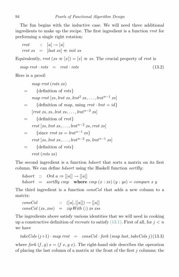
94 Pearls of Functional Algorithm Design
The fun begins with the inductive case. We will need three additionalingredients to make up the recipe. The first ingredient is a function rrot forperforming a single right rotation:
rrot :: [a]→ [a]rrot xs = [last xs] ++ init xs
Equivalently, rrot (xs ++ [x ]) = [x ] ++ xs. The crucial property of rrot is
map rrot · rots = rrot · rots (13.2)
Here is a proof:
map rrot (rots xs)
= {definition of rots}map rrot [xs, lrot xs, lrot2 xs, . . . , lrotn−1 xs]
= {definition of map, using rrot · lrot = id}[rrot xs, xs, lrot xs, . . . , lrotn−2 xs]
= {definition of rrot}rrot [xs, lrot xs, . . . , lrotn−2 xs, rrot xs]
= {since rrot xs = lrotn−1 xs}rrot [xs, lrot xs, . . . , lrotn−2 xs, lrotn−1 xs]
= {definition of rots}rrot (rots xs)
The second ingredient is a function hdsort that sorts a matrix on its firstcolumn. We can define hdsort using the Haskell function sortBy :
hdsort :: Ord a ⇒ [[a]]→ [[a]]hdsort = sortBy cmp where cmp (x : xs) (y : ys) = compare x y
The third ingredient is a function consCol that adds a new column to amatrix:
consCol :: ([a], [[a]])→ [[a]]consCol (xs, xss) = zipWith (:) xs xss
The ingredients above satisfy various identities that we will need in cookingup a constructive definition of recreate to satisfy (13.1). First of all, for j < nwe have
takeCols (j+1) ·map rrot = consCol · fork (map last , takeCols j )(13.3)
where fork (f , g) x = (f x , g x ). The right-hand side describes the operationof placing the last column of a matrix at the front of the first j columns; the
The Burrows–Wheeler transform 95
left-hand side describes the operation of performing a single right rotationon each row and then taking the first j+1 columns. The identity expressesthe fact that these two operations give the same result.
The second identity is
takeCols (j+1) · hdsort = hdsort · takeCols (j+1) (13.4)
In words, sorting an n × n matrix on its first column and then taking apositive number of columns of the result yields exactly the same result asfirst taking the same number of columns and then sorting on the first column.
The third identity, the key one, is not so obvious:
hdsort ·map rrot · sort · rots = sort · rots (13.5)
In words, the following transformation on a matrix of sorted rotations is theidentity: move the last column to the front and then resort the rows on thenew first column. In fact, (13.5) is true only if hdsort is a stable sortingalgorithm, meaning that columns with the same first element appear inthe output in the same order that they appeared in the input. Under thisassumption we have, applied to an n × n matrix, that
sort = (hdsort ·map rrot)n
This identity states that one can sort an n × n matrix (in fact, an arbitrarylist of lists all of which have length n) by repeating n times the operation ofrotating the last column into first position and then stably sorting accordingto the first column only. Since it captures essentially the operation ofradix sort, we will call it the radix sort property. It can be proved byinduction on n, but we omit details. It leads, with a little help, to the proofof (13.5):
hdsort ·map rrot · sort · rots= {radix sort property}
(hdsort ·map rrot)n+1 · rots= {composition}
(hdsort ·map rrot)n · hdsort ·map rrot · rots= {radix sort property}
sort · hdsort ·map rrot · rots= {identity (13.2)}
sort · hdsort · rrot · rots= {since sort · hdsort = sort}

96 Pearls of Functional Algorithm Design
sort · rrot · rots= {since sort · rrot = sort}
sort · rots
The two identities used in the last two steps generalise to sort · perm = sortfor any permutation perm of the input.
We are now ready to deal with recreate. Writing sr = sort ·rots for brevity,we calculate:
recreate (j+1) ·map last · sr= {specification (13.1)}
takeCols (j+1) · sr= {property (13.5)}
takeCols (j+1) · hdsort ·map rrot · sr= {property (13.4)}
hdsort · takeCols (j+1) ·map rrot · sr= {property (13.3)}
hdsort · consCol · fork (map last , takeCols j ) · sr= {specification (13.1)}
hdsort · consCol · fork (map last , recreate j ·map last) · sr= {since fork (f · h, g · h) = fork (f , g) · h}
hdsort · consCol · fork (id , recreate j ) ·map last · sr
Hence, recreate (j+1) = hdsort · consCol · fork (id , recreate j ).
A faster algorithm
But, and it is a big but, the idea of recreating the complete matrix of sortedrotations before selecting one particular row leads to an unacceptably in-efficient method for computing untransform. Recreating an n × n matrixtakes Ω(n2) steps and a quadratic time algorithm for untransform is simplyno good. In fact, the above definition of recreate n takes Ω(n2 log n) stepsbecause hdsort is computed a total of n times. In this section we show howto compute untransform in Θ(n log n) steps.
In order to calculate a better algorithm for untransform, we need yetmore ingredients. First of all, note that head-sorting a list of singletons isequivalent to sorting a list:
hdsort ·map wrap = map wrap · sort
The Burrows–Wheeler transform 97
Here, wrap x = [x ]. Second, it is not necessary to apply hdsort repeat-edly, since each sort involves one and the same permutation. More precisely,suppose
sort ys = apply p ys
where p, which depends on ys, is a permutation of [0 .. n−1] and applyapplies a permutation to a list. The permutation p is defined by
p = map snd (sort (zip ys [0 .. n−1]))
and apply by
apply p xs = [xs !! (p !! i) | i ← [0 .. n−1]]
The first fact about apply is that for any permutation p
apply p · consCol = consCol · pair (apply p) (13.6)
where pair f (x , y) = (f x , f y). More generally, if beside (M ,N ) denotes theoperation of placing matrix M beside matrix N , then
apply p · beside = beside · pair (apply p)
Property (13.6) is the special case in which M is a 1 × n matrix. Using(13.6), we reason:
recreate (j+1)
= {definition}hdsort · consCol · fork (id , recreate j )
= {taking hdsort = apply p, where p is as defined above}apply p · consCol · fork (id , recreate j )
= {(13.6)}consCol · pair (apply p) · fork (id , recreate j )
= {since pair f · fork (g , h) = fork (f · g , f · h)}consCol · fork (apply p, apply p · recreate j )
Hence, recreate satisfies
recreate 0 = map (const [ ])recreate (j+1) = consCol · fork (apply p, apply p · recreate j )
In this version of recreate, repeated applications of hdsort are replaced byrepeated applications of apply p.
98 Pearls of Functional Algorithm Design
The next step is to use this recursive definition of recreate to find analternative definition of recreate. In a word, we solve the recursion. We aregoing to show that
recreate j = tp · take j · tail · iterate (apply p) (13.7)
is just such a solution. The new ingredient is a function tp, short fortranspose, a standard Haskell function that transposes a matrix. We willneed three properties of tp:
tp · take 0 = map (const [ ]) (13.8)
tp · take (j+1) = consCol · fork (head , tp · take j · tail) (13.9)
apply p · tp = tp ·map (apply p) (13.10)
Property (13.8) says in effect that the transpose of a 0×n matrix is an n×0matrix. The transpose of an empty list, a list containing no lists of lengthn, is a list of length n of empty lists. Property (13.9) says that to transposea (j+1) × n matrix one can prefix the first row as a new first column tothe transpose of a j × n matrix formed from the remaining rows. Finally,(13.10), which can be phrased in the equivalent form
apply p = tp ·map (apply p) · tp
says that one can apply a permutation to the rows of a matrix by transposingthe matrix, applying the permutation to each column and then transposingback again.
Property (13.8) immediately justifies (13.7) in the case j = 0. For theinductive step we start with
recreate (j+1) = consCol · fork (apply p, apply p · recreate j )
and reason:
fork (apply p, apply p · recreate j )
= {assuming (13.7)}fork (apply p, apply p · tp · take j · tail · iterate (apply p))
= {(13.10)}fork (apply p, tp ·map (apply p) · take j · tail · iterate (apply p))
= {since map f · take j = take j ·map f andmap f · tail = tail ·map f }
fork (apply p, tp · take j · tail ·map (apply p) · iterate (apply p))
= {since map f · iterate f = tail · iterate f }fork (apply p, tp · take j · tail · tail · iterate (apply p))
The Burrows–Wheeler transform 99
= {since f = head · tail · iterate f andfork (f · h, g · h) = fork (f , g) · h}
fork (head , tp · take j · tail) · tail · iterate (apply p)
Now we use (13.9) to obtain
recreate (j+1) = tp · take (j+1) · tail · iterate (apply p)
This completes the proof of (13.7).We are ready for our last calculation. Recall that
untransform (ys, k) = (recreate n ys) !! k
where n = length ys. We reason:
(!!k) · recreate n
= {(13.7)}(!!k) · tp · take n · tail · iterate (apply p)
= {since (!!k) · tp = map (!!k)}map (!!k) · take n · tail · iterate (apply p)
= {since map f · take n = take n ·map f andmap f · tail = tail ·map f }
take n · tail ·map (!!k) · iterate (apply p)
For the final step we need a law of iterate, namely
map (⊕y) (iterate f x ) = map (x⊕) (iterate g y)
provided that f x ⊕y = x ⊕ g y . The proof uses induction on n to show thatf n x ⊕ y = x ⊕ gn y ; details are left to the reader.
Since (apply p ys) !! k = ys !! (p !! k), the above law gives
map (!!k) (iterate (apply p ys)) = map (ys!!) (iterate (p!!) k)
In summary, untransform (ys, k) is computed by
take (length ys) (tail (map (ys!!) (iterate (p!!) k)))
If only (!!) were a constant-time operation, this computation would takelinear time. But (!!) is not constant time, so the dish is not quite ready toleave the kitchen. The very last step is to bring in Haskell arrays:
untransform (ys, k) = take n (tail (map (ya!) (iterate (pa!) k)))where n = length ys
ya = listArray (0,n−1) yspa = listArray (0,n−1) (map snd (sort (zip ys [0..])))

100 Pearls of Functional Algorithm Design
The revised definition of untransform makes use of the library Data.Arrayof Haskell arrays. The expression listArray (0,n−1) ys builds an array withbounds 0 to n−1 whose values are the elements of ys. This functiontakes linear time. Unlike the list-indexing operation (!!), the array-indexingoperation (!) takes constant time. The computation of pa takes Θ(n log n)steps, but the rest of the computation takes Θ(n) steps.
Transform revisited
Finally, let us revisit transform to see whether we can improve its perfor-mance too. The key fact is that sorting the rotations of a list can be expressedin terms of sorting the suffixes of a related list. Suppose tag xs = xs ++[eof ],where eof (short for “end of file”) is some element guaranteed not to be inthe list xs. For example, when xs is a string, we can take eof to be the nullcharacter; and when xs is a list of natural numbers, we can take x = −1.Because eof is different from all other elements of xs, the permutation thatsorts the first n suffixes of tag xs is the same permutation that sorts the nrotations of xs. Hence:
sort (rots xs) = apply p (rots xs)
where
p = map snd (sort (zip (tails (tag xs)) [0 .. n−1]))
The standard function tails returns the suffixes or tail segments of a list indecreasing order of length. Now we reason:
map last · sort · rots= {with above definition of p}
map last · apply p · rots= {since map f · apply p = apply p ·map f }
apply p ·map last · rots= {since map last · rots = rrot}
apply p · rrot
Hence, map last · sort · rots = apply p · rrot . Moreover:
position xs (sort (rots xs))
= {with above definition of p}position xs (apply p (rots xs))
The Burrows–Wheeler transform 101
= {since position xs (rots xs) = 0}position 0 p
Hence:
transform xs = ([xa ! (pa ! i) | i ← [0 · ·n−1]], k)where n = length ys
k = length (takeWhile (�= 0) ps)xa = listArray (0,n−1) (rrot xs)pa = listArray (0,n−1) psps = map snd (sort (zip (tails (tag xs))[0 .. n−1]))
The bottleneck in this algorithm is the computation of ps; apart from that,the rest of the computation takes Θ(n) steps. As we saw in the previouspearl, finding the permutation that sorts the tails of a list of length n canbe done in Θ(n log n) steps. In fact, if the list is a list of elements over afixed finite alphabet, then one can sort its suffixes in linear time by buildinga suffix tree; see Gusfield (1997).
Final remarks
The BWT was first described by Burrows and Wheeler (1994), though thealgorithm was actually discovered by Wheeler in 1983. Nelson (1996), inwriting the article that brought the BWT to the world’s attention, showedthat the resulting compression algorithm could outperform many commercialprograms available at the time. The BWT has now been integrated into ahigh-performance utility bzip2, available from www.bzip.org. Radix sortis treated in Gibbons (1999), where it is derived using pointless calculationfrom tree sort.
ReferencesBurrows, M. and Wheeler, D. J. (1994). A block-sorting lossless data compression
algorithm. Research report 124, Digital Systems Research Center, Palo Alto,USA.
Gibbons, J. (1999). A pointless derivation of radix sort. Journal of FunctionalProgramming 9 (3) 339–46.
Gusfield, D. (1997). Algorithms on Strings, Trees and Sequences. CambridgeUniversity Press, Cambridge, UK.
Nelson, M. (1996). Data compression with the Burrows–Wheeler transform.Dr. Dobb’s Journal, September.

14
The last tail
Introduction
Suppose the tails of a list are sorted into dictionary order. What tail comeslast? For example, the last tail of “introduction” is “uction” but the last tailof “tomato” is “tomato” itself, since “to” precedes “tomato” in dictionaryorder. It follows from an earlier pearl on ranking and sorting suffixes (seePearl 12) that this problem can be solved in Θ(n log n) steps for a list oflength n. But can we compute the last tail in Θ(n) steps? The answerturns out to be yes, but the algorithm is surprisingly complicated for such asimply stated problem, and its derivation seems to require substantial effort.So, be warned.
An inductive definition
Our problem is to compute
maxtail :: Ord a ⇒ [a]→ [a]maxtail = maximum · tails
Here, tails is the standard Haskell function that returns the possibly emptytails of a possibly empty list, so maxtail [ ] = [ ]. The function maximumreturns the largest list in lexicographic order. Direct execution of maxtailtakes quadratic time in the worst case, for example when the list consists ofn repetitions of the same value.
Our strategy for doing better is to head for an inductive definition ofmaxtail . That is, we aim to express maxtail on a list of length n+1 interms of maxtail on a list of length n. Since maxtail [ ] = [ ], the basecase is immediate. For the inductive case the two options are to expressmaxtail (x : xs) in terms of x and maxtail xs, or to express maxtail (xs ++[x ])in such terms. But, for instance, the maximum suffix of “zebra”, namely“zebra” itself, cannot be expressed in terms of “z” and the maximum suffixof “ebra”, namely “ra”. Hence, we will look for an operation op such that
102
The last tail 103
maxtail (xs ++ [x ]) = op (maxtail xs) x (14.1)
In other words, we seek an op so that maxtail = foldl op [ ].To this end, let maxtail xs = ys and maxtail (xs ++ [x ]) = zs ++ [x ]. To
satisfy (14.1) we have to show that zs ∈ tails ys. Since both ys and zs aretails of xs we have zs ≤ ys and ys ++ [x ] ≤ zs ++ [x ] by the definition ofmaxtail . But these inequalities imply that zs is a prefix of ys; in symbols,zs ys. Suppose zs ≤ ys but zs is not a prefix of ys. Let us be the longestcommon prefix of zs and ys. Then us ++ [z ] zs and us ++ [y ] ys, wherez < y . In such a case zs ++ [x ] < ys ++ [x ].
Thus, zs is a prefix of ys. But both are tails of xs, so zs is both a prefixand a suffix of ys. Consequently, op can be defined in two ways:
op ys x = maximum [zs ++ [x ] | zs ← tails ys]
op ys x = maximum [zs ++ [x ] | zs ← tails ys, zs ys] (14.2)
The first step has been accomplished, though neither definition provides alinear-time algorithm.
Borders
Definition (14.2) of op has more structure than its companion and so meritsfurther investigation. Consider the function borders, defined by
borders xs = [ys | ys ← tails xs, ys xs] (14.3)
In “stringology” (Crochemore and Rytter, 2003), the borders of a list arethose suffixes that are also prefixes. Two examples are
borders “7412741274” = [“7412741274”, “741274”, “74”, “”]borders “mammam” = [“mammam”, “mam”, “m”, “”]
Rather than define border by (14.3) we can also define
borders [ ] = [[ ]]borders xs = xs : borders (border xs)
where border xs is the longest proper common prefix and suffix of xs. Thesecond definition has the same form as that of tails:
tails [ ] = [[ ]]tails xs = xs : tails (tail ys)
Restated in terms of borders, (14.2) now reads:
op ys x = maximum [zs ++ [x ] | zs ← borders ys]
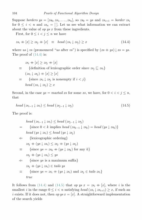
104 Pearls of Functional Algorithm Design
Suppose borders ys = [zs0, zs1, . . . , zsn ], so zs0 = ys and zsi+1 = border zsifor 0 ≤ i < n and zsn = [ ]. Let us see what information we can extractabout the value of op ys x from these ingredients.
First, for 0 ≤ i < j ≤ n we have
zsi ++ [x ] ≥ zsj ++ [x ] ≡ head (zsi ↓ zsj ) ≥ x (14.4)
where us ↓ vs (pronounced “us after vs”) is specified by (xs ++ ys) ↓ xs = ys.The proof of (14.4) is:
zsi ++ [x ] ≥ zsj ++ [x ]
≡ {definition of lexicographic order since zsj zsi}(zsi ↓ zsj ) ++ [x ] ≥ [x ]
≡ {since zsi ↓ zsj is nonempty if i < j}head (zsi ↓ zsj ) ≥ x
Second, in the case ys = maxtail xs for some xs, we have, for 0 < i < j ≤ n,that
head (zsi−1 ↓ zsi) ≤ head (zsj−1 ↓ zsj ) (14.5)
The proof is:
head (zsi−1 ↓ zsi) ≤ head (zsj−1 ↓ zsj )
= {since 0 < k implies head (zsk−1 ↓ zsk ) = head (ys ↓ zsk )}head (ys ↓ zsi) ≤ head (ys ↓ zsj )
⇐ {lexicographic ordering}zsj ++ (ys ↓ zsi) ≤ zsj ++ (ys ↓ zsj )
≡ {since ys = zsk ++ (ys ↓ zsk ) for any k}zsj ++ (ys ↓ zsi) ≤ ys
⇐ {since ys is a maximum suffix}zsj ++ (ys ↓ zsi) ∈ tails ys
≡ {since ys = zsi ++ (ys ↓ zsi) and zsj ∈ tails zsi}true
It follows from (14.4) and (14.5) that op ys x = zsi ++ [x ], where i is thesmallest i in the range 0 ≤ i < n satisfying head (zsi ↓ zsi+1) ≥ x , if such ani exists. If it does not, then op ys x = [x ]. A straightforward implementationof the search yields
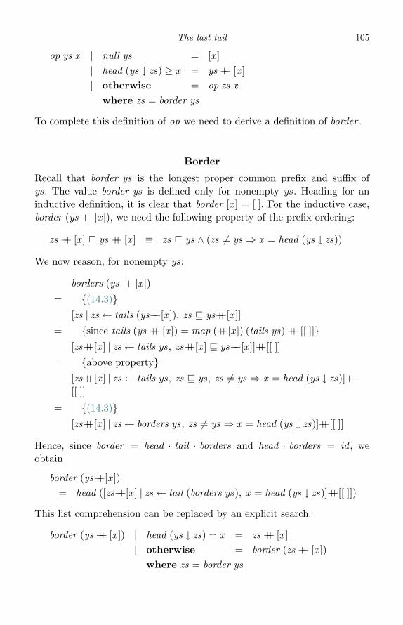
The last tail 105
op ys x | null ys = [x ]| head (ys ↓ zs) ≥ x = ys ++ [x ]| otherwise = op zs x
where zs = border ys
To complete this definition of op we need to derive a definition of border .
Border
Recall that border ys is the longest proper common prefix and suffix ofys. The value border ys is defined only for nonempty ys. Heading for aninductive definition, it is clear that border [x ] = [ ]. For the inductive case,border (ys ++ [x ]), we need the following property of the prefix ordering:
zs ++ [x ] ys ++ [x ] ≡ zs ys ∧ (zs �= ys ⇒ x = head (ys ↓ zs))
We now reason, for nonempty ys:
borders (ys ++ [x ])
= {(14.3)}[zs | zs ← tails (ys++[x ]), zs ys++[x ]]
= {since tails (ys ++ [x ]) = map (++[x ]) (tails ys) ++ [[ ]]}[zs++[x ] | zs ← tails ys, zs++[x ] ys++[x ]]++[[ ]]
= {above property}[zs++[x ] | zs ← tails ys, zs ys, zs �= ys ⇒ x = head (ys ↓ zs)]++[[ ]]
= {(14.3)}[zs++[x ] | zs ← borders ys, zs �= ys ⇒ x = head (ys ↓ zs)]++[[ ]]
Hence, since border = head · tail · borders and head · borders = id , weobtain
border (ys++[x ])= head ([zs++[x ] | zs ← tail (borders ys), x = head (ys ↓ zs)]++[[ ]])
This list comprehension can be replaced by an explicit search:
border (ys ++ [x ]) | head (ys ↓ zs) x = zs ++ [x ]| otherwise = border (zs ++ [x ])
where zs = border ys
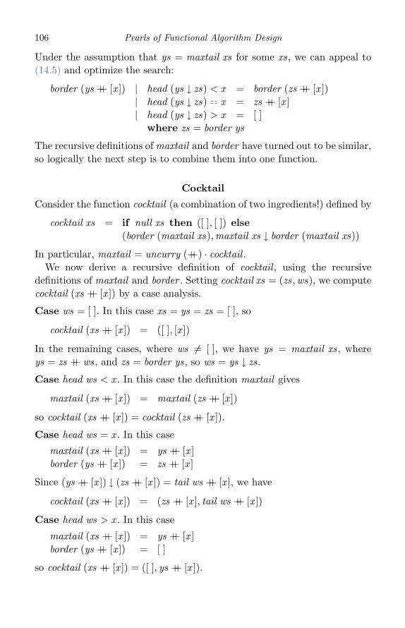
106 Pearls of Functional Algorithm Design
Under the assumption that ys = maxtail xs for some xs, we can appeal to(14.5) and optimize the search:
border (ys ++ [x ]) | head (ys ↓ zs) < x = border (zs ++ [x ])| head (ys ↓ zs) x = zs ++ [x ]| head (ys ↓ zs) > x = [ ]
where zs = border ys
The recursive definitions of maxtail and border have turned out to be similar,so logically the next step is to combine them into one function.
Cocktail
Consider the function cocktail (a combination of two ingredients!) defined by
cocktail xs = if null xs then ([ ], [ ]) else(border (maxtail xs),maxtail xs ↓ border (maxtail xs))
In particular, maxtail = uncurry (++) · cocktail .We now derive a recursive definition of cocktail , using the recursive
definitions of maxtail and border . Setting cocktail xs = (zs,ws), we computecocktail (xs ++ [x ]) by a case analysis.
Case ws = [ ]. In this case xs = ys = zs = [ ], so
cocktail (xs ++ [x ]) = ([ ], [x ])
In the remaining cases, where ws �= [ ], we have ys = maxtail xs, whereys = zs ++ ws, and zs = border ys, so ws = ys ↓ zs.
Case head ws < x . In this case the definition maxtail gives
maxtail (xs ++ [x ]) = maxtail (zs ++ [x ])
so cocktail (xs ++ [x ]) = cocktail (zs ++ [x ]).
Case head ws = x . In this case
maxtail (xs ++ [x ]) = ys ++ [x ]border (ys ++ [x ]) = zs ++ [x ]
Since (ys ++ [x ]) ↓ (zs ++ [x ]) = tail ws ++ [x ], we have
cocktail (xs ++ [x ]) = (zs ++ [x ], tail ws ++ [x ])
Case head ws > x . In this case
maxtail (xs ++ [x ]) = ys ++ [x ]border (ys ++ [x ]) = [ ]
so cocktail (xs ++ [x ]) = ([ ], ys ++ [x ]).
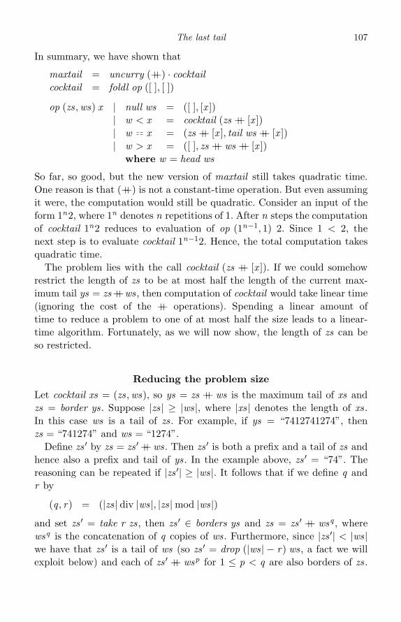
The last tail 107
In summary, we have shown that
maxtail = uncurry (++) · cocktailcocktail = foldl op ([ ], [ ])
op (zs,ws) x | null ws = ([ ], [x ])| w < x = cocktail (zs ++ [x ])| w x = (zs ++ [x ], tail ws ++ [x ])| w > x = ([ ], zs ++ ws ++ [x ])
where w = head ws
So far, so good, but the new version of maxtail still takes quadratic time.One reason is that (++) is not a constant-time operation. But even assumingit were, the computation would still be quadratic. Consider an input of theform 1n2, where 1n denotes n repetitions of 1. After n steps the computationof cocktail 1n2 reduces to evaluation of op (1n−1, 1) 2. Since 1 < 2, thenext step is to evaluate cocktail 1n−12. Hence, the total computation takesquadratic time.
The problem lies with the call cocktail (zs ++ [x ]). If we could somehowrestrict the length of zs to be at most half the length of the current max-imum tail ys = zs ++ws, then computation of cocktail would take linear time(ignoring the cost of the ++ operations). Spending a linear amount oftime to reduce a problem to one of at most half the size leads to a linear-time algorithm. Fortunately, as we will now show, the length of zs can beso restricted.
Reducing the problem size
Let cocktail xs = (zs,ws), so ys = zs ++ ws is the maximum tail of xs andzs = border ys. Suppose |zs| ≥ |ws|, where |xs| denotes the length of xs.In this case ws is a tail of zs. For example, if ys = “7412741274”, thenzs = “741274” and ws = “1274”.
Define zs ′ by zs = zs ′ ++ ws. Then zs ′ is both a prefix and a tail of zs andhence also a prefix and tail of ys. In the example above, zs ′ = “74”. Thereasoning can be repeated if |zs ′| ≥ |ws|. It follows that if we define q andr by
(q , r) = (|zs| div |ws|, |zs|mod |ws|)
and set zs ′ = take r zs, then zs ′ ∈ borders ys and zs = zs ′ ++ wsq , wherewsq is the concatenation of q copies of ws. Furthermore, since |zs ′| < |ws|we have that zs ′ is a tail of ws (so zs ′ = drop (|ws| − r) ws, a fact we willexploit below) and each of zs ′ ++ wsp for 1 ≤ p < q are also borders of zs.
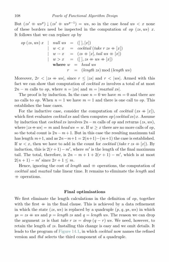
108 Pearls of Functional Algorithm Design
But (zs ′ ++ wsp) ↓ (zs ′ ++ wsp−1) = ws, so in the case head ws < x noneof these borders need be inspected in the computation of op (zs,ws) x .It follows that we can replace op by
op (zs,ws) x | null ws = ([ ], [x ])| w < x = cocktail (take r zs ++ [x ])| w x = (zs ++ [x ], tail ws ++ [x ])| w > x = ([ ], zs ++ ws ++ [x ])
where w = head wsr = (length zs) mod (length ws)
Moreover, 2r < |zs ++ ws|, since r ≤ |zs| and r < |ws|. Armed with thisfact we can show that computation of cocktail xs involves a total of at most2n −m calls to op, where n = |xs| and m = |maxtail xs|.
The proof is by induction. In the case n = 0 we have m = 0 and there areno calls to op. When n = 1 we have m = 1 and there is one call to op. Thisestablishes the base cases.
For the inductive case, consider the computation of cocktail (xs ++ [x ]),which first evaluates cocktail xs and then computes op (cocktail xs)x . Assumeby induction that cocktail xs involves 2n−m calls of op and returns (zs,ws),where |zs++ws| = m and headws = w . If w ≥ x there are no more calls of op,so the total count is 2n−m +1. But in this case the resulting maximum tailhas length m+1, and as 2n−m+1 = 2(n+1)−(m+1) the case is established.If w < x , then we have to add in the count for cocktail (take r zs ++ [x ]). Byinduction, this is 2(r +1)−m ′, where m ′ is the length of the final maximumtail. The total, therefore, is 2n − m + 1 + 2(r + 1) − m ′, which is at most2(n + 1)−m ′ since 2r + 1 ≤ m.
Hence, ignoring the cost of length and ++ operations, the computation ofcocktail and maxtail take linear time. It remains to eliminate the length and++ operations.
Final optimisations
We first eliminate the length calculations in the definition of op, togetherwith the first ++ in the final clause. This is achieved by a data refinementin which the state (zs,ws) is replaced by a quadruple (p, q , ys,ws) in whichys = zs ++ ws and p = length zs and q = length ws. The reason we can dropthe argument zs is that take r zs = drop (q − r) ws. We need, however, toretain the length of zs. Installing this change is easy and we omit details. Itleads to the program of Figure 14.1, in which cocktail now names the refinedversion and thd selects the third component of a quadruple.

The last tail 109
maxtail = thd · cocktailcocktail = foldl op (0, 0, [ ], [ ])
op (p, q , ys,ws) x| q 0 = (0, 1, [x ], [x ])| w < x = cocktail (drop (q−r) ws ++ [x ])| w x = (p+1, q , ys ++ [x ], tail ws ++ [x ])| otherwise = (0, p+q+1, ys ++ [x ], ys ++ [x ])
where w = head wsr = p mod q
Fig. 14.1 The result of data refinement
Now we are left only with (++[x ]) operations. One way to ensure that(++[x ]) takes constant time is to convert all the lists into queues and to usean efficient implementation of queues that guarantees insertion at the rearof the queue as well as that removal from the front takes constant time.But another method is suggested by the observation that each of the listsys and ws arising during the computation of cocktail xs is a tail of xs. Theoperation op constructs these tails step by step, but a more efficient methodis to construct them all at once. The way to do this is to convert what wehave into an iterative algorithm.
More precisely, suppose we define step by
step (p, q , ys ′,ws ′, xs) = thd (foldl op (p, q , ys ′ ↑ xs,ws ′ ↑ xs) xs)
where us ↑ vs (pronounced “us before vs”) is what remains when the tail vsof us is removed from us. Thus, us = (us ↑ vs) ++ vs. In particular:
maxtail (x : xs) = thd (foldl op (0, 1, [x ], [x ]) xs)= thd (foldl op (0, 1, (x : xs) ↑ xs, (x : xs) ↑ xs) xs)= step (0, 1, x : xs, x : xs, xs)
Next we derive a recursion for step (p, q , ys ′,ws ′, xs). Since us ↑ [ ] = us weobtain
step (p, q , ys ′,ws ′, [ ]) = ys ′
In the case that xs is not empty (so neither of ys ′ or ws ′ is empty) we have
step (p, q , ys ′,ws ′, x : xs)= thd (foldl op (p, q , ys ′ ↑ (x : xs),ws ′ ↑ (x : xs)) (x : xs))= thd (foldl op (op (p, q , ys ′ ↑ (x : xs),ws ′ ↑ (x : xs)) x ) xs)
Now we need a case analysis.

110 Pearls of Functional Algorithm Design
Case head (ws ′ ↑ (x : xs)) < x . In this case
op (p, q , ys ′ ↑ (x : xs),ws ′ ↑ (x : xs)) x =cocktail ′ (drop (q−r) (ws ′ ↑ (x : xs)) ++ [x ])
where r = p mod q . Abbreviating drop (q−r) (ws ′ ↑ (x : xs)) to vs, weargue
step (p, q , ys ′,ws ′, x : xs)
= {definition and case assumption}thd (foldl op (cocktail ′ (vs ++ [x ])) xs)
= {definition of cocktail ′}thd (foldl op (foldl op (0, 0, [ ], [ ], [ ]) (vs ++ [x ])) xs)
= {since foldl f (foldl f e xs) ys = foldl f e (xs ++ ys)}thd (foldl op ([ ], [ ], [ ]) (vs ++ x : xs))
= {since drop (q−r) (ws ′ ↑ (x : xs)) ++ x : xs = drop (q−r) ws ′}thd (foldl op ([ ], [ ], [ ]) (drop (q−r) ws ′))
= {definition of maxtail}maxtail (drop (q−r) ws ′)
Case head (ws ′ ↑ (x : xs)) = x . In this case
op (p, q , ys ′ ↑ (x : xs),ws ′ ↑ (x : xs)) x =(p+1, q , ys ′ ↑ (x : xs) ++ [x ], tail (ws ′ ↑ (x : xs)) ++ [x ])
= (p+1, q , ys ′ ↑ xs, tail (ws ′ ↑ xs))
Hence, step (p, q , ys ′,ws ′, x : xs) = (p+1, q , ys ′, tail ws ′, xs).
Case head (ws ′ ↑ (x : xs)) > x . In this case
op (p, q , ys ′ ↑ (x : xs),ws ′ ↑ (x : xs)) x =(0, p+q+1, ys ′ ↑ (x : xs) ++ [x ], ys ′ ↑ (x : xs) ++ [x ])
= (0, p+q+1, ys ′ ↑ xs, ys ′ ↑ xs)
Hence, step (p, q , ys ′,ws ′, x : xs) = (0, p+q+1, ys ′, ys ′, xs).Summarising all the above, we have arrived at our final program:
maxtail [ ] = [ ]maxtail (x : xs) = step (0, 1, x : xs, x : xs, xs)
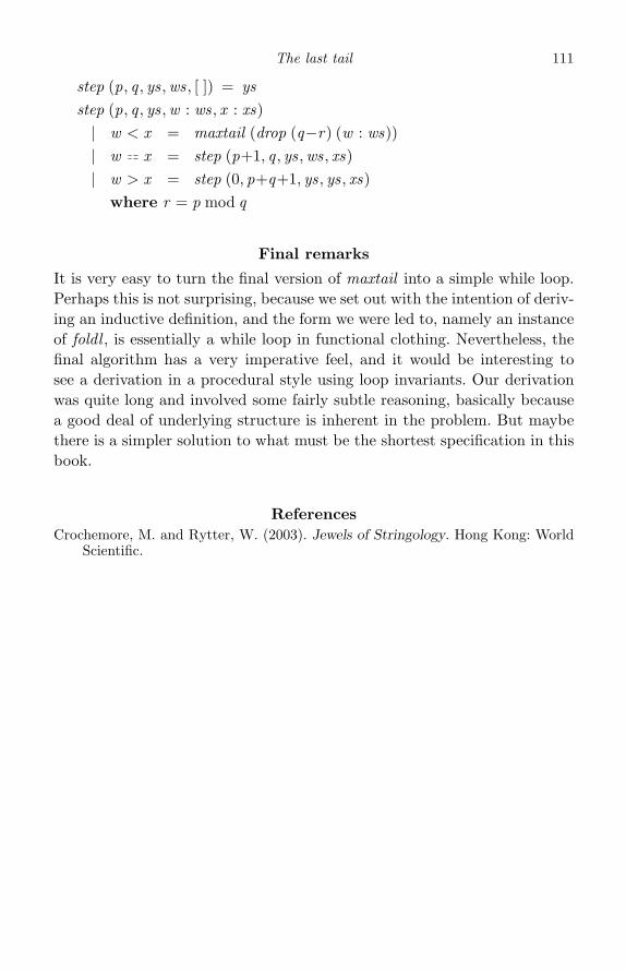
The last tail 111
step (p, q , ys,ws, [ ]) = ysstep (p, q , ys,w : ws, x : xs)| w < x = maxtail (drop (q−r) (w : ws))| w x = step (p+1, q , ys,ws, xs)| w > x = step (0, p+q+1, ys, ys, xs)
where r = p mod q
Final remarks
It is very easy to turn the final version of maxtail into a simple while loop.Perhaps this is not surprising, because we set out with the intention of deriv-ing an inductive definition, and the form we were led to, namely an instanceof foldl , is essentially a while loop in functional clothing. Nevertheless, thefinal algorithm has a very imperative feel, and it would be interesting tosee a derivation in a procedural style using loop invariants. Our derivationwas quite long and involved some fairly subtle reasoning, basically becausea good deal of underlying structure is inherent in the problem. But maybethere is a simpler solution to what must be the shortest specification in thisbook.
ReferencesCrochemore, M. and Rytter, W. (2003). Jewels of Stringology. Hong Kong: World
Scientific.

15
All the common prefixes
Introduction
Let llcp xs ys denote the length of the longest common prefix of two listsxs and ys. For example llcp “common” “computing” = 3. Now consider thefunction allcp, short for all the common prefixes, defined by
allcp xs = map (llcp xs) (tails xs)
where tails xs returns the nonempty tails of xs. For example:
xs a b a c a b a c a ballcp xs 10 0 1 0 6 0 1 0 2 0
The first element of allcp xs is, of course, length xs. Executed directly, thedefinition of allcp gives a quadratic-time algorithm. But can it be done inlinear time? Yes it can, and the aim of this pearl is to show how. The functionallcp is an important component of the Boyer–Moore algorithm for stringmatching, a problem we will take up in the following pearl, so a linear-timesolution is of practical as well as theoretical interest.
A key property
The key property of llcp on which the fast algorithm rests is the followingone. Let us, vs and ws be any three lists. Then, with llcp us vs = m andllcp vs ws = n, we have
llcp us ws ={
min m n if m �= nm + llcp (drop m us) (drop m ws) if m = n
(15.1)
For the proof, observe that the first min m n elements are common to allthree lists. If m < n, then the next element of us (if any) is differentfrom the next element of vs, while the next element of vs is the same asthe next element of ws. Hence llcp us ws = m. The reasoning is dual ifm > n. Finally, if m = n, then matching has to continue with drop m usand drop m ws.
112
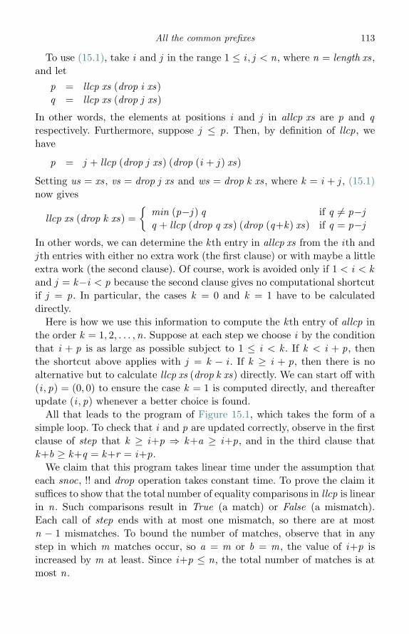
All the common prefixes 113
To use (15.1), take i and j in the range 1 ≤ i , j < n, where n = length xs,and let
p = llcp xs (drop i xs)q = llcp xs (drop j xs)
In other words, the elements at positions i and j in allcp xs are p and qrespectively. Furthermore, suppose j ≤ p. Then, by definition of llcp, wehave
p = j + llcp (drop j xs) (drop (i + j ) xs)
Setting us = xs, vs = drop j xs and ws = drop k xs, where k = i + j , (15.1)now gives
llcp xs (drop k xs) ={
min (p−j ) q if q �= p−jq + llcp (drop q xs) (drop (q+k) xs) if q = p−j
In other words, we can determine the kth entry in allcp xs from the ith andj th entries with either no extra work (the first clause) or with maybe a littleextra work (the second clause). Of course, work is avoided only if 1 < i < kand j = k−i < p because the second clause gives no computational shortcutif j = p. In particular, the cases k = 0 and k = 1 have to be calculateddirectly.
Here is how we use this information to compute the kth entry of allcp inthe order k = 1, 2, . . . ,n. Suppose at each step we choose i by the conditionthat i + p is as large as possible subject to 1 ≤ i < k . If k < i + p, thenthe shortcut above applies with j = k − i . If k ≥ i + p, then there is noalternative but to calculate llcp xs (drop k xs) directly. We can start off with(i , p) = (0, 0) to ensure the case k = 1 is computed directly, and thereafterupdate (i , p) whenever a better choice is found.
All that leads to the program of Figure 15.1, which takes the form of asimple loop. To check that i and p are updated correctly, observe in the firstclause of step that k ≥ i+p ⇒ k+a ≥ i+p, and in the third clause thatk+b ≥ k+q = k+r = i+p.
We claim that this program takes linear time under the assumption thateach snoc, !! and drop operation takes constant time. To prove the claim itsuffices to show that the total number of equality comparisons in llcp is linearin n. Such comparisons result in True (a match) or False (a mismatch).Each call of step ends with at most one mismatch, so there are at mostn − 1 mismatches. To bound the number of matches, observe that in anystep in which m matches occur, so a = m or b = m, the value of i+p isincreased by m at least. Since i+p ≤ n, the total number of matches is atmost n.

114 Pearls of Functional Algorithm Design
allcp xs = fst4 (until (done n) (step xs) ([n], 0, 0, 1))where n = length xs
done n (as, i , p, k) = k n
step xs (as, i , p, k)| k ≥ i + p = (snoc as a, k , a, k + 1)| q �= r = (snoc as (min q r), i , p, k + 1)| q r = (snoc as b, k , b, k + 1)
where q = as !! (k − i)r = p − (k − i)a = llcp xs (drop k xs)b = q + llcp (drop q xs) (drop (q + k) xs)
fst4 (a, b, c, d) = asnoc xs x = xs ++ [x ]
llcp xs [ ] = 0llcp [ ] ys = 0llcp (x : xs) (y : ys) = if x y then 1 + llcp xs ys else 0
Fig. 15.1 The initial program
Data refinement
However, snoc, (!!), and drop do not take constant time. The remainder of thedevelopment is just data refinement to ensure that they can be implementedby constant-time operations.
Let us deal with drop first. The idea is to bring in the library Data.Array ofHaskell arrays and replace llcp by another version that uses index operationson a (global) array xa = listArray (0,n − 1) xs, where n = length xs:
llcp ′ j k | j n ∨ k n = 0| xa ! j xa ! k = 1 + llcp ′ (j + 1) (k + 1)| otherwise = 0
That means we can replace the definitions of a and b in step by
a = llcp ′ 0 kb = q + llcp ′ q (q + k)
It remains to deal with the snoc and (!!) operations. The obvious step isagain to use an array. However, adding an element to the end of an arrayis only a constant-time operation if we embed the whole computation in asuitable monad, and that is something we choose to avoid. Another optionis to use Haskell’s Data.Sequence library. This library provides a constant-time snoc, but only a logarithmic-time indexing operation. Good enough in

All the common prefixes 115
allcp xs = extract (until done step (as, empty , 0, 1)))whereextract (as, qs, h, k) = elems asdone (as, qs, h, k) = (k n)n = length xsas = insert empty nxa = listArray (0,n−1) xsstep (as, qs, h, k) | k ≥ h = (insert as a, insert as ′ a, k + a, k + 1)
| q �= r = (insert as m, insert qs ′ m, h, k + 1)| q r = (insert as b, insert as ′ b, k + b, k + 1)
where as ′ = snd (remove as)(q , qs ′) = remove qsr = h − km = min q ra = llcp′ 0 kb = q + llcp′ q (q + k)
llcp′ j k | j n ∨ k n = 0| xa ! j xa ! k = 1 + llcp (j + 1) (k + 1)| otherwise = 0
Fig. 15.2 The final program
practice, but we promised a linear-time solution, so we have to work a littleharder.
Our solution is to use a queue, in fact two of them. Chris Okasaki’s im-plementation of queues (Okasaki, 1995) provides a type Queue a with thefollowing four operations:
insert :: Queue a → a → Queue aremove :: Queue a → (a,Queue a)empty :: Queue aelems :: Queue a → [a]
The function insert inserts a new element at the rear of the queue, removereturns the first element and the remaining elements of a nonempty queue,empty gives an empty queue, and elems returns the list of elements in aqueue. The first three operations take constant time, while elems takes timeproportional to the length of the queue.
We replace the component as in the argument of step with a queue, alsocalled as, and add in a second queue qs, representing the suffix drop (k−i)as.Then q = as !! (k − i) is the first element of qs. There is no need to maintainargument i , so we can remove it and replace p by h = i +p. Installing thesechanges is straightforward and leads to the final program of Figure 15.2.
116 Pearls of Functional Algorithm Design
Final remarks
The problem of computing allcp is identified as the fundamental prepro-cessing step of string matching by Gusfield (1997), where it is called “theZ algorithm”. The same problem is dealt with by Crochemore and Rytter,under the name “table of prefixes”. Our treatment follows Gusfield quiteclosely, except for the identification of (15.1) as the key property of llcp thatenables everything to work, and the use of queues to make the snoc and !!operations efficient.
ReferencesCrochemore, M. and Rytter, W. (2003). Jewels of Stringology. Hong Kong: World
Scientific.Gusfield, D. (1997). Algorithms on Strings, Trees and Sequences. Cambridge, UK:
Cambridge University Press.Okasaki, C. (1995). Simple and efficient purely functional queues and deques. Jour-
nal of Functional Programming, 5 (4), 583–92.

16
The Boyer–Moore algorithm
Introduction
The problem of string matching consists of finding all occurrences of onenonempty string, called the pattern, in another string, called the text. Hereis the specification:
matches :: Eq a ⇒ [a]→ [a]→ [Int ]matches ws = map length · filter (endswith ws) · inits
The function inits returns a list of the prefixes of the text in order ofincreasing length. The expression endswith ws xs tests whether the patternws is a suffix of xs. The value matches ws xs is a list of integers p such thatws is a suffix of take p xs. For example:
matches “abcab” “ababcabcab” = [7, 10]
In other words, matches ws xs returns a list integers p such that ws appearsin xs ending at position p (counting positions from 1).
The function matches is polymorphic, so any algorithm for the problemhas to rely only on an equality test ( ) :: a → a → Bool for informationabout the elements of the two lists. Polymorphic string matching rules outany algorithm that depends upon a being finite. Assuming it takes constanttime to carry out an equality test, the running time of matches ws xs isΘ(mn) steps in the worst case, where m = length ws and n = length xs.Our aim in this pearl is to derive the famous Boyer–Moore (BM) algorithmfor string matching, which reduces the time to Θ(m + n) steps. In thefollowing pearl we will derive the equally famous Knuth–Morris–Pratt (KMP)algorithm for the same problem with the same complexity. And the trick issimply to apply appropriate efficiency-improving laws dictated by the formof the expression under manipulation.
117

118 Pearls of Functional Algorithm Design
The scan lemma
For string matching, indeed for any problem involving the function inits,the most important law is known as the scan lemma:
map (foldl op e) · inits = scanl op e
The expression on the left is evaluated on a list of length n with Θ(n2)evaluations of op, while the equivalent expression in terms of the standardHaskell function scanl requires only Θ(n) evaluations.
Although there is a map in the definition of matches, there is also a filter ,so the first step in transforming matches is to rewrite the specification usinganother law:
map f · filter p = map fst · filter snd ·map (fork (f , p)) (16.1)
where fork (f , p) x = (f x , p x ). The law is used simply to bring a map nextto inits in preparation for applying the scan lemma. Use of (16.1) leads to
matches ws= map fst · filter snd ·map (fork (length, endswith ws)) · inits
The next question to ask is: can fork (length, endswith ws) be cast as aninstance of foldl? Certainly, length = foldl count 0 where count n x = n + 1.Suppose for the moment that we can also find e and op, both of which willdepend on ws, so that
endswith ws = foldl op e (16.2)
Then we are in a position to apply another standard law: the tupling lawfor foldl . This law states that
fork (foldl op1 e1, foldl op2 e2) = foldl op (e1, e2)
where op (a, b) x = (op1 a x , op2 b x ). Use of the tupling law results in
fork (length, endswith ws) = foldl step (0, e)step (n, x ) y = (n + 1, op x y)
Finally, we can apply the scan lemma to arrive at
matches ws = map fst · filter snd · scanl step (0, e)
If op takes constant time, or at least amortized constant time, then so doesstep, and the result is a linear-time program. That, in a nutshell, is thegenesis of all efficient polymorphic string-matching algorithms.
The problem is that there is no op and e to satisfy (16.2). The functionendswithws returns a single Boolean value and this is insufficient information
The Boyer–Moore algorithm 119
to express it as an instance of foldl . The next best thing is to expressendswith ws as a composition
endswith ws = p · foldl op e (16.3)
The form of (16.3) is dictated solely by the desire to apply the scan lemma.Instead of (16.1) we can use a slight generalisation:
map f · filter (p · g) = map fst · filter (p · snd) ·map (fork (f , g)) (16.4)
Then we obtain
matches ws = map fst · filter (p · snd) · scanl step (0, e)
Provided p and op take amortized constant time, matches will still takelinear time.
What remains is to find p, op and e to satisfy (16.3). But we have not yetdefined endswith formally. Here are two reasonable definitions:
endswith ws xs = reverse ws reverse xsendswith ws xs = ws ∈ tails xs
In the first definition, us vs if us is a prefix of vs. It is clear that ws is asuffix of xs if and only if the reverse of ws is a prefix of the reverse of xs.The prefix relation is easier to implement than the suffix relation:
[ ] vs = True(u : us) [ ] = False(u : us) (v : vs) = (u v ∧ us vs)
Although both definitions of endswith define the same function, they havedifferent forms. And, since it is form rather than function that dictatesthe course of development, we are at a crossroads. As we will see, taking thefirst path leads to the BM algorithm, while taking the second leads tothe KMP algorithm. In the rest of this pearl we will take the first path.In the following pearl we will explore the second path.
The Boyer–Moore algorithm
The first definition of endswith can be restated as a composition:
endswith ws = (reverse ws ) · reverse

120 Pearls of Functional Algorithm Design
Consequently, appeal to (16.4) leads to
matches ws= map fst · filter ((sw ) · snd) ·map (fork (length, reverse)) · inits
where sw = reverse ws
But reverse = foldl (flip (:)) [ ], so we can again make use of the tupling lawof foldl , followed by the scan lemma, to obtain
matches ws = map fst · filter ((sw ) · snd) · scanl step (0, [ ])where sw = reverse ws
step (n, sx ) x = (n + 1, x : sx )
This is the basic form of the BM algorithm. Application of scanl generatessuccessive “windows” of the text together with their position. Each windowcontains the reversal of some initial segment of the text, with successivewindows differing in just one position, so there is a “shift” of length oneat each stage. The terms “window” and “shift” are from Lecroq (2003),which contains a very readable introduction to string matching. Each ofthese windows is processed by matching against the pattern ws from rightto left.
Shifting
As it stands, the BM algorithm still takes Ω(mn) steps in the worst casebecause the test (sw ) can take Ω(m) steps (in all that follows we fixm = length ws and assume m �= 0). For example, one worst case arises whenthe pattern is a list of m repetitions of a single value and the text is a listof n repetitions of the same value. The way to make the worst case better isto see if we can shift over some windows because they cannot be candidatesfor matching. Such shifts depend on how much of a match there is at thecurrent window.
Let llcp sw sx denote the length of the longest common prefix of sw andsx . We encountered this function in the previous pearl. Clearly, sw sx ifand only if m = llcp sw sx . Given i = llcp sw sx for the current window(n, sx ), can we put a lower bound on the position n + k of the next windowat which there can be a match? Certainly, we must have 0 < k ≤ m or wemight miss a match. Suppose the next window has the form (n +k , ys ++sx ),where k = length ys. If there is a match at this window, so sw ys ++ sx ,then take k sw = ys and drop k sw sx .
Using this information and setting i = llcp sw sx , we can now show that
llcp sw (drop k sw) = min i (m−k) (16.5)
The Boyer–Moore algorithm 121
First, assume i < m−k . Then
take i (drop k sw)
= {since drop k sw sx implies drop k sw = take (m−k) sx}take i (take (m−k) sx )
= {since i ≤ m−k}take i sx
= {since i = llcp sw sx}take i sw
Similar reasoning gives
take (i+1) (drop k sw) �= take (i+1) sw
In other words, if i < m−k , then llcp sw (drop k sw) = i . In the other case,i ≥ m−k , we reason:
drop k sw
= {since length (drop k sw) = m−k ≤ i}take i (drop k sw)
{since drop k sw sx}take i sx
= {since i = llcp sw sx}take i sw
{definition of }sw
But drop k sw sw ≡ llcp sw (drop k sw) = m−k , establishing (16.5).Now, given any i in the range 0 ≤ i ≤ m, let k be the smallest positive
value in the range 1 ≤ k ≤ m satisfying (16.5). Provided m �= 0, the valuek = m satisfies (16.5) if nothing smaller does. It follows that we can skipthe next k−1 windows without missing a match. The value k is specified ask = shift sw i , where
shift sw i = head [k | k ← [1 .. m], llcp sw (drop k sw) min i (m−k)]
This is not a very good way to compute shift sw i , as the computation cantake Ω(m2) steps in the worst case. In the following section we will showhow to compute map (shift sw) [0 .. m] in O(m) steps.
In summary, after a match of length i at the current window (n, sx ), thenext shift sw i windows can safely be ignored without missing any additional
122 Pearls of Functional Algorithm Design
matches. That means we can redefine matches to read
matches ws = test · scanl step (0, [ ])wheretest [ ] = [ ]test ((n, sx ) : nxs) = if i m
then n : test (drop (k−1) nxs)else test (drop (k−1) nxs)where i = llcp sw sx
k = shift sw i(sw ,m) = (reverse ws, length ws)
Note that two versions of matches are equivalent only if m �= 0.
A final improvement
There is one final improvement we can make. As before, let i = llcpsw sx andk = shift sw i . Furthermore, suppose m−k ≤ i , so llcp sw (dropk sw) = m−k .That means that drop k sw is a prefix of sw . Since m−k ≤ i , it follows thatllcp (drop k sw) sx = m−k .
Now, the next window to be tried is (n+k , ys ++ sx ), where length ys = k .We reason:
llcp sw (ys ++ sx )
= {setting i ′ = llcp sw ys, so i ′ ≤ k}if i ′ k then k + llcp (drop k sw) sx else i ′
= {above, since llcp (drop k sw) sx = m−k if m−k ≤ i}if i ′ k then m else i ′
Hence, provided m−k ≤ i , the length of the longest common prefix of swand the text at the next window can be computed by comparing only thefirst k elements. If m−k > i , then there is no saving and the next windowmay require up to m comparisons.
The improvement can be implemented by equipping the function testwith an additional parameter j , indicating how much of the next candidatewindow to check. Installing this final refinement, we obtain the program ofFigure 16.1, which is complete except for the definitions of llcp and shift .This program is Galil’s (1979) version of the BM algorithm. Ignoring thetime to compute shift , the running time of matches is O(m + n) stepsfor a text of length n. For a proof of this claim, which is non-trivial, seeTheorem 3.2.3 of Gusfield (1997).
The Boyer–Moore algorithm 123
matches ws = test m · scanl step (0, [ ])wheretest j [ ] = [ ]test j ((n, sx ) : nxs) | i m = n : test k (drop (k−1) nxs)
| m−k ≤ i = test k (drop (k−1) nxs)| otherwise = test m (drop (k−1) nxs)
where i ′ = llcp sw (take j sx )i = if i ′ j then m else i ′k = shift sw i
(sw ,m) = (reverse ws, length ws)
Fig. 16.1 The final program
Computing shifts
The definition of shift sw given in the previous section leads to a cubic-timealgorithm for computing shifts sw = map (shift sw) [0 .. m]: computationof shift sw i can take quadratic time and there are m+1 values of i . If wecan compute shifts sw in linear time and store the result in an array a, thenreplacing shift sw i by a !i gives a linear-time algorithm for matches. The aimof this section is to show how to compute shifts sw in linear time. Arguably,this is the most subtle aspect of the BM algorithm.
First of all, set f (k) = llcp sw (drop k sw) for brevity. Note that f (m) = 0and f (k) ≤ m−k . We first reason, for any i in the range 0 ≤ i ≤ m:
shift sw i
= {definition}minimum [k | k ← [1 .. m], f (k) min i (m−k)]
= {case analysis on min}minimum ([k | k ← [1 .. m−i ], f (k) i ] ++
[k | k ← [m−i+1 .. m], f (k)+k m])
= {since f (k) = i ⇒ k ≤ m−i}minimum ([k | k ← [1 .. m], f (k) i ] ++
[k | k ← [m−i+1 .. m], f (k)+k m])
Next we bring in the Haskell library Data.Array and, in particular, thefunction accumArray . This function first made an appearance in Pearl 1.The following fact about accumArray is immediate from its definition:
(accumArray op e (0,m) vks) ! i = foldl op e [k | (v , k)← vks, v i ]
124 Pearls of Functional Algorithm Design
for all i in the range 0 ≤ i ≤ m, provided map fst vks ⊆ [0 ..m]. The provisois necessary because accumArray is undefined if any index is out of the givenrange. In particular, with
a = accumArray min m (0,m) vksvks = [(f (k), k) | k ← [1 .. m]]
we have
a ! i = minimum ([k | k ← [1 .. m], f (k) i ] ++ [m])
for 0 ≤ i ≤ m. That deals with the first term in the definition of shift sw i .We now have to factor in the second term. The idea is to replace a by
a = accumArray min m (0,m) (vks ++ vks ′)
where the list vks ′ is any convenient permutation of
[(i ,minimum [k | k ← [m−i+1 .. m], f (k)+k m]) | i ← [1 .. m]]
Then we have shift sw i = a ! i .We claim that the following definition of vks ′, which computes the list
above in reverse order, does the job:
vks ′ = zip [m,m−1 .. 1] (foldr op [ ] vks)vks = [(f (k), k) | k ← [1 .. m]]op (v , k) ks = if v + k m then k : ks else head ks : ks
Note that op (f (m),m) [ ] = [m] because f (m) = 0 and so f (m) + m = m.For example, with xs = foldr op [ ] vks we have
f 2 4 0 5 2 3 0 2 0k 1 2 3 4 5 6 7 8 9xs 4 4 4 4 6 6 9 9 9
The ith element of xs (counting from 0) is the smallest k > i such thatf (k)+k = m. In vks ′ the index m−i is paired with xs !! i ; equivalently, i ispaired with xs !! (m−i), which is just what is required.
As the final step, recall the function allcp from the previous pearl:
allcp xs = [llcp xs (drop k xs) | k ← [0 .. length xs − 1]]
There we showed how to compute allcp in linear time. For present purposeswe need a variant of allcp xs in which the first element is dropped and anadditional element llcp xs [ ] is added at the end. This additional value iszero, so we define
allcp ′ xs = tail (allcp xs) ++ [0]

The Boyer–Moore algorithm 125
Finally, we can reason:
[(f (k), k) | k ← [1 .. m]]
= {definition of f }[(llcp sw (drop k sw), k) | k ← [1 .. m]]
= {definition of zip}zip [llcp sw (drop k sw) | k ← [1 .. m]] [1 .. m]
= {definition of allcp ′}zip (allcp′ sw) [1 .. m]
Putting these pieces together, we obtain
a = accumArray min m (0,m) (vks ++ vks ′)wherem = length swvks = zip (allcp ′ sw) [1 .. m]vks ′ = zip [m,m−1 .. 1] (foldr op [ ] vks)op (v , k) ks = if v + k m then k : ks else head ks : ks
Replacing shift sw i by a ! i in Figure 16.1 gives a linear-time algorithm formatches.
Final remarks
The BM algorithm was first described in Boyer and Moore (1977); see alsoCormen et al. (2001), Crochemore and Rytter (2003) and Gusfield (1997) forfurther exploration and discussion of the method. Most often the algorithmis explained in terms of two rules, the bad character rule and the good
suffix rule, neither of which appear explicitly above. Our derivation of theBM algorithm, at least in its basic form, was a simple exercise in symbolicmanipulation, applying appropriate efficiency-improving laws dictated solelyby the form of the expressions being considered. Chief among these laws werethe scan lemma and the tupling law of foldl . Moreover, the key idea of theBM algorithm, namely the idea of matching the pattern to the text in right-to-left order, emerged simply as the consequence of one very reasonable wayto define endswith. Subsequent optimisations depended more on the contentof the expressions than their form, but this is to be expected in any algorithmcontaining subtle ideas.
ReferencesBoyer, R. S. and Moore, J. S. (1977). A fast string searching algorithm. Commu-
nications of the ACM 20, 762–72.

126 Pearls of Functional Algorithm Design
Cormen, T. H., Leiserson, C. E., Rivest, R. L. and Stein, C. (2001). Introductionto Algorithms, second edition. Cambridge, MA: The MIT Press.
Crochemore, M. and Rytter, W. (2003). Jewels of Stringology. Hong Kong: WorldScientific.
Galil, Z. (1979). On improving the worst cast of the Boyer–Moore string matchingalgorithm. Communications of the ACM 22 (9), 505–8.
Gusfield, D. (1997). Algorithms on Strings, Trees and Sequences. Cambridge, UK:Cambridge University Press.
Lecroq, T. (2003). Experimental results on string matching algorithms. Software –Practice and Experience 25 (7), 727–65.
17
The Knuth–Morris–Pratt algorithm
Introduction
In this pearl we continue with the problem of string matching and take theother fork in the road, the one that begins with the following definition ofendswith:
endswith ws xs = ws ∈ tails xs
The path turns out to lead to the KMP algorithm. Remember, the goal isto find functions p and op, and value e, so that endswith ws = p · foldl op e.Then we have
matches :: Eq a ⇒ [a]→ [a]→ [Int ]matches ws = map fst · filter (p · snd) · scanl step (0, e)step (n, x ) y = (n + 1, op x y)
The value of matches ws xs is a list of integers n for which the pattern wsappears in the text xs ending at position n. Provided p and op take constanttime, or at least amortized constant time, the computation of matches takesΘ(m + n) steps on a pattern of length m and a text of length n.
First steps
One way of writing endswith ws as a composition is
endswith ws = not · null · filter (= ws) · tails
But filter (= ws) · tails cannot be defined as an instance of foldl becauseit returns either an empty list or [ws], and this is insufficient informationto define the function inductively. More promising is filter ( ws) · tails.Applied to xs, this function returns in decreasing order of length all tails ofxs that are prefixes of ws. The first element of this list is ws if and only ifendswith ws xs. Thus:
endswith ws = (= ws) · head · filter ( ws) · tails
127
128 Pearls of Functional Algorithm Design
Of course, the first function (= ws) is no longer a constant-time test. Thatproblem is solved by generalising filter ( ws) · tails to a function split ,defined by
split ws xs = head [(us,ws ↓ us) | us ← tails xs, us ws]
The operation ↓ is defined by (us ++ vs) ↓ us = vs. Hence, split ws xs splitsws into two lists us and vs so that us ++ vs = ws. The value of us is thelongest suffix of xs that is a prefix of ws. For example:
split “endnote” “append” = (“end”, “note”)
Now we have endswith ws = null · snd · split ws. It remains to find opand e so that split ws = foldl op e. Equivalently, we want e and op tosatisfy
split ws [ ] = esplit ws (xs ++ [x ]) = op (split ws xs) x
We have split ws [ ] = ([ ],ws), which gives us e, so it remains to discover op.The crucial observation is that
split ws xs = (us, vs) ⇒ split ws (xs ++ [x ]) = split ws (us ++ [x ])
In words, the longest suffix of xs ++ [x ] that is a prefix of ws is a suffix ofus ++ [x ]. It cannot be a longer suffix, for that would mean there is a longersuffix of xs than us that is a prefix of ws, contradicting the definition of usas the longest such suffix.
To discover op we first express split recursively:
split ws xs = if xs ws then (xs,ws ↓ xs) else split ws (tail xs)
Now, setting split ws xs = (us, vs), so ws = us ++ vs, we reason:
split ws (xs ++ [x ])
= {observation above}split ws (us ++ [x ])
= {recursive definition of split}if us ++ [x ] ws then (us ++ [x ],ws ↓ (us ++ [x ]))else split ws (tail (us ++ [x ]))
= {since ws = us ++ vs and definitions of and ↓}if [x ] vs then (us ++ [x ], tail vs)else split ws (tail (us ++ [x ]))
The Knuth–Morris–Pratt algorithm 129
= {case analysis on us}if [x ] vs then (us ++ [x ], tail vs)else if null us then ([ ],ws)else split ws (tail us ++ [x ])
This calculation gives us our definition of op:
op (us, vs) x | [x ] vs = (us ++ [x ], tail vs)| null us = ([ ],ws)| otherwise = op (split ws (tail us)) x
Summarising where we are at this point:
matches ws = map fst · filter (null · snd · snd) ·scanl step (0, ([ ],ws))
step (n, (us, vs)) x = (n + 1, op (us, vs) x )
This is the basic form of the KMP algorithm: each step maintains a currentsplit (us, vs) of the pattern ws in which us is the longest prefix of ws match-ing some suffix of the current portion of the text. Positions for which vs = [ ]are those where the pattern matches exactly and are recorded.
The problem with op is that it is inefficient: the third clause requirescomputation of split ws (tail us), which in turn may involve computing andpossibly recomputing split ws zs for an arbitrary substring zs of ws. Clearly,op does too much work and we need something better.
Data refinement
One way to improve efficiency is to seek a change of representation of thefirst argument to op, namely the current split (us, vs) of the pattern ws.Specifically, suppose abs and rep are functions with types
abs :: Rep ([a], [a])→ ([a], [a])rep :: ([a], [a])→ Rep ([a], [a])
for some data type Rep. The function rep is the representation function,while abs is the abstraction function. The terminology is standard in datarefinement. We also want abs · rep = id , so abs is left-inverse to rep. Thiscondition states that the abstract value can be recovered from any rep-resentation of it. The other direction rep · abs = id will only hold if thechange of representation is a bijection, which is not normally the case indata refinement.
If we can find the necessary ingredients to ensure
foldl op ([ ],ws) = abs · foldl op′ (rep ([ ],ws)) (17.1)

130 Pearls of Functional Algorithm Design
as well as ensure that abs and op ′ take constant time, then we can redefinematches to read
matches ws = map fst · filter (null · snd · abs · snd) ·scanl step (0, rep ([ ],ws))
step (n, r) x = (n + 1, op ′ r x )
To find abs, op′ and rep satisfying (17.1) we appeal to the fusion law offoldl .This laws states the f · foldl g a = foldl h b provided three conditionsare met: (i) f is a strict function; (ii) f a = b; and (iii) f (g y x ) = h (f y) xfor all x and y . The first condition is not needed if we want to assert thatthe fusion law holds only for all finite lists. The twist here is that we wantto apply the law in the anti-fusion or fission direction, splitting a fold intotwo parts.
The second fusion condition is immediate: abs (rep ([ ],ws)) = ([ ],ws).And there is an obvious definition of op ′ that satisfies the third fusioncondition, namely
op ′ r = rep · op (abs r) (17.2)
Then we have
abs (op ′ r x ) = abs (rep (op (abs r) x )) = op (abs r) x
Installing the definition of op in (17.2) we obtain
op ′ r x | [x ] vs = rep (us ++ [x ], tail vs)| null us = rep ([ ],ws)| otherwise = op ′ (rep (split ws (tail us))) x
where (us, vs) = abs r
It remains to choose Rep and the two functions abs and rep.
Trees
In functional programming, practically all efficient representations involve atree of some kind, and this one is no different. We define
data Rep a = Null |Node a (Rep a) (Rep a)
So Rep is a binary tree. The function abs is defined by
abs (Node (us, vs) � r) = (us, vs) (17.3)
and clearly takes constant time. The function rep is defined by
rep (us, vs) = Node (us, vs) (left us vs) (right us vs) (17.4)
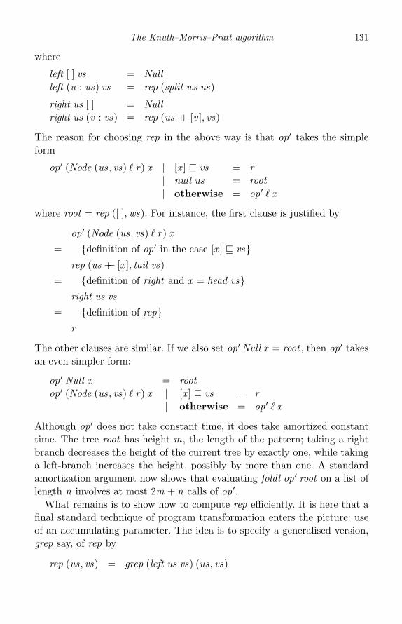
The Knuth–Morris–Pratt algorithm 131
where
left [ ] vs = Nullleft (u : us) vs = rep (split ws us)
right us [ ] = Nullright us (v : vs) = rep (us ++ [v ], vs)
The reason for choosing rep in the above way is that op′ takes the simpleform
op ′ (Node (us, vs) � r) x | [x ] vs = r| null us = root| otherwise = op ′ � x
where root = rep ([ ],ws). For instance, the first clause is justified by
op′ (Node (us, vs) � r) x
= {definition of op ′ in the case [x ] vs}rep (us ++ [x ], tail vs)
= {definition of right and x = head vs}right us vs
= {definition of rep}r
The other clauses are similar. If we also set op ′ Null x = root , then op ′ takesan even simpler form:
op ′ Null x = rootop ′ (Node (us, vs) � r) x | [x ] vs = r
| otherwise = op ′ � x
Although op ′ does not take constant time, it does take amortized constanttime. The tree root has height m, the length of the pattern; taking a rightbranch decreases the height of the current tree by exactly one, while takinga left-branch increases the height, possibly by more than one. A standardamortization argument now shows that evaluating foldl op ′ root on a list oflength n involves at most 2m + n calls of op ′.
What remains is to show how to compute rep efficiently. It is here that afinal standard technique of program transformation enters the picture: useof an accumulating parameter. The idea is to specify a generalised version,grep say, of rep by
rep (us, vs) = grep (left us vs) (us, vs)

132 Pearls of Functional Algorithm Design
and then to derive a direct definition of grep. From (17.4) we have
grep � (us, vs) = Node (us, vs) � (right us vs)
Now, by the definition of right , we have right us [ ] = Null and
right us (v : vs) = rep (us ++ [v ], vs)= grep (left (us ++ [v ]) vs) (us ++ [v ], vs)
To simplify left (us ++ [v ]) vs we need a case analysis on us. In the caseus = [ ] we reason:
left ([ ] ++ [v ]) vs
= {definition of left}rep (split ws [ ])
= {definition of split}rep ([ ],ws)
= {definition of root}root
In the inductive case u : us we reason:
left (u : us ++ [v ]) vs
= {definition of left}rep (split ws (us ++ [v ]))
= {definition of split}rep (op (split ws us) v)
= {definition (17.2) of op ′}op ′ (rep (split ws us)) v
= {definition of left}op ′ (left (u : us) vs) v
Summarising this calculation:
left (us ++ [v ]) vs = if null us then root else op ′ (left us vs) v
Hence, grep can be defined by
grep � (us, [ ]) = Node (us, [ ]) � Nullgrep � (us, v : vs) = Node (us, v : vs) �
(grep (op ′ � v) (us ++ [v ], vs))
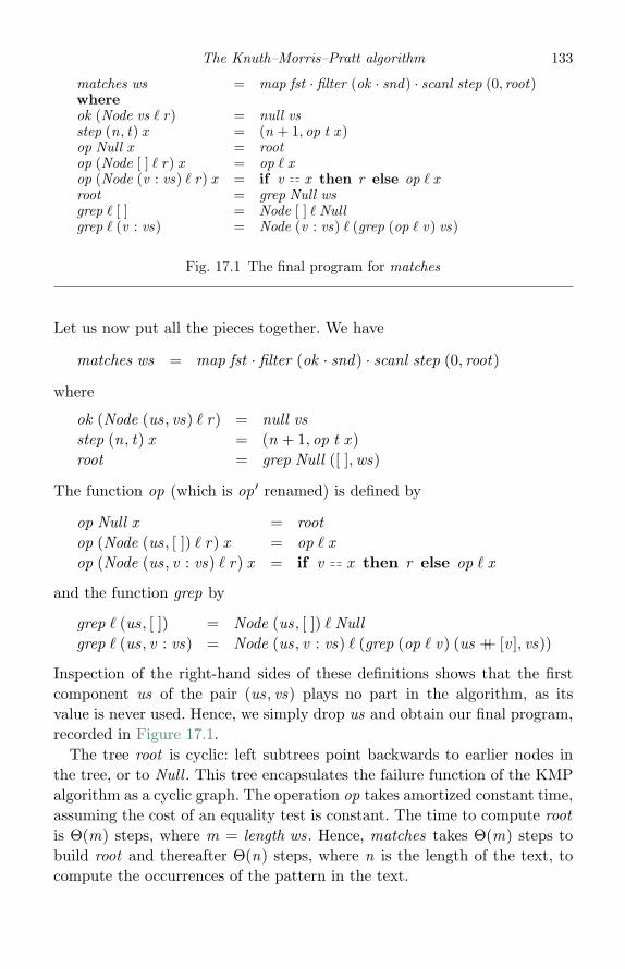
The Knuth–Morris–Pratt algorithm 133
matches ws = map fst · filter (ok · snd) · scanl step (0, root)whereok (Node vs � r) = null vsstep (n, t) x = (n + 1, op t x )op Null x = rootop (Node [ ] � r) x = op � xop (Node (v : vs) � r) x = if v x then r else op � xroot = grep Null wsgrep � [ ] = Node [ ] � Nullgrep � (v : vs) = Node (v : vs) � (grep (op � v) vs)
Fig. 17.1 The final program for matches
Let us now put all the pieces together. We have
matches ws = map fst · filter (ok · snd) · scanl step (0, root)
where
ok (Node (us, vs) � r) = null vsstep (n, t) x = (n + 1, op t x )root = grep Null ([ ],ws)
The function op (which is op ′ renamed) is defined by
op Null x = rootop (Node (us, [ ]) � r) x = op � xop (Node (us, v : vs) � r) x = if v x then r else op � x
and the function grep by
grep � (us, [ ]) = Node (us, [ ]) � Nullgrep � (us, v : vs) = Node (us, v : vs) � (grep (op � v) (us ++ [v ], vs))
Inspection of the right-hand sides of these definitions shows that the firstcomponent us of the pair (us, vs) plays no part in the algorithm, as itsvalue is never used. Hence, we simply drop us and obtain our final program,recorded in Figure 17.1.
The tree root is cyclic: left subtrees point backwards to earlier nodes inthe tree, or to Null . This tree encapsulates the failure function of the KMPalgorithm as a cyclic graph. The operation op takes amortized constant time,assuming the cost of an equality test is constant. The time to compute rootis Θ(m) steps, where m = length ws. Hence, matches takes Θ(m) steps tobuild root and thereafter Θ(n) steps, where n is the length of the text, tocompute the occurrences of the pattern in the text.
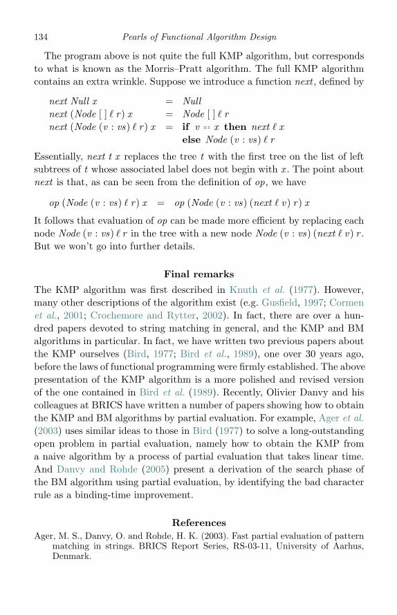
134 Pearls of Functional Algorithm Design
The program above is not quite the full KMP algorithm, but correspondsto what is known as the Morris–Pratt algorithm. The full KMP algorithmcontains an extra wrinkle. Suppose we introduce a function next , defined by
next Null x = Nullnext (Node [ ] � r) x = Node [ ] � rnext (Node (v : vs) � r) x = if v x then next � x
else Node (v : vs) � r
Essentially, next t x replaces the tree t with the first tree on the list of leftsubtrees of t whose associated label does not begin with x . The point aboutnext is that, as can be seen from the definition of op, we have
op (Node (v : vs) � r) x = op (Node (v : vs) (next � v) r) x
It follows that evaluation of op can be made more efficient by replacing eachnode Node (v : vs) � r in the tree with a new node Node (v : vs) (next � v) r .But we won’t go into further details.
Final remarks
The KMP algorithm was first described in Knuth et al. (1977). However,many other descriptions of the algorithm exist (e.g. Gusfield, 1997; Cormenet al., 2001; Crochemore and Rytter, 2002). In fact, there are over a hun-dred papers devoted to string matching in general, and the KMP and BMalgorithms in particular. In fact, we have written two previous papers aboutthe KMP ourselves (Bird, 1977; Bird et al., 1989), one over 30 years ago,before the laws of functional programming were firmly established. The abovepresentation of the KMP algorithm is a more polished and revised versionof the one contained in Bird et al. (1989). Recently, Olivier Danvy and hiscolleagues at BRICS have written a number of papers showing how to obtainthe KMP and BM algorithms by partial evaluation. For example, Ager et al.(2003) uses similar ideas to those in Bird (1977) to solve a long-outstandingopen problem in partial evaluation, namely how to obtain the KMP froma naive algorithm by a process of partial evaluation that takes linear time.And Danvy and Rohde (2005) present a derivation of the search phase ofthe BM algorithm using partial evaluation, by identifying the bad characterrule as a binding-time improvement.
ReferencesAger, M. S., Danvy, O. and Rohde, H. K. (2003). Fast partial evaluation of pattern
matching in strings. BRICS Report Series, RS-03-11, University of Aarhus,Denmark.
The Knuth–Morris–Pratt algorithm 135
Bird, R. S. (1977). Improving programs by the introduction of recursion. Commu-nications of the ACM 20 (11), 856–63.
Bird, R. S., Gibbons, J. and Jones, G. (1989). Formal derivation of a pattern match-ing algorithm. Science of Computer Programming 12, 93–104.
Cormen, T. H., Leiserson, C. E., Rivest, R. L. and Stein, C. (2001). Introductionto Algorithms, second edition. Cambridge, MA: MIT Press.
Crochemore, M. and Rytter, W. (2002). Jewels of Stringology. Hong Kong: WorldScientific.
Danvy, O. and Rohde, H. K. (2005). On obtaining the Boyer–Moore string-matchingalgorithm by partial evaluation. BRICS Research Report RS-05-14, Universityof Aarhus, Denmark.
Gusfield, D. (1997). Algorithms on Strings, Trees and Sequences. Cambridge, UK:Cambridge University Press.
Knuth, D. E., Morris, J. H. and Pratt, V. B. (1977). Fast pattern matching instrings. SIAM Journal on Computing 6, 323–50.
18
Planning solves the Rush Hour problem
Introduction
Rush Hour is an intriguing sliding-block puzzle, invented some years ago bythe celebrated puzzlist Nob Yoshigahara and marketed by Think Fun.1 It isplayed on a 6× 6 grid and can be solved in reasonable time by a brute-forcebreadth-first search. The generalised version – played on an n × n grid –is known to be PSPACE-complete, so a better than exponential-time solveris very unlikely. Still, with the help of a suitable planning algorithm, it ispossible to improve significantly on the brute-force approach, and the aimof this pearl is to show how. Further details of how Rush Hour is played arepostponed until later, because we want to start out with a more abstractformulation of puzzles, breadth-first search and planning.
Puzzles
Consider an abstract puzzle defined in terms of two finite sets, a set of statesand a set of moves. Given are three functions
moves :: State → [Move]move :: State → Move → Statesolved :: State → Bool
The function moves determines the legal moves that can be made in agiven state and move returns the new state that results when a given moveis made. The function solved determines which states are a solution tothe puzzle. Described in this way, a puzzle is essentially a deterministicfinite automaton. Solving the puzzle means finding some sequence of moves,preferably a shortest such sequence, that leads from a given initial state tosome solved state:
solve :: State → Maybe [Move]
1 Rush Hour is obtainable from http://www.puzzles.com/products/rushhour.htm.
136

Planning solves the Rush Hour problem 137
The value of solve q is Nothing if there is no sequence of moves beginningin state q that leads to a solved state and returns Just ms otherwise, wherems satisfies solved (foldl move q ms).
We can implement solve by carrying out either a breadth-first or a depth-first search. In either case the key idea is to introduce the synonyms
type Path = ([Move],State)type Frontier = [Path]
A path consists of a sequence of moves made in some given starting state,together with the resulting state. A frontier is a list of paths waiting to beexplored further. Then, a breadth-first search can be defined by
bfsearch :: [State]→ Frontier → Maybe [Move]bfsearch qs [ ] = Nothingbfsearch qs (p@(ms, q) : ps)
| solved q = Just ms| q ∈ qs = bfsearch qs ps| otherwise = bfsearch (q : qs) (ps ++ succs p)
where
succs :: Path → [Path]succs (ms, q) = [(ms ++ [m],move q m) | m ←moves q ]
The first component qs of bfsearch represents the set of analysed states.In a breadth-first search the frontier is managed as a queue, so paths atthe same distance from the starting state are analysed before their suc-cessors. Analysing a path means accepting it if the final state is a solvedstate, rejecting it if the final state has already been analysed, and otherwiseadding its successors to the end of the current frontier for future exploration.A breadth-first search will find a shortest solution if a solution exists.
With one change, the definition of depth-first search is exactly the same asthat of breadth-first search. The change is to replace the term ps ++ succs pby succs p ++ps. In a depth-first search the frontier is maintained as a stack,so the successors of a path are analysed before any other path at the samelevel. A depth-first search will find a solution if one exists, but it probablywon’t be the shortest.
Under breadth-first search the current frontier can be exponentially longerthan under depth-first search. Consequently, as defined above, bfsearch takesmuch more time than dfsearch. The reason is that evaluation of ps ++succs ptakes time proportional to the length of the frontier ps. One way to make the

138 Pearls of Functional Algorithm Design
code faster, though it does not reduce the space complexity, is to introducean accumulating parameter, defining bfsearch ′ by
bfsearch ′ qs pss ps = bfsearch qs (ps ++ concat (reverse pss))
Then, after some simple calculation which we omit, we obtain
bfsearch ′ :: [State]→ [Frontier ]→ Frontier → Maybe [Move]bfsearch ′ qs [ ] [ ] = Nothingbfsearch ′ qs pss [ ] = bfsearch ′ qs [ ] (concat (reverse pss))bfsearch ′ qs pss (p@(ms, q) : ps)| solved q = Just ms| q ∈ qs = bfsearch ′ qs pss ps| otherwise = bfsearch ′ (q : qs) (succs p : pss) ps
In fact, there is a simpler version of bfsearch ′ in which the accumulatingparameter is of type Frontier rather than [Frontier ]:
bfsearch ′ :: [State]→ Frontier → Frontier → Maybe [Move]bfsearch ′ qs [ ] [ ] = Nothingbfsearch ′ qs rs [ ] = bfsearch ′ qs [ ] rsbfsearch ′ qs rs (p@(ms, q) : ps)| solved q = Just ms| q ∈ qs = bfsearch ′ qs rs ps| otherwise = bfsearch ′ (q : qs) (succs p ++ rs) ps
This version of bfsearch ′ has a different behaviour than the previous one inthat successive frontiers are traversed alternately from left to right and fromright to left, but a shortest solution will still be found if a solution exists.
We can now define
bfsolve q = bfsearch ′ [ ] [ ] [([ ], q)]
The function bfsolve implements solve using a breadth-first search.
Planning
But what we have got so far is simply the strategy of trying every possiblesequence of moves until finding one that works. That is not the way humanssolve puzzles. Instead they make plans. For our purposes a plan is a sequenceof moves that, if the moves can be carried out, leads to a solved state. Thus:
type Plan = [Move]
Plans have to consist of non-repeated moves, otherwise the plan cannot becarried out. If, in order to make move m, a plan requires move m to be made
Planning solves the Rush Hour problem 139
first, then clearly the plan cannot be implemented. An empty plan meanssuccess. Otherwise, suppose the first move in the current plan is move m. Ifmove m can be carried out in the current state, then it is made. If it cannot,then we make use of a function premoves :: State → Move → [[Move]] suchthat, for each alternative pms in premoves q m, the move m can be madeprovided the preparatory moves pms are made first. In turn, moves in pmsmay require further preparatory moves, so we have to form new, extendedplans by iterating premoves:
newplans :: State → Plan → [Plan]newplans q ms = mkplans mswheremkplans ms | null ms = [ ]
| m ∈ qms = [ms]| otherwise = concat [mkplans (pms ++ ms) |
pms ← premoves q m,
all (/∈ms) pms]where m = head ms; qms = moves q
The result of newplans q ms is a possibly empty list of nonempty plans,the first move of each of which can be made in state q . To kick-start theplanning process we assume that a puzzle in state q can be solved by makingthe moves in goalmoves q , where goalmoves :: State → Plan.
Using just the two new functions goalmoves and premoves we can nowformulate an alternative search process based on the idea of an augmentedpath and frontier:
type APath = ([Move],State,Plan)type AFrontier = [APath]
An augmented path consists of moves already made from some startingstate, the state that results and a plan for the remaining moves. The searchconsists of exploring augmented paths in order until either one plan succeedsor all plans fail:
psearch :: [State]→ AFrontier → Maybe [Move]psearch qs [ ] = Nothingpsearch qs (p@(ms, q , plan) : ps)| solved q = Just ms| q ∈ qs = psearch qs ps| otherwise = psearch (q : qs) (asuccs p ++ ps ++ bsuccs p)
140 Pearls of Functional Algorithm Design
where
asuccs, bsuccs :: APath → [APath]asuccs (ms, q , plan)
= [(ms++[m],move q m, plan ′) | m : plan ′← newplans q plan]bsuccs (ms, q , )
= [(ms++[m], q ′, goalmoves q ′) | m ←moves q , let q ′ = move q m]
In psearch qs ps all the plans in the frontier ps are tried first in a depth-firstmanner. If all of them fail, then we add in further plans, each of which con-sists of making some legal move and starting over with a new goal. Theseadditional plans, expressed by the term bsuccs, are necessary for complete-ness. Simple puzzles may be solvable by suitable planning, but plans mayfail even though there is a solution. This is a consequence of the fact thatplans are executed greedily and moves that can be made are made. To ensurea complete strategy we have to be willing to make additional plans at eachstage.
As with a breadth-first search, we can make psearch faster by introducingan accumulating parameter:
psearch ′ :: [State]→ AFrontier → AFrontier → Maybe [Move]psearch ′ qs [ ] [ ] = Nothingpsearch ′ qs rs [ ] = psearch ′ qs [ ] rspsearch ′ qs rs (p@(ms, q , plan) : ps)| solved q = Just (reverse ms)| q ∈ qs = psearch ′ qs rs ps| otherwise = psearch ′ (q : qs) (bsuccs p ++ rs) (asuccs p ++ ps)
The function psolve can now be defined by
psolve :: State → Maybe [Move]psolve q = psearch ′ [ ] [ ] [([ ], q , goalmoves q)]
The function psolve implements solve using planning. It is possible to definea variation of psearch that explores plans in a breadth-first manner, but wewill leave details to the reader. Note that psearch will find a solution if oneexists, but not necessarily the shortest one.
Rush Hour
Let us now apply the above ideas to Rush Hour. As mentioned before, thisis a puzzle consisting of a 6× 6 grid of 36 cells. Covering some of these cellsare vehicles. Each vehicle is either vertical or horizontal and occupies eithertwo cells or three cells, depending on whether the vehicle is a car or truck.
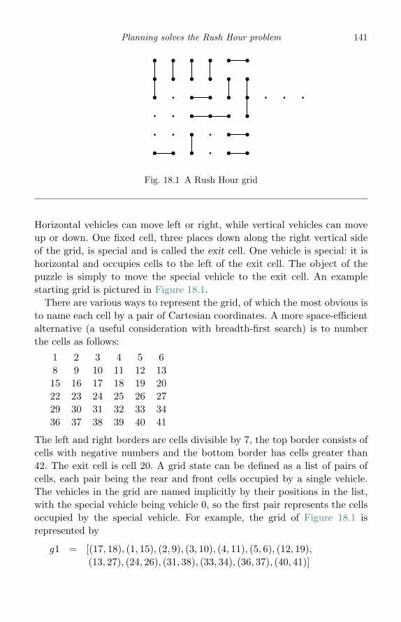
Planning solves the Rush Hour problem 141
� � � � � �
� � � � � �
� � � � � �
� � � � � � � � �
� � � � � �
� � � � � �
� ��
�
�
�
�
�
�
�
� � �
�
�
�
�
�
� � �
�
� � �
� � � �
Fig. 18.1 A Rush Hour grid
Horizontal vehicles can move left or right, while vertical vehicles can moveup or down. One fixed cell, three places down along the right vertical sideof the grid, is special and is called the exit cell. One vehicle is special: it ishorizontal and occupies cells to the left of the exit cell. The object of thepuzzle is simply to move the special vehicle to the exit cell. An examplestarting grid is pictured in Figure 18.1.
There are various ways to represent the grid, of which the most obvious isto name each cell by a pair of Cartesian coordinates. A more space-efficientalternative (a useful consideration with breadth-first search) is to numberthe cells as follows:
1 2 3 4 5 68 9 10 11 12 1315 16 17 18 19 2022 23 24 25 26 2729 30 31 32 33 3436 37 38 39 40 41
The left and right borders are cells divisible by 7, the top border consists ofcells with negative numbers and the bottom border has cells greater than42. The exit cell is cell 20. A grid state can be defined as a list of pairs ofcells, each pair being the rear and front cells occupied by a single vehicle.The vehicles in the grid are named implicitly by their positions in the list,with the special vehicle being vehicle 0, so the first pair represents the cellsoccupied by the special vehicle. For example, the grid of Figure 18.1 isrepresented by
g1 = [(17, 18), (1, 15), (2, 9), (3, 10), (4, 11), (5, 6), (12, 19),(13, 27), (24, 26), (31, 38), (33, 34), (36, 37), (40, 41)]
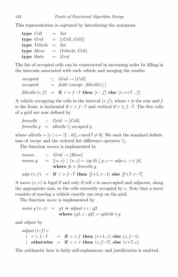
142 Pearls of Functional Algorithm Design
This representation is captured by introducing the synonyms
type Cell = Inttype Grid = [(Cell ,Cell)]type Vehicle = Inttype Move = (Vehicle,Cell)type State = Grid
The list of occupied cells can be constructed in increasing order by filling inthe intervals associated with each vehicle and merging the results:
occupied :: Grid → [Cell ]occupied = foldr (merge · fillcells) [ ]
fillcells (r , f ) = if r > f−7 then [r .. f ] else [r , r+7 .. f ]
A vehicle occupying the cells in the interval (r , f ), where r is the rear and fis the front, is horizontal if r > f−7 and vertical if r ≤ f−7. The free cellsof a grid are now defined by
freecells :: Grid → [Cell ]freecells g = allcells \\ occupied g
where allcells = [c | c← [1 ..41], c mod7 �= 0]. We omit the standard definit-ions of merge and the ordered list difference operator \\.
The function moves is implemented by
moves :: Grid → [Move]moves g = [(v , c) | (v , i)← zip [0..] g , c← adjs i , c ∈ fs]
where fs = freecells g
adjs (r , f ) = if r > f−7 then [f +1, r−1] else [f +7, r−7]
A move (v , c) is legal if and only if cell c is unoccupied and adjacent, alongthe appropriate axis, to the cells currently occupied by v . Note that a moveconsists of moving a vehicle exactly one step on the grid.
The function move is implemented by
move g (v , c) = g1 ++ adjust i c : g2where (g1, i : g2) = splitAt v g
and adjust by
adjust (r , f ) c| r > f−7 = if c > f then (r+1, c) else (c, f−1)| otherwise = if c < r then (c, f−7) else (r+7, c)
The arithmetic here is fairly self-explanatory and justification is omitted.
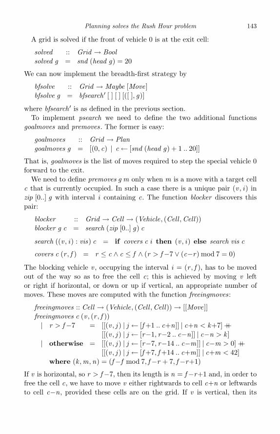
Planning solves the Rush Hour problem 143
A grid is solved if the front of vehicle 0 is at the exit cell:
solved :: Grid → Boolsolved g = snd (head g) = 20
We can now implement the breadth-first strategy by
bfsolve :: Grid → Maybe [Move]bfsolve g = bfsearch ′ [ ] [ ] [([ ], g)]
where bfsearch ′ is as defined in the previous section.To implement psearch we need to define the two additional functions
goalmoves and premoves. The former is easy:
goalmoves :: Grid → Plangoalmoves g = [(0, c) | c← [snd (head g) + 1 .. 20]]
That is, goalmoves is the list of moves required to step the special vehicle 0forward to the exit.
We need to define premoves g m only when m is a move with a target cellc that is currently occupied. In such a case there is a unique pair (v , i) inzip [0..] g with interval i containing c. The function blocker discovers thispair:
blocker :: Grid → Cell → (Vehicle, (Cell ,Cell))blocker g c = search (zip [0..] g) c
search ((v , i) : vis) c = if covers c i then (v , i) else search vis c
covers c (r , f ) = r ≤ c ∧ c ≤ f ∧ (r > f−7 ∨ (c−r) mod 7 = 0)
The blocking vehicle v , occupying the interval i = (r , f ), has to be movedout of the way so as to free the cell c; this is achieved by moving v leftor right if horizontal, or down or up if vertical, an appropriate number ofmoves. These moves are computed with the function freeingmoves:
freeingmoves :: Cell → (Vehicle, (Cell ,Cell))→ [[Move]]freeingmoves c (v , (r , f ))| r > f−7 = [[(v , j ) | j ← [f +1 .. c+n]] | c+n < k+7] ++
[[(v , j ) | j ← [r−1, r−2 .. c−n]] | c−n > k ]| otherwise = [[(v , j ) | j ← [r−7, r−14 .. c−m]] | c−m > 0] ++
[[(v , j ) | j ← [f +7, f +14 .. c+m]] | c+m < 42]where (k ,m,n) = (f−f mod 7, f−r + 7, f−r+1)
If v is horizontal, so r > f−7, then its length is n = f−r+1 and, in order tofree the cell c, we have to move v either rightwards to cell c+n or leftwardsto cell c−n, provided these cells are on the grid. If v is vertical, then its
144 Pearls of Functional Algorithm Design
length is n = (f − r) div 7 + 1 and we have to move v either upwards to cellc−7n or downwards to cell c+7n, again provided these cells are on the grid.The value of m in this case is m = 7× n.
Now we can define premoves by
premoves :: Grid → Move → [[Move]]premoves g (v , c) = freeingmoves c (blocker g c)
However, the definition of newplans given in the previous section needs to bemodified in order to work with Rush Hour. To see why, imagine the currentplan consists of the goal moves [(0, 19), (0, 20)] where vehicle 0 occupies thecells [17, 18] on the opening grid. Suppose the first move (0, 19) is not possibleuntil the preparatory moves pms are made. Now it is perfectly possible thatone of the moves in pms is (0, 16), moving vehicle 0 one place to the left.After executing pms in preparation for the move (0, 19) we see that (0, 19)is no longer a well-defined move in the resulting grid because it requires 0 tomove two steps forward, and so has first to be expanded to the single-stepmoves [(0, 18), (0, 19)]. Hence, we need to modify newplans to read
newplans :: Grid → Plan → [Plan]newplans g [ ] = [ ]newplans g (m : ms) = mkplans (expand g m ++ ms)where mkplans ms = if m ∈ gms then [ms] else
concat [mkplans (pms ++ ms) |pms ← premoves g m,
all (/∈ ms) pms]where m = head ms; gms = moves g
The new function expand , which expands a possibly invalid move into asequence of valid moves, is defined by
expand :: Grid → Move → [Move]expand g (v , c)| r > f−7 = if c > f then [(v , p) | p ← [f +1 .. c]]
else [(v , p) | p ← [r−1, r−2 .. c]]| otherwise = if c > f then [(v , p) | p ← [f +7, f +14 .. c]]
else [(v , p) | p ← [r−7, r−14 .. c]]where (r , f ) = g !! v
We can now implement the planning algorithm by
psolve :: Grid → Maybe [Move]psolve g = psearch ′ [ ] [ ] [([ ], g , goalmoves g)]
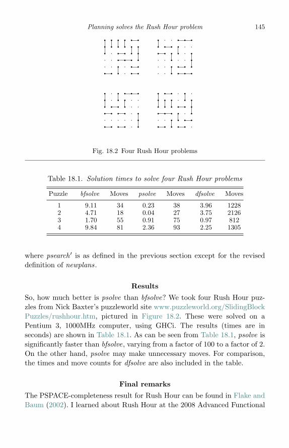
Planning solves the Rush Hour problem 145
� � � � � �
� � � � � �
� � � � � �
� � � � � �
� � � � � �
� � � � � �
� ��
�
�
�
�
�
�
�
� � �
�
�
�
�
�
� � �
�
� � �
� � � � � � � � � �
� � � � � �
� � � � � �
� � � � � �
� � � � � �
� � � � � �
� �
�
� � � �
� �
�
�
�
�
�
�
�
�
� � �
� � �
� � � � � �
� � � � � �
� � � � � �
� � � � � �
� � � � � �
� � � � � �
� ��
�
�
�
� � � �
�
�
� � � �
�
�
�
� � � � � � � � � �
� � � � � �
� � � � � �
� � � � � �
� � � � � �
� � � � � �
� ��
�
� � �
�
�
�
�
�
�
�
�
�
� � �
�
�
�
� � �
� � � �
Fig. 18.2 Four Rush Hour problems
Table 18.1. Solution times to solve four Rush Hour problems
Puzzle bfsolve Moves psolve Moves dfsolve Moves
1 9.11 34 0.23 38 3.96 12282 4.71 18 0.04 27 3.75 21263 1.70 55 0.91 75 0.97 8124 9.84 81 2.36 93 2.25 1305
where psearch ′ is as defined in the previous section except for the reviseddefinition of newplans.
Results
So, how much better is psolve than bfsolve? We took four Rush Hour puz-zles from Nick Baxter’s puzzleworld site www.puzzleworld.org/SlidingBlockPuzzles/rushhour.htm, pictured in Figure 18.2. These were solved on aPentium 3, 1000MHz computer, using GHCi. The results (times are inseconds) are shown in Table 18.1. As can be seen from Table 18.1, psolve issignificantly faster than bfsolve, varying from a factor of 100 to a factor of 2.On the other hand, psolve may make unnecessary moves. For comparison,the times and move counts for dfsolve are also included in the table.
Final remarks
The PSPACE-completeness result for Rush Hour can be found in Flake andBaum (2002). I learned about Rush Hour at the 2008 Advanced Functional
146 Pearls of Functional Algorithm Design
Programming Summer School (Jones, 2008), where Mark Jones presented aseries of lectures about the benefits of thinking functionally about problems.He gave a breadth-first solution, but he also challenged participants at thesummer school to come up with a faster solution. This pearl was composedin response to Jones’ challenge.
ReferencesFlake, G. W. and Baum, E. B. (2002). Rush Hour is PSPACE-complete, or “Why
you should generously tip parking lot attendants”. Theoretical ComputerScience 270 (1), 895–911.
Jones, M. P. (2008). Functional thinking. Advanced Functional ProgrammingSummer School, Boxmeer, The Netherlands.

19
A simple Sudoku solver
How to play: Fill in the grid so that every row, every column and every 3 × 3box contains the digits 1–9. There’s no maths involved. You solve the puzzle withreasoning and logic.
Advice on how to play Sudoku, The Independent Newspaper
Introduction
The game of Sudoku is played on a 9× 9 grid. Given a matrix, such as thatin Figure 19.1, the idea is to fill in the empty cells with the digits 1 to 9so that each row, column and 3 × 3 box contains the numbers 1 to 9. Ingeneral there may be one, none or many solutions, though in a good Sudokupuzzle there should always be a unique solution. Our aim in this pearl isto construct a Haskell program to solve Sudoku puzzles. Specifically, wewill define a function solve for computing all the ways a given grid maybe completed. If only one solution is wanted, then we can take the headof the list. Lazy evaluation means that only the first result will then becomputed. We begin with a specification, then use equational reasoning tocalculate a more efficient version. There is no maths involved, just reasoningand logic!
Specification
We begin with some basic data types, starting with matrices:
type Matrix a = [Row a]type Row a = [a]
An m×n matrix is a list of m rows in which each row has the same length n.A grid is a 9× 9 matrix of digits:
type Grid = Matrix Digittype Digit = Char
147
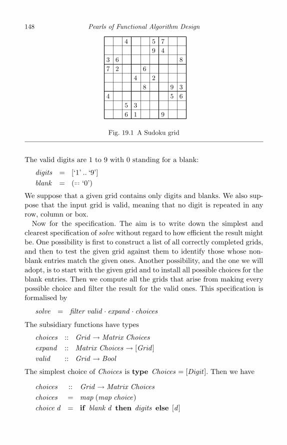
148 Pearls of Functional Algorithm Design
4
73
26
65
4
13
48
62
95
9
47
59
63
8
Fig. 19.1 A Sudoku grid
The valid digits are 1 to 9 with 0 standing for a blank:
digits = [‘1’ .. ‘9’]blank = ( ‘0’)
We suppose that a given grid contains only digits and blanks. We also sup-pose that the input grid is valid, meaning that no digit is repeated in anyrow, column or box.
Now for the specification. The aim is to write down the simplest andclearest specification of solve without regard to how efficient the result mightbe. One possibility is first to construct a list of all correctly completed grids,and then to test the given grid against them to identify those whose non-blank entries match the given ones. Another possibility, and the one we willadopt, is to start with the given grid and to install all possible choices for theblank entries. Then we compute all the grids that arise from making everypossible choice and filter the result for the valid ones. This specification isformalised by
solve = filter valid · expand · choices
The subsidiary functions have types
choices :: Grid → Matrix Choicesexpand :: Matrix Choices → [Grid ]valid :: Grid → Bool
The simplest choice of Choices is type Choices = [Digit ]. Then we have
choices :: Grid → Matrix Choiceschoices = map (map choice)choice d = if blank d then digits else [d ]
A simple Sudoku solver 149
If the cell is blank, then all digits are installed as possible choices; otherwisethere is no choice and a singleton is returned.
Next, expansion is just matrix Cartesian product:
expand :: Matrix Choices → [Grid ]expand :: cp ·map cp
The Cartesian product of a list of lists is given by
cp :: [[a]]→ [[a]]cp [ ] = [[ ]]cp (xs : xss) = [x : ys | x ← xs, ys ← cp xss]
For example, cp [[1, 2], [3], [4, 5]] = [[1, 3, 4], [1, 3, 5], [2, 3, 4], [2, 3, 5]]. Thus,map cp returns a list of all possible choices for each row and cp · map cpinstalls each choice for the rows in all possible ways.
Finally, we deal with valid . A valid grid is one in which no row, columnor box contains duplicates:
valid :: Grid → Boolvalid g = all nodups (rows g) ∧
all nodups (cols g) ∧all nodups (boxs g)
The standard function all p applied to a finite list xs returns True if allelements of xs satisfy p and False otherwise. The function nodups can bedefined by
nodups :: Eq a ⇒ [a]→ Boolnodups [ ] = Truenodups (x : xs) = all (�= x ) xs ∧ nodups xs
The function nodups takes quadratic time. As an alternative we could sortthe list of digits and check that it is strictly increasing. Sorting can bedone in Θ(n log n) steps. However, with n = 9 it is not clear that sortingthe digits is worthwhile. What would you prefer: 2n2 steps or 100n log2 nsteps?
It remains to define rows, cols and boxs. If a matrix is given by a list ofits rows, then rows is just the identity function on matrices:
rows :: Matrix a → Matrix arows = id
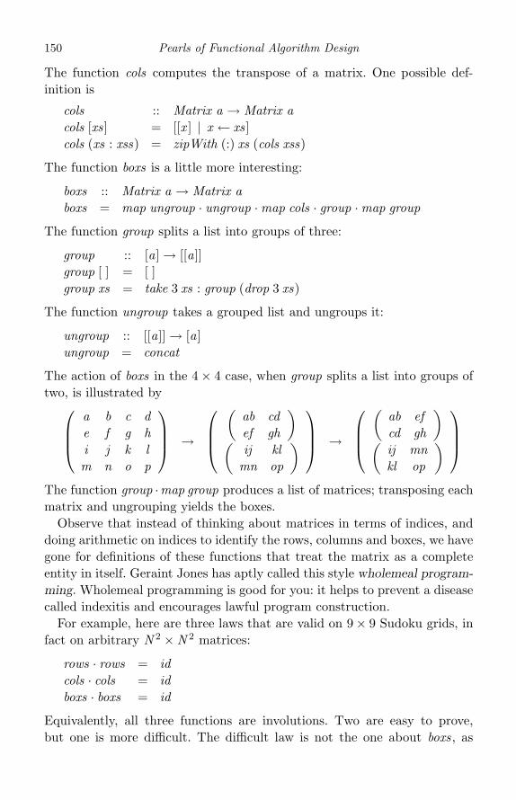
150 Pearls of Functional Algorithm Design
The function cols computes the transpose of a matrix. One possible def-inition is
cols :: Matrix a → Matrix acols [xs] = [[x ] | x ← xs]cols (xs : xss) = zipWith (:) xs (cols xss)
The function boxs is a little more interesting:
boxs :: Matrix a → Matrix aboxs = map ungroup · ungroup ·map cols · group ·map group
The function group splits a list into groups of three:
group :: [a]→ [[a]]group [ ] = [ ]group xs = take 3 xs : group (drop 3 xs)
The function ungroup takes a grouped list and ungroups it:
ungroup :: [[a]]→ [a]ungroup = concat
The action of boxs in the 4× 4 case, when group splits a list into groups oftwo, is illustrated by⎛
⎜⎜⎝a b c de f g hi j k lm n o p
⎞⎟⎟⎠ →
⎛⎜⎜⎝
(ab cdef gh
)(
ij klmn op
)⎞⎟⎟⎠ →
⎛⎜⎜⎝
(ab efcd gh
)(
ij mnkl op
)⎞⎟⎟⎠
The function group ·map group produces a list of matrices; transposing eachmatrix and ungrouping yields the boxes.
Observe that instead of thinking about matrices in terms of indices, anddoing arithmetic on indices to identify the rows, columns and boxes, we havegone for definitions of these functions that treat the matrix as a completeentity in itself. Geraint Jones has aptly called this style wholemeal program-
ming. Wholemeal programming is good for you: it helps to prevent a diseasecalled indexitis and encourages lawful program construction.
For example, here are three laws that are valid on 9× 9 Sudoku grids, infact on arbitrary N 2 ×N 2 matrices:
rows · rows = idcols · cols = idboxs · boxs = id
Equivalently, all three functions are involutions. Two are easy to prove,but one is more difficult. The difficult law is not the one about boxs, as
A simple Sudoku solver 151
you might expect, but the involution property of cols. Though intuitivelyobvious, proving it from the definition of cols is slightly tricky. The involutionproperty of boxs is an easy calculation using the involution property of cols,simple properties of map and the fact that group · ungroup = id .
Here are three more laws, valid on N 2 ×N 2 matrices of choices:
map rows · expand = expand · rows (19.1)
map cols · expand = expand · cols (19.2)
map boxs · expand = expand · boxs (19.3)
We will make use of these laws in a short while.
Pruning the matrix of choices
Though executable in theory, the specification of solve is hopeless in practice.Assuming about a half of the 81 entries are fixed initially (a generous esti-mate), there are about 940, or
147 808 829 414 345 923 316 083 210 206 383 297 601
grids to check! We therefore need a better approach. To make a moreefficient solver, a good idea is to remove any choices from a cell c thatalready occur as singleton entries in the row, column and box contain-ing c. A singleton entry corresponds to a fixed choice. We therefore seek afunction
prune :: Matrix Choices → Matrix Choices
so that
filter valid · expand = filter valid · expand · prune
How can we define prune? Well, since a matrix is a list of rows, a goodplace to start is by pruning a single row. The function pruneRow isdefined by
pruneRow :: Row Choices → Row ChoicespruneRow row = map (remove fixed) row
where fixed = [d | [d ]← row ]
The function remove removes choices from any choice that is not fixed:
remove xs ds = if singleton ds then ds else ds \\ xs
The function pruneRow satisfies
filter nodups · cp = filter nodups · cp · pruneRow (19.4)
The proof is left as an exercise.

152 Pearls of Functional Algorithm Design
We are now nearly ready for a calculation that will determine the functionprune. Nearly, but not quite, because we are going to need two laws aboutfilter . The first is that if f · f = id , then
filter (p · f ) = map f · filter p ·map f (19.5)
Equivalently, filter (p · f ) ·map f = map f · filter p. The second law is that
filter (all p) · cp = cp ·map (filter p) (19.6)
Proofs of (19.5) and (19.6) are again left as exercises.Now for the calculation. The starting point is to rewrite filtervalid ·expand :
filter valid · expand = filter (all nodups · boxs) ·filter (all nodups · cols) ·filter (all nodups · rows) · expand
The order in which the filters appear on the right is not important. Theplan of attack is to send each of these filters into battle with expand . Forexample, in the boxs case we argue:
filter (all nodups · boxs) · expand
= {(19.5), since boxs · boxs = id}map boxs · filter (all nodups) ·map boxs · expand
= {(19.3)}map boxs · filter (all nodups) · expand · boxs
= {definition of expand}map boxs · filter (all nodups) · cp ·map cp · boxs
= {(19.6) and map f ·map g = map (f · g)}map boxs · cp ·map (filter nodups · cp) · boxs
= {(19.4)}map boxs · cp ·map (filter nodups · cp · pruneRow) · boxs
= {(19.6)}map boxs · filter (all nodups) · cp ·map cp ·map pruneRow · boxs
= {definition of expand}map boxs · filter (all nodups) · expand ·map pruneRow · boxs
= {(19.5) in the form map f · filter p = filter (p · f ) ·map f }filter (all nodups · boxs) ·map boxs · expand ·map pruneRow · boxs
= {(19.3)}filter (all nodups · boxs) · expand · boxs ·map pruneRow · boxs

A simple Sudoku solver 153
We have shown that
filter (all nodups · boxs) · expand= filter (all nodups · boxs) · expand · pruneBy boxs
where pruneBy f = f · map pruneRow · f . Repeating the same calculationfor rows and cols, we obtain
filter valid · expand = filter valid · expand · prune
where
prune = pruneBy boxs · pruneBy cols · pruneBy rows
In conclusion, the previous definition of solve can be replaced with anew one:
solve = filter valid · expand · prune · choices
In fact, rather than just one prune, we can have as many prunes as we like.This is sensible, because after one round of pruning some choices may beresolved into singleton choices and another round of pruning may removestill more impossible choices. The simplest Sudoku problems are solved justby repeatedly pruning the matrix of choices until only singleton choicesare left.
Single-cell expansion
For more devious puzzles we can combine pruning with another idea:expanding the choices for a single cell only. While expand installed allpossible choices in all cells on the grid in one go, single-cell expansionpicks on one cell and installs all the choices for that cell only. The hope isthat mixing prunes with single-cell expansions can lead to a solution morequickly.
Therefore, we construct a function expand1 that expands the choices forone cell only. This function is required to satisfy the property that, up tosome permutation of the answer:
expand = concat ·map expand · expand1 (19.7)
A good choice of cell on which to perform expansion is one with the small-est number of choices (not equal to one of course). A cell with no choicesmeans that the puzzle is unsolvable, so identifying such a cell quickly isa good idea. Think of cell containing cs choices as sitting in the middleof a row row , so row = row1 ++ [cs] ++ row2, in the matrix of choices,
154 Pearls of Functional Algorithm Design
with rows rows1 above this row and rows rows2 below it. Then we candefine
expand1 :: Matrix Choices → [Matrix Choices]expand1 rows = [rows1 ++ [row1 ++ [c] : row2] ++ rows2 | c← cs]where (rows1, row : rows2) = break (any smallest) rows
(row1, cs : row2) = break smallest rowsmallest cs = length cs nn = minimum (counts rows)
counts = filter (�= 1) ·map length · concat
The value n is the smallest number of choices, not equal to one, in any cellof the matrix of choices. If the matrix of choices contains only singletonchoices, then n is the minimum of the empty list, which is not defined. Thestandard function break p splits a list into two:
break p xs = (takeWhile (not · p) xs, dropWhile (not · p) xs)
Thus, break (any smallest) rows breaks the matrix into two lists of rowswith the head of the second list being some row that contains a cell withthe smallest number of choices. A second appeal to break then breaks thisrow into two sub-rows, with the head of the second being the element cswith the smallest number of choices. Each possible choice is installed andthe matrix reconstructed. If there are zero choices, then expand1 returns anempty list.
It follows from the definition of n that (19.7) holds only when applied tomatrices with at least one non-singleton choice. Say a matrix is complete
if all choices are singletons and unsafe if the singleton choices in any row,column or box contain duplicates. Incomplete and unsafe matrices can neverlead to valid grids. A complete and safe matrix of choices determines a uniquevalid grid. These two tests can be implemented by
complete = all (all single)
where single is the test for a singleton list, and
safe m = all ok (rows m) ∧ all ok (cols m) ∧ all ok (boxs m)
where ok row = nodups [d | [d ]← row ].Assuming a matrix is safe but incomplete, we can calculate:
filter valid · expand
= {since expand = concat ·map expand · expand1on incomplete matrices}

A simple Sudoku solver 155
filter valid · concat ·map expand · expand1
= {since filter p · concat = concat ·map (filter p)}concat ·map (filter valid · expand) · expand1
= {since filter valid · expand = filter valid · expand · prune}concat ·map(filter valid · expand · prune) · expand1
Introducing search = filter valid · expand · prune, we therefore have, on safebut incomplete matrices, that
search · prune = concat ·map search · expand1
And now we can replace solve by a third version:
solve = search · choicessearch m | not (safe m) = [ ]
| complete m ′ = [map (map head) m ′]| otherwise = concat (map search (expand1 m ′))| where m ′ = prune m
This is our final simple Sudoku solver.
Final remarks
We tested the solver on 36 puzzles recorded at the website http://haskell.org/haskellwiki/Sudoku. It solved them in 8.8 s (on a 1GHz Pentium 3 PC). Wealso tested them on six minimal puzzles (each with 17 non-blank entries)chosen randomly from the 32 000 given at the site. It solved them in 111.4 s.There are about a dozen different Haskell Sudoku solvers at the site. All ofthese, including a very nice solver by Lennart Augustsson, deploy coordi-nate calculations. Many use arrays and most use monads. Ours is abouttwice as slow as Augustsson’s on the nefarious puzzle (a particularly hardpuzzle with the minimum 17 non-blank entries), but about 30 times fasterthan Yitz Gale’s solver on easy puzzles. We also know of solvers that reducethe problem to Boolean satisfiability, constraint satisfaction, model checkingand so on. I would argue that the one presented above is certainly one ofthe simplest and shortest. And at least it was derived, in part, by equationalreasoning.
20
The Countdown problem
Introduction
Countdown is the name of a game from a popular British televisionprogramme; in France it is called Le Conte est Bon. Contestants are givensix source numbers, not necessarily all different, and a target number, all ofwhich are positive integers. The aim is to use some of the source numbersto build an arithmetic expression whose value is as close to the target aspossible. Expressions are constructed using only the four basic operations ofaddition, subtraction, multiplication and division. Contestants are allowed30 s thinking time. For example, with source numbers [1, 3, 7, 10, 25, 50] andtarget 831 there is no exact solution; one expression that comes closestis 7 + (1 + 10) × (25 + 50) = 832. Our aim in this pearl is to describevarious programs for solving Countdown, all based in one way or anotheron exhaustive search. Countdown is attractive as a case study in exhaus-tive search because the problem is simply stated and the different solutionsillustrate the space and time trade-offs that have to be taken into accountin comparing functional programs.
A simple program
Here is a straightforward program for Countdown:
countdown1 :: Int → [Int ] → (Expr ,Value)countdown1 n = nearest n · concatMap mkExprs · subseqs
First of all, the source numbers are given as a list; the order of the elementsis unimportant, but duplicates do matter. We will suppose that the listis in ascending order, a fact that is exploited later on. Each selection istherefore represented by a nonempty subsequence. For each subsequencexs, all possible arithmetic expressions that can be constructed from xs are
156

The Countdown problem 157
determined, along with their values.1 The results are concatenated and onenearest the target is selected.
The ingredients making up countdown1 are defined as follows. First,subseqs returns a list of all the nonempty subsequences of a nonempty list:
subseqs [x ] = [[x ]]subseqs (x : xs) = xss ++ [x ] : map (x :) xss
where xss = subseqs xs
Next, the data types of expressions and values can be declared by
data Expr = Num Int | App Op Expr Exprdata Op = Add | Sub | Mul | Divtype Value = Int
The value of an expression is computed by
value :: Expr → Valuevalue (Num x ) = xvalue (App op e1 e2) = apply op (value e1) (value e2)
where applyAdd = (+), applySub = (−) and so on. However, not all possibleexpressions are valid in Countdown. For instance, the result of a subtractionshould be a positive integer, and division is valid only when the divisordivides the dividend exactly. An expression is valid if its subexpressions are,and if the operation at the root passes the test legal , where
legal :: Op → Value → Value → Boollegal Add v1 v2 = Truelegal Sub v1 v2 = (v2 < v1)legal Mul v1 v2 = Truelegal Div v1 v2 = (v1 mod v2 0)
The next ingredient is mkExpr , which creates a list of all legal expressionsthat can be built using the given subsequence:
mkExprs :: [Int ] → [(Expr ,Value)]mkExprs [x ] = [(Num x , x )]mkExprs xs = [ev | (ys, zs)← unmerges xs,
ev1←mkExprs ys,ev2←mkExprs zs,ev ← combine ev1 ev2]
1 Logically there is no need to return both expressions and values as the latter can be determinedfrom the former. But, as we have seen in the pearl “Making a century” (Pearl 6), it is a goodidea to avoid computing values more than once, so this optimisation has been incorporated fromthe outset.
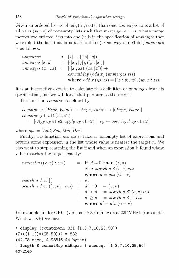
158 Pearls of Functional Algorithm Design
Given an ordered list xs of length greater than one, unmerges xs is a list ofall pairs (ys, zs) of nonempty lists such that merge ys zs = xs, where mergemerges two ordered lists into one (it is in the specification of unmerges thatwe exploit the fact that inputs are ordered). One way of defining unmergesis as follows:
unmerges :: [a]→ [([a], [a])]unmerges [x , y ] = [([x ], [y ]), ([y ], [x ])]unmerges (x : xs) = [([x ], xs), (xs, [x ])] ++
concatMap (add x ) (unmerges xss)where add x (ys, zs) = [(x : ys, zs), (ys, x : zs)]
It is an instructive exercise to calculate this definition of unmerges from itsspecification, but we will leave that pleasure to the reader.
The function combine is defined by
combine :: (Expr ,Value)→ (Expr ,Value)→ [(Expr ,Value)]combine (e1, v1) (e2, v2)
= [(App op e1 e2, apply op v1 v2) | op ← ops, legal op v1 v2]
where ops = [Add ,Sub,Mul ,Div ].Finally, the function nearest n takes a nonempty list of expressions and
returns some expression in the list whose value is nearest the target n. Wealso want to stop searching the list if and when an expression is found whosevalue matches the target exactly:
nearest n ((e, v) : evs) = if d 0 then (e, v)else search n d (e, v) evswhere d = abs (n − v)
search n d ev [ ] = evsearch n d ev ((e, v) : evs) | d ′ 0 = (e, v)
| d ′ < d = search n d ′ (e, v) evs| d ′ ≥ d = search n d ev evs
where d ′ = abs (n − v)
For example, under GHCi (version 6.8.3 running on a 2394MHz laptop underWindows XP) we have
> display (countdown1 831 [1,3,7,10,25,50])(7+((1+10)*(25+50))) = 832(42.28 secs, 4198816144 bytes)> length $ concatMap mkExprs $ subseqs [1,3,7,10,25,50]4672540
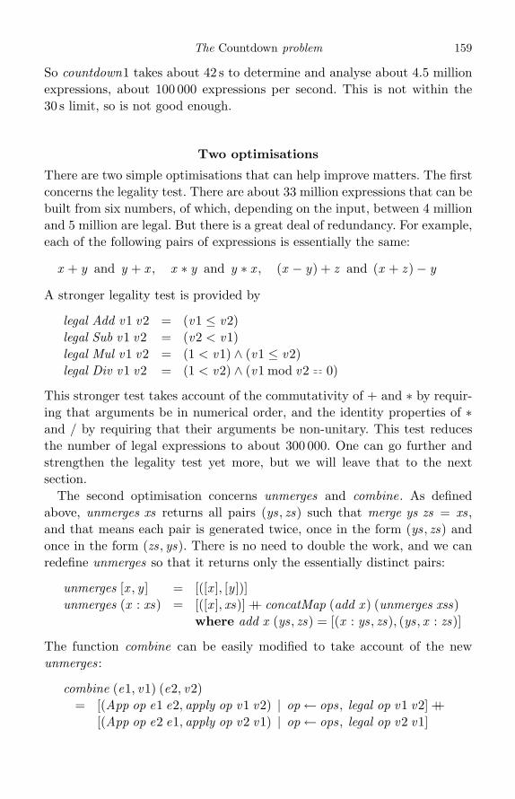
The Countdown problem 159
So countdown1 takes about 42 s to determine and analyse about 4.5 millionexpressions, about 100 000 expressions per second. This is not within the30 s limit, so is not good enough.
Two optimisations
There are two simple optimisations that can help improve matters. The firstconcerns the legality test. There are about 33 million expressions that can bebuilt from six numbers, of which, depending on the input, between 4 millionand 5 million are legal. But there is a great deal of redundancy. For example,each of the following pairs of expressions is essentially the same:
x + y and y + x , x ∗ y and y ∗ x , (x − y) + z and (x + z )− y
A stronger legality test is provided by
legal Add v1 v2 = (v1 ≤ v2)legal Sub v1 v2 = (v2 < v1)legal Mul v1 v2 = (1 < v1) ∧ (v1 ≤ v2)legal Div v1 v2 = (1 < v2) ∧ (v1 mod v2 0)
This stronger test takes account of the commutativity of + and ∗ by requir-ing that arguments be in numerical order, and the identity properties of ∗and / by requiring that their arguments be non-unitary. This test reducesthe number of legal expressions to about 300 000. One can go further andstrengthen the legality test yet more, but we will leave that to the nextsection.
The second optimisation concerns unmerges and combine. As definedabove, unmerges xs returns all pairs (ys, zs) such that merge ys zs = xs,and that means each pair is generated twice, once in the form (ys, zs) andonce in the form (zs, ys). There is no need to double the work, and we canredefine unmerges so that it returns only the essentially distinct pairs:
unmerges [x , y ] = [([x ], [y ])]unmerges (x : xs) = [([x ], xs)] ++ concatMap (add x ) (unmerges xss)
where add x (ys, zs) = [(x : ys, zs), (ys, x : zs)]
The function combine can be easily modified to take account of the newunmerges:
combine (e1, v1) (e2, v2)= [(App op e1 e2, apply op v1 v2) | op ← ops, legal op v1 v2] ++
[(App op e2 e1, apply op v2 v1) | op ← ops, legal op v2 v1]
160 Pearls of Functional Algorithm Design
comb1 (e1, v1) (e2, v2)= [(App Add e1 e2, v1 + v2), (App Sub e2 e1, v2− v1)] ++
if 1 < v1 then[(App Mul e1 e2, v1 ∗ v2)] ++ [(App Div e2 e1, q) | r = 0]else [ ]where (q , r) = divMod v2 v1
comb2 (e1, v1) (e2, v2)= [(App Add e1 e2, v1 + v2)] ++
if 1 < v1 then[(App Mul e1 e2, v1 ∗ v2), (App Div e1 e2, 1)]else [ ]
Fig. 20.1 Definitions of comb1 and comb2
However, a faster method is to incorporate the stronger legality test directlyinto the definition of combine:
combine (e1, v1) (e2, v2)| v1 < v2 = comb1 (e1, v1) (e2, v2)| v1 v2 = comb2 (e1, v1) (e2, v2)| v1 > v2 = comb1 (e2, v2) (e1, v1)
The function comb1 is used when the first expression has a value strictly lessthan the second, and comb2 when the two values are equal. Their definitionsare given in Figure 20.1. Installing these changes leads to countdown2, whosedefinition is otherwise the same as countdown1. For example:
> display (countdown2 831 [1,3,7,10,25,50])(7+((1+10)*(25+50))) = 832(1.77 secs, 168447772 bytes)> length $ concatMap mkExprs $ subseqs [1,3,7,10,25,50]240436
This is better, in that it takes only about 2 s to determine and analyse about250 000 expressions, but there is still room for improvement.
An even stronger legality test
In an attempt to restrict still further the number of expressions that haveto be considered, let us say that an expression is in normal form if it is asum of the form
[(e1 + e2) + · · ·+ em ]− [(f1 + f2) + · · ·+ fn ]
The Countdown problem 161
where m ≥ 1 and n ≥ 0, both e1, e2, . . . and f1, f2, . . . are in ascending orderof value, and each ej and fj is a product of the form
[(g1 ∗ g2) ∗ · · · ∗ gp ]/[(h1 ∗ h2) ∗ · · · ∗ hq ]
where p ≥ 1 and q ≥ 0, both g1, g2, . . . and h1, h2, . . . are in ascending orderof value and each gj and hj is either a single number or an expression innormal form.
Up to rearrangements of subexpressions with equal values, each expressionhas a unique normal form. Of the 300 000 expressions over six numbers thatare legal according to the earlier definition, only about 30 000 to 70 000are in normal form. However, normal form does not eliminate redundancycompletely. For example, the expressions 2 + 5 + 7 and 2 ∗ 7 have the samevalue, but the latter is built out of numbers that are a subsequence of theformer. There is, therefore, no need to build the former. But we will notexplore the additional optimisation of “thinning” a list of expressions toretain only the really essential ones. Experiments show that thinning turnsout to be not worth the candle: the savings made in analysing only thereally essential expressions are outweighed by the amount of effort neededto determine them.
We can capture normal forms by strengthening the legality test, but thistime we have to consider expressions as well as values. First let us definenon by
non :: Op → Expr → Boolnon op (Num x ) = Truenon op1 (App op2 e1 e2) = op1 �= op2
Then the stronger legality test is implemented by
legal :: Op → (Expr ,Value) → (Expr ,Value) → Boollegal Add (e1, v1) (e2, v2)
= (v1 ≤ v2) ∧ non Sub e1 ∧ non Add e2 ∧ non Sub e2legal Sub (e1, v1) (e2, v2)
= (v2 < v1) ∧ non Sub e1 ∧ non Sub e2legal Mul (e1, v1) (e2, v2)
= (1 < v1 ∧ v1 ≤ v2) ∧ non Div e1 ∧ non Mul e2 ∧ non Div e2legal Div (e1, v1) (e2, v2)
= (1 < v2 ∧ v1 mod v2 = 0) ∧ non Div e1 ∧ non Div e2
Just as before, we can incorporate the above legality test into a modifieddefinition of combine. It is necessary only to change comb1 and comb2. Therevised definitions are given in Figure 20.2.

162 Pearls of Functional Algorithm Design
comb1 (e1, v1) (e2, v2)= (if non Sub e1 ∧ non Sub e2 then
[(App Add e1 e2, v1 + v2) | non Add e2] ++ [(App Sub e2 e1, v2− v1)]else [ ]) ++(if 1 < v1 ∧ non Div e1 ∧ non Div e2 then[(App Mul e1 e2, v1 ∗ v2) | non Mul e2] ++ [(App Div e2 e1, q) | r 0]else [ ])where (q , r) = divMod v2 v1
comb2 (e1, v1) (e2, v2)= [(App Add e1 e2, v1 + v2) | non Sub e1, non Add e2, non Sub e2] ++
(if 1 < v1 ∧ non Div e1 ∧ non Div e2 then[(App Mul e1 e2, v1 ∗ v2) | non Mul e2] ++ [(App Div e1 e2, 1)]else [ ])
Fig. 20.2 New definitions of comb1 and comb2
Calling the result of installing these changes countdown3, we have
> display (countdown3 831 [1,3,7,10,25,50])(7+((1+10)*(25+50))) = 832(1.06 secs, 88697284 bytes)> length $ concatMap mkExprs $ subseqs [1,3,7,10,25,50]36539
Now it takes only 1 s to determine and analyse about 36 000 expressions,which is roughly double the speed of countdown2.
Memoisation
Even ignoring the redundancy in the set of expressions being determined,computations are repeated because every subsequence is treated as anindependent problem. For instance, given the source numbers [1 .. 6],expressions with basis [1 .. 5] will be computed twice, once for the subse-quence [1 .. 5] and once for [1 .. 6]. Expressions with basis [1 .. 4] will becomputed four times, once for each of the subsequences
[1, 2, 3, 4], [1, 2, 3, 4, 5], [1, 2, 3, 4, 6], [1, 2, 3, 4, 5, 6]
In fact, expressions with a basis of k numbers out of n source numbers willbe computed 2n−k times.
One way to avoid repeated computations is to memoise the computa-tion of mkExprs. In memoisation, the top-down structure of mkExprs ispreserved but computed results are remembered and stored in a memo table
The Countdown problem 163
for subsequent retrieval. To implement memoisation we need a data typeMemo on which the following operations are supported:
empty :: Memofetch :: Memo → [Int ]→ [(Expr ,Value)]store :: [Int ] → [(Expr ,Value)]→ Memo → Memo
The value empty defines an empty memo table, fetch takes a list of sourcenumbers and looks up the computed expressions for the list, while storetakes a similar list together with the expressions that can be built fromthem, and stores the result in the memo table.
We can now rewrite mkExprs to read
mkExprs :: Memo → [Int ]→ [(Expr ,Value)]mkExprs memo [x ] = [(Num x , x )]mkExprs memo xs = [ev | (ys, zs)← unmerges xs,
ev1← fetch memo ys,ev2← fetch memo zs,ev ← combine ev1 ev2]
This code assumes that for any given subsequence xs of the input, all thearithmetic expressions for ys and zs for each possible split of xs have alreadybeen computed and stored in the memo table. This assumption is valid if welist and process the subsequences of the source numbers in such a way that ifxs and ys are both subsequences of these numbers, and xs is a subsequenceof ys, then xs appears before ys in the list of subsequences. Fortunately, thegiven definition of subseqs does possess exactly this property. We can nowdefine
countdown4 :: Int → [Int ] → (Expr ,Value)countdown4 n = nearest n · extract ·memoise · subseqs
where memoise is defined by
memoise :: [[Int ]]→ Memomemoise = foldl insert emptyinsert memo xs = store xs (mkExprs memo xs) memo
The function extract flattens a memo table, returning a list of all theexpressions in it. This function is defined below when we fix on the structureof Memo.
One possible structure for Memo is a trie:
data Trie a = Node a [(Int ,Trie a)]type Memo = Trie [(Expr ,Value)]

164 Pearls of Functional Algorithm Design
A trie is a Rose tree whose branches are labelled, in this case with an integer.The empty memo table is defined by empty = Node [ ] [ ]. We search a memotable by following the labels on the branches:
fetch :: Memo → [Int ] → [(Expr ,Value)]fetch (Node es xms) [ ] = esfetch (Node es xms) (x : xs) = fetch (follow x xms) xs
follow :: Int → [(Int ,Memo)]→ Memofollow x xms = head [m | (x ′,m)← xms, x x ′]
Note that searching a table for an entry with label xs returns an undefinedresult (the head of an empty list) if there is no path in the trie whosebranches are labelled with xs. But this is not a problem, because the defini-tion of subseqs guarantees that entries are computed in the right order, soall necessary entries will be present.
Here is how we store new entries:
store :: [Int ] → [(Expr ,Value)]→ Memo → Memostore [x ] es (Node fs xms) = Node fs ((x ,Node es [ ]) : xms)store (x : xs) es (Node fs xms)
= Node fs (yms ++ (x , store xs es m) : zms)where (yms, (z ,m) : zms) = break (equals x ) xms
equals x (z ,m) = (x z )
The definition of store assumes that if an entry for xs ++[x ] is new, then theentries for xs are already present in the table. The Haskell function break pwas defined in the previous pearl.
Finally, we can extract all entries from a memo table by
extract :: Memo → [(Expr ,Value)]extract (Node es xms) = es ++ concatMap (extract · snd) xms
Now we have, for example:
> display (countdown4 831 [1,3,7,10,25,50])(10*((1+7)+(3*25))) = 830(0.66 secs, 55798164 bytes)
The computation returns a different expression, owing to the different orderin which expressions are analysed, but at a cost of about half that ofcountdown3.
The Countdown problem 165
Skeleton trees
Memoisation of countdown comes at a cost: building the memo table makesheavy demands on the heap and much time is spent in garbage collec-tion. How can we keep the advantage of memoisation while reducing spacerequirements?
Suppose we ignore the operators in an expression, focusing only on theparenthesis structure. How many different oriented binary trees can webuild? In an oriented tree the order of the subtrees is not taken into account.We exploited this idea in an “oriented” definition of unmerges. It turns outthat there are only 1881 oriented binary trees with a basis included in sixgiven numbers. An oriented binary tree may also be called a skeleton tree.For an algorithm that is economical in its use of space we could, therefore,build these trees first, and only afterwards insert the operators.
Pursuing this idea, consider the following type of tip-labelled binarytree:
data Tree = Tip Int | Bin Tree Tree
Instead of memoising expressions we can memoise trees:
type Memo = Trie [Tree]
We can build trees in exactly the same way as we built expressions:
mkTrees :: Memo → [Int ] → [Tree]mkTrees memo [x ] = [Tip x ]mkTrees memo xs = [Bin t1 t2 | (ys, zs)← unmerges xs,
t1← fetch memo ys,t2← fetch memo zs]
We can convert a tree into a list of expressions by inserting operators in alllegal ways:
toExprs :: Tree → [(Expr ,Value)]toExprs (Tip x ) = [(Num x , x )]toExprs (Bin t1 t2) = [ev | ev1← toExprs t1, ev2← toExprs t2,
ev ← combine ev1 ev2]
Now we have
countdown5 n= nearest n · concatMap toExprs · extract ·memoise · subseqs

166 Pearls of Functional Algorithm Design
File countdown1 countdown2 countdown3 countdown4 countdown5Total GC Total GC Total GC Total GC Total GC
d6 1.56 0.78 0.19 0.08 0.09 0.05 0.08 0.02 0.05 0.00d7 77.6 36.9 2.03 1.19 0.44 0.09 0.53 0.30 0.33 0.02d8 − − 99.8 57.2 13.8 7.30 16.9 9.02 7.22 0.31
Fig. 20.3 Running times of countdown for inputs of six, seven and eight sourcenumbers
where memoise is defined by
memoise :: [[Int ]]→ Memomemoise = foldl insert emptyinsert memo xs = store xs (mkTrees memo xs) memo
Running our standard example yields
> display (countdown5 831 [1,3,7,10,25,50])(10*((1+7)+(3*25))) = 830(1.06 secs, 88272332 bytes)
So it seems on the evidence of this single test that memoising skeleton treesrather than expressions may not have been such a good idea. But the situ-ation merits a closer look.
A further experiment
Let us see how the five versions of countdown described above perform withan optimising compiler. We compiled the five programs under GHC, version6.8.3, with the −O2 flag set. The statistics were gathered using GHC’srun-time system with the −s flag. There were three files, d6, d7 and d8containing six, seven and eight source numbers respectively. In each case weensured there was no exact match, so the full space of possible expressionswas explored. The statistics are provided in Figure 20.3. Shown are the totaltime and the time spent in garbage collection; all times are in seconds. Theprogram countdown1 was not run on d8.
Three main conclusions can be drawn from the experiment. First and mostobviously, compilation gives a substantial improvement over interpretation.Second, for six or seven source numbers, there is not much difference betweencountdown3 (the version with the strong legality test), countdown4 (theversion with both the strong legality test and memoisation) and countdown5(the version with the strong legality test and memoisation of skeleton trees
The Countdown problem 167
rather than expressions). But for eight source numbers, the final versioncountdown5 has begun to pull away, running about twice as fast as theothers, mostly owing to the reduced time spent in garbage collection, in factabout 5% of the total time, compared with about 50% for countdown3 andcountdown4.
Final remarks
This pearl has been based on material extracted and modified from Bird andMu (2005), which presents the specification of Countdown in a relationalsetting, and goes on to calculate a number of programs using the algebraiclaws of fold and unfold. None of these calculations has been recorded above.Countdown was first studied in an earlier pearl (Hutton, 2002) as an illus-tration of how to prove that functional programs meet their specification.Hutton’s aim was not to derive the best possible algorithm, but to presentone whose correctness proof required only simple induction. Essentially,Hutton’s proof dealt with the correctness of countdown2.
ReferencesBird, R. S. and Mu, S.-C. (2005). Countdown: a case study in origami programming.
Journal of Functional Programming 15 (6), 679–702.Hutton, G. (2002). The Countdown problem. Journal of Functional Programming
12 (6), 609–16.
21
Hylomorphisms and nexuses
Introduction
It was Erik Meijer who coined the name hylomorphism to describe acomputation that consists of a fold after an unfold. The unfold producesa data structure and the fold consumes it. The intermediate data structurecan be eliminated from the computation, a process called deforestation. Theresult is a pattern of recursion that fits most of the recursive definitions oneis likely to meet in practice. Nevertheless, the intermediate data structurehas its uses. It defines the call-tree of the hylomorphism, and can be madethe workhorse of an alternative, and sometimes faster, implementation ofthe hylomorphism. Improvements in speed are possible when the call-treecontains shared nodes, nodes with more than one incoming edge. A tree withshared nodes is called a nexus and a nexus arises with any recursion whoserecursive subproblems overlap, as is typical with dynamic programming.Our aim in this pearl is to illustrate how to build nexuses by consideringtwo or three particularly interesting examples.
Folds, unfolds and hylomorphisms
Rather than discuss ideas in an abstract setting, we will consider just oneexample of an intermediate data structure, namely the following kind ofleaf-labelled tree:
data Tree a = Leaf a | Node [Tree a]
The fold and unfold functions for Tree a depend on the isomorphism
Tree a ≈ Either a [Tree a]
To fold over a tree one has to supply an accumulating function with typeEither a [b]→ b, and to unfold into a tree one has to supply a function withtype b → Either a [b]. More precisely:
168
Hylomorphisms and nexuses 169
fold :: (Either a [b]→ b)→ Tree a → bfold f t = case t of
Leaf x → f (Left x )Node ts → f (Right (map (fold f ) ts)
unfold :: (b → Either a [b])→ b → Tree aunfold g x = case g x of
Left y → Leaf yRight xs → Node (map (unfold g) xs)
Defining hylo f g = fold f · unfold g and deforesting, we obtain
hylo f g x = case g x ofLeft y → f (Left y)Right xs → f (Right (map (hylo f g) xs))
The pattern of this recursive definition is less familiar than it might be,mostly because the presence of the type Either obscures what is going on.So, let us simplify a little, while maintaining full generality. A function withtype Either a [b] → b can be unpacked into two component functions andfold can be expressed in the alternative form
fold :: (a → b)→ ([b]→ b)→ Tree a → bfold f g (Leaf x ) = f xfold f g (Node ts) = g (map (fold f g) ts)
Similarly, a function with type b → Either a [b] can be unpacked into threesimpler functions, and unfold can be expressed in the alternative form
unfold :: (b → Bool)→ (b → a) → (b → [b])→ b → Tree aunfold p v h x = if p x then Leaf (v x ) else
Node (map (unfold p v h) (h x ))
With these new definitions, hylo = fold f g · unfold p v h can be deforestedto read
hylo x = if p x then f (v x ) else g (map hylo (h x ))
This is better than before, but now we see that the function v is redundantsince its effect can be absorbed into a modified definition of f . Removing itgives
hylo x = if p x then f x else g (map hylo (h x )) (21.1)
as the general form of a hylomorphism over Tree a. In words, if the argumentx is basic (p x ), then compute the result f x directly; otherwise decom-pose x into subproblems (h x ), compute the result of each subproblem
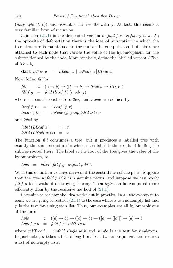
170 Pearls of Functional Algorithm Design
(map hylo (h x )) and assemble the results with g . At last, this seems avery familiar form of recursion.
Definition (21.1) is the deforested version of fold f g · unfold p id h. Asthe opposite of deforestation there is the idea of annotation, in which thetree structure is maintained to the end of the computation, but labels areattached to each node that carries the value of the hylomorphism for thesubtree defined by the node. More precisely, define the labelled variant LTreeof Tree by
data LTree a = LLeaf a | LNode a [LTree a]
Now define fill by
fill :: (a → b)→ ([b]→ b)→ Tree a → LTree bfill f g = fold (lleaf f ) (lnode g)
where the smart constructors lleaf and lnode are defined by
lleaf f x = LLeaf (f x )lnode g ts = LNode (g (map label ts)) ts
and label by
label (LLeaf x ) = xlabel (LNode x ts) = x
The function fill consumes a tree, but it produces a labelled tree withexactly the same structure in which each label is the result of folding thesubtree rooted there. The label at the root of the tree gives the value of thehylomorphism, so
hylo = label · fill f g · unfold p id h
With this definition we have arrived at the central idea of the pearl. Supposethat the tree unfold p id h is a genuine nexus, and suppose we can applyfill f g to it without destroying sharing. Then hylo can be computed moreefficiently than by the recursive method of (21.1).
It remains to see how the idea works out in practice. In all the examples tocome we are going to restrict (21.1) to the case where x is a nonempty list andp is the test for a singleton list. Thus, our examples are all hylomorphismsof the form
hylo :: ([a]→ b)→ ([b]→ b)→ ([a]→ [[a]])→ [a]→ bhylo f g h = fold f g ·mkTree h
where mkTree h = unfold single id h and single is the test for singletons.In particular, h takes a list of length at least two as argument and returnsa list of nonempty lists.
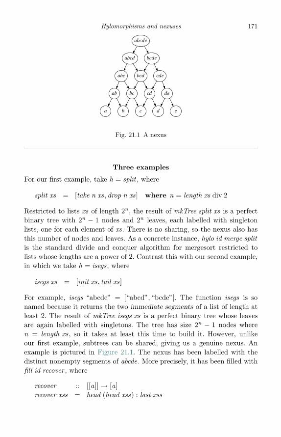
Hylomorphisms and nexuses 171
abcde
abcd bcde
abc bcd cde
ab bc cd de
a b c d e
Fig. 21.1 A nexus
Three examples
For our first example, take h = split , where
split xs = [take n xs, drop n xs] where n = length xs div 2
Restricted to lists xs of length 2n , the result of mkTree split xs is a perfectbinary tree with 2n − 1 nodes and 2n leaves, each labelled with singletonlists, one for each element of xs. There is no sharing, so the nexus also hasthis number of nodes and leaves. As a concrete instance, hylo id merge splitis the standard divide and conquer algorithm for mergesort restricted tolists whose lengths are a power of 2. Contrast this with our second example,in which we take h = isegs, where
isegs xs = [init xs, tail xs]
For example, isegs “abcde” = [“abcd”, “bcde”]. The function isegs is sonamed because it returns the two immediate segments of a list of length atleast 2. The result of mkTree isegs xs is a perfect binary tree whose leavesare again labelled with singletons. The tree has size 2n − 1 nodes wheren = length xs, so it takes at least this time to build it. However, unlikeour first example, subtrees can be shared, giving us a genuine nexus. Anexample is pictured in Figure 21.1. The nexus has been labelled with thedistinct nonempty segments of abcde. More precisely, it has been filled withfill id recover , where
recover :: [[a]]→ [a]recover xss = head (head xss) : last xss
172 Pearls of Functional Algorithm Design
abcde
abcd abce abde acde bcde
abc abd acd bcd abe ace bce ade bde cde
ab ac bc ad bd cd ae be ce de
a b c d e
Fig. 21.2 Another nexus
The function recover satisfies recover · isegs = id . The nexus has n(n +1)/2nodes for an input of length n, so sharing gives a significant reduction insize.
For our third example, take h = minors, where
minors [x , y ] = [[x ], [y ]]minors (x : xs) = map (x :) (minors xs) ++ [xs]
For example, minors “abcde” = [“abcd”, “abce”, “abde”, “acde”, “bcde”].The function minors returns those subsequences of its argument in whichjust one element is dropped.1 The result returned by mkTree minors xs,where xs is a nonempty list, is once again a tree labelled with singletons. Foran input of length n the tree has size S (n), where S (0) = 0 and S (n+1) =1 + (n+1)S (n). Solving this recurrence gives
S (n) = n!n∑
k=1
1k !
so S (n) is between n! and en!2 Again, there is potential for sharing, andone nexus is pictured in Figure 21.2. The nexus has been labelled withthe distinct nonempty subsequences of abcde; more precisely, it has beenfilled by fill id recover , where recover is the same as in our second example.The nexus has only 2n − 1 nodes, which is a substantial reduction over thetree.1 The function minors appears again in the following two pearls in connection with matrices.2 The sequence appears as A002627 in Sloane’s integer sequences, which gives S(n) = �(e−1)n!�.
Hylomorphisms and nexuses 173
Building a nexus
We now turn to the problem of how to build a nexus and how to fill itwithout destroying sharing. In all our examples the nexus has its leaves atthe same depth, so one obvious idea is to build the nexus fill f g ·mkTree hlayer by layer from bottom to top. Building stops when we have a singletonlayer. It also seems obvious that each layer should be a list of labelled trees,i.e. [LTree a], but this decision is premature. Instead, we postulate a typeLayer a, so that each layer is an element of Layer (LTree a). The generalbottom-up scheme for constructing the nexus of fill f g ·mkTree h for varioush is then implemented by
mkNexus f g = label · extractL · until singleL (stepL g) · initialL f
where the subsidiary functions have the following types:
initialL :: ([a]→ b)→ [a]→ Layer (LTree b)stepL :: ([b]→ b)→ Layer (LTree b) → Layer (LTree b)singleL :: Layer (LTree b)→ BoolextractL :: Layer (LTree b)→ LTree b
Our aim is to find implementations of these four functions for each of thethree instantiations, h = split , h = isegs and h = minors.
The first two, h = split and h = isegs, are easy because we can get awaywith choosing Layer a = [a] and defining
initialL f = map (lleaf f · wrap)singleL = singleextractL = head
where wrap x = [x ]. Thus, the initial layer is a list of leaves. The definitionof stepL for h = split is
stepL g = map (lnode g) · group
where group :: [a]→ [[a]] groups a list into pairs and is defined by
group [ ] = [ ]group (x : y : xs) = [x , y ] : group xs
With these definitions we have, for example, that mkNexus id merge xs,where xs is a list whose length is a power of 2, is a bottom-up definition ofmergesort in which elements are merged in pairs, then merged in fourths,and so on.
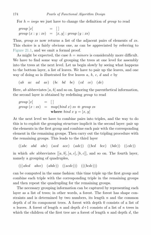
174 Pearls of Functional Algorithm Design
For h = isegs we just have to change the definition of group to read
group [x ] = [ ]group (x : y : xs) = [x , y ] : group (y : xs)
Thus, group xs now returns a list of the adjacent pairs of elements of xs.This choice is a fairly obvious one, as can be appreciated by referring toFigure 21.1, and we omit a formal proof.
As might be expected, the case h = minors is considerably more difficult.We have to find some way of grouping the trees at one level for assemblyinto the trees at the next level. Let us begin slowly by seeing what happensto the bottom layer, a list of leaves. We have to pair up the leaves, and oneway of doing so is illustrated for five leaves a, b, c, d and e by
(ab ac ad ae) (bc bd be) (cd ce) (de)
Here, ab abbreviates [a, b] and so on. Ignoring the parenthetical information,the second layer is obtained by redefining group to read
group [x ] = [ ]group (x : xs) = map(bind x ) xs ++ group xs
where bind x y = [x , y ]
At the next level we have to combine pairs into triples, and the way to dothis is to exploit the grouping structure implicit in the second layer: pair upthe elements in the first group and combine each pair with the correspondingelement in the remaining groups. Then carry out the tripling procedure withthe remaining groups. This leads to the third layer
((abc abd abe) (acd ace) (ade)) ((bcd bce) (bde)) ((cde))
in which abc abbreviates [[a, b], [a, c], [b, c]], and so on. The fourth layer,namely a grouping of quadruples,
(((abcd abce) (abde)) ((acde))) (((bcde)))
can be computed in the same fashion: this time triple up the first group andcombine each triple with the corresponding triple in the remaining groupsand then repeat the quadrupling for the remaining groups.
The necessary grouping information can be captured by representing eachlayer as a list of trees; in other words, a forest. The forest has shape con-straints and is determined by two numbers, its length n and the commondepth d of its component trees. A forest with depth 0 consists of a list ofn leaves. A forest of length n and depth d+1 consists of a list of n trees inwhich the children of the first tree are a forest of length n and depth d , the

Hylomorphisms and nexuses 175
children of the second tree are a forest of length n−1 and depth d , and so on,down to the final tree whose children are a forest of length 1 and depth d .The bottom layer of our nexus is a forest of length n and depth 0, the nextlayer a forest of length n−1 and depth 1, and so on, with the top layer beinga forest of length n and depth n−1. As a data type, a forest is an elementof [Tree a], so we define Layer a = [Tree a]. The fact that we started outthe pearl with the type Tree a is purely fortuitous; we would have had todeclare the type Tree a anyway to define forests.
Here are the implementations of initialL, singleL and extractL for buildinga nexus with h = minors:
initialL f = map (Leaf · lleaf f · wrap)singleL = singleextractL = extract · head
where extract (Leaf x ) = xextract (Node [t ]) = extract t
The function initialL constructs a forest of depth 0 whose labels are theleaves of a labelled tree (an element of LTree a). The function extractL takesa forest of length 1 and some depth d and extracts its label. It is a bit mind-boggling that the computation of mkNexus is carried out in terms of a datastructure of type [Tree (LTree a)], a list of trees of labelled trees.
It remains to define stepL, which is given by
stepL g = map (mapTree (lnode g)) · group
where mapTree is the map function for Tree a and
group :: [Tree a]→ [Tree [a]]group [t ] = [ ]group (Leaf x : vs)
= Node [Leaf [x , y ] | Leaf y ← vs] : group vsgroup (Node us : vs)
= Node (zipWith combine (group us) vs) : group vs
combine (Leaf xs) (Leaf x ) = Leaf (xs ++ [x ])combine (Node us) (Node vs) = Node (zipWith combine us vs)
These definitions formalise the verbal description of the process given earlier.To justify them we have to prove that
mkNexus f g = fill f g ·mkTree minors
However, the proof is rather long and we omit it.
176 Pearls of Functional Algorithm Design
Why build the nexus?
A good question. Everything we have said above about building a nexusbottom up and layer by layer applies equally well if we throw away thenexus and just retain the labelling information. Take the case h = isegs andconsider solve, where
solve :: [a]→ b)→ ([b]→ b)→ [a]→ bsolve f g = head · until single (map g · group) ·map (f · wrap)
and group is the function associated with isegs. The function solve f g imple-ments the hylomorphism hylo f g isegs without building a nexus. Similarly,consider solve, where
solve f g = extractL · until singleL (step g) ·map (Leaf · f · wrap)step g = map (mapTree g) · group
and extractL, singleL and group are the functions associated with minors.Again, solve f g implements the hylomorphism hylo f g minors withoutbuilding a nexus.
The answer to the question is that the nexus is useful when we want toconsider problems that are variants of the ones discussed above. For example,a standard problem involving segments is the problem of optimal bracketing,in which one seeks to bracket an expression x1 ⊕ x2 ⊕ · · · ⊕ xn in the bestpossible way. It is assumed that ⊕ is an associative operation, so the way inwhich the brackets are inserted does not affect the value. However, differentbracketings may have different costs. The cost of computing x ⊕ y dependson the sizes of x and y , and the recursive solution makes use not of isegsbut the function uncats, where
uncats [x , y ] = [([x ], [y ])uncats (x : xs) = ([x ], xs) : map (cons x ) (uncats xs)
where cons x (ys, zs) = (x : ys, zs)
For example, uncats “abcde” is
[(“a”, “bcde”), (“ab”, “cde”), (“abc”, “de”), (“abcd”, “e”)]
Each of these pairs represents a possible initial bracketing, and a minimumcost solution is obtained by recursively computing the cost and sizes of eachcomponent in each pair and then taking a minimum of the costs of combiningthem.
Using uncats in place of isegs does not give us an element of Tree a but amore complicated kind of tree in which each “subtree” is a list of pairs of sub-trees. Nevertheless, we can solve the bracketing problem by computing the
Hylomorphisms and nexuses 177
nexus for isegs, provided we replace the definition of the smart constructorlnode with another one:
lnode g [u, v ] = LNode (g (zip (lspine u) (rspine v))) [u, v ]
The functions lspine, rspine :: LTree a → [a] are defined by
lspine (LLeaf x ) = [x ]lspine (LNode x [u, v ]) = lspine u ++ [x ]rspine (LLeaf x ) = [x ]rspine (LNode x [u, v ]) = [x ] ++ rspine r
For example, the left and right spines of the two subtrees of the tree ofFigure 21.1 are [a, ab, abc, abcd ] and [bcde, cde, de, e]. Zipping them togethergives uncats abcde. The definition of lspine takes quadratic time, but it iseasy to make it take linear time with the help of an accumulating parameter.
As a second example, consider the nexus of subsequences in Figure 21.2.One example of a problem involving subsequences is the Countdown exampleconsidered in the previous pearl. In that problem we made use of a functionunmerges defined by
unmerges [x , y ] = [([x ], [y ])]unmerges (x : xs) = [([x ], xs)] ++ concatMap (add x ) (unmerges xss)
where add x (ys, zs) = [(x : ys, zs), (ys, x : zs)]
For example, unmerges “abcd” is
[(“a”, “bcd”), (“ab”, “cd”), (“b”, “acd”), (“abc”, “d”),(“bc”, “ad”), (“ac”, “bd”), (“c”, “abd”)]
The order in which the pairs of subsequences appear in this list is notimportant, and neither is the order within each pair. What is importantis that each subsequence is paired with its complement. In Countdown, theset of possible expressions one can build from a list xs of integers in ascend-ing order is computed by recursively building the expressions for each list ineach component of unmerges xs and then combining results.
Using unmerges in place of minors does not give us an element of Tree a,but rather a more complicated data structure. Nevertheless, just as before,we can solve Countdown by computing the nexus for minors provided wereplace the definition of the smart constructor lnode with another one. Whatwe have to do, in effect, is to find some way of extracting unmerges fromthe labels of the nexus associated with a node. That means retrieving every

178 Pearls of Functional Algorithm Design
abcd
abc
ab
a b
ac
c
bc
abd
ad
d
bd
acd
cd
bcd
Fig. 21.3 A binomial spanning tree
label of the nexus. In principle this can be done by carrying out a breadth-
first traversal of the nexus. For example, the breadth-first traversal of thenexus associated with abcd in Figure 21.2, minus its first element, is
abc, abd , acd , bcd , ab, ac, bc, ad , bd , cd , a, b, c, d
If we split this list into two halves and zip the first half with the reverse ofthe second half, we arrive at unmerges “abcd”, though the pairs appear ina different order, as do the components of each pair.
However, any traversal of a graph requires us to keep track of nodes visited,and this is not possible with a nexus because two nodes cannot be checkedfor equality. The alternative is first to construct a spanning tree of the nexusand then to traverse its subtrees in breadth-first order. Traversing a forestis implemented by
traverse :: [LTree a]→ [a]traverse [ ] = [ ]traverse ts = map label ts ++ traverse (concatMap subtrees ts)
subtrees (LLeaf x ) = [ ]subtrees (LNode x ts) = ts
One spanning tree of the nexus associated with abcd in Figure 21.2 ispictured in Figure 21.3. This tree is a binomial tree of rank 4. Binomialtrees are close cousins of the trees in the forest used to construct the nexus.A binomial tree of rank n has n children, which are, in order, binomial treesof ranks n−1,n−2, . . . , 0. To construct the binomial spanning tree of thenexus, we have to drop children, none from the first subtree, one from thesecond subtree and so on. The same recipe has to be applied recursively tothe children. Thus, for the kth child we have to drop k children from its first

Hylomorphisms and nexuses 179
child, k + 1 children from its second child and so on. The function forest k ,defined by
forest k (LLeaf x : ts) = LLeaf x : tsforest k (LNode x us : vs)
= LNode x (forest k (drop k us)) : forest (k + 1) vs
carries out this pruning. Now we can define
lnode g ts = LNode (g (zip xs) (reverse ys)) tswhere (xs, ys) = halve (traverse (forest 0 ts))
where halve xs = splitAt (length xs div 2) xs.
Final remarks
The name hylomorphism first appeared in Meijer (1992); see also Meijeret al. (1991). The material in this pearl has been drawn from two mainsources. Nexus building was described first in Bird and Hinze (2003), whereanother way of building the nexus for minors was given, one that used acyclic tree with up and down pointers. Later on, in Bird (2008), it was shownthat for some problems, admittedly of a fairly restricted class, the essentialfunction group for building each layer of the nexus could be expressed as thetranspose of the decomposition function h of the hylomorphism.
ReferencesBird, R. S. and Hinze, R. (2003). Trouble shared is trouble halved. ACM SIGPLAN
Haskell Workshop, Uppsala, Sweden.Bird, R. S. (2008). Zippy tabulations of recursive functions. In LNCS 5133:
Proceedings of the Ninth International Conference on the Mathematics ofProgram Construction, ed. P. Audebaud and C. Paulin-Mohring. pp. 92–109.
Meijer, E. (1992). Calculating compilers. PhD thesis, Nijmegen University, TheNetherlands.
Meijer, E., Fokkinga, M. and Paterson, R. (1991). Functional programming withbananas, lenses, envelopes and barbed wire. Proceedings of the 5th ACMConference on Functional Programming Languages and Computer Architec-ture. New York, NY: Springer-Verlag, pp. 124–44.

22
Three ways of computing determinants
Introduction
The determinant, det(A), or |A|, of an n×n matrix A = (aij ) can be definedby the Leibniz formula
|A| =∑
π
sign (π)∏
1≤j≤n
ajπ(j )
The sum is taken over all permutations π of [1 ..n] and sign (π) = 1 for evenpermutations (those that have an even number of inversions), and −1 forodd ones. Executed directly, the computation of |A| takes Θ(n × n!) steps.One way to reduce the time to Θ(n3) is to convert the matrix to uppertriangular form using Gaussian elimination. Gaussian elimination brings indivision as an additional operation, so if A is an integer matrix and thedeterminant has to be computed exactly, then the result of each division hasto be exact. That means using rational division. Rational division involvesnormalising numerators and denominators, so time is spent computing thegreatest common divisor of two integers.
One method that avoids rational division is known as Chio’s pivotal
condensation algorithm. This is essentially a variant of Gaussian eliminationthat uses integer division only. Chio’s method requires Θ(n3) multiplicationsbut only Θ(n) divisions (and exponentiations). The downside is that the sizeof the intermediate results grows exponentially. However, there is a variantof the algorithm in which the intermediate results are kept reasonably small,but the number of integer divisions goes up to Θ(n3).
Finally, there are methods for computing the determinant reasonablyquickly that avoid division altogether. One is based on iterated matrix multi-plication. The size of the intermediate results is small, but the operationcount goes up to Θ(n4). Since we will need to calculate determinantsin the following pearl, we devote this pearl to describing and comparingthese three kinds of algorithm.
180

Three ways of computing determinants 181
The school-book method
As a warm-up let us first implement the school-book method of computingdeterminants. This involves recursively computing the determinant of theminors of the matrix. For example:∣∣∣∣∣∣
a11 a12 a13
a21 a22 a23
a31 a32 a33
∣∣∣∣∣∣ = a11
∣∣∣∣ a22 a23
a32 a33
∣∣∣∣− a21
∣∣∣∣ a12 a13
a32 a33
∣∣∣∣ + a31
∣∣∣∣ a12 a13
a22 a23
∣∣∣∣With matrices represented as a list of rows, the school-book method isimplemented by
det :: [[Integer ]]→ Integerdet [[x ]] = xdet xss = foldr1 (−) (zipWith (∗) col1 (map det (minors cols)))
where col1 = map head xsscols = map tail xss
The 1 × 1 case is computed directly. Otherwise, each element of the firstcolumn is multiplied by the determinant of the corresponding minor of theremaining columns and the results are combined with an alternating sum.The function minors, which made an appearance in the previous pearl, isdefined by
minors :: [a]→ [[a]]minors [ ] = [ ]minors (x : xs) = xs : map (x :) (minors xs)
For example, minors “abcd” = [“bcd”, “acd”, “abd”, “abc”].Although the definition of det is short and sweet, the associated compu-
tation takes exponential time. The recurrence relation for T (n), the numberof steps needed to compute the determinant of an n × n matrix, satisfiesT (n) = nT (n−1) + Θ(n), with solution T (n) = Θ(n!). Nevertheless, it isgood enough when n = 2 or n = 3.
Using rational division
Gaussian elimination depends on the fact that adding any multiple of onerow to any other row does not change the value of the determinant. Assumingthe leading entry of the first row is not zero, we can add suitable multiplesof the first row to the other rows to reduce the elements in the first columnto zero. Repeating this process on the submatrix formed by eliminatingthe first row and column reduces the matrix to upper triangular form. The
182 Pearls of Functional Algorithm Design
determinant of an upper triangular matrix is the product of the elements onthe diagonal.
The process is complicated by the fact that the leading entry of the matrixmay be zero. In such a case we have to find an appropriate row whose firstentry, the pivot, is not zero. The function det is defined by
det :: [[Ratio Integer ]]→ Ratio Integerdet [[x ]] = xdet xss =case break ((�= 0) · head) xss of(yss, [ ]) → 0(yss, zs : zss) → let x = head zs ∗ det (reduce zs (yss ++ zss))
in if even (length yss) then x else − x
The expression break ((�= 0) · head) xss breaks a matrix into two parts(yss, zss) in which either zss is empty or the head of its first row zs isnot zero. In the former case the matrix is singular and its determinant iszero. In the latter case the remaining rows (yss ++ zss) are reduced to an(n−1)× (n−1) matrix by adding a suitable multiple of zs to each row anddiscarding the first column:
reduce xs yss = map (reduce1 xs) yssreduce1 (x : xs) (y : ys) = zipWith(λa b → b − d ∗ a) xs ys
where d = y/x
Finally, the determinant of the reduced matrix is negated if the parity of theposition of the pivotal row in the matrix is odd. Division (/) is implementedas rational division.
Using integer division
Another way to compute |A| is based on the following fact. Define the matrixX by setting xjk = a11 ∗ ajk − a1k ∗ aj1 for 2 ≤ j , k ≤ n. Equivalently,
xjk =∣∣∣∣ a11 a1k
aj1 ajk
∣∣∣∣So X is an (n−1)× (n−1) matrix. Then |A| = |X |/an−2
11 provided a11 �= 0.This is Chio’s identity. The determinant of an n × n matrix is expressed interms of the determinant of a “condensed” (n−1)× (n−1) whose entries arethe determinants of 2× 2 matrices. Although Chio’s identity also makes useof division, the division is exact and can be implemented as integer division.Note the assumption that the leading entry a11 is not zero. If it is, then, just
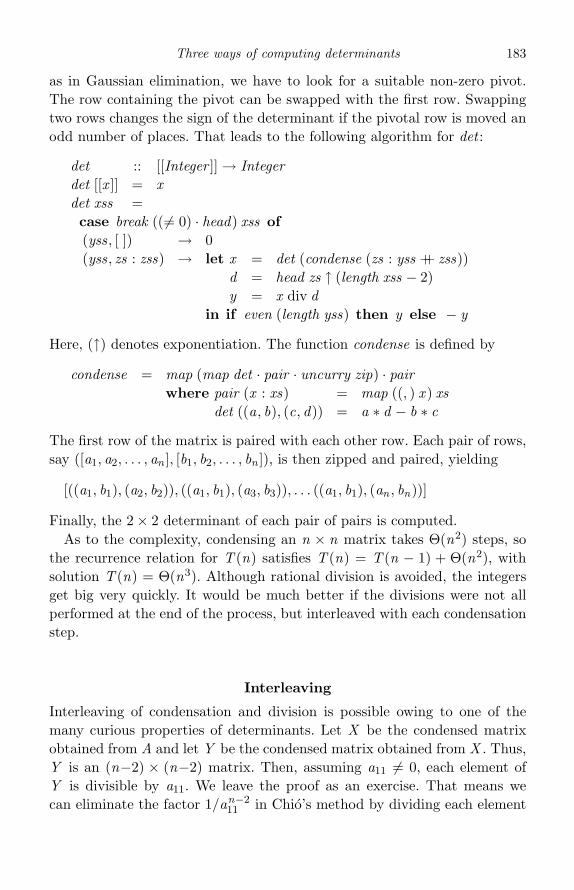
Three ways of computing determinants 183
as in Gaussian elimination, we have to look for a suitable non-zero pivot.The row containing the pivot can be swapped with the first row. Swappingtwo rows changes the sign of the determinant if the pivotal row is moved anodd number of places. That leads to the following algorithm for det :
det :: [[Integer ]]→ Integerdet [[x ]] = xdet xss =case break ((�= 0) · head) xss of(yss, [ ]) → 0(yss, zs : zss) → let x = det (condense (zs : yss ++ zss))
d = head zs ↑ (length xss − 2)y = x div d
in if even (length yss) then y else − y
Here, (↑) denotes exponentiation. The function condense is defined by
condense = map (map det · pair · uncurry zip) · pairwhere pair (x : xs) = map ((, ) x ) xs
det ((a, b), (c, d)) = a ∗ d − b ∗ c
The first row of the matrix is paired with each other row. Each pair of rows,say ([a1, a2, . . . , an ], [b1, b2, . . . , bn ]), is then zipped and paired, yielding
[((a1, b1), (a2, b2)), ((a1, b1), (a3, b3)), . . . ((a1, b1), (an , bn))]
Finally, the 2× 2 determinant of each pair of pairs is computed.As to the complexity, condensing an n × n matrix takes Θ(n2) steps, so
the recurrence relation for T (n) satisfies T (n) = T (n − 1) + Θ(n2), withsolution T (n) = Θ(n3). Although rational division is avoided, the integersget big very quickly. It would be much better if the divisions were not allperformed at the end of the process, but interleaved with each condensationstep.
Interleaving
Interleaving of condensation and division is possible owing to one of themany curious properties of determinants. Let X be the condensed matrixobtained from A and let Y be the condensed matrix obtained from X . Thus,Y is an (n−2) × (n−2) matrix. Then, assuming a11 �= 0, each element ofY is divisible by a11. We leave the proof as an exercise. That means wecan eliminate the factor 1/an−2
11 in Chio’s method by dividing each element
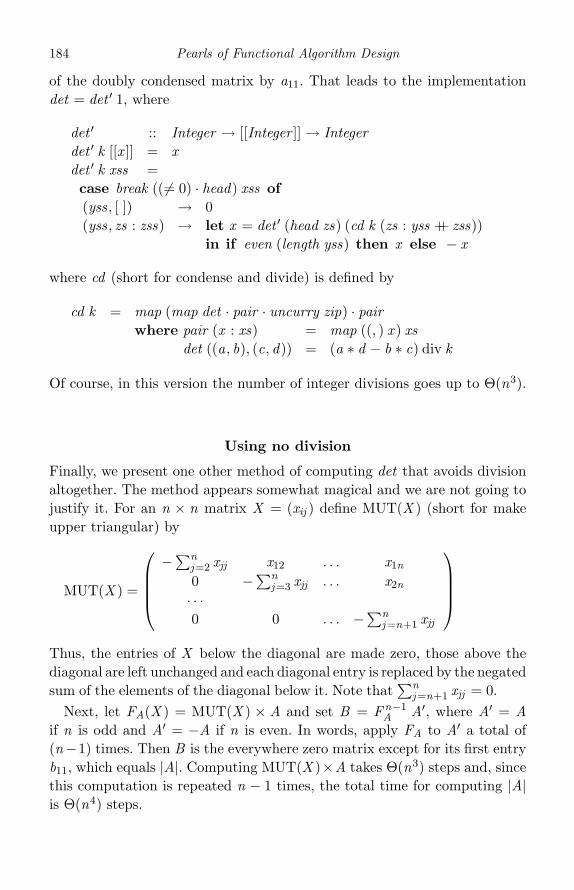
184 Pearls of Functional Algorithm Design
of the doubly condensed matrix by a11. That leads to the implementationdet = det ′ 1, where
det ′ :: Integer → [[Integer ]]→ Integerdet ′ k [[x ]] = xdet ′ k xss =case break ((�= 0) · head) xss of(yss, [ ]) → 0(yss, zs : zss) → let x = det ′ (head zs) (cd k (zs : yss ++ zss))
in if even (length yss) then x else − x
where cd (short for condense and divide) is defined by
cd k = map (map det · pair · uncurry zip) · pairwhere pair (x : xs) = map ((, ) x ) xs
det ((a, b), (c, d)) = (a ∗ d − b ∗ c) div k
Of course, in this version the number of integer divisions goes up to Θ(n3).
Using no division
Finally, we present one other method of computing det that avoids divisionaltogether. The method appears somewhat magical and we are not going tojustify it. For an n × n matrix X = (xij ) define MUT(X ) (short for makeupper triangular) by
MUT(X ) =
⎛⎜⎜⎜⎝−
∑nj=2 xjj x12 . . . x1n
0 −∑n
j=3 xjj . . . x2n
· · ·0 0 . . . −
∑nj=n+1 xjj
⎞⎟⎟⎟⎠
Thus, the entries of X below the diagonal are made zero, those above thediagonal are left unchanged and each diagonal entry is replaced by the negatedsum of the elements of the diagonal below it. Note that
∑nj=n+1 xjj = 0.
Next, let FA(X ) = MUT(X ) × A and set B = F n−1A A′, where A′ = A
if n is odd and A′ = −A if n is even. In words, apply FA to A′ a total of(n−1) times. Then B is the everywhere zero matrix except for its first entryb11, which equals |A|. Computing MUT(X )×A takes Θ(n3) steps and, sincethis computation is repeated n − 1 times, the total time for computing |A|is Θ(n4) steps.
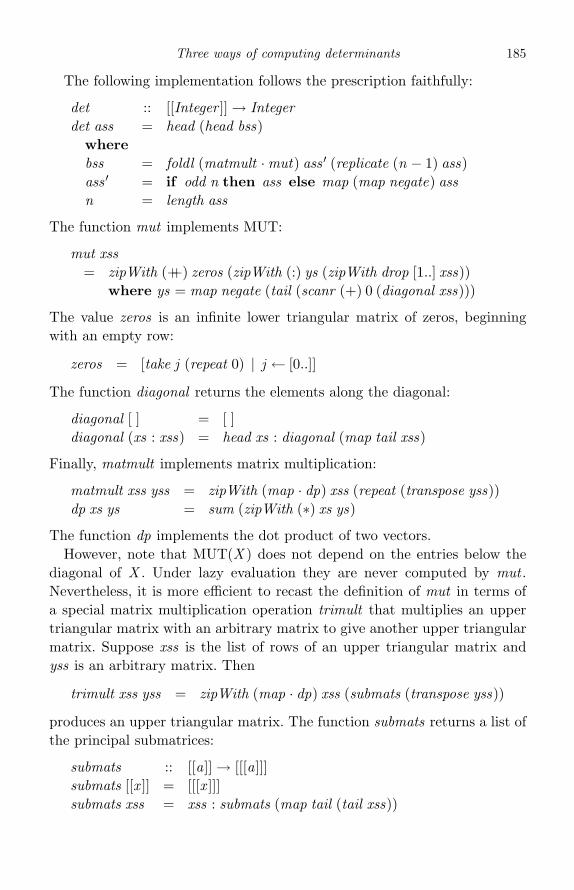
Three ways of computing determinants 185
The following implementation follows the prescription faithfully:
det :: [[Integer ]]→ Integerdet ass = head (head bss)
wherebss = foldl (matmult ·mut) ass ′ (replicate (n − 1) ass)ass ′ = if odd n then ass else map (map negate) assn = length ass
The function mut implements MUT:
mut xss= zipWith (++) zeros (zipWith (:) ys (zipWith drop [1..] xss))
where ys = map negate (tail (scanr (+) 0 (diagonal xss)))
The value zeros is an infinite lower triangular matrix of zeros, beginningwith an empty row:
zeros = [take j (repeat 0) | j ← [0..]]
The function diagonal returns the elements along the diagonal:
diagonal [ ] = [ ]diagonal (xs : xss) = head xs : diagonal (map tail xss)
Finally, matmult implements matrix multiplication:
matmult xss yss = zipWith (map · dp) xss (repeat (transpose yss))dp xs ys = sum (zipWith (∗) xs ys)
The function dp implements the dot product of two vectors.However, note that MUT(X ) does not depend on the entries below the
diagonal of X . Under lazy evaluation they are never computed by mut .Nevertheless, it is more efficient to recast the definition of mut in terms ofa special matrix multiplication operation trimult that multiplies an uppertriangular matrix with an arbitrary matrix to give another upper triangularmatrix. Suppose xss is the list of rows of an upper triangular matrix andyss is an arbitrary matrix. Then
trimult xss yss = zipWith (map · dp) xss (submats (transpose yss))
produces an upper triangular matrix. The function submats returns a list ofthe principal submatrices:
submats :: [[a]]→ [[[a]]]submats [[x ]] = [[[x ]]]submats xss = xss : submats (map tail (tail xss))
186 Pearls of Functional Algorithm Design
For upper triangular matrices xss the definition of mut xss simplifies to
mut xss = zipWith (:) ys (map tail xss))where ys = map negate (tail (scanr (+) 0 (map head xss)))
The diagonal of an upper triangular matrix xss is map head xss and theelements above the diagonal are map tail xs.
We can now rewrite det in the form
det :: [[Integer ]]→ Integerdet ass = head (head bss)
wherebss = foldl (trimult ·mut) ass ′ (replicate (n − 1) ass)ass ′ = if odd n then upper ass
else map (map negate) (upper ass)n = length ass
where upper = zipWith drop [0..].
A brief comparison
So, which of the three methods described above is best? Rational divi-sion (Gaussian elimination), integer division (two versions, one using Chio’sidentity and one using condense and divide) or no division (by iteratedmatrix multiplication)?
We carried out a brief comparison of the methods, using random matricesfor various sizes of n, each with entries in the range (−20, 20). As mightbe expected, the original Chio version was hopeless, but the second versionthat combined condensation steps and division was the clear winner. Forn = 150, Gaussian elimination took about 30 s, the modified Chio versiontook 10 s and the iterated multiplication method took 40 s.
Final remarks
Chio’s method, which goes back 150 years, is described at http://mathworld.wolfram.com/ChioPivotalCondensation.html. The modified version isreally due to Bareiss (1968), who based its justification on Sylvester’s iden-tity, a more general version of Chio’s identity. However, the history of theiterated multiplication method is more obscure. The main fact on which itdepends still awaits a purely algebraic proof. We extracted it from an algo-rithm of Mahajan and Vinay (1997) that was based on the idea of clow
sequences. The word clow is an acronym for “closed walk”, and a clowsequence is a generalisation of the cycle decomposition of a permutation in
Three ways of computing determinants 187
which each cycle can contain repetitions of intermediate elements; hence, aclosed walk. Mahajan and Vinay showed that all the signed matrix terms forclow sequences that do not correspond to permutations cancel each otherout, leaving just those terms a1π(1)a2π(2) · · · anπ(n) that do correspond topermutations. But their proof is not trivial. The signed matrix term corre-sponding to a clow sequence can be expressed as a path in a layered directedacyclic graph to one of two endpoints and the computation of the sum ofsuch factors computed as a path problem. By recasting the associated recur-sive definition directly back into matrix operations, the identity describedabove was discovered. Although we cannot find any reference to it in theliterature, it is almost certainly not new.
One point not emphasised in the narrative was that no Haskell arrayswere harmed in the description of the algorithms, immutable or otherwise.Instead, each matrix was quietly represented as a list of its rows. Thatenabled each algorithm to be expressed fairly concisely. But perhaps a betteralternative is to define a suitable abstract type for matrices in which thenecessary operations, first column, first row, diagonal, principal submatricesand so on, are provided as primitives.
ReferencesBareiss, E. H. (1968). Sylvester’s identity and multi-step integer preserving
Gaussian elimination. Mathematics of Computation 22 (103), 565–78.Mahajan, M. and Vinay, V. (1997). Determinant: combinatorics, algorithms and
complexity. Chicago Journal of Theoretical Computer Science, Article 5.
23
Inside the convex hull
Introduction
The problem of computing the convex hull of a set of points is central tomany tasks in computational geometry and has been much studied. Findingthe hull makes sense in any finite dimension d , but most textbooks focusprimarily on the cases d = 2 and d = 3. Our aim in this pearl is simplyto specify the d dimensional form of the problem and then to describe astraightforward incremental algorithm for computing the hull. The incre-mental algorithm is well known and a number of sophisticated improvementshave been proposed, but we deal only with the basic idea. We will not derivethe algorithm, but instead show how to test it using the Claessen and HughesQuickCheck library. In fact, testing revealed an error in the code, an errorwe have deliberately left in to see if the reader can spot it.
Background
Many geometric algorithms fall apart when the arithmetic is not exact, soit is a good idea to stay within the realm of integer arithmetic and confineattention to the subset Q(d) of d -dimensional Euclidean space E (d) con-sisting of those points whose Cartesian coordinates are rational numbers.A point in Q(d) can be represented by a list of d+1 integers [x0, x1, . . . , xd ]in which xd �= 0; this list represents the d rational Cartesian coordinates[x0/xd , x1/xd , . . . , xd−1/xd ]. Hence, we define Point = [Integer ]. The dimen-sion of a point is given by
dimension :: Point → Intdimension ps = length ps − 1
By definition, a d -simplex is a list of d+1 points in Q(d) together with avalue, +1 or −1, indicating the orientation of the simplex that arises fromthe way the points are listed:
type Simplex = ([Point ], Int)
188
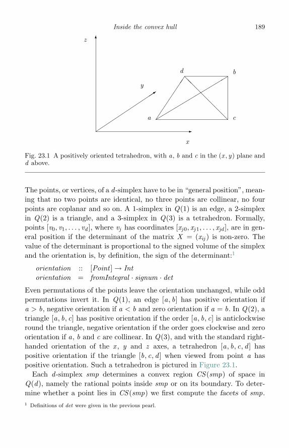
Inside the convex hull 189
���
��
��
��
���
�
x
z
y
��
��
��
��
���
��
��
���
��
��
���
a
b
c
d
Fig. 23.1 A positively oriented tetrahedron, with a, b and c in the (x , y) plane andd above.
The points, or vertices, of a d -simplex have to be in “general position”, mean-ing that no two points are identical, no three points are collinear, no fourpoints are coplanar and so on. A 1-simplex in Q(1) is an edge, a 2-simplexin Q(2) is a triangle, and a 3-simplex in Q(3) is a tetrahedron. Formally,points [v0, v1, . . . , vd ], where vj has coordinates [xj0, xj1, . . . , xjd ], are in gen-eral position if the determinant of the matrix X = (xij ) is non-zero. Thevalue of the determinant is proportional to the signed volume of the simplexand the orientation is, by definition, the sign of the determinant:1
orientation :: [Point ]→ Intorientation = fromIntegral · signum · det
Even permutations of the points leave the orientation unchanged, while oddpermutations invert it. In Q(1), an edge [a, b] has positive orientation ifa > b, negative orientation if a < b and zero orientation if a = b. In Q(2), atriangle [a, b, c] has positive orientation if the order [a, b, c] is anticlockwiseround the triangle, negative orientation if the order goes clockwise and zeroorientation if a, b and c are collinear. In Q(3), and with the standard right-handed orientation of the x , y and z axes, a tetrahedron [a, b, c, d ] haspositive orientation if the triangle [b, c, d ] when viewed from point a haspositive orientation. Such a tetrahedron is pictured in Figure 23.1.
Each d -simplex smp determines a convex region CS (smp) of space inQ(d), namely the rational points inside smp or on its boundary. To deter-mine whether a point lies in CS (smp) we first compute the facets of smp.1 Definitions of det were given in the previous pearl.

190 Pearls of Functional Algorithm Design
A facet of a d -simplex is a list of d points, together with an associated orien-tation derived from the simplex. The facets of an edge are its two endpointvertices, the facets of a triangle are its three edges and so on. The facets ofa simplex and the associated orientations are defined by
facets :: Simplex → [Facet ]facets (us, b) = zip (minors us) (cycle [b,−b])
minors :: [a]→ [[a]]minors [ ] = [ ]minors (x : xs) = xs : map (x :) (minors xs)
where Facet = ([Point ], Int). The minors of a list is a list of subsequences.For example, minors “abcd” = [“bcd”, “acd”, “abd”, “abc”]. We met thisfunction in the two previous pearls. For an edge [a, b] in Q(1) with positiveorientation the facets are the 0-simplexes [b] and [a] with associated orien-tations +1 and −1 respectively. A point p is strictly inside the region of thesimplex [a, b] if the simplex [p, b] has the same orientation as [b] has, namely+1, and [p, a] has the same orientation as [a], namely −1. In other words,b < p < a. The same reasoning holds in higher dimensions. Thus, in Q(2),a triangle [a, b, c] with positive orientation has the three facets
([b, c], +1), ([a, c],−1), ([a, b], +1)
and a point p is strictly inside [a, b, c] if the three simplexes [p, b, c], [p, a, c]and [p, a, b] have orientations +1, −1 and +1, implying that p is to the leftof the edge from b to c, to the right of the edge from a to c and to the leftof the edge from a to b.
The region CS (smp) of those points strictly inside smp or on its boundaryis defined by a predicate:
insideCS :: Simplex → Point → BoolinsideCS smp p
= and [0 ≤ b ∗ orientation (p : us) | (us, b)← facets smp]
A point p is strictly inside CS (smp) if b = orientation (p : us) for each facet(us, b) of smp and on the boundary of smp if orientation (p : us) = 0 for atleast one facet (us, b) of smp.
Convex hulls
The convex hull CH (vs) of a set of points vs in Q(d) is a region of Q(d).It can be defined in a number of mathematically equivalent ways, includingthe following: CH (vs) is the union of the sets CS (smp) for all d -simplexes
Inside the convex hull 191
smp determined by points of vs. For example, in Q(2) the convex hull of vsis the union of the regions determined by all triangles whose vertices are invs. The set CH (vs) can therefore be characterised by a predicate:
insideCH :: [Point ]→ Point → BoolinsideCH vs p = or [insideCS smp p | smp ← simplexes vs]
where simplexes vs lists the simplexes of vs:
simplexes :: [Point ]→ [Simplex ]simplexes vs = [(us, b) | us ← tuples (d + 1) vs,
let b = orientation us, b �= 0]where d = dimension (head vs)
The value of tuples n vs is a list of all n-tuples of vs; that is, all subsequencesof vs of length n. The definition of tuples is left as an exercise.
According to the above definition of insideCH , the set CH (vs) is emptyif vs has no simplexes. A set of points vs in Q(1) has no 1-simplexes if thepoints are coincident, in Q(2) if they are collinear and in Q(3) if they arecoplanar. It is possible to define the convex hull for such sets of points byreducing the dimension, but we will leave the specification as it is.
An incremental algorithm
There are Ω(nd+1) possible d -simplexes among n points, so evaluating theexpression insideCH vs p takes Ω(nd+1) steps. Most of these simplexes over-lap, indeed some may coincide, and it is necessary only to consider somesubset that covers the hull without overlap. Therefore, a more efficient al-gorithm is obtained by replacing simplexes with another function partition,with the same type, that partitions the hull. Then we can replace insideCHby insideCH ′, where
insideCH ′ :: [Point ]→ Point → BoolinsideCH ′ vs p = or [insideCS smp p | smp ← partition vs]
The function partition can be defined by a process that starts with a singlesimplex and then adds new simplexes as each additional point outside thecurrent hull is inspected:
partition :: [Point ]→ [Simplex ]partition vs
= case findSimplex vs ofNothing → [ ]Just [smp] → foldl update [smp] (vs \\ vertices smp)

192 Pearls of Functional Algorithm Design
The vertices of a simplex are listed by
vertices :: Simplex → [Point ]vertices = sort · fst
The vertices are listed in order; so, if vs is maintained as a sorted list, then\\ can be implemented efficiently as ordered list difference. The functionfindSimplex finds a simplex if there is one. If there is not one, then there isno partition and an empty hull. Otherwise the simplex is used as a startingpoint and its vertices are removed from the list of additional points thatneed to be considered. It remains to define findSimplex and update. We dealwith these functions separately.
Finding a simplex
One obvious way of defining findSimplex is
findSimplex vs = if null smps then Nothing else Just (head smps)where smps = simplexes vs
But in the worst case the cost of findSimplex vs is Ω(nd+1) steps, whichrather undercuts the aim of finding a more efficient algorithm. The worstcase is unlikely in practice, so the above definition is probably good enough,but there is an alternative method. The idea is to start with the first pointv0 of vs and then to carry out a single search of the rest of vs to find theremaining points. First, a second point v1 is found so that v0 and v1 are notcoincident. Then the search continues with the elements of vs after v1 to finda third point v2 that is not collinear with v0 and v1, and so on until d + 1points are found that are in general position. The tricky aspect is not thesearch but the fact that the non-degeneracy of k + 1 points in Q(d) cannotbe determined by a simple determinant test: the associated matrix of pointcoordinates has size (k+1)× (d+1), which is not square if k < d .
Instead we need to consider square submatrices. Consider the matrix Xof size (k+1)× (d+1) obtained from the first k+1 vertices and the subma-trices of size (k+1)× (k+1) formed by taking every possible combination ofk columns from the first d columns, together with the last column (the de-nominators of the rational coordinates of the vertices). Then the k+1 pointsare degenerate if the determinants of all these square submatrices are zero.The degeneracy test is implemented by
degenerate k = all ( 0) ·map det · submatrices k · transposesubmatrices k vs = map (++[last vs]) (tuples k (init vs))
Inside the convex hull 193
The function transpose transposes a matrix, so submatrices selects columnsof a matrix by selecting rows of the transposed matrix. The determinant of amatrix is the determinant of its transpose. Since there are O(dk ) submatricesof the transposed matrix, and computing the determinant takes O(k3) steps,the computation of degenerate k vs for a list of k+1 points vs in Q(d), wherek ≤ d , takes O(k3dk ) = O(dd+3) steps.
The function findSimplex is now implemented by
findSimplex :: [Point ]→ Maybe SimplexfindSimplex [ ] = NothingfindSimplex (v : vs) = search (length v − 1) 1 [v ] vs
where the function search is defined by
search d k us vs| k d + 1 = Just (us, orientation us)| null vs = Nothing| degenerate k (v : us) = search d k us (tail vs)| otherwise = search d (k + 1) (v : us) (tail vs)
where v = head vs
The running time of findSimplex vs, where vs has n points, is O(dd+3n)steps, which is linear in n, though with a large constant factor.
Update
In order to define the remaining function update, consider a set smps of sim-plexes that partition the convex hull for the points considered so far. Thefacets of these simplexes are of two kinds: the internal facets – those that oc-cur exactly twice (with opposite orientations); and the external facets – thosethat occur exactly once. For example, take the vertices of a square [a, b, c, d ]in Q(2). There are two possible triangulations: the triangles [a, b, c] and[c, d , a], or [a, b, d ] and [b, c, d ]. In the first triangulation the edge [a, c] isinternal and in the second the edge [b, d ] is internal. The external facets arecomputed by
external :: [Simplex ]→ [Facet ]external = foldr op [ ] · sort · concatMap facets
where
op smp [ ] = [ ]op smp (smp′ : smps) = if vertices smp vertices smp ′ then smps
else smp : smp ′ : smps

194 Pearls of Functional Algorithm Design
The cost of computing external smps is O(dS log dS ), where S is size ofsmps, since the dominating time is the time to sort the facets of smps andthere are O(dS ) of them.
Each new point v splits the external facets into two: the visible facetsand the invisible ones. Imagine a light-bulb situated at v ; this light-bulbilluminates just the visible facets. A facet (us, b) is visible to v if v is strictlyoutside it, meaning that orientation (v : us) has opposite sign to b:
visible :: Point → [Facet ]→ [Facet ]visible v fs = [(us, b) | (us, b)← fs, b ∗ orientation (v : us) < 0]
There are no visible facets if v is inside or on the current hull. In particular,if v is a copy of one of the vertices processed so far, then the current hullwill be unchanged, so it does not matter if vs contains repeated points (andit does not matter if we do not remove the vertices of the starting simplexfrom the starting points).
To update the hull we add to smps a new simplex for each visible facet:
newSimplex :: Point → Facet → SimplexnewSimplex v (us, b) = (v : us,−b)
The orientation assigned to the new simplex is correct because if (us, b) isvisible to v , then b∗orientation(v : us) < 0, and so orientation(v : us) = −b.
Now we can define update by
update :: [Simplex ]→ Point → [Simplex ]update smps v
= smps ++ map (newSimplex v) (visible v (external smps))
The time to compute update smps is dominated by the time to compute thevisible facets, and this takes O(dS log dS ) steps, where S is the size of smps.The complexity of insideCH ′ as a function of n, the number of points in vs,is therefore O(dnS log dS ), where S is the maximum number of simplexesmaintained at each stage. It is known that S = O(ne), where e = �d/2�,so evaluating insideCH ′ vs takes O(ne+1 log n) steps. This is better thaninsideCH , but we can improve insideCH ′ yet further.
An improvement
As described above, the incremental algorithm computes a set of simplexesthat partition the hull. At each stage the external facets of the hull aredetermined in order to discover those that are visible to a new point, and newsimplexes are then added to the hull. It is clearly more sensible to maintain
Inside the convex hull 195
the external facets of the simplexes rather than the simplexes themselves.If we set faces = external · partition, then we can replace insideCH ′ byinsideCH ′′, where
insideCH ′′ vs p = and [0 ≤ b ∗ orientation (p : us) | (us, b)← faces vs]
The function faces has type [Point ] → [Facet ]. In computational geometryone of the usual ways of describing a convex hull is by listing its externalfacets.
An efficient computation of faces can be derived by appealing to the fusionlaw of foldl . We need to find update ′ :: [Facet ]→ Point → [Facet ], so that
external (update smps v) = update ′ (external smps) v
Since the external facets of a single simplex are all its facets we then obtain
faces vs= case findSimplex vs of
Nothing → [ ]Just [smp] → foldl update ′ (facets smp) (vs \\ vertices vs)
We will not go into the derivation of update ′ but just state the result:
update ′ fs v = (fs \\ fs ′) ++ map (newFacet v) (external fs ′)where fs ′ = visible v fs
newFacet v (us, b) = (v : us, b)
In words, the facets visible to the new point are removed from the currentset of facets and new facets are added. The visible facets form a connectedset and their boundary is the set of their external sub-facets, namely a set of(d−2)-simplexes that occur exactly once. For example, in Q(3) the facets aretriangles and the external sub-facets of a visible set of connected trianglesare the set of edges that form its boundary. The orientation assigned to eachnew facet is just the orientation of the associated sub-facet. To appreciatethis last point, consider an edge ([a, b], +1) in Q(2) that is visible to a pointc and in which b is a boundary point (so the following edge beginning withb is not visible). The 0-simplex associated with b has positive orientationand the new edge [c, b] has to be directed towards b, so also has positiveorientation.
The running time of faces is dominated by the time to discover the facetsvisible to a new point. In order to find these facets, every single facet ofthe hull is inspected; that is clearly an inefficient method, since the visiblefacets form a small locally connected set. It is here that more sophisticated
196 Pearls of Functional Algorithm Design
algorithms, such as the Bulldozer algorithm of Blelloch et al. (2001), enterthe picture, but we will not go into further details.
QuickCheck
Koen Claessen and John Hughes have produced a very useful suite of func-tions, called QuickCheck , for testing Haskell programs; see Claessen andHughes (2000). It would take up too much space to explain the details ofQuickCheck , but we briefly show how to use the functions in the suite tocheck the two versions of the convex hull algorithm described above.
First we need a generator for generating a point in Q(d):
point :: Int → Gen [Integer ]point d = do {xs ← vector d ; return (xs ++ [1])}
The utility vector d returns a randomly generated list of d values, hereintegers. The result of point d is a generator that returns a list of d+1integers in which the last integer is 1.
Next we need a generator for generating a list of n points:
points :: Int → Int → Gen [[Integer ]]points d 0 = return [ ]points d (n + 1) = do {p ← point d ; ps ← points d n;
return (p : ps)}Now we can define a property prop Hull that checks the incremental algo-rithm against the specification:
prop Hull :: Int → Int → Propertyprop Hull d n = forAll (points d n) $ λvs →
forAll (point d) $ λv →insideCH vs v insideCH ′ vs v
For example, evaluating quickCheck (prop Hull 3 10) produces the output
OK, passed 100 tests.
However, replacing insideCH ′ by insideCH ′′ in prop Hull reveals an error:
Main> quickCheck (prop_Hull 2 4)Falsifiable, after 2 tests:[[0,0,1],[0,0,1],[0,0,1],[-1,-1,1]][1,0,1]
Oh dear, what has gone wrong? Well, the problem is that the four points arecollinear, so there is no partition and no faces. While insideCH vs correctly

Inside the convex hull 197
returns False when vs are collinear points in Q(2), the test insideCH ′′ vsreturns True. We need to rewrite insideCH ′′ to read
insideCH ′′ vs v = if null fs then False elseand [0 ≤ b ∗ orientation (v : us) | (us, b)← fs]where fs = faces vs
Then QuickCheck is happy. Did you spot the error?
Final remarks
There are numerous textbooks on computational geometry that deal withconvex-hull algorithms; O’Rourke (1998) and Preparata and Shamos (1985)are just two of them. In particular, O’Rourke’s excellent book devotes twocarefully crafted chapters to the topic, and his bibliography contains refer-ences to most of the literature, though Dijkstra’s (1976) treatment of thethree-dimensional case is missing. This particular pearl arose as a result oftrying to come to grips with the details of Karimipour and Frank (2009),but the details differ significantly. I would like to thank Irina Voiculescufor a number of profitable discussions about the convex hull and how tocompute it.
ReferencesClaessen, K. and Hughes, J. (2000). QuickCheck: a lightweight tool for random
testing of Haskell programs. ACM SIGPLAN International Conference ofFunctional Programming, Montreal, Canada, pp. 268–79. See also http://www.cs.chalmers.se/∼rjmh/QuickCheck/.
Blelloch, G., Burch, H., Crary, K., et al. (2001). Persistent triangulations. Journalof Functional Programming 11 (5), 441–66.
Dijkstra, E. W. (1976). A Discipline of Programming. Englewood Cliffs, NJ:Prentice-Hall.
Karimipour, F. and Frank, A. U. (2009). A dimension independent convex hullalgorithm. Unpublished.
O’Rourke, J. (1998). Computational Geometry, second edition. Cambridge, UK:Cambridge University Press.
Preparata, F. P. and Shamos, M. I. (1985). Computational Geometry. New York,NY: Springer-Verlag.
24
Rational arithmetic coding
Introduction
This pearl, and the one following, is all about arithmetic coding, a wayof doing data compression. Unlike other methods, arithmetic coding doesnot represent each individual symbol of the text as an integral number ofbits; instead, the text as a whole is encoded as a binary fraction in theunit interval. Although the idea can be traced back much earlier, it was notuntil the publication of an “accessible implementation” by Witten, Neal andCleary in 1987 that arithmetic coding became a serious competitor in theworld of data compression. Over the past two decades the method has beenrefined and its advantages and disadvantages over rival schemes have beenelucidated. Arithmetic coding can be more effective at compression thanrivals such as Huffman coding, or Shannon–Fano coding, and is well suitedto take account of the statistical properties of the symbols in a text. On theother hand, coding and decoding times are longer than with other methods.
Arithmetic coding has a well-deserved reputation for being tricky toimplement; nevertheless, our aim in these two pearls is to give a formal devel-opment of the basic algorithms. In the present pearl, coding and decodingare implemented in terms of arbitrary-precision rational arithmetic. Thisimplementation is simple and elegant, though expensive in time and space.In the following pearl, coding and decoding are reimplemented in terms offinite-precision integers. This is where most of the subtleties of the problemreside.
Arithmetic coding with rational arithmetic
The basic idea behind arithmetic coding is to:
(i) Break the source text into symbols, where a symbol is some logicalgrouping of characters such as a word, or perhaps just a single char-acter. For simplicity, we assume that the number of possible symbolsis finite.
198

Rational arithmetic coding 199
(ii) Associate each distinct symbol with a semi-open interval of the unitinterval [0, 1). Such an association is provided by a model.
(iii) Successively narrow the unit interval by an amount determined bythe interval associated with each symbol in the text.
(iv) Choose some suitably short fraction in the final interval.
We can capture the basic data types in Haskell by defining
type Fraction = Ratio Integertype Interval = (Fraction,Fraction)
A fraction is represented by the ratio of two arbitrary-precision integers(elements of Integer) and an interval by two fractions. A proper fraction fis one in which 0 ≤ f < 1. The unit interval is represented by (0, 1) and wewrite f ∈ (�, r) to mean � ≤ f < r , so intervals are closed on the left andopen on the right. We also write i ⊆ j to mean that i is a subinterval of j .
Narrowing
The value i � j narrows an interval i by an interval j , returning a subintervalk of i such that k is in the same relationship to i as j is to the unit interval:
(�) :: Interval → Interval → Interval(�1, r1) � (�2, r2) = (�1+(r1−�1)∗�2, �1+(r1−�1)∗r2)
The operation � is associative with (0, 1) as unit, a good reason to denote itwith an infix symbol. It is easy to check that if f ∈ i � j , then f ∈ i . Hence,i � j ⊆ i . Also, if f ∈ i � j then (f � i) ∈ j , where the operation (�) widens afraction:
(�) :: Fraction → Interval → Fractionf � (�, r) = (f − �)/(r − �)
In summary:
f ∈ i � j ⇒ f ∈ i ∧ (f � i) ∈ j (24.1)
In fact, (24.1) is an equivalence. Furthermore, if we extend � to an operationon intervals by defining (�, r) � j = (� � j , r � j ), then (i � j ) � i = j , so � hasall the properties of a mathematical group.
Models
In order to encode a text, each possible symbol has to be associated witha given interval. For our purposes, Model is an abstract type representing
200 Pearls of Functional Algorithm Design
a finite mapping from a finite set of Symbols to Intervals with associatedfunctions:
interval :: Model → Symbol → Intervalsymbol :: Model → Fraction → Symbol
Thus, intervalmx is the interval associated with symbol x in model m, whilesymbol m f is the symbol associated with the unique interval containing theproper fraction f . We suppose that the intervals associated with symbolspartition the unit interval, so
x = symbol m f ≡ f ∈ interval m x (24.2)
for every model m and proper fraction f .As an important practical refinement on the basic idea, the model is
allowed to change as each symbol of the text is read. Such a scheme is calledadaptive encoding. For instance, one can begin with a simple model in whichall symbols are associated with intervals of the same width and then let themodel adapt by widening the intervals associated with the more frequentlyoccurring symbols in the text. The wider an interval is, the more scope thereis for finding a short fraction within it. More sophisticated adaptations arealso possible. For example, in English the letter “q” is nearly always followedby a “u”. Therefore, on encountering a symbol “q”, the interval for “u” canbe widened in the expectation that the next symbol is a “u”.
It is not our purpose to study model adaptation in detail. Instead, we willjust suppose the existence of an additional function
adapt :: Model → Symbol → Model
The function intervals :: Model → [Symbol ]→ [Interval ] is now defined by
intervals m [ ] = [ ]intervals m (x : xs) = interval m x : intervals (adapt m x ) xs
Each symbol of the text is converted into an interval by applying intervalto a succession of models. As long as the decoder knows the initial modeland adapt , it can perform the necessary adaptations to the model as eachsymbol is reconstructed. Crucially, there is no need to transmit the variousmodels along with the text.
Encoding
Having defined the relevant data types and auxiliary operations, we can nowspecify the function encode:
Rational arithmetic coding 201
encode :: Model → [Symbol ]→ Fractionencode m = pick · foldl (�) (0, 1) · intervals m
where pick i ∈ i . The intervals associated with the symbols of the text areused to narrow the unit interval to some final interval, from which somefraction is chosen.
Here is a simple example. Suppose m is a static model that contains fivesymbols with intervals given by
[(e, (0, 3/8)), (g , (3/8, 1/2)), (n, (1/2, 5/8)), (r , (5/8, 7/8)), (v , (7/8, 1))]
Thenencode m “evergreen”
= pick((0, 1) � (0, 3/8) � (7/8, 1) · · · � (1/2, 5/8))= pick(11445828/225, 11445909/225)
The best choice for pick returns (89 421/218), the unique fraction in thisinterval with the shortest binary expansion, namely 010101110101001101.So the nine characters of “evergreen” can be encoded as 18 bits, or threecharacters. In fact, since the numerator of a shortest fraction has to be odd,the last bit is always 1 and can be omitted, so only the first 17 bits needbe output. The best that Huffman encoding can achieve is 19 bits. We willreturn to an appropriate choice of pick later on; for now we assume onlythat pick i ∈ i .
Decoding
The obvious way to specify decode is by the condition
xs = decode m (encode m xs)
for all finite lists of symbols xs. However, for reasons given in a moment, thespecification is weakened to require only that
xs decode m (encode m xs) (24.3)
where is the prefix relation on lists, so xs ys if ys = xs ++zs for some zs.Thus, decode is left-inverse to encode, in that it is required to produce thesequence of symbols that encode encodes but is not required to stop afterproducing them.
To define decode, let the input to encode be xs = [x0, x1, . . . , xn−1]. Letm0 be the initial model and j0 = (0, 1) the initial interval. Define
mk+1 = adapt mk xk
ik = interval mk xk
jk+1 = jk � ik+1
202 Pearls of Functional Algorithm Design
for 0 ≤ k < n. Thus, by definition of encode, if f = encode m0 xs then f ∈ jn .Now we can reason for n > 0:
f ∈ jn≡ {definition of jn}
f ∈ (jn−1 � in)
⇒ {(24.1)}f ∈ jn−1 ∧ (f � jn−1) ∈ in
≡ {definition of in}f ∈ jn−1 ∧ (f � jn−1) ∈ interval mn xn
≡ {(24.2)}f ∈ jn−1 ∧ xn = symbol mn (f � jn−1)
Hence, by induction, we can compute
xk = symbol mk (f � jk−1) (24.4)
in the order k = n−1,n−2, . . . , 0. Equally well, (24.4) can used to computethe symbols in the order k = 0, 1, . . . ,n−1. However, since the decoderdoes not know the number of symbols, it will continue to produce moresymbols indefinitely. Note that the associativity of � was not exploited inthe reasoning above.
We implement decoding using the Haskell function unfoldr , defined by
unfoldr :: (b → Maybe (a, b))→ b → [a]unfoldr f b = case f b of
Just (a, b ′) → a : unfoldr f b′
Nothing → [ ]
The function decode is defined by
decode :: Model → Fraction → [Symbol ]decode m f = unfoldr step (m, (0, 1), f )step (m, i , f ) = Just (x , (adapt m x , i � interval m x , f ))
where x = symbol m (f � i)
The proof that this definition of decode satisfies (24.3) is by induction onxs. The details add nothing to the informal description above and we omitthem.
That leaves the problem of termination. There are two possible methodsfor dealing with termination. Provided the number of symbols in the text isknown beforehand, this number can be transmitted prior to encoding. Thendecode can be stopped after producing the required number of symbols.

Rational arithmetic coding 203
The second method is to use a special end-of-file symbol EOF, appended tothe end of each text. Then decode is stopped when this special symbol isgenerated. The second method is the one usually adopted in practice, buthas the disadvantage of forcing each model to allocate an interval, howeversmall, for EOF, thereby restricting the total width of the intervals availablefor the other symbols.
Incremental encoding and decoding
Simple and elegant as the above definitions of encode and decode are, theyproduce and consume fractions. And the denominators of fractions get bigvery quickly. We would prefer coding and decoding to produce and consumelists of bits, not least because it opens up the possibility of producing someoutput before consuming all the input and reducing denominator size.
To this end we decompose pick into two functions, toBits :: Interval →[Bit ] and toFrac :: [Bit ] → Fraction, so that pick = toFrac · toBits. Thedefinitions of encode and decode are revised to read:
encode :: Model → [Symbol ]→ [Bit ]encode m = toBits · foldl (�) (0, 1) · intervals m
decode :: Model → [Bit ]→ [Symbol ]decode m bs = unfoldr step (m, (0, 1), toFrac bs)step (m, i , f ) = Just (x , (adapt m x , i � interval m x , f ))
where x = symbol m (f � i)
The new version of encode consumes symbols and produces bits, while decodeconsumes bits and produces symbols. The functions toBits and toFrac haveyet to be determined, but as long as toFrac (toBits i) ∈ i for all intervals iwe are guaranteed that (24.3) is satisfied.
The new definition of encode consumes all its input before delivering anyoutput. We first show how to make encode incremental, because it will sug-gest appropriate definitions of toBits and toFrac.
Streaming
Consider the function stream defined by
stream f g s xs = unfoldr step (s, xs)where step (s, xs) = case f s of
Just (y , s ′) → Just (y , (s ′, xs))Nothing → case xs of
x : xs ′ → step (g s x , xs ′)[ ] → Nothing

204 Pearls of Functional Algorithm Design
This function describes a process that alternates between producing outputand consuming input. Starting in state s, control is initially passed to theproducer function f , which delivers output until no more can be produced.Control is then passed to the consumer process g , which consumes the nextinput x and delivers a new state. The cycle then continues until the inputis exhausted.
The following theorem, called the streaming theorem, relates stream tothe composition of an unfoldr with a foldl .
Theorem 24.1 Suppose f and g satisfy the streaming condition
f s = Just (y , s ′) ⇒ f (g s x ) = Just (y , g s ′ x )
for all s and x . Then unfoldr f (foldl g s xs) = stream f g s xs for all s andall finite lists xs.
The proof of the streaming theorem is postponed to the Appendix. Toapply it to encode, suppose toBits = unfoldr bit for some function bitsatisfying
bit i = Just (b, ib) ⇒ bit (i � j ) = Just (b, ib � j ) (24.5)
Then we have
encode m = stream bit (�) (0, 1) · intervals m
The result is an incremental algorithm for encode.In order to satisfy (24.5) we need a suitable definition of bit . We also
have to satisfy toFrac (toBits i) ∈ i . Observe that (24.5) demands that,whenever bit i produces a bit b, the same bit has to be produced by bit i ′
for any subinterval i ′ of i . This severely constrains the definition of bit . Onepossibility is to take
bit (�, r) | r ≤ 1/2 = Just (0, (2∗�, 2∗r))| 1/2 ≤ � = Just (1, (2∗�−1, 2∗r−1))| otherwise = Nothing
Thus, bit i produces nothing if i strictly straddles 1/2; otherwise it producesa 0 if i ⊆ (0, 1/2) and a 1 if i ⊆ (1/2, 1). This choice is reasonable, sincefractions in (0, 1/2) have binary expansions that begin with a zero, whilefractions in (1/2, 1) have expansions that begin with a one.
If bit i does produce a bit b, then so does bit i ′ for any subinterval i ′ of i ,including i � j . Furthermore:
(2∗�, 2∗r) = (0, 2) � (�, r)(2∗�−1, 2∗r−1) = (−1, 1) � (�, r)

Rational arithmetic coding 205
Hence, if bit i does produce a bit b, then bit i = Just (b, jb � i), wherej0 = (0, 2) and j1 = (−1, 1). And jb � (i � j ) = (jb � i)� j since � is associative.Therefore, (24.5) is satisfied with ib = jb � i .
The length of toBits i is finite; in fact
length (toBits (�, r)) ≤ �log2 1/(r−�)�
For the proof, note that toBits applied to an interval of width greater than1/2 yields the empty sequence of bits, since such an interval strictly strad-dles 1/2. Moreover, each evaluation of bit is on an interval of double thewidth of its predecessor. Hence, if 1/2k+1 < r − � ≤ 1/2k , equivalently ifk = �log2[1/(r−�)]�, then termination is guaranteed after at most k bitshave been produced.
With the above choice of toBits the companion function toFrac isdefined by
toFrac = foldr (λ b f → (b+f )/2) (1/2)
Equivalently, toFrac bs = foldr (λb f → (b+f )/2)0(bs ++[1]). Thus, toFrac bsin effect appends a 1 bit to the end of bs and converts the result into a fractionin the usual way. It is easy to check that toFrac bs = (2n+1)/2k+1, wherek = length bs and n = toInt bs, the binary integer represented by bs.
To show that pick i ∈ i , where pick = toFrac · toBits, observe that pickis the composition of a function that consumes a list with a function thatproduces a list. The intermediate list can be eliminated, giving a directdefinition
pick (�, r) | r ≤ 1/2 = pick (2∗�, 2∗r)/2| 1/2 ≤ � = (1 + pick (2∗�−1, 2∗r−1))/2| otherwise = 1/2
The proof that pick i ∈ i (indeed, pick i is strictly contained in i) now followsby fixpoint induction. In a fixpoint induction the hypothesis is assumed andthen shown to hold under recursive calls. Thus, a fixpoint induction proofis essentially a proof by induction on the depth of recursion. Further detailsare left as an exercise.
That leaves the problem of how to implement decoding incrementally.It is possible to get decode to work incrementally, but we will not go intodetails because the work would be wasted: the reimplementation of encodeand decode in terms of finite-precision integers to come in the next pearlrequires a completely different approach.

206 Pearls of Functional Algorithm Design
Final remarks
The material in these two pearls is drawn from Bird and Gibbons (2003)and Stratford (2005). Witten et al. (1987) described “accessible implementa-tion”. For details of Huffman and Shannon–Fano coding, see Huffman (1952)and Fano (1961). For recent perspectives on the subject of arithmetic coding,see Moffat et al. (1998) and Mackay (2003). The streaming theorem is new,and was created specifically for the purposes of formulating an incrementalversion of encoding, but it has other applications; see Gibbons (2007). Agood example of practice leading to new theory.
ReferencesBird, R. S. and Gibbons, J. (2003). Arithmetic coding with folds and unfolds.
Advanced Functional Programming 4, Volume 2638 of Lecture Notes inComputer Science, ed. J. Jeuring and S. Peyton Jones. Springer-Verlag,pp. 1–26.
Fano, R. M. (1961). Transmission of Information. Cambridge, MA/New York, NY:MIT Press/Wiley.
Gibbons, J. (2007). Metamorphisms: streaming representation-changers. Science ofComputer Programming 65, 108–39.
Huffman, D. A. (1952). A method for the construction of minimum-redundancycodes. Proceedings of the Institute of Radio Engineers 40 (9), 1098–101.
Mackay, D. (2003). Information Theory, Learning and Inference Algorithms.Cambridge, UK: Cambridge University Press.
Moffat, A., Neal, R. M. and Witten, I. H. (1998). Arithmetic coding revisited. ACMTransactions on Information Systems 16 (3), 256–94.
Stratford, B. (2005). A formal treatment of lossless data compression. DPhil thesis,Oxford University Computing Laboratory, Oxford, UK.
Witten, I. H., Neal, R. M. and Cleary, J. G. (1987). Arithmetic coding for datacompression. Communications of the ACM 30 (6), 520–40.
Appendix
The streaming theorem can be proved by appealing to a more generaltheorem about unfoldr . This theorem states that unfoldr f · g = unfoldr hprovided two conditions are satisfied:
h x = Nothing ⇒ f (g x ) = Nothingh x = Just (y , x ′) ⇒ f (g x ) = Just (y , g x ′)
This result is known as the fusion law of unfoldr . In particular, the fusionconditions for
unfoldr step (s, xs) = unfoldr f (foldl g s xs)
where xs is restricted to be a finite list and

Rational arithmetic coding 207
step (s, xs) = case f s ofJust (y , s ′) → Just (y , (s ′, xs))Nothing → case xs of
x : xs → step (g s x , xs)[ ] → Nothing
come down to
step (s, xs) = Nothing ⇒ f (foldl g s xs) = Nothing
and
step (s, xs) = Just (y , (s ′, xs ′))⇒ f (foldl g s xs) = Just (y , foldl g s ′ xs ′)
for all finite lists xs. The first condition is easy to verify and the secondcondition follows from
f s = Just (y , s ′) ⇒ f (foldl g s xs) = Just (y , foldl g s ′ xs)
for all finite lists xs, which can be proved by induction on xs, given that thestreaming condition holds for f and g .

25
Integer arithmetic coding
Introduction
This pearl continues the study of arithmetic coding begun in the previousone. The aim is to replace rational arithmetic with integer arithmetic. Thebasic idea is to represent the interval being narrowed by a pair of limited-precision integers (�, r), where 0 ≤ � < r ≤ 2e and e is a fixed integer;this pair represents the subinterval (�/2e , r/2e) of the unit interval. Theintervals supplied by models are represented in exactly the same way butwith a different integer d . As we will see below, d and e have to satisfyd ≤ e−2, so they cannot be the same. The values of e and d , assumed to beglobal constants in what follows, are chosen to be sufficiently small that allcalculations can be done with limited-precision integers, for example withthe Haskell type Int .
New definitions
We now take Interval = (Int , Int), so interval m x returns a pair (p, q)of limited-precision integers, representing the interval (p/2d , q/2d ). Thefunction symbol m takes an integer n in the range 0 ≤ n < 2d andreturns a symbol x . As before, x = symbolmn if and only if n ∈ intervalmx ,except that n is now an integer.
Next, we change the definition of narrowing by replacing � with �,defined by
(�) :: Interval → Interval → Interval(�, r) � (p, q) = (�+�(r−�)∗p/2d�, �+�(r−�)∗q/2d�)
The largest integer that can arise in evaluations of � is 2e+d (because(r−�)∗q can be that big) and, provided this integer is in Int , all intervalcalculations can now be done with Int .
Next, recall the function toBits of the previous pearl. This function con-verted a fractional interval into a list of bits. We have toBits = unfoldr bit ,where
208
Integer arithmetic coding 209
bit (�, r) | r ≤ 1/2 = Just (0, (2∗�, 2∗r))| 1/2 ≤ � = Just (1, (2∗�−1, 2∗r−1))| otherwise = Nothing
For integer encoding, bit is replaced by ibit , so that ibit too uses limited-precision integer arithmetic:
ibit (�, r) | r ≤ 2e−1 = Just (0, (2∗�, 2∗r))| 2e−1 ≤ � = Just (1, (2∗�−2e , 2∗r−2e))| otherwise = Nothing
The function ibit is a version of bit that works on intervals scaled by 2e , sosatisfies 2e ∗ toFrac (unfoldr ibit i) ∈ i .
Installing the above revisions leads to a new definition of encode, namely
encode1 m = unfoldr ibit · foldl (�) (0, 2e) · intervals m (25.1)
In words, symbols of the text are converted into intervals which are thenused to narrow the interval (0, 2e) to some final interval i from which a bitstring is produced that, when converted to a fraction and scaled by 2e , givesa number in i . It all seems straightforward.
The problem with (25.1), however, is that it just simply does not work!Narrowing with � will eventually collapse an interval to the empty interval,something that cannot happen with �. To illustrate, take e = 5, d = 3 andsuppose m associates the interval (3, 5) with the letter “a” and (5, 6) withthe letter “b”. With adapt m x = m, so m is a static model, we have
encode1 m“bba”= foldl (�) (0, 32) [(5, 6), (5, 6), (3, 5)]= foldl (�) (20, 24) [(5, 6), (3, 5)]= foldl (�) (22, 23) [(3, 5)]= (22, 22)
Moreover, unfoldr ibit (22, 22) generates infinite garbage. Whoops!
Incremental encoding and interval expansion
What saves the day is a combination of two ideas: incremental encoding andinterval expansion. First, suppose we replace (25.1) by
encode2 m = stream ibit (�) (0, 2e) · intervals m (25.2)
The operations ibit and � do not satisfy the streaming condition because� is not an associative operation and encode2 �= encode1. Indeed, revisitingthe example above, we have

210 Pearls of Functional Algorithm Design
encode2 m “bba”= stream ibit (�) (0, 32) [(5, 6), (5, 6), (3, 5)]= stream ibit (�) (20, 24) [(5, 6), (3, 5)]= 101 : stream ibit (�) (0, 32) [(5, 6), (3, 5)]= 101101 : stream ibit (�) (0, 32) [(3, 5)]= 101101 : stream ibit (�) (12, 20) [ ]= 101101
Interval collapse is avoided. That is the good news. On the other hand:
encode2 m “aab”= stream ibit (�) (0, 32) [(3, 5), (3, 5), (5, 6)]= stream ibit (�) (12, 20) [(3, 5), (5, 6)]= stream ibit (�) (15, 17) [(5, 6)]= stream ibit (�) (16, 16) [ ]= 0111 . . .
Interval collapse is not avoided because each intermediate interval straddles16, the midpoint, and ibit returns Nothing on such intervals.
The conclusion is that incremental encoding alone is not quite enough toavoid interval collapse. The problem is with intervals straddling 2e−1, andthe purpose of the second idea, interval expansion, is to increase the widthof such intervals to at least 2e−2. A narrowed interval (�, r) � (p, q) will notcollapse if
�(r−�) ∗ p/2d� < �(r−�) ∗ q/2d�
for all p < q , equivalently if �(r−�) ∗ p/2d� < �(r−�) ∗ (p+1)/2d� for all p.Since �x� < �y� provided x + 1 ≤ y , this condition is satisfied if 2d ≤ r−�.Hence, collapse is avoided provided r−� ≤ 2e−2 and so if d ≤ e−2.
Interval expansion
Interval expansion is a data refinement in which an interval (�, r) isrepresented by a triple of the form (n, (�′, r ′)), where �′ = widen n � andr ′ = widen n r and
widen n x = 2n(x − 2e−1) + 2e−1
A fully expanded interval is one in which n is as large as possible, subject tothe bounds 0 ≤ �′ < r ′ ≤ 2e . For example, taking e = 5, the interval (13, 17)of width 4 can be represented by the fully expanded interval (2, (4, 20)) ofwidth 16.
Integer arithmetic coding 211
The function expand takes an interval and fully expands it. To defineexpand , and to avoid writing fractions and exponentials in what follows,define the four integers ei for 1 ≤ i ≤ 4 by ei = (i/4)2e . Observe that
0 ≤ 2 ∗ (�−e2) + e2 ≡ e1 ≤ �
2 ∗ (r−e2) + e2 ≤ e4 ≡ r ≤ e3
Hence, we can further expand (n, (�, r)) if e1 ≤ � and r ≤ e3. This leads tothe definition of expand in terms of a subsidiary function extend :
expand i = extend (0, i)extend (n, (�, r))| e1 ≤ � ∧ r ≤ e3 = extend (n+1, 2∗�−e2, 2∗r−e2)| otherwise = (n, (�, r))
The converse of expand is contract , defined by
contract (n, (�, r)) = (shorten n �, shorten n r)
where shorten n x = (x −e2)/2n +e2. We have shorten n ·widen n = id , fromwhich follows contract · expand = id , but, in general, expand · contract �= id .This is the usual situation with the abstraction and representation functionsof a data refinement.
Next, define enarrow , short for extend and narrow, by
enarrow :: (Int , Interval) → Interval → (Int , Interval)enarrow ei j = (n, i � j ) where (n, i) = extend ei
Thus, enarrow takes a partially expanded interval, fully expands it and thennarrows the result with �. Consequently, (�, r) is narrowed only when � < e1
or e3 < r . If, in addition, � < e2 < r , then either � < e1 and e2 < r , or � < e2
and e3 < r . In either case, e1 < r−�, which is exactly what is required.
A new definition
We now replace (25.2) by yet a third, completely new definition:
encode3 m = stream ebit enarrow (0, (0, 2e)) · intervals m (25.3)
The function ebit is a counterpart to ibit that works on expanded intervals,and is specified by the property
unfoldr ebit = unfoldr ibit · contract (25.4)
where ibit was defined above. An explicit definition of ebit is developedbelow. The function ebit will return Nothing on intervals that straddle e2,

212 Pearls of Functional Algorithm Design
so encode3 ensures that an interval is narrowed by � only if its width is atleast e1, thereby avoiding interval collapse if d ≤ e−2.
The function encode3 is different from all previous versions of encode.That means we are back to square one with the problem of how to definedecode. We postpone discussion of the relationship between encode3 m xsand xs until after constructing an explicit definition of ebit .
Equation (25.4) suggests appeal to the fusion law of unfoldr . This law(which was used in the Appendix of the previous pearl) states that
unfoldr h = unfoldr f · g
provided the following two fusion conditions are satisfied:
h x = Nothing ⇒ f (g x ) = Nothingh x = Just (y , x ′) ⇒ f (g x ) = Just (y , g x ′)
Taking h = ebit , f = ibit and g = contract , we have to show
ebit x = Nothing ⇒ ibit (contract x ) = Nothingebit x = Just (y , x ′) ⇒ ibit (contract x ) = Just (y , contract x ′)
Here is the definition of ebit that satisfies these conditions:
ebit (0, (�, r))| r ≤ e2 = Just (0, (0, (2∗�, 2∗r)))| e2 ≤ � = Just (1, (0, (2∗�−e4, 2∗r−e4)))| otherwise = Nothing
ebit (n+1, (�, r))| r ≤ e2 = Just (0, (n, (�+2n∗e2, r+2n∗e2)))| e2 ≤ � = Just (1, (n, (�−2n∗e2, r−2n∗e2)))| otherwise = Nothing
This definition will be simplified shortly. Setting contract (n, (�, r)) = (�′, r ′)it is easy to check that r ≤ e2 ≡ r ′ ≤ e2 and e2 ≤ � ≡ e2 ≤ �′, so thefirst fusion condition is satisfied. The second condition is immediate inthe case n = 0, since contract (0, i) = i . The remaining case comes down tothe identity
2∗shorten (n+1) x − e4∗b = shorten n (x + (1−2b)∗2n∗e2)
for b = 0 and b = 1, and is easily verified.The definition of ebit is inefficient as well as clumsy, but it can be
improved. Observe that e2 ≤ � + 2ne2 and r − 2ne2 ≤ e2 for all n ≥ 0.Thus, in the case r ≤ e2 the computation of unfoldr ebit (n, (�, r)) proceeds
Integer arithmetic coding 213
unfoldr ebit (n, (�, r))= 0 : unfoldr ebit (n−1, (�+2n−1e2, r+2n−1e2))= 01 : unfoldr ebit (n−2, (�+2n−2e2, r+2n−2e2))= . . .
= 01n−1 : unfoldr ebit (0, (�+e2, r+e2))= 01n : unfoldr ebit (0, (2�, 2r))
where 01n denotes a zero followed by n ones. Similarly, if e2 ≤ �, then
unfoldr ebit (n, (�, r)) = 10n : unfoldr ebit (0, (2�−e4, 2r − e4))
Hence, unfoldr ebit = concat · unfoldr ebits, where
ebits (n, (�, r))| r ≤ e2 = Just (bits n 0, (0, (2∗�, 2∗r)))| e2 ≤ � = Just (bits n 1, (0, (2∗�−e4, 2∗r−e4)))| otherwise = Nothing
and bits n b = b : replicate n (1− b) returns a b followed by n copies of 1− b.It follows that we can replace (25.3) by the equivalent but more efficientversion
encode3 m
= concat · stream ebits enarrow (0, (0, 2e)) · intervals m (25.5)
Definition (25.5) is our final program for encode.
A crucial question
But, what does encode3 actually do? How is its output related to its input?The version of encode in the previous pearl satisfied
toFrac (encode m xs) ∈ foldl (�) (0, 1) (intervals m xs)
But this cannot be the case with encode3.To answer this crucial question, define the variant encode ′3 of encode3 that
includes the starting interval as an extra argument, something we could havedone from the outset:
encode ′3 m ei = concat · stream ebits enarrow ei · intervals m
Then we have
2e ∗ toFrac (encode ′3 m ei xs) ∈ contract ei (25.6)
for all models m, expanded intervals ei and lists of symbols xs. Property(25.6), whose proof is given in the Appendix, is crucial for implementingdecode.

214 Pearls of Functional Algorithm Design
A final problem
Unfortunately, (25.5) is not guaranteed to give a version of encode thatworks with limited-precision arithmetic in all cases. The problem is with thenumber n in a fully expanded interval (n, i). It is conceivable that n canbe very large, so large that it is not representable by an element of Int . Forexample, imagine narrowing (0, e4) a very large number of times with aninterval such as (3/8, 5/8). The narrowed interval strictly straddles e2, sothe output of encode is the empty list of bits. But interval expansion appliedat each step will produce an expanded interval of the form (n, (0, e4)), wheren can exceed the upper limit of a limited-precision integer. Of course, thesituation is extremely unlikely in practice, but it is logically possible. Theplain fact of the matter is that no version of arithmetic coding is guaranteedto work with any form of limited-precision arithmetic. If the situation abovedoes arise, then the two options are either to abort encoding with a suitableerror message or to switch back to rational arithmetic coding.
Inverting streams
Now we tackle the problem of decoding. The function decode is specified bythe condition xs decode m (encode m xs). With (25.3), or the equivalent(25.5), as the definition of encode, the only way to satisfy this condition isto show how to invert streams. To this end we will make use of a functiondestream defined by
destream f g h s ys = unfoldr step (s, ys)where step (s, ys) = case f s of
Just (y , s ′) → step (s ′, ys ↓ [y ])Nothing → Just (x , (g s x , ys))where x = h s ys
The operation ↓ is defined by (us ++ vs) ↓ us = vs. The function destream isdual to stream: when f s produces some output y , then y is removed fromthe head of the input ys; when f s returns nothing, an element of the outputis produced using the “helper” function h.
The relationship between stream and destream is given by the followingtheorem, called the destreaming theorem, whose proof is also given in theAppendix.
Theorem 25.1 Suppose stream f g s xs returns a finite list and h satisfiesh s (stream f g s (x : xs)) = x if f s = Nothing. Under these assumptions wehave xs destream f g h s (stream f g s xs)
Integer arithmetic coding 215
To apply the destreaming theorem to encode, take f = ebit , g = enarrowand s = ei . Then we have
decode m = destream ebit enarrow h (m, (0, (0, e4)))
provided that the helper function h satisfies
h (m, ei) (encode ′3 m ei (x : xs)) = x (25.7)
for all intervals ei that straddle e2.Just as (25.3) can be improved to (25.5) by replacing ebit with ebits, so
can the above definition of decode. The result is
decode m bs = unfoldr step (m, (0, (0, e4)), bs)step (m, (n, (�, r)), bs)| r ≤ e2 = step (m, (0, (2∗�, 2∗r)), bs ↓ bits n 0)| e2 ≤ � = step (m, (0, (2∗�−e4, 2∗r−e4)), bs ↓ bits n 1)| otherwise = Just (x , (adapt m x ,
enarrow (n, (�, r)) (interval m x ), bs))where x = h (m, (n, (�, r))) bs
It remains to discover the helper function h.
The helper function
We begin with a calculation that produces a definition of �, the operationthat plays the same role for � as � did for �. Recall that
f � (�, r) = (f − �)/(r − �)
and f ∈ i � j ≡ (f � i) ∈ j . The calculation exploits an important propertyknown as the rule of floors: n ≤ f ≡ n ≤ �f � for all integers n and reals f .Let k , �, r , p and q be any numbers. We calculate:
k ∈ (�, r) � (p, q)
≡ {definition of �}�+�(r−�)∗p/2d� ≤ k < �+�(r−�)∗q/2d�
≡ {arithmetic}�(r−�)∗p/2d� < k − � + 1 ≤ �(r−�)∗q/2d�
≡ {rule of floors}(r−�)∗p/2d < k − � + 1 ≤ (r−�)∗q/2d
≡ {arithmetic}p ≤ ((k − � + 1)∗2d − 1)/(r − �) < q

216 Pearls of Functional Algorithm Design
≡ {rule of floors}p ≤ �((k − � + 1)∗2d − 1)/(r − �)� < q
Hence, k ∈ (i � j ) ≡ (k � i) ∈ j , where
(�) :: Int → Interval → Intk � (�, r) = ((k − � + 1)∗2d − 1) div (r − �)
Next, recall property (25.6) from the previous section: for all ei and xs
2e ∗ toFrac (encode ′3 m ei xs) ∈ contract ei
Equivalently, using the definition of contract and widen, we have
widen n (2e∗toFrac (encode ′3 m (n, i) xs)) ∈ i
Assuming the interval i has integer bounds and using the rule of floors again,the above is equivalent to
�widen n (2e∗toFrac (encode ′3 m (n, i) xs))� ∈ i
Next, take (n, i) to be a fully expanded interval straddling e2, so
encode ′3 m (n, i) (x : xs)= encode ′3 (adapt m x ) (n, i � interval m x ) xs
Then we obtain
�widen n (2e∗toFrac (encode ′3 m (n, i) (x : xs)))� ∈ i � interval m xs
Finally, recall the relationship between symbol and interval , namely thatx = symbol m n if and only if n ∈ interval m x . It follows that h can bedefined by
h (m, ei) bs = symbol m (�widen n (2e ∗ toFrac bs)�� i)where (n, i) = extend ei
Incremental decoding
The current definition of decode has a number of deficiencies: it uses rationalarithmetic (in the computation of h, since toFrac bs is a fraction), it is notincremental and it is very inefficient. The computation of extend isduplicated both in evaluation of h and enarrow , the function toFrac isre-evaluated for every output symbol and widen n involves exponentiation,an expensive operation. All in all, decode sucks. But by making decodeincremental we can overcome all these deficiencies.
Integer arithmetic coding 217
We make decode incremental in three stages. First, we eliminate alldependency on the function extend by including the relevant computationin a revision to step:
step (m, (n, (�, r)), bs)| r ≤ e2 = step (m, (0, (2∗�, 2∗r)), bs ↓ bits n 0)| e2 ≤ � = step (m, (0, (2∗�−e4, 2∗r−e4)), bs ↓ bits n 1)| e1 ≤ � ∧ r ≤ e3 = step (m, (n+1, (2∗�−e2, 2∗r−e2)), bs)| otherwise = Just (x ,
(adapt m x , (n, (�, r) � interval m x ), bs))where x = symbol m (�widen n (e4∗toFrac bs)�� (�, r))
The point is that, when step (m, ei , bs) returns something, ei will now be afully expanded interval, so enarrow can be replaced by �.
Next, we show how to avoid repeated computations of toFrac. Define fand step ′ by
f n bs = widen n (e4∗toFrac bs)step ′ (m, (n, i), f n bs) = step (m, (n, i), bs)
Here the idea is to maintain f n bs rather than bs as the third argument ofstep, where n is the expansion factor in the second argument. We leave itas an exercise to show that
f 0 (bs ↓ bits n b) = 2∗f n bs − e4∗bf (n+1) bs = 2∗f n bs − e2
This leads to the following version of decode, in which step ′ is renamed stepagain:
decode m bs = unfoldr step (m, (0, (0, e4)), e4∗toFrac bs) (25.8)
where
step (m, (n, (�, r)), f )| r ≤ e2 = step (m, (0, (2∗�, 2∗r)), 2∗f )| e2 ≤ � = step (m, (0, (2∗�−e4, 2∗r−e4)), 2∗f−e4)| e1 ≤ � ∧ r ≤ e3 = step (m, (n+1, (2∗�−e2, 2∗r−e2)), 2∗f−e2)| otherwise = Just (x ,
(adapt m x , (n, (�, r) � interval m x ), f ))where x = symbol m (�f �� (�, r))

218 Pearls of Functional Algorithm Design
decode m bs = unfoldr step (m, (0, e4), toInt (take e bs ′), drop e bs ′)where bs ′ = bs ++ 1 : repeat 0
step (m, (�, r),n, b : bs)| r ≤ e2 = step (m, (2∗�, 2∗r), 2∗n+b, bs)| e2 ≤ � = step (m, (2∗�−e4, 2∗r−e4), 2∗n−e4 + b, bs)| e1 ≤ � ∧ r ≤ e3 = step (m, (2∗�−e2, 2∗r−e2), 2∗n−e2 + b, bs)| otherwise = Just (x ,
(adapt m x , (�, r) � interval m x ,n, b : bs))where x = symbol m (n � (�, r))
Fig. 25.1 The final version of decode
Now we see that n is a redundant variable, so we can drop it:
step (m, (�, r), f )| r ≤ e2 = step (m, (2∗�, 2∗r), 2∗f )| e2 ≤ � = step (m, (2∗�−e4, 2∗r−e4), 2∗f−e4)| e1 ≤ � ∧ r ≤ e3 = step (m, (2∗�−e2, 2∗r−e2), 2∗f−e2)| otherwise = Just (x ,
(adapt m x , (�, r) � interval m x , f ))where x = symbol m (�f �� (�, r))
Finally, we are ready for incremental computation. Observe in (25.8) that,because e4 = 2e , the term �e4∗toFracbs� depends only on the first e elementsof bs. In fact
�e4∗toFrac bs� = toInt (take e (bs ++ 1 : repeat 0))
where toInt = foldl (λn b → 2∗n + b) 0 converts a bit string into an integer.The string bs has to be extended with sufficient elements of 1 : repeat 0to ensure that the total length of the result is a least e. Moreover, withbs ′ = bs ++ 1 : repeat 0 we have
�2∗e4∗toFrac bs� = toInt (take (e+1) bs ′)= 2∗toInt (take e bs ′) + head (drop e bs ′)
That means we can replace the third argument f in the definition of stepby a pair (n, ds), where n = toInt (take e bs ′) and ds = drop e bs ′ andbs ′ = bs ++1 : repeat 0. And this leads to our final version of decode recordedin Figure 25.1

Integer arithmetic coding 219
Final remarks
The reader who has followed us to the bitter end will appreciate that thereis rather a lot of arithmetic in arithmetic coding, and that includes thearithmetic of folds and unfolds as well as numbers. As we said in the previ-ous pearl, arithmetic coding is a simple idea, but one that requires care toimplement with limited-precision integer arithmetic.
Appendix
The proof of Theorem 25.1 depends on the following two properties, bothof which are easy consequences of the definitions of stream and destream:
f s = Nothing ⇒stream f g s (x : xs) = stream f g (g s x ) xs ∧destream f g h s ys = x : destream f g h (g s x ) ys
f s = Just (y , s ′) ⇒stream f g s xs = y : stream f g s ′ xs ∧destream f g h s (y : ys) = destream f g h s ′ ys
In the first property x is defined by x = h s ys. We now prove
xs destream f g h s (stream f g s xs)
by a double induction on xs and n, where n is the length of stream f g s xs.
Case [ ]: Immediate since [ ] is a prefix of every list.
Case x : xs: First consider the subcase f s = Nothing . The first propertyabove gives
destream f g h s (stream f g s (x : xs))= x : destream f g h (g z x ) (stream f g (g z x ) xs)
Since x : xs x : xs ′ if and only if xs xs ′, an appeal to induction establishesthe case.
In the case f s = Just (y , s ′) the second property above gives
destream f g h s (stream f g s (x : xs))= destream f g h s ′ (stream f g s ′ (x : xs))
But since length (stream f g z ′ (x : xs)) = n − 1 in this case, we can againappeal to induction to establish the case and complete the proof.
The final task is to prove that e4∗toFrac (encode ′3 m ei xs) ∈ contract ei .
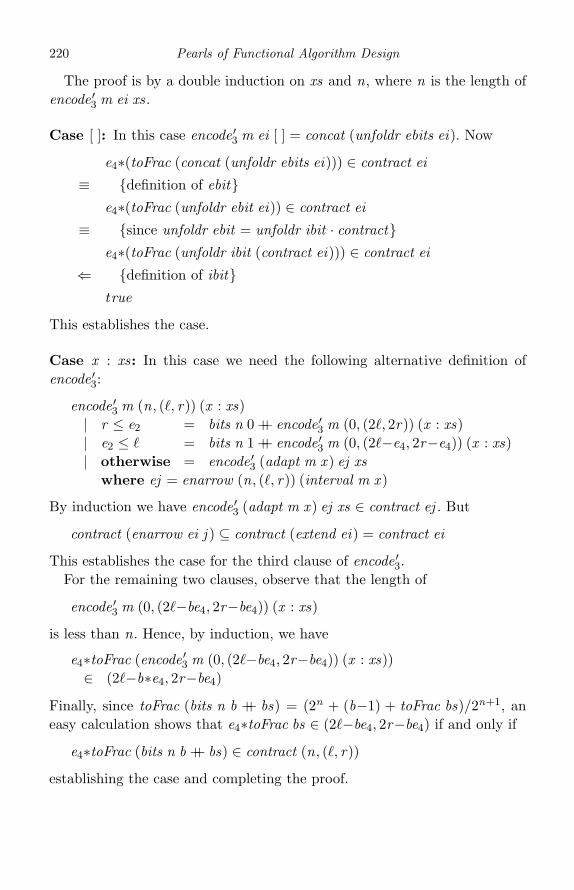
220 Pearls of Functional Algorithm Design
The proof is by a double induction on xs and n, where n is the length ofencode ′3 m ei xs.
Case [ ]: In this case encode ′3 m ei [ ] = concat (unfoldr ebits ei). Now
e4∗(toFrac (concat (unfoldr ebits ei))) ∈ contract ei
≡ {definition of ebit}e4∗(toFrac (unfoldr ebit ei)) ∈ contract ei
≡ {since unfoldr ebit = unfoldr ibit · contract}e4∗(toFrac (unfoldr ibit (contract ei))) ∈ contract ei
⇐ {definition of ibit}true
This establishes the case.
Case x : xs: In this case we need the following alternative definition ofencode ′3:
encode ′3 m (n, (�, r)) (x : xs)| r ≤ e2 = bits n 0 ++ encode ′3 m (0, (2�, 2r)) (x : xs)| e2 ≤ � = bits n 1 ++ encode ′3 m (0, (2�−e4, 2r−e4)) (x : xs)| otherwise = encode ′3 (adapt m x ) ej xs
where ej = enarrow (n, (�, r)) (interval m x )
By induction we have encode ′3 (adapt m x ) ej xs ∈ contract ej . But
contract (enarrow ei j ) ⊆ contract (extend ei) = contract ei
This establishes the case for the third clause of encode ′3.For the remaining two clauses, observe that the length of
encode ′3 m (0, (2�−be4, 2r−be4)) (x : xs)
is less than n. Hence, by induction, we have
e4∗toFrac (encode ′3 m (0, (2�−be4, 2r−be4)) (x : xs))∈ (2�−b∗e4, 2r−be4)
Finally, since toFrac (bits n b ++ bs) = (2n + (b−1) + toFrac bs)/2n+1, aneasy calculation shows that e4∗toFrac bs ∈ (2�−be4, 2r−be4) if and only if
e4∗toFrac (bits n b ++ bs) ∈ contract (n, (�, r))
establishing the case and completing the proof.
26
The Schorr–Waite algorithm
Introduction
The Schorr–Waite algorithm is a method for marking the nodes of a directedgraph reachable from a given starting node. The graph is restricted to haveout-degree 2. The algorithm consists of an iterative loop that carries outa depth-first traversal of the graph, but does not use an explicit stack tocontrol the traversal. Instead, it simulates the stack by modifying the graph,taking care to restore the graph to its initial state at the end of the markingprocess. The algorithm is fairly subtle. Morris (1982) described it as “thatmost recalcitrant algorithm” and Bornat (2000) as “the first mountain thatany formalism for pointer aliasing should climb”.
The aim of this pearl is to present the Schorr–Waite algorithm as anexercise in explaining an algorithm by program transformation. We beginwith a simple version of the marking algorithm and then describe three trans-formations that result in the final algorithm. Each transformation describesa different representation of the stack, culminating in a representation as alinked list embedded in the graph.
Specification
In Schorr and Waite’s formulation of the problem, the graph represents aMcCarthy S-expression McCarthy (1960) and so has out-degree 2. Nodesare represented by positive integers. Thus, we declare
type Node = Inttype Graph = Node → (Node,Node)
The operations left , right :: Graph → Node → Node extract the informationassociated with a given node and
setl , setr :: Graph → Node → Node → Graph
update the information associated with a node. So left (setl g x y)x = y , andsimilarly for setr .
221
222 Pearls of Functional Algorithm Design
The marking function mark takes a graph g and a starting node rootand returns a Boolean-valued function m so that m x = True if and onlyif node x is reachable from root . We will implement mark g as a functionthat returns both g and m. The reason is that the final algorithm modifiesg during the course of execution; so, by showing that the various versions ofmark are equivalent, we guarantee that not only is the final value of m thesame for each version, but also the final value of g . Thus, mark has type
mark :: Graph → Node → (Graph,Node → Bool)
A perfectly reasonable alternative is to embed the marking function in thegraph, so that a graph becomes a mapping from nodes to triples. Then markneeds only return the final graph. But the present arrangement of keepingthe marking function separate is both clearer and easier to reason about.
The function mark is implemented with a standard stack-based algorithmthat carries out a depth-first search of the graph:
mark g root = seek0 (g , const False) [root ]
seek0 (g ,m) [ ] = (g ,m)seek0 (g ,m) (x : xs)| not (m x ) = seek0 (g , set m x ) (left g x : right g x : xs)| otherwise = seek0 (g ,m) xs
The functions set and unset (needed later) are defined by
set , unset :: (Node → Bool)→ Node → (Node → Bool)set f x = λy → if y x then True else f yunset f x = λy → if y x then False else f y
This definition of mark is our starting point.
Safe replacement
When reasoning about any algorithm that involves the manipulation ofpointers, one sooner or later comes up against the problem of safe replace-
ment. To illustrate, define the function replace by
replace :: Eq a → (a → b)→ a → b → (a → b)replace f x y = λz → if z = x then y else f z
Thus, replace is a generalised version of the function set introduced above.When is it safe to use replace? For instance, when do the identities
map f xs = map (replace f x y) xsfilter p xs = filter (replace p x y) xs

The Schorr–Waite algorithm 223
hold? The answer is not surprising: it is when x is not on the list xs. Theother answer, when y = f x or y = p x , is also correct but not interesting.Also not interesting is the proof of the correctness of the first answer. Wewill see a number of appeals to safe replacement below, all signified with thehint “safe replacement”.
Eliminating duplicate entries
Returning to the problem in hand, the stack is eliminated in stages bytransforming mark into successively different but equivalent versions. Theaim of the first transformation is to eliminate duplicate entries on the stackby using it to store only those nodes that have been marked. This transfor-mation sets things up for later appeals to safe replacements. The functionseek0 is converted into a new function seek1, defined by
seek1 (g ,m) x xs = seek0 (g ,m) (x : map (right g) xs)
and subject to the invariant clean m xs = all m xs ∧ nodups xs. Synthesizinga direct definition of seek1 is straightforward and leads to the followingreplacement for mark :
mark g root = seek1 (g , const False) root [ ]seek1 (g ,m) x xs| not (m x ) = seek1 (g , set m x ) (left g x ) (x : xs)| null xs = (g ,m)| otherwise = seek1 (g ,m) (right g (head xs)) (tail xs)
Since x is added to the stack only when x is marked, and nodes are markedat most once, the new version of the stack is a clean one.
Threading the stack
The second transformation is designed to ensure that, in addition to beingclean, the stack is threaded, meaning that for each pair x , y of adjacententries, either x = left g y or x = right g y . This is not the case with seek1.Consider the expression seek1 (g ,m) (left g x ) (x : y : xs), in which left g x ismarked but right g x is not. Then seek1 replaces x on the stack with right g x ,which is not in general the left-value or right-value of y . If, however, we cancontrive to leave x on the stack, flagging it in some way to avoid processingit twice, then adding right g x to the top will maintain the constraint. Theelement x is removed later when all of its offspring have been marked.
224 Pearls of Functional Algorithm Design
This effect is achieved with the help of a second marking function p. Defineseek2 by
seek2 (g ,m) p x xs = seek1 (g ,m) x (filter p xs)
subject to the invariant threaded g m p x xs on the arguments of seek2, where
threaded g m p x xs = clean m xs ∧and [link u v | (u, v)← zip (x : xs) xs]
where link u v = if p v then u = left g v else u = right g v
Below we refer to the following fact with the hint “threadedness”: providedm x and x /∈ xs, we have
threaded g m p x xs ⇒ threaded g m (set p x ) (left g x ) (x : xs) ∧threaded g m (unset p x ) (right g x ) (x : xs)
We now synthesise a new version of mark based on seek2. It is clear that
mark g x = seek2 (g , const False) (const False) x [ ]
so it remains to calculate a direct definition of seek2. In the case not (m x )we reason:
seek2 (g ,m) p x xs
= {definition}seek1 (g ,m) x (filter p xs)
= {case assumption not (m x )}seek1 (g , set m x ) (left g x ) (x : filter p xs)
= {safe replacement, since x /∈ xs}seek1 (g , set m x ) (left g x ) (x : filter (set p x ) xs)
= {since set p x x = True}seek1 (g , set m x ) (left g x ) (filter (set p x ) (x : xs))
= {definition of seek2, and threadedness}seek2 (g , set m x ) (set p x ) (left g x ) (x : xs)
Hence, seek2 (g ,m) p x xs = seek2 (g , set m x ) (set p x ) (left g x ) (x : xs).In the case m x we have to search for the first element on the stack
satisfying p because that is the next element to be processed. We thereforeintroduce a function find2, defined by
find2 (g ,m) p xs = seek1 (g ,m) x (filter p xs)
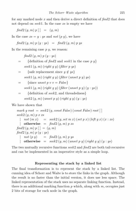
The Schorr–Waite algorithm 225
for any marked node x and then derive a direct definition of find2 that doesnot depend on seek1. In the case xs is empty we have
find2 (g ,m) p [ ] = (g ,m)
In the case xs = y : ys and not (p y), we have
find2 (g ,m) p (y : ys) = find2 (g ,m) p ys
In the remaining case p y , we reason:
find2 (g ,m) p (y : ys)
= {definition of find2 and seek1 in the case p y}seek1 (g ,m) (right g y) (filter p ys)
= {safe replacement since y /∈ ys}seek1 (g ,m) (right g y) (filter (unset p y) ys)
= {since unset p v v = False}seek1 (g ,m) (right g y) (filter (unset p y) (y : ys))
= {definition of seek2, and threadedness}seek2 (g ,m) (unset p y) (right g y) (y : ys)
We have shown that
mark g root = seek2 (g , const False) (const False) root [ ]seek2 (g ,m) p x xs| not (m x ) = seek2 (g , set m x ) (set p x ) (left g x ) (x : xs)| otherwise = find2 (g ,m) p xs
find2 (g ,m) p [ ] = (g ,m)find2 (g ,m) p (y : ys)| not (p y) = find2 (g ,m) p ys| otherwise = seek2 (g ,m) (unset p y) (right g y) (y : ys)
The two mutually recursive functions seek2 and find2 are both tail-recursiveand can be implemented in an imperative style as a simple loop.
Representing the stack by a linked list
The final transformation is to represent the stack by a linked list. Thecunning idea of Schorr and Waite is to store the links in the graph. Althoughthe result is no faster than the initial version, it does use less space. Thelinked representation of the stack uses no separate linking function. Instead,there is an additional marking function p which, along with m, occupies just2 bits of storage for each node in the graph.
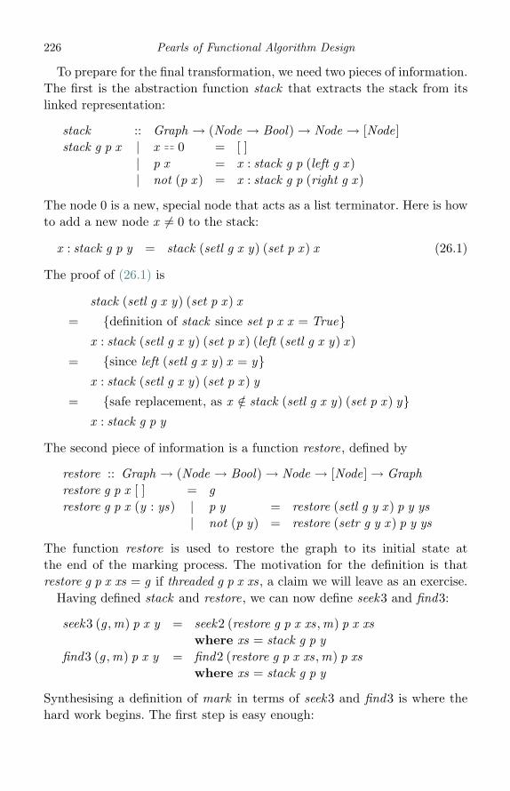
226 Pearls of Functional Algorithm Design
To prepare for the final transformation, we need two pieces of information.The first is the abstraction function stack that extracts the stack from itslinked representation:
stack :: Graph → (Node → Bool)→ Node → [Node]stack g p x | x 0 = [ ]
| p x = x : stack g p (left g x )| not (p x ) = x : stack g p (right g x )
The node 0 is a new, special node that acts as a list terminator. Here is howto add a new node x �= 0 to the stack:
x : stack g p y = stack (setl g x y) (set p x ) x (26.1)
The proof of (26.1) is
stack (setl g x y) (set p x ) x
= {definition of stack since set p x x = True}x : stack (setl g x y) (set p x ) (left (setl g x y) x )
= {since left (setl g x y) x = y}x : stack (setl g x y) (set p x ) y
= {safe replacement, as x /∈ stack (setl g x y) (set p x ) y}x : stack g p y
The second piece of information is a function restore, defined by
restore :: Graph → (Node → Bool)→ Node → [Node]→ Graphrestore g p x [ ] = grestore g p x (y : ys) | p y = restore (setl g y x ) p y ys
| not (p y) = restore (setr g y x ) p y ys
The function restore is used to restore the graph to its initial state atthe end of the marking process. The motivation for the definition is thatrestore g p x xs = g if threaded g p x xs, a claim we will leave as an exercise.
Having defined stack and restore, we can now define seek3 and find3:
seek3 (g ,m) p x y = seek2 (restore g p x xs ,m) p x xswhere xs = stack g p y
find3 (g ,m) p x y = find2 (restore g p x xs ,m) p xswhere xs = stack g p y
Synthesising a definition of mark in terms of seek3 and find3 is where thehard work begins. The first step is easy enough:
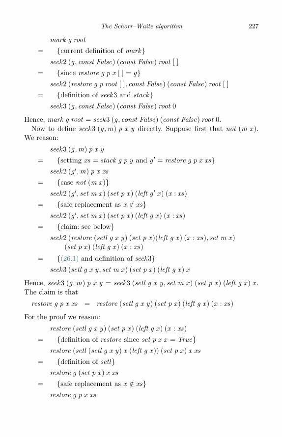
The Schorr–Waite algorithm 227
mark g root
= {current definition of mark}seek2 (g , const False) (const False) root [ ]
= {since restore g p x [ ] = g}seek2 (restore g p root [ ], const False) (const False) root [ ]
= {definition of seek3 and stack}seek3 (g , const False) (const False) root 0
Hence, mark g root = seek3 (g , const False) (const False) root 0.Now to define seek3 (g ,m) p x y directly. Suppose first that not (m x ).
We reason:
seek3 (g ,m) p x y
= {setting xs = stack g p y and g ′ = restore g p x xs}seek2 (g ′,m) p x xs
= {case not (m x )}seek2 (g ′, set m x ) (set p x ) (left g ′ x ) (x : xs)
= {safe replacement as x /∈ xs}seek2 (g ′, set m x ) (set p x ) (left g x ) (x : xs)
= {claim: see below}seek2 (restore (setl g x y) (set p x )(left g x ) (x : xs), set m x )
(set p x ) (left g x ) (x : xs)
= {(26.1) and definition of seek3}seek3 (setl g x y , set m x ) (set p x ) (left g x ) x
Hence, seek3 (g ,m) p x y = seek3 (setl g x y , set m x ) (set p x ) (left g x ) x .The claim is that
restore g p x xs = restore (setl g x y) (set p x ) (left g x ) (x : xs)
For the proof we reason:
restore (setl g x y) (set p x ) (left g x ) (x : xs)
= {definition of restore since set p x x = True}restore (setl (setl g x y) x (left g x )) (set p x ) x xs
= {definition of setl}restore g (set p x ) x xs
= {safe replacement as x /∈ xs}restore g p x xs
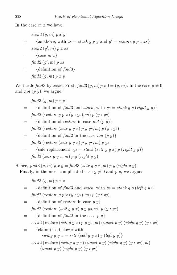
228 Pearls of Functional Algorithm Design
In the case m x we have
seek3 (g ,m) p x y
= {as above, with xs = stack g p y and g ′ = restore g p x xs}seek2 (g ′,m) p x xs
= {case m x}find2 (g ′,m) p xs
= {definition of find3}find3 (g ,m) p x y
We tackle find3 by cases. First, find3 (g ,m)p x 0 = (g ,m). In the case y �= 0and not (p y), we argue:
find3 (g ,m) p x y
= {definition of find3 and stack , with ys = stack g p (right g y)}find2 (restore g p x (y : ys),m) p (y : ys)
= {definition of restore in case not (p y)}find2 (restore (setr g y x ) p y ys,m) p (y : ys)
= {definition of find2 in the case not (p y)}find2 (restore (setr g y x ) p y ys,m) p ys
= {safe replacement: ys = stack (setr g y x ) p (right g y)}find3 (setr g y x ,m) p y (right g y)
Hence, find3 (g ,m) p x y = find3 (setr g y x ,m) p y (right g y).Finally, in the most complicated case y �= 0 and p y , we argue:
find3 (g ,m) p x y
= {definition of find3 and stack , with ys = stack g p (left g y)}find2 (restore g p x (y : ys),m) p (y : ys)
= {definition of restore in case p y}find2 (restore (setl g y x ) p y ys,m) p (y : ys)
= {definition of find2 in the case p y}seek2 (restore (setl g y x ) p y ys,m) (unset p y) (right g y) (y : ys)
= {claim (see below): withswing g y x = setr (setl g y x ) y (left g y)}
seek2 (restore (swing g y x ) (unset p y) (right g y) (y : ys),m)(unset p y) (right g y) (y : ys)

The Schorr–Waite algorithm 229
= {safe replacement: y : ys = stack (swing g y x ) (unset p y) y}seek3 (swing g y x ,m) (unset p y) (right g y) y
Hence, find3 (g ,m) p x y = seek3 (swing g y x ,m) (unset p y) (right g y) y .The claim in the penultimate step is that
restore (setl g y x ) p y ys= restore (swing g y x ) (unset p y) (right g y) (y : ys)
where swing g y x = setr (setl g y x ) y (left g y). Here is the proof:
restore (swing g y x ) (unset p y) (right g y) (y : ys)
= {definition of restore since unset p y y = False}restore (setr (swing g y x ) y (right g y)) (unset p y) y ys
= {since setr (swing g y x ) y (right g y) = setl g y x}restore (setl g y x ) (unset p y) y ys
= {safe replacement as y /∈ ys}restore (setl g y x ) p y ys
In summary:
mark g root = seek3 (g , const False) (const False) root 0seek3 (g ,m) p x y| not (m x ) = seek3 (setl g x y , set m x ) (set p x ) (left g x ) x| otherwise = find3 (g ,m) p x y
find3 (g ,m) p x y| y 0 = (g ,m)| p y = seek3 (swing g y x ,m) (unset p y) (right g y) y| otherwise = find3 (setr g y x ,m) p y (right g y)
where swing g y x = setr (setl g y x ) y (left g y)
This is the Schorr–Waite marking algorithm.
Final remarks
The Schorr–Waite algorithm was first described in Schorr and Waite (1967).Formal reasoning about the algorithm using loop invariants includes Bornat(2000), Butler (1999), Gries (1979), Morris (1982) and Topor (1979), butthis list is not exhaustive. Moller (1997, 1999) used relations and relationalalgebras to reason about the algorithm, while Mason (1988) used Lisp andmutable update functions.
Any treatment of the Schorr–Waite algorithm is bound to be fairly detailed,and the present one is no different. Particularly important is the need for
230 Pearls of Functional Algorithm Design
various safe replacement properties. An alternative approach to safe replace-ment using separation logic is presented by O’Hearn et al. (2004). We doclaim, however, that each definition of seek in terms of previous versionshas a coherent motivation, is reasonably simple to understand and is a goodway to present the algorithm.
ReferencesBornat, R. (2000). Proving pointer programs in Hoare logic. LNCS 1837: 5th
Mathematics of Program Construction Conference, pp. 102–26.Butler, M. (1999). Calculational derivation of pointer algorithms from tree
operations. Science of Computer Programming 33 (3), 221–60.Gries, D. (1979). The Schorr–Waite graph marking algorithm. Acta Informatica
11, 223–32.McCarthy, J. (1960). Recursive functions of symbolic expressions and their
computation by machine. Communications of the ACM 3, 184.Mason, I. A. (1988). Verification of programs that destructively manipulate data.
Science of Computer Programming 10 (2), 177–210.Moller, B. (1997). Calculating with pointer structures. IFIP TC2/WG2.1
Working Conference on Algorithmic Languages and Calculi. Chapman andHall, pp. 24–48.
Moller, B. (1999). Calculating with acyclic and cyclic lists. Information Sciences119, 135–54.
Morris, J. M. (1982). A proof of the Schorr–Waite algorithm. Proceedings of the1981 Marktoberdorf Summer School, ed. M. Broy and G. Schmidt. Reidel,pp. 25–51.
O’Hearn, P. W., Yang, H. and Reynolds, J. C. (2004). Separation and informationhiding. 31st Principles of Programming Languages Conference. ACM Publica-tions, pp. 268–80.
Schorr, H. and Waite, W. M. (1967). An efficient machine-independent procedurefor garbage collection in various list structures. Communications of the ACM10, 501–6.
Topor, R. W. (1979). The correctness of the Schorr–Waite marking algorithm. ActaInformatica 11, 211–21.

27
Orderly insertion
Introduction
Consider the problem of inserting the elements of a list of N distinct elementsof some ordered type A one by one into an initially empty array of size N insuch a way that at each stage the inserted elements are in increasing order,though possibly with gaps between them. If you like, think of the list asa big pile of books on the floor in some jumbled order and the array as abookshelf divided into slots. At each stage the books on the shelf have to bein alphabetical order. You pick up the topmost book on the pile and place iton the shelf. In general, that can only be done by moving some of the booksalready on the shelf to make room. The object of the exercise is to minimisethe total number of moves – the distance of the move is not relevant. Forexample, with A = Char , one way of inserting the elements of the string“PEARLS” into an array of size 6 is given by
1 2 3 4 5 6 Moves
– – – P – – 0– E – P – – 0A – – E – P 2A – – E P R 1A E L – P R 1A E L P R S 2
with a total number of six moves. Our aim in this pearl is to construct afunction that does the job with a total of Θ(N log3 N ) moves, which hasbeen conjectured to be the best possible. The algorithm is not derived, butestablishing the time bound involves some subtle calculation.
231
232 Pearls of Functional Algorithm Design
A naive algorithm
Let us begin by recording the minimum number m(N ) of moves necessaryto insert any list of N elements into an array of size N for 1 ≤ N ≤ 12:
N = 1 2 3 4 5 6 7 8 9 10 11 12m(N ) = 0 1 2 4 6 8 11 14 17 21 24 29
It is an interesting diversion to find a strategy which guarantees that anylist of six elements can be inserted in an array of size six with at most eightmoves (just because PEARLS can be inserted with six moves does not meanthat all six-letter words can be). No asymptotic formula for m(N ) is known,though there is strong evidence that m(N ) = Θ(N log3 N ).
There is one obvious algorithm for the problem, though it has a poorworst-case performance. Insert the first element in the first position andinsert subsequent elements by shifting previously inserted elements justenough spaces to make room. So, if the kth element is smaller than allprevious values, the k−1 previously inserted elements have each to be shiftedup one position. This naive algorithm requires N (N−1)/2 moves in the worstcase.
Slightly better, but not by much, is the strategy of inserting each elementin the middle of the available free slots, if any. The first �log N � elementscan then be inserted without any moves. However, after half the elementshave been inserted, the moves begin to build up, leading once again to aquadratic-time worst-case performance.
One reasonable refinement on the basic strategy is periodically to insertsome elements in such a way as to leave an even distribution of free slotsfor those that follow. Suppose we choose some integer M and call elementsnumbered iM , where 1 ≤ i ≤ k and kM ≤ N < (k + 1)M , the special
elements. A special element iM is inserted by moving every inserted elementto leave an even spread, and therefore may require iM −1 moves. This givesa total cost of at most
k∑i=1
(iM − 1) = Θ(N 2/M )
moves for inserting all special elements.When special element iM has been inserted, suppose the N −iM free slots
are evenly distributed with, roughly, Ci = iM /(N − iM ) elements on eitherside of each free slot. The naive algorithm for inserting the next M−1 (orfewer if i = k) non-special elements can then force at most
Orderly insertion 233
M−1∑j=1
(jCi + j − 1) = Θ(CiM 2)
moves. The total number of moves for inserting all the non-special elementsis then
Θ
⎛⎝N/M∑
i=1
CiM 2
⎞⎠ = Θ
⎛⎝M 2
N/M∑i=1
iMN − iM
⎞⎠ = Θ(MN log N )
Now, if we choose M so that N 2/M ≈ MN log N so M ≈√
N / log N ,the total number of moves is Θ(
√N 3 log N ), which is a little worse than
Θ(N 1·5).
An improved algorithm
The strategy of the previous section can be improved in two ways: wecan choose a different sequence of special elements and we can choose abetter method for inserting the non-special ones. The two improvements areindependent, but we will need both in order to meet the required asymptoticbound.
Instead of having special elements evenly spaced, suppose we allow moreof them as the slots fill up. More specifically, let the special elements be thosenumbered n1,n2, . . . ,nk , where n1 = �N /2�, n2 = �3N /4�, n3 = �7N /8� andso on up to nk = �(2k−1)N /2k�, where 2k−1 < N ≤ 2k , so k = log N �. Forexample, when N = 1000 the special elements are
500, 750, 875, 937, 968, 984, 992, 996, 998, 999
The final element is inserted with at most N−1 moves. Since k = log N �,the total cost for inserting special elements is at most
k∑i=1
(ni − 1) ≤k∑
i=1
N = Θ(N log N )
Now we must deal with the non-special elements. Consider non-specialelement numbered n in phase i , meaning ni−1 < n < ni , where n0 = 0.Suppose this element needs to be inserted after the element at positionp − 1 but before the element at position q ; in other words, in the interval[p, q). If p < q , so there are free slots, the element can be inserted at index�(p + q)/2�. If p = q , so there are no free slots, the elements in some regionsurrounding p have to be moved to make room. The crunch question is:what region should be selected?
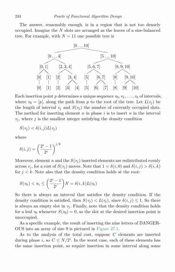
234 Pearls of Functional Algorithm Design
The answer, reasonably enough, is in a region that is not too denselyoccupied. Imagine the N slots are arranged as the leaves of a size-balancedtree. For example, with N = 11 one possible tree is
[0 . . . 10]
[0 . . . 4]���
���[0, 1]
�� [0]
[0]
[1]
[1]
[2, 3, 4]����
[2]
[2]
[3, 4]��
[3] [4]
[5 . . . 10]����
����[5, 6, 7]
����[5]
[5]
[6, 7]��
[6] [7]
[8, 9, 10]����
[8]
[8]
[9, 10]����
[9] [10]
Each insertion point p determines a unique sequence v0, v1, . . . , vk of intervals,where v0 = [p], along the path from p to the root of the tree. Let L(vj ) bethe length of interval vj and S (vj ) the number of currently occupied slots.The method for inserting element n in phase i is to insert n in the intervalvj , where j is the smallest integer satisfying the density condition
S (vj ) < δ(i , j )L(vj )
where
δ(i , j ) =(
2i − 12i
)j/k
Moreover, element n and the S (vj ) inserted elements are redistributed evenlyacross vj , for a cost of S (vj ) moves. Note that 1 = δ(i , 0) and δ(i , j ) > δ(i , k)for j < k . Note also that the density condition holds at the root:
S (vk ) < ni ≤(
2i − 12i
)N = δ(i , k)L(vk )
So there is always an interval that satisfies the density condition. If thedensity condition is satisfied, then S (vj ) < L(vj ), since δ(i , j ) ≤ 1. So thereis always an empty slot in vj . Finally, note that the density condition holdsfor a leaf v0 whenever S (v0) = 0, so the slot at the desired insertion point isunoccupied.
As a specific example, the result of inserting the nine letters of DANGER-OUS into an array of size 9 is pictured in Figure 27.1.
As to the analysis of the total cost, suppose C elements are insertedduring phase i , so C ≤ N /2i . In the worst case, each of these elements hasthe same insertion point, so require insertion in some interval along some
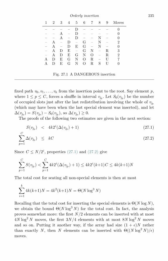
Orderly insertion 235
1 2 3 4 5 6 7 8 9 Moves
– – – – D – – – – 0– – A – D – – – – 0– – A – D – – N – 0– A – D – G – N – 2– A – D E G – N – 0– A D E – G N – R 3– A D E G N O – R 2A D E G N O R – U 7A D E G N O R S U 0
Fig. 27.1 A DANGEROUS insertion
fixed path v0, v1, . . . , vk from the insertion point to the root. Say element p,where 1 ≤ p ≤ C , forces a shuffle in interval vjp . Let S0(vjp ) be the numberof occupied slots just after the last redistribution involving the whole of vjp
(which may have been when the last special element was inserted), and letΔ(vjp ) = S (vjp )− S0(vjp ), so Δ(vjp ) ≥ 0.
The proofs of the following two estimates are given in the next section:
S (vjp ) < 4k2i(Δ(vjp ) + 1) (27.1)C∑
p=1
Δ(vjp ) ≤ kC (27.2)
Since C ≤ N /2i , properties (27.1) and (27.2) give
C∑p=1
S (vjp ) <C∑
p=1
4k2i(Δ(vjp ) + 1) ≤ 4k2i(k+1)C ≤ 4k(k+1)N
The total cost for seating all non-special elements is then at most
k∑i=1
4k(k+1)N = 4k2(k+1)N = Θ(N log3 N )
Recalling that the total cost for inserting the special elements is Θ(N log N ),we obtain the bound Θ(N log3 N ) for the total cost. In fact, the analysisproves somewhat more: the first N /2 elements can be inserted with at most4N log2 N moves, the first 3N /4 elements with at most 8N log2 N movesand so on. Putting it another way, if the array had size (1 + ε)N ratherthan exactly N , then N elements can be inserted with Θ((N log2 N )/ε)moves.
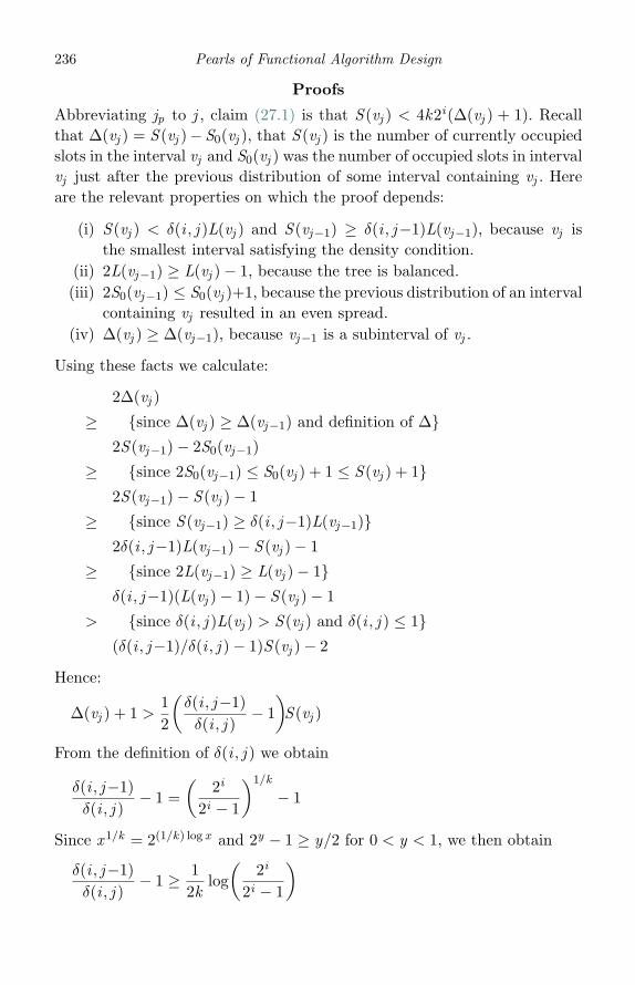
236 Pearls of Functional Algorithm Design
Proofs
Abbreviating jp to j , claim (27.1) is that S (vj ) < 4k2i(Δ(vj ) + 1). Recallthat Δ(vj ) = S (vj )− S0(vj ), that S (vj ) is the number of currently occupiedslots in the interval vj and S0(vj ) was the number of occupied slots in intervalvj just after the previous distribution of some interval containing vj . Hereare the relevant properties on which the proof depends:
(i) S (vj ) < δ(i , j )L(vj ) and S (vj−1) ≥ δ(i , j−1)L(vj−1), because vj isthe smallest interval satisfying the density condition.
(ii) 2L(vj−1) ≥ L(vj )− 1, because the tree is balanced.(iii) 2S0(vj−1) ≤ S0(vj )+1, because the previous distribution of an interval
containing vj resulted in an even spread.(iv) Δ(vj ) ≥ Δ(vj−1), because vj−1 is a subinterval of vj .
Using these facts we calculate:
2Δ(vj )
≥ {since Δ(vj ) ≥ Δ(vj−1) and definition of Δ}2S (vj−1)− 2S0(vj−1)
≥ {since 2S0(vj−1) ≤ S0(vj ) + 1 ≤ S (vj ) + 1}2S (vj−1)− S (vj )− 1
≥ {since S (vj−1) ≥ δ(i , j−1)L(vj−1)}2δ(i , j−1)L(vj−1)− S (vj )− 1
≥ {since 2L(vj−1) ≥ L(vj )− 1}δ(i , j−1)(L(vj )− 1)− S (vj )− 1
> {since δ(i , j )L(vj ) > S (vj ) and δ(i , j ) ≤ 1}(δ(i , j−1)/δ(i , j )− 1)S (vj )− 2
Hence:
Δ(vj ) + 1 >12
(δ(i , j−1)δ(i , j )
− 1)S (vj )
From the definition of δ(i , j ) we obtain
δ(i , j−1)δ(i , j )
− 1 =(
2i
2i − 1
)1/k
− 1
Since x 1/k = 2(1/k) log x and 2y − 1 ≥ y/2 for 0 < y < 1, we then obtain
δ(i , j−1)δ(i , j )
− 1 ≥ 12k
log(
2i
2i − 1
)

Orderly insertion 237
�
a q p
Δ(vjp ) = 3
b
jqjp
�
sum 2sum 1
a b−d b
djb
Fig. 27.2 Decomposition of P(a, b, k) into two sums
Finally, since 2i log[2i/(2i − 1)] ≥ 1, we get 4k2i(Δ(vj ) + 1) > S (vj ), whichis (27.1).
Claim (27.2) is that∑C
p=1 Δ(vjp ) ≤ kC . More generally, we show that
b∑p=a
Δ(vjp ) ≤ k(b−a+1)
for 1 ≤ a ≤ b ≤ C . Let P(a, b, k) denote the sum on the left, where wehave made the dependency on k , the height of the tree, explicit. Considerthe sequence of points ja , . . . , jb , where 0 ≤ jp ≤ k . Each point denotes theinterval in which an element is inserted. The value Δ(vjp ) is the number ofelements in the interval vjp that have been inserted since the last redistri-bution at an interval containing vjp , say at jq , and is therefore equal to thenumber of points between q and p. The situation is depicted in the firstdiagram of Figure 27.2.
To estimate P(a, b, k), suppose Δ(vjb ) = d , so 0 ≤ d ≤ b−a. Then Pcan be decomposed into two sums, as shown in Figure 27.2: the sum from aup to b−d−1 and the sum from b−d to b−1, where we know in the secondsum that the maximum j value is jb − 1. This leads to the estimate thatP(a, b, k) is at most
(max d : 0 ≤ d ≤ b−a : P(a, b−d−1, k) + P(b−d , b−1, jb−1) + d)
Since jb ≤ k and P is monotonic in its third argument, we have thatP(a, b, k) is at most
(max d : 0 ≤ d ≤ b−a : P(a, b−d−1, k) + P(b−d , b−1, k−1) + d)
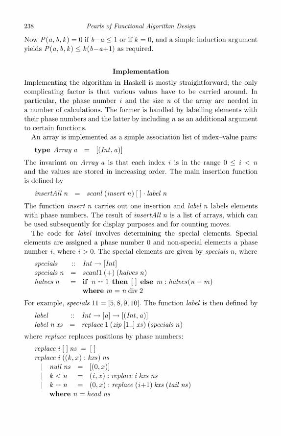
238 Pearls of Functional Algorithm Design
Now P(a, b, k) = 0 if b−a ≤ 1 or if k = 0, and a simple induction argumentyields P(a, b, k) ≤ k(b−a+1) as required.
Implementation
Implementing the algorithm in Haskell is mostly straightforward; the onlycomplicating factor is that various values have to be carried around. Inparticular, the phase number i and the size n of the array are needed ina number of calculations. The former is handled by labelling elements withtheir phase numbers and the latter by including n as an additional argumentto certain functions.
An array is implemented as a simple association list of index–value pairs:
type Array a = [(Int , a)]
The invariant on Array a is that each index i is in the range 0 ≤ i < nand the values are stored in increasing order. The main insertion functionis defined by
insertAll n = scanl (insert n) [ ] · label n
The function insert n carries out one insertion and label n labels elementswith phase numbers. The result of insertAll n is a list of arrays, which canbe used subsequently for display purposes and for counting moves.
The code for label involves determining the special elements. Specialelements are assigned a phase number 0 and non-special elements a phasenumber i , where i > 0. The special elements are given by specials n, where
specials :: Int → [Int ]specials n = scanl1 (+) (halves n)halves n = if n 1 then [ ] else m : halves(n −m)
where m = n div 2
For example, specials 11 = [5, 8, 9, 10]. The function label is then defined by
label :: Int → [a]→ [(Int , a)]label n xs = replace 1 (zip [1..] xs) (specials n)
where replace replaces positions by phase numbers:
replace i [ ] ns = [ ]replace i ((k , x ) : kxs) ns| null ns = [(0, x )]| k < n = (i , x ) : replace i kxs ns| k n = (0, x ) : replace (i+1) kxs (tail ns)
where n = head ns
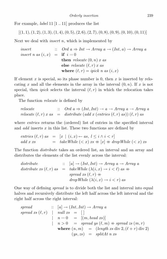
Orderly insertion 239
For example, label 11 [1 .. 11] produces the list
[(1, 1), (1, 2), (1, 3), (1, 4), (0, 5), (2, 6), (2, 7), (0, 8), (0, 9), (0, 10), (0, 11)]
Next we deal with insert n, which is implemented by
insert :: Ord a ⇒ Int → Array a → (Int , a) → Array ainsert n as (i , x ) = if i 0
then relocate (0,n) x aselse relocate (�, r) x aswhere (�, r) = ipick n as (i , x )
If element x is special, so its phase number is 0, then x is inserted by relo-cating x and all the elements in the array in the interval (0,n). If x is notspecial, then ipick selects the interval (�, r) in which the relocation takesplace.
The function relocate is defined by
relocate :: Ord a ⇒ (Int , Int) → a → Array a → Array arelocate (�, r) x as = distribute (add x (entries (�, r) as)) (�, r) as
where entries returns the (ordered) list of entries in the specified intervaland add inserts x in this list. These two functions are defined by
entries (�, r) as = [x | (i , x )← as, l ≤ i ∧ i < r ]add x xs = takeWhile (< x ) xs ++ [x ] ++ dropWhile (< x ) xs
The function distribute takes an ordered list, an interval and an array anddistributes the elements of the list evenly across the interval:
distribute :: [a]→ (Int , Int) → Array a → Array adistribute xs (�, r) as = takeWhile (λ(i , x ) → i < �) as ++
spread xs (�, r) ++dropWhile (λ(i , x ) → i < r) as
One way of defining spread is to divide both the list and interval into equalhalves and recursively distribute the left half across the left interval and theright half across the right interval:
spread :: [a]→ (Int , Int) → Array aspread xs (�, r) | null xs = [ ]
| n 0 = [(m, head xs)]| n > 0 = spread ys (�,m) ++ spread zs (m, r)
where (n,m) = (length xs div 2, (� + r) div 2)(ys, zs) = splitAt n xs

240 Pearls of Functional Algorithm Design
The next function to tackle is ipick . The definition is
ipick :: Ord a ⇒ Int → Array a → (Int , a) → (Int , Int)ipick n as (i , x ) = if p < q then (p, q) else
head [(�, r) | (j , (�, r))← zip [0..] (ipath n p),let s = length (entries (�, r) as),densityTest i j n s (r − �)]
where (p, q) = ipoint n x as
First, the insertion point for element x is determined by ipoint . The resultis an interval (p, q) containing no elements. If p < q , so the interval is notempty, then the result of ipick is (p, q). Subsequent relocation with (p, q)will ensure that x is placed in the middle of the interval. If p = q , so theinterval is empty, then the path of intervals from the insertion point p tothe root of the virtual tree is computed by ipath. The first interval satisfyingthe density test densityTest is then selected.
The function ipoint is implemented by
ipoint :: Ord a ⇒ Int → a → Array a → (Int , Int)ipoint n x as = search (0,n) aswhere search (p, q) [ ] = (p, q)
search (p, q) ((i , y) : as) = if x < y then (p, i)else search (i+1, q) as
The value ipath n p is computed by reversing the path from the root (0,n)to p:
ipath n p = reverse (intervals (0,n) p)
where
intervals (�, r) p | � + 1 r = [(�, r)]| p < m = (�, r) : intervals (�,m) p| m ≤ p = (�, r) : intervals (m, r) p
where m = (l + r) div 2
It remains to deal with the density test, for which we use arbitrary-precisioninteger arithmetic rather than real arithmetic. All five arguments of thefunction densityTest are limited-precision integers, so they have to beconverted to arbitrary precision:
densityTest i ′ j ′ n s ′ w ′ = 2 ↑ (i ∗ j ) ∗ s ↑ k < (2 ↑ i − 1) ↑ j ∗ w ↑ kwhere (i , j , s,w) = convert toInteger (i ′, j ′, s ′,w ′)
k = toInteger (ceiling (logBase 2 (fromIntegral n)))
The function convert is defined by convert f (a, b, c, d) = (f a, f b, f c, f d).

Orderly insertion 241
Final remarks
The problem of inserting elements of an ordered list of length N into anarray of size N is a restricted version of a more general problem known asonline list labelling (Bender et al., 2002), in which the aim is to maintain amapping from a dynamic set of M elements (so elements can be deleted aswell as inserted in the array) from some linearly ordered set to integers in therange 0 to N − 1 such that the order of the labels matches the order of thecorresponding elements. The primary use of online list labelling is in a relatedproblem known as order maintenance. This problem involves maintaininga list, initially consisting of a single base element, subject to insertions,deletions and order queries. Insertions take the form insert(x , y), mean-ing inserting a new element x into the list immediately after the (existing)element y . The delete(x ) operation deletes x from the list and query(x , y)returns true or false, depending on whether x precedes y in the list. Althoughorder maintenance does not require that labels be attached to each element,most solutions do indeed use online labelling as a component.
The interest in the algorithm lies not, of course, in the Haskell implementa-tion, but in the intriguing choice of density function and the analysis of whythe Θ(N log3 N ) behaviour is obtained. No-one knows whether Ω(N log3 N )is a lower bound on the problem, although Zhang (1993) proves that this is alower bound for any algorithm that restricts movements to result always ina position in which the free slots are evenly spaced. The algorithm above is“smooth” in this sense, and it seems unlikely that a non-smooth algorithmcould achieve fewer movements, but it appears difficult to rule such analgorithm out.
Finally, this pearl has been adapted from Bird and Sadnicki (2007), wherefurther references to the literature of the problem can be found.
ReferencesBender, M. A., Cole, R., Demaine, E. D., Frach-Colton, M. and Zito, J. (2002).
Two simplified algorithms for maintaining order in a list. Lecture Notes inComputer Science, Volume 2461. Springer-Verlag, pp. 139–51.
Bird, R. S. and Sadnicki, S. (2007). Minimal on-line labelling. Information Process-ing Letters 101 (1), 41–5.
Zhang, J. (1993). Density control and on-line labeling problems. Technical Report481 and PhD thesis, Computer Science Department, University of Rochester,New York, USA.

28
Loopless functional algorithms
Introduction
Imagine a program for generating combinatorial patterns of some kind,patterns such as the subsequences or permutations of a list. Suppose thateach pattern is obtained from its predecessor by a single transition. For sub-sequences a transition i could mean “insert or delete the element at positioni”. For permutations a transition i could mean “swap the item in positioni with the one in position i − 1”. An algorithm for generating all patternsis called loopless if the first transition is produced in linear time and eachsubsequent transition in constant time. Note that it is the transitions thatare produced in constant time, not the patterns; writing out a pattern is notusually possible in constant time.
Loopless algorithms were formulated in a procedural setting, and manyclever tricks, such as the use of focus pointers, doubly linked lists and corou-tines, have been used to construct them. This pearl and the following twoexplore what a purely functional approach can bring to the subject. Wewill calculate loopless functional versions of the Johnson–Trotter algorithmfor producing permutations, the Koda–Ruskey algorithm for generating allprefixes of a forest and its generalisation to Knuth’s spider spinning algo-rithm for generating all bit strings satisfying given inequality constraints.These novel functional algorithms rely on nothing more fancy than lists, treesand queues. The present pearl is mostly devoted to exploring the topic andgiving some warm-up exercises. Bear in mind, though, that loopless algo-rithms are not necessarily faster than their non-loopless counterparts. Toquote from Knuth (2001):
The extra contortions that we need to go through in order to achieve looplessnessare usually ill-advised, because they actually cause the total execution time to belonger than it would be with a more straightforward algorithm. But hey, looplessnesscarries an academic cachet. So we might as well treat this task as a challengingexercise that might help us to sharpen our algorithmic wits.
242

Loopless functional algorithms 243
Change the penultimate word to “calculational” and you will appreciate thereal point of the exercise.
Loopless algorithms
We formulate the idea of a loopless algorithm in terms of the standardfunction unfoldr , defined by
unfoldr :: (b → Maybe (a, b))→ b → [a]unfoldr step b = case step b of
Just (a, b ′) → a : unfoldr step b ′
Nothing → [ ]
By definition a loopless algorithm is one that is expressed in the form
unfoldr step · prolog
where step takes constant time and prolog x takes O(n) steps, where n issome suitable measure of the size of x . Every loopless algorithm has to beof the above form, with these constraints on the ingredients.
There is a slightly tricky problem about our formulation of looplessness.In the framework of a lazy functional language such as Haskell our definitionof a loopless program will not, in general, give a loopless computation withconstant delay between each output. In a lazy language, the work done byprolog is distributed throughout the computation, not concentrated all atonce at the beginning. Therefore, we should really interpret the compositionoperator (·) between unfoldr step and prolog as being fully strict, meaningthat prolog is evaluated fully before the unfolding begins. Although it is notpossible to define a general fully strict composition operator in Haskell, wewill take pains to ensure that prolog and step take linear and constant timeunder a strict as well as a lazy semantics.
Four warm-up exercises
The simplest warm-up exercise is the identity function on lists. Followingthe required recipe to the letter, we have
id :: [a]→ [a]id = unfoldr uncons · prolog
prolog :: [a]→ [a]prolog = id
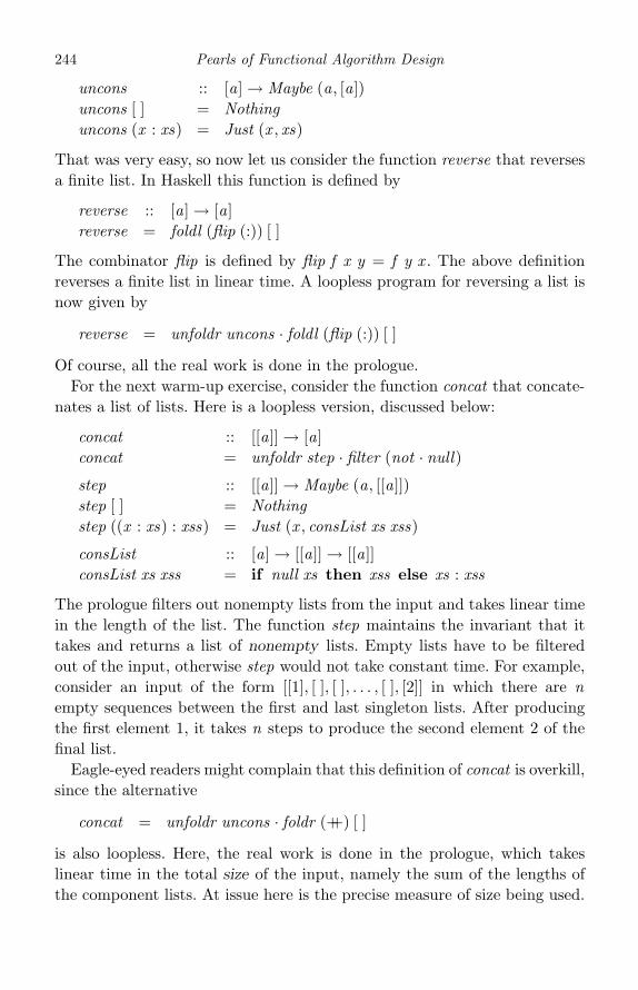
244 Pearls of Functional Algorithm Design
uncons :: [a]→ Maybe (a, [a])uncons [ ] = Nothinguncons (x : xs) = Just (x , xs)
That was very easy, so now let us consider the function reverse that reversesa finite list. In Haskell this function is defined by
reverse :: [a]→ [a]reverse = foldl (flip (:)) [ ]
The combinator flip is defined by flip f x y = f y x . The above definitionreverses a finite list in linear time. A loopless program for reversing a list isnow given by
reverse = unfoldr uncons · foldl (flip (:)) [ ]
Of course, all the real work is done in the prologue.For the next warm-up exercise, consider the function concat that concate-
nates a list of lists. Here is a loopless version, discussed below:
concat :: [[a]]→ [a]concat = unfoldr step · filter (not · null)
step :: [[a]]→ Maybe (a, [[a]])step [ ] = Nothingstep ((x : xs) : xss) = Just (x , consList xs xss)
consList :: [a]→ [[a]]→ [[a]]consList xs xss = if null xs then xss else xs : xss
The prologue filters out nonempty lists from the input and takes linear timein the length of the list. The function step maintains the invariant that ittakes and returns a list of nonempty lists. Empty lists have to be filteredout of the input, otherwise step would not take constant time. For example,consider an input of the form [[1], [ ], [ ], . . . , [ ], [2]] in which there are nempty sequences between the first and last singleton lists. After producingthe first element 1, it takes n steps to produce the second element 2 of thefinal list.
Eagle-eyed readers might complain that this definition of concat is overkill,since the alternative
concat = unfoldr uncons · foldr (++) [ ]
is also loopless. Here, the real work is done in the prologue, which takeslinear time in the total size of the input, namely the sum of the lengths ofthe component lists. At issue here is the precise measure of size being used.
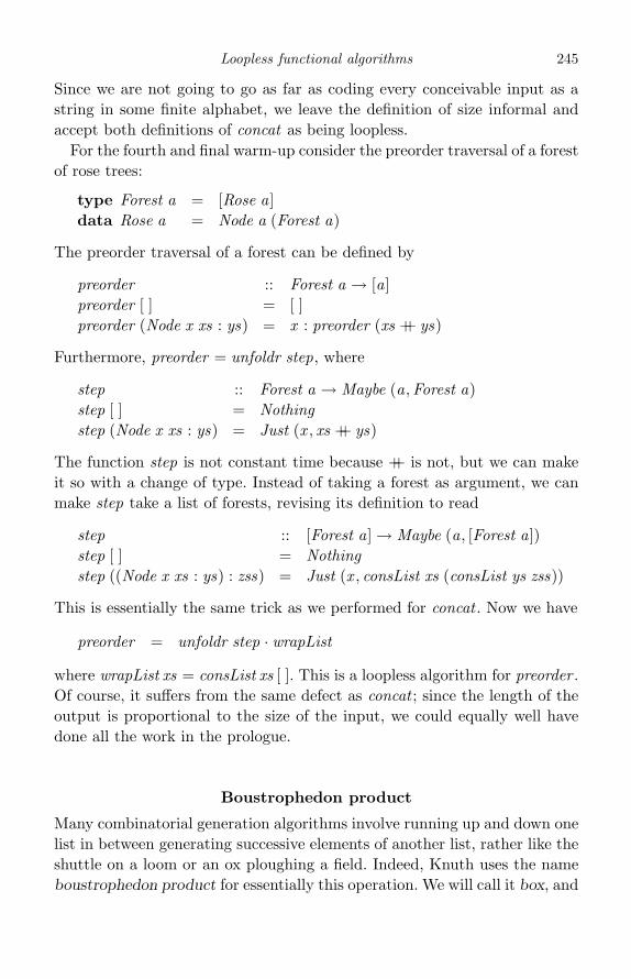
Loopless functional algorithms 245
Since we are not going to go as far as coding every conceivable input as astring in some finite alphabet, we leave the definition of size informal andaccept both definitions of concat as being loopless.
For the fourth and final warm-up consider the preorder traversal of a forestof rose trees:
type Forest a = [Rose a]data Rose a = Node a (Forest a)
The preorder traversal of a forest can be defined by
preorder :: Forest a → [a]preorder [ ] = [ ]preorder (Node x xs : ys) = x : preorder (xs ++ ys)
Furthermore, preorder = unfoldr step, where
step :: Forest a → Maybe (a,Forest a)step [ ] = Nothingstep (Node x xs : ys) = Just (x , xs ++ ys)
The function step is not constant time because ++ is not, but we can makeit so with a change of type. Instead of taking a forest as argument, we canmake step take a list of forests, revising its definition to read
step :: [Forest a]→ Maybe (a, [Forest a])step [ ] = Nothingstep ((Node x xs : ys) : zss) = Just (x , consList xs (consList ys zss))
This is essentially the same trick as we performed for concat . Now we have
preorder = unfoldr step · wrapList
where wrapList xs = consList xs [ ]. This is a loopless algorithm for preorder .Of course, it suffers from the same defect as concat ; since the length of theoutput is proportional to the size of the input, we could equally well havedone all the work in the prologue.
Boustrophedon product
Many combinatorial generation algorithms involve running up and down onelist in between generating successive elements of another list, rather like theshuttle on a loom or an ox ploughing a field. Indeed, Knuth uses the nameboustrophedon product for essentially this operation. We will call it box, and

246 Pearls of Functional Algorithm Design
denote it with an infix symbol �, because the name is short, pronounceable,and contains an “ox”. Here is the definition:
(�) :: [a]→ [a]→ [a][ ] � ys = ys(x : xs) � ys = ys ++ [x ] ++ (xs � reverse ys)
For example:
[3, 4] � [0, 1, 2] = [0, 1, 2, 3, 2, 1, 0, 4, 0, 1, 2]
The definition of � leads to an inefficient computation, since ys is reversedat each step. Better is the following version, which reverses ys only once:
xs � ys = mix xs (ys, reverse ys)mix [ ] (ys, sy) = ysmix (x : xs) (ys, sy) = ys ++ [x ] ++ mix xs (sy , ys)
The operation � is associative with the empty list as identity element, a goodreason to denote it with an infix symbol. We leave the proof of associativityto the reader, but it depends on two subsidiary identities that we will spellout now, as they are used later on:
(xs ++ [y ] ++ ys) � zs = (xs � zs) ++ [y ] ++ (ys � zs ′) (28.1)
reverse (xs � ys) = (reverse xs) � ys ′ (28.2)
where zs ′ and ys ′ are defined by
zs ′ = if even (length xs) then reverse zs else zsys ′ = if even (length xs) then reverse ys else ys
Thus, both (28.1) and (28.2) depend on parity information about the lengthof xs.
Just as concat distributes ++ over a list of lists, so boxall distributes �over a list of lists:
boxall :: [[a]]→ [a]boxall = foldr (�) [ ]
For a list of length n of lists each of length m the output of boxall has length(m +1)n −1, which is exponential in mn, the total length of the input. Nowwe can state our final exercise, which is to make boxall loopless.
Tupling
Since boxall (xs : xss) = xs � (boxall xss) and the definition of xs � ysinvolves reverse ys, it is clear that as well as computing boxall we also need

Loopless functional algorithms 247
to compute reverse · boxall . That suggests it is sensible to construct bothboxall and reverse · boxall at the same time. To do so we make use of thetupling law of foldr . This law states that
(foldr f a xs, foldr g b xs) = foldr h (a, b) xs
where h x (y , z ) = (f x y , g x z ).Suppose we can find an operation � so that
reverse · boxall = foldr (�) [ ]
Then the tupling law of foldr gives
(boxall xs, reverse (boxall xs)) = foldr op ([ ], [ ]) xs
where
op xs (ys, sy) = (xs � ys, xs � sy) (28.3)
The sequences ys and sy are each the reverse of the other, hence their names.To discover � we appeal to the fusion law of foldr . This law states that
f (foldr g a xs) = foldr h b xs for all finite lists xs provided f a = b andf (g x y) = h x (f y) for all x and y . We have reverse [ ] = [ ], so it remainsto find a definition of � satisfying
reverse (xs � ys) = xs � (reverse ys)
Since reverse (reverse xs) = xs for all finite lists xs, we can define
xs � sy = reverse (xs � (reverse sy))
We can also give a direct, recursive definition of �:
[ ] � sy = sy(x : xs) � sy = (xs � (reverse sy)) ++ [x ] ++ sy
Alternatively, we can express � by appealing to (28.2):
xs � sy = if even (length xs) then (reverse xs) � (reverse sy)else (reverse xs) � sy
Using (28.3) and the definition of �, the first recursive definition of � leadsto the following definition of op, renamed as op1:
op1 [ ] (ys, sy) = (ys, sy)op1 (x : xs) (ys, sy) = (ys ++ [x ] ++ zs, sz ++ [x ] ++ sy)
where (zs, sz ) = op1 xs (sy , ys)
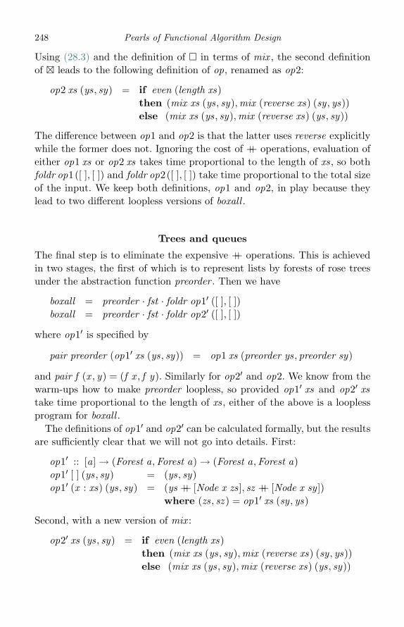
248 Pearls of Functional Algorithm Design
Using (28.3) and the definition of � in terms of mix , the second definitionof � leads to the following definition of op, renamed as op2:
op2 xs (ys, sy) = if even (length xs)then (mix xs (ys, sy),mix (reverse xs) (sy , ys))else (mix xs (ys, sy),mix (reverse xs) (ys, sy))
The difference between op1 and op2 is that the latter uses reverse explicitlywhile the former does not. Ignoring the cost of ++ operations, evaluation ofeither op1 xs or op2 xs takes time proportional to the length of xs, so bothfoldr op1([ ], [ ]) and foldr op2([ ], [ ]) take time proportional to the total sizeof the input. We keep both definitions, op1 and op2, in play because theylead to two different loopless versions of boxall .
Trees and queues
The final step is to eliminate the expensive ++ operations. This is achievedin two stages, the first of which is to represent lists by forests of rose treesunder the abstraction function preorder . Then we have
boxall = preorder · fst · foldr op1′ ([ ], [ ])boxall = preorder · fst · foldr op2′ ([ ], [ ])
where op1′ is specified by
pair preorder (op1′ xs (ys, sy)) = op1 xs (preorder ys, preorder sy)
and pair f (x , y) = (f x , f y). Similarly for op2′ and op2. We know from thewarm-ups how to make preorder loopless, so provided op1′ xs and op2′ xstake time proportional to the length of xs, either of the above is a looplessprogram for boxall .
The definitions of op1′ and op2′ can be calculated formally, but the resultsare sufficiently clear that we will not go into details. First:
op1′ :: [a]→ (Forest a,Forest a) → (Forest a,Forest a)op1′ [ ] (ys, sy) = (ys, sy)op1′ (x : xs) (ys, sy) = (ys ++ [Node x zs], sz ++ [Node x sy ])
where (zs, sz ) = op1′ xs (sy , ys)
Second, with a new version of mix :
op2′ xs (ys, sy) = if even (length xs)then (mix xs (ys, sy),mix (reverse xs) (sy , ys))else (mix xs (ys, sy),mix (reverse xs) (ys, sy))

Loopless functional algorithms 249
3
4
1
4 3 2
3
4
and 4 3 2
3
4
1
4 3
Fig. 28.1 Two forests produced by foldr op1′ ([ ], [ ]) [[1, 2], [3, 4]]
3
4
1
4
3
2
3
4
and 4
3
2
3
4
1
4
3
Fig. 28.2 Two forests produced by foldr op2′ ([ ], [ ]) [[1, 2], [3, 4]]
mix [ ] (ys, sy) = ysmix (x : xs) (ys, sy) = ys ++ [Node x (mix xs (sy , ys))]
The definitions of op1′ and op2′ lead to different pairs of forests. For example,see Figures 28.1 and 28.2. In each case the preorders of the pair of forestsare the same, so either definition will serve.
We are still not quite out of the wood yet, for appending a tree to theend of a forest is not a constant-time operation. Obvious ideas for solvingthis problem, such as turning appends into cons operations by reversing theforest, or bringing in an accumulating parameter, do not work. The mostdirect method, and one we will exploit for other purposes in subsequentpearls, is to introduce queues, redefining a forest to be a queue of trees ratherthan a list. Okasaki’s implementation of queues provides a type Queue a,for which the following operations all take constant time:
insert :: Queue a → a → Queue aremove :: Queue a → (a,Queue a)empty :: Queue aisempty :: Queue a → Bool

250 Pearls of Functional Algorithm Design
To install queues, we redeclare the type Forest to read
type Forest a = Queue (Rose a)data Rose a = Node a (Forest a)
The functions op1′ and op2′ are the same as before except that expressionsof the form as ++ [Node x bs] are replaced by insert as (Node x bs). Now wehave
boxall = unfoldr step · wrapQueue · fst · foldr op1′ (empty , empty)boxall = unfoldr step · wrapQueue · fst · foldr op2′ (empty , empty)
where
step :: [Forest a]→ Maybe (a, [Forest a])step [ ] = Nothingstep (zs : zss) = Just (x , consQueue xs (consQueue ys zss))
where (Node x xs, ys) = remove zs
consQueue :: Queue a → [Queue a]→ [Queue a]consQueue xs xss = if isempty xs then xss else xs : xss
wrapQueue :: Queue a → [Queue a]wrapQueue xs = consQueue xs [ ]
Both definitions of boxall are loopless.
Final remarks
The term loopless was coined by Ehrlich (1973). A number of loopless algo-rithms for generating combinatorial patterns appear in Knuth’s publisheddrafts of three sections of Volume 4 of The Art of Computer Program-
ming (Knuth, 2005). These fascicles contain references to much of the lit-erature on looplessness. The quote from Knuth appears in Knuth (2001).Okasaki’s implementation of queues can be found in Okasaki (1995).
ReferencesEhrlich, G. (1973). Loopless algorithms for generating permutations, combinations,
and other combinatorial configurations. Journal of the ACM 20, 500–13.Knuth, D. E. (2001). SPIDERS: a program downloadable from
www-cs-faculty.stanford.edu/∼knuth/programs.html.Knuth, D. E. (2005). The Art of Computer Programming, Volume 4, Fascicles 2,3,4.
Reading, MA: Addison-Wesley.Okasaki, C. (1995). Simple and efficient purely functional queues and deques.
Journal of Functional Programming 5 (4), 583–92.

29
The Johnson–Trotter algorithm
Introduction
The Johnson–Trotter algorithm is a method for producing all the permuta-tions of a given list in such a way that the transition from one permutationto the next is accomplished by a single transposition of adjacent elements.In this pearl we calculate a loopless version of the algorithm. The main ideais to make use of one of the loopless programs for the generalised boustro-phedon product boxall developed in the previous pearl.
A recursive formulation
In the Johnson–Trotter permutation algorithm the transitions for a list oflength n of length greater than one are defined recursively in terms of thetransitions for a list of length n−1. Label the elements of the list with posi-tions 0 through n−1 and let the list itself be denoted by xs ++[x ]. Begin witha downward run [n−1,n−2, . . . , 1], where transition i means “interchangethe element at position i with the element at position i−1”. The effect is tomove x from the last position to the first, resulting in the final permutation[x ] ++ xs. For example, the transitions [3, 2, 1] applied to the string “abcd”result in the three permutations “abdc”, “adbc” and “dabc”. Next, supposethe transitions generating the permutations of xs are [j1, j2, . . .]. Apply thetransition j1+1 to the current permutation [x ] ++ xs. We have to increase j1by one because xs is now one position to the right of the “runner” x . Next,run x upwards again to the last position by applying the transition sequence[1, 2, . . . ,n−1]. This results in a final permutation ys ++ [x ], where ys is theresult of applying transition j1 to xs. For example, the transitions [3, 1, 2, 3]applied to “dabc” result in four more permutations “dacb”, “adcb”, “acdb”and “acbd”. For the next step, apply the second transition j2 for xs and runx down again. We do not have to modify the transition j2 after upward runsbecause the relevant permutation is to the left of x . Continue in the samefashion, interleaving runs of x downwards and upwards, with the transitionsfor n−1.
251
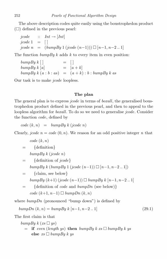
252 Pearls of Functional Algorithm Design
The above description codes quite easily using the boustrophedon product(�) defined in the previous pearl:
jcode :: Int → [Int ]jcode 1 = [ ]jcode n = (bumpBy 1 (jcode (n−1))) � [n−1,n−2 .. 1]
The function bumpBy k adds k to every item in even position:
bumpBy k [ ] = [ ]bumpBy k [a] = [a + k ]bumpBy k (a : b : as) = (a + k) : b : bumpBy k as
Our task is to make jcode loopless.
The plan
The general plan is to express jcode in terms of boxall , the generalised bous-trophedon product defined in the previous pearl, and then to appeal to theloopless algorithm for boxall . To do so we need to generalise jcode. Considerthe function code, defined by
code (k ,n) = bumpBy k (jcode n)
Clearly, jcode n = code (0,n). We reason for an odd positive integer n that
code (k ,n)
= {definition}bumpBy k (jcode n)
= {definition of jcode}bumpBy k (bumpBy 1 (jcode (n−1)) � [n−1,n−2 .. 1])
= {claim, see below}bumpBy (k+1) (jcode (n−1)) � bumpBy k [n−1,n−2 .. 1]
= {definition of code and bumpDn (see below)}code (k+1,n−1) � bumpDn (k ,n)
where bumpDn (pronounced “bump down”) is defined by
bumpDn (k ,n) = bumpBy k [n−1,n−2 .. 1] (29.1)
The first claim is that
bumpBy k (xs � ys)= if even (length ys) then bumpBy k xs � bumpBy k ys
else xs � bumpBy k ys
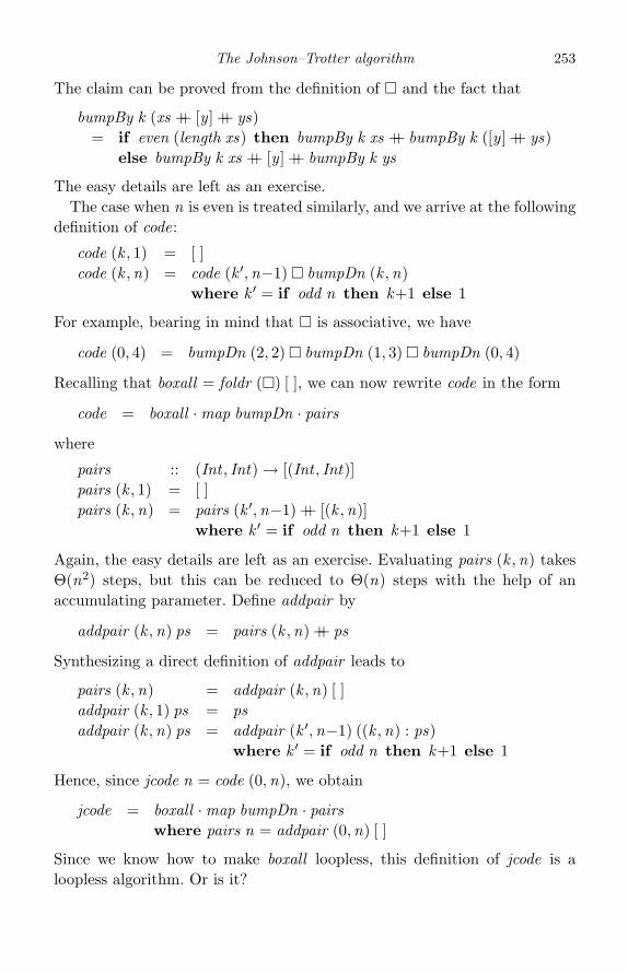
The Johnson–Trotter algorithm 253
The claim can be proved from the definition of � and the fact that
bumpBy k (xs ++ [y ] ++ ys)= if even (length xs) then bumpBy k xs ++ bumpBy k ([y ] ++ ys)
else bumpBy k xs ++ [y ] ++ bumpBy k ys
The easy details are left as an exercise.The case when n is even is treated similarly, and we arrive at the following
definition of code:
code (k , 1) = [ ]code (k ,n) = code (k ′,n−1) � bumpDn (k ,n)
where k ′ = if odd n then k+1 else 1
For example, bearing in mind that � is associative, we have
code (0, 4) = bumpDn (2, 2) � bumpDn (1, 3) � bumpDn (0, 4)
Recalling that boxall = foldr (�) [ ], we can now rewrite code in the form
code = boxall ·map bumpDn · pairs
where
pairs :: (Int , Int) → [(Int , Int)]pairs (k , 1) = [ ]pairs (k ,n) = pairs (k ′,n−1) ++ [(k ,n)]
where k ′ = if odd n then k+1 else 1
Again, the easy details are left as an exercise. Evaluating pairs (k ,n) takesΘ(n2) steps, but this can be reduced to Θ(n) steps with the help of anaccumulating parameter. Define addpair by
addpair (k ,n) ps = pairs (k ,n) ++ ps
Synthesizing a direct definition of addpair leads to
pairs (k ,n) = addpair (k ,n) [ ]addpair (k , 1) ps = psaddpair (k ,n) ps = addpair (k ′,n−1) ((k ,n) : ps)
where k ′ = if odd n then k+1 else 1
Hence, since jcode n = code (0,n), we obtain
jcode = boxall ·map bumpDn · pairswhere pairs n = addpair (0,n) [ ]
Since we know how to make boxall loopless, this definition of jcode is aloopless algorithm. Or is it?
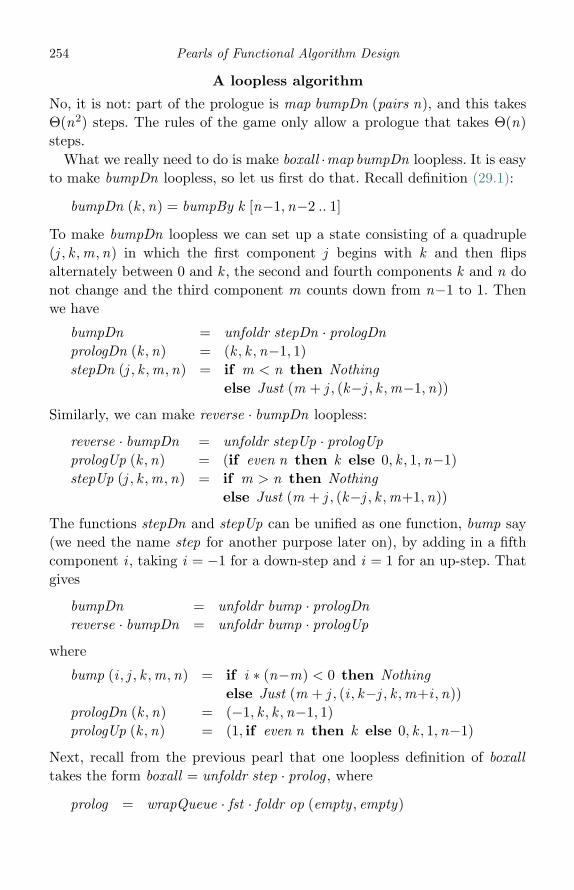
254 Pearls of Functional Algorithm Design
A loopless algorithm
No, it is not: part of the prologue is map bumpDn (pairs n), and this takesΘ(n2) steps. The rules of the game only allow a prologue that takes Θ(n)steps.
What we really need to do is make boxall ·map bumpDn loopless. It is easyto make bumpDn loopless, so let us first do that. Recall definition (29.1):
bumpDn (k ,n) = bumpBy k [n−1,n−2 .. 1]
To make bumpDn loopless we can set up a state consisting of a quadruple(j , k ,m,n) in which the first component j begins with k and then flipsalternately between 0 and k , the second and fourth components k and n donot change and the third component m counts down from n−1 to 1. Thenwe have
bumpDn = unfoldr stepDn · prologDnprologDn (k ,n) = (k , k ,n−1, 1)stepDn (j , k ,m,n) = if m < n then Nothing
else Just (m + j , (k−j , k ,m−1,n))
Similarly, we can make reverse · bumpDn loopless:
reverse · bumpDn = unfoldr stepUp · prologUpprologUp (k ,n) = (if even n then k else 0, k , 1,n−1)stepUp (j , k ,m,n) = if m > n then Nothing
else Just (m + j , (k−j , k ,m+1,n))
The functions stepDn and stepUp can be unified as one function, bump say(we need the name step for another purpose later on), by adding in a fifthcomponent i , taking i = −1 for a down-step and i = 1 for an up-step. Thatgives
bumpDn = unfoldr bump · prologDnreverse · bumpDn = unfoldr bump · prologUp
where
bump (i , j , k ,m,n) = if i ∗ (n−m) < 0 then Nothingelse Just (m + j , (i , k−j , k ,m+i ,n))
prologDn (k ,n) = (−1, k , k ,n−1, 1)prologUp (k ,n) = (1, if even n then k else 0, k , 1,n−1)
Next, recall from the previous pearl that one loopless definition of boxalltakes the form boxall = unfoldr step · prolog , where
prolog = wrapQueue · fst · foldr op (empty , empty)
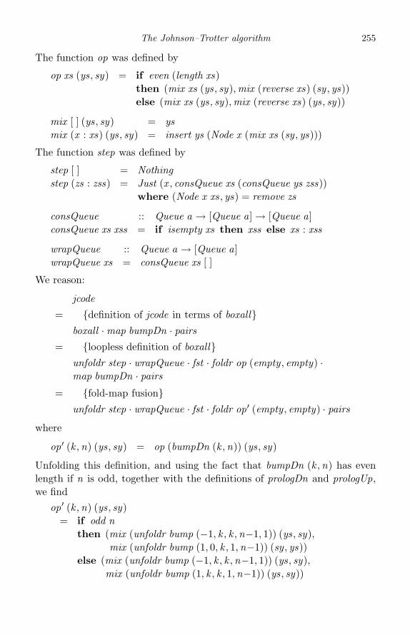
The Johnson–Trotter algorithm 255
The function op was defined by
op xs (ys, sy) = if even (length xs)then (mix xs (ys, sy),mix (reverse xs) (sy , ys))else (mix xs (ys, sy),mix (reverse xs) (ys, sy))
mix [ ] (ys, sy) = ysmix (x : xs) (ys, sy) = insert ys (Node x (mix xs (sy , ys)))
The function step was defined by
step [ ] = Nothingstep (zs : zss) = Just (x , consQueue xs (consQueue ys zss))
where (Node x xs, ys) = remove zs
consQueue :: Queue a → [Queue a]→ [Queue a]consQueue xs xss = if isempty xs then xss else xs : xss
wrapQueue :: Queue a → [Queue a]wrapQueue xs = consQueue xs [ ]
We reason:
jcode
= {definition of jcode in terms of boxall}boxall ·map bumpDn · pairs
= {loopless definition of boxall}unfoldr step · wrapQueue · fst · foldr op (empty , empty) ·map bumpDn · pairs
= {fold-map fusion}unfoldr step · wrapQueue · fst · foldr op′ (empty , empty) · pairs
where
op′ (k ,n) (ys, sy) = op (bumpDn (k ,n)) (ys, sy)
Unfolding this definition, and using the fact that bumpDn (k ,n) has evenlength if n is odd, together with the definitions of prologDn and prologUp,we find
op ′ (k ,n) (ys, sy)= if odd n
then (mix (unfoldr bump (−1, k , k ,n−1, 1)) (ys, sy),mix (unfoldr bump (1, 0, k , 1,n−1)) (sy , ys))
else (mix (unfoldr bump (−1, k , k ,n−1, 1)) (ys, sy),mix (unfoldr bump (1, k , k , 1,n−1)) (ys, sy))
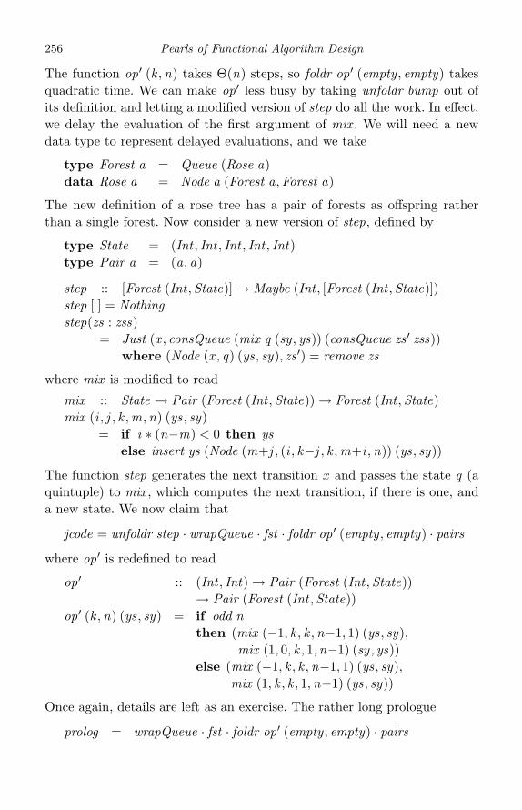
256 Pearls of Functional Algorithm Design
The function op ′ (k ,n) takes Θ(n) steps, so foldr op ′ (empty , empty) takesquadratic time. We can make op ′ less busy by taking unfoldr bump out ofits definition and letting a modified version of step do all the work. In effect,we delay the evaluation of the first argument of mix . We will need a newdata type to represent delayed evaluations, and we take
type Forest a = Queue (Rose a)data Rose a = Node a (Forest a,Forest a)
The new definition of a rose tree has a pair of forests as offspring ratherthan a single forest. Now consider a new version of step, defined by
type State = (Int , Int , Int , Int , Int)type Pair a = (a, a)
step :: [Forest (Int ,State)] → Maybe (Int , [Forest (Int ,State)])step [ ] = Nothingstep(zs : zss)
= Just (x , consQueue (mix q (sy , ys)) (consQueue zs ′ zss))where (Node (x , q) (ys, sy), zs ′) = remove zs
where mix is modified to read
mix :: State → Pair (Forest (Int ,State)) → Forest (Int ,State)mix (i , j , k ,m,n) (ys, sy)
= if i ∗ (n−m) < 0 then yselse insert ys (Node (m+j , (i , k−j , k ,m+i ,n)) (ys, sy))
The function step generates the next transition x and passes the state q (aquintuple) to mix , which computes the next transition, if there is one, anda new state. We now claim that
jcode = unfoldr step · wrapQueue · fst · foldr op′ (empty , empty) · pairs
where op′ is redefined to read
op ′ :: (Int , Int) → Pair (Forest (Int ,State))→ Pair (Forest (Int ,State))
op ′ (k ,n) (ys, sy) = if odd nthen (mix (−1, k , k ,n−1, 1) (ys, sy),
mix (1, 0, k , 1,n−1) (sy , ys))else (mix (−1, k , k ,n−1, 1) (ys, sy),
mix (1, k , k , 1,n−1) (ys, sy))
Once again, details are left as an exercise. The rather long prologue
prolog = wrapQueue · fst · foldr op′ (empty , empty) · pairs
The Johnson–Trotter algorithm 257
takes Θ(n) steps when applied to n, and step takes constant time, so thisfinally is a genuine 24-carat loopless program for jcode.
Final remarks
If it were not for the very picky requirement that the prologue had to takelinear time, we could have stopped calculating as soon as we had reachedthe definition
jcode = boxall ·map bumpDn · pairs
What this definition really shows is the usefulness of the generalised boustro-phedon product function boxall in the generation of many kinds ofcombinatorial patterns. We will see more uses in the final pearl.
The Johnson–Trotter algorithm was described independently in Johnson(1963) and Trotter (1962). As mentioned in the previous pearl, Ehrlich(1973), which introduced the concept of a loopless algorithm, was mainlydevoted to describing a loopless program for the Johnson–Trotter algorithm.
ReferencesEhrlich, G. (1973). Loopless algorithms for generating permutations, combinations,
and other combinatorial configurations. Journal of the ACM 20, 500–13.Johnson, S. M. (1963). Generation of permutations by adjacent transpositions.
Mathematics of Computation 17, 282–5.Trotter, A. F. (1962). Perm (Algorithm 115). Communications of the ACM 5,
434–5.
30
Spider spinning for dummies
Oh what a tangled web we weavewhen first we practise to derive.
(With apologies to Sir Walter Scott)
Introduction
Consider the problem of generating all bit strings a1a2 . . . an of length nsatisfying given constraints of the form ai ≤ aj for various i and j . The gen-eration is to be in Gray path order, meaning that exactly one bit changesfrom one bit string to the next. The transition code is a list of integersnaming the bit that is to be changed at each step. For example, withn = 3, consider the constraints a1 ≤ a2 and a3 ≤ a2. One possible Graypath is 000, 010, 011, 111, 110 with transition code [2, 3, 1, 3] and startingstring 000.
The snag is that the problem does not always have a solution. For example,with n = 4 and the constraints a1 ≤ a2 ≤ a4 and a1 ≤ a3 ≤ a4, the sixpossible bit strings, namely 0000, 0001, 0011, 0101, 0111 and 1111, cannotbe permuted into a Gray path. There are four strings of even weight (thenumbers of 1s) and two of odd weight, and in any Gray path the parity ofthe weights has to alternate.
Constraints of the form ai ≤ aj on bit strings of length n can be repre-sented by a digraph with n nodes in which a directed edge i←j is associatedwith a constraint ai ≤ aj . Knuth and Ruskey showed how to construct aGray path provided the digraph was totally acyclic, meaning that the undi-rected graph obtained by dropping the directions on the edges is acyclic.They called a connected totally acyclic digraph a spider, because when anedge i ← j is drawn with i below j the digraph can be made to look like anarachnid (see Figure 30.1 for a three-legged spider). They called a totallyacyclic digraph a tad, but, since its connected components are spiders, wewill continue the arachnid metaphor and call it a nest of spiders.
258
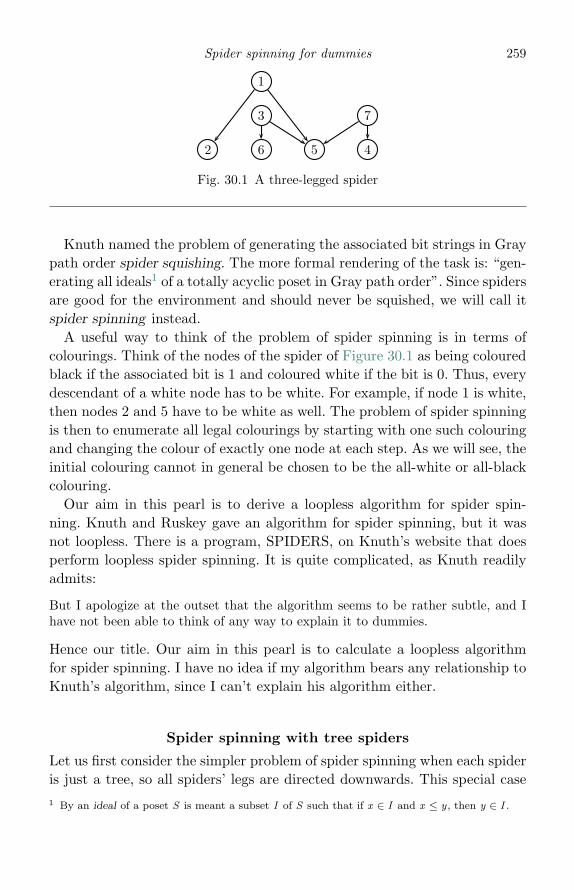
Spider spinning for dummies 259
1
2 5
3
6
7
4
Fig. 30.1 A three-legged spider
Knuth named the problem of generating the associated bit strings in Graypath order spider squishing. The more formal rendering of the task is: “gen-erating all ideals1 of a totally acyclic poset in Gray path order”. Since spidersare good for the environment and should never be squished, we will call itspider spinning instead.
A useful way to think of the problem of spider spinning is in terms ofcolourings. Think of the nodes of the spider of Figure 30.1 as being colouredblack if the associated bit is 1 and coloured white if the bit is 0. Thus, everydescendant of a white node has to be white. For example, if node 1 is white,then nodes 2 and 5 have to be white as well. The problem of spider spinningis then to enumerate all legal colourings by starting with one such colouringand changing the colour of exactly one node at each step. As we will see, theinitial colouring cannot in general be chosen to be the all-white or all-blackcolouring.
Our aim in this pearl is to derive a loopless algorithm for spider spin-ning. Knuth and Ruskey gave an algorithm for spider spinning, but it wasnot loopless. There is a program, SPIDERS, on Knuth’s website that doesperform loopless spider spinning. It is quite complicated, as Knuth readilyadmits:
But I apologize at the outset that the algorithm seems to be rather subtle, and Ihave not been able to think of any way to explain it to dummies.
Hence our title. Our aim in this pearl is to calculate a loopless algorithmfor spider spinning. I have no idea if my algorithm bears any relationship toKnuth’s algorithm, since I can’t explain his algorithm either.
Spider spinning with tree spiders
Let us first consider the simpler problem of spider spinning when each spideris just a tree, so all spiders’ legs are directed downwards. This special case1 By an ideal of a poset S is meant a subset I of S such that if x ∈ I and x ≤ y, then y ∈ I .
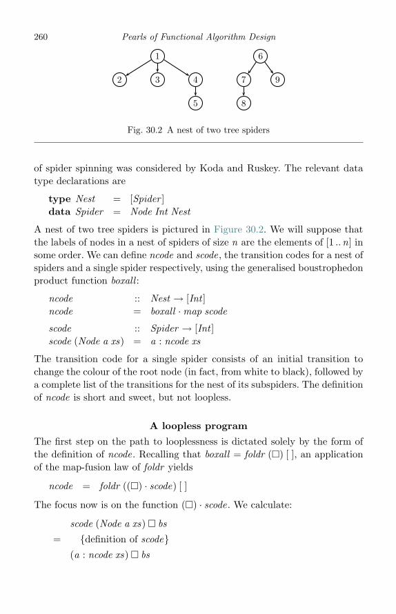
260 Pearls of Functional Algorithm Design
1
2 3 4
5
6
7
8
9
Fig. 30.2 A nest of two tree spiders
of spider spinning was considered by Koda and Ruskey. The relevant datatype declarations are
type Nest = [Spider ]data Spider = Node Int Nest
A nest of two tree spiders is pictured in Figure 30.2. We will suppose thatthe labels of nodes in a nest of spiders of size n are the elements of [1 ..n] insome order. We can define ncode and scode, the transition codes for a nest ofspiders and a single spider respectively, using the generalised boustrophedonproduct function boxall :
ncode :: Nest → [Int ]ncode = boxall ·map scode
scode :: Spider → [Int ]scode (Node a xs) = a : ncode xs
The transition code for a single spider consists of an initial transition tochange the colour of the root node (in fact, from white to black), followed bya complete list of the transitions for the nest of its subspiders. The definitionof ncode is short and sweet, but not loopless.
A loopless program
The first step on the path to looplessness is dictated solely by the form ofthe definition of ncode. Recalling that boxall = foldr (�) [ ], an applicationof the map-fusion law of foldr yields
ncode = foldr ((�) · scode) [ ]
The focus now is on the function (�) · scode. We calculate:
scode (Node a xs) � bs
= {definition of scode}(a : ncode xs) � bs
Spider spinning for dummies 261
= {definition of �}bs ++ [a] ++ (ncode xs � (reverse bs))
= {initial definition of ncode}bs ++ [a] ++ (boxall (map scode xs) � (reverse bs))
The third term of this expression takes the form
(foldr (�) [ ] ass) � cs
in which ass = map scode xs and cs = reverse bs. This suggests the useof the fold-fusion law of foldr . Setting f as = as � cs, we have that f isstrict and f [ ] = cs, since [ ] is the identity of �. Hence, the fold-fusion lawgives
(foldr (�) [ ] ass) � cs = foldr h cs ass
provided we can find an h such that (as � bs) � cs = h as (bs � cs). But �is associative, so we can take h = (�).
Putting these calculations together, we obtain:
scode (Node a xs) � bs
= {above}bs ++ [a] ++ (boxall (map scode xs) � (reverse bs))
= {fold fusion}bs ++ [a] ++ foldr (�) (reverse bs) (map scode xs)
= {map fusion}bs ++ [a] ++ foldr ((�) · scode) (reverse bs) xs
Hence, setting op = (�) · scode, we have calculated that
ncode = foldr op [ ]op (Node a xs) bs = bs ++ [a] ++ foldr op (reverse bs) xs
The remaining steps are to eliminate reverse by computing both ncode andreverse · ncode at the same time, and to represent each of their results by aqueue of rose trees under the abstraction function preorder . Rose trees arehere declared by
type Forest a = Queue (Rose a)data Rose a = Fork a (Forest a)

262 Pearls of Functional Algorithm Design
1
2 5
3
6
7
4
5
1
2
3
6
7
4
Fig. 30.3 A spider and an associated tree
We have performed these steps with the derivation of a loopless program forboxall , so we will just state the result:
ncode = unfoldr step · wrapQueue · fst · foldr op (empty , empty)op (Node a xs) (bs, sb)
= (insert bs (Fork a cs), insert sc (Fork a sb))where (cs, sc) = foldr op (sb, bs) xs
The remaining functions step and wrapQueue are exactly as they weredefined in the loopless algorithm for boxall . Since foldr op (empty , empty)takes linear time in the size of the nest, this is a loopless program for ncode.
Spider spinning with general spiders
Now we are ready to tackle the general spider-spinning problem. First,observe that by picking a spider up by one of its nodes we get a tree withdirected edges, such as that shown in Figure 30.3. Different trees arisedepending on which node is picked up, but they all represent the sameconstraints. It follows that we can model general spiders with the typedeclarations
type Nest = [Spider ]data Spider = Node Int [Leg ]data Leg = Dn Spider | Up Spider
A spider has legs, not edges. A spider’s leg points upwards or downwards toanother spider.
There is one complication when dealing with general spiders that doesnot arise with simpler species: the starting bit string is not necessarily astring consisting of all 0s. For example, with n = 3 and the constraintsa1 ≥ a2 ≤ a3, the five possible bit strings, namely 000, 001, 100, 101 and111, can only be arranged in Gray path order by starting with one of theodd-weight strings: 001, 100, or 111. However, we postpone consideration of
Spider spinning for dummies 263
the function seed :: Nest → [Bit ] for determining the starting string untillater on.
As with tree spiders, we can define
ncode :: Nest → [Int ]ncode = boxall ·map scode
We define scode to be the concatenation of two lists, a white code and ablack code:
scode :: Spider → [Int ]scode (Node a legs) = wcode legs ++ [a] ++ bcode legs
The white code, wcode, for a spider Node a legs is a valid transition sequencewhen the head node a is coloured white (corresponding to a 0 bit) and theblack code is a valid sequence when a is coloured black (corresponding to a1 bit). Thus, scode is defined as the sequence that goes through the whitecode, changes the colour of a from white to black and then goes throughthe black code. Note that when the spiders are tree spiders, so all legs pointdownwards, the white code is the empty sequence.
For scode to be correct, the final spider colouring after executing wcode legshas to be the initial colouring on which bcode legs starts. In order for thecolourings to match up we need to define wcode in terms of a variant of �,which we will denote by ♦ and pronounce “cox”.2 The operation ♦ is theconjugate of �:
as ♦ bs = reverse ((reverse as) � (reverse bs))
Whereas as � bs begins with as and ends with either bs or reverse bsdepending on whether as has even length, as ♦ bs ends with bs and beginswith either bs or reverse bs. For example:
[2, 3, 4] � [0, 1] = [0, 1, 2, 1, 0, 3, 0, 1, 4, 1, 0][2, 3, 4] ♦ [0, 1] = [1, 0, 2, 0, 1, 3, 1, 0, 4, 0, 1]
We can express � in terms of ♦ by conjugation, but there is another way:
as � bs
= if even (length as) then as ♦ bs else as ♦ (reverse bs) (30.1)
A similar equation defines ♦ in terms of �. Equation (30.1) will be neededbelow.2 By the way, “to box and cox” means “to take turns”, which is certainly what both operations
do and is the real reason for their names. The term comes from the comic play Box and Cox –A Romance of Real Life in One Act, by John Maddison Morton. Box and Cox were two lodgerswho shared their rooms – one occupying them by day and the other by night.
264 Pearls of Functional Algorithm Design
The operation ♦ is associative with the empty sequence as identity element.The proof is left as an exercise, but it depends on the fact that
(as ++ [b] ++ bs) ♦ cs = (as ♦ cs ′) ++ [b] ++ (bs ♦ cs)
where cs ′ = if even (length bs) then reverse cs else cs. A similar propertywas needed to prove � was associative.
Setting coxall = foldr (♦) [ ], we can now define
wcode, bcode :: [Leg ]→ [Int ]wcode = coxall ·map wcbcode = boxall ·map bc
where wc, bc :: Leg → [Int ] are yet to be defined. Use of coxall in thedefinition of wcode ensures that the final colouring after executing wcodewill be the union of the final colourings generated by the wc transitions, anduse of boxall in the definition of bcode means that this colouring will also bethe union of the colourings on which the bc transitions start.
It remains to define wc and bc. Given the choices above, the followingdefinitions are forced:
wc (Up (Node a legs)) = wcode legs ++ [a] ++ bcode legswc (Dn (Node a legs)) = reverse (wcode legs)bc (Up (Node a legs)) = reverse (bcode legs)bc (Dn (Node a legs)) = wcode legs ++ [a] ++ bcode legs
Look first at wc (Upx ). When the head of the mother spider of x is white andis connected to x by an upwards edge, there are no constraints on wc (Up x ),so we can define it to be either scode x or its reverse. But the subsequenttransitions affecting x are those in the list bc (Up x ), and the only way tomatch up the final colouring of the former with the initial colouring of thelatter is with the definitions above. The reasoning is dual with bc (Dn x ) andwc (Dn x ).
Finally, we show that ncode can be expressed in terms of bcode:
ncode xs
= {definition of ncode}boxall (map scode xs)
= {definition of scode and bc}boxall [bc (Dn x ) | x ← xs]
= {definition of bcode}bcode [(Dn x ) | x ← xs]
Spider spinning for dummies 265
ncode :: Nest → [Int ]ncode = bcode ·map Dn
bcode,wcode :: [Leg ] → [Int ]bcode = boxall ·map bcwcode = coxall ·map wc
bc,wc :: Leg → [Int ]bc (Up (Node a legs)) = reverse (bcode legs)bc (Dn (Node a legs)) = wcode legs ++ [a] ++ bcode legswc (Up (Node a legs)) = wcode legs ++ [a] ++ bcode legswc (Dn (Node a legs)) = reverse (wcode legs)
Fig. 30.4 The starting program for ncode
The complete program for ncode, apart from boxall and coxall , is listed inFigure 30.4. Our task is to make ncode loopless.
A loopless algorithm
The transformation to loopless form follows the same path as the simplerproblem of a nest of tree spiders. Specifically, we are going to:
(i) Eliminate boxall and coxall from the definition of ncode by appeal tomap fusion and fold fusion.
(ii) Eliminate reverse by appeal to tupling.(iii) Eliminate the remaining complexity by introducing queues.
It is the appeal to fold fusion in the first step that is the trickiest. As aneasy first step we apply map fusion to the definitions of wcode and bcode,obtaining
bcode = foldr ((�) · bc) [ ]wcode = foldr ((♦) · wc) [ ]
The focus of attention now is on the terms (�) · bc and (♦) ·wc. Everythingwe discover about the first will apply to the second with the obvious changes.We will follow the path of the tree-spider calculation as closely as possible.
There are two clauses in the definition of bc and we consider them in turn.First we have
bc (Up (Node a legs)) � cs
= {definition of bc}reverse (bcode legs) � cs
= {definition of bcode}reverse (boxall (map bc legs)) � cs
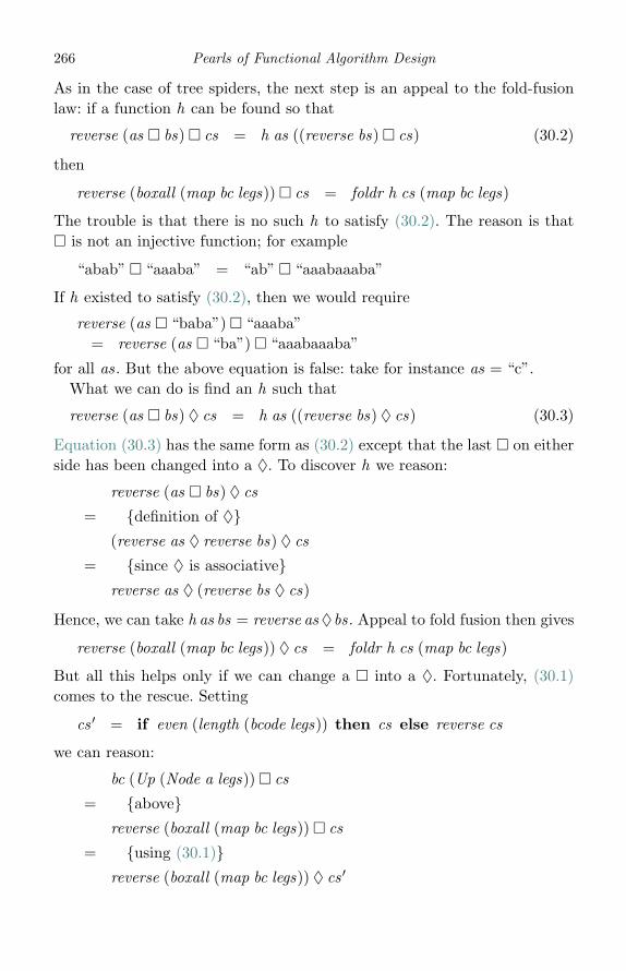
266 Pearls of Functional Algorithm Design
As in the case of tree spiders, the next step is an appeal to the fold-fusionlaw: if a function h can be found so that
reverse (as � bs) � cs = h as ((reverse bs) � cs) (30.2)
then
reverse (boxall (map bc legs)) � cs = foldr h cs (map bc legs)
The trouble is that there is no such h to satisfy (30.2). The reason is that� is not an injective function; for example
“abab” � “aaaba” = “ab” � “aaabaaaba”
If h existed to satisfy (30.2), then we would require
reverse (as � “baba”) � “aaaba”= reverse (as � “ba”) � “aaabaaaba”
for all as. But the above equation is false: take for instance as = “c”.What we can do is find an h such that
reverse (as � bs) ♦ cs = h as ((reverse bs) ♦ cs) (30.3)
Equation (30.3) has the same form as (30.2) except that the last � on eitherside has been changed into a ♦. To discover h we reason:
reverse (as � bs) ♦ cs
= {definition of ♦}(reverse as ♦ reverse bs) ♦ cs
= {since ♦ is associative}reverse as ♦ (reverse bs ♦ cs)
Hence, we can take h as bs = reverse as ♦bs. Appeal to fold fusion then gives
reverse (boxall (map bc legs)) ♦ cs = foldr h cs (map bc legs)
But all this helps only if we can change a � into a ♦. Fortunately, (30.1)comes to the rescue. Setting
cs ′ = if even (length (bcode legs)) then cs else reverse cs
we can reason:
bc (Up (Node a legs)) � cs
= {above}reverse (boxall (map bc legs)) � cs
= {using (30.1)}reverse (boxall (map bc legs)) ♦ cs ′

Spider spinning for dummies 267
= {fold fusion}foldr ((♦) · reverse) cs ′ (map bc legs)
Having transformed � into ♦ we now transform ♦ back into � with anotherapplication of fold fusion. The fusion condition
reverse ((reverse as) ♦ cs) = as � (reverse cs)
is just the conjugate property of � and ♦ and it leads to
reverse · foldr((♦) · reverse) cs ′ = foldr (�) (reverse cs ′)
Thus:
bc (Up (Node a legs)) � cs
= {above}foldr ((♦) · reverse) cs ′ (map bc legs)
= {fold fusion}reverse (foldr ((�) · bc) (reverse cs ′) legs)
Introducing bop = (�) · bc, we have shown that bcode = foldr bop [ ], where
bop (Up (Node a legs)) cs = reverse (foldr bop cs ′ legs)where cs ′ = if even (length (bcode legs))
then reverse cs else cs
Entirely dual reasoning with wop = (♦)·wc establishes wcode = foldr wop [ ],where
wop (Dn (Node a legs)) cs = reverse (foldr wop cs ′ legs)where cs ′ = if even (length (wcode legs))
then reverse cs else cs
That was quite a bit of effort, but it disposes of only two clauses, so morework remains. We now tackle the clause bc (Dn (Node a legs))� cs and startoff by reasoning:
bc (Dn (Node a legs)) � cs
= {definition of bc}(wcode legs ++ [a] ++ bcode legs) � cs
= {distributing ++ over �}(wcode legs � cs) ++ [a] ++ (bcode legs � cs ′)
where
cs ′ = if even (length (wcode legs)) then reverse cs else cs
268 Pearls of Functional Algorithm Design
The rule for distributing ++ over � was given in the first pearl onlooplessness:
(xs ++ [y ] ++ ys) � zs = (xs � zs) ++ [y ] ++ (ys � zs ′)where zs ′ = if even (length xs) then reverse zs else zs
We tackle each of the terms bcode legs � cs ′ and wcode legs � cs in turn.First:
bcode legs � cs ′
= {definition of bcode}foldr (�) [ ] (map bc legs) � cs ′
= {fold fusion (exercise)}foldr (�) cs ′ (map bc legs)
= {map fusion and definition of bop}foldr bop cs ′ legs
Second:
wcode legs � cs
= {using (30.1)}wcode legs ♦ reverse cs ′
= {definition of wcode}foldr (♦) [ ](map wc legs) ♦ reverse cs ′
= {fold fusion (exercise)}foldr (♦) (reverse cs ′) (map bc legs)
= {map fusion and definition of wop}foldr wop (reverse cs ′) legs
Hence, we have derived
bop (Dn (Node a legs)) cs = foldr wop (reverse cs ′) legs ++ [a] ++foldr bop cs ′ legs
where cs ′ = if even (length (wcode legs)) then reverse cs else cs
Dual reasoning establishes a similar result for wop (Up (Node a legs)) cs andleads to the program summarised in Figure 30.5. It is not very attractive andcertainly not efficient, mostly on account of the repeated need to computeparity information.
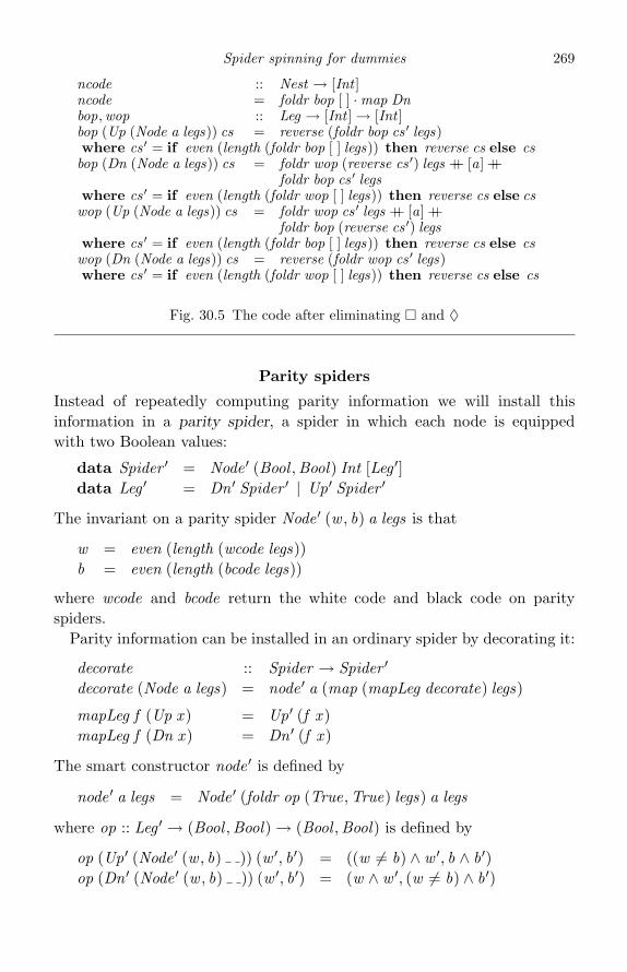
Spider spinning for dummies 269
ncode :: Nest → [Int ]ncode = foldr bop [ ] ·map Dnbop,wop :: Leg → [Int ] → [Int ]bop (Up (Node a legs)) cs = reverse (foldr bop cs ′ legs)where cs ′ = if even (length (foldr bop [ ] legs)) then reverse cs else csbop (Dn (Node a legs)) cs = foldr wop (reverse cs ′) legs ++ [a] ++
foldr bop cs ′ legswhere cs ′ = if even (length (foldr wop [ ] legs)) then reverse cs else cswop (Up (Node a legs)) cs = foldr wop cs ′ legs ++ [a] ++
foldr bop (reverse cs ′) legswhere cs ′ = if even (length (foldr bop [ ] legs)) then reverse cs else cswop (Dn (Node a legs)) cs = reverse (foldr wop cs ′ legs)where cs ′ = if even (length (foldr wop [ ] legs)) then reverse cs else cs
Fig. 30.5 The code after eliminating � and ♦
Parity spiders
Instead of repeatedly computing parity information we will install thisinformation in a parity spider, a spider in which each node is equippedwith two Boolean values:
data Spider ′ = Node ′ (Bool ,Bool) Int [Leg ′]data Leg ′ = Dn ′ Spider ′ | Up ′ Spider ′
The invariant on a parity spider Node ′ (w , b) a legs is that
w = even (length (wcode legs))b = even (length (bcode legs))
where wcode and bcode return the white code and black code on parityspiders.
Parity information can be installed in an ordinary spider by decorating it:
decorate :: Spider → Spider ′
decorate (Node a legs) = node ′ a (map (mapLeg decorate) legs)
mapLeg f (Up x ) = Up ′ (f x )mapLeg f (Dn x ) = Dn ′ (f x )
The smart constructor node ′ is defined by
node ′ a legs = Node ′ (foldr op (True,True) legs) a legs
where op :: Leg ′ → (Bool ,Bool)→ (Bool ,Bool) is defined by
op (Up ′ (Node ′ (w , b) )) (w ′, b ′) = ((w �= b) ∧ w ′, b ∧ b ′)op (Dn ′ (Node ′ (w , b) )) (w ′, b ′) = (w ∧ w ′, (w �= b) ∧ b ′)
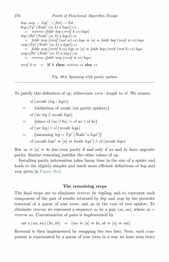
270 Pearls of Functional Algorithm Design
bop,wop :: Leg ′ → [Int ] → Intbop (Up′ (Node ′ (w , b) a legs)) cs
= reverse (foldr bop (revif b cs) legs)bop (Dn ′ (Node ′ (w , b) a legs)) cs
= foldr wop (revif (not w) cs) legs ++ [a] ++ foldr bop (revif w cs) legswop (Up′ (Node ′ (w , b) a legs)) cs
= foldr wop (revif b cs) legs ++ [a] ++ foldr bop (revif (not b) cs) legswop (Dn ′ (Node ′ (w , b) a legs)) cs
= reverse (foldr wop (revif w cs) legs)
revif b cs = if b then reverse cs else cs
Fig. 30.6 Spinning with parity spiders
To justify this definition of op, abbreviate even · length to el . We reason:
el (wcode (leg : legs))
= {definition of wcode (on parity spiders)}el (wc leg ♦ wcode legs)
= {since el (as ♦ bs) = el as ∧ el bs}el (wc leg) ∧ el (wcode legs)
= {assuming leg = Up ′ (Node ′ a legs ′)}el (wcode legs ′ ++ [a] ++ bcode legs ′) ∧ el (wcode legs)
But as ++ [a] ++ bs has even parity if and only if as and bs have oppositeparity. Similar reasoning justifies the other values of op.
Installing parity information takes linear time in the size of a spider andleads to the slightly simpler and much more efficient definitions of bop andwop given in Figure 30.6.
The remaining steps
The final steps are to eliminate reverse by tupling and to represent eachcomponent of the pair of results returned by bop and wop by the preordertraversal of a queue of rose trees, just as in the case of tree spiders. Toeliminate reverse we represent a sequence as by a pair (as, sa), where sa =reverse as. Concatenation of pairs is implemented by
cat a (ws, sw) (bs, sb) = (ws ++ [a] ++ bs, sb ++ [a] ++ sw)
Reversal is then implemented by swapping the two lists. Next, each com-ponent is represented by a queue of rose trees in a way we have seen twice

Spider spinning for dummies 271
ncode = unfoldr step · prologprolog = wrapQueue · fst · foldr bop (empty , empty) ·map (Dn ′ · decorate)
bop (Up′ (Node ′ (w , b) a legs)) ps= swap (foldr bop (swapif b ps) legs)
bop (Dn ′ (Node ′ (w , b) a legs)) ps= cat a (foldr wop (swapif (not w) ps) legs) (foldr bop (swapif w ps) legs)
wop (Up′ (Node ′ (w , b) a legs)) ps= cat a (foldr wop (swapif b ps) legs) (foldr bop (swapif (not b) ps) legs)
wop (Dn ′ (Node ′ (w , b) a legs)) ps= swap (foldr wop (swapif w ps) legs)
cat a (ws, sw) (bs, sb)= (insert ws (Fork a bs), insert sb (Fork a sw))
swap (xs, ys) = (ys, xs)swapif b (xs, ys) = if b then (ys, xs) else (xs, ys)
Fig. 30.7 The final loopless program
before. The result of these manoeuvres gives our final loopless program,summarised in Figure 30.7
Even though the prologue is now a four-act play, involving characterssuch as spiders, lists, queues and trees, and strange actions like swappingand folding, it nevertheless takes linear time in the size of the nest; so thisfinally is a loopless program for spider spinning.
The initial state
One task remains, namely to define seed :: Nest → [Bit ], the function thatreturns the starting bit string a1a2 . . . an for a nest of spiders whose labels are[1 ..n] in some order. We will just sketch the reasoning behind the definitionof seed . We will need the Haskell library Data.Map of finite mappings forrepresenting colourings. This library provides a type Mapk a for representingfinite mappings from keys (k) to values (a) and includes the following fourfunctions:
empty :: Map k ainsert :: Ord k ⇒ k → a → Map k a → Map k aunion :: Ord k → Map k a → Map k a → Map k aelems :: Map k a
The value empty denotes the empty mapping, insert inserts a new bindinginto a mapping, union unions two mappings and elems returns the range ofvalues in a mapping in increasing key order. We define a spider’s state to be
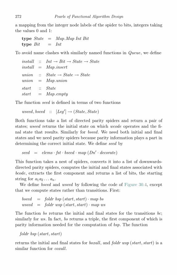
272 Pearls of Functional Algorithm Design
a mapping from the integer node labels of the spider to bits, integers takingthe values 0 and 1:
type State = Map.Map Int Bittype Bit = Int
To avoid name clashes with similarly named functions in Queue, we define
install :: Int → Bit → State → Stateinstall = Map.insert
union :: State → State → Stateunion = Map.union
start :: Statestart = Map.empty
The function seed is defined in terms of two functions
wseed , bseed :: [Leg ′] → (State,State)
Both functions take a list of directed parity spiders and return a pair ofstates; wseed returns the initial state on which wcode operates and the fi-nal state that results. Similarly for bseed . We need both initial and finalstates and we need parity spiders because parity information plays a part indetermining the correct initial state. We define seed by
seed = elems · fst · bseed ·map (Dn ′ · decorate)
This function takes a nest of spiders, converts it into a list of downwards-directed parity spiders, computes the initial and final states associated withbcode, extracts the first component and returns a list of bits, the startingstring for a1a2 . . . an .
We define bseed and wseed by following the code of Figure 30.4, exceptthat we compute states rather than transitions. First:
bseed = foldr bsp (start , start) ·map bswseed = foldr wsp (start , start) ·map ws
The function bs returns the initial and final states for the transitions bc;similarly for ws. In fact, bs returns a triple, the first component of which isparity information needed for the computation of bsp. The function
foldr bsp (start , start)
returns the initial and final states for boxall , and foldr wsp (start , start) is asimilar function for coxall .
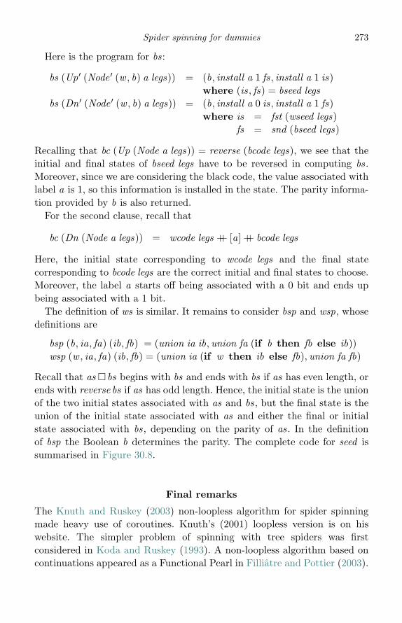
Spider spinning for dummies 273
Here is the program for bs:
bs (Up ′ (Node ′ (w , b) a legs)) = (b, install a 1 fs, install a 1 is)where (is, fs) = bseed legs
bs (Dn ′ (Node ′ (w , b) a legs)) = (b, install a 0 is, install a 1 fs)where is = fst (wseed legs)
fs = snd (bseed legs)
Recalling that bc (Up (Node a legs)) = reverse (bcode legs), we see that theinitial and final states of bseed legs have to be reversed in computing bs.Moreover, since we are considering the black code, the value associated withlabel a is 1, so this information is installed in the state. The parity informa-tion provided by b is also returned.
For the second clause, recall that
bc (Dn (Node a legs)) = wcode legs ++ [a] ++ bcode legs
Here, the initial state corresponding to wcode legs and the final statecorresponding to bcode legs are the correct initial and final states to choose.Moreover, the label a starts off being associated with a 0 bit and ends upbeing associated with a 1 bit.
The definition of ws is similar. It remains to consider bsp and wsp, whosedefinitions are
bsp (b, ia, fa) (ib, fb) = (union ia ib, union fa (if b then fb else ib))wsp (w , ia, fa) (ib, fb) = (union ia (if w then ib else fb), union fa fb)
Recall that as � bs begins with bs and ends with bs if as has even length, orends with reverse bs if as has odd length. Hence, the initial state is the unionof the two initial states associated with as and bs, but the final state is theunion of the initial state associated with as and either the final or initialstate associated with bs, depending on the parity of as. In the definitionof bsp the Boolean b determines the parity. The complete code for seed issummarised in Figure 30.8.
Final remarks
The Knuth and Ruskey (2003) non-loopless algorithm for spider spinningmade heavy use of coroutines. Knuth’s (2001) loopless version is on hiswebsite. The simpler problem of spinning with tree spiders was firstconsidered in Koda and Ruskey (1993). A non-loopless algorithm based oncontinuations appeared as a Functional Pearl in Filliatre and Pottier (2003).
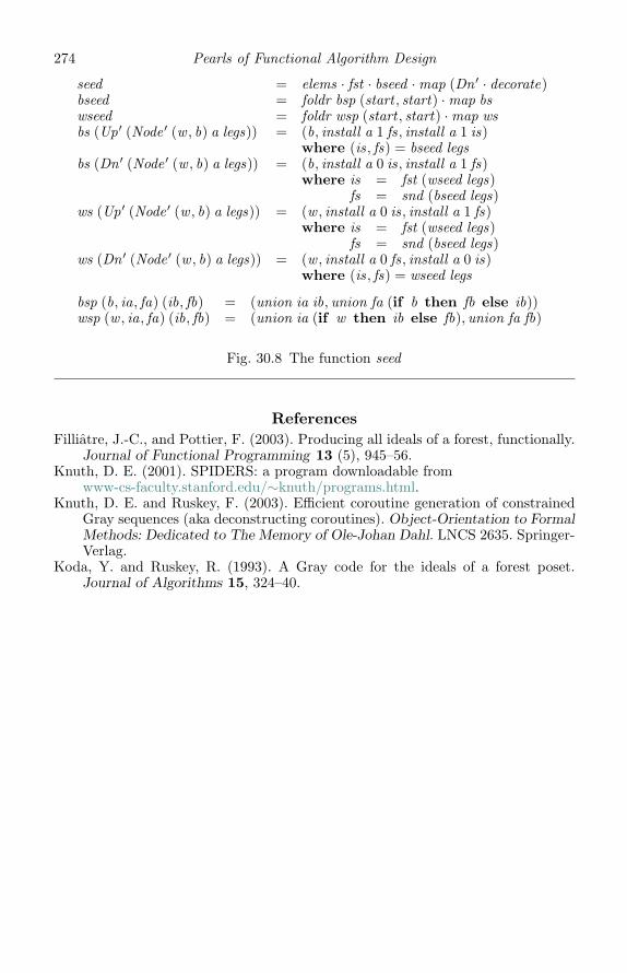
274 Pearls of Functional Algorithm Design
seed = elems · fst · bseed ·map (Dn ′ · decorate)bseed = foldr bsp (start , start) ·map bswseed = foldr wsp (start , start) ·map wsbs (Up′ (Node ′ (w , b) a legs)) = (b, install a 1 fs, install a 1 is)
where (is, fs) = bseed legsbs (Dn ′ (Node ′ (w , b) a legs)) = (b, install a 0 is, install a 1 fs)
where is = fst (wseed legs)fs = snd (bseed legs)
ws (Up′ (Node ′ (w , b) a legs)) = (w , install a 0 is, install a 1 fs)where is = fst (wseed legs)
fs = snd (bseed legs)ws (Dn ′ (Node ′ (w , b) a legs)) = (w , install a 0 fs, install a 0 is)
where (is, fs) = wseed legs
bsp (b, ia, fa) (ib, fb) = (union ia ib, union fa (if b then fb else ib))wsp (w , ia, fa) (ib, fb) = (union ia (if w then ib else fb), union fa fb)
Fig. 30.8 The function seed
ReferencesFilliatre, J.-C., and Pottier, F. (2003). Producing all ideals of a forest, functionally.
Journal of Functional Programming 13 (5), 945–56.Knuth, D. E. (2001). SPIDERS: a program downloadable from
www-cs-faculty.stanford.edu/∼knuth/programs.html.Knuth, D. E. and Ruskey, F. (2003). Efficient coroutine generation of constrained
Gray sequences (aka deconstructing coroutines). Object-Orientation to FormalMethods: Dedicated to The Memory of Ole-Johan Dahl. LNCS 2635. Springer-Verlag.
Koda, Y. and Ruskey, R. (1993). A Gray code for the ideals of a forest poset.Journal of Algorithms 15, 324–40.
Index
Data.Array, 2, 25, 29, 100, 114, 123Data.Array.ST , 3Data.Map, 271Data.Sequence, 114Data.Set , 70Either , 168Ix , 2Queue, 115, 249QuickCheck , 188, 196Ratio, 182, 199↓ – after, 128↑ – before, 109\\ – list difference, 1, 3, 22, 59, 64,
142, 192↑ – exponentiation, 183∧∧ – merge, 9, 10, 29!! – list index, 87, 93, 100! – array index, 25, 29, 87, 100 – prefix, 103, 119, 127accumArray, 2, 5, 82, 123applyUntil , 82array, 29, 85bounds, 25break , 154, 164, 182compare, 29concatMap, 42elems, 85foldrn – fold over nonempty lists, 42fork , 35, 83, 94, 118inits, 66, 67, 117listArray, 25, 100minors, 172nodups, 149nub, 64partition, 4partitions, 38reverse, 119, 244scanl , 118, 238scanr , 70sort , 28, 95sortBy, 29, 94span, 67subseqs, 57, 65, 157, 163tails, 7, 79, 100, 102transpose, 98, 150, 193unfoldr , 202, 243
zip, 35, 83zipWith, 83
Abelian group, 27abides property, 3, 22abstraction function, 129, 211, 226accumulating function, 2accumulating parameter, 131, 138, 140,
177, 253adaptive encoding, 200amortised time, 5, 118, 131, 133annotating a tree, 170arithmetic decoding, 201arithmetic expressions, 37, 156array update operation, 3, 6arrays, 1, 2, 21, 29, 85, 99association list, 29, 238asymptotic complexity, 27
bags, 25, 50, 51balanced trees, 21, 54, 234Bareiss algorithm, 186bijection, 129binary search, 7, 10, 14, 15, 19, 54binomial trees, 178bioinformatics, 77, 90Boolean satisfiability, 155borders of a list, 103bottom-up algorithm, 41boustrophedon product, 245, 251, 260breadth-first search, 136, 137, 178Bulldozer algorithm, 196bzip2, 101
call-tree, 168Cartesian coordinates, 141, 155Cartesian product, 149celebrity clique, 56Chio’s identity, 182clique, 56combinatorial patterns, 242comparison-based sorting, 10, 16, 27computaional geometry, 188conjugate, 263constraint satisfaction, 155continuations, 273coroutines, 273
275

276 Index
cost function, 41, 48, 52cyclic structures, 133, 179
data compression, 91, 198data mining, 77data refinement, 5, 48, 108, 114, 129, 210deforestation, 168depth-first search, 137, 221, 222destreaming, 214destreaming theorem, 214Dilworth’s theorem, 54divide and conquer, 1, 3, 5, 7, 8, 15, 21–23,
27, 29, 30, 65, 81, 171dot product, 185dynamic programming, 168
EOF (end-of-file symbol), 203exhaustive search, 12, 33, 39, 57, 148, 156
facets, 190failure function, 133fictitious values, 14, 77finite automaton, 74, 136fission law of foldl , 130fixpoint induction, 205forests, 42, 174fringe of a tree, 41frontier, 137fully strict composition, 243fusion law of foldl , 76, 130, 195fusion law of foldr , 34, 51, 52, 61, 247, 260,
261, 265fusion law of foldrn, 43fusion law of fork , 35fusion law of unfoldr , 206, 212
Galil’s algorithm, 122garbage collection, 165, 166Garsia–Wachs algorithm, 49Gaussian elimination, 180graph traversal, 178, 221Gray path order, 258greedy algorithms, 41, 48, 50, 140Gusfield’s Z algorithm, 116
Hu–Tucker algorithm, 49Huffman coding, 91, 198, 201
immutable arrays, 25incremental algorithm, 188, 191, 204incremental decoding, 216incremental encoding, 203, 209indexitis, 150inductive algorithm, 42, 93, 102integer arithmetic, 182, 198, 208integer division, 182intermediate data structure, 168interval expansion, 209, 210inversion table, 10inverting a function, 12, 93involution, 150iterative algorithm, 10, 82, 109, 113
Knuth and Ruskey algorithm, 258Knuth’s spider spinning algorithm, 242Koda–Ruskey algorithm, 242
law of iterate, 99laws of filter , 118, 152laws of fork , 35lazy evaluation, 33, 147, 185, 243leaf-labelled trees, 41, 165, 168left spines, 43, 45, 177left-inverse, 129Leibniz formula, 180lexicographic ordering, 45, 52, 64, 102, 104linear ordering, 43linked list, 225longest common prefix, 103, 112, 120longest decreasing subsequence, 54loop invariants, 62, 111lower bounds, 16, 27, 28, 64
Mahajan and Vinay’s algorithm, 186majority voting problem, 62matrices, 147, 181matrix Cartesian product, 149maximum marking problems, 77maximum non-segment sum, 73maximum segment sum, 73maximum surpasser count, 7McCarthy S-expression, 221memo table, 163memoisation, 162merge, 26, 142, 158mergesort, 29, 89, 171, 173minimal element, 53minimum cost tree, 44minimum element, 53minors, 181model checking, 155monads, 3, 114, 155monotonicity condition, 48, 53move-to-front encoding, 91multisets, 25
narrowing, 199nondeterministic functions, 43, 51normal form, 160
online list labelling, 241Open Problems Project, 31optimal bracketing, 176optimisation problems, 48, 176order-maintenance problem, 241overflow, 214
parametricitiy, 62partial evaluation, 134partial ordering, 53partial preorder, 52partition sort, 85partition sorting, 87perfect binary trees, 171
Index 277
permutations, 79, 90, 91, 96, 97, 180,189, 242, 251
planning algorithm, 136, 138plumbing combinators, 36prefix, 66prefix ordering, 103, 105, 119preorder traversal, 245, 270principal submatrices, 185program transformation, 221PSPACE completeness, 136
queues, 109, 137, 248, 249Quicksort, 5, 85, 89
radix sort, 95, 101ranking a list, 79rational arithmetic, 180, 188, 198rational division, 181recurrence relations, 15, 31, 88refinement, 44, 48, 51–53, 80regular cost function, 49regular expression, 74relations, 48, 167, 229representation function, 129, 211right spines, 177Rose trees, 164, 245rotations of a list, 91rule of floors, 215run-length encoding, 91
saddleback search, 14safe replacement, 222scan lemma, 118, 125segments, 73, 171Shannon–Fano coding, 198sharing, 168, 173shortest upravel, 50simplex, 188skeleton trees, 165sliding-block puzzle, 136smart constructors, 48, 170, 177
smooth algorithms, 241solving a recursion, 98sorting, 9, 10, 16, 91, 149sorting numbers, 1, 3sorting permutation, 10space/time trade-offs, 156spanning tree, 178stable sorting algorithm, 86, 95stacks, 137, 221, 222streaming, 203, 214streaming theorem, 204string matching, 112, 117, 127stringology, 103subsequences, 50, 64, 74, 162,
177, 242suffix tree, 101suffixes, 79, 100Sylvester’s identity, 186
thinning algorithm, 161top-down algorithm, 41totally acyclic digraph, 258transitions, 242trees, 130, 165, 248tries, 163tupling law of foldl , 118, 125tupling law of foldr , 247
unfolds, 168unmerges, 158, 159, 165unravel, 50upper triangular matrix, 185
Vandermonde’s convolution, 17
well-founded recursion, 4, 30while loop, 111, 113wholemeal programming, 150windows of a text, 120
Young tableau, 28