this is page 517 14 - university of...
TRANSCRIPT

This is page 517Printer: Opaque this
14State Space Models
14.1 Introduction
The state space modeling tools in S+FinMetrics are based on the algo-rithms in SsfPack 3.0 developed by Siem Jan Koopman and described inKoopman, Shephard and Doornik (1999, 2001)1. SsfPack is a suite of Croutines for carrying out computations involving the statistical analysis ofunivariate and multivariate models in state space form. The routines allowfor a variety of state space forms from simple time invariant models tocomplicated time-varying models. Functions are available to put standardmodels like ARMA and spline models in state space form. General rou-tines are available for filtering, smoothing, simulation smoothing, likelihoodevaluation, forecasting and signal extraction. Full details of the statisticalanalysis is provided in Durbin and Koopman (2001). This chapter gives anoverview of state space modeling and the reader is referred to the papers byKoopman, Shephard and Doornik for technical details on the algorithmsused in the S+FinMetrics/SsfPack functions.This chapter is organized as follows. Section 14.2 describes the gen-
eral state space model and state space representation required for theS+FinMetrics/SsfPack state space functions. Subsections describe thevarious S+FinMetrics/SsfPack functions for putting common time seriesmodels into state space form. The process of simulating observations froma given state space model is also covered. Section 14.3 summarizes the main
1Information about Ssfpack can be found at http://www.ssfpack.com.
518 14. State Space Models
algorithms used for the analysis of state space models. These include theKalman filter, Kalman smoother, moment smoothing, disturbance smooth-ing and forecasting. Estimation of the unknown parameters in a state spacemodel is described in Section 14.4. The chapter concludes with a short dis-cussion of simulation smoothing.Textbook treatments of state space models are given in Harvey (1989,
1993), Hamilton (1994), West and Harrison (1997), and Kim and Nelson(1999). Interesting applications of state space models in finance are givenin Engle and Watson (1987), Bomhoff (1994), Duan and Simonato (1999),and Harvey, Ruiz and Shephard (1994), Carmona (2001) and Chan (2002).
14.2 State Space Representation
Many dynamic time series models in economics and finance may be rep-resented in state space form. Some common examples are ARMA mod-els, time-varying regression models, dynamic linear models with unob-served components, discrete versions of continuous time diffusion processes,stochastic volatility models, non-parametric and spline regressions. The lin-ear Gaussian state space model may be represented as the system of equa-tions
αt+1m×1
= dtm×1
+ Ttm×m
· αtm×1
+Htm×r
· ηtr×1
(14.1)
θtN×1
= ctN×1
+ ZtN×m
· αtm×1
(14.2)
ytN×1
= θtN×1
+ GtN×N
· εtN×1
(14.3)
where t = 1, . . . , n and
α1 ∼ N(a,P), (14.4)
ηt ∼ iid N(0, Ir) (14.5)
εt ∼ iid N(0, IN ) (14.6)
and it is assumed thatE[εtη
0t] = 0
In (14.4), a and P are fixed and known but that can be generalized. Thestate vector αt contains unobserved stochastic processes and unknown fixedeffects and the transition equation (14.1) describes the evolution of thestate vector over time using a first order Markov structure. The measure-ment equation (14.3) describes the vector of observations yt in terms of thestate vector αt through the signal θt and a vector of disturbances εt. Itis assumed that the innovations in the transition equation and the innova-tions in the measurement equation are independent, but this assumption

14.2 State Space Representation 519
can be relaxed. The deterministic matrices Tt, Zt,Ht,Gt are called systemmatrices and are usually sparse selection matrices. The vectors dt and ctcontain fixed components and may be used to incorporate known effects orknown patterns into the model; otherwise they are equal to zero.The state space model (14.1)-(14.6) may be compactly expressed asµ
αt+1
yt
¶= δt
(m+N)×1+ Φt(m+N)×m
· αtm×1
+ ut(m+N)×1
, (14.7)
α1 ∼ N(a,P) (14.8)
ut ∼ iid N(0,Ωt) (14.9)
where
δt =
µdtct
¶,Φt =
µTt
Zt
¶,ut =
µHtηtGtεt
¶,Ωt =
µHtH
0t 0
0 GtG0t
¶The initial value parameters are summarized in the (m+ 1)×m matrix
Σ =
µPa0
¶(14.10)
For multivariate models, i.e. N > 1, it is assumed that the N ×N matrixGtG
0t is diagonal. In general, the system matrices in (14.7) are time varying.
14.2.1 Initial Conditions
The variance matrix P of the initial state vector α1 is assumed to be ofthe form
P = P∗ + κP∞ (14.11)
where P∞ and P∗ are symmetric m ×m matrices with ranks r∞ and r∗,respectively, and κ is a large scalar value, e.g. κ = 106. The matrix P∗captures the covariance structure of the stationary components in the ini-tial state vector, and the matrix P∞ is used to specify the initial variancematrix for nonstationary components. When the ith diagonal element ofP∞ is negative, the corresponding ith column and row of P∗ are assumedto be zero, and the corresponding row and column of P∞ will be takeninto consideration. When some elements of state vector are nonstation-ary, the S+FinMetrics/SsfPack algorithms implement an “exact diffuseprior” approach as described in Durbin and Koopman (2001) and Koop-man, Shephard and Doornik (2001).
14.2.2 State Space Representation inS+FinMetrics/SsfPack
State space models in S+FinMetrics/SsfPack utilize the compact repre-sentation (14.7) with initial value information (14.10). The following ex-
520 14. State Space Models
amples describe the specification of a state space model for use in theS+FinMetrics/SsfPack state space modeling functions.
Example 92 State space representation of the local level model
Consider the following simple model for the stochastic evolution of thelogarithm of an asset price yt
αt+1 = αt + η∗t , η∗t ∼ iid N(0, σ2η) (14.12)
yt = αt + ε∗t , ε∗t ∼ iid N(0, σ2ε) (14.13)
α1 ∼ N(a, P ) (14.14)
where it is assumed that E[ε∗t η∗t ] = 0. In the above model, the observedasset price yt is the sum of two unobserved components, αt and ε∗t . Thecomponent αt is the state variable and represents the fundamental value(signal) of the asset. The transition equation (14.12) shows that the fun-damental values evolve according to a random walk. The component ε∗trepresents random deviations (noise) from the fundamental value that areassumed to be independent from the innovations to αt. The strength ofthe signal in the fundamental value relative to the random deviation ismeasured by the signal-to-noise ratio of variances q = σ2η/σ
2ε. The model
(14.12)-(14.14) is called the random walk plus noise model, signal plus noisemodel or the local level model.2
The state space form (14.7) of the local level model has time invariantparameters
δ =
µ00
¶,Φ =
µ11
¶,Ω =
µσ2η 00 σ2ε
¶(14.15)
with errors σηηt = η∗t and σεεt = ε∗t . Since the state variable αt is I(1),the unconditional distribution of the initial state α1 doesn’t have finitevariance. In this case, it is customary to set a = E[α1] = 0 and P = var(α1)to some large positive number, e.g. P = 107, in (14.14) to reflect that noprior information is available. Using (14.11), the initial variance is specifiedwith P∗ = 0 and P∞ = 1. Therefore, the initial state matrix (14.10) for thelocal level model has the form
Σ =
µ −10
¶(14.16)
where −1 implies that P∞ = 1.In S+FinMetrics/SsfPack, a state space model is specified by creating
either a list variable with components giving the minimum components
2A detailed technical analysis of this model is given in Durbin and Koopman (2001),chapter 2.

14.2 State Space Representation 521
State space parameter List component nameδ mDelta
Φ mPhi
Ω mOmega
Σ mSigma
TABLE 14.1. State space form list components
necessary for describing a particular state space form or by creating an“ssf” object. To illustrate, consider creating a list variable containing thestate space parameters in (14.15)-(14.16), with ση = 0.5 and σε = 1
> sigma.e = 1
> sigma.n = 0.5
> a1 = 0
> P1 = -1
> ssf.ll.list = list(mPhi=as.matrix(c(1,1)),
+ mOmega=diag(c(sigma.n^2,sigma.e^2)),
+ mSigma=as.matrix(c(P1,a1)))
> ssf.ll.list
$mPhi:
[,1]
[1,] 1
[2,] 1
$mOmega:
[,1] [,2]
[1,] 0.25 0
[2,] 0.00 1
$mSigma:
[,1]
[1,] -1
[2,] 0
In the list variable ssf.ll.list, the component names match the statespace form parameters in (14.7) and (14.10). This naming convention, sum-marized in Table 14.1, must be used for the specification of any valid statespace model. Also, notice the use of the coercion function as.matrix. Thisensures that the dimensions of the state space parameters are correctlyspecified.An “ssf” object may be created from the list variable ssf.ll.list
using the S+FinMetrics/SsfPack function CheckSsf:
> ssf.ll = CheckSsf(ssf.ll.list)
> class(ssf.ll)
[1] "ssf"

522 14. State Space Models
> names(ssf.ll)
[1] "mDelta" "mPhi" "mOmega" "mSigma" "mJPhi"
[6] "mJOmega" "mJDelta" "mX" "cT" "cX"
[11] "cY" "cSt"
> ssf.ll
$mPhi:
[,1]
[1,] 1
[2,] 1
$mOmega:
[,1] [,2]
[1,] 0.25 0
[2,] 0.00 1
$mSigma:
[,1]
[1,] -1
[2,] 0
$mDelta:
[,1]
[1,] 0
[2,] 0
$mJPhi:
[1] 0
$mJOmega:
[1] 0
$mJDelta:
[1] 0
$mX:
[1] 0
$cT:
[1] 0
$cX:
[1] 0
$cY:
[1] 1
14.2 State Space Representation 523
$cSt:
[1] 1
attr(, "class"):
[1] "ssf"
The function CheckSsf takes a list variable with a minimum state spaceform, coerces the components to matrix objects and returns the full param-eterization of a state space model used in many of the S+FinMetrics/SsfPackstate space modeling functions. See the online help for CheckSsf for de-scriptions of the components of an “ssf” object.
Example 93 State space representation of a time varying parameter re-gression model
Consider the Capital Asset Pricing Model (CAPM) with time varyingintercept and slope
rt = αt + βtrM,t + νt, νt ∼ GWN(0, σ2ν) (14.17)
αt+1 = αt + ξt, ξt ∼ GWN(0, σ2ξ) (14.18)
βt+1 = βt + ςt, ςt ∼ GWN(0, σ2ς ) (14.19)
where rt denotes the return on an asset in excess of the risk free rate,and rM,t denotes the excess return on a market index. In this model, boththe abnormal excess return αt and asset risk βt are allowed to vary overtime following a random walk specification. Let αt = (αt, βt)
0, yt = rt,xt = (1, rM,t)
0, Ht = diag(σξ, σς)0 and Gt = σν . Then the state space form
(14.7) of (14.17) - (14.19) isµαt+1
yt
¶=
µI2x0t
¶αt +
µHηtGεt
¶and has parameters
Φt =
µI2x0t
¶, Ω =
σ2ξ 0 0
0 σ2ς 00 0 σ2ν
(14.20)
Since αt is I(1) the initial state vector α1 doesn’t have finite variance soit is customary to set a = 0 and P = κI2 where κ is large. Using (14.11),the initial variance is specified with P∗ = 0 and P∞ = I2. Therefore, theinitial state matrix (14.10) for the time varying CAPM has the form
Σ =
−1 00 −10 0

524 14. State Space Models
The state space parameter matrixΦt in (14.20) has a time varying systemelement Zt= x
0t. In S+FinMetrics/SsfPack, the specification of this time
varying element in Φt requires an index matrix JΦ and a data matrixX to which the indices in JΦ refer. The index matrix JΦ must have thesame dimension as Φt. The elements of JΦ are all set to −1 except theelements for which the corresponding elements of Φt are time varying. Thenon-negative index value indicates the column of the data matrix X whichcontains the time varying values.The specification of the state space form for the time varying CAPM
requires values for the variances σ2ξ , σ2ς , and σ2ν as well as a data ma-
trix X whose rows correspond with Zt = x0t = (1, rM,t). For example, let
σ2ξ = (0.01)2, σ2ς = (0.05)2 and σ2ν = (0.1)2 and construct the data ma-trix X using the excess return data in the S+FinMetrics “timeSeries”excessReturns.ts
> X.mat = cbind(1,
+ as.matrix(seriesData(excessReturns.ts[,"SP500"]))
The state space form may be created using
> Phi.t = rbind(diag(2),rep(0,2))
> Omega = diag(c((.01)^2,(.05)^2,(.1)^2))
> J.Phi = matrix(-1,3,2)
> J.Phi[3,1] = 1
> J.Phi[3,2] = 2
> Sigma = -Phi.t
> ssf.tvp.capm = list(mPhi=Phi.t,
+ mOmega=Omega,
+ mJPhi=J.Phi,
+ mSigma=Sigma,
+ mX=X.mat)
> ssf.tvp.capm
$mPhi:
[,1] [,2]
[1,] 1 0
[2,] 0 1
[3,] 0 0
$mOmega:
[,1] [,2] [,3]
[1,] 0.0001 0.0000 0.00
[2,] 0.0000 0.0025 0.00
[3,] 0.0000 0.0000 0.01
$mJPhi:
[,1] [,2]

14.2 State Space Representation 525
Parameter index matrix List component nameJδ mJDelta
JΦ mJPhi
JΩ mJOmega
Time varying component data matrix List component nameX mX
TABLE 14.2. S+FinMetrics time varying state space components
[1,] -1 -1
[2,] -1 -1
[3,] 1 2
$mSigma:
[,1] [,2]
[1,] -1 0
[2,] 0 -1
[3,] 0 0
$mX:
numeric matrix: 131 rows, 2 columns.
SP500
1 1 0.002803
2 1 0.017566
...
131 1 -0.0007548
Notice in the specification of Φt the values associated with x0t in the third
row are set to zero. In the index matrix JΦ, the (3,1) element is 1 andthe (3,2) element is 2 indicating that the data for the first and secondcolumns of x0t come from the first and second columns of the componentmX, respectively.In the general state space model (14.7), it is possible that all of the system
matrices δt, Φt and Ωt have time varying elements. The correspondingindex matrices Jδ, JΦ and JΩ indicate which elements of the matrices δt,Φt
and Ωt are time varying and the data matrix X contains the time varyingcomponents. The naming convention for these components is summarizedin Table 14.2.
14.2.3 Missing Values
The S+FinMetrics/SsfPack state space modeling functions can handlemissing values in the vector of response variables yt in (14.3). Missingvalues are not allowed in the state space system matrices Φt, Ωt, Σ andδt. Missing values are represented by NA in S-PLUS.

526 14. State Space Models
In the S+FinMetrics/SsfPack state space functions, the observation vec-tor yt with missing values will be be reduced to the vector y
†t without
missing values and the measurement equation will be adjusted accordingly.For example, the measurement equation yt= ct+Ztαt+Gtεt with
yt =
5
NA3
NA
, ct =
1234
, Zt =
Z1,tZ2,tZ3,tZ4,t
, Gt =
G1,tG2,tG3,tG4,t
reduces to the measurement equation y†t= c
†t+Z
†tαt+G
†tεt with
y†t =µ53
¶, c†t =
µ13
¶, Z†t =
µZ1,tZ3,t
¶, G†
t =
µG1,tG3,t
¶The SsfPack algorithms in S+FinMetrics automatically replace the ob-servation vector yt with y
†t when missing values are encountered and the
system matrices are adjusted accordingly.
14.2.4 S+FinMetrics/SsfPack Functions for Specifying theState Space Form for Some Common Time SeriesModels
S+FinMetrics/SsfPack has functions for the creation of the state spacerepresentation of some common time series models. These functions andmodels are described in the following sub-sections.
ARMA Models
Following Harvey (1993, Section 4.4), the ARMA(p, q) model with zeromean3
yt = φ1yt−1 + · · ·+ φpyt−p + ξt + θ1ξt−1 + · · ·+ θqξt−q (14.21)
may be put in state space form with transition and measurement equations
αt+1 = Tαt +Hξt, ξt ∼ N(0, σ2ε)
yt = Zαt
3Note that the MA coefficients are specified with positive signs, which is the oppositeof how the MA coefficients are specified for models estimated by the S-PLUS functionarima.mle.
14.2 State Space Representation 527
and time invariant system matrices
T =
φ1 1 0 · · · 0φ2 0 1 0...
. . ....
φm−1 0 0 1φm 0 0 · · ·
, H =
1θ1...
θm−1θm
, (14.22)
Z =¡1 0 · · · 0 0
¢where d, c and G of the state space form (14.1)-(14.3) are all zero andm = max(p, q + 1). The state vector αt has the form
αt =
yt
φ2yt−1 + · · ·+ φpyt−m+1 + θ1ξt + · · ·+ θm−1ξt−m+2φ3yt−1 + · · ·+ φpyt−m+2 + θ2ξt + · · ·+ θm−1ξt−m+3
...φmyt−1 + θm−1ξt
(14.23)
In compact state space form (14.7), the model isµαt+1
yt
¶=
µTZ
¶αt +
µH0
¶ξt
= Φαt + ut
and
Ω =
µσ2ξHH
0 0
0 0
¶If yt is stationary then αt ∼ N(0,V) is the unconditional distribution ofthe state vector, and the covariance matrixV satisfiesV = TVT0+σ2ξHH
0,which can be solved for the elements of V. The initial value parameters arethen
Σ =
µV00
¶The S+FinMetrics/SsfPack function GetSsfArma creates the state space
system matrices for any univariate stationary and invertible ARMA model.The arguments expected by GetSsfArma are
> args(GetSsfArma)
function(ar = NULL, ma = NULL, sigma = 1, model = NULL)
where ar is the vector of p AR coefficients, ma is the vector of q MA coef-ficients, sigma is the innovation standard deviation σξ, and model is a listwith components giving the AR, MA and innovation standard deviation.If the arguments ar, ma, and sigma are specified, then model is ignored.The function GetSsfArma returns a list containing the system matrices Φ,Ω and the initial value parameters Σ.

528 14. State Space Models
Example 94 AR(1) and ARMA(2,1)
Consider the AR(1) model
yt = 0.75yt−1 + ξt, ξt ∼ GWN(0, (0.5)2)
The state space form may be computed using
> ssf.ar1 = GetSsfArma(ar=0.75,sigma=.5)
> ssf.ar1
$mPhi:
[,1]
[1,] 0.75
[2,] 1.00
$mOmega:
[,1] [,2]
[1,] 0.25 0
[2,] 0.00 0
$mSigma:
[,1]
[1,] 0.5714
[2,] 0.0000
In the component mSigma, the unconditional variance of the initial stateα1 is computed as var(α1) = (0.5)
2/(1− 0.752) = 0.5714.Next, consider the ARMA(2,1) model
yt = 0.6yt−1 + 0.2yt−2 + εt − 0.2εt−1, εt ∼ GWN(0, 0.9)
The state space system matrices may be computed using
> arma21.mod = list(ar=c(0.6,0.2),ma=c(-0.2),sigma=sqrt(0.9))
> ssf.arma21 = GetSsfArma(model=arma21.mod)
> ssf.arma21
$mPhi:
[,1] [,2]
[1,] 0.6 1
[2,] 0.2 0
[3,] 1.0 0
$mOmega:
[,1] [,2] [,3]
[1,] 0.90 -0.180 0
[2,] -0.18 0.036 0
[3,] 0.00 0.000 0
14.2 State Space Representation 529
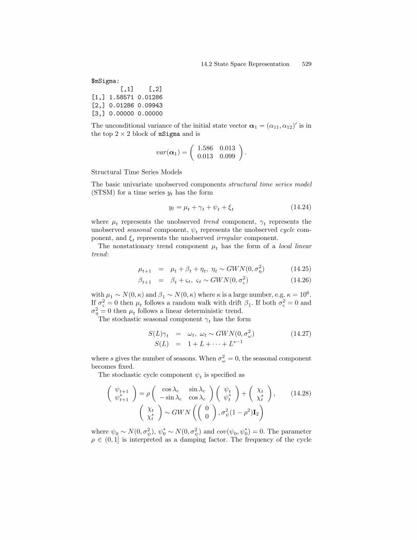
$mSigma:
[,1] [,2]
[1,] 1.58571 0.01286
[2,] 0.01286 0.09943
[3,] 0.00000 0.00000
The unconditional variance of the initial state vector α1 = (α11, α12)0 is in
the top 2× 2 block of mSigma and is
var(α1) =
µ1.586 0.0130.013 0.099
¶.
Structural Time Series Models
The basic univariate unobserved components structural time series model(STSM) for a time series yt has the form
yt = µt + γt + ψt + ξt (14.24)
where µt represents the unobserved trend component, γt represents theunobserved seasonal component, ψt represents the unobserved cycle com-ponent, and ξt represents the unobserved irregular component.The nonstationary trend component µt has the form of a local linear
trend :
µt+1 = µt + βt + ηt, ηt ∼ GWN(0, σ2η) (14.25)
βt+1 = βt + ςt, ςt ∼ GWN(0, σ2ς ) (14.26)
with µ1 ∼ N(0, κ) and β1 ∼ N(0, κ) where κ is a large number, e.g. κ = 106.If σ2ς = 0 then µt follows a random walk with drift β1. If both σ2ς = 0 andσ2η = 0 then µt follows a linear deterministic trend.The stochastic seasonal component γt has the form
S(L)γt = ωt, ωt ∼ GWN(0, σ2ω) (14.27)
S(L) = 1 + L+ · · ·+ Ls−1
where s gives the number of seasons. When σ2ω = 0, the seasonal componentbecomes fixed.The stochastic cycle component ψt is specified asµ
ψt+1ψ∗t+1
¶= ρ
µcosλc sinλc− sinλc cosλc
¶µψtψ∗t
¶+
µχtχ∗t
¶, (14.28)µ
χtχ∗t
¶∼ GWN
µµ00
¶, σ2ψ(1− ρ2)I2
¶where ψ0 ∼ N(0, σ2ψ), ψ
∗0 ∼ N(0, σ2ψ) and cov(ψ0, ψ
∗0) = 0. The parameter
ρ ∈ (0, 1] is interpreted as a damping factor. The frequency of the cycle

530 14. State Space Models
Argument STSM parameterirregular σηlevel σξslope σςseasonalDummy sseasonalTrig σω, sseasonalHS σω, scycle0 σψ, λc, ρ...
...cycle9 σψ, λc, ρ
TABLE 14.3. Arguments to the S+FinMetrics function GetSsfStsm
is λc = 2π/c and c is the period. When ρ = 1 the cycle reduces to adeterministic sine-cosine wave.The S+FinMetrics/SsfPack function GetSsfStsm creates the state space
system matrices for the univariate structural time series model (14.24). Thearguments expected by GetSsfStsm are
> args(GetSsfStsm)
function(irregular = 1, level = 0.1, slope = NULL,
seasonalDummy = NULL, seasonalTrig = NULL, seasonalHS
= NULL, cycle0 = NULL, cycle1 = NULL, cycle2 = NULL,
cycle3 = NULL, cycle4 = NULL, cycle5 = NULL, cycle6 =
NULL, cycle7 = NULL, cycle8 = NULL, cycle9 = NULL)
These arguments are explained in Table 14.3.
Example 95 Local level model
The state space for the local level model (14.12)-(14.14) may be con-structed using
> ssf.stsm = GetSsfStsm(irregular=1, level=0.5)
> class(ssf.stsm)
[1] "list"
> ssf.stsm
$mPhi:
[,1]
[1,] 1
[2,] 1
$mOmega:
[,1] [,2]
[1,] 0.25 0
[2,] 0.00 1
14.2 State Space Representation 531
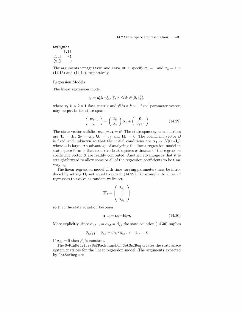
$mSigma:
[,1]
[1,] -1
[2,] 0
The arguments irregular=1 and level=0.5 specify σε = 1 and ση = 1 in(14.13) and (14.14), respectively.
Regression Models
The linear regression model
yt= x0tβ+ξt, ξt ∼ GWN(0, σ2ξ),
where xt is a k × 1 data matrix and β is a k × 1 fixed parameter vector,may be put in the state spaceµ
αt+1
yt
¶=
µIkx0t
¶αt +
µ0
σξεt
¶(14.29)
The state vector satisfies αt+1= αt= β. The state space system matricesare Tt = Ik, Zt = x0t, Gt = σξ and Ht = 0. The coefficient vector βis fixed and unknown so that the initial conditions are α1 ∼ N(0, κIk)where κ is large. An advantage of analyzing the linear regression model instate space form is that recursive least squares estimates of the regressioncoefficient vector β are readily computed. Another advantage is that it isstraightforward to allow some or all of the regression coefficients to be timevarying.The linear regression model with time varying parameters may be intro-
duced by setting Ht not equal to zero in (14.29). For example, to allow allregressors to evolve as random walks set
Ht =
σβ1...
σβk
so that the state equation becomes
αt+1= αt+Htηt (14.30)
More explicitly, since αi,t+1 = αi,t = βi,t the state equation (14.30) implies
βi,t+1 = βi,t + σβi · ηi,t, i = 1, . . . , kIf σβi = 0 then βi is constant.The S+FinMetrics/SsfPack function GetSsfReg creates the state space
system matrices for the linear regression model. The arguments expectedby GetSsfReg are
532 14. State Space Models
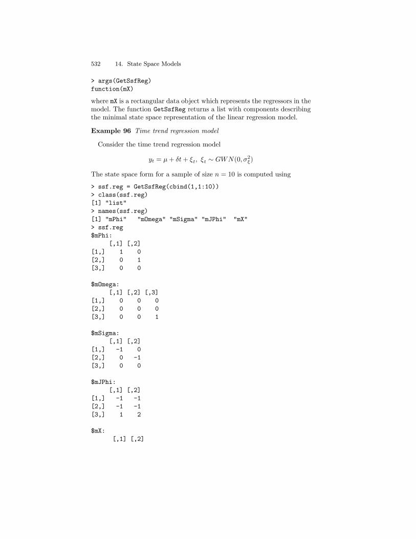
> args(GetSsfReg)
function(mX)
where mX is a rectangular data object which represents the regressors in themodel. The function GetSsfReg returns a list with components describingthe minimal state space representation of the linear regression model.
Example 96 Time trend regression model
Consider the time trend regression model
yt = µ+ δt+ ξt, ξt ∼ GWN(0, σ2ξ)
The state space form for a sample of size n = 10 is computed using
> ssf.reg = GetSsfReg(cbind(1,1:10))
> class(ssf.reg)
[1] "list"
> names(ssf.reg)
[1] "mPhi" "mOmega" "mSigma" "mJPhi" "mX"
> ssf.reg
$mPhi:
[,1] [,2]
[1,] 1 0
[2,] 0 1
[3,] 0 0
$mOmega:
[,1] [,2] [,3]
[1,] 0 0 0
[2,] 0 0 0
[3,] 0 0 1
$mSigma:
[,1] [,2]
[1,] -1 0
[2,] 0 -1
[3,] 0 0
$mJPhi:
[,1] [,2]
[1,] -1 -1
[2,] -1 -1
[3,] 1 2
$mX:
[,1] [,2]

14.2 State Space Representation 533
[1,] 1 1
[2,] 1 2
[3,] 1 3
[4,] 1 4
[5,] 1 5
[6,] 1 6
[7,] 1 7
[8,] 1 8
[9,] 1 9
[10,] 1 10
Since the system matrix Zt= x0t, the parameter Φt is time varying and
the index matrix JΦ, represented by the component mJPhi, determines theassociation between the time varying data in Zt and the data supplied inthe component mX.To specify a time trend regression with a time varying slope of the form
δt+1 = δt + ζt, ζt ∼ GWN(0, σ2ζ) (14.31)
one needs to specify a non-zero value for σ2ζ in Ωt. For example, if σ2ζ = 0.5
then
> ssf.reg.tvp = ssf.reg
> ssf.reg.tvp$mOmega[2,2] = 0.5
> ssf.reg.tvp$mOmega
[,1] [,2] [,3]
[1,] 0 0.0 0
[2,] 0 0.5 0
[3,] 0 0.0 1
modifies the state space form for the time trend regression to allow a timevarying slope of the form (14.31).
Regression Models with ARMA Errors
The ARMA(p, q) models created with GetSsfArma do not have determinis-tic terms (e.g., constant, trend, seasonal dummies) or exogenous regressorsand are therefore limited. The general ARMA(p, q) model with exogenousregressors has the form
yt = x0tβ + ξt
where ξt follows an ARMA(p, q) process of the form (14.21). Let αt bedefined as in (14.23) and let
α∗t =µαt
βt
¶(14.32)
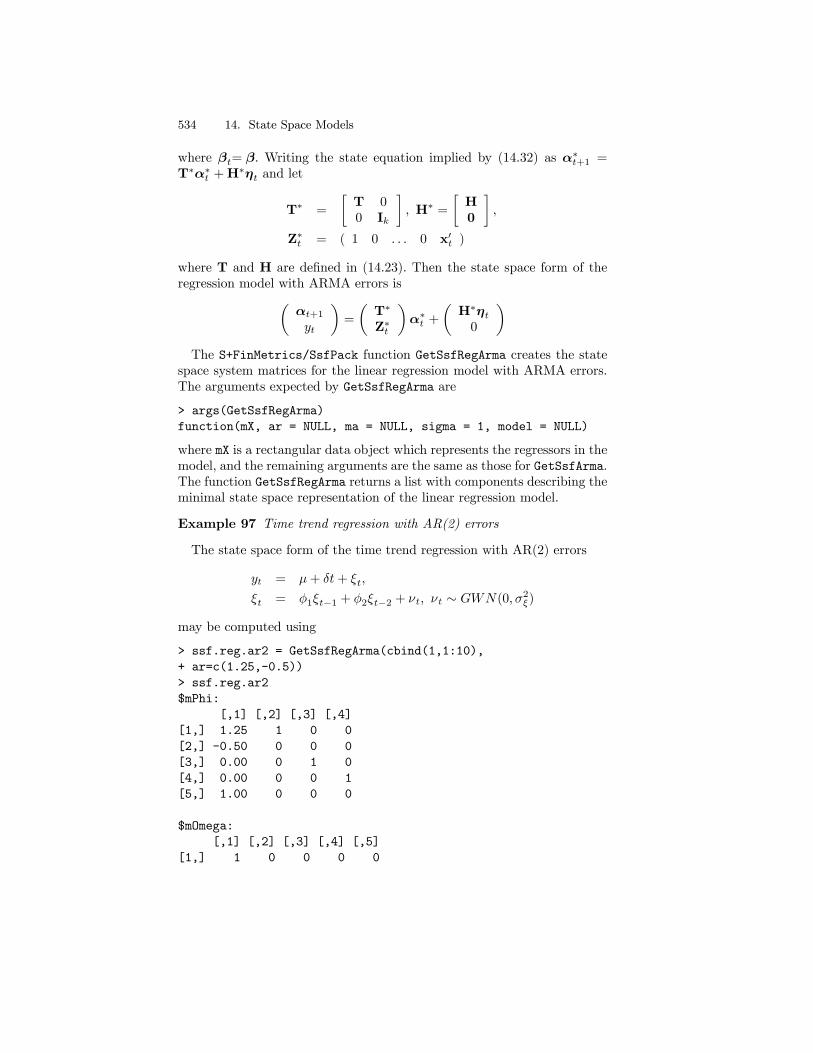
534 14. State Space Models
where βt= β. Writing the state equation implied by (14.32) as α∗t+1 =T∗α∗t +H
∗ηt and let
T∗ =
·T 00 Ik
¸, H∗ =
·H0
¸,
Z∗t = ( 1 0 . . . 0 x0t )
where T and H are defined in (14.23). Then the state space form of theregression model with ARMA errors isµ
αt+1
yt
¶=
µT∗
Z∗t
¶α∗t +
µH∗ηt0
¶The S+FinMetrics/SsfPack function GetSsfRegArma creates the state
space system matrices for the linear regression model with ARMA errors.The arguments expected by GetSsfRegArma are
> args(GetSsfRegArma)
function(mX, ar = NULL, ma = NULL, sigma = 1, model = NULL)
where mX is a rectangular data object which represents the regressors in themodel, and the remaining arguments are the same as those for GetSsfArma.The function GetSsfRegArma returns a list with components describing theminimal state space representation of the linear regression model.
Example 97 Time trend regression with AR(2) errors
The state space form of the time trend regression with AR(2) errors
yt = µ+ δt+ ξt,
ξt = φ1ξt−1 + φ2ξt−2 + νt, νt ∼ GWN(0, σ2ξ)
may be computed using
> ssf.reg.ar2 = GetSsfRegArma(cbind(1,1:10),
+ ar=c(1.25,-0.5))
> ssf.reg.ar2
$mPhi:
[,1] [,2] [,3] [,4]
[1,] 1.25 1 0 0
[2,] -0.50 0 0 0
[3,] 0.00 0 1 0
[4,] 0.00 0 0 1
[5,] 1.00 0 0 0
$mOmega:
[,1] [,2] [,3] [,4] [,5]
[1,] 1 0 0 0 0
14.2 State Space Representation 535
[2,] 0 0 0 0 0
[3,] 0 0 0 0 0
[4,] 0 0 0 0 0
[5,] 0 0 0 0 0
$mSigma:
[,1] [,2] [,3] [,4]
[1,] 4.364 -1.818 0 0
[2,] -1.818 1.091 0 0
[3,] 0.000 0.000 -1 0
[4,] 0.000 0.000 0 -1
[5,] 0.000 0.000 0 0
$mJPhi:
[,1] [,2] [,3] [,4]
[1,] -1 -1 -1 -1
[2,] -1 -1 -1 -1
[3,] -1 -1 -1 -1
[4,] -1 -1 -1 -1
[5,] -1 -1 1 2
$mX:
[,1] [,2]
[1,] 1 1
[2,] 1 2
...
[10,] 1 10
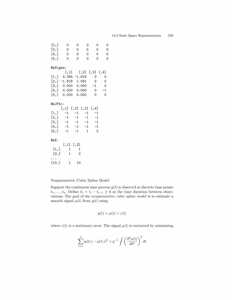
Nonparametric Cubic Spline Model
Suppose the continuous time process y(t) is observed at discrete time pointst1, . . . , tn. Define δi = ti − ti−1 ≥ 0 as the time duration between obser-vations. The goal of the nonparametric cubic spline model is to estimate asmooth signal µ(t) from y(t) using
y(t) = µ(t) + ε(t)
where ε(t) is a stationary error. The signal µ(t) is extracted by minimizing
nXi=1
(y(ti)− µ(ti))2 + q−1
Z µ∂2µ(t)
∂t2
¶2dt

536 14. State Space Models
where the second term is a penalty term that forces µ(t) to be “smooth”4,and q may be interpreted as a signal-to-noise ratio. The resulting functionµ(t) may be expressed as the structural time series model
µ(ti+1) = µ(ti) + δiβ(ti) + η(ti) (14.33)
β(ti+1) = β(ti) + ς(ti)
where µη(ti)ς(ti)
¶˜N
·µ00
¶, σ2ς δi
µ13δ2i
12δi
12δi 1
¶¸Combining (14.33) with the measurement equation
y(ti) = µ(ti) + ε(ti)
where ε(ti) ∼ N(0, σ2ε) and is independent of η(ti) and ς(ti), gives thestate space form for the nonparametric cubic spline model. The state spacesystem matrices are
Φt =
1 δi0 11 0
, Ωt =
qδ2t3
qδ2t2 0
qδ2t2 qδt 00 0 1
When the observations are equally spaced, δi is constant and the abovesystem matrices are time invariant.The S+FinMetrics/SsfPack function GetSsfSpline creates the state
space system matrices for the nonparametric cubic spline model. The ar-guments expected by GetSsfSpline are
> args(GetSsfSpline)
function(snr = 1, delta = 0)
where snr is the signal-to-noise ratio q, and delta is a numeric vectorcontaining the time durations δi (i = 1, . . . , n). If delta=0 then δi is as-sumed to be equal to unity and the time invariant form of the model iscreated. The function GetSsfSpline returns a list with components de-scribing the minimal state space representation of the nonparametric cubicspline model.
Example 98 State space form of non-parametric cubic spline model
The default non-parametric cubic spline model with δt = 1 is createdusing
4This process can be interpreted as an interpolation technique and is similar to thetechnique used in the S+FinMetrics functions interpNA and hpfilter. See also thesmoothing spline method described in chapter sixteen.

14.2 State Space Representation 537
> GetSsfSpline()
$mPhi:
[,1] [,2]
[1,] 1 1
[2,] 0 1
[3,] 1 0
$mOmega:
[,1] [,2] [,3]
[1,] 0.3333 0.5 0
[2,] 0.5000 1.0 0
[3,] 0.0000 0.0 1
$mSigma:
[,1] [,2]
[1,] -1 0
[2,] 0 -1
[3,] 0 0
$mJPhi:
NULL
$mJOmega:
NULL
$mX:
NULL
For unequally spaced observations
> t.vals = c(2,3,5,9,12,17,20,23,25)
> delta.t = diff(t.vals)
and q = 0.2, the state space form is
> GetSsfSpline(snr=0.2,delta=delta.t)
$mPhi:
[,1] [,2]
[1,] 1 1
[2,] 0 1
[3,] 1 0
$mOmega:
[,1] [,2] [,3]
[1,] 0.06667 0.1 0
[2,] 0.10000 0.2 0
[3,] 0.00000 0.0 1
538 14. State Space Models
$mSigma:
[,1] [,2]
[1,] -1 0
[2,] 0 -1
[3,] 0 0
$mJPhi:
[,1] [,2]
[1,] -1 1
[2,] -1 -1
[3,] -1 -1
$mJOmega:
[,1] [,2] [,3]
[1,] 4 3 -1
[2,] 3 2 -1
[3,] -1 -1 -1
$mX:
[,1] [,2] [,3] [,4] [,5] [,6] [,7] [,8]
[1,] 1.00000 2.0000 4.000 3.0 5.000 3.0 3.0 2.0000
[2,] 0.20000 0.4000 0.800 0.6 1.000 0.6 0.6 0.4000
[3,] 0.10000 0.4000 1.600 0.9 2.500 0.9 0.9 0.4000
[4,] 0.06667 0.5333 4.267 1.8 8.333 1.8 1.8 0.5333
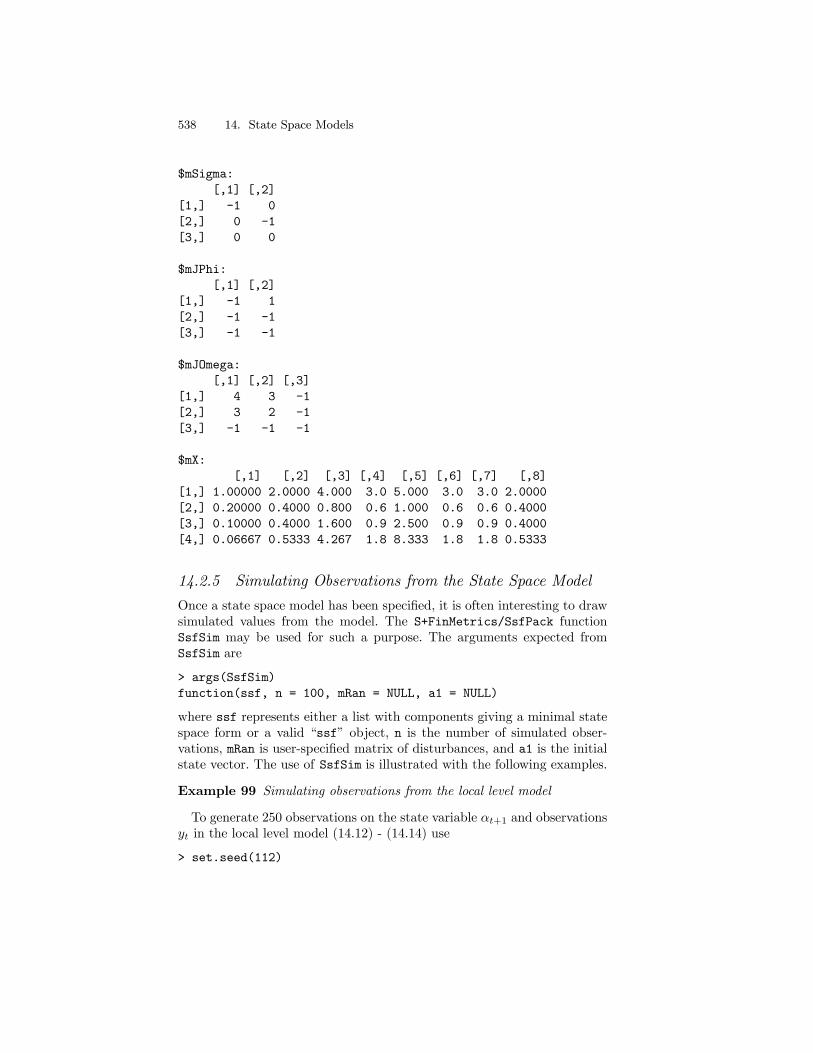
14.2.5 Simulating Observations from the State Space Model
Once a state space model has been specified, it is often interesting to drawsimulated values from the model. The S+FinMetrics/SsfPack functionSsfSim may be used for such a purpose. The arguments expected fromSsfSim are
> args(SsfSim)
function(ssf, n = 100, mRan = NULL, a1 = NULL)
where ssf represents either a list with components giving a minimal statespace form or a valid “ssf” object, n is the number of simulated obser-vations, mRan is user-specified matrix of disturbances, and a1 is the initialstate vector. The use of SsfSim is illustrated with the following examples.
Example 99 Simulating observations from the local level model
To generate 250 observations on the state variable αt+1 and observationsyt in the local level model (14.12) - (14.14) use
> set.seed(112)
14.2 State Space Representation 539
0 50 100 150 200 250
-6-4
-20
24
6StateResponse
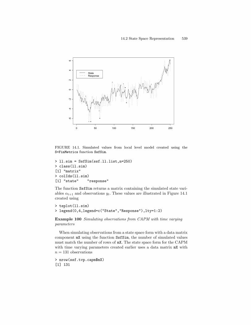
FIGURE 14.1. Simulated values from local level model created using theS+FinMetrics function SsfSim.
> ll.sim = SsfSim(ssf.ll.list,n=250)
> class(ll.sim)
[1] "matrix"
> colIds(ll.sim)
[1] "state" "response"
The function SsfSim returns a matrix containing the simulated state vari-ables αt+1 and observations yt. These values are illustrated in Figure 14.1created using
> tsplot(ll.sim)
> legend(0,4,legend=c("State","Response"),lty=1:2)
Example 100 Simulating observations from CAPM with time varyingparameters
When simulating observations from a state space form with a data matrixcomponent mX using the function SsfSim, the number of simulated valuesmust match the number of rows of mX. The state space form for the CAPMwith time varying parameters created earlier uses a data matrix mX withn = 131 observations
> nrow(ssf.tvp.capm$mX)
[1] 131
540 14. State Space Models
Time varying intercept
alph
a(t)
0 20 40 60 80 100 120
-0.1
5-0
.05
Time varying slope
beta
(t)
0 20 40 60 80 100 120
0.2
0.6
1.0
Simulated returns
retu
rns
0 20 40 60 80 100 120
-0.4
-0.2
0.0
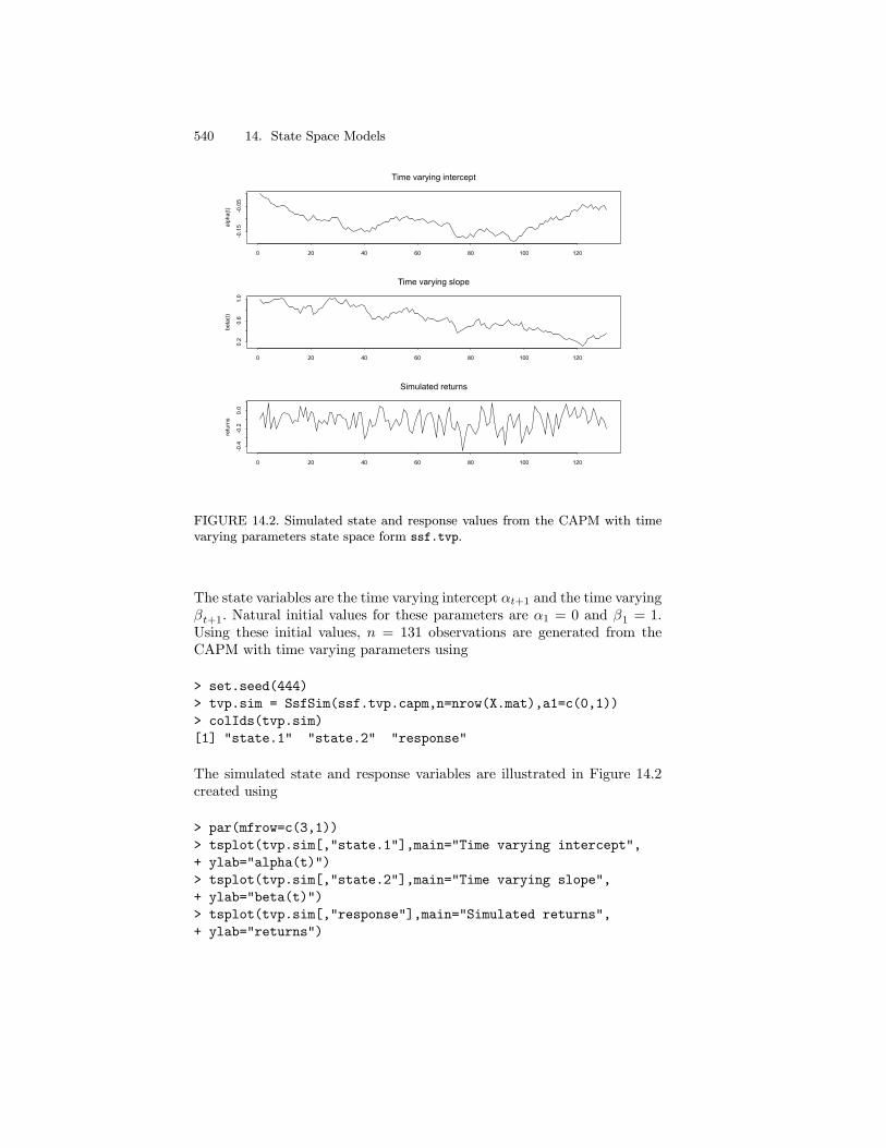
FIGURE 14.2. Simulated state and response values from the CAPM with timevarying parameters state space form ssf.tvp.
The state variables are the time varying intercept αt+1 and the time varyingβt+1. Natural initial values for these parameters are α1 = 0 and β1 = 1.Using these initial values, n = 131 observations are generated from theCAPM with time varying parameters using
> set.seed(444)
> tvp.sim = SsfSim(ssf.tvp.capm,n=nrow(X.mat),a1=c(0,1))
> colIds(tvp.sim)
[1] "state.1" "state.2" "response"
The simulated state and response variables are illustrated in Figure 14.2created using
> par(mfrow=c(3,1))
> tsplot(tvp.sim[,"state.1"],main="Time varying intercept",
+ ylab="alpha(t)")
> tsplot(tvp.sim[,"state.2"],main="Time varying slope",
+ ylab="beta(t)")
> tsplot(tvp.sim[,"response"],main="Simulated returns",
+ ylab="returns")

14.3 Algorithms 541
14.3 Algorithms
14.3.1 Kalman Filter
The Kalman filter is a recursive algorithm for the evaluation of momentsof the normally distributed state vector αt+1 conditional on the observeddata Yt = (y1, . . . , yt). To describe the algorithm, let at = E[αt|Yt−1]denote the conditional mean of αt based on information available at timet− 1 and let Pt = var(αt|Yt−1) denote the conditional variance of αt.The filtering or updating equations of the Kalman filter compute at|t =
E[αt|Yt] and Pt|t = var(αt|Yt) using
at|t = at+Ktvt (14.34)
Pt|t = Pt−PtZ0tK0t (14.35)
where
vt = yt−ct − Ztat (14.36)
Ft = ZtPtZ0t+GtG
0t (14.37)
Kt = PtZ0tF−1t (14.38)
The variable vt is themeasurement equation innovation or prediction error,Ft = var(vt) and Kt is the Kalman gain matrix.The prediction equations of the Kalman filter compute at+1 and Pt+1
using
at+1 = Ttat|t (14.39)
Pt+1 = TtPt|tT0t+HtH0t (14.40)
In the Kalman filter recursions, if there are missing values in yt thenvt= 0, F
−1t = 0 and Kt = 0. This allows out-of-sample forecasts of αt and
yt to be computed from the updating and prediction equations.
14.3.2 Kalman Smoother
The Kalman filtering algorithm is a forward recursion which computes one-step ahead estimates at+1 and Pt+1 based on Yt for t = 1, . . . , n. TheKalman smoothing algorithm is a backward recursion which computes themean and variance of specific conditional distributions based on the fulldata set Yn = (y1, . . . , yn). The smoothing equations are
r∗t = T0trt, N
∗t = TtNtT
0t, K
∗t =N
∗tKt (14.41)
et = F−1t vt −K0
tr∗t , Dt= F
−1t +KtK
∗0t
and the backwards updating equations are
rt−1 = Z0tet + r∗t , Nt−1 = Z0tDtZt− < K∗tZt > +N
∗t (14.42)

542 14. State Space Models
for t = n, . . . , 1 with initializations rn = 0 and Nn = 0. For any squarematrix A, the operator < A >= A+A0. The values rt are called statesmoothing residuals and the values et are called response smoothing residu-als. The recursions (14.41) and (14.42) are somewhat non-standard. Durbinand Koopman (2001) show how they may be re-expressed in more standardform.
14.3.3 Smoothed State and Response Estimates
The smoothed estimates of the state vector αt and its variance matrixare denoted αt = E[αt|Yn] and var(αt|Yn), respectively. The smoothedestimate αt is the optimal estimate of αt using all available informationYn, whereas the filtered estimate at|t is the optimal estimate only usinginformation available at time t,Yt. The computation of αt and its variancefrom the Kalman smoother algorithm is described in Durbin and Koopman(2001).The smoothed estimate of the response yt and its variance are computed
using
yt = θt = E[θt|Yn] = ct+Ztαt
var(yt|Yn) = Ztvar(αt|Yn)Z0t
14.3.4 Smoothed Disturbance Estimates
The smoothed disturbance estimates are the estimates of the measure-ment equations innovations εt and transition equation innovations ηt basedon all available information Yn, and are denoted εt = E[εt|Yn] andηt = E[ηt|Yn], respectively. The computation of εt and ηt from theKalman smoother algorithm is described in Durbin and Koopman (2001).These smoothed disturbance estimates are useful for parameter estimationby maximum likelihood and for diagnostic checking. See chapter seven inDurbin and Koopman (2001) for details.
14.3.5 Forecasting
The Kalman filter prediction equations (14.39) - (14.40) produces one-stepahead predictions of the state vector, at+1 = E[αt+1|Yt], along with pre-diction variance matrices Pt+1. Out of sample predictions, together withassociated mean square errors, can be computed from the Kalman filterprediction equations by extending the data set y1, . . . ,yn with a set ofmissing values. When yτ is missing, the Kalman filter reduces to the pre-diction step described above. As a result, a sequence of m missing valuesat the end of the sample will produce a set of h-step ahead forecasts forh = 1, . . . ,m.
14.3 Algorithms 543
14.3.6 S+FinMetrics/SsfPack Implementation of StateSpace Modeling Algorithms
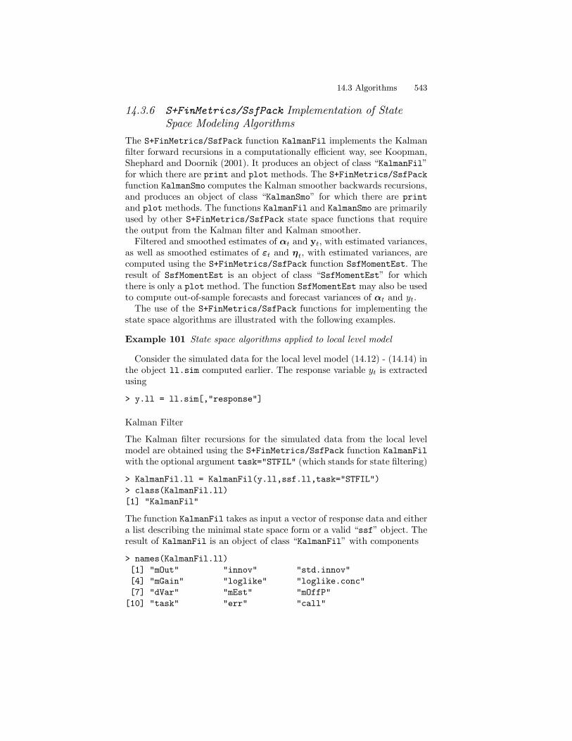
The S+FinMetrics/SsfPack function KalmanFil implements the Kalmanfilter forward recursions in a computationally efficient way, see Koopman,Shephard and Doornik (2001). It produces an object of class “KalmanFil”for which there are print and plot methods. The S+FinMetrics/SsfPackfunction KalmanSmo computes the Kalman smoother backwards recursions,and produces an object of class “KalmanSmo” for which there are printand plot methods. The functions KalmanFil and KalmanSmo are primarilyused by other S+FinMetrics/SsfPack state space functions that requirethe output from the Kalman filter and Kalman smoother.Filtered and smoothed estimates of αt and yt, with estimated variances,
as well as smoothed estimates of εt and ηt, with estimated variances, arecomputed using the S+FinMetrics/SsfPack function SsfMomentEst. Theresult of SsfMomentEst is an object of class “SsfMomentEst” for whichthere is only a plot method. The function SsfMomentEst may also be usedto compute out-of-sample forecasts and forecast variances of αt and yt.The use of the S+FinMetrics/SsfPack functions for implementing the
state space algorithms are illustrated with the following examples.
Example 101 State space algorithms applied to local level model
Consider the simulated data for the local level model (14.12) - (14.14) inthe object ll.sim computed earlier. The response variable yt is extractedusing
> y.ll = ll.sim[,"response"]
Kalman Filter
The Kalman filter recursions for the simulated data from the local levelmodel are obtained using the S+FinMetrics/SsfPack function KalmanFilwith the optional argument task="STFIL" (which stands for state filtering)
> KalmanFil.ll = KalmanFil(y.ll,ssf.ll,task="STFIL")
> class(KalmanFil.ll)
[1] "KalmanFil"
The function KalmanFil takes as input a vector of response data and eithera list describing the minimal state space form or a valid “ssf” object. Theresult of KalmanFil is an object of class “KalmanFil” with components
> names(KalmanFil.ll)
[1] "mOut" "innov" "std.innov"
[4] "mGain" "loglike" "loglike.conc"
[7] "dVar" "mEst" "mOffP"
[10] "task" "err" "call"

544 14. State Space Models
A complete explanation of the components of a “KalmanFil” object is givenin the online help for KalmanFil. These components are mainly used byother S+FinMetrics/SsfPack functions and are only briefly discussed here.The component mOut contains the basic Kalman filter output.
> KalmanFil.ll$mOut
numeric matrix: 250 rows, 3 columns.
[,1] [,2] [,3]
[1,] 0.00000 1.0000 0.0000
[2,] -1.28697 0.5556 0.4444
...
[250,] -1.6371 0.3904 0.6096
The first column of mOut contains the prediction errors vt, the second col-umn contains the Kalman gains, Kt, and the last column contains theinverses of the prediction error variances, F−1t . Since task="STFIL" thefiltered estimates at|t and yt|t = Ztat|t are in the component mEst
> KalmanFil.ll$mEst
numeric matrix: 250 rows, 4 columns.
[,1] [,2] [,3] [,4]
[1,] 1.10889 1.10889 1.0000 1.0000
[2,] 0.39390 0.39390 0.5556 0.5556
...
[250,] 4.839 4.839 0.3904 0.3904
The plotmethod allows for a graphical analysis of the Kalman filter output
> plot(KalmanFil.ll)
Make a plot selection (or 0 to exit):
1: plot: all
2: plot: innovations
3: plot: standardized innovations
4: plot: innovation histogram
5: plot: normal QQ-plot of innovations
6: plot: innovation ACF
Selection:
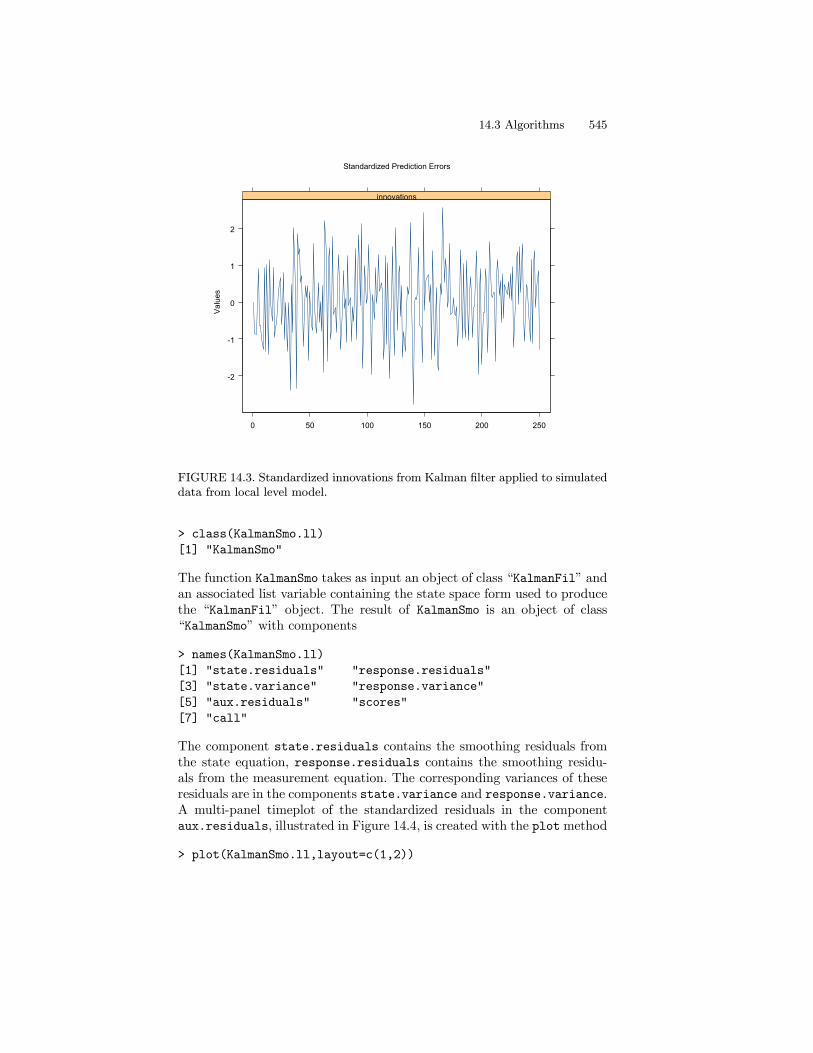
The standardized innovations vt/Ft are illustrated in Figure 14.3.
Kalman Smoother
The Kalman smoother backwards recursions for the simulated data fromthe local level model are obtained using the S+FinMetrics/SsfPack func-tion KalmanSmo
> KalmanSmo.ll = KalmanSmo(KalmanFil.ll,ssf.ll)
14.3 Algorithms 545
-2
-1
0
1
2
0 50 100 150 200 250
innovations
Valu
es
Standardized Prediction Errors
FIGURE 14.3. Standardized innovations from Kalman filter applied to simulateddata from local level model.
> class(KalmanSmo.ll)
[1] "KalmanSmo"
The function KalmanSmo takes as input an object of class “KalmanFil” andan associated list variable containing the state space form used to producethe “KalmanFil” object. The result of KalmanSmo is an object of class“KalmanSmo” with components
> names(KalmanSmo.ll)
[1] "state.residuals" "response.residuals"
[3] "state.variance" "response.variance"
[5] "aux.residuals" "scores"
[7] "call"
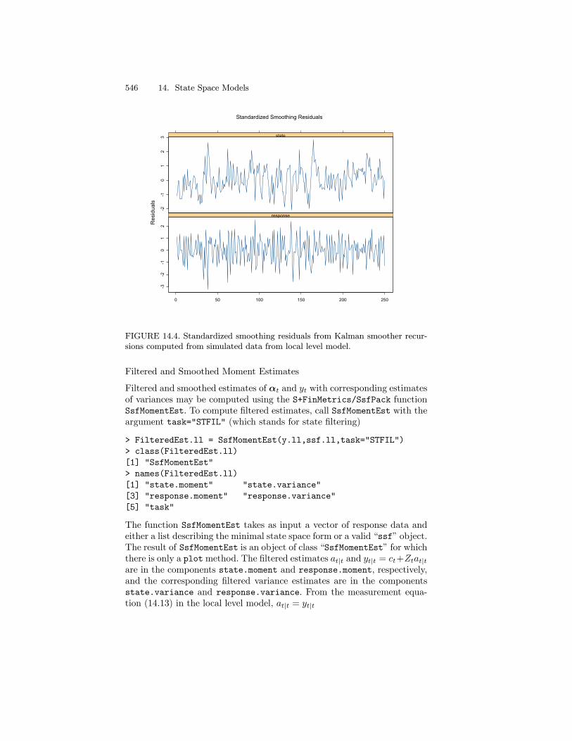
The component state.residuals contains the smoothing residuals fromthe state equation, response.residuals contains the smoothing residu-als from the measurement equation. The corresponding variances of theseresiduals are in the components state.variance and response.variance.A multi-panel timeplot of the standardized residuals in the componentaux.residuals, illustrated in Figure 14.4, is created with the plotmethod
> plot(KalmanSmo.ll,layout=c(1,2))
546 14. State Space Models
-3-2
-10
12
0 50 100 150 200 250
response
-2-1
01
23 state
Res
idua
ls
Standardized Smoothing Residuals
FIGURE 14.4. Standardized smoothing residuals from Kalman smoother recur-sions computed from simulated data from local level model.
Filtered and Smoothed Moment Estimates
Filtered and smoothed estimates of αt and yt with corresponding estimatesof variances may be computed using the S+FinMetrics/SsfPack functionSsfMomentEst. To compute filtered estimates, call SsfMomentEst with theargument task="STFIL" (which stands for state filtering)
> FilteredEst.ll = SsfMomentEst(y.ll,ssf.ll,task="STFIL")
> class(FilteredEst.ll)
[1] "SsfMomentEst"
> names(FilteredEst.ll)
[1] "state.moment" "state.variance"
[3] "response.moment" "response.variance"
[5] "task"
The function SsfMomentEst takes as input a vector of response data andeither a list describing the minimal state space form or a valid “ssf” object.The result of SsfMomentEst is an object of class “SsfMomentEst” for whichthere is only a plotmethod. The filtered estimates at|t and yt|t = ct+Ztat|tare in the components state.moment and response.moment, respectively,and the corresponding filtered variance estimates are in the componentsstate.variance and response.variance. From the measurement equa-tion (14.13) in the local level model, at|t = yt|t
14.3 Algorithms 547
-4-2
02
4
0 50 100 150 200 250
response
-4-2
02
4
state
Valu
es
State Filtering
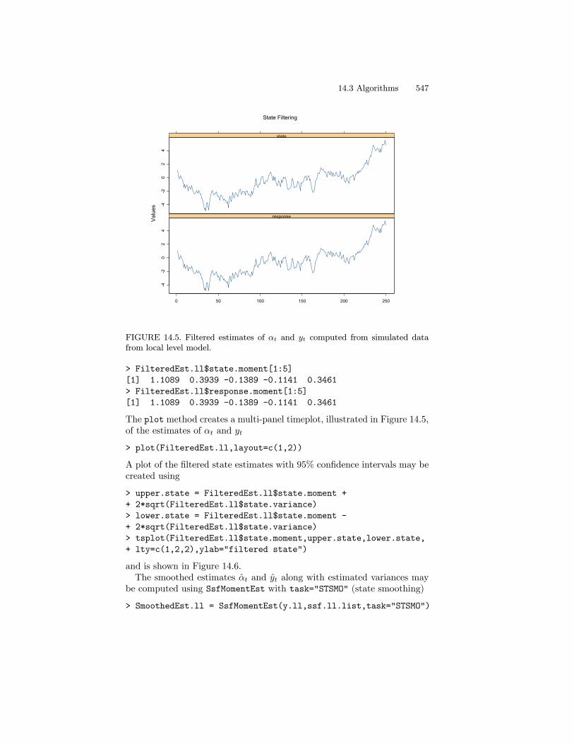
FIGURE 14.5. Filtered estimates of αt and yt computed from simulated datafrom local level model.
> FilteredEst.ll$state.moment[1:5]
[1] 1.1089 0.3939 -0.1389 -0.1141 0.3461
> FilteredEst.ll$response.moment[1:5]
[1] 1.1089 0.3939 -0.1389 -0.1141 0.3461
The plot method creates a multi-panel timeplot, illustrated in Figure 14.5,of the estimates of αt and yt
> plot(FilteredEst.ll,layout=c(1,2))
A plot of the filtered state estimates with 95% confidence intervals may becreated using
> upper.state = FilteredEst.ll$state.moment +
+ 2*sqrt(FilteredEst.ll$state.variance)
> lower.state = FilteredEst.ll$state.moment -
+ 2*sqrt(FilteredEst.ll$state.variance)
> tsplot(FilteredEst.ll$state.moment,upper.state,lower.state,
+ lty=c(1,2,2),ylab="filtered state")
and is shown in Figure 14.6.The smoothed estimates αt and yt along with estimated variances may
be computed using SsfMomentEst with task="STSMO" (state smoothing)
> SmoothedEst.ll = SsfMomentEst(y.ll,ssf.ll.list,task="STSMO")

548 14. State Space Models
filte
red
stat
e
0 50 100 150 200 250
-6-4
-20
24
6
FIGURE 14.6. Filtered estimates of αt with 95% confidence intervals computedfrom simulated values from local level model.
In the local level model, αt = yt
> SmoothedEst.ll$state.moment[1:5]
[1] 0.24281 0.02629 -0.13914 -0.13925 -0.15455
> SmoothedEst.ll$response.moment[1:5]
[1] 0.24281 0.02629 -0.13914 -0.13925 -0.15455
The smoothed state estimates with 95% confidence bands are illustratedin Figure 14.7. Compared to the filtered state estimates, the smoothedestimates are “smoother” and the confidence bands are slightly smaller.Smoothed estimates of αt and yt without estimated variances may be
obtained using the S+FinMetrics/SsfPack function SsfCondDens with theargument task="STSMO" (which stands for state smoothing)
> smoothedEst.ll = SsfCondDens(y.ll,ssf.ll.list,task="STSMO")
> class(smoothedEst.ll)
[1] "SsfCondDens"
> names(smoothedEst.ll)
[1] "state" "response" "task"
The object smoothedEst.ll is of class “SsfCondDens” with componentsstate, giving the smoothed state estimates αt, response, which gives thesmoothed response estimates yt, and task, naming the task performed. The

14.3 Algorithms 549
smoo
thed
sta
te
0 50 100 150 200 250
-4-2
02
46
FIGURE 14.7. Smoothed estimates of αt with 95% confidence intervals computedfrom simulated values from local level model.
smoothed estimates yt and αt may be visualized using the plot methodfor “SsfCondDens” objects
> plot(smoothedEst.ll)
The resulting plot has the same format at the plot shown in Figure 14.5.
Smoothed Disturbance Estimates
The smoothed disturbance estimates εt and ηt may be computed usingSsfMomentEst with the optional argument task="DSSMO" (which standsfor disturbance smoothing)
> disturbEst.ll = SsfMomentEst(y.ll,ssf.ll,task="DSSMO")
> names(disturbEst.ll)
[1] "state.moment" "state.variance"
[3] "response.moment" "response.variance"
[5] "task"
The estimates ηt are in the component state.moment, and the estimates εtare in the component response.moment. These estimates may be visualizedusing the plot method.
550 14. State Space Models
Koopman, Shephard and Doornik (1999) point out that, in the local levelmodel, the standardized smoothed disturbances
ηtpdvar(ηt) , εtpdvar(εt) (14.43)
may be interpreted as t-statistics for impulse intervention variables in thetransition and measurement equations, respectively. Consequently, largevalues of (14.43) indicate outliers and/or structural breaks in the locallevel model.
Forecasting
To produce out-of-sample h-step ahead forecasts yt+h|t for h = 1, . . . , 5 asequence of 5 missing values is appended to the end of the response vectory.ll
> y.ll.new = c(y.ll,rep(NA,5))
The forecast values and mean squared errors are computed using thefunction SsfMomentEst with the argument task="STPRED"
> PredictedEst.ll = SsfMomentEst(y.ll.new,ssf.ll,task="STPRED")
> y.ll.fcst = PredictedEst.ll$response.moment
> fcst.var = PredictedEst.ll$response.variance
The actual values, forecasts and 95% confidence bands are illustrated inFigure 14.8 created by
> upper = y.ll.fcst + 2*sqrt(fcst.var)
> lower = y.ll.fcst - 2*sqrt(fcst.var)
> upper[1:250] = lower[1:250] = NA
> tsplot(y.ll.new[240:255],y.ll.fcst[240:255],
+ upper[240:255],lower[240:255],lty=c(1,2,2,2))
14.4 Estimation of State Space Models
14.4.1 Prediction Error Decomposition of Log-Likelihood
The prediction error decomposition of the log-likelihood function for theunknown parameters ϕ of a state space model may be conveniently com-puted using the output of the Kalman filter
lnL(ϕ|Yn) =nXt=1
ln f(yt|Yt−1;ϕ) (14.44)
= −nN2ln(2π)− 1
2
nXt=1
¡ln |Ft|+ v0tF−1t vt
¢

14.4 Estimation of State Space Models 551
1 2 3 4 5 6 7 8 9 10 11 12 13 14 15 16
34
56
7
FIGURE 14.8. Actual values, h-step forecasts and 95% confidence intervals foryt from local level model.
where f(yt|Yt−1;ϕ) is a conditional Gaussian density implied by the statespace model (14.1) - (14.6). The vector of prediction errors vt and pre-diction error variance matrices Ft are computed from the Kalman filterrecursions.A useful diagnostic is the estimated variance of the standardized predic-
tion errors for a given value of ϕ:
σ2(ϕ) =1
Nn
nXt=1
v0tF−1t vt (14.45)
As mentioned by Koopman, Shephard and Doornik (1999), it is helpful tochoose starting values for ϕ such that σ2(ϕstart) ≈ 1. For well specifiedmodels, σ2(ϕmle) should be very close to unity.
Concentrated Log-likelihood
In some models, e.g. ARMA models, it is possible to solve explicitly for onescale factor and concentrate it out of the log-likelihood function (14.44).The resulting log-likelihood function is called the concentrated log-likelihoodor profile log-likelihood and is denoted lnLc(ϕ|Yn). Following Koopman,Shephard and Doornik (1999), let σ denote such a scale factor, and let
yt= θt +Gctε
ct

552 14. State Space Models
with εct ∼ iid N(0, σ2I) denote the scaled version of the measurementequation (14.3). The state space form (14.1) - (14.3) applies but with Gt =σGc
t and Ht = σHct . This formulation implies that one non-zero element
of σGct or σH
ct is kept fixed, usually at unity, which reduces the dimension
of the parameter vector ϕ by one. The solution for σ2 from (14.44) is givenby
σ2(ϕ) =1
Nn
nXt=1
v0t (Fct)−1vt
and the resulting concentrated log-likelihood function is
lnLc(ϕ|Yn) = −nN
2ln(2π)− nN
2ln¡σ2(ϕ) + 1
¢− 12
nXt=1
ln |Fct | (14.46)
14.4.2 Fitting State Space Models Using theS+FinMetrics/SsfPack Function SsfFit
The S+FinMetrics/SsfPack function SsfFit may be used to computeMLEs of the unknown parameters in the state space model (14.1)-(14.6)from the prediction error decomposition of the log-likelihood function (14.44).The arguments expected by SsfFit are
> args(SsfFit)
function(parm, data, FUN, conc = F, scale = 1, gradient =
NULL, hessian = NULL, lower = - Inf, upper = Inf,
trace = T, control = NULL, ...)
where parm is a vector containing the starting values of the unknown pa-rameters ϕ, data is a rectangular object containing the response variablesyt, and FUN is a character string giving the name of the function which takesparm together with the optional arguments in ... and produces an “ssf”object representing the state space form. The remaining arguments controlaspects of the S-PLUS optimization algorithm nlminb. An advantage of us-ing nlminb is that box constraints may be imposed on the parameters ofthe log-likelihood function using the optional arguments lower and upper.See the online help for nlminb for details. A disadvantage of using nlminbis that the value of the Hessian evaluated at the MLEs is returned only ifan analytic formula is supplied to compute the Hessian. The use of SsfFitis illustrated with the following examples.
Example 102 Exact maximum likelihood estimation of AR(1) model
Consider estimating by exact maximum likelihood the AR(1) model dis-cussed earlier. First, n = 250 observations are simulated from the model
> ssf.ar1 = GetSsfArma(ar=0.75,sigma=.5)
> set.seed(598)

14.4 Estimation of State Space Models 553
> sim.ssf.ar1 = SsfSim(ssf.ar1,n=250)
> y.ar1 = sim.ssf.ar1[,"response"]
Least squares estimation of the AR(1) model, which is equivalent to MLEconditional on the first observation, gives
> OLS(y.ar1~tslag(y.ar1)-1)
Call:
OLS(formula = y.ar1 ~tslag(y.ar1) - 1)
Coefficients:
tslag(y.ar1)
0.7739
Degrees of freedom: 249 total; 248 residual
Residual standard error: 0.4921
The S+FinMetrics/SsfPack function SsfFit requires as input a func-tion which takes the unknown parameters ϕ = (φ, σ2)0 and produces thestate space form for the AR(1). One such function is
> ar1.mod = function(parm)
+ phi = parm[1]
+ sigma2 = parm[2]
+ ssf.mod = GetSsfArma(ar=phi,sigma=sqrt(sigma2))
+ CheckSsf(ssf.mod)
+
In addition, starting values for ϕ are required. Somewhat arbitrary startingvalues are
> ar1.start = c(0.5,1)
> names(ar1.start) = c("phi","sigma2")
The prediction error decomposition of the log-likelihood function evalu-ated at the starting values ϕ = (0.5, 1)0 may be computed using theS+FinMetrics/SsfPack function KalmanFil with task="KFLIK"
> KalmanFil(y.ar1,ar1.mod(ar1.start),task="KFLIK")
Call:
KalmanFil(mY = y.ar1, ssf = ar1.mod(ar1.start), task =
"KFLIK")
Log-likelihood: -265.5222
Prediction error variance: 0.2851
Sample observations: 250
554 14. State Space Models
Standardized Innovations:
Mean Std.Error
-0.0238 0.5345
Notice that the standardized prediction error variance (14.45) is 0.285, farbelow unity, which indicates that the starting values are not very good.The MLEs for ϕ = (φ, σ2)0 using SsfFit are computed as
> ar1.mle = SsfFit(ar1.start,y.ar1,"ar1.mod",
+ lower=c(-.999,0),upper=c(0.999,Inf))
Iteration 0 : objective = 265.5
Iteration 1 : objective = 282.9
...
Iteration 18 : objective = 176.9
RELATIVE FUNCTION CONVERGENCE
In the call to SsfFit, the stationarity condition −1 < φ < 1 and thepositive variance condition σ2 > 0 is imposed in the estimation. The resultof SsfFit is a an object of class “SsfFit” with components
> names(ar1.mle)
[1] "parameters" "objective" "message" "grad.norm" "iterations"
[6] "f.evals" "g.evals" "hessian" "scale" "aux"
[11] "call" "vcov"
The exact MLEs for ϕ = (φ, σ2)0 are
> ar1.mle
Log-likelihood: -176.9
250 observations
Parameter Estimates:
phi sigma2
0.77081 0.2402688
and the MLE for σ is
> sqrt(ar1.mle$parameters["sigma2"])
sigma2
0.4902
These values are very close to the least squares estimates. Standard errorsand t-statistics are displayed using
> summary(ar1.mle)
Log-likelihood: -176.936
250 observations
Parameters:
Value Std. Error t value
phi 0.7708 0.03977 19.38
sigma2 0.2403 0.02149 11.18

14.4 Estimation of State Space Models 555
Convergence: RELATIVE FUNCTION CONVERGENCE
A summary of the log-likelihood evaluated at the MLEs is
> KalmanFil(y.ar1,ar1.mod(ar1.mle$parameters),
+ task="KFLIK")
Call:
KalmanFil(mY = y.ar1, ssf = ar1.mod(ar1.mle$parameters),
task = "KFLIK")
Log-likelihood: -176.9359
Prediction error variance: 1
Sample observations: 250
Standardized Innovations:
Mean Std.Error
-0.0213 1.0018
Notice that the estimated variance of the standardized prediction errors isequal to 1.
Example 103 Exact maximum likelihood estimation of AR(1) model us-ing re-parameterization
An alternative function to compute the state space form of the AR(1) is
ar1.mod2 = function(parm)
phi = exp(parm[1])/(1 + exp(parm[1]))
sigma2 = exp(parm[2])
ssf.mod = GetSsfArma(ar=phi,sigma=sqrt(sigma2))
CheckSsf(ssf.mod)
In the above model, a stationary value for φ between 0 and 1 and apositive value for σ2 is guaranteed by parameterizing the log-likelihoodin terms of γ0 = ln(φ/(1 − φ)) and γ1 = ln(σ2) instead of φ and σ2.
By the invariance property of maximum likelihood estimation, φmle =exp(γ0,mle)/(1 + exp(γ0,mle)) and σ2mle = exp(γ1,mle) are the MLEs forφ and σ2. The MLEs for ϕ = (γ0, γ1)
0 computed using SsfFit are
> ar1.start = c(0,0)
> names(ar1.start) = c("ln(phi/(1-phi))","ln(sigma2)")
> ar1.mle = SsfFit(ar1.start,y.ar1,"ar1.mod2")
Iteration 0 : objective = 265.5222
...
Iteration 10 : objective = 176.9359
556 14. State Space Models
RELATIVE FUNCTION CONVERGENCE
> summary(ar1.mle)
Log-likelihood: -176.936
250 observations
Parameters:
Value Std. Error t value
ln(phi/(1-phi)) 1.213 0.22510 5.388
ln(sigma2) -1.426 0.08945 -15.940
Convergence: RELATIVE FUNCTION CONVERGENCE
The MLEs for φ and σ2, and estimated standard errors computed usingthe delta method, are5
> ar1.mle2 = ar1.mle
> tmp = coef(ar1.mle)
> ar1.mle2$parameters[1] = exp(tmp[1])/(1 + exp(tmp[1]))
> ar1.mle2$parameters[2] = exp(tmp[2])
> dg1 = exp(-tmp[1])/(1 + exp(-tmp[1]))^2
> dg2 = exp(tmp[2])
> dg = diag(c(dg1,dg2))
> ar1.mle2$vcov = dg%*%ar1.mle2$vcov%*%dg
> summary(ar1.mle2)
Log-likelihood: -176.936
250 observations
Parameters:
Value Std. Error t value
ln(phi/(1-phi)) 0.7708 0.03977 19.38
ln(sigma2) 0.2403 0.02149 11.18
Convergence: RELATIVE FUNCTION CONVERGENCE
and exactly match the previous MLEs.
Example 104 Exact maximum likelihood estimation of AR(1) model us-ing concentrated log-likelihood
In the AR(1) model, the variance parameter σ2 can be analytically con-centrated out of the log-likelihood. The advantages of concentrating thelog-likelihood are to reduce the number of parameters to estimate, and toimprove the numerical stability of the optimization. A function to computethe state space form for the AR(1) model, as a function of φ only, is
ar1.modc = function(parm)
5Recall, if√n(θ−θ) d→ N(θ, V ) and g is a continuous function then
√n(g(θ)−g(θ)) d→
N(0, ∂g∂θ0 V
∂g∂θ0
0).
14.4 Estimation of State Space Models 557
phi = parm[1]
ssf.mod = GetSsfArma(ar=phi)
CheckSsf(ssf.mod)
By default, the function GetSsfArma sets σ2 = 1 which is required for thecomputation of the concentrated log-likelihood function from (14.46). Tomaximize the concentrated log-likelihood function (14.46) for the AR(1)model, use SsfFit with ar1.modc and set the optional argument conc=T :
> ar1.start = c(0.7)
> names(ar1.start) = c("phi")
> ar1.cmle = SsfFit(ar1.start,y.ar1,"ar1.modc",conc=T,
+ lower=0,upper=0.999)
Iteration 0 : objective = 178.506
...
Iteration 4 : objective = 176.9359
RELATIVE FUNCTION CONVERGENCE
> summary(ar1.cmle)
Log-likelihood: -176.936
250 observations
Parameters:
Value Std. Error t value
phi 0.7708 0.03977 19.38
Convergence: RELATIVE FUNCTION CONVERGENCE
Notice that with the concentrated log-likelihood, the optimizer convergesin only four interations. The values of the log-likelihood and the MLE forφ are the same as found previously. The MLE for σ2 may be recovered byrunning the Kalman filter and computing the variance of the predictionerrors:
> ar1.KF = KalmanFil(y.ar1,ar1.mod(ar1.cmle$parameters),
+ task="KFLIK")
> ar1.KF$dVar
[1] 0.2403
One disadvantage of using the concentrated log-likelihood is the lack of anestimated standard error for σ2.
Example 105 Maximum likelihood estimation of CAPM with time vary-ing parameters
Consider estimating the CAPM with time varying coefficients (14.17) -(14.19) using monthly data on Microsoft and the S&P 500 index over the pe-riod February, 1990 through December, 2000 contained in the S+FinMetrics“timeSeries” excessReturns.ts. The parameters of the model are the

558 14. State Space Models
variances of the innovations to the transition and measurement equations;σ2ξ , σ
2ς and σ2ν . Since these variances must be positive the log-likelihood
is parameterized using ϕ = (ln(σ2ξ), ln(σ2ς ), ln(σ
2ν))
0. Since the state spaceform for the CAPM with time varying coefficients requires a data matrix Xcontaining the excess returns on the S&P 500 index, the function SsfFitrequires as input a function which takes both ϕ and X and returns theappropriate state space form. One such function is
tvp.mod = function(parm,mX=NULL)
parm = exp(parm) # 3 x 1 vector containing log variances
ssf.tvp = GetSsfReg(mX=mX)
diag(ssf.tvp$mOmega) = parm
CheckSsf(ssf.tvp)
Starting values for ϕ are specified as
> tvp.start = c(0,0,0)
> names(tvp.start) = c("ln(s2.alpha)","ln(s2.beta)","ln(s2.y)")
The maximum likelihood estimates for ϕ based on SsfFit are computedusing
> tvp.mle = SsfFit(tvp.start,msft.ret,"tvp.mod",mX=X.mat)
Iteration 0 : objective = 183.2
...
Iteration 22 : objective = -123
RELATIVE FUNCTION CONVERGENCE
The MLEs for ϕ = (ln(σ2ξ), ln(σ2ς ), ln(σ
2ν))
0 are
> summary(tvp.mle)
Log-likelihood: 122.979
131 observations
Parameters:
Value Std. Error t value
ln(s2.alpha) -12.480 2.8030 -4.452
ln(s2.beta) -5.900 3.0890 -1.910
ln(s2.y) -4.817 0.1285 -37.480
Convergence: RELATIVE FUNCTION CONVERGENCE
The estimates for the standard deviations σξ, σς and σν as well as estimatedstandard errors, from the delta method, are:
> tvp2.mle = tvp.mle
> tvp2.mle$parameters = exp(tvp.mle$parameters/2)\qquad \qquad
> names(tvp2.mle$parameters) = c("s.alpha","s.beta","s.y")
> dg = diag(tvp2.mle$parameters/2)
14.4 Estimation of State Space Models 559
> tvp2.mle$vcov = dg%*%tvp.mle$vcov%*%dg
> summary(tvp2.mle)
Log-likelihood: 122.979
131 observations
Parameters:
Value Std. Error t value
s.alpha 0.001951 0.002734 0.7135
s.beta 0.052350 0.080860 0.6474
s.y 0.089970 0.005781 15.5600
Convergence: RELATIVE FUNCTION CONVERGENCE
It appears that the estimated standard deviations for the time varyingparameter CAPM are close to zero, suggesting a constant parameter model.The smoothed estimates of the time varying parameters αt and βt as
well as the expected returns may be extracted and plotted using
> smoothedEst.tvp = SsfCondDens(y.capm,
+ tvp.mod(tvp.mle$parameters,mX=X.mat),
+ task="STSMO")
> plot(smoothedEst.tvp,strip.text=c("alpha(t)",
+ "beta(t)","Expected returns"),main="Smoothed Estimates",scales="free")
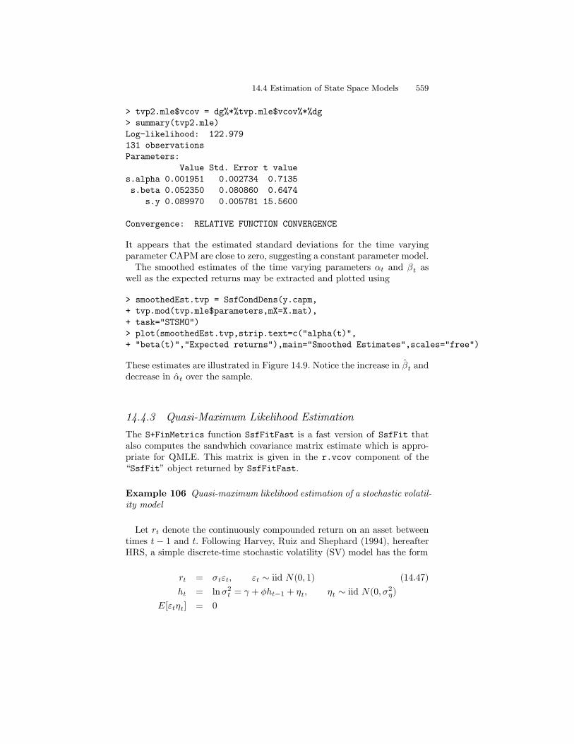
These estimates are illustrated in Figure 14.9. Notice the increase in βt anddecrease in αt over the sample.
14.4.3 Quasi-Maximum Likelihood Estimation
The S+FinMetrics function SsfFitFast is a fast version of SsfFit thatalso computes the sandwhich covariance matrix estimate which is appro-priate for QMLE. This matrix is given in the r.vcov component of the“SsfFit” object returned by SsfFitFast.
Example 106 Quasi-maximum likelihood estimation of a stochastic volatil-ity model
Let rt denote the continuously compounded return on an asset betweentimes t − 1 and t. Following Harvey, Ruiz and Shephard (1994), hereafterHRS, a simple discrete-time stochastic volatility (SV) model has the form
rt = σtεt, εt ∼ iid N(0, 1) (14.47)
ht = lnσ2t = γ + φht−1 + ηt, ηt ∼ iid N(0, σ2η)
E[εtηt] = 0
560 14. State Space Models
-0.2
-0.1
0.0
0.1
0 20 40 60 80 100 120
Expected returns
0.01
00.
015
0.02
00.
025
alpha(t)
1.4
1.5
1.6
1.7
1.8 beta(t)
Mea
n
Smoothed Estimates
FIGURE 14.9. Smoothed estimates of αt and βt from CAPM with time varyingparameter fit to the monthly excess returns on Microsoft.
Defining yt = ln r2t , and noting that E[ln ε
2t ] = −1.27 and var(ln ε2t ) = π2/2
an unobserved components state space representation for yt has the form
yt = −1.27 + ht + ξt, ξt ∼ iid (0, π2/2)ht = γ + φht−1 + ηt, ηt ∼ iid N(0, σ2η)
E[ξtηt] = 0
If ξt were iid Gaussian then the parameters ϕ = (γ, σ2η, φ)0 of the SV
model could be efficiently estimated by maximizing the prediction errordecomposition of the log-likelihood function constructed from the Kalmanfilter recursions. However, since ξt = ln ε
2t is not normally distributed the
Kalman filter only provides minimum mean squared error linear estimatorsof the state and future observations. Nonetheless, HRS point out that eventhough the exact log-likelihood cannot be computed from the predictionerror decomposition based on the Kalman filter, consistent estimates ofϕ = (γ, σ2η, φ)
0 can still be obtained by treating ξt as though it were iidN(0, π2/2) and maximizing the quasi log-likelihood function constructedfrom the prediction error decomposition.The state space representation of the SV model has system matrices
δ =
µγ−1.27
¶, Φ =
µφ1
¶, Ω =
µσ2η 00 π2/2
¶

14.4 Estimation of State Space Models 561
Assuming that |φ| < 1, the initial value matrix has the form
Σ =
µσ2η/(1− φ2)γ/(1− φ)
¶If φ = 1 then use
Σ =
µ −10
¶A function to compute the state space form of the SV model given a
vector of parameters, assuming |φ| < 1, issv.mod = function(parm)
g = parm[1]
sigma2.n = exp(parm[2])
phi = parm[3]
ssf.mod = list(mDelta=c(g,-1.27),
mPhi=as.matrix(c(phi,1)),
mOmega=matrix(c(sigma2.n,0,0,0.5*pi^2),2,2),
mSigma=as.matrix(c((sigma2.n/(1-phi^2)),g/(1-phi))))
CheckSsf(ssf.mod)
Notice that an exponential transformation is utilized to ensure a positivevalue for σ2η. A sample of T = 1000 observations are simulated from theSV model using the parameters γ = −0.3556, σ2η = 0.0312 and φ = 0.9646:> parm.hrs = c(-0.3556,log(0.0312),0.9646)
> nobs = 1000
> set.seed(179)
> e = rnorm(nobs)
> xi = log(e^2)+1.27
> eta = rnorm(nobs,sd=sqrt(0.0312))
> sv.sim = SsfSim(sv.mod(parm.hrs),
+ mRan=cbind(eta,xi),a1=(-0.3556/(1-0.9646)))
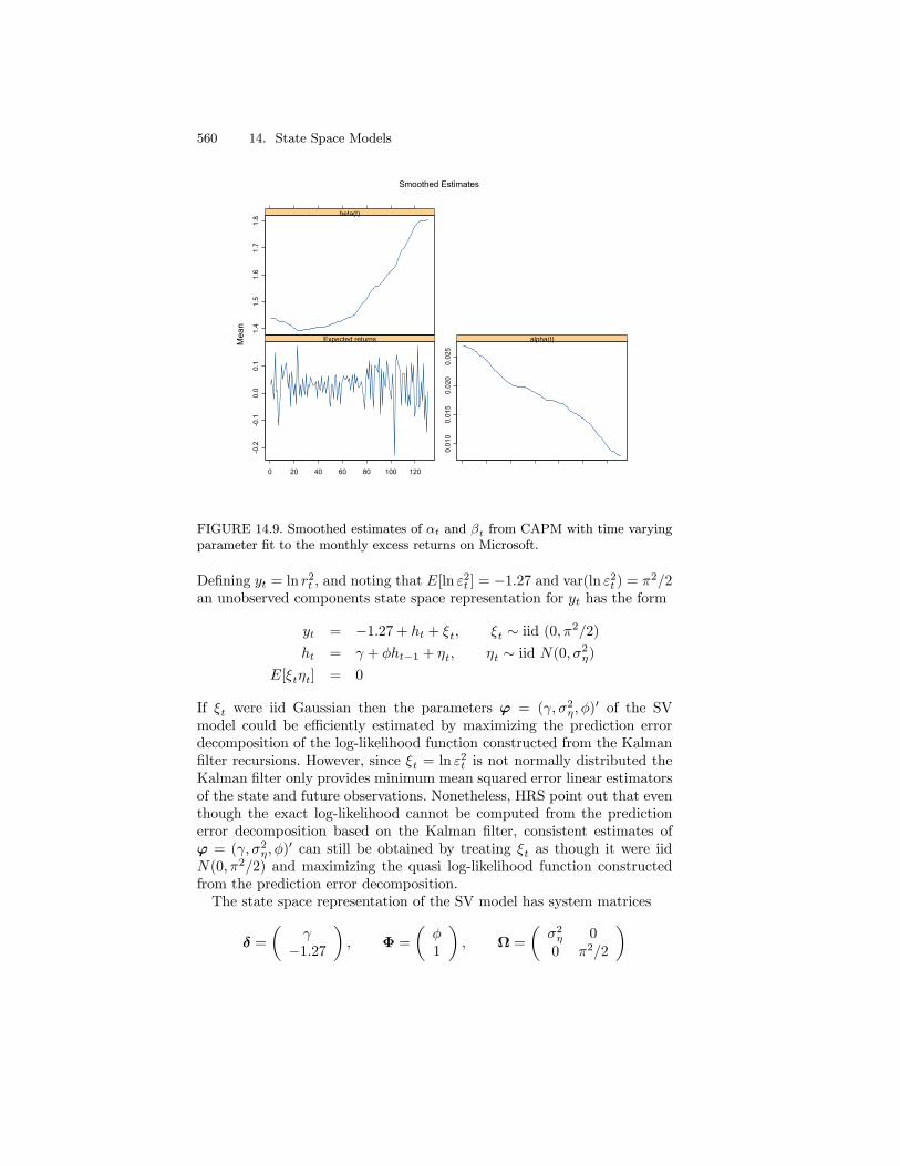
The first 250 simulated squared returns, r2t , and latent squared volatilities,σ2t , are shown in Figure 14.10.Starting values for the estimation of ϕ = (γ, lnσ2η, φ)
0 are values close tothe true values:
> sv.start = c(-0.3,log(0.03),0.9)
> names(sv.start) = c("g","ln.sigma2","phi")
Using SsfFitFast, the quasi-maximum likelihood (QML) estimates are
> low.vals = c(-Inf,-Inf,-0.999)
> up.vals = c(Inf,Inf,0.999)
> sv.mle = SsfFitFast(sv.start,sv.sim[,2],"sv.mod",
562 14. State Space Models
Simulated values from SV model
0 50 100 150 200 250
0.0
0.00
020.
0004
0.00
06
volatilitysquared returns
FIGURE 14.10. Simulated values from SV model.
+ lower=low.vals,upper=up.vals)
Iteration 0 : objective = 5.147579
...
Iteration 15 : objective = 2.21826
RELATIVE FUNCTION CONVERGENCE
To show the estimates with the QMLE standard errors use summary withthe optional argument method=\qmle"
> summary(sv.mle,method="qmle")
Log-likelihood: -2218.26
1000 observations
Parameters:
Value QMLE Std. Error t value
g -0.4810 0.18190 -2.644
ln.sigma2 -3.5630 0.53020 -6.721
phi 0.9509 0.01838 51.740
Convergence: RELATIVE FUNCTION CONVERGENCE
Using the delta method, the QMLE and estimated standard error for σ2ηare 0.02834 and 0.01503, respectively.The filtered and smoothed estimates of log-volatility are computed using
> ssf.sv = sv.mod(sv.mle2$parameters)
14.5 Simulation Smoothing 563
Log-Volatility
0 50 100 150 200 250
-11
-10
-9-8
actualfilteredsmoothed
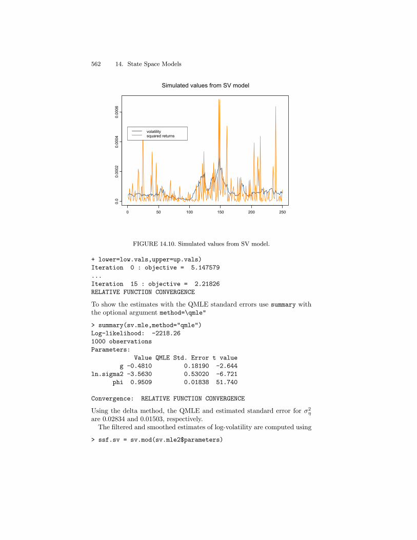
FIGURE 14.11. Log-volatility along with filtered and smoothed estimates fromSV model.
> filteredEst.sv = SsfMomentEst(sv.sim[,2],ssf.sv,task="STFIL")
> smoothedEst.sv = SsfCondDens(sv.sim[,2],ssf.sv,task="STSMO")
The first 250 estimates along with actual log-volatility are illustrated inFigure 14.11
14.5 Simulation Smoothing
The simulation of state and response vectors αt and yt or disturbancevectors ηt and εt conditional on the observations Yn is called simula-tion smoothing. Simulation smoothing is useful for evaluating the appro-priateness of a proposed state space model and for the Bayesian analysis ofstate space models using Markov chain Monte Carlo (MCMC) techniques.The S+FinMetrics/SsfPack function SimSmoDraw generates random drawsfrom the distributions of the state and response variables or from the dis-tributions of the state and response disturbances. The arguments expectedby SimSmoDraw are
> args(SimSmoDraw)
function(kf, ssf, task = "DSSIM", mRan = NULL, a1 = NULL)
564 14. State Space Models
where kf is a “KalmanFil” object, ssf is a list which either contains theminimal necessary components for a state space form or is a valid “ssf”object and task determines whether the state smoothing (“STSIM”) ordisturbance smoothing (“DSSIM”) is performed.
Example 107 Simulation smoothing from the local level model
Simulated state and response values from the local level model may begenerated using
> KalmanFil.ll = KalmanFil(y.ll,ssf.ll,task="STSIM")
> ll.state.sim = SimSmoDraw(KalmanFil.ll,ssf.ll,
+ task="STSIM")
> class(ll.state.sim)
[1] "SimSmoDraw"
> names(ll.state.sim)
[1] "state" "response" "task"
The resulting simulated values may be visualized using
> plot(ll.state.sim,layout=c(1,2))
To simulate disturbances from the state and response equations, settask="DSSIM" in the calls to KalmanFil and SimSmoDraw.
14.6 References
[1] Bomhoff, E. J. (1994). Financial Forecasting for Business and Eco-nomics. Academic Press, San Diego.
[2] Carmona, R. (2001). Statistical Analysis of Financial Data, with animplementation in Splus. Textbook under review.
[3] Chan, N.H. (2002). Time Series: Applicatios to Finance. John Wiley& Sons, New York.
[4] Durbin, J. and S.J. Koopman (2001). Time Series Analysis byState Space Methods. Oxford University Press, Oxford.
[5] Duan, J.-C. and J.-G. Simonato (1999). “Estimating Exponential-Affine Term Structure Models by Kalman Filter,” Review of Quanti-tative Finance and Accounting, 13, 111-135.
[6] Hamilton, J.D. (1994). Time Series Analysis. Princeton UniversityPress, Princeton.
[7] Harvey, A. C. (1989). Forecasting, Structural Time Series Modelsand the Kalman Filter. Cambridge University Press, Cambridge.
14.6 References 565
[8] Harvey, A.C. (1993). Time Series Models, 2nd edition. MIT Press,Cambridge.
[9] Harvey, A.C., E. Ruiz and N. Shephard (1994). “MultivariateStochastic Variance Models,” Review of Economic Studies, 61, 247-264.
[10] Kim, C.-J., and C.R. Nelson (1999). State-Space Models withRegime Switching. MIT Press, Cambridge.
[11] Koopman, S.J., N. Shephard, and J.A. Doornik (1999). “Sta-tistical Algorithms for State Space Models Using SsfPack 2.2,” Econo-metrics Journal, 2, 113-166.
[12] Koopman, S.J., N. Shephard, and J.A. Doornik (2001). “Ssf-Pack 3.0beta: Statistical Algorithms for Models in State Space,” un-published manuscript, Free University, Amsterdam.
[13] Engle, R.F. and M.W. Watson (1987). “The Kalman Filter: Ap-plications to Forecasting and Rational Expectations Models,” in T.F.Bewley (ed.) Advances in Econometrics: Fifth World Congress, Vol-ume I. Cambridge University Press, Cambridge.
[14] West, M. and J. Harrison (1997). Bayesian Forecasting and Dy-namic Models, 2nd edition. Springer-Verlag, New York.
[15] Zivot, E., Wang, J. and S.J. Koopman (2004). “State SpaceModels in Economics and Finance Using SsfPack in S+FinMetrics,”chapter 14 in Unobserved Components Models (A. Harvey, S.J. Koop-man, and N. Shephard eds.), Cambridge University Press.