ESTIMATION OF THE CRITICAL TIME STEPFOR EXPLICIT INTEGRATION

J. Plesek, R. Kolman, D. Gabriel*

Abstract: Explicit integration plays a key role in many problems of linear and non-linear dynamics. Forexample, the finite element method applied to spatial discretization of continua leaves a system of ordinarydifferential equations to be solved, which is often done by the central difference method. This and similarexplicit schemes suffer from magnification of the round-off errors if the time step exceeds certain fixed lengthknown as the critical time step.The corresponding critical Courant number (Cr, dimensionless time step) isinversely proportional to the maximum natural frequency of the system. The well known recommendationCr = 1 is deemed as the best. In fact, for some configurations this choice may dangerously overestimate thetrue value. It was shown in an earlier paper by the same authors that by increasing the number of elementsin the finite element mesh one will paradoxically improve the mesh’s stability towards its theoretical limit.The present paper refines some details, presenting small scale numerical tests. The first test involves along truss/bar consisting of one row of elements whose critical Courant number changes as elements areadded one after another. Since this increases the critical number one may pick up a time step such thatit is supercritical to a certain mesh but becomes subcritical by merely adding one element. In a similarfashion, a square area is tested in the second example, using different arrangements of edge supports. It isconcluded that the usual setting, Cr = 1, is not entirely safe.

Keywords: Explicit integration, Courant number, Critical time step, Wave propagation, Dispersion

1. INTRODUCTION

Detailed analysis of accuracy and stability of finite element wave propagation solutions was presentedin review paper Plesek et al. (2010) and references cited therein for various finite elements includingconsistent and lumped mass matrices. The critical Courant number limiting the length of the time stepin explicit integration schemes, namely the central difference method, follows from the famous formula

Crcrit =2

ω(1)

where ω is the dimensionless frequency

ω =ωmaxH

c1(2)

with ωmax being the maximum natural frequency of a finite element mesh, H the element size, andc1 the speed of the fasted wave propagating in a continuum, typically the longitudinal wave. Nearlyequally famous recommendation Cr = 1 (or slightly less to be on the safe side) for linear finite elements,also known to engineers as “rule of thumb” is deemed to be best. In fact, this observation comes fromdispersion analysis but, as it has been shown in Ref. Plesek et al. (2010), for some configurations itmay dangerously overestimate the critical time step. It was also shown that by increasing the numberof elements, N , in the finite element mesh one will improve the mesh’s stability towards Crcrit = 1 asN →∞, which is rather a paradoxical finding.

The present paper refines these details, presenting small scale numerical tests, which exemplify somepeculiarities. The first test involves a long truss/bar consisting of one row of elements whose criticalCourant number changes as elements are added one after another. Since this increases the critical numberone may pick up a time step such that it is supercritical to a certain mesh but becomes subcritical by

*Ing. Jirı Plesek, CS., Ing. Radek Kolman, PhD., Ing. Dusan Gabriel, PhD., Institute of Thermomechanics, Dolejskova 5,Praha 8, 182 00, Czech Republic

m2012

. 18thInternational ConferenceENGINEERING MECHANICS 2012 pp. 1001–1010Svratka, Czech Republic, May 14 – 17, 2012 Paper #292

merely adding one element. In a similar fashion, a square area is tested in the second example, usingdifferent arrangements of edge supports. It turns out that the numerical solutions to wave propagationmay be strongly influenced by small variation of distant boundary conditions, which should normally bephysically insignificant. Finally, the third illustration shows the direct numerical results relevant to theabove mentioned choices of sub and supercritical times steps.

2. PROBLEM DESCRIPTION

This section concerns with essentials of wave propagation in homogeneous solids, finite element tech-nology and dispersion computation.

2.1. Propagation of waves in an elastic isotropic continuum

The ith equation of motion in linear elastodynamics reads

(Λ +G)uj,ji +Gui,jj = ρui (3)

In this equation, Λ and G are Lame’s constants, ρ is the mass density and ui is the ith component ofthe displacement vector. Furthermore, a comma placed before subscripts refers to spatial differentiationwhereas the superimposed dots denote the time derivatives. The summation convention on repeatedindices is assumed. The Lame constants Λ, G may be related to engineering constants E, ν as

Λ =νE

(1 + ν) (1− 2ν), G =

E

2 (1 + ν)(4)

where E and ν are Young’s modulus and Poisson’s ratio.

In an unbounded isotropic continuum, two types of planar waves exist: the longitudinal wave andtwo transversal waves, featuring mutually orthogonal polarisation. The longitudinal wave propagateswith the speed

c1 =

√Λ + 2G

ρ(5)

The speed of the two transversal waves is

c2 =

√G

ρ(6)

The standard continuum is said to be non-dispersive. This is, by d’Alembert’s solution, because the waveprofile (wavelength) does not affect the velocity of propagation.

As a special case, one may consider a plane harmonic solution to Eqn. (3) as

ui = Ui(x) exp(ik (p · x± ct)) (7)

or its equivalent formui = Ui(x) exp(i(k · x± ωt)) (8)

where i =√−1 is the imaginary unit; x is a position vector; t is time; k is the wave number; p is the unit

normal to the wave front; k is the wave vector, k = kp; c is the phase velocity; ω is the angular velocity;and Ui is the ith component of the amplitude vector at the point defined by the position vector x. Fora given wavelength λ, the wave number k may be computed from

k =2π

λ(9)

The phase velocity c is related to ω and k by

c =ω

k(10)

Finally, the group velocity cg is defined as

cg =dωdk

(11)

In non-dispersive systems, c is a constant and since ω = ck, we get cg = c. Thus, in the absence ofdispersion the group velocity equals the phase velocity. On the other hand, cg 6= c indicates dispersion.

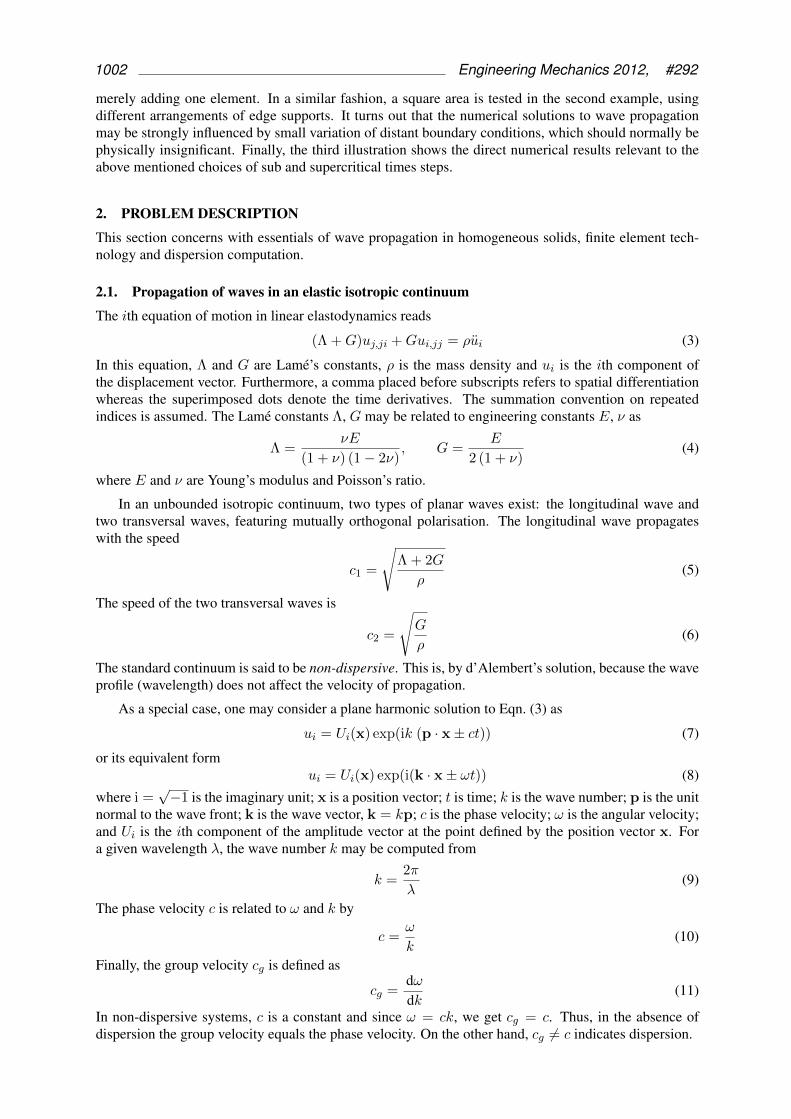
1002 Engineering Mechanics 2012, #292

2.2. Finite element method

Spatial discretization by the finite element of an elastodynamic problem introduces the ordinary differ-ential system

Mu + Ku = R (12)

Here, M is the mass matrix, K the stiffness matrix, R is the time-dependent load vector, and u and ucontain nodal displacements and accelerations. The element mass and stiffness matrices are given by

Me =

∫

VρHTH dV (13)

andKe =

∫

VBTCB dV (14)

where C is the elasticity matrix, B is the strain-displacement matrix, H stores the displacement interpo-lation functions and integration is carried over the element domain. Global matrices are assembled in theusual fashion. Under plane strain conditions, the elastic matrix C takes the form

C =E

1− ν2

1 ν 0ν 1 0

0 0 1−ν22(1+ν)

(15)

The mass matrix defined by Eqn. (13) is called the consistent mass matrix.

Explicit integration methods, such as the central difference method discussed later, require the massmatrix inverted. Thus, it is advantageous to have it diagonal or lumped. In contrast to consistent matrices,which are uniquely defined by the variational formulation, lumping procedures are not strictly prescribed.The only common principle is the ability of FEM to assemble diagonal global matrix from the elementmass matrices, thus, lumping may be performed on an element basis. Out of many methods renderingthe mass matrix diagonal we shall refer to the simplest: the row sum method (RS) for bilinear elementsand the Hinton-Rock-Zienkiewicz method (HRZ) for quadratic elements—see Ref Plesek et al. (2010).

In the subsequent analysis, a regular Hx × Hy mesh composed of plane rectangular elements isconsidered with Hx and Hy measuring the length of element edges aligned with coordinate axes. Itproves useful to define reference matrices Me, Ke for a parent element having unit properties E and ρ,unit thickness b and unit length Hx = 1. Then performing integration over the reference domain 1 × rone gets

Me = brH2xρMe (16)

andKe = bEKe (17)

Therefore, a class of problems is defined by two constants: the Poisson ratio ν and the aspect ratior = Hy/Hx. Within this class, the reference stiffness matrix Ke is a function of ν and r whereas thereference mass matrix Me is independent of both. Denote by ωe the maximum natural frequency ofa single element described by these unit matrices. For example, one may compute ωe = 2.39 for thebilinear RS elements or ωe = 7.61 for the quadratic serendipity HRZ elements.

2.3. Dispersion computation

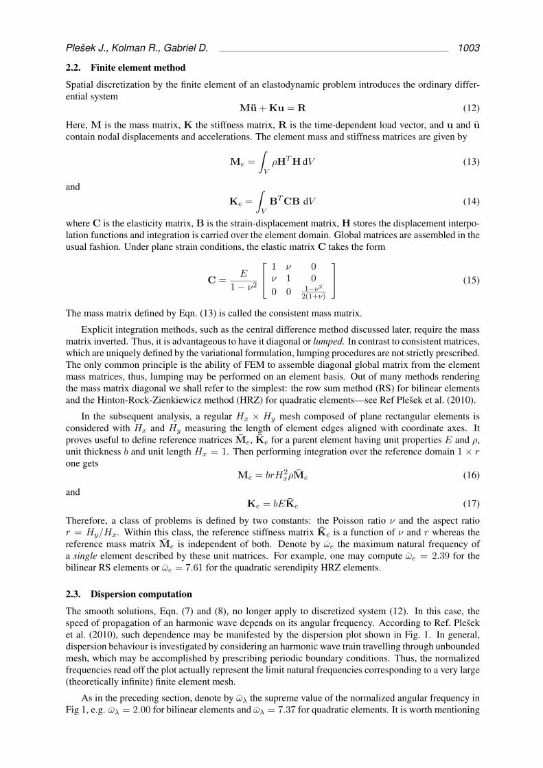
The smooth solutions, Eqn. (7) and (8), no longer apply to discretized system (12). In this case, thespeed of propagation of an harmonic wave depends on its angular frequency. According to Ref. Pleseket al. (2010), such dependence may be manifested by the dispersion plot shown in Fig. 1. In general,dispersion behaviour is investigated by considering an harmonic wave train travelling through unboundedmesh, which may be accomplished by prescribing periodic boundary conditions. Thus, the normalizedfrequencies read off the plot actually represent the limit natural frequencies corresponding to a very large(theoretically infinite) finite element mesh.

As in the preceding section, denote by ωλ the supreme value of the normalized angular frequency inFig 1, e.g. ωλ = 2.00 for bilinear elements and ωλ = 7.37 for quadratic elements. It is worth mentioning

Plesek J., Kolman R., Gabriel D. 1003

0 0.2 0.4 0.5 0.6 0.8 10

2

4

6

8

H / λh

ω H

/ c 1

longitudinalexact

transverseexact

0 0.2 0.4 0.5 0.6 0.8 10

2

4

6

7.3748

H / λh

ω H

/ c 1

longitudinalexact

transverseexact

Fig. 1: Dispersion curves for bilinear (left) and serendipity (right) elements.

that ωλ < ωe in every case. It should also be noted that the dispersion diagrams discussed in this textare entirely due to spatial dispersion, neglecting effects of time integration—refer to paper Plesek et al.(2010) for complete treatise. This by no means oversimplifies actual problems since they are namelythese theoretical values that enter stability criteria.

2.4. Explicit time integration and numerical stability

As a representative of explicit schemes, reviewed in Reference Subbaraj and Dokainish (1989), the cen-tral difference method (CDM) will be discussed. Its discrete operator reads

1

∆t2Mut+∆t = Rt − (K− 2

∆t2M)ut − 1

∆t2Mut−∆t (18)

where Rt contains forces acting on the nodal points at time t. It is well known that CDM is onlyconditionally stable, Ref. Park (1977), that is

∆t ≤ 2

ωmax(19)

where ωmax is the maximum eigenfrequency of the finite element mesh. The highest frequency canbe computed by the standard FE software, aiming at the lowest eigenvalue with K and M swapped.This method was indeed employed in all the numerical computations presented here. Alternatively, thecrititical time step may be estimated analytically as in Ref. Flanagan (1981).

At this point, it is convenient to introduce the Courant dimensionless number defined as

Cr =c1∆t

H(20)

In elastodynamics, c1 is the velocity of the longitudinal wave. Using the latter definition and that of ω inEqn. (2), the stability condition (19) can be rephrased as

Cr ≤ 2

ω(21)

or, defining Crcrit, in the form of Eqn. (1). Inequality Cr ≤ 1 then exactly manifests the Courant-Friedrichs-Lewy stability condition for the linear truss element Subbaraj and Dokainish (1989) but forother elements it may not be generally valid. On the other hand, we know, by Fried’s theorem Fried(1972), which is a direct consequence of Sturm’s polynomial separation property, that the maximumfrequency is bounded by ωe obtained as the maximum eigevalue taken over all the elements in the FEmesh.

If the mesh is regular, composed only of rectangular elements of the same aspect ratio (the so-calledstructured mesh), one may devise another estimate of the critical time step, which lends some interesting

1004 Engineering Mechanics 2012, #292

Fig. 2: Eigenvector corresponding to the highest frequency of a bar with free ends.

insight into the problem of numerical stability in general. One asymptotic case arises for the infinitemesh, when ωmax equals the supremum taken over all the dispersion curves for the particular element,i.e., ωλ is exploited. Tentatively, one may conjecture

ωλ ≤ ω ≤ ωe (22)

This expression is indeed valid for an abitrary body with free boundary, Γu = ∅, but does not hold for aconstrained mesh, for instance, if some displacement boundary conditions are prescribed. The meaningof the statement (22) will be clarified in full by examples shown in the next section.

Finally, it should be pointed out, that precisely because of the inequality (22), the true frequency of areal mesh will probably be higher than the estimate stemming from dispersion theory. Hence, the popularformula c1∆t = H for the determination of time step length is not entirely safe.

3. NUMERICAL EXPERIMENTS

Unit dimensions were set in the numerical tests as follows: mass density ρ = 1, Poisson’s ratio ν = 0.3,and Young’s modulus E = 0.7428 . . . so that c1 = 1 and c2 = 0.5345 . . .. Furthemore, plane strainsquare bilinear elements with edge length H = 1 and unit thickness, b = 1, were employed. The reasonfor chosing linear rather than quadratic elements to illustrate stability properties is that the differencebetween ωλ = 2.00 and ωe = 2.39 is greater for these elements. Having N elements in the mesh, thetotal mass is m = NρH2b = N .

3.1. Plane strain bar

As the first example we consider a plane strain bar whose length is variable depending on the number ofelements used. Fig 2 shows the eigenmode corresponding to the bar’s maximum frequency for 40 × 1discretization. The value of frequencies computed for various Ns are listed in Tab. 1.

One important observation following the inspection of Tab. 1 is that starting from the 20× 1 bar, themaximum frequency does not change within the first 8 digits, which suggests an existence of the limit.Alas, this limit, ω = 2.16, differs from the theoretical value ωλ = 2.00. On the one hand, our sequencecorrectly starts at ωe = 2.39 for 1 × 1 discretization, but on the other, the asymptotics Crcrit = 1 hasnever been reached. Why is it so? The answer lies in Fig 2. Since only the free ends vibrate, themaximum eigenvalue does not depend on the bar’s length but solely on this boundary effect. The limitsolution will not fit the periodical boundary conditions characteristic of the dispersion approach.

Tab. 1: Critical Courant numbers for the bilinear finite element mesh of a free bar.

N ω Crcrit

1x1 2.3904568 0.83666022x1 2.1837346 0.91586223x1 2.1865457 0.91468484x1 2.1664669 0.92316205x1 2.1649080 0.92382686x1 2.1621023 0.92502567x1 2.1616266 0.9252292

N ω Crcrit

8x1 2.1612303 0.92539889x1 2.1611334 0.925440310x1 2.1610747 0.925465420x1 2.1610454 0.925478040x1 2.1610454 0.925478080x1 2.1610454 0.9254780

100x1 2.1610454 0.9254780

Plesek J., Kolman R., Gabriel D. 1005

Another interesting observation follows from the graphical representation depicted in Fig. 3 on thelog scale. Apart from the limit, there is a pronounced gap between the three and four element configura-tions. Selecting Cr = 0.92, the time step is stable for the 4 × 1 mesh but unstable for the smaller 3 × 1mesh. This motivates the critical test defined in Fig. 4.

100

101

102

0.80

0.85

0.9

0.9255

0.95

1.00

Number of elements

Crit

ical

Cou

rant

num

ber

Fig. 3: Distribution of the critical Courant number for the bar with free ends.

F = 1/2 F(t)1

H

H

N H

F = 1/2 F(t)2 A

Fig. 4: Transient problem with Heaviside load; unstable configuration.

A three-element bar is loaded by the Heaviside step function F (t) = 1 for t > 0. Since Cr =0.92 > Crcrit one expects an incursion of instability after some time has elapsed but a stable solution if afour-element problem had been considered instead. In both the cases, parabolic displacement evolution

u(t) =F

2mt2 =

t2

2N(23)

applies to the motion of the whole body. The average acceleration, 1/N , measured at the control pointA for the 4 × 1 configuration equals 0.25. The existence of the stable solution is confirmed by plotsshown in Fig. 5. The oscillatory course of acceleration history is due to waves reflection about the meanvalue 0.25, which matches the rigid body motion. By contrast, the unstable 3 × 1 problem exhibits thesolution’s uncotrolled blow up at about t = 3000, see Fig. 6. The instability commences even muchearlier after several wave reflections, which is nicely captured in Fig. 7.

Let us return to the original eigenvalue problem shown in Fig. 2. This time the boundary conditionsare modified by clamping the right end. The corresponding eigenvector and the frequencies computedare shown in Fig. 8 and Tab. 2, respectively. The same limit ω = 2.16 is reached already by the 8 × 1discretization, which is not surprising. Indeed, the vibration modes roughly correspond to those of thefree bar twice the length of the free-fixed bar. A more interesting fact is that the maximum frequencynow increases. This is because the results converge to the same limit as before but for each N -elementbar the constrained configuration has lower maximum frequency than the free one. The critical Courantnumber distribution is shown in Fig. 9

We close our discussion concerning this example with the remark that the conjecture (22) does nothold for a constrained problem. For example, for the free-fixed bar ωλ > ω1×1, because the maximu

1006 Engineering Mechanics 2012, #292

0 2000 4000 6000 8000 100000

2

4

6

8

10

12x 10

6

Time [s]

Dis

plac

emen

t [m

]

0 2000 4000 6000 8000 100000

500

1000

1500

2000

2500

Time [s]

Vel

ocity

[m/s

]0 2000 4000 6000 8000 10000

−1

−0.5

0

0.5

1

1.5

Time [s]

Acc

eler

atio

n [m

/s2 ]

Fig. 5: Displacement, velocity and acceleration in the stable 4× 1 computation.

0 1000 2000 3000 4000−3

−2

−1

0

1

2

3x 10

307

Time [s]

Dis

plac

emen

t [m

]

0 1000 2000 3000 4000−6

−4

−2

0

2

4

6

8x 10

306

Time [s]

Vel

ocity

[m/s

]

0 1000 2000 3000 4000−1−1

0.12

1.241.24x 10

308

Time [s]

Acc

eler

atio

n [m

/s2 ]

Fig. 6: Displacement, velocity and acceleration in the unstable 3× 1 computation.

frequency has been reduced by the imposition of the boundary condition. Theoretically, one could evenhave had ω = 0 if all the nodes had been fixed. By contrast, ωe always forms the upper bound.

3.2. Plane strain square domain

Similar examples as in the preceding section may be analysed. Consider a plane strain square do-main shown in Fig. 10 and the critical Courant number distributions for both (fixed and free) boundaryconfigurations—Fig. 11.

In this case, convergence to the limit Crcrit = 0.99 is observed. Similarly as for the free bar this num-ber is slightly less than the theoretical value Crcrit = 1. The reason can again been seen in Fig. 10, which

Plesek J., Kolman R., Gabriel D. 1007

0 10 20 30 40 50−8000

−6000

−4000

−2000

0

2000

4000

6000

8000

Time [s]

Acc

eler

atio

n [m

/s2 ]

Fig. 7: Detail of acceleration build up.

Fig. 8: A free-fixed bar.

suggests that it is the vibration of the corner elements that is responsible for the maximum frequency andis, in fact, independent of the mesh size.

A new phenomenon is detected with the constrained mesh. Comparing it with the free-fixed barone notices that, here, zero displacements are prescribed along the whole boundary. This means thatadding extra elements is merely equivalent to mesh refinement, which in turn implies the increase of thedimensionless maximum frequency. Since the mesh grading is regular and there are no boundary effects,monotonous convergence to the theoretical limit, Crcrit = 1, follows. It is interesting to note that also inthis situation ω < ωλ, which violates condition (22) as the present problem is fully constrained.

4. CONCLUSIONS

It might seem at first glance that, except illustrating certain mathematical principles, the present studybears little importance to real-world computation. On the one hand, todays engineering problems areextremely large (rendernig N → ∞ effectively) and, on the other, one may safely use the upper boundby calculating the maximum eigenvalue of a single element.

Tab. 2: Critical Courant numbers for the free-fixed bar.

N ω Crcrit

1x1 1.8403500 1.08674982x1 2.1530847 0.92889983x1 2.1587386 0.92646704x1 2.1608547 0.92555975x1 2.1609985 0.92549816x1 2.1610395 0.92548057x1 2.1610425 0.9254793

N ω Crcrit

8x1 2.1610454 0.92547809x1 2.1610454 0.925478010x1 2.1610454 0.925478020x1 2.1610454 0.925478040x1 2.1610454 0.925478080x1 2.1610454 0.9254780100x1 2.1610454 0.9254780

1008 Engineering Mechanics 2012, #292

100

101

102

0.80

0.85

0.90

0.9255

0.95

1.00

1.05

1.10

Number of elements

Crit

ical

Cou

rant

num

ber

Fig. 9: Distribution of the Critical Courant number for the free-fixed bar.

Fig. 10: Maximum eigenmode of a free square domain (left) and the domain with fixed edges (right).

100

101

102

0.80

0.85

0.90

0.9913

0.95

1.00

1.05

Number of elements

Crit

ical

Cou

rant

num

ber

1 2 10 1000.8

0.9

1

1.1

1.2

1.3

1.4

1.5

1.6

Number of elements

Crit

ical

Cou

rant

num

ber

Fig. 11: Critical Courant numbers for free (left) and fixed domain (right).

It should be borne in mind that Fried’s estimate, ω ≤ ωe, is only useful for a structured mesh whenall the elements have the same spectrum. For an unstructured mesh, this information is hardly availableand one must resort to other estimates. It is namely under such circumstances that the analysts use theωλ limit derived from dispersion diagrams often unaware of its pitfalls. It must be emphasised that forthe reasons exaplained in the paper the frequent recommendation c1∆t = H is not entirely safe.

Plesek J., Kolman R., Gabriel D. 1009

The examples involving free bodies clearly demonstrated the way the vibration of corner elementschanged the stability limits. Hence, we conclude that even distant boundary conditions, which shouldnormally be physically insignificant, may considerably influence numerical solution.

Acknowledgements

This work was supported by GACR 101/09/1630 granted project in the framework of AV0Z20760514research plan.

References

Plesek, J. , Kolman, R., Gabriel, D. (2010) Dispersion errors of finite element discretizations in elasto-dynamics. Computational Technology Reviews Vol. 1, Saxe-Coburg Publications, 251–279.

Dokainish, M.A., Subbaraj, K. (1989) A survey of direct time-integration methods in computationalstructural dynamics - I: Explicit methods. Computers & Structures, 32, 1371–1386.

Park, K.C. (1977) Practical aspect of numerical time integration. Computers & Structures, 7, 343–353.

Flanagan, D.P., Belytschko, T. (1981) A uniform strain hexahedron and quadrilateral with orthogonalhourglass control. Int. J. Num. Methods Engng., 17, 679–706.

Fried, I. (1972) Bounds on the extremal eigenvalues of the finite element stiffness and mass matrices andtheir spectral condition number. Journal of Sound and Vibration, 22, 407–418.

1010 Engineering Mechanics 2012, #292