think comparch - olin college
TRANSCRIPT
Think CompArch
Samantha Kumarasena, Anne Wilkinson, Tenzin Choetso
December 17, 2014
1 Introduction
Hi, future Computer Architecture student! Are you confused by all this HDL stuff? Do wires and regs notmake sense? Having trouble with assign statements? Have no idea what any of that means? Well, this guideis for you! Verilog, although its syntax is C-like, is very different from other programming languages youmight be familiar with. We’ll describe the basic concepts behind the features of the Verilog language, andexplain how they might be used. We’ll also provide annotated code examples, but make sure to focus on theconcepts behind the code! If you don’t, you’re in for a Verilog night.
(That was a joke. Say it out loud.)
1.1 How to Use This Guide
This guide will be split into three sections. The first part will be an introduction to the Verilog programminglanguage. The next part will be a collection of ModelSim tips and tricks. The final section will be anoverview of the MIPS instruction set, which will be useful if you’re simulating your own CPU. We’ll includecode examples and walkthroughs. All code examples are included in the Files For Verilog Examplessection, and on our GitHub: https://github.com/skumarasena/ThinkCompArch. Links to other sectionswill be bolded and in red boxes (just like they are here). Please note that you can click on them.
Figure 1: Go on, turn to the next page! A wonderful world of simulation awaits you!
1

Contents1 Introduction 1
1.1 How to Use This Guide . . . . . . . . . . . . . . . . . . . . . . . . . . . . . . . . . . . . . . . 1
2 Think Verilog 4
2.1 Intro and Basic Gates . . . . . . . . . . . . . . . . . . . . . . . . . . . . . . . . . . . . . . . . 4
2.2 Modules . . . . . . . . . . . . . . . . . . . . . . . . . . . . . . . . . . . . . . . . . . . . . . . . 4
2.3 Syntax . . . . . . . . . . . . . . . . . . . . . . . . . . . . . . . . . . . . . . . . . . . . . . . . . 6
2.3.1 Numbers . . . . . . . . . . . . . . . . . . . . . . . . . . . . . . . . . . . . . . . . . . . 7
2.3.2 x’s and z’s . . . . . . . . . . . . . . . . . . . . . . . . . . . . . . . . . . . . . . . . . . 7
2.3.3 Conditionals . . . . . . . . . . . . . . . . . . . . . . . . . . . . . . . . . . . . . . . . . 7
2.3.4 Concatenation . . . . . . . . . . . . . . . . . . . . . . . . . . . . . . . . . . . . . . . . 7
2.3.5 Delays . . . . . . . . . . . . . . . . . . . . . . . . . . . . . . . . . . . . . . . . . . . . . 8
2.3.6 Keywords . . . . . . . . . . . . . . . . . . . . . . . . . . . . . . . . . . . . . . . . . . . 9
2.3.7 Generate Syntax . . . . . . . . . . . . . . . . . . . . . . . . . . . . . . . . . . . . . . . 9
2.4 Wire Assignment . . . . . . . . . . . . . . . . . . . . . . . . . . . . . . . . . . . . . . . . . . . 10
2.5 Behavioral vs Structural . . . . . . . . . . . . . . . . . . . . . . . . . . . . . . . . . . . . . . . 10
2.6 Registers . . . . . . . . . . . . . . . . . . . . . . . . . . . . . . . . . . . . . . . . . . . . . . . . 12
2.7 Procedural Blocks: initial/always . . . . . . . . . . . . . . . . . . . . . . . . . . . . . . . . 12
2.7.1 initial Blocks . . . . . . . . . . . . . . . . . . . . . . . . . . . . . . . . . . . . . . . . 13
2.7.2 always Blocks . . . . . . . . . . . . . . . . . . . . . . . . . . . . . . . . . . . . . . . . 13
2.8 Test Benches . . . . . . . . . . . . . . . . . . . . . . . . . . . . . . . . . . . . . . . . . . . . . 16
2.9 Useful Links . . . . . . . . . . . . . . . . . . . . . . . . . . . . . . . . . . . . . . . . . . . . . . 20
3 Think ModelSim 21
3.1 What is ModelSim? . . . . . . . . . . . . . . . . . . . . . . . . . . . . . . . . . . . . . . . . . 21
3.2 Creating a Project . . . . . . . . . . . . . . . . . . . . . . . . . . . . . . . . . . . . . . . . . . 21
3.3 .do Files . . . . . . . . . . . . . . . . . . . . . . . . . . . . . . . . . . . . . . . . . . . . . . . . 21
3.3.1 Clearing Libraries . . . . . . . . . . . . . . . . . . . . . . . . . . . . . . . . . . . . . . 23
3.3.2 Generating Waveforms . . . . . . . . . . . . . . . . . . . . . . . . . . . . . . . . . . . . 23
3.4 Debugging: Common Errors and Explanations . . . . . . . . . . . . . . . . . . . . . . . . . . 25
3.4.1 Debugging x And z . . . . . . . . . . . . . . . . . . . . . . . . . . . . . . . . . . . . . 27
3.5 Using Waveforms in Debugging . . . . . . . . . . . . . . . . . . . . . . . . . . . . . . . . . . . 28
3.5.1 Early-Transitioning . . . . . . . . . . . . . . . . . . . . . . . . . . . . . . . . . . . . . . 29
3.5.2 Looking At Wire/Reg Values . . . . . . . . . . . . . . . . . . . . . . . . . . . . . . . . 29
3.5.3 Data Flow . . . . . . . . . . . . . . . . . . . . . . . . . . . . . . . . . . . . . . . . . . . 30
3.5.4 Adding Waves to a Waveform . . . . . . . . . . . . . . . . . . . . . . . . . . . . . . . . 32
3.6 Procedural Blocks Are Hard . . . . . . . . . . . . . . . . . . . . . . . . . . . . . . . . . . . . . 36
3.7 Useful Links . . . . . . . . . . . . . . . . . . . . . . . . . . . . . . . . . . . . . . . . . . . . . . 39
4 Think MIPS 40
4.1 What is MIPS? . . . . . . . . . . . . . . . . . . . . . . . . . . . . . . . . . . . . . . . . . . . . 40
4.2 RTL: Register Transfer Language . . . . . . . . . . . . . . . . . . . . . . . . . . . . . . . . . . 40
4.3 Register Assignments . . . . . . . . . . . . . . . . . . . . . . . . . . . . . . . . . . . . . . . . . 40
4.4 Intro to MIPS commands . . . . . . . . . . . . . . . . . . . . . . . . . . . . . . . . . . . . . . 41
4.5 R-type . . . . . . . . . . . . . . . . . . . . . . . . . . . . . . . . . . . . . . . . . . . . . . . . . 41
4.6 I-type . . . . . . . . . . . . . . . . . . . . . . . . . . . . . . . . . . . . . . . . . . . . . . . . . 43
4.7 J-type . . . . . . . . . . . . . . . . . . . . . . . . . . . . . . . . . . . . . . . . . . . . . . . . . 45
4.8 Useful Links . . . . . . . . . . . . . . . . . . . . . . . . . . . . . . . . . . . . . . . . . . . . . . 47
2

5 Files For Verilog Examples 48
5.1 Behavioral vs. Structural Example: Gates . . . . . . . . . . . . . . . . . . . . . . . . . . . . . 49
5.2 Procedural Blocks Example: countingClocks . . . . . . . . . . . . . . . . . . . . . . . . . . . . 51
5.3 Test Benches Example: Adders . . . . . . . . . . . . . . . . . . . . . . . . . . . . . . . . . . . 53
3

2 Think Verilog
2.1 Intro and Basic Gates
Verilog is a Hardware Description Language (HDL). This means that Verilog is a language that describesthe physical hardware of a circuit. Since the language essentially describes a circuit, it is different from theconventional software programming languages that you might be used to – we will cover lots of conceptualdifferences, so be sure to read the following sections carefully! Verilog is used to design circuits and circuitcomponents and simulate the behavior of these circuits. In this class, you’ll start with small structures andbuild up; eventually, the final lab for our year’s class was to design and test our own CPU! It was prettycool.
You’ll start by designing and testing small circuits out of logic gates. Verilog supports all the basic logicgates you’ve come to know and love (which are known as gate primitives): AND, NAND, OR, NOR, XOR,XNOR, and NOT. Below is an example of an AND gate and an OR gate being used in Verilog. In Verilog,gates have one output and can have as many inputs as you like (in this case, our example gates are shownwith two inputs). The Verilog code is shown above the representative circuit diagram – the bolded gatetypes, and and or in the code below determines what type of gate we are using, “andgate” and “orgate”are their respective names, “out” is the output of each gate, and “in0” and “in1” are the two inputs. Notethat order matters for the parameters – the output parameter must be included before all input parameterswhen using logic gates.
1 and andgate(out , in0 , in1); or orgate(out , in0 , in1);
Figure 2: an AND gate and an OR gate. The Verilog code is included above the gate diagrams, and therepresentative diagram is included below. The inputs, output, and gate names are labeled.
If you’ve programmed in object-oriented languages before, you’ll notice that this syntax is similar to that ofinitializing an object. You can think of “andgate”/“orgate” as being instances of the and/or gate-primitiveclasses, respectively. Note that you cannot have more than one instance of the same name within the samemodule.
But what if you want to use more complicated components than mere logic gates? You’ll have to connect abunch of gates together. But it would be a pain to copy-paste these structures over and over if you wantedto use them more than once. You’ll have to define a module.
2.2 Modules
Modules are the basic building block for circuit design in Verilog. You can use modules to design, initialize,and use complicated components. Their syntax is similar to a function – they have a definition, have inputsand outputs, and can be called elsewhere in the program – but think of them more like objects. You canuse them just like the logic gate primitives we looked at earlier. You can have multiple instances of a givenmodule and wire them in the appropriate configurations. Think of them as circuit components, like a chipin a circuit board that performs a particular function.
4

Much like an actual chip in a circuit board, modules have input and output wires. (If you look back at theand and or examples from the previous section, you’ll notice that out, in0, and in1 are all wires as well).Note that so far, we have not really explained what wires are. You may be thinking of them as variables ina conventional programming language. Don’t make this mistake – modules are not functions, wires are notvariables.
We’ve emphasized that wires are not variables. Well, what are they? Wires are connections, and modulesare components. Wires connect components to other components. They serve as inputs and outputs to thesecomponents. If you ever get confused by the structure of your program, make the analogy to a circuit on acircuit board, and think of them as physical wires between components.
In a module, you’re going to have a bunch of assignments, gates and logic. In many programming languages,statements are executed procedurally – that is, the first statement must finish before the second beginsexecution. In a conventional programming language, the following example...
1 count = count + 1; // executes first
2 count = count + 1; // executes second
...would result in count being incremented by 2. However, in Verilog, statements are executed simultane-ously. This means that the code example we just looked at...
1 //both execute at the same time! whoa ...
2 count = count + 1;
3 count = count + 1;
...would result in count being incremented by 1, since both statements draw from the same value of count.Keep this in mind when writing your code – the order of your statements (largely) does not matter. Thereare a few scenarios in which it does matter: (1) if you try to use a wire before it’s been declared, you’ll getan error, so don’t do that (2) if you use blocking assignments in an always block (3) if you use delays in aninitial block. Those last two scenarios probably don’t make sense to you – don’t worry about it. We’lltalk about them later in this guide, in the initial Blocks and always Blocks sections, respectively.
We’ve included the skeleton of a module below. Just like gate primitives, modules have names and inputsand outputs. However, unlike gate primitives, you can have as many outputs and inputs as you like. You canalso put these outputs and inputs wherever you like (although some people like to put outputs before inputs.Just make sure you’re consistent when you initialize the module – Verilog will not know which wires are in-puts and outputs.) Moreover, these inputs and outputs can be of different sizes. Take a look at this example:
1 /* block comment here */
2 module moduleName(out0 , out1 , in0 , in1);
3 // these declarations don ’t have to be in any order
4 input [5:0] in0; //6-bit input
5 input in1; // default size is one
6 output[7:0] out0; //8-bit output
7 output out1; //again , default size one
8
9 //Code Here
10
11 endmodule
Notice that we declare input wires using input, and output wires using output. The input and outputdeclarations do not have to be in any particular order. Also notice that some of the input and output
5

declarations have [some number: 0] prior to the input name. These brackets specify how large the inputsare. In the in0 declaration, the [5:0] indicates that the input is 6 bits long. In our circuit analogy, thiswould be like having 6 separate wires feeding into this particular input.
Generally speaking, the syntax to declare an input is “input [size-1:0] inputname” where size is thesize of the input in bits. Similarly, the syntax to declare an output is “output [size-1] outputname”. Touse the module we have just created, we would initialize it as shown below:
1 wire [7:0] outwire0; // Initializing output wires to be used.
2 wire outwire1;
3 wire [5:0] inwire0; // Initializing input wires to be used.
4 wire inwire1; //In a real circuit , these wires would
5 //come from somewhere important.
6
7 moduleName instanceName(outwire0 , outwire1 , inwire0 , inwire1 );
When we declare these wires, we don’t specifically have to declare them as inputs or outputs because wiresconnect components to other components – they aren’t directional. However, within a module, you do haveto specify which wires are inputs and which wires are outputs.
Also note that wires are not indexed in the left-to-right fashion that is typical of arrays in other programminglanguages. Instead, they are indexed from the least-significant bit to the most-significant bit. A diagram isshown below:
Figure 3: A diagram of Verilog’s indexing. Notice that the indexing starts with the least-significant bit(LSB) on the left, and increases toward the most-significant bit (MSB) on the right. This is the opposite ofhow most arrays are indexed, so be careful when you’re trying to refer to specific bits!
Sometimes you will want to refer to specific bits of a given wire, in which case remembering how Verilogindexes its bits is critical. Say you have a 32-bit wire a, and you want to refer to bits 2 through 10 (again,zero-indexed from the least-significant bit). In our circuit analogy, this is like splitting a multi-wire cable.We’ve included the syntax for doing so below:
1 wire [31:0] a;
2 wire b = a[10:2];
This example will assign wire b to bits 2 through 10 of a (so wire b is a total of 9 bits, or 9 wires in ouranalogy). Again, these bits are arranged in reverse order – index decreases as you move to the right.
2.3 Syntax
So far, we’ve exclusively been talking about how Verilog programs are structured. We’ll break for a bit totalk about syntax because we’ll be using some of these syntax details later. For a more comprehensive syntaxreference guide, see http://web.stanford.edu/class/ee183/handouts_win2003/VerilogQuickRef.pdf
6
Some of this has already been implied in previous sections, but for formality’s sake: Verilog is a whitespace-independent (i.e. placement of tabs and spaces does not matter) langauge with C-like syntax. It featuresthe standard logical (&, |, !, etc), comparison (==, >=, <=, !=, etc.) and arithmetic (+, −, /, ∗, etc.)operators.
2.3.1 Numbers
When using numbers in your program, you will need to specify size and radix. A binary number will beformatted as [size]’b[number]. For example, the 6-bit binary representation of d5 is 6’b000101. This canalso be written as 6’b101, as Verilog will substitute any non-specified leading bits with zeros. Similarly, the6-bit decimal representation of d10 would be 6’d000010, while the 6-bit hexadecimal representation of 31would be 6’h00001f.
2.3.2 x’s and z’s
When Verilog cannot determine what the value of an input or an output is, it will often tell you that its valueis x or z. The latter often occurs if a wire is not driven at all, and indicates a high-impedance output. Theformer indicates that Verilog can’t determine whether your signal is a 1 or a 0. We’ll talk about this more inthe Debugging x And z section of “Think ModelSim”. Just note that there are more possibilities than 1 or0 – you might have an x or a z, so be careful with your comparison statements. There are special operators(known as “case comparison” operators) that deal with the possibility of the value being x or z. The “caseequality” operator (===) will determine whether two values are equal, including x and z. Similarly, the“case inequality” operator (!==) will determine whether two values are not equal, including x and z.
2.3.3 Conditionals
To implement a conditional statement, use begin and end for each case. You can think of begin and end
as being analogues for the curly braces that are often used to distinguish blocks in other programming lan-guages. Here’s an example framework:
1 i f (A == B) begin2 //Case 1
3 end4 e l se i f (A==C) begin5 //Case 2
6 end7 e l se begin8 //Case 3
9 end
2.3.4 Concatenation
Sometimes you want to concatenate the values of two wire types. Using our circuit analogy, this is likecombining two bundles of wires. Say we want to combine wires a and b into a single wire c. Wires a and b
are defined below:
7

1 wire a;
2 wire [1:0] b; // represents two physical wires!
Note that while wire a represents a single wire in our circuit analogy, wire b represents two separate wiresbundled together. If we extend our circuit analogy to concatenation, the diagram below illustrates whatoccurs: we are combining bundles of wires together.
Figure 4: Concatenation of wires a and b to create wire c. Before concatenation wire a is a single wire andwire b is a “bundle” of two wires in our circuit analogy. After concatenation, wire c becomes a bundle ofthree wires.
The following syntax accomplishes the same thing. We have assigned wire a to the value b1 and wire b tothe value b00. As a result, wire c becomes b100:
1 // Concatenates a and b
2 wire a = 1’b1; // binary representation of a
3 wire [1:0] b = 2’b00; // binary representation of b
4 wire [2:0] c;
5 assign c = {a,b} // Assigns c to 3’b100
Since wire a comes first in the concatenation, its value (b1) is placed in the most-significant bit of c. Wireb comes second, so its value (b00) is placed in the two least-significant bit places.
2.3.5 Delays
Delays are useful for simulating the timing of a physical circuit, because all components have some degree ofpropagation delay. You can put delays in your code by using #[delay amount], where the amount of delayis specified in nanoseconds. For example, #300 would specify a delay time of 300 ns. A delay can be put ona gate, like so:
1 and #300 andgate(out , in0 , in1);
In this case, the gate has a 300-nanosecond delay between the time at which its inputs are set and the timeat which its output changes. Delays can also be used in initial blocks, and we’ll talk about this in theinitial Blocks section.
8

2.3.6 Keywords
Also be sure not to use Verilog keywords in your variable names. Some examples: assign, case, while,
wire, reg, and, or, nand, module. For a full list, see: http://www.xilinx.com/support/documentation/sw_manuals/xilinx13_1/ite_r_verilog_reserved_words.htm
2.3.7 Generate Syntax
A Verilog feature you might find useful is the generate block. A generate block tells the Verilog compilerto repeat your statement a bunch of times. It’s often used to reduce the repetitive aspect of instantiatinglarge structures. It must be defined within a module and can have for loops, if-else statements andcase decisions to control what objects are generated. Note that it sort of looks like a for-loop. This is nottechnically the case. What a generate block actually does is repeat all statements inside many times. We’llshow you what we mean in the example below.
This section introduces a new data type, genvar. The genvar data type stores positive integer values, isused in a generate block, and indicates which variable is iterated upon in the generate block.
Here is an example that uses generate that iterates through two 32-bit input wires, a and b, and performsa bitwise-AND. The result of the bitwise-AND is put in the 32-bit out wire.
1 wire [31:0] a; // wires a, b would come from someplace
2 wire [31:0] b; // meaningful in an actual use case
3 wire [31:0] out;
4
5 generate6 genvar index;
7 for (index = 0; index <32; index = index + 1) begin8 and andgate(out[index], a[index], b[index ]);
9 end10 endgenerate
This syntax iterates over a and b, ANDs both bits together, and stores the result in the appropriate indexof out. Note that Verilog is really just repeating the statement inside the generate block a bunch of times.What Verilog actually executes is:
1 and andgate(out[0], a[0], b[0]);
2 and andgate(out[1], a[1], b[1]);
3 and andgate(out[2], a[2], b[2]);
4
5 //... and so on...
6
7 and andgate(out[31], a[31], b[31]);
When using generate blocks, you must label the variable you intend to iterate on (index, in this case) as“genvar”. This is because all that changes here is the index, which is why you must declare the index as agenvar.
The generate syntax is particularly useful because Verilog does not allow 2-dimensional inputs or outputs(silly, we know). As a result, you’ll often need to repeat lines of code many times with increasing indices.
9
Now, back to your regularly scheduled programming. (Oh look, another bad pun.)
2.4 Wire Assignment
We’ve already introduced wires and the concepts behind them. But because the concept is so important,we’re doing our best to be super clear.
Again, wires represent structural connections and are analogous to wires in an actual circuit. An exampleof an 8-bit wire initialization is shown below:
1 wire [7:0] a;
Here, a is an 8-bit wire. To assign values to wires, you can use the outputs of primitives or modules, aswe’ve seen above. Additionally, you can assign wires to other wires or to specific values, as shown below:
1 wire d = a && b;
This sets the value of wire d to the logical AND of wires a and b. The assign keyword can also be used toassign the values of wires. (In the previous example, the assign is implicitly assumed.)
1 wire d; // explicit assignment statement
2 assign d = a && b;
These two examples do the same thing – they assign a wire to the same value. These assignments (andall assignments involving wires) are continuous assignments; it happens constantly for the duration of yourprogram. This is important because later in this guide, we’ll talk about other sorts of assignment that aren’tcontinuous (in the Registers section).
2.5 Behavioral vs Structural
Up until now, all of the examples have been for Structural Verilog. In Structural Verilog, the emphasis is onimplementation – you are using circuit components to create a module. Behavioral Verilog involves a higherlevel of abstraction, and the focus is on what a module does versus how it is built.
Here is a simple example of the same behavior written in both Structural and Behavioral Verilog:
1 // Structural Verilog
2 wire d;
3 and andgate(d, a, b);
4 not inv(c, d);
5
6
7 // Behavioral Verilog
8 assign c = !(a && b);
The two code blocks have the same functionality. The Structural Verilog example uses gates to create aninverted AND gate (a NAND), whereas Behavioral uses logical operators on the wires to produce the sameresult.
10
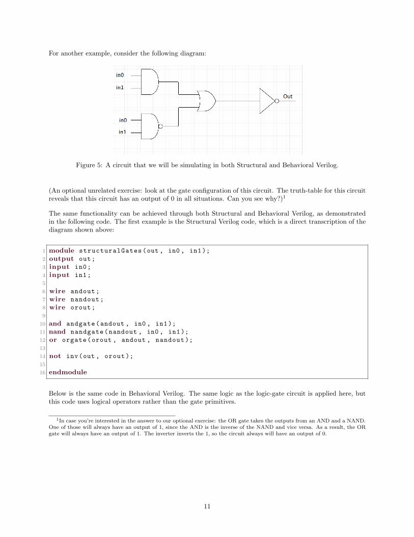
For another example, consider the following diagram:
Figure 5: A circuit that we will be simulating in both Structural and Behavioral Verilog.
(An optional unrelated exercise: look at the gate configuration of this circuit. The truth-table for this circuitreveals that this circuit has an output of 0 in all situations. Can you see why?)1
The same functionality can be achieved through both Structural and Behavioral Verilog, as demonstratedin the following code. The first example is the Structural Verilog code, which is a direct transcription of thediagram shown above:
1 module structuralGates(out , in0 , in1);
2 output out;
3 input in0;
4 input in1;
5
6 wire andout;
7 wire nandout;
8 wire orout;
9
10 and andgate(andout , in0 , in1);
11 nand nandgate(nandout , in0 , in1);
12 or orgate(orout , andout , nandout );
13
14 not inv(out , orout);
15
16 endmodule
Below is the same code in Behavioral Verilog. The same logic as the logic-gate circuit is applied here, butthis code uses logical operators rather than the gate primitives.
1In case you’re interested in the answer to our optional exercise: the OR gate takes the outputs from an AND and a NAND.One of those will always have an output of 1, since the AND is the inverse of the NAND and vice versa. As a result, the ORgate will always have an output of 1. The inverter inverts the 1, so the circuit always will have an output of 0.
11

1 module behavioralGates(out , in0 , in1);
2 output out;
3 input in0;
4 input in1;
5
6 assign out = !(( in0 && in1) || !(in0 && in1));
7
8 endmodule
The benefit of Behavioral Verilog is that it allows you to quickly implement and model larger, more complexstructures that would otherwise involve a lot of gates and wires. The drawback is that Behavioral Verilog isoften slower and less efficient than Structural Verilog. If you were to synthesize this code on an FPGA, youwould find that the Behavioral Verilog module requires a lot more resources.
Now that we’ve started to introduce more complicated code examples, we’ll provide complete Verilog filesand .do files so you can try running them yourself. See the Behavioral vs. Structural Example: Gatessection under Files For Verilog Examples at the end of our guide for the full code files. (We’ll talk abouthow to make .do files of your own in “Think ModelSim”, in the .do Files section). You can also find thefull code examples on GitHub: https://github.com/skumarasena/ThinkCompArch.
2.6 Registers
Now, we’ll talk about an alternative to wires: registers. You might have been wondering why we put emphasison the fact that wires use continuous assignment in the Wire Assignment section. It’s mainly becauseregisters don’t use continuous assignment.
An example of a register declaration is shown below. In this example, we have declared a 4-bit registernamed “myregister”:
1 reg [3:0] myregister;
Notice that the declaration syntax is very similar to wire declaration. The data type, reg, is followed by thesize (which is formatted as [size-1:0]), which is followed by the register name.
Registers, like wires, have values. Unlike wires, these values are only assigned at specific points in theprogram. This is because the “register” type in Verilog is based on hardware registers, which store theirvalues until they are explicitly changed. As a result, registers need to be used in contexts in which they areassigned at very specific times. You can’t use a register with an assign statement. You also can’t set aregister equal to a value outside of the context of a procedural block.
But what is a procedural block? Funny you should ask. . .
2.7 Procedural Blocks: initial/always
A procedural block is a block where the steps inside occur at very specific, scheduled times. This is in contrastto wires, which are continually assigned to a particular value. Procedural blocks begin with a begin, andend with an end, just like conditional statements. There are two types of procedural blocks: initial blocksand always blocks.
12
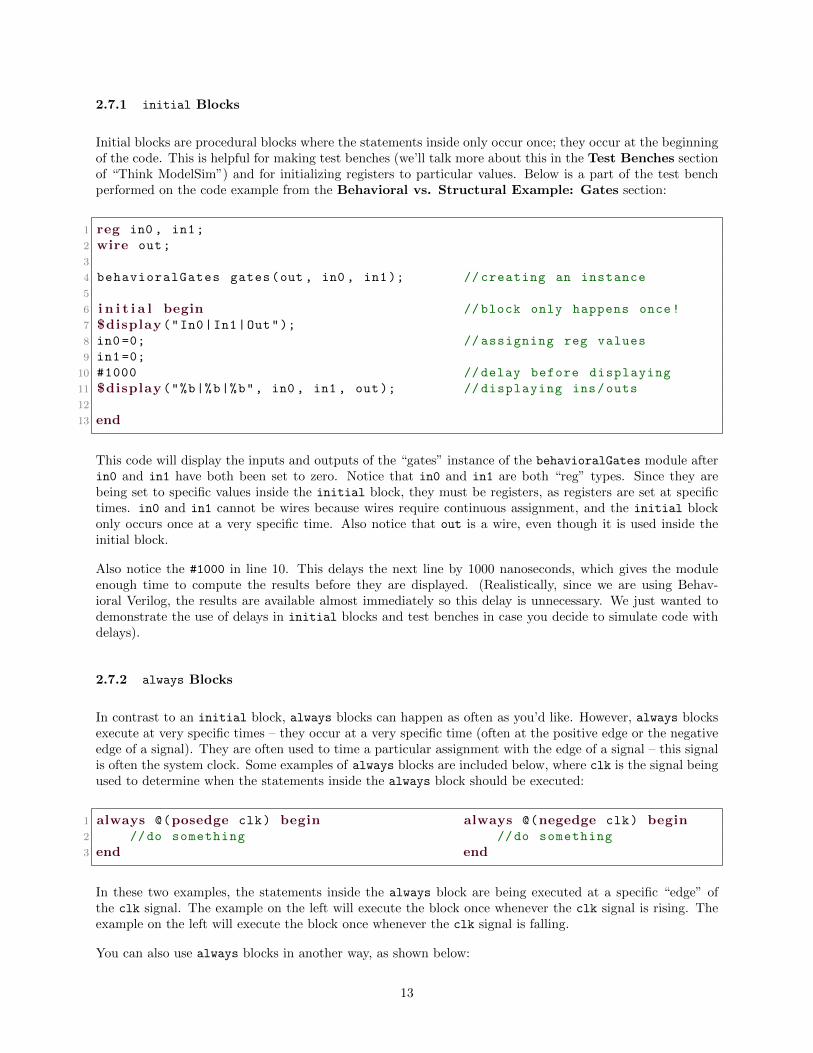
2.7.1 initial Blocks
Initial blocks are procedural blocks where the statements inside only occur once; they occur at the beginningof the code. This is helpful for making test benches (we’ll talk more about this in the Test Benches sectionof “Think ModelSim”) and for initializing registers to particular values. Below is a part of the test benchperformed on the code example from the Behavioral vs. Structural Example: Gates section:
1 reg in0 , in1;
2 wire out;
3
4 behavioralGates gates(out , in0 , in1); // creating an instance
5
6 i n i t i a l begin // block only happens once!
7 $display("In0|In1|Out");8 in0 =0; // assigning reg values
9 in1 =0;
10 #1000 //delay before displaying
11 $display("%b|%b|%b", in0 , in1 , out); // displaying ins/outs
12
13 end
This code will display the inputs and outputs of the “gates” instance of the behavioralGates module afterin0 and in1 have both been set to zero. Notice that in0 and in1 are both “reg” types. Since they arebeing set to specific values inside the initial block, they must be registers, as registers are set at specifictimes. in0 and in1 cannot be wires because wires require continuous assignment, and the initial blockonly occurs once at a very specific time. Also notice that out is a wire, even though it is used inside theinitial block.
Also notice the #1000 in line 10. This delays the next line by 1000 nanoseconds, which gives the moduleenough time to compute the results before they are displayed. (Realistically, since we are using Behav-ioral Verilog, the results are available almost immediately so this delay is unnecessary. We just wanted todemonstrate the use of delays in initial blocks and test benches in case you decide to simulate code withdelays).
2.7.2 always Blocks
In contrast to an initial block, always blocks can happen as often as you’d like. However, always blocksexecute at very specific times – they occur at a very specific time (often at the positive edge or the negativeedge of a signal). They are often used to time a particular assignment with the edge of a signal – this signalis often the system clock. Some examples of always blocks are included below, where clk is the signal beingused to determine when the statements inside the always block should be executed:
1 always @(posedge clk) begin always @(negedge clk) begin2 //do something //do something
3 end end
In these two examples, the statements inside the always block are being executed at a specific “edge” ofthe clk signal. The example on the left will execute the block once whenever the clk signal is rising. Theexample on the left will execute the block once whenever the clk signal is falling.
You can also use always blocks in another way, as shown below:
13

1 always @(*) begin2 //do something
3 end
This procedural block triggers on all events during the simulation. Note that this is as close to continuousassignment as you’ll get with a procedural block, but it is by no means actually continuous assignment. Thisblock still only occurs at very specific, discrete times.
Using always blocks can be complicated, so we’ve included a more in-depth example below:
1 module countingClocks(out , clk);
2 output reg [3:0] out;
3 input clk;
4
5 reg [3:0] count;
6 i n i t i a l count = 0;
7 always @(posedge clk) begin8 count <= count + 1; // increments counter at every pos edge
9 out <= count; //"<=" is actually an assignment operator!
10 //We ’ll talk about this soon.
11 end12 endmodule
This code will increment the count variable at the positive edge of clk. To run this code, we’ll use thefollowing module:
1 module testClocks;
2 wire [3:0] out;
3 reg clk;
4
5 countingClocks clock(out , clk); // initializing module to be tested
6 i n i t i a l clk = 0; //hey look , an initial block!
7 always #100 clk=!clk; //clk alternates value every 100ns
8 endmodule
When running this code, a positive edge of clk happens every 200 ns. As a result, we’ll expect out toincrement by 1 every 200 ns, at every positive edge. Running this code produces the following waveform(don’t worry, we’ll discuss how to make waveforms in the Generating Waveforms section of “ThinkModelSim”):
14

Figure 6: A waveform representing the output of the countingClocks module. The upper waveform repre-sents the clk input, which changes every 100 ns. The second waveform represents out, which increments atevery positive edge.
We’ve included the full Verilog source file and a .do file at the end of the guide, if you’d like to try runningthis for yourself. See the Procedural Blocks Example: countingClocks section under Files ForVerilog Examples at the end of our guide. You can also find the full code examples on GitHub: https:
//github.com/skumarasena/ThinkCompArch.
If you’re wondering what the red line in out is (0 ns - 100 ns); that’s what an x looks like in ModelSim’swaveforms. Looking at the code, we can see why this might be an x – the out wire is not assigned to anythinginitially, and so it takes on no value at the beginning. After the first positive edge of the clock, however, outchanges from 4’h0 to 4’h1 to 4’h2 to 4’h3. If you refer back to the “Syntax” section, you will notice thatthose values correspond to hexadecimal 0, 1, 2, and 3. Our counter is counting! (Note that the counter’szero-indexed.)
Looking at the statements inside the always block, you may also be wondering what the “<=” operator is,since we’ve only seen “=” in assignments so far. The “<=” operator (only used in the context of always
blocks) is known as a non-blocking assignment. Since we’re using the “<=” operator for the assignmentsinside the always block, both statements happen simultaneously. This means that the value of out isactually count, and not count + 1.
Assignments that use “=” in always blocks are known as blocking assignments because they perform theassignment immediately, wait for the assignment to execute, and then move on to the next line of code. Inother words, if we were to rewrite the example using blocking assignments as shown below...
1 always @(posedge clk) begin // blocking version!
2 count = count + 1; // increments the counter at
3 //every positive edge
4 out = count; // occurs after the count increment
5 end
...the count = count + 1 statement would execute first, and the out = count statement would executeimmediately afterward. Remember how in the Modules section we talked about a scenario where statementorder might matter? This is it. With non-blocking assignments, both assignments would be set to executesimultaneously at the positive edge of the clock. Note that because these are non-blocking assignments, thevalue of out is actually count + 1! The statements are being executed procedurally. Moral of the story: ifyou want a bunch of statements to execute simultaneously at a particular event within an always block, usenon-blocking assignment. If you don’t particularly care, blocking assignment is fine.
A lot of CompArch students (including ourselves) get confused because they try to use assign statementswith registers, or they try to use initial/always blocks with wires. If you remember anything fromthis section, remember that these combinations are fundamentally incompatible. Assign statements are
15

continuous – they happen all the time, and so they are used for wires. Initial/always blocks occur at veryspecific times, and so they are used with registers. If you try to use an assign statement inside an always
block, Verilog will throw an error. (Any sort of wire assignment will fail, because all wire assignments mustbe continuous).
2.8 Test Benches
Now, we’ll move on to discussing how you should go about testing your code. This may seem silly at first,but it becomes extremely important later on when your designs become bigger.
First of all, what should you expect your test bench to do? A test bench should thoroughly test every aspectof your design, confirm that it behaves as you expect in all situations, and most importantly : be capable ofdiagnosing errors in your design. Test benches should be able to find where your design is broken. Theyare as much a debugging tool as a verification that your design works. Be sure to think about your testbench design as you are designing a module! As you’re designing the module, think about what behaviorsyou want to test, and where things could go wrong. Then test them in your test bench.
Make test benches early and often. If you’re writing multi-module code, don’t write a bunch of modules andexpect them to integrate with each other perfectly. Test every aspect of your design, and then integrate.Also important to note: Verilog errors are often useless. They don’t tell you where the problem is – theytell you where the error has caused a fatal problem in program execution (which is often in a very differentplace). This is part of the reason why you need good test benches; Verilog will not help you.
All right – our rant on test benches is over! First, here’s an example of some functional code we’ll write atest bench for. This code example will be a one-bit full adder written in Behavioral Verilog. A one-bit fulladder performs a single “column” of binary addition, including a carry-in digit from the previous column ofaddition and a carry-out digit into the next one. A block diagram of a one-bit full adder is shown below:2
Figure 7: A block diagram showing the inputs and outputs of a one-bit full adder. Inputs A and B are thedigits from the current column of addition. Input Cin is the carry-in from the previous column of addition.Input Cout is the carry-out into the next column.
Here is a Behavioral Verilog implementation of this one-bit full adder. (By the way, this example is theBehavioral Verilog one-bit full adder example that was given to us in Homework 2. It may be given to youtoo.)
2This diagram was taken from Wikipedia: http://upload.wikimedia.org/wikipedia/commons/thumb/4/48/1-bit_
full-adder.svg/220px-1-bit_full-adder.svg.png
16
1 module behavioralFullAdder(sum , carryout , a, b, carryin );
2 output sum , carryout;
3 input a, b, carryin;
4 assign {carryout , sum}=a+b+carryin;
5 endmodule
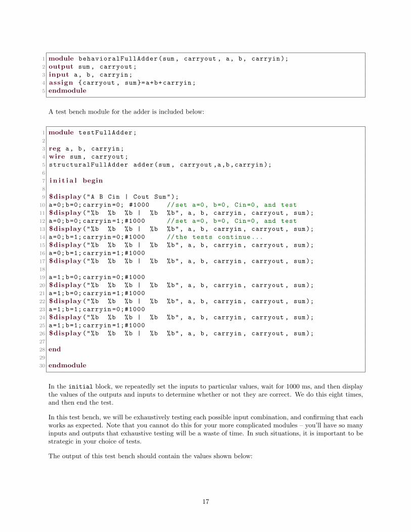
A test bench module for the adder is included below:
1 module testFullAdder;
2
3 reg a, b, carryin;
4 wire sum , carryout;
5 structuralFullAdder adder(sum , carryout ,a,b,carryin );
6
7 i n i t i a l begin8
9 $display("A B Cin | Cout Sum");
10 a=0;b=0; carryin =0; #1000 //set a=0, b=0, Cin=0, and test
11 $display("%b %b %b | %b %b", a, b, carryin , carryout , sum);
12 a=0;b=0; carryin =1;#1000 //set a=0, b=0, Cin=0, and test
13 $display("%b %b %b | %b %b", a, b, carryin , carryout , sum);
14 a=0;b=1; carryin =0;#1000 //the tests continue ...
15 $display("%b %b %b | %b %b", a, b, carryin , carryout , sum);
16 a=0;b=1; carryin =1;#1000
17 $display("%b %b %b | %b %b", a, b, carryin , carryout , sum);
18
19 a=1;b=0; carryin =0;#1000
20 $display("%b %b %b | %b %b", a, b, carryin , carryout , sum);
21 a=1;b=0; carryin =1;#1000
22 $display("%b %b %b | %b %b", a, b, carryin , carryout , sum);
23 a=1;b=1; carryin =0;#1000
24 $display("%b %b %b | %b %b", a, b, carryin , carryout , sum);
25 a=1;b=1; carryin =1;#1000
26 $display("%b %b %b | %b %b", a, b, carryin , carryout , sum);
27
28 end29
30 endmodule
In the initial block, we repeatedly set the inputs to particular values, wait for 1000 ms, and then displaythe values of the outputs and inputs to determine whether or not they are correct. We do this eight times,and then end the test.
In this test bench, we will be exhaustively testing each possible input combination, and confirming that eachworks as expected. Note that you cannot do this for your more complicated modules – you’ll have so manyinputs and outputs that exhaustive testing will be a waste of time. In such situations, it is important to bestrategic in your choice of tests.
The output of this test bench should contain the values shown below:
17
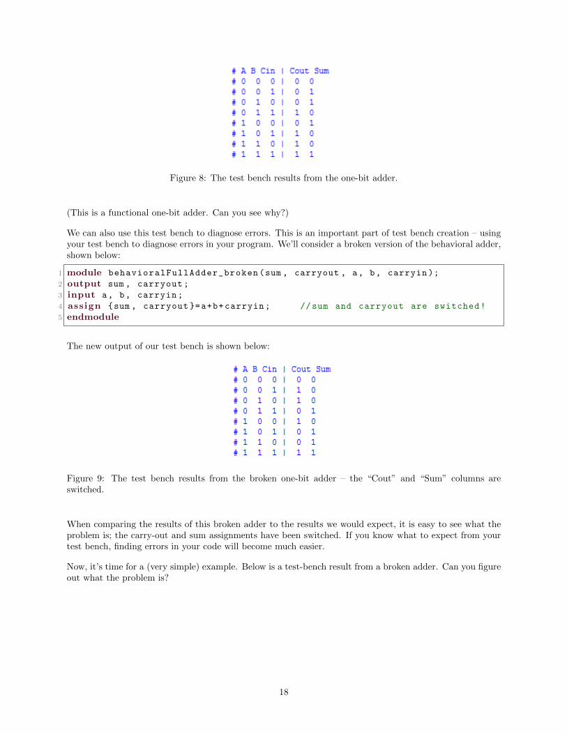
Figure 8: The test bench results from the one-bit adder.
(This is a functional one-bit adder. Can you see why?)
We can also use this test bench to diagnose errors. This is an important part of test bench creation – usingyour test bench to diagnose errors in your program. We’ll consider a broken version of the behavioral adder,shown below:
1 module behavioralFullAdder_broken(sum , carryout , a, b, carryin );
2 output sum , carryout;
3 input a, b, carryin;
4 assign {sum , carryout }=a+b+carryin; //sum and carryout are switched!
5 endmodule
The new output of our test bench is shown below:
Figure 9: The test bench results from the broken one-bit adder – the “Cout” and “Sum” columns areswitched.
When comparing the results of this broken adder to the results we would expect, it is easy to see what theproblem is; the carry-out and sum assignments have been switched. If you know what to expect from yourtest bench, finding errors in your code will become much easier.
Now, it’s time for a (very simple) example. Below is a test-bench result from a broken adder. Can you figureout what the problem is?
18

Figure 10: The test bench results from yet another broken one-bit adder. Can you find the problem? Hint:look at the carry-in bit, and look at the two outputs.
To figure out the answer: note that when carry-in is 1, the adder works fine. When carry-in is 0, the adderproduces the wrong results – the results are 1 higher than what you would expect. This indicates the carry-invalue is broken – it is set to 1 no matter what.
Now, this is a really artificial error – you are highly unlikely to make this mistake. But this example highlightsthe importance and usefulness of test benches in debugging. Make sure you know what values you expect,and compare the expected values to the values you receive.
We’ve also included the full Verilog source file and .do file at the end of the guide, if you’d like to tryrunning this for yourself. See the Test Benches Example: Adders section under Files For VerilogExamples at the end of our guide. The full code example can also be found on our Github: https:
//github.com/skumarasena/ThinkCompArch.
19

2.9 Useful Links
We’ve included some links you might find useful. Enjoy!
Mark Chang’s Verilog tutorial. A description of the basics of Structural Verilog as well as some othersyntax details we haven’t gone into here: http://ca.olin.edu/cawiki/attachments/Fall(20)2010(2f)
Materials/VerilogTutorial.pdf
A Verilog tutorial that goes over some of the basic concepts behind Verilog and HDLs. Chapters 1, 2, and3 will be the most helpful to you: http://www.verilogtutorial.info/
A quick-reference guide to Verilog syntax. http://web.stanford.edu/class/ee183/handouts_win2003/
VerilogQuickRef.pdf
Another Verilog tutorial. It can help to see concepts explained in a bunch of different ways, so we’re includinga bunch of different tutorials: http://www.ee.unlv.edu/~meiyang/cpe302/Verilog_Tutorial.pdf
A short explanation of some syntax details. It’s not the most comprehensive guide, but still useful: http:
//www.sutherland-hdl.com/papers/2001-SNUG-paper_Verilog-2000_standard.pdf
A side note: the cat picture on the front page is from http://media.tumblr.com/tumblr_lxn8wsCzYT1r4nok1.
png and has been modified in MS Paint.
20
3 Think ModelSim
3.1 What is ModelSim?
ModelSim is a simulator for HDL languages. In this class, we will be using ModelSim to simulate our Verilogprograms. This section will be much less conceptual than our “Think Verilog” guide. Instead, we’ll includelots of how-to tutorials: how to make .do files, how to make waveforms, and some helpful debugging tips.We’ll also include some common compile-errors and potential solutions.
Before we begin, we’d like to issue a warning to all who haven’t used ModelSim before – don’t Ctrl-Z! InModelSim, Ctrl-Z will usually work as you expect; it will undo your most recent change. However, ModelSimhas been known to undo up to several hours worth of changes before with a single Ctrl-Z. Furthermore,ModelSim often will not allow you to “redo” these changes. This has happened to a few people in our year’sclass. So don’t Ctrl-Z. Just don’t. It’ll probably be fine, but there’s always the slightest chance that it won’tbe fine.
3.2 Creating a Project
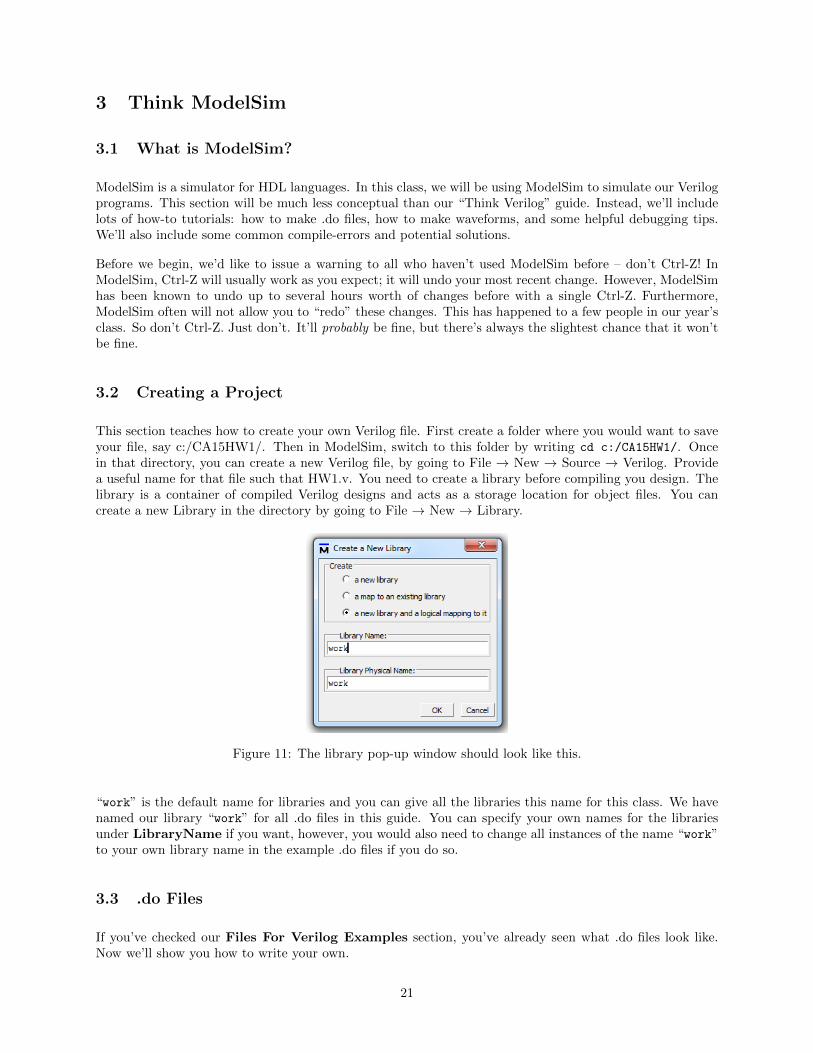
This section teaches how to create your own Verilog file. First create a folder where you would want to saveyour file, say c:/CA15HW1/. Then in ModelSim, switch to this folder by writing cd c:/CA15HW1/. Oncein that directory, you can create a new Verilog file, by going to File → New → Source → Verilog. Providea useful name for that file such that HW1.v. You need to create a library before compiling you design. Thelibrary is a container of compiled Verilog designs and acts as a storage location for object files. You cancreate a new Library in the directory by going to File → New → Library.
Figure 11: The library pop-up window should look like this.
“work” is the default name for libraries and you can give all the libraries this name for this class. We havenamed our library “work” for all .do files in this guide. You can specify your own names for the librariesunder LibraryName if you want, however, you would also need to change all instances of the name “work”to your own library name in the example .do files if you do so.
3.3 .do Files
If you’ve checked our Files For Verilog Examples section, you’ve already seen what .do files look like.Now we’ll show you how to write your own.
21

Here’s the .do file we’ve included for the structuralGates/behavioralGates code example from “ThinkVerilog” (see Behavioral vs Structural for the guide section, and Behavioral vs. Structural Example:Gates for the full code example). A .do file runs your code, and gives you lots of options for how to runyour code. To create and run a do file, go to File → New → Source → Do.
1 #make comments like this!
2 vlog -reportprogress 300 -work work gates.v
3 vsim -voptargs="+acc" testGates
4 run 5000
The first line is an example of a comment – note that comment syntax in .do files is different from Verilog files.The second line runs the code file specified (in this case, “gates.v”) using the library work (the default namefor a library in ModelSim). In the third line, vsim loads testGates for simulation. The “-reportprogress300” provides debugging information during compilation if something goes wrong and -voptargs="+acc"
makes sure the compiler allows you to see all the signals in your design. The last line, “run 5000”, runsyour code for 5000 ns. Additionally, you can change the last line to run -all to run your code file untilModelSim determines execution has finished. If you do this, be sure that your code actually terminates –otherwise you’ll have to quit the simulation and ModelSim will not display your results.
Save your .do file (and all your .v files) in the top-level directory of your project folder. Do not put your codein the “work” folder! Remember, the default library name is “work”, so this folder is for internal ModelSimstuff. Don’t touch it.
To run this code, type “do [name of your .do file]” (in our case this would be “do dogates.do”) intoModelSim’s Transcript window. In the screenshot below, we’ve outlined the Transcript window in red:
Figure 12: The Transcript window in ModelSim is outlined in red at the bottom. If you can’t see thiswindow, the Layout drop-down menu is in the top right. Change the layout to “Simulate” or “NoDesign”.
After typing “do [name of your .do file]” into the Transcript window, run it by pressing Enter. Youshould see the results of the test show up in the Transcript window.
22

Now, this is the most basic .do file you could have. What if you want to try some fancier things? Thisis a great reference for .do file commands: http://cseweb.ucsd.edu/classes/fa10/cse140L/lab/docs/
modelsim_ref.pdf. We’ll go into a couple detailed examples of using these commands, since you’ll findsome examples particularly useful.
3.3.1 Clearing Libraries
One important thing to note about libraries is that they store all wires, registers, gates, and modules thatyou’ve initialized in the past. If you end up deleting or renaming any of these elements, you’ll find that theold versions stick around – and can still be referenced! Since this can be a problem, it can be very helpful toclear your library each time you run your code. We can modify our .do file from the same example to clearthe library:
1 vdel -lib work -all
2 vlib work
3
4 vlog -reportprogress 300 -work work gates.v
5
6 vsim -voptargs="+acc" testGates
7
8 run 5000
Here, two lines have been added to the beginning of the .do file from the previous example. The first lineclears the current library. The second line recreates it.
3.3.2 Generating Waveforms
Finally, the moment you’ve been waiting for: we’ll learn how to generate waveforms! Waveforms are in-credibly useful in debugging and verifying simulations – they tell you how inputs and outputs change overtime.
For this example, we’ll talk about the waveform-generating .do file from the countingClocks example in“Think Verilog”. If you’d like to see the full code, see the Procedural Blocks Example: countingClockssection under Files For Verilog Examples. If you’d like to see the guide section, see the always Blockssection. The .do file from this example is included below:
1 vdel -lib work -all
2 vlib work
3
4 vlog -reportprogress 300 -work work always.v
5 vsim -voptargs="+acc" testClocks
6
7 add wave -position insertpoint \
8 sim:/ testClocks/clk \
9 sim:/ testClocks/out
10
11 run 1000
12 wave zoom full
The first and second lines clear and recreate the library, as we discussed earlier. Lines 4 and 5 run the codeand provide debugging information. Lines 7-9 generate the waveform. Line 7 indicates that waves need to be
23

added to the waveform. Line 8 displays the waveform for clk from inside the testClocks module. Similarly,line 9 displays the waveform for out from inside the testClocks. Line 11 runs the simulation for 1000 ns,and line 12 views the waveform in ModelSim.
There is a \ at the end of lines 7 and 8 – this indicates that the statement is continued on the next line.Note that .do files are not whitespace-independent like Verilog is. If you try to put an empty line betweenthose lines, like so...
1 vdel -lib work -all
2 vlib work
3
4 vlog -reportprogress 300 -work work always.v
5 vsim -voptargs="+acc" testClocks
6
7 add wave -position insertpoint \
8
9 sim:/ testClocks/clk \
10
11 sim:/ testClocks/out
12
13 run 1000
14 wave zoom full
...your .do file will not run. Generally speaking, be careful about whitespace in your .do files.
If everything runs properly, you should obtain the waveform we saw earlier in the “Think Verilog” example,as shown below:
Figure 13: A waveform representing the output of the countingClocks module.
But what if you want to know the values of other variables – say, the value of “count” inside the countingClocksmodule? If you want to refer to the value of a particular register or wire within a given submodule, you’llneed to refer to these variables by the name of the instance of the module. An example of this is shown below:
24

1 vdel -lib work -all
2 vlib work
3
4 vlog -reportprogress 300 -work work always.v
5 vsim -voptargs="+acc" testClocks
6
7 add wave -position insertpoint \
8 sim:/ testClocks/clk \
9 sim:/ testClocks/out \
10 sim:/ testClocks/clock/count
11
12 run 1000
13 wave zoom full
In line 10, we are displaying the waveform for count. Since count is a part of the countingClocks module,we must refer to the count variable using the name of the countingClocks instance (which is clock, in thiscase). The resulting waveform is shown below:
Figure 14: The same waveform as in the previous example, now with the count wave included.
Generally speaking, if you want to refer to a wire or reg inside a given module, try the following:
1 sim:/ testName/moduleInstanceName/name
where testName is the name of the test module, moduleInstanceName is the name of the instance of themodule where the wire/reg is defined, and name is the name of the wire/reg.
Now that you know how to generate waveforms: if you’d like to learn how to use and interact with waveforms,see the Using Waveforms in Debugging section!
3.4 Debugging: Common Errors and Explanations
Verilog error messages are not known for being particularly helpful. They tend to indicate where the problemforced the simulation to stop executing, as opposed to the actual source of the issue. We’ll talk about a fewcommon error messages in this section. This is by no means a comprehensive list – we will only introduce afew error messages, but we feel these are error messages you are likely to see while debugging.
When you run your code and get errors, your errors will show up in the Transcript window, which is whereyou typed in the command to run your code. Your errors are likely to end with the following:
25

1 Error: C:/ Modeltech_pe_edu_10 .3c/win32pe_edu/vlog failed.
2 Error in macro ./[ name of .do file] line 1
3 invalid command name "vsim_increment_error_count"
(In this example, replace “name of .do file” with the name of your .do file.) This error just means thatthe .do file failed. Your .do file could not complete because the simulation could not execute. This is prettymeaningless – every compile-error will end with these lines. You’ll need to scroll up in the Transcript windowto see the full error (and hopefully Verilog will provide you with some more useful information about itssource).
First, we’ll start with a simple (almost-reassuring) error:
1 Error: [file_name ]([ line_num ]): near "end": syntax error , unexpected end
(In this example, file name and line num will be replaced by your Verilog file’s name and the line numberwhere the error occurred.) If you get this error, don’t panic. As the error says, this is most likely a syntaxerror that occurs within a procedural block. Check your block. Have you missed a semicolon, bracket,comma, or apostrophe? Additionally, there’s another cause of this error; do you have delays after the laststatement in your program? If you try the following:
1 // module code up here ...
2 reg a, b, c;
3
4 i n i t i a l begin5 a = 0; #500
6 b = 0; #500
7 c = 0; #500
8
9 end10
11 // module code down here ...
The #500 (a 500-nanosecond delay) at the end of line 7 is the cause of an error. Don’t try to put delays atthe end of your intial block. Delays at this point are useless – there is no ”next statement” that will bedelayed. This is interpreted as a syntax error.
Next up, we have another simple fix with an error message that can be hard to interpret – no error messageat all! In other words, all you receive is the following, as we discussed in our first code example of the section:
1 Error: C:/ Modeltech_pe_edu_10 .3c/win32pe_edu/vlog failed.
2 Error in macro ./[ name of .do file] line 1
3 invalid command name "vsim_increment_error_count"
(In this example, replace “name of .do file” with the name of your .do file.) Like we said earlier, thisjust tells you that your code failed to run. However, when you try to scroll up, there are no other errors tobe found. What gives?
This usually means there is an error in your .do file, since no errors were found in the Verilog file. Have youchecked that your library and file names are spelled properly in the .do file? Have you included the “.v” atthe end of your Verilog file name?
26

Another common error is mismatched variable sizes. If you declare a module’s input or output as a given sizeand then assign a differently-sized variable to that input/output when you initialize it, you will get a ”portsize” warning. These warnings are important – your code will usually not run properly with a port size error.
1 # ** Warning: (vsim -3015) always.v(20): [PCDPC] -
2 Port size ([size in module definition ]) does not match connection size
3 ([size in initialization ]) for port ’[portname]’.
4 The port definition is at: [file_name ]([ line_num ]).
5
6 # Region: /[ module_name ]/[ instance_name]
In this example, file name and line num will be replaced by your Verilog file’s name and the line numberwhere the error occurred. module name and instance name includes the instance of the module wherethe error was detected. Finally, ”size in module definition” and ”size in initialization” will bereplaced by the input’s size as declared by the module definition and the size of the corresponding variablein the initialization, respectively.
Finally, we have the common wire-reg confusion errors. These occur when regs are used in situations thatdemand wires, and vice versa. Make sure you understand the conceptual differences between regs and wires! Ifyou feel unsure, go back to our Wire Assignment, Registers, and Procedural Blocks: initial/alwayssections of ”Think Verilog”.
If you try to use a wire in a procedural block, you will get the following error:
1 ** Error: [file_name }({ line_num )): (vlog -2110)
2 Illegal reference to net "[wire_name]".
Wires are fundamentally incompatible with initial or always blocks because these procedural blocks willassign at very specific times, and wires require continuous assignment. Again, see ”Think Verilog if you’restill not sure why this occurs (or ask your NINJAs)!
If you make the opposite mistake – using a register in a continuous-assignment framework – you will get thefollowing error:
1 # ** Error: [file_name ]([ line_num ]):
2 Port mode is incompatible with declaration: [reg_name]
Again, this occurs because registers are meant to be updated at very specific times within procedural frame-works – not continuously. Remember that wires are assigned continuously (think assign statements), andregisters are assigned in procedural blocks (think initial and always blocks). Do not try to mix the two;it’ll end poorly.
Generally speaking, when you run into errors, don’t focus on the error message too much – these can oftenbe unhelpful. Instead, look at the inputs and outputs of each portion of your code, and try to trace the errorback to its source. Waveforms are particularly useful for this because they display the values of inputs andoutputs at all times. if you find yourself struggling to find an error, looking at a waveform is often your bestoption.
3.4.1 Debugging x And z
While testing or debugging, you’ll often find yourself coming across values that, instead of being 1 or 0, aresimply labeled x or z. If you didn’t write your simulation with the intent to output these values, they’remost likely due to an error somewhere in your code.
27

An x refers to a value that cannot be resolved to either a 0 or a 1. This usually means that an assignment isnot being performed properly. This can be due to miswiring a module, so check all your module initializations.Note that x signals will propagate – if one of your modules outputs an x and another module uses that inputto perform a task, the output of that second module will most likely also be an x. This may seem unfortunate,but it’s actually quite useful in debugging – it’s easy to trace an x back to its source. In waveforms, x’s willshow up as red lines as opposed to the normal green lines.
A z refers to a “high-impedance” output. This means that the signal is neither a 0 nor a 1. This indicatesthat a signal is not being driven. z’s can be useful in tri-state buffers and logic – in some scenarios, you maywant an output to be neither 0 nor 1. However, if you’re not in one of those situations, a z often comes froman unconnected output. Make sure all your signals are being driven properly. In waveforms, z’s will showup as blue lines as opposed to the normal green lines.
3.5 Using Waveforms in Debugging
Waveforms are awesome. They’re very useful from a debugging standpoint, and we’ve spent some time in.do Files talking about how to generate them – see that section for more information. In this section, we’lldiscuss how you can interact with them.
If you just want to read values at a specific time, you can use the yellow data cursor to see the values ofeach wave at any given time – drag it around, and the values in the gray sidebar to the left of the waveformwill change. See the screenshot below:
Figure 15: The data cursor has been dragged to the right, to 210 ns. The values of the variables at this timeare indicated in the gray sidebar to the left.
If you look at the gray sidebar, you’ll note that the values next to each wave indicate the value of eachvariable at 210 ns – clk is 0, out is 0, and count is 1. If you were to move the data cursor, the values ofthese numbers would change.
Waveforms are particularly useful for debugging because they display the values of all inputs and outputs atall points in your program. This way, it’s super easy to look for incorrect behavior. If there is an incorrectoutput in your code, trace it back to its inputs. Make sure it is connected properly, and that it is receivingthe right values at the right time.
If you don’t want to read all the values in a waveform in hexadecimal, you can easily change the viewingradix to binary or decimal. Simply right-click on a variable name, select ’Radix’ and change it to binary,decimal, octal – whichever is most convenient.
28

Figure 16: A screenshot where we select the viewing radix in the gray sidebar to the left of the waveform.Right-click, select “Radix”, and go!
3.5.1 Early-Transitioning
An important thing to note about waveforms in ModelSim is that waveforms will display values when theyare available, not when they are assigned.
If you find yourself working on a clocked component (i.e. a component which acts on a clock edge), you willsometimes notice that the values you expect appear a clock cycle early. You might initially think this is aproblem with your code, and it might very well be a problem with your code. But if you find no error inyour code, there is another explanation.
In simulation, the results of a given computation are available immediately. If the component fires on thepositive edge of the result, the results are available on that same positive edge if there are no #[delay]
statements in your code. This means that what looks like the current state of the system is actually thenext state – the state that it is about to transition to on the next clock.
If you think this is the case with your code, read it over to make sure that your code is synchronized theway you think it is. If you believe the structure of your code, then proceed. But do take care to make surethis is actually the issue, and you’re not just setting your signals improperly.
3.5.2 Looking At Wire/Reg Values
In addition to looking at wire or reg values in a waveform, you can also look at them within your code (Figure17). During a simulation, you can simply hover your cursor over a variable in your code and ModelSim willdisplay its hexadecimal value. Note that this is the value of the variable at the specific point in time yourcursor is set to within the waveform window.
29
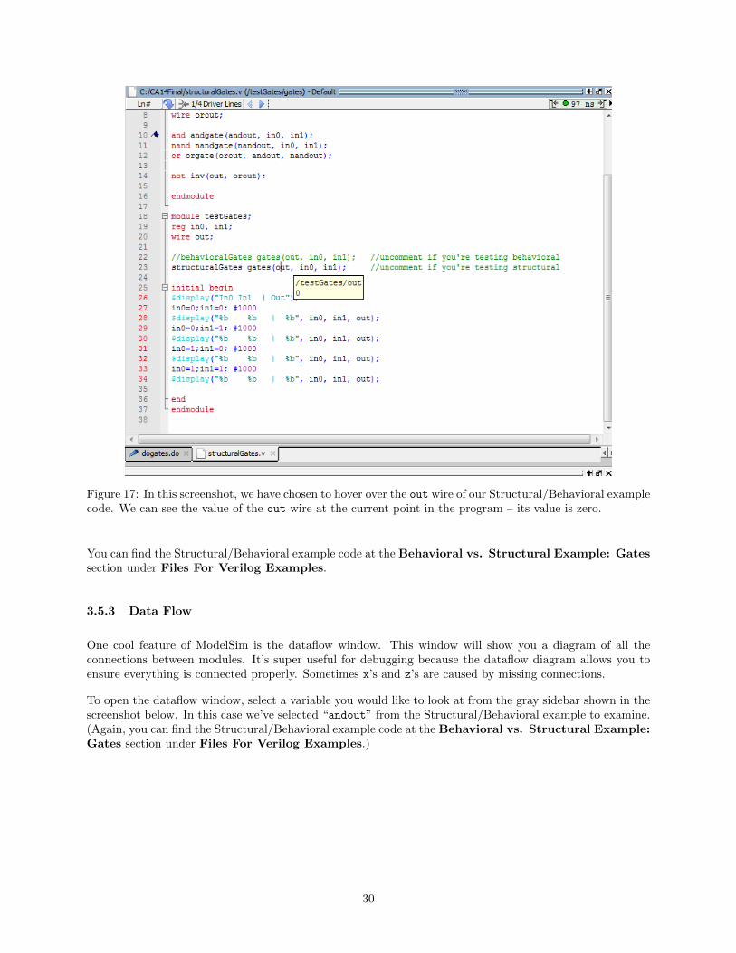
Figure 17: In this screenshot, we have chosen to hover over the out wire of our Structural/Behavioral examplecode. We can see the value of the out wire at the current point in the program – its value is zero.
You can find the Structural/Behavioral example code at the Behavioral vs. Structural Example: Gatessection under Files For Verilog Examples.
3.5.3 Data Flow
One cool feature of ModelSim is the dataflow window. This window will show you a diagram of all theconnections between modules. It’s super useful for debugging because the dataflow diagram allows you toensure everything is connected properly. Sometimes x’s and z’s are caused by missing connections.
To open the dataflow window, select a variable you would like to look at from the gray sidebar shown in thescreenshot below. In this case we’ve selected “andout” from the Structural/Behavioral example to examine.(Again, you can find the Structural/Behavioral example code at the Behavioral vs. Structural Example:Gates section under Files For Verilog Examples.)
30

Figure 18: Select a variable and double-click.
Double-clicking on the cursor within the waveform window will cause a dataflow window to pop up inModelSim.
Figure 19: Initially, this will pop up in the dataflow window. You’ve only selected the AND gate’s output,so only the AND gate will show up.
In this example, the AND gate named andgate (as well as its output and two inputs) pop up in the dataflowwindow. If you hover your mouse over each input and output, you’ll see an arrow. If you click on the arrow itwill expand the diagram. The fully-expanded dataflow diagram for the structuralGates/behavioralGatesexample is shown below in Figure 20.
Figure 20: Dataflow for the full structuralGates/behavioralGates example. This shows the full circuitdiagram as well as the initial block.
This dataflow diagram shows the exact circuit diagram we designed in the structuralGates/behavioralGatesexample in “Think Verilog”. Additionally, it shows one more block on the right – it shows the initial block,where the values of the inputs are assigned. The initial block is connected to the inputs of the logic gatecircuit, showing that the assigned values are coming from the initial block.
31
3.5.4 Adding Waves to a Waveform
You might find that once you’ve generated a waveform, you’d like to look at the waves for other wires orregisters. You could edit your .do file, include the wave you want to see, and rerun your code. (If you’reunsure of how to do this, see our “Waveforms” section under “.do Files”!). This is a bit of a lengthy process,especially if you’re debugging a particularly troublesome error and you find yourself wanting to add moreand more waves to a waveform.
There is an alternative: you can just add the new wave to the waveform directly. Take our countingClocksexample. (You can find the example code at the Procedural Blocks Example: countingClocks section.)What if we forgot to include the out waveform? Say we started with the following waveform, with just theclk signal:
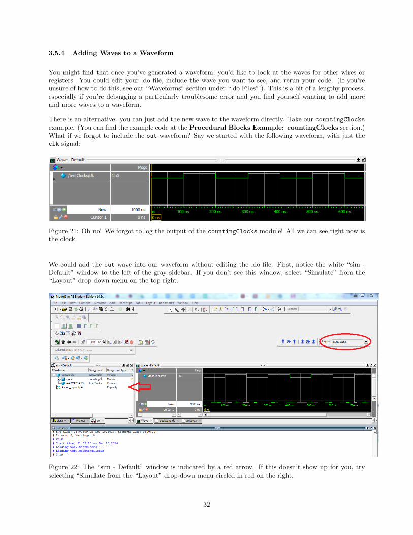
Figure 21: Oh no! We forgot to log the output of the countingClocks module! All we can see right now isthe clock.
We could add the out wave into our waveform without editing the .do file. First, notice the white “sim -Default” window to the left of the gray sidebar. If you don’t see this window, select “Simulate” from the“Layout” drop-down menu on the top right.
Figure 22: The “sim - Default” window is indicated by a red arrow. If this doesn’t show up for you, tryselecting “Simulate from the “Layout” drop-down menu circled in red on the right.
32
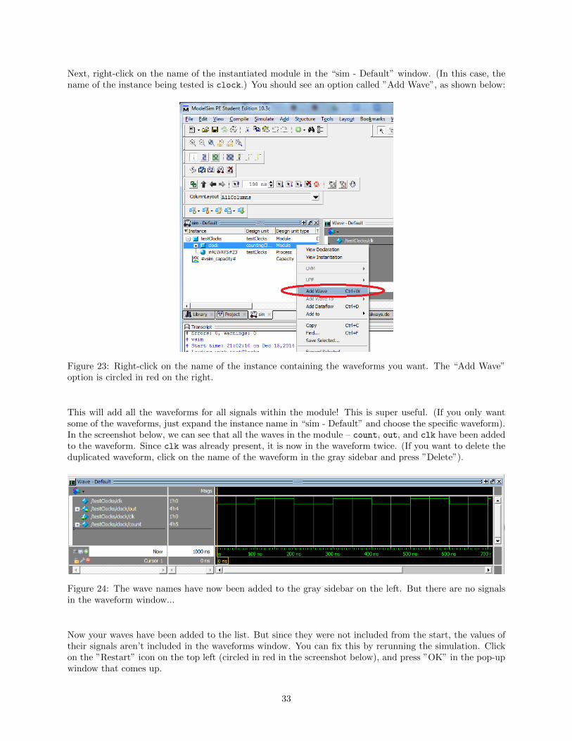
Next, right-click on the name of the instantiated module in the “sim - Default” window. (In this case, thename of the instance being tested is clock.) You should see an option called ”Add Wave”, as shown below:
Figure 23: Right-click on the name of the instance containing the waveforms you want. The “Add Wave”option is circled in red on the right.
This will add all the waveforms for all signals within the module! This is super useful. (If you only wantsome of the waveforms, just expand the instance name in “sim - Default” and choose the specific waveform).In the screenshot below, we can see that all the waves in the module – count, out, and clk have been addedto the waveform. Since clk was already present, it is now in the waveform twice. (If you want to delete theduplicated waveform, click on the name of the waveform in the gray sidebar and press ”Delete”).
Figure 24: The wave names have now been added to the gray sidebar on the left. But there are no signalsin the waveform window...
Now your waves have been added to the list. But since they were not included from the start, the values oftheir signals aren’t included in the waveforms window. You can fix this by rerunning the simulation. Clickon the ”Restart” icon on the top left (circled in red in the screenshot below), and press ”OK” in the pop-upwindow that comes up.
33
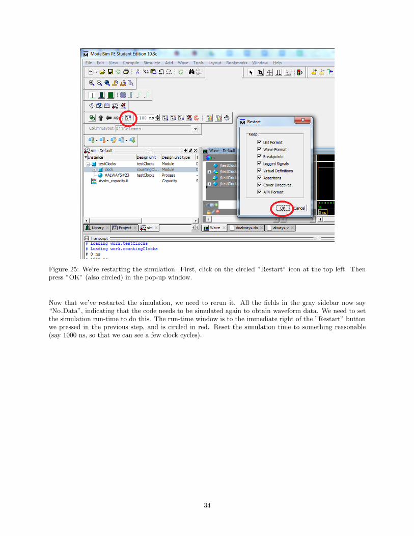
Figure 25: We’re restarting the simulation. First, click on the circled ”Restart” icon at the top left. Thenpress ”OK” (also circled) in the pop-up window.
Now that we’ve restarted the simulation, we need to rerun it. All the fields in the gray sidebar now say“No Data”, indicating that the code needs to be simulated again to obtain waveform data. We need to setthe simulation run-time to do this. The run-time window is to the immediate right of the ”Restart” buttonwe pressed in the previous step, and is circled in red. Reset the simulation time to something reasonable(say 1000 ns, so that we can see a few clock cycles).
34
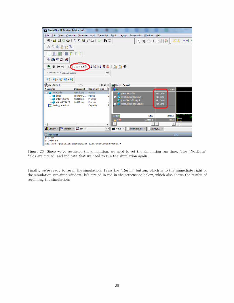
Figure 26: Since we’ve restarted the simulation, we need to set the simulation run-time. The ”No Data”fields are circled, and indicate that we need to run the simulation again.
Finally, we’re ready to rerun the simulation. Press the ”Rerun” button, which is to the immediate right ofthe simulation run-time window. It’s circled in red in the screenshot below, which also shows the results ofrerunning the simulation:
35

Figure 27: We have just pressed the ”Rerun” button, circled in the top left. The results are shown in thewaveforms window – now we can see all the results for the waves we’ve added.
Now that we’ve included all internal waveforms for the clocks instance of the countingClocks module,we can see how countingClocks behaves. Debugging becomes much easier when you can see how all theexternal and internal values change over time.
3.6 Procedural Blocks Are Hard
We have already seen the perils of misusing wires and registers. However, you should also consider theimplications of using wires and registers in your design. You most likely won’t run into the sort of errorwe’re about to describe until you’re at least halfway through the class. However, we’re going to include ithere because we hope this guide will be useful to you throughout your time in CompArch.
Say you have a structure you’re trying to design. You have a clocked element that serves as the address ofa multiplexer. (In this case, when we say “clocked element”, we mean that this element runs on either thepositive or negative edge of a given clock signal). The multiplexer is choosing between signals from a numberof clocked elements. All of these clocked elements run on the same edge of the same clock. This all seemsvery abstract, but trust us: this sort of design can come in handy. The diagram below illustrates what we’retalking about:
36

Figure 28: A type of design you may wish to implement at some point. The D flip-flops represent clockedelements. The multiplexer is addressed with a clocked input, and chooses between two clocked inputs (whichare also triggered on the same edge of the same clock). Seems simple, right? Well...
Unfortunately, it’s not quite so simple. If you think about how you might implement this in Verilog, boththe multiplexer’s address signal and the two inputs of the multiplexer will be within always blocks that aretriggered on the same edge of the clock. Instead of using a Structural Verilog multiplexer, you might use aBehavioral Verilog if-else or case statement. We’ve included a “code example” below that illustrates howyou might implement such a system in Behavioral Verilog:
1 reg muxaddr;
2 reg a, b, out;
3
4 always @(posedge clk) begin5 muxaddr = ... //"mux" address is assigned
6 end7
8 always @(posedge clk) begin9 i f (muxaddr == 0) begin //if -else acts as mux
10 out <= a; //out is assigned based on muxaddr
11 end12 e l se i f (muxaddr == 1) begin13 out <= b;
14 end15 end
In this code example (which would never run if we tried to simulate it), the multiplexer’s address muxaddr isassigned according to the positive edge of a clock signal clk. The output out of the multiplexer is assignedto either a or b based on the value of muxaddr.
Notice that because the address signal is dependent on a clock edge, the choice the multiplexer makes willalso be dependent on the clock edge. And since the inputs to the multiplexer are themselves clocked onthat edge, the desired output of the multiplexer can sometimes take one more clock cycle than you wouldlike. This will manifest itself in your waveforms as a signal that mysteriously occurs a clock cycle late. Thiseffectively adds an extra D flip-flop to your output, delaying it by a clock cycle:
37

Figure 29: This diagram demonstrates what you’ve actually created. By doing this, you’ve added a delay ofa clock cycle, an extra D flip-flop.
The solution? Get rid of the clocking on the multiplexer input. In other words, reconfigure your code suchthat the multiplexer assigns an output continuously. Take your if-else or case statements out of the always
block, and your problem will disappear. We could reconfigure our code example to fix this problem, as shownbelow:
1 reg muxaddr , muxout;
2 reg a, b, out;
3
4 always @(posedge clk) begin5 muxaddr = ... //"mux" address is assigned
6 end7
8 Mux mux(muxout , a, b, muxaddr ); // choice happens here!
9
10
11 always @(posedge clk) begin12 out <= muxout; // assignment happens here
13 end
In this code example, we have effectively taken the “choice” out of the always block. Instead of having anif-else inside an always block, we’ve created a Structural Verilog multiplexer module called Mux that willcontinuously choose an output of the mux. Now, all that’s left in the second always block is the assignmentof the output.
Tricky, right? The majority of our class ran into this problem while simulating our CPUs. Don’t make thesame mistakes we did. If you’re not sure whether you’re making a similar mistake in your own code, don’thesitate to ask a NINJA! This is a really difficult problem to recognize and solve on your own.
38

3.7 Useful Links
A ModelSim reference guide. Contains tutorials with screenshots. It covers a lot more features than our guidedoes, so if you’re looking for information on how to do something in ModelSim, this guide will most likelyhave it. Also contains a guide to all .do file flags. http://ca.olin.edu/cawiki/attachments/Fall(20)
2010(2f)Materials/modelsim_se_tut.pdf
A ModelSim quick-reference guide to commands. http://ca.olin.edu/cawiki/attachments/Fall(20)
2010(2f)Materials/m_qk_guide.pdf
39

4 Think MIPS
4.1 What is MIPS?
MIPS (which stands for Microprocessor without Interlocked Pipeline Stages) is a reduced instruction setarchitecture, which means that it has fewer instructions implemented than conventional architectures. It isprimarily used as a teaching tool because the structure of its commands is intuitive and consistent. You’lllikely be simulating a 32-bit MIPS-based CPU, if your CompArch class is anything like ours. Because of this,we decided to include a guide to MIPS instructions. The documentation on MIPS is not condensed terriblywell, so we wanted to make a guide for MIPS instructions and their formats. Note that we will not cover allthe MIPS instructions. Instead, we will cover several important examples for each instruction format.
This guide, like the ModelSim guide, is not nearly as conceptual as the Verilog guide. Use this section as areference for MIPS instructions – the purpose of this guide is to consolidate information. Ideally, you’ll havecovered all of the conceptual material in this section during class, but we’ll provide a recap anyway.
A reference for all MIPS commands can be found at the following site: http://www.mrc.uidaho.edu/mrc/people/jff/digital/MIPSir.html. This includes instruction formats, opcodes, and RTL (we’ll explainwhat this acronym means in the next section). It unfortunately does not feature detailed explanations.
A great guide to the MIPS architecture (as well as an explanation of instruction formats) can be foundhere: http://www.cs.umd.edu/class/sum2003/cmsc311/Notes/. This includes a lot of general informa-tion, which is very useful for deciphering the instructions provided in the reference guide linked above.
4.2 RTL: Register Transfer Language
RTL is an acronym for “Register Transfer Language”. RTL is another way of writing a MIPS assemblycommand. It’s a way of envisioning what is really happening between the registers in order to execute yourassembly command. For example, the assembly command add $a0,$a0,$t0) can be rewritten as $a0 =
$a0 + $t0 in RTL. What is happening is that the program is taking the value stored in $a0, adding thatvalue to the value stored in $t0, and storing the result in $a0.
We will be using RTL for some of the explanations of these commands. When we do so, we will point outthe abstraction and explain what we mean.
4.3 Register Assignments
In MIPS, registers are allocated as shown in the diagram below. This diagram is taken straight from Eric’sslides. Please don’t memorize these! Use this chart as a reference.
40

Figure 30: Register assignments in MIPS. The most important thing to take away from this chart: whichregisters you shouldn’t be using.
Follow the instructions in this chart. Generally speaking, use the $v-registers to store answers to yourcomputations. Use the temporaries to store intermediate computations. Don’t write to the $sp, $fp, or $raregisters unless you’re writing a stack pointer, frame-pointer, or return address!
For more information on register assignments, consult the slides, or reference this guide: https://courses.cs.washington.edu/courses/cse410/09sp/examples/MIPSCallingConventionsSummary.pdf. However,don’t worry too much about this – as long as you don’t use the registers that have been specifically mentionedas ”off-limits”, you should be fine.
4.4 Intro to MIPS commands
In the 32-bit MIPS architecture, each instruction is 32 bits long. This instruction must contain all thenecessary information to execute the instruction – register addresses, opcodes, shift-amount, immediates –and so the 32 bits are divided up into sections. The 32 bits can be divided up in different ways, dependingon the instruction format.
There are three main formats for MIPS instructions: R-type, I-type, and J-type. R-type instructions area catch-all category of instructions that don’t require an immediate or offset. I-type instructions are in-structions that contain a 16-bit immediate. J-type instructions are direct-jump instructions that jump to aparticular part of program memory. We will explain each of these formats in the sections below.
4.5 R-type
A diagram showing a generic R-type instruction is shown below:
41

Figure 31: A diagram of a generic R-type instruction. From left to right, R-type instructions include: a 6-bitop-code, two 5-bit register addresses to read from, a 5-bit register address to write to, a 5-bit shift amount,and a 6-bit function.
The 6 most-significant bits of an R-type instruction are devoted to the op-code. The op-code tells the CPUwhich operation it needs to perform. However, the op-code for all R-type instructions is the same: 000000.
In order to differentiate between all the R-type commands, bits 5 through 0 of the instruction specify whichR-type command is being used. These five bits are called the function, since they tell the CPU which functionis being performed. R-type commands involve three different register addresses: RS, RT and RD (as labeledin the diagram above). RS and RT are the two register addresses that are being read and operated on, andRD is where the end result of the operation is stored.
The ”SHAMT” field refers to a“shift amount”; that is, if the instruction involves a shift operation, this fieldwill tell the instruction how many bits it needs to shift. None of the instructions examined here will use the“SHAMT” field.
Some R-type instructions you might use are add, jr, and syscall. Descriptions of how to implement theseinstructions are given below:
add: Add RegisterThis instruction adds the values of registers RS and RT together, and stores the result in a third register,RD.
A table describing all the pieces of this instruction is shown below:
Opcode Reg Reg Reg Shift Amount Function0000 00 ss sss t tttt dddd d 000 00 10 0000
The RTL steps for this instruction are: $d = $s + $t; PC = PC + 4. Here, we’ve chosen to represent theregisters RS, RT, and RD as s, t, and d respectively. The RTL line $d = $s + $t represents the addition ofthe values contained within registers RS and RT, and that the result of the addition is stored inside registerRD. The RTL line PC = PC + 4 is also included because the program counter needs to be incremented torefer to the next instruction.
The function code “100000” tells the CPU that this is an “add” instruction. The “SHAMT” (shift amount)is “00000”, because this instruction has no shift in it.
jr: Jump RegisterThis instruction jumps to a particular part of the program text, where the jump location is contained withina register.
A table describing all the pieces of this instruction is shown below:
Opcode Reg Reg Reg Shift Amount Function0000 00 ss sss 0 0000 0000 0 000 00 00 1000
The RTL for this instruction is: PC = $s. The RTL is so simple because the program counter is being set
42
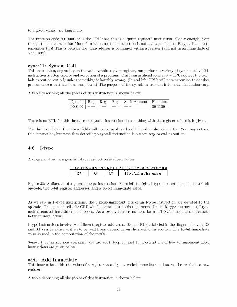
to a given value – nothing more.
The function code “001000” tells the CPU that this is a “jump register” instruction. Oddly enough, eventhough this instruction has ”jump” in its name, this instruction is not a J-type. It is an R-type. Be sure toremember this! This is because the jump address is contained within a register (and not in an immediate ofsome sort).
syscall: System CallThis instruction, depending on the value within a given register, can perform a variety of system calls. Thisinstruction is often used to end execution of a program. This is an artificial construct – CPUs do not typicallyhalt execution entirely unless something is horribly wrong. (In real life, CPUs will pass execution to anotherprocess once a task has been completed.) The purpose of the syscall instruction is to make simulation easy.
A table describing all the pieces of this instruction is shown below:
Opcode Reg Reg Reg Shift Amount Function0000 00 – — - —- —- - — – 00 1100
There is no RTL for this, because the syscall instruction does nothing with the register values it is given.
The dashes indicate that these fields will not be used, and so their values do not matter. You may not usethis instruction, but note that detecting a syscall instruction is a clean way to end execution.
4.6 I-type
A diagram showing a generic I-type instruction is shown below:
Figure 32: A diagram of a generic I-type instruction. From left to right, I-type instructions include: a 6-bitop-code, two 5-bit register addresses, and a 16-bit immediate value.
As we saw in R-type instructions, the 6 most-significant bits of an I-type instruction are devoted to theop-code. The op-code tells the CPU which operation it needs to perform. Unlike R-type instructions, I-typeinstructions all have different opcodes. As a result, there is no need for a “FUNCT” field to differentiatebetween instructions.
I-type instructions involve two different register addresses: RS and RT (as labeled in the diagram above). RSand RT can be either written to or read from, depending on the specific instruction. The 16-bit immediatevalue is used in the computation of the result.
Some I-type instructions you might use are addi, beq, sw, and lw. Descriptions of how to implement theseinstructions are given below:
addi: Add ImmediateThis instruction adds the value of a register to a sign-extended immediate and stores the result in a newregister.
A table describing all the pieces of this instruction is shown below:
43

Opcode Reg Reg Immediate0010 00 ss sss t tttt iiii iiii iiii iiii
The op-code “001000” tells the CPU that this is an addi instruction.
The RTL for this instruction is: $t = $s + imm; PC = PC + 4. (Again, we represent RT as t and RS ass in this RTL.) The first line of RTL, $t = $s + imm, tells us that the CPU will compute the sum of RSand the immediate and then store the sum in RT. The second line of RTL, PC = PC + 4, increments theprogram counter to move to the next instruction.
beq: Branch-If-EqualThis instruction checks whether two registers have equal value. If they do, the program counter jumps tosome other point in the program.
A table describing all the pieces of this instruction is shown below:
Opcode Reg Reg Immediate0001 00 ss sss t tttt iiii iiii iiii iiii
The op-code “000100” tells the CPU that this is a beq instruction.
The RTL for this instruction is:
1 i f \$s == \$t:2 PC = PC + (immediate $<<$ 2)
3 e l se :4 PC = PC + 4
(Again, we represent RT as t and RS as s in this RTL.) The first two lines of RTL are the first part of theconditional: if the values of registers RS and RT are equal, then the program counter jumps to a part ofthe program specified by the immediate value. Note that the immediate value is shifted to the left by twobits. This occurs because the program counter is incremented by 4 with each instruction. As a result, theprogram counter will always be divisible by 4. Since the program counter is always divisible by 4, the lasttwo bits of the program counter will always be 0 (and therefore are meaningless from a “storing information”perspective). These last two bits are omitted from the immediate to reduce the immediate’s size. As a result,the immediate must be shifted over by two bits when it is added to the program counter.
In this instruction, the immediate is often known as an “offset”, because it is the number you need to addto the program counter to make it jump to the right place.
Note that ble and bne (branch-less-equal and branch-not-equal, respectively) have similar RTL. The onlydifferences between all these instructions are the comparison statements and the op-codes. In ble, theop-code is “000110” and the if-statement becomes if $s <= $t. In bne, the op-code is “000101” and theif-statement becomes if $s != $t.
sw: Store wordThis instruction stores a word in data memory.
A table describing all the pieces of this instruction is shown below:
44
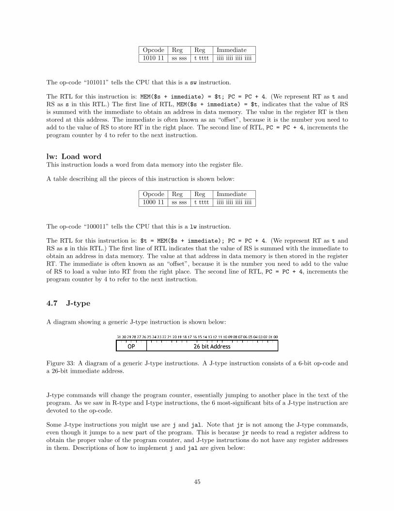
Opcode Reg Reg Immediate1010 11 ss sss t tttt iiii iiii iiii iiii
The op-code “101011” tells the CPU that this is a sw instruction.
The RTL for this instruction is: MEM($s + immediate) = $t; PC = PC + 4. (We represent RT as t andRS as s in this RTL.) The first line of RTL, MEM($s + immediate) = $t, indicates that the value of RSis summed with the immediate to obtain an address in data memory. The value in the register RT is thenstored at this address. The immediate is often known as an “offset”, because it is the number you need toadd to the value of RS to store RT in the right place. The second line of RTL, PC = PC + 4, increments theprogram counter by 4 to refer to the next instruction.
lw: Load wordThis instruction loads a word from data memory into the register file.
A table describing all the pieces of this instruction is shown below:
Opcode Reg Reg Immediate1000 11 ss sss t tttt iiii iiii iiii iiii
The op-code “100011” tells the CPU that this is a lw instruction.
The RTL for this instruction is: $t = MEM($s + immediate); PC = PC + 4. (We represent RT as t andRS as s in this RTL.) The first line of RTL indicates that the value of RS is summed with the immediate toobtain an address in data memory. The value at that address in data memory is then stored in the registerRT. The immediate is often known as an “offset”, because it is the number you need to add to the valueof RS to load a value into RT from the right place. The second line of RTL, PC = PC + 4, increments theprogram counter by 4 to refer to the next instruction.
4.7 J-type
A diagram showing a generic J-type instruction is shown below:
Figure 33: A diagram of a generic J-type instructions. A J-type instruction consists of a 6-bit op-code anda 26-bit immediate address.
J-type commands will change the program counter, essentially jumping to another place in the text of theprogram. As we saw in R-type and I-type instructions, the 6 most-significant bits of a J-type instruction aredevoted to the op-code.
Some J-type instructions you might use are j and jal. Note that jr is not among the J-type commands,even though it jumps to a new part of the program. This is because jr needs to read a register address toobtain the proper value of the program counter, and J-type instructions do not have any register addressesin them. Descriptions of how to implement j and jal are given below:
45

j: JumpThis instruction jumps to a calculated address. A table describing all the peices of this instruction is shownbelow:
Opcode Immediate0000 10 ii iiii iiii iiii iiii iiii iiii
The op-code “000010” tells the CPU that this is a j instruction.
The RTL for this instruction is: PC = (OldPC & 0xf0000000) | (immediate << 2);. The first part ofthis line, (OldPC & 0xf0000000), is a bitwise-AND of the program counter and a 28-bit-long binary stringof zeros. This will preserve bits 31 through 28 of the program counter, and all the rest will be set to zero.The second part of this line, (immediate << 2), shifts the immediate over by 2 bits. To understand whythe immediate is shifted over by two bits, recall that the program counter is incremented by 4 with eachinstruction. This means that the program counter will always be a multiple of 4 (and therefore that the lasttwo bits of the program counter will always be zero). Since these last two bits will always be zero, we don’thave to account for them in the immediate – we can save space. See the beq instruction for another exampleof immediate-shifting.
In the end, the PC becomes the following: OldPC31:28Imm25:000, where “Imm” represents the immediate value.
jal: Jump-And-LinkThis instruction jumps to a calculated address, and stores the return address in $31 so it can get back towhere it was. In other words, it performs the same steps as a j (jump) instruction, but stores its returnaddress as well. jal is often paired with jr, as jal will store the return-address jr must return to.
A table describing all the peices of this instruction is shown below:
Opcode Immediate0000 11 ii iiii iiii iiii iiii iiii iiii
The op-code “000011” tells the CPU that this is a jal instruction.
The RTL for this instruction is: $31 = OldPC + 8; PC = (OldPC & 0xf0000000) | (immediate << 2).The first line, $31 = OldPC + 8, indicates that the original value of the program counter is incremented by8 and then stored in the return-address register (register $31). Why OldPC + 8, though? You might thinkthis should be OldPC + 4. The return address should return to the next instruction, right?
The reason for this is that depending on the way your MIPS simulator is configured, an extra instruction maybe inserted immediately after the jump-and-link statement. This extra instruction is known as a branch-delay slot instruction, and its purpose is to ensure that the jump address has been calculated in pipelinedarchitectures (remember the hazards associated with pipelined architectures?). For more information, seehttp://www.cs.umd.edu/class/sum2003/cmsc311/Notes/Mips/jump.html for some more explanation ofjump instructions.
The second line of RTL, PC = (OldPC & 0xf0000000) | (immediate << 2), is the same exact instructionas in the j (jump) command introduced earlier. In short, this line preserves bits 31 through 28 of theprogram counter, and concatenates that with the 26-bit immediate and two zeros. The end result is thatthe PC becomes the following: OldPC31:28Imm25:000, where “Imm” represents the immediate value. See thej command for more information on how this works.
46

4.8 Useful Links
A set of class notes detailing the use of MIPS instructions. Also contains a lot of useful information about theinstruction types themselves. This set of class notes helped us a lot with the branch/jump type instructions.http://www.cs.umd.edu/class/sum2003/cmsc311/Notes/
A MIPS instruction reference. Contains a complete list of MIPS instructions, their formats, and their RTLdescriptions: http://www.mrc.uidaho.edu/mrc/people/jff/digital/MIPSir.html
A guide to MIPS instructions and their formats: http://www.eng.ucy.ac.cy/mmichael/courses/ECE314/LabsNotes/02/MIPS_Instruction_Coding_With_Hex.pdf
47
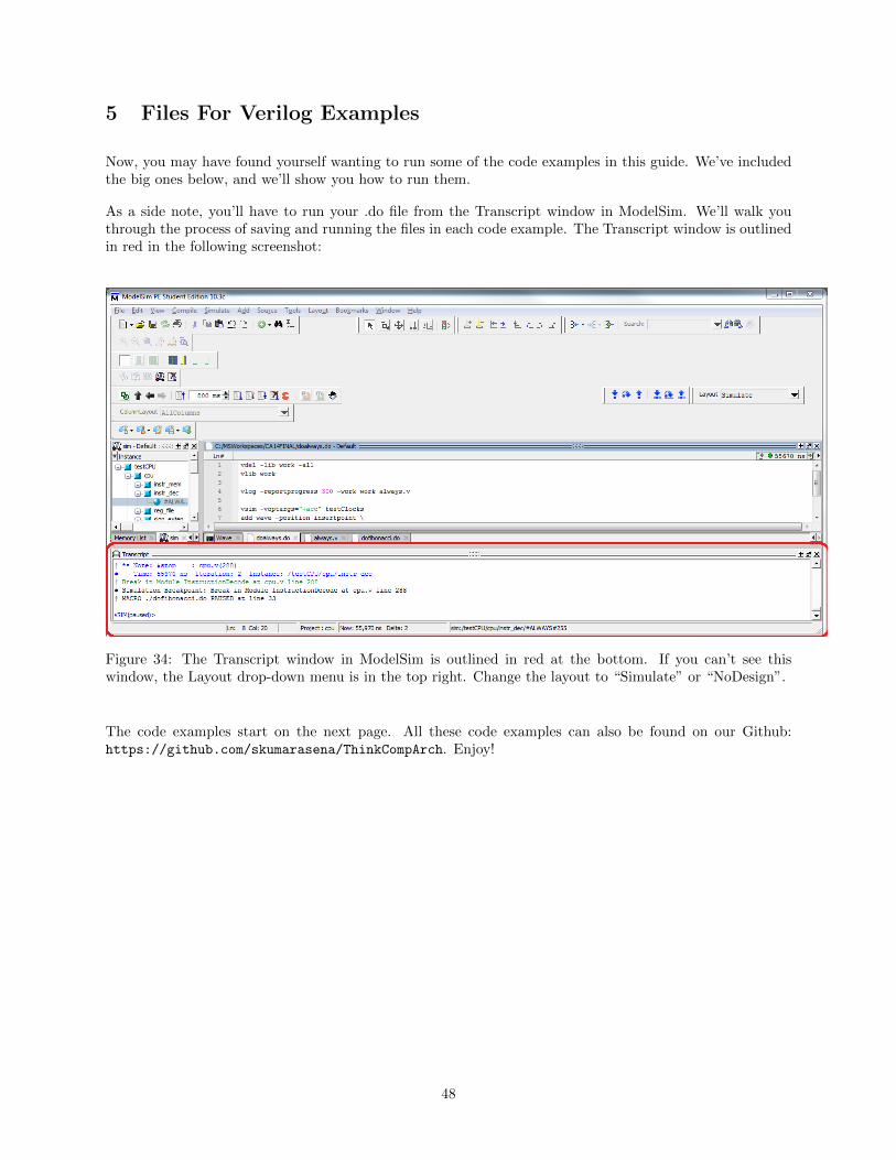
5 Files For Verilog Examples
Now, you may have found yourself wanting to run some of the code examples in this guide. We’ve includedthe big ones below, and we’ll show you how to run them.
As a side note, you’ll have to run your .do file from the Transcript window in ModelSim. We’ll walk youthrough the process of saving and running the files in each code example. The Transcript window is outlinedin red in the following screenshot:
Figure 34: The Transcript window in ModelSim is outlined in red at the bottom. If you can’t see thiswindow, the Layout drop-down menu is in the top right. Change the layout to “Simulate” or “NoDesign”.
The code examples start on the next page. All these code examples can also be found on our Github:https://github.com/skumarasena/ThinkCompArch. Enjoy!
48

5.1 Behavioral vs. Structural Example: Gates
First, save the following code as “gates.v”. Note that this file is configured to test the “structuralGates”module. If you’d like to test the “behavioralGates” module, look at the “testGates” module, uncommentthe behavioralGates initialization, and comment the structuralGates initialization.
1 /*
2 The ‘‘structuralGates" module , which directly transcribes
3 the circuit diagram in Fig. 3 into Verilog.
4 */
5 module structuralGates(out , in0 , in1);
6 output out;
7 input in0;
8 input in1;
9
10 wire andout;
11 wire nandout;
12 wire orout;
13
14 and andgate(andout , in0 , in1);
15 nand nandgate(nandout , in0 , in1);
16 or orgate(orout , andout , nandout );
17
18 not inv(out , orout);
19
20 endmodule21
22
23 /*
24 The ‘‘behavioralGates" module , which takes a behavioral
25 approach to produce the same result as structuralGates.
26 */
27 module behavioralGates(out , in0 , in1);
28 output out;
29 input in0;
30 input in1;
31
32 assign out = !(( in0 && in1) || !(in0 && in1));
33
34 endmodule35
36
37 /*
38 The test bench module for both the structuralGates and
39 behavioralGates modules.
40 */
41
42 module testGates;
43 reg in0 , in1;
44 wire out;
45
46 // uncomment if you ’re testing behavioralGates
47 // behavioralGates gates(out , in0 , in1);
49

48
49 // uncomment if you ’re testing structuralGates
50 structuralGates gates(out , in0 , in1);
51
52 i n i t i a l begin53 $display("In0 In1 | Out");
54 in0 =0; in1 =0; #1000
55 $display("%b %b | %b", in0 , in1 , out);
56 in0 =0; in1 =1; #1000
57 $display("%b %b | %b", in0 , in1 , out);
58 in0 =1; in1 =0; #1000
59 $display("%b %b | %b", in0 , in1 , out);
60 in0 =1; in1 =1; #1000
61 $display("%b %b | %b", in0 , in1 , out);
62
63 end64
65 endmodule
Now, save the following file as any name you want. (We suggest “dogates.do”, or something that tells youwhich Verilog file you’re testing. Otherwise you’re going to end up with a lot of .do files with similar names.)
1 #If you ’re wondering what these two lines do,
2 #see our section on .do files in "Think ModelSim"!
3 vdel -lib work -all
4 vlib work
5
6 vlog -reportprogress 300 -work work gates.v
7
8 vsim -voptargs="+acc" testGates
9
10 run 5000
Now if you want to run this code, type “do [name of your .do file]” (in our case this would be “dodogates.do”) into ModelSim’s Transcript window, and run it by pressing Enter. You should see the resultsof the test show up in the Transcript window.
50

5.2 Procedural Blocks Example: countingClocks
First, save the following code as “always.v”. This file is configured for non-blocking assignment in the alwaysblock – change the assignment operator to “=” if you’d like to see blocking assignment.
1 /*
2 The counter module. It increments itself at the positive clock edge.
3 Note that this counter is zero -indexed.
4 */
5 module countingClocks(out , clk);
6 output reg [3:0] out;
7 input clk;
8
9 reg [3:0] count;
10 i n i t i a l count = 0;
11 always @(posedge clk) begin12 count <= count + 1; // change assignment operator to "="
13 out <= count; //to see blocking assignment!
14 end15 endmodule16
17 /*
18 A test module for the counter. This will display a waveform that
19 shows you how the output value changes over time.
20 */
21
22 module testClocks;
23 wire [3:0] out;
24 reg clk;
25
26
27 countingClocks clock(out , clk);
28
29 i n i t i a l clk = 0;
30 always #100 clk=!clk;
31
32
33 endmodule
Now, save the following file as any name you want. (We suggest “doalways.do”, or something that tells youwhich Verilog file you’re testing. Otherwise you’re going to end up with a lot of .do files with similar names.)
1 #If you ’re wondering what these two lines do,
2 #see our section on .do files in "Think ModelSim"!
3 vdel -lib work -all
4 vlib work
5
6 vlog -reportprogress 300 -work work always.v7
8 vsim -voptargs="+acc" testClocks
9 add wave -position insertpoint \
10 sim:/ testClocks/clk \
51

11 sim:/ testClocks/out
12
13 run 1000
14 wave zoom full
Now if you want to run this code, type “do [name of your .do file]” (in our case this would be “dodoalways.do”) into ModelSim’s Transcript window, and run it by pressing Enter. You should see theresults of the test show up in the Waveforms window that pops up. If you’d like to switch back to theoriginal ModelSim layout, set the Layout bar at the top right to “NoDesign”.
52

5.3 Test Benches Example: Adders
First, save the following code as “brokenadders.v”. This file is configured for the functional adder. If you’dlike to change the file to test one of the broken adders, uncomment one of the lines in the test bench asindicated.
1 /*
2 The functional full adder. Behaves just like a one -bit full adder
3 should.
4 */
5 module behavioralFullAdder(sum , carryout , a, b, carryin );
6 output sum , carryout;
7 input a, b, carryin;
8 assign {carryout , sum}=a+b+carryin;
9 endmodule10
11 /*
12 The first broken full adder example. Sum and carryout are switched.
13 */
14 module behavioralFullAdder_broken(sum , carryout , a, b, carryin );
15 output sum , carryout;
16 input a, b, carryin;
17 assign {sum , carryout }=a+b+carryin;
18 endmodule19
20 /*
21 The second broken full adder example. Note that the carry -in has
22 been artifically set to 1. It ’s highly unlikely anyone would make
23 this mistake , but the point of that example was to show you how
24 test benches can serve as a diagnostic tool.
25 */
26 module behavioralFullAdder_broken2(sum , carryout , a, b, carryin );
27 output sum , carryout;
28 input a, b, carryin;
29 assign {sum , carryout }=a+b+1’b1;
30 endmodule31
32
33 module testFullAdder;
34
35 reg a, b, carryin;
36 wire sum , carryout;
37
38 // uncomment for working adder
39 behavioralFullAdder adder0(sum , carryout ,a,b,carryin );
40
41 // uncomment for broken adder 1
42 // behavioralFullAdder_broken adder1(sum , carryout ,a,b,carryin );
43
44 // uncomment for broken adder 2
45 // behavioralFullAdder_broken2 adder2(sum , carryout ,a,b,carryin );
46
47 i n i t i a l begin
53

48
49 $display("A B Cin | Cout Sum");
50 a=0;b=0; carryin =0; #1000
51 $display("%b %b %b | %b %b", a, b, carryin , carryout , sum);
52 a=0;b=0; carryin =1;#1000
53 $display("%b %b %b | %b %b", a, b, carryin , carryout , sum);
54 a=0;b=1; carryin =0;#1000
55 $display("%b %b %b | %b %b", a, b, carryin , carryout , sum);
56 a=0;b=1; carryin =1;#1000
57 $display("%b %b %b | %b %b", a, b, carryin , carryout , sum);
58
59 a=1;b=0; carryin =0;#1000
60 $display("%b %b %b | %b %b", a, b, carryin , carryout , sum);
61 a=1;b=0; carryin =1;#1000
62 $display("%b %b %b | %b %b", a, b, carryin , carryout , sum);
63 a=1;b=1; carryin =0;#1000
64 $display("%b %b %b | %b %b", a, b, carryin , carryout , sum);
65 a=1;b=1; carryin =1;#1000
66 $display("%b %b %b | %b %b", a, b, carryin , carryout , sum);
67
68
69 end70
71 endmodule
Next, save the following file as any name you want. (We suggest “dobroken.do”, or something that tells youwhich Verilog file you’re testing. Otherwise you’re going to end up with a lot of .do files with similar names.)
1 #If you ’re wondering what these two lines do,
2 #see our section on .do files in "Think ModelSim"!
3 vdel -lib work -all
4 vlib work
5
6 vlog -reportprogress 300 -work work brokenadders.v
7
8 vsim -voptargs="+acc" testFullAdder
9
10 run 10000
Now if you want to run this code, type “do [name of your .do file]” (in our case this would be “dodobroken.do”) into ModelSim’s Transcript window, and run it by pressing Enter. You should see theresults of the test show up in the Transcript window.
54