Direct Closed-Form Design of Finite Alphabet

Constant Envelope Waveforms for MIMO radar

Beampatterns

Thesis by

Taha Bouchoucha

In Partial Fulfillment of the Requirements

For the Degree of

Masters of Science

King Abdullah University of Science and Technology, Thuwal,

Kingdom of Saudi Arabia

April, 2015

2

The thesis of Your Full Name is approved by the examination committee

Committee Chairperson: Tareq Al-Naffouri

Committee Member: Mohamed-Slim Alouini

Committee Member: Ahmed Kamal Sultan Salem

Committee Member: Sajid Ahmed

3

Copyright ©2015

Taha Bouchoucha

All Rights Reserved

4

ABSTRACT

Direct Closed-Form Design of Finite Alphabet Constant

Envelope Waveforms for MIMO radar Beampatterns

Taha Bouchoucha

Multiple Input Multiple Output (MIMO) radar systems have attracted lately a lot of

research attention thanks to their advantages over the classical phased array radar sys-

tems. We site among these advantages the improvement of parametric identifiability,

the achievement of higher spatial resolution and the design of complex beampatterns.

In colocated MIMO radar systems, it is usually desirable to steer the transmitted

power in the region-of-interest in order to increase the Signal to Noise Ratio (SNR)

and reduce any undesired signal and thus improve the detection process. This prob-

lem is also known as transmit beampattern design. To achieve this goal, conventional

methods optimize the waveform covariance matrix, R, for the desired beampattern,

which is then used to generate the actual transmitted waveforms. Both steps require

constrained optimization. Most of the existing methods use iterative algorithms to

solve these problems, therefore their computational complexity is very high which

makes them hard to use in practice especially for real time radar applications. In

this work, we provide a closed-form solution to design the covariance matrix for a

given beampattern in the three dimensional space using narrowband planar arrays.

The expression of the covariance matrix is then used to derive a novel closed-form

algorithm to directly design the finite-alphabet constant-envelope waveforms. The

5

proposed algorithm exploits the two-dimensional discrete Fourier transform which is

implemented using fast Fourier transform algorithm. Consequently, the computa-

tional complexity of the proposed beampattern solution is very low allowing it to be

used for large arrays to change the beampattern in real time. We also show that the

number of required snapshots in each waveform depends on the beampattern and that

it is always less than the total number of transmit antennas. In addition, we show

that the proposed waveform design method can be used with the wideband system

model in order to improve the range resolution of the radar. The performance of our

proposed algorithms compares favorably with the existing iterative methods in terms

of mean square error.

Keywords: Multiple-input multiple-output radars, beampattern design, closed-

form solution, waveform design, two-dimensional fast-Fourier-transform.

6

ACKNOWLEDGEMENTS

I would like to express my recognition to Dr. Sajid Ahmed for his guidance, time and

attention throughout the thesis research. Thanks to his feedback and advice we were

able to achieve the objectives that we fixed. I also learned a lot from his experience

on how to conduct a research work in general and his expertise in the field of radar

systems in particular.

I would also like to thank my adviser Prof. Tareq Al-Naffouri and my co-adviser

Prof. Mohamed Slim Alouini for their advice, support and for providing me with the

best research opportunities and environment that I could have.

Finally, I would like to express my deepest gratitude to my beloved parents and

family for their encouragement and moral support.

7

TABLE OF CONTENTS

Examination Committee Approval 2

Copyright 3

Abstract 4

Acknowledgements 6

List of Abbreviations 9

List of Symbols 11

List of Figures 13

List of Tables 15

1 Introduction 16

1.1 Introduction to Radar systems . . . . . . . . . . . . . . . . . . . . . . 16

1.1.1 History and applications of Radar systems . . . . . . . . . . . 16

1.1.2 Phased array radars . . . . . . . . . . . . . . . . . . . . . . . 17

1.1.3 MIMO radars . . . . . . . . . . . . . . . . . . . . . . . . . . . 18

1.1.4 Thesis outline . . . . . . . . . . . . . . . . . . . . . . . . . . . 23

1.1.5 Notations . . . . . . . . . . . . . . . . . . . . . . . . . . . . . 25

2 Transmit Beampattern design for narrowband radars 26

2.1 Problem formulation . . . . . . . . . . . . . . . . . . . . . . . . . . . 26

2.2 Proposed solution for the waveform covariance matrix . . . . . . . . . 29

2.3 Proposed solution for direct waveform design . . . . . . . . . . . . . . 34

2.3.1 Transmitter implementation . . . . . . . . . . . . . . . . . . . 36

2.4 Performance evaluation . . . . . . . . . . . . . . . . . . . . . . . . . . 36

2.4.1 Peak to Average Power Ratio . . . . . . . . . . . . . . . . . . 37

2.4.2 Computational complexity . . . . . . . . . . . . . . . . . . . . 38

8

2.4.3 Non-Symmetric beampatterns . . . . . . . . . . . . . . . . . . 38

2.5 Conclusion . . . . . . . . . . . . . . . . . . . . . . . . . . . . . . . . . 41

3 Wideband radar systems 42

3.1 Wideband transmitter design . . . . . . . . . . . . . . . . . . . . . . 43

3.2 Wideband beampattern . . . . . . . . . . . . . . . . . . . . . . . . . . 44

3.3 Detection of targets with different ranges . . . . . . . . . . . . . . . . 46

3.4 Conclusion . . . . . . . . . . . . . . . . . . . . . . . . . . . . . . . . . 48

4 Numerical Simulations 49

4.1 Narrowband radars . . . . . . . . . . . . . . . . . . . . . . . . . . . . 49

4.1.1 Beampattern design . . . . . . . . . . . . . . . . . . . . . . . 49

4.1.2 Mean Square Error . . . . . . . . . . . . . . . . . . . . . . . . 50

4.1.3 Beampattern Shapes variations . . . . . . . . . . . . . . . . . 52

4.1.4 Linear arrays . . . . . . . . . . . . . . . . . . . . . . . . . . . 55

4.1.5 Target detection . . . . . . . . . . . . . . . . . . . . . . . . . 55

4.2 Wideband radars . . . . . . . . . . . . . . . . . . . . . . . . . . . . . 56

4.2.1 Beampattern design . . . . . . . . . . . . . . . . . . . . . . . 57

4.2.2 Detection of targets with different ranges . . . . . . . . . . . . 57

4.3 Conclusion . . . . . . . . . . . . . . . . . . . . . . . . . . . . . . . . . 59

5 Conclusion 60

5.1 Summary . . . . . . . . . . . . . . . . . . . . . . . . . . . . . . . . . 60

5.2 Future work . . . . . . . . . . . . . . . . . . . . . . . . . . . . . . . . 60

References 61

Appendices 64

9

LIST OF ABBREVIATIONS

2D-DFT Two Dimensional Discrete-Fourier-Transform

2D-FFT Two Dimensional Fast-Fourier-Transform

2D-IDFT Two Dimensional Inverse Discrete-Fourier-

Transform

APES Amplitude and Phase Estimator

AWGN Additive White Gaussian Noise

BPSK Binary Phase-Shift Keying

DOA Direction Of Arrival

DOD Direction Of Departure

DOF Degree Of Freedom

FACE Finite-Alphabet Constant-Envelop

FFT Fast Fourier-Transform

GLRT Generalised Likelihood Ratio Test

IES Inter-Element-Spacing

MIMO Multiple Input Multiple Output

MSE Mean Square Error

PAPR Peak-to-Average Power Ratio

RCS Radar Cross Section

RFPA Radio-Frequency Power Amplifier

ROI Region Of Interest

10

RV Random Variable

SAR Synthetic Aperture Radar

SIMO Single Input Multiple Output

SNR Signal to Noise Ratio

SQP Semi-definite Quadratic Programming

ULA Uniform Linear Array

11

LIST OF SYMBOLS

ar Receive steering vector

as Transmit steering vector

B Received power

dx Inter-space distance in the x-axis

dy Inter-space distance in the y-axis

Es Shifitng matrix

fx Normalized Cartesian coordinate on the x-axis

fy Normalized Cartesian coordinate on the y-axis

Hf Frequency domain coefficients

Ht Time domain coefficients

Na Number of non zero elements

Pd Desired power

R Waveform covariance matrix

Rhh Designed covariance matrix

Rs Shifted covariance matrix

y The vector of received symbols

r The received signal at the target

S Waveforms matrix

si Waveform transmitted from the ith antenna

φ Elevation angle

12

λ Wavelength

θ Azimuth angle

x The vector of transmitted symbols

z The vector of additive white Gaussian noise

13

LIST OF FIGURES

1.1 Distributed MIMO radar. . . . . . . . . . . . . . . . . . . . . . . . . 19

1.2 Bi-Static MIMO radar. . . . . . . . . . . . . . . . . . . . . . . . . . . 20

1.3 Mono-Static MIMO radar. . . . . . . . . . . . . . . . . . . . . . . . . 20

1.4 Linear planar array of M ×N transmit antennas. . . . . . . . . . . . 21

2.1 Circular shaped beampattern. . . . . . . . . . . . . . . . . . . . . . . 33

2.2 Block diagram of the transmitter implementation. . . . . . . . . . . . 36

2.3 Computational complexity comparison between the FFT-based algo-

rithm and the SQP method. . . . . . . . . . . . . . . . . . . . . . . . 38

2.4 3D Non-symmetric beampattern design . . . . . . . . . . . . . . . . . 40

2.5 2D Non-symmetric beampattern design . . . . . . . . . . . . . . . . . 40

3.1 Diagram of wideband MIMO radar system. . . . . . . . . . . . . . . . 45

4.1 The designed beampattern using SQP based method. Here the ROI is

−0.1 ≤ fx ≤ 0.1 and −0.1 ≤ fy ≤ 0.1 and M = N = 10. . . . . . . . . 50

4.2 The designed beampattern using the proposed FFT-based algorithm.

Here, the ROI is −0.1 ≤ fx ≤ 0.1 and −0.1 ≤ fy ≤ 0.1 and M = N = 10. 51

4.3 MSE comparison between the FFT-based algorithm and the SQP method

for different planar array dimensions. . . . . . . . . . . . . . . . . . . 52

4.4 FFT-based transmit Beampattern, N = M = 20, ROI focused in the

corners. . . . . . . . . . . . . . . . . . . . . . . . . . . . . . . . . . . 53

4.5 FFT-based transmit Beampattern, N = M = 20, ROI focused in the

borders. . . . . . . . . . . . . . . . . . . . . . . . . . . . . . . . . . . 53

4.6 FFT-based transmit beampattern design, N = M = 20. Here, the

transmitted power needs to be focused in the center and the borders. 54

4.7 FFT-based transmit beampattern design, N = M = 20. Here, the

ROI has a circular shape. . . . . . . . . . . . . . . . . . . . . . . . . . 54

14

4.8 Comparison of direct waveform design methods for the desired beam-

pattern using linear array. Here, in both algorithms each waveform

transmits 10 symbols. . . . . . . . . . . . . . . . . . . . . . . . . . . . 55

4.9 Two targets detection using matched filter, targets location: (fx, fy) =

{(−0.1,−0.1), (0.1, 0.1)} . . . . . . . . . . . . . . . . . . . . . . . . . 56

4.10 Wideband beampattern design, ROI: θ ∈ [−30◦, 30◦]. . . . . . . . . . 57

4.11 Detection of two targets with different ranges. . . . . . . . . . . . . . 58

4.12 Detection of two targets with different ranges (Projection). . . . . . . 58

15

LIST OF TABLES

2.1 Steps to compute R . . . . . . . . . . . . . . . . . . . . . . . . . . . . 33

16

Chapter 1

Introduction

This chapter is dedicated to introduce radar systems. We first present the phased

array radar systems and show their limitations. Next, we introduce Multiple In-

put Multiple Output (MIMO) radars and present their advantages and the future

challenges related to this field. An overview of the system model adopted to design

the transmitted and received waveforms in colocated planar MIMO radars is also

provided. We finally, enumerate the outline of the thesis and the adopted notations.

1.1 Introduction to Radar systems

1.1.1 History and applications of Radar systems

The word radar is originally an acronym for RAdio Detection and Ranging. Like

any invention, the idea appeared with the theoretical work of Hertz on radio waves

reflection in 1886. Later in 1900, Tesla investigated the electromagnetic detection

and the velocity measurement. The first radar experience was conducted in 1904 at

the famous bridge of Cologne by the German engineer Hulsmeyer who was able to

detect a ship using radio wave reflection. Afterwards, other experiences with different

targets were conducted spreading the development of radar technology all over the

world in the middle and late 1930s. [1, 2]

17

The early radar applications were exclusively military applications including surveil-

lance, navigation and weapons guidance [3]. Nowadays, radar technology enjoys an

increasing range of civil applications [4]. The traffic radar is used to control the

speed limit in highways. The polarimetric doppler weather radar is very useful in the

weather monitoring and prediction field. Another important and vital application is

the air traffic control used to guide and track the airplanes in order to avoid collision

and severe weather conditions. A similar technology is being recently implemented

in automobile industries as well. Synthetic Aperture Radar (SAR) technology is used

to perform high resolution images of the ground and remote sensing and mapping of

the surfaces of both the Earth and other celestial objects. Although the presented

sketch of radar applications is far from being exhaustive it gives an idea about the

important role of this technology and the necessity to conduct further research work

in this field in order to improve radar systems performance.

1.1.2 Phased array radars

Phased array radars, also known as Single Input Multiple Output (SIMO) radars,

are one of the most common radar configurations. They are widely used in both

civilian and military applications. A phased array radar is composed of a number

of radiating elements each with a phase shifter. In order to steer the emitted beam

in the desired direction or Region Of Interest (ROI), constructive and destructive

interferences between the phase shifted emitted signals are exploited. The multiple

transmitter elements can cohere and steer the transmitted energy toward a desired

direction by transmitting delayed versions of a single waveform. This beamforming

technique was introduced in the 1960s in order to replace the mechanical systems

previously used to steer the transmitted power of the radar. We distinguish between

analog beamforming which uses different phase shifters and digital beamforming via

adaptive processing. Digitally switched phase shifters benefit from a number of ad-

18

vantages among them we can cite the coherent processing gain [5] and the ability to

change the beam direction in a very short time period. Several beams can also be

simultaneously transmitted to achieve multifunction tasks such as tracking multiple

targets at the same time. However, phased array radars have some drawbacks like

a coverage limited to 120 degree sector in azimuth and elevation angles. They also

have low frequency agility and very complex structure. We should also note that in

the case of phased array radars, the waveforms are fully correlated which results in

deterioration of not only transmit beamforming operations but also target detection

in the receiver side due to high side lobes levels. To overcome some of these draw-

backs, Multiple Input Multiple Output (MIMO) radar systems have been introduced

with the advantage of transmitting orthogonal waveforms.

1.1.3 MIMO radars

During the last decades, the need of sophisticated and accurate radar functions has

been rising in many application fields. MIMO radar systems are expected to be the

solution which will help achieve this goal. That’s why MIMO radars field has been

lately an interesting research topic thanks to the introduction of a novel method of

signal transmission and reception in the radar systems field. In a MIMO architecture,

each transmit antenna radiates an arbitrary waveform independently form the other

antennas [6, 7]. Thus, unlike the phased array systems, the different waveforms

transmitted by a MIMO radar can be correlated or uncorrelated with each other.

Advantages of MIMO radars

MIMO radars have a number of advantages over the classical phased array radars.

For example, they yield significant improvement in parameter identifiability and tar-

get detection [8]. Moreover, an antenna field of nT transmitters and nR receivers

mathematically results in a virtual field of nT × nR elements which provides en-

19

larged virtual aperture and thus a capability of detecting larger number of targets

[6, 7, 9, 10]. Thanks to the concept of virtual arrays, we also benefit from extra De-

grees Of Freedom (DOF)[11, 12] which lead to enhanced flexibility to design transmit

beampatterns and improved angular resolution.

Types of MIMO radars

We can distinguish between two categories of MIMO radar systems depending on the

locations of the transmitting and receiving elements:

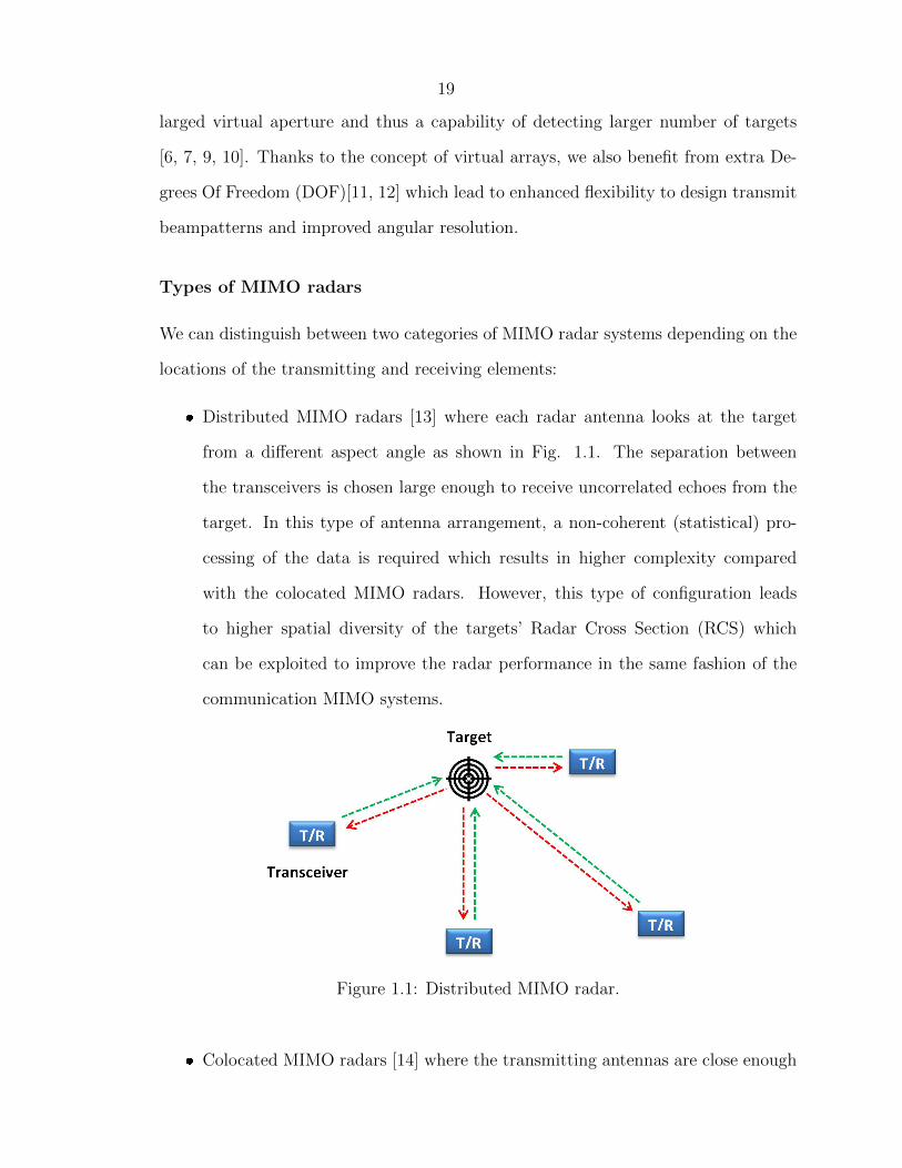
� Distributed MIMO radars [13] where each radar antenna looks at the target

from a different aspect angle as shown in Fig. 1.1. The separation between

the transceivers is chosen large enough to receive uncorrelated echoes from the

target. In this type of antenna arrangement, a non-coherent (statistical) pro-

cessing of the data is required which results in higher complexity compared

with the colocated MIMO radars. However, this type of configuration leads

to higher spatial diversity of the targets’ Radar Cross Section (RCS) which

can be exploited to improve the radar performance in the same fashion of the

communication MIMO systems.

Figure 1.1: Distributed MIMO radar.

� Colocated MIMO radars [14] where the transmitting antennas are close enough

20

(usually half of the working wavelength) such that the RCSs observed by the

different antennas are the same. While this type of configuration does not ben-

efit from spatial diversity as the distributed MIMO configuration, an increased

spatial resolution can be achieved by a coherent processing of the different time

delays from all the transmitting and receiving paths. This type of configuration

also benefits from a good interference rejection and beampattern design flexi-

bility. Colocated MIMO radars can further be classified into Bi-static MIMO

radars, Fig. 1.2, with widely separated transmitter and receiver arrays and

mono-static MIMO radars, Fig. 1.3, with closely spaced transmitter and re-

ceiver arrays.

Figure 1.2: Bi-Static MIMO radar.

Figure 1.3: Mono-Static MIMO radar.

21

In this work, we focus on the colocated mono-static MIMO radar configuration. The

signal model used is presented in the following section.

System model

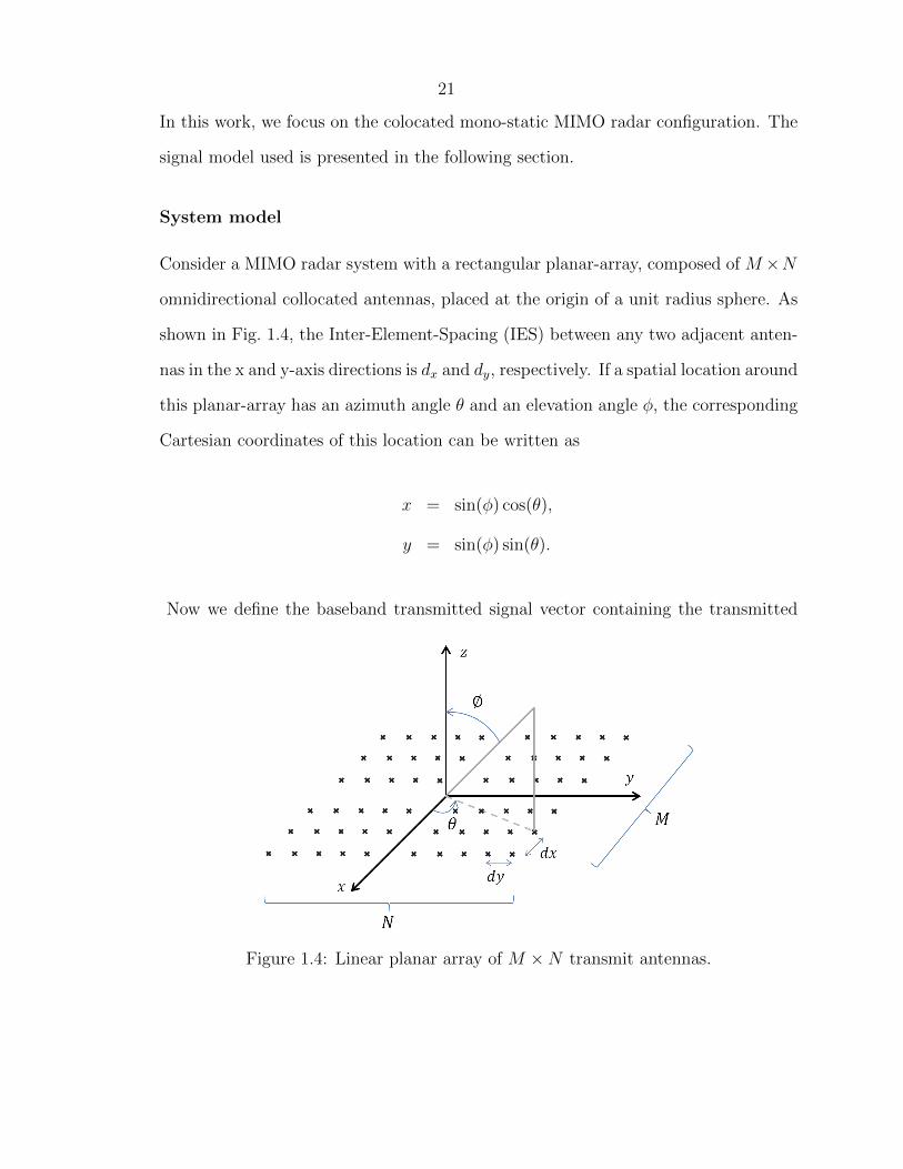
Consider a MIMO radar system with a rectangular planar-array, composed of M ×N

omnidirectional collocated antennas, placed at the origin of a unit radius sphere. As

shown in Fig. 1.4, the Inter-Element-Spacing (IES) between any two adjacent anten-

nas in the x and y-axis directions is dx and dy, respectively. If a spatial location around

this planar-array has an azimuth angle θ and an elevation angle φ, the corresponding

Cartesian coordinates of this location can be written as

x = sin(φ) cos(θ),

y = sin(φ) sin(θ).

Now we define the baseband transmitted signal vector containing the transmitted

Figure 1.4: Linear planar array of M ×N transmit antennas.

22

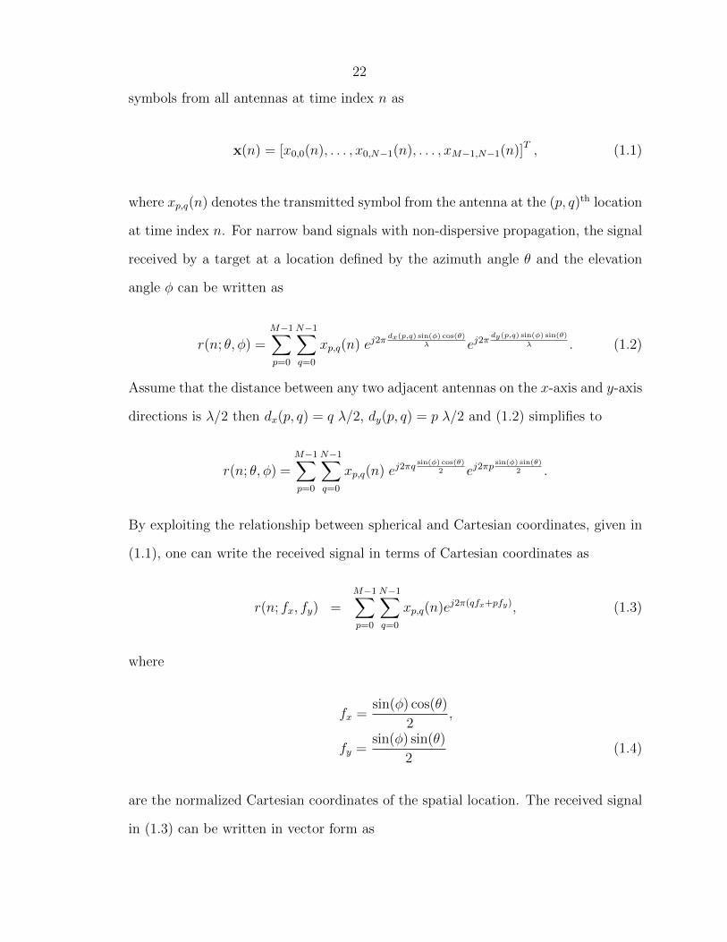
symbols from all antennas at time index n as

x(n) = [x0,0(n), . . . , x0,N−1(n), . . . , xM−1,N−1(n)]T , (1.1)

where xp,q(n) denotes the transmitted symbol from the antenna at the (p, q)th location

at time index n. For narrow band signals with non-dispersive propagation, the signal

received by a target at a location defined by the azimuth angle θ and the elevation

angle φ can be written as

r(n; θ, φ) =M−1∑p=0

N−1∑q=0

xp,q(n) ej2πdx(p,q) sin(φ) cos(θ)

λ ej2πdy(p,q) sin(φ) sin(θ)

λ . (1.2)

Assume that the distance between any two adjacent antennas on the x-axis and y-axis

directions is λ/2 then dx(p, q) = q λ/2, dy(p, q) = p λ/2 and (1.2) simplifies to

r(n; θ, φ) =M−1∑p=0

N−1∑q=0

xp,q(n) ej2πqsin(φ) cos(θ)

2 ej2πpsin(φ) sin(θ)

2 .

By exploiting the relationship between spherical and Cartesian coordinates, given in

(1.1), one can write the received signal in terms of Cartesian coordinates as

r(n; fx, fy) =M−1∑p=0

N−1∑q=0

xp,q(n)ej2π(qfx+pfy), (1.3)

where

fx =sin(φ) cos(θ)

2,

fy =sin(φ) sin(θ)

2(1.4)

are the normalized Cartesian coordinates of the spatial location. The received signal

in (1.3) can be written in vector form as

23

r(n; fx, fy) = aHs (fx, fy) x(n), (1.5)

where

as(fx, fy) =

1

ej2πfy

...

ej2π(M−1)fy

⊗

1

ej2πfx

...

ej2π(N−1)fx

. (1.6)

Using (1.5), the received power at the location (fx, fy) can be easily written as

B(fx, fy) = E{aHs (fx, fy) x(n) x(n)H as(fx, fy)}

= aHs (fx, fy) R as(fx, fy), (1.7)

where R = E{x(n)x(n)H} is the MN ×MN covariance matrix of the transmitted

waveforms which have (MN)2+MN2

DOF.

1.1.4 Thesis outline

In this work, we study the beampattern design problem in planar MIMO radars with

collocated and mono-static antennas. In the narrowband case, our goal is to maximize

the transmitted power, given by (1.7), around the locations of the targets of interest.

The regions of interest are defined in the three dimensional space with the azimuth

angle θ and the elevation angle φ. We present a closed-form solution to design the

waveform covariance matrix for the desired 3D beampatterns using a MIMO planar

array of dimensions M ×N . In order to reduce the computational complexity of our

algorithm, the 3D beampattern design problem is mapped onto the two dimensional

24

(2D) fast-Fourier-transform (2D-FFT). In addition, by exploiting the derivations of

the covariance matrix in the proposed algorithm, a novel method to directly design

the finite-alphabet constant-envelop (FACE) waveforms is also proposed for any de-

sired 3D beampattern. The direct design of waveforms does not require the synthesis

of covariance matrix and the performance is the same compared with the approach us-

ing covariance matrix. Therefore, the proposed direct design of the waveforms yields

significant reduction in the computational complexity and can achieve the best pos-

sible performance among existing direct waveform design algorithms. The proposed

method is also shown to be efficient in the case of non symmetric beampatterns.

In the wideband case, we aim to design transmit beampatterns and, most impor-

tantly, to resolve targets with different ranges thanks to the wideband signal model.

The rest of this manuscript is organized as follows. In Chapter 2, we present the

signal model adopted for the planar array and formulate the optimization problem

for the beampattern design. Next, by exploiting 2D-FFT, we solve the beampattern

design problem using two approaches. In the first approach, using the waveform

covariance matrix, we propose a computationally efficient algorithm to design the

covariance matrix for a given beampattern. In the second approach, we perform

direct waveform design without synthesizing any covariance matrix. Next, the per-

formance of the proposed waveform solution is studied. Chapter 3 deals with the

case of wideband radar systems. We achieve beampattern design by exploiting the

methods developed in Chapter 2. By using the wideband signal property, we realize

the detection of targets located at the same angular position but at different ranges.

Chapter 4 is dedicated to numerical simulations to evaluate the proposed methods

and compare them with the previous works and illustrate with various examples of

beampattern realizations. Conclusions are finally drawn in Chapter 5.

25

1.1.5 Notations

The following notations are adopted in this thesis. Small letters (e.g. a), bold small

letters (e.g. a), and bold capital letters (e.g. A) respectively designate scalars, vectors,

and matrices. If A is a matrix, then AH and AT respectively denote the Hermitian

transpose and the transpose of A. v(i) denotes the ith element of vector v. A(i, j)

denotes the entry in the ith row and jth column of matrix A. The Kronecker product

is denoted by ⊗ and the Hadamard product by �. Modulo M operation on an integer

i is denoted by 〈i〉M and bicM denotes the quotient of i over M . Finally, the statistical

expectation is denoted by E{·}.

26

Chapter 2

Transmit Beampattern design for

narrowband radars

Transmit beampattern techniques are used in order to focus the transmitted power

in a certain ROI [15, 16, 17, 18, 19, 20]. This process turns out to be essential in a

number of applications. For example, imaging radars are generally required to focus

the transmitted power, as much as possible, into the pre-defined ROI. This reduces

the power of received signals coming out of the ROI and increases the Signal to Noise

Ratio (SNR)[21].

The remainder of this chapter is as follows. In section 2.1, we formulate the optimiza-

tion problem relative to beampattern design with planar arrays. In section 2.2, we

detail the proposed solution for the covariance matrix design for a given beampattern.

Next, we propose in section 2.3 a method to directly design the waveforms for a given

beampattern without synthesizing the covariance matrix. Finally, we evaluate the

performance of the proposed waveforms design in section 2.4.

2.1 Problem formulation

In order to transmit power into the given ROI i.e. perform transmit beampattern

design, the following two approaches are available in the literature:

27

� The first approach is based on waveform covariance matrix design. It is known

that the transmit beampattern of a collocated antenna array depends on the

cross-correlation between the transmitted waveforms from different antennas.

Therefore, to design variety of transmit beampatterns, early solutions have re-

lied on a two-step process [15, 16, 17, 18, 19, 20]. In the first step, the user

designs the waveform covariance matrix such that the theoretical transmitted

power matches the desired beampattern as closely as possible. The second step

involves the design of the actual waveforms that can realize the designed covari-

ance matrix. Both of these steps require constrained optimization and most of

the available literature uses iterative algorithms.

� In the second approach, the waveforms which realize the desired beampattern

are directly designed without synthesizing the covariance matrix.

For the first approach, efficient iterative algorithms are proposed in [16, 19, 22] to syn-

thesize the waveform covariance matrix for a given beampattern. These algorithms

are computationally very expensive for real-time applications. In order to synthe-

size the waveform covariance matrix, a reduced complexity closed-form solution is

proposed in [23]. To reduce the computational complexity, this algorithm exploits

the fast Fourier-transform (FFT). Once the covariance matrix is synthesized, the

corresponding waveforms fulfilling some practical constraints such as close to unity

peak-to-average power ratio (PAPR) are designed. An iterative algorithm to design

constant envelope waveforms is proposed in [24]. The computational complexity of

this algorithm is also very high, moreover it generates non-finite alphabets that can be

challenging to use in practice. In [25], by mapping Gaussian Random Variables (RV)

onto binary phase-shift keying (BPSK) symbols, a closed-form solution to generate

BPSK waveforms to realize the given covariance matrix and an iterative algorithm

to achieve best possible beampattern are proposed. The main drawback of this algo-

rithm is that its performance depends on the beampattern.

28

Using the second approach, a sub-optimal algorithm to directly design the waveforms

for a uni-modal symmetric beampattern is presented in [26]. In this algorithm, a

scalar coefficient controls the width of the beampattern. This method requires a

large number of transmitting antennas in order to achieve good approximation of

the desired beampattern. In [20], various strategies for Hybrid MIMO phased-array

radar, based on multiplication of signal sets by a pseudo-noise spreading sequence,

are proposed for different transmit 3D beampatterns.

We have noticed that the solutions proposed in the previous works deal only with

linear arrays and thus regions of interest defined only by one parameter which is the

azimuth angle θ. In the planar array radar systems, the transmitting antennas form

a plan and an additional dimension called the elevation angle φ is taken into account

in order to provide a larger radar aperture. This allows us to characterize the ROI in

the three-dimensional (3D) space.

In the conventional transmit beampattern design problem, a covariance matrix,

R, is synthesized to match the transmitted power B(fx, fy), whose expression is given

in (1.7), to the desired beampattern which involves the minimization of the following

cost function

J(R) =L∑l=1

K∑k=1

∣∣∣aHs (fx(l), fy(k))Ras(fx(l), fy(k))− αPd(fx(l), fy(k))∣∣∣22, (2.1)

where Pd(fx(l), fy(k)) is the desired beampattern defined over the two dimensional

grid({fx(l)}Ll=1, {fy(k)}Kk=1

)and α is a scaling factor. Since R is a covariance ma-

trix, it should be positive semi-definite. Moreover, radio-frequency power amplifiers

(RFPA) have limited dynamic range and they can not transmit all power levels with

the same power efficiency. If we want to design variety of transmit beampatterns

without changing any hardware, the RFPA should transmit same power levels for any

beampattern. Therefore, to satisfy these constraints using the conventional methods,

29

we define the following minimization problem:

min J(R)

subject to

C1 : R � 0

C2 : R(n, n) = c, n = 1, 2, . . . ,MN.

(2.2)

where C1 represents the semi-definite constraint and C2 ensures a uniform constant

elemental power. One approach to solve the problem (2.2) was proposed in [16] where

the authors proposed a Semi-Definite Quadratic Programming (SQP) algorithm which

is an iterative method. The goal of the proposed method is to choose the matrix R

such that the available transmit power is used to maximize the probing signal power

at the locations of the targets of interest and to minimize it anywhere else. The

constrained problem in (2.2) can be optimally solved using the iterative SQP method.

However, for large number of antennas the computational complexity of SQP becomes

prohibitively large. Therefore, such solutions are not feasible for planar-arrays of high

sizes.

In order to reduce the computational cost, a closed-form solution to R exploiting 2D-

FFT algorithm is proposed in the following section. The SQP algorithm is considered

hereafter as a benchmark.

2.2 Proposed solution for the waveform covariance

matrix

Given an M × N time domain matrix Ht, the M × N frequency domain matrix

Hf can be easily generated. The relationship between the time domain coefficients

Ht(m,n) and the frequency domain coefficients Hf (k1, k2) is given by the following

30

2D discrete-Fourier-transform (2D-DFT) formula

Hf (k1, k2) =M−1∑m=0

N−1∑n=0

Ht(m,n) e−j2πk1m/Me−j2πk2n/N . (2.3)

Similarly, given frequency domain coefficients, the time domain coefficients are ob-

tained with the 2D inverse discrete-Fourier-transform (2D-IDFT)

Ht(m,n) =1

MN

M−1∑k1=0

N−1∑k2=0

Hf (k1, k2) ej2πk1m/Mej2πk2n/N . (2.4)

Using the 2D-DFT formula of (2.3), we obtain the following lemma which is proved

in Appendix A.

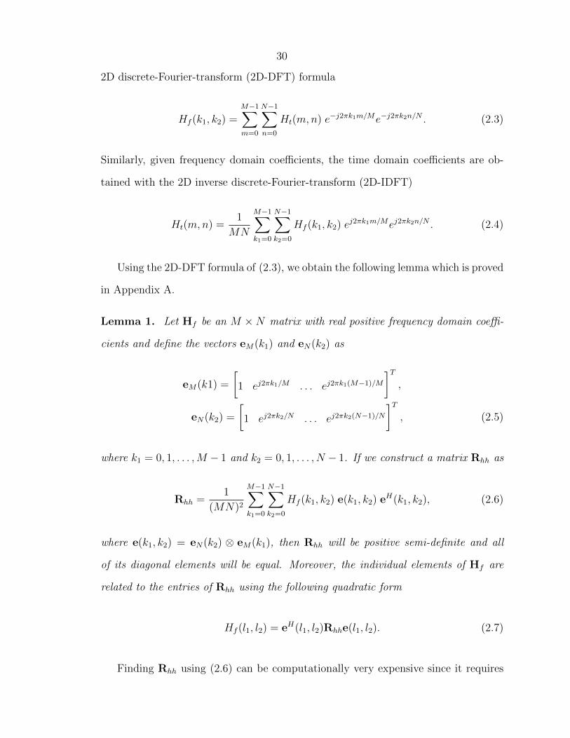
Lemma 1. Let Hf be an M ×N matrix with real positive frequency domain coeffi-

cients and define the vectors eM(k1) and eN(k2) as

eM(k1) =

[1 ej2πk1/M . . . ej2πk1(M−1)/M

]T,

eN(k2) =

[1 ej2πk2/N . . . ej2πk2(N−1)/N

]T, (2.5)

where k1 = 0, 1, . . . ,M − 1 and k2 = 0, 1, . . . , N − 1. If we construct a matrix Rhh as

Rhh =1

(MN)2

M−1∑k1=0

N−1∑k2=0

Hf (k1, k2) e(k1, k2) eH(k1, k2), (2.6)

where e(k1, k2) = eN(k2) ⊗ eM(k1), then Rhh will be positive semi-definite and all

of its diagonal elements will be equal. Moreover, the individual elements of Hf are

related to the entries of Rhh using the following quadratic form

Hf (l1, l2) = eH(l1, l2)Rhhe(l1, l2). (2.7)

Finding Rhh using (2.6) can be computationally very expensive since it requires

31

the outer product of MN vectors and the addition of MN corresponding matrices. To

reduce the computational complexity, we use (2.6) to express the individual elements

of Rhh as

Rhh(i1, i2) =1

(MN)2

M−1∑k1=0

N−1∑k2=0

Hf (k1, k2)× ej2πk1〈i1−i2〉M

M ej2πk2(bi1cM−bi2cM )

N , (2.8)

where i1, i2 = 0, 1, . . . ,MN − 1. Comparing (2.8) with (2.4) yields

Rhh(i1, i2) =1

MNHt(〈i1 − i2〉M , bi1cM − bi2cM). (2.9)

As we know, for a given frequency domain matrix Hf , the time domain matrix Ht can

be found using the 2D-FFT. Therefore, finding Rhh using Ht is computationally less

expensive. It should also be noted here that since Hf is real, Ht(−m,−n) = H∗t (m,n),

moreover, as e−j2πk1mM = ej

2πk1(M−m)M the matrix Rhh will be block Toeplitz.

Note that the case of Uniform Linear Array (ULA), studied in [23], can be con-

sidered as the special case of our proposed planar array when N = 1. In this case,

the frequency and time domain matrices Hf and Ht are reduced to M × 1 vectors

denoted respectively as hf and ht. The correlation matrix Rhh becomes of dimension

M ×M and by using formula (2.6) the individual elements of Rhh can be found as

Rhh(i1, i2) =1

M2

M−1∑k1=0

hf (k1)e2jπk1〈i1−i2〉M

M ,

=1

M2

M−1∑k1=0

hf (k1)e2jπk1(i1−i2)

M . (2.10)

Similarly, using the fact that hf is real, the matrix Rhh can be found using the time

domain coefficients of hf as

Rhh(i1, i2) =1

Mht(i1 − i2). (2.11)

32

Since ht(−i) = h∗t (i), the matrix Rhh is the same Toeplitz matrix proposed in [23].

Thus, our generalized method for the 3D beampatterns using planar arrays (defined

by θ and φ) is also valid in the case of 2D beampatterns using linear arrays (defined

only by θ) as proposed in [23].

Since the matrix Rhh is positive semi-definite and all of its diagonal elements

are equal, it satisfies both the C1 and C2 constraints of the optimization transmit

beampattern design problem in (2.2). Therefore, if Rhh is considered to be the wave-

form covariance matrix, by comparing (1.7) with (2.7), it can be easily seen that the

problem of transmit beampattern design can be mapped to the result obtained in

the Lemma 1. This transformation only requires the mapping of the steering vector

as(fx, fy) to e(k1, k2). This can be done by mapping the values of fx and fy to k1 and

k2, respectively, using the expressions given in (2.12). It should be noted here that

−0.5 ≤ {fx, fy} ≤ +0.5.

fx 7→ −0.5 + k1

M−1 , k1 = 0 . . .M − 1

fy 7→ −0.5 + k2N−1 , k2 = 0 . . . N − 1.

(2.12)

Note that by using this mapping, fx and fy defining the desired beampattern are

mapped to discrete values. This can represent a drawback for small antenna sized

planar arrays due to the small spatial resolution. In the proposed method, the desired

beampattern will be defined in terms of fx and fy, however the beampattern in terms

of spherical coordinates can be easily found using (1.4).

The three dimensional space can then be defined by a two dimensional grid({(fx)(l)}Ml=1, {(fy)(k)}Nk=1

)represented by an M × N matrix Hf . Thus, the en-

try Hf (m,n) corresponds to fx = −0.5 + mM−1 and fy = −0.5 + n

N−1 . In order to

define the ROI of the desired beampattern, we just have to assign 1 to the entries

of Hf which are inside the ROI and 0 everywhere else. The different steps of our

33

method are summarized in the following algorithm

Table 2.1: Steps to compute R

Step 0: Define Hf according to the ROI

Step 1: Ht ← 2D-IDFT(Hf )

Step 2: Compute Rhh using (2.9)

Step 3: Use Rhh as the waveform covariance matrix R

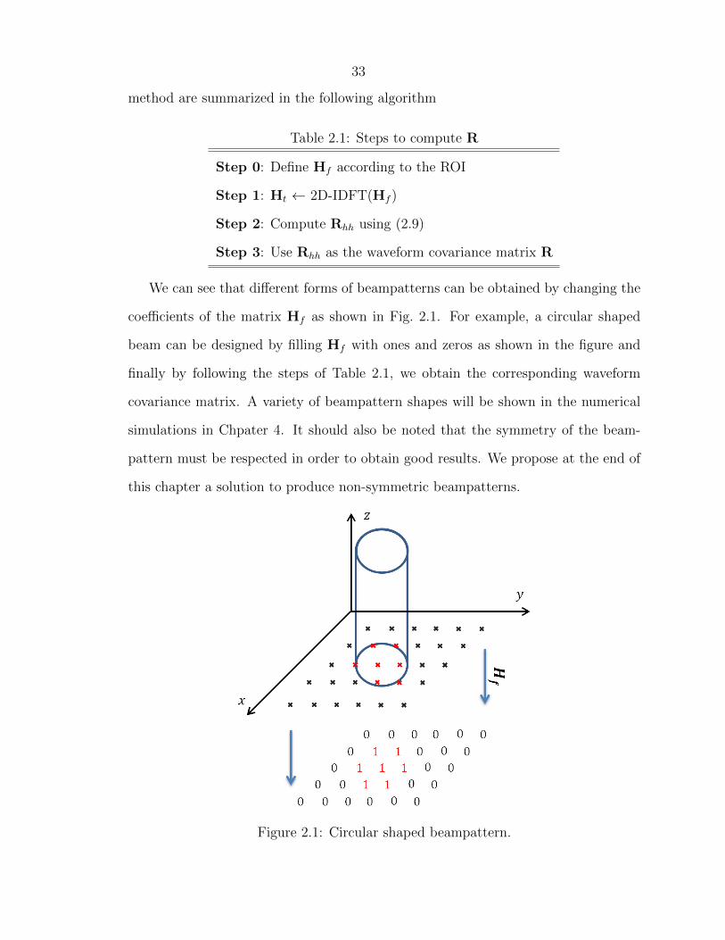
We can see that different forms of beampatterns can be obtained by changing the

coefficients of the matrix Hf as shown in Fig. 2.1. For example, a circular shaped

beam can be designed by filling Hf with ones and zeros as shown in the figure and

finally by following the steps of Table 2.1, we obtain the corresponding waveform

covariance matrix. A variety of beampattern shapes will be shown in the numerical

simulations in Chpater 4. It should also be noted that the symmetry of the beam-

pattern must be respected in order to obtain good results. We propose at the end of

this chapter a solution to produce non-symmetric beampatterns.

Figure 2.1: Circular shaped beampattern.

34

2.3 Proposed solution for direct waveform design

In this section, a closed-form expression to directly design the waveforms for the

desired beampattern is proposed. We start from (2.6) where the (i1, i2) element of

the designed covariance matrix can also be written as

R(i1, i2)=M−1∑k1=0

N−1∑k2=0

(√Hf (k1, k2)

MNej

2πk1〈i1〉MM ej

2πk2bi1cMN

)

×

(√Hf (k1, k2)

MNej

2πk1〈i2〉MM ej

2πk2bi2cMN

)∗. (2.13)

Assuming k = k1 +Mk2 = 〈k〉M +MbkcM , both terms in the above equation can be

considered as the kth elements of the waveforms si1 and si2 that can be written as

si1(k) =

√Hf (〈k〉M , bkcM)

MNej

2π〈k〉M 〈i1〉MM ej

2πbkcM bi1cMN ,

si2(k) =

√Hf (〈k〉M , bkcM)

MNej

2π〈k〉M 〈i2〉MM ej

2πbkcM bi2cMN ,

where k = 0, 1, . . . ,MN − 1 represents the time index. Thus, the cross-correlation

between the waveforms {si1(k)} and {si2(k)} can be written as

R(i1, i2) =MN−1∑k=0

si1(k) si2(k)∗. (2.14)

35

The corresponding waveform vector can be written as

si =

vi0...

viM−1

(2.15)

=

√Hf (0,0)

MNej

2π(0)bicMN ej

2π(0)〈i〉MM

...√Hf (0,N−1)MN

ej2π(N−1)bicM

N ej2π(0)〈i〉M

M

...

...√Hf (M−1,0)MN

ej2π(0)bicM

N ej2π(M−1)〈i〉M

M

...√Hf (M−1,N−1)

MNej

2π(N−1)bicMN ej

2π(M−1)〈i〉MM

where

vip =

1

MN

√Hf (p, 0)ej

2π(0)bicMN ej

2πp〈i〉MM

...

1MN

√Hf (p,N − 1)ej

2π(N−1)bicMN ej

2πp〈i〉MM

, (2.16)

where p = 0, 1, . . . ,M −1. Therefore, for any transmitting element of the rectangular

array at location (m,n) where m = 0 . . .M − 1 and n = 0 . . . N − 1, we assign the

waveform si defined in (2.15) with i = m+ nM .

Note that each waveform si contains MN time domain symbols. These symbols de-

pend on the matrix Hf which contains non null values only in the ROI and zeros

everywhere else. Thus, depending on the desired beampattern, some of the trans-

mitted symbols may be equal to zero. If Na is the number of non-zero elements in

the matrix Hf , each waveform will transmit only Na non-zero symbols. Therefore, to

achieve the desired beampattern only Na < MN snapshots will be required.

36

2.3.1 Transmitter implementation

The block diagram of the system is shown in Fig. 2.2. As we can see in the diagram,

the desired beampattern which is the input of the system, is a matrix of ones and

zeros. The total number of elements in the matrix defines the grid points of spatial

locations. If the power is desired at some location, the corresponding element in the

desired beampattern matrix is assigned one otherwise it is assigned zero. For an input

beampattern, waveforms are directly designed using the algorithms mentioned in sec-

tion 2.3. Next, the real and imaginary parts of the symbols of the designed waveform

are coded into the corresponding digital bit streams. Each coded bit stream is fed

into the corresponding storage unit, then converted into analogue IQ data stream.

Finally, IQ data is modulated, amplified, and transmitted at the symbol transmission

rate from the corresponding antenna. In this radar system, the beampattern can be

changed adaptively.

Figure 2.2: Block diagram of the transmitter implementation.

2.4 Performance evaluation

We evaluate in this section the performance of the proposed method for direct wave-

form design. We investigate the PAPR for the proposed waveforms. Then, we com-

pare the computational complexity of our method with the iterative SQP method.

We finally propose an extension of the proposed method to the non-symmetric beam-

patterns.

37

2.4.1 Peak to Average Power Ratio

Let us investigate the performance of our waveform design method in terms of its

PAPR. The ith waveform will be transmitting Na non-zero time domain symbols.

Therefore, the average transmitted power from the (m,n)th antenna can be written

as

Pi(avg) =1

Na

sHi si,

=1

Na

MN−1∑k=0

1

(MN)2si(k)s∗i (k),

=Na

Na(MN)2.

We note that the average transmitted power does not depend on the antenna location,

which confirms that the uniform elemental power constraint is satisfied. Similarly,

the peak power of the ith waveform can be derived as

Pi(peak) = maxk

∣∣∣∣√Hf (〈k〉M , bkcM)

MNej

2π〈k〉M 〈i〉MM ej

2πbkcM bicMN

∣∣∣∣2,= max

k

∣∣∣∣Hf (〈k〉M , bkcM)

(MN)2

∣∣∣∣ =1

(MN)2. (2.17)

Therefore, the PAPR can be found as

PAPR =Pi(peak)

Pi(avg)=

1/(MN)2

1/(MN)2= 1. (2.18)

From (2.18), it can be noted that the PAPR is equal to unity for any antenna in the

planar array and for any desired beampattern.

38

2.4.2 Computational complexity

As we can notice from Table 2.1, the only computational complexity of the proposed

method comes from the IDFT computation step. The NM IDFT coefficients are

computed using one of the famous FFT algorithms which have a complexity equal

to O(MN log(MN)) operations. Contrast this with the SQP method which has a

complexity of the order O(log( 1η) (MN)3.5) for a given accuracy η [25]. As shown

in Fig. 2.3, the gap of computational complexity between our FFT-based and SQP-

based algorithms increases with the number of antennas which makes our method

more suitable for real time radar applications.

10 20 30 40 5010

−2

100

102

104

106

108

Number of antennas

Com

plex

ity

Proposed methodSQP method

Figure 2.3: Computational complexity comparison between the FFT-based algorithmand the SQP method.

2.4.3 Non-Symmetric beampatterns

We propose in this section a direct waveform solution for non-symmetric beampatterns

using the solution that we derived in Section 2.3. A non symmetric beampattern can

be obtained by shifting a symmetric beampattern with an azimuth shifting angle

θs and an elevation shifting angle φs. Let S be the waveform matrix of a given

39

symmetric beampattern where the ith row represents the waveform transmitted from

the ith transmitting element. S can be directly designed using the FFT-Based method

proposed in Section 2.3. Thus, R = SHS is the correlation matrix of the symmetric

beampattern. The correlation matrix Rs of the non-symmetric (shifted) beampattern

is obtained as follows:

Rs = R� Es = SHSEs (2.19)

where Es = eseHs is a shifting matrix where

es =

1

ejπ sin(θs)

...

ejπ(N−1) sin(θs)

⊗

1

ejπ sin(φs)

...

ejπ(M−1) sin(φs)

. (2.20)

We can also write Rs = SHs Ss where the new waveform matrix Ss for the shifted

beampattern is constructed from the waveform matrix S by multiplying the ith row

of S by e−jπ(〈i〉M−1−12)sin(θs) e−jπ(bicM−1−

12)sin(φs), i = 1, . . . ,MN . Thus, the modified

expression of the waveform s′i transmitted from the ith transmitting antenna is given

as follows

s′i = si e−jπ(〈i〉M−1− 1

2)sin(θs) e−jπ(bicM−1−

12)sin(φs), i = 1, . . . ,MN (2.21)

In Fig. 2.4, we plotted the result of shifting a symmetric beampattern by θs = 30◦ .

In the case of a linear array of N antennas the result is also valid. The corresponding

shifting matrix Es = eseHs is now defined only in function of the azimuth shifting

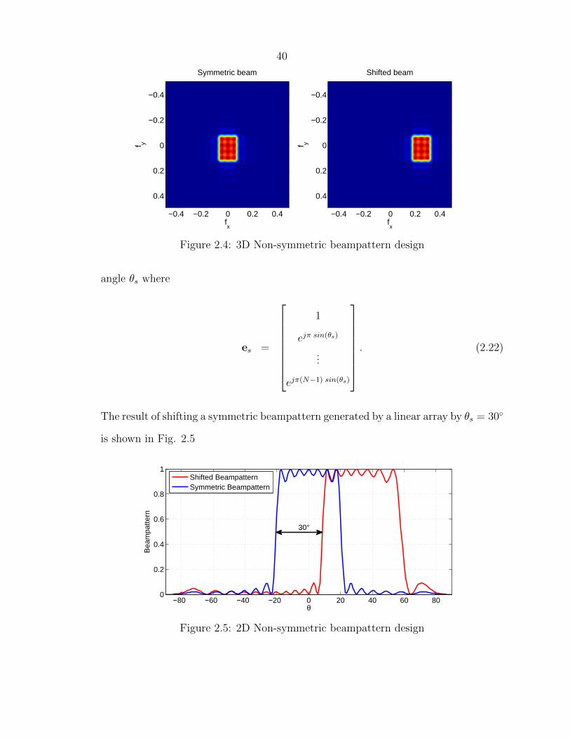
40

fx

f y

Symmetric beam

−0.4 −0.2 0 0.2 0.4

−0.4

−0.2

0

0.2

0.4

fx

f y

Shifted beam

−0.4 −0.2 0 0.2 0.4

−0.4

−0.2

0

0.2

0.4

Figure 2.4: 3D Non-symmetric beampattern design

angle θs where

es =

1

ejπ sin(θs)

...

ejπ(N−1) sin(θs)

. (2.22)

The result of shifting a symmetric beampattern generated by a linear array by θs = 30◦

is shown in Fig. 2.5

−80 −60 −40 −20 0 20 40 60 800

0.2

0.4

0.6

0.8

1

θ

Bea

mpa

ttern

Shifted BeampatternSymmetric Beampattern

30°

Figure 2.5: 2D Non-symmetric beampattern design

41

2.5 Conclusion

The goal on this chapter was to study the problem of designing beampatterns which

are defined in the three dimensional space in function of the azimuth angle θ and the

elevation angle φ using narrowband planar MIMO arrays. Two approaches were in-

vestigated. In the first approach, we presented a closed form solution of the waveforms

covariance matrix for the desired beampattern. The proposed method is computa-

tionally efficient since it exploits a mapping between the studied problem and the

2D-FFT algorithm. In the second approach, a direct closed form expression for the

waveforms realizing the desired beampattern is provided using the derivations ob-

tained in the first approach. The number of transmitted snapshots of the designed

waveforms is related to the desired beampattern. We also showed that the designed

waveforms have good PAPR properties with constant unit value of the PAPR for any

desired beampattern. We verified the considerable advantage of our method in terms

of computational complexity compared with iterative methods thanks to the use of

FFT algorithm. Finally, we adapted our method to the non-symmetric beampattern

case.

42

Chapter 3

Wideband radar systems

The need for resolution in angle, range and velocity is constantly increasing with

sophisticated radar applications. The high resolution helps mitigate clutter and jam-

ming and improves the identification of the targets. The angular resolution is im-

proved by deploying MIMO radar systems with high degrees of freedom and by using

narrow band signals to develop super resolution Direction Of Arrival (DOA) estima-

tion methods which use Capon, APES and iterative Generalised Likelihood Ratio

Test (GLRT). However, the drawback of narrowband signals is that they limit the

information capability of radar systems, like any radio system, where the quantity of

transmitted information is directly related the bandwidth of the transmitted signals.

Lately, wideband radar systems attracted research attention thanks to the advantages

that they offer. We can site the amelioration of target class and type identification

since the received signal carries information about the different parts of the target,

the improvement of radar immunity to external narrowband electromagnetic radi-

ation and noise and, most importantly, the range resolution improvement allowing

the radar to distinguish between targets having same angular location but different

ranges.

As in the narrowband case, the design of transmit beampatterns in wideband radar

systems is required to focus the transmitted power in the desired region of interest.

Similar approaches to the narrowband case have been proposed to design wideband

43

beampatterns. In [27], the authors proposed a numerical convex optimization method

to synthesize the cross-spectral density matrix for a desired spatial beampattern. An

iterative method to design unit-modulus MIMO waveforms to match a given wideband

transmit beampattern is proposed in [28].

3.1 Wideband transmitter design

We consider a linear colocated MIMO radar system with nT transmitting antennas

and nR receiving antennas. The transmitted signal from the mth antenna over the

carrier frequency fc is given by

sm(t) = xm(t) ej2πfct. (3.1)

The received signal from the nT transmitting antennas at a target located by the

azimuth angle θ can be written as

r(t) =

nT−1∑m=1

sm(t− τm),

where τm = m d cos(θ)c

and where d denotes the spacing between antennas and c the

speed of light. Thus, we obtain

sm(t− τm) = xm

(t− m d cos(θ)

c

)ej2πfc(t−

md cos(θ)c

). (3.2)

Therefore,

r(t) =

nT−1∑m=0

xm

(t− m d cos(θ)

c

)ej2πfc(t−

md cos(θ)c

). (3.3)

Let us consider Na time intervals noted as [Ti, Ti+1] where i = 0, . . . , Na − 1 and

Ti+1−Ti = T, ∀i = 0, . . . , Na−1. In each interval [Ti, Ti+1] we define the transmitted

44

signal xim(t) which has a bandwidth B. Thus the frequency domain signal X im(f)

and the time domain signal xim(t) are related to each other with the following Fourier

transform formulas:

X im(f) =

∫ Ti+1

Ti

xim(t)e−j2πftdt, f ∈[−B

2,B

2

](3.4)

xim(t) =

∫ B/2

−B/2X im(f)ej2πftdf, t ∈ [Ti, Ti+1] (3.5)

Using (3.5), the received signal in (3.3) can be written as

r(t+ iT ) =

nT−1∑m=0

∫ B/2

−B/2X im(f)ej2πf(t+iT−

md cos(θ)c )dfej2πfc(t+iT−

md cos(θ)c

)

=

∫ B/2

−B/2

nT−1∑m=0

X im(f)ej2π(f+fc)(t+iT−

md cos(θ)c )df

=

∫ B/2

−B/2

nT−1∑m=0

X im(f)e−j2π(f+fc)(

md cos(θ)c )ej2π[(fc+f)iT+fct]ej2πftdf

=

∫ B/2

−B/2Y i(θ, f)ej2πftdf, (3.6)

where Y i(θ, f) = X im(f)e−j2π(f+fc)(

md cos(θ)c )ej2π[(fc+f)iT+fct].

To design the transmitter of our wideband radar, we discretize the frequency f into

K values {f1, . . . , fK}. Next, we transmit form each antenna the frequency domain

coefficients over the K frequencies as shown in Fig. 3.1.

3.2 Wideband beampattern

From Parseval theorem, we know that the energy of a time domain signal x(t) defined

in [0, T ] and its frequency version X(f) of bandwidth B are equal

∫ T

0

|x(t)|2dt =

∫ B/2

−B/2|X(f)|2df (3.7)

45

X inT(f1)

X inT(fK)

ej2πf1t

ej2πfKt

...

ej2πfct

X i1(f1)

X i1(fK)

ej2πf1t

ej2πfKt

...

ej2πfct

......

. . .

xi1(t)xinT (t)

...

.

...

.

.

Figure 3.1: Diagram of wideband MIMO radar system.

By investigating (3.6), we conclude that r(t) is equivalent to Y i(θ, f). Thus, the power

at location θ and frequency f is obtained by taking the expectation of |Y i(θ, f)|2 over

the symbols transmitted during the intervals [Ti, Ti+1]. By using the fact that d = λ2

and c = λ fc, we obtain the following expression for the power:

P (θ, f) = E{|Y i(θ, f)|2}

= E

∣∣∣∣∣nT−1∑m=0

X im(f)e−j2π(f+fc)(

md cos(θ)c )

∣∣∣∣∣2

= E

∣∣∣∣∣nT−1∑m=0

e−jπf+fcfc

m cos(θ)X im(f)

∣∣∣∣∣2

= E{∣∣aHs (θ; f)X(f)

∣∣2}= aHs (θ; f) E{X(f) XH(f)} as(θ; f)

= aHs (θ; f) R(f) as(θ; f), (3.8)

46

Here, as(θ; f) is the transmitting steering vector at frequency f given by

as(θ; f) =[1, e−jπ

f+fcfc

cos(θ), . . . , e−jπf+fcfc

(nT−1) cos(θ)]T, (3.9)

and X(f) is an nT ×Na matrix where the mth row represents the Na symbols trans-

mitted from the mth antenna at frequency f as follows

X(f) =

X1

1 (f) . . . XNa1 (f)

... . . ....

X1nT

(f) . . . XNanT

(f)

. (3.10)

For a fixed frequency f , the problem in (3.8) is similar to (1.7). Thus, for each

frequency f , we can apply the method developed in section 2.2 to find the covariance

matrix R(f) for a given beampattern. We can also directly design the waveforms X(f)

for each frequency f using the direct waveform design method derived in section 2.3.

3.3 Detection of targets with different ranges

In colocated MIMO radar systems, the signal r(t) received by the targets and given

by (3.3) is reflected back to the radar system. The vector z(t, θ) of the signals received

by each antenna is given by

z(t, θ) = ar(θ; f) r(t), (3.11)

where ar(θ; f) is the receiving steering vector which is equal to the the transmitting

steering vector as(θ; f) in the colocated radar configuration. We consider the presence

of two targets at locations defined by the same azimuth angle θ = θT but at different

ranges. θT is also called the direction of departure (DOD). Let t1 and t2 be the delays

after which the transmitted signal arrives, respectively, at the first and the second

47

target. In the receiver side, the signal z(t, θR) arriving from the DOA denoted as θR

can be written as

z(t, θR) = ar(θR; f) [r(t− 2t1, θT ) + r(t− 2t2, θT )] + n(t), (3.12)

where n(t) is a vector of Additive White Gaussian Noise (AWGN). Note here that

θR = θT since we are in the colocated radar configuration case.

The received vector z(t, θR) is of dimensions (nR × 1) and it depends on time. If

we sweep Nb time values we obtain the matrix Z and N of dimensions (nR × Nb)

where the kth column represents, respectively, the receiving vector and the AWGN

at the kth time value. We first seek to cancel the distortion caused by the AWGN.

We follow the Capon method by generating, for different values of θ, a weight vector

wCap(θ) which maximizes the SNR without distorting the signal itself which leads to

the following optimization problem

wCap(θ) =

argmax

w

E(||wHZ||2)E(wHN)

s.t. wHar(θ; f) = 1

(3.13)

The solution is given by

wCap(θ, f) =R−1NNar(θ; f)

aHr (θ; f)R−1NNar(θ; f), (3.14)

where RNN = NHN the covariance matrix of the AWGN.

For each value of θ we compute the correlation c(θ, t) between wHCap(θ)z(t, θ; f) and

aHs (θ; f)X(f). The multivariable function c(θ, t) reaches its maximum value when a

target is detected. In our case the maximum is reached at (θT , 2 t1) and (θT , 2 t2). Note

that the range of the ith target denoted as ri is easily derived from the corresponding

48

arrival time of the transmitted signal denoted as ti using the following expression

ri = ti c (3.15)

3.4 Conclusion

In this chapter, we investigated the wideband MIMO radar system which benefits

from improved performance especially in terms of range resolution. In order to achieve

beampattern design, we use the waveform covariance matrix and the direct waveform

design solutions proposed in Chapter 2. At the receiver side, we use Capon estimator

to detect targets located at the same angular position but at different ranges.

49

Chapter 4

Numerical Simulations

In this chapter, we evaluate the performance of the beampattern design methods

developed for the narrowband case (Chapter 2) and the wideband case (Chapter 3).

4.1 Narrowband radars

In this section, the performance of the proposed FFT-based algorithm is investigated.

For simulation, a rectangular planar array composed of M×N antennas is considered.

The spacing between any two adjacent antennas on the x− and y−axis of the planar

array is kept λ/2.

4.1.1 Beampattern design

In the first simulation, the ROI is defined as −0.1 ≤ fx ≤ 0.1 and −0.1 ≤ fy ≤ 0.1

and we use N = M = 10. To design this beampattern, we start by synthesizing R

using SQP method proposed in [16]. The designed beampattern using the synthesized

covariance matrix is shown in Fig. 4.1, which is the best possible designed beampat-

tern. Note that the beampattern is normalized by dividing by α. For this simulation,

the total number of antennas is 100, therefore, to synthesize the covariance matrix,

the simulation is very time consuming. Here, the actual waveforms to realize the

synthesized covariance matrix are not designed as they also require iterative algo-

50

rithms with very high computational complexity. The designed beampattern with

the actual waveforms may be degraded too. In order to reduce the computational

complexity of the beampattern design, we use in the second simulation our proposed

closed-form 2D-FFT based low complexity algorithm with the same number of an-

tennas N = M = 10. The corresponding designed beampattern, using the covariance

matrix R obtained by our proposed algorithm, is shown in Fig. 4.2. The designed

beampattern shown is the beampattern of the covariance matrix. The algorithm to

directly design the waveforms corresponding to the desired beampattern is proposed

in Section 2.3.

−0.5−0.4

−0.3−0.2

−0.10

0.10.2

0.30.4

0.5

−0.5−0.4

−0.3−0.2

−0.10

0.10.2

0.30.4

0.50

0.2

0.4

0.6

0.8

1

fx

fy

Bea

mpa

ttern

Figure 4.1: The designed beampattern using SQP based method. Here the ROI is−0.1 ≤ fx ≤ 0.1 and −0.1 ≤ fy ≤ 0.1 and M = N = 10.

4.1.2 Mean Square Error

In order to compare the performance of the two algorithms shown in the previous two

simulations, we compare the corresponding MSE for different planar array dimensions

and for an ROI defined by −0.1 ≤ fx ≤ 0.1 and −0.1 ≤ fy ≤ 0.1.

51

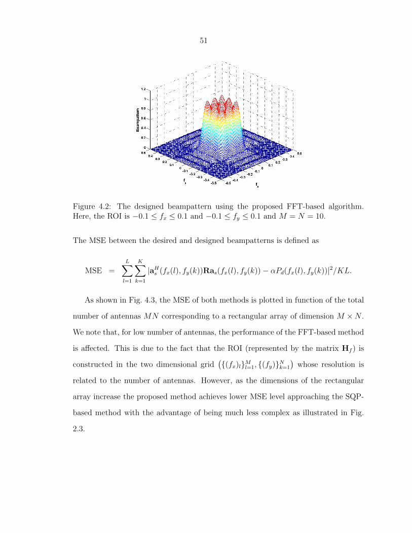
Figure 4.2: The designed beampattern using the proposed FFT-based algorithm.Here, the ROI is −0.1 ≤ fx ≤ 0.1 and −0.1 ≤ fy ≤ 0.1 and M = N = 10.

The MSE between the desired and designed beampatterns is defined as

MSE =L∑l=1

K∑k=1

|aHs (fx(l), fy(k))Ras(fx(l), fy(k))− αPd(fx(l), fy(k))|2/KL.

As shown in Fig. 4.3, the MSE of both methods is plotted in function of the total

number of antennas MN corresponding to a rectangular array of dimension M ×N .

We note that, for low number of antennas, the performance of the FFT-based method

is affected. This is due to the fact that the ROI (represented by the matrix Hf ) is

constructed in the two dimensional grid({(fx)l}Ml=1, {(fy)}Nk=1

)whose resolution is

related to the number of antennas. However, as the dimensions of the rectangular

array increase the proposed method achieves lower MSE level approaching the SQP-

based method with the advantage of being much less complex as illustrated in Fig.

2.3.

52

0 50 100 150 200 250 300 350 400 450 5000

0.05

0.1

0.15

0.2

0.25

0.3

0.35

0.4

0.45

0.5

Number of antennas

MS

E

FFT Based Method SQP Method

Figure 4.3: MSE comparison between the FFT-based algorithm and the SQP methodfor different planar array dimensions.

4.1.3 Beampattern Shapes variations

Next, we perform various beampattern shapes design by manipulating the ROI and

plugging it into the FFT-based algorithm described in Table 2.1 to obtain the cor-

responding covariance matrix. The shape of the beampattern is determined by the

ROI, which is defined by the positions of the non-zero coefficients in the matrix Hf .

Note that in order to obtain good results, the symmetry of the beampattern must

be respected. Otherwise, we need to apply the shifting method proposed in section

2.4.3 to generate non-symmetric beampatterns. Figs. 4.4-4.7 show some of the various

beampattern configurations that can be designed using a planar array of dimensions

N = M = 20. For display purposes, we only show a two dimensional graph repre-

senting the projection of the designed beampattern in the (fx− fy) plane. In Fig. 4.4

the transmitted power is focused only in the corners. Fig. 4.5 shows the beampattern

obtained when we want to transmit only on the borders. Fig. 4.6 shows a beampat-

tern which is focused both in the borders and in the center. Finally, Fig. 4.7 shows a

circular shaped beampattern as illustrated in Fig. 2.1.

53

fx

f y

−0.5 0 0.5

−0.5

−0.4

−0.3

−0.2

−0.1

0

0.1

0.2

0.3

0.4

0.5

0.1

0.2

0.3

0.4

0.5

0.6

0.7

0.8

0.9

1

Figure 4.4: FFT-based transmit Beampattern, N = M = 20, ROI focused in thecorners.

fx

f y

−0.5 0 0.5

−0.5

−0.4

−0.3

−0.2

−0.1

0

0.1

0.2

0.3

0.4

0.5

0.1

0.2

0.3

0.4

0.5

0.6

0.7

0.8

0.9

1

Figure 4.5: FFT-based transmit Beampattern, N = M = 20, ROI focused in theborders.

54

fx

f y

−0.5 0 0.5

−0.5

−0.4

−0.3

−0.2

−0.1

0

0.1

0.2

0.3

0.4

0.5

0.1

0.2

0.3

0.4

0.5

0.6

0.7

0.8

0.9

1

Figure 4.6: FFT-based transmit beampattern design, N = M = 20. Here, thetransmitted power needs to be focused in the center and the borders.

fx

f y

−0.5 0 0.5

−0.5

−0.4

−0.3

−0.2

−0.1

0

0.1

0.2

0.3

0.4

0.5 0

0.1

0.2

0.3

0.4

0.5

0.6

0.7

0.8

0.9

Figure 4.7: FFT-based transmit beampattern design, N = M = 20. Here, the ROIhas a circular shape.

55

4.1.4 Linear arrays

In the following simulation, a linear array of 10 antennas is used. To transmit the

power between the azimuth angles −30◦ and 30◦, waveforms are directly designed

using our proposed algorithm and the algorithm in [20]. The simulation results are

shown in Fig. 4.8. It can be seen in the figure that the algorithm in [20] yields

almost uniform transmit power in the ROI, however, the designed beampattern has

slower roll-off and higher side-lobe-levels compared to our proposed algorithm. An

other advantage of using our proposed algorithm is that it generates finite alphabet

symbols for each waveform.

−80 −60 −40 −20 0 20 40 60 800

0.2

0.4

0.6

0.8

1

Beam

pattern

Angle

Direct Waveform Design Algorithm in [20]Proposed Direct Waveform Design Algorithm

Figure 4.8: Comparison of direct waveform design methods for the desired beam-pattern using linear array. Here, in both algorithms each waveform transmits 10symbols.

4.1.5 Target detection

For a collocated planar MIMO radar, the signal at the receiver can be written as

y(n; fx, fy) =L∑l=1

ar(fx, fy)aTs (fxl , fyl)x(n) + z(n), (4.1)

56

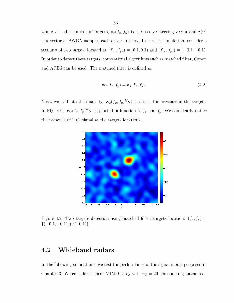
where L is the number of targets, ar(fx, fy) is the receive steering vector and z(n)

is a vector of AWGN samples each of variance σz. In the last simulation, consider a

scenario of two targets located at (fx1 , fy1) = (0.1, 0.1) and (fx2 , fy2) = (−0.1,−0.1).

In order to detect these targets, conventional algorithms such as matched filter, Capon

and APES can be used. The matched filter is defined as

wc(fx, fy) = as(fx, fy). (4.2)

Next, we evaluate the quantity |wc(fx, fy)Hy| to detect the presence of the targets.

In Fig. 4.9, |wc(fx, fy)Hy| is plotted in function of fx and fy. We can clearly notice

the presence of high signal at the targets locations.

Figure 4.9: Two targets detection using matched filter, targets location: (fx, fy) ={(−0.1,−0.1), (0.1, 0.1)}

4.2 Wideband radars

In the following simulations, we test the performance of the signal model proposed in

Chapter 3. We consider a linear MIMO array with nT = 20 transmitting antennas.

57

4.2.1 Beampattern design

We define a ROI with θ ∈ [−30◦, 30◦] and the carrier frequency fc = 1 GHz. Next, we

design the transmitted waveforms corresponding to the desired ROI, as described in

section 3.2, for frequency values going from 0.9 GHz to 1.1 GHz. We plot in Fig. 4.10

the generated beampattern in function of θ and f . We clearly notice that we are able

to focus the transmitted power in the desired ROI for any value of the frequency.

Figure 4.10: Wideband beampattern design, ROI: θ ∈ [−30◦, 30◦].

4.2.2 Detection of targets with different ranges

We implement in this section the Capon estimator detailed in section 3.3. We consider

the presence of two targets at θ = 20◦. The ranges of the first and the second target

are, respectively, r1 = 3 Km and r2 = 9 Km. We plot in Fig. 4.11 the correlation

function c(θ, t) in function of θ and the target’s range.

We can clearly notice that the correlation function reaches its maximum in the

exact locations of the targets. A projection of Fig. 4.11 on the 2D (θ−Range) plan is

shown in Fig. 4.12 where we can estimate the location and the ranges of the targets.

58

Figure 4.11: Detection of two targets with different ranges.

θ (Deg)

Ran

ge (

Km

)

−50 0 500

5

10

15

20

25

30

0

1

2

3

4

5

6

7

8

9

10

x 105

Figure 4.12: Detection of two targets with different ranges (Projection).

59

4.3 Conclusion

In this chapter dedicated to numerical simulations, we started with the narrowband

case where we applied our waveform design method to realize a given 3D beampattern

and observed the obtained result which confirms the transmitted power is focused in

the desired ROI. Next, we showed that the MSE performance of our closed form

solution is comparable with existing iterative methods. By manipulating the matrix

Hf , we proved the flexibility of our method to design different 3D beampattern shapes

with planar arrays as well as 2D beampatterns with linear arrays.

For the wideband case, we generate a beampattern for a given ROI and then we

resolve two targets having same angle θ and different ranges using the signal model

proposed for the wideband system.

60

Chapter 5

Conclusion

5.1 Summary

In this work, we presented in Chapter 2 a closed-form method of covariance matrix

design for the planar narrowband MIMO transmit beamforming problem by exploit-

ing the IDFT coefficients. The positive semi-definition and uniform element power

constraints are verified by the designed matrix. Next, we proposed a method of direct

waveform design exploiting the expression of the covariance matrix that we found.

The proposed waveform solution is adapted to the non symmetric beampattern case

as well as to the wideband radar configuration which was studied in Chapter 3. The

numerical simulations presented in Chapter 4 confirm that the proposed method is

computationally efficient and performs closely to the iterative SQP-based method in

terms of MSE as the number of antennas increases.

5.2 Future work

As a future work, we will study an On-Off scheme which will use the minimum number

of antennas for a given beampattern.

61

REFERENCES

[1] M. Skolnik, Introduction to Radar Systems. New York: McGraw-Hill Book

Company, 1980.

[2] M. Richards, Fundamentals of Radar Signal Processing. New York: McGrawHill

Book Company, 2005.

[3] R. Watson and R. Watson, Radar Origins Worldwide: History of Its Evolution

in 13 Nations Through World War II. Trafford Publishing (UK) Limited, 2009.

[4] H. Jol, Ground Penetrating Radar Theory and Applications. Elsevier Science,

2008.

[5] R. H. R. Monzingo and T. Miller, Introduction to Adaptive Arrays, 2nd Edition.

Institution of Engineering and Technology, 2011.

[6] D. J. Rabideau and P. Parker, “Ubiquitous mimo multifunction digital array

radar,” Conference Record of the Thirty-Seventh Asilomar Conference on Sig-

nals, Systems and Computers, vol. 1, pp. 1057–1064, Nov 2004.

[7] D. Bliss and K. Forsythe, “Multiple-input multiple-output (MIMO) radar and

imaging: degrees of freedom and resolution,” Conference Record of the Thirty

Seventh Asilomar Conference on Signals, Systems and Computers, vol. 1, pp.

54–59, Nov 2003.

[8] J. Li and P. Stoica, MIMO Radar Signal Processing. John Wiley & Sons, Inc,

2008.

[9] D. B. K. Forsythe and G. S. Fawcett, “Multiple-input multiple-output(MIMO)

radar: performance issues,” Conference Record of the Thirty-Eighth Asilomar

Conference on Signals, Systems and Computers, vol. 1, pp. 310–315, Nov 2004.

62

[10] D. W. J. M. F. Robey, S. Coutts and K. Cuomo, “MIMO radar theory and exper-

imental results,” Conference Record of the Thirty-Eighth Asilomar Conference

on Signals, Systems and Computers, vol. 1, pp. 300–304, Nov 2004.

[11] E. Fishler, A. Haimovich, R. Blum, D. Chizhik, L. Cimini, and R. Valenzuela,

“MIMO radar: An idea whose time has come,” in Proceedings of the IEEE Radar

Conference,, April 2004, pp. 71–78.

[12] E. Fishler, A. Haimovich, R. Blum, L. Cimini, D. Chizhik, and R. Valenzuela,

“Spatial diversity in radars-models and detection performance,” IEEE Transac-

tions on Signal Processing,, vol. 54, no. 3, pp. 823–838, March 2006.

[13] R. B. A. Haimovich and L. Cimini, “MIMO radar with widely separated anten-

nas,” IEEE Signal Processing Magazine, vol. 25, no. 1, pp. 116–129, 2008.

[14] J. Li and P. Stoica, “MIMO radar with colocated antennas,” IEEE Signal Pro-

cessing Magazine, vol. 24, no. 5, pp. 106–114, 2007.

[15] D. Fuhrmann and G. San Antonio, “Transmit beamforming for MIMO radar

systems using signal cross-correlation,” IEEE Transactions on Aerospace and

Electronic Systems,, vol. 44, no. 1, pp. 171–186, January 2008.

[16] P. Stoica, J. Li, and Y. Xie, “On probing signal design for MIMO radar,” IEEE

Transactions on Signal Processing,, vol. 55, no. 8, pp. 4151–4161, Aug 2007.

[17] T. Aittomaki and V. Koivunen, “Signal covariance matrix optimization for trans-

mit beamforming in MIMO radars,” in Conference Record of the Forty-First

Asilomar Conference on Signals, Systems and Computers,, Nov 2007, pp. 182–

186.

[18] ——, “Low-complexity method for transmit beamforming in MIMO radars,”

in IEEE International Conference on Acoustics, Speech and Signal Processing,,

vol. 2, April 2007, pp. II–305–II–308.

[19] S. Ahmed, J. Thompson, Y. Petillot, and B. Mulgrew, “Unconstrained synthesis

of covariance matrix for MIMO radar transmit beampattern,” IEEE Transac-

tions on Signal Processing,, vol. 59, no. 8, pp. 3837–3849, Aug 2011.

63

[20] D. Fuhrmann, J. Browning, and M. Rangaswamy, “Signaling strategies for the

hybrid MIMO phased-array radar,” IEEE Journal of Selected Topics in Signal

Processing,, vol. 4, no. 1, pp. 66–78, Feb 2010.

[21] W.-Q. Wang, “MIMO SAR Chirp modulation diversity waveform design,” IEEE

Geoscience and Remote Sensing Letters,, vol. 11, no. 9, pp. 1644–1648, Sept

2014.

[22] D. Fuhrmann and G. San Antonio, “Transmit beamforming for MIMO radar

systems using partial signal correlation,” in Conference Record of the Thirty-

Eighth Asilomar Conference on Signals, Systems and Computers,, vol. 1, Nov

2004, pp. 295–299 Vol.1.

[23] J. Lipor, S. Ahmed, and M.-S. Alouini, “Fourier-based transmit beampattern

design using MIMO radar,” IEEE Transactions on Signal Processing,, vol. 62,

no. 9, pp. 2226–2235, May 2014.

[24] P. Stoica, J. Li, X. Zhu, and B. Guo, “Waveform synthesis for diversity-based

transmit beampattern design,” in IEEE/SP 14th Workshop on Statistical Signal

Processing,, Aug 2007, pp. 473–477.

[25] S. Ahmed, J. Thompson, Y. Petillot, and B. Mulgrew, “Finite alphabet constant-

envelope waveform design for MIMO radar,” IEEE Transactions on Signal Pro-

cessing,, vol. 59, no. 11, pp. 5326–5337, Nov 2011.

[26] D. Fuhrmann, J. Browning, and M. Rangaswamy, “Constant-modulus partially

correlated signal design for uniform linear and rectangular MIMO radar arrays,”

in International Waveform Diversity and Design Conference,, Feb 2009, pp. 197–

201.

[27] G. San Antonio and D. Fuhrmann, “Beampattern synthesis for wideband mimo

radar systems,” in IEEE International Workshop on Computational Advances in

Multi-Sensor Adaptive Processing, Dec 2005, pp. 105–108.

[28] H. He, P. Stoica, and J. Li, “Wideband mimo systems: Signal design for transmit

beampattern synthesis,” IEEE Transactions on Signal Processing, vol. 59, no. 2,

pp. 618–628, Feb 2011.

64

APPENDICES

A Lemma 1 proof

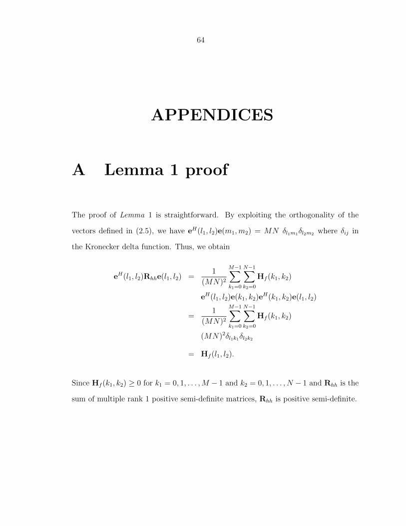
The proof of Lemma 1 is straightforward. By exploiting the orthogonality of the

vectors defined in (2.5), we have eH(l1, l2)e(m1,m2) = MN δl1m1δl2m2 where δij in

the Kronecker delta function. Thus, we obtain

eH(l1, l2)Rhhe(l1, l2) =1

(MN)2

M−1∑k1=0

N−1∑k2=0

Hf (k1, k2)

eH(l1, l2)e(k1, k2)eH(k1, k2)e(l1, l2)

=1

(MN)2

M−1∑k1=0

N−1∑k2=0

Hf (k1, k2)

(MN)2δl1k1δl2k2

= Hf (l1, l2).

Since Hf (k1, k2) ≥ 0 for k1 = 0, 1, . . . ,M − 1 and k2 = 0, 1, . . . , N − 1 and Rhh is the

sum of multiple rank 1 positive semi-definite matrices, Rhh is positive semi-definite.

65

To prove that all the diagonal elements of Rhh are equal, let us find the expression

the ith diagonal element Rhh(i, i) from the formula in (2.6)

Rhh(i, i) =1

(MN)2

M−1∑k1=0

N−1∑k2=0

Hf (k1, k2)[e(k1, k2) eH(k1, k2)

](i, i).

Since[e(k1, k2) eH(k1, k2)

](i, i) = 1 for any index value i, we can write

Rhh(i, i) =1

(MN)2

M−1∑k1=0

N−1∑k2=0

Hf (k1, k2)

=Na

(MN)2, (A.1)

where Na is the number non-zero elements in the frequency domain matrix Hf .

66

B Papers Submitted and Under

Preparation

• T. Bouchoucha, S. Ahmed, T. Y. Al-Naffouri and M.-S. Alouini, “Direct Design of

Finite Alphabet Constant Envelope Waveforms for Planar Array Beampatterns”, in

IEEE Transactions on Signal Processing (under second revision).

• T. Bouchoucha, S. Ahmed, T. Y. Al-Naffouri and M.-S. Alouini, “Closed-form So-

lution to Directly Design FACE Waveforms for Beampatterns Using Planar Array”,

In proceedings IEEE International Conference on Acoustics, Speech and Signal Pro-

cessing (ICASSP-2015), Brisbane Australia, Apr. 2015.

• S. Ahmed, T. Bouchoucha, T. Y. Al-Naffouri and M.-S. Alouini, “Closed-form So-

lution to Directly Design FACE Waveforms for Beampatterns Using Planar Array”,

(submitted Patent), 2015.

• T. Bouchoucha, S. Ahmed, T. Y. Al-Naffouri and M.-S. Alouini, “Beampattern de-

sign for wideband radars”, in IEEE Transactions on Signal Processing (under prepa-

ration).

• T. Bouchoucha, Mohamed F. A. Ahmed, T. Y. Al-Naffouri and M.-S. Alouini, “Dis-

tributed Estimation Based on Observations Prediction in Wireless Sensor Networks”,

in IEEE Signal Processing Letters 2015.

• H. Ghazzai, T. Bouchoucha, A. Alsharoa, E. Yaacoub, M.-S. Alouini and T. Y.

Al-Naffouri, “Energy-Efficient LTE Resource Allocation and eNodeB Planning for

67

High-Speed Trains with Multiple Moving Relays”, in IEEE Transactions on Vehicu-

lar Technology (Submitted).