thesis jongha
TRANSCRIPT

8/2/2019 Thesis Jongha
http://slidepdf.com/reader/full/thesis-jongha 1/126
TACTILE SENSATION IMAGING SYSTEM AND ALGORITHMS FORTUMOR DETECTION
A DissertationSubmitted to
the Temple University Graduate Board
in Partial Fulfillment
of the Requirements for the DegreeDOCTOR OF PHILOSOPHY
byJong-Ha LeeAugust, 2011
Examining Committee Members:
Chang-Hee Won, Advisory Chair, Electrical and Computer EngineeringJoseph Picone, Electrical and Computer EngineeringSaroj Biswas, Electrical and Computer EngineeringKurosh Darvish, Mechanical EngineeringShan Lin, Computer and Information Sciences

8/2/2019 Thesis Jongha
http://slidepdf.com/reader/full/thesis-jongha 2/126
ACKNOWLEDGEMENTS
I would like to extend my heart-felt gratitude to my adviser, Dr. Chang-Hee Won of the Electri-
cal and Computer Engineering Department at Temple University. He was an unending source
of patience, advice, and encouragement during my years of study. Dr. Chang-Hee Won en-
couraged me to grow as an engineer and to become an independent thinker. I am fortunate to
have had an adviser who gave me constant support while encouraging my independence and
self-sufficiency. Dr. Chang-Hee Won taught me to express my individuality while providing a
strong foundation on which to rely. His mentorship inspired me to become well-rounded in my
studies, supporting me as I formulated and worked towards my long-term goals.
I also wish to offer my thanks to Dr. Joseph Picone, Dr. Saroj Biswas, Dr. Kurosh Darvish,
and Dr. Shan Lin, the other members of my doctoral committee at Temple University. Words
cannot express the value of their guidance, comments, and suggestions.
In addition, I would like to thank my labmates. I especially appreciate the friendship of
Dr. Bei Kang and Firdous Saleheen as we often found ourselves working closely to answer thesame questions, and gave each other encouragement.
I would also like to thank my parents, Soo-Kon Lee and Young-Soo Kim, for having faith
in me and encouraging me to fulfill all my ambitious dreams. Their drive for success and
willingness to tackle challenges gave me wonderful examples with which to build my own
professional and personal life. I would also like to take this opportunity to thank my wife’s
parents, Byung-Oh Cho and Bok Im, who offered their help and encouragement throughout this
endeavor. My friends, Kyung Jun Park and Young Woo Shin, and their families must also be
mentioned. Their ongoing support helped me to successfully complete my studies.
Most of all, I want to thank my wife, Yun-Sook Cho, for loving and supporting me through-
ii

8/2/2019 Thesis Jongha
http://slidepdf.com/reader/full/thesis-jongha 3/126
out the development of this work. Her quiet patience, support, and encouragement were given
with unfaltering love, and became the firm ground on which I have built the past five years. Her
near-infinite forbearance of my occasional bad mood is a testament of a partner with unlimited
love and devotion.
Finally, I would like to extend my thanks for the financial support from National Science
Foundation ECS-0554748 and ECCS-0969430, Pennsylvania Department of Health Tobacco
Formula Fund, and the Office of the Senior Vice Provost for Research and Graduate Education
at Temple University.
iii

8/2/2019 Thesis Jongha
http://slidepdf.com/reader/full/thesis-jongha 4/126
ABSTRACT
Diagnosing early formation of tumors or lumps, particularly those caused by cancer, has been a
challenging problem. To help physicians detect tumors more efficiently, various imaging tech-
niques with different imaging modalities such as computer tomography, ultrasonic imaging,
nuclear magnetic resonance imaging, and mammography have been developed. However, each
of these techniques has limitations, including exposure to radiation, excessive costs, and com-
plexity of machinery. Tissue elasticity is an important indicator of tissue health, with increased
stiffness pointing to an increased risk of cancer. In addition to increased tissue elasticity, ge-
ometric parameters such as size of a tissue inclusion are also important factors in assessing
the tumor. The combined knowledge of tissue elasticity and its geometry would aid in tumor
identification. In this research, we present a tactile sensation imaging system (TSIS) and algo-
rithms which can be used for practical medical diagnostic experiments for measuring stiffness
and geometry of tissue inclusion. The TSIS incorporates an optical waveguide sensing probe
unit, a light source unit, a camera unit, and a computer unit. The optical method of total inter-nal reflection phenomenon in an optical waveguide is adapted for the tactile sensation imaging
principle. The light sources are attached along the edges of the waveguide and illuminates at a
critical angle to totally reflect the light within the waveguide. Once the waveguide is deformed
due to the stiff object, it causes the trapped light to change the critical angle and diffuse outside
the waveguide. The scattered light is captured by a camera. To estimate various target param-
eters, we develop the tactile data processing algorithm for the target elasticity measurement
via direct contact. This algorithm is accomplished by adopting a new non-rigid point match-
ing algorithm called “topology preserving relaxation labeling (TPRL).” Using this algorithm, a
series of tactile data is registered and strain information is calculated. The stress information
iv

8/2/2019 Thesis Jongha
http://slidepdf.com/reader/full/thesis-jongha 5/126
is measured through the summation of pixel values of the tactile data. The stress and strain
measurements are used to estimate the elasticity of the touched object. This method is validated
by commercial soft polymer samples with a known Young’s modulus. The experimental results
show that using the TSIS and its algorithm, the elasticity of the touched object can be estimated
within 5.38% relative estimation error. We also develop a tissue inclusion parameter estimation
method via indirect contact for the characterization of tissue inclusion. This method includes
developing a forward algorithm and an inversion algorithm. The finite element modeling (FEM)
based forward algorithm is designed to comprehensively predict the tactile data based on the
parameters of an inclusion in the soft tissue. This algorithm is then used to develop an artificial
neural network (ANN) based inversion algorithm for extracting various characteristics of tissue
inclusions, such as size, depth, and Young’s modulus. The estimation method is then validated
by using realistic tissue phantoms with stiff inclusions. The experimental results show that the
minimum relative estimation errors for the tissue inclusion size, depth, and hardness are 0.75%,
6.25%, and 17.03%, respectively. The work presented in this dissertation is the initial step
towards early detection of malignant breast tumors.
v

8/2/2019 Thesis Jongha
http://slidepdf.com/reader/full/thesis-jongha 6/126
TABLE OF CONTENTS
Page
ACKNOWLEDGEMENTS . . . . . . . . . . . . . . . . . . . . . . . . . . . . . . . . . . . . . . . . . . . ii
ABSTRACT . . . . . . . . . . . . . . . . . . . . . . . . . . . . . . . . . . . . . . . . . . . . . . . . . . iv
LIST OF FIGURES . . . . . . . . . . . . . . . . . . . . . . . . . . . . . . . . . . . . . . . . . . . . . . . ix
CHAPTER
1 INTRODUCTION . . . . . . . . . . . . . . . . . . . . . . . . . . . . . . . . . . . . . . . . . . . . . 1
1.1 CONTRIBUTIONS . . . . . . . . . . . . . . . . . . . . . . . . . . . . . . . . . . . . . . . . . 4
1.2 DISSERTATION SCOPE AND OUTLINE . . . . . . . . . . . . . . . . . . . . . . . . . . . . 4
2 BACKGROUND AND LITERATURE REVIEW . . . . . . . . . . . . . . . . . . . . . . . . . . . . . 6
2.1 HUMAN TACTILE SENSING MECHANISM . . . . . . . . . . . . . . . . . . . . . . . . . . 6
2.1.1 TISSUE STRUCTURE . . . . . . . . . . . . . . . . . . . . . . . . . . . . . . . . . . 6
2.1.2 MECHANORECEPTOR FUNCTIONALITY . . . . . . . . . . . . . . . . . . . . . . 7
2.2 ARTIFICIAL TACTILE SENSORS . . . . . . . . . . . . . . . . . . . . . . . . . . . . . . . . 8
2.2.1 CAPACITIVE SENSORS . . . . . . . . . . . . . . . . . . . . . . . . . . . . . . . . 8
2.2.2 PIEZORESISTIVE SENSORS . . . . . . . . . . . . . . . . . . . . . . . . . . . . . . 9
2.2.3 PIEZOELECTRIC SENSORS . . . . . . . . . . . . . . . . . . . . . . . . . . . . . . 10
2.2.4 MAGNETIC-BASED SENSORS . . . . . . . . . . . . . . . . . . . . . . . . . . . . 10
2.2.5 OPTICAL SENSORS . . . . . . . . . . . . . . . . . . . . . . . . . . . . . . . . . . 11
2.3 ELASTICITY DETERMINATION SYSTEM . . . . . . . . . . . . . . . . . . . . . . . . . . . 11
2.3.1 ELASTOGRAPHY . . . . . . . . . . . . . . . . . . . . . . . . . . . . . . . . . . . . 12
2.3.2 ELASTICITY IMAGING USING TACTILE SENSORS . . . . . . . . . . . . . . . . 14
vi

8/2/2019 Thesis Jongha
http://slidepdf.com/reader/full/thesis-jongha 7/126
2.4 APPLICATION OF BREAST TUMOR DETECTION . . . . . . . . . . . . . . . . . . . . . . 16
3 TACTILE SENSATION IMAGING PRINCIPLE AND NUMERICAL SIMULATIONS . . . . . . . . 23
3.1 TOTAL INTERNAL REFLECTION . . . . . . . . . . . . . . . . . . . . . . . . . . . . . . . . 23
3.2 ANALYTICAL SOLUTION: WAVE OPTICS . . . . . . . . . . . . . . . . . . . . . . . . . . . 24
3.3 NUMERICAL SIMULATIONS: WAVE OPTICS . . . . . . . . . . . . . . . . . . . . . . . . . 30
3.4 GEOMETRIC OPTICS APPROXIMATION . . . . . . . . . . . . . . . . . . . . . . . . . . . . 32
3.5 MULTI-LAYERED SENSING PROBE CHARACTERIZATION . . . . . . . . . . . . . . . . . 35
4 TACTILE SENSATION IMAGING SYSTEM . . . . . . . . . . . . . . . . . . . . . . . . . . . . . . 39
4.1 OVERVIEW OF TACTILE SENSATION IMAGING SYSTEM . . . . . . . . . . . . . . . . . 39
4.2 HARDWARE DESIGN OF TACTILE SENSATION IMAGING SYSTEM . . . . . . . . . . . . 40
4.2.1 COMPONENTS . . . . . . . . . . . . . . . . . . . . . . . . . . . . . . . . . . . . . 40
4.2.2 OPTICAL WAVEGUIDE FABRICATION . . . . . . . . . . . . . . . . . . . . . . . 44
4.3 SOFTWARE IMPLEMENTATION OF TACTILE SENSATION IMAGING SYSTEM . . . . . 46
4.3.1 OVERVIEW . . . . . . . . . . . . . . . . . . . . . . . . . . . . . . . . . . . . . . . 46
4.3.2 PROCEDURE AND FUNCTIONALITY OF TSIS SOFTWARE . . . . . . . . . . . . 47
4.4 SAMPLE TACTILE IMAGE . . . . . . . . . . . . . . . . . . . . . . . . . . . . . . . . . . . . 51
4.5 THE SPECIFICATION OF THE TACTILE SENSATION IMAGING SYSTEM . . . . . . . . . 52
5 TARGET HARDNESS ESTIMATION BY DIRECT CONTACT . . . . . . . . . . . . . . . . . . . . 54
5.1 STRESS ESTIMATION . . . . . . . . . . . . . . . . . . . . . . . . . . . . . . . . . . . . . . 54
5.2 STRAIN ESTIMATION . . . . . . . . . . . . . . . . . . . . . . . . . . . . . . . . . . . . . . 58
5.2.1 PROBLEM DEFINITION . . . . . . . . . . . . . . . . . . . . . . . . . . . . . . . . 59
5.2.2 TOPOLOGY PRESERVING RELAXATION LABELING (TPRL) ALGORITHM . . 62
5.2.3 SEARCHING POINT CORRESPONDENCE . . . . . . . . . . . . . . . . . . . . . . 62
5.2.4 TRANSFORMATION FUNCTION . . . . . . . . . . . . . . . . . . . . . . . . . . . 66
5.2.5 VALIDATION AND PERFORMANCE EVALUATION . . . . . . . . . . . . . . . . 68
5.3 YOUNG’S MODULUS ESTIMATION FROM STRESS AND STRAIN . . . . . . . . . . . . . 76
vii

8/2/2019 Thesis Jongha
http://slidepdf.com/reader/full/thesis-jongha 8/126
5.4 EXPERIMENTAL RESULTS . . . . . . . . . . . . . . . . . . . . . . . . . . . . . . . . . . . 76
5.5 DISCUSSIONS . . . . . . . . . . . . . . . . . . . . . . . . . . . . . . . . . . . . . . . . . . . 78
6 TISSUE INCLUSION PARAMETER ESTIMATION BY INDIRECT CONTACT . . . . . . . . . . . 81
6.1 PROBLEM FORMULATION . . . . . . . . . . . . . . . . . . . . . . . . . . . . . . . . . . . 81
6.2 RELATIVE TISSUE INCLUSION PARAMETER ESTIMATION . . . . . . . . . . . . . . . . 82
6.2.1 RELATIVE SIZE ESTIMATION METHOD . . . . . . . . . . . . . . . . . . . . . . 82
6.2.2 RELATIVE SIZE ESTIMATION EXPERIMENTAL RESULTS . . . . . . . . . . . . 83
6.2.3 RELATIVE DEPTH ESTIMATION METHOD . . . . . . . . . . . . . . . . . . . . . 85
6.2.4 RELATIVE DEPTH ESTIMATION EXPERIMENTAL RESULTS . . . . . . . . . . . 87
6.2.5 RELATIVE HARDNESS ESTIMATION METHOD . . . . . . . . . . . . . . . . . . 89
6.2.6 RELATIVE HARDNESS ESTIMATION EXPERIMENTAL RESULTS . . . . . . . . 89
6.2.7 OTHER TISSUE INCLUSION PARAMETERS – SHAPE AND MOBILITY . . . . . 92
6.3 ABSOLUTE TISSUE INCLUSION PARAMETER ESTIMATION . . . . . . . . . . . . . . . 93
6.3.1 FORWARD ALGORITHM . . . . . . . . . . . . . . . . . . . . . . . . . . . . . . . . 94
6.3.2 MAPPING TACTILE DATA . . . . . . . . . . . . . . . . . . . . . . . . . . . . . . . 97
6.3.3 INVERSION ALGORITHM . . . . . . . . . . . . . . . . . . . . . . . . . . . . . . . 98
6.3.4 EXPERIMENTAL RESULTS . . . . . . . . . . . . . . . . . . . . . . . . . . . . . . 99
6.4 SENSITIVITY AND SPECIFICITY TEST . . . . . . . . . . . . . . . . . . . . . . . . . . . . 102
6.5 DISCUSSIONS . . . . . . . . . . . . . . . . . . . . . . . . . . . . . . . . . . . . . . . . . . . 104
7 CONCLUSIONS AND FUTURE WORKS . . . . . . . . . . . . . . . . . . . . . . . . . . . . . . . . 107
7.1 CONCLUSIONS . . . . . . . . . . . . . . . . . . . . . . . . . . . . . . . . . . . . . . . . . . 107
7.2 FUTURE WORKS . . . . . . . . . . . . . . . . . . . . . . . . . . . . . . . . . . . . . . . . . 109
viii

8/2/2019 Thesis Jongha
http://slidepdf.com/reader/full/thesis-jongha 9/126
LIST OF FIGURES
1.1 THE GRAPHICAL OVERVIEW OF THE DISSERTATION SCOPE. . . . . . . . . . . . . . . 5
2.1 THE STRUCTURE OF THE SKIN AND LOCATION OF ITS PRIMARY MECHANORE-
CEPTORS. . . . . . . . . . . . . . . . . . . . . . . . . . . . . . . . . . . . . . . . . . . . . . 7
2.2 THE SCHEMATIC OF CAPACITIVE SENSOR (?). . . . . . . . . . . . . . . . . . . . . . . . 9
2.3 THE SCHEMATIC OF PIEZORESISTIVE SENSOR (?). . . . . . . . . . . . . . . . . . . . . 9
2.4 THE SCHEMATIC OF PIEZOELECTRIC SENSOR. (A) RANDOMLY DIRECTED DIPOLES
IN CERAMIC STRUCTURE (?). (B) ALIGNMENT OF DIPOLES IN THE DIRECTION OFAPPLIED ELECTRIC FIELD (?). . . . . . . . . . . . . . . . . . . . . . . . . . . . . . . . . . 10
2.5 THE ULTRASONIC ELASTOGRAPHY SYSTEM AND ITS IMAGE SAMPLE. (A) THE
CONVENTIONAL ULTRASONIC ELASTOGRAPHY MODALITY (?), (B) THE BREAST
ELASTOGRAM (?). . . . . . . . . . . . . . . . . . . . . . . . . . . . . . . . . . . . . . . . . 13
2.6 THE SURETOUCH VISUAL MAPPING SYSTEM OF MEDICAL TACTILE INC (?). . . . . 15
2.7 THE PIEZOELECTRIC FINGER USING PIEZOELECTRIC ZIRCONATE TITANATE (PZT)
(?). . . . . . . . . . . . . . . . . . . . . . . . . . . . . . . . . . . . . . . . . . . . . . . . . . . 15
2.8 THE EXAMPLE OF THE BREAST SELF-EXAMINATION. (A) THE PATTERN OF SEARCH,(B) THE PALPATION METHOD. . . . . . . . . . . . . . . . . . . . . . . . . . . . . . . . . . 17
2.9 THE MAMMOGRAPHY MODALITY AND ITS IMAGE SAMPLE. (A) THE CONVEN-
TIONAL MAMMOGRAM MODALITY (?), (B) THE BREAST MAMMOGRAPHY (?). . . . 18
2.10 THE ULTRASOUND IMAGING MODALITY AND ITS IMAGE SAMPLE. (A) THE CON-
VENTIONAL ULTRASOUND MODALITY (?), (B) THE BREAST ULTRASOUND IMAGE
(?). . . . . . . . . . . . . . . . . . . . . . . . . . . . . . . . . . . . . . . . . . . . . . . . . . . 19
2.11 THE MAGNETIC RESONANCE IMAGING MODALITY AND ITS IMAGE SAMPLE. (A)
THE CONVENTIONAL MAGNETIC RESONANCE IMAGING MODALITY (?), (B) THE
BREAST MAGNETIC RESONANCE IMAGE (?). . . . . . . . . . . . . . . . . . . . . . . . . 20
2.12 THE THERMOGRAPHY IMAGING MODALITY AND ITS IMAGE SAMPLE. (A) THE
CONVENTIONAL THERMOGRAPHY IMAGING MODALITY (?), (B) THE BREAST THER-
MOGRAPHY IMAGE (?). . . . . . . . . . . . . . . . . . . . . . . . . . . . . . . . . . . . . . 21
ix

8/2/2019 Thesis Jongha
http://slidepdf.com/reader/full/thesis-jongha 10/126
3.1 THE SNELL’S LAW DESCRIPTION. (A) THE INCIDENCE ANGLE IS SMALLER THANTHE CRITICAL ANGLE. (B) THE ANGLE OF INCIDENCE IS EQUAL TO THE CRITICAL
ANGLE. (C) THE ANGLE OF INCIDENCE IS BIGGER THAN THE CRITICAL ANGLE. . . 24
3.2 THE SCHEMATIC DIAGRAM OF THE TACTILE SENSATION IMAGING PRINCIPLE. (A)
THE LIGHT IS INJECTED INTO THE WAVEGUIDE TO TOTALLY REFLECT. (B) THE
LIGHT SCATTERS AS THE WAVEGUIDE DEFORMS DUE TO THE EXTERNAL FORCE
PRESENTED BY A STIFF OBJECT. . . . . . . . . . . . . . . . . . . . . . . . . . . . . . . . 25
3.3 THE SCHEMATIC DIAGRAM OF THE MULTI-LAYERED OPTICAL WAVEGUIDE. THEWAVEGUIDE CONSISTS OF THREE DIFFERENT DENSITIES OF POLYDIMETHYL-
SILOXANE (PDMS) LAYERS AND ONE GLASS PLATE LAYER. THE WAVEGUIDE ISSURROUNDED BY AIR. . . . . . . . . . . . . . . . . . . . . . . . . . . . . . . . . . . . . . 25
3.4 (A) THE MULTI-LAYERED OPTICAL WAVEGUIDE SENSING PROBE AS SEEN FROM
ITS SIDE. (B) THE LIGHT PROPAGATION UNDER THE TOTAL INTERNAL REFLEC-
TION IN THE WAVEGUIDE. . . . . . . . . . . . . . . . . . . . . . . . . . . . . . . . . . . . 31
3.5 (A) THE MULTI-LAYERED WAVEGUIDE WITH SMALL DEFORMATION AT A DIS-
TANCE OF 1000 MM AS SEEN FROM ITS SIDE. (B) THE LIGHT DISPERSION IN THE
WAVEGUIDE. NOTICE THAT SCATTERING LIGHTS GOING OUT OF THE WAVEG-
UIDE AT A DISTANCE OF 1000 MM. . . . . . . . . . . . . . . . . . . . . . . . . . . . . . . 32
3.6 THE SCATTERED LIGHT CAPTURED FROM THE TOP SURFACE OF THE WAVEGUIDE
WHEN (A) THE WAVEGUIDE IS VERTICALLY DEFORMED WITH 0 MM DEFORMA-
TION DEPTH, (B) THE WAVEGUIDE IS VERTICALLY DEFORMED WITH 2 MM DE-
FORMATION DEPTH, (C) THE WAVEGUIDE IS VERTICALLY DEFORMED WITH 4 MM
DEFORMATION DEPTH (D) THE WAVEGUIDE IS VERTICALLY DEFORMED WITH 6MM DEFORMATION DEPTH. . . . . . . . . . . . . . . . . . . . . . . . . . . . . . . . . . . 33
3.7 GRAPHIC REPRESENTATION OF LIGHT PROPAGATION AS A RAY, PROPAGATING IN
THE WAVEGUIDE AT PROPAGATION ANGLES γ I , I = 0, 1, 2, 3, 4, 5. . . . . . . . . . . . . 34
3.8 THE SCHEMATIC OF THE THREE-LAYERED SENSING PROBE. . . . . . . . . . . . . . . 35
3.9 MAXIMUM DEFORMATION OF SENSING PROBE WHEN THE UNIFORM FORCE F IS
APPLIED TO THE SURFACE OF SENSING PROBE. . . . . . . . . . . . . . . . . . . . . . . 37
3.10 DEFORMATION AREA OF SENSING PROBE WHEN THE UNIFORM FORCE F IS AP-
PLIED TO THE SURFACE OF SENSING PROBE. . . . . . . . . . . . . . . . . . . . . . . . . 37
4.1 THE DESIGN OVERVIEW OF THE TACTILE SENSATION IMAGING SYSTEM. . . . . . . 39
4.2 (A) DESIGN SCHEMATIC, (B) WIRING DIAGRAM OF TACTILE SENSATION IMAGING
SYSTEM. . . . . . . . . . . . . . . . . . . . . . . . . . . . . . . . . . . . . . . . . . . . . . . 41
4.3 THE RESPONSE OF GUPPY-038 CAMERA. . . . . . . . . . . . . . . . . . . . . . . . . . . 42
4.4 THE FABRICATED OPTICAL WAVEGUIDE SENSING PROBE. THE OPTICAL WAVEG-
UIDE IS FLEXIBLE AND TRANSPARENT. (A) THE SAMPLE OF OPTICAL WAVEG-
UIDE, (B) THE OPTICAL WAVEGUIDE WITH LED LIGHT INJECTION. . . . . . . . . . . 46
x

8/2/2019 Thesis Jongha
http://slidepdf.com/reader/full/thesis-jongha 11/126
4.5 THE BLOCK DIAGRAM OF THE SOFTWARE ARCHITECTURE. . . . . . . . . . . . . . . 47
4.6 INITIAL WINDOW OF TACTILE SENSATION IMAGING SYSTEM SOFTWARE. . . . . . . 48
4.7 THE GRAPHICAL USER INTERFACE OF TACTILE SENSATION IMAGING SYSTEM
SOFTWARE. . . . . . . . . . . . . . . . . . . . . . . . . . . . . . . . . . . . . . . . . . . . . 49
4.8 THE TACTILE IMAGING EXPERIMENTS FOR A TISSUE INCLUSION. (A) OBTAINING
TACTILE IMAGE OF A TISSUE INCLUSION USING TSIS, (B) RAW GRAY-SCALE TAC-
TILE IMAGE, (C) COLOR VISUALIZATION WITH 3-D RECONSTRUCTION. . . . . . . . 51
5.1 THE LOADING MACHINE EXPERIMENT SETUP. THIS SETUP IS USED TO FIND THE
RELATIONSHIP BETWEEN THE NORMAL FORCE AND THE SUMMATION OF PIXEL
VALUES IN TACTILE DATA. . . . . . . . . . . . . . . . . . . . . . . . . . . . . . . . . . . . 55
5.2 THE PIXEL VALUE ALONG THE CONTACT AREA (HORIZONTAL DIRECTION) AS
THE NORMAL FORCE VARIES. . . . . . . . . . . . . . . . . . . . . . . . . . . . . . . . . . 56
5.3 THE RELATIONSHIP CURVE BETWEEN THE NORMAL FORCE AND THE SUMMA-
TION OF PIXEL VALUES IN TACTILE DATA. . . . . . . . . . . . . . . . . . . . . . . . . . 57
5.4 THE RELATIONSHIP BETWEEN THE NORMAL FORCE AND SUMMATION OF PIXEL
VALUES IN TACTILE DATA IN RESPONSE TO THE DIFFERENT LOADING MACHINE
TIP RADIUS. . . . . . . . . . . . . . . . . . . . . . . . . . . . . . . . . . . . . . . . . . . . . 58
5.5 TRACKING CONTROL POINTS EXTRACTED FROM SURFACE OF TWO DIFFERENT
TACTILE DATA TO ESTIMATE THE STRAIN. . . . . . . . . . . . . . . . . . . . . . . . . . 59
5.6 THE DISTANCE AND ANGLE COMPUTATION. (A) DIAGRAM OF LOG-POLAR BINS
USED IN COMPUTING THE DISTANCE AND ANGLE. WE USE 5 BINS FOR THE DIS-
TANCES AND 12 BINS FOR THE ANGLES. (B) A POINT S I ∈ S (BLACK) FROM THEFISH SHAPE WITH ITS SETS DS (S I ) AND AN G(S I ) OF ITS 6 ADJACENT POINTS IN
S . (C) THE POINT T J ∈ T (BLACK) IN THE DEFORMED FISH SHAPE WHICH HAVE 6
ADJACENT POINTS AND ITS DISTANCE AND ANGLE SETS DS (T J ) AND AN G(T J ). . 64
5.7 THE GENERAL CASE OF THE CORRELATION STRENGTH DEPENDS ON THE DIF-
FERENCES OF DISTANCE AND ANGLE BETWEEN POINT PAIRS. THE SIMILARITY
CONSTRAINTS α, β AND THE SPATIAL SMOOTHNESS CONSTRAINT γ COMPRISE
THE FINAL COMPATIBILITY COEFFICIENT FOR THE RELAXATION LABELING PRO-
CESS. . . . . . . . . . . . . . . . . . . . . . . . . . . . . . . . . . . . . . . . . . . . . . . . . 65
5.8 SYNTHESIZED ORIGINAL DATA SETS FOR STATISTICAL TESTS. (A) FISH SHAPE.
(B) CHINESE CHARACTER SHAPE. . . . . . . . . . . . . . . . . . . . . . . . . . . . . . . 69
5.9 SYNTHESIZED DEFORMATION DATA SETS FOR STATISTICAL TESTS. (A) FISH SHAPE.
(B) CHINESE CHARACTER SHAPE. . . . . . . . . . . . . . . . . . . . . . . . . . . . . . . 69
5.10 SYNTHESIZED NOISE DATA SETS FOR STATISTICAL TESTS. (A) FISH SHAPE. (B)
CHINESE CHARACTER SHAPE. . . . . . . . . . . . . . . . . . . . . . . . . . . . . . . . . . 69
5.11 SYNTHESIZED OUTLIER DATA SETS FOR STATISTICAL TESTS. (A) FISH SHAPE. (B)
CHINESE CHARACTER SHAPE. . . . . . . . . . . . . . . . . . . . . . . . . . . . . . . . . . 70
xi

8/2/2019 Thesis Jongha
http://slidepdf.com/reader/full/thesis-jongha 12/126
5.12 SYNTHESIZED ROTATION DATA SETS FOR STATISTICAL TESTS. (A) FISH SHAPE.(B) CHINESE CHARACTER SHAPE. . . . . . . . . . . . . . . . . . . . . . . . . . . . . . . 70
5.13 SYNTHESIZED OCCLUSION DATA SETS FOR STATISTICAL TESTS. (A) FISH SHAPE.
(B) CHINESE CHARACTER SHAPE. . . . . . . . . . . . . . . . . . . . . . . . . . . . . . . 70
5.14 COMPARISON OF THE MATCHING PERFORMANCE OF TPRL () WITH SHAPE CON-TEXT (), TPS-RPM (∗), RPM-LNS (), AND CPD (). (A) FISH SHAPE DEFORMATION
TEST. (B) CHARACTER SHAPE DEFORMATION TEST. . . . . . . . . . . . . . . . . . . . 71
5.15 COMPARISON OF THE MATCHING PERFORMANCE OF TPRL () WITH SHAPE CON-
TEXT (), TPS-RPM (∗), RPM-LNS (), AND CPD (). (A) FISH SHAPE NOISE TEST. (B)
CHARACTER SHAPE NOISE TEST. . . . . . . . . . . . . . . . . . . . . . . . . . . . . . . . 72
5.16 COMPARISON OF THE MATCHING PERFORMANCE OF TPRL () WITH SHAPE CON-
TEXT (), TPS-RPM (∗), RPM-LNS (), AND CPD (). (A) FISH SHAPE OUTLIER TEST.
(B) CHARACTER SHAPE OUTLIER TEST. . . . . . . . . . . . . . . . . . . . . . . . . . . . 72
5.17 COMPARISON OF THE MATCHING PERFORMANCE OF TPRL () WITH SHAPE CON-
TEXT (), TPS-RPM (∗), RPM-LNS (), AND CPD (). (A) FISH SHAPE ROTATION TEST.(B) CHARACTER SHAPE ROTATION TEST. . . . . . . . . . . . . . . . . . . . . . . . . . . 73
5.18 COMPARISON OF THE MATCHING PERFORMANCE OF TPRL () WITH SHAPE CON-
TEXT (), TPS-RPM (∗), RPM-LNS (), AND CPD (). (A) FISH SHAPE OCCLUSIONTEST. (B) CHARACTER SHAPE OCCLUSION TEST. . . . . . . . . . . . . . . . . . . . . . 73
5.19 SEQUENCE IMAGES OF TOY HOTEL. (A) FRAMES 0, (B) FRAMES 10, (C) FRAMES 20,
(D) FRAMES 30, (E) FRAMES 40, (F) FRAMES 50, (G) FRAMES 60, (H) FRAMES 70, (I)FRAMES 80, (J) FRAMES 90, (J) FRAMES 100. . . . . . . . . . . . . . . . . . . . . . . . . . 74
5.20 COMPARISON OF THE MATCHING PERFORMANCE OF TPRL () WITH SHAPE CON-
TEXT (), TPS-RPM (∗), RPM-LNS (), AND CPD () IN THE HOTEL SEQUENCE FOR
INCREASING FRAME SEPARATION AND DIFFERENT OCCLUSION RATIO [(A) 0.0,
(B) 0.1, (C) 0.2, (D) 0.3]. ERROR BARS CORRESPOND TO THE STANDARD DEVIA-
TION OF EACH PAIR’S RMS ERROR. . . . . . . . . . . . . . . . . . . . . . . . . . . . . . . 75
5.21 ROBUSTNESS TEST ON LARGE DATA SET. (A) A STRAW IMAGE AND (B) 1000 POINTS
EXTRACTED FROM THE STRAW IMAGE. . . . . . . . . . . . . . . . . . . . . . . . . . . . 76
5.22 CONTROL POINTS EXTRACTED FROM TWO TACTILE DATA OBTAINED UNDER DIF-
FERENT LOADING FORCES ON THE SAME OBJECT. (A) BEFORE POINT MATCHING,
(B) AFTER POINT MATCHING. . . . . . . . . . . . . . . . . . . . . . . . . . . . . . . . . . 77
5.23 THE HARDNESS ESTIMATION RESULTS OF SOFT POLYMERS, CL2000X AND CL2003X. 77
6.1 THE CROSS-SECTION OF AN IDEALIZED BREAST TISSUE MODEL FOR ESTIMAT-ING INCLUSION PARAMETERS. THE TISSUE INCLUSION HAS THREE PARAMETERS– DIAMETER D, DEPTH H , AND HARDNESS E . . . . . . . . . . . . . . . . . . . . . . . . 82
6.2 THE SCHEMATIC OF THE SIZE PHANTOM. . . . . . . . . . . . . . . . . . . . . . . . . . . 84
6.3 THE MANUFACTURED SIZE PHANTOM. . . . . . . . . . . . . . . . . . . . . . . . . . . . 84
xii

8/2/2019 Thesis Jongha
http://slidepdf.com/reader/full/thesis-jongha 13/126
6.4 THE TACTILE DATA OF THREE INCLUSIONS EMBEDDED IN THE SIZE PHANTOM.(A) 2 MM SIZE INCLUSION, (B) 8 MM SIZE INCLUSION, (C) 14 MM SIZE INCLUSION. . 84
6.5 ERROR BAR CHART OF ESTIMATED RELATIVE DIAMETER OF EACH INCLUSION. . . 85
6.6 DEFINITION OF MOMENT OF A FORCE. . . . . . . . . . . . . . . . . . . . . . . . . . . . 85
6.7 N POINT MASSES SITUATED ALONG A HORIZONTAL LINE. . . . . . . . . . . . . . . . 86
6.8 THE SCHEMATIC OF THE DEPTH PHANTOM. . . . . . . . . . . . . . . . . . . . . . . . . 87
6.9 THE MANUFACTURED DEPTH PHANTOM. . . . . . . . . . . . . . . . . . . . . . . . . . . 87
6.10 THE TACTILE DATA OF THREE INCLUSIONS EMBEDDED IN THE DEPTH PHANTOM.
(A) 4 MM DEPTH INCLUSION, (B) 8 MM DEPTH INCLUSION, (C) 12 MM DEPTH IN-
CLUSION. . . . . . . . . . . . . . . . . . . . . . . . . . . . . . . . . . . . . . . . . . . . . . 88
6.11 ERROR BAR CHART OF ESTIMATED RELATIVE DEPTH OF EACH INCLUSION. . . . . 88
6.12 THE SCHEMATIC OF THE HARDNESS PHANTOM. . . . . . . . . . . . . . . . . . . . . . 90
6.13 THE MANUFACTURED HARDNESS PHANTOM. . . . . . . . . . . . . . . . . . . . . . . . 90
6.14 THE TACTILE DATA OF THREE INCLUSIONS EMBEDDED IN THE HARDNESS PHAN-
TOM. (A) 40 KPA YOUNG’S MODULUS INCLUSION, (B) 70 KPA YOUNG’S MODULUSINCLUSION, (C) 100 KPA YOUNG’S MODULUS INCLUSION. . . . . . . . . . . . . . . . . 91
6.15 ERROR BAR CHART OF ESTIMATED RELATIVE HARDNESS OF EACH INCLUSION. . . 91
6.16 THE FEM MODEL OF AN IDEALIZED BREAST TISSUE MODEL. THE SENSING PROBE
OF TSIS IS ALSO MODELED ON TOP OF THE BREAST TISSUE MODEL. IN FEM, THEDEFORMED SHAPE OF THE SENSING PROBE IS CAPTURED AS MAXIMUM DEFOR-
MATION, TOTAL DEFORMATION, AND DEFORMATION AREA. . . . . . . . . . . . . . . 94
6.17 THE DIAGRAM OF INPUT VARIABLES (D, H , E ) AND OUTPUT VARIABLES (O1
FEM ,
O2
FEM , O3
FEM ) IN FORWARD ALGORITHM. . . . . . . . . . . . . . . . . . . . . . . . . . 95
6.18 (A) THE MAXIMUM DEFORMATIONO1
FEM , (B) TOTAL DEFORMATION VALUEO2
FEM ,
(C) DEFORMATION AREA O3
FEM OF TSIS SENSING PROBE DEPENDING ON THE IN-
CLUSION SIZE D, DEPTH H , AND YOUNG’S MODULUS E . THE 4-D DIMENSION
SHOWS THE MAXIMUM DEFORMATION VALUE O1
FEM , RESCALED FROM 0 TO 255. . 96
6.19 THE LINEAR REGRESSION RESULTS BETWEEN FEM TACTILE DATA AND TSIS TAC-
TILE DATA. (A) THE LINEAR REGRESSION RESULT BETWEEN MAXIMUM DEFOR-
MATION O1
FEM AND MAXIMUM PIXEL VALUE O1
TSIS, (B) THE LINEAR REGRES-
SION RESULT BETWEEN TOTAL DEFORMATION O2
FEM AND TOTAL PIXEL VALUEO2
TSIS, (C) THE LINEAR REGRESSION RESULT BETWEEN DEFORMATION AREA
O3
FEM AND DEFORMATION AREA OF PIXEL O3
TSIS. . . . . . . . . . . . . . . . . . . . . 98
6.20 THE DIAGRAM OF INPUT VARIABLES AND OUTPUT VARIABLES IN INVERSION
ALGORITHM. . . . . . . . . . . . . . . . . . . . . . . . . . . . . . . . . . . . . . . . . . . . 99
xiii

8/2/2019 Thesis Jongha
http://slidepdf.com/reader/full/thesis-jongha 14/126
6.21 THE MULTI-LAYERED ARTIFICIAL NEURAL NETWORK STRUCTURE. . . . . . . . . . 100
6.22 THE MEAN SQUARE ERROR OF INCLUSION’S PARAMETER ESTIMATION OVER 100EXPERIMENTS. (A) INCLUSION SIZE CASE, (B) INCLUSION DEPTH CASE, (C) IN-
CLUSION HARDNESS CASE. . . . . . . . . . . . . . . . . . . . . . . . . . . . . . . . . . . 101
6.23 RECEIVER OPERATING CHARACTERISTIC (ROC) CURVE OF TSIS. . . . . . . . . . . . 103
7.1 REPRESENTS OPTIMAL HYPERPLANE DISCRIMINATING TWO CLASSES. THE BLACKCIRCLE AND THE BLACK SQUARE REPRESENT THE SUPPORT VECTORS. . . . . . . 111
xiv

8/2/2019 Thesis Jongha
http://slidepdf.com/reader/full/thesis-jongha 15/126
CHAPTER 1
INTRODUCTION
Tactile sensation, or touch sensation, is the information produced by mechanoreceptors in the
skin. When a fingertip presses onto an object, pressure information is induced at the interface by
mechanoreceptors. Sensing and processing this pressure information provides humans with a
rich source of information about the physical environment. This information can be used for ob-
ject detection and characterization through the determination of object size, shape, temperature,
and hardness (?), (?).
Much as they are for humans, the measurement and processing of tactile information have
been shown to be of great importance in many applications, such as robotic systems or medical
devices. A number of articles provide reviews of the tactile sensors in the robotic field ( ?), (?),
(?), (?). Several articles also cover the topic of tactile sensors in minimally invasive surgery and
medical diagnostics tools (?), (?), (?). The tasks accomplished with tactile data processing may
be grouped into two broad categories: object detection and object characterization.
In the first category, many researchers have shown artificial tactile sensing to be useful in
executing many tasks of object detection by measuring contact pressure (?). For instance, tactile
sensors have been used to detect surface texture (?), (?). Object shape and curvature have also
been detected with tactile elements array (?), (?). Tactile elements have been used as the sensing
mechanism for feature recognition algorithms capable of identifying edges, corners, and holes
(?).
Compared to object detection, object characterization using tactile information has beeninvestigated relatively infrequently. This is because most tactile sensors have a form of pres-
sure sensor array, which makes it difficult to obtain three-dimensional (3-D) tactile data of the
contacted object. In addition, high-resolution tactile data are necessary for the precise con-
1

8/2/2019 Thesis Jongha
http://slidepdf.com/reader/full/thesis-jongha 16/126
tact pressure measurement, but the current array type tactile sensor has limitations in tactile
resolution. Recently, some tactile sensors that use microelectromechanical systems (MEMS)
technology have provided good spatial resolution (?), (?). However, in comparison to the hu-
man fingertip with its millions of mechanoreceptors per square inch of skin, most tactile sensors
have limited resolution. Moreover, the small measurable force range due to the brittle sensing
elements, such as piezoresistors, has not proven to be effective in real applications.
It is widely agreed that artificial tactile sensors will play an important role in the future
realization of diagnostic devices (?). For instance, artificial tactile sensors can be applicable
to early breast tumor warning. This application can be realized based on the observation that
breast nodule stiffness is an indicator of breast health, and increased tissue stiffness of nodules
points to an increased risk of breast cancer. In fact, palpation of the breast to identify a stiff
tumor is an established screening method. This is referred to as breast self examination (BSE)
or clinical breast examination (CBE). BSE is still recommended for the early detection of tu-
mors, whereas CBE is performed by a medical specialist and has a sensitivity of over 57 % and
specificity of 97% (?). Another study shows that a sensitivity of CBE is approximately 59% and
a specificity of CBE is approximately 93% (?). The major drawbacks of BSE and CBE are that
the examinations are subjective and the performance is highly dependent upon the healthcare
provider. The efficacy of CBE is also limited by the experience of the physician.
To help physicians detect tumors more efficiently, various imaging techniques utilizing dif-
ferent modalities such as computer tomography (CT), ultrasonic imaging (US), magnetic reso-
nance imaging (MRI), and mammography (MG) have been developed (?), (?), (?), (?). How-
ever, each of these techniques has disadvantages, such as harmful radiation to the body (CT,
MG), low specificity (MRI), complicated systems (US, MRI), etc. Moreover, these techniques
can provide only spatial information on the tumor. They do not directly measure the mechanical
characteristics (e.g. stiffness), which are very important in detecting the severity of the tumor
(?). The use of tissue stiffness helps in differentiating between benign and malignant tumors
(?). In addition to increased tissue stiffness, geometric properties such as size and depth of an
inclusion are also important factors in assessing the tumor. The combined knowledge of tis-
2

8/2/2019 Thesis Jongha
http://slidepdf.com/reader/full/thesis-jongha 17/126
sue stiffness and its geometry would aid breast tumor identification. Thus, a non-invasive and
real-time method using artificial tactile sensors for estimating and recording tissue inclusion
properties such as size, depth, and hardness would offer great clinical utility.
The scope of this dissertation is focused on estimating and recording the mechanical proper-
ties of biological tissue and tissue inclusion. The primary goal of the research is the development
of a new tactile sensor named “tactile sensation imaging system (TSIS),” which can be used for
practical medical diagnostic experiments for measuring stiffness and geometry of tissue inclu-
sion. The TSIS incorporates an optical waveguide unit, a light source unit, a camera unit, and
a computer unit. The optical waveguide is the main sensing probe of TSIS. The multi-layered
polydimethylsiloxane (PDMS) is fabricated for the sensing probe. The mechanical properties
of each sensing probe layer have been designed to emulate the biological human tissue layers
in order to maximize the touch sensation. The optical method of total internal reflection (TIR)
phenomenon in a multi-layered sensing probe has been adapted for the tactile sensation imag-
ing principle. A complementary metal oxide semiconductor (CMOS) camera is used to measure
contact pressure resulting from scattered light due to the sensing probe deformation. Since the
scattered light is directly captured by a CMOS camera, the tactile resolution is based on the
resolution of the camera.
The second goal, which is to develop the tactile data processing algorithm for the target hard-
ness estimation, is accomplished by adopting a new non-rigid point matching algorithm called
“topology preserving relaxation labeling (TPRL).” Using this algorithm, a series of tactile data
is registered and strain information is calculated. The stress information is measured throughout
the integration of pixel values of the tactile data. The stress and strain measurements are taken
for unique identification of the elasticity of the touched object. The measurement method is
validated by commercial polymer samples with a known hardness.
The third goal is to develop a tissue inclusion parameter estimation method for the charac-
terization of tissue inclusion. This includes the developing a forward algorithm and an inversion
algorithm. The finite element modeling (FEM) based forward algorithm is designed to compre-
hensively predict the tactile data based on the parameters of an inclusion in the soft tissue. This
3

8/2/2019 Thesis Jongha
http://slidepdf.com/reader/full/thesis-jongha 18/126
algorithm is then used to develop an artificial neural network (ANN) based inversion algorithm
for extracting various characteristics of tissue inclusions, such as size, depth, and hardness. The
estimation method is then validated by using realistic tissue phantoms with stiff inclusions.
1.1 Contributions
The major contributions of this dissertation are as follows.
• A new tactile sensation imaging apparatus for detecting the touched object via TIR imaging
principle is presented.
• A new approach to estimating the elasticity of the touched object based on registering the
series of tactile data is developed and tested.
• A new approach to estimating tissue inclusion parameters such as size, depth, and hardness
by the forward and inversion algorithms is developed and validated.
• Evaluation of tactile sensation imaging method for tissue inclusion detection and charac-
terization tasks in a realistic tissue phantom is conducted.
1.2 Dissertation Scope and Outline
The primary goal of this dissertation is the development of a tactile sensation imaging ap-
paratus together with its algorithms for tumor detection. The graphical overview of this disser-
tation scope is given in Fig. 1.1
The document is composed of seven chapters, this being the first. In Chapter 2, a review of
relevant tactile sensing mechanisms is presented, followed by a discussion of current artificial
tactile sensors and elasticity determination systems developed thus far. Modern breast cancer
detection methods are also discussed in this chapter. Chapter 3 describes the tactile sensation
imaging principle, which utilizes the TIR in the optical sensing probe. The analytic formulation,
numerical simulation, and geometric optics approximation of the imaging principle are also
provided.
Chapter 4 presents the hardware and software design descriptions of the TSIS. The descrip-
tion of each component for the TSIS hardware design is presented first, followed by the optical
4

8/2/2019 Thesis Jongha
http://slidepdf.com/reader/full/thesis-jongha 19/126
Direct / Indirect contactIndirect contact
Direct contact
Stress/Strain
measurement
algorithm
Forward algorithm
Inversion algorithm
Artificial neuralnetwork
Finite element
modeling
Object
Size
Hardness
Depth
Elasticity
Sensing probe
Tactile image Processed data
Tactile
display
Tactile data
processing
Tactile sensation imaging system (TSIS)
Figure 1.1: The graphical overview of the dissertation scope.
waveguide fabrication method and software design description.
In Chapter 5, the target stiffness estimation method via direct contact is outlined. To estimate
the strain information of the contacted object, the non-rigid point matching algorithm called
TPRL is developed and presented. Soft polymer experiments are presented, which validate the
ability of the algorithm to measure the absolute elasticity.
If the object is embedded into the bulk medium such as tissue, the direct stiffness measure-
ment method described in Chapter 5 is not accurate. Chapter 6 concerns the general case of
estimating hardness as well as geometric properties, such as size and depth, of tissue inclu-
sions. We provide relative and absolute inclusion parameter estimation methods. To estimate
the absolute inclusion mechanical properties, the finite element modeling (FEM) based forward
algorithm and artificial neural network (ANN) based inversion algorithm are provided. The
results of those studies using realistic tissue phantoms are then presented and compared.
Chapter 7 provides a conclusion with a summary of the major results and a discussion of
the future work.
5

8/2/2019 Thesis Jongha
http://slidepdf.com/reader/full/thesis-jongha 20/126
CHAPTER 2
BACKGROUND AND LITERATURE REVIEW
In this chapter, we present a background and literature review of artificial tactile sensors. A
review of the human tactile sensing mechanism is presented, followed by a review of various
artificial tactile sensor designs, and elasticity determination systems. The application of modern
breast tumor detection methods is also discussed.
2.1 Human Tactile Sensing Mechanism
The tactile sensation, also called touch sensation, is where external objects or forces are
perceived through physical contact, mainly with the skin (?). Whereas the other four senses -
smell, taste, sight, and hearing - are located in specific areas of the body, human tactile sensors
are located throughout the body (?), (?). It is known that human tactile perception is largely
dependent upon the properties of mechanoreceptors in the skin (?). When a mechanoreceptor is
stimulated, potential impulses are generated and transmitted along myelinated axons to the cen-
tral nervous system (?), (?). There are several types of mechanoreceptors, and each generates adifferent type of stimulus. The existence of a variety of mechanoreceptor types provides addi-
tional evidence for the peripheral processing that occurs in human tactile sensing mechanism.
2.1.1 Tissue Structure
In terms of the human skin anatomy, the layers of human skin, epidermis, dermis, and sub-
cutanea, have different mechanical properties and distinct physical properties. The outermost
layer, the epidermis, is the stiffest layer (1.4 × 10⁵
Pa) and is approximately 1 to 2 mm thick.
The middle layer, the dermis, is softer than the epidermis (8.0 × 10⁴ Pa) and is approximately
1 to 3 mm thick. The bottom layer, the subcutanea, is the softest layer (3.4 × 10⁴ Pa) and is
composed of fat. The thickness of the subcutanea layer is over 3 mm (?). Due to the difference
6

8/2/2019 Thesis Jongha
http://slidepdf.com/reader/full/thesis-jongha 21/126
in hardness of each layer, when the pressure is applied to the tissue, the inner layers (dermis and
subcutanea) deform more than the outermost layer (epidermis). Fig. 2.1 shows the structure of
the skin and the locations of mechanoreceptors.
Epidermis
Dermis
Subcutaneous fat Merkel disk
Meissner corpuscle
Pacinian corpuscle
Ruffini ending
Figure 2.1: The structure of the skin and location of its primary mechanoreceptors.
2.1.2 Mechanoreceptor Functionality
The human mechanoreceptors are correlated with the four response characteristics. Thus
mechanoreceptors can also be classified into four types based on functionality: Meissener’s
corpuscles, Merkel’s disks, Pacinian corpuscles, and Ruffini endings (?), (?).
Meissener corpuscles are located in the boundary of the epidermis and dermis layers, and
they are effective in detecting the surface roughness. They detect vibration of the skin and
respond in a range of approximately 20 to 100 Hz. Merkel disks are composed of a group
of spherical tactile cells, each in close association with a nerve terminal that is attached to a
single myelinated axon. Among the four main types of mechanoreceptors, Merkel disks are the
most sensitive to vibrations at low frequencies. The firing frequency of Merkel disks is 0 to
200 Hz. Pacinian corpuscles are located in the subcutaneous fat. They respond to deep-pressure
touch, for which they have a wide receptive field. The response to vibrations occurs at relatively
high frequencies of 100 to 300 Hz. Finally, Ruffini endings have a wide receptive field and are
believed to detect pressure and elongation. It is also believed that they are useful for monitoring
7

8/2/2019 Thesis Jongha
http://slidepdf.com/reader/full/thesis-jongha 22/126
the slippage or the grip of objects.
2.2 Artificial Tactile Sensors
Many artificial tactile sensors have been developed over the past decade or so to mimic the
tactile spatial resolution of the human finger (?). Artificial tactile sensors can be categorized
using different sensing principles. Sensing mechanism, defined as the conversion of one form
of energy into another, occurs when human mechanoreceptors receive stimuli and transduce
physical energy into a nervous signal. Several types of artificial tactile sensors exist according
to the different sensing mechanism available. In this section, some examples of artificial tactile
sensors are presented.
2.2.1 Capacitive Sensors
The capacitive type of tactile sensor transforms the applied force into capacitance variation
(?), (?), (?). A single tactile sensor consists of three layers, while parallel-plate capacitors and
dielectric materials fill the gaps between the plates. The dielectric layer is usually made up of
air or silicone. If force is applied to one plate, the distance between the two plates decreases,
resulting in increased capacitance (?), (?). By measuring the increased capacitance, the tac-
tile data can be perceived. The basic principle behind capacitive sensors is that they monitor
changes in capacitance resulting from contact. The diagram of the capacitive sensor is shown
in Fig. 2.2. Let A be the area of the plates and d be the distance between the top and bottom
plates, and it is much smaller than the plate dimensions. Then the capacitance of the cell can be
expressed by
C = ε0εr(A/d), (2.1)
where ε0 = 8.85 × 10⁻¹²F · m−1 is the permittivity and εr is the dielectric constant of the
dielectric layer (?).
The main advantage of capacitive sensors is their high density due to the small size of
the sensor (?), (?). Some researchers have reported 8 × 8 capacitive sensor arrays within a
1 mm spatial resolution; this shows compatible spatial resolution of human mechanoreceptors
8

8/2/2019 Thesis Jongha
http://slidepdf.com/reader/full/thesis-jongha 23/126
d Electrodes
Area of the plates is A
Figure 2.2: The schematic of capacitive sensor (?).
(?). The disadvantages of this type of sensor include significant hysteresis and temperature
sensitivity (?).
2.2.2 Piezoresistive Sensors
The tactile sensing method for piezoresistive sensors is to monitor the resistance change in
a conductive material under the applied force (?). The resistance value is maximum when there
is no force, and it decreases as the applied force increases. Most conductive material is made
from carbon (?). Fig. 2.3 shows the schematic of the cylinder-shaped piezoresistive sensor (?).
The advantages of these types of sensors are their high sensitivity, low cost, and wide dynamic
range (?). However, they can measure only a single touch, not a multi-touch at the same time.
Also, they consume a great deal of power. Their limited tactile spatial resolution is another
disadvantage (?).
Contact line Metal electrodes
Silicone-rubber
electrode
Figure 2.3: The schematic of piezoresistive sensor (?).
9

8/2/2019 Thesis Jongha
http://slidepdf.com/reader/full/thesis-jongha 24/126
2.2.3 Piezoelectric Sensors
The piezoelectric sensors use the piezoelectric effect, which is the voltage generation across
a piezoelectric material when the force is applied (?). Fig. 2.4(a) and Fig. 2.4(b) show the
general concept of the piezoelectric mechanism (?). In a piezoelectric material, the dipoles are
randomly spread without voltage. Once the electricity is applied, the dipoles are aligned along
the direction of the applied electric field. Under this condition, when the sensors are pressed by
an external force, the dipoles shift from the axis, causing the charges to become unbalanced and
the voltage to be induced (?). The applied force is measured by the generated voltage due to
the imbalance in charge. Many tactile sensors have been developed based on the piezoelectric
mechanism (?), (?). These types of sensors have a wide dynamic range and durability. They
are also simple, inexpensive, and easy to fabricate; however they are sensitive to temperature
(?). Furthermore, as with the piezoresistive tactile sensor, limited tactile spatial resolution and
hysteresis are disadvantages (?).
(a)
Poling
direction
Poling
voltage
+
_
(b)
Figure 2.4: The schematic of piezoelectric sensor. (a) Randomly directed dipoles in ceramic struc-
ture (?). (b) Alignment of dipoles in the direction of applied electric field (?).
2.2.4 Magnetic-Based Sensors
Magnetic-based sensors measure the movement of a small magnet by an applied force gen-
erating flux density. This phenomenon is known as the Villari effect (?). The sensor uses mag-
netoelastic material, which deforms under force, causing changes in its magnetic characteristics
(?). A micro-machined, magnetic-based sensor is introduced in (?), demonstrating that the sen-
sor is very small, sensitive, and requires little power consumption. The general advantages of
the magnetic-based sensor include its good dynamic range, lack of mechanical hysteresis, high
10

8/2/2019 Thesis Jongha
http://slidepdf.com/reader/full/thesis-jongha 25/126
sensitivity, and linear response. However, this type of sensor can be used only in non-magnetic
objects, which is a major drawback.
2.2.5 Optical Sensors
The optical sensor is also commonly used in artificial tactile sensors. This type of sensor
uses the optical tactile sensing mechanism called “phenomenon of photoelasticity” (?). If pres-
sure is applied to the photoelastic sensing probe of optical sensors while light is injected into it,
light intensity changes, which can be measured. Various research groups have explored optical
sensors for tactile sensing, primarily because these sensors are immune to elastomagnetic noise,
and have the ability to process tactile data using a charged-coupled device (CCD) without com-
plex wiring (?). In (?), optical sensors are developed using an elastic sheet and a transparent
board parallel to the sheet. The applied force makes the protrusion contact of the sheet, and the
amount of force is measured by the contact area. The optical sensor that uses markers inside
an elastic body and a fiber scope is introduced in (?). The sensor is formed as a miniaturized
fingertip shape, which measures a relatively small amount of force. An optical-based three axial
tactile sensor capable of measuring the normal and shear forces is also reported in (?), (?), (?),
(?). The general advantages of this type of sensor include its high resolution, flexibility, sensi-
tivity, and electromagnetic interference immunity, whereas common disadvantages are loss of
light by chirping and bending, difficulty in calibration, as well as bulkiness (?), (?).
2.3 Elasticity Determination System
Tissue stiffness or elasticity is an indicator of tissue health, with increased tissue stiffness
pointing to an increased risk of cancer. Over the past two decades, various methods have been
devised for measuring or estimating soft tissue stiffness (?), (?). Generally, this is called “elas-
ticity determination system.” In this section, we review the current elasticity determination sys-
tem.
11

8/2/2019 Thesis Jongha
http://slidepdf.com/reader/full/thesis-jongha 26/126
2.3.1 Elastography
Elastography is a non-invasive method in which tissue elasticity is used to detect or clas-
sify tumors (?). When a compression or vibration is applied to the tissue, the included tumor
deforms less than the surrounding tissue. Under this observation, elastography records the
distribution of tissue elasticity (?). Elastography has been successfully applied to tumor charac-
terization to improve diagnostic accuracy and surgical guidance. It is currently performed using
ultrasonic, magnetic resonance (MR), and atomic force microscopy (AFM).
Ultrasonic elastography is the most intensely investigated area of elastography (?). There
are three types of ultrasonic elastography: compressive elastography, transient elastography,
and sonoelastography. In compressive elastography, controlled compression of the transducer
probe is loaded to the tissue, and signals of pre- and post-compression are compared to calculate
the tissue stiffness distribution map (?). The compression is applied by the operator or the
external compressor attached in the transducer probe. Transient elastography uses a transient
vibration, produced by the transient probe, that generates under low frequency to create tissue
deformation. The transient probe consists of a transducer probe which is located at the end
of a vibrating piston. The piston produces a vibration of low amplitude and frequency, which
generates a shear wave that passes through the tissue. The quantity of tissue deformation is
then detected by pulse-echo ultrasound. Sonoelastography uses a real-time ultrasound Dopplertechnique to record the propagation pattern through the tissue with low-frequency shear waves.
The linear array broad-band transducer probe with a frequency range of 6 to 14 MHz is used to
produce the low-frequency shear waves.
Ultrasonic elastography in three different groups is carried out with the same equipment
except the transducer probe. The embedded software module with an algorithm is also different
to process different techniques. Ultrasonic elastography is a well-developed method and can
be used in a wide range of medical applications (?), (?). However, compared to the TSIS that
we propose in this dissertation, ultrasonic elastography is computationally expensive, making
it challenging to display data in real time (?). Other disadvantage is that the ultrasonic elas-
12

8/2/2019 Thesis Jongha
http://slidepdf.com/reader/full/thesis-jongha 27/126
tography is very expensive (over $150K for eSie Touch Elasticity Imaging System, ACUSON
S2000). Fig. 2.5(a) shows the conventional ultrasonic elastography modality and Fig. 2.5(b)
shows the breast elastogram.
(a) (b)
Figure 2.5: The ultrasonic elastography system and its image sample. (a) The conventional ultra-
sonic elastography modality (?), (b) The breast elastogram (?).
MR elastography is another elastography technique capable of measuring tissue stiffness. It
provides a tissue stiffness map using propagating cyclic waves in the tissue. External vibrations
are applied into the tissue in order to generate propagating waves within the tissue. The external
vibrations are matched with motion encoding gradients (MEG) in the image sequence, which
extracts the motion in the phase of MR images. These images are then processed to generate
the final tissue stiffness map. Although MR elastography is successfully tested to static organs
such as breast, brain, and liver, the modality is still expensive and it is cumbersome to use in the
small size of clinic room (?).
AFM is a very high resolution scanning probe microscopy, with the order of fractions of a
nanometer resolution (?). AFM elastography combines indentation and imaging modalities
to map the spatial distribution of cell mechanical properties such as stiffness, nonlinearity,
anisotropy, and heterogeneity. Despite its high-resolution imaging capability, AFM elastog-
raphy is suitable only for local area measurements and is not suitable to the large tissue area
such as breast (?).
13

8/2/2019 Thesis Jongha
http://slidepdf.com/reader/full/thesis-jongha 28/126
2.3.2 Elasticity Imaging Using Tactile Sensors
Recently, a new technological method entitled “elasticity imaging using tactile sensor” has
been explored (?), (?). This type of technology calculates and visualizes tissue elasticity by
sensing mechanical stresses on the surface of tissues using tactile sensors. Elasticity imaging
using tactile sensors is also called mechanical imaging, tactile imaging, elastic modulus imag-
ing, or biomechanical imaging (?), (?), (?), (?).
The medical device named “SureTouch Visual Mapping System” produced by Medical Tac-
tile Inc. is an elasticity imaging system using capacitive tactile sensors (?). The device consists
of a probe with capacitive pressure sensor arrays and electronic units to transmit tactile data to
the computer. Using a 32 × 32 capacitive tactile sensor array, the device obtains the stress dis-
tribution on the tissue surface (?), (?), (?). The device is capable of computing and visualizing
the pressure pattern of the tissue. One of its advantages is that it is small and portable, thus it
is easy to use. Also it utilizes no ionizing radiation and magnetic fields, unlike CT or MRI. A
disadvantages is that the tactile spatial resolution of the device is not as good as the optically
based tactile sensing method. Thus, obtaining precise tissue stiffness map through this device
is difficult. It also requirs extensive calibration. In addition, the device is expensive because it
requires extra sensors to detect the applied force.
To estimate tissue inclusion parameters using tactile data obtained from capacitive tactilesensors, different approaches have been explored. In (?), the FEM based forward algorithm and
Gaussian fitting model-based inversion algorithm are devised. This work was extended in (?)
to attempt to find a more complete set of tissue inclusions. They showed that the estimation
results are more accurate in determining the size of a tissue inclusion than manual palpation.
Nevertheless, the results are limited to tissue inclusions at least 100 times stiffer than the sur-
rounding tissues. In addition, other tissue inclusion parameters such as depth and hardness
are not available. In (?), the FEM based forward algorithm and transformation matrix based
inversion algorithm are proposed to estimate size, depth, and hardness of the tissue inclusion.
However, the relative error in estimating the tissue inclusion modulus was still large (over 90%).
14

8/2/2019 Thesis Jongha
http://slidepdf.com/reader/full/thesis-jongha 29/126
Fig. 2.6 shows the SureTouch Visual Mapping System using capacitive tactile sensors ( ?).
Figure 2.6: The SureTouch Visual Mapping System of Medical Tactile Inc (?).
Another type of elasticity imaging system using tactile sensors is the “piezoelectric finger
(PEF)” (?). In this work, the micro-machined artificial finger using a piezoelectric tactile sens-
ing mechanism is introduced. The PEF is a type of cantilever system. For driving, a top layer
consists of piezoelectric zirconate titanate (PZT); for sensing, a bottom layer consists of PZT
(?). In the initial condition, an electric field is induced to the top layer for driving, causing
the PEF to bend. Under this condition, if an external force is applied to the sensing layer, the
sensing layer bends more and the voltage is induced across it. By measuring this voltage, the
PEF measures the elasticity of the target. The PEF has several advantages, such as low cost,
small form factor, and large dynamic range. However, it is sensitive to temperature variation
and, thus requires somewhat extensive calibration. Furthermore, limited spatial resolution and
hysteresis are disadvantages. Fig. 2.7 shows the PEF using PZT.
Figure 2.7: The piezoelectric finger using piezoelectric zirconate titanate (PZT) (?).
The elasticity imaging system using a piezoelectric polyvinylidene fluoride (PVDF) tactile
15

8/2/2019 Thesis Jongha
http://slidepdf.com/reader/full/thesis-jongha 30/126
sensor is also investigated in (?). The PVDF sensor structure consists of three layers. The top
layer is a tooth-like protrusion using a silicon wafer. The middle layer is a patterned PVDF
film and works as a transducer. These two layers are sustained by a plexiglas bottom layer.
Although PVDF is capable of measuring tissue property such as hardness, the calculation of
other important parameters such as size, depth, and shape is still unavailable. To estimate
tissue inclusion parameters using PVDF, the FEM based forward algorithm and ANN based
inversion algorithm are investigated in (?). For the ANN training algorithm, they used the
resilient back-propagation algorithm. In their work, a small number of forward algorithm data
used to train an inversion algorithm also makes the parameter estimation results less accurate.
Also, the calculation of inclusion parameters such as size, depth, and shape is still not available.
In addition, the performance of the proposed method was validated using only simulated data
without phantom experimental data or clinical data.
The piezoresistive tactile sensor for tissue elasticity measurement is also investigated in (?).
In their work, an array of force sensing resistors (FSRs) is integrated into the polymer sheet to
get a tactile distribution of a target. The obtained low resolution tactile image is improved by
the super-resolution image processing algorithm. The study shows that the elasticity imaging
system using FSRs has the capability to distinguish between a hard and soft object. However,
the absolute tissue inclusion parameter estimation is still impossible through this device and
algorithms.
2.4 Application of Breast Tumor Detection
The TSIS, proposed in this dissertation, will be applicable to various areas. The one ap-
plicable area is early breast tumor monitoring and warning. In this dissertation, we focus our
attention on the human breast; however, the technology can be applicable to other soft tissues
throughout the body.
According to the American Cancer Society, more than 178,000 women and 2,000 men in
the U.S. are found to be afflicted with breast cancer every year; international statistics report an
estimated 1,152,161 new cases annually (?), (?). In 2009, approximately 40,610 people were
16

8/2/2019 Thesis Jongha
http://slidepdf.com/reader/full/thesis-jongha 31/126
dying of breast cancer in the United States (?). This form of the disease is the leading killer
of females aged between 40 and 55 years and is statistically the second cause of death overall
in women. The current approach to this disease involves early detection and treatment. This
approach yields a 98% survival rate of those women who are diagnosed at the early stages of
the disease (stages 0 - I); whereas for those where the cancer has progressed to stage III, the
survival rate for 10 years is 65% (?).
Clearly, early detection and diagnosis is the key to surviving this fatal illness (?). There
are many methods used today to detect various forms of breast tumor. The criteria for breast
tumor detection modalities include high sensitivity, acceptable specificity, accuracy, ease of
use, acceptability in terms of levels of discomfort and time taken to perform the test, and cost
effectiveness. This section reviews the modern breast tumor detection techniques.
Breast Self-Examination
The breast self-examination (BSE) is still recommended for the early detection of tumors,
and a clinical breast examination (CBE) performed by a medical specialist has a sensitivity of
over 57.14% and a specificity of 97.11% (?). Another study shows that a sensitivity of CBE is
approximately 59% and a specificity of CBE is approximately 93% (?). Figs. 2.8(a) and 2.8(b)
shows how we palpate the breast manually. In the pattern of search, a vertical strip pattern is
used to search the full extent of breast tissue. In the palpation, the middle three fingers are used
to palpate a breast at a time to detect stiffness beneath the breast surface.
(a) (b)
Figure 2.8: The example of the breast self-examination. (a) The pattern of search, (b) The palpation
method.
17

8/2/2019 Thesis Jongha
http://slidepdf.com/reader/full/thesis-jongha 32/126
Although these methods cannot determine the degree of malignancy, they do detect lesions
that require further testing. In comparison with patients who have not been screened, patients
who are screened with CBE and BSE received twice as many biopsies (?). However, there
are several drawbacks to these methods. The main drawbacks of CBE and BSE are that the
physicians record the verbal description of their palpable finding along with a hand drawing of
target mass. Thus the examination is subjective and the performance is highly dependent upon
the healthcare provider.
Mammography
One breast tumor imaging technique that has been in use for the past 30 years and is still
widely used today is the mammography (?), (?). This method of breast tumor detection is
widely acclaimed as the best available at present (?). It uses X-rays to photograph the breast
while it is compressed, giving 83% to 95% true-positive results and 0.9% to 6.5% false-positive
results. The main disadvantage of mammography is that it uses harmful radiation. Also, the
results are skewed at times by the density of the breast tissue, body mass index, age, and even
genetic issues. Mammography has to be performed by a specially trained mammography tech-
nician on a dedicated machine, using radiographic film that requires chemicals to develop the
picture; after this point, a radiologist is required to diagnose the results. Fig. 2.9(a) shows the
conventional mammogram modality and Fig. 2.9(b) shows the example of the breast mammog-
raphy.
(a) (b)
Figure 2.9: The mammography modality and its image sample. (a) The conventional mammogram
modality (?), (b) The breast mammography (?).
18

8/2/2019 Thesis Jongha
http://slidepdf.com/reader/full/thesis-jongha 33/126
Ultrasound Imaging
Ultrasound, also known as sonomammography, is a method used to create an image of pal-
pable breast masses using sound waves (?), (?). This method is non-invasive and is performed
by a technician who rotates a handheld transducer on the breast surface to form an image of what
is directly below the transducer (?). Ultrasound is most commonly used on pregnant women
who cannot be subjected to X-rays, as X-rays may harm the fetus. The downside of this method
is that each individual image has to be labeled by the technician performing the test to create
a map of each breast. Interference, such as specks, often shows up to blur the image, and the
lateral margins of lesions are not easy to detect. Furthermore, in general, ultrasound suffers
from low contrast. Fig. 2.10(a) shows the conventional ultrasound modality and Fig. 2.10(b)
shows the example of the breast ultrasound image.
(a) (b)
Figure 2.10: The ultrasound imaging modality and its image sample. (a) The conventional ultra-
sound modality (?), (b) The breast ultrasound image (?).
Magnetic Resonance Imaging
Another non-invasive breast tumor detection method is magnetic resonance imaging (MRI),
which generates either 2-D or 3-D images of the breast, and has been in use since 1977 (?). The
advantages of MRI over other methods of early breast cancer detection are: 1) it does not use
radiation; 2) it forms images from multiple angles and is able to capture the difference between
soft and hard tissues; and 3) the image has high resolution and contrast ( ?). MRI uses radio
waves and a magnetic field in order to change the alignment of hydrogen nuclei which, in turn,
create the image. The process of capturing an MRI image is complicated because fat in the
19

8/2/2019 Thesis Jongha
http://slidepdf.com/reader/full/thesis-jongha 34/126
breast has to be suppressed. In order to get around this problem, contrasting dyes or agents,
which are usually gadolinium-based, are used to distinguish the different tissues in the image.
The major drawback of the MRI is that it is expensive due to the combination of the cost of the
actual machine, the cost of running it, and the expenses incurred in having a trained professional
to operate it and a specialist radiologist to interpret the images. In addition, MRI has relatively
low specificity. Fig. 2.11(a) shows the conventional MRI modality and Fig. 2.11(b) shows the
example of the breast MRI image.
(a) (b)
Figure 2.11: The magnetic resonance imaging modality and its image sample. (a) The conventional
magnetic resonance imaging modality (?), (b) The breast magnetic resonance image (?).
Thermography Imaging
The thermography imaging method measures the temperature potential across breasts through
an infrared scan (?). Because malignant tumors are fed through neoangiogenesis as well as ex-
isting blood vessels, blood circulation is higher and so is the temperature of the suspicious
region. The thermograph performs best when the patient’s body temperature is most stable.
Dense breast tissue increases specificity in thermography, and larger tumors are easier to detect
as well. The disadvantage of the thermograph is that it is highly affected by procedural effects,
such as how cool the breast is and how the breast is positioned. Large breasts and surround-
ing areas receive poor imaging, and uneven body temperature distribution usually results infalse-positives or false-negatives. Fig. 2.12(a) shows the conventional thermography imaging
modality and Fig. 2.11(b) shows the example of the breast thermography image.
20

8/2/2019 Thesis Jongha
http://slidepdf.com/reader/full/thesis-jongha 35/126
(a) (b)
Figure 2.12: The thermography imaging modality and its image sample. (a) The conventional
thermography imaging modality (?), (b) The breast thermography image (?).
Sensitivity and Specificity
Sensitivity and specificity are good measures for the performance evaluation of each breast
tumor detection modality. In statistics, sensitivity means the performance measures of the actual
positives which are correctly identified, and specificity means the performance measures of the
actual negatives (?). Imagine a scenario where people are tested for a tumor. The test outcome
can be positive (tumor) or negative (healthy), whereas the actual health status of the people may
be different. The true-positive, T p, false-positive, F p, true-negative, T n, and false-negative, F n,
can be defined as below (?).
1) True-positive, T p: Tumor patient correctly diagnosed as tumor.
2) False-positive, F p: Healthy people incorrectly identified as tumor.
3) True-negative, T n: Healthy people correctly identified as healthy.
4) False-negative, F n: Tumor patient incorrectly identified as healthy.
Then the sensitivity and the specificity can be calculated as follows.
Sensitivity =Number of true positive, T p
Number of subjects with the tumor, (2.2)
Specificity =Number of true negative, T n
Number of subjects without the tumor. (2.3)
Table 2.1 shows the literature survey of sensitivity and specificity of various breast tumor
detection modalities.
21

8/2/2019 Thesis Jongha
http://slidepdf.com/reader/full/thesis-jongha 36/126
Table 2.1: The sensitivity and specificity of breast tumor detection modality.
Sensitivity Specificity
Clinical breast examination (?) 57.14% 97.11%
Mammography (?) 68.6% 91.4%
Doppler ultrasound (?) 68.1% 95.1%
Magnetic resonance imaging (?) 88.2% 67.7%
Positron emission tomography (?) 96.4% 77.3%
Thermography imaging (?) 97.3% 14.1%
22

8/2/2019 Thesis Jongha
http://slidepdf.com/reader/full/thesis-jongha 37/126
CHAPTER 3
TACTILE SENSATION IMAGING PRINCIPLE AND NUMERICAL SIMULATIONS
During the past decades, many artificial tactile sensors have been proposed. Some have provided
good tactile spatial resolution using MEMS technology. However, in comparison to human
fingertips, with millions of mechanoreceptors per square inch of skin, most artificial tactile
sensors still lack tactile spatial resolution. In this chapter, we present a new artificial tactile
traction mechanism using the TIR principle to achieve the high spatial resolution.
3.1 Total Internal Reflection
The proposed tactile sensation imaging is based on the TIR principle. According to Snell’s
law, if two mediums have different refraction indices, and the light is shone throughout those
two mediums, then a fraction of light is transmitted and the rest is reflected (?). This is TIR. The
angle above which the light is completely reflected is the critical angle. Figs. 3.1(a) to 3.1(c)
explain the TIR phenomenon. In Fig. 3.1(a), the incidence angle is smaller than the critical
angle. Thus, the light is transmitted to the other medium. In Fig. 3.1(b), the angle of incidenceis equal to the critical angle. The critical angle is the minimum angle for the TIR. In Fig. 3.1(c),
the incidence angle is larger than the critical angle, and TIR occurs.
In the TSIS design, the optical waveguide sensing probe is surrounded by air, having a
lower refractive index than any of the layers in the waveguide, and the incident light directed
into the waveguide can be trapped inside the waveguide. The basic principle of TSIS lies in
the monitoring of the reflected light caused by changing of the critical angle by the contacted
object. Figs. 3.2(a) and 3.2(b) illustrate the conceptual diagram of the imaging principle.
In the next section, we analyze the light propagation pattern in the optical waveguide using
the wave optics analysis method. From this analysis, we show that TIR can be achieved in
23

8/2/2019 Thesis Jongha
http://slidepdf.com/reader/full/thesis-jongha 38/126
>a) Angle of Incidence n1
n1
n2
n2
1θ1θ
2θ
criticalθ >
(a)
> b) Critical Angle
=
90o
n1
n1 n2
n2
1θ
1θ criticalθ
(b)
>c) TIR >
n1
n1 n2
n2
1θ
1θ criticalθ
2θ
(c)
Figure 3.1: The Snell’s law description. (a) The incidence angle is smaller than the critical angle.
(b) The angle of incidence is equal to the critical angle. (c) The angle of incidence is bigger than
the critical angle.
the multi-layered optical waveguide and the light is scattered out the waveguide if the force is
applied to the waveguide. Second, we consider the geometric optics approximation to calculate
the acceptance angle of light for the TIR in the waveguide. The obtained acceptance angle is
finally used for the position of the light source in the TSIS design.
3.2 Analytical Solution: Wave Optics
In this section, we investigate the TSIS principle using the wave optics analysis method.
The optical analysis for the one-layer waveguide case is done by the optical communications
area (?). In this section, we extend the one-layer waveguide case into the four-layer waveguide
case. Fig. 3.3 represents an optical waveguide consisting of three PDMS layers with one glass
plate layer on top.
The refractive indices n0 and n5 are the refractive indices of the medium surrounding the
waveguide; in this case it is the air. The refractive index of air is n0
= n5
= 1. The waveguide
layers are positioned in the order of increasing refractive index, n1 > n2 > n3 > n4 > n0 = n5.
Light propagates in z-direction, and the layers are positioned in x-direction. We assume an
infinite length in planar y-direction.
24

8/2/2019 Thesis Jongha
http://slidepdf.com/reader/full/thesis-jongha 39/126
(a) (b)
Figure 3.2: The schematic diagram of the tactile sensation imaging principle. (a) The light is
injected into the waveguide to totally reflect. (b) The light scatters as the waveguide deforms due
to the external force presented by a stiff object.
PDMS1 h1 a1
a2a3
a4
h2
h3
h4
no
n1
n2
n3
n4
n5
PDMS3
PDMS2
Glass
x
z
Air
Air y
Figure 3.3: The schematic diagram of the multi-layered optical waveguide. The waveguide consists
of three different densities of polydimethylsiloxane (PDMS) layers and one glass plate layer. The
waveguide is surrounded by air.
1) Layer 1: PDMS, refractive index n1 and height h1,
2) Layer 2: PDMS, refractive index n2 and height h2,
3) Layer 3: PDMS, refractive index n3 and height h3,
4) Layer 4: Borosilicate glass plate, refractive index n4 and height h4.
Let us begin with the Maxwell wave equation describing light propagation in an optical
waveguide (?).
∇2E(x,y,z,t) − [n2/c2]∂ 2E(x,y,z,t)/∂t2 = 0. (3.1)
Here E(x,y,z,t) is the electric field, n is the refractive index, and c is the speed of light in
25

8/2/2019 Thesis Jongha
http://slidepdf.com/reader/full/thesis-jongha 40/126
vacuum. A similar equation is valid for the magnetic field H(x,y,z,t):
∇2H(x,y,z,t) − [n2/c2]∂ 2H(x,y,z,t)/∂t2 = 0. (3.2)
Since the components of electric and magnetic fields can be generally determined from one
another, we will only focus on the electric field. For monochromatic waves with frequency ω,
the solution of Eq. (3.1) has the following form.
E(x,y,z,t) = E(x,y,z) exp(iωt). (3.3)
Using form given in Eq. (3.3) into Eq. (3.1), the spatial distribution of electric field E(x,y,z)
follows below form (?).
∂ 2E(x,y,z)
∂x2
+∂ 2E(x,y,z)
∂y2
+∂ 2E(x,y,z)
∂z2
+ k20n2E(x,y,z) = 0, (3.4)
where k0 is the wave vector in vacuum: k0 = ω/c. Since the waveguide is uniform in z-
direction, we can look for only planar wave solutions.
E(x,y,z) = E(x, y) exp(−iβz), (3.5)
where β is the propagation constant. Since we are only looking for plane wave solutions, which
are independent of y-direction, the field distribution varies only across x-direction. Given that
form, the spatial distribution of electric field
E(x, y) = E(x). (3.6)
Further, let us first consider the solution for the transverse y-component of the electric field. For
that purpose, let us assume
E(x) = e(x) j, (3.7)
where j is the unit vector along the y-direction. By substituting Eq. (3.5) into Eq. (3.4) we can
reduce it to the following ordinary differential equation.
d2e(x)/dx2 + [k20n2 − β2]e(x) = 0. (3.8)
26

8/2/2019 Thesis Jongha
http://slidepdf.com/reader/full/thesis-jongha 41/126
This equation has to hold throughout all regions including the waveguide and the air.
d2e(x)/dx + [k20n2
0 − β2]e(x) = 0, Region 0: x < 0 (3.9)
d2e(x)/dx + [k20n2
1 − β2]e(x) = 0, Region 1: 0 < x < a1 (3.10)
d2e(x)/dx + [k20n2
2 − β2]e(x) = 0, Region 2: a1 < x < a2 (3.11)
d2e(x)/dx + [k20n2
3 − β2]e(x) = 0, Region 3: a2 < x < a3 (3.12)
d2e(x)/dx + [k20n2
4 − β2]e(x) = 0, Region 4: a3 < x < a4 (3.13)
d2e(x)/dx + [k20n2
5 − β2]e(x) = 0. Region 5: x > a4 (3.14)
Here regions 0 and 5 are outside the waveguide, and regions 1 to 4 are inside each respective
waveguide layer. Since no light propagates outside the waveguide, the assumed solution in
region 0 and 5 must decay exponentially with the distance from the surface. In the meantime,
the propagating lights in region 1, 2, 3, 4 are oscillating and have sinusoidal form. Thus we
assume that the solution form of Eqs. (3.9) to (3.14) as below.
e(x) = e0 exp[κ0x], Region 0: x < 0 (3.15)
e(x) = e1 cos[κ1x + ϕ1], Region 1: 0 < x < a1 (3.16)
e(x) = e2 cos[κ2x + ϕ2], Region 2: a1 < x < a2 (3.17)
e(x) = e3 cos[κ3x + ϕ3], Region 3: a2 < x < a3 (3.18)
e(x) = e4 cos[κ4x + ϕ4], Region 4: a3 < x < a4 (3.19)
e(x) = e5 exp[κ5(a4 − x)]. Region 5: x > a4 (3.20)
The solutions are determined with unknown parameters such as amplitudes ei, transverse wave
vectors κi, and phases ϕi, i = 0, 1, 2, 3, 4, 5. These parameters will have to be determined from
the boundary conditions, matching the fields in different regions. Substituting these pieces of
the solution in Eqs. (3.15) to (3.20) into their respective equation in Eqs. (3.9) to (3.14), we
27

8/2/2019 Thesis Jongha
http://slidepdf.com/reader/full/thesis-jongha 42/126
obtain the following dispersion relations:
−κ20 + β2 = k2
0n20, Region 0: x < 0 (3.21)
κ21 + β2 = k2
0n21, Region 1: 0 < x < a1 (3.22)
κ22 + β2 = k2
0n22, Region 2: a1 < x < a2 (3.23)
κ23 + β2 = k20n23, Region 3: a2 < x < a3 (3.24)
κ24 + β2 = k2
0n24, Region 4: a3 < x < a4 (3.25)
−κ25 + β2 = k2
0n25. Region 5: x > a4 (3.26)
Further, we need to apply the boundary conditions and match the field components. For that
purpose, we need to first determine the magnetic field. It has a similar form to the electric field,
but now has only one nonzero component along the z-direction.
H(x,y,z) = kh(x) exp(−iβz + iωt), (3.27)
wherek is the unit vector along z-direction. Substituting Eqs. (3.5) and (3.27) into the following
Maxwell equation,
∇ × E = −(1/c)∂ H/∂t, (3.28)
where c is the speed of light in vacuum. Then we can obtain the following general solution for
the magnetic field, expressed through the same parameters, as the electric field:
h(x) = −(ic/ω)κ0e0 exp[κ0x], Region 0: x < 0 (3.29)
h(x) = (ic/ω)κ1e1 sin[κ1x + ϕ1], Region 1: 0 < x < a1 (3.30)
h(x) = (ic/ω)κ2e2 sin[κ2x + ϕ2], Region 2: a1 < x < a2 (3.31)
h(x) = (ic/ω)κ3e3 sin[κ3x + ϕ3], Region 3: a2 < x < a3 (3.32)
h(x) = (ic/ω)κ4e4
sin[κ4x + ϕ
4], Region 4: a
3< x < a
4(3.33)
h(x) = (ic/ω)κ5e5 exp[κ5(a4 − x)]. Region 5: x > a4 (3.34)
The ratio between the field amplitude of the electric and magnetic fields, h(x)/e(x), is called
impedance. The impedance h(x)/e(x) has to stay continuous on all boundaries at x = 0,
28

8/2/2019 Thesis Jongha
http://slidepdf.com/reader/full/thesis-jongha 43/126
x = a1, x = a2, x = a3, x = a4 as below.
−(ic/ω)κ0e0 exp[κ0x]/e0 exp[κ0x]
= (ic/ω)κ1e1 sin[κ1x + ϕ1]/e1 cos[κ1x + ϕ1], Boundary 1: x = 0 (3.35)
(ic/ω)κ1e1 sin[κ1x + ϕ1]/e1 cos[κ1x + ϕ1]
= (ic/ω)κ2e2 sin[κ2x + ϕ2]/e2 cos[κ2x + ϕ2], Boundary 2: x = a1 (3.36)
(ic/ω)κ2e2 sin[κ2x + ϕ2]/e2 cos[κ2x + ϕ2]
= (ic/ω)κ3e3 sin[κ3x + ϕ3]/e3 cos[κ3x + ϕ3], Boundary 3: x = a2 (3.37)
(ic/ω)κ3e3 sin[κ3x + ϕ3]/e3 cos[κ3x + ϕ3]
= (ic/ω)κ4e4 sin[κ4x + ϕ4]/e4 cos[κ4x + ϕ4], Boundary 4: x = a3 (3.38)
(ic/ω)κ4e4 sin[κ4x + ϕ4]/e4 cos[κ4x + ϕ4]
= (ic/ω)κ5e5 exp[κ5(a4 − x)]/e5 exp[κ5(a4 − x)].Boundary 5: x = a4 (3.39)
Then we get the following equations:
κ0 = −κ1 tan(ϕ1), Boundary 1: x = 0 (3.40)
κ1 tan(κ1a1 + ϕ1) = κ2 tan(κ2a1 + ϕ2), Boundary 2: x = a1 (3.41)
κ2 tan(κ2a2 + ϕ2) = κ3 tan(κ3a2 + ϕ3), Boundary 3: x = a2 (3.42)
κ3 tan(κ3a3 + ϕ3) = κ4 tan(κ4a3 + ϕ4), Boundary 4: x = a3 (3.43)
κ4 tan(κ4a4 + ϕ4) = κ5, Boundary 5: x = a4 (3.44)
where the following substitutions must be made.
ϕ1 = − arctan(κ0/κ1), (3.45)
ϕ2 = arctan[(κ1/κ2)tan(κ1a1 + ϕ1)] − κ2a2, (3.46)
ϕ3 = arctan[(κ4/κ3)tan(κ4a3 + ϕ4)] − κ3a3, (3.47)
ϕ4 = arctan(κ5/κ4) − κ4a4, (3.48)
κ0 =
β2 − k0
2n02, (3.49)
29

8/2/2019 Thesis Jongha
http://slidepdf.com/reader/full/thesis-jongha 44/126
κ1 =
k0
2n12 − β2, (3.50)
κ2 =
k0
2n22 − β2, (3.51)
κ3 =
k0
2n32 − β2, (3.52)
κ4 = k02n4
2 − β2, (3.53)
κ5 =
β2 − k52n5
2. (3.54)
Field amplitudes e are also determined from the boundary conditions.
e1 = e0 cos(ϕ1), Boundary 1: x = 0 (3.55)
e2 = e1 cos(κ1a1 + ϕ1)/ cos(κ2a1 + ϕ2), Boundary 2: x = a1 (3.56)
e3 = e2 cos(κ2a2 + ϕ2)/ cos(κ3a2 + ϕ3), Boundary 3: x = a2 (3.57)
e4 = e3 cos(κ3a3 + ϕ3)/ cos(κ4a3 + ϕ4), Boundary 4: x = a3 (3.58)
e5 = e4 cos(κ4a4 + ϕ4). Boundary 5: x = a4 (3.59)
After all substitutions of Eqs. (3.45) to (3.54) into Eqs. (3.40) to (3.44) are made, the only
remaining variable is the propagation constant β. The solutions of Eqs (3.40) to (3.44) provide
the complete spectrum of the light propagation in the waveguide.
3.3 Numerical Simulations: Wave Optics
In this section, the tactile sensation imaging principle is numerically simulated using Eqs.
(3.40) to (3.44). Throughout the numerical simulation, we obtain the electromagnetic wave
pattern in the multi-layered optical waveguide and demonstrate the TIR. We also show that if
an optical waveguide is deformed by an external force, the light is scattered and seen from
the surface of an optical waveguide. The wave optics analysis in Section 3.2 becomes too
complex for a thick waveguide such as ours because the number of modes in the thick waveguide
becomes too large. Therefore, in the numerical simulation, we assume the waveguide is very
thin. For a thick waveguide (i.e. few millimeters or larger), the light should be approximated as
a ray that uses the geometric optics approximation method. This method will be described in
Section 3.4.
30

8/2/2019 Thesis Jongha
http://slidepdf.com/reader/full/thesis-jongha 45/126
Fig. 3.4(a) represents an optical waveguide sensing probe before the light injection, as seen
from its side. Three PDMS layers and one glass plate layer are represented by different colors.
We assume that the light is injected from the left side of the waveguide. The light injection
result is shown in Fig. 3.4(b). Once the light is injected into the waveguide, a small portion
of light diffracts away because of the discontinuity of the mediums, air, and the waveguide.
However, due to Snell’s law, the sinusoidal oscillation of the other light is clearly seen, and it
continues to propagate in the waveguide.
Length of sensing probe (mm) H e
i g h t o
f s e n s
i n g p r o
b e
( μ m
0 500 1000 1500
100
200
300
400
500
600
700
800
900
1000
0.05
0.1
0.15
0.2
0.25
0.3
0.35
(a)
Length of sensing probe (mm) H e
i g h t o
f s e n s
i n g p r o
b e
( μ m
0 500 1000 1500
100
200
300
400
500
600
700
800
900
1000
0.2
0.4
0.6
0.8
1
1.2
1.4
(b)
Figure 3.4: (a) The multi-layered optical waveguide sensing probe as seen from its side. (b) The
light propagation under the total internal reflection in the waveguide.
Next, we investigate the light scattering in the case of waveguide deformation. In this sim-
ulation, we use the same waveguide as before, except it is compressed with a 10-mm-radius tip
for about 5-mm vertical deformation depth (white arrow). The optical waveguide with a small
deformation is shown in Fig. 3.5(a). Fig. 3.5(b) shows the light injection result. Once we inject
the light into the waveguide, we can clearly see that the light hits the deformed region, which
causes the scattering light from the surface of the waveguide (white arrows).
We also simulated to capture the scattering light from the top surface of the waveguide.
Fig. 3.6(a) shows the simulation result when the waveguide is not deformed. We can verify
that because the light is completely reflected in the waveguide, there is no scattering light that
is captured from the top surface of the optical waveguide. Figs. 3.6(b) to 3.6(d) represent the
scattered light when the waveguide is deformed vertically with 0, 2, 4, and 6 mm deformation
31

8/2/2019 Thesis Jongha
http://slidepdf.com/reader/full/thesis-jongha 46/126
Length of sensing probe (mm) H e
i g h t o
f s e n s
i n g p r o
b e
( μ m
0 500 1000 1500
100
200
300
400
500
600
700
800
900
1000
0.05
0.1
0.15
0.2
0.25
0.3
0.35
(a)
Length of sensing probe (mm) H e
i g h t o
f s e n s
i n g p r o
b e
( μ m
0 500 1000 1500
100
200
300
400
500
600
700
800
900
1000
0.2
0.4
0.6
0.8
1
1.2
1.4
(b)
Figure 3.5: (a) The multi-layered waveguide with small deformation at a distance of 1000 mm as
seen from its side. (b) The light dispersion in the waveguide. Notice that scattering lights going out
of the waveguide at a distance of 1000 mm.
depth. We can notice that the total amount of scattered light is proportional to the waveguide
deformation depth.
3.4 Geometric Optics Approximation
In Section 3.2 and Section 3.3, we considered light propagation in the optical waveguide as
an electromagnetic wave, which can be mathematically represented by a solution of Maxwell’s
equations, subject to boundary conditions at the interfaces between PDMS layers. The theory
of this wave propagation is suitable for a waveguide with layers only a few microns thick (?).
The wave optic analysis becomes too complex for a case as thick as a few millimeters or larger.
Therefore, light propagating in the thick waveguide should be considered as rays. This method,
called geometric optics approximation, is an alternative to the wave optics method and is appli-
cable in a waveguide with thick layers as a few millimeters or larger (?). Using the geometric
optics approximation, the critical angle and acceptance angle of the light for the TIR can be
analyzed. The acceptance angle is the maximum angle within which light is accepted for TIR.
To calculate the critical angle and acceptance angle, we used the geometric optics approxima-
tion. In this approximation, we assume the light wave as a ray. This allows for determining the
direction of light illumination. Consider the geometry as shown in Fig. 3.7. Due to Snell’s law,
32

8/2/2019 Thesis Jongha
http://slidepdf.com/reader/full/thesis-jongha 47/126
Length of sensor (mm)
W i d t h o f s e n s o r ( m m )
100 200 300 400 500 600
100
200
300
400
500
600 0
0.1
0.2
0.3
0.4
0.5
0.6
0.7
0.8
0.9
1
(a)
Length of sensor (mm)
W i d t h o f s e n s o r ( m m )
50 100 150 200 250
50
100
150
200
250
0
5
10
15
20
25
30
35
40
45
50
(b)
Length of sensor (mm)
W i d t h o f s e n s o r ( m m )
50 100 150 200 250
50
100
150
200
250
0
10
20
30
40
50
60
70
(c)
Length of sensor (mm)
W i d t h o f s e n s o r ( m m )
50 100 150 200 250
50
100
150
200
250
0
10
20
30
40
50
60
70
80
90
(d)
Figure 3.6: The scattered light captured from the top surface of the waveguide when (a) the waveg-
uide is vertically deformed with 0 mm deformation depth, (b) the waveguide is vertically deformed
with 2 mm deformation depth, (c) the waveguide is vertically deformed with 4 mm deformation
depth (d) the waveguide is vertically deformed with 6 mm deformation depth.
the propagation angles γ in each layer i, i = 0, 1, 2, 3, 4, 5. are bound by the following relations.
n1 sin γ 1 = n0 sin γ 0, (3.60)
n2 sin γ 2 = n1 sin γ 1, (3.61)
n3 sin γ 3 = n2 sin γ 2, (3.62)
n4 sin γ 4 = n3 sin γ 3, (3.63)
n5 sin γ 5 = n4 sin γ 4. (3.64)
The TIR condition has been achieved when γ 0 = γ 5 = 90o at the boundaries between the waveg-
uide and air. Light propagating in the waveguide with angles γ i or higher in their respective
33

8/2/2019 Thesis Jongha
http://slidepdf.com/reader/full/thesis-jongha 48/126
layers will be trapped inside the waveguide. The critical angle indicates the minimum propaga-
tion angle γ i. To make the propagation angle γ i above the critical angle, the acceptance angle
θi for the incident light to the waveguide is calculated.
TIR
TIR
n5
n4
n3
n2
n1
n0
4θ 490°-γ
390°-γ
90°
90°
290°-γ
190°-γ
3θ
2θ
1θ
γ4 γ4
γ3γ3
γ2
γ1γ1
γ2
PDMS1
PDMS3
PDMS2
Glass
Figure 3.7: Graphic representation of light propagation as a ray, propagating in the waveguide at
propagation angles γ i, i = 0, 1, 2, 3, 4, 5.
The acceptance angle θi is the maximum angle, under which the light directed into the
waveguide remains trapped inside it. The propagation angle γ i are related to the acceptance
angle θi by the same Snell’s law:
sin θi = ni sin(90o − γ i) = ni cos γ i. (3.65)
Further, transforming Eq. (3.65), we obtain
sin θi = ni cos γ i = ni(1 − sin2γ i)1/2 = (n2
i − n2i sin2γ i)
1/2. (3.66)
But from Eqs. (3.60) to (3.64), all ni sin γ i are equal to n0, which is equal to 1 for air. Therefore,
we finally have the acceptance angle θi for each layer i:
θi = asin[(n2i − 1)1/2]. (3.67)
Light, incident on layer i under the acceptance angle θi, will be trapped inside the waveguide.
The necessary acceptance angle for TIR is calculated. In the current TSIS design, PDMS
layer 1 is the hardest, PDMS layer 2 is the medium, and PDMS layer 3 is the softest. Because
the refractive index is increasing as the material becomes harder, we set the refractive index of
34

8/2/2019 Thesis Jongha
http://slidepdf.com/reader/full/thesis-jongha 49/126
each layer as 1.16, 1.15, 1.14, and 1.13. Then acceptance angles θi are calculated using Eq.
(3.67). The results are θ1 = 36.00o, θ2 = 34.60o, θ3 = 33.18o, and θ4 = 31.75o. Thus, for the
TIR in the waveguide, the spatial radiation pattern of light-emitting diode (LED) light with the
angle less than 31.75o has been chosen and placed to inject the light.
3.5 Multi-layered Sensing Probe Characterization
To maximize the touch sensation of the TSIS, the TSIS sensing probe is fabricated by em-
ulating the three-layered tissue structure. In this section, we demonstrate the advantage of the
TSIS three-layered sensing probe over the TSIS single-layered sensing probe. For this purpose,
the sensing probe characterization test is carried out to determine the effect of a three-layered
sensing probe compared to the single-layered sensing probe on deformation patterns in response
to the external force. We first calculate the effective modulus, E eff , of the three-layered sensing
probe. Fig. 3.8 shows the schematic of the three-layered sensing probe.
PDMS1
x1
x2
x3
x4
E1
E2
E3 L3
L2
L1
PDMS3
PDMS2
Glass
Figure 3.8: The schematic of the three-layered sensing probe.
The conventional stress and strain relation is as below.
σ = Eε, (3.68)
where σ is the stress, ε is the strain, and E is the Young’s modulus. If the uniform force F
is applied on the sensing probe surface, then the stress and strain relation can be expressed as
below.
F/A = E × (Δx/L), (3.69)
35

8/2/2019 Thesis Jongha
http://slidepdf.com/reader/full/thesis-jongha 50/126
F/Δx = (E × A)/L, (3.70)
where A is the cross-sectional area of three layers. Then the stress and strain relations in each
layer can be expressed as below.
F/(x1 − x2) = (E 1 × A)/L1, (3.71)
F/(x2 − x3) = (E 2 × A)/L2, (3.72)
F/(x3 − x4) = (E 3 × A)/L3. (3.73)
Here E 1, E 2, E 3 are the respective Young’s modulus, L1, L2, L3 are the respective thickness for
three layers, and x1, x2, x3, x4 are displacements of layers under the force F . If we assume that
x4 = 0, the displacements of each layer x1, x2, x3 are as below.
x1 = (F/A) × (L1/E 1 + L2/E 2 + L3/E 3), (3.74)
x2 = (F/A) × (L2/E 2 + L3/E 3), (3.75)
x3 = (F × L3)/(E 3 × A). (3.76)
Then the spring constant K probe of sensing probe can be expressed as below.
K probe = F/x1 = A/(L1/E 1 + L2/E 2 + L3/E 3) = (A × E eff )/(L1 + L2 + L3). (3.77)
Finally, the effective modulus E eff is as follows.
E eff = (L1 + L2 + L3)/(L1/E 1 + L2/E 2 + L3/E 3). (3.78)
Thus for a single-layered sensing probe, we need to use an effective modulus E eff of (L1 +
L2 + L3)/(L1/E 1 + L2/E 2 + L3/E 3).
To compare the characteristics between single-layered and three-layered sensing probe, the
indenter test has been carried out using finite element modeling (FEM) on both single and three-
layered sensing probe. In single-layered case, we set the modulus of the sensing probe as the
effective modulus E eff . Meanwhile in three-layered case, we set three different modulus E 1,
E 2, E 3 in each PDMS layer. Fig. 3.9 and Fig. 3.10 show the maximum deformation and total
36

8/2/2019 Thesis Jongha
http://slidepdf.com/reader/full/thesis-jongha 51/126
0.2 0.4 0.6 0.8 1 1.2 1.4 1.60.2
0.4
0.6
0.8
1
1.2
1.4
1.6
1.8
2
2.2
Force (mN)
M a x . d e f o r m a t i o n ( m m )
Multi layer
Single layer
Figure 3.9: Maximum deformation of sensing probe when the uniform forceF is applied to the
surface of sensing probe.
0.2 0.4 0.6 0.8 1 1.2 1.4 1.60
2
4
6
8
10
12
14
16
18
20
Force (mN)
D e f o r m
a t i o n a r e a ( m m
2 )
Multi layer
Single layer
Figure 3.10: Deformation area of sensing probe when the uniform force F is applied to the surface
of sensing probe.
deformation area curves for two types of sensing probe under the same force F applied to thesurface of sensing probe.
FEM simulation shows that the deformation area of the multi-layered case varies more than
the single-layered case under the same uniform force F applied onto the sensing probe surface.
37

8/2/2019 Thesis Jongha
http://slidepdf.com/reader/full/thesis-jongha 52/126
See Fig. 3.10. However, in response to the maximum deformation, the difference between
single-layered and multi-layered is not significant. See Fig. 3.9. From these results, we can
conclude that, in terms of deformation area, when the same uniform force F is applied to the
sensing probe, the multi-layered case is more sensitive to the external force than the single-
layered case. But in terms of maximum deformation, the sensitivity to applied force between
single-layered and multi-layered cases is not significant. Thus, in the current TSIS design, the
three-layered sensing probe is considered, but in the next TSIS design, both the single-layered
and multi-layered sensing probe can be considered for the similar sensitivity to the applied
force.
38

8/2/2019 Thesis Jongha
http://slidepdf.com/reader/full/thesis-jongha 53/126
CHAPTER 4
TACTILE SENSATION IMAGING SYSTEM
In this chapter, we present the hardware and software design concepts of the TSIS using the
TIR-based imaging principle.
4.1 Overview of Tactile Sensation Imaging System
Fig. 4.1 shows the design overview of the TSIS. The TSIS incorporates an optical waveguide
unit, a light source unit, a camera unit, and a computer unit (?).
Figure 4.1: The design overview of the tactile sensation imaging system.
The optical waveguide is the main sensing probe of the TSIS. The waveguide is composed
of polydimethylsiloxane (PDMS, Si(CH3)2), which is a high-performance silicone elastomer
(?), (?). In the current design, the waveguide needs to be flexible and transparent, and PDMS
meets this requirement. To reach the level of the human touch sensation, the tissue structure of
39

8/2/2019 Thesis Jongha
http://slidepdf.com/reader/full/thesis-jongha 54/126
the human finger is emulated in the sensing probe (?). The human tissue is composed of three
layers with different hardness (?). The epidermis is the hardest layer and it is approximately
1 to 2 mm thick. The dermis is a softer layer, and is approximately 1 to 3 mm thick. The
subcutaneous fat is the softest layer, which fills the space between the dermis and bone. It is
composed mainly of fat and functions as a cushion when the load is applied to the surface.
The thickness of subcutaneous layer is over 3 mm. Due to the difference in hardness of each
layer, the inner layer deforms more than the outmost layer when the finger presses onto the
object (?). To emulate this structure, three PDMS layers with different hardness were stacked
together. PDMS layer 1 is the hardest layer, PDMS layer 2 is the layer with medium hardness,
and PDMS layer 3 is the least stiff layer (?). The height of each layer is approximately 2 mm
for PDMS layer 1, 3 mm for PDMS layer 2, and 5 mm for PDMS layer 3.
The camera is a mono-cooled complementary CMOS camera with 8.4 μm × 9.8 μm in-
dividual pixel size (Guppy F038, Allied Vision Technology, Germany). The camera is placed
below an optical waveguide. A glass plate is placed between the camera and the waveguide to
support an optical waveguide (McMaster-Carr, NJ). The internal light source is a LED with a
diameter of 3 mm (Parts-Express, OH). There are four LED light sources placed on four sides
of the waveguide to provide enough illumination. The direction and incident angle of light is
calibrated so that light is totally reflected in the waveguide. The captured tactile data are trans-
ferred to a local computer to process and display the tactile data. In the following sections, the
hardware and software designs of the TSIS are described in detail.
4.2 Hardware Design of Tactile Sensation Imaging System
In this section, the hardware implementation of the TSIS is described.
4.2.1 Components
Each component of the design for the TSIS is carefully selected so that the proper operation
of the TSIS is achieved. Fig. 4.2(a) shows the TSIS hardware design schematic and Fig. 4.2(b)
shows the wiring diagram for circuit design.
40

8/2/2019 Thesis Jongha
http://slidepdf.com/reader/full/thesis-jongha 55/126
Camera
IEEE 1394 (6 pin)
Connection
Computer screen
Camera lens
(1.18 inch)LED
(0.12 inch)
LED
(0.12 inch)
Optical waveguide
sensing probe
Glass plate
(2 inch)
Battery holder (2 AA)
Circuit
On/Off switch Light intensity
dial
Rubber
(a)
DC 6 volts
On/Off
Switch R fixed
35 Ohm 0 - 1k Ohm
R potentiometer
3.6 Volts
LED (4)
Parallel
(b)
Figure 4.2: (a) Design schematic, (b) Wiring diagram of tactile sensation imaging system.
In the following, each component for the TSIS hardware design is described in detail.
Components List
Table 4.1 shows the complete component list for TSIS hardware design.
Camera
For the camera of the TSIS, the mono-cooled complementary CMOS camera with 8.4 μm
× 9.8 μm individual pixel size is used (Guppy-038, Allied Vision Technology, Germany). The
pixel array is 768 (H) × 492 (V) with 8-bit depth and its maximum resolution is 0.4 megapixel.
41

8/2/2019 Thesis Jongha
http://slidepdf.com/reader/full/thesis-jongha 56/126
Table 4.1: The complete component list of tactile sensation imaging system.
Component Manufacturer Vender Quantity Price (per unit)
Guppy F-038b camera /c Allied Vision Technology Edmund Optics 1 $750.00
Square glass plate 2” × 2” McMaster-Carr McMaster-Carr 1 $2.10
AA Battery 1.5 V Varta Part-Express 4 $2.45
AA cell baterry holder Varta Part-Express 1 $0.91
White LED 3 mm Part-Express Part-Express 4 $1.40
Toggle switch Part-Express Part-Express 1 $1.1410K potentiometer Part-express Part-Express 1 $1.55
Rubber plate 1/8” thick McMaster-Carr Part-Express 1 $9.81
The camera uses IEEE 1394 (Firewire) interface. The specification of the camera for the TSIS
is given below.
1) Parameter controllable such as shutter speed, gain, and brightness
2) Price (Affordable price)
3) Interface (USB or IEEE 1394 (Firewire))
4) Size (The dimension of Guppy-038 camera is 48.2 mm × 30 × 30 mm (L × W × H))
5) Resolution (The resolution of Guppy-038 camera is 768 (H) × 494 (V))
6) Response (The response of Guppy-038 camera is shown in Fig. 4.3.)
4000%
10%
20%30%
40%
50%
60%
500 600 700 800 900 1000 1100
Wavelength (nm)
Q u a n t u m E f f i c i e n c y
Figure 4.3: The response of Guppy-038 camera.
LED
Four ultra-bright white 3-mm LED are used as the light sources of the TSIS (Parts-Express,
OH). They are chosen due to their small size (3 mm) and high-output white light intensity (1,500
42

8/2/2019 Thesis Jongha
http://slidepdf.com/reader/full/thesis-jongha 57/126
mcd). Each LED is rated at a typical forward voltage of 3.6 V, a forward current of 20 mA, and
a viewing angle of 30o. The LEDs are arranged in parallel configuration for a common forward
current of 3.6 V.
Power Source
Four AA batteries are selected as the DC input power source for four LEDs (Parts-Express,
OH). The batteries are rated at 1.5 V each and are configured in series for a total input voltage
of 6 V.
Resistor
A 35 Ω resistor is selected based on the input voltage, forward current, and forward voltage
of the LEDs. Using Ohm’s law, the proper resistance needed can be calculated as below.
V i − V f I
= R, (4.1)
where V i is the input voltage, V f is the forward voltage, I is the forward current, and R is the
resistance value. Because the four LEDs are in parallel configuration, they share a common
forward voltage of 3.6 V and a total forward current of 80 mA (4 × 20 mA). Then the necessary
resistance R for each LED can be calculated as below.
6V − 3.6V
80mA= R. (4.2)
Based on Eq. (4.2), R equals 30 Ω. Therefore, the minimum resistance needed to safely operate
the LEDs is 30 Ω. Any resistance greater than 30 Ω will suffice but will affect LED bright-
ness. A 35 Ω resistor is chosen to preserve high LED light intensity while safely meeting the
minimum of at least 30 Ω.
Potentiometer
A potentiometer of 0 to 1 kΩ was selected so that additional resistance can be added to
the circuit to control the light intensity of the LEDs (Parts-Express, OH). By increasing the
43

8/2/2019 Thesis Jongha
http://slidepdf.com/reader/full/thesis-jongha 58/126
resistance in the circuit, the input voltage to the LED is decreased, thereby creating a dimming
effect in the LED light intensity.
Manual Toggle Switch
A manual on/off toggle switch is used to manually control the current on or off into the
circuit (Parts-Express, OH).
4.2.2 Optical Waveguide Fabrication
In this section, the fabrication method of optical waveguide for the TSIS sensing probe is
introduced. For the material of the optical waveguide, one of the polydimethylsiloxane (PDMS,
Si(CH3)2) dielectric gels, RTV6186, is used (Momentive Performance Materials Inc., NC).
These are low viscosity liquid silicones which cure to form a very soft gel-like elastomer. Two
PDMS component materials (part A and part B) are supplied, where part A is a base agent and
part B is a curing agent. By mixing these two components, the final PDMS optical waveguide
can be produced.
Materials
Table 4.2 represents the material list for the PDMS optical waveguide fabrication.
Table 4.2: Materials for optical waveguide sensing probe fabrication.
Description Vendor Quantity
Rectangular cuboid, 25 mm × 20 mm × 14 mm Amazon 1
RTV-6186 (Part A and Part B) Momentive/R.S. Hughes 1
Electronic balance Amazon 1
Stirring rod Amazon 1
Knife Amazon 1
Plastic glasses Amazon 2
Principle
Cured properties of PDMS can be ensured if they are mixed at a ratio of 1:1 (by weight).
Increasing the ratio of part A to part B will yield a softer PDMS (higher penetration value)
whereas decreasing the ratio of part A to part B will result in a harder PDMS (lower penetration
44

8/2/2019 Thesis Jongha
http://slidepdf.com/reader/full/thesis-jongha 59/126
value).
Procedure
The procedure of optical waveguide fabrication is as follows.
1) Place the rectangular mold on the scale and the mass of the mold will be displayed. By
pressing the zero button at this point, the balance will reset to zero and ignore the mass of the
mold. Then, only the weight of the liquid will be shown on the display.
2) Keep the mold on the scale and pour silicones part A and part B components with the
desired ratio. For the softest PDMS, the mixing ratio between part A and part B should be 1 : 1
in weight. For the medium PDMS, the mixing ratio should be 1 : 1.3 in weight. Finally, for the
hardest PDMS, the mixing ratio should be 1 : 1.4 in weight.
3) Stir the silicone mixture for 3 minutes. During the mixing, a lot of bubbles can be
generated. In order to remove these generated bubbles, the silicone mixture can be deaerated
using stirrer or vacuum pump. The deaerated process should be repeated until all of the bubbles
have been completely removed.
4) Keep the silicone mixture for 1 day at room temperature.
5) Cut the sides and bottom of the mold carefully to produce a homogeneous silicone mix-
ture.
6) For preparation of silicone mixture for three layers on different mixing ratios, one should
repeat steps from 1 to 5. After three PDMS are done, take them out of the mold and stack them
together.
There are cautions during the optical waveguide fabrication process.
1) In order to maximize adhesion of PDMS silicone and minimize potential for cure inhi-
bition, all parts should be as dry and clean as possible prior to the application of the silicone
gel.
2) Care should be taken to minimize the amount of air entrapment. No bubble should be
formed in the final PDMS. Get rid of the bubble by stirrers or vacuum pump.
3) If the mix ratio is 1 : 1 in weight, the cure time is over 24 hours at room temperature.
45

8/2/2019 Thesis Jongha
http://slidepdf.com/reader/full/thesis-jongha 60/126
4) Part B can generate highly flammable hydrogen gas upon contact with acidic or oxidizing
materials. Such contact should be avoided.
5) RTV 6186 should not be left open for a long time.
6) Take some time to take a reading on the scale since it needs time to give a stable reading.
Fablicated PDMS Optical Waveguide
The fabricated PDMS optical waveguide sensing probe is shown in Fig. 4.4(a). The optical
waveguide is flexible and transparent. The optical waveguide with LED light injection is also
shown in Fig. 4.4(b).
(a) (b)
Figure 4.4: The fabricated optical waveguide sensing probe. The optical waveguide is flexible
and transparent. (a) The sample of optical waveguide, (b) The optical waveguide with LED light
injection.
4.3 Software Implementation of Tactile Sensation Imaging System
In this section, the software implementation of the TSIS is described in detail. The TSIS
software is built using MATLAB software, a numerical computing environment and fourth-
generation programming language (MathWorks Inc., MA).
4.3.1 Overview
The TSIS software is made to be able to be viewed by an IEEE 1394 (Firewire) camera,
webcam camera, USB camera, or any digital camera that is capable of being recognized in
MATLAB software. The graphical user interface (GUI) uses the MATLAB Image Acquisition
Toolbox to create a link to the camera in the TSIS and computer. The GUI connects the camera,
46

8/2/2019 Thesis Jongha
http://slidepdf.com/reader/full/thesis-jongha 61/126
sets up the camera variables when it is started, and starts the video feed automatically. The
basic functionality of GUI is to be able to start and stop the camera, to view a snapshot or
current tactile image of the processed video, and to save the current tactile image to file. Fig.
4.5 shows the block diagram of the TSIS software architecture.
Input video
camera throughCMU or AVT
drivers
Start / StopCamera
Select function
Process image
through selected
function and
display on GUI
Large video
window
Get and save
snapshot
Open new
window: Show
captured and
processed image
Save to file in
current directory
Button or text Video window MATLAB code
Figure 4.5: The block diagram of the software architecture.
The video that comes through the camera is frame-by-frame and has the format specific to
the manufacturer of the camera itself. For example, for the Guppy F-038 camera, the camera
sends the IIDC/DCAM specified Format 7 Mode 0 type data, which is a bitmap array with
8-bits per pixel. For this camera, there is either the choice of using the CMU 1394 Digital
Camera Driver to connect to the camera or using a “.dll” adapter file provided by AVT and using
their UniversalPackage drivers. Basically, all types of digital input devices like IEEE 1394 or
USB cameras work with the TSIS software as long as they are setup correctly to function with
MATLAB.
4.3.2 Procedure and Functionality of TSIS Software
Before the TSIS software main window, there is a “Select Camera” function that detects
any connected cameras that are compatible with MATLAB. This is shown through a small GUI
window which has the camera name, manufacturer, and the resolution or mode which the user
47

8/2/2019 Thesis Jongha
http://slidepdf.com/reader/full/thesis-jongha 62/126
can select. This allows for an easy switch to another camera or different resolution without
having to alter the internal code of the TSIS software. Fig. 4.6 shows the initial window of the
TSIS software.
Figure 4.6: Initial window of tactile sensation imaging system software.
The left side of the “Select Camera” window has the manufacturer-specific name of the
camera, i.e. “AVT Guppy F038C NIR”. The second field has the different supported resolutions
or “modes” that the camera selected offers. The AVT cameras have different “Format” and
“Mode” settings that are used to display video. The AVT Guppy F038 camera uses the “F7M0-
Mono8-768 × 492” setting, or the Format7 and Mode0, 8-bit monochrome, 768 vertical by
492 horizontal pixels. The main window of the TSIS software is shown in Fig. 4.7. The main
window has the following functional buttons.
Start/Stop Camera Checkbox
The default state of this checkbox is “on”, as the software starts the camera upon startup.
When clicking the checkbox to an “off” state, the window tries to execute a “stop” command.
To start the camera again, a “start” command should be issued again by clicking the checkbox
to an “on” state. While this checkbox is in the “on” state, the video will continue to process and
show on the GUI.
48

8/2/2019 Thesis Jongha
http://slidepdf.com/reader/full/thesis-jongha 63/126
Figure 4.7: The graphical user interface of tactile sensation imaging system software.
Save Snapshot Button
This button brings up a new figure which shows the image capture of the current video.
The video continues to run in the background, and this figure is a default MATLAB figure with
no extra properties. The other functionality of this button is to write the image to file with a
selected format and name. The current format writes a “.bmp” file format and uses the current
timestamp and the desired target number as the name of the image. Thus, the saved image would
appear in a folder under the current working directory, the target number folder, as “Target1-
020411-131112.bmp”, for an example target number of 1. The “020411” corresponds to the
date (February, 2, 2011) and “131112” corresponds to the time (13 : 11 : 12) in hour : minute :
second format. Consequently, there will never be overlapping images since the file name uses
the current second in the timestamp. The image format could be changed to specify different
image formats such as “.bmp”, “.jpeg”, “.jpg”, “.png”. The current default setting is a 24-bit
RGB Bitmap color. This function saves both the processed image (color image), and the raw
gray-scale image together as an identical file with the raw gray-scale image having a “-raw” tag
49

8/2/2019 Thesis Jongha
http://slidepdf.com/reader/full/thesis-jongha 64/126
appended to the file name.
Target Selection User Interface
The target selection user interface is for choosing the target number. The interface consists
of the target number starting at the default target number of 1 and increasing or decreasing the
selected value with the “+” or “–” interface or manually typing in the desired number into the
edit field. This selects the target number and the folder name where they can store the image.
Image Processing Function Selection List Menu
The image processing function selection list menu selects the image processing algorithm
to be done on the video feed, taking each frame that is returned by the camera and processing
it through the selected function before showing it onto the GUI. The current implemented func-
tions are the original gray-scale image, the false coloring using a specific color-map, and the
“gtoc” false coloring function. The gray-scale is the default camera output without alterations.
The false coloring function takes the gray-scale values and assigns a color value to each gray-
scale value. The “gtoc” function first normalizes the image to be in the range of 0 to 1 using
a histogram stretching method, and then uses the default MATLAB colormap to display the
image. Depending upon which selection is highlighted, the resulting code will execute before
showing the image on the GUI.
Camera Settings Panel
A few available camera settings are found and shown on the right side of the GUI, showing
values such as brightness, gain, and shutter speed. In the camera setting panel, an edit box
is created and controls the settings directly. Once the value in the camera setting panel is
changed, the Guppy F038 camera will change its internal settings and the video will propagate
the changes. There are two added buttons next to the camera setting panel, for allowing a quick
change of settings with either a “default” or a “minimal” state that selects values for each of the
setting parameters and sends them to the camera.
Gain is a determining factor in how much light the image shows as it directly amplifies the
50

8/2/2019 Thesis Jongha
http://slidepdf.com/reader/full/thesis-jongha 65/126
image luminosity. The “default” is the best chosen setting for the current Guppy F038 camera
(brightness of 0, gain of 0, shutter of 200) and can be changed, where the minimum selects the
lowest possible settings for use in high light conditions (brightness of 0, gain of 0, and shutter
of 1). The brightness value is a level offset of the luminance. In the Guppy F038 camera, the
gain range is from 0 to 24 dB. Higher gain also produces greater image noise and this reduces
image quality. The shutter speed setting value is a measure of the “shutter register value” or the
length that the camera sensor stays open and is able to capture pixel values. A higher shutter
value captures brighter image as more data are being captured.
4.4 Sample Tactile Image
Sample tactile images are obtained using the TSIS and its software. To get a sample tactile
image of tissue inclusion, a realistic breast tissue phantom with a 2-mm diameter spherically
shaped inclusion is manufactured (MammaCare Corp., FL). Using the TSIS, the tactile data of
an inclusion are obtained with a 0.7 N normal compression ratio. Fig. 4.8(a) shows the initial
gray-scale tactile data. In Fig. 4.8(b), a color-scale replace the original gray-scale for the clear
visualization. Then, the 3-D reconstruction of tactile image is performed using the pixel value
as the depth information in Fig. 4.8(c).
(a) (b) (c)
Figure 4.8: The tactile imaging experiments for a tissue inclusion. (a) Obtaining tactile image of
a tissue inclusion using TSIS, (b) Raw gray-scale tactile image, (c) Color visualization with 3-D
reconstruction.
From the sample tactile image, we notice that since the light scatters from the optical waveg-
uide on the contact area, the pixel values of the tactile image distribute in a bell shape, where
the pixel intensity is the highest at the centroid of the data and decreases as the distance from
51

8/2/2019 Thesis Jongha
http://slidepdf.com/reader/full/thesis-jongha 66/126
the centroid of the data increases. In Chapters 5 and 6, the advanced tactile data processing
algorithms will be introduced to estimate the hardness of the touched object or the parameters
of tissue inclusion such as size, depth, and hardness using tactile image.
4.5 The Specification of the Tactile Sensation Imaging System
In this section, the TSIS is characterized and compared with the specification of the human
fingertip. The detailed description of the TSIS specification is given below.
1) Spatial resolution between sensing points: The spatial resolution between sensing points
of the fingertip is at least 0.1 mm, which translates into an approximately 200 × 300 elements
grid on a fingertip size area (20 mm × 30 mm) (?), (?). The spatial resolution of the TSIS is the
pixel size of the camera. In the TSIS, the pattern discrimination ability is 9.8 μm and translates
into an approximately 2041 × 3061 elements grid on the same fingertip size area. This makes
the TSIS have high tactile spatial resolution.
2) Temporal resolution: With regard to the human fingertip temporal resolution, the finger-
tip vibration bandwidth is a few Hz for separate touches and a hundred Hz for sensing vibration
(?), (?). The Guppy F038 camera that is used in the TSIS provides 768 × 492 resolution at 30
frames per second (30 Hz).
3) Force sensitivity: Force sensitivity is described in terms of the smallest input physical
signal (input) to generate the output electrical signal (?). Force sensitivity of the TSIS is ap-
proximately 2.5 × 10⁻³ N compared to the human fingertip force sensitivity of 2.0 × 10⁻² N.
4) Hysteresis: Human fingertip does not return to the same output value (skin relax) when
the input stimulus (applied force onto the fingertip) returns to its original value in a path different
from the path that was previously used (?). This difference is due to hysteresis. The TSIS does
not show hysteresis. In addition, the TSIS is stable, repeatable and continuous in its variable
output signal.
Table 4.3 summarizes the sensory specification of the human fingertip and TSIS.
52

8/2/2019 Thesis Jongha
http://slidepdf.com/reader/full/thesis-jongha 67/126
Table 4.3: Sensory specification of the human fingertip and tactile sensation imaging system.
Design criteria Human fingertip Tactile sensation imaging system
Spatial resolution 0.1 mm 9.8 μm
Temporal resolution 0∼100 Hz 0∼30 Hz
Force Sensitivity 2.5 × 10⁻² N 2.0 × 10⁻³ N
Hysteresis High Low
53

8/2/2019 Thesis Jongha
http://slidepdf.com/reader/full/thesis-jongha 68/126
CHAPTER 5
TARGET HARDNESS ESTIMATION BY DIRECT CONTACT
In this chapter, we estimate the hardness of the touched object using tactile data. The word
“hardness” is used to describe the mechanical property of the touched object obtained by palpa-
tion. The hardness is expressed by the Young’s modulus, E , having units of force per unit area.
Young’s modulus is the ratio of stress to strain. The stress is defined as the applied force per
unit area. The strain is the fraction change in length in response to the stress. Thus the Young’s
modulus is expressed as stress over strain as below,
E = stress/strain. (5.1)
In this chapter, we estimate the Young’s modulus of the touched object using tactile data ob-
tained by the TSIS.
5.1 Stress Estimation
The stress is measured as force per unit area. In the TSIS design, if the optical sensing probeof TSIS is compressed by a touched object, it is deformed. Then the light scatters at the contact
area. This scattered light is captured by a camera. Let I (x, y) be the individual pixel value of
the captured tactile data. Since I (x, y) is proportional to the stress, P (x, y), it can be expressed
as follows:
P (x, y) = f (I (x, y)), (5.2)
where f is the conversion function. If C is designated as the contact area, then the force F is
obtained by integrating the stress over the contact area as follows:
F =
C
P (x, y)dC. (5.3)
54

8/2/2019 Thesis Jongha
http://slidepdf.com/reader/full/thesis-jongha 69/126
The relationship between force and summation of pixel values in tactile data is established via
experiments using a loading machine.
Figure 5.1: The loading machine experiment setup. This setup is used to find the relationship
between the normal force and the summation of pixel values in tactile data.
As shown in Fig. 5.1, the loading machine that we used have a force gauge (Mecmesin,
West Sussex, UK) to detect the applied force to the waveguide. The force gauge has a probe
to measure the force from the range of 0 to 50 N with the resolution of 1.0 × 10⁻³ N. Since
the camera is an 8-bit digital camera, each pixel has a minimum value of 0 and a maximum
value of 255. We attached a small tip with 2 mm radius to the force gauge to compress the
waveguide. In this experiment, starting from the initial force of 0 N, the force was increased in
the steps of 0.1 N. When the force reached the maximum value of 2.0 N, it was decreased in a
stepwise fashion until it returned to 0 N. The resulting scattered light caused by compression
of the waveguide was captured by a camera, and the corresponding applied force was measured
by the force gauge using the tactile data.
Fig. 5.2 shows the pixel values along the contact area’s of horizontal cross-sections of
the tactile data. As expected, the graph is Gaussian shape and the maximum value is at the
centroid of the tactile data. The plot of summation of pixel values in tactile data versus applied
normal force is shown in Fig. 5.3. As shown in the result, TSIS exhibits a linear response,
good repeatability and low hysteresis. The hysteresis loop is not observed in the curve. To find
55
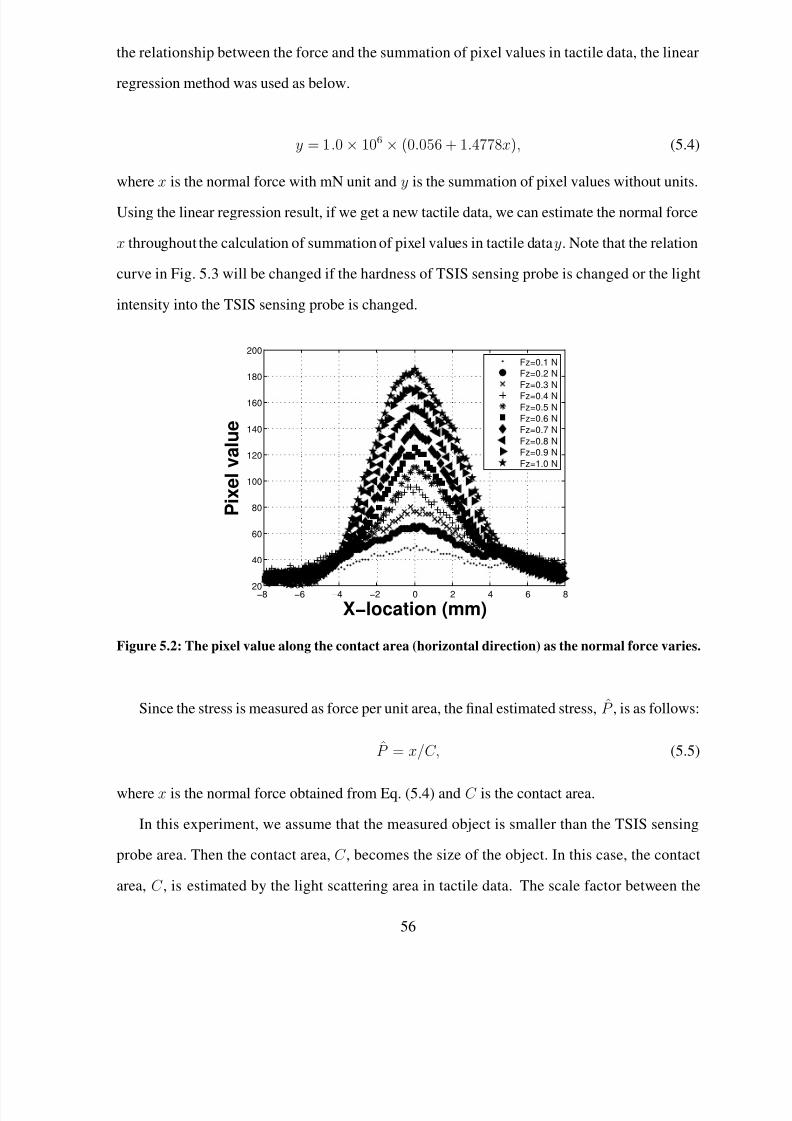
8/2/2019 Thesis Jongha
http://slidepdf.com/reader/full/thesis-jongha 70/126
the relationship between the force and the summation of pixel values in tactile data, the linear
regression method was used as below.
y = 1.0 × 106 × (0.056 + 1.4778x), (5.4)
where x is the normal force with mN unit and y is the summation of pixel values without units.
Using the linear regression result, if we get a new tactile data, we can estimate the normal force
x throughout the calculation of summation of pixel values in tactile data y. Note that the relation
curve in Fig. 5.3 will be changed if the hardness of TSIS sensing probe is changed or the light
intensity into the TSIS sensing probe is changed.
−8 −6 −4 −2 0 2 4 6 820
40
60
80
100
120
140
160
180
200
X−location (mm)
P i x e l v a l u e
Fz=0.1 N
Fz=0.2 N
Fz=0.3 N
Fz=0.4 NFz=0.5 N
Fz=0.6 N
Fz=0.7 N
Fz=0.8 N
Fz=0.9 N
Fz=1.0 N
Figure 5.2: The pixel value along the contact area (horizontal direction) as the normal force varies.
Since the stress is measured as force per unit area, the final estimated stress, P , is as follows:
P = x/C, (5.5)
where x is the normal force obtained from Eq. (5.4) and C is the contact area.
In this experiment, we assume that the measured object is smaller than the TSIS sensing
probe area. Then the contact area, C , becomes the size of the object. In this case, the contact
area, C , is estimated by the light scattering area in tactile data. The scale factor between the
56

8/2/2019 Thesis Jongha
http://slidepdf.com/reader/full/thesis-jongha 71/126
0 200 400 600 800 1000 1200 1400 1600 1800 2000 22000
1.5
3
4.5
6
7.5
9
10.5
x 107
x, Normal Force (mN)
y ,
S u m m a n t
i o n o f p i x e l v a l u e s
Loading
Unloading
Fitting resulty=1.0e+006*(0.056+1.4778x)
Figure 5.3: The relationship curve between the normal force and the summation of pixel values in
tactile data.
actual size and the image pixel distance is 6.79×10⁻³ mm per pixel. We obtained this ratio by
the calibration.
In this experiments, the relationship curve in Fig. 5.3 was obtained using a small, stiff tip
indenter. Strictly speaking, the relationship curve is only valid for a stiff material. But we use
this curve for the soft polymer, because both materials are homogeneous and isotropic. There
will be some errors due to the material differences. In addition, we have obtained the calibration
curve using the loading machine with 2 mm radius tip. Theoretically, the relationship curve can
be used to estimate forces applied on the objects of different sizes. To investigate the applied
normal force estimation capability using tactile data in more samples of bigger size, we find the
relationship curve in response to the different tip size of the loading machine. The size of tips
we used were radius of 10 mm and 14 mm. We obtained 15 tactile data of each tip size case
under different loading forces and calculated the summation of pixel values in tactile data. Then
the linear regression line was obtained. The experimental results are shown in Fig. 5.4.
According to the Hertzian contact theory, the relationship curve should match each other
regardless of the different indenter sizes (?). However, the result shows that there exist some
57

8/2/2019 Thesis Jongha
http://slidepdf.com/reader/full/thesis-jongha 72/126
0 100 200 300 400 500 600 700 800 9000
1.5
3
4.5
6
7.5
9
10.5
12
13.5
15x 10
7
x, Normal force (mN)
y ,
S u m m a n t
i o n o f p i x e l v a l u e s
14 mm radius tip
Regression result
10 mm radius tip
Regression result
Figure 5.4: The relationship between the normal force and summation of pixel values in tactile
data in response to the different loading machine tip radius.
differences between linear regression lines. At 800 mN normal force, the error between two
cases is 2.45%. There can be many reasons for this error. The impurity of the optical waveguide
is one reason. The unequal distribution of lights in the optical waveguide due to the misalign-
ment of LED position is another reason. In this experiment, we assume that this error is included
with the total estimation error.
5.2 Strain Estimation
The other value needed for the Young’s modulus estimation is the strain. Strain is the geo-
metrical deformation measure indicating the relative displacement between points on the object.
Thus if we know the displacement of any particular set of points on tactile data obtained under
different loading forces, then we can find the strain of the compressed object. The point dis-
placements can be calculated by matching each point sets between tactile data and compute the
distance between point position in one tactile data and point position in another tactile data (?).
To matching two different tactile data efficiently, a novel non-rigid point matching algorithm
called “topology preserving relaxation labeling (TPRL)” has been developed (?). The essence
of this algorithm is to automatically measure the displacement by tracking the change in posi-
58

8/2/2019 Thesis Jongha
http://slidepdf.com/reader/full/thesis-jongha 73/126
tion of control points extracted from two different tactile data ( ?), (?). Fig. 5.5 represents the
concept of tracking control points between 3-D reconstructed tactile data obtained under two
different loading forces on the same object. The 3-D reconstruction of tactile data is performed
using the pixel value as the depth information.
( x, y, z)
( x´, y´, z´ )
p
q
Figure 5.5: Tracking control points extracted from surface of two different tactile data to estimate
the strain.
TPRL uses iterative algorithm to find appropriate correspondence and transformation func-
tion between control points. The displacement of the contacted object deformation is obtained
from the transformation function. This displacement function is finally used to estimate the
strain information. We show that the proposed TPRL algorithm significantly improves the
matching performance compared to other state-of-the-art point matching algorithms in (?). That
is the reason why we use TPRL for the strain estimation. In this section, TPRL algorithm for
strain estimation is described in detail.
5.2.1 Problem Definition
The point matching using point features is widely used in computer vision and pattern recog-
nition as point representations are generally easy to extract (?), (?). The point matching prob-
lem can be categorized as rigid matching and non-rigid matching based on the deformation
of objects captured in the images. Compared with a rigid case, a non-rigid matching is morecomplex. Most non-rigid point matching methods use an iterated estimation framework to find
appropriate correspondence and transformation (?), (?).
The iterated closest point (ICP) algorithm is one of the most well-known heuristic ap-
59

8/2/2019 Thesis Jongha
http://slidepdf.com/reader/full/thesis-jongha 74/126
proaches (?). It utilizes the relationship by assigning the correspondence with binary values
of zero or one. However, in the case of non-rigid transformation this binary assumption is no
longer valid, especially when the deformation is large.
The thin plate spline robust point matching (TPS-RPM) algorithm is an expectation maxi-
mization (EM) algorithm to jointly solve for the feature correspondence as well as the geometric
transformation (?). The minimizing cost function is the summation of Euclidean distances be-
tween the matching points. In TPS-RPM, the binary correspondence value of ICP is relaxed
to the continuous value between zero and one. This soft-assign method improves the matching
performance as the correspondences are able to improve gradually and continuously, without
jumping around in the space of binary permutation matrices (?). The algorithm is robust com-
pared to ICP in the non-rigid case, but the joint estimation of correspondence and transforma-
tion increases the algorithm complexity. Furthermore, the Euclidean distance makes sense only
when there are at least rough initial alignments of the shapes. If the initial points are not aligned
well, the matching result is poor.
The coherent point drift (CPD) method is another probabilistic algorithm applied to the non-
rigid point matching problem (?). The CPD algorithm utilizes the displacement field between
two point sets and it has been extended to the general non-rigid registration framework with
TPS-RPM as a special case.
Another approach is the shape context (SC) method, which uses an object recognizer based
on the shape (?). For each point, the distributions of the distance and orientation to the neigh-
boring points are estimated through a histogram. There distributions are used as the attribute
relations for the points. The correspondences are chosen by comparing each point’s attributes
in one set with the attributes of the other. Only the attributes are considered, thus a search for
the correspondences can be conducted more easily compared to ICP and TPS-RPM. Generally
speaking, the SC method performs better in the handling of complex patterns than TPS-RPM.
A recently proposed matching method, the robust point matching-preserving local neigh-
borhood structures (RPM-LNS) algorithm, employs a neighborhood structure concept for the
general point matching problem (?). In RPM-LNS the cost function is formulated as an opti-
60

8/2/2019 Thesis Jongha
http://slidepdf.com/reader/full/thesis-jongha 75/126
mization problem to preserve local neighborhood relations. The matching probability is refined
through the relaxation labeling process. We will compare the performance of these algorithms
with our approach.
Another interesting point matching approach is the kernel correlation (KC) based method
(?). The cost function of KC is proportional to the correlation of two kernel density estimates.
The work was extended by using the L2 distance between Gaussian mixture models repre-
senting the point set (?). Since the RMS matching errors of the KC approach and the L2
distance approach are relatively higher than the other available algorithms such as TPS-RPM,
SC, RPM-LNS, and CPD, we have not included the matching results of these two methods in
the experimental results.
To develop an efficient non-rigid point matching algorithm, we generalize RPM-LNS by
introducing the optimal compatibility coefficient for the relaxation labeling method to solve a
non-rigid point matching problem. The relaxation labeling is an iterative procedure that reduces
local ambiguities and achieves global consistency by exploiting contextual information which
is quantitatively represented by “compatibility coefficient” (?), (?). It is widely known that the
relaxation labeling process is greatly affected by the choice of the compatibility coefficient (?),
(?).
In the method of Zheng and Doermann, the compatibility coefficient value was a binary
value of zero or one, depending on whether a point and its neighboring point have corresponding
points (?). In our method, the correlation between point pairs is measured by the proposed com-
patibility function, which quantifies the amount of similarity and spatial smoothness between
the point pairs in n-discrete values. This contextual information combined with a relaxation
labeling process is used to search for a correspondence. Then the transformation is calculated
by the thin plate spline (TPS) model (?). These two processes are iterated until the optimal
correspondence and transformation are found. The proposed relaxation labeling, with a new
compatibility coefficient, preserves a topology of point set, thus we call our method the topol-
ogy preserving relaxation labeling (TPRL) algorithm (?). It is important to note that changing
compatibility coefficient improves the matching performance significantly. In the next section,
61

8/2/2019 Thesis Jongha
http://slidepdf.com/reader/full/thesis-jongha 76/126
we describe TPRL in detail.
5.2.2 Topology Preserving Relaxation Labeling (TPRL) algorithm
Let two 3-D reconstructed tactile data obtained under different loading forces as O1 and
O2. From the surface of O1 and O2, a number of control points are extracted. Let P =
{ p1, p2,...,pI }, pi ∈ 3
be a point set extracted from O1 and Q = {q1, q2,...,qJ }, q j ∈ 3
be a point set extracted from O2. If the object is deformed by the contact of the sensing probe,
the distance between the points changes, especially when points are far apart. However, the
local adjacent points of each point will not change much due to physical constraints (?). So we
define the local adjacent points of each point. For a given point, pi ∈ P , one can select adjacent
points N pia , a = 1, 2,...,A, which are in the circle centered at pi. We set the radius of a circle
as the median value of all Euclidean distances between point pairs in P . Similarly, for a point,
q j ∈ Q, adjacent points are N qjb , b = 1, 2,...,B. We determine the fuzzy correspondence matrix
M . Each element of M piqj has continuous value between [0,1] and it indicates the correspon-
dence weight between pi and q j . Same as M piqj , M N
pia N
qjb
has continuous value between [0,1]
and it indicates the correspondence weight between N pia and N qjb .
The optimal match M is found by maximizing the energy function as follows.
M = arg maxM
E (M ), (5.6)
where
E (M ) =I
i=1
Bb=1
J j=1
Aa=1
M piqjM N
pia N
qj
b
(5.7)
subject toI
i=1
M piqj = 1, ∀i, andJ
j=1
M piqj = 1, ∀ j, and M piqj ∈ [0, 1].
5.2.3 Searching Point Correspondence
Initially, each point pi ∈ P is assigned with a set of matching probability based on the
shape context distance. After the initial probability assignment, the relaxation labeling process
updates the matching probability. The purpose of the subsequent process is to assign a matching
probability that maximizes C (P , Q, M ) under the relaxed condition as M piqj ∈ [0, 1]. At the
62

8/2/2019 Thesis Jongha
http://slidepdf.com/reader/full/thesis-jongha 77/126
end of the relaxation labeling process, it is expected that each point will have one unambiguous
matching probability. We follow the relaxation labeling updating rule as below (?).
1) Compute the compatibility coefficient which imposes the similarity and spatial smooth-
ness constraints between point pairs.
2) Compute the support function from all compatibility coefficients related to the point.
3) Update the matching probability depending on its support function.
The determination of the compatibility coefficients is crucial because the performance of
the relaxation labeling process depends on them. As a key contribution, we define a new com-
patibility coefficient to relax the binary value into multiple discrete values. The proposed com-
patibility coefficient quantifies the degree of agreement between the hypothesis that pi matches
to q j and N pia matches to N qjb . It is measured by the set of vectors originating from a point and
extending to all other sample points. The full set of vectors increases the algorithm complexity
and processing time. To simplify and speed up the process, log distance and polar angle bins
are used to capture the coarse location information (?). The bins are uniform in log-polar space,
which makes the descriptor more sensitive to positions of adjacent points than to those of points
far apart. In the diagram, the distance is defined as zero in the origin and incremented by one
towards the outer bins as shown in Fig. 5.6(a).
Let d( pi, N pia ) ∈ N be the distance between origin point pi and its nearest adjacent points.
Then the distance set of an origin point pi is defined as
DS ( pi) = {d( p1, N p1a ), d( p2, N p2a ),...,d( pi, N pia )}. For the computation of the angle between
point pairs, the alignment of a diagram with a reference point is necessary. In this research, the
mass center of a point set is used as a reference point. The direction from a point to the center
of mass is set as the positive x-axis of the descriptor. From this axis, the angle is incremented
by 1 in a counter clockwise direction. Let l( pi, N pia ) ∈ N be the angle between origin point
si and its nearest adjacent points. The angle set of an origin point si is given as AN G( pi) =
{d( p1, N p1a ), d( p2, N p2a ),...,d( pi, N pia )}. Every point can be an origin and the origin varies with
points in consideration to calculate the location information. Figs. 5.6(b) and 5.6(c) show the
distance and angle sets for a given point pi ∈ P and its corresponding point q j ∈ Q.
63

8/2/2019 Thesis Jongha
http://slidepdf.com/reader/full/thesis-jongha 78/126
d l
12 3 4 5
1
23
4
5
6
7
8 9 10
11
(a)
DS ( si)={4, 3, 3, 3, 3, 4, 1}
ANG ( si)={6, 6, 5, 4, 3, 3, 10}
(b)
DS (t j)={5, 4, 4, 4, 4, 4, 2}
ANG (t j)={6, 6, 6, 5, 5, 5, 11}
(c)
Figure 5.6: The distance and angle computation. (a) Diagram of log-polar bins used in computing
the distance and angle. We use 5 bins for the distances and 12 bins for the angles. (b) A pointsi ∈ S
(black) from the fish shape with its sets DS (si) and AN G(si) of its 6 adjacent points in S . (c) The
point t j ∈ T (black) in the deformed fish shape which have 6 adjacent points and its distance and
angle sets DS (t j) and AN G(t j).
In the non-rigid degradation of point sets, we note that a point set is usually distorted;
however the neighboring structure of a point is generally preserved due to physical constraints.
The displacement of a point and its adjacent point between two point sets constrain one another.
Thus, if the distance and angle of a point pair ( pi, N pia ) in the model shape and its corresponding
point pair (q j, N qja ) in the target shape are similar, we say that they have high correlation.
This is further strengthened if a point pair ( pi, N pia ) in the model shape is closer to each other.
To quantify this knowledge, we introduce the similarity constraint α, β as well as the spatial
smoothness constraint γ .
The first constraint is the similarity which is related to the differences between the distances
and angles of ( pi, N pia ) and (q j , N qja ). This first constraint imposes that if ( pi, N pia ) has smaller
distance and angle differences with (q j , N qja ), then they are more compatible. The disparities
between ( pi, N pia ) and (q j , N qja ) are defined as follows.
α( pi, N pia ; q j, N qja )
= 1 − (di( pi, N pia
) − d j(q j, N qj
b
))/ maxi,j
{di( pi, N pia
), d j(q j, N qj
b
)} , (5.8)
β( pi, N pia ; q j , N qja )
=
1 −
(li( pi, N pia ) − l j(q j, N qjb ))/ max
i,j{li( pi, N pia ), l j(q j, N
qjb )}
. (5.9)
64

8/2/2019 Thesis Jongha
http://slidepdf.com/reader/full/thesis-jongha 79/126
The second constraint, spatial smoothness, is measured by the distance between pi and N pia .
γ ( pi, N pia ) =
1 −
di( pi, N pia )
maxi
(di( pi, N pia ))
, (5.10)
where maxi
(di( pi, N pia )) is the longest edge of point-adjacent point pairs. Two points pi and N pia
are the most salient if γ ( pi, N pia ) is 1 and the least salient if γ ( pi, N pia ) is 0. The constraining
relations are illustrated in Fig. 5.7.
Figure 5.7: The general case of the correlation strength depends on the differences of distance and
angle between point pairs. The similarity constraints α, β and the spatial smoothness constraint γ
comprise the final compatibility coefficient for the relaxation labeling process.
We define a total compatibility coefficient by
r piqj( N pia N qjb ) = α( pi, N pia ; qi, N qib ) · β( pi, N pia ; qi, N qib ) · γ ( pi, N pia ). (5.11)
Clearly, r piqj ( N
pi
a N
qj
b ) ranges from 0 to 1. A high value of r piqj( N
pi
a N
qj
b ) corresponds tohigh matching probability between ( pi, N pia ) and (q j , N
qjb ), and a low value corresponds to
incompatibility. The support function qsitj in the k-th iteration is given by
qk piqj =I
i=1
J j=1
r piqj( N pia N qjb )M k
N pia N
qj
b
=I
i=1
J j=1
α( pi, N pia ; qi, N qib ) · β( pi, N pia ; qi, N qib ) · γ ( pi, N pia )M k N
pia N
qj
b
.
(5.12)
Note that r piqj( N pia N qjb ) is weighted by mk N
pia N
qj
b
because it depends on the likelihood of adja-
cent point pairs matching probability. Finally, M k piqj is updated according to
M k+1 piqj = M k piqjqk piqj/J
j=1
M k piqjqk piqj . (5.13)
65

8/2/2019 Thesis Jongha
http://slidepdf.com/reader/full/thesis-jongha 80/126
The optimization process is as follows. If a matching probability between pi and q j is supported
from their adjacent points N pia and N qjb , then the probability of being matched increases. The
probability decreases if they have relatively small support from their adjacent points.
Traditionally sum of rows (or columns) in the matrix M is used as a constraint in the re-
laxation labeling process. In this research, we use sum of rows and columns as a two-way
constraints. In order to meet these constrains, alternated row and column normalization of the
matrix M is performed after each relaxation labeling updates. This procedure is known as
Sinkhorn normalization and it showed that the procedure always converges to a doubly stochas-
tic matrix (?).
After pre-defined relaxation labeling iteration, the estimated matching probability is as-
signed to every point. To handle outliers, the points with maximum matching probability less
than mmin (mmin=0.95) are labeled as outliers and match them with a dummy point. The outlier
rejection scheme is performed throughout the relaxation labeling process.
5.2.4 Transformation Function
Given a finite set of correspondences between P and Q, we can proceed to estimate a plane
transformation T : 3 → 3 that may be used to map arbitrary points from one image to
the other. In this study, we use thin-plate spline (TPS) model, which is commonly used for
representing flexible coordinate transformations (?), (?).
Let vi denote the target function values at corresponding locations pi = (xi, yi, zi) in the
plane, with i = 1, 2,...,n. We set vi equal to xi, yi, zi to obtain the transformation. In 3-D
interpolation problem, the TPS interpolant f (x,y,z) minimizes the bending energy
I f =
3
∂ 2f
∂x2
2
+
∂ 2f
∂y2
2
+
∂ 2f
∂z2
2
+2( ∂ 2f
∂x∂y2
+ ∂ 2f
∂x∂z2
+ ∂ 2f
∂y∂z2
)
dxdydz (5.14)
and the interpolant form is
f (x,y,z) = a1 + axx + ayy + azz +
ni=1
wiU ((xi, yi, zi) − (x,y,z)). (5.15)
66

8/2/2019 Thesis Jongha
http://slidepdf.com/reader/full/thesis-jongha 81/126
where a1, ax, ay, az are the coefficients and wi’s are the weighting factors. The kernel function
U (r) is defined by U (r) = r3 log r3. In order for f (x,y,z) to have square integrable second
derivatives, we require the boundary conditionn
i=1
wi = 0 andn
i=1
wixi =n
i=1
wiyi =n
i=1
wizi =0.
A special characteristic of the thin-plate spline is that the resulting transformation is always
decomposed into a global transformation and a local non-affine warping component. The first
four terms describe global affine transform and the remaining terms describe non-linear (non-
global) transformation. Together with the interpolation conditions, f (xi, yi, zi) = vi, this yields
a linear system for the TPS coefficients:⎛⎜⎝ K P
P T 0
⎞⎟⎠⎛⎜⎝ W
A
⎞⎟⎠ =
⎛⎜⎝ V
0
⎞⎟⎠ , (5.16)
where K =
⎡⎢⎢⎢⎢⎢⎢⎢⎣
0 U (r12) · · · U (r1n)
U (r21) 0 · · · U (r2n)
· · · · · · · · · · · ·
U (rn1) U (rn2) · · · 0
⎤⎥⎥⎥⎥⎥⎥⎥⎦and P =
⎡⎢⎢⎢⎢⎢⎢⎢⎣
1 x1 y1 z1
1 x2 y2 z1
· · · · · · · · · · · ·
1 xn yn z1
⎤⎥⎥⎥⎥⎥⎥⎥⎦.
Here, rij = ||P i − P j|| is the Euclidean distance between points P i and P j . W and A are
column vectors formed from W = (w1, w2,...,wn)T and A = (a1, ax, ay, az)T , respectively.
V = (v1, v2,...,vn) is any n-vector. The matrix⎛⎜⎝ K P
P T 0
⎞⎟⎠is nonsingluar and it is invertable.
Thus we can determine the coefficients W and A by multiplication of matrices
⎛⎜⎝ K P
P T 0
⎞⎟⎠
−1
and
⎛⎜⎝ V
0
⎞⎟⎠. The weighting factors and coefficients W and A determine TPS interpolants
f (x,y,z) = [f x(x,y,z), f y(x,y,z), f z(x,y,z)] is a vector-valued, and this maps each point
(xi, yi, zi) to its correspondence (xi, yi, zi), the x, y, z coordinates of the transformation. The
resulting function f (x,y,z) = [f x(x,y,z), f y(x,y,z), f z(x,y,z)] maps each point (xi, yi, zi)
to its correspondence point (xi, yi, zi). It provides a continuous displacement field between
O1 and O2. Finally, the nonlinear Lagrangian strain tensor component of the uniaxial loading
67

8/2/2019 Thesis Jongha
http://slidepdf.com/reader/full/thesis-jongha 82/126
configuration ezz is determined as follows:
ezz = ∂f z(x,y,z)∂z
+ 12
∂f x(x,y,z)
∂z
3+
∂f y(x,y,z)∂z
3+∂f z(x,y,z)
∂z
3.
(5.17)
From Eq. (5.17), we can estimate the final strain information.
5.2.5 Validation and Performance Evaluation
In order to access the performance of the proposed algorithm, we have compared our match-
ing results with the state-of-the-art algorithms such as SC, TPS-RPM, RPM-LNS, and CPD
method. In the experiments, we set 300 as the number of labeling updates and the alternate
iteration with TPS transformation as 10.
Simulations Based on Synthetic Data
We have tested our proposed method and the state-of-the-art algorithms with respect to
different degrees of deformation, noise, outliers, rotation and occlusion ratio on synthetic data
set. The data set consists of two different shape models. The first model consists of 96 points
to represent a fish shape. The second model is a more complex pattern consisting of 108 points
to represent a Chinese character (“blessing”).
In each test, one of the distortions is applied to a model set to create a target set. Fig. 5.8
to Fig. 5.13 show examples of synthesized data sets (?). A total of 100 data sets is generated
at each distortion level. The matching performance of each algorithm is compared by the mean
and standard deviation of the registration error of 100 trials in each distortion level. We use root
mean square (RMS) error for the registration error metric. The statistical results, error means
and standard deviations for each setting, are shown in from Fig. 5.14 to Fig. 5.18.
In the deformation test results, Figs. 5.14(a) and 5.14(b), five algorithms achieve similar
matching performance in both fish and character shape at low deformation ratio. However,
as the degree of deformation increases, we observe that TPRL shows the robustness to large
deformation compared with other algorithms. The degree of deformation such as 0, 0.035,
0.05, 0.065, and 0.08 indicates the deformation ratio. This measures the percentage of the
68

8/2/2019 Thesis Jongha
http://slidepdf.com/reader/full/thesis-jongha 83/126
(a) (b)
Figure 5.8: Synthesized original data sets for statistical tests. (a) fish shape. (b) Chinese character
shape.
(a) (b)
Figure 5.9: Synthesized deformation data sets for statistical tests. (a) fish shape. (b) Chinese
character shape.
(a) (b)
Figure 5.10: Synthesized noise data sets for statistical tests. (a) fish shape. (b) Chinese character
shape.
deformation degree from the original image. The higher ratio shows the higher deformation
degree. The small ratio shows the lower deformation degree.
The presence of noise makes the point’s location ambiguous. Therefore, this type of data is
more challenging than the deformation data. The noise test results of Figs. 5.15(a) and 5.15(b)
show that all algorithms are affected by this type of data distortion. However, we notice that
69

8/2/2019 Thesis Jongha
http://slidepdf.com/reader/full/thesis-jongha 84/126
(a) (b)
Figure 5.11: Synthesized outlier data sets for statistical tests. (a) fish shape. (b) Chinese character
shape.
(a) (b)
Figure 5.12: Synthesized rotation data sets for statistical tests. (a) fish shape. (b) Chinese character
shape.
(a) (b)
Figure 5.13: Synthesized occlusion data sets for statistical tests. (a) fish shape. (b) Chinese charac-
ter shape.
TPRL compensates the location ambiguity and finds more accurate correspondences than the
other four.
In addition to the deformation and noise test, present outliers further complicate the point
matching problem. To evaluate the performance of our method with outliers, we added maxi-
mum of 405 outliers to the target set. From the results of Figs. 5.16(a) and 5.16(b) we note that
70

8/2/2019 Thesis Jongha
http://slidepdf.com/reader/full/thesis-jongha 85/126
SC and CPD in both shapes and RPM-LNS in a character shape are easily confused by outliers
and start to fail once the outlier level becomes relatively high. The TPS-RPM are not affected
by outliers as much, but the error is still higher than TPRL. The TPRL is very robust regardless
of the outlier level.
In Figs. 5.17(a) and 5.17(b) we evaluate the influence of rotation. From this result, we
notice that the applied transformation (rotation) does not affect the performance of SC, RPM-
LNS and TPRL. All error curves except TPS-RPM and CPD are relatively constant. Note that
until 30 degrees of rotation, the errors of TPS-RPM and CPD are lower than SC and RPM-LNS.
But from 60 degree of rotation, TPS-RPM and CPD deteriorate quickly. The TPRL is rotation
invariant and consistently outperforms four other algorithms in all degrees of rotations.
Occlusion is also an important degradation in real applications. We use six occlusion levels
to test the five algorithms. As shown in Figs. 5.18(a) and 5.18(b), the RMS error of TPS-RPM
is the largest compared to the other four algorithms. The TPRL achieves the best result in both
fish and character shapes.
0.035 0.05 0.065 0.08
0
0.01
0.02
0.03
0.04
Fish − Degree of Deformation
R o o t M e a n S q
u r e E r r o r
SC
TPS−RPM
RPM−LNS
CPDTPRL
(a)
0.02 0.035 0.05 0.065 0.08
0
0.01
0.02
0.03
0.04
0.05
0.06
Character − Degree of Deformation
R o o t M e a n S q
u r e E r r o r
SCTPS−RPM
RPM−LNS
CPD
TPRL
(b)
Figure 5.14: Comparison of the matching performance of TPRL () with shape context (), TPS-
RPM (∗), RPM-LNS (), and CPD (). (a) Fish shape deformation test. (b) Character shape
deformation test.
71

8/2/2019 Thesis Jongha
http://slidepdf.com/reader/full/thesis-jongha 86/126
0 0.01 0.02 0.03 0.04 0.05
0
0.01
0.02
0.03
0.04
Fish − Noise Level
R o o t M
e a n S q u r e E r r o r
SC
TPS−RPM
RPM−LNS
CPDTPRL
(a)
0 0.01 0.02 0.03 0.04 0.050
0.01
0.02
0.03
0.04
0.05
Character − Noise Level
R o o t M
e a n S q u r e E r r o r
SCTPS−RPM
RPM−LNS
CPD
TPRL
(b)
Figure 5.15: Comparison of the matching performance of TPRL () with shape context (), TPS-
RPM (∗), RPM-LNS (), and CPD (). (a) Fish shape noise test. (b) Character shape noise test.
0 0.5 1 1.5 2
0
0.02
0.04
0.06
0.08
0.1
0.12
0.14
Fish − Outlier to Data Ratio
R o o t M e a n S q u r e E r r o r
SCTPS−RPM
RPM−LNSCPD
TPRL
(a)
0 0.5 1 1.5 2
0
0.03
0.06
0.09
0.12
Character − Outlier to Data Ratio
R o o t M e a n S q u r e E r r o r
SCTPS−RPM
RPM−LNS
CPDTPRL
(b)
Figure 5.16: Comparison of the matching performance of TPRL () with shape context (), TPS-
RPM (∗), RPM-LNS (), and CPD (). (a) Fish shape outlier test. (b) Character shape outlier
test.
Simulations Based on Real World Data
We also conducted experiments on real world data. For this experiment, we have used the
Carnegie Mellon University (CMU) hotel sequence available. The database consists of 101
frames of a moving sequence of a toy hotel. We obtained 11 frames as shown in Figs. from
5.19(a) to 5.19(j). In total, 100 points were manually selected from each frame and matched
all images spaced by 10, 20, 30, 40, 50, 60, 70, 80, 90, 100 frames. The experiments were
72

8/2/2019 Thesis Jongha
http://slidepdf.com/reader/full/thesis-jongha 87/126
0 30 60 90 120 180
0
0.1
0.2
0.3
0.4
Fish − Degree of Rotation
R o o t M
e a n S q u r e E r r o r
SCTPS−RPM
RPM−LNS
CPD
TPRL
(a)
0 30 60 90 120 180
0
0.15
0.3
0.45
0.6
Character − Degree of Rotation
R o o t M
e a n S q u r e E r r o r
SCTPS−RPM
RPM−LNS
CPD
TPRL
(b)
Figure 5.17: Comparison of the matching performance of TPRL () with shape context (), TPS-
RPM (∗), RPM-LNS (), and CPD (). (a) Fish shape rotation test. (b) Character shape rotation
test.
0 0.1 0.2 0.3 0.4 0.5
0
0.025
0.05
0.075
0.1
0.125
Fish − Occlusion Ratio
R o o t M e a n S q u r e E r r o r
SC
TPS−RPM
RPM−LNS
CPDTPRL
(a)
0 0.1 0.2 0.3 0.4 0.5
0
0.05
0.1
0.15
0.2
Character − Occlusion Ratio
R o o t M e a n S q u r e E r r o r
SCTPS−RPM
RPM−LNS
CPD
TPRL
(b)
Figure 5.18: Comparison of the matching performance of TPRL () with shape context (), TPS-
RPM(∗), RPM-LNS (), and CPD (). (a) Fish shape occlusion test. (b) Character shape occlusion
test.
conducted under four different occlusion ratios: 0.0 (100 × 100), 0.1 (90 × 100), 0.2 (80 ×
100), and 0.3 (70 × 100).
Figs. 5.20(a) to 5.20(d) show the results for these experiments. We note that without oc-
clusion, Fig. 5.20(a), five algorithms achieve similar matching performance until 30 frames of
separation. However, as the frame separation increases, we observe that TPRL shows the ro-
bustness compared to other algorithms. The increased mean RMS error from 10 to 100 frames
73

8/2/2019 Thesis Jongha
http://slidepdf.com/reader/full/thesis-jongha 88/126
(a) (b) (c) (d) (e)
(f) (g) (h) (i) (j)
Figure 5.19: Sequence images of toy hotel. (a) Frames 0, (b) Frames 10, (c) Frames 20, (d) Frames
30, (e) Frames 40, (f) Frames 50, (g) Frames 60, (h) Frames 70, (i) Frames 80, (j) Frames 90, (j)
Frames 100.
separation is 0.001 mm compared to 0.049 mm in SC, 0.027 mm in TPS-RPM, 0.021 mm in
RPM-LNS, and 0.025 mm in CPD. Figs. 5.20(b) to Fig. 5.20(d) show the results with occlu-
sion. With 0.3 occlusion ratio, the increased mean RMS error is 0.005 mm from 10 to 100
frames of separation, compared to 0.05 mm in RPM-LNS, the second smallest change among
the algorithms.
Simulations Based on Large Data
We also tested the TPRL performance under a larger data set as shown in Figs. 5.21(a) and
5.21(b). From the image, 1000 points were extracted by curvature scale space corner detector
(?). After a model set was chosen, we applied a randomly generated non-rigid transformation to
warp it and added 1000 to 3000 outliers. The TPRL performed the best with 0.35 ± 0.22 mm,
0.38 ± 0.24 mm, and 0.39 ± 0.25 mm RMS errors for the 1000 × 2000, 1000 × 3000, and 1000
× 4000 size point matching, respectively. The CPD method gave the second highest matching
performance with 0.61 ± 0.51 mm, 0.66 ± 0.56 mm, and 0.67 ± 0.56 mm RMS errors in the
same scenario.
Processing Times
In order to compare algorithms, it is necessary to analyze the processing time of each algo-
rithm. Assume that both model set and target set have points. The algorithms are based on the
74

8/2/2019 Thesis Jongha
http://slidepdf.com/reader/full/thesis-jongha 89/126
10 20 30 40 50 60 70 80 90 100
0
0.01
0.02
0.03
0.04
0.05
0.06
Separation between frames
R o o t M
e a n S q u r e E r r o r
SCTPS−RPM
RPM−LNS
CPD
TPRL
(a)
10 20 30 40 50 60 70 80 90 100
0
0.01
0.02
0.03
0.04
0.05
0.06
Separation between frames
R o o t M
e a n S q u r e E r r o r
SCTPS−RPM
RPM−LNS
CPD
TPRL
(b)
10 20 30 40 50 60 70 80 90 100
0
0.04
0.08
0.12
Separation between frames
R o o t M e a n S q u r e E r r o r
SCTPS−RPM
RPM−LNSCPD
TPRL
(c)
10 20 30 40 50 60 70 80 90 100
0
0.05
0.1
0.15
0.2
Separation between frames
R o o t M e a n S q u r e E r r o r
SCTPS−RPM
RPM−LNSCPD
TPRL
(d)
Figure 5.20: Comparison of the matching performance of TPRL () with shape context (), TPS-
RPM (∗), RPM-LNS (), and CPD () in the hotel sequence for increasing frame separation anddifferent occlusion ratio [(a) 0.0, (b) 0.1, (c) 0.2, (d) 0.3]. Error bars correspond to the standard
deviation of each pair’s RMS error.
NP-hard problem and have similar computational complexity of O(N 2) for matching in 2 and
O(N 3) for matching in 3. Among the compared algorithms, the CPD method performs with
the fastest registration time under a large distortion of the data set. The TPRL algorithm takes a
slightly longer time to compute compared to the CPD method. For a 105 × 105 point matching,
the TPRL algorithm takes about 1.69 seconds and the CPD method takes about 1.08 seconds on
a desktop PC with Core 2 Duo CPU with 2.13GHz and 2GB RAM.
75

8/2/2019 Thesis Jongha
http://slidepdf.com/reader/full/thesis-jongha 90/126
(a)
0 0.2 0.4 0.6 0.8 1
0
0.1
0.2
0.3
0.4
0.5
0.6
0.7
0.8
0.9
1
(b)
Figure 5.21: Robustness test on large data set. (a) A straw image and (b) 1000 points extracted
from the straw image.
5.3 Young’s Modulus Estimation from Stress and Strain
To determine the Young’s modulus of the contacted object, the strain component ezz are
averaged to yield the average strain ezz . Given the applied normal stress P zz , the Young’s
modulus E of the object is then determined from the following equation,
E = P zz/ezz . (5.18)
The proposed Young’s modulus estimation method is validated in the next section.
5.4 Experimental Results
To validate the target hardness estimation method based on the tactile data, Versaflex CL2000X
and CL2003X (GLS, McHenry, Illinois) soft polymers of Young’s moduli 103 kPa and 62 kPa
have been used. The soft polymer was spherical shape with 3 mm radius. In this experiment, the
TSIS compressed the polymer samples while slowly increasing the compression ratio. At 0.7
N and 1.2 N applied forces, two tactile data have been captured. The obtained tactile data were
then reconstructed to 3-D, and control points were extracted from the surface of 3-D recon-
structed tactile data. The correspondence and transformation function between control points
were estimated using the proposed TPRL algorithm described in Section 5.2.1.
Fig. 5.22(a) represents 200 control points distributions extracted from each of CL2000X soft
polymer tactile data in Fig. 5.5. The point matching result using the proposed TPRL algorithm
is represented in Fig. 5.22(b). Fig. 5.23 represents the experimental result. The lines represent
76

8/2/2019 Thesis Jongha
http://slidepdf.com/reader/full/thesis-jongha 91/126
theoretical CL2000X and CL2003X modulus values from the manufacturer, and the circles and
crosses represent the measured values from the TSIS. The errors of the estimated moduli were
within 4.23% relative error for CL2000X and 5.38% relative error for CL2003X.
00.2
0.40.6
0.81
0
0.2
0.4
0.6
0.8
10
0.2
0.4
0.6
0.8
1
x−axisy−axis
z − a x i s
0.7 N
1.2 N
(a)
00.2
0.40.6
0.81
0
0.2
0.4
0.6
0.8
10
0.2
0.4
0.6
0.8
1
x−axisy−axis
z − a x i s
0.7 N
1.2 N
(b)
Figure 5.22: Control points extracted from two tactile data obtained under different loading forces
on the same object. (a) Before point matching, (b) After point matching.
0 0.0015 0.003 0.0045 0.006 0.0075 0.009 0.0105 0.0120
0.2
0.4
0.6
0.8
1
1.2
1.4
Compressive strain
C o m p r e s s i v e s t r e s s ( k P a )
CL2000X theoretical modulus
CL2000X experimental measured value
CL2003X theoretical modulus
CL2003X experimental measured value
Figure 5.23: The hardness estimation results of soft polymers, CL2000X and CL2003X.
77

8/2/2019 Thesis Jongha
http://slidepdf.com/reader/full/thesis-jongha 92/126
5.5 Discussions
In this chapter, the tactile data processing algorithm capable of estimating the hardness of
the touched object via direct contact are developed and experimentally evaluated. The hardness
of the contacted object is estimated using the tactile data obtained by the TSIS. In order to obtain
the hardness of the contacted object, a new non-rigid pattern matching algorithm called “TPRL”
is developed. The performance of the target hardness estimation method is experimentally
verified using the soft polymers. The results show that when using the TSIS, the hardness of
the touched object can be estimated within 5.38% relative error.
The measured object must be smaller than the area of the TSIS sensing probe. If we are
measuring the elasticity of a surface object, the contact area must be smaller than the TSIS
sensing probe area. However, if we measure a sub-surface object such as tumor, the TSIS sens-
ing probe area can be smaller than the contact tissue surface, as long as the inclusion is smaller
than the probe area. In this case, the contact area, C , is the area of the sensing probe with the
known value. Thus, even if the hidden tumor exists in a variety of sizes and shapes, the contact
area, C , is always a constant, which is the sensing probe area. One possible application of the
TSIS is the early detection of breast cancer. The common breast tumor size is approximately 20
mm or smaller in stages 0 and I (?). In stage II, it is approximately 20 to 50 mm (?). To detect
the 50 mm breast tumor, the sensing probe should be bigger than 50 mm.Generally, the background light disturbance and drifting of the light source are issues for the
tactile sensor that operates based on the detection of light illumination (?). If the background
light is too bright compared to the light of the tactile sensor, it causes measurement errors of
the TSIS. To prevent this, we use the TSIS in a relatively dark room, which minimizes the
background light disturbance. The drifting of light occurs if light sources of the TSIS are
positioned incorrectly and the camera captures the spurious light. In this case, the drifted light
is shown as noise in the tactile data. To prevent this, precise positioning and directionality of
the light source are required. We carefully positioned and calibrated four light sources with
acceptance angles. These two methods prevented the light disturbance and drifting of the light
78

8/2/2019 Thesis Jongha
http://slidepdf.com/reader/full/thesis-jongha 93/126
source issues during the preliminary experiments. In the future work, we will also consider
using the image segmentation techniques. More specifically, Canny edge detection technique
can be used to extract the boundary of the desired light scattering area in the tactile data and
remove the noise (?).
Typically, in the LED operation, approximately 20% input power is converted to light and
80% to heat (?). Heat at the junction of the LED affects the overall performance of the LED
in terms of light output and spectrum. The amount of light emitted by the LED decreases as
the junction temperature rises. Thus, LED luminaries require a thermal management system
for LED cooling, since most of the energy for the LED is converted to heat rather than light.
Without an appropriate thermal management system, the generated heat can degrade the inten-
sity of the LED and finally affect the calibration result of the TSIS. In the current TSIS design,
the LED is directly connected to the power source, resulting in the intensity drift caused by the
temperature effect and the variation of the resistance in the power source. In our experiments,
the TSIS takes approximately 20 seconds to take a tactile data of the touched object. Thus, the
LED intensity drift caused by the temperature effect is not large. In the next TSIS design, we
will consider a thermal management system such as heat sinks to release heat from the LED.
The flip-chip package type LED will also be considered to reduce the thermal resistance of the
LED. To prevent the variation of the resistance in the power source, we will also consider the
constant current LED drive circuit.
Eq. (5.2) is material-dependent. Depending upon the material, the relationship could be
linear or nonlinear. In this research, we assumed that the touched object is homogeneous and
isotropic. In this case, the relationship curve between the normal force and the summation of
pixel values in tactile data is linear. Thus, the applied force is estimated from the summation of
pixel values in tactile data using the normal force versus the summation of pixel values table,
which is previously obtained by the calibration. Then the applied stress, which is the force per
unit area, is obtained by dividing the applied force by the contact area. We have verified this
approach in Section 5.4 for the homogeneous and isotropic material. If the touched object is
inhomogeneous and anisotropic, Eq. (5.2) will not be valid. We will have to re-derive Eq. (5.2)
79

8/2/2019 Thesis Jongha
http://slidepdf.com/reader/full/thesis-jongha 94/126
for the inhomogeneous and anisotropic material case.
The measurement range of the TSIS is controlled by the hardness of the TSIS sensing probe.
This is determined by how we mix two components of PDMS, the viscous fluid silicone (part A)
and the catalyst (part B). The viscous fluid silicone is hardened by the catalyst. If the amount of
catalyst increases, the hardness of the PDMS increases. If the amount of catalyst decreases, the
hardness of the PDMS decreases. In this research, the measurement range of the TSIS designed
for the soft polymer hardness estimation is from a normal force of 0 to 2500 mN. In future work,
we will investigate the different measurement ranges of the TSIS depending upon the different
hardness of the TSIS sensing probe.
80

8/2/2019 Thesis Jongha
http://slidepdf.com/reader/full/thesis-jongha 95/126
CHAPTER 6
TISSUE INCLUSION PARAMETER ESTIMATION BY INDIRECT CONTACT
The mechanical properties of tissue inclusion such as hardness and its geometry are very im-
portant in detecting and characterizing the severity of the tumor. In this chapter, we devise a
methodology for estimating three parameters of the tissue inclusion: size, depth, and hardness.
The estimated parameters are extracted from the tactile data obtained at the tissue surface using
the TSIS. Two different estimation approaches are proposed in this chapter. The first approach is
to estimate the relative parameters of tissue inclusion. Using the salient features of the captured
tactile data, we estimate the relative inclusion parameters such as size, depth, and hardness.
The second approach is to estimate the absolute parameters of tissue inclusion. The estimation
method consists of the forward algorithm and inversion algorithm. The forward algorithm is
designed to comprehensively predict the tactile data based on the parameters of the inclusion
in the soft tissue. This algorithm is used to develop the inversion algorithm that can be used to
extract the size, depth, and hardness of an inclusion. The proposed algorithms are then validated
by the realistic tissue phantoms with stiff inclusions.
6.1 Problem Formulation
To estimate tissue inclusion’s parameters, we consider the following idealized tissue model
in Fig. 6.1. The assumptions used in the idealized tissue model are as follows (?).
1) Most breast tumors are found in the upper outer quadrant of the breast where the tissue is
relatively thin and flat. Therefore, in our breast tissue model, the breast tissue is approximated
as a slab of material of constant thickness that is fixed to a flat, incompressible chest wall.
2) The tissue inclusion is assumed to be spherical and stiffer than the surrounding tissue.
3) We assume that both breast tissue and tissue inclusion are linear and isotropic.
81
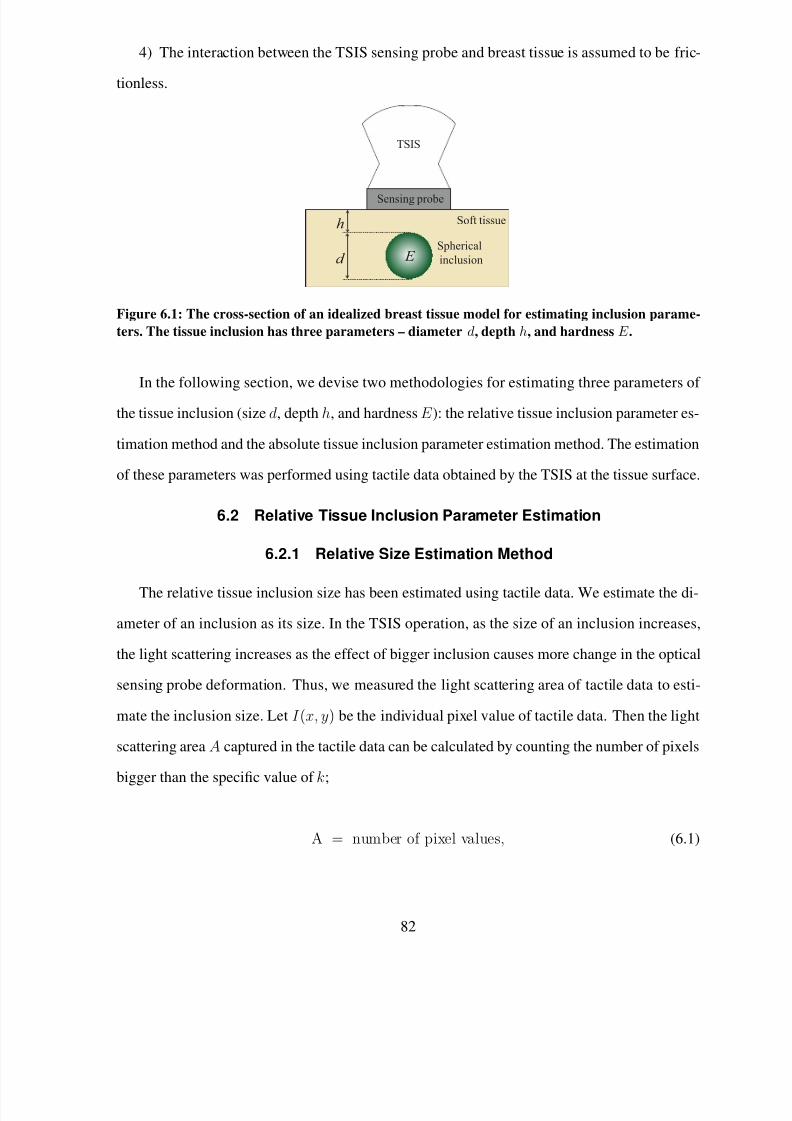
8/2/2019 Thesis Jongha
http://slidepdf.com/reader/full/thesis-jongha 96/126
4) The interaction between the TSIS sensing probe and breast tissue is assumed to be fric-
tionless.
Spherical
inclusion
Soft tissue
d
h
Sensing probe
E
TSIS
Figure 6.1: The cross-section of an idealized breast tissue model for estimating inclusion parame-
ters. The tissue inclusion has three parameters – diameter d, depth h, and hardness E .
In the following section, we devise two methodologies for estimating three parameters of
the tissue inclusion (size d, depth h, and hardness E ): the relative tissue inclusion parameter es-
timation method and the absolute tissue inclusion parameter estimation method. The estimation
of these parameters was performed using tactile data obtained by the TSIS at the tissue surface.
6.2 Relative Tissue Inclusion Parameter Estimation
6.2.1 Relative Size Estimation Method
The relative tissue inclusion size has been estimated using tactile data. We estimate the di-
ameter of an inclusion as its size. In the TSIS operation, as the size of an inclusion increases,
the light scattering increases as the effect of bigger inclusion causes more change in the optical
sensing probe deformation. Thus, we measured the light scattering area of tactile data to esti-
mate the inclusion size. Let I (x, y) be the individual pixel value of tactile data. Then the light
scattering area A captured in the tactile data can be calculated by counting the number of pixels
bigger than the specific value of k
;
A = number of pixel values, (6.1)
82

8/2/2019 Thesis Jongha
http://slidepdf.com/reader/full/thesis-jongha 97/126
that is the number of I (x, y) > k . k is the pixel threshold value and we set it as 5. The area of
Eq. (6.1) is the pixel area in the tactile data. To transform the pixel area to the real area, the
scale factor is used. We used the scale factor between the actual area and the tactile data pixel
area as (6.79 × 10⁻³)2 mm2 per pixel area. We obtained this ratio by the calibration. Then a
relative size d of a tissue inclusion can be found as follows.
d = 2
(6.79 × 10⁻³)2 × A/π. (6.2)
The unit of the relative inclusion size is millimeters. In this research, we assume that a tissue
inclusion is spherical and there is only one inclusion in the tissue. Also, we assume that there
is no noise in the tactile data. In addition, when we calculate the size of tissue inclusion, we did
not consider other two parameters, depth and Young’s modulus.
6.2.2 Relative Size Estimation Experimental Results
We demonstrate the capability of the proposed relative size estimation method. For this
experiment, the realistic tissue phantoms with embedded hard inclusions (simulated tumor)
have been manufactured (CIRS Inc., VA). The phantom includes three hard inclusions with
sizes, 2, 8, and 14 mm. Each inclusion was placed 5 mm below the surface of the phantom (?).
The phantom was made of a silicone composite having a Young’s modulus of approximately
5 kPa. The inclusion was made using another silicone composite, the stiffness of which was
higher than the surrounding tissue phantom. The Young’s modulus of each inclusion was 120
kPa, which is for fibrous tissue at 5% pre-compression with loading frequency of 4.0 Hz ( ?).
The schematic of the size phantom is shown in Fig. 6.2 and the manufactured size phantom
is shown in Fig. 6.3. To obtain the tactile data, first we placed the phantom in the desk. We
then placed the TSIS onto the phantom surface where the tissue inclusion was embedded and
pressed it to obtain the tactile data. To compare the tactile data between three different tissue
inclusions, we applied the same loading forces of the TSIS on three different tissue inclusions.
For each tissue inclusion case, we obtained 15 tactile data. The relative size of an inclusion has
been estimated using Eq. (6.2) and averaged. Fig. 6.4 represents the sample tactile data of each
inclusion.
83

8/2/2019 Thesis Jongha
http://slidepdf.com/reader/full/thesis-jongha 98/126
Figure 6.2: The schematic of the size phantom.
2 mm 8 mm
Size phantom
14 mm
Figure 6.3: The manufactured size phantom.
(a) (b) (c)
Figure 6.4: The tactile data of three inclusions embedded in the size phantom. (a) 2 mm size
inclusion, (b) 8 mm size inclusion, (c) 14 mm size inclusion.
The relative size estimation results are shown in Fig. 6.5. The plot shows that the 14 mm
size case had the highest mean size of 8.77 mm and the most variation, with a standard deviation
of 1.24 mm. Conversely, the 2 mm size case had the lowest mean size of 1.67 mm, and the least
variation, with a standard deviation of 0.48 mm. Because we estimated the relative value, the
comparison ratio of each estimated size is also important. The ratio of real size of inclusions
was approximately 1 : 4 : 7. The estimated ratio of relative size was approximately 1 : 3.86
: 5.26. This corresponds to 3.5% and 24.9% relative error. The error is larger for larger size
84

8/2/2019 Thesis Jongha
http://slidepdf.com/reader/full/thesis-jongha 99/126
inclusion.
2 8 141
2
3
4
5
6
7
8
9
10
11
True Diameter (mm)
E s t i m a t e d V a l u e ( m m )
Figure 6.5: Error bar chart of estimated relative diameter of each inclusion.
6.2.3 Relative Depth Estimation Method
As the depth of inclusion increases, the light scattering due to the waveguide deformation
decreases as the effect of an inclusion becomes reduced. Because we have assumed that the
inclusion is spherical, the pixel values of the tactile data distribute in a bell shape, where the
pixel intensity is the highest at the centroid of the pixel values of tactile data and decreases with
increasing distance from the centroid. Thus, we used a centroid pixel value of tactile data to
estimate a relative inclusion depth. To obtain equations for locating centroids of the tactile data,
first we find the moment of a force as referred to in Fig. 6.6.
Fulcrum
d
F
Figure 6.6: Definition of moment of a force.
85

8/2/2019 Thesis Jongha
http://slidepdf.com/reader/full/thesis-jongha 100/126
The moment M of a force F about some fixed fulcrum is defined as (?)
M = F d, (6.3)
where d is the distance from the fulcrum to the line of action of the force F . Then, assume a
system n point masses situated along a horizontal line, as shown in Fig. 6.7.
d
n1 2 3
F
Figure 6.7: n point masses situated along a horizontal line.
The expression of the moment M is as follows.
M 1 = w1x1 + w2x2 + w3x3 + · · · wnxn, (6.4)
F d = w1x1 + w2x2 + w3x3 + · · · wnxn. (6.5)
Thus the distance from the fulcrum to the line of action of the force F is
d =w1x1 + w2x2 + w3x3 + · · · wnxn
w1 + w2 + w3 + · · · wn. (6.6)
Now, this concept is extended to the case of centroids of x-and y-coordinates of the tactile data.
Since the tactile data is 2-D, the centroid of tactile data, (X c, Y c), are calculated by (?), (?)
X c =
x
y
I (x, y)xdxdyx
y
I (x, y)dxdy, (6.7)
Y c =
x
y
I (x, y)ydxdyx
y
I (x, y)dxdy. (6.8)
Then a relative depth of a tissue inclusion h can be calculated as below.
h = I (X c, Y c). (6.9)
Because the calculated depth is the pixel distance, using the scale fact 6.79×10⁻³ mm2 per pixel
distance, we transform the pixel distance to the actual distance. Same as the relative inclusion
86

8/2/2019 Thesis Jongha
http://slidepdf.com/reader/full/thesis-jongha 101/126
size case, the unit of the relative inclusion depth is millimeters. As with the size estimation
case, we assume that a tissue inclusion is spherical and there is only one inclusion in the tissue.
Also, we assume that there is no noise in the tactile data. In addition, when we calculate the
depth of tissue inclusion, we do not consider the other two parameters, size and hardness.
6.2.4 Relative Depth Estimation Experimental Results
The depth tissue phantom has three inclusions with different depths: 4, 8, and 12 mm. The
size of all inclusion was 7 mm and their Young’s modulus was 100 kPa, which is about the
invasive ductal carcinoma hardness (?). The schematic of the depth phantom is shown in Fig.
6.8 and the manufactured depth phantom is shown in Fig. 6.9. Consistent with the size phantom
experiment case, we obtained 15 tactile data of each inclusion using the same experimental steps
in subsection 6.2.2. Then, the relative depth of an inclusion was estimated using Eq. (6.9) and
averaged. Fig. 6.10 represents the sample tactile data of each inclusion.
Figure 6.8: The schematic of the depth phantom.
4 mm 8 mm
Depth phantom
12 mm
Figure 6.9: The manufactured depth phantom.
87

8/2/2019 Thesis Jongha
http://slidepdf.com/reader/full/thesis-jongha 102/126
(a) (b) (c)
Figure 6.10: The tactile data of three inclusions embedded in the depth phantom. (a) 4 mm depth
inclusion, (b) 8 mm depth inclusion, (c) 12 mm depth inclusion.
4 8 120.25
0.3
0.35
0.4
0.45
0.5
0.55
0.6
0.65
True Depth (mm)
E s t i m a t e d
V a l u e ( m m )
Figure 6.11: Error bar chart of estimated relative depth of each inclusion.
The depth estimation result is shown in Fig. 6.11. The plot shows that the 4 mm depth case
had the highest mean depth of 0.59 mm and the least variation, with a standard deviation of
0.03 mm, whereas the 12 mm depth case had the lowest mean depth of 0.34 mm and the most
variation with a standard deviation of 0.08 mm. The ratio of the real depth of inclusions was
approximately 1 : 1.5 : 3. The estimated relative depth ratio was approximately 1 : 0.74 : 0.57.
This is a relative error of 50.7% and 81.0% for the latter two inclusion depths with respect to
the first inclusion. This shows larger error for the deepter inclusion estimation.
88

8/2/2019 Thesis Jongha
http://slidepdf.com/reader/full/thesis-jongha 103/126
6.2.5 Relative Hardness Estimation Method
The word “hardness” is expressed by the Young’s modulus E . The relative Young’s modulus
or relative hardness is expressed as relative stress over relative strain. The relative stress is
measured as force per unit area. In this research, we estimate the force F using the summation
of pixels in tactile data M (?). The relationship between the force F and the integrated pixel
value M is obtained from the initialization.
The other value needed for the relative Young’s modulus is the relative strain. The strain
is the fraction change in length in response to the stress. Strain is the geometrical deformation
measure indicating the relative displacement between points on the target. Thus, if we know
the displacement of any particular set of points on tactile data obtained under different loading
forces to the target, then we can find the relative strain presented by the loading forces. To
find the relative stain T , first we obtained two different tactile data under different compression
ratios. We then measured the relative size from each tactile data using Eq. (6.2). The estimate
strain T is measured by the difference of the each relative size as below.
T =d1 − d2
d1, (6.10)
where d1 is the estimated tissue inclusion size using first tactile data and d2 is the estimated
tissue inclusion size using second tactile data. The obtained stress and strain are finally used toestimate the relative hardness of an inclusion. The unit of the relative hardness of an inclusion
is P a. In this research, we assume that a tissue inclusion is spherical and there is only one
inclusion in the tissue. Also we assume that there is no noise in the tactile data.
6.2.6 Relative Hardness Estimation Experimental Results
The hardness tissue phantom has three inclusions with different Young’s modulus: 40, 70,
and 100 kPa. The Young’s modulus of the tissue inclusion was chosen to represent normal
glandular tissue (40 kPa) and invasive ductal carcinoma (100 kPa) at 5% precompression with a
loading frequency of 4.0 Hz (?). Next we added one more inclusion with the in between elastic
modulus of 70 kPa. The size of inclusions was 10 mm, and they were placed 5 mm below the
89

8/2/2019 Thesis Jongha
http://slidepdf.com/reader/full/thesis-jongha 104/126
surface of the phantom. The schematic of the hardness phantom is shown in Fig. 6.12 and the
manufactured hardness phantom is shown in Fig. 6.13. To obtain the tactile data under different
compression ratios, first we placed the phantom in the desk. We then placed the TSIS onto the
phantom surface where the tissue inclusion was embedded and pressed the TSIS to obtain one
tactile data and pressed the TSIS again with a higher compression ratio to obtain another tactile
data. Under two different compression ratios, we obtained 15 tactile data of each inclusion. The
relative hardness of a tissue inclusion was estimated using Eq. (6.10) and averaged. Fig. 6.14
represents the sample tactile data of each inclusion.
Figure 6.12: The schematic of the hardness phantom.
100 kPa 70 kPa 40 kPa
Hardness phantom
Figure 6.13: The manufactured hardness phantom.
The Young’s modulus estimation result is shown in Fig. 6.15. The plot shows that the
40 kPa Young’s modulus case had the lowest mean of 82.59 kPa, and the smallest standard
deviation, indicating that the observations were close to the mean. On the contrary, the 100
kPa Young’s modulus case had the more widely spread out Young’s modulus, with a 252.25
kPa mean value and 35.87 kPa standard deviation, as can be seen in its error bar chart. The
90

8/2/2019 Thesis Jongha
http://slidepdf.com/reader/full/thesis-jongha 105/126
(a) (b) (c)
Figure 6.14: The tactile data of three inclusions embedded in the hardness phantom. (a) 40 kPa
Young’s modulus inclusion, (b) 70 kPa Young’s modulus inclusion, (c) 100 kPa Young’s modulus
inclusion.
70 kPa Young’s modulus case had an average of 149.93 kPa and standard deviation of 29.83
kPa. The ratio of the real Young’s modulus of inclusions was approximately 1 : 1.75 : 2.5.
The estimated ratio of relative hardness was approximately 1 : 1.81 : 3.05. This corresponds
to about 3.43% and 22.0% relative error compared to the first inclusion. The error was larger
for the stiffer inclusion. Nevertheless, we could distinguish relative hardness of the inclusions
from the tactile data.
40 70 10050
100
150
200
250
300
True Modulus (kPa)
E s t i m a t e d V
a l u e ( k P a )
Figure 6.15: Error bar chart of estimated relative hardness of each inclusion.
91

8/2/2019 Thesis Jongha
http://slidepdf.com/reader/full/thesis-jongha 106/126
6.2.7 Other Tissue Inclusion Parameters – Shape and Mobility
In addition to inclusion parameters of size, depth, and hardness, shape and mobility are two
additional important parameters that can be used for the tissue inclusion characterization. The
descriptions of these two parameters are given below.
Inclusion Shape Estimation
To estimate the tissue inclusion shape, it is necessary to segment the tactile data into regions
(on their contours) corresponding to the touched object. Thresholding is one of the popular
methods for image segmentation purposes. From a gray-scale tactile data, the thresholding
technique is used to generate the binary data. During the segmenration process, individual pixels
in the tactile data are marked as “object” pixels if the value is higher than some threshold value
(assuming an object to be brighter than the background) and as “background” pixels otherwise.Typically, an object pixel is assigned a “1” value and a background pixel is assigned a “0” value.
Finally, depending upon a pixel’s label, a binary tactile image is generated by assigning each
pixel white or black. If g(x, y) is a thresholded pixel of I (x, y) at some threshold T ,
g(x, y) =
⎧⎪⎪⎨
⎪⎪⎩
1 if I (x, y) ≥ T ,
0 otherwise.
(6.11)
One of the popular thresholding methods is the clustering algorithm using K -means variation
(?), (?). In our case, two clusters (background and object ) are considered. Let threshold be
T , and μB(T ) be the mean of all pixels less than the threshold (background) and μO(T ) be the
mean of all pixel values higher than the threshold (object). Then the threshold can be found as
follows:
∀I ≥ T : |I − μB(T )| ≥ |I − μO(T )|, (6.12)
and
∀I < T : |I − μB(T )| < |I − μO(T )|. (6.13)
The basic idea of K -means variation is to start by estimating μB(T ) as the average of the four
corner pixels (assumed to be background) and μO(T ) as the average of everything else. Set the
92

8/2/2019 Thesis Jongha
http://slidepdf.com/reader/full/thesis-jongha 107/126
threshold T to be halfway between μB(T ) and μO(T ), thus separating the pixels according to
how close their intensities are to μB(T ) and μO(T ), respectively. Now, update the estimates of
μB(T ) and μO(T ) by actually calculating the means of the pixels on each side of the threshold
T by reducing the threshold T . This process repeats until the threshold T is below the specified
level and labels all tactile data pixels into “object” and “background”. From this process, we can
segment the “object” and the “background”. Based on the segmented “object”, we can finally
estimate the shape of a tissue inclusion.
Inclusion Mobility Estimation
The mobility of the tissue inclusion can be estimated as a Euclidean distance between the
centroid (X c, Y c) of tactile data obtained through continuous time t. Let the centroids of tactile
data obtained at time t − 1 be (X ct−1, Y ct−1) and centroid of tactile data obtained at time t be
(X ct, Y ct). The inclusion mobility M then can be calculated as follows.
M =
|X ct − X ct−1|2 + |Y ct − Y ct−1|2. (6.14)
The mobility of the tissue inclusion is estimated as a Euclidean distance between tactile image
centroids. In other words, the longer Euclidean distance means the larger mobility characteristic
of a tissue inclusion, and the shorter Euclidean distance means the smaller mobility character-
istic of a tissue inclusion.
6.3 Absolute Tissue Inclusion Parameter Estimation
In this section, the absolute tissue inclusion parameter estimation method is proposed to
measure the hardness as well as geometric parameters of a target. The estimation is performed
based on the tactile data obtained at the surface of the tissue using the TSIS. The forward algo-
rithm is designed to comprehensively predict the tactile data based on the mechanical properties
of tissue inclusion using FEM. This forward information is used to develop an inversion algo-
rithm that will be used to extract the size, depth, and Young’s modulus of a tissue inclusion from
the tactile data. We utilize ANN for the inversion algorithm. The proposed estimation method
was validated by the realistic tissue phantom with stiff inclusions.
93

8/2/2019 Thesis Jongha
http://slidepdf.com/reader/full/thesis-jongha 108/126
6.3.1 Forward Algorithm
The purpose of the forward algorithm is to find the relationship between tissue inclusion
parameters and tactile data. In this research, a FEM is considered for the forward algorithm.
The FEM modeling based on the idealized breast tissue model is performed using ANSYS ver.
11.0, an engineering simulation software package (ANSYS Inc., PA). The FEM model consists
of a three-layered sensing probe, soft tissue and inclusion. All are modeled using SOLID95
3D elements available in ANSYS. Appropriate surface-to-surface contact elements have been
defined in the ANSYS database model. The model consists of 3,000 finite elements. In addition,
the following assumptions are used for the FEM forward modeling (?; ?).
1) The breast tissue and inclusions are elastic and isotropic. This means that the properties
of a material are identical in all directions.
2) The Poisson’s ratio of each material is set to 0.49 because the breast tissue is elastic.
3) The breast tissue is assumed to be sitting on non-deformable hard surfaces such as bones.
The FEM model that we constructed is shown in Fig. 6.16.
Figure 6.16: The FEM model of an idealized breast tissue model. The sensing probe of TSIS is alsomodeled on top of the breast tissue model. In FEM, the deformed shape of the sensing probe is
captured as maximum deformation, total deformation, and deformation area.
94

8/2/2019 Thesis Jongha
http://slidepdf.com/reader/full/thesis-jongha 109/126
If the TSIS compresses against the tissue surface containing a stiff tissue inclusion, the sens-
ing probe of the TSIS deforms. In FEM, the deformed shape of the sensing probe is captured in
response to the different inclusion parameters of size d, depth h, and Young’s modulus E . To
quantify the amount of sensing probe deformation, the following definitions are used.
1) Maximum deformation, O1FEM , is defined as the largest vertical displacement of the
FEM element of the sensing probe from the non-deformed position.
2) Total deformation, O2FEM , is defined as the vertical displacement summation of FEM
elements of the sensing probe from the non-deformed position.
3) Deformation area, O3FEM , is defined as the projected area of the deformed surface of the
sensing probe.
In the forward algorithm, (d, h, E ) are input variables and maximum deformation O1FEM ,
total deformation O2FEM , and deformation area O
3FEM of the sensing probe are output variables.
The diagram of input variables (d, h, E ) and output variables (O1FEM , O2
FEM , O3FEM ) of FEM
is shown in Fig. 6.17.
Figure 6.17: The diagram of input variables (d, h, E ) and output variables (O1FEM , O
2FEM , O
3FEM )
in forward algorithm.
To investigate the relationship between the input variables (d, h, E ) and the output vari-
ables (O1FEM , O2
FEM , O3FEM ), 134 input variables (d, h, E ) are randomly generated with the
minimum and maximum constraints of d as [0 mm; 15 mm], h as [4 mm; 12 mm], and E as
[40 kPa; 120 kPa] (?). Then 134 output variables (O1FEM , O2
FEM , O3FEM ) corresponding to
134 input variables (d, h, E ) are generated using FEM. Figs. 6.18(a) to 6.18(c) represents 134
output variables of maximum deformation O1FEM , total deformation O2
FEM , and deformation
area O3FEM with respect to changing input variables (d, h, E ). To visualize 134 output variable
O1FEM in 3-D space, the values of O1
FEM are rescaled to [0; 255] and displayed as circles at
the locations specified by input variables (d, h, E ). The size of each circle is determined by the
95

8/2/2019 Thesis Jongha
http://slidepdf.com/reader/full/thesis-jongha 110/126
values.
0
5
10
15
4
6
8
10
1240
60
80
100
120
Inclusionsize (mm)
Inclusiondepth (mm)
I n c
l u s i o n
Y o u n g ’ s m
o d u l u s ( k P a )
50
100
150
200
250
(a)
0
5
10
15
4
6
8
10
1240
60
80
100
120
Inclusionsize (mm)
Inclusiondepth (mm)
I n c
l u s i o n
Y o u n g ’ s m
o d u l u s ( k P a )
50
100
150
200
250
(b)
0
5
10
15
4
6
8
10
1240
60
80
100
120
Inclusionsize (mm)
Inclusiondepth (mm)
I n c l u s i o n
Y o u n g ’ s m o d u l u s ( k
P a )
50
100
150
200
250
(c)
Figure 6.18: (a) The maximum deformationO1FEM , (b) Total deformation valueO2
FEM , (c) Defor-
mation area O3FEM of TSIS sensing probe depending on the inclusion size d, depth h, and Young’s
modulus E . The 4-D dimension shows the maximum deformation value O1FEM , rescaled from 0 to
255.
We notice that as the size of inclusion d increases, the maximum deformation O1FEM in-
creases as the effect of bigger tissue inclusion causes more change in the sensing probe defor-
mation. As the depth of inclusion h increases, the maximum deformation O1FEM decreases as
the effect of stiff inclusion gets reduced and the sensing probe presses the soft tissue. Also, as
the Young’s modulus E of inclusion increases, the maximum deformation O1FEM increases as
the stiff inclusion makes the sensing probe deform more. We noticed that the other two output
variables O2FEM and O3
FEM , have similar patterns.
96

8/2/2019 Thesis Jongha
http://slidepdf.com/reader/full/thesis-jongha 111/126
6.3.2 Mapping Tactile Data
It is necessary to relate FEM tactile data (O1FEM , O2
FEM , O3FEM ) and tactile data (O1
TSIS ,
O2TSIS , O3
TSIS ). To map two different tactile data, realistic calibration tissue phantom with
nine embedded stiff inclusions has been manufactured (CIRS, Inc., VA). This calibration tissue
phantom was made of a silicone composite having Young’s modulus of approximately 5 kPa.
The inclusion was made using another silicone composite with the stiffness higher than the
surrounding tissue phantom. We custom designed the calibration tissue phantom with varying
parameters (d, h, E ) as shown in Table 6.2.
To map TSIS tactile data to FEM tactile data, tactile data of nine inclusions in calibration
tissue phantoms were obtained using the TSIS. In order to quantify TSIS tactile data, maximum
pixel value O1TSIS , total pixel value O2
TSIS , and deformation area of pixel O3TSIS of TSIS tactile
data are computed. We assume that there is no noise in the tactile data.
1) Maximum pixel value, O1TSIS , is defined as the pixel value in the centroid of the tactile
data.
2) Total pixel value, O2TSIS , is defined as the summation of pixel values in the tactile data.
3) Deformation area of pixel, O3TSIS , is defined as the number of pixel greater than the
specific threshold value k in the tactile data.
To find the relationship between TSIS tactile data and FEM tactile data, the graphs of (O1
FEM
: O1TSIS ), (O2
FEM : O2TSIS ), and (O3
FEM : O3TSIS ) were generated. Then, using the linear regres-
sion method, the relationship between TSIS tactile data and FEM tactile data is found. Figs.
6.19(a) to 6.19(c) represent linear regression results. Because the tactile data is normalized,
three data in each graph exist in the same position (1,1). Using these three relationships, the
newly obtained TSIS tactile data (O1TSIS , O2
TSIS , O3TSIS ) can be transformed into the FEM tac-
tile data (O1FEM , O2
FEM , O3FEM ). In this way, we relate TSIS tactile data with FEM tactile
data.
97

8/2/2019 Thesis Jongha
http://slidepdf.com/reader/full/thesis-jongha 112/126
0 0.1 0.2 0.3 0.4 0.5 0.6 0.7 0.8 0.9 1
0
0.1
0.2
0.3
0.4
0.5
0.6
0.7
0.8
0.9
1
Maximum pixel value O 1
APD
M a x
i m u m
d e
f o r m a
t i o n
O 1 F
E M
(a)
0 0.1 0 .2 0 .3 0 .4 0 .5 0 .6 0 .7 0 .8 0.9 1
0
0.1
0.2
0.3
0.4
0.5
0.6
0.7
0.8
0.9
1
Total pixel value O 2
APD
T o
t a l d e
f o r m a
t i o n
O 2 F
E M
(b)
0 0.1 0.2 0.3 0.4 0.5 0.6 0.7 0.8 0.9 1
0
0.1
0.2
0.3
0.4
0.5
0.6
0.7
0.8
0.9
1
Deformation area of pixel O 3
APD
D e
f o r m a
t i o n a r e
a O
3 F E M
(c)
Figure 6.19: The linear regression results between FEM tactile data and TSIS tactile data. (a) The
linear regression result between maximum deformation O1FEM and maximum pixel value O
1TSIS ,
(b) The linear regression result between total deformation O2FEM and total pixel value O2
TSIS ,
(c) The linear regression result between deformation area O3FEM and deformation area of pixel
O3TSIS .
6.3.3 Inversion Algorithm
The goal of an inversion algorithm is to estimate (d, h, E ) through newly obtained TSIS
tactile data (O1TSIS , O2
TSIS , O3TSIS ). In the FEM forward modeling, 134 input variables (d, h, E )
and their corresponding output variables (O1
FEM , O2
FEM , O3
FEM ) are investigated. Also using
the tissue phantom experiments, the linear regression relationships between (O1FEM , O2
FEM ,
O3FEM ) and (O1
TSIS , O2TSIS , O3
TSIS ) are obtained. Now, we design an inversion algorithm to
estimate (d, h, E ) using newly obtained (O1TSIS , O2
TSIS , O3TSIS ). Fig. 6.20 shows the diagram of
98

8/2/2019 Thesis Jongha
http://slidepdf.com/reader/full/thesis-jongha 113/126
input variables (O1TSIS , O2
TSIS , O3TSIS ) and output variables (d, h, E ) of the inversion algorithm.
Figure 6.20: The diagram of input variables and output variables in inversion algorithm.
In this research, the multi-layered ANN is considered as an inversion algorithm (?). ANN
is a computational model that is inspired by the structure and functional aspects of biological
neural networks and is trained using the input variables to obtain the desired output variables.
The multi-layered ANN consists of neurons united in layers. Each i layer is connected with
i-1 and i+1 layers and neurons within the layer are not connected to each other. To train the
ANN, 125 input variables (O1FEM , O2FEM , O3FEM ) and corresponding output variables (d, h,
E ) are used. The remaining nine variables (d, h, E ), which are used for the tissue phantom
design, are used for the trained the ANN validation. In ANN, too many neurons would lead
to over-fitting and large variance of error, but not enough neurons would cause high mean-
squared error results. Thus, the numbers of neurons and layers were set experimentally to three
layers. The 1st layer uses 10 neurons with sigmoid activation function. The 2nd layer uses
four neurons with sigmoid activation function. The 3rd layer uses three neurons with linear
activation function. Fig. 6.21 shows the ANN structure.
For the training ANN algorithm, scaled conjugate gradient algorithm (SCGA) is utilized
due to its simple and robustness characteristics compared to the other learning algorithm ( ?).
SCGA is based upon a class of optimization techniques well known in numerical analysis as
the conjugate gradient methods. SCGA uses second order information from ANN but requires
only O(N ) memory usage, where n is the number of weights in ANN.
6.3.4 Experimental Results
To validate the performance of the proposed estimation method, tactile data of nine tissue
inclusions were obtained using the TSIS and then quantified as (O1TSIS , O2
TSIS , O3TSIS ). These
99

8/2/2019 Thesis Jongha
http://slidepdf.com/reader/full/thesis-jongha 114/126
Input 1
Input
Layer
Hidden
Layer
Output
Layer
Output 1
Output 2
Output 3
Input 2
Input 3
Figure 6.21: The multi-layered artificial neural network structure.
(O1TSIS , O2
TSIS , O3TSIS ) are used to estimate inclusion parameters (d, h, E ) through the trained
ANN. To validate the performance of the proposed estimation method, the cross-validation
method called leave-one-out-cross-validation (LOOCV) metric is considered (?). The LOOCV
is a special case of k-fold cross-validation where k equals the number of instances in the data
(?). After getting new TSIS tactile data of each inclusion, inclusion parameters (d, h, E ) of
each inclusion were estimated using the ANN with the LOOCV. These estimation trials were
performed 100 times per inclusion and the results were averaged.
First we used the root mean squared error (RMSE) performance metric. Let T be the true
inclusion parameters (d, h, E ) in Table. 6.2, and Y be the estimated inclusion parameters ( d, h,
E ) in Table. 6.2. Then the RMSE e j can be calculated as follows.
e j =
1
n×
ni=1
(T ij − Y ij)2 (6.15)
where i is the number of inclusions which is nine and j is the number of tissue inclusion param-
eters, which is three in our case. Figs. 6.22(a) to 6.22(c) show the RMSE of each parameter ( d,
h, E ) with 100 experimental trials. Figs. 6.22(a) to 6.22(c) shows the RMSE of each parame-
ter (d, h, E ) estimation over 100 trials. Table 6.1 shows the RMSE of all inclusion parameter
estimation results.
Next, we calculate the relative error for the validation of the estimation performance. The
relative estimation errors of each inclusion case are shown in Table. 6.2. The results show
100

8/2/2019 Thesis Jongha
http://slidepdf.com/reader/full/thesis-jongha 115/126
0 10 20 30 40 50 60 70 80 90 1000
0.01
0.02
0.03
0.04
0.05
0.06
0.07
0.08
0.09
0.1
Numer of trials
M S E
− I n c l u s i o n s i z e
(a)
0 10 20 30 40 50 60 70 80 90 1000
0.01
0.02
0.03
0.04
0.05
0.06
0.07
0.08
0.09
0.1
Numer of trials
M S E −
I n c l u s i o n d e p t h
(b)
0 10 20 30 40 50 60 70 80 90 1000
0.01
0.02
0.03
0.04
0.05
0.06
0.07
0.08
0.09
0.1
Numer of trials
M S E − I n c l u s i o n h
a r d n e s s
(c)
Figure 6.22: The mean square error of inclusion’s parameter estimation over 100 experiments. (a)
Inclusion size case, (b) Inclusion depth case, (c) Inclusion hardness case.
Table 6.1: The root mean squared error (RMSE) of inclusion parameter estimation.
Inclusion parameter RMSE
Size (d) 1.25 mm
Depth (h) 2.09 mm
Modulus (E ) 28.65 kPa
that the minimum and maximum relative estimation errors for the tissue inclusion size case are
0.75% and 115.5%. The mean estimation error is 22.54% with 36.03% standard deviation. For
the depth estimation case, the minimum and maximum relative errors are 6.25% and 79.25%.
101

8/2/2019 Thesis Jongha
http://slidepdf.com/reader/full/thesis-jongha 116/126
The mean error is 36.34% with 23.64% standard deviation. For the Young’s modulus estimation
case, the minimum and maximum relative errors are 17.03% and 123.27%. The mean error is
38.32% with 32.99% standard deviation.
As can be seen in the results, the size and depth was estimated precisely compared to the
Young’s modulus. The reason for the higher estimation error of Young’s modulus case com-
pared to other two property cases is that the inclusion Young’s modulus change is not large once
the Young’s value is greater than the specific threshold value. Conversely, inclusion size and
depth variations appear more variable in the tactile data. Thus, estimation errors of inclusion
size and depth cases are lower than the Young’s modulus estimation case.
Table 6.2: The actual parameters (d, h, E ) and estimated parameters (d, h, E ) with relative esti-
mation errors of 9 inclusions in the calibration tissue phantom.
No. True d Est. d Err. True h Est. h Err. True E Est. E Err.
1 2mm 4.31mm 115.5% 5mm 8.2mm 64% 120kpa 77.12kPa 35.73%
2 8mm 7.38mm 7.75% 5mm 7.41mm 48.2% 120kpa 78.31kPa 34.74%
3 13mm 9.73mm 25.15% 5mm 6.55mm 31% 120kpa 80.35kPa 33.04%
4 7mm 7.34mm 4.86% 4mm 7.17mm 79.25% 100kpa 82.1kPa 17.89%
5 7mm 5.52mm 20.57% 8mm 8.5mm 6.25% 100kpa 77.06kPa 22.94%
6 7mm 5.56mm 29.43% 12mm 7.75mm 35.41% 100kpa 79.92kPa 20.08%
7 10mm 10.09mm 0.9% 5mm 5.88mm 17.6% 40kpa 89.31kPa 123.28%
8 10mm 10.07mm 0.75% 5mm 5.85mm 17% 70kpa 98.12kPa 40.17%
9 10mm 10.64mm 6.41% 5mm 6.42mm 28.34% 100kpa 82.97kPa 17.03%
Mn. 22.54% 36.34% 38.32%
Std. 36.03% 23.64% 32.99%
6.4 Sensitivity and Specificity Test
In this section, the sensitivity and specificity of the TSIS are investigated. To measure the
sensitivity and specificity of the TSIS, we used the tissue phantom which contains eight tissue
inclusions (MammaCare Corp., FL). The sensitivity of the TSIS was obtained by calculating
true-positive results, T p, and false-positive results, F p, through detecting eight tissue inclusions
in the phantom using the TSIS. To measure the specificity of the TSIS, the number of true-
negative results, T n, and number of false-negative results, F n, was calculated while scanning
the tissue phantom without tissue inclusions. The experimental results show that the number of
102

8/2/2019 Thesis Jongha
http://slidepdf.com/reader/full/thesis-jongha 117/126
true-positive results, T p, was six and the number of false-negative results, F n, was two, resulting
in a sensitivity of 75% for the TSIS. For the specificity, the number of true-negative results, T n,
was seven and the number of false-positive results, F p, was one. Thus, the specificity is 87.5%.
These are the preliminary results of the TSIS sensitivity and specificity test. If we increase the
number of samples, then we may collect more precise TSIS sensitivity and specificity data.
The relationship between sensitivity and specificity can be illustrated by the receiver oper-
ating characteristic (ROC) curve, which is a graphical plot of the true-positive rate (sensitivity),
against the false-positive rate (1-specificity) (?). A ROC curve facilitates advanced analysis of
the classification accuracy of a diagnostic method (?). An ROC curve for TSIS sensitivity and
specificity is shown in Fig. 6.23. The graph is plotted using the true-positive rate (sensitivity)
and false-positive rate (1-specificity).
0 0.2 0.4 0.6 0.8 10
0.1
0.2
0.3
0.4
0.5
0.6
0.7
0.8
0.9
1
False positive rate
T
r u e p o s i t i v e r a t e
Figure 6.23: Receiver operating characteristic (ROC) curve of TSIS.
Generally, the closer the ROC curve follows the left-hand border of the graph and then
the top border of the graph, the more accurate the test. The closer the curve comes to the
45o diagonal of the graph, the less accurate the test. The shape of the ROC curve can be
determined by the area under the curve (AUC). Thus, the AUC can be used as a measure of test
accuracy. An AUC of 1 represents a perfect test and an AUC of 0.5 represents a worthless test.
103

8/2/2019 Thesis Jongha
http://slidepdf.com/reader/full/thesis-jongha 118/126
A experimental result that gives a larger AUC indicates a better method than one with a smaller
area (?). In general terms, an AUC above 0.8 is considered excellent, between 0.75 and 0.8 is
very good, between 0.7 to 0.75 is good, between 0.6 to 0.7 is poor, and between 0.5 to 0.6 is a
fail (?). Because the AUC of the TSIS ROC curve is 0.735, according to the classification of
(?), the TSIS experimental results can be considered as good.
6.5 Discussions
In this chapter, the tissue inclusion parameter estimation method is proposed to quantify
the hardness and geometric parameters of tissue inclusions. The estimation is performed based
on the tactile data obtained by the TSIS. Two different estimation approaches are proposed in
this chapter. The first approach is to estimate the relative parameters of tissue inclusion. Using
the salient features of the captured tactile data, we estimate relative inclusion parameters such
as size, depth, and hardness. The second approach is to estimate the absolute parameters of
tissue inclusion. To design the absolute parameter estimation method, we used the FEM based
forward algorithm and the ANN based inversion algorithm. The performance of the method
was experimentally verified using realistic tissue phantoms with embedded stiff inclusions. The
experimental results showed that the relative size and hardness estimation errors were smaller
than the relative depth estimation errors. If the inclusion’s size was smaller, the estimation error
was also smaller. Also the shallower depth inclusion case has smaller depth estimation error
than the inclusions embedded deeper. Furthermore, if the Young’s modulus of an inclusion was
smaller, the estimation error was smaller than the higher Young’s modulus case. We conclude,
however, that we could distinguish between soft, medium, and hard inclusions, which will
allow us to distinguish malignant and benign tumors. For the absolute parameter estimation
experiments, the proposed estimation method can measure the size, depth, and Young’s modulus
of a tissue inclusion with 1.1%, 2.86%, and 17.79% minimum relative errors, respectively. This
work is the initial step towards achieving the TSIS and associated parameter estimation method
for early breast tumor detection and characterization.
The tissue inclusion parameter estimation method is a phantom - or patient - dependent
104

8/2/2019 Thesis Jongha
http://slidepdf.com/reader/full/thesis-jongha 119/126
approach. The forward algorithm using FEM has been constructed based on the idealized breast
tissue model. Different women have different breast thickness, shape, and Young’s modulus,
so the parameters of the FEM model should be updated to the new geometry for the better
estimation results. For this purpose, the FEM model that we used is parameterized and can be
easily changed depending upon the different patient geometry.
To map TSIS tactile data to FEM tactile data, only nine inclusions were used. Although
we showed that the relationship between TSIS tactile data and FEM tactile data can be ap-
proximately linear, the number of sample data is not enough to describe the whole relationship
between TSIS tactile data and FEM tactile data. If we use more tissue inclusions for the map-
ping purpose, the relationship would be more accurate and estimation errors will be reduced.
In this research, we estimate three parameters such as size, depth, and hardness of tissue
inclusion using three salient features of tactile image simultaneously. This method has been
performed by finding relationships between three parameters and three salient features of tactile
image using forward algorithm and then train the inversion algorithm with forward algorithm
data. In the future work, we will investigate the individual relationship between each parameter
and each salient feature of tactile image. This way will allow us to investigate more accurate
relationship between tissue inclusion parameters and tactile images.
The accurate classification of cancer at an early stage can prevent unnecessary future diag-
nostic tests. In this regard, a classification system is the important tool. The primary objective
of the classification system is to minimize potential diagnosis errors and to provide medical
examination results in an elaborated manner and within very short time. Previously, various
classification systems using statistical learning algorithms have been successfully implemented
on different bioinformatics applications like diagnosis of leukemia, lung cancer, ovarian cancer,
and brain cancer (?), (?), (?). Although these implementations turned out to be a success, there
is still a need for the robust and efficient classification algorithm. In future work, the support
vector machine (SVM) can be considered for the tactile data classifier design for cancer classi-
fication. The SVM is a set of related statistical supervised learning algorithms. It was originally
designed for classification and regression tasks as a potential alternative to conventional ANNs
105

8/2/2019 Thesis Jongha
http://slidepdf.com/reader/full/thesis-jongha 120/126
(?). Usually, the prediction accuracy of the SVM-based classifier is higher than that of the ANN
(?).
106

8/2/2019 Thesis Jongha
http://slidepdf.com/reader/full/thesis-jongha 121/126
CHAPTER 7
CONCLUSIONS AND FUTURE WORKS
7.1 Conclusions
In this dissertation, a tactile sensation imaging system (TSIS) and associated algorithms ca-
pable of measuring the characteristics of tissue inclusions were designed and experimentally
evaluated. The main focus of this dissertation was on breast tumor warning application, specif-
ically identifying tumor parameter estimation such as size, depth, and hardness. The work
presented in this dissertation will extend to other applications such as prostate or thyroid tumor
detection.
In Chapter 2, we presented a background and literature review of artificial tactile sensor. A
review of the human tactile sensing mechanism was presented, followed by a review of various
artificial tactile sensor designs and elasticity determination systems. The application of modern
breast tumor detection methods was also discussed.
In Chapter 3, we described the principle of the tactile sensation imaging, which utilizes the
total internal reflection (TIR) in the optical sensing probe. We analyzed the feasibility of the
tactile sensation imaging principle using wave optics, which clearly showed that the tactile data
can be obtained when the TSIS sensing probe is compressed by the external force. The analyti-
cal solution of tactile sensation imaging was then verified using the numerical simulations.
In Chapter 4, we presented the hardware and software design descriptions of the TSIS. The
description of each component for the TSIS hardware design is presented first, followed by
the optical waveguide fabrication method and software design description. The specification
of the TSIS was also provided. To get a sample tactile image of tissue inclusion, a realistic
breast tissue phantom with a 2-mm diameter spherically shaped inclusion was manufactured.
Througout the phantom experiments, the TSIS enabled the successful detection of stiff tissue
107

8/2/2019 Thesis Jongha
http://slidepdf.com/reader/full/thesis-jongha 122/126
inclusions.
In Chapter 5, we presented the tactile data processing algorithm for the target hardness
estimation which is accomplished by adopting a new non-rigid point matching algorithm called
“topology preserving relaxation labeling (TPRL).” Using this algorithm, a series of tactile data
was registered and strain information was calculated. The stress information was measured
throughout the integration of pixel values of the tactile data. The stress and strain measurements
were taken for unique identification of the elasticity of the touched object. The measurement
method was validated by commercial polymer samples with a known hardness. The results
showed that using the TSIS, the hardness of the touched object was estimated within 5.38%
relative error.
In Chapter 6, we investigated the capability of the TSIS to quantify the hardness and geo-
metric parameters of tissue inclusion via indirect contact. The estimation was performed based
on the tactile data obtained at the surface of the tissue using the TSIS. Two different estimation
approaches are investigated. The first approach is to estimate the relative parameters of tissue
inclusion. Using the salient features of the captured tactile data, we estimate relative inclusion
parameters such as size, depth, and hardness. The second approach is to estimate the absolute
parameters of tissue inclusion. The estimation method consists of the forward algorithm and
inversion algorithm. The forward algorithm is designed to comprehensively predict the tac-
tile data based on the parameters of the inclusion in the soft tissue. This algorithm is used to
develop the inversion algorithm that can be used to extract the size, depth, and hardness of an in-
clusion. The performance of the estimation method was experimentally verified using realistic
tissue phantoms with nine embedded stiff inclusions. For the relative tissue inclusion parameter
estimation case, the experimental results showed that the relative size and hardness estima-
tion errors were smaller than the relative depth estimation errors. Furthermore, if the Young’s
modulus of an inclusion was smaller, the estimation error was smaller than the higher Young’s
modulus case. For the absolute tissue inclusion parameter estimation case, the experimental
results showed that the minimum and maximum relative estimation errors for the tissue inclu-
sion size case were 0.75% and 115.5%. The mean estimation error was 22.54% with 36.03%
108

8/2/2019 Thesis Jongha
http://slidepdf.com/reader/full/thesis-jongha 123/126
standard deviation. For the depth estimation case, the minimum and maximum relative errors
were 6.25% and 79.25%. The mean error was 36.34% with 23.64% standard deviation. For the
Young’s modulus estimation case, the minimum and maximum relative errors were 17.03% and
123.27%. The mean error was 35.97% with 33.38% standard deviation.
7.2 Future Works
The work presented in this dissertation is the initial step towards developing a TSIS for early
breast tumor detection and characterization. Here are some future works.
The TSIS developed in this dissertation is not robust to the background light disturbance
and drifting of the light source. If the background light is too bright compared to the light of
the TSIS, it causes error. Thus, TSIS should be used in a relatively dark room to minimize the
background light disturbance. In addition, the drifting of light occurs if the light sources of TSIS
are positioned incorrectly and the camera captures the spurious light. In this case, the drifted
light is shown as noise in the tactile data. To prevent this, precise positioning and direction of
the TSIS light source are required. Future works may focus on the digital image processing of
tactile image using image segmentation algorithm. More specifically, the image segmentation
technique can be used to extract the boundary of the desired light scattering area in the tactile
data and remove the noise. This will generate the final tactile image without noise and light
disturbance.
Usually the LED is quite sensitive to the light intensity drift which is possibly caused by the
variation of the resistance in the power source. To prevent the variation of the resistance in the
power source, we will consider the constant current LED drive circuit in the TSIS. The constant
current circuit will prevent the intensity drift of LED light sources of the TSIS.
Breast tissue mechanically behaves as a viscoelastic polymer, meaning it is both viscous
and elastic (?), (?). If the breast tissue is pressed by the TSIS, it needs time to be stabilized.
Thus, we press the TSIS onto the breast tissue and wait for specific time without releasing the
pressure until the deformed breast tissue stabilizes. The required waiting time would be from
few seconds to several minutes depending upon the breast tissue density and composition. In
109

8/2/2019 Thesis Jongha
http://slidepdf.com/reader/full/thesis-jongha 124/126
future work, we will investigate the relationship between the viscoelastic behavior of breast
tissue and the TSIS performance, and we will also investigate the exact specific waiting time
required for breast tissue stabilization.
The tissue inclusion parameter estimation method, proposed in this dissertation, is a phan-
tom or patient dependent approach. The FEM based forward algorithm has been constructed
based on the idealized breast tissue model. Because women have different tissue parameters,
rather than the idealized breast tissue model, if the patient is changing, the FEM based forward
algorithm should be redesigned to regenerate the proper tactile data for the better estimation
results. For this purpose, the FEM model in this dissertation is parameterized and can be easily
changed depending upon the different patient organ geometry.
There are large variations in the tissue inclusion parameter estimation errors. The one reason
of this is because of the variation of the ANN performance. In this research, we utilized the
Scaled Conjugate Gradient algorithm (SCGA) as the ANN learning algorithm for its simplicity
and low complexity. Despite of its advantages, however, we found that the SCGA fails to find
the final optimal solution of ANN in some cases. In future works, we will consider to use
advanced ANN learning algorithm such as Levenberg-Marquardt algorithm (LMA). The LMA
interpolates between the Gauss-Newton algorithm (GNA) and the gradient descent method. The
LMA is more robust than the GNA, which means that in many cases it finds an optimal solution
even if it starts very far off the final minimum. We believe that if we use the advanced ANN
learning algorithm, the final parameter estimation error will be decreased.
In the future, we will consider SVM model with three different data sets (normal, benign,
and malignant of a tissue inclusion) having multiple dimensional feature spaces (size, depth,
and Young’s modulus of a tissue inclusion) for classification. Prior to classification, detailed
statistical analyses of tactile data obtained from the TSIS will also be performed for normal (no
tumor), benign, and malignant.
110

8/2/2019 Thesis Jongha
http://slidepdf.com/reader/full/thesis-jongha 125/126
SVM for linearly separable data
Let us denote a feature vector by = (x1, x2,...,xn) and its class label by y such that y =
{+1, −1}. Therefore, consider the problem of separating the set of n training patterns belonging
to two classes, (xi, yi), i ∈ n, yi = {+1, −1}, i = 1, 2,...,n. A linear SVM can be used to
classify linearly separable data sets. An SVM linear classifier attempts to maximize the margin
between hyperplanes. Fig. 7.1 illustrates the example of such a hyperplane.
margin
class -1
w*x +b < -1
class +1
w*x +b > 1
separating hyperplanew*x +b = 0
Figure 7.1: Represents optimal hyperplane discriminating two classes. The black circle and the
black square represent the support vectors.
As shown in the given example, there may be various hyperplanes separating two classes of
data. With regard to the optimal hyperplane choice, the most optimized hyperplane is the one
that makes the biggest possible margin, or the distance between a closest vector and an optimal
hyperplane. The patterns for the maximal margins are support vectors. The hyperplane with the
greatest margin is the maximum margin hyperplane. The construction of the maximum margin
hyperplane is the actual essence of the SVM method.
The discriminative function in the linear SVM is described in the following form:
g(x) = wT x + b, (7.1)
with g(i) ≥ 0 for yi = 1 and g(i) < 0 for yi = −1. The hyperplane g(x) = wT x + b = 0
separates the data sets into two unique classes. The linear SVM generates the hyperplane which
generates the largest separation between the decision function values from two classes. The
total width between two margins is
2/wT w
and this is to be maximized. This hyperplane can
111

8/2/2019 Thesis Jongha
http://slidepdf.com/reader/full/thesis-jongha 126/126
be obtained by minimizing the following cost function:
J (w) =1
2wT w, (7.2)
subjected to constraints wT xi + b ≥ +1 for yi = +1 or wT xi + b ≤ +1 for yi = −1, i =
1, 2,...,n.
The detailed solutions for the optimal hyperplane decision function in the linearly separable
data case, linearly non-separable data case, and non-linear SVM with kernel function case can
be found in (?), (?).
Higher-Dimensional, Multi-class classification
In the previous example, we had only two variables, and we were able to plot the data on a
2-D plane. If we add a third variable, then we can use its value for a third dimension and plot
the data in a 3-D cube. Data on a 2-D plane can be separated by a 1-D line. Similarly, data in
a 3-D cube can be separated by a 2-D plane. To classify three data sets (negative, benign, and
malignant of a tissue inclusion), a 3-D SVM should be used. In this example, 1st data can be
the size of the tumor, 2nd data can be the depth of the tumor, and 3rd data can be the Young’s
modulus of the tissue inclusion.
Although the SVM algorithm is normally adapted for discriminating data from the two
classes, it can also easily be converted into a classification algorithm with multiple classes. In
future work we shall find the most optimal and ultimate hyperplane decision method to classify